

Groundwater Residence Times in Glacial Aquifers—A New General Simulation-Model Approach Compared to Conventional Inset Models
Links
- Document: Report (6.69 MB pdf) , HTML , XML
- Data Release: USGS data release - MODPATH-NWT and MODPATH6 models used to compare a new general simulation model approach with a conventional inset model approach for groundwater residence time in glacial aquifers
- NGMDB Index Page: National Geologic Map Database Index Page (html)
- Download citation as: RIS | Dublin Core
Abstract
Groundwater is important as a drinking-water source and for maintaining base flow in rivers, streams, and lakes. Groundwater quality can be predicted, in part, by its residence time in the subsurface, but the residence-time distribution cannot be measured directly and must be inferred from models. This report compares residence-time distributions from four areas where groundwater flow and travel time were simulated with conventional simulation-inset models (IMs) and with a new automated model-construction method called general simulation models (GSMs). The comparison provides an opportunity to explore controls on travel time and improve the methods used in the creation of GSMs. These models can be useful for three main-use cases: (1) rapid testing of relationships that govern groundwater flow and age, (2) generation of consistent examples for training a machine-learning metamodel, and (3) serving as a starting point for more detailed models.
Comparison of the GSMs to IMs indicated a qualified pattern of agreement for residence-time distributions as indicated by the Nash-Sutcliffe efficiency and Spearman’s correlation coefficient. The agreement was best for the median values of the simulated residence times in young fractions of groundwater (defined as the fractions of groundwater in samples less than 65 years old) at the scale of the eight-digit hydrologic-unit code. Generally, the median values of the young fractions in the IMs were correlated with the median values from the GSMs. The relative trends across the four areas also were similar for the other residence-time metrics. The medians of residence-time metrics at finer scales show a fair degree of scatter. The GSM results compared most poorly for median travel times in the older fraction of groundwater (older than 65 years).
The GSM approach is intended as a flexible framework for developing models that can be useful individually as screening tools or collectively to support projects in statistical learning. Although one set of GSM algorithms was presented here, the approach can accommodate many types of data and also different categories of prior information. Comparison of GSMs and IMs suggests ways in which the GSMs, while remaining easy to construct and calibrate, can be improved for estimating groundwater travel times. IMs do not yield exact travel times, and matching GSMs to IMs does not guarantee an improvement; however, IMs provide a convenient benchmark against which to explore relations between physical characteristics of watersheds and the distribution of travel times within them.
This effort was undertaken as part of the National Water Quality Program of the U.S. Geological Survey to assist in determining the susceptibility of groundwater in glacial aquifers to a variety of natural and anthropogenic contaminants.
Introduction
Groundwater is an important source of water for drinking, commerce, industry, and agriculture and for maintaining base flow in rivers, streams, and lakes. The chemical quality of groundwater affects its potential use as a drinking-water source and its ability to support healthy ecosystems. Some indicators of groundwater quality can be predicted, in part, by its residence time in the subsurface (Eberts and others, 2013). Residence time cannot be measured directly and must be inferred from models. Numerical models are especially useful in yielding estimates of groundwater flow and residence time that can be used for management objectives because of their flexibility and ability to better represent basin-specific characteristics (Anderson and others, 2015).
Traditional multilayer, large-scale numerical models draw on a complex assemblage of databases to define the geometry, boundary conditions, aquifer properties, and calibration targets that constitute the model and therefore can require substantial time and effort to construct and calibrate. It sometimes is necessary to create a second generation of models, which are called inset models (IMs), extracted from the parent model to address specific management objectives. IMs incorporate detailed and complex data for a basin and are useful for addressing site-specific issues of interest to local stakeholders. For example, Feinstein and others (2018) created IMs from a regional model of the Lake Michigan Basin in order to assess groundwater ages in specific areas. The regional model was originally created by Feinstein and others (2010).
The effort of constructing and calibrating groundwater-flow models can limit their utility as tools for quick, responsive resource management. If a suitable model already exists, as in the previous example, it can be used to construct IMs; however, if no model exists, alternative approaches can be pursued. One such area not yet modeled is the glacial-aquifer system in the United States. A single, multilayer, large-scale model of this area does not exist, and an alternative to IMs is needed. One approach to this challenge is to use a recently developed method for the rapid automated construction and calibration of simplified models called general simulation models (GSMs; Starn and Belitz, 2018). GSMs rely on national-scale geospatial datasets and can be constructed for any area in the glacial-aquifer system, albeit with less site-specific detail than IMs. GSMs have not yet been tested outside the glacial-aquifer system but could be used in other areas if the appropriate datasets were available (for example, regolith thickness). IMs and GSMs have important roles in addressing hydrologic questions and improving understanding of groundwater-flow systems. GSMs can be useful for three main-use cases: (1) for rapid testing of relationships that govern groundwater flow and age, (2) to generate consistent examples for training a machine-learning metamodel, and (3) to serve as a starting point for more detailed models.
Purpose and Scope
This study was undertaken as part of the National Water Quality Program of the U.S. Geological Survey to determine the susceptibility of groundwater in glacial aquifers to a variety of natural and anthropogenic contaminants (Eberts and others, 2013). The purpose of this report is to compare differences between two different methods (IMs and GSMs) that were used in travel-time calculations for glacial aquifers. This report compares the input and output from four areas where groundwater flow and travel time were simulated with IMs (Feinstein and others, 2018; Fienen and others, 2018) and GSMs (Starn and Belitz, 2018). The overlap of these modeled areas enables the comparison of the GSMs to the IMs and provides opportunities to explore controls on travel time and to improve the GSM method for glacial aquifers.
Significantly, neither of these sets of models was calibrated to tracer data, although the GSMs were shown to be consistent with tritium concentrations measured in samples from wells (Starn and Belitz, 2018). The comparison between GSMs and IMs can highlight how systematic differences in model structure affect the calculation of residence-time distributions (RTDs) but may not provide insight into which modeling approach better depicts reality.
The models in this study encompass four watershed areas near Lake Michigan in the States of Wisconsin, Illinois, and Michigan (fig. 1). The models and supporting data are available from Kauffman and others (2023). The watershed boundaries were derived from the Watershed Boundary Dataset (WBD) component of the National Hydrologic Dataset Plus (NHDPlus; U.S. Geological Survey, 2016). The WBD delineates watersheds and assigns them numeric hydrologic-unit codes (HUC). HUCs are hierarchical, with the leading digits indicating larger basins and trailing digits indicating subbasins. The four watershed areas represent four eight-digit HUC (HUC8) watersheds averaging 1,663 square miles (mi2) in area. Within these 4 HUC8 watersheds are 40 ten-digit HUC (HUC10) watersheds averaging 166 mi2 in area and 230 twelve-digit HUC (HUC12) watersheds averaging 29 mi2 in area (fig. 1; table 1). These models represent a large area that contains diverse glacial deposits in the Lake Michigan Basin (Feinstein and others, 2010), including
-
• the Kalamazoo (KALA) basin in the Lower Peninsula of Michigan (HUC8 04050003),
-
• the Boardman-Charlevoix (BOARD) basin in the Lower Peninsula of Michigan (HUC8 04060105),
-
• the Upper Fox (UPFOX) basin in northeastern Illinois (HUC8 07120006), and
-
• the Manitowoc-Sheboygan (MANI) basin in eastern Wisconsin (HUC8 04030101).
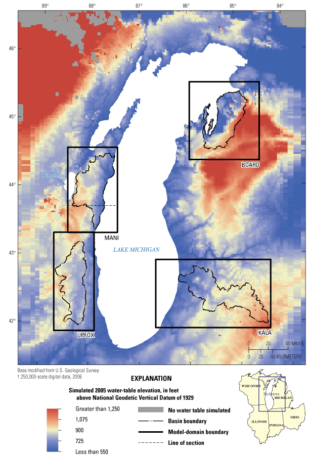
Map showing locations of eight-digit hydrologic-unit code (HUC8) basins and simulated water-table elevations in 2005 for four watershed areas near the Lake Michigan Basin. The HUC8 boundaries are enclosed within the boundaries of the domains of the inset models: KALA, Kalamazoo model; BOARD, Boardman-Charlevoix model; UPFOX, Upper Fox model; MANI, Manitowoc-Sheboygan model.
Table 1.
Areas of 8-, 10-, and 12-digit hydrologic-unit code basins in four groundwater travel-time models: the Kalamazoo, Boardman-Charlevoix, Upper Fox, and Manitowoc-Sheboygan basin models in Michigan.[HUC8, 8-digit hydrologic-unit code; HUC10, 10-digit hydrologic-unit code; HUC12, 12-digit hydrologic-unit code. Basins shown on figure 4]
The northern part of the Boardman-Charlevoix Basin-model watershed was excluded from the map (fig. 1) and table.
Background
Groundwater travel time (sometimes referred to as groundwater age) is defined as the elapsed time for a particle of water to travel from its point of entry into the saturated part of the aquifer, typically at the water table, to a point of interest within the aquifer. Groundwater that discharges to wells or surface-water bodies includes a mixture (or distribution) of different travel times because flow paths converge in these locations. This study is concerned primarily with the RTD of the groundwater in the aquifer, which represents a static snapshot of the ages of the groundwater in an aquifer. The related travel-time distribution (TTD) represents the ages of water exiting an aquifer, such as into a stream or well. TTDs reported for catchments often are much younger than their RTDs (Berghuijs and Kirchner, 2017). The difference is the result of the probability that catchments will drain younger water over older water in storage; however, the two are related through reservoir theory (Bolin and Rodhe, 1973; Eriksson, 1971).
Numerical simulation models of RTDs involve solving the master age-density equation of Ginn and others (2009) either directly on a grid or by tracking the locations of many particles moving through a simulated flow field. Recent research highlights the need for understanding how RTDs are related to landscape (Basu and others, 2012; Condon and Maxwell, 2015; Kirchner and others, 2001; Leray and others, 2016; Maxwell and others, 2016; McDonnell and others, 2010; McGuire and McDonnell, 2006; Remondi and others, 2019; Sprenger and others, 2019; Starn and Belitz, 2018). The relation between groundwater flow and hydrogeographic features has long been noted. For example, Carlston (1966) found that groundwater discharge is proportional to drainage density in streams in the northeastern United States, including nonglaciated areas. Groundwater gradients and flow-path lengths in heterogeneous aquifers are affected by drainage density (Broers, 2004; Goderniaux and others, 2013), and drainage density and groundwater discharge are partly a function of local and regional topography (Tóth, 1970; Winter, 1999, 2007). The position of the surface that separates local flow discharging to nearby streams from underflow to more distant streams is a function of drainage density and recharge (Goderniaux and others, 2013). The presence of local and regional multiscale flow systems and their associated stagnation points leads to fractal scaling of RTDs (Cardenas and Jiang, 2010; Jiang and others, 2012; Kollet and Maxwell, 2008). Aquifer geometry as well as spatial variation of recharge have been found to result in complex RTD shapes (Leray and others, 2016).
Methods
Groundwater flow was simulated for four watersheds by using two methods of model construction, GSM and IM. Construction of GSMs and IMs (table 2) is discussed in detail in Starn and Belitz (2018) and Feinstein and others (2018), respectively. A summary of the two types of model construction and a discussion of the major differences between them are presented in appendix 1. The different methods of construction resulted in structural differences between the model types (figs. 2 and 3). These differences and their effects on RTDs (and to a lesser extent on TTDs) are discussed in this report. Computations in both the GSMs and IMs were done with the U.S. Geological Survey (USGS) model codes known as MODFLOW–NWT (Niswonger and others, 2011) and MODPATH (version 6; Pollock, 2012).
Table 2.
Major construction details of general simulation and inset models.[HUC8, 8-digit hydrologic-unit code; ft, foot]
| General simulation model | Inset model |
|---|---|
| HUC8 watershed boundary | Rectangle enclosing HUC8 watershed boundary |
| 1,000 ft | 500 ft |
| Three equally thick but nonuniform layers | One layer up to 100 ft thick; additional layer(s) up to 200 ft as required |
| One uniform layer 100 ft thick | Variable, to depth of pre-Cambrian basement |
| From Trost and others (2018); distributed to fine and coarse zones | From Westenbroek and others (2010); distributed cell-by-cell from parent model |
| Gaining streams | Gaining and losing streams |
| High hydraulic-conductivity zone connected to drain cells | Drain cells |
| Calibrated for fine and coarse zones | Distributed cell-by-cell from parent model |
| One calibrated value | Distributed cell-by-cell from parent model based on lithologic units |
| One calibrated value | Distributed cell-by-cell from parent model based on lithologic units |
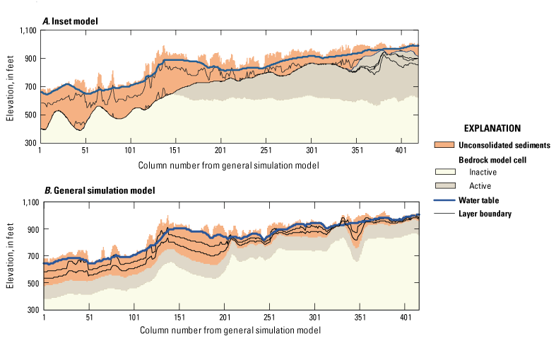
Cross sections through the center row of the general simulation model for the Lake Michigan Basin, showing model layers, the water table, and generalized geology from the A, inset model and B, general simulation model. Groundwater flow is simulated only for active model cells.
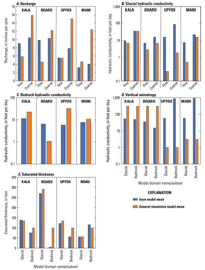
Graphs showing A, recharge; B, glacial and C, bedrock hydraulic conductivities; D, vertical anisotropy (ratio of vertical to horizontal hydraulic conductivity); and E, saturated thickness for the general simulation and inset models of the four eight-digit hydrologic-unit code (HUC8) basins in the Lake Michigan Basin: KALA, Kalamazoo model; BOARD, Boardman-Charlevoix model; UPFOX, Upper Fox model; MANI, Manitowoc-Sheboygan model.
MODPATH Inputs for Simulating Groundwater Travel Time
MODPATH was used to calculate groundwater travel-time distributions for both GSMs and IMs by tracking particles backwards from their starting locations to their points of recharge. Two million particles were started in each model and distributed among model cells in proportion to the flux of water moving through the cell. In this way, the RTDs were weighted by the amount of flow associated with each particle (as opposed to weighting by the volume associated with each particle). This differentiation from a volume-based RTD, where each particle represents an equal volume of water in the aquifer, is important. The reason for a flow-based RTD in the aquifer was that it should represent the travel time of discharge to wells or streams at any point within the aquifer. Particles within each cell were started at random three-dimensional locations. TTDs for streams were calculated in a similar fashion, except that particles were started only in discharge cells and distributed randomly on the top cell faces. Particles in the IMs were started only within the GSM boundary corresponding to a HUC8 basin, although the IMs have active areas outside the GSM boundaries.
MODPATH requires additional input beyond what is required for GSMs or IMs: these two model-type inputs were made as consistent as possible. Sources and sinks of water (recharge, drains, streams, and lakes) were placed on the upper faces of model cells. A correction to travel time in surface-water cells was applied (Abrams, 2013): if both sources and sinks were in the same model cell, the net value of flux was used.
For the purpose of comparison, the effective porosity was set uniformly to 0.20. Although this is a reasonable value for effective porosity overall, it is probably high for the bedrock part of the system and likely low in parts of the glacial sediments.
The SFR (streamflow-routing package in MODFLOW) was used to represent streams in the IMs, which allows water to leak back into the groundwater system. Generally, the flow paths followed by the stream leakage are short, and any water lost to the aquifer generally discharges back into a downgradient stream reach within a short distance. Because most of the MODFLOW-simulated stream leakage into the groundwater system resulted from the way that streams were discretized and stream altitudes were assigned, these flow paths were not used in the computation of the RTD and corresponding travel-time metrics.
Model-Input Characteristics Used for Comparison
A set of 26 model-input characteristics (including the mean and standard deviation) was calculated for each model type and for each HUC8 watershed and their HUC12 subwatersheds (fig. 4; table 3). These factors can be divided into four groups related to (1) the volumetric amount of water available (in the form of recharge for GSMs and of recharge and stream losses for IMs) compared to the volume of the saturated aquifer, (2) the surface-water network, (3) the ease of lateral flow, and (4) the ease of vertical flow. The mean and standard deviation were calculated in log space for factors related to transmissivity, hydraulic conductivity, and vertical anisotropy (the ratio of horizontal to vertical hydraulic conductivity), so that the expected value would be the geometric mean, and the standard deviation would be the log-based standard deviation defined in National Institute of Standards and Technology (2003).
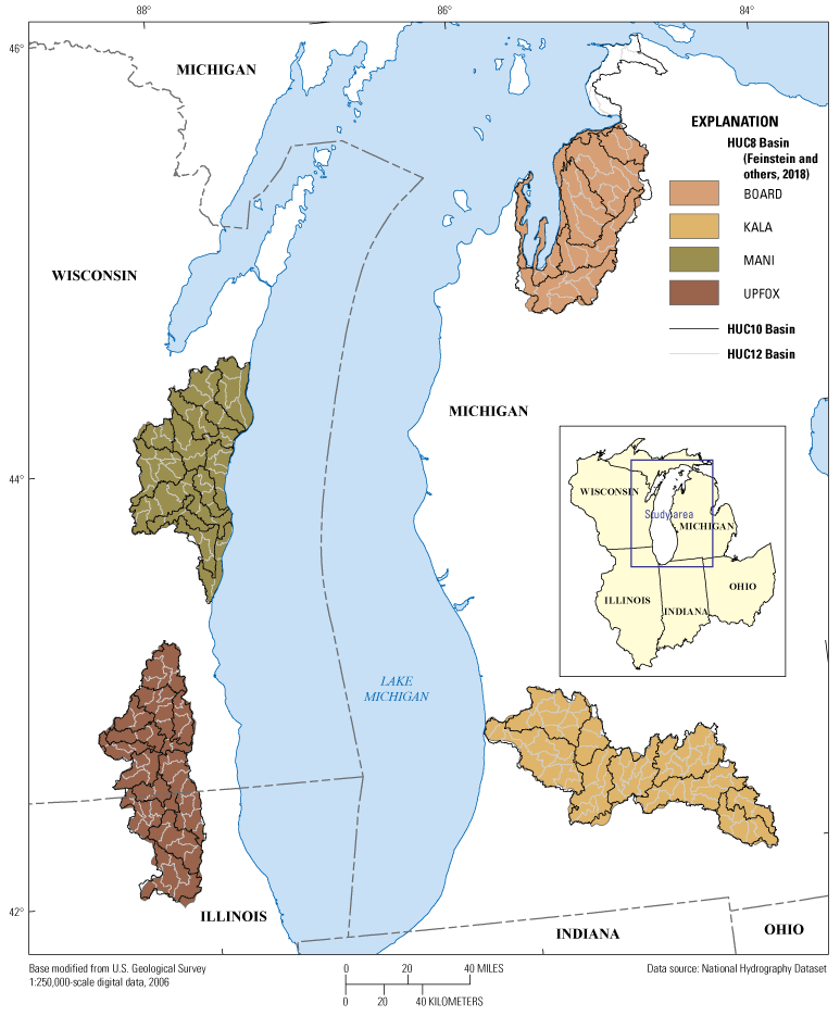
Map showing delineations of the 10- and 12-digit hydrologic-unit code (HUC10 and HUC12) basins within the four 8-digit hydrologic-unit code (HUC8) basins in the Lake Michigan Basin. KALA, Kalamazoo model; BOARD, Boardman-Charlevoix model; UPFOX, Upper Fox model; MANI, Manitowoc-Sheboygan model.
Table 3.
Possible explanatory factors for travel-time results from general simulation and inset models.[Factors are from MODFLOW and are defined in Niswonger and others (2011). Shallow bedrock in the inset models refers to bedrock above the first aquitard with hydraulic resistance equal to 50,000 days; in general simulation models, the shallow bedrock corresponds to a 100-foot-thick unit representing bedrock. in/yr, inch per year; m, meter; yr, year; —, dimensionless; m2/d, square meter per day; m/d, meter per day; K, hydraulic conductivity; GSM, general simulation model; SFR, MODFLOW Streamflow-Routing Package; DRN, MODFLOW Drain Package; IM, Inset Model]
Some factors were calculated for the glacial part of the saturated-flow system, some for the bedrock, and some for the total-flow system. In the GSMs, bedrock refers to the single bedrock layer and any parts of overlying layers with the same bedrock hydraulic conductivity. For the IMs, bedrock refers to the multiple layers assigned to bedrock units above a depth where the ratio of thickness to the vertical hydraulic conductivity of a geologic unit is greater than 50,000 days. This depth, corresponding to shallow bedrock, varies on a cell-by-cell basis in the IMs.
After preliminary analysis, 17 of the 26 potential explanatory factors were shown to influence results sufficiently enough to warrant more extended correlation analysis. Because of the importance of the zonal structure in the GSMs, several factors were calculated for these zones in the corresponding areas in the IMs, including recharge, horizontal glacial hydraulic conductivity, and shallow-bedrock hydraulic conductivity.
The differences and similarities between the two model types were summarized by using the ratios of model-input parameters (GSM:IM; fig. 5). A value of 1 indicates that the parameter is the same in both model types, and a departure from 1 in either direction indicates less agreement between the characteristics of the two model types.
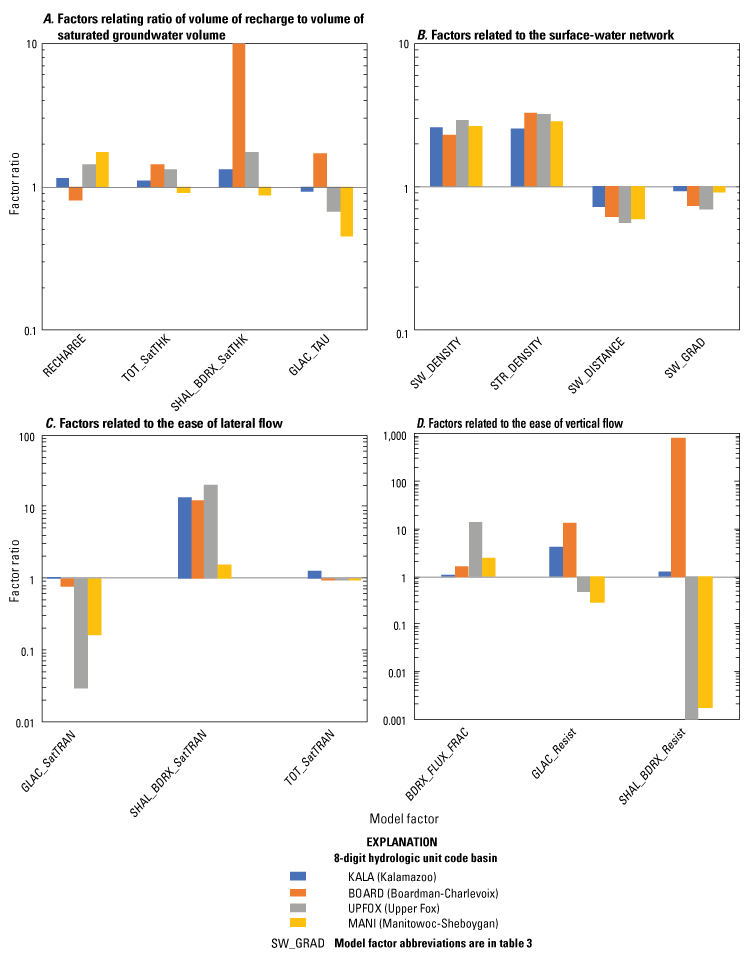
Graphs showing ratios of explanatory factors from the general simulation models to the inset models for the Lake Michigan Basin for A, volume of recharge to saturated groundwater, B, the surface-water network, C, the ease of lateral flow, and D, the ease of vertical flow.
Characteristics related to saturated volume (fig. 5A) showed agreement for recharge and glacial tau (the ratio of saturated glacial volume to recharge rate, generally equivalent to the time needed to flush the glacial material and thus directly tied to residence time). Differences related to the surface-water network (fig. 5B) were attributable in large measure to the cell-size difference in the models; more GSM cells contained surface water. The small but consistent gradient difference in the computed GSM:IM ratio between the water table at locations within the HUC8 and the nearest downgradient stream also could have been a function of grid size and could cause slower velocities in the GSMs. Characteristics related to ease of flow (fig. 5C–D) differed between the two model types, with notable differences in horizontal hydraulic conductivity of bedrock (Kb) and three characteristics related to vertical flow.
Groundwater RTD Metrics and Comparison Metrics
Four RTD metrics were computed on the basis of particle-tracking results. A threshold of 65 years was used to split young and old water to correspond roughly with bomb testing, which released large amounts of tritium into the atmosphere and thus allowed tritium concentrations to become a travel-time indicator in the groundwater system. Also, this threshold (water with a travel time less than 65 years) was considered a general indicator of potential anthropogenic contamination. In addition to the RTD, the following travel-time metrics were computed:
-
• Young fraction—the fraction of particles with travel times less than 65 years;
-
• Median travel time—the median travel time of all the particles;
-
• Median travel time of young fraction—the median travel time of all particles whose travel times were less than 65 years; and
-
• Median travel time of old fraction—the median travel time of all particles whose travel times were greater than or equal to 65 years.
The agreement between model types was evaluated by using the Nash-Sutcliffe efficiency coefficient (NSE). NSE is the proportion of variance in one model that is predicted by the other model and can have values from −∞ to 1.0. An NSE of 0 indicates that the mean of observations is the best predictor of the observations (as opposed to a more complicated model). Values less than zero indicate that predictions are worse than those predicted by the mean, and that values close to 1 indicate greater correlation among RTDs. The equation for the NSE is
wheren
is the number of samples,
i
is the number of a specific observation,
y
is the IM value,
i
is the GSM value, and
is the mean observed value.
Results
The RTD and TTD model types showed similarities and differences; the differences are most likely a result of systematic differences in the construction of the two model types (figs. 6 and 7). Metrics based on RTDs indicate several consistent patterns, but the quality of the agreement is partly a matter of scale. For example, GSMs and IMs are more similar when aggregated for HUC8 than for HUC12 basins.
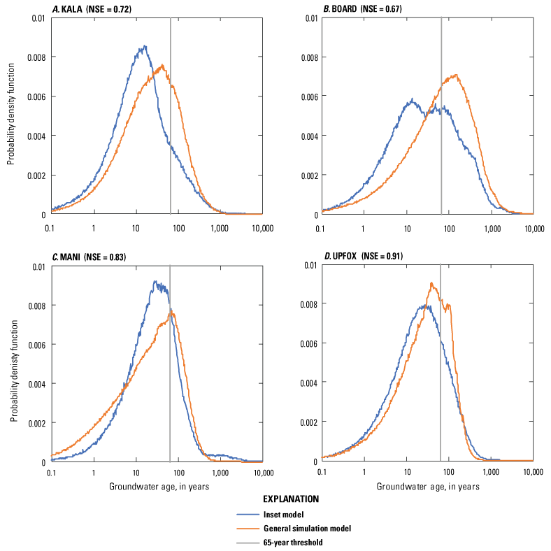
Graphs showing comparison of probability-density functions of residence-time distributions for aquifers in the general simulation and inset models for the A, Kalamazoo (KALA), B, Boardman-Charlevoix (BOARD), C, Manitowoc-Sheboygan (MANI), and D, Upper Fox (UPFOX) eight-digit hydrologic-unit code (HUC8) basins within the Lake Michigan Basin. NSE, Nash-Sutcliffe efficiency coefficient. The vertical light gray line is at the age of 65 years.
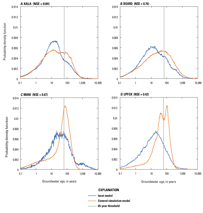
Graphs showing comparison of probability-density functions of travel-time distributions for streams in the general simulation and inset models for the A, Kalamazoo (KALA), B, Boardman-Charlevoix (BOARD), C, Manitowoc-Sheboygan (MANI), and D, Upper Fox (UPFOX) eight-digit hydrologic-unit code (HUC8) basins within the Lake Michigan Basin. NSE, Nash-Sutcliffe efficiency coefficient. The vertical light gray line is at the age of 65 years.
Comparison of RTDs in Aquifers and TTDs in Streams by HUC8 Basin
The NSEs for simulated RTDs in the aquifers between IMs and GSMs ranged from 0.67 in the BOARD model to 0.91 in the UPFOX model (fig. 6). RTDs from the GSMs indicated generally older water than from the IMs for all four basins. The shapes of the curves generally are similar within a given model, the most obvious exceptions being in BOARD, where the IM had a broader and possibly bimodal peak (fig. 6B). RTDs from the GSMs were less symmetrical, or more skewed, than those from the IMs and had a greater density of travel times less than the peak travel time.
The NSEs for simulated TTDs for streams were less than for aquifer RTDs for models of the MANI and UPFOX basins and greater for models of the KALA and BOARD basins (fig. 7). GSMs generally simulated older water than the IMs, as with the aquifer RTDs. Three of the stream RTDs for both model types were generally unimodal with a well-defined mode (fig. 7A–C); the UPFOX GSM RTD suggests two modes (fig. 7D). Stream TTDs from the GSM, like the aquifer RTDs, are less symmetrical than those from the IMs and have a greater density of travel times less than the peak travel time, especially in the MANI and UPFOX models. The IM TTD peaks were earlier than the GSM peaks in all cases due to a faster rising limb, indicating that the IMs tended to produce large groundwater velocities and small flow paths. The 65-year travel-time cutoff (between young and old fractions) crosses the falling limb for three of four IMs, whereas it is near the peak for all GSMs (fig. 7).
NSE values between aquifer RTDs and stream TTDs ranged from 0.83 to 0.96 for IMs, indicating that the age distributions of water in the aquifer and in discharge were similar, and the effect of water flowing through bedrock to streams was minimal (fig. 8A, C, E, and G). NSE values for aquifer RTDs and stream RTDs were lower for GSMs, ranging from 0.57 to 0.85 and thus suggesting a more important role for bedrock (fig. 8B and H).
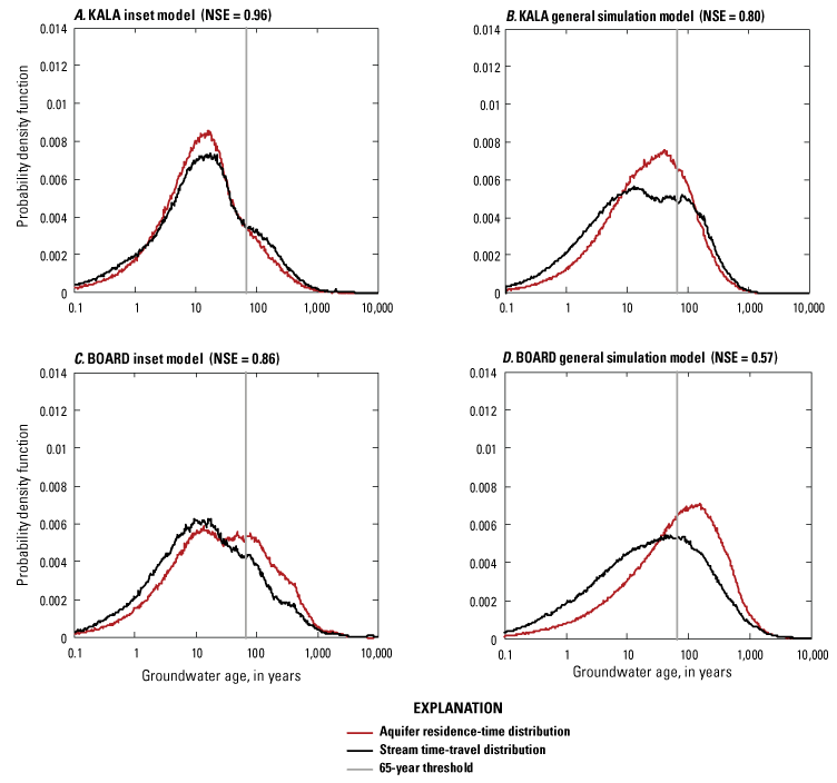
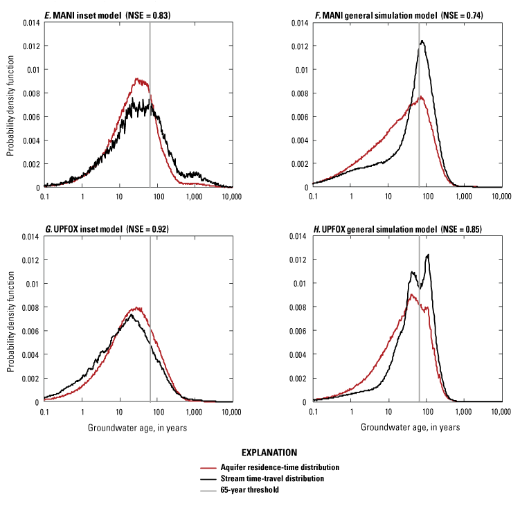
Graphs showing comparisons of probability-density functions of residence time and travel-time distribution for the inset and general simulation models for the A and B, Kalamazoo (KALA); C and D, Boardman-Charlevoix (BOARD); E and F, Manitowoc-Sheboygan (MANI); and G and H, Upper Fox (UPFOX) model eight-digit hydrologic-unit code (HUC8) basins within the Lake Michigan Basin. NSE, Nash-Sutcliffe efficiency coefficient.
Comparison of RTD Metrics Aggregated Over HUC8 and HUC12 Watersheds
The median age for groundwater in both the HUC8 (fig. 9A) and HUC12 (table 4) basins typically was higher for the GSMs than the IMs, particularly in the case of BOARD; they are almost equal in the case of MANI. The mean young fraction (less than 65 years) was always greater for the IMs (fig. 9B), a finding also made evident by their RTDs (fig. 6). The median age was generally younger for the IMs (fig. 8A and C) than for the GSMs, except for the MANI basin (fig. 6C). The median ages of the “old” fraction of water (greater than 65 years) generally were the same for both types of models (fig. 9D).
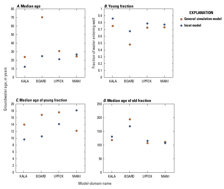
Graphs showing comparisons of A, median age, B, young fraction, and median ages of C, young and D, old fractions for the residence-time distributions from the general simulation and inset models for the eight-digit hydrologic-unit code (HUC8) basins in the Lake Michigan Basin. KALA, Kalamazoo; BOARD, Boardman-Charlevoix; UPFOX, Upper Fox; MANI, Manitowoc-Sheboygan.
Table 4.
Residence-time distribution statistics for all 230 twelve-digit hydrologic-unit code basins calculated by general simulation and inset models.[Young fraction is the fraction of groundwater less than 65 years old. GSM, general simulation model; IM, inset model]
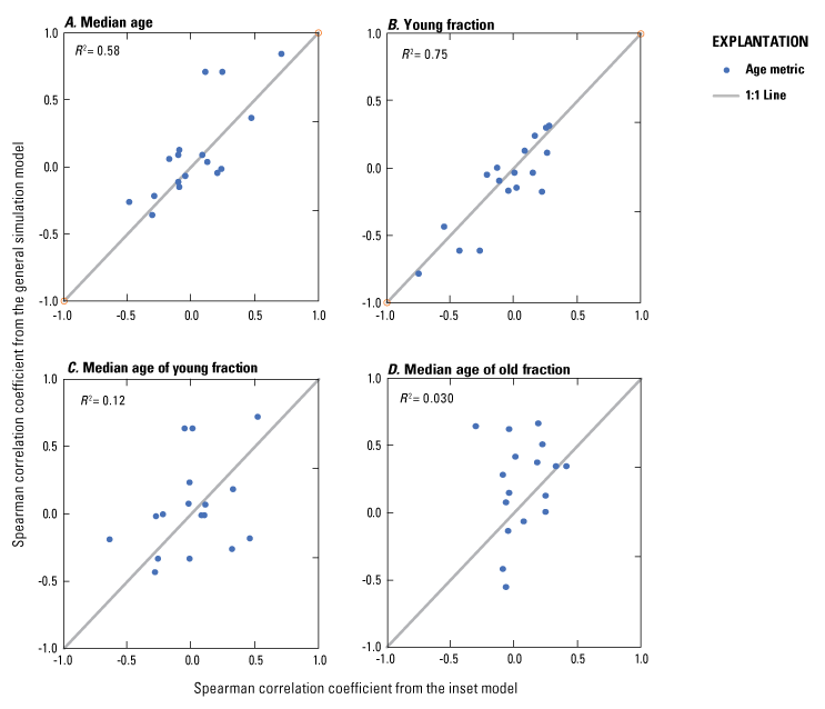
Although the GSMs and IMs used in this study were constructed at the HUC8 watershed scale, age metrics were also calculated for HUC12 watersheds in this study to determine how they would compare to the age metrics of the IMs at smaller scales. The RTD metrics (fig. 10) showed substantial scatter and a different correlation between the GSM and IM for each modeled area. The largest differences were in the metrics for the BOARD basin, where the GSM predicted older median ages of young water in all and a smaller fraction of young water in all but one of the HUC12 basins. The correlations were positive in all cases, but the slope of the trendline was always less than one, possibly pointing to some bias in the GSM results compared to the results from IMs. The slope of the trendline in the predicted fraction of old water was close to 0 in the MANI basin (fig. 10D); this result could indicate that the IM produces a greater variability in the age of the old water than does the GSM—results that are consistent with differences observed in the RTDs.
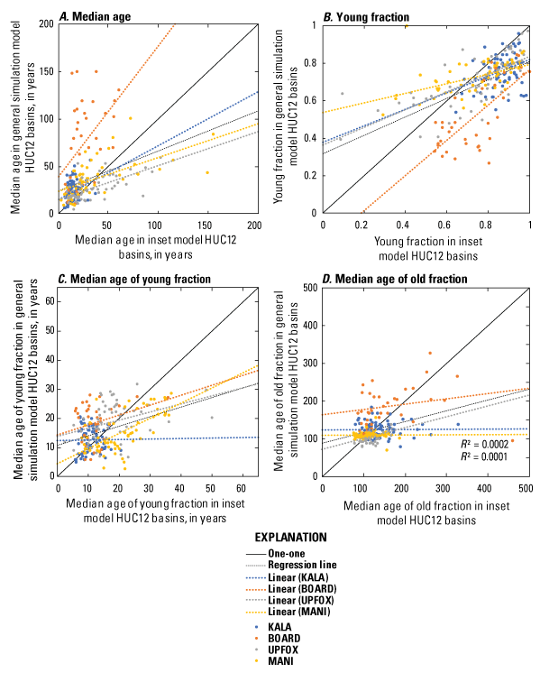
Graphs showing comparisons of A, median age, B, young fraction, C median age of young fraction, and D, median age of old fraction for the residence-time distributions calculated by the general simulation and inset models summarized for the 12-digit hydrologic-unit code (HUC12) basins within the Kalamazoo (KALA), Boardman-Charlevoix (BOARD), Manitowoc-Sheboygan (MANI), and Upper Fox (UPFOX) models.
Correlation of RTD Metrics With Model-Input Characteristics
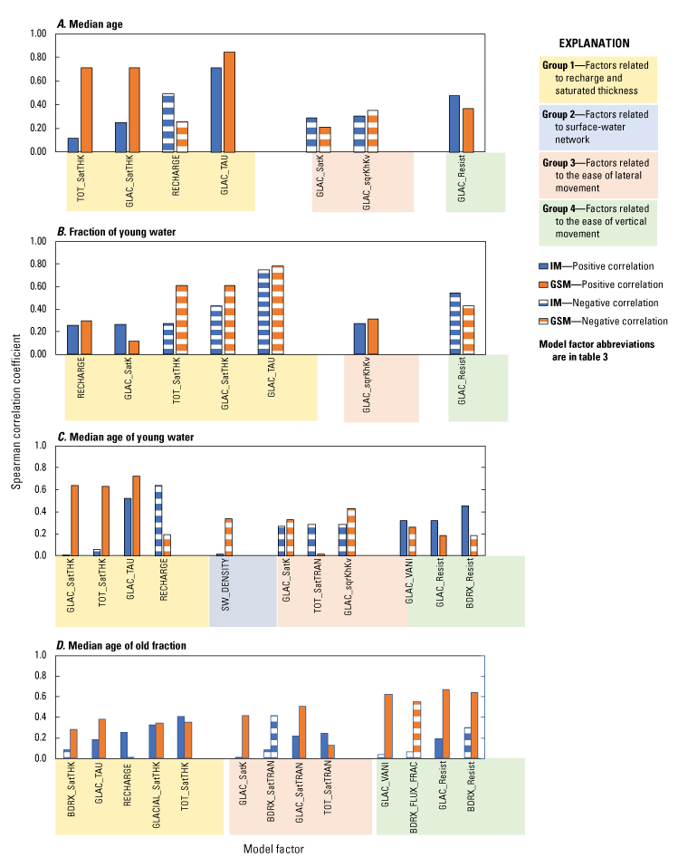
Correlation between model-input characteristics and RTD metrics generally showed that characteristics strongly correlated with RTD metrics (either positively or negatively) for the IMs also were correlated strongly with RTD metrics for the GSMs (fig. 11). The median age of glacial sediments across HUC12 watersheds for both model types was negatively correlated with recharge rate and the magnitude of glacial hydraulic conductivity: the higher those parameters, the lower the median age. The median age was positively correlated with the vertical resistance of saturated glacial material and the ratio of the volume of saturated glacial material to the recharge rate (glacial tau, variable name GLAC_tau) (fig. 11A).
Graphs showing comparison of Spearman correlation coefficients (ρ) of A, median age, B, young fraction, and median ages of C, young and D, old fractions to explanatory factors for the general simulation (GSM) and inset (IM) models for the 12-digit hydrologic-unit code (HUC12) basins in the Lake Michigan Basin.
Seven characteristics had correlations that exceeded 0.25 for the fraction of young water. Total saturated thickness, glacial saturated thickness, vertical resistance of glacial material, and glacial tau were negatively correlated, with glacial tau having the highest correlation. Recharge and glacial hydraulic conductivity were less strong but positively correlated (fig. 11B).
The median age of young water was strongly and positively correlated to glacial tau for both model types (fig. 11C). Recharge and glacial hydraulic conductivity were negatively correlated to this metric, whereas glacial vertical resistance was positively correlated. The pattern is less consistent for average glacial vertical anisotropy and shallow bedrock resistance.
The median age of the old fraction of water in both model types was most strongly and positively correlated to glacial recharge and glacial and total saturated thickness. The direction of correlation was opposite for many other factors. The negative correlations in the cases of the IMs may indicate that high bedrock resistance tends to keep many of the long flow paths in the glacial part of the system yielding younger water for residence times greater than 65 years, whereas the positive correlation for the GSMs may be affected by the higher proportion of flow which enters the bedrock (fig. 11D), which, having entered, tends to be older.
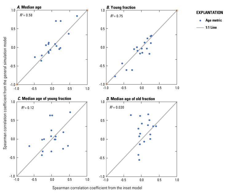
Spearman’s ρ for all the potential factors showed that the two model types agreed better with respect to the relative explanatory power of each factor for the median age and young- fraction metrics (fig. 12A and B) than they did for the median age of young fraction and median age of old fraction (fig. 12C and D). The model types disagreed the most for the median age of old fraction, with almost no correlation between model inputs and that metric (fig. 12D). This result complements the finding that, between the two types of models, the simulated median age and young-fraction metrics tend to correlate better than do the median ages of young and old fractions for both RTDs (table 4).
Scatter plots showing comparison of Spearman correlation coefficients (ρ) for A, median age, B, young fraction, and median ages of C, young and D, old fractions for the general simulation and inset models for the 12-digit hydrologic-unit code (HUC12) subbasins in the Lake Michigan Basin.
Discussion
Differences in model construction and parameter values affect flow patterns (for example, partitioning flow between glacial sediment and bedrock) and partly explained differences in RTDs between the two model types. Starn and Belitz (2018) found that glacial tau had the largest effect on the shape of the RTD; other factors included the ratio of recharge from land surface to recharge from bedrock; horizontal hydraulic conductivity (Kh) of glacial sediment, Kh of bedrock, the ratio of horizontal to vertical hydraulic conductivity (Kh:Kv); the fraction of surface area occupied by surface-water bodies; and the ratio of glacial thickness to bedrock thickness. They also found that interaction among these characteristics was significant in estimating RTDs—any of the univariate correlations could behave differently if considered jointly with other model inputs. It is not surprising that model-input characteristics that differed in value between the two model types were similarly important in affecting RTDs, especially characteristics related to saturated volume and the ease of horizontal and vertical movement of groundwater.
Of considerable interest in this study were the characteristics relative to vertical and horizontal ease of flow. These characteristics play a large role in partitioning flow deep into the glacial sediments and into bedrock. Starn and Belitz (2018) found that although vertical anisotropy was important in determining the shape of the RTD graph, values derived from the GSM were not sensitive to the calibration method and thus were highly uncertain. GSM calibration produced high vertical-anisotropy ratios for the KALA and BOARD models and low ratios for the UPFOX and MANI models (fig. 3D). In addition, the transmissivity of glacial sediments in GSMs was generally lower for IMs, and the transmissivity of the bedrock was appreciably higher (fig. 5B). These characteristics together condition the ratios of recharge (plus surface-water loss in the case of the IMs) to the downward flow into bedrock for the four HUC8 areas. The ratio of recharge at the water table to flow into bedrock, which is known to be a significant factor in RTD shape (Starn and Belitz, 2018), was several times higher in three of the four GSMs than in the corresponding IMs (fig. 5A).
The comparison between aquifer RTDs and stream TTDs in the KALA and BOARD GSMs differed from the comparison between those in the MANI and UPFOX basins. Stream TTDs in the BOARD and KALA GSMs generally are skewed younger than the aquifer RTDs, particularly for the young fraction of water, while in the MANI and UPFOX GSMs, the stream TTDs in the young fraction generally are shifted older. As noted above, differences in the IM vertical anisotropy (lower in BOARD and KALA and higher in MANI and UPFOX; fig. 3D) may help explain the shifts. For all the basins, the mean vertical anisotropy values from the IMs are intermediate to the range of the GSM values; this comparison may help explain why there is more agreement between the aquifer RTDs and stream TTDs in the IM models.
Aquifer RTDs were calculated only considering water in glacial sediments; however, some water in glacial sediments may have flowed through bedrock at some point along its path. On the other hand, stream TTDs represent travel times between the recharge and discharge points. Differences between aquifer and stream RTDs reflect how much groundwater discharged as base flow primarily through glacial sediments compared to through bedrock. RTDs and TTDs in IMs were similar, and the effect of water flowing through bedrock to streams was minimal. RTDs and TTDs in GSMs were lower but also similar, suggesting a more important role for bedrock (fig. 8B, D, F, and H).
The structure of the models, as opposed to the values of model parameters, also can affect age. Model-structure considerations apply to both GSMs and IMs, but the magnitudes of these effects are difficult to test and quantify. Boundary effects can be important. For example, groundwater was free to flow across the HUC8 watershed boundary in the IMs, and this flow could add or subtract individual particle travel times from the ensemble averages for the HUC8. In addition to simulating more streams, smaller grid spacing enables finer resolution of groundwater-velocity gradients.
Future Work
The GSM approach was intended as a flexible framework for developing models that can be useful individually as screening tools or collectively to support projects in statistical learning. Although one set of GSM algorithms was presented here, the approach can accommodate many types and categories of data. Comparison of GSMs and IMs points to ways in which the GSMs, while remaining easy to construct and calibrate, can be improved for estimating groundwater travel times. IMs were constructed with more detailed data than GSMS; however, IMs do not yield exact travel times, and matching GSMs to IMs does not necessarily guarantee an improvement in GSMs. Direct measurements of RTDs do not exist, and IMs provide a reasonable benchmark against which to explore relations between physical characteristics of watersheds and the distribution of travel times within them. Here are some ways in which GSMs could be improved without altering the paradigms that underlie their development:
-
• incorporating distributed arrays for recharge and glacial hydraulic conductivity,
-
• adding more choices for model-edge boundary conditions,
-
• constraining bedrock anisotropy by using prior information,
-
• applying separate anisotropy ratios to the glacial and bedrock layers,
-
• assigning bedrock hydraulic conductivity based on rock type, and,
-
• through further testing:
Summary and Conclusions
Numerical simulation models provide one way to estimate groundwater ages over large spatial areas. One method to rapidly develop models is the general simulation model (GSM) method. The GSM method automates model construction by using large-scale data layers (for inputs such as land surface, recharge distribution, and surface-water network) to rapidly generate numerical models. GSMs represent a tradeoff between time and resources (they can be constructed more quickly) and the level of detail (they are less detailed) relative to conventional models. GSMs can be useful for three main-use cases: (1) rapid testing of relationships that govern groundwater flow and age, (2) generation of consistent examples for training a machine-learning metamodel, and (3) serving as a starting point for more detailed models.
An important consideration is whether GSMs capture the essential mechanisms that affect travel-time simulation in conventional groundwater-flow models. This study directly compares GSMs to conventional inset models (IMs) that simulate glacial and bedrock groundwater conditions in the same basins in the Upper Midwest. Direct measurements of residence-time distributions (RTDs) do not exist, and IMs provide a reasonable benchmark against which to explore relations among physical characteristics of watersheds and the distributions of travel times within them. The comparison is designed
-
• to evaluate the degree to which GSMs reproduce behavior simulated by flow models that offer a more detailed representation of the subsurface (IMs); and,
-
• by means of the comparison, to deepen our overall understanding about controls on travel time useful for the management of groundwater vulnerable to contamination by constituents typically dissolved in either younger or older waters.
The set of four IMs and companion GSMs evaluated in this report are steady-state models centered on four eight-digit hydrologic-unit code (HUC8) topographic basins, two of which are in the southern peninsula of Michigan, one in southeastern Wisconsin, and one in northeastern Illinois. The same particle- tracking techniques were used for both model types to calculate residence-time distributions for water in glacial sediments and travel-time distributions at stream-discharge locations. The GSM and IM results were then analyzed and compared in terms of
-
• RTDs;
-
• metrics based on RTDs: median age, young fraction, median travel time of young fraction and median travel time of old fraction, (young groundwater defined as having a travel time less than 65 years); and
-
• the correlation of RTD metrics with model-input characteristics.
Comparison of the GSMs to IMs indicated a qualified pattern of agreement for RTD (as indicated by Nash-Sutcliffe efficiency) and RTD metrics (as indicated by Spearman’s correlation coefficient [ρ]). The agreement was best for the median values of the simulated young fraction of groundwater residence times at the HUC8 scale. Where the IMs showed the median value of the young fraction to be relatively high or low at the HUC8 scale, so did the GSMs. The relative trends across the four HUC8 basins also were similar for the other RTD metrics.
The RTDs for the two types of models show a distinct difference in their shapes. The rising limbs of the IM RTDs tend to be steeper and shifted younger than the corresponding parts of the GSM RTDs. The reasons for this difference may be that parameter combinations in the GSMs—including lower glacial transmissivity, higher bedrock transmissivity, and lower overall vertical resistance to flow—that allow more bedrock flux than in the IMs tend to produce longer flow paths. Because the vertical anisotropy ratios in the GSMs are insensitive to the calibration process, it is possible that the GSMs underestimate vertical resistance to flow and therefore overestimate the bedrock component of flux and the proportion of older water that follows longer flow paths.
The correlation of explanatory factors to RTD metrics sheds light not only on the areas of agreement and disagreement between the GSMs and IMs, but also on shared controls of simulated travel time. There was marked agreement for both sets of models in the set of factors positively or negatively correlated with (and assumed to explain) the young fraction simulated across all 12-digit hydrologic-unit code (HUC12) basins within the four simulated HUC8 basins. Agreement among factors also was strong for median age. In particular, the glacial tau factor, equivalent to the ratio of saturated glacial volume to recharge flux, was a dominant (negatively correlated) control on young fraction and a dominant (positively correlated) control on median travel time for both the GSMs and the IMs (consistent with Starn and Belitz, 2018). Other factors, such as glacial vertical resistance, are similar in their effect (magnitude and direction of correlation) on young fraction and median travel time at the HUC12 scale for both sets of models.
There was less agreement between the two sets of models in the model-input characteristics for median travel time of the young fraction and especially for median travel time of the old fraction. The strength and even the direction of correlation differed, in some cases appreciably. Glacial tau was an important positively correlated factor for median travel time of young fraction, but for both GSMs and IMs, it had less explanatory power for median travel time of the old fraction. No specific factor was strongly correlated with median travel time of the old fraction for the IMs, whereas factors associated with vertical resistance to flow were correlated most strongly in the case of GSMs. RTDs in both model types may be influenced jointly by many types of model inputs, including boundary conditions, aquifer properties, and sources and sinks.
Characteristics of the surface-water network did not appear to affect RTDs in this study; however, the effect of increasing the surface-water-network density lowers the vertical position of the interface between young and old water (Broers, 2004); the RTDs in this study were averaged over watershed areas at all depths. Stream density may be more important for studies in which depth-dependent travel time is important.
There likely would be more confidence in model results for HUC8 watersheds than for those at the HUC12 scale. Agreement of RTDs was much better at the larger HUC8 scale, at which local variation is averaged over a wider range of values. Less agreement among HUC12 watersheds for all metrics may indicate a systematic bias in metrics produced by GSMs. This bias in HUC12 metrics may be caused by significant differences in recharge and hydraulic conductivity and possibly also by movement of particles in or out of the IM watersheds. Because these factors produce the same effects in both types of models, the models can be applied in the metamodel approach. Subsequently, these rankings, in combination with other data- or model-based predictors and through machine-learning techniques, could be used to map vulnerability to contamination across an aquifer system.
Model construction and calibration had a large effect on the resulting RTD; however, GSMs and IMs, produced with different levels of detail and effort, showed qualified agreement. The RTD metrics for HUC8 watersheds generally were similar in magnitude and trend between GSMs and IMs. This finding supports one of the intended uses of GSMs, which was providing training examples in statistical learning, particularly in gradient-boosted regression (Fienen and others, 2018; Nolan and others, 2015). This qualified agreement persists in the face of large differences in parameters that govern the ease of horizontal and vertical flow. It may be that the GSM calibration process will select other parameter values that compensate for the single and relatively insensitive vertical anisotropy factor. The fact that the ordinal position of RTD metrics is maintained in the two model types indicates that these metrics are robust against details of model construction. Use of these metrics in metamodeling may be useful in predicting groundwater age and, by extension, susceptibility of groundwater to contamination.
Although structural differences between the two model types limit conclusions as to the applicability of GSMs, there is enough evidence to indicate that GSMs would work best where flow across lateral boundaries is limited, and where the lower boundary can be readily defined. Depth-related heterogeneity seems to pose a potential challenge as well.
Acknowledgments
The authors acknowledge insightful and constructive reviews by Donald Walter and Jason Pope of the USGS. The report benefited from extensive discussions with Ken Belitz and the Glacial Principal Aquifer Modelling and Mapping team within the USGS National Water Quality Program.
References Cited
Abrams, D., 2013, Correcting Transit Time Distributions in Coarse MODFLOW-MODPATH Models: Groundwater, v. 51, no. 3, p. 474–478. [Also available at https://doi.org/10.1111/j.1745-6584.2012.00985.x.]
Bakker, M., Post, V., Langevin, C.D., Hughes, J.D., White, J.T., Starn, J.J., and Fienen, M.N., 2016, Scripting MODFLOW model development using Python and FloPy: Groundwater, v. 54, no. 5, p. 733–739. [Also available at https://doi.org/10.1111/gwat.12413.]
Basu, N.B., Jindal, P., Schilling, K.E., Wolter, C.F., and Takle, E.S., 2012, Evaluation of analytical and numerical approaches for the estimation of groundwater travel time distribution: Journal of Hydrology, v. 475, p. 65–73. [Also available at https://doi.org/10.1016/j.jhydrol.2012.08.052.]
Berghuijs, W.R., and Kirchner, J.W., 2017, The relationship between contrasting ages of groundwater and streamflow: Geophysical Research Letters, v. 44, no. 17, p. 8925–8935. [Also available at https://doi.org/10.1002/2017GL074962.]
Bolin, B., and Rodhe, H., 1973, A note on the concepts of age distribution and transit time in natural reservoirs: Tellus. Series A, Dynamic Meterology and Oceanography, v. 25, no. 1, p. 58–62. [Also available at https://doi.org/10.1111/j.2153-3490.1973.tb01594.x.]
Broers, H.P., 2004, The spatial distribution of groundwater age for different geohydrological situations in the Netherlands—Implications for groundwater quality monitoring at the regional scale: Journal of Hydrology, v. 299, nos. 1–2, p. 84–106. [Also available at https://doi.org/10.1016/j.jhydrol.2004.04.023.]
Cardenas, M.B., and Jiang, X.W., 2010, Groundwater flow, transport, and residence times through topography-driven basins with exponentially decreasing permeability and porosity: Water Resources Research, v. 46, no. 11, article W11538. [Also available at https://doi.org/10.1029/2010WR009370.]
Carlston, C.W., 1966, The effect of climate on drainage density and streamflow: International Association of Scientific Hydrology Bulletin, v. 11, no. 3, p. 62–69. [Also available at https://doi.org/10.1080/02626666609493481.]
Condon, L.E., and Maxwell, R.M., 2015, Evaluating the relationship between topography and groundwater using outputs from a continental-scale integrated hydrology model: Water Resources Research, v. 51, no. 8, p. 6602–6621. [Also available at https://doi.org/10.1002/2014WR016774.]
Doherty, J., 2008a, PEST, Model Independent Parameter Estimation—Addendum to user manual (5th ed.): Brisbane, Australia, Watermark Numerical Computing, accessed October 1, 2009, at http://www.pesthomepage.org/Downloads.php.
Doherty, J., 2008b, PEST, Model Independent Parameter Estimation—User manual (5th ed.): Brisbane, Australia, Watermark Numerical Computing, accessed October 1, 2009, at http://www.pesthomepage.org/Downloads.php.
Eberts, S.M., Thomas, M.A., and Jagucki, M.L., 2013, The quality of our Nation’s waters—Factors affecting public-supply-well vulnerability to contamination—Understanding observed water quality and anticipating future water quality: U.S. Geological Survey Circular 1385, 120 p., accessed June 6, 2020, at https://pubs.usgs.gov/circ/1385/.
Eriksson, E., 1971, Compartment models and reservoir theory: Annual Review of Ecology and Systematics, v. 2, no. 1, p. 67–84. [Also available at https://doi.org/10.1146/annurev.es.02.110171.000435.]
Fienen, M.N., Nolan, B.T., Kauffman, L.J., and Feinstein, D.T., 2018, Metamodeling for groundwater age forecasting in the Lake Michigan Basin: Water Resources Research, v. 54, no. 7, p. 4750–4766. [Also available at https://doi.org/10.1029/2017WR022387.]
Feinstein, D.T., Hunt, R.J., and Reeves, H.W., 2010, Regional groundwater-flow model of the Lake Michigan Basin in support of Great Lakes Basin water availability and use studies: U.S. Geological Survey Scientific Investigations Report 2010–5109, 379 p. [Also available at https://doi.org/10.3133/sir20105109.]
Feinstein, D.T., Kauffman, L.J., Haserodt, M.J., Clark, B.R., and Juckem, P.F., 2018, Extraction and development of inset models in support of groundwater age calculations for glacial aquifers: U.S. Geological Survey Scientific Investigations Report 2018–5038, 96 p., accessed December 2, 2021, at https://doi.org/10.3133/sir20185038.
Fullerton, D.S., and Richmond, G.M., compilers, [1983–2007], Quaternary geologic atlas of the United States: U.S. Geological Survey Miscellaneous Investigations Series Map I–1420, 33 quadrangles, scale 1:1,000,000, accessed December 2, 2021, at https://on.doi.gov/2vwOIXJ.
Ginn, T. R., Haeri, H., Massoudieh, A., and Foglia, L., 2009, Notes on groundwater age in forward and inverse modeling: Transport in Porous Media, v. 79, special issue 1, p. 117–134. [Also available at https://doi.org/10.1007/s11242-009-9406-1.]
Goderniaux, P., Davy, P., Bresciani, E., De Dreuzy, J.R., and Le Borgne, T., 2013, Partitioning a regional groundwater flow system into shallow local and deep regional flow compartments: Water Resources Research, v. 49, no. 4, p. 2274–2286. [Also available at https://doi.org/10.1002/wrcr.20186.]
Handman, E.H., Haeni, F.P., and Thomas, M.P., 1986, Water resources inventory of Connecticut, part 9—Farmington River Basin: Connecticut Water Resources Bulletin no. 29, 92 p., 4 pls., scale 1:48,000. [Also available at https://pubs.usgs.gov/unnumbered/70038342/report.pdf.]
Jiang, X.W., Wan, L., Ge, S., Cao, G.L., Hou, G.C., Hu, F.S., Wang, X.-S., Li, H., and Liang, S.-H., 2012, A quantitative study on accumulation of age mass around stagnation points in nested flow systems: Water Resources Research, v. 48, no. 12, article W12502. [Also available at https://doi.org/10.1029/2012WR012509.]
Kauffman, L.J., Jones, P., and Feinstein, D.T., 2023, MODPATH-NWT and MODPATH6 models used to compare a new general simulation model approach with a conventional inset model approach for groundwater residence time in glacial aquifers: U.S. Geological Survey data release, https://doi.org/10.5066/P9HS83JL.
Kirchner, J.W., Feng, X., and Neal, C., 2001, Catchment-scale advection and dispersion as a mechanism for fractal scaling in stream tracer concentrations: Journal of Hydrology, v. 254, nos. 1–4, p. 82–101. [Also available at https://doi.org/10.1016/S0022-1694(01)00487-5.]
Kollet, S. and Maxwell, R., 2008, Demonstrating fractal scaling of baseflow residence time distributions using a fully coupled groundwater and land surface model: Geophysical Research Letters, v. 35, no. 7, article L07402. [Also available at https://doi.org/10.1029/2008GL033215.]
Leray, S., Engdahl, N.B., Massoudieh, A., Bresciani, E., and McCallum, J., 2016, Residence time distributions for hydrologic systems—Mechanistic foundations and steady-state analytical solutions: Journal of Hydrology, v. 543, p. 67–87. [Also available at https://doi.org/10.1016/j.jhydrol.2016.01.068.]
Maxwell, R.M., Condon, L.E., Kollet, S.J., Maher, K., Haggerty, R., and Forrester, M.M., 2016, The imprint of climate and geology on the residence times of groundwater: Geophysical Research Letters, v. 43, no. 2, p. 701–708, accessed April 6, 2020, at https://doi.org/10.1002/2015GL066916.
McDonnell, J.J., McGuire, K., Aggarwal, P., Beven, K.J., Biondi, D., Destouni, G., Dunn, S., James, A., Kirchner, J., Kraft, P., Lyon, S., Maloszewski, P., Newman, B., Pfister, L., Rinaldo, A., Rodhe, A., Sayama, T., Seibert, J., Solomon, K., Soulsby, C., Stewart, M., Tetzlaff, D., Tobin, C., Troch, P., Weiler, M., Western, A., Wörman, A., and Wrede, S., 2010, How old is streamwater? Open questions in catchment transit time conceptualization, modelling and analysis: Hydrological Processes, v. 24, no. 12, p. 1745–1754. [Also available at https://doi.org/10.1002/hyp.7796.]
McGuire, K.J., and McDonnell, J.J., 2006, A review and evaluation of catchment transit time modeling: Journal of Hydrology, v. 330, no. 3–4, p. 543–563. [Also available at https://doi.org/10.1016/j.jhydrol.2006.04.020.]
Moore, R.B., and Dewald, T.G., 2016, The Road to NHDPlus—Advancements in digital stream networks and associated catchments: Journal of the American Water Resources Association, v. 52, no. 4, p. 890–900. [Also available at https://doi.org/10.1111/1752-1688.12389.]
National Institute of Standards and Technology, 2003, Lognormal distribution, 1.3.6.6.9 of NIST/SEMATECH e-handbook of statistical methods: National Institute of Standards and Technology website, accessed September 2019 at https://doi.org/10.18434/M32189.
Niswonger, R.G., Panday, S., and Ibaraki, M., 2011, MODFLOW-NWT—A Newton formulation for MODFLOW-2005: U.S. Geological Survey Techniques and Methods, book 6, chap. A37, 44 p. [Also available at https://doi.org/10.3133/tm6A37.]
Nolan, B.T., Fienen, M.N., and Lorenz, D.L., 2015, A statistical learning framework for groundwater nitrate models of the Central Valley, California, USA: Journal of Hydrology, v. 531, p. 902–911. [Also available at https://doi.org/10.1016/j.jhydrol.2015.10.025.]
Oliphant, T.E., 2007, Python for scientific computing: Computing in Science & Engineering, v. 9, no. 3, p. 10–20. [Also available at https://doi.org/10.1109/MCSE.2007.58.]
Perez, F., and Granger, B., 2007, IPython—A system for interactive scientific computing: Computing in Science & Engineering, v. 9, no. 3, p. 21–29. [Also available at https://doi.org/10.1109/MCSE.2007.53.]
Pollock, D.W., 2012, User guide for MODPATH version 6 – A particle tracking model for MODFLOW: U.S. Geological Survey Techniques and Methods, book 6, chap. A41, 58 p. [Also available at https://doi.org/10.3133/tm6A41.]
Remondi, F., Botter, M., Burlando, P., and Fatichi, S., 2019, Variability of transit time distributions with climate and topography—A modelling approach: Journal of Hydrology, v. 569, p. 37–50. [Also available at https://doi.org/10.1016/j.jhydrol.2018.11.011.]
Schilling, K.E., 2009, Investigating local variation in groundwater recharge along a topographic gradient, Walnut Creek, Iowa, USA: Hydrogeology Journal, v. 17, no. 2, p. 397–407. [Also available at https://doi.org/10.1007/s10040-008-0347-5.]
Soller, D.R., and Garrity, C.P., 2018, Quaternary sediment thickness and bedrock topography of the glaciated United States east of the Rocky Mountains: U.S. Geological Survey Scientific Investigations Map 3392, 2 sheets, scale 1:5,000,000. [Also available at https://doi.org/10.3133/sim3392.]
Sprenger, M., Stumpp, C., Weiler, M., Aeschbach, W., Allen, S.T., Benettin, P., Dubbert, M., Hartmann, A., Hrachowitz, M., Kirchner, J.W., McDonnell, J.J., Orlowski, N., Penna, D., Pfahl, S., Rinderer, M., Rodriguez, N., Schmidt, M., and Werner, C., 2019, The demographics of water—A review of water ages in the critical zone: Reviews of Geophysics, v. 57, no. 3, p. 800–834. [Also available at https://doi.org/10.1029/2018RG000633.]
Starn, J.J., and Belitz, K., 2018, Regionalization of groundwater residence time using metamodeling: Water Resources Research, v. 54, no. 9, p. 6357–6373. [Also available at https://doi.org/10.1029/2017WR021531.]
Tóth, J., 1970, A conceptual model of the groundwater regime and the hydrogeologic environment: Journal of Hydrology, v. 10, no. 2, p. 164–176. [Also available at https://doi.org/10.1016/0022-1694(70)90186-1.]
Trost, J.J., Roth, J.L., Westenbroek, S.M., and Reeves, H.W., 2018, Simulation of potential groundwater recharge for the glacial aquifer system east of the Rocky Mountains, 1980–2011, using the Soil-Water-Balance model: U.S. Geological Survey Scientific Investigations Report 2018–5080, 51 p., accessed December 2, 2021, at https://doi.org/10.3133/sir20185080.
U.S. Geological Survey, 2016, USGS water data for the Nation: U.S. Geological Survey National Water Information System database, accessed September 28, 2016, at https://doi.org/10.5066/F7P55KJN.
Westenbroek, S.M., Kelson, V.A., Dripps, W.R., Hunt, R.J., and Bradbury, K.R., 2010, SWB—A modified Thornthwaite-Mather soil-water balance code for estimating ground-water recharge: U.S. Geological Survey Techniques and Methods 6–A31, 65 p., accessed December 2, 2021, at https://doi.org/10.3133/tm6A31.
Winter, T.C., 1999, Relation of streams, lakes, and wetlands to groundwater flow systems: Hydrogeology Journal, v. 7, no. 1, p. 28–45. [Also available at https://doi.org/10.1007/s100400050178.]
Winter, T.C., 2007, The role of ground water in generating streamflow in headwater areas and in maintaining base flow: Journal of the American Water Resources Association, v. 43, no. 1, p. 15–25. [Also available at https://doi.org/10.1111/j.1752-1688.2007.00003.x.]
Appendix 1. Description of the General Simulation Models
Scatter plots showing comparison of Spearman correlation coefficients (ρ) for A, median age, B, young fraction, and median ages of C, young and D, old fractions for the general simulation and inset models for the 12-digit hydrologic-unit code (HUC12) subbasins in the Lake Michigan Basin. (Duplicate of figure 12 in the main report.)
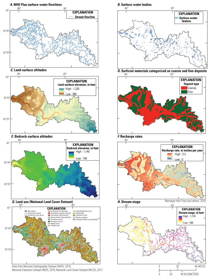
Maps showing the A, National Hydrologic Dataset Plus (NHD Plus) surface-water flowlines, B, surface-water bodies, C, land-surface altitudes, D, surficial materials categorized as coarse and fine deposits, E, bedrock-surface altitudes, F, recharge rates, G, land use (National Land Cover Dataset), and H, stream-stage layers of the Kalamazoo general simulation model for the Lake Michigan Basin.
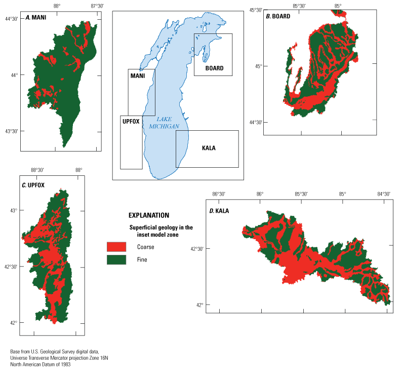
Maps showing general surface geology at the A, Manitowoc-Sheboygan (MANI), B, Boardman-Charlevoix (BOARD), C, Upper Fox (UPFOX), and D, Kalamazoo (KALA) eight-digit hydrologic-unit code (HUC8) basins at the Lake Michigan Basin.
h
is the model-calculated head,
LR
is land-surface altitude,
NR
is the number of nondrain cells,
HD
is drain elevation, and
ND
is the number of drain cells.
Table 1.1.
General simulation model-calibrated parameter values and calibration statistics.[Kh is horizontal hydraulic conductivity; VANI ratio is ratio of horizontal to vertical hydraulic conductivity; HYDRO error is perennial streams simulated as dry drain cells; TOPO error is fraction of cells with water table above land surface. ft/d, foot per day]
Inset Models
Four IMs (Feinstein and others, 2018) were derived from a regional groundwater-flow model of the Lake Michigan Basin (Feinstein and others, 2010) in the same areas as the GSMs. The Lake Michigan Basin (LMB) model has a 5,000-by-5,000-ft-grid spacing that was deemed too coarse to reliably capture key mechanisms that affect groundwater travel time. To overcome the limits imposed by the regional-grid spacing, IMs of four basins were extracted from the LMB model domain to simulate groundwater-flow conditions in different glacial settings at a refined grid spacing of 500 by 500 ft. This finer resolution allows for a more precise location of wells and surface-water features and a more detailed representation of heterogeneous glacial deposits. A telescopic-mesh refinement technique (Rumbaugh and Rumbaugh, 2011) was applied to the parent LMB model to extract and modify the domains shown in figure 1 of this report. The lateral-grid spacing of square cells was refined so that each cell in the LMB model corresponds to 100 cells in the IMs. The LMB model was not refined in the vertical direction; therefore, the LMB model and the IMs derived from it have the same layering. Recharge and hydraulic conductivity in the IMs were based on values shown in the LMB model (figs. 1.4 and 1.5) and distributed cell-by-cell.
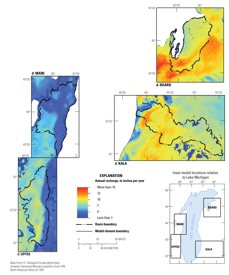
Maps showing annual recharge in the inset model for the A, Kalamazoo (KALA), B, Boardman-Charlevoix (BOARD), C, Upper Fox (UPFOX), and D, Manitowoc-Sheboygan (MANI) eight-digit hydrologic-unit code (HUC8) basins within the Lake Michigan Basin.
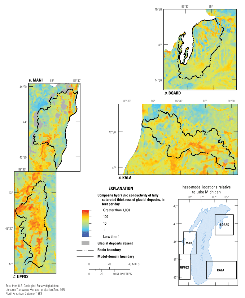
Maps showing composed (thickness-weighted) hydraulic conductivity in the glacial layers of the inset model for the A, Kalamazoo (KALA), B, Boardman-Charlevoix (BOARD), C, Upper Fox (UPFOX), and D, Manitowoc-Sheboygan (MANI) eight-digit hydrologic-unit code (HUC8) basins within the Lake Michigan Basin.
The original IMs (Feinstein and others, 2018) contained glacial and bedrock wells pumping at rates indicated by recent records. The GSM method can accommodate pumping wells, but in this application of the method, GSMs were designed to simulate undisturbed conditions and did not include pumping. To make the model types comparable, groundwater withdrawals from the IMs were set to zero. The lateral boundaries of these “no-pumping” versions were changed to a no-flow boundary condition. Unlike the GSMs, however, the no-flow conditions in the IMs are typically many miles from the boundary of the target HUC8 basins (fig. 1.6). Comparison of the “no-pumping” heads and fluxes to those from the original IMs showed only small differences; in particular, the removal of the wells resulted in only a very small increase in the fraction of cells with groundwater levels above land surface. Because pumping is considered to have minimal effects on the water levels or groundwater flow in the modeled area, it can be disregarded.
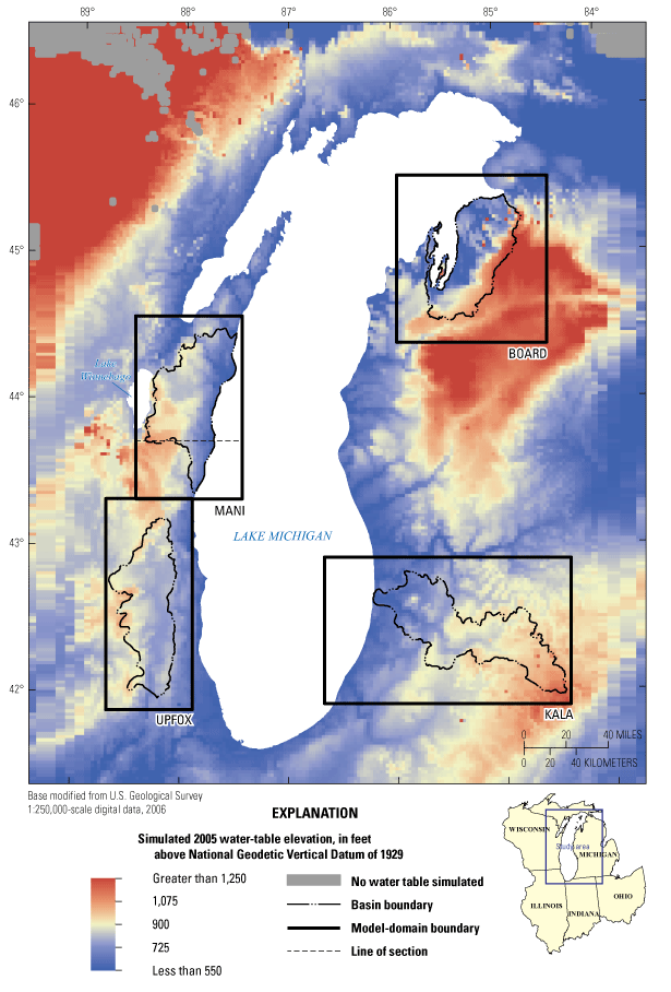
Map showing locations of eight-digit hydrologic-unit code (HUC8) basins and simulated water-table elevations in 2005 for four watershed areas near the Lake Michigan Basin. The HUC8 boundaries are enclosed within the boundaries of the domains of the inset models: KALA, Kalamazoo model; BOARD, Boardman-Charlevoix model; UPFOX, Upper Fox model; MANI, Manitowoc-Sheboygan model. (Duplicate of figure 1 in the main report.)
The IMs were not calibrated individually; the final parameters were derived from the calibration of the parent LMB model, with some adjustments described in Feinstein and others (2018). The parent model was calibrated by using conventional inversion techniques that are available through the PEST code (Doherty, 2008a, b) and that affect heads and flux observations (Feinstein and others, 2010).
A fifth IM was presented Feinstein and others (2018) but was not used in this study. The area corresponds to the combined Tacoosh-Whitefish and Fishdam-Sturgeon basins (WHITEDAM) in the Upper Peninsula of Michigan. This area was distinguished by very thin glacial deposits (with saturated thickness of about 20 ft), a high density of water bodies (largely swamps), and simulated travel times that were very young (Fienen and others, 2018). The IM simulation for these basins also was characterized by an unrealistically high degree of flooding; in about one-third of the area, simulated groundwater levels are more than 5 ft above land surface, giving rise to spuriously high hydraulic gradients near surface-water features. For this reason, the calculated residence times and base-flow ages for the WHITEDAM model were not considered a reliable standard for comparison to corresponding GSM results and were accordingly excluded from the overall analysis.
Systematic Differences in Model Construction
Boundary conditions, lateral extent, and grid spacing (both horizontally and vertically) differ between GSMs and IMs. IMs are complex distributed-parameter models, whereas the GSMs have simpler parameter structure and boundary conditions. Model parameters for both model types, averaged over the same zones, showed systematic similarities and differences.
GSMs had no-flow boundaries at the HUC8 watershed boundary; therefore, the only flow out of the model was through streams within the HUC8 watershed. IMs had no-flow boundaries on the rectangle bounding the HUC8 watershed, and the model domain was two to four times larger than the HUC8 watershed. Flows to and from the HUC8 watershed in IMs accounted for 5 to 14 percent of inflow and 5 to 17 percent of outflow. Grid spacing in the GSMs was 1,000 ft, whereas the IMs had a 500-ft grid spacing. The glacial deposits in both the GSMs and IMs were divided into three layers. Layers in the GSMs were roughly of uniform thickness; however, there were only one or two layers representing all glacial deposits over much of the IM domains.
Sources and sinks of water also differed between the two model types. Recharge to both GSMs and IMs was based on different applications of the SWB-derived estimates. GSMs used Trost and others (2018), and IMs used Westenbroek and others (2010). In addition, the GSMs used one uniform recharge rate assigned to the coarse zone and a second to the fine zone; in the IMs, a recharge value was inherited from the parent model cell and was assigned to each refined grid cell in the IM. In both model types, water discharged through streams and standing water bodies such as lakes and large wetlands. The stream networks in both the GSMs and IMs were derived from all orders contained in the NHDplus network; however, streams were simulated by using different MODFLOW–NWT packages: IMs simulated streams with the streamflow routing package (SFR), and GSMs simulated streams with the DRAIN package. Water discharged to streams in both model types into cells where the head in the aquifer was greater than the specified stream elevation. Water in GSMs discharges only to streams, whereas water in the IMs also can discharge from the stream to the aquifer if the specified stream elevation is greater than the head in the aquifer, and if baseflow is available from upstream.
Water bodies such as lakes and large wetlands were simulated in both model types by using somewhat different approaches, but both approaches functioned similarly with water leaving the model through drain cells. Water bodies (other than streams) in IMs were simulated with the MODFLOW–NWT DRAIN package. Water bodies in GSMs were simulated as zones of very high hydraulic conductivity that were connected to drain cells representing streams; this structure focuses water through the features and directs the water out of the model through the drain cells.
Hydraulic properties also differed between GSMs and IMs. Horizontal hydraulic conductivity of glacial sediments (Kh) in GSMs was defined in two zones that corresponded to sediment texture, whereas in IMs, it was estimated cell-by-cell on the basis of the category of glacial material and interpolated maps of coarse fraction (Feinstein and others, 2018). Horizontal hydraulic conductivity of bedrock (Kb) in the GSMs was assigned a single value; in the IMs, it was assigned cell-by-cell on the basis of rock type and aquifer-test results. Bedrock in the IMs was divided into multiple layers representing distinct lithologic types, whereas the bedrock was represented by a single layer with uniform thickness in the GSMs. The bottom of the basal layer of both model types was a no-flow boundary. This was defined as the top of the Precambrian rock or at the top of an aquitard in the IMs and as a constant depth below the bottom of glacial sediments in the GSMs. The GSMs contained a single Kh:Kv (vertical anisotropy) ratio for all four model layers. The glacial Kv values for the IMs varied cell-by-cell on the basis of the category of glacial material and interpolated maps of coarse fraction. Vertical anisotropy between glacial sediments and bedrock for the IMs also was distributed on a cell-by-cell or zone basis.
Recharge was distributed to zones representing fine and coarse materials in GSMs by use of a fixed ratio, whereas recharge did not vary as a function of surficial geology in IMs. Kh values from glacial sediments from IMs were similar to those from GSMs in the two models KALA and BOARD and dissimilar in the two models UPFOX and, to a lesser extent, MANI. The Kh values of bedrock were somewhat similar between model types except for the UPFOX model. Estimates of Kh:Kv varied widely among model types but not in a systematic way; anisotropy values in GSMs were higher than those for IMs for two models (KALA and BOARD) and lower for two models (UPFOX and MANI). Vertical anisotropy ratios for the bedrock units in the Upper Midwest region clustered around 50:1 and were associated with the IMs (Feinstein and others, 2018), whereas for the four HUC8 areas, the GSM calibration process yielded a much larger range of values applied jointly to unconsolidated and bedrock layers. All of these inputs affect the results generated by the two sets of models.
References Cited
Bakker, M., Post, V., Langevin, C.D., Hughes, J.D., White, J.T., Starn, J.J., and Fienen, M.N., 2016, Scripting MODFLOW model development using Python and FloPy: Groundwater, v. 54, no. 5, p. 733–739. [Also available at https://doi.org/10.1111/gwat.12413.]
Doherty, J., 2008a, PEST, Model Independent Parameter Estimation—Addendum to User Manual (5th ed.): Brisbane, Australia, Watermark Numerical Computing, accessed October 1, 2009, at http://www.pesthomepage.org/Downloads.php.
Doherty, J., 2008b, PEST, Model Independent Parameter Estimation—User Manual (5th ed.): Brisbane, Australia, Watermark Numerical Computing, accessed October 1, 2009, at http://www.pesthomepage.org/Downloads.php.
Feinstein, D.T., Hunt, R.J., and Reeves, H.W., 2010, Regional groundwater-flow model of the Lake Michigan Basin in support of Great Lakes Basin water availability and use studies: U.S. Geological Survey Scientific Investigations Report 2010–5109, 379 p. [Also available at https://doi.org/10.3133/sir20105109.]
Feinstein, D.T., Kauffman, L.J., Haserodt, M.J., Clark, B.R., and Juckem, P.F., 2018, Extraction and development of inset models in support of groundwater age calculations for glacial aquifers: U.S. Geological Survey Scientific Investigations Report 2018–5038, 96 p. [Also available at https://doi.org/10.3133/sir20185038.]
Fienen, M.N., Nolan, B.T., Kauffman, L.J., and Feinstein, D.T., 2018, Metamodeling for groundwater age forecasting in the Lake Michigan Basin: Water Resources Research, v. 54, no. 7, p. 4750–4766. [Also available at https://doi.org/10.1029/2017WR022387.]
Fullerton, D.S., and Richmond, G.M., compilers, [1983–2007], Quaternary geologic atlas of the United States: U.S. Geological Survey Miscellaneous Investigations Series Map I–1420, 33 quadrangles, scale 1:1,000,000, accessed December 2, 2021, at https://on.doi.gov/2vwOIXJ.
Handman, E.H., Haeni, F.P., and Thomas, M.P., 1986, Water resources inventory of Connecticut, part 9—Farmington River Basin: Connecticut Water Resources Bulletin no. 29, 92 p., 4 pls., scale 1:48,000. [Also available at https://pubs.usgs.gov/unnumbered/70038342/report.pdf.]
Moore, R.B., and Dewald, T.G., 2016, The road to NHDPlus—Advancements in digital stream networks and associated catchments: Journal of the American Water Resources Association, v. 52, no. 4, p. 890–900. [Also available at https://doi.org/10.1111/1752-1688.12389.]
Niswonger, R.G., Panday, S., and Ibaraki, M., 2011. MODFLOW-NWT—A Newton formulation for MODFLOW-2005: U.S. Geological Survey Techniques and Methods, book 6, chap. A37, 44 p. [Also available at https://doi.org/10.3133/tm6A37.]
Oliphant, T.E., 2007, Python for scientific computing: Computing in Science & Engineering, v. 9, no. 3, p. 10–20. [Also available at https://doi.org/10.1109/MCSE.2007.58.]
Perez, F., and Granger, B., 2007, IPython—A system for interactive scientific computing: Computing in Science & Engineering, v. 9, no. 3, p. 21–29. [Also available at https://doi.org/10.1109/MCSE.2007.53.]
Schilling, K.E., 2009, Investigating local variation in groundwater recharge along a topographic gradient, Walnut Creek, Iowa, USA: Hydrogeology Journal, v. 17, no. 2, p. 397–407. [Also available at https://doi.org/10.1007/s10040-008-0347-5.]
Soller, D.R., and Garrity, C.P., 2018, Quaternary sediment thickness and bedrock topography of the glaciated United States east of the Rocky Mountains: U.S. Geological Survey Scientific Investigations Map 3392, 2 sheets, scale 1:5,000,000. [Also available at https://doi.org/10.3133/sim3392.]
Starn, J.J., and Belitz, K., 2018, Regionalization of groundwater residence time using metamodeling: Water Resources Research, v. 54, no. 9, p. 6357–6373. [Also available at https://doi.org/10.1029/2017WR021531.]
Trost, J.J., Roth, J.L., Westenbroek, S.M., and Reeves, H.W., 2018, Simulation of potential groundwater recharge for the glacial aquifer system east of the Rocky Mountains, 1980–2011, using the Soil-Water-Balance model: U.S. Geological Survey Scientific Investigations Report 2018–5080, 51 p. [Also available at https://doi.org/10.3133/sir20185080.]
U.S. Geological Survey, 2016, USGS water data for the Nation: U.S. Geological Survey National Water Information System database, accessed September 28, 2016, at https://doi.org/10.5066/F7P55KJN.
Westenbroek, S.M., Kelson, V.A., Dripps, W.R., Hunt, R.J., and Bradbury, K.R., 2010, SWB—A modified Thornthwaite-Mather soil-water balance code for estimating ground-water recharge: U.S. Geological Survey Techniques and Methods, book 6, chap. A31, 65 p. [Also available at https://doi.org/10.3133/tm6A31.]
Datum
Vertical coordinate information is referenced to the National Geodetic Vertical Datum of 1929 (NGVD 29).
Horizontal coordinate information is referenced to the North American Datum of 1983 (NAD 83).
Elevation, as used in this report, refers to distance above the vertical datum.
Abbreviations
BOARD
Boardman-Charlevoix model
DRN
Drain package in MODFLOW
GSM
general simulation model
HUC
hydrologic-unit code
IM
inset model
KALA
Kalamazoo model
Kh
horizontal hydraulic conductivity
Kv
vertical hydraulic conductivity
LMB
Lake Michigan Basin [model]
MANI
Manitowoc-Sheboygan model
NHD
National Hydrologic Dataset
NHDPlus
National Hydrologic Dataset Plus (enhanced version of NHD)
NSE
Nash-Sutcliffe model-efficiency coefficient
RTD
residence-time distribution
SFR
streamflow-routing package in MODFLOW
SWB
soil water balance
TTD
travel-time distribution
UPFOX
Upper Fox model
USGS
U.S. Geological Survey
VANI
vertical-anisotropy ratio
WBD
Watershed Boundary Dataset
For more information, contact
Director, New England Water Science Center
U.S. Geological Survey
10 Bearfoot Road
Northborough, MA 01532
dc_nweng@usgs.gov
or visit our website at
https://www.usgs.gov/centers/new-england-water-science-center
Disclaimers
Any use of trade, firm, or product names is for descriptive purposes only and does not imply endorsement by the U.S. Government.
Although this information product, for the most part, is in the public domain, it also may contain copyrighted materials as noted in the text. Permission to reproduce copyrighted items must be secured from the copyright owner.
Suggested Citation
Starn, J.J., Kauffman, L.J., and Feinstein, D.T., 2023, Groundwater residence times in glacial aquifers—A new general simulation-model approach compared to conventional inset models: U.S. Geological Survey Scientific Investigations Report 2021–5142, 37 p., https://doi.org/10.3133/sir20215142.
ISSN: 2328-0328 (online)
Study Area
| Publication type | Report |
|---|---|
| Publication Subtype | USGS Numbered Series |
| Title | Groundwater residence times in glacial aquifers—A new general simulation-model approach compared to conventional inset models |
| Series title | Scientific Investigations Report |
| Series number | 2021-5142 |
| DOI | 10.3133/sir20215142 |
| Publication Date | June 01, 2023 |
| Year Published | 2023 |
| Language | English |
| Publisher | U.S. Geological Survey |
| Publisher location | Reston, VA |
| Contributing office(s) | New England Water Science Center, New Jersey Water Science Center, Wisconsin Water Science Center |
| Description | Report: v, 37 p.; Data Release |
| Country | United States |
| State | Illinois, Indiana, Michigan, Wisconsin |
| Online Only (Y/N) | Y |
| Additional Online Files (Y/N) | N |