

Application of a Soil-Water-Balance Model to Estimate Annual Groundwater Recharge for Long Island, New York, 1900–2019
Links
- Document: Report (5.43 MB pdf) , HTML , XML
- Data Releases:
- USGS data release - Soil-water-balance model archive for Long Island, NY, 1900-2019
- USGS data release - Soil-water-balance groundwater recharge model results for Long Island, NY, 1900-2019
- USGS data release - Soil-water-balance model archive for Long Island, NY, 1900-2019
- NGMDB Index Page: National Geologic Map Database Index Page (html)
- Download citation as: RIS | Dublin Core
Abstract
A soil-water-balance (SWB) model was developed for Long Island, New York, to estimate the potential amount of annual groundwater recharge to the Long Island aquifer system from 1900 to 2019. The SWB model program is a computer code based on a modified Thornthwaite-Mather SWB approach and uses spatially and temporally distributed meteorological, land-cover, and soil properties as input to compute potential daily groundwater recharge. Simulated outputs indicate that island-wide potential groundwater recharge trends, as a percentage of precipitation, have increased approximately 3 percent during the 120-year period. The simulated results account for both climatic and land-cover changes that have occurred during the period. A change from undeveloped (forested land cover) to low- and medium-density residential land cover or land use increased potential groundwater recharge because of a decrease in evapotranspiration. During the 30-year period from 1900 to 1930, the simulated potential average groundwater recharge rate on Long Island was estimated to be 18.50 inches per year (in/yr), or a total of 1,243 million gallons per day, during the 30-year period from 1985 to 2015, the simulated potential average groundwater recharge rate estimate increased to 20.73 in/yr (a total of around 1,393 million gallons per day).
During the 1900–2019 simulation period, the potential average annual groundwater recharge rate was about 19.24 in/yr. The data for that period included values for a 3-year meteorological drought from 1963 to 1965, where the mean precipitation was about 26.5 percent lower than the long-term average of 46.7 in/yr, and the potential groundwater recharge rate was about 12.3 in/yr. During a 3-year wet period from 1982 to 1984, where mean precipitation was about 19.6 percent higher than the long-term average, the estimated potential groundwater recharge rate was about 26.8 in/yr.
Introduction
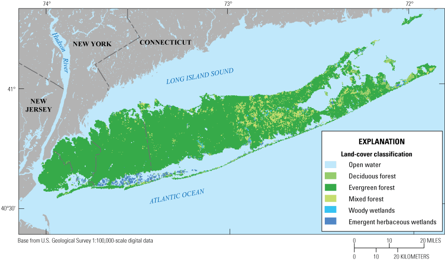
Long Island is part of southeastern New York and includes Kings, Queens, Nassau, and Suffolk Counties (fig. 1). The island is approximately 120 miles long, 1,400 square miles in area, and varies widely in both land cover and population density. Western Long Island, which includes Kings and Queens Counties, is a highly developed and urbanized area where the population density ranks second and fourth, respectively, when compared to all U.S. counties (Manson and others, 2018). The general west-to-east trend in land cover from central to eastern Long Island (Nassau and Suffolk Counties) is a transition from highly developed areas to medium- and low-intensity developed areas. Eastern Long Island is characterized primarily by low-intensity developed area (single-family housing units, undeveloped land, and agricultural land cover; fig. 2).
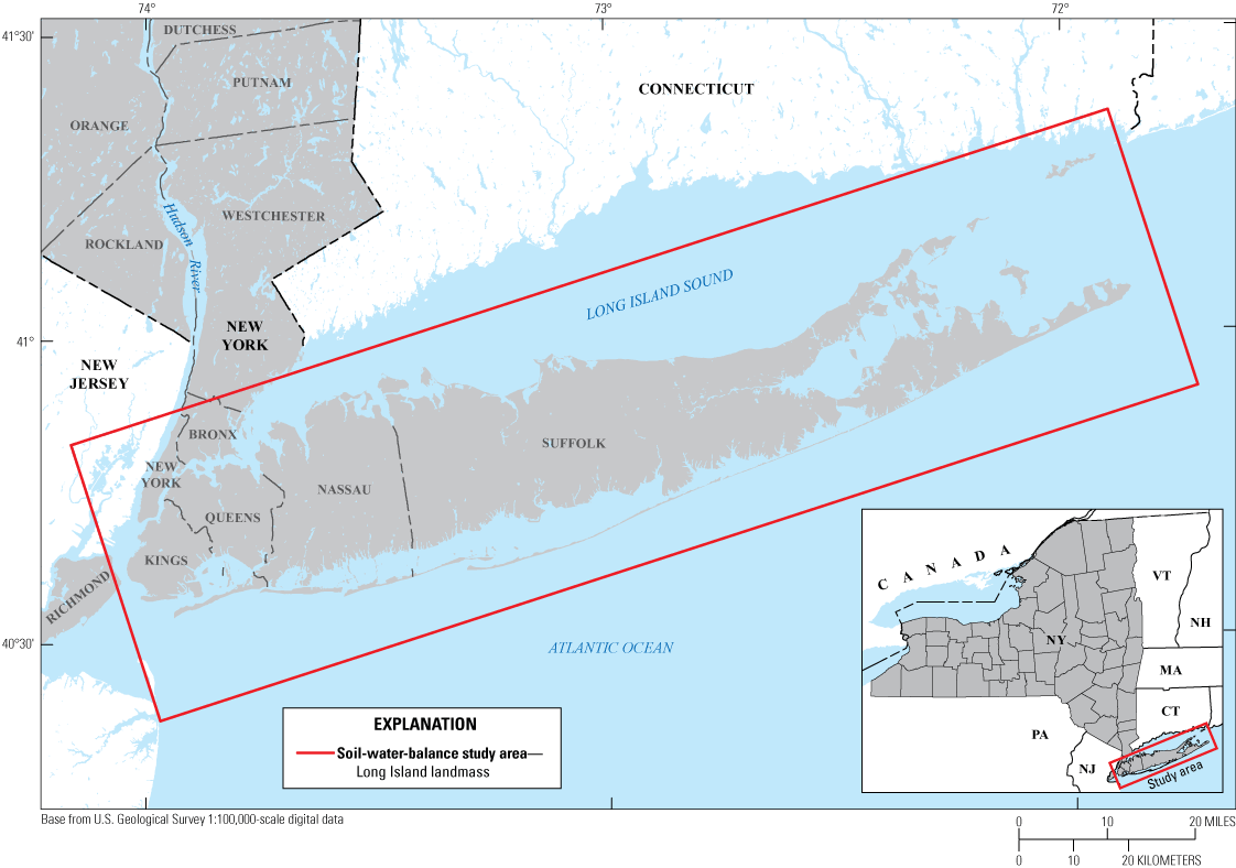
Map showing location of the Long Island, New York study area, which includes Kings, Queens, Nassau, and Suffolk Counties.
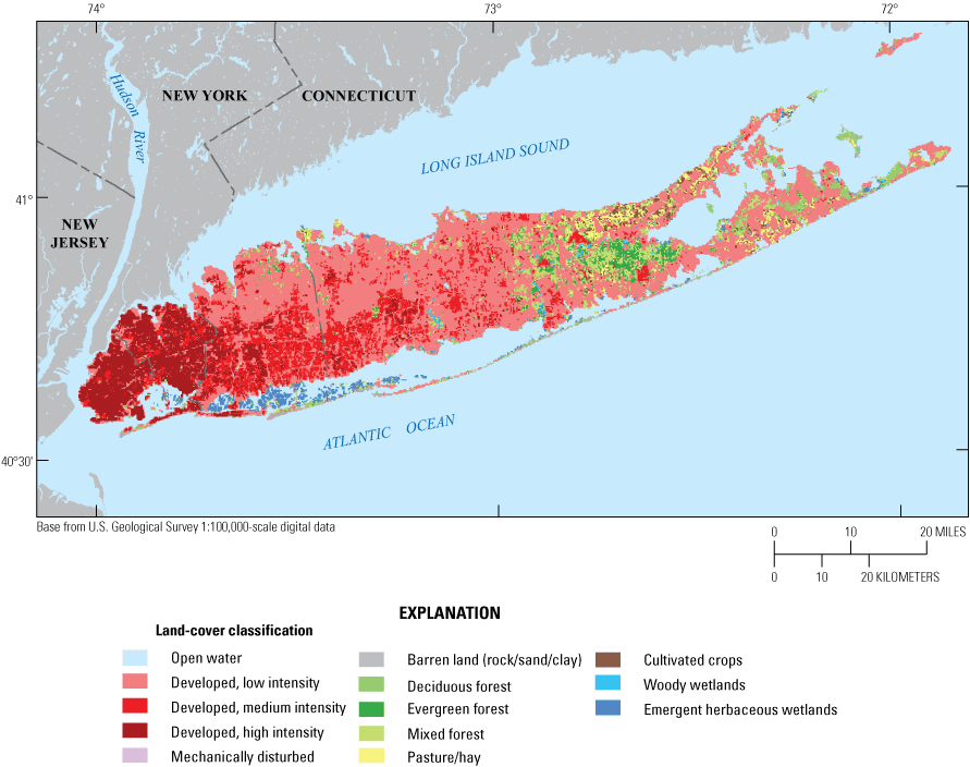
Map showing land-cover input for the soil-water-balance model, Long Island, New York, for 2015; modified from Sohl, Sayler, and others (2018).
The sole source of freshwater entering the Long Island aquifer system is groundwater recharge (referred to herein as recharge or potential recharge) from precipitation. The rate of recharge is influenced by many factors such as temperature, total precipitation, soil characteristics, and land cover.
A soil-water-balance (SWB) model (Westenbroek and others, 2010) was used to estimate recharge for Long Island on an annual basis during the 1900–2019 period. The model was designed to calculate the spatial distribution of potential shallow recharge over time using a gridded data structure and computing daily, monthly, or annual averaged datasets (Westenbroek and others, 2010). The model was based on a modified version of the Thornthwaite-Mather approach to calculate potential recharge (Thornthwaite and Mather, 1955, 1957).
Purpose and Scope
This report describes the development and results of the SWB model used to estimate potential recharge from 1900 to 2019 for the Long Island, New York regional aquifer system. Two SWB simulations were conducted for this study, with land cover being the factor that differentiated them. The first simulation used existing land-cover datasets (Sohl, Reker, and others, 2018; Sohl, Sayler, and others, 2018) to estimate the annual potential recharge with changing land-cover patterns from 1900 to 2019 (referred to herein as the postdevelopment simulation). The second simulation changed all land-cover categories including developed, mechanically disturbed, barren land, pasture and hay, and cultivated crops to the land cover category mixed forest to represent a predevelopment land-cover condition annually from 1900 to 2019 (referred to herein as the predevelopment simulation). This simulation was designed to calculate potential recharge for a predevelopment setting, without any human-induced changes to the land cover. These simulations were designed to calculate the amount of water affected by impervious surfaces in urbanized areas (referred to herein as rejected recharge or potential rejected recharge) by subtracting the predevelopment from the postdevelopment simulations for the equivalent year.
Previous Studies
Several previous studies discussed or estimated recharge to the Long Island aquifer system. Lusczynski (1952) and Soren (1971) discussed the relation of water levels to groundwater recharge in Kings and Queens Counties, respectively. Peterson (1987) used the tables in Thornthwaite and Mather (1957) to calculate evapotranspiration in Nassau and Suffolk Counties on the basis of precipitation values, climate maps, and land-use maps. Peterson (1987) also calculated direct runoff to streams and tidewater calculated from streamflow records and drainage-area maps. Peterson used all of these datasets to calculate recharge. Masterson and others (2013) used a SWB model to calculate potential recharge for the Northern Atlantic Coastal Plain aquifer system, which included Long Island.
Model Description and Input Requirements
The SWB computer model (Westenbroek and others, 2010) calculates potential recharge by using a modified Thornthwaite-Mather soil-water-balance approach (Thornthwaite and Mather, 1955, 1957). Potential recharge is defined as water that has infiltrated into the root zone, which may eventually leave the bottom of the root zone and become recharge (Westenbroek and others, 2018). This was calculated at daily time steps for each grid cell from 1900 to 2019 across Long Island. Each grid cell was a 100- by 100-meter square. The gridded data format of the SWB model allows the potential recharge grid to be rescaled to match the resolution of a differently sized groundwater-flow model grid (Westenbroek and others, 2010).
The gridded data inputs required for the SWB model to calculate potential recharge for each grid cell included (1) daily climate data, (2) hydrologic soil group categories and available water capacity measurements, (3) land-cover categories, and (4) groundwater-flow directions (fig. 3). The SWB model for this study calculated potential annual recharge from 1900 to 2019, but not all the data were available for the entire study period; therefore, a unique approach to expand the data resources was used.
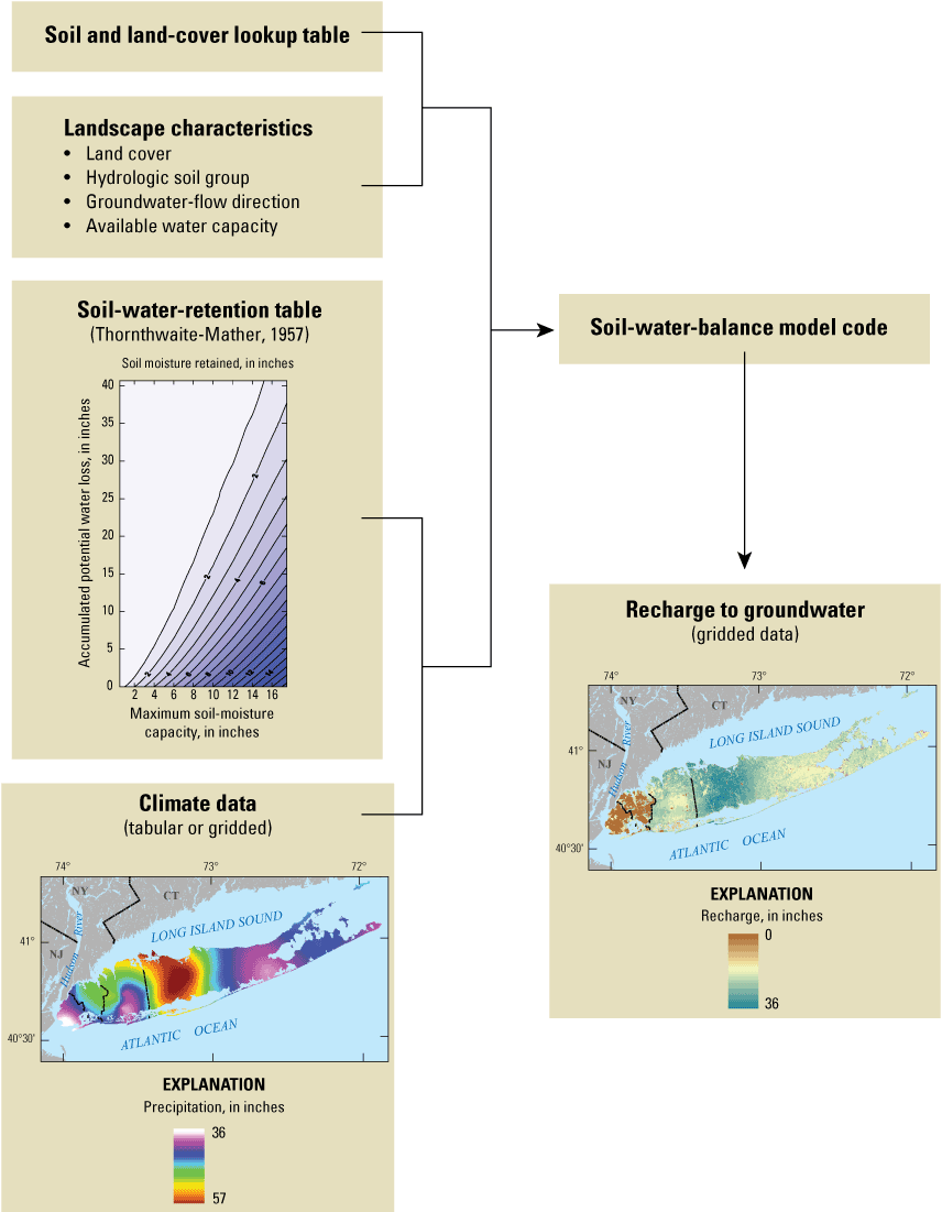
Flowchart showing interaction between the soil-water-balance model code and input data. Modified from Westenbroek and others (2010).
To reduce model computation time, the SWB model was divided into several smaller models of generally 11-year increments, whereby the starting year for each incremental model period acted as the precondition year for the remaining 10 model years and the outputs for the precondition year were discarded. For example, one smaller SWB model covered the years 1920–30, where 1920 was the precondition year generated by the 1910–20 SWB model output.
Meteorological Data Inputs
The meteorological data inputs needed for this SWB model were (1) total daily precipitation, (2) daily maximum temperature, and (3) daily minimum temperature. Gridded meteorological data were downloaded from the Oak Ridge National Laboratory (ORNL; Thornton and others, 2014), for the years 1980–2019. Gridded meteorological data prior to 1980 were created by interpolating daily weather-station data from the National Oceanic and Atmospheric Administration (NOAA; National Oceanic and Atmospheric Administration, 2020) using a geographic information system (GIS).
The SWB model required the climate data to be in the same format for the entirety of each incremental model. As stated previously, the SWB model required a precondition year to be run, which meant the model would have to start 1 year before the simulation period, in 1899. The year 1980 acted as the pivot year between the two meteorological datasets. The SWB model outputs for 1980 were modeled as a part of the 1970–80 incremental model, which used the interpolated NOAA weather-station data. ORNL data was used as the input for 1980 (and every year after), which acted as the precondition year for the 1980–90 incremental model.
Daymet Data for 1980–2019
Meteorological data were obtained from the ORNL’s Daymet dataset, which included daily data collected at meteorological stations across North America. These data were interpolated to gridded outputs at a 1-square-kilometer resolution each day between 1980 and 2019 (Thornton and others, 2014, 2017, 2020). Daymet version 2 data were used for years 1981–2011, version 3 data were used for years 2012–16, and version 4 data were used for years 2017–19.
These gridded datasets were downloaded as Network Common Data Form (NetCDF) files for inputs to the incremental SWB models. The precipitation data were converted to inches, and the temperature data were converted to degrees Fahrenheit. These conversions were directly applied within the SWB code.
National Oceanic and Atmospheric Station Data for 1899–1980
Meteorological data were available from a network of 150 NOAA meteorological stations during the period 1899–1980 (National Oceanic and Atmospheric Administration, 2020). Although the data collected at all the stations were not continuous throughout the period, and the number of stations with available data changed throughout the period, these were the best available data to use for generating raster grids representing the meteorological data necessary for the SWB model.
To ensure that the entire modeled area was represented in the daily interpolations, the selection of meteorological stations extended beyond Long Island. Data were collected from stations in southern New York, Connecticut, Rhode Island, Massachusetts, and northeastern New Jersey (fig. 4). Table 1 (in back of report) lists the locations of the stations along with the years for which data were used.
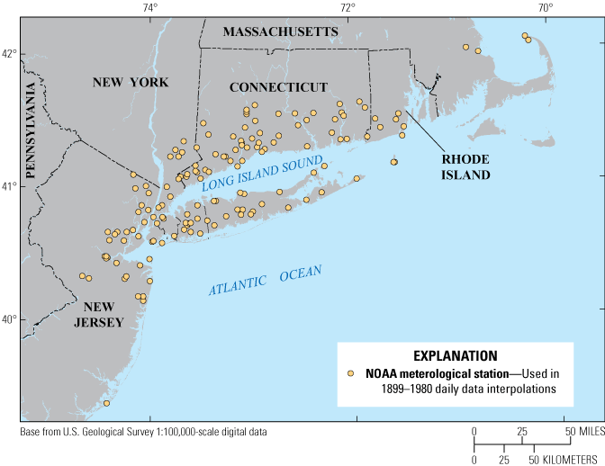
Map showing location of National Oceanic and Atmospheric Administration (NOAA) meteorological stations that provided input for the Long Island soil-water-balance model, 1899–1980.
For this study, the GIS interpolation tool Spline with Barriers (Esri, 2019) was used for generating the daily grids from the NOAA data. This tool interpolated a continuous surface between data points. The tool had several mandatory fields: (1) input point features (the latitude and longitude position), (2) a Z-value for each input point, and (3) an output raster. There were several optional fields: (1) input barrier features (features used to constrain the interpolation), (2) output cell size, and (3) smoothing factor. The daily meteorological station data points were the input point features. The Z-values included the daily measurements of either precipitation (in inches) or the maximum or minimum temperatures (in degrees Fahrenheit). The output rasters were either the daily precipitation (PRECIP) or the daily maximum (TMAX) and minimum (TMIN) temperatures, depending on the Z-value used as input. The output cell size was set to 1,000 meters, the smoothing factor input was set to 0.9, and the input barrier features were not used. The daily PRECIP, TMAX and TMIN output rasters were created by using the different input Z-values and executing the spline interpolation tool three individual times. A conditional tool was also used on the PRECIP raster to remove any negative interpolated values created by the spline interpolator. These daily gridded raster outputs became the daily meteorological inputs of the SWB model from 1899 to 1980.
Both the interpolated NOAA and Daymet datasets for Long Island were used to create the daily meteorological data input for 1899–2019 required by the SWB model code. A graph of the spatially averaged temperature and total precipitation for each year from 1900 to 2019 for Long Island is shown in figure 5. The temperature trend line shows an increase of 2.7 degrees Fahrenheit during the 120-year period. An increase of 4.6 inches (in.) can be seen in the precipitation trend line, despite a major drought that occurred on Long Island during the 1960s.
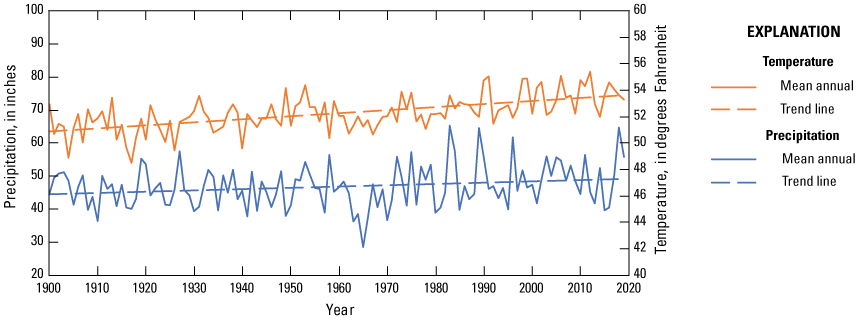
Graph showing mean annual temperature and precipitation for Long Island, New York, for each year from 1900 to 2019.
Hydrologic Soil Groups and Available Water-Capacity Inputs
Soil-related datasets were additional gridded input requirements for the SWB model code. They were the (1) hydrologic soil group dataset and (2) the available water capacity dataset. Both datasets were available through the Natural Resources Conservation Service Soil Data Development Toolbox extension in ArcMap (Peaslee, 2020). A hydrologic soil group category and an available water capacity value were assigned to every SWB model grid cell. The categories and values were unchanged throughout the 120-year period and did not vary between the pre- and postdevelopment SWB model simulations.
The soils were categorized and grouped using a letter designation of A through D on the basis of the soil infiltration rate (Peaslee, 2020). Soils in group A had the highest infiltration rate (greater than 0.30 inches per hour) and consisted mostly of sandy soils, whereas those in group D had the lowest rate (less than 0.05 inches per hour) and consisted mostly of clayey soil (Natural Resources Conservation Service, 2019). Soils in group A are most common in Nassau and Suffolk Counties, whereas soils in group B are most common in Kings and Queens Counties (fig. 6; table 2).
The available water capacity is defined as the amount of water that a soil can store for potential use by plants (Smith and Westenbroek, 2015). Figure 7 shows the available water capacities for soils on Long Island (Peaslee, 2020). These data are expressed in inches of water per foot of soil thickness. Generally, available water capacity varies depending on the organic matter content, texture, and structure of the soil (Natural Resources Conservation Service, 2019). In general, coarse-grained soils have a lower water capacity than fine-grained soils because of the larger pore spaces between the coarse grains, which allow the water to drain more freely.
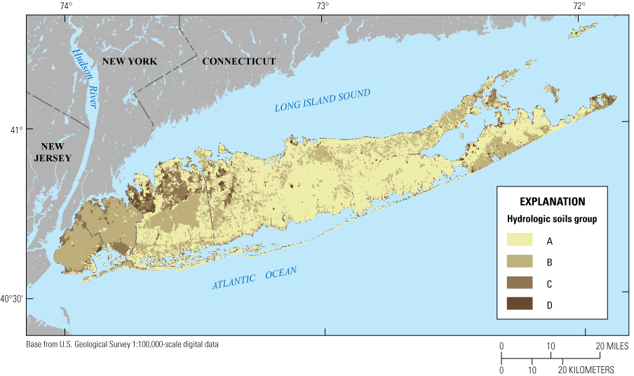
Map showing hydrologic soil groups on Long Island, New York, at a 100-meter resolution, modified from Peaslee (2020).
Table 2.
Distribution of hydrologic soil groups over the Long Island, New York study area.[Hydrologic soil group designations are based on Peaslee (2020)]
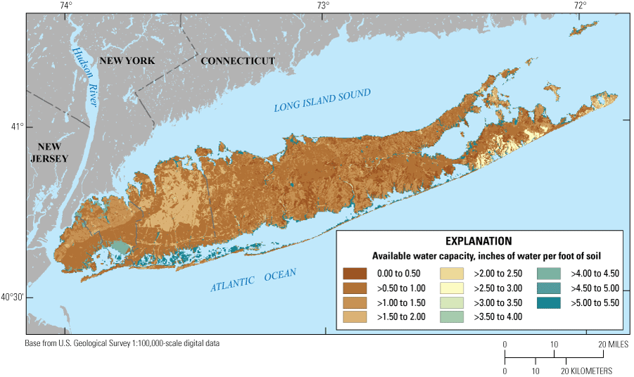
Map showing available water capacity for soils on Long Island, New York, at a 100-meter resolution, modified from Peaslee (2020).
Land-Cover Inputs
Annual land-cover grids for inputs to the SWB model are available from 1938 to 1992 in Sohl, Reker, and others (2018) and from 1992 to 2005 in Sohl, Sayler, and others (2018). These gridded data have a spatial resolution of 250-m pixels with 14 unique land-cover categories, although not all of those categories applied to Long Island. The published data were arranged in an Albers Equal Area Conic projection and were reprojected to a Universal Transverse Mercator (UTM) projection for the SWB model.
Modifying Land-Cover Data
A limitation to using the Sohl, Reker, and others (2018) dataset was that they used one land-cover category to represent developed areas. They identified developed areas based on available U.S. Census housing density data. Because all developed areas were recognized as one category, it was not possible to represent variable population densities or the various impervious surfaces that are present across Long Island.
For this SWB model, the developed areas from Sohl, Reker, and others (2018) were broken into three different categories based on development intensity: low, medium, and high. Identifying the development intensity was done using U.S. Census population totals for each year. Every 10 years, the U.S. Census Bureau publishes population totals at varying spatial scales: tract, block group, and block (Manson and others, 2018). These population totals were apportioned over a 500-foot model grid of Long Island; this grid was the same as was used in a groundwater-flow model for Long Island by Walter and others (2020). A linear progression of population growth or decline was assumed during each 11-year interval to assign a unique population total to each model grid cell for every year from 1900 to 2019. The derived population grid was applied to the 250-m resolution land-cover dataset for each year. If a grid cell was classified as developed in Sohl, Reker, and others (2018), it was made more specific by assigning an intensity level based on the population count within that grid cell. A cell with a population between 1 and 50 represented low-intensity development, a population of 51 to 100 represented medium-intensity development, and a population greater than 100 represented high-intensity development.
In addition to expanding the developed land-cover category into the three unique classes, other modifications were made to model potential recharge from 1900 to 2019. Prominent airports, parks and cemeteries in Kings and Queens Counties, commercial lands, and some water bodies across Long Island were not reflected appropriately in the USGS land-cover datasets. Therefore, the land-cover datasets were modified based on when an airport or commercial area was built. With respect to the land-cover categories, airports were changed to represent either high- or medium-intensity development (matching it with the surrounding land cover), parks and cemeteries in Kings and Queens Counties were changed to represent either medium- or low-intensity development, and commercial lands were changed to represent either high- or medium-intensity development (matching it with the surrounding land cover).
Land-Cover Data for 1900–37 and 2006–19
The 1938 and 2005 land-cover datasets from Sohl, Reker, and others (2018) were used as a starting point to create the land-cover inputs for 1900–37 and 2006–19, respectively. The 1900–37 data use the same land-cover categories as 1938 across Long Island. From 1900 to 1937, the only grid cells that changed categories were those of developed land (low-, medium-, and high-intensity development), which were dependent on the U.S. Census population within a grid cell for each year (described in the previous section). The land-cover datasets for 2006 to 2019 had the same categorical spatial distribution as that published for 2005. The development intensity was again adjusted to reflect the population changes during the 2006–19 period and those associated categorical changes were in turn made to the model grid. Figure 8 shows the modified SWB model land-cover data for Long Island during 1900 and 2019.
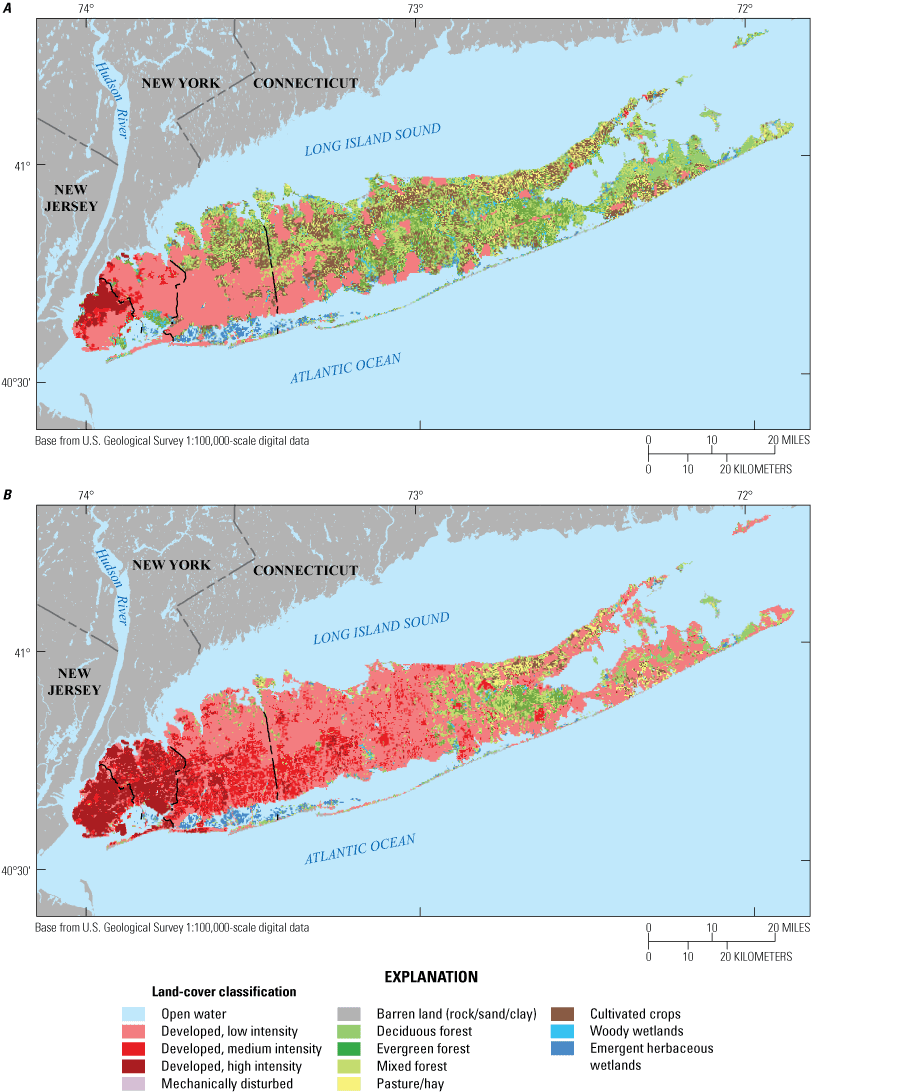
Maps showing land-cover input for the postdevelopment soil-water-balance model for A, 1900; and B, 2019, for Long Island, New York; modified from Sohl, Reker, and others (2018) and Sohl, Sayler, and others (2018).
Soil and Land-Cover Lookup Tables
Soil and land-cover lookup tables associated with the SWB model allow users to assign model cell properties related to the amount of recharge a particular soil and land-cover combination will absorb. The lookup table values for the soil parameters (runoff curve values and root zone depths), maximum recharge rate, and precipitation interception storage are provided for each land-cover or land cover and soil-group combination and used as input to the SWB model. The SWB model code calculates potential recharge, evaporation, transpiration, interception, runoff, and a few other water-balance components for each model cell. This calculation is done by cross-referencing the value of the gridded inputs (land-cover category, meteorological data, hydrologic soil group, and available water capacity) with the values in the lookup table.
There are two lookup tables for this study: a postdevelopment lookup table (table 3) and predevelopment lookup table (table 4). The parameters for each were modified from lookup table descriptions in a larger study of the Northern Atlantic Coastal Plain aquifer system (Masterson and others, 2013), which included Long Island. The predevelopment simulation lookup table was modified to reflect mixed forest properties in several land-cover categories including: all three categories of developed land, mechanically disturbed land, barren land (rock, sand, and clay), pasture and hay, and cultivated crops.
Table 3.
Postdevelopment scenario lookup table for the soil-water-balance model, showing land-cover categories and corresponding recharge rates and hydrologic soil group properties for Long Island, New York. Modified from Masterson and others (2013).Table 4.
Predevelopment scenario lookup table for the soil-water-balance model, showing land-cover categories and their corresponding recharge rates and hydrologic soil group properties for Long Island, New York. Modified from Masterson and others (2013).Interpretation of Land-Cover Inputs Used in Soil-Water-Balance Model Simulations
The two SWB simulations completed for this study required the land-cover inputs to be represented differently. The postdevelopment SWB simulation land-cover inputs depict the land cover as it changed over time. Figure 8B illustrates the SWB model land-cover input used for the postdevelopment simulation for 2019. Figure 9 illustrates the SWB model land-cover input used for the predevelopment simulation for 2019. The predevelopment SWB model simulated land-cover inputs depict land cover in a simulation with many of the land-cover categories changed to properties of the mixed forest land cover (fig. 9). The result simulates a development-free landscape for Long Island. Adjusting the recharge properties of the land-cover categories for the predevelopment simulation was also done through adjusting the predevelopment lookup table (table 4).
Map showing representation of land cover based on the lookup-table modifications for the predevelopment simulation of the soil-water-balance model for Long Island, New York, for 2019.
Recharge Analysis
The SWB model was used to estimate potential recharge for Long Island on an annual basis for 1900–2019 for both the postdevelopment and predevelopment simulations. The model created annual potential recharge outputs in the form of American Standard Code for Information Interchange (ASCII) files. The SWB model simulated the daily meteorological data to estimate an annual mean potential recharge value for each year under both simulations.
Comparing potential recharge results from both the postdevelopment and predevelopment simulations can be used to estimate the amount of potential rejected recharge, which represents the amount of potential recharge lost due to urbanization. Recharge is rejected mainly because of human-induced changes to the landscape during the 120-year period.
The mean annual potential recharge amounts for both simulations are shown for Long Island as a whole (fig. 10) and for each of the four Long Island counties (fig. 11). The results suggest how the variability in potential recharge across Long Island might be due to the spatial changes in the land-cover data.
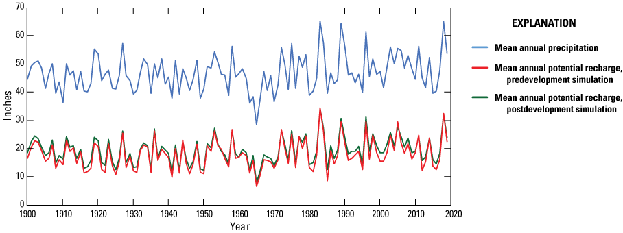
Graph showing mean annual potential recharge for both the predevelopment and postdevelopment soil-water balance simulations compared to mean annual precipitation.
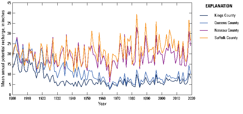
Graph showing mean annual potential recharge for Long Island counties.
Postdevelopment and Predevelopment Simulation Results
The SWB model simulated both postdevelopment and predevelopment conditions from 1900 to 2019. The postdevelopment simulation shows that the mean annual potential recharge rate across Long Island varied from a low of 7.57 inches per year (in/yr) in 1965 to a maximum of 34.44 in/yr in 1983 (fig. 10). The predevelopment simulation results show that the mean annual potential recharge rate ranged from 6.43 in/yr in 1965 to 34.28 in/yr in 1983 (fig. 10). These simulation results indicated that—on average—40.7 percent of precipitation was recharged to the aquifers under postdevelopment conditions and 37.5 percent of precipitation was recharged under predevelopment conditions. The mean annual potential recharge rate across Long Island was 19.24 in/yr (1,293 million gallons per day [Mgal/d]) and 17.81 in/yr (1,197 Mgal/d) for the post- and predevelopment simulations, respectively. Despite the increase in impervious surfaces during the postdevelopment simulation, the overall increase in the island-wide recharge rate likely reflects deforestation in the eastern part of the island.
The deforestation that has occurred on Long Island has reduced evapotranspiration, which allows for more precipitation to infiltrate the ground (Yang and others, 2014). Despite the impervious surfaces that are present, precipitation infiltrated the ground at a higher rate in the postdevelopment simulation than in the predevelopment simulation, in which forested conditions and low- to medium-intensity developed areas were prevalent; however, for the high-intensity development areas, where impervious surfaces are much more widespread, infiltration rates were lower and the rejected recharge amounts were higher, thus increasing overland surface runoff. A breakdown of the data by county helps illustrate these relations and is discussed in the following section. When comparing the spatial distribution of recharge for the postdevelopment and predevelopment simulations in 2019, potential recharge is higher in western Long Island in the predevelopment simulation, and higher in eastern Long Island in the postdevelopment simulation (fig. 12). This was a common pattern in each year of the predevelopment simulation.
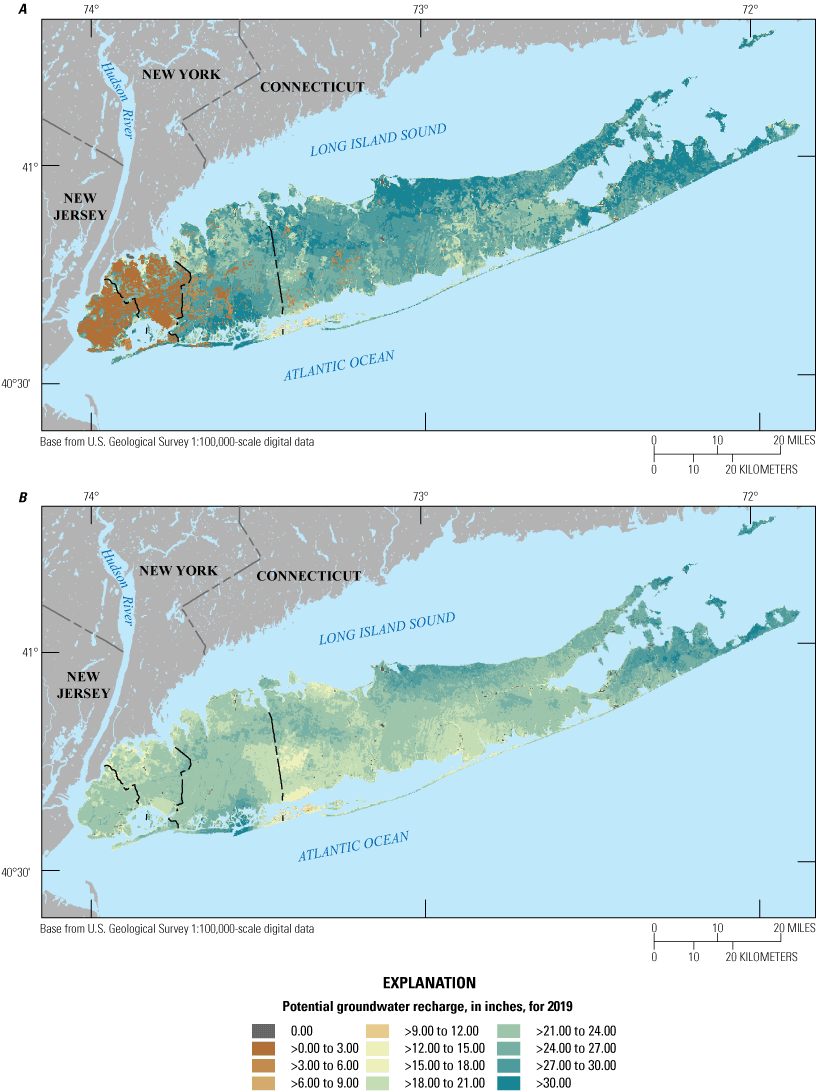
Maps showing potential recharge on Long Island for 2019, as computed by the soil-water-balance model, for A, postdevelopment simulation; and B, predevelopment simulation.
Most of Kings and Queens Counties in western Long Island was simulated to receive only 1 to 2 in. of potential recharge in the postdevelopment model because of the influence of high-intensity development and the land-cover lookup table inputs used in table 4. The predevelopment model, using forested land cover, provided an approach to estimate the amount of water that would have recharged into the aquifer system under natural conditions. This approach was used to determine the potential rejected groundwater recharge (lost recharge) that would be captured in storm drains, retention basins, and—in the case of Kings and Queens Counties—the combined sewer system (fig. 13). The difference between the pre- and postdevelopment SWB model simulations estimated a potential rejected recharge of 19.24 in. (around 167 Mgal/d) for 2019 in Kings and Queens Counties combined. No rejected recharge amounts are shown where there was more potential recharge occurring during the postdevelopment SWB model simulation (much of Nassau and Suffolk Counties).
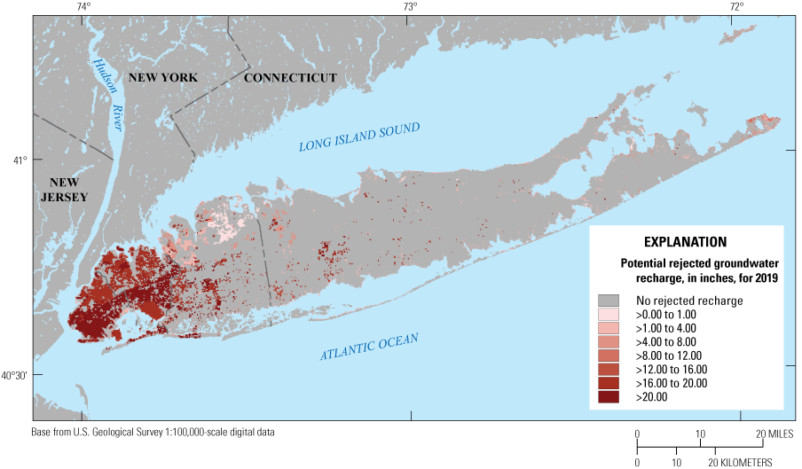
Map showing potential rejected groundwater recharge (predevelopment results minus postdevelopment results) on Long Island for 2019, as computed by the soil-water-balance model.
The overall postdevelopment simulated potential recharge (fig. 12A) was greater than the predevelopment simulated potential recharge (fig. 12B) in the low- to medium-intensity developed areas, which were mostly located in Suffolk and Nassau Counties. The predevelopment simulation results with forested land cover showed that more evapotranspiration occurred in what are now low-to medium-density developed areas, meaning less water was available to infiltrate and recharge the aquifer (fig. 14).
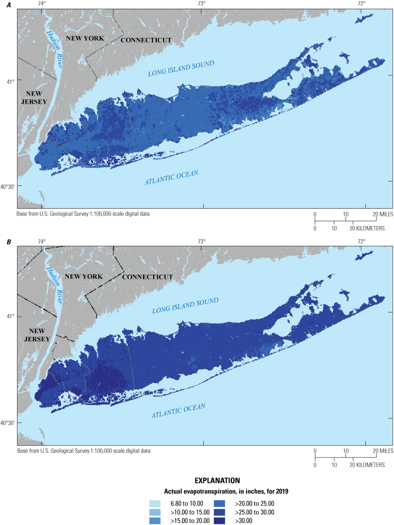
Maps showing actual evapotranspiration on Long Island for 2019, as computed by the soil-water-balance model, for A, postdevelopment simulation; and B, predevelopment simulation.
Recharge Totals by County
The potential recharge amounts simulated and averaged for all of Long Island (fig. 10) do not provide insight into the spatial variability of potential recharge seen across the island (fig. 12). A graph of the mean annual potential recharge for the postdevelopment land-cover simulation by county (fig. 11) shows recharge for Kings and Queens Counties diverges from Nassau and Suffolk Counties over time. This divergence between the two sets of counties is largely the result of impervious surface development in western relative to eastern Long Island.
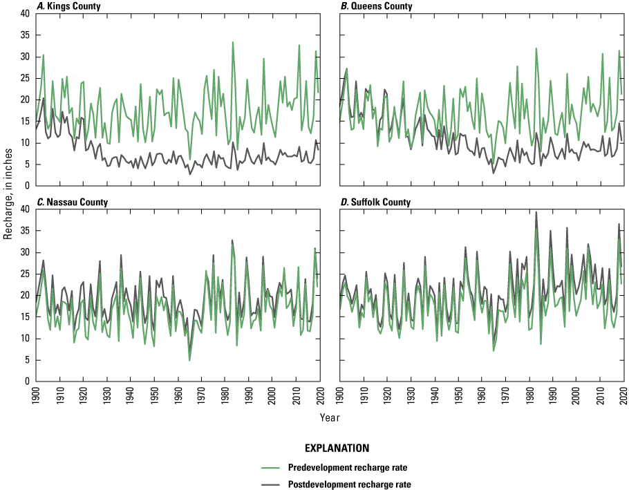
Graphs showing mean annual potential recharge rates for Long Island counties for both the predevelopment and postdevelopment land-cover simulations, from 1900 to 2019. A, Kings County; B, Queens County; C, Nassau County; and D, Suffolk County.
Both pre- and postdevelopment land-cover simulations for Nassau and Suffolk Counties indicate that the annual differences in recharge rates are relatively small (2.8 and 2.56 in. respectively) compared with Kings and Queens Counties (10 and 5.76 in. respectively). The mean annual potential recharge for Suffolk County is 21.16 in. for the postdevelopment and 18.36 in. for the predevelopment simulation. Similarly, the mean annual potential rechange for Nassau County is 19.13 in. for the postdevelopment and 16.57 in. for the predevelopment simulation. Although the differences are small, recharge rates are almost always greater during the postdevelopment simulation (fig. 15) and are likely attributed to the loss of forested land cover in what are now low- and medium-intensity developed areas throughout both Nassau and Suffolk Counties.
In Kings and Queens Counties, the differences between pre- and postdevelopment simulated potential recharge rates are much more pronounced than those for Nassau and Suffolk. The mean annual potential recharge for Kings County is 7.52 in. for the postdevelopment and 17.52 in. for the predevelopment simulation. Similarly, the mean annual potential rechange for Queens County is 10.92 in. for the postdevelopment and 16.68 in. for the predevelopment simulation. The large differences between the post- and predevelopment simulations for the two counties highlight the effects of the high-intensity development and the impervious surfaces in these highly urbanized areas.
Comparison to Previous Studies
Lusczynski (1952) did not provide a quantitative estimate of recharge for Kings County; however, he indicated that the development and increase of impervious surfaces that occurred in Kings County from the early 1900s through 1930 coupled with lower-than-average precipitation rates in the early 1930s caused a reduction in natural recharge. These factors—along with the increased groundwater withdrawal that accompanied population growth—caused a substantial depression in the water table. Although this study did not evaluate groundwater levels, the decline in natural recharge from 1900 through the 1930s, as discussed by Lusczynski (1952), is consistent with the mean annual potential recharge simulated by the SWB model (fig. 15A).
Soren (1971) estimated that the average recharge rate from precipitation in Queens County during the mid-1900s was about 55 Mgal/d (10.41 in/yr) and that the recharge rate from precipitation during the drought years of 1962–66 declined to about 40 Mgal/d (7.57 in/yr) or less. The mean potential recharge rate for 1930 to 1970 in Queens County estimated by the SWB model is 9.32 in/yr; this time period includes the drought years for which Soren (1971) estimated recharge. The SWB model estimated that the potential recharge rate for the drought years 1962–66 was about 5.00 in/yr for Queens County, about 2.5 in. less than the rate estimated by Soren (1971).
For the period 1968–75, Peterson (1987) estimated the regional groundwater recharge rate for Nassau County to be 20.6 in/yr (47.6 percent of precipitation) and the evapotranspiration rate to be 21.8 in/yr (50.3 percent of precipitation). For Suffolk County, Peterson (1987) estimated the recharge rate to be 23.5 in/yr (51.2 percent of precipitation) and the evapotranspiration rate to be 22.1 in/yr (48.1 percent of precipitation). The precipitation rates used by Peterson (1987) were 43.3 in/yr for Nassau County and 45.9 in/yr for Suffolk County. At the time, these values validated using 50 percent of precipitation to estimate recharge for Long Island.
For the period 1900–2019 for Nassau County, the SWB model estimated that the average recharge rate was 19.13 in/yr (41.1 percent of precipitation) and the average evapotranspiration rate was 23.10 in/yr (49.6 percent of precipitation). For the same period for Suffolk County, the SWB model estimated that the average recharge rate was 21.16 in/yr (45.2 percent of precipitation) and the average evapotranspiration rate was 22.68 in/yr (48.4 percent of precipitation). The average precipitation rate for 1900–2019 was 46.6 in/yr for Nassau County and 46.8 in/yr for Suffolk County. For the period 1968–75 (the period studied by Peterson, 1987) for Nassau County, the SWB model estimated that the average recharge rate was 19.63 in/yr (42.3 percent of precipitation) and the average evapotranspiration rate was 21.19 in/yr (45.7 percent of precipitation). For the same period for Suffolk County, the SWB model estimated that the average recharge rate was 21.61 in/yr (46.9 percent of precipitation) and the average evapotranspiration rate was 21.69 in/yr (47.1 percent of precipitation). All of these calculations indicate that using an assumed recharge rate of 50 percent of precipitation may have resulted in an overestimation of recharge.
Lastly, Masterson and others (2013) used a SWB model to calculate potential recharge for 2005–9 for the Northern Atlantic Coastal Plain aquifer system, in which Long Island was a part. Recharge rates were not broken down by State or county; however, they indicated that the mean annual potential recharge rate on eastern Long Island reached as high as 37.3 in/yr, which was the highest throughout their entire study area. For the same time period for eastern Long Island, the SWB model used in this study estimated that the mean annual potential recharge rate to be slightly higher, at around 39 in/yr.
Limitations of Soil-Water-Balance Model Analysis
This SWB model analysis has a number of limitations and uncertainties related to the input datasets. The greatest are related to (1) the spatial distribution of the U.S. Census population, which was used to classify low-, medium-, and high-intensity development; (2) the interpolation of meteorological data to generate daily precipitation and maximum and minimum temperature grids for the years 1900–80, as well as the interpolation processes used by the ORNL for the Daymet datasets for 1980–2019; and (3) modifications of the predevelopment simulation lookup table to assume a widespread forested land-cover type. All recharge grids generated as a part of this analysis are representative of potential recharge and do not yield actual recharge values.
The U.S. Census collects data on 100 percent of the population every decade. The population totals are grouped and summed into different census shapes (tracts, block groups, blocks). These shapes are not consistent and vary from decade to decade. To standardize the population counts for the SWB model, all decadal population counts were distributed to the Long Island model grid used for the groundwater-flow model (Walter and others, 2020). A linear interpolation between decadal census years was applied to each grid cell so that a continuous annual population dataset from 1900 to 2019 could be used to identify spatial differences in population intensity. Because the 2020 census was not available at the time of this analysis, the same rate of population change was applied to years 2011–19 as was seen for years 2000–10.
The annual population totals were then applied to the land-cover grids and reclassified as either low-, medium-, or high-intensity development. A population between 1 and 50 was designated as low, a population between 51 and 100 was medium, and any grid cell with a population greater than 100 was high. Altering these population bins changed all land-cover inputs to the SWB model; however, it was a necessary measure to add more detail to the land-cover inputs because, in their published state, only one population category was present. The reclassification was a way to show the variability of population across Long Island during the entire period.
Daily climate data were not available in a gridded data structure before 1980; therefore, an interpolation tool (Spline with Barriers) was used to generate the daily climate grids in ArcGIS Desktop. The tool interpolated a continuous surface between the NOAA weather stations (fig. 4) for precipitation, maximum temperature, and minimum temperature. The output raster grids are the climate parameters necessary to run the SWB model.
Additional limiting assumptions included changes made to the land-cover lookup table to group various land-cover types. For example, in the predevelopment simulation, most of the land cover was set to evergreen forest conditions because the land-cover properties for evergreen forest are an averaged value of all three forested land-cover types present on Long Island.
It is also important to note that for the purposes of this application, both soil coverages (hydrologic soil group and available water capacity) were assumed to be constant throughout the simulation period. And lastly, surface-water flow direction was not included as part of the SWB model. This option is sometimes selected to channel overland flow between cells within the model domain (Smith and Westenbroek, 2015); however, its exclusion in this SWB model means that any rejected recharge did not get redirected to neighboring SWB model grid cells.
Summary
Understanding and quantifying the amount of groundwater recharge, both spatially and temporally, is an important part of any hydrologic study. To that end, a soil-water-balance (SWB) model was developed for Long Island, New York, to estimate the potential amount of annual groundwater recharge to the Long Island aquifer system from 1900 to 2019. The SWB computer model estimated recharge by using a modified Thornthwaite-Mather SWB approach. The model provided recharge simulations for both predevelopment and postdevelopment land-cover conditions for the 120-year period. Assessing the simulated results on a county-by-county basis provides a better understanding of the effects of land-cover change on recharge compared to an aggregated island-wide analysis.
From 1900 to 2019, the SWB model estimated the mean annual recharge rate to be 19.24 inches per year, which is roughly 41.2 percent of the mean island-wide precipitation. The SWB analysis showed an average increase in recharge over time across Long Island, suggesting that the shift in land cover from undeveloped, forested areas to the low- to medium-intensity-developed areas in central and eastern Long Island has more than offset the development of impervious surfaces in western Long Island. The net effect of this landscape evolution is for a greater percentage of precipitation to recharge the aquifer system than had occurred under predevelopment conditions.
The county-level results more clearly illustrate the effects that land cover and development have on groundwater recharge. The differences in potential recharge between the postdevelopment and predevelopment simulations for Kings and Queens Counties are much larger than estimated in the same simulations for Nassau and Suffolk Counties. The impervious surfaces and high-intensity developed areas limited the amount of potential recharge in the postdevelopment simulation. More potential recharge occurs in Kings and Queens Counties under the forested predevelopment simulation, whereas the potential recharge is slightly higher under the postdevelopment simulation for Nassau and Suffolk Counties.
Any user of these data should be sure to understand the model limitations and assumptions that are described in preceding sections in this report. Two U.S. Geological Survey data releases (Finkelstein, 2022 and Finkelstein and others, 2022) document the SWB model construction, results, and other model information.
Table 1.
National Oceanic and Atmospheric Administration meteorological stations that provided inputs for the Long Island soil-water-balance model, 1899–1980.[NOAA, National Oceanic and Atmospheric Administration]
References Cited
Esri, 2019, Spline with barriers (spatial analyst): Esri web page, accessed July 20, 2020, at https://pro.arcgis.com/en/pro-app/latest/tool-reference/spatial-analyst/spline-with-barriers.htm.
Finkelstein, J.S., 2022, Soil-water-balance model archive for Long Island, NY, 1900-2019: U.S. Geological Survey data release, https://doi.org/10.5066/P94OLK6Z.
Finkelstein, J.S., Monti, J., Masterson, J.P., and Walter, D.A., 2022, Soil-water-balance groundwater recharge model results for Long Island, NY, 1900-2019: U.S. Geological Survey data release, https://doi.org/10.5066/P9V2NMUB.
Lusczynski, N.J., 1952, The recovery of ground-water levels in Brooklyn, New York, from 1947 to 1950: U.S. Geological Survey Circular 167, 29 p. [Also available at https://doi.org/10.3133/cir167.]
Masterson, J.P., Pope, J.P., Monti, J., Jr., Nardi, M.R., Finkelstein, J.S., and McCoy, K.J., 2013, Hydrogeology and hydrologic conditions of the Northern Atlantic Coastal Plain aquifer system from Long Island, New York, to North Carolina (ver. 1.1, September 2015): U.S. Geological Survey Scientific Investigations Report 2013–5133, 76 p. [Also available at https://doi.org/10.3133/sir20135133.]
Manson, S., Schroeder, J., Van Riper, D., Kugler, T., and Ruggles, S., 2018, National historical geographic information system—Version 13: IPUMS database, accessed in 2019, at https://www.ipums.org/projects/ipums-nhgis/d050.v13.0.
National Oceanic and Atmospheric Administration, 2020, Climate data online [daily summaries dataset for stations in Connecticut, Massachusetts, New Jersey, New York, and Rhode Island, by county, for January 1, 1899, to December 31, 1980]: National Oceanic and Atmospheric Administration database, accessed August 1, 2020, at https://www.ncdc.noaa.gov/cdo-web/datasets.
Natural Resources Conservation Service, 2019, Web soil survey: Natural Resources Conservation Service web page, accessed June 4, 2019, at https://websoilsurvey.sc.egov.usda.gov/App/WebSoilSurvey.aspx.
Peaslee, S., 2020, SoilDataDevelopmentToolbox [sic]: National Resources Conservation Service software, accessed May 20, 2020, at https://github.com/ncss-tech/SoilDataDevelopmentToolbox.
Peterson, D.S., 1987, Ground-water-recharge rates in Nassau and Suffolk Counties, New York: U.S. Geological Survey Water-Resources Investigations Report 86–4181, 19 p. [Also available at https://doi.org/10.3133/wri864181.]
Smith, E.A., and Westenbroek, S.M., 2015, Potential groundwater recharge for the State of Minnesota using the soil-water-balance model, 1996–2010: U.S. Geological Survey Scientific Investigations Report 2015–5038, 85 p., accessed May 20, 2020, at https://doi.org/10.3133/sir20155038.
Sohl, T.L., Reker, R., Bouchard, M., Sayler, K., Dornbierer, J., Wika, S., Quenzer, R., and Friesz, A., 2018, Modeled historical land use and land cover for the conterminous United States—1938–1992: U.S. Geological Survey data release, accessed May 6, 2019, at https://doi.org/10.5066/F7KK99RR.
Sohl, T.L., Sayler, K.L., Bouchard, M.A., Reker, R.R., Freisz, A.M., Bennett, S.L., Sleeter, B.M., Sleeter, R.R., Wilson, T., Soulard, C., Knuppe, M., and Van Hofwegen, T., 2018, Conterminous United States land cover projections—1992 to 2100: U.S. Geological Survey data release, accessed May 6, 2019, at https://doi.org/10.5066/P95AK9HP.
Soren, J., 1971, Ground-water and geohydrologic conditions in Queens County, Long Island, New York: U.S. Geological Survey Water-Supply Paper 2001–A, 39 p. [Also available at https://doi.org/10.3133/wsp01A.]
Thornton, P.E., Thornton, M.M., Mayer, B.W., Wilhelmi, N., Wei, Y., Devarakonda, R., and Cook, R.B., 2014, Daymet—Daily surface weather data on a 1-km grid for North America, version 2 [data for January 1, 1980, to December 31, 2015]: Oak Ridge National Laboratory Distributed Active Archive Center for Biogeochemical Dynamics database, accessed July 9, 2018, at https://doi.org/10.3334/ORNLDAAC/1219.
Thornton, M.M., Thornton, P.E., Wei, Y., Vose, R.S., and Boyer, A.G., 2017, Daymet—Station-level inputs and model predicted values for North America, version 3 [data for January 1, 2012, to December 31, 2016]: Oak Ridge National Laboratory Distributed Active Archive Center for Biogeochemical Dynamics database, accessed July 9, 2018, at https://doi.org/10.3334/ORNLDAAC/1391.
Thornton, M.M., Shrestha, R., Wei, Y., Thornton, P.E., Kao, S., and Wilson, B.E., 2020, Daymet—Daily surface weather data on a 1-km grid for North America, version 4 [data for January 1, 2017, to December 31, 2019]: Oak Ridge National Laboratory Distributed Active Archive Center for Biogeochemical Dynamics database, accessed December 28, 2020, at https://doi.org/10.3334/ORNLDAAC/1840.
Walter, D.A., Masterson, J.P., Finkelstein, J.S., Monti, J., Jr., Misut, P.E., and Fienen, M.N., 2020, Simulation of groundwater flow in the regional aquifer system on Long Island, New York, for pumping and recharge conditions in 2005–15: U.S. Geological Survey Scientific Investigations Report 2020–5091, 75 p., accessed December 21, 2021, at https://doi.org/10.3133/sir20205091.
Westenbroek, S.M., Kelson, V.A., Dripps, W.R., Hunt, R.J., and Bradbury, K.R., 2010, SWB—A modified Thornthwaite-Mather soil-water-balance code for estimating groundwater recharge: U.S. Geological Survey Techniques and Methods book 6, chap. A31, 59 p., accessed May 17, 2016, at https://doi.org/10.3133/tm6A31.
Westenbroek, S.M., Engott, J.A., Kelson, V.A., and Hunt, R.J., 2018, SWB version 2.0—A soil-water-balance code for estimating net infiltration and other water-budget components: U.S. Geological Survey Techniques and Methods, book 6, chap. A59, 118 p., accessed November 23, 2021, at https://doi.org/10.3133/tm6A59.
Yang, Q., Tian, H., Li, X., Tao, B., Ren, W., Chen, G., Lu, C., Yang, J., Pan, S., Banger, K., and Zhang, B., 2014, Spatiotemporal patterns of evapotranspiration along the North American east coast as influenced by multiple environmental changes: Ecohydrology, v. 8, no. 4, p. 714–725, accessed August 19, 2019, at https://doi.org/10.1002/eco.1538.
Conversion Factors
Temperature in degrees Fahrenheit (°F) may be converted to degrees Celsius (°C) as follows:
°C = (°F – 32) / 1.8.
Abbreviations
GIS
geographic information system
NetCDF
network common data form
NOAA
National Oceanic and Atmospheric Administration
ORNL
Oak Ridge National Laboratory
PRECIP
daily precipitation
SWB
soil-water-balance
TMAX
daily maximum temperature
TMIN
daily minimum temperature
USGS
U.S. Geological Survey
UTM
Universal Transverse Mercator
For more information about this report, contact:
Director, New York Water Science Center
U.S. Geological Survey
425 Jordan Road
Troy, NY 12180–8349
dc_ny@usgs.gov
or visit our website at
https://www.usgs.gov/centers/ny-water
Publishing support provided by the Pembroke Publishing Service Center
Disclaimers
Any use of trade, firm, or product names is for descriptive purposes only and does not imply endorsement by the U.S. Government.
Although this information product, for the most part, is in the public domain, it also may contain copyrighted materials as noted in the text. Permission to reproduce copyrighted items must be secured from the copyright owner.
Suggested Citation
Finkelstein, J.S., Monti, J., Jr., Masterson, J.P., and Walter, D.A., 2022, Application of a soil-water-balance model to estimate annual groundwater recharge for Long Island, New York, 1900–2019: U.S. Geological Survey Scientific Investigations Report 2021–5143, 25 p., https://doi.org/10.3133/sir20215143.
ISSN: 2328-0328 (online)
Study Area
| Publication type | Report |
|---|---|
| Publication Subtype | USGS Numbered Series |
| Title | Application of a soil-water-balance model to estimate annual groundwater recharge for Long Island, New York, 1900–2019 |
| Series title | Scientific Investigations Report |
| Series number | 2021-5143 |
| DOI | 10.3133/sir20215143 |
| Publication Date | June 17, 2022 |
| Year Published | 2022 |
| Language | English |
| Publisher | U.S. Geological Survey |
| Publisher location | Reston, VA |
| Contributing office(s) | New York Water Science Center |
| Description | Report: v, 25 p.; 2 Data Releases |
| Country | United States |
| State | New York |
| Other Geospatial | Long Island |
| Online Only (Y/N) | Y |
| Additional Online Files (Y/N) | N |