

Hydraulics of Freshwater Mussel Habitat in Select Reaches of the Big River, Missouri
Links
- Document: Report (12.9 MB pdf) , HTML , XML
- Dataset: USGS National Water Information System database —USGS water data for the Nation
- Data Release: USGS data release - Hydraulic measurements from select reaches of the Big River, Missouri
- NGMDB Index Page: National Geologic Map Database Index Page (html)
- Download citation as: RIS | Dublin Core
Acknowledgments
Funding for this project was provided by the U.S. Department of the Interior Natural Resource Damage Assessment and Restoration Program via the Columbia, Missouri, field office of the U.S. Fish and Wildlife Service and the U.S. Geological Survey (USGS) Columbia Environmental Research Center. We thank the people and local land management agencies who provided access to the Big River study reaches for surveying.
We also appreciate reviews provided by Katy Klymus and Andrew Gendaszek (USGS). Tyrell Helmuth, Brian Anderson, and Edward Bulliner (USGS Columbia Environmental Research Center) devoted many hours to collecting field data for this project. Additional field assistance was provided by Garth Lindner (USGS Missouri Cooperative Fish and Wildlife Research Unit, University of Missouri School of Natural Resources).
Abstract
The Big River is a tributary to the Meramec River in south-central Missouri. It drains an area that has been historically one of the largest lead producers in the world, and associated mine wastes have contaminated sediments in much of the river corridor. This study investigated hydraulic conditions in four study reaches to evaluate the potential contribution of physical habitat dynamics to mechanical and physiological stress on native mussel populations. We quantified hydraulic conditions and relative bed stability in previously identified and delineated mussel habitats (MHs) and in the surrounding reaches to refine understanding of the reach-scale (about 1 kilometer) hydraulic characteristics that affect the distribution of mussel aggregations in the river. Two-dimensional hydrodynamic models were compiled for discharge scenarios from base flow (90-percent flow exceedance) to the approximate bankfull discharge (2-year mean return interval peak flow) for the reaches. Discharge, velocity, and water-surface elevation data were collected at all four study reaches at various discharges to calibrate the models across a range of discharges. Shields values to predict incipient motion of the substrate were computed for the MHs and surrounding reaches using bed-surface sediment data collected during this study and previous studies.
The distributions of hydraulic values at the range of simulated discharge scenarios were significantly different among the MHs. Depth values in the MHs ranged from 0.03 to 5.7 meters, with parts remaining dry at some lower flow scenarios (for example, 90- and 50-percent flow exceedance). MH velocities and bed shear stresses (shear stresses) reached 3.1 meters per second and 31 newtons per square meter, respectively. Through the range of simulated discharges, velocity and shear stress within the MHs were limited by reach-scale hydraulic behavior.
Our calculations predicted sand mobility within at least 50 percent of the wetted area of all four MHs for discharges from the 50-percent exceedance flow to the approximate bankfull discharge, whereas 50th-percentile (median) particle size fraction mobility was only predicted within a small area of one of the MHs at the 2-year peak discharge. These results indicate that finer size fractions are mobile within the four MHs, but the larger framework grains of the substrate are predominantly stable at the most frequent discharges.
Our results indicate that suitable mussel habitat on the Big River cannot be identified within a narrow range of velocities, depths, and shear stresses. However, the consistent patterns of sediment mobility and the slow increase of hydraulic forces with increasing discharge within all the MHs indicate that flushing flows at low discharges and coarse sediment stability at higher discharges are important for habitat suitability in the Big River. These patterns of sediment mobility are comparable among the robust and depauperate MHs, indicating that the depauperate beds are likely not impaired by bed instability or siltation. Coarse sediment stability up to bankfull discharges further indicates that bed instability is not widespread in these modeled reaches and is likely not related to the spatial distribution of mussels in these locations.
Introduction
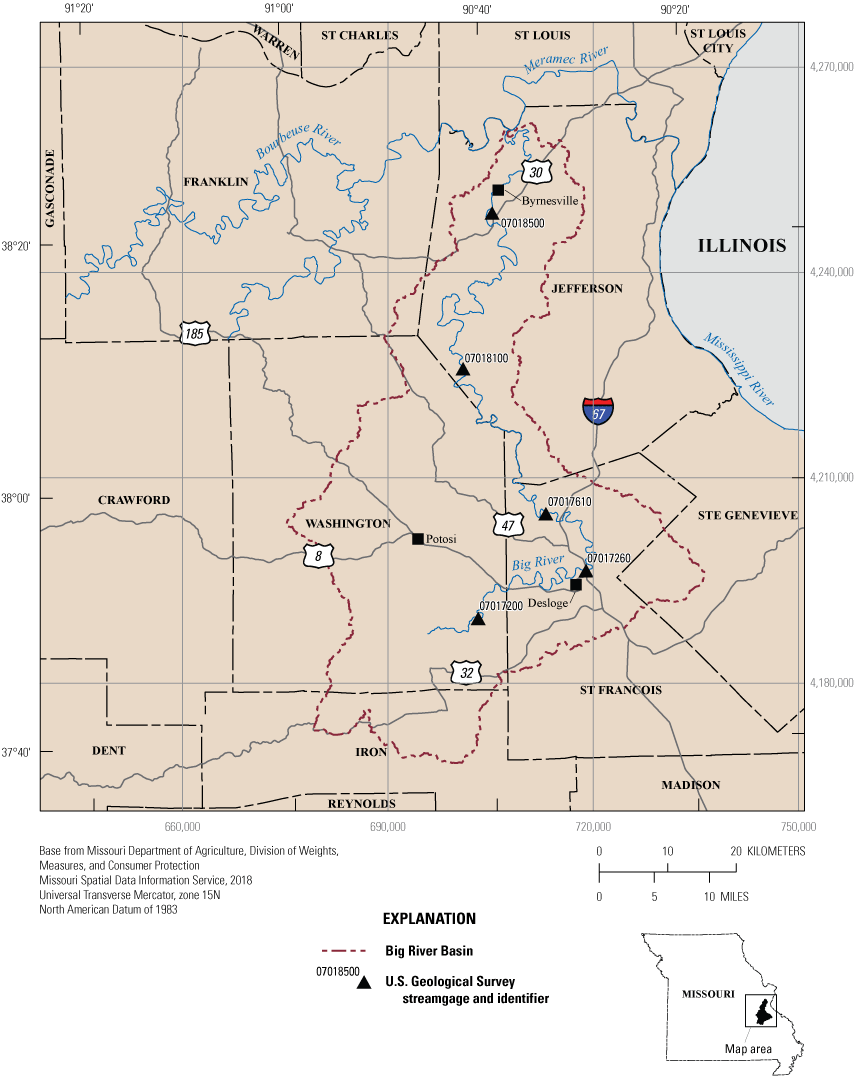
The Big River, a tributary to the Meramec River in south-central Missouri (fig. 1), drains an area that was historically one of the largest lead producers in the world. Mine wastes associated with lead mining activities have contaminated sediments in and along 144 kilometers (km) of the Big River and its tributaries with lead, cadmium, and zinc (Roberts and others, 2009). Although other tributaries in the Meramec drainage continue to be a stronghold for freshwater mussels (Bivalvia: Margaritiferidae and Unionidae), the 37 mussel species known from the Big River are affected by heavy metal contamination (Roberts and others, 2009, 201657; Hinck and others, 2012). Recent studies indicate that contaminated sediments have negatively affected mussel populations in the Big River downstream from mining areas (Besser and others, 2009; Roberts and others, 2009; Hinck and others, 2012; Allert and others, 2013); however, additional study is needed to quantify and further refine understanding of what range of hydraulic conditions constitutes suitable physical habitat for mussels in the Big River Basin to provide a basis for differentiating chemical and physical stressors. Specifically, are depauperate mussel populations associated with streambed instability or siltation compared to robust mussel populations?
The Big River Basin, along with the Meramec and Bourbeuse Rivers, Missouri.
The field measurements and two-dimensional1 (2D) hydrodynamic modeling described in this report refine understanding of the landscape-scale factors and physical characteristics of areas that may provide suitable habitat for freshwater mussels. This information can be used by managers to evaluate plans for restoration and reintroduction efforts, not only in the Big River but also for other Ozark river systems. The results presented here further elucidate the localized hydraulic variables that help to control mussel distributions at reach scales in Ozark rivers. The relations between hydraulic variables and mussel location and density provide insight into the spatial organization and patterning of mussel beds within the active channel.
Two-dimensional hydrodynamic models are averaged in the vertical dimension (depth) and vary in the lateral and longitudinal dimensions.
Background
Freshwater mussel habitat suitability has been extensively investigated across a range of spatial and temporal scales. Landscape-scale studies have highlighted broad hydrologic predictors such as stream order (Drew and others, 2018) and median annual stream discharge (Daniel and others, 2018). Nevertheless, the spatial resolution of these broader scale predictors does not permit reach and channel-unit-scale2 differentiation of habitat suitability. Mussels commonly live in “mussel beds,” concentrated aggregations of multiple species, indicating common habitat requirements, yet spatially variable abundance has been documented within scales as fine as individual mussel beds (Strayer and others, 2004; Newton and others, 2008), indicating that localized differences in habitat may affect abundance (Hardison and Layzer, 2001).
We use the hierarchical stream classification approach introduced by Frissell and others (1986) to denote spatial scales of streams. “Segment” refers to long sections of streams between major tributaries that substantially alter flow or sediment-transport regime. “Reach” is a shorter length of stream (about 1 kilometer) defined by one or more riffle-pool sequences. A channel unit is a habitat descriptor of fairly uniform areas of depth, velocity, and substrate of one to tens of square meters (Bisson and others, 2006). “Patch” is equivalent to a microhabitat, an area (less than 1 meter) of fairly uniform depth, velocity, and substrate.
At the reach to patch scales, simple habitat predictors like depth, current velocity, and sediment composition have had variable success in predicting the presence or density of mussels (Newton and others, 2008; Strayer, 2008). Several studies have detected no association or only a weak association between presence and current velocity (Strayer and Ralley, 1993; Strayer, 1999) or an inconsistent relation between mussel density and depth and current velocity among different reaches (Hardison and Layzer, 2001). Grain size was positively correlated with mussel density in the upper Mississippi River (Steuer and others, 2008) but was not associated with presence in two rivers in southeastern New York (Strayer, 1999). Within the Big River itself, the presence of two mussel species has been positively correlated with coarse sediment (Albers and others, 2016), although overall mussel density has not been correlated with substrate size (Roberts and others, 2016).
These inconsistent results indicate that simple hydraulic or substrate measures may not be adequate predictors of suitable habitat (Newton and others, 2008), possibly in part because of the variety of life-stage strategies used by mussels and the interactions among mussels, sediment, and local hydraulic forces. Mussels are capable of passive modification of their hydraulic environment by reducing near-bed flow velocities (Sansom and others, 2018a) and stabilizing the bed (Sansom and others, 2020). Furthermore, mussels may capitalize on finer particles like sand to help in burrowing (Schwalb and Pusch, 2007) and may use larger particles for refugia from hydraulic forces (Vannote and Minshall, 1982; Layzer and Madison, 1995; Pandolfo and others, 2016). Still, bed shear stress (shear stress), which quantifies the friction forces of the water on the bed surface, has proven to be a successful predictor of habitat suitability. Shear stress was negatively correlated with density in the upper Mississippi River (Steuer and others, 2008) and was limiting to mussel abundance in Appalachian streams (Gangloff and Feminella, 2007) and Oklahoma streams (Allen and Vaughn, 2010).
Collectively, these findings may indicate an important interplay between hydraulics and substrate in mussel beds. A common hypothesis in habitat studies is that mussels tend to live in “flow refugia” with stable sediment (Vannote and Minshall, 1982; Strayer and Ralley, 1993; Strayer, 1999). This phenomenon was observed on two rivers in southeastern New York, where mussels were in areas in which less movement of seeded tracer particles was documented (Strayer, 1999). Substrate instability at higher discharges was determined to be limiting to mussel distribution (Morales and others, 2006) and species richness and abundance (Allen and Vaughn, 2010). Hydrodynamic modeling on the Trinity River in California indicated that mussels were in the most stable areas of a reach (May and Pryor, 2016). Absent any behavioral interactions and responses such as burrowing, this stability hypothesis effectively regards the mostly sedentary mussel as a bedload particle susceptible to entrainment. Therefore, adult mussel presence may indicate bed stability for a minimum duration on the order of a mussel’s lifespan, which is typically between 15 and 40 years for most species (Haag, 2012). Nevertheless, the stability hypothesis is not universally supported. For example, hydraulic models simulated bed-sediment transport near mussel locations for 2-year peak discharges at two streams in New York, indicating that the mussels could be adapted to bedload-transporting discharges (Sansom and others, 2018b). Moreover, mussels can be sensitive to siltation (Vaughn and Pyron, 1995; Galbraith and others, 2008, 2010) and may require minimum flows to flush fine sediment from the bed and to deliver nutrients and oxygen (Steuer and others, 2008).
Considering the range of results observed in previous investigations, we examined multiple hydraulic parameters and sediment characteristics within mussel habitats3 in the Big River. Using high-resolution 2D hydrodynamic model outputs and sediment-size data, we investigated spatially variable hydraulic conditions and predicted bed-surface sediment stability and instability within four delineated mussel habitats (MHs) and within the surrounding reaches. To address short-term (about 0 to 2 years) temporal variability in conditions, we simulated MH hydraulics across a range of discharges. As largely sedentary organisms, mussel persistence in a particular location depends on the range of conditions they experience rather than on a single discharge (Layzer and Madison, 1995; Doyle and others, 2005). Therefore, we focus on the range of conditions and discharge events experienced most frequently: discharges from base flow (90-percent flow exceedance) to approximate bankfull discharge (2-year peak flow).
We use the term “mussel habitat” rather than “mussel bed” because the mussel communities in these reaches range from depauperate to robust. The term “mussel bed” typically refers to a dense aggregation of individuals of multiple species. We use “robust” to describe mussel communities with high abundance and species richness and “depauperate” to indicate communities with low abundance, low species richness, or both.
Purpose and Scope
The purpose of this report is to quantify hydraulic characteristics and bed stability of freshwater mussel habitat in the Big River in Missouri to inform understanding of the reach-scale hydraulic factors affecting the distribution of mussel aggregations in the river. These physical characteristics are based on 2D hydrodynamic model simulations over a range of discharges, extending from approximate base flow to bankfull conditions. Field data were collected between December 2018 and May 2020 at four reaches along the Big River.
We compared the statistical distributions of simulated hydraulic variables within the study reaches and within MHs delineated based on reach-scale field surveys of mussel communities between 2010 and 2014 (Roberts and others, 2016). A schematic depicting the hypothetical extent of an MH is shown in figure 2. The reach-scale field delineations consist of two robust and two depauperate MHs, allowing an examination of any potential hydraulic contribution to diminished mussel populations. Contextual habitat polygons (locations of comparative sediment-size data collection; introduced in the “Substrate Size Data Collection” section) are shown. Note the dry area within the MH and the edge discrepancies between the MH and wetted cells at 90-percent exceedance (fig. 2 detail map). Also note that this diagram is hypothetical and does not depict an actual reach, habitat delineation, or model simulation on the Big River.
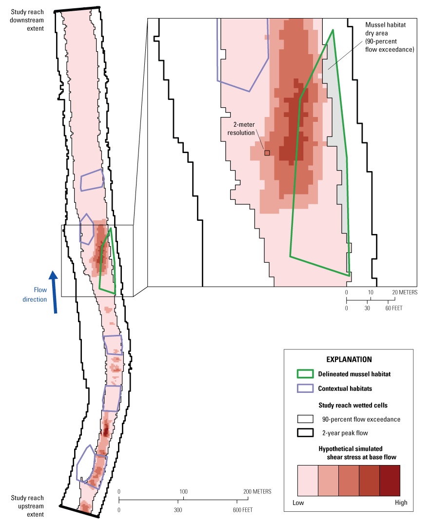
A hypothetical study reach with locations and extents of independent delineated polygons, wetted cells, and longitudinal study reach extents.
Description of Study Area
The Big River, which drains a 2,473-square kilometer drainage basin, flows northeast towards its confluence with the Meramec River (drainage area: 10,308 square kilometers) near the city of Eureka, in St. Louis County, Missouri (fig. 1). The 2010 human population in the Big River drainage basin was 98,252 (Missouri Department of Natural Resources, 2013). The river system is within the Ozark Plateaus physiographic province (not shown; hereafter referred to as “the Ozarks”), a rugged montane region occupying much of southern Missouri and northern Arkansas. The region consists of four distinct physiographic provinces: the St. Francois Mountains, Salem Plateau, Springfield Plateau, and the Boston Mountains (not shown). The Big River headwaters originate in the St. Francois Mountains (not shown), a region consisting of Precambrian rhyolites and granites that form the crest of the Ozark dome. Much of the Big River drainage basin is on the Salem plateau (not shown), a region of rolling uplands formed by cherty dolomites and limestone of Ordovician age, with some sandstone and shale (Sims and others, 1987; Pavlowsky and others, 2017). The mean annual precipitation is 112 centimeters (cm), and the mean monthly temperatures range from −0.6 to 26.0 degrees Celsius, based on basin means of the 30-year normals for 1981 to 2010 (PRISM Climate Group, 2012a, b). The drainage basin is composed of 72-percent forest, 18-percent grassland, 7-percent developed area, and 1-percent cropland (Missouri Department of Natural Resources, 2013). The Big River is unregulated but contains several low-head dams.
The Big River drains the Old Lead Belt subdistrict of the southeastern Missouri lead mining district. The Old Lead Belt was one of the leading lead producers in the United States for more than a century, and legacies of mining activities persist today (Schmitt and Finger, 1982; Gale and others, 2002; Pavlowsky and others, 2017). Elevated concentrations of lead, zinc, and other metals supplied by erosion of mine tailings from the Old Lead Belt are present throughout the 171 km of the Big River downstream from sources near Leadwood, Mo. (Besser and others, 2009; Pavlowsky and others, 2017). Previous studies have determined an inverse relation between concentrations of metals in substrate sediments in the Big River and the abundance of aquatic organisms, including fish and benthic macroinvertebrates such as mussels and crayfish (Roberts and others, 2009; Allert and others, 2013; Albers and others, 2016; Krause and others, 2019).
For managers to evaluate the effects of contamination on mussel populations, it is necessary to differentiate contaminant effects from those of other physical habitat factors, such as bed instability, that could affect the distribution and abundance of mussels in the river. As part of broader monitoring efforts, Key and others (2021) developed a basin-scale model of physical habitat suitability for mussels in the Meramec River Basin, including the Meramec, Big, and Bourbeuse Rivers (fig. 1). This statistical model of habitat suitability was developed using river hydrogeomorphic attributes characterized from remotely sensed data in conjunction with basinwide surveys of mussel distributions (Key and others, 2021). Gravel-bar proximity and a metric for water availability emerged as the most important explanatory variables, indicating a connection between the local hydrogeomorphic variables and habitat suitability (Key and others, 2021). The work presented here builds on this basin-scale study of mussel habitat to provide reach-scale understanding of hydraulic factors affecting the distribution of mussels. Improved understanding of the ways in which reach-scale hydraulic patterns affect habitat suitability is critical to differentiate the factors leading to mussel declines in the Big River.
Methods of Study
Our general approach to this study was to develop hydraulic and geomorphic information about mussel habitat at the reach scale through the collection of field data and hydrodynamic modeling. Steps consisted of (1) selection of study reaches containing areas representative of supportive habitats; (2) collection of field data for reach characterization and model compilation, calibration, and evaluation; (3) simulations of hydrodynamic models for a relevant range of discharges; and (4) evaluation of model results related to understanding of mussel habitat affinities and bed stability.
Selection of Study Reaches
We selected four reaches for detailed measurements and hydrodynamic modeling: site W (STW, river kilometer [RKM] 2.5; river kilometers are locations upstream from the confluence of the Big River with the Meramec River), Rockford Beach (RFB, RKM 16.5), Phelps Bend (PHB, RKM 41), and Washington State Park (WSP, RKM 105.7; fig. 3, table 1). Selection of study reaches was based on previous studies completed to identify areas with physical characteristics suitable for supporting freshwater mussels (Roberts and others, 2016). Roberts and others (2016) completed a detailed survey of mussel habitat in the Big River, consisting of two phases. The first phase was a reconnaissance-level survey of the downstream 125 km of the Big River to identify reaches with characteristics associated with mussel beds. The second phase involved more detailed characterization of reaches identified in phase I, including quantitative surveys of mussels and measurement of habitat metrics such as substrate size.
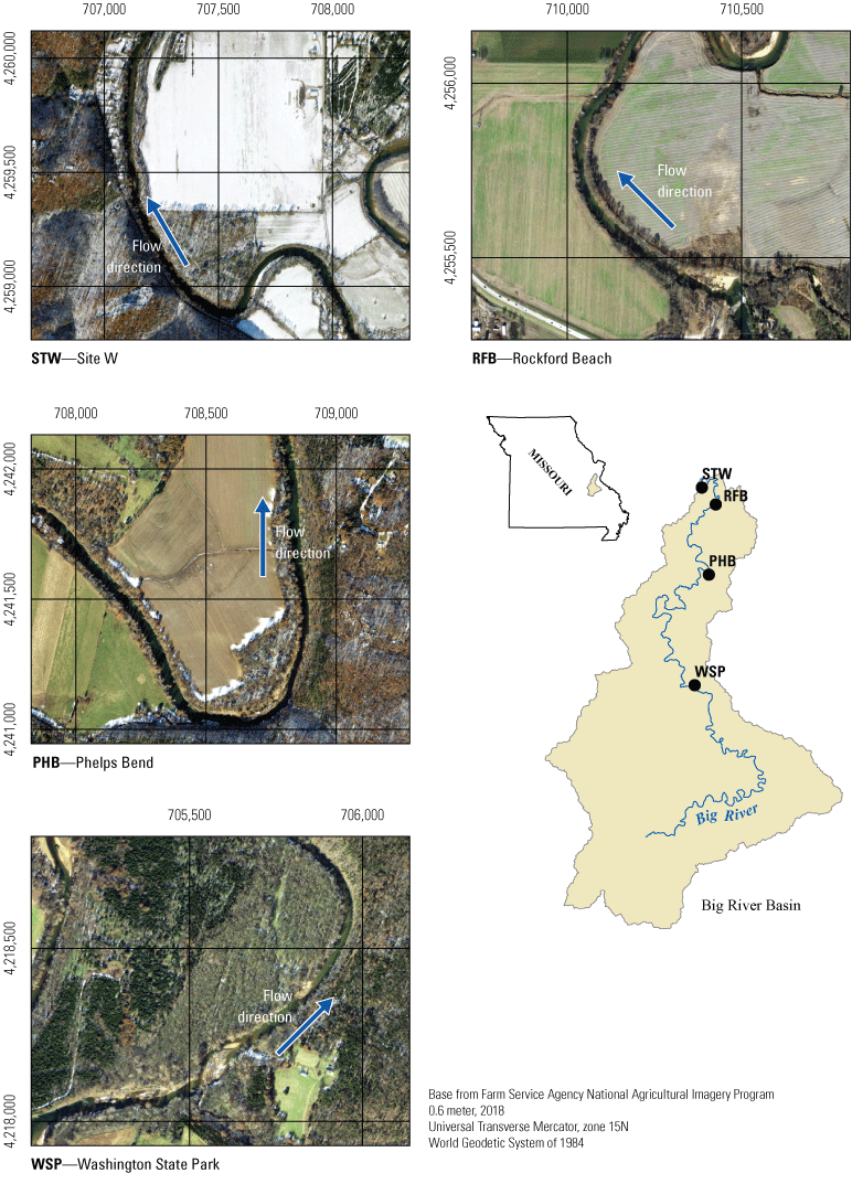
The four study reaches on the Big River, Missouri. The reaches are site W, Rockford Beach, Phelps Bend, and Washington State Park.
Table 1.
Study reach and interpreted delineated mussel habitat characteristics, including phase II habitat assessment characterization (Albers and others, 2016; Roberts and others, 2016). Drainage basins were delineated using StreamStats (Ries and others, 2008, 2017). Areal statistics were computed using ArcGIS (Esri).[km2, square kilometer; m2, square meter; STW, site W; RFB, Rockford Beach; PHB, Phelps Bend; WSP, Washington State Park]
The four reaches selected for this study were identified as containing suitable habitat in the assessment of Roberts and others (2016). The phase II assessment of Roberts and others (2016), however, indicated a longitudinal trend in mussel density that corresponded to a longitudinal trend in heavy metal concentration in sediment; reaches farther upstream (closer to historical mining)—with higher concentrations of metals—contained fewer mussels and lower species richness, whereas reaches farther downstream—with lower concentrations of metals—demonstrated higher abundance, higher densities, and higher species richness. The four study reaches we selected for this investigation each contained a discrete, delineated area with characteristics of good habitat (MH) but differed in species richness, abundance, and density metrics as determined during the phase II quantitative surveys (Roberts and others, 2016; table 1). Specifically, the mussel communities at the two downstream reaches (STW and RFB) were determined to be robust whereas those at the two upstream reaches (PHB and WSP) were determined to be depauperate, thus allowing a comparison of the hydraulics between the two types of MHs. Additionally, the reaches we selected represent upstream to downstream variation in the Big River. Based on field reconnaissance, the reaches seem to be representative of geomorphic conditions along the river, with each reach incorporating variability at the riffle-pool scale. Each reach MH was defined as a polygonal zone of similar habitat in the river that was delineated using a handheld Global Positioning System unit once field surveys confirmed the presence of mussels within those habitats (Roberts and others, 2016). The polygons were provided to us as digital geographic information system files by the U.S. Fish and Wildlife Service; the polygons are not available for distribution to the public and are not shown in this report because they may include locations of endangered mussel species. The four MH polygons are 797–15,949 square meters (m2) in size (table 1) and in most areas do not span the width of the active channel. A hypothetical MH, comparable in shape, scale, and channel position to the four investigated MHs, is shown in figure 2.
Wolman pebble-count surveys (Wolman, 1954) were used to document that the bed surface of the MHs at all four reaches is largely composed of fine, medium, and coarse gravel (2–8, 9–16, and 17–64 millimeters [mm], respectively) and cobbles (65–256 mm), with less than 10 percent composed of sand or finer particles (less than [<] 2 mm; fig. 4A, B; Albers and others, 2016; Roberts and others, 2016). All measurements were based on the intermediate axis of the particle. Cobbles (65–256 mm) and boulders (greater than 256 mm) were classified within grain-size classes but not measured. Grain-size distributions (fig. 4A) are plotted from the semicontinuous pebble-count dataset, which is available in a U.S. Geological Survey (USGS) data release (Roberts and others, 2022). The pebble-count data are provided in categorical format in Albers and others (2016) and Roberts and others (2016).
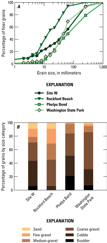
(A) Surface grain-size distribution and (B) composition by category within delineated mussel habitats at the four study reaches, estimated from Wolman pebble counts (Wolman, 1954) completed between September 2012 and November 2014 as part of previous mussel surveys (Albers and others, 2016; Roberts and others, 2016).
The median (50th-percentile particle size fraction [D50]) MH grain sizes were 53 mm at STW, 15 mm at RFB, and 46 mm at WSP. The median grain size at PHB falls within the cobble category and therefore could not be determined precisely. The 16th percentile particle size fraction (D16; representing the smaller size fractions) grain sizes were 7 mm at STW, 5 mm at RFB, 17 mm at PHB, and 18 mm at WSP. The bed-surface composition is finest at RFB and coarsest at PHB, and the nominal distributions were significantly different among different reach MHs, even when comparing just the coarser habitats (STW, PHB, and WSP; chi-square test for independence, probability value [p] <0.01). MH sand composition was 9 percent at STW and RFB, 0 percent at PHB, and 2 percent at WSP.
Field Measurements
Study reach lengths were delineated based on a geographic information system estimate of bankfull channel width using State aerial light detection and ranging (lidar) data (Surdex Corporation, 2011). Bankfull width was visually estimated using breaks in slope from cross sections of extracted lidar elevations at the MH polygons. Reach lengths extended beyond the MH polygons by a distance of at least five times the estimated bankfull width in the upstream and downstream directions. A hypothetical example of longitudinal study reach extents is shown in the schematic in figure 2.
All data were collected using single-base real-time kinematic (RTK) global navigation satellite system (GNSS) surveying with a temporary bench mark at each study reach. The base station equipment system consisted of a Trimble R8 or R8s base receiver, leveled and centered on a tribrach and a fixed-height tripod, and a radio antenna with a Trimble TDL 450H series RTK broadcast radio. During initial field reconnaissance, a temporary bench mark was established at each reach with rebar and a survey cap. Static bench mark position observations were logged with a Trimble R8 or R8s GNSS base receiver unit for at least 5 hours, and the acquired coordinates were corrected using static postprocessing with the National Geodetic Survey Online Positioning User Service (OPUS) tool (Mader and others, 2003). The overall root mean square errors (RMSEs) of the OPUS solutions for the four reach bench marks ranged from 0.015 to 0.023 meter (m). For subsequent field excursions, the base station was set up over the bench mark using the OPUS-corrected coordinates.
Field survey data were collected and processed in Universal Transverse Mercator (UTM) Zone 15 North coordinates in the World Geodetic System of 1984 horizontal datum and the North American Vertical Datum of 1988. The final datasets exclusively consist of data collected in RTK-fixed integer solution status. Any acquired data that were not RTK fixed were discarded during editing.
Collection of Bathymetric and Topographic Data
Four datasets were obtained to create elevation layers for each reach: State aerial lidar (Surdex Corporation, 2011), bathymetric single-beam echosounder data, manually collected GNSS survey points, and terrestrial lidar.
Bathymetric data were collected using a CEE HydroSystems CEEPULSE 100 series survey grade single-beam echosounder mounted in a Z-Boat 1800 remote hydrographic survey boat (Teledyne Oceanscience, Inc.). Positioning data were collected using a Trimble R2 GNSS receiver mounted to the top of the Z-Boat. Bathymetric data were collected by driving the Z-Boat along planned cross sections spaced about 2.5 m apart. Bathymetric and positioning data were transmitted via Bluetooth or from the Hydrolink boat radio to the Hydrolink shore radio and recorded in Hypack 2017–18 (Xylem, Inc.).
Topographic data were collected on exposed banks and bars within the study reaches using a terrestrial mobile laser scanning system attached to a modular rail that was mounted in a canoe or motorized boat. This lidar system includes a Velodyne LiDAR Puck LITE, an SBG Systems Ellipse2-D Inertial Motion Unit, and a Trimble R7 GNSS system with a Zephyr antenna for inertial navigation. The Velodyne LiDAR Puck LITE has a range of 100 m and has 16 channels and a 360-degree field of view around its axis. The Puck LITE was configured to record the last return with six beams at 600 rotations per minute. Lidar data were collected while paddling or motoring either upstream or downstream during periods of low discharge (< about (~) 20 cubic meters per second [m3/s]) and leaf-off conditions for maximum bank and bar exposure. Data were recorded in Hypack 2017 (Xylem, Inc.) using Hysweep Survey.
To supplement the lidar and single-beam data, additional topographic and bathymetric data were collected manually using a Trimble R2 GNSS receiver mounted on an adjustable survey rod with a Trimble TSC3 data recorder. These points were collected on vegetated bars and shallow areas where data acquisition with neither the lidar system nor Z-Boat was feasible. Manual GNSS points were primarily collected at breaks in slope, with horizontal and vertical RMSEs of less than 3 cm.
Topographic data for areas beyond the active channel were acquired in LAS 1.2 format from Missouri aerial lidar data (Surdex Corporation, 2011). Lidar data covering the study reaches were flown between December 2010 and April 2011 and have horizontal and vertical accuracies of 60 cm and 18.5 cm, respectively. These datasets were obtained in North American Datum of 1983 UTM Zone 15 North and the North American Vertical Datum of 1988. The horizontal coordinate system was projected to the project coordinate system (World Geodetic System of 1984 UTM Zone 15 North) in ArcGIS (Esri).
Collection of Model Calibration and Evaluation Data
Model calibration and initialization data were collected for a range of discharge events up to bankfull discharge. For each event, calibration data consisted of a discharge measurement and a water-surface profile.
Discharge measurements were collected using a 600-kilohertz RiverRay acoustic Doppler current profiler (ADCP; Teledyne RD Instruments) mounted in a Z-Boat remote hydrographic survey boat (Teledyne Oceanscience, Inc.) or motorboat. Positioning data were recorded with a Trimble R2 GNSS receiver. Before data collection, an ADCP compass calibration was completed by spinning the boat slowly until a compass error of less than 0.5 degree was achieved. Discharge measurements were collected at a minimum of four reciprocal transects at a single-thread location within the study reach. Discharge transect data were collected until at least two transect measurements in each direction (right bank to left bank and left bank to right bank) were obtained, each with a discharge error of less than 5 percent of the mean discharge (Mueller and others, 2009). Discharge data were transmitted via Bluetooth or between the Hydrolink boat and shore radios and recorded in WinRiver II (Teledyne Marine).
Accompanying water-surface profiles were recorded for every discharge measurement using a Trimble R2 GNSS receiver. Measured profile extents encompass either most or all of the length of the study reach (appendix 1, fig. 1.1). The profiles were either collected manually with the receiver mounted on an adjustable rod or with the receiver mounted on a Z-Boat, motorboat, or kayak with a known offset between the receiver and the water surface. Water-surface profiles collected by boat were recorded in Hypack while the boat was driven along the study reach in the downstream direction.
Model evaluation data were collected for all reaches except PHB for at least one high-flow event where discharge was measured as well (because of logistical challenges, no separate velocity evaluation data were collected for PHB). For each evaluation event, one to two separate velocity measurements were collected at various single-thread or split-channel locations within the study reach to provide robust evaluation of model calibration. Velocity measurements were collected with a RiverRay ADCP using the same procedure used for discharge measurements, with a maximum permitted transect discharge error of 10 percent of the mean discharge.
Substrate Size Data Collection
To provide local comparative grain-size data, bed-surface grain sizes were measured at seven contextual habitats within the study reach at WSP. These contextual habitats represent a variety of discrete stream habitat units4 of fairly uniform hydraulics and grain-size distribution and provide an opportunity to compare MH hydraulics to those of other habitats in a study reach. The intermediate axes of ~100 clasts were measured at each contextual habitat location using Wolman pebble counts (Wolman, 1954), following methods similar to those used at the MHs in earlier surveys (Albers and others, 2016; Roberts and others, 2016). Grains smaller than 2 mm were classified as 2 mm in size.
Pebble-count locations were recorded using a Trimble R2 GNSS receiver. For each pebble-count location, a contextual habitat polygon was delineated in ArcGIS using the recorded coordinates and surface and substrate features visible in aerial imagery (Farm Service Agency, 2016). These polygons are not available for distribution to the public and are not shown in this report because they identify the location of the MH at WSP, which may include locations of endangered mussel species. A representation of the scale and distribution of contextual habitats is shown in the schematic in figure 2. Pebble-count data from another MH within the study reach, near RKM 106.5 (Albers and others, 2016; Roberts and others, 2016), also were incorporated in the contextual grain-size data.
To compare the grain-size distributions of different habitats, hypothesis tests were completed using the SciPy 1.2.1 package in Python 3.7.3 (Python Software Foundation). Wilcoxon rank-sum tests were used to compare continuous grain-size distributions at the different WSP pebble-count locations. These tests did not include the grain-size data from the MH surveys (Albers and others, 2016; Roberts and others, 2016), which are only continuous below the cobble grain-size category. Instead, these data and the pebble-count data for WSP were classified into grain-size categories, and the chi-square test for independence was used to compare the nominal distributions.
Data Availability
The final elevation rasters, contextual habitat bed grain-size data, and calibration data are available in a USGS data release (Roberts and others, 2022). Previously collected semicontinuous MH particle-size data used in the study also are available in the data release.
Hydrodynamic Modeling
Our study is based on hydrodynamic models that are used to quantify hydraulics potentially affecting habitat over a range of relevant flow exceedances. We emphasize detailed topographic and bathymetric measurements because high-quality, high-resolution topographic and bathymetric data are essential to generate useful hydrodynamic model results (Pasternack and others, 2006). Our modeling assumes that topographic changes related to erosion and deposition over the range of modeled flows and over the time frame of interest are insignificant.
Development of Topographic and Bathymetric Elevation Layers
Bathymetry transect data collected with the CEEPULSE single-beam echosounder were manually edited using the Hypack single-beam editor to remove erroneous points and points where the GNSS position solution was not fixed. These data were then converted to an Esri shapefile. State aerial lidar data were filtered to remove all nonground points and converted to an Esri shapefile (fig. 5A).
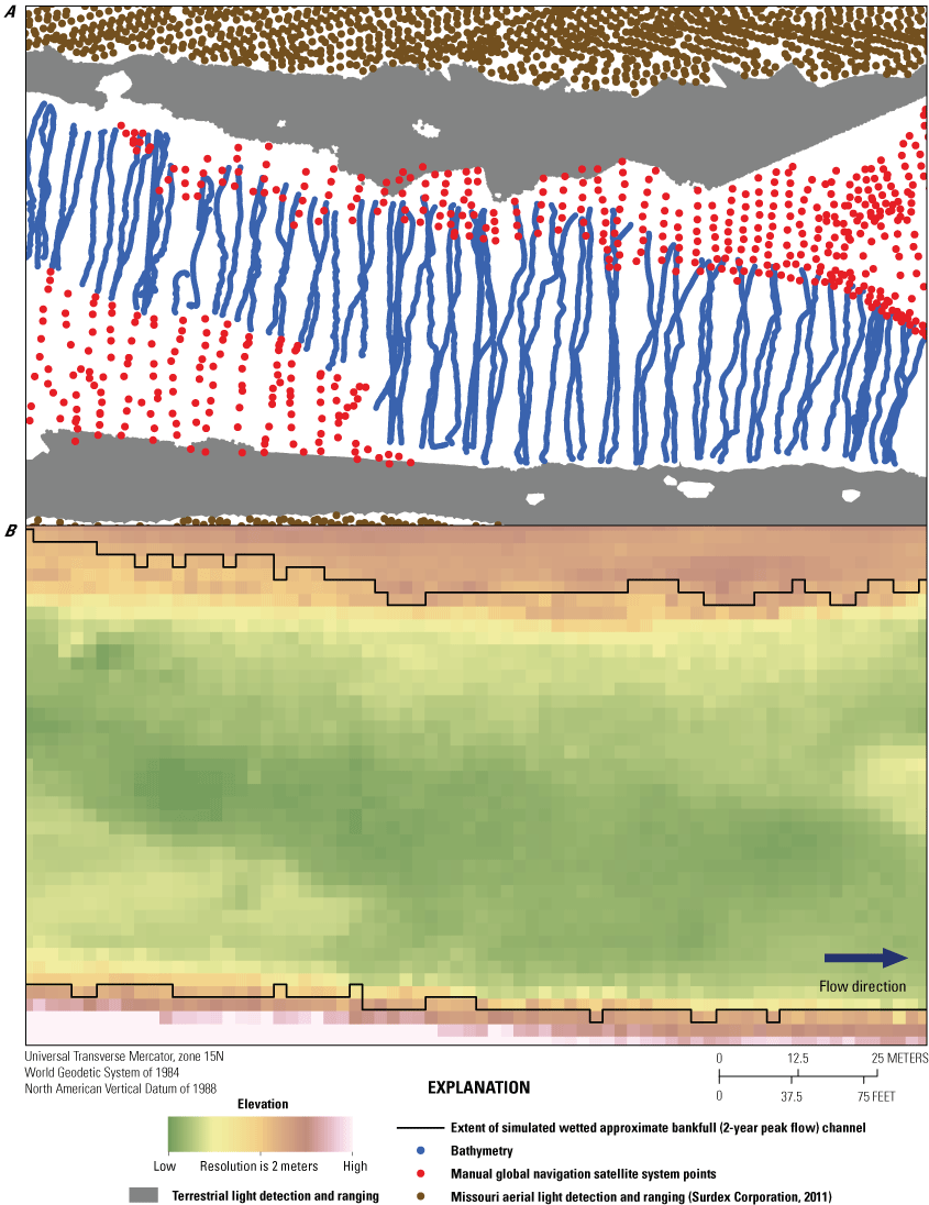
Sample bathymetric and topographic data at Phelps Bend reach. (A) Edited and clipped datasets from manual global navigation satellite system points, bathymetry, terrestrial light detection and ranging, and State aerial light detection and ranging. (B) Tag Image File Format elevation raster (resolution is 2 meters) created from bathymetric and topographic datasets.
Terrestrial lidar data were first manually edited using the Hypack MBMAX64 HYSWEEP Editor. Cloud points were removed if they were not collected under RTK fixed conditions or if they resembled objects other than the ground surface, such as vegetation or buildings. Cloud data were then converted to LAS format. The terrestrial lidar data were filtered using automated methods to remove any remaining vegetation. This filtering procedure used the established ground surface elevations from the other field datasets and aerial lidar to aid in identifying the ground surface in the terrestrial lidar. The terrestrial lidar cloud data were combined with the bathymetry data, the manually collected topographic data, and State lidar data, all in LAS format. This combined dataset was classified and filtered to remove nonground points in the terrestrial lidar using the Point Data Abstraction Library package (PDAL Contributors, 2018) in Python (Python Software Foundation). The data were classified and filtered using the Simple Morphological Filter (Pingel and others, 2013) using the default settings.
The filtered terrestrial lidar dataset was then clipped to an outline of the bank areas captured by the lidar and thinned to a sampling distance of 0.25 m. State aerial lidar data were clipped to cover only areas not captured by the field-collected bathymetric and topographic data. The bathymetry data, manual GNSS points, terrestrial lidar, and State aerial lidar yield a combined elevation dataset with comprehensive coverage of the river channel and adjacent floodplain (fig. 5A).
All topographic and bathymetric data were converted to shapefile format and combined to generate a triangulated irregular network (TIN) for each reach using Delaunay conforming triangulation. The boundaries of the datasets were vectorized and incorporated in the TINs as soft breaklines to prevent the generation of artifacts and abrupt breaks in slope between datasets with different horizontal resolutions. The reach TINs also were edited to smooth out small tributary drainages that could cause water to “leak” out of the main channel during modeling. These TINs were used to generate a 2-m cell size Tag Image File Format raster (fig. 5B) for each reach using a linear interpolation method.
Editing Calibration and Evaluation Data
Discharge and velocity transect data were processed in WinRiver II (Teledyne Marine). The discharge values were determined from the mean discharge of the four measured transects. Velocity and depth data from the transects were converted to shapefile format.
As with the bathymetry transect data, the water-surface profiles collected using Hypack were manually edited using the Hypack single-beam editor to remove erroneous points and points where the GNSS position solution was not fixed. These data were then converted to an Esri shapefile. The water-surface profiles collected manually were converted directly to Esri shapefiles.
To supplement the calibration data, we also used water-surface elevation data from bathymetry surveys and terrestrial lidar surveys in which most of the study reach was surveyed. The edited bathymetry data were thinned and snapped to the closest point along a stream centerline, and the corresponding water-surface measurements were used to create a water-surface profile. The edited terrestrial lidar data were converted to a 0.25-m raster using the mean value as the assigned cell value. Then the elevation values were extracted along the bathymetry survey transect lines. Because the terrestrial lidar system used does not penetrate water, the lowest elevation value for each transect was assumed to be the water-surface elevation.
The calibration discharges for these water-surface profiles were estimated by scaling the midday discharge from the nearest streamgage by relative drainage area. Discharge also was estimated in the same way for calibration surveys in which a water-surface profile or high-water-mark profile was collected but conditions did not permit a discharge measurement.
Flow and Sediment Transport with Morphological Evolution of Channels
The 2D hydrodynamic modeling was completed using the Flow and Sediment Transport with Morphological Evolution of Channels (FaSTMECH) computational solver (Nelson and others, 2003), executed within the International River Interface Cooperative numerical simulation interface (Nelson and others, 2016). Automated batch model runs were completed using a custom script in Python 3.7.3 (Python Software Foundation).
FaSTMECH is a quasi-steady 2D and quasi-three-dimensional flow model that uses an orthogonal curvilinear computational grid (Nelson and others, 2003). The 2D modeling feature yields a vertically averaged calculation with the option to compute the vertical structure of the flow (quasi-three dimensional). The FaSTMECH model assumes that flow is steady, incompressible, and hydrostatic and that changes in momentum caused by turbulence can be captured using lateral eddy viscosity (LEV; Nelson and others, 2003). Energy losses from grains and bedforms (that is, hydraulic roughness) are accounted for in the calibrated drag coefficient (Cd).
Model Grid Creation
Numerical grids (table 2; fig. 6) were generated for each reach by manually drawing a stream centerline for the study reaches and designating a grid resolution (2 m) and a channel width sufficient to model the discharge range of interest. Elevation data were linearly interpolated to this grid using a Delaunay triangulation algorithm. Aside from elevation, no other geographic attributes were interpolated to the grids.
Table 2.
Computational-grid characteristics for each reach.[m, meter; STW, site W; RFB, Rockford Beach; PHB, Phelps Bend; WSP, Washington State Park]
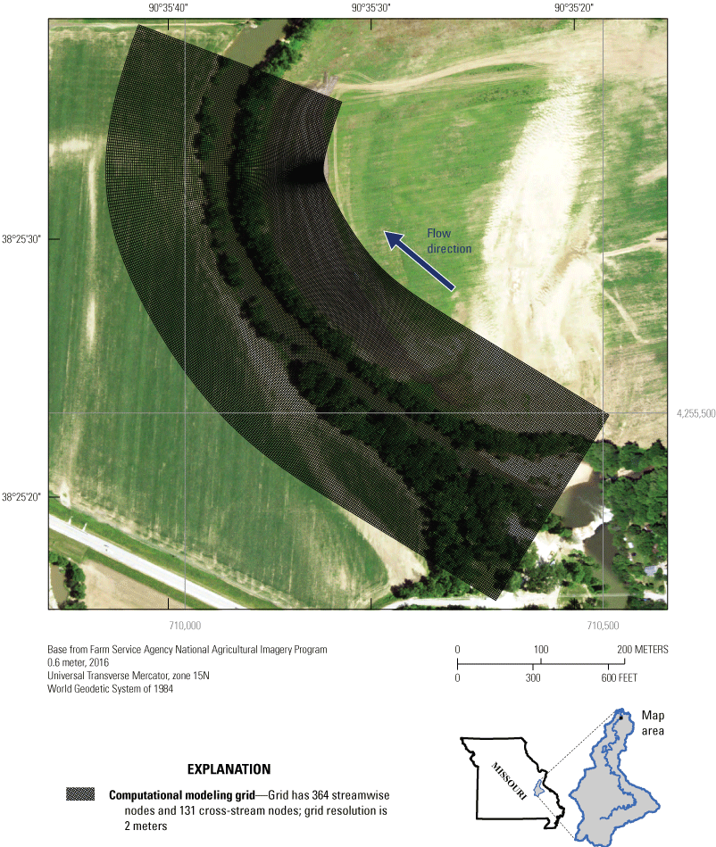
Example of Flow and Sediment Transport with Morphological Evolution of Channels computational modeling grid at Rockford Beach.
Model Calibration
All hydrodynamic models for each reach were run at a steady discharge for 2,000–10,000 iterations to ensure a stable solution. The simulation and final calibration runs were set to compute for 10,000 iterations. Model inputs were optimized for each reach to achieve model stability and to best reflect measured conditions (table 3).
Table 3.
Flow and Sediment Transport with Morphological Evolution of Channels model input parameters for each study reach.[STW, site W; RFB, Rockford Beach; PHB, Phelps Bend; WSP, Washington State Park; LEV, lateral eddy viscosity, in square meters per second; Q, discharge, in cubic meters per second; <, less than; m, meter; 1D, one dimensional; NA, not applicable; ERelax, URelax, ARelax, numerical solver parameters that control how quickly the water-surface elevation, velocity, and slope change between model iterations]
Hydrodynamic models for each reach were calibrated using discharge and water-surface profiles measured in the field. These discharges encompass a range of conditions up to the approximate bankfull discharge. These calibration data were used to determine the relations between discharge and the model input parameters of LEV, Cd, and downstream water-surface elevation for each reach. These calibration curves were then used to determine the optimum LEV, Cd, and downstream water-surface elevation (stage) for a range of target simulation discharges. ERelax, URelax, and ARelax are numerical solver parameters that control how quickly the water-surface elevation, velocity, and slope change between model iterations; these parameters were kept constant at default values.
The Cd characterizes the roughness of the riverbed surface, including friction from the grain texture, bedforms, vegetation, and channel form. This parameter is difficult to measure in the field but effectively represents a loss in energy that is manifested in the energy slope of the river. Calibrating the Cd so that the simulated profile matches the measured profile ensures that the loss in energy from friction is captured in the model.
Models were calibrated by adjusting the Cd until the simulated water-surface elevations throughout the reach most closely matched the observed water-surface elevations by minimizing the RMSE. For two calibration discharges at RFB with sparse (<20) measurements of the water-surface profile, denser water-surface profiles were generated at points along the reach using a linear regression of the measured water-surface elevations. For all calibration and scenario simulation runs, a uniform Cd was used for the study reach. Although bed friction is likely variable throughout a reach, we did not collect sufficient information to develop a spatially variable roughness map.
LEV is another required input parameter for the hydrodynamic model. Initial LEV values were set to a single value for all calibration discharges; the initial LEV was determined by trial and error to produce stable models across all discharges. After the first round of calibration tests, we refined these estimates using the area-weighted mean depth and velocity from the model output for all wetted cells, calculated as
whereLEV
is lateral eddy viscosity, in square meters per second;
davg
is the mean depth, in meters; and
vavg
is the mean velocity, in meters per second.
These computed LEV values were typically too low to produce stable models and were therefore uniformly increased by a constant value for all calibration discharges. Calibration runs and LEV estimates were completed iteratively in this way for five to six separate trials when LEV values for each discharge converged. Readers seeking more information on the LEV parameter are encouraged to consult Nelson and others (2003).
Model calibration for each discharge was evaluated based on the RMSE values for the water-surface elevations measured along the study reaches. The parameters that produced the lowest water-surface RMSE through the reach were selected as the optimized conditions for that discharge. The final optimized calibration runs yielded water-surface elevation RMSE values of about 0.04–0.11 m for STW, about 0.03–0.09 m for RFB, about 0.03–0.09 m for PHB, and about 0.07–0.28 m for WSP (table 4). The final iteration mean discharge errors for the optimized calibration runs ranged from 0.10 to 1.1 m3/s across all four reaches.
Table 4.
Discharge error, water-surface slope, and water-surface elevation root mean square error for calibration models at the optimum values of lateral eddy viscosity, downstream stage, and drag coefficient.[Calibration data consist of measurements where discharge and water-surface profiles were collected (measurement type “DP”) and those where only a water-surface profile was collected and discharge was estimated from the nearest streamgage (measurement type “P”). See appendix 1 (fig. 1.1) for plots of the measured and simulated calibration profiles; dates shown as year–month–day; m3/s, cubic meter per second; RMSE, root mean square error; m, meter; m/m, meter per meter; STW, site W; RFB, Rockford Beach; PHB, Phelps Bend; WSP, Washington State Park]
The measured and simulated calibration water-surface profiles for STW, PHB, and WSP indicated an overall decrease in water-surface slope with increasing discharge, and the profiles for RFB varied as much as plus or minus (±) 0.00024 meter per meter between the smallest and largest calibration discharges (table 4; appendix 1, fig. 1.1). The optimum Cd and LEV values for each calibration discharge were used to develop Cd-discharge and LEV-discharge calibration-curve relations for each reach. Downstream stage values, determined either from direct measurements or interpolation of measured calibration data, were used to develop a stage-discharge relation for the downstream boundary of the model. Calibration curves were determined manually by fitting power law, linear, and second-degree polynomial functions to the calibration values to find the best fit. The coefficient of determination values for the fitted calibration relations were between 0.82 and 0.99 across all reaches (table 5). See appendix 2 (fig. 2.1) for plots of the calibration curves for each parameter at the four reaches.
Table 5.
Calibration-curve equations and coefficient of determination values for lateral eddy viscosity, drag coefficient, and downstream stage at all reaches. Curves were fit to the calibration data using the best fit of linear, power law, or second-order polynomial relations.[R2, coefficient of determination; STW, site W; LEV, lateral eddy viscosity; Q, discharge, in cubic meters per second; Cd, drag coefficient; RFB, Rockford Beach; e, denotes exponentiation; PHB, Phelps Bend; WSP, Washington State Park]
Across all four reaches, LEV and downstream stage increased with increasing discharge and Cd decreased with increasing discharge. The representative equations for each best fit yielded a single optimized Cd, LEV, and downstream stage for each discharge.
Model Evaluation
Calibration models were evaluated qualitatively and quantitatively by comparing the simulated flow velocities to the measured flow velocities at ADCP transects for each of the reaches (fig. 7). For all reaches except PHB, velocity transects were collected at different locations from the discharge measurement location. The calibration and evaluation water-surface profiles (measured and simulated) are plotted in appendix 1 (fig. 1.1), along with the streamwise (distance along reach) locations of the velocity evaluation transects. Because of logistical challenges at PHB, the evaluation data used are those collected for the discharge measurement. The RMSE for the velocity measurements ranged from 0.1 to 0.28 meter per second (m/s) across all four reaches.
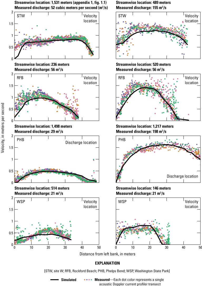
Measured and simulated flow velocities for model evaluation at each reach. Measured velocity values represent the vertically averaged velocities collected along four transects by the acoustic Doppler current profiler at measured discharges. [Note that evaluation data shown for Washington State Park were collected at similar discharges (19.3 and 20.4 cubic meters per second) on different days (December 2, 2018, and March 20, 2019)]
Evaluation using velocity data is based on evaluating the general cross-sectional shape of the simulated velocities to see if broad features of the velocity field have been captured. The degree of agreement possible between ADCP velocity data and the simulated data is inherently limited because ADCP data are an instantaneous snapshot of a velocity field that is characterized by high spatial and temporal variability caused by turbulence, whereas the simulated data are steady state and spatially averaged. Compared with the velocity evaluation results for STW, RFB, and PHB, the evaluation results at the WSP transects indicate that the model for WSP did not simulate velocities as effectively. There are several possible causes for this discrepancy. First, because the bathymetry and velocity transects were collected on different days, the channel shape at the transect locations may differ slightly between the reach’s elevation layer and the ADCP transects. Such differences are unlikely, however, because no appreciable topographic change was observed at any of the reaches during the study period. A more likely explanation is that the uniform roughness distribution used in modeling may not accurately characterize the channel roughness of this study reach, which contains several heavily vegetated bars.
Scenario Development
Simulation discharges were selected to represent the range of conditions most commonly experienced at each of the reaches on the Big River, approximate base flow to approximate geomorphic bankfull discharge. We therefore selected the following simulation discharge scenarios: the 90-, 50-, 10-, 5-, 3-, 2-, and 1-percent exceedance probability (flow exceedance) discharges and the 2-year peak flood (table 6).
Table 6.
Discharge scenarios and nearest U.S. Geological Survey streamgage information for each study reach. Exceedance probability flows were determined for each reach by scaling the StreamStats flow exceedance discharges for the reach’s nearest streamgage by drainage area. The 2-year peak flow values were determined using the StreamStats urban 2-year peak flood estimate.[STW, site W; m3/s, cubic meter per second; RFB, Rockford Beach; PHB, Phelps Bend; WSP, Washington State Park; %, percent]
Bankfull discharge is commonly approximated using the 2-year peak flood discharge (Doyle and others, 2007). This statistic was determined for each reach using the StreamStats (v. 4.3.11) web application, which uses nearby streamgage records to estimate discharge statistics for locations without streamgages (Ries and others, 2008, 2017). A drainage basin was delineated for each of the four study reaches using a designated drainage point at the approximate center of the study reach’s MH to obtain discharge statistics using StreamStats. StreamStats estimates the 2-year peak discharge for urban (Southard, 2010) and rural (Southard and Veilleux, 2014) ungaged sites in Missouri. Trial simulations with the urban 2-year peak discharges yielded water-surface elevations that were close to bankfull without overtopping the banks, whereas the substantially higher rural 2-year peak discharge estimates (Southard and Veilleux, 2014) overtopped the banks. Therefore, we used the urban 2-year peak flood discharge (Southard, 2010) to approximate bankfull discharge for the reaches.
StreamStats does not compute flow exceedance statistics for ungaged sites on the Big River; however, such statistics are available in station reports for streamgages on the Big River (Ries and others, 2008, 2017; Granato and others, 2017). Discharge values for the 1-, 2-, 3-, 5-, 10-, 50-, and 90-percent flow exceedance scenarios were obtained for the nearest USGS streamgages, either Big River at Byrnesville, Mo. (07018500), or Big River at Richwoods, Mo. (07018100; table 6, fig. 1). These streamgage discharges were scaled to each of the study reaches by multiplying them by the ratio of drainage area of the reach to the drainage area at the nearest streamgage. Drainage areas for the streamgages were obtained from the USGS National Water Information System database (U.S. Geological Survey, 2021). Drainage basins for each reach were delineated using StreamStats (v. 4.3.11; Ries and others, 2008, 2017), as described previously, and their drainage areas were computed using ArcGIS.
The 1-percent exceedance and 2-year peak flow scenarios were omitted from the simulations for STW because these discharges produced substantial overbank flow that spread to the boundaries of the model grid. In effect, our simulations indicate that geomorphic bankfull discharge at this reach is less than the estimated 1-percent flow exceedance discharge. Additionally, the 90- and 50-percent flow exceedance scenarios were modeled at WSP but omitted from the habitat analysis because of simulation discharge errors (see “Hydrodynamic Model Results” section.
Scenario Simulations
Scenario simulation model runs were completed using parameters determined from the Cd -discharge, LEV-discharge, and downstream stage-discharge relations established during calibration (table 5). Simulation runs were set to compute for 10,000 iterations under the same settings used during each reach’s model calibration (table 3).
The 2D model output values include water-surface elevation, depth, vertically averaged velocity, and vertically averaged bed shear stress (shear stress). Bed shear stress is computed using the streamwise and cross-stream velocity components (Nelson and others, 2003):
whereτ
is the bed shear stress, in newtons per square meter;
ρf
is the fluid density, 1,000 kilograms per cubic meter;
Cd
is the drag coefficient (unitless); and
u and v
are the vertically averaged streamwise and cross-stream velocity components, respectively, in meters per second.
Model results were exported from FaSTMECH as cell-by-cell values in comma-delimited format. These results were converted first to TINs using Delaunay triangulation and then converted to 2-m cell size Tag Image File Format rasters using linear interpolation in ArcGIS (see hypothetical shear-stress raster in fig. 2). Model output values within the MH polygons were extracted to determine the hydraulic characteristics of each MH. Raster cells were included in the extraction if their cell centers were within the MH polygons. MH values were compared to values extracted from all wetted cells within the study reach. In addition, water-surface profiles were extracted at ~2.5-m intervals along stream centerlines of the study reaches for each of the scenario discharges.
Sensitivity Analysis
Simulation runs also were completed at 85 percent and 115 percent of the calibrated Cd for all discharge scenarios to evaluate how uncertainties in this parameter could affect results. Varying the Cd drives resultant variation in water-surface slope, depth, and velocity of all wetted cells within the study reaches.
The sensitivity analysis simulations yielded a maximum difference of ±0.00003 meter per meter between the water-surface slopes simulated using the optimized Cd and the sensitivity analysis simulated slopes across all reaches (appendix 3, table 3.1). Adjusting the Cd varied the median depths of all wetted cells as much as ±0.1 m, the median velocities as much as ±0.1 m/s, and the median shear stresses as much as ±0.9 newton per square meter (N/m2) across all reaches (appendix 3, table 3.2). Maximum depths changed as much as ±0.2 m, maximum velocities as much as ±0.5 m/s, and maximum shear stresses as much as ±6 N/m2 across all reaches (appendix 3, table 3.2).
Sediment Stability
The stability of different sediment-size fractions may contribute to habitat suitability in several ways. First, fine sediment may be detrimental to mussels if deposited in large quantities on the surface of the habitat (Vaughn and Pyron, 1995; Galbraith and others, 2008, 2010). In addition, the presence of larger sediment may stabilize the bed surface and provide protection from the flow (Vannote and Minshall, 1982; Layzer and Madison, 1995; Pandolfo and others, 2016). Taken together, these ideas may indicate an affinity for conditions in which hydraulic forces are strong enough to flush any excess fine sediment from the MH surface yet not so great as to mobilize the framework bed-surface grains. To examine these ideas, we used model outputs to predict the stability of fine and coarse sediment within the MHs and contextual habitats.
To predict sediment stability, we use the dimensionless Shields parameter (Shields, 1936), a commonly used measure to predict the onset of sediment motion in gravel-bedded rivers. The Shields parameter is calculated as
whereτ*
is the Shields parameter (dimensionless);
τ
is the bed shear stress, in newtons per square meter;
ρs
is the sediment density, in kilograms per cubic meter;
ρf
is the fluid density (1,000 kilograms per cubic meter);
g
is the gravitational acceleration (9.81 meters per square second); and
D
is the sediment particle diameter, in meters.
Because most of the Big River Basin is composed of cherty dolomite (Sims and others, 1987; Pavlowsky and others, 2017), we assume a sediment density (ρs) of 2,660 kilograms per cubic meter, the mean particle density of sampled Bonne Terre dolomite (Manger, 1963). This assumed density is consistent with measured particle densities of other chert-rich dolomites in the basin (Kleeschulte and Seeger, 2000). We computed Shields values for fine and coarse sediment, using D=0.002 m (sand) to represent fine sediment; the 16th-percentile particle size fraction, D=D16, to represent the finer fraction of grains represented on the bed; and the 50th-percentile particle size fraction, D=D50, to represent the gravel-bed framework of the habitat.
For a particular grain size, we assume a critical movement threshold of τ*=0.05, based on reported critical Shields values for incipient bedload motion in gravel-dominated rivers (Buffington and Montgomery, 1997). Shields values were calculated across all simulated, analyzed discharge scenarios for the MHs and the sampled contextual habitat types at WSP.
Results of Hydrodynamic Models and Sediment Stability Assessments
The following section presents results by reach geomorphic characteristics and by hydrodynamic modeling. Geomorphic characteristics of reaches can provide useful information about variation in habitat independent of assessments of hydrodynamics. Hydrodynamic modeling results increase information content by quantifying distributions of hydraulic variables (water-surface elevations, depths, velocities, and shear stresses) and predictions of sediment stability.
Study Reach Characteristics
The four study reaches are sinuous in planform with riffle-pool morphology and with exposed bars at low discharges (fig. 3). The reach sinuosity indices, the ratio of channel distance to straight-line distance (Mueller, 1968), are as follows: 1.5 for STW, 1.1 for RFB, 2.2 for PHB, and 1.2 for WSP. STW is roughly 2.5 km upstream from the confluence with the Meramec River and generally has slower flow velocities than the other reaches. The STW reach may be affected by backwater from the Meramec River under some hydrologic conditions. The RFB study reach is just downstream from a sizeable tributary and a partially breached run-of-river dam.
The four MHs are generally shallow, with moderate to swift current at base flow, and consist of combinations of riffle, race, and (or) glide habitats.4 The MHs at all reaches except RFB are bordered mostly or entirely by a steep bluff on one side, and the habitats at PHB and WSP are immediately adjacent to bars exposed at lower discharges (<10-percent flow exceedance).
We use the stream habitat classification developed by Panfil and Jacobson (2001) to classify habitat units of Ozarks streams. Glides are low gradient, trapezoidal in cross-section shape, and upstream or downstream from riffles. Races are higher gradient, V-shaped transitions from riffles to pools.
Contextual pebble-count grain-size statistics from the study reach at WSP are listed in table 7, and the cumulative size distributions are shown in figure 8A and B. All contextual grain-size data for WSP were collected at locations upstream from, within, or adjacent to the MH, including a part of the riffle that overlaps the MH (MH riffle). Also plotted are grain-size data from the four MHs collected in previous surveys, as well as substrate data from an additional MH within the WSP study reach at RKM 106.5 (MH106.5; Albers and others, 2016; Roberts and others, 2016).
Table 7.
Bed-surface grain-size statistics for the contextual sediment sampling locations in the Washington State Park study reach. Clasts were measured on the intermediate axis.[MH riffle, part of the riffle that overlaps the mussel habitat; MH106.5, delineated mussel habitat within the Washington State Park study reach at river kilometer 106.5; D50, 50th-percentile (median) particle size fraction; mm, millimeter; D16, 16th-percentile particle size fraction; <, less than]
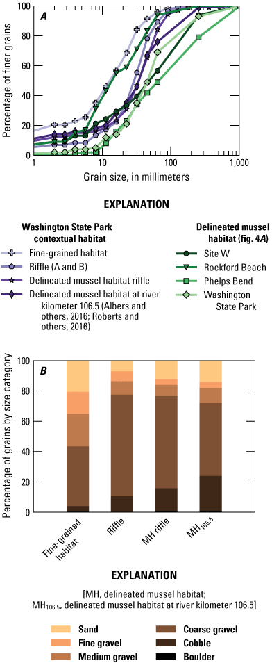
(A) Cumulative grain-size distribution data and (B) composition by category for contextual habitats in the Washington State Park study reach. Distributions are grouped by habitat type. Also shown are the grain-size distributions from surveys of the four delineated mussel habitats, and the grain-size distribution from another delineated mussel habitat within the study reach. Clasts were measured on the intermediate axis.
Contextual habitats were categorized as either fine grained or coarse grained (table 7). The fine-grained habitats consist of the bar, race, and glides, and the coarse-grained habitats consist of the riffles and MH106.5. Data from the fine-grained habitats were combined for bedload mobility analyses, as were data from the two contextual riffles (A and B).
The representative framework grain size (D50) for the habitat types ranges from fine to coarse gravel (table 7). The finer sediment fraction, represented by D16, ranges from sand and finer sediment (<2 mm) at the bar and glides to gravel at the riffles (table 7). Sand was present in all habitat types. The smallest fractions were in riffles and the race, and the largest fractions were in the glides.
The MHs at STW, PHB, and WSP generally contain coarser substrate than most of the sampled contextual habitat types at WSP (fig. 8A), and their distributions are significantly different from those of both the fine-grained contextual habitats and the riffles not associated with mussel presence (riffles A and B; hereafter referred to as “riffle” habitat; pairwise chi-square test for independence, p<0.01). The size distribution of the MH at RFB is most similar to that of the fine-grained contextual habitats (pairwise chi-square test for independence, p=0.06). The MH at WSP was not significantly different in categorical grain-size distribution from MH106.5 (pairwise chi-square test for independence, p=0.01), though the size distribution in MH106.5 was significantly different from those of the other three MHs (p=0.01).
Hydrodynamic Model Results
The results of discharge scenario simulations extending from the 90-percent flow exceedance to the 2-year peak flow are reported in this section. Model discharge errors for all discharge simulations for the calibrated Cd at STW, RFB, and PHB were less than 15 percent of the total modeled discharge; discharge errors for simulations less than or equal to the 10-percent flow exceedance were less than 1 percent of the modeled discharge (table 8). Discharge errors at WSP were less than 3 percent at discharges greater than or equal to the 10-percent flow exceedance but were 51.0 and 14.8 percent for the 90- and 50-percent flow exceedance scenarios, respectively. These high errors are the result of an unstable model solution for low discharges. Although the error for the 50-percent flow exceedance is comparable to the highest discharge errors at some of the other reaches, this scenario discharge is only 3.7 m3/s higher than that of the 90-percent flow exceedance and also is likely affected by inadequate calibration. Therefore, the 50- and 90-percent flow exceedance simulation data for WSP were omitted from the habitat analysis.
Table 8.
Percentage error on discharge for the final iteration of flow scenario simulations.[%, percent; STW, site W; RFB, Rockford Beach; PHB, Phelps Bend; WSP, Washington State Park; NA, not applicable]
Model outputs include hydraulic parameters of interest for each scenario: water-surface elevation, depth, depth-averaged velocity, and shear stress. Reported hydraulic values are the results of simulations using the calibrated Cd unless otherwise noted. Results for the hydraulic parameters were extracted from model outputs for discrete zones of interest: the modeled wetted area of the study reaches and the MH polygons. The hydraulic patterns and spatial extent of wetted cells within these discrete zones vary depending on the simulated discharge (fig. 2). The distributions of the hydraulic parameters within each zone were compared in pairwise fashion using a pairwise two-sample Kolmogorov-Smirnov (K–S) test completed using the SciPy 1.2.1 package in Python 3.7.3 (Python Software Foundation). Pairwise two-sample K–S comparisons were completed for the discrete zones in a reach and for the corresponding zones between reaches. Any areas of spatial overlap were removed from the distributions before completing tests. For example, a K–S test of the study reach and the MH hydraulic values would be a comparison of the MH wetted cells and the study reach wetted cells minus the MH wetted cells.
Water-Surface Elevation
Measured and simulated water-surface profiles for STW and PHB indicated an overall decrease in water-surface slope with increasing discharge (fig. 9; appendix 1, fig. 1.1; appendix 3, table 3.1). This trend is partly due to the reduced water-surface gradient of the riffles as discharge increases (Leopold and others, 1964; Keller, 1971; Lisle, 1979) and also may be partly attributable to backwater effects at STW. STW is about 2.5 km upstream from the confluence with the Meramec River. During local high-flow events, higher stages in the Meramec River produce a higher local base level for the Big River to drain into, creating a backwater effect near the mouth. In contrast to the other two reaches, the simulated water-surface profiles for RFB and WSP (ignoring the 90- and 50-percent flow exceedance scenarios at WSP) show an overall increase in gradient with increasing discharge.
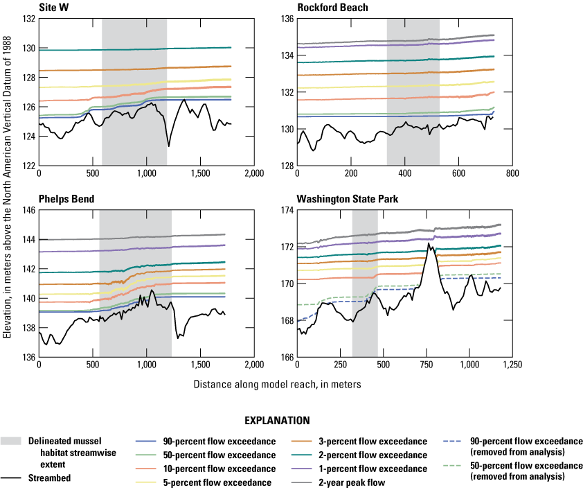
Streambed and simulated water-surface profiles at the four reaches for all discharge scenarios. Plotted elevations are values along stream centerlines; therefore, the water-surface profiles may intersect exposed bars at some discharges (for example, Phelps Bend, Washington State Park). For the analyzed discharge scenarios (solid color lines), line thickness represents the range of water-surface elevations from 85 to 115 percent of the optimum calibrated drag coefficient generated in the sensitivity analysis. The maximum difference between the optimized drag coefficient simulated slope and the sensitivity analysis simulated slopes was plus or minus 0.00003 meter per meter (appendix 3, table 3.1). Flow direction is from right to left. Note that streambed profiles have been smoothed using one-dimensional linear interpolation.
The steep drop off at the downstream end of the 90-percent flow exceedance water-surface profile for WSP may indicate an inadequate calibration relation for lower discharges at the reach, consistent with the high discharge errors reported at low-flow (50- and 90-percent flow exceedance) simulations (table 8). As explained previously, the data from the 50- and 90-percent flow exceedance simulations at WSP were omitted from the habitat analyses (dashed lines in fig. 9).
Depth
Depth values for all wetted cells within the study reaches for each discharge simulation are shown in figure 10. The depth distributions increasingly differ among the reaches with decreasing flow exceedance. Across the simulated discharge scenarios, STW has the largest flow depths, and WSP has the smallest.
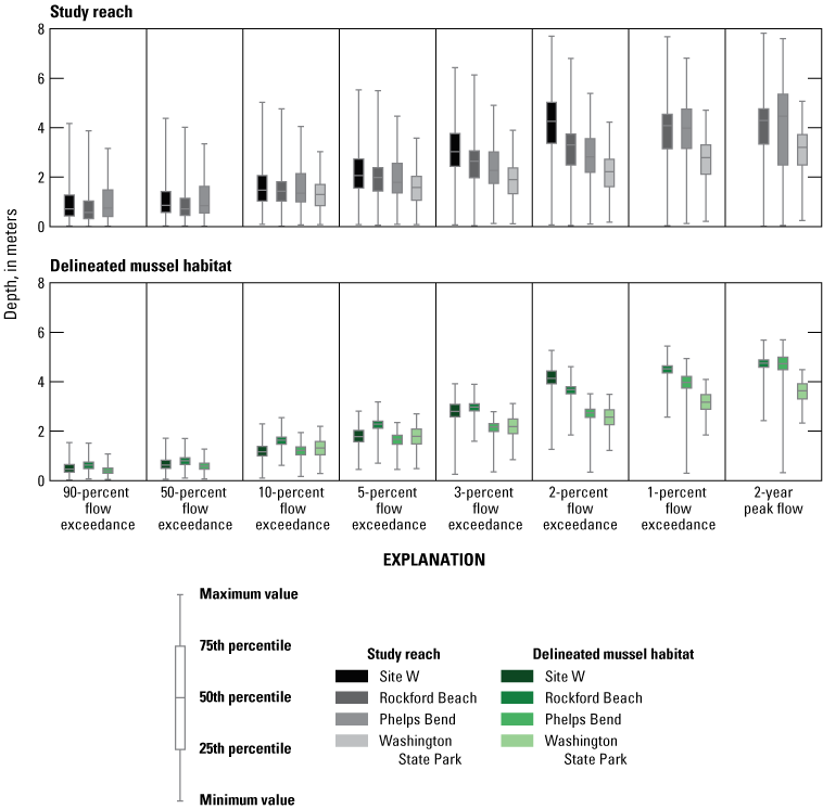
Depth distributions for wetted cells within the four study reaches and delineated mussel habitats across all discharge scenarios. Boxplot whiskers show full data range.
Flow depths within the MHs at all four reaches follow a similar pattern; depths tend to differ more among reaches with decreasing flow exceedance. Depths within the MHs range from 0.03 to 5.7 m, and study reach depths range from 0 to 7.8 m across all scenarios. Depth distributions in the MHs were statistically different in pairwise two-sample K–S tests between reaches across all discharge scenarios (p<0.01), except for STW and WSP, where differences lacked significance at the 5-percent flow exceedance scenario (p=0.07).
The depth distribution data for each reach across all simulated, analyzed discharge scenarios are shown in figure 11. Data were plotted using a Gaussian kernel density function, showing the density of observations by class for the reach and the MH. Note that the 90- and 50-percent flow exceedance scenarios at WSP were omitted from the analysis, and the 1-percent flow exceedance and 2-year peak flow scenarios at STW were not simulated. Also note that the plots show all values from each discrete zone, but statistical comparisons using the pairwise two-sample K–S test did not include areas of spatial overlap.
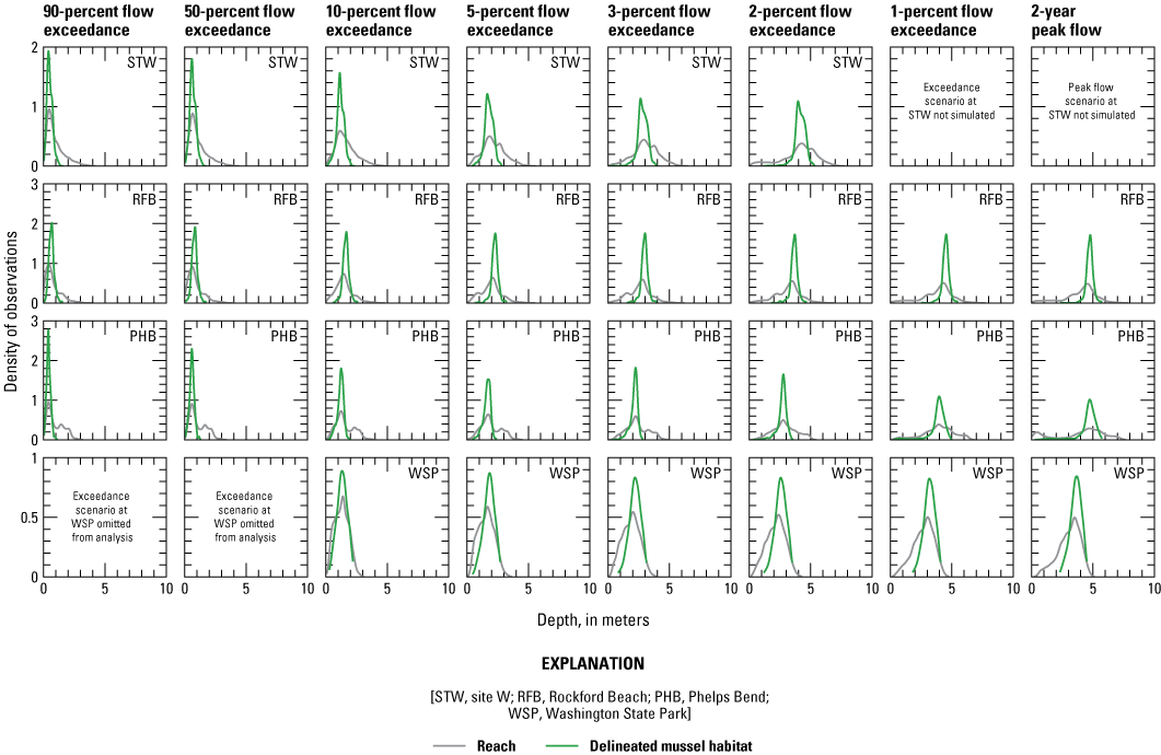
Gaussian kernel density distributions of depth values for wetted cells within the study reach and the delineated mussel habitat.
Reach by reach, the peak densities of MH depths are visibly consistent with those of the study reach for low and high discharges, although the MHs consist of a narrower range of depths. Nevertheless, the distributions of MH depths are significantly different (pairwise two-sample K–S test, p<0.01) compared to the whole of their respective study reaches.
Notably, parts of all four MHs remained dry at some discharge scenarios. Across the range of discharge scenarios, the percentages of wetted area within the MHs were as follows: (1) STW, 87.1–99.6-percent wetted (90- to 2-percent flow exceedance); (2) RFB, 95.3–100-percent wetted; (3) PHB, 74.3–99.7-percent wetted; and (4) WSP, 97.6–100-percent wetted (10-percent exceedance to the 2-year peak flow). For the most part, the presence of simulated dry areas is not due to the incompatible geometries of rasters and vectors (that is, pixelated edge versus smooth edge). For at least one scenario at each MH, the dry areas were wider than one cell width. See figure 2 for a hypothetical but representative example of simulated dry areas within an MH.
Velocity
Study reach velocity values ranged from 0 to 3.2 m/s, and velocity values within the MHs ranged from 0 to 3.1 m/s for all discharge scenarios (fig. 12). The highest reach velocities were simulated at the 2-year peak flow at WSP, and the highest MH velocities were simulated at PHB at the 3-percent flow exceedance. MH velocity distributions were statistically different between all reaches across all discharge scenarios (pairwise two-sample K–S test, p<0.01). For STW and PHB, the highest velocities were within the MHs for a subset of discharges (10–2-percent exceedance and all but the 1-percent exceedance, respectively). The highest reach velocities at RFB were outside of the MH for all discharge scenarios. For WSP, the highest reach velocities were outside of the MH for all discharge scenarios except the 10-percent flow exceedance.
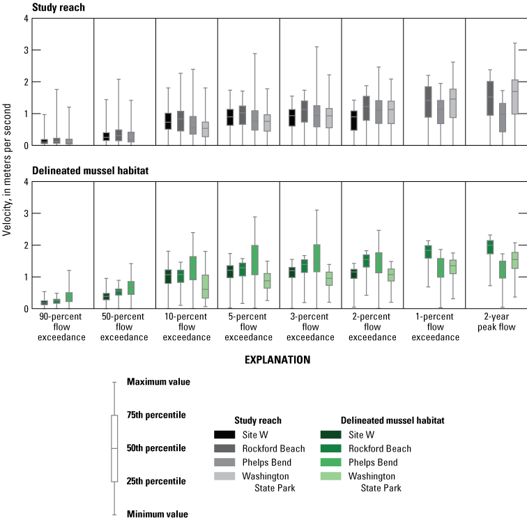
Velocity distributions within the four study reaches and delineated mussel habitats across all discharge scenarios. Boxplot whiskers show full data range.
Flow velocity values for all wetted cells within each study reach show different trends for different reaches (fig. 12). For RFB and WSP, median velocity increased with increasing discharge, whereas median velocity at STW and PHB increased with discharge to a certain flow exceedance (3-percent and 1-percent flow exceedance, respectively) and decreased at discharges greater than that. The same general pattern is evident in the median velocities within the MHs. The maximum reach velocities for RFB and WSP increased overall with discharge, increasing to the 10- and 3-percent flow exceedances, respectively, decreasing at the next higher discharge scenario, then increasing again with discharge greater than that. In contrast, the maximum reach velocities at STW and PHB increased to a certain discharge (10-percent and 3-percent flow exceedance, respectively) and then decreased with increasing discharge.
As discharge increases, a corresponding increase in velocity and cross-sectional area is expected to transmit the additional influx of water, yet maximum reach velocity does not monotonically increase with discharge at the four reaches. This behavior may be due to a homogenization of flow velocities with increasing discharge, caused by uniform roughness used in modeling. As discharge increases, any vegetated areas within the bankfull channel will eventually be submerged. Because of the vegetation, such areas typically have higher roughness than the low-flow (<10-percent flow exceedance) channel. Our flow models used a spatially uniform roughness (Cd) distribution, which does not account for variable roughness because of vegetation; therefore, the models may produce an overly homogenous velocity distribution throughout the wetted channel, possibly reducing the maximum values. Given the good agreement between the measured and simulated flow velocity transects (fig. 7), however, this scenario is unlikely.
The nonmonotonic behavior in reach maximum velocities also may be caused by velocity homogenization in riffles because of riffle-pool flow convergence routing. At higher discharges, convergent flow around submerged obstacles causes faster velocities in pools, and divergent flow causes slower, homogenous velocities in riffles (MacWilliams and others, 2006). Within each reach, riffles experience the highest velocities at low discharges. Flow convergence routing may diminish maximum riffle velocities at higher discharges and thus could explain a peak and subsequent decrease in maximum reach velocities at a moderate discharge. Still, the patterns at STW and PHB are unusual in that maximum reach velocities decrease with increasing discharge at the lower flow exceedances, an anomaly that requires further exploration.
At STW, this velocity trend is likely affected by backwater effects because of the proximity of the reach to the confluence of the Big River with the Meramec River; however, no data are presently available to document backwater effects. In unregulated systems, higher discharges in a tributary like the Big River usually coincide with higher discharges in the main stem (Meramec River) because of regional hydrologic conditions. A higher main stem discharge creates an elevated local base level at the confluence, thus raising the water-surface elevations and reducing flow velocities near the mouth of the tributary.
At PHB, there is no indication of a constriction or local base level that could produce similar backwater effects. Within the reach, the fastest velocities for all discharge scenarios were within riffles or riffle-adjacent habitat, within the zone of maximum meander bend curvature in the reach. Between the 90- and 3-percent flow exceedances, the reach maximum velocity increased with increasing discharge; at the 2-percent exceedance and greater, the maximum velocity decreased with increasing discharge.
One possible cause of the velocity trend with increasing discharge at PHB is the meander bend. The simulated water surfaces in the cross-stream direction produced superelevation along the outside edge of the bend, a flow behavior characteristic of meander bends (appendix 4, fig. 4.1). This phenomenon is caused by helical secondary flow in the cross-stream direction, created as the thalweg migrates across the channel width, and leading to an accumulation of water at the outer edge. Such meander-induced changes in flow direction cause a greater loss in energy compared to a similar straight reach (Leopold and others, 1960). Although this secondary flow is affected by vertical flow structure not simulated in 2D (vertically averaged models like FaSTMECH), these models are nevertheless capable of simulating such cross-stream water-surface variations. Between the 50- and 5-percent flow exceedance discharges at PHB, the superelevation increased with discharge but only extended to the middle of the channel, seemingly limited by the presence of midchannel bars. At discharges greater than the 3-percent flow exceedance, the bars and islands within the meander become mostly or entirely submerged, and the superelevation behavior extends across the active channel. That our simulations only produced a decrease in maximum velocities with increasing discharge at discharges greater than the 3-percent flow exceedance indicates that any meander-induced energy loss is not manifested until the superelevation spans the active channel.
The trend of decreasing velocity with increasing discharge at PHB also is associated with a reduction in water-surface slope at higher discharges (fig. 9; appendix 3, table 3.1), particularly within the swift-moving, riffle-bearing zone of high curvature. Because much of the total reach length at PHB is dominated by the presence of bars and riffles, coupled with high curvature, any homogenization or reduction in velocities in this region would likely cause an overall reduction in maximum reach velocities. These changes reflect an increase in energy loss with higher discharges. The velocity distribution data for each reach across all simulated, analyzed discharge scenarios are shown in figure 13. The MH velocity distributions differed significantly from those of the study reaches (pairwise two-sample K–S test, p<0.01). Note that the 90- and 50-percent flow exceedance scenarios at WSP were omitted from the analysis, and the 1-percent flow exceedance and 2-year peak flow scenarios at STW were not simulated.
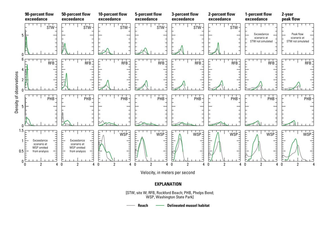
Gaussian kernel density distributions of velocity values for wetted cells within the study reach and the delineated mussel habitat.
For RFB and WSP, where maximum velocities increased overall with increasing discharge, the MHs did not have the highest velocities for any discharge scenario except the 10-percent exceedance flow at WSP. In contrast, the maximum velocities at STW and PHB were within the MH for most discharge scenarios, peaked at a moderate flow exceedance, and decreased with increasing discharge greater than that. In effect, as discharge approaches approximate bankfull, maximum velocities within the MHs are exceeded by those elsewhere in the reach or, alternatively, decrease in reaches where the MHs contain the highest current velocities. Both situations tend to diminish velocities within the MHs at the highest modeled discharges.
Bed Shear Stress
Study reach shear-stress values ranged from 0 to 59 N/m2, and values for the MHs ranged from 0 to 31 N/m2 (fig. 14). The highest reach shear-stress values were produced at STW at the 90-percent flow exceedance, and the highest MH shear-stress values were produced at PHB during the 5-percent flow exceedance. Shear-stress distributions within the MHs were statistically different between all reaches across all discharge scenarios (pairwise two-sample K–S test, p<0.01). For STW and PHB, the highest shear stresses were within the MHs for most discharge scenarios (10–2-percent exceedance and all but the 1-percent exceedance, respectively). At RFB and WSP, the highest shear stresses within the reach were not within the MHs at any discharge scenario, except for WSP at the 10-percent flow exceedance.
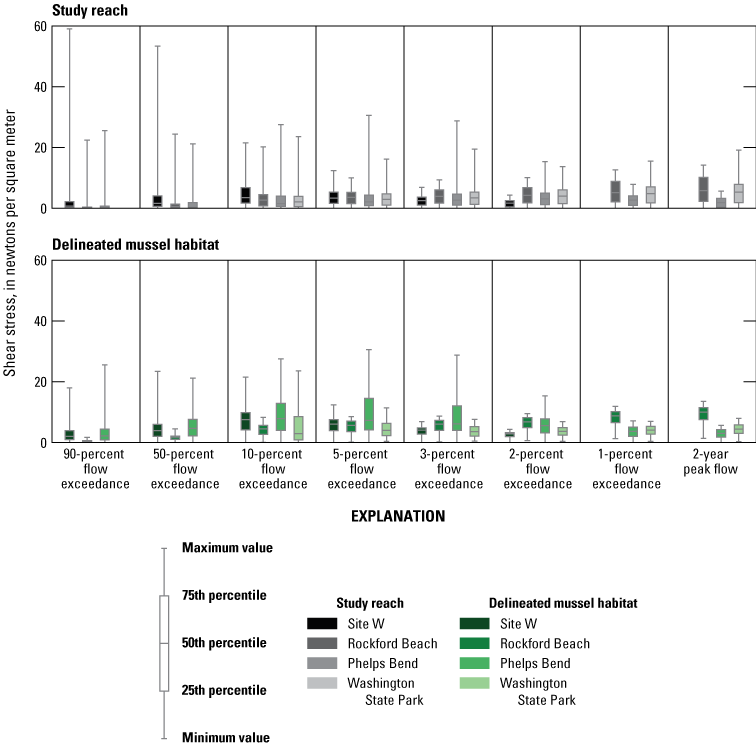
Bed shear-stress distributions within the four study reaches and delineated mussel habitats across all discharge scenarios. Boxplot whisker extents show full data range.
Similar to the median velocity values, median shear-stress values for RFB and WSP increased with increasing discharge, and median shear-stress values for STW and PHB increased with discharge to a certain flow exceedance (10 percent for STW; 2 percent for PHB) and then decreased (fig. 14). The same pattern was evident in the median MH shear-stress values. The maximum reach shear-stress values decreased overall with increasing discharge at all four reaches. The maximum MH shear stresses increased at RFB and decreased overall at the other three reaches with increasing discharge.
The maximum reach shear-stress values at the four reaches mostly reflect the patterns in maximum reach velocities, which makes sense given the use of the streamwise and cross-stream velocity components to compute shear stress (eq. 2). The maximum reach shear-stress values at RFB and WSP increased with discharge at discharges greater than the 3- and 2-percent flow exceedances, respectively, although maximum reach shear stress decreased overall between the lowest and highest simulated discharges. The maximum reach shear-stress values at STW and PHB decreased overall with increasing discharge. Similar to the patterns in maximum velocity, the overall decrease may be due to a homogenization of shear stress across the channel width at higher discharges, caused by the attribution of uniform vegetation roughness in modeling, or more likely, by riffle-pool flow convergence routing (MacWilliams and others, 2006). As discussed previously, the overall decreases at STW and PHB also may be affected by a reduction in flow energy caused by backwater effects or by meander-induced redirection of flow, respectively.
The distributions of shear stress for the MHs and reaches (not plotted) were similar to the patterns observed in the velocity distributions because of the dependence of shear stress on velocity (eq. 2). Comparison between the shear-stress distributions of the MHs and reaches yielded statistically significant differences (pairwise two-sample K–S test, p<0.01) at all simulated, analyzed discharges at all reaches.
For RFB and WSP, where maximum reach shear-stress values increased as discharge approached the 2-year peak flow, the highest shear-stress values were outside of the MHs for most discharge scenarios. For STW and PHB, the maximum shear-stress values were within the MH for most discharge scenarios and decreased with increasing discharge at the highest discharges. In both cases, as discharge approached approximate bankfull, maximum shear-stress values within the MHs were either exceeded by those elsewhere in the reach or decreased in reaches where the MHs had the highest shear stresses. As with the maximum velocities, these trends modulate the maximum shear stresses within the MHs for the range of simulated discharges.
Sediment Stability
Shields-stress (τ*, eq. 3) values were computed for all cells within the MHs using the shear-stress values simulated at each discharge scenario (fig. 15). Shields values were calculated for the sand-size class (2 mm), the 16th-percentile size class (D16), and the median-percentile size class (D50) measured within the MHs during the phase II surveys (Albers and others, 2016; Roberts and others, 2016). Because grain sizes greater than 64 mm were categorized but not measured, the 48th-percentile measurement of 59 mm was used to approximate the D50 for PHB. Note that the 90- and 50-percent flow exceedance scenarios at WSP were omitted from the analysis, and the 1-percent flow exceedance and 2-year peak flow scenarios at STW were not simulated.
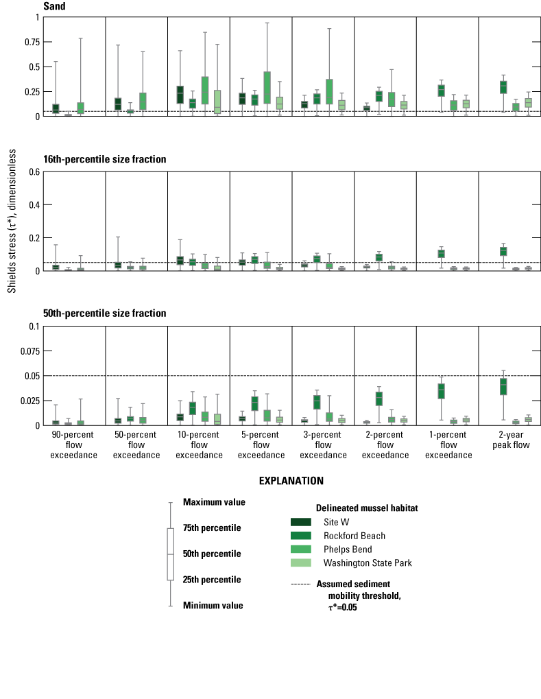
Delineated mussel habitat Shields stress for sand (2 millimeters), the 16th-percentile particle size fraction, and the 50th-percentile particle size fraction. Boxplot whisker extents show full data range.
Based on an incipient motion criterion of a Shields value greater than or equal to 0.05 (Buffington and Montgomery, 1997), movement of the D50 within the mussel beds was not predicted at any of the reaches at the simulated discharges except for RFB at the 2-year peak flow (fig. 15). Movement of the D16 size class was predicted within all four MHs for at least one discharge scenario less than or equal to the 2-year peak flow. For all reaches except RFB, D16 mobility was not predicted in the MHs greater than the 2-percent exceedance flow, and the D16 at the WSP MH was only predicted to move at the lowest discharge simulated in the reach (10-percent flow exceedance). Sand movement was predicted for all MHs at all simulated, analyzed discharge scenarios, except for RFB at the 90-percent exceedance.
Shields values also were computed for contextual habitats within the WSP study reach where additional grain-size data were collected. Shields values were calculated for sand and the D16 and D50 size classes and were grouped by habitat type (fine grained, riffle, and MHs; fig. 16). Note that the 90- and 50-percent flow exceedance scenarios at WSP were omitted from the analysis.
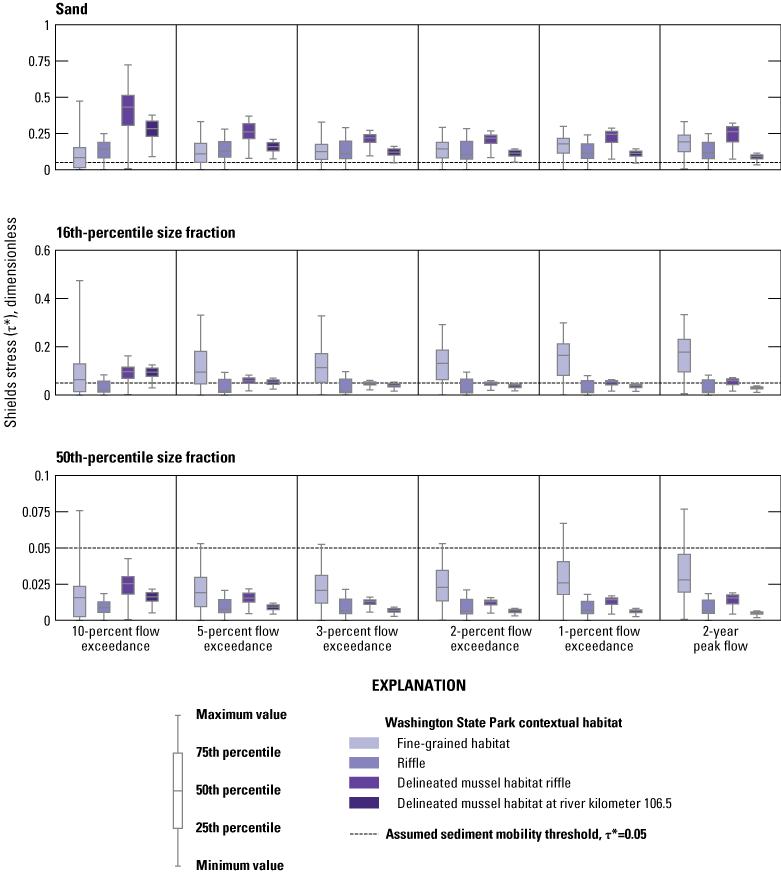
Shields stress for sand (2 millimeters), the 16th-percentile particle size fraction, and the 50th-percentile particle size fraction at pebble-count locations (contextual habitats) within the Washington State Park study reach, grouped by habitat type. Boxplot whisker extents show full data range.
Using the same critical threshold for mobility, τ*=0.05, sand movement was predicted within all the contextual pebble-count habitats at all simulated, analyzed discharge scenarios. Mobilization of the D16 was predicted within all the contextual habitats for at least one discharge scenario up to the 2-year peak flow. Shields values for the D16 were highest for the fine-grained habitats. D50 movement was predicted within submerged areas of the fine-grained contextual habitats at discharges less than or equal to the 2-year peak flow; however, none of the riffles or mussel-bearing areas were predicted to have mobilized the D50.
Cumulative frequency distributions of the Shields values were plotted for sand and the D16 and the D50 size fractions at all discharge scenarios (fig. 17A, B) to compare the relative mobilities of the four MHs to those of the contextual habitats. The cumulative Shields distributions for the sand-size fraction were fairly similar among the MHs and contextual habitats. Because the same grain diameter, D=0.002 m, was used for these Shields calculations, any variation is due to differences in the shear-stress values simulated within the habitats. Sand mobility was predicted within at least 50 percent of the wetted area of all contextual habitats and the MHs at STW, PHB, and WSP for all simulated, analyzed discharge scenarios (fig. 17A, B). Sand mobility was not predicted anywhere in the MH at RFB for the 90-percent flow exceedance; however, mobility was predicted for more than 50 percent of the wetted MH area for all other discharge scenarios.
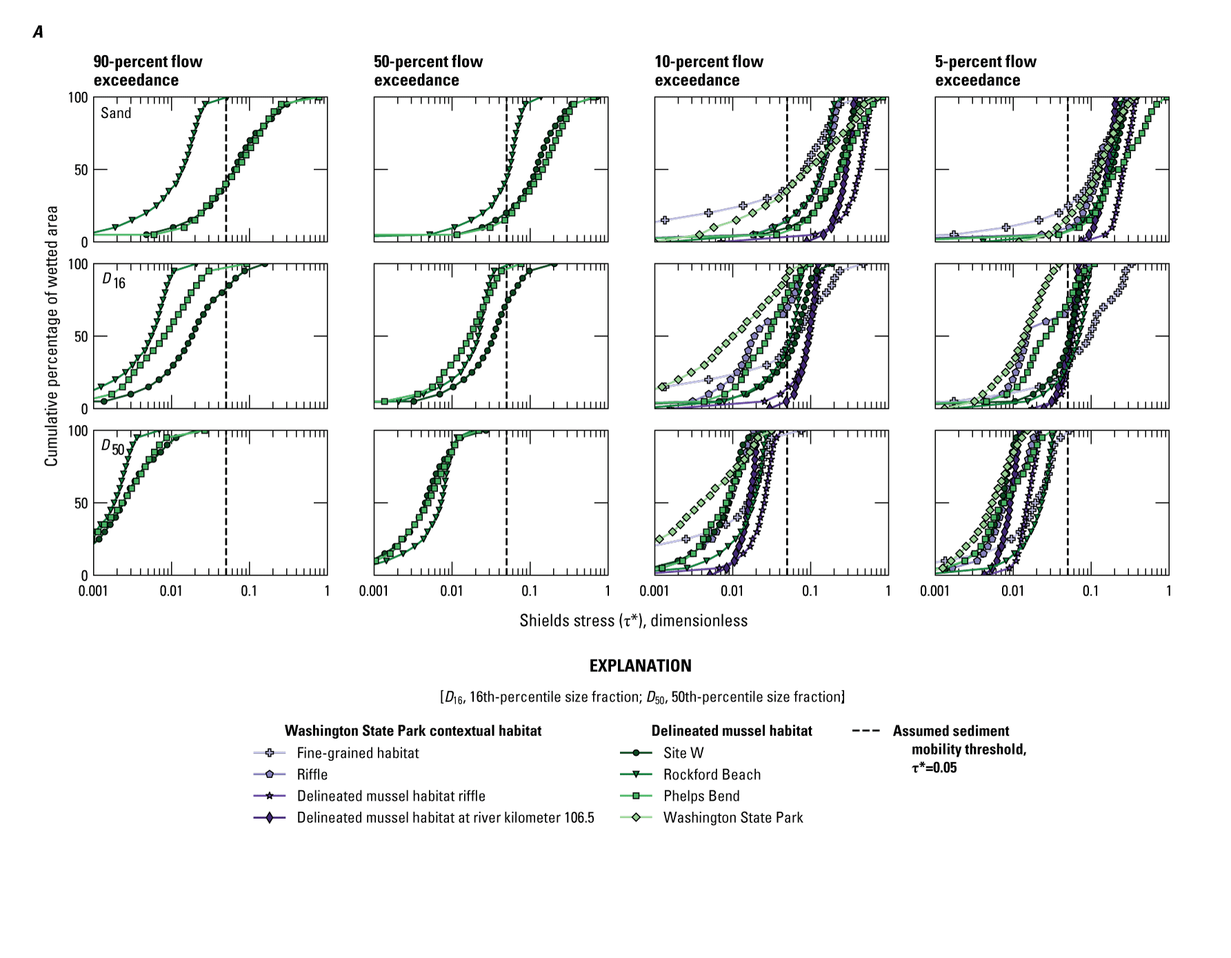
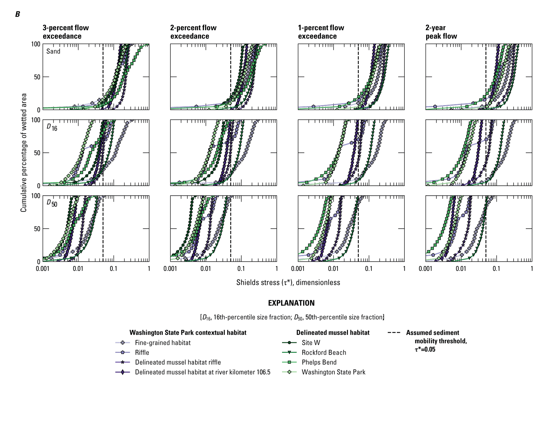
Cumulative frequency distributions of Shields stress for sand (2 millimeters), the 16th-percentile particle size fraction, and the 50th-percentile particle size fraction at the four delineated mussel habitats and the contextual habitats in the Washington State Park study reach. (A) results plotted for the 90-, 50-, 10-, and 5- percent flow exceedance scenarios; (B) results plotted for the 3-, 2-, and 1- percent flow exceedance and 2-year peak flow scenarios. Note that the 90- and 50-percent flow exceedance scenarios at Washington State Park were omitted from the analysis, and that the 1-percent flow exceedance and 2-year peak flow scenarios at site W were not simulated.
Compared with the sand Shields values, the Shields values of the D16 size fraction were more variable among habitats because of the additional variation in D16 among reaches. For the MH at RFB, the percentage of wetted area capable of mobilizing the D16 increased with discharge, with a mobile area of 96 percent at the 2-year peak flow. For the other MHs, as well as MH106.5, the fraction of mobile wetted area decreased with increasing discharge for flow exceedances less than either the 10- or 5-percent, with no mobile wetted area at the highest simulated discharges for each reach. This indicates that the mobile areas are spatially concentrated and do not expand with increasing discharge. In contrast, the percentage of mobile area for the D16 within the fine-grained habitats increased with increasing discharge, and the percentage of mobile area for the D16 within the riffles stayed roughly between 30 and 34 percent across the range of discharges. D16 Shields values were generally higher for the fine-grained contextual habitats than for the MHs.
Similarly, Shields values for the D50 size fraction were generally higher within the fine-grained contextual habitats than those within the STW, PHB, and WSP MHs and MH106.5. Of the four investigated MHs, only RFB had D50 mobility, which was simulated within 16 percent of its wetted area at the 2-year peak flow. The fine-grained contextual habitats incurred small areas of mobility at all simulated, analyzed discharges, with mobility predicted in 16 percent of the wetted area at the 2-year peak flow.
Factors Controlling Mussel Habitats in the Big River
This section discusses what the hydrodynamic modeling results indicate about the MHs. Sensitivity analyses indicate that errors in calibration of the model input parameters produce only negligible variability in the hydraulic outputs (appendix 3, tables 3.1 and 3.2). Our assessment of mussel habitats relies on the MH delineations, polygons consisting of mussel-occupied areas and contiguous areas of similar, suitable habitat (Roberts and others, 2016), as the best available information for actual habitat occupancy.
Through field observation and hydraulic simulations, we determined that the specific features and range of conditions of each examined Big River MH are substantially different among study reaches. This difference among reaches illustrates the challenge of predicting mussel habitat suitability using only depth, velocity, and shear stress. In fact, the contrasting morphology, hydraulics, and substrate compositions of the two robust sites at STW and RFB demonstrate that mussel communities can flourish in different physical conditions, which is not surprising because other studies have had varying success in predicting mussel density or presence using hydraulic variables (Newton and others, 2008; Strayer, 2008). The ability to relate occurrence to hydraulic variables also may be diminished by additional factors, such as the following:
-
• substrate distributions that reflect rare bedload-transporting events or sequences of events that exceed the 2-year peak discharge and were not documented during our study;
-
• variable detection probabilities for mapping mussels and delineating habitats;
-
• incomplete occupation of suitable habitats because of complexities of mussel life histories, including interactions with host fish and inability to migrate; or
-
• water- or sediment-quality effects, such as contamination, that may limit mussel occupation.
Nonetheless, some hydraulic relations are apparent. The relation between MH and reach hydraulic forces followed similar patterns at all reaches for the range of simulated discharges (figs. 12, 14); that is, maximum velocities and shear stresses in MHs were moderated by reach-scale patterns in velocity and shear stress. As discharge approached approximate bankfull, maximum velocities and shear stresses within the MHs were either exceeded by those elsewhere in the reach or, alternatively, decreased with increasing discharge in reaches where the MHs contain the highest flow speeds and shear stresses. These patterns are likely affected by the same reach-scale velocity and shear-stress trends discussed previously: riffle-pool flow convergence routing (MacWilliams and others, 2006), backwater effects, and meander-induced redirection of flow. Our simulations indicate that the four MHs investigated on the Big River experience their maximum velocities and shear stresses at moderate exceedances or experience lower maximum velocities and shear stresses relative to their reaches.
The other major similarity across the four Big River MHs is theoretical bed-sediment stability and instability. Although contextual habitats within one of the study reaches had predicted mobility of the median grain size and the finer size fractions across all simulated, analyzed discharges (fig. 16), the MHs were comparatively less mobile (fig. 15). For all four MHs, the hydraulic models predicted sand mobility and some mobility of the D16 size fraction at the simulated discharges but almost no mobility of the D50 size fraction. One implication of these results is that the habitats are frequently subjected to discharges that transport fine sediment and thereby prevent clogging of substrate interstices (also known as embeddedness), but discharges in excess of bankfull (less frequent than 2-year mean return interval) may be needed to mobilize the bed and therefore disturb mussel populations.
These model results are supported by field data and observations during frequent visits to the WSP study reach between 2018 and 2020. After an above-bankfull discharge event, and after the subsequent hydrograph peaks, investigators noted large amounts of newly deposited sand in several areas in the reach. Still, substantial sand deposition was not observed within the reach’s MH, even though predicted sand mobility at the 2-year peak flow was high within the nearby contextual habitats. Similarly, substantial fine sediment deposition was not observed within the other three MHs. Previous investigations on the Big River (Barr, 2016) reported high availability of fine sediment and attributed about 30 percent of suspended sediment loads to high-flow events. Even so, fine sediment was only a minor component of the surface substrate composition within these 4 MHs (fig. 4A, B) and within 14 other Big River MHs (Albers and others, 2016; Roberts and others, 2016). Although fine sediment is evidently mobile throughout the Big River, especially during high-flow events, our simulations, observations, and available empirical data indicate that it does not linger within the MHs because of mobility of finer grains at lower discharges or during the declining limb of a flood hydrograph. This interpretation is consistent with observations and predictions of freshwater mussel habitat by other investigators. Mussels can be adversely affected by deposition of sand and finer sediments (Vaughn and Pyron, 1995; Galbraith and others, 2008, 2010) because of interference with feeding activity (Ellis, 1936) and burrowing (Box and Mossa, 1999). Similarly, Steuer and others (2008) determined that mussels may require minimum hydraulic conditions to remove waste from the bed and to deliver nutrients and oxygen.
Our simulations also support the theory of overall bed stability in suitable habitats (Vannote and Minshall, 1982; Strayer and Ralley, 1993; Strayer, 1999). Stability was predicted for the median grain size at all four habitats across the range of discharge scenarios, with slight exception at RFB, where a small area of the MH is capable of transporting the median grain size (medium gravel) at the 2-year peak discharge, the most energetic conditions simulated (fig. 17A, B). During repeat visits to the four reaches, we did not observe any signs of appreciable erosion (or deposition) or any change in bed-sediment texture within the MHs. The coarsest grained MH, at PHB, was noticeably armored with interlocking cobbles and coarse gravel clasts that were difficult to move. Other investigators have observed, anecdotally and quantitatively, that freshwater mussels are associated with areas of stable sediment (Vannote and Minshall, 1982; Strayer and Ralley, 1993; Strayer, 1999; Johnson and Brown, 2000; Morales and others, 2006; Allen and Vaughn, 2010; May and Pryor, 2016). Predictions and simulations of bed stability in mussel habitats could be further validated through bedload tracer studies that can furnish direct measurements of bedload particle mobility and immobility within and adjacent to mussel habitats.
We propose that the hydraulic conditions and the associated localized mobility and stability of sediment through a range of discharges together constitute an important factor in habitat suitability in the Big River. The MHs examined in this study frequently experience shear stresses sufficient to flush excess fine sediment from the bed, yet the most frequent higher energy discharges up to bankfull discharge do not produce sufficient shear stresses to mobilize larger substrate within the MHs. In other words, suitability seems to relate to a “sweet spot” of hydraulic forces that are sufficient to transport fine sediment but insufficient to cause wholesale disturbance of the bed. That this pattern was modeled at all four MHs indicates that the depauperate beds at PHB and WSP are not impaired by bed instability or siltation relative to the robust beds at STW and RFB. The pattern of stability and flushing also may explain the variability in the importance of certain discharges with respect to mussel presence, density, or both as reported in other studies. In some cases, abundance was thought to be limited by high-flow conditions (Gangloff and Feminella, 2007; Allen and Vaughn, 2010), and in other cases, low-flow (50-percent exceedance) hydraulics were determined to be stronger predictors of mussel density (Steuer and others, 2008). Zigler and others (2008) observed that low and high discharge conditions were strong predictors of abundance. These inconsistencies in quantification of freshwater mussel habitat conditions may reflect a dependency on the interactions of low and high discharges with the local sediment regime.
This investigation furnished simulations of Big River mussel habitat conditions across a wide range of discharges; still, given the reported variability in limiting discharge conditions described previously, these results could be expanded by examining mussel habitat hydraulics across a higher range of discharges. Although our simulations indicate fine sediment flushing and overall bed stability in the four Big River MHs at discharges up to approximate bankfull, it is not known if these conditions persist at higher discharges. Within a typical mussel’s lifetime of 15–40 years (Haag, 2012), it will likely be exposed to several flood events much greater than bankfull. Simulating discharges with recurrence intervals as much as the typical lifespan would yield the full range of conditions that individuals within a mussel bed community can theoretically endure. These extended models may reveal hitherto undetected controls on habitat suitability, disturbance regime, and possibly additional patterns among the MHs.
One important consideration is the potential effect of the temporal differences between the MH delineation surveys and the field surveys completed for this investigation because each survey period may reflect a different ecological and morphodynamic state in the reaches. Between the 2010–14 MH delineation and survey period (Roberts and others, 2016) and our 2018–20 data collection, the Big River experienced multiple floods, including a greater than 50-year peak flood event (Southard and Veilleux, 2014) in 2017 (U.S. Geological Survey, 2021). Such floods are beyond the bankfull limits of the present modeling study but may alter mussel communities and channel morphology; consequently, the modeled MH hydraulic conditions may correspond to a different mussel community and geomorphic state from those of the original surveys because of dynamic changes in the mussel populations or reach morphologies. Additional quantitative mussel surveys, contemporaneous with the hydrogeomorphic sampling of this investigation, would help resolve these questions (Roberts and others, 2009).
Another challenge in hydraulic habitat studies is the treatment and interpretation of species-presence data representing discrete time intervals and occupancy in the context of spatially continuous model simulations. Our high-resolution modeling approach produced continuous layers that document substantial variation in hydraulic variables at a fine scale (see hypothetical example in fig. 2). The mussel data (the MHs) were provided in the form of polygonal areas of similar, suitable habitat within which live mussels were present (Roberts and others, 2016). For the purposes of this study, we treat all areas within the MHs uniformly, though they may contain areas devoid of mussels because of the inclusion of adjacent areas of similar, suitable habitat (Roberts and others, 2016); furthermore, individual mussel beds typically have heterogeneity in mussel distribution and density (Strayer and others, 2004; Newton and others, 2008). Moreover, though some of these MHs have been revisited since delineation (for example, Roberts and others, 2009, 2016), they effectively represent a snapshot in time and may over or underrepresent potential areas of occupancy. Mussels are capable of lateral and vertical movement and may move in response to gradually changing conditions such as drought (Newton and others, 2015). Evidently, a uniformity assumption has limitations; it does not account for the heterogeneity and dynamism of mussel presence and density nor for the unknown heterogeneity of mussel occupancy because of delineation methodology. For example, our model simulations predicted that parts of all four MHs are dry at some lower discharges (90-, 50-, and 10-percent flow exceedances) and that as much as 25 percent of the MH at PHB may be exposed during dry conditions. Because of the delineation methods (Roberts and others, 2016), these dry areas may represent areas of similar habitat unoccupied by mussels. Alternatively, dry areas may be areas with lower mussel density than the remainder of the MH or areas that are vacated by mussels during drought periods. It may be necessary to further refine the relations between mussel density and hydraulics as permitted by model output resolution. Because quantitative mussel surveys are commonly completed using a high-resolution quadrat method, it is conceivable to examine hydraulics and density at a complementary scale.
This documented heterogeneity also may be due to localized variability of hydraulic forces within mussel beds. As small, mostly sedentary benthic organisms, mussels inhabit a complex intergranular space in which the hydraulic forces are variable because of the spatial arrangement and relative sizes of objects on the bed (Chow, 1959); that is, the mussels and sediment particles. Mussels may burrow in sand (Schwalb and Pusch, 2007) or shelter from the current behind large sediment particles (Vannote and Minshall, 1982; Layzer and Madison, 1995; Pandolfo and others, 2016). These observations indicate that mussels are subject to, and participate in, sediment-mobility effects such as hiding, in which particles are protected from entrainment by nearby larger grains (Wilcock, 1988; Wilcock and Southard, 1988), and exposure, in which particles are vulnerable to mobilization because of exposure to the current (Fenton and Abbott, 1977). Mussels also are capable of modifying near-bed hydraulic conditions, reducing flow velocities and shear stresses and stabilizing the bed (Sansom and others, 2018a, 2020). Such fine-scale variations may play an important role in habitat suitability in the Big River, but they cannot be captured at the resolution of the measurements and simulations of this investigation. Bedload sediment tracer, mussel tracer, and laboratory flume studies may help resolve these questions by providing direct measurements of the fine-scale interactions between mussels, sediment particles, and hydraulics.
Summary
The Big River, located in south-central Missouri, is a tributary to the Meramec River and drains an area with contaminated sediments associated with historical lead production. This study investigated the hydraulic conditions at four study reaches containing known mussel habitats (MHs) on the Big River in Missouri to characterize the hydraulic habitat affinities of freshwater mussels and the stability of their habitats and to evaluate the potential contribution of physical habitat dynamics to mechanical and physiological stress on native mussels. Two-dimensional hydrodynamic models were compiled for discharge scenarios from base flow (90-percent flow exceedance) to the bankfull discharge (approximated by the 2-year peak discharge) for model reaches containing the MHs. Detailed bathymetric and topographic data were collected to create reach elevation layers used for the models. Discharge, velocity, and water-surface elevation data were collected at all four study reaches at various discharges to calibrate the models across a range of discharges. Shields values were computed for the MHs and contextual habitats using bed-surface sediment data collected during this study and previous studies to predict incipient motion of the substrate.
We determined that the distributions of hydraulic variables at the range of simulated discharge scenarios were significantly different among the MHs. Depth values in the MHs ranged from 0.03 to 5.7 meters, with parts remaining dry at some low-discharge scenarios. MH velocities and shear stresses reached 3.1 meters per second and 31 newtons per square meter, respectively. Through the range of simulated discharges, maximum velocity and shear stress within the MHs were constrained by reach-scale hydraulic trends.
Our calculations predicted sand mobility within at least 50 percent of the wetted area of all four MHs for all discharge scenarios greater than the 90-percent flow exceedance discharge, whereas the 50th-percentile (median) particle size fraction mobility was only predicted within a small area of just one of the habitats at the 2-year peak discharge. These results indicate that finer size fractions are mobile within the four MHs, yet the larger framework grains of the substrate are largely immobile at the most frequent discharges.
Collectively, these results indicate that suitable habitat for freshwater mussels on the Big River does not entail a specific range of velocities, depths, and shear stresses. Rather, the consistent patterns of sediment mobility and the suppression of hydraulic forces within all the MHs indicate that flushing flows at low discharges and coarse sediment stability at higher discharges are important for mussel habitat suitability in the Big River. Notably, these comparable patterns in sediment mobility among robust and depauperate MHs also indicate that the depauperate beds are likely not impaired by bed instability or siltation. Stability of coarse sediment up to bankfull discharges further indicates that bed instability is not widespread in these reaches.
Appendix 1
The following figure (fig. 1.1) shows the measured and simulated water-surface profiles for the calibration discharges, along with the streambed profiles for the four reaches. Measured water-surface elevations are values that were either collected along a driven profile or snapped to a stream centerline. Streambed and simulated elevations are values collected or extracted along stream centerlines; therefore, the water-surface profiles may intersect exposed bars at some discharges (for example, Phelps Bend, Washington State Park). Model calibration for each discharge was evaluated based on the root mean square error values between the measured and simulated water-surface elevations along the study reaches (table 4 in the main report). The parameters (drag coefficient, lateral eddy viscosity, and downstream stage) that produced the lowest water-surface root mean square error through the reach were selected as the optimized conditions for that calibration discharge. The calibration discharge values are as follows: 43.4, 52.4, 86.8, and 155 cubic meters per second (m3/s) at site W; 5.21, 25.6, 37.0, 55.7, 111, 175, and 254 m3/s at Rockford Beach; 5.93, 7.81, 29.0, and 198 m3/s at Phelps Bend; and 11.5, 16.0, 20.9, 41.0, and 91.5 m3/s at Washington State Park.
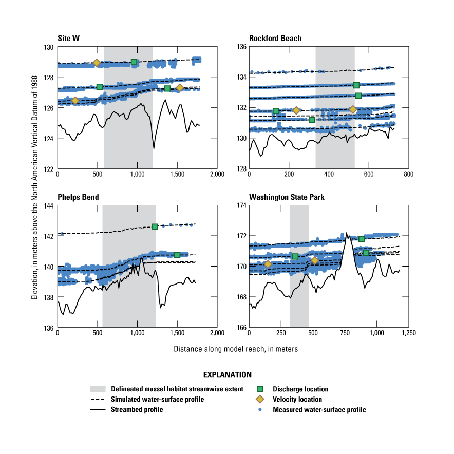
Measured and simulated water-surface profiles and streambed profiles for the calibration discharges at all four reaches. Streamwise locations of discharge measurement transects, velocity evaluation transects (fig. 7 in the main report), and mussel habitats also are plotted. Flow direction is right to left. Note that streambed profiles have been smoothed using one-dimensional linear interpolation.
Appendix 2
The following figure (fig. 2.1) shows the optimized calibration values and the corresponding calibration curves for the drag coefficient, lateral eddy viscosity, and downstream stage. The optimized calibration values include data points where a discharge measurement and a water-surface profile were collected and data points where only a water-surface profile was collected and discharges were estimated from neighboring streamgages (table 4 in the main report). Calibration curves were determined by manually fitting power law, linear, and second-degree polynomial functions to the calibration values to find the best fit (table 5 in the main report). The representative best fit equations yielded a single optimized drag coefficient, lateral eddy viscosity, and downstream stage for each discharge.
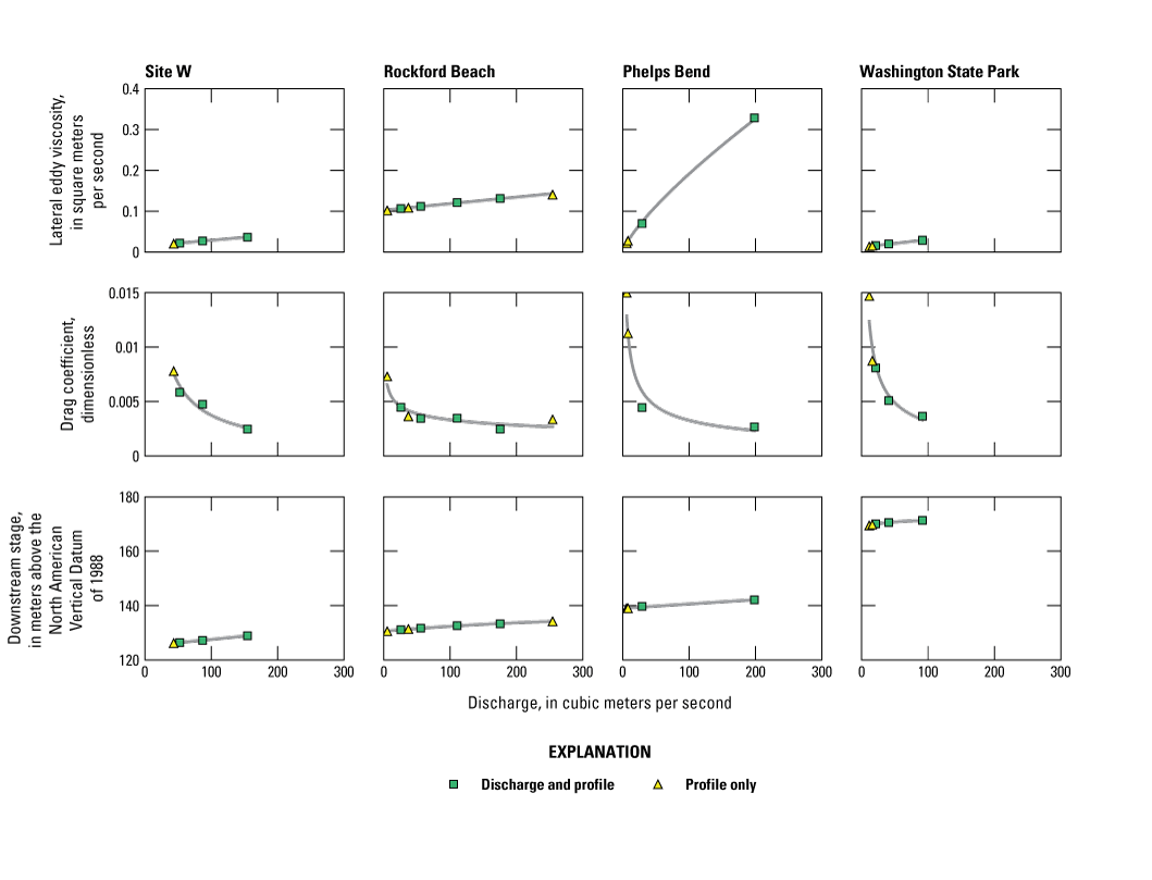
Calibration data and curves for downstream stage, drag coefficient, and lateral eddy viscosity at all reaches.
Appendix 3
The simulated water surface slopes at the optimized drag coefficient (Cd), 85 percent of the optimized Cd, and 115 percent of the optimized Cd are provided in table 3.1. These sensitivity analysis simulations were run for the simulation discharges to evaluate how uncertainties in Cd could affect model results.
Table 3.1.
Simulated study reach water-surface slopes at the four reaches for all the discharge scenarios. The water-surface slopes at the optimum drag coefficient and at 85 and 115 percent of the optimum drag coefficient also are shown as part of the sensitivity analysis. The maximum difference between the optimized drag coefficient simulated slope and the sensitivity analysis simulated slopes was plus or minus 0.00003 meter per meter.[Cdopt, optimum drag coefficient; Cd85%, 85 percent of the optimum drag coefficient; Cd115%, 115 percent of the optimum drag coefficient; m/m, meter per meter; STW, site W; %, percent; e, denotes exponentiation; RFB, Rockford Beach; PHB, Phelps Bend; WSP, Washington State Park]
The median and maximum values for depth, velocity, and shear stress at the optimized Cd, 85 percent of the optimized Cd, and 115 percent of the optimized Cd are provided in table 3.2. These sensitivity analysis simulations were run for the simulation discharges to evaluate how uncertainties in Cd could affect model results.
Table 3.2.
Sample model results for all wetted cells of the study reaches for each scenario simulation model. Scenarios were run at the calibration-determined optimum drag coefficient and at 85 and 115 percent of the optimum drag coefficient.[m3/s, cubic meter per second; m, meter; m/s, meter per second; N/m2, newton per square meter; med, median; max, maximum; STW, site W; %, percent; Cdopt, optimum drag coefficient; Cd85%, 85 percent of the optimum drag coefficient; Cd115%, 115 percent of the optimum drag coefficient; RFB, Rockford Beach; PHB, Phelps Bend; WSP, Washington State Park]
Appendix 4
The following figure (fig. 4.1) shows simulated water-surface elevations in the cross-stream direction for a cross section located with the meander bend in the Phelps Bend study reach. The simulated water surfaces show superelevation, an accumulation of water, along the outer edge of the bend. This phenomenon is caused by changes in flow direction induced by the meander and is a possible explanation for the decrease in maximum velocity with increasing discharge at discharges greater than the 3-percent flow exceedance at Phelps Bend (see “Velocity” section in the main report).
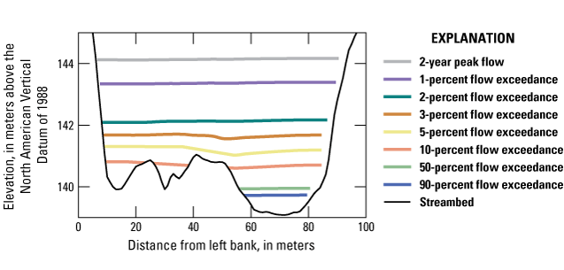
Simulated water-surface elevations for a cross section within the meander bend in the Phelps Bend study reach. The transect is about 897 meters upstream from the downstream end of the study reach. The outside edge of the meander is on the right bank; the transect is plotted facing downstream.
References Cited
Albers, J.L., Besser, J.M., Schmitt, C.J., and Wildhaber, M.L., 2016, Mussel community associations with sediment metal concentrations and substrate characteristics in the Big River, Missouri, U.S.A.: U.S. Geological Survey Administrative Report, 82 p. [Also available at https://www.fws.gov/midwest/es/ec/nrda/SEMONRDA/pdf/MusselCommunityAssociations_Albersetal2016.pdf.]
Allen, D.C., and Vaughn, C.C., 2010, Complex hydraulic and substrate variables limit freshwater mussel species richness and abundance: Journal of the North American Benthological Society, v. 29, no. 2, p. 383–394. [Also available at https://doi.org/10.1899/09-024.1.]
Allert, A.L., DiStefano, R.J., Fairchild, J.F., Schmitt, C.J., McKee, M.J., Girondo, J.A., Brumbaugh, W.G., and May, T.W., 2013, Effects of historical lead–zinc mining on riffle-dwelling benthic fish and crayfish in the Big River of southeastern Missouri, USA: Ecotoxicology (London, England), v. 22, no. 3, p. 506–521. [Also available at https://doi.org/10.1007/s10646-013-1043-3.]
Barr, M.N., 2016, Surface-water quality and suspended-sediment quantity and quality within the Big River Basin, southeastern Missouri, 2011–13: U.S. Geological Survey Scientific Investigations Report 2015–5171, 50 p., accessed June 25, 2020, at https://pubs.er.usgs.gov/publication/sir20155171.
Besser, J.M., Brumbaugh, W.G., Hardesty, D.K., Hughes, J.P., and Ingersoll, C.G., 2009, Assessment of metal-contaminated sediments from the Southeast Missouri (SEMO) mining district using sediment toxicity tests with amphipods and freshwater mussels: U.S. Geological Survey Administrative Report 08–NRDAR–02, 59 p. plus appendix.
Box, J.B., and Mossa, J., 1999, Sediment, land use, and freshwater mussels—Prospects and problems: Journal of the North American Benthological Society, v. 18, no. 1, p. 99–117. [Also available at https://doi.org/10.2307/1468011.]
Buffington, J.M., and Montgomery, D.R., 1997, A systematic analysis of eight decades of incipient motion studies, with special reference to gravel‐bedded rivers: Water Resources Research, v. 33, no. 8, p. 1993–2029. [Also available at https://doi.org/10.1029/96WR03190.]
Daniel, W.M., Cooper, A.R., Badra, P.J., and Infante, D.M., 2018, Predicting habitat suitability for eleven imperiled fluvial freshwater mussels: Hydrobiologia, v. 809, no. 1, p. 265–283. [Also available at https://doi.org/10.1007/s10750-017-3473-z.]
Doyle, M.W., Shields, D., Boyd, K.F., Skidmore, P.B., and Dominick, D., 2007, Channel-forming discharge selection in river restoration design: Journal of Hydraulic Engineering (New York, N.Y.), v. 133, no. 7, p. 831–837. [Also available at https://doi.org/10.1061/(ASCE)0733-9429(2007)133:7(831).]
Doyle, M.W., Stanley, E.H., Strayer, D.L., Jacobson, R.B., and Schmidt, J.C., 2005, Effective discharge analysis of ecological processes in streams: Water Resources Research, v. 41, art. W11411, 16 p. [Also available at https://doi.org/10.1029/2005WR004222.]
Drew, C.A., Eddy, M., Kwak, T.J., Cope, W.G., and Augspurger, T., 2018, Hydrologic characteristics of freshwater mussel habitat—Novel insights from modeled flows: Freshwater Science, v. 37, no. 2, p. 343–356. [Also available at https://doi.org/10.1086/697947.]
Ellis, M.M., 1936, Erosion silt as a factor in aquatic environments: Ecology, v. 17, no. 1, p. 29–42. [Also available at https://doi.org/10.2307/1932951.]
Farm Service Agency, 2016, National Agriculture Imagery Program: U.S. Department of Agriculture web page, accessed January 18, 2018, at https://earthexplorer.usgs.gov/.
Fenton, J.D., and Abbott, J.E., 1977, Initial movement of grains on a stream bed—The effect of relative protrusion: Proceedings of the Royal Society A—Mathematical, Physical and Engineering Sciences, v. 352, no. 1,671, p. 523–537. [Also available at https://doi.org/10.1098/rspa.1977.0014.]
Frissell, C.A., Liss, W.J., Warren, C.E., and Hurley, M.D., 1986, A hierarchical framework for stream habitat classification—Viewing streams in a watershed context: Environmental Management, v. 10, no. 2, p. 199–214. [Also available at https://doi.org/10.1007/BF01867358.]
Galbraith, H.S., Spooner, D.E., and Vaughn, C.C., 2008, Status of rare and endangered freshwater mussels in southeastern Oklahoma: The Southwestern Naturalist, v. 53, no. 1, p. 45–50. [Also available at https://doi.org/10.1894/0038-4909(2008)53[45:SORAEF]2.0.CO;2.]
Galbraith, H.S., Spooner, D.E., and Vaughn, C.C., 2010, Synergistic effects of regional climate patterns and local water management on freshwater mussel communities: Biological Conservation, v. 143, no. 5, p. 1175–1183. [Also available at https://doi.org/10.1016/j.biocon.2010.02.025.]
Gale, N.L., Adams, C.D., Wixson, B.G., Loftin, K.A., and Huang, Y.-W., 2002, Lead concentrations in fish and river sediments in the old lead belt of Missouri: Environmental Science & Technology, v. 36, no. 20, p. 4262–4268. [Also available at https://doi.org/10.1021/es020545o.]
Gangloff, M.M., and Feminella, J.W., 2007, Stream channel geomorphology influences mussel abundance in southern Appalachian streams, USA: Freshwater Biology, v. 52, no. 1, p. 64–74. [Also available at https://doi.org/10.1111/j.1365-2427.2006.01673.x.]
Granato, G.E., Ries, K.G., III, and Steeves, P.A., 2017, Compilation of streamflow statistics calculated from daily mean streamflow data collected during water years 1901–2015 for selected U.S. Geological Survey streamgages: U.S. Geological Survey Open-File Report 2017–1108, 17 p., accessed February 20, 2020, at https://doi.org/10.3133/ofr20171108.
Hardison, B.S., and Layzer, J.B., 2001, Relations between complex hydraulics and the localized distribution of mussels in three regulated rivers: Regulated Rivers, v. 17, no. 1, p. 77–84. [Also available at https://doi.org/10.1002/1099-1646(200101/02)17:1<77::AID-RRR604>3.0.CO;2-S.]
Hinck, J.E., McMurray, S.E., Roberts, A.D., Barnhart, M.C., Ingersoll, C.G., Wang, N., and Augspurger, T., 2012, Spatial and temporal trends of freshwater mussel assemblages in the Meramec River Basin, Missouri, USA: Journal of Fish and Wildlife Management, v. 3, no. 2, p. 319–331. [Also available at https://doi.org/10.3996/052012-JFWM-038.]
Johnson, P.D., and Brown, K.M., 2000, The importance of microhabitat factors and habitat stability to the threatened Louisiana pearl shell, Margaritifera hembeli (Conrad): Canadian Journal of Zoology, v. 78, no. 2, p. 271–277. [Also available at https://doi.org/10.1139/z99-196.]
Keller, E.A., 1971, Areal sorting of bed-load material—The hypothesis of velocity reversal: Geological Society of America Bulletin, v. 82, no. 3, p. 753–756. [Also available at https://doi.org/10.1130/0016-7606(1971)82[753:ASOBMT]2.0.CO;2.]
Key, K.N., Rosenberger, A.E., Lindner, G.A., Bouska, K., and McMurray, S.E., 2021, Riverscape-scale modeling of fundamentally suitable habitat for mussel assemblages in an Ozark river system, Missouri: Freshwater Mollusk Biology and Conservation, v. 24, no. 2, p. 43–58. [Also available at https://doi.org/10.31931/fmbc-d-20-00002.]
Kleeschulte, M.J., and Seeger, C.M., 2000, Depositional environment, stratigraphy, and vertical hydraulic conductivity of the St. Francois confining unit in the Fristoe Unit of the Mark Twain National Forest: Missouri: U.S. Geological Survey Water-Resources Investigations Report 2000–4037, 65 p. [Also available at https://doi.org/10.3133/wri004037.]
Krause, K.P., Wu, C.-L., Chu, M.L., and Knouft, J.H., 2019, Fish assemblage-environment relationships suggest differential trophic responses to heavy metal contamination: Freshwater Biology, v. 64, no. 4, p. 632–642. [Also available at https://doi.org/10.1111/fwb.13248.]
Layzer, J.B., and Madison, L.M., 1995, Microhabitat use by freshwater mussels and recommendations for determining their instream flow needs: Regulated Rivers, v. 10, no. 2–4, p. 329–345. [Also available at https://doi.org/10.1002/rrr.3450100225.]
Leopold, L.B., Bagnold, R.A., Wolman, M.G., and Brush, L.M., Jr., 1960, Flow resistance in sinuous or irregular channels: U.S. Geological Survey Professional Paper 282–D, 24 p. [Also available at https://doi.org/10.3133/pp282D.]
Lisle, T., 1979, A sorting mechanism for a riffle-pool sequence: Geological Society of America Bulletin, v. 90, no. 7, part II, p. 1142–1157. [Also available at https://doi.org/10.1130/GSAB-P2-90-1142.]
MacWilliams, M.L., Jr., Wheaton, J.M., Pasternack, G.B., Street, R.L., and Kitanidis, P.K., 2006, Flow convergence routing hypothesis for pool-riffle maintenance in alluvial rivers: Water Resources Research, v. 42, no. 10, 21 p. [Also available at https://doi.org/10.1029/2005WR004391.]
Mader, G.L., Weston, N.D., Morrison, M.L., and Milbert, D.G., 2003, The On-line Positioning User Service (OPUS): Professional Surveyor Magazine, v. 23, no. 5, p. 26–28. [Also available at https://www.ngs.noaa.gov/web/data_imagery/CORS/Articles/Toolkit2.pdf.]
Manger, G.E., 1963, Porosity and bulk density of sedimentary rocks: U.S. Geological Survey Bulletin 1144–E, 55 p. [Also available at https://doi.org/10.3133/b1144E.]
May, C.L., and Pryor, B.S., 2016, Explaining spatial patterns of mussel beds in a Northern California River—The role of flood disturbance and spawning salmon: River Research and Applications, v. 32, no. 4, p. 776–785. [Also available at https://doi.org/10.1002/rra.2894.]
Missouri Department of Natural Resources, 2013, Our Missouri waters—Big River watershed (HUC 07040104): Missouri Department of Natural Resources Fact Sheet, 6 p., accessed June 2020 at https://dnr.mo.gov/omw/documents/omw-bigriver-factsheet.pdf.
Morales, Y., Weber, L.J., Mynett, A.E., and Newton, T.J., 2006, Effects of substrate and hydrodynamic conditions on the formation of mussel beds in a large river: Journal of the North American Benthological Society, v. 25, no. 3, p. 664–676. [Also available at https://doi.org/10.1899/0887-3593(2006)25[664:EOSAHC]2.0.CO;2.]
Mueller, J.E., 1968, An introduction to the hydraulic and topographic sinuosity indexes: Annals of the Association of American Geographers, v. 58, no. 2, p. 371–385. [Also available at https://doi.org/10.1111/j.1467-8306.1968.tb00650.x.]
Mueller, D.S., Wagner, C.R., Rehmel, M.S., Oberg, K.A., and Rainville, F., 2009, Measuring discharge with acoustic Doppler current profilers from a moving boat (ver. 2.0, December 2013): U.S. Geological Survey Techniques and Methods, book 3, chap. A–22, 95 p. [Also available at https://doi.org/10.3133/tm3A22.]
Nelson, J.M., Bennett, J.P., and Wiele, S.M., 2003, Flow and sediment-transport modeling, chap. 18 of Kondolf, G.M., and Piégay, P., eds., Tools in fluvial geomorphology: New York, N.Y., John Wiley & Sons, p. 539–576. [Also available at https://doi.org/10.1002/0470868333.ch18.]
Nelson, J.M., Shimizu, Y., Abe, T., Asahi, K., Gamou, M., Inoue, T., Iwasaki, T., Kakinuma, T., Kawamura, S., Kimura, I., Kyuka, T., McDonald, R.R., Nabi, M., Nakatsugawa, M., Simões, F.R., Takebayashi, H., and Watanabe, Y., 2016, The international river interface cooperative—Public domain flow and morphodynamics software for education and applications: Advances in Water Resources, v. 93, part A, p. 62–74. [Also available at https://doi.org/10.1016/j.advwatres.2015.09.017.]
Newton, T.J., Woolnough, D.A., and Strayer, D.L., 2008, Using landscape ecology to understand and manage freshwater mussel populations: Journal of the North American Benthological Society, v. 27, no. 2, p. 424–439. [Also available at https://doi.org/10.1899/07-076.1.]
Newton, T.J., Zigler, S.J., and Gray, B.R., 2015, Mortality, movement and behaviour of native mussels during a planned water‐level drawdown in the Upper Mississippi River: Freshwater Biology, v. 60, no. 1, p. 1–15. [Also available at https://doi.org/10.1111/fwb.12461.]
Pandolfo, T.J., Kwak, T.J., and Cope, W.G., 2016, Microhabitat suitability and niche breadth of common and imperiled Atlantic Slope freshwater mussels: Freshwater Mollusk Biology and Conservation, v. 19, no. 2, p. 27–50. [Also available at https://doi.org/10.31931/fmbc.v19i2.2016.27-50.]
Panfil, M.S., and Jacobson, R.B., 2001, Relations among geology, physiography, land use, and stream habitat conditions in the Buffalo and Current River systems, Missouri and Arkansas: Biological Science Report 2001–0005, 111 p. [Also available at https://pubs.er.usgs.gov/publication/bsr010005].
Pasternack, G.B., Gilbert, A.T., Wheaton, J.M., and Buckland, E.M., 2006, Error propagation for velocity and shear stress prediction using 2D models for environmental management: Journal of Hydrology (Amsterdam), v. 328, no. 1–2, p. 227–241. [Also available at https://doi.org/10.1016/j.jhydrol.2005.12.003.]
Pavlowsky, R.T., Lecce, S.A., Owen, M.R., and Martin, D.J., 2017, Legacy sediment, lead, and zinc storage in channel and floodplain deposits of the Big River, Old Lead Belt Mining District, Missouri, USA: Geomorphology, v. 299, p. 54–75. [Also available at https://doi.org/10.1016/j.geomorph.2017.08.042.]
PDAL Contributors, 2018, PDAL point data abstraction library (1.8.0 ed.): Zenodo web page, accessed September 3, 2019, at https://doi.org/10.5281/zenodo.2556738.
Pingel, T.J., Clarke, K.C., and McBride, W.A., 2013, An improved simple morphological filter for the terrain classification of airborne LIDAR data: ISPRS Journal of Photogrammetry and Remote Sensing, v. 77, p. 21–30. [Also available at https://doi.org/10.1016/j.isprsjprs.2012.12.002.]
PRISM Climate Group, 2012a, United States average annual precipitation, 1981–2010: Oregon State University web page, accessed September 15, 2020, at https://prism.oregonstate.edu/normals/.
PRISM Climate Group, 2012b, United States average monthly and annual mean temperature, 1981–2010: Oregon State University web page, accessed September 15, 2020, at https://prism.oregonstate.edu/normals/.
Ries, K.G., III, Guthrie, J.D., Rea, A.H., Steeves, P.A., and Stewart, D.W., 2008, StreamStats—A water resources web application: U.S. Geological Survey Fact Sheet 2008–3067, 6 p., accessed February 20, 2020, at https://doi.org/10.3133/fs20083067.
Ries, K.G., III, Newson, J.K., Smith, M.J., Guthrie, J.D., Steeves, P.A., Haluska, T.L., Kolb, K.R., Thompson, R.F., Santoro, R.D., and Vraga, H.W., 2017, StreamStats, version 4: U.S. Geological Survey Fact Sheet 2017–3046, 4 p. [Also available at https://doi.org/10.3133/fs20173046.]
Roberts, A., Hundley, J., Mosby, D., Rosenberger, A., Bouska, K.L., Simmons, B., and Lindner, G., 2016, Quantitative survey of freshwater mussels (Unionoidea) and assessment of sediment contamination in the Big River, Missouri: U.S. Fish and Wildlife Service, 69 p. [Also available at https://www.fws.gov/Midwest/es/ec/nrda/SEMONRDA/pdf/BigRiverNRDAFinalReport07Nov2016.pdf.]
Roberts, A.D., Mosby, D., Weber, J., Besser, J., Hundley, J., McMurray, S., and Faiman, S., 2009, An assessment of freshwater mussel (Bivalvia—Margaritiferidae and Unionidae) populations and heavy metal sediment contamination in the Big River, Missouri: U.S. Fish and Wildlife Service, 110 p. [Also available at https://www.fws.gov/midwest/es/ec/NRDA/SEMONRDA/documents/bigrivermusselsedfinal12-09.pdf.]
Roberts, M.O., Jacobson, R.B., and Erwin, S.O., 2022, Hydraulic measurements from select reaches of the Big River, Missouri: U.S. Geological Survey data release, https://doi.org/10.5066/P9K3ENAX.
Sansom, B.J., Atkinson, J.F., and Bennett, S.J., 2018a, Modulation of near-bed hydrodynamics by freshwater mussels in an experimental channel: Hydrobiologia, v. 810, no. 1, p. 449–463. [Also available at https://doi.org/10.1007/s10750-017-3172-9.]
Sansom, B.J., Bennett, S.J., Atkinson, J.F., and Vaughn, C.C., 2018b, Long-term persistence of freshwater mussel beds in labile river channels: Freshwater Biology, v. 63, no. 11, p. 1469–1481. [Also available at https://doi.org/10.1111/fwb.13175.]
Sansom, B.J., Bennett, S.J., Atkinson, J.F., and Vaughn, C.C., 2020, Emergent hydrodynamics and skimming flow over mussel covered beds in rivers: Water Resources Research, v. 56, no. 8, 17 p. [Also available at https://doi.org/10.1029/2019WR026252.]
Schwalb, A.N., and Pusch, M.T., 2007, Horizontal and vertical movements of unionid mussels in a lowland river: Journal of the North American Benthological Society, v. 26, no. 2, p. 261–272. [Also available at https://doi.org/10.1899/0887-3593(2007)26[261:HAVMOU]2.0.CO;2.]
Sims, P.K., Kisvarsanyi, E.B., and Morey, G., 1987, Geology and metallogeny of Archean and Proterozoic basement terranes in the northern midcontinent, USA; an overview: U.S. Geological Survey Bulletin 1815, 51 p. [Also available at https://doi.org/10.3133/b1815.]
Southard, R.E., 2010, Estimating the magnitude and frequency of floods in urban basins in Missouri: U.S. Geological Survey Scientific Investigations Report 2010–5073, 27 p. [Also available at https://doi.org/10.3133/sir20105073.]
Southard, R.E., and Veilleux, A.G., 2014, Methods for estimating annual exceedance-probability discharges and largest recorded floods for unregulated streams in rural Missouri: U.S. Geological Survey Scientific Investigations Report 2014–5165, 39 p. [Also available at https://doi.org/10.3133/sir20145165.]
Steuer, J.J., Newton, T.J., and Zigler, S.J., 2008, Use of complex hydraulic variables to predict the distribution and density of unionids in a side channel of the Upper Mississippi River: Hydrobiologia, v. 610, no. 1, p. 67–82. [Also available at https://doi.org/10.1007/s10750-008-9423-z.]
Strayer, D.L., 1999, Use of flow refuges by unionid mussels in rivers: Journal of the North American Benthological Society, v. 18, no. 4, p. 468–476. [Also available at https://doi.org/10.2307/1468379.]
Strayer, D.L., Downing, J.A., Haag, W.R., King, T.L., Layzer, J.B., Newton, T.J., and Nichols, J.S., 2004, Changing perspectives on pearly mussels, North America’s most imperiled animals: Bioscience, v. 54, no. 5, p. 429–439. [Also available at https://doi.org/10.1641/0006-3568(2004)054[0429:CPOPMN]2.0.CO;2.]
Strayer, D.L., and Ralley, J., 1993, Microhabitat use by an assemblage of stream-dwelling unionaceans (Bivalvia), including two rare species of Alasmidonta: Journal of the North American Benthological Society, v. 12, no. 3, p. 247–258. [Also available at https://doi.org/10.2307/1467459.]
Surdex Corporation, 2011, LAS1.2: Missouri Spatial Data Information Service, Washington University, accessed April 5, 2019, at ftp://lidar.wustl.edu/.
U.S. Geological Survey, 2021, USGS water data for the Nation: U.S. Geological Survey National Water Information System database, accessed January 21, 2020, at https://doi.org/10.5066/F7P55KJN.
Vannote, R.L., and Minshall, G.W., 1982, Fluvial processes and local lithology controlling abundance, structure, and composition of mussel beds: Proceedings of the National Academy of Sciences of the United States of America, v. 79, no. 13, p. 4103–4107. [Also available at https://doi.org/10.1073/pnas.79.13.4103.]
Wilcock, P.R., 1988, Methods for estimating the critical shear stress of individual fractions in mixed-size sediment: Water Resources Research, v. 24, no. 7, p. 1127–1135. [Also available at https://doi.org/10.1029/WR024i007p01127.]
Wilcock, P.R., and Southard, J.B., 1988, Experimental study of incipient motion in mixed‐size sediment: Water Resources Research, v. 24, no. 7, p. 1137–1151. [Also available at https://doi.org/10.1029/WR024i007p01137.]
Wolman, M.G., 1954, A method of sampling coarse river-bed material: Eos, Transactions of the American Geophysical Union, v. 35, no. 6, p. 951–956. [Also available at https://doi.org/10.1029/TR035i006p00951.]
Zigler, S.J., Newton, T.J., Steuer, J.J., Bartsch, M.R., and Sauer, J.S., 2008, Importance of physical and hydraulic characteristics to unionid mussels—A retrospective analysis in a reach of large river: Hydrobiologia, v. 598, no. 1, p. 343–360. [Also available at https://doi.org/10.1007/s10750-007-9167-1.]
Conversion Factors
International System of Units to U.S. customary units
Temperature in degrees Celsius (°C) may be converted to degrees Fahrenheit (°F) as follows:
°F = (1.8 × °C) + 32.
Datum
Vertical coordinate information is referenced to the North American Vertical Datum of 1988 (NAVD 88).
Horizontal coordinate information projected in Universal Transverse Mercator (UTM) Zone 15 North is referenced to the World Geodetic System of 1984 (WGS 84). Field survey data are referenced to UTM Zone 15 North coordinates in WGS 84 and NAVD 88.
Elevation, as used in this report, is referenced to the NAVD 88.
Supplemental Information
Slope is given in meters per meter (m/m).
1Two-dimensional hydrodynamic models are averaged in the vertical dimension (depth) and vary in the lateral and longitudinal dimensions.
2We use the hierarchical stream classification approach introduced by Frissell and others (1986) to denote spatial scales of streams. “Segment” refers to long sections of streams between major tributaries that substantially alter flow or sediment-transport regime. “Reach” is a shorter length of stream (about 1 kilometer) defined by one or more riffle-pool sequences. A channel unit is a habitat descriptor of fairly uniform areas of depth, velocity, and substrate of one to tens of square meters (Bisson and others, 2006). “Patch” is equivalent to a microhabitat, an area (less than 1 meter) of fairly uniform depth, velocity, and substrate.
3We use the term “mussel habitat” rather than “mussel bed” because the mussel communities in these reaches range from depauperate to robust. The term “mussel bed” typically refers to a dense aggregation of individuals of multiple species. We use “robust” to describe mussel communities with high abundance and species richness and “depauperate” to indicate communities with low abundance, low species richness, or both.
4We use the stream habitat classification developed by Panfil and Jacobson (2001) to classify habitat units of Ozarks streams. Glides are low gradient, trapezoidal in cross-section shape, and upstream or downstream from riffles. Races are higher gradient, V-shaped transitions from riffles to pools.
Abbreviations
ADCP
acoustic Doppler current profiler
Cd
drag coefficient
D16
16th-percentile particle size fraction
D50
50th-percentile (median) particle size fraction
FaSTMECH
Flow and Sediment Transport with Morphological Evolution of Channels
GNSS
global navigation satellite system
K–S
Kolmogorov-Smirnov [test]
LEV
lateral eddy viscosity
lidar
light detection and ranging
MH
[Delineated] mussel habitat (reach-scale, polygonal field delineations investigated in current study)
OPUS
Online Positioning User Service
p
probability value
PHB
Phelps Bend
RFB
Rockford Beach
RKM
river kilometer
RMSE
root mean square error
RTK
real-time kinematic
STW
site W
TIN
triangulated irregular network
USGS
U.S. Geological Survey
WSP
Washington State Park
2D
two dimensional
~
about
<
less than
±
plus or minus
For more information about this publication, contact:
Director, USGS Columbia Environmental Research Center
4200 New Haven Road
Columbia, MO 65201
573–875–5399
For additional information, visit: https://www.usgs.gov/centers/cerc
Publishing support provided by the
Rolla and Sacramento Publishing Service Centers
Disclaimers
Any use of trade, firm, or product names is for descriptive purposes only and does not imply endorsement by the U.S. Government.
Although this information product, for the most part, is in the public domain, it also may contain copyrighted materials as noted in the text. Permission to reproduce copyrighted items must be secured from the copyright owner.
Suggested Citation
Roberts, M.O., Jacobson, R.B., and Erwin, S.O., 2022, Hydraulics of freshwater mussel habitat in select reaches of the Big River, Missouri: U.S. Geological Survey Scientific Investigations Report 2022–5002, 49 p., https://doi.org/10.3133/sir20225002.
ISSN: 2328-0328 (online)
Study Area
| Publication type | Report |
|---|---|
| Publication Subtype | USGS Numbered Series |
| Title | Hydraulics of freshwater mussel habitat in select reaches of the Big River, Missouri |
| Series title | Scientific Investigations Report |
| Series number | 2022-5002 |
| DOI | 10.3133/sir20225002 |
| Publication Date | April 26, 2022 |
| Year Published | 2022 |
| Language | English |
| Publisher | U.S. Geological Survey |
| Publisher location | Reston, VA |
| Contributing office(s) | Columbia Environmental Research Center |
| Description | Report: viii, 49 p.; Data Release; Dataset |
| Country | United States |
| State | Missouri |
| Online Only (Y/N) | Y |