

Geology, Hydrology, and Groundwater Contamination in the Vicinity of the Central Chemical Facility, Hagerstown, Maryland
Links
- Document: Report (13.7 MB pdf) , HTML , XML
- NGMDB Index Page: National Geologic Map Database Index Page (html)
- Download citation as: RIS | Dublin Core
Acknowledgments
The authors wish to thank Don Gunster of NewFields (consulting firm) for providing data and documentation for the site. The authors also wish to thank Dr. Michelle Lorah, Emily Majcher, and Phillip Goodling of the Maryland-Delaware-D.C. Water Science Center, U.S. Geological Survey for additional help, technical guidance, and support in producing this report.
Abstract
The soil and groundwater at the Central Chemical facility, Hagerstown, Maryland, are contaminated due to the blending and production of pesticides and fertilizers during much of the 20th century. Remedial investigations focus on two operable units (OU) consisting of the surface soils and waste disposal lagoon (OU-1) and the groundwater (OU-2). The contaminants of concern (COC) for groundwater include 41 compounds categorized within the subgroups of volatile organic compounds (VOCs), semi-volatile organic compounds (SVOCs), pesticides, and metals. The purpose of this report is to provide a conceptual site model of the hydrogeology and groundwater contaminant transport at and near the Central Chemical facility. The conceptual model was developed through review, synthesis, and interpretation of the results of hydrogeologic, soil, and other environmental investigations conducted at and in the vicinity of the facility in recent decades and is intended to support plans for environmental remediation of the groundwater in OU-2.
The extent and nature of the groundwater contaminant plume associated with the bedrock was characterized for OU-2 of the site. Lithologic and structural comparisons between shallow soil, weathered rock, and epikarst and deeper competent but bedded, dipping, fractured, and karstic limestones illustrate two connected flow systems—a surficial flow system consisting of the unconsolidated overburden and epikarst and a structurally dominant bedrock flow system below the epikarst. Uncertainties exist regarding the nature and transport of contaminants within the epikarst system particularly within voids and perched epikarst water tables. Karst dissolution features are observed within the site including sinkholes and dissolution voids within wells at the site. Of interest, one well in the northern part of the study area (MW-J-71) appears to have a dissolution void connected to an offsite well (OW-2-115) farther to the north. This connection is supported by groundwater level data and elevated concentrations of total suspended solids (TSS) and chlorobenzene in both wells. The high level of TSS supports the possibility of offsite transport of particle-bound contaminants within the conduit system. Episodically elevated concentrations of COC from different groups also were observed within select wells in the epikarst near the waste disposal lagoon (particularly MW-A-51). The variability observed between different COC within the same well may be the result of additional contaminated source materials unrelated to the disposal lagoon. Storage and episodic transport of contaminated material within the epikarst system has the potential to hinder remediation efforts if not considered in the remedial action.
Introduction
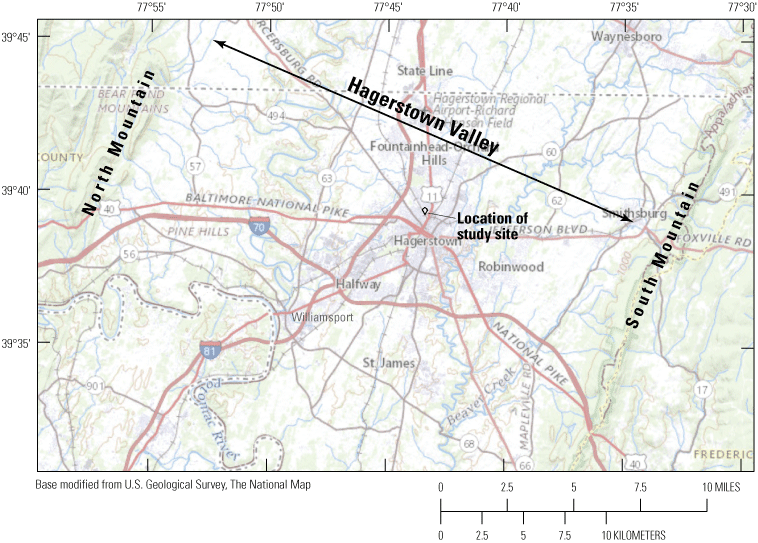
The Central Chemical facility (U.S. Environmental Protection Agency [EPA] identification number MDD003061447) in Hagerstown, Maryland (fig. 1) was listed in 1997 on the National Priorities List (NPL) under the Comprehensive Environmental Response, Compensation, and Liability Act (U.S. Environmental Protection Agency, 2009; Maryland Department of the Environment, 2017). Operations related to the blending and production of pesticides and fertilizers during much of the 20th century contributed to known contamination of soils and water resources at and near the facility. Remediation activities were established in 2009 to address soil contamination and a former waste disposal area (lagoon) at the facility (U.S. Environmental Protection Agency, 2009). Designing remediation strategies to address contamination in groundwater requires sufficient understanding of the complex local geologic setting, groundwater hydrology, and resulting contaminant fate and transport in the area.
Agricultural pesticides and fertilizers were blended at the Central Chemical facility from 1937 through 1984 (Maryland Department of the Environment, 2017). Contaminants of concern (COC) include, but are not limited to, the pesticides that were produced or blended at the facility including aldrin, chlordane, Daconil (chlorothalonil), dichlorodiphenyldichloroethane (DDD), dichlorodiphenyltrichloroethane (DDT), dieldrin, endrin, guthion (azinphos-methyl), lead arsenate, methoxychlor, miscible oils, Omite (propargite), Sevin (carbaryl), and toxaphene (U.S. Environmental Protection Agency, 2009). Facility operations included grinding and blending with air or hammer mills, preparation of liquid pesticides using organic solvents, and onsite waste disposal (Maryland Department of the Environment, 1993, 2017; U.S. Environmental Protection Agency, 2009).
Site Remedial Actions
The history of environmental investigations and regulatory activity related to the Central Chemical facility has been summarized by the Maryland Department of the Environment (1989, 2017) and the U.S. Environmental Protection Agency (2009) and is synopsized here. Briefly, guthion concentrations measured in air samples collected in 1962 in response to odor complaints from residents were deemed nonhazardous by the Maryland Department of Health. In 1970, the Washington County Health Department inspected the facility and directed the consolidation and coverage with soil of refuse disposed onsite and regrading to direct surface runoff away from the lagoon disposal area. DDT was detected in sediments in Antietam Creek in 1976. Soil samples collected from the Central Chemical facility and vicinity, as part of subsequent investigations later that same year, contained DDT, lead, and arsenic at concentrations as high as 1,650 parts per million (ppm), 395 ppm, and 300 ppm, respectively. Because of a subsequent hydrogeologic investigation ordered by the Maryland Water Resources Administration, waste disposal areas at the facility were closed and covered with clay, soil, and stabilizing vegetation. Further environmental investigation was ordered by the Maryland Department of the Environment (MDE) following the discovery of buried “chemical materials” near the onsite former lagoon waste disposal area as part of sewer construction in 1987 and the detection of pesticides, naphthalene, and volatile organic compounds (VOCs) in soils. Soil and groundwater samples collected as part of subsequent studies contained VOCs, pesticides, and heavy metals and borings through the former waste lagoon (fig. 1) included powders and other materials of various colors and petroleum odors. Results of a site inspection published by the MDE in 1996 determined that pesticide contamination in soils at and near the facility posed no significant cancer risk to pedestrians but did pose a slightly increased health risk for young children. The Agency for Toxic Substances and Disease Registry (2005) similarly concluded that exposure to chemicals from the site’s soils, sediments, and water resources represented no apparent hazard to public health.
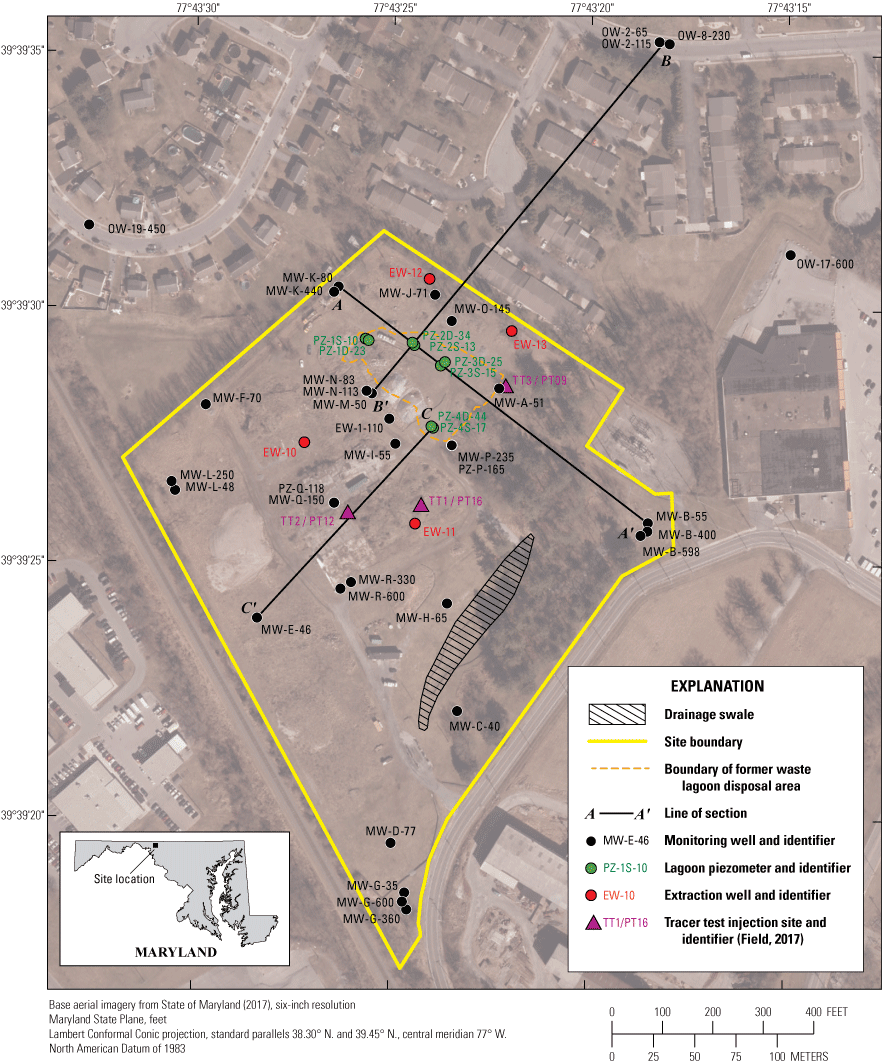
Map showing the location of the study area at the Central Chemical facility and vicinity, Hagerstown, Maryland.
Following the inclusion of the Central Chemical facility on the NPL in 1997, remedial investigations were conducted in two parallel units (Maryland Department of the Environment, 2017). Soils at the facility and waste material in the former disposal lagoon were included in operable unit 1 (OU-1), whereas groundwater was included in operable unit 2 (OU-2; Maryland Department of the Environment, 2017). Remedial activities related to the soil and former waste lagoon at the Central Chemical facility (OU-1) are described by the U.S. Environmental Protection Agency (2009), and included permanent sequestration of onsite contamination through (1) the solidification and stabilization or excavation and removal of material in the former waste lagoon, (2) consolidation of contaminated soils from elsewhere at the facility to the area of the former lagoon, (3) installation of a low permeability cover over the consolidation area at the former lagoon, and (4) monitoring and treatment of groundwater to prevent the movement of contaminants from the consolidation area. The groundwater treatment system was expected to be completed during 2020 and the solidification and stabilization of the former waste lagoon was expected to begin in 2021 (U.S. Environmental Protection Agency, 2019). Remedial investigations related to groundwater at and near the Central Chemical facility (OU-2) are ongoing.
Purpose and Scope
A conceptual model of the hydrogeology and groundwater contaminant fate and transport at and near the Central Chemical facility (fig. 1) is presented and described in this report. The conceptual model was developed through review, synthesis, and interpretation of the results of hydrogeologic, soil, and environmental investigations conducted at and near the facility in recent decades and is intended to support plans for environmental remediation of OU-2. The geologic setting, groundwater hydrology, and environmental fate and transport of pesticides and other contaminants at the facility are discussed, as well as limitations of the current understanding of contaminant transport within the groundwater system. This report does not include an assessment of risk associated with the COC.
Methods
The following sub-sections describe the methodology and approach of the U.S. Geological Survey (USGS) to construct the conceptual site model of the Central Chemical facility. Data from the existing groundwater monitoring network and other monitoring efforts conducted at the site were provided to the USGS and are available in the Central Chemical Records Collection (U.S. Environmental Protection Agency, 2021). This includes documentation of a tracer test by the EPA (Field, 2017) where fluorescein dye was injected into sinkholes at the facility and monitored at select monitoring wells and nearby springs.
Hydrologic Cross Sections
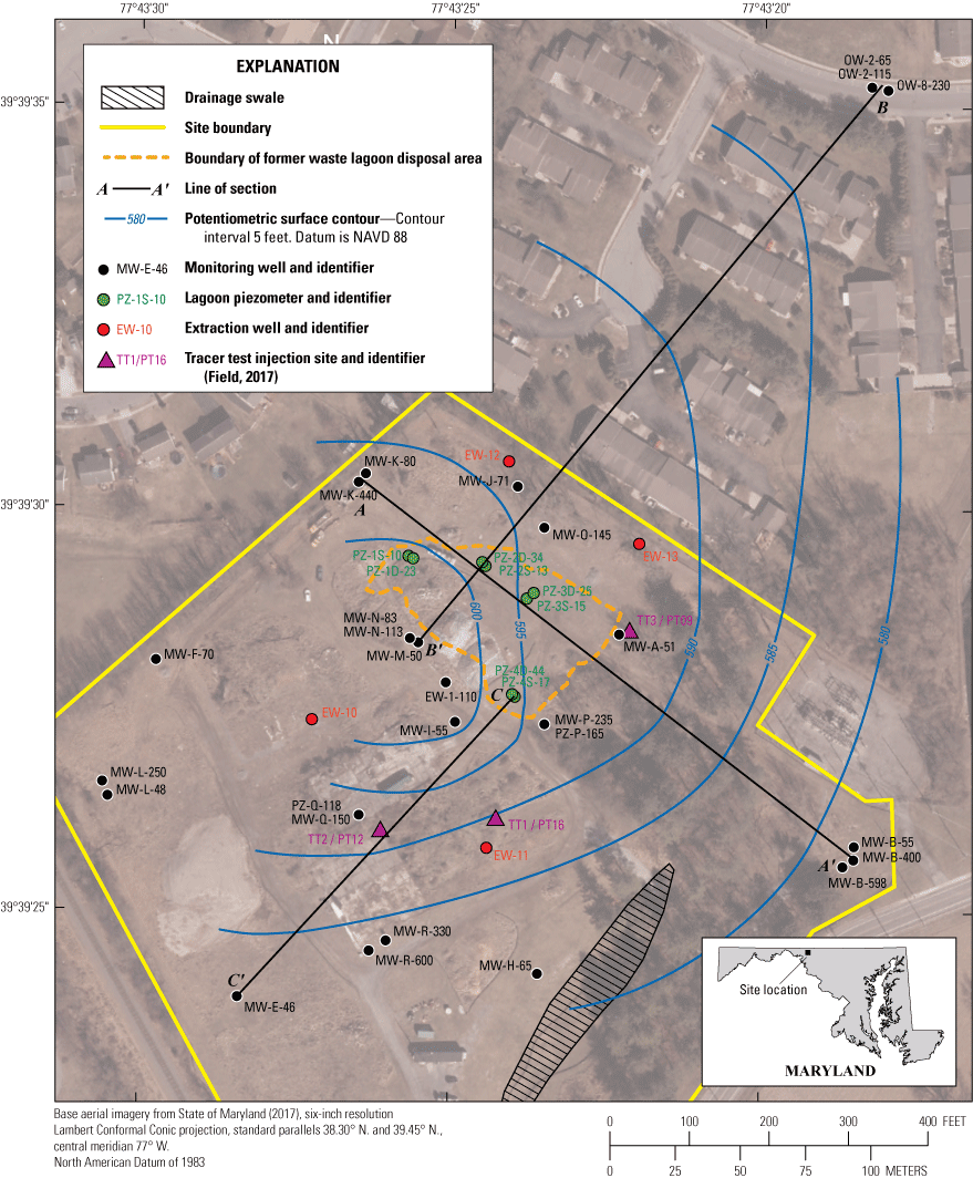
Three cross sections were constructed for analysis of groundwater flow pathways at the Central Chemical facility. Section A-A' occurs from northwest to southeast along the approximate bedrock dip direction (Maryland Department of the Environment, 1989; U.S. Environmental Protection Agency, 2009; Brezinski, 2013) from monitoring wells MW-K-80 and MW-K-440 in the northwest to MW-B-55, MW-B-400, and M-B-598 in the southeast (fig. 1). Because of the complexly folded nature of the site’s geology, dip direction and angle vary depending on location on the fold limb, but the bedrock dips primarily perpendicular to the dominant regional northeast-southwest strike. Lagoon piezometer cluster nests PZ-1, PZ-2, and PZ-3, monitoring well MW-A-51, and the sinkhole used in EPA Tracer Test 3 (TT3; Field, 2017; fig. 1) are projected onto section A-A' along strike. Cross sections B-B' and C-C' (fig. 1) occur along the approximate strike direction of bedrock (Maryland Department of the Environment, 1989; U.S. Environmental Protection Agency, 2009; Brezinski, 2013). Cross section B-B' extends from offsite wells OW-2-65, OW-2-115, and OW-8-230 in the northeast to MW-M-50 located near the southwest flank of the lagoon (fig. 1). Projected onto this section are monitoring wells MW-J-71, MW-O-145, MW-N-83, and MW-N-113, and lagoon piezometers PZ-2S-13 and PZ-2D-34 (where section B-B' intersects section A-A') (fig. 1). Cross section C-C' starts at lagoon piezometers PZ-4D-44 and PZ-4S-17, which are located approximately 135 feet (ft) southeast of MW-M-50 on section B-B'. Monitoring wells MW-P-235, MW-I-55, and MW-Q-150 and the sinkhole used as the injection location for the Environmental Protection Agency (EPA) Tracer Test 2 (TT2; Field, 2017) are projected onto section C-C', which terminates at monitoring well MW-E-46 to the southwest (fig. 1). Despite the proximity of well EW-1-110 to sections B-B' and C-C', this well was omitted from the sections because its longer 50-ft open-interval length limits the usefulness of its groundwater level data.
Reported groundwater level data were contoured on cross sections and two maps to observe the distribution of hydraulic heads in the subsurface and infer characteristics of the groundwater flow system beneath the site. Tables 1.1 and 1.2 contain all reported groundwater data from the site, as well as relevant well construction information. Construction information and groundwater data from 2014, 2016, and 2017 were reported by Amec Foster Wheeler (2018). Data from 2018 were reported by Wood Environment & Infrastructure Solutions, Inc., (2019). Appendix 1 also contains the total head drawdowns during 2019 aquifer tests (Geosyntec, 2019) and tracer-test detections in 2014–2015 (Field, 2017). No data were collected by the USGS. Data from the October 2016 synoptic groundwater measurement event were the lowest groundwater levels reported for much of the site (appendix 1). Data from the October 2018 synoptic groundwater level measurement event were generally the highest groundwater levels reported (appendix 1). Thus, contouring data from both October 2016 and October 2018 allows for comparison of differences in conceptual groundwater flow pathways between dry (October 2016) and wet (October 2018) conditions. The October 2018 dataset was collected during the wettest calendar year and wettest fall season on record for Maryland (National Oceanic and Atmospheric Administration, 2019), which is likely what contributed to the higher groundwater levels during that measurement event compared to earlier events. After contouring reported groundwater levels on cross sections, maps were created to observe subsurface groundwater level conditions at specific depths or elevations in the subsurface. Potentiometric surface maps were produced at the bottom of the epikarst and at an elevation of 52 ft (North American Vertical Datum of 1988 [NAVD 88]). Further explanation of the approach used in contouring the cross sections and maps is discussed later in this report.
Annual Evapotranspiration Calculations
Estimates of evapotranspiration (ET) were produced using the operational remote-sensing-based Simplified Surface Energy Balance (SSEBop) model (Senay and others, 2013) from 2003 to 2019. The SSEBop is based on the Simplified Surface Energy Balance (SSEB) approach (Senay and others, 2007, 2011). The global ET is derived from the integration of Moderate Resolution Imaging Spectroradiometer (MODIS)-based land surface temperature, maximum air temperature from WorldClim, and reference ET derived from global data assimilation systems (GDAS). A comprehensive validation of the SSEBop model was conducted by Velpuri and others (2013) over the conterminous United States at both point and basin scales.
Contaminant Transport
To evaluate contaminant transport in the epikarst, four wells (MW-A-51, MW-B-55, MW-M-50, and MW-E-46) were selected based on their depth below the surface and location in the study area. Along cross section A-A' (fig. 1), MW-A-51 and MW-B-55 were determined to be completed within the epikarst of the site (described later in the Epikarst section of this report). MW-A-51 is located to the southeast of the lagoon waste disposal area, whereas MW-B-55 is located at the eastern edge of the site boundary. Dye from the 2017 EPA tracer test study was detected in MW-A-51 demonstrating a connection between the surface where the dye was released and the well (Field, 2017). MW-M-50 is located just to the southwest of the lagoon waste disposal area along the transect B-B'. MW-E-46 is shown on cross section C-C' and is located to the southwest of the waste disposal lagoon at the boundary of the site (fig. 1).
Concentrations of COC measured in samples collected from MW-A-51, MW-B-55, MW-M-50, and MW-E-46 are presented in appendix figures 2.1 to 2.16. Concentrations of COC and water quality measurements were extracted from Wood Environment & Infrastructure Solutions, Inc. (2019) 2018 Groundwater Monitoring Report for OU-2 and are available through the U.S. Environmental Protection Agency (2021). COC concentrations measured during sampling events were plotted then fitted with a local polynomial regression fitting (LOESS) as a solid line with corresponding standard errors in gray. Years 2016 and 2018 are highlighted with red bars corresponding to the “dry” and “wet” conditions previously described. These two years provide an opportunity to evaluate how changes in the water table affect COC.
To evaluate contaminant transport within the conduit system or dissolution voids, three compounds were selected to compare between the different wells. Wells MW-I-55, MW-J-71, MW-M-50, MW-N-113. MW-O-145, MW-P-235, OW-2-65, OW-2-115, and OW-8-235 were selected for comparison due to proximity to possible dissolution voids reported by Weston, Inc. (1989) and Amec Foster Wheeler (2018) (table 1). Chlorobenzene was identified as a compound of interest for comparison due to its frequent detections in many of the wells (appendix 2). For comparison, 1,2,4-trichlorobenzene (1,2,4-TCB), n-octanol-water partition coefficient (log Kow = 4.02), was selected due to its similarity to chlorobenzene (log Kow = 2.84) and was selected due to its similarity to chlorobenzene (log Kow=2.84) but is more hydrophobic and more likely to sorb to matrix materials than chlorobenzene. 1,2,4-TCB has a hydrophobicity closer to benzene hexachloride (BHC) isomers (log Kow=3.72), commonly grouped as technical-BHC. COC concentration data are plotted by well with respect to time and fitted with a LOESS as a solid line (appendix 3). Years 2016 and 2018 are highlighted with red bars to compare groundwater level effects as previously described. Box and whisker plots were generated for each well and grouped by compound to evaluate variability in concentration by compound and well (appendix 3).
Table 1.
Dissolution features reported driller’s logs from wells, Central Chemical facility, Hagerstown, Maryland.[Descriptions in quotes are verbatim of that reported. --, not available]
| Well | Cross section | Reported depth interval below land surface (feet) | Reported desciption1 | Data source | Comment |
|---|---|---|---|---|---|
| MW-A-51 | A-A' | 50–51 | “mud-filled void” | Amec Foster Wheeler (2018) | -- |
| MW-J-71 | B-B' | 64–67 | “mud-filled void” | Amec Foster Wheeler (2018) | -- |
| MW-N-83 | B-B' | 74.5–79.5 | “mud-filled void” | Amec Foster Wheeler (2018) | -- |
| MW-N-113 | B-B' | 104–105 | “mud-filled void” | Amec Foster Wheeler (2018) | -- |
| B-B' | 74.5–79.5 | “void” | -- | ||
| MW-O-145 | B-B' | 65.5–68.5 | “extremely soft mud” | Amec Foster Wheeler (2018) | -- |
| B-B' | 78.5–80 | “extremely soft mud” | -- | ||
| OW-5-90 | none | 79–92 | “possible loss of return water” | Amec Foster Wheeler (2018) | -- |
| MW-1 | A-A' | 26–43 | “open cavern” | Weston, Inc. (1989) | Former well “near MW-K” |
| MW-2 | none | 15–25 | “void space/weathered zone” | Weston, Inc. (1989) | Former well “near MW-P” |
| C-C' | 28–32 | “void space/mud-filled cavity” | |||
| MW-4 | B-B' | 18–20 | “mud-filled void” | Weston, Inc. (1989) | Former well “near MW-M” |
| B-B' | 27–42 | “mud-filled void” | -- | -- | |
| MW-6 | none | 27–32 | “mud-filled void” | Weston, Inc. (1989) | Former well “northeast of MW-E” |
| MW-7 | none | 24–27.5 | “mud-filled void” | Weston, Inc. (1989) | Former well “near MW-L” |
| none | 95–97 | “soft mud” |
Geologic Setting
The Central Chemical facility is located in western Maryland (fig. 1) within the Great Valley (locally known as the Hagerstown Valley) along the eastern edge of the wider Valley and Ridge Physiographic Province (U.S. Environmental Protection Agency, 2009). The valley is underlain by lower Paleozoic (Cambrian and Ordovician) shale, limestone, and dolomite that were deposited in a shallow marine environment and later compressed into tight folds and partially eroded (Brezinski, 2018).
Soil
Soil at the Central Chemical facility is generally fine grained, varies in thickness, and is classified as Hagerstown silt loam, which is 80 percent silt with some clay and laterally discontinuous thin sand lenses (Maryland Department of the Environment, 1989; U.S. Environmental Protection Agency, 2009). The soil is derived from chemical weathering of the underlying carbonate bedrock, is generally well drained, and varies in thickness at the facility from 0 ft at bedrock outcrops to more than 40 ft (fig. 2) (Maryland Department of the Environment, 1989; U.S. Environmental Protection Agency, 2009; Amec Foster Wheeler, 2018). Surface permeability ranging from 0.06 to 0.6 inches per hour (in/h) have been reported for the Hagerstown silt loam (Maryland Department of the Environment, 1993). Overlying the natural soil in some locations is as much as 13 ft of fill, including brown silt with some coarse-to-fine sand and gravel (U.S. Environmental Protection Agency, 2009).
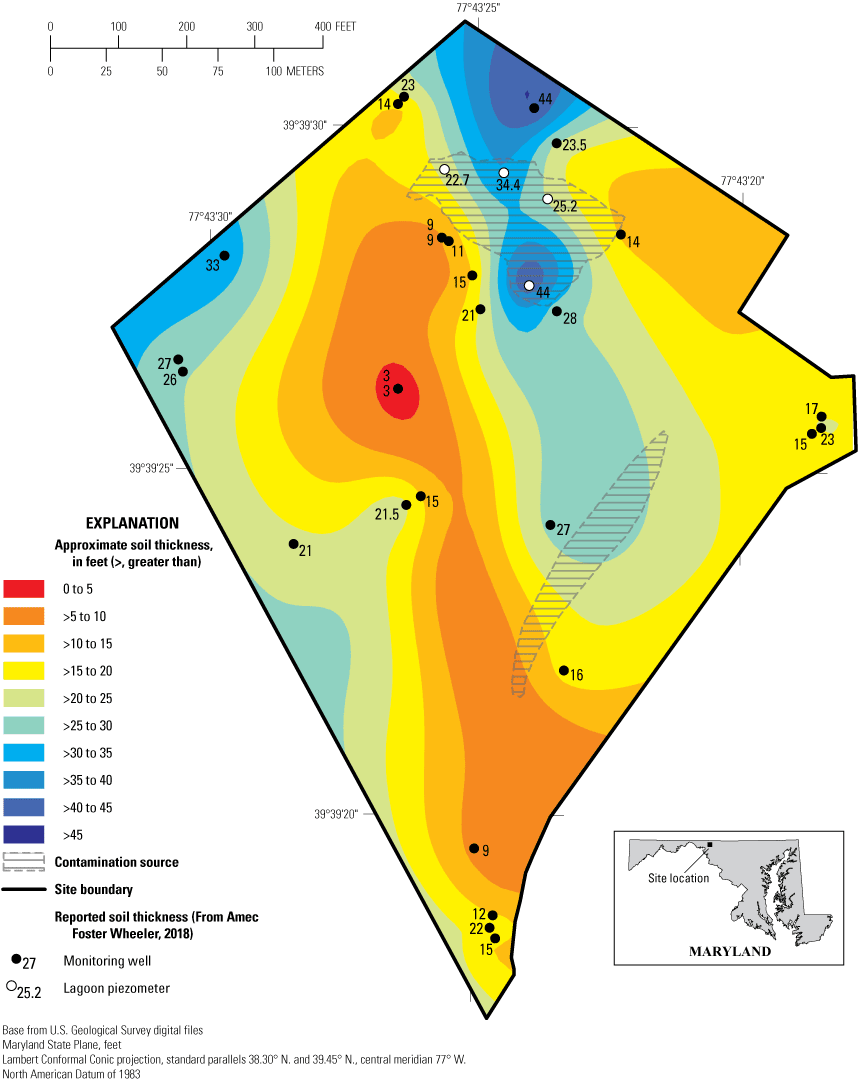
Map showing soil thickness at the Central Chemical facility, Hagerstown, Maryland.
Geologic Formations
The Central Chemical facility and vicinity are underlain by the Conococheague Formation, Stonehenge Limestone of the Beekmantown Group (Stonehenge Limestone), and Rockdale Run Formation of the Beekmantown Group (Rockdale Run Formation; figs. 3 and 4), which include primarily carbonate rocks (Brezinski, 2013, 2018). The lithology, stratigraphy, and nomenclature applied to rocks of these formations in the Hagerstown Valley and wider Great Valley are described in detail in Brezinski (2018) and are briefly summarized herein.
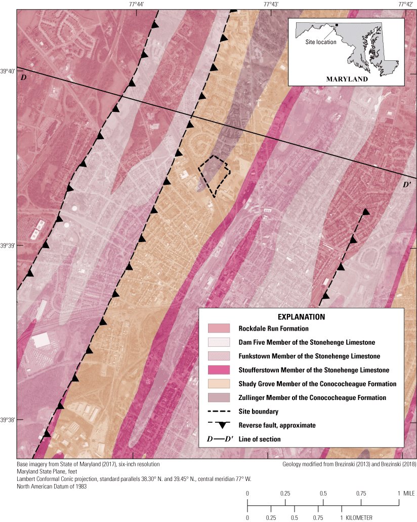
Map showing the Central Chemical facility and vicinity, Hagerstown, Maryland.
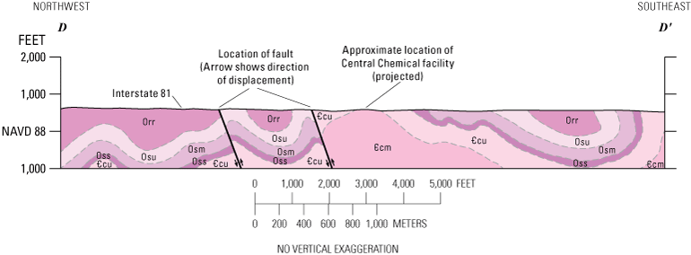
Generalized geologic cross section D-D' in the vicinity of the Central Chemical facility, Hagerstown, Maryland. Modified from Brezinski (2013). [Orr, Rockdale Run Formation; Osu, Dam Five Member of the Stonehenge Limestone; Osm, Funkstown Member of the Stonehenge Limestone; Oss, Stoufferstown Member of Stonehenge Limestone; Ꞓcu, Shady Grove Member of Conococheague Formation; Ꞓcm, Zullinger Member of Conococheague Formation; NAVD 88, North American Vertical Datum of 1988]
The Central Chemical facility is underlain by the Zullinger and Shady Grove Members of the Conococheague Formation (Brezinski, 2018; figs. 3 and 4). The Zullinger Member, previously described as the “middle member” of the Conococheague Formation, includes 1,600 to 1,900 ft of alternating sequences of thick beds of thrombolitic limestone and ribbony, laminated dolomitic limestone. These sequences alternate on the scale of 200 to 300 ft. Above these alternating sequences of the Zullinger Member are younger ribbony limestone, sandy dolomite, and chert of the Shady Grove Member, which was previously described as the “upper member” of the Conococheague Formation. The Shady Grove Member of the Conococheage Formation is between 350 and 500 ft thick.
Overlying the Conococheague Formation to the southeast and northwest of the Central Chemical facility are the younger rocks of the Stonehenge Limestone (figs. 3 and 4), which include three members with a combined thickness of approximately 850 ft (Brezinski, 2018). At the base of the Stonehenge Limestone is the Stoufferstown Member, which is 175 to 275 ft thick and composed of thin (less than or equal to 1 inch) beds and ribbons of siliceous lime mudstone. Included among the thin beds of the Stoufferstown Member is an atypical 3- to 9-ft-thick massive thrombolitic lime mudstone. The Stoufferstown Member is overlain by the Funkstown Member of the Stonehenge Limestone, which is 350 to 450 ft in thickness and composed of thick beds of organically bound limestone. Above the Funkstown Member is the Dam Five Member of the Stonehenge Limestone, which is composed of medium bedded, locally ribbony mechanically deposited limestone that varies in thickness from 330 to 450 ft. The Funkstown Member and Dam Five Member were previously mapped as the “middle” and “upper” members of the Stonehenge Limestone, respectively.
The Rockdale Run Formation overlies the Stonehenge Limestone in the vicinity of the Central Chemical facility (figs. 3 and 4) and exceeds 2,700 ft in thickness (Brezinski, 2018). Included within the lower 350 to 450 ft of the formation are cyclical sequences of organically bound limestone, limestone ribbons, laminated dolomite, and chert (Brezinski, 2018). These rocks are overlain, in turn, by interbedded oolitic lime packstone and dolomite, approximately 200 ft thick, and by more than 1,000 ft of additional cyclical carbonates (Brezinski, 2018).
Geologic Structure
The complex folding and faulting of the carbonate geologic units in the Hagerstown Valley reflect compression in a generally westward direction that occurred during the orogenic event that created the Appalachian Mountains (Maryland Department of the Environment, 1989; Brezinski, 2018). This compression created folds in the rock units spanning several orders of magnitude in scale with axes that trend generally to the north-northeast (Brezinski, 2018; fig. 5). Fractures, including bedding-plane partings, joints, and faults, are common in the rock units in the valley and are commonly oriented parallel or perpendicular to the north-northeastern strike of the rock formations (fig. 5); faulting reflects movement over scales from inches to hundreds of miles (Brezinski, 2009, 2018).
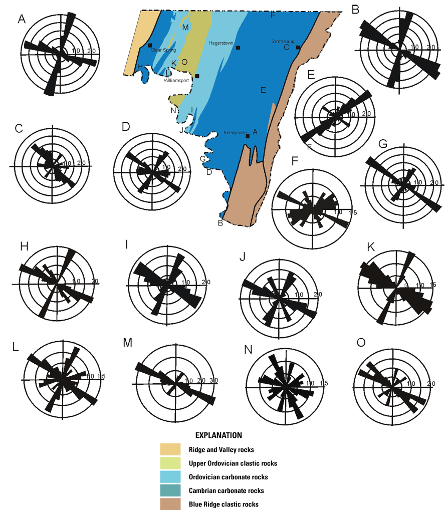
Rose diagrams showing orientation of fractures in rocks of the Hagerstown Valley, Maryland. Modified from Brezinski (2018).
The Central Chemical facility is located to the southeast of the axis of a structural anticline that trends to the north-northeast and plunges to the southwest (fig. 4) (Maryland Department of the Environment, 1989; U.S. Environmental Protection Agency, 2009). Bedding planes at and near the facility generally dip more steeply (between 55 and 90 degrees) on the northwestern limb of this anticline than on the southeastern limb (between 25 and 45 degrees) (Maryland Department of the Environment, 1989; U.S. Environmental Protection Agency, 2009).
Secondary meso-scale folds also occur at the site and have been named the Western Boundary Anticline, the Former Plant Syncline, the Former Plant Anticline, the Drainage Swale Syncline, and the Mitchell Avenue Anticline (Amec Foster Wheeler, 2018). Bedding planes dip more steeply to the west than to the east on either side of the secondary anticlines, similar to those of the primary anticline (U.S. Environmental Protection Agency, 2009). Section A-A' of figure 6A, 6B is aligned with the approximate dip of the regional anticline and intersects several of the meso-scale folds beneath the facility. Although no attempt at bedding correlations was made, the generalized fold structure reported in the cross sections in Amec Foster Wheeler (2018) was checked against reported acoustic televiewer logs collected during construction of boreholes MW-K-440 and MW-B-400 in Amec Foster Wheeler (2018). Borehole MW-K-440 had reported dominant fracture azimuths to the north and west-northwest in the upper 100 ft and to the east and east-southeast at a depth from 100 to 250 ft. These orientations are consistent with MW-K-440 being located within the Western Boundary Anticline, where the upper portion dips toward the northwest near the tilted axial trace and the deeper portion along the lower southeast-dipping limb. For borehole MW-B-400, the dip azimuths are predominantly toward the northwest and southeast directions, which is consistent with the location of MW-B-400 near the middle of the axial trace of the Mitchell Avenue Anticline. In the upper 200 ft, the orientation is more dominant to the southeast, so MW-B-400 was drawn on section A-A' as being southeast of the axial trace (fig. 6A, 6B).
The axial trace of the Drainage Swale Syncline was mapped by Amec Foster Wheeler (2018) as occurring approximately 150 ft northwest of MW-B-55 at the screen elevation and was incorporated on cross section A-A' (fig. 6A, 6B). Although the reported Former Plant Syncline (Amec Foster Wheeler, 2018) occurs along section A-A', it was omitted because of the unclear structure of this fold and the Former Plant Anticline that is reported to terminate south of this cross section. The cross sections interpreted by Amec Foster Wheeler (2018) that cross this area also do not include the Former Plant Syncline.
The geologic structure depicted on the cross sections was not determined by any other means than as represented in Amec Foster Wheeler (2018). Therefore, the actual dip angles and overall structural geometry may differ from those depicted here, which should be considered generalized approximations. On the northwest-dipping limb of the Western Boundary Anticline and the limb between he Drainage Swale Syncline and Mitchell Avenue Anticline on section A-A' (fig. 6A, 6B), the dips are approximately 45 degrees. Beds located on the limb between the Western Boundary Anticline and Drainage Swale Syncline are drawn by Amec Foster Wheeler (2018) as dipping approximately 27 degrees southeast (100 ft in elevation for every 200 ft in distance). Sections B-B' and C-C' are aligned approximately in the northeast-southwest strike direction and no meso-scale folds are included on these sections (fig. 7A, 7B, 7C). Amec Foster Wheeler (2018) shows beds tilted 14 degrees southwest along the strike direction (decreasing approximately 100 ft in elevation over 400 ft of distance). The same bed orientations were incorporated on cross sections B-B' and C-C' as those in Amec Foster Wheeler (2018), but whether these orientations correspond to the strikes and dip angles mapped by Brezinski (2013) is unknown. Since many fewer structural data are available along the strike direction, the true structure along strike is unclear.
Rock fractures observed in the vicinity of the Central Chemical facility are generally oriented in a manner similar to those in the wider Hagerstown Valley. Fractures near the land surface generally strike to the north-northeast or to the northwest and are steeply inclined or nearly vertical (Maryland Department of the Environment, 1989). These fractures may be wider near the crest of anticlines due to extensional stresses during convex folding (Maryland Department of the Environment, 1989; U.S. Environmental Protection Agency, 2009). Rock strata are offset along a reverse fault to the west of the facility near the axis of the major anticline (fig. 3; Brezinski, 2013; Field, 2017).
Karst Features
Karst features, including closed depressions, sinkholes, springs, and caves, are common in carbonate rocks of the Hagerstown Valley (Duigon, 2001; Brezinski, 2018). Because these features are formed through the dissolution of the rock matrix by groundwater, their occurrence is related to the solubility of individual lithologic units and to the distribution of fractures available as conduits for groundwater flow (Brezinski, 2018). Karst features occur in all rock formations in the vicinity of the Central Chemical facility, although the Rockdale Run Formation is generally more susceptible to karst development than the Conococheague Formation, but less so than the Stonehenge Limestone. In the Hagerstown Valley, springs and sinkholes commonly occur near the surface trace of faults and rock dissolution is common along bedding planes. Solution cavities that form along joints in the rock tend to be wider in formations with more massive bedding and more purely carbonate lithology. Karst features are also common in areas where groundwater flow may be increased by a locally depressed water table or in areas of stormwater impoundments or unlined drainage.
Karst features have been observed at and near the Central Chemical facility. Numerous sinkholes and closed depressions have been reported at and within a few kilometers of the facility (Maryland Department of the Environment, 1993; Field, 2017). Caverns and voids in the bedrock exceeding 5 meters (m) in height have been encountered during subsurface drilling at the facility and in-situ permeability as high as 1,042 feet per year has been reported (Maryland Department of the Environment, 1993). Fractures enlarged by solution have been observed in outcropping rocks of the Conococheague Formation at the facility (Field, 2017).
Overlying the Conococheague Formation at the Central Chemical facility is highly fractured bedrock of the epikarst (U.S. Environmental Protection Agency, 2009). The contact of the bedrock with the overlying soil and epikarst is highly irregular and the soil thickness consequently varies substantially (Maryland Department of the Environment, 1989; U.S. Environmental Protection Agency, 2009). Vertical pathways of high permeability have been reported in the epikarst at the facility (U.S. Environmental Protection Agency, 2009).
Hydrology
The site is located within the drainage basin of the Potomac River, which is located approximately 6 mi southwest of the site (fig. 8). The topographic altitude of the site ranges from 633 ft along the northern boundary to 596 ft along the southern boundary. The major local tributaries of the Potomac River include Antietam Creek and Conococheague Creek that drain southerly along the regional northeast-southwest trending bedrock structural grain (fig. 8) into the Potomac River. Conococheague Creek is approximately 5 mi to the west of the site. The meander patterns of Conococheague Creek and the smaller Antietam Creek follow the local northeast-southwest structural grain with elongated stream segments that parallel fractures striking northwest-southeast cutting across the regional structural grain (bedrock strike).
Mean annual precipitation, from 2003 to 2019, in the Hagerstown area averaged 1,078 millimeters per year (mm/yr), mostly in the form of rain (Abatzoglou, 2013). Mean annual potential evapotranspiration (PET) averaged 1,168 mm/yr and mean annual actual evapotranspiration (AET) averaged 364 mm/yr from 2003 to 2019 (Senay and others, 2013). The difference between mean precipitation and mean AET (in this case 714 mm/yr) either infiltrates the soil and recharges groundwater or runs off over the land surface. Streamflow is generated from overland flow and groundwater discharge, such as from springs.
Regionally, the site is located approximately 0.5 mi southeast of the regional groundwater divide that demarcates flow toward Antietam Creek (to the southeast) and flow toward Conococheague Creek (to the west and southwest) with inferred regional groundwater flow direction in the vicinity of the site to the southeast towards Antietam Creek approximately 2.1 mi from the site (Duigon, 2001). At a more local scale, lithological and structural contrasts between shallow soil, weathered rock, and epikarst and deeper competent but bedded, dipping, fractured, and karstic limestones give rise to two connected groundwater flow systems, including a shallow hydrogeologic system containing epikarst and unconsolidated surficial overburden and a deeper hydrogeologic system in the bedrock (figs. 6, 7, 9, and 10).
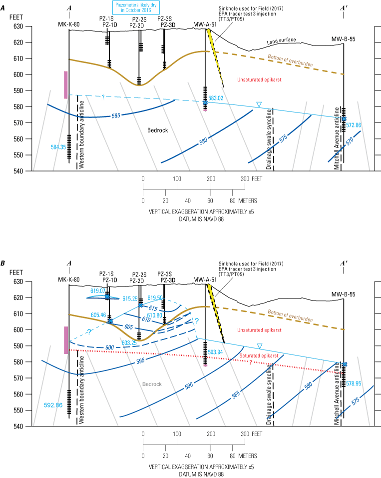
Hydrogeologic cross sections showing A, shallow potentiometric surface contours on Section A-A', October 2016; B, shallow potentiometric surface contours on Section A-A', October 2018; C, deep potentiometric surface contours on Section A-A', October 2018. [NAVD 88, North American Vertical Datum of 1988]
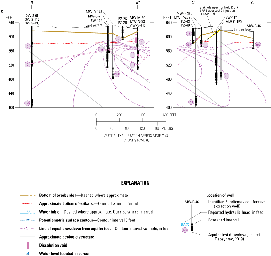
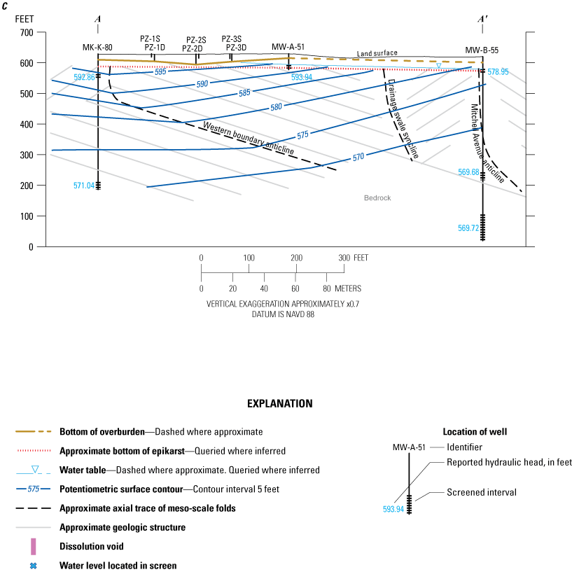
Hydrogeologic cross sections showing A, potentiometric surface contours on Section B-B' and C-C', October 2016; B, potentiometric surface contours on Section B-B' and C-C', October 2018; C, water-level drawdown from reported aquifer tests on Section B-B' and C-C'. [NAVD 88, North American Vertical Datum of 1988]
Map showing major topographic and drainage features in the Hagerstown Valley.
Map showing generalized potentiometric surface at the approximate bottom of the epikarst, October 2018, Central Chemical facility, Hagerstown, Maryland.
Map showing potentiometric surface at an approximate altitude of 525 feet above the North American Vertical Datum of 1988, October 2018, Central Chemical facility, Hagerstown, Maryland.
Surficial and Epikarst Hydrogeologic System
The shallow hydrogeologic system encompasses the unsaturated vadose zone through the depths at which the regional water table fluctuates within the bedrock and consists of two portions: (1) the surficial sediments, and (2) the subcutaneous epikarst portion of bedrock.
Unconsolidated Surficial Overburden
The zone of surficial materials at the site consists of soil and unconsolidated overburden that boring logs (Amec Foster Wheeler, 2018) indicate consist of silty-clays to clayey-silts, with minor amounts of sand (Weston, Inc., 1989). The lagoon disposal area is included in this zone, which also contains sludge and waste debris such as plastic bags that may contribute heterogeneity to this hydrogeologic zone. The unconsolidated zone begins at the land surface and has highly variable thickness owing to the weathering and dissolution of the underlying carbonate bedrock. Additional dissolution may have occurred due to the use and disposal of various acids onsite. Unconsolidated overburden thickness, estimated from cores (Weston, Inc. 1989) and from monitoring well records (table 2-2 in Amec Foster Wheeler, 2018), indicate a thickness of 2 to 41 ft and 9 to 44 ft, respectively. The overburden is nonexistent where grikes expose the underlying bedrock and thickest in collapsed sinkholes where the bedrock is most weathered. Exact locations of grikes, sinkholes, and similar features are not included on the cross sections unless already explicitly identified elsewhere, such as the sinkholes noted near MW-Q-150 and MW-A-51 associated with EPA tracer test injections 3 and 2, respectively (Field, 2017; Amec Foster Wheeler, 2018).
The unconsolidated overburden sediments are a porous media in which groundwater flow is not dependent on the structure of the bedrock nor on effects of carbonate dissolution, except at boundaries where groundwater encounters grikes. Groundwater flow within the overburden is most readily assessed within the lagoon disposal area. Piezometers PZ-1D, PZ-1S, PZ-2D, PZ-2S, PZ-3D, PZ-3S, PZ-4D, and PZ-4S are located directly in the lagoon and are the only wells onsite screened exclusively in the overburden. Hydraulic heads on section A-A' indicate that groundwater flow in the overburden of the lagoon is downward toward PZ-2D, which is the deepest lagoon piezometer and has the lowest hydraulic head on that section (fig. 6). October 2018 hydraulic heads in the PZ-1D and PZ-1S piezometer nest also indicate perched water table conditions occurred in the lagoon; during that synoptic event, both piezometers had groundwater levels within their screened intervals, which indicates their screens intersected the water table at the boundary with the vadose zone (appendix 1; fig. 6). Since the two piezometers are nested, the groundwater at PZ-1S was likely a perched water table that may not have extended to the other piezometers in cross section A-A', whose heads were more aligned with PZ-1D and representative of a deeper overburden water table within the lagoon (fig. 6).
The dominance of clay and silt within the overburden suggests overall low permeability and slow movement of groundwater through this zone. Contractors reported lagoon piezometers going dry and producing insufficient groundwater quantity during low-flow purge sampling (Wood Environment & Infrastructure Solutions, Inc., 2019), which would correspond to the expected low permeability. Furthermore, based on piezometer groundwater levels during drier periods, such as October 2016 (appendix 1; fig. 6), portions of the unconsolidated overburden that are sometimes saturated with groundwater may become dry and unsaturated at other times. So, despite the low permeability sediments in the overburden, sufficient downward gradient exists to drain the groundwater out of the lagoon on section A-A' into deeper portions of the aquifer. This observation has implications for how contaminants move through the lagoon, as repeated high concentrations of contaminants in the lagoon piezometers during dry periods indicates continued storage of the contaminants within the soils surrounding and within the lagoon that become mobile during wet periods. Groundwater levels were reported in the lagoon piezometers during the October 2016 synoptic groundwater level measurement event (Amec Foster Wheeler, 2018), but reported groundwater elevations ranged from 0.13 to 0.38 ft above the reported bottom of the screen for PZ-1D, PZ-2D, PZ-3S, and PZ-3D (appendix 1). These short water column heights may be residual water pooled in the tailpiece of the well below the actual openings at the bottom of the screen, and not represent actual hydrologic conditions at the time. Alternatively, if these measurements were representative of lagoon groundwater-level conditions, a 0.38-ft or shorter water column within a 5-ft long screen may indicate perched water tables in the lagoon, perhaps associated with the bottom of the “waste material” depths to which Amec Foster Wheeler (2018) reported PZ-3S was completed as well as the top of bedrock surface to which PZ-1D, PZ-2D, and PZ-3D were completed. A third possibility is evident in the reported groundwater levels from PZ-1S and PZ-2S in October 2016, which were deeper than the reported bottom of the piezometers (Amec Foster Wheeler, 2018; appendix 1) and suggests an error in reporting the groundwater level or casing elevation data. These errors may affect the other piezometers in the lagoon and (or) other measurement events. This report interpreted that the lagoon piezometers were dry in October 2016, as implications of that condition would have the most substantial effect on how groundwater flow paths and contaminant transport will occur at the site. This assumption is justified given that the hydraulic head in PZ-2D was 603.25 ft in October 2018 (5 ft above the reported top of the screen) and 583.63 ft in October 2016 (about 0.38 ft above the bottom of the screen set at the top of bedrock). October 2018 conditions indicated flow toward PZ-4D, so the nearly 10 ft drop of groundwater level indicates substantial drying of the lagoon, regardless of whether the 0.38 ft of water was perched atop the bedrock surface or trapped in the tailpiece below the screen. No groundwater analytical results were collected in piezometers during October 2016 (Amec Foster Wheeler, 2018), but whether that is due to those piezometers not being scheduled for sampling or whether not enough water was present in those piezometers to sample was not reported; so, no other data are available to indicate the exact hydrologic conditions at the time.
On sections B-B' and C-C' (fig. 7), piezometers PZ-4S and PZ-4D did not go dry in October 2016 and heads remained above the piezometer screens (appendix 1). This trend indicates the southeastern portion of the lagoon contains groundwater even when other portions of the lagoon go dry. Groundwater flow in the lagoon, in addition to occurring downward, also may occur toward PZ-4D which consistently has the lowest hydraulic head of the eight lagoon piezometers (appendix 1). The southeast portion of the lagoon is topographically lower than other portions of the lagoon, so runoff from the land surface will accumulate more likely near the PZ-4 nest and be infiltrated at that location. Notably, PZ-4D is reportedly the only lagoon piezometer that responded to aquifer testing (fig. 7); all other lagoon piezometers did not indicate groundwater level responses despite being located closer to the extraction wells (Geosyntec, 2019), which would be expected given the low permeability of lagoon sediments. This observation indicates a strong hydraulic connection between the lagoon near PZ-4 and deeper portions of the flow system, including the possibility that the PZ-4 area is the primary connection between the lagoon and deeper units. However, not enough data are available to make that comparison definitively.
The lagoon piezometers provide the only groundwater level measurements available from the unconsolidated overburden zone. Therefore, the hydrology of this zone cannot be assessed for any other location at the site. The high hydraulic heads in shallow lagoon piezometers are considered in Sections A-A', B-B', and C-C' to be local only to the lagoon because those are the only measurements available; saturated surficial sediments may exist elsewhere onsite where the water table may extend beyond the lagoon, particularly in areas such as near MW-E-46 where thick overburden is reported and where a low topographic elevation likely accumulates runoff.
Epikarst
The epikarst zone is located below the overburden. Epikarst refers to subcutaneous areas within the karstic carbonate bedrock located above the water table (the prefix “epi-” meaning “above” or “over”). Therefore, the epikarst is primarily a vadose zone through which infiltrating groundwater must pass to recharge the regional water table that exists within the bedrock (Duigon, 2001; Williams, 2008; Yager and others, 2013; Hartmann and others, 2014). Other approaches to defining epikarst, such as those based on the degree of karstic bedrock weathering and fracture sizes (Kozar and others, 2007), are more applicable to coarser-resolution, regional-scale hydrologic investigations such as the detection of tracer tests at springs (Field, 2017), for which generalizing properties over large distances is required for analysis. Previous work at the site (Amec Foster Wheeler, 2018) considered the epikarst to extend to depths of 100 ft below the land surface and sometimes more than 75 ft below the water table, which would apply to this approach. However, a less generalized hydrologic definition of epikarst is required for higher resolution site-scale groundwater flow investigations so heterogeneities occurring over shorter distances that affect contaminant transport can be studied. Hydrologic properties such as hydraulic conductivity will vary depending on scale of observation. Because these properties can vary over several orders of magnitude in karst aquifers and affect the distribution and transport from the source area, scale becomes very important and too low a resolution may neglect or overgeneralize a particular mechanism (Hartmann and others, 2014; Worthington and others, 2017).
Epikarst is associated with diffuse infiltration where the infiltrating water causes dissolution of the carbonates on contact at the lower boundary of the overburden. Diffuse infiltration occurs at all locations where water infiltrates through the vadose zone and recharges the water table. In karst aquifers, diffuse infiltration is distinct from the rapid point infiltration through karst features such as sinkholes. Dissolution fractures and voids in the epikarst created by diffuse infiltration will often be oriented more vertically in the direction of the downward infiltration flow through the vadose zone (Duigon, 2001; Williams, 2008; Yager and others, 2013; Hartmann and others, 2014), which is imprinted atop the geologic structure of the bedrock that dominates flow regimes below the water table (discussed in the next section). Any non-impervious surface at the land surface can exhibit this type of infiltration, so this process occurs on a more laterally extensive scale across the site compared to point infiltration where the infiltrating water is funneled into deeper portions of the aquifer through sinkholes.
Perched water tables are a common occurrence within the vertically oriented fractures in epikarst (Duigon, 2001; Williams, 2008). As the acids within the diffusely infiltrating groundwater create dissolution fractures in the vertical direction, enough dissolution of carbonates eventually will occur to neutralize the acidity and the dissolution will cease, creating “dead end” vertical fractures. If the vertical fractures terminate before reaching the main water table and (or) before encountering a structural fracture that would enable the groundwater to flow in a different direction, a perched epikarstic water table can form, trapping the groundwater in the epikarst. In such instances, the perched groundwater in the vertical “dead end” fractures will have minimal routes for outflow until more acidic infiltration takes its place to cause further dissolution and the fracture size grows wide and (or) deep enough to increase leakage or intersect another fracture through which the water can escape, or until the groundwater is removed by evapotranspiration if the overburden is thin and fractures shallow enough. These perched water table conditions within epikarst have implications for the long-term storage of contaminants at shallow depths.
The bottom of the epikarst in this study (figs. 6 and 7) was considered to coincide with the lowest groundwater level measured in monitoring wells that have reported groundwater levels located within the screened interval or within an arbitrarily chosen depth of 1 ft of the screened interval. This depth represents the lowest depth at which the water table would fluctuate at those locations. Deeper portions of the epikarst would exhibit features characteristic of both epikarstic vadose zone infiltration processes and flow-through geologic structure of the bedrock (discussed in the next section) at the locations where infiltration through the epikarst meets the main water table in the bedrock. Thus, the bottom of the epikarst zone is more of a transitional zone between those two dominant groundwater flow regimes rather than a sharp interface.
On cross section A-A' (figs. 1 and 6), MW-A-51 and MW-B-55 had low groundwater levels within their screen intervals that were used to determine epikarst depth. On cross sections B-B' and C-C' (figs. 1 and 8), wells OW-2-65, MW-M-50, MW-I-55, and MW-E-46 had groundwater levels within their screened intervals. The lowest measured groundwater level in these wells occurred in October 2016, except MW-M-50 and MW-I-55 which occurred in January 2017 (appendix 1). For MW-A-51, the lowest groundwater level reported was 583.02 ft in October 2016 (appendix 1). This groundwater level is near the midpoint of the screened interval of MW-A-51, thus elevation of the bottom of the epikarst was taken to be 583.02 ft at MW-A-51 (fig. 6). The reported bottom of the unconsolidated surficial overburden at MW-A-51 was reported to be about 14 ft below the land surface, or at an altitude of approximately 614 ft (Amec Foster Wheeler, 2018), indicating an epikarst thickness of 35 ft at this location. In October 2018, the groundwater level in MW-A-51 was 10 ft shallower than in October 2016 and about 1 ft above the MW-A-51 screened interval (appendix 1), indicating 25 ft of unsaturated epikarst above the water elevation (fig. 6). MW-A-51 is located near the edge of the lagoon, which had high groundwater levels during this time (appendix 1; fig 6). Given the epikarst's potential as a transition zone between the surface and the main bedrock aquifer with the possibility to form perched water tables, this large difference of hydraulic heads between the lagoon and MW-A-51 may indicate perched water tables in the epikarst in this area. If contaminated groundwater near the edges of the lagoon infiltrate directly into the epikarst, the perched water table may consist of contaminated groundwater rather than first flowing toward PZ-2D or PZ-4D. This is the case illustrated on section A-A' (fig. 6). However, if groundwater near the edges of the lagoon preferentially flows toward PZ-2D or PZ-4D, diffuse infiltration would be expected to occur throughout the entire unconsolidated overburden, such as the area in the immediate vicinity of MW-A-51. In this case, a perched water table would likely still exist, but may contain recharge that did not pass through the lagoon and therefore may be less contaminated. MW-A-51 will be discussed further in the contaminant fate and transport section of this report.
The bottom of the epikarst was interpreted to be above an unfractured bedrock unit located above the screen in well MW-K-80, which does not have groundwater levels that fall within its screen (appendix 1; fig. 6). Reported acoustic televiewer and caliper logs from the MW-K borehole (collected prior to construction of the MW-K wells; Amec Foster Wheeler, 2018) do not indicate any fractures present from depths of 40 to 60 ft below the land surface at this location. Reported natural gamma logs from this borehole (Amec Foster Wheeler, 2018) indicate low gamma intensities in this interval, which also correlate with the less fractured portions of the bedrock. The lack of fractures from 40 to 60 ft in MW-K-80 indicate a shallow and thin epikarst at this location. For this reason, the October 2018 water table in section A-A' was interpreted as having a hydraulic connection between PZ-2D and the bedrock monitoring wells on the section (fig. 6), despite the lack of aquifer test drawdown observed by Geosyntec (2019) at this location. Weston, Inc. (1989) reported a borehole “near MW-K” that contained a large, cavernous feature from 26 to 43 ft depth, which was not reported in MW-K (Amec Foster Wheeler, 2018). Applying a 40-ft epikarst depth at MW-K, the bottom of the epikarst would correspond approximately to the bottom of this cavernous feature (fig. 6). How this feature is connected to other reported dissolution features, such a 5-ft thick cavernous feature reported in MW-N-113 (fig. 7), is unknown.
In general, most wells less than 70 ft deep have a reported groundwater level in or close to its screened interval in at least one synoptic event from 2014 to 2018 (appendix 1). However, the depth and thickness of epikarst will vary depending on the height of the water table at a particular location, the thickness of the overlying overburden, and whether sinkholes, grikes, or other karst features are present at a location (Yager and others, 2013). Observing actual epikarst hydrological processes such as groundwater infiltration and perched water tables is challenging without more detailed characterization of the bedrock between the overburden and the main water table. Only lagoon piezometer groundwater level measurements are available for the unconsolidated overburden, so additional measurements in other areas, particularly where nested with monitoring wells open to bedrock, will assist in observing the vertical distribution of heads with respect to potential perched water tables within the epikarst transitional zone.
Bedrock Hydrogeologic System
The site is underlain by the Zullinger and Shady Grove Members of the Conococheague Formation. In the site area, the Stonehenge Limestone overlies the Conococheague Formation. Amec Foster Wheeler (2018) categorized the bedrock at the site into three general lithologic units: a dark gray, fine-grained limestone with a high degree of fracturing; a light to medium gray, coarse-grained limestone with few fractures but large apertures when present; and a light gray to tan coarse-grained limestone/dolomite interbedded with fine, dark gray limestone. Amec Foster Wheeler (2018) mapped the contact between the Conococheague Formation and Stonehenge Limestone at the site as a thrust fault. Bedding correlations between boreholes from Amec Foster Wheeler (2018) were assumed to be correct and no attempt was made to recategorize these geologic units or reinterpret bedding correlations between boreholes. Bedding on cross sections A-A', B-B', and C-C' in this report (figs. 6 and 7) are included to delineate the generalized schematic bedrock structure geometry only and do not imply any location-specific or borehole-specific lithologic information.
Dissolution of carbonate bedrock will occur preferentially within joints and bedding plane fractures determined by the geologic structure (Duigon, 2001; Brezinski, 2018); in other words, the structure of the dissolution voids (tertiary porosity) follows the structure of joints and fractures (secondary porosity). Groundwater flows more easily through fractures than through the primary porosity of the rock matrix. As groundwater flows through fractures over time, acidic water will cause dissolution, enlarging fractures. Rock matrix not adjacent to fractures has lower permeability and porosity than fractures, thereby more quickly neutralizing dissolved acids in the groundwater. Groundwater flow is slow through the rock matrix and acids can be more quickly neutralized and dissolution of the bedrock stops. The amount of time to replace the “used up” neutralized groundwater with incoming acidic groundwater that will restart dissolution will subsequently be longer than in fractures. Conversely, acids in groundwater flowing through fractures may not be neutralized and the replacement of these acids in the fractures and joints will be faster than in the rock matrix because groundwater in fractures is being replaced continuously, and thus these features will become enlarged by dissolution more readily and to a greater degree than in the rock matrix. The prevalence of dissolution-enlarged fractures typically decrease with depth (Duigon, 2001), but groundwater flow directions in bedrock occur predominantly along the structure of the bedrock, regardless of whether that feature is associated with secondary or tertiary porosity (Amec Foster Wheeler, 2018).
Three scales at which structural bedrock folds occur each affect groundwater flow differently. Regionally, the site’s location on the limb of the large anticline whose axis is located to the northwest of the site (Brezinski, 2013, 2018) will affect direction(s) of groundwater flow away from the site and may affect interpretation of tracer-test detection at springs. Too few offsite data are available for this study to accurately discuss groundwater flow directions at the regional scale. Imprinted on this regional fold are smaller meso-scale folds that can be considered “site-scale” structural features with the greatest effect on groundwater flow and contaminant transport within the boundaries of the site. These folds include the Western Boundary Anticline, Drainage Swale Syncline, Mitchell Avenue Anticline, and other named folds (Amec Foster Wheeler, 2018). Micro-scale folds also occur with the potential to affect groundwater flow at the borehole scale. Micro-scale folds are important for packer test and geophysical log interpretations, but likely have negligible effect on site-scale processes.
Contouring Approach
The bedrock hydrogeologic system is discussed here as the portion of the groundwater flow system within the bedrock aquifer below the water table, regardless of depth. By basing the contouring of groundwater elevations (and contaminant concentrations) on cross sections, the vertical heterogeneity is accounted for without categorization into shallow and deep at an arbitrary depth. Furthermore, the shallow and deep categorization utilizes a less strict definition of epikarst than that described here. Although the prevalence of karst conduits decreases with depth, geologic structure still will have the dominant influence as discussed in the previous section, so shallow non-epikarst bedrock beneath the water table likely has generalized groundwater flow geometries more similar to deeper bedrock than the epikarst vadose-zone infiltration processes.
The maps in figures 9 and 10 show hydraulic head potentiometric contours from cross sections in map view at select depth “slices” of the subsurface. After contouring groundwater levels in cross section (figs. 7 and 8), the location where the contour line intersects the given elevation or depth “slice” is transferred onto the map, where the contours inferred from each cross section are connected in lateral view. This method incorporates the effects of vertical hydraulic gradients on the lateral flow directions and generalized potentiometric surfaces in the horizontal direction by first contouring in cross section view and provides a three-dimensional context of groundwater level conditions in map view. Such an approach has been utilized at other fractured rock-aquifer contamination sites with highly dipping, complex geologic structure (Lacombe, 2000; Fiore and Lacombe, 2020). Figures 9 and 10 show the potentiometric surface contours in October 2018 at the bottom of the epikarst and at an arbitrary elevation of 525 ft, respectively. The bottom of the epikarst corresponds to the approximate top of the deeper zone where geologic structure, rather than infiltration through the vadose zone, is the dominant influence on karst structure. The 525 ft elevation occurs at an average depth of 100 ft below the land surface, depending on exact land surface elevation. The 525 ft elevation was arbitrarily chosen as an approximate midpoint where sufficient groundwater-level data are available in cross sections. Only the potentiometric surface from October 2018 was contoured on maps; less recharge would have occurred during the drier conditions in October 2016, preventing a more direct translation for interpretation of conditions necessary for episodic release of contaminants from the lagoon, which would not have occurred in October 2016 when the lagoon was dry.
Potentiometric surfaces contoured manually in fractured rock and karst settings and their associated groundwater flow directions should be considered generalized interpretations, rather than actual, considering the complex geologic structure, highly dipping beds, and possibility of cavernous karst voids that may have gone undetected. Although flow directions for the site are based on geometry inferred from bedrock structure, the configuration of fracture connectivity, the variability of transmissivity, and resulting anisotropy of flow pathways would require numerical groundwater flow and transport models for a more accurate estimation (Tiedeman and others, 2018).
Potentiometric Surfaces and Generalized Groundwater Flow Directions
Previous work at the site identified the highest hydraulic heads in the area of the lagoon, creating a “mound” of groundwater with hydraulic gradients extending radially away from the lagoon (Amec Foster Wheeler, 2018; Geosyntec, 2019; Wood Environment & Infrastructure Solutions, Inc., 2019). Potentiometric surface contours on the cross sections and maps presented here indicate similar groundwater flow divides in the bedrock (figs. 6, 7, 9, and 10).
On cross section A-A', hydraulic heads from October 2016 and October 2018 indicate that a groundwater divide is present near the approximate lagoon area, and that the location of the divide changes depending on dry or wet conditions (figs. 1 and 6). In October 2016, lagoon piezometers were dry and the hydraulic head at MW-K-80 was higher than MW-A-51 (appendix 1; fig. 6). Higher heads occurred at MW-K-80 in all synoptic events except October 2018, during which time MW-A-51 was higher (appendix 1). In October 2018, the lagoon contained groundwater that contributed recharge to the deeper system, so the heads were elevated around the lagoon, but when the lagoon was dry the groundwater divide was shifted toward the northwest (fig. 6). However, lagoon piezometers are the only measurement collected in the unconsolidated overburden, so locating the groundwater divide is biased to locations where the data are available. If the unconsolidated overburden near MW-K-80 has higher heads than the lagoon piezometers during wetter conditions and has hydraulic connection to the bedrock, the groundwater divide may be more consistently located toward the northwest. MW-K-80 also does not contain epikarst within its screened interval and the exact location of the bottom of the epikarst could not be estimated at this location using water-level data. Therefore, hydraulic heads above MW-K-80 are not available to estimate the exact water table height and downward gradient from the land surface at this location, which potentiometric surfaces indicate may exhibit higher heads than deeper lagoon piezometers PZ-2D (fig. 6).
The northwestern shift of the groundwater divide along A-A' during dry conditions is likely associated with the tendency for groundwater in the bedrock to flow along structure; if the input from the surface is decreased, the groundwater drainage through the bedrock along the strike- and dip-aligned fractures is more noticeable. The drainage divide along Section A-A' may be associated with the axial trace of the Western Boundary Anticline that changes the dip orientations of the fractures through which the groundwater is draining, from a southeastern dip and southwestern gradient on one side of the axial trace and northwestern dip and northwestern gradient on the other side (fig. 6).
Strike sections B-B' and C-C' also show the groundwater divide located around the lagoon, more predominantly on the southern end near the PZ-4 piezometer nest (figs. 1 and 7). This is consistent with the hydraulic heads available for PZ-4S and PZ-4D during dry October 2016 conditions, unlike the other lagoon piezometers that were dry. At this location, the epikarst is thin and the boundary with the bedrock blurred because of the constant influx of newly infiltrated groundwater, indicating the localized groundwater high at this location would have better connection with the land surface and that perched water tables or trapped groundwater in epikarstic “dead end” fractures may be less likely near the PZ-4 nest than at other locations.
With dip-aligned section A-A' indicating a divide west of the lagoon and strike-aligned sections B-B' and C-C' indicating a divide south of the lagoon, the associated contour maps based on these sections indicate the mound of radial groundwater flow directions is centered west-southwest of the lagoon, rather than under the lagoon itself (figs. 9 and 10). Notably, the west-southwest location of the mound occurs in wetter October 2018 conditions when high groundwater levels occurred in the lagoon. Lagoon piezometers had high heads, so the radial mound in the unconsolidated overburden would coincide within the lagoon boundary itself where those measurements occurred. The radial mound at the bottom of the epikarst (fig. 9) and within the bedrock (fig. 10) are not at the same location as the lagoon piezometer mound and are approximately at the same location as each other despite slightly different shapes. Therefore, the high hydraulic heads in a wet lagoon have a minor effect on the overall groundwater flow paths in the bedrock, even if the bedrock is in hydraulic connection with the lagoon.
Strike sections B-B' and C-C' also include karst dissolution features reported in wells along those sections (table 1), which correspond to the distribution of hydraulic heads. In October 2018, offsite well OW-2-115 had a higher head than the shallower OW-2-65 and deeper OW-8-230 (appendix 1; fig. 8). Well OW-2-115 also has a possible 2-ft-thick dissolution void within its well screen, which is approximately aligned along strike with the dissolution void in MW-J-71 (table 1; figs. 8 and 11). Potentiometric surfaces from October 2018, absent of any knowledge of karstic conduits, indicate flow from MW-J-71 to OW-2-115 in a similar direction as a potential connection between the dissolution voids (figs. 8 and 10), which indicates that a connection at this location is possible. The potentiometric surface map at the 525-ft elevation strongly indicates this connection with the shape of the 585-ft head contour (fig. 10). In the map view in particular, the strike-alignment of the 585-ft contour is clearer compared to the cross-section view and supports a conceptual model of dissolution void karst feature orientations being aligned with strike and dip orientations in the bedrock. The reported dissolution features in table 1 were based only on drilling log descriptions (Weston, Inc., 1989; Amec Foster Wheeler, 2018). There are likely additional features that can be identified on geophysical logs such as acoustic televiewer or caliper, but no geophysical log analyses were incorporated into this study nor by Amec Foster Wheeler (2018) for this purpose. The likelihood of encountering a large-cavernous feature, such as a 5-ft-thick feature reported in MW-N-113, is generally low (Brezinski, 2018), and many dissolution features will be indistinguishable from non-dissolution fractures on geophysical logs. Therefore, reported geophysical logs indicating large and highly fractured portions of bedrock, such as the 168 through 170 ft and 389 through 393 ft depths on the geophysical log for MW-B (Amec Foster Wheeler, 2018), are likely dissolution features that should be included in analysis of the geometry and connectivity of these features within a structural framework.
In April 2014, October 2016, January 2017, and April 2017, the groundwater level in OW-2-115 was lower than OW-2-65, whereas in July 2017 and October 2018 the reported water-level measurements in OW-2-115 had greater water-level elevations than OW-2-65. This difference may be caused by the dissolution voids preferentially directing excess groundwater toward OW-2-115 in high-head conditions, with excess groundwater occurring due to wetter than typical conditions (such as October 2018) and (or) following a precipitation event; more groundwater was present in October 2018 to flow through those conduits toward the intersection with OW-2-115 compared to portions of the bedrock above and below with lower transmissivity than a dissolution void. As calendar year 2018 was the wettest on record (National Oceanic and Atmospheric Administration, 2019), the voids upgradient of OW-2-115 may have contained excess groundwater in October 2018 than typical conditions that subsequently raised the head in downgradient areas along the flow path. Note that the heads in MW-J-71 do not vary with the same magnitude as those in OW-2-115 (appendix 1), which is counter to the expectation if the two wells were connected by a high transmissivity dissolution feature. The disparity may be caused by additional conduits affecting groundwater levels in one well not affecting the other and (or) that the connection of dissolution voids between MW-J-71 and OW-2-115 are not directly connected between the two wells but have connections within their respective general area along strike direction.
Aquifer tests (Geosyntec, 2019) did not report drawdown in OW-2-115 but did report 1.9 ft of drawdown in MW-J-71 and 0.25 ft of drawdown in OW-8-230, which is located near OW-2-115 but is screened about 100 ft deeper (appendix 1; fig. 8). Well OW-8-230 also has reported tracer-test detection (Field, 2017), so another strong connection likely exists between the site and OW-8-230. Aquifer test drawdown also correlates with the general geologic structure, with drawdown oriented along the dipping beds of B-B' and C-C' (fig. 7) as well as reportedly 0.04 ft of drawdown in deep well MW-B-400 (appendix 1; Geosyntec, 2019), which reportedly occurs along a thrust fault within the Conococheague Formation (Amec Foster Wheeler, 2018). If the reported 0.04 ft of drawdown is accurate, this would indicate the fault is a permeable conduit for groundwater flow, which has been identified elsewhere in the Hagerstown Valley (Brezinski, 2018).
Effects of dissolution voids along bedrock structure are not apparent for the potentiometric surface map of the bottom of the epikarst (fig. 9), representing the top of the fully saturated bedrock, because the vertical dissolution void fractures associated with vadose zone processes within the epikarst are dominant over structural effects at that transitional boundary. Similar dissolution features are also present in MW-N-83, MW-N-113, and MW-I-55 (table 1). The connections of the dissolution features in sections B-B' and C-C' (fig. 7) all follow the generalized geologic structure similar to the possible OW-2-115 connection and provide further evidence that tertiary porosity orientations and subsequent groundwater flow directions are determined by orientations of geologic structure.
Extrapolating the conduit connection from MW-N-113 to MW-I-55 upward to the land surface on section C-C' aligns with the sinkhole used as the injection location during EPA Tracer Test 2 (fig. 6). Wells along the path of these dissolution void connections had reported tracer detections (Field, 2017), which may indicate these connections as important conduits for tracer movement during the tracer tests. However, only wells instrumented with the fluorometer during the tracer tests could display tracer detections, and many of the wells in the cross sections were not instrumented with a fluorometer (Field, 2017). Thus, lack of tracer detection in a non-instrumented well cannot indicate whether a tracer flowed to that well and the tracer test has limited use for the understanding of site-scale groundwater flow pathways. For example, Field (2017) reported tracer detections at OW-8-230, but not OW-2-115—not because the tracer was non-detect at OW-2-115, but because no tracer monitoring occurred at OW-2-115. Tracer detections were reported at offsite springs and indicate regional-scale flowpaths away from the site (Field, 2017), but too few data are available between the site and the springs to delineate these paths of groundwater flow.
Groundwater Contaminants
The groundwater COC for the site consist of 41 compounds identified in the 2009 Record of Decision for the site (U.S. Environmental Protection Agency, 2009). For discussion purposes, these compounds can be grouped into subcategories of VOCs, SVOCs, pesticides, and metals. A brief description of these compounds by group is included below. In discussing the fate and transport of these compounds, this report will focus primarily on COC which exceeded either a maximum contaminant level (MCL) or regional screening level (RSL) during the 2018 sampling events listed below and can be found in table 4.1. COC concentrations were provided to the USGS by NewFields consulting company from past sampling events and reports associated with the site (Wood Environment & Infrastructure Solutions, Inc., 2019; U.S. Environmental Protection Agency, 2021).
Known sources of COC to the groundwater of the site include the former waste lagoon, a drainage swale trench with possible sinkhole, contaminated soils, and unknown waste disposal sites outside the former waste lagoon. The waste lagoon is a major source of COC to the groundwater and a focus for remedial efforts of OU-1, however, the historical use of the site may have resulted in multiple complex COC sources to the groundwater.
VOCs comprise a large group of carbon-containing chemicals characterized by high vapor pressure and low water solubility. This group of compounds is of interest due to their ability to contribute to ozone-producing atmospheric reactions, their role in the formation of secondary organic aerosols, and their documented potential for harmful effects to human health. SVOCs are a subgroup of VOCs that tend to have higher molecular weights and lower vapor pressures than VOCs. These compounds are of interest for the same reasons listed above.
Pesticides in the study area can be broken into three main chemical classes: organochlorines, organophosphates, and carbamates. All of the pesticides (insecticides and herbicides) listed as COC for the site are classified as organochlorines. Organochlorines are characterized by low water solubility. High persistence in the environment, carcinogenicity, and low biodegradability are reasons for concern in this class of compounds.
In contrast to the previously described contaminant groups, metals are inorganic elements that can be reactive and subject to reduction-oxidation reactions through environmental chemistry. Changes in redox conditions can increase the mobility of inorganics and mobilize naturally occurring inorganics within soils and rock. Metals are naturally occurring and some, at low levels, are essential for living organisms. However, at elevated levels these same metals are toxic.
Dissolved Phase Aqueous Transport
Contaminants transported within the dissolved phase of groundwater will primarily follow the dominant groundwater flowpath (advective transport) as discussed within the Hydrology section of this report. COC dissolve into groundwater either through recharge events where rainwater dissolves soluble COC from contaminated soils or desorb hydrophobic contaminants from contaminated soils and sediments. Depending on the chemical properties of the COC, dissolved phase transport can be rapid (in the case of soluble, freely available COC) or slow (due to diffusion from within particles). The concentrations of water-soluble compounds are generally limited by the solubility of those compounds if raw source material is present such as in the waste lagoon. As groundwater moves from the source material, dilution and dispersion occur as the groundwater moves along the dominant flow path. While solubility limits do exist for more hydrophobic compounds, the dissolved phase within groundwater is generally limited by partitioning between the dissolved (aqueous) phase and the solid phase where compounds are sorbed to a solid matrix. Dissolved hydrophobic contaminants within the groundwater will sorb and desorb from solid materials based on the thermodynamic chemical activity of the water and the solid materials. The chemical activity of a compound in a mixture is used to define chemical potential and determine directional flux as a system moves to equilibrium. A compound is at equilibrium between states when the chemical activities are equal. When contaminated groundwater with a high activity coefficient is in contact with solid materials with a lower activity coefficient, the contaminants will sorb to the solid material due to the directional flux from high to low. Contaminants will continue to sorb until equilibrium is established. If the concentration within the groundwater changes to a lower activity coefficient, such as a period of high recharge, the thermodynamic flux is reversed and COC are mobilized into the dissolved phase. The contact time of the groundwater with the source material can have an impact on the concentration. Slow desorbing hydrophobic (log Kow>4) compounds may increase in concentration within the groundwater during periods of low recharge due to the longer contact time.
Inorganic contaminants and metals found within the groundwater at the study site are affected both by solubility and the redox chemistry of the groundwater. Changes in the redox chemistry or pH of the site may mobilize or immobilize contaminants within the groundwater. The carbonate rock found within the bedrock system has a buffering effect on the pH. Changes in groundwater chemistry within the epikarst layer would be more variable as recharge enters the groundwater and water levels change within the unconsolidated overburden. Fast recharge events coupled with a change in redox state may result in mobilizing contaminants to deeper portions of the aquifer via conduit flow.
As mentioned in the hydrology discussion of this report, the water table periodically rose above the disposal lagoon. During high water levels, groundwater was likely in direct contact with raw materials such as DDT that would typically be bound to soils and sediments, increasing the potential for mobilization.
Colloidal (Particle-Bound) Transport
White (2018) identified two potential transport mechanisms for hydrophobic COC in a karst system. First, water-soluble contaminants and dissolved COC generally move with the dominant flow path of the water in an aquifer. Second, hydrophobic compounds move and are stored within the system sorbed either to particles or colloids that do not necessarily correspond with the movement of water in an aquifer. Dense non-aqueous phase liquids (DNAPLs), such as the chlorinated organic contaminants (for example, 1,2-dichlorobenzene and 1,2-dichloroethane), can settle into pockets, such as voids or caves, within the conduit system where the contaminants can accumulate with settled particulate materials (Vesper and others, 2001). Slow mobilization of hydrophobic contaminants into the dissolved phase then can occur through a slow diffusion process as less contaminated water flows over deposited contaminated sediments. In the event of higher energy flows within the conduit, a second mobilization of the sediment can occur rapidly transporting the sediment to a new location. This type of mobilization, caused by high energy flows within the conduit system, would be difficult to observe and measure since this type of flow can be episodic and unpredictable. Additionally, wells are traditionally installed and screened to reflect the dominant groundwater flow and not to target a conduit with irregular flows patterns. Due to the hydrophobicity of many of the COC, the mass associated with the dissolved phase will likely be many orders of magnitude less than the concentration associated with the solid phase.
Various epikarst features, such as mud-filled voids and caves, were observed during well installations as part of the Remedial Investigation and other OU-2 remedial actions at the site. These features were observed between 18 and 106 ft depth. The source of the mud and sediment filling the voids was not determined at the time of the installation, however, three of the wells (MW-A-51, MW-N-113, and MW-O-145) connect with surface-level conduits (sinkholes) demonstrated by the detection of dye in these wells during the dye tracer study conducted by the EPA in 2017 and will be discussed in a later section of this report. It is important to note that the dye for the EPA study was not injected into a well but into sinkholes present at the site. Without analysis of the material found within the voids, it is not possible to conclusively determine if COC are present, but there is evidence that these voids are connected hydraulically with a surface sinkhole at the site. The connection between the surface and an epikarst conduit system could allow for particle-bound COC to enter and accumulate within these voids. As discussed in the Epikarst section of this report, perched epikarst water tables can form vertical “dead ends” for groundwater flow before reaching the aquifer. These features can trap COC that may mobilize to the deeper aquifer under specific conditions or water levels. Storm sampling events in June 2003 observed site-related pesticides and heavy metals within the stormwater leaving the site via stormwater sheet flow that also may enter the various sinkholes present on the site (U.S. Environmental Protection Agency, 2009). An initial site investigation report observed some onsite surface-water travel to a depression that contains a sinkhole approximately 2 ft in diameter located to the north of the entrance to Central Chemical Corporation (Maryland Department of the Environment, 1989). COC entering the groundwater system from contaminated material at the surface will not contain the same composition as the COC from the disposal lagoon. High levels of COC were found throughout the site from improper handling during the manufacturing process and disposal which included dumping material down sinkholes (Maryland Department of the Environment, 1989). Well locations and screen intervals were selected to monitor the site contaminant transport based on identification of the disposal lagoon as a primary source of groundwater contamination. As discussed in the Hydrology section of this report, the only location where the overburden was sampled was in piezometers associated with the lagoon. Without additional sampling locations within the site, it is not possible to determine the extent and transport of COC associated with non-lagoon sources.
Groundwater monitoring activities for OU-2 in 2018 and 2019 reported detectable quantities of total suspended solids (TSS) that lessened in quantity with depth, as shown in figure 11. Most TSS were detected within or near the epikarst zones but also were detected in deeper parts of the system indicating the potential for sedimentation at depth to occur. Without analysis of the TSS, it is not possible to determine the source of the TSS, although they provide additional evidence of sedimentation occurring within the groundwater flow system.
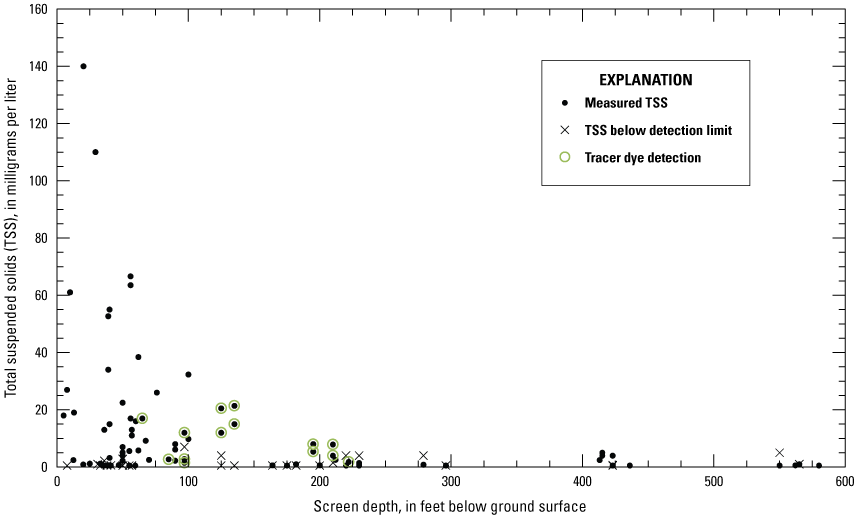
Graph showing total suspended solids concentration in milligrams per liter with respect to screen depth in feet below ground surface, at the Central Chemical facility, Hagerstown, Maryland. Dye detections were extracted from Field (2017) and TSS concentrations are available through the U.S. Environmental Protection Agency (2021).
Contaminant Transport Near the Water Table
Wells MW-A-51 and MW-M-50 are located on the periphery of the waste disposal lagoon. Concentrations of VOCs within MW-A-51 do not show a decreasing trend but are highly variable (appendix 2; fig. 2.1). During 2016 when groundwater levels were low, concentrations of 1,2-dichloroethane, 1,2,4-TCB, benzene, chlorobenzene, ethylbenzene, and toluene increased. Concentrations of these compounds decreased during 2018 and fit closer with the LOESS. The increase in 2016 may be the result of VOCs being released from contaminated material with longer contact time to enable material to diffuse out of the matrix. Concentrations of VOCs in MW-M-50 (fig. 2.5) do not share the same variability as MW-A-51 with lower concentrations measured in 2016. COC in MW-M-50 (figs. 2.5–2.8) generally follow a trend of elevated concentrations prior to 2010, followed by lower concentrations after 2010. The general pattern within MW-M-50 follows a contamination source based on desorption-dissolution from contaminated soils in which levels would decrease with time as the source material is depleted. The exception to this pattern is observed in chlorobenzene, diphenamid, and bis(2-ethylhexyl)phthalate (fig. 2.6). These three COC remain elevated and may be the result of a different source material not associated with the waste disposal lagoon. The presence of elevated levels of bis(2-ethylhexyl)phthalate may be related to an indirect release of plastics including polyvinyl chloride (PVC). Solvents disposed of at the site could leach bis(2-ethylhexyl)phthalate into the groundwater where they came into contact with various plastics.
Wells MW-B-55 and MW-E-46 are located at the edge of the study area boundary. VOCs and SVOCs generally decrease in concentration over time within these wells (appendix 2; figs. 2.9, 2.10, 2.13, 2.14). Pesticide concentrations of DDX (combined isomers of DDT, DDD, and DD), endrin, gamma-BHC, alpha-BHC, and pentachlorophenol all decrease with time in well MW-E-46 (appendix 2, fig. 2.15). A bell-shaped pattern is observed for beta-BHC and heptachlor epoxide that is not observed in MW-B-55 (appendix 2, fig. 2.11). The concentration of the SVOC diphenamid in well MW-B-55 (appendix 2, fig. 2.10) increases with time possibly caused by recharge desorbing contaminants from surface soils then reabsorbing to the deeper materials. Desorption could result in a steady increase in diphenamid until either the source material is removed or the matrix reaches equilibrium.
The variable COC concentrations and patterns observed near the water table do not provide conclusive evidence of dominant transport mechanisms or sources. The variability observed between different COC within the same well may be the result of additional source materials unconnected to the disposal lagoon. Storage of contaminated material within the epikarst system has the potential to hinder remediation efforts if not considered in the remedial action. Gaps in the sampling frequency add uncertainty to COC transport if affected by water-level changes within the epikarst as observed in MW-A-51. Increased sampling frequency and a targeted approach to capture changes in water level and recharge events may provide clarity in understanding COC transport within the epikarst.
Contaminant Transport Within Dissolution Voids
Specific wells depicted in sections B-B' and C-C' in figure 7 contain reported dissolution voids with possible connections, as seen in the figure. Additionally, these cross sections contain wells with tracer detections from the EPA tracer test study (Field, 2017). Therefore, these wells indicate possible contaminant transport within dissolution voids. A possible conduit connection from MW-N-113 to MW-I-55 on section C-C' may be aligned with the sinkhole used as the injection location during EPA Tracer Test 2. Dissolution features also are present in MW-N-83 and may also be connected to this sinkhole. Wells MW-J-71 and MW-N-113 also have a possible void connection within section B-B’. Although no void is depicted in wells MW-P-235 and MW-N-113, there is some groundwater connectivity based on detection of dye during the EPA tracer test study (Field, 2017). Wells OW-2-65, OW-2-115, and OW-8-230 located offsite also were evaluated due to the possible dissolution void connecting MW-J-71 to OW-2-115.
TSS concentrations in MW-I-55 measured in 2018 and 2019 were between 15 and 55 microgram per liter (mg/L), which may result from direct recharge through the sinkhole used in the tracer test study. MW-J-71 also had elevated levels of TSS measured in 2018 and 2019 with concentrations between 17 and 67 mg/L. MW-J-71 and MW-I-55 both had the highest concentrations of TSS of the wells sampled that was not a shallow piezometer. Elevated chlorobenzene levels were measured in MW-J-71 with fluctuating concentrations and no observed decrease over the sampling period (fig. 12A). 1,2,4-TCB exhibits similar elevated levels but at an order of magnitude lower concentration (fig. 12B). The more hydrophobic 1,2,4-TCB (log Kow=4.02) has higher sorption to solid materials (like TSS) than chlorobenzene (log Kow=2.84), resulting in approximately an order of magnitude difference in the aqueous concentration if the initial release were the same. BHC isomers have a similar hydrophobicity (log Kow=3.72) to 1,2,4-TCB, but concentrations decrease with respect to time. Chlorobenzene and 1,2,4-TCB may be associated with accumulated sediments within the dissolution void acting as a reservoir for the contaminants.
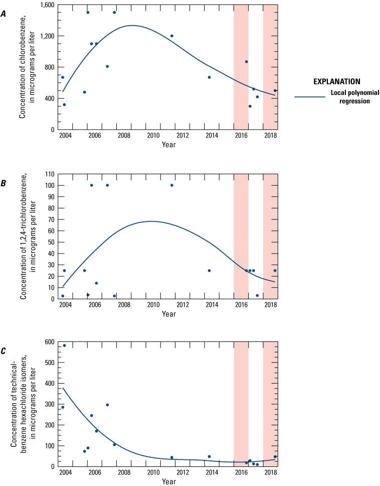
Graphs showing concentrations of, A, chlorobenzene, B, 1,2,4-trichlorobenzene, and C, technical-BHC (Benzene hexachloride isomers) in well MW-J-71, Central Chemical facility, Hagerstown, Maryland. Years 2016 and 2018 are highlighted with red bar.
Evaluating wells within cross section B-B’ (fig. 7) that may be connected to MW-J-71, elevated levels (greater than the RSL) of chlorobenzene and 1,2,4-TCB were observed in MW-O-145 and OW-2-115 though there was no significant pattern change with time (appendix 3). TSS concentrations in MW-O-145 were between 12 and 21 mg/L and in OW-2-115 between 9.8 and 32 mg/L. MW-O-145 is not depicted with a possible void connection and is within the vicinity of MW-J-71 (fig. 7). MW-O-145 also had detections of dye during the EPA tracer test with some connection to surface conduit flow systems. The elevated levels of both chlorobenzene and TSS in OW-2-115 support the possible void connection depicted in cross section A-A' of figure 7C. Within the well cluster containing OW-2-115, TSS were measured in OW-8-235 to range from 4.0 to 7.8 mg/L and had dye detections during the 2017 study. The shallowest well within the cluster, OW-2-65, had TSS concentrations between 4.0 and 7.0 mg/L. Elevated levels of contaminants generally were not observed in OW-2-65, as concentrations were significantly lower than deeper wells within the cluster. Chlorobenzene concentrations within OW-8-230 increased with time. This increase is not observed with 1,2,4-TCB or technical-BHC. Chlorobenzene associated with particles may be a transport mechanism offsite via the possible dissolution void connecting MW-J-71 to OW-2-115.
Well MW-N-113 is also depicted with a possible void connection to MW-J-71 and has some connection to MW-P-235 based on detection from the EPA tracer test (fig. 7). Chlorobenzene concentrations in both MW-N-113 and MW-P-235 decreased with time supporting the hydraulic connectivity observed in the tracer test (fig. 3.1). Elevated levels of TSS were not observed in MW-N-113 during this same period with concentrations near the detection limits, which may be the reason for the decrease in concentration with respect to time if there is no significant storage of contaminant within sediments allowing for dilution of the contaminants. MW-P-235 had detectable quantities of TSS between 5.4 and 8.0 mg/L and may have buffered reduction with time due to TSS compared to MW-N-113. 1,2,4-TCB also decreased with time in MW-N-113 but was variable in MW-P-235 (fig. 3.3). Technical-BHC decreased with respect to time in MW-N-113 until the wetter period of 2018, where the concentration increased to earlier levels (fig. 3.5). Although the void connecting MW-J-71 to MW-N-113 may exist, it does not seem to be contributing to contaminant transport associated with particles.
Limitations and Considerations for Future Study
Karst features, especially dissolution voids, are poorly defined in the subsurface despite their importance to groundwater flow and contaminant transport. Driller’s logs provided the primary dataset to identify karstic dissolution voids in boreholes (Amec Foster Wheeler, 2018), but driller’s logs have inherent limitations with regards to the accuracy of depth and interval thicknesses that may cause many voids to go unnoticed. Most dissolution voids are open (not mud-filled) and marginally thicker than typical secondary porosity lithostatic fractures and joints (Duigon, 2001), but are particularly difficult to identify with driller’s logs. Geophysical logs such as acoustic televiewer (ATV) logs could be utilized and collected in a larger number of boreholes to identify zones of 1-ft or greater thickness that are likely to be dissolution voids, whose presence then could be incorporated into the conceptual site model.
Characterization of site hydrogeology is limited by the dearth of measurements collected within the surficial sediments and epikarst. The lagoon piezometers are the only locations at the site where data are collected in the surficial sediments. The lack of groundwater in most piezometers during periods of low rainfall, despite the lagoon remaining a source area leaching residual contaminants from storage into the groundwater, indicates that the surficial component of the site hydrogeology should be better investigated. Similarly, the characterization of the epikarst used in previous iterations of the conceptual site model is based on a definition of epikarst that consolidates the entire subsurface 100 ft below the land surface as a generalized, low-resolution epikarst zone. This characterization is more suited for a regional-scale assessment than for a site-scale investigation. No data have been collected at the site to assess the presence of perched epikarstic water tables above the main water table that may exist as areas of long-term storage of contaminants, a possibility for which indirect indicators provide evidence in this study. Additional monitoring well nests in areas such as near MW-A-51 that contain screens in the unconsolidated surficial sediments and at various depths in the shallow bedrock would assist with that identification.
Continuous data are important to understand the hydrology of karst aquifers because of the faster flow times that water moves through karst voids following precipitation events compared to fractures and joints. Continuous surface-water data, such as stage (surface-water level) and discharge, could be collected in parallel with continuous groundwater data to observe responses to precipitation and identify bedrock zones that may exhibit responses similar to surface water. For example, the EPA tracer test study (Field, 2017) contained only discrete spring discharge monthly measurements. The addition of continuous discharge data would allow for analysis of the spring responses to precipitation events that might have affected tracer detections at various offsite locations over time. These new data could potentially provide more information regarding hydraulic connections at the Central Chemical facility and provide a better understanding of flow processes and pathways. Future passive sampling to monitor for hydrophobic organic contaminant concentrations at the site and nearby springs, coupled with spring discharge data, may better define hydraulic connections at the site.
This current study, as well as previous efforts at the Central Chemical facility, have represented the subsurface using 2-dimensional maps and cross sections, which creates challenges when illustrating depth changes on maps and lateral correlations between cross sections. The conceptual model for the site would benefit from three-dimensional (3D) modeling of the subsurface to observe geologic and hydrologic correlations between boreholes in all directions. Hydrologic and contaminant concentration data could be emplaced on these 3D views.
Contaminant transport within dissolution voids is difficult to sample and quantify. Flows through conduits or voids can be episodic requiring frequent sampling to catch recharge events that may mobilize particle-bound contaminants. Additionally, wells are not typically installed to sample voids. This study identifies the TSS material measured throughout the site and surrounding wells as possible contaminant transport mechanisms and sinks for more hydrophobic contaminants. Filtering samples to collect and measure TSS in wells where high concentrations of COC and TSS have been detected would confirm or deny the role of particles in transporting COC. Well MW-J-71 and associated wells would be viable locations to test for COC and TSS. Additional sampling and analysis of the TSS found in select wells may provide additional confirmation if COC are bound and transported within the site. Future remedial actions taken to address contaminant transport within OU-2 may need to address sediment-bound COC within voids that could mobilize or act as secondary source material as COC desorb into treated groundwater. A water budget for the site may aid in quantifying what fraction of groundwater recharge is associated with conduit systems flowing offsite compared to moving deeper into the system. The water budget could be linked to local surface water discharge sites identified in the EPA tracer study to provide further evidence of the extent to which the site is hydraulically connected to the surface water sites. Future passive sampling work at surrounding surface water discharge locations may provide evidence to understand the extent to which COC are transported offsite via dissolution voids.
Additionally, this report does not specifically address the contaminant dioxin that was detected at the site in 2018 (U.S. Environmental Protection Agency, 2019). The presence of dioxin at the site may result in additional risk due to the associated toxicity. Additional sampling and monitoring would be necessary at the site to determine the fate, transport, and possible source of dioxin.
Not addressed in this study is the role or potential role of microbial degradation and transformation of the COC found at the site. Halogenated organic compounds can be degraded by a variety of microorganisms that may already exist at the site. For example, sulfate-reducing bacteria Desulfococcus multivorans DSM 2059 and Desulfovibrio gigas DSM 1382 have been found to reduce lindane through co-metabolism (Badea and others, 2009). Sulfate-reducing bacteria may be enriched at the site due to past production of lime sulfur resulting in a sulfate plume. In situ and ex situ microcosm and microbial-community sampling could determine the feasibility that microbial degradation may have in future contaminant reductions.
Summary
The soil and groundwater of the Central Chemical facility in Hagerstown, Maryland are contaminated due to operations related to the blending and production of pesticides and fertilizers during much of the 20th century. Remedial investigations at the site focus on two operable units—the surface soils and waste disposal lagoon (OU-1) and the groundwater (OU-2). The contaminants of concern (COC) for groundwater consists of 41 compounds categorized within the subgroups of volatile organic compounds (VOCs), semi-volatile organic compounds (SVOCs), pesticides, and metals. The purpose of this report is to provide a conceptual site model of the hydrogeology and groundwater contaminant transport at and near the Central Chemical facility. The conceptual model was developed through review, synthesis, and interpretation of hydrogeologic, soil, and other environmental investigations conducted at and in the vicinity of the facility in recent decades and is intended to support plans for environmental remediation of OU-2.
The Central Chemical facility and vicinity are underlain by the Conococheague Formation, Stonehenge Limestone, and Rockdale Run Formation, which include primarily carbonate rocks (Brezinski, 2013, 2018). Overlying the Conococheague Formation at the Central Chemical facility is highly fractured bedrock of the epikarst (U.S. Environmental Protection Agency, 2009). The contact of the bedrock with the overlying soil and epikarst is highly irregular and the soil thickness consequently varies substantially (Maryland Department of the Environment, 1989; U.S. Environmental Protection Agency, 2009). Vertical pathways of high permeability have been reported in the epikarst at the facility (U.S. Environmental Protection Agency, 2009). The Central Chemical facility is underlain by the Zullinger and Shady Grove Members of the Conococheague Formation (Brezinski, 2018).
The extent and nature of the groundwater plume associated with the deeper bedrock has been characterized for OU-2 of the site. Lithologic and structural contrasts between shallow soil, weathered rock, and epikarst and deeper competent but bedded, dipping, fractured, and karstic limestones give rise to two connected flow systems. Uncertainties exist in the nature and transport of contaminants within the epikarst system particularly within voids and perched epikarst groundwater. Contaminated and raw materials within the waste disposal lagoon are in contact with the groundwater. Based on piezometer groundwater levels during drier periods, such as October 2016 (appendix 1; fig. 6), portions of the unconsolidated overburden that are sometimes saturated with groundwater can become unsaturated at other times.
Karst dissolution features, including sinkholes and dissolution voids, were observed in wells at the site during their installation. Of interest, MW-J-71 appears to have a dissolution void connecting it to offsite well OW-2-115. This connection is supported by water-level data and elevated concentrations of total suspended solids (TSS) and chlorobenzene. The high levels of TSS support the possibility of offsite transport of contaminants via particle-bound contaminants in the conduit system due to the hydrophobicity of the COC and the preferential partitioning to solids. Additional sampling would be necessary to confirm this transport phenomena. Variable concentrations of COCs also were observed in certain wells within the epikarst near the waste disposal lagoon, particularly MW-A-51. The variability observed between different COC within the same well may be the result of other source materials unconnected to the disposal lagoon. Storage of contaminated material within the epikarst system has the potential to hinder remediation efforts if not considered.
This study was limited by the available data for the site and no data were generated by the U.S. Geological Survey to complete this report. Additional studies focusing on the epikarst and developing a water budget for the site may provide a better characterization of the groundwater system and contaminant transport.
References Cited
Abatzoglou, J.T., 2013, Development of gridded surface meteorological data for ecological applications and modelling: International Journal of Climatology, v. 33, no. 1, p. 121–131. [Also available at https://doi.org/10.1002/joc.3413.]
Agency for Toxic Substances and Disease Registry, 2005, Public health assessment for Central Chemical Site, Hagerstown, Washington County, Maryland: U.S. Department of Health and Human Services document, 34 p., accessed October 27, 2021, at https://semspub.epa.gov/work/03/2100479.pdf.
Amec Foster Wheeler, 2017, Operable Unit 2 Remedial Investigation Report Part 1: Central Chemical Site Hagerstown, Maryland: Amec Foster Wheeler, [n.p.], accessed October 27, 2021, at https://semspub.epa.gov/work/03/2316146.pdf.
Amec Foster Wheeler, 2018, Draft operable unit 2 remedial investigation report: Central Chemical Site Hagerstown, Maryland: Amec Foster Wheeler, [n.p.], accessed October 27, 2021, at https://semspub.epa.gov/work/03/2316185.pdf.
Badea, S.L., Vogt, C., Weber, S., Danet, A.F., and Richnow, H.H., 2009, Stable isotope fractionation of γ-Hexachlorocyclohexane (Lindane) during reductive dechlorination by two strains of sulfate-reducing bacteria: Environmental Science & Technology, v. 43, no. 9, p. 3155–3161, accessed October 27, 2021, at https://doi.org/10.1021/es801284m.
Field, M.S., 2017, Tracer-test results for the Central Chemical Superfund Site, Hagerstown, Md., May 2014–December 2015: U.S. Environmental Protection Agency Report EPA/600/R-17/032, 282 p., accessed October 27, 2021, at https://semspub.epa.gov/work/03/2316142.pdf.
Fiore, A.R., and Lacombe, P.J., 2020, Groundwater levels and generalized potentiometric surfaces, former Naval Air Warfare Center, West Trenton, New Jersey, 2018: U.S. Geological Survey Open-File Report 2020–1016, 28 p., accessed October 27, 2021, at https://doi.org/10.3133/ofr20201016.
Geosyntec, 2019, Aquifer testing data report—Central Chemical Superfund Site Hagerstown, Maryland: Geosyntec, [n.p.], accessed October 27, 2021, at https://semspub.epa.gov/work/03/2316143.pdf.
Hartmann, A., Goldscheider, N., Wagener, T., Lange, J., and Weiler, M., 2014, Karst water resources in a changing world—Review of hydrological modeling approaches: Reviews of Geophysics, v. 52, no. 3, p. 218–242, accessed October 27, 2021, at https://doi.org/10.1002/2013RG000443.
Kozar, M.D., McCoy, K.J., Weary, D.J., Field, M.S., Pierce, H.A., Schill, W.B., and Young, J.A., 2007, Hydrogeology and water quality of the Leetown area, West Virginia: U.S. Geological Survey Open-File Report 2007–1358, 109 p., accessed October 27, 2021, at https://pubs.usgs.gov/of/2007/1358.
Lacombe, P.J., 2000, Hydrogeologic framework, water levels, and trichloroethylene contamination, Naval Air Warfare Center, West Trenton, New Jersey, 1993–97: U.S. Geological Survey Water-Resources Investigations Report 98–4167, 139 p., accessed October 12, 2021, at https://doi.org/10.3133/wri984167.
Maryland Department of the Environment, 1989, Screening site investigation of Central Chemical Corporation, Hagerstown, MD, MD-302: Maryland Department of the Environment document, [n.p.], accessed October 27, 2021, at https://semspub.epa.gov/work/03/128905.pdf.
Maryland Department of the Environment, 2017, Central Chemical NPL Site—What you need to know: Maryland Department of the Environment Fact Sheet, 3 p., accessed October 27, 2021, at https://mde.maryland.gov/programs/LAND/MarylandBrownfieldVCP/Documents/CentralChemicalnewfs4-17.pdf.
Maryland Department of the Environment, 1993, DRAFT Expanded Site Inspection of the Central Chemical—Hagerstown Site, MD–302: Maryland Department of the Environment document, [n.p.], accessed October 27, 2021, at https://semspub.epa.gov/work/03/124300.pdf.
National Oceanic and Atmospheric Administration, 2019, State of the Climate—National Climate Report for 2018: NOAA National Centers for Environmental Information webpage, accessed December 9, 2020, at https://www.ncdc.noaa.gov/sotc/national/201813/supplemental/page-3.
Senay, G.B., Bohms, S., Singh, R.K., Gowda, P.H., Velpuri, N.M., Alemu, H., and Verdin, J.P., 2013, Operational evapotranspiration mapping using remote sensing and weather datasets—A new parameterization for the SSEB approach: Journal of the American Water Resources Association, v. 49, no. 3, p. 577–591, accessed December 9, 2020, at https://doi.org/10.1111/jawr.12057.
Senay, G.B., Budde, M., Verdin, J.P., and Melesse, A.M., 2007, A coupled remote sensing and simplified surface energy balance approach to estimate actual evapotranspiration from irrigated fields: Sensors (Basel), v. 7, no. 6, p. 979–1000, accessed October 27, 2021, at https://doi.org/10.3390/s7060979.
Senay, G.B., Budde, M.E., and Verdin, J.P., 2011, Enhancing the Simplified Surface Energy Balance (SSEB) approach for estimating landscape ET—Validation with the METRIC model: Agricultural Water Management, v. 98, no. 4, p. 606–618, accessed October 27, 2021, at https://doi.org/10.1016/j.agwat.2010.10.014.
Tiedeman, C.R., Shapiro, A.M., Hsieh, P.A., Imbrigiotta, T.E., Goode, D.J., Lacombe, P.J., DeFlaun, M.F., Drew, S.R., Johnson, C.D., Williams, J.H., and Curtis, G.P., 2018, Bioremediation in fractured rock—1. Modeling to inform design, monitoring, and expectations: Ground Water, v. 56, no. 2, p. 300–316, accessed October 12, 2021, at https://doi.org/10.1111/gwat.12585.
U.S. Environmental Protection Agency, 2009, EPA Superfund Program Record of Decision, Central Chemical Superfund Site, Hagerstown, Maryland: U.S. Environmental Protection Agency, [n.p.], accessed October 27, 2021, at https://semspub.epa.gov/work/03/2101283.pdf.
U.S. Environmental Protection Agency, 2019, Fall 2019 Community Update Fact Sheet, Central Chemical Superfund Site, Hagerstown, Washington County, Maryland: U.S. Environmental Protection Agency Fact Sheet, 2 p., accessed October 27, 2021, at https://semspub.epa.gov/work/03/2289269.pdf
U.S. Environmental Protection Agency, 2021, Table: Groundwater COC & TSS Results: Central Chemical (Hagerstown) Records Collections database, 342 p., accessed October 21, 2021, at https://semspub.epa.gov/work/03/2316147.pdf.
Velpuri, N.M., Senay, G.B., Singh, R.K., Bohms, S., and Verdin, J.P., 2013, A comprehensive evaluation of two MODIS evapotranspiration products over the conterminous United States—Using point and gridded FLUXNET and water balance ET: Remote Sensing of Environment, v. 139, p. 35–49, accessed October 27, 2021, at https://doi.org/10.1016/j.rse.2013.07.013.
Weston, Inc., 1989, Phase 1 Environmental Investigation, Central Chemical Corporation: Roy F. Weston Inc., West Chester, Penn. [n.p], accessed October 27, 2021, at https://semspub.epa.gov/work/03/2100476.pdf.
White, W.B., 2018, Contaminant transport in karst aquifers—Systematics and mechanisms, in White, W.B., Herman J.S., Herman, E.K., Rutligliano, M., eds., Karst groundwater contamination and public health—Advances in karst science: Springer International Publishing, Cham, Switzerland., p. 55–81, accessed October 27, 2021, at https://doi.org/10.1007/978-3-319-51070-5_7.
Williams, P.W., 2008, The role of the epikarst in karst and cave hydrogeology—A review: International Journal of Speleology, v. 37, no. 1, p. 1–10, accessed October 27, 2021, at https://doi.org/10.5038/1827-806X.37.1.1.
Wood Environment & Infrastructure Solutions, Inc., 2019, Draft 2018 groundwater monitoring report—Central Chemical Operable Unit 2 (OU-2): Wood Environment & Infrastructure Solutions, Inc., [n.p.], accessed October 27, 2021, at https://semspub.epa.gov/work/03/2316144.pdf.
Worthington, S.R.H., Jeannin, P.Y., Alexander, E.C., Jr., Davies, G.J., and Schindel, G.M., 2017, Contrasting definitions for the term ‘karst aquifer’: Hydrogeology Journal, v. 25, no. 5, p. 1237–1240, accessed October 27, 2021, at https://doi.org/10.1007/s10040-017-1628-7.
Yager, R.M., Plummer, L.N., Kauffman, L.J., Doctor, D.H., Nelms, D.L., and Schlosser, P., 2013, Comparison of age distributions estimated from environmental tracers by using binary-dilution and numerical models of fractured and folded karst—Shenandoah Valley of Virginia and West Virginia, USA: Hydrogeology Journal, v. 21, no. 6, p. 1193–1217, accessed October 27, 2021, at https://doi.org/10.1007/s10040-013-0997-9.
Appendix 1. Reported Well Construction Information, Groundwater Level Measurements, Groundwater Level Drawdown from Aquifer Tests, and Tracer Test Detections, Central Chemical Facility, Hagerstown, Maryland
Table 1.1.
Reported well construction information, Central Chemical facility, Hagerstown, Maryland.[Datum is North American Vertical Datum of 1988.]
Table 1.2.
Reported groundwater level measurements, groundwater level drawdown from aquifer tests, and tracer detections, Central Chemical facility, Hagerstown, Maryland.[NAVD 88, North American Vertical Datum of 1988; NA, not applicable; NM, not measured; ND, not detected]
| Well | April 14, 2014 synoptic (Amec Foster Wheeler, 2018) | October 21, 2016 synoptic (Amec Foster Wheeler, 2018) | January 19, 2017 synoptic (Amec Foster Wheeler, 2018) | April 20, 2017 synoptic (Amec Foster Wheeler, 2018) | July 26, 2017 synoptic (Amec Foster Wheeler, 2018) | October 22, 2018 synoptic (Wood Environment & Infrastructure Solutions, Inc., 2019) | May 21–24, 2019 aquifer test (Geosyntec, 2019) | EPA tracer test1, 2014–2015 (Field, 2017) | ||||||||
|---|---|---|---|---|---|---|---|---|---|---|---|---|---|---|---|---|
| Water level depth below casing (feet) | Head (feet) | Water level depth below casing (feet) | Head (feet) | Water level depth below casing (feet) | Head (feet) | Water level depth below casing (feet) | Head (feet) | Water level depth below casing (feet) | Head (feet) | Water level depth below casing (feet) | Head (feet) | Total draw-down (feet) | Detection during tracer test 1 | Detection during tracer test 2 | Detection during tracer test 3 | |
| EW-10 | NA | NA | NA | NA | NA | NA | NA | NA | NA | NA | 29.26 | 592.99 | 22 | NM | NM | NM |
| EW-11 | NA | NA | NA | NA | NA | NA | NA | NA | NA | NA | 37.92 | 580.86 | 36 | NM | NM | NM |
| EW-12 | NA | NA | NA | NA | NA | NA | NA | NA | NA | NA | 40.09 | 590.45 | 37.5 | NM | NM | NM |
| EW-13 | NA | NA | NA | NA | NA | NA | NA | NA | NA | NA | 38.66 | 593.35 | 23 | NM | NM | NM |
| EW-1-110 | 25.45 | 598.38 | 36.88 | 586.95 | 37.07 | 586.76 | 29.46 | 594.37 | 30.57 | 593.26 | 24.96 | 598.87 | 0.5 | NM | NM | NM |
| MW-A-51 | 36.24 | 593.8 | 47.02 | 583.02 | 46.74 | 583.3 | 42.29 | 587.75 | 42.3 | 587.74 | 36.1 | 593.94 | 1 | Yes | ND | Yes |
| MW-B-55 | 42.51 | 579.21 | 48.86 | 572.86 | 47.54 | 574.18 | 45.44 | 576.28 | 43.65 | 578.07 | 42.77 | 578.95 | 0 | NM | NM | NM |
| MW-B-400 | NA | NA | 56.98 | 564.68 | 57.07 | 564.59 | 55.39 | 566.27 | 55.21 | 566.45 | 51.98 | 569.68 | 0.04 | NM | NM | NM |
| MW-B-598 | NA | NA | 55.58 | 564.81 | 55.73 | 564.66 | 54.07 | 566.32 | 53.86 | 566.53 | 50.67 | 569.72 | 0 | NM | NM | NM |
| MW-C-40 | 27.49 | 582.67 | 32.11 | 578.05 | 31.91 | 578.25 | 27.96 | 582.2 | 29.76 | 580.4 | 27.91 | 582.25 | 0 | NM | NM | NM |
| MW-D-77 | 25.75 | 582.04 | 28.46 | 579.33 | 31.44 | 576.35 | 32.08 | 575.71 | 31.8 | 575.99 | 25.88 | 581.91 | 0 | NM | NM | NM |
| MW-E-46 | 23.47 | 592.7 | 33 | 583.17 | 32.05 | 584.12 | 25.19 | 590.98 | 26.31 | 589.86 | 32.45 | 583.72 | 0.5 | NM | NM | NM |
| MW-F-70 | 41.7 | 578.95 | 50.32 | 570.33 | 50.23 | 570.42 | 46 | 574.65 | 44.76 | 575.89 | 41.27 | 579.38 | 0 | NM | NM | NM |
| MW-G-35 | 19.3 | 581.09 | 24.74 | 575.65 | 26.58 | 573.81 | 20.84 | 579.55 | 21.93 | 578.46 | 18.25 | 582.14 | 0 | NM | NM | NM |
| MW-G-360 | NA | NA | 33.84 | 564.54 | 33.56 | 564.82 | 31.51 | 566.87 | 31.25 | 567.13 | 27.65 | 570.73 | 0.3 | NM | NM | NM |
| MW-G-600 | NA | NA | 36.17 | 563.1 | 36.36 | 562.91 | 34.6 | 564.67 | 34.39 | 564.88 | 30.72 | 568.69 | 0 | NM | NM | NM |
| MW-H-65 | 29.6 | 585.5 | 35.63 | 579.47 | 34.77 | 580.33 | 31.43 | 583.67 | 32.65 | 582.45 | 29.65 | 585.45 | 0 | NM | NM | NM |
| MW-I-55 | 27.05 | 598.88 | 38.63 | 587.3 | 38.93 | 587 | 31.11 | 594.82 | 32.2 | 593.73 | 26.53 | 599.4 | 0 | NM | NM | NM |
| MW-J-71 | 37.59 | 593.25 | 47.94 | 582.9 | 45.39 | 585.45 | 42 | 588.84 | 42.84 | 588 | 37.59 | 593.25 | 1.9 | NM | NM | NM |
| MW-K-80 | 35.97 | 593.36 | 44.98 | 584.35 | 44.46 | 584.87 | 38.95 | 590.38 | 39.42 | 589.91 | 36.47 | 592.86 | 0.75 | Yes | ND | Yes |
| MW-K-440 | NA | NA | 64.1 | 565.45 | 64.48 | 565.07 | 62.59 | 566.96 | 62.22 | 567.33 | 58.51 | 571.04 | 0 | NM | NM | NM |
| MW-L-48 | 28.13 | 592.01 | 36.13 | 584.01 | 34.38 | 585.76 | 29.19 | 590.95 | 30.82 | 589.32 | 29.43 | 590.71 | 0 | NM | NM | NM |
| MW-L-250 | NA | NA | 54.63 | 564.84 | 55.02 | 564.45 | 53.13 | 566.34 | 52.75 | 566.72 | 48.6 | 570.87 | 0 | NM | NM | NM |
| MW-M-50 | 26.1 | 599.34 | 36.87 | 588.57 | 37.98 | 587.46 | 29.17 | 596.27 | 30.67 | 594.77 | 25.36 | 600.08 | 0 | NM | NM | NM |
| MW-N-83 | 34.48 | 590.76 | 44.31 | 580.93 | 43.88 | 581.36 | 37.87 | 587.37 | 37.66 | 587.58 | 33.67 | 591.57 | 13 | NM | NM | NM |
| MW-N-113 | 34.91 | 590.31 | 44 | 581.22 | 44.1 | 581.12 | 38.3 | 586.92 | 38.11 | 587.11 | 34.17 | 591.05 | 11.8 | Yes | Yes | Yes |
| MW-O-145 | 52 | 580.49 | 59.58 | 572.91 | 58.67 | 573.82 | 55.37 | 577.12 | 55.2 | 577.29 | 51.17 | 581.32 | 3.4 | ND | Yes | Yes |
| PZ-P-165 | 46.75 | 579.82 | 54.48 | 573.09 | 53.65 | 573.92 | 50.38 | 577.19 | 49.97 | 577.6 | NM | NM | 16 | NM | NM | NM |
| MW-P-235 | 50.49 | 576.02 | 57.53 | 568.98 | 56.94 | 569.57 | 54.16 | 572.35 | 53.84 | 572.67 | 50.05 | 576.46 | 2 | Yes | Yes | Yes |
| PZ-Q-118 | 40.12 | 590.5 | 50.22 | 580.4 | 49.91 | 580.71 | 43.81 | 586.81 | 43.86 | 586.76 | NM | NM | 5.9 | NM | NM | NM |
| MW-Q-150 | 47.78 | 582.81 | 56.21 | 574.38 | 55.74 | 574.85 | 51.4 | 579.19 | 51.15 | 579.44 | 47.25 | 583.34 | 6.3 | ND | Yes | Yes |
| MW-R-330 | NA | NA | 52.4 | 566.63 | 52.09 | 566.94 | 49.7 | 569.33 | 49.4 | 569.63 | 45.85 | 573.18 | 0.9 | NM | NM | NM |
| MW-R-600 | NA | NA | 55.13 | 564.85 | 55.46 | 564.52 | 53.59 | 566.39 | 53.62 | 566.36 | 49.77 | 570.31 | 0 | NM | NM | NM |
| OW-1-62 | 49.6 | 576.49 | 55.61 | 570.48 | 59.47 | 566.62 | 53.47 | 572.62 | 53.13 | 572.96 | 48.48 | 577.61 | 0 | NM | NM | NM |
| OW-1-105 | 50.2 | 575.85 | 56.49 | 569.56 | 56.33 | 569.72 | 53.95 | 572.1 | 53.52 | 572.53 | 48.4 | 577.65 | NM | NM | NM | NM |
| OW-2-65 | 44.32 | 585.49 | 50.07 | 579.74 | 47.88 | 581.93 | 47.86 | 581.95 | 46.77 | 566.83 | 47.28 | 582.53 | 0 | NM | NM | NM |
| OW-2-115 | 47.36 | 582.52 | 55.93 | 573.95 | 53.93 | 575.95 | 51.49 | 578.39 | 50.07 | 579.81 | 44.53 | 585.35 | 0 | NM | NM | NM |
| OW-3-55 | 41.76 | 573.36 | 50 | 565.12 | 50.69 | 564.43 | 49.15 | 565.97 | 48.29 | 566.83 | 42.03 | 573.09 | NM | NM | NM | NM |
| OW-3-105 | 42.38 | 572.71 | 50.21 | 564.88 | 50.78 | 564.31 | 49.23 | 565.86 | 48.52 | 566.57 | 41.77 | 573.32 | NM | NM | NM | NM |
| OW-4-70 | 31.62 | 572.45 | 40.19 | 563.88 | 39.29 | 564.78 | 37.35 | 566.72 | 35.46 | 568.61 | 31.45 | 572.62 | NM | NM | NM | NM |
| OW-5-90 | 36.12 | 565.25 | 44.44 | 556.93 | 43.93 | 557.44 | 41.9 | 559.47 | 41.11 | 560.26 | 36.3 | 565.07 | NM | ND | ND | ND |
| OW-7-242 | 37.37 | 564.59 | 42.7 | 559.26 | 44.01 | 557.95 | 50.29 | 551.67 | 41.8 | 560.16 | 33.6 | 568.36 | NM | ND | ND | Yes |
| OW-7-410 | NA | NA | 41.65 | 562.1 | 41.8 | 561.95 | 39.99 | 563.76 | 39.66 | 564.09 | 35.65 | 568.1 | 0 | NM | NM | NM |
| OW-8-230 | 52.53 | 577.2 | 59.9 | 569.83 | 58.76 | 570.97 | 56.84 | 572.89 | 55.9 | 573.83 | 52.01 | 577.72 | 0.25 | ND | Yes | Yes |
| OW-9-125 | 29.3 | 573.5 | 34.19 | 568.61 | 33.69 | 569.11 | 32.07 | 570.73 | 31.7 | 571.1 | 28.2 | 574.6 | NM | ND | Yes | Yes |
| OW-10-250 | 35.77 | 570.51 | 40.06 | 566.22 | 39.41 | 566.87 | 38.19 | 568.09 | 37.65 | 568.63 | 34.61 | 571.67 | NM | NM | NM | NM |
| OW-11-240 | 45.32 | 567.36 | 52.22 | 560.46 | 50.54 | 562.14 | 49.39 | 563.29 | 48.56 | 564.12 | 45.57 | 567.11 | NM | NM | NM | NM |
| OW-11-600 | NA | NA | 55.78 | 559.08 | 54.78 | 560.08 | 53.88 | 560.98 | 53.44 | 561.42 | 51.18 | 563.68 | 0.1 | NM | NM | NM |
| OW-12-232 | 54.76 | 556.86 | 62.98 | 548.64 | 62.49 | 549.13 | 61.89 | 549.73 | 60.31 | 551.31 | 52.68 | 558.94 | NM | NM | NM | NM |
| OW-13-250 | 13.08 | 561.4 | 20.31 | 554.17 | 19.99 | 554.49 | 18.03 | 556.45 | 17.75 | 556.73 | 14 | 560.48 | NM | NM | NM | NM |
| OW-14-96 | 19.51 | 565.17 | 27.57 | 557.11 | 27.58 | 557.1 | 25.56 | 559.12 | 25.13 | 559.55 | 18.7 | 565.98 | NM | NM | NM | NM |
| OW-14-235 | 18.42 | 566.27 | 25.74 | 558.95 | 25.91 | 558.78 | 23.97 | 560.72 | 23.54 | 561.15 | 17.63 | 567.06 | NM | NM | NM | NM |
| OW-15-202 | 19.23 | 571.17 | 26.23 | 564.17 | 27.09 | 563.31 | 25.32 | 565.08 | 25.02 | 565.38 | 19.12 | 571.28 | NM | NM | NM | NM |
| OW-16-448 | NA | NA | 47.12 | 562.5 | 47.87 | 561.75 | 46.2 | 563.42 | 25.79 | 583.83 | 41.09 | 568.53 | NM | NM | NM | NM |
| OW-17-600 | NA | NA | 47.36 | 565.66 | 47.47 | 565.55 | 45.99 | 567.03 | 45.84 | 567.18 | 42.73 | 570.29 | NM | NM | NM | NM |
| OW-18-597 | NA | NA | 43.41 | 559.13 | 42.95 | 559.59 | NM | NM | 41.39 | 561.15 | 38.12 | 564.42 | NM | NM | NM | NM |
| OW-19-450 | NA | NA | 59.82 | 565.58 | 60.42 | 564.98 | 58.54 | 566.86 | 58.2 | 567.2 | 53.61 | 571.79 | NM | NM | NM | NM |
| PZ-1S | 9.17 | 619.09 | 11.64 | 616.62 | 11.13 | 617.13 | 9.08 | 619.18 | 10.91 | 617.35 | 9.19 | 619.07 | 0 | NM | NM | NM |
| PZ-1D | 24.15 | 604.28 | 24.2 | 604.23 | 24.28 | 604.15 | 24.32 | 604.11 | 24.25 | 604.18 | 22.97 | 605.46 | NM | NM | NM | NM |
| PZ-2S | 12.87 | 616.81 | 15.76 | 613.02 | 15.91 | 613.77 | 13.75 | 615.93 | 14.88 | 614.8 | 13.39 | 615.29 | NM | NM | NM | NM |
| PZ-2D | 30.11 | 599.56 | 36.04 | 593.63 | 36.16 | 593.51 | 36.22 | 593.45 | 35.78 | 593.89 | 26.42 | 603.25 | 0 | NM | NM | NM |
| PZ-3S | 11 | 619.08 | 16.64 | 613.44 | 16.73 | 613.35 | 14.12 | 615.96 | 14.99 | 615.09 | 10.58 | 619.5 | 0 | NM | NM | NM |
| PZ-3D | 21.22 | 608.92 | 27.06 | 603.08 | 27.16 | 602.98 | 27.22 | 602.92 | 26.75 | 603.39 | 19.34 | 610.8 | 0 | NM | NM | NM |
| PZ-4S | 6.42 | 619.17 | 11.79 | 613.8 | 11.53 | 614.06 | 8.2 | 617.39 | 9.47 | 616.12 | 6.01 | 619.58 | 0.2 | NM | NM | NM |
| PZ-4D | 26.1 | 599.52 | 36.62 | 589 | 38.16 | 587.46 | 31.28 | 594.34 | 31.68 | 593.94 | 25.37 | 600.25 | 0 | NM | NM | NM |
Appendix 2. Concentrations of Contaminants of Concern Observed Over Time in Wells MW-A-51, MW-M-50, MW-B-55, and MW-E-56 at the Central Chemical Facility in Hagerstown, Maryland
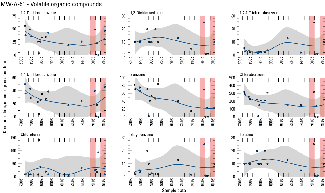
Graphs showing select volatile organic compounds (VOC) concentrations reported for well MW-A-51, Central Chemical facility, Hagerstown, Maryland. Years 2016 and 2018 are highlighted with red bars, a local polynomial regression is depicted with a blue line, and the 95 percent confidence interval in grey. All concentrations for contaminants of concern are available through the U.S. Environmental Protection Agency (2021).
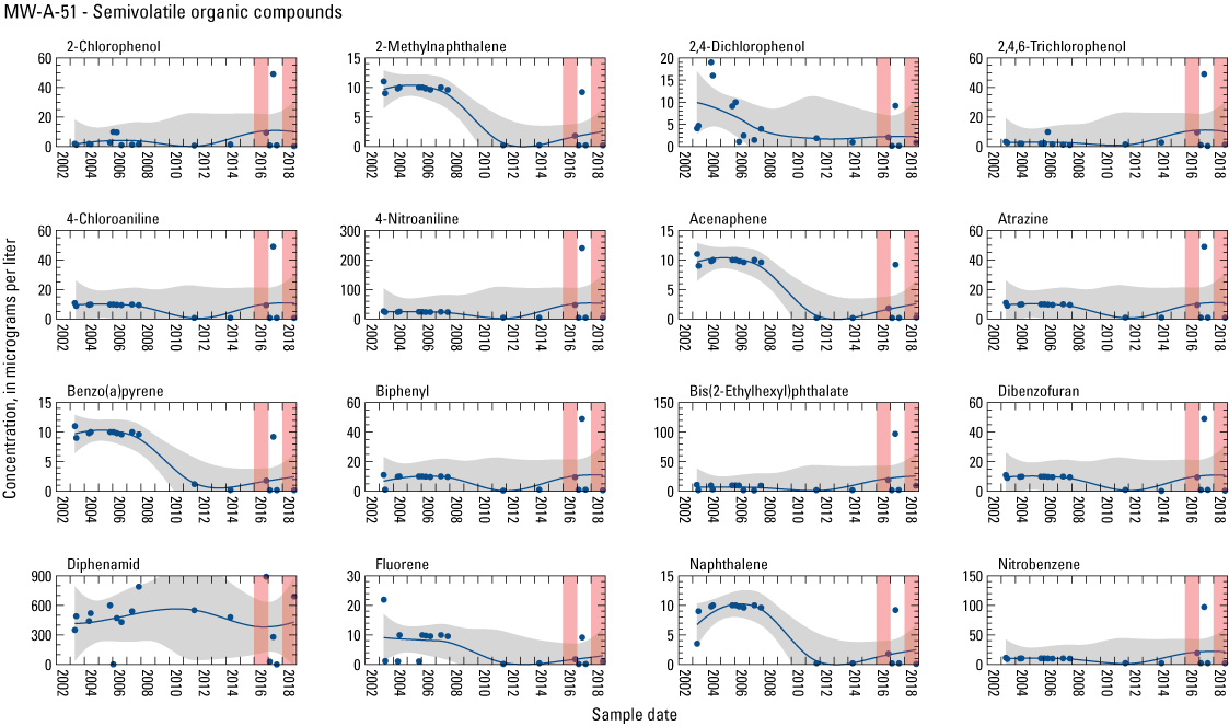
Graphs showing select semi-volatile organic compounds (SVOC) concentrations reported for well MW-A-51, Central Chemical facility, Hagerstown, Maryland. Years 2016 and 2018 are highlighted with red bars, a local polynomial regression is depicted with a blue line, and the 95 percent confidence interval in grey. All concentrations for contaminants of concern are available through the U.S. Environmental Protection Agency (2021).
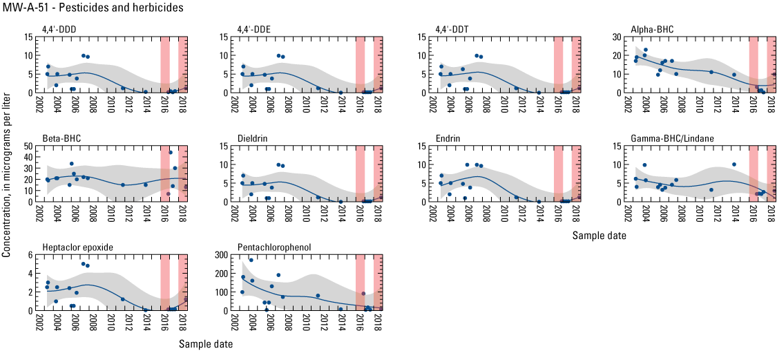
Graphs showing select pesticide and herbicide concentrations reported for well MW-A-51, Central Chemical facility, Hagerstown, Maryland. Years 2016 and 2018 are highlighted with red bars, a local polynomial regression is depicted with a blue line, and the 95 percent confidence interval in grey. All concentrations for contaminants of concern are available through the U.S. Environmental Protection Agency (2021). [Dichlorodiphenyltrichloroethane, DDT; Dichlorodiphenyldichloroethylene, DDE; Dichlorodiphenyldichloroethane, DDD; Benzene hexachloride, BHC]
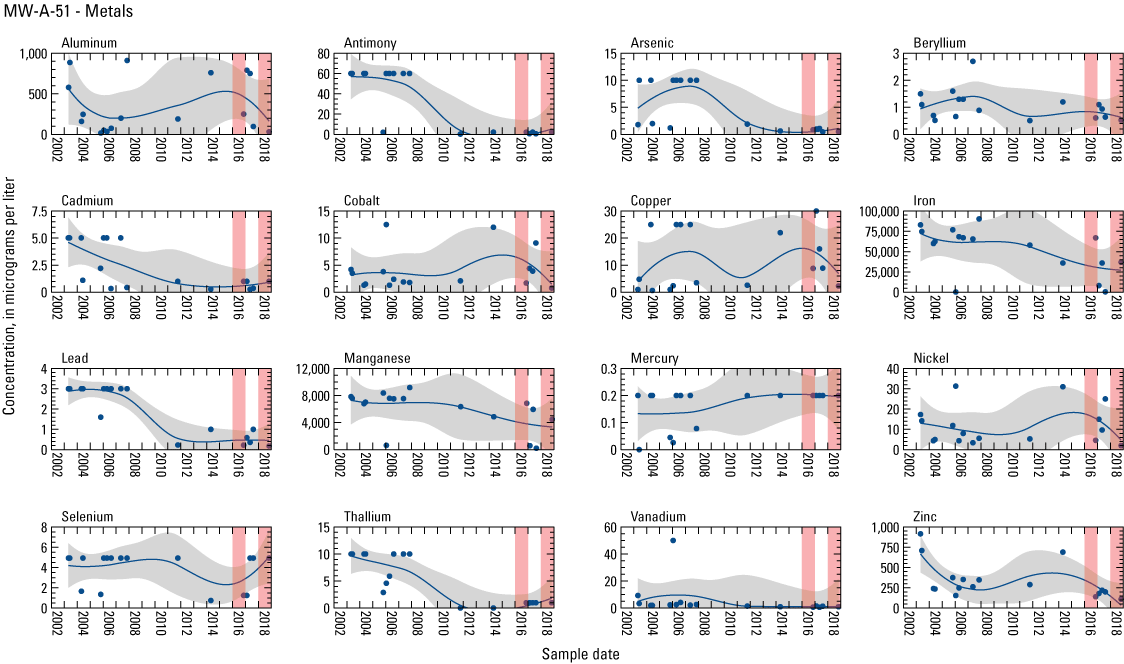
Graphs showing select metal concentrations reported for well MW-A-51, Central Chemical facility, Hagerstown, Maryland. Years 2016 and 2018 are highlighted with red bars, a local polynomial regression is depicted with a blue line, and the 95 percent confidence interval in grey. All concentrations for contaminants of concern are available through the U.S. Environmental Protection Agency (2021).
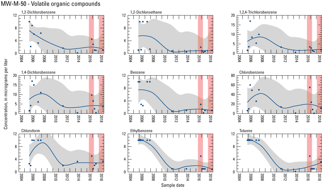
Graphs showing select volatile organic compounds (VOC) concentrations reported for well MW-M-50, Central Chemical facility, Hagerstown, Maryland. Years 2016 and 2018 are highlighted with red bars, a local polynomial regression is depicted with a blue line, and the 95 percent confidence interval in grey. All concentrations for contaminants of concern are available through the U.S. Environmental Protection Agency (2021).
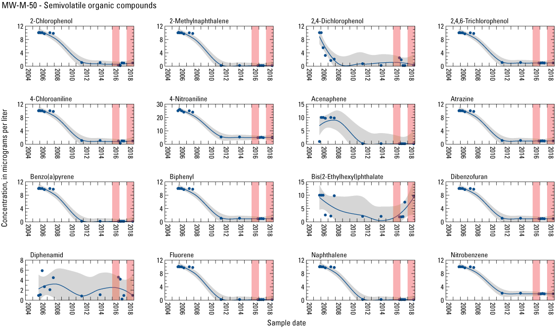
Graphs showing select semi-volatile organic compounds (SVOC) concentrations reported for well MW-M-50, Central Chemical facility, Hagerstown, Maryland. Years 2016 and 2018 are highlighted with red bars, a local polynomial regression is depicted with a blue line, and the 95 percent confidence interval in grey. All concentrations for contaminants of concern are available through the U.S. Environmental Protection Agency (2021).
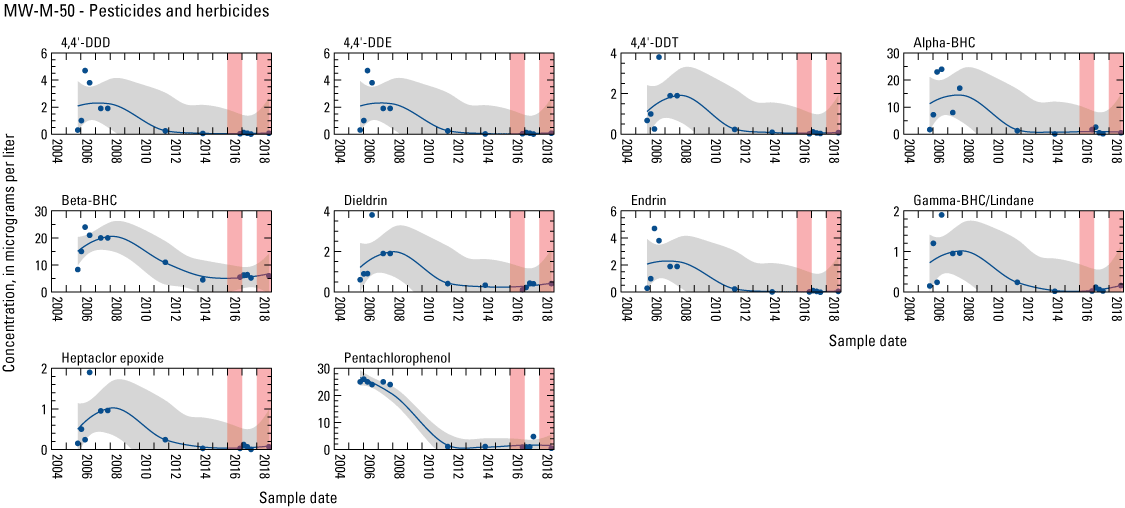
Graphs showing select pesticide and herbicide concentrations reported for well MW-M-50, Central Chemical facility, Hagerstown, Maryland. Years 2016 and 2018 are highlighted with red bars, a local polynomial regression is depicted with a blue line, and the 95 percent confidence interval in grey. All concentrations for contaminants of concern are available through the U.S. Environmental Protection Agency (2021). [Dichlorodiphenyltrichloroethane, DDT; Dichlorodiphenyldichloroethylene, DDE; Dichlorodiphenyldichloroethane, DDD; Benzene hexachloride, BHC]
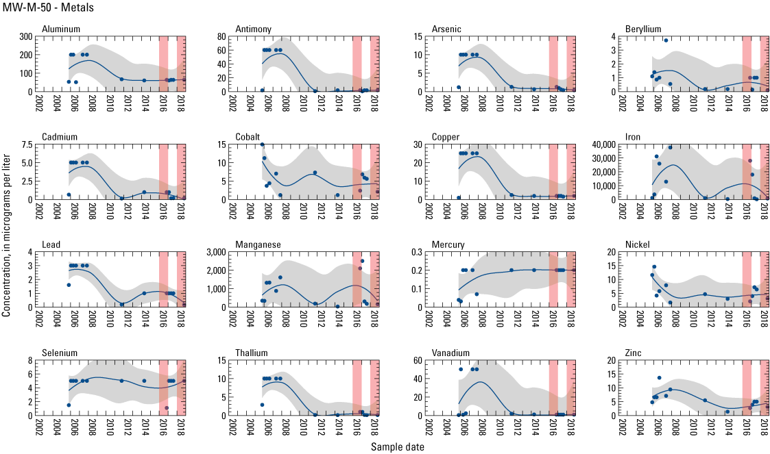
Graphs showing select metal concentrations reported for well MW-M-50, Central Chemical facility, Hagerstown, Maryland. Years 2016 and 2018 are highlighted with red bars, a local polynomial regression is depicted with a blue line, and the 95 percent confidence interval in grey. All concentrations for contaminants of concern are available through the U.S. Environmental Protection Agency (2021).
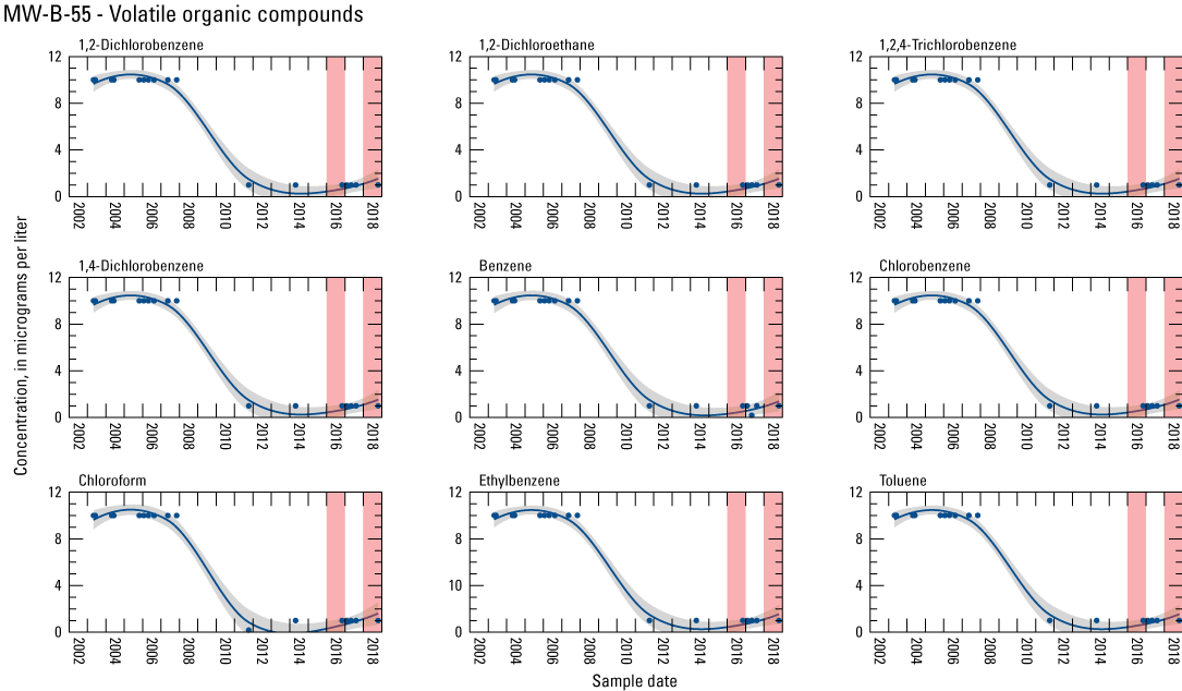
Graphs showing select volatile organic compounds (VOC) concentrations reported for well MW-B-55, Central Chemical facility, Hagerstown, Maryland. Years 2016 and 2018 are highlighted with red bars, a local polynomial regression is depicted with a blue line, and the 95 percent confidence interval in grey. All concentrations for contaminants of concern are available through the U.S. Environmental Protection Agency (2021).
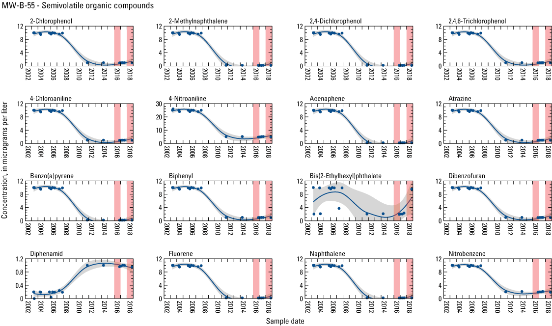
Graphs showing select semi-volatile organic compounds (SVOC) concentrations reported for well MW-B-55, Central Chemical facility, Hagerstown, Maryland. Years 2016 and 2018 are highlighted with red bars, a local polynomial regression is depicted with a blue line, and the 95 percent confidence interval in grey. All concentrations for contaminants of concern are available through the U.S. Environmental Protection Agency (2021).
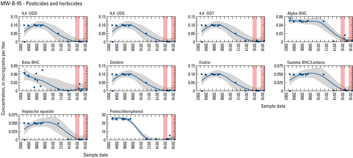
Graphs showing select pesticide and herbicide concentrations reported for well MW-B-55, Central Chemical facility, Hagerstown, Maryland. Years 2016 and 2018 are highlighted with red bars, a local polynomial regression is depicted with a blue line, and the 95 percent confidence interval in grey. All concentrations for contaminants of concern are available through the U.S. Environmental Protection Agency (2021). [Dichlorodiphenyltrichloroethane, DDT; Dichlorodiphenyldichloroethylene, DDE; Dichlorodiphenyldichloroethane, DDD; Benzene hexachloride, BHC]
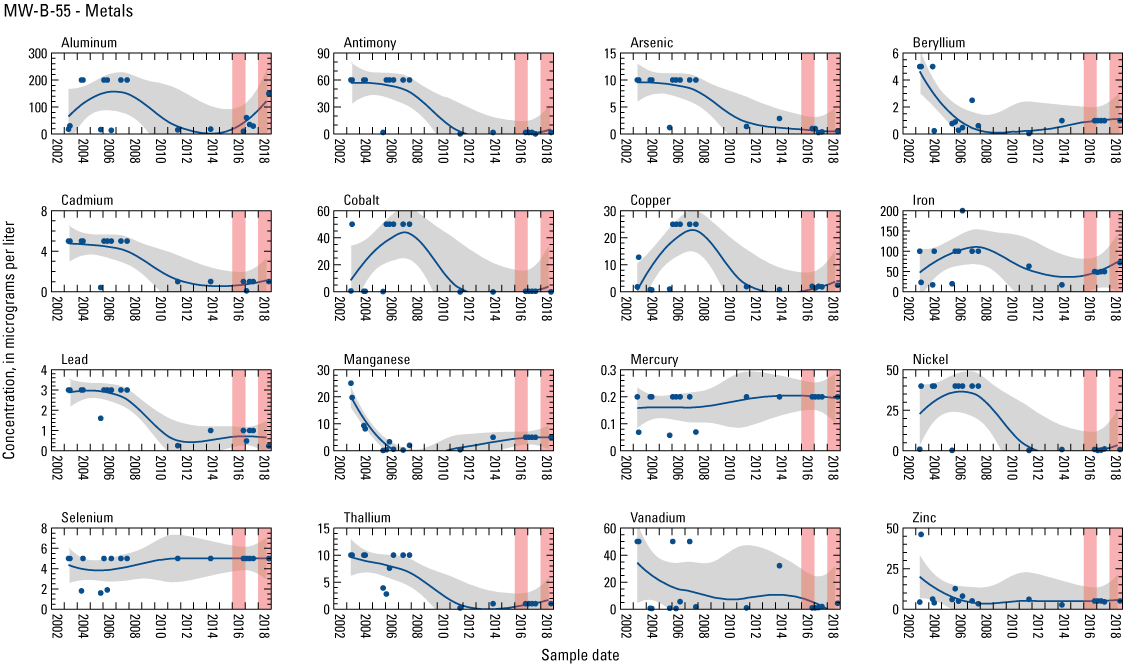
Graphs showing select metal concentrations reported for well MW-B-55, Central Chemical facility, Hagerstown, Maryland. Years 2016 and 2018 are highlighted with red bars, a local polynomial regression is depicted with a blue line, and the 95 percent confidence interval in grey. All concentrations for contaminants of concern are available through the U.S. Environmental Protection Agency (2021).
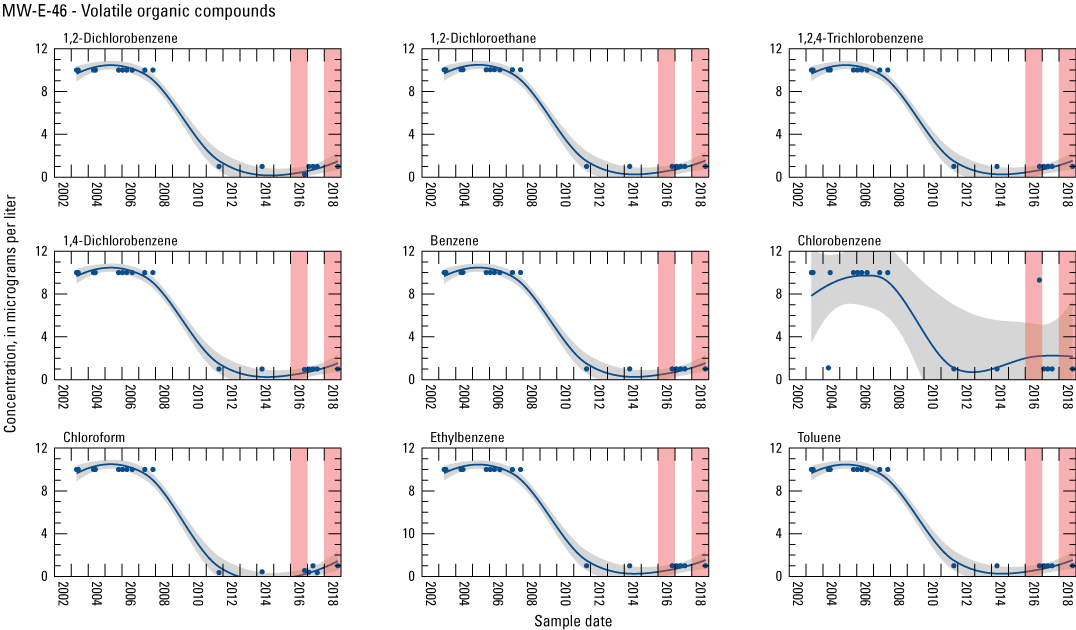
Graphs showing select volatile organic compounds (VOC) concentrations reported for well MW-E-46, Central Chemical facility, Hagerstown, Maryland. Years 2016 and 2018 are highlighted with red bars, a local polynomial regression is depicted with a blue line, and the 95 percent confidence interval in grey. All concentrations for contaminants of concern are available through the U.S. Environmental Protection Agency (2021).
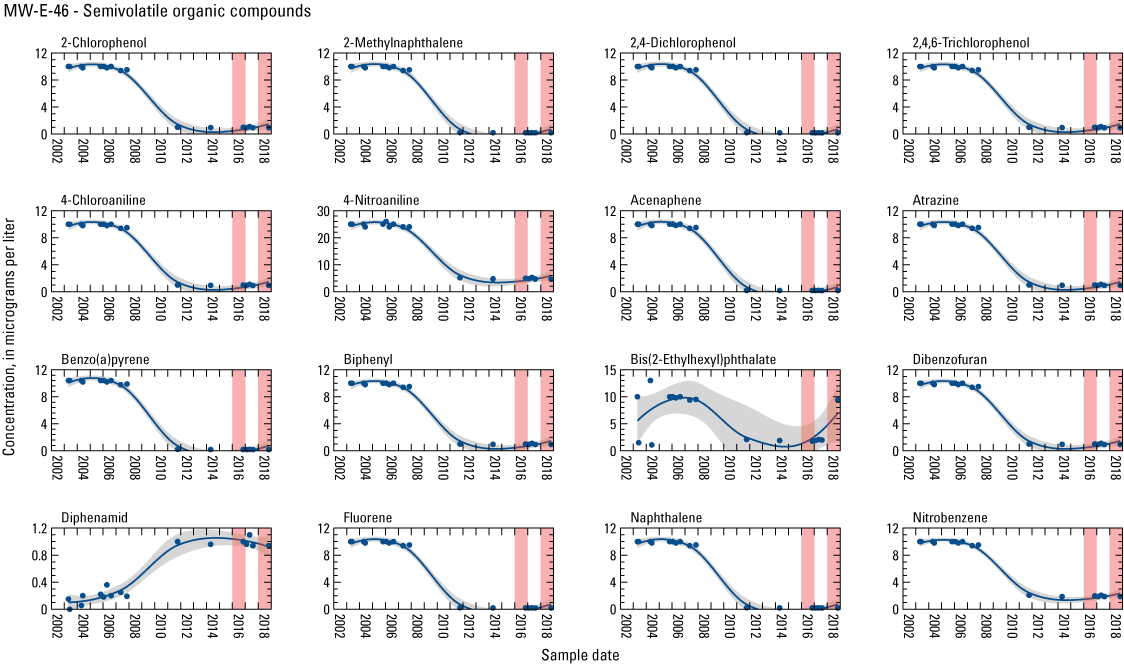
Graphs showing select semi-volatile organic compounds (SVOC) concentrations reported for well MW-E-46, Central Chemical facility, Hagerstown, Maryland. Years 2016 and 2018 are highlighted with red bars, a local polynomial regression is depicted with a blue line, and the 95 percent confidence interval in grey. All concentrations for contaminants of concern are available through the U.S. Environmental Protection Agency (2021).
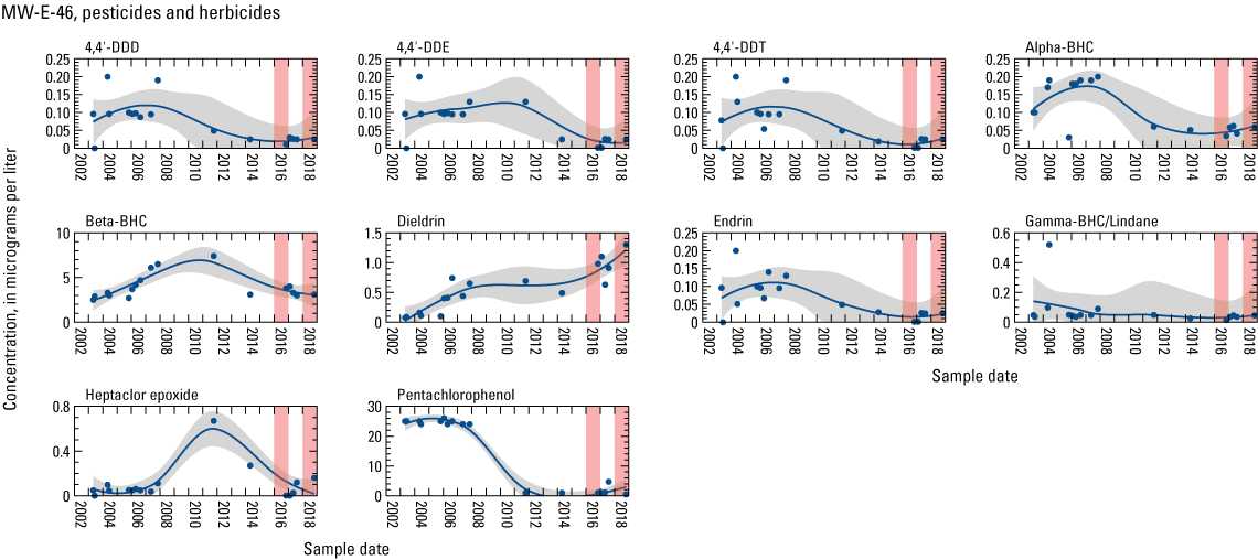
Graphs showing select pesticide and herbicide concentrations reported for well MW-E-46, Central Chemical facility, Hagerstown, Maryland. Years 2016 and 2018 are highlighted with red bars, a local polynomial regression is depicted with a blue line, and the 95 percent confidence interval in grey. All concentrations for contaminants of concern are available through the U.S. Environmental Protection Agency (2021). [Dichlorodiphenyltrichloroethane, DDT; Dichlorodiphenyldichloroethylene, DDE; Dichlorodiphenyldichloroethane, DDD; Benzene hexachloride, BHC]
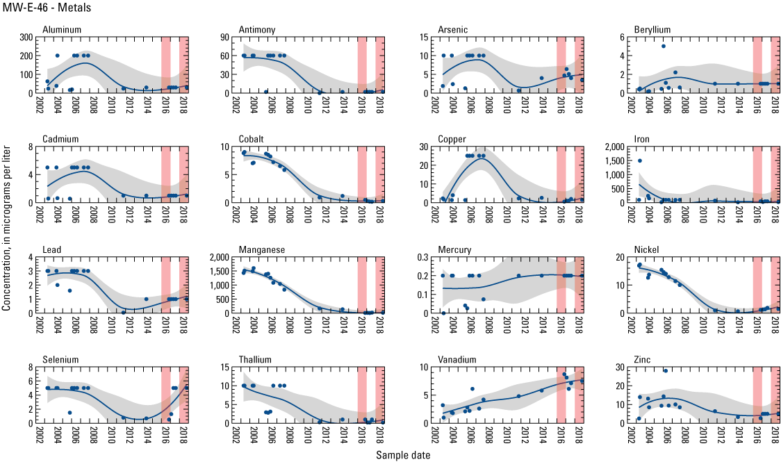
Graphs showing select metal concentrations reported for well MW-E-46, Central Chemical facility, Hagerstown, Maryland. Years 2016 and 2018 are highlighted with red bars, a local polynomial regression is depicted with a blue line, and the 95 percent confidence interval in grey. All concentrations for contaminants of concern are available through the U.S. Environmental Protection Agency (2021).
Appendix 3. Concentrations of Chlorobenzene, 1,2,4-trichlorobenzene, and Technical-Benzene Hexachloride (BHC) in Select Wells at the Central Chemical Facility in Hagerstown, Maryland
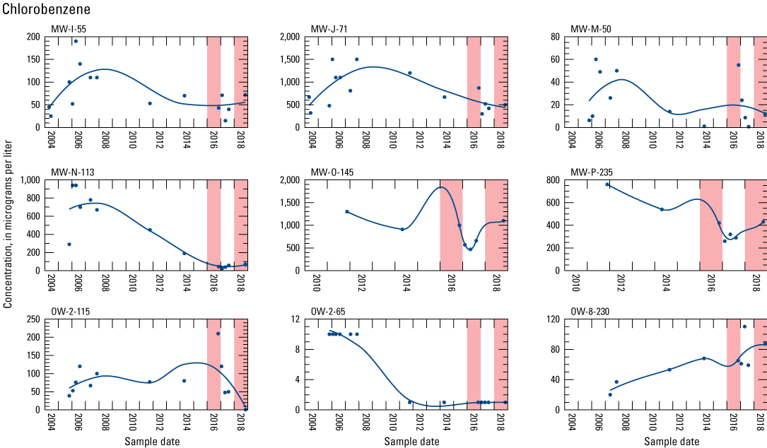
Graphs showing concentrations of chlorobenzene reported for wells MW-I-55, MW-J-71, MW-M-50, MW-N-113, MW-O-145, MW-P-235, OW-2-115, OW-2-65, and OW-8-230, Central Chemical facility, Hagerstown, Maryland. Years 2016 and 2018 are highlighted with red bars and a local polynomial regression is depicted with a blue line. All concentrations for contaminants of concern are available through the U.S. Environmental Protection Agency (2021).
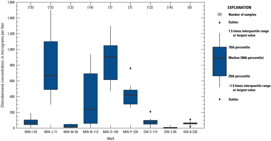
Boxplots showing chlorobenzene concentrations in micrograms per liter (μg/L) reported for wells MW-I-55 (sample size [n]=15), MW-J-71(n=15), MW-M-50(n=13), MW-N-113 (n=14), MW-O-145 (n=7), MW-P-235 (n=7), OW-2-115 (n=13), OW-2-65 (n=14), and OW-8-230 (n=9), Central Chemical facility, Hagerstown, Maryland. All concentrations for contaminants of concern are available through the U.S. Environmental Protection Agency (2021).
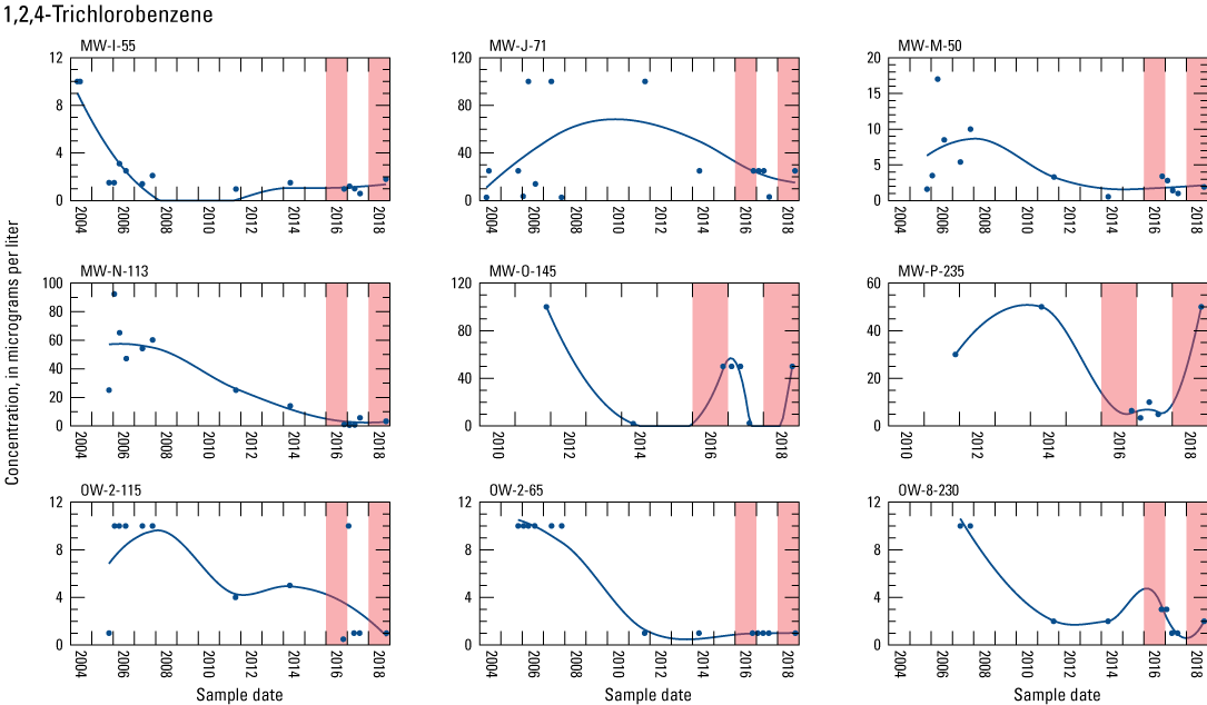
Graphs showing concentrations of 1,2,4-trichlorobenzene reported for wells MW-I-55, MW-J-71, MW-M-50, MW-N-113, MW-O-145, MW-P-235, OW-2-115, OW-2-65, and OW-8-230, Central Chemical facility, Hagerstown, Maryland. Years 2016 and 2018 are highlighted with red bars and a local polynomial regression is depicted with a blue line. All concentrations for contaminants of concern are available through the U.S. Environmental Protection Agency (2021).
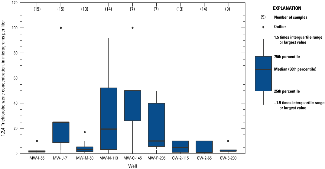
Boxplots showing 1,2,4-trichlorobenzene concentrations in micrograms per liter (μg/L) reported for wells MW-I-55 (sample size [n]=15), MW-J-71(n=15), MW-M-50 (n=13), MW-N-113 (n=14), MW-O-145 (n=7), MW-P-235 (n=7), OW-2-115 (n=13), OW-2-65 (n=14), and OW-8-230 (n=9), Central Chemical facility, Hagerstown, Maryland. All concentrations for contaminants of concern are available through the U.S. Environmental Protection Agency (2021).
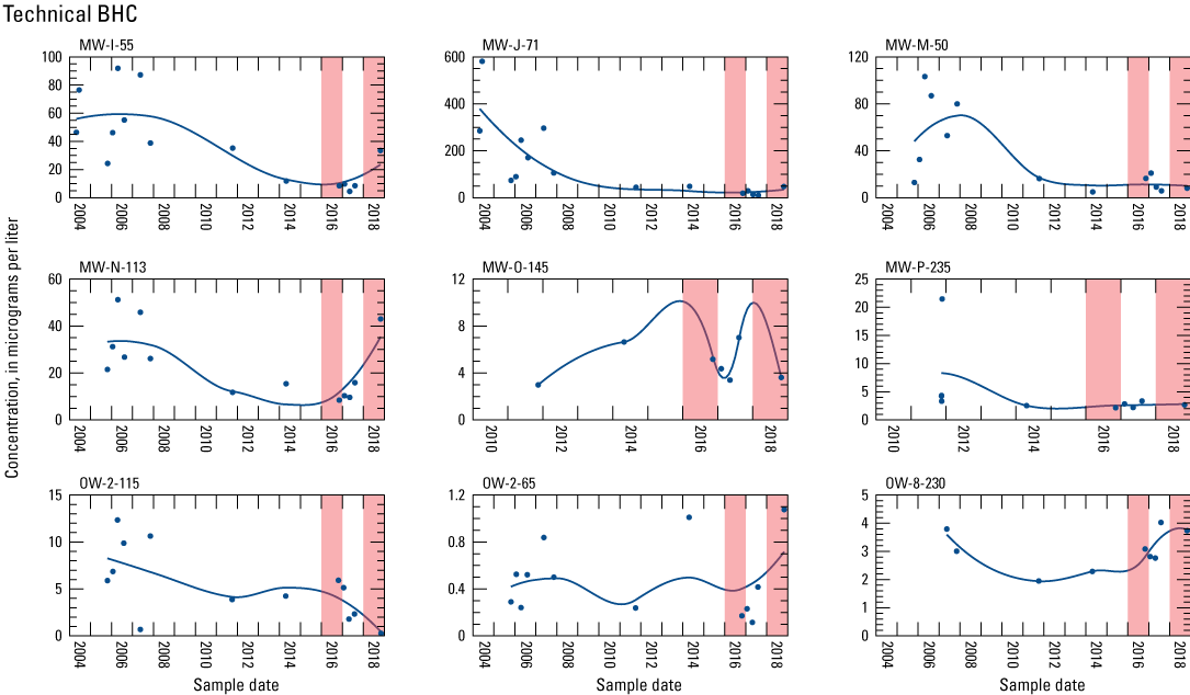
Graphs showing concentrations of technical benzene hexachloride (BHC) reported for wells MW-I-55, MW-J-71, MW-M-50, MW-N-113, MW-O-145, MW-P-235, OW-2-115, OW-2-65, and OW-8-230, Central Chemical facility, Hagerstown, MD. Years 2016 and 2018 are highlighted with red bars and a local polynomial regression is depicted with a blue line. All concentrations for contaminants of concern are available through the U.S. Environmental Protection Agency (2021).
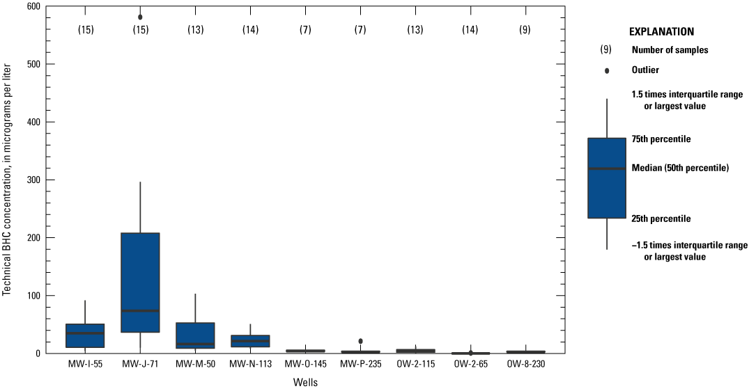
Boxplots showing technical benzene hexachloride (BHC) concentrations in micrograms per liter (μg/L) reported for wells MW-I-55 (sample size [n]=15), MW-J-71 (n=15), MW-M-50 (n=13), MW-N-113 (n=14), MW-O-145 (n=7), MW-P-235 (n=7), OW-2-115 (n=13), OW-2-65 (n=14), and OW-8-230 (n=9), Central Chemical facility, Hagerstown, Maryland. All concentrations for contaminants of concern are available through the U.S. Environmental Protection Agency (2021).
Appendix 4. Contaminants of Concern for Groundwater Vicinity of the Central Chemical Facility
Table 4.1.
Contaminants of Concern properties and reported maximum concentrations for the Central Chemical facility, Hagerstown, Maryland. Maximum Contaminant Level and Regional Screening Level reported in Wood Environment & Infrastructure Solutions, Inc. (2019).[All concentrations for contaminants of concern are available through the U.S. Environmental Protection Agency (2021). CAS number, Chemical Abstracts Service identification number; log, logarithm; Kow, n-octanol-water partition coefficient; mg/L, milligrams per liter; MCL, maximum contaminant level; µg/L, micrograms per liter; RSL, remedial screening level; –, not available]
Conversion Factors
U.S. customary units to International System of Units
International System of Units to U.S. customary units
Temperature in degrees Celsius (°C) may be converted to degrees Fahrenheit (°F) as follows: °F = (1.8 × °C) + 32.
Temperature in degrees Fahrenheit (°F) may be converted to degrees Celsius (°C) as follows: °C = (°F – 32) / 1.8.
Datum
Vertical coordinate information is referenced to North American Vertical Datum of 1988 (NAVD 88).
Horizontal coordinate information is referenced to North American Datum of 1983 (NAD 83).
Abbreviations
1,2,4-TCB
1,2,4-Trichlorobenzene
μg/L
micrograms per liter
AET
actual evapotranspiration
BHC
benzene hexachloride
COC
contaminants of concern
DDD
dichlorodiphenyldichloroethane
DDE
dichlorodiphenyldichloroethylene
DDT
dichlorodiphenyltrichloroethane
DDX
combined isomers of DDT, DDD, and DDE
DNAPL
dense nonaqueous phase liquid
EPA
U.S. Environmental Protection Agency
ET
evapotranspiration
GDAS
Global Data Assimilation Systems
LOESS
Local Polynomial Regression
MCL
maximum contaminant level
MDE
Maryland Department of the Environment
mg/L
milligrams per liter
Modis
Moderate Resolution Imaging Spectroradiometer
MW
monitoring wells
NAVD 88
North American Vertical Datum of 1988
NPL
National Priorities List
OU
operable unit
OU-1
operable unit 1
OU-2
operable unit 2
OW
offsite wells
PET
potential evapotranspiration
ppm
parts per million
PVC
polyvinyl chloride
PZ
piezometer
RI
remedial investigation
RSL
remedial screening level
SSEB
simplified surface energy balance
SSEBop
operational simplified surface energy balance
SVOC
semivolatile organic compound
TSS
total suspended solids
USGS
U.S. Geological Survey
VOC
volatile organic compound
For additional information, contact:
Director, Maryland-Delaware-D.C. Water Science Center
U.S. Geological Survey
5522 Research Park Drive
Catonsville, MD 21228
Or visit our website at:
https://www.usgs.gov/centers/md-de-dc-water
Publishing support provided by the Baltimore Publishing Service Center
Disclaimers
Any use of trade, firm, or product names is for descriptive purposes only and does not imply endorsement by the U.S. Government.
Although this information product, for the most part, is in the public domain, it also may contain copyrighted materials as noted in the text. Permission to reproduce copyrighted items must be secured from the copyright owner.
Suggested Citation
Needham, T.P., Fiore, A.R., Ator, S.W., Raffensperger, J.P., Smith, M.B., Bellmyer, N.M., Dugan, C.M., and Morel, C.J., 2023, Geology, hydrology, and groundwater contamination in the vicinity of Central Chemical facility, Hagerstown, Maryland: U.S. Geological Survey Scientific Investigations Report 2022–5011, 62 p., https://doi.org/10.3133/sir20225011.
ISSN: 2328-0328 (online)
Study Area
| Publication type | Report |
|---|---|
| Publication Subtype | USGS Numbered Series |
| Title | Geology, hydrology, and groundwater contamination in the vicinity of Central Chemical facility, Hagerstown, Maryland |
| Series title | Scientific Investigations Report |
| Series number | 2022-5011 |
| DOI | 10.3133/sir20225011 |
| Publication Date | September 20, 2023 |
| Year Published | 2023 |
| Language | English |
| Publisher | U.S. Geological Survey |
| Publisher location | Reston, VA |
| Contributing office(s) | Maryland-Delaware-District of Columbia Water Science Center |
| Description | ix, 62 p. |
| Country | United States |
| State | Maryland |
| City | Hagerstown |
| Other Geospatial | Central Chemical Facility |
| Online Only (Y/N) | Y |
| Additional Online Files (Y/N) | N |