
Status and Understanding of Groundwater Quality in the Sacramento Metropolitan Domestic-Supply Aquifer Study Unit, 2017: California GAMA Priority Basin Project
Links
- Document: Report (20 MB pdf) , HTML , XML
- Data Release: Potential explanatory variables for groundwater quality in the Sacramento Metropolitan Domestic-Supply Aquifer study unit, 2017—California GAMA Priority Basin Project
- NGMDB Index Page: National Geologic Map Database Index Page (html)
- Download citation as: RIS | Dublin Core
Acknowledgments
Funding for this work was provided by the California State Water Resources Control Board Groundwater Ambient Monitoring and Assessment Program and by U.S. Geological Survey Cooperative Matching Funds. We especially thank the site owners and water purveyors for their cooperation in allowing the U.S. Geological Survey to collect samples from their sites.
For consistent presentation of results from the California Groundwater Ambient Monitoring and Assessment Program Priority Basin Project (GAMA-PBP), parts of this report were written following a previously developed template.
Abstract
Groundwater quality in the Sacramento Metropolitan Domestic-Supply Aquifer study unit (SacMetro-DSA) was studied from August to November 2017 as part of the second phase of the Priority Basin Project of the California Groundwater Ambient Monitoring and Assessment (GAMA) Program. The study unit is in parts of Amador, Placer, Sacramento, and Sutter Counties, and the extent of the study unit was defined by the location of three California Department of Water Resources groundwater subbasins: the North American, the South American, and the Cosumnes. The SacMetro-DSA focused on groundwater resources used for domestic drinking-water supply, which generally correspond to shallower parts of aquifer systems than those of groundwater resources used for public drinking water supply in the same area. The assessments characterized the quality of untreated groundwater, not the quality of drinking water.
This study included two components: (1) a status assessment, which characterized the status of the quality of the groundwater resources used for domestic supply and (2) an understanding assessment, which evaluated the natural and human factors potentially affecting water quality in those resources. The first component of this study—the status assessment—was based on water-quality data collected from 49 sites sampled by the U.S. Geological Survey for the GAMA Priority Basin Project in 2017. The samples were analyzed for volatile organic compounds, pesticides, and naturally present inorganic constituents, such as major ions and trace elements. To provide context, concentrations of constituents measured in groundwater were compared to U.S. Environmental Protection Agency and California State Water Resources Control Board Division of Drinking Water regulatory and non-regulatory benchmarks for drinking-water quality. The status assessment used a grid-based method to estimate the proportion of the groundwater resources that had concentrations of water-quality constituents approaching or above benchmark concentrations. This method provides statistically unbiased results at the study-area scale and permits comparisons to other GAMA Priority Basin Project study areas. The second component of this study—the understanding assessment—identified the natural and human factors that potentially affect groundwater quality by evaluating land-use characteristics, groundwater age, and geochemical and hydrologic conditions of the domestic-supply aquifer and related these data to constituents identified in the status assessment for further evaluation.
In the SacMetro-DSA study unit, arsenic was the only inorganic constituent detected above health-based benchmarks and was detected in 10 percent of the domestic-supply aquifer system. Inorganic constituents were detected above the non-health-based California State Water Resources Control Board—Division of Drinking Water secondary maximum contaminant levels (SMCL-CA) in 16 percent of the system. The inorganic constituents detected above the SMCL-CA were chloride, iron, manganese, and total dissolved solids (TDS). Organic constituents (volatile organic compounds and pesticides) with health-based benchmarks were not detected above health-based benchmarks; however, chloroform was detected at concentrations higher than 10 percent of the health-based benchmark (80 micrograms per liter) in 2 percent of the domestic-supply aquifer system. Of the 310 organic constituents analyzed, 16 constituents were detected; however, only bentazon and chloroform had detection frequencies greater than 10 percent.
Inorganic constituents with health-based benchmarks that were evaluated in the understanding assessment included arsenic and hexavalent chromium. Arsenic and hexavalent chromium are natural constituents of aquifer sediments in the study unit and did not appear to be influenced by anthropogenic processes; rather, the presence of arsenic and hexavalent chromium appeared to be related to geochemical conditions controlled by oxidation–reduction reactions in the aquifer system. Naturally occurring inorganic constituents with SMCL-CAs evaluated in the understanding assessment were the trace elements iron and manganese, the major ion chloride, and TDS. Like arsenic and hexavalent chromium, the presence of iron and manganese was most strongly related to geochemical conditions in the aquifer system, specifically reducing conditions, which were most common near the western edge of the study unit close to the Sacramento River. Concentrations of chloride and TDS are indicators of salinity and were correlated with variables related to well location and included redox, agricultural land use, and elevation. Chloride and TDS were positively correlated to reducing conditions, and agricultural land use was negatively correlated to elevation and well depth. Observed correlations among variables were likely driven by the characteristics of the western part of the study unit, such as its higher proportion of agricultural land use and its relatively low elevation. A large portion of the western edge of the study unit is located in the center of the Sacramento Valley, defined by the location of the Sacramento River. The special-interest constituent perchlorate, also included in the understanding assessment, has natural and anthropogenic sources. Perchlorate was detected frequently and at moderate relative concentrations. In some areas of the study unit, concentrations of perchlorate were higher than what might be expected in nature; therefore, anthropogenic introduction of perchlorate or anthropogenically induced migration of native perchlorate could be occurring.
Introduction
Groundwater can supply approximately half of the water used for public and domestic drinking-water supply in California at times (California Department of Water Resources, 2016). To assess the quality of ambient groundwater in aquifers used for drinking-water supply and to establish a baseline groundwater-quality monitoring program, the California State Water Resources Control Board (SWRCB), in collaboration with the U.S. Geological Survey (USGS) and Lawrence Livermore National Laboratory (LLNL), implemented the Groundwater Ambient Monitoring and Assessment (GAMA) Program (https://www.waterboards.ca.gov/gama/). The SWRCB initiated the GAMA Program in 2000 in response to legislative mandates (State of California, 1999, 2001a).
In 2020, the program had two active projects: the GAMA Priority Basin Project (GAMA-PBP), carried out by the USGS (https://ca.water.usgs.gov/gama/), and the online GAMA Groundwater Information System, led by the SWRCB (https://gamagroundwater.waterboards.ca.gov/gama/gamamap/public/Default.asp). The SWRCB’s GAMA Domestic Well Project sampled private domestic wells on a voluntary, first-come, first-served basis in six counties between 2002 and 2011. The GAMA-PBP was initiated in response to the Groundwater Quality Monitoring Act of 2001 to assess and monitor the quality of groundwater in California, to help identify and better understand risks to groundwater resources, and to increase the availability of information about groundwater quality to the public (State of California, 2001b). For the GAMA-PBP, the USGS, in collaboration with the SWRCB, developed a monitoring plan to assess groundwater basins using statistically reliable sampling approaches (Belitz and others, 2003; California State Water Resources Control Board, 2003).
From 2004 through 2012, the GAMA-PBP assessed water quality for groundwater resources used for public drinking water. The 35 study units sampled in this first phase covered more than 95 percent of the groundwater water resources used for public supply statewide (Belitz and others, 2015). Groundwater basins and areas outside of basins were prioritized for sampling primarily on the basis of the distribution of wells listed in the State of California’s database of public-supply wells (Belitz and others, 2003). In 2012, the GAMA-PBP began water-quality assessments of domestic-supply aquifers, the groundwater resources typically used for private domestic and small system drinking-water supplies. These groundwater resources typically are shallower than the groundwater resources used for public drinking-water supplies. For this phase of the GAMA-PBP, a different method of prioritization was required because there was no statewide database of domestic or small-system wells with which to prioritize areas for sampling. To prioritize domestic-supply aquifers, the distribution of households relying on domestic wells was estimated from U.S. Census data (U.S. Census Bureau, 1990) and from water-use and well-location information compiled from well-completion reports submitted to the California Department of Water Resources (CDWR; Johnson and Belitz, 2015).
Study units were designed to facilitate comparison of groundwater quality among the domestic-supply aquifer systems assessed in this second phase of the GAMA-PBP and the deeper aquifer systems assessed in the first phase. The Sacramento Metropolitan Domestic-Supply Aquifer study unit (SacMetro-DSA) was the seventh study unit assessed in the second phase of the GAMA-PBP. The SacMetro-DSA is in the Central Valley hydrogeologic province described by Belitz and others (2003; fig. 1). The SacMetro-DSA includes all of the eastern study areas (North American, South America, and Uplands) included in the GAMA-PBP assessment of groundwater resources used for public drinking water in the southern Sacramento Valley, as defined by Bennett and others (2011), and parts of the Cosumnes and Uplands study areas included in the GAMA-PBP assessment of groundwater resources used for public drinking water in the northern San Joaquin Valley as defined by Bennett and others (2010).
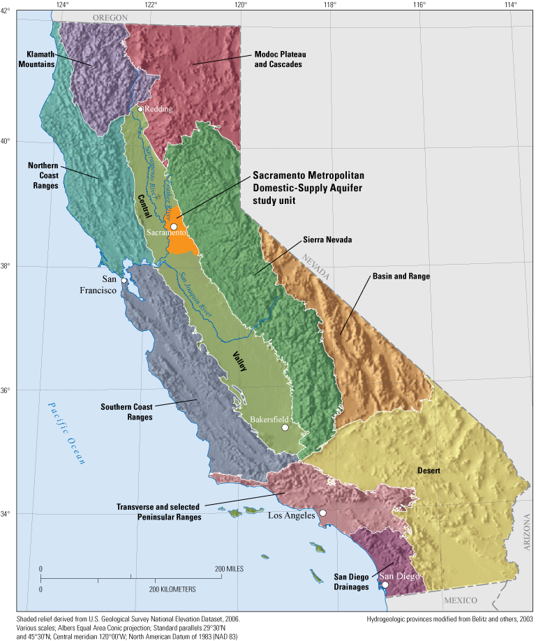
Hydrogeologic provinces of California (modified from Belitz and others, 2003) and the location of the Sacramento Metropolitan Domestic-Supply Aquifer study unit, 2017 (Bennett and others, 2019), California Groundwater Ambient Monitoring and Assessment Program Priority Basin Project (U.S. Geological Survey, 2022).
The GAMA-PBP was designed to (1) assess the status of the quality of the groundwater resources, (2) identify natural and human factors likely affecting groundwater quality, and (3) monitor changes in groundwater quality. These three objectives were modeled after those of the USGS National Water-Quality Assessment (NAWQA) Program (Hirsch and others, 1988). The sample collection protocols used in this study were designed to obtain representative samples of groundwater. The quality of groundwater can differ from the quality of drinking water because water chemistry can change as a result of contact with plumbing systems or the atmosphere or because of treatment, disinfection, or blending with water from other sources. The assessments in this report apply to the depth zone in the aquifer system containing groundwater resources used for domestic drinking water.
This USGS Scientific Investigations Report (SIR) is like other USGS SIRs written for the GAMA-PBP study units sampled to date and is the third in a series of reports presenting the water-quality data collected in the SacMetro-DSA (Bennett, 2019; Bennett and others, 2019). All published reports addressing the status, understanding, and trends of the water-quality assessments done by the GAMA-PBP are available from the USGS (U.S. Geological Survey, 2021a) and the SWRCB (California State Water Resources Control Board, 2021a).
The purposes of this report are to provide (1) an assessment of the groundwater quality in the domestic-supply aquifer system of the SacMetro-DSA in 2017 and (2) a general identification of natural and anthropogenic factors that could be affecting groundwater quality. Temporal trends in groundwater quality in the domestic-supply aquifer systems are beyond the scope of this report. Characteristics of groundwater resources used for domestic drinking water, including overlying land-use characteristics, depth and hydrologic conditions, and groundwater age and geochemical conditions, are described using ancillary data compiled for the groundwater sites sampled by USGS for GAMA (USGS-GAMA) in the SacMetro-DSA.
The status assessment was designed to provide a statistically representative characterization of groundwater resources used for domestic drinking water at the study-area scale for the time span of the assessment (Belitz and others, 2003, 2010, 2015). This report describes methods used to design the sampling network for the status assessment and estimate aquifer-scale proportions for constituents (Belitz and others, 2010). Aquifer-scale proportion is defined as the areal proportion of the groundwater resource having groundwater of defined quality (Belitz and others, 2010). Water-quality data from 49 wells sampled by USGS-GAMA for the SacMetro-DSA (Bennett and others, 2019) were used for the status assessment. Aquifer-scale proportions for constituents and classes of constituents were computed for the SacMetro-DSA as a whole by using a stratified, random sampling design (the USGS grid method) based on a 56-cell grid (49 of which had a sampled well) covering the study unit (Belitz and others, 2010, 2015).
To provide context, the water-quality data described in this report were compared to California and Federal regulatory and non-regulatory benchmarks for treated drinking water delivered by public water systems. Groundwater quality is defined in terms of relative concentrations (RCs), which are calculated by dividing the concentration of a constituent in groundwater by the concentration of the benchmark for that constituent. The assessments in this report characterize the quality of untreated groundwater resources in the domestic-supply aquifer system of the study unit. The quality of drinking water provided by domestic wells is not regulated by the State of California. Resources to help private domestic well owners understand and potentially address issues related to their wells have been compiled by the SWRCB and other entities like the National Groundwater Association and Water Systems Council (California State Water Resources Control Board, 2020a; National Groundwater Association, 2021; Water Systems Council, 2021).
The evaluation of natural and human factors that could be affecting groundwater quality in the study unit is based primarily on relations between groundwater quality and potential explanatory variables. These relations are examined with statistical tests and graphical analyses and are discussed in the context of the hydrogeologic setting of the SacMetro-DSA study unit. The following potential explanatory variables were evaluated and compared to the water-quality data collected in the SacMetro-DSA study unit: land use, hydrologic conditions, depth, groundwater age, geochemical conditions, underground storage-tank density, and septic tank density.
Hydrogeologic Setting
The SacMetro-DSA covers an area of approximately 1,250 square miles (mi2), lies along the eastern edge of the Central Valley hydrogeologic province (fig. 1), and includes parts of Amador, Placer, Sutter, and Sacramento Counties (fig. 2). The SacMetro-DSA study unit is split into three study areas that correspond to groundwater subbasin boundaries of the same name defined by the CDWR: the North American, South American, and Cosumnes (fig. 2; California Department of Water Resources, 2016; Bennett and others, 2019). Descriptions of the hydrogeologic setting for each of the three study areas have been described in previous GAMA-PBP assessment reports that detailed the results of the public-supply aquifer assessments for the southern end of the Sacramento Valley (Bennett and others, 2011) and the northern end of the San Joaquin Valley (Bennett and others, 2010).
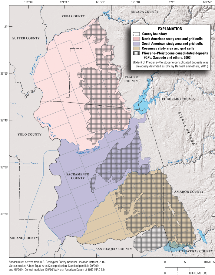
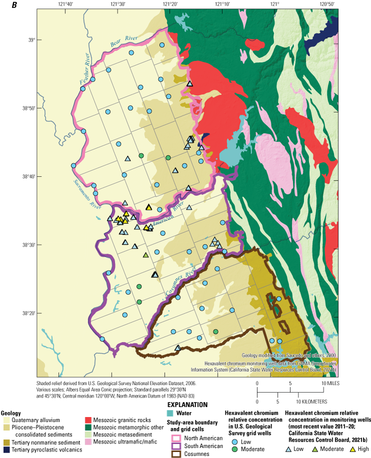
Location and boundaries of the Sacramento Metropolitan Domestic-Supply Aquifer study unit, 2017, and the North American, South American, and Cosumnes study areas and grid cells (Bennett and others, 2019), California Groundwater Ambient Monitoring and Assessment Program Priority Basin Project (U.S. Geological Survey, 2022). Extent of Pliocene-Pleistocene consolidated deposits was previously delimited as QPc by Bennett and others (2011).
Sediments containing fresh groundwater in the SacMetro-DSA study unit are primarily composed of Quaternary alluvial and fluvially deposited continental and volcanic sediments derived from the Sierra Nevada to the east, which have been dispersed in the Central Valley by numerous watersheds draining the western slope of the Sierra Nevada (California Department of Water Resources, 1978; Page, 1986). Underlying the Quaternary deposits are older Pliocene–Pleistocene consolidated deposits that crop out along the eastern edge of the study unit (fig. 2; California Department of Water Resources, 1978; Page, 1986, Saucedo and others, 200075). The extent of these Pliocene–Pliestocene consolidated deposits was used by the GAMA-PBP to define upland study areas in the public-supply well assessments of the southern Sacramento Valley and the northern Sacramento Valley (unit QPc of Bennett and others, 2010, 2011). In the SacMetro-DSA, the upland areas present in each of the three study areas was not used to define a separate study area. The SacMetro-DSA study unit is bound to the north by the Bear River, to the west by the Feather and Sacramento Rivers, to the south by the Sacramento and San Joaquin County line, and to the east by the Sierra Nevada (fig. 2).
The SacMetro-DSA study unit has a Mediterranean climate with hot and dry summers and cool and wet winters, with average annual precipitation (1991–2000) in Sacramento of about 20 inches per year (PRISM Group, 2021). Aquifers in the study unit are recharged by rainfall, stream seepage, irrigation return flows, and subsurface inflows from outside the study unit. Reservoirs upstream from some of the larger rivers release water throughout the year to sustain flows during the dry summers. The proportion of each recharge source was estimated by the Sacramento Central Groundwater Authority (SCGA), which developed a recharge map that covers a large part of the South American study area and a small part of the Cosumnes study area. The SCGA found that most of the recharge came from stream seepage (41 percent) and the combination of rainfall and applied irrigation water (43 percent), with the remaining recharge coming from subsurface inflows (Sacramento Central Groundwater Authority, 2015). Regional groundwater flow in the study unit generally follows groundwater elevation gradients, which have been perturbed by groundwater extractions, resulting in pumping depressions (fig. 3). In all three study areas, groundwater withdrawals have resulted in the formation of regional cones of depression near the centers of the study areas (Sacramento County Water Agency, 2004; Sacramento Groundwater Authority, 2008; South Area Water Council, 2011, Central Valley Regional Water Quality Control Board, 2016; Sacramento Central Groundwater Authority, 2019).
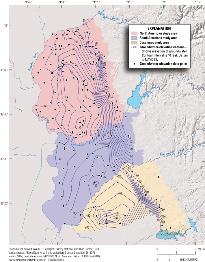
Groundwater elevation contours, fall 2017 (California Department of Water Resources, 2022), in the Sacramento Metropolitan Domestic-Supply Aquifer study unit, 2017, and the North American, South American, and Cosumnes study areas (Bennett and others, 2019), California Groundwater Ambient Monitoring and Assessment Program Priority Basin Project (U.S. Geological Survey, 2022).
Methods
This section describes the methods used for the status and understanding assessments for water quality in the SacMetro-DSA. Compiled data for the potential explanatory variables are presented in Bennett (2022). Methods used to collect and analyze groundwater samples and results for the evaluation of quality-control data are described by Bennett and others (2019).
Status Assessment
The status assessment was designed to provide a quantitative summary of groundwater quality in the domestic-supply aquifer system of the SACMetro-DSA. This section describes the methods used for (1) defining groundwater quality, (2) assembling the dataset used for the assessment, (3) selecting constituents for evaluation, and (4) calculating aquifer-scale proportions.
Groundwater Quality Defined as Relative Concentrations
In this study, groundwater-quality data are presented as relative concentrations (RCs), which are defined as the ratio of a constituent’s concentration measured in a groundwater sample to the concentration of a constituent’s regulatory or non-regulatory benchmark used to evaluate drinking-water quality (eq. 1). The use of RC is similar to the approaches implemented by other studies to place the concentrations of constituents in groundwater in a toxicological context (U.S. Environmental Protection Agency, 1986; Toccalino and others, 2004; Toccalino and Norman, 2006; Rowe and others, 2007). The RC is defined as follows:
An RC value less than 1.0 indicates that the sample concentration was less than the benchmark concentration, and an RC value greater than 1.0 indicates that the sample concentration was greater than the benchmark concentration. Using RCs creates a single scale for comparing constituents that can be present at a wide range of concentrations. An RC can only be computed for constituents with water-quality benchmarks; therefore, constituents without water-quality benchmarks are not included in the status assessment.
Regulatory and non-regulatory benchmarks apply to treated water that is served to the consumer, not to untreated groundwater. To provide some context for the results, however, concentrations of constituents measured in the untreated groundwater were compared to benchmarks established by the U.S. Environmental Protection Agency (EPA), SWRCB division of drinking water (DDW), and USGS. The benchmarks used for each constituent were selected in the following order of priority:
-
1. Regulatory, health-based levels established by the SWRCB-DDW and the EPA (U.S. Environmental Protection Agency, 2018; California State Water Resources Control Board, 2022a): SWRCB-DDW and EPA maximum contaminant levels (MCL-CA and MCL-US, respectively), EPA action levels (AL-US), and EPA treatment technique levels (TT-US).
-
2. Non-regulatory, aesthetic-based levels established by the SWRCB-DDW and EPA (U.S. Environmental Protection Agency, 2018; California State Water Resources Control Board, 2022a): California and EPA secondary maximum contaminant levels (SMCL-CA and SMCL-US). The salinity indicators chloride, sulfate, and total dissolved solids (TDS) have recommended and upper SMCL-CA levels, and the values for the upper levels were used.
-
3. Non-regulatory, health-based levels established by the EPA, SWRCB-DDW, and USGS (Toccalino and others, 2004; U.S. Environmental Protection Agency, 2017, 2018; California State Water Resources Control Board, 2022b): SWRCB-DDW response levels (RL-CA), EPA lifetime health advisory levels (HAL-US), EPA risk-specific doses for at a risk factor of 10−5 (RSD5-US), lowest value of EPA human-health benchmarks for pesticides for cancer and non-cancer end points (HHBP-C and HHBP-NC), and USGS health-based screening levels (HBSL).
For constituents with multiple types of benchmarks, this hierarchy might not result in selection of the benchmark with the lowest concentration. If a constituent has both an RL-CA and HAL-US, the lower benchmark of the two was selected. Additional information on the types of benchmarks and listings of the benchmarks for all constituents analyzed is provided by Bennett and others (2019).
Toccalino and others (2004), Toccalino and Norman (2006), and Rowe and others (2007) used the ratio of measured sample concentration to the benchmark concentration, either MCL-US or HBSL and defined this ratio as the benchmark quotient (BQ). The term RC is used in this report rather than BQ because the two values are not the same for constituents that have MCL-CA values that differ from their MCL-US values or for constituents that have neither MCL-US nor HBSL values (thus, no associated BQ).
For ease of discussion, RCs of constituents were classified in low, moderate, and high categories. The RC values greater than 1.0 were defined as “high” for all constituents. The RCs for nine constituents were calculated using SWRCB-DDW RL-CAs (sec-butylbenzene; carbon disulfide; diazinon; 1,4-dioxane; n-nitrosodiethylamine; n-propylbenzene; tert-butyl alcohol; 1,2,4-trimethylbenzene; and vanadium). The RL-CAs were paired with SWRCB-defined notification levels (NL-CA) set at concentrations ranging from 10 to 100 times less than the RL-CA (California State Water Resources Control Board, 2022b). For these nine constituents, the NL-CA was the benchmark concentration used to calculate the RC divide between “moderate” and “low.” For boron, which has an RL-CA and HAL-US, the HAL-US was used when calculating the initial RC. The NL-CA, however, was used to calculate the RC divide between “moderate” and “low,” as was done for the constituents that only had an RL-CA.
For constituents without RL-CAs, the divide between “moderate” and “low” was determined by constituent class. For inorganic constituents (trace elements, nutrients, radioactive constituents, and inorganic constituents having SMCL-US or SMCL-CA benchmarks), RC values greater than 0.5 and less than or equal to 1.0 were defined as “moderate,” and RC values less than or equal to 0.5 were defined as “low.” For organic and special-interest constituents, RC values greater than 0.1 and less than or equal to 1.0 were defined as “moderate,” and RC values less than or equal to 0.1 were defined as “low.” Although more complex classifications could be devised based on the properties and sources of individual constituents, use of a single threshold value for each of the two major groups of constituents (except for those with an RL-CA) provided a consistent objective criterion for distinguishing constituents present at moderate, rather than low, concentrations.
Dataset Used for Status Assessment
Groundwater-quality data used for the SacMetro-DSA status assessment came from sites sampled by the USGS for the GAMA-PBP (fig. 4). Detailed descriptions of the methods used to identify and select sites for sampling are given in Bennett and Fram (2014). Briefly, the SacMetro-DSA study unit was divided into three study areas: the North American, South American, and Cosumnes. The study-area boundaries were equivalent to CDWR-defined groundwater subbasins of the same name (California Department of Water Resources, 2016). Each study area was divided into equal-area grid cells (Scott, 1990): 24 cells in the North American study area, 17 cells in the South American study area, and 15 cells in the Cosumnes study area. The target cell size in all three study areas was approximately 22 square miles (mi2). The objective of defining grid cells was for the USGS to collect water-quality samples from one site in each cell. Candidate sites in each grid cell were identified by compiling lists of available wells in each cell from drillers’ log information obtained from the CDWR. The lists of sites (grid-cell inventories) were then taken into the field, and USGS staff went door-to-door to request permission to sample a well in each grid cell. The USGS was granted permission to sample sites in 49 of 56 grid cells (referred to here as USGS grid sites). The USGS grid sites were named with an alphanumeric GAMA identifier consisting of the prefix “S7-SAC-NA,” “S7-SAC-SA,” or “S7-SAC-C” and a number indicating the order of sample collection. The prefix represents the seventh (S7) domestic-supply assessment and the respective study area: North American (NA), South America (SA), or Cosumnes (C).
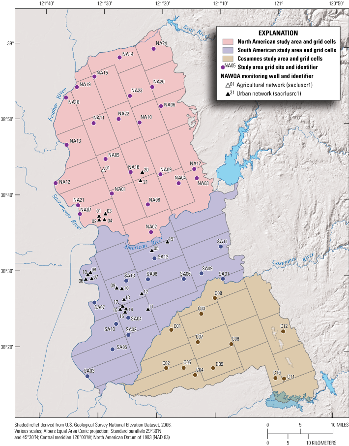
Locations of U.S. Geological Survey grid sites in grid cells for each study area in the Sacramento Metropolitan Domestic-Supply Aquifer study unit, 2017 (Bennett and others, 2019), and locations of monitoring wells sampled as part of the U.S. Geological Survey National Water Quality (NAWQA) Program land-use studies (Kingsbury and others, 2021), California Groundwater Ambient Monitoring and Assessment Priority Basin Project (U.S. Geological Survey, 2022).
Samples collected from all USGS grid sites sampled by USGS were analyzed for 379 constituents (table 1). Water-quality data collected by USGS-GAMA are tabulated in Bennett and others (2019) and are available from the SWRCB’s publicly accessible GAMA Groundwater Information System and the USGS GAMA-PBP Groundwater-Quality Results web map (Jurgens and others, 2018; California State Water Resources Control Board, 2021b).
Table 1.
Summary of constituent groups and number of constituents sampled for each constituent group in the Sacramento Metropolitan Domestic-Supply Aquifer study unit, 2017 (Bennett and others, 2019), California Groundwater Ambient Monitoring and Assessment Priority Basin Project (U.S. Geological Survey, 2022).[Unless otherwise noted, constituent analyses were performed at the U.S. Geological Survey National Water Quality Laboratory or the U.S. Geological Survey laboratory. Abbreviations and symbols: Ar, argon; C, carbon; H, hydrogen; He, helium; Kr, krypton; N, nitrogen; Ne, neon; O, oxygen; Xe, xenon; δ - delta notation; the ratio of a heavier isotope of an element]
Concurrent with the SacMetro-DSA sampling effort, the USGS NAWQA Program staff sampled 22 monitoring wells in the study unit as part of ongoing NAWQA studies of groundwater quality in different land-use settings (fig. 4). Of the 22 wells sampled, 21 were part of an urban land-use network, and 1 was part of a rice land-use network. The NAWQA monitoring wells were sampled for a suite of analytes similar to those of the SacMetro-DSA sampling effort, including field water-quality constituents, volatile organic compounds (VOCs), pesticide and pesticide degradates, nutrients, major ions and trace elements, dissolved organic carbon, perchlorate, hexavalent chromium, stable isotopic ratios, and tritium. Results from NAWQA monitoring wells, presented by Kingsbury and others (2021), are not included in the status or understanding assessment of the SacMetro-DSA because they are not representative of typical domestic wells.
Selection of Constituents for Discussion
Aquifer-scale proportions were calculated and are presented for the 9 constituents that were present at high or moderate RCs in samples from the 49 USGS grid sites (table 2). Aquifer-scale proportion results also are presented for chloroform and bentazon because they had detection frequencies of greater than 10 percent in samples from the USGS grid sites (table 2).
Table 2.
Constituents selected for additional evaluation in the status assessment of groundwater quality in the Sacramento Metropolitan Domestic-Supply Aquifer study unit, 2017 (Bennett and others, 2019), California Groundwater Ambient Monitoring and Assessment Priority Basin Project (U.S. Geological Survey, 2022)[Inorganic constituents selected if maximum concentration measured in U.S. Geological Survey-Groundwater Ambient Monitoring and Assessment Program (USGS-GAMA) samples were greater than 0.5 times the benchmark concentration. Organic and special interest constituents selected if maximum concentration was greater than 0.1 times the benchmark concentration, or if detection frequency at any concentration was greater than 10 percent. Benchmark type: Regulatory, health-based benchmarks: MCL-US, U.S. Environmental Protection Agency (EPA) maximum contaminant level; MCL-CA, California State Water Resources Control Board Division of Drinking Water (SWRCB-DDW) maximum contaminant level. Non-regulatory health-based benchmarks: HBSL, USGS Health Based Screening Level; NL-CA, SWRCB-DDW notification level. Non-regulatory aesthetic-based benchmarks: SMCL-CA, SWRCB-DDW secondary maximum contaminant level. Benchmark units: mg/L, milligrams per liter; ng/L, nanograms per liter; µg/L, micrograms per liter; pCi/L, picocuries per liter]
Maximum contaminant level benchmarks are listed as MCL-US when the MCL-US and MCL-CA are identical and as MCL-CA when the MCL-CA is less than the MCL-US or no MCL-US exists. Sources of benchmarks: MCL-CA: California State Water Resources Control Board (2022a), MCL-US: U.S. Environmental Protection Agency (2018), SMCL-CA: California State Water Resources Control Board (2022a), and USGS-HBSL: Toccalino and others (2004).
The relative concentration divide between low and moderate concentrations for boron was calculated using its NL-CA, 1,000 µg/L (California State Water Resources Control Board, 2022b), rather than one-half of the HAL-US.
MCL-US benchmark for trihalomethanes is for the sum of chloroform, bromodichloromethane, dibromochloromethane, and bromoform.
An additional 36 inorganic constituents, 14 organic constituents, and 12 tracers or isotopes were detected but either have no drinking-water quality benchmarks or were only detected at low RCs (table 3). Aquifer-scale proportions are not presented for constituents only detected at low RCs because the proportion of the groundwater resource having low RCs for those constituents was 100 percent. Of the 379 constituents analyzed in samples collected for the SacMetro-DSA, 306 were not detected in any of the samples (Bennett and others, 2019).
Table 3.
Constituents that lack benchmarks, and were detected in samples, were present only at low relative concentrations or (for organics) were detected in less than 10 percent of the grid samples (Bennett and others, 2019), Sacramento Metropolitan Domestic-Supply Aquifer study unit, 2017, California Groundwater Ambient Monitoring and Assessment Priority Basin Project (U.S. Geological Survey, 2022).[Relative concentration (RC) is defined as the measured value divided by the benchmark value. For inorganic constituents, RC>1.0 is defined as high and 1≥RC >0.5 is defined as moderate. For organic constituents, RC>1.0 is defined as high and 1≥RC>0.1 is defined as moderate. Benchmark types: Regulatory, health-based benchmarks: AL-US, U.S. Environmental Protection Agency (EPA) action level; HAL-US, EPA lifetime health advisory level; MCL-CA, California State Water Resources Control Board—Division of Drinking Water (SWRCB-DDW) maximum contaminant level; MCL-US, EPA maximum contaminant level. Non-regulatory health-based benchmarks: HBSL, U.S. Geological Survey (USGS) Health Based Screening Level; NL-CA, SWRCB-DDW notification level; RL-CA, SWRCB-DDW response level. Non-regulatory aesthetic-based benchmarks: SMCL-CA, SWRCB-DDW secondary maximum contaminant level. Abbreviations: cm3STP/gH20, cubic centimeter at standard temperature and pressure per gram of water; fg/kg, femtogram per kilogram; H, hydrogen; mg/L, milligrams per liter; ng/L, nanograms per liter; na, not available; N, nitrogen; O, oxygen; pCi/L, picocuries per liter; >, greater than; δ, delta notation; ≥, greater than or equal to; μg/L, micrograms per liter; per mil, part per thousand]
Calculation of Aquifer-Scale Proportions
A grid-based statistical approach (Belitz and others, 2010) was used to calculate the proportions of the domestic-supply aquifer system in the SacMetro-DSA with high, moderate, and low RCs of constituents. For ease of discussion, these proportions are referred to as “high RC,” “moderate RC,” and “low RC” aquifer-scale proportions. Aquifer-scale proportions were calculated for each study area and for the study unit. Calculations of aquifer-scale proportions were made for individual constituents and for classes of constituents. The classes consisted of groups of related individual constituents. Aquifer-scale proportions for constituent classes were calculated by using the maximum RC for any constituent in the class to represent the class. For example, a site having a high RC for arsenic, moderate RC for boron, and low RCs for molybdenum, selenium, and other trace elements would be counted as having a high RC for the class of trace elements with health-based benchmarks.
The USGS grid-site dataset was used for grid-based calculations. Aquifer-scale proportions were calculated for each of the study areas for comparison. Study areas had equal-area cell sizes; therefore, the proportions of RCs among study areas can be compared directly. High-RC aquifer-scale proportion was calculated as the fraction of the USGS grid cells in the study area having high RCs for a constituent (eq. 2). The moderate-RC aquifer-scale proportion was calculated similarly.
whereis the grid-based high RC aquifer-scale proportion for the study area SA,
is the number of cells in the study area represented by a site having a high RC for the constituent, and
is the number of cells in the study area having a site with data for the constituent (the value of this parameter is 24 for the North American study area, 13 for the South American study area, and 12 for the Cosumnes study area because data were available for all the constituents evaluated from all the USGS grid sites).
High RC aquifer-scale proportions for the study unit were calculated as an area-weighted combination of the aquifer-scale proportions for the three study areas (eq. 3). Moderate-RC aquifer-scale proportions for the study unit were calculated the same way.
whereis the area-weighted high-RC aquifer-scale proportion for the SacMetro-DSA study unit,
is the high-RC aquifer-scale proportion for study area SA,
is the fraction of the study-unit gridded area occupied by study area SA, and
is summation over the three study areas.
Study-unit detection frequencies for organic constituents were also calculated as area-weighted detection frequencies. The detection frequency in each study area was calculated by using equation 2 with replaced by the number of samples with detections, and the detection frequency for the study unit as a whole was calculated by using equation 3 after making the corresponding replacement.
Understanding Assessment
The understanding assessment was done in two steps. The first step was selection of constituents for additional evaluation. The second step was the statistical analysis of relationships between potential explanatory variables and the constituents selected for additional evaluation.
Selection of Constituents for Additional Evaluation
The understanding assessment places groundwater quality within physical and chemical contexts based on the potential explanatory variables. A subset of constituents was selected for additional evaluation in the understanding assessment on the basis of the following two criteria:
-
(1) Constituents with high aquifer-scale proportions greater than 2 percent. These constituents were selected to focus the assessment for understanding on those constituents that have the greatest effect on groundwater quality.
-
(2) Classes of organic constituents that included constituents with study-unit detection frequencies greater than 10 percent, regardless of concentration.
These criteria resulted in selection of five inorganic constituents (arsenic, chloride, iron, manganese, and TDS), two organic constituents (bentazon and chloroform), and the special-interest constituent perchlorate for evaluation in the understanding assessment. Additionally, hexavalent chromium, which did not meet the listed selection criteria, is included in the understanding assessment because it is considered a special-interest constituent. California’s regulatory statutes were updated in 2014 and established an MCL-CA for hexavalent chromium in drinking water of 10 micrograms per liter (µg/L; California State Water Resources Control Board, 2020b). The MCL-CA was later invalidated in September 2017 by the Superior Court of Sacramento County because it “failed to properly consider the economic feasibility of complying with the MCL.” However, the SWRCB is likely to establish a new MCL-CA for hexavalent chromium, which could be at the same level as the previously suspended MCL-CA of 10 µg/L (California State Water Resources Control Board, 2020b). Hexavalent chromium has been detected at concentrations close to or greater than the previously established MCL-CA in groundwater used for public and domestic supply throughout the State. Therefore, understanding the processes that can lead to elevated hexavalent chromium concentrations in groundwater was the focus of several recent studies (Izbicki and others, 2015; Manning and others, 2015; Hausladen and others, 2018). In this report, hexavalent chromium concentrations are compared to the USGS-HBSL of 20 µg/L because the previously established MCL-CA was suspended.
Statistical Relations Among Potential Explanatory Variables and Groundwater Quality
Nonparametric statistical tests were used to test the significance of correlations among potential explanatory variables and water-quality constituents. Nonparametric statistics are robust techniques that generally are not affected by outliers and do not require that the data follow any particular distribution (Helsel and others, 2020). All statistical analyses were done using Spotfire S+ for Windows, version 8.1 (TIBCO Software, Inc.). The probability value (p-value) used for hypothesis testing for this report was compared to a level of significance (α) of 5 percent (α=0.05) to evaluate whether the relation was statistically significant (p-value<α).
Two different statistical tests were used because the set of potential explanatory variables included categorical and continuous variables. Groundwater-age class, oxidation–reduction (redox) class, and study area were treated as categorical variables. Land use, septic-tank density, leaking (or formerly leaking) underground fuel-tank (LUFT) density, aridity index, elevation, well depth, depth to top of screened or open interval, pH, and dissolved oxygen (DO) were treated as continuous variables. Concentrations of water-quality constituents also were treated as continuous variables. Correlations between potential explanatory variables and water-quality constituents were tested for significance. Correlations between continuous variables were evaluated using the Spearman’s rho test (cor.test function in Spotfire S+ version 8.1) to calculate the rank-order coefficient (ρ, rho) and to determine whether the correlation was significant (p-value<α). Values of ρ could range from −1 (complete inverse, or negative, correlation) to 0 (no correlation) to 1 (complete positive correlation). Relations between categorical variables and continuous variables were evaluated using the Kruskal-Wallis and Wilcoxon rank-sum test functions in Spotfire S+ version 8.1 (Helsel and others, 2020). The null hypothesis for these tests is that the distributions of the continuous variables among multiple groups (Kruskal-Wallis test), or between two groups (Wilcoxon rank sum test), are not significantly different from one another.
Potential Explanatory Variables
Features of the hydrogeologic setting are described on the scale of the entire SacMetro-DSA study unit; features of specific subbasins are not discussed. Land-use patterns and hydrologic conditions of the study unit are summarized. Characteristics of the domestic-supply aquifer system are described using explanatory variable data compiled for the 49 USGS grid sites sampled by the USGS–GAMA for the study unit (Bennett and others, 2019). Correlations among explanatory variables can confound interpretation of correlations between explanatory variables and groundwater quality, so correlations among explanatory variables are discussed in this section. The categories or values for each of the explanatory variables assigned to wells in the SacMetro-DSA are compiled and presented in Bennett (2022).
For this report, the domestic-supply aquifer system is defined by the depth intervals of domestic wells. The use of the term “domestic-supply aquifer system” is not meant to imply that a discrete aquifer unit exists. In most groundwater basins, public-supply wells generally are screened or open at greater (deeper) depths than domestic wells (Burow and others, 2008; Burton and others, 2012). Thus, the public-supply aquifer system generally corresponds to the deeper part of the aquifer system tapped by public drinking-water supply wells, and the domestic-supply aquifer system that is tapped mostly by private domestic wells corresponds to a generally shallower part of the aquifer than that of the public-supply aquifer system.
Apparent correlations between potential explanatory variables and water-quality constituents could result from inherent characteristics of the potential explanatory variables; therefore, identification of statistically significant correlations between potential explanatory variables may be important (tables 4, 5). In the SacMetro-DSA, redox classification correlated to about half of the explanatory variables and most of the selected water-quality constituents. Differences between study areas were observed more frequently for hydrologic conditions than for land use, geochemical conditions, or selected water-quality constituents (table 4).
Table 4.
Results of Kruskal-Wallis and Wilcoxon rank-sum tests for differences in values of land-use, hydrologic conditions, geochemical conditions (Bennett, 2022), and selected water-quality constituents (Bennett and others, 2019) between samples classified in groups by age class, redox class, or study area, Sacramento Metropolitan Domestic-Supply Aquifer study unit, 2017, California Groundwater Ambient Monitoring and Assessment Priority Basin Project (U.S. Geological Survey, 2022).[Relation of median values in sample groups tested shown for Kruskal-Wallis and Wilcoxon rank-sum tests if they were determined to be significantly different (two-sided test) on the basis of p-values (not shown) less than level of significance (α) of 0.05. p-values were calculated using the Kruskal-Wallis test; if significant, then Wilcoxon rank-sum tests were used to determine which differences were significant. Explanation: How to read results for significant differences. "Pre > Mod" for elevation means the following: The elevation values in pre-modern age class sites are significantly greater than elevation values in modern age class sites. Age class: Mod, modern; Mix, mixed (modern and pre-modern); Pre, pre-modern. Study area: COS, Cosumnes; NAM, North American; SAM, South American. Other abbreviations: >, greater than; ns, test indicated no significant differences between the sample groups; LUFT, leaking (or formerly leaking) underground fuel tank]
Table 5.
Results of Spearman's rho (ρ) test for correlation between selected potential explanatory variables (Bennett, 2022) and selected water-quality constituents (Bennett and others, 2019), Sacramento Metropolitan Domestic-Supply Aquifer study unit, 2017, California Groundwater Ambient Monitoring and Assessment Priority Basin Project (U.S. Geological Survey, 2022).[ρ values are shown for tests in which the variables were determined to be significantly correlated on the basis of p-values (not shown) being less than the level of significance (α) of 0.05. Abbreviations: LUFTs, leaking (or formerly leaking) underground fuel tanks; ns, Spearman's test indicates no significant correlation between factors; blue text, significant positive correlation; red text, significant negative correlation]
Land Use
Land use derived from the U.S. conterminous wall-to-wall anthropogenic land-use trends (NWALT) dataset (Falcone, 2015) was simplified to three land-use categories: natural, urban, and agricultural. Percentages of the three types were calculated for the study unit as a whole and for circles with a radius of 1,640 feet (ft; 1,640-ft buffers) around each USGS grid site (Johnson and Belitz, 2009). As of 2002, land use in the SacMetro-DSA study unit was 33 percent natural, 31 percent urban, and 36 percent agricultural (figs. 5, 6; Falcone, 2015). Urban land use was primarily along the banks of the American River in the central part of SacMetro-DSA study unit (fig. 6). Agricultural land use was primarily in the northwestern part of North American study area but was also in the westernmost parts of the South American and Cosumnes study areas (fig. 6).
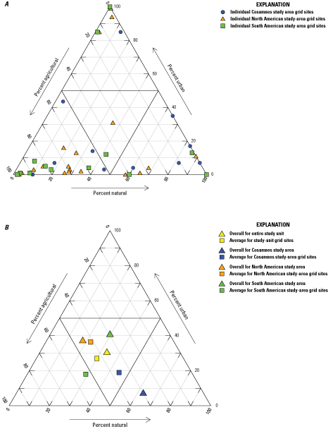
Ternary diagram of the percentages of urban, agricultural, and natural land use (Bennett, 2022) in the Sacramento Metropolitan Domestic-Supply Aquifer study unit, 2017, California Groundwater Ambient Monitoring and Assessment Priority Basin Project (U.S. Geological Survey, 2022): A, surrounding individual USGS grid sites (Bennett and others, 2019); and B, averages in the study unit and around USGS grid sites (Bennett and others, 2019).
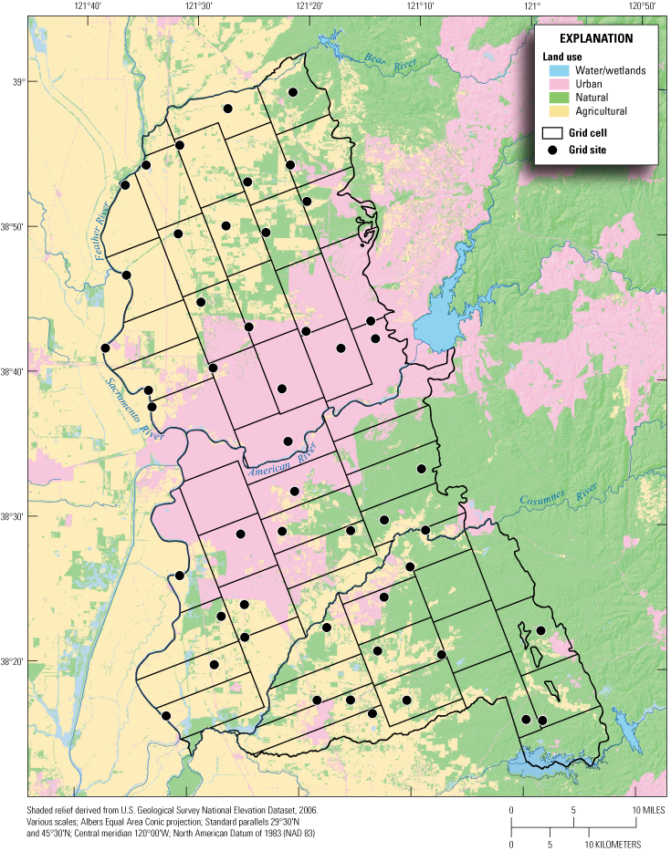
The 2002 land uses (Falcone, 2015; Bennett, 2022) and locations of U.S. Geological Survey grid sites (Bennett and others, 2019) in the Sacramento Metropolitan Domestic-Supply Aquifer study unit, 2017, California Groundwater Ambient Monitoring and Assessment Priority Basin Project (U.S. Geological Survey, 2022).
The proportions of land use within the 1,640-ft buffers surrounding the sampled USGS grid sites in the SacMetro-DSA study unit, collectively, were 30 percent natural, 27 percent urban, and 43 percent agricultural. The proportions varied by study area, with USGS grid sites sampled in the North American study area having the highest proportion of urban land use (36 percent) in the 1,640-ft buffers; the Cosumnes and South American each had about 18 percent urban land use in the buffered area around sampled USGS grid sites (fig. 5). The USGS grid sites in the Cosumnes study area had the highest proportion of natural land use (45 percent) in the buffered area, and the South American had the highest proportion of agricultural land use (53 percent) of the three study areas (figs. 5, 6). Around individual USGS grid sites, urban land use ranged from 0 to 100 percent urban, with 21 of 49 USGS grid sites surrounded by greater than 10 percent urban land use (fig. 6; Bennett, 2022).
Septic tanks and LUFTs are also markers of land-use patterns. Their densities around a site may be indicators of potential sources of anthropogenic contaminants from the land surface. The LUFT density was determined using a Thiessen polygon approach for spatial interpolation (Heywood and others, 1998; Tyler Johnson, USGS, written commun., 2012) and data from the California Environmental Protection Agency (2001). Thiessen polygons were created initially with the LUFT in the center of the polygon. The polygon edges were increased in all directions until they extended halfway to a neighboring LUFT (or until they reached the California border). The result is a unique shape for each LUFT. In most cases, only one LUFT was in a polygon, but occasionally multiple LUFTs were in a polygon. The total number of LUFTs per polygon was divided by the area of the polygon to generate a density of LUFTs for each polygon. The USGS grid sites were then overlaid on the Thiessen polygon map, and each GAMA site was assigned the LUFT density from the Thiessen polygon in which it was located (Bennett, 2022).
Septic-tank density was determined from the 1990 Census of Population and Housing: Summary Tape File 3A dataset (U.S. Census Bureau, 1990). The density of septic tanks in each housing census block was calculated from the number of tanks and block area. The density of septic tanks around each USGS–GAMA grid site was then calculated from the area-weighted mean of the block densities in a 1,640-ft buffer around the site (Tyler Johnson, U.S. Geological Survey, written commun., 2013; Bennett, 2022).
The density of LUFTs around USGS grid sites ranged from 0.004 to 1.24 tanks per square mile (tanks/mi2), and the median density was 0.01 tanks/mi2 (Bennett, 2022). The density of septic tanks around USGS grid sites ranged from 0.19 to 21 tanks/mi2, and the median density was 1.3 tanks/mi2 (Bennett, 2022).
Percentages of land-use types in the 1,640-ft buffers surrounding the sampled USGS grid sites rarely correlated with age, redox, or study area in the SacMetro-DSA study unit (table 4). The only significant correlation was with agricultural land use, where pre-modern samples were associated with a higher percentage of agricultural land use than samples classified as modern (table 4). LUFT density was only correlated with study-area classifications; the North American and South American study areas had significantly higher LUFT densities than the Cosumnes study area (table 4). This relation reflects the fact that the North and South American study areas have greater proportions of urban land use than the Cosumnes study area (figs. 5, 6). Septic-tank density was only correlated with redox classification; samples classified as oxic had significantly higher septic densities than samples classified as anoxic (table 4). This relation is counterintuitive given that contributions of organic matter from septic tanks to groundwater could be expected to lead to more anoxic conditions. Redox conditions in the USGS grid sites sampled for the SacMetro-DSA were primarily oxic (38 of 49 USGS grid sites; Bennett, 2022). The USGS grid sites with anoxic conditions were close to the Sacramento River along the western edge of the study unit. A low population density and a relatively low number of septic systems likely explain the observed correlation between septic-tank density and redox conditions in the SacMetro-DSA.
Hydrologic Conditions
Hydrologic conditions are represented by elevation and aridity index at the site. Land-surface elevations of the USGS grid sites sampled in the SacMetro-DSA study unit range from near sea level along the southwestern boundary of the study unit to about 300 ft. in the dissected uplands in the southeastern part of the study unit (fig. 2). In general, the study unit has relatively low-slope alluvial plains west of rolling and dissected uplands composed of Pliocene–Pleistocene consolidated deposits (identified as QPc by Bennett and others, 2011) along the eastern margin of the Sacramento Valley (fig. 2; Saucedo and others, 2000). The climate in the study unit is typically defined as “Mediterranean,” meaning warm, dry summers and cold, wet winters. Average annual precipitation in the SacMetro-DSA (1991–2020) is about 20 inches, with average daily minimum and maximum temperatures of 8 and 23 degrees Celsius, respectively (PRISM Group, 2021).
Aridity index was used as a proxy for climate. Aridity index is defined as average annual precipitation divided by average annual evapotranspiration and is equal to the United Nations Educational, Scientific, and Cultural Organization Aridity Index (United Nations Educational, Scientific, and Cultural Organization, 1979; United Nations Environment Programme, 1997). All USGS grid sites sampled in the SacMetro-DSA study unit had an aridity index in the semi-arid category (aridity index of 0.2 to 0.5) as defined by the United Nations Environment Programme (1997). Aridity index values at sampled USGS grid sites ranged from 0.35 to 0.49 (Bennett, 2022). Aridity index values were correlated to elevation, pH, redox classification, and study area. Aridity index was significantly positively correlated to elevation, meaning that wetter conditions were observed at higher elevations. Aridity index was significantly negatively correlated to pH in the SacMetro-DSA study unit (table 5). The USGS grid sites classified as oxic had significantly greater aridity-index values than USGS grid sites classified as anoxic (table 4). The correlations of aridity index to pH and oxic conditions result from the lowest elevations in the study unit, close to the Sacramento River in the trough of the basin, having higher pH groundwater and groundwater with anoxic conditions. The North American study area had significantly greater aridity-index values than the Cosumnes and South American study areas (table 4).
Depth and Groundwater-Age Characteristics of the Shallow Aquifer System
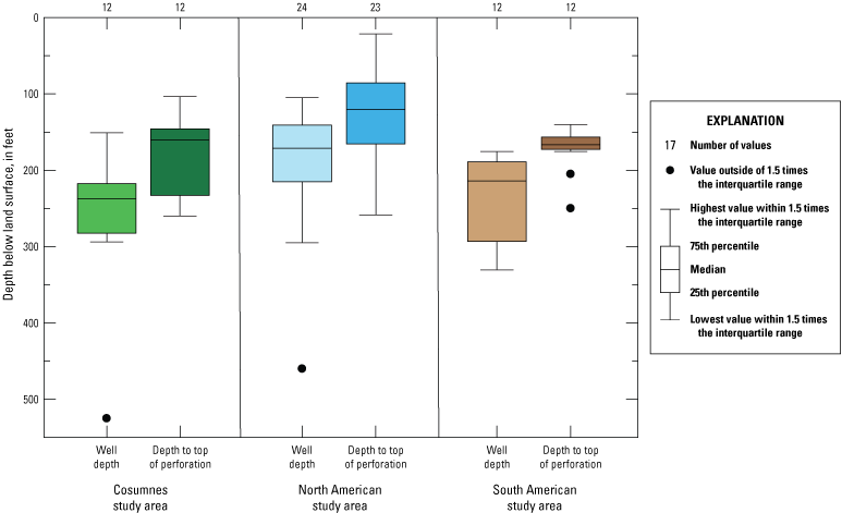
The domestic-supply aquifer system in the SacMetro-DSA study unit is defined by the depths of domestic wells that are shallower on average than the perforation intervals of public-supply wells (public-supply aquifer system). Median public-supply well depth in the USGS grid sites sampled in the North American and South American study areas for the GAMA-PBP public-supply assessment in 2005 was about 300 ft (Bennett and others, 2011), whereas the median depth of domestic-supply USGS grid sites in the SacMetro-DSA was about 200 ft (Bennett and others, 2019). USGS grid sites sampled by USGS–GAMA are considered representative of the domestic-supply aquifer system; thus, depth characteristics of these USGS grid sites can be used to define the domestic-supply aquifer system.
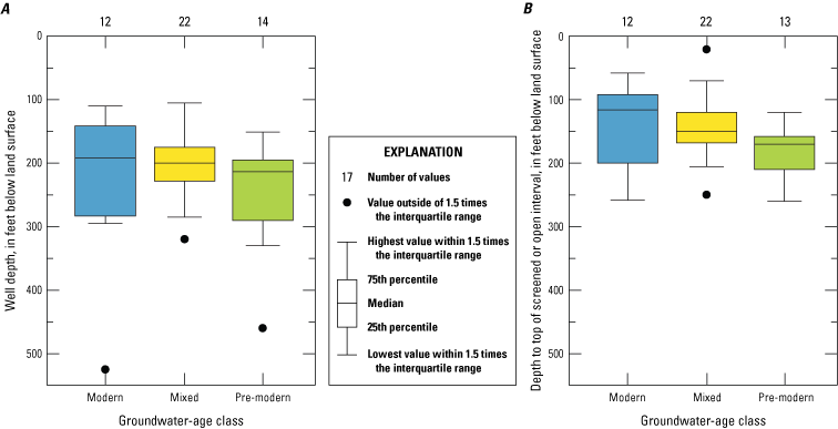
Well-depth information was available for 48 of the 49 wells sampled (Bennett and others, 2019). Comparison of USGS grid wells from the Cosumnes, North American, and South American study areas showed significant differences between well depths or depths of tops of screened or open intervals (fig. 7). The Cosumnes and South American study areas had significantly deeper well depths and top of screened or open intervals than the North American study area (table 4; fig. 7). Depths of USGS grid wells ranged from 105 to 525 ft below land surface; the median depth was 207 ft (fig. 7). Depths of tops of screened or open intervals were available for 47 of those 48 wells with construction information (Bennett and others, 2019). Depths to the tops of the screened or open intervals ranged from 21 to 260 ft, with a median of 159 ft. The screened or open interval length ranged from 11 to 366 ft, with a median of 40 ft.
Well depths and depths to tops of screened or open intervals for U.S. Geological Survey grid sites (Bennett and others, 2019), Sacramento Metropolitan Domestic-Supply Aquifer study unit, 2017, California Groundwater Ambient Monitoring and Assessment Priority Basin Project (U.S. Geological Survey, 2022).
Groundwater age was included as a potential explanatory variable because it indicates the time since the groundwater was recharged to the aquifer system and was last in contact with the atmosphere. Groundwater age can be used to interpret groundwater-quality data for wells affected by relatively recent anthropogenic activities or by longer timescale reactions in an aquifer as groundwater migrates through the system. In this report, the method used to estimate groundwater “age” is based on tritium concentrations and is detailed by Lindsey and others (2019). The method is used to calculate geographically specific tritium-concentration thresholds (modern and premodern thresholds) based on estimated amounts of tritium in precipitation from 1953 to 2012 (Michel and others, 2018). These thresholds can then be compared with groundwater tritium measurements, and results can be classified as modern, mixed, or premodern (Lindsey and others, 2019). For tritium results obtained from grid-well samples collected for the SacMetro-DSA, the premodern and modern thresholds were 0.18 tritium units (TU) and 1.40 TU, respectively. For example, a SacMetro-DSA groundwater sample with a tritium concentration of 2.76 TU was classified as modern (greater than the modern threshold), and a sample with a tritium concentration of 0.09 TU was classified as premodern (less than the premodern threshold). Samples with tritium concentrations between the thresholds were classified as mixed. Using this method, samples from 12 USGS grid sites were classified as modern, 23 USGS grid sites were classified as mixed (having a component of both modern and pre-modern waters), and 14 USGS grid sites were classified as pre-modern (Bennett, 2022).
Classified groundwater ages typically increase (get older) with well depth and with depth to the top of the screened or open interval (Jurgens and others, 2008); however, in the SacMetro-DSA study unit, well depth did not significantly correlate with any of the age-classification comparisons (fig. 8; table 4). The only significant difference between the age categories and well construction was that the mean depth to the top of the screened interval was greater for USGS grid sites classified as pre-modern than for USGS grid sites classified as mixed (fig. 8; table 4). Differences in water levels across the three study areas could be confounding the expected correlation of groundwater age and well depth when combining the data for analysis at the study-unit scale. Water levels in the Cosumnes study area were substantially deeper than water levels in either the North American or South American study area (fig. 3). The median depths to water measured prior to sampling for the Cosumnes, North American, and South American study areas were 143, 59, and 68 ft below land surface, respectively (Bennett, 2022). Because water at the water table is presumed to be the youngest water in the groundwater system, having to construct wells that go considerably deeper in the Consumes study area to access groundwater skews the well-depth relation. Comparing age classifications and well-depth information using just the North American and South American study-area wells (which have more comparable median water levels) showed that the median well depth of wells classified as modern was significantly shallower than the median well depth of wells classified as pre-modern (p-value=0.04), and wells classified as mixed had a shallower median well depth than wells classified as pre-modern (p-value=0.04).
Groundwater age in wells (Bennett, 2022), Sacramento Metropolitan Domestic-Supply Aquifer study unit, 2017, California Groundwater Ambient Monitoring and Assessment Priority Basin Project (U.S. Geological Survey, 2022): A, by depth (Bennett and others, 2019); and B, by depth to top of screened or open interval (Bennett and others, 2019).
Geochemical Conditions
Geochemical conditions of the aquifer are described by oxidation–reduction (redox) processes and pH. Redox conditions influence the mobility of many organic and inorganic constituents (McMahon and Chapelle, 2008). Along groundwater flow paths, redox conditions generally proceed along a well-documented sequence of terminal electron acceptor processes (TEAP), such that one TEAP typically dominates at a particular time and aquifer location (Chapelle and others, 1995; Chapelle, 2001). The predominant TEAPs are oxygen-reduction, nitrate-reduction, manganese-reduction, iron-reduction, sulfate-reduction, and methanogenesis. Groundwater samples may contain chemical species that indicate more than one TEAP is active. Evidence for more than one TEAP can indicate mixing of waters from different redox zones upgradient from the site, a site that is screened across more than one redox zone, or spatial variability in microbial activity in the aquifer.
Oxidation–reduction (redox) conditions for the 49 USGS grid sites sampled by USGS–GAMA were classified using the redox classification framework of McMahon and Chapelle (2008) and Jurgens and others (2009). Groundwater conditions were commonly oxic (38 of 49 USGS grid sites; Bennett, 2022). Dissolved-oxygen concentrations were significantly positively correlated to elevation and significantly negatively correlated to pH (table 5). Values for pH ranged from 6.6 to 8.3 (Bennett and others, 2019). Values for pH were significantly greater in samples classified as anoxic compared with samples classified as oxic (table 4). Aridity index and elevation were also significantly negatively correlated to pH (table 5). Relations with pH indicate that anoxic conditions and greater values of pH were predominantly measured near the Sacramento River, which also generally represents the lowest elevations in the study unit. In flood basins of the Sacramento Valley adjacent to the Sacramento River, aquifers composed of fine-grained clay rich sediments create reducing conditions that affect concentrations of redox sensitive constituents like arsenic, iron, and manganese (Hull, 1984; Dawson, 2001a, b39). All the wells classified as anoxic in the SacMetro-DSA were close to the Sacramento River.
Status and Understanding of Groundwater Quality in the Shallow Aquifer System
The following discussion of the status and understanding assessment results is divided into two parts: one for inorganic constituents and the other for organic and special-interest constituents. Each part describes a survey of the number of constituents that were detected at any concentration compared to the number of constituents analyzed and presents a graphical summary of the RCs of constituents detected in the USGS grid sites. Aquifer-scale proportions are then presented for constituent classes and for the individual constituents that were present at moderate or high RCs (constituents present only at low RCs have aquifer-scale proportions of 100 percent low-RC). Finally, results of statistical tests for relations among water quality and potential explanatory variables are presented for the individual constituents and constituent classes that met additional criteria based on RCs. Organic constituents for which detection frequencies were greater than 10 percent, even if all the RCs were low, were also included in the statistical tests comparing water-quality results to the potential explanatory variables.
Inorganic Constituents
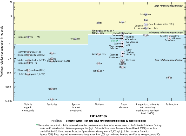
Inorganic constituents are generally natural in groundwater, although their concentrations may be influenced by human activities as well as by natural factors (Hem, 1985). Of the 48 inorganic constituents analyzed by USGS–GAMA, 44 were detected in the SacMetro-DSA study unit. Of these 44 constituents, 27 had regulatory or non-regulatory health-based benchmarks, 6 had non-regulatory aesthetic-based benchmarks, and 11 did not have established benchmarks (tables 2, 3). Most constituents without benchmarks are major or minor ions that are present in nearly all groundwater. Perchlorate, an inorganic salt with natural and anthropogenic sources, was considered a constituent of special interest when the GAMA Priority Basin Project began in 2001 because it had been observed in, or was considered to have the potential to reach, drinking-water supplies (California State Water Resources Control Board, 2020c). Despite being a naturally present inorganic constituent, perchlorate is discussed with the organic constituents because concentrations near or above the MCL-CA are typically from an anthropogenic source (California State Water Resources Control Board, 2020c).
Eight inorganic constituents were detected at moderate or high RCs in the USGS grid sites: trace elements with health-based benchmarks (arsenic, boron, and hexavalent chromium), the nutrient nitrate, and inorganic constituents with aesthetic-based SMCL benchmarks (chloride, iron, manganese, and TDS; table 2; figs. 9, 10). Five inorganic constituents were selected for further evaluation in the understanding assessment because they were present at high RCs in greater than 2 percent of the domestic-supply aquifer system: arsenic, chloride, iron, manganese, and TDS. Additionally, hexavalent chromium was included in the understanding assessment because it is considered a special-interest constituent on the basis of an established MCL-CA enacted in 2014. The MCL-CA was later withdrawn in 2017 (California State Water Resources Control Board, 2020b); however, a new MCL-CA for hexavalent chromium may be established in the future (California State Water Resources Control Board, 2020b).
Maximum relative concentrations for constituents detected in U.S. Geological Survey-grid sites by type of constituent (Bennett and others, 2019), Sacramento Metropolitan Domestic-Supply Aquifer study unit, 2017, California Groundwater Ambient Monitoring and Assessment Priority Basin Project (U.S. Geological Survey, 2022).
Relative concentrations of selected constituent classes in samples from U.S. Geological Survey grid sites (Bennett and others, 2019), Sacramento Metropolitan Domestic-Supply Aquifer study unit, 2017, California Groundwater Ambient Monitoring and Assessment Program Priority Basin Project (U.S. Geological Survey, 2022): A, trace elements; B, nutrients; and C, inorganic constituents (with non-regulatory aesthetic-based benchmarks).
Inorganic constituents were combined in groupings defined by their benchmarks for further discussion. The RCs of inorganic constituents with health-based benchmarks were high, moderate, and low in 10 percent, 39 percent, and 51 percent, respectively, of USGS grid sites in domestic-supply aquifer system (table 6). The RCs of inorganic constituents having aesthetic-based benchmarks were high, moderate, and low in 16 percent, 2 percent, and 82 percent, respectively, of USGS grid sites in the domestic-supply aquifer system.
Table 6.
Summary of aquifer-scale proportions for inorganic, organic, and special-interest constituent classes with health-based and aesthetic-based benchmarks (Bennett and others, 2019), Sacramento Metropolitan Domestic-Supply Aquifer study unit, 2017, California Groundwater Ambient Monitoring and Assessment Priority Basin Project (U.S. Geological Survey, 2022).[Relative-concentration categories: high, concentration of at least one constituent in group greater than water-quality benchmark; moderate, concentration of at least one constituent in group greater than 0.5 (for inorganics) or 0.1 (for organics) of benchmark and no constituents in group with concentration greater than benchmark; low, concentrations of all constituents in group are less than or equal to 0.5 (for inorganics) or 0.1 (for organics) of benchmark. Abbreviation: TDS, total dissolved solids]
Trace Elements
Most trace elements analyzed in the SacMetro-DSA study unit were detected at low RCs (fig. 9). The RCs (for one or more constituents) of trace elements with health-based benchmarks were high, moderate, and low in 10 percent, 31 percent, and 59 percent, respectively, of USGS grid sites in the domestic-supply aquifer system (table 6). Arsenic was the only trace element present at a high RC; boron and hexavalent chromium were present at moderate RCs (table 7; fig. 10A).
Table 7.
Grid-based aquifer-scale proportions for constituents that met criteria for additional evaluation in the status assessment (Bennett and others, 2019), Sacramento Metropolitan Domestic-Supply Aquifer study unit, 2017, California Groundwater Ambient Monitoring and Assessment Priority Basin Project (U.S. Geological Survey, 2022).[Grid-based aquifer-scale proportions for organic constituents are based on samples collected by the U.S. Geological Survey from 49 grid sites during August to November 2017. Relative-concentration categories: high; concentrations greater than benchmark; moderate, concentrations less than benchmark and greater than or equal to 0.1 (for organic constituents) or 0.5 (for inorganic constituents) of benchmark; low, concentrations less than 0.1 (for organic constituents) or 0.5 (for inorganic constituents) of benchmark]
Study unit grid-based aquifer scale proportions are the area-weighted combination of the aquifer-scale proportions for the North American, South American, and Cosumnes study areas.
Understanding Assessment for Arsenic
Arsenic is a semi-metallic trace element that is often naturally present in groundwater. Arsenic concentrations in groundwater are typically controlled by the abundance and dissolution rates of arsenic-bearing minerals in the aquifer and specific geochemical conditions that are conducive to arsenic mobilization (reduced or anoxic) and allow for the desorption of arsenic from mineral surfaces (Welch and others, 2000; Smedley and Kinniburgh, 2002). Pyrite is a common sulfide mineral in aquifers and may contain up to several percent of arsenic. Copper ore smelting, coal combustion, arsenical pesticides, and wood preservatives are other anthropogenic sources of arsenic (Welch and Stollenwerk, 2003). Mining activities for copper, gold, and other metals can increase the rate of dissolution of natural arsenic-bearing minerals such as pyrite (Smedley and Kinniburgh, 2002).
The MCL-US for arsenic was lowered from 50 µg/L to 10 µg/L in 2002; however, chronic exposure to arsenic concentrations between 10 µg/L and 50 µg/L in drinking water has been linked to increased cancer risk and to non-cancerous effects including skin damage and circulatory problems (U.S. Environmental Protection Agency, 2001). An estimated 8 percent of groundwater resources used for drinking water in the United States have high concentrations of arsenic (greater than 10 µg/L; Focazio and others, 2000; Welch and others, 2000), and high concentrations of arsenic in groundwater resources used for drinking water are a worldwide concern (Smedley and Kinniburgh, 2002; Welch and others, 2006).
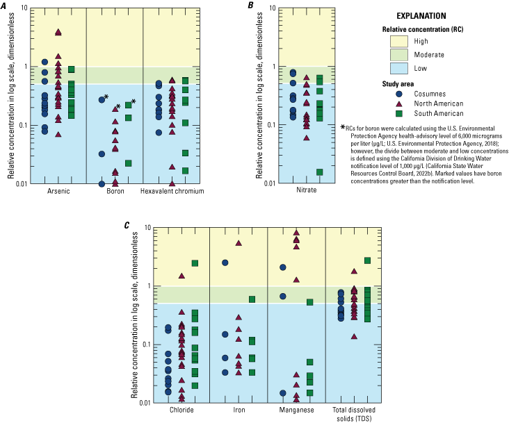
Arsenic was present at high and moderate RCs in 10 percent and 20 percent, respectively, of USGS grid sites in the domestic-supply aquifer system (table 7). The proportion of the domestic-supply aquifer system having high RCs of arsenic was highest in the North American study area (17 percent), followed by Cosumnes study area (8 percent), and then the South American study area (0 percent; table 7; fig. 10). Previous studies and a review of elevated arsenic in groundwater have identified two primary mechanisms for arsenic mobilization related to these conditions: (1) desorption from, or inhibition of sorption to, aquifer materials concurrent with increasing pH and (2) release of arsenic from dissolution of iron or manganese oxyhydroxides under iron- or manganese-reducing conditions (Smedley and Kinniburgh, 2002; Belitz and others, 2003; Welch and others, 2006). The first mechanism (desorption) requires pH values greater than 7.8, the value above which the primary arsenate species (HAsO4−2) is relatively soluble (Smedley and Kinniburgh, 2002). The accumulation of elevated arsenic concentrations in groundwater is also affected by hydrologic conditions in the aquifer system. Longer contact times between groundwater and aquifer materials increases the reaction time with aquifer materials (Smedley and Kinniburgh, 2002).
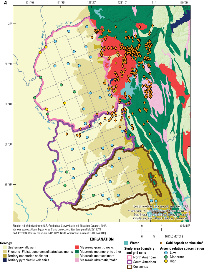
In the SacMetro-DSA study unit, high and moderate RCs of arsenic were detected mostly in samples from USGS grid sites in the North American study area, either along or relatively close to the Sacramento River (fig. 11A). High RCs of arsenic were primarily detected in anoxic groundwater (DO less than 1 milligram per liter, reducing conditions) and water classified as pre-modern or mixed, although one anoxic sample was classified as modern (fig. 12; table 4). About half of the samples with moderate concentrations were classified as anoxic, and about half were also classified as modern (fig. 12). Arsenic concentrations had a significant negative correlation to DO (table 8) and significant positive correlations to iron and manganese (table 9). Mobilization of arsenic appears to be primarily related to reducing conditions in the aquifer system, particularly in the North American study area. These observations are consistent with previous studies in the Sacramento Valley (Hull, 1984; Dawson, 2001a). Reducing conditions conducive to arsenic mobilization have been described in fine-grained flood basin deposits in the central part of the valley close to the Sacramento River (Hull, 1984; Dawson, 2001a).
Relative concentrations of selected trace elements in U.S. Geological Survey grid sites (Bennett and others, 2019), Sacramento Metropolitan Domestic-Supply Aquifer study unit, 2017, California Groundwater Ambient Monitoring and Assessment Priority Basin Project (U.S. Geological Survey, 2022): A, arsenic (Bennett and others, 2019); and B, hexavalent chromium (Bennett and others, 2019).
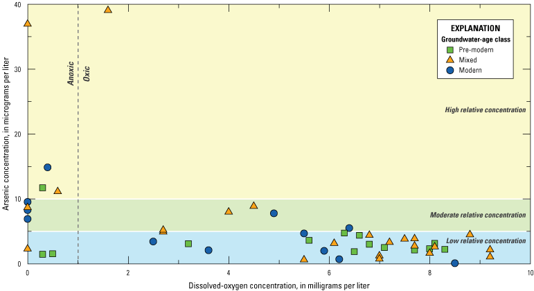
Relation of arsenic concentration to dissolved-oxygen concentration (Bennett and others, 2019) and groundwater-age class (Bennett, 2022), Sacramento Metropolitan Domestic-Supply Aquifer study unit, 2017, California Groundwater Ambient Monitoring and Assessment Program Priority Basin Project (U.S. Geological Survey, 2022).
Table 8.
Results of Spearman's rho (ρ) tests for correlations between selected potential explanatory variables (Bennett, 2022) and selected water-quality constituents (Bennett and others, 2019), Sacramento Metropolitan Domestic-Supply Aquifer study unit, 2017, California Groundwater Ambient Monitoring and Assessment Priority Basin Project (U.S. Geological Survey, 2022).[ρ values are shown for tests in which the variables were determined to be significantly correlated on the basis of p-values (not shown) being less than the level of significance (α) of 0.05. Abbreviations: LUFTs, leaking (or formerly leaking) underground fuel tanks; ns, Spearman's test indicates no significant correlation between factors; blue text, significant positive correlation; red text, significant negative correlation]
Table 9.
Results of Spearman's rho (ρ) tests for correlations between selected water-quality constituents (Bennett and others, 2019), Sacramento Metropolitan Domestic-Supply Aquifer study unit, 2017, California Groundwater Ambient Monitoring and Assessment Priority Basin Project (U.S. Geological Survey, 2022).[ρ values are shown for tests in which the variables were determined to be significantly correlated on the basis of p-values (not shown) being less than the critical level (α) of 0.05. Abbreviations: ns, Spearman's test indicates no significant correlation between factors; blue text, significant positive correlation; red text, significant negative correlation]
The foothills of the Sierra Nevada east of the SacMetro-DSA study unit has a long history of mining (U.S. Geological Survey, 2021b), and gold has been extracted in some locations from gravel deposits associated with the American River and along the eastern edge of the North American study area (fig. 11A). Mining activities, however, likely are not responsible for elevated concentrations of arsenic because wells with high or moderate concentrations of arsenic were not close to any of the USGS grid sites with a history of gold extraction (fig. 11A).
Understanding Assessment for Hexavalent Chromium
Chromium is a transition metal commonly found in minerals associated with ultramafic igneous rocks (Hem, 1985). Chromium has also been shown to be present at high enough concentrations in granitic rocks to contribute appreciable amounts of chromium to groundwater (Izbicki and others, 2015). Chromite, a mineral highly resistant to weathering, is the most common chromium bearing mineral. However, chromium can substitute into minerals like amphiboles, garnets, micas, pyroxenes, and spinels, which are more easily weathered and therefore could be important sources of chromium to the environment (Izbicki and others, 2015). There are several industrial uses for chromium, such as its inclusion as an alloy in stainless steels, in chrome plating, as a pigment in paints, and as a wood preservative (California State Water Resources Control Board, 2020b). Chromium is also discharged to the atmosphere during the manufacture and combustion of gas and coal (California State Water Resources Control Board, 2020b).
Transition metals like chromium often have more than one thermodynamically stable oxidation state. Chromium-3 is the most common oxidation state in most minerals (Nriagu and Nieboer, 1988). In groundwater, dissolved chromium is either reduced ionic forms of chromium-3 or oxidized anionic forms of hexavalent chromium, like chromate and dichromate (Hem, 1985). The presence and relative abundance of natural chromium-3 and hexavalent chromium on mineral surfaces or dissolved in groundwater are controlled by the following factors: (1) chromium concentrations in primary minerals; (2) mineral weathering rates; (3) the presence of manganese oxides that convert chromium-3 to hexavalent chromium; and (4) the presence of reducing agents that allow for the reduction of hexavalent chromium to chromium-3, which can be mediated through abiotic or microbial pathways (Izbicki and others, 2015). Dissolved total chromium concentrations were compared to hexavalent chromium concentrations in paired samples collected by the GAMA-PBP from more than 900 public-supply wells throughout California; about 90 percent of the dissolved chromium was hexavalent chromium (Izbicki and others, 2015). Similarly, dissolved chromium concentrations were predominantly hexavalent chromium in the SacMetro-DSA samples from public-supply wells (fig. 13).
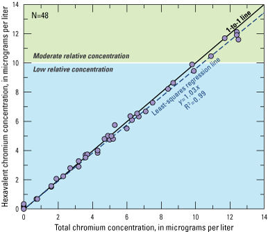
Relation of hexavalent chromium to total chromium in U.S. Geological Survey grid sites (Bennett and others, 2019), Sacramento Metropolitan Domestic-Supply Aquifer study unit, 2017, California Groundwater Ambient Monitoring and Assessment Priority Basin Project (U.S. Geological Survey, 2022). Abbreviations: N, number; R2, coefficient of determination; =, equals.
Hexavalent chromium was detected in 83 percent of wells sampled in the SacMetro-DSA study unit, with detected concentrations ranging from 0.06 to 12.1 µg/L (Bennett and others, 2019). The hexavalent chromium sample was accidentally missed at one well during sample collection, so hexavalent chromium data are available for 48 of the 49 grid wells. Wells with moderate concentrations of hexavalent chromium, greater than one-half of the USGS HBSL of 20 µg/L, were observed in all three study areas (fig. 10A). Comparing hexavalent chromium concentrations by age class showed that samples classified as mixed had higher hexavalent chromium concentrations than samples classified as modern. Comparing hexavalent chromium concentrations by redox classification showed oxic samples had higher concentrations than anoxic samples (table 4; fig. 14). Significant differences were not observed in the concentration ranges of hexavalent chromium by study area (table 4). Concentrations of hexavalent chromium were significantly positively correlated to the density of septic tanks and dissolved-oxygen concentrations but were significantly negatively correlated to pH (table 8). Significant positive correlations to nitrate and perchlorate and significant negative correlations to iron and manganese were also observed for hexavalent chromium concentrations (table 9). In addition to the statistical comparison made with constituents selected for discussion in the status assessment, hexavalent chromium was significantly positively correlated to vanadium (p<0.0001) and selenium (p=0.03). Vanadium and selenium share similar chemistries with chromium and form soluble oxyanions in the plus six oxidation state (Izbicki and others, 2015).
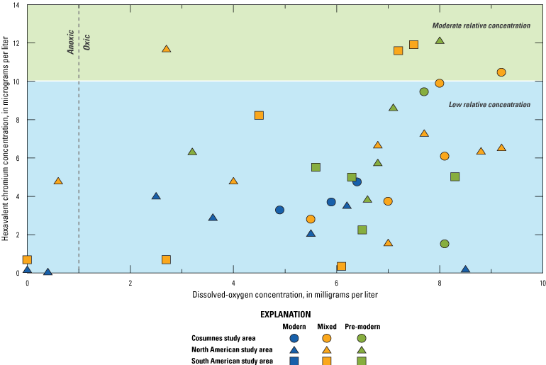
Relations of hexavalent-chromium concentration (Bennett and others, 2019) to dissolved-oxygen concentration and groundwater-age class by study unit (Bennett, 2022) in samples from U.S. Geological Survey grid sites (Bennett and others, 2019), Sacramento Metropolitan Domestic-Supply Aquifer study unit, 2017, California Groundwater Ambient Monitoring and Assessment Priority Basin Project (U.S. Geological Survey, 2022).
Geogenic hexavalent chromium that is naturally derived from aquifer materials containing chromium-bearing minerals appears to be the source of hexavalent chromium observed in samples collected in the SacMetro-DSA. Hexavalent chromium is positively correlated to oxic conditions, negatively correlated to pH (more hexavalent chromium in more alkaline waters), and positively correlated with nitrate, which in some areas of agricultural land use has been suggested as an indicator of hexavalent chromium mobilization related to irrigation returns (Hausladen and others, 2018). Hexavalent chromium that is naturally derived from aquifer materials containing chromium-bearing minerals has been shown be a significant source of hexavalent chromium in aquifers for large areas of California (Izbicki and others, 2015; Manning and others, 2015; Hausladen and others, 2018).
Conversely, anthropogenic discharges of hexavalent chromium related to industrial processes or oxidation of chromium-3 to hexavalent chromium resulting from remediation efforts to clean up organic solvent pollution are known to occur in some urbanized areas of California (Hausladen and others, 2018). Hexavalent chromium concentrations in monitoring wells (wells typically installed near sites with known industrial contamination) throughout the State exhibited correlations to volatile organic compounds (VOCs), specifically 1,1-dichloroethene (1,1-DCE), 1,1-dichloroethane (1,1-DCA), and 1,4-dioxane, which track with their uses in industrial processes related to metal manufacturing and chrome-plating processes (Hausladen and others, 2018). However, no VOCs were detected in the SacMetro-DSA samples that indicated industrial contamination. For additional analysis, monitoring wells in the SacMetro-DSA study unit for which hexavalent chromium was measured within the last 10 years were retrieved from the GAMA Groundwater Information System (California State Water Resources Control Board, 2021b). Because these monitoring wells are associated with known groundwater contamination sites, they were assumed to indicate the locations of potential industrial sources of hexavalent chromium and the relative proximity of these potential anthropogenic sources were compared to the SacMetro-DSA grid wells (fig. 11B). SacMetro-DSA grid wells with moderate concentrations of hexavalent chromium were not near any of the monitoring wells in which hexavalent chromium was at high or moderate RCs, further indicating that hexavalent chromium observed in the grid wells likely did not originate from an industrial source.
Nutrients
As a class, nutrients were not present at high RCs but were present at moderate RCs in 12 percent of USGS grid sites in the domestic-supply aquifer system of the SacMetro-DSA study unit. Nitrate was present at moderate RCs (table 7). Nitrate in groundwater has anthropogenic and natural sources (Dubrovsky and others, 2010); however, concentrations greater than 2 milligrams per liter (mg/L) as nitrogen (RC of 0.2) generally are considered to indicate presence of nitrate from anthropogenic sources (Mueller and Helsel, 1996).
Inorganic Constituents with Aesthetic-Based Benchmarks
The RCs for constituents with aesthetic-based benchmarks (SMCLs) were high, moderate, and low in 16, 2, and 82 percent, respectively, of USGS grid sites in the domestic-supply aquifer system (table 6). Constituents with SMCLs can affect the aesthetic properties of water, such as taste, color, and odor, or can create technical problems, such as scaling and staining. Chloride, iron, manganese, and TDS were the constituents with high RCs in the grid-site network (table 7). Chloride and TDS are indicators of salinity, whereas iron and manganese are trace elements. The major ion chloride and TDS have recommended and upper SMCL-CA values. In this report, data were compared to the upper SMCL-CA values.
Understanding Assessment for Iron and Manganese
Iron and manganese have similar chemistries and mineral associations. Weathering and dissolution of igneous rocks and mafic minerals that are relatively high in iron and manganese is a natural source to groundwater (Hem, 1985). In addition, iron-bearing silicate, sulfide, or oxide minerals are in most rocks and sediments. Once released from their primary minerals, iron and manganese often reprecipitate as oxyhydroxide and oxide coatings on mineral and sediment grains (Hem, 1985). The solubility of iron and manganese is strongly dependent on oxidation–reduction conditions; the more reduced species are more soluble (McMahon and Chapelle, 2008).
Comparison benchmarks used in this study for iron and manganese were the SMCLs of 300 and 50 µg/L, respectively. The SMCL-CA is established as the concentrations at which iron and manganese become nuisances and can affect the aesthetic properties of water but have minimal adverse effects on human health. For USGS grid sites in the SacMetro-DSA domestic-supply aquifer system, high concentrations of iron and manganese were detected in 4 and 14 percent of samples, respectively, and moderate concentrations of iron and manganese were detected in 2 and 4 percent of samples, respectively (table 7). Iron and manganese were significantly higher in samples from USGS grid sites classified as anoxic than from USGS grid sites classified as oxic (table 4; fig. 15). Iron and manganese were significantly negatively correlated to dissolved oxygen, elevation, and well depth and significantly positively correlated to pH (table 8). Iron was also significantly negatively correlated to density of septic tanks (table 8). Iron and manganese were significantly positively correlated to each other, arsenic, and TDS and significantly negatively correlated to hexavalent chromium, nitrate, and perchlorate (table 9). Additionally, iron was positively correlated to bentazon (table 9).
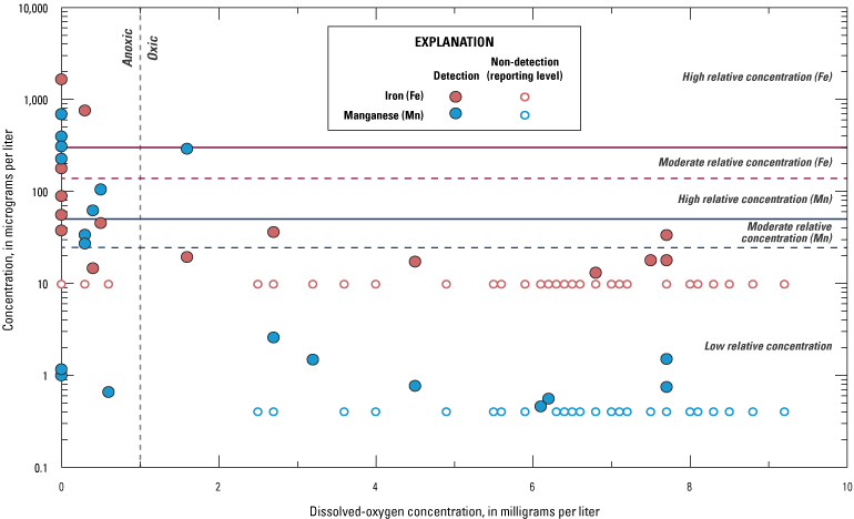
Relations of iron and manganese concentrations to dissolved-oxygen concentrations (Bennett and others, 2019), Sacramento Metropolitan Domestic-Supply Aquifer study unit, 2017, California Groundwater Ambient Monitoring and Assessment Priority Basin Project (U.S. Geological Survey, 2022).
Reducing conditions that are conducive to the mobilization of iron and manganese in alluvial aquifers typically form when DO is consumed by the oxidation of organic matter within the sediments (Appelo and Postma, 2005). In the SacMetro-DSA study unit, groundwater was primarily oxic; however, anoxic, suboxic, or mixed conditions were found in 22 percent of the USGS grid sites sampled, most often along the western boundary of the study unit in wells close to the Sacramento River (fig. 16). This is consistent with a general pattern of decreasing DO concentrations as groundwater flows along the regional flowpath from east to west (Landon and others, 2010). The lowest concentrations of DO typically are near the trough of the basin, notably in the fine-grained sediments of the flood basin deposits near the Sacramento River, as has been described in other studies of the Sacramento Valley (Hull, 1984; Dawson, 2001a).
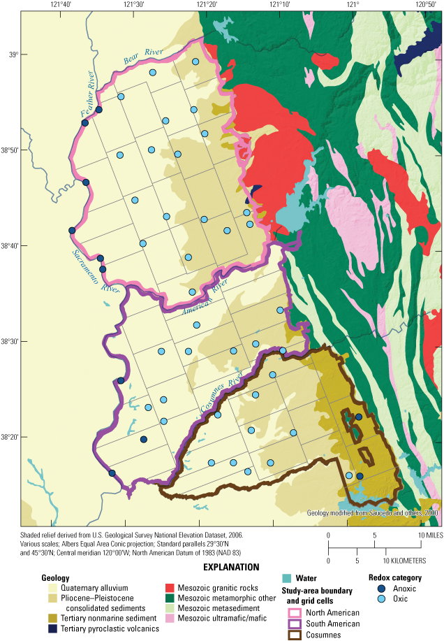
Redox categorization (Bennett, 2022) at U.S. Geological Survey grid sites (Bennett and others, 2019), Sacramento Metropolitan Domestic-Supply Aquifer study unit, 2017, California Groundwater Ambient Monitoring and Assessment Priority Basin Project (U.S. Geological Survey, 2022).
Chloride and Total Dissolved Solids (Salinity Indicators)
The weathering and dissolution of minerals in soils, sediments, and rocks is a primary source of TDS to groundwater. Concentrations of TDS in groundwater can also be affected by mixing with hydrothermal solutions or other saline waters, interactions with sediments of marine or lacustrine origins, or evaporative concentration of shallow groundwater (Hem, 1985). Groundwater recharged from water used for irrigation and wastewater discharge is a potential anthropogenic source of TDS (Hem, 1985). Total dissolved solids were present at high and moderate RCs in 2 percent of the SacMetro-DSA (table 7). The South American study area had one site with a high RC of TDS, and the North American study area had one site with a moderate RC (table 7). Chloride is a component of TDS; the one site with a high RC of TDS in the South American study area also had high a RC of chloride.
The TDS concentrations were higher in groundwater classified as anoxic than as oxic with respect to redox conditions (table 4). The TDS concentrations were significantly positively correlated to agricultural land use and to concentrations of chloride, iron, manganese, and bentazon (tables 8, 9). Concentrations of TDS were significantly negatively correlated to natural land use, elevation, well depth, and DO concentrations (table 8). The observed correlations are generally consistent with associations or processes known to affect concentrations of TDS. Generally, TDS was higher in agricultural areas that have higher recharge rates because of irrigation at the land surface, which can transport additional solutes to the aquifer. Recharge water from precipitation is low in TDS, and precipitation increases as elevation increases. Higher elevations also correlate to higher proportions of natural land use in the eastern parts of the study unit. The USGS grid sites with high and moderate concentration of TDS were on the western edge of the study unit close to the Sacramento River. Concentrations of TDS in these wells were noticeably higher than the rest of the USGS grid sites in the SacMetro-DSA study unit (fig. 17). The median TDS concentration for USGS grid sites sampled in the SacMetro-DSA was 239 mg/L (Bennett and others, 2019), which is less than the upper SMCL-CA of 500 mg/L. Although beyond the scope of this report, concentrations of TDS in the Sacramento Valley aquifer system (in particular, in the low-lying floodbasin areas) have been discussed as potentially being related to several factors, such as evaporative concentration of agricultural recharge, aquifer residence time, sediment lithology, or contributions from deeper more saline parts of the aquifer (Hull, 1984; Dawson, 2001b).
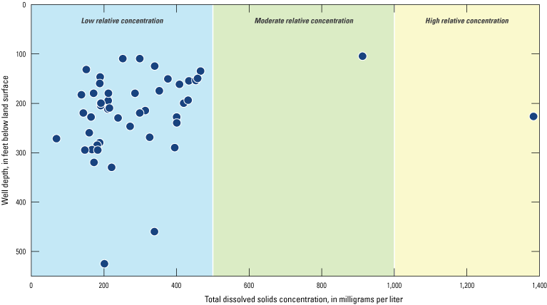
Relation of total dissolved solids concentration and well depth (Bennett and others, 2019), Sacramento Metropolitan Domestic-Supply Aquifer study unit, 2017, California Groundwater Ambient Monitoring and Assessment Priority Basin Project (U.S. Geological Survey, 2022).
Organic and Special-Interest Constituents
The organic constituents assessed in this study are VOCs and pesticides. The VOCs are characterized by a tendency to evaporate. Paints, solvents, fuels, refrigerants, fumigants, and byproducts of water disinfection are sources of VOCs to the environment. Because groundwater is isolated from the atmosphere, VOCs entrained in water recharging the aquifer can persist longer than VOCs in surface water. Pesticides are used to control weeds, fungi, or insects in agricultural and urban settings. Perchlorate, an inorganic salt with natural and anthropogenic sources, was considered a constituent of special interest when the GAMA-PBP began in 2001, after perchlorate had been observed in, or was considered to have the potential to reach, drinking-water supplies (California State Water Resources Control Board, 2020c). An MCL-CA for perchlorate of 6 µg/L became effective in October 2007 (California State Water Resources Control Board, 2020c). Although trace amounts of perchlorate are natural in some waters, perchlorate in groundwater at concentrations near or above the MCL-CA is typically from anthropogenic sources (California State Water Resources Control Board, 2020c). Therefore, perchlorate is discussed with the anthropogenically derived organic constituents; however, perchlorate is not included when summarizing organic constituents as a class.
One or more organic constituents were found in 24 of the 49 USGS grid sites sampled in the study unit. Of the 310 organic constituents analyzed, 16 were detected in at least one site in the SacMetro-DSA study unit (tables 2, 3). Of these 16 constituents, 6 have regulatory health-based benchmarks (tables 2, 3). As a group, organic constituents were not present at high RCs in the shallow aquifer system but were present at moderate RCs in 2 percent, low RCs in 49 percent, and not detected in 49 percent of the shallow aquifer system (table 6). Two organic constituents were selected for additional evaluation in the understanding assessment: bentazon, was selected for additional evaluation on the basis of prevalence and chloroform was selected for additional evaluation on the basis of prevalence and concentration (figs. 18, 19).
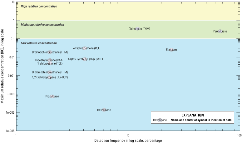
Detection frequency and maximum relative concentration of organic and special-interest constituents detected in samples from U.S. Geological Survey grid sites (Bennett and others, 2019), Sacramento Metropolitan Domestic-Supply Aquifer study unit, 2017, California Groundwater Ambient Monitoring and Assessment Priority Basin Project (U.S. Geological Survey, 2022).
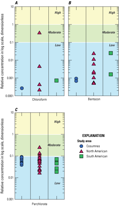
Relative concentrations of selected organic and special-interest constituents in samples from U.S. Geological Survey grid sites (Bennett and others, 2019), Sacramento Metropolitan Domestic-Supply Aquifer study unit, 2017, California Groundwater Ambient Monitoring and Assessment Priority Basin Project (U.S. Geological Survey, 2022): A, chloroform (VOC); B, bentazon (pesticide); and C, perchlorate (special-interest constituent).
Perchlorate was detected at low RCs in 58 percent of SacMetro-DSA USGS grid sites and at moderate RCs in 8 percent of the SacMetro-DSA USGS grid sites, with all moderate detections in the North American study area (tables 6, 7). Perchlorate is discussed further in the understanding assessment presented later because it is a special-interest constituent that was detected frequently at moderate concentrations.
Understanding Assessment for Bentazon
Bentazon was the most detected pesticide in the SacMetro-DSA, with a detection frequency of 24 percent (fig. 18). Bentazon was only detected at low RCs (fig. 19B). Bentazon is an herbicide used to control broadleaf weeds and sedges that has been used on a variety of crop types including corn, dry beans, peanuts, peas, rice, soybeans, and sorghum (U.S. Environmental Protection Agency, 1985). In its commercial form (sodium bentazon), bentazon is moderately soluble in water and has a low soil adsorption coefficient that causes bentazon to be leached from soils and carried to the groundwater system (California Office of Environmental Health Hazard Assessment, 1999). Bentazon can degrade in the environment over time; however, degradation can be slowed or stopped under anoxic conditions (California Office of Environmental Health Hazard Assessment, 1999). The use of bentazon on rice in California was suspended in 1989 because bentazon was detected in groundwater wells in the vicinity of rice-growing areas (California Department of Food and Agriculture, 1990). At that time, most of the bentazon use in California was on rice fields, and approximately 60 percent of rice fields were treated annually (California Department of Food and Agriculture, 1990). Although banned on rice, the use of bentazon on corn, sorghum, peas, and dry beans was still permitted in California (with certain limitations) because there had not been any detections of bentazon in groundwater associated with use on those crops (California Department of Food and Agriculture, 1990).
Bentazon was detected in the SacMetro-DSA only in wells classified as modern or mixed with respect to groundwater age, but concentrations were not significantly different between the modern and mixed categories (table 4). Bentazon concentration was significantly positively correlated to agricultural land use and concentrations of arsenic, chloride, iron, and TDS; bentazon concentration was significantly negatively correlated to elevation and concentrations of perchlorate (tables 8, 9). A previous study showed high detection frequencies of bentazon in areas of rice agriculture (Dawson, 2001b). Comparing the locations of wells with detections of bentazon to crop types where bentazon is (or was in the case of rice) approved for use in California showed that most of the detections were near areas of rice agriculture in the North American study area (fig. 20). The four detections of bentazon in wells in the South American and Cosumnes study areas are south of the rice growing regions of the Sacramento Valley. However, a previous study examining groundwater quality beneath recently urbanized areas of Sacramento found bentazon in shallow groundwater wells near the Sacramento River and attributed the detections to the movement of agriculturally affected Sacramento River water to the shallow aquifer system (Shelton, 2005).
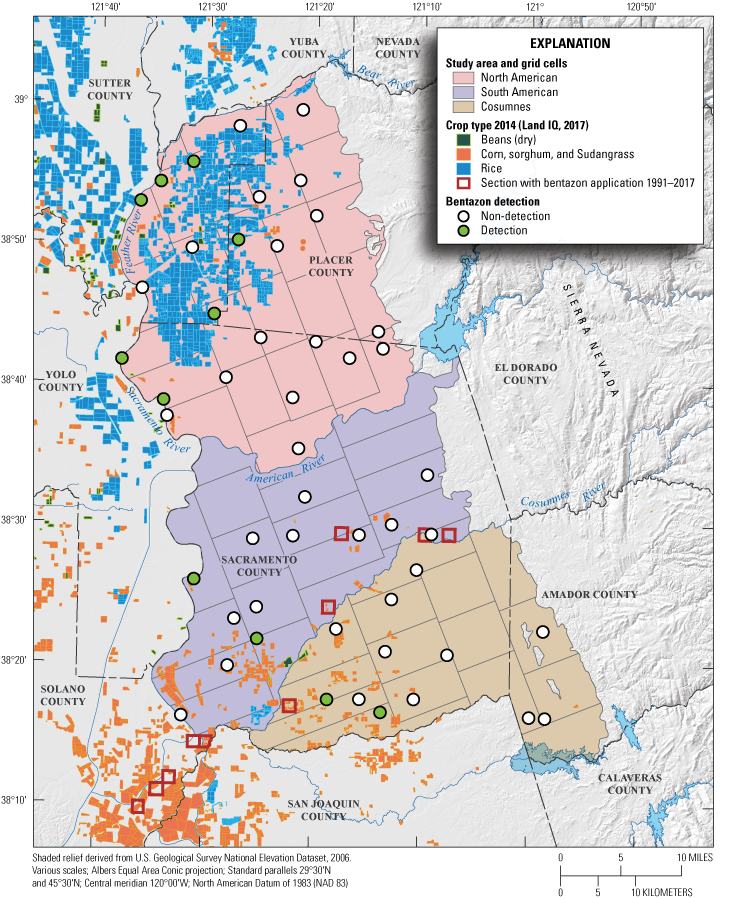
Selected crop-type location (Land IQ, 2017), sections with bentazon applications between 1991 and 2017 (California Department of Pesticide Regulation, 2020), and bentazon detections in U.S. Geological Survey grid sites (Bennett and others, 2019) sampled for U.S. Geological Survey Sacramento Metropolitan Domestic-Supply Aquifer study unit, 2017, California Groundwater Ambient Monitoring and Assessment Priority Basin Project (U.S. Geological Survey, 2022).
In the late 1990s, nearly a decade after being banned for use on rice fields, bentazon was still being detected in the Sacramento River and its tributaries (Domagalski, 2000). Only one of the four detections outside of rice growing areas was close to the Sacramento River. As of 2014, agricultural land use compiled for the California Department of Water Resources by Land IQ, LLC, showed that the predominant crop type in the vicinity of the three detections in the southernmost wells was corn, sorghum, Sudangrass, or beans (fig. 20; Land IQ, 2017). Except for Sudangrass, bentazon use is still approved for use on these crops. Querying the California Pesticide Information Portal (CalPIP) shows bentazon applications in Sacramento County between 1991 and 2017 (California Department of Pesticide Regulation, 2020).
From 1991 to 1995, the use of bentazon in the county was limited to landscape maintenance, ornamental turf, and rights of way; however, the California Department of Pesticide Regulation noted some exceptions to reporting requirements for home-and-garden use and for most industrial and institutional uses (California Department of Pesticide Regulation, 2020). In 1995, 1996, 1998, 2014, and 2017, there were registered applications of bentazon on beans or peas within the county; however, there were no reported uses on corn or sorghum (California Department of Pesticide Regulation, 2020). The Land IQ dataset did not identify peas as a unique crop type. About half of the reported bentazon use in Sacramento County between 1991 and 2017 was accompanied with location information accurate to the township, range, and section (1-square mile), which could then be compared with locations of wells with detections of bentazon and with areal distributions of crop types for which bentazon use was approved (fig. 20). There were no reported uses on corn or sorghum, however, and the identifiable sections of land with known applications were not near the wells with detections. Therefore, we cannot clearly determine whether approved applications of bentazon to crops contributed to detections of bentazon in wells at the southern end of the study unit.
Understanding Assessment for Chloroform
The trihalomethane (THM) chloroform was the most detected VOC in the SacMetro-DSA study unit. Chloroform was detected in 12 percent of USGS grid sites and in all three study areas (figs. 18, 19A). Nationally, chloroform is one of the most frequently detected VOCs in groundwater used for public or domestic supply (Schaap and Zogorski, 2006; Ivahnenko and Zogorski, 2006; Zogorski and others, 2006). Although frequently detected, concentrations of chloroform in drinking-water supplies are usually far below the MCL-US of 80 µg/L. The MCL-US applies to the sum concentration of the following THMs: bromodichloromethane, chloroform, dibromochloromethane, and tribromomethane. In the SacMetro-DSA, only bromodichloromethane (one detection) and chloroform (six detections) were observed in the USGS grid sites. One site had a moderate RC of chloroform and a low RC detection of bromodichloromethane. The combined concentration of the two THMs remained moderate.
Chloroform is a disinfection by-product resulting from the treatment of water supplies or wastewater with chlorine to prevent waterborne diseases (Ivahnenko and Zogorski, 2006; Carter and others, 201231). The distribution of chlorine-treated water for municipal use, or post-treatment discharge back to the environment (in the case of regulated wastewater), provides opportunities for chloroform to be carried into the groundwater system. For example, application of chlorinated public-supply water to lawns, parks, or golf courses as irrigation can discharge chloroform back to the environment. Furthermore, distribution pipes or sewer systems carrying treated water can leak and release chloroform to the groundwater system (Ivahnenko and Zogorski, 2006; Carter and others, 201231). Outside of urban areas, domestic-well disinfection to prevent or treat bacterial issues typically is done by pouring chlorine solutions directly into the well, thus providing a direct pathway for THMs to enter the aquifer system (Wright, 1997; Centers for Disease Control and Prevention and U.S. Department of Housing and Urban Development, 2006). Septic systems in rural areas can also be a source of chloroform to the aquifer system (Ivahnenko and Zogorski, 2006).
Chloroform concentrations were not significantly correlated to age class, redox class, or study area (table 4). Chloroform concentrations were significantly positively correlated to percent of urban land use and LUFT density and were significantly negatively correlated to the depth to top of perforation (table 8). Chloroform concentrations were not significantly correlated to other selected water-quality constituents (table 9). The correlation of chloroform to LUFT density likely is coincidental with the fact the LUFTs are more common in urban areas because LUFTs are not a known source of chloroform to the environment.
Understanding Assessment for Perchlorate
Perchlorate is a highly soluble inorganic constituent for which an MCL-CA of 6 µg/L was established in 2007 (California State Water Resources Control Board, 2020c). Perchlorate was present at moderate RCs in 8 percent of the SacMetro-DSA study unit (table 7). Perchlorate was also detected at low RCs in 58 percent of the SacMetro-DSA study unit across all three study areas (table 6; figs. 18, 19C).
Perchlorate concentrations are commonly affected by the same factors affecting nitrate concentrations, given that they have similar oxidation–reduction potentials (Coates and Achenbach, 2004). Concentrations of perchlorate were significantly higher in oxic than in anoxic conditions (table 4). Comparing study areas, the only significant difference observed was that perchlorate concentrations were higher in the Cosumnes study area than in the South American study area (table 4). Perchlorate concentrations were significantly negatively correlated to pH and significantly positively correlated to elevation and dissolved-oxygen concentration (table 8). Finally, perchlorate was significantly positively correlated to hexavalent chromium and nitrate and significantly negatively correlated to arsenic, iron, manganese, and bentazon (table 9).
Perchlorate has natural and anthropogenic sources. An investigation of perchlorate occurrence and distribution throughout California and the southwestern United States, primarily from public-supply wells, showed that concentrations of perchlorate above certain thresholds can indicate anthropogenic activity, and concentrations below these thresholds are likely the result of natural sources (Fram and Belitz, 2011). Methods developed in Fram and Belitz (2011) were used to compare actual and predicted probabilities of perchlorate detections in this study.
Only samples that were oxic or suboxic and had a perchlorate measurement were included in the analysis because perchlorate is reduced at about the same redox conditions as nitrate. This screening process resulted in 40 samples: 10 Cosumnes study-area samples, 19 North American study-area samples, and 11 South American study-area samples.
Median aridity-index values of 0.384, 0.434, and 0.386, and detection frequencies of 0.1 µg/L, 0.5 µg/L, and 1 µg/L, were calculated for the Cosumnes, North American, and South American study-area samples, respectively. For example, of the 19 samples in the North American study area, 15 had detections of perchlorate at concentrations greater than 0.1 µg/L, which equates to a 79-percent detection frequency (fig. 21). In the Cosumnes and North American study areas, detection frequencies of perchlorate at concentrations greater than 0.1 µg/L and greater than 0.5 µg/L were higher than would be expected under natural conditions (fig. 21), indicating anthropogenic contributions of perchlorate to the groundwater system are likely in these areas. All other combinations of study area and threshold had observed detections that were within the 90-percent Jeffreys confidence intervals (Brown and others, 2001) for the predicted detection frequencies and were therefore consistent with expectations for natural conditions (Fram and Belitz, 2011).
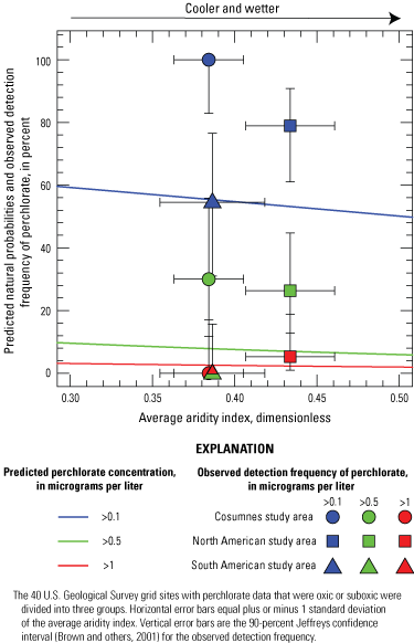
Predicted natural probabilities and observed detection frequencies of perchlorate in groundwater as a function of aridity index (Bennett, 2022) and specified subjective threshold values for U.S. Geological Survey Sacramento Metropolitan Domestic-Supply Aquifer study unit, 2017, California Groundwater Ambient Monitoring and Assessment Priority Basin Project (U.S. Geological Survey, 2022). Abbreviation: >, greater than.
Perchlorate is used in rocket fuels, explosives, road flares, automobile air-bag systems, and other products that can release perchlorate to the environment (California State Water Resources Control Board, 2020c). The EPA-designated Aerojet General Corporation Superfund site in Rancho Cordova, Calif., is known to have contaminated a 27-square mile area with chemicals associated with rocket propellants that include perchlorate (Sacramento County Water Agency, 2004; Sacramento Groundwater Authority, 2008; U.S. Environmental Protection Agency, 2021). The Aerojet General Corporation Superfund site is in the north central part of the South American study area (fig. 22). Data from the GAMA Groundwater Information System for all three study areas highlight the locations of monitoring wells where perchlorate was measured, which include monitoring wells downgradient from the Aerojet General Corporation Superfund site (fig. 22; California State Water Resources Control Board, 2021b). The USGS grid sites sampled in the South American study area were not close to the monitoring wells, and concentrations of perchlorate in the closest grid wells were either non-detections or low RCs (less than 0.6 µg/L; fig. 22). As discussed previously, the detection frequencies of perchlorate at concentrations greater than 0.1, 0.5, or 1 µg/L in the South American study area were consistent with or less than the predicted detection frequencies of perchlorate from natural sources.
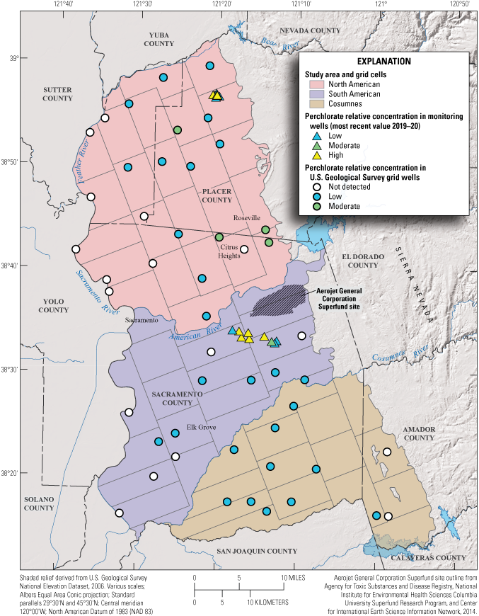
Relative concentrations of perchlorate in U.S. Geological Survey grid sites (Bennett and others, 2019) and relative concentrations of perchlorate from monitoring-well data obtained from the Groundwater Ambient Monitoring and Assessment (GAMA) Groundwater Information System (California State Water Resources Control Board, 2021b), Sacramento Metropolitan Domestic-Supply Aquifer study units (SacMetro-DSA), 2017, GAMA Program Priority Basin Project (U.S. Geological Survey, 2022).
Another potential anthropogenic source of perchlorate is the transport of natural perchlorate present in the unsaturated zone to the groundwater aquifer by irrigation recharge (Fram and Belitz, 2011). Perchlorate is also a natural minor component of salts associated with a fertilizer imported into the United States from the Atacama Desert in Chile (Böhlke and others, 2009). This Chilean fertilizer has been linked to elevated perchlorate concentrations in groundwater (Böhlke and others, 2009; Fram and Belitz, 2011). The import and use of Chilean nitrate in the United States as fertilizer began in the early part of the 20th century but has declined in recent years (Dasgupta and others, 2006).
The variety of sources of perchlorate to the environment confounds efforts to connect elevated concentrations of perchlorate observed in the SacMetro-DSA study unit to specific pathways of perchlorate contamination that could be mitigated. Perchlorate isotope analyses could potentially help identify sources of perchlorate, but such analyses are beyond the scope of this report.
Summary
Groundwater quality in the approximately 1,250-square-mile Sacramento Metropolitan Domestic-Supply Aquifer study unit (SacMetro-DSA) was studied by the U.S. Geological Survey in cooperation with the California State Water Resources Control Board as part of the Priority Basin Project (PBP) of the Groundwater Ambient Monitoring and Assessment (GAMA) Program. The study unit is in parts of Amador, Placer, Sacramento, and Sutter Counties, and the extent of the study unit was defined by the location of three California Department of Water Resources groundwater subbasins: the North American, the South American, and the Cosumnes. The GAMA-PBP provides a spatially unbiased characterization of untreated groundwater quality in the domestic-supply aquifer system. The domestic-supply aquifer was defined using wells with depth intervals that were shallower on average than the public-supply wells listed in the California State Water Resources Control Board Division of Drinking-Water water-quality database.
This report presented a description of the hydrogeologic setting of the SacMetro-DSA, a status assessment of the groundwater quality in the domestic-supply aquifer system of the SacMetro-DSA during 2017, and an understanding assessment that presented the general identification of natural and anthropogenic variables that could be affecting groundwater quality. The status and understanding assessments were based on water-quality data collected from 49 groundwater U.S. Geological Survey (USGS) grid sites by the USGS in 2017. Potential relations with natural and anthropogenic variables were examined with statistical tests and graphical analyses and were discussed in the context of the hydrogeologic setting of the study unit.
The status assessment of the groundwater resource used for domestic supply in 2017 was completed using data from samples analyzed for volatile organic compounds, pesticides, and naturally existing inorganic constituents, such as trace elements and major and minor ions. The status assessment characterized the quality of groundwater resources in the domestic-supply aquifer system of the SacMetro-DSA study unit, not the treated drinking water delivered to consumers by water purveyors. Relative concentrations (RCs, which are sample concentrations divided by the health- or aesthetic-based benchmark concentrations) were used for evaluating groundwater quality for constituents that have Federal or California regulatory or non-regulatory benchmarks for drinking-water quality.
Aquifer-scale proportion was used as the primary metric in the status assessment for evaluating regional-scale groundwater quality. A stratified, random sampling design and grid-based statistical approach provided the basis for aquifer-scale proportions for individual constituents. The SacMetro-DSA was divided into three study areas, and each was stratified using a grid of cells: the North American study area had 24 cells; the South American study area had 17 cells; and the Cosumnes study areas had 15 cells. In each cell, one groundwater site was randomly selected to represent the groundwater resource used for domestic supply. Aquifer-scale proportion was defined as the percentage of the domestic-supply aquifer system in a specified range of relative concentrations for a constituent or class of constituents; the proportion was based on an areal rather than a volumetric basis. High aquifer-scale proportion was defined as the percentage of the domestic-supply aquifer system with relative concentrations greater than 1.0. The threshold between moderate and low RCs was 0.5 for most inorganic constituents (there were some exceptions) and 0.1 for organic constituents. Moderate and low aquifer-scale proportions were defined as the percentages of the domestic-supply aquifer system with moderate and low RCs, respectively.
Of the 28 inorganic constituents with regulatory or non-regulatory health-based benchmarks (HBB), 4 were detected at moderate or high RCs. As a group, inorganic constituents with HBB were present at high and moderate RCs in 10 and 39 percent, respectively, of USGS grid sites in the domestic-supply aquifer system. The only inorganic constituent with an HBB having a high aquifer-scale proportion was arsenic. The inorganic constituents with California secondary maximum contaminant levels (SMCL-CAs), non-regulatory aesthetic-based benchmarks, were present at high and moderate RCs in 16 and 2 percent, respectively, of the USGS grid sites in the domestic-supply aquifer system. Chloride, iron, manganese, and total dissolved solids were the constituents with high RCs.
One or more organic constituents were detected in 24 of the 49 USGS grid sites (49 percent) sampled in the study unit. Of the 14 organic constituents detected, 9 have HBBs. As a group, organic constituents were not found at high RCs in the domestic-supply aquifer system. Chloroform was the only organic constituent detected at moderate RCs. Chloroform and bentazon were the only organic constituents detected in more than 10 percent of the wells sampled.
In the understanding assessment, statistical correlations between concentrations of constituents and values of selected potential explanatory variables were used to identify the factors potentially affecting the concentrations and distribution of constituents detected at high RCs, constituents of special interest, and organic constituents with study-unit detections of more than 10 percent. The potential explanatory variables evaluated were land use, hydrologic conditions, depth, groundwater age, and geochemical conditions.
Inorganic constituents with health-based benchmarks that were evaluated in the understanding assessment included arsenic and hexavalent chromium. Inorganic constituents that are natural in the environment and have aesthetic, non-health-based benchmarks evaluated in the understanding assessment were the trace elements iron and manganese, the major ion chloride, and total dissolved solids. Bentazon, chloroform, and perchlorate (a special-interest constituent) were also included because they were detected in more than 10 percent of USGS grid sites sampled in the SacMetro-DSA.
Redox class (oxic, mixed, or anoxic), dissolved-oxygen concentrations, and land use were the explanatory variables most strongly correlated to detection patterns of most inorganic constituents. High concentrations of arsenic, iron, and manganese were primarily associated with groundwater classified as anoxic rather than oxic, whereas hexavalent-chromium concentrations were positively correlated to oxic conditions. Concentrations of arsenic, iron, and manganese were negatively correlated to dissolved-oxygen concentrations and pH, whereas hexavalent chromium was positively correlated to dissolved oxygen and pH. Arsenic, iron, and manganese are all constituents natural to the environment. Hexavalent chromium has known anthropogenic sources that have contaminated wells in California; however, hexavalent chromium is also natural. The broad existence of hexavalent chromium at relatively low concentrations (moderate concentrations were observed) indicates most detections were likely of hexavalent chromium natural to the aquifer materials that are part of the SacMetro-DSA study unit. Furthermore, a lack of co-detections with other specific anthropogenically derived constituents such as solvents, which might indicate industrial sources, supports the hypothesis of natural concentrations of hexavalent chromium in the SacMetro-DSA study unit.
Bentazon concentrations were positively correlated to agricultural land use and concentrations of arsenic, chloride, iron, and total dissolved solids; bentazon concentrations were negatively correlated to elevation. Chloroform concentrations were positively correlated to urban land use and underground storage-tank density and negatively correlated to depth to top of perforations. Perchlorate concentrations were positively correlated to elevation and concentrations of hexavalent chromium, nitrate, and dissolved oxygen; chloroform concentrations were negatively correlated to pH and concentrations of arsenic, iron, manganese, and bentazon. Correlations of bentazon and perchlorate concentrations to elevation likely resulted from co-relations with other factors related to elevation. For example, there were higher proportions of agricultural land use and more reducing (anoxic) conditions at lower elevations, whereas oxic conditions and lower proportions of agricultural land were observed at higher elevations throughout the study unit. In some areas of the study unit, concentrations of perchlorate were higher than what might be expected naturally; therefore, introduction of perchlorate or migration of natural perchlorate could be anthropogenically mediated.
References Cited
Agency for Toxic Substances and Disease Registry, National Institute for Environmental Health Sciences Columbia University Superfund Research Program and Center for International Earth Science Information Network, 2014, Agency for toxic substances and disease registry hazardous waste site polygon data with Center for International Earth Science Information Network modifications, version 2: NASA Socioeconomic Data and Applications Center (SEDAC), accessed December 20, 2021, at https://doi.org/10.7927/H4DF6P5Z.
Belitz, K., Dubrovsky, N.M., Burow, K.R., Jurgens, B., and Johnson, T., 2003, Framework for a ground-water quality monitoring and assessment program for California: U.S. Geological Survey Water-Resources Investigations Report 03–4166, 78 p. [Available at https://doi.org/10.3133/wri034166.]
Belitz, K., Jurgens, B., Landon, M.K., Fram, M.S., and Johnson, T., 2010, Estimation of aquifer-scale proportion using equal-area grids—Assessment of regional-scale groundwater quality: Water Resources Research, v. 46, no. 11, 14 p. [Available at https://doi.org/10.1029/2010WR009321.]
Belitz, K., Fram, M.S., and Johnson, T.D., 2015, Metrics for assessing the quality of groundwater used for public-supply, CA, USA—Equivalent-Population and area: Environmental Science & Technology, v. 49, no. 14, p. 8330–8338. [Available at https://doi.org/10.1021/acs.est.5b00265.]
Bennett, G.L., V, 2019, Groundwater quality in the Sacramento Metropolitan shallow aquifer, California: U.S. Geological Survey Open-File Report 2019–1047, 4 p. [Available at https://doi.org/10.3133/ofr20191047.]
Bennett, G.L., V, 2022, Potential explanatory variables for groundwater quality in the Sacramento Metropolitan Domestic-Supply Aquifer study unit, 2017—California GAMA Priority Basin Project: U.S. Geological Survey data release, available at https://doi.org/10.5066/P9H4P0XF.
Bennett, G.L., V, Fram, M.S., Belitz, K., and Jurgens, B.C., 2010, Status and understanding of groundwater quality in the northern San Joaquin Basin, 2005—California GAMA Priority Basin Project: U.S. Geological Survey Scientific Investigations Report 2010–5175, 82 p. [Available at https://doi.org/10.3133/sir20105175.]
Bennett, G.L., V, Fram, M.S., and Belitz, K., 2011, Status of groundwater quality in the Southern, Middle, and Northern Sacramento Valley study units, 2005–08—California GAMA Priority Basin Project: U.S. Geological Survey Scientific Investigations Report 2011–5002, 120 p. [Available at https://doi.org/10.3133/sir20115002.]
Bennett, G.L., V, and Fram, M.S., 2014, Groundwater-quality data in the North San Francisco Bay Shallow Aquifer study unit, 2012—Results from the California GAMA Program: U.S. Geological Survey Data Series 865, 94 p. [Available at https://doi.org/10.3133/ds865.]
Bennett, G.L., V, Shelton, J.L., Watson, E., Johnson, T.D., and Jasper, M., 2019, Groundwater-quality data in the Sacramento Metro shallow aquifer study unit, 2017—Results from the California GAMA Priority Basin Project: U.S. Geological Survey data release, available at https://doi.org/10.5066/P9BPGEGH.
Böhlke, J.K., Hatzinger, P.B., Sturchio, N.C., Gu, B., Abbene, I., and Mroczkowski, S.R., 2009, Atacama perchlorate as an agricultural contaminant in groundwater—Isotopic and chronologic evidence from Long Island, New York: Environmental Science & Technology, v. 43, no. 15, p. 5619–5625. [Available at https://doi.org/10.1021/es9006433.]
Brown, L.D., Cai, T.T., and DasGupta, A., 2001, Interval estimation for a binomial proportion: Statistical Science, v. 16, no. 2, p. 101–117. [Available at https://doi.org/10.1214/ss/1009213286.]
Burow, K.R., Jurgens, B.C., Kauffman, L.J., Phillips, S.P., Dalgish, B.A., and Shelton, J.L., 2008, Simulations of groundwater flow and particle pathline analysis in the zone of contribution of a public-supply well in Modesto, eastern San Joaquin Valley, California: U.S. Geological Survey Scientific Investigations Report 2008–5035, 41 p. [Available at https://doi.org/10.3133/sir20085035.]
Burton, C.A., Shelton, J.L., and Belitz, K., 2012, Status and understanding of groundwater quality in the two southern San Joaquin Valley study units, 2005–2006—California GAMA Priority Basin Project: U.S. Geological Survey Scientific Investigations Report 2011–5218, 150 p. [Available at https://doi.org/10.3133/sir20115218.]
California Department of Food and Agriculture, 1990, Bentazon findings and recommendations: Subcommittee of the pesticide registration and evaluation committee, Implementation of the pesticide contamination prevention act, 13 p. [Available at https://www.cdpr.ca.gov/docs/emon/grndwtr/bentazon/findings_and_recommendations.pdf.]
California Department of Pesticide Regulation, 2020, Pesticide use reporting, accessed September 10, 2020, at https://www.cdpr.ca.gov/docs/pur/purmain.htm.
California Department of Water Resources, 2016, California's groundwater: California Department of Water Resources Bulletin 118—Interim Update 2016, 45 p., accessed January 30, 2020, at https://water.ca.gov/Programs/Groundwater-Management/Bulletin-118.
California Department of Water Resources, 2022, SGMA Data Viewer: Groundwater Levels: California Department of Water Resources website, accessed January 2022, at https://sgma.water.ca.gov/webgis/?appid=SGMADataViewer#gwlevels.
California Environmental Protection Agency, 2001, Geographic environmental information management system geoTracker (GEIMS) leaking underground fuel/storage tank database (LUFT) [digital data]: Sacramento, California, California Environmental Protection Agency, State Water Resources Control Board, Division of Water Quality.
California Office of Environmental Health Hazard Assessment, 1999, Public health goal for bentazon in drinking water: California Environmental Protection Agency, 45 p. [Available at https://citeseerx.ist.psu.edu/viewdoc/download?doi=10.1.1.491.8152&rep=rep1&type=pdf.]
California State Water Resources Control Board, 2003, A comprehensive groundwater quality monitoring program for California: Assembly Bill 599, Report to the Governor and Legislature, March 2003, 121 p., accessed December 28, 2020, at https://www.loc.gov/item/2004483131/.
California State Water Resources Control Board, 2020a, GAMA—Well Owners—Water quality in private domestic wells: accessed March 4, 2021, at https://www.waterboards.ca.gov/water_issues/programs/gama/well_owners.html.
California State Water Resources Control Board, 2020b, Chromium-6 drinking water MCL: accessed December 28, 2020, at https://www.waterboards.ca.gov/drinking_water/certlic/drinkingwater/Chromium6.html.
California State Water Resources Control Board, 2020c, Perchlorate in drinking water: accessed December 18, 2020, at https://www.waterboards.ca.gov/drinking_water/certlic/drinkingwater/Perchlorate.html.
California State Water Resources Control Board, 2021a, GAMA—Publications: California State Water Resources Control Board website accessed April 29, 2021, at https://www.waterboards.ca.gov/water_issues/programs/gama/publications.html.
California State Water Resources Control Board, 2021b, GAMA—Groundwater information system: California State Water Resources Control Board website accessed April 29, 2021, at https://gamagroundwater.waterboards.ca.gov/gama/gamamap/public/.
California State Water Resources Control Board, 2022a, California drinking water-related laws–Drinking water-related statutes and regulations, accessed March 31, 2022, at https://www.waterboards.ca.gov/drinking_water/certlic/drinkingwater/Lawbook.html.
California State Water Resources Control Board, 2022b, Drinking water notification levels and response levels—An overview: accessed December 28, 2020, at https://www.waterboards.ca.gov/drinking_water/certlic/drinkingwater/documents/notificationlevels/notification_response_level_overview_2022_02_09.pdf.
Carter, J.M., Moran, M.J., Zogorski, J.S., and Price, C.V., 2012, Factors associated with sources, transport, and fate of chloroform and three other trihalomethanes in untreated groundwater used for drinking water: Environmental Science and Technology, v. 46, no. 15, p. 8189–8197. [Available at https://doi.org/10.1021/es301839p.]
Central Valley Regional Water Quality Control Board, 2016, Groundwater quality assessment report: Prepared by CH2M Hill on behalf of the Northern California Water Association Sacramento Valley Water Quality Coalition, 370 p. [Available at https://www.svwqc.org/wp-content/themes/svwqc-2015/docs/Groundwater-Quality-Assessment-Report-20160128.pdf.]
Chapelle, F.H., McMahon, P.B., Dubrovsky, N.M., Fujii, R.F., Oaksford, E.T., and Vroblesky, D.A., 1995, Deducing the distribution of terminal electron-accepting processes in hydrologically diverse groundwater systems: Water Resources Research, v. 31, no. 2, p. 359–371. [Available at https://doi.org/10.1029/94WR02525.]
Coates, J.D., Achenbach, L.A., 2004, Microbial perchlorate reduction—Rocket-fuelled metabolism: Nature Reviews Microbiology, v. 2, p. 569–580. [Available at https://doi.org/10.1038/nrmicro926.]
Dasgupta, P.K., Dyke, J.V., Kirk, A.B., and Jackson, W.A., 2006, Perchlorate in the United States—Analysis of relative source contributions to the food chain: Environmental Science & Technology, v. 40, no. 21, p. 6608–6614. [Available at https://doi.org/10.1021/es061321z.]
Dawson, B.J., 2001a, Groundwater quality in the Southeastern Sacramento Valley Aquifer, California, 1996: U.S. Geological Survey Water-Resources Investigations Report 01–4125, 24 p. [Available at https://doi.org/10.3133/wri014125.]
Dawson, B.J., 2001b, Shallow groundwater quality beneath rice areas in the Sacramento Valley, California, 1997: U.S. Geological Survey Water-Resources Investigations Report 01–4000, 33 p. [Available at https://doi.org/10.3133/wri014000.]
Domagalski, J.L., 2000, Pesticides in surface water measured at select sites in the Sacramento River Basin, California, 1996–1998: U.S. Geological Survey Water-Resources Investigations Report 00–4203, 24 p. [Available at https://doi.org/10.3133/wri004203.]
Dubrovsky, N.M., Burow, K.R., Clark, G.M., Gronberg, J.M., Hamilton, P.A., Hitt, K.J., Mueller, D.K., Munn, M.D., Nolan, B.T., Puckett, L.J., Rupert, M.G., Short, T.M., Spahr, N.E., Sprague, L.A., and Wilber, W.G., 2010, The quality of our Nation’s waters—Nutrients in the Nation’s streams and groundwater, 1992–2004: U.S. Geological Survey Circular 1350, 174 p. [Available at https://doi.org/10.3133/cir1350.]
Falcone, J.A., 2015, U.S. conterminous wall-to-wall anthropogenic land use trends (NWALT), 1974–2012: U.S. Geological Survey Data Series 948, 33 p. [Available at https://doi.org/10.3133/ds948.]
Focazio, M.J., Welch, A.H., Watkins, S.A., Helsel, D.R., and Horn, M.A., 2000, A retrospective analysis on the occurrence of arsenic in ground-water resources of the United States and limitations in drinking-water-supply characterizations: U.S. Geological Survey Water-Resources Investigations Report 99–4279, 21 p. [Available at https://doi.org/10.3133/wri994279.]
Fram, M.S., and Belitz, K., 2011, Probability of detecting perchlorate under natural conditions in deep groundwater in California and the southwestern United States: Environmental Science & Technology, v. 45, no. 4, p. 1271–1277. [Available at https://doi.org/10.1021/es103103p.]
Hausladen, D.M., Alexander-Ozinskas, A., McClain, C., and Fendorf, S., 2018, Hexavalent chromium sources and distribution in California Groundwater: Environmental Science & Technology, v. 52, no. 15, p. 8242–8251. [Available at https://doi.org/10.1021/acs.est.7b06627.]
Helsel, D.R., Hirsch, R.M., Ryberg, K.R., Archfield, S.A., and Gilroy, E.J., 2020, Statistical methods in water resources: U.S. Geological Survey Techniques and Methods, book 4, chapter A3, 458 p. [Supersedes USGS Techniques of Water-Resources Investigations, book 4, chapter A3, version 1.1; available at https://doi.org/10.3133/tm4a3.]
Hem, J.D., 1985, Study and interpretation of the chemical characteristics of natural water (3d ed.): U.S. Geological Survey Water-Supply Paper 2254, 213 p. [Available at https://doi.org/10.3133/wsp2254.]
Hirsch, R.M., Alley, W.M., and Wilber, W.G., 1988, Concepts for a National Water-Quality Assessment Program: U.S. Geological Survey Circular 1021, 42 p. [Available at https://doi.org/10.3133/cir1021.]
Hull, L.C., 1984, Geochemistry of ground water in the Sacramento Valley, California: U.S. Geological Survey Professional Paper 1401–B, 36 p. [Available at https://doi.org/10.3133/pp1401B.]
Ivahnenko, T., and Zogorski, J.S., 2006, Sources and occurrence of chloroform and other trihalomethanes in drinking-water supply wells in the United States, 1996–2001: U.S. Geological Survey Scientific Investigations Report 2006–5015, 13 p. [Available at https://doi.org/10.3133/sir20065015.]
Izbicki, J.A., Wright, M.T., Seymour, W.A., McCleskey, R.B., Fram, M.S., Belitz, K., and Esser, B.K., 2015, Cr(VI) occurrence and geochemistry in water from public-supply wells in California: Applied Geochemistry, v. 63, p. 203–217. [Available at https://doi.org/10.1016/j.apgeochem.2015.08.007.]
Johnson, T.D., and Belitz, K., 2009, Assigning land use to supply wells for the statistical characterization of regional groundwater quality—Correlating urban land use and VOC occurrence: Journal of Hydrology (Amsterdam), v. 370, nos. 1–4, p. 100–108. [Available at https://doi.org/10.1016/j.jhydrol.2009.02.056.]
Johnson, T.D., and Belitz, K., 2015, Identifying the location and population served by domestic wells in California: Journal of Hydrology: Regional Studies, v. 3, p. 31–86. [Available at https://doi.org/10.1016/j.ejrh.2014.09.002.]
Jurgens, B.C., Burow, K.R., Dalgish, B.A., Shelton, J.L., 2008, Hydrogeology, water chemistry, and factors affecting the transport of contaminants in the zone of contribution of a public-supply well in Modesto, eastern San Joaquin Valley, California: U.S. Geological Survey Scientific Investigations Report 2008–5156, 78 p. [Available at https://doi.org/10.3133/sir20085156.]
Jurgens, B.C., McMahon, P.B., Chapelle, F.H., and Eberts, S.M., 2009, An Excel® workbook for identifying redox processes in ground water: U.S. Geological Survey Open-File Report 2009–1004, 8 p. [Available at https://doi.org/10.3133/ofr20091004.]
Jurgens, B.C., Jasper, M., Nguyen, D.H., and Bennett, G.L., 2018, USGS CA GAMA-PBP Groundwater-Quality Results—Assessment and Trends: U.S. Geological Survey web page, available at https://doi.org/10.5066/P91WJ2G1.
Kingsbury, J.A., Bexfield, L.M., Arnold, T., Musgrove, M., Erickson, M.L., Degnan, J.R., Tesoriero, A.J., Lindsey, B.D., and Belitz, K., 2021, Groundwater-quality and select quality-control data from the National Water-Quality Assessment Project, January 2017 through December 2019: U.S. Geological Survey Data Series 1136, 97 p. [Available at https://doi.org/10.3133/ds1136.]
Land IQ, 2017, Land Use–2014–Land IQ [ds2677]: Land IQ dataset prepared for the California Department of Water Resources, accessed May 29, 2020, at https://map.dfg.ca.gov/metadata/ds2677.html.
Landon, M.K., Belitz, K., Jurgens, B.C., Kulongoski, J.T., and Johnson, T.D., 2010, Status and understanding of groundwater quality in the Central Eastside San Joaquin Basin, 2006—California GAMA Priority Basin Project: U.S. Geological Survey Scientific Investigations Report 2009–5266, 97 p. [Available at https://doi.org/10.3133/sir20095266.]
Lindsey, B.D., Jurgens, B.C., and Belitz, K., 2019, Tritium as an indicator of modern, mixed, and premodern groundwater age: U.S. Geological Survey Scientific Investigations Report 2019–5090, 18 p. [Available at https://doi.org/10.3133/sir20195090.]
Manning, A.H., Mills, C.T., Morrison, J.M., and Ball, L.B., 2015, Insights into controls on hexavalent chromium in groundwater provided by environmental tracers, Sacramento Valley, California, USA: Applied Geochemistry, v. 62, p. 186–199. [Available at https://doi.org/10.1016/j.apgeochem.2015.05.010.]
McMahon, P.B., and Chapelle, F.H., 2008, Redox processes and water quality of selected principal aquifer systems: Ground Water, v. 46, no. 2, p. 259–271, accessed December 28, 2010, at https://doi.org/10.1111/j.1745-6584.2007.00385.x.
Michel, R.L., Jurgens, B.C., and Young, M.B., 2018, Tritium deposition in precipitation in the United States, 1953–2012: U.S. Geological Survey Scientific Investigations Report 2018–5086, 11 p. [Available at https://doi.org/10.3133/sir20185086.]
Mueller, D.K., and Helsel, D.R., 1996, Nutrients in the Nation’s waters—Too much of a good thing?: U.S. Geological Survey Circular 1136, 24 p. [Available at https://doi.org/10.3133/circ1136.]
National Groundwater Association, 2021, Well Owner Resources: accessed March 4, 2021, at https://wellowner.org/.
Page, R.W., 1986, Geology of the fresh ground-water basin of the Central Valley, California, with texture maps and sections, Regional Aquifer-System Analysis: U.S. Geological Survey Professional Paper 1401–C, 54 p. [Available at https://doi.org/10.3133/pp1401C.]
PRISM Group, 2021, United States average annual precipitation, maximum and minimum temperature, 1991–2020: PRISM Group, accessed March 1, 2022, at https://prism.oregonstate.edu/normals/.
Rowe, B.L., Toccalino, P.L., Moran, M.J., Zogorski, J.S., and Price, C.V., 2007, Occurrence and potential human-health relevance of volatile organic compounds in drinking water from domestic wells in the United States: Environmental Health Perspectives, v. 115, no. 11, p. 1539–1546. [Available at https://doi.org/10.1289/ehp.10253.]
Sacramento Central Groundwater Authority, 2015, Recharge mapping and field study: Technical Memorandum prepared by RMC Water and Environment, available at https://scgah2o.saccounty.net/Documents/Recharge%20Mapping%20and%20Field%20Study_SCGA_Task%203%20TM_121615_final.pdf.
Sacramento Central Groundwater Authority, 2019, 2018 SGMA Annual report South American subbasin (5-021.65): Sacramento Central Groundwater Authority and GEI Consultants, Inc. 147 p., available at https://scgah2o.saccounty.net/Documents/2018%20SCGA%20Annual%20Report%20South%20American%20Subbasin%205-021.65_20180329.pdf.
Sacramento County Water Agency, 2004, Groundwater management plan–Zone 40: Prepared for the Sacramento County Water Agency by MWH, 114 p., available at https://waterresources.saccounty.net/Zone%2040/GMPFinal.pdf.
Sacramento Groundwater Authority, 2008, Groundwater management plan: Prepared for the Sacramento Groundwater Authority by MWH, 128 p., available at https://www.sgah2o.org/wp-content/uploads/2016/06/2008-SGA-GMP-FINAL-20090206-print_ready.pdf.
Schaap, B.D., and Zogorski, J.S., 2006, Occurrence of trihalomethanes in the Nation’s ground water and drinking water supply wells, 1985–2002: U.S. Geological Survey Scientific Investigations Report 2006–5068, 64 p. [Available at https://doi.org/10.3133/sir20065068.]
Scott, J.C., 1990, Computerized stratified random site selection approaches for design of a groundwater quality sampling network: U.S. Geological Survey Water-Resources Investigations Report 90–4101, 109 p. [Available at https://doi.org/10.3133/wri904101.]
Shelton, J.L., 2005, Assessment of shallow groundwater quality in recently urbanized areas of Sacramento, California, 1998: U.S. Geological Survey Scientific Investigations Report 2005–5148, 51 p. [Available at https://doi.org/10.3133/sir20055148.]
Smedley, P.L., and Kinniburgh, D.G., 2002, A review of the source, behavior, and distribution of arsenic in natural waters: Applied Geochemistry, v. 17, no. 5, p. 517–568. [Available at https://doi.org/10.1016/S0883-2927(02)00018-5.]
South Area Water Council, 2011, South Basin groundwater management plan: Prepared for the South Area Water Council by Robertson-Bryan, Inc. and Water Resources & Information Management Engineering, Inc., 152 p., available at http://sscawa.org/sscawa/projectdocs/SOUTH_BASIN_GMP_FINAL_2011.pdf.
State of California, 1999, Supplemental report of the 1999 budget act 1999–00 fiscal year: Item 3940-001-0001, State Water Resources Control Board, accessed December 28, 2020, at http://www.lao.ca.gov/1999/99-00_supp_rpt_lang.html#3940.
State of California, 2001a, Assembly Bill No. 599, Chapter 522, accessed December 28, 2020, at http://www.leginfo.ca.gov/pub/01-02/bill/asm/ab_0551-0600/ab_599_bill_20011005_chaptered.pdf.
State of California, 2001b, Groundwater monitoring act of 2001: California Water Code, part 2.76, Sections 10780–10782.3, accessed December 28, 2020, at https://leginfo.legislature.ca.gov/faces/codes_displayText.xhtml?lawCode=WAT&division=6.&title=&part=2.76.&chapter=&article=.
Toccalino, P.L., Norman, J., Phillips, R., Kauffman, L., Stackelberg, P., Nowell, L., Krietzman, S., and Post, G., 2004, Application of health-based screening levels to groundwater quality data in a state-scale pilot effort: U.S. Geological Survey Scientific Investigations Report 2004–5174, 14 p. [Available at https://doi.org/10.3133/sir20045174.]
Toccalino, P.L., and Norman, J.E., 2006, Health-based screening levels to evaluate U.S. Geological Survey groundwater quality data: Risk Analysis, v. 26, no. 5, p. 1339–1348. [Available at https://doi.org/10.1111/j.1539-6924.2006.00805.x.]
U.S. Census Bureau, 1990, Census of population and housing, summary tape file 3A: accessed May 19, 2015, at ftp://ftp2.census.gov/census_1990/.
U.S. Environmental Protection Agency, 1985, Pesticide fact sheet—Bentazon and Sodium Bentazon: U.S. Environmental Protection Agency, Office of Pesticides and Toxic Substances, Office of Pesticide Programs (TS-768C), 9 p., available at https://nepis.epa.gov/Exe/ZyPURL.cgi?Dockey=91024T9J.txt.
U.S. Environmental Protection Agency, 1986, Guidelines for the health risk assessment of chemical mixtures: U.S. Environmental Protection Agency, Office of Research and Development, Risk Assessment Forum EPA/630/R-98/002, September 1986, 29 p., accessed December 28, 2020, at https://www.epa.gov/sites/production/files/2014-11/documents/chem_mix_1986.pdf.
U.S. Environmental Protection Agency, 2001, Technical fact sheet—Final rule for arsenic in drinking water: U.S. Environmental Protection Agency website, accessed March 9, 2021, at https://nepis.epa.gov/Exe/ZyPdf.cgi?Dockey=20001XXE.txt.
U.S. Environmental Protection Agency, 2017, Human health benchmarks for pesticides: Updated 2017 Technical Document, EPA 822-R-17-001, accessed December 22, 2020, at https://www.epa.gov/sites/production/files/2015-10/documents/hh-benchmarks-techdoc.pdf.
U.S. Environmental Protection Agency, 2018, 2018 Edition of the drinking water standards and health advisory tables: EPA 822-F-18-001, accessed September 17, 2019, at https://nepis.epa.gov/Exe/ZyPDF.cgi/P100U7U8.PDF?Dockey=P100U7U8.PDF.
U.S. Environmental Protection Agency, 2021, Case summary—EPA issues order for Aerojet General Corporation Superfund Site: U.S. Environmental Protection Agency, accessed February 11, 2021, at https://www.epa.gov/enforcement/case-summary-epa-issues-order-aerojet-general-corporation-superfund-site.
U.S. Geological Survey, 2021a, Groundwater Ambient Monitoring & Assessment (GAMA) Publications: U.S. Geological Survey, accessed April 29, 2021, at https://ca.water.usgs.gov/projects/gama/includes/GAMA_publications.html.
U.S. Geological Survey, 2021b, Mineral Resources Data System (MRDS): U.S. Geological Survey, accessed April 29, 2021, at https://mrdata.usgs.gov/mrds/.
U.S. Geological Survey, 2022, Groundwater Ambient Monitoring & Assessment (GAMA): U.S. Geological Survey, accessed February 14, 2022, at https://ca.water.usgs.gov/gama/.
Water Systems Council, 2021, Water well help for well owners: accessed March 4, 2021, at https://www.watersystemscouncil.org/water-well-help/.
Welch, A.H., Westjohn, D.B., Helsel, D.R., and Wanty, R.B., 2000, Arsenic in ground water of the United States—Occurrence and geochemistry: Ground Water, v. 38, no. 4, p. 589–604. [Available at https://doi.org/10.1111/j.1745-6584.2000.tb00251.x.]
Welch, A.H., and Stollenwerk, K.G., eds., 2003, Arsenic in ground water—Geochemistry and occurrence: New York, Springer, 475 p. [Available at https://doi.org/10.1007/b101867.]
Welch, A.H., Oremland, R.S., Davis, J.A., and Watkins, S.A., 2006, Arsenic in groundwater—A review of the current knowledge and relation to the CALFED solution area with recommendations for needed research: San Francisco Estuary & Watershed Science, v. 4, no. 2, 32 p. [Available at https://escholarship.org/uc/item/8342704q.]
Wright, M., 1997, Disinfection of a domestic well with shock chlorination: University of New Mexico, Cooperative Extension Service, College of Agriculture and Home Economics, Guide M-115, 2 p. [Available at https://aces.nmsu.edu/pubs/_m/M115.pdf.]
Zogorski, J.S., Carter, J.M., Ivahnenko, T., Lapham, W.W., Moran, M.J., Rowe, B.L., Squillace, P.J., and Toccalino, P.L., 2006, Volatile organic compounds in the Nation’s ground water and drinking-water supply wells: U.S. Geological Survey Circular 1292, 101 p. [Available at https://doi.org/10.3133/circ1292.]
Conversion Factors
Datum
Vertical coordinate information is referenced to the North American Vertical Datum of 1988 (NAVD 88).
Horizontal coordinate information is referenced to the North American Datum of 1983 (NAD 83).
Elevation, as used in this report, refers to distance above the vertical datum.
Supplemental Information
Specific conductance is given in microsiemens per centimeter at 25 degrees Celsius (µS/cm at 25 °C).
Concentrations of chemical constituents in water are given in milligrams per liter (mg/L), micrograms per liter (µg/L), or nanograms per liter (ng/L).
Activities for radioactive constituents in water are given in picocuries per liter (pCi/L).
Results for measurements of stable isotopes of an element (with symbol E) in water, solids, and dissolved constituents commonly are expressed as the relative difference in the ratio of the number of the less abundant isotope (iE) to the number of the more abundant isotope of a sample with respect to a measurement standard.
Abbreviations
AL-US
U.S. Environmental Protection Agency action level
BQ
benchmark quotient
CDWR
California Department of Water Resources
cm3STP/gH2O
cubic centimeters of gas at standard temperature and pressure per gram of water
DO
dissolved oxygen
EPA
U.S. Environmental Protection Agency
GAMA
Groundwater Ambient Monitoring and Assessment Program
GAMA-PBP
Groundwater Ambient Monitoring and Assessment Program Priority Basin Project
HAL-US
U.S. Environmental Protection Agency lifetime health advisory level
HBSL
health-based screening level
HHBP-C
human health benchmarks for pesticides—cancer end point
HHBP-NC
human health benchmarks for pesticides—non-cancer end point
LLNL
Lawrence Livermore National Laboratory
LUFT
leaking (or formerly leaking) underground fuel tank
MCL-CA
California State Water Resources Control Board Division of Drinking Water maximum contaminant level
MCL-US
U.S. Environmental Protection Agency maximum contaminant level
NAWQA
USGS National Water-Quality Assessment Program
NL-CA
California State Water Resources Control Board—Division of Drinking Water notification level
NWALT
U.S. Conterminous Wall-to-Wall Anthropogenic Land Use Trends, 1974–2012
p-value
probability value
RC
relative concentration
RL-CA
California State Water Resources Control Board—Division of Drinking Water response level
RSD5-US
U.S. Environmental Protection Agency risk-specific dose at a risk factor of 10−5
SCGA
Sacramento Central Groundwater Authority
SacMetro-DSA
Sacramento Metropolitan Domestic-Supply Aquifer study unit
SIR
scientific investigations report
SMCL-CA
California State Water Resources Control Board—Division of Drinking Water secondary maximum contaminant level
SMCL-US
U.S. Environmental Protection Agency secondary maximum contaminant level
SWRCB
California State Water Resources Control Board
SWRCB-DDW
California State Water Resources Control Board—Division of Drinking Water (California Department of Public Health Prior to July 1, 2014)
TEAP
terminal electron acceptor process
TDS
total dissolved solids
THM
trihalomethane
TT-US
EPA treatment technique levels
TU
tritium unit
USGS
U.S. Geological Survey
VOC
volatile organic compound
α
Greek letter alpha representing the level of significance used in statistical tests
ρ
Greek letter rho representing the test statistic from Spearman’s rank-order correlation test
For more information concerning the research in this report, contact the
Director, California Water Science Center
U.S. Geological Survey
6000 J Street, Placer Hall
Sacramento, California 95819
Publishing support provided by the U.S. Geological Survey
Science Publishing Network, Sacramento Publishing Service Center
Disclaimers
Any use of trade, firm, or product names is for descriptive purposes only and does not imply endorsement by the U.S. Government.
Although this information product, for the most part, is in the public domain, it also may contain copyrighted materials as noted in the text. Permission to reproduce copyrighted items must be secured from the copyright owner.
Suggested Citation
Bennett, G.L., V, 2022, Status and understanding of groundwater quality in the Sacramento Metropolitan Domestic-Supply Aquifer study unit, 2017—California GAMA Priority Basin Project: U.S. Geological Survey Scientific Investigations Report 2022–5021, 52 p., https://doi.org/10.3133/sir20225021.
ISSN: 2328-0328 (online)
ISSN: 2328-031X (print)
Study Area
| Publication type | Report |
|---|---|
| Publication Subtype | USGS Numbered Series |
| Title | Status and understanding of groundwater quality in the Sacramento Metropolitan Domestic-Supply Aquifer study unit, 2017—California GAMA Priority Basin Project |
| Series title | Scientific Investigations Report |
| Series number | 2022-5021 |
| DOI | 10.3133/sir20225021 |
| Publication Date | May 26, 2022 |
| Year Published | 2022 |
| Language | English |
| Publisher | U.S. Geological Survey |
| Publisher location | Reston, VA |
| Contributing office(s) | California Water Science Center |
| Description | Report: xi, 52 p.; Data Release |
| Country | United States |
| State | California |
| Other Geospatial | Sacramento Metropolitan Domestic-Supply Aquifer |
| Online Only (Y/N) | N |
| Additional Online Files (Y/N) | Y |