

Data Sources and Methods for Digital Mapping of Eight Valley-Fill Aquifer Systems in Upstate New York
Links
- Document: Report (4.36 MB pdf) , HTML , XML
- Related Works:
- Scientific Investigations Report 2021–5083 - Areas Contributing Recharge to Selected Production Wells in Unconfined and Confined Glacial Valley-Fill Aquifers in Chenango River Basin, New York
- Scientific Investigations Report 2021–5112 - Areas Contributing Recharge to Priority Wells in Valley-fill Aquifers in the Neversink River and Rondout Creek Drainage Basins, New York
- Data Release: USGS data release - Interpolated hydrogeologic framework and digitized datasets for upstate New York study areas
- NGMDB Index Page: National Geologic Map Database Index Page (html)
- Download citation as: RIS | Dublin Core
Abstract
Digital hydrogeologic maps were developed in eight study areas in upstate New York by the U.S. Geological Survey in cooperation with the New York State Department of Environmental Conservation. The digital maps define the hydrogeologic framework of the valley-fill aquifers and surrounding till-covered uplands in the vicinity of the villages of Ellenville and Wurtsboro and hamlets of Woodbourne and South Fallsburg in Sullivan and Ulster Counties, town of Greene in Chenango County, city of Cortland and town of Cincinnatus in Cortland County, city of Jamestown in Chautauqua County, city of Olean and village of Ellicottville in Cattaraugus County, and villages of Fishkill and Wappinger Falls in Dutchess County. The hydrogeologic framework provided the foundation for groundwater-flow models that were used in the delineation of areas contributing groundwater flow to production wells screened in four of the eight valley-fill aquifers considered in this study. The hydrogeologic framework for the other four study areas was developed for potential future use in groundwater contributing-area studies.
Data used in the creation of all digital surfaces and thicknesses included published surficial geology; aquifer maps and hydrogeologic sections; light detection and ranging (lidar) datasets; the Soil Survey Geographic Database; and lithologic well logs from the National Water Information System, New York State Department of Environmental Conservation, New York State Department of Transportation, and Empire State Organized Geologic Information System databases. Digital maps of the surficial geology; thickness of the surficial sand and gravel aquifers; and tops of the confining lacustrine silt and clay units, confined sand and gravel aquifers, and bedrock surfaces were created by using ArcGIS (a geographic information system). All surfaces and thicknesses were generated by using one of the following ArcGIS interpolation tools: Topo to Raster, Natural Neighbors, Kriging, or Empirical Bayesian Kriging. The datasets developed in this study provide a greater understanding of the underlying hydrogeologic framework in glacial valley-fill aquifers and can be applied in the evaluation of groundwater-supply development and protection.
Introduction
Digital hydrogeologic data were developed for eight groundwater study areas in upstate New York by the U.S Geological Survey (USGS), in cooperation with the New York State Department of Environmental Conservation (NYSDEC), in a study conducted from 2019 to 2021. The maps developed for this study define the hydrogeologic framework of the valley-fill aquifers and surrounding till-covered uplands in each study area. Digital mapping of the hydrogeologic framework from numerous published and unpublished data sources provides the foundation for investigation of areas contributing groundwater flow to selected production wells screened in the valley-fill aquifers. Groundwater-flow models were developed by Corson-Dosch and others (2022) and Friesz and others (2022) in four of the eight study areas (fig. 1).
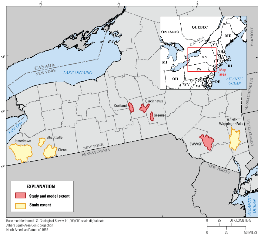
The locations of the eight groundwater study areas in upstate New York. Groundwater-flow models were developed by Corson-Dosch and others (2022) and Friesz and others (2022) for four of the eight study areas, and these four areas are shown in red. EWWSF, The villages of Ellenville and Wurtsboro and hamlets of Woodbourne and South Fallsburg.
The villages of Ellenville and Wurtsboro and hamlets of Woodbourne and South Fallsburg (EWWSF) study area is the focus of this report and is representative of the methods used for the other seven study areas. The methods detailed in this report offer a novel procedure to create continuous subsurface hydrogeologic data layers in areas with limited hydrogeologic data. These methods can be applied to similar study areas to interpolate the different hydrogeologic layer altitudes, which are useful for multiple applications, including groundwater-flow models, aquifer mapping, and bedrock-surface mapping.
Purpose and Scope
The purpose of this report is to describe the data sources and methods used to create digital hydrogeologic maps in the eight study areas in upstate New York. The scope of this effort included the interpretation and evaluation of the hydrogeologic framework derived from light detection and ranging (lidar) datasets, surficial geology, soil descriptions, aquifer maps, and lithologic well logs. The surficial geology; thickness of the surficial aquifers (primarily sand and gravel); and tops of the confining units (primarily lacustrine silt and clay), confined aquifers (primarily sand and gravel), and bedrock (primarily shale and sandstone) surfaces were interpolated and digitally mapped.
Description of Study Areas
The eight study areas encompass the valley-fill aquifers and surrounding till-covered uplands in the vicinity of the villages of Ellenville and Wurtsboro and hamlets of Woodbourne and South Fallsburg (EWWSF) in Sullivan and Ulster Counties, town of Greene in Chenango County, city of Cortland and town of Cincinnatus in Cortland County, city of Jamestown in Chautauqua County, city of Olean and village of Ellicottville in Cattaraugus County, and villages of Fishkill and Wappinger Falls in Dutchess County (fig. 1). The boundaries of the study areas were delineated by using 12-digit hydrologic unit code (HUC) surface-water drainage boundaries to include the valley-fill aquifer reaches of interest and the adjacent uplands (U.S. Geological Survey, 2020a). In some areas, slight modifications were made to the 12-digit HUC study-area boundaries on the basis of visual inspection of topographic maps. The regions of high altitude surrounding the study areas are a critical source of groundwater and tributary flow to the respective valley-fill aquifers (Randall, 2001) and were included in each study area to provide supporting information for the associated groundwater-flow models and potential future groundwater-contributing area investigations.
Hydrogeologic Settings of Valley-Fill Aquifers
During multiple continental glaciations beginning about 120,000 years ago, glacial ice deeply eroded existing stream and river valleys throughout the northeastern United States. Almost all of the unconsolidated sediments filling the valleys in the study areas were deposited during the most recent deglaciation, which occurred between 18,500 and 13,000 years ago (Cadwell, 1986). The uplands are typically covered by till with local bedrock outcrops. The till consists of unsorted silt, clay, sand, and clasts directly deposited by glacial ice as lodgement till and during deglaciation as ablation till. The valley fill as described by Randall (2001) primarily consists of three depositional facies that are locally successive but are transgressive over longer distances (tens of kilometers). The three depositional facies are the following: (1) early deglacial, proximal, or ice-contact facies deposited after the Wisconsin glacial maximum, composed of predominantly gravel, sand, and silt, varying widely in degree of sorting, and deposited close to active ice or amid abundant stagnant ice masses (referred to as kame deposits in this report, and kame moraines where deposits are contiguous); (2) mid-deglacial distal facies of lacustrine silt and clay deposited in moderately large bodies of water (proglacial lakes) at distance from the active glacial ice; and (3) late deglacial and postglacial facies of surficial gravel, sand, and silt that can be well sorted, deposited as alluvium, alluvial fans, and outwash, most commonly atop early and mid-deglacial facies (Randall, 2001, p. B12). All three depositional facies are present in many postglacial valleys; however, in some valleys, only one or two of the depositional facies are present. The lacustrine facies generally are the most extensive and thickest of the three facies. Figure 2 provides definitions of the geologic units that are referenced throughout the text and figures.
The hydrogeologic framework of the valley-fill aquifers resulting from this depositional sequence is depicted in figure 3. Where surficial alluvial and ice-contact deposits are saturated, they form an unconfined sand and gravel aquifer. The base of the unconfined sand and gravel aquifer is in contact with either the top of the lacustrine unit or bedrock. The lacustrine deposits of silt and clay form a confining to semiconfining unit for underlying ice-contact deposits of sand and gravel.
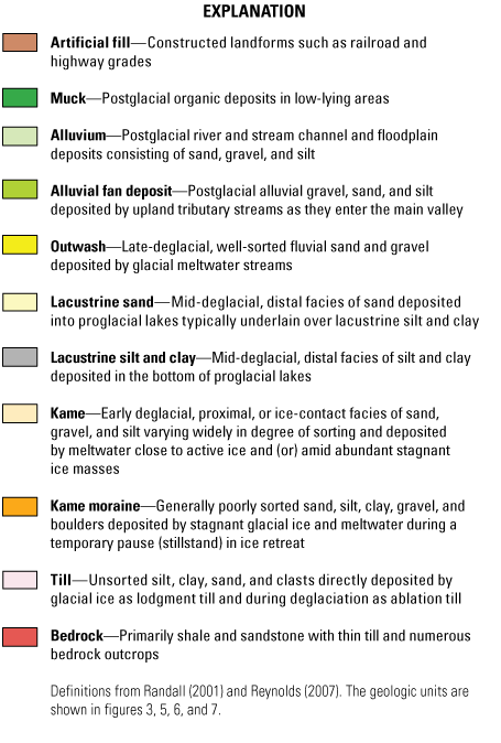
Definitions of geologic units referenced within the text and figures 3, 5, 6, and 7, from Randall (2001) and Reynolds (2007).
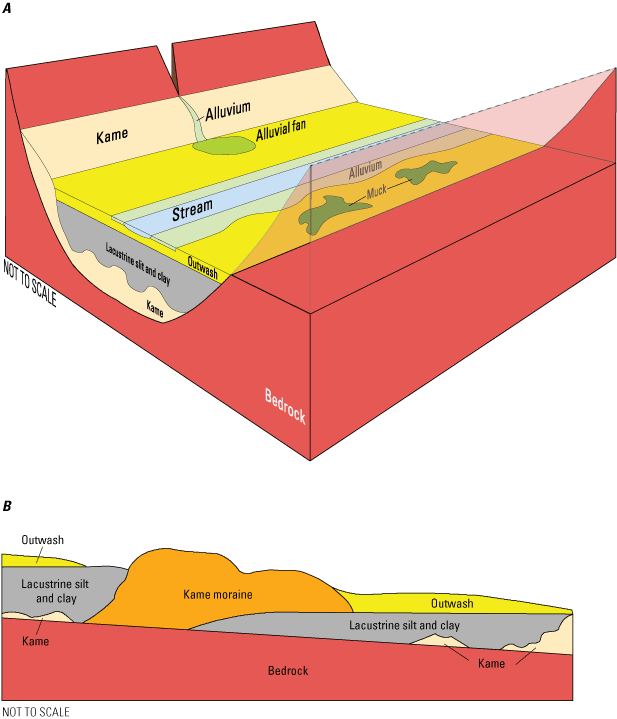
Idealized representations of the hydrogeologic framework of a valley-fill aquifer: A, cross-valley view and B, down-valley view (modified from Miller and others, 1988). See figure 2 for definitions of the geologic units.
Data Sources
The digital hydrogeologic maps were primarily derived from lidar datasets, published surficial geology and other aquifer maps and hydrogeologic cross sections, Soil Survey Geographic Database (SSURGO) data layers, and lithologic well logs. Much of the supporting hydrogeologic information was derived from publications generated as part of the Federal-State cooperative aquifer-mapping program for New York. Since the early 1980s, the USGS in cooperation with the NYSDEC and New York State Department of Health has mapped more than 40 valley-fill aquifers in upstate New York (U.S. Geological Survey, undated). The mapping has included development of 1:24,000-scale maps of surficial geology, aquifer surfaces and thicknesses, hydrogeologic sections, and well log and test-hole data compilations. The published surficial geology map products from the program were previously georeferenced and digitized as part of the U.S. Environmental Agency Brownfields Program. The published maps of aquifer surfaces, thicknesses, and extents within the study areas were georeferenced and digitized as part of the present study (table 1).
Table 1.
Hydrogeologic maps digitized for use in this study in upstate New York.[OFR, Open-File Report; WRI, Water-Resources Investigations Report; SIM, Scientific Investigations Map; WSP, Water-Supply Paper]
| Local area of report (see figure 1) |
Report number | Georeferenced and digitized sections | Reference | Report web page |
|---|---|---|---|---|
| City of Cortland and towns of Cortlandville, Homer, and Preble, Cortland County | OFR 081–1022 | Plates 4, 5 | Miller and Brooks (1981) | https://doi.org/10.3133/ofr811022 |
| City of Cortland and town of Cortlandville, Cortland County | WRI 96–4255 | Figures 7, 8, 10 | Miller and others (1998) | https://doi.org/10.3133/wri964255 |
| Chenango River Valley, village of Greene and Chenango Valley State Park area, Chenango County | SIM 2005–2914 | Plates 3, 4, 5, 6, 7 | Hetcher-Aguila and Miller (2005) | https://doi.org/10.3133/sim2914 |
| Chenango River valley, Chenango County | OFR 2003–242 | Plates 3, 4, 5, 6 | Hetcher and others (2003) | https://doi.org/10.3133/ofr03242 |
| Hamlets of South Fallsburg and Woodbourne area, town of Fallsburg, Sullivan County | OFR 82–112 | Plates 2, 4 | Anderson and others (1982a) | https://doi.org/10.3133/ofr82112 |
| Port Jervis Trough area, Sullivan and Ulster Counties | SIM 2007–2960 | Sheets 3, 4 | Reynolds (2007) | https://doi.org/10.3133/sim2960 |
| Orange and Ulster Counties | WSP 1985 | Plate 2 | Frimpter (1972) | https://doi.org/10.3133/wsp1985 |
| Jamestown area, Chautauqua County | OFR 82–113 | Sheets 4, 5 | Anderson and others (1982b) | https://doi.org/10.3133/ofr82113 |
| Jamestown area, Chautauqua and Cattaraugus Counties | Bulletin 58–1960 | Plates 1, 2, 3, 4 | Crain (1966) | https://archive.org/details/usgswaterresourcesnewyork-nywrc_bull_58 |
| Allegheny River, Olean Creek, Fivemile Creek, Haskell Creek, and tributary valleys, towns of Allegany, Olean, and Portville, Cattaraugus County | WRI 85–4157 | Plates 2, 4, 5, 6, 9 | Zarriello and Reynolds (1987) | https://doi.org/10.3133/wri854157 |
| City of Olean area, Cattaraugus County | WRI 85–4082 | Plates 1, 2 | Bergeron (1987) | https://doi.org/10.3133/wri854082 |
| City of Olean area, Cattaraugus County | WRI 87–4043 | Plates 2, 3, 4 | Yager and Bergeron (1988) | https://doi.org/10.3133/wri874043 |
| Town of Fishkill, Dutchess County | OFR 80–437 | Plates 2, 3 | Snavely (1980) | https://doi.org/10.3133/ofr80437 |
| Sprout and Fishkill Creek valleys, Dutchess County | SIM 3136 | Sheets 3, 4 | Reynolds and Calef (2010) | https://doi.org/10.3133/sim3136 |
Data layers from SSURGO were obtained from the Cornell University Geospatial Information Repository (U.S. Department of Agriculture, 2013a, b, 2014a, b, 2015). Nomenclature within the SSURGO datasets sometimes differed between counties, so similar soil types were correlated and sorted into geologic groups. Lidar datasets were sourced from the New York State Geographic Information Systems Clearinghouse (New York State Geographic Information Systems Clearinghouse, undated). In a study area where no published 1:24,000-scale surficial mapping was available, SSURGO data layers (lidar data, topographic maps, and lithologic well logs) were used to map the surficial geology.
Well logs, test-hole records, and lithologic well logs were obtained from published reports and databases including the USGS National Water Information System (NWIS; U.S. Geological Survey, 2021b), the NYSDEC Water Well Permit (WWP) database (available from the New York State Department of Environmental Conservation upon request), and the New York State Department of Transportation (NYSDOT) test-boring database (available from the New York State Department of Transportation upon request). The locations of production wells obtained from NWIS were verified through inspection of aerial images and adjusted when the listed latitude and longitude did not coincide with the aerial imagery. The locations of wells from the NYSDEC WWP database were also verified through inspection of aerial images to resolve cases where the driller’s log conflicted with other surface or subsurface information.
Well and test-boring records and lithologic well logs used in this study are available in a companion USGS data release (Woda and others, 2022) and on the USGS Geolog Locator (USGS, 2021a).
Methods
The methods used to create the digital hydrogeologic maps are described in the following sections. These maps include the interpretation of the altitude of hydrogeologic surfaces of interest from surficial geology and aquifer maps, lidar datasets, and lithologic well logs based on geographic information system (GIS) methods and interpolation tools. All geoprocessing was done by using ArcGIS Desktop 10.7.1 (Esri, 2019). To reduce redundancy, the following methods and accompanying figures focus on the EWWSF study area (fig. 1). Additional detail and minor modifications in the application of the methods and data sources for each study area are described in this report and companion data release and metadata files (Woda and others, 2022).
Raster Surface Interpolation and Evaluation for the Villages of Ellenville and Wurtsboro and Hamlets of Woodbourne and South Fallsburg Study Area
Digital surfaces were created by using an array of point and contour inputs and common interpolation tools including Topo to Raster, Natural Neighbors, Kriging, and Bayesian Kriging (Esri, 2019). Interpolations were calibrated and validated for each dataset by using a stepwise statistical-testing approach (Jahn, 2020). Interpolation tools tested include those listed above and incorporated multiple kriging (simple, universal, and ordinary) and model types (stable, circular, spherical, exponential, rational quadratic, Gaussian, K-Bessel, and J-Bessel) (Esri, 2019). Each kriging and model type produces a different interpolation of the data tested in this study.
The testing consisted of excluding 10 percent of all data points from the initial interpolation. A raster was then generated for the remaining 90 percent of points. Using this newly generated raster, the absolute difference was calculated at every data point. The models with the smallest amount of mean and median absolute difference were chosen on the basis of statistical results, visual inspection, and representation of local hydrogeology. In cases where the majority data type was contour lines (which was the result only for the bedrock surface in the Cortland study area) (fig. 1), the Topo to Raster interpolation method was used because both contour and point data types can be incorporated with this method.
Land Surface
The land-surface altitude was compiled from multiple New York State lidar dataset collections obtained from the New York State GIS Clearinghouse (New York State Geographic Information Systems Clearinghouse, undated). The lidar datasets were developed by multiple agencies (USGS, NYSDEC, and New York State Department of Environmental Protection) or by the county of interest. These collections all have a resolution of 1, 2, or 3 meters (m). A lidar-derived, land-surface altitude map for the EWWSF study area is shown in figure 4. The land-surface altitude coverage shown is a mosaic dataset of three individual lidar sources (Terrapoint USA, 2008; New York State Department of Environmental Preservation, 2009; U.S. Geological Survey, 2015). To match the resolution of the other interpolated geologic layers, the land-surface raster cell size was up-scaled to a 38.1 m (125-foot [ft]) discretization. The land-surface altitude for each grid cell was assigned the minimum lidar value within the cell. Cell altitudes were calculated in this fashion for groundwater-modeling purposes.
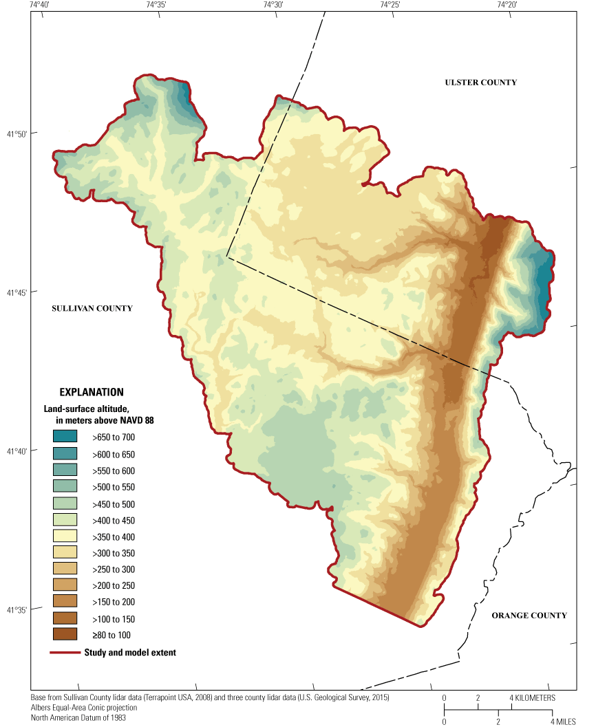
Land-surface altitude, derived from light detection and ranging (lidar), in the valleys and uplands of the villages of Ellenville and Wurtsboro and hamlets of Woodbourne and South Fallsburg study area, upstate New York. The land surface is represented in meters above the North American Vertical Datum of 1988 (NAVD 88).
Surficial Geology
Surficial geology was determined from published 1:24,000-scale maps (from Anderson and others, 1982a; Reynolds, 2007) and supplemented with data layers from the SSURGO, lidar, topographic maps, and lithologic well logs where published surficial geology was limited. In study areas with no published surficial geology, the geology was approximated by using SSURGO data layers, lidar, topographic maps, and lithologic well logs. The extent of surficial sand and gravel aquifers in the valleys and their contact with the till-covered bedrock uplands was defined by the extent of contiguous valley-fill sediments of alluvium, alluvial-fan deposits, outwash, deltaic and lacustrine sand, and kame deposits (fig. 5). Peat and muck in contact with sand and gravel deposits in the valleys were included in the extent. Contiguous deposits constituting kame moraine were also included, despite these deposits often containing discontinuous till, silt, and clay beds. Till moraine was excluded even though these deposits contain scattered beds of sand and gravel. An example of the surficial geology and its relation with the subsurface geology near Wurtsboro in the EWWSF study area is presented in figures 6 and 7. The surficial geology shown in figure 6 is underlain by a hillshade base layer derived from lidar (Terrapoint USA, 2008). This hillshade effect highlights the steep topography prevalent throughout the study area.
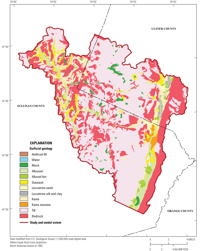
Surficial geology in the valleys and uplands of the villages of Ellenville and Wurtsboro and hamlets of Woodbourne and South Fallsburg study area, upstate New York. See figure 2 for definitions of the geologic units.
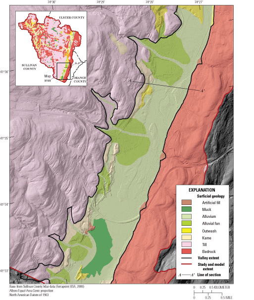
Surficial geology in selected area of Sullivan County, upstate New York. See figure 2 for definitions of the geologic units. lidar, light detection and ranging.
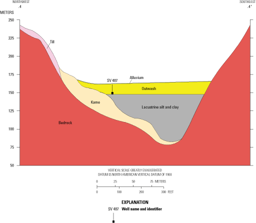
Subsurface geology along geologic section A–A′ in Sullivan County, upstate New York (modified from Reynolds, 2007). Well SV 487 is projected onto the geologic section for reference. Section A–A′ shown in figure 6. See figure 2 for definitions of the geologic units.
Thickness of Surficial Sand and Gravel Unconfined Aquifer
The thickness of the surficial sand and gravel aquifer in the valleys was defined by subtracting the top of the confining lacustrine silt and clay, where present, from the land-surface altitude. Bedrock-surface altitude was subtracted from the land-surface altitude if the confining unit was not present. Lithologic well logs from NYSDEC, NYSDOT, and USGS were individually evaluated to determine the altitude of the top of the confining unit (if present). Hydrogeologic sections were also used from previous USGS reports for the EWWSF study area (Anderson and others, 1982a; Reynolds, 2007).
The thickness of the surficial sand and gravel aquifer for the EWWSF study area is shown in figure 8. Where lacustrine silt and clay is mapped at the surface, it is assumed that there is no aquifer present at that location (fig. 8B). In areas where a confining unit was not identified (fig. 9), it is assumed that the thickness of the surficial sand and gravel aquifer represents the entire thickness between land surface and bedrock surface.
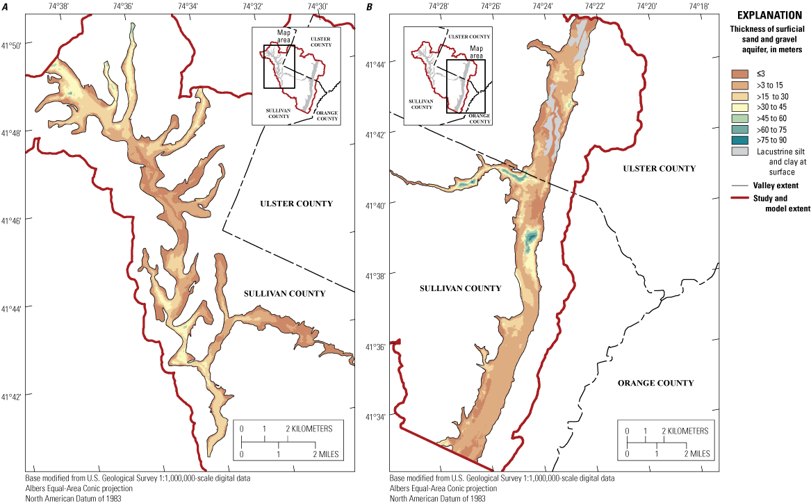
Thickness of surficial sand and gravel aquifer in the villages of Ellenville and Wurtsboro and hamlets of Woodbourne and South Fallsburg study area, upstate New York, for the A, western valley and B, eastern valley.
Top of Lacustrine Silt and Clay Confining Unit
The top of the lacustrine silt and clay confining unit was defined by the contact with overlying surficial sand and gravel aquifer or land surface where the silt and clay were exposed at the surface. As stated above, the confining-unit extent and thickness were primarily obtained from lithologic well logs and published hydrogeologic sections. The top altitude of the confining unit was interpolated by using the Topo to Raster tool. For example, the spatial extent and altitude of the top of the confining unit in the EWWSF study area are shown in figure 9. The confined extent illustrates where a thickness of at least 1 m of laterally continuous lacustrine silt and clay was present. This extent was established from published reports and sections (Anderson and others, 1982a; Reynolds, 2007) and lithologic well logs.
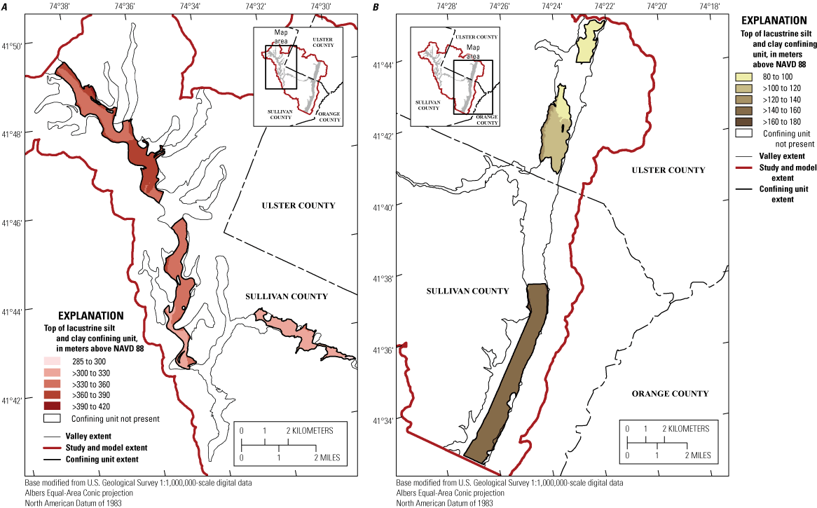
Top of the lacustrine silt and clay confining unit in the villages of Ellenville and Wurtsboro and hamlets of Woodbourne and South Fallsburg study area, upstate New York, for the A, western valley and B, eastern valley. NAVD 88, North American Vertical Datum of 1988.
Top of Sand and Gravel Confined Aquifer
The top surface of the sand and gravel confined aquifer was defined by the contact with the overlying confining unit. This surface was interpolated by using the Topo to Raster tool. The spatial extent and altitude of the top of the sand and gravel confined aquifer in the EWWSF study area are shown in figure 10. The confined unit was assumed to have a minimum thickness of 1 m in areas with no nearby sections or lithologic well logs. The bottom of this unit is inferred to be the top of bedrock, although till deposits may locally be present above the bedrock.
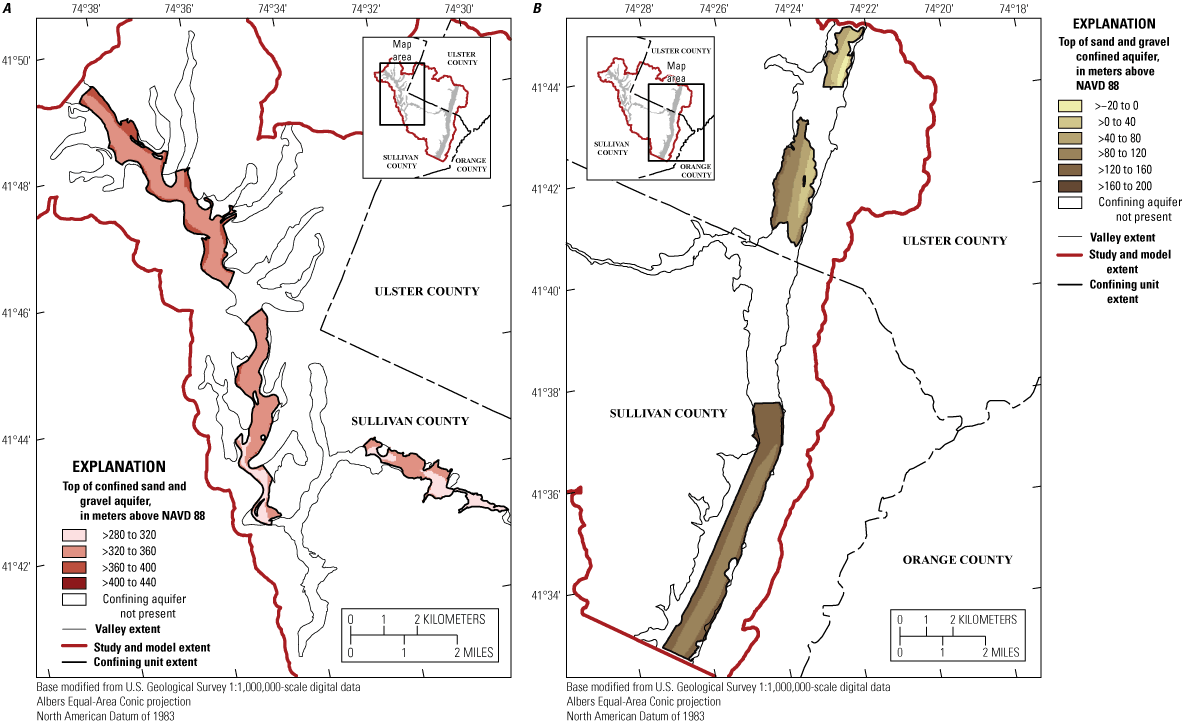
Top of the sand and gravel confined aquifer in the villages of Ellenville and Wurtsboro and hamlets of Woodbourne and South Fallsburg study area, upstate New York, for the A, western valley and B, eastern valley. NAVD 88, North American Vertical Datum of 1988.
Bedrock Surface
The bedrock surface defines the bottom of unconsolidated deposits. Although the completed bedrock-surface maps are presented as a singular continuous surface (fig. 11), different interpolation methods were applied in the valleys and the uplands. Although the methods differed, the same interpolation tool (Topo to Raster) was used for both the valleys and uplands.
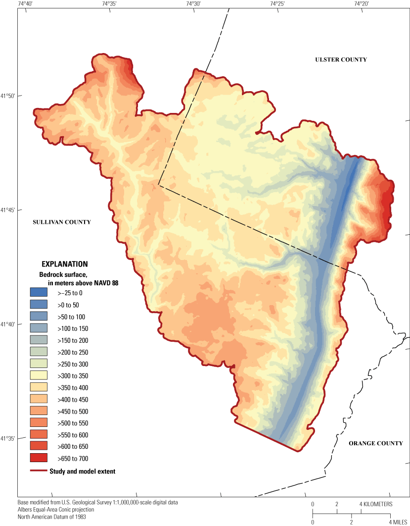
Bedrock surface in the valleys and uplands of the villages of Ellenville and Wurtsboro and hamlets of Woodbourne and South Fallsburg study area, upstate New York. Bedrock inputs are shown in figure 12. NAVD 88, North American Vertical Datum of 1988.
In the valleys, published hydrogeologic sections and lithologic well logs were used to create the bedrock surface. Glaciated valleys are commonly U-shaped; therefore, when extrapolating the bedrock surface from sections and logs, the following technique was applied to ensure that the interpolated bedrock surface approximated a U-shape. A series of points were generated 61 m (200 ft) apart down the center of the entire valley (fig. 12). These points, referred to as smoothing points, were each assigned a bedrock-surface altitude based on nearby lithologic well logs or published cross sections. In areas where lithology logs and sections were unavailable, the bedrock-surface altitude was linearly interpolated between two known values.
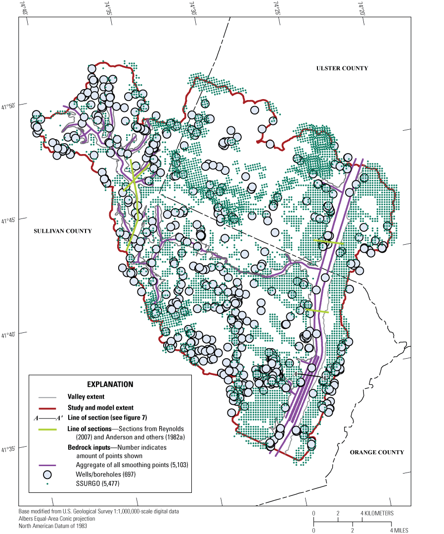
Data and interpolation points for mapping top of bedrock input points in the villages of Ellenville and Wurtsboro and hamlets of Woodbourne and South Fallsburg study area, upstate New York. Wells and borings include a compilation of lithologic well logs from the New York State Department of Environmental Conservation, the U.S. Geological Survey National Water Information System database, and the New York State Department of Transportation. Soil Survey Geographic Database (SSURGO) points reference locations where SSURGO indicated that bedrock was at or near the surface (bedrock depth of 3 meters (10 feet) was used to reflect these data) values. Valley edge points are not shown but are discussed in the text.
The process of adding points and assigning altitudes within the valley was also used along the valley walls. To best interpolate a U-shaped surface, the point inputs must reflect a continuous rise in bedrock altitude from the center of the valley to the valley walls. Along the valley walls, it was assumed the bedrock surface was approximately 3 m (10 ft) below land surface in areas that lacked hydrogeologic sections and lithologic well log data. A thickness of 3 m (10 ft) was used to accommodate the minimum thicknesses of the other layers in the hydrogeologic framework, which was done for groundwater-modeling purposes. The exception to this application was if there was a well nearby that indicated an appreciable depth (greater than 3 m) to bedrock. That depth to bedrock value was then assigned to the valley wall edge points near the well location.
In areas within the valley where little to no bedrock data were available, the altitude was obtained and extrapolated from the closest known values. In these cases, it was assumed that the bedrock-surface altitude was not constant. For example, valley point altitudes parallel to the valley (perpendicular to geologic section lines) were obtained and extrapolated from each geologic section (fig. 12). This process was necessary so that the Topo to Raster interpolation could generate the assumed U-shaped valley bottom.
In some local upland areas, especially where data were lacking, casing depths in wells were used to estimate depth to bedrock. In general, there is a consistent relation between casing depth and depth to bedrock. Drillers commonly set casing 3 m (10 ft) into bedrock. Thus, the assumption was made that in wells where the total well depth was at least 6 m (20 ft) greater than the casing depth, the unconsolidated thickness was estimated to be 3 m (10 ft) less than casing length.
In the upland area, published surficial geologic maps and SSURGO data layers were used with lithologic well logs to define the top of the bedrock surface. Instead of using bedrock-altitude data directly for the interpolations, the thickness of unconsolidated deposits was interpolated and then subtracted from the land-surface altitude to create the bedrock-surface altitude. The reason this method was used is that the steep and variable upland topography causes interpolated bedrock surfaces to be substantially above or below land surface in areas where data were sparse. The surficial-geology map units designated as “rock” (from Anderson and others, 1982a; Reynolds, 2007) and SSURGO map units described as rock outcrop and thin soils were assigned depths to bedrock of 3 m (10 ft) below land surface. Points were added within these surficial and SSURGO polygons in a gridded fashion, spaced approximately 100 m (300 ft) apart. The equidistant spacing of these points was altered depending on the amount of SSURGO bedrock representative polygons within the eight study areas.
Modifications for Cortland, Cincinnatus, and Greene Study Areas
Hydrogeologic mapping of the Cortland, Cincinnatus, and Greene study areas (fig. 1) was generally completed by using the same methods as used for the EWWSF study area. However, variations in available data or site-specific hydrogeologic conditions commonly required minor deviations from the methods described above. The modifications to the methods applied for each study area are described below.
One reason for the slight variation in methods among the eight study areas is the range of data available from previous reports for the study areas. Different data types were available for each study area, which required slightly different methods for each study area to achieve the required hydrogeologic framework. For example, published bedrock contours were available in the Cortland and Green study areas but not in the EWWSF or Cincinnatus study areas. Subsequently, where bedrock contour lines were available, these lines were used as the basis for the bedrock surface raster (Cortland and Greene study areas). In contrast, the major inputs for bedrock surface raster interpolation for EWWSF and Cincinnatus groundwater-flow model areas were lithologic well log data, geologic sections from published reports, SSURGO data layers, and implementation of smoothing points. The large variation in data required different interpolation methods to best fit the data for each study area. The interpolation methods used for these study areas differed from the EWWSF study area, where all surfaces were interpolated using the Topo to Raster tool. Metadata in Woda and others (2022) details the interpolation method for each digital layer of the hydrogeologic framework for each study area.
The Cortland hydrogeologic framework has been extensively studied (Miller and Brooks, 1981; Miller and others, 1998). The published data were adequate to allow for creation of all the necessary digital layers of the hydrogeologic framework without intensive analysis of lithologic well logs. However, the abundance of data within this study area required different methods from those used in other study areas when interpolating the altitude of the hydrogeologic surfaces. For example, the bottom of the surficial sand and gravel aquifer was based on published contour lines of the potentiometric-surface altitude and the unconfined aquifer thickness (Miller and Brooks, 1981, available in Woda and others, 2022). These contour lines were then interpolated to create two separate raster layers. The resulting unconfined aquifer thickness raster was subtracted from the potentiometric-surface altitude raster, and the resultant raster represents the bottom of the surficial sand and gravel aquifer, or the top of the lacustrine silt and clay confining unit (where lacustrine silt and clay are present).
Another difference in the Cortland study area, as compared to the other study areas, is that the use of smoothing points was unnecessary in the main valley because a U-shaped valley bottom was already depicted in published reports (modified from Miller and others, 1998). Slight adjustments to the published contours were made to reflect newly available data. In addition, the confining-unit bottom altitude (and thickness) was derived primarily by using previously published cross sections (Miller and Brooks, 1981).
In contrast to the Cortland study area, no published report data were available for the Cincinnatus study area. Consequently, all layers in the hydrogeologic framework were interpolated by using lithologic well logs, lidar, SSURGO data layers, and geologic interpretation. Where data were unavailable, smoothing points were implemented, as described above for the EWWSF study area.
Data available for the Greene study area (fig. 1) varied, as published report data were available in some parts of the area (Hetcher and others, 2003; Hetcher-Aguila and Miller, 2005), whereas no data were available in other parts. Data from multiple reports were used in the analysis, and in some areas the data conflicted, such as conflicting water-table altitudes or aquifer thicknesses. Where data from the reports conflicted, contours were modified to reflect multiple datasets, with all available data in those parts of the study area taken into consideration.
Smoothing points and valley-edge points were used in areas without existing data. In these cases, smoothing points were given an assumed altitude that best reflected the known characteristics of the valley-fill aquifer.
Modifications for Fishkill-Wappinger Falls, Jamestown, Olean, and Ellicottville Study Areas
Hydrogeologic mapping of the Fishkill-Wappinger Falls, Jamestown, Olean, and Ellicottville study areas was generally completed by using the same methods applied in the EWWSF study area. However, unlike the other four study areas, the hydrogeologic maps developed for these study areas were not applied to the groundwater-flow models. Consequently, methods were modified and changes were applied to both the hydrogeologic framework and its presentation to make the data usable by a wider audience. Notably, data for all four study areas were not mapped to a specific model grid developed for these four study areas. Instead, hydrogeologic surfaces were produced as raster datasets for general use and application.
The interpolated hydrogeologic surfaces for the study areas without models included the altitude of the bedrock surface and the altitude of the top and bottom of the confining unit. These three surfaces, along with the land-surface altitude, allow for the calculation of the thickness of the surficial sand and gravel aquifer (land-surface altitude minus either the altitude of the bedrock surface or the altitude of the top of the confining unit). A calculation of the thickness of the sand and gravel confined aquifer, if present, can also be performed (altitude of the bottom of the confining unit minus the bedrock-surface altitude). Method variations and notable observations by study area are described below.
No published aquifer maps or other hydrogeologic studies were available for the Ellicottville study area (fig. 1). The available lithologic well logs in this area indicated that the valley fill consists primarily of sand and gravel. Relatively thin beds of silt and clay (less than 5 m thick) are discontinuously present at intermediate depths, so no continuous confining unit was recognized, and therefore only the top of the bedrock surface was produced. The thickness of the surficial sand and gravel aquifer was calculated as the difference between the bedrock and land-surface altitudes.
The valley-fill sediments in the Jamestown study area (fig. 1) were extremely thick. The bedrock at its deepest recorded location was about 300 m below land surface. The top of bedrock in these thick valley-fill areas was mapped on the basis of lithologic well logs from oil and gas wells in the Empire State Organized Geologic Information System (ESOGIS) (New York State Museum, 2021). The ESOGIS wells facilitated an update of bedrock surface contour lines mapped by Crain (1960, 1966) and provided an opportunity to interpolate the bedrock altitude in previously unmapped areas. In addition, thick lacustrine units were prevalent throughout the Jamestown study area and in some areas were exposed at land surface, as indicated by the surficial geology. Available data in Anderson and others (1982b) and in lithologic well logs were used to map the upper confining unit. However, thick intervals of the valley fill (in some areas hundreds of meters of thickness) and a lack of data limited any additional hydrogeologic mapping in this area. Therefore, the hydrogeologic framework provided for the Jamestown study area defined the surficial sand and gravel aquifer thickness, the top and bottom of the upper confining unit, and top of the upper sand and gravel confined aquifer. Additional lacustrine confining units and deeper confined aquifers may be present below what was defined.
The Olean study area (fig. 1) featured an abundance of published report data (see Woda and others, 2022), including numerous geologic sections in the main valley area. These sections were used with lithologic well logs to map the extent and thickness of the primary lacustrine confining unit. Additionally, confining units were excluded from areas where kame deposits were mapped at land surface, as was the case for all study areas. The confining-unit extent produced for this study area may not include all areas where a confining unit is present, especially where data were lacking. In addition, data from multiple reports, geologic sections, and lithologic well logs highlighted multiple confining units near the center of the study area. The abundance of available data allowed the extent and altitude of a second confining unit to be mapped. The Olean study area was unique in that the southern part of the area was not covered by the most recent glaciation (Zarriello and Reynolds, 1987). The published surficial geology in this study area (from Zarriello and Reynolds, 1987) was further refined by using the SSURGO mapping dataset.
The Fishkill-Wappinger Falls study area (fig. 1) was distinctive because the hydrogeologic framework differed appreciably from the typical glacial valley-fill system found in most of upstate New York. This difference required an adjustment from the methods used in the other study areas. Notably, the process of smoothing lines and setting the valley edge points to assume a minimum thickness to bedrock was omitted for the Fishkill-Wappinger Falls study area because the bedrock surface did not clearly define a U-shaped valley bordered by uplands. Valley edge points were used to smooth the edges of the interpolation between the valley and upland areas. The bedrock altitude of the valley edge points was determined by using the valley bedrock interpolation, and this interpolation was used as input for the upland bedrock interpolation. In addition, the complex shape of the valley coupled with a lack of data made it difficult to map lacustrine confining units. This difficulty also was described in Reynolds and Calef (2010). Consequently, the lacustrine confining unit was only mapped in one small section in the southern part of the study area on the basis of lithologic well log data. The production wells associated with this study area were near this section; therefore, accurately depicting the confining unit here was a priority. The raster for the bottom of the confining unit was generated by using a constant thickness derived from only one lithologic well log. In areas where the constant thickness indicated that the bottom of the confining unit was below the top of the bedrock, the bottom of the confining unit was assumed to be 1 m higher than the top of bedrock surface.
Limitations, Postprocessing, and Use of Data
The development of the digital hydrogeologic data surfaces in this study came with challenges that resulted in limitations in the extent to which surfaces could be developed. Lithologic data were unevenly distributed throughout the eight study areas (fig. 1). Confidence in the hydrogeologic surfaces varied depending on data availability. To address areas where data were lacking, hydrogeologic assumptions were made to increase data density.
Additional checking and postprocessing of the interpolated hydrogeologic surfaces were performed because of data limitations. There were instances where interpolation results indicated that the bedrock surface was at a higher altitude than land surface, or other layers that should be above land surface. This result was observed in many of the interpolations and can be attributed to data gaps, where the interpolation tools could not account for locations where the bedrock altitude should always be at or lower than land surface. These locations were observed, and the interpolation artifacts were adjusted through use of the Raster Calculator tool (Esri, 2019). Each adjustment would consist of either raising or lowering the altitude of the layers at locations that conflicted with the altitude of another layer. For example, if the bedrock altitude subtracted from the land-surface raster resulted in a negative value, that would indicate that bedrock is at a higher altitude than land surface. For groundwater-flow modeling purposes, a minimum thickness was applied to each model grid cell, such that the thickness of material below a surface must always be at least 1 m.
Digital datasets of the locations of well and boring sites, land-surface altitudes, surficial geology, thicknesses of surficial sand and gravel, tops of lacustrine confining silt and clay and confined sand and gravel, and the bedrock surface are presented in Woda and others (2022). The hydrogeologic datasets are downloadable in GIS shapefiles and raster format, with a 38.1-m discretization. These data were used as inputs to groundwater-flow models used to determine source-water protection for select public supply wells (Corson-Dosch and others, 2022; Friesz and others, 2022). Replication of the analyses described in this report can be used to achieve the same goals for other sites and study areas in New York and elsewhere with similar hydrogeologic conditions. These datasets provide a greater understanding of the underlying hydrogeologic framework in glacial valley-fill aquifers and can be applied in the evaluation of groundwater-supply development.
Summary
Digital hydrogeologic data were developed for eight groundwater study areas in upstate New York (in parts of Chautauqua, Cattaraugus, Allegany, Cortland, Tompkins, Chenango, Sullivan, Ulster, Dutchess, and Putnam Counties) by the U.S Geological Survey, in cooperation with the New York State Department of Environmental Conservation, in a study conducted from 2019 to 2021. The eight study areas are referred to as Jamestown (Chautauqua and Cattaraugus Counties), Ellicottville (Cattaraugus County), Olean (Cattaraugus and Allegany Counties), Cortland (Cortland and Tompkins County), Cincinnatus (Cortland and Chenango Counties), Greene (Chenango County), and EWWSF (the villages of Ellenville and Wurtsboro and hamlets of Woodbourne and South Fallsburg in Sullivan and Ulster Counties), and Fishkill and Wappinger Falls (Dutchess and Putnam Counties). All hydrogeologic framework data described in this report are available in a companion U.S. Geological Survey data release. Groundwater-flow models were developed for the Cortland, Cincinnatus, Greene, and EWWSF study areas.
Challenges in the development of the digital surfaces resulted in limitations in the extent to which the surfaces could be created. Various methods were applied, and assumptions were made to increase data density in areas where hydrogeologic data were lacking. Additional checking and postprocessing of the interpolated hydrogeologic surfaces was performed because of the sparsity of available data.
The hydrogeologic surfaces were interpolated by using previously published and unpublished data, including lithologic well logs, surficial-geology data, bedrock and confining-unit contour lines and extents, and valley geologic sections. The ArcMap interpolation tool that was selected for each individual surface coverage was determined by use of a Python script that calculates the mean and median absolute error of the interpolation.
The datasets developed in this study provide a greater understanding of the underlying hydrogeologic framework in glacial valley-fill aquifers underlying upstate New York. The methods described in this report can be applied to other study areas to assist in developing the hydrogeologic framework for use in developing groundwater-flow models or other hydrogeologic applications.
References Cited
Anderson, H.R., Dineen, R.J., Stelz, W.G., and Belli, J.L., 1982a, Geohydrology of the valley-fill aquifer in the South Fallsburg-Woodbourne area, Sullivan County, New York: U.S. Geological Survey Open-File Report 82–112, 6 sheets. [Also available at https://doi.org/10.3133/ofr82112.]
Anderson, H.R., Stelz, W.G., Belli, J.L., and Allen, R.V., 1982b, Geohydrology of the valley-fill aquifer in the Jamestown area, Chautauqua County, New York: U.S. Geological Survey Open-File Report 82–113, 7 sheets. [Also available at https://doi.org/10.3133/ofr82113.]
Bergeron, M.P., 1987, Effect of reduced industrial pumpage on the migration of dissolved nitrogen in an outwash aquifer at Olean, Cattaraugus County, New York: U.S. Geological Survey Water-Resources Investigations Report 85–4082, 38 p. [Also available at https://doi.org/10.3133/wri854082.]
Cadwell, D.H., 1986, The Wisconsinan stage of the First Geological District, eastern New York: New York State Museum Bulletin Number 455, 192 p., accessed September 13, 2019, at https://purl.org/net/nysl/nysdocs/15099341.
Corson-Dosch, N.T., Fienen, M.N., Finkelstein, J.S., Leaf, A.T., White, J.T., Woda, J., and Williams, J.H., 2022, Areas contributing recharge to priority wells in valley-fill aquifers in the Neversink River and Rondout Creek drainage basins, New York: U.S. Geological Survey Scientific Investigations Report 2021–5112, 50 p., https://doi.org/10.3133/sir20215112.
Crain, L.J., 1966, Ground-water resources of the Jamestown area, New York—With emphasis on the hydrology of the major stream valleys: State of New York Conservation Department Bulletin 58, prepared by the U.S. Geological Survey, 167 p. [Also available at https://archive.org/details/usgswaterresourcesnewyork-nywrc_bull_58.]
Friesz, P.J., Williams, J.H., Finkelstein, J.S., and Woda, J.C., 2022, Areas contributing recharge to selected production wells in unconfined and confined glacial valley-fill aquifers in Chenango River Basin, New York: U.S. Geological Survey Scientific Investigations Report 2021–5083, 48 p., https://doi.org/10.3133/sir20215083.
Frimpter, M.H., 1972, Ground-water resources of Orange and Ulster Counties, New York: U.S. Geological Survey Water-Supply Paper 1985, 80 p., accessed September 13, 2019, at https://doi.org/10.3133/wsp1985.
Hetcher, K.K., Miller, T.S., Garry, J.D., and Reynolds, R.J., 2003, Geohydrology of the valley fill aquifer in the Norwich-Oxford-Brisben area, Chenango County, New York: U.S. Geological Survey Open-File Report 2003–242, 7 pls., scale 1:24,000, accessed September 13, 2019, at https://doi.org/10.3133/ofr03242.
Hetcher-Aguila, K.K., and Miller, T.S., 2005, Geohydrology of the valley-fill aquifers between the Village of Greene, Chenango County and Chenango Valley State Park, Broome County, New York; 2005: U.S. Geological Survey Scientific Investigations Map 2914, 8 pls., scale 1:24,000, accessed September 13, 2019, at https://pubs.er.usgs.gov/publication/sim2914.
Jahn, K.L., 2020, Arcpro-interpol-compare python script: GitHub repository, accessed September 21, 2020, at https://github.com/kallejahn/arcpro-interpol-compare.
Miller, T.S., and Brooks, T.D., 1981, Geohydrology of the valley-fill aquifer in the Cortland-Homer-Preble area, Cortland and Onondaga Counties, New York: U.S. Geological Survey Open-File Report 81–1022, 7 pls. [Also available at https://doi.org/10.3133/ofr811022.]
Miller, T.S., Sherwood, D.A., Jeffers, P.M., and Mueller, N., 1998, Hydrogeology, water quality, and simulation of ground-water flow in a glacial-aquifer system, Cortland County, New York: U.S. Geological Survey Water Resources Investigations Report 96–4255, 84 p., 5 pls., accessed September 13, 2019, at https://doi.org/10.3133/wri964255.
Miller, T.S., Sherwood, D.A., and Krebs, M.M., 1988, Hydrogeology and water quality of the Tug Hill glacial aquifer in northern New York: U.S. Geological Survey Water-Resources Investigations Report 88–4014. [Also available at https://doi.org/10.3133/wri884014.]
New York State Department of Environmental Preservation, Division of Water, Watershed GIT Support Group, 2009, West of Hudson lidar, point data: New York State department of Environmental Preservation dataset, accessed July 29, 2020, at ftp://ftp.gis.ny.gov/elevation/LIDAR/NYCDEP_WestOfHudson2009/.
New York State Geographic Information Systems Clearinghouse, [undated], New York State geographic information systems clearinghouse: New York State Geographic Information Systems Clearinghouse data catalog, accessed July 27, 2020, at https://gis.ny.gov/.
New York State Museum, 2021, Oil and gas well data in New York State: Empire State Organized Geologic Information System database, accessed February 15, 2021, at https://esogis.nysm.nysed.gov/.
Randall, A.D., 2001, Hydrogeologic framework of stratified-drift aquifers in the glaciated northeastern United States: U.S. Geological Survey Professional Paper 1415–B, 190 p., accessed September 13, 2019, at https://doi.org/10.3133/pp1415B.
Reynolds, R.J., 2007, Hydrogeologic appraisal of the valley-fill aquifer in the Port Jervis Trough, Sullivan and Ulster Counties, New York: U.S. Geological Survey Scientific Investigations Map 2960, 5 sheets, accessed September 13, 2019, at https://doi.org/10.3133/sim2960.
Reynolds, R.J., and Calef, F.J., III, 2010, Hydrogeologic data update for the stratified-drift aquifer in the Sprout and Fishkill Creek valleys, Dutchess County, New York: U.S. Geological Survey Scientific Investigations Map 3136, 4 sheets, scale 1:24,000, accessed September 13, 2019, at https://doi.org/10.3133/sim3136.
Snavely, D.S., 1980, Ground-water appraisal of the Fishkill-Beacon area, Dutchess County, New York: U.S. Geological Survey Open-File Report 80–437, 3 pls., 14 p. [Also available at https://doi.org/10.3133/ofr80437.]
Terrapoint USA, 2008, New York State LiDAR survey—Delaware and Susquehanna River Basin, point data: Terrapoint USA dataset, accessed July 29, 2020, at ftp://ftp.gis.ny.gov/elevation/LIDAR/FEMA_SusqehannaBasin2007/.
U.S. Department of Agriculture, 2013a, SSURGO soils, Sullivan County NY: Cornell University Geospatial Information Repository, accessed July 29, 2020, at https://cugir.library.cornell.edu/catalog/cugir-007917.
U.S. Department of Agriculture, 2013b, SSURGO soils, Ulster County NY: Cornell University Geospatial Information Repository, accessed July 29, 2020, at https://cugir.library.cornell.edu/catalog/cugir-007920.
U.S. Department of Agriculture, 2014a, SSURGO soils, Cortland County NY: Cornell University Geospatial Information Repository, accessed July 29, 2020, at https://cugir.library.cornell.edu/catalog/cugir-007903.
U.S. Department of Agriculture, 2014b, SSURGO soils, Orange County NY: Cornell University Geospatial Information Repository, accessed July 29, 2020, at https://cugir.library.cornell.edu/catalog/cugir-007911.
U.S. Department of Agriculture, 2015, SSURGO soils, Chenango County NY: Cornell University Geospatial Information Repository, accessed July 29, 2020, at https://cugir.library.cornell.edu/catalog/cugir-007902.
U.S. Geological Survey, 2015, 3-County LiDAR, point data: U.S. Geological Survey dataset, accessed July 29, 2020, at ftp://ftp.gis.ny.gov/elevation/LIDAR/USGS_3County2014/.
U.S. Geological Survey, 2020a, Hydrologic Unit Maps: U.S. Geological Survey web page, accessed March 10, 2021, at https://water.usgs.gov/GIS/huc.html.
U.S. Geological Survey, 2020b, National water information system—Mapper: U.S. Geological Survey database, accessed July 27, 2021, at https://maps.waterdata.usgs.gov/mapper.
U.S. Geological Survey, 2021a, GeoLog Locator: U.S. Geological Survey web application, accessed December 7, 2021, at https://webapps.usgs.gov/GeoLogLocator/#!/.
U.S. Geological Survey, 2021b, USGS water data for the Nation: U.S. Geological Survey National Water Information System database, accessed July 27, 2021, at https://doi.org/10.5066/F7P55KJN.
U.S. Geological Survey, [undated], Detailed aquifer mapping program in upstate New York: U.S Geological Survey web page, accessed July 27, 2020, at https://www.usgs.gov/centers/ny-water/science/detailed-aquifer-mapping-program-upstate-new-york.
Woda, J.C., Finkelstein, J.S., and Williams, J.H., 2022, Interpolated hydrogeologic framework and digitized datasets for upstate New York study areas: U.S. Geological Survey data release, https://doi.org/10.5066/P96R5K5R.
Yager, R.M., and Bergeron, M.P., 1988, Nitrogen transport in a shallow outwash aquifer at Olean, Cattaraugus County, New York: U.S. Geological Survey Water-Resources Investigations Report 87–4043, 6 pls., 51 p. [Also available at https://doi.org/10.3133/wri874043.]
Zarriello, P.J., and Reynolds, R.J., 1987, Hydrogeology of the Olean area, Cattaraugus County, New York: U.S. Geological Survey Water-Resources Investigations Report 85–4157, 9 sheets [8 maps and 1 data sheet]. [Also available at https://doi.org/10.3133/wri854157.]
Datum
Vertical coordinate information is referenced to North American Vertical Datum of 1988 (NAVD 88).
Horizontal coordinate information is referenced to the North American Datum of 1983 (NAD 83).
Altitude, as used in this report, refers to distance above the vertical datum.
Abbreviations
GIS
geographic information system
HUC
hydrologic unit code
lidar
light detection and ranging
NWIS
National Water Inventory System
NYSDEC
New York State Department of Environmental Conservation
NYSDOT
New York State Department of Transportation
SSURGO
Soil Survey Geographic Database
USGS
U.S. Geological Survey
WWP
Water Well Permit
For more information about this report, contact:
Director, New York Water Science Center
U.S. Geological Survey
425 Jordan Road
Troy, NY 12180–8349
(518) 285–5602
or visit our website at
https://www.usgs.gov/centers/ny-water
Publishing support provided by the
Pembroke Publishing Service Center
Disclaimers
Any use of trade, firm, or product names is for descriptive purposes only and does not imply endorsement by the U.S. Government.
Although this information product, for the most part, is in the public domain, it also may contain copyrighted materials as noted in the text. Permission to reproduce copyrighted items must be secured from the copyright owner.
Suggested Citation
Finkelstein, J.S., Woda, J.C., and Williams, J.H., 2022, Data sources and methods for digital mapping of eight valley-fill aquifer systems in upstate New York: U.S. Geological Survey Scientific Investigations Report 2022–5024, 21 p., https://doi.org/10.3133/sir20225024.
ISSN: 2328-0328 (online)
Study Area
| Publication type | Report |
|---|---|
| Publication Subtype | USGS Numbered Series |
| Title | Data sources and methods for digital mapping of eight valley-fill aquifer systems in upstate New York |
| Series title | Scientific Investigations Report |
| Series number | 2022-5024 |
| DOI | 10.3133/sir20225024 |
| Publication Date | May 02, 2022 |
| Year Published | 2022 |
| Language | English |
| Publisher | U.S. Geological Survey |
| Publisher location | Reston, VA |
| Contributing office(s) | New York Water Science Center |
| Description | Report: v, 21 p.; Data Release |
| Country | United States |
| State | New York |
| Online Only (Y/N) | Y |
| Additional Online Files (Y/N) | Y |