

Simulation of Regional Groundwater Flow and Groundwater/Lake Interactions in the Central Sands, Wisconsin
Links
- Document: Report (92.7 MB pdf) , HTML , XML
- Dataset: USGS National Water Information System database —USGS water data for the Nation
- Data Release: USGS data release - MODFLOW models used to simulate groundwater flow in the Wisconsin Central Sands Study Area, 2012-2018
- NGMDB Index Page: National Geologic Map Database Index Page (html)
- Download citation as: RIS | Dublin Core
Acknowledgments
The Wisconsin Geological and Natural History Survey and the University of Wisconsin were valuable technical partners and provided data and technical information.
The authors are grateful for invaluable technical advice from and discussions with Daniel Feinstein, Joe Hughes, Randy Hunt, Chris Langevin, John Masterson, Howard Reeves, and Dale Robertson of the U.S Geological Survey.
Abstract
A multiscale, multiprocess modeling approach was applied to the Wisconsin Central Sands region in central Wisconsin to quantify the connections between the groundwater system, land use, and lake levels in three seepage lakes in Waushara County, Wisconsin: Long and Plainfield (The Plainfield Tunnel Channel Lakes), and Pleasant Lakes. A regional groundwater-flow model, the Newton Raphson formulation of the U.S. Geological Survey modular finite-difference flow model groundwater-modeling package (MODFLOW-NWT), centered on the lakes, was used to extend regional surface-water boundaries to provide boundary conditions for two focused inset models, in the hydrologic simulation modeling package (MODFLOW 6), at higher resolution around the lakes. Land use and groundwater use were simulated at a regional scale using the Soil Water Balance model, which provided recharge and water-use boundary conditions for the MODFLOW models. Agricultural irrigation is the primary groundwater use in the area. Land and groundwater-use scenarios representing no irrigation, current (2018) irrigation, and potential future irrigation were simulated with the groundwater-flow model and the lake levels over a 38-year representative climate period.
Introduction
The effect of groundwater withdrawals on lake levels in the Wisconsin Central Sands region in central Wisconsin is of increasing concern. This report provides the necessary information concerning the application of numerical models for simulating regional groundwater flow and groundwater/lake interactions. The study was performed by the U.S. Geological Survey, with the Wisconsin Department of Natural Resources (WDNR), for the Central Sands region in central Wisconsin. Information described here was included as a technical appendix in a report to the Wisconsin State Legislature (Fienen and others, 2021a) by the WDNR (WDNR, 2021) in response to 2017 Wisconsin Act 10. This legislation directed WDNR to determine whether current (2018) and potential groundwater withdrawals are causing or are likely to cause significant reduction of mean seasonal water levels at Pleasant Lake, Long Lake, and Plainfield Lake (s. 281.34(7m)(2)(b), Wisconsin Statutes) in Waushara County, Wisconsin (fig. 1). To evaluate the potential hydrologic connection between groundwater withdrawals and the nearby study lakes, hydrologic models were developed that focused on the lakes of interest and covered the major hydrologic boundaries of the natural flow system. The areas near the lakes used finer-scale grid discretization (or spacing) to better represent the lakes and streams in the model simulation, but also needed to cover a large enough area to include the groundwater withdrawal locations that have the potential to lower water levels in the lakes. To accomplish these goals, three groundwater models were developed: a regional model extending to major hydrologic boundaries and two inset models, inheriting boundaries from the regional model but focused near the lakes. Each of the inset models, in turn, included a detailed area close to the lakes surrounded by an area at the same spatial scale as the regional model (fig. 1).
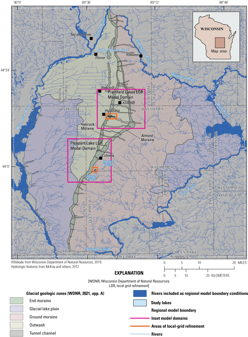
Central Sands region study area extent, moraines, streams, and study lakes, central Wisconsin.
For evaluating the connection between groundwater withdrawals and lake levels, a representative period was needed to compare land use with and without irrigated agriculture and for WDNR to evaluate potential lake stage and flux changes related to irrigated agriculture. WDNR chose the climate period of 1981–2018 to be representative of a typical period and provided two land-use scenarios—one with no irrigated agriculture and one with assumed crop rotations similar to current (2018) conditions. These conditions were simulated with the groundwater models and then the models were used to simulate lake responses. These model simulations are not intended to simulate hydrologic conditions during 1981–2018 because land use has changed appreciably in the area. Instead, model simulations are intended to provide a basis on which to compare land use with and without irrigation-related groundwater withdrawals based on the current arrangement of land use and a varied climatic period. Groundwater withdrawals focused on irrigated agriculture-related water use because greater than 95 percent of groundwater withdrawal in the two focused inset models around the study lakes is for irrigated agriculture water use.
The period 2012–18 was used for parameter estimation (synonymously referred to as “history matching”) for the groundwater models. This period was chosen because it includes the most complete water-use records to simulate groundwater withdrawals. History matching was performed using groundwater elevations, lake levels, and streamflow observations and processed observations derived from those data.
Climatic data were incorporated into the model using a soil-water balance approach. A soil-water balance model was constructed at the scale of the regional groundwater model to calculate recharge based on land use and climate, and in the long-term representative climate period simulations. The soil-water balance approach was used to estimate water use needed for irrigated agriculture and boundary conditions in the regional groundwater-flow model in the absence of reported water-use values over the representative climate period.
Purpose and Scope
The purpose of this report is to document the various conceptual and numerical models developed by the U.S. Geological Survey in cooperation with the WDNR for quantifying regional groundwater flow, the connections between groundwater conditions, and land use and lake levels in three seepage lakes in Waushara County, Wisconsin: two of the Plainfield Tunnel Channel Lakes (Long and Plainfield), and Pleasant Lake. Accompanying this documentation is background information, the parameter estimation, and uncertainty analysis used to estimate parameters for the models. Parameters are estimated to balance prior understanding of parameter values with correspondence between measured values and collocated model-simulated outputs. Uncertainty analysis evaluates the confidence in the model outputs. Finally, the model-simulated scenarios comparing varying land uses over the representative climate period are documented.
The model construction and analysis were performed to address the main study question of whether groundwater extraction related to agricultural irrigation significantly adversely affects lake hydrology in the Central Sands region in central Wisconsin. This report is focused solely on the technical aspects of the model development, parameter estimation, and uncertainty analysis, as well as the land use and representative long-term climate model scenarios.
Study Area Description and Hydrogeologic Setting
The Wisconsin Central Sands region is defined as the contiguous area east of the Wisconsin River with surficial sand-and-gravel deposits greater than 50 feet (ft) thick (Bradbury and others, 2017). The study area defined here extends to major surface-water features. These features were used later on to establish boundary conditions for the regional groundwater-flow model. This regional model (described in detail later in the report), in turn, supplies boundaries for focused models on the study lakes (Long, Plainfield, and Pleasant Lakes). The regional model domain covers about the southern 75 percent of the Central Sands region, extending from the Little Plover River (Bradbury and others, 2017) south to the border between Adams and Columbia Counties, and west to east from the Wisconsin River to the Tomorrow, Waupaca, Wolf, and Fox Rivers (fig. 1). Various end moraines of the Green Bay Lobe run north to south through the center of the study area. The moraines form the topographic high point between the Wisconsin River and the rivers that bound the study area to the east. The area around the moraines and the adjacent outwash plain to the west is characterized by a lack of surface-water drainage and marks the hydrologic divide between the Great Lakes and Mississippi River Basins. The Plainfield Tunnel Channel Lakes are between the Hancock and Almond Moraines, which merge south of Plainfield, Wisconsin, to form a single moraine that continues south past the western edge of Pleasant Lake to the southern boundary of the regional model.
The area west of the moraines is characterized by flat topography and undisturbed outwash sediments at land surface. Beneath the outwash, fine-grained deposits of the Quaternary-aged New Rome Member of the Big Flats Formation (hereafter referred to as the “New Rome Member”), associated with Glacial Lake Wisconsin, thicken to the southwest. Near the Hancock Moraine and eastward, the New Rome Member is absent. The area between the Hancock and Almond Moraines consists of flat outwash plain broken by a series of tunnel channel features with surface expressions that are 5–30 ft deep, east-west oriented linear depressions formed by glacial collapse. The subsurface between the two moraines is dominated by sand and gravel, but is more heterogeneous west of the Hancock Moraine (fig. 1), including discontinuous patches of fine-grained sediments deposited by various pro-, sub-, and supra-glacial processes. East of the Almond Moraine (fig. 1), the landscape is hummocky, underlain by collapsed sand and gravel outwash that is more heterogeneous than the outwash west of the moraines. Toward the eastern edge of the model, the coarser, sandy sediments transition to fine-grained deposits associated with Glacial Lake Oshkosh (WDNR, 2021: app. A). More details on the geologic history and subsurface lithology underlying the study area are from WDNR (WDNR, 2021: app. A).
Conceptualization of Groundwater Flow in the Central Sands Region
The groundwater-flow system was conceptualized, simulated, and analyzed at two scales. The regional scale encompasses much of the Central Sands region and was included to later provide model boundary conditions for the study lakes. The local-scale groundwater-flow systems were focused around the Plainfield Tunnel Channel Lakes (including Long and Plainfield Lakes) and Pleasant Lake [fig. 1]).
Regional Groundwater-Flow System
The study area is at the groundwater divide between two major drainage basins. The regional groundwater-flow system is fed almost entirely by terrestrial recharge. This recharge creates high points in the water table between surface-water features. Groundwater flows laterally away from these high points, until the water table meets the land surface, allowing groundwater to discharge into wetlands and streams. Many streams on the outwash plain west of the moraines begin as drainage ditches that were constructed to lower the water table for agriculture. East of the moraines, springs and local flowing artesian conditions are common (WDNR, 2021, app. A). Most groundwater flow occurs in the Quaternary-aged surficial aquifer made up of glacial lake, outwash, end moraine, till, stagnant ice, and stream sediment from a wide variety of formations (hereafter the “surficial aquifer”). Horizontal hydraulic conductivity in the surficial aquifer is an order of magnitude greater than hydraulic conductivity in the Cambrian-aged sandstone bedrock of the Elk Mound and Tunnel City Groups (hereafter referred to as “sandstone bedrock”). Most of the groundwater discharge is to interior streams, which are almost all gaining streams.
Typically, most recharge to the groundwater system occurs in March through May, after the spring freshet, with little to no recharge occurring during the growing season followed by a pulse of recharge in the fall after crops are harvested and by negligible recharge in the winter when the ground is frozen. On the outwash plain west of the moraines, the water table is generally within 5 m of land surface, and the lag between infiltration events and groundwater recharge arriving at the water table is minimal. Elsewhere in the study area, the depth of the water table varies with topography, but is generally deeper along the moraines, where it can locally exceed 100 ft. In areas of greater depth to water, the water-table response may lag infiltration events by a month or more (for example, Hunt and others, 2008). During the spring recharge period, groundwater storage has a net gain. With the onset of the growing season, recharge decreases quickly, and the groundwater system transitions from a condition of net storage gain to a condition of net storage loss. In the summer months, groundwater extraction can account for up to about half of the total groundwater discharge. In the fall months, there is often some recharge, but, typically, a net loss of groundwater storage to streamflow is observed, maintaining a generally stable supply of water to streams as base flow.
Hydrologic Budget
Much can be learned about a hydrologic system through analysis of the soil-water balance. Thornthwaite (1948) recognized the value of observing the “march of actual evapotranspiration” over the course of a year to quantify the growing-season periods where natural precipitation inputs are insufficient to balance evapotranspiration needs of crops and other vegetation. The components of the soil-water-balance are used here to estimate net infiltration—the amount of soil moisture that passes through the root zone and into the unsaturated soil zone that lies beneath it in most places throughout the Central Sands region. With time, most of this net infiltration eventually flows to the water table, becoming groundwater recharge. Net infiltration estimates are input directly into the groundwater-flow models described later in the report.
Net infiltration is one of the most difficult components of the hydrologic budget to estimate; limited direct observations of net infiltration are available. The use of a soil-water-balance approach depends on properly defining the remaining components of the water budget; net infiltration may then be calculated as the difference between the inputs and outputs of water to the root zone soil layer. A simplified description of the root zone soil-water balance is , where is the change in soil moisture from one day to the next (Westenbroek and others, 2010, 2018).
Annual precipitation in the Central Sands region ranges from less than 30 inches [in.] in 2012 to more than 114.3 cm (45 in. in 2018 [fig. 2]). For reference, the 30-year mean annual precipitation (calculated for the years 1981 through 2010) ranges between 81.3 and 86.4 cm (32 and 34 in., respectively) across the Central Sands region (PRISM Climate Group, 2020). The mean annual precipitation amount received over the Central Sands region during 2016–18 was well above the 30-year mean annual precipitation amount (fig. 2).
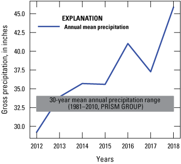
Gross annual mean precipitation and 30-year mean annual precipitation range for the Central Sands region, central Wisconsin, 2012–18.
Actual evapotranspiration (ET), the sum of bare soil evaporation and plant transpiration, varies widely with land use, crop or vegetative cover type, and the time of year. Actual ET over the region is generally low—less than 1 in.—for January, February, and March (Reitz and others, 2017a). Actual ET increases steadily with springtime vegetation and crop growth, peaking in about July at about 5 in. per month. Actual ET continues to decrease through August, September, and October, and is generally less than 1 in. per month for November and December.
Runoff in the Central Sands region is generally low but does affect the water budget. Annual mean runoff amounts for the study area range between 2 and 4 in., respectively; Reitz and others, 2017b); the years with larger runoff amounts than other years are the same years for which gross precipitation is higher than the 30-year “normal” amounts.
Irrigation amounts, as estimated by means of the Food and Agriculture Organization of the United Nations irrigation and drainage paper 56 (FAO-56) methodology (Allen and others, 1998), vary appreciably from year to year and from one crop type to another. Use of reported or metered irrigation amounts in the water-budget calculations would be preferable to use over estimated values, but reported values were only available for the history-matching period of 2012–18. For the longer range of climatic conditions required for the Lake Ecosystem Response Assessment (LERA) scenarios (1981–2018) simulated in the lake study, irrigation amounts computed by Soil Water Balance (SWB) (see SWB subsection of the “Numerical Models” section for a detailed description) were used. Irrigation amounts represent between 0.8 and 1.3 cm (0.3 and 0.5 inch per year, respectively) of water when averaged over the entire study area during 2012–18.
Finally, the net annual infiltration amount can be estimated once all the other water-budget components have been accounted for. Net infiltration averaged over the study area ranges from 6 in. in 2012 to 13 in. in 2018. April and October tend to have the highest estimated net infiltration amounts, with June, July, and August having the lowest amounts.
Aquifer Properties
The surficial aquifer ranges in thickness from thin to absent near topographic high points in the bedrock surface, to more than 100 m thick along the Almond Moraine (fig. 1) east of Plainfield, Wisconsin. Horizontal hydraulic conductivity in the surficial aquifer ranges from less than 1 m per day locally to 150 m per day or more, and values of 10–80 m per day are common (Weeks and Stangland, 1971; Hart and others, 2015; Bradbury and others, 2017). Horizontal hydraulic conductivity is generally higher in the well-sorted, undisturbed outwash west of the moraines, especially in the northwestern part of the study area. Vertical to horizontal anisotropy is commonly between 10 and 100. Specific yield in the surficial aquifer ranges from about 0.12 to 0.33, with a mean of about 0.17 (Weeks and Stangland, 1971; Hart and others, 2015; Bradbury and others, 2017).
Local-Scale Groundwater-Flow Systems
To simulate the potential interactions between irrigated agriculture and the study lakes, two local-scale groundwater-flow systems were analyzed and simulated (as described later), inset into the regional Central Sands region flow system. These two local-scale systems, Plainfield Tunnel Channel Lakes and Pleasant Lake (fig. 1), are discussed in the following sections.
Plainfield Tunnel Channel Lakes
The Plainfield Tunnel Channel Lakes area is focused on two of the study lakes, Plainfield and Long Lakes. Both lakes are shallow (no more than 15 ft deep) and were formed in a collapsed tunnel channel (for example, WDNR, 2021, app. A). The tunnel channel area near Plainfield contains several lakes in addition to the two (Plainfield and Long Lakes) considered in this area for this study. Hydraulically, the Plainfield Tunnel Channel Lakes are near the groundwater divide, in an area with no streams. Regional groundwater flow in this area is from north to south and towards the stream networks to the east and west (Central Sands model: Mechenich, 2012). Throughflow is the typical flow condition in the Plainfield Tunnel Channel Lake. Groundwater discharges into the north side of both lakes, and leakage flows out of the southern side of both lakes into the surficial aquifer (as described later in the “Regional Model Results” section). However, the lack of streams in this area results in greater fluctuations in groundwater levels in response to changes in recharge and pumping than in areas with more streams, where surface water buffers water-table fluctuations. This result is consistent with observations in seepage lakes in a similar glacial environment in Cape Cod, Massachusetts (McCobb and others, 1999), where the faster response of the surrounding groundwater system relative to the lake results in reversal of flow into or out of the lake depending on whether surrounding groundwater levels are rising or falling. In the spring of 2019, after an extended rise in the water table (WDNR, 2021, app. A), a transition to nearly all groundwater discharge around the perimeter of Plainfield and Long Lakes was observed, making the lakes act as sinks to the groundwater system. At other times, when water levels are declining, the lakes may leak around their perimeters and act as sources of water to the groundwater system. Variable groundwater levels and shallow bathymetries make the Plainfield Tunnel Channel Lakes prone to large changes in exposed shoreline, volume and surface area, and even periodic drying.
Pleasant Lake
The third study lake—Pleasant Lake—is relatively deep (nearly 25 feet) compared to the Plainfield Tunnel Channel Lakes and situated in a collapse feature just east of the moraine, near two headwater streams (Chaffee Creek and Tagatz Creek) (fig. 1). Regional groundwater flow in this area is to the east-southeast, away from the undrained area toward Chaffee Creek to the east and Tagatz Creek to the south as described later in the “Regional Model Results” section. The typical flow condition of Pleasant Lake is, therefore, one of groundwater discharge into the western and northern sides and leakage out to the groundwater system on the southern and eastern sides. Hydraulic gradients around Pleasant Lake are generally stable because of nearby streams and because the lake is downgradient from the groundwater divide. The steeper sides and greater depth of the Pleasant Lake Basin also make the lake shoreline area less sensitive to seasonal water-level fluctuations. Unlike the Plainfield Tunnel Channel Lakes, where depth to bedrock is 164 ft or more, bedrock depth around Pleasant Lake is much shallower, approximately 30 ft, near the northern and southeastern edges of the lake, and cropping out in nearby areas south of the lake as discussed further by WDNR (WDNR, 2021, app. A). Shallow bedrock and steeper topography around Pleasant Lake (than around the other lakes considered) result in more surface runoff than in the Plainfield Tunnel Channel Lakes. Shallow bedrock also results in decreased groundwater exchange with Pleasant Lake.
Simulation of Groundwater Flow and Groundwater/Lake Interaction
Numerical computer models developed for this study are intended as tools for simulating groundwater and lake interactions in the Central Sands region. The models focus in particular on the study lakes—Pleasant, Plainfield, and Long Lakes—and nearby streams. An SWB model partitions available precipitation data into rainfall and snowfall and simulates the transformation of rainfall, snowmelt, and irrigation water into surface runoff, bare soil evaporation, plant transpiration, and net infiltration that can become groundwater recharge (Dripps and Bradbury, 2007; Westenbroek and others, 2010, 2018). Three groundwater-flow models were developed for this study: (1) a regional model covering most of the Central Sands region, (2) an inset model focused on the Plainfield Tunnel Channel Lakes, and (3) an inset model focused on Pleasant Lake. The locations of these model domains, which are referred to throughout the report as the “regional model,” the Plainfield Tunnel Channel Lakes Inset Model, and the Pleasant Lake Inset Model, respectively, are shown on figure 1.
The transmissive surficial aquifer and relative lack of streams, particularly in the Plainfield Tunnel Channel Lakes area (as compared to other areas), need a large model area to incorporate major surface-water boundaries and pumping wells that may affect the lakes of interest, thus posing a key challenge to detailed simulation of local-scale features. With a regular finite-difference grid, high resolution near the lakes must be carried throughout the model domain, resulting in a large number of model cells and possible slow model runtimes. To overcome this challenge, a telescopic mesh refinement (TMR; for example, Anderson and others, 2015) of a regional model was combined with local-grid refinement (LGR; for example, Mehl and others, 2006; Langevin and others, 2017) near the lakes.
At the regional scale, a model was developed using the Newton Raphson formulation of the U.S. Geological Survey (USGS) modular finite-difference flow model groundwater-modeling package (MODFLOW-NWT) (Niswonger and others, 2011) to provide a connection to regional hydrologic boundary conditions, including the Tomorrow and Waupaca Rivers to the east and the Wisconsin River to the west in the study area (fig. 1). The TMR inset models for the Plainfield Tunnel Channel Lakes and Pleasant Lake were then created within the regional model based on the USGS code MODFLOW 6 (Langevin and others, 2017, 2020) with time-varying specified heads (water levels) from the regional model solution around the model perimeters. All model domains are shown in figure 1. Within the focused inset models, LGR was used to provide a high level of hydrologic detail around the lakes, with minimal extra model cells. This approach leverages the capacity of MODFLOW 6 to include multiple models that are solved simultaneously as a single solution, reducing model runtimes by more than an order of magnitude as compared to a regular grid. This approach allows a formulation in MODFLOW 6 resulting in an efficient, simultaneous execution of the two inset models. Initially, MODFLOW-NWT was to be used for all the models, but as the study progressed, the LGR capacities of MODFLOW 6 became increasingly important for the multiscale simulation of lakes within a large enough region to appropriately represent land use. As a result, the two model codes were used in this study.
History matching (matching model output with field observations for a designated period) was performed to estimate model parameters that result in model outputs consistent with field observations. The main stresses within the model domains were well pumping, as reported water use from WDNR for the history-matching period considered here (2012–18) (https://dnr.wisconsin.gov/topic/WaterUse/data.html) indicates, and recharge, as modeled runs with SWB indicate. Long-term (38 years) scenario model runs in support of the LERA were performed using a representative set of hydrologic model parameters from the history matching process. For the stresses, however, estimated water use and recharge were provided from SWB model runs (see section below).
Soil Water Balance (SWB)
Soil-water balance modeling is often used in support of groundwater-flow modeling to provide estimates of the amount and timing of inputs of water to the water table (Scanlon and others, 2002; Healy, 2010). The USGS SWB code was designed to provide groundwater models with gridded estimates of net infiltration: the water that has infiltrated the soil and has migrated past the effective root zone of surface vegetation (Dripps and Bradbury, 2007; Westenbroek and others, 2010, 2018).
Net infiltration in the SWB approach is simulated to occur when infiltration is added to soils that are already at field capacity. To assess when soil-moisture conditions are near field capacity, SWB tracks daily soil-moisture conditions (for example, snowfall and runoff) within a single layer for each day in the simulation. Snowfall and snowmelt are simulated to provide more realistic additions of snowmelt to the soil layer. Interception by vegetation is accounted for with a simple bucket approach. Runoff is calculated by means of the Soil Conservation Service Curve Number Approach (Cronshey and others, 1986). Bare soil evaporation and transpiration are simulated by application of FAO-56 methodology (Allen and others, 1998). The FAO-56 submodel estimates crop water demand and plant transpiration by means of crop-coefficient curves specific to each major crop type.
Four gridded dataset categories are required in SWB modeling:
-
• land use,
-
• hydrologic soil group,
-
• available water capacity, and
-
• daily weather variables (precipitation and minimum/maximum air temperature).
In addition, a set of table values must be supplied defining parameter values for every combination of hydrologic soil group and land-use code contained in the gridded datasets.
For the history matching simulation period (2012–18), Natural Resources Conservation Service Cropland Data Layer files were supplied to SWB to define the spatial distribution of crop types (U.S. Department of Agriculture, 2020). The available water capacity of the soil and hydrologic soil group grids were derived from the U.S. Department of Agriculture’s Gridded Soil Survey Geographic (gSSURGO) Database for the conterminous United States (Soil Survey Staff, 2019). Any areas of missing data within the gSSURGO product were filled with data from the U.S. Department of Agriculture’s Digital General Soil Map of the United States (STATSGO2; Soil Survey Staff, 2018).
Gridded daily weather data were obtained from the PRISM Climate Group (2020); grids for the conterminous United States were obtained from 1981 through 2018 and were resampled and reprojected to Wisconsin Transverse Mercator (Geodetic Parameter Dataset [EPSG]; 3071; Wisconsin State Cartographer’s Office, 2009).
The amount of water required for crop irrigation is one of the most important components of the water budget considered in this report; the WDNR’s Water Use database is especially useful for quantifying this amount. However, when applying SWB to hypothetical conditions involved in model-scenario testing, it is useful to have another way to estimate irrigation water requirements. SWB uses the FAO-56 methodology (Allen and others, 1998) to estimate basic water requirements for crops. The FAO-56 parameters used for the SWB model runs were taken from the values used in Bradbury and others (2017).
SWB tracks soil moisture on a daily basis for each model cell. Irrigation is “applied” by SWB whenever the simulated soil moisture deficit in a cell exceeds a predefined maximum allowable depletion value. “Maximum allowable depletion” is a parameter supplied to SWB in a lookup table; the value reflects the amount of soil-moisture deficit that may be tolerable before triggering an irrigation event. Maximum allowable depletion values were generally taken from values published in Allen and others (1998).
Remote sensing of “actual” evapotranspiration is commonly performed; one such product that was considered for use as direct input to SWB is based on the satellite based Moderate Resolution Imaging Spectroradiometer (MODIS) (Mu and others, 2013). The MODIS product provides an estimate of actual evapotranspiration approximately every 8 days; hydrologic conditions between satellite passes are unknown. For use in applying a continuous simulation model, such as SWB, MODIS estimates include several major challenges: evapotranspiration in and around urban areas cannot be estimated and is reported as zero; and estimates are questionable during periods of snow cover. Furthermore, satellite-derived data may work well for more recent (the last two decades) periods but are unavailable for hypothetical conditions and drivers associated with scenario testing, much like the irrigation water-use data. Finally, the experimental use of MODIS data as a direct input to SWB during initial model development introduced mass-balance errors; sometimes, MODIS estimates more moisture extracted from the soil-moisture reservoirs than could be held within the root zone as parameterized within the SWB model. Based on these challenges and considerations, general correspondence between MODIS and SWB estimates was used to confirm SWB model results (Westenbroek and Fienen, 2022), but MODIS estimates were not used as a direct input to the SWB model.
The LERA simulations involve pre-satellite timeframes and weather drivers, so the MODIS data product was used as a verification of the SWB-generated actual evapotranspiration values. FAO-56 dual crop-coefficient procedures for estimating soil-moisture depletion under “non-standard” conditions were used in the model. “Non-standard” indicates conditions that might be less than ideal (fully watered) for plant growth. “Dual crop coefficient” procedures account for bare soil evaporation separate from plant transpiration; this procedure is described as being best for use in irrigation scheduling software or other similar applications (Allen and others, 1998). Parameters used in the parameter estimation run were largely the same as those used in Bradbury and others (2017).
Regional Model
A regional groundwater-flow model MODFLOW-NWT (Niswonger and others, 2011) was developed to provide hydraulic head boundary conditions to the MODFLOW 6 lake inset models. The regional model was developed under transient conditions with monthly stress periods from 2012 through 2018 and began with a steady-state stress period representing long-term mean conditions over the entire period of interest (2012–18). Each transient stress period was subdivided into five time steps using a time-step multiplier of 1.5. Model files are provided in the model archive associated with this report (Fienen and others, 2021b).
Model Domain
The regional model boundary is shown in figure 1. The active model extent was selected to include natural flow boundaries, where available, and all pumping stresses that may affect the hydraulic heads at the specified boundaries of the two lake inset models. Regional model flow boundaries are the Wisconsin and Plover Rivers to the west; the Tomorrow, Waupaca, and Wolf Rivers to the north; and the Fox River to the east. Areas beyond the regional boundaries were inactive in the model.
Model Grid and Layering
The regional model consists of a uniform grid of 572 rows and 533 columns of 200-m cells. The model contains four layers to represent the hydrostratigraphic units discussed in the “Conceptualization of Groundwater Flow in the Central Sands Region” section and includes the following:
-
• Layer 1—Upper glacial layer (surficial aquifer) representing unsorted glacial sediments to the east and more homogenous glacial sediments to the west;
-
• Layer 2—Middle glacial layer representing glacial sediments in the moraines and collapsed outwash to the east and the New Rome Member to the southwest. Areas west of the moraines where the New Rome Member is absent are pinched out in this layer;
-
• Layer 3—Lower glacial layer representing glacial sediments to the east and more homogenous glacial sediments to the west;
-
• Layer 4—Bedrock layer representing the sandstone bedrock.
The top elevation of layer 1 is resampled from a 10-m digital elevation model (DEM) of the model domain (WDNR, 2019). The bottom elevations of layers 1 and 2 are defined by the bottom of the upper coarse layer and middle fine layer discussed in WDNR (2021, app. A). The bottom of layer 3 is the top of the sandstone bedrock unit, and the bottom of the layer 4 is the top of the Precambrian bedrock. Additional geologic information concerning the model layers is available from WDNR (WDNR, 2021, app. A).
Boundary Conditions
Boundary conditions that affected groundwater movement in the regional model included infiltration originating from precipitation and snowmelt, groundwater exchanges through the model perimeter and the stream network, and groundwater withdrawals through pumping. Boundary conditions used in the regional model are shown in figure 3.
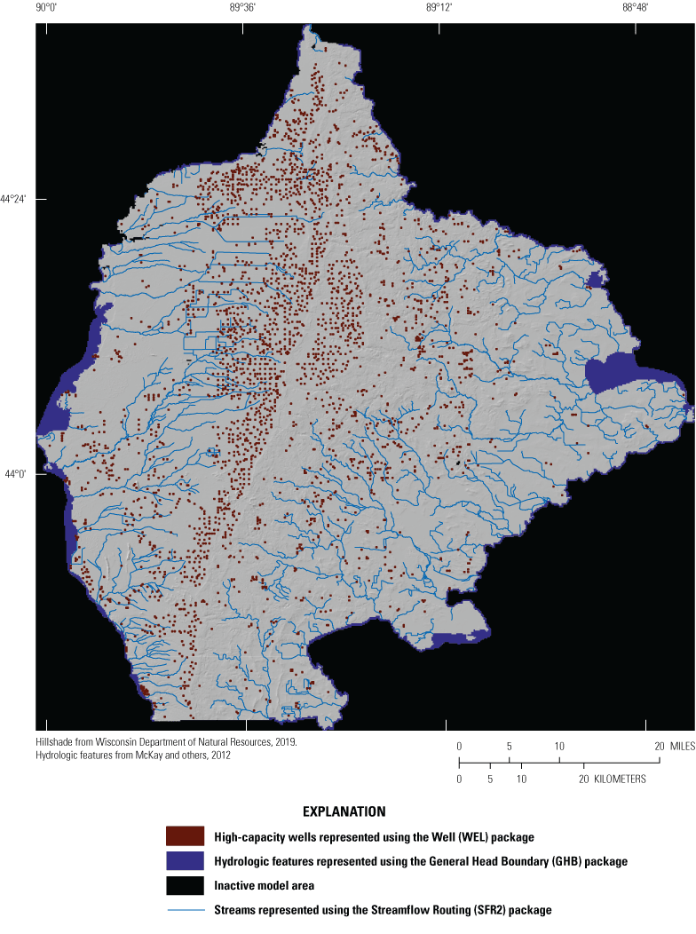
Model boundary conditions used for the regional groundwater-flow model, Central Sands region, central Wisconsin.
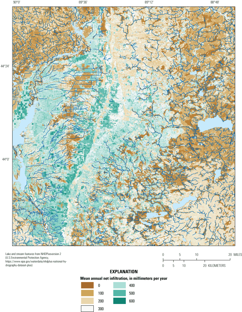
Mean (2012–18) annual net infiltration estimated by Soil-Water-Balance modeling, Central Sands region, central Wisconsin.
Spatially averaged net infiltration (aquifer recharge) for the 2012–18 period ranged from about 3.9–23.6 in/y in the regional model domain (fig. 4). This net infiltration was specified using the MODFLOW Recharge (RCH) package (Harbaugh, 2005).
High-capacity pumping wells operating during any part of the 2012–18 period were included in the regional model (fig. 3). Pumping was specified using the MODFLOW Well (WEL) package (Harbaugh, 2005). Well construction and reported monthly pumping information for high-capacity wells were provided by the WDNR (https://dnr.wisconsin.gov/topic/WaterUse/data.html). Well locations were assigned to the model layer with highest transmissivity within the well’s open interval. Wells without open-interval information were assigned to the model layer with the highest transmissivity at their location.
Lateral flow boundaries were represented in the regional model using the MODFLOW General Head Boundary (GHB) package (Harbaugh, 2005). These flow boundaries included the Wisconsin and Plover Rivers to the west, the Tomorrow, Waupaca, and Wolf Rivers to the north, and the Fox River to the east (figs. 1 and 3). Groundwater exchanges with GHB cells are computed using the difference between the simulated hydraulic head in the aquifer and the assigned GHB elevation, and a conductance term. The elevation of the GHB cells was set to the minimum DEM elevation (WDNR, 2019) within the model-cell area. The conductance term is a function of the cell area, the assumed thickness of the riverbed, and the vertical hydraulic conductivity of the riverbed material. GHB cells were assigned a conductance of 0.5 meter squared per day (m2/d), which, assuming a 1-m thick riverbed, is equivalent to a 1.25×10⁻⁵ meter per day (m/d) vertical hydraulic conductivity. This conductance was adjusted during history matching to 3.9 m2/day, which is equivalent to a 9.75×10⁻⁵ m/d (3.20×10⁻⁴ feet per day [ft/d]) vertical hydraulic conductivity. This value is similar to the calibrated vertical hydraulic conductivity of 4×10⁻⁴ ft/d for GHB cells representing Lake Superior in Leaf and others (2015).
Lateral flow boundaries form the perimeter of the active area of the regional model except along the southern boundary. The southern model boundary has no major river nearby and is far enough from the study lakes as not to affect groundwater flow near the lakes. As a result, the southern model boundary was set as a no-flow boundary, consistent with a previous two-layer groundwater-flow model (Mechenich, 2012) of the Central Sands region (referred to here as the Mechenich Model), located parallel to the assumed groundwater-flow direction east to the Fox River or west to the Wisconsin River.
Streams were represented in the regional model using the MODFLOW-NWT Streamflow Routing (SFR2) package (fig. 3) (Niswonger and Prudic, 2005). SFR2 calculates exchanges between the aquifer and stream system while accounting for total streamflow in the channel. SFR2 input was developed from National Hydrography Dataset version 2 hydrography using the SFRmaker software (Leaf and others, 2021). National Hydrography Dataset flowline features were joined spatially to the model grids, with the resulting line/grid cell intersections and associated attributes forming the basis for SFR2 reaches. Streambed-top elevations were sampled from the light detection and ranging (lidar)-based DEM (WDNR, 2019) as the minimum elevation within a 100-m buffer around each SFR2 reach. Similar to the GHB, SFR2 has a conductance term that represents the thickness of the streambed, the model-cell area of the SFR2 cell, and the vertical hydraulic conductivity of the streambed. The vertical hydraulic conductivity of the streambed was estimated for each stream reach during history matching. Vertical hydraulic conductivity values of the streambed started (initial model-simulation run) at 1 m/d with final calibrated (history matching) values ranging from 0.03 to 80.5 m/d.
Aquifer Properties
Aquifer properties represented in the regional model include vertical and horizontal hydraulic conductivity, specific storage, and specific yield. Initial values were assigned based on literature values described throughout the report and then adjusted during history matching.
The initial horizontal hydraulic conductivity for the eastern half of the unconsolidated model layers (1–3) was estimated using the coarse/fine fractions from WDNR (WDNR, 2021, app. A) and a power-law approach similar to Feinstein and others (2010). The power-law parameters were optimized so that the mean of the initial hydraulic conductivity values produced by the power law agreed with the mean values from the Mechenich Model. Hydraulic conductivity for the western half of the unconsolidated layers, west of the terminal moraine, where coarse/fine fraction estimates were not made in WDNR (2021, app. A), used information from the upper model layer, representing unconsolidated materials, of the two-layer Mechenich Model of the Central Sands region. The initial hydraulic conductivity of the sandstone bedrock in the regional model (layer 4) came from layer 2, representing bedrock, in the Mechenich Model. Lakes across the model domain were included as high hydraulic conductivity zones in layer 1 with a horizontal hydraulic conductivity of 10,000 m/d.
Initial vertical hydraulic conductivity of the fine-grained New Rome Member simulated in layer 2 was set to 0.01 m/d based on vertical hydraulic conductivity estimates for the New Rome Member of 0.2 and 8×10⁻⁵ m/d from Hart and others (2015). The initial horizontal hydraulic conductivity of the New Rome Member was set at 0.1 m/d, which is 10 times the vertical hydraulic conductivity. The specific yield for the New Rome Member was set to 0.20 based on a range of literature values for silt, clay, and fine sand specific yields of 0.06–0.33 (Duffield, 2019). The specific storage was set to 9.2×10⁻⁴m−1, slightly less than the Hart and others (2015) estimate of 9.8×10⁻⁴ m−1 for the transition zone of the New Rome and at the lower end of the literature range of 9.2×10⁻⁴–2.0×10⁻² m−1 (2.8×10⁻⁴–6.2×10⁻³ft−1) for clays (Duffield, 2019). The aquifer properties of the New Rome Member after history matching were a horizontal hydraulic conductivity of 9.2×10⁻² m/d, vertical hydraulic conductivity of 2.0×10⁻³ m/d, a specific yield of 0.2, and a specific storage of 9.2×10⁻⁴ m−1. The horizontal hydraulic aquifer properties of the regional model after history matching are shown in figure 5.
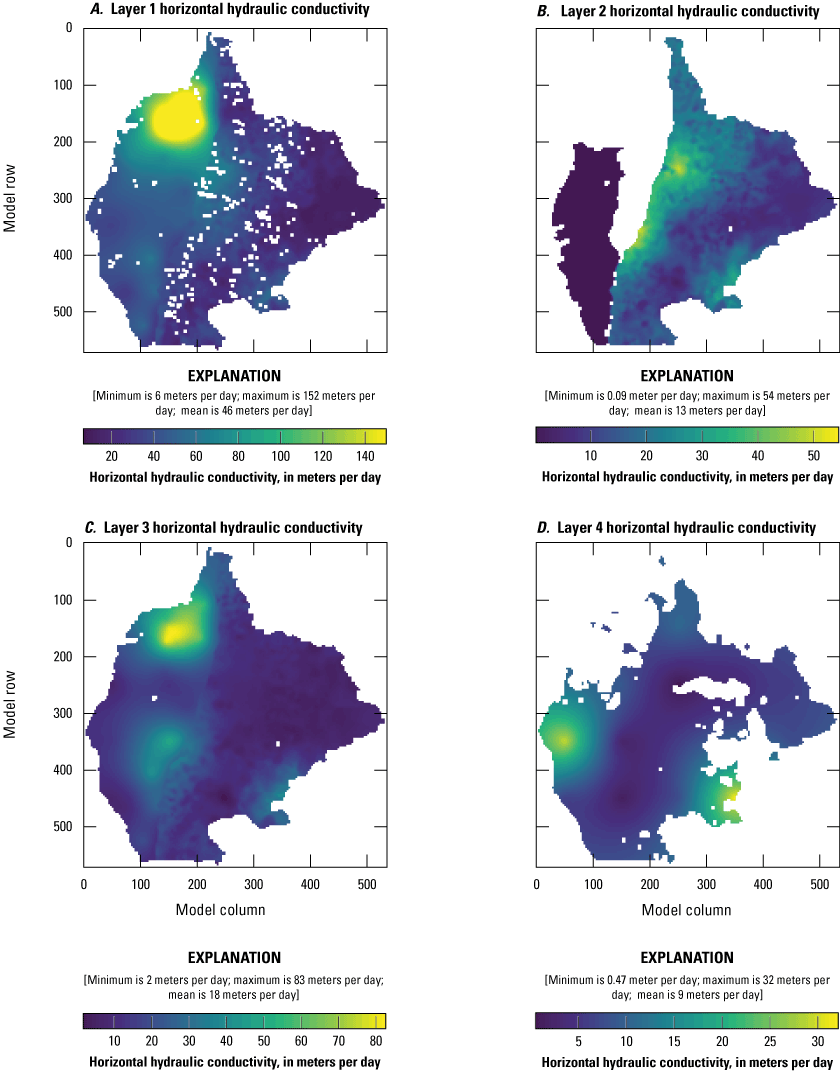
Horizontal hydraulic conductivity values after history matching for each of the four regional model layers (A, layer 1 [upper glacial]; B, layer 2 [middle glacial including New Rome Member where present]; C, layer 3 [lower glacial]; and D, layer 4 [sandstone bedrock]) in the Central Sands region, central Wisconsin.
Horizontal hydraulic conductivities ranged from 0.09 to 152 m/d in the three unconsolidated model layers (layers 1–3) (fig. 5). The mean horizontal hydraulic conductivity was highest in layers 1 and 3 (46 and 18 m/d, respectively) and lowest in layer 2 (13 m/d). These values are consistent with layers 1 and 3 representing coarser glacial material and layer 2 representing finer material to the east and the New Rome Member to the west. The mean horizontal hydraulic conductivity was 9 m/d (30 ft/d) for the sandstone bedrock, represented by model layer 4.
Vertical hydraulic conductivities of the three unconsolidated model layers ranged from 0.002 to 2.93 m/d, with a mean that was lowest in layer 2 (0.37 m/d) and highest in layer 1 (1.01 m/d) (fig. 6). The vertical hydraulic conductivity of the sandstone bedrock (layer 4) had a mean of 0.13 m/d (0.43 ft/d).
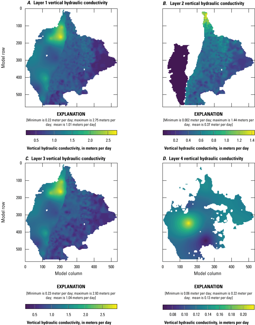
Vertical hydraulic conductivity values after history matching for each of the four regional model layers (A, layer 1 [upper glacial]; B, layer 2 [middle glacial layer including New Rome Member where present]; C, layer 3 [lower glacial]; and D, layer 4 [sandstone bedrock]) in the Central Sands region, central Wisconsin.
The specific yield means for the three unconsolidated layers (1–3) ranged from 0.19 to 0.37 and was 0.14 for the bedrock sandstone (layer 4) (fig. 7). These values are within the literature ranges for till, clay, sand, and gravel specific yields of 0.06–0.33 and within the literature ranges for the sandstone bedrock of 0.06–0.27 (Duffield, 2019). The mean specific storage for the three unconsolidated layers ranged from about 3.3×10⁻⁴ to 4.8×10⁻⁴m−1 (fig. 8). Model values for the unconsolidated material (layers 1–3) fell within the specific storage literature ranges (Duffield, 2019) for loose to dense sand and gravel (from 1.0×10⁻⁴ to 4.3×10⁻⁴ m−1) and clays (from 9.2×10⁻⁴ to 2.0×10⁻²m−1) and close to the Hart and others (2015) estimate of specific storage in the sandy aquifer underlying the New Rome Member of 3.0×10⁻⁴m−1 (9×10⁻⁵ft−1). The specific storage was about 9.8×10⁻⁵m−1(3.0×10⁻⁵m−1) for the sandstone bedrock (layer 4) and is just above the literature ranges (Duffield, 2019) for fissured rock from 3.3×10⁻⁶ to 6.9×10⁻⁵m−1.
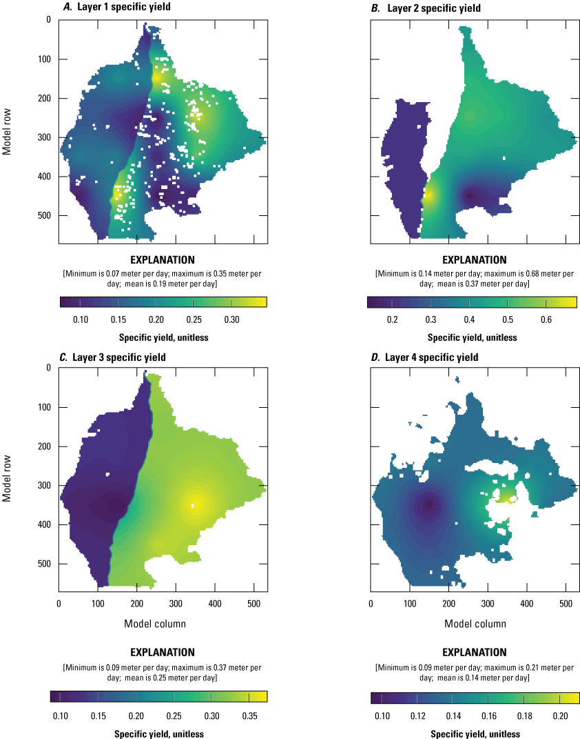
Specific-yield values after history matching for each of the four regional model layers (A, layer 1 [upper glacial]; B, layer 2 [middle glacial layer including New Rome Member where present]; C, layer 3 [lower glacial]; and D, layer 4 [sandstone bedrock]) in the Central Sands region, central Wisconsin.
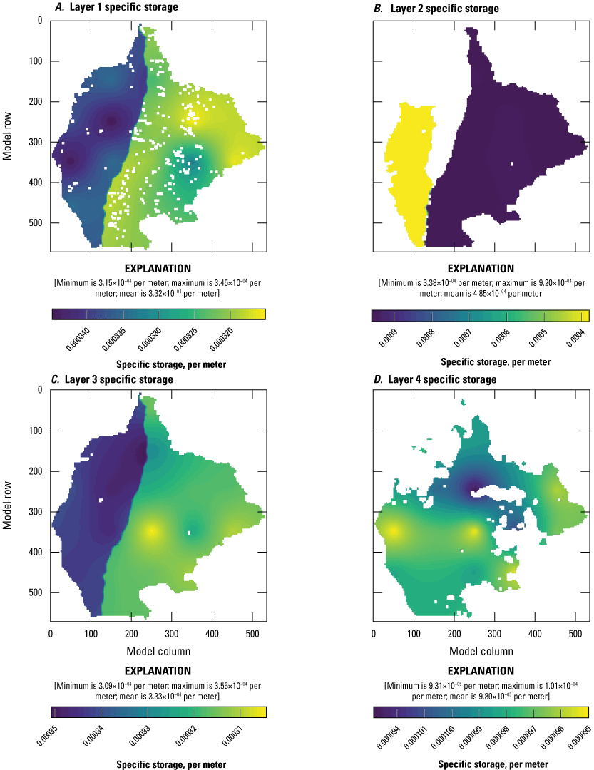
Specific-storage values after history matching for each of the four regional model layers (A, layer 1 [upper glacial]; B, layer 2 [middle glacial layer including New Rome Member where present]; C, layer 3 [lower glacial]; and D, layer 4 [sandstone bedrock]) in the Central Sands region, central Wisconsin.
History-Matching Approach and Results
History matching was performed with the regional model. History matching is a process referred to as “parameter estimation” and, sometimes, “model calibration,” although “calibration” implies a precise unique fit of the model to data. As described herein, calibration is not an accurate representation of the history-matrching process to systematically adjust parameter values in the model such that associated model outputs are consistent with historical observations including hydraulic-head and base-flow values. The general history matching approach follows Bayes’ theorem (Tarantola, 2005) for parameter estimation. In this approach, a prior estimate of model parameters and their credible ranges (uncertainty) is first used. These prior parameter values and uncertainty are selected by expert knowledge, literature values, and available direct measurements. Through a systematic conditioning step, the parameter values are updated to be consistent with observations that correspond to model outputs. This step is referred to as an “update” and results in a posterior set of parameter values (“posterior” meaning “after the update”). Many algorithms can be used to perform this conditioning step. For the regional model, the parameter estimation package for high-performance computing ([PEST++]; White and others, 2021) software was used. The choice of software, in part, reflects rapid development of PEST-related tools throughout the study timeframe. The iterative ensemble smoother (iES) history matching algorithm in White and others (2021) was used for the inset models. The history matching files are provided in Fienen and others (2021b).
The measured values of groundwater hydraulic heads and streamflow used for history matching (referred as “targets”) came from various data sources that are summarized in table 1. Data from a total of 177 streamflow and 464 well and lake-level observation locations were used during the history matching. Streamflow measurements were processed to focus on base flow using the techniques of Sloto and Crouse (1996) and Wahl and Wahl (1988). Simulated groundwater elevations, lake-level elevations, and streamflow from the steady-state period at the start of the transient model were compared to data targets averaged over the 2012–18 period. Simulated groundwater elevations, lake-level elevations, and streamflow from the transient stress periods were compared with targets closest to the end of the month represented by each stress period, for stress periods where measured data were available.
A post-history-matching comparison between the measured and simulated values for lake and groundwater-elevation targets are shown on figure 9, and the streamflow targets are shown on figure 10. The closer these values plot along the 1:1 line, the closer the match between the simulated and measured values. Groundwater-elevation targets mostly plotted on or near the 1:1 line with some outliers scattered above and below the line. The streamflow targets generally plotted on or near the 1:1 line with a slight under-estimated bias (simulated lower than measured values), particularly in comparison to the WDNR base-flow data (fig. 10).
Table 1.
Measured groundwater elevation (head) and streamflow data sources used for history matching in the regional parent mode, Central Sands region, central Wisconsin.[PEST++, parameter estimation package; WGNHS, Wisconsin Geological and Natural History Survey; USGS, U.S. Geological Survey; NWIS, National Water Information System database; WDNR, Wisconsin Department of Natural Resources]
| Group name in the PEST files | Target type | Description | Number of locations | Data source |
|---|---|---|---|---|
| hds_wgnhs_tr, heads_wgnhs | Head | Well-construction report groundwater elevation measured after a well was drilled. Locations were determined by the WGNHS. | 299 | WDNR, 2022 |
| nwis_dvs, nwisdvs_tr | Head | Groundwater elevations at locations with daily data that were collected by the USGS. | 31 | USGS, 2021 |
| nwis_fm, nwisfm_tr | Head | Groundwater elevations at locations with miscellaneous measurements that were measured by the USGS. | 23 | USGS, 2021 |
| wdnr_wells | Head | Wells installed for this study and measured by WGNHS and WDNR. | 36 | WDNR, 2022 |
| wdnr_lakes, wdnrlks_tr | Head | Lake elevations measured by the WDNR. | 70 | WDNR, 2022 |
| usgs_stages | Head | Lake elevation measured by the USGS. | 5 | USGS, 2021 |
| nr_diff | Head difference (vertical) | Hydraulic-head difference measurement across New Rome Member. | 1 | Hart and others (2015) |
| hd_diff | Head difference (temporal) | Calculated as the difference between two hydraulic-head measurments made at the same location for any hydraulic-head dataset where two or more measurements were made. | 1,573 differences; some locations have multiple differences if more than 2 groundwater elevations were collected. | All hydraulic-head target datasets in this table. |
| nwis_dv_flx, nwisdvflx_tr | Streamflow | Streamflow measurements at USGS streamgages with daily data. Data have been adjusted using base-flow separation techniques to reflect base-flow conditions. | 6 | USGS, 2021 |
| nwis_fm_flx, nwisfmflx_tr | Streamflow | Miscellaneous streamflow measurements collected by the USGS. Data have been adjusted to base-flow conditions using streamgages with daily data. | 5 | USGS, 2021 |
| wdnr_miscflx, wdnrflx_tr | Streamflow | WDNR streamflow measurements made during base-flow conditions. No adjustments made. | 166 | WDNR, 2022 |

Measured and simulated groundwater elevations for the steady-state and transient hydraulic head (water-level) targets for the regional model, Central Sands region, central Wisconsin.
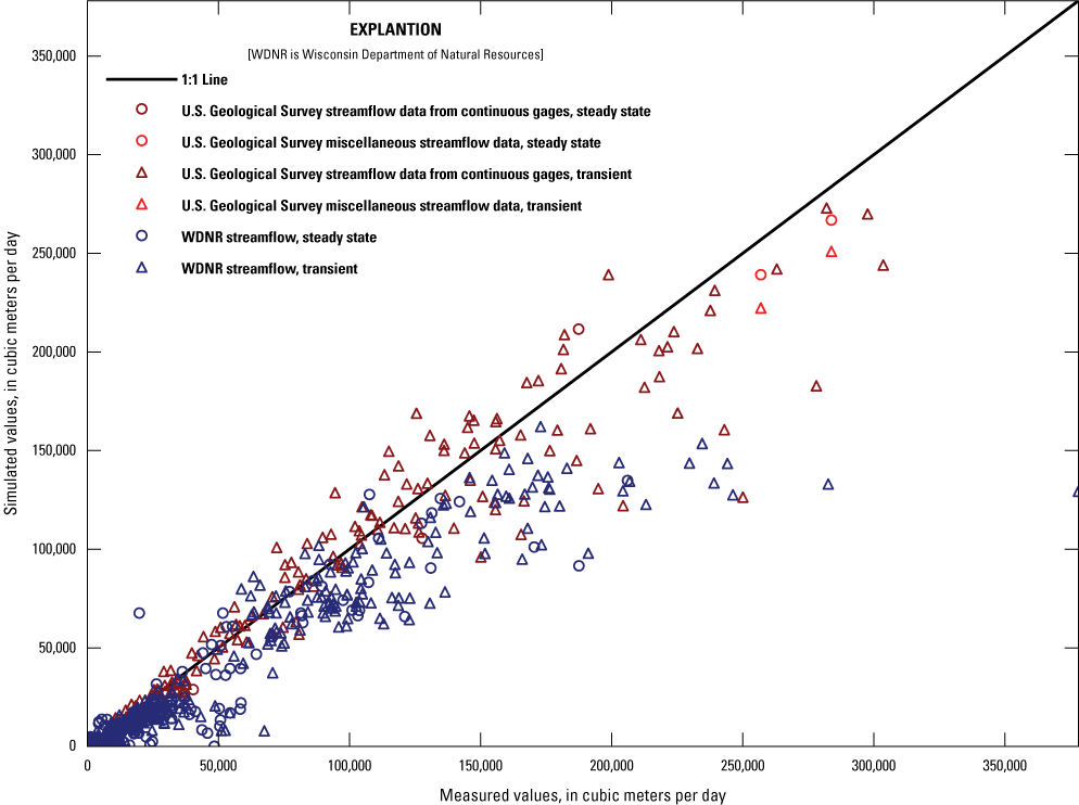
Measured and simulated streamflow under base-flow conditions for the transient streamflow targets for the regional model, Central Sands region, central Wisconsin.
The residuals (differences between simulated and measured values) for the steady-state hydraulic-head and streamflow targets are shown spatially in figures 11 and 12, respectively. Most hydraulic-head targets are from well-construction reports, with accurate locations limited to the central eastern part of the model domain, where location-corrected values were provided by the Wisconsin Geological and Natural History Survey (WDNR, 2021, app. A), focused close to the study lakes. Hydraulic-head residuals were generally well distributed throughout the model domain with some locally biased over-estimated values (simulated higher than measured values) in the central part of the domain. A comparison of flux (streamflow) target residuals indicates a general pattern of under-estimated streamflows, although the bias is less near the inset model areas (for example, Upper Pine River, Chaffee Creek, and Tagatz Creek; fig. 12).
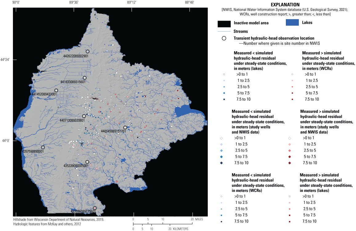
Steady-state hydraulic-head (water-level) target residuals displayed by calibration group for the regional model, Central Sands region, central Wisconsin.
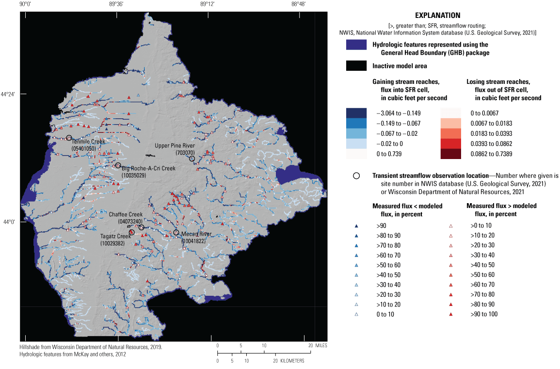
Steady-state streamflow residuals and gaining and losing stream reaches for the regional model, Central Sands region, central Wisconsin.
Transient hydraulic-head and streamflow targets for a select subset of wells and streams are shown in figures 13 and 14, respectively. Well locations with with long-term records (covering the entire calibration period) (fig. 13) were selected to represent wells across the model domain and included a range of good to poorly matched simulated and measured water levels. Overall, the simulated transient hydraulic heads at most wells were in good agreement with measured long-term groundwater-level data.
Few stream locations had daily streamflow data in the model domain. Tenmile Creek (fig. 12) has the most complete daily record for the history-matching period, and the simulated fluxes generally were in good agreement with the trends and timing of peak flows for the period of record. The simulated fluxes generally were lower than the measured streamflow highs but were in good agreement with the mid and lower base flows. Simulated fluxes in the headwater streams near the focus area lakes reasonably matched the magnitude and trends measured in these streams, except for Tagatz Creek, where the simulated base flows in the headwaters were appreciably lower than measured base flows. This resulted, in part, because of bedrock anomalies in the area around Tagatz Creek. These anomalies were addressed in the inset models by locally adjusting the bedrock elevation near the creek to simulate incision of the stream.
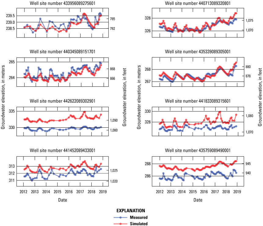
Simulated transient groundwater levels at select wells with long-term records (well locations shown in fig. 11) for the regional model, Central Sands region, central Wisconsin. Site numbers are from National Water Information System database [U.S. Geological Survey, 2021]). Groundwater levels are shown in meters and feet above North American Vertical Datum of 1988 (NAVD88).
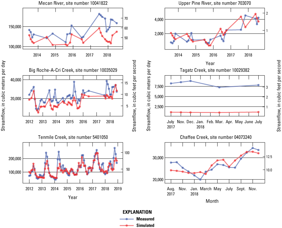
Simulated transient streamflow at select stream locations near the study lakes with long-term records for the regional model, Central Sands region, central Wisconsin (stream locations shown in fig. 12); site numbers are from U.S. Geological Survey National Water Information System database (U.S. Geological Survey, 2021).
Model parameters (totalling 1,775) were adjusted during the history matching and included:
-
• the conductance of the GHB cells representing perimeter boundary conditions;
-
• the vertical hydraulic conductivity of each stream segment;
-
• a grid of pilot-point multipliers across the aquifer property arrays representing the unconsolidated and sandstone units, except for the New Rome Member;
-
• a zone aquifer property multiplier for each array with pilot points;
-
• the aquifer properties of the New Rome Member;
-
• a 0.8–1.2 temporally variable multiplier on the SWB-estimated net infiltration for each monthly stress period; and
-
• a 0.75–1.25 multiplier on the reported pumping rates for all wells in each monthly stress period.
The aquifer properties included in the history matching were horizontal and vertical hydraulic conductivity, specific storage, and specific yield. These properties had initial values assigned as discussed in the “Aquifer Properties” section. These initial parameter arrays were then adjusted using a network of pilot points representing multipliers and zone multipliers for each layer. Zones and pilot points are shown in figure 15 for each of the four regional model layers and include:
-
• a zone for each of the unconsolidated layers with a coarse/fine fraction assigned for materials (WDNR, 2021, app. A) on the eastern half of the model domain in layers 1–3 (zones 2, 3, and 5, respectively);
-
• a zone for the consolidated materials in the western half of layers 1 and 3 (zones 1 and 4, respectively);
-
• a zone (zone 6) for the bedrock sandstone unit represented by layer 4.
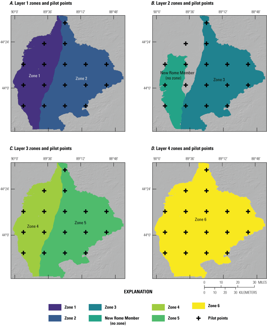
Pilot points and multiplier zones for each of the four regional model layers, Central Sands region, central Wisconsin: A, layer 1; B, layer 2; C, layer 3, and D, layer 4. Note, pilot points extend past the zone boundaries in layer 2 to allow for kriging, but the aquifer properties in the New Rome Member and pinched areas are not affected by pilot-point multipliers.
The aquifer properties after history matching are presented and discussed in the “Aquifer Properties” section. The GHB conductance is discussed in the “Boundary Conditions” section. The final multipliers on the SWB-estimated net infiltration ranged from 0.8 to 1.2 with a mean of 1.02, meaning that, on average, the adjustment to net infiltration was a 2 percent increase over what was estimated with SWB. The final multipliers on the reported well-pumping rates ranged from 0.75 to 1.25 with a mean of 0.95, meaning that, on average, the adjustment to reported pumping rates was a 5 percent decrease in the reported rates.
Regional Model Results
The water-table elevation contours and cumulative simulated streamflow for the regional model are presented in figure 16. The water table is mounded along the topographic high formed by the moraine that runs north-south through the center of the model domain. Groundwater flows from this water table high to the east and west towards the major rivers that form the major hydrologic boundaries in the region. Groundwater-flow directions are assumed to be generally perpendicular to water-table elevation contours.
A simulated water budget of the major changes in inflows and outflows from 2012 to 2018 is shown in figure 17. Water enters the groundwater system through recharge and stream leakage under losing streamflow conditions and exits through streams under gaining streamflow conditions, pumping from high-capacity wells, and discharge to the major rivers at the lateral boundaries of the groundwater system. Excess inflows and outflows are balanced throughout the system by groundwater storage replenishment and depletion. During periods of high recharge (often in the spring), groundwater storage has a gain, which can be thought of as excess water leaving the groundwater system and entering into storage (Storage_in on fig. 17). During the growing season, when pumping is higher and recharge is lower, water is being removed from groundwater storage and entering the groundwater system (Storage_out on fig. 17).
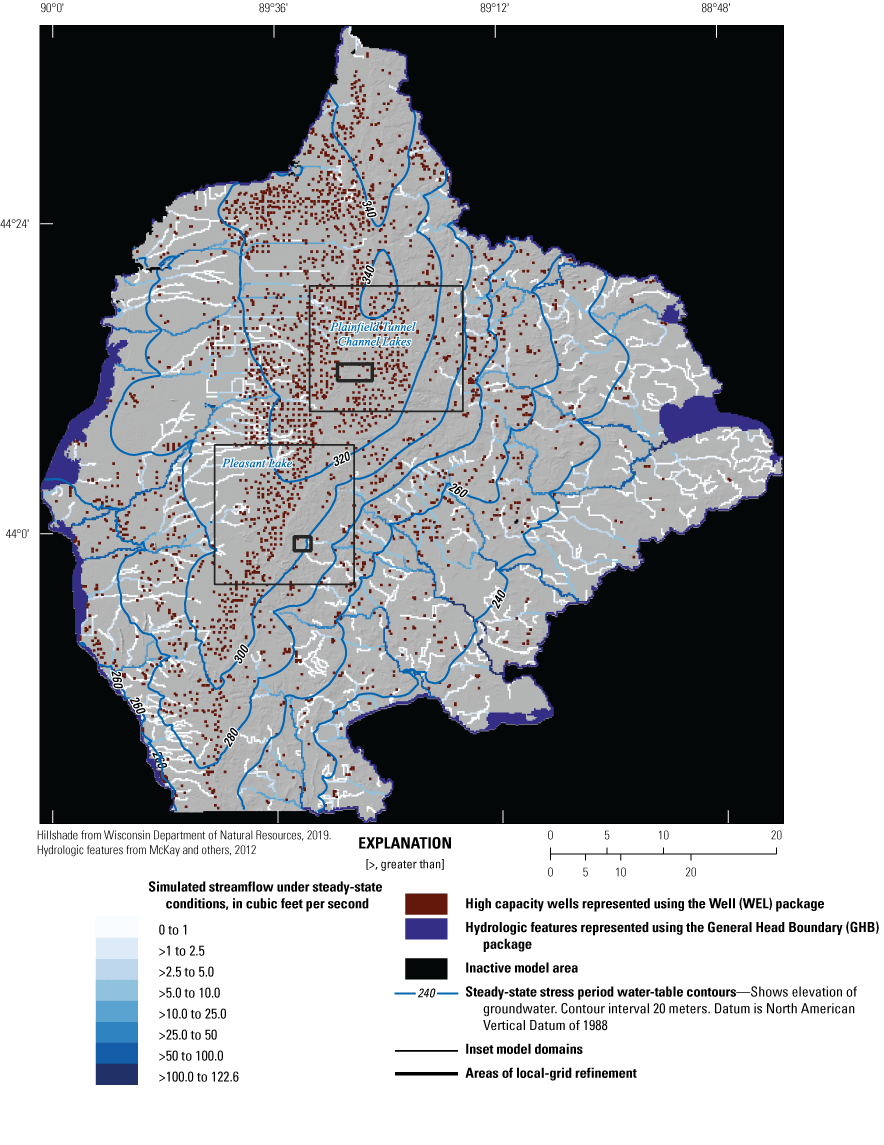
Simulated water table and streamflow for the regional model during the steady-state stress period representing mean conditions from 2012 to 2018, Central Sands region, central Wisconsin.
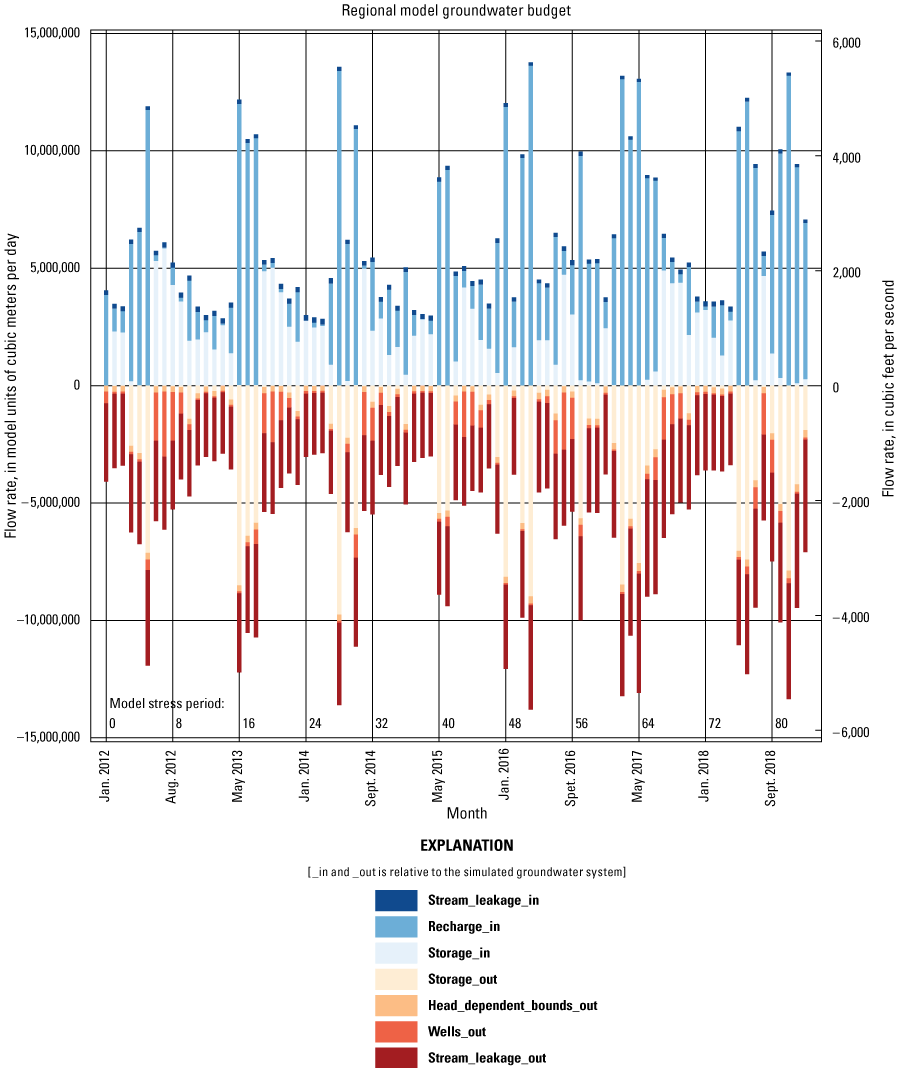
Regional model groundwater budget showing the major model inflows and outflows for each stress period. Inflows and outflows are named using the MODFLOW list file convention, Central Sands region, central Wisconsin.
Focus Area Inset Models
Two focus area inset models were developed from the regional groundwater-flow model, for the areas around the Plainfield Tunnel Channel Lakes (Plainfield Tunnel Channel Lakes model) and Pleasant Lake (Pleasant Lake model) (fig. 1). The inset models were developed to simulate the study lakes and their competing sinks—streams and boundaries—in detail sufficient for lake-level simulation. This detail is not possible with the regional-scale model. Base-case versions of each inset model were created for history matching from 2012 through 2018. Model parameters estimated from history matching were then applied to scenario-testing versions of the two inset models, which are described in the “Lake Ecosystem Response Assessment (LERA)” section. Model files are provided in the model archives associated with this report (Fienen and others, 2021b and Westenbroek and Fienen, 2022).
Inset Model Domains and Horizontal Discretization
The inset model domains were designed to encompass the nearest headwater streams to the east and west of the study lakes and most of the high-capacity wells that may affect the lake water balances, while maintaining reasonable model runtimes. A uniform grid with 20-m horizontal resolution in an area surrounding the lakes was selected to adequately represent the detailed bathymetry and shoreline geometry of the lake basins. Initial testing of runtimes with the MODFLOW-NWT code and a 20-m grid spacing over the entire inset model domains resulted in unacceptably long runtimes (on the order of hours).
Because of the long runtimes, an LGR approach was adopted using the multiple model capabilities of MODFLOW 6 (Langevin and others, 2017). The models focused on the lakes each consist of two submodels—the “inset” submodel aligned with the regional model grid at the same 200-m (656.2-ft) resolution and a locally refined “LGR” submodel with a uniform 20-m resolution encompassing a rectangular area around the lake(s) of interest (fig. 18 for Plainfield Tunnel Channel Lakes and fig. 19 for Pleasant Lake). The Plainfield Tunnel Channel Lakes inset submodel contains 90 rows and 110 columns, and the LGR submodel contains 120 rows and 250 columns. The Pleasant Lake inset submodel contains 100 rows and 100 columns, and the LGR submodel contains 100 rows and 120 columns. Within MODFLOW 6, the two submodels for each lake(s) are coupled within the same solution matrix and solved simultaneously as a “simulation” (Langevin and others, 2017). This coupling greatly reduced the overall number of model cells, cutting the runtimes for the base-case simulation (2012–18 period) to approximately 10 minutes.
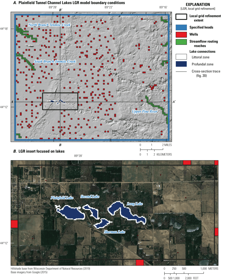
Plainfield Tunnel Channel Lakes model domain, Central Sands region, central Wisconsin. A, boundary conditions and B, local-grid refinement extent.
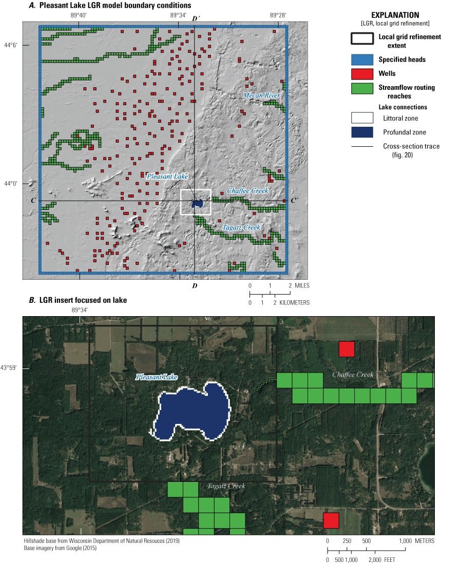
Pleasant Lake model domain, Central Sands region, central Wisconsin. A, boundary conditions and B, local-grid refinement extent.
Inset Model Layering
Layering in the inset models was developed from the same data sources as the regional model; however, the exception being that layer 1 was typically split into two layers for the inset models and was adjusted for lake bathymetry where the lakes are simulated. The model top (top of layer 1) is based on mean elevations sampled for each model cell from a lidar-based DEM (WDNR, 2019), except within the basins of Plainfield, Long, and Pleasant Lakes. Bathymetry for these lakes, developed by WDNR (2019), was subtracted from the DEM elevations to develop the model top. The layer bottom surfaces in the inset models, where lakes are not present, are congruent with the regional model except that layers 1 and 2 are evenly subdivided from layer 1 in the regional model to better represent hydraulic gradients near surface-water features.
Unlike MODFLOW-NWT, MODFLOW 6 allows for discontinuous layering, meaning that model cells can be removed from the model solution in places where a hydrogeologic unit is absent. In the Plainfield Tunnel Channel Lakes inset model, this feature was used to remove cells from layer 3 in areas west of the Hancock Moraine, where “layer 2” from WDNR (2021, app. A) was not defined (fig. 20). Similarly, in the Pleasant Lake inset model, cells were removed from “layer 3” in places where the New Rome Member or “layer 2” from WDNR (2021, app. A) were absent. Cells were also removed from the models in places where the layer bottoms were within a meter of the land surface, for example, near high points in bedrock surface or along lake bottoms. Removing unneeded model cells, which would otherwise need to be carried throughout the model at some minimum thickness (for example, 1 m), can further increase the stability and speed of the model-simulation run.
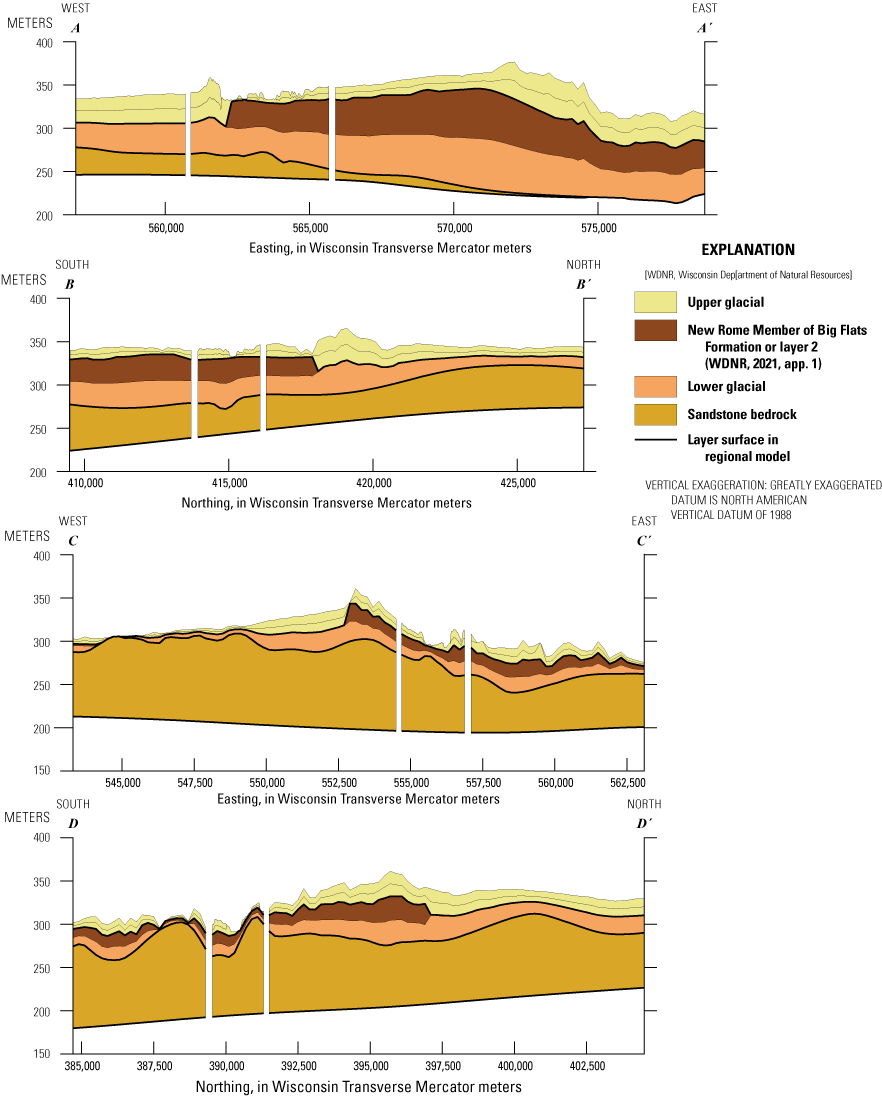
Inset and parent regional model layer surfaces, Central Sands region, central Wisconsin. Gaps in the cross sections indicate the extent of the refined areas within the inset models. Cross-section locations are shown in figures 18 and 19.
Time Discretization
Time discretization for the base versions of the inset models is similar to the regional parent model with the exception that the initial steady-state period represents mean conditions for the period from 2012 through 2015. Subsequent transient monthly stress periods represent mean conditions for each month through 2018. Each transient stress period was subdivided into five time steps using a time-step multiplier of 1.2. This time-step multiplier differs from the regional model multiplier of 1.5 because inset model convergence is more difficult with the lake package, and a lower multiplier can sometimes improve model convergence.
Boundary Conditions
Boundary conditions within the inset model domains include regional groundwater flow across the model perimeters; terrestrial recharge originating from precipitation, snowmelt and irrigation; and groundwater/surface-water interactions with lakes and streams. The model-perimeter boundaries were simulated as specified-head values obtained from the regional model.
Recharge
Recharge for the inset models was resampled from the net infiltration output of the SWB simulation to the model-cell centers using a nearest-neighbor approach. This approach is mass conservative because the subdivided inset model cells fall evenly within the parent cells. For the initial steady-state period, mean recharge from 2012 through 2015 was used. Monthly mean net infiltration was sampled from SWB for the subsequent monthly stress periods. Recharge was simulated in MODFLOW 6 using the Recharge (RCH) package with array-based input (Langevin and others, 2020).
Streams
Streams were simulated with the MODFLOW-6 Streamflow Routing (SFR) package (Langevin and others, 2020). SFR input was developed using the same methods as the regional model (Leaf and others, 2021), except the National Hydrography Dataset flowlines were edited to more accurately represent the spring complexes at the headwaters of Chaffee and Tagatz Creeks and the Mecan River (fig. 19). In the Pleasant Lake model, Chaffee and Tagatz Creeks originate within the inset submodel and flow out to the parent submodel (fig. 19). These streams are linked between the two submodels using the Water Mover (MVR) package with each model simulation (Langevin and others, 2020).
Lakes
The study lakes were represented in the LGR portion of the inset models using the Lake (LAK) package in MODFLOW 6, which couples a lake water balance and simulation of lake stage with the groundwater-flow model solution (Langevin and others, 2017). In the Plainfield Tunnel Channel Lakes model, Plainfield, Long, Second, and Sherman Lakes (fig. 18) were simulated with the LAK package. In the Pleasant Lake model (fig. 19), only Pleasant Lake was simulated using the LAK package. All other lakes in the MODFLOW-6 inset models continue to be simulated with high hydraulic conductivity zones, as in the regional parent model.
Lake extents obtained from the WDNR 24k hydro dataset (WDNR, 2015) were intersected with the model grid to develop the lake-connections cells. Within the lake extents, the model top was set at the lake bottom, based on bathymetric surfaces developed by the WDNR (Aaron Pruitt, WDNR, written commun., 2020), which are available in the accompanying model archive (Fienen and others, 2021b). In areas where the lake bathymetry indicated lake bottoms incised deeper than the bottom of the regional model layer 1, those layer-bottom elevations were also set to the lake bottom, resulting in zero thicknesses for those cells. The zero thickness cells were removed from the model (idomain set to −1), and vertical lake connections were made with the uppermost active cells beneath the lake footprints. Lakebed leakance was assigned to two zones—a littoral zone of approximately 1 cell (20-m) width around the lake perimeter and a profundal zone representing the interior of the lake basin (figs. 18 and 19). Within the LAK package solution, lake volumes were defined by the computed lake stage and the elevation of the lake bottom, as defined by the model top (a separate bathymetry file defining the stage/area/volume relation was not used).
The LAK package water balance requires input of direct precipitation over the lakes and lake evaporation. Precipitation input was obtained for the lake locations from the PRISM dataset (PRISM Climate Group, 2019), which also includes daily mean air-temperature estimates. Mean monthly open water evaporation rates were estimated from the air temperatures using the unmodified Hamon method (Harwell, 2012). Based on analysis by Pruitt (WDNR, 2021, app. E) who implemented the General Lake Model (Hipsey and others, 2019) for the study lakes, a systematic correction was made to decrease highest and increase lowest evaporation inputs by 25 percent. This correction is consistent with the Hamon method, which often calculates extreme values too far from the mean. For the initial steady-state period, precipitation and evaporation were averaged for the period from 2012 through 2015 resulting in a net influx of water to the lake from the surface.
Water Use
High-capacity wells operating during any part of the 2012–18 period were represented with the Well (WEL) package for MODFLOW 6 (Langevin and others, 2017). Pumping well locations are shown on figures 18 and 19. WEL package input was developed from reported pumping (https://dnr.wisconsin.gov/topic/WaterUse/data.html), with the same methods used for the regional model. Wells were assigned to the model layer with highest transmissivity within the well’s open interval. Wells without open interval information were assigned to the highest transmissivity layer at their location.
Aquifer Properties
Horizontal and vertical hydraulic conductivity were initially set at the values estimated for the regional model by history matching. To avoid having parameters adjusted to extreme values in the local-scale models’ history matching process, when applying multipliers to localized values that are already approaching extreme values, specific storage (Ss) was initially set to 1×10⁻⁶ m−1.. Specific yield (Sy) was initially set uniformly to 0.15 (dimensionless) throughout the model domain, based on previous investigations for similar deposits.
Parameter Estimation and Uncertainty Analysis
The history matching approach used in this analysis is described in detail in Corson-Dosch and others (2022). Similar to history matching with the regional model, history matching was performed to refine parameter estimates for the inset and LGR models with the same observation data used for the regional model analysis, with additional observations in the area around the lakes. For the inset models, the iES implementation (White, 2018) of PEST++ (version 5.0.0; White and others, 2021) was applied. The goal of iES is to provide parameter estimates and to quantify the uncertainty of those estimates. This uncertainty is characterized by a range of estimated parameters that each reproduce simulated hydraulic heads and streamflows within an acceptable range of measured values. Each observation is assigned an observation weight that, in principle, corresponds to the inverse of the standard deviation assuming a normal distribution of uncertainty around the measured observation value. As a result, in comparing the model output with measured values, the uncertainty of the measured and simulated values warrant consideration and, ideally, these values would overlap.
The Iterative Ensemble Smoother Method and Uncertainty Quantification
iES is an ensemble method, meaning at every stage of analysis, an ensemble of parameter sets (or realizations) is generated consistent with their inherent uncertainty and the assumed uncertainty in the observations. Simulations are then made using each parameter set from this ensemble to produce a range of model output. Empirical correlations between parameter and observation ensembles are used in iES to iteratively reduce the uncertainty and discrepancy between the simulated values and measured observations, providing a posterior parameter ensemble that reflects the inherent uncertainty in the parameters conditioned on the available data. A single “base-case” realization represents the minimum error variance solution and can be used when a single set of parameter values is required for model simulation. This base-case realization is used for the scenario testing described here and documented in the report.
Observation Data
Observation data were compiled for the inset models from the same dataset used for history matching in the regional parent model. Some additional observations focused around the study lakes were added for the inset models and some spatial water-level difference observations (measures of the horizontal hydraulic gradient between shallow piezometers (usually less than 10 m deep) installed near the lakes and the simulated lake elevations) were added along with the temporal difference observations. Observation weights were initially assigned based on assumptions regarding a level of fit between model outputs and nearby observations. These weights were adjusted to balance the objective function that drives the iES regression including assigning a weight of 0.0 to some classes of observations. These adjustments are all intended to steer the iES results toward a model design that is focused on the complex groundwater/surface-water interactions in the study area, and, in particular, matching observed lake elevations and streamflow values—a key objective of this analysis. The observations used, by observation group, and values and observation weights for the Pleasant Lake and Plainfield Tunnel Channel Lakes inset models are summarized in tables 2 and 3, respectively.
Table 2.
Observation data groups, values, and descriptions for Pleasant Lake inset model, Central Sands region, central Wisconsin.[PEST, parameter estimation package; WGNHS, Wisconsin Geological and Natural History Survey; NA, not applicable; USGS, U.S. Geological Survey; NWIS, National Water Information System database; WDNR, Wisconsin Department of Natural Resources]
| Group name in the PEST files | Observed values | Target type | Description | Total number of observations | Number of weighted observations | Number of zero-weighted observations | Weight | Weight-informed standard deviation | Data source |
|---|---|---|---|---|---|---|---|---|---|
| hds_wgnhs_tr, heads_wgnhs | 280.311 to 327.17 | Hydraulic head | Well-construction report that includes groundwater elevation measured after a well was drilled. Locations were determined by the WGNHS. | 100 | 0 | 100 | 0 | NA | WDNR, 2022 |
| nwis_dvs | 298.00 to 314.72 | Hydraulic head | Groundwater elevations at locations with daily data collected by USGS. | 14 | 14 | 0 | 3.78 to 7.13 | 0.14 to 0.26 | USGS, 2021 |
| nwis_fm | 264.09 to 300.84 | Hydraulic head | Groundwater elevations at miscellaneous locations measured by USGS. | 2 | 0 | 2 | 0 | NA | USGS, 2021 |
| nwisdvs_tr | 297.75 to 315.47 | Hydraulic head | Groundwater elevations at locations with daily data collected by USGS. | 133 | 133 | 0 | 1.26 to 2.04 | 0.49 to 0.79 | USGS, 2021 |
| nwisdvs_tr_tdiff | −0.25 to 0.54 | Head temporal difference | Groundwater elevations at locations with daily data collected by USGS. | 119 | 119 | 0 | 7.32 | 0.14 | Derived from data elsewhere in this table |
| nwisfm_tr | 263.12 to 300.84 | Hydraulic head | Groundwater elevations at miscellaneous locations measured by USGS. | 5 | 0 | 5 | 0 | NA | USGS, 2021 |
| nwisfm_tr_tdiff | 0.12 to 0.59 | Hydraulic head temporal difference | Groundwater elevations at miscellaneous locations measured by USGS. | 3 | 0 | 3 | 0 | NA | Derived from data elsewhere in this table |
| usgs_stages | 299.09 | Lake level | Lake elevations measured by USGS. | 1 | 1 | 0 | 63.67 | 0.02 | USGS, 2021 |
| usgs_stages_tr | 298.94 to 299.25 | Lake level | Transient lake elevations measured by USGS. | 8 | 8 | 0 | 50.46 | 0.02 | USGS, 2021 |
| nwisdvflx_tr | 19,963 to 34,446 | Streamflow | Streamflow at locations with daily data measured by USGS. | 16 | 16 | 0 | 0.0012 to 0.00215134 | 464.83 to 802.05 | USGS, 2021 |
| wdnrflx_tr | 0 to 14, 8776 | Streamflow | WDNR streamflow measurements made during base-flow conditions. No adjustments made. | 171 | 127 | 44 | 0 to 0.0040 | 247.22 to 6552.83 | WDNR, 2022 |
| wdnr_lakes | 298.98 | Lake level | Lake elevations measured by WNDR. | 1 | 1 | 0 | 93.99 | 0.01 | WDNR, 2022 |
| wdnr_lb | 298.98 to 299.12 | Lakebed head | Lakebed piezometer groundwater elevation measured by WDNR. | 10 | 10 | 0 | 6.04 | 0.17 | WDNR, 2022 |
| wdnr_lb_sdiff | –0.11 to 0.05 | Lakebed head spatial difference | Lakebed piezometer groundwater elevation measured by WDNR. | 10 | 10 | 0 | 8.19 | 0.12 | WDNR, 2022 |
| wdnrlks_ann_tr | 298.42 to 299.16 | Lake level | Lake elevations measured by WNDR—long term. | 6 | 6 | 0 | 61.019 | 0.016 | WDNR, 2022 |
| wdnrlks_mon_tr | 298.92 to 299.18 | Lake level | Lake elevations measured by WNDR—recent (2017–18) | 9 | 9 | 0 | 54.75 | 0.018 | WDNR, 2022 |
| wdnrwells_tr | 297.29 to 299.88 | Hydraulic head | Wells installed for this study and measured by WGNHS and WDNR. | 68 | 68 | 0 | 1.25 to 2.45 | 0.4084 to 0.80 | WDNR, 2022 |
| wdnrwells_tr_sdiff | –0.61 to 1.80 | Hydraulic head spatial difference | Wells installed for this study and measured by WGNHS and WDNR. | 56 | 56 | 0 | 2.31 to 4.52 | 0.22 to 0.43 | Derived from data elsewhere in this table |
| wdnrwells_tr_tdiff | –0.062 to 0.29 | Hydraulic head temporal difference | Wells installed for this study and measured by WGNHS and WDNR. | 56 | 56 | 0 | 12 | 0.083 | Derived from data elsewhere in this table |
Table 3.
Observation data groups, values, and descriptions for Plainfield Tunnel Channel Lakes inset model, Central Sands region, central Wisconsin.[PEST, parameter estimation package; WGNHS, Wisconsin Geological and Natural History Survey; NA, not applicable; USGS, U.S. Geological Survey; NWIS, National Water Information System database; WDNR, Wisconsin Department of Natural Resources]
| Group name in the PEST files | Observed values | Target type | Description | Total number of observations | Number of weighted observations | Number of zero-weighted observations | Weight | Weight-informed standard deviation | Data source |
|---|---|---|---|---|---|---|---|---|---|
| hds_wgnhs_tr, heads_wgnhs | 299.61 to 335.15 | Hydraulic head | Well-construction report that includes groundwater elevation measured after a well was drilled. Locations were determined by the WGNHS. | 106 | 0 | 106 | 0 | NA | WDNR, 2022 |
| nwis_dvs | 330.79 to 334.91 | Hydraulic head | Groundwater elevations at locations with daily data collected by USGS. | 4 | 4 | 0 | 16.38 to 26.16 | 0.038 to 0.06 | USGS, 2021 |
| nwis_fm | 310.75 to 327.11 | Hydraulic head | Groundwater elevations at miscellaneous locations measured by USGS. | 2 | 0 | 2 | 0 | NA | USGS, 2021 |
| nwisdvs_tr | 329.90 to 335.35 | Hydraulic head | Groundwater elevations at locations with daily data collected by USGS. | 82 | 82 | 0 | 2.32 to 3.76 | 0.27 to 0.43 | USGS, 2021 |
| nwisdvs_tr_tdiff | −0.26 to 2.01 | Hydraulic head temporal difference | Groundwater elevations at locations with daily data collected by USGS. | 78 | 78 | 0 | 0.79 to 9.50 | 0.11 to 1.26 | NA |
| nwisfm_tr | 310.44 to 327.46 | Hydraulic head | Groundwater elevations at miscellaneous locations measured by USGS. | 64 | 0 | 64 | 0 | NA | USGS, 2021 |
| nwisfm_tr_tdiff | −0.57 to 0.80 | Hydraulic head temporal difference | Groundwater elevations at miscellaneous locations measured by USGS. | 62 | 0 | 62 | 0 | NA | Derived from data elsewhere in this table. |
| usgs_stages | 330.69 to 335.22 | Lake level | Lake elevations measured by USGS. | 3 | 3 | 0 | 17.70 | 0.056 | USGS, 2021 |
| wdnrflx_tr | 0 to 14434.8 | Streamflow | WDNR streamflow measurements made during base flow conditions. No adjustments made. | 88 | 73 | 15 | 0 to 0.00808321 | 123.71 to 1149.53 | WDNR, 2022 |
| wdnrlks_ann_tr | 333.65 to 334.97 | Lake level | Lake elevations measured by WNDR—long term | 10 | 10 | 0 | 25.15 | 0.040 | WDNR, 2022 |
| wdnrlks_mon_tr | 334.74 to 335.47 | Lake level | Lake elevations measured by WNDR—recent (2017–18). | 16 | 16 | 0 | 16.62 | 0.060 | WDNR, 2022 |
| wdnrwells_tr | 334.82 to 335.58 | Hydraulic head | Wells installed for this study and measured by WGNHS and WDNR. | 121 | 121 | 0 | 0.10 to 1.95 | 0.51 to 1.00 | WDNR, 2022 |
| wdnrwells_tr_sdiff | −0.16 to 0.36 | Hydraulic head spatial difference | Wells installed for this study and measured by WGNHS and WDNR. | 105 | 105 | 0 | 3.99 to 7.80 | 0.13 to 0.25 | Derived from data elsewhere in this table. |
| wdnrwells_tr_tdiff | −0.065 to 0.21 | Hydraulic head temporal difference | Wells installed for this study and measured by WGNHS and WDNR. | 97 | 97 | 0 | 10.32 | 0.097 | Derived from data elsewhere in this table. |
Water level and streamflow observations were assigned their values at the end of the month in which they were measured. In this way, intermediate results at a timescale shorter than the stress periods are not considered. Intermediate results were not considered to be consistent with the way stresses (including pumping and recharge) are implemented in model simulation. With monthly stress periods, all stresses that occur at any time in the month must be applied uniformly at the start of the stress period. As a result, observations at intermediate times within the month are not truly representative of their submonthly timescale location, so the end of the month is considered most representative. For streamflow, total streamflow was used to assign observation value with the assumptions that there may be some stormflow in the observations that are not simulated in the model as only base flow is simulated. However, base flow is assumed to compose most of the streamflow in this area.
The locations of water-level observations for the Pleasant Lake and Plainfield Tunnel Channel Lakes inset models are shown in figures 21 and 22, respectively. The labels correspond to observation names that were used in the PEST++ input files.
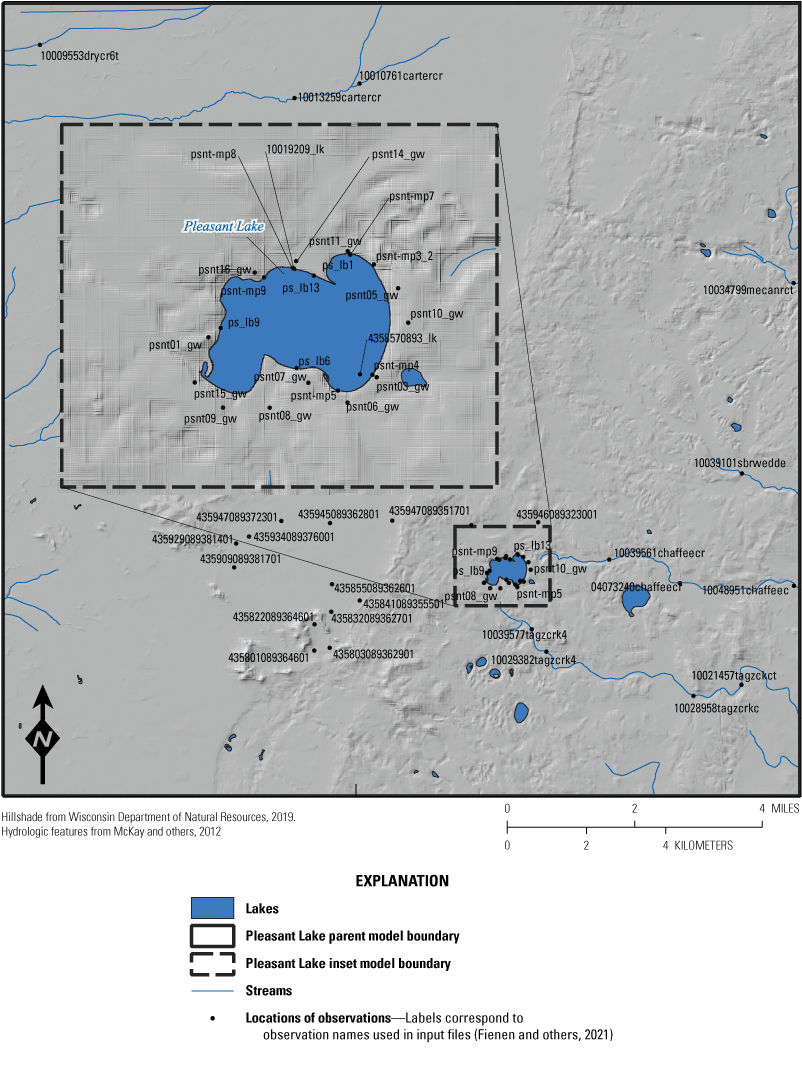
Locations of observations that were assigned observation weight greater than zero for the Pleasant Lake inset model, Central Sands region, central Wisconsin.
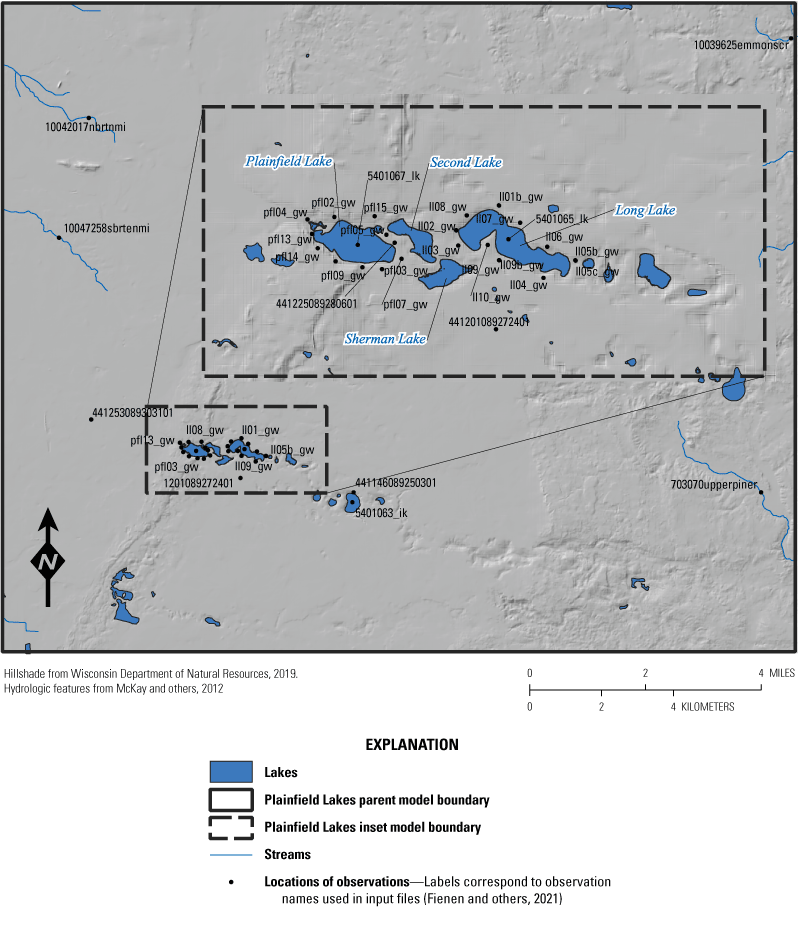
Locations of observations that were assigned observation weight greater than zero for the Plainfield Tunnel Channel Lakes inset model, Central Sands region, central Wisconsin.
Parameterization
The parameterization strategy for the inset models was to use multipliers for most parameters to preserve, to the extent possible, the prior conceptualization of the regional parent model. In this approach, the initial parameter values used in the inset models resulted from the previous history matching in the regional model. The multipliers all were set to an initial value of 1.0 and were given narrow upper and lower bounds for adjustment. In this way, particularly with pilot points that apply to a small spatial footprint in the property fields, only minor parameter adjustments are allowed. This approach avoids overfitting with iES. For specific storage and specific yield, however, a multiscale approach to multipliers was applied following the techniques of McKenna and others (2019) and White and others (2020). In this approach, multipliers to entire zones (or, in this case, model layers) can be combined with multipliers at a finer scale (in this case, pilot points). Streambed conductance and lakebed conductivity were both parameterized using values in the properties’ actual measurement units rather than multipliers. The parameterization for the Pleasant Lake and Plainfield Tunnel Channel Lakes inset models are summarized in tables 4 and 5, respectively. Pilot-point locations for horizontal and vertical hydraulic conductivity, specific storage, and specific yield are described and shown in the “Parameter Estimates” section for the Plainfield Tunnel Channel inset model and Pleasant Lake inset model.
Table 4.
Parameter groups, values, and descriptions for Pleasant Lake inset model, Central Sands region, central Wisconsin.[PEST, parameter estimation package; K, hydraulic conductivity; SFR, Streamflow Routing package]
Table 5.
Parameter groups, values, and descriptions for Plainfield Tunnel Channel Lakes inset model, Central Sands region, central Wisconsin.[PEST, parameter estimation package; K, hydraulic conductivity; SFR, Streamflow Routing package]
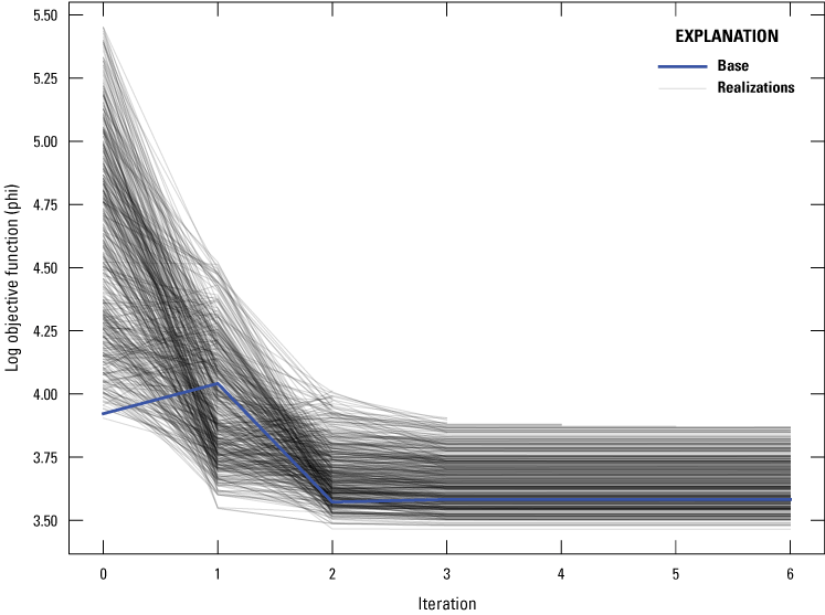
Summary of ensemble realization and base objective function progress by iterative ensemble smoother (iES) history matching algorithm iteration for Pleasant Lake inset model, Central Sands region, central Wisconsin.
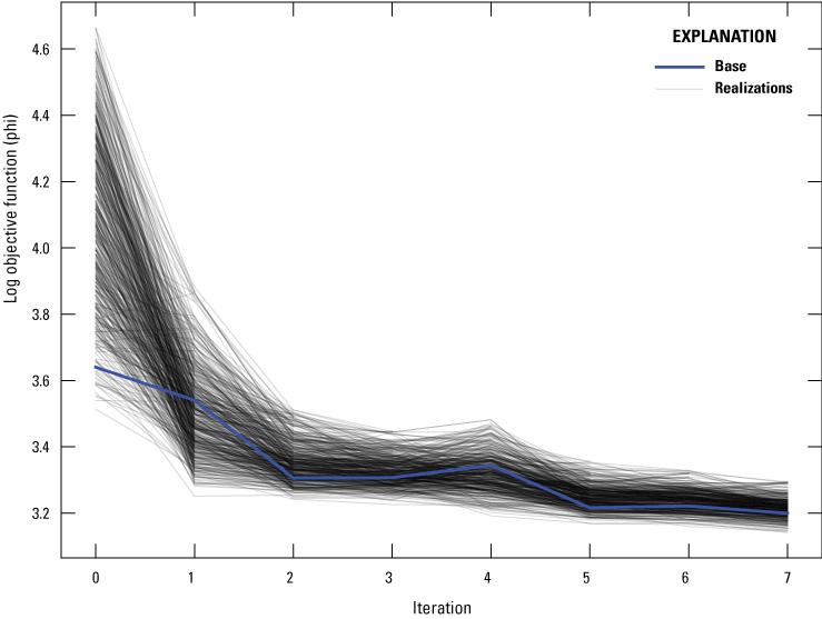
Summary of ensemble realization and base objective function progress by iterative ensemble smoother (iES) history matching algorithm iteration for Plainfield Tunnel Channel Lakes inset model, Central Sands region, central Wisconsin.
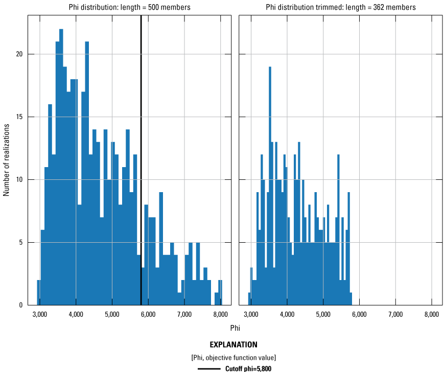
Rejection sampling for the Pleasant Lake inset model, Central Sands region, central Wisconsin. A subjective decision, based on professional judgment, was made to only retain ensemble realizations at or less than a selected cutoff value. For Pleasant Lake, this cutoff was 5,800.
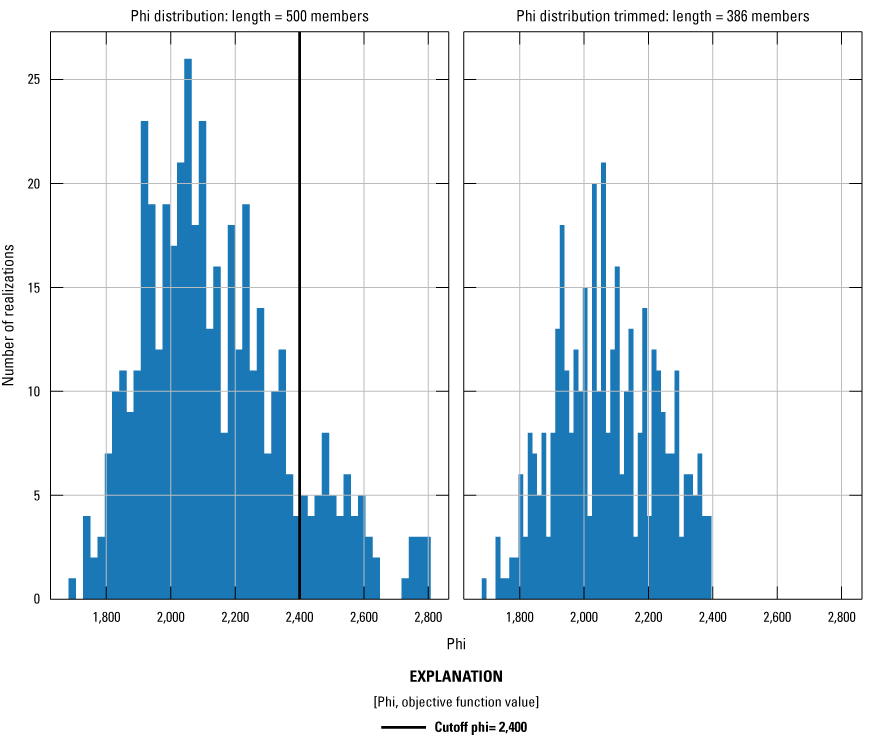
Rejection sampling for the Plainfield Tunnel Channel Lakes inset model, Central Sands region, central Wisconsin. A subjective decision based on professional judgment was made to only retain ensemble realizations at or less than a selected cutoff value. For the Plainfield Tunnel Channel Lakes, this cutoff was 2,400.
History-Matching Results
The ensemble approach in iES results in an ensemble of objective function values from iteration to iteration for the Pleasant Lake and Plainfield Tunnel Channel Lakes inset models (figs. 23 and 24, respectively). The blue curve represents the base ensemble realization, and the lighter gray lines indicate the trajectories of all the other ensemble realizations (figs. 23 and 24). A wide range of parameter combinations can be examined with this approach, and some of those combinations result in MODFLOW-6 models that fail to run to completion. Others result in poor correspondence between model outputs and observations, expressed as high objective function values. As a result, two subjective steps considered here are required to settle on a final posterior distribution of parameters and model outputs. First, an iteration is chosen from the objective function progress. This selection is made based on a heuristic balance between level of fit and variability in the ensemble. At later iterations, overfitting and collapse of the ensemble are common; therefore, an early iteration typically is chosen. In both inset models, the third iteration was chosen as an acceptable level of fit. Second, a histogram of objective function values is evaluated at the chosen iteration and a cutoff of the objective function is chosen to remove outlier ensemble realizations that result in an unacceptably high objective function value—this process is referred to as “rejection sampling.” The histograms, cutoff objective function values, and effects on ensemble size for the Pleasant and Plainfield Tunnel Channel Lakes inset models are shown on figures 25 and 26, respectively.
Comparison of Measured and Simulated Observations—By Observation Group
The match between model-simulated and measured observation values can be evaluated for each observation group as a 1:1 line plot and as residuals. Residuals are calculated by subtracting the model-simulated value from the measured value for each observation. As described previously for the regional model, values plotting closer to the 1:1 line indicate a better match between model-simulated and measured values. The residuals plots provide a means to assess prediction bias in the history matching results over the entire range of observation values. The uncertainty of both the observations and the ensembles of model outputs for those observations is depicted as +/−2xσ, where σ is calculated as the inverse of the observation weights and is calculated empirically from the ensembles for model outputs. This is a general metric of uncertainty in how much information is expected to be provided by each observation and how variable the resulting parameter estimate ensembles are. The fit and residuals plots for the Pleasant Lake inset model are shown in figures 27–34, and the fit and residuals plots for the Plainfield Tunnel Channel Lakes inset model are shown in figures 35–39. The observation group names are defined in tables 2 and 3.
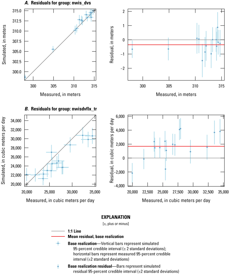
Fit between measured and simulated values at observation (measured) locations for observation groups A, nwis_dvs and B, nwisdvflx_tr for the Pleasant Lake inset model, Central Sands region, central Wisconsin. The observation group names are defined in tables 2 and 3.
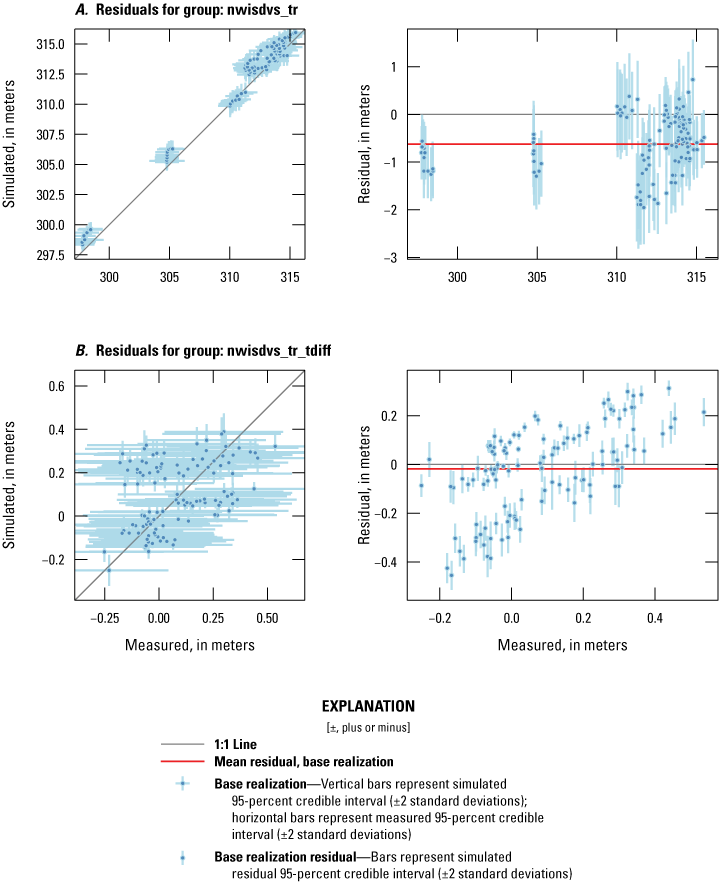
Fit between measured and simulated values at observation (measured) locations for observation groups A, nwis_dvs_tr and B, nwisdvflx_tr_tdiff for the Pleasant Lake inset model, Central Sands region, central Wisconsin. The observation group names are defined in tables 2 and 3.
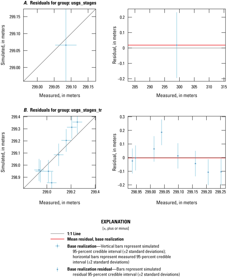
Fit between measured and simulated values at observation locations for observation groups A, usgs_stages and B, usgs_stages_tr for the Pleasant Lake inset model, Central Sands region, central Wisconsin. The observation group names are defined in tables 2 and 3.
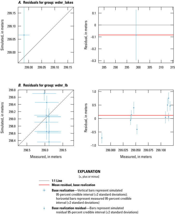
Fit between measured and simulated values at observation locations for observation groups A, wdnr_lakes and B, wdnr_lb for the Pleasant Lake inset model, Central Sands region, central Wisconsin. The observation group names are defined in table 2.
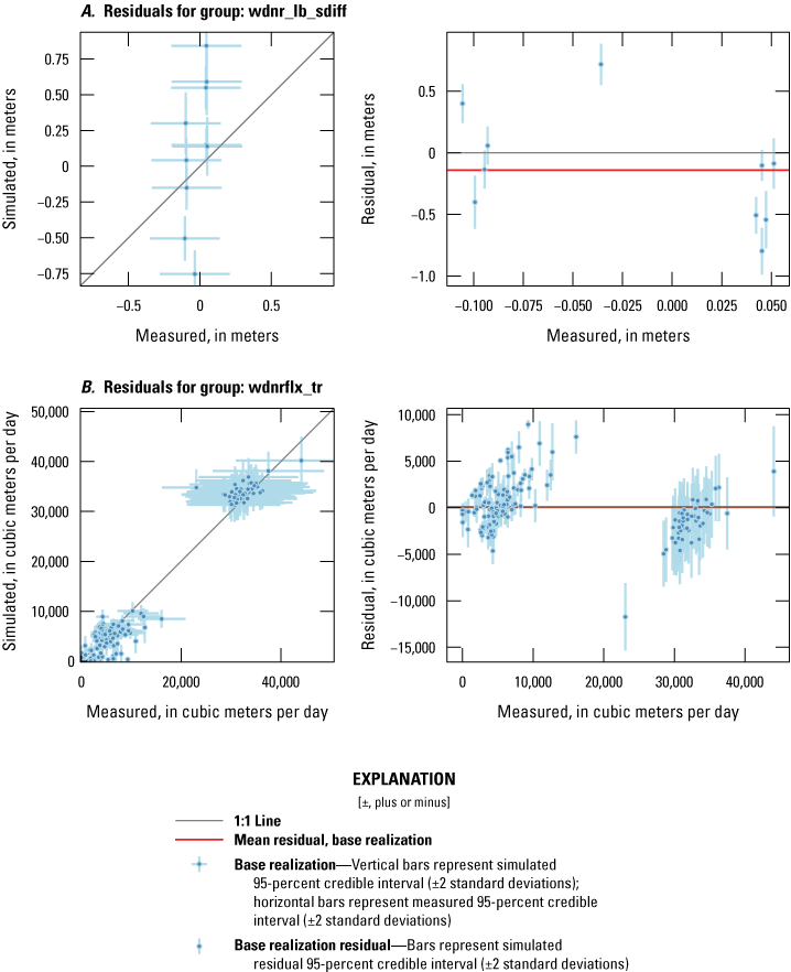
Fit between measured and simulated values at observation locations for observation groups A, wdnr_lb_sdiff and B, wdnrflx_tr for the Pleasant Lake inset model, Central Sands region, central Wisconsin. The observation group names are defined in table 2.
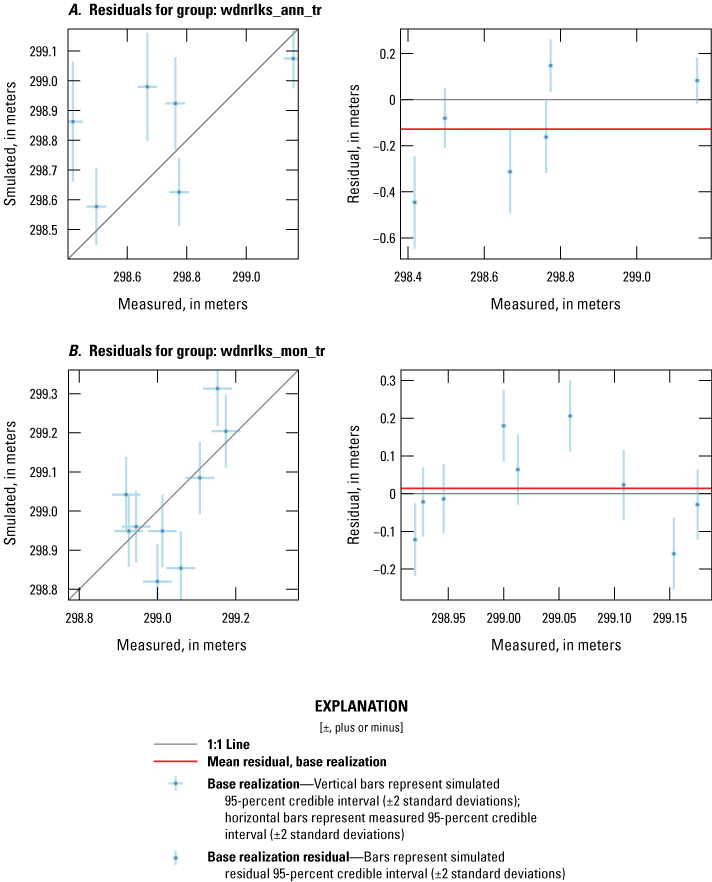
Fit between measured and simulated values at observation locations for observation groups A, wdnrlks_ann_tr and B, wdnrlks_mon_tr for the Pleasant Lake inset model, Central Sands region, central Wisconsin. The observation group names are defined in table 2.
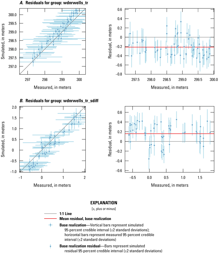
Fit between measured and simulated values at observation locations for observation groups A, wdnrwells_tr and B, wdnrwells_tr_sdiff for the Pleasant Lake inset model, Central Sands region, central Wisconsin. The observation group names are defined in table 2.
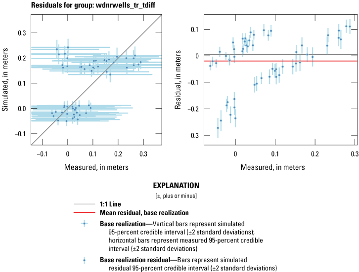
Fit between measured and simulated values at observation locations for observation group wdnrwells_tr_tdiff for the Pleasant Lake inset model, Central Sands region, central Wisconsin. The observation group names are defined in table 2.
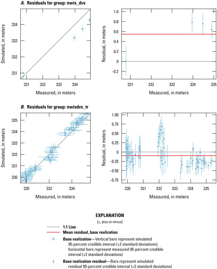
Fit between measured and simulated values at observation locations for observation groups A, nwis_dvs and B, nwisdvs_tr for the Plainfield Tunnel Channel Lakes inset model, Central Sands region, central Wisconsin. The observation group names are defined in table 3.
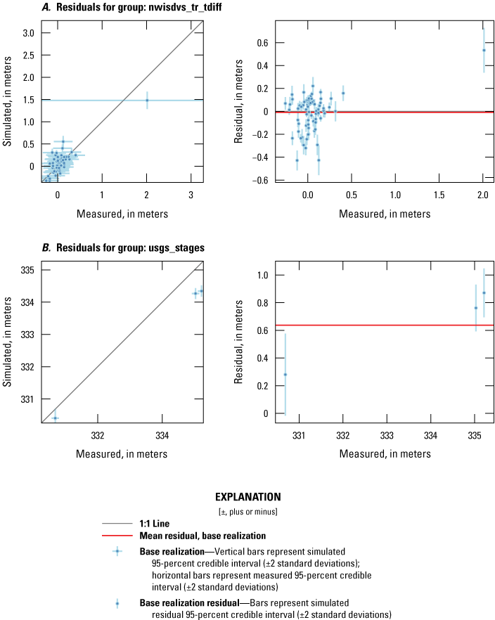
Fit between measured and simulated values at observation locations for observation groups A, nwisdvs_tr_tdiff and B, usgs_stages for the Plainfield Tunnel Channel Lakes inset model, Central Sands region, central Wisconsin. The observation group names are defined in table 3.
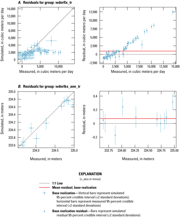
Fit between measured and simulated values at observation locations for observation groups A, wdnrflx_tr and B, wdnrlks_ann_tr for the Plainfield Tunnel Channel Lakes inset model, Central Sands region, central Wisconsin. The observation group names are defined in table 3.
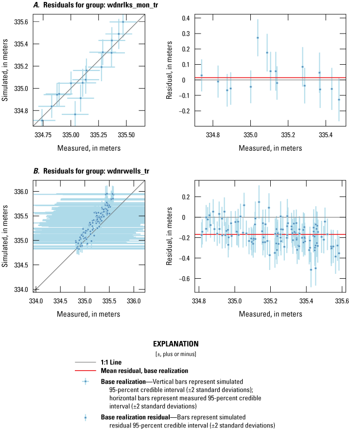
Fit between measured and simulated values at observation locations for observation groups A, wdnrlks_mon_tr and B, wdnrwells_tr for the Plainfield Tunnel Channel Lakes inset model, Central Sands region, central Wisconsin. The observation group names are defined in table 3.
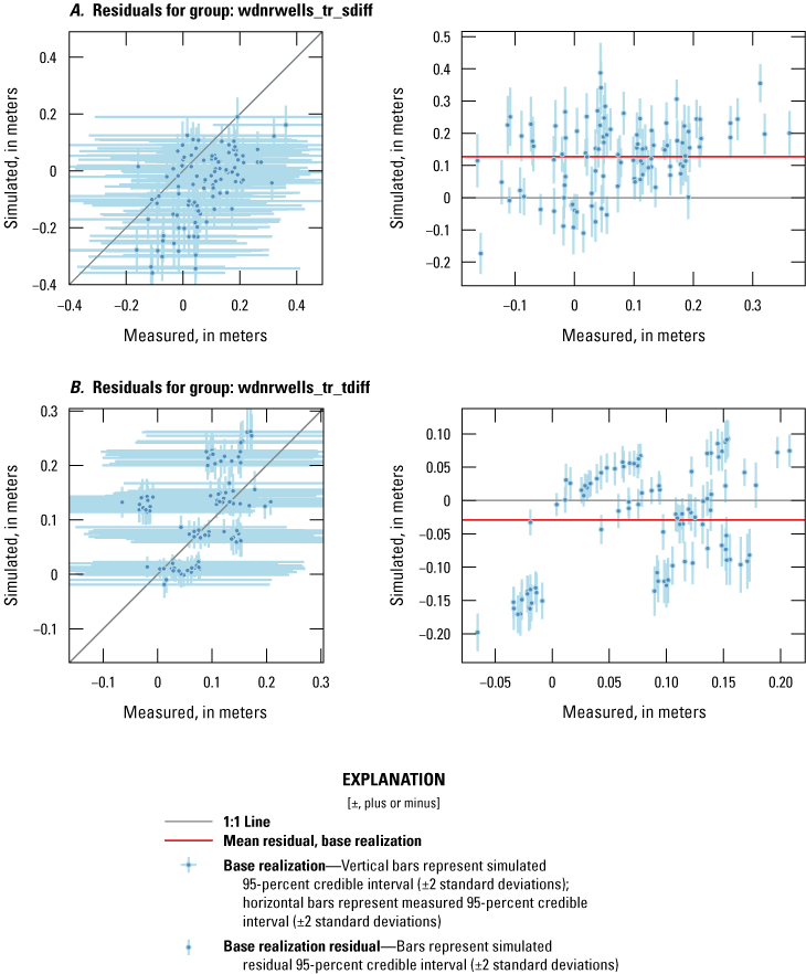
Fit between measured and simulated values at observation locations for observation groups A, wdnrwells_tr_sdiff and B, wdnrwells_tr_tdiff for the Plainfield Tunnel Channel Lakes inset model, Central Sands region, central Wisconsin. The observation group names are defined in table 3.
Fit Between Measured and Model-Simulated Observations—Spatial Distributions
The spatial patterns of weighted residuals for observations used for history matching in the Pleasant Lake and Plainfield Tunnel Channel Lakes inset models are shown in figures 40 and 41, respectively. These results were derived only from the base-case parameter set obtained from the iES ensembles, and, therefore, do not reflect the range of simulation results available in the ensembles. Most of the observations represent transient conditions; therefore, the mean of the base realization over the entire simulation time is presented. Only a partial understanding of the history matching process can be determined from figures 40 and 41, but these figures are useful for examining spatial patterns. Residuals showed spatial bias; for example, water levels near the lake were simulated greater than measured values, but the magnitude of residuals was small. In general, simulated values that were greater than measured values were closer in fit than when simulated values were less than measured values. The streamflow observations showed little spatial bias with a mix of simulated values greater and less than measured values. Subsequent sections describe the relation of simulated and measured values at specific locations in time series are discussed in detail below.
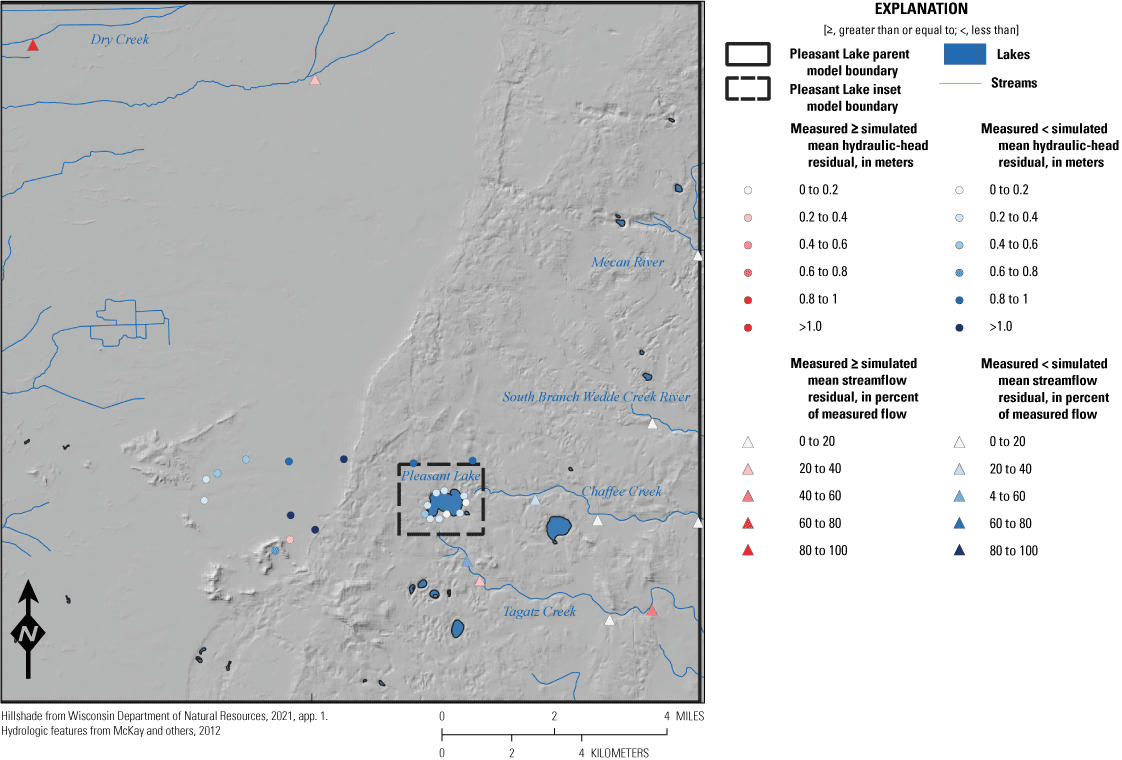
Spatial pattern of mean fit between measured and simulated observations for Pleasant Lake inset model, Central Sands region, central Wisconsin.
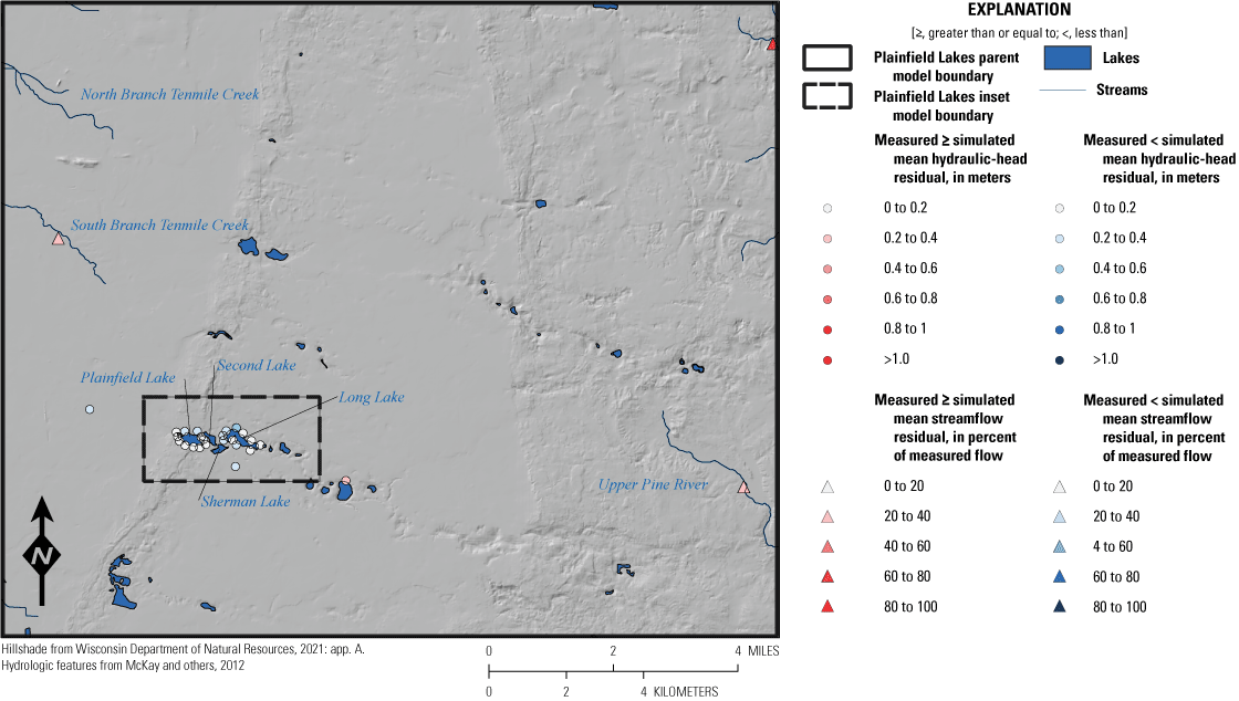
Spatial pattern of mean fit between measured and simulated observations for Plainfield Tunnel Channel Lakes inset model, Central Sands region, central Wisconsin.
Fit Between Measured and Simulated Observations–Time Series by Observation Location
Individual observation locations with transient data (hydraulic head and streamflow) provide multiple targets for history matching yet may result in multiple fit values for each location, spanning over model-simulation time. The uncertainty of the observed values, as determined for the iES process as the inverse of their observation weight, can be expressed as a 95-percent credible interval using bars that extend two times σ above and below the observed value at a given time. Unlike the 1:1 plots (figs. 38 and 39), an accompanying bar for the simulated values is not in figure 42. Instead, the time series for each ensemble realization is displayed separately as a thin gray line. This time series indicates not only the uncertainty of both observations and simulated values but also the continuity of values over time in each ensemble realization.
Observation points labeled as prior data conflict (PDC) indicate observations that were under prior data conflict, meaning that, in these cases, the initial ensemble evaluated by iES identifies observations where simulated values are statistically distant (White and others, 2021) from the measured values. Because iES evaluates a wide range of parameters in this initial run, the history matching process is unlikely to result in a reasonable set of parameters that will make the model fit close enough to be considered valid. In other words, the model is being used to flag observations that cannot be fit with the indicated model parameters. This can result from observation errors or from deficiencies in the model conceptualization or validity of model parameters, or both. In PEST++, these observations may be systematically assigned zero observation weight to prevent them from affecting the history matching process. Alternatively, PDC can serve as a diagnostic tool to point out areas of concern that would benefit from additional study to improve the quality of the observations, model conceptualization, and/or model parameters. In this study, the PDC labels were assigned to observations in prior data conflict to indicate that observations were unlikely to result in low residuals. These observations were retained with their initially assigned observation weight. Results for time series in each of the two inset models are described below.
The general patterns of observed lake levels are reproduced in the Pleasant Lake inset model and, at most times, the simulated results from the model realizations overlap with the measured values (fig. 42). The bars indicating uncertainty of the measured values are not visible in these plots because the observation weight was assigned high enough to these important observations that the implied uncertainty is small. The model results at the beginning of the simulation period may be affected by a need for a “spin-up” or “warm start” for the simulation of the lake level to reach a dynamic equilibrium with respect to changes in groundwater storage. To account for this potential discrepancy between simulated and measured lake levels, recent observations were assigned higher observation weight than values for time steps early in the model-simulation run that include data from early in the simulation period. The other period of large differences, between simulated and measured values, occured in the spring of 2018. This result may indicate that the lake level was anomalously high because of above-average surface runoff associated with the spring melt that year. Surface runoff is not simulated in this model, so under-simulation of the lake level under that above-average runoff condition is expected.
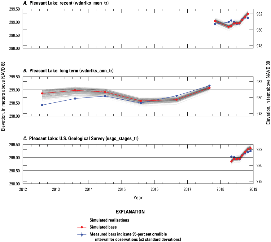
Time series of measured and simulated results for lake level observations in the Pleasant Lake inset model, Central Sands region, central Wisconsin: A, observation group wdnrlks_mon_tr; B, observation group wdnrlks_ann_tr; and C, observation group usgs_stages_tr. The observation group names are defined in table 2.
The patterns and magnitudes of simulated streamflow were generally similar to the measured values throughout the Pleasant Lake inset model (figs. 43–46). Various observations are labeled as PDC. These PDC observations are typically locations where either the measured streamflow was already low and dropped to near zero or represented as high flow because of runoff. Whereas the streamflows in the study area generally are dominated by base flow, some storm events do occur and the SFR package in MODFLOW 6 does not include explicit consideration of storm runoff.
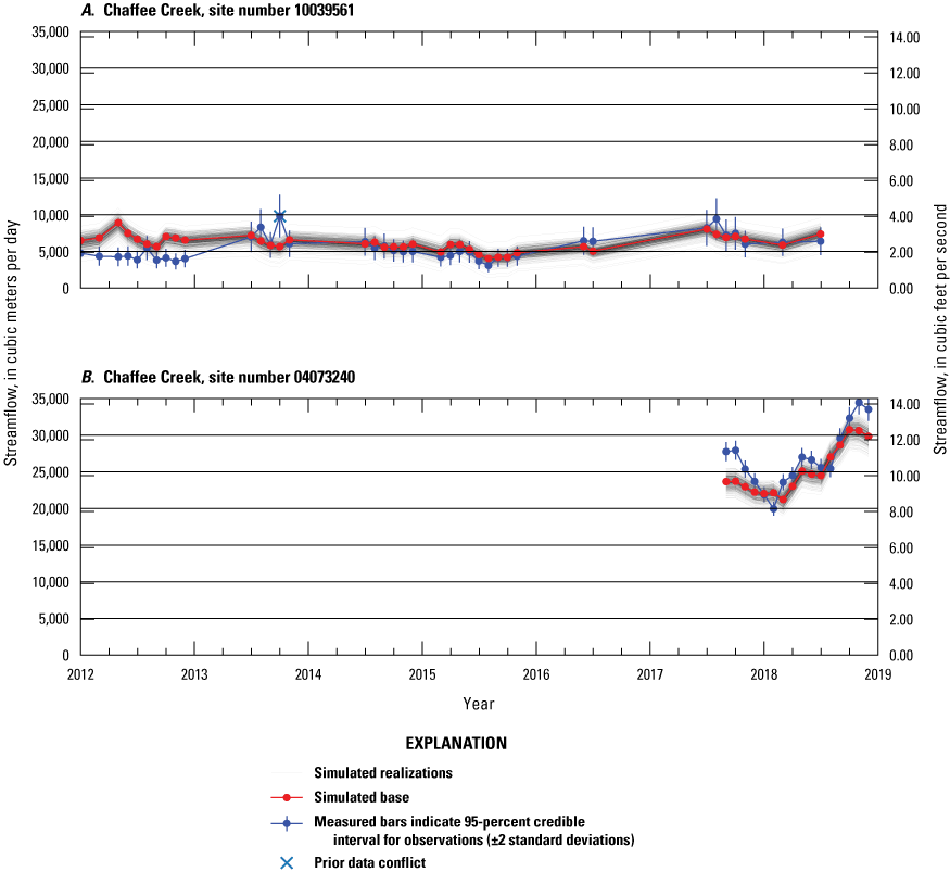
Time series of measured and simulated results for streamflow observations in Chaffee Creek sites A, 10039561chaffeecr and B, 04073240chaffeecr in observation groups wdnr_miscflx and nwis_dv_flx, respectively, in the Pleasant Lake inset model, Central Sand region, central Wisconsin. The observation group names are defined in table 1. Locations of sites are shown on figure 21.
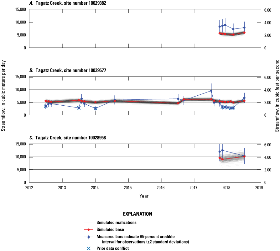
Time series of measured and simulated results for streamflow observations in the observation group wdnr_miscflx for Tagatz Creek sites A, 10029382tagzcrk4; B, 10039577tagzcrk4; and C, 10028958 tagzcrkc in the Pleasant Lake inset model, Central Sands region, central Wisconsin. Locations of sites are shown in figure 21.
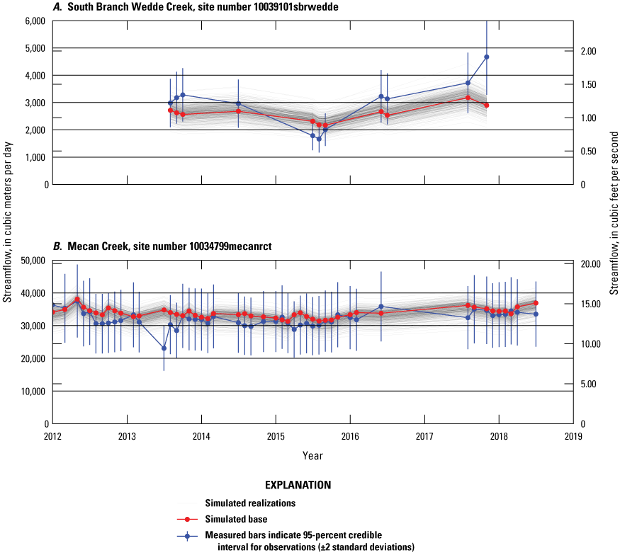
Time series of measured and simulated results over time for streamflow observations in the observation group wdnr_miscflx, A, South Branch Wedde Creek site 10039101sbrwedde and B, Mecan Creek site 10034799mecanrct, Central Sands region, central Wisconsin. The observation group names are defined in table 2. Locations of sites are shown in figure 21.
The time-series results for the piezometers near Pleasant Lake in the wdnrwells_tr group—wells that represent hydraulic head conditions around the lake perimeter—are shown in figures 46–47. These model results are nearly all within the 95-percent credible range for the observations. The observation group names are defined in tables 2 and 3.
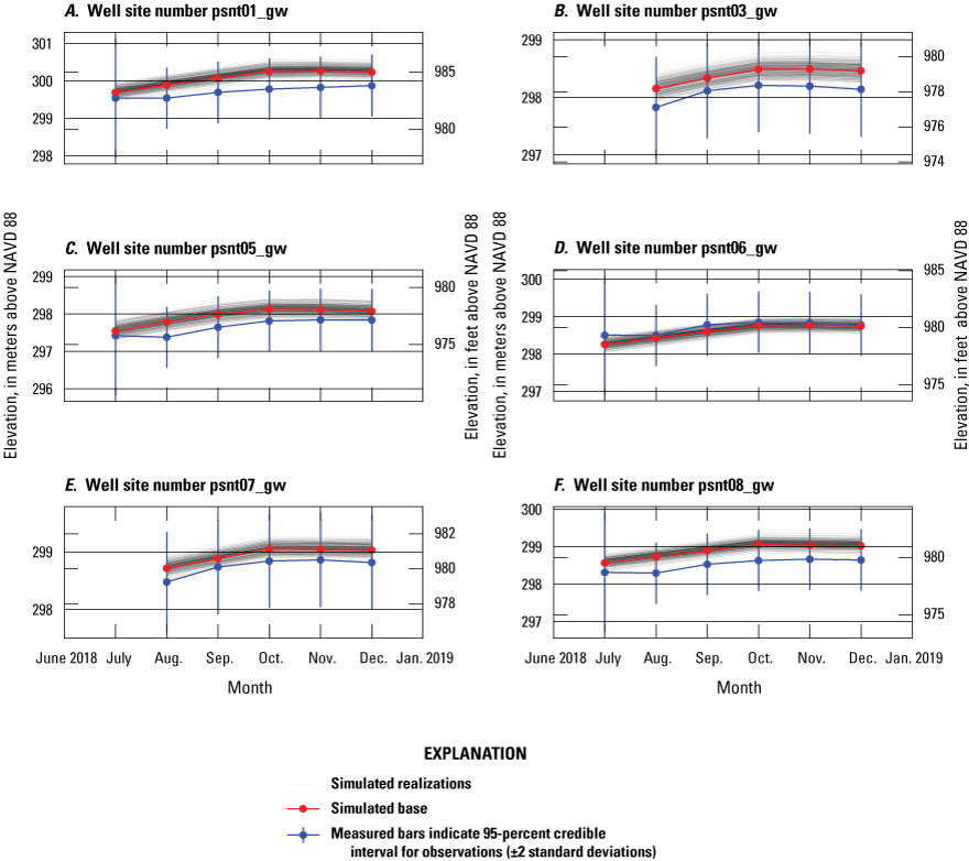
Time series of measured and simulated results for transient piezometers near Pleasant Lake in the observation group wdnrwells_tr, (part 1), Central Sands region, central Wisconsin: A, psnt01_gw; B, psnt03_gw; C, psnt05_gw; D, psnt06_gw; E, psnt07_gw; and F, psnt08_gw. The observation group names are defined in table 2. Locations of sites are shown in figure 21.
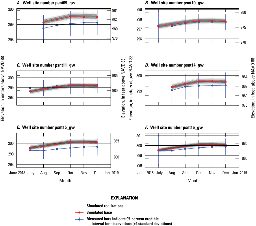
Time series of measured and simulated results for transient piezometers near Pleasant Lake in the observation group wdnrwells_tr (part 2), Central Sands region, central Wisconsin. The observation group names are defined in table 2. Location of sites are shown in figure 21.
The groundwater hydraulic-head values (water levels) in the wells of the observation group nwisdvs_tr for which daily values are available in the National Water Information System database (U.S. Geological Survey, 2021) are shown in figures 48 and 49. Water levels measured in these wells reflect the overall pattern of groundwater levels in recent time. Where the greatest discrepancies are observed (particularly in fig. 49), the simulated values typically are too high rather than too low. This bias may be, at least in part, an unintended consequence caused by the assignment of high observation weight on streamflow and lake-level observations that results in a parameter set yielding higher water levels in the aquifer to better match those observations. For streamflow, in particular, this parameter could be compensating for water that enters the streams through processes not explicitly simulated in these models.
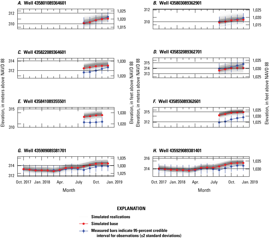
Time series of measured and simulated results for hydraulic heads (water levels) in wells with daily values in the U.S. Geological Survey National Water Information System in the Pleasant Lake inset model in the group nwisdvs_tr (part 1), Central Sands region, central Wisconsin: A, well 435801089364601; B, well 435803089362901; C, well 435822089364601; D, well 435832089362701; E, well 435841089355501; F, well 435855089362601; G, well 435909089381701; H, well 435929089381401. The observation group names are defined in table 2. Locations of sites are shown in figure 21.
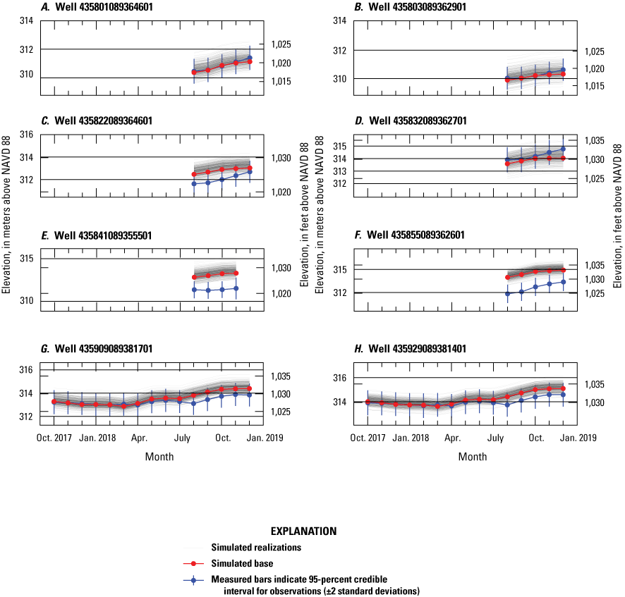
Time series of measured and simulated results for heads in wells with daily values in the U.S. Geological Survey National Water Information System in the Pleasant Lake inset model in the group nwisdvs_tr (part 2), Central Sands region, central Wisconsin: A, well 435801089364601; B, well 435803089362901; C, well 435822089364601; D, well 435832089362701; E, well 435841089355501; F, well 435855089362601; G, well 435909089381701; H, well 435929089381401. The observation group names are defined in table 2. Locations of sites are shown in figure 21.
The lake-level time series for the Plainfield Tunnel Channel Lakes inset model are shown in figure 50. The recent (2018) and long-term patterns (2017–18) for Plainfield Lake are shown in panels A and B, respectively. The recent (2018) and long-term (2013–18) patterns for Long Lake are shown in panels C and D respectively. The general patterns of lake levels are reproduced, and at most times the simulated realizations overlap with the observed (measured) values. Unlike Pleasant Lake, where some appreciable differences likely resulted from spring runoff, in Plainfield and Long Lakes, the overall dynamics are visible in the most recent monthly data as shown in panels A and C, respectively.

Time series of measured and simulated results for lake level observations in the Pleasant Lake inset model, Central Sands region, central Wisconsin: A, Plainfield Lake, observation group wdnrlks_mon_tr; B, Plainfield Lake, observation group wdnrlks_ann_tr; C, Long Lake, observation group wdnrlks_mon_tr; and D, Long Lake, observation group wdnrlks_ann_tr. The observation group names are defined in table 3.
The time series of streamflow in the two streams (North Branch Tenmile Creek and Upper Pine River) with history matching data in the Plainfield Tunnel Channel Lakes inset model are shown in figure 51. The patterns and magnitudes of simulated streamflow were generally similar to the measured values. Nearly all ensemble simulated values fall within the 95-percent credible intervals for the streams. Streamflow in North Branch Tenmile Creek is simulated as higher values than those measured at the extremely low observed streamflow conditions between 2012 and 2015. Such low values are difficult to represent accurately with the model and difficult to quantify when measured in the field, as indicated by the relatively large credible interval around the observations. Similar to some of the observations in the Pleasant Lake model, at least one storm event in late 2017 simulated too low in both streams, likely because of runoff not being explicitly represented in the model. The simulated results in the Upper Pine River are closer to measured values with the exception of the late 2017 storm event.
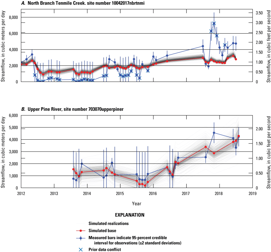
Time series of measured and simulated results for streamflow observations in A, North Branch Tenmile Creek site 10042017nbrtnmi and B, Upper Pine River site 703070upperpiner in the Plainfield Tunnel Channel Lakes inset model, Central Sands region, central Wisconsin. Locations of sites are shown in figure 22.
The time-series results for the piezometers near Long Lake in the wdnrwells_tr observation group are shown in figures 52 and 53; the time-series results for the piezometers near Plainfield Lake in the wdnrwells_tr observation group are shown in figures 54 and 55. These wells represent hydraulic-head conditions around the lake perimeter, and the simulated results are nearly all within the 95-percent credible range for the observations.
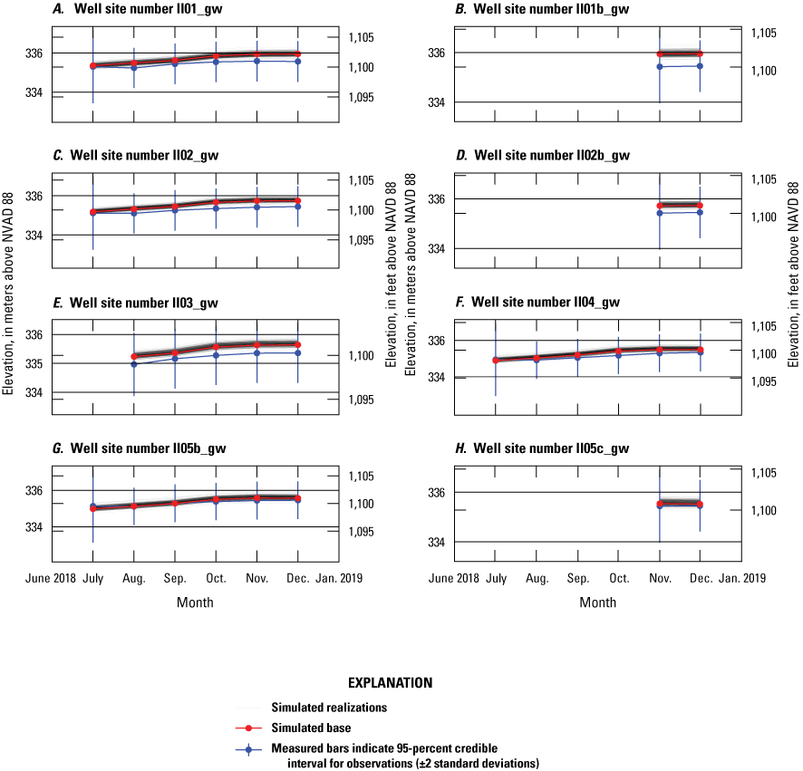
Time series of measured and simulated results for transient piezometers near Long Lake in the observation group wdnrwells_tr (part 1), Central Sands region, central Wisconsin: A, well number ll01_gw; B, well number ll01b_gw; C, well number ll02_gw; D, well number ll02b_gw; E, well number ll03_gw; F, well number ll04_gw; G, well number ll05b_gw; and H, well number ll05c_gw. The observation group names are defined in table 3. Locations of sites are shown in figure 22.
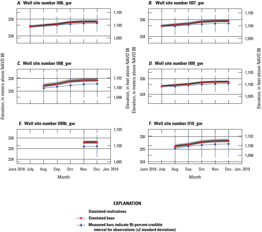
Time series of measured and simulated results for transient piezometers near Long Lake in the observation group wdnrwells_tr (part 2), Central Sands region, central Wisconsin: A, well number ll06_gw; B, well number, ll07_gw; C, well number ll08_gw; D, well number ll09_gw; E, ll09b_gw; and F, well number ll10_gw. The observation group names are defined in table 3. Locations of sites are shown in figure 22.
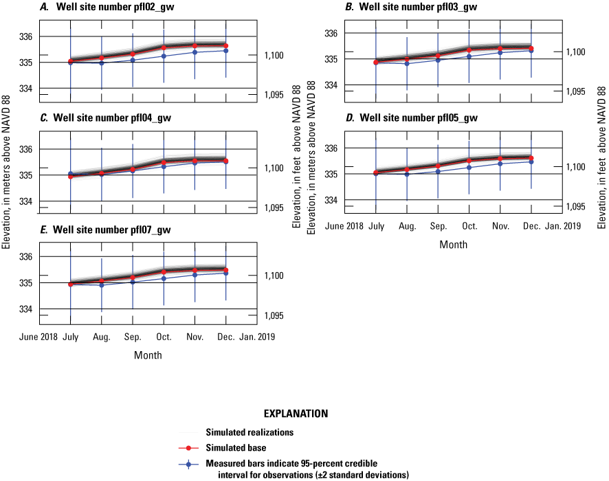
Time series of measured and simulated results for transient piezometers near Plainfield Lake in the observation group wdnrwells_tr (part 1), Central Sands region, central Wisconsin: A, well site number pfl02_gw; B, well site number pfl03_gw; C, well site number pfl04_gw; D, well site number pfl05_gw; and E, well site number pfl07_gw. The observation group names are defined in table 3. Locations of sites are shown in figure 22.
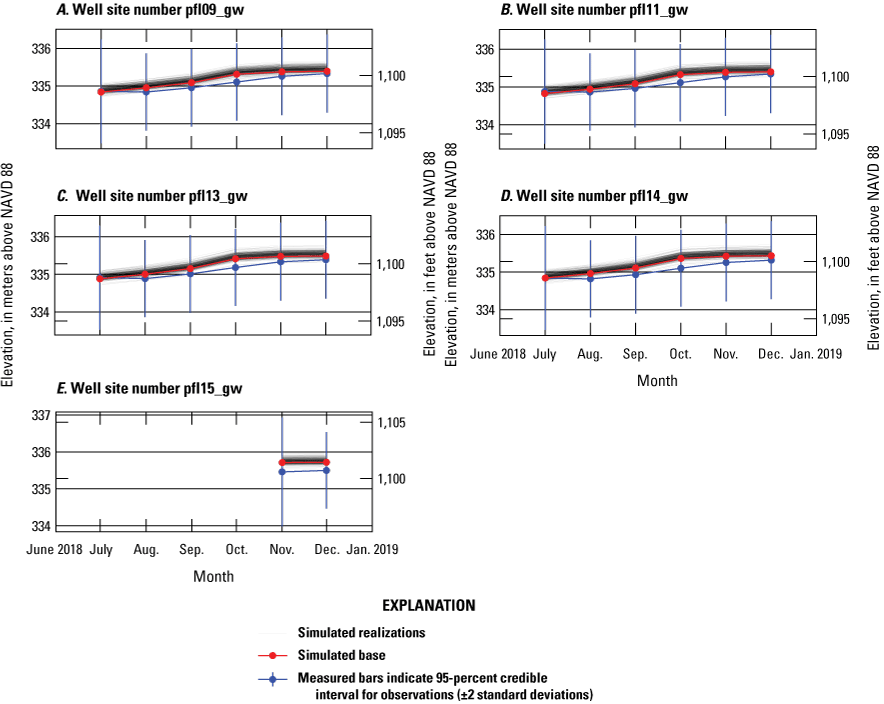
Time series of measured and simulated results for transient piezometers near Plainfield Lake in the observation group wdnrwells_tr (part 2), Central Sands region, central Wisconsin: A, well site number pfl09_gw; B, well site number pfl11_gw; C, well site number pfl13_gw; D, well site number pfl14_gw; E, well site number pfl15_gw. The observation group names are defined in table 3. Location of sites are shown in figure 22.
Time series for groundwater hydraulic-head values in the wells of the nwisdvs_tr group, for which daily values are available in the USGS National Water Information System database, are shown in figure 56. Site 441146089250301, which includes observations from the beginning of the simulation, is shown in panel A. Time series for the wells shown in panels B, C, and D represent recent time (2018–19). Similar to the Pleasant Lake inset model, where the fit is poorest, simulated values generally are higher than measured values. An exception is the winter of 2017–18, where simulated values briefly decreased while measured values were increasing at site 441146089250301 (fig. 56A); however, the overall water-level response is similar in increasing water-level elevations at the end of the simulation period.
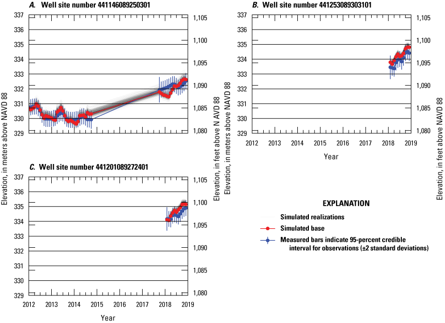
Time series of measured and simulated results for hydraulic heads (water levels) in wells with daily values in the U.S. Geological Survey National Water Information System database (U.S. Geological Survey, 2021) in the Plainfield Tunnel Channel Lakes inset model in the group nwisdvs_tr, Central Sands region, central Wisconsin: A, well site number 441146089250301; B, well site number 441253089303101; and C, well site number 441201089272401. The observation group names are defined in table 3. Location of sites are shown in figure 22.
Focus Area Inset Model Results
After history matching, both inset models were updated with the “base” parameter set from iES iteration number 3, which represents the single best or “minimum error variance” estimate of parameter values (see the “Parameter Estimation and Uncertainty Analysis” section). The updated models were then run for the history matching period from 2012 through 2018 and used for the scenarios described in the “Lake Ecosystem Response Assessment (LERA)section. Results for the 2012 through 2018 history matching period are described below.
Parameter Estimates
The base parameter set spatial distributions for the inset models, after history matching, are shown in figures 57–64. The use of multipliers against the parameter values estimated at the regional scale resulted in parameter fields similar to those values in the regional model. In the Pleasant Lake model, in particular, some greater changes in parameter values were estimated in the inset models focused around the lake relative to the parent model region. The high observation weight assigned to lake elevation observations and the presence of headwater streams that are highly sensitive to small changes in parameters make the parameters in the inset models particularly critical for accurate model simulation and subject to greater changes than the surrounding area.
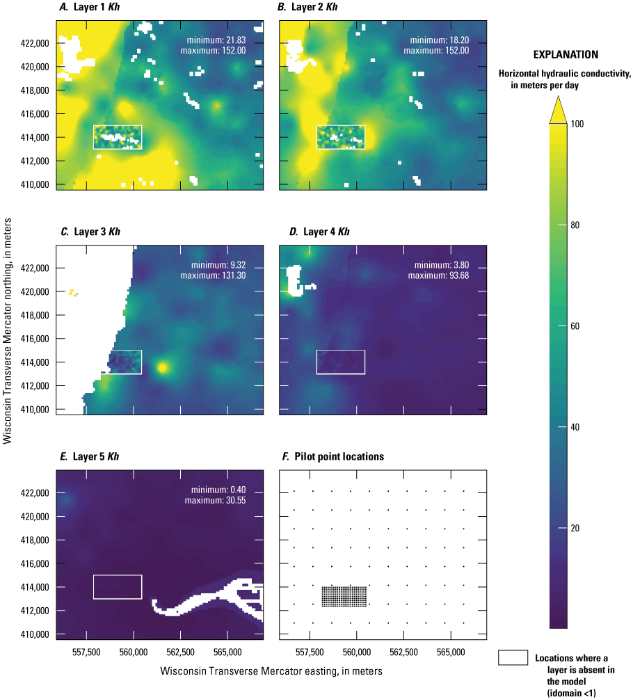
Horizontal hydraulic conductivity (Kh) estimates for the Plainfield Tunnel Channel Lakes model, Central Sands region, central Wisconsin: A, layer 1 Kh; B, layer 2 Kh; C, layer 3 Kh; D, layer 4 Kh; E, layer 5 Kh; and F, pilot point locations. Pilot-point locations apply to all model layers.
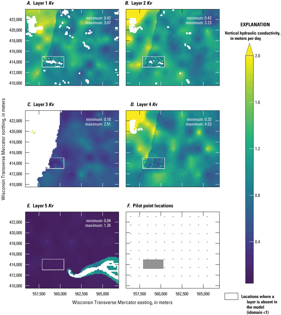
Vertical hydraulic conductivity (Kv) estimates for the Plainfield Tunnel Channel Lakes model, Central Sands region, central Wisconsin: A, layer 1 Kv; B, layer 2 Kv; C, layer 3 Kv; D, layer 4 Kv; E, layer 5 Kv; and F, pilot point locations. Pilot-point locations apply to all model layers.
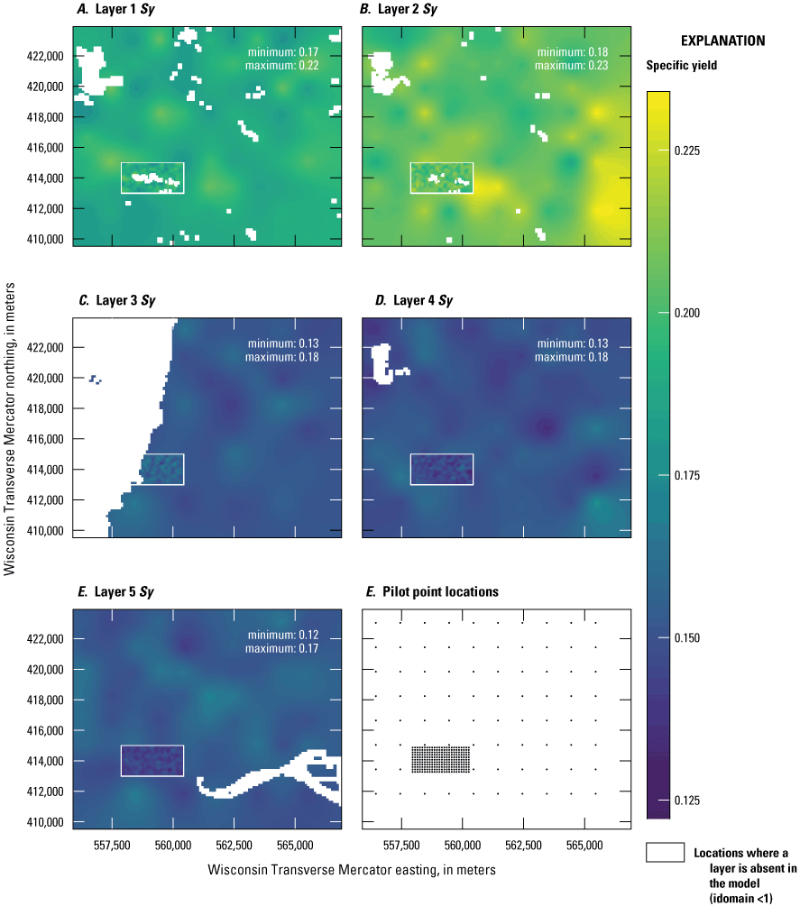
Specific yield (Sy) estimates for the Plainfield Tunnel Channel Lakes model, Central Sands region, central Wisconsin: A, layer 1 Sy; B, layer 2 Sy; C, layer 3 Sy; D, layer 4 Sy; E, layer 5 Sy; and F, pilot point locations. Pilot-point locations apply to all model layers.
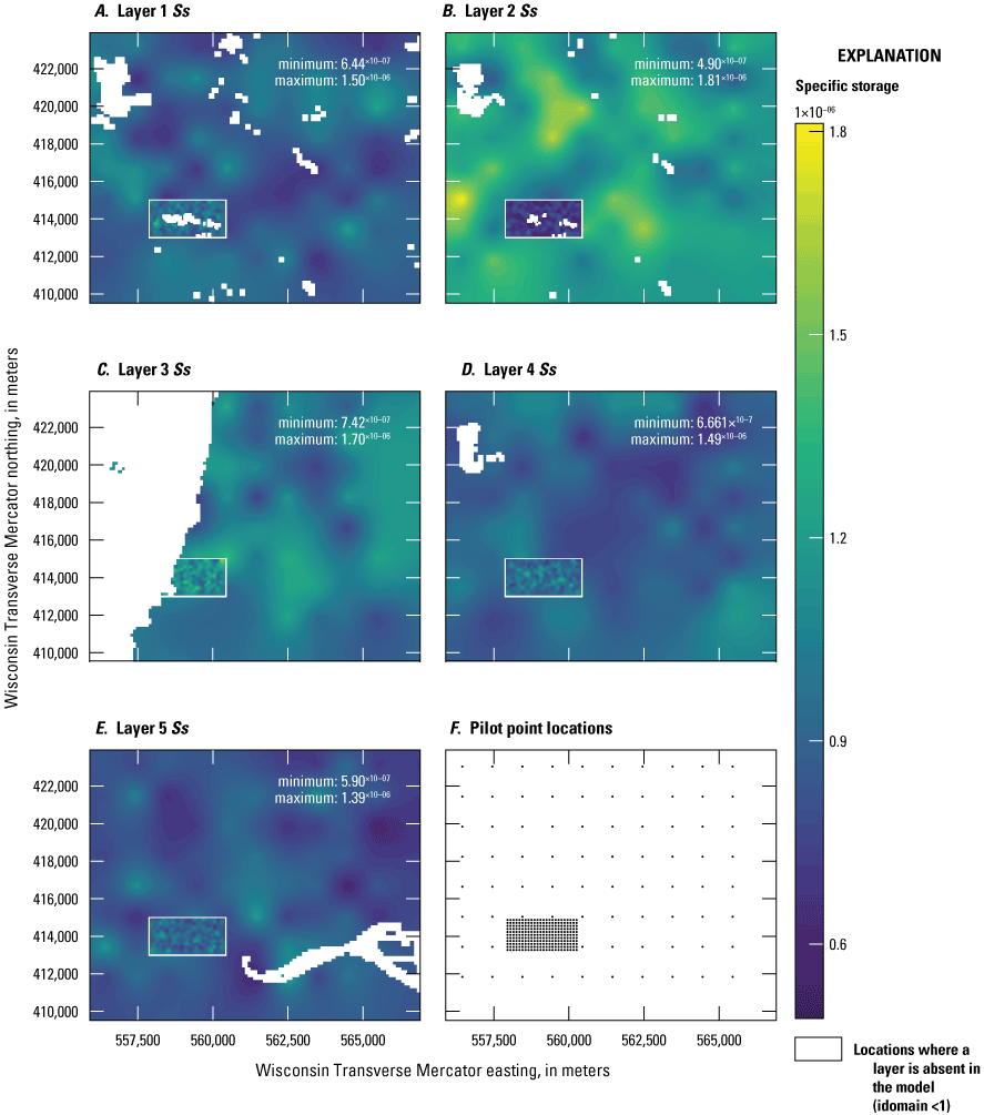
Specific storage (Ss) estimates for the Plainfield Tunnel Channel Lakes model, Central Sands region, central Wisconsin: A, layer 1 Ss; B, layer 2 Ss; C, layer 3 Ss; D, layer 4 Ss; E, layer 5 Ss; and F, pilot point locations. Pilot point locations apply to all model layers.
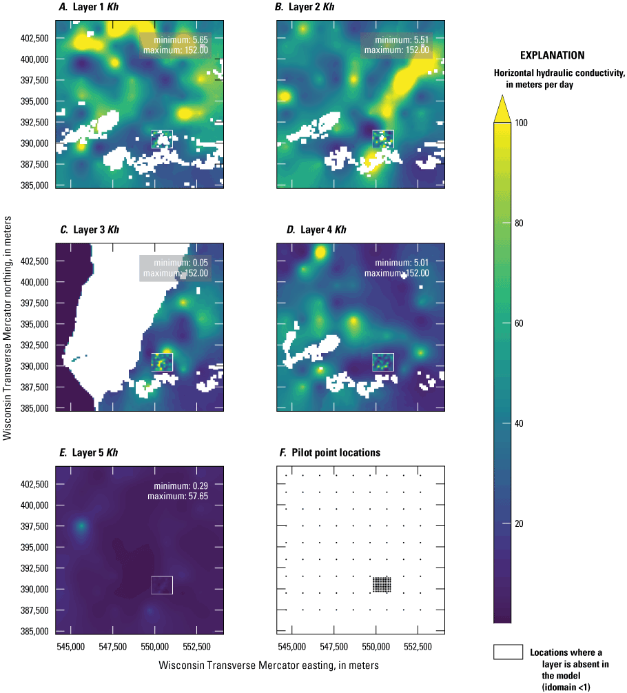
Horizontal hydraulic conductivity (Kh) estimates for the Pleasant Lake model, Central Sands region, central Wisconsin: A, layer 1 Kh; B, layer 2 Kh; C, layer 3 Kh; and D, layer 4 Kh. White areas indicate locations where a layer is absent in the model (idomain=0). Pilot-point locations apply to all model layers.
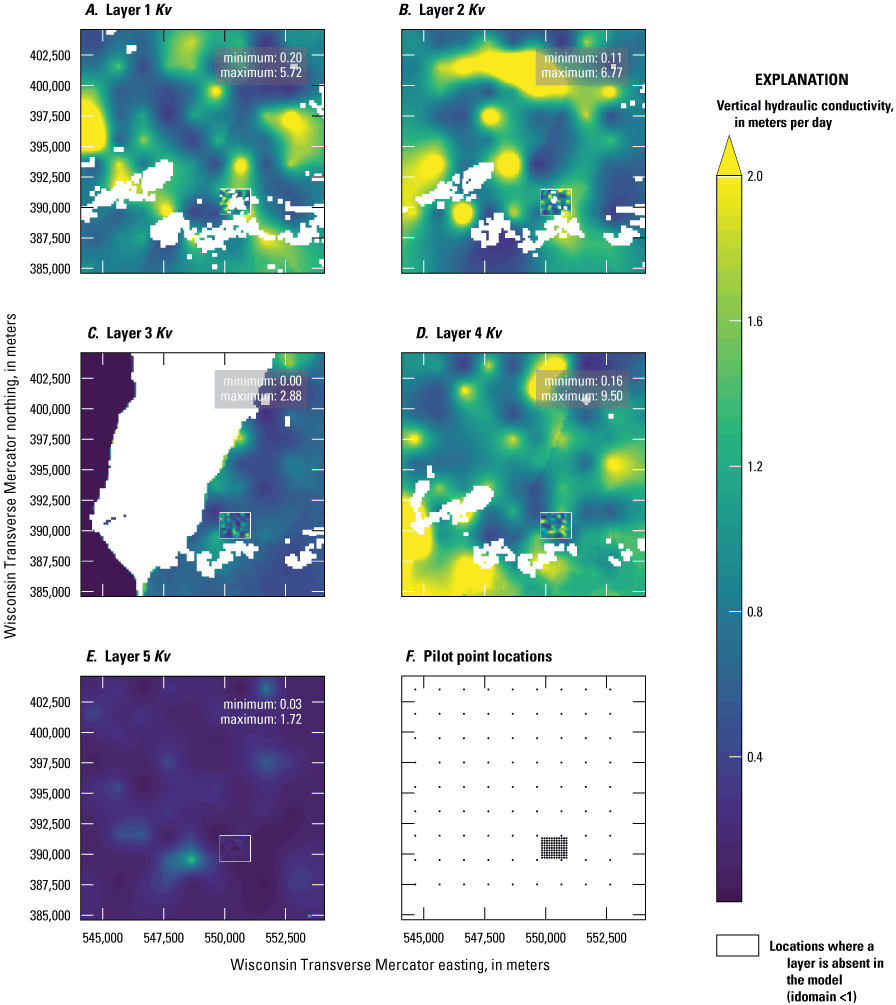
Vertical hydraulic conductivity (Kv) estimates for Pleasant Lake model, Central Sands region, central Wisconsin: A, layer 1 Kv; B, layer 2 Kv; C, layer 3 Kv; D, layer 4 Kv; E, layer 5 Kv; F, pilot point locations White areas indicate locations where a layer is absent in the model (idomain=0). Pilot-point locations apply to all model layers.

Specific yield (Sy) estimates for the Pleasant Lake model, Central Sands region, central Wisconsin: A, layer 1 Sy; B, layer 2 Sy; C, layer 3 Sy; D, layer 4 Sy; E, layer 5 Sy; and F, pilot point locations. White areas indicate locations where a layer is absent in the model (idomain=0). Pilot-point locations apply to all model layers.
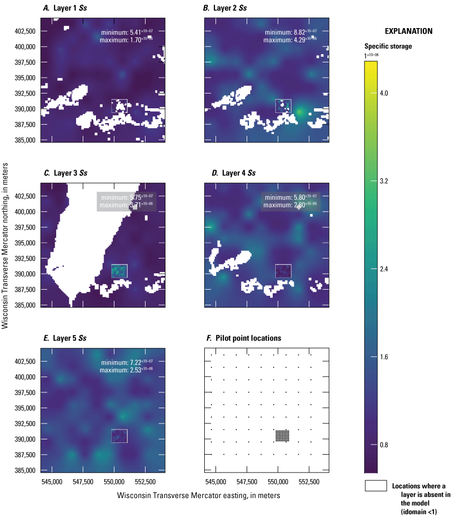
Specific storage (Ss) estimates for the Pleasant Lake model, Central Sands region, central Wisconsin: A, layer 1 Ss; B, layer 2 Ss; C, layer 3 Ss; D, layer 4 Ss; E, layer 5 Ss; F, Pilot point locations. White areas indicate locations where a layer is absent in the model (idomain=0). Pilot-point locations apply to all model layers.
Groundwater Flow and Boundary-Condition Fluxes for Mean (2012–15) Conditions
Simulated steady-state water-table elevations and boundary-condition fluxes for both inset models, under mean conditions for the period of 2012–15, are shown in figures 65 and 66. Discharge from the groundwater-flow system to streams, wells, or across the specified-head perimeter boundaries out of the model domain is represented with a red color scale. A blue color scale represents discharge to the simulated groundwater-flow system from stream leakage or inflow into the model domain through the specified-head boundaries. Note that for streams, this color scheme is opposite of that shown in figure 12 for the regional parent model, where blue colors indicate groundwater discharge to streams (inflows from the perspective of the streams). Lake/groundwater interactions are displayed separately from the perspective of the lakes, with blue indicating groundwater discharge to the lakes and red indicating lake leakage to groundwater.
The overall flow patterns indicated by the simulated water-table elevation contours are consistent with the regional model (fig. 16). In both inset models, groundwater discharge along the perimeter is simulated mostly as leaving the model domains, a result of the model domains being located along the groundwater divide that runs through the streamless portion of the study area. A small amount of groundwater flow enters the domains from the north, consistent with regional flow patterns. Similarly, streams within the inset models are mostly gaining groundwater, with the exception of the Upper Pine River (fig. 12) and Tagatz Creek (fig. 66), which are in the hummocky collapsed terrain east of the moraines. Simulated groundwater discharge to and from the study lakes reflects the simulated water-table gradients, with the lakes gaining groundwater on the upgradient side and losing water to the groundwater system on the downgradient side.
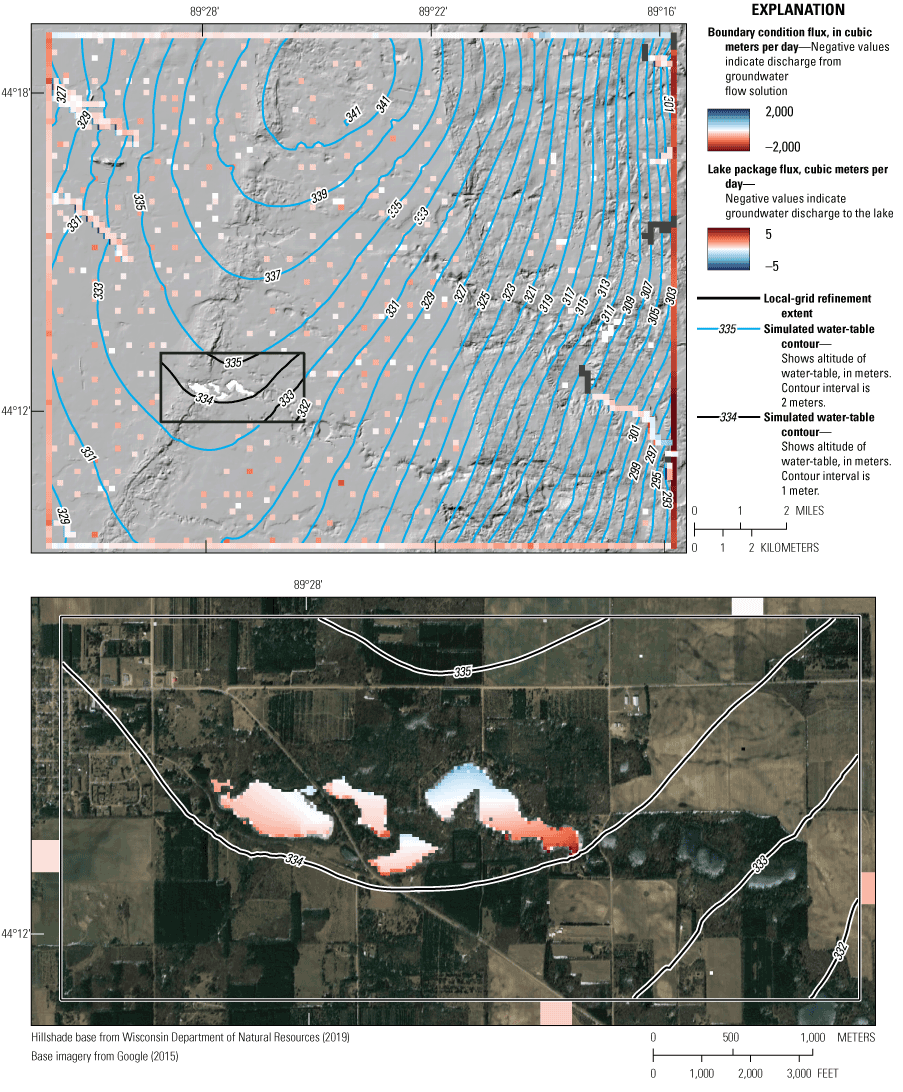
Plainfield Tunnel Channel Lakes model steady-state water table and boundary fluxes, Central Sands region, central Wisconsin.
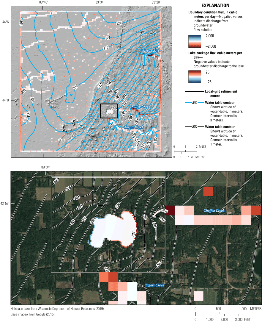
Pleasant Lake model steady-state water table and boundary fluxes, Central Sands region, central Wisconsin.
Groundwater Flow and Boundary-Condition Fluxes for Transient (2012–18) Conditions
Because the local-grid refinement for the inset models is implemented using linked models (within a MODFLOW-6 simulation), global water-budget results are reported separately for the parent (figs. 67 and 68) and LGR (figs. 69 and 70) submodels within each inset model. The parent submodel budgets indicate seasonal trends that are similar to the regional model—a spring recharge period when groundwater is added to storage, followed by a summer pumping period when groundwater is removed from storage, and a less pronounced fall recharge period. In both inset models, recharge increases in 2018 in response to above-normal precipitation that year. Flow out of the specified-head boundaries is relatively steady in both models, although flow increases in 2018 in the Plainfield Tunnel Channel Lakes model in response to the increase in recharge. A key difference between the two inset models is the greater amount of stream outflow in the Pleasant Lake model (approximately 20-40 percent of the total water budget) compared to the Plainfield Tunnel Channel Lakes model (where stream outflow is generally less than 10 percent of the total water budget).
Groundwater Flow and Boundary-Condition Fluxes for Mean (2012–15) Conditions
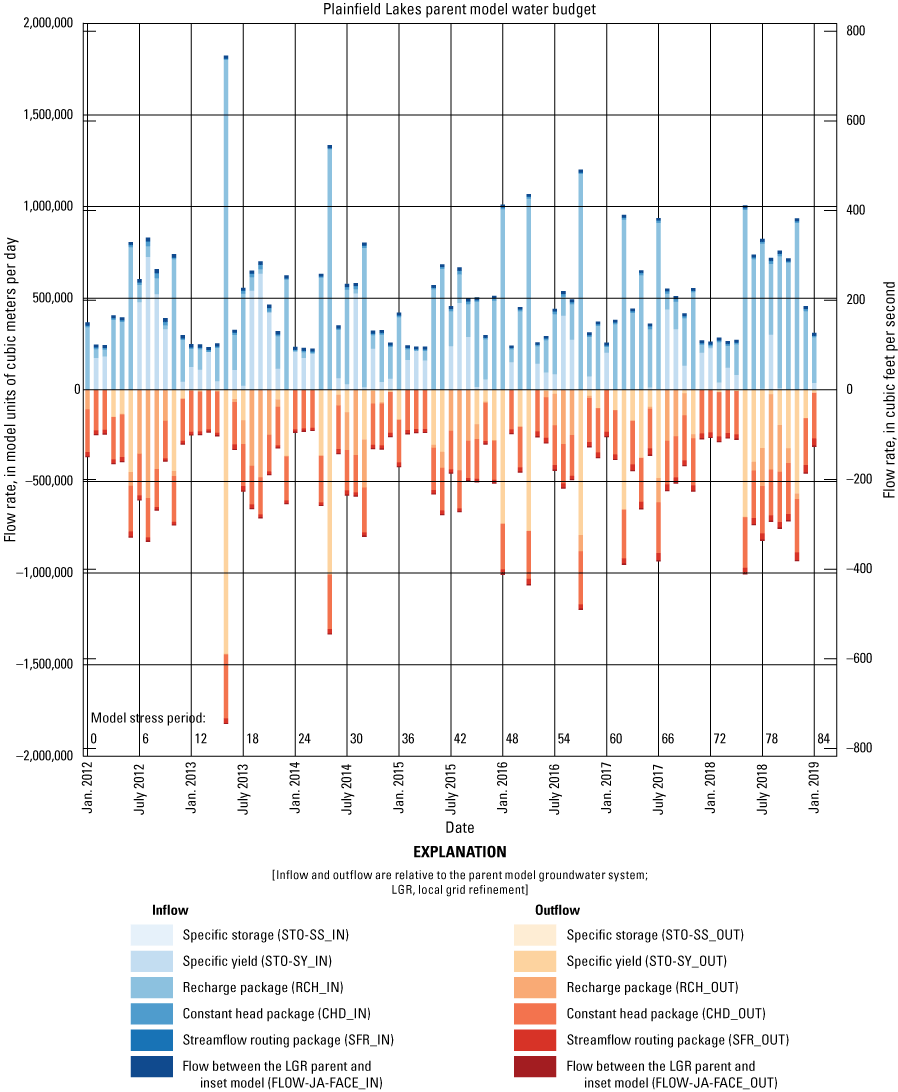
Plainfield Tunnel Channel Lakes parent model water budget, Central Sands region, central Wisconsin. Inflows and outflows are named using the MODFLOW list file convention.
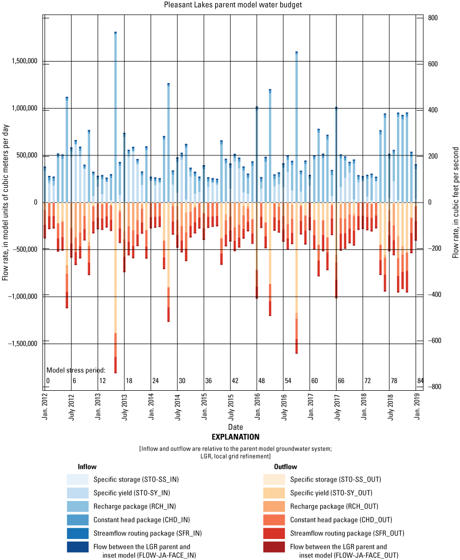
Pleasant Lake parent model water budget, Central Sands region, central Wisconsin. Inflows and outflows are named using the MODFLOW list file convention.
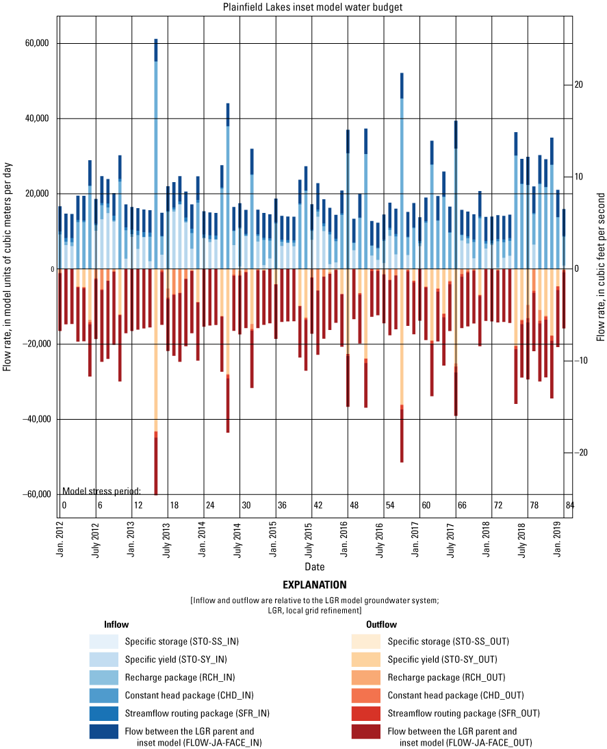
Plainfield Tunnel Channel Lakes local grid refinement submodel water budget, Central Sands region, central Wisconsin. Inflows and outflows are named using the MODFLOW List file convention.
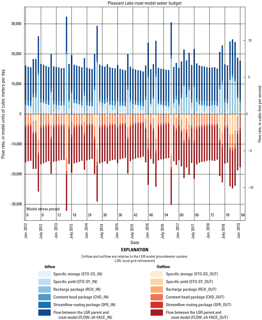
Pleasant Lake local-grid refinement submodel water budget, Central Sands region, central Wisconsin. Inflows and outflows are named using the MODFLOW List file convention.
The inset submodel budgets are dominated by flows exchanged with the parent submodels (“FLOW-JA-FACE” term). This result is acceptable because the two submodels are fully coupled at the inner iteration level, meaning continuity in the groundwater-flow model final solution is preserved throughout the inset model domain. Otherwise, the inset submodel water budgets show some of the same seasonal trends as the parent submodel. Also, the inset submodel budget indicates a small magnitude of flux through the lakes relative to other sources and sinks.
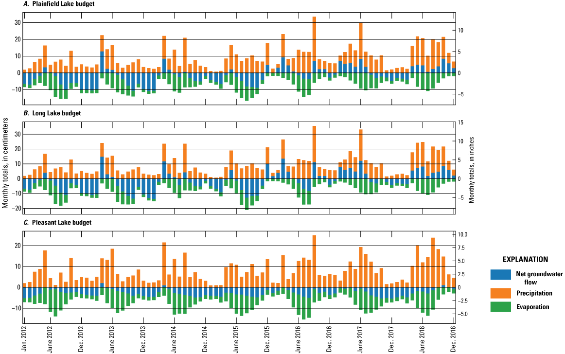
Lake model-simulated water budgets for A, Plainfield; B, Long; and C Pleasant Lakes, Central Sands region, central Wisconsin.
The simulated water budgets for Plainfield and Long Lakes (fig. 71) show a seasonal pattern of mostly net groundwater outflow (out of the model domain) in the fall and winter months, with net groundwater inflow (into the model domain) in the spring, when groundwater levels are high. In both lakes, there is a pattern towards predominantly gaining conditions later in the simulation, with net groundwater inflow for most of 2018, consistent with the field observations by WDNR (WDNR, 2021, app. A). In contrast, Pleasant Lake has a relatively stationary seasonal cycle of predominantly positive net groundwater outflow, presumably because of the stabilizing effects of nearby Chaffee and Tagatz Creeks on the water table.
Lake Ecosystem Response Assessment (LERA)
One of the goals of this study was to evaluate the potential local-scale effects of agricultural water and land-use practices on lakes as well as on the regional groundwater-flow system. To accomplish this goal, WDNR generated two potential land-use scenarios to be assessed with the groundwater-flow models (WDNR, 2021, app. F) for details). One land-use scenario, referred to as the “current irrigated agriculture” scenario, is based on current (2018) land-use and irrigation practices (fig. 72). This scenario can be considered a “control” or “business as usual” case that reflects the best estimate of hydrologic responses given current conditions. A second land-use scenario, referred to as the “no irrigated agriculture” scenario, is one in which present (2018) irrigated agriculture areas are replaced with a land cover consistent with slope, soil-type, and other factors of the surrounding areas (fig. 73) (WDNR, 2021, app. F). This alternative land use is meant to represent a land-use pattern if irrigated agriculture had not been introduced to the Central Sands region. As a result, unlike land use in irrigated agricultural fields, where crop type varies from year to year, the land use for this alternative no irrigated agriculture scenario is static over time. In areas of the model domain where irrigated agricultural land use is not simulated for 2018 conditions, the two scenarios are the same. The no irrigated agriculture scenario is meant to provide a comparison point, which compared with the current irrigation scenario, helps identify potential effects from irrigated agriculture. These two land-use scenarios were run for a 38-year simulation time with the SWB code at the regional model scale to provide recharge and water-use values as needed for input into the regional model. The results from the regional model simulations then provided specified-head boundary conditions for the two focused lake inset models. The recharge and water use from the SWB simulations (Westenbroek and Fienen, 2022) were also assigned to the two inset models to provide lake-level and base-flow model outputs at the same locations as the history matching data. This analysis enabled a comparison of long-term responses in lakes and streams to land/water use with and without irrigated agriculture.
The 38-year period (climate years 1981–2018) is the timeframe for which daily PRISM precipitation and air-temperature data were available, both of which are necessary inputs to SWB and the MODFLOW-6 LAK package. This is referred to as “climate years” to highlight that only the climate signal is used for that time period—land use is defined separately, and the scenarios are not meant to simulate overall conditions in the specific climate years. Furthermore, this period included multiple cycles of the typical range of weather variability seen in the region (see WDNR 2021, app. B for additional discussion).
The land-use code for a given SWB model cell defines the kind of vegetation in the land parcel the cell is associated with. This code controls how evapotranspiration is calculated in SWB. For the no irrigated agriculture scenario, the vegetation assemblage was assumed to remain static in each cell over the 38-year LERA simulations.
The current (2018) irrigated agriculture scenario is dynamic through time, as most agriculture in the region is, and involves rotations of multiple crops. To account for this land-use variability in SWB, each parcel was assigned a crop rotation (WDNR, 2021, app. F) based on four categories that describe prevailing agricultural practices. The distribution of the main crop rotations that include “potato/vegetable,” “cash grain,” “dairy,” and “pasture/hay” is shown in figure 74. Non-agricultural land use is quantified as land that is owned by farms but not used for growing crops. Within each crop rotation, the current distribution (2018) of land-use codes was evaluated resulting in a discrete distribution of land-use codes for all parcels in the model domain assigned a rotation. The rotation determines which assemblage of crops are rotated through that location over time, and the discrete distributions within each rotation are used to assign specific crops for each year. To assign land use in each climate year, the full complement of parcels assigned a rotation was filled with a proportion of land-use codes corresponding to the current distributions as shown in figure 75.
The spatial distributions of the crop rotations and the alternative no irrigated agriculture scenario land use assumed in the same parcels for the regional model domain are shown in figures 72 and 73, respectively. The spatial distributions of crop rotations and the alternative no irrigated agriculture scenario land use assumed in the same parcels for the Plainfield Tunnel Channel Lakes and Pleasant Lake inset models are shown in figures 76 and 77, respectively. The intermorainal areas, where the study lakes are located, are areas where the “potato/vegetable” rotation is more prevalent relative to the other rotations more commonly in the outlying parts of the study area (figs. 76 and 77). For the no irrigated agriculture scenario, the alternate land use is assumed to be dominated by forest land use (WDNR, 2021, app. F).
For the purpose of this analysis, special consideration was given to potatoes within the “potato/vegetable” rotation parcels because potatoes (land-use code 43) account for 25 percent of total land in the “potato/vegetable” rotation (fig. 75). To account for typical growing practices, a 4-year recurrence of potatoes was enforced so that every parcel in the “potato/vegetable” rotation was simulated as growing potatoes once every 4 years, while still maintaining that 25 percent of all the “potato/vegetable” rotation be simulated as growing potatoes. After this requirement was met, the remaining parcels were randomly assigned crops following the distribution shown in figure 75.
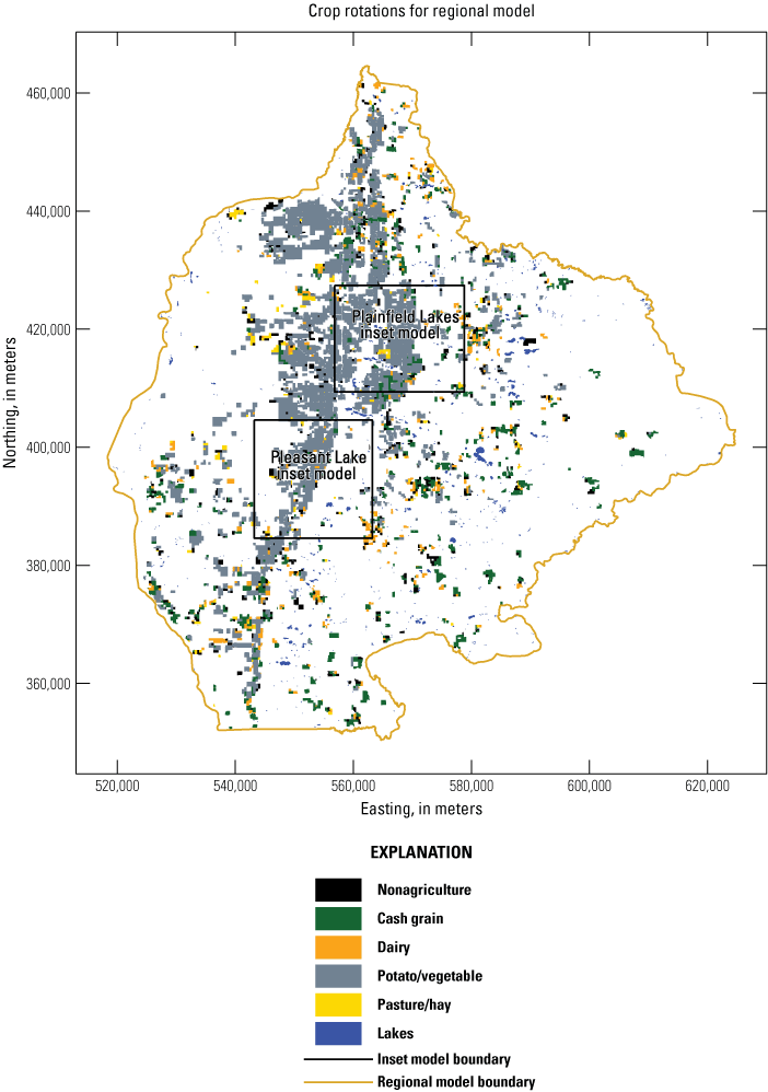
Spatial distribution of the major crop rotations in the regional model domain, Central Sands region, central Wisconsin (Wisconsin Department of Natural Resources, 2021, app. F).
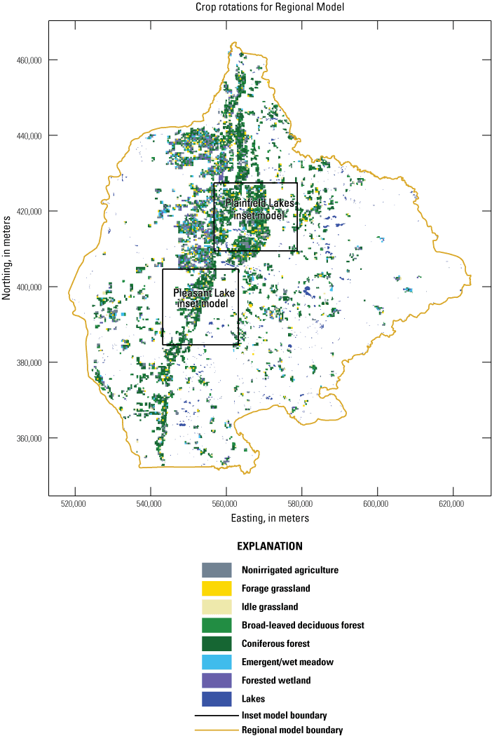
Spatial distribution of alternative land use assumed for the no irrigated agriculture scenario in the regional model domain, Central Sands region, central Wisconsin (Wisconsin Department of Natural Resources, 2021, app. F).
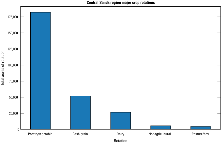
Total acres of each major crop rotation in the regional model domain, Central Sands region, central Wisconsin (Wisconsin Department of Natural Resources, 2021, app. F).
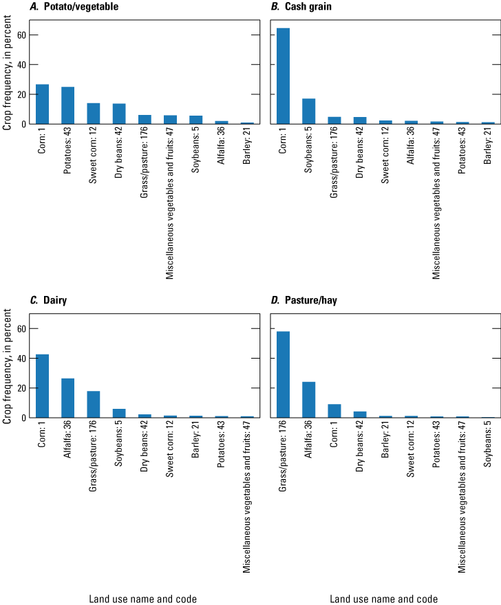
Frequency of each land-use code/crop within the four crop rotations as a percentage of area for A, potato/vegetable; B, cash grain; C, dairy; and D, pasture/hay; in the Central Sands region, central Wisconsin (Wisconsin Department of Natural Resources, 2021, app. F).
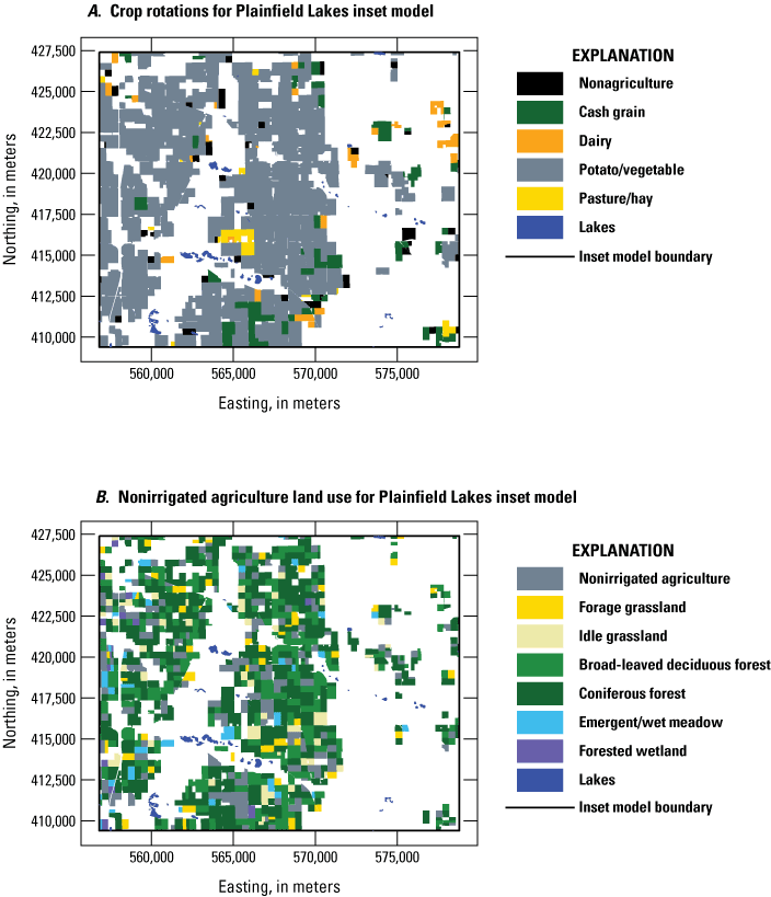
Spatial distribution of the A, major crop rotations and the alternative land use assumed for the B, no irrigated agriculture scenario in the Plainfield Tunnel Channel Lakes inset model, Central Sands region, central Wisconsin. From (Wisconsin Department of Natural Resources, 2021, app. F).
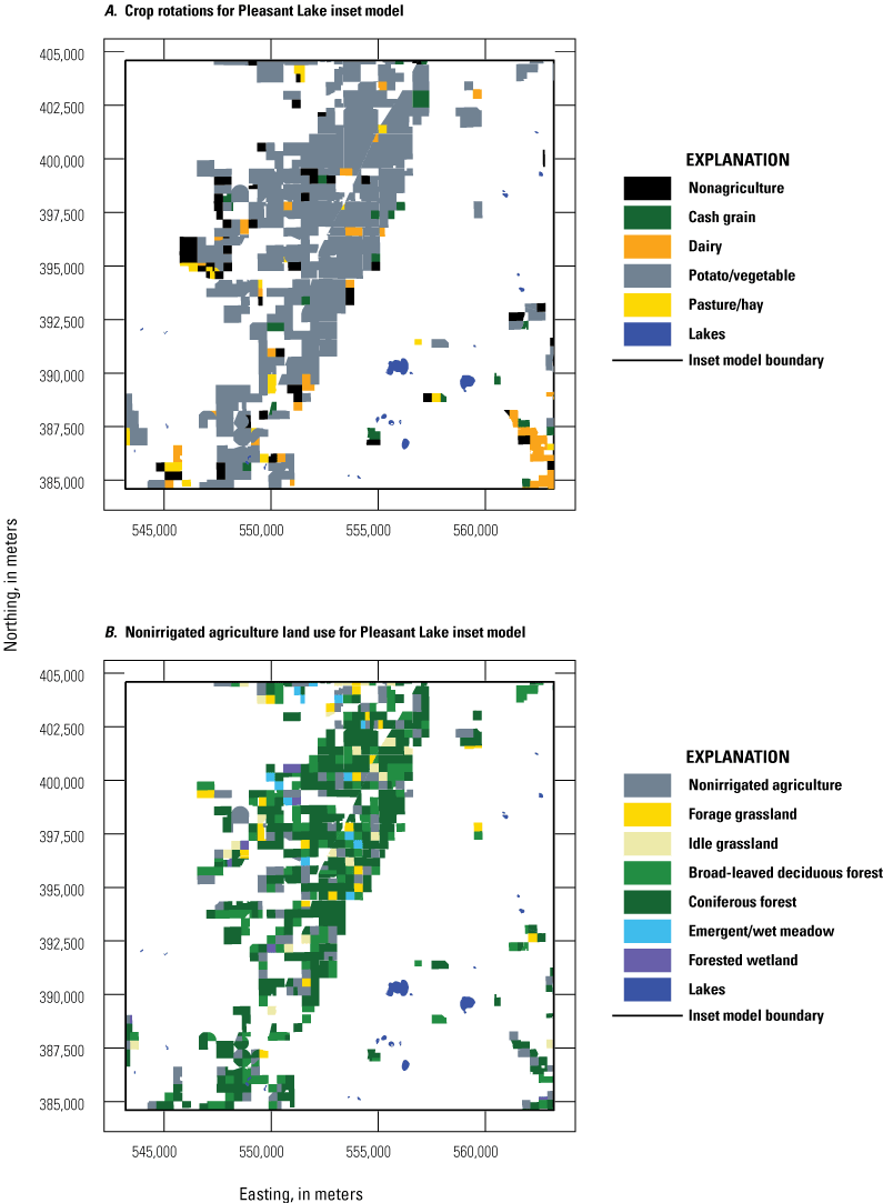
Spatial distribution of the A, major crop rotations and the alternative land use assumed for the B, no irrigated agriculture scenario in the Pleasant Lake inset model, Central Sands region, central Wisconsin (Wisconsin Department of Natural Resources, 2021, app. F).
The land-use files for the no irrigated agriculture scenario and the current irrigated agriculture scenario were provided as input to SWB, along with representative climate data from PRISM resulting in grids of agricultural demand and net infiltration, aggregated to monthly stress periods. Using parcel mapping from WDNR (WDNR, 2021, app. F), water estimated by the agricultural demand was aggregated to permitted irrigation wells. The resulting recharge and well information was then input to the regional model for simulation over the climate years to provide specified-head boundary conditions for the inset models. The inset models were then run using the boundaries available from the updated regional model, the recharge and well pumping data from the SWB runs, and evapotranspiration and precipitation input for the LAK package, updated using the representative PRISM data. The other parameters for the three MODFLOW models were obtained from history matching and using the optimal parameters for the regional model and the base realizations for the two inset models. To focus on differences between the no irrigated agriculture and current (2018) irrigated agriculture scenarios, the same specified-head boundaries from the regional model (the no irrigated agriculture results) were used for all inset model LERA runs.
Three-hundred fifty SWB parameter sets were generated using a Monte Carlo approach. These parameters are assumed to vary about the values assigned during the base SWB run. The parameters that were allowed to vary include many parameters related to the FAO-56 calculations: irrigation starting and ending dates, planting dates, crop-coefficient curve midpoint (Kcbmid), the maximum allowable depletion (responsible for triggering virtual irrigation events), and the depletion fraction defining soil-moisture conditions leading to plant stress. The plant rooting depth was a non-FAQ-56 related parameter allowed to vary.
Each of the parameter sets discussed above was simulated with SWB, and the outputs were then used as input to the inset models to examine the responses and associated uncertainties of lake levels and streamflows derived from varying SWB input parameters. The simulated lake levels for all the study lakes are shown in figure 78. The darker blue and orange lines indicate the results for the base run parameter set for the Monte Carlo SWB runs for the no irrigation and current irrigation scenarios, respectively. Lighter blue lines show the ensemble of results resulting from sampling the uncertainty of the SWB parameters. Note that in panel B, short periods indicate that the lake level was simulated at the bottom of the lake bathymetry for some realizations. Similar plots for streamflow in two selected streams from the Plainfield Tunnel Channel Lakes inset model are shown in figure 79. Streamflow results for two sets of selected streams in the Pleasant Lake inset model are shown in figures 80 and 81.
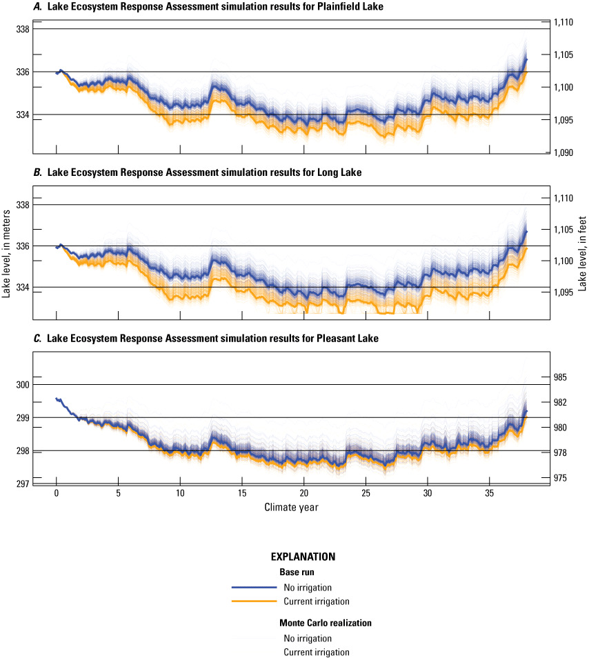
Simulated lake levels for the three study lakes, A, Plainfield; B, Long; and C, Pleasant, over the Lake Ecosystem Response Assessment (LERA) representative climate, Central Sands region, central Wisconsin. Blue lines indicate Monte Carlo ensemble realizations for the no irrigation scenario, and orange lines indicate ensemble realizations for the current (2018) irrigation scenario.
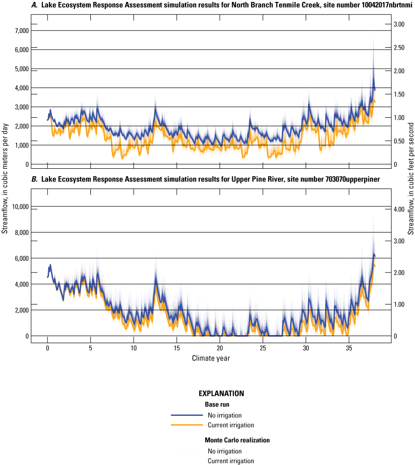
Simulated streamflow in selected streams in the Plainfield inset model over the Lake Ecosystem Response Assessment (LERA) representative climate period, Central Sands region, central Wisconsin: A, North Branch Tenmile Creek (site number 10042017nbrtnmi) and B, the Upper Pine River (site number 703070upperpiner). Blue lines indicate Monte Carlo ensemble realizations for the no irrigation scenario, and orange lines indicate ensemble realizations for the current (2018) irrigation scenario.
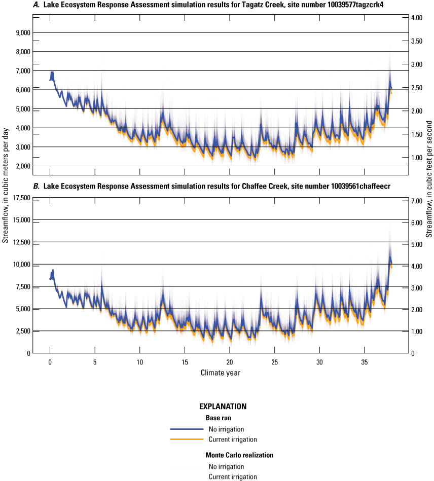
Simulated streamflow in selected streams in the Pleasant inset model over the Lake Ecosystem Response Assessment (LERA) representative climate period, Central Sands region, central Wisconsin: A, Tagatz Creek (site number 10039577tagzcrk4) and B, Chaffee Creek (site number 10039561chaffeecr). Blue lines indicate Monte Carlo ensemble realizations for the no irrigation scenario, and orange lines indicate ensemble realizations for the current irrigation scenario.
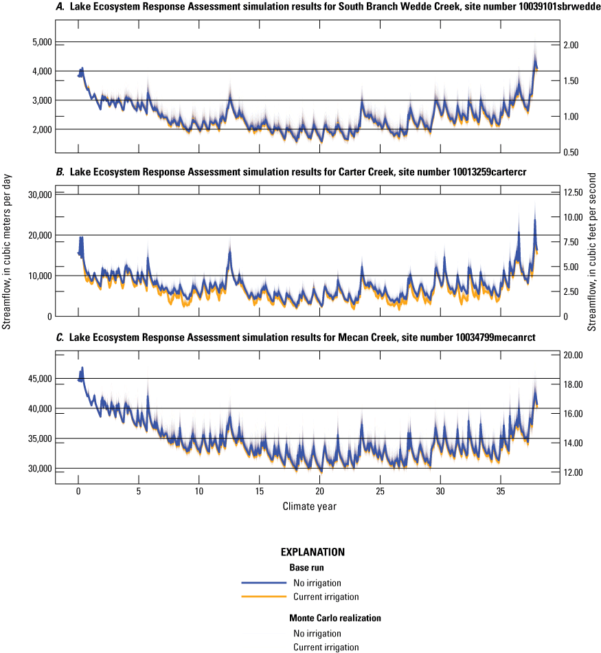
Simulated streamflow in selected streams in the Pleasant inset model over the Lake Ecosystem Response Assessment (LERA) representative climate period, Central Sands region, central Wisconsin: A, South Branch Wedde Creek (site number 10039101sbrwedde); B, Carter Creek (site number 10013259cartercr); and C, Mecan Creek (site number 10034799mecanrct). Blue lines indicate Monte Carlo ensemble realizations for the no irrigation scenario, and orange lines indicate ensemble realizations for the current irrigation scenario.
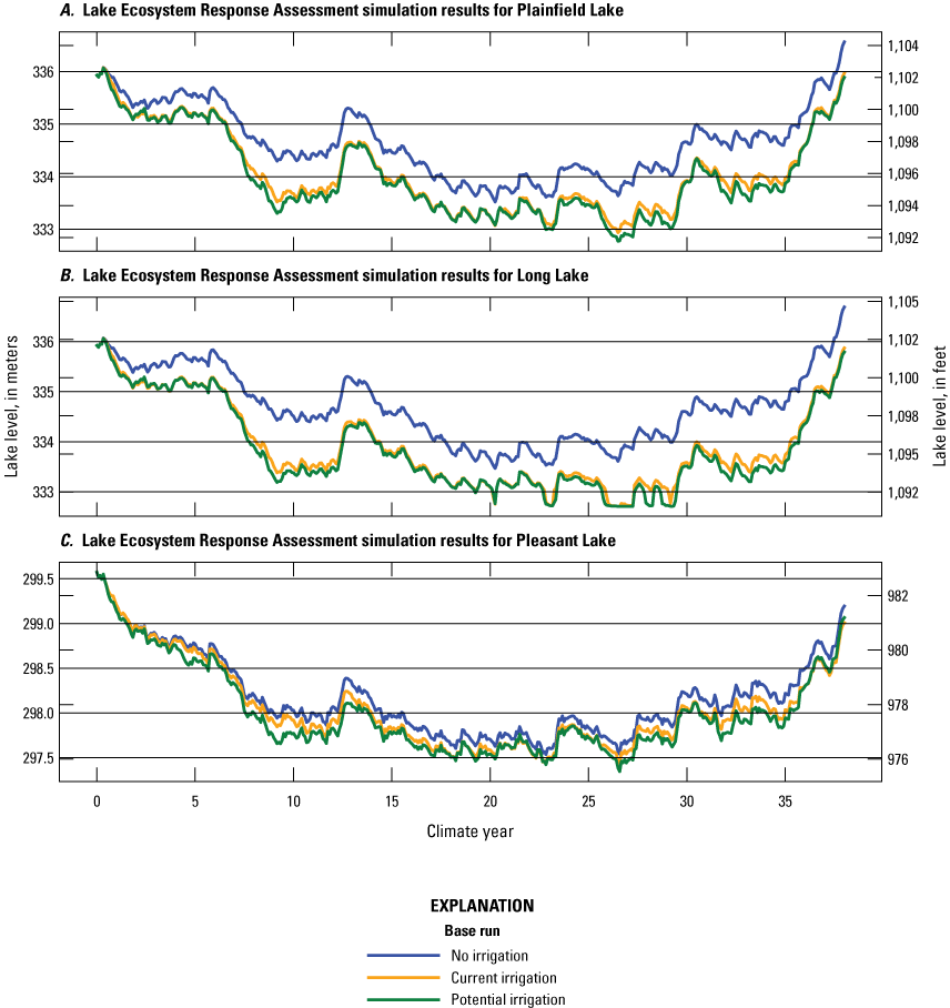
Simulated lake levels for the three study lakes, A, Plainfield; B, Long; and C, Pleasant, over the Lake Ecosystem Response Assessment (LERA) representative climate for the base Soil Water Balance model parameters, Central Sands region, central Wisconsin. In each panel, the blue line depicts the no irrigated agriculture scenario, the orange line depicts the current (2018) irrigated agriculture scenario, and the green line depicts the potential irrigated agriculture scenario.
A final LERA analysis run was a potential irrigated agriculture scenario where a land-use scenario was generated (WDNR, 2021, app. F). In this scenario, all land considered suitable for irrigated agriculture was simulated as irrigated agriculture. The land-use patterns were assigned rotations and annual crop distributions following the same methodology as the current irrigation scenario discussed above. Only the base SWB parameters were simulated for this sensitivity run and the lake stages for the base SWB parameters for the no irrigated agriculture, current irrigated agriculture, and potential irrigated agriculture scenarios are shown in figure 82.
Two final evaluations following the same conceptualization as the LERA runs were performed to more precisely evaluate the connection between irrigation and land use at individual parcels and the responses in lake levels. These were the “distance” and the “lag-time” evaluations, both of which were limited to Long Lake as a proof-of-concept. The distance from the geometric centroid of Long Lake to each permitted high-capacity well was used to rank wells from 0 (closest) to 319 (farthest). Using this information, the two scenarios evaluated (1) converted each well, cumulatively, from wells 0 to 319, in sequence, from current irrigated agriculture to no irrigated agriculture (the distance scenario) and (2) divided the 320 wells into 20 groups of 16 wells and converted all wells in each group from current irrigated agriculture to no irrigated agriculture (the lag-time scenario). The distance scenario illustrates the cumulative effects of pumping on lake levels as a function of distance. The lag-time scenario illustrates the magnitude and timing of effects from smaller well groups assigned based on similar distance on lake levels. The conversion from current irrigated agriculture to no irrigated agriculture was simulated for both scenarios by (1) removing the high-capacity well(s) from the simulation and (2) substituting the recharge calculated for the no irrigated agriculture in place of the recharge calculated for the current irrigated agriculture scenario for the parcel(s) associated with the well(s). This is the same conceptualization as the LERA runs above, but with subsets of wells selected for evaluation.
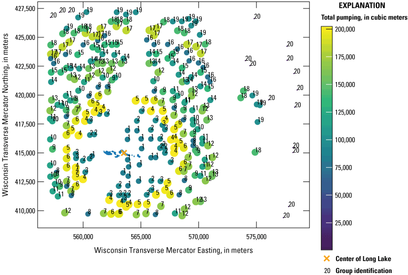
Group identification based on distance from the center of Long Lake, irrigation wells in the Plainfield inset model, and total pumping over the Lake Ecosystem Response Assessment (LERA) simulation time, Central Sands region, central Wisconsin. Orange “x” indicates the center of Long Lake. Numbers indicate group identification.
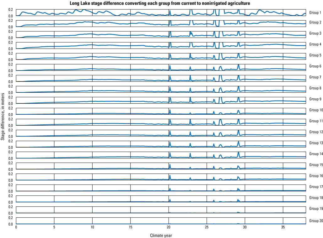
Lake-level changes in Long Lake resulting from each well group simulated as converted from current irrigation to no irrigation recharge and water use, Central Sands region, central Wisconsin. Positive responses indicate an increase in lake level because of the conversion. Group locations are shown in figure 83.
Results of the distance scenario are presented and discussed further by the WDNR (WDNR, 2021, app. B). For the lag-time scenario, the 20 groups of 16 wells each, grouped as quantiles of distance rank from the center of Long Lake, are shown in figure 83. The colors indicate the total amount of water simulated as pumped for irrigation in each group. The differences, over time, in the level of Long Lake over the 38-year LERA simulation time, simulating the wells in each group using the no irrigated agriculture recharge and pumping scenario relative to the current irrigated agriculture recharge and pumping scenario, are shown in figure 84. Positive values indicate higher lake levels in the no irrigated agriculture scenario relative to the current irrigated agriculture scenario.
Model Limitations
All hydrologic models—including those described in this study—are necessarily simplifications of the natural world and, thus, subject to limitations. Limitations include the spatial and temporal discretization of the study area and hydrologic process simplification. These simplifications are necessary to balance computational expense with supporting data and ancillary information.
The spatial discretization used in modeling the study area is intended to capture as much hydrogeologic complexity as is practical, but when it is combined with inherent limitations in the ability to measure hydrogeologic properties, actual detail in the hydrogeologic system is not represented at the spatial scales. Similarly, higher spatial discretization and resolution (smaller model cells) were used to capture the greatest amount of detail around the study lakes, but these inset-focused models are still simplifications of the hydrogeologic system.
Monthly stress periods were used in the temporal discretization for the history matching and LERA models. This discretization was limited by the availability of water-use data on a monthly timescale from WDNR.
The SWB model represents the plant growth and infiltration processes within the root zone in a simplified manner. Rooting depth defines the size of the single soil-moisture reservoir used to track daily soil-moisture values. Although the rooting depth is allowed to vary and progress in a manner congruent with the crop-coefficient curve, the representation is clearly simplified. The FAO-56 procedure is widely used as a way to implement irrigation scheduling (see, for example, Kebede and others, 2014; Pereira and others, 2015); however, the method relies on parameters that might not be widely transferable from one study area to another. The assumption that “net infiltration” occurs only after soil-moisture conditions have reached field capacity is another model simplification; in reality, gravity drainage of the root zone likely occurs before soil-moisture values reach field capacity. The simplified treatment of root-zone dynamics causes the timing of net-infiltration estimates from the root zone to be less realistic; the aggregation of the SWB results to the monthly stress periods of the MODFLOW models mitigates this timing issue.
The MODFLOW-NWT and MODFLOW-6 models are derived and implemented from the perspective of the groundwater system. As a result, other aspects of the hydrologic cycle are simplified. Specifically, the streamflow routing packages (SFR2 and SFR) simulated the groundwater component of streamflow (base flow) but not surface runoff. The streams simulated within the model area are interpreted to flow primarily by base flow, but some stormflow certainly occurs and is not simulated by the model explicitly. Recharge is provided by the SWB model for all the MODFLOW models, but, in reality, the quantity calculated by SWB is deep drainage from the soil zone. MODFLOW-NWT and MODFLOW 6 both simulate this deep drainage as reaching the water table at the time it is applied immediately; in reality, deep drainage reaches the water table because of downward movement through the unsaturated zone which indicates a time delay for that movement to occur. Because of the necessity of using monthly stress periods in model simulation, errors resulting from this delay are at least partially mitigated. An alternative methodology would be to explicitly simulate the unsaturated zone using the Unsaturated-Zone Flow (UZF) package in MOFFLOW 6. Early model simulations indicated small differences in model outputs using the UZF package but incurred a greater effort and computational expense.
For the LGR approach in MODFLOW 6, the ghost node correction option was not used in linking the inset and parent models. Evaluation with and without this correction option showed a small difference in lake level (approximately 3 cm in Pleasant Lake level and approximately 4 mm in the Plainfield Tunnel Channel Lakes level). As a result, some parameter compensation likely was incurred in other model parameters resulting in the fit between measured and simulated results (groundwater, lake levels, and streamflows) obtained during history matching. In future work, the ghost node correction may enhance stability of model simulations and remove some minor parameter compensation. Also in the inset models, the spatially distributed parameters, such as hydraulic conductivity and storage, were not estimated continuously across the inset and parent model boundaries. This allows for some discontinuity in the properties at that artificial model boundary. The results on the model solution are not significant, but future development of parameterization methods in such a case would benefit from enforcing continuity.
In the parameter estimation process, some of the limitations of the formulation are compensated for by estimated parameters responding to data where the data and parameters are not related. This concept of parameter compensation is in all parameter estimation efforts as discussed by Doherty and Welter (2010). Focusing on the dominant hydrologic processes limits this behavior as much as possible. This focus, on lake levels and streamflows, highlights the importance of considering potential parameter compensation if using the models discussed here for other purposes. Furthermore, for each of the inset LGR models, the two distinct models representing the two spatial discretization scales are parameterized separately without enforcing continuity across model boundaries. As a result, some discontinuities in the spatially distributed properties are inevitable. However, the use of multipliers helps mitigate the magnitude of this discontinuity and the effect on the model-simulation results is minimal.
Summary
The effect of groundwater withdrawals on lake levels in the Wisconsin Central Sands region in central Wisconsin is of increasing concern. To address this concern, a study of the hydrogeology of the region and the application of numerical models for simulating regional groundwater flow and groundwater/lake interactions was performed by the U.S. Geological Survey, in cooperation with the Wisconsin Department of Natural Resources (WDNR), for the Central Sands region in central Wisconsin. Information in this report was included as a technical appendix in the report to the Wisconsin State Legislature by the WDNR. A regional groundwater-flow model for the region and two focused inset models for three seepage lakes (Long, Plainfield, and Pleasant Lakes) in Waushara County were developed. The focused inset models were used to determine the connections between the groundwater system, land use, and lake levels.
The regional groundwater-flow model, constructed in MODFLOW-NWT, provided boundary conditions for two focused inset models, constructed in MODFLOW 6, that represented the lakes at higher resolutions. Land and groundwater use were simulated at a regional scale using the Soil Water Balance model, which provided recharge and water-use boundary conditions for the MODFLOW regional and inset models. The models were calibrated based on parameter estimation using the history-matching approach. Agricultural irrigation is the primary groundwater use in the area. Land and groundwater-use scenarios representing no irrigation, current irrigation, and potential future irrigation were simulated with the regional groundwater-flow model and the lake levels reported over a 38-year climate period.
The focus on lake levels and streamflow in the inset models highlights the importance of considering potential parameter compensation in using these models for other purposes than described in this report. Model-simulation results indicate that the use of multipliers in the parameter estimation process helps mitigate the magnitude of discontinuities in the spatially distributed properties, and the effect on the model-simulation results are minimal.
References Cited
Bradbury, K.R., Fienen, M.N., Kniffin, M.L., Krause, J.J., Westenbroek, S.M., Leaf, A.T., and Barlow, P.M., 2017, A groundwater flow model for the Little Plover River basin in Wisconsin’s Central Sands: Wisconsin Geological and Natural History Survey Bulletin 111, 82 p., accessed April 28, 2022, at https://water.usgs.gov/GIS/dsdl/gwmodels/WGNHS2017-LittlePlover/WGNHS2017_B111-report.pdf.
Corson-Dosch, N.T., Fienen, M.N., Finkelstein, J.S., Leaf, A.T., White, J.T., Woda, J., and Williams, J.H., 2022, Areas contributing recharge to priority wells in valley-fill aquifers in the Neversink River and Rondout Creek drainage basins, New York: U.S. Geological Survey Scientific Investigations Report 2021–5112, 50 p., accessed August 18, 2022, at https://doi.org/10.3133/sir20215112.
Cronshey, R., McCuen, R., Miller, N., Rawls, W., Robbins, S., and Woodward, D., 1986, Urban hydrology for small watersheds—Technical release 55: U.S. Department of Agriculture, Soil Conservation Service, Engineering Division, accessed March 24, 2022, at https://www.nrcs.usda.gov/Internet/FSE_DOCUMENTS/16/stelprdb1044171.pdf.
Doherty, J., 2020, PEST for highly parallelized computing environments: Brisbane, Australia, Watermark Numerical Computing, 88 p., accessed April 28, 2020, at http://www.pesthomepage.org/Downloads.php.
Doherty, J. and Welter, D., 2010, A short exploration of structural noise: Water Resources Research, v. 46, no. 5, accessed May 7, 2021, at https://doi.org/10.1029/2009wr008377.
Dripps, W.R., and Bradbury, K.R., 2007, A simple daily soil–water balance model for estimating the spatial and temporal distribution of groundwater recharge in temperate humid areas: Hydrogeology Journal, v. 15, no. 3, p. 433–444, accessed August 16, 2022, at https://doi.org/10.1007/s10040-007-0160-6.
Duffield, G.M., 2019, Representative values of hydraulic properties: AQTESOLV web page, accessed March 24, 2022, at http://www.aqtesolv.com/aquifer-tests/aquifer_properties.htm.
Feinstein, D.T., Hunt, R.J., and Reeves, H.W., 2010, Regional groundwater-flow model of the Lake Michigan Basin in support of Great Lakes Basin water availability and use studies: U.S. Geological Survey Scientific Investigations Report 2010–5109, 379 p., accessed August 16, 2022, at https://doi.org/10.3133/sir20105109.
Fienen, M.N., Haserodt, M.J., Leaf, A.T., and Westenbroek, S.M., 2021a, Appendix C—Central Sands Lakes Study Technical Report—Modeling documentation in Central Sands Lakes Study Report—Findings and recommendations: Report to the Wisconsin Legislature, May 27, 2021, accessed March 24, 2022, at https://doi.org/10.5281/zenodo.5708760.
Fienen, M.N., Haserodt, M.J., and Leaf, A.T, 2021b, MODFLOW models used to simulate groundwater flow in the Wisconsin Central Sands Study Area, 2012-2018: U.S. Geological Survey data release, accessed March 24, 2022, at https://doi.org/10.5066/P9BVFSGJ.
Harbaugh, A.W., 2005, MODFLOW-2005—The U.S. Geological Survey modular ground-water model—The ground-water flow process: U.S. Geological Survey Techniques and Methods, book 6, chap. A16 [variously paged], accessed August 16, 2022, at https://doi.org/10.3133/tm6A16.
Hart, D., Bradbury, K., and Parsen, M., 2015, Using the New Rome Formation as a geologic weighing lysimeter for water management in Wisconsin’s sands plain: Wisconsin Department of Natural Resources Project Report for Project Number 14-HDG-03, accessed May 7, 2021, at https://www.wri.wisc.edu/research/using-the-new-rome-formation-as-a-geologic-weighing-lysimeter-for-water-management-in-wisconsins-sand-plain/.
Harwell, G.R., 2012, Estimation of evaporation from open water—A review of selected studies, summary of U.S. Army Corps of Engineers data collection and methods, and evaluation of two methods for estimation of evaporation from five reservoirs in Texas: U.S. Geological Survey Scientific Investigations Report 2012–5202, 96 p., accessed March 24, 2022, at https://doi.org/10.3133/sir20125202.
Healy, R.W., 2010, Estimating groundwater recharge: Cambridge University Press, 245 p., accessed August 16, 2022, at https://doi.org/10.1017/CBO9780511780745.
Hipsey, M.R., Bruce, L.C., Boon, C., Busch, B., Carey, C.C., Hamilton, D.P., Hanson, P.C., Read, J.S., de Sousa, E., Weber, M., and Winslow, L.A., 2019, A general lake model (GLM 3.0) for linking with high-frequency sensor data from the Global Lake Ecological Observatory Network (GLEON): Geoscientific Model Development, v. 12, no. 1, p. 473–523. [Also available at https://doi.org/10.5194/gmd-12-473-2019.]
Hunt, R.J, Prudic, D.E., Walker, J.F. and Anderson, M.P., 2008, Importance of unsaturated zone flow for simulating recharge in a humid climate: Groundwater, v. 46, no. 4, 551–560. https://doi.org/10.1111/j.1745-6584.2007.00427.x.
Kebede, H., Fisher, D.K., Sui, R., and Reddy, K.N., 2014, Irrigation methods and scheduling in the delta region of Mississippi—Current status and strategies to improve irrigation efficiency: American Journal of Plant Sciences, v. 5, no. 20, p. 2917–2928, https://doi.org/10.4236/ajps.2014.520307.
Langevin, C.D., Hughes, J.D., Banta, E.R., Niswonger, R.G., Panday, S., and Provost, A.M., 2017, Documentation for the MODFLOW 6 groundwater flow model: U.S. Geological Survey Techniques and Methods, book 6, chap. A55, 197 p., accessed March 24, 2022, at https://doi.org/10.3133/tm6A55.
Langevin, C.D., Hughes, J.D., Banta, E.R., Provost, A.M., Niswonger, R.G., and Panday, S., 2020, MODFLOW 6 Modular Hydrologic Model version 6.2.0: U.S. Geological Survey Software Release, accessed October 22, 2020, at https://doi.org/10.5066/F76Q1VQV.
Leaf, A.T., Fienen, M.N., Hunt, R.J., and Buchwald, C.A., 2015, Groundwater/surface-water interactions in the Bad River Watershed, Wisconsin: U.S. Geological Survey Scientific Investigations Report 2015–5162, 110 p., https://doi.org/10.3133/sir20155162.
Leaf, A.T., Fienen, M.N., and Reeves, H.W., 2021, SFRmaker and Linesink-maker—Rapid construction of streamflow routing networks from hydrography data: Groundwater, v. 59, no. 5, accessed August, 18, 2022, at https://doi.org/10.1111/gwat.13095.
McCobb, T.D., LeBlanc, D.R., and Hess, K.M., 1999, Determination of temporal and spatial variability of hydraulic gradients in an unconfined aquifer using three-point triangulation, Cape Cod, Massachusetts, in Morganwalp, D.W., and Buxton, H.T., eds., U.S. Geological Survey Toxic Substances Hydrology Program—Proceedings of the technical meeting, Charleston, S.C., March 8–12, 1999: U.S. Geological Survey Water Resources Investigations Report 99-4018C, v. 3, p. 349–360, accessed August 16, 2022, at https://doi.org/10.3133/wri994018C.
McKay, L., Bondelid, T., Dewald, T., Johnston, J., Moore, R., and Rea, A., 2012, NHDPlus Version 2—User guide: NHDPlus Version 2 web page, accessed November 15, 2014, at http://www.horizon-systems.com/NHDPlus/ NHDPlusV2documentation.php.
McKenna, S.A., Akhriev, A., Ciaurri, D.E., and Zhuk, S., 2019, Efficient uncertainty quantification of reservoir properties for parameter estimation and production forecasting: Mathematical Geosciences, v. 52, p. 233–251, accessed August 16, 2022, at https://doi.org/10.1007/s11004-019-09810-y.
Mechenich, D.J., 2012, Extending the Wisconsin Central Sands groundwater flow model, app. B of Kraft, G.J., Mechenich, D.J. and Haucke, J., 2012, Information support for groundwater management in the Wisconsin Central Sands, 2009-2011—A report to the Wisconsin Department of Natural Resources—In Completion of Project NMA00000253: Center for Watershed Science and Education, College of Natural Resources, University of Wisconsin-Stevens Point/Extension, accessed May 7, 2021, at https://www.uwsp.edu/cnr-ap/watershed/Documents/kraft_centralsands_2012.pdf.
Mehl, S., Hill, M.C., and Leake, S.A., 2006, Comparison of local grid refinement methods for MODFLOW: Groundwater, v. 44, no. 6, p. 792–796, accessed August 16, 2022, at https://doi.org/10.1111/j.1745-6584.2006.00192.x..
Mu, Q., Zhao, M., and Running, S.W., 2013, MODIS global terrestrial evaporation (ET) product (NASA MOD16A2/A3)—Algorithm theoretical basis document—Collection 5: Numerical Terradynamic Simulation Group, University of Montana, 55 p., accessed February 5, 2021, at https://modis-land.gsfc.nasa.gov/pdf/MOD16ATBD.pdf.
Niswonger, R.G., and Prudic, D.E., 2005, Documentation of the Streamflow-Routing (SFR2) Package to include unsaturated flow beneath streams—A modification to SFR1: U.S. Geological Survey Techniques and Methods, book 6, chap. A13, 50 p., accessed August 16, 2022, at https://doi.org/10.3133/tm6A13.
Niswonger, R.G., Panday, S., and Ibaraki, M., 2011, MODFLOW–NWT—A Newton formulation for MODFLOW–2005: U.S. Geological Survey Techniques and Methods, book 6, chap. A37, 44 p., accessed August 16, 2022, at https://doi.org/10.3133/tm6A37.
Pereira, L.S., Allen, R.G., Smith, M., and Raes, D., 2015, Crop evapotranspiration estimation with FAO56—Past and future: Agricultural Water Management, v. 147, p. 4–20, accessed August 16, 2022, at https://doi.org/10.1016/j.agwat.2014.07.031.
PRISM Climate Group, Oregon State University, 2019, Time series values for individual locations: PRISM Climate Group web page, accessed December 10, 2019, at https://prism.oregonstate.edu/explorer/.
PRISM Climate Group, 2020, Oregon State University PRISM Climate Data: PRISM Climate Group web page, accessed December 16, 2020, at https://prism.oregonstate.edu/.
Reitz, M., Senay, G.B., and Sanford, W.E., 2017a, Combining remote sensing and water-balance evapotranspiration estimates for the conterminous United States: Remote Sensing, v. 9, no. 12, 17 p., https://doi.org/10.3390/rs9121181.
Reitz, M., Sanford, W.E., Senay, G.B., and Cazenas, J., 2017b, Annual estimates of recharge, quick-flow runoff, and evapotranspiration for the contiguous U.S. using empirical regression equations: JAWRA Journal of the American Water Resources Association, v. 53, no. 4, p. 961–983, accessed August 16, 2022, at https://doi.org/10.1111/1752-1688.12546.
Scanlon, B.R., Healy, R.W., and Cook, P.G., 2002, Choosing appropriate techniques for quantifying groundwater recharge: Hydrogeology Journal, v. 10, no. 1, p. 18–39. [Also available at https://doi.org/10.1007/s10040-001-0176-2.]
Soil Survey Staff, 2018, Web soil survey: U.S. Department of Agriculture, Natural Resources Conservation Service, accessed December 2018 at https://websoilsurvey.nrcs.usda.gov/.
Soil Survey Staff, 2019, Gridded soil survey geographic (gSSURGO) database for the conterminous United States, accessed August 16, 2022, at https://gdg.sc.egov.usda.gov/.
Tarantola, A., 2005, Inverse problem theory and methods for model parameter estimation: Philadelphia, Pa., Society for Industrial and Applied Mathematics, 354 p. [Also available at https://doi.org/10.1137/1.9780898717921.]
Thornthwaite, C.W., 1948, An approach toward a rational classification of climate: Geographical Review, v. 38, no. 1, p. 55–94. [Also available at https://doi.org/10.2307/210739.]
U.S. Department of Agriculture, 2020, Cropscape and Cropland Data Layer, accessed on December 16, 2020, at https://www.nass.usda.gov/Research_and_Science/Cropland/SARS1a.php.
U.S. Geological Survey, 2021, USGS water data for the Nation: U.S. Geological Survey National Water Information System database, accessed March 2021, at https://doi.org/10.5066/F7P55KJN.
Wahl, K.L., and Wahl, T.L., 1988, Effects of regional ground-water level declines on streamflow in the Oklahoma Panhandle, in Waterstone, M., and Burt, R.J., ed., Proceedings of the symposium on water-use data for water resources management, [Tuscon, Ariz.], 1988: Tuscon, Ariz., American Water Resources Association, 830 p.
Weeks, E.P., and Stangland, H.G., 1971, Effects of irrigation on streamflow in the Central Sand Plain of Wisconsin: U.S. Geological Survey Open-File Report 70-362, 113 p, accessed August 16, 2022, at https://doi.org/10.3133/ofr70362.
Westenbroek, S.M., Kelson, V.A., Dripps, W.R., Hunt, R.J., and Bradbury, K.R., 2010, SWB—A modified Thornthwaite-Mather Soil-Water-Balance code for estimating groundwater recharge: U.S. Geological Survey Techniques and Methods book 6, chap. A31, 61 p, accessed August 16, 2022, at https://doi.org/10.3133/tm6A31.
Westenbroek, S.M., Engott, J.A., Kelson, V.A., and Hunt, R.J., 2018, A Soil-Water-Balance code for estimating net infiltration and other water-budget components: U.S. Geological Survey Techniques and Methods book 6, chap. A59, 118 p., accessed at https://doi.org/10.3133/tm6A59.
Westenbroek, S.M., and Fienen, M.N., 2022, Soil-Water-Balance model developed to simulate net infiltration, irrigation water requirements, and other water budget components in support of the Central Sands Lakes Study: U.S. Geological Survey data release, https://doi.org/10.5066/P9SOJ01N.
White, J.T., 2018, A model-independent iterative ensemble smoother for efficient history-matching and uncertainty quantification in very high dimensions: Environmental Modelling & Software, v. 109, p. 191–201. [Also available at https://doi.org/10.1016/j.envsoft.2018.06.009.]
White, J.T., Hunt, R.J., Fienen, M.N., and Doherty, J.E., 2021, Approaches to highly parameterized inversion—PEST++ version 5, a software suite for parameter estimation, uncertainty analysis, management optimization and sensitivity analysis: U.S. Geological Survey Techniques and Methods 7C26, 52 p., https://doi.org/10.3133/tm7C26.
Wisconsin Department of Natural Resources (WDNR), 2015, WDNR 24K Hydro Geodatabase, 1:24,000: accessed June 8, 2016, at ftp://dnrftp01.wi.gov/geodata.
Wisconsin Department of Natural Resources (WDNR), 2019, Digital elevation model (DEM)—10 meter: Wisconsin Department of Natural Resources Open Data web page, accessed at https://data-wi-dnr.opendata.arcgis.com/search?q=DEM.
Wisconsin Department of Natural Resources (WDNR), 2021, Central Sands Lakes study report—Findings and recommendations: Wisconsin Department of Natural Resources, Report to the Wisconsin Legislature, May 27, 2021, accessed June 4, 2021, at https://dnr.wisconsin.gov/topic/Wells/HighCap/CSLStudy.html#reports.
Wisconsin Department of Natural Resources (WDNR), 2022, Central Sands Lake Study—Water quantity monitoring sites (as of 2019): Wisconsin Department of Natural Resources Open Data web page, accessed August 16, 2022, at https://data-wi-dnr.opendata.arcgis.com/datasets/wi-dnr::central-sands-lake-study-water-quantity-monitoring-sites-as-of-2019/explore?location=43.99927 6%2C-89.483190%2C10.87.
Conversion Factors
U.S. customary units to International System of Units
International System of Units to U.S. customary units
Datum
Horizontal coordinate information is referenced to the North American Datum of 1983 (NAD 83).
Vertical coordinate information is referenced to the North American Vertical Datum of 1988 (NAVD 88).
Elevation, as used in this report, refers to distance above the vertical datum.
Abbreviations
DEM
digital elevation model
ET
evapotranspiration
FAO-56
Food and Agriculture Organization of the United Nations irrigation and drainage paper 56
GHB
MODFLOW General Head Boundary package
iES
iterative ensemble smoother history matching algorithm
LAK
MODFLOW Lake package
LERA
Lake Ecosystem Response Assessment
LGR
local-grid refinement
MODFLOW-NWT
Newton Raphson formulation of the U.S. Geological Survey modular finite-difference flow model (MODFLOW) groundwater-modeling package
MODFLOW 6
U.S. Geological Survey modular finite-difference flow model hydrologic simulation modeling package
MODIS
Moderate Resolution Imaging Spectroradiometer
PDC
prior data conflict
PEST++
parameter estimation package
PRISM
climate group in the Northwest Alliance for Computational Science and Engineering
RCH
MODFLOW Recharge package
SFR
MODFLOW-6 Streamflow Routing package
SFR2
MODFLOW-NWT Streamflow Routing package
SWB
Soil Water Balance
USGS
U.S. Geological Survey
WDNR
Wisconsin Department of Natural Resources
For more information about this publication, contact:
Director, USGS Upper Midwest Water Science Center
1 Gifford Pinchot Drive
Madison, WI 53726
For additional information, visit: https://www.usgs.gov/centers/upper-midwest-water-science-center
Publishing support by the Indianapolis Publishing Service Center
Disclaimers
Any use of trade, firm, or product names is for descriptive purposes only and does not imply endorsement by the U.S. Government.
Although this information product, for the most part, is in the public domain, it also may contain copyrighted materials as noted in the text. Permission to reproduce copyrighted items must be secured from the copyright owner.
Suggested Citation
Fienen, M.N., Haserodt, M.J., Leaf, A.T., and Westenbroek, S.M., 2022, Simulation of regional groundwater flow and groundwater/lake interactions in the Central Sands, Wisconsin: U.S. Geological Survey Scientific Investigations Report 2022–5046, 111 p., https://doi.org/10.3133/sir20225046.
ISSN: 2328-0328 (online)
Study Area
| Publication type | Report |
|---|---|
| Publication Subtype | USGS Numbered Series |
| Title | Simulation of regional groundwater flow and groundwater/lake interactions in the Central Sands, Wisconsin |
| Series title | Scientific Investigations Report |
| Series number | 2022-5046 |
| DOI | 10.3133/sir20225046 |
| Publication Date | September 29, 2022 |
| Year Published | 2022 |
| Language | English |
| Publisher | U.S. Geological Survey |
| Publisher location | Reston, VA |
| Contributing office(s) | Upper Midwest Water Science Center |
| Description | Report: xii, 111 p.; Data Release; Dataset |
| Country | United States |
| State | Wisconsin |
| Other Geospatial | Central Sands |
| Online Only (Y/N) | Y |