

Hydrogeology and Simulation of Groundwater Flow in the Lucerne Valley Groundwater Basin, California
Links
- Document: Report (20 MB pdf) , HTML , XML
- Appendix: Appendix 1 (27 KB txt) - Sites with groundwater-level data available on the U. S. Geological Survey National Water Inventory System Web service (NWISWeb) from 1911-2016 within the Lucerne Valley, California
- Related Work: Open-File Report 2022-1063 - Groundwater Quality of the Lucerne Valley Groundwater Basin, California
- Data Release: MODFLOW-OWHM model used to simulate groundwater flow and evaluate storage in the Lucerne Valley Groundwater Basin, California
- Download citation as: RIS | Dublin Core
Acknowledgments
The authors would like to express gratitude to the many organizations and individuals who supplied data or contributed to the completion of this study and report. This project could not have been completed without the continued support, technical input, collaboration, and groundwater-level data collected by the Mojave Water Agency and the pumpage data provided by the Mojave Water Agency Watermaster. We are grateful to our U.S. Geological Survey illustrator Donna Knifong and editor Dawn Nahhas for their help in completing the report. A special acknowledgement is extended to the U.S. Geological Survey colleagues who made significant contributions during the early stages of this project, including Jill Densmore, John Freckleton, and Clark Londquist. Finally, a debt of gratitude is owed to the authors and field investigators who contributed to the previous investigations in the Lucerne Valley.
Abstract
The Lucerne Valley is in the southwestern part of the Mojave Desert and is about 75 miles northeast of Los Angeles, California. The Lucerne Valley groundwater basin encompasses about 230 square miles and is separated from the Upper Mojave Valley groundwater basin by splays of the Helendale Fault. Since its settlement, groundwater has been the primary source of water for agricultural, industrial, municipal, and domestic uses. Groundwater withdrawal from pumping has exceeded the amount of water recharged to the basin, causing groundwater declines of more than 100 feet between 1917 and 2016 in the center of the basin. The continued withdrawal has resulted in an increase in pumping costs, reduced well efficiency, and land subsidence near Lucerne Lake. Although the volume of pumping has declined in recent years, there is concern that new agricultural growth and limits on imported water will continue to strain the sustainability of the groundwater system.
To address these concerns, the U.S. Geological Survey entered into a cooperative agreement with the Mojave Water Agency to develop a better understanding of the Lucerne Valley hydrogeologic system and provide tools to help evaluate and manage the effects of future development in the Lucerne Valley. The objectives of this study were to (1) improve the understanding of the aquifer system, (2) improve the understanding of subsidence in the basin, and (3) incorporate the understanding into a groundwater-flow model that can be used to help manage the groundwater resources in the Lucerne Valley. The model developed for this study covers the period of 1942–2016 and can help evaluate various proposed water-management scenarios during different climatic and hydrologic conditions.
The aquifer system consists of a shallow aquifer, a confining unit, and middle and lower aquifers. These layered water-bearing units were identified based on geologic units of the mostly unconsolidated sediments and hydrologic properties. These alluvial deposits consist of clay, silt, sand, and gravel; some places also contain clay and silty clay lacustrine deposits. Several faults act, at least in part, as barriers to groundwater flow on the eastern, southern, and western edges of the basin. Present-day natural recharge is primarily from the infiltration of runoff from the San Bernardino Mountains to the south; however, stable and radioactive isotopes show that groundwater from the middle of the Lucerne Valley was older than about 10,000 years and probably was recharged as infiltration from streams draining the mountains in the Mojave Desert to the north, which probably does not occur under present-day climatic conditions. The annual average natural recharge for 1942–2016, estimated by a Basin Characterization Model, was about 635 acre-feet per year; the average amount of treated wastewater effluent transferred to the Lucerne Valley for artificial recharge annually ranged from about 1,500 to 4,000 acre-feet per year during 1980–2016. Pumpage estimates for 1942–2016 ranged from about 3,000 acre-feet in 1942 to about 18,300 acre-feet in 1984. The total cumulative amount of groundwater removed from the basin by pumping between 1942 and 2016 was estimated to be about 700,000 acre-feet, which was about 10 times greater than the cumulative amount of recharge to the entire Lucerne Valley groundwater basin. Before groundwater development, the direction of groundwater flow was from the southern part of the basin northward to discharge areas near Lucerne Lake, where it discharged through springs along the Helendale Fault and by evapotranspiration. Since the early 1900s, groundwater-level declines have mostly eliminated the areas where natural discharge occurred and exceeded 100 feet in the middle of the basin between the early 1950s and mid-1990s, and as much as 25 feet near the margins from about the mid-1950s to 2000s. A decrease in the rate of pumping after the mid-1990s lessened the hydraulic stress on the middle and lower aquifers and enabled hydraulic heads in the middle of the basin to recover slightly as groundwater near the margins of the basin moved toward the pumping depression. Although trends in groundwater levels in the center of the basin have reversed since the mid-1990s, levels at the basin margins continue to decline as the movement of groundwater from the margins fills the pumping depression and gradually flattens the groundwater table throughout the basin.
The long-term extraction of groundwater and associated dewatering of the fine-grained sediments present within the aquifer system has resulted in aquifer compaction and consequently land subsidence, primarily near Lucerne Lake. Analysis of interferometric synthetic aperture radar data shows that almost 11 inches of land subsidence has occurred south of Lucerne Lake between April 1992 and November 2009; less subsidence occurred elsewhere in the basin during this period. This differential land subsidence has caused fissures and cracks in the ground surface, which have buckled the pavement and undercut roads in several locations.
The Lucerne Valley Hydrologic Model was developed using the finite-difference groundwater modeling software One Water Hydrologic Model to represent the hydrologic conditions and stresses during 1942–2016. The model has a uniform grid of approximately 92 acres per cell (2,000 feet by 2,000 feet) and has four layers representing the water-bearing units. The results from the calibrated model simulations indicated that groundwater pumpage exceeded recharge, resulting in an estimated net cumulative depletion of groundwater storage (discharge minus recharge) of about 465,000 acre-feet from 1942 to 2016. The model simulated as much as 7.5 feet (90 inches; 2,286 millimeters) of aquifer compaction, which indicates the extensive fine-grained deposits and measured subsidence near Lucerne Lake.
Introduction
In most parts of the Mojave Desert, surface water from washes and ephemeral streams is neither reliable nor sufficient for water supply in developed areas. Late-19th century settlers and miners in the Lucerne Valley (fig. 1) relied on natural springs and flowing or hand-dug wells for domestic and farming water-supply needs, and by the late 1880s to early 1900s, several ranches had been established around some of the well-known springs in the valley (Mendenhall, 1909). As more homesteads were built and farming expanded, the water table declined, and deeper wells were drilled to meet increasing water-use demands. By 1916, 40–50 wells had been drilled, and several wells were as deep as 500 feet (ft); one was reported to be 778 ft deep (Thompson, 1929). Eventually, the flowing wells ceased, most springs dried up, and groundwater became the sole source of water in the Lucerne Valley. The California Department of Water Resources (CA-DWR) estimated that between 1936 and 1961, more than 72,000 acre-feet (acre-ft), or about 2,800 acre-feet per year (acre-ft/yr), of water had been removed from groundwater storage to meet water-supply demands (California Department of Water Resources, 1967); this imbalance between the amount of natural recharge and groundwater withdrawn by pumping has resulted in declines in groundwater levels since measurements were first reported by Thompson (1929). By 1976, groundwater-level declines were reported to be as much as 60 ft (Schaefer, 1979), and by 2016, declines were as much as 125 ft in some areas with historical agricultural land use. These declines have prompted concern about the amount of groundwater removed from the basin, the effects on groundwater quality, and the potential for land subsidence caused by groundwater withdrawal. Extensive clays present throughout most of the groundwater basin not only act as a confining unit that separates the upper and lower water-bearing units, but they also are susceptible to compaction and indicate areas with potential for land subsidence.
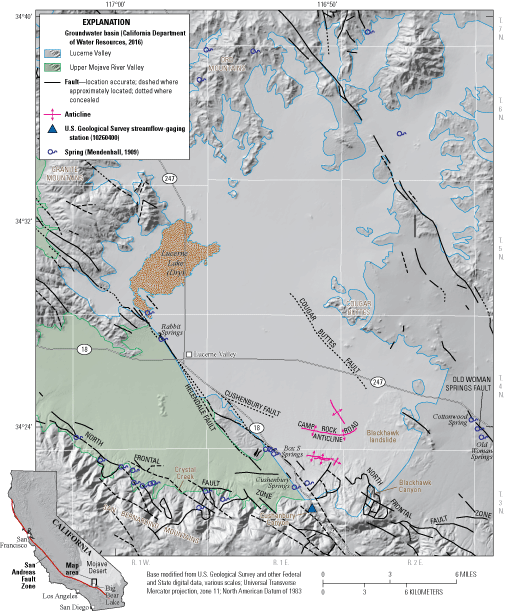
Location of the study area and the Lucerne Valley and Upper Mojave River Valley groundwater basins, Lucerne Valley, California.
The study area comprises most of the Lucerne Valley groundwater basin, which is adjacent to, but hydrologically separate from, the Upper Mojave River Valley groundwater basin to the west (California Department of Water Resources, 2016; fig. 1). Both basins are part of the Mojave Basin Area that was adjudicated in 1993. In the Court Judgment (Riverside County Superior Court, 1996), the Mojave Water Agency (MWA) was appointed as Watermaster to ensure that water rights are allocated. As Watermaster, the MWA is responsible for monitoring and verifying water production, collecting required assessments, conducting studies, and preparing an annual report of its findings and activities for the Mojave Basin Area to the Superior Court of California, County of Riverside. In addition, the passage of California’s Sustainable Groundwater Management Act (SGMA) in 2014 (California Department of Water Resources, 2015) has heightened interest in understanding groundwater basins throughout California and established a framework of priorities and requirements to help local agencies, such as the MWA, to sustainably manage groundwater basins in their management areas.
During the 1970s, a cooperative study by the U.S. Geological Survey (USGS) and the MWA (Schaefer, 1979) was done to evaluate the potential for artificially recharging the basin with imported water conveyed through a pipeline from the California State Water project. The purposes of that study were to help find methods to ensure the basin’s sustainability and to halt or alleviate groundwater-level declines. Although the effects of artificially recharging water through a pipeline were considered, no facilities have been built.
To reassess the hydrogeologic conditions in the Lucerne Valley, the USGS began a cooperative study with the MWA in 1994 with the purpose of documenting the changes to the groundwater system and developing management tools to help the MWA sustainably manage the groundwater basin. This study was extended in 2017 to update estimates of pumpage, examine the potential for subsidence, and address concerns about the impacts of future changes in land use.
The objectives of the study were to evaluate and describe (1) the surface and subsurface geology to better understand the hydrologic controls on the aquifer system and (2) the hydrogeologic and geochemical characteristics of the basin using existing groundwater-level and groundwater-quality data. In addition, a calibrated groundwater-flow model was developed to (1) quantify the losses and gains to the groundwater system, (2) evaluate potential changes in land use and future groundwater-use scenarios, and (3) evaluate the land subsidence that has already occurred. The groundwater-flow model is a valuable tool that can be used to evaluate future scenarios for managed aquifer recharge, changes in land use, and potential land subsidence.
Purpose and Scope
The purpose of this report is to document (1) the results of detailed geologic mapping and subsurface geologic interpretation, (2) the evaluation of the hydrogeology of the groundwater system, and (3) the calibrated groundwater-flow model. The geologic mapping and interpretation were done in the mid-to-late 1990s and helped define the aquifer system and controls on groundwater flow. Groundwater levels measured in wells from 1911 to 2016 were used to determine the groundwater-level elevations. Data available from wells from 1911 to 2016 and information recorded in drillers’ logs were used to help define sources of groundwater and identify the individual aquifer units.
Accessing Groundwater Data
The groundwater-level data presented in this report can be accessed through the USGS National Water Information System Web service (NWISWeb) at (https://waterdata.usgs.gov/ca/nwis/gw/; U.S. Geological Survey, 2021) and can be accessed by interactive map with NWIS Mapper (U.S. Geological Survey, 2022). The NWISWeb serves as an interface to a database of site information, including current and historical groundwater, surface-water, and water-quality data collected from locations throughout the United States and elsewhere. Data can be retrieved by state, category, and geographic area and can be selectively refined by specific location or parameter field. NWISWeb can output groundwater-level and water-quality graphs, site maps, and data tables (in Hypertext Markup Language [HTML] and American Standard Code for Information Exchange [ASCII] formats). At the time of this study, there were about 570 sites with groundwater-level measurements from 1911 to 2016 available on NWISWeb for the Lucerne Valley study area (appendix 1); sites with data available in the study area can be accessed by clicking here.
Description of the Study Area
The study area encompasses an area of about 175 square miles (mi2) in the southwestern part of the Mojave Desert and is about 75 miles (mi) northeast of Los Angeles, California (fig. 1). The Lucerne Valley is a closed, alluvial-filled desert basin dominated by northwest-southeast trending strike-slip faults and is bordered by the San Bernardino Mountains to the south, the Granite Mountains to the west, the Ord Mountains to the north, and Cougar Buttes to the east. The Lucerne Valley is surrounded and underlain by plutonic, metamorphic, and volcanic rocks that were considered non-water bearing for this study.
Groundwater is the sole source of water supply and is derived entirely within the Lucerne Valley groundwater basin, which encompasses about 230 mi2 (fig. 1; California Department of Water Resources, 2016). There are no perennial sources of surface water available; any surface water that occurs is a result of precipitation on the valley floor and in the surrounding hills and episodic flash floods from storms and snowmelt from the San Bernardino Mountains that is conveyed by small ephemeral washes originating along the boundaries of the basin. Land-surface elevations range from more than 4,500 ft above the North American Vertical Datum of 1988 (NAVD 88) at the base of the San Bernardino Mountains to about 2,850 ft at Lucerne Lake, a dry playa that lies in the topographically lowest part of the valley (fig. 1).
Climate
The climate of the area is typical of arid desert environments, with high summer temperatures, high evaporation rates, and minimal precipitation. Humidity is low and temperatures frequently exceed 100 degrees Fahrenheit (°F) in the summer and can drop below freezing in the winter. The average annual precipitation measured at the Lucerne Valley weather station was 4.04 inches (in.) for 1919–73 (Western Regional Climate Center, 2017a); about 60 percent of precipitation fell during the months of November–February. Precipitation records from the San Bernardino County Department of Public Works (2017) show that the average annual rainfall for water years 1991–2016 was 3.35 in. In contrast, the average annual precipitation measured for 1960–2016 at the City of Big Bear Lake (fig. 1), which is in the San Bernardino Mountains at an elevation of 6,790 ft above NAVD 88, was 21.85 in., and the average annual snowfall was 62.6 in. (Western Regional Climate Center, 2017b). A water year is the 1-year period from October 1st through the following September 30th and is named for the year in which it ends. All other results presented in this report are based on calendar years.
Land and Groundwater Use
Other than native vegetation, agriculture has been the major vegetation type in Lucerne Valley; wells and springs were observed being used for the irrigation of orchards and alfalfa in 1905 by Mendenhall (1909). Early ranchers recognized the suitability and economic benefits of growing alfalfa in the valley because of the plentiful sunshine and water provided by the numerous natural springs and artesian, or flowing, wells. By the time investigators documented springs and desert watering places in the early 1900s (Mendenhall, 1909), alfalfa farming was already prevalent in the Lucerne Valley, which was named after the French word for alfalfa. In 1954, Riley (1956) noted that the Lucerne Valley was highly developed and was being irrigated much more heavily than the surrounding towns and communities, and he inventoried almost 70 more irrigation wells than the combined total in the 3 adjacent groundwater basins. Schaefer (1979) reported that about 23,000 acre-ft of water were being used for about 3,500 acres of irrigated land in 1954, and about 15,000 acre-ft were being used for about 2,500 acres in 1976, primarily for alfalfa.
Detailed crop-type information was not available before 2007, but aerial photographs (San Bernardino County Department of Public Works, 2003; University of California Santa Barbara, 2003) representing 8 years between 1942 and 1993 were used to estimate the total irrigated area, presumably for alfalfa and native vegetation (figs. 2A–H), where native vegetation represents the non-irrigated, undisturbed land with desert-type vegetation. The aerial photographs show that the amount of irrigated land did not reach 6 percent of the total acreage between 1942 and 2016, and that the total irrigated area ranged from about 350 acres in 2008 to about 3,405 acres in 1977. Schaefer (1979) estimated that irrigated acreage was about 2,500 acres in 1976, which is about 27-percent less than the acreage that was estimated from aerial photographs for 1977. Between 2007 and 2016, detailed crop classifications were available (Mojave Water Agency, 2017), and the distribution of crop types are shown in greater detail for 2007, 2010, and 2016 on figures 2I–K. The estimated irrigated acreage for these selected 3 years did not exceed about 2 percent of the study area.
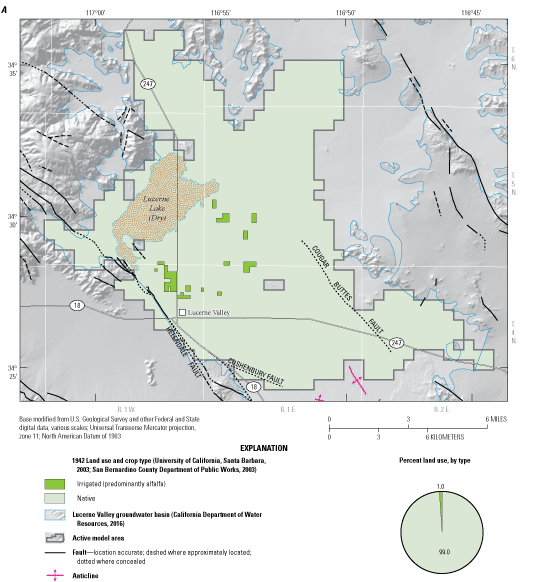


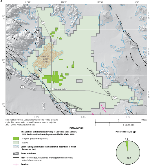

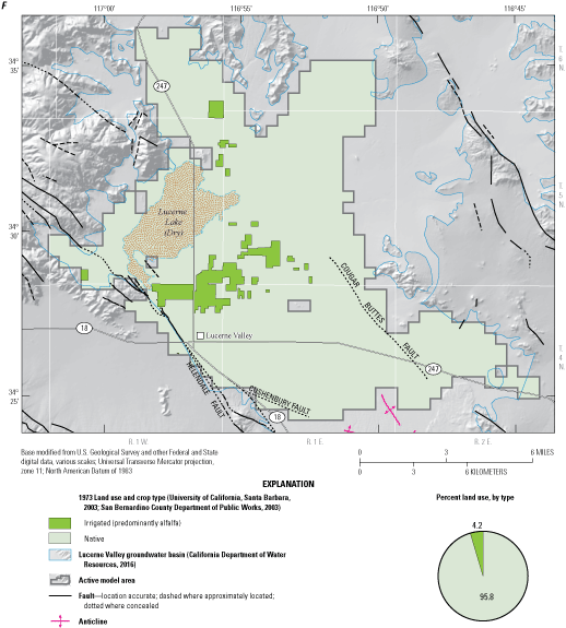
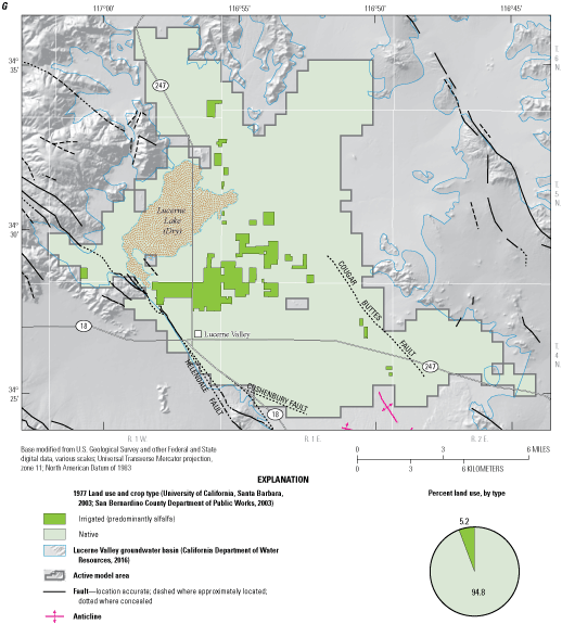
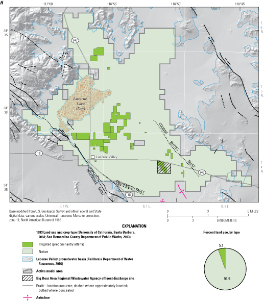
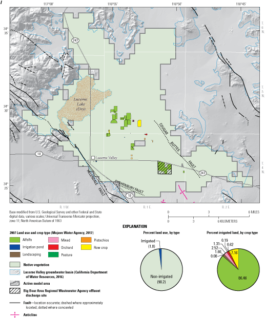
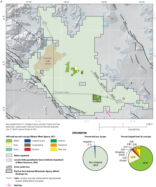
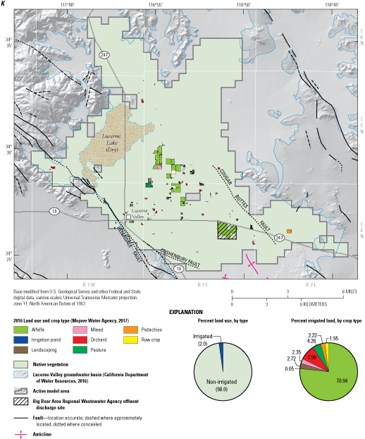
Land use for A, 1942; B, 1953; C, 1959; D, 1965; E, 1968; F, 1973; G, 1977; H, 1993; and land use and crop type for I, 2007; J, 2010; and K, 2016, Lucerne Valley, California.
Alfalfa remained the predominant crop between 2007 and 2016 (figs. 2I–K); however, its prevalence decreased somewhat as planting practices shifted in the later years toward grain, pasture, orchards, and other crops (figs. 2I–K, 3A). Alfalfa accounted for about 87 percent of the irrigated land in 2007 (fig. 2I) but decreased to about 68 percent in 2010 (fig. 2J) and was about 71 percent in 2016 (fig. 2K). Orchards covered about 1 percent of the irrigated land in 2007 but increased over time and became the second-most common crop in 2016, covering about 8 percent of irrigated land (fig. 3A).
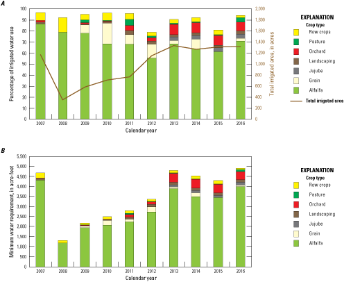
A, Percentage of irrigated acreage of selected crops (Mojave Water Agency, 2017); and B, estimated water requirement for selected crops for 2007–16, Lucerne Valley, California.
The water requirement for selected crops in the Lucerne Valley for 2007–16 was estimated using plant and soil evapotranspiration (ET) estimates available from either the Irrigation Training and Research Center (2003) or Sun and others (2012; fig. 3B). The water requirement was estimated based on land-use area, crop type, crop coefficient, and on the assumptions that the crops would be grown during the entire year, irrigation practices were 100-percent efficient, and that the crops received their full water requirement, with no excess water applied to the fields. Based on these assumptions and the crop types grown, the estimated water requirement for agriculture during 2007–16 ranged from about 1,420 to about 5,190 acre-ft (for 2008 and 2013, respectively; fig. 3B). Alfalfa was the highest groundwater-demand crop, requiring a minimum of about 67–90 percent of groundwater used for agriculture (fig. 3B). In reality, the groundwater demand could be greater because of inefficient irrigation loss, soil salinity, and salinity management practices, or groundwater demand could be less because crops commonly are rotated, fields usually are fallowed during some months, and crop-water demand likely is not fully met.
Residential and commercial development has been relatively small—the mostly rural community of Lucerne Valley, including the town of Lucerne Valley (fig. 2), had an estimated population of about 250 in 1928 (The Desert Gazette, 2017), about 4,000 in 1970 (Schaefer, 1979), and about 5,810 in April 2010 (U.S. Census Bureau, 2017). Residents occupy widely dispersed dwellings throughout the valley, and the amount of water for domestic use has been relatively small compared to of the amount of water used for agriculture. Although there were several domestic wells documented before 1916 (Thompson, 1929), the amount of groundwater pumped likely was minimal. In 1954, domestic-water use was estimated to be about 200 acre-ft, or only 1 percent of total water use, and about 1,200 acre-ft, or about 7 percent of total water use, in 1976 (Schaefer, 1979). In 2016, domestic-water use was estimated to be about 760 acre-ft, or about 20 percent of total water use (Mojave Water Agency, 2017).
Hydrogeology
The hydrogeologic framework of the Lucerne Valley groundwater basin (fig. 1) was defined by reviewing previous investigations, mapping the surficial geology, compiling geologic and hydrologic data from drillers’ logs, and examining the lithologic and geophysical logs and drill cuttings from wells that were drilled during the early part of this study (Huff and others, 2002). Geologic mapping in and around Lucerne Valley was conducted (1) as part of the Southern California Areal Mapping Project (SCAMP), a cooperative project sponsored jointly by the USGS and the California Geological Survey (Powell and Matti, 2000; Miller and Matti, 2001; Miller and others, 2001; Miller, 2004); (2) during more recent USGS efforts (Phelps and others, 2012); and (3) during older studies by those two agencies (Dibblee, 1964, 1967b; Bortugno and Spittler, 1986). The geologic map of the study area (fig. 4) shows the geologic units that (1) record the geologic framework and history of Lucerne Valley and vicinity (Powell and Matti, 2000) and (2) define the aquifer system in the Lucerne Valley groundwater basin. In conjunction with our geologic mapping in Lucerne Valley, we used lithologic and geophysical logs from USGS monitoring wells installed as part of this study (appendix 1) and lithologic logs from commercially drilled water wells; records were obtained from the Mojave Water Agency (2017) and the California Department of Water Resources (2020) to construct intersecting hydrogeologic cross sections that linked our surface mapping with subsurface records (fig. 5). A stratigraphic and structural framework for the Lucerne Valley was developed from geologic mapping and hydrogeologic cross sections that were further informed by hydrologic and geophysical data from the USGS monitoring wells.
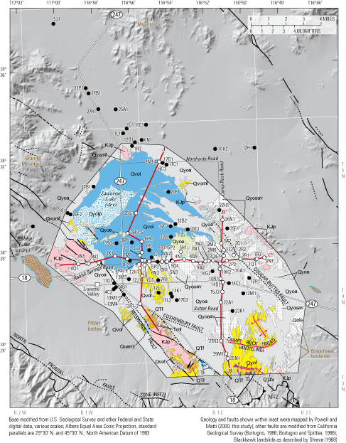

Geology, location of wells used to interpret the subsurface geology (California Department of Water Resources, 2020), and location of hydrogeologic cross sections, shown on figure 5, Lucerne Valley, California. See table 1 for more complete descriptions and discussion of geologic map units, ages, and stratigraphic framework. Abbreviation: <, less than.
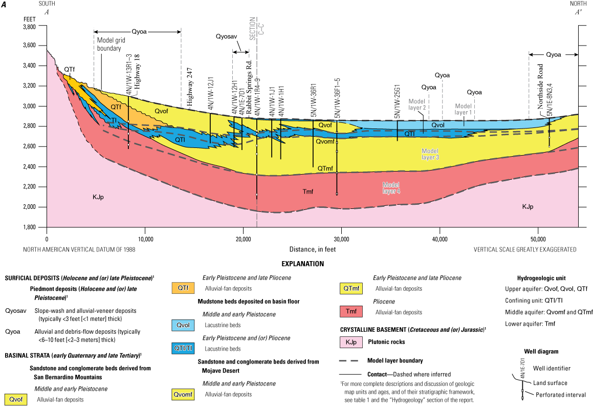

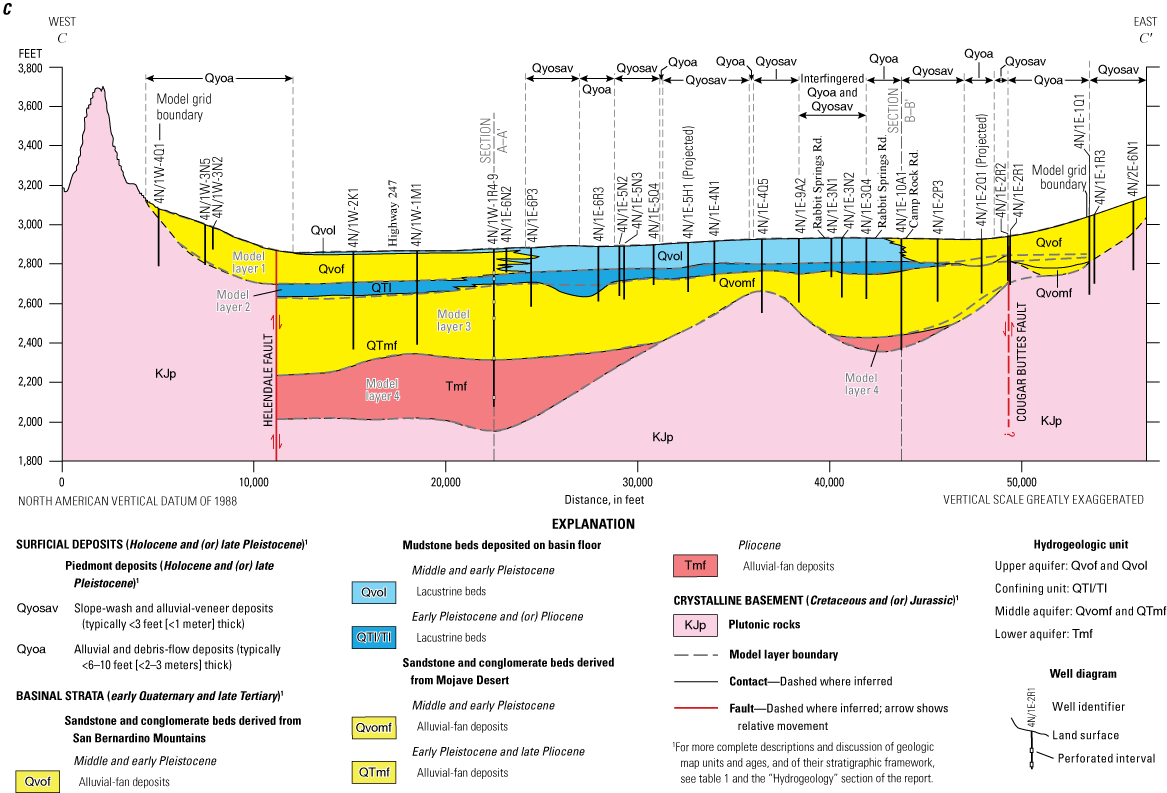
Generalized hydrogeologic cross sections showing geology (California Department of Water Resources, 2020) and corresponding model layers. A, south to north (A–A’); B, south to north (B–B’); and C, west to east (C–C’), Lucerne Valley, California. (Section lines shown on fig. 4). See table 1 for more complete descriptions and discussion of geologic map units, ages, and stratigraphic framework. Abbreviation: <, less than.
For the geologic map shown on figure 4, new geologic mapping was carried out in the Lucerne Valley quadrangle (this study), then we combined that mapping with a generalized representation of the geology shown in the published Cougar Buttes quadrangle. By so doing, we were able to generate a map that shows the surface exposure of the units we had developed from well-log data to represent the late Tertiary through middle Pleistocene basinal strata shown in the geologic sections (fig. 5). The late Pleistocene and Holocene surficial deposits are so thin in the Lucerne Valley area that they are not reliably recorded in the well logs used to construct the geologic sections; therefore, we (1) generalized and simplified the map representation of the surficial units on figure 4 and (2) emphasized that where surficial deposits are not recorded in the well logs, the geologic sections on figure 5 do not show these deposits, even where the deposits do appear on the geologic map (fig. 4).
Tectonic activity associated with the San Andreas Fault has greatly influenced the geologic structure, climate, and hydrologic setting of the Lucerne Valley groundwater basin. On a regional scale, transpressive contraction across this basin was accompanied by uplift of the San Bernardino Mountains during the Pliocene and Quaternary (Meisling and Weldon, 1989; Matti and Morton, 1993; Cox and others, 2003). On a local scale, the evolution and hydrologic setting of the Lucerne Valley groundwater basin have been influenced by its interaction with northwest-trending right-lateral faults of the Eastern California Shear Zone (Dokka and Travis, 1990a). Studying the subsurface geology, determining the location and effects of the faults in the valley, and documenting the physical setting of the basin help us to understand the characteristics and complexity of the aquifer system.
Geologic Framework
Synoptic Overview
The modern Lucerne Valley is a closed, desert basin that is flanked to the south by the San Bernardino Mountains and ringed to the north by highlands of the Mojave Desert, including the Granite Mountains, Ord Mountains, and Cougar Buttes. The basin—a bolson—has a central playa fed by alluvial fans that emanate from surrounding bedrock mountain ranges and inselbergs. Intervening between the principal fans are broad piedmont slopes covered by veneers of Pleistocene and Holocene slope wash and alluvium. In many cases, the piedmont slopes are pediments that have been beveled across tilted Pliocene and early Pleistocene sedimentary strata and underlying igneous and metamorphic rocks.
The Lucerne Valley basin is part of a regionally extensive trough that developed during the Pliocene and Quaternary coincident with uplift of the San Bernardino Mountains. Basement rocks capped by saprolite that formed beneath a widespread, deeply weathered erosion surface and overlain by late Miocene basalt and older strata were all warped downward during the early Pliocene between the rising San Bernardino Mountains to the south and highlands in the Mojave Desert to the north (Sadler, 1982e; figure 12 in Meisling and Weldon, 1989; Powell and Matti, 2000). The developing trough received sediment from both these upland sources. Uplift of the San Bernardino Mountains was accentuated during the late Pliocene and Quaternary in concert with the onset of northward-vergent thrusting within the North Frontal Fault Zone along the San Bernardino Mountains front (figs. 1, 4; for fuller documentation of thrust faults, see Sadler, 1982e, fig. 1; Bortugno, 1986; Miller, 1987, 2004; Meisling and Weldon, 1989; Powell and Matti, 2000; Spotila and Sieh, 2000; Spotila and Anderson, 2004; equivalent to North Frontal thrust sytem shown in U.S. Geological Survey, 2020).
Throughout its history, the Lucerne Valley basin-fill, like other basins north of the San Bernardino Mountains (fig. 1; Cox and others, 2003), has been characterized by three interfingering sedimentary facies: (1) alluvial deposits derived from the Mojave Desert highlands to the north, (2) alluvial deposits derived from the San Bernardino Mountains to the south, and (3) intervening basin-floor lacustrine and playa deposits that interfinger northward with the Mojave Desert-derived alluvial deposits and southward with the alluvial deposits derived from the San Bernardino Mountains. The geologic sections (fig. 5) indicate that these three sedimentary facies are arranged in a diachronous sequence of Mojave Desert-derived strata interfingering with and overlain by basin-floor strata to the south, in turn interfingering with and overlain by strata derived from the San Bernardino Mountains farther south. This stratigraphic sequence indicates that, generally, the depocenter of the Lucerne Valley closed basin was migrating northward with continuing uplift of the San Bernardino Mountains. There are, however, significant retrogressive variations in the generally northward-migrating position of facies transitions that are likely due to fluctuations in climate and tectonic activity.
The Lucerne Valley basin has evolved in conjunction with uplift of the San Bernardino Mountains to the south and displacement on northwest-trending right-lateral faults of the of the Mojave Desert (Spotila and Anderson, 2004), in particular the Helendale section of the Helendale-South Lockhart fault zone (U.S. Geological Survey, 2020; herein called the Helendale Fault), the Old Woman Springs Fault, and the Cougar Buttes Fault (figs. 1, 4) that form part of the Eastern California Shear Zone (Dokka and Travis, 1990a, b). Where the regional trough that flanks the San Bernardino Mountains to the north is transected by these faults of the Mojave Desert province, that trough has been segmented into discrete basins like Lucerne Valley.
Movement on the northeast-trending faults was accompanied by the growth of dome-shaped and anticlinal folds on the San Bernardino Mountains piedmont (figs. 1, 4; Eppes and others, 1998, 2002; Powell and Matti, 2000; Pearce and others, 2004). These folds warped the desert floor and the sediments beneath it in the latest Pliocene and Quaternary. In contrast to the north vergence of thrusting along the range-front, the asymmetry of the anticlinal folds on the piedmont indicates south-vergent strain.
Within this evolving tectonic setting, local and regional climatic fluctuations have contributed to an evolving landscape underlain by a wide variety of Quaternary sedimentary deposits (Powell and Matti, 1998a, b, 2000). The stratigraphic and structural frameworks outlined here are further developed in the “Geologic Units” and “Geologic Structure” sections that follow.
Geologic Units
The geologic map of the study area (fig. 4) shows the geologic units that frame and define the aquifer system in the Lucerne Valley groundwater basin. These units fall into three major categories that have been generalized from the work of previous studies (Powell and Matti, 2000; Miller and Matti, 2001; Miller and others, 2001; Miller, 2004): (1) crystalline basement rocks exposed around the basin and encountered in wells that penetrated through overlying basinal strata, (2) late Cenozoic basinal strata (basin-fill deposits; fig. 5), and (3) thin to very thin surficial deposits that unconformably overlie the basement and basin-fill overlying the basement rocks.
Crystalline Basement
Mesozoic, Paleozoic, and Proterozoic igneous and metamorphic rocks crop out regionally around the margins of the Lucerne Valley groundwater basin. The basement rocks that are exposed immediately adjacent to the groundwater basin (fig. 4) and are penetrated by wells drilled through the basinal strata (fig. 5) are predominantly Cretaceous or Jurassic plutonic rocks, or both (unit KJp). The many water wells in the Lucerne Valley basin that penetrate basement provide subsurface control on downwarping and faulting of the basement surface and on the three-dimensional size and shape of the Lucerne Valley groundwater basin. Moreover, significant differences between the basement rock types exposed in the San Bernardino Mountains and those exposed in the Mojave Desert provide insight into the provenance and hydrologic properties of the various basin-fill deposits and defining the three major diachronous lithostratigraphic packages that characterize the basin-fill overlying the basement rocks.
The crystalline basement exposed around the Lucerne Valley basin includes igneous, metamorphosed igneous, and metamorphosed sedimentary rocks. To the south, metamorphosed limestone is widely exposed along the San Bernardino Mountains range-front and is the source for most of the debris in the Blackhawk landslide (figs. 1, 4; table 1; Shreve, 1968), but limestone has not been identified beneath the Lucerne Valley basin-fill. Similarly, Triassic plutonic rocks are widespread in the crystalline rocks exposed west of the Helendale Fault and to the west of the geologic map shown on figure 4, but they have not been recognized beneath the Lucerne Valley basin-fill.
During the Miocene, a widespread regional erosion surface developed on the basement rocks of the Mojave Desert and San Bernardino Mountains (Oberlander, 1972, 1974; Powell and Matti, 2000; Spotila and Sieh, 2000), although this surface likely represents multiple cycles of weathering and erosion, perhaps extending as far back as the Cretaceous (Vaughan, 1922; Dibblee, 1967a; Meisling and Weldon, 1982, 1989). Granitic rocks, especially, were deeply weathered, forming a saprolite unit. The erosion surface has been warped and faulted because the crust in the Lucerne Valley region has deformed in response to the growth of the San Bernardino Mountains (Spotila and Sieh, 2000). Saprolite is exposed in the San Bernardino Mountains and in the Mojave Desert highlands, and nearly all the lithologic logs for wells that penetrate basement in the Lucerne Valley basin record a 20–40-ft interval of decomposed granite between sedimentary basin-filling deposits and fresh granitic basement rocks—indicating that the saprolite unit is widely preserved beneath the basin (Powell and Matti, 2000).
Late Miocene basalt flows associated with local eruptive centers overlie the saprolite and basement erosion surface. These flows are commonly underlain by and interbedded with sedimentary deposits, at least in part reworked from saprolite—for example, on Cougar Buttes, near Old Woman Springs, and near Pioneertown (not shown) on the eastern flank of the San Bernardino Mountains (Oberlander, 1972; F.K. Miller, in Woodburne, 1975, p. 83; Neville and Chambers, 1982; Sadler, 1982e; Powell and Matti, 2000). Basalt is described in the lithologic log for one of the wells in Lucerne Valley near the small granite inselberg just north of geologic section C–C’ (fig. 5C, log not shown on section) and about 1.3 mi west of Camp Rock Road. Some unrecognized late Miocene strata could be present atop saprolite at the base of the Pliocene-Quaternary section, in Lucerne Valley.
Basinal Strata
During the Pliocene and Quaternary, gravelly, sandy, and muddy sediment was transported from basement rocks around the basin margin and deposited in a variety of alluvial and lacustrine settings up to thicknesses of 1,500 ft. In the next section, we integrate information about these sedimentary materials, gleaned from outcrops around the margins of Lucerne Valley and from subsurface lithologic and geophysical well logs, to arrive at a basin-wide three-dimensional stratigraphic framework useful for hydrogeologic modeling (fig. 5).
Stratigraphic Sequence and Nomenclature
This report classifies the Lucerne Valley groundwater basin sedimentary fill into three diachronous lithostratigraphic packages (figs. 4, 5; table 1): (1) sandstone and conglomerate beds that originated as deposits in alluvial fans derived from the San Bernardino Mountains, (2) mudstone beds that accumulated in lakes that occupied the Lucerne Valley floor throughout much of the basin’s history, and (3) sandstone and conglomerate beds that originated as deposits in alluvial fans and braided streams derived from the Mojave Desert. These sequences are not considered geologic-map units, but rather, they represent sedimentary facies packages that result from our integration of the surface geology and subsurface-boring data. The geologic sections on figure 5 use the three sequences identified earlier to represent the water-bearing units of the Lucerne Valley groundwater basin, discussed further in the “Hydrogeologic Units and Framework” section. Map-unit labels within a stratigraphic sequence indicate where units mapped at the surface at the basin margin could be encountered in the subsurface throughout the Lucerne Valley groundwater basin.
Table 1.
Lithologic descriptions of geologic units and stratigraphic sequences in the Lucerne Valley, California.[(See figures 4, 5, and 15). Aridic soil notations used here (Birkeland, 1999); master soil horizons indicated by capital letters (A, B, C); soil subhorizons indicated by lower-case letters following master horizon (Av; Bk, Bt, Bw; Cox [soil subhorizon]). For more information, see the "Supplemental Information" section of this report. Soil colors in this table are identified by comparison to color chips in the Munsell soil color chart (Munsell Color, 1975). Colors are specified by color name followed by parenthetical grouping of notations representing hue (YR for yellow-red), color chart value (in the range 2.5–8), and chroma (in the range 1 to 8). Notations used in this table are (10YR, 7/3) and (10YR, 6/4)]
| Unit name | Unit labels (map and hydrogeologic- cross-section units) |
Map-unit age | Lithologic description |
|---|---|---|---|
| Eolian deposits | Qyoe | Holocene and late Pleistocene | Windblown sand in relict dunes, ramps, and coppices. Unconsolidated and pale yellow on natural surfaces; firm to indurated and slightly reddened where exposed in roadcuts. Deposited on moderately old lacustrine deposits (Qvol), on pavemented surface of old alluvial fan deposits, and on pavemented surface of young and old slope-wash and alluvial deposits (Qyosav). |
| Lacustrine and playa deposits | Qyolp | Holocene and late Pleistocene | Micaceous silt and clay with minor sand; scattered granules and pebbles. Playa deposits are very pale to pale brown. Light-colored surface. Little or no soil profile development. Sparsely to moderately vegetated. Active playa deposits have a white surface and exhibit mud cracks. Lacustrine deposits on the floor of Lucerne Valley are darker and browner than the playa deposits. Older parts of this unit overlain locally by windblown sand, distal fan, and slope-wash deposits. |
| Slope-wash and alluvial-veneer deposits | Qyosav | Holocene and late Pleistocene | Veneers of sand and pebbly sand that mantle piedmont slopes flanking the San Bernardino Mountains and Mojave Desert inselbergs. Young slope-wash units exhibit slightly dissected geomorphic surfaces characterized by Av/Cox and Av/Bw/C soil profiles typical of middle-to-early late Holocene surfaces (Bull, 1991; Eppes and others, 1998, 2002; Powell and Matti, 2000). Buried early Holocene and latest Pleistocene deposits are probably present. Older subunits consist of weakly to moderately pavemented slope wash and alluvium. Pavement consists of scattered, moderately varnished pebbles and small cobbles underlain by Av horizon of vesicular calcareous silt. On the fan debouching from Cushenbury Canyon, pavement and Av horizon overlie chalky-cemented, unsorted sand and pebbly sand; firm to hard; cemented to moderately well cemented. Bedding features absent or obscured by cementation process. Cemented deposits exposed in trenches, roadcuts, and roadbeds. In places, pavement and Av horizon overlie strongly reddened argillic B-horizon. As mapped, unit is partially covered by windblown sand and incised by shallow channels containing young wash deposits. Logs from commercially drilled water wells indicate that this unit is a thin cap above interbedded lacustrine clay and fluvio-lacustrine silt, sand, and fine gravel. In wells spudded below about 2,900 feet, the unit overlies deposits described as clay, interpreted herein as lake deposits. In wells spudded above 2,900 feet, the unit overlies deposits described as sand and gravel, interpreted herein as distal fan-delta deposits. Deposits in this unit are commonly less than about 3 feet thick. |
| Alluvial and debris-flow deposits | Qyoa | Holocene and late Pleistocene | Young and old alluvial deposits on the north piedmont of San Bernardino Mountains and on piedmonts in the Mojave Desert occur in nested complexes of alluvial fans that grew progressively basin-ward down the piedmont across a landscape inherited from the middle Pleistocene. The youngest deposits occur in young and modern washes and fans, consist of sand and pebbly sand deposited by channelized flow, and show slight to no soil development. These deposits are inset into abandoned, slightly dissected geomorphic surfaces characterized by Av/Cox and Av/Bw/C soil profiles typical of middle-to-early late Holocene surfaces (Bull, 1991; Eppes and others, 1998, 2002; Powell and Matti, 2000). Av horizons consist of loess-like, vesicular light brown (10YR 6/4) calcareous silt. Buried early Holocene and latest Pleistocene deposits may be present. A subunit of old surficial deposits occurs in alluvial fans on piedmont slopes, and in colluvial debris aprons. Old deposits exhibit slightly to moderately dissected geomorphic surfaces; granitic debris characterized by Av/Bt/Bk/Cox soil profiles. These old deposits form a thin mantle of consolidated sand and pebbly to cobbly gravel draped over an inherited older Pleistocene landscape; rarely observed to be thicker than about 6 feet. Old deposits characterized by well-developed pavement containing moderately to strongly varnished pebbles. Pavement underlain by pedogenic Av horizon of very pale brown (10YR 7/3) loess-like, vesicular silt. Graded to base-level lake with prominent shoreline gravel beach and bar deposits in Lucerne Valley. As mapped, this unit includes some slope-wash and eolian deposits. Deposits in unit Qyoa are commonly 6–10 feet thick or less. On the pediment flanking Cougar Buttes, on distal parts of the San Bernardino Mountains piedmont, and on a pediment on the north flank of the Camp Rock Road Anticline, younger parts of unit Qyoa overlap and are inset into older parts of the slope-wash and alluvial veneer deposits of unit Qyosav. |
| Landslide breccia | Qols | Late Pleistocene | Rock-avalanche breccia that constitutes the Blackhawk landslide. Breccia is derived chiefly from metamorphosed Paleozoic carbonate strata and subordinately from Pliocene conglomeratic sandstone and granitic rocks. |
| Breccia | QTbr | Quaternary and (or) Tertiary | Breccia is derived chiefly from metamorphosed Paleozoic carbonate strata and subordinately from Pliocene conglomeratic sandstone and granitic rocks. It likely formed as a rock-avalanche landslide deposit. |
| Alluvial-fan deposits | Qvof | Middle and early Pleistocene | Gravel, sandy gravel, gravelly sand, and sand locally interlayered with minor muddy sediment; grain size fines northward toward Lucerne Valley and increases south and southwest toward the San Bernardino Mountains. Clasts consist mainly of San Bernardino Mountains type, locally dominated by calcitic and dolomitic marble or granitic and gneissic detritus, depending on bedrock source. On the granitic inselberg southeast of the town of Lucerne Valley (fig. 4), units Tf and QTf contain clasts derived from the Mojave Desert and deposited by streams flowing into Lucerne Valley from the west. Overlying unit Qvof represents a significant pulse of San Bernardino Mountains derived sediment that unconformably overlies the older Mojave Desert-derived units. Unit Tf is shown in the subsurface in the hydrogeologic cross sections (fig. 5), but it is not mapped at the surface (fig. 4). |
| QTf | Early Pleistocene and late Pliocene | ||
| Tf | Pliocene | ||
| Lacustrine deposits | Qvol | Middle and early Pleistocene | Greenish- to brownish-colored sediment and sedimentary rock consisting mainly of clay- and silt-size particles; referred to as “clay” and “silt” in drillers' logs; also includes subordinate very fine and fine sand-size particles. Surface exposures weather into smooth recessive slopes. From older to younger, units Tl, QTl, and Qvol represent deposits of a lake or series of lakes that persisted on the Lucerne Valley floor throughout Pliocene and Quaternary time. This lake migrated back and forth across the Lucerne Valley basin during this period, yielding deposits that generally are lithologically uniform; however, differences in color, consolidation, and geophysical properties occur locally due to differences in mineralogic composition. Geologic consulting reports identify clay minerals mainly as smectites (montmorillonite and related minerals) and kaolins (kaolinite and related minerals); the former shrink and swell with the subtraction and addition of water, leading to shrinkage and expansion cracks and other kinds of ground-surface deformation (Fife, 1977, 1980). It is possible that some of the montmorillonite- and kaolinite-bearing intervals represent playa deposits interlayered within this unit. Unit QTl is shown in the subsurface in the hydrogeologic cross sections (fig. 5), but it is not mapped at the surface (fig. 4). |
| QTl | Early Pleistocene and late Pliocene | ||
| Tl | Pliocene | ||
| Alluvial-fan deposits | Qvomf | Middle and early Pleistocene | Light-colored sandy and gravelly sediment and sedimentary rock consisting mainly of sand- and granule-size particles along with pebbles and small cobbles of granitic, metavolcanic, and gneissic debris and sparse basalt clasts. Formed as fluvial deposits derived from Mojave Desert sources north of Lucerne Valley. From older to younger, units Tmf, QTmf, and Qvomf represent a wedge of alluvial-fan and fan-delta sediment that prograded across the Lucerne Valley basin during early Pliocene through middle Pleistocene time. In southern parts of Lucerne Valley, these sediments are described from the lower parts of well logs; in central and northern parts of the Valley, they comprise most of the well-log descriptions (fig. 5). Unit QTmf is shown in the subsurface in the hydrogeologic cross sections (fig. 5), but it is not mapped at the surface (fig. 4). |
| QTmf | Early Pleistocene and late Pliocene | ||
| Tmf | Pliocene | ||
| Plutonic rocks | KJp | Cretaceous and (or) Jurassic | Predominantly biotite monzogranite; scattered older bodies of granodiorite, quartz diorite, diorite, and Mesozoic or Proterozoic orthogneiss. |
As displayed in the geologic sections (fig. 5), sedimentary facies units in the Lucerne Valley groundwater basin have complex interfingering relations with one another. The cross-sectional geometry reflects that each of the depositional settings that generated each sedimentary unit—lacustrine settings that generated silt- and clay-rich deposits, low-energy fluvial settings that generated silty and sandy deposits, and high-energy fluvial settings that generated coarser sand-and-gravel deposits—have migrated back and forth (north and south) across the Lucerne Valley landscape throughout the Pliocene–Quaternary interval. As a result, lithologic facies units not only succeed each other vertically in any individual surface outcrop or subsurface boring, but interfinger laterally across the basin. This characterization is depicted in the geologic sections by fingers of one lithology that project laterally toward another.
Sandstone and Conglomerate Beds Derived from the San Bernardino Mountains (Tf, QTf, Qvof)
Around the southern margin of Lucerne Valley, conglomerate, conglomeratic sandstone, and sandstone, all rich in clasts of San Bernardino Mountains type, interfinger with and overlie greenish mudrock of the lacustrine sequence. These coarse-grained deposits have been interpreted as detritus eroded from the San Bernardino Mountains as they were uplifted in the latest Pliocene and Pleistocene (Shreve, 1959, 1968; Richmond, 1960; Dibblee, 1964; Sadler, 1982a–e; Miller, 1987; Meisling and Weldon, 1989; Spotila and Sieh, 2000; Cox and others, 2003). The particle makeup of the San Bernardino Mountains-derived sediment wedge depends on its location relative to bedrock source areas. East of State Route 18, where bedrock is mainly calcitic and dolomitic marble, the wedge is dominated by marble clasts; west of State Route 18, the marble bedrock is intruded by granitic rocks, and the sediment wedge becomes progressively richer in quartz, feldspar, and granitoid clasts as it is traced westward toward Pitzer buttes (fig. 4; Dibblee, 1964; Pearce and others, 2004).
Deposits of sandy and gravelly sediment containing Mojave Desert-type clasts occur in the stratal sequence (unit QTf; figs. 4, 5A) surrounding the granitic inselberg southeast of the town of Lucerne Valley. These beds, which unconformably overlie units Tmf and Tl, contain clasts of metavolcanic rocks, distinctive granitoids, and gneiss typical of Mojave Desert sources but have paleocurrent indicators pointing east into the Lucerne Valley region from sources to the west or northwest. Although these deposits contain a clast assemblage derived from the Mojave Desert basement, they have a different paleogeographic vector, and it is not yet clear whether they were derived directly from the Mojave Desert crystalline rocks or recycled from older Mojave Desert-derived sedimentary deposits in the San Bernardino Mountains.
The San Bernardino Mountains-derived sequence has not been recognized in subsurface-boring logs in the northern part of the Lucerne Valley groundwater basin. This observation, together with well-log data, leads to the interpretation that the San Bernardino Mountains-derived sequence (units Tf, QTf, and Qvof) is confined to the southern half of the Lucerne Valley groundwater basin and interfingers northward with the lacustrine sequence (units Tl, QTl, and Qvol), which in turn interfingers northward with the Mojave Desert-derived sequence (units Tmf, QTmf, and Qvomf). These relations are shown in hydrogeologic cross sections A–A’ and B–B’ (figs. 5A, 5B). Units Tf, QTl, and QTmf are shown in the subsurface in the geologic sections but have not been mapped at the surface (fig. 4).
Near wells 4N/1W-13R1–3 (figs. 4, 5), the San Bernardino Mountains-derived deposits formed a large alluvial fan that, several hundred thousand years ago, radiated northward and northeastward into Lucerne Valley from streams that flowed past the northern tip of the granitic inselberg southeast of Lucerne Valley. This fan-deposited sediment lies unconformably on top of an erosional landscape beveled onto tilted older units depicted at the south end of geologic section A–A’ (fig. 5A). At that location, unit Qvof contains carbonate and granitic pebbles and cobbles, reflecting multiple sources of parent material in the San Bernardino Mountains (table 1).
The San Bernardino Mountains-derived wedge probably formed as a series of coalescing alluvial fans that extended basinward from the mountains. As with modern fans, grain size diminished downslope toward the valley floor—where penetrated by subsurface borings, sedimentary materials of the San Bernardino Mountains-derived wedge are progressively finer grained the farther north the boring is located. For unit Qvof, well logs show a broad transition from basinward fining alluvial sand through interlayered fine sand and mud to lacustrine mud. This transition is similar to that described for fan-deltas (Nemec and Steel, 1988) that develop where distal streams reach the standing water of lakes and, as such, these transitional deposits are included in unit Qvol for this report (figs. 4, 5A). As mapped and shown in the geologic sections, units Tl and QTl likely contain fan-delta deposits as well.
Mudstone Beds Deposited on Basin-Floor (TI, QTI, Qvol)
Distinctive greenish to brownish mudrock intervals (claystone, siltstone) occur throughout the Lucerne Valley region in surface exposures and in the subsurface (Powell and Matti, 1998a, b, 2000). These intervals have been interpreted as low-energy deposits that accumulated in lacustrine (lake) settings that developed from time to time on the Lucerne Valley floor (Shreve, 1959, 1968; Dibblee, 1964; Sadler, 1982c, d). Because some intervals described in well-logs include montmorillonite- and kaolinite-bearing layers, it is possible that playa deposits are included within the lacustrine units (table 1).
Isolated surface exposures of mudrock crop out from the range-front of the San Bernardino Mountains as far north as the granitic inselberg (labeled as unit “KJp” on fig. 4) about 3 mi southeast of the town of Lucerne Valley. There, intervals of tilted mudrock dip gently northward and northeastward toward the basin center (fig. 5A); these outcrops yielded late Pliocene-early Pleistocene vertebrate fossils described by May and Repenning (1982). Clay-rich sedimentary materials have also been reported in drillers’ logs throughout the subsurface of Lucerne Valley, either as thin intervals interspersed intermittently with other lithologic types or as thicker intervals that occur widely in the subsurface. These intervals consist of fine-grained clayey and silty deposits that contain abundant brown clay variously described as “sticky” and “hard” or as having high plasticity. Such deposits are penetrated from about 260 to 340 ft below land surface (bls) by wells 4N/1W-13R1–3, from about 140 to 180 ft bls by wells 4N/1W-1R4–9 and from about 140 to 170 ft bls in wells 5N/1W-36F1–5 (fig. 5A). The clay layers limit the vertical movement of groundwater that cause perched conditions in the southern and western parts of the basin and are discussed further in the “Hydrogeologic Units and Framework” section.
The southernmost occurrences of clay-rich strata along the range front of the San Bernardino Mountains are probably Pliocene and are labeled as unit Tl on figures 5A–C. On a regional basis, these deposits appear to interfinger with the lower part of unit Tmf, suggesting that during the Pliocene, lake settings in the Lucerne Valley region were restricted to the southern part of the Lucerne Valley groundwater basin, near the current position of the San Bernardino Mountains front. In central and northern Lucerne Valley, occurrences of the clay-rich interval are depicted as late Pliocene through middle Pleistocene and are labeled as units QTl and Qvol on figures 5A–C. Regionally, these deposits appear to interfinger with deposits of units QTmf, Qvomf, QTf, and Qvof.
Sandstone and Conglomerate Beds Derived from the Mojave Desert (Tmf, QTmf, Qvomf)
The deepest sedimentary materials penetrated by water wells in the Lucerne Valley groundwater basin consist of a thick unit of mixed sandy sediment, gravelly sediment, and conglomeratic sedimentary rock. In boreholes at USGS monitoring wells 4N/1W-1R4–9 and 5N/1W-36F1–4, the unit was penetrated at about 500 ft bls. Cuttings from these boreholes consist of angular sand- and granule-size granitic debris and fragments of metavolcanic rock derived from the Sidewinder Volcanics, a unit that is diagnostic of having a source in the basement complex of the Mojave Desert north of Lucerne Valley. The unit probably was deposited as alluvial-fan and braided-stream deposits by streams flowing southward into the Lucerne Valley groundwater basin during the Pliocene and early to middle Pleistocene.
Mojave Desert-sourced sediments in the Lucerne Valley groundwater basin have been interpreted as evidence that the San Bernardino Mountains did not form a major landscape feature or provide a sediment source for the Mojave Desert region until the late Pliocene or early Pleistocene when the mountains were uplifted (Shreve, 1959, 1968; Dibblee, 1964; Sadler, 1982a, e105; May and Repenning, 1982; Meisling and Weldon, 1989; Powell and Matti, 1998a, b; Spotila and Sieh, 2000; Cox and others, 2003). Thus, during the deposition of units Tmf and the early part of QTmf (figs. 5A, 5B), the Lucerne Valley region was inundated by sediment that was derived from Mojave Desert mountains and inselbergs, accumulated in piedmont alluvial fans and pediment alluvial aprons flanking the mountains and inselbergs, and was swept southward, southeastward, and southwestward by streams flowing across a braided flood plain that extended as far south as the ancestral San Bernardino Mountains front. As in the case of sediment derived from the San Bernardino Mountains, the Mojave Desert-derived sand and gravel likely transitioned into fan-deltas that interfingered with valley-floor lacustrine deposits. Although probably not a major feature early in this cycle, the San Bernardino Mountains were a positive-landscape element that shed sediment northward.
Surficial Deposits
Overlying Pliocene through middle Pleistocene sediments and rock are thin accumulations (typically less than 6–10 ft thick) and veneers (typically less than 3 ft thick) of late Quaternary (late Pleistocene through Holocene) sedimentary material that have been deposited at the land surface in the Lucerne Valley groundwater basin during the last hundred thousand years. These materials generally are unconsolidated, although some consolidation is observed at depth and in the late Pleistocene units. The surficial units are so thin that they generally cannot be depicted on the geologic sections (figs. 5A–C), especially given that the uppermost parts of well holes typically are not described fully or consistently in the logs.
In general, surficial sedimentary materials consist of interlayered sandy and gravelly deposits along the flanks of the basin and consist of interlayered clay, silt, and fine sand on the valley floors. Like with their older counterparts, the surficial sedimentary materials occur in three major geomorphic and depositional settings: (1) the northward-sloping piedmont of the San Bernardino Mountains; (2) the relatively flat and featureless floor of Lucerne Valley; and (3) slopes and flanks of bedrock inselbergs and mountains around the northern reaches of Lucerne Valley, including pediments that flank the inselbergs of Cougar Buttes.
Surficial Deposits on Piedmonts Flanking Lucerne Valley
During the late Pleistocene and Holocene, several generations of gravelly and sandy sediment (unit Qyoa on fig. 4) have been transported northward from sources in canyons of the San Bernardino Mountains and deposited in various piedmont locations (Eppes and others, 1998, 2002; Powell and Matti, 2000). For the most part, these Qyoa deposits are alluvial sediments deposited by streamflows that coursed down alluvial-fan surfaces or down streams between fans. Similarly, alluvial sediments were deposited by streams flowing southward across piedmonts (commonly pediments) of the mountains of the Mojave Desert north of Lucerne Valley. Streams emanating from granite inselbergs of the Mojave Desert, such as Cougar Buttes, formed smaller, thinner, and lower-relief alluvial fans than those on the mountain piedmonts. Young sandy and gravelly Quaternary sediments on both sets of these piedmonts feather out basinward onto the relatively flat surface of Lucerne Valley, where they transition into slope-wash veneers (unit Qyosav on fig. 4). The slope-wash deposits consist of materials derived from reworking young alluvial and eolian material and intermixing these materials with reddened sand and petrocalcite-cemented clasts reworked from soil profiles that formed atop older and unconformably underlying middle and early Pleistocene basin-fill strata (units Qvof, Qvomf, and Qvol).
Piedmont domains between the young alluvial-fan deposits are also covered by slope-wash veneers (unit Qyosav on fig. 4). Unit Qyosav rests unconformably atop older basin-fill deposits on the north flank of the Camp Rock Road Anticline (figs. 1, 4) on the San Bernardino Mountains piedmont. On the Cougar Buttes piedmont, unit Qyosav lies on pediments planed across granite basement and the middle and early Pleistocene deposits that overlie the basement.
Surficial Deposits on Lucerne Valley Floor
Geologic mapping and subsurface studies for this report indicate that young sediment deposited in the Lucerne Valley is not very thick and in some instances is not present at all. For example, in the eastern part of the Lucerne Valley region, the Powell and Matti (2000) map shows only veneers of young deposits overlying a hard, thick petrocalcic horizon (Pearce and others, 2004); these veneers appear to correlate with similar layers that cap very old San Bernardino Mountains-derived sedimentary rock farther south on the piedmont (units QTf and Qvof on figs. 4, 5A–C).
Mapping for this study indicates that young Quaternary surficial materials derived from the San Bernardino Mountains have been deposited mainly on the piedmont of the San Bernardino Mountains and have not extended in appreciable amounts onto the Lucerne Valley floor. In general, older parts of the young deposits were deposited in proximal and medial piedmont positions, and younger parts of the young deposits were deposited in medial and distal positions. After depositing their sediment loads on piedmont surfaces, streams flowed northward onto the valley floor and either deposited very thin veneers of alluvium unconformably over older deposits of Qvo age or incised channels into these older deposits as the streams worked their way to the lowest part of the Lucerne Valley floor. The remainder of the Lucerne Valley floor either is washed by unconfined sheet flow that leaves only trivial volumes of sediment or is swept by wind that deposits thin veneers of eolian sediment (sand, silt; Powell and Matti, 2000). Late Pleistocene and Holocene lake and playa deposits (unit Qyolp on inset map fig. 4) in the northwestern part of the Lucerne Valley floor occupy a relatively small footprint on the modern landscape (see also, Sadler, 1982d). The modern Lucerne Lake (dry) is ephemeral, and its playa periodically floods and receives fine clay- and silt-rich sediment and sometimes accumulates windblown sand.
Eolian Deposits
The Lucerne Valley floor is mantled with thin patches of Holocene and late Pleistocene wind-deposited (eolian) sediment. The sediment consists of deposits of sand, silt, and granules that occur as thin sheets and stringers, as small, rounded patches of vegetation-stabilized sediment (coppice dunes), and as relatively large dunes that migrate eastward across the valley floor in response to prevailing winds (unit Qyoe on fig. 4; Powell and Matti, 2000).
Geologic Structure
Within the broader context of the regional tectonic framework presented in the “Synoptic Overview” section, the discussion of geologic structures here focuses on faults and folds that deform the late Cenozoic sedimentary fill of the Lucerne Valley as shown on the geologic map on figure 4.
Helendale Fault
The Helendale Fault trends northwest across the Lucerne Valley region and separates the Lucerne Valley groundwater basin from the Upper Mojave River Valley groundwater basin to the west (fig. 1). The Helendale Fault acts as a barrier to groundwater flow along that boundary (Riley, 1956; Schaefer, 1979; Stamos and others, 2001; Teague and others, 2016). In the vicinity of the town of Lucerne Valley, the fault forms a conspicuous northeast-facing scarp; fault studies (Bryan and Rockwell, 1995) indicate one or more ground-rupturing earthquakes in the last few thousand years, making the Helendale Fault an active fault comparable to those that ruptured during the 1992 Landers earthquake (Hauksson and others, 1993) and the 1999 Hector Mine earthquake (Hauksson and others, 2002) farther to the east in the Eastern California Shear Zone (Dokka and Travis, 1990a, 1990b).
Directly southeast of the town of Lucerne Valley, the trace of the Helendale Fault is concealed by very young alluvial sediment, but slightly elevated ground east of the concealed trace indicates vertical movements on the fault. In the vicinity of the granitic inselberg southeast of the town of Lucerne Valley, the Helendale Fault splits into two strands: one having a mainly concealed trace that trends southeastward along the west side of the inselberg and one that crosses the inselberg and trends along its east side (fig. 4) toward the Cushenbury Canyon area to the southeast (fig. 1). The western trace is the older of the two, and relations between the two fault strands indicate that the younger eastern trace developed as a left-step in the Helendale Fault.
Lucerne Lake Fault
Existence of the Lucerne Lake fault (not shown) first was proposed by Riley (1956) who extended the fault from the Granite Mountains to the southeast edge of the dry bed of Lucerne Lake; it has been projected farther southeast based on a step in groundwater levels (Goodrich, 1978; Schaefer, 1979; Brose, 1987). The fault purportedly trends northwest across the center of the Lucerne Valley groundwater basin parallel to the Helendale Fault and presumably is related to it. The Lucerne Lake fault has attracted considerable interest because of its possible impact on groundwater flow. Although various unpublished consulting reports refer to photo lineaments as evidence for the fault, a long trench excavated across these lineaments yielded no evidence of faulting in deposits we have assigned to unit Qvol. If present here, the Lucerne Lake fault must be older than, and concealed by, clay-rich sediment of unit Qvol in geologic section A–A’ (fig. 5A). No hydrogeologic or geologic evidence of the Lucerne Lake fault was detected during this study (see “Groundwater Levels, Flow, and Movement” section).
Cougar Buttes Fault
In the southeastern part of the Lucerne Valley groundwater basin, the Cougar Buttes fault (figs. 1, 4) is inferred based on mismatches in lithologic logs from subsurface borings and from differences in groundwater levels in adjacent, similarly constructed wells. The fault has not been mapped at the surface to the northwest of the Blackhawk landslide, although a roughly colinear fault segment mapped to the southeast of the Blackhawk landslide and shown southeast of the geologic map (fig. 4) forms a conspicuous northeast-facing scarp in late Pleistocene alluvial deposits. The Cougar Buttes Fault parallels the Helendale Fault and, as such, could be part of the Eastern California Shear Zone.
Cushenbury Fault
Geologic mapping for this study indicates that a concealed fault (referred to in this report as the Cushenbury Fault) is associated with the Camp Rock Road Anticline (fig. 4). The fault is not observable at the surface because it is concealed by Holocene and late Pleistocene alluvial deposits. However, its existence is inferred from the geometry of the Camp Rock Road Anticline (discussed later) and from differences in groundwater levels in its vicinity. Groundwater-level differences could be caused exclusively by the anticline; fracturing of folded brittle rock layers and changes in their dip along the south limb of the anticline could be enough to impede groundwater flow. However, a fault is the simplest explanation to all geologic, geomorphic, and hydrogeologic issues in this vicinity. We interpret the Cushenbury Fault as a north-dipping fault, having a component of reverse slip; movement on the fault probably was synchronous with growth of the Camp Rock Road Anticline, and both structures probably are south vergent—that is, their geometries indicate tectonic transport directed south toward the San Bernardino Mountain front rather than north toward the Mojave Desert.
Camp Rock Road Anticline
On the San Bernardino Mountains piedmont, in the southeast part of the Lucerne Valley groundwater basin, Pleistocene conglomerate—that Shreve (1968) included within the unit he mapped as Cushenbury Springs Formation—is warped into a conspicuous anticlinal fold (not shown; Dibblee, 1964; Powell and Matti, 2000; Pearce and others, 2004). Pearce and others (2004) called this anticlinal fold the “Cougar Buttes anticline,” but that name is misleading because the fold is not located near Cougar Buttes; in this report, the fold is defined and named the Camp Rock Road Anticline (fig. 4). The east-trending fold is asymmetric, showing a shorter south limb that is back-tilted compared to the north limb, which roughly parallels the regional northward dip of the stratigraphic section (fig. 5B; Pearce and others, 2004); the axial plane is not well exposed but appears to be inclined northward. The fold’s core exposes greenish-colored mudrock that Powell and Matti (2000) assigned to the Old Woman Sandstone, but that is shown as unit Tl in this report. Rocks exposed in the core of the fold are riven with fractures and small faults, one of which appears to be a north-vergent thrust fault that forms a low north-facing scarp on the fold’s gently dipping north limb (Pearce and others, 2004; fig. 4).
In this report, the asymmetric Camp Rock Road Anticline is interpreted as a south-vergent structure, as suggested by the geometry of the fold and by the concave-north plan view of the fold trace (Powell and Matti, 2000). The overall fold geometry suggests the presence of a concealed fault (Cushenbury Fault) that appears to splay southeastward from the Helendale Fault, then bend eastward to break across the stratigraphic section along the south flank of the anticline (figs. 4, 5). The coextensive traces of the Camp Rock Road Anticline and the Cushenbury Fault form barriers to groundwater flow in this vicinity and are probably the cause of groundwater-level differences west to State Route 18 (fig. 4).
San Bernardino Mountains Piedmont Folds
Other folds and dome-shaped upwarps have been described along the San Bernardino Mountains piedmont just west of the geologic map shown on figure 4 (Eppes and others, 2002), as well as along the west part of its southern margin (Pearce and others, 2004; fig. 4). These structures deform Pleistocene gravel and conglomerate deposits of the San Bernardino Mountains-derived sediment wedge (Eppes and others, 2002; fig. 4). Although the origins and structural roles of these features are not fully known, they have grown synchronously with deposition of younger parts of the San Bernardino Mountains-derived sediment wedge, and their growth has affected late Pleistocene fluvial geomorphology and pedogenesis (Eppes and others, 2002; Pearce and others, 2004).
Hydrogeologic Units and Framework
The water-bearing deposits in Lucerne Valley generally are unconsolidated Quaternary and Tertiary alluvial deposits, which consist of sediments that vary in size from fine silt and clay to coarse sand and gravel, depending on location and depositional history. The crystalline basement exposed in and around Lucerne Valley includes igneous, metamorphosed igneous, and metamorphosed sedimentary rocks, but these are not considered water-bearing, and no wells penetrated the deeply weathered granitic basement rocks underlying the alluvial deposits. The aquifer system consists of four main units: the upper aquifer, a confining unit, middle aquifer, and lower aquifer (fig. 5). The total thickness of these water-bearing deposits varies throughout the basin depending on the elevation of the underlying basement rocks but has a maximum of about 1,000 ft (fig. 5). The upper aquifer is about 180 ft thick in some areas and generally is composed of fine-grained to moderately permeable Quaternary sedimentary deposits. The groundwater quality of the upper aquifer generally is poor in agricultural areas because of the infiltration of irrigation-return water (Schaefer, 1979); the total dissolved-solids concentrations in the upper aquifer averaged about 2,700 milligrams per liter (mg/L) in 1976 and about 2,800 mg/L in 2010 (Schaefer, 1979; Metzger and others, 2015); these concentrations rendered the water from some wells too poor in quality for domestic or agricultural uses (Schaefer, 1979).
The unconsolidated deposits of the upper aquifer overlie and interfinger with a lacustrine clay confining unit (primarily units QTI and TI) that mainly is present in the southern and western part of the basin (fig. 5). Where present, this confining unit creates “perched” conditions in some parts of the upper aquifer; this means that there are saturated materials on top of the confining unit, which is underlain by an unsaturated zone in the middle aquifer below. This layering results in pronounced differences in the groundwater-level elevations between the upper and middle aquifers that were reported by Riley (1956) and Schaefer (1979) and shown areally by Smith (2003) and Stamos and others (2007). The middle aquifer underlies the confining unit (fig. 5) and ranges in thickness from about 50 to as much as 500 ft in some places. The middle aquifer is coarser grained and more permeable than the overlying confining unit and is mainly made up of Quaternary–Tertiary alluvial deposits (units Qvomf and QTmf), primarily derived from Mojave Desert sources to the north and east. Most wells in the valley are perforated in, and withdraw groundwater from, the middle aquifer because it yields favorable-quality groundwater readily to wells; reported well yields ranged from 800 to 2,000 gallons per minute (gal/min; Riley, 1956). The lower aquifer ranges in thickness from 0 to 300 ft (fig. 5) and generally is less permeable than both the upper and middle aquifers. The lower aquifer, which is the deepest groundwater-bearing unit, is comprised of Tertiary alluvial fan deposits (unit Tmf) derived primarily from Mojave Desert sediments to the north. Total dissolved-solids concentrations from the middle and lower aquifers generally were lowest in the areas south of the playa and ranged from 300 to 1,200 mg/L in 1976; groundwater near and north of the playa was high in sodium and chloride and had an average total dissolved-solids concentration of 5,000 mg/L (Schaefer, 1979).
Similar to other southwestern Mojave Desert basins that are dominated by tectonics and movement along the San Andreas Fault, geologic features such as folds and northwest-to southeast trending faults control groundwater flow within and into the Lucerne Valley groundwater basin. The Helendale Fault is the most influential hydrologic structure in the valley and defines the southwestern boundary of the Lucerne Valley groundwater basin (fig. 1); this fault was suspected by Thompson (1929) as the cause of the many springs and flowing wells that he observed in 1917. As discussed later in the “Natural Discharge” section, numerous studies have corroborated his interpretation and have identified the Helendale Fault as a barrier to groundwater flow. The extent of the Lucerne Lake fault, which initially was mapped for about a mile near the dry lakebed and parallel to the Helendale Fault by Riley (1956), was extended to the southeast by Schaefer (1979). However, geologic evidence of this fault south of the playa has not been reported in the upper aquifer sediments; therefore, the Lucerne Lake fault is not shown on figure 4 (see the “Lucerne Lake Fault” section). The potential effect of this suggested fault on the aquifer system is uncertain. Concealed or unmapped faults are common in alluvial-filled basins located near the San Andreas fault zone. Although they may not have any surficial expression, such as the Cushenbury Fault described earlier (fig. 4), these subsurface structures often affect the regional groundwater-flow systems, and their influence could become evident with increased groundwater withdrawals (Li and Martin, 2011).
Sources of Recharge
Recharge to the Lucerne Valley is by the infiltration of water from the washes draining the San Bernardino Mountains to the south and by anthropogenic sources such as septic and sewage effluent and irrigation return. Geochemical methods of sampling for stable isotopes and carbon-14 have been used to identify the sources of recharge, and the regional-scale model was used to estimate the components of the groundwater budget between 1942 and 2016 (see the “Lucerne Valley Hydrologic Model” section) .
Natural Recharge
Natural recharge to the Lucerne Valley occurs primarily by the infiltration of sporadic runoff from ephemeral washes at the base of the San Bernardino Mountains to the south, mostly during the winter months (Western Regional Climate Center, 2017a). Some surface water could enter the basin from washes emanating from the lesser mountains surrounding the valley during the occasional brief summer monsoonal storms, but most of the runoff into the valley occurs from the south through Cushenbury Creek and the small wash along the west side of the Blackhawk landslide (fig. 4). Measured streamflow records from the streamgage station at Cushenbury Creek (USGS streamgage 10260400; fig. 1) are available only for when the streamgage was in operation between 1957 and 1971 but show an annual mean discharge during that time of 0.03 cubic foot per second (ft3/s), which mostly occurred during November–May, in response to storms in the San Bernardino Mountains. Based on these existing records at Cushenbury Creek, any streamflow in the other minor washes to the south of Lucerne Valley likely is very small. The CA-DWR estimated that the average annual surface-water inflow to the Lucerne Valley was 1,050 acre-ft/yr during 1936–61, about 600 acre-ft of which was derived from the south and about 450 acre-ft from the north (California Department of Water Resources, 1967). However, geochemical data indicate that infiltration and recharge from the northern mountain sources probably do not occur under present-day climatic conditions (Izbicki, 2004).
Sources of Natural Recharge
Stable isotope ratios of oxygen (18O/16O) and hydrogen (2H/1H) have long been used as standard hydrologic tools to provide a record of the source and evaporative history of water and can be used as a tracer of the movement of the water (International Atomic Energy Agency, 1981; Friedman and others, 1992; Izbicki and others, 1995). Precipitation that forms at cooler temperatures is isotopically lighter than precipitation that forms at warmer temperatures, which is often associated with lower altitudes, warmer climatic regimes, or lower latitudes (International Atomic Energy Agency, 1981). Lighter isotopes of oxygen and hydrogen are preferentially evaporated; water that falls as precipitation and infiltrates beyond the root zone as recharge in arid climates is isotopically heavier. The isotopic composition of recharge ceases to change below the root zone; therefore, any subsequent changes in the isotopic composition of groundwater along a flow path generally indicate only the mixing in the aquifer system or concentration by evaporation in a discharge area.
Radioactive isotopes of hydrogen (tritium; 3H) and carbon (carbon-14; 14C) are additional geochemical tools that are used to determine the movement and age (time since recharge) of groundwater. Tritium is a naturally occurring radioactive isotope of hydrogen that has a half-life of 12.43 years; it was introduced into the atmosphere in abundance when it was released as a result of nuclear testing during 1952–62 (International Atomic Energy Agency, 1981). Tritium concentration of precipitation was first demonstrated as a tracer of the movement of surface water, groundwater, and oceanic circulation during the 1950s (Begemann and Libby, 1957). Tritium concentrations are especially useful in arid environments for identifying the movement of groundwater and identifying areas where groundwater recharge occurs since about 1952 (Froehlich and Yurtsever, 1995) and have been used to estimate the movement of water through thick unsaturated zones present throughout most of the Mojave Desert (Izbicki and others, 2000). Carbon-14 present in groundwater as dissolved inorganic carbon has a half-life of about 5,730 years and has been used in hydrologic studies to determine the time since recharge of older groundwater (Vogel and Ehhart, 1963). The combination of the stable and radioactive isotopes is particularly effective in arid environments for identifying sources of recharge, determining the age (time since recharge) of groundwater, and geologic controls on the movement of water (Froehlich and Yurtsever, 1995; Izbicki and Michel, 2004).
Izbicki (2004) and Izbicki and Michel (2004) analyzed water samples from wells in the southeastern Mojave Desert collected between 1992 and 2000 to evaluate the mechanisms of recharge and identify the regional sources, movement, and age of groundwater. Their research compared the geochemistry of regional precipitation and local groundwater that included samples from about 40 wells in the Lucerne Valley. The areal distribution of stable isotope ratios of oxygen and hydrogen, and carbon-14 in the Lucerne Valley groundwater basin indicated that the groundwater was very old in areas away from the base of the San Bernardino Mountains, and recharge occurred when the climate of the western Mojave Desert was different from the present-day climate (Izbicki, 2004). Despite pumping and subsequent drawdown, which can induce the mixing of water types in some aquifers, the areal distribution of stable isotope ratios from the Lucerne Valley reflects contributions of predevelopment sources of recharge (Izbicki, 2004). The isotopic ratios are lighter than those found in present-day precipitation or water from wells sampled in adjacent groundwater basins, such as in the Upper Mojave River Valley groundwater basin (fig. 1), where recent recharge occurs from the Mojave River. The stable isotope data indicate that the groundwater in the Lucerne Valley probably was recharged as infiltration from streams draining the mountains in the Mojave Desert to the north and that the infiltration and recharge from these sources probably does not occur during present-day climatic conditions (Izbicki, 2004).
Water containing tritium, interpreted as water recharged after 1952, commonly is used as a tracer of the movement of groundwater recharged less than about 70 years before present (Izbicki and Michel, 2004). The presence of tritium can be an appropriate estimate of the initial carbon activity when carbon-14 activities are not available. Izbicki and Michel (2004) used tritium to infer carbon-14 activities in the Lucerne Valley (fig. 6A). Wells sampled in the study area yielded tritium only in a small area near Cushenbury Springs, at the base of the San Bernardino Mountains (fig. 4); measurable tritium was not detected in any other wells sampled in the Lucerne Valley (Izbicki and Michel, 2004; fig. 6A). As expected from the stable isotope and tritium data, the inorganic carbon-14 activity of groundwater was highest along the mountain front at the southern edge of Lucerne Valley, where the groundwater contained greater than 90-percent modern carbon (pmC; fig. 6B). Based on uncorrected ages, groundwater with inorganic carbon-14 activities of 90-pmC would have recharged about 370 years before present, and groundwater with 50-pmC would have recharged about 5,730 years before present. Most of the Lucerne Valley contains water with less than 30-pmC, which indicates uncorrected groundwater ages of greater than about 10,000 years before present (Izbicki and Michel, 2004).
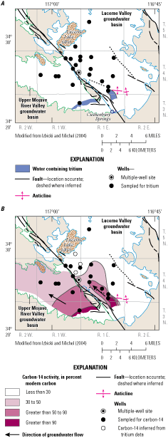
Approximate area of groundwater containing A, tritium; and B, carbon-14 activities, for 1992–2000, Lucerne Valley, California (modified from Izbicki and Michel, 2004; U.S. Geological Survey, 2021137).
Recharge from present-day precipitation in the Lucerne Valley groundwater basin likely is negligible, an interpretation that is supported by the absence of tritium in the groundwater in the valley and the fact that evaporation far exceeds precipitation in this arid environment. As discussed earlier, the average rainfall on the valley floor was 4.04 in. for 1919–73 (Western Regional Climate Center, 2017a), and the estimated average annual pan-evaporation rate was 111.59 in. for 1948–2005 for Mojave, California, which is also in the southwestern part of the Mojave Desert (Western Regional Climate Center, 2017c).
Natural Recharge Estimates from the Basin Characterization Model
In arid basins where surface-water data are lacking, such as the Lucerne Valley, the potential in-place recharge and potential runoff into the groundwater system can be estimated using the regional-scale California Basin Characterization Model (CA-BCM; Flint and others, 2013). The CA-BCM uses a monthly regional water-balance model to simulate hydrologic responses to climate and renders estimates of basin recharge and runoff. This model has been used in other desert basins to estimate underflow from adjacent mountains and basins and potential runoff in stream channels to downgradient groundwater basins where surface-water data are sparse or nonexistent (Rewis and others, 2006; Flint and others, 2012; Flint and others, 2013; Faunt and others, 2015). Using a suite of hydrologic components that included, but were not limited to, streamflow data from similar nearby basins, snowpack and the timing of snowmelt, temperature, types of vegetation, and precipitation in the San Bernardino Mountains, the CA-BCM simulated average annual potential recharge for 1981–2010 ranging from 0 in. on the valley floor to a maximum of about 16 in. on the north side of the San Bernardino Mountains (fig. 7A). The potential annual recharge estimated for 2000–13 was lower, and the CA-BCM simulated essentially no recharge to the valley floor and less recharge in the surrounding mountains areas overall (fig. 7B). However, the CA-BCM model domain included the watersheds that drain into the Lucerne Valley and the adjacent, but separate, Upper Mojave River Valley groundwater basin, west of the Helendale Fault (fig. 7). Therefore, the estimated potential recharge to the Lucerne Valley groundwater basin and study area (active model area for the Lucerne Valley Hydrologic Model) was calculated only from the CA-BCM cells east of the Helendale Fault. Applying the CA-BCM to this area, potential recharge to the study area for 1942–2016 (the period discussed in the “Lucerne Valley Hydrologic Model” section) was estimated to range from about 2 to 1,890 acre-ft/yr, with an average of about 635 acre-ft/yr for the study area (area of the active Lucerne Valley Hydrologic Model grid). For the same period, the potential annual recharge to the area covered by the entire Lucerne Valley groundwater basin was estimated to range from about 325 to 2,340 acre-ft, with an average of about 940 acre-ft (fig. 8), and an estimated cumulative total of about 70,600 acre-ft for 1942–2016.
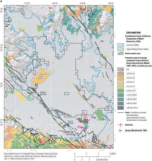

Spatially distributed estimated potential annual recharge to the Lucerne Valley and surrounding areas, California, for A, 1981–2010, and B, 2000–13, from the California Basin Characteristic Model (Flint and others, 2013). Abbreviation: >, greater than.
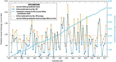
Estimated potential annual recharge and cumulative recharge to the study area and the Lucerne Valley groundwater basin, California, for 1942–2016, from the California Basin Characteristic Model (Flint and others, 2013).
Although the CA-BCM is a useful tool for estimating recharge in areas lacking surface-water data, the potential recharge simulated by the model is not necessarily equivalent to actual recharge and can be affected by many physical factors. Because water that infiltrates past the root zone does not always reach the groundwater table (Rewis and others, 2006; Flint and others, 2012), the potential differences between estimated net infiltration and actual groundwater recharge tend to increase with increases in the unsaturated-zone thickness, travel time of infiltration through the unsaturated zone, climate variability, and geologic heterogeneity in the unsaturated zone. In mountainous areas, where the unsaturated zone is likely to be more geologically heterogeneous, the potential for localized perching and lateral groundwater flow in the shallow subsurface increases. Lateral groundwater flow in the shallow subsurface (underflow) can divert a portion of net infiltration to downgradient springs or to subsurface locations within the zone of ET. Underflow is most likely in steep mountain watersheds underlain by low-permeability bedrock, where water from the higher elevation areas of the watersheds can drain into basins at lower elevations, such as to the Lucerne Valley. The net effect of underflow on a basinwide scale is a decrease in recharge balanced by an increase in ET and streamflow. Flint and others (2012) showed this effect in a study that was done near the City of Big Bear Lake (in the high elevations of the San Bernardino Mountains; fig. 1) by comparing results from an infiltration model that was modified to simulate lateral flow in the shallow groundwater system to those from the CA-BCM. In the Flint and others (2012) study, it was estimated that approximately 35 percent of the potential recharge resulted in groundwater recharge. Likewise, Rewis and others (2006) reported that mountain-front recharge estimated using an infiltration model without lateral underflow needed to be reduced to about 43 percent of the upstream recharge. Although the percentage of recharge that becomes underflow to the Lucerne Valley is unknown, the percentage of potential recharge to the groundwater system from contributing watersheds is probably even lower than percentages estimated for these studies because of the steep mountain drainage basins underlain by low-permeability rock in an arid environment (Rewis and others, 2006; Flint and others, 2012).
The CA-BCM simulated recharge on the north side of the basin (fig. 7), which contradicts the results of the geochemical studies and results presented by Izbicki (2004) and Izbicki and Michel (2004), are summarized earlier in this report section. Removing the estimates from the northern part of the basin slightly lowers the simulated potential annual recharge. Thus, the potential annual recharge estimates presented here were considered as initial values and were adjusted during the calibration process for the groundwater-flow model that was done as part of this study (see the “Lucerne Valley Hydrologic Model” section).
Anthropogenic Recharge
After the Lucerne Valley was developed in the 20th century, anthropogenic sources of artificial recharge were introduced, such as the infiltration of effluent from domestic septic systems, treated wastewater effluent, and irrigation-return water, which is infiltrated water applied to agricultural fields that is not used by plants or lost through evaporation and reaches the water table. The potential for the delivery of imported water from the California State Water Project (California Department of Water Resources, 2022) through a pipeline to spreading basins proposed south of State Route 247 near well 4N/1E-17L1 (fig. 4) was evaluated by Schaefer (1979) in the mid-1970s to alleviate groundwater-level declines, and although a pipeline was built in 1994 to convey California State Water Project water to groundwater basins to the east (not shown; Mojave Water Agency, 2022), there were no facilities or recharge operations in the Lucerne Valley at the time of this study.
The town of Lucerne Valley (fig. 2) and surrounding basin is an unincorporated rural area (U.S. Census Bureau, 2017) and therefore relies on private septic disposal systems to dispose of wastewater. Potential recharge from this water use is difficult to quantify but is assumed to be negligible. A rough estimate of the potential recharge from private domestic septic systems can be made based on the population and an assumed volume of effluent discharged to septic systems. Umari and others (1995) used an average septic-tank effluent of 70 gallons per person per day to estimate the quantity of septic wastewater that mixed with the underlying groundwater in Victorville, a desert community with similar hydrogeology located about 30 mi to the west. Using the 1928 and 2010 population estimates for the Lucerne Valley of 250 and 5,810 residents, respectively (described earlier in the “Land and Groundwater Use” section), the amount of potential recharge from septic effluent ranged from about 20 to 455 acre-ft/yr during those years. Indoor water-use rates from a minimal-producer study for 2007 and 2014 (Mojave Water Agency, 2017) yielded estimates of 0.204 and 0.178 acre-ft/yr, respectively. Mills (2009) estimated a 50-percent loss rate of septic-return flow caused by evaporation and transpiration in the Borrego Valley (not shown); considering these assumptions, the infiltration from septic systems in the Lucerne Valley could range from 0.089 to 0.102 acre-ft/yr per parcel. The actual average amount of this type of anthropogenic recharge could be less after accounting for a lower population before 1928, losses from evaporation of near-surface septic systems, and the travel time necessary for the effluent to migrate through the thick unsaturated zone to the groundwater table.
Treated wastewater effluent from the City of Big Bear Lake, which is in the high elevations of the San Bernardino Mountains south of the study area (fig. 1), has been piped down the mountain and discharged to the Lucerne Valley since 1980. This anthropogenic source of recharge from the Big Bear Area Regional Wastewater Agency (BBARWA) has been released to infiltration ponds and also has been used to irrigate alfalfa fields in the southeastern part of the valley (figs. 2I–K). Between 1980 and 2016, the amount of treated effluent transferred to the Lucerne Valley annually ranged from about 1,470 to 4,000 acre-ft (N. Flores, Big Bear Area Regional Wastewater Agency, written commun., 2017; fig. 9). Although some loss through evaporation and consumptive use by alfalfa occurs, the total volume of water from this source of artificial recharge is about 3.5 times greater than the natural recharge estimated by previous studies (California Department of Water Resources, 1967; Schaefer, 1979) or by the CA-BCM (Flint and others, 2013).
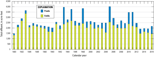
Total effluent from the Big Bear Area Regional Wastewater Agency, 1980–2016, Lucerne Valley, California.
Irrigation return is groundwater that has been pumped to irrigate agricultural fields but is not consumed by the crops and subsequently returns to the groundwater system. The amount of water that is lost through plant use and evaporation and does not return to the groundwater table is considered consumptive use. The consumptive use, or net pumpage, associated with each land-use type was simulated in this study based on the percentage of irrigated land, reference ET, and crop coefficients. The methods used to estimate net pumpage, and the magnitudes of these estimates, are described in more detail in the “Lucerne Valley Hydrologic Model” section of this report. Estimates of recharge based on crop type, crop efficiencies, and irrigation requirements for 2005–16 from the calibrated groundwater-flow model are discussed later in the “Landscape-Water Use and the Farm Management Process” section.
Mechanisms of Discharge
Groundwater discharge from the Lucerne Valley has taken place through natural mechanisms mostly as evaporation, ET, and possibly a small amount of flow to adjacent groundwater basins. However, the amount of groundwater removed from the basin by pumpage is much larger, and the consequent lowering of the water table has greatly reduced most sources of natural discharge.
Natural Discharge
Before groundwater development in the valley, natural discharge from the basin occurred through a few springs along the Helendale Fault (fig. 7), as evaporation at the playa surface, and by ET from the sparse desert vegetation. Evaporation likely occurred from several springs that existed along the Helendale Fault and its splays; Mendenhall (1909) observed that many areas had small and constant flow when he visited Lucerne Valley in about 1905. Because of the high predevelopment-groundwater table and areas with artesian conditions, farming was established early in the valley. The extraction of groundwater by pumping since the turn of the 20th century has lowered the elevation of the groundwater table and has caused most, if not all, of the artesian wells and springs to go dry, eliminating this type of discharge. Current surface-water evaporation is limited primarily to the moisture in the clay-rich soils of the dry lakebed and any water that ponds on the playa surface after sporadic storm runoff.
Except for stands of cottonwood (Populus spp.) trees at the springs south of Lucerne Lake and at the southern part of the Lucerne Valley that were reported by Mendenhall (1909), there are few documented observations of phreatophytes in the valley by previous researchers; it is likely that early development of the valley and groundwater extraction lowered the groundwater table beyond the root zone of phreatophytes in most places by the beginning of the 20th century. In 1917, Thompson (1929) observed some flowing wells and springs next to areas with saltgrass along the Helendale Fault, but noted that saltgrass (Distichlis spp.), which requires the groundwater table to be within a few feet of land surface, and phreatophytes were generally absent in the southern part of the valley. Later, the CA-DWR reported that about 12.5 acre-ft/yr of water was used by phreatophytes during 1936–40 (California Department of Water Resources, 1967). Schaefer (1979) reported the presence of pickleweed (Salicornia spp.), salt-loving plants that commonly grow near shores and playas along the edge of Lucerne Lake. Plants growing near the dry lakebed are tolerant of soils with high salinity and have small root systems that survive on moisture stored in the playa clays, in areas where competing plants are absent (Ellison, 1987).
The CA-DWR estimated that the average annual subsurface groundwater outflow from the Lucerne Valley to the Upper Mojave River Valley groundwater basin during 1936–61 was 100 acre-ft/yr (California Department of Water Resources, 1967). However, the Helendale Fault separates these two adjacent groundwater basins, and its effectiveness as a groundwater-flow barrier is well documented (Riley, 1956; Schaefer, 1979; Stamos and others, 2001; Teague and others, 2016). Thompson (1929) noted that the groundwater table was about 50–75 ft higher on the west side of the fault than on the east side; more recent groundwater-level data and flow patterns depicted by Schaefer (1979), Stamos and Predmore (1992), Trayler and Koczot (1995), and Dick and Kjos (2017), and also noted in the “Groundwater Levels, Flow, and Movement” section of this report, showed large differences in groundwater levels on either side of the Helendale Fault. Carbon-14 activities and tritium values indicate that groundwater on the west side of the fault flows toward the Upper Mojave River Valley groundwater basin, away from the Lucerne Valley groundwater basin (Izbicki and Michel, 2004; fig. 6). Some groundwater could be exchanged across the fault near the base of the mountain, where historical differences in the groundwater table have been smaller (Thompson, 1929), but the steep drop of the groundwater table along most of the fault trace indicates that any groundwater crossing the fault would flow from the Upper Mojave River Valley groundwater basin eastward to the Lucerne Valley groundwater basin.
Pumpage
As mentioned previously, groundwater development and the use of wells in the valley probably began in the late 1880s because Mendenhall (1909) noted that several wells had been drilled and flowing wells were reported at established ranches by 1905. Groundwater use in the basin was primarily for irrigated agriculture, with some cattle and poultry farming and a small amount for homesteads. Schaefer (1979) estimated that pumpage from agricultural sources during 1950–76 ranged from 4,000 to 13,000 acre-ft. The estimated irrigated area reported in Schaefer (1979) was about 3,500 acres in 1954 and 2,500 acres in 1976, which is a considerably larger area than what was determined from the aerial imagery discussed in the “Land and Groundwater Use” section. Pumpage for industrial use did not begin until 1960 (fig. 10). Estimates of total pumpage for 1942–2016 ranged from about 3,010 acre-ft in 1942 to about 18,300 acre-ft in 1984.
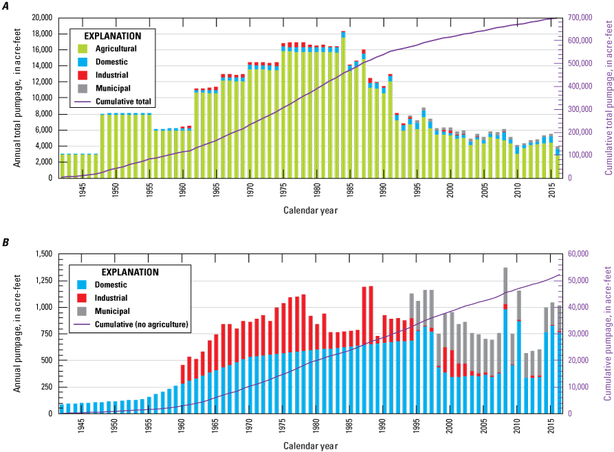
Annual and cumulative pumpage for 1942–2016. A, all water uses; and B, water uses not including agriculture, Lucerne Valley, California (Mojave Water Agency, 2017).
Agricultural pumpage estimates were estimated from aerial land-use photographs between 1942 and 1993 (figs. 2A–H) and estimates reported by the Mojave Water Agency for 1994–2016 (figs. 2I–K; Mojave Water Agency, 2017). The annual agricultural pumpage from 1942 to 1993 was estimated by multiplying the amount of irrigated acreage and the consumptive-use requirements for alfalfa. Consumptive use for agriculture is the unit amount of water consumed in a unit area by transpiration, building of plant tissue, and evaporation from adjacent soil. Estimates of consumptive use for alfalfa, the main crop in the Lucerne Valley since the late 19th century, vary from about 6.0 feet per year (ft/yr) in Arizona (Erie and others, 1965) to as high as 6.50 ft/yr in fields along the Colorado River between California and Arizona (Owen-Joyce and Raymond, 1996). Stamos and others (2001) assumed a consumptive-use rate of 7.0 ft/yr to estimate total pumpage for alfalfa. For this study, an assumed consumptive-use rate of 6.0 ft/yr was used to estimate total pumpage. Estimates of agricultural pumpage ranged from about 3,000 acre-ft in the early 1940s to a high of about 17,600 acre-ft in 1984 (fig. 10A). Within 10 years, total pumpage had declined by about two thirds (to about 6,800 acre-ft in 1993). This decrease in agricultural pumpage (since the mid-1980s) likely resulted from the increase in costs associated with pumping groundwater from greater depths as the groundwater table declined. Agricultural pumping continually decreased after 1993, and by 2016, the estimated annual pumpage was about 2,900 acre-ft, the lowest volume estimated during the study period.
Pumpage for domestic groundwater use was estimated by previous researchers; for this study, pumpage was estimated by using historical population estimates and results from verified pumpage studies in later years. Schaefer (1979) estimated that domestic pumpage was about 200 acre-ft in 1954 and about 1,200 acre-ft in 1976, but other domestic-use pumpage estimates were not available; therefore, domestic pumpage between 1942 and 1993 was estimated based on population estimates (Schaefer, 1979; San Bernardino County, 2007). Linear interpolation was used to estimate the population between years when population data were available. Based on values from verified production or pumpage from 1994 (Mojave Water Agency, 2017), average domestic water use was assumed to be 169 gallons per person per day; accordingly, domestic pumpage was estimated to have ranged from about 90 acre-ft in 1942 to about 670 acre-ft in 1993 (fig. 10B). From 1994 through 2016, verified pumpage was used to estimate most of the domestic groundwater use in Lucerne Valley (Mojave Water Agency, 2017). As mentioned in the “Land and Groundwater Use” section, a minimal producer study was done by the Mojave Water Agency Watermaster to estimate any additional unverified, rural, residential water usage in the Lucerne Valley for 2007 and 2014 (Mojave Water Agency, 2017); this study estimated that the average domestic water use was 0.204 and 0.178 acre-ft per year per parcel, respectively. These additional estimates for unverified rural water use were included in the estimates of domestic pumpage from 2007 through 2016 (fig. 10).
Groundwater withdrawal for industrial use mainly has been for a cement plant located at the base of the San Bernardino Mountains. Industrial pumpage estimates between 1960 and 2017 ranged from about 1 acre-ft in 2011 to about 545 acre-ft in the late 1980s (fig. 10B; Mojave Water Agency, 2017).
The total cumulative amount of groundwater removed from the basin by pumping between 1942 and 2016 was estimated to be about 700,000 acre-ft (fig. 10A), which was about 10 times greater than the cumulative amount of recharge to the entire Lucerne Valley groundwater basin (of about 70,600 acre-ft), as estimated by the CA-BCM (Flint and others, 2013; fig. 8). This difference in volume between inflow and outflow in the basin, about 630,000 acre-ft, represents the approximate cumulative total amount of groundwater that has been removed from aquifer storage by pumpage between 1942 and 2016. As a comparison, this volume approaches the capacity of Lake Havasu on the Lower Colorado River, which can store about 646,000 acre-ft (U.S. Bureau of Reclamation, 2018).
Assessment of Groundwater in the Lucerne Valley
Lucerne Valley’s reliance on groundwater, in conjunction with the basin’s history of rural development and long-established irrigation practices, have caused substantial changes to the depth and direction of groundwater flow since about the 1890s. When the area was first visited by W.C. Mendenhall in about 1905, there were several springs and many areas with artesian conditions that had flowing wells (fig. 11; Mendenhall, 1909). By 1917, D.G. Thompson (1929) observed flowing wells only in a small area about 6 mi northwest of Box S Springs (fig. 7). Since then, pumping has lowered the groundwater table so that there are no longer any artesian wells. A small seep was observed at Rabbit Springs in 2018 (T. Winkel, Mojave Water Agency, written commun., 2018); however, most of the springs have gone dry. In addition to the hydrologic effects of lowering the groundwater table, the increasing depths that wells must reach to access groundwater has resulted in an increase in drilling and pumping costs and reduced well efficiency.
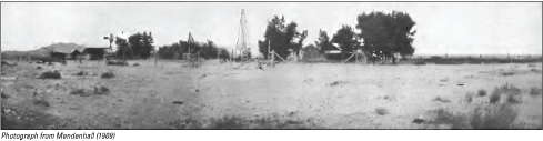
Photograph of an artesian well at Box S Ranch (about 6 miles northwest of Box S Springs). Reproduced from Mendenhall (1909), circa 1905, Lucerne Valley, California.
Groundwater Levels, Flow, and Movement
The installation of production wells for irrigation began sometime in the 1890s. The earliest comprehensive assessment of the region’s hydrology was conducted decades later in 1916–17 by Thompson (1929), who reported groundwater-level measurements for 43 wells and observed many places where the groundwater table was within a few feet of land surface. Thompson’s data indicated that the direction of groundwater flow in Lucerne Valley was from the outer margins of the basin toward the discharge area of the dry playa, Lucerne Lake, which is the topographically lowest part of the valley. In 1916–17, groundwater-level elevations (hydraulic heads) ranged from higher than 2,900 ft above NAVD 88 in the southern areas to less than 2,820 ft above NAVD 88 near Lucerne Lake (fig. 12A), where the depth to groundwater was between 20 and 30 ft bls. Schaefer (1979) constructed a groundwater-level contour map for the valley using Thompson’s 1916–17 groundwater-level data (contours from map reproduced herein with modification on fig. 12A). Thompson’s groundwater-level data, reviewed for this study, showed some inconsistencies between the groundwater-level data reported by Thompson and the contours drawn by Schaefer; these inconsistencies may be attributable to the effects of local pumping and inexact well locations.
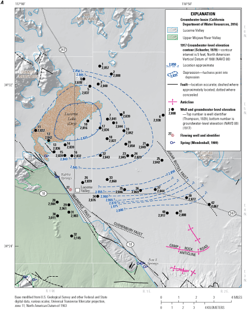
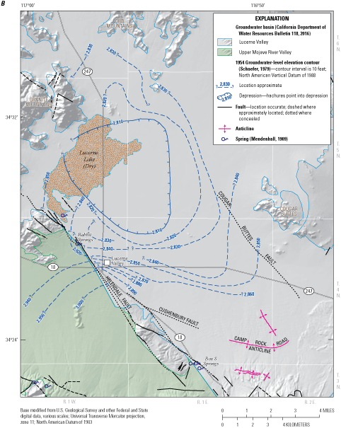
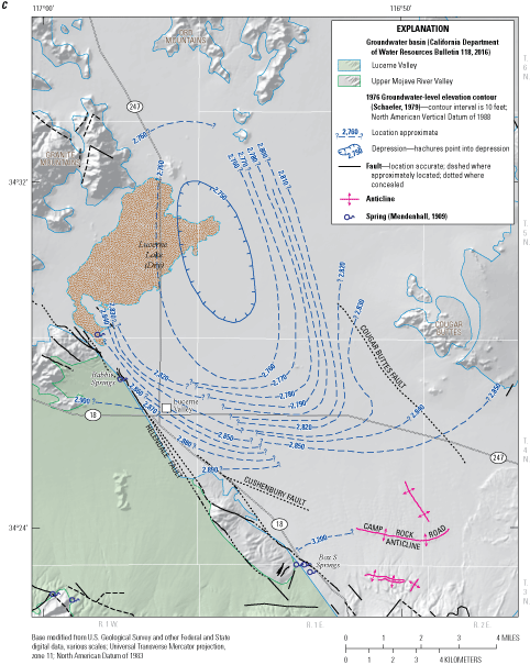
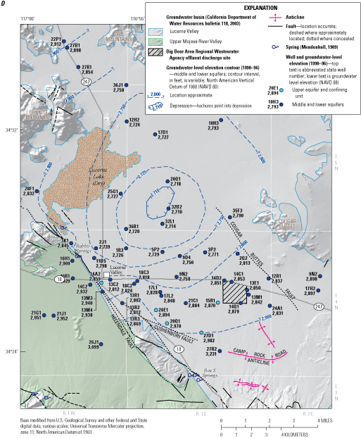
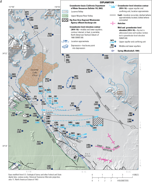
A, 1917 groundwater-level data from Thompson (1929) and modified groundwater-level elevation contours from Schaefer (1979); B, 1954 groundwater-level elevation contours using data from Riley (1956); C, 1976 groundwater-level elevation contours from Schaefer (1979); D, 1990–96 groundwater-level data (U.S. Geological Survey, 2021) and contours; and E, 2014–16 groundwater-level data and contours, in the Lucerne Valley, California (North American Vertical Datum of 1988, NAVD 88).
In 1954, Riley (1956) inventoried and measured about 460 wells in the Lucerne Valley to provide records for as many wells as possible in anticipation of subsequent groundwater investigations and the valley’s development. Groundwater levels in the inventoried wells ranged from flowing to more than 380 ft bls, with the greatest depths to groundwater in the southern part of the basin. During his field reconnaissance, Riley observed 12 wells near the Helendale Fault that were either flowing or had hydraulic heads above land surface.
Using Riley’s data from 1956, Schaefer (1979) constructed another groundwater-level contour map for 1954 (contours from map reproduced herein with modification on fig. 12B). A comparison of the 1917 and 1954 groundwater-level contour maps (figs. 12A, 12B) indicates that the continued and increased pumping since 1917 had lowered the groundwater table in most parts of the valley, particularly in the area southeast of Lucerne Lake playa where most of the groundwater pumping continued to occur. In the area southeast of the playa, Schaefer’s maps show that the groundwater table had declined by about 30 ft. The maps also indicate that the predominant direction of regional groundwater flow—from the basin margins to the playa—had not changed since 1917, but that the area with the lowest groundwater-level elevations had expanded and migrated south toward the pumping center.
During an assessment for potential artificial recharge in the Lucerne Valley to offset groundwater-level declines, Schaefer (1979) collected groundwater-level data in 1976 and constructed a third groundwater-level contour map (contours from maps reproduced herein with modification on figs. 12C). On a basinwide scale, the groundwater-level data and contours from 1976 show the continued steepening of the horizontal hydraulic gradient and the enlargement and southward migration of the pumping depression as pumping continued to remove large quantities of groundwater from aquifer storage.
Riley (1956) brought to light the complexity of the hydrogeology of the basin by recognizing the presence of separate aquifers in the area about 2 mi south of the Lucerne Lake, where he noted the largest withdrawals had occurred and where pumping was “heavy.” Riley documented higher groundwater-level elevations in what he called the “shallow body” or upper aquifer than those measured in the “deeper body,” or middle and lower aquifers. Although Schaefer (1979) noted “strong evidence of a two-aquifer system consisting of a deep and a shallow aquifer separated by a confining layer,” he did not distinguish the groundwater-level measurements taken from the upper, middle, or lower aquifers, so the contours constructed by Schaefer (1979; figs. 12A, 12B, 12C) in the southern part of the basin represent a composite of hydraulic heads from the three water-bearing units. However, because of the poor water quality of the shallow aquifer (Schaefer, 1979), most wells were completed in the middle and lower aquifers; therefore, in this study, we assumed that the contours from Schaefer represented the middle and lower aquifers in most parts of the Lucerne Valley.
When constructing the maps for 1917, 1964, and 1976, Schaefer considered the “Lucerne Lake Fault,” which was first proposed by Riley (1956), but this fault is not supported by the geologic findings from this study (see the “Lucerne Lake Fault” and “Hydrogeologic Units and Framework” sections). As discussed earlier, Schaefer’s groundwater-level contour maps for 1917, 1954, and 1976 (figs. 12A, 12B, 12C) represent a mixture of data from the upper, middle, and lower aquifers that likely is the cause for abrupt differences in groundwater elevations measured in adjacent wells. During earlier investigations, well-depth information was available for less than one-half of the wells measured, and well-construction information, such as perforated interval, was sparsely available for existing wells; consequently, groundwater-level data were sometimes compared between wells of varying depths or reported from wells perforated in multiple water-bearing units.
Groundwater-level data were collected in the Lucerne Valley as part of 12 previous regional studies that included nearby and adjacent groundwater basins in the western Mojave Desert on the Mojave Groundwater Resources website (https://ca.water.usgs.gov/mojave/; U.S. Geological Survey, variously dated). In those previous regional studies, groundwater-level data were collected to construct 13 regional groundwater-level contour maps, biennially, for calendar years 1992–2016. The Mojave Groundwater Resources website can be used to view these historical data and contour maps; it also describes the methods used to collect the data used for this study and how the contours were drawn (U.S. Geological Survey, variously dated).
For this study, groundwater-level data for 1990–96 and 2014–16 were used to construct groundwater-level contour maps because of the insufficient amount of annual data for a single year during those periods (figs. 12D, 12E). These data and the associated contour maps indicate groundwater-level declines in the middle and lower aquifers were largest during 1990–96, when groundwater levels were more than 100 ft lower than in 1917 (figs. 12A, 12D). Where available, the data for 1990–96 and the associated contour map also indicated that groundwater levels from the upper aquifer and confining unit were at least 45 ft, and in places greater than 100 ft, higher than those in the deeper aquifers. By 2014–16, the depth to groundwater in the area south of the playa, where groundwater-level elevations were lowest in 1917, increased from between 20 and 30 ft bls to as much as 100 ft bls, and the cone of depression caused by pumping had migrated more than 3.5 mi to the southeast since development in the valley began (figs. 12A, 12E). The difference in hydraulic head between the upper and lower aquifers ranged from about 20 to 25 ft near the playa to about 140 ft in the southern part of the basin.
Long-Term Trends in Groundwater Levels
Long-term groundwater-level data from individual wells with multiple measurements provide insight into how stresses on the aquifer system affect groundwater levels over time. The historical data available in the Lucerne Valley are invaluable for documenting the long-term groundwater-level elevation trends throughout the basin. To show trends during the longest possible period, groundwater-level data were combined from wells that are near and similarly constructed so that the effects of subsurface geologic structures on groundwater movement and the consequences of long-term pumping could be evaluated. Using groundwater-level data from 1905 to 2016 (figs. 13, 14), 20 long-term hydrographs were constructed for wells located throughout the basin. Most of the hydrographs show a long-term groundwater-level decline, particularly for wells in the center of the basin where pumpage historically has been the greatest. In this area, the hydrographs show groundwater levels have declined more than 100 ft between the mid-1940s and the mid-1990s. Wells located farther from the pumping center and along the margins of the basin showed less decline during the same period. Since the early 1990s, some wells in the southeastern part of the basin had very slight declines in groundwater levels (for example, wells 4N/1E-9D4 and 4N/1E-15R1 [hydrographs 14 and 19, respectively, on figs. 13, 14]). The slight increase in groundwater levels in well 4N/1E-2Q2 (hydrograph 10 on figs. 13, 14) may be attributable to the effects of the BBARWA-treated sewage effluent that is discharged to the south; however, no data are available to evaluate the migration of this source of artificial recharge and its potential effect on groundwater levels.
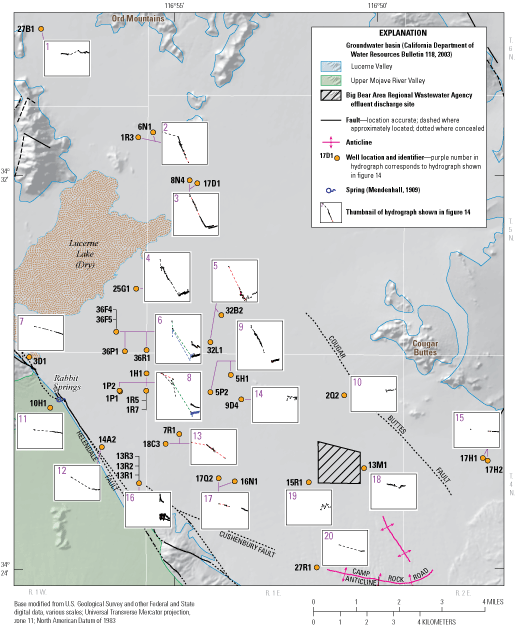
Location of wells with groundwater-level hydrographs shown on figure 14, Lucerne Valley, California (U.S Geological Survey, 2021).
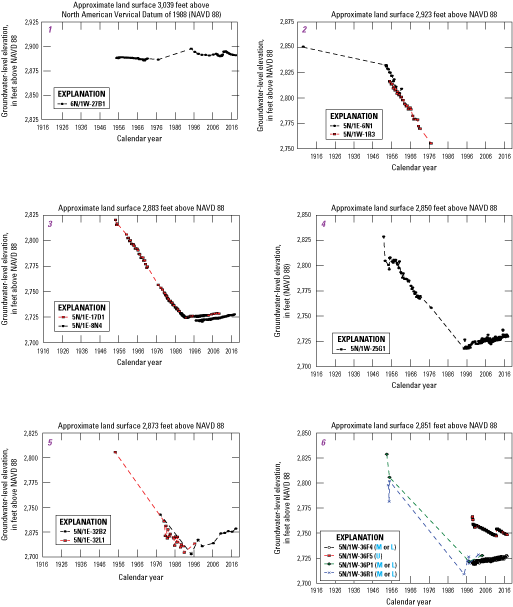
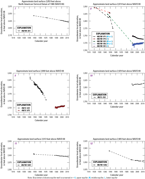
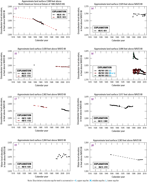
Measured groundwater levels in wells in the Lucerne Valley, California, 1916–2016. (Location of wells shown on fig. 13).
Groundwater-level declines were largest in the early-to-mid 1990s, following decades of pumping rates that often exceeded 10,000 acre-ft/yr (figs. 10, 14). Since the early 1950s, groundwater-level declines had exceeded 100 ft in the middle of the basin. After the early-to-mid 1990s, the hydrographs show an upward trend in groundwater levels; these trends followed a period when pumpage sharply decreased from previous years. Pumping rates continued to decline since the mid-1990s and were comparable to those in the early 1940s and late 1950s. The lower groundwater withdrawal rates decreased the stress on the aquifer system; consequently, groundwater levels rose in the middle of the basin and groundwater levels at the margins of the basin continued to decline as the hydraulic gradient in the basin approaches a new equilibrium.
Groundwater-level data from three separate periods (1911–35, 1990–96, and 2014–16) were used to evaluate and illustrate groundwater-table decreases throughout the basin through time (fig. 15). Data were evaluated and selected to ensure groundwater-level elevations were representative of the groundwater table for these three periods. The profiles of the groundwater-level elevations shown on figure 15 were interpreted using data from wells along or near the section lines shown on figure 4. Some data could reflect composite groundwater-level elevations because wells often are completed in multiple aquifers; however, any difference in hydraulic head between the aquifers would be dwarfed by the greatly exaggerated vertical scale necessary to show the data (fig. 15).
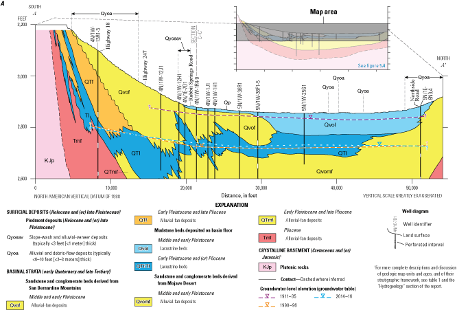
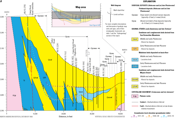
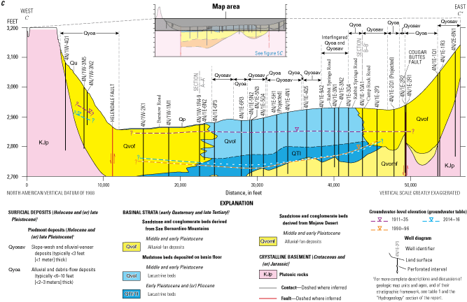
Generalized geologic sections A, south to north (A–A’); B, south to north (B–B’); and C, west to east (C–C’), showing the approximate groundwater table from 1911–35, 1990–96, and 2014–16, Lucerne Valley, California. (California Department of Water Resources, 2020; U.S. Geological Survey, 2021; location of wells and sections shown on fig. 4). See table 1 for more complete descriptions and discussion of geologic map units, ages, and stratigraphic framework. Abbreviation: <, less than.
As indicated by the data shown on figure 15, the elevation of the groundwater table from 1911 to 1935 was higher than in later years. During the early-to-mid 1990s, the groundwater levels were at historical lows; the largest declines occurred in the middle of the basin where most of the pumping was concentrated (figs. 15A, 15C). After pumping rates were reduced, groundwater levels rose slightly in the middle and lower aquifers by 2014–16, mostly in the middle of the valley (figs. 14, 15C). The decrease in the amount of pumping after the early-to-mid 1990s (fig. 10) lessened the hydraulic stress on the middle and lower aquifers and enabled hydraulic heads to recover slightly in the middle of the basin as groundwater from storage flowed from the basin margins toward the pumping depression. This migration of groundwater caused groundwater-level elevations in the center of the basin to increase since 1990–96 and resulted in the continued decline in groundwater-level elevations at the margins. As much as 25 ft of groundwater-level decline occurred near the margins of the basin since 1990–96 as the groundwater table throughout the basin gradually flattened (figs. 15A, 15C). The decline of groundwater levels along the margins of the basin (shown on figs. 13–15) is expected to continue as groundwater from aquifer storage migrates toward the pumping depression that has been created in the middle of the basin.
Several hydrographs on figure 14 show how the vertical distribution of pumpage had affected the hydraulic head in the individual aquifers and reveal the extent and hydrologic influence of the confining unit. In early field studies, groundwater-level differences between adjacent wells completed at different depths were difficult to distinguish because the hydraulic head in the aquifers probably were similar and most wells were completed in more than one aquifer. However, the long-term extraction of groundwater, mostly from the middle and lower aquifers, lowered their hydraulic heads below those that were measured in the upper aquifer. These differences in hydraulic head became more pronounced over time because the lacustrine deposits that are present below the upper aquifer (fig. 15) impeded the downward movement of water. As discussed earlier, Riley (1956) noted differences in hydraulic heads between adjacent wells south of the playa that were completed at different depths; these differences were evident in adjacent wells completed in the different aquifers and have become more pronounced over time. For example, the hydraulic head measured in 1954 in well 4N/1W-1P2 (59 ft deep and completed in the upper aquifer) was about 13 ft higher than in well 4N/1W-1P1 (450 ft deep and completed in the deeper aquifers; hydrograph 8 on figs. 13, 14). By the mid-1990s, differences in the hydraulic heads in that same area were more than 30 ft between the upper aquifer (well 4N/1W-1R7) and the middle aquifer (well 4N/1W-1R5; hydrograph 8 on fig. 13).
Land Subsidence
Land subsidence can occur in aquifer systems that contain, in part, fine-grained sediments and that have undergone extensive groundwater development and dewatering. Land subsidence associated with groundwater-level declines has been documented as a large-scale problem with costly financial impacts in the Central Valley of California (Poland and others, 1975; Faunt, 2009; Sneed and others, 2013) and has been recognized as a potential problem in several parts of the southwestern Mojave Desert, including the Lucerne Valley (Sneed and others, 2003; Stamos and others, 2007; Solt and Sneed, 2014; Brandt and Sneed, 2017; U.S. Geological Survey, variously dated).
When groundwater is removed by pumping in quantities that result in large groundwater-level declines, the pore-fluid pressure is reduced in the intergranular pore spaces between grains and particles of the sediments that compose the aquifer-system deposits. This decrease in fluid pressure increases the effective stress on the aquifer materials, which can cause the rearrangement of sediment grains and deformation, particularly in aquifer systems that contain extensive clays and fine-grained deposits. An aquifer system comprised primarily of fine-grained sediments, such as silt and clay, is much more compressible than one that consists primarily of coarse-grained sediments, such as sand and gravel (Solt and Sneed, 2014). The rearrangement of the fine-grained material causes the sediments to compact and consolidate, which results in deformation. The vertical component of this deformation often results in the irreversible compaction of the aquifer system and land subsidence and associated reduction in the storage and transmissive properties of the aquifer system.
Global Positioning System (GPS) surveys and interferometric synthetic aperture radar (InSAR) methods rely on satellite-based methods to record ground-surface elevation, which are used to calculate changes in ground-surface elevation through time and have been used to examine land subsidence in many areas. An in-depth discussion of these methods is provided in Massonnet and others (1997), Sneed and others (2003), and Solt and Sneed (2014). Maps have been produced using these methods and can be used to identify areas of subsidence and potentially vulnerable infrastructure, such as roads, pipelines, and canals. Because land subsidence usually occurs at variable rates across the landscape and over time, the resulting deformation and fissures (or cracks) have the potential to alter surface-drainage routes and damage infrastructure, and associated repair costs for cities and local municipalities can be substantial. Galloway and others (1999) provided a review and selected case studies of land subsidence caused by aquifer-system compaction in the United States.
Measurements from GPS stations, historical data from leveling surveys of monuments in a geodetic network, and InSAR data have been used in previous studies to determine the location, extent, and magnitude of vertical land-surface changes in Lucerne Valley (Sneed and others, 2003; Solt and Sneed, 2014; Brandt and Sneed, 2017). Land subsidence in the Lucerne Valley has been examined in previous studies because of the large groundwater-level declines and the presence of areally extensive clays and fine-grained lacustrine deposits, primarily in the confining unit (fig. 15). In addition to InSAR and GPS data from an existing monitoring network of stations (fig. 16), leveling data have been available for the area since as early as 1944 (Sneed and others, 2003).
In the Lucerne Valley, Sneed and others (2003) reported that about 2 ft±5 ft of subsidence could have occurred at GPS stations GOBR, HOLM, and RAIN south and southeast of Lucerne Lake (fig. 16) between 1975 and 1998, at GPS station GOBR between 1975 and 1998, and at GPS stations HOLM and RAIN between 1969 and 1998. InSAR data indicated that between April 1992 and November 1999, an area southeast of Lucerne Lake subsided about 3.5 in. (about 89 millimeters [mm]) and that the area along the western shore of the lake subsided about 2.4 in. (about 61 mm; Sneed and others, 2003). Land subsidence also was observed surrounding the Lucerne Lake and extending almost 4 mi to the southeast (fig. 16) from periods of varying temporal duration between April 1992 and November 1999 (Sneed and others, 2003), May 1999 and December 2000, and June 2003 and September 2004. From July 2004 to November 2009, nearly 3.15 in. (about 80 mm) of land subsidence occurred south of the playa at a fairly steady rate of about 0.6 inch per year (in/yr; Solt and Sneed, 2014 [about 15.2 millimeters per year, mm/yr]). The compaction likely occurred in the upper aquifer and the confining unit and was not attributed to the middle or lower aquifers, which do not contain clay or other fine-grained sediments susceptible to compaction.
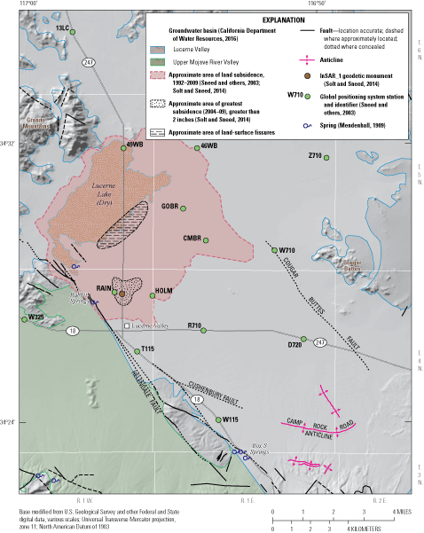
Approximate area of land subsidence for 1992–2009, the area of land subsidence greater than 2 inches for 2004–09, and area of land-surface fissures, Lucerne Valley, California.
Brandt and Sneed (2017) reported nearly 11 in. (about 279 mm) of subsidence between April 1992 and November 2009, with an average rate of about 0.6 in/yr (15 mm/yr) at InSAR_1 geodetic monument (figs. 16, 17). This average rate varied and increased from about 0.5 in/yr (13 mm/yr) during 1992–99 to about 0.7 in/yr (18 mm/yr) during 1999–2009. Some of this land subsidence is permanent and has been attributed to lowering groundwater levels that have persistently declined below historical lows (fig. 14; Brandt and Sneed, 2017) and to the compaction of thick clays and fine-grained materials in the upper aquifer and confining unit, where grains of sediment have been rearranged and pore spaces have been reduced or eliminated.
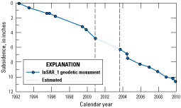
Measured subsidence from interferometric synthetic aperture radar (InSAR) data and estimated subsidence at InSAR_1 geodetic monument, April 1992–November 2009 (Brandt and Sneed, 2017), Lucerne Valley, California (location shown on fig. 16).
The highest land-subsidence rates and deformation occurred south of the playa where most of the agricultural pumpage has occurred and where groundwater-level declines have been greatest (figs. 12–17). Between September 2003 and November 2009, the area around InSAR_1 subsided more than 4 in. (figs. 16, 17; Brandt and Sneed, 2017). Surficial evidence of this differential land subsidence near and around Lucerne Lake is expressed by fissures that have formed on the land surface southeast of the playa as the structure of the aquifer system is stretched (figs. 16, 18A). These fissures, which often are exacerbated by erosion, have caused damage to State Route 247 in several locations where they have buckled the pavement and undercut the road (figs. 16, 18B; Brandt and Sneed, 2017).
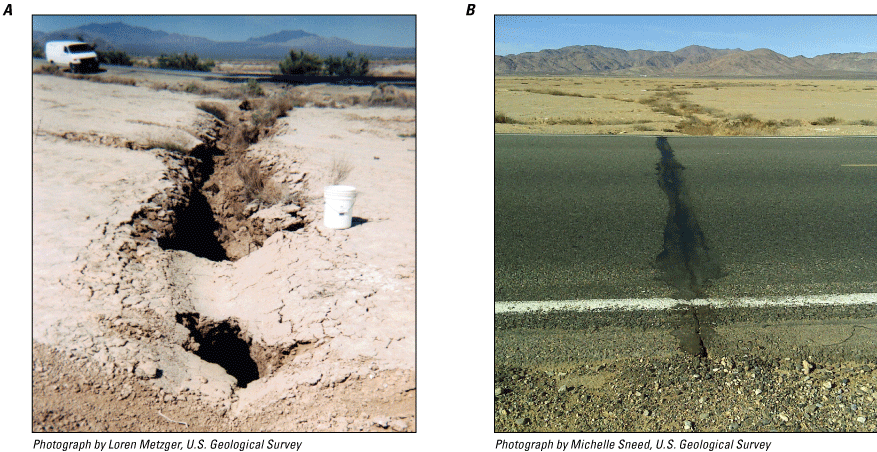
A, Fissures on the southeastern edge of Lucerne Lake (see fig. 16 for location; Brandt and Sneed, 2021), photograph with 5-gallon bucket for scale by Loren Metzger, U.S. Geological Survey, May 2001; and B, repair to damage caused by fissures across State Route 247 in the Lucerne Valley, California. Photograph by Michelle Sneed, U.S. Geological Survey, January 2018.
Groundwater-level declines and land subsidence are expected to persist in this area (Brandt and Sneed, 2017), and the rate of subsidence observed since 1999 has accelerated. Though beyond the period of this study, further analysis by Brandt and Sneed (2021) showed that about 1 in. of subsidence occurred during 2014–19, resulting in a total of about 14 in. of subsidence during 1992–2019. Extensometers, or vertical compaction recorders, currently are the only tools that can measure compaction at depth-specific intervals; they also can be used to analyze the aquifer-system’s response to groundwater-level changes in individual aquifer units. Knowing where the land subsidence is occurring, particularly at what depths and in which groundwater-bearing units, helps guide future water-resource management strategies.
Lucerne Valley Hydrologic Model
A numerical groundwater-flow model of the Lucerne Valley groundwater basin was developed to better understand the hydrologic conditions within the basin and be used by resource managers to provide insight into the effects of future stresses within the groundwater basin. The model can be used to assess groundwater availability based on predicted future scenarios that describe demands for groundwater resources, changes in natural recharge patterns, and changes in artificial recharge distribution and quantity. Resource managers can use results from future scenarios to gain insights for managing future groundwater resources and challenges. Assumptions and approximations are made in numerical models that simplify the groundwater-flow system, and these simplifications cannot capture the full complexity of a groundwater-flow system. Further discussion of model limitations is presented later in the “Model Uncertainty, Limitations, and Improvements” section.
The Lucerne Valley Hydrologic Model (LVHM; Larsen, 2022) is a three-dimensional (3D) finite-difference numerical model based on the U.S. Geological Survey three-dimensional modular finite-difference groundwater-flow model (MODFLOW-2005; Harbaugh, 2005) that was enhanced by features available using the One Water Hydrologic Model version 2 (OWHM2; Boyce and others, 2019). The OWHM2 is a refinement of the MODFLOW-2005 groundwater-flow modeling software that incorporates packages that provide more stability for model cell wetting and drying from the Newtonian formulation for MODFLOW-2005 (MODFLOW-NWT; Niswonger and others, 2011). The OWHM2 also extends functionality by adding specialized features for irrigated agriculture through the Farm Management Process (FMP; Schmid and Hanson, 2009). Model versions and packages used for the LVHM are shown in table 2 and are available in Larsen (2022).
Table 2.
Summary of model packages and processes used in the Lucerne Valley Hydrologic Model (Larsen, 2022), Lucerne Valley, California.[Global Process (GLO), Observation Process (OBS), and Farm Management Process (FMP)]
| Computer program (packages, processes, parameter estimation) |
Function | Reference |
|---|---|---|
| Groundwater Flow (GWF) Processes of MODFLOW-2005 | Setup and solve equations simulating a basic groundwater-flow model. | Harbaugh (2005), Harbaugh and others (2000), McDonald and Harbaugh (1988), Hill and others (2000) |
| Newton-Raphson Solver Package (NWT) | Solves groundwater flow-equations; requires convergence of heads and (or) flow rates. | Niswonger and others (2011) |
| Farm Management Process (FMP) | Setup and solve equations simulating use and movement of water on the landscape as irrigated agriculture, municipal landscape, and natural vegetation. | Schmid and others (2006a, b), Schmid and Hanson (2009), Hanson and others (2014)114 |
| Name File (Name) | Controls the capabilities of MODFLOW-2005 FMP during a simulation. Lists most of the files used by the GLO, OBS, and FMP. | Harbaugh (2005) |
| Output Control Option (OC) | Used in conjunction with flags in other packages to output head, drawdown, and budget information for specified time periods into separate files. | Harbaugh (2005) |
| List File (LIST) | Output file for allocation information, values used by the GWF process, and calculated results, such as head, drawdown, and the water budget. | Harbaugh (2005) |
| Basic Package (BAS6) | Defines the initial conditions and some of the boundary conditions of the model. | Harbaugh (2005) |
| Discretization Package (DIS) | Space and time information. | Harbaugh (2005) |
| Zones (ZONE) | Defines arrays of different zones. Parameters may be composed of one or many zones. | Harbaugh (2005) |
| Upstream-weighted Property Flow Package (UPW) | Calculates the hydraulic conductance between cell centers. | Niswonger and others (2011) |
| Hydrologic Flow Barriers (HFB6) | Simulates a horizontal-flow barrier by defining a hydraulic conductance between two adjacent cells in the same layer. | Hsieh and Freckleton (1993), Harbaugh and others (2000), Harbaugh (2005) |
| Subsidence and Aquifer-System Compaction Package (SUB) | Simulates the drainage, changes in groundwater storage, and compaction of aquifers and confining units that constitute an aquifer system. | Hoffmann and others (2003) |
| Drains (DRN) | Head-dependent flux boundary condition used along the vertical edge of historic discharge areas within the model to allow groundwater to flow out of the model under a regional gradient. | Harbaugh (2005) |
| Multi-node Wells (MNW2) | Simulates pumpage from wells with screens that span multiple layers. | Konikow and others (2009) |
| Well (WEL) | Simulates pumpage from wells with screens that span a single layer. | Harbaugh (2005) |
| Head Observation (HOB) | Defines the head observation and weight by layer(s), row, column, and time and generates simulated values for comparison with observed values. | Hill and others (2000), Harbaugh (2005) |
| Hydmod (HYD) | Generates simulated values for specified locations at each time-step for groundwater levels and streamflow attributes. | Hanson and Leake (1999) |
| Parameter File (PVAL) | Specifies parameter values used in other packages. | Harbaugh (2005) |
Model development involved defining the model discretization, model boundaries, hydrologic properties of the aquifer system, recharge, discharge, and anthropogenic stresses. The model was calibrated using a mixed trial-and-error approach coupled with parameter estimation using PEST++ code (https://www.usgs.gov/centers/upper-midwest-water-science-center/science/pest-parameter-estimation-code-optimized-large; Welter and others, 2015). PEST ++ is a non-linear automated parameter-estimation software that uses a widely used algorithm known as the Gauss-Marquardt-Levenberg method (Levenberg, 1944; Marquardt, 1963). Steady-state conditions, or initial conditions, were based on groundwater-level data from 1917 (Thompson, 1929), and the period of 1942–2016 was used for the transient-state model.
Discretization and Boundaries
The LVHM includes the water-bearing alluvial and lacustrine deposits of the Lucerne Valley and is bounded on the west by the Helendale Fault and the Granite Mountains, on the southeast by Cougar Buttes, on the north by the Ord Mountains (figs. 19A, 19B), and on the south by the San Bernardino Mountains (fig. 1). The rectangular finite-difference model grid was discretized into rows and columns that form cells. When overlain onto a map of the study area, each cell of the model grid represents a small part of the region. Cells that coincide with areas of the aquifer system are the “active” cells of the model grid. The values for the model input parameters assigned to each active cell represent the average value for each parameter for the groundwater system represented by that model cell. Every active cell in the model area is assigned a value for all necessary model input parameters, thereby describing the areal distribution of the aquifer properties.
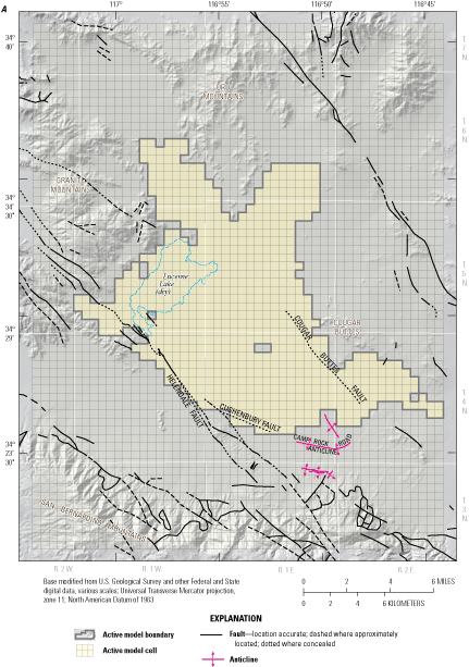
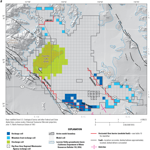
Location of A, model grid; and B, boundaries, horizontal-flow barriers (see table 10 for identifiers), and discharge and recharge cells for the Lucerne Valley Hydrologic Model (Larsen, 2022), Lucerne Valley, California.
Spatial Discretization
The finite-difference grid, designed to represent the land surface and the subsurface alluvial deposits, consists of orthogonal square cells oriented in the north-south direction that are 2,000 by 2,000 ft (92 acres per cell). The total model grid covers an area of about 92.83 square miles (59,413 acres) that was represented by 64 rows, 50 columns, and 4 layers (12,800 cells; fig. 19A). About 18 percent of the cells (561 cells in layer 1, 528 cells in layer 2, 631 cells in layer 3, and 538 cells in layer 4) were within the active area of the hydrological model; only active model cells simulate groundwater flow, and only areas with a sufficient amount of data were included in the active model domain (fig. 19B). The grid orientation and cell size were chosen to be roughly parallel to the general direction of regional groundwater flow and align with the adjacent groundwater-flow model grid for the Upper Mojave River Valley groundwater basin created by Stamos and others (2001). The coordinates for the LVHM grid are shown in table 3.
Table 3.
Coordinates of the Lucerne Valley Hydrologic Model (Larsen, 2022), Lucerne Valley, California.[NAD 83, North American Datum of 1983; UTM, Universal Transverse Mercator]
The model layers were aligned to represent the individual hydrogeologic units of the aquifer system (figs. 5, 20). The top of the hydrologic model (layer 1) represented the elevation of the land surface. Layer 1 ranged in thickness from a minimum of about 32 ft near the southern margin of Lucerne Lake to a maximum of about 320 ft adjacent to the southernmost part of the Helendale Fault. This top layer represented the shallow alluvial-fan and lacustrine deposits (units Qvof, QTf, Tmf, and TI) along the edges of the model and the lacustrine deposits (unit Qvol) near the center (fig. 5A). Layer 2 mainly represented the lacustrine deposits (units Qvol and QTI) of the confining unit and ranged in thickness from about 1 ft in the northern part of the model to a maximum of about 172 ft in the southern part (fig. 5B). Layer 3 represented the middle aquifer and ranged in thickness from about 58 ft in the northeastern part of the basin to about 380 ft in the center (figs. 5B, 5C). Layer 4 represented Mojave Desert derived alluvial fan deposits and fan-delta deposits (unit Tmf) of the lower aquifer and ranged in thickness from about 3 ft adjacent to the Cougar Buttes Fault to about 400 ft near the Helendale Fault (fig. 5C).
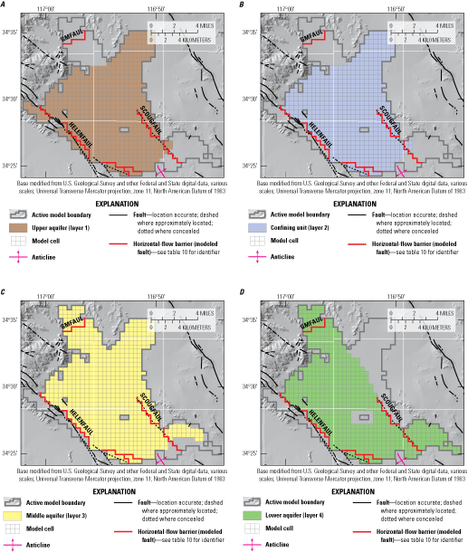
Model grid with active model cells representing the upper aquifer, confining unit, middle aquifer, and lower aquifer in the Lucerne Valley Hydrologic Model (Larsen, 2022) for A, layer 1; B, layer 2; C, layer 3; and D, layer 4, Lucerne Valley, California.
Temporal Discretization
The total simulation period for the LVHM spanned 76 years, from January 1941 through December 2016. The first stress period (representing 1941) was a steady-state simulation that defined the initial condition for the transient-state simulation (1942–2016). Periods of user-specified model inflows, outflows, and boundary heads are referred to as stress periods. Variations in stresses were simulated by changing these model inputs from one stress period to the next. The temporal discretization of the model was designed to better simulate the agricultural water demands during the growing season, the dynamics of varying recharge and discharge, and potential evapotranspiration (PET) that collectively drive the major water components of the basin. The inputs that included groundwater pumping, precipitation, PET, and water applied to irrigate crops, were assumed to be constant in each stress period; stress periods were further divided into time steps to make the model run faster while still maintaining acceptable accuracy. The transient-state simulation (from 1942 to 2004) had two stress periods each year to represent a non-growing season from January 1 through March 31 and a growing season from April 1 through December 31, for a total of 126 stress periods (stress periods 2–127). Starting in 2005, finer resolution land-use and pumpage data were available, and the transient-state stress periods from 2005 to 2016 (stress periods 128–271) were discretized into 144 monthly stress periods.
Hydraulic Properties
The model layering represented the individual aquifers and confining unit with the uppermost model layer (1) representing the upper aquifer and the bottommost layer (4) representing the lower aquifer (fig. 5). Layer 1 was simulated as unconfined; layers 2 and 3, representing the confining unit and the middle aquifer, respectively, were simulated as convertible. This approach allowed layers 2 and 3 to convert from confined to unconfined conditions to simulate gravity drainage in some parts of the basin. As the groundwater table (water-free surface) declined below the bottom of an unconfined layer, that layer went dry, and the underlying layer was converted from confined to unconfined. For unconfined model layers, the saturated thickness and associated transmissivity changed with declining or rising groundwater levels; saturated thickness and transmissivity were constant for confined layers. Layer 4 was simulated as confined because the water-free surface did not intersect the lower aquifer at any point during the simulation.
The individual water-bearing units in the Lucerne Valley aquifer system were characterized by variations in coarse- and fine-grained textual content and were sourced from different depositional environments (figs. 4, 5; table 1). The hydraulic properties assigned to each corresponding model layer represented the ability of the aquifer to transmit water and store or release water; hydraulic properties differ according to grain size, cementation, and the degree of sorting of the sediments, which are functions of lithology and depositional environment. Thus, considerable spatial variation exists in the hydraulic properties of the heterogeneous aquifer system. The hydraulic (water-transmitting) properties of aquifer sediments were represented by their horizontal and vertical hydraulic conductivities. The storage properties of aquifer sediments were represented by specific yield in the unconfined model layers and specific storage in the confined model layers. The relation among hydrogeologic units, lithology, sediment texture, and hydraulic properties has been described in many previous studies (Stamos and others, 2001; Nishikawa and others, 2004; Siade and others, 2014; Faunt and others, 2015). Areas with similar geologic features and hydrologic properties were grouped together into zones and assigned equal hydraulic properties (fig. 21). The initial and calibrated values of the hydraulic properties for each zone are shown in table 4.
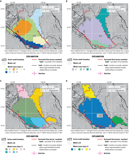
Zones of simulated hydraulic properties (horizontal hydraulic conductivity, vertical hydraulic conductivity, specific yield, and specific storage) used in the Lucerne Valley Hydrologic Model (Larsen, 2022) for A, layer 1; B, layer 2; C, layer 3; and D, layer 4, Lucerne Valley, California. (See table 4 for zone values).
Table 4.
Summary of initial and calibrated hydraulic properties used in the Lucerne Valley Hydrologic Model (Larsen, 2022), Lucerne Valley, California.[see figure 21 for location of zones. Abbreviations: ft/d, foot per day; —, not applicable]
Hydraulic Conductivity
Hydraulic conductivity is a function of the physical properties (porosity, skeletal structure, saturated hydraulic radius, and pore connectivity) of a porous medium and the physical properties of the fluid passing through the porous medium. A porous medium will transmit groundwater through a geologic section of unit area, measured at a right angle to the direction of flow, under a hydraulic head gradient if the medium transmits (Lohman, 1972). The OWHM2 requires horizontal and vertical hydraulic conductivity values for confined and unconfined aquifers. Initial estimates of hydraulic conductivity values (table 4) were derived from specific-capacity tests and driller’s logs; initial horizontal hydraulic conductivity values ranged from 0.001 to 100 feet per day (ft/d), and initial vertical hydraulic conductivity values were 0.0001 and 0.00001 ft/d. Calibrated horizontal hydraulic conductivity values ranged from 0.0013 to 40 ft/d, and calibrated vertical hydraulic conductivity values ranged from 0.000068 to 0.269 ft/d (table 4). These horizontal and vertical hydraulic conductivity values were assigned to model cells according to the zonation patterns shown on figure 21.
Specific Yield and Specific Storage
Water is stored and released from an aquifer by two processes: (1) the filling and draining of pores due to gravity and (2) the expansion and compression of water and the aquifer skeleton (Freeze and Cherry, 1979). Specific yield is associated with the filling and draining of pores by gravity and is a much larger contribution to the total storativity of an aquifer than specific storage. Specific yield applies only to unconfined systems and represents the drainable porosity of an aquifer as the groundwater table changes. For confined aquifer systems, water is released from storage when pumpage causes a decrease in hydraulic head. The change in pressure, from a decrease in hydraulic head, is transmitted into the confined aquifer system; water is produced by a slight compression of the aquifer skeleton and the expansion of water as an effect of the pumpage stress.
The upper aquifer, confining unit, and middle aquifer (layers 1, 2, and 3, respectively) were simulated under convertible conditions; therefore, specific yield and specific storage were specified in the Upstream Weighting Package (UPW; Niswonger and others, 2011). The lower aquifer (layer 4) was simulated under confined conditions and only specific storage was parameterized. Initial estimates of specific yield and specific storage were taken from groundwater-flow models done for the Antelope Valley (Siade and others, 2014) and Joshua Tree (Nishikawa and others, 2004) groundwater basins. Initial estimates of specific yield ranged from 0.05 to 0.125, and initial estimates of specific storage were 4.20E-07 ft–1. Initial estimates of specific yield and specific storage for model zones are listed in table 4, and model zones are shown on fig. 21.
Storage Properties
The Subsidence and Aquifer-System Compaction Package (SUB; Hoffmann and others, 2003) was used to simulate elastic (recoverable) compaction and expansion and inelastic (permanent) compaction of compressible fine-grained beds or interbeds within the aquifer; the SUB was used to simulate the instantaneous drainage of the fine-grained interbeds in model layers 1–3. As discussed earlier in the “Land Subsidence” section, removing water from storage within the fine-grained silts and clays interbedded in the aquifer system causes these highly compressible sediments to compact, resulting in land subsidence. The deformation of the interbeds is caused by hydraulic-head or pore-pressure changes and, thus, by changes in effective stress within the interbeds. Interbeds in model layer 1 consist primarily of the playa and lake deposits visible on the land surface (fig. 4); these interbeds were assumed to compact instantaneously when dewatered. Layer 2 consists of Quaternary fine-grained lacustrine deposits (mainly unit Qvol and some unit QTI; fig. 5) that compact when dewatered. Layer 3 contained fine-grained interbeds in a few places but was mainly composed of sand- and granule-size particles. Layer 4 is assumed to have low compressibility, and therefore, was assumed to be minimally susceptible to compaction because the deposits of this aquifer range from moderate- to well-consolidated fluvial coarse-grained deposits associated with the geologic unit Tmf described in table 1. Delayed drainage was not simulated in this model because we were unable to simulate the magnitude and trend of subsidence near Lucerne Lake while using delayed drainage. Subsidence was therefore simulated using only instantaneous drainage.
Storage and subsidence related properties associated with instantaneous drainage (fluid-pressure equilibration) of interbeds were estimated from Siade and others (2014) and were used as initial values for the SUB package in the LVHM. These initial parameter values included the properties of elastic and inelastic storage coefficients ( and , respectively).
In general, the storage coefficient (, dimensionless) is the sum of the skeletal storage () and the storage attributed to the compression/expansion of water (). These storage coefficients can be expressed as a product of sediment thickness, , and the corresponding specific-storage value, for the aquifer skeleton, and for water. Generally, because it is assumed that only the fine-grained deposits (interbeds and confining units) deform inelastically (Hoffmann and others, 2003),
whereSkv is the inelastic storage coefficient,
Sskv is the inelastic skeletal storage coefficient, and
b(f) is the thickness of fine-grained deposits.
Values for can be defined for the fine-grained and coarse-grained deposits :
whereSke is the elastic storage coefficient,
Ske (f) is the elastic storage coefficient of fine-grained deposits,
Ske (c) is the elastic storage coefficient of coarse-grained deposits,
Sske (f) is the skeletal storage coefficient of fine-grained deposits,
Sske (c) is the skeletal storage coefficient of coarse-grained deposits,
b(f) is the thickness of fine-grained deposits,
b(c) is the thickness of course-grained deposits, and
b is the total thickness of both fine- and coarse-grained deposits.
For this model, only the fine-grained component was specified in the SUB package, and only deformation of the fine-grained deposits was simulated. The aquifer-system specific storage, , specified in the UPW, accounts for the volume of elastic storage changes resulting from and in model cells where aquifer-system compaction and subsidence were simulated. Generally, values were on the order of 10–4 and values were on the order of 10–6, similar to specific storage .
Preconsolidation head (), or preconsolidation stress, is another parameter used by the SUB package that strongly affects storage changes, particularly the timing of those changes. Poland (1984, p. 335) defined preconsolidation head as “the maximum antecedent effective stress to which a deposit has been subjected, and which it can withstand without undergoing additional permanent deformation.” The preconsolidation stress represents the threshold value that determines whether changes in stress deform the aquifer skeleton elastically or inelastically. If the stress is less than the preconsolidation stress of the sediments, the deformation is elastic; if the stress is greater than the preconsolidation stress, the deformation is inelastic. Therefore, once the hydraulic head in an interbed, or confining unit, falls below the preconsolidation head, permanent inelastic compaction of that interbed occurs. During the modeling process, a new preconsolidation head is calculated at the end of each transient-state time step and is then used in the subsequent time step (Hoffmann and others, 2003). For the LVHM, the initial preconsolidation head values for all layers were estimated at 2,850 ft, which were about equal to the steady-state groundwater levels that were present near the center of the basin. The preconsolidation head values were adjusted using trial-and-error calibration techniques; they did not vary spatially within an individual layer in the LVHM.
Horizontal-Flow Barriers
As discussed in the “Hydrogeology” section, faults in the Lucerne Valley have been documented as, or are suspected to be, barriers to groundwater flow. The faults within the model domain were simulated using the Horizontal-Flow Barrier (HFB6) package (Hsieh and Freckleton, 1993; Harbaugh and others, 2000; Harbaugh, 2005; table 10). The HFB6 package allows for the simulation of thin, vertical, low-permeability geologic features situated between adjoining model grid cells. The HFB6 package assumes that the width of the fault is negligible in comparison with the horizontal dimension of the model grid cell. Conductance through the fault is controlled by a hydraulic characteristic that implicitly includes fault width (Harbaugh and others, 2000). Initially, the hydraulic characteristic value for each fault was set to a large value, allowing groundwater to freely flow across each fault. Through calibration, the hydraulic characteristic values were lowered until simulated groundwater levels matched closely to measured observations.
Three mapped faults (HELENFAUL, CUSHENBURY, SCOUGFAUL) and two previously unidentified barriers (HELENSPLAY, GMFAUL) that affected groundwater flow in the Lucerne Valley were simulated using the HFB6 package (fig.19; table 10). Model fault HELENFAUL simulated the Helendale Fault with a hydraulic characteristic value of 3.6E-06 ft/d; however, its trace was adjusted near the southern end of the simulated extent because measured groundwater levels by Thompson (1929) indicated a discontinuity in this area. Model fault CUSHENBURY simulated the Cushenbury Fault with a hydraulic characteristic value of 2.27E-06 ft/d. The horizonal-flow barrier HELENSPLAY was associated with the San Andreas fault zone (figs. 1, 19), which was described earlier in the “Geologic Structure” section and was simulated with a hydraulic characteristic value of 4.54E-06 ft/d. HELENSPLAY was inferred from groundwater-level data in the southern part of the basin (fig. 12E), which showed large groundwater-level differences between adjacent wells. Model fault SCOUGFAUL follows the trace of the Cougar Buttes Fault (fig. 19; table 10) and was simulated with a hydraulic characteristic value of 6.0E-05 ft/d. An additional horizontal-flow barrier (GMFAUL) was used in the northern part of the basin (fig. 19B) to more accurately simulate the discontinuities shown by the measured groundwater-level data (figs. 12, 14); this horizontal-flow barrier was simulated with a hydraulic characteristic value of 9.1E-06 ft/d.
Landscape-Water Use and the Farm Management Process
The evolution of the landscape is a combination of changes in land use and changes in land ownership in the Lucerne Valley during the 74-year transient-state simulation of 1942–2016. Before 2005, only areas of agriculture and native desert vegetation were able to be defined from aerial photographs. For the period of 1942–84, aerial photographs were only available in periods of varying time increments (fig. 2); after 1984, aerial photographs were available in annual increments. The agricultural pumpage before 2005 was estimated based on the aerial photographs and simulated using the Multi-Node Well (MNW2) package (Konikow and others, 2009; table 2). Because more detailed land-use data were available from 2005 to 2016, it was possible to more accurately depict areas of similar water-use demand or crop type to create water-balance subregions (WBSs). Using WBSs facilitates the calibration process by making it easier to adjust the hydraulic properties for similar crop types over a large area. The changes in land use and crop types were considered yearly, thus changing the footprint of these WBSs and creating different annual configurations of WBSs between 2005 and 2016. Figure 22 shows how the WBSs differed to represent the water demands of the changing land use shown on figures 2I–K for 2007, 2010, and 2016. The land use and crop type assigned to the respective WBSs determined the water demand for native vegetation and irrigated crops, which was used to calculate the required groundwater pumping to meet the irrigation requirements for each WBS.
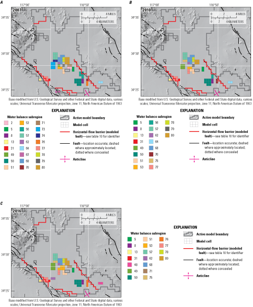
Distribution of water-balance subregions used in the Lucerne Valley Hydrologic Model (Larsen, 2022) to estimate groundwater pumpage for selected years, A, 2007; B, 2010; and C, 2016, Lucerne Valley, California.
The FMP (table 2) provided a coupled simulation of the groundwater and surface-water components of the hydrologic cycle for irrigated and non-irrigated areas for 2005–16. A dynamic allocation of groundwater recharge and groundwater pumping was simulated based on residual crop-water demand after root uptake from shallow groundwater. For a given stress period, the estimation of irrigation groundwater pumping in the FMP was dependent on satisfying demands for ET from precipitation and variable irrigation efficiencies that govern the availability of excess water available for deep percolation. A complete description of these components is provided in Schmid and others (2006a). Inflows and outflows throughout the WBSs on the landscape were simulated by the FMP. The FMP not only estimates supply, demand, movement, and consumption of irrigation water, but also estimates these components for natural vegetation. The use and movement of water on the landscape is fully coupled with surface water, when available, and groundwater flow and is dependent on atmospheric and soil conditions through precipitation and ET.
The FMP simulates the demand components representing the crop irrigation requirements (CIR) that are subject to crop- and farm-specific irrigation efficiencies and the supply components representing precipitation, direct uptake from groundwater, uptake of soil moisture, and irrigation from groundwater pumping. The FMP also simulates additional head-dependent inflows and outflows from the landscape, such as surface runoff from precipitation and irrigation to the streamflow network, and groundwater recharge as deep percolation of water in excess of actual evapotranspiration () and runoff (Schmid and others, 2006a, b; Schmid and Hanson, 2009). Changes in soil moisture were not simulated by the FMP and were assumed to be negligible at the monthly time scale.
Water mass within each WBS was calculated and balanced for each time step in the simulation from 2005 to 2016 (Schmid and others, 2006a, b; Schmid and Hanson, 2009). To dynamically integrate irrigation water demand from ET with water supply and irrigation efficiencies, the FMP first calculates crop-water demand as the transpiration or consumption of water by plants and the related evaporation based on cell-by-cell estimations for each WBS. The FMP then determines a residual plant-water demand that cannot be satisfied by precipitation and by root uptake from groundwater, if available, from shallow groundwater near the root zone. The residual water demand is the vegetation’s irrigation requirement for the cells with irrigated crops (that is, exclusive of any natural vegetation), which is the CIR and is calculated on a cell-by-cell basis.
The CIR is then adjusted by accounting for evaporative losses from irrigation and other inefficiency losses to yield a final total farm delivery requirement (TFDR). For the Lucerne Valley, where groundwater is the only source of irrigation water, the FMP attempts to satisfy the TFDR by using groundwater pumpage. This demand is not met when the demand exceeds the capacity of the wells for a specific WBS, either because groundwater levels dropped below the maximum depth of the perforated interval, or the maximum pumping rate of a given well is exceeded. The amount of excess water from irrigation (irrigation efficiencies) and precipitation that is not effectively used for crop growth then becomes either overland runoff to nearby streams or groundwater recharge as deep percolation below the root zone, based on the parameters specified in the FMP. In the LVHM, precipitation is negligible, and excess water ultimately becomes groundwater recharge. Thus, FMP dynamically links the demand, supply, and related change in hydraulic head.
To estimate the inflows and outflows, the FMP dynamically simulates the supply and demand components for a WBS by integrating the following computational components specific to Lucerne Valley’s hydrologic setting:
-
1 TFDR, which is largely dependent on the CIR, also depends on efficiency, climate variability (PET and precipitation), and variable aquifer head;
-
2 groundwater pumping, which is equivalent to the TFDR in the LVHM;
-
3 net recharge (deep percolation) to groundwater, which is the sum of excess irrigation and precipitation minus ET.
The OWHM2 maintains a mass balance for each WBS budget for the aquifer system. Flows between these budgets are accommodated by head-dependent inflows and outflows, such as , runoff and infiltration, or ET from groundwater. For the LVHM, the processes of evaporation, transpiration, runoff, deep percolation to groundwater, and groundwater pumping were simulated. The simulated groundwater pumpage reflects climatic differences in agricultural practices (including irrigation method) among defined WBSs. The LVHM model provides a detailed transient-state analysis of changes in groundwater storage in relation to climatic variability, urbanization, land use, and changes in irrigated agriculture.
Delivery Requirement
The TFDR is determined as the CIR of all WBS cells for irrigated crops and is increased sufficiently to compensate for irrigation efficiencies and ET from groundwater. The amount of ET from groundwater is a function of soil type, groundwater-table elevation, land-use type, root depths, and the anoxia and wilting points assigned to each land-use type. The TFDR data requirements for computing consumptive use on a cell-by-cell basis include soil type, land use (distribution of crop types and natural vegetation, including phreatophytes), and climate data. The consumptive use of each land-use type is simulated in this study based on root depths, irrigation efficiencies, runoff coefficients, crop coefficients, and the percentage of agricultural land use (tables 5–7). Although the exact value of these variables is uncertain, the basis of these estimates comes from various agricultural water-use and plant physiology studies (Rasse and others, 2000; Schenk and Jackson, 2002; Irrigation Training and Research Center, 2003; Food and Agriculture Organization of the United Nations, 2004; Sun and others, 2012; Ma and others, 2013).
Table 5.
Summary of consumptive-use factors for the land-use or crop types used in the Lucerne Valley Hydrologic Model (Larsen, 2022), Lucerne Valley, California.[FMP, Farm Management Process (see table 2); —, not applicable]
| Land-use type (FMP crop-index number) |
Irrigated | Root depth (feet) |
Fraction of surface-water runoff from precipitation (dimensionless) |
Fraction of surface-water runoff from irrigation (dimensionless) |
Rooting depth references |
|---|---|---|---|---|---|
| Alfalfa (1) | Yes | 4.59 | 0.20 | 0.31 | Rasse and others, 2000 |
| Apples (2) | Yes | 5.24 | 0.20 | 0.20 | Food and Agriculture Organization of the United Nations, 2004 |
| Grain (3) | Yes | 3.94 | 0.20 | 0.17 | Food and Agriculture Organization of the United Nations, 2004 |
| Grapes (4) | Yes | 6.56 | 0.20 | 0.20 | Food and Agriculture Organization of the United Nations, 2004 |
| Grass (5) | Yes | 2.62 | 0.20 | 0.20 | Food and Agriculture Organization, of the United Nations, 2004 |
| Jujube (6) | Yes | 11.15 | 0.20 | 0.20 | Ma and others, 2013 |
| Irrigation pond (7) | Yes | — | — | — | — |
| Landscaping (8) | Yes | 5.25 | 0.20 | 0.19 | Food and Agriculture Organization of the United Nations, 2004 |
| Mixed (9) | Yes | 3.94 | 0.20 | 0.19 | Food and Agriculture Organization of the United Nations, 2004 |
| Orchard (10) | Yes | 5.25 | 0.20 | 0.19 | Food and Agriculture Organization of the United Nations, 2004 |
| Pasture (11) | Yes | 3.94 | 0.20 | 0.20 | Food and Agriculture Organization of the United Nations, 2004 |
| Pistachios (12) | Yes | 3.94 | 0.20 | 0.21 | Food and Agriculture Organization of the United Nations, 2004 |
| Row crop (13) | Yes | 5.25 | 0.20 | 0.19 | Food and Agriculture Organization of the United Nations, 2004 |
| Native (14) | No | 5.58 | 0.19 | — | Schenk and Jackson, 2002 |
Table 6.
Monthly crop coefficients for each land-use type simulated in the Lucerne Valley Hydrologic Model (Larsen, 2022), Lucerne Valley, California.[FMP, Farm Management Process (see table 2)]
January, February, November, and December adjusted to crop coeficient for orchard Region 14 (Irrigation Training and Research Center, 2003).
Table 7.
Percentage of land-use type simulated annually for 2007–16, Lucerne Valley Hydrologic Model (Larsen, 2022), Lucerne Valley, California.[FMP, Farm Management Process (see table 2)]
Soils
The LVHM soils were simplified into six texture categories based on soil textural properties—sand, sandy loam, loamy sand, silty sand, silty loam, silty clay loam—from the Soil Survey Geographic Database (SSURGO; Natural Resources Conservation Service, 2017; fig. 23). Soil textural properties (percent sand, silt, and clay) were used to parameterize the soil textual properties program, Rosetta (Schaap and others, 2001), and estimate soil-water characteristic parameters using pedotransfer functions (Wösten and others, 2001). Rosetta is a program that models soil hydraulic properties, based on textural information, using neural network analysis (Schaap and others, 2001). The capillary fringe was estimated from the Brooks and Corey (1964) air-entry coefficient. These soil attributes were used for the entire simulation period, and the cell-by-cell distribution was independent of the crop type (table 5) and WBS. The FMP associates the distributed soil types with the specified capillary fringes and internal coefficients that allow individual analytical solutions for the calculation of ET (Schmid and others, 2006a).
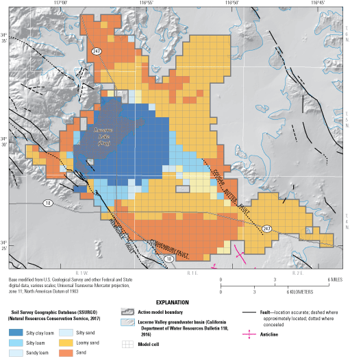
Soil texture zones categorized from soil textural properties for the Lucerne Valley Hydrologic Model (Larsen, 2022), Lucerne Valley, California.
Land Use
The FMP can be used to estimate components of consumptive use for a wide variety of land uses, including vegetation in irrigated or non-irrigated agriculture, fallow fields, phreatophytes and other natural vegetation, golf courses, and residential and municipal landscape settings. The FMP also can be used to simulate an assortment and spectrum of irrigation methods, including sprinklers and drip irrigation.
In the LVHM, the land-use attributes were defined on a cell-by-cell basis and included agricultural and native uses. Multiple land-use fractions were assigned to each cell when multiple land uses were present. Land use can change gradually or rapidly in response to changes in climate, urbanization, zoning, or farming practices. For the LVHM, the land-use patterns from 2005 to 2016 were changed on a yearly basis using crop distribution data (Mojave Water Agency, 2017). During this period, simulated land use had a maximum irrigated agricultural coverage (including landscaping) of 2.06 percent of the basin in 2013 (fig. 2; table 7). There were 14 land-use categories, referred to as “virtual crops,” that were defined based on crop-type indexes; these virtual crops were represented by an index number in the FMP (tables 5–7). For the simulation period for 2005–16, these virtual crops were used to drive the use and movement of water for each WBS.
Simulation of Recharge
Recharge to Lucerne Valley comes from natural and anthropogenic sources. As discussed previously, the primary source of natural recharge to the basin is infiltration from ephemeral washes coming from the San Bernardino Mountains to the south. Natural recharge was simulated along intermittent washes identified by Busby (1977) by using the direct recharge array in the FMP (fig. 19B). This package allowed groundwater to recharge the aquifer to the upper-most active layer. Recharge as underflow from tilted exposures of Pliocene and Pleistocene sediment exposed near inselbergs and in the San Bernardino Mountains was simulated in layers 3 and 4 using injection wells in the Well package (WEL; fig. 19; table 2). The initial estimate of average annual natural recharge from the CA-BCM was about 635 acre-ft/yr (Flint and others, 2013; fig. 8) and was used as a starting point for model calibration. Final estimates for average annual natural recharge were about 635 acre-ft/yr and accounted for sources of water derived from parts of the groundwater basin that were not included in the model area. These components included runoff, underflow, and mountain-front recharge from the San Bernardino Mountains to the south.
In addition to these natural sources of recharge, irrigation-return flow from agricultural fields and the infiltration of treated wastewater also contribute to recharge. Before 2005 (for 1941–2004 simulation), about 10–30 percent of water applied as irrigation was assumed to be recharged back to the groundwater system based on estimates from another desert basin (Faunt and others, 2015). After 2004, irrigation-return flow from agricultural fields and treated wastewater imported by the BBARWA and applied as irrigation to alfalfa fields was simulated as part of the FMP (fig. 19). Recharge from untreated wastewater from septic tanks was negligible because any effluent that infiltrates from septic tanks likely does not reach the water table for decades and is dependent on the application rate, depth to water, properties of the unsaturated zone, the initial water content of the unsaturated zone, and the landscape ET rate (Izbicki and others, 2000).
Simulation of Discharge
Before Lucerne Valley was developed, groundwater discharge consisted of evaporation at the playa surface, some ET, and discharge at springs. As the valley was developed, the primary discharge changed to groundwater pumped for agricultural, industrial, domestic, and municipal uses.
Natural Discharge
Natural discharge occurred primarily as evaporation from the playa surface of Lucerne Lake (fig. 16). Historically, phreatophytes were sparse; some saltgrass survives along the edges of Lucerne Lake playa. Natural discharge was simulated near Lucerne Lake using the Drain package (DRN), but only during pre-development conditions and the first few years of the transient-state model (fig. 19) because by 1929, areas of natural discharge were no longer observed in the basin because of declining groundwater levels (Schaefer, 1979).
Groundwater Pumpage
Groundwater pumpage is the largest stress on the aquifer system of Lucerne Valley and is grouped into three categories for this study: (1) agricultural; (2) industrial; and (3) domestic, which includes municipal, domestic, and rural-residential supply. Agricultural pumpage estimates include pumpage from wells used to supply water for irrigation of crops and recreational uses and were either specified in the MNW2 package for 1942–2004 that pump from as many as three aquifers or estimated by crop demand using the FMP for 2005–16. Pumpage for industrial, municipal, and domestic water supply was specified by reported values (Mojave Water Agency, 2017) and estimated pumpage based on population described in the “Mechanisms of Discharge” section.
Agricultural Pumpage
Discharge from agricultural wells has not been metered in Lucerne Valley, and production estimates were not available before 1994. Therefore, agricultural water use was simulated by a combination of direct and indirect estimates of pumpage. Consumptive use derived from aerial photography data gave estimates of irrigated acreage, and a consumptive-use factor was applied to derive pumpage. Aerial imagery estimates are limited because they do not account for the combined consumption of precipitation and water applied for irrigation and do not capture the variability in consumption with climate (Schmid and others, 2006a; Hanson and others, 2014). The estimation of pumpage by using the FMP provides physically based, dynamic, and linked pumpage estimates as an alternative to indirect methods (Schmid and others, 2006a).
Before 1994, agricultural pumpage was estimated using aerial photography because detailed pumpage data were not available for Lucerne Valley. Agricultural water use was estimated to be 6 ft/yr based on the consumptive-use estimates for alfalfa (Erie and others, 1965). Because of limited agricultural well information, MNW2 well cells were distributed throughout the model domain based on land-use imagery, and pumpage was specified for each of these wells. From 1942 through 1977, aerial imagery was limited to seven datasets; changes in land use were only applied for years in which data were available, otherwise the last available aerial dataset was used. Starting in 1984, aerial imagery data were available for each year. Annual pumpage estimates by well were available from 1994 to 2016 (Mojave Water Agency, 2017) and were used to specify the agricultural pumpage volume and distribution from 1994 through 2004. Pumpage for agricultural supply from 2005 to 2016 was estimated using the FMP.
Pumpage for agricultural supply using the FMP is estimated as a combination of CIR and efficiencies required to satisfy the TFDR for all wells that deliver water to a particular WBS. Efficiencies include those from irrigation-water conveyance (canals or irrigation pipes) and potential losses from runoff and deep percolation below the root zone during irrigation. The groundwater pumpage required to satisfy TFDR can be estimated by considering any potential surface-water supply, the efficiency of irrigation, effective precipitation, and fractions of transpiration and evaporation within each model cell. Because all irrigation is supplied by groundwater pumpage in Lucerne Valley, surface-water supplies were not simulated. Pumpage is estimated by the FMP based on the TFDR. As many as 37 wells were used to simulate pumpage for irrigation; the number of wells and the pumpage varied during 2005–16 (fig. 24). Verified estimates of pumpage (Mojave Water Agency, 2017) were used as additional calibration data for agricultural pumpage.
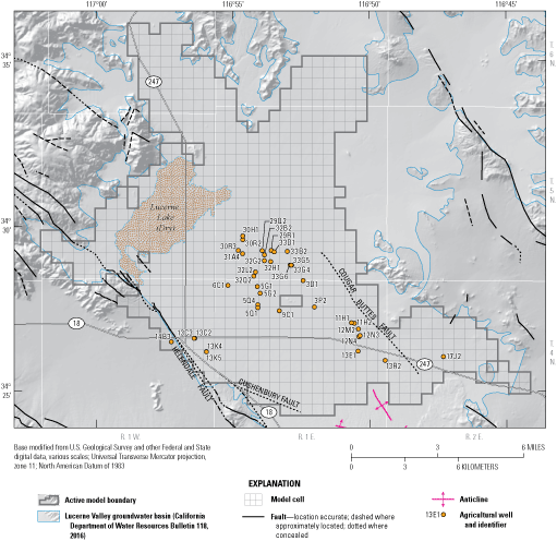
Location of wells used to simulate pumpage for agricultural irrigation in the Lucerne Valley Hydrologic Model (Larsen, 2022), Lucerne Valley, California (Mojave Water Agency, 2017; appendix 1; U.S. Geological Survey, 2021).
For each well, the aquifer for which pumpage was simulated was based on the available construction information. Specifically, the drillers’ logs were analyzed, and the top and bottom screened intervals for each well were assigned where available. The FMP allocated pumpage to wells within a WBS by the average fraction of total required pumpage. Total pumpage for each WBS was distributed to each of the wells within the WBS based on the average pumping rate (Schmid and others, 2006a). Pumping rates are then limited by the maximum pumping capacity of each well.
Industrial Pumpage
Industrial pumpage was specified from reported data (Mojave Water Agency, 2017). The approximate locations of industrial supply wells were used to assign pumpage to cells within the model. The WEL package was used to simulate industrial pumpage because all industrial pumping was confined to model layer 3.
Domestic and Municipal Pumpage
Pumpage for the domestic and rural residential water supply was simulated using the WEL. Because of the relatively small amount of extraction from these wells compared to agricultural pumping and limited information available about domestic well depth in the basin, these wells were simulated in the upper active aquifer, with few exceptions. Before 1994, domestic pumpage was based on population estimates from Schaefer (1979), San Bernardino County (2007), and Feller (2017). Domestic pumpage values from the mid-1990s were used as reference values to calculate population-based pumpage extrapolations going back to 1942. After 1994, reported municipal and domestic pumpage estimates were used (Mojave Water Agency, 2017); rural residential water-use studies done by the MWA in 2007 and 2014 were used to specify pumpage and distribution of the rural residential water supply after 2005 (Mojave Water Agency, 2017).
Model Calibration and Results
The results of the model simulations provide information about the hydrogeologic system before there was substantial groundwater development in the basin as well as the subsequent responses caused by the anthropogenic stresses to the aquifer system. Results of the model calibration and sensitivity analysis provide insight into model conceptualization, limitations of the current model, and a foundation for future refinements.
The LVHM was calibrated by a combination of trial-and-error and automated parameter-estimation methods. Hydraulic properties, hydraulic characteristics of faults, recharge rates, and agricultural demand were modified as part of this process. These parameters were estimated by PEST++ (Welter and others, 2015). This method adjusts initial parameter values so that the weighted sum of the squared differences between the observations and their corresponding model-simulated values (the objective function) is minimized. Each model cell must have values for each physical property (for example, hydraulic conductivity or specific yield). For most groundwater models, this requirement can result in many parameters that can be reduced using parameterization techniques, such as parameter zonation. In the LVHM, parameter estimation was performed with PEST++ to characterize the following properties:
-
• Horizontal and vertical hydraulic conductivities for all zones in all layers.
-
• Specific yield values for model layers 1–3 and specific storage values for model layers 1–4 for all zones.
-
• Hydraulic characteristics of horizontal-flow barriers in layers 1–4.
-
• Recharge rates by recharge cell.
-
• CIR parameters including crop coefficients, surface water loss fraction from precipitation, and surface water loss fraction from irrigation for all virtual crops.
-
• TFDR parameters including precipitation and PET which were adjusted through scale factors.
PEST Observation Groups and Parameter Weights
Four observation groups were defined in PEST++: (1) groundwater levels for initial conditions, (2) transient-state groundwater levels, (3) drawdown, and (4) agricultural pumpage calculated by the FMP. Groundwater-level observations for initial conditions, which represented predevelopment conditions (steady state), included measurements in 32 wells documented in 1917 by Thompson (1929) and 21 “virtual” observations created from interpolated hydraulic head observations in the 1950s were used for steady-state calibration (fig. 25). Transient-state groundwater-level observations included 5,290 measurements in 86 wells (fig. 26) that represented conditions during 1942–2016. The 4,761 drawdown observations were based on the transient-state groundwater levels and were calculated as the groundwater-level rise or decline compared to 1942. Agricultural pumpage observations were based on 384 reported pumping volumes from 37 wells during the 2005–16 period. An additional 12 pumping observations were calculated as basin-wide annual agricultural pumping from reported pumping volumes at individual wells and used as calibration observations from 2005 to 2016.
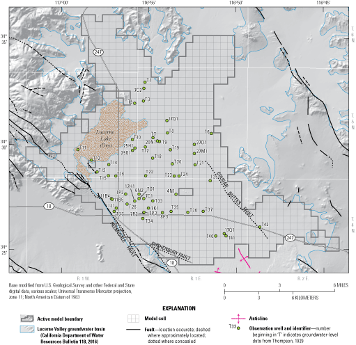
Location of observation wells used for the steady-state calibration of the Lucerne Valley Hydrologic Model (Larsen, 2022), Lucerne Valley, California (appendix 1; U.S. Geological Survey, 2021).
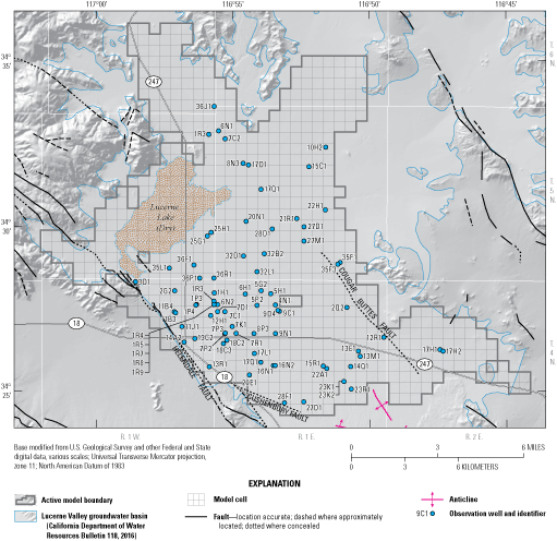
Location of observation wells used for the transient-state calibration of the Lucerne Valley Hydrologic Model (Larsen, 2022), Lucerne Valley, California (appendix 1; U.S. Geological Survey, 2021).
Although calibration weights varied throughout the calibration process, final calibration weight values in the transient-state model were constant for hydraulic-head and drawdown observations. For the final calibration, sites with long-term observation records were weighted more heavily than sites with few observations so that long-term head and drawdown trends in the basin could be matched. The highest weights (1, 6, or 10) were given to steady-state hydraulic-head observations, and the transient-state hydraulic-head observations were given a weight equal to 1. Pumping observations were given a weight of 0.1, and basinwide annual agricultural pumping was given a weight of 1.
Comparison Between the Simulated Results and Observed Data
The ability of the transient hydrologic-flow model to accurately represent the observed data was evaluated throughout the calibration process. Observed data were the groundwater-level, drawdown, and land-subsidence measurements observed in the field, in addition to the reported agricultural pumpage. A comparison of the simulated and the observed values for pumpage was done to assess the capacity of the LVHM to reasonably simulate the effects of changing stresses on the aquifer system over time. The comparison of measured and simulated data provided an indication of model performance spatially and temporally. The resulting error distributions constrained the values of each simulated parameter, and the comparisons between the observed and simulated values provided a basis for the sensitivity values of selected parameters, discussed later in the “Sensitivity Analysis” section.
Simulated hydraulic heads were compared directly with measured groundwater-level elevations if the wells were perforated in a single model layer. For wells perforated in multiple model layers, OWHM2 calculated a composite, simulated equivalent hydraulic head, which is a function of the simulated model layers. The equivalent hydraulic head is calculated by using the hydraulic properties of the perforated model layers with the hydraulic-head observation (HOB) package (Hill and others, 2000).Measures of model fit included the following:
-
• statistics for residuals (measured value minus simulated value) such as average, median, minimum, maximum, and root-mean-square error (RMSE);
-
• measured groundwater-level elevations compared to simulated hydraulic heads on a 1:1 graph;
-
• hydrographs showing measured groundwater levels and simulated hydraulic heads for the transient-state simulation period (1942–2016);
-
• comparison of observed land-surface deformation and simulated subsidence for the observed period of subsidence.
These statistics are measures of model fit; if the model results matched the measured groundwater-level data and observed land-surface deformation exactly, they would be equal to the simulated hydraulic head and subsidence. Similarly, when plotting the residuals against the simulated hydraulic heads, all the points would be at zero residual if the model results matched the data exactly.
Simulated Hydraulic Head and Measured Groundwater Levels
To determine how well the LVHM results reflected the measured data, the average RMSE between the simulated hydraulic head and the measured groundwater-level elevations (“groundwater levels”) were compared; the average RMSE for the entire transient-state simulation was calculated from RMSE values in table 8 as 14.91 ft, indicating a good fit, overall, of the simulated heads to the measured groundwater levels. The RMSE was small relative to the observed and simulated hydraulic head values that ranged more than 100 ft during the study period. The RMSE was lowest at well 5N/1E-15C1 in zone 33 (0.45 ft) and largest at well 5N/1E-22H1 in zone 33 (65.24 ft; figs. 21A, 21C; table 8), which was due to noisy observation data.
Table 8.
Summary of model-fit statistics for differences between simulated hydraulic heads and measured groundwater-level elevations (U.S. Geological Survey, 2021) for the transient-state simulation, Lucerne Valley Hydrologic Model (Larsen, 2022), 1942–2016, Lucerne Valley, California.[NWIS, National Water Information System; USGS, U.S. Geological Survey; ft, foot]
Another measure of model fit compares the simulated hydraulic head to the measured groundwater levels on a graph; an exact match would cause all observations to lie on the one-to-one (1:1) correlation line. The simulated hydraulic heads for the LVHM are plotted against the measured groundwater levels shown on figure 27. Simulated hydraulic heads that are above the 1:1 correlation line indicate that the model overestimated the measured groundwater levels; conversely, simulated hydraulic heads that are below the line indicate the model underestimated the measured groundwater levels. Overall, the simulated hydraulic heads and measured groundwater levels generally followed a 1:1 correlation line (fig. 27); however, 84 percent of the residuals were below the 1:1 correlation line, indicating that the model tended to underestimate groundwater levels. In addition, based on simulated residuals calculated from the difference between simulated hydraulic heads and measured groundwater levels (fig. 27), about 12-percent uncertainty was estimated for hydraulic-head results.
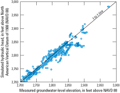
Simulated hydraulic heads compared to measured groundwater-level elevations (U.S. Geological Survey, 2021) for the Lucerne Valley Hydrologic Model (Larsen, 2022), 1942–2016, Lucerne Valley, California.
The location of a subset of observation wells and their corresponding hydrographs showing the simulated hydraulic heads and measured groundwater levels used for the transient-state model calibration are shown on figures 26 and 28, respectively. The simulated heads from layers corresponding to the measured groundwater levels from a well are shown on figure 28; the simulated heads from other layers are not shown. The wells were selected to represent temporal variations (groundwater-level trends, seasonal fluctuations, and vertical gradients) and optimize spatial coverage. Hydrographs that show measured data from multiple wells were compared with the average simulated hydraulic head between the wells’ locations.
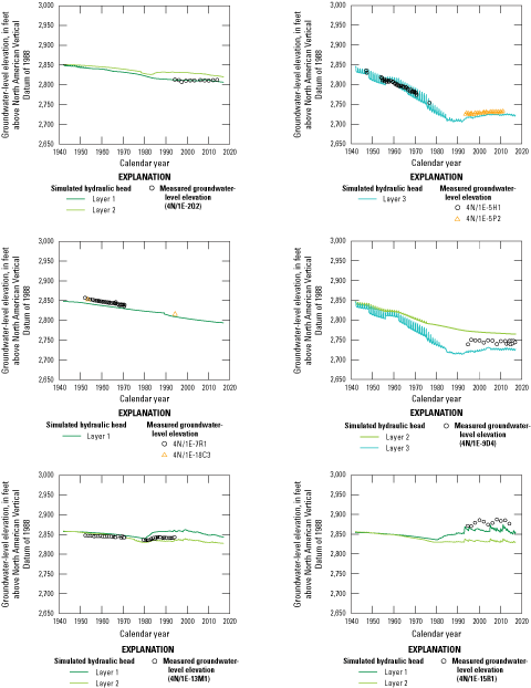
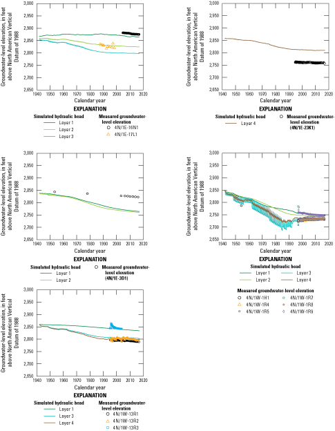
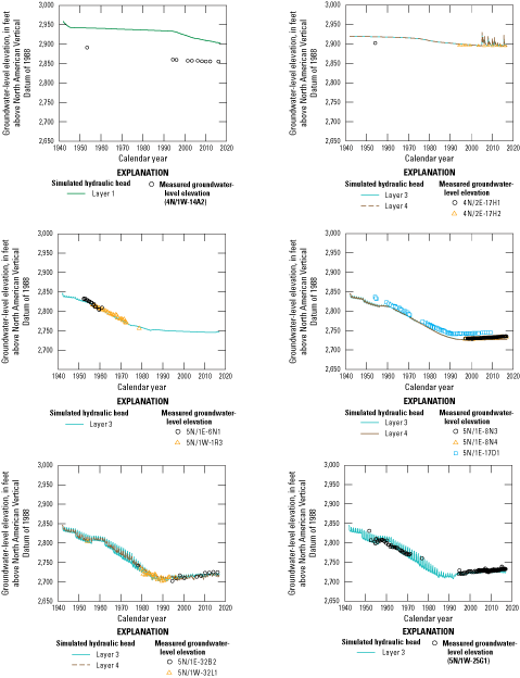
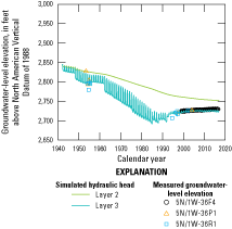
Selected hydrographs showing simulated hydraulic heads and measured groundwater-level elevations (U.S. Geological Survey, 2021) for the Lucerne Valley Hydrologic Model (Larsen, 2022), Lucerne Valley, California, 1942–2016.
The simulated hydraulic heads indicated that the model reasonably simulated the timing and magnitude of groundwater-level changes in Lucerne Valley. The greatest difference between simulated hydraulic heads and measured groundwater levels was in the southern part of the basin (figs. 26, 28). The discrepancies in this southern part of the basin could be attributed to uncertainties in the spatial discretization and distribution of geologic heterogeneity, particularly interbedded fine-grained materials with low hydraulic conductivity values, and the presence of unknown barriers to flow, such as faults. Mismatches between simulated hydraulic heads and measured groundwater levels can be attributed, at least in part, to uncertainty in the estimated distribution and magnitude of annual basin-wide pumpage for 1942–95. Estimates of the spatial and temporal distribution of pumpage from limited available data could result in excess or insufficient pumpage in some locations, causing an overestimation or an underestimation, respectively, of measured groundwater levels. Local variabilities in the hydraulic properties of the aquifer materials may not be adequately represented within the parameter zones of equal values, which also would contribute to the overestimation or underestimation of the measured groundwater levels.
The long-term measured groundwater-level data were used to evaluate the drawdowns, either decreases or increases, in hydraulic heads from the LVHM in all areas of the basin. To determine the drawdown in a well, the first groundwater-level measurement was assumed as the reference value and subsequent drawdowns were calculated as deviations from that first value. For the LVHM, drawdown was defined as the difference between the hydraulic heads from the steady-state simulation (before January 1942) and the end of the transient-state simulation (December 2016). Negative drawdown values represent increases in hydraulic heads compared to the reference value from the steady-state simulation. The drawdown data were evaluated for the three different periods to emphasize the importance of relative changes in groundwater levels at different points in time. The areal distribution of drawdown data for all model layers for 1942–2016 are shown on figure 29.
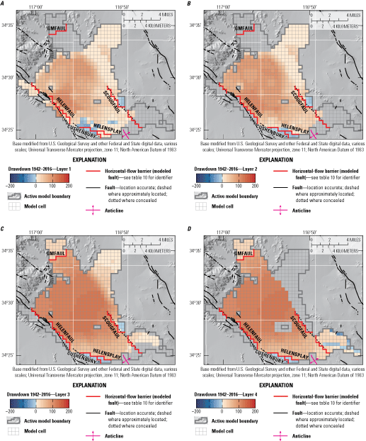
Simulated drawdown for the period 1942–2016 from the Lucerne Valley Hydrologic Model (Larsen, 2022) for A, layer 1; B, layer 2; C, layer 3; and D, layer 4, Lucerne Valley, California.
At the end of the model simulation period (2016), the drawdowns in all model layers generally were largest near the center of the basin and were less near the basin margins (fig. 29), which followed the trends observed by the measured data (figs. 12–14). In model layer 1, domestic and rural residential pumpage contributed to the simulated drawdown, but the amount of drawdown in layer 1 was less than that in the deeper layers because of the predominance of pumpage from the deeper layers and subsequent agricultural-return flows, as well as the artificial recharge from the BBARWA simulated effluent in the southern part of the basin (fig. 29A). The simulated drawdowns in model layer 1 ranged from about 110 ft near the center of the basin to an increase of about 35 ft near the BBARWA. The simulated drawdown pattern in layer 2 was similar to layer 1, with a decline of approximately 110 ft in the center of the basin and an increase of about 27 ft south of the Cushenbury Fault and Helendale Fault splay (figs. 29A, 29B). The simulated drawdown in model layer 3, which represented the middle aquifer, where most groundwater was withdrawn by agricultural pumpage, indicated widespread groundwater-level declines throughout most of the basin (fig. 29C). The simulated drawdown in layer 3 was spatially variable; about 125 ft of drawdown was simulated near the center of the basin, and hydraulic head increased about 14 ft south of the Helendale Fault splays and increased about 5 ft east of the Cougar Buttes Fault. Simulated drawdown in layer 4 also was spatially variable; about 130 ft of drawdown was simulated near the central part of the basin, hydraulic head increased about 10 ft south of the Helendale Fault splays and increased about 60 ft near the southeast margin of the model (fig. 29D).
Evaluating simulated drawdown for different periods can show how variations in hydraulic stresses cause groundwater levels to fluctuate temporally, areally, and with depth. Maps of the simulated drawdown for two additional periods (figs. 30, 31) were constructed to demonstrate the reversal of the groundwater-level trends observed in the measured data starting in the mid-1990s (figs. 13, 14). Figure 30 shows the drawdown by layer during 1942–95, which corresponds to the period with the largest pumpage volumes (fig. 10). The simulated drawdown for this period showed that the maximum decrease in hydraulic heads occurred in the center of the basin; the maximum simulated drawdowns from layers 3 and 4 were about 135 and 140 ft, respectively (figs. 30C, 30D).
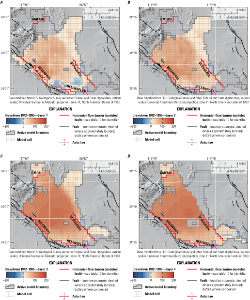
Simulated drawdown for the period 1942 through 1995 for the Lucerne Valley Hydrologic Model (Larsen, 2022) for A, layer 1; B, layer 2; C, layer 3; and D, layer 4, Lucerne Valley, California.
As discussed in the “Long-Term Trends in Groundwater Levels” section, the amount of annual pumpage decreased after about 1996 (fig. 10), lessening the hydraulic stress on the aquifer system, and consequently, resulting in less drawdown and increases in groundwater-levels in the center of the basin (figs. 13, 14, 31). After the decline in the agricultural pumpage rates, groundwater in storage near the edges of the basin continued to migrate toward the center where the largest drawdowns were observed in the mid-1990s (figs. 15, 30, 31). Drawdown was evaluated for the later part of the simulation (1996–2016) to show how the decrease in the pumpage rates since the mid-1990s affected the simulated hydraulic heads across the basin. During 1996–2016, there were increases in the simulated hydraulic heads in all layers, particularly in layer 3 where most pumpage had occurred (fig. 31C). The pattern observed in the simulated drawdown for 1996–2016 is a reversal of the pattern that occurred for the entire simulation period of 1942–2016 (fig. 29) and for the early part of the simulation period of 1942–95 (fig. 30) and corresponds to the increase in the measured groundwater levels and simulated hydraulic heads discussed previously (figs. 14, 28). Simulated drawdowns in layer 3, for 1996–2016, showed increases in hydraulic heads as much as 15 ft in the center of the basin (fig. 31C). The migration of groundwater from the edges of the model to the center resulted in continued declines in the simulated hydraulic heads in the northern, eastern, and southern edges of the basin that ranged from about 5 to 15 ft between 1996 and 2016, whereas the simulated hydraulic heads increased in the center.
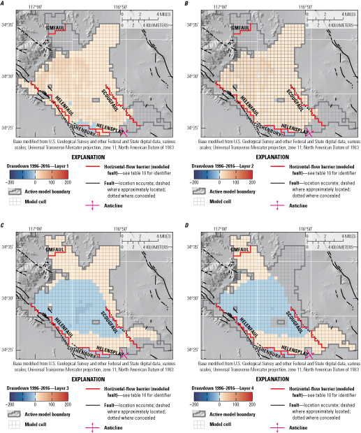
Simulated drawdown for the period 1996 through 2016 for the Lucerne Valley Hydrologic Model (Larsen, 2022) for A, layer 1; B, layer 2; C, layer 3; and D, layer 4, Lucerne Valley, California.
Subsidence Observations
Subsidence observation points were selected based on (1) monument locations from Sneed and others (2003) and (2) the location of maximum subsidence reported by the InSAR data for Lucerne Valley (Brandt and Sneed, 2017; fig. 32). Simulated subsidence and compaction for all observation points during July 2004 through November 2009, are shown on figure 33. Data were not available to determine when subsidence began, so the observed and simulated values began at 0 ft. Sneed and others (2003) estimated about 2 ft±5 ft of subsidence had occurred near the southern margin of Lucerne Lake from 1969 to 1998, and very little subsidence had occurred at the other observation points shown on figure 32. Subsidence likely began before 1969 because of the long history of pumpage, declining groundwater levels, and extensive clays and fine-grained materials at depth in Lucerne Valley. Simulated relative subsidence (relative to the beginning of the simulation period) ranged from almost no subsidence at observation point 13LC to about 7.5 ft (90 in.) at observation point InSAR_1 (fig. 33). Relative subsidence was slightly overestimated at observation points InSAR_1, RAIN, HOLM, and 49WB from Sneed and others (2003; fig. 33).
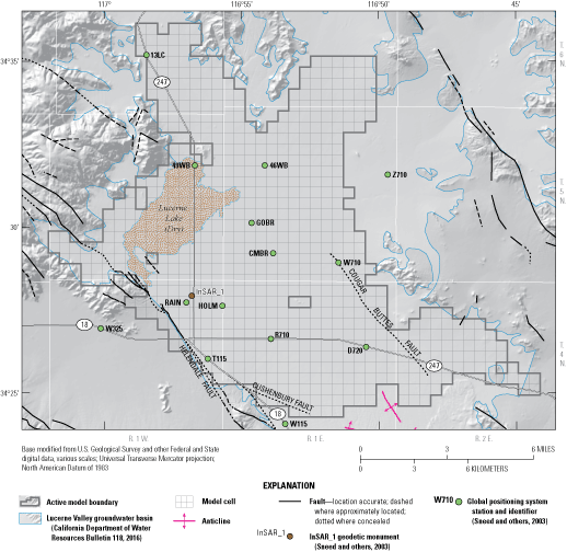
Locations of interferometric synthetic aperture radar (InSAR) observation points for the Lucerne Valley Hydrologic Model (Larsen, 2022), Lucerne Valley, California.
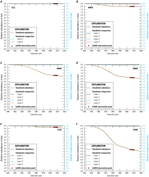

Interferometric synthetic aperture radar (InSAR) subsidence from 1992 to 2009, simulated subsidence, and simulated compaction from 1942 to 2016 at stations from Sneed and others (2003): A, 13LC; B, 46WB; C, 49WB; D, CMBR; E, D720; F, GOBR; G, HOLM; H, InSAR_1; I, R710; J, RAIN; K, T115; and L, W710, for the Lucerne Valley Hydrologic Model (Larsen, 2022), Lucerne Valley, California.
The maximum amount of subsidence in the Lucerne Valley that was estimated by the InSAR data, about 7.5 ft (2,286 mm), was simulated near observation point InSAR_1, which consists of the extensive fine-grained deposits near Lucerne Lake (figs. 16, 17). In the southern part of the basin, simulated subsidence ranged from greater than 1 ft at observation point R710 to less than 0.5 ft (152 mm) at observation point D720 (figs. 32, 33). Southeast of Lucerne Lake, simulated subsidence ranged from more than 4 ft (1,219 mm) of subsidence near the lake (observation point GOBR) to less than 0.5 ft (152 mm) near the Cougar Buttes Fault (observation point W710; figs. 32, 33). Simulated subsidence at station 49WB, located in the northeastern part of Lucerne Lake, indicated about 2.0 ft (610 mm) of subsidence and followed a pattern similar to the observed InSAR data in this area (figs. 32, 33).
The InSAR estimated land-surface deformation is plotted against simulated subsidence for all subsidence observations on figure 34. Simulated subsidence observations above the 1:1 trend line indicated that the model overestimated subsidence; conversely, simulated subsidence observations below the 1:1 trend line indicated that the model underestimated subsidence. Overall, the simulated subsidence skews above the 1:1 trend line, indicating some overprediction by the model. The total residual error for all simulated subsidence observations was 0.378 ft (115 mm), with a mean error in each observation of 0.008 ft (2 mm). The residual bias shows a tendency for the model to overestimate subsidence because there were a larger number of residuals greater than zero (88 percent) than there were less than zero (12 percent).
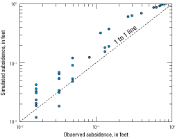
Simulated subsidence compared to observed subsidence from analysis of interferometric synthetic aperture radar data (Sneed and others, 2003) for the Lucerne Valley Hydrologic Model (Larsen, 2022), Lucerne Valley, California.
Mismatches between the observed and simulated subsidence values primarily can be attributed to the uncertainty in the thickness and lateral heterogeneity of the fine-grained sediments in model layer 2, which represents the confining unit. Uncertainties associated with the interpretation of the interferograms described in the “Land Subsidence” section of this report also can contribute to mismatches between measured and simulated subsidence.
Groundwater Budgets
The components of the groundwater budget for the 75-year transient-state simulation period (1942–2016) are shown on figure 35 and table 9. For the 1942–2016 simulation period, about 227,000 acre-ft of water was recharged into the Lucerne Valley groundwater basin, and about 692,000 acre-ft of groundwater was discharged from the basin, resulting in groundwater storage depletion of about 465,000 acre-ft (table 9). Almost all water discharged from the basin for the 1942–2016 simulation period was through pumpage (almost 100 percent of total discharge), most of which was for agricultural use (about 641,000 acre-ft or about 93 percent of total pumpage and total discharge; table 9). The total amount of municipal, industrial, and domestic pumpage accounted for a about 50,500 acre-ft or about 7 percent of the total pumpage and total discharge from the basin.
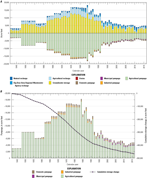
Simulated A, groundwater budget components; and B, pumpage and cumulative loss of groundwater from storage, 1942–2016, for the Lucerne Valley Hydrologic Model (Larsen, 2022), Lucerne Valley, California.
Table 9.
Simulated hydrologic budget for the Lucerne Valley Hydrologic Model (Larsen, 2022), 1942–2016, Lucerne Valley, California.For the 1942–2016 simulation period, natural recharge was about 48,000 acre-ft, or about 21 percent of total recharge, and artificial recharge was about 35,000 acre-ft, or about 15 percent of total recharge (fig. 35B; table 9). Recharge from irrigation-return water, the amount of groundwater that returns to the aquifer system after being removed by pumpage, was a much larger component of total recharge than natural and artificial recharge for the 1942–2016 simulation period, accounting for a total of about 144,000 acre-ft, or about 63 percent of total recharge (fig. 35B; table 9). The volume of irrigation-return water was variable on an annual basis and averaged about 1,900 acre-ft/yr (fig. 35B; table 9). The simulated annual average recharge of treated wastewater that was applied to alfalfa fields and infiltration ponds between 1996–2016 (started in 1980; see the “Anthropogenic Recharge” section) was about 900 acre-ft/yr (fig. 35B; table 9).
Reduced pumping (beginning in the mid-1990s) decreased the rate of groundwater storage depletion. The annual average depletion in groundwater storage was about 7,700 acre-ft/yr for 1942–95 and about 2,900 acre-ft/yr for 1996–2016, which was a decrease of about 4,800 acre-ft or about 62-percent less depletion for the later period (table 9).
Sensitivity Analysis
A sensitivity analysis was performed on the model parameters and stresses to test the robustness of the parameter values estimated during the calibration process. The analysis involved keeping all input parameters and tested model stresses constant, except the one being analyzed, and perturbating that parameter or stress through a range of values that included the uncertainties in that parameter. Varying a parameter or stress by a small amount causes a large change in the simulation result for a sensitive parameter (more robust); an insensitive parameter causes a small change in the simulation results (less robust). Model sensitivity was evaluated using PEST++ (Welter and others, 2015).
The sensitivity process in PEST++ identifies the sensitivity of computed values at observation locations to changes in model parameters. PEST++ was used to identify which parameters to include in the parameter estimation process (Hill and others, 2000) and to adjust the parameter values during calibrations. Results of the sensitivity process indicated that the model was most sensitive to about 20 parameters related to scale factors of the crop coefficients, climate scale factors from 2005 to 2016, and crop water-use efficiencies. The sensitivity of all parameters is shown in table 10, and selected parameters are shown on figure 36. The model was most sensitive to the hydraulic conductivity parameter, hk42, which represents the horizontal hydraulic conductivity of zone 42 (figs. 21D, 36). The next-most important parameter was related to the vertical conductivity of zone 12 (figs. 21D, 36), which controls the vertical movement of water between layers. Other sensitive parameters were scale factors related to the scaling of crop coefficients, which control groundwater demand, irrigation efficiency for alfalfa, an agricultural pumping scalar, and hydraulic conductivities.
Table 10.
Parameter values estimated for the Lucerne Valley Hydrologic Model (Larsen, 2022), Lucerne Valley, California.[Zones are shown in figure 22. Abbreviations: ft/d, foot per day; Mts, Mountains; ft3/d, cubic foot per day; —, not applicable]
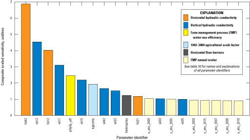
Relative composite sensitivities for the 20 most-sensitive parameters for the Lucerne Valley Hydrologic Model (Larsen, 2022; see table 10 for all parameter values), Lucerne Valley, California.
Model Uncertainty, Limitations, and Improvements
The model documented in this report and in Larsen (2022) can be used to evaluate water-management scenarios throughout Lucerne Valley. However, to use the LVHM effectively, the uncertainty associated with its simulated hydrologic conditions needs to be understood. The LVHM is a simplification of the Lucerne Valley hydrogeologic system that has some inherent limitations. The accuracy of model results is related strongly to the quality and spatial distribution of input data and of measurements of the components, or inputs, of the groundwater system (such as groundwater-level and pumpage data) used to constrain model calibration. The inflows and outflows in the model were a combination of measured values, adjustments to represent conceptualizations of the system, and other landscape and hydrologic values specified for simulating hydrologic processes using the model codes, One Water Hydrologic Model (OWHM), and associated numerical processes (for example, FMP) and packages (for example, MNW2). Differences between simulated and actual hydrologic conditions arise from several sources and are collectively known as model error that results in potential model uncertainty.
Although the model was designed with the capability to represent the actual groundwater system, the conceptual and numerical model still retains simplifications that could restrict appropriate use of the current model to regional and subregional spatial scales and within seasonal to inter-annual temporal scales. Potential future refinements and enhancements could improve the level of accuracy and the spatial and temporal resolution. Limitations of the modeling software, assumptions made during model development, and results of model calibration and sensitivity analysis are factors that could constrain the appropriate use of this model. However, the current model can be used to identify areas where improvements are needed in the simulation of specific processes or in the data used to simulate existing features that would likely improve model accuracy and relevance.
Model discretization, in space and time, can be a potential source of error and uncertainty. Models represent an aquifer system as a series of discrete spatial units through which intrinsic properties and flows are assumed to be uniform. The use of a discretized model to represent an aquifer system introduces limitations from features that occur at scales smaller than the discretization. The transient-state model runs are further discretized into a series of discrete units of time during which specified hydrologic inflows and outflows are held constant. The use of 126 twice-yearly stress periods (1942–2004) followed by 144 monthly stress periods (2005–16) in the LVHM inherently assumes that temporal variations of inflows, outflows, and groundwater levels could be approximated as piecewise linear changes during the specified time intervals. Changes at shorter time scales were not simulated and were not discernible in the model results, and this could contribute to some additional temporal uncertainty. The temporal scale used in the LVHM was specifically designed to separate the supply and demand components of agriculture. The temporal scale of the model changes from twice-yearly stress periods to monthly stress periods in 2005 and corresponds to decreased uncertainty in the distribution of agricultural input parameters.
Differences between simulated and measured hydrologic variables also can arise from the numerical solution, which attempts to provide a cell-by-cell mass balance of inflows and outflows by using an iterative approximation of the governing flow equations. Mass-balance errors are minimized by ensuring the model solution reaches a reasonable state of mass balance, or closure criteria, within each time step, as specified by a user-defined tolerance. The cumulative mass balance of the final model simulation was within 0.5 percent of the total mass flow during the 75-year period (1942–2016).
An additional component of model error arises from how well model-input values represent the actual aquifer system. The accuracy of the calibrated model is contingent on the accuracy of the specified inflows and the specified comparison flows. Model calibration provides a means to use comparisons to constrain the differences between real-world and simulated mass flows indirectly. Thus, the degree to which a simulated condition provides a reasonable representation of the aquifer system can be evaluated by comparing the simulated hydrologic conditions with those observed in the field, which, in turn, provides a mass-constrained calibration. The performance and accuracy of the LVHM are constrained primarily by groundwater levels (which are usually infrequent), pumping, and, to a lesser degree, hydraulic-head differences. The model solves for average conditions within each 92-acre cell for each time step with the parameters interpolated or extrapolated from measurements or estimated during calibration. Thus, for comparative analysis and generalized estimates of flow, results from the model are most appropriate for subregional spatial scales and annual to inter-annual temporal scales.
Several estimates from the model are uncertain and would require additional study to improve the accuracy of the simulation of groundwater flow, the regional groundwater-storage changes, and the use and movement of water across the landscape. For example, some of the inputs to the FMP that are necessary to calculate water use remain uncertain, and model features, such as agricultural pumpage, could be sensitive to a few of these parameters, such as crop coefficients, irrigation efficiencies, crop rotations, or monthly land use. More accurate estimates of agricultural pumpage would improve the model results. In addition, yearly information regarding land use from 1942 to 2004 would greatly improve the accuracy of the simulation. Many of the stresses that are driven by these land uses varied throughout the simulation period and were at a higher frequency than the lower frequency (variable; minimum, 1 per year) estimates of land use. These variations also are driven by climatic conditions and growing periods. Because the land use was based on a generalized classification for 1942–2004, an assigned pumpage was based on an estimated consumptive use. This assigned pumpage assumes the farmer would be growing the same type of crop in a given area during the time frame of the hydrologic simulation when that land-use map was used. Although the principal crop was alfalfa, in some cases, the crops could have changed several times during the years.
Model uncertainty could be reduced by using additional field estimates, such as horizontal and vertical hydraulic conductivities and storage properties. Additional estimates of horizontal hydraulic conductivities could be obtained by using slug tests at observation wells, pumping tests, including drawdown measurements, at multiple observation wells in the area of greatest groundwater-level declines, or specific-capacity approximations from single-aquifer supply wells to constrain the model properties further. A particular focus on gathering field data in the southern part of the basin, where discontinuities and large head gradients exist when compared to the central and northern part of the basin, could improve the LVHM considerably.
A groundwater-flow model is a tool for testing the conceptualization of the hydrogeologic system and for predicting the response of the system to changes in aquifer stresses. However, a model is only an approximation of the actual aquifer system and, therefore, does not exactly represent the actual system. The model relies on estimates of aquifer properties and stresses, which have some degree of uncertainty. Although some of this uncertainty has been evaluated in this work, the model still lacks the small-scale spatial and temporal variability that is present in the actual system.
Groundwater-levels and drawdowns calculated by the model are average values for the area represented by each model cell. Simulated groundwater levels can vary considerably from measured groundwater levels because of well location, depth, and construction. For example, wells could be screened throughout a depth represented by more than one model layer, whereas the corresponding measured groundwater levels could represent an unknown composite of the hydraulic heads across this screened interval. However, the size of the model cells and the length of the stress periods of the model used in this work are appropriate for the resolution of available data and for simulations on a regional scale; the model generally is not meant to be used to address detailed, local-scale questions.
Natural and agricultural recharge are difficult to measure; therefore, the recharge rates and temporal distribution of recharge were based on the model calibration results. The calibration process resulted in a lower rate of natural recharge than had been estimated in previous studies. Additional hydrologic data are needed to assess the accuracy of the natural recharge rates used in the model.
Because of the uncertainty in some parameters used in the model (especially hydraulic properties in the southern part of the basin) and in some components of the model structure (such as the agricultural component of pumping), the model is not ideally suited for predicting actual groundwater levels; the model estimated an uncertainty of about 12 percent for the simulated groundwater levels. The most appropriate application of the model is comparing the relative effects of different water-management scenarios on the aquifer system.
In summary, some potential components that could improve the accuracy and reduce uncertainty of the simulation could include, but are not limited to, the following:
-
• Improved temporal estimates of land use;
-
• Improved estimation and application of crop and irrigation practices;
-
• Improved estimates of hydraulic properties through field tests;
-
• Improved geologic texture estimates;
-
• Improved simulation of multi-aquifer wells to account for well pumping capacities;
-
• Inclusion of antecedent soil moisture in the FMP.
Despite these potential limitations, the LVHM represents the most realistic, accurate, and reliable means, at present, for understanding many aspects of the hydrogeologic system of the Lucerne Valley that are needed for planning and evaluating scenarios for managing water resources. Although all models have limitations, the options for testing alternative scenarios would be much more limited without the hydrologic information provided by the LVHM. When used correctly, the LVHM can contribute to a better understanding of the hydrogeologic system. As more data become available and more modeling capabilities are developed, the LVHM can provide a foundation for updates and refinements to improve its usefulness as a tool for the management of water resources in the Lucerne Valley.
Summary and Conclusions
Lucerne Valley is in the southwestern part of the Mojave Desert and is about 75 miles northeast of Los Angeles, California. The study area lies within the Lucerne Valley groundwater basin, encompasses about 175 square miles, and is separated from the Upper Mojave River Valley groundwater basin by the Helendale Fault. Since the late 19th century, groundwater has been the primary source of water for agricultural, industrial, municipal, and domestic uses. For most years, groundwater withdrawal from pumping exceeded the amount of water replenishing the basin and, by the mid-1990s, had caused groundwater levels to decline more than 100 feet in the center of the basin. Continued withdrawal has resulted in increases in pumping costs, reduced well efficiency, and land subsidence. Although the volume of groundwater pumped annually has decreased since about 1996, agricultural water use, primarily for the irrigation of alfalfa, and the lack of imported water continue to strain the sustainability of the aquifer system. To reassess the hydrogeologic conditions in the Lucerne Valley, the U.S. Geological Survey began a cooperative study with the Mojave Water Agency in 1994. The purpose of the study was to document the changes to the groundwater system and develop management tools to help sustainably manage the groundwater basin.
The aquifer system in the Lucerne Valley consists of a shallow aquifer, a confining unit, and a middle and lower aquifer. These separate layered water-bearing units were identified based on hydrogeologic properties, such as age and depth of the mostly unconsolidated sediments. These alluvial deposits consist of clay, silt, sand, and gravel, and in some places, contain clay and silty clay lacustrine deposits. Several barriers, primarily faults, affect groundwater flow on the eastern, southern, and western edges of the basin. Present-day natural recharge to the study area occurs primarily from the infiltration of runoff from the San Bernardino Mountains to the south, and the average annual natural recharge for 1942–2016, estimated by a Basin Characterization Model, was about 635 acre-feet per year. Stable and radioactive isotopes indicate that groundwater from the middle of the Lucerne Valley is very old, with ages of greater than about 10,000 years before present, and probably was recharged as infiltration from streams draining the mountains in the Mojave Desert to the north; however, the infiltration and recharge from these sources probably does not occur during the drier present-day climatic conditions. Since the 1980s, treated sewage effluent imported by Big Bear Area Regional Wastewater Agency has been an additional source of recharge to the groundwater system; the average amount of treated wastewater effluent transferred to the Lucerne Valley for artificial recharge annually ranged from about 1,470 to 4,000 acre-feet per year during 1980–2016. Pumpage estimates for 1942–2016 ranged from about 3,000 acre-feet in the early 1940s to about 18,300 acre-feet in 1984. Between 1942 and 2016, the total cumulative amount of groundwater removed from the basin by pumping was estimated to be about 700,000 acre-feet, which was about 10 times greater than the cumulative amount of recharge (70,600 acre-feet) to the entire Lucerne Valley groundwater basin.
The predominant direction of groundwater flow during pre-development conditions was from the southern part of the basin northward to areas near Lucerne Lake, where it was discharged through springs along the Helendale Fault and by evapotranspiration. Pumpage since the early 1900s and the consequent groundwater-level declines mostly have eliminated the natural sources of discharge. The long-term extraction of groundwater has caused groundwater levels to decrease by more than about 100 feet in the middle of the basin between the early 1950s and mid-1990s and as much as 25 feet near the margins from about the mid-1950s to 2016. Pumpage rates after about the mid-1990s decreased the hydraulic stress on the middle and lower aquifers and enabled hydraulic heads to recover slightly in the middle of the basin as groundwater from storage migrated from the margins toward the pumping depression. Although patterns in groundwater levels in the center of the basin have reversed since the mid-1990s, levels at the basin margins continue to decline as the migration of groundwater from the margins fills the pumping depression and gradually flattens the groundwater table throughout the basin.
The long-term extraction of groundwater and dewatering of the fine-grained sediments present within the aquifer system has resulted in aquifer compaction and land subsidence, primarily near Lucerne Lake. Analysis of interferometric synthetic aperture radar (InSAR) results for 1992–2009 shows that the highest rates of land subsidence occurred south of the playa, where most of the agricultural pumpage was located (before 2007) and where groundwater-level declines have been greatest. Nearly 0.9 feet of subsidence was observed between 1992 and 2009, with an average rate of about 0.05 ft per year at an observation point south of Lucerne Lake. This average rate varied and increased from about 0.04 ft per year during 1992–99 to about 0.06 ft per year during 1999–2009. The land subsidence has caused fissures and cracks to the ground surface and roads; as land-subsidence rates continue or accelerate, the potential alteration of surface-drainage routes and damage to infrastructure could result in large repair costs for local municipalities.
A numerical groundwater-flow model of the Lucerne Valley groundwater basin was developed to gain a better understanding of the hydrological conditions within the basin and to provide a management tool that can provide insight into the effects of future stresses within the groundwater basin. The Lucerne Valley Hydrologic Model (LVHM) was developed with the finite-difference groundwater modeling software One Water Hydrologic Model (OWHM). The OWHM is a numerical code that incorporates a dynamically integrated water supply-and-demand accounting in areas of agricultural and native vegetation and has made more detailed and realistic simulations of aquifer systems possible. The OWHM is based on MODFLOW-NWT and incorporates an updated version of the Farm Management Process (FMP) as well as updated MODFLOW packages. The LVHM finite-difference model grid consists of 64 rows, 50 columns, and 4 layers (12,800 cells). About 18 percent of the cells (561 cells in layer 1,528 cells in layer 2,631 cells in layer 3, and 538 cells in layer 4) were an active part of the hydrologic model. The model had a uniform horizontal discretization of 92 acres per cell (2,000 ft by 2,000 ft) and the grid was oriented to true north. The orientation and the cell size were chosen to be roughly parallel to the general direction of regional groundwater flow and to align with an adjacent groundwater-flow model grid for the Upper Mojave River Valley groundwater basin.
Vertically, the model has four layers with varying thicknesses representing the upper aquifer, a fine-grained lacustrine confining unit, the middle aquifer, and the lower aquifer. The Helendale Fault, on the western side of the basin, acts as a horizontal-flow barrier and forms the western boundary of the model. In the southeastern part of the basin, the Cougar Buttes Fault acts as a horizontal barrier to flow and creates the eastern boundary of the model. The surrounding mountains form most of the remaining model boundaries. The model was calibrated using groundwater-level data to simulate pre-development, or steady-state, conditions representing 1941 and transient-state conditions for 1942–2016. Initial estimates of aquifer-system properties were estimated from field data and from previous studies of other groundwater basins in the Mojave Desert. Estimates of aquifer stresses were obtained from hydrologic, land subsidence, and geochemical data, and from results of a Basin Characterization Model of recharge for the watershed. Some of these initial estimates were modified during calibration.
The main sources of recharge to the aquifer system came from anthropogenic sources, such as agricultural irrigation-return flow, irrigated fields, and infiltration ponds that used imported treated wastewater from the Big Bear Area Regional Wastewater Agency. During the 75-year study period, the simulated natural recharge from the Basin Characterization Model averaged about 630 acre-feet per year. The simulated excess irrigation water, or agricultural return, averaged about 1,930 acre-feet per year. The simulated average recharge of treated wastewater to irrigated alfalfa fields and infiltration ponds from 1996–2016 was about 900 acre-feet per year.
Groundwater discharge in the Lucerne Valley occurs by the (1) sparse seepage from Rabbit Springs in the eastern part of the basin and (2) groundwater pumping for agricultural, industrial, municipal, and domestic uses. Evapotranspiration from the ground and through the direct uptake of plants in Lucerne Valley generally does not occur because by 1942, the water table was below the reach of phreatophyte root zones. Groundwater pumpage for agriculture was estimated based on irrigated acreage and consumptive-use data. Values of pumpage for the industrial and municipal supply were compiled from water-use records. Values of pumpage for the domestic supply was estimated from population data or compiled from water-use records.
Comparisons of the measured groundwater levels and simulated hydraulic-head data helped assess the performance of the model during the 1941–2016 study period. Simulated hydraulic heads were compared to the measured groundwater levels along a 1:1 correlation line, long-term hydrographs, and drawdowns throughout the basin. The comparisons show that the model performed well in most areas but underestimated or overestimated the hydraulic heads in some areas. Mismatches between simulated hydraulic heads and measured groundwater levels can be attributed, at least in part, to uncertainty in the estimated distribution and coarseness of the annual pumpage available for 1942–95, local variabilities in the hydraulic properties of the aquifers, uncertainties in the spatial discretization and distribution of geologic heterogeneity, particularly interbedded fine-grained materials with low hydraulic conductivity values, and the presence of unknown barriers to flow, such as faults. The simulated drawdowns for two additional periods demonstrated the reversal of the groundwater-level trends observed in the measured data starting in the mid-1990s. Simulated drawdowns during the period of 1942–96, when pumping rates were highest, were as much at 140 feet in the middle of the basin. After pumpage rates decreased, the simulated drawdowns showed that the trend of declining hydraulic heads reversed and simulated hydraulic heads increased as much as 15 feet in the center of the basin between 1996 and 2016.
Despite the short-term increases in simulated hydraulic heads shown for the later years (1996–2016), the results from the calibrated model simulations indicated that groundwater pumpage exceeded recharge in all years, resulting in an estimated net cumulative depletion of groundwater storage (discharge minus recharge) of about 465,000 acre-feet from 1942 to 2016. The LVHM simulated as much as 7.5 feet (90 in.; 2,286 mm) of aquifer compaction, which was consistent with the extensive fine-grained deposits and measured subsidence near Lucerne Lake.
The LVHM can be used by resource managers to simulate future water-management scenarios; however, because of the uncertainty in some parameters used in the model in some components of the model structure, model results from any proposed predictive simulations should address these inadequacies. The most appropriate application of the model is comparing the relative effects of different future water-management scenarios on the aquifer system.
Periodic updates are required for numerical groundwater-flow models like the LVHM to ensure that the model accurately describes conditions that may change through time. As changing conditions of the aquifer system continue to respond to the stresses and as new information on the groundwater systems becomes available, the LVHM could be updated to improve the model performance and its utility as a water-management tool for the Lucerne Valley.
References Cited
Begemann, F., and Libby, W.F., 1957, Continental water balance, ground water inventory and storage times, surface ocean mixing rates and world-wide water circulation patterns from cosmic-ray and bomb tritium: Geochimica et Cosmochimica Acta, v. 12, no. 4, p. 277–296. [Available at https://doi.org/10.1016/0016-7037(57)90040-6.]
Boyce, S.E., Hanson, R.T., Ferguson, I., Henson, W., Schmid, W., Reimann, T., Steffen, M., and Earll, M.M., 2019, One-water—Legacy version: U.S. Geological Survey software release, available at https://doi.org/10.5066/P9CZM46C.
Brandt, J., and Sneed, M., 2017, Land subsidence in the southwestern Mojave Desert, California, 1992–2009: U.S. Geological Survey Fact Sheet 2017–3053, 6 p. [Available at https://doi.org/10.3133/fs20173053.]
Brandt, J.T., and Sneed, M., 2021, Land subsidence in the Mojave River and Morongo Groundwater Basins, southwestern Mojave Desert, California, 2014–19: U.S. Geological Survey website, https://doi.org/10.5066/P9306T67.
Busby, M.W., 1977, Flood-hazard study—100-year flood stage for Lucerne Lake, San Bernardino County, California: U.S. Geological Survey Open-File Report 77–597, 32 p. [Available at https://doi.org/10.3133/ofr77597.]
California Department of Water Resources, 2015, California sustainable groundwater management act: California Department of Water Resources, accessed December 29, 2015, at https://water.ca.gov/programs/groundwater-management/sgma-groundwater-management.
California Department of Water Resources, 2016, California’s groundwater—Working toward sustainability: California Department of Water Resources Bulletin 118 Interim Update 2016, 45 p., accessed September 21, 2021, at https://cawaterlibrary.net/document/bulletin-118-californias-groundwater-interim-update-2016/.
California Department of Water Resources, 2020, Well completion reports: California Department of Water Resources web page, accessed April 15, 2020, at https://water.ca.gov/Programs/Groundwater-Management/Wells/Well-Completion-Reports.
California Department of Water Resources, 2022, State Water Project: California Department of Water Resources web page, accessed March 8, 2022, at https://water.ca.gov/Programs/State-Water-Project.
Cox, B.F., Hillhouse, J.W., and Owen, L.A., 2003, Pliocene and Pleistocene evolution of the Mojave River, and associated tectonic development of the Transverse Ranges and Mojave Desert, based on borehole stratigraphy studies and mapping of landforms and sediments near Victorville, California, in Enzel, Y., Wells, S.G., and Lancaster, N., eds., Paleoenvironments and paleohydrology of the Mojave and southern Great Basin Deserts—Boulder, Colo: The Geological Society of America Special Paper 368, p. 1–42. [Available at https://doi.org/10.1130/0-8137-2368-X.1.]
Dibblee, T.W., Jr., 1964, Geologic map of the Lucerne Valley quadrangle, San Bernardino County, California: U.S. Geological Survey Miscellaneous Geologic Investigations Map I–426, scale 1:62,500. [Available at https://doi.org/10.3133/i426.]
Dibblee, T.W., Jr., 1967a, Areal geology of the western Mojave Desert, California: U.S. Geological Survey Professional Paper 522, 153 p. [Available at https://doi.org/10.3133/pp522.]
Dibblee, T.W., Jr., 1967b, Geologic map of the Old Woman Springs Quadrangle, San Bernardino County, California: U.S. Geological Survey Miscellaneous Geologic Investigations Map I–518, scale 1:62,500. [Available at https://doi.org/10.3133/i518.]
Dick, M.C., and Kjos, A.R., 2017, Regional water table (2016) in the Mojave River and Morongo groundwater basins, southwestern Mojave Desert, California: U.S. Geological Survey Scientific Investigations Map 3391, scale 1:170,000. [Available at https://doi.org/10.3133/sim3391.]
Dokka, R.K., and Travis, C.J., 1990a, Late Cenozoic strike-slip faulting in the Mojave Desert, California: Tectonics, v. 9, no. 2, p. 311–340. [Available at https://doi.org/10.1029/TC009i002p00311.]
Dokka, R.K., and Travis, C.J., 1990b, Role of the eastern California shear zone in accommodating Pacific–North American plate motion: Geophysical Research Letters, v. 17, no. 9, p. 1323–1326. [Available at https://doi.org/10.1029/GL017i009p01323.]
Ellison, A.M., 1987, Effects of competition, disturbance, and herbivory on Salicornia Europaea: Ecology, v. 68, no. 3, p. 576–586. [Available at https://doi.org/10.2307/1938463.]
Eppes, M.C., McFadden, L.D., Matti, J., and Powell, R., 2002, Influence of soil development on the geomorphic evolution of landscapes—An example from the Transverse Ranges of California: Geology, v. 30, no. 3, p. 195–198. [Available at https://doi.org/10.1130/0091-7613(2002)030%3C0195:IOSDOT%3E2.0.CO;2.]
Erie, L.J., French, O.F., and Harris, K., 1965, Consumptive use of water by crops in Arizona: Tucson, Ariz., University of Arizona, Agricultural Experiment Station Technical Bulletin 169, 46 p., accessed June 4, 2021, at http://arizona.openrepository.com/arizona/bitstream/10150/607084/1/TB169.pdf.
Faunt, C.C., ed., 2009, Groundwater availability of the Central Valley Aquifer, California: U.S. Geological Survey Professional Paper 1766, 227 p. [Available at https://doi.org/10.3133/pp1766.]
Faunt, C.C., Stamos, C.L., Flint, L.E., Wright, M.T., Burgess, M.K., Sneed, M., Brandt, J., Martin, P., and Coes, A.L., 2015, Hydrogeology, hydrologic effects of development, and simulation of groundwater flow in the Borrego Valley, San Diego County, California: U.S. Geological Survey Scientific Investigations Report 2015–5150, 135 p. [Available at https://doi.org/10.3133/sir20155150.]
Feller, W., 2017, History of Lucerne Valley: Desert Gazette, March 23, 2017, accessed December 16, 2020, at http://desertgazette.com/blog/?p=1774.
Flint, L.E., Brandt, J., Christensen, A.H., Flint, A.L., Hevesi, J.A., Jachens, R., Kulongoski, J.T., Martin, P., and Sneed, M., 2012, Geohydrology of Big Bear Valley, California—Phase 1—Geologic framework, recharge, and preliminary assessment of the source and age of groundwater: U.S. Geological Survey Scientific Investigations Report 2012–5100, 112 p. [Available at https://doi.org/10.3133/sir20125100.]
Flint, L.E., Flint, A.L., Thorne, J.H., and Boynton, R., 2013, Fine-scale hydrologic modeling for regional landscape applications—The California Basin characterization model development and performance: Ecological Processes, v. 2, no. 1, p. 25, accessed June 2, 2021, at https://doi.org/10.1186/2192-1709-2-25.
Food and Agriculture Organization of the United Nations, 2004, Scaling soil nutrient balances—Enabling mesolevel applications for African realities: Rome, FAO Fertilizer and Plant Nutrition Bulletin no. 15, 132 p., accessed June 2, 2021, at http://www.fao.org/fileadmin/templates/cpesap/C-RESAP_Info_package/Links/Module_5/scaling_soil_nutrient_balances.pdf.
Friedman, I., Smith, G.I., Gleason, J.D., Warden, A., and Harris, J.M., 1992, Stable isotope composition of waters in southeastern California—1. Modern precipitation: Journal of Geophysical Research, v. 97, no. D5, p. 5795–5812. [Available at https://doi.org/10.1029/92JD00184.]
Galloway, D.L., Jones, D.R., and Ingebritesen, S.E., 1999, Land subsidence in the United States: U.S. Geological Survey Circular 1182, 177 p. [Available at https://doi.org/10.3133/cir1182.]
Hanson, R.T., Boyce, S.E., Schmid, W., Hughes, J.D., Mehl, S.M., Leake, S.A., Maddock, T., III, and Niswonger, R.G., 2014, One-water hydrologic flow model (MODFLOW-OWHM): U.S. Geological Survey Techniques and Methods 6–A51, 120 p. [Available at https://doi.org/10.3133/tm6A51.]
Hanson, R.T., and Leake, S.A., 1999, Documentation for HYDMOD—A program for extracting and processing time-series data from the U.S. Geological Survey’s modular three-dimensional finite-difference ground-water flow model: U.S. Geological Survey Open-File Report 98–564, 57 p. [Available at https://doi.org/10.3133/ofr98564.]
Harbaugh, A.W., 2005, MODFLOW-2005—The U.S. Geological Survey modular ground-water model—The ground-water flow process: U.S. Geological Survey Techniques and Methods 6–A16, variously paged. [Available at https://doi.org/10.3133/tm6A16.]
Harbaugh, A.W., Banta, E.R., Hill, M.C., and McDonald, M.G., 2000, MODFLOW-2000, The U.S. Geological Survey modular ground-water model—User guide to modularization concepts and the ground-water flow process: U.S. Geological Survey Open-File Report 2000–92, 121 p. [Available at https://doi.org/10.3133/ofr200092.]
Hauksson, E., Jones, L.M., and Hutton, K., 2002, The 1999 Mw 7.1 Hector Mine, California, Earthquake Sequence—Complex conjugate strike-slip faulting: Bulletin of the Seismological Society of America, v. 92, no. 4, p. 1154-1170. [Available at https://doi.org/10.1785/0120000920.]
Hauksson, E., Jones, L.M., Hutton, K., and Eberhart-Phillips, D., 1993, The 1992 Landers earthquake sequence—Seismological observations: Journal of Geophysical Research, v. 98, no. B11, p. 19835–19858. [Available at https://doi.org/10.1029/93JB02384.]
Hill, M.C., Banta, E.R., Harbaugh, A.W., and Anderman, E.R., 2000, MODFLOW-2000—The U.S. Geological Survey modular ground-water model—User guide to the observation, sensitivity, and parameter-estimation processes and three post-processing programs: U.S. Geological Survey Open-File Report 2000–184, 210 p. [Available at https://doi.org/10.3133/ofr00184.]
Hoffmann, J., Leake, S.A., Galloway, D.L., and Wilson, A.M., 2003, MODFLOW-2000 ground-water model-user guide to the subsidence and aquifer-system compaction (SUB) package: U.S. Geological Survey Open-File Report 2003–233, 44 p. [Available at https://doi.org/10.3133/ofr03233.]
Hsieh, P.A., and Freckleton, J.R., 1993, Documentation of a computer program to simulate horizontal-flow barriers using the U.S. Geological Survey modular three-dimensional finite-difference ground-water flow model: U.S. Geological Survey Open-File Report 92–477, 32 p. [Available at https://doi.org/10.3133/ofr92477.]
Huff, J.A., Clark, D.A., and Martin, P., 2002, Lithologic and ground-water data for monitoring sites in the Mojave River and Warren Valley basins, San Bernardino County, California, 1992–98: U.S. Geological Survey Open-File Report 2002–354, 416 p. [Available at https://doi.org/10.3133/ofr02354.]
International Atomic Energy Agency, 1981, Stable isotope hydrology—Deuterium and oxygen-18 in the water cycle: Vienna, Austria, International Atomic Energy Agency, Technical Reports Series no. 210, 339 p., accessed June 2, 2021, at https://inis.iaea.org/collection/NCLCollectionStore/_Public/13/677/13677657.pdf?r=1.
Irrigation Training and Research Center, 2003, California crop and soil evapotranspiration for water balances and irrigation scheduling/design: San Luis Obispo, California, California Polytechnic State University, Irrigation Training and Research Center report no. 03–001, 57 p., accessed June 2, 2021, at https://www.waterboards.ca.gov/waterrights/water_issues/programs/bay_delta/california_waterfix/exhibits/docs/dd_jardins/part2/ddj_267.pdf.
Izbicki, J.A., 2004, Source and movement of ground water in the western part of the Mojave Desert, southern California, USA: U.S. Geological Survey Water-Resources Investigations Report 2003–4313, 28 p. [Available at https://doi.org/10.3133/wri034313.]
Izbicki, J.A., Martin, P., and Michel, R.L., 1995, Source, movement and age of groundwater in the upper part of the Mojave River Basin, in Adair, E.M., and Leibundgut, C., eds., Application of tracers in arid zone hydrology: International Association of Hydrological Sciences Publication no. 232, p. 43–56.
Izbicki, J.A., and Michel, R.L., 2004, Movement and age of ground water in the western part of the Mojave Desert, southern California, USA: U.S. Geological Survey Water-Resources Investigations Report 2003–4314, 35 p. [Available at https://doi.org/10.3133/wri034314.]
Izbicki, J.A., Radyk, J., and Michel, R.L., 2000, Water movement through a thick unsaturated zone underlying an intermittent stream in the western Mojave Desert, southern California, USA: Amersterdam, Journal of Hydrology, v. 238, nos. 3–4, p. 194–217, accessed June 2, 2021, at https://doi.org/10.1016/S0022-1694(00)00331-0.
Konikow, L.F., Hornberger, G.Z., Halford, K.J., and Hanson, R.T., 2009, Revised multi-node well (MNW2) package for MODFLOW ground-water flow model: U.S. Geological Survey Techniques and Methods 6–A30, 67 p. [Available at https://doi.org/10.3133/tm6A30.]
Larsen, J.D., 2022, MODFLOW-OWHM model used to simulate groundwater flow and evaluate storage in the Lucerne Valley Groundwater Basin, California: U.S. Geological Survey data release, available at https://doi.org/10.5066/P94W41EL.
Levenberg, K., 1944, A method for the solution of certain non-linear problems in least squares: Quarterly of Applied Mathematics, v. 2, no. 2, p. 164–168, accessed March 15, 2022, at https://doi.org/10.1090/qam/10666.
Li, Z., and Martin, P., 2011, Geohydrology, simulation of regional groundwater flow, and assessment of water-management strategies, Twentynine Palms area, California: U.S. Geological Survey Scientific Investigations Report 2010–5249, 106 p. [Available at https://doi.org/10.3133/sir20105249.]
Lohman, S.W., 1972, Ground-water hydraulics: U.S. Geological Survey Professional Paper 708, 70 p. [Available at https://doi.org/10.3133/pp708.]
Ma, L., Liu, X., Wang, Y., and Wu, P., 2013, Effects of drip irrigation on deep root distribution, rooting depth, and soil water profile of jujube in a semiarid region: Plant and Soil, v. 373, nos. 1–2, p. 995–1006, accessed June 2, 2021, at https://doi.org/10.1007/s11104-013-1880-0.
Marquardt, D., 1963, An algorithm for least-squares estimation of nonlinear parameters: Journal of the Society for Industrial and Applied Mathematics, v. 11, no. 2, p. 431–441, accessed March 15, 2021, at https://doi.org/10.1137/0111030.
Massonnet, D., Holzer, T., and Vadon, H., 1997, Land subsidence caused by the East Mesa geothermal field, California, observed using SAR interferometry: Geophysical Research Letters, v. 24, no. 8, p. 901–904. [Available at https://doi.org/10.1029/97GL00817.]
Matti, J.C., and Morton, D.M., 1993, Paleogeographic evolution of the San Andreas Fault in southern California—A reconstruction based on a new cross-fault correlation, chap. 2 of Powell, R.E., Weldon, R.J., II, and Matti, J.C., eds., The San Andreas fault system—Displacement, palinspastic reconstruction, and geologic evolution: Geological Society of America Memoir, v. 178, p. 107–160. [Available at https://doi.org/10.1130/MEM178-p107.]
May, S.R., and Repenning, C.A., 1982, New evidence for the age of the Old Woman Sandstone, Mojave Desert, California, in Sadler, P.M., and Kooser, M.A., eds., Late Cenozoic stratigraphy and structure of the San Bernardino Mountains, field trip 6 of Cooper, J.D., comp., Geologic excursions in the Transverse Ranges: Geological Society of America, Cordilleran Section, 78th Annual Meeting, Anaheim, Calif., Volume and Guidebook, p. 93–96.
McDonald, M.G, and Harbaugh, A.W., 1988, A modular three-dimensional finite-difference ground-water flow model: U.S. Geological Survey Techniques of Water-Resources Investigations, book 6, chap. A1, 588 p. [Available at https://doi.org/10.3133/twri06A1.]
Meisling, K.E., and Weldon, R.J., 1982, The late-Cenozoic structure and stratigraphy of the western San Bernardino Mountains, in Cooper, J. D., comp., Geologic excursions in the Transverse Ranges, southern California; Geological Society of America Cordilleran Section Annual Meeting Volume and Guidebook: Fullerton, Calif., California State University Department of Geological Sciences, p. 75–81.
Meisling, K.E., and Weldon, R.J., 1989, Late Cenozoic tectonics of the northwestern San Bernardino Mountains, southern California: Geological Society of America Bulletin, v. 101, no. 1, p. 106–128. [Available at https://doi.org/10.1130/0016-7606(1989)101%3C0106:LCTOTN%3E2.3.CO;2.]
Mendenhall, W.C., 1909, Some desert watering places in southeastern California and southwestern Nevada: U.S. Geological Survey Water Supply Paper 224, 98 p., 1 pl. [Available at https://doi.org/10.3133/wsp224.]
Metzger, L.F., Landon, M.K., House, S.F., and Olsen, L.D., 2015, Mapping selected trace elements and major ions, 2000–2012, Mojave River and Morongo Groundwater Basins, Southwestern Mojave Desert, San Bernardino County, California: U.S. Geological Survey data release, available at https://doi.org/10.5066/F7Q23X95.
Miller, F.K., 1987, Reverse-fault system bounding the north side of the San Bernardino Mountains, chap. 5 of Recent reverse faulting in the Transverse Ranges, California: U.S. Geological Survey Professional Paper 1339, p. 83–95. [Available at https://doi.org/10.3133/pp1339.]
Miller, F.K., 2004, Preliminary geologic map of the Big Bear City 7.5' quadrangle, San Bernardino County, California (ver. 1.0): U.S. Geological Survey Open-File Report 2004–1193, scale 1:24,000. [Available at https://doi.org/10.3133/ofr20041193.]
Miller, F.K., and Matti, J.C., 2001, Geologic map of the Fifteenmile Valley 7.5' quadrangle, San Bernardino County, California (ver. 1.0): U.S. Geological Survey Open-File Report 2001–132, 24 p., 1 sheet, scale 1:24,000. [Available at https://doi.org/10.3133/ofr01132.]
Miller, F.K., Matti, J.C., Brown, H.J., and Powell, R.E., 2001, Digital geologic map of the Fawnskin 7.5' quadrangle, San Bernardino County, California (ver. 1.1): U.S. Geological Survey Open-File Report 98–579, 32 p., 1 sheet, scale 1:24,000, accessed June 4, 2021, at https://doi.org/10.3133/ofr98579.
Mills, W.R., 2009, Borrego Water District integrated water resources management plan final report: Borrego Water District, 128 p., accessed August 8, 2018, at https://websitetonight.godaddy.com/projects/1/3/3/9/1339578/uploads/Borrego_Valley_IWMP_Final_2009.pdf.
Mojave Water Agency, 2017, Annual report of the Mojave Basin Area Watermaster: Mojave Water Agency web page, accessed November 15, 2017, at https://www.mojavewater.org/annual_report.html.
Mojave Water Agency, 2022, Morongo Basin Pipeline: Mojave Water Agency web page, accessed March 8, 2022, at https://www.mojavewater.org/morongo-pipeline.html.
Natural Resources Conservation Service, 2017, Web soil survey: United States Department of Agriculture, accessed November 6, 2017, at https://websoilsurvey.nrcs.usda.gov/.
Neville, S.L., and Chambers, J.M., 1982, Late Miocene alkaline volcanism, northeastern San Bernardino Mountains and adjacent Mojave Desert, in Cooper, J. D., comp., Geologic excursions in the Transverse Ranges, southern California: Geological Society of America, Cordilleran Section Annual Meeting Volume and Guidebook, California State University, Fullerton Department of Geological Sciences, p. 103–106.
Nishikawa, T., Izbicki, J.A., Hevesi, J.A., Stamos, C.L., and Martin, P., 2004, Evaluation of geohydrologic framework, recharge estimates, and ground-water flow of the Joshua Tree area, San Bernardino County, California: U.S. Geological Survey Scientific Investigations Report 2004–5267, 115 p. [Available at https://doi.org/10.3133/sir20045267.]
Niswonger, R.G., Panday, S., and Ibaraki, M., 2011, MODFLOW-NWT, A Newton formulation for MODFLOW-2005: U.S. Geological Survey Techniques and Methods 6–A37, 44 p. [Available at https://doi.org/10.3133/tm6A37.]
Oberlander, T.M., 1972, Morphogenesis of granitic boulder slopes in the Mojave Desert, California: The Journal of Geology, v. 80, no. 1, p. 1–20. [Available at https://doi.org/10.1086/627710.]
Oberlander, T.M., 1974, Landscape inheritance and the pediment problem in the Mojave Desert of southern California: American Journal of Science, v. 274, no. 8, p. 849–875. [Available at https://doi.org/10.2475/ajs.274.8.849.]
Owen-Joyce, S.J., and Raymond, L.H., 1996, An accounting system for water and consumptive use along the Colorado River, Hoover Dam to Mexico: U.S. Geological Survey Water Supply Paper 2407, 94 p. [Available at https://doi.org/10.3133/wsp2407.]
Pearce, S.A., Pazzaglia, F.J., and Eppes, M.C., 2004, Ephemeral stream response to growing folds: The Geological Society of America Bulletin, v. 116, no. 9–10, p. 1223–1239, accessed June 3, 2021, at https://doi.org/10.1130/B25386.1.
Phelps, G.A., Bedford, D.R., Lidke, D.J., Miller, D.M., and Schmidt, K.M., 2012, Preliminary surficial geologic map of the Newberry Springs 30’ x 60’ quadrangle, California: U.S. Geological Survey Open-File Report 2011–1044, 68 p., 1 sheet, scale 1:100,000. [Available at https://doi.org/10.3133/ofr20111044.]
Poland, J.F., ed., 1984, Guidebook to studies of land subsidence due to ground-water withdrawal—Studies and Reports in Hydrology 40, prepared for the International Hydrological Programme, Working Group 8.4: Paris, France, United Nations Educational, Scientific and Cultural Organization (UNESCO), 305 p., 5 appendixes.
Poland, J.F., Lofgren, B.E., Ireland, R.L., and Pugh, A.G., 1975, Land subsidence in the San Joaquin Valley, California, as of 1972: U.S. Geological Survey Professional Paper 437–H, 78 p. [Available at https://doi.org/10.3133/pp437H.]
Powell, R.E., and Matti, J.C., 2000, Geologic map and digital database of the Cougar Buttes 7.5′ quadrangle, San Bernardino County, California: U.S. Geological Survey Open-File Report 2000–175, 19 p. [Available at https://doi.org/10.3133/ofr00175.]
Rasse, D.P., Smucker, A.J.M., and Santos, D., 2000, Alfalfa root and shoot mulching effects on soil hydraulic properties and aggregation: Soil Science Society of America, v. 64, no. 2, p. 725–731. [Available at https://doi.org/10.2136/sssaj2000.642725x.]
Rewis, D.L., Christensen, A.H., Matti, J.C., Hevesi, J.A., Nishikawa, T., and Martin, P., 2006, Geology, ground-water hydrology, geochemistry, and ground-water simulation of the Beaumont and Banning storage units, San Gorgonio Pass area, Riverside County, California: U.S. Geological Survey Scientific Investigations Report 2006–5026, 173 p. [Available at https://doi.org/10.3133/sir20065026.]
Riley, F.S., 1956, Data on water wells in Lucerne, Johnson, Fry, and Means Valleys, San Bernardino County, California: U.S. Geological Survey Open-File Report 56–100, 150 p., 1 pl. [Available at https://doi.org/10.3133/ofr56100.]
Sadler, P.M., 1982a, An introduction to the San Bernardino Mountains as the product of young orogenesis, in Sadler, P.M., and Kooser, M.A., eds., Late Cenozoic stratigraphy and structure of the San Bernardino Mountains, field trip 6 of Cooper, J.D., comp., Geologic excursions in the Transverse Ranges, southern California: Geological Society of America, Cordilleran Section, 78th Annual Meeting, Anaheim, Calif., 1982, Volume and Guidebook, p. 57–65.
Sadler, P.M., 1982e, Provenance and structure of late Cenozoic sediments in the northeast San Bernardino Mountains, in Sadler, P.M., and Kooser, M.A., eds., Late Cenozoic stratigraphy and structure of the San Bernardino Mountains, field trip 6 of Cooper, J.D., comp., Geologic excursions in the Transverse Ranges, southern California: Geological Society of America, Cordilleran Section, 78th Annual Meeting, Anaheim, Calif., 1982, Volume and Guidebook, p. 83–92.
San Bernardino County, 2007, Lucerne Valley community plan: San Bernardino County, accessed January 30, 2019, at http://www.sbcounty.gov/uploads/lus/communityplans/lucernevalleycp.pdf.
San Bernardino County Department of Public Works, 2003, Aerial photo information: San Bernardino County Department of Public Works website. [Available at http://cms.sbcounty.gov/dpw/FloodControl/AerialPhotoInformation.aspx.]
San Bernardino County Department of Public Works, 2017, Precipitation data, zone 6: San Bernardino County Department of Public Works, accessed November 29, 2017, at http://www.sbcounty.gov/dpw/pwg/Precip_Data/Zone_6_Precip_Stations.htm.
Schaap, M.G., Leij, F.J., and van Genuchten, M.Th., 2001, Rosetta—A computer program for estimating soil hydraulic parameters with hierarchical pedotransfer functions: Amsterdam, Journal of Hydrology, v. 251, nos. 3–4, p. 163–176, accessed June 3, 2021, at https://doi.org/10.1016/S0022-1694(01)00466-8.
Schaefer, D.H., 1979, Ground-water conditions and potential for artificial recharge in Lucerne Valley, San Bernardino County, California: U.S. Geological Survey Water-Resources Investigations Report 78–118, 37 p. [Available at https://doi.org/10.3133/wri78118.]
Schenk, J.H., and Jackson, R.B., 2002, Rooting depths, lateral root spreads and below-ground/above-ground allometries of plants in water-limited ecosystems: Journal of Ecology, v. 90, no. 3, p. 480–494. [Available at https://doi.org/10.1046/j.1365-2745.2002.00682.x.]
Schmid, W., and Hanson, R.T., 2009, The farm process version 2 (FMP2) for MODFLOW-2005—Modifications and Upgrades to FMP1: U.S. Geological Survey Techniques and Methods 6–A32, 102 p. [Available at https://doi.org/10.3133/tm6A32.]
Schmid, W., Hanson, R.T., Maddock, T.M., III, and Leake, S.A., 2006a, User guide for the farm process (FMP1) for the U.S. Geological Survey’s modular three-dimensional finite-difference ground-water flow model, MODFLOW-2000: U.S. Geological Survey Techniques and Methods 6–A17, 127 p. [Available at https://doi.org/10.3133/tm6A17.]
Siade, A.J., Nishikawa, T., Rewis, D.L., Martin, P., and Phillips, S.P., 2014, Groundwater-flow and land-subsidence model of Antelope Valley, California: U.S. Geological Survey Scientific Investigations Report 2014–5166, 136 p. [Available at https://doi.org/10.3133/sir20145166.]
Smith, G.A., 2003, Regional water table (2000) and ground-water-level changes in the Mojave River and the Morongo ground-water basins, southwestern Mojave Desert, California: U.S. Geological Survey Water-Resources Investigations Report 2002–4277, 36 p. [Available at https://doi.org/10.3133/wri024277.]
Sneed, M., Brandt, J.T., and Solt, M., 2013, Land subsidence along the Delta-Mendota Canal in the northern part of the San Joaquin Valley, California, 2003–10: U.S. Geological Survey Scientific Investigations Report 2013–5142, 86 p. [Available at https://doi.org/10.3133/sir20135142.]
Sneed, M., Ikehara, M.E., Stork, S.V., Amelun, F., and Galloway, D.L., 2003, Detection and measurement of land subsidence using interferometric synthetic aperture radar and Global Positioning System, San Bernardino County, Mojave Desert, California: U.S. Geological Survey Water-Resources Investigations Report 2003–4015, 60 p. [Available at https://doi.org/10.3133/wri034015.]
Solt, M., and Sneed, M., 2014, Subsidence (2004–2009) in and near lakebeds of the Mojave River and Morongo groundwater basins, southwest Mojave Desert, California: U.S. Geological Survey Scientific Investigations Report 2014–5011, unpaginated, accessed June 3, 2021, at https://doi.org/10.3133/sir20145011.
Spotila, J.A., and Anderson, K.B., 2004, Fault interaction at the junction of the Transverse Ranges and Eastern California shear zone—A case study of intersecting faults: Tectonophysics, v. 379, nos. 1–4, p. 43–60, accessed June 3, 2021, at https://doi.org/10.1016/j.tecto.2003.09.016.
Spotila, J.A., and Sieh, K., 2000, Architecture of transpressional thrust faulting in the San Bernardino Mountains, southern California, from deformation of a deeply weathered surface: Tectonics, v. 19, no. 4, p. 589–615, accessed June 3, 2021, https://doi.org/10.1029/1999TC001150.
Stamos, C.L., Glockhoff, C.S., McPherson, K.R., and Julich, R.J., 2007, Water-level and land-subsidence studies in the Mojave River and Morongo groundwater basins: U.S. Geological Survey Scientific Investigations Report 2007–5097, unpaginated. [Available at https://doi.org/10.3133/sir20075097.]
Stamos, C.L., Martin, P., Nishikawa, T., and Cox, B.F., 2001, Simulation of ground-water flow in the Mojave River Basin, California (ver. 3): U.S. Geological Survey Water-Resources Investigations Report 2001–4002, 129 p. [Available at https://doi.org/10.3133/wri014002.]
Stamos, C.L., and Predmore, S.K., 1992, Data and water-table map the of the Mojave River ground-water basin, San Bernardino County, California, November 1992: U.S. Geological Survey Water-Resources Investigations Report 95–4148, 1 sheet, scale 1:125,000. [Available at https://doi.org/10.3133/wri954148.]
Sun, H., Shao, L., Liu, X., Miao, W., Chen, S., and Zhang, X., 2012, Determination of water consumption and the water-saving potential of three mulching methods in a jujube orchard: European Journal of Agronomy, v. 43, p. 87–95. [Available at https://doi.org/10.1016/j.eja.2012.05.007.]
Teague, N.F., Dick, M.C., House, S.F., and Clark, D.A., 2016, Regional water table (2014) in the Mojave River and Morongo groundwater basins, southwestern Mojave Desert, California (ver. 2, March 2017): U.S. Geological Open-File Report 2016–1105, 1 sheet, scale 1:170,000. [Available at https://doi.org/10.3133/ofr20161105.]
The Desert Gazette, 2017, History of Lucerne Valley: The Desert Gazette web page, accessed December 11, 2021, at https://desertgazette.com/blog/.
Thompson, D.G., 1929, The Mohave Desert region, California—A geographic, geologic, and hydrologic reconnaissance: U.S. Geological Survey Water Supply Paper 578, 759 p. [Available at https://doi.org/10.3133/wsp578.]
Trayler, C.R., and Koczot, K.M., 1995, Regional water table (1994) and water-level changes in the Morongo Basin, San Bernardino County, California: U.S. Geological Survey Water-Resources Investigations Report 95–4209, 1 sheet, scale 1:125,000. [Available at https://doi.org/10.3133/wri954209.]
Umari, A.M.J., Martin, P., Schroeder, R.A., Duell, L.F.W., Jr., and Fay, R.G., 1995, Potential for ground-water contamination from movement of wastewater through the unsaturated zone, upper Mojave River Basin, California: U.S. Geological Survey Water-Resources Investigations Report 93–4137, 83 p. [Available at https://doi.org/10.3133/wri934137.]
University of California Santa Barbara, 2003, Geospacial collection: University of California Santa Barbara library. [Available at https://www.library.ucsb.edu/geospatial/aerial-photography.]
U.S. Bureau of Reclamation, 2018, Projects and facilities database: U.S. Bureau of Reclamation web service, accessed November 11, 2018, at https://www.usbr.gov/projects/index.php?id=207.
U.S. Census Bureau, 2017, State and county QuickFacts, population data: U.S. Census Bureau web service, accessed September 5, 2017, at https://www.census.gov/quickfacts/fact/table/lucernevalleycdpcalifornia,US/PST045216#viewtop.
U.S. Geological Survey, 2020, Quaternary fault and fold database interactive fault map: U.S. Geological Survey database. [Available at https://doi.org/10.5066/F7S75FJM.]
U.S. Geological Survey, 2021, USGS groundwater data for California, in USGS water data for the Nation: U.S. Geological Survey National Water Information System database, accessed June 6, 2021, at https://doi.org/10.5066/F7P55KJN. [Site data are directly accessible at https://waterdata.usgs.gov/ca/nwis/gw/.]
U.S. Geological Survey, 2022, USGS Mapper, in USGS water data for the Nation: U.S. Geological Survey National Water Information System database, accessed March 7, 2022, at https://doi.org/10.5066/F7P55KJN. [Site data are directly accessible at https://waterdata.usgs.gov/ca/nwis/gw/.]
U.S. Geological Survey, variously dated, Mojave groundwater resources—Water-level, water-quality, and land-subsidence studies in the Mojave River and Morongo Groundwater Basins: U.S. Geological Survey website, accessed February 22, 2019, at https://ca.water.usgs.gov/mojave/.
Vogel, J.C., and Ehhart, D., 1963, The use of carbon isotopes in groundwater studies: Vienna, Austria, International Atomic Energy Agency, Radioisotopes in Hydrology symposium, Tokyo, Japan, March 5–9, 1963, p. 383–395, accessed June 3, 2021, at https://inis.iaea.org/collection/NCLCollectionStore/_Public/44/053/44053949.pdf?r=1.
Welter, D.E., White, J.T., Hunt, R.J., and Doherty, J.E., 2015, Approaches in highly parameterized inversion—PEST++ Version 3, a Parameter ESTimation and uncertainty analysis software suite optimized for large environmental models: U.S. Geological Survey Techniques and Methods 7-C12, 54 p. [Available at https://doi.org/10.3133/tm7C12.]
Western Regional Climate Center, 2017a, Lucerne Valley, California (045182), period of record monthly climate summary, 09/29/1919 to 09/30/1973: Western Regional Climate Center web page, accessed September 5, 2017, at https://wrcc.dri.edu/cgi-bin/cliMAIN.pl?ca5182.
Western Regional Climate Center, 2017b, Big Bear Lake, California (040741), period of record monthly climate summary, 07/01/1960 to 06/09/2016: Western Regional Climate Center web page, accessed September 7, 2017, at https://wrcc.dri.edu/cgi-bin/cliMAIN.pl?ca0741.
Western Regional Climate Center, 2017c, Evaporation stations and standard daily pan evaporation, Mojave, California, 1948–2005: Western Regional Climate Center web page, accessed December 11, 2021, at https://wrcc.dri.edu/Climate/comp_table_show.php?stype=pan_evap_avg.
Woodburne, M.O., 1975, Cenozoic stratigraphy of the Transverse Ranges and adjacent areas, southern California: The Geological Society of America Special Paper, v. 162, 91 p. [Available at https://doi.org/10.1130/SPE162-p1.]
Wösten, J.H.M., Pachepsky, Ya.A., and Rawls, W.J., 2001, Pedotransfer functions—Bridging the gap between available basic soil data and missing soil hydraulic characteristics: Journal of Hydrology, v. 251, nos. 3–4, p. 123–150, accessed June 3, 2021, at http://https://doi.org/10.1016/S0022-1694(01)00464-4.
Appendix 1. Sites with Groundwater-Level Data Available on the U.S. Geological Survey National Water Inventory System Web System (NWISWeb) from 1911 to 2016, in the Lucerne Valley, California
Conversion Factors
U.S. customary units to International System of Units
Temperature in degrees Celsius (°C) may be converted to degrees Fahrenheit (°F) as follows:
°F = (1.8 × °C) + 32.
Temperature in degrees Fahrenheit (°F) may be converted to degrees Celsius (°C) as follows:
°C = (°F – 32) / 1.8.
Datum
Vertical coordinate information is referenced to the North American Vertical Datum of 1988 (NAVD 88).
Horizontal coordinate information is referenced to the North American Datum of 1983 (NAD 83).
Elevation, as used in this report, refers to distance above the vertical datum. Measurements of the distance to subsurface data are referred to as below land surface (bls).
Supplemental Information
Carbon-14 (14C) concentrations are given in units of percent modern carbon (pmC).
Concentrations of chemical constituents in water are given in milligrams per liter (mg/L).
Aridic soil notations used are reported in table 1 of this report after Birkeland (1999). Listed from top down, master horizons are indicated by capital letters; subsidiary horizons indicated by lower-case letters:
A A horizon: surficial accumulation of unaltered mineral grains derived from parent material
Av Vesicular silty subhorizon
B B horizon: subsurface layer of secondary accumulation of altered parent or illuviated material, or both
Bk Subhorizon characterized by abundant carbonate
Bt Subhorizon dominated by abundant silicate clay
Bw Weakly altered (cambic) subhorizon showing redder hue than C horizon
C C horizon: bedrock parent material, grading downward from slightly altered to unweathered material
Cox Oxidized subhorizon
Well-Numbering System
Wells are identified and numbered according to their location in the rectangular system for the subdivision of public lands. Identification consists of the township number, north or south; the range number, east or west; and the section number. Each section is divided into 16, 40-acre tracts, lettered consecutively (except “I” and “O”), beginning with “A” in the northeast corner of the section and progressing in a sinusoidal manner to “R” in the southeast corner. Within the 40-acre tract, wells are sequentially numbered in the order they are inventoried. The final letter refers to the base line and meridian. In California, there are three base lines and meridians: Humboldt (H), Mount Diablo (M), and San Bernardino (S). All wells in the study area are referenced to the San Bernardino base line and meridian (S). Well numbers consist of 15 characters and follow the format 005N001W25G001S. In this report, well numbers are abbreviated and written 5N/1W-25G1. Wells in the same township and range are referred to only by their section designation, 25G1. The following diagram shows how the number for well 5N/1W-25G1 is derived.

Abbreviations
BBARWA
Big Bear Area Regional Wastewater Agency
CA-BCM
California Basin Characteristic Model
CA-DWR
California Department of Water Resources
CIR
crop irrigation requirement
ET
evapotranspiration
actual evapotranspiration
FMP
Farm Management Process
GPS
Global Positioning System
HFB6
Horizontal-Flow Barrier
InSAR
interferometric synthetic aperture radar
LVHM
Lucerne Valley Hydrologic Model
MODFLOW-2005
U.S. Geological Survey modular finite-difference groundwater-flow model
MWA
Mojave Water Agency
MNW2
Multi-Node Well
NWISWeb
National Water Information System Web page
OWHM
One Water Hydrologic Model
OWHM2
One Water Hydrologic Model version 2
PET
potential evapotranspiration
RMSE
root-mean-square error
S
aquifer storage coefficient
Sk
aquifer skeletal storage
Sw
aquifer storage from compression/expansion of water
Ske
elastic storage coefficient
Skv
inelastic storage coefficient
Ss
specific storage of aquifer
Ssk
specific storage of aquifer skeleton
Sske
elastic skeletal specific storage
Sske(f)
elastic skeletal specific storage of fine-grained materials
Sske(c)
elastic skeletal specific storage of coarse-grained materials
Sskv
inelastic skeletal specific storage
Ssw
specific storage of water
SUB
Subsidence and Aquifer-System Compaction package
TFDR
total farm delivery requirement
USGS
U.S. Geological Survey
WBS
water-balance subregion
WEL
Well package
For more information concerning the research in this report, contact the
Director, California Water Science Center
U.S. Geological Survey
6000 J Street, Placer Hall
Sacramento, California, 95819
Publishing support provided by the U.S. Geological Survey
Science Publishing Network, Sacramento Publishing Service Center
Disclaimers
Any use of trade, firm, or product names is for descriptive purposes only and does not imply endorsement by the U.S. Government.
Although this information product, for the most part, is in the public domain, it also may contain copyrighted materials as noted in the text. Permission to reproduce copyrighted items must be secured from the copyright owner.
Suggested Citation
Stamos, C.L., Larsen, J.D., Powell, R.E., Matti, J.C., and Martin, P., 2022, Hydrogeology and simulation of groundwater flow in the Lucerne Valley groundwater basin, California: U.S. Geological Survey Scientific Investigations Report 2022-5048, 120 p., https://doi.org/10.3133/sir20225048.
ISSN: 2328-0328 (online)
Study Area
| Publication type | Report |
|---|---|
| Publication Subtype | USGS Numbered Series |
| Title | Hydrogeology and simulation of groundwater flow in the Lucerne Valley groundwater basin, California |
| Series title | Scientific Investigations Report |
| Series number | 2022-5048 |
| DOI | 10.3133/sir20225048 |
| Publication Date | June 28, 2022 |
| Year Published | 2022 |
| Language | English |
| Publisher | U.S. Geological Survey |
| Publisher location | Reston, VA |
| Contributing office(s) | California Water Science Center, Geology, Minerals, Energy, and Geophysics Science Center |
| Description | Report: xi, 120 p.; Appendix; Data Release |
| Country | United States |
| State | California |
| Other Geospatial | Lucerne Valley Groundwater Basin |
| Online Only (Y/N) | Y |
| Additional Online Files (Y/N) | Y |