

Hydrogeologic Characterization of Area B, Fort Detrick, Maryland
Links
- Document: Report (51.8 MB pdf) , HTML , XML
- Data Releases:
- USGS data release - Supporting datasets for hydrogeological characterization of Area B, Fort Detrick, Maryland
- USGS data release - Soil water balance model developed for Maryland and Pennsylvania
- USGS data release - Supporting Datasets for Hydrogeological Characterization of Ft. Detrick Area B, Maryland
- NGMDB Index Page: National Geologic Map Database Index Page (html)
- Download citation as: RIS | Dublin Core
Acknowledgments
The authors thank the following agencies for their coordination and assistance: Watermark-ECC for providing split-well samples for fluorometric analysis, Arcadis Inc. for logistical coordination regarding site access.
The authors would like to thank the following U.S. Geological Survey colleagues for data collection efforts in this study: Roberto Cruz, Nicole Bellmyer, Brian Banks, Taylor Naglieri, Chance Bowersox, Ellie Foss, Caitlyn Dugan, Shane Mizelle, Andrew Greise, Logan Jeffries, Rich Janke, Cory Wright, and Erica Warner. The authors thank Carole Johnson for assistance in geophysical log interpretation and Steve Westenbroek and Martha Nielson for assistance in applying the soil-water balance model. Mitchell McAdoo and Mark Kozar are thanked for reviews which greatly improved the manuscript.
Abstract
Groundwater in the karst groundwater system at Area B of Fort Detrick in Frederick County, Maryland, is contaminated with chlorinated solvents from the past disposal of laboratory wastes. In cooperation with U.S. Army Environmental Command and U.S. Army Garrison Fort Detrick, the U.S. Geological Survey performed a 3-year study to refine the conceptual model of groundwater flow in and around Area B of Fort Detrick at the site- to regional-scale. The investigation was designed to review the geologic setting, assess the temporal variability of the hydrologic system, evaluate the potential for interbasin groundwater flow, determine the degree of vertical connectivity of the aquifer, characterize the sources and timing of groundwater recharge, and identify if dyes from previous tracer tests continue to drain from the aquifer. This study established a continuous hydrologic monitoring network of 12 water level gages, 2 streamgages, a precipitation gage, and in situ fluorometric monitoring. A water budget analysis was performed using hydrologic monitoring data and a soil-water balance model constructed for the study. In this study each individual water budget term is calculated using available data or through modeling, and a water budget residual term is calculated. If the water budget residual term is small relative to the uncertainty of the underlying data, then an additional import or export of water (in other words, interbasin transfer) is not needed to fully describe the hydrologic system. Groundwater and spring samples from 20 locations were collected in a 2019 synoptic geochemical sampling event and analyzed for a suite of analytes that included groundwater age tracer constituents.
The karst groundwater system was found to be highly responsive to hydrologic events, with strong water level and stream base flow responses to individual storm events and a historic wet period in 2017 and 2018. The water budget analysis included historic flooding in May 2018, though more typical hydrologic patterns were observed in 2019 and 2020. During most evaluated intervals, the water budget residual was less than the estimated uncertainty on the residual for the two Carroll Creek watersheds, which suggested no substantial net interbasin flow occurs from these watersheds. The watershed difference area, a region that includes Area B, had a significant negative water budget residual, which may be the result of a net interbasin import of groundwater or the result of focused groundwater recharge not simulated by the soil-water balance model. Geochemical analysis and groundwater age dating reveals shallow groundwater (approximately less than [<] 150 feet deep) appears to be relatively young (approximately <30 years) and to be recharged in the vicinity of Area B. In the deep groundwater sampled in this study (approximately greater than [>] 150 feet deep), older groundwater from a differing recharge source, based on stable isotopes and noble gas analyses, is observed and interpreted to represent less direct connectivity to the surface and increased proportions of water recharged to the north and (or) west of Area B. A clustering analysis to reveal groupings within the suite of geochemical data was used to define seven groups. The groupings generally show that wells in similar depths and lateral aquifer positions generally cluster together, with some exceptions. Although limited by suspended sediments, the in situ fluorometric monitoring at springs did not detect any dye leaving the system above the limit of detection for the method. Dye was only detected above the limit of detection in one well, which was used as an injection well during a previous dye tracer test.
The results of this study support and refine the conceptual site model of groundwater hydrology at Area B. The geologic and geophysical log review in this study agrees with prior assessments of physical controls on groundwater flow. A literature review of mid-Atlantic karst studies identified similar controls reported in these environments. The additional characterization of hydrologic responsiveness in this study suggests that hydrologic conditions and events are important considerations when interpreting potentiometric surfaces and contaminant trends over time and highlights the importance of continuous hydrologic monitoring. There is evidence to suggest that either intense focused groundwater recharge occurs in the vicinity of Area B or net along-valley groundwater interbasin flow from the upper study watershed enters the lower watershed and discharges to Carroll Creek. Geochemical analyses also suggest that water recharged from Catoctin Mountain and the elevated areas to the north and (or) west of the site may be present in the older and deeper Area B groundwater.
Introduction
The U.S. Geological Survey (USGS), in cooperation with the U.S. Army Environmental Command and U.S. Army Garrison Fort Detrick, collected and interpreted hydrologic information to refine the groundwater conceptual site model in the vicinity of the active U.S. Army installation of Fort Detrick, Frederick, Maryland (fig. 1). The installation consists of three separate areas known as Area A, Area B, and Area C. Areas A and B are the site of groundwater contamination resulting from the past disposal of industrial and laboratory wastes. Administratively, the groundwater contamination is addressed separately for these two areas. The groundwater system at Area B is the focus of this report.
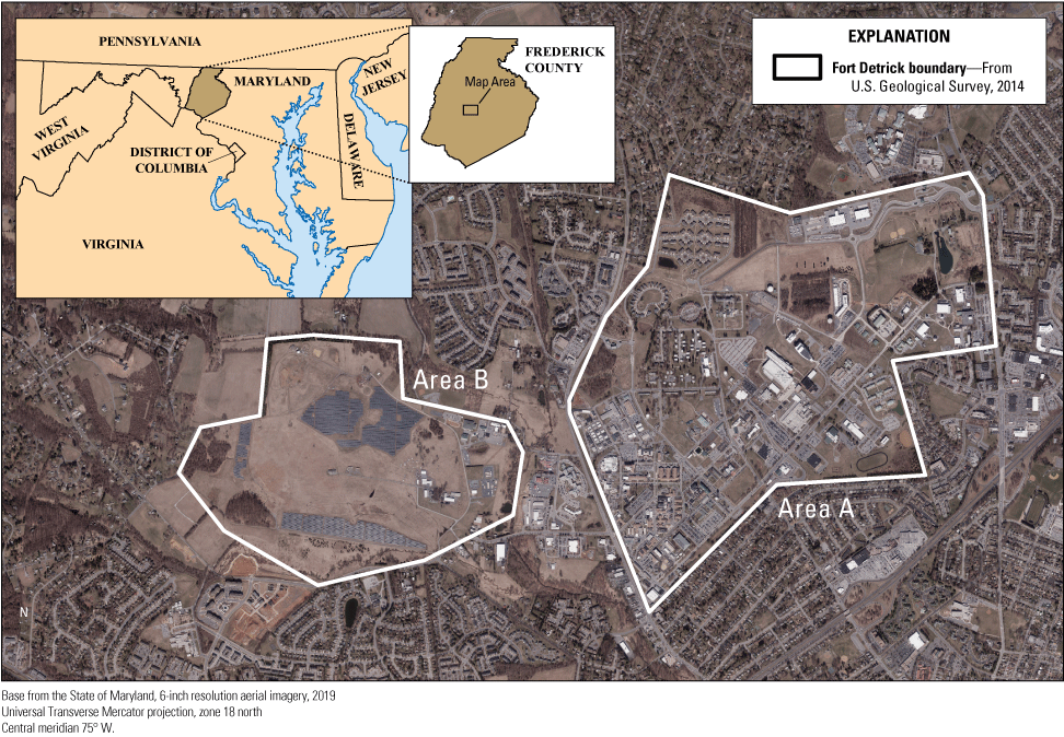
Locations of Areas A and B, Fort Detrick, Maryland.
Groundwater Contamination at Area B of Fort Detrick
Groundwater contamination at Area B of Fort Detrick primarily consists of volatile organic compounds (VOCs). A total of 13 VOCs have been detected in groundwater above the U.S. Environmental Protection Agency’s (EPA) maximum contaminant level, including the chlorinated solvents trichloroethane (TCE) and tetrachloroethane (PCE), the chlorinated fluorocarbon CFC-11, benzene, and other compounds (Arcadis Inc., written commun., December 20191 ). Biological and radiological materials, herbicides, and defoliants were also disposed of in Area B. Eight sites within Area B have been identified as former disposal sites that received laboratory and demolition wastes from the 1950s through the 1970s (Arcadis Inc., written commun., December 2019). These sites are primarily within the southwestern portion of Area B, though additional waste disposal sites that are sources of VOCs in groundwater are present in north-central Area B. Laboratory wastes including 55-gallon drums of TCE were disposed of in southwest Area B in a region designated “B-11.” High groundwater concentrations of TCE and PCE observed in the mid-1990s suggested TCE and PCE may be present as dense nonaqueous phase liquids. An interim removal action of the laboratory wastes and associated soils was performed in B-11 from 2001 to 2004, though the scope of the excavation was affected when live biological wastes were encountered (Arcadis Inc., written commun., December 2019). Although approximately 4,000 tons of soil, chemical containers, biological and medical waste, and construction debris were removed during the interim removal action, contaminated soils remained at the base of the excavation pits and the area was capped with impervious cover in 2010. Due to the presence of VOCs within the surficial karst limestone aquifer at Area B, in 2009 Area B Groundwater (site FTD-72) was placed on the National Priorities List with the EPA’s Comprehensive Environmental Response, Compensation, and Liability Act (CERCLA; also known as Superfund) Program (Arcadis Inc., written commun., December 2019).
At the time of publication, data were not available from Arcadis Inc.
Previous Investigations of Area B Groundwater
Numerous environmental investigations at Area B of Fort Detrick have been conducted from the early 1970s through the present. Over the course of the past five decades, more than 160 wells have been drilled and sampled as part of a series of investigations to understand the hydrogeological system well enough to fully characterize the nature and extent of contamination and design a suitable remedial strategy. This section summarizes the key previous investigations to understand the hydrogeologic system underlying Area B. A complete review of investigations to date is summarized by the draft final remedial investigation report (Arcadis Inc., written commun., December 2019).
Groundwater well installation at Area B took place during several phases (Arcadis Inc., written commun., December 2019). From 1974 to 1992, 51 groundwater monitoring wells were installed across Area B and sampled to characterize the presence of hazardous constituents. Limited lithologic and well construction data are available for some of these wells. Additional wells were installed during remedial investigation activities from 1994 to 1997; 16 wells were installed in 1994–95, and 6 wells were installed in 1997. In 1998, two additional wells were installed to expand the groundwater monitoring network. In 2011–12, 29 new monitoring wells were installed at Area B, including 8 nested well pairs. In 2013–14, eight monitoring wells were installed in six borehole locations in Area B and on private property to the southwest of Area B and in between Areas A and B. In addition to bedrock wells, 12 shallow offsite groundwater wells were installed in 2017 at or above the soil-bedrock interface. In 2017–18, 5 replacement wells and 16 new monitoring wells were installed across Area B.
Geophysical data has been collected at Fort Detrick Area B to characterize the hydrogeologic system. Several studies have attempted to characterize a geologic contact that occurs in the center of Area B between units of Cambrian and Triassic age, due to its potential influence on groundwater flow. The first was a seismic refraction study (Llopis and Simms, 1994), which also characterized the depth to bedrock and identified the contact between geologic units within the center of the site. The second was a surface geophysical survey undertaken in 2000 using magnetic, frequency-domain electromagnetics, electrical resistivity, and spontaneous potential methods (Arcadis Inc., written commun., December 2019). A third geophysical survey using an azimuthal square-array direct current resistivity method in the southeast corner of Area B was used to identify the presence of a fault or unconformity using these methods (Tepper and Phelan, 2001). An airborne geophysical survey using magnetic and electromagnetic sensors was completed in 2001 (Oak Ridge National Laboratory, 2001). Borehole geophysical data were collected in 2011–12; these data are discussed in a following section.
Studies to characterize the regional controls on groundwater and surface-water flow and identify preferential flow have also been undertaken. In 2000, the U.S. Army Corps of Engineers Research and Development Center performed lineaments analysis on a predevelopment aerial photograph of the Fort Detrick area from 1937 (U.S. Army Corps of Engineers, 2000). In this analysis, the orientation of linear features was recorded, as these can represent the orientations of fractures, faults, joints, and other linear structural features that can serve as preferential groundwater flowpaths. Approximately 17 percent of the features were field checked to ensure they were not anthropogenic. In 2000–01, the USGS undertook a seepage gain/loss study to identify stretches of Carroll Creek and other streams that considerably gained or lost flow. At streams surrounding Fort Detrick, the stream discharge, specific conductance, water temperature, and pH were collected. The results of the streamflow data collection were published in tabular format in James and others (2002).
In karst terranes, where the flow of groundwater can be rapid and complex because of dissolution features, dye tracing is often used as a tool to identify hydrologic boundaries, the rate of groundwater movement, and features relevant to contaminant transport including those determining transverse spread. Three qualitative dye tracer studies have been conducted at Fort Detrick, two at Area B and one at Area A. In these studies, activated charcoal passive samplers were used as the primary means for dye detection, which are useful for detecting the presence of dye at low levels but are not as effective as sample collection or fluorometric monitoring for determining the actual concentrations of tracer in the water (Taylor and Greene, 2008).
During the first tracer study in 1995, eosine, fluorescein, and rhodamine WT were injected at five locations across the eastern and northern portions of Area B and were monitored at 139 groundwater wells, springs, and surface water locations for 13–17 weeks (Ozark Underground Laboratory, Inc., 1997; White and others, 2015). The dye injection points included four 6-inch (in.) diameter shallow injection wells designed to inject water to the base of the epikarst, a zone of solution weathering that was estimated to include the uppermost 30 feet (ft) of the bedrock. The fifth injection point (called EDIP5) was a sinkhole that serves as a resurgence point for a stream (named “Stream 1”) and received rhodamine WT dye. Each injection point accepted 500 gallons of water at a minimum rate of 1 gallon per minute (gpm). Subsequent monitoring for residual dyes in 2008 at seven locations was conducted using activated charcoal passive samplers, with the goal of evaluating the presence of dyes injected in the 1995 test.
In 2001, a second groundwater tracing study was undertaken at Area A, to the east of Carroll Creek. Pyranine dye was injected at well ARW190-1, a 25-ft-deep well with a screened interval of 19 ft. The dye injection consisted of 10 pounds (lb) of 77-percent pyranine flushed with nearly 1,500 gallons of water at a rate of 3.5 gpm. Monitoring occurred for 139 days at 47 locations, including the injection well, Area A monitoring wells, offsite wells, Carroll Creek, and springs (Ozark Underground Laboratory, Inc., 2002). Activated charcoal passive samplers were used as the primary means to detect the dye, with a secondary reliance on grab samples.
In 2013, the most recent dye tracer study was implemented with the intent of characterizing the deeper flow system and identifying if deeper groundwater discharges to Carroll Creek (Arcadis Inc., 2018). On May 21, 2013, 15 lb of fluorescein were injected into well BMW68E with a screened interval of 313–328 ft below land surface (bls), at a previously identified void. The following day, 23 lb of eosine dye was introduced into well BMW67C, which is screened at a depth of 140–155 ft bls. Samples were collected at 127 locations, including monitoring wells, springs, streams, ponds, and private wells. The monitoring period for the study was 9 months.
In addition to the work described above, in the course of remedial investigation activities from 2010 to 2017, horizontal flow meter surveys at 81 well locations, synoptic groundwater sampling events for potential groundwater contaminants, spring and stream surveys, and potentiometric mapping were performed (Arcadis Inc., written commun., December 2019).
Purpose and Scope
This report supports refinement of the conceptual site model of Area B at Fort Detrick using hydrologic data collected at the site from 2017 to 2020 and the results of prior investigations at the site. The report includes a review of the regional and site hydrogeology, the results of a 2019 synoptic groundwater chemistry sampling event, and a water budget analysis using a groundwater and stream-monitoring network established at the site as part of this study. The results of this study are interpreted to refine the following aspects of the hydrogeologic conceptual site model:
-
• Evaluation of structural controls on regional groundwater flow.
-
• Characterization of groundwater system responsiveness to hydrologic events ranging from individual storm events to interannual variability.
-
• Evaluation of potential for regional interbasin groundwater flow that bypasses Carroll Creek.
-
• Characterization of the sources and timing of groundwater recharge.
-
• Determination of the degree of vertical connectedness and geochemical similarity between different regions of the aquifer.
-
• Evaluation of in situ monitoring methods to quantify residual dye concentrations from prior dye tracer tests.
The aspects of the conceptual site model listed above advance the understanding of the complex karst aquifer underlying the site at a range of temporal (daily to interannual) and spatial (sitewide to regional) scales. Informed decision-making about remedial strategies, the interpretation of contaminant concentration trends, and the assessment of contaminant fate and transport benefit from a conceptual model that characterizes the physical hydrology using multiple independent approaches and that is refined as new data are collected (Interstate Technology and Regulatory Council, 2017). In this study, regional groundwater flow assessments including the evaluation of interbasin groundwater flow, structural controls on groundwater flow, and the sources of groundwater recharge provide information on the ultimate destination of water recharged at Fort Detrick Area B on long timescales. Site-scale groundwater flow assessments including responsiveness to hydrologic events, variability in groundwater gradients, and the degree of vertical connectivity within the aquifer provide information to support the interpretation of contaminant patterns and trends collected in separate monitoring programs at the site.
Background
The following sections describe the geologic and hydrologic setting of Fort Detrick, a description of karst hydrogeologic processes, and the findings of regional karst hydrogeologic studies. The previously described conceptual site model for Fort Detrick Area B is introduced and opportunities for refining this conceptual model are identified.
Geologic Setting
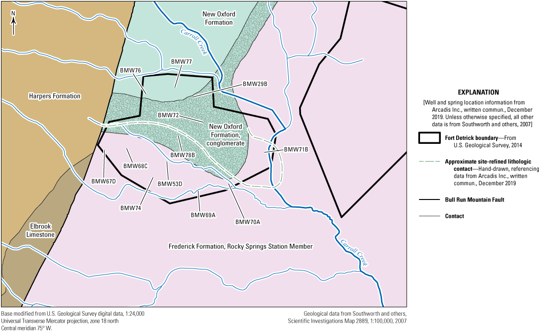
Fort Detrick Area B is located at the west edge of the Fredrick Valley synclinorium and in the Piedmont physiographic province in Maryland, a region characterized by a humid subtropical climate, rolling hills, and well-developed fertile soils. The geologic setting is summarized in figure 2. The geologic units underlying Fort Detrick Area B are shown in figure 2A. The dashed line in A indicates the approximate boundary between the conglomerate of the New Oxford Formation and the Rocky Springs Station Member of the Frederick Formation, which is refined in the study area based on boring logs and field outcrop observations. The physiographic regions in the vicinity of Fort Detrick are shown in figure 2B. The extent of Cambrian and Triassic units within the western Frederick Valley are shown in figure 2C, and figure 2D presents a stereonet with the bedding orientation of select units in the western Frederick Valley shown as poles to the plane. The locations of these bedding observations are shown in figure 2C.
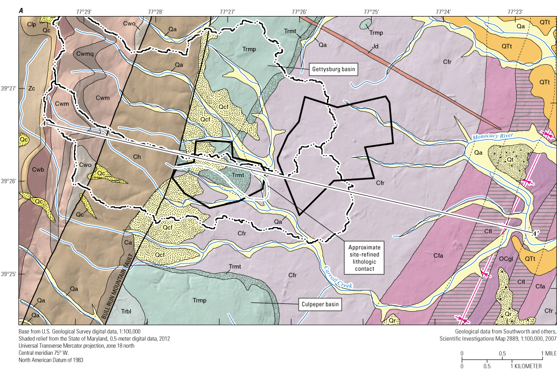
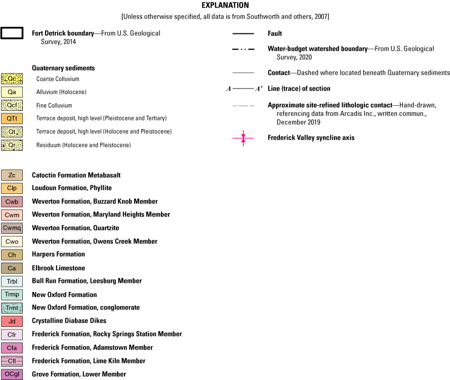
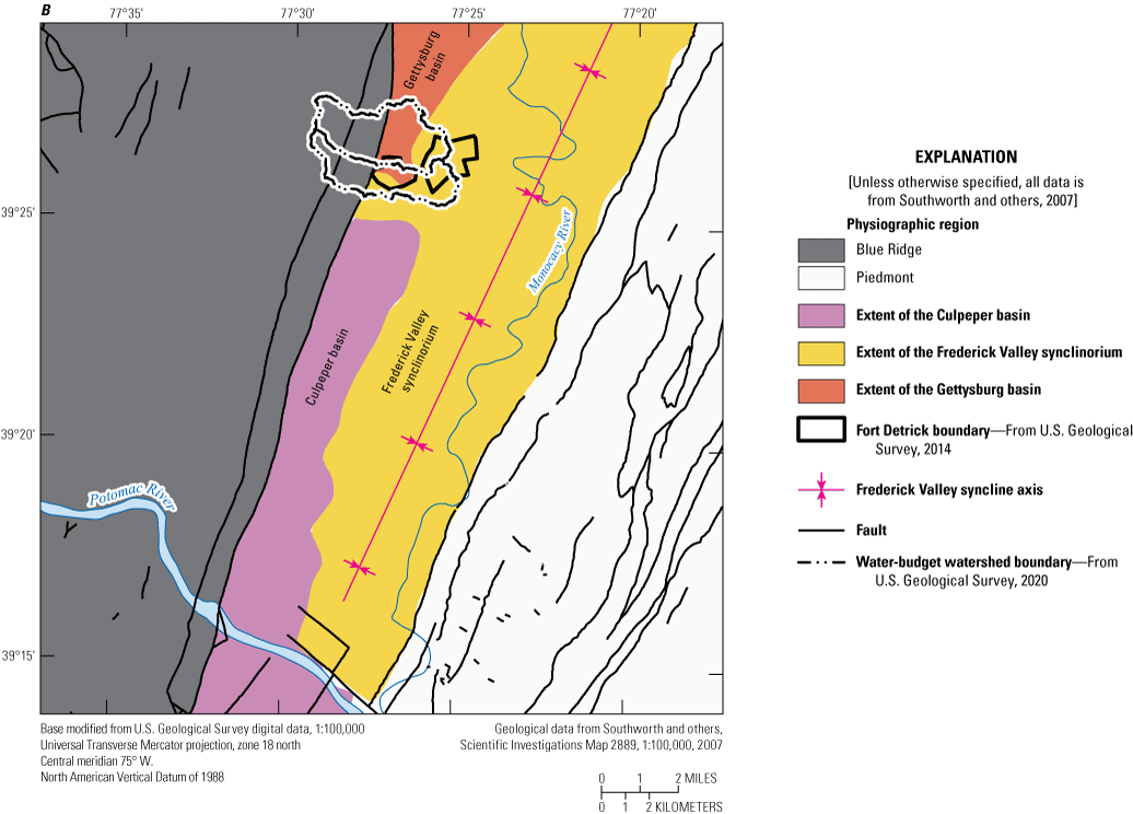
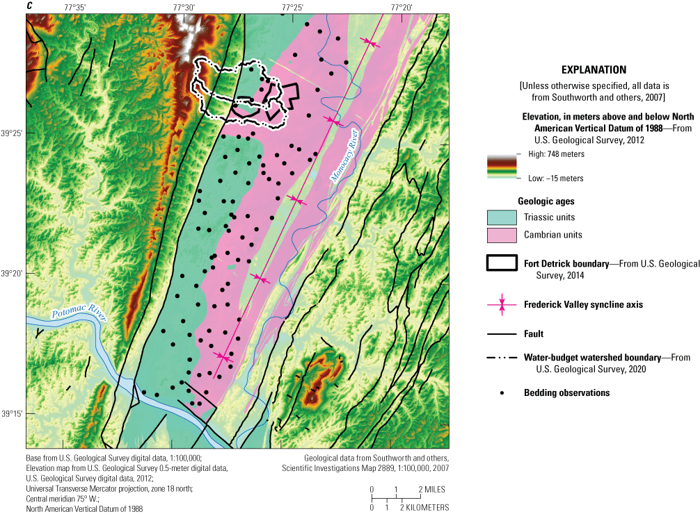
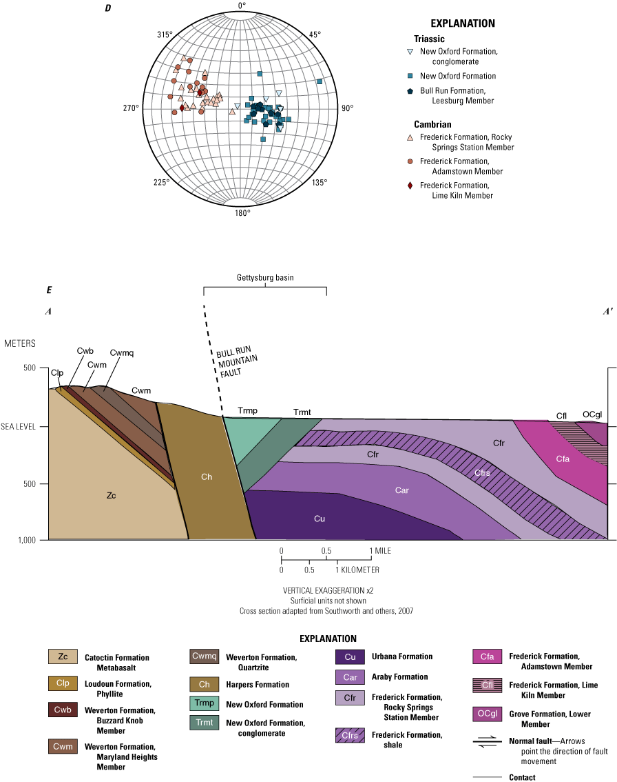
Geologic units and structural features in the vicinity of Fort Detrick Area B adapted from Southworth and others (2007), including A, site map of geologic units; B, regional physiographic provinces; C, extent of Cambrian and Triassic units within the western Frederick Valley; D, the orientations of western Frederick Valley bedding; and E, a geologic cross-section adapted from Southworth and others (2007).
To the west of Area B lies the Bull Run Mountain Fault, a regional normal fault that marks the boundary between the Piedmont and Blue Ridge physiographic provinces. Near Area B, the strike of the Bull Run Mountain Fault is 72°. Immediately to the west of Area B are Early Cambrian rocks of the Harpers Formation and Weverton Formation, which were metamorphosed during the late Paleozoic Alleghenian orogeny (Southworth and others, 2007). The carbonate and sedimentary rocks that compose the Frederick Valley synclinorium were deposited in a shallow marine environment in the Late Cambrian (Southworth and others, 2007). Much later, extensional forces created the Bull Run Mountain Fault, which was active throughout the Triassic and Jurassic. This fault created two half-graben basins near Area B: the Gettysburg basin to the north and the Culpeper basin to the south. Arkosic sandstones, claystones, and breccias were deposited in both basins and the units currently dip 20–30° W. (Southworth and others, 2007).
Site Geologic Units
Within the study area, there are several mapped geologic units that comprise the surficial fractured rock and karstic groundwater aquifer system. These units can be grouped into structural features that form the Blue Ridge, Frederick Valley synclinorium, and Triassic basins.
Blue Ridge Units
In the western portion of the study watersheds, the Blue Ridge is underlain by the Lower Cambrian Weverton Formations of the Chilhowee Group. The Weverton Formation is stratigraphically lower and crops out further to the west within the Blue Ridge anticlinorium. Its members (Owens Creek, Maryland Heights, and Buzzard Knob) are all primarily quartzite with minor interbedded siltstone. The mapped Chilhowee Group unit within the study watersheds (fig. 2A) is the Harpers Formation, a foliated metasiltstone and biotite-chlorite-muscovite-quartz phyllite (Southworth and others, 2007).
Frederick Valley Synclinorium Units
The Frederick Formation is composed of thick intervals of limestone and dolostone with minor amounts of shale and sandstone. The unit was divided into three separate members by Reinhardt (1974). These are, in ascending order, the Rocky Springs Station Member, the Adamstown Member, and the Lime Kiln Member. The basal Rocky Springs Station Member is the surficial unit within the southern portion of the Area B boundary. It is a clast-containing, dark-gray, lumpy-bedded dolomitic limestone that was deposited at the base of the continental slope. Southworth and others (2007) describe the upsection intervals of the Rocky Springs member as a flaggy-bedded limestone with dusky-yellow to light-olive-gray, silty, dolomitic partings and laminations. Intervals of medium-dark-gray polymictic breccia (cemented angular clasts from multiple rock types) as thick as 30 ft are present as a consequence of repeated continental slope submarine sides; these intervals grade upsection into planar-bedded arenaceous limestone. Clasts range from sand size to 20 in. in diameter on the west side of the Frederick Valley. Southworth and others (2007) mapped a contiguous interval of grayish-black shale as interbedded within the Rocky Springs Station Member that is as much as 60-ft thick. This unnamed shale unit is shown to crop out on the more steeply dipping east side of the Fredrick Valley synclinorium. In cross-section they show the shale unit to be present at depth of less than (<) 300 ft on the west side of the syncline and the unit does not crop out at Fort Detrick Area B. The bedding of the Rocky Springs Station Member of the Frederick Formation west of the city of Frederick is shown to consistently dip east-southeast at ~30°. The Adamstown and Lime Kiln Members, also limestone units, crop out further to the east of the study area. The bedding information for the Cambrian units between the Potomac River and the north edge of the mapped quadrangle, between the Bull Run Mountain Fault and the central axis of the Frederick Valley syncline are shown in figure 2D; these units dip to the southeast.
Triassic Basin Deposits
The sandstone and conglomerate units of the Triassic New Oxford Formation were deposited within the half-grabens formed by the Bull Run Mountain Fault, and the southern part of the Gettysburg basin is identified as the New Oxford Formation. There have been some differences in how authors have described the geologic units in the Gettysburg and Culpeper basins. Southworth and others (2007), following previous workers, designated the sandstone unit in the Culpeper basin as the Manassas Sandstone. Both the New Oxford Formation and Manassas Sandstone are described as containing an upper reddish-brown, medium-coarse grained sandstone and claystones underlain by a basal carbonate conglomerate to breccia. Southworth and others (2007) group the depositional units in the Culpeper and Gettysburg basins using the nomenclature established for the Culpeper basin. In this report we use the nomenclature for the Gettysburg basin, as that is the Triassic basin that underlies Fort Detrick Area B. A description of the geologic nomenclature after that of Weems and Olsen (1997) and Southworth and others (2007) is shown in table 1. Bedding information for the Triassic units in both basins between the Potomac River and the north edge of the mapped quadrangle, between the Bull Run Mountain Fault and the central axis of the Frederick Valley syncline, is shown in figure 2D; these units dip gently to the west. The difference in orientation between the Triassic units and Cambrian units is also illustrated in cross section in figure 2E.
Table 1.
Relation of geologic units underlying Fort Detrick, Area B described by Weems and Olsen (1997) and Southworth and others (2007).Site Hydrologic Setting
Area B is located within the Monocacy River Basin and is bordered by multiple streams and springs (fig. 3). On its east edge, Area B is bordered by Carroll Creek. A small perennial stream is located along the south edge that is referred to as “Stream 2” by prior investigations (Arcadis Inc., 2014). The central portion of Area B contains a local depression with an ephemeral wetland area; during wet intervals, water flows through channels in the tall grass at the site and during dry intervals the channels become dry or stagnant. Previous investigations have named these channels “Stream 3” and “Stream 4.” Standing surface water is also present at times along the west edge of Area B, where water from culverts underneath Kemp Lane enters the site. In previous investigations, water entering the western portion of the site is called Stream 1. Stream 1 terminates in a swallet, where the stream enters the groundwater system directly.
Hydrologic features near Fort Detrick, Frederick, Maryland.
Karst Hydrogeology
Karst features such as sinkholes, subsurface conduits, and springs are the result of geologic, geomorphic, anthropogenic, and climatic factors. Within Maryland’s Frederick Valley (in which Area B is located), the presence of karst features is determined by the principal factors of lithology, fracturing, and ancestral drainage patterns (Brezinski, 2004, 200710). The early Paleozoic carbonates (including the Rocky Springs Station Member of the Frederick Formation) and the Triassic units that comprise the Culpeper and Gettysburg basins (including the New Oxford Formation) have similar physiographic and solubility characteristics. However, there is a considerable difference in the predominant orientation of fractures and joints between the Ordovician Grove Formation (within the Frederick Valley synclinorium) and the Triassic Leesburg Member of the Bull Run Formation of Southworth and others (2007), within the Culpepper basin (Brezinski, 2007). The difference reflects the tectonic stresses acting on these units during the formation of these units. The Grove Formation has a predominant joint strike of 288°, nearly perpendicular to the Bull Run Mountain Fault, whereas the Leesburg Member has a predominant joint strike of 87°, subparallel to the fault. Karst features, including sinkholes, often align with the dominant joint directions (Brezinski, 2007). These structural controls are inferred to enhance the formation of solutionally enlarged features by way of preferential routing of water along the predominant joint directions.
Studies of groundwater movement within karst in the region surrounding Fort Detrick provide a framework for understanding groundwater flow. Although outside of Area B, intensive field studies, dye tracing, geospatial analysis, and modeling work has taken place in the Valley and Ridge Province of Virginia, a region underlain by carbonate rocks and containing karstic features that continues into Maryland in the Hagerstown area. The Valley and Ridge Province is composed of different geologic units with a differing geologic history; however, the similarity of climate and geomorphic influences means that these studies are useful analogues for the regions of the Frederick valley underlain by carbonates.
A series of studies have informed groundwater flow in the vicinity of Leetown, West Virginia and within the Hopewell Run watershed area (Kozar and others, 2008), which has been extended to the larger Opequon Creek watershed (Kozar and Weary, 2009; Yager and others, 2013) located in Clarke County, Virginia (Nelms and Moberg, 2010), and draws upon previous assessments of groundwater flow developed in Frederick County, Virginia (Harlow and others, 2005) and in Jefferson and Berkely Counties of West Virginia (Kozar and others, 1991; Shultz and others, 1995). This body of work has contributed to the conceptualization of groundwater flow in these karst environments.
The major findings of these analogous studies indicate that groundwater flow in the Valley and Ridge Province is complex. Groundwater primarily resides within fractures and solutionally enlarged bedding planes. The fractures and conduits that transmit much of the water are a small proportion of the overall aquifer volume. The orientation and size of these features, and therefore the rate and direction of groundwater flow, is strongly controlled by complex geologic structures such as cross-strike faults and overturned or tightly folded bedding. Where bedding planes dip steeply, groundwater may circulate to deeper depths than is typical in karst groundwater systems. Low permeability geologic units can act as barriers to flow, increasing flow through fractures, faults, and other sources of secondary and tertiary porosity. The locations of groundwater discharge to the surface, including springs, are typically associated with structural features or lithologic contacts with low-permeability units. Groundwater recharge occurred primarily as a distributed process across a broad area, except during intense localized rainfall. Under those conditions, focused recharge to sinkholes can occur.
The surficial weathered zone of the aquifer underlying the soil, called epikarst, is an important control on shallow groundwater movement. The epikarst is characterized by a high degree of carbonate dissolution, high-angle joints that allow rapid infiltration into the aquifer, and relatively fast groundwater flow (on the order of tens to hundreds of feet per day) as indicated by tracer tests, and is discussed in a following section. The reported depths of the epikarstic zone are between 30 and 60 ft. Below the epikarst is a zone of fractured carbonate bedrock (referred to as the “intermediate zone” by Kozar and others [2008]) with decreasing fracture size and density with depth that has a decreased hydraulic conductivity relative to the epikarst. Estimates of the groundwater age in this zone are approximately 15 to 50 years (McCoy and Kozar, 2008). Below a depth of approximately 250 ft, the fracture apertures decrease and aquifer-test data show that the hydraulic conductivity decreases by half from the intermediate zone. Limited information is available on the groundwater age within the deeper portions of karst aquifers in the Valley and Ridge Province of Virginia. In the fractured and folded karst of the Opequon Creek watershed, Yager and others (2013) reported that 20 sampled springs had a median apparent age of 4.4 years and a median of 14 percent of the water in the samples was recharged prior to 1953.
Dye tracer tests conducted within the Valley and Ridge Province of Virginia and Maryland provide a basis of comparison for the properties of the epikarst and for the results of previous tracer tests at Fort Detrick. Dye tracer tests were conducted at the USGS Leetown Science Center in 1979–80 (Kozar and others, 2008); at the Leetown Pesticide Site and Jefferson County Landfill Site (NUS, 1986); in Jefferson County, West Virginia (Kozar and others, 1991); in the Leetown area in 2004–05 (Kozar and others, 2008); and at the Central Chemical site in Hagerstown, Maryland in 2014–15 (Field, 2017). These studies contain some common observations. Dye recovery at springs typically takes place on the order of weeks and detections can take place several miles from the injection point. Estimated groundwater interpreted linear velocities range from (1) 171 ft/day (NUS, 1986); (2) 50–840 ft/day (along strike) to 30–235 ft/day (perpendicular to strike) (Kozar and others, 1991); (3) 12.5–610 ft/day with a median of 50 ft/day (Kozar and others, 2008); and (4) 16–66 ft/day (Field, 2017). Although these linear velocities are much more rapid than other types of aquifers, the rates are much slower than many reported in conduit-dominated karst aquifers where velocities of 1,000–10,000 ft/day are reported (Jones, 1997; Kozar and others, 2008). This has been interpreted to reflect the presence of a slow-flow component connected with the more rapid transport pathways. More rapid interpreted linear velocities and stronger recoveries were generally observed when dye was released in losing stream reaches (Kozar and others, 2008). Heavy precipitation events were observed to mobilize dye that was sequestered in the subsurface in relatively immobile zones. Dye resurgence was typically observed at multiple points. An interpreted linear velocity of 1,640 ft/day was estimated by Doctor and others (2011) for a karst spring in the northern Shenandoah valley, though only 12 percent dye mass recovery after 5 weeks of monitoring was interpreted to reflect a considerable interaction with slow-moving groundwater.
The groundwater budgets developed by previous studies in the region show that the rock type, and therefore the prevalence of solution conduits, has a strong influence on groundwater recharge rates. Groundwater recharge in the Opequon Creek watershed, as estimated from stream base flow records, were found to range from 6.6 to 9.8 inches per year (in/yr) for carbonate rocks and 3.6 to 5.5 in/yr for siliciclastic rocks (Yager and others, 2013). The water budget of the karstic Hopewell Run watershed reported per unit stream base flow as 17.73 in/yr (46 percent of precipitation) and evapotranspiration (ET) as 24.23 in/yr (63 percent of precipitation) for the period of October 2003–September 2005 (Kozar and others, 2008).
Previously Described Conceptual Site Model at Fort Detrick
Based on the previous work to characterize the site, a conceptual site model (CSM) for groundwater at Area B has been described (Arcadis Inc., 2014; Arcadis Inc., written commun., December 2019). The descriptions of the groundwater system contained within these two reports are referred to in the rest of the report as “the CSM” or “the previously described CSM.” This section details the primary features of this CSM concerning Area B hydrology and the results of studies used to form the hydrogeologic descriptions within the CSM.
In the previously described CSM, Area B hydrology is strongly influenced by karst features within the carbonate lithology, which is visible as sinkholes, springs, and in subsurface voids that are interpreted to be solutionally widened. The surface of Area B is described as mantled by a heterogeneous soil overburden layer that is locally as much as 30-ft deep and thins to a few feet deep near Carrol Creek. Seismic refraction surveys show that the depth to the bedrock-soil interface is locally highly variable (Llopis and Simms, 1994). Several attempts to characterize the contact between the limestone of the Frederick Formation and the basal conglomerate of the New Oxford Formation generally confirm the presence of this geologic transition in the center of the site, though the contact is interpreted as nonlinear and complex. The previously described CSM describes the contact as a steeply dipping strike-slip transfer fault, though a lack of wells intersecting this feature leave the physical nature of this contact unconfirmed.
In most of Area B, the water table is described as occurring within the soil overburden layer. Below the soil layer, weathered bedrock containing subsurface voids is present, with a decreasing frequency and size of solution features to a depth of approximately 150 ft. The greatest proportion of solution features are observed at depths of 32–65 ft, with decreasing proportions to 131–161 ft deep, after which very few features are observed (White and others, 2015). However, solution voids more than 300-ft deep are also observed in some locations. The two primary geologic units underlying Area B are the limestone of the Frederick Formation and the basal conglomerate of the New Oxford Formation. The units are described as equally influenced by karst dissolution processes and have similar bulk hydraulic properties, but multiple interpretations are presented as to whether the units are hydraulically connected or the geologic contact acts as a flow barrier. For example, the presence of springs in Carroll Creek at the location where it crosses the contact between the limestone of the Frederick Formation and the basal conglomerate of the New Oxford Formation has been suggested to result from differing hydrologic properties. A steepening of hydrologic gradients close to Carroll Creek and within the conglomerate of the New Oxford Formation are also attributed to a decrease in transmissivity in the conglomerate (Arcadis Inc., written commun., December 2019). Conversely, the results from dye tracing studies, further discussed in the following section, show transport of dye upward and downward across the geologic contact. In Arcadis Inc. (2014), the contact was described as “transparent” from a hydrostratigraphic perspective, with similar bulk hydrographic properties between the two geologic units resulting in no influence on groundwater flow. A third unit (the sandstone or claystone member of the New Oxford Formation) is observed in the northern part of Area B and is not karst-forming or as transmissive as the two other units.
The flow of groundwater within the bedrock, although complex and locally driven by the presence and orientation of fractures and voids, is generally from west to east towards Carroll Creek. The exception is a local hydrologic mound or high point in the northern portion of the site adjacent to an active landfill that is attributed to the local presence of the lower transmissivity of the claystone of the New Oxford Formation (Arcadis Inc., written commun., December 2019). A potentiometric surface map developed using water elevations reported in the draft final Remedial Investigation Report is shown in figure 4 (Arcadis Inc., written commun., December 2019). Groundwater gradients are generally steeper along the west edge of Area B than within central Area B. Groundwater gradients indicate convergence of flow along the Carroll Creek corridor, though interpreted flow paths do not converge precisely at the stream channel. Both upwards and downwards vertical gradients are observed in periodic potentiometric levels, though most reported gradients are upwards. Generally, the western region of Area B is described as an area of focused groundwater recharge as streams flow from the crystalline bedrock of Catoctin Mountain onto valley karstic units. Streams in this area are observed to lose flow to groundwater and at least one swallet is observed.
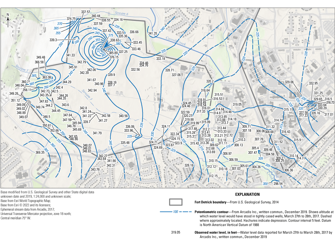
Potentiometric surfaces of water elevations reported by Arcadis Inc., written commun., December 2019.
The previously described CSM identifies geologic bedding, fracture and joint sets, and geologic contacts as potential controls on groundwater flow and the development of karst features that act as preferential flow paths. The bedding orientation of the New Oxford Formation at Area B is described as gently westward dipping, whereas the bedding orientation of the Rocky Springs Station Member of the Frederick Formation is more complex and varied, with local dips exceeding 30 degrees, including under the waste disposal areas in the southwest of Area B. The previously described CSM defines a joint orientation perpendicular to the Bull Run Mountain Fault based on a regional geologic analysis conducted by Brezinski (2007). In the vicinity of Area B, 122 linear features were identified through photogeologic analysis, with a predominant northwest-southeast strike direction roughly perpendicular to the Bull Run Mountain Fault (U.S. Army Corps of Engineers, 2000). The presence of numerous springs within a concentrated area along Carroll Creek suggests an association with the contact between the New Oxford Formation and Frederick Formation, possibly as a result of preferential flow along the contact and a difference of hydrologic properties between the formations. The Bull Run Mountain Fault is not considered a preferential flow zone.
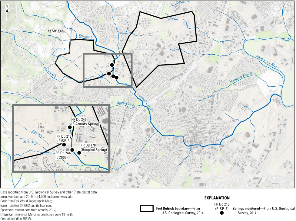
A key aspect of this CSM is all groundwater flow from Area B eventually discharges into Carroll Creek; deep recirculation may occur, but all flow converges into the so-called primary discharge zone. This proposed zone, located along Carroll Creek from Area B to the confluence of “Stream 2” shown in figure 3, contains numerous springs that discharge groundwater to Carroll Creek; the springs have been identified in previous investigations and are located both on and off the Area B footprint. There are several springs that reach the surface at a higher elevation than the banks of Carroll Creek, including South Armory Spring, RISP-3, Hospital Spring, and CC003. The documented springs are primarily on the west bank of Carroll Creek, though springs (including Hospital Spring) are also located on the east side. Springs are not reported within the stream along the south boundary of Area B. The location of gaining and losing reaches of Carroll Creek were assessed in the 2000–01 seepage run data reported by James and others (2002). The mapped results of this data are presented in figures 1.1–1.10 of appendix 1. In general, stream discharge, specific conductance, and pH increase along the stream network leading to the Monocacy River. The increasing specific conductance and pH is consistent with the addition of groundwater having greater contact time with the carbonate rocks in the drainage basin. Strongly gaining conditions are observed along the east edge of Area B, reflecting the input of numerous springs. These conditions are slightly more pronounced in April 2001 than September 2000. Losing conditions are observed at some locations along the south boundary of Area B during both September 2000 and April 2001. Streamflow was lower in September 2000 than April 2001.
The previously described CSM was developed, in part, on the interpretation of the three dye trace studies conducted at Area A and Area B from 1995 to 2013. During the 1995 tracer study, rhodamine, eosine, and fluorescein injected into the shallow borehole injection points were detected during the study period at wells and springs to the east of the dye injection points, indicating the west-to-east movement of groundwater toward Carroll Creek (Ozark Underground Laboratory, Inc., 1997; White and others, 2015). During the test, dye was not detected at monitoring points south of Area B. The travel rates calculated for fluorescein and eosine dye using a straight-line distance and the first arrival after introduction range from 79 to 246 ft/day, with a mean of 151 ft/day. No rhodamine dye was detected during the test, but a fluorescent dye was detected during a subsequent dye test 18 years later in 2013 at eight springs and one well. The fluorescence peak properties of this material were close to, but out of range of, typical rhodamine peaks. These peaks were interpreted to be rhodamine affected by a deaminoalkylation process that is perhaps related to the alteration of the dye in the environment over the 18-year span (White and others, 2015). The fluorescent dye could also be an unknown material with similar fluorescent properties. The detection of rhodamine-like dye was observed east of the rhodamine dye injection point and along Carroll Creek. A summary of the interpreted flowpaths for the 1995 test, with the assumption that the rhodamine-like observations originated from the rhodamine injection point are shown in figure 5. Dye injected in the limestone of the Frederick Formation was detected in the conglomerate of the New Oxford Formation, indicating hydrologic connectivity between those two units.
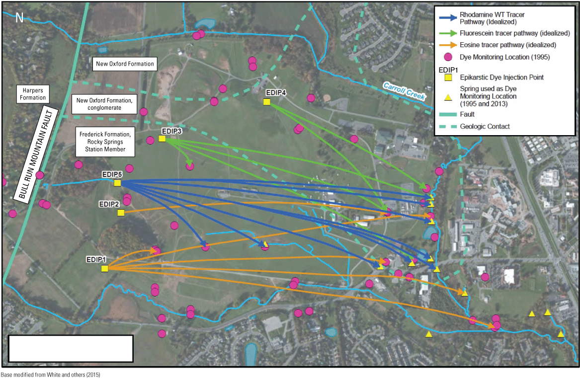
Summary of injection locations and detections of dye during the 1995 dye tracer test at Area B, Fort Detrick, Maryland (modified from White and others, 2015).
During the 2001 dye tracer study on Area A, no pyranine dye was detected within any of the springs or surface water locations, which was interpreted as a slow transport rate within the aquifer, though no linear velocities were calculated in the study (Ozark Underground Laboratory, Inc., 2002). Dye was detected in a radial pattern from the injection point, with the greatest number of detections south of the injection point. A summary of detections during the 2001 dye tracer test is shown in figure 6.
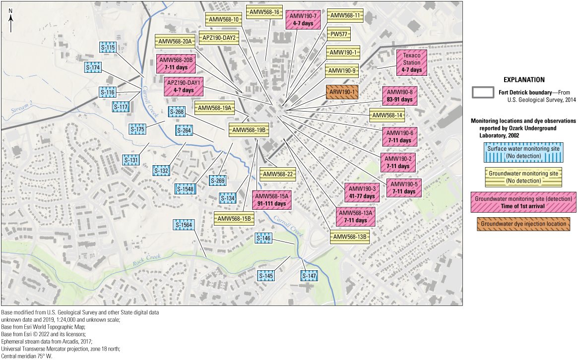
Summary of injection locations and detections of dye during the 2001 dye tracer test at Area A, Fort Detrick, Maryland.
During the 2013 dye tracer study, eosine was detected at more locations (34) than fluorescein (6). All dye was detected to the east of the injection locations, as shown in figure 7. The interpreted linear velocities of first arrival between the injection locations and springs along Carroll Creek were 91–168 ft/day (eosine from BMW67C) and 30 ft/day (fluorescein from BMW68E) (White and others, 2015). The mean linear velocity from injection locations to monitoring wells was 51 ft/day (eosine from BMW67C) and 10.5 ft/day (fluorsecein from BMW68E) (White and others, 2015). The detection of both dyes at springs indicated the presence of upward transport paths and a hydrologic connection between the deep groundwater and Carroll Creek springs. The dye tracer injected at intermediate well BMW67C (eosine) was detected at more monitoring locations and arrived more quickly than dye tracer injected at deep well BMW68E (fluorescein). Dye injected in the limestone of the Frederick Formation was detected in the conglomerate of the New Oxford Formation, indicating hydrologic connectivity.
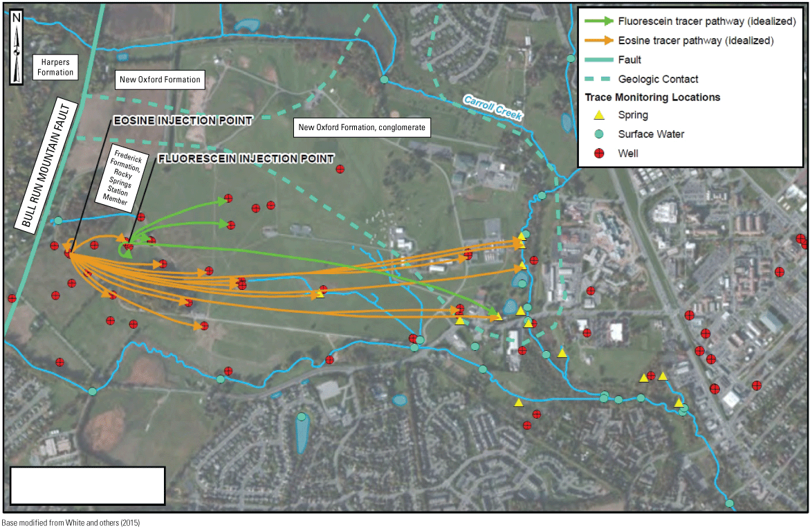
Summary of injection locations and detections of dye during the 2013 dye tracer test at Area B, Fort Detrick, Maryland (modified from White and others, 2015).
Taken together, these three tracer tests are interpreted in the previously described CSM to indicate that groundwater from Area B discharges exclusively to Carroll Creek, though the karst aquifer has a notable storage component arising from poorly interconnected karst conduits that retains dye mass and results in dye detections over the course of many years following dye injection. The CSM interprets these studies and the body of hydrogeological work at Area B as supportive of “a standard hydrologic basin model in which groundwater and surface water flow are contained within a single coincident drainage basin” (Arcadis Inc., written commun., December 2019).
Opportunities To Improve the CSM
The CSM previously described by Arcadis Inc. (2014) and the draft final remedial investigation report (Arcadis Inc., written commun., December 2019) is based on a synthesis of a considerable body of site investigations spanning from the 1970s through 2017. As discussed in these documents, a robust conceptual site model is developed when possible from multiple independent lines of evidence. When multiple potential interpretations of the hydrogeologic data are present, a weight-of-evidence approach can synthesize independent results into a holistic conceptual model. Conceptual models for complex hydrogeologic systems are typically refined as additional data are collected at a site (Interstate Technology and Regulatory Council, 2017). A review of the previously described CSM identified several opportunities for further refinement through the collection of new data and independent evaluation of previously collected data.
The site geologic setting is complex and has a direct influence on the formation of karst features, the preferential flow of water within the fractured rock, and the location of springs. Although the previously described CSM discusses the local site geology in detail, regional structural influences on the groundwater flow system receive less consideration. Additionally, comparison of the Area B groundwater system to other well-studied karst groundwater systems within the mid-Atlantic will either further support the CSM or identify gaps in understanding. In this study we include an independent review of regional geologic structures, geophysical data, the state of knowledge on their influence on the Area B groundwater system, and provide a comparison with other karst groundwater systems to refine this aspect of the conceptual site model.
Karst systems are highly dynamic and rapidly respond to hydrologic changes. Depending on the conduit density, conduit connectivity, and structural controls within the aquifer, the magnitude and temporal scale of hydrologic responses to hydrologic events can vary. The responses can include changes in flow directions, changes to the locations of surface watershed and groundwatershed boundaries, and activation of different portions of the karstic and epikarstic conduit network (White, 1999). Understanding this variability is the key to characterizing any karst groundwater system. To date, groundwater gradients, water levels, and streamflow at Area B have primarily been characterized using synoptic (point-in-time) observations. These point-in-time observations may be suitable for characterizing seasonal or interannual responses but may not adequately characterize short-lived but important hydrologic responses. In this study, improved high-frequency hydrologic monitoring characterizes the event-driven changes to the aquifer.
One of the primary challenges of characterizing a karst groundwater system is to define the groundwatershed. In some systems this may be quite different from the topographically defined surficial watershed resulting in what is termed interbasin groundwater flow. Understanding the groundwatershed and its relation to the topographic watershed is important to characterize the ultimate destination of water recharged into the aquifer. Due to the orientation of Catoctin Mountain and the Monocacy River, regional groundwater flow from the west to east beneath Area B that bypasses the surficial watershed should be considered. The two prior dye tracer studies implemented at Area B were intended to help define the groundwatershed and determine the destination of water recharged within Area B contaminant source areas. As discussed in the draft final remedial investigation report (Arcadis Inc., written commun., December 2019), the design and interpretations of the study did not rule out a deeper regional groundwater flow path that bypasses Carroll Creek and flows to Monocacy. An independent assessment on the potential for interbasin groundwater flow will provide an additional line of evidence that can support the interpretation of the dye tracer results. In this study, a water budget approach is used to evaluate the potential for interbasin groundwater flow.
The depth of groundwater circulation and the influence of multiple porosities on connectivity within the aquifer underlying Area B has important implications for understanding contaminant transport and developing potential remedial strategies. One of the motivations for the 2013 dye tracer study was to investigate the depth of surface connection within the groundwater system and elucidate the connectedness of the deep and shallow flow within the aquifer by injecting dye into the deep portion of the aquifer. Dye injected deep within the aquifer was subsequently detected at surface springs, indicating a connectivity with the surface. However, observed dye retention at the injection locations also indicates that at depth within the aquifer there is the potential for storage in flowpaths relatively disconnected from the surface at the timescale of interest. Improved understanding of the degree of vertical mixing within the aquifer and identification of the connectivity between different locations within the aquifer using independent methods will support the interpretation of the past dye tracer studies. In this study, a synoptic age dating and geochemical analysis provides independent lines of evidence on the vertical structure, lateral connectivity, and sources of groundwater recharge across the aquifer.
The presence of dyes reported long after their injection informs the understanding of the hydrologic system. Continued evaluation for the presence of dyes from the 1995 and 2013 injection events on a periodic basis is beneficial for interpreting these studies and understanding the storage and release of the dyes. To date, passive sampling and grab sampling techniques have been employed. In situ monitoring methods for dye concentrations are also employed during dye tracer tests (for example, Field [2017]). These methods have an improved ability to characterize the timing of dye resurgence, though they can be limited by interference due to site-specific factors. In this study, we analyzed water samples collected during a routine sampling event for residual dyes, applied in situ monitoring to three spring sites, and performed benchtop laboratory experiments to quantify the detection limit of these methods at Fort Detrick.
Methods of Data Collection
This study included the collection of hydrologic and geochemical data to characterize the hydrogeologic system. A network of sensors was placed in groundwater wells, springs, and Carroll Creek to record the raw data used to evaluate groundwater gradients, calculate a water budget, estimate aquifer storage changes, and evaluate the presence of fluorescent dyes. A single geochemical sampling event in September-October 2019 collected samples from which the age and geochemical characteristics of the water were evaluated.
Hydrologic Monitoring Network
A telemetered hydrologic monitoring network was installed at Area B to monitor the responsiveness of the aquifer to changes in hydrologic conditions and to conduct the water budget analysis. Two USGS streamgages were installed on Carroll Creek and monitored for stream stage, discharge, specific conductance, and water temperature from October 2017 to October 2020. The upstream Carroll Creek streamgage has an area of 4.21 square miles (mi2) (10.90 square kilometers [km2]), and the lower Carroll Creek streamgage has an area of 7.30 mi2 (18.90 km2). A precipitation gage was installed at the upstream gage on the north edge of Area B. Water-level monitoring was conducted at eight monitoring wells from September 2018 to October 2020. An additional four wells were added in December 2019 to increase the extent of the network along the south and west edges of Area B. All water monitoring data were collected using standard USGS techniques and methods and published using the National Water Information System (NWIS; Cunningham and Schalk, 2011). A summary of the hydrologic monitoring conducted for this study and the locations of these monitoring points are shown in figure 8 and table 2.
Table 2.
Summary of the hydrologic monitoring network.[Depths are rounded to the nearest foot. ID, identification; USGS, U.S. Geological Survey; NO, New Oxford Formation; NOC, New Oxford Formation conglomerate; FFRS, Frederick Formation Rocky Springs Station Member; HF, Harpers Formation; GC, geochemistry synoptic sample; WL, water level monitoring; DF, discrete fluorometric monitoring; CF, continuous fluorometric monitoring; Q, stream discharge; P, precipitation; SC, specific conductance; T, temperature; —, not applicable]
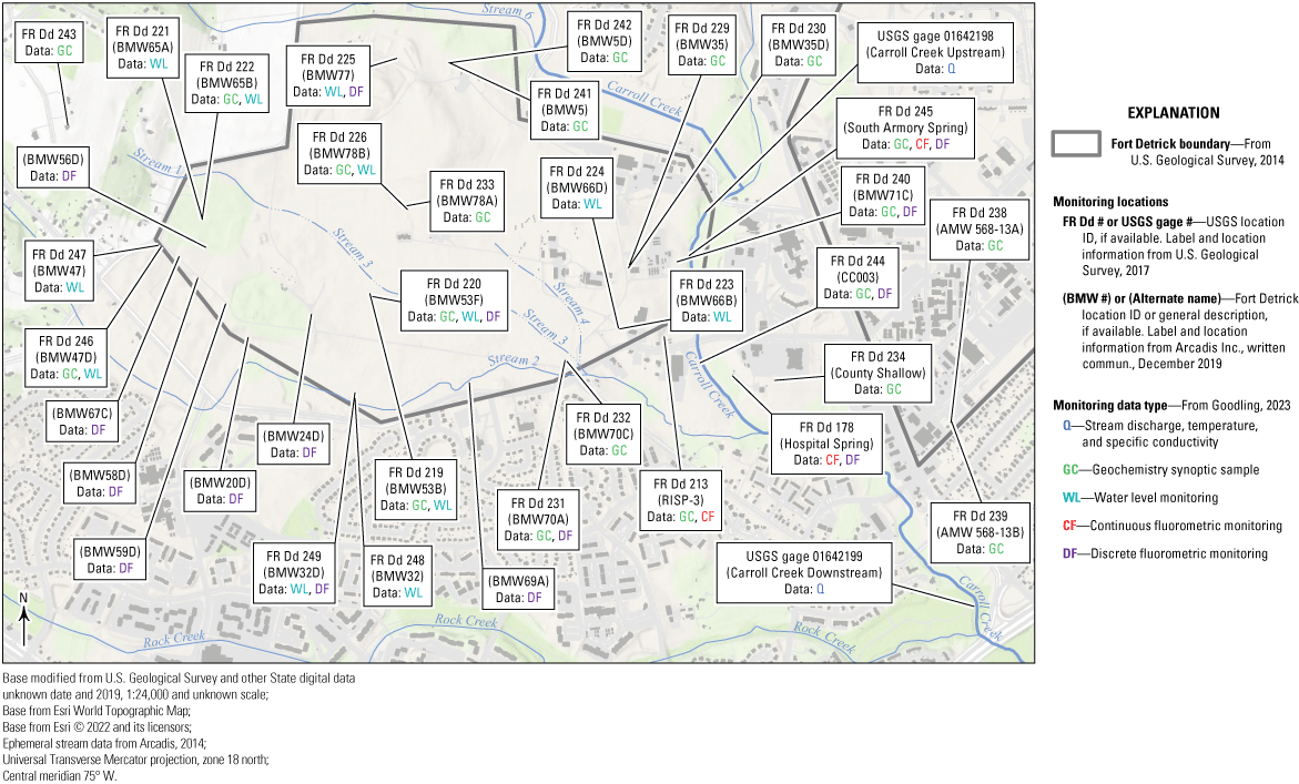
Hydrologic, geochemical, and fluorometric monitoring locations within this study. USGS, U.S. Geological Survey.
Fluorometric Monitoring
Continuous water-quality monitoring for fluorescent dyes at three spring sites using in situ fluorometric monitoring was undertaken to determine if detectable amounts of dye were present from previous dye tracing efforts undertaken in 1995 and 2013. These locations are named FR Dd 213 (RISP-3), FR Dd 178 (Hospital Spring), and FR Dd 245 (South Armory Spring) and their locations are shown in figure 8. These three sites were selected due to the suitability (in other words, sufficient water depth) for in situ monitoring and the prior detection of dyes following the 1995 and 2013 dye tracer tests. At each spring site, a calibrated Turner Scientific C6 submersible fluorimeter was deployed along with a YSI Multiparameter Sonde for an approximately 3-month period to measure concentrations of rhodamine, fluorescein, dissolved oxygen, pH, specific conductivity, temperature, and turbidity. The unit was calibrated prior to each 3-month deployment using an eight-point calibration. The calibration was checked at the end of each 3-month deployment to identify sensor drift. When sensor drift was identified, the values were corrected using standard USGS procedures described by Wagner and others (2006). FR Dd 213 (RISP-3) was monitored from November 6, 2019, to January 30, 2020; FR Dd 178 (Hospital Spring) was monitored from February 14 to May 21, 2020; and FR Dd 245 (South Armory Spring) was monitored from June 18 to October 14, 2020.
Discrete dye observations were also collected as 1-liter split samples from 12 sites within the Fort Detrick quarterly landfill monitoring network December 1–9, 2020. These samples were collected following well purging performed during the periodic sampling for site contaminants. Hand-dipped grab samples from FR Dd 245 (South Armory Spring) and FR Dd 178 (Hospital Spring) were also collected at that time. The concentration of rhodamine, fluorescein, turbidity, and the temperature were recorded using a calibrated Turner Scientific C6 submersible fluorimeter in a laboratory setting. Eosine dye was also injected during previous dye tracer tests. To evaluate the potential influence of the presence of eosine dye on apparent detections of rhodamine and fluorescein, a 5,000 micrograms per liter (µg/L) standard eosine solution was evaluated on the fluorimeter used in this study. Apparent dye concentrations of 480.0 µg/L fluorescein and 400.0 µg/L rhodamine were reported by the instrument, indicating eosine has an interfering effect at high concentrations.
In situ fluorometric monitoring can be affected by the interference of turbidity within the water column, as suspended sediment either blocks or reflects light into the optical sensor on the fluorimeter (for example, Saraceno and others [2017]). To understand the influence of suspended particulates on the observed continuous monitoring results, a series of benchtop experiments were conducted by systematically varying the turbidity of water samples between 0 and 100 Nephelometric Turbidity Units (NTU) using standard solutions, while recording the apparent rhodamine and fluorescein concentrations. This evaluation was repeated in March and October 2020.
2019 Synoptic Groundwater Well and Spring Sampling
In September and October 2019, 20 samples were collected from 16 monitoring wells, 3 springs, and a domestic supply well for a suite of constituents including tritium (3H), dissolved noble gasses, sulfur hexafluoride (SF6), trace metals, major ions, nutrients, stable isotopes of water, and carbon isotopes. The sampling locations are shown in figure 8. Prior to sampling, wells were evaluated using slug tests to ensure wells had a high degree of connectivity with the aquifer. A submersible pump was used to purge at least three well volumes from the well, then monitoring for stability in field parameters including temperature, specific conductance, turbidity, pH, dissolved oxygen, and water level using a YSI Multiparameter Sonde, flow-through cell, and electric water-level tape in accordance with USGS groundwater sampling procedures (U.S. Geological Survey, 2006). In two wells, excessive drawdown in the wells indicated a poor connectivity between the well and the aquifer and alternate well locations were selected. Copper tube pinch clamp samples (Weiss, 1968) were collected by running sample water in-line through refrigeration grade copper tubing. Clear tubing was placed upstream to monitor for bubbles and the copper tubes were clamped under back pressure to limit gas exsolution during sample collection. Water was pulled through the sampling tubing using a peristaltic pump operating at an extremely low setting to avoid bubble creation within the tubing. Springs were sampled by inserting the copper tube directly into the flowing stream orifice as far as practical to ensure water was sampled before reaching the atmosphere. Samples at the domestic well were collected from a point upstream of water treatment systems within the home.
Water analyses were performed at the USGS National Water Quality Laboratory, the USGS Groundwater Dating Laboratory, the USGS Stable Isotope Laboratory, Woods Hole Oceanographic Institute, the USGS Denver Noble Gas Laboratory, and the USGS Menlo Park Tritium Laboratory. The data are available in a companion data release (Goodling, 2023).
Methods of Analysis
The following sections describe the methods used to interpret previously collected geologic and geophysical data, perform a water budget analysis, and interpret the geochemical data collected in this study. These methods were applied to (1) evaluate structural controls on groundwater flow, (2) characterize groundwater system responsiveness to hydrologic events ranging from individual storm events to interannual variability, (3) evaluate the potential for regional interbasin groundwater flow that bypasses Carroll Creek, (4) characterize the sources and timing of groundwater recharge, and (5) determine the degree of vertical connectedness and geochemical similarity between different regions of the aquifer.
Geological Data Interpretation
Previously collected geologic and geophysical data from Area B were evaluated primarily to provide an overview of the presence and orientation of features that control the magnitude and direction of groundwater flow. These features include solutionally enlarged fractures, cavities, and voids as well as the orientation of bedding and unweathered fractures.
Boring Log Reanalysis
The records produced during well drilling activities—including drillers’ boring logs and descriptions produced by onsite geologists—provide a valuable primary documentation of the subsurface conditions. At Fort Detrick Area B, a total of 76 drilling log records were reported in appendix A of the draft final remedial investigation report (Arcadis Inc., written commun., December 2019). These records were summarized to identify (1) the thickness of the reported soil overburden by recording the first occurrence of competent bedrock, (2) the number of voids or cavities encountered during drilling, (3) the reported depth of the deepest void or cavity, and (4) the degree of reported weathering and depth to which this weathering occurred. Using this information, the presence or absence of an epikarst zone was interpreted and the depth of the bottom of the zone was estimated. The determination of the epikarstic depth was not conducted for 16 wells whose drilling logs were too short or not complete enough to perform an analysis. The bottom of the epikarstic zone was identified as the deepest reported void zone and (or) the deepest zone of substantial weathering before a transition into unweathered fracture-dominated bedrock. The results of these analyses were mapped to identify spatial patterns within the subsurface data. Due to the heterogeneity of the subsurface within karst systems and the limited spatial extent of an individual borehole, interpolation between boreholes was not performed.
Geophysical Log Reanalysis
Geophysical log data were collected in 23 geophysical logs from 13 wells by ARM Geophysics of Hershey, Pennsylvania while a series of new wells were constructed in 2011 and 2012. The locations of the geophysical logs, which are named with “BMW” followed by a 2-digit identifier are shown in figure 9. The names provided within appendix D of Arcadis Inc. (2014) are retained in this report. Individual logs were sometimes collected at the same location but at different depth intervals; the letters A–E following the location name denote the relative depth interval of the data collection. The data were reviewed and the optical and acoustic televiewer (OTV and ATV, respectively) data were independently analyzed using WellCad version 5.2 to identify the orientation of bedding, fractures, and voids. Imagery data collected during logging included OTV and ATV. Line data collected during logging included 3-arm caliper, gamma radiation, fluid resistivity, fluid temperature, and formation resistivity. These data files and well logs are available in appendix D of Arcadis Inc. (2014). The raw data logs were reinterpreted by the USGS to evaluate the orientation of features that commonly act as preferential flow conduits, including bedding, voids, and fractures.
The location of geophysical log data interpreted in this study. Geologic units shown are adapted from Southworth and others (2007) and are shown in figure 2A.
The following steps were undertaken in WellCad to prepare the data and to collect the strike and dip of bedding features and fractures within the geophysical logs. In several wells, multiple geophysical logging events occurred in the same borehole at different depth intervals; these data were assimilated for interpretation. Linear data collected at the site were inspected to ensure that variations in gamma and resistivity were within natural instrumental bounds. In some cases, the resistivity or gamma values were spurious and were not interpreted. Where multiple readings were collected in the same borehole at the same interval, the data were overlain to evaluate the consistency of the observations.
The imagery data was primarily used to make designations of strike and dip of fractures and bedding. Several processing steps were necessary to ensure the accuracy of strike and dip measurements. The instruments used to collect the data use Earth’s magnetic field to orient to magnetic north. Therefore, a rotation is required to transform to true north. A 10.5° clockwise rotation was applied to all image logs to ensure their true north orientation, as the declination at Fort Detrick is 10.5° W. In some cases, the OTV or ATV logs appeared offset from each other or the depth interval collected during one instrument run differed from the other. In this case, common features of both logs were used to apply a stretch or shrink to one log to ensure a consistent depth observation. The gamma and caliper logs assisted in making this determination.
When the imagery logs were properly oriented and aligned, linear features in the logs were identified and classified. As the geophysical logs represent the imagery of the interior of a cylinder, linear features appeared as sinusoids in geophysical logs. Fractures and bedding were interpreted by considering variations in grain size, rock color, variations in the caliper log, and acoustic travel time and intensity. There were many intervals where cloudy sediment impeded the view of the optical log and only ATV logs were used to identify fractures. Large void spaces were encountered in many logs. The orientation of these features was estimated by fitting sinusoids to the sides and middles of the voids; however, the orientation of these features is less certain than the linear features.
Once these features were classified, several corrections were applied to ensure the strike and dip represented the true rock units. First, a correction for borehole deviation was applied by using the tilt and azimuth provided in the ATV logs. This correction is required because drilled boreholes are typically not perfectly vertical. Second, the strikes and dips were corrected for variations in borehole diameter. The diameter may vary from the drilled diameter, which will affect the true dip. Once these corrections were applied, the strikes and dips were determined. Polar plots indicating the poles to the plane of these features projected onto the southern hemisphere of a stereonet plot allow the features to be examined on a well-by-well basis.
Hydrological Data Analysis
The following sections describe the methods applied to interpret the streamflow, water level, and precipitation data collected in this study at Fort Detrick Area B. The interpretations support a water budget analysis to evaluate the potential for interbasin transfer. The methods applied also characterize the hydrologic system during the observation period.
Base-Flow Separation
Hydrograph separation was used to differentiate the observed Carroll Creek stream flow into two components—base flow and quickflow. Stream base flow represents discharge from the groundwater systems into the stream-channel network. Stream quickflow represents short residence time water—including surface runoff or shallow lateral subsurface flow—that reaches the stream network following precipitation events. Seasonal and interannual variability in stream base flow reflects changes in groundwater storage. There are many techniques that are designed to separate the base flow component from the quickflow component of stream discharge; many of these are graphical in nature and use the shape of discharge time series to distinguish between two or more components, often base flow and quickflow discharge. These graphical hydrograph separation techniques, although reproducible, do not have a physical basis and are not amenable to estimation of uncertainty.
Chemical hydrograph separation allows for a more physically based determination of the relative influence of base flow and quickflow and incorporates stream chemistry into the algorithm. Specific conductance (SC) is often used as a proxy for groundwater-derived total dissolved solutes in stream, as precipitation typically has low SC whereas groundwater typically has elevated SC resulting from its longer contact time with aquifer materials. In this study, we use optimal hydrograph separation (OHS; Raffensperger and others, 2017; Foks and others, 2019), a method of chemical hydrograph separation that employs the use of a two-parameter recursive digital filter. The two dimensionless parameters are a recession constant (α) and the maximum value of the base-flow index (β). The value of α is calculated using streamflow recession analysis and the value β is optimized using a mass balance constraint. OHS has the following key features
-
1. Assumes that stream flow is a mixture of two components: base flow and quickflow;
-
2. Assumes that the groundwater system acts as a linear reservoir;
-
3. Assumes the SC of quickflow (derived primarily from precipitation) is constant, whereas groundwater SC varies in a prescribed manner through time; and
-
4. Provides a measure of model fit by comparing observed and simulated values of SC.
Two-component hydrograph separation, or separation of base flow from quick flow, for the chosen sites was performed using a recursive digital filter (RDF). Eckhardt (2005) proposed the following RDF to estimate the base flow component of streamflow:
whereα and β
are dimensionless adjustable parameters,
Q
is streamflow in units of length cubed per unit time [L3/T],
QB
is base flow in units of length cubed per unit time [L3/T], and
J
is an index representing the time step (typically a day).
The recession constant parameter, α, was derived for each study site using the log-linear slope of the recession hydrograph for storm events within the period of record, using the methods of Rutledge (1998). An α value was calculated for each recession period of sufficient length and then the median α from all storm recessions was taken as the α used in the OHS calculations. Only α values computed from significant (p>0.05) log-linear regressions were retained. The minimum number of days for α to be calculated was determined using the formula of Linsley and others (1982), which states that the number of days (N) is proportional to the drainage basin area in square miles (A):
The second adjustable parameter in the two-parameter RDF, β, is a fitted, unmeasurable parameter that ranges from 0 to 1 (Eckhardt, 2005; Raffensperger and others, 2017). For sites without available SC data, the model parameter β was determined using a method developed by Collischonn and Fan (2013), referred to as “CaF.” This method for estimating β is based entirely on discharge records. The method applies a backward-moving filter using a previously calculated recession parameter. Collischonn and Fan (2013) tested the filter using data from 15 streamflow sites in Brazil with differing physical characteristics and showed that the β values obtained were comparable to the predefined values suggested by Eckhardt (2005) based on the class of aquifers encountered in each basin.
For sites with SC data, OHS was applied, in which model parameter β is optimized by applying a SC mass balance constraint (Rimmer and Hartmann, 2014; Raffensperger and others, 2017). Streamflow is initially separated into two components, base flow (QB) and quick flow (QS), while values of SC are proposed for the base flow (CB) and quick flow (CS) components. These variables, as well as streamflow (Q), are used to estimate stream SC (Csep) by
The root-mean-square error, E, between the estimated stream SC and observed stream SC (Cobs) is calculated as This process is repeated until there is minimized error, E, implying that the parameter value for β is also optimized (Rimmer and Hartmann, 2014; Raffensperger and others, 2017). Optimization was performed in version 3.4.3 of R (R Core Team, 2018) using the algorithm “Bound Optimization by Quadratic Approximation” (BOBYQA) in the R package nloptr, version 1.0.4 (Powell, 2009; Ypma, 2018).Two OHS models were used to estimate base flow SC (CB) (Raffensperger and others, 2017). The first OHS model estimated SC by way of a sine-cosine function over time (sin-cos model) to emulate seasonal variation and is defined as
in which the base flow SC on day j () is a sum of sine and cosine functions of time (tj) with an annual period, described by a mean value (), amplitudes (,), and a beginning time/day (t0). In the optimization, the following values are estimated that minimize the root-mean-square error (RMSE; eqs. 1–3): β, , , t0, , and CS.The second OHS model estimates CB by using a peak-identification algorithm and linear interpolation (SCfit model). Peaks in the observed SC data were identified using the function “findpeaks” in the R package pracma (Borchers, 2021), whereas CB values were estimated with linear interpolation between the identified peaks. The SCfit model has only two variables to optimize (β, ). SCfit and sin-cos models were accepted if the Nash-Sutcliffe efficiency coefficient (NSE) (Nash and Sutcliffe, 1970) was greater than 0.3 and did not converge to a user-defined optimization bound (lower bound=0.00001; upper bound=1.0) (Raffensperger and others, 2017; Foks and others, 2019). The NSE cutoff value of 0.3 is the same as that used in Raffensperger and others (2017).
Comparing the base flow separation results to other regional watersheds provides insights on the groundwater-surface water exchange processes occurring at Fort Detrick Area B and the applicability of conceptual models developed in other hydrogeologic settings. The intercomparison of base flow separation will focus on two metrics calculated for all available streamgages for the period of October 1, 2017, to September 30, 2020, a period of 3 water years. These metrics are (1) groundwater base flow per unit area (in in/yr) and (2) the base flow index, which is the proportion of base flow to total streamflow and ranges from 0 to 1. A base flow index closer to 0 is expected in basins with flashy storm responses (flashiness describes short-lived and rapid storm hydrograph peaks) and a base flow index closer to 1 is expected in basins with muted storm responses and steady inter-storm flow sustained by groundwater.
The two primary base flow separation techniques discussed in this report are OHS and the CaF method. An additional widely applied method for base flow separation is a graphical method called PART, which is described by Rutledge (1998). This third method is included for comparison because it is more widely used within regional studies of karst hydrogeology and it is readily applied to all available streamgages using only a time series of discharge. The part() function of the USGS DVStats package version 0.3.4 was used to perform this analysis on the daily mean streamflow values stored in the USGS NWIS database (Lorentz and DeCicco, 2021). To apply the method, gaps of 3 days or less in the streamflow record were filled using linear interpolation.
To interpret the base flow separation results, a binary classification of lithology was used to identify watersheds with a potential for influence by karst processes. Using geologic data reported by the USGS state geologic map compilation (Horton and others, 2017), watersheds were classified as “karst” if more than 50 percent of the watershed area was underlain by carbonate geologic units. Although a simple classification scheme, this designation captured many of the USGS streamgages reported in the regional literature to be located in karst environments in Virginia, West Virginia, and Maryland.
Groundwater Gradients
In karst environments, hydraulic gradients, the number of active conduits, flow routes, and directions of groundwater flow may change rapidly with changing hydrologic conditions (Taylor and Greene, 2008). At Area B, previous studies have produced potentiometric surface maps (fig. 4). Although in karst environments potentiometric mapping may not fully characterize preferential flowpaths arising from anisotropy and highly heterogenous subsurface processes, it is still a useful tool for guiding other types of analyses, including the design and interpretation of groundwater tracer tests (Taylor and Greene, 2008). However, potentiometric mapping is limited in its ability to characterize short-lived responses to hydrologic events. The groundwater gradient, along with hydraulic conductivity and cross-sectional area, determines the groundwater flow magnitude along a groundwater flow path. In karst systems, conduits and preferential flow paths may have extremely low hydraulic conductivity. In this case, very low gradients may still convey large flow volumes.
In this analysis we focus on temporal changes in the observed groundwater gradient between wells in the hydrologic monitoring network to characterize the short-lived responses to hydrologic events. Changes to the flow direction and hydraulic conductivity resulting from the complexity of the subsurface conduit system are possible, though the approach we take assumes that the changes in flow direction and hydraulic conductivity through time are negligible. We examine temporal changes to hydraulic gradients between individual well pairs. The selection of these pairs is guided by the potentiometric surface mapping. The magnitude of the gradients is not intended to guide estimates of total groundwater discharge for the reasons previously discussed.
Groundwater gradient time series were computed from the daily mean water levels. Horizontal groundwater gradients between well pairs were computed by dividing the difference in water level elevation by the Euclidean distance, neglecting the influence of topography and observation depth. Vertical groundwater gradients between well pairs were computed by dividing the water level elevation difference by the difference in observation depth below land surface.
Soil-Water Balance Modeling
Accurate estimates of the temporal and spatial variations in water budget components require accounting of water inputs and removal from the hydrologic system. Input to the groundwater system in Pennsylvania and western Maryland is dominated by precipitation infiltrating the soil. Water output from the Pennsylvania and Maryland aquifer systems include processes such as runoff, ET from the ground and vegetation, and withdrawals for human uses such as irrigation or domestic water supply. The soil-water balance (SWB) code developed by Westenbroek and others (2010) was used to compute the water budget components for a regional area spanning portions of western and central Maryland and Pennsylvania using readily available gridded datasets. The ET outputs from this model are used in the water budget calculation described in a following section. The SWB code utilizes a modified version of the Thornthwaite-Mather soil-water balance approach at a daily time step (Thornthwaite, 1948; Thornthwaite and Mather, 1957) and incorporates spatially distributed soil, meteorological, and land cover data (Westenbroek and others, 2010).
In the water budget analysis in this study, the groundwater recharge and ET components of the budget were estimated using the USGS SWB 2.0 model (Westenbroek and others, 2018). The Pennsylvania-Maryland (PAMD) SWB model area is considerably larger than the area of interest around Fort Detrick. The size of the entire model domain was designed to include sufficient watersheds with streamflow data to fit the modeled budget components to observed streamflow and base flow. The entire model domain contained 55 watersheds varying from 0.37 to 817 mi2 in total area (mean watershed size was 96 mi2 and the median was 22 mi2). The model domain considered for the Fort Detrick water balance calculations was 14,960 mi2. The PAMD SWB model grid consisted of 614,760 cells arranged in 705 columns by 872 rows, where each cell was a square with sides 250 meters (m) (approximately 820 ft) long.
Data Requirements for the SWB Model
In this model, commonly available gridded datasets that describe the climate, soil hydrologic characteristics, land use, and topography are used to estimate soil water budget components using a modified Thornthwaite-Mather soil-moisture accounting method. Input data for the SWB included tabular and gridded datasets of (1) daily meteorological parameters (precipitation and temperature), (2) land-use and land cover classification, (3) hydrologic soil groups, and (4) estimated available soil-water capacity, all of which are required soil water budget components on a cell-by-cell basis as described in detail in the SWB model documentation (Westenbroek and others, 2010).
Precipitation and Temperature
The SWB model code calculates soil water budget components from meteorological data on a daily time step and compiles this information to a user-defined period (daily, monthly and [or] annually). Meteorological data can be gridded or stacked grid files such as NetCDF, which allow for time series analysis. Two different meteorological data sources, Parameter-elevation Regressions on Independent Slopes (PRISM) (PRISM Climate Group, 2021) and Daymet (Thornton and others, 2020), were initially used and compared. An analysis between these and the USGS precipitation gage indicated that the PRISM model agreed better with observed precipitation data. PRISM outputs were therefore selected for the model simulations. Data were downloaded and run in the SWB model using NetCDF grids. Data from PRISM were supplied as model inputs using its native 4 x 4 km grid cell resolution.
Land-Use Classification
Land cover information is required for the SWB model to calculate recharge, as differing land uses will have different impervious cover and percolation rates for various soil types. Land-use cover within the PAMD SWB model area is primarily forest, agriculture, and urban. Land-use classification inputs to the model are assigned using the 30-m pixel resolution 2016 National Land Cover Dataset (Dewitz, 2019).
Hydrologic Soil Groups
The SWB model requires information on hydrologic properties of soils to determine if there is runoff or infiltration on any given piece of land. The U.S. Department of Agriculture’s Natural Resources Conservation Service (NRCS) has classified soils across the United States based principally on their infiltration capacity and runoff potential (Natural Resources Conservation Service Staff, 2009). The PAMD SWB model used soil hydrologic grouping data provided in the NRCS Soil Survey Geographic Database (SSURGO) dataset. Soil hydrologic data compiled to a 90-m raster resolution by Wieczorek (2014) was used in the model. The soils data was numbered to correspond to various lookup tables that the SWB model used to calculate recharge.
Soils are generally assigned one of seven combinations of letter designations (using A–D) with A having the greatest infiltration rate and D having the lowest infiltration rate and highest runoff potential (Natural Resources Conservation Service Staff, 2009). The data provided for the whole model domain of the soil-water balance had seven different soil types: A, B, C, D, A/D, B/D, and C/D. The dual soil classes exist in areas where a near-surface water table or other feature can delay infiltration. Summary statistics on the model domain indicated that a considerable portion of the cells held dual hydrologic classes. Previous reports using the SWB dealt with the hydrologic soil groups by classifying the dual groups as either the higher or lower of the two. During the comparisons with regional streamflow for this SWB model, the authors determined that the higher soil class provided a better fit. Thus, a soil identified as A/D would be considered an A for modeling purposes. The relation between the NRCS soil classes and the properties used in the SWB model are shown in table 3.
Table 3.
Relation of soil classes and soil groups used in soil-water balance modeling in this study.[SWB, soil-water balance; NRCS, Natural Resources Conservation Service. Letters A–D refer to soil classes defined by the Natural Resources Conservation Service (Natural Resources Conservation Service Staff, 2009), with A having the greatest infiltration rate and D having the lowest infiltration rate. Dual soil classes (for example, C/D) exist where a near-surface water table or other feature can delay infiltration]
Soil data grids typically have missing values. The missing value areas are generally under large bodies of water but can also occur on land. To avoid issues with running the model, no-data grid cells were filled by averaging the soil characteristics around the cells missing data. This was done by passing a rectangular shape over the raster. Any cell without data would then receive the mean value of the surrounding five raster cells. This process was done five times until all no-data values were removed.
Available Water Capacity
The SWB model calculates the available water capacity of individual grid cells by comparing land cover information with soil physical properties. Available water is defined as the water held by soil in between field capacity (water held in soil despite gravity) and the permanent wilting point (the point at which plants cannot remove additional water). The SWB calculates available water for plant consumption/recharge by multiplying the rooting depth by the available soil water, which is dependent on soil texture. Information on the moisture holding capacity of various soil types has been measured in soil surveys and published by the U.S. Department of Agriculture for the conterminous United States. The PAMD SWB model utilized soil hydrologic data characteristics from the U.S. General Soils Map available from SSURGO and compiled by Wieczorek (2014). Missing data in the available water capacity grids were filled using the same methods as the hydrologic soil lookup tables.
Lookup Tables
The SWB model uses user-modified tables of land use, soil, and crop-specific information to assign model cell values to calculate recharge. The land-use lookup tables include information such as rooting depth for different types of vegetation, runoff curve numbers, and maximum possible recharge based on the land-use designation.
The PAMD SWB model’s land-use lookup tables included literature values for the rooting depth of vegetation, which is used to determine the amount of water available for ET. Values of rooting depth were taken from literature and applied across various soil types. Runoff curve values used in SWB lookup tables are empirically derived parameters originally developed by the U.S. Department of Agriculture Soil Conservation Service, which estimated the percentage of rainfall running off of various land uses (Hjelmfelt, 1991).
Spatial and Temporal Resolution
Gridded inputs to the SWB model were available at differing scales, requiring a regridding to produce the SWB outputs. Fine resolution inputs included the 30-m resolution land use data and 90-m resolution soil data; coarse resolution inputs included the 4-km resolution precipitation and temperature datasets. The output resolution of the PAMD model was an intermediate 250-m resolution. SWB version 2.0 performs this data assimilation process by way of nearest-neighbor resampling (Westenbroek and others, 2018). In the case of the PAMD model, the 4-km grid resolution climate data that corresponds to the centroid of the 250-m cell is used. This type of interpolation can produce the illusion of greater output resolution than is supported by the underlying data. In this analysis, we only interpret the outputs at the watershed spatial mean scale. The 10.9 km2 upper Carroll Creek watershed has an area equivalent to a 3.3 × 3.3 km2 and the 18.9 km2 lower Carrol Creek watershed has an area equivalent to a 4.3 × 4.3 km2. To illustrate the output resolution, we present the gridded SWB outputs at the 250-m resolution, though we do not interpret the patterns at the subwatershed scale. SWB model outputs are computed at a daily time step, though the results for individual days may differ appreciably from observed conditions due to misrepresentation in timing from the climate datasets. In this study we limit interpretation for the SWB model outputs to periods aggregated to 1 water year or greater.
Parameter Adjustment
The PAMD model parameters were adjusted by comparing estimated recharge with base flow estimates from reference watersheds in the surrounding region. As the Carroll Creek gaging station was only in operation from 2017 onward, a larger group of gages with longer records was required to compare SWB recharge estimates. Of 55 total available gages, the authors selected 34 that (1) were less than 1,000 mi2 in area, (2) weren’t dominated by urban areas, and (3) lacked flow-regulation features such as hydroelectric generation. The 34 reference watersheds, in addition to the 2 Carroll Creek streamgages, provided information on base flow conditions. After the initial SWB setup, parameters were adjusted to match base flow as best as possible. These decisions included the hydrologic soil groups, noted above, where dual soil classes were determined to follow the higher soil class. In addition, parameters within the lookup tables were adjusted, such as rooting depth, readily evaporable water, and total evaporable water. As with previous SWB reports, the authors found that altering the rooting depth in areas with soil group B had the greatest impact on recharge. The adjustment process involved running the entire SWB model domain, which included the 36 watersheds (inclusive of the two Carroll Creek watersheds), from January 1, 2000, through December 31, 2020. Recharge and ET estimates produced by SWB model were then compared to base flow estimates and parameters were adjusted manually for the best fit.
Sensitivity Analysis
To determine model sensitivity to model parameters, a series of 140 sensitivity runs were completed for the entire model domain. Parameters altered to evaluate sensitivity were contained in the land use and irrigation lookup tables. The parameters in the sensitivity analysis included the runoff curve number, rooting depth, readily evaporable water, and total evaporable water; these parameters were highly sensitive in a recent SWB modeling study (Nielsen and Westenbroek, 2019). The values of the four sensitivity parameters were adjusted sequentially for each soil type to 80, 90, 100, 110, and 120 percent of the original values.
Water Budget Analysis
Determining the water budget components in the vicinity of Fort Detrick Area B is critical to evaluate key aspects of the previously described CSM. The focus of the study design is to determine whether there is evidence that interbasin groundwater flow is a significant process. Interbasin groundwater flow, sometimes termed “underflow,” occurs when the groundwatershed is not coincident with the surface watershed and can be the result of topographic effects, structural controls, or anthropogenic influences. Because assessing this process is a primary goal, the water budget analysis makes no assumption that the water budget is a closed system. Many water budget analyses assume a closed system to estimate difficult-to-measure water budget components, most commonly ET. However, imposing this assumption would necessarily prevent an evaluation of interbasin groundwater flow. Instead, in this study each individual water budget term is calculated using available data or through modeling, and a water budget residual term is calculated. If the water budget residual term is small relative to the uncertainty of the underlying data, then an additional import or export of water (in other words, interbasin transfer) is not needed to fully describe the hydrologic system. Refer to Kampf and others (2020) for further discussion or water budget analyses that do not assume a closed system, including examples of this approach to identify groundwater interbasin transfer.
A water budget analysis is used to describe the inputs and outputs of water within an area. In general, the components of a water budget for a given amount of time are summarized by equation 6.
On sufficiently long time scales, the changes in storage may be set to zero on the assumption that over the time period of interest the change in storage is negligible when compared to the magnitude of the inputs and outputs. In this study, this assumption is likely not valid for the relatively short (approximately 3 year) monitoring period. We therefore use the hydrologic monitoring network to create an independent estimate of the storage change during the water budget period.
In this analysis, the water budget components defined in equation 7 are evaluated within the two nested topographic watersheds at the Carroll Creek streamgages. The budget components are evaluated within each watershed to compute the water budget residual. The following sections describe the methods for quantifying each component. A schematic representation of the water-budget calculation is shown in figure 10.
whereP
is the spatial average precipitation within the watershed in units of length per unit time [L/T],
ET
is the spatial average evapotranspiration from the watershed in units of length per unit time [L/T],
I
is the spatial average interception by vegetation in units of length per unit time [L/T],
R
is the spatial average groundwater recharge in units of length per unit time [L/T],
A
is the topographically defined area of the watershed in units of length squared [L2],
is the total stream flow from Carroll Creek at the watershed outlet in units of length cubed per unit time [L3/T],
∆Stot
is the spatial average change in storage of water within the watershed in units of length per unit time [L/T], and
εtot
is the spatial average residual from the total water budget calculation in units of length per unit time [L/T].
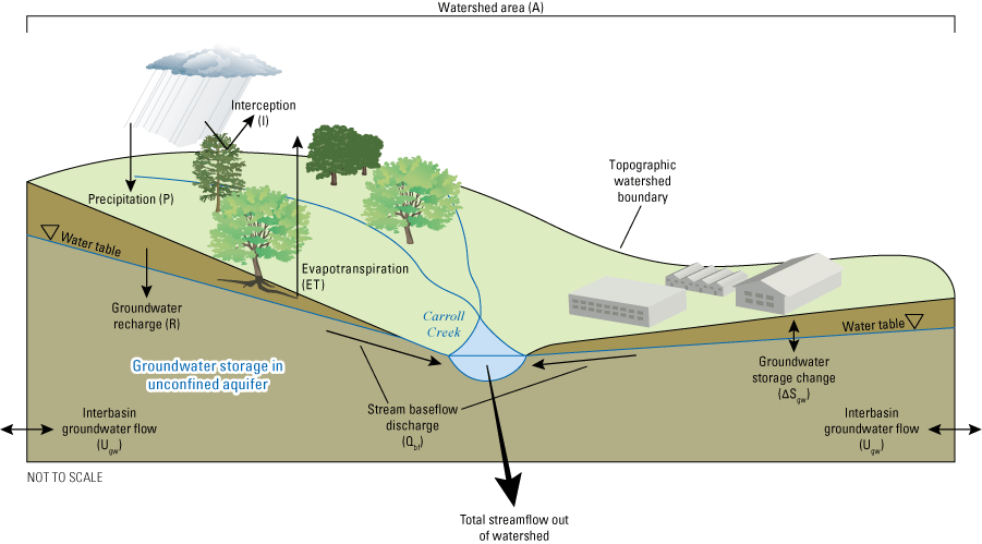
The water budget components considered within this study.
Uncertainty is an important consideration for evaluating the residual term from a water budget analysis. Though the values for individual water-budget components can be subject to substantial uncertainty, many water budget studies neglect this completely (Healy and others, 2007). The water budget residual includes all the errors associated with the individual water budget components, as well as any unquantified budget components. To assess if a residual indicates the presence of an unquantified budget component, it must be compared to the propagated errors from all of the components in the calculation. In this analysis, we estimate the uncertainty of each water-budget component and combine them into an overall standard deviation error of the residual using addition in quadrature, as described in equation 8. Addition in quadrature is appropriate under the assumption that the errors for the components are normally distributed and independent.
whereEi
is error associated with the ith water budget component; and
Etot
is the error associated with the water budget residual term, which will provide uncertainty on the residual (Kampf and others, 2020).
If Etot from equation 8 is greater than or equal to εtot from equation 7, then this analysis will consider the water budget residual to be insignificant. An insignificant water budget residual suggests that the hydrologic system can be reasonably conceptualized as a closed system and that there is no evidence to support significant interbasin transfer. Due to the uncertainties inherent in a water budget analysis and the coarse spatial representation of the analysis, small amounts of interbasin transfer cannot be ruled out. However, the water budget analysis would be able to evaluate if large magnitude interbasin transfer is occurring.
Precipitation
Precipitation represents the input of water to the water budget and was evaluated through a combination of direct observations and published gridded datasets. Precipitation was recorded at the upstream USGS streamgage location using an Ott Pluvio 2 weight volume gage along with a Water Log tipping bucket rain gage as a backup in case of malfunction. Gridded estimates of precipitation in this study are from the PRISM model (PRISM Climate Group, 2021). This model estimates daily precipitation at 4-km grid cells for the conterminous United States and is the official spatial climate dataset of the U.S. Department of Agriculture. In order to perform the water budget calculation, the spatial mean of the precipitation within each watershed was extracted from the gridded precipitation dataset using the R package “exactextractr” version 0.3.0 (Baston, 2021). Using this method, grid cells with partial intersection with the watershed boundary were weighted by the fraction of intersecting cell area. To estimate the uncertainty on the precipitation estimates, the observed precipitation is compared to modeled precipitation for the location of the precipitation gage, adjacent to the upstream Carroll Creek streamgage.
Evapotranspiration
Evapotranspiration (ET) within the water budget is estimated using the SWB model. In SWB, gridded estimates of actual ET are created for given air temperatures, vegetation types, soil classes, and antecedent precipitation events. In the SWB definition, actual ET is the water extracted from storage in the soil reservoir and is distinct from water evaporated from vegetation surfaces, which is classified as interception and described in the following section (Westenbroek and others, 2018).
Independent gridded estimates of ET exist for the study area, though these are derived from remote sensing products and may not capture smaller scale variability or may require bias correction for application in small-scale water budget studies. The operational Simplified Surface Energy Balance (SSEBOP; Senay and others, 2013) is a 1-km resolution estimate of actual ET derived from six hourly weather datasets, the standardized Penman-Monteith equation to estimate the daily short grass reference ET, and a parameterized fraction of ET. The MOD16A2 version 6 ET product is a 500-m resolution estimate of ET using the Penman-Monteith equation and a blend of inputs from daily meteorological data and remotely sensed inputs including vegetation property dynamics, albedo, and land cover (Mu and others, 2011). TerraClimate is a 4-km resolution monthly water balance dataset (Abatzoglou and others, 2018). The TerraClimate dataset first calculates a reference ET using the Penman-Monteith equation, then a modified one-dimensional Thornthwaite-Mather water balance model is constructed to estimate actual ET. Although useful as a reference or first-order approximation, the large spatial scale ET estimates from individual remotely sensed products may not be suitable as a direct input into a small water budget without additional evaluation (Allen and others, 2011).
In many water budget studies, ET is estimated by measuring all other components of the water budget and assuming that interbasin transfer is negligible. Although we do not take that approach in this study, the values of ET from the SWB, SSEBOP, MOD16A2, and TerraClimate datasets are compared to the value of total precipitation from PRISM minus the basin-normalized total streamflow measured at the USGS streamgages and the change in storage. This value is representative of a simple estimate of ET assuming no interbasin transfer and does not account for the uncertainty in streamflow, precipitation, or storage; it is provided as a reference only.
Actual ET is difficult to estimate at an appropriate scale for a water budget analysis and is subject to a high degree of uncertainty (Winter, 1981; Healy and others, 2007). A review by Allen and others (2011) identifies typical errors for field instruments including lysimeters (5–15 percent error), soil water measurements (10–30 percent error), and eddy covariance measurements (15–30 percent error) as well as for remote sensing methods (10–40 percent error).
Interception
Interception is the process by which precipitation is captured on the leaves of vegetation and does not reach the ground surface before evaporating. Although some definitions of ET may include this process (Savenije, 2004), the definitions used in the SWB model for ET and interception are separate and therefore both must be accounted for to ensure all budget components are included.
Total Streamflow
The total streamflow in Carroll Creek is reported by the two USGS streamgages, one located at the upstream boundary of Area B and one located within Waterford Park, south of Area B (fig. 8). At each location, a rating curve was developed and a continuous record of streamflow was produced for the period from October 1, 2017, to December 31, 2020.
The uncertainty in total streamflow measurements at USGS streamgages is estimated using a quality code system, where discharge measurements that are rated as excellent, good, or fair are considered to be within 5, 10, and 15 percent, respectively, of the actual daily streamflow 95 percent of the time. Poor records have less accuracy than fair, though the percentage is not estimated. The accuracy of the discharge record is determined by both the stability of the stage-discharge relation established at the site and the accuracy of the observations of stage and measurements of discharge in the field. The downstream Carroll Creek gage (station ID 01642199) discharge for the period of record was rated good, except for discharges above 350 cubic feet per second (ft3/s) and estimated discharges, which were rated as poor. The upstream Carroll Creek gage (station ID 01642198) discharge for the period of record was rated as fair, except for discharges above 200 ft3/s, which were rated as poor.
Changes in Storage
In this study the changes in total water storage are approximated to be equal to the changes in groundwater storage. This approximation is justified by the lack of large water bodies within the study watersheds. The changes to the amount of water stored in the shallow unconfined aquifer system is quantified by examining the changes in groundwater levels within the hydrologic monitoring network. In karstic and fractured rock settings, well hydrograph variations may not represent changes in water level (and groundwater storage). For example, this can occur when fractures and voids are rapidly filled with recharging water while the rock matrix remains unsaturated (Healy and Cook, 2002). Although considerable uncertainty will be present in estimates of groundwater storage using water level data, several techniques in this study are applied to minimize these to the extent possible.
Due to the variability of groundwater responsiveness from the heterogeneous karstic aquifer, this analysis uses water level data from across the monitoring network to reduce the influence of individual wells and characterize the changes in storage across Area B. The change in groundwater storage is calculated by multiplying the change in water level by the specific yield (Healy and Cook, 2002). Stream base flow can be another measure of the changes in groundwater storage. For a closed system with no interbasin transfers, stream base flow discharge will be a function of the groundwater storage; in some cases, this is approximated with a power law relation on the basis of theory and observations (Wittenberg, 1999). However, as a result of the complexity of the karst storage processes at the scale of interest and the potential for interbasin transfers, we do not apply any restriction to the functional form of the discharge-storage relation. Instead, we use a regression approach to identify the relation between storage derived from groundwater levels and stream base flow. A suitable regression equation between these two quantities will enable the groundwater storage to be estimated. The magnitude of the storage change is determined by the specific yield value estimated for the wells in this study (described in a previous section). The following steps are used to estimate changes in groundwater storage from the hydrologic monitoring network:
-
1. A mean monthly groundwater level deviation was calculated using the groundwater monitoring network for the longest possible interval. To construct this mean, wells with shorter records (BMW47D, BMW47, BMW32, and BMW32D) and wells affected by pumping (BMW65A) were removed. The long-term mean groundwater level was subtracted from each groundwater-level time series to create a groundwater level deviation. The daily mean deviation was created by averaging across all seven wells. Then the monthly mean deviation was created by averaging the value across all days in a month. The resulting time series characterizes monthly change in the groundwater level across the hydrologic network.
-
2. The monthly mean groundwater level deviation was converted to groundwater storage deviation by multiplying by the specific yield determined for the well network. The methodology to determine this specific yield is described in a previous section. A unit conversion from feet to inches was applied.
-
3. The monthly mean groundwater storage deviation was related to stream base flow, as determined using the OHS method using regression. Two regression models were created and the base flow time series from both Carroll Creek streamgages were used. The lm() and summary() functions from R version 4.1.0 (R Core Team, 2018) were used to create the regression equations using ordinary least squares, and the package hydroGOF() version 0.4-0 (Zambrano-Bigiarini, 2020) was used to calculate goodness-of-fit statistics.
Using the two regression models, the estimated storage at the beginning and end of the water budget period was estimated. The change in these two values is used as the ∆Stot term in equation 7. The ∆Stot for the downstream Carroll Creek gage is used, as the wells are within this watershed. The change in groundwater storage estimated using the methodology outlined above has several sources of uncertainty. The approximation that the mean groundwater level changes within the observed monitoring network at Fort Detrick represents changes in groundwater throughout the water budget watersheds introduces uncertainty. The monitored wells are primarily in karstic geologic units that do not span the entirety of the study watersheds. However, the log-linear regression with stream base flow is a way to evaluate the representativeness of this assumption. Uncertainty is also introduced with the use of the regression model to extend the mean water level time series. However, this uncertainty is small when compared to the uncertainty introduced by assuming a single specific yield value for the entire watershed. In this analysis, an uncertainty of 50 percent is applied to the specific yield value. Assuming that all other uncertainties are negligible when compared to this uncertainty, the resulting change in storage value also has an uncertainty of 50 percent.
Groundwater Recharge
Groundwater recharge is defined as the water that enters the groundwater system vertically through the unsaturated soil zone. In karst systems, preferential vertical flowpaths including sinkholes, swallets, and solutionally enlarged conduits can enable rapid, focused recharge. The heterogeneity of groundwater recharge in karst systems makes this a difficult component of the hydrologic system to estimate. In this study, several methods were used to estimate groundwater recharge at Fort Detrick within the Carroll Creek watersheds, each with independent assumptions and limitations. However, due to the difficulty of representing the heterogeneous karst system using these methods, the estimated groundwater recharge is not used in a budget calculation; instead, the information is provided to evaluate the temporal changes during the water budget period and to place the hydrologic system observed at Fort Detrick into a regional context. The following sections describe the multiple methods used to estimate groundwater recharge.
Soil-Water Balance Net Infiltration
The application of the USGS SWB 2.0 model (Westenbroek and others, 2018) produces estimates of the net infiltration of water on a daily time step for the model domain. In this deterministic model, commonly available gridded datasets that describe the climate soil hydrologic characteristics, land use, and topography are used to estimate soil water budget components using a modified Thornthwaite-Mather soil-moisture accounting method. Daily gridded estimates for net infiltration, which is the water that infiltrates past the plant rooting zone and represents the estimated groundwater recharge, are an output of the SWB model created for this study. The output grid cells have a spatial resolution of 250 × 250 m. These gridded groundwater recharge estimates were extracted for the Carroll Creek watershed areas using a spatial average and included in water budget calculations. The Thornthwaite-Mather soil moisture accounting approach applied by SWB for this study neglects the effects of focused groundwater recharge that bypasses the soil zone. In the karstic environment within the Carroll Creek watersheds, where focused groundwater recharge is an important process, the model may overestimate the amount of surface runoff and underestimate the amount of groundwater recharge.
Episodic Master Recession Analysis
Groundwater recharge occurs as both a constant-rate and episodic process. Episodic recharge from precipitation occurs during discrete storm events that cause increases in the static water table elevation and is particularly evident in regions with well-drained soils, small unsaturated zones, and preferential flowpaths including in karst areas. The water-table fluctuation method (for example, Healy and Cook [2002], Nimmo and others [2015]) estimates the amount of water recharged to the groundwater system during discrete events using time series of water table elevations. Water table rises are quantified by calculating the difference between water level peaks and the water table elevation that would have been present without the episodic recharge. In between recharge events, the water table in an unconfined aquifer decreases along a recession curve as water drains to stream base flow and ET occurs. The rate of recession is typically highest during wet periods with high water-table altitudes and lower during drought periods with low water-table altitudes. A master recession curve is the relation between the rate of recession and the water table elevation and may be linear or a piecewise function depending on the underlying structure and function of the aquifer.
In this study, the Episodic Master Recession (EMR) algorithms introduced by Nimmo and Perkins (2018) were applied to time series of water-table elevation recorded at site wells. Two wells (FR Dd 221/BMW65A and FR Dd 222/BMW65B) were excluded from the analysis because the time series lacked evidence of episodic rises and falls related to precipitation events. The wells may be disconnected from the secondary and tertiary porosity within the aquifer that rapidly transmits changes in hydraulic head within the aquifer.
The EMR method requires the use of parameters to accurately select discrete recharge events and build the master recession curve. A manual adjustment process was implemented to identify combinations of parameters that reasonably captured all major recharge events without any false detections of events. The number and elevations of the piecewise splits in the master recession curve were manually determined for each well based on visual inspection of the slope (dH/dt) versus water table elevation (H) graphs.
Specific Yield Estimation
The specific yield is a unitless groundwater aquifer property that describes the volume of water drained by gravity for a given volume of aquifer material; it is typically expressed as a fraction between zero and one or as a percentage. The specific yield is an important aquifer property in this study because it is used to (1) estimate the episodic recharge using the EMR analysis described in the preceding section and (2) estimate changes in groundwater storage as described in a following section. The specific yield in fractured rock and karst settings is a combination of the drainable matrix, fracture, and void specific yields. Fractures and voids generally comprise a low proportion of the total aquifer storage but drain much more rapidly than the aquifer matrix. In settings such as these, the fluctuation of water levels in wells may be more representative of storage changes in fractures and voids than of the matrix (Healy and Cook, 2002). The application of a single time-invariant specific yield in these settings is subject to a high amount of uncertainty and should be evaluated with care (Healy and Cook, 2002).
The water budget method described by Olmsted and Hely (1962) and Risser and others (2005) was used to determine the apparent specific yield for each well. As noted by Healy and Cook (2002), this method is the most widely used technique for estimating the specific yield in fractured rock settings. Risser and others (2005) applied the method to a 2.8 mi2 research watershed in fractured bedrock in the Valley and Ridge Province of Pennsylvania and Olmsted and Hely (1962) applied it to a 287 mi2 watershed in the Piedmont Province of Pennsylvania. Using this method, the apparent specific yield is shown in equation 9:
whereSy
is the apparent specific yield [unitless],
S
is stream base flow volume per unit area during a recession period consisting of only groundwater discharge and limited evapotranspiration [inches], and
∆h
is the average decline in water-table altitude during the recession period [inches].
The method assumes that the water yielded under gravity drainage (gravity yield) during short periods is equivalent to the specific yield. Though the gravity yield is likely less than the specific yield due to incomplete drainage of the geologic material, the specific yield estimated using this method may be suitable because this complete drainage is unlikely under natural (unstressed) conditions. In this study the specific yield derived from this method is the apparent specific yield. The method also assumes a groundwater system with insignificant interbasin transfer during the recession periods and a linear groundwater system that can be characterized with a single specific yield. Delayed storage effects are not included, so the response time of the aquifer to changes in storage are estimated to occur within 1 day.
Risser and others (2005) report that by using a weighted average of 10 upland wells to calculate ∆h, they derived similar apparent specific yield estimates to what was determined by a separate study that included lysimeter percolate (Gburek and Folmar, 1999). When the calculated apparent specific yield was multiplied by changes in water-table altitude to estimate recharge, the method was found to estimate mean annual recharge comparable to estimates from seven other methods examined by the authors (Risser and others, 2005). The water table fluctuation method tended to underestimate recharge, though the mean annual recharge was statistically significantly different from only one of the seven methods (RORA computer program; Rorabaugh, 1964). However, the authors do caution that the variability of water-level responses in fractured bedrock environments and the errors in estimating specific yield mean that, when possible, estimates of recharge from multiple wells should be used.
To apply this method with the Fort Detrick hydrologic monitoring network, recession periods with minimal ET and precipitation were selected for which streamflow and groundwater level data were available. Evapotranspiration was assumed to be negligible from October–May, as in Risser and others (2005). In this analysis, only the downstream Carroll Creek gage (01642199) was used since the monitoring wells are not within the upstream watershed drainage basin. Wells FR Dd 222 (BMW65B) and FR Dd 223 (BMW65D) were excluded, as muted and delayed water level responses suggest disconnection from surficial recharge pathways and are not suitable for this method. The summed daily mean stream base flow discharge was used to calculate S in equation 9, while the difference in daily mean water level in each well was used as ∆h. Recession periods were identified as periods (1) with assumed negligible ET (between October 1 and May 1), (2) at least 5 days without precipitation at the USGS precipitation gage, (3) where stream base flow (determined by OHS) was approximately equal to total streamflow, and (4) with no irregularities in the groundwater level time series.
A linear model was constructed between ∆h and S for each period of declining water level and was forced through 0, since conceptually in a closed system with no streamflow there would be no change in water level. The R version 4.1.0 functions lm(), confint(), and summary() were used in this analysis. The slope of the line from the linear model represents the specific yield. A minimum threshold of 10 qualifying recession events was considered suitable for creating a regression model. Only regression models where the p-value calculated using the t-statistic from the t-distribution was less than 0.05 were retained (indicating 95-percent confidence that the slope is not zero) and where the adjusted R2 value exceeded 0.66 (indicating greater than 66 percent of the variance is explained by the linear model). The estimated 95-percent confidence interval on the specific yield is also reported for the accepted regression models.
RORA Computer Program
An additional method of estimating groundwater recharge is using the recession-curve displacement method incorporated in the RORA computer program (Rorabaugh, 1964). The method estimates the groundwater recharged for each peak in a streamflow hydrograph and is based on a one-dimensional mathematical equation describing the instantaneous and uniform rise in groundwater hydraulic head throughout the aquifer contributing to a stream. The method assumes a closed system with no interbasin transfers of water. The method represents the net groundwater recharge, which is the total recharge minus any evaporation from the groundwater system through plant roots. Due to the model assumptions regarding the hydrologic system and timing, Rutledge (2000) recommends comparing the results of the recession-curve displacement method to other methods of estimating groundwater recharge and at a timescale greater than 3 months.
To apply the method, a basin recession index, K, describing the time required for stream discharge to decline one log cycle is required. The recession index, α, determined for the Carroll Creek streamgages in the application of OHS using the program RECESS, was also applied in the application of RORA, with a unit conversion as described in Raffensperger and others (2017). Sensitivity tests in Rutledge (2000) indicate a relative insensitivity to variations in the recession constant. In this analysis, the function rora() from the DVStats R package (Lorentz and DeCicco, 2021) was used to perform the analysis. Aggregation of recharge events to the water year were used for comparison with other groundwater recharge estimation methods.
Methods of Geochemical Interpretation
The geochemical data collected at 20 locations during the 2019 synoptic sampling event were interpreted to inform the overall conceptual understanding of the physical hydrologic system. The focus of the geochemical interpretation is identifying spatial patterns and depth relations that may indicate groundwater recharge sources and similarity of flow-path geochemical processes. Groundwater samples were analyzed for major ions and trace metals, stable isotopes of oxygen and hydrogen in water (δ18O, δ2H) for recharge source identification, carbon isotopes of dissolved inorganic carbon (δ13C, 14C) for age dating, dissolved gases (Ar/N2, Ne, Ar, Kr, Xe, 3He, 4He, SF6) for characterizing recharge conditions and age dating, and tritium (3H) for age dating. The geochemical analysis consisted of a combination of statistical and geochemical modeling analyses.
Oxidation-Reduction
Oxidation-reduction (redox) reaction describe the transfer of electrons and chemical potential energy between ions and is a crucial determinant of metal, nutrient, and microbial activity in groundwater. The oxidized or reduced state observed in a sample may only be a recent event in the geochemical evolution along the flow path. Conservative estimates of redox state are made in this study to guide geochemical characterization of the sample and system. In groundwater, dissolved oxygen (DO) is the primary oxidizer, after which NO3, manganese, iron, and then SO4, in succession, begin to donate electrons as the water is in an increasingly reduced state.
In this study, a categorical assignment of redox condition was made for each sample following established criteria (McMahon and Chapelle, 2008; Jurgens and others, 2009). The redox condition of each sample was categorized as “oxic” if concentrations of DO were greater than or equal to 0.5 milligram per liter (mg/L) and iron was less than or equal to 100 micrograms per liter (µg/L), or “anoxic” if concentrations of DO were less than 0.5 mg/L and iron was greater than 100 μg/L (McMahon and Chapelle, 2008; Jurgens and others, 2009). Samples that met the criteria for both oxic and anoxic conditions were categorized as “mixed.” During dissolved gas analysis, anoxic or mixed conditions were used as indicators for the possibility of excess N2 gas resulting from denitrification; anoxic or mixed conditions were also used as indicators during 14C geochemical corrections for the possible influence of organic carbonate geochemistry.
Stable Isotopes of Water
Stable isotopes of water are useful indicators of the source of recharging water to groundwater. In addition to information about the precipitation sources, the methods can indicate if substantial evapotranspiration occurred between precipitation and groundwater recharge. Typical sources of postprecipitation evaporation include evaporation from surface water bodies and plant transpiration. Understanding the isotopic composition of precipitation at the study area is essential in stable isotope analysis. For this study, the isotopic composition of precipitation was compiled from Rice and others (1993), Plummer and others (2001), and Good and others (2014) to include observations within 100 mi of the study area. A local meteoric water line (LMWL) was fit by least-squares to the observed precipitation isotope data. The line-conditioned excess (LC-excess; Landwehr and Coplen, 2006) was calculated for groundwater samples to indicate additional evaporative fractionation relative to the LMWL. Negative LC-excess values indicate that postprecipitation evaporation likely occurred, whereas positive LC-excess values indicate an input from distinct recharge source(s), including higher elevations or stronger seasonal influence, with stable isotope compositions different from the assumed regional modern precipitation.
Carbon Isotopes
Carbon isotopes provide information on biologic and abiotic processes within the carbon cycle. Additionally, carbon-14 (14C) is a useful tracer for old (hundreds to thousands of years old) groundwater. Use of 14C for groundwater age dating often requires geochemical correction for nonatmospheric dissolved inorganic carbon (DIC) contributions. Analytical solutions describing the combined effects of differing DIC isotope sources on the 14C and δ13C of groundwater provide one method of estimating the nonatmospheric contributions. The graphical method of Han and others (2012) facilitates estimation of the isotopic composition of the various carbon exchange reservoirs, grouping of groundwater samples, and identification of dominant reactions and reaction pathways through carbon isotopic space. In combination with observed carbonate lithology and groundwater chemistry, the graphical method indicated the Revised Fontes and Garnier (RFG; Han and Plummer, 2013) analytical correction model is appropriate for most samples in accounting for DIC from soil zone gas and saturated aquifer carbonates. Carbon-14 and δ13C values for the soil zone gas and the aquifer carbonates were estimated from the plot and further refined by checking corrected final 14C values against other tracers. Sites appropriately captured by the RFG model were corrected using the open-system model, which accounts for continued gas exchange between the atmosphere and groundwater.
Dissolved Gases
Dissolved gases were used in this study to estimate groundwater recharge conditions and dissolved gas exchange/production along groundwater flow paths. Dissolved gases were collected with two methods and analyzed at separate USGS laboratories.
Copper tube samples were analyzed at the Denver Noble Gas Laboratory for isotopes of He, Ne, Ar, Kr, and Xe. Dissolved gases O2, CO2, N2, and CH4 were analyzed at the USGS Reston Groundwater Dating Laboratory. Measured helium isotopes are of particular interest and reported as the ratio of helium-3 to helium-4 in the sample (R) divided by the ratio of helium-3 to helium-4 in the atmosphere (Ra; 1.38 × 10⁻⁶). By definition, air equilibrated water (AEW) R/Ra values close to 1 indicate an atmospheric source. Values less than 1 indicate a crustal terrigenic source and greater than 1 indicate tritium decay or a mantle source (Solomon and Cook, 2000). Dissolved noble gas concentrations of Ne, Ar, Kr, and Xe were interpreted using the closed-equilibrium (CE) model (Aeschbach-Hertig and others, 2000) to determine noble gas recharge temperature (NGT), a proxy for elevation and seasonal timing of recharge, excess air (EA; dissolved gas at time of recharge, which is related to the entrapped air [Ae] CE model parameter by the equation EA=Ae–F×Ae), and the fractionation factor (F) of the gases during recharge. Inverse CE models were optimized by minimizing the sum of chi-squared statistic (χ2) between measured and modeled gas concentrations. Noble gas samples were modeled both including and excluding N2 as a fitting parameter in the CE model. Helium isotope mass balance following Solomon and Cook (2000) was used to calculate the helium contribution from the atmosphere, the decay of 3H (3Hetrit), and terrigenic sources from radioactive decay (4Heterr). The atmospheric contribution of AEW+EA is differentiated from nonatmospheric radiogenic sources based on the helium isotopes. In cases where a large proportion of helium comes from radiogenic sources, the helium balance is too uncertain to accurately estimate the tritiogenic component.
Septum stopper glass bottles were collected and analyzed for Ar, N2, O2, CO2, and CH4 in accordance with USGS Reston Groundwater Dating Laboratory sampling procedures. No attempt was made to halt biological activity in the copper tube sample after collection, whereas stoppered N2/Ar bottles were chilled to slow such activity. CE-modeled concentrations of DO, CO2, and CH4 were compared to measured concentrations from stoppered bottles to determine the relative change in reactive gases from estimated recharge conditions to sampled groundwater conditions.
Age Tracers
Groundwater age dating is the technique of inferring the time since groundwater recharge using the concentration of specific constituents in the water as a proxy for the age (Cook and Herczeg, 2000). One class of constituents used for age dating are atmospheric tracers. These constituents are typically gasses that have had a varying concentration in the atmosphere (typically as a result of human activity). When precipitation enters the groundwater system, it carries information about the concentration of these atmospheric tracers, which are used to estimate the time of groundwater recharge. In some cases, these atmospheric tracers are radioactive, which can provide additional information on the time since groundwater recharge. Another class of constituents used for age dating are accumulating tracers. These constituents enter groundwater through natural processes as it flows through natural aquifer materials. If the rate of accumulation can be estimated, the time since recharge can be calculated.
To estimate the age (time since recharge) of the water samples collected in this study, samples were analyzed for a suite of age tracers, an approach commonly taken because of the varying time sensitivities of age tracers. Under ideal conditions, multiple tracers can be used together to increase confidence in age estimates. In this study, we evaluate 3H (tritium), 3He (helium-3), 4He (helium-4), SF6 (sulfur hexafluoride), and 14C (carbon-14). Chlorofluorocarbons (CFCs) are also commonly used in groundwater age dating, but these constituents are reported as widespread contaminants within Fort Detrick Area B and are therefore not suitable for groundwater age interpretation in this study. There are multiple ways to estimate groundwater age; the methods applied in this study reflect the best available methods consistent with the conceptual understanding of the hydrologic system and the available tracers analyzed in this study.
The past concentration of 3H in the atmosphere at the study location determines if 3H may be used as a stand-alone age tracer. Nonatmospheric tritium inputs must be considered at Fort Detrick Area B since laboratory and medical wastes are sources of groundwater contamination. The atmospheric background concentration of 3H at Fort Detrick was approximately 10.4 tritium units (TU) (Michel and others, 2018) in 1950 and would have decayed to 0.22 TU in the year 2019. Because Fort Detrick was established as a research center in 1943, nonatmospheric contributions of 3H to groundwater likely occur near to or after the 1950 cut-off. In this study, we define “modern” water as recharged after 1950 and “pre-modern” water as recharged prior to 1950. The presence of modern water can be identified in a sample by a 3H concentration greater than the decayed background level of 0.22 TU.
Tritium/helium-3 dating (Solomon and Cook, 2000) is based on the ratio of parent (3H) to daughter product (3Hetrit) and is not influenced by the variable concentration of 3H in the atmosphere. If the components of the helium budget are reasonably constrained, 3H/3He ages are insensitive to initial 3H concentration and to mixing with groundwater containing no tritium. Comparing the estimated initial 3H (3H0; sum of 3H and 3Hetrit) to the atmospheric 3H concentration for a given 3H/3Hetrit estimated recharge validates the helium budget calculations and identifies nonatmospheric 3H. Nonatmospheric 3H affects the parent-daughter ratio; therefore, the 3H/3Hetrit ages provide a minimum age estimate when nonatmospheric 3H is present. The 3H/3Hetrit method provides an estimate of groundwater age assuming no mixing along or between flow paths, approximating a piston flow system. It is recognized that piston flow conditions are infrequent in natural systems and the resultant age is often referred to as the “apparent” tracer age. Apparent 3H/3Hetrit ages are quantitative and provide a good relative measure of age of the modern component, but do not represent the full distribution of flow paths captured at a sample location with 3H-dead (negligible 3H) premodern groundwater being specifically excluded.
As a quantitative estimate of premodern groundwater contributions, 3H can be used to estimate the fraction of modern recharge in the sample (Jasechko, 2016). The model assumes mixing of two well mixed reservoirs, approximating exponential mixing, of modern recharge post-1950 and pre-modern recharge. That representation potentially is not representative of physical hydrology in Area B but provides a simplified estimate for the contribution of premodern recharge in each sample. The 3H modern fraction is calculated using a cut-off year of 1950 and the 3H atmospheric history corrected to the respective sample date. The estimated values of 3H modern fraction for samples with likely 3H contamination from nonatmospheric sources are greater than 1 and are not meaningful.
Terrigenic 4He (Heterr) accumulates in groundwater from radioactive decay along flow paths such that it can, in some instances, be used to estimate groundwater age (Solomon and others, 1996; Solomon, 2000). The challenge in a quantitative 4He age analysis is identification of any potential discrete sources of helium and determining an appropriate effective He accumulation rate along flow paths (Torgersen and Ivey, 1985). Helium-4 accumulation rates can be estimated through comparison to other age tracers (for example, Plummer and others [2012]), but more often the elevated 4He is used to qualitatively identify the presence of old groundwater.
Sulphur hexafluoride (SF6) is an anthropogenically sourced tracer released to the atmosphere resulting from industrial processes starting in the 1960s, making it an effective tracer for young groundwater. Noble gas closed-equilibrium solubility-modeled recharge conditions were used to convert measured concentrations to air-equilibrium values that can then be related to historical atmospheric concentrations to estimate groundwater age (Busenberg and Plummer, 2000).
Groundwater Age Lumped Parameter Models
Age tracer concentrations were analyzed using TracerLPM (Jurgens and others, 2012), which applies lumped parameter models (LPMs) to understand the source and relative contribution of varying flow paths. In most cases, a groundwater sample is a mixture of flow paths with varying ages, and the age distribution represents the probability of a water parcel with a given estimated age occurring in the sample. Age distributions are estimated by LPMs constrained to represent the physical hydrologic system and optimized to minimize the misfit between multiple measured and modeled tracer concentrations. In groundwater studies, fitted age distributions are interpreted to represent the aquifer dimensions and the extent of flow path mixing. Groundwater age metrics, including the mean age and the susceptibility index (described in a following section), provide a useful summary of the fitted age distributions. The four groundwater age metrics used in this study, along with the conceptualization of groundwater age as a distribution of mixed young and old components, are shown in figure 11. The conceptualization of groundwater age observed at a well as a mixture of younger water that reaches the well more directly through fractures and conduits, and older water that has a less direct or slower flowpath is shown in figure 11A; an example age distribution of this conceptualization is shown in figure 11B. The modern fraction metric used in this study, where water recharged prior to 1950 is considered to be pre-modern and its fractional contribution to the water age distribution is estimated using a binary mixing approach, is shown in figure 11C. This date is the cutoff date because the tritium isotopic system used in this study relies on atmospheric concentrations following this date. The mean LPM age metric used in this study is shown in figure 11D. The age distribution is modelled using the tritium isotopic system, so the mean age of the distribution is not sensitive to pre-1950 water. The apparent tritium-helium age, which represents the age as a very narrow distribution (minimal mixing is assumed), is shown in figure 11E. The susceptibility index used in this study, where the LPM modeled modern water age distribution is compared to a reference distribution (in this study a piston flow age distribution with an age of 1 year), is shown in figure 11F. One metric (apparent tritium-helium age) assumes no mixing and the other two metrics (modern fraction mean age and susceptibility index) incorporate mixing and reflect the distribution of estimated post-1950 ages. A modified version of the USGS program TracerLPM (Jurgens and others, 2009) was used for calibration of LPMs from which these two age dating metrics are derived.
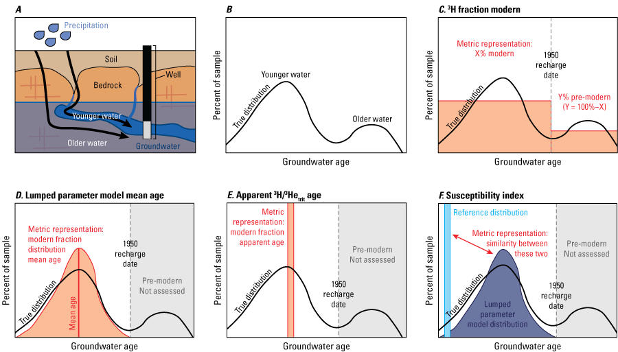
Conceptual diagrams showing the representation of groundwater age used in this study including A, the conceptualization of groundwater age; B, a hypothetical age distribution; C, the 3H fraction modern metric; D, the lumped parameter model mean age metric; E, apparent 3H/3Htrit age metric; and F, susceptibility index metric.
The approach for LPM selection and interpretation was dictated by the utility of the various tracers for age dating, comparison of tracer concentrations to expected atmospheric inputs, and the conceptual hydrogeology. At Fort Detrick Area B, the dispersion model (DM) that describes the output tracer concentrations according to the advection-dispersion equation was selected for LPMs. The fitted dispersion parameter (DP) is directly proportional to the amount of mixing along and between flow paths, with low DP values (DP=0.001) approximating piston flow and high values (DP=3) approximating exponential mixing of flow paths. The limited number of tracers useful for input to LPMs in this study reduce how well the models are constrained and are representative of all flow paths captured in a sample. As a result of tracer selection, LPM-derived age metrics of this study provide information on the young portion of the true age distribution.
Susceptibility Index
The susceptibility index (SI) provides a quantitative estimate of susceptibility of a well to land surface contamination. More specifically, it is a relative measure of how soon a conservative contaminant in the groundwater recharge area would arrive at the well. The SI is calculated as the normalized difference between the LPM-derived cumulative distribution function (CDF) of age and a reference CDF (Solder and others, 2020) as described by the following equations.
where DH is the Hellinger distance calculated as whereP(i)
is the cumulative probability of the age distribution of interest for a given time-step,
Q(i)
is the cumulative probability of the reference age distribution for a given time-step,
i
is the time-step of the cumulative distribution function, and
k
is the age corresponding to the last time-step.
The reference CDF was defined in this study as a piston-flow model with a mean age of 1 year. The SI is unitless and ranges between 1 (indicating young ages and a narrow age distribution) and approaching 0 (indicating older ages and a broad age distribution). Implicit in the calculated SI are the limitations of the LPMs in this study.
Statistical Methods
To assess the geochemical similarity among samples, multivariate statistical methods were applied. Statistical analyses provide a formal measure of the multivariate relation of groundwater chemistry across sample sites. The statistical similarity between sample chemistries were interpreted here to indicate similarity of recharge source(s) and flow-paths. Variables for analysis included select tracer data and the major ion chemistry. Variables were removed prior to analysis based on (1) a combination of correlation coefficients (Spearman’s ρ) greater than 0.7 (p-value <0.05), (2) having similar geochemical signals based on working knowledge of system chemistry and ion sources, and (3) a high number of censored values, in other words, greater than 10 percent of values below the laboratory reporting limit. Censored values for the remaining censored variables (Br, Ba, B, Sr, V, Li, Se, and U) were set to the reporting limit. For some kinds of statistical analyses, reporting limit substitution can be problematic due to sample-by-sample variations in reporting limit. In this analysis the laboratory analytical methods and reporting limits were the same across samples and this substitution creates equal values that do not inject false distinctions between values during clustering. Furthermore, the conservative use of substitution for constituents with 10 percent or fewer censored values likely has a relatively small impact on clustering results. Variable values were standardized prior to analysis to the sample population mean and a standard deviation of one. Hierarchical cluster analysis (HCA) was applied to 30 selected constituents. HCA provides an objective method of evaluating the similarity in groundwater chemistry between sample sites for a suite of chemical constituents. Constituent values were centered and scaled, a distance matrix was computed using Euclidean distance, and Ward’s method of minimum variance (Ward, 1963) was applied to cluster samples with similar geochemical characteristics. The heatmaply package (Galili and others, 2018) in R statistical software (R Core Team, 2018) was used to apply the HCA and visualize the results using these methods. HCA produces a dendrogram from which groups can be defined. In this study we use the HCA-produced dendrogram along with professional judgement to define and interpret the groupings.
Correlations between groundwater chemistry and sample site characteristics (including depth of sample interval and site location) were assessed to determine the spatial relation of groundwater chemistry. Correlation coefficients for Pearson’s r, indicating the deviation of sample values from a linear relation, and Spearman’s ρ, indicating a monotonic relation between the variables, were calculated at the 95-percent confidence level. Only statistically significant correlations are reported with a preference toward Spearman’s ρ if both correlation metrics are meaningful. Correlation coefficients and respective statistical significance (p-values) were determined using cor.test() function in R (R Core Team, 2018).
Results
The following sections describe the observed geologic, hydrologic, and geochemical data collected at Fort Detrick Area B. These data were interpreted to characterize the potential controls on groundwater flow, characterize the responsiveness of the coupled groundwater and surface water system, evaluate the potential for interbasin transfer by conducting a water budget analysis, and inform the characteristics of the aquifer underlying Area B through a synoptic groundwater age dating and geochemical analysis.
Geological Data Interpretation
The geological and geophysical data interpreted in this study were collected in previous investigations at Fort Detrick Area B (Arcadis Inc., 2014; Arcadis Inc., written commun., December 2019). The data were interpreted in this report to identify the potential geological controls acting on the groundwater system and to characterize the potential controls that are not well described by the available data.
Boring Log Reanalysis
The 76 available logs recorded by drillers and onsite geologists during the installation of monitoring wells across Area B were interpreted to identify (1) the depth of the soil-rock contact, (2) the number of voids or cavities reported during well drilling, and (3) the interpreted thickness of the epikarst, a conceptualized layer of increased transmissivity resulting from solutionally enlarged fractures and weathering. Although the soil-rock contact is readily identified in the boring logs, the number of cavities/voids and the epikarstic thickness require professional judgement to identify. In some cases, a zone of numerous voids was reported; in this analysis we provide the number of distinct voids or void zones reported even though these may vary in thickness. Where these were not clearly enumerated, we indicated the number with a greater than symbol. The transition from epikarst to the fracture-dominated competent rock is rarely abrupt and the degree of confidence in identifying this layer is dependent to some extent on the level of detail within the drillers’ or geologists’ logs. In some cases, this layer is evidently missing, as there are no reported weathered zones matching the conceptualized features of an epikarst.
The depth to the soil-rock contact for individual reported boring logs generally decreases from west to east across Area B, with this depth commonly reported to be 20 to 40 ft on the west edge of Area B and 5–20 ft in the eastern third of Area B and to the east of Carroll Creek (fig. 12). The greatest depths to the soil-rock contact are reported south of the west Area B boundary, where depths of 75 ft (WVLY-2), 65 ft (WVLY-5), and 51 ft (WVLY-1) are reported. The average depth across all 73 reported soil-rock contact depths is 24.5 ft.
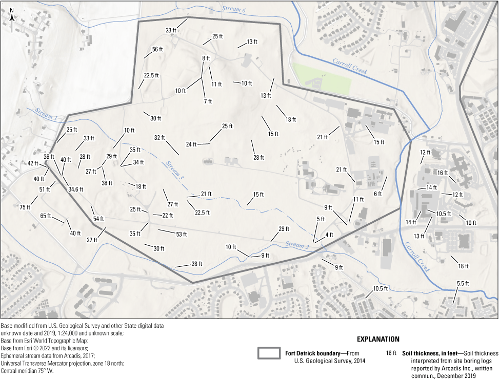
Reported soil thickness in drilling logs, Fort Detrick, Frederick, Maryland. Boring log data reported by Arcadis Inc., written commun., December 2019. Ft, feet.
Of the 75 boring logs from which the number of distinct voids could be evaluated, 41 (54.6 percent) had at least one void reported during drilling and 14 (18.6 percent) had three or more distinct voids or void zones. The greatest number of distinct voids were reported along the southwest boundary of Area B, with three wells (BMW58D, BMW59D, and BMW47D) having six or more distinct, solutionally enlarged cavities large enough to be detected during drilling. This region also contains a greater number of voids encountered during drilling (fig. 13). The majority of wells drilled in the western third of Area B encountered at least one void large enough to be noticed during drilling. Voids are also encountered elsewhere across Area B, including in the north, which is underlain by the New Oxford Formation, and to the east of Carroll Creek.

Voids reported during drilling, Fort Detrick, Frederick, Maryland. Boring log data reported by Arcadis Inc., written commun., December 2019.
Of the 60 boring logs from which the depth to the bottom of the epikarst could be evaluated, 19 (31.6 percent) had no identifiable zones of weathering or no reported voids. No epikarst was identified in these wells and are labeled with “None” in figure 14. The remaining 41 boring logs had an average depth to the bottom of the epikarstic zone of 86 ft below ground surface, with a median value of 59 ft. Six boring logs had voids and weathering to a depth greater than 100 ft below ground surface. One boring, BMW67E, had a reported water-bearing void at 326 ft below ground surface. The thickness to the bottom of the epikarst is variable and, although depths exceeding 75 ft below ground surface were most commonly observed in wells along or south of the southwest Area B boundary, the available data do not have readily apparent trends. This likely reflects the subsurface heterogeneity, the variable detail in reported site boring logs, the varying depths of the logs, and the challenge in interpreting this feature. However, the presence of sites throughout Area B that have limited reported weathering and solution-enlarged cavities suggests that the epikarst is not a laterally continuous layer and that is observed in the boring logs. This interpretation agrees with the description in Arcadis Inc. (2014) of the epikarstic layer as laterally discontinuous.
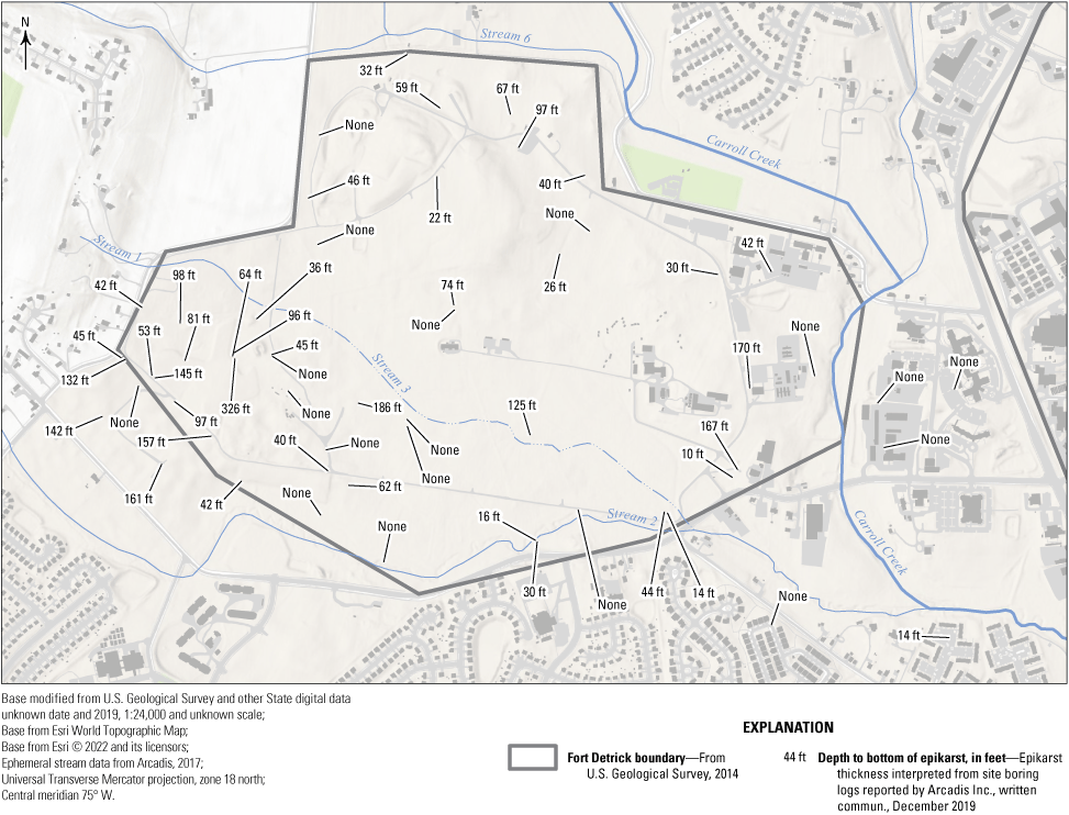
Interpreted depth to bottom of epikarstic zone, Fort Detrick, Frederick, Maryland. Boring log data reported by Arcadis Inc., written commun., December 2019. Ft, feet.
Geophysical Log Reanalysis
The orientation of fractures and linear features interpreted from geophysical log data reported in appendix D of Arcadis Inc. (2014) are shown in figure 15. Individual logs were sometimes collected at the same location but at different depth intervals, with the relative depth interval of the data collection denoted by letters A–E following the location name. Each point on figure 15 represents the projection of a point orthogonally intersecting a plane, as projected into the lower half of a sphere. The geophysical logs are grouped by lithology and ordered alphanumerically within each group.
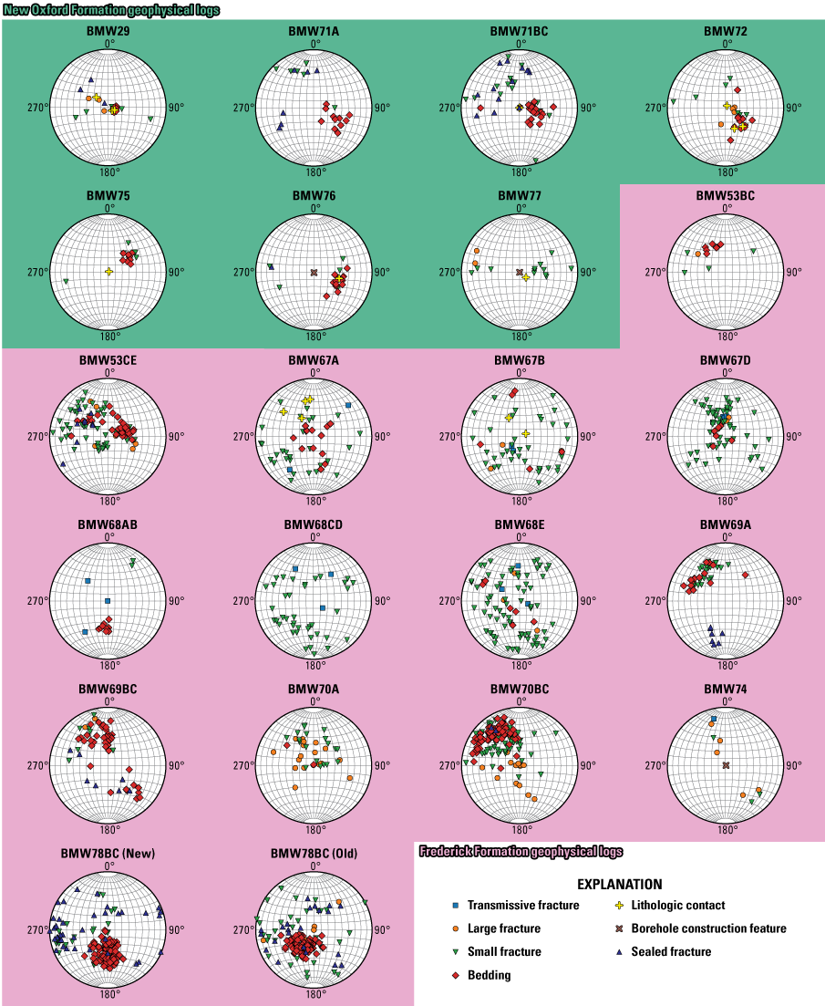
Stereonets indicating the orientation of planar features identified in the geophysical log data.
The bedding orientation interpretations generally agree with what is presented in Arcadis Inc. (2014), such that the New Oxford Formation units in the northern portion of the site dip gently to the west (BMW29, BMW71A, BMW71BC, BMW72, BMW75, BMW76), whereas the bedding direction in the Frederick Formation is less consistent. Some geophysical logs (BMW70BC, BMW69A, and BMW53BC) show the limestone of the Frederick Formation dipping to the southeast, consistent with regional mapping of the Cambrian units (fig. 2). Some logs (BMW68AB, BMW78BC [New], BMW78BC [Old]) show bedding dipping to the north, and yet other logs show no clear directionality to the bedding (BMW68CD, BMW69BC, BMW74, BMW67A, BMW67B, BMW67D). In all logs, fracture and void orientations were also recorded. A dominant orientation of fractures is not observed, except in the case when small fractures tend to follow the bedding orientation (BMW69A, BMW70BC).
Hydrologic Monitoring Results
The hydrologic data collected from the monitoring network of streamgages, wells, and precipitation characterizes the responsiveness of the system to individual storm events, seasonal variation, and interannual variability. The data collected in this study for the period from October 1, 2017, to December 31, 2020, are shown in figure 16, including the Palmer Drought Severity Index (Palmer, 1968), as reported by the GridMET dataset (fig. 16A; Abatzoglou, 2013). This metric is derived from estimates of precipitation and temperature data to estimate the cumulative deviation from normal hydrologic conditions. Negative values indicate drier than normal conditions and positive values indicate wetter conditions, with the magnitude indicating the severity of the deviation. The monthly total precipitation recorded at the USGS gage adjacent to the upstream streamgage on Fort Detrick Area B is shown in figure 16B. During the monitoring period at Fort Detrick, an abrupt transition from slightly drier than normal conditions to very wet conditions was driven by historically high precipitation beginning in May 2018. Through the rest of the monitoring period, conditions remained wetter than normal, but the severity of the departure began to decrease beginning in mid-2019. The daily mean total streamflow and stream base flow for the two Carroll Creek USGS streamgages are shown in figure 16C; note the logarithmic y axis. Base flow is calculated using the OHS method (Raffensperger and others, 2017). The daily mean stream temperature and specific conductance observed at the two Carroll Creek USGS streamgages are shown in figure 16D. The daily mean water table elevations observed at 12 groundwater monitoring wells on Fort Detrick Area B are shown in figure 16E. The monitoring period for the wells began in October 2018.
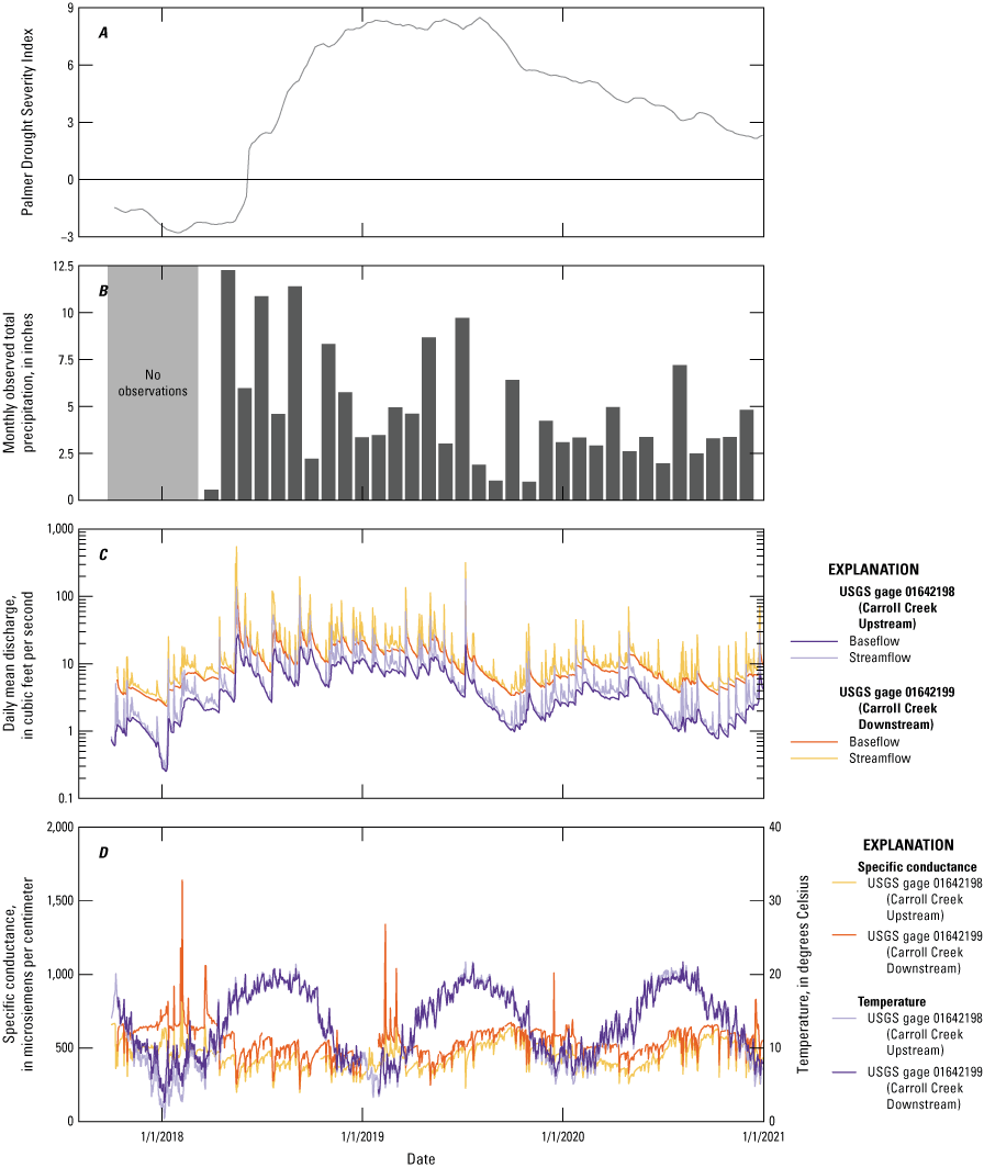
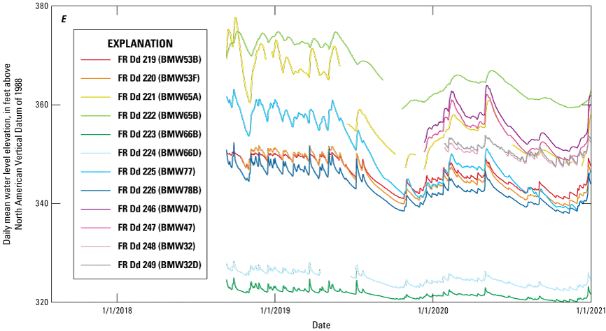
Hydrologic data collected at Fort Detrick Area B, Frederick, Maryland including the A, Palmer Drought Severity Index; B, monthly observed total precipitation; C, daily mean discharge; D, daily mean stream temperature and specific conductance; and E, daily mean water table elevations. A logarithmic axis is used in panel C and a dual y-axis is used in panel D. USGS, U.S. Geological Survey.
Streamflow Monitoring
Streamflow monitoring at the two streamgage locations revealed important dynamics in the total streamflow and stream base flow during the change from dry to historically wet conditions observed during the monitoring period. Total streamflow peaked during a flood event on May 17, 2018, and stream base flow remained elevated from May 2018 until June 2019, when decreased precipitation accumulation led to a decline in streamflow through the late summer and early fall of 2019 (fig. 16C). In 2020, a more typical seasonal pattern of higher spring streamflow and lower fall streamflow was present. The downstream Carroll Creek streamgage record of stream base flow began on October 11, 2017. In order to estimate the total stream base flow observed for the full water budget period, the October 2017 stream base flow was estimated using a linear regression model (y=1.01x+0.348; R2=0.984) with the upstream Carroll Creek gage monthly totals.
Base flow at the two streamgage locations revealed the seasonal patterns of groundwater discharge (base flow) and surface runoff (quickflow) to Carroll Creek. The two streamgage locations bound the Carroll Creek stream reach that includes numerous springs. By evaluating the differences in stream base flow and quickflow between the streamgages, the aggregate net changes in groundwater discharge and surface runoff to the stream were evaluated. To allow direct comparison between quickflow and base flow, values were normalized by the watershed area and reported in units of a length per unit watershed area (fig. 17). To compute the watershed difference values, the difference in monthly total base flow or quickflow volume between the two streamgages was normalized by the area shown in yellow in figure 17B. Throughout the monitoring period the area-normalized quickflow for the two streamgages was generally similar in timing and magnitude, although the downstream gage usually exhibited slightly more quickflow per unit area, with the exception of May 2018—a period of intense precipitation and flooding. The downstream watershed encompasses more urbanized area and impervious surface in the vicinity of Area A, a likely cause of greater quickflow per unit area within the watershed difference area.
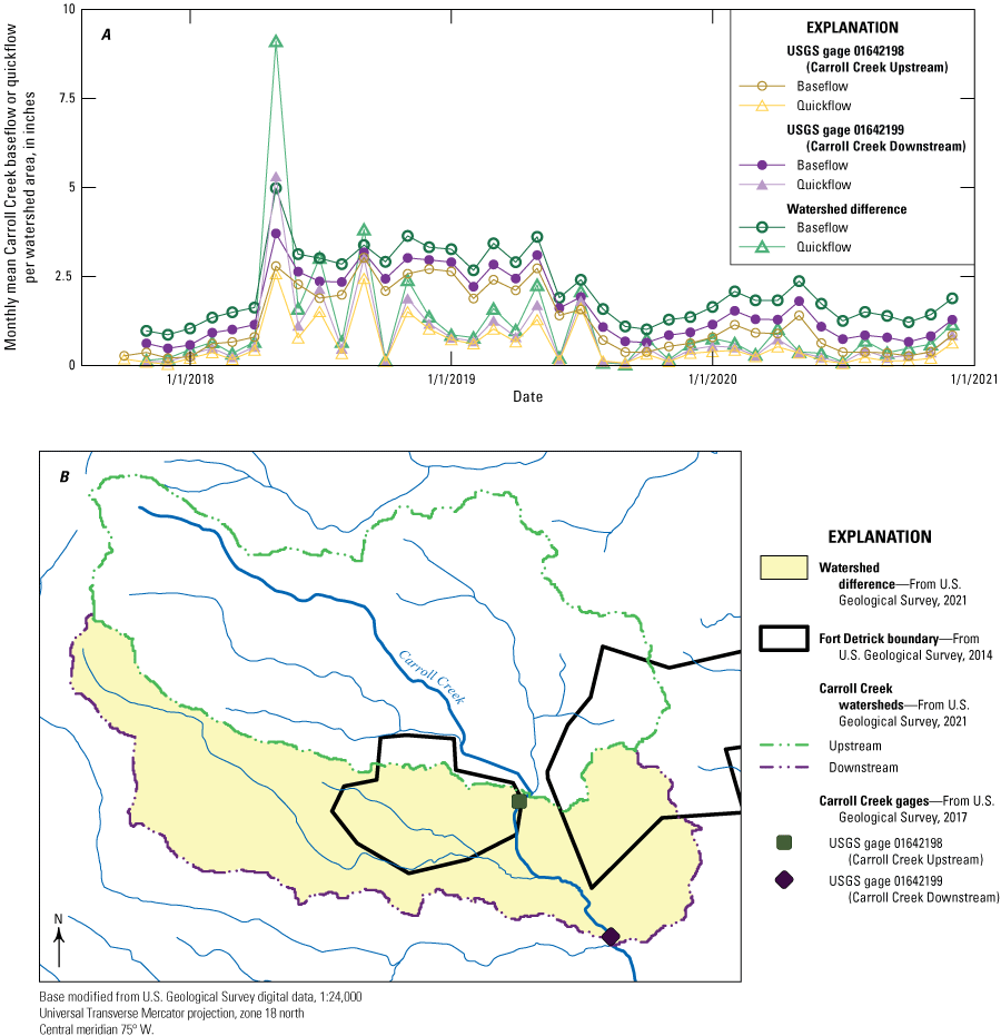
Monthly mean stream hydrograph separation results for the upstream and downstream Carroll Creek streamgages. USGS, U.S. Geological Survey.
Both streamgages typically have more monthly mean base flow than quickflow. This is especially clear in late 2018 and early 2019, when stream quickflow declines but base flow remains elevated. Base flow increases once again in the spring of 2020. The downstream gage consistently has more base flow per unit area than the upstream gage. That requires high values of base flow per unit area within the watershed difference area, which encompasses the region with identified springs on the east edge of Area B.
The observed stream temperatures (fig. 16D) exhibited a strong sinusoidal annual variation, with the annual daily mean temperature ranging from 5 to 20 degrees Celsius (°C). In this area, stream temperatures typically reach their maximum value in July and their minimum value in January. The temperatures observed at both streamgages were similar, except for a period around the annual maximum and minimum, when the upstream gage had a greater maximum or lesser minimum. Observed specific conductance, also shown in figure 16D, exhibited a lagged annual sinusoidal variation during 2019 and 2020, reaching its maximum value of 600–700 microsiemens per centimeter (µS/cm) in October and its minimum value of 350–450 µS/cm in May of those years. This pattern was disrupted from the beginning of the monitoring period through early 2019, with no evident annual maximum in the summer months of 2018. The summer of 2018 was a period of elevated stream base flow (fig. 16C). During individual storm events, the specific conductance exhibited short-term variation representing different sources of water input to the stream. Most often, a storm event causes the specific conductance to abruptly decrease as relatively low specific conductance water reached the stream through precipitation and overland runoff. The specific conductance increased as base flow became the predominant water source. During winter months, several storm events exhibited the opposite behavior, with pronounced spikes in specific conductance exceeding 800 µS/cm. These spikes represent the influence of road salt applied to roadways that reached the stream in snowmelt or other runoff periods. For most of the observation period, the specific conductance in the downstream gage exceeded the upstream gage, which is consistent with increases in downstream specific conductance observed in synoptic USGS monitoring shown in appendix 1.
Stream Base-Flow Results
The results of the OHS and CaF base-flow separations are shown in table 4 for the 52 streamgages within the region surrounding and including Fort Detrick Area B that are evaluated in the SWB domain. Only five streamgages have the specific conductance time series required for OHS analysis; the remaining gages are evaluated with the CaF method. The computed alpha values range within the 52 watersheds from 0.91 to 0.99, with a mean of 0.96. A mean of 0.95 was reported by Raffensperger and others (2017) for selected Chesapeake Bay watersheds.
Table 4.
Results of optimal hydrograph separation (OHS) and Collischonn and Fan (CaF) for accepted models.[USGS, U.S. Geological Survey; MM, two-digit month; DD, two-digit day, YYYY, four-digit year; SC, specific conductance; SCfit, peak-fitting base flow OHS SC model; OHS Beta, optimized value of beta using optimal hydrograph separation; CaF Beta, beta determined using the method of Collischonn and Fan (2013); CS, quickflow SC; RMSE, root-mean-square error of modeled and observed SC in OHS model; μS/cm, microseimens per centimeter; ft3/s, cubic feet per second; NS, Nash-Sutcliffe efficiency of modeled and observed SC in OHS model; —, no value]
The two streamgages installed for this study on Carroll Creek (USGS station numbers 01642198 and 01642199) were both successfully evaluated with OHS, with Nash-Sutcliffe efficiencies of 0.71 and 0.69, respectively. The results of the OHS evaluation for each streamgage are presented in figures 18 and 19. Values of β are suggested to be related to aquifer material, with values of 0.8 for perennial streams with porous aquifers, 0.5 for ephemeral streams with porous aquifers, and 0.25 for perennial streams with hard rock aquifers (Eckhardt, 2005; Raffensperger and others, 2017). The values calculated for the two Carroll Creek gages (0.737 and 0.763) are consistent with a karstic environment with a relatively porous aquifer material.
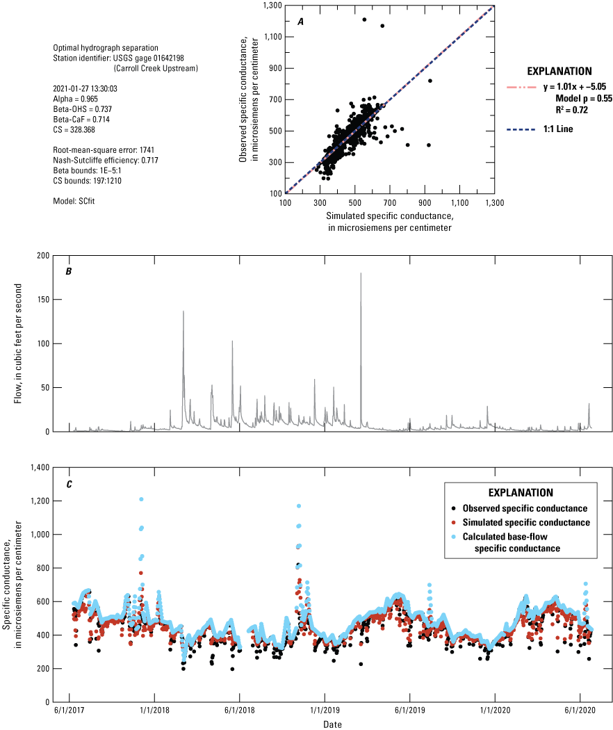
Optimal hydrograph separation (OHS) results using the SCfit model for base-flow specific conductance (SC) for U.S. Geological Survey (USGS) gage 01642198, the upstream Carroll Creek gage, showing, A, simulated compared to observed SC, B, the streamflow hydrograph, and C, time series of simulated and observed SC values and simulated SC base flow. CaF, method developed by Collischonn and Fan (2013); CS, quickflow SC; Model p, model significance level of regression; R2, coefficient of determination.
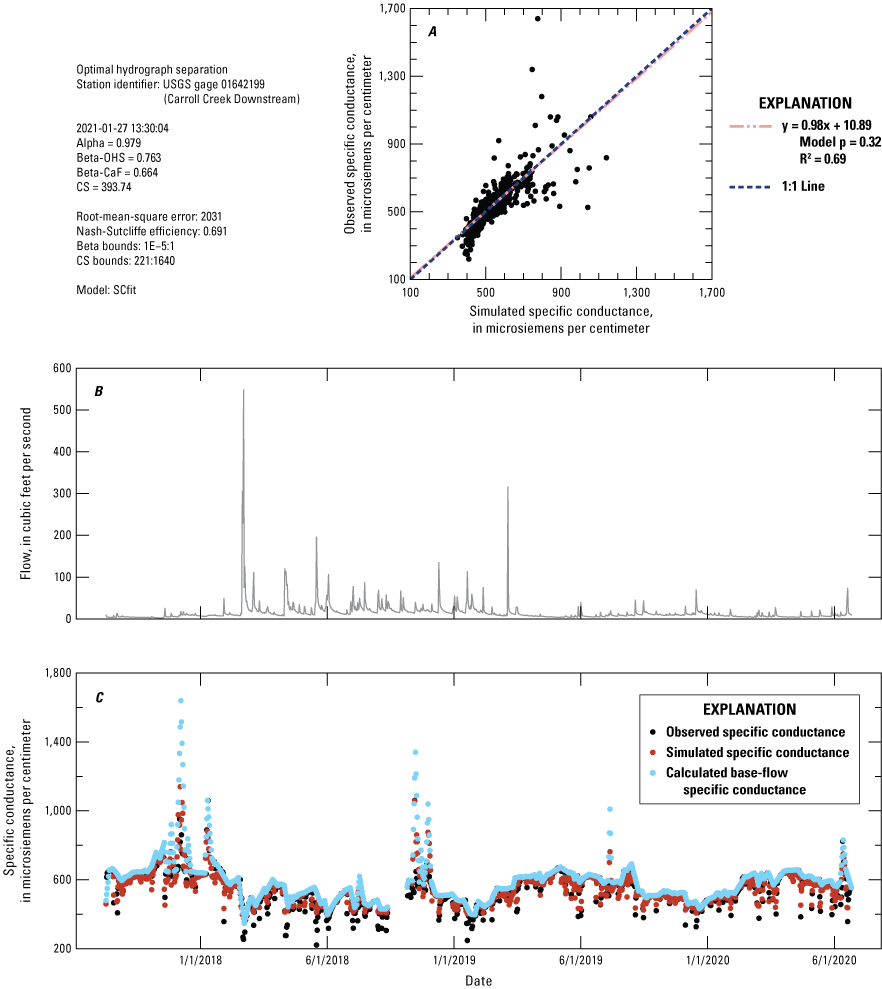
Optimal hydrograph separation (OHS) results using the SCfit model for base-flow specific conductance (SC) for U.S. Geological Survey (USGS) gage 01642199, the downstream Carroll Creek gage, showing, A, simulated compared to observed SC, B, the streamflow hydrograph, and C, time series of simulated and observed SC values and simulated SC base flow. CaF, method developed by Collischonn and Fan (2013); CS, quickflow SC; Model p, model significance level of regression; R2, coefficient of determination.
A comparison between three different hydrograph separation methods (fig. 20) shows that the characteristics of the Carroll Creek watersheds relative to 52 regional streamgages are consistent regardless of which method is used, even if the values differ slightly among the methods. The results of comparisons between PART, OHS, and CaF for two base flow separation metrics include (1) the annual average (water years 2017–20) base flow per unit area (fig. 20A–C) and (2) the base flow index (fig. 20D–F). During the monitoring period, numerous large storm events resulting from localized intense precipitation for the Carroll Creek gages led to flood events in water years 2018 and 2019 (fig. 16) that were not experienced by all regional gages. However, the results for water year 2020 were generally consistent with 3 water-year values shown in figure 20. For the five streamgages for which OHS could be applied, there is close agreement in the estimated recharge per year, though PART slightly overestimates the base flow per unit area when compared to OHS (fig. 20B) and CaF (fig. 20C). The karst-designated watersheds tend to have a slightly higher base flow per unit area (fig. 20C) than those designated non-karst, though there is considerable overlap. The downstream Carroll Creek gage (01642199) had the highest base flow per unit area of all the gages examined over this 3-year period, regardless of which separation method was used. For water year 2020 alone, this watershed had the third highest base flow per unit area (PART) or the sixth highest base flow per unit area (CaF), depending on the algorithm. The upstream Carroll Creek gage (01642198) had a base flow per unit area more typical of other regional karst watersheds. This result suggests that focused groundwater recharge and discharge processes within the lower watershed compose a greater proportion of the total streamflow than many regional karst streamgages.
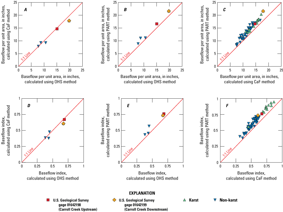
Comparison of computed base flow per unit area per year (A–C) and base flow index (D–F) for 52 streamgages in the region surrounding Fort Detrick, Area B for water years 2017–20. OHS, optimal hydrograph separation; CaF, method developed by Collischonn and Fan (2013).
The base flow index values computed using OHS and CaF are generally in close agreement for the five USGS gages for which CaF and OHS could be computed (fig. 20D). PART tends to overestimate the base flow index relative to both OHS (fig. 20E) and CaF (fig. 20F). This is somewhat in contrast to the results of Sanford and others (2012) for Virginia watersheds, but more consistent with Chesapeake Bay watersheds (Raffensperger and others, 2017). The karst-designated watersheds have a higher base flow index (0.75+) than non-karst watersheds (0.38–0.75), regardless of which method is used. The two Carroll Creek streamgages have intermediate values between these two groups (fig. 20F), indicating that the flashiness of the system is greater than many other regional karst watersheds. Contributing factors to this relative flashiness in the Carroll Creek watersheds may include geology (those watersheds are only composed of approximately 50 percent carbonate units) and development (the lower watershed area [Area A] is developed and impervious surfaces efficiently route stormwater to the stream).
Groundwater Monitoring
Groundwater levels from the monitoring network were interpreted to evaluate several aspects of the hydrologic system. The timeseries of groundwater levels were used to (1) identify the responsiveness of the groundwater system, (2) examine changes in potentiometric gradients during varying hydrologic conditions, (3) estimate a specific yield required for the water budget calculations reported in a subsequent section, and (4) estimate recharge using the EMR method.
Water Level Results
Groundwater levels observed within the groundwater monitoring network reveal a highly responsive groundwater system at Fort Detrick Area B. Daily mean groundwater levels across the site (fig. 16E) show rapid rises to individual storm events that can be on the order of several feet. The water levels time series show a similar pattern to the stream base flow (fig. 16C). The least responsive water level time series were collected at FR Dd 221 (BMW65A) and FR Dd 222 (BMW65B), located on the east edge of Area B. Large drawdowns in water level that take several days to recover are observed when these locations are sampled, leading to gaps in the observational record. These drawdowns, along with limited responsiveness to individual storm events may indicate these wells are not as connected to larger fractures and voids. However, the seasonal to interannual variability within these wells does agree with the rest of the monitoring network.
Specific Yield
Thirteen periods of recession were identified from which the apparent specific yield could be calculated (table 5). The recession period streamflow from the lower Carroll Creek gage (01642199) is described in table 5.
Table 5.
Recession periods from the lower Carroll Creek streamgage (01642199) used to calculate specific yield.[MM, two-digit month; DD, two-digit day, YYYY, four-digit year]
Using the criteria defined for this project, 6 of the 12 available groundwater-level time series had suitable data completeness and regression model fit statistics so that the apparent specific yield could be calculated. The fit statistics for the linear regression models are shown in table 6; the average of the calculated specific yields is 0.067 and the median value is 0.06. Only one well, FR Dd 219 (BMW53B), had an apparent specific yield confidence interval that included the mean and median values, perhaps indicating a bimodal distribution of apparent specific yields, although the number of available values was too few to make this determination. Olmsted and Hely (1962) calculated a value of 0.063–0.074 using wells within the Brandywine Creek basin in Pennsylvania, a 287 mi2 watershed underlain by fractured rock and carbonate units. Risser and others (2005) reported an average specific yield of 0.013 in fractured and folded shales, sandstones, and siltstones, though the apparent specific yields in upland wells ranged from 0.0035 to 0.035. Delle Rose and others (2018) apply this method to a deep, highly developed karst aquifer in the Salento peninsula, Italy, a region with extensive cave development, and report a much higher apparent specific yield of 0.45–0.49. In Berkely County, West Virginia, Shultz and others (1995) calculated specific yields using stream base flow records and groundwater level fluctuations in a 60 mi2 area underlain by carbonate rocks; the calculated specific yields ranged from 0.044 to 0.049. Based on the results from these studies, the observed median value of 0.06 and a range of 0.04 to 0.11 is consistent with the storage and release of water from secondary porosity (fractured rock) and relatively poorly developed karstic tertiary porosity (with drainage from solutionally enlarged fractures but not large caves). Due to the variability in observed specific yields, an uncertainty of ±50 percent to the median apparent specific yield value is applied in the water budget analysis, a range that includes the lowermost 95-percent confidence interval value (0.03) and the uppermost 95-percent confidence interval value (0.12).
Table 6.
Calculated specific yield values for six monitoring wells, Fort Detrick, Area B.[R2, coefficient of determination; p, significance level of regression; <, less than]
Groundwater Gradients
Hydraulic gradients observed between monitoring locations at Fort Detrick Area B were consistently from west to east and generally upwards, although the vertical well nest containing FR Dd 220 (BMW53F) and FR Dd 219 (BMW53B) showed a consistent downward gradient. Daily mean horizontal hydraulic gradients, daily mean vertical hydraulic gradients, and a schematic showing the well locations are shown in figure 21A–C, respectively. The greatest west-to-east hydraulic gradients were observed during the period of high-water levels in late 2018 and early 2019. These gradients decreased in late 2019 during a drier period, then steepened again slightly in the spring of 2020 during a period of higher water levels and stream base flow (fig. 16). During the fall of 2020, gradients again declined. These results indicate an influence of hydrologic regime on the observed west-east hydraulic gradient.
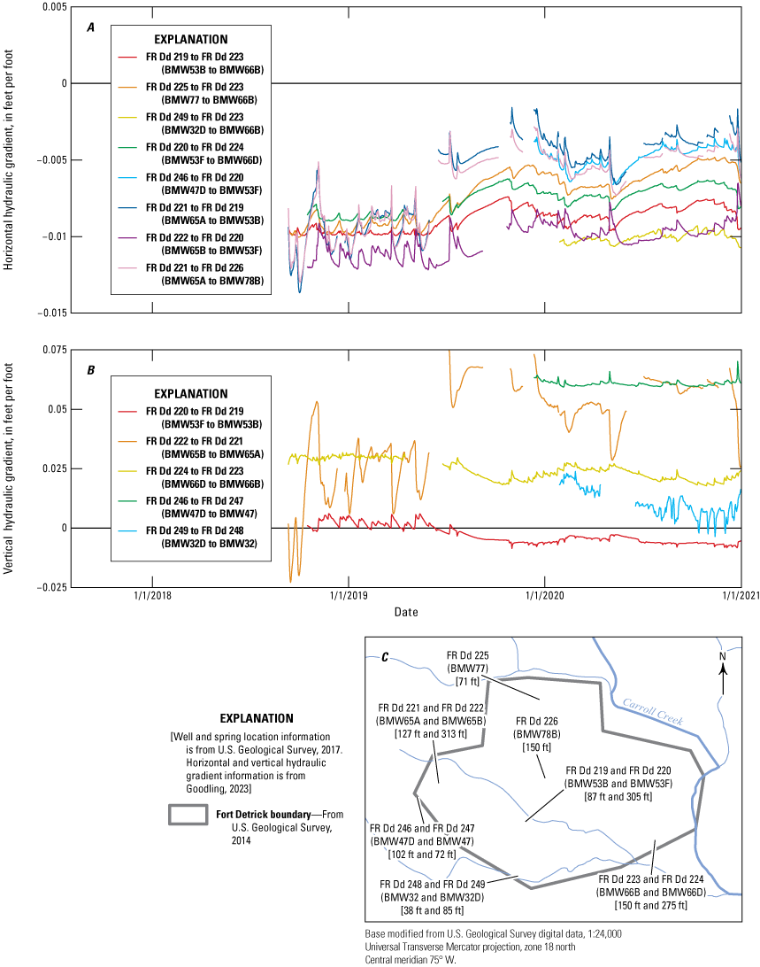
A, horizontal hydraulic gradients and, B, vertical hydraulic gradients between, C, selected well pairs. In A, negative is from west to east, and in B, positive is upwards. Ft, feet.
Vertical hydraulic gradients at five nested well pairs are shown in figure 21B. The nested well pair of FR Dd 222 and FR Dd 221 (BMW65B and BMW65A) are influenced by pumping and show the most delayed and muted of the water-level responses within the hydrologic network (fig. 16E). The highly variable vertical hydraulic gradient in response to storm events is explained by a lag in the response time for deeper well FR Dd 222 (BMW65B) relative to shallower well FR Dd 221 (BMW65A). During most of the monitoring period, the shallow well responded first, briefly resulting in a decreased vertical upward gradient until the deeper well responded. Small downward gradients were observed at this well network in late 2018, though for most of the period upward gradients were observed. The upward gradient was greatest during relatively dry periods (fall 2019 and 2020) and least during relatively wet periods (early 2019 and 2020), which stands in contrast to the pattern observed in three well pairs: FR Dd 224/223 (BMW66B/D), FR Dd 219/220 (BMW53B/F), and FR Dd 248/249 (BMW32/BMW32D). In those well nests, during relatively wet periods the upward gradient steepens and during relatively dry periods the upward gradient decreases or reverses entirely. Wells FR Dd 219/220 (BMW53B/F) had a slight upward vertical gradient during the extremely wet conditions at the beginning of the monitoring period. Since that time, a slight downward gradient was observed. This well nest is located within a low-lying ephemerally wet marshy area in the center of Area B. In late 2019, artesian conditions were observed in well FR Dd 220 (BMW53F). Consistent upward gradients were observed in well pair FR Dd 246/247 (BMW47/BMW47D). The magnitude of these vertical gradients generally agrees with the well nest FR Dd 221/FR Dd 222 (BMW65A/B) that is also located on the west edge of Area B.
EMR Results
EMR analysis was successfully applied to 10 of 12 groundwater-level time series, allowing estimates of groundwater recharge to be calculated from the well data. In addition to quantifying the episodic recharge entering the aquifer during storm events and overall aquifer responsiveness, this analysis also characterizes the physical properties of the aquifer through recession slope analysis. Wells FR Dd 221 (BMW65A) and FR Dd 222 (BMW65B) were excluded from this analysis, as the muted water-level responses and influence of groundwater pumping make these water-level records unsuitable for evaluation. The master recession curves for all wells are shown in figure 22.
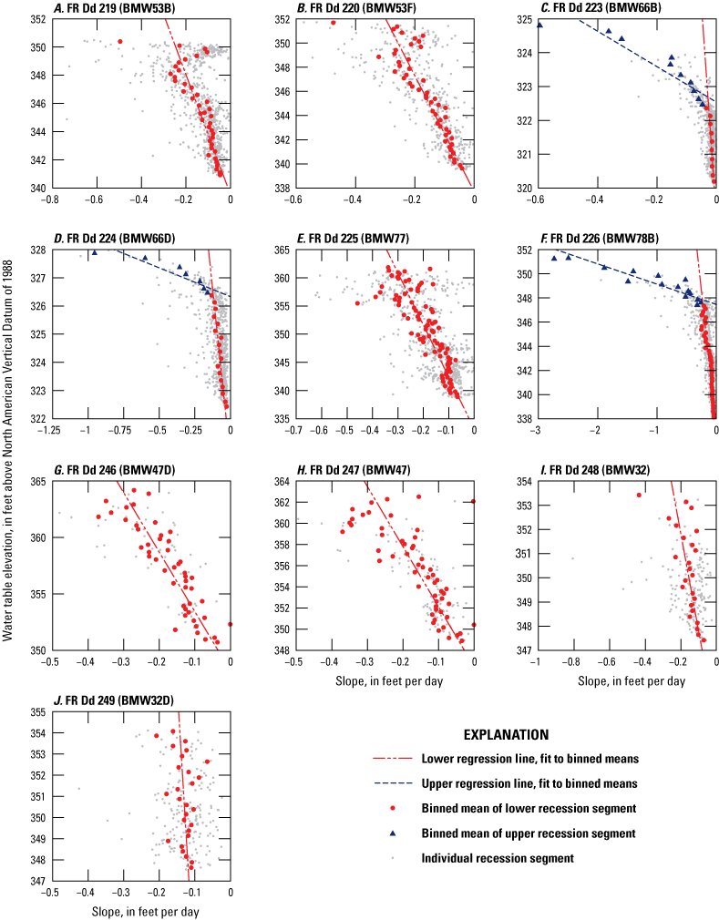
Master recession curves developed for 10 water-level time series collected at wells at Fort Detrick Area B.
Seven of the ten wells have simple linear relation between recession slope and water level elevation, which can be fit with linear regression (fig. 22). However, three wells show a break in slope in the master recession curve, with higher water table elevations having a much faster rate of recession than when the water table is lower: FR Dd 223 (BMW66B), FR Dd 224 (BMW66D), and FR Dd 226 (BMW78B). A break in slope in the master recession curve can be related to different physical processes, including the drainage of lithologies with different specific yields and the draining of fractures of voids within shallow karst aquifers (Nimmo and Perkins, 2018). A water table starting within the epikarst or a zone of high fracture transmissivity and lowering to a zone with less transmissivity can produce these effects. Due to the highly localized nature of preferential flow features, which may or may not intersect the monitoring well screen, predicting the recession behavior of unmonitored wells or unmonitored portions of the aquifer is problematic. However, this analysis shows the presence of this process.
Water-level fluctuations in response to storm events provide information about the water recharged to the groundwater system episodically during individual storm events. Nimmo and Perkins (2018) introduced a set of codes in the R language environment that can rapidly and reproducibly convert records of water level and precipitation observations to estimates of groundwater recharge using a set of adjustable parameters. For this study, the R scripts were applied to 10 groundwater-level time series recorded at Fort Detrick Area B. Wells FR Dd 221 (BMW65A) and FR Dd 222 (BMW65B) were excluded from this analysis, as the muted water level responses and influence of groundwater pumping make these water level records unsuitable for this analysis. The precipitation data used in this analysis was recorded by the USGS at the upstream Carroll Creek streamgage. Prior to the analysis, which requires continuous groundwater level records, the instantaneous records of groundwater level and precipitation were resampled to 15-minute intervals using linear interpolation and converted to fractional days since October 1, 2018, the beginning of many of the groundwater observations. Following the procedure outlined in Nimmo and Perkins (2018), a manual adjustment process for each site took place to ensure that (1) recession periods were adequately characterized to create a master recession curve relating the water table elevation and recession slope, and (2) recharge events were adequately characterized to capture the water table rise amounts, recorded as a linear distance. The parameters used to perform this analysis are shown in table 7. The master recession curves for all wells in this analysis are shown in figure 22. The specific yield is needed to convert the water table rises to estimates of recharge. The specific yields reported in table 6 were used for the six wells in the table; the remaining wells were assigned the median specific yield value of 0.06.
Table 7.
Parameters used to apply the methods of Nimmo and Perkins (2018) to 10 water-level time series collected at Fort Detrick Area B.[MRC, master recession curve; EMR, episodic master recession, NAVD88, North American Vertical Datum of 1988; dH/dt, change in elevation (dH) per unit of time (dt); —, not applicable]
Changes in Groundwater Storage
The relation between the monthly groundwater storage deviation and the monthly mean base flow computed using OHS is well-fit with a log-linear regression (fig. 23), indicating that the representation of groundwater storage in the groundwater monitoring network and stream base flow are highly related. The suitability of the log-linear regression ensures that changes in storage from the well network reasonably approximate the storage changes observed throughout the portion of the watershed draining to Carroll Creek. The regression equations shown in figure 23 allow the monthly groundwater storage to be estimated during the entire water budget period (fig. 24). The estimated change in groundwater storage for the water budget periods using the regression equations is shown in table 8, along with the estimated uncertainty. The estimated uncertainty is derived from the 50-percent uncertainty on the specific yield.
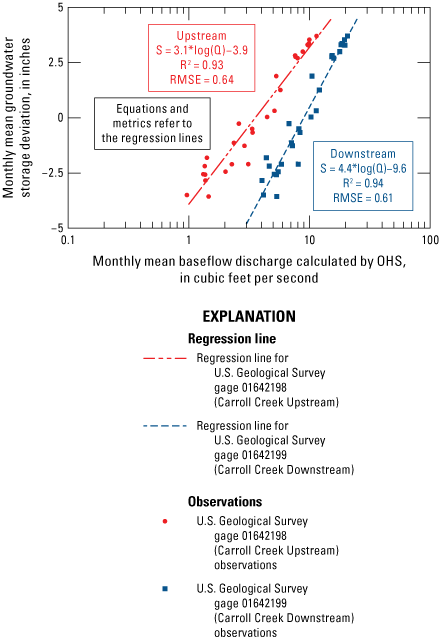
Regression relations between monthly groundwater level storage deviation and monthly stream base flow. RMSE, root-mean-square error; OHS, optimal hydrograph separation; R2, coefficient of determination.
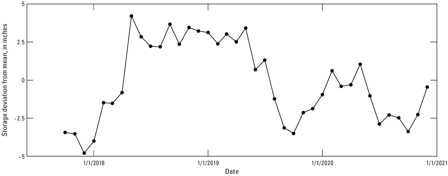
Monthly estimated groundwater storage at Fort Detrick Area B, shown as deviation from the mean value.
Table 8.
Change in storage for key water budget periods.The values reported in figure 24 and table 8 show that historically wet weather in early to middle 2018 led to a large increase in groundwater storage from the beginning of the water budget period, which by the end of 2020 had mostly returned to the original level of groundwater storage. High levels of groundwater storage are observed throughout the second half of 2018 and the first half of 2019. By the second half of 2019 through the end of the monitoring period, an annual pattern typical of the mid-Atlantic is shown; low amounts of groundwater storage in the fall and winter and increased groundwater storage in the spring. The net change in groundwater storage from the beginning (October 2017) to the end of the observation period (December 2020) was 2.97 in., a net increase of approximately 1 in/yr.
Precipitation Monitoring
Monthly precipitation totals observed at the upstream Carroll Creek streamgage are shown in figure 16B. As previously discussed, historically high precipitation in the spring and summer of 2018 was observed. For the water budget analysis, gridded precipitation estimates spanning the watersheds of interest are needed. In this study, PRISM data are used as an input to the SWB model. To ensure the precipitation estimates, which are developed at a national scale, are suitable for use at the watershed scale, a comparison was made between the gridded estimates and the observed precipitation. This comparison was made at two different time intervals; at a monthly interval and for the full duration for which both measures are available (May 1, 2018–December 31, 2020). The total USGS-reported total precipitation and PRISM data agree to within 3.3 percent (157.1 in and 162.3 in, respectively). The monthly observed and PRISM precipitation sums (fig. 25) are more variable but generally show a good agreement. Overall, there is a root mean squared error of 0.81 in. There is a slight (−3.2 percent) bias where low USGS-observed precipitation amounts are overestimated by PRISM. During wet months (greater than 5 in of observed precipitation), observations and PRISM agree within 15 percent. Because longer periods of record will have less relative uncertainty than shorter periods of record (as random noise cancels; see Winter [1981]), a 5-percent estimate of precipitation uncertainty is used, which is more representative of the difference between measured and PRISM totals over the water budget period than individual monthly totals.
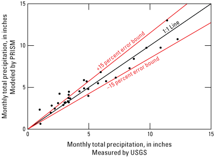
Monthly total observed precipitation at the U.S. Geological Survey (USGS) precipitation gage and modeled by Parameter-elevation Regressions on Independent Slopes (PRISM) from May 1, 2018, through December 31, 2020, the period for which both measures are available.
Fluorometric Monitoring
Fluorometric monitoring evaluated if quantifiable concentrations of dye are present within the groundwater system from the previous dye tracer tests in 1995 and 2013. Discrete split samples were collected in December 2020 and continuous fluorometric monitoring at key spring sites occurred for a duration of approximately 3 months each.
Discrete Monitoring
The 1-liter samples collected as split samples from quarterly monitoring and spring grab samples were analyzed for rhodamine and fluorescein on the Turner Scientific C6 Fluorometer in a laboratory setting. The apparent dye concentrations associated with varying levels of turbidity were also evaluated in a benchtop experiment, which indicated that low-level interference from turbidity was observed with this instrumentation (fig. 26A and B). The apparent rhodamine observed from turbidity interference is greater than the apparent fluorescein, though the relation between rhodamine and turbidity is better fit with a linear function than fluorescein. Although there were slight differences in the slope of the regression lines, overall, the magnitude of the interference for both the March 2019 and October 2020 tests were similar, showing good reproducibility of this evaluation.
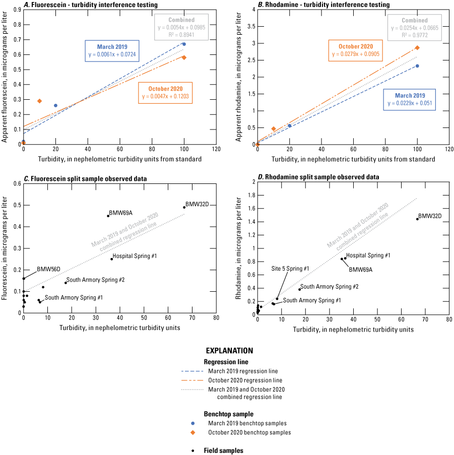
Results of benchtop turbidity experiment and discrete fluorometric sample analysis. The line shown in C and D is from the combined regression equations in A and B. The sample from BMW67C is not plotted in C and D; in that sample, 487.47 micrograms per liter (μg/L) fluorescein and 406.28 μg/L rhodamine were observed, and the sample was visibly pink. R2, coefficient of determination.
The observed dye concentrations in discrete samples collected for this study as a function of the sample turbidity are shown in figure 26C and D; the results are available in tabular format in table 9. The combined regression lines shown in figure 26A and B are also shown in figure 26C and D. All samples except BMW67C have low-level observed apparent dye concentrations that are explained by the natural particulates within the water; dye is not detected at a level above the instrument’s ability to resolve the dye. Concentrations of 487.47 μg/L fluorescein and 406.28 μg/L rhodamine were recorded in BMW67C. This well was the site of Eosine dye injections in the 2013 dye tracer study. It is likely that the recorded concentrations of fluorescein and rhodamine reflect the interference of Eosine dye in this well. To evaluate this, a 5,000 µg/L standard solution of eosine was evaluated on the fluorometer used in this study and the concentrations of apparent fluorescein and rhodamine were recorded. Apparent concentrations of 480.0 µg/L fluorescein and 400.0 µg/L rhodamine were observed, which indicates that Eosine interferes with the detection of these dyes in this well.
Table 9.
Discrete sample results from split well samples analyzed for fluorescein and rhodamine dyes.[MM, two-digit month; DD, two-digit day; YYYY, four-digit year; µg/L, micrograms per liter; FNU, Formazin Nephelometric Unit; °C, degrees Celsius; —, no note recorded]
Continuous Monitoring
Continuous monitoring at the three springs was conducted sequentially between November 2019 and October 2020. The complete time series of data collected at each site is shown in figures 27–29. All three springs had stable temperatures between 12.5 and 14.5 °C and pH values between 7.1 and 7.4, which is consistent with groundwater discharging from carbonate aquifers (Hem, 1985). Two of the springs (RISP-3 and Hospital Spring) are located within completed spring boxes, whereas South Armory Spring is in a channel originating approximately 20 ft from Carroll Creek. To maintain a sufficient water level for in situ monitoring, a temporary weir from sandbags was constructed. Intermittent leaks or rearrangement of this weir from Carroll Creek storm events led to some gaps in the monitoring period. The difference between the springs in completed box structures and the South Armory Spring is evident in the dissolved oxygen time series. RISP-3 and the Hospital Spring had diurnal fluctuations in dissolved oxygen consistent with plant and algal activity, whereas no such pattern exists in the South Armory Spring. The difference is also observable in the turbidity; the completed spring boxes had turbidities below 5 formazin nephelometric units (FNU) for the duration of the monitoring period and South Armory Spring had reported turbidities exceeding 60 FNU.
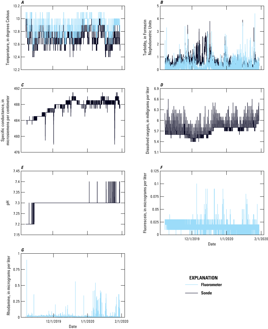
A, observed temperature, B, turbidity, C, specific conductance, D, dissolved oxygen, E, pH, F, apparent fluorescein, and, G, apparent rhodamine concentrations at spring FR Dd 213 (RISP-3). Two sensors were deployed at this location; the results of both sensors are provided.
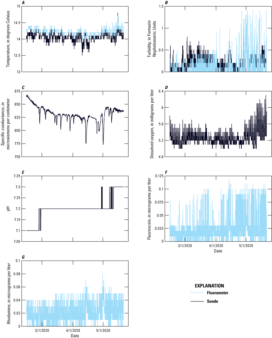
A, observed temperature, B, turbidity, C, specific conductance, D, dissolved oxygen, E, pH, F, apparent fluorescein, and, G, apparent rhodamine concentrations at spring FR Dd 178 (Hospital Spring). Two sensors were deployed at this location; the results of both sensors are provided.
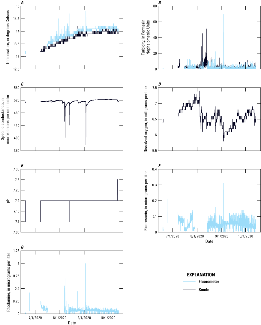
A, observed temperature, B, turbidity, C, specific conductance, D, dissolved oxygen, E, pH, F, apparent fluorescein, and, G, apparent rhodamine concentrations at spring FR Dd 245 (South Armory Spring). Two sensors were deployed at this location; the results of both sensors are provided.
Hospital Spring had a much higher specific conductance (775–875 μS/cm) than the other two springs (400–500 μS/cm) for the duration of the monitoring period. Freshening events from rainfall were apparent in all three springs, though these were much more pronounced in the South Armory and Hospital Springs. These freshening events may represent a mixture between groundwater and recharge from precipitation that represents quickflow or lateral vadose zone flow within the soil and (or) epikarst.
The observed apparent fluorescein and rhodamine concentrations are very low, with all concentrations below 1 μg/L for both dyes. These apparent detections must be considered in the context of the influence of suspended particulates (turbidity), which is explored further in the preceding section. The low-level and spiky nature of the apparent dye detections suggest that dyes are not observed in situ at a level greater than the ability of the sensor to detect the dyes in natural waters found at Fort Detrick.
Soil-Water Balance Model Results
The SWB model created for this study used the best available inputs of land cover, land use, climate, topography, and process-based information controlling the routing of water within the Fort Detrick watersheds. Additional detail on the implementation of the model including the complete outputs are available in an accompanying data release (Soroka, 2023). For the water budget calculation in this study (eq. 7), two water budget components (ET and interception) are assessed using the SWB. An additional SWB output, net infiltration, is presented though is not used in the water budget. This section is focused on the SWB model results at the watershed scale and timescales of 1 year or greater, as this is the scale relevant to the water budget calculation
Comparisons with Regional Streamflow
The SWB model was compared against regional streamflow records to evaluate the suitability of the ET, interception, and net infiltration outputs at the watershed scale and annual time period. Since the Carroll Creek streamgages had a short period of stream gaging (2017–present), a model domain much greater than the Carroll Creek watershed was used to capture streams with a longer record of streamflow data. Of the total monitored watersheds in the region (n=55) the authors selected 34 reference gages that had less than 1,000 mi2 of area, weren’t dominated by urban land-use areas, and didn’t have flow control structures such as hydroelectric facilities. A total of 36 watersheds were selected for comparison with the SWB model (34 reference gages and the 2 Carroll Creek gages; fig. 30A). The model was run for the entire domain for the period from January 1, 2000, to December 31, 2020. A simple steady-state budget that did not consider changes of storage was calculated for each gage for each year where streamflow data was available (fig. 30B); observed total streamflow per unit area is shown on the x axis and the net water entering the watershed as precipitation exceeding ET and interception is shown on the y axis. The SWB model in this study tends to slightly underpredict the total streamflow per unit area within the total watershed domain, with a –7.1 percent negative bias. The model consistently underpredicts the downstream Carroll Creek total streamflow, potentially due to local factors not represented in the model. Although there is scatter in the annual total streamflow per unit area, potentially resulting from interannual storage changes, focused groundwater recharge, or other processes not represented by SWB, the fit was deemed acceptable for the purposes of using ET and infiltration component estimates from SWB in the water budget calculation.
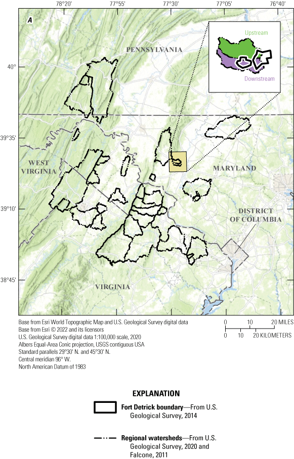
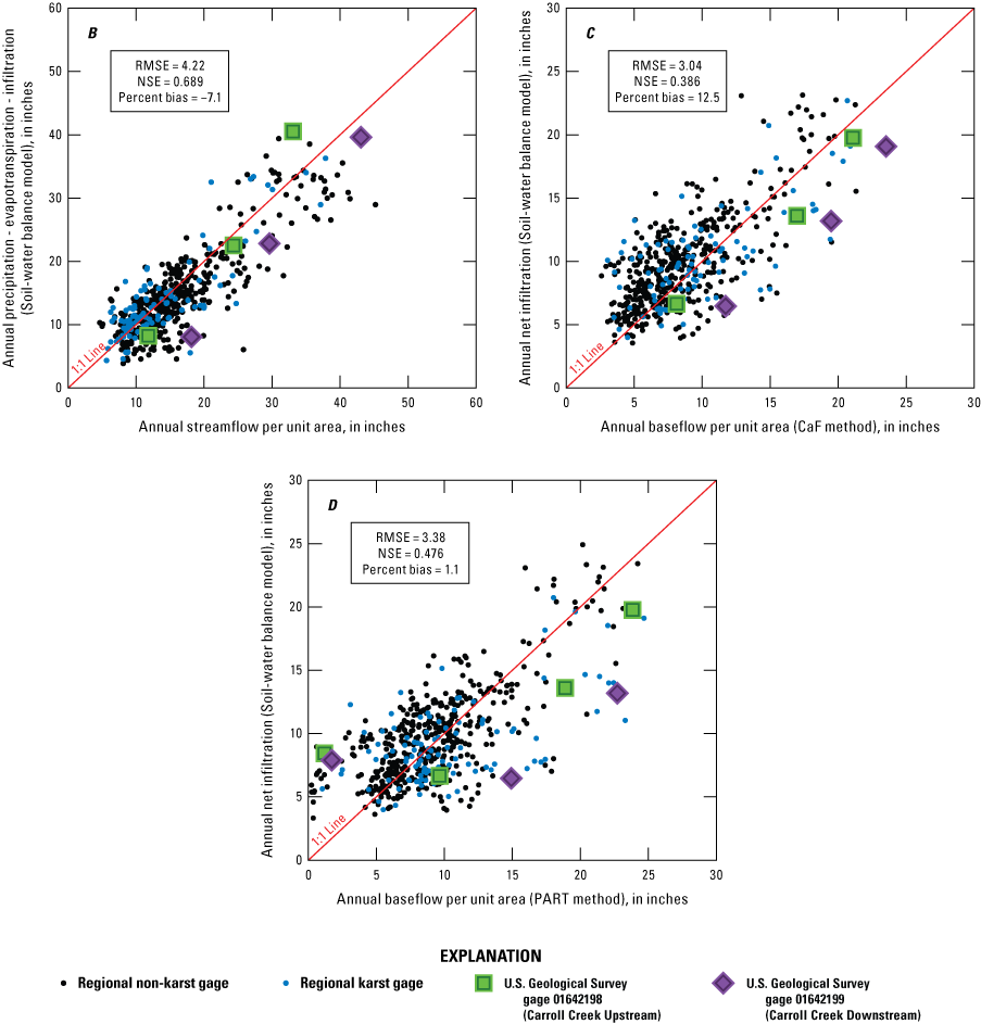
Comparisons between soil-water balance model outputs, streamflow, and stream base flow computed at, A, 36 watersheds within the region surrounding Fort Detrick for, B, observed streamflow, C, stream base flow using the CaF method and, D, stream base flow using the PART method. USGS, U.S. Geological Survey; RMSE, root-mean-square error; NSE, Nash-Sutcliffe efficiency coefficient; CaF, method developed by Collischonn and Fan (2013).
The annual results for the SWB infiltration are compared against base flow estimates computed using the CaF method (fig. 30C) and the PART method (fig. 30D). Again, for this evaluation changes in storage are not considered. The SWB model in this study tends to overestimate the annual base flow per unit area calculated with the CaF method, though the model consistently underpredicts the base flow per unit area for the Carroll Creek watersheds. The SWB model does not overestimate the base flow values derived from PART as much (1.1 percent bias), though a greater amount of scatter is observed. Taken together, the fit between observed stream base flow and simulated net infiltration was not deemed to be suitable enough for the net infiltration output of SWB to be used in the water budget calculation.
Carroll Creek Watersheds Results
Two SWB model outputs (ET and interception) and one SWB input (precipitation) are used directly in the water budget calculations in this study; these gridded values are presented in figure 31 for the area including the two watersheds evaluated. The period shown is the total water budget period from October 1, 2017, to December 31, 2020; the annualized values are reported as inches per year.
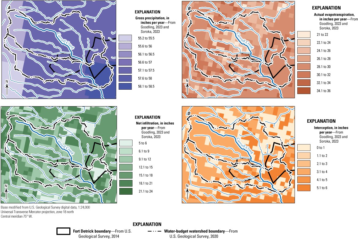
A, annualized gridded values for gross precipitation, B, actual evapotranspiration, C, net infiltration, and, D, interception from October 1, 2017, to December 31, 2020, for components used in the water budget calculation.
Sensitivity Analysis
The results of the sensitivity analysis indicate modeled actual ET and net infiltration are most sensitive to soil curve number. Sensitivity analysis was completed on the full model domain, the results for the lower Carroll Creek watershed (which encompasses the upper Carroll Creek watershed) are shown in figure 32. Changes in soil curve number inputs to as much as ±20 percent result in net infiltration output changes of approximately –5 percent or +30 percent, respectively. Soil groups 1, 3, and 4 were found to exhibit the most sensitivity in lower Carroll Creek watershed. Additional sensitivity to root zone is observed but results in less than 5 percent changes in net infiltration output for changes of 20 percent in root zone depth. Very little sensitivity to changes in readily evaporable water or total evaporable water is observed in the three examined SWB outputs.
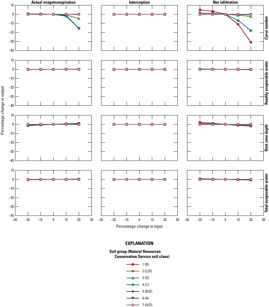
Results of a sensitivity analysis examining the sensitivity of changes of select model parameters to select model outputs.
Actual Evapotranspiration
In the SWB model, the actual ET represents the water evaporated or transpired from the soil. This amount is a function of the available water to be evapotranspired as well as the climate conditions and season, which determine the amount that could potentially be evapotranspired if available. In this study, the actual ET is computed using the SWB model. For comparison, the annual total actual ET estimated in this study was compared to four other sources of actual ET estimates. These products are inclusive of water transpired from the soil as well as evaporated from intercepted vegetation; therefore, the products are most comparable to the sum of the SWB actual ET and interception outputs. The SSEBOP, MOD16A2, and TerraClimate gridded evaporation products are remote-sensing based estimates of ET. A fourth method relies on a simplistic water budget equation (ET = P − Q / A − ΔS, where P is precipitation, Q is total streamflow, A is the watershed area, and ΔS is the change in storage) that neglects interbasin transfer and uncertainty; it is provided as a reference.
A comparison between the estimates of ET is shown in figure 33. The results are presented as the spatial watershed mean for the two study watersheds at the annual to 3-year timescale. In general, the estimates of actual ET at this temporal and spatial scale have a wide range, with 3 water-year mean values ranging from 17.6 to 35.7 in. The difference between the products reflects varying data sources, methodologies, and spatial resolutions. The TerraClimate dataset shows little interannual variability and consistently exceeds the other estimates of actual ET. The remaining products generally show increased actual ET during water year 2018, the wettest year monitored. Conversely, the lowest rates of actual evapotranspiration are reported during water year 2018, the driest year monitored. The P – Q / A – ΔS estimate of ET differs between the two gages, resulting from greater streamflow per unit area in the lower watershed. During all four intervals shown in figure 33, the SWB actual ET and interception sum is within 20 percent of one or both P – Q / A – ΔS estimates.
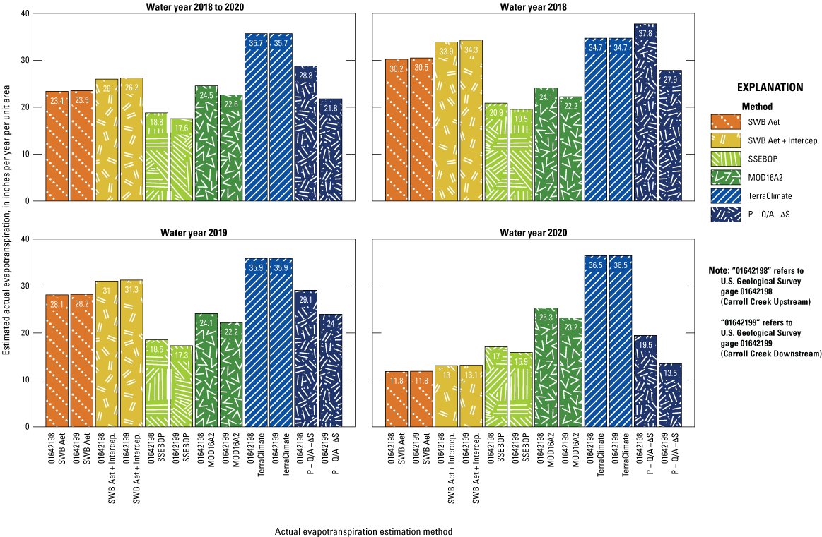
Comparison between estimated actual evapotranspiration between the soil-water balance (SWB) model used in this study and four alternative estimates of evapotranspiration. Aet, actual evapotranspiration; intercep., interception; P, precipitation; Q, stream discharge; A, watershed area; ΔS, change in groundwater storage.
Interception
Interception, the process by which vegetation surfaces prevent precipitation from reaching the ground surface, is sometimes combined with the overall flux of ET though it is represented as a distinct process in the SWB model. The importance of interception as a water budget term varies with rainfall amount and intensity, as well as the properties of the vegetation, including species and season (Kampf and others, 2020). There are few readily available global or national datasets with a temporal scale that aligns with the study time period. However, Miralles and others (2010) estimated the canopy interception using a multisatellite approach with data from the period of 2003–07. Globally, they report a canopy interception of 19 percent of precipitation for broadleaf deciduous forests. In forested regions of the mid-Atlantic United States, 10 to 20 percent of precipitation is estimated as interception. The interception estimated by the SWB model accounts for approximately 5 percent of the total precipitation during the water budget period. According to the 2016 National Land Cover Database, the upper and lower watersheds are 25.6 percent and 22.3 percent deciduous forest by land area (Dewitz, 2019). If in these forested areas of the watersheds approximately 20 percent of precipitation were intercepted, that would account for an approximate watershed-mean interception value of 5 percent of overall precipitation.
Net Infiltration
In the SWB model, the water that recharges the groundwater system is termed net infiltration. It is a representation of the water estimated to bypass the root zone and approximates the groundwater recharge if unsaturated zone flow and focused groundwater recharge is assumed negligible. In karst systems, this assumption may not be valid. The SWB estimated net infiltration is compared against other estimates of groundwater recharge in figure 34 for the 3 water-year period and for individual years. The SWB net infiltration is compared to (1) stream base flow per unit area, as calculated using OHS, which would equal groundwater recharge if there were no change in storage, no interbasin transfer, and no riparian zone ET; (2) the recharge estimated using the RORA displacement curve method; and (3) the recharge estimated for individual wells using the EMR analysis. The EMR results are only available for water years 2019 and 2020. The EMR method estimates recharge at individual well locations rather than the entire watershed; these wells are all located in the lower watershed area. The median value of estimated recharge from 10 groundwater wells, with the range of reported recharge shown by a vertical black error bar, is shown in figure 34.
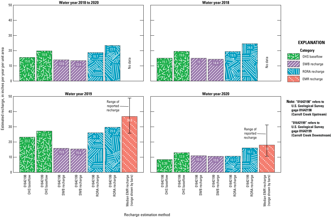
Comparison between estimated net infiltration from the soil-water balance (SWB) model used in this study to other data sources. EMR, episodic master recession; OHS, optimal hydrograph separation; RORA, RORA computer program.
Over the 3 water-year period, the recharge estimated from SWB for the lower watershed is consistently less than the stream base flow, recharge estimated using the RORA method, and recharge from EMR analysis. This difference likely reflects the effect of focused groundwater recharge, which is not simulated in SWB but would be characterized by the methods using streamflow (OHS base flow and RORA) and methods using groundwater time series data (EMR). The lower watershed contains a greater proportion of the karstic Rocky Springs Station Member of the Frederick Formation and identified springs and sinkholes than the upper watershed. The SWB recharge equals or exceeds the stream base flow in water year 2018 and water year 2020 and approximately equals the RORA recharge in water year 2020. The closer correspondence between the SWB outputs and other methods for the upper watershed likely reflects less focused groundwater recharge in this watershed, which contains the less karstic Triassic units. Water year 2019 contained a transition from historically wet conditions to more typical hydrologic conditions. Water was released from storage over this period (table 8), which may account for the discrepancy as SWB recharge is simulated to occur instantaneously following precipitation, whereas in the real system stream base flow remains high following a wet period.
Water Budget Results
The water budget described in equation 7, as well as the estimated uncertainties used to calculate the uncertainty in the water budget residual (eq. 8) were calculated in this study for six time intervals. Four of these are defined by the water year, which begins on October 1 and is often used in water budget studies as autumn is typically a period of low streamflow. These four intervals are (1) the 3 water-year period (October 1, 2017–September 30, 2020), (2) water year 2018, (3) water year 2019, (4) water year 2020. The budget was also computed for the full monitoring period (October 1, 2017–December 31, 2020), and the period following the anomalous May 2018 flooding (June 1, 2018–December 31, 2020).
Uncertainty in the water budget components was estimated using available information in the hydrologic monitoring, SWB model sensitivity evaluation, and when possible, through comparisons with independent datasets. Percentage uncertainties are assigned on the basis of this available information in a manner comparable to other studies (Maupin and Weakland, 2009; Winter, 1981). An uncertainty of 10 percent was assigned to streamflow totals, 5-percent uncertainty to precipitation totals, 30-percent uncertainty to actual ET calculated by the SWB model, and 10-percent uncertainty to interception calculated by the SWB model. Uncertainty in groundwater storage changes was estimated to be 50 percent.
The calculation results are shown in table 10 for the six time periods. For each time period, the calculation was completed for three spatial areas: the upstream Carroll Creek watershed, the downstream Carroll Creek watershed, and the watershed difference area, which represents the area within the downstream watershed that is not in the upstream watershed. The table presents the annualized budget components in inches per year. The water budget residual, as defined in equation 7 and the uncertainty on the residual as defined in equation 8 are presented for each time period and each spatial area. The interpretation of the water budget residual is only meaningful when the absolute value of the residual exceeds the absolute value of the uncertainty. Meaningful residuals are indicated with a footnote in table 10.
Table 10.
Water budget summary table.[in/yr, inches per year; P, precipitation; ET, evapotranspiration; I, interception; ΔS, change in groundwater storage; Q, stream discharge; R, residual; SWB, soil-water balance; PRISM, Parameter-elevation Regressions on Independent Slopes]
| Components | Upstream watershed | Downstream watershed | Watershed difference area | |||||
|---|---|---|---|---|---|---|---|---|
| Equation term | Data source | Uncertainty applied (percent) | Value (in/yr) |
Uncertainty (in/yr) |
Value (in/yr) |
Uncertainty (in/yr) |
Value (in/yr) |
Uncertainty (in/yr) |
| P | PRISM | 5 | 51.4 | 2.6 | 51.3 | 2.6 | 51.1 | 2.6 |
| ET | SWB | 30 | 23.4 | 7 | 23.5 | 7.1 | 23.7 | 7.1 |
| I | SWB | 10 | 2.6 | 0.3 | 2.7 | 0.3 | 2.8 | 0.3 |
| Q | Observed | 10 | 22.6 | 2.3 | 29.6 | 3 | 39.3 | 3.9 |
| ΔS | Calculated | 50 | 0 | 0 | 0 | 0 | 0 | 0 |
| Residual (P − ET − I − Q − ΔS = R) |
Calculated (eq. 7) |
Sum of squared errors (eq. 8) |
2.8 | 7.8 | −4.5 | 8.1 | −14.7a | 8.5 |
| P | PRISM | 5 | 67.8 | 3.4 | 67.1 | 3.4 | 66.1 | 3.3 |
| ET | SWB | 30 | 30.2 | 9.1 | 30.5 | 9.2 | 30.9 | 9.3 |
| I | SWB | 10 | 3.7 | 0.4 | 3.8 | 0.4 | 3.9 | 0.4 |
| Q | Observed | 10 | 24.2 | 2.4 | 33.7 | 3.4 | 46.9 | 4.7 |
| ΔS | Calculated | 50 | 5.8 | 2.9 | 5.8 | 2.9 | 5.8 | 2.9 |
| Residual (P − ET − I − Q − ΔS = R) |
Calculated (eq. 7) |
Sum of squared errors (eq. 8) |
3.9 | 10.4 | −6.7 | 10.7 | −21.5a | 11.3 |
| P | PRISM | 5 | 55.3 | 2.8 | 55.9 | 2.8 | 56.7 | 2.8 |
| ET | SWB | 30 | 28.1 | 8.4 | 28.2 | 8.5 | 28.4 | 8.5 |
| I | SWB | 10 | 2.9 | 0.3 | 3 | 0.3 | 3.2 | 0.3 |
| Q | Observed | 10 | 32.1 | 3.2 | 37.7 | 3.8 | 45.6 | 4.6 |
| ΔS | Calculated | 50 | −5.9 | −2.9 | −5.9 | −2.9 | −5.9 | −2.9 |
| Residual (P − ET − I − Q − ΔS = R) |
Calculated (eq. 7) |
Sum of squared errors (eq. 8) |
−2 | 9.9 | −7.3 | 10.1 | −14.7a | 10.5 |
| P | PRISM | 5 | 31.1 | 1.6 | 30.9 | 1.5 | 30.6 | 1.5 |
| ET | SWB | 30 | 11.8 | 3.5 | 11.8 | 3.5 | 11.8 | 3.6 |
| I | SWB | 10 | 1.2 | 0.1 | 1.3 | 0.1 | 1.3 | 0.1 |
| Q | Observed | 10 | 11.6 | 1.2 | 17.3 | 1.7 | 25.3 | 2.5 |
| ΔS | Calculated | 50 | 0.1 | 0.1 | 0.1 | 0.1 | 0.1 | 0.1 |
| Residual (P − ET − I − Q − ΔS = R) |
Calculated (eq. 7) |
Sum of squared errors (eq. 8) |
6.4a | 4 | 0.4 | 4.2 | −8a | 4.6 |
| P | PRISM | 5 | 47.4 | 2.4 | 47.3 | 2.4 | 47.1 | 2.4 |
| ET | SWB | 30 | 21.6 | 6.5 | 21.9 | 6.6 | 21.9 | 6.6 |
| I | SWB | 10 | 2.4 | 0.2 | 2.5 | 0.2 | 2.6 | 0.3 |
| Q | Observed | 10 | 21.6 | 2.2 | 28.6 | 2.9 | 38.3 | 3.8 |
| ΔS | Calculated | 50 | 0.9 | 0.5 | 0.9 | 0.5 | 0.9 | 0.5 |
| Residual (P − ET − I − Q − ΔS = R) |
Calculated (eq. 7) |
Sum of squared errors (eq. 8) |
0.9 | 7.2 | −6.6 | 7.6 | −16.6a | 8 |
| P | PRISM | 5 | 47.1 | 2.4 | 47.3 | 2.4 | 47.4 | 2.4 |
| ET | SWB | 30 | 22.5 | 6.7 | 22.7 | 6.8 | 22.9 | 6.9 |
| I | SWB | 10 | 2.6 | 0.3 | 2.6 | 0.3 | 2.8 | 0.3 |
| Q | Observed | 10 | 23.3 | 2.3 | 29.6 | 3 | 38.3 | 3.8 |
| ΔS | Calculated | 50 | −1.3 | −0.7 | −1.3 | −0.7 | −1.3 | −0.7 |
| Residual (P − ET − I − Q − ΔS = R) |
Calculated (eq. 7) |
Sum of squared errors (eq. 8) |
0.1 | 7.6 | −6.3 | 7.8 | −15.2a | 8.2 |
Water budget residuals differ between the upstream, downstream, and watershed difference areas during the six water budget time intervals. These differences during a given time period are largely a result of differences in the streamflow per unit area. For example, during the water year 2018–water year 2020 period, the range in the streamflow per unit area varied from 22.6 in/yr for the upstream watershed to 39.3 inches per area for the watershed difference area. The precipitation, ET, and interception used in this budget vary little between these three areas and the change in storage is assumed to vary uniformly across the watersheds.
The watershed difference area consistently has a large magnitude negative water budget residual across all six water budget time periods, indicating a greater loss of water per unit area than gain per unit area. The significance of this residual indicates that a water budget term is missing or misrepresented. There are two primary possible explanations for the large magnitude residual. The first is that focused groundwater recharge within karst features located in western Area B allows water to quickly enter the groundwater system, leading precipitation to bypass vegetation and the soil zone, and ultimately discharging to Carroll Creek through springs. Rapid recharge in this process would result in the ET component used in this study to be an overestimate. An ET component with approximately half the magnitude would be required for the watershed difference area residual to be less than the uncertainty. The second possible explanation is that the interbasin transfer of water brings water from outside the watershed difference area defined by the surface topography. As no anthropogenic transfers are present, this would likely occur through interbasin groundwater flow where the groundwater is recharged from an area outside the topographic watershed boundary. Depending on the time interval, the interbasin transfer component would need to be 3.4 to 10.1 in/yr per unit area for the watershed difference area residual to be less than the uncertainty.
The water budget residuals for the upstream Carroll Creek watershed were not significant for the 3 water-year period, water year 2018, and water year 2019. However, during water year 2020, the driest interval, the upstream watershed has a significant positive water budget residual. Similar to the above discussion, the cause of these significant residuals could be a result of a misrepresentation of one of the water budget components or interbasin transfer. In the case of the upper watershed, a positive residual is observed, suggesting that either ET is underestimated or water leaves the basin through groundwater flow. During the water budget periods examined, the downstream watershed did not have any significant water budget residuals.
Geochemical Interpretation Results
The geochemical interpretation in this study seeks to evaluate the recharge source(s) and degree of connectivity between groundwater flow-paths underlying Fort Detrick Area B. The geochemical data used in this study includes major ion composition and groundwater tracers including dissolved noble gases, isotopes of hydrogen and oxygen in water, and age tracers. Major ion composition was used to characterize the primary water-rock interactions controlling groundwater chemistry and identify patterns of groundwater chemistry across the site. Tracers were used to identify recharge sources, estimate residence times, and further refine the understanding of groundwater flow-paths. Results for each of the approaches provide specific information about the system and were interpreted holistically to inform the conceptual site model.
Major Ions
The major ion data describe the primary dissolved constituents in groundwater (table 11). For the most part, dissolved ions in groundwater are derived from water-rock interactions with some additional sources from anthropogenic activities.
Table 11.
Select groundwater field parameters, major ion concentrations, trace metal concentrations, and redox classification, Fort Detrick Area B, Maryland.[—Left][USGS, U.S. Geological Survey; ID, identification; °C, degrees Celsius; µS/cm, microseimens per centimeter at 25 °C; DO, dissolved oxygen; mg/L, milligrams per liter; N, nitrogen; P, phosphorus; SiO2, silica dioxide; µg/L, micrograms per liter; <, less than; Cl:Br, mass ratio of chloride to bromide; —, no note recorded]
General Chemistry
The major ion data indicate that multiple water types are present (table 11), indicative of the different processes and (or) groundwater and rock contact times with the various geologic units across the study area. Bicarbonate (HCO3) and chloride (Cl) are the primary anions and calcium (Ca), magnesium (Mg), and sodium (Na) are the primary cations in solution. A trilinear diagram showing the major ion composition of samples is shown in figure 35 (Hem, 1985). The majority of samples are Ca-Mg bicarbonate type water (fig. 35) with higher amounts of calcium relative to magnesium at sites along the west and south boundaries of the study area (fig. 36). Calcium and magnesium were present in a 2:1 molar ratio for most samples and, when combined, accounted for about 50 percent of the total cations. Ca:Mg molar ratios are about 1 to 1.5 at deep wells across the center to eastern part of the study area (FR Dd 220 [BMW53F], FR Dd 226 [BMW78B], FR Dd 239 [AMW 568-13B], and FR Dd 240 [BMW71C]) indicative of an ion source distinct from the other sample locations. Conversely, Ca:Mg molar ratios are greater than 4 in wells traversing the study area from the higher elevations (FR Dd 243 [PW]) along the south boundary (FR Dd 231 [BMW70A], FR Dd 232 [BMW70C]) to the shallow aquifer on the east side of Carroll Creek (FR Dd 238 [AMW 568-13A], and FR Dd 234 [County Shallow]).
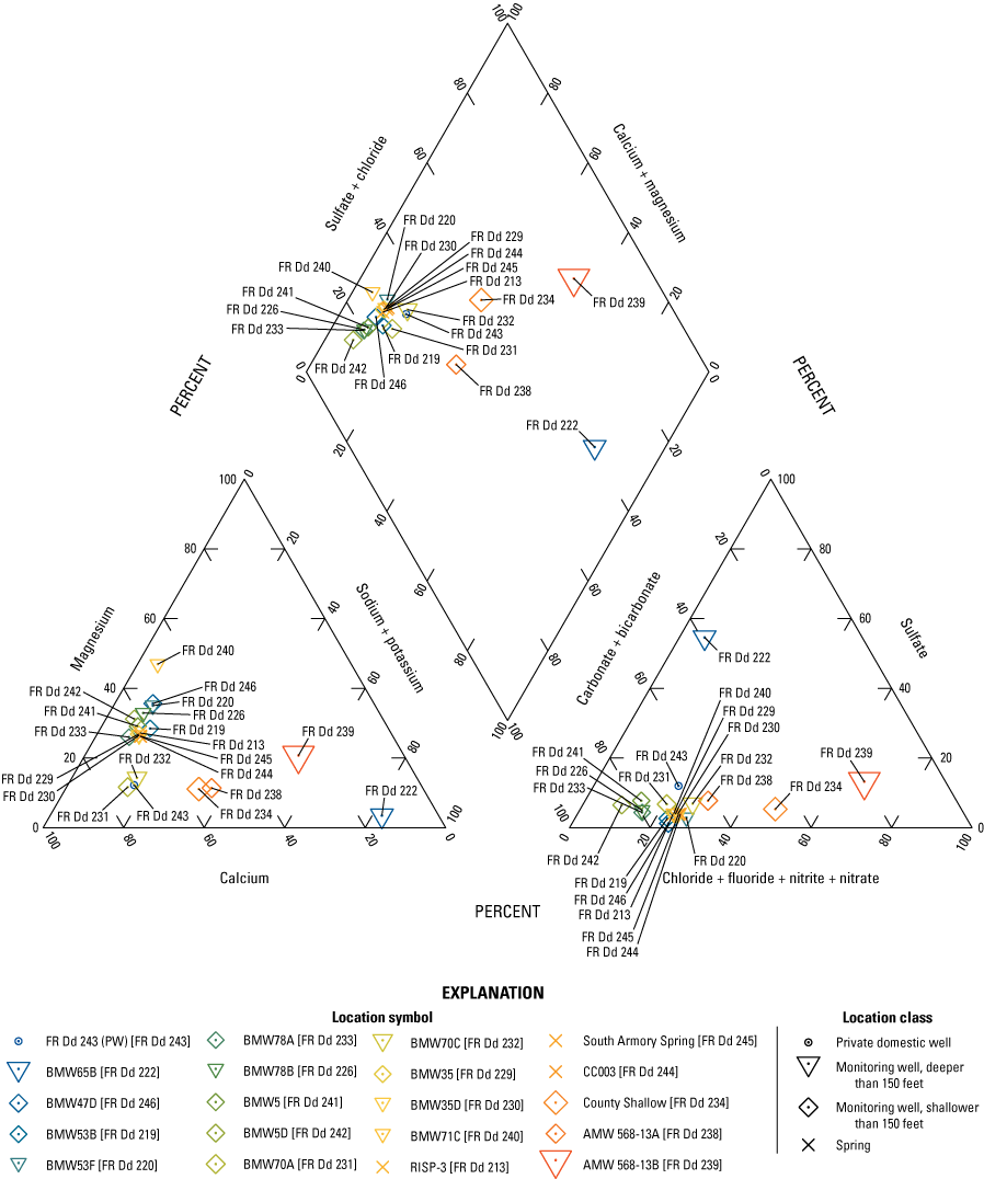
Major ion chemistry of water samples at Fort Detrick Area B, Maryland. Symbol sizes are scaled by the sum of cation concentrations, in milliequivalents.
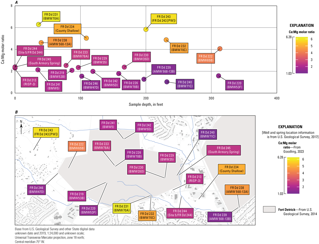
Stable isotope line conditioned (LC) excess, A, with depth and, B, in plan view, Fort Detrick Area B, Maryland.
Three sites have distinctly different major ion compositions from the other sites. Samples collected from FR Dd 234 (County Shallow) and FR Dd 238 (AMW 568-13A) have higher sodium relative to the other sites, but still contain bicarbonate as the dominant anion. Samples collected from FR Dd 239 (AMW 568-13B) and FR Dd 222 (BMW65B) show chloride and sulfate (SO4) to be the dominant anions (fig. 35), making those samples Na-Cl and Na-SO4 type waters, respectively.
Chloride and Bromide
Cl:Br and Na:Cl ratios are used to identify the influence of nongeologically derived chloride and to evaluate the potential source. As shown in table 11, high mass ratios of Cl:Br (greater than [>] 2,000) are associated with high chloride concentrations (>50 mg/L), which is consistent with the addition of nongeologic chloride across the site. The highest Cl:Br mass ratios were measured in FR Dd 238 (AMW 568-13A), FR Dd 239 (AMW 568-13B), and FR Dd 234 (County Shallow). The lowest values were measured in FR Dd 243 (PW) and FR Dd 222 (BMW65B), which possibly represent background conditions unaffected by nongeologic sources. The Na:Cl molar ratio for most samples is less than 1, with the exceptions of the FR Dd 222 (BMW65B), FR Dd 238 (AMW 568-13A), and FR Dd 243 (PW), which suggests that road salt (NaCl) alone does not explain the elevated chloride. If road salt is the primary chloride source, the Na:Cl molar ratio would be expected to be near 1, though deviations from this idealized Na:Cl molar ratio could be explained by additional processes involving uptake of sodium, including sodium-clay formation and ion exchange, or possibly the use of different road salts including MgCl.
The presence of chlorinated solvent contaminants within the aquifer (Arcadis Inc., 2014) suggests the excess chloride is possibly derived from the degradation of these contaminants. However, the sample locations monitored in this study do not have high current or historical chlorinated solvent concentrations and aren’t representative of contaminant source areas, so the observation of excess nongeologic chloride does not directly inform the assessment of contaminant degradation in those areas. Chlorinated solvent dissolution may also serve as a chloride source even in the absence of active biodegradation. Additional potential anthropogenic sources of chloride include landfill leachate, irrigation, and water treatment (Granato and others, 2015). Although the complete chloride budget is not constructed in this study, the Cl:Br and Na:Cl ratios suggests that elevated Cl:Br ratios are then likely a good indicator of the connectivity to the surface and increasing Cl:Br may indicate a larger relative fraction of anthropogenically affected groundwater.
Oxidation and Reduction
The majority of samples indicate oxic conditions with high dissolved oxygen (DO) and nitrate (NO3) with the exception of three sites (FR Dd 222 [BMW65B], FR Dd 231 [BMW70A], and FR Dd 239 [AMW 568-13B]) that are anoxic, denitrified (except FR Dd 231 [BMW70A]), and have elevated concentrations of metals (table 11). An oxic categorization does not exclude some reductive consumption of electron donors in the groundwater sample. Chemical reduction is possible if the oxic conditions occurred in a more limited capacity, such that the threshold criteria of Jurgens and others (2009) is not met, or that the groundwater has since become more oxidized along the flow path closer to the sample point after being in a reduced state. Overall, the high concentrations of DO in samples across the study area suggest that chemically reducing conditions do not affect groundwater chemistry along the flow paths intercepted by the majority of samples collected in this study. However, the sample locations in this study were selected to evaluate the conceptual site model and not to characterize contamination source areas.
Tracers
Groundwater tracer chemistry was interpreted to improve understanding of groundwater source and movement across Area B. The tracers discussed in this section include stable isotopes of water, carbon isotopes, dissolved noble and reactive gases, as well as tritium and tritogenic helium-3.
Stable Isotopes
Stable isotopes of water were evaluated to identify variation in recharge source across Area B by comparing the observed isotopic composition in groundwater to the isotopic composition reported in precipitation. Values of δ2H and δ18O in groundwater and spring samples collected for this study range from −39.8 to −48.1 per mil (‰) and −6.34 to −7.84‰, respectively. Reported δ2H and δ18O in precipitation from within a 100-mile radius of the study site (n=262 and 250, respectively) fall along a well-defined LMWL (δ2H=8.24 x δ18O+15.4; fig. 37) that indicates a slight enrichment of isotopes in precipitation relative to the global meteoric water line (δ2H=8 x δ18O+10; Craig, 1961). Values of LC-excess are generally close to zero, indicating that the observed precipitation data and respective least-squares fit line is a relatively good estimation of recharge sources (table 12). Values of LC-excess decrease from west to east (Spearman’s ρ=−0.46, p-value=0.04) indicating increased evaporative signal in groundwater recharge in eastern samples. LC-excess is greater than 1 at FR Dd 222 (BMW65B), FR Dd 240 (BMW71C), and FR Dd 243 (PW) (fig. 38), consistent with a larger component of a distinct recharge source, possibly from the higher elevations within Catoctin Mountain, that is not well represented by the regional precipitation dataset. LC-excess is less than 1 at FR Dd 232 (BMW70C), FR Dd 238 (AMW 568-13A), and FR Dd 239 (AMW 568-13B) indicating an evaporative signal, possibly a result of precipitation runoff from impermeable surfaces and isotopically enriched recharge from the marshy central portion of Area B.
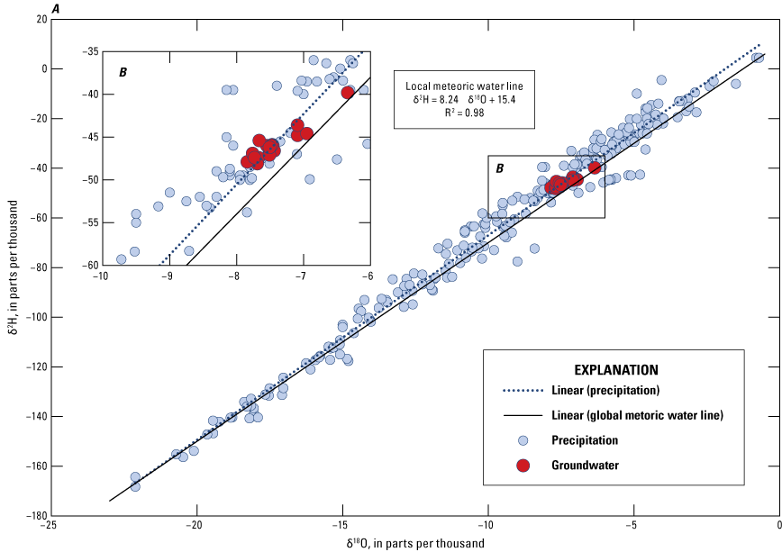
Stable isotopes in groundwater samples (red) and regional precipitation (blue), Fort Detrick Area B, Maryland. Inset shows zoomed in region of δ2H versus δ18O space around groundwater samples. R2, coefficient of determination.
Table 12.
Select groundwater tracer concentrations and interpretations, Fort Detrick Area B, Maryland.[ID, identification; MM, two-digit month; DD, two-digit day; YYYY, four-digit year; δ2H, delta hydrogen-2; ‰, per mil; δ18O, delta oxygen-18; LC-excess, line-conditioned excess; 3He, helium-3; TU, tritium units; ND, not determined; ccSTP/g, cubic centimeters per gram at standard temperature and pressure (25 degrees Celsius, 1 atmosphere); 4He, helium-4; Heterr, terrigenic helium; Hetot, total helium; NGT, noble gas recharge temperature; SF6, sulfur hexafluoride; pptv, parts per trillion by volume; 14C, carbon-14; pmC, percent modern carbon; δ13C, delta carbon-13; —, no data]
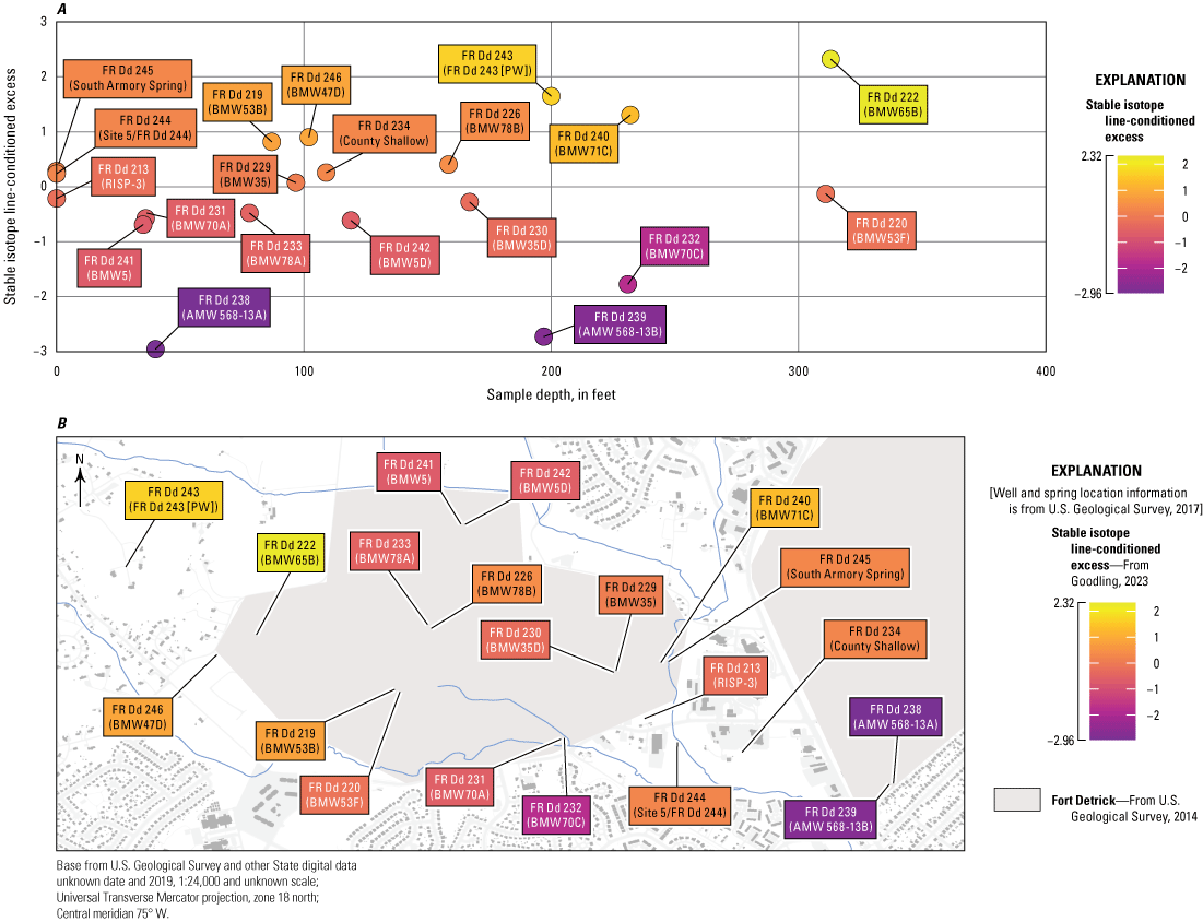
Stable isotope line conditioned (LC) excess, A, with depth and, B, in plan view, Fort Detrick Area B, Maryland.
Carbon Isotopes
Carbon isotope data (table 12; fig. 39) show two distinct groups of samples: samples with δ13C values greater than –20‰ and those with δ13C less than –20‰. The majority of samples have δ 13C values greater than –20‰. These samples approximately fall along the so-called zero- age line for the open system Revised Fonts and Garnier (RFG) analytical model (Han and Plummer, 2013) parameterized with values for δ13C soil gas and solid carbonates of –25 and 3‰, respectively (fig. 39). The δ13C values used in the model are consistent with typical soil-zone gases and marine carbonate isotopic compositions (Cerling and others, 1991; Clark and Fritz, 1997). The relative goodness of fit between measured values and the modeled zero-age line suggests that dissolution of aquifer carbonates and gas exchange with the atmosphere are reasonable as the dominant controls of DIC in those samples. The final adjusted 14C values (table 12) for these samples range between about 106 and 124 percent modern carbon (pmC). The corrected 14C values are generally consistent with other tracers and indicate that recent recharge along relatively local flow-paths is captured at these locations. Carbon-14 has limited utility for quantitative age dating of these modern samples due to elevated atmospheric 14C (greater than 100 pmC) from above-ground nuclear testing since late 1950s and high sensitivity of modern interpreted ages to the geochemical correction. High values of 14C and 3H indicate there is no, or very little, pre-modern water in these samples.
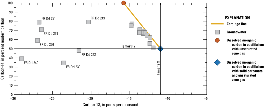
Carbon-13 isotopic ratio (δ13C) versus carbon-14 (14C) of dissolved inorganic carbon (DIC) in groundwater, Fort Detrick Area B, Maryland. Carbon isotope values for carbonate species in isotopic equilibrium with unsaturated zone carbon dioxide (CO2) and aquifer carbonates indicated by points. Hypothetical carbon isotope evolution pathways from open-system (orange line). Full description of plot features is provided by Han and others (2012).
The remaining samples do not fall along the zero-age line and do not indicate open system behavior dominated by inorganic carbonate reactions. The δ13C less than –20‰ of these samples suggests additional processes affecting carbon isotope chemistry. The more fractionated δ13C signal of these samples is possibly driven by organic carbon oxidation and the influence of microbial processes and (or) contaminants, but additional sampling is needed to confirm and potentially correct for these processes and carbon sources. Without appropriate correction, the 14C has limited utility for quantification of groundwater age for these remaining samples.
Dissolved Noble and Reactive Gases
Measured concentrations of nonreactive noble gases (Ne, Ar, Kr, and Xe) were generally consistent with solubility equilibrium with the atmosphere. The helium isotopic ratio (R/Ra) supports this finding with most samples having R/Ra values close to 1. Four samples, collected from FR Dd 222 (BMW65B), FR Dd 232 (BMW70C), FR Dd 234 (County Shallow), and FR Dd 243 (PW), with R/Ra values less than 1 indicate a potential crustal terrigenic helium (Heterr) source. High amounts of Heterr (greater than about 30 percent) relative to the total helium at these sites may be related to elevated helium accumulation rates such as at FR Dd 243 (PW), which is located in the fractured crystalline bedrock, or possibly indicates capture of longer (older) flow paths, as discussed in the Groundwater Age section of this report.
Dissolved noble gas data were well-fit by solubility models with statistically significant model solutions (χ2 values less than critical value of 3.84; one-sided, one degree of freedom, 95- percent confidence) and recharge conditions were generally well described by the model (χ2 less than about 0.2, except for FR Dd 245 [South Armory Spring] and FR Dd 239 [AMW 568-13B]; table 13). Noble gas solubility models provide a good estimate of the groundwater recharge temperature (referred to as noble gas recharge temperature; NGT) and the amount of excess (entrapped) air for each sample. Modeled NGTs are relatively warm (table 13) and generally group around the mean annual air temperature modeled for Fort Detrick (13.0 °C, 55.4 °F; 1980–2020 mean temperature; PRISM Climate Group, 2021). Cooler recharge temperatures are observed in the center of the study area. Ephemeral stream flow and wetlands overlie the sites with cool recharge temperatures. The deep western sample site (FR Dd 222 [BMW65B]) shows a cooler recharge temperature of 9.9 °C, possibly from the capture of longer regional flow or focused recharge from higher elevation. The warmest temperatures of about 15 and 17 °C were observed in shallow sample sites east of Carroll Creek (FR Dd 234 [County Shallow] and FR Dd 238 [AMW 568-13A]). Solubility-modeled NGTs increase from west to east (fig. 40; Spearman’s ρ=0.55, p-value=0.01) indicating increasing contribution of low-elevation warmer recharge in the eastern samples. Solubility model results are insensitive to assumed recharge elevation and show little difference in NGT, with less than a 1° difference over the 500-m elevation difference in local topography to the west. Use or exclusion of N2 as a fitted parameter generally had a small effect on solutions for NGT and fractionation factor (F) (<2.5 percent difference except for FR Dd 234 [PW]) with the larger variability in entrapped air (Ae) (±50 percent) as expected with addition of excess N2.
Table 13.
Measured dissolved gas concentrations from septum bottles, helium isotopic ratio, noble gas solubility modeled recharge conditions, and modeled solubility equilibrium gas concentrations, Fort Detrick Area B, Maryland.[USGS, U.S. Geological Survey; MM, two-digit month; DD, two-digit day; YYYY, four-digit year; ID, identification; Meas., measured; CH4, methane; mg/L, milligram per liter; CO2, carbon dioxide; N2, dissolved nitrogen gas; O2, dissolved oxygen gas; DO, dissolved oxygen; R, ratio of helium-3 to helium-4 in the sample; Ra, ratio of helium-3 to helium-4 in atmosphere; Est., estimated; m, meters; NGT, noble gas recharge temperature; °C, degrees Celsius; Ae, entrapped air; ccSTP/g, cubic centimeters per gram at standard temperature and pressure (25 °C, 1 atmosphere); F, fractionation factor; χ2, chi-squared; Xe, xenon; v., very; mod., moderate; —, no note recorded]
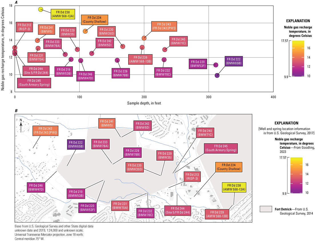
Modeled noble gas recharge temperatures (NGT), A, with depth and, B, in plan view, Fort Detrick Area B, Maryland.
FR Dd 239 (AMW 568-13B) appears to have been partly re-equilibrated as evidenced by (1) the poor ability of the solubility models to capture measured xenon concentrations, (2) low excess air, and (3) lack of fractionation, which is inconsistent with all other sites (table 13). Forcing unfractionated excess air (F=0), the closed-equilibrium (CE) model indicated reasonable NGT and Ae (table 13). With inclusion of N2, a solution with a warmer temperature with a small amount of fractionated excess air was found but had a poor fit (NGT=13 °C, Ae=0.006 cubic centimeters per gram at standard temperature and pressure [ccSTP/g], F=0.76, χ2=12.6). CE model parameters and the helium mass balance calculations for FR Dd 239 (AMW 568-13B) are less certain. As a result of the potential gas loss, there is high uncertainty in the calculated 3Hetrit and the 3H/3He age is a likely minimum age of the young fraction; helium concentrations exceed atmospheric solubility in the sample. Internal radiogenic sources from decay of tritium or uranium- and thorium-series decay are the most likely explanation, with an R/Ra value of 0.94 supporting the latter terrigenic source.
Elevated helium concentrations above 4E-6 ccSTP/g at FR Dd 222 (BMW65B) and FR Dd 243 (PW) are from subsurface radiogenic decay. Helium isotope ratios (R/Ra; table 13) less than 1 indicate the fractured crystalline and fine-grained sedimentary bedrock that form the deepest water-bearing units within Catoctin Mountain are the likely source of high 4He at these sites. Due to the uncertainty in terrigenic helium isotopic ratio, 3Hetrit could not be reliably estimated for these two samples, limiting the tracer set for age determination.
Helium-4 cannot be used for age calculations as there is not a clear relation between 3H and elevated 4Heterr (FR Dd 243 [PW] and FR Dd 222 [BMW65B]; table 12) and use of 14C for estimating old groundwater age is difficult, limiting the estimation of 4He accumulation rates. Elevated 4He is still useful for identification of the samples with similar chemistry but cannot be tied to a single helium source or group of groundwater flow paths. Another five sample sites (392611077270801, 392553077264501, 392603077263702, 392605077263001, and 392625077270302) with a relatively higher fraction of terrigenic helium (table 13) do not cluster near the proposed fractured-rock helium source (fig. 41), suggesting other discrete helium source pathways, possibly along karst conduits, or gradual accumulation of helium along the flow paths associated with longer travel times.
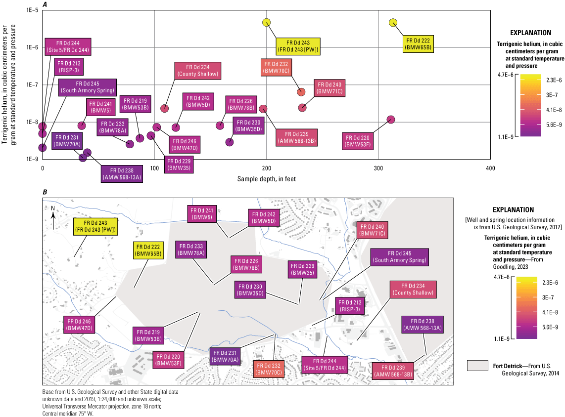
Calculated terrigenic helium (Heterr), A, with depth and, B, in plan view, Fort Detrick, Frederick, Maryland. A logarithmic scale is used for the vertical axis in A and the color scale for both panels.
Measured reactive gas concentrations (table 13), with high CO2 and N2 and low O2 relative to equilibrium solubility modeled concentrations, are potentially indicative of biologic activity, as discussed below. Reactive gas concentration data from septum stoppered samples were combined with noble gas solubility models to describe the addition or removal of reactive gases. Total measured N2 differed between the two collection and analysis methods by generally less than 10 percent, suggesting the N2 gas production/loss after sample collection may have been relatively minor. Conversely, measured O2 from the stoppered bottles is much lower than field measurements of DO, possibly suggestive of continued microbial respiration after sample collection. Estimates of excess CO2 (difference between modeled solubility equilibrium and measured values) support microbial respiration. Oxic conditions in the aquifer as measured by in situ DO (table 11) suggest a low likelihood of wide-spread nitrate reducing conditions in the aquifer, although localized conditions may not be captured in the composite samples.
Tritium and Tritiogenic Helium-3
Tritium and tritiogenic helium-3 results indicate that the majority of groundwater underlying Area B is modern recharge since 1950. Measured 3H concentrations are greater than 2.5 TU for 19 of the 20 sites (table 12). The remaining site (FR Dd 222 [BMW65B]) is dominantly premodern groundwater with a 3H value (0.25 TU) close to the pre-1950 cutoff of 0.22 TU. Tritiogenic helium-3 ranges between about 1.3 TU and 15 TU. Concentrations of 3Hetrit could not be quantified for two samples (FR Dd 243 [PW], FR Dd 222 [BMW65B]) as a result of high Heterr and increased uncertainty in the helium mass balance. Calculated 3H/3Hetrit ages are reported in the Groundwater Age section of this report.
Elevated 3H values above background levels (approximately 10 TU) were observed at three sites (FR Dd 239 [AMW 568-13B], FR Dd 241 [BMW5], FR Dd 242 [BMW5D]). This is indicative of additional nonatmospheric local source of 3H, such as tritiated laboratory waste disposal, in Area B. A bomb-pulse elevated atmospheric source of 3H can be distinguished from local 3H sources based on (1) 14C, which increased in the atmosphere over the same period in response to above-ground nuclear testing, and (2) comparison of initial 3H (3H0) to the atmospheric 3H record. For two of these three samples (FR Dd 241 [BMW5] and FR Dd 242 [BMW5D]), the corrected final 14C values could be calculated using the RFG model (although 14C based ages cannot be assigned). At these wells, elevated 3H does not correspond with elevated 14C, so nonatmospheric 3H is likely present. As a result, groundwater ages based on 3H/3He are likely minimum estimates and LPM ages based on atmospheric 3H histories are unreliable. Comparison of 3H0 to the atmospheric record (fig. 42) provides evidence that no local source of 3H is present in other samples besides FR Dd 239 (AMW 568-13B), FR Dd 241 (BMW5), and FR Dd 242 (BMW5D). Wells without a local 3H source likely have reliable calculated groundwater ages and tritium can be used to estimate the fraction of post-1953 water (referred to as 3H fraction modern estimates, shown graphically in fig. 11C).
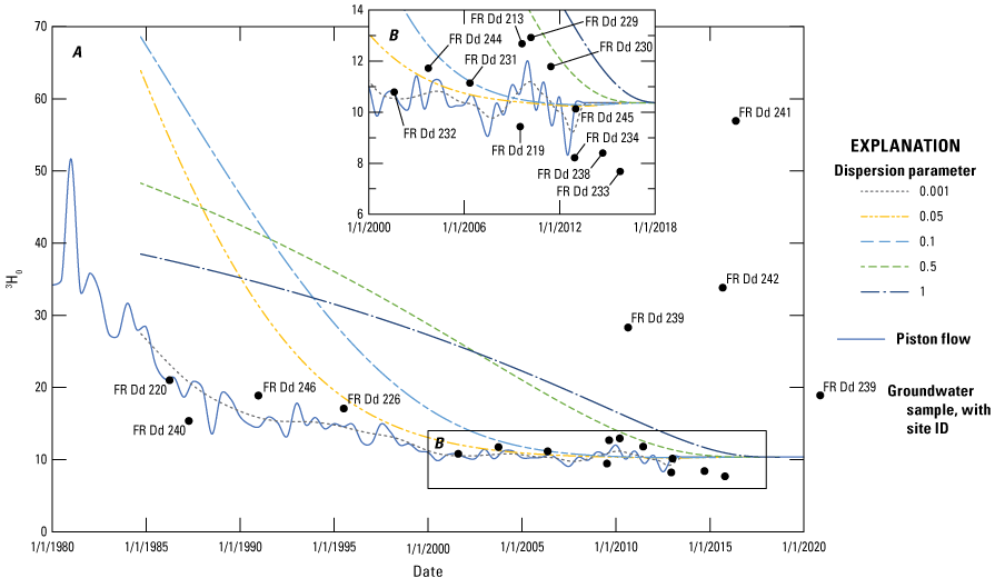
Initial tritium (3H0) versus recharge year as estimated in the historical atmospheric record (lines) and as calculated in groundwater samples (points labeled with site identification number), Fort Detrick Area B, Maryland. Estimated atmospheric 3H0 variation by recharge year, according to various lumped parameter models, indicated by line color. Piston-flow estimated 3H0 history indicated by the labeled blue line.
Groundwater Age
Groundwater age was evaluated through multiple techniques using the 3H and 3Hetrit results to understand contributing flow paths and time since groundwater recharge at sample sites across Area B. Observed SF6 samples corrected for excess air exceeded the expected atmospheric inputs, indicating regional SF6 contamination, likely from industrial sources, and unreliability of SF6 for groundwater age dating at Area B. As detailed in other sections of the report, this study does not fully describe the carbon isotope evolution and 14C could not be used for estimating groundwater ages. Limited to 3H and 3Hetrit, groundwater age interpretations in this study quantify age metrics for groundwater recharged since approximately 1950 (modern) and the relative proportion of recharge prior to 1950 (premodern). A more complete description of the full distribution of groundwater ages, including quantified ages of the premodern component, was not possible. The metrics used in this study are shown conceptually in figure 11.
Results of the 3H fraction modern analysis indicate the relative contribution of premodern (pre-1950) groundwater in samples. Although the mean age of the premodern component cannot be estimated, the 3H fraction modern provides valuable information on the portion of the age distribution not captured in the 3H/3He ages and LPM results. Results show 16 of the 20 sites are estimated to have equal to or greater than 50 percent modern water (fig. 43, table 14) indicating that although the majority of sampled Area B groundwater is modern (recharged after 1950), substantial fractions of premodern water exist, particularly deeper within the aquifer. The correlation between 3H fraction modern and depth of sample interval (springs set to 0-ft deep) is statistically significant (Pearson’s r=0.48, p-value=0.042), indicating increasing amounts of premodern groundwater with depth. Decreasing values of 3H fraction modern with depth indicate longer flow paths, potentially from fracture flow or diffusion-dominated portions of the aquifer and (or) regional groundwater flow, being captured at the sample sites. Without useful tracers for determining premodern groundwater ages, it is not possible to determine the most likely source of this premodern groundwater with any confidence.
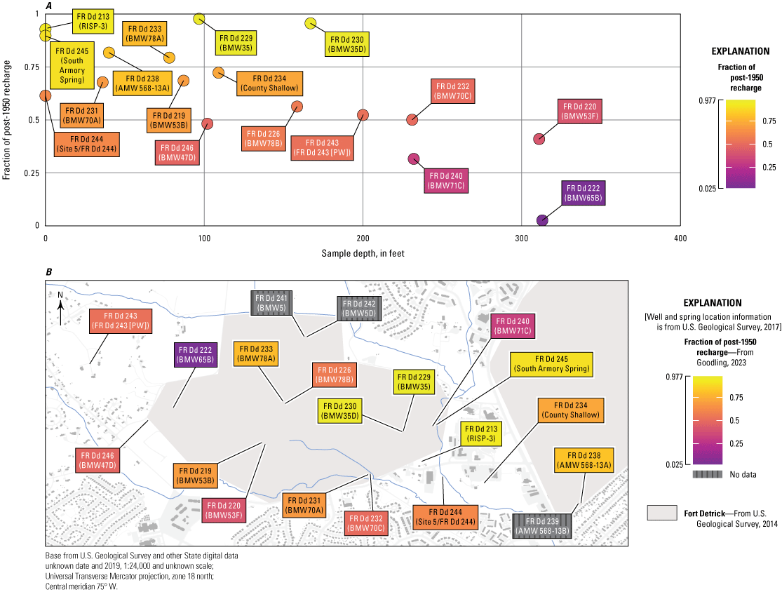
Fraction of post-1950 modern water in each sample, A, with depth and, B, in plan view, Fort Detrick Area B, Maryland. Three wells with nonatmospheric sources of tritium are excluded from A.
Table 14.
Estimated groundwater age metrics and model fit parameters, Fort Detrick Area B, Maryland.USGS, U.S. Geological Survey; ID, identification; MM, two-digit month; DD, two-digit day; YYYY, four-digit year; 3H, tritium; 3He, helium-3; LPM, lumped parameter model; 3Hetrit, tritiogenic helium-3; RSE, relative square error; DP, dispersion parameter; 14C, carbon-14; <, less than; —, no data]
Apparent 3H/3Hetrit groundwater ages describe the modern component of the sample age and are insensitive to contributions of 3H-dead premodern water and nonatmospheric 3H. Apparent 3H/3Hetrit ages range from about 3 to about 33 years (table 12) at Area B. Elevated Heterr increased uncertainty in the helium balance and precluded calculation of 3H/3Hetrit ages for samples from FR Dd 222 (BMW65B) and FR Dd 243 (PW). Calculated 3H0 values are in relatively good agreement with the historical atmospheric record of 3H in precipitation (fig. 42), providing further validation of helium mass balance calculations and increasing confidence in 3H/3Hetrit ages. Apparent 3H/3Hetrit ages increase with depth of the sample interval below land surface (Pearson’s r=0.61, p-value=0.007). Ages of modern recharge are oldest along the south boundary of the study area (fig. 44). These sample locations are deeper and located further downgradient in the Carroll Creek watersheds.
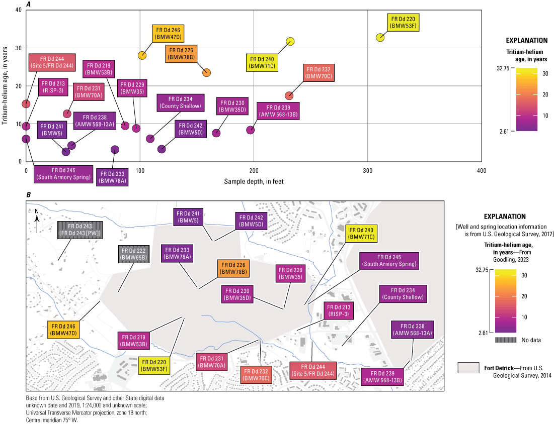
Apparent tritium-helium (3H/3He) age, A, with depth and, B, in plan view, Fort Detrick Area B, Maryland.
Lumped-parameter models (LPMs) estimate age distributions for each sample by describing the mixing behavior of groundwater along and between flow paths. In this study dispersion model (DM) LPMs were fit to 3H and 3Hetrit. The selected tracers and model provided the best fit and estimates of the groundwater age distribution for the data. Three measures of the groundwater age were derived from the LPM solutions: mean age, the dispersion parameter, and the susceptibility index.
Lumped parameter model (LPM) mean ages range from about 3 to about 72 years (table 14; fig. 45) and are in general good agreement with apparent 3H/3Hetrit ages. Mean ages could not be estimated by LPMs—which rely on atmospheric tracer histories—for three sites with indications of nonatmospheric 3H (FR Dd 239 [AMW 568-13B], FR Dd 241 [BMW5], and FR Dd 242 [BMW5D]). The largest differences in LPM and 3H/3Hetrit ages are for samples with young ages, where relative age differences approach method resolution, and for samples with large LPM dispersion parameters consistent with increasing mixing that is not accounted for in the apparent age analysis. The two sample sites with the oldest LPM mean ages are located within the fractured crystalline bedrock (FR Dd 243 [PW]) or within a deep sample interval along the valley margin (FR Dd 222 [BMW65B]), suggestive of a flow system disconnected from the shallow groundwater in Area B. LPM mean ages increase with sample interval depth (Spearman’s ρ=0.66, p-value=0.004) and from east to west (Spearman’s ρ= −0.57, p-value=0.01), supporting increased capture of regional groundwater flow paths at increasing depth.
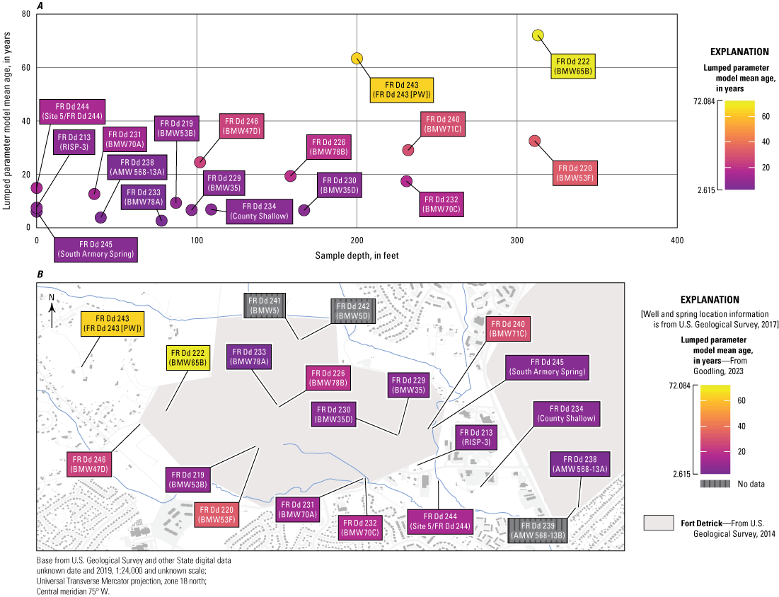
Lumped parameter model estimated mean ages, A, with depth and, B, in plan view, Fort Detrick Area B, Maryland.
The LPM-calculated dispersion parameter (DP) ranges from about 0.001, which approximates piston flow and limited mixing, to about 0.9 (table 14). A DP of 0.001 was assumed for two sites (FR Dd 222 [BMW65B] and FR Dd 243 [PW]) for which 3Hetrit could not be reliably calculated and the DM was underparameterized. Dispersion parameters are highest for samples collected from the middle of the Area B study area (fig. 46), indicating greater mixing along (longitudinal dispersion) and between (wider range of flow path lengths) flow paths captured at those respective sample sites. In this study, increased dispersion might be related to capture of additional recharge sources from the center of Area B. Conversely, decreased dispersion with depth (fig. 46) suggests more focused recharge and (or) advection dominated flow at greater depths consistent with recharge at sink hole locations and groundwater flow through solution enlarged cavities in the deeper carbonate aquifer. It should be reiterated that estimates of dispersion in this study are based on young groundwater tracers, and as such have limited utility for identifying the most likely premodern groundwater sources.
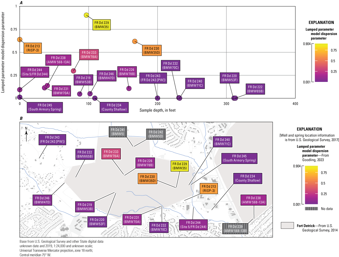
Lumped parameter model estimated dispersion parameter, A, with depth and, B, in plan view, Fort Detrick Area B, Maryland.
The susceptibility index (SI) is a comparative measure of the deviation of the full LPM age distribution from a reference piston flow age distribution with mean age of 1 year (in other words, highly susceptible groundwater). As with the other age metric presented in this report, the SI does not account for potential differences in transport properties between the age tracers used to derive the SI and contaminants of concern. Values of SI range from about 0.11 to about 0.61 (table 14), indicating a wide range of relative susceptibility to land surface contamination across Area B. As a combined metric of LPM mean age and DP, values of SI show a similar pattern across Area B (fig. 47) with groundwater being most susceptible to land surface contamination across the center of Area B. Values of SI decrease with depth (Spearman’s ρ = −0.64, p-value=0.005) supportive of local recharge source across Area B and potential for connectivity between local recharge and the deeper groundwater flow system. Sample sites with high values of SI have higher concentrations of NO3 (Spearman’s ρ=0.48, p-value=0.054), illustrating an observable connection of interpreted susceptibility to land surface activity. Statistically meaningful relations between the SI and nitrate in this study and various land-surface contaminants in another study (Solder and others, 2020) suggest the relative values of SI are useful for understanding susceptibility across Area B.
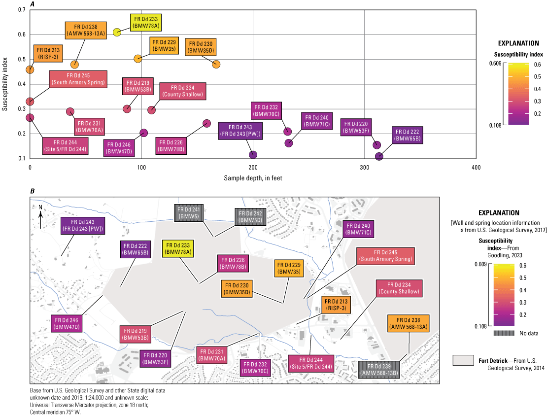
Calculated susceptibility index, A, with depth and, B, in plan view, Fort Detrick Area B, Maryland.
Hierarchical Cluster Analysis
Hierarchical cluster analysis (HCA) provides an objective method of evaluating the similarity in groundwater chemistry between sample sites for a suite of chemical constituents. The HCA combines the set of 20 samples into seven groups based on geochemical similarity (figs. 48–50; table 15).
Group 1 (table 15) represents shallow groundwater with a substantial component of recharge from within or near Area B. Group 1 is composed of springs and wells BMW35 (FR Dd 229) and BMW35D (FR Dd 230) in the New Oxford Formation (fig. 49). This group is characterized by relatively high NO3 and PO4—a possible anthropogenic impact—and δ13C, consistent with open-system carbon exchange. The group 1 samples generally have line- conditioned (LC)-excess centered on zero, indicative of similarity to regional precipitation, and Ca:Mg mole ratios that narrowly range from about 2.3 to about 2.4 (fig. 48; table 11). The group 1 samples have a major ion composition that is tightly clustered when plotted on a Piper diagram (fig. 50).
Group 2 samples represent deep groundwater recharged from precipitation from higher elevations and farther from Area B. Group 2 wells generally have deep screened intervals in the Fredrick Formation, with the exception of FR Dd 240 (BMW71C), which is screened in the New Oxford Formation, and chemistry that is characterized by low CO2 and low 14C consistent with groundwater interaction with carbonate aquifer units. Group 2 samples have high LC-excess and cooler noble gas temperatures, indicative of higher elevation recharge. The spatial pattern of group 2 samples along the south study area boundary are somewhat suggestive of preferential flow (fig. 49). Group 2 samples generally have a lower 3H relative to the remaining samples, with the exception of FR Dd 222 (BMW65B), indicating older groundwater and lack of connection with shallower groundwater flowpaths with elevated 3H across Area B. On a Piper diagram (fig. 50), group 2 samples have a similar major ion chemistry to group 1, though with increased variability.
Group 3 samples represent a possible mixture of heavily evaporated and high Cl:Br recharge from shallow flowpaths and deeper groundwater from a high-elevation recharge source (group 2). Group 3 wells (1) have a wide range of screened interval depths, from 36 to 231 ft bls; (2) are all located in the Frederick Formation; (3) are tightly grouped in the southeastern part of the study area (fig. 49), and (4) have geochemistry that is characterized by high Cl, Ca:Mg mole ratios, Sr, δ18O, Ca, and K (table 15). The increasing LC-excess with depth and average-to-warm noble gas temperatures of group 3 samples indicate a mixture of shallow and deeper groundwater flow paths at these wells. Elevated calcium and Ca:Mg ratios in combination with high CO2, HCO3, and average pH (table 11) suggest interaction between recent recharge with high CO2 from unsaturated zone processes and carbonate aquifer units, although very low δ13C at two of the wells (FR Dd 231 [BMW70A] and FR Dd 238 [AMW 568-13A]) indicate carbonate chemistry may be impacted by organic carbon sources. Group 3 samples have relatively high sodium and SO4 (table 11, fig. 48), possibly a result of interaction with more geochemically evolved waters, as represented by samples from FR Dd 222 (BMW65B) and FR Dd 239 (AMW 568-13B), or as a result of the complex carbonate geochemistry previously mentioned. The sodium and SO4 values result in a grouping distinct from groups 1 and 2 on the Piper diagram, especially for the cation composition (fig. 50).
Group 4 consists of two wells (FR Dd 241 and FR Dd 241), completed in the sandstone of the New Oxford Formation in the northern part of the study area near the active landfill area. Group 4 has the highest 3H values, possibly from an anthropogenic source. It has high magnesium, moderate SO4, and low NO3 and Cl concentrations and plots similarly to group 2 samples on the Piper diagram (fig. 50). Finally, three samples are distinct from the other groups (table 15), indicating a unique geochemical composition at those sites relative to the other groundwater samples. FR Dd 243 (PW) has relatively high silica and low HCO3, indicative of the hydrologic position of the well in the crystalline bedrock upgradient of the carbonate aquifer units. Although it plots similarly to group 3 samples on the Piper diagram (fig. 50), the magnitude of the ion concentrations is much lower.
Both FR Dd 222 (BMW65B) and FR Dd 239 (AMW 568-13B) have relatively high trace metals, low NO3, and high excess N2 in the case of FR Dd 239 (AMW 568-13B), likely associated with the anoxic conditions at the two sites (table 11). FR Dd 222 (BMW65B) has relatively high sodium and SO4, possibly related to the well location and depth along the western basin margin, and low 3H and δ18O that indicate old groundwater recharged from winter precipitation. Water level monitoring shows this well is slow to recover from pumping and to respond to recharge compared to other wells in the study area. This suggests the well is completed in part of the Frederick Formation with a weak hydraulic connection to the rest of the groundwater system in the study area. The well may be representative of the fracture- and matrix-diffuse flow part of the aquifer rather than conduit-flow dominated parts. FR Dd 239 (AMW 568-13B) has relatively high chloride and Cl:Br mass ratio, likely as a result of land surface contamination, high sodium possibly related to well depth, and relatively low LC-excess indicative of a more evaporated recharge source. The elevated sodium, chloride, and SO4 in these wells results in a distinct water type (fig. 50).
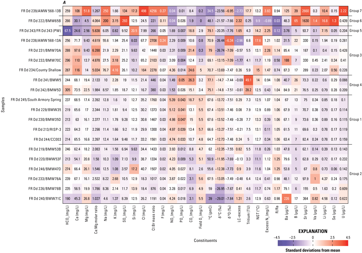
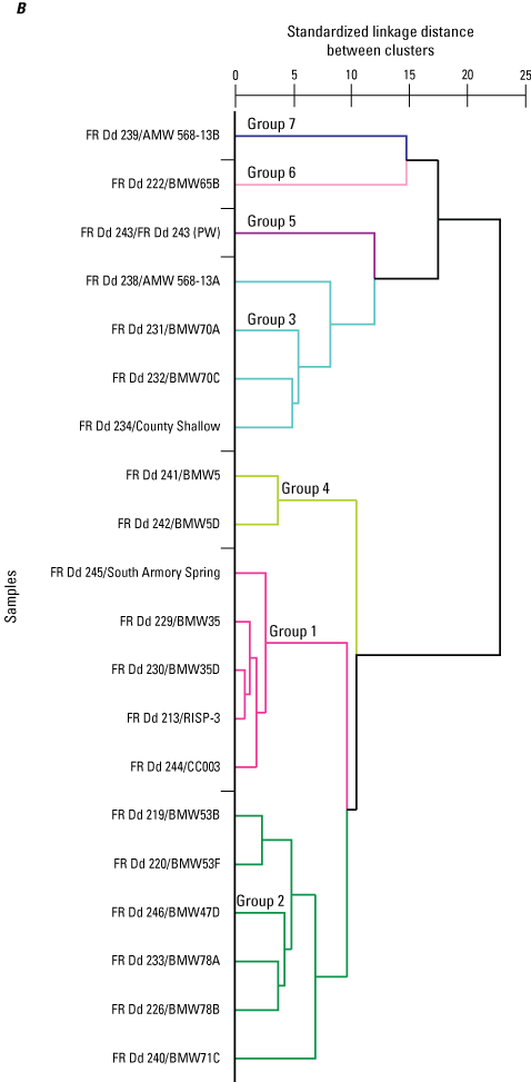
Geochemical data used to perform hierarchical cluster analysis (HCA) with dendrogram defining the HCA cluster groups. Mg/L, milligrams per liter; pmC, percent modern carbon; ‰, per mil; LC-excess, line-conditioned excess; TU, tritium units; NGT, noble gas recharge temperature; °C, degrees Celsius; R/Ra, helium isotope ratio (R) relative to air (Ra); µg/L, micrograms per liter.
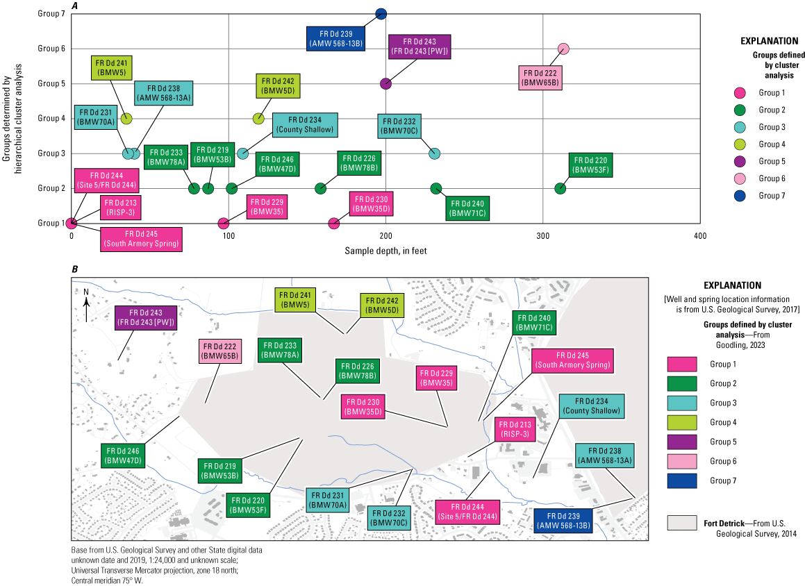
Hierarchical cluster analysis-defined groups, A, with depth and, B, in plan view, from groundwater sample data, Fort Detrick Area B, Maryland.
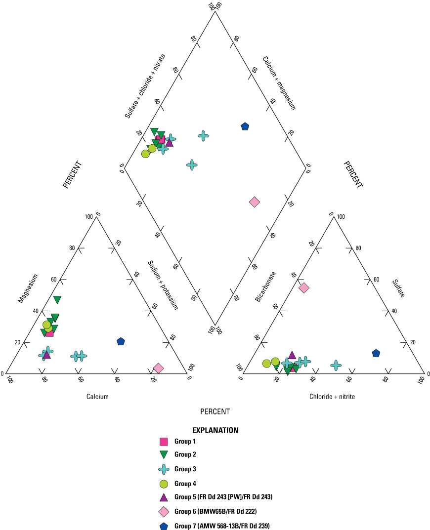
Major ion chemistry grouped by hierarchical cluster analysis-defined groups.
Table 15.
Summary of hierarchical cluster analysis on select geochemical constituents, Fort Detrick Area B, Frederick, Maryland.[Si, silica; HCO3, bicarbonate; PO4, phosphate; δ13C, delta carbon-13; LC excess, line-conditioned excess; O2, oxygen gas; Ca:Mg, calcium to magnesium mole ratio; CO2, carbon dioxide gas; 14C, carbon-14; δ18O, delta oxygen-18; Ca, calcium; K, potassium; Na, sodium; SO4, sulfate; NO3, nitrate; Cl, chloride; Mg, magnesium; Cl:Br, chloride to bromide mass ratio; N2, nitrogen gas; R/Ra, helium isotope ratio (R) relative to air (Ra); NGT, noble gas recharge temperature]
Discussion
The geologic, hydrologic, and geochemical data evaluated in this study have provided additional means to evaluate and refine the CSM at Fort Detrick Area B. The focus of this study has been to (1) place Fort Detrick Area B groundwater within a regional hydrogeologic context, (2) characterize the hydrologic system behavior at multiple timescales, (3) evaluate the potential for interbasin groundwater flow, (4) establish geochemical lines of evidence to evaluate vertical structure and lateral connectivity in the aquifer, and (5) monitor for dyes from previous tracer tests.
Structural Controls on Groundwater Flow
The review of the geologic setting, regional hydrogeologic literature, and previously collected geophysical log data shows general agreement with the previously described CSM. The study area lies at the junction of the regional Bull Run Mountain Fault and a steeply dipping unconformable contact between Triassic sandstones and Cambrian limestones. Although described by the previous CSM as a transfer fault, some ambiguity remains on the physical nature of the contact from the inconclusive results of several geophysical characterizations and the lack of a borehole data that intersect the contact. Regionally, a contrast in bedding and predominant joint strike between the Triassic sandstones and Cambrian limestones could potentially exert a structural control on regional groundwater flow. Preferential flow and the formation of karst features is anticipated in a direction subparallel to the Bull Run Mountain Fault in the Triassic units and perpendicular to the fault in the Cambrian units, based on the orientation regional of fractures and joints reported by Brezinski (2007). However, within Area B, geophysical logs collected show that although beds in the Triassic New Oxford Formation dip gently westward, the bedding orientations in the Cambrian Frederick Formation are less consistent. Additionally, fractures and voids observed in the available geophysical logs do not have a dominant orientation across the units, though depending on the spacing of the joint sets, a limited number of boreholes may not be sufficient to evaluate this orientation. The orientation of lineaments in the vicinity of Area B from prior photogeologic analysis strikes approximately perpendicular to the Bull Run Mountain Fault, consistent with the regional joints in the Cambrian units reported by Brezinski (2007). Limited geologic or geophysical data are available for the geologic units within Catoctin Mountain to the west of the study area, and the hydrologic influence of the Bull Run Mountain Fault is not well understood.
The contact between geologic units in Area B is spatially associated with springs, sinkholes, and swallets, as has been noted in regional karst settings (Kozar and Weary, 2009). A greater concentration of sinkholes and voids found during drilling are reported in western Area B. The interaction of low ionic-strength groundwater and surface water in the metamorphic Catoctin Mountain units with the carbonate Rocky Springs Station Member of the Frederick Formation is a probable determinant of the predominance of these karst features close to the fault. Within the center of Area B and through its intersection with Carroll Creek, the contact between the Triassic and Cambrian units is associated with a swallet, intermittent streams, a marshy wetland, artesian well conditions (at BMW53F [FR Dd 220]), and the location of perennial springs along Carroll Creek from RISP-3 to Stream 2. Past tracer test results and consistent VOC detections suggest these springs are fed by water originating from a zone of preferential flow that routes water from west to east. The hydraulic functioning of this feature has been discussed inconsistently in Arcadis Inc. (2014; Arcadis Inc., written commun., December 2019). The contact was described as hydrostratigraphically “transparent” in Arcadis Inc. (2014), though is described by the draft remedial investigation report as a determinant of the presence of springs due to differing hydraulic properties between the units (Arcadis Inc., written commun., December 2019). The latter interpretation is more consistent with observations in regional karst hydrogeologic studies. Potentiometric mapping does not indicate a hydraulic head depression associated with a preferential flow path in the center of the site, though this is unsurprising because in karst environments individual wells have a low probability of intersecting conduits that transmit a majority of the flow. The hydraulic functioning of preferential flow features such as faults may change under differing hydrologic conditions. Despite the presence of preferential flow features within mid-Atlantic karst systems in the literature, reported tracer tests from the Valley and Ridge Province of Maryland and Virginia show there is also often a substantial slow-flow component. Slower transport rates and lower dye mass recoveries are reported in these regional studies than from conduit-dominated karst aquifers elsewhere.
Groundwater Responsiveness to Hydrologic Events
The monitoring network established for this study improved the characterization of temporal variability of the hydrologic system beyond the point-in-time observations of water level and streamflow presented in the previously described CSM. Hydrologic monitoring for the period of October 1, 2017, to December 31, 2020, characterized the hydrologic system for conditions ranging from historically wet to typical climatic conditions. Extremely high levels of precipitation in 2018 had a prolonged effect on the hydrologic system during this period. The groundwater and stream monitoring reveals a highly responsive and dynamic system suggestive of highly transmissive tertiary porosity within the karst system. However, one deep well pair (BMW65A and BMW65B) shows a more muted water level response, reflective of the fracture-dominated secondary porosity network. Under wet conditions with high groundwater levels, 3 of 10 master recession curves exhibit a break in slope. This suggests that within some locations of the aquifer, highly transmissive karst or epikarstic tertiary porosity is filled and then drained. Under lower water-level conditions, small and less transmissive voids or secondary porosity is filled and drained. Specific yields calculated for individual wells using groundwater and streamflow data have a median value of 0.06 and a range of 0.04 to 0.11, which is consistent with the storage and release of water from secondary porosity (fractured rock) and relatively poorly developed karstic tertiary porosity (with drainage from solutionally enlarged fractures but not large caves). Water-level gradients analysis shows generally upward gradients and west-to-east gradients between selected well pairs. These gradients (both upwards and west-to-east) are stronger during wetter periods than more typical hydrologic conditions. Carroll Creek is strongly gaining between the two USGS streamgages, which is consistent with the seepage run mapping collected in 2000 and 2001 and the identification of numerous springs in other work performed at this site. The gains from base flow between the streamgages are greater during wet periods (spring 2018 to fall 2019) than in drier periods (fall 2019 and fall 2020). The water years 2018–20 base flow per unit area for the Carroll Creek watershed is higher than any regional watershed; the upstream Carroll Creek watershed base flow per unit area is typical of karst watersheds in the region. Both watersheds have lower base flow indices than other karst watersheds. Taken together, these results suggest that focused groundwater discharge and recharge processes are even more important in the lower watershed than many regional karst environments, though the Carroll Creek watersheds are also relatively flashy and experience more stormflow-dominated periods than regional karst watersheds typically do.
Groundwater Flow Beneath Carroll Creek
A water budget was constructed as an independent line of evidence to evaluate the potential for interbasin transfer. The previously described CSM defines the Carroll Creek watershed as a system where the groundwatershed and topographic watershed coincide, with no interbasin transfer of groundwater. The water budget approach in this study used an open water budget approach, where independently calculated water budget components, along with their uncertainties, were used to determine if the water budget residual was significant. A significant residual indicates a water budget component is missing or misrepresented. In this study, the watershed difference area, which includes portions of Area B and Area A, consistently has a large negative water budget residual, indicating a greater loss of water per unit area than gain per unit area using the inputs in this analysis. This result is the opposite of what would be observed if there were a net interbasin groundwater flow that bypassed Carroll Creek. There are two primary possible explanations for the large magnitude residual. The first is that water budget components are mischaracterized by this analysis. In this scenario, focused groundwater recharge within karst features located in western Area B allows water to quickly enter the groundwater system, leading precipitation to bypass vegetation and the soil zone, and ultimately discharge to Carroll Creek through springs. Rapid recharge in this process would result in the ET component used in this study to be an overestimate. An ET component of approximately half the magnitude would be required for the watershed difference area residual to be less than the uncertainty. The previously described CSM discusses focused groundwater recharge associated with sinkholes in western Area B. The second possible explanation is that the interbasin transfer of water brings water from outside the watershed difference area defined by the surface topography. In this scenario the source of this water could be the upper watershed area, which during the 2019 water budget period has a significant positive water budget residual. This result suggests that under dry conditions north-to-south interbasin transfer occurs, which then discharges to Carroll Creek between the two USGS gages in the area designated by the previously described CSM as the “primary discharge zone.” This process is not described in the CSM.
Groundwater Recharge and Vertical Mixing
The geochemical analysis in this study refines the conceptualization of vertical mixing within the aquifer and identifies the sources of recharge to the groundwater. In general, the groundwater chemistry is typical of karst groundwater; the majority of samples collected in this study are young, oxic, and have a carbonate-type major ion signature. Due to the high density of samples across a small site, the geochemical differences between many of the samples are subtle. Exceptions to this include two deeper wells (FR Dd 239 [AMW 568-13B] and FR Dd 223 [BMW65B]) with reducing conditions and higher sulfate concentrations. These locations reflect the deeper groundwater system that are potentially in a fracture-dominated portion of the aquifer. Statistical analysis using HCA shows that the differences among samples are primarily driven by differences in HCO3, PO4, SO4, Ca:Mg molar ratio, trace metals, δ18O, and age tracers (3H and 14C). The clustering analysis was used to define seven groups, which generally show that wells in similar depths and lateral positions relative to groundwater flow group together. Exceptions include FR Dd 239 (AMW 568-13B) and FR Dd 223 (BMW65B), where anoxic conditions drive differences in trace metal chemistry, and FR Dd 242 (BMW5D) and FR Dd 241 (BMW5), where low-level 3H contamination is observed, likely from the disposal of radiological tracers associated with historic laboratory wastes (Arcadis Inc., written commun., December 2019). There do not appear to be geochemical differences between the New Oxford and Frederick Formations that would allow the water to be traced to these units using geochemistry alone. Groundwater collected in the crystalline rock units of Catoctin Mountain directly west of Area B has a unique major ion composition, though that same major ion composition wasn’t observed in the Area B wells. This is likely a result of carbonate water-rock interaction overprinting the major ion geochemical signature from the crystalline rock aquifer and is not conclusive regarding groundwater flow across the Bull Run Mountain Fault.
The geochemical information interpreted in this study was used to identify three general sources of groundwater recharge to the groundwater system underlying Fort Detrick. The first source is recharge in the vicinity of Area B and is typically observed at wells and springs with shallow and young water in the center of Area B. This recharge signature has a stable isotope composition that reflects regional precipitation patterns, a recharge temperature representative of mean annual temperatures, and elevated phosphate and nitrate that commonly indicate a land surface connection. The second source is recharge located farther from Area B (most likely the north and [or] west) and is observed at deeper and older wells in the southern portion of Area B, east of contaminant source Area B-11. This recharge signature has a stable isotope composition and recharge temperature that is consistent with cooler or higher elevation recharge and has lower phosphate and nitrate. The third source is recharge with a potential urbanization or evaporative signal that occurs in southeastern Area B and to the east of Carroll Creek at a range of well depths and groundwater ages. This recharge signature has a stable isotope composition indicative of postprecipitation evaporation, has recharge temperatures warmer than mean annual temperatures, and has higher chloride content relative to sodium and bromide than the majority of samples.
The results of the age dating analysis generally agree with the previously described CSM’s description of vertical mixing within the aquifer. Groundwater age dating indicates that at most wells the majority of the sampled water was recharged since 1950, with the exception of well FR Dd 222 (BMW65B), FR Dd 240 (BMW71C), and FR Dd 220 (BMW53F). The mean age of the post-1950 fraction of water increases with depth, though samples collected as much as ~150 ft below the surface have a generally consistent age (LPM mean ages <20 years, see fig. 45). Below a depth of 150 ft, water with mean LPM ages of 20–75 years old is observed. This result suggests a high degree of young groundwater mixing to a depth of ~150 ft, below which a decreasing conduit and fracture density and (or) longer flow paths leads to older groundwater that is less connected with the surface. The dispersion parameter used to fit the geochemical models also suggests that the degree of mixing decreases with depth. This vertical gradient in groundwater ages and interpreted groundwater dispersion is not abrupt, suggesting that the conceptualization of a single connected system with slowly varying properties is reasonable. The susceptibility of groundwater to surficial influence is highest at FR Dd 213 (RISP-3), FR Dd 233 (BMW78A), FR Dd 229 (BMW35), FR Dd 230 (BMW35D), and FR Dd 238 (AMW 568-13A). At these locations one would expect the shortest time between surficially recharged contaminants and observation.
Dyes From Previous Tracer Studies
Fluorometric monitoring undertaken at springs and on groundwater samples does not reveal any detection of rhodamine and fluorescein above the instrument’s ability to detect the dyes in situ. Background monitoring was performed prior to the 2013 study (Arcadis Inc., 2014) and in 2008 (Shaw Environmental, Inc., 2010), where fluorescein and rhodamine were detected in charcoal passive samplers. However, differences between the charcoal passive samplers and in situ monitoring methodology can account for the apparent contrast in the findings of those results and the results of this study. Passive charcoal samplers are generally recognized to have a greater sensitivity to detection, but the quantification of dye and timing of arrival is less precise (Taylor and Greene, 2008). A series of benchtop experiments examined the influence of suspended particulates (turbidity) on the ability to resolve dyes using in situ fluorometric monitoring at Fort Detrick. The results show that low-level (<1 µg/L) interference from turbidity should be considered when undertaking in situ flurometric monitoring. Additionally, eosine dye was found to interfere with the ability to quantify rhodamine and fluorescein using the in situ sensor. Apparent detections of rhodamine and fluorescein in well BMW67C are explained by the presence of visible eosine dye in the well, the result of injection during the 2013 dye test.
Limitations
This 3-year study to characterize the hydrogeology of the aquifer underlying Fort Detrick Area B occurred during a wetter-than-normal period. The results of the water budget analysis, hydrologic monitoring, and geochemical sampling may therefore not well represent average or drought conditions. The water budget analysis provides a line of evidence that there is not significant net interbasin groundwater flow leaving the lower Carroll Creek watershed. However, water budgets give information on the net transfer of water at the basin scale; they do not exclude or include small amounts of water transferring between basins through springs or conduits. The water budget approach taken in this study used the best available data along with the SWB model. The SWB model was not formally calibrated to the monitoring data; physically reasonable model parameters were used to represent the system and the outputs were evaluated against independent sources. A formal uncertainty analysis could not be applied with the approach taken. Instead, uncertainty in the watershed components were estimated and the error on the water budget residual term was estimated by assuming the errors are uncorrelated. The assigned uncertainty within the water budget is based on typical uncertainty values reported in other studies, intercomparison of different data sources when available, and professional judgement. The SWB modelling approach and gridded ET products used in this analysis do not represent focused groundwater recharge processes that occur in karst systems such as sinkhole or swallet recharge. As a result, the SWB method likely underestimates groundwater recharge, particularly for the region of southwestern Area B with a greater density of karst features and during the wetter water year 2018 and water year 2019 periods (fig. 34). The gridded and SWB-modeled actual-ET estimates are likely overestimates in the same area and for the same reasons (fig. 33).
The geochemical and age dating analysis is based on a single synoptic sampling event as the hydrologic system responded to historical wetness. The magnitude of the effect of this hydrologic disturbance on the interpreted results is unknown without multiple sampling events. Although the sample data are likely a reasonable representation of groundwater chemistry, the composite chemistry of the 20 samples does not necessarily represent all groundwater at Area B. The age dating analysis was primarily limited to characterizing the post-1950 water due to interference for two tracers (SF6 and 14C). A simple estimation of the fraction of pre-1950 water present in samples suggests that for all but one well (FR Dd 222 [BMW65B]), most of the water in each sample was recharged post-1950, so this reliance on interpreting the post-1950 water fraction is supported. The representation of age in the groundwater age dating samples is not directly comparable with a travel time from a dye tracer study; its use is most appropriate as an indicator of patterns and trends within the groundwater system. Dye tracer tests are best suited to characterizing the more rapid transport of groundwater within the epikarst and conduit-dominated portions of the aquifer; this work applies alternate methodologies to also characterize fracture-dominated portions of the system where groundwater velocities are slower. Karst groundwater in particular is difficult to date using these methods due to the variability of groundwater transport rates over several orders of magnitude (Shapiro, 2011).
Summary and Conclusions
This 3-year study added to the hydrogeologic characterization of the groundwater system underlying Area B of Fort Detrick. The hydrologic data collected and analyzed in this study provide information about aspects of the groundwater system that can be considered during future site activities and that refine the hydrologic conceptual model. Specifically, this study summarized the regional and site geology and reinterpreted geophysical logs collected at the site to evaluate structural controls on groundwater flow. The review of the geologic setting, regional hydrogeologic literature, and previously collected geophysical log data shows general agreement with the previously described conceptual site model (CSM). A regional difference in bedding and joint directions between geologic units that form the aquifer at Area B is not clearly observed in site boreholes. The presence of a low-lying marshy wetland, swallet, and springs along the contact between Cambrian and Triassic units at the site suggests that the contact influences groundwater flow, which is described in more detail in the draft remedial investigation report (Arcadis Inc., written commun., December 2019). The influence of the Bull Run Mountain Fault on regional groundwater flowpaths remains unclear.
The groundwater system was shown to be highly responsive to individual storm events and to interannual variability in hydrologic conditions, features that were not well-described in the CSM. A transition from historically wet to more normal conditions was documented with groundwater and stream base flow data. Under wet conditions, west-to-east hydrologic gradients are stronger and stream base flow increases for the region of Carroll Creek between the two USGS streamgages. The responsiveness of the groundwater system suggests the hydrologic condition should be considered when evaluating potentiometric data and geochemical data collected at wells, and that high frequency observations or passive sampling may be best suited for characterizing the system.
The water budget analysis conducted in this study suggests that significant negative water budget residuals are observed for the watershed difference area that encompasses Area B. This significant residual indicates either that focused groundwater recharge—which is not represented by the models applied in this study—is an influential process in this region or that a net import of groundwater through interbasin transfer is occurring. During typical hydrologic conditions, such as in water year 2020, a positive residual in the upper watershed and negative residual in watershed difference area was observed, consistent with north-south groundwater interbasin transfer during that period. Focused groundwater recharge in Area B sinkholes is described in the CSM, whereas north-south groundwater flow is not. In the lower study watershed that encompasses Area B, the water budget residual is less than the uncertainty under wet-to-normal conditions, suggesting that regional interbasin groundwater flow is not present during the study period at levels substantial enough to be measured.
Most of the groundwater sampled in this study was young, oxic, and typical of karst aquifers. The results of the age dating analysis generally agree with the previously described CSM’s report of vertical mixing within the aquifer. Shallow groundwater (approximately less than [<] 150 feet [ft] deep) appears to be relatively well mixed and to be recharged in the vicinity of Area B. In the deep groundwater sampled in this study (approximately greater than [>] 150 ft deep), older groundwater is observed with less direct connectivity to the surface, which is interpreted, along with stable isotope and noble gas analyses, as representing increased proportions of water recharged to the north and (or) west of Area B. The geochemical analysis identified widespread nongeologic chloride, three sites with nonatmospheric tritium sources, and indications of warm water that recharged following evaporative concentration at the surface.
Fluorometric monitoring for the presence of dyes using in situ sensors did not identify the presence of dyes within three springs. A series of benchtop experiments determined that the sensor detection limit is influenced by suspended particulates. For the turbidity observed in the springs (to approximately 60 Nephelometric Turbidity Units), approximately 0.4 micrograms per liter (μg/L) apparent fluorescein and 1.5 μg/L apparent rhodamine is expected to be reported by the sensor, which places important limits on the use of in situ sensors in future monitoring. No dye was detected in 11 of 12 groundwater samples split from quarterly monitoring samples. In well BMW67C, an injection well for eosine dye in a past study, high concentrations of eosine dye were observed.
References Cited
Abatzoglou, J.T., 2013, Development of gridded surface meteorological data for ecological applications and modelling: International Journal of Climatology, v. 33, no. 1, p. 121–131, accessed June 2021 at https://doi.org/10.1002/joc.3413.
Abatzoglou, J.T., Dobrowski, S.Z., Parks, S.A., and Hegewisch, K.C., 2018, TerraClimate, a high-resolution global dataset of monthly climate and climatic water balance from 1958–2015: Scientific Data, v. 5, no. 1, article 170191, 12 p., accessed September 2021 at https://doi.org/10.1038/sdata.2017.191.
Aeschbach-Hertig, W., Peeters, F., Beyerle, U., and Kipfer, R., 2000, Palaeotemperature reconstruction from noble gases in ground water taking into account equilibration with entrapped air: Nature, v. 405, no. 6790, p. 1040–1044, accessed June 2021 at https://doi.org/10.1038/35016542.
Allen, R.G., Pereira, L.S., Howell, T.A., and Jensen, M.E., 2011, Evapotranspiration information reporting—I. Factors governing measurement accuracy: Agricultural Water Management, v. 98, no. 6, p. 899–920, accessed October 2021 at https://doi.org/10.1016/j.agwat.2010.12.015.
Baston, D., 2021, exactextractr (ver. 0.3.0): ISciences, LLC GitHub web page, accessed June 2021 at https://github.com/isciences/exactextractr.
Borchers, H.W., 2021, pracma-package— Practical numerical math functions (ver. 2.1.6): GitHub web page, accessed June 2021 at https://github.com/hwborchers/pracma-manual.
Brezinski, D.K., 2007, Geologic and anthropogenic factors influencing karst development in the Frederick region of Maryland: Environmental Geoscience, v. 14, no. 1, p. 31–48, accessed September 2021 at https://doi.org/10.1306/eg.01050605014.
Busenberg, E., and Plummer, L.N., 2000, Dating young groundwater with sulfur hexafluoride—Natural and anthropogenic sources of sulfur hexafluoride: Water Resources Research, v. 36, no. 10, p. 3011–3030, accessed June 2021 at https://doi.org/10.1029/2000WR900151.
Cerling, T.E., Solomon, D.K., Quade, J., and Bowman, J.R., 1991, On the isotopic composition of carbon in soil carbon dioxide: Geochimica et Cosmochimica Acta, v. 55, no. 11, p. 3403–3405, accessed June 2021 at https://doi.org/10.1016/0016-7037(91)90498-T.
Collischonn, W., and Fan, F.M., 2013, Defining parameters for Eckhardt’s digital baseflow filter: Hydrological Processes, v. 27, no. 18, p. 2614–2622, accessed June 2021 at https://doi.org/10.1002/hyp.9391.
Cook, P.G., and Herczeg, A.L., eds., 2000, Environmental tracers in subsurface hydrology: Boston, Kluwer Academic Publishers, 529 p., accessed June 2021 at https://doi.org/10.1007/978-1-4615-4557-6.
Craig, H., 1961, Isotopic variations in meteoric waters: Science, v. 133, no. 3465, p. 1702–1703, accessed June 2021 at https://doi.org/10.1126/science.133.3465.1702.
Cunningham, W.L., and Schalk, C.W., comps., 2011, Groundwater technical procedures of the U.S. Geological Survey: U.S. Geological Survey Techniques and Methods, book 1, chap. A1, 151 p., accessed June 23, 2021, at https://doi.org/10.3133/tm1A1.
Delle Rose, M., Fidelibus, C., and Martano, P., 2018, Assessment of specific yield in karstified fractured rock through the water-budget method: Geosciences, v. 8, no. 9, 12 p., accessed August 2021 at https://doi.org/10.3390/geosciences8090344.
Dewitz, J., 2019, National Land Cover Database (NLCD) 2016 products: U.S. Geological Survey data release, https://doi.org/10.5066/P96HHBIE.
Doctor, D.C., Farrar, N.C., and Herman, J.S., 2011, Interaction between shallow and deep groundwater components at Fay Spring in the northern Shenandoah Valley karst—USGS Karst Interest Group Proceedings, Fayetteville, Arkansas, April 26–29: U.S. Geological Survey Scientific Investigation Report 2011–5031, 212 p., accessed June 2021 at https://doi.org/10.3133/sir20115031.
Eckhardt, K., 2005, How to construct recursive digital filters for baseflow separation: Hydrological Processes, v. 19, no. 2, p. 507–515, accessed June 2021 at https://doi.org/10.1002/hyp.5675.
Falcone, J.A., 2011, GAGES-II—Geospatial Attributes of Gages for Evaluating Streamflow: Reston, Va., U.S. Geological Survey, accessed October 10, 2018, at https://doi.org/10.3133/70046617.
Field, M., 2017, Tracer-test results for the Central Chemical Superfund site, Hagerstown, Md., May 2014 – December 2015: U.S. Environmental Protection Agency Report EPA/600R-17/032, 282 p., accessed June 2021 at https://semspub.epa.gov/work/03/2316142.pdf.
Foks, S.S., Raffensperger, J.P., Penn, C.A., and Driscoll, J.M., 2019, Estimation of base flow by optimal hydrograph separation for the conterminous United States and implications for national-extent hydrologic models: Water (Basel), v. 11, no. 8, article 1629, 25 p., accessed June 2021 at https://doi.org/10.3390/w11081629.
Galili, T., O’Callaghan, A., Sidi, J., and Sievert, C., 2018, heatmaply—An R package for creating interactive cluster heatmaps for online publishing: Bioinformatics (Oxford, England), v. 34, no. 9, p. 1600–1602, accessed October 2021 at https://doi.org/10.1093/bioinformatics/btx657.
Gburek, W.J., and Folmar, G.J., 1999, A groundwater recharge field study—Site characterization and initial results: Hydrological Processes, v. 13, no. 17, p. 2813–2831, accessed August 2021 at https://doi.org/10.1002/(SICI)1099-1085(19991215)13:17<2813::AID-HYP901>3.0.CO;2-6.
Good, S.P., Mallia, D.V., Lin, J.C., and Bowen, G.J., 2014, Stable isotope analysis of precipitation samples obtained via crowdsourcing reveals the spatiotemporal evolution of superstorm Sandy: PLoS One, v. 9, no. 3, article e91117, 7 p., accessed June 2021 at https://doi.org/10.1371/journal.pone.0091117.
Goodling, P.J., 2023, Supporting datasets for hydrogeological characterization of Area B, Fort Detrick, Maryland: U.S. Geological Survey data release, https://doi.org/10.5066/P9AYWBXU.
Granato, G.E., DeSimone, L.A., Barbaro, J.R., and Jeznach, L.C., 2015, Methods for evaluating potential sources of chloride in surface waters and groundwaters of the conterminous United States: U.S. Geological Survey Open-File Report 2015–1080, 104 p., accessed June 23, 2021, at https://doi.org/10.3133/ofr20151080.
Han, L.-F., and Plummer, L.N., 2013, Revision of Fontes & Garnier’s model for the initial 14C content of dissolved inorganic carbon used in groundwater dating: Chemical Geology, v. 351, p. 105–114, accessed June 2021 at https://doi.org/10.1016/j.chemgeo.2013.05.011.
Han, L.-F., Plummer, L.N., and Aggarwal, P., 2012, A graphical method to evaluate predominant geochemical processes occurring in groundwater systems for radiocarbon dating: Chemical Geology, v. 318–319, p. 88–112, accessed June 2021 at https://doi.org/10.1016/j.chemgeo.2012.05.004.
Harlow, G.E., Jr., Orndorff, R.C., Nelms, D.L., Weary, D.J., and Moberg, R.M., 2005, Hydrogeology and ground-water availability in the carbonate aquifer system of Frederick County, Virginia: U.S. Geological Survey Scientific Investigations Report 2005–5161, 30 p., accessed June 23, 2021, at https://doi.org/10.3133/sir20055161.
Healy, R.W., and Cook, P.G., 2002, Using groundwater levels to estimate recharge: Hydrogeology Journal, v. 10, no. 1, p. 91–109, accessed June 2021 at https://doi.org/10.1007/s10040-001-0178-0.
Hem, J.D., 1985, Study and interpretation of the chemical characteristics of natural water (3d ed.): U.S. Geological Survey Water-Supply Paper 2254, 263 p., accessed June 23, 2021, at https://doi.org/10.3133/wsp2254.
Hjelmfelt, A.T., Jr., 1991, Investigation of curve number procedure: Journal of Hydraulic Engineering, v. 117, no. 6, p. 725–737, accessed June 2021 at https://doi.org/10.1061/(ASCE)0733-9429(1991)117:6(725).
Horton, J.D., San Juan, C.A., and Stoeser, D.B., 2017, The State Geologic Map Compilation (SGMC) geodatabase of the conterminous United States (ver. 1.1, August 2017): U.S. Geological Survey Data Series 1052, 46 p., accessed June 23, 2021, at https://doi.org/10.3133/ds1052.
Interstate Technology and Regulatory Council, 2017, Characterization and remediation of fractured rock. FracRx-1: Washington, D.C., Interstate Technology & Regulatory Council, Fractured Rock Team, accessed June 2021 at https://fracturedrx-1.itrcweb.org/.
James, R., Saffer, R., Pentz, R., and Tallman, A., 2002, Water resources data Maryland and Delaware water year 2001—Volume 1. Surface-water data: U.S. Geological Survey Water-Data Report MD-DE-01-1, 474 p., accessed June 23, 2021, at https://doi.org/10.3133/wdrMDDEDC011.
Jasechko, S., 2016, Partitioning young and old groundwater with geochemical tracers: Chemical Geology, v. 427, p. 35–42, accessed June 2021 at https://doi.org/10.1016/j.chemgeo.2016.02.012.
Jurgens, B.C., Böhlke, J.K., and Eberts, S.M., 2012, TracerLPM (version 1)—An Excel workbook for interpreting groundwater age distributions from environmental tracer data: U.S. Geological Survey Techniques and Methods, book 4, chap. F3, 60 p., accessed June 23, 2021, at https://doi.org/10.3133/tm4F3.
Jurgens, B.C., McMahon, P.B., Chapelle, F.H., and Eberts, S.M., 2009, An Excel workbook for identifying redox processes in ground water: U.S. Geological Survey Open-File Report 2009–1004, 8 p., accessed June 23, 2021, at https://doi.org/10.3133/ofr20091004.
Kampf, S.K., Burges, S.J., Hammond, J.C., Bhaskar, A., Covino, T.P., Eurich, A., Harrison, H., Lefsky, M., Martin, C., McGrath, D., Puntenney‐Desmond, K., and Willi, K., 2020, The case for an open water balance—Re‐envisioning network design and data analysis for a complex, uncertain world: Water Resources Research, v. 56, no. 6, 19 p., accessed June 2021 at https://doi.org/10.1029/2019WR026699.
Kozar, M.D., Hobba, W.A., Jr., and Macy, J.A., 1991, Geohydrology, water availability, and water quality of Jefferson County, West Virginia, with emphasis on the carbonate area: U.S. Geological Survey Water-Resources Investigations Report 90–4118, 93 p., accessed June 23, 2021, at https://doi.org/10.3133/wri904118.
Kozar, M.D., McCoy, K.J., Weary, D.J., Field, M.S., Pierce, H.A., Schill, W.B., and Young, J.A., 2008, Geohydrology and water quality of the Leetown area, West Virginia: U.S. Geological Survey Open-File Report 2007–1358, 100 p., accessed June 23, 2021, at https://doi.org/10.3133/ofr20071358.
Kozar, M.D., and Weary, D.J., 2009, Hydrogeology and ground-water flow in the Opequon Creek watershed area, Virginia and West Virginia: U.S. Geological Survey Scientific Investigations Report 2009–5153, 61 p., accessed June 23, 2021, at https://doi.org/10.3133/sir20095153.
Landwehr, J.M., and Coplen, T.B., 2006, Line-conditioned excess—A new method for characterizing stable hydrogen and oxygen isotope ratios in hydrologic systems: Isotopes in Environmental Studies, Aquatic Forum 2004, Conference & Symposium Papers, Proceedings, Monaco, October 25–29, 2004, p. 132–135, accessed June 23, 2021, at https://inis.iaea.org/search/search.aspx?orig_q=RN:37043527.
Llopis, J.L., and Simms, J.E., 1994, Seismic refraction and electromagnetic surveys at Fort Detrick, Maryland: U.S. Army Corps of Engineers Miscellaneous Paper GL-94-10, 51 p., accessed June 2021 at https://apps.dtic.mil/sti/pdfs/ADA279304.pdf.
Lorentz, D., and DeCicco, L., 2021, DVstats-package—Functions for manipulating daily values (ver. 0.3.4): U.S. Geological survey GitHub web page, accessed June 2021 at https://github.com/USGS-R/DVstats/.
Maupin, M.A., and Weakland, R.J., 2009, Water budgets for Coeur d’Alene Lake, Idaho, water years 2000–2005: U.S. Geological Survey Scientific Investigations Report 2009–5184, 15 p., accessed June 23, 2021, at https://doi.org/10.3133/sir20095184.
McCoy, K.J., and Kozar, M.D., 2008, Use of sinkhole and specific capacity distributions to assess vertical gradients in a karst aquifer: Environmental Geology (Berlin), v. 54, no. 5, p. 921–935, accessed July 2021 at https://doi.org/10.1007/s00254-007-0889-1.
McMahon, P.B., and Chapelle, F.H., 2008, Redox processes and water quality of selected principal aquifer systems: Ground Water, v. 46, no. 2, p. 259–271, accessed June 2021 at https://doi.org/10.1111/j.1745-6584.2007.00385.x.
Michel, R.L., Jurgens, B.C., and Young, M.B., 2018, Tritium deposition in precipitation in the United States, 1953–2012: U.S. Geological Survey Scientific Investigations Report 2018–5086, 19 p., accessed June 23, 2021, at https://doi.org/10.3133/sir20185086.
Miralles, D.G., Gash, J.H., Holmes, T.R.H., de Jeu, R.A.M., and Dolman, A.J., 2010, Global canopy interception from satellite observations: Journal of Geophysical Research, v. 115, no. D16, article D16122, 8 p., accessed June 2021 at https://doi.org/10.1029/2009JD013530.
Mu, Q., Zhao, M., and Running, S.W., 2011, Improvements to a MODIS global terrestrial evapotranspiration algorithm: Remote Sensing of Environment, v. 115, no. 8, p. 1781–1800, accessed June 2021 at https://doi.org/10.1016/j.rse.2011.02.019.
Natural Resources Conservation Service Staff, 2009, Chapter 7. Hydrologic soil groups, in Part 630 Hydrology National Engineering Handbook 210–VI–NEH: U.S. Department of Agriculture, Natural Resources Conservation Service web page, 5 p., accessed June 2021 at https://directives.sc.egov.usda.gov/OpenNonWebContent.aspx?content=22526.wba.
Nash, J.E., and Sutcliffe, J.V., 1970, River flow forecasting through conceptual models part I—A discussion of principles: Journal of Hydrology, v. 10, no. 3, p. 282–290, accessed June 2021 at https://doi.org/10.1016/0022-1694(70)90255-6.
Nelms, D.L., and Moberg, R.M., Jr., 2010, Hydrogeology and groundwater availability in Clarke County, Virginia: U.S. Geological Survey Scientific Investigations Report 2010–5112, 119 p., accessed June 23, 2021, at https://doi.org/10.3133/sir20105112.
Nielsen, M.G., and Westenbroek, S.M., 2019, Groundwater recharge estimates for Maine using a soil-water-balance model—25-year average, range, and uncertainty, 1991 to 2015: U.S. Geological Survey Scientific Investigations Report 2019–5125, 68 p., accessed June 23, 2021, at https://doi.org/10.3133/sir20195125.
Nimmo, J.R., Horowitz, C., and Mitchell, L., 2015, Discrete-storm water-table fluctuation method to estimate episodic recharge: Ground Water, v. 53, no. 2, p. 282–292, accessed June 2021 at https://doi.org/10.1111/gwat.12177.
Nimmo, J.R., and Perkins, K.S., 2018, Episodic master recession evaluation of groundwater and streamflow hydrographs for water-resource estimation: Vadose Zone Journal, v. 17, no. 1, 25 p., accessed June 2021 at https://doi.org/10.2136/vzj2018.03.0050.
Olmsted, F.H., and Hely, A.G., 1962, Relation between ground water and surface water in Brandywine Creek basin, Pennsylvania: U.S. Geological Survey Professional Paper 417A, 21 p., accessed June 23, 2021, at https://doi.org/10.3133/pp417A.
Plummer, N., Busenberg, E., Böhlke, J.K., Nelms, D.L., Michel, R.L., and Schlosser, P., 2001, Groundwater residence times in Shenandoah National Park, Blue Ridge Mountains, Virginia, USA—A multi-tracer approach: Chemical Geology, v. 179, no. 1–4, p. 93–111, accessed June 2021 at https://doi.org/10.1016/S0009-2541(01)00317-5.
Plummer, L.N., Eggleston, J.R., Andreasen, D.C., Raffensperger, J.P., Hunt, A.G., and Casile, G.C., 2012, Old groundwater in parts of the upper Patapsco aquifer, Atlantic Coastal Plain, Maryland, USA—Evidence from radiocarbon, chlorine-36 and helium-4: Hydrogeology Journal, v. 20, no. 7, p. 1269–1294, accessed June 2021 at https://doi.org/10.1007/s10040-012-0871-1.
Powell, M.J.D., 2009, The BOBYQA algorithm for bound constrained optimization without derivatives: Cambridge, United Kingdom, University of Cambridge, Department of Applied Mathematics and Theoretical Physics, Technical Report NA2009/06, p. 26–46, accessed June 2021 at https://www.damtp.cam.ac.uk/user/na/NA_papers/NA2009_06.pdf.
PRISM Climate Group, 2021, AN81d dataset—Daily 4-kilometer resolution minimum temperature (tmin), maximum temperature (tmax), and total precipitation (ppt): Oregon State University web page, accessed May 2021 at https://prism.oregonstate.edu.
R Core Team, 2018, R—A language and environment for statistical computing: R Foundation for Statistical Computing, Vienna, Austria, accessed May 2021 at https://www.r-project.org/.
Raffensperger, J.P., Baker, A.C., Blomquist, J.D., and Hopple, J.A., 2017, Optimal hydrograph separation using a recursive digital filter constrained by chemical mass balance, with application to selected Chesapeake Bay watersheds: U.S. Geological Survey Scientific Investigations Report 2017–5034, 51 p., accessed June 23, 2021, at https://doi.org/10.3133/sir20175034.
Reinhardt, J., 1974, Stratigraphy, sedimentology, and Cambro-Ordovician paleogeography of the Frederick valley, Maryland: Maryland Geological Survey Report of Investigations 23, 74 p., accessed June 2021 at https://ngmdb.usgs.gov/Prodesc/proddesc_90361.htm
Rice, K.C., Kennedy, M.M., Bricker, O.P., and Donnelly, C.A., 1993, Data on the quantity and chemical quality of precipitation, Catoctin Mountain, north-central Maryland, 1982–91: U.S. Geological Survey Open-File Report 93–169, 50 p., accessed June 23, 2021, at https://doi.org/10.3133/ofr93169.
Rimmer, A., and Hartmann, A., 2014, Optimal hydrograph separation filter to evaluate transport routines of hydrological models: Journal of Hydrology, v. 514, p. 249–257, accessed June 2021 at http://www.sciencedirect.com/science/article/pii/S0022169414003072.
Risser, D.W., Gburek, W.J., and Folmar, G.J., 2005, Comparison of methods for estimating ground-water recharge and base flow at a small watershed underlain by fractured bedrock in the eastern United States: U.S. Geological Survey Scientific Investigations Report 2005–5038, 31 p., accessed June 23, 2021, at https://doi.org/10.3133/sir20055038.
Rutledge, A.T., 1998, Computer programs for describing the recession of ground-water discharge and for estimating mean ground-water recharge and discharge from streamflow records—update: U.S. Geological Survey Water-Resources Investigations Report 98–4148, 43 p., accessed June 2021 at https://doi.org/10.3133/wri984148.
Rutledge, A.T., 2000, Considerations for use of the RORA program to estimate ground-water recharge from streamflow records: U.S. Geological Survey Open-File Report 2000–2156, 44 p., accessed June 23, 2021, at https://doi.org/10.3133/ofr00156.
Sanford, W.E., Nelms, D.L., Pope, J.P., and Selnick, D.L., 2012, Quantifying components of the hydrologic cycle in Virginia using chemical hydrograph separation and multiple regression analysis: U.S. Geological Survey Scientific Investigations Report 2011–5198, 152 p., accessed June 23, 2021, at https://doi.org/10.3133/sir20115198.
Saraceno, J.F., Shanley, J.B., Downing, B.D., and Pellerin, B.A., 2017, Clearing the waters— Evaluating the need for site-specific field fluorescence corrections based on turbidity measurements: Limnology and Oceanography, Methods, v. 15, no. 4, p. 408–416, accessed June 2021 at https://doi.org/10.1002/lom3.10175.
Savenije, H.H.G., 2004, The importance of interception and why we should delete the term evapotranspiration from our vocabulary: Hydrological Processes, v. 18, no. 8, p. 1507–1511, accessed June 2021 at https://doi.org/10.1002/hyp.5563.
Senay, G.B., Bohms, S., Singh, R.K., Gowda, P.H., Velpuri, N.M., Alemu, H., and Verdin, J.P., 2013, Operational evapotranspiration mapping using remote sensing and weather datasets—A new parameterization for the SSEB approach: Journal of the American Water Resources Association, v. 49, no. 3, p. 577–591, accessed June 2021 at https://doi.org/10.1111/jawr.12057.
Shapiro, A.M., 2011, The challenge of interpreting environmental tracer concentrations in fractured rock and carbonate aquifers: Hydrogeology Journal, v. 19, no. 1, p. 9–12, accessed June 2021 at https://doi.org/10.1007/s10040-010-0678-x.
Shultz, R.A., Hobba, W.A., Jr., and Kozar, M.D., 1995, Geohydrology, ground-water availability, and ground-water quality of Berkeley County, West Virginia, with emphasis on the carbonate-rock area: U.S. Geological Survey Water-Resources Investigations Report 93–4073, 88 p., accessed June 23, 2021, at https://doi.org/10.3133/wri934073.
Solder, J.E., Jurgens, B., Stackelberg, P.E., and Shope, C.L., 2020, Environmental tracer evidence for connection between shallow and bedrock aquifers and high intrinsic susceptibility to contamination of the conterminous U.S. glacial aquifer: Journal of Hydrology (Amsterdam), v. 583, article 124505, 12 p., accessed June 2021 at https://doi.org/10.1016/j.jhydrol.2019.124505.
Solomon, D.K., 2000, 4He in Groundwater, inCook, P.G., and Herczeg, A.L., eds., Environmental tracers in subsurface hydrology: Boston, Kluwer, p. 425–439, accessed June 2021 at https://doi.org/10.1007/978-1-4615-4557-6_14.
Solomon, D.K., and Cook, P.G., 2000, 3H and 3He, inCook, P.G., and Herczeg, A.L., eds., Environmental tracers in subsurface hydrology: Boston, Kluwer, p. 397–424, accessed June 2021 at https://doi.org/10.1007/978-1-4615-4557-6_13.
Solomon, D.K., Hunt, A., and Poreda, R.J., 1996, Source of radiogenic helium 4 in shallow aquifers—Implications for dating young groundwater: Water Resources Research, v. 32, no. 6, p. 1805–1813, accessed June 2021 at https://doi.org/10.1029/96WR00600.
Soroka, A.M., 2023, Soil water balance model developed for Maryland and Pennsylvania: U.S. Geological Survey data release, https://doi.org/10.5066/P9GTTX8Q.
Southworth, S., Brezinski, D.K., Drake, A.A., Jr., Burton, W.C., Orndorff, R.C., Froelich, A.J., Reddy, J.E., Denenny, D., and Daniels, D.L., 2007, Geologic map of the Frederick 30′ x 60′ quadrangle, Maryland, Virginia, and West Virginia: U.S. Geological Survey Scientific Investigations Map 2889, 48 p., scale 1:100,000, accessed June 2021 at https://doi.org/10.3133/sim2889.
Taylor, C.J., and Greene, E.A., 2008, Hydrogeologic characterization and methods used in the investigation of karst hydrology, chap. 3 of Rosenberry, D.O., and LaBaugh, J.W., eds., Field techniques for estimating water fluxes between surface water and ground water: U.S. Geological Survey Techniques and Methods, book 4, chap. D2, 44 p., accessed June 23, 2021, at https://doi.org/10.3133/tm4D2.
Tepper, D.H., and Phelan, D.J., 2001, Use of azimuthal square-array direct-current resistivity to locate a geologic structure at Fort Detrick, Maryland: U.S. Geological Survey Open-File Report 2001–285, 48 p., accessed June 23, 2021, at https://doi.org/10.3133/ofr01285.
Thornthwaite, C.W., 1948, An approach toward a rational classification of climate: Geographical Review, v. 38, no. 1, 48 p., accessed June 2021 at https://doi.org/10.2307/210739.
Thornton, M.M., Shrestha, R., Wei, Y., Thornton, P.E., Kao, S., and Wilson, B.E., 2020, Daymet—Daily surface weather data on a 1-km grid for North America, version 4: Oak Ridge National Laboratory Distributed Active Archive Center web page, accessed May 1, 2021, at https://doi.org/10.3334/ORNLDAAC/1840.
Torgersen, T., and Ivey, G.N., 1985, Helium accumulation in groundwater. II—A model for the accumulation of the crustal 4He degassing flux: Geochimica et Cosmochimica Acta, v. 49, no. 11, p. 2445–2452, accessed June 2021 at https://doi.org/10.1016/0016-7037(85)90244-3.
U.S. Geological Survey, 2006, Chapter A4. Collection of water samples: U.S. Geological Survey Techniques of Water-Resources Investigations 09–A4, 231 p., accessed June 23, 2021, at https://doi.org/10.3133/twri09A4.
U.S. Geological Survey, 2012, The National Map—Data Delivery: U.S. Geological Survey website, accessed October 5, 2020, at https://viewer.nationalmap.gov.
U.S. Geological Survey, 2014, USGS 1:1,000,000-scale federal lands of the United States 201412 FileGDB: National Atlas of the United States, accessed August 6, 2020, at https://www.sciencebase.gov/catalog/item/5d150464e4b0941bde5b7653.
U.S. Geological Survey, 2017, USGS water data for the Nation: U.S. Geological Survey National Water Information System database, accessed December 5, 2021, at https://waterdata.usgs.gov/nwis.
U.S. Geological Survey, 2020, StreamStats: U.S. Geological Survey website, accessed April 15, 2021, at https://streamstats.usgs.gov/ss/.
U.S. Geological Survey, 2021, StreamStats: U.S. Geological Survey website, accessed April 15, 2021, at https://streamstats.usgs.gov/ss/.
Wagner, R.J., Boulger, R.W., Jr., Oblinger, C.J., and Smith, B.A., 2006, Guidelines and standard procedures for continuous water-quality monitors—Station operation, record computation, and data reporting: U.S. Geological Survey Techniques and Methods, book 1, chap. D3, 51 p., 8 attachments, accessed June 23, 2021, at https://doi.org/10.3133/tm1D3.
Ward, J.H., Jr., 1963, Hierarchical grouping to optimize an objective function: Journal of the American Statistical Association, v. 58, no. 301, p. 236–244, accessed June 2021 at https://doi.org/10.1080/01621459.1963.10500845.
Weems, R., and Olsen, P., 1997, Synthesis and revision of groups within the Newark Supergroup, eastern North America: Geological Society of America Bulletin, v. 109, no. 2, p. 195–209, accessed June 2021 at https://doi.org/10.1130/0016-7606(1997)109<0195:SAROGW>2.3.CO;2.
Weiss, R.F., 1968, Piggyback sampler for dissolved gas studies on sealed water samples: Deep-Sea Research and Oceanographic Abstracts, v. 15, no. 6, p. 695–699, accessed June 2021 at https://doi.org/10.1016/0011-7471(68)90082-X.
Westenbroek, S.M., Engott, J.A., Kelson, V.A., and Hunt, R.J., 2018, SWB Version 2.0—A soil-water-balance code for estimating net infiltration and other water-budget components: U.S. Geological Survey Techniques and Methods, book 6, chap. A59, 118 p., accessed June 23, 2021, at https://doi.org/10.3133/tm6A59.
Westenbroek, S.M., Kelson, V.A., Dripps, W.R., Hunt, R.J., and Bradbury, K.R., 2010, SWB-A modified Thornthwaite-Mather soil-water-balance code for estimating groundwater recharge: U.S. Geological Survey Techniques and Methods, book 6, chap. A31, 60 p., accessed June 23, 2021, at https://doi.org/10.3133/tm6A31.
White, K., Cobb, M., Aley, T., and Weikel, E., 2015, Tracer studies conducted nearly two decades apart elucidate groundwater movement through a karst aquifer in the Frederick valley of Maryland, in National Cave and Karst Research Institute Symposium 5—Sinkholes and the Engineering and Environmental Impacts of Karst: Proceedings of the Fourteenth Multidisciplinary Conference: University of South Florida Tampa Library, Rochester, Minnesota, p. 101–112, accessed June 2021 at https://doi.org/10.5038/9780991000951.1061.
White, W.B., 1999, Conceptual models for karstic aquifers, in Karst modeling: Karst Waters Institute Special Publication 5, Leesburg, Va., p. 11–16, accessed June 2021 at https://speleogenesis.com/pdf/seka_pdf2.pdf.
Wieczorek, M., 2014, Area- and depth- weighted averages of selected SSURGO variables for the conterminous United States and District of Columbia: U.S. Geological Survey Data Series 866, accessed June 23, 2021, at https://doi.org/10.3133/ds866.
Winter, T.C., 1981, Uncertainties in estimating the water balance of lakes: Journal of the American Water Resources Association, v. 17, no. 1, p. 82–115, accessed June 2021 at https://doi.org/10.1111/j.1752-1688.1981.tb02593.x.
Wittenberg, H., 1999, Baseflow recession and recharge as nonlinear storage processes: Hydrological Processes, v. 13, no. 5, p. 715–726, accessed June 2021 at https://doi.org/10.1002/(SICI)1099-1085(19990415)13:5<715::AID-HYP775>3.0.CO;2-N.
Yager, R.M., Plummer, L.N., Kauffman, L.J., Doctor, D.H., Nelms, D.L., and Schlosser, P., 2013, Comparison of age distributions estimated from environmental tracers by using binary-dilution and numerical models of fractured and folded karst—Shenandoah Valley of Virginia and West Virginia, USA: Hydrogeology Journal, v. 21, no. 6, p. 1193–1217, accessed July 2021 at https://doi.org/10.1007/s10040-013-0997-9.
Ypma, J., 2018, Introduction to nloptr—An R interface to NLopt: The Comprehensive R Archive Network web page, accessed June 2021 at https://cran.r-project.org/web/packages/nloptr/index.html.
Zambrano-Bigiarini, M., 2020, hydroGOF—Goodness-of-fit functions for comparison of simulated and observed hydrological time series (ver. 0.4-0): Zenodo web page, R package, accessed July 2021 at https://zenodo.org/record/3707013.
References Cited
James, R., Saffer, R., Pentz, R., and Tallman, A., 2002, Water resources data Maryland and Delaware water year 2001—Volume 1. Surface-water data: U.S. Geological Survey Water-Data Report MD-DE-01-1, 474 p., accessed June 23, 2021, at https://doi.org/10.3133/wdrMDDEDC011.
Rosenberry, D.O., and LaBaugh, J.W., 2008, Field techniques for estimating water fluxes between surface water and ground water: U.S. Geological Survey Techniques and Methods 4–D2, 128 p., accessed June 2021 at https://doi.org/10.3133/tm4D2.
Appendix 1. Mapped Results of the 2000–01 U.S. Geological Survey Seepage Study of Fort Detrick Area B Streams
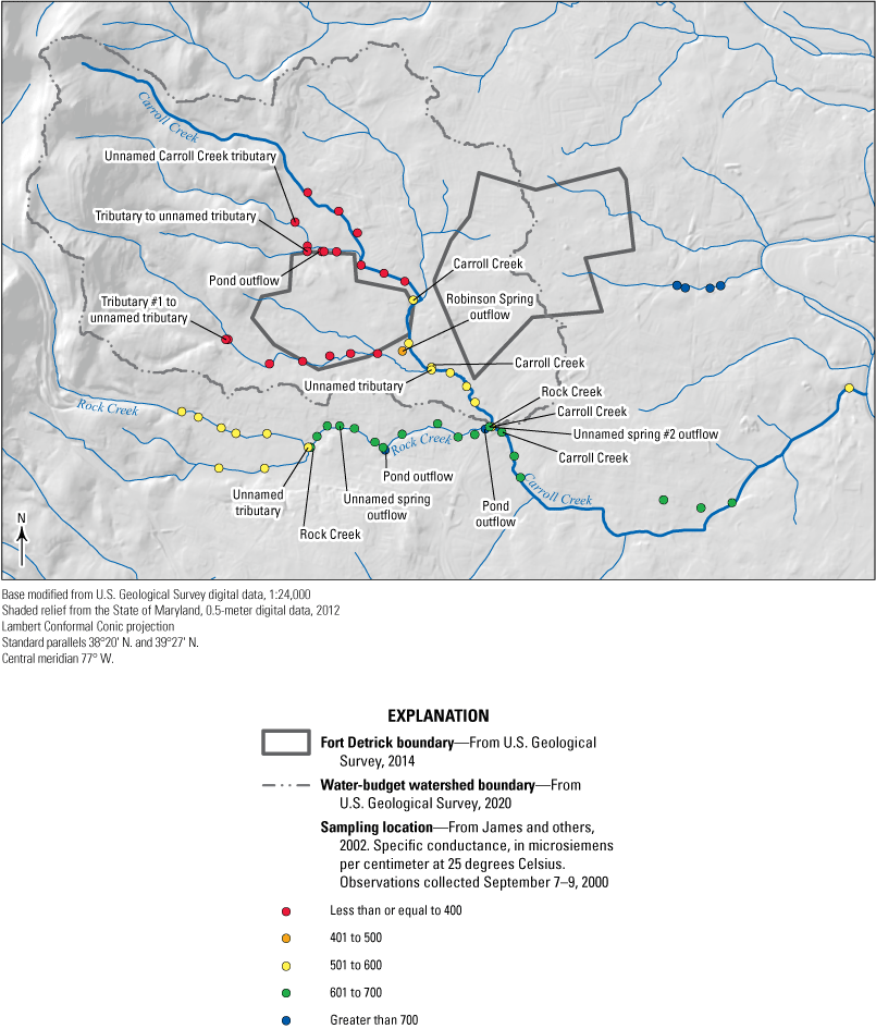
Specific conductance observed in streams surrounding Area B, Fort Detrick, Maryland September 7–9, 2000, by James and others (2002). Points along streams were collected in that stream unless a different water body is labelled. If unlabeled, streams are designated “unnamed tributary” in James and others (2002). Points are labeled as in James and others (2002).
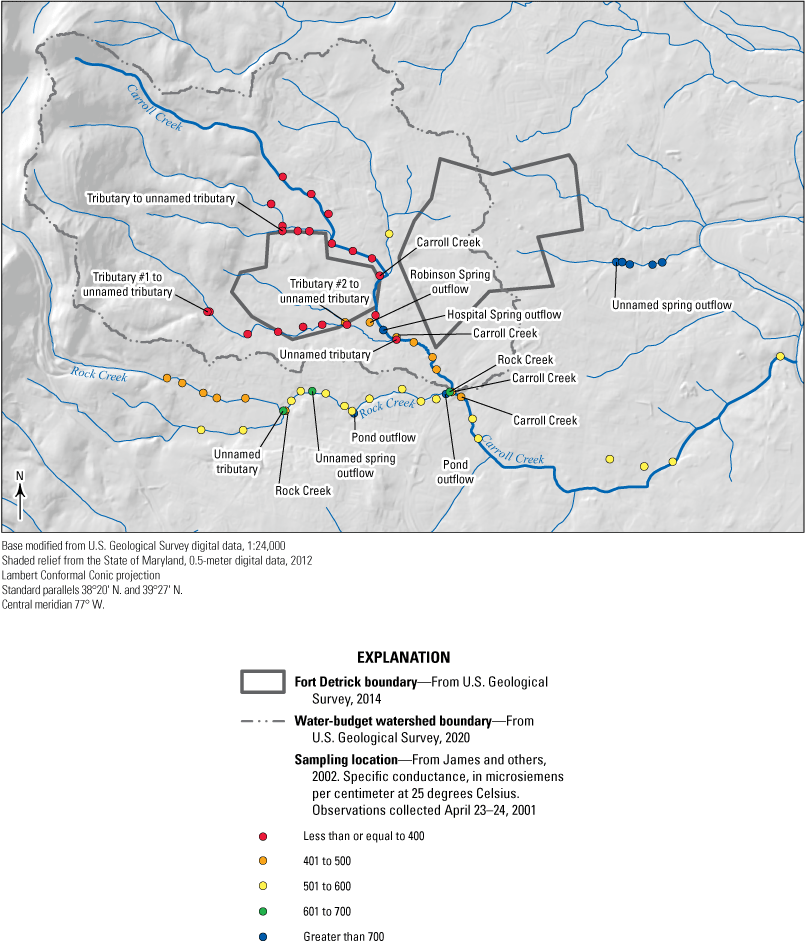
Specific conductance observed in streams surrounding Area B, Fort Detrick, Maryland April 23–24, 2001, by James and others (2002). Points along streams were collected in that stream unless a different water body is labelled. If unlabeled, streams are designated “unnamed tributary” in James and others (2002). Points are labeled as in James and others (2002).
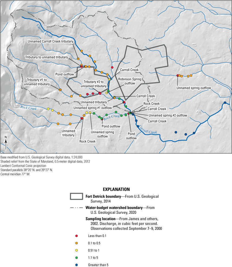
Stream discharge observed in streams surrounding Area B, Fort Detrick, Maryland September 7–9, 2000, by James and others (2002). Points along streams were collected in that stream unless a different water body is labelled. If unlabeled, streams are designated “unnamed tributary” in James and others (2002). Points are labeled as in James and others (2002).
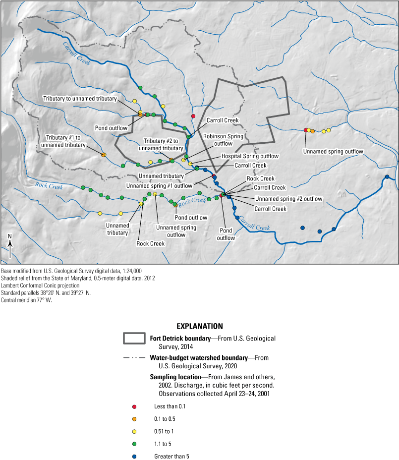
Stream discharge observed in streams surrounding Area B, Fort Detrick, Maryland April 23–24, 2001, by James and others (2002). Points along streams were collected in that stream unless a different water body is labelled. If unlabeled, streams are designated “unnamed tributary” in James and others (2002). Points are labeled as in James and others (2002).
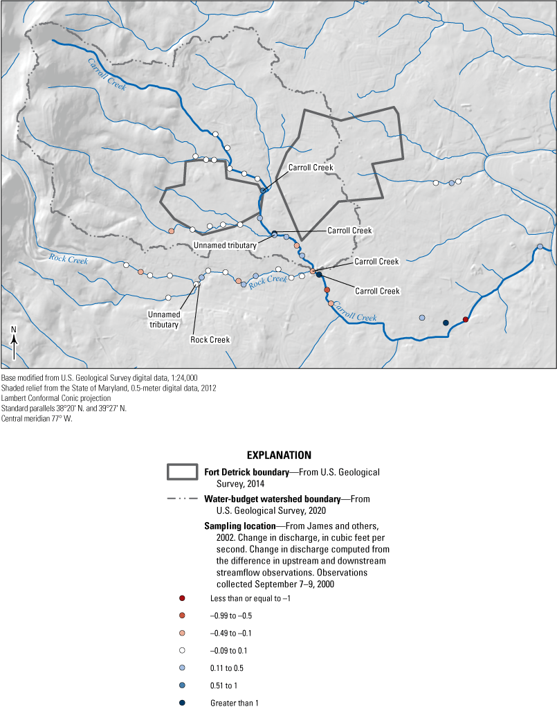
Calculated stream gain and loss in streams surrounding Area B, Fort Detrick, Maryland September 7–9, 2000, by James and others (2002). Points along streams were collected in that stream unless a different water body is labelled. If unlabeled, streams are designated “unnamed tributary” in James and others (2002). Points are labeled as in James and others (2002).
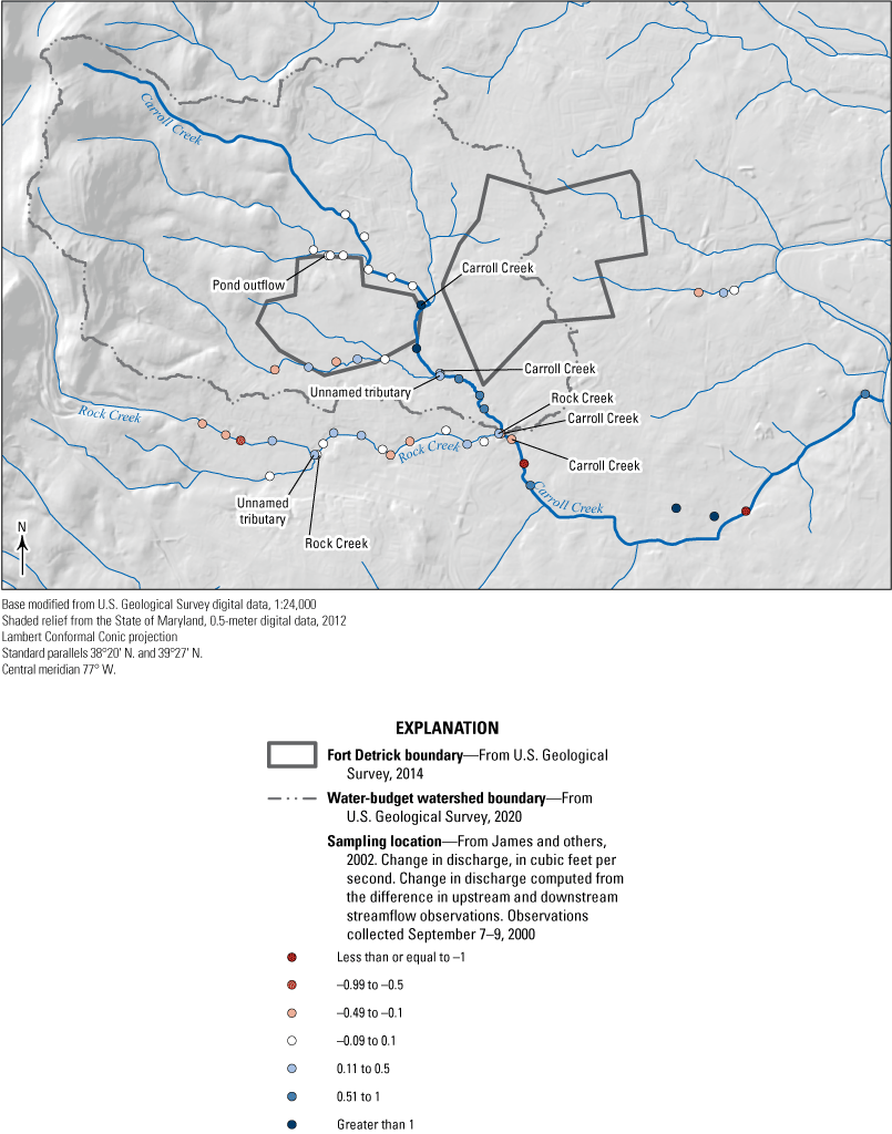
Calculated stream gain and loss in streams surrounding Area B, Fort Detrick, Maryland April 23–24, 2001, by James and others (2002). Points along streams were collected in that stream unless a different water body is labelled. If unlabeled, streams are designated “unnamed tributary” in James and others (2002). Points are labeled as in James and others (2002).
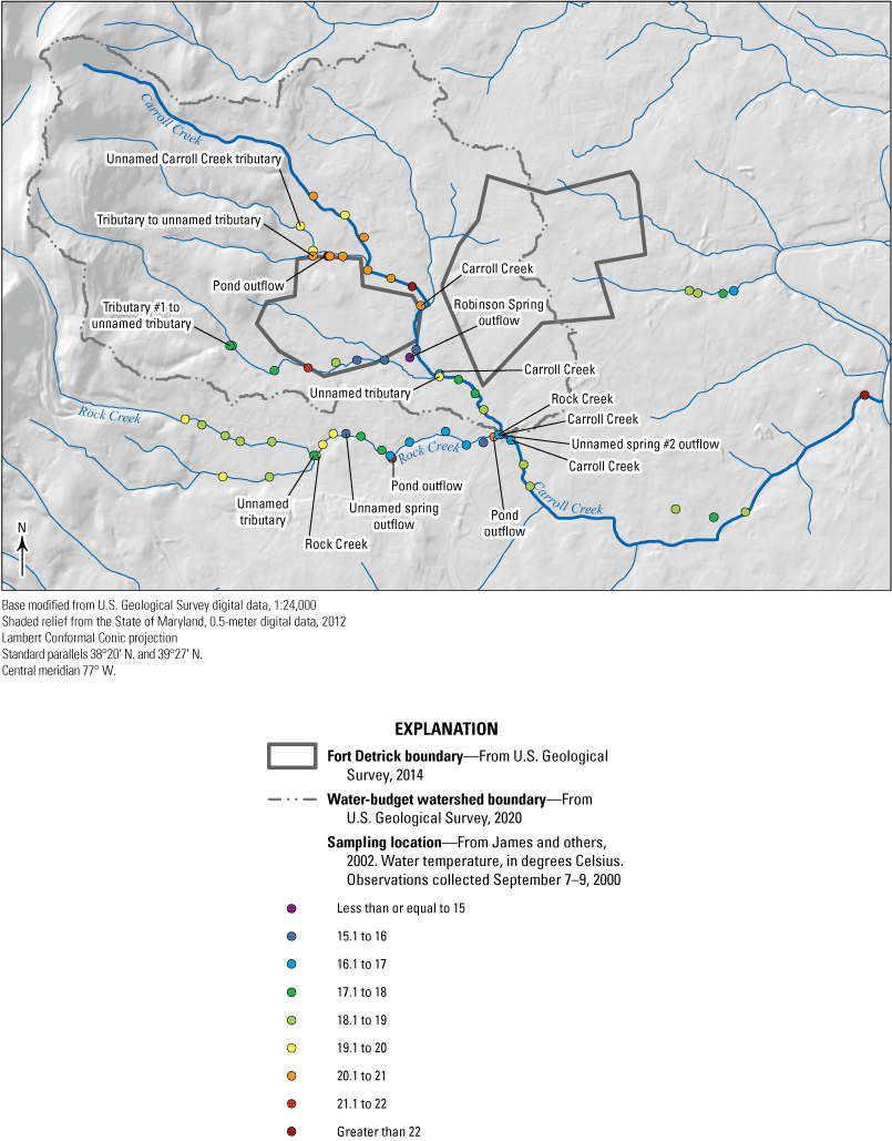
Observed temperature in streams surrounding Area B, Fort Detrick, Maryland September 7–9, 2000, by James and others (2002). Points along streams were collected in that stream unless a different water body is labelled. If unlabeled, streams are designated “unnamed tributary” in James and others (2002). Points are labeled as in James and others (2002).
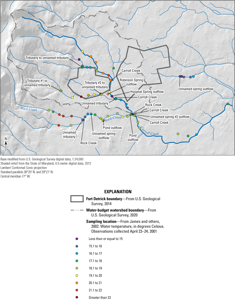
Observed temperature in streams surrounding Area B, Fort Detrick, Maryland April 23–24, 2001, by James and others (2002). Points along streams were collected in that stream unless a different water body is labelled. If unlabeled, streams are designated “unnamed tributary” in James and others (2002). Points are labeled as in James and others (2002).
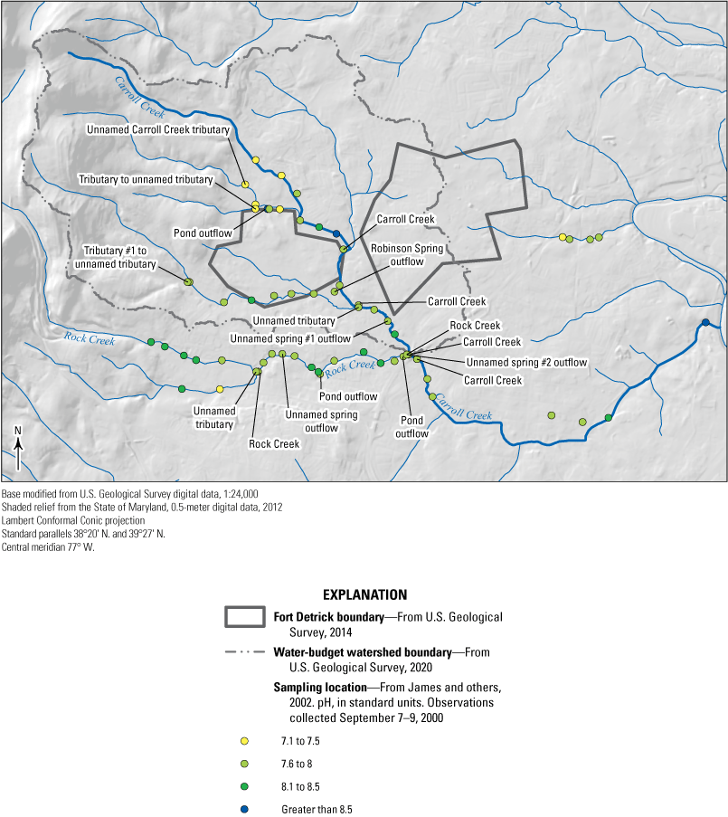
Observed pH in streams surrounding Area B, Fort Detrick, Maryland, September 7–9, 2000, by James and others (2002). Points along streams were collected in that stream unless a different water body is labelled. If unlabeled, streams are designated “unnamed tributary” in James and others (2002). Points are labeled as in James and others (2002).
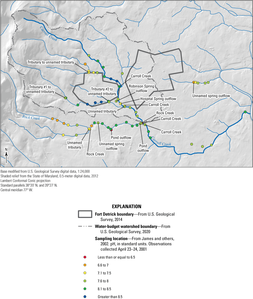
Observed pH in streams surrounding Area B, Fort Detrick, Maryland April 23–24, 2001, by James and others (2002). Points along streams were collected in that stream unless a different water body is labelled. If unlabeled, streams are designated “unnamed tributary” in James and others (2002). Points are labeled as in James and others (2002).
Conversion Factors
U.S. customary units to International System of Units
International System of Units to U.S. customary units
Temperature in degrees Celsius (°C) may be converted to degrees Fahrenheit (°F) as follows: °F = (1.8 × °C) + 32.
Temperature in degrees Fahrenheit (°F) may be converted to degrees Celsius (°C) as follows: °C = (°F – 32) / 1.8.
Datum
Vertical coordinate information is referenced to the North American Vertical Datum of 1988 (NAVD 88).
Horizontal coordinate information is referenced to North American Datum of 1983 (NAD 83) Universal Transverse Mercator (UTM) zone 18N.
Altitude, as used in this report, refers to distance above the vertical datum.
Supplemental Information
Specific conductance is given in microsiemens per centimeter at 25 degrees Celsius (µS/cm at 25 °C).
Concentrations of chemical constituents in water are given in either milligrams per liter (mg/L) or micrograms per liter (µg/L).
Activities for radioactive constituents in water are given in picocuries per liter (pCi/L).
Results for measurements of stable isotopes of an element (with symbol E) in water, solids, and dissolved constituents commonly are expressed as the relative difference in the ratio of the number of the less abundant isotope (iE) to the number of the more abundant isotope of a sample with respect to a measurement standard.
Abbreviations
Ae
entrapped air
AEW
air equilibrated water
ATV
acoustic televiewer
bls
below land surface
CE
closed-equilibrium
CDF
cumulative distribution function
CFC
chlorofluorocarbon
CSM
conceptual site model
DIC
dissolved inorganic carbon
DM
dispersion model
DO
dissolved oxygen
DOD
U.S. Department of Defense
DP
dispersion parameter
EMR
Episodic Master Recession
EPA
U.S. Environmental Protection Agency
ET
evapotranspiration
F
fractionation factor
FNU
Formazin Nephelometric Unit
gpm
gallons per minute
HCA
hierarchical cluster analysis
HCPC
hierarchical clustering on principal components
LC-excess
line-conditioned excess
LMWL
local meteoric water line
LPM
lumped parameter model
NAD 83
North American Datum of 1983
NAVD 88
North American Vertical Datum of 1988
NRCS
Natural Resources Conservation Service
NGVD 29
National Geodetic Vertical Datum of 1929
NGT
noble gas recharge temperature
NSE
Nash-Sutcliffe efficiency coefficient
NTU
Nephelometric Turbidity Units
NWIS
National Water Information System
OHS
optimal hydrograph separation
OTV
optical televiewer
PAMD
Pennsylvania-Maryland
PCA
Principal component analysis
PCE
tetrachloroethane
ppm
parts per million
PRISM
Parameter-elevation Regressions on Independent Slopes
R
ratio of helium-3 to helium-4 in a sample
Ra
ratio of helium-3 to helium-4 in the atmosphere
RDF
recursive digital filter
RFG
Revised Fontes and Garnier
RMSE
root-mean-square error
SC
specific conductance
SI
susceptibility index
SSEBOP
Simplified Surface Energy Balance
SSURGO
Soil Survey Geographic Database
SWB
Soil-Water Balance model
TCE
trichloroethane
USGS
U.S. Geological Survey
VOC
volatile organic compound
For additional information, contact:
Director, MD-DE-DC Water Science Center
U.S. Geological Survey
5522 Research Park Drive
Baltimore, MD 21228
Or visit our website at
https://www.usgs.gov/centers/md-de-dc-water
Publishing support provided by the West Trenton Publishing Service Center
Disclaimers
Any use of trade, firm, or product names is for descriptive purposes only and does not imply endorsement by the U.S. Government.
Although this information product, for the most part, is in the public domain, it also may contain copyrighted materials as noted in the text. Permission to reproduce copyrighted items must be secured from the copyright owner.
Suggested Citation
Goodling, P.J., Fleming, B.J., Solder, J., Soroka, A., and Raffensperger, J., 2023, Hydrogeologic characterization of Area B, Fort Detrick, Maryland: U.S. Geological Survey Scientific Investigations Report 2022–5054, 128 p., https://doi.org/10.3133/sir20225054.
ISSN: 2328-0328 (online)
Study Area
| Publication type | Report |
|---|---|
| Publication Subtype | USGS Numbered Series |
| Title | Hydrogeologic characterization of Area B, Fort Detrick, Maryland |
| Series title | Scientific Investigations Report |
| Series number | 2022-5054 |
| DOI | 10.3133/sir20225054 |
| Publication Date | May 02, 2023 |
| Year Published | 2023 |
| Language | English |
| Publisher | U.S. Geological Survey |
| Publisher location | Reston, VA |
| Contributing office(s) | Maryland-Delaware-District of Columbia Water Science Center |
| Description | Report: xiv, 128 p.; 2 Data Releases |
| Country | United States |
| State | Maryland |
| Other Geospatial | Fort Detrick |
| Online Only (Y/N) | Y |
| Additional Online Files (Y/N) | N |