

Simulation of Monthly Mean and Monthly Base Flow of Streamflow using Random Forests for the Mississippi River Alluvial Plain, 1901 to 2018
Links
- More information: Publisher Index Page (via DOI)
- Document: Report (2.15 MB pdf) , HTML , XML
- Tables:
- Table 1.1 (41.6 kB xlsx) —U.S. Geological Survey streamgages used to train and evaluate performance in the random forest model in the Mississippi alluvial plain area, 1901–2018.
- Table 1.1 (24.3 kB csv) —U.S. Geological Survey streamgages used to train and evaluate performance in the random forest model in the Mississippi alluvial plain area, 1901–2018.
- Table 3.1 (35.8 kB xlsx) —Performance metrics of comparing the observed monthly mean streamflows with estimated flows for the random forest models using leave-one-out cross validation in the Mississippi embayment regional aquifer system, 1901–2016.
- Table 3.1 (17.4 kB csv) —Performance metrics of comparing the observed monthly mean streamflows with estimated flows for the random forest models using leave-one-out cross validation in the Mississippi embayment regional aquifer system, 1901–2016.
- Table 3.2 (51.9 kB xlsx) —Performance metrics of comparing to the observed monthly mean streamflows with estimated streamflows for the model trained with all gaged sites in the Mississippi embayment regional aquifer system, 1901–2016.
- Table 3.2 (16.8 kB csv) —Performance metrics of comparing to the observed monthly mean streamflows with estimated streamflows for the model trained with all gaged sites in the Mississippi embayment regional aquifer system, 1901–2016.
- Table 3.3 (51.9 kB xlsx) —Performance metrics of comparing to the computed monthly base flows with estimated base flows for the model trained with all gaged sites in the Mississippi embayment regional aquifer system, 1901–2018.
- Table 3.3 (16.8 kB csv) —Performance metrics of comparing to the computed monthly base flows with estimated base flows for the model trained with all gaged sites in the Mississippi embayment regional aquifer system, 1901–2018.
- Dataset: USGS National Water Information System database —USGS water data for the Nation
- Data Release: USGS data release - Input data, trained model data, and model outputs for predicting streamflow and base flow for the Mississippi embayment regional study area using a random forest model
- NGMDB Index Page: National Geologic Map Database Index Page (html)
- Software Release: USGS software release —mapRandomForest—Monthly flow estimation in the Mississippi Alluvial Plain by means of random forest modeling
- Download citation as: RIS | Dublin Core
Abstract
Improved simulations of streamflow and base flow for selected sites within and adjacent to the Mississippi River Alluvial Plain area are important for modeling groundwater flow because surface-water flows have a substantial effect on groundwater levels. One method for simulating streamflow and base flow, random forest (RF) models, was developed from the data at gaged sites and, in turn, was used to make monthly mean streamflow and base-flow predictions at 162 ungaged sites in the study area. Daily streamflow observations and computed base flow from 247 streamgages were used as the basis for the development of these RF models. RF models were constructed from basin and climatic characteristics and related to observed monthly mean streamflow values; models were used to compute monthly base-flow estimates from selected streamgages in and adjacent to the Mississippi River Alluvial Plain extent, which includes streamflows from parts of Alabama, Arkansas, Colorado, Florida, Illinois, Indiana, Kansas, Kentucky, Louisiana, Mississippi, Missouri, New Mexico, Tennessee, and Texas. The explanatory variables for the models were selected to represent physical characteristics and climatic time series for the contributing drainage basins to the streamgages and ungaged locations of interest. The Nash-Sutcliffe efficiency between observed and simulated monthly mean streamflow was greater than 0.80 for 155 of the 247 streamgages, with a median Nash-Sutcliffe efficiency value of 0.83. The streamflow and base-flow simulations can be used to improve inflow values and to verify the Mississippi River Alluvial Plain groundwater flow model. The statistical model, input data, and response data (simulated monthly mean streamflows) are available as a U.S. Geological Survey software release and a U.S. Geological Survey data release.
Introduction
Through the U.S. Geological Survey (USGS) Water Availability and Use Science Program, the USGS is involved in a multiyear, multidiscipline regional water-availability study for the Mississippi River Alluvial Plain, south-central United States. For the Mississippi Alluvial Plain study, the USGS, in cooperation with more than 10 Federal, State, and local stakeholders, is comprehensively studying and modeling the Mississippi River Alluvial Plain area, the Mississippi River Valley alluvial aquifer, and associated hydrogeologic units (Clark and others, 2011).
The Mississippi River Alluvial Plain and nearby contributing river basins consist of an extensive flat alluvial plain extending beyond the historical floodplain of the Mississippi River and other proximal streams (Kleiss and others, 2000; Clark and others, 2011; U.S. Geological Survey, 2018). The Mississippi River Alluvial Plain is a major physiographic feature spanning parts of eight States (Alabama, Arkansas, Illinois, Kentucky, Louisiana, Mississippi, Missouri, and Tennessee). The northern and central sections of the Mississippi River Alluvial Plain area mostly are used for intensive production agriculture, and the primary crops include cotton, rice, and soybeans.
The Mississippi River Valley alluvial aquifer is the surficial aquifer in the Mississippi River Alluvial Plain area (fig. 1), extending southward from the head of the Mississippi embayment regional aquifer system (Clark and others, 2011) and merging with the Coastal Lowlands aquifer system (Martin and Whiteman, 1999; Barlow and Belitz, 2016). The Mississippi River Valley alluvial aquifer is critical for irrigation-based production agriculture (Reba and others, 2017), which contributes to the Mississippi River Alluvial Plain area being a premiere agricultural region of the Nation.
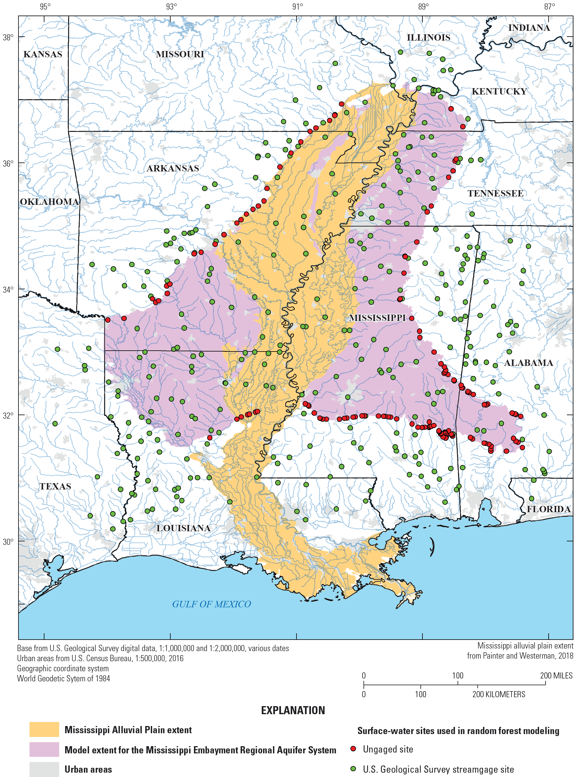
Location of the study area.
The hydrology and hydrogeology of the Mississippi River Alluvial Plain and Mississippi River Valley alluvial aquifer are greatly affected by many streams and rivers that incise it (fig. 1; Clark and others, 2011). For example, when a stream incises the Mississippi River Valley alluvial aquifer, the stream may (1) recharge the Mississippi River Valley alluvial aquifer, (2) receive streamflow from the Mississippi River Valley alluvial aquifer, or (3) temporally do either. In many parts of the Mississippi River Valley alluvial aquifer, large groundwater withdrawals have resulted in multidecadal declines of water levels in some areas and have diminished Mississippi River Valley alluvial aquifer streamflows to some of the streams (Barlow and Clark, 2011). Further, Reba and others (2017) documented contemporaneous water-level declines in areas of the Mississippi River Valley alluvial aquifer and detailed scenarios for mitigation such as tail-water recovery systems and managed aquifer recharge systems. The identification of distributed groundwater recharge zones in the Mississippi River Valley alluvial aquifer is complicated by surface water and by discontinuous low permeability units, which form confining or semiconfining units and affect recharge (Dyer and others, 2015).
Accurate assessments of water availability in the Mississippi River Alluvial Plain area require improved representation of surface-water and groundwater interactions (Feinstein and others, 2006). Simulations of streamflow for selected sites (stream reaches) within and adjacent to the Mississippi River Alluvial Plain aquifer system are important because surface-water flows have a substantial effect on groundwater storage in the Mississippi River Valley alluvial aquifer (Reba and others, 2017). The simulations of streamflow can provide boundary conditions and calibration targets for components of groundwater models such as the MODFLOW Streamflow-Routing (SFR2) Package (Niswonger and Prudic, 2005). Although streamgage records measured on orders of decades are available at sites on many streams in the Mississippi River Alluvial Plain system area, streamflow associated with those streamgages is applicable only to the reach near the streamgage and does not necessarily accurately represent streamflow on reaches between streamgages or on tributaries. Further, the streamgage network itself within the Mississippi River Valley alluvial aquifer area is not as spatially or temporally dense as in the region surrounding the Mississippi River Alluvial Plain area. Most of the sites are on the Mississippi River Alluvial Plain boundary, where monthly mean streamflow needed to constrain the groundwater modeling efforts is not coincident with USGS streamgages (fig. 1). Streamflow simulations derived from streamgage records or from statistical models of streamflow for selected stream reaches can be used with the SFR2 Package (Niswonger and Prudic, 2005) to provide inflows and model verification to the Mississippi River Alluvial Plain and Mississippi River Valley alluvial aquifer groundwater models. For this study, the R software package (R Core Team, 2016) was used to develop a statistical model of monthly streamflow and generate simulations of streamflow for selected stream reaches in the Mississippi River Alluvial Plain area and nearby stream basins. The model, the input data, and simulated streamflow and base-flow data generated during this study are available as a USGS software release (Westenbroek and others, 2021) and a USGS data release (Westenbroek and others, 2022).
Purpose and Scope
The primary purpose of this report is to document the construction and assessment of a surface-water hydrologic statistical model built to simulate monthly streamflows in and near the Mississippi River Alluvial Plain model area from 1901 to 2018. The statistical model described is constructed to support concurrent and future groundwater investigations involving groundwater-withdrawal scenarios, optimization, and surface-water monitoring network analyses. For this study, random forest (RF) statistical models were developed from streamflow observations and used to make simulations for sites in the Mississippi River Alluvial Plain area. A secondary purpose of this report is to describe the general application of the methods herein for predictions of monthly streamflow using differing datasets as new information is acquired in and near the Mississippi River Alluvial Plain area. The scope of this report is limited to the description, application, and assessment of RF models to simulate monthly mean streamflow and base flow at ungaged rivers in and near the Mississippi River Alluvial Plain area (fig. 1).
Study Area Description and Site Selection
The Mississippi River Alluvial Plain area generally overlies the Mississippi embayment regional aquifer system area. The Mississippi embayment regional aquifer system area is about 78,000 square miles (mi2), is in the humid southern United States, and underlies parts of 8 States—Alabama, Arkansas, Illinois, Kentucky, Louisiana, Mississippi, Missouri, and Tennessee (Clark and Hart, 2009). The Mississippi River Alluvial Plain contains a low-lying plain in which the Mississippi River and associated tributaries have deposited and reworked sediments. Streams in the area have slopes generally flatter than streams in the bordering uplands.
For this study, the surface-water model included 247 gaged sites (fig. 1) within and adjacent to the Mississippi River Alluvial Plain groundwater model boundary. The study area is larger than the Mississippi River Alluvial Plain area because of the need to acquire sufficient spatial and temporal representation of streamflow information and to include areas needed as part of other hydrologic modeling within the Mississippi River Alluvial Plain groundwater modeling study. The basin boundaries for streamgages used in the study included parts of States: Alabama, Arkansas, Colorado, Florida, Illinois, Kansas, Kentucky, Louisiana, Mississippi, Missouri, New Mexico, Oklahoma, Tennessee, and Texas. The criteria used for selecting streamgages used in the study were based on the availability and completeness of streamflow record. Some examples of streamgages not used are streamgages with peak streamflows only, partial-record low-flow or flood-flow sites, springflow sites, and sites with less than 12 months of observations. The streamgages selected are listed in appendix 1, table 1.1.
The 162 ungaged sites were selected at locations where simulations of surface-water flow were needed for other components of the Mississippi River Alluvial Plain study. The ungaged sites were near the boundaries of the Mississippi River Alluvial Plain model area in eight States: Alabama, Arkansas, Kentucky, Louisiana, Mississippi, Missouri, Tennessee, and Texas (fig. 1).
Random Forest Prediction Model Construction
RF prediction modeling is a statistical method using classification trees built on many explanatory variables to predict a response variable (Breiman, 2001; Kuhn and Johnson, 2016). RF models are a powerful generalization of regression trees and rule-based models. Output from RF models can either be a discrete classification or a continuous numerical value (regression; Breiman, 1998). RFs begin with many bootstrapped random samples from the data, resulting in about 63 percent of the original observations occurring at least once (Cutler and others, 2007). RFs aggregate bootstrap samples by splitting the data into branches using the best among a subset of predictors randomly chosen at that branch point (Liaw and Wiener, 2002). This type of classification tree, which divides the data based on the explanatory variables, is repeated many times, and each successive tree does not depend on earlier trees—each tree is independently constructed using a bootstrap sample of the dataset and, in the end, a collection of many trees is used for classification or regression based on the explanatory variables (Liaw and Wiener, 2002). Kuhn and Johnson (2016) provide valuable information for RF modeling, providing additional conceptual detail, comparison to other predictive statistical approaches, and numerous references, many of which are cited in this report.
RF models are deemed useful to this study because of the ability of the methodology to identify important predictor variables with minimal human intervention. Exploration of many potential predictor variables that act in difficult-to-describe nonlinear ways to affect streamflow can be time consuming when developing traditional regression models. Further, the use of meteorological variables with varying degrees of lag time adds complexity that is difficult to exhaustively examine for use in linear models. The RF algorithm has a practical advantage over using traditional statistical models because the algorithm can handle large numbers of potential input variables and makes no prior assumptions regarding the type of distribution of the input variables. The RF algorithm can identify the relative importance of potential input variables in an automated way that can facilitate model refinement as new datasets become available. Although linear models may potentially exceed the performance of RF models, the RF algorithm was chosen for this study for the potential practical advantages of implementation and flexibility to adapt to new data.
Recently, Miller and others (2018) used RF modeling to simulate natural monthly mean streamflows for more than 2.5 million stream reaches in the conterminous United States with the RF simulated and observed streamflows corresponding to about 2,000 streamgages. However, these data were not available at the time the Mississippi River Alluvial Plain aquifer system study began and do not necessarily coincide with the sites in the periods of interest of the Mississippi River Alluvial Plain study; therefore, a similar methodology was used to develop RF models to simulate streamflows in the Mississippi River Alluvial Plain region.
In this study, an RF surface-water statistical model is used to simulate streamflow in the study area. RF models were developed from data at the gaged sites and were in turn used to make monthly mean streamflow and base-flow predictions at 162 ungaged sites in the study area and monthly mean streamflows for missing periods at gaged sites in the Mississippi River Alluvial Plain area. The modeling is based on the statistical relation between explanatory variables and response variables. The explanatory variables were based on the physical characteristics and climatic time series representative of the drainage basins above streamgages. Physical characteristics that were initially used as explanatory variables in the RF model included drainage area size and location, elevation and slope of land surface, surficial geologic age classification, and climatic data, which included monthly precipitation, evapotranspiration, and temperature. The response variable for the model was the time series of monthly mean streamflow and monthly mean base flow. The RF model treats each set of explanatory and corresponding response variables as independent observations; however, lagged time-series data are included in the explanatory variables for each observation.
Site Selection
Sites within and adjacent to the Mississippi River Alluvial Plain model boundary (Clark and others, 2011) with long-term streamgages were selected for the development of the surface-water model. Sites with regulated peak flows were not considered for development of the model; however, sites were not screened for surface-water irrigation withdrawals or density of impoundments. Daily mean streamflow was available for the 247 gaged sites from the USGS National Water Information System database (U.S. Geological Survey, 2018). Although monthly streamflow and base flow were the targeted response variables for this study, daily streamflows were needed to estimate base flow. Base-flow separation was completed on all daily streamflow values using an R programming language implementation of the PART method of base-flow-record estimation (Rutledge, 1998). Daily mean streamflow and base-flow time series were aggregated into monthly time series.
A total of 162 ungaged basins at the groundwater flow model boundary were selected with outlets at locations that were deemed suitable for groundwater model inputs. The trained RF model was used to simulate streamflow at these sites. Simulations of streamflow at these locations can be used with the SFR2 Package (Niswonger and Prudic, 2005) to help constrain groundwater model boundary conditions and provide calibration targets at critical locations.
Explanatory Variables
Considerable preparation of input datasets was needed to assemble the potential explanatory variables used in the RF modeling. Two main categories of explanatory variables were considered for the RF model: physical drainage basin characteristics and meteorological characteristics. Physical drainage basin characteristics were properties of the drainage basin area upstream from the sites that describe the land surface and surficial geology that were assumed to remain constant over time. Meteorological characteristics were times-series data that described components of the atmospheric water balance in the area upstream from the sites such as precipitation, temperature, and evapotranspiration.
Physical drainage basin characteristics including variables such as drainage area and basin slope represent assumed immutable features that materially affect streamflow through basic principles that streamflow is expected to increase with drainage area and stream velocity is expected to increase with slope. A drainage basin that is steeper, or has a greater slope, will have less attenuation relative to the time that it takes precipitation to reach a given point in a stream from the time it falls on the land surface within that drainage basin. Other physical characteristics such as basin elevation and land use have secondary effects on streamflow patterns. As part of statistical model building, it is important to aggregate various properties and evaluate their predictive performance. Complex interaction between streamflow and drainage basin properties can occur, and some drainage basin properties can be interrelated.
Basins corresponding to the area upstream from each streamgage were delineated using the USGS StreamStats web-based geographic information system tool (Ries and others, 2004, 2017; Funkhouser and others, 2008; Law and others, 2009; Hedgecock and Lee, 2010; Southard and Veilleux, 2014). StreamStats is built on elevation data including the National Elevation Dataset (U.S. Geological Survey, 2016) and other geospatial datasets that allow users to estimate physical characteristics of basins. Basin boundaries were generated for the 247 streamgages and for the 162 ungaged basins. Drainage areas for the sites used in this study ranged from 18 to 18,417 mi2 for gaged basins and from less than 1 to 22,252 mi2 for ungaged sites. The latitudes and longitudes of the basin centroids were used as explanatory variables (appendix 1, table 1.1).
Meteorological characteristics have a direct effect on runoff and streamflow. The amount of runoff within a stream at a given point is related to the precipitation that has fallen over the basin upstream from the respective point. Natural streamflow is affected by meteorological characteristics at various time scales. Short durations of large rainfall (storms) produce short-term flooding typically lasting less than a week, whereas periods of abundant rainfall produce long durations of elevated streamflow and possibly flooding in contrast to drought periods. Additionally, processes within the drainage basin such as evapotranspiration and infiltration may affect the volume and the timing of the arrival of precipitation to a specific point in a stream. To this end, a lag in time (as much as months) of meteorological predictor variables is needed and assessed through exploratory development of a statistical model.
Monthly time series of total precipitation, maximum temperature, and minimum temperature were obtained based on the basin centroid for the gaged and ungaged basins from 1895 to 2015 using gridded climate data from the Parameter-elevation Regressions on Independent Slopes Model (PRISM Climate Group, 2018). Precipitation and temperature meteorological data were compiled from available Parameter-elevation Regressions on Independent Slopes Model datasets of monthly or daily values, which extend from January 1895 to 2021 (PRISM Climate Group, 2018). Monthly precipitation values ranged from 0 to 22.0 inches (in.) for gaged basins.
Monthly time series of evapotranspiration were created using the Hargreaves equation (Hargreaves and Samani, 1985) from the meteorological data for the gaged and ungaged basins. The Hargreaves equation includes other input parameters such as latitude, and for this study, the latitude used was that of the basin centroid. Monthly evapotranspiration values ranged from 0.47 to 11.18 in. for gaged basins.
Because streamflow response can be attenuated with respect to meteorological data, time series of meteorological data lagged by 1 and 2 months were created and used as additional explanatory variables; for example, for each month in the time series, the precipitation for the previous 2 months was used as an explanatory variable. Similarly, for each month, the maximum temperature, mean temperature, minimum temperature, and evapotranspiration for the previous 2 months were used as explanatory variables. The sum of precipitation from the preceding 6 months also was calculated for each month and used as a potential explanatory variable. The previous 6-month cumulative precipitation values ranged from 6.30 to 65.7 in. for gaged basins. The value of 6 months that was used for the final modeling of this study was qualitatively derived through preliminary exploratory data analyses.
During model development, surficial geologic basin characteristics also were used as potential explanatory variables. The basin boundaries obtained from StreamStats were used to extract geologic basin characteristics from the “Generalized Geologic Map of the Conterminous United States, Puerto Rico, and the U.S. Virgin Islands” (Reed and Bush, 2005). The fractions of the basin area were computed for land surface immediately underlain by nine categories of bedrock or surficial deposits: Quaternary, Neogene, Paleogene, Cretaceous, upper Paleozoic, middle Paleozoic, lower Paleozoic, middle Proterozoic, and a category for deposits of all other types. The fraction corresponding to waterbodies (Reed and Bush, 2005) also was computed for each basin.
Streamflows as Response Variables
Two types of streamflow were acquired or computed and act as the response variables in the RF development: (1) monthly mean streamflow (total streamflow) reported by the streamgages and (2) monthly base flow. Monthly mean streamflow was designated as the primary response variable. Monthly mean streamflows for each streamgage were compiled from daily streamflow records obtained from the USGS National Water Information System database using the R dataRetrieval package (Hirsch and De Cicco, 2015; U.S. Geological Survey, 2018). The daily streamflows were accumulated to monthly streamflows for each streamgage. The dates of monthly mean streamflow values ranged from water years 1901 through 2018, and the count of monthly mean streamflow values per site ranged from 15 to 1,144 values. The water year ranges are the overall starting and ending points (appendix 1, table 1.1) and do not reflect the fact that each streamgage has its own period of record. Because the RF model uses each set of explanatory and corresponding response variables independently, sites with fewer observations can still be useful in helping to train the model.
For this study, monthly base-flow separation was used to create monthly time-series datasets for use as response variables in RF modeling. A computerized method of base-flow-record estimation (PART) was selected for this study (Rutledge, 1998). The PART is a method of estimating base flow from daily mean streamflows (Rutledge, 1998). Specifically, the computer program PART uses daily streamflow partitioning to estimate a daily record of groundwater discharge under the streamflow record. The method (1) designates groundwater discharge to be equal to streamflow on days that fit a requirement of antecedent recession, (2) linearly interpolates groundwater discharge for other days, and (3) is applied to the streamflow record to obtain an estimate of the mean rate of groundwater discharge. It is important to remark that daily mean streamflow is the basis of the base-flow separation. The separated daily base flows can then be accumulated into estimated monthly base-flow values for the gaged sites and used as a response variable in the RF model. As with the monthly mean streamflows, for this study, the dates of monthly base-flow values ranged from water years 1901 to 2018, and the count of monthly base-flow values per site ranged from 15 to 1,144 values.
Random Forest Model Development
The RF model was developed within the R language (R Core Team, 2016). For purposes of disclosure, the R packages used to “train” the RF model included caret (Kuhn, 2018), Modern Applied Statistics with S (MASS) (Venables and Ripley, 2002), randomForests (Liaw and Wiener, 2002), and R packages doParallel (R Core Team, 2017a) and foreach (R Core Team, 2017b) to improve the speed of execution. In a simplistic sense, the training data are a subset of all the streamgages and their corresponding streamflows (monthly means and monthly base flow) and attendant potential explanatory variables. The subset of data not used for training is used for cross validation, which is important to ensure that the model does not overfit the data (Kuhn and Johnson, 2016).
Training control parameters required for the tuning of the RF model included the resampling method and the number of resampling iterations. RF models are trained to optimize model performance. The out-of-bag (OOB) estimation of error (Breiman, 1998) is a technique that uses the part of the model input data that is left out of the bootstrapped data selected for training within a particular classification tree (typically 37 percent is used with RF in most software implementations [Breiman, 1998] to evaluate the performance of the training set). The OOB estimation error technique was the resampling method used for this study. A grid of the number of variables randomly sampled as candidate predictor variables at each split in the classification trees (the “mtry” parameter) was used to tune the model based on optimization of OOB estimation of error for each candidate value of “mtry.”
The model was trained using explanatory and response variables from 247 streamgages (appendix 1, table 1.1). During preliminary model development, several iterations of differing model schemes were tested to examine the importance of explanatory variables. By evaluating measures of variable importance, explanatory variables were removed from the model training if the variables did not improve model performance. An advantage of eliminating unimportant explanatory variables is a reduction in the computational time required to run the model.
Results of Random Forest Model Performance
This section of the report describes the RF model performance. The RF model results were compared against the observed streamflows and base flows to evaluate model performance.
Random Forest Performance
Measures of variable importance for an RF model of simulation of monthly mean streamflow indicated that drainage area (drainage_area_va), current month precipitation (precip), 1-month lagged evapotranspiration (ET0Sub1), 2-month lagged evapotranspiration (ET0Sub2), and preceding 6-month precipitation (preTot6) were the most important predictors for monthly mean streamflow within the study area (appendix 2, table 2.1). The inclusion of geologic basin characteristics during model testing did not improve the model performance, and therefore, geologic basin characteristics were not used as explanatory variables in the final models. Also, temperature was not determined to be an important variable, which is perhaps logically consistent with the relatively higher importance of precipitation and evapotranspiration, likely because precipitation and evapotranspiration have a direct effect on water mass (liquid or vapor) in streamflow whereas temperature has a high correlation with evapotranspiration as an indirect driver to the process.
Model Validation
The RF training used for this study has leave-one-out cross validation built into the model training procedure. This training procedure can exclude a certain percentage of observations in the input dataset used to train the model. This is to ensure that the model does not overfit the input dataset; however, observations from all gaged sites in the input dataset are available for random selection to be used in training the model unless the site is explicitly removed from the input dataset. For this study, to quantify the predictive accuracy of RF model results, and to quantify the overall predictive accuracy of the RF model, an additional cross-validation procedure was used wherein an RF model was trained with the dataset of streamflow and base flow for all gaged sites with the exception of one gaged site. In this procedure, for each of the gaged sites, a separate RF model was trained using predictor variables and monthly mean streamflows for all gaged sites excluding the “current site,” which was left out from the data available for training the model. This procedure ensured that no observations from the excluded site were available for random selection during the training process. The RF model trained on all the data except the excluded site was then used to predict monthly mean flows at the excluded site. Model performance metrics were computed for the observed monthly mean streamflows and simulated monthly mean streamflows for the excluded site for the period of available observations at the site, which varied depending on the length of operation of the site. This procedure was repeated for each of the 247 sites.
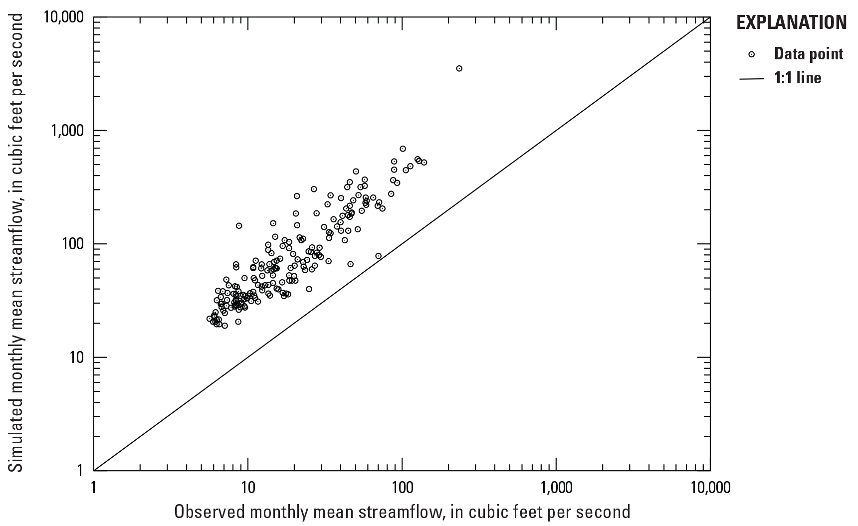
Seven cross-validation and goodness-of-fit performance metrics were calculated for the computed monthly mean base flows and simulated streamflows at 247 streamgages and summarized (table 1, fig. 2; appendix 3, table 3.1). The Nash-Sutcliffe efficiency (NSE; Nash and Sutcliffe, 1970) values were greater than 0.80 at 155 sites, and the Nash-Sutcliffe efficiency of the natural-logarithmically transformed streamflow prediction (NSEL) values were greater than 0.80 at 109 sites (appendix 3, table 3.1). The mean root mean square error (RMSE) was 871.8 cubic feet per second (ft3/s), and the root mean square error-observation standard deviation ratio (RSR; Moriasi and others, 2007) was less than 0.60 at 210 sites (appendix 3, table 3.1). The absolute value of the percentage of bias (PBIAS; Moriasi and others, 2007) was less than 10 percent at 128 sites. The Pearson correlation coefficient (Helsel and Hirsch, 1992) between observed and simulated streamflow ranged from 0.74 to 0.99, and the Spearman correlation ranged from 0.75 to 0.99 (appendix 3, table 3.1).
Table 1.
Cross-validation performance metrics from comparing the observed monthly mean streamflows with simulated monthly mean streamflows, Mississippi River Alluvial Plain area, 1901–2018.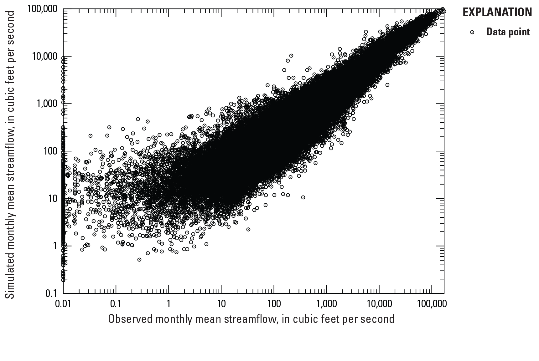
Comparison of observed and simulated monthly mean streamflows at 247 sites, Mississippi River Alluvial Plain area, 1901–2018.
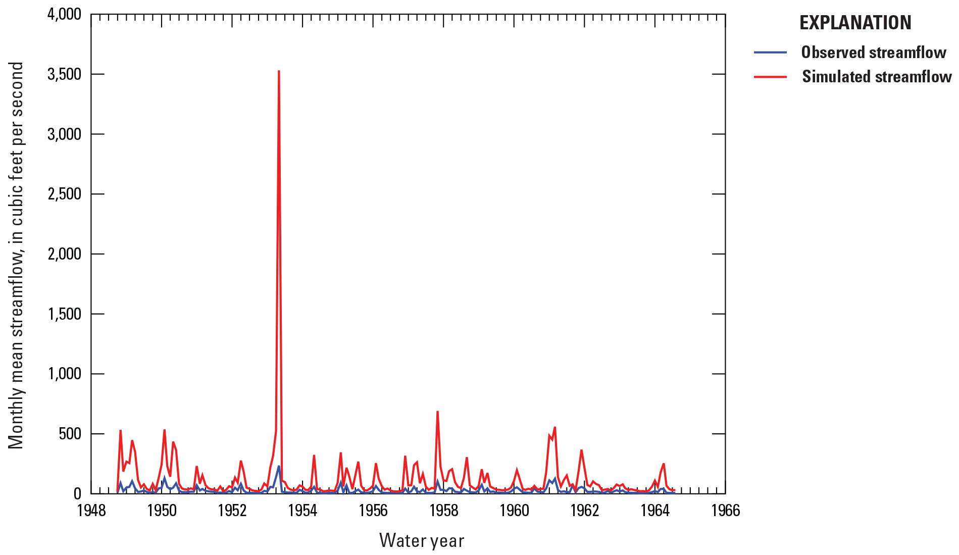
An example site with good performance metrics is the Obion River at Obion, Tennessee, site (USGS station 07026000; NSE=0.975). Performance metrics and graphical comparisons of the data (figs. 3, 4) indicate correlation between observed and simulated monthly streamflows and similarity in magnitude.
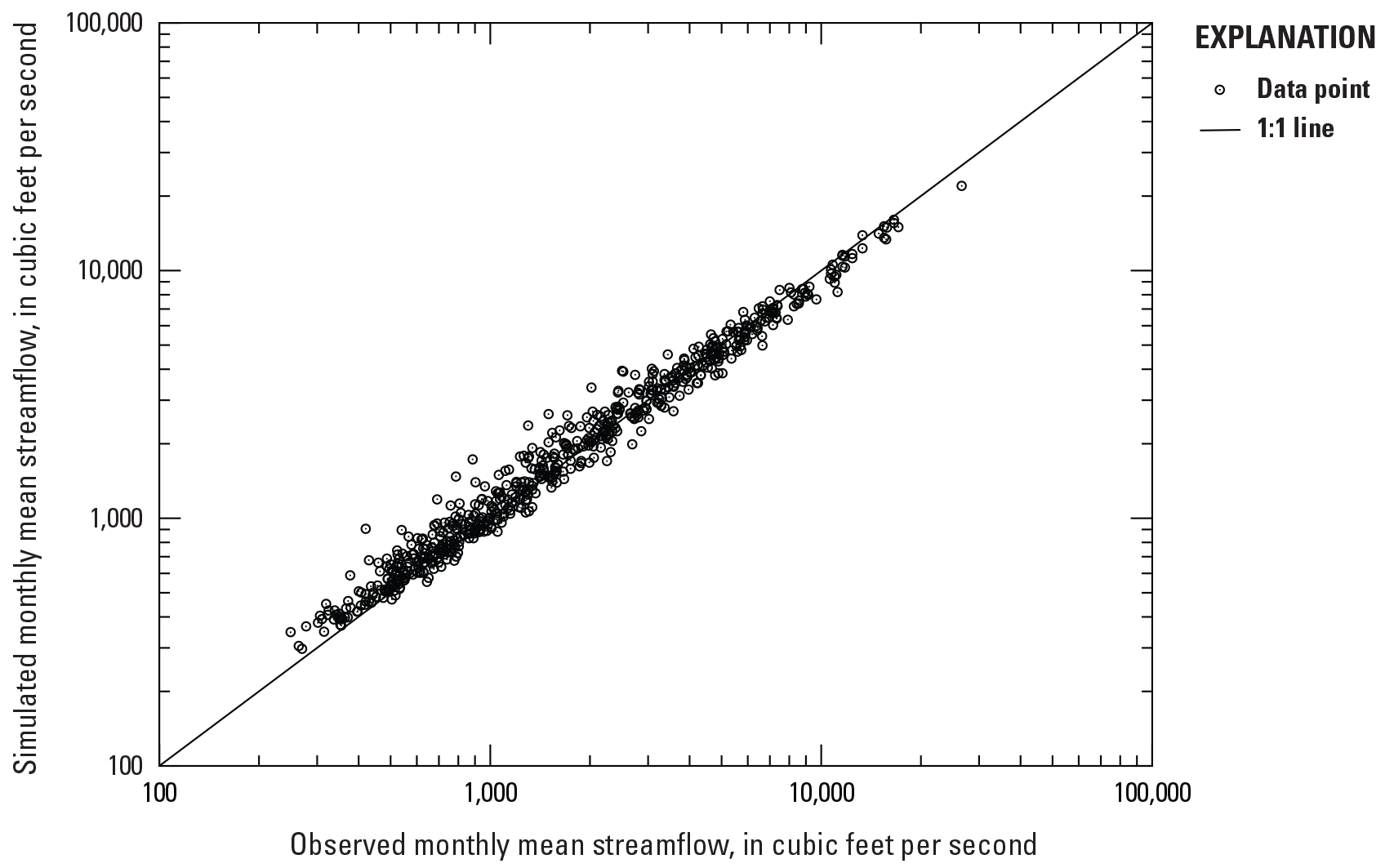
Comparison of observed and simulated monthly mean streamflows at Obion River at Obion, Tennessee (U.S. Geological Survey station 07026000).
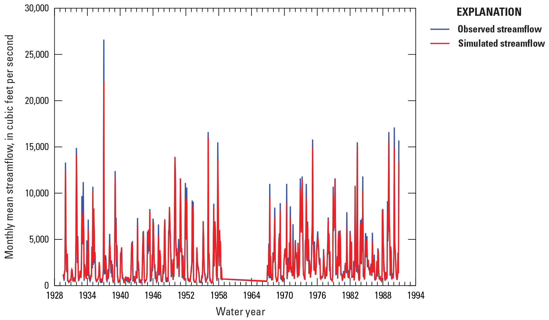
Comparison of hydrographs from observed and simulated monthly mean streamflows at Obion River at Obion, Tennessee (U.S. Geological Survey station 07026000).
An example site with poor performance metrics is the Hemphill Creek near Hot Wells, Louisiana, site (USGS station 07355000; NSE=−83.5). The negative NSE value indicates that the observed mean is a better predictor than the model. Although the performance metrics and graphical comparisons of the data (figs. 5, 6) indicate correlation between observed and simulated monthly streamflows, the simulated flows are higher for almost all monthly mean flows. Because the most important variable in the RF model is drainage area, it is possible that difficulties related to accurately delineating low-slope basins such as the one associated with Hemphill Creek near Hot Wells, La., can bias the simulated flows.
Comparison of observed and simulated monthly mean streamflows at Hemphill Creek near Hot Wells, Louisiana (U.S. Geological Survey station 07355000).
Comparison of hydrographs from observed and simulated monthly mean streamflows at Hemphill Creek near Hot Wells, Louisiana (U.S. Geological Survey station 07355000).
Monthly Mean Streamflow Simulation
The model validation procedure was repeated without excluding any particular site from the model training dataset; therefore, this validation represents a model trained with observations from all sites and does not leave any specific site out from potentially being sampled for training. Seven cross-validation and goodness-of-fit performance metrics for the model trained with all gaged sites were computed for the observed monthly mean streamflows and simulated streamflows at 247 streamgages and summarized (table 2; appendix 3, table 3.2). The NSE values were greater than 0.80 at 244 sites, and the NSEL values were greater than 0.80 at 227 sites. The mean RMSE was 326.5 ft3/s, and the RSR was less than 0.60 at 244 sites. The absolute value of PBIAS was less than 10 percent at 242 sites. The Pearson correlation coefficient between observed and simulated streamflow ranged from 0.906 to 0.998, and the Spearman correlation ranged from 0.893 to 0.998 (appendix 3, table 3.2).
Table 2.
Summary of performance metrics comparing the observed monthly mean streamflows with simulated streamflows from the trained random forest model for the model trained with all gaged sites, Mississippi River Alluvial Plain area, 1901–2018.Monthly Base-Flow Simulation
The model validation procedure was repeated for base flow. For this procedure, no particular site was excluded from the model training; therefore, this validation represents a model trained with observations from all sites and does not leave any specific site out from potentially being sampled for training. Seven cross-validation and goodness-of-fit performance metrics were calculated for the computed monthly mean base flows and simulated base flows at 247 streamgages and summarized (table 3). The NSE values were greater than 0.80 at 241 sites, and the NSEL values were greater than 0.80 at 213 sites. The mean RMSE was 234.4 ft3/s, and the RSR was less than 0.60 at 246 sites. The absolute value of PBIAS was less than 10 percent at 204 sites. The Pearson correlation coefficient between observed and simulated streamflow ranged from 0.958 to 0.995, and the Spearman correlation ranged from 0.796 to 0.995 (appendix 3, table 3.3).
Table 3.
Summary of performance metrics comparing the computed monthly mean base flows with simulated monthly mean base flows from the trained random forest model for the model trained with all gaged sites, Mississippi River Alluvial Plain area, 1901–2018.The performance metrics indicate that the RF model can provide time-series simulations of streamflow and base flow at gaged sites that are responsive to physical basin characteristics and meteorologic data. The performance metrics indicate that simulated streamflow and base flow based on the model for ungaged locations would improve simulations of surface-water inputs to groundwater models, which are often based on long-term mean flows at streamgages that may not be near the areas of interest or may have missing data. Therefore, the RF model was used to simulate monthly mean streamflow and base flow for the 162 ungaged drainage basins. The outlets of the drainage basins corresponded to nodes in the domain of the groundwater model. The models, the input data, and simulated streamflow and base-flow data generated during this study are available as a USGS software release (Westenbroek and others, 2021) and a USGS data release (Westenbroek and others, 2022).
Limitations and Assumptions
When evaluating the results of the model simulations, limitations and assumptions must be considered. The explanatory variables used in the RF model take into consideration a limited number of spatial and temporal components that affect surface-water flows; however, the model does not account for a wide range of physical conditions and the cumulative effects of flow alterations that might be localized to ungaged basins compared to nearby gaged basins. For example, the RF model does not account for surface-water irrigation withdrawals, density of impoundments, or other human activities that could substantially alter streamflows. Another important consideration relates to the range of explanatory variables used to predict flows. The performance metrics for the RF models are unknown outside of the ranges of the explanatory variables used to train the model, and therefore, flow simulations may be substantially less accurate for combinations outside the ranges of those used in training.
Summary
Improved simulations of streamflow and base flow for selected sites within and adjacent to the Mississippi River Alluvial Plain area are important for modeling groundwater flow because surface-water flows have a substantial effect on groundwater levels in the Mississippi River Valley Alluvial Plain area. For this study, 247 gaged and 162 ungaged sites within and adjacent to the Mississippi River Alluvial Plain model boundary were selected for inclusion in a random forest (RF) model to simulate streamflow and base flow. Daily streamflow observations and computed base flow from 247 streamgages were used as the basis for the development of these RF models. The basin boundaries for streamgages used in the study included parts of States: Alabama, Arkansas, Colorado, Florida, Illinois, Kansas, Kentucky, Louisiana, Mississippi, Missouri, New Mexico, Oklahoma, Tennessee, and Texas.
RF models were developed for gaged and ungaged sites in and near the Mississippi River Alluvial Plain area. RF models were developed from data at the gaged sites and were in turn used to make monthly mean streamflow and base-flow predictions at 162 ungaged sites in the study area and monthly mean streamflows for missing periods at gaged sites. The explanatory variables for the RF models were based on physical characteristics of the basin including drainage size, elevation, slope, and geologic and climatic data. The climatic data included precipitation, evapotranspiration, and temperature records representative of the drainage basins above streamgages or ungaged locations of interest. The response variables for the models were time series of monthly mean streamflow and monthly mean base flow.
Seven metrics of model performance and goodness of fit were calculated, using the results of model validation, on the observed total monthly mean streamflows at 247 streamgages compared to simulated streamflows. The Nash-Sutcliffe efficiency between observed and simulated monthly mean streamflow was greater than 0.80 for 155 of the 247 streamgages, with a median Nash-Sutcliffe efficiency value of 0.83. The performance metrics indicate that the RF models are responsive to physical basin characteristics and climatic meteorologic data and would improve simulations of surface-water inputs to groundwater models for predicting the monthly streamflow and base-flow values at ungaged sites and for missing periods at gaged sites; therefore, the RF model was used to simulate monthly time-series data for 162 ungaged drainage basins. The streamflow and base-flow simulations can be used to improve inflow values and to verify the Mississippi River Alluvial Plain groundwater flow model. The statistical model, the input data, and simulated monthly mean streamflow and base flow are available as a U.S. Geological Survey software release and a U.S. Geological Survey data release.
References Cited
Barlow, J.R.B., and Belitz, K., 2016, Groundwater quality in the Coastal Lowlands aquifer system, south-central United States: U.S. Geological Survey Fact Sheet 2016–3077, 4 p., accessed September 2021 at https://doi.org/10.3133/fs20163077.
Barlow, J.R.B., and Clark, B.R., 2011, Simulation of water-use conservation scenarios for the Mississippi Delta using an existing regional groundwater flow model: U.S. Geological Survey Scientific Investigations Report 2011–5019, 14 p. [Also available at https://doi.org/10.3133/sir20115019.]
Breiman, L., 1998, Out-of-bag estimation: Berkley, California, University of California, 13 p., accessed September 13, 2018, at https://www.stat.berkeley.edu/~breiman/OOBestimation.pdf.
Breiman, L., 2001, Random forests: Machine Learning, v. 45, no. 1, p. 5–32. [Also available at https://doi.org/10.1023/A:1010933404324.]
Clark, B.R., and Hart, R.M., 2009, The Mississippi Embayment Regional Aquifer Study (MERAS)—Documentation of a groundwater-flow model constructed to assess water availability in the Mississippi embayment: U.S. Geological Survey Scientific Investigations Report 2009–5172, 61 p., accessed September 2021 at https://doi.org/10.3133/sir20095172.
Clark, B.R., Hart, R.M., and Gurdak, J.J., 2011, Groundwater availability of the Mississippi embayment: U.S. Geological Survey Professional Paper 1785, 62 p. [Also available at https://doi.org/10.3133/pp1785.]
Cutler, D.R., Edwards, T.C., Jr., Beard, K.H., Cutler, A., Hess, K.T., Gibson, J., and Lawler, J.J., 2007, Random forests for classification in ecology: Ecology, v. 88, no. 11, p. 2783–2792. [Also available at https://doi.org/10.1890/07-0539.1.]
Dyer, J., Mercer, A., Rigby, J.R., and Grimes, A., 2015, Identification of recharge zones in the Lower Mississippi River alluvial aquifer using high-resolution precipitation estimates: Journal of Hydrology, v. 531, no. part 2, p. 360–369. [Also available at https://doi.org/10.1016/j.jhydrol.2015.07.016.]
Feinstein, D.T., Haitjema, H.M., and Hunt, R.J., 2006, Towards more accurate leakage and conjunctive use simulations—A coupled GFLOW-MODFLOW application, in Poeter, E., Hill, M., and Zheng, C., eds., MODFLOW and more 2006—Managing ground water systems—Proceedings v. 1: Golden, Colo., International Ground Water Modeling Center, School of Mines, p. 109–113.
Funkhouser, J.E., Eng, K., and Moix, M.W., 2008, Low-flow characteristics and regionalization of low-flow characteristics for selected streams in Arkansas: U.S. Geological Survey Scientific Investigations Report 2008‒5065, 162 p., accessed September 2021 at https://doi.org/10.3133/sir20085065.
Hargreaves, G.H., and Samani, Z.A., 1985, Reference crop evapotranspiration from temperature: Applied Engineering in Agriculture, v. 1, no. 2, p. 96–99. [Also available at https://doi.org/10.13031/2013.26773.]
Hedgecock, T.S., and Lee, K.G., 2010, Magnitude and frequency of floods for urban streams in Alabama, 2007: U.S. Geological Survey Scientific Investigations Report 2010–5012, 17 p. [Also available at https://doi.org/10.3133/sir20105012.]
Hirsch, R.M., and De Cicco, L.A., 2015, User guide to Exploration and Graphics for RivEr Trends (EGRET) and dataRetrieval—R packages for hydrologic data (ver. 2.0, February 2015): U.S. Geological Survey Techniques and Methods, book 4, chap. A10, 93 p., accessed September 2021 at https://doi.org/10.3133/tm4A10.
Kleiss, B.A., Coupe, R.H., Gonthier, G., and Justus, B.G., 2000, Water quality in the Mississippi Embayment, Mississippi, Louisiana, Arkansas, Missouri, Tennessee, and Kentucky, 1995–98: U.S. Geological Survey Circular 1208, 36 p. [Also available at https://doi.org/10.3133/cir1208.]
Kuhn, M., 2018, caret—Classification and regression training (ver. 6.0–80): R package, accessed September 13, 2018, at https://cran.r-project.org/web/packages/caret/index.html.
Law, G.S., Tasker, G.D., and Ladd, D.E., 2009, Streamflow-characteristic estimation methods for unregulated streams of Tennessee: U.S. Geological Survey Scientific Investigations Report 2009–5159, 212 p., 1 pl. [Also available at https://doi.org/10.3133/sir20095159.]
Martin, A., Jr., and Whiteman, C.D., Jr., 1999, Hydrology of the Coastal Lowlands aquifer system in parts of Alabama, Florida, Louisiana, and Mississippi: U.S. Geological Survey Professional Paper 1416–H, 51 p., 8 pl. [Also available at https://doi.org/10.3133/pp1416H.]
Miller, M.P., Carlisle, D.M., Wolock, D.M., and Wieczorek, M., 2018, A database of natural monthly streamflow estimates from 1950 to 2015 for the conterminous United States: Journal of the American Water Resources Association, v, 54, no. 6, p. 1258–1269. [Also available at https://doi.org/10.1111/1752-1688.12685.]
Moriasi, D.N., Arnold, J.G., Van Liew, M.W., Bingner, R.L., Harmel, R.D., and Veith, T.L., 2007, Model evaluation guidelines for systematic quantification of accuracy in watershed simulations: Transactions of the ASABE, v. 50, no. 3, p. 885–900. [Also available at https://doi.org/10.13031/2013.23153.]
Nash, J.E., and Sutcliffe, J.V., 1970, River flow forecasting through conceptual models part I—A discussion of principles: Journal of Hydrology, v. 10, no. 3, p. 282–290. [Also available at https://doi.org/10.1016/0022-1694(70)90255-6.]
Niswonger, R.G., and Prudic, D.E., 2005, Documentation of the Streamflow-Routing (SFR2) Package to include unsaturated flow beneath streams—A modification to SFR1: U.S. Geological Survey Techniques and Methods, book 6, chap. A13, 48 p., accessed September 2021 at https://doi.org/10.3133/tm6A13.
Painter, J.A., and Westerman, D.A., 2018, Mississippi Alluvial Plain extent, November 2017: U.S. Geological Survey data release, accessed January 2020 at https://doi.org/10.5066/F70R9NMJ.
PRISM Climate Group, 2018, PRISM climate data: PRISM Climate Group web page, accessed January 2020 at https://prism.oregonstate.edu/.
R Core Team, 2016, R—A language and environment for statistical computing: Vienna, Austria, R Foundation for Statistical Computing, 3795 p., accessed September 2021 at http://www.R-project.org/.
R Core Team, 2017a, R—A language and environment for statistical computing, version 1.0.11 (doParallel): R Foundation for Statistical Computing software release, accessed September 13, 2018, at https://cran.r-project.org/src/contrib/Archive/doParallel/doParallel_1.0.11.tar.gz.
R Core Team, 2017b, R—A language and environment for statistical computing, version 1.4.4 (foreach): R Foundation for Statistical Computing software release, accessed September 13, 2018, at https://cran.r-project.org/src/contrib/Archive/foreach/.
Reba, M.L., Massey, J.H., Adviento-Borbe, M.A., Leslie, D., Yaeger, M.A., Anders, M., and Farris, J., 2017, Aquifer depletion in the Lower Mississippi River Basin—Challenges and solutions: Journal of Contemporary Water Research & Education, v. 162, no. 1, p. 128–139, accessed August 9, 2018, at https://doi.org/10.1111/j.1936-704X.2017.03264.x.
Reed, J.C., Jr., and Bush, C.A., 2005, Generalized geologic map of the conterminous United States, Puerto Rico, and the U.S. Virgin Islands: U.S. Geological Survey, scale 1:7,500,000, accessed September 13, 2018, at https://pubs.usgs.gov/atlas/geologic/.
Ries, K.G., III, Newson J.K., Smith, M.J., Guthrie, J.D., Steeves, P.A., Haluska, T.L., Kolb, K.R., Thompson, R.F., Santoro, R.D., and Vraga, H.W., 2017, StreamStats, version 4: U.S. Geological Survey Fact 2017–3046, 4 p. [Also available at https://doi.org/10.3133/fs20173046.] [Supersedes USGS Fact Sheet 2008–3067.]
Ries, K.G., III, Steeves, P.A., Coles, J.D., Rea, A.H., and Stewart, D.W., 2004, StreamStats—A U.S. Geological Survey web application for stream information: U.S. Geological Survey Fact Sheet 2004–3115, 4 p. [Also available at https://doi.org/10.3133/fs20043115.]
Rutledge, A.T., 1998, Computer programs for describing the recession of ground-water discharge and for estimating mean ground-water recharge and discharge from streamflow records—Update: U.S. Geological Survey Water-Resources Investigations Report 98–4148, 43 p. [Also available at https://doi.org/10.3133/wri984148.]
Southard, R.E., and Veilleux, A.G., 2014, Methods for estimating annual exceedance-probability discharges and largest recorded floods for unregulated streams in rural Missouri: U.S. Geological Survey Scientific Investigations Report 2014–5165, 39 p. [Also available at https://doi.org/10.3133/sir20145165.]
U.S. Geological Survey, 2016, USGS National Elevation Dataset (NED) 1 arc-second downloadable data collection from The National Map 3D Elevation Program (3DEP)—National Geospatial Data Asset (NGDA) National Elevation Data Set (NED): U.S. Geological Survey digital data, accessed September 2021 at https://data.globalchange.gov/dataset/usgs-national-elevation-dataset-ned-1-arc-second.
U.S. Geological Survey, 2018, USGS water data for the Nation: U.S. Geological Survey National Water Information System database, accessed January 2020 at https://doi.org/10.5066/F7P55KJN.
Westenbroek, S.M., Dietsch, B.J., and Breaker, B.K., 2021, mapRandomForest—Monthly flow estimation in the Mississippi Alluvial Plain by means of random forest modeling: U.S. Geological Survey software release, accessed September 2021 at https://doi.org/10.5066/P92UE6EG.
Westenbroek, S.M., Dietsch, B.J., and Breaker, B.K., 2022, Input and datasets and random forest model outputs for predicting stream flow and base flow for the Mississippi Alluvial Plain: U.S. Geological Survey data release, accessed May 2022 at https://doi.org/10.5066/P9QCK8HY.
Appendix 1. Stations Used in Analysis
Appendix 2. Explanatory Variables Used in the Random Forest Model
Table 2.1.
Explanatory variables used in the random forest model.References Cited
PRISM Climate Group, 2018, PRISM climate data: PRISM Climate Group web page, accessed January 2020 at https://prism.oregonstate.edu/.
Ries, K.G., III, Newson J.K., Smith, M.J., Guthrie, J.D., Steeves, P.A., Haluska, T.L., Kolb, K.R., Thompson, R.F., Santoro, R.D., and Vraga, H.W., 2017, StreamStats, version 4: U.S. Geological Survey Fact 2017–3046, 4 p. [Also available at https://doi.org/10.3133/fs20173046.] [Supersedes USGS Fact Sheet 2008–3067.]
Appendix 3. Performance Metrics
Conversion Factors
Datum
Vertical coordinate information is referenced to the North American Vertical Datum of 1988 (NAVD 88).
Horizontal coordinate information is referenced to the North American Datum of 1983 (NAD 83).
Elevation, as used in this report, refers to distance above the vertical datum.
Supplemental Information
A water year is the 12-month period from October 1 through September 30 and is designated by the calendar year in which it ends.
Abbreviations
NSE
Nash-Sutcliffe efficiency
NSEL
Nash-Sutcliffe efficiency of natural-logarithmically transformed streamflow predictions
OOB
out of bag
PBIAS
percentage of bias
RF
random forest
RMSE
root mean square error of streamflow predictions
RSR
root mean square error-observation standard deviation ratio
SFR2
Streamflow-Routing [Package]
USGS
U.S. Geological Survey
For more information about this publication, contact:
Director, USGS Nebraska Water Science Center
5231 South 19th Street
Lincoln, NE 68512
402–328–4100
For additional information, visit: https://www.usgs.gov/centers/ne-water
Publishing support provided by the
Rolla Publishing Service Center
Disclaimers
Any use of trade, firm, or product names is for descriptive purposes only and does not imply endorsement by the U.S. Government.
Although this information product, for the most part, is in the public domain, it also may contain copyrighted materials as noted in the text. Permission to reproduce copyrighted items must be secured from the copyright owner.
Suggested Citation
Dietsch, B.J., Asquith, W.H., Breaker, B.K., Westenbroek, S.M., and Kress, W.H., 2023, Simulation of monthly mean and monthly base flow of streamflow using random forests for the Mississippi River Alluvial Plain, 1901 to 2018: U.S. Geological Survey Scientific Investigations Report 2022–5079, 17 p., https://doi.org/10.3133/sir20225079.
ISSN: 2328-0328 (online)
Study Area
| Publication type | Report |
|---|---|
| Publication Subtype | USGS Numbered Series |
| Title | Simulation of monthly mean and monthly base flow of streamflow using random forests for the Mississippi River Alluvial Plain, 1901 to 2018 |
| Series title | Scientific Investigations Report |
| Series number | 2022-5079 |
| DOI | 10.3133/sir20225079 |
| Publication Date | March 01, 2023 |
| Year Published | 2023 |
| Language | English |
| Publisher | U.S. Geological Survey |
| Publisher location | Reston, VA |
| Contributing office(s) | Nebraska Water Science Center, Wisconsin Water Science Center, Lower Mississippi-Gulf Water Science Center |
| Description | Report: v, 17 p.; Tables: 4; Data Release; Dataset; Software Release |
| Country | United States |
| State | Alabama, Arkansas, Illinois, Kentucky, Louisiana, Mississippi, Missouri, Tennessee |
| Other Geospatial | Mississippi River Alluvial Plain |
| Online Only (Y/N) | Y |
| Additional Online Files (Y/N) | Y |