

Recent History of Glacial Lake Outburst Floods, Analysis of Channel Changes, and Development of a Two-Dimensional Flow and Sediment Transport Model of the Snow River near Seward, Alaska
Links
- Document: Report (11.7 MB pdf) , HTML , XML
- Data Releases:
- USGS data release - GIS and Hydraulic Model data in Support of a Geomorphic and Hydraulic Assessment of Glacial Outburst Floods on the Snow River near Seward, Alaska
- USGS data release - Water Surfaces Elevations During an Outburst Flood from Pressure Transducers at Snow River, Alaska, 2019
- NGMDB Index Page: National Geologic Map Database Index Page (html)
- Download citation as: RIS | Dublin Core
Acknowledgments
Karenth Dworksy, Schyler Knopp, and Ellen Justis provided invaluable assistance with field surveys. Jeff Conaway, Paul Kinzel and Crane Johnson of the National Weather Service thoughtfully reviewed the manuscript and made constructive suggestions. Scott Hogan of Federal Highways, Yong Lai of the Bureau of Reclamation, and Lyle Zevenbergen provided technical reviews of the model at different stages of development. The Alaska Railroad Corporation, especially Blake Adolfae and Brian O’Dowd, facilitated access to much of the study area during floods and provided observations, survey data, and aerial photographs in addition to funding the project. Janie Dusel of Alaska Water Resources and Kristen Valentine of the Alaska Department of Transportation and Public Facilities shared aerial imagery, field observations, and survey data for the Bridge 605 area.
Abstract
Snow Lake, a glacially dammed lake on the Snow Glacier near Seward, Alaska, drains rapidly every 14 months–3 years, causing flooding along the Snow River. Highway, railroad, and utility infrastructure on the lower Snow River floodplain is vulnerable to flood damage. Historical hydrology, geomorphology, and two-dimensional hydraulic and sediment transport modeling were used to assess the flood risks from Snow Lake outburst floods. Floods have become more frequent, peaked more rapidly, and have had generally higher peaks over the last 20 years as the Snow Glacier has thinned, translating to a greater potential for flood damage. Rapidly shifting channel locations and the occasional introduction of large volumes of debris to the river also threaten infrastructure on the floodplain and in the channel. An assessment of the historical channel planform between 1951 and 2019 showed that there have been more and less stable segments along the lower Snow River and that channel migration has generally been toward the east. An analysis of floodplain elevations using 2008 light detection and ranging (lidar) showed that the main channel is relatively high compared to floodplain channels that carry floodwaters along the railroad grade, so that once the main channel banks are overtopped water rapidly disperses throughout the floodplain. A two-dimensional flow and sediment transport model was developed, and its simulation results were compared to three past outburst floods from 2007, 2017, and 2019. Despite the complex floodplain and channel geometry, coarse resolution of the mesh, and sediment input data, the model successfully simulated areas of observed scour along the railroad grade and at the guidebank to the highway bridge. The modeled water-surface elevations generally replicated peak elevations recorded at a streamgage in the middle of the model domain and at pressure transducers installed on the floodplain and main channel, although there were discrepancies on the rising limb and some locations had a poorer fit than others. A model of a hypothetical check flood, approximately 150 percent of the largest recorded outburst flood, was developed to provide hydraulic variables to use when planning for infrastructure upgrades.
Introduction
The Snow River near Seward, Alaska floods every 2–3 years from a glacier dammed lake (GDL) draining rapidly from the Snow Glacier (fig. 1). GDLs form after tributary glaciers detach from the larger trunk glacier and the resultant basin fills with glacial meltwater and runoff from adjacent slopes. GDLs are typically ephemeral and can drain rapidly under the glacier which increases discharge at the glacier terminus substantially. As glacier ice thins and retreats, there is a potential for glacial lake outburst floods (GLOFs) in Alaska to change in character, temporarily becoming larger or more frequent as well as occurring in new locations. The 2017 outburst flood was the third largest flood recorded at the Snow River streamgage. At nearly 30,000 cubic feet per second (ft3/s), it is one of the three largest outburst peaks estimated by the National Weather Service since 1949. At over 40,000 ft3/s, the 2019 flood was the largest peak measured (Chapman, 1981; National Weather Service, 2019). While the 2017 outburst flood was augmented by precipitation, there was no antecedent or concurrent precipitation that contributed to the 2019 flood.
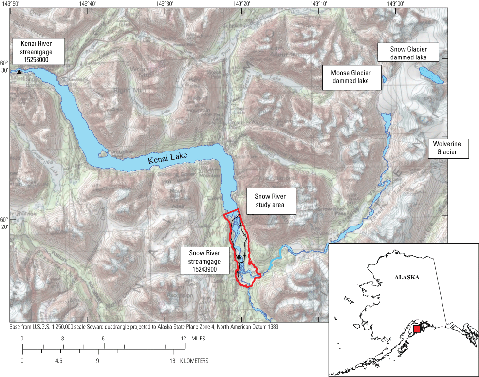
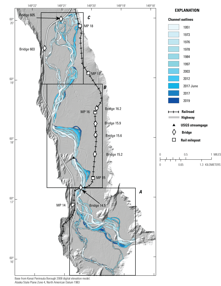
Snow River from Snow Glacier to Kenai Lake and relevant streamgages, near Seward, Alaska. Snow River study area outlines area of geomorphology and modeling analyses.
About 20 miles downstream of the Snow Glacier, railroad tracks and the Seward Highway flank the Snow River valley (fig. 2). Infrastructure potentially affected by the Snow River outburst floods include an Alaska Railroad (ARRC) bridge and 4 miles of track with smaller drainage structures, about 4 miles of the Seward Highway, two highway bridges, and electrical utilities. Floodwaters have eroded fill from beneath the railroad tracks on the east side of the river, damaged culverts and small bridges, and overtopped and eroded guide banks and revetments designed to protect the highway bridge and adjacent electrical utilities. In 2017, bank erosion and channel avulsion contributed thousands of mature spruce trees to the river, some of which hung up on bridge piers, reducing the conveyance capacity of the main bridges. As of this writing (2021), rafts of spruce logs remain on gravel bars and banks for future floods to redistribute.
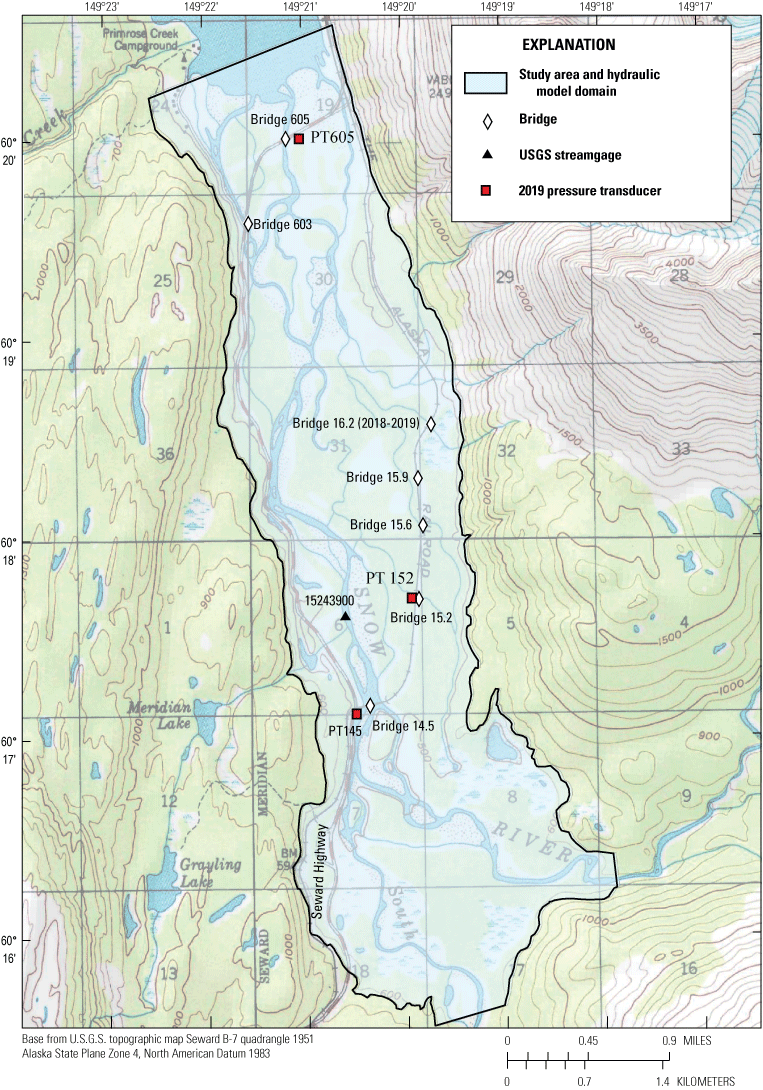
Lower Snow River, including extent of model domain, highway, and rail infrastructure near Seward, Alaska.
Purpose and Scope
This report describes the flood history, geomorphic analysis, and development of a two-dimensional hydraulic and sediment transport model of the Snow River. The purpose of the geomorphic analysis is to identify trends in the position of the Snow River channels, historically stable and unstable areas, and patterns of debris recruitment. The purpose of the two-dimensional model is to simulate inundation extents and hydraulic variables for use by partners to evaluate hazards posed by floodwaters and to determine possible engineering solutions to maintain infrastructure in the floodplain. The sediment transport component of the model simulates erosion and deposition during floods which can identify areas prone to scour and channel change.
Flood History
Two GDLs currently form along the Snow Glacier: Snow Lake at about 2,500 feet (ft) on the east side of the glacier and much smaller Moose Lake at the same elevation (but closer to the terminus) on the west side of the glacier (fig. 1). Moose Lake fills and drains several times each summer, but its contribution is too small to cause flooding on the Snow River. Snow Lake forms in a basin formerly occupied by the Snow Glacier. This basin does not have a significant catchment area for precipitation or snowmelt and fills primarily from glacial meltwater. Outburst floods from Snow Lake have been documented since 1949 (Chapman, 1981, NWS, 2019) and occur every 2–4 years. Lake levels at Snow Lake have been measured from the air using elevation markers first painted in 1969 (Chapman, 1981).
The National Weather Service (NWS) reconstructed most flood peaks from Snow Lake prior to 1998 using the hydrograph measured at U.S. Geological Survey streamgage 15258000 (U.S. Geological Survey, 2022), Kenai River at Cooper Landing, located downstream of Kenai Lake (fig. 1). NWS also estimated lake volume using the area under the hydrograph at streamgage 15258000. In 1974 and every year since 1998, U.S. Geological Survey streamgage 15243900 (U.S. Geological Survey, 2022) on the Snow River near Seward has measured flood peaks in outburst and non-outburst years (fig. 3). The largest measured outburst flood peak is 43,800 ft3/s, in 2019. The largest two meteorological flood peaks in the streamgage record were just under 20,000 ft3/s in 2002 and 2006. The peak and duration of GLOFs depends on the lake volume and the thermal development of subglacial drainage paths beneath the Snow Glacier. Concurrent precipitation sometimes increases flow during these events. There is evidence that the glacier and lake system have changed over time. Comparison between a 1951 aerial photograph of the area surrounding the lake and a more recent image acquired in 2019 (fig. 4) shows significant glacial ice loss around the lake, and measurements on adjacent Wolverine Glacier (fig. 2) show recent rapid thinning (O’Neel and others, 2014; Baker and others, 2018). While an investigation of the subglacial drainage process is beyond the scope of this study, some general trends in the character of the outburst flood can be partially explained by glacial thinning. The most apparent trend is toward lower water-surface elevation lake releases since 1982 (fig. 5). This is consistent with a similar long-term record of annual outburst floods at Hidden Lake Creek in the Wrangell Mountains, which has released at lower and lower lake elevations over the last 90 years as the glacial dam thinned (Rickman and Rosenkrans, 1997). Floods also appear to be becoming more frequent. All floods between 2001 and 2019 have occurred after 2 years of filling, and the most recent flood in 2020 occurred after just 14 months of filling. Between 1949 and 2001, 12 floods occurred after 3 years and 6 occurred after 2 years. One exceptionally high-volume flood in 1974 occurred 4 years after the previous flood (fig. 5). There is a weak trend over time toward larger (higher peak) outburst floods but no apparent trend in flood volume (fig. 3). Finally, since the Snow River streamgage near Seward was established in 1998, there is a trend toward floods peaking faster (shorter time from start of rise to peak flow). The especially rapid peaks in 2017 and 2019 accentuate this trend (fig. 6). Records from the downstream streamgage 15258000 on Kenai River at Cooper landing show that the Snow Glacier outburst floods in 1964, 1967, and 1979 appear to have peaked as rapidly as floods from 2017 and 2019, while the remainder of the floods peaked more slowly (fig. 6).
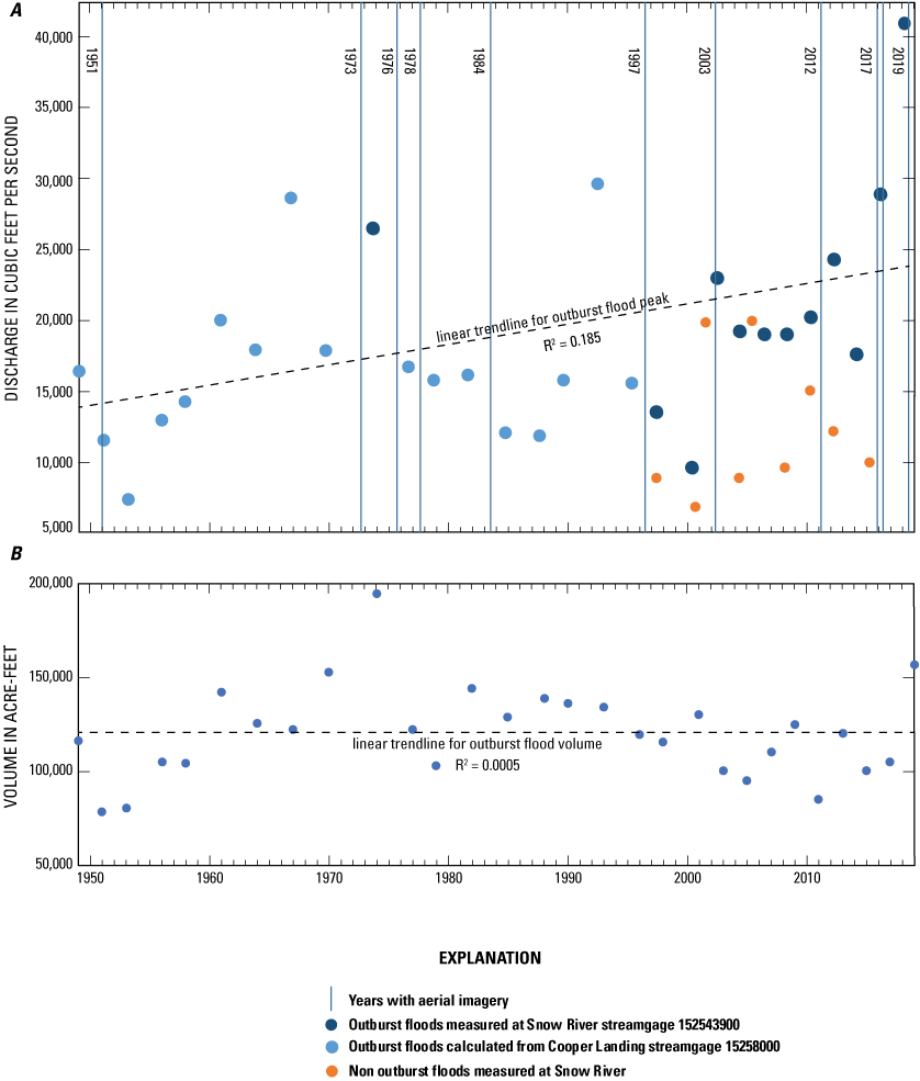
Peak discharges (A) and flood volumes (B) of the Snow River outburst flood since 1949, near Seward, Alaska. Estimated peaks and volume data from National Weather Service (National Weather Service, 2019).
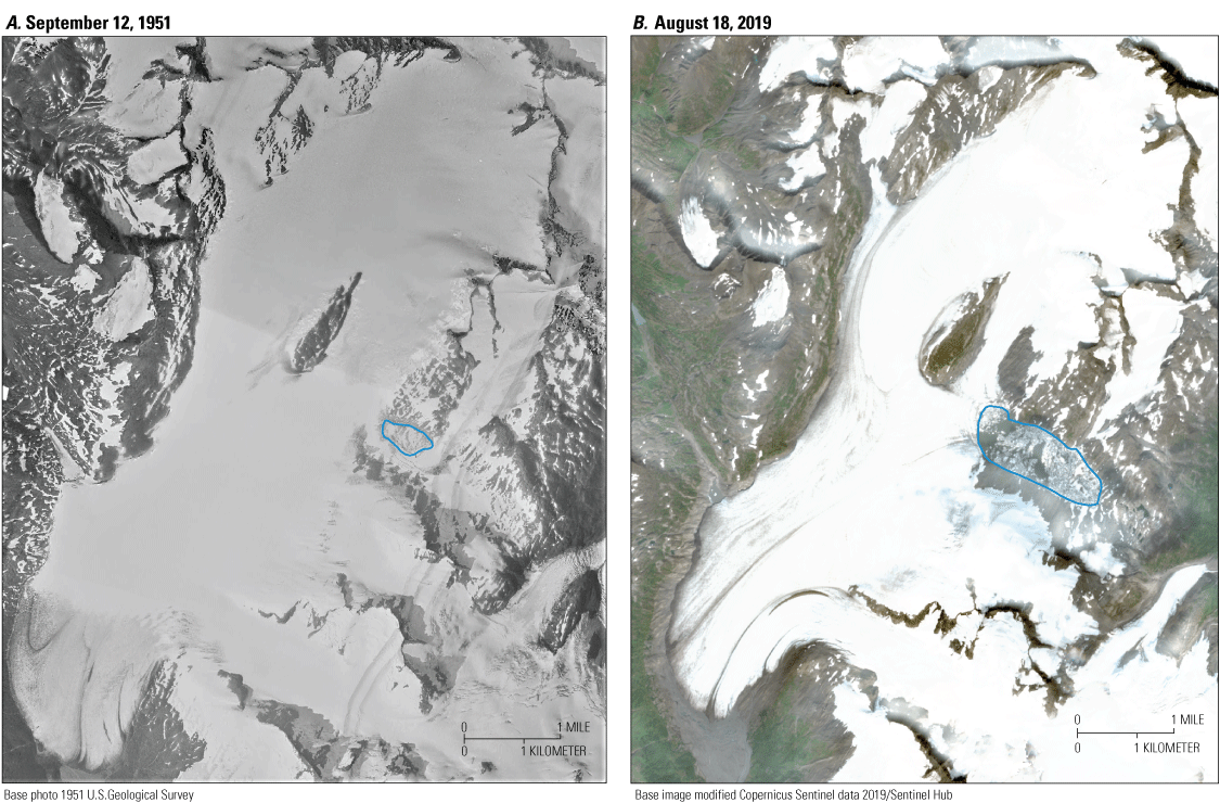
Comparison of Snow Glacier in (A) 1951 and (B) 2019, prior to floods in both years, near Seward, Alaska. Visible water in lake outlined in blue.
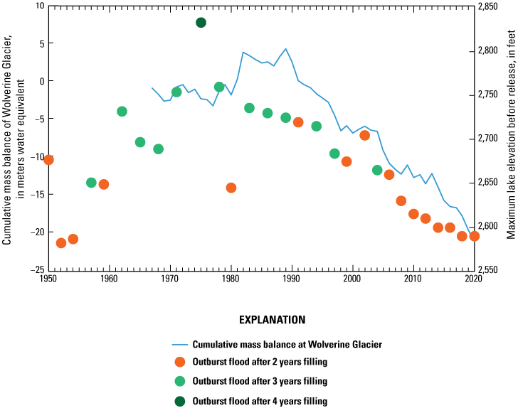
Approximate peak Snow Lake elevation before release and cumulative mass balance of Wolverine Glacier since 1949, near Seward, Alaska. Data from the National Weather Service (2019).
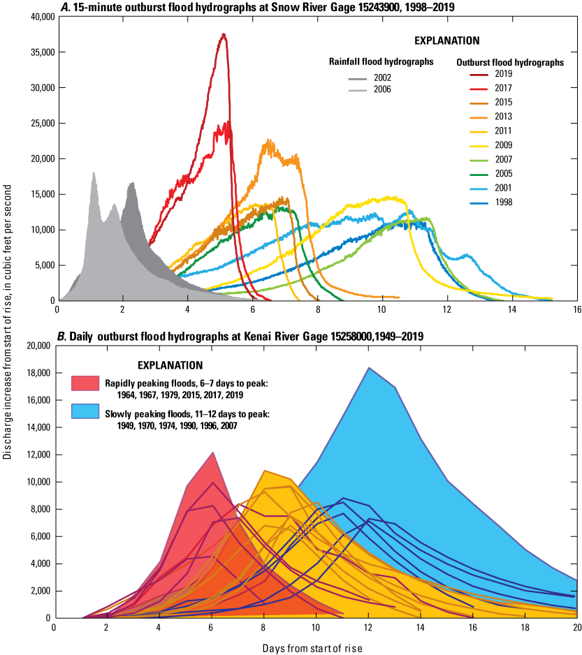
Comparison of Snow Glacier outburst flood hydrographs from 1998 to 2019 and rainfall floods from 2002 and 2006 at Snow River streamgage (A) and comparison of daily hydrographs during Snow Glacier outburst floods from 1949 to 2019 at Kenai River streamgage downstream of Kenai Lake (B), near Seward, Alaska (U.S. Geological Survey, 2022).
Snow Lake outburst flood hydrographs differ from meteorological hydrographs in duration, volume, and peak discharge magnitude. Water draining from the lake flows over 4 miles through subglacial conduits to reach the river. Discharge increases as the conduits are enlarged by the flowing water. Thus, the conduits are largest and discharge is highest when the lake is nearly empty. After the peak, discharge from the lake drops precipitously. Rainfall floods have rapid increases and short duration peaks, even compared to the flashier 2017 and 2019 outburst events (fig. 6).
Geomorphic Setting and Human Environment
The Snow River in the study area is a braided channel with high sediment loads typical of glacial rivers. The floodplain is mostly forested with spruce, cottonwood, and birch trees, and cut with relatively stable side channels. The floodplain below the confluence of the Snow River and the South Fork of Snow River varies from just less than 3,000 ft wide at the railroad bridge crossing to nearly 6,000 ft wide in the middle of the study reach and is bounded by a bedrock plateau on the west side and a mountain slope on the east side. No major tributaries enter the reach downstream of the South Fork of Snow River.
Historical maps show that railroad tracks have traversed the lower 3.5 miles of the eastern Snow River floodplain at least since the Alaska Northern Railway survey in 1916 (Alaska Engineering Commission, 1916). The 712-ft truss bridge at rail milepost (MP) 14.5 was built in 1957, about 1,000 ft downstream of the original crossing. As of 2021, four small bridges and several culverts drain water through the rail embankment in the floodplain (fig. 2). At least one additional bridge is planned at MP 16.1 to drain floodplain flow across the railroad grade.
The Seward Highway was extended from Seward northward along the west side of the floodplain in 1923, but the bridges across the Snow River were not complete until 1946. From 1946 to 1966, three bridges crossed Snow River on the west, center, and east braid of the river. In 1966, the Seward Highway was realigned, and two bridges were built. Bridge 603 (188-ft long) crosses the far western channel, and Bridge 605 (649-ft long) crosses the center channel. The eastern channel was blocked and makes a 90-degree turn at the old highway embankment to join the main channel. Sometime between the 1966 bridge construction and the 1973 aerial photograph, a berm was constructed blocking the western channel where it branched off the main Snow River channel. This has resulted in limited flow to Bridge 603 and substantial vegetation encroachment. Flood flow still reaches the channel, though not enough to scour the vegetation.
Typical of braided rivers, the main channel of the Snow River has shifted locations. The consequences of shifting channels include the recruitment of woody debris to the channel and floodplain, inefficient flow approach angles at bridges, and the potential for the main channel to directly threaten the rail and highway embankments.
Recent Damage to Infrastructure Caused by Outburst Floods
The eastern guidebank at Bridge 605 is necessary to align the flow with the bridge opening. The guidebank toe has been undercut repeatedly by scour during outburst floods, resulting in loss of 85 ft of length since construction in 1966, about 50 ft of which occurred after 2008, based on the 2008 lidar dataset (Kenai Watershed Forum, 2008) (fig. 7). Flow parallel to the highway has overtopped a riprap revetment and scoured the highway embankment.
The railroad grade between MPs 14.5 and 18 is located mostly on a low-elevation floodplain. At higher flows, floodwaters leave the main channel and cross the grade through drainage structures at MPs 15.2 and 15.6 or bypass Bridge 14.5 and enter the floodplain to the east of the grade. An alluvial fan prevents flow from traveling along the grade past MP 16.7, and here the grade acts like a dam, preventing flow that has become trapped east of the grade from returning to the main channel (fig. 7). In 2017 and 2019, enough water was trapped to overtop and erode the grade between MPs 16.4 and 16.7. The 28-ft long bridge at MP 16.2 suffered over 14 ft of scour and lost fill from sheet-pile abutments during the 2019 flood. The rail grade has also been overtopped at low areas near MPs 15 and 17 and suffered loss of ballast from below the tracks (fig. 7).
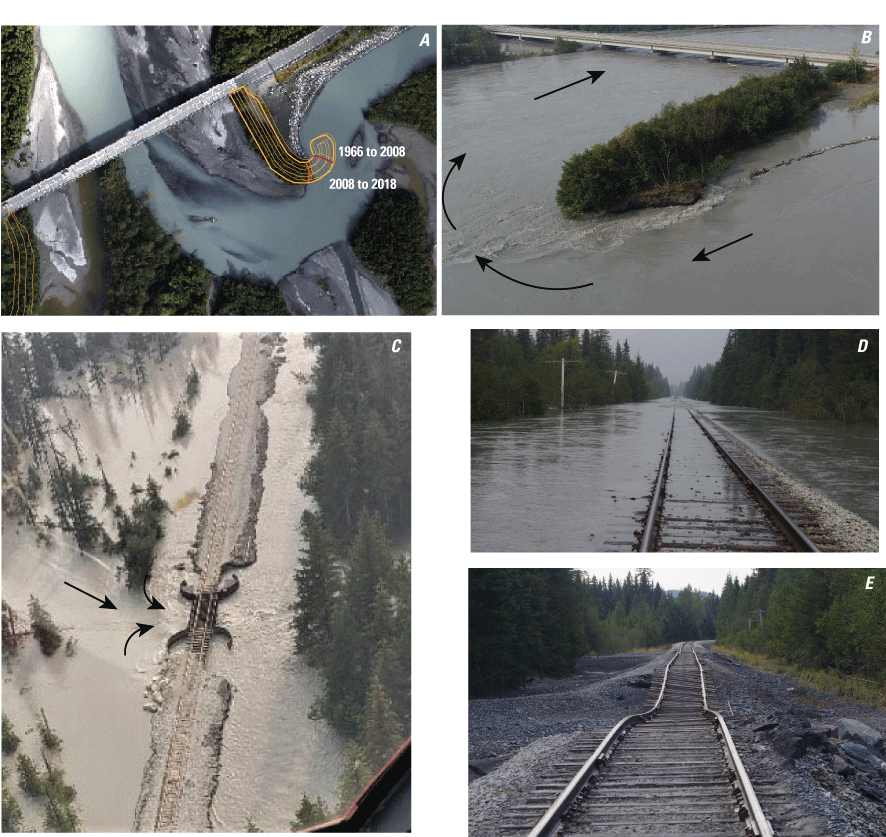
Damage from outburst floods on the Snow River near Seward, Alaska. (A) As-built dimensions of eastern guidebank at Bridge 605 overlaid on 2018 aerial photography (Kinzel and Legleiter, 2021). 2008 and 2018 extents of guidebank delineated. (B) Uncrewed Aircraft System photograph of eastern guidebank during the August, 2019 flood. Photograph taken by Kirsten Valentine, Alaska Department of Transportation and Public Facilities. Arrows follow flow path. (C) Bridge 16.2 during peak of 2019 flood showing loss of fill from sheet pile cells. Photograph taken by Blake Aldolfae, Alaska Railroad Corporation. (D) Train tracks as seen looking east near milepost 15 along railroad grade near the 2019 flood peak. (E) Train tracks as seen looking west near milepost 15 after the peak of the 2019 flood. (D) and (E) are U.S. Geological Survey photos taken August 24, 2019, and August 26, 2019, respectively.
Channel Change, Geomorphology, and Debris Recruitment Analysis Methods
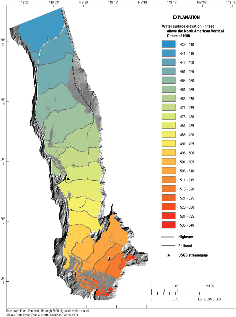
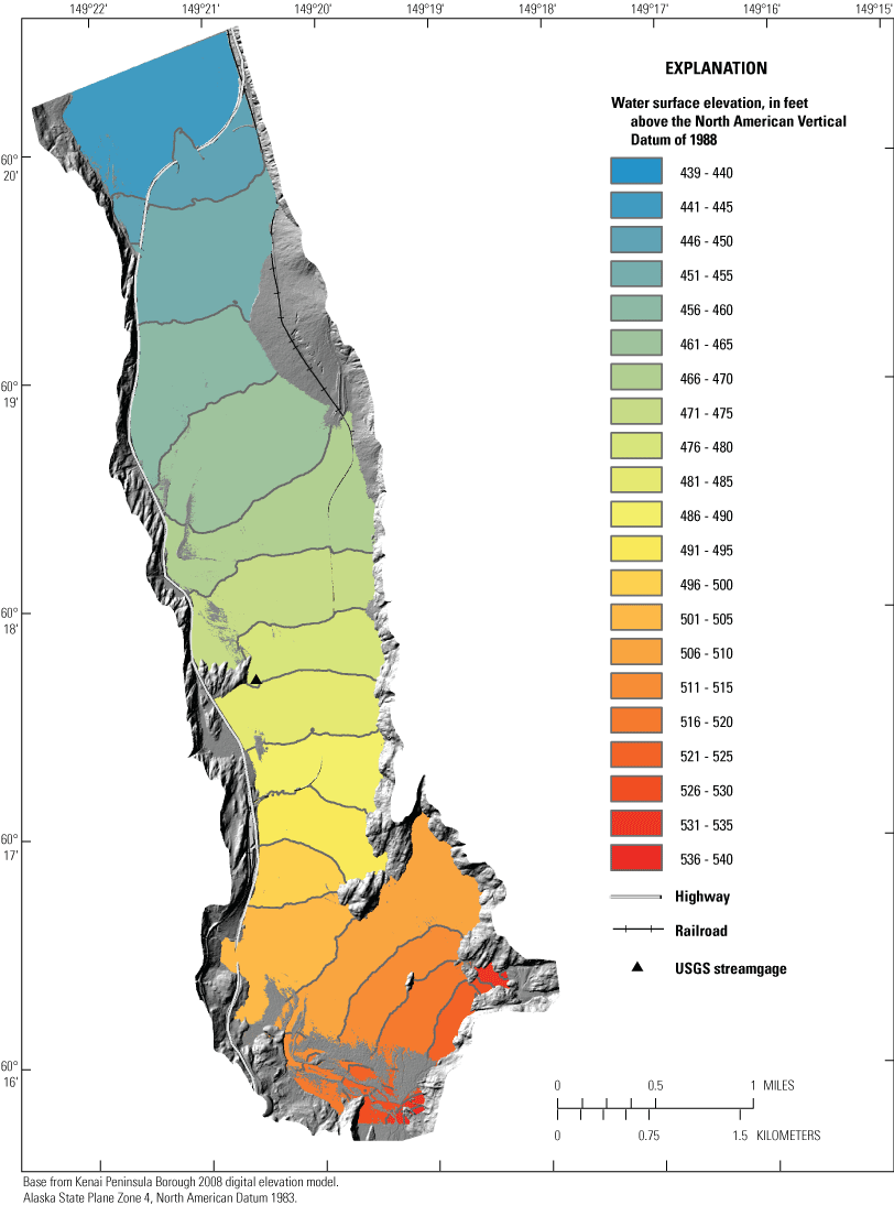
Aerial photographs and satellite imagery (Beebee, 2022) from 1951, 1973, 1976, 1978, 1984, 1997, 2003, 2012, 2017 (June), 2017 (October), and 2019 (September) were georeferenced with ArcGIS (Esri, 2018), using the 1997 digital orthoquad (DOQ) as a base standard. The analysis is bounded by the railroad to the east, the highway to the west and north, and the southern extent of the model domain. The main channel thalweg and vegetated floodplain were digitized to be accurate at a scale of approximately 1:10,000, although the imagery varied greatly in resolution (fig. 8). A “height above river” (HAR) raster was derived by creating a digital elevation model (DEM) approximating the main channel water surface at a flow of 1,000 ft3/s and subtracting the 2008 lidar DEM from it, generally following the steps of Olson and others (2014). These visualizations illustrate where the floodplain is higher and lower relative to the main river channel (figs. 9, 10, 11). Vegetated areas were compared between photo years to derive patterns of vegetation loss by channel migration for each interval between photos. A forest type coverage produced by the Chugach National Forest in 2008 was overlain on erosion areas to show where trees have been lost and recruited as debris since the forest inventory in the 1980s. Finally, the visible extent of the active Snow River fan where it meets upper Kenai Lake was digitized for 1951, 1973, 1978, 1984, 1997, 2003, 2012, and 2018 (Beebee, 2022).
Analysis Results
The study area was divided into three reaches based on channel planform: reaches A and C are wide and braided, while reach B is a relatively narrow single channel (fig. 8). At reaches A and C, flow has been distributed among multiple main channels across distances of 3,000 ft and more. At reach B, the active braidplain width varies from 300 to 1,200 ft. Channels are shaded by year, with the palest in 1951 and darkest in September 2019, to show the eastward migration of meander bends in reach B (fig. 8).
Historical main channel locations and analysis reaches overlaid on hillshade of 2008 lidar (Kenai Watershed Forum, 2008), near Seward, Alaska.
Reach A—South Fork of the Snow River Confluence and Approach to Rail Bridge 14.5
The confluence of the South Fork of the Snow River with the main fork of the Snow River is a broad alluvial plain broken up by bedrock knobs. As measured from the 2008 lidar, the main channel slope is about 0.3 percent. The channel change in reach A is important because it recruits and transports woody debris to Bridge 14.5 and determines the approach angle of flow to the bridge (fig. 9). The main channel also flows against Seward Highway embankment in this reach. The smaller South Fork of the Snow River channel has remained relatively stable in an active braid plain compared to the larger Snow River channel. However, in the 1978 and 1997 imagery, the main flow detoured north through a channeled wetland (A1) and rejoined the prevalent channel over a mile downstream (fig. 9). From 1951 to 2012, the main Snow River meander bend at A3 migrated eastward. In June 2017, the main channel of the Snow River was split, with some of the flow occupying the wetland and forested side channels at A2. After the 2017 flood, the meander bend at A3 was completely cut off and the main channel flowed through A2. The new channel contributed most of the mature trees found on the floodplain and against the rail bridge downstream. The flood in 2019 widened the channel at A2. The main channel has been on the west side of the island at A4 in every image reviewed, although it has approached the island from different locations. Erosion of the island at A4 could make flow through the rail bridge more orthogonal. If the side channel east of the island captures the main flow, it would increase the risk of flooding around the rail embankment. The HAR raster shows generally lower elevations in the area between the South Fork of the Snow River and the main channel of the Snow River. These low-lying areas are more likely to be inundated during floods now that the main channel has abandoned the meander bend to the north (A3).
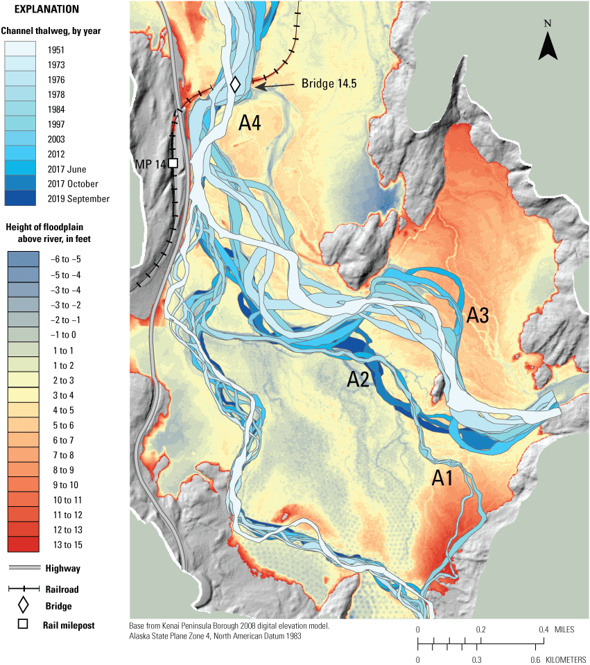
Analysis of reach A with historical channel locations overlaid on a Height Above River raster, near Seward, Alaska.
Reach B—Downstream of Rail Bridge 14.5
Within reach B, eastward migrating meander bends (B1 and B4) alternate with narrow reaches impinging on bedrock to the west (B3, B5) (fig. 10). The main channel slope measured from 2008 lidar is about 0.2 percent. Meander bends are migrating toward the railroad embankment. The bend at B1 has moved 900 ft closer since 1951 and 1,400 ft closer at B4. The bend at B1 as of September 2019 occupied a former side channel of Snow River and was about 200 ft from the tracks.
Generally, lower floodplain elevations east of the main channel, as shown in the HAR raster, explain why floodwaters flow so readily toward and behind the railroad grade, becoming trapped around B6 (MP 16.1–16.4), as well as why floodwaters seem more likely to flow east rather than occupy perennial side channels such as at B2 that are surrounded by a floodplain a few ft higher.
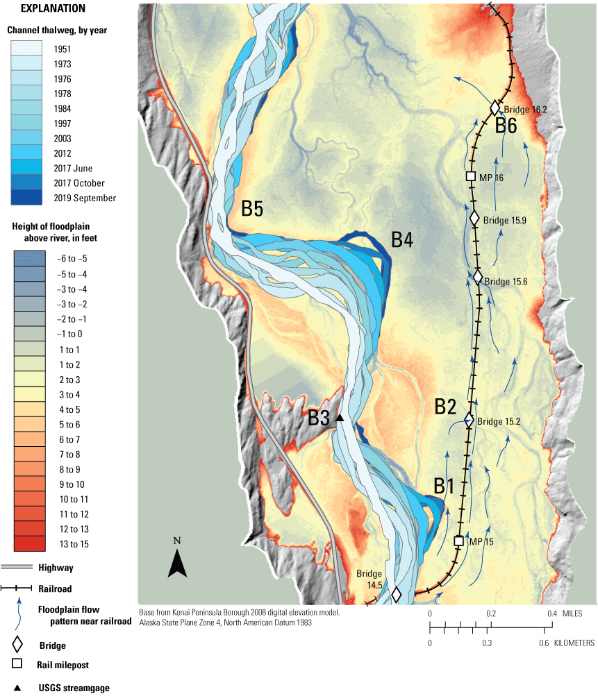
Analysis of reach B with historical channel locations overlaid on a Height Above River raster, near Seward, Alaska.
Reach C—Approach to Highway Bridges 603 and 605
As the slope decreases to 0.15 percent upstream of Kenai Lake, the Snow River spreads out into multiple channels approaching the highway bridges from the east and west (fig. 11). A berm to block flow to Bridge 603 was built at C1 between 1951 and 1973, otherwise the entire floodplain is low-lying. The last aerial image showing a main channel flowing by C1 is from 1984. The main channel shifted to C2 between 2012 and 2017, although side channels have been there since 1978. Floodwaters at C2 have overtopped the railroad tracks and eroded the highway embankment in 2015, 2017 and 2019. The recent path of the channel from C2 to C3 creates scour and erosion at the eastern guidebank at C3, which is needed to realign the flow 90 degrees to approach the bridge. The HAR raster here shows a low-lying area near the railroad tracks that may be captured by the channel at C4, as well as the high gravel bar near C3. This gravel bar splits flow going under the bridge and reduces bridge capacity during high flows.
Downstream of the bridge the Snow River enters Kenai Lake. The extent of the active fan has changed since 1951 (fig. 12). The western fan seen in the 1951 imagery rapidly disappears after the berm at C1 reduced flow through Bridge 603. The eastern fan has steadily progressed about 0.2 miles since 1951. This functionally lengthens the distance from Bridge 605 to Kenai Lake. The fan progression and the relatively high main channel compared to floodplain as seen in the HAR rasters both suggest that the Snow River is aggrading (generally depositing sediment) over time rather than incising. The progression of the active fan further from Bridge 605 also means that channel banks nearest the bridge are becoming vegetated and likely more stable.
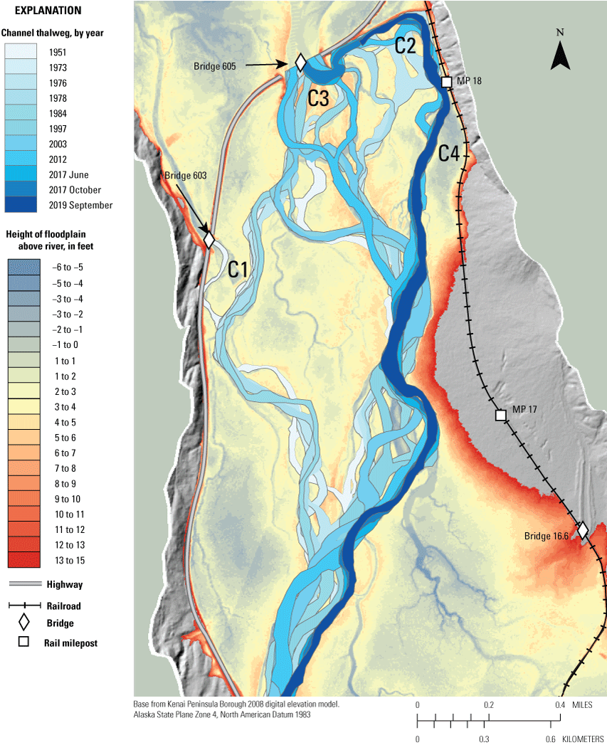
Analysis of reach C with historical channel locations overlaid on a Height Above River raster, near Seward, Alaska .
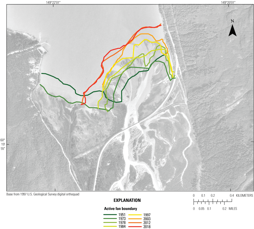
Historical linear extents of the Snow River fan overlaid on a 1997 digital orthoquad, near Seward, Alaska.
Channel Change During the 2017 and 2019 Floods
Satellite images bracketing the 2017 and 2019 floods show changes that can clearly be attributed to each flood. Earlier imagery is not timed adequately to determine whether previous outburst floods were also responsible for channel change. During the 2017 flood, the main channel moved to an entirely new location at A2, abandoning a meander and eroding through 26 acres of densely forested floodplain. The meanders and B1 and B4 also eroded 100 and 200 ft eastward toward the railroad tracks, respectively (fig. 13). Although the avulsion at A2 in figure 13 did not directly threaten any infrastructure, it introduced thousands of trees to the river. Despite the higher peak flow, the 2019 flood did not appear to cause as widespread lateral channel change. The largest change was the eastward migration of the meander bend at B4 of nearly 300 ft. The meander bend at B1 did not appear to erode during the flood, and this may be because the bank was protected by a large logjam, introduced by the 2017 flood, that extended the length of the outer bend (fig. 13).
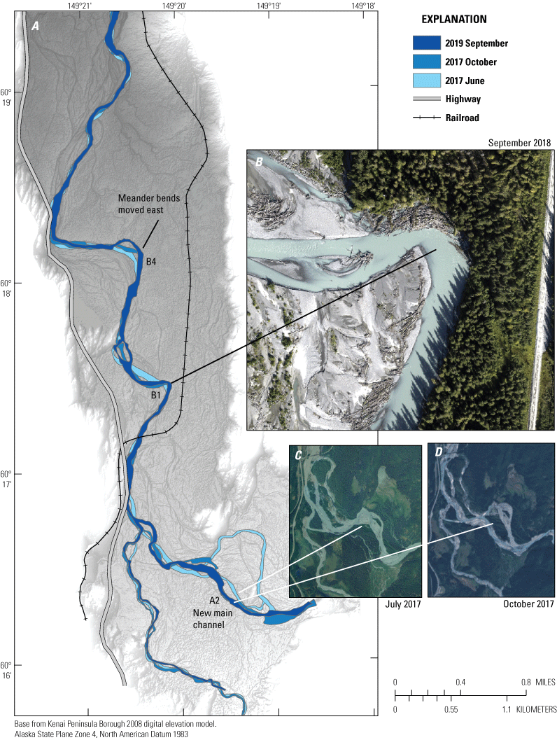
(A) Channel thalwegs from June of 2017, October of 2017, and September of 2019 are overlaid on a digital elevation model to show areas where the stream channel changed during the 2017 and 2019 floods, near Seward, Alaska. (B) Aerial photo of meander bend B1 with freshly eroded debris (Kinzel and Legleiter, 2021). (C) Satellite imagery of A2 prior to avulsion (Copernicus Sentinel data 2017, processed by ESA). (D) Satellite image after avulsion at A2 (Copernicus Sentinel data 2017, processed by ESA).
Debris Recruitment
Lateral shifts in the Snow River channel can introduce mature trees into the channel from the forested floodplain, and the 2017 flood was notable both for channel changes and the large volume of driftwood carried downstream. The much larger 2019 flood, which caused fewer channel changes, also recruited less debris. The new channel avulsion at A2 was the largest source of wood to the channel in 2017, though erosion of the meander bends at B1 and B4 also likely contributed hundreds of trees. This driftwood, also known as large woody debris (LWD), can play an important role in maintaining or changing the form of river channels, with its significance depending on channel size compared to log size (Montgomery and others, 2003). Because the active channel of the Snow River, like most braided rivers, is large compared to the average log size, the direct impact of LWD on the active channel is limited. However, studies on similar braided rivers show that wood accumulations play an important role in building and stabilizing bars and islands, increasing roughness, and blocking or reducing flow to smaller channels (Welber, 2013). After the 2017 flood, the reach between rail Bridge 14.5 and the streamgage had the highest concentration of LWD along the channel (fig. 13). Field observations during the even-larger 2019 flood showed that much of this debris remained in place, suggesting that these debris piles may be helping to stabilize and convert formerly bare gravel bars into islands or vegetated bars. The meander bend at B1 (fig. 14), which was choked with logs along the outer bank, did not visibly migrate during the 2019 flood as it did in 2017. LWD can also accumulate on bridge piers (fig. 14), reducing bridge capacity and, in some cases, increasing pier scour potential (Arneson and others, 2012). Trees introduced to the river generally do not travel far downstream, hanging up on the many shallow bars and islands (Welber, 2013). Thus, mapping forested floodplain and historical channel change gives insight into the locations most affected by debris recruitment over time. Overlaying the forested areas mapped in 1980 with the main channel locations from 1984 onward shows that losses in vegetated area are concentrated around areas where the main channel has migrated a large distance, as depicted in reaches A and B. Fewer forested areas were mapped in reach C where frequent channel change also occurs, suggesting that reach C has historically been less important for recruiting debris (fig. 15).
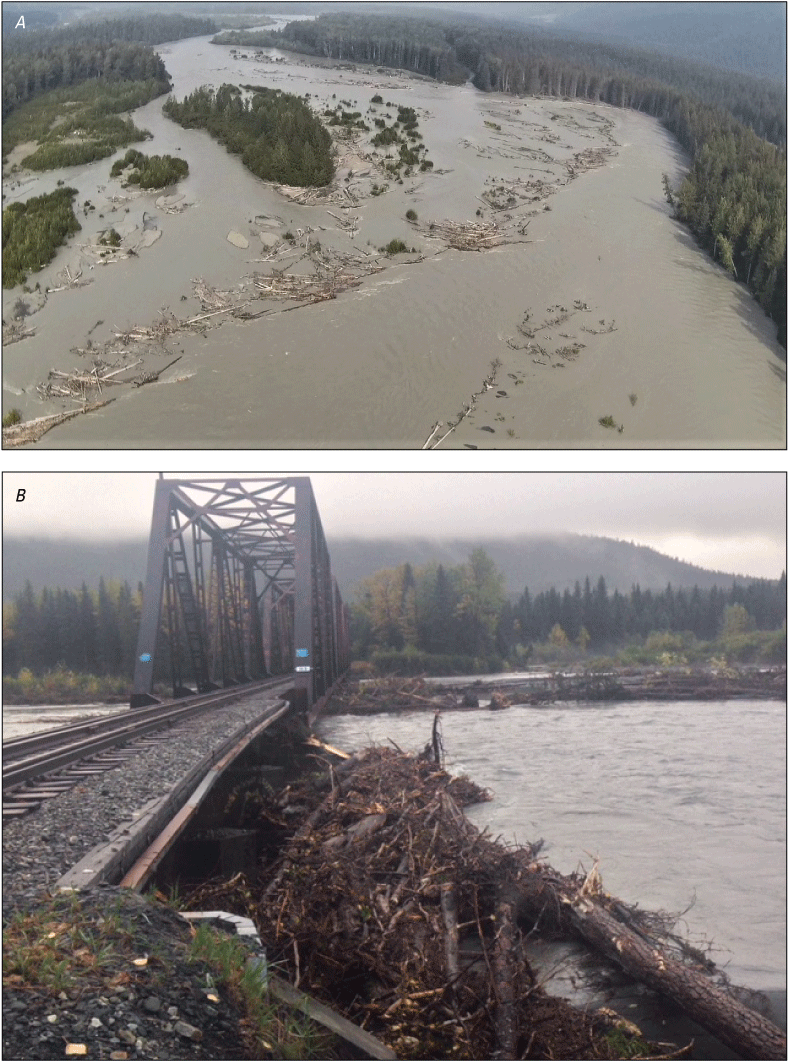
Debris at (A) meander bend at B1 during 2019 outburst flood and surrounding inundated gravel bars with debris from 2017 on them (Alaska Railroad photo, August 23, 2019) and (B) debris caught on the railroad Bridge 14.5 after the 2017 flood (Alaska Railroad photo, October 4, 2017), near Seward, Alaska.
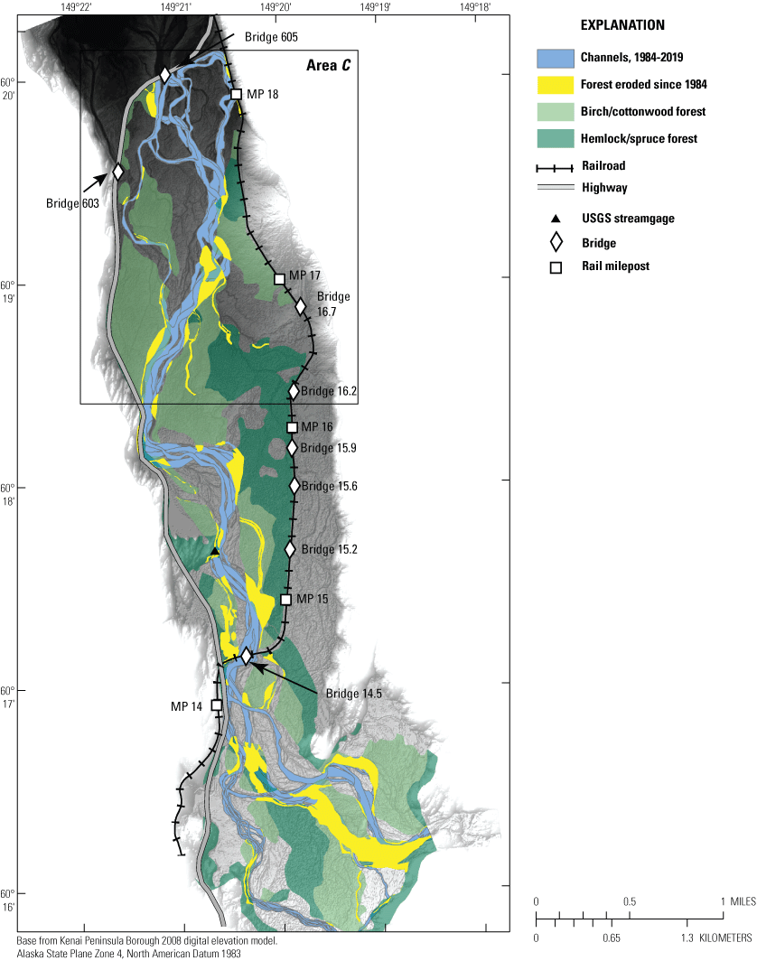
Forested areas eroded since 1984 overlaid on forested areas as mapped by the U.S. Forest Service, near Seward, Alaska (U.S. Forest Service, 2020).
Hydraulic and Sediment Transport Modeling
The purpose of two-dimensional hydraulic modeling is to simulate the inundation extents of different discharges and hydraulic variables for use by cooperators to evaluate the hazards posed by floodwaters and to design engineering solutions to maintain infrastructure in the floodplain. While verifying the hydraulic model, variations in water-surface elevation measured in the field but not simulated by the model appeared to be driven by rapid bed elevation changes at high discharges. The purpose of adding sediment transport modeling was to better simulate water-surface elevations during periods of rapid erosion and deposition, as well as identify areas of high scour risk. SRH-2D (Lai, 2008, 2019) within the SMS interface (SMS version 13.0.14, Aquaveo, 2018) was used to simulate flood flows and sediment transport in the Snow River. The steps for building a model from hydrology and elevation data include developing a computational mesh that represents the topography and bathymetry, estimating and assigning Manning’s n (roughness) to the model domain, and choosing upstream and downstream flow boundary conditions. Additional input for the mobile-bed simulations included specifying sediment size classes for each erodible area of the mesh, delineation of unerodable areas and a sediment input boundary condition, sediment size classes, and selecting an appropriate sediment transport equation. Model results for the 2007, 2017 and 2019 floods were compared with observed water-surface elevations.
Computational Mesh
The computational mesh is based on lidar and field surveys. The changing nature of the channel and structures built after 2007 along the railroad tracks means that the mesh does not represent conditions during the flood of 2007 as well as for the floods of 2017 and 2019, but the differences are likely to be small and localized. Mobile bed simulations using SMS 13.0 require less than 60,000 elements to run. Finer elements were used along the main channel and near structures, while larger elements were used in flat and distal areas of the floodplain. Hydraulic variables are likely to better represent actual conditions where the mesh has a higher resolution (fig. 16) (Beebee, 2021).
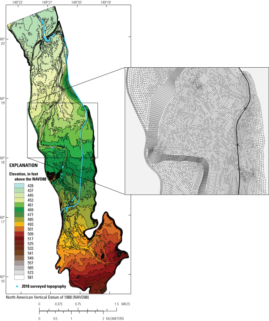
Full computational mesh of the study area (left) and detail of variable size mesh elements in box (right), near Seward, Alaska (Beebee, 2022).
Survey Data
Ground surveys were focused on the reaches immediately around bridges. A total station was used to survey the elevation of the bridge deck, water surface, guidebanks, and main channel banks at the railroad bridge at mile 14.5 and at Bridge 605. Three smaller rail bridges at MPs 15.2, 15.6, and 15.9 (fig. 2) were sounded with a weight and tagline upstream and downstream, and channel elevations were determined using top of bridge elevations from a 2018 railroad geometry survey. Channel bathymetry was surveyed in 2018 at moderate flow using a remote-control boat and acoustic Doppler current profiler (ADCP) near railroad Bridge 14.5 and Bridge 605. A real-time kinematic (RTK) GPS was used to survey water-surface elevations, and a crewed boat and ADCP were used to measure depths at three cross-section locations away from the bridges. Three additional cross-sections were measured in 2019 during discharge measurements at the streamgage. A total of 60 surveyed cross-sections were used to define the bathymetry throughout the model (fig. 16)(Beebee, 2022).
Other Topography Data
Floodplain and gravel bar elevations were taken from a 2018 lidar survey (Kinzel and others, 2019) and 2008 lidar (Kenai Watershed Forum, 2008) in areas that were outside the extent of the 2018 lidar. Between surveyed cross-sections, the channel bed surface was approximated by interpolating from nearby surveyed cross-sections and adjusting elevations by channel slope using the HEC-RAS cross-section interpolation tools (Brunner, 2016). Dimensions for highway Bridges 603, 605, and the railroad bridges at MPs 14.5 and 16.2 were taken from as-built plans. The railroad embankment elevations were taken from geometry surveys in the spring of 2018. Elevations for the guidebank and revetment on the east side of Bridge 605 were taken from a 2016 as-built survey. Some channels approaching Bridge 605 were too shallow to survey with the remote-control boat, which requires a minimum of about 2 ft of water to collect continuous data. The bathymetry of these channels was approximated by subtracting 2 ft from the 2018 lidar water surface. All topographic data were compiled in ArcMap (ESRI, 2018) and referenced to a common datum of NAVD88 and projection of Alaska State Plane Zone 4.
Manning’s Roughness Coefficients
Roughness was estimated using aerial photos and visual comparison techniques (Arcement and Schneider, 1989; Hicks and Mason, 1998) for the channel, gravel bars, and floodplain, and compared to values calculated for different locations on Snow River using the Manning equation (fig. 17; table 1). Main channel and gravel bar roughness was split into two areas. From the upstream boundary to just upstream of the streamgage, the roughness of the main channel and bare gravel bars was set at 0.04 to account for the higher gradient, larger bed material size, and widespread debris in this reach. The channel roughness in the reach downstream of the streamgage was set to 0.025. Outside of the channel, roughness estimates vary with vegetation, from 0.02 for paved surfaces to 0.1 for forests. Because roughness changes with flow magnitude and shifting channel locations, estimates for the model are necessarily greatly simplified from field conditions. Manning’s n was not used as a variable to calibrate the model to perfectly match water-surface elevations, as is commonly done. Matching peak flows would mean introducing greater error at lower flows. Sensitivity to n was tested by increasing and decreasing all values by 20 percent and comparing model output.
Table 1.
Measurements used for instantaneous estimates of Manning’s n, near Seward, Alaska.[Dates are in month/day/year. Abbreviations: n, Manning’s n; RTK, real-time kinematic]
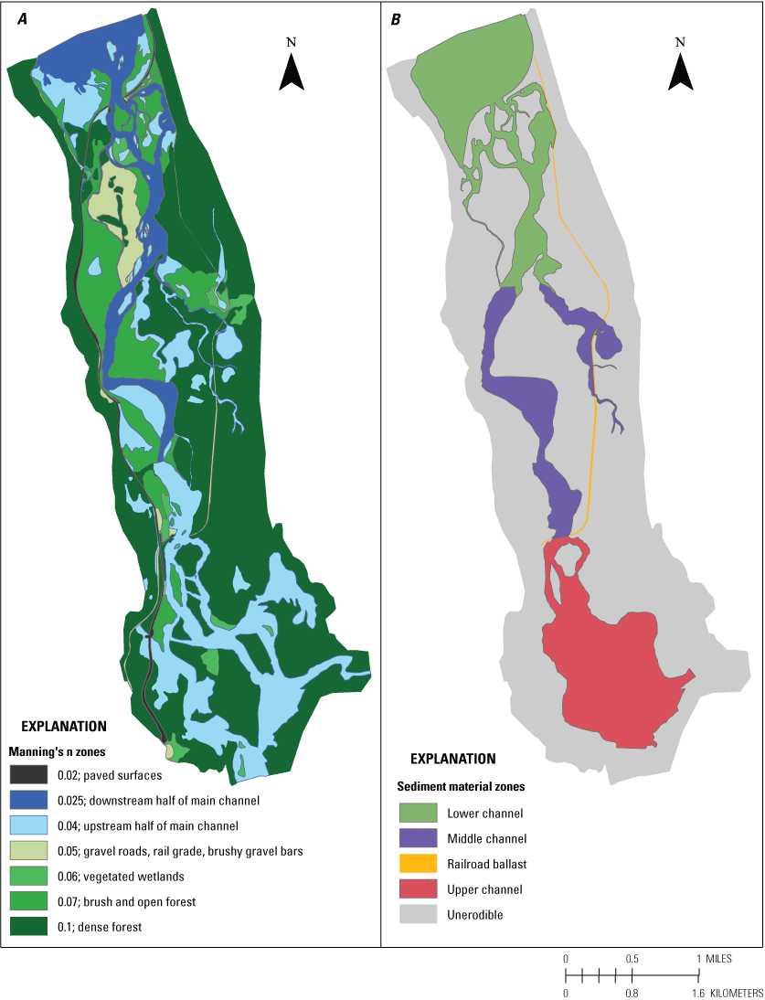
Materials coverage defining different Manning’s n zones (A) and sediment materials coverage defining different gradations (B), near Seward, Alaska.
Sediment Size Classes
The bed material of the Snow River is predominantly gravel in the study reach, but deposits of silt and sand are found on bars and islands and places where velocity is low. Bed material ranges from coarse gravel and cobbles upstream of Bridge 14.5 to fine gravel and sand at Bridge 605, consistent with the lower gradient near the inlet of Kenai Lake. Riverbed sediment is spatially variable even around Bridge 605, where some bars are covered with medium and coarse gravel while parts of the streambed are fine sand. Delineating bed material for the entire 5-mile reach was beyond the scope of this study, so three main channel reaches corresponding to the geomorphic reaches A, B, and C defined earlier were each assigned a single surface sediment gradation (table 2). A single surface Wolman count (Wolman, 1954) was conducted in 2018 upstream of Bridge 14.5 for reach A. An image analysis using Hydraulic Toolbox software (Bergendahl and Arneson, 2014) of four surface samples was performed in 2019 between Bridge 14.5 and the streamgage or reach B. An image analysis was performed for three surface samples immediately downstream of Bridge 605. The streambed was also sampled at Bridge 605 during an outburst flood in 1970 (Norman, 1975), and those gradations were significantly finer than those found in this study. The difference could be because Norman sampled bedload during the flood or because the depositional environment has changed with the aggradation of the fan below the bridge into Kenai Lake. A gradation was assigned to the railroad embankment using an image analysis of transported ballast at a washout near rail Bridge 15.2 immediately after the 2019 flood. A short reach including the upstream boundary condition on the main channel is mostly bedrock and was assigned as unerodable. The forested floodplain was assigned as unerodable outside of major channels. This is a simplifying assumption that avoids the difficulty of assigning a shear stress to the rooted soil layer protecting the floodplain sediments, but it prohibits the model from simulating channel migration through the forested floodplain as it occurs in meander bends. Scour in meander bends is planned to be included in a future version of SRH-2D (Lai, 2019).
Table 2.
Sediment gradation and layers used in Snow River hydraulic and sediment transport model, near Seward, Alaska.[Dx, sediment size where x% of grains in the sample are smaller. Layer 1 is the top layer, with successive layers underneath. Abbreviations: mm, millimeter; ft, foot]
Flow Boundary Conditions and Model Runs
Most hydraulic engineering studies use a combination of known floods and floods estimated to have a particular exceedance probability using a statistical flood frequency analysis. This analysis is used to estimate a design flood, typically with a 1 percent annual exceedance probability, and a check flood, typically with a 0.2 percent exceedance probability, even if floods of this magnitude have not been measured (Arneson and others, 2012). GLOFs challenge this type of statistical treatment, as they are not necessarily independent and stochastic events. Therefore, flow simulations were run for three known glacial lake outburst hydrographs and one hypothetical check flood: 18,900 ft3/s (2007 flood used as hydrograph, average outburst flood size since 1949, and similar to 1970 flood peak), 28,800 ft3/s (2017 flood, approximate 1974 flood peak), 43,6001 ft3/s (2019 flood) and 60,000 ft3/s (check flood) (table 3). Selecting a check flood is inherently subjective because of our limited knowledge of the mechanism of the subglacial release. However, there is some basis for choosing 60,000 ft3/s. The record flood of 43,500 ft3/s occurred in 2019 during a dry period with no antecedent or concurrent precipitation. Large precipitation-only floods have reached nearly 20,000 ft3/s and have occurred in the same months as outburst floods.
The peak flow was initially reported as 40,100 cubic feet per second (ft3/s), then revised to 43,800 ft3/s. The peak used for modeling was 43,600 ft3/s because this was the highest sustained flow. 43,800 ft3/s appears to be a single spike in the 15-minute gage-heights (NWIS, 2020).
Table 3.
SRH-2D model simulation boundary conditions for three known glacial lake outburst flood hydrographs in 2007, 2017, and 2019, one hypothetical check flood, and four model sensitivity tests.[Abbreviations: ft3/s, cubic feet per second; —, not applicable; n, Manning’s roughness coefficient]
There are two inlet (upstream) boundaries for each modeled flow, one at the main fork of Snow River below the Snow Glacier, which carries the outburst flood, and the other at the South Fork of Snow River, which is unaffected by the outburst flood. Both inlet boundary conditions add up to the total discharge measured at the streamgage 2.5 miles downstream. Because the total drainage area of the South Fork of the Snow River is approximately 6.3 percent of the total Snow River drainage area at the streamgage, the South Fork inlet boundary condition is a steady flow of 6.3 percent of the initial discharge and the main channel inlet boundary condition is the flood hydrograph minus the steady input at the South Fork (table 3). It is likely that the true hydrograph at the upstream boundary condition is slightly sharper-peaked. The downstream boundary of the model is 0.5 miles downstream of Bridge 605 near the downstream end of the Snow River fan. During outburst floods, the lake level rises to the downstream boundary. For simplicity, the downstream boundary condition was set as the time-series of water-surface elevations of Kenai Lake as measured at USGS streamgage 1528000 (U.S. Geological Survey, 2022) during the outburst flood plus 1.5 ft. The 1.5-ft offset is the difference between the September 1, 2018 lidar water surface at the upstream end of Kenai Lake and the gaged water surface at Cooper Landing downstream of Kenai Lake. To check if the downstream boundary condition affects flow at the nearest location of interest at the highway bridge, the model was run varying the downstream boundary elevations by plus and minus 2 ft. No difference was seen in water-surface elevations at the highway bridge between the regular and minus-2-ft boundary conditions, while the plus-2-ft boundary condition water surface was 0.3 ft higher. Because a lower water surface at the downstream boundary did not propagate upstream as far as Bridge 605, the check flood was run with the same downstream boundary condition as the 2019 flood.
Prior to running each unsteady model, a steady, fixed bed (no sediment transport) model of the initial discharge for each hydrograph was run to provide a starting condition for the unsteady mobile bed model. This reduced computation time and error at the start of the simulation. Model time-steps ranged from 1 to 8 seconds and were chosen as the longest that allowed the simulation to run successfully.
Sediment Transport Boundary Conditions
The additional parameters for a mobile-bed simulation include sediment input at the upstream end, particle diameter thresholds, the selected sediment transport equation and several coefficients. Four transport equations are available in SRH-2D for gravel-bedded streams, and all have the same basic shape but use different coefficients. Each transport equation recommended for gravel-bedded streams was verified with the 2019 flood. The Parker (1990) transport equation best reproduced the observed water-surface elevations and bed changes. The default Shield’s parameter (0.0386) and suspended load coefficients were used, and water temperature was set at 2.0 degrees Celsius. The adaptation length for bedload transport, which is the distance required for sediment transport to reach equilibrium, was set at 330 ft (recommended as 1–5 times active channel width) and the active layer thickness at twice the D90, as recommended for gravel-bedded rivers. The capacity option, which uses the Parker (1990) sediment capacity equation to calculate sediment input, was used as the upstream boundary condition. The upstream boundary condition is nearly 2 miles upstream of the rail bridge, thus the bed exchange calculated by the model will have reduced error introduced by the initial condition assumption at the reach of interest.
2007, 2017, and 2019 Flood Verification
Water-surface elevation during the 2017 and 2007 floods was only monitored at the streamgage in the middle of the reach. There is photographic evidence of the water-surface elevation along the revetment at the highway bridge in 2017 and 2019. There are also observations from the 1970 flood at Bridge 605. Water-surface elevations during the 2019 flood were monitored at three additional locations with submersible pressure transducers (fig. 2) (Beebee and Justis, 2020). These pressure transducers were placed just upstream of rail Bridge 14.5, on the abutment of rail Bridge 15.2 in the floodplain, and on the riprap toe of the revetment on the approach to highway Bridge 605. Scour was measured at rail Bridge 16.2 following the 2019 flood, and at the guidebank to Bridge 605 during the 1970 flood and after the 2017 flood. Additionally, two discharge measurements were taken during the 2019 flood just downstream of the highway bridge (NWIS, 2019).
Water-surface elevation data for three GLOF events at the streamgage and for the 2019 GLOF at three additional locations is used for model verification. Of these, the pressure transducers placed at the rail bridge at MP 14.5 and 15.2 during the 2019 flood have the best agreement (table 4; fig. 18). The model overestimates the peak at the downstream pressure transducer near the highway bridge by nearly 0.6 ft but underestimates the water-surface elevation during the rising limb and falling limb. This may indicate that the model is not accurately distributing flow among the many channels approaching the highway bridge. The model overestimates the peak water-surface elevation at the streamgage by 0.5 ft in the 2019 model run and underestimates the peak water-surface elevation by 0.2–0.3 ft in the 2017 and 2007 model runs (table 4). Because the model both under- and over-estimated water-surface elevations during each flood, no attempt was made to further calibrate the model using roughness coefficients. Instead, sensitivity to roughness was tested by varying Manning’s n by plus or minus 20 percent for the 2019 flood simulation. Water-surface elevation variation owing to roughness was generally less than the total difference between measured and simulated elevations (fig. 18), suggesting that roughness is not likely the main source of error.
Table 4.
Comparison between measured and modeled water-surface elevations, near Seward, Alaska.[Abbreviations: ft, foot; WSE, water-surface elevation]
The reason for the disagreement at the streamgage is unknown, although the water surface at the streamgage surges by up to 0.3 ft during high flows, and the rating curve is poorly defined at moderate to high flows because of rating shifts associated with scour and fill of the channel control. During the 2019 flood, two discharge measurements were made during the rise and two during the fall of the flood. The water level was 0.8 ft higher for a lower discharge measurement on the rising limb compared to the falling limb. This indicates that channel geometry changes during the flood were sufficient to affect the water-surface elevation on the order of a foot. Earlier outburst floods were only measured once during either the rising or falling limb, thus the estimated peak discharge is likely much more accurate in 2019. Besides issues with defining the rating at higher flows, larger-scale channel changes may also have affected the rating between 2007 and 2019.
The model compares well with the discharge measurement made 80 ft downstream of Bridge 605 on August 23, 2019, but less well with the measurement made in the same location on August 24, 2019, on the falling limb of the hydrograph (table 5). This may be due to the rapidly changing conditions compared to temporal model resolution (the measured discharge occurs between model outputs and 116 and 115 hours) as well as challenges routing stored water from the floodplain back into the channel.
Table 5.
Hydraulic data as measured by acoustic Doppler current profiler during the 2019 flood (NWIS, 2019) compared to model results, near Seward, Alaska.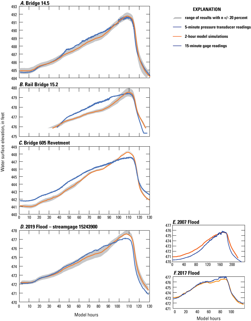
Pressure transducer and streamgage water surface records during the 2019 flood compared to model simulations. Inset box shows streamgage comparisons for 2007 and 2017 outburst floods, near Seward, Alaska. Measurement locations shown in figure 2.
Results
Unsteady multi-dimensional hydraulic models are effective in simulating flow in overbank areas where there are variations in water-surface elevation, flow direction, and velocity. Simulating overbank flow is particularly important during Snow River outburst floods because of impacts to the railroad grade and associated structures in the floodplain (fig. 19). During the 2019 flood, field crews confirmed that silty water from the main channel (as opposed to clear water from hillslope channels) had crossed Bridge 15.2 and reached just downstream of Bridges 15.4 and 15.9 when the streamgage reported about 6,000 ft3/s. The model correctly simulates flow first overtopping channel banks and crossing the rail embankment at Bridge 15.2 at about 5,000 ft3/s and reaching Bridges 15.4 and 15.9 at about 6,000 ft3/s (fig. 20). Floodwaters overtop channel banks upstream of Bridge 14.5 and bypass the bridge at about 8,000 ft3/s in the model. The model simulates an increasing percentage of flow bypassing Bridge 14.5 and flowing east of the railroad tracks, from 1,405 ft3/s at 18,900 ft3/s (less than 10 percent) to 4,170 ft3/s at 28,800 ft3/s, to 10,570 ft3/s at 43,600 ft3/s, and to 16,230 ft3/s at 60,000 ft3/s (over 25 percent). These floodwaters travel parallel to the rail embankment, then return to the channel between MPs 15.9 and 16.4. More detailed results from Bridge 14.5, the railroad grade, and Bridge 605 follow.
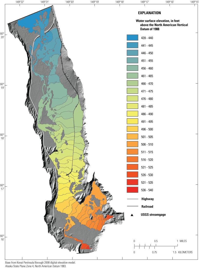
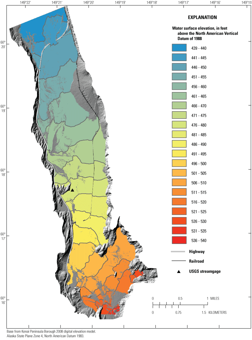
SRH-2D simulation water-surface elevations and inundation extent for flood flows of (A) 18,900, (B) 28,800, (C) 43,600, and (D) 60,000 cubic feet per second, near Seward, Alaska.
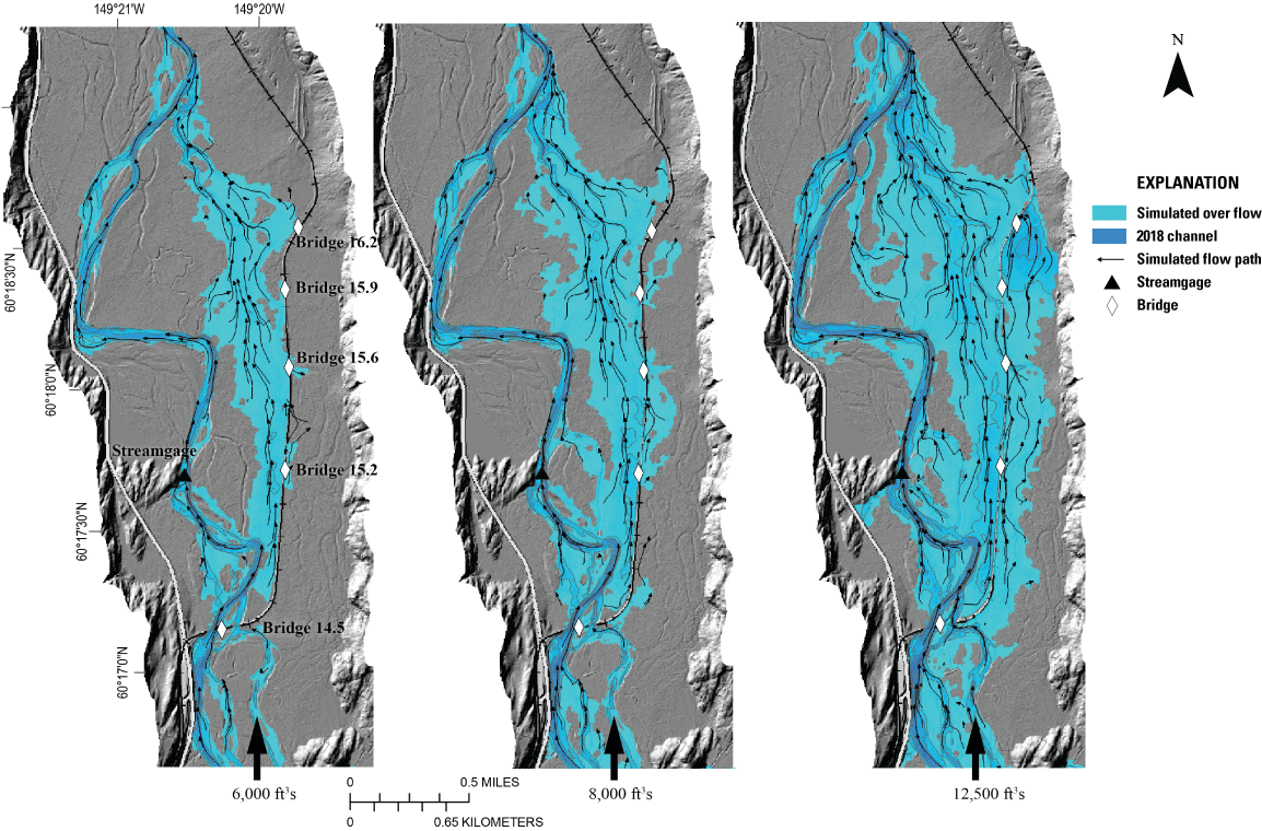
Simulated overflow from main channel toward rail embankment during the rising limb of the outburst flood for flows of (A) 6,000, (B) 8,000, and (C) 12,500 cubic feet per second, near Seward, Alaska.
Rail Bridge 14.5
Photographs taken during each of the last three GLOFs show the water surface highest in the center of the channel and just overtopping the fourth pier from the left bank in 2019 (fig. 21). Model simulations show higher water surfaces at the left side of the bridge compared to observations. The blocking of piers with woody debris (fig. 14), not simulated in the model, may locally raise water levels at the bridge. Sediment transport simulations show flow skewed to the bridge opening and scour predominantly on the left bank side of piers. This is consistent with the flow pattern observed during floods. The lowest measured point on the cross-section in 2018 is 477 ft, while the lowest modeled point on the cross-section during the peak of the 2019 flood is 473.4 ft, just below the top of footing elevation of 474 ft. As described above, an increasing percentage of flow bypasses the railroad bridge to the east and flows behind the railroad tracks. If bypass flow is redirected through the bridge with engineering structures or as a result of channel change, both scour and water-surface elevation would increase.
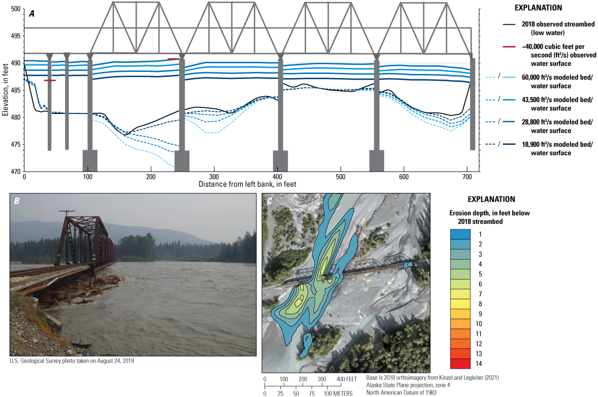
(A) Model results and measured water surfaces, (B) flood peak on August 24, 2019, and (C) scour as simulated by SRH-2D (Lai, 2008), from railroad Bridge 14.5, Snow River near Seward, Alaska. Photograph taken by U.S. Geological Survey.
Railroad Grade
Simulating flood inundation and flood damage potential along the railroad grade was one of the primary goals of the SRH-2D modeling. The 2019 flood model simulated approximately 14 ft of scour at Bridge 16.2, as well as up to 6 ft of fill loss where the grade was overtopped at MP 16.4 (fig. 22) and up to 2 ft of fill loss at MP 15. Fill loss was not documented post-flood at MP 16.4. Photographs at MP 15 suggest up to 3 ft of fill loss (fig. 7).
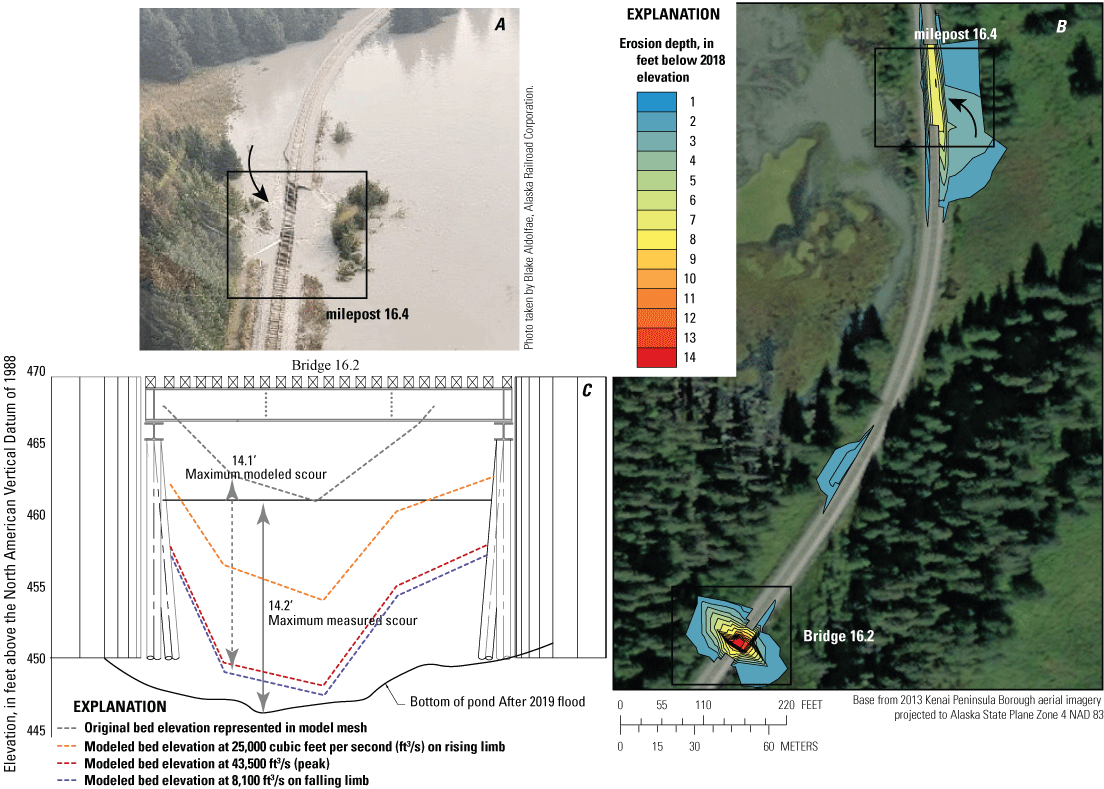
(A) Fill loss around MP 16.4, (B) scour as simulated by SRH-2D (Lai, 2008) from MP 16.2 to 16.4, and (C) Bridge 16.2 with measured post-flood scour and simulated scour, near Seward, Alaska.
Bridge 605 and Revetment
Bridge 605 has not had observed capacity or scour issues during outburst floods, but the eastern guidebank and approach have suffered scour. The model simulated 9.5–10.5-ft deep scour holes during the 2007, 2017, and 2019 floods (fig. 23), and a 14-ft deep scour hole during the 60,000 ft3/s check flood. These compare well to measured scour holes of 10-ft deep during the 1970 flood (Norman, 1975) and 7-ft deep the year after the 2017 flood. Modeled water-surface elevations are higher than the eastern guidebank for the 60,000 ft3/s check flood.
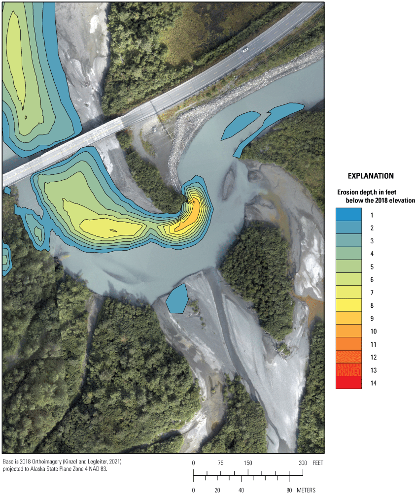
Highway Bridge 605 scour hole at eastern guidebank formed in 2019 flood simulation on 2018 aerial photograph, Snow River near Seward, Alaska. Photograph taken from Kinzel and Legleiter, U.S. Geological Survey, 2021.
Summary
Flooding on the Snow River from glacial lake outbursts over the last 2 decades has been occurring more frequently and more rapidly, allowing for higher peak discharges, without overall greater flood volume. Thinning of the Snow Glacier has resulted in lower elevation lake releases over the last 30 years. A large flood in 2017 and a record flood in 2019 contribute to a weak trend over time toward larger flood peak magnitude. The 2019 flood, at over 40,000 cubic feet per second (ft3/s), is the largest outburst flood peak measured on the Snow River since 1949. The 2007 outburst flood, at 18,900 ft3/s, is the mean peak discharge. Although both slowly peaking (10–12 days to peak from start of rise) and rapidly peaking (5–6 days to peak from start of rise) floods have occurred throughout the period of record, floods in the last 2 decades have been peaking more and more rapidly. Floods have also become more frequent, with a record short time between floods in 2020 only 14 months after the record high 2019 flood. The outburst floods have caused damage to the guidebanks at Bridge 605 and Bridge 16.2 and to the railroad grade between MPs 14.8 and 18. Rapid bank erosion, channel change, and large woody debris (LWD) recruitment were observed during the flood in 2017, and to a lesser extent during the flood in 2019.
The channel of the Snow River has changed frequently over the last 68 years for which aerial imagery has been collected; however, there are historically stable and historically unstable reaches. Migrating channels upstream of the railroad bridge erode through forested floodplain and deliver LWD to the railroad bridge. Low-lying forest remains near the channel for future debris recruitment. Downstream of the railroad bridge, the channel is relatively stable except for two meander bends that have been steadily eroding toward the east, approaching the rail embankment. Continued channel migration in this reach could cause the main channel to impinge against the rail embankment. The downstream-most reach upstream of the highway bridges is less forested than upstream areas and features multiple channels that have been historically unstable. The main channel has become established on the far east side of the floodplain in the last 10 years, resulting in a nearly parallel approach to Bridge 605. This approach will likely continue to erode the guidebank on the east side of Bridge 605 unless flow in the center channel is reestablished.
Areas of inundation and scour in the study reach were simulated with mobile-bed hydraulic modeling of the 2007, 2017, and 2019 floods, and a theoretical check flood of 60,000 ft3/s. The model results agree well with observations of inundation along the railroad grade and with water-surface elevations recorded by pressure transducers near the rail bridges at mileposts 14.5 and 15.2. While modeling the entire reach provides information about where and when water leaves the main channel and how it interacts with structures in the floodplain, it also requires using coarse resolution mesh elements in many places. Results where mesh elements are coarser are averaged over a larger area and are thus less accurate. The modeled water surfaces do not agree as well with the recorded water surfaces at the streamgage mid-reach or at the approach to Bridge 605. Model inaccuracy may be due to rapid sediment transport and channel change at the streamgage and challenges distributing flow between multiple channels approaching Bridge 605 for which bathymetry may not be accurate. The mobile-bed sediment transport model successfully reproduced observed erosion at the toe of the guidebank near Bridge 605 and along the railroad grade at mileposts 15 and Bridge 16.2. These simulations demonstrate the utility of a multi-dimensional mobile-bed sediment transport model for evaluating the susceptibility of highway and railroad infrastructure to large floods, even in relatively complex channel and floodplain systems with limited input data.
References Cited
Alaska Engineering Commission, 1916, Map of Alaska northern railway and alternative survey, Seward to Turnagain Arm (MAP): Alaskan Engineering Commission, House document No. 610, 64th Congress, 1st session, Map II, accessed on June 25, 2018, at https://vilda.alaska.edu/digital/collection/cdmg11/id/17085/rec/4.
Aquaveo, 2018, SMS 13.0: Aquaveo, Surface Modeling System Software, accessed July 8, 2020, at https://www.aquaveo.com/downloads-sms.
Baker, E. H., McNeil, C. J., Sass, L. C., and O'Neel, S. R., 2018, Point raw glaciological data— Ablation stake, snow pit, and probed snow depth data on USGS benchmark glaciers, 1981–2016: U.S. Geological Survey data release, https://doi.org/10.5066/F76Q1WHK.
Beebee, R.A., 2022, GIS and hydraulic model data in support of a geomorphic and hydraulic assessment of glacial outburst floods on Snow River near Seward, Alaska: U.S. Geological Survey data release, https://doi.org/10.5066/P9X2YE9O.
Beebee, R. A. and Justis, E. B., 2020, Water surfaces elevations during an outburst flood from pressure transducers at Snow River, Alaska, 2019: U.S. Geological Survey data release, https://doi.org/10.5066/P9VVQH9D.
Bergendahl, B.S., and Arneson, L.A., 2014, FHWA hydraulic toolbox (version 4.2): Federal Highway Administration, accessed March 3, 2021, at https://www.fhwa.dot.gov/engineering/hydraulics/software/toolbox404.cfm.
Chapman, D.L., 1981, Jokulhlaups of Snow River in southcentral Alaska—A compilation of recorded and inferred hydrographs and a forecast procedure: National Oceanic and Atmospheric Administration Technical Memorandum NWS AR-31, National Weather Service Regional Headquarters, Anchorage, Alaska, 48 p., accessed on September 13, 2019, at https://repository.library.noaa.gov/view/noaa/18825.
ESRI, 2018, ArcMAP 10.2: ESRI, accessed April 12, 2022, at http://www.esri.com.
Kenai Watershed Forum, 2008, 2008 Eastern Kenai watershed lidar: Kenai Watershed Forum, accessed March 24, 2021, at https://coast.noaa.gov/dataviewer/#/lidar/search/where:ID=2512.
Kinzel, P.J., Legleiter, C.J., LeWinterm, A.L., Gadomski, P.J., and Filiano, D.L., 2019, Topographic LiDAR surveys of rivers in Alaska, August 27–September 1, 2018: U.S. Geological Survey data release, https://doi.org/10.5066/P9A4YP05.
Kinzel, P.J., and Legleiter, C.J., 2021, Geo-referenced orthophotographs of the Snow River, Alaska, acquired September 1, 2018: U.S. Geological Survey data release, https://doi.org/10.5066/P9G8LKCK.
National Water Information Service [NWIS], 2019, Field measurements at Snow River gage 15243900: NWIS, accessed March 25, 2021, at https://nwis.waterdata.usgs.gov/ak/nwis/measurements/?site_no=15243900&agency_cd=USGS.
National Weather Service, 2019, Glacier dammed lake data (website): National Weather Service, accessed June 25, 2019, at https://www.weather.gov/aprfc/gdlData?10.
U.S. Forest Service, Chugach National Forest GIS—Cover type: U.S. Forest Service, accessed January 5, 2020, at https://data.fs.usda.gov/geodata/rastergateway/alaska/chugach/covtyp.php.
U.S. Geological Survey (USGS), 2022, USGS water data for the Nation: U.S. Geological Survey National Water Information System database, accessed October 4, 2022, at https://doi.org/10.5066/F7P55KJN.
Conversion Factors
For more information concerning the research in this report, contact the
U.S. Geological Survey
4210 University Drive
Anchorage, Alaska 99508
Manuscript approved on September 14, 2022
Publishing support provided by the U.S. Geological Survey
Science Publishing Network, Tacoma Publishing Service Center
Edited by Jeff Suwak
Layout and design by Luis Menoyo
Illustration support by JoJo Mangano
Disclaimers
Any use of trade, firm, or product names is for descriptive purposes only and does not imply endorsement by the U.S. Government.
Although this information product, for the most part, is in the public domain, it also may contain copyrighted materials as noted in the text. Permission to reproduce copyrighted items must be secured from the copyright owner.
Suggested Citation
Beebee, R.A., 2022, Recent history of glacial lake outburst floods, analysis of channel changes, and development of a two-dimensional flow and sediment transport model of the Snow River near Seward, Alaska: U.S. Geological Survey Scientific Investigations Report 2022–5099, 39 p., https://doi.org/10.3133/sir20225099.
ISSN: 2328-0328 (online)
Study Area
| Publication type | Report |
|---|---|
| Publication Subtype | USGS Numbered Series |
| Title | Recent history of glacial lake outburst floods, analysis of channel changes, and development of a two-dimensional flow and sediment transport model of the Snow River near Seward, Alaska |
| Series title | Scientific Investigations Report |
| Series number | 2022-5099 |
| DOI | 10.3133/sir20225099 |
| Publication Date | January 12, 2023 |
| Year Published | 2023 |
| Language | English |
| Publisher | U.S. Geological Survey |
| Publisher location | Reston, VA |
| Contributing office(s) | Alaska Science Center Water |
| Description | vi, 39 p. |
| Country | United States |
| State | Alaska |
| City | Seward |
| Online Only (Y/N) | Y |