

Application of the Precipitation-Runoff Modeling System (PRMS) to Simulate the Streamflows and Water Balance of the Red River Basin, 1980–2016
Links
- Document: Report (16.9 MB pdf) , HTML , XML
- Data Release: USGS data release—Model input and output from Precipitation Runoff Modeling System (PRMS) simulation of the Red River Basin 1981–2016
- NGMDB Index Page: National Geologic Map Database Index Page (html)
- Download citation as: RIS | Dublin Core
Acknowledgements
Many Federal, regional, local, and private agencies and organizations contributed water-use data that were used to estimate streamflow. The work of former and present U.S. Geological Survey colleagues who provided their expertise in the areas of streamflow modeling and water-use and were integral in the planning and construction of the model used in this analysis is gratefully acknowledged.
Abstract
The Precipitation-Runoff Modeling System (PRMS) was used to develop and calibrate a streamflow and water balance model for the Red River Basin as part of the U.S. Geological Survey National Water Census, a research effort focused on developing innovative water accounting tools and conducting assessments of water use and availability at regional and national spatial scales. The PRMS is a deterministic model that simulates the effects of climate, land cover, and water use on watershed hydrology on the basis of physical processes and spatial attributes of the watershed. The model was used to estimate streamflow at daily and monthly temporal scales for the 1980–2016 period and to evaluate the impacts of natural and anthropogenic influences on streamflow and water budget components.
Sixty-seven percent of streamgages were calibrated successfully for the monthly time step and 43 percent of streamgages were successfully calibrated for the daily time step. Some of the challenges of calibrating streamgages included estimating low amounts of streamflow in dry areas of the basin and accurately representing watershed characteristics related to evapotranspiration in the basin, among other factors. The model estimated streamflow with some accuracy for 36 percent and 26 percent of the 73 streamgages used to evaluate the model at monthly and daily time steps, respectively. Relative to no-water-use conditions, water use increased streamflow volumes (that is, return flow from reservoir releases) the most on the main stem of the Red River, the North Fork of the Red River, and the Ouachita River. Water withdrawal decreased streamflow volumes most in the Red River near the outlet of the basin and in Caney Creek. Streamflow volumes on the North Fork of the Red River changed most as a result of water use. The Red River Basin PRMS model provided estimates of streamflow that were limited in their accuracy by (1) the availability of accurate water-use data; (2) the coarse resolution of spatial parameters (such as those for impervious area or plant canopy), which leads to the homogenization of physical features in small watersheds in the model domain; and (3) the accuracy of spatial patterns of precipitation distribution across the model domain. Improvements in the quality and quantity of available water-use data and finer resolution spatial parameter and climate data could lead to the development of better-informed models in the future that are capable of making more accurate estimates of streamflow, because they are more representative of physical and hydrologic conditions in the Red River Basin.
Introduction
The U.S. Geological Survey (USGS) was mandated in the Secure Water Act of 2009 to establish a “national water availability and use assessment program” (42 U.S.C. 10361 et seq.). This mandate was prompted by the increasing complexity and severity of water resource issues across the Nation. In response to the mandate set forth by Congress, the Department of Interior established the Sustain and Manage America’s Resources for Tomorrow (WaterSMART) program (https://www.doi.gov/watersmart). The intent of the WaterSMART program was to help resource managers develop strategies to improve water conservation activities and sustainable water use across the Nation. In support of the Department of Interior WaterSMART program, the USGS established scientific programs to conduct multidisciplinary studies of human and climatic influences on water availability and water use. With support from the USGS Water Availability and Use Science Program, the National Water Census (NWC) project was established. The USGS NWC is a research program that focuses on developing new tools for assessing water availability and use at regional and national scales. The NWC is one of six major science directions identified by the USGS in its 2007 Science Plan (U.S. Geological Survey, 2007). The goal of the NWC is to address the wide range of water resource topics related to current and future water availability for human ecological activities as well as future water demands across the Nation. An important function of the NWC is to collect and report national-scale data on water withdrawals and returns, consumptive use, and diversions of streamflow by water-use category.
As a part of the NWC, Focus Area Studies (FAS) were established to conduct water availability assessments in major river basins consisting of four components: (1) compilation of water-use data, (2) simulation and evaluation of surface-water hydrology, (3) simulation and evaluation of groundwater flow, and (4) an assessment of ecosystem responses to surface-water and groundwater conditions (Evenson and others, 2018). The FAS are stakeholder driven and target basins with known or potential conflicts over water resources. Six FAS basins were selected: (1) the Apalachicola-Chattahoochee-Flint River Basin, (2) basins in the Coastal Carolinas, (3) the Colorado River Basin, (4) the Delaware River Basin, (5) the Red River Basin, and (6) the Upper Rio Grande River Basin.
One objective of the Red River Basin FAS is to provide resource managers in the basin with scientific tools that may be used to better inform water-resources management strategies. Management challenges surrounding water resources in the Red River Basin have been on the rise because of (1) increasing demand for water in the rapidly growing Dallas-Fort Worth, Texas, area; (2) ongoing severe drought in Texas and Oklahoma; and (3) increases in water use for power generation and other purposes (Evenson and others, 2018). As a result of historical challenges faced by resource managers in the basin, Congress established the Red River Compact (RRC) (Public Law 96–564, 94 Stat. 3305). The RRC is an agreement among the four basin States (Arkansas, Louisiana, Oklahoma, and Texas) that apportions volumes of streamflow from the Red River to each of the States. The purpose of the compact was to create a legislative tool that could be used to resolve debates over water in the Red River Basin, such as a legislative battle related to the RRC Tarrant Regional Water District v. Hermann, 569 U.S. Supreme Court, 614 (2013), which was a dispute between Texas and Oklahoma over access to apportioned water. In a separate case, in Oklahoma, the Chickasaw and Choctaw Nations have been in litigation against the State to limit exports of surface water from 22 counties in southeastern Oklahoma to Oklahoma City. This dispute has led many Tribes in Oklahoma to develop Tribal water management plans based on present and likely future water needs, with goals of preserving water levels in lakes and ecologically sustainable flows in streams (Greetham, 2018).
Oklahoma State Senate (2014) Resolution No. 32 requested that the USGS conduct a comprehensive water-resource assessment of the entire Red River Basin to characterize the quantity of groundwater and surface water through (1) various modeling efforts and (2) an accounting of water use. The results of the assessment are to be used as a basis for making decisions about sustainable water use and to predict the water supplies likely to be available in the basin during future conditions. This study will compliment studies being conducted by the Chickasaw and Choctaw Nations in cooperation with the USGS South Central Climate Adaptation Science Center and the Bureau of Reclamation’s ongoing work to characterize water availability in southwest Oklahoma by also analyzing the effects of climate change on water availability for the entire region (Simmons, 2017). The goal of this study is to add to the current understanding of water availability in the basin by investigating the effects of human activities—for example, surface-water withdrawal and returns—and climate conditions on water availability.
Purpose and Scope
The purpose of this report is to document the construction of a calibrated watershed model of the Red River Basin from 1980 through 2016, integrating basin-wide monthly water-use and yearly land-cover change data. The watershed model was constructed using the Precipitation Runoff Modeling System (PRMS; Leavesley and others, 1983; Hay and others, 2006; Markstrom and others, 2015) to simulate the effects of precipitation, temperature, land use, and water use on Red River Basin hydrology. The Red River Basin watershed model simulates the effects of land-cover change on basin hydrology using time series of model parameters related to basin impervious area and plant canopy precipitation interception for model units where these parameters vary over the simulation period from 1980 to 2016. In addition to land cover, monthly estimates of water use were obtained from Arkansas, Louisiana, Oklahoma, and Texas State agencies to simulate the effect of water use on streamflow in the basin. Simulations were made with and without water use for the period 1980–2016 for each State and included all categories of surface-water use. The relative difference in streamflow and the difference in streamflow magnitude were computed for streams across the basin. Model input and output files generated during this study are available as a USGS data release (Roland, 2023).
Study Area Description
The Red River is approximately 2,189 kilometers (km) long and has a total drainage area of approximately 241,389 square kilometers (km2) (fig. 1). Tierra Blanca Creek, in New Mexico, constitutes the headwater of the Red River and flows eastward across the New Mexico-Texas State line. In northern Texas, Tierra Blanca Creek and Palo Duro Creek converge, forming the Prairie Dog Town Fork of the Red River. The main stem of the Red River begins on the Oklahoma-Texas State line at the convergence of the Prairie Dog Town Fork and North Fork of the Red River. East of the convergence, a portion of the south bank delineates the Texas-Oklahoma State line, and further east the river delineates the Texas-Arkansas State line before flowing into Arkansas. The Red River ends in Louisiana where its waters discharge into the Atchafalaya River. Some major tributaries of the main stem of the river include the Washita River, Oklahoma, the Wichita River, Tex., the Little River, Louisiana, the Sulfur River, Tex., Big Cypress Bayou, Tex., and the Black River, Arkansas.
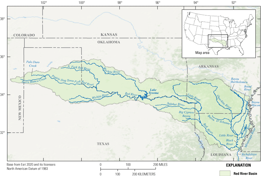
Location of the Red River Basin study area, major tributaries, and Lake Texoma, which divides the upper basin (above Lake Texoma) and lower basin (below Lake Texoma).
The land cover of the Red River Basin is largely characterized by flat agricultural land, with more forested areas and wetlands occurring in the eastern part of the basin than the western part. From 2006 to 2016, land cover in the basin remained largely unchanged (table 1). Most of the basin is covered by forest and shrublands; however, pastures and cultivated cropland cover 24.5 percent of the basin area. Developed areas accounted for 4.6 percent of the land cover in the basin in 2016.
Table 1.
Land-cover percentages in the Red River Basin.[NLCD, National Land Cover Database]
The Red River Basin supports a growing population of approximately 4.3 million people that is largely concentrated around urbanized areas. The two largest cities in the basin are Amarillo, Tex. and Wichita Falls, Tex., which have respective populations of 199,371 and 104,683 (U.S. Census Bureau, 2019). In addition to these cities within the basin, the Red River Basin also provides water for cities outside the basin such as Dallas, Tex., which had a population of over 1 million people in 2010 and was expected to grow more than 12 percent by the year 2019 (U.S. Census Bureau, 2019). Over the same period, Amarillo, Tex., was expected to grow by 5 percent and Wichita Falls, Tex., by less than 0.5 percent. All or part of 155 counties are located in the Red River Basin, including 2 in New Mexico, 35 in Oklahoma, 54 in Texas, 33 in Arkansas, and 31 in Louisiana. The basin comprises 74 8-digit hydrologic units (HUC8s) and 4,371 12-digit hydrologic units (HUC12s). There are 473 individual HUC8 and county combinations in the basin.
Ensuring that each State in the Red River Basin receives fair access to the river has been the subject of past litigation and has culminated in the ratification of the RRC (Public Law 96–564, 94 Stat. 3305), which divided the Red River Basin into five reaches. Reach I, henceforth referred to as “the upper basin,” encompasses 102,823 km2 upstream from Denison Dam on the Lake Texoma reservoir (fig. 1). In the upper basin, Texas is apportioned 60 percent and Oklahoma is apportioned 40 percent of the annual flow of seven tributaries of the river. The storage of Lake Texoma is apportioned in equal shares of 200,000 acre-feet (acre-ft) to each of those States. Reaches II through V, henceforth referred to as “the lower basin,” encompasses 138,566 km2 downstream from Lake Texoma to the Arkansas-Louisiana border. In the lower basin, Oklahoma is apportioned water from all intrastate streams flowing to the Red River between Lake Texoma and the Arkansas State line. The apportioning of reservoir storage from Lake Texoma was an important part of the RRC because of the influence hydraulic control structures have on streamflow. The decision to consider reservoir storage also demonstrates the important role of reservoirs and other control structures, such as locks and dams, in the management of water resources in the basin.
In modeling the hydrology of watersheds, it is important to account for streamflow alteration, which refers to human activities that affect the natural streamflow regime. Streamflow alteration can take on many forms, such as increasing streamflow velocity in response to channelization or increasing the extent of impervious area in a watershed, which can cause rapid increases in runoff generation. Other drivers of streamflow alteration include the construction of hydraulic structures, namely dams and reservoirs, on stream channels in response to growing water demand, water scarcity, or flooding. The effects of hydraulic structures can vary based on their desired functions. For example, dams designed for flood control may increase reservoir storage and release water gradually to prevent flooding downstream after heavy precipitation events. Because of the seasonality of climatic conditions in the Red River Basin, reservoirs can affect streamflow by releasing more or less water during dry or wet seasons.
Reservoirs are a crucial component of water resource management in the Red River Basin. Much of the Red River Basin, particularly the upper basin, is dry much of the year and therefore is reliant on water stored in reservoirs and impoundments to meet water demand throughout the year. In the lower basin, impoundments and other control structures are used for important functions such as flood control. Five locks and dams located along the southern portion of the Red River comprise the J. Bennett Johnston Waterway with a total lift of 43 meters (Derosier, 2017). The Red River Basin has 68 major reservoirs with surface areas greater than 3.9 km2. Lake Texoma, one of the largest reservoirs in the country and the 12th largest U.S. Army Corps of Engineers-controlled Lake, is the largest reservoir in the Red River Basin (U.S. Army Corps of Engineers Tulsa District, 2017). Impounded by Denison Dam and having a surface area of 277 km2 and capacity of more than 2 million acre-ft, Lake Texoma acts as a climatological transition zone between the upper and lower parts of the Red River Basin.
The climate within the Red River Basin varies greatly. The upper part of the basin experiences some of the driest conditions in the United States, whereas the lower part of the basin experiences increasing annual precipitation in the downstream direction from west to east. Rainfall and temperature data obtained from the PRISM Climate Group (2016) indicate the following. Rainfall increases appreciably across the basin from an average of 12 to 16 inches (in.) per year near the border of Texas and New Mexico to 48 to 70 in. per year near the border of Arkansas and Texas. Average annual temperatures in the upper basin range from 57 to 68 degrees Fahrenheit (°F). Average temperatures in the lower basin range from 30 to above 90 °F. The gradient of precipitation from the upper basin to the southeastern part of the basin at the confluence with the Atchafalaya River influences natural land cover. The upper basin is dominated by scrub, shrub, and herbaceous land cover that transitions to forested, wetland, and cultivated crop land cover in the lower basin, which has remained largely unchanged over the past decade (table 1).
The geology of the Red River Basin varies from the upper basin to the lower basin. The basin is situated between the Southern Rocky Mountains physiographic province to the west and the Ozark Plateaus physiographic province to the east (Fenneman and Johnson, 1946). The lower basin overlaps the Ouachita and Coastal Plain physiographic provinces (fig. 2). The northeast part of the basin is located in the Ouachita Province. The principal feature in this physiographic province is the Ouachita Mountains, which consist of a series of small mountains that form the northern boundary of the Red River Basin. One of the more notable features in this area of the basin is Fourche Mountain, which forms the divide between the Red River Basin and the Arkansas River Basin. The remainder of the lower Red River Basin is located in the Coastal Plain physiographic province, the geology of which consists primarily of Tertiary sand and clay deposits (Hosman, 1991). The eastern boundary of the basin is formed by the floodplain of the Mississippi River, and the geology consists predominantly of alluvial deposits that compose the Mississippi embayment. Further south in Louisiana are deposits of marine clays and silts. The upper Red River Basin includes part of the Great Plains and Central Lowland physiographic provinces (fig. 2). The predominant geology of this part of the basin consists largely of flat-lying sedimentary rock formations, which are reflected in the low relief of the area, with the Wichita Mountains being the exception (Trimble, 1980). Some geologic units in the upper basin contain oil, gas, and mineral deposits that have been mined for commercial use for the past several decades.
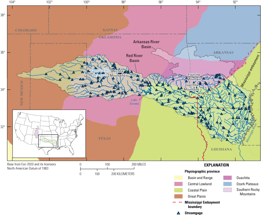
Location, hydrography, and physiology of the Red River Basin. Physiographic province boundaries from Fenneman and Johnson (1946).
Groundwater aquifers in the region range from semiconsolidated sand aquifers in the southeastern part of the Red River Basin (southern Arkansas, northern Louisiana, and southeastern Texas), to sandstones and carbonate aquifers in the central part of the basin (near Lake Texoma), to sandy and gravel aquifers near the western boundary of the basin (northwest Texas and southwest Oklahoma) (Renken, 1998). The Arkansas-White-Red region comprises the following six aquifer types: (1) stream-valley alluvium; (2) terrace alluvium; (3) alluvium of intermontane valleys and buried alluvial valleys; (4) carbonate and gypsum; (5) sand and sandstone; and (6) undifferentiated sandstone, carbonate rock, shale, and (or) basalt. The principal aquifers in the basin are (1) the Texas coastal uplands aquifer system, which extends from southwestern Texas into northern Louisiana, and (2) the Arbuckle-Simpson aquifer in southeastern Arkansas. The Trinity aquifer is the principal aquifer in the central part of the basin.
Previous Investigations
The Red River Basin has been the subject of many studies and data collection efforts. The USGS published a series of surface-water and groundwater data reports in the 1970s, 1990s, and early 2000s (USGS, 1977; USGS, 1980; Blazs and others, 1995; Blazs and others, 1996; Blazs, and others, 2000; Blazs and others, 2002, Blazs and others, 2003). In addition, several studies were conducted in the North Fork subbasin of the Red River Basin in the 1970s and 1980s. Studies conducted by Paukstaitis (1981), and Kent (1980) use numerical models to determine the maximum water yield from alluvium and terrace deposits under a range of different pumping conditions. Prior to this study, the USGS in collaboration with the Oklahoma Water Resources Board conducted a comprehensive study of the alluvial deposits to determine the amount of available water (Burton, 1965; Hollowell, 1965). These assessments have provided important data regarding the volume of groundwater available for pumping and how groundwater conditions have changed over time.
Surface water and groundwater interactions in the Red River Basin can have substantial influence on streamflow. Generally, the North Fork of the Red River is a gaining stream, and groundwater maintains base flow throughout most of the year; however, there are stream reaches that become dry during the summer months (Paukstaitis, 1981). Naus and others (2006) observed that measured streamflow did not increase with annual average water yield, which suggested the presence of gaining and losing stream reaches in some areas of the Red River Basin. Smith and Wahl (2003) analyzed streamflow trends for the period from 1945 to 1999 near Lake Altus, Okla. The authors described decreasing peak streamflow in the North Fork possibly caused by groundwater pumping from the High Plains aquifer. The findings of groundwater studies in the basin demonstrated the linkages between groundwater and surface water in addition to the usefulness of numerical models in conducting assessments of groundwater resources and the implications for surface-water modeling.
Several studies have used computational models to simulate hydrologic processes in the Red River. In the 1990s, a series of published models and model applications focused on the simulation of Red River Basin hydrology (Abdulla and others, 1996; Lohmann and others, 1998; Betts and others, 1998; Ewen and others, 1999; Kilsby and others, 1999). More recent modeling studies of the basin have focused on high-resolution modeling through improved model parameterization and by furthering investigations of total basin water storage (Duan and Schaake, 2003), long-term multidecadal simulations of basin hydrology (Sharif and others, 2007), and past and future drought scenarios (Liu and others, 2013). The results of these studies demonstrated the need for more sophisticated models to improve model accuracy and represent a growing body of scientific research aimed at developing methodologies for constructing models that utilize physically based parameterization for modeling hydrology at basin-wide, national, and continental scales.
Precipitation-Runoff Modeling System
Application of the PRMS to the Red River Basin
The goal of the Red River Basin PRMS model is to advance modeling of the basin hydrology by constructing a model that accounts for changes in climate, water use, and land cover in streamflow predictions. Because it is unfeasible to measure streamflow in all streams in the basin, the model will also provide predictions of streamflow for ungaged streams in the basin. Water-resource managers and researchers can use the streamflow predictions provided by the model in assessments of the impacts of human activities or climate on critical ecosystems in the basin (for example, wetlands), or to improve water conservation efforts, or to project the impacts of future climate conditions on the hydrology of the basin. This research represents an advance in modeling of the Red River Basin by accounting for water use and land-cover change to reach the goals of the focus area study through the integration of streamflow, groundwater flow, and ecological models.
Overview of the PRMS model
The PRMS (Leavesley and others, 1983; Markstrom and others, 2015) is a modular, deterministic, distributed-parameter, physical-process-based modeling system used to simulate hydrologic conditions related to the various compartments (evaporated water, precipitation, or runoff) of the hydrologic cycle shown in figure 3. The need to analyze the effects of a variety of climatic factors and watershed characteristics, along with user-specified scenario simulation options, on hydrologic response and the distribution of water across watersheds led to the development of the PRMS. The PRMS computes streamflow and water fluxes from and to the atmosphere and water storage in the plant canopy, on the land surface, in snowpack, surface depressions, shallow subsurface zone, deep aquifers, stream segments, and lakes on daily time steps with simulation periods that range from days to centuries. Physical characteristics, including topography, soils, vegetation, geology, and land use, are used to characterize and derive parameters required in simulation algorithms, spatial discretization, and topological connectivity. Computations of the hydrologic processes use historical, current, and (or) potential future climate data consisting of daily precipitation and minimum and maximum air temperature. To simulate future climate conditions with the PRMS, the model may be specified with projected values of the climate model input. These data are products of other models that are used to forecast daily climate. The PRMS simulations can also incorporate other datasets, such as those for potential evapotranspiration (PET), solar radiation (SR), streamflow, plant transpiration period, wind speed, and humidity.
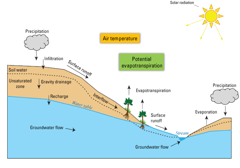
Conceptual flow model representing the hydrologic processes of the Red River Basin (modified from Regan and LaFontaine, 2017).
The PRMS simulates the hydrologic response of a geographic area called a “model domain.” The model domain is typically discretized into spatial features called hydrologic response units (HRUs) for which the PRMS computes water flux and storage in response to daily air temperature extremes and precipitation. Figure 4 presents a schematic of the hydrologic processes conceptualized in the PRMS. Channelized flow in the model domain is represented by using stream segments. The stream segments form the stream network and are connected with HRUs to simulate streamflow. For each HRU, contributing component flows to stream segments are aggregated by the PRMS. Figure 5 displays PRMS-conceptualized examples of contributing flows, such as slow interflow, originating from the soil zone of each HRU. The computation of the aggregated segment streamflow is executed for each HRU for every time step of the simulation. The PRMS can also simulate additional types of waterbodies that are not directly connected to the stream network, such as lakes, reservoirs, or surface depressions (for example, farm ponds). A conceptual schematic of the fluxes of water simulated for surface depressions is displayed in figure 6.
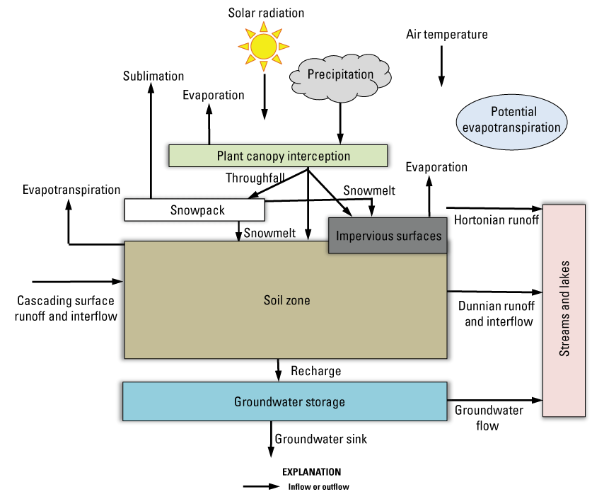
Schematic diagram illustrating the hydrologic processes as conceptualized in the Precipitation-Runoff Modeling System (modified from Regan and LaFontaine, 2017). In the diagram, throughfall is equal to net rain plus net snow. Surface-depression storage not shown.
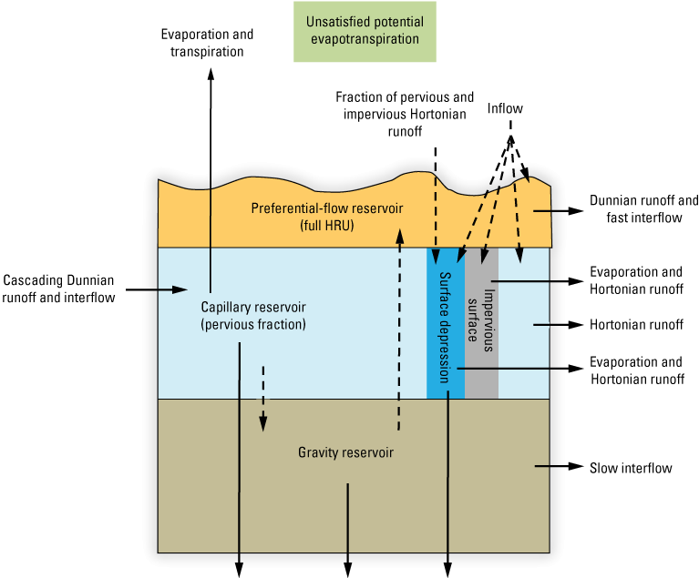
Schematic illustrating the Precipitation-Runoff Modeling System soil zone (modified from Regan and LaFontaine, 2017). In the diagram, inflow is equal to throughfall, snowmelt, and cascading Hortonian runoff.
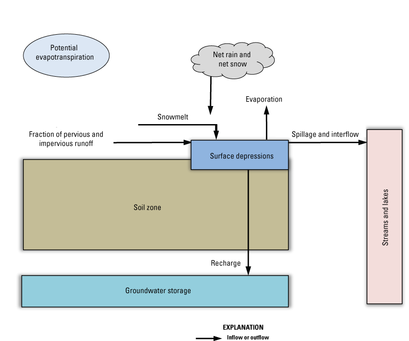
Schematic diagram illustrating the Precipitation Runoff Modeling System surface-depression storage computations (modified from Regan and LaFontaine, 2017).
Regan and LaFontaine (2017) describe recent enhancements to the PRMS, including the incorporation of water-use data. In the current version of the PRMS (version 5; Markstrom and others, 2015), water can be withdrawn from or added (as return flows) to five conceptual storages (stream segments, groundwater reservoirs, surface-depression storage, external locations, and lakes). In addition, water can be added to two other storages—the capillary reservoir of the soil zone and the plant canopy. This new capability allows for the simulation of surface-water and groundwater withdrawals and return flows in PRMS models.
Description of Water-Use and Dynamic Land-Cover Modules
Previous versions of the PRMS lacked the capability to account for constant or dynamically changing water transfers throughout a model domain. In addition, they also lacked the ability to simulate transfers within the model domain. Because of these deficiencies, previous models were unable to evaluate the impacts of these transfers on hydrologic processes. The water_use_read module was developed to add these capabilities to the PRMS (Regan and LaFontaine, 2017). The module allows for specification of historical, current, and projected water-use information as a time series of water transfers based on water availability at storage locations internal and external to the model domain. For each transfer, the date, source, destination, and flow rate are specified. The date specifies the day on which the transfer is effective. The source and destination represent the spatial and temporal redistribution of water by human activities and natural processes. The transfer rate remains constant for each time period between events for each source/destination pair.
Water can be withdrawn from five sources: (1) stream segment flow, (2) groundwater storage, (3) surface-depression storage, (4) external locations, and (5) lake storage. Source water can be transferred to any of eight destinations: (1) stream segments, (2) groundwater storage, (3) surface-depression storage, (4) external locations, (5) lake storage, (6) soil zone storage, (7) internal consumptive-use locations, and (8) plant canopy storage. Water transfers can occur between any combination of sources and destinations. Moreover, multiple transfers can originate from each source and destinations may receive water transfers from multiple sources.
Specification of the water transfers demonstrates connectivity between storage locations and usage destinations within watersheds that may result from natural processes and (or) human activities. The module can be used to account for naturally existing flows from, to, across, and under HRUs, application domain boundaries, and stream segments. Examples of water use include (1) diversion from stream segments to surface-depression storage, (2) withdrawal of groundwater storage applied to the plant canopy to approximate irrigation, (3) transbasin inflow from an external location, (4) consumptive use, and (5) streams terminating within an HRU. Examples of projected scenarios that could be evaluated include changing agricultural practices that require pumping from aquifers and (or) streamflow diversions and consumptive-use requirements as population distributions change.
Previous iterations of the PRMS utilized static watershed characteristics and parameter values used by model algorithms to produce streamflow estimates; however, this approach can become problematic because of the inability of the model to account for temporal changes in the watershed. In an earlier version of the PRMS, watershed characteristics and parameters were derived from historical data sources that did not change over the course of the simulation period. This approach can be insufficient to evaluate hydrologic responses when changes in landscape and climate occur over the time period of any particular simulation. Using dynamic watershed characteristics may improve model calibration results, improve the performance of hydrologic models, and add capability to the model to evaluate possible impacts of these changes on hydrologic processes (for example, streamflow, evaporation, transpiration, runoff, infiltration, interflow, and water availability). Accounting for dynamic watershed characteristics may be particularly important for models having decadal or multidecadal time periods and models with regional or continental spatial extents. The dynamic_parameter_read module was developed to provide this capability (Regan and LaFontaine, 2017).
The use of static parameters in climate-based modeling assumes stationarity, meaning that watershed characteristics and parameters have a consistent range of variability. However, this assumption has become inappropriate because anthropogenic perturbations of natural processes are altering the range of natural variability with respect to climate and hydrologic processes (Milly and others, 2008). Nonstationarity, in contrast to stationarity, refers to the “alteration of the means and extremes of precipitation, evapotranspiration, and rates of discharge of rivers” as a result of anthropogenic disturbances in river basins (Milly and others, 2008). The authors support their hypothesis by citing contributing factors such as landscape changes resulting from changing population dynamics, water use, water quality, and behavioral changes that have affected natural hydrologic processes. Because of the limitations of static model parameterization, alternative methodologies were developed to account for nonstationarity in the physical environment. One PRMS application of dynamic parameterization was demonstrated by Van Beusekom and others (2014), who evaluated changes in streamflow resulting from changes in land cover and land use in Puerto Rico for a 70-year period. Conditional parameterization is another “nontraditional” parameterization methodology, as discussed by Luo and others (2012). The authors describe conditional parameterization as the calibration of a hydrologic model in which model parameters may change by using different calibration time periods that have different climate conditions. They conclude that conditional parameterization could improve streamflow predictions from models; however, the authors note that the best approach to model parameterization is catchment dependent. As part of this study, parameters related to impervious area, land cover, and plant canopy were included in the model to represent temporal variability of land cover in the basin.
Stream Network and Hydrologic Response Unit Development
The stream network of the Red River Basin PRMS was extracted from the Geospatial Fabric (GF), which forms the infrastructure of the National Hydrologic Model (NHM; Viger and Bock, 2014). The GF within the NHM provides a means for developing consistent models across the conterminous United States. This is achieved through the creation of common feature geometries, namely HRUs and stream segments, that are identified by using a common identification scheme and by determining flow connectivity among the HRUs and stream segments that make up the GF. These characteristics of the GF make it possible to compare outputs of different NHM-based models with relative ease (Regan and others, 2018).
The GF aggregates spatial catchments and flowlines of the National Hydrography Dataset NHDPlus version 1 (Horizon Systems Corporation, 2007). The HRUs of the Red River Basin PRMS were delineated by using NHDplus catchment data representing the local contributing area for each HRU and stream segment pair and by analyzing the homogeneity of features with respect to slope, elevation, vegetation, geology, and soils. Viger and Bock (2014) divided the local contributing area (HRU) of each stream segment into two areas—a unit on the left (left bank) and a unit on the right (right bank) of each stream segment. Because of the configuration of the stream network and catchment area geometry that resulted from the work of Viger and Bock (2014), it is possible for a stream segment to be assigned to more than two HRUs or assigned to only one HRU. This extraction resulted in 3,065 HRUs and 1,614 stream segments (fig. 7A, B). HRUs ranged from 0.05 to 2,856 km2 in extent, with an average of 78.7 km2 and median of 38.1 km2 (Roland, 2023). Stream segments ranged in length from 0.003 to 85.6 km with an average of 16.3 km.
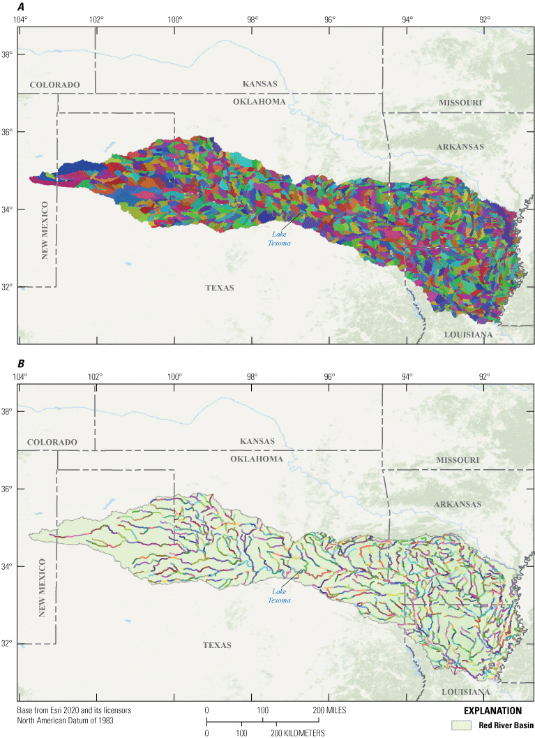
A, Basin hydrologic response units delineated for the Red River Basin Precipitation-Runoff Modeling System model, and B, the stream segments used in the Red River Basin Precipitation-Runoff Modeling System.
PRMS Parameterization
In addition to providing HRU and stream segment feature geometries, also included in the GF are tabular attributes associated with physical parameters that served as the initial set of parameters for each HRU and stream segment in the Red River Basin PRMS model. Soil parameter values in the GF were derived from the Soil Survey Geographic Database (Natural Resources Conservation Service, 2013) and with near-surface soil permeability data from Gleeson and others (2011). Groundwater-flow parameters of the GF were derived from recession coefficient analysis of hydrographs of USGS streamgages, as detailed in LaFontaine and others (2013). Surface-depression storage parameter values were derived from the high-resolution version of the National Hydrography Dataset (McDonald and others, 2012) as the aggregate sum of waterbodies within each HRU (Regan and LaFontaine, 2017). The land-use and land-cover (LULC) data were obtained from the USGS Earth Resources Observation and Science Center and cover the time period of 1980–2014. A LULC dataset was obtained for each year, thereby allowing for certain LULC parameters to be dynamically altered on a yearly basis throughout the simulation.
Streamflow Routing Parameters
Muskingum routing was used for the Red River Basin PRMS model to compute inflow and outflow from stream segments in the model domain. Using the continuity equation, Muskingum routing calculates flow in a stream channel or river as a function of inflow, outflow, and the change in instream storage over time. In the Muskingum routing, two storage parameters must be calculated, namely the storage constants K_coef and x_coef, as described in the PRMS. These storage parameters describe the storage characteristics of any given stream reach. The K_coef values were calculated by Viger and Bock (2014) and were used in the approximation of the hourly streamflow travel time through each stream segment in the GF. These travel times were computed by summing values from the NHDPlus version 1 (Horizon Systems Corporation, 2007) dataset flowlines that composed each stream segment of the model. The x_coef constant, as defined in the PRMS, is a weighting factor that describes the amount of attenuation of streamflow that occurs in a stream segment. The default value of x_coef in the PRMS is 0.2; this value was adjusted during calibration of the model. A more detailed discussion of the Muskingum routing module in the PRMS can be found in Markstrom and others (2015).
HRU Subsurface Reservoir Parameters
Parameters describing the unsaturated zones between land surface and the groundwater reservoir were developed using the near-surface permeability data from Gleeson and others (2011). The parameterization of subsurface reservoirs was conducted using the methods described in LaFontaine and others (2013). This process provides a spatially distributed range of values that are then calibrated, providing the initial spatial variation that was lacking in past PRMS applications that used the same initial value for all HRUs (Viger and Bock, 2014).
HRU Groundwater Reservoir Parameters
The groundwater flow parameter, gwflow_coef, was derived from an analysis of the groundwater recession constants using USGS streamflow data and methodologies similar to those described by Rutledge and Mesko (1996) and Bernhail and others (2012). The individual values of gwflow_coef for each of the HRUs were estimated using a multiple-linear regression equation based on geographic information systems (GIS) data for the contiguous United States. The regression equation included components of geology, drainage density, aquifer and vegetation type, and base-flow index information as described in Markstrom and others (2015). Annual groundwater recession constants were computed for streamgages identified by Falcone (2011) to have had streamflow periods relatively free of anthropogenic influence (that is, GAGES-II dataset). The approximated values of the gwflow_coef parameter were used as initial values and were adjusted during model calibration.
Climate Data and Algorithm
The PRMS requires time series of daily air temperature minima and maxima and daily accumulated precipitation. The climatic inputs of the Red River Basin model included gridded data, preprocessed from the USGS Geo Data Portal (GDP; Blodgett and others, 2011). National gridded Daymet climate data were clipped to a GIS shapefile of the discretized model domain in the GDP, which then associated the location of the model domain with the locations of nearby weather stations and computed the weighted-areal average of the maximum and minimum air temperature and precipitation for each day of the study period. These daily climate inputs were distributed to the HRUs in the model domain using the climate_hru module, as described in Markstrom and others (2015). Because the climate data were preprocessed and applied to each HRU in the model domain by the GDP, the output of the GDP was directly applied to the HRUs in the model.
The Daymet version 3 gridded climate dataset was developed at Oak Ridge National Laboratory using a collection of algorithms and computer software to interpolate and extrapolate from daily meteorological observations (Thornton and others, 2016). The weather parameters generated included daily minimum and maximum air temperature, precipitation, humidity, and SR produced on a 1-km2 gridded surface over the conterminous United States, Mexico, and Southern Canada for the period 1980–2016 (Thornton and others, 2016). This type of gridded climate dataset is convenient for large-scale hydrologic modeling applications, but such applications may be limited by the available period of record and local scale deficiencies.
Streamflow Data
Streamflow data for USGS streamgages are published in the USGS National Water Information System (U.S. Geological Survey, 2017) and were obtained using the R dataRetrieval package found in R Foundation for Statistical Computing software (R Core Team, 2020). Currently, there are more than 400 active streamgages in the Red River Basin (U.S. Geological Survey, 2017). Of these available streamgages, 202 streamgages were included in the development of the Red River Basin PRMS model (fig. 8). Information for each of the streamgages included in the study is presented in table 1.1 of appendix 1 and in Roland (2023). Of the 202 streamgages used in the study, 165 were selected for calibration because they had 5 years or more of streamflow record during the model calibration period from 1980 to 2016 or were included in the GF for the NHM. Of the 165 streamgages selected for calibration, only 129 streamgages were successfully calibrated. The remaining 36 streamgages were removed from the calibration dataset. Model performance was evaluated using 73 streamgages from across the basin. Streamgage information for each of the calibration and evaluation streamgages is presented in table 1.1 of appendix 1 and in Roland (2023).
Water-Use Inputs
Each of the States in the model area define and manage water use differently. Water-use data for each respective State were obtained from a variety of different agencies and compiled into a useable time step and format for model simulation. When the model was constructed, the most current available water-use data used in our study covered the period from 1980 to 2014. Because the model period extended through 2016, water use was held constant at the 2014 rates for the 2015–16 model period. The Arkansas Natural Resources Commission conducts an annual inventory of groundwater and surface-water withdrawals in Arkansas in cooperation with the USGS. The water-withdrawal data are stored in the Arkansas Natural Resources Commission Water-Use Data Base System (WUDBS), which has been maintained by the USGS from 1985 to the present. The WUDBS provides information about the amount of water withdrawn and how the water was used, in addition to the amount of water returned for water-resource managers and policy makers. Site-specific water-withdrawal data for Arkansas were obtained from WUDBS for the period from 1980 to 2014. Water-withdrawal data are compiled for 10 categories of water use, including public supply, self-supplied withdrawals (for example, commercial and industrial), mining, livestock, aquaculture, irrigation, and thermoelectric power generation. Water users that withdraw 1 acre-ft or more of surface water per year report their withdrawals annually. Because of incomplete reporting, it is necessary in some cases to supplement these data with data from other sources such as the Natural Resources Conservation Service, U.S. Army Corps of Engineers, Arkansas Department of Environmental Quality, Arkansas Department of Health, and National Agricultural Statistics Service.
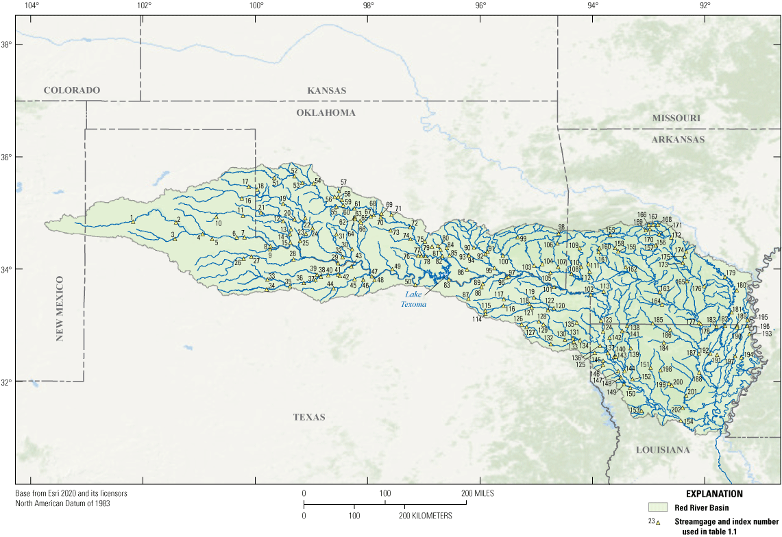
U.S. Geological Survey streamgages included in the development of the Red River Basin Precipitation-Runoff Modeling System model.
The USGS, in cooperation with the Louisiana Department of Transportation and Development, has collected and published water-use information on a 5-year basis since 1960. Since 1980, all water-use information has been maintained by the USGS office in Baton Rouge, La. The Louisiana State University Agricultural Center Cooperative Extension Service publishes an annual report titled “Louisiana Summary—Agriculture and Natural Resources,” which provides information for computing aquaculture, irrigation, and livestock water use (Louisiana State University Agricultural Center Cooperative Extension Service, 2014). For this investigation, information from each annual report for the years 1980–2014, as well as data from major water users and the 5-year compilations, were used to characterize surface-water withdrawals in the Louisiana portion of the study area.
In Oklahoma, surface water is known as “stream water” and is considered publicly owned and subject to appropriation by the Oklahoma Water Resources Board (OWRB). Stream water is defined as a “watercourse in a definite, natural channel with defined beds and banks, originating from a definite source or sources of supply” that may have intermittent or irregular flow and is regulated by the 9-member OWRB, which issues water-use permits for surface-water diversions (OWRB, 2008). Water-use categories provided in the diversion data include aquaculture, commercial, industrial, irrigation, livestock, mining, power generation, and public supply.
In Texas, water-withdrawal data are reported primarily by three agencies: the Texas Commission on Environmental Quality (TCEQ), the Texas Railroad Commission, and the Texas Water Development Board. Surface water is defined by TCEQ as water in lakes, flowing in streams and rivers, or water imported into the State using navigable streams or State operated facilities. Texas is a water rights State, which means that water is held in trust by the State. The State grants permits to individual users such as farmers, industries, cities, and other public and private entities. Surface-water withdrawal and return amounts were both obtained from the TCEQ by retrieving permit information for the period from 1980 to 2014 (Texas Commission on Environmental Quality, 2019). Water-use categories were also obtained from the permit data and include public supply, irrigation, livestock, aquaculture, commercial, industrial, and hydroelectric power generation.
Dominant uses of water in the Red River Basin range from irrigation in the western part of the basin to public supply, thermoelectric power, and livestock in the central and southeastern parts. Total estimated water use in 2010 by the four principal States in the basin was nearly 83,616 ft3/s (45,000 Mgal/d). Surface-water withdrawals accounted for approximately 52,028 ft3/s (28,000 Mgal/d) (Maupin and others, 2014). Texas withdrew the most surface water in the basin (fig. 9A). Thermoelectric power generation in Texas and Louisiana accounted for the majority of surface-water withdrawals in the basin. Texas also withdrew the most water for public supply and a large fraction of water used for irrigation in the basin, second to Arkansas. Arkansas and Texas also withdrew the most groundwater, which was primarily used for irrigation (fig. 9B).
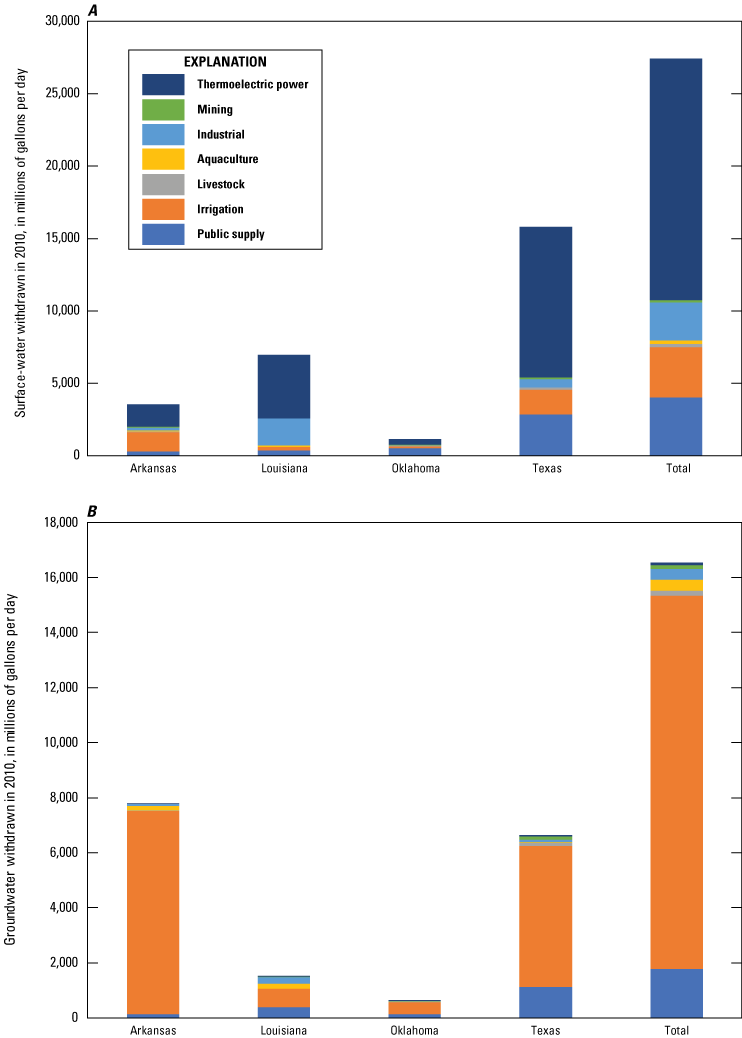
Groundwater and surface-water use in the four States in the Red River Basin, 2010 (adapted from Maupin and others, 2014).
Mapping to Hydrologic Modeling Units
Water-use estimates were mapped to the PRMS model units (HRUs and stream segments) through a GIS overlay analysis with the water-use locations; the estimates included irrigation, public supply, commercial and industrial, hydroelectric power generation, basin import and exports, return flow, and recreation. The surface-water-based withdrawals and returns were mapped to stream segments. To simulate water use in the PRMS, the water-use estimates were formatted into PRMS-specific water-use types based on the destination of the water being transferred. Agricultural, commercial, industrial, power generation, and unspecified water use were treated as consumptive water use. Only transfers for irrigation were assigned to the canopy storage reservoir of an HRU. The water-use data were then processed for PRMS-specified input files as specified in Regan and LaFontaine (2017). Separate water-use input files were created for (1) water transfers to and from stream segments, and (2) import and export water transfers and returning flow.
Red River Basin Water-Use Summary
Water use in the Red River Basin model domain consisted of surface-water withdrawals and returns. A summary of water use used in the Red River Basin model by water-use type is shown in table 2. Mean monthly surface withdrawals ranged from 177 to 370 ft3/s (95 to 199 Mgal/d) over the period 1980–2016. Mean monthly return flow ranged from 4.75 to 19.3 ft3/s (2.56 to 10.4 Mgal/d). Mean monthly withdrawals were greatest during the months of June, July, and August and monthly returns were greatest in April.
Table 2.
Summary of mean monthly water withdrawals for the Red River Basin, by type, for the period 1980–2016.[Withdrawals are in cubic feet per second]
PRMS Model Sensitivity
Understanding relationships between the parameters of a model and the variety of physical hydrologic processes simulated by the model is critical. Sensitivity analysis is a useful tool for conducting model assessments that help determine which physical processes described by the model parameterization have more or less impact on the hydrologic simulations performed by the model. Markstrom and others (2016) performed a sensitivity analysis of the contiguous United States using the Fourier Amplitude Sensitivity Test (Cukier and others, 1973; Schaibly and Shuler, 1973; Cukier and others, 1975; Saltelli and others, 2006). The analysis included 110,000 HRUs from the NHM for the period from 1990 to 2000. This approach was then used as a part of an automated calibration process. The results of the sensitivity analysis by Markstrom and others (2016) showed that the dominant hydrologic process in the Red River Basin was evapotranspiration. The least dominant hydrologic processes in the basin were base flow, infiltration, runoff (that is, the total flow from an HRU that contributes to the flow of a connected downstream stream segment), and surface runoff (that is, precipitation or snowmelt water that moves across the land surface and into the stream segment assigned to an HRU). Results from the sensitivity analysis performed by Markstrom and others (2016) were used to select the parameters for calibration of the Red River Basin PRMS model.
Calibration of the Red River Basin PRMS Model
Calibration of the PRMS model was completed using a sequential modular parameter optimization methodology for each of the 165 streamgages selected to calibrate the model. The calibration process began with the analysis of the stream network using the Lumen tool (Hay and Umemoto, 2006). Lumen is a computer application that creates schematic visualizations of the stream network and modular stream networks that are assigned to streamgages during model calibration. The Lumen tool was used for two purposes: (1) to delineate the contributing watershed (combination of HRUs and stream segments) for the calibration streamgages, and (2) to determine the calibration sequence for each of the calibration watersheds on the basis of the stream order of the gaged stream segment. Sequential calibration began at headwater streamgages and progressed downstream to each streamgage location. Stream segments with no downstream streamgage that could be used for calibration were also identified visually using geospatial analysis software. Stream segments that were not assigned to a downstream calibration streamgage were assigned to a nearby streamgage that was hydrologically connected to the upstream stream segment but not influenced by the stream segments that were not assigned to a calibration gage. Each process (SR, PET, streamflow) simulated by the modules was calibrated individually. Parameters influencing a specific process used in the calibration of that process are listed in table 3.
Table 3.
Calibration procedure using LUCA (Let Us Calibrate) software (Hay and others, 2006; Hay and Umemoto, 2006).[HRU, hydrologic response unit]
The PRMS model was calibrated using the Let Us Calibrate (LUCA) software tool (Hay and Umemoto, 2006). The LUCA program is a multi-objective-function, stepwise calibration procedure that uses the Shuffled Complex Evolution optimization algorithm (Duan and others, 1992) to estimate optimal parameter values. The Shuffled Complex Evolution randomly samples values of a specified set of parameters. Objective functions are then calculated and optimized for the set of parameters. The values of the objective functions are ranked from largest to smallest. Small objective function values indicate an optimal fit to the parameter and are retained for the complex evolution process. The best-fitting objective functions are divided into a user-defined number of complexes that are evolved using the simplex downhill search algorithm developed by Nelder and Mead (1965). This process creates an iterative loop for testing objective functions and parameter values until one of the following conditions are met:
-
1. The maximum number of sub-model executions is met.
-
2. The percentage change between objective function values of the current shuffling loop is less than a specified value when compared to objective function values of several preceding shuffling loops.
-
3. Optimized values of the objective function converge on a small range of values between the upper and lower bounds of a given parameter.
This process is repeated, decreasing the number of complexes by one with each iteration. The output of LUCA is a parameter file containing parameter values generated using the best objective function values.
The calibration procedure used for the Red River Basin model was divided into two phases based on the processes the sensitivity analysis results indicated were most critical to accurately representing the hydrology of the basin. The parameters selected for calibration in each step are shown in table 3 and discussed in detail next.
Phase 1: Calibration of Solar Radiation and Potential Evapotranspiration
In phase 1 of calibration, model parameters were calibrated to optimize the simulation of SR and PET in steps 1 and 2, respectively. Observed SR and PET data may be used as additional input to the climate_hru module; however, when these data are not present, alternative PRMS modules must be specified to distribute SR and PET to the HRUs. The ddsolrad module estimates and distributes SR based on maximum temperature per degree day, which is defined as the difference between the daily mean temperature and 65 °F (Markstrom and others, 2015). The Red River Basin PRMS model uses the ddsolrad module to estimate SR. Similarly, when observed PET data are not available, a methodology for estimating PET must be specified from several modules within the PRMS. The Red River Basin model uses the potet_jh module, which is based on the Jensen-Haise formulation (Jensen and Haise, 1963) to estimate PET.
The parameter-calibration objective function targets minimization of the absolute difference (Markstrom and others, 2015) between simulated and measured SR and PET on a mean monthly time step. The absolute difference is calculated as follows:
whereAbsDiff
is the absolute difference objective function,
m
is the month,
SIMm
is the mean of measured values for the SR or PET for simulated values,
MSDm
is the mean of measured values for SR or PET for month,
Once calibrated, the new parameter values were merged into the basin-wide PRMS parameter file.
Phase 2: Calibration of Streamflow Volume and Timing
In step 1 of phase 2, annual and monthly streamflow volume parameters were calibrated. Parameters associated with streamflow timing were calibrated in step 2 through step 4 of the calibration process. During this phase, parameters adjusted to match measured streamflow volume were optimized for annual, monthly, and mean monthly time steps. Parameters adjusted to match streamflow timing for high, low, and all flows were optimized using the same procedure as streamflow volume, but only at the daily time step. The objective functions for this phase of calibration minimized the ratio of the root mean square error to the standard deviation of the measured streamflow (RSR; Moriasi and others, 2007) between measured and simulated streamflow as follows:
wheren
is the time step,
nstep
is the total number of time steps,
SIMn
are the simulated streamflow values for time step n,
MSDn
are the measured streamflow values for time step n, and
MN
is the mean of all measured streamflow values for the objective function time period.
Further assessment of hydrologic simulations of streamflow volume and timing was performed using the Nash-Sutcliffe efficiency (NSE; Nash and Sutcliffe, 1970; eq. 3) and by calculating the percent bias (Pbias; eq. 4) of the total streamflow volume. The NSE metric was calculated as follows:
The NSE provides a metric that quantifies the accuracy of model simulated streamflow relative to observed streamflow. If the simulated streamflow replicates streamflow observations perfectly, then the value of the NSE would be 1.0. The accuracy of simulations decreases as the value of the NSE decreases. If the NSE value is equal to zero, then the simulated values represent the hydrologic response as well as the mean of the measured values. Negative NSE values indicate that the mean of the measured values provides a better fit than the simulation values. The Pbias metric was calculated using the following equation:
A negative Pbias value indicates that model simulated streamflow is underestimated in comparison to the observed flow, and a positive value indicates that the model simulated streamflow is overestimated in comparison to observed flow.
Red River Basin PRMS Model Calibration and Evaluation
Phase 1
Basin characteristics produce great variability in measured and simulated SR and PET across the basin. During model development, SR was calibrated in two regions: the upper basin and the lower basin. Results from the SR calibration indicated that model-estimated monthly mean SR for the basin showed good agreement (NSE ≥0.7) with observed record for the same period. Figure 10 shows examples of model calibration at streamgage locations across the Red River Basin. The observational SR data used in calibration were downloaded from the Daymet version 3 (Thornton and others, 2016) gridded climate database using the USGS Geo Data Portal. The simulated and observed monthly mean SR follow a similar pattern for much of the year. SR increased through the first 6 months of the year, peaked in July when SR was most intense, and declined through the remainder of the year.
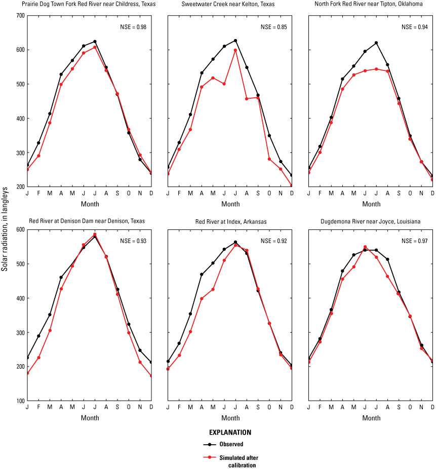
Solar radiation calibration results for sites across the Red River Basin.
Potential evapotranspiration calibration results showed more variability than SR but were generally in good agreement (NSE ≥0.5) with observed evapotranspiration results (fig. 11). The model tended to overpredict PET in many areas across the basin. In the upper portion of the basin, the arid climatic conditions promote relatively large values of PET as demonstrated by the model simulated PET, which was not in agreement with observed PET. In the lower part of the basin where PET was lower, the model more closely predicted observed PET. The variability in the amount of PET can be explained by a number of factors, which may include the quality of the PET observations, the effects of evaporation from the surfaces of reservoirs, groundwater and surface-water interaction, and the effects of water withdrawal. The temporal pattern of potential evapotranspiration varied similarly to that of SR. Evapotranspiration increased through the year and peaked during the months of June and July when SR and daily maximum air temperatures were highest. Evapotranspiration decreased through the second half of the year as high temperatures and the intensity of SR declined.
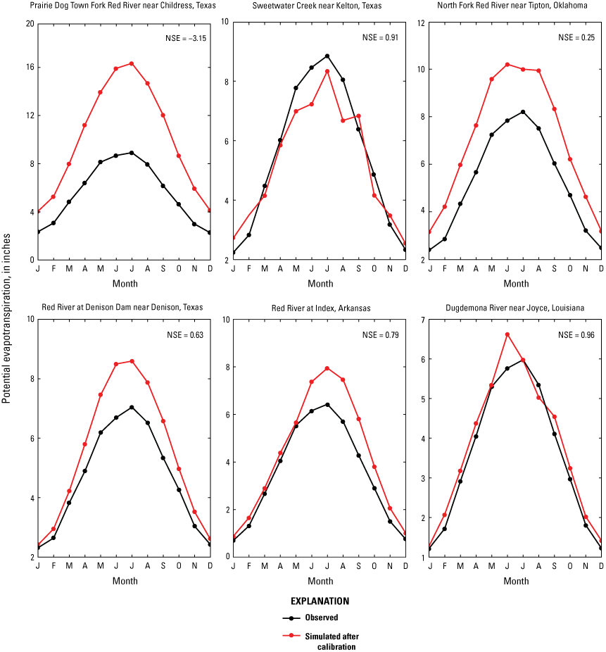
Potential evapotranspiration calibration results for sites across the Red River Basin.
Phase 2
Data from 129 streamgages were used to calibrate the Red River Basin PRMS model (appendix 1; table 1.1). Using LUCA software, the model parameters were adjusted for each subbasin relative to the adjustment made to the HRUs and stream segments in the calibration streamgage’s catchment. The relative distribution of model parameter values in each subbasin were preserved because the LUCA software was used to optimize the model parameters to match the measured streamflow at each calibration streamgage. The model parameters were optimized using LUCA by comparing USGS measured streamflow and the PRMS variable, seg_outflow, for the PRMS model stream segment associated with the calibration streamgage. Performance metrics for NSE, RSR, and Pbias for each calibration and evaluation streamgage for the results of daily and monthly calibrations are shown in table 1.2 of the appendix. The passing performance threshold for the NSE was defined as 0.5 or greater, the threshold for RSR was defined as 0.7 or less, and the threshold for Pbias was defined as within plus or minus 10.0. Simulations at each streamgage location were evaluated on the basis of how many performance metrics were within the acceptable criteria. A calibration or evaluation streamgage location was rated “good” if all three of the performance criteria (NSE, RSR, and Pbias) for daily or monthly time steps were passing or acceptable, “fair” if two of the three metrics were acceptable, and “poor” if less than 2 of the performance metrics were acceptable. Figures 12 and 13 display model calibration ratings for streamgages across the basin from calibration on a daily time step and monthly time step, respectively. Calibration results at a monthly time step were typically better than calibration results at a daily time step. The results of calibration and evaluation for the monthly time step indicated that 110 streamgages were rated as fair or better (table 4). Daily time step calibration and evaluation results indicated 73 streamgages were rated fair or better. These results indicate that the predictive capacity of the PRMS to simulate streamflow in the Red River Basin is strongest at a monthly time step. These results also demonstrate the challenging nature of predicting streamflow in arid regions like the upper basin and the complexities related to anthropogenic influences on streamflow. Considering these factors and their associated uncertainty, the model provided the best representation of the hydrologic conditions with respect to the inputs used to construct the model. Moreover, these results indicate that further studies are needed to improve watershed models where arid conditions and anthropogenic influences exist.
Table 4.
Summary of monthly and daily time-step performance statistics for Red River Basin Precipitation-Runoff Modeling System simulations.[Values shown in cells are site counts]
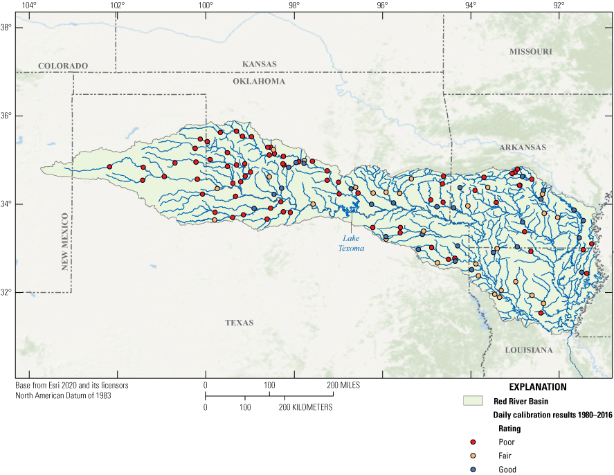
Performance metric ratings for 129 streamgages across the Red River Basin calibrated at a daily time step.
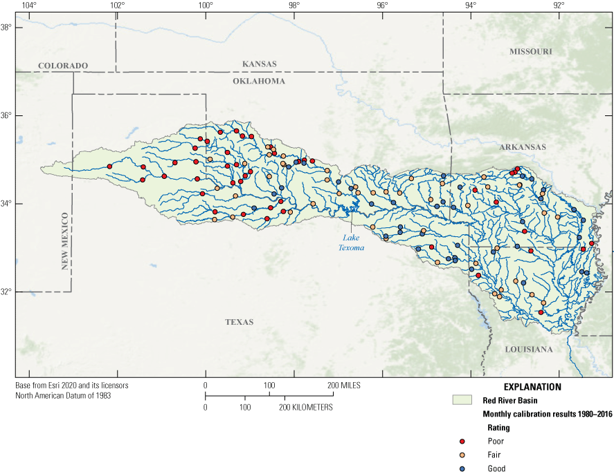
Performance metric ratings for 129 streamgages across the Red River Basin calibrated at a monthly time step.
Water Budget Components and Overall Trends
Water budget components for the period from 2008 to 2016 are similar in spatial distribution but different in magnitude than water-balance components for the long-term period from 1980 to 2016 (figs. 14, 15). Within the context of the long-term record, the study period has similar spatial distributions of water-balance components, but the magnitudes differ. Precipitation, evapotranspiration, and recharge in the Red River Basin show similar spatial patterns over the period from 2008 to 2016 and the period from 1980 to 2016. Predictions of precipitation and evapotranspiration for the 2008–16 period were slightly greater than the long-term period in the basin. Precipitation varied across the basin, with larger volumes of precipitation generally concentrated in the lower basin, which also coincided with more evapotranspiration. In addition to areas that received large amounts of precipitation, evapotranspiration was also greatest in urban areas as a result of the presence of more impervious areas and less vegetative cover owing to the heat island effect.
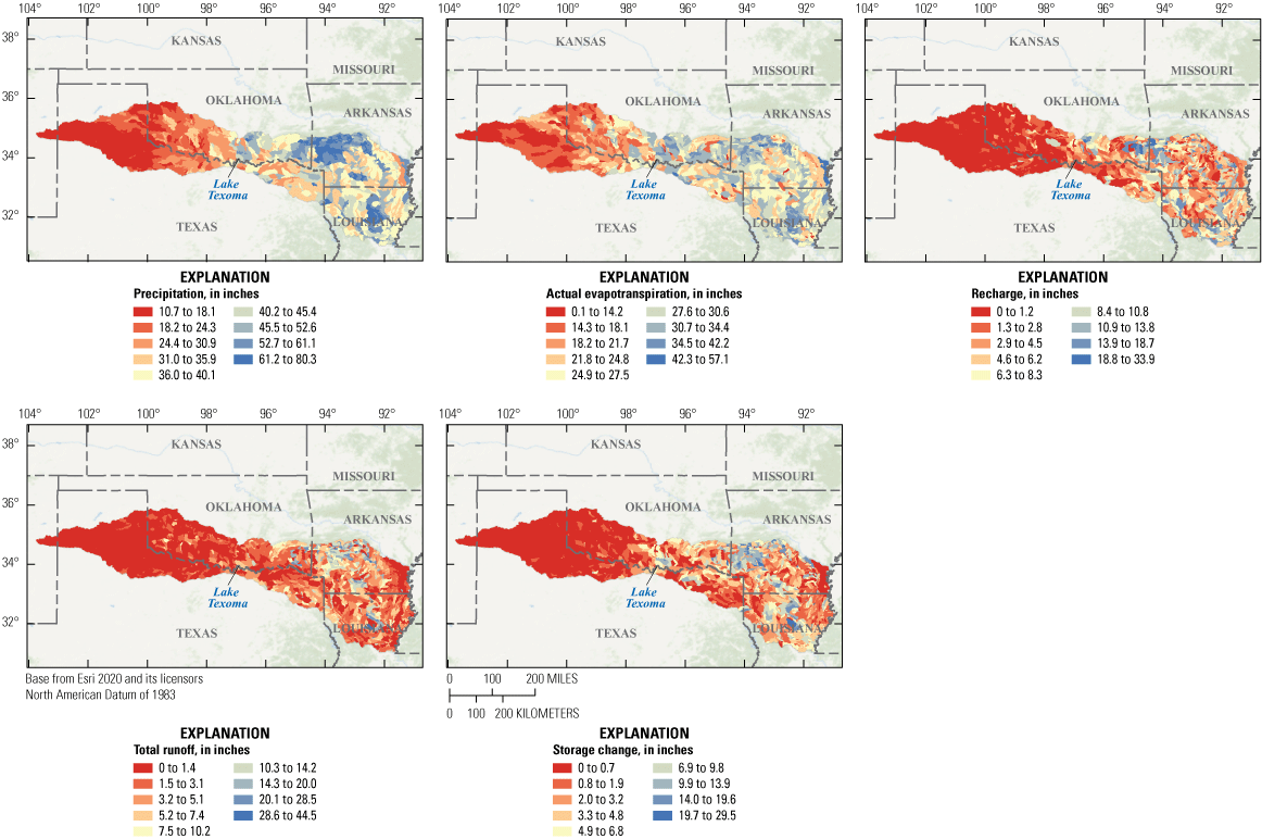
Water balance components for the full study period from 1980 to 2016.
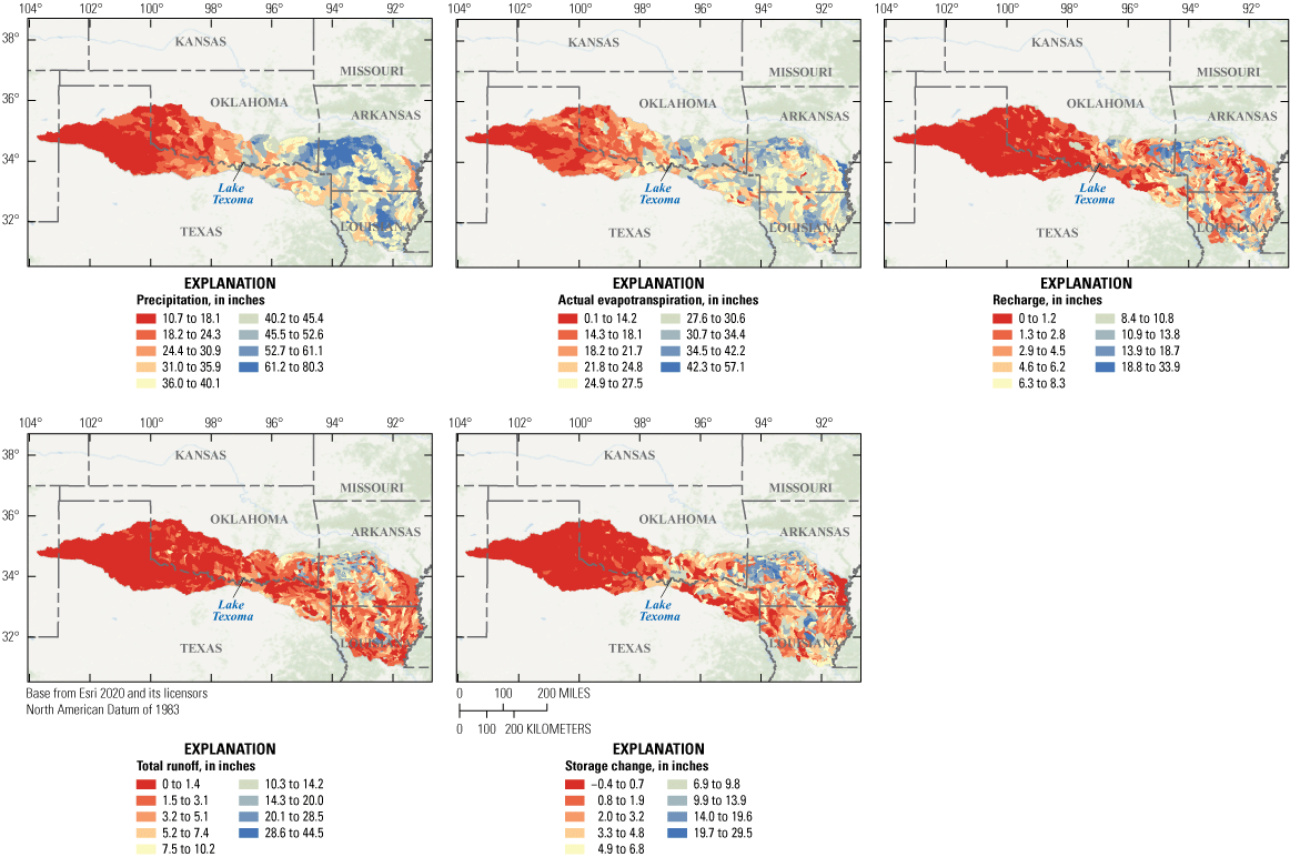
Water balance components for the period from 2008 to 2016.
Recharge in the basin varied spatially, with most recharge occurring along the northern border of the basin near to the Arkansas-Oklahoma State line and near the Oklahoma-Texas State line in the vicinity of Lake Texoma (figs. 14 and 15). Total runoff in the basin from 2008 to 2016 was greater than the long-term average from 1980 to 2016. Runoff generation is largely controlled by precipitation, which resulted in more runoff in areas that received the most precipitation. The most runoff occurred in the northernmost portion of the basin in central Arkansas and in northern Louisiana. Runoff generation was less in areas where evapotranspiration and recharge were greatest.
Recharge by reservoirs is facilitated by extended residence times of the water in the reservoirs, which results in extended periods of water migration downward to the water table. Storage in the conceptual reservoirs of the Red River Basin PRMS model (for example, plant canopy, soil water, groundwater, surface depressions) generally increased for the period from 2008 to 2016 relative to the period from 1980 to 2016. Storage changed most in areas that received the most precipitation. The largest changes in storage occurred in southwestern Arkansas along the northernmost border of the lower basin and in northern Louisiana (figs. 14 and 15). Many areas having large changes in storage corresponded to areas with mostly vegetative cover. This indicated the amount of water stored in the plant canopy and soil reservoirs varied the most. Outside the areas having large changes in storage, the basin experienced smaller changes in storage. Consistent with the other water balance components, storage changed less in areas that received relatively smaller amounts of precipitation.
The predominant water uses in the central Red River Basin are consumptive use (which includes industrial, power generation, and municipal usage) and recreational and habitat conservation. Irrigation and canopy storage were the predominant water uses in the lower basin. Imports and exports of water into and from the Red River Basin primarily occur in the upper basin. Streamflow in this area was also affected by returning streamflow that originated from reservoirs. Reservoir return flow also increased streamflow in south central Arkansas. Upstream and downstream from Lake Texoma, water use affects total streamflow on the main stem of the Red River differently, reflecting differences in the dynamics of water use in the upper and lower basin. Water use affected streamflow more in areas upstream from Lake Texoma than in areas downstream. Because of imported water and replacement flow from reservoirs in the area, the main stem gained streamflow in the upper basin (fig. 16A). Streamflow increases most upstream from Lake Texoma on the main stem and further upstream on the North Fork of the Red River. Supplemental streamflow in this area is crucial because of the dry conditions that are characteristic to this part of the model domain. Because of these conditions, which consequently result in small streamflow volumes, added streamflow causes a large relative percentage of change (fig. 16B). In contrast to water-use increasing streamflow upstream from Lake Texoma, water use decreases streamflow downstream from Lake Texoma because water use is greater in this part of the basin (fig. 16A). Total streamflow decreases most on the main stem of the Red River downstream from Lake Texoma and along the eastern border of the basin on the Ouachita River (fig. 16A). Decreasing streamflow was typical of most areas in the lower basin; however, streamflow in Bayou Macon increased because of water use. Because of the accumulation of streamflow from the headwaters of the Red River to the outlet of the basin, the total amount of streamflow is greatest in the lower basin. The combined effects of more intense water use and more streamflow result in lower relative percentages of change downstream from Lake Texoma than upstream from the lake. Although water use is more intense in this part of the basin than in the upper part, the range of the relative percentage of change resulting from water use was smaller for streams in the lower basin than for streams in the upper basin.
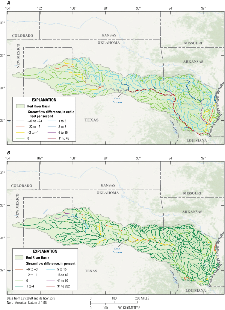
Water-use effects on streamflow in the Red River Basin for the period 2008–16. Effects are shown as A, a difference in streamflow between no-water-use streamflow and water-use streamflow, in cubic feet per second, and B, a percent difference between no-water-use streamflow and water-use streamflow. A positive percent difference indicates streamflow increased relative to the no-water-use scenario and a negative percent difference indicates streamflow decreased relative to the no-water-use scenario.
The streamflow patterns resulting from water use may include a seasonal component. Streamflow in the basin varied most in winter and spring, and flow variability in the basin decreased from late spring through early fall. Relative to monthly streamflow, monthly water withdrawals are greatest during the spring and summer. Return streamflow is also greatest during these seasons. This demonstrates that the demand for water is greatest when water supplies are lowest. Agricultural water use during the growing season may potentially explain some of the variation in streamflow that occurs throughout the year.
Red River Basin PRMS Model Limitations and Potential Improvements
Given the amount of uncertainty in modeling regions with arid climates and areas with large water withdrawals, the Red River Basin model presented herein is the best representation of the hydrology that could be obtained using the PRMS with respect to the inputs used to construct the model. The results of the model calibration indicated that areas in the wetter part of the basin were typically better calibrated to predict monthly and daily streamflow. In many areas of the basin, however, the model was either less capable or not capable of making meaningful predictions of streamflow because of the inherent uncertainty in the model input. Specifically, the quantity and quality of climatic input, the parameterization of physical and hydrologic features of the HRUs in the model domain, and the quality of withdrawal data made it challenging to calibrate streamgages where these uncertainties were most prevalent. The use of an automated calibration procedure provided the most viable option for calibrating the volume of streamgages used in this study, but this approach may have affected the overall predictability of the model. An alternative to automated calibration, such as manually calibrating streamgages (particularly in headwater streams in dry areas where streamflow can be most variable), may have yielded improved calibrations. Manual calibration of the model would have allowed for a more regionalized representation of hydrologic conditions in many areas across the model domain.
The use of gridded climate data is critical to the development of hydrologic models because it provides spatially continuous data for model domains. The gridded data are created by integrating measurements of various climatic parameters from weather stations to create estimates where observations are unavailable. This process has inherent errors that are byproducts of the uncertainty associated with the spatial resolution of the integrated parameters, the spatial distribution of the weather stations used in the integration of the climate data, and the methodology used to integrate the gridded parameter. As a result, the ability of the Red River Basin PRMS model to accurately simulate the hydrologic processes in the basin is limited by these factors.
The results from the calibration of the Red River Basin PRMS model demonstrated the role of climate forcing and its effect on model performance. Streamgages in the Red River Basin PRMS model that had acceptable calibration results for monthly streamflow predictions accounted for 63 percent of calibration streamgages. In comparison, streamgages in the model that had acceptable calibration results for daily streamflow predictions only accounted for 43 percent of calibration streamgages. The calibration streamgages located on small streams and intermittent streams typically had poor calibration results for monthly and daily streamflow predictions. Streamgages on the North Fork of the Red River and on headwater streams such as the Prairie Dog Town Fork are examples of streamgages that were unsuccessfully calibrated as a result of climatic forcing in the model. The challenge of calibrating these streamgages and others in the upper half of the model domain was a consequence of an inability of the model to resolve the water balance within HRUs and their assigned stream segments across the time steps of the model. In general, streams near the western boundary of the model domain have less streamflow than streams in the middle and eastern portions of the domain. The upper portion of the Red River Basin is dominated by desert lands that receive less than 25 in. of rain annually, which is less than half the amount of precipitation in much of the lower part of the basin. In addition to the relatively dry conditions, the upper part of the model domain had warmer air temperature and more intense SR than the lower part. As a result of the climatic conditions in the area, the availability of water for evapotranspiration, runoff generation, groundwater recharge, or storage in the soil zone was limited. As a consequence, the parameterization of the model was unable to reproduce the characteristics of streamflow in response to the climate input data during simulations. These results demonstrated the role of climate with relation to the parameterization and subsequent calibration during model development. Potential improvements that address the performance of the Red River Basin PRMS model can be obtained by increasing the spatial and temporal resolution of climate data in addition to incorporating additional parameters capable of providing a more detailed characterization of the dynamic conditions of HRUs across the model domain.
The Red River Basin PRMS model used dynamic land-cover parameters to account for changes in land cover and land use over 24 of the nearly 40 years simulated by the model. This period represented the best available data at the time during the development of the model but may not completely capture the signal of different types of land-cover changes occurring on spatial scales smaller than the 30-meter spatial resolution of the National Land Cover Database. Creating higher resolution land-cover data may improve the accuracy of the characterization of land-cover types and improve model performance around urban areas in the model domain. Land-cover models have become a necessity in basin-scale watershed modeling. These models have historically been developed by using aerial photography, surveys by landowners and managers, field observations, and satellite-based remote sensing data. Advances in land-cover classification methods have improved the temporal and spatial scales of cover estimates; however, many automated classification methods have been based on coarse imagery, which results in less accurate land-cover classification when compared to high resolution imagery (Stoian and others, 2019). This is particularly relevant to the classification of urban areas. As a result, models like the Red River Basin PRMS are limited by the temporal and spatial scales of available land-cover data, the accuracy of that data, as well as the inherent uncertainty associated with modeled land-cover change estimates. Advancements in land-cover modeling and data collection will become more critical as demand for high resolution temporal and spatial hydrologic models grows. Such advancements provide a better understanding of the relationship between hydrologic processes, water use, water availability, and human behavioral changes and thus better inform water-resources management in the Red River Basin.
The water-use data used in this study were provided on monthly and annual temporal scales by State agencies who oversee the Red River Basin. In cases where only annual water-use quantities were reported, the data were processed into monthly estimates by assuming the water use was distributed evenly for each month of the year. This approach does not account for seasonal changes in water use, such as decreases between growing seasons. This may have led to decreased accuracy in estimations of streamflow, because potentially less water is being used for irrigation and other agricultural activities outside the growing season. In addition to model error that could stem from data collection methodologies and the assumption of nonseasonality in water-use data when monthly values were not reported, the classification system used to report the type of water use (for example, municipal or recreational use) also varied. Accurately representing the type of water use was critical to processing the data used by the model, given it was the basis for reclassifying the data to conform to the more general classification required by the PRMS. Accurately designating water-use types has implications for the water budget calculated for HRUs and estimates of stream segment inflow and outflow. For example, consumptive use and basin exports remove water from the water balance computed by the model; however, water used for irrigation remains in the water balance of the model.
The inaccurate identification of source water transfers in water-use data also introduced uncertainty into the model that could have affected streamflow estimates. The locations of water withdrawals were reported as either a specific point in space or at the county scale. The locations of stream segments where water transfers originated were determined by georeferencing the reported locations of withdrawals to the network of streams in the model. When the reported location of a transfer did not intersect with a particular stream segment, the location of the transfer was assigned to the nearest stream segment. County-scale transfer data were assigned using all available information (for example, stream name). In the absence of a stream assignment for withdrawals, the withdrawal location was assumed to occur at the furthest upstream stream segment in the county.
During model development, the locations of transfer sources were adjusted incrementally, because the PRMS could not simulate transfers from stream segments that did not have enough flow to support the transfer rate of a withdrawal event. Because the model cannot simulate negative flow conditions, these instances resulted in an immediate termination of the simulation. To resolve this problem, the location of the withdrawal was adjusted to reference a nearby segment with enough flow for the transfer. Because of the uncertainty associated with this adjustment, it contributes to model error. These errors could manifest as underpredictions of flow in the newly assigned stream segment relative to physical conditions.
In addition to adjusting the location of water transfer sources, the quantities of water being transferred were also adjusted when withdrawals exceeded the amount of available streamflow. These exceedances could result from (1) errors in source-water associations, (2) the unregulated nature of reported water-use quantities, or (3) human error in reported withdrawal quantities. During model development, it was assumed that reported water use from municipal systems, reported imports and exports, and replacement flow were most accurate. Irrigation, agricultural, and other types of water use in the model were assumed to have more uncertainty, in part because of self-reporting. During model simulations, reported withdrawals were decreased to avoid transfers from stream segments that did not have adequate streamflow for a given transfer. Most transfers were adjusted to 10 percent of the original transfer rate.
Soil, land cover, topographic, geographic, surface-depression, and subsurface flux parameters used in the Red River Basin PRMS model were derived from the GF, which supports the national scale NHM PRMS. Because the Red River Basin PRMS model, in simplest terms, is a subset of the NHM, the use of NHM parameters in the construction of the Red River Basin PRMS was appropriate. Data from the GF provided the initial parameter estimates used to derive the final parameter estimates used by the Red River Basin PRMS model. Because the initial values were derived from the coarser resolution GF of the NHM, the accuracy of the parameter estimates in the Red River Basin PRMS model was limited by the accuracy of the NHM parameter estimates. To improve on this limitation in future models, parameter estimates from the NHM could be supplemented with smaller spatial-scale data that would allow for a more detailed and more accurate representation of the physical characteristics across the model domain.
The Red River Basin PRMS model provides predictions of the water budget for catchments in the Red River Basin. In this application of the PRMS, impoundments and on-channel lakes are not explicitly defined in the discretization of the model domain. The configuration of the Red River Basin PRMS model therefore does not provide information that can be applied to reservoir management. The current configuration of the Red River Basin PRMS model reservoir returns and withdrawals are treated as transfers to and from the stream network. The total available flow in any stream segment includes outflow from the upstream segment and lateral inflow from the associated HRU. Further discretization of the model domain by adding HRUs that represent lakes would allow water to be withdrawn directly from lakes and reservoirs. By adding this functionality to the model, the Red River Basin PRMS model could support the development of reservoir management strategies. Moreover, explicit inclusion of lakes and reservoirs in the model stream network would also improve the simulation of evaporation in areas of the model domain that have substantial amounts of evaporation from these types of waterbodies.
Calibration of the Red River Basin PRMS model was limited by the quality and quantity of available climate and spatial data. Model calibration results could therefore be improved by using higher resolution climate, spatial, and water-use data. Calibration failed for approximately one quarter of the streamgages that had an adequate length of record to be included in the calibration set. The uncalibrated streamgages were typically located in the dry region of the Red River Basin near its western boundary and in the headwaters of several tributaries in the eastern half of the basin. Calibration at these gages was a challenge because of the arid environmental conditions that result in little runoff generation, evapotranspiration, recharge, and storage. Precipitation events in this area produce rapid increases in runoff generation and streamflow responses that are short lived and difficult to simulate. Higher resolution precipitation and spatial data that are locally informed could help improve calibration results and streamflow predictions. In addition to streamgages in arid parts of the basin, some nested streamgages were also a challenge to calibrate. This issue was encountered when the sum of streamflow from nested streamgages exceeded flow at the outlet of the subbasin. This problem may be the result of poor climate or spatial data, and the improvement of such data could improve data calibration results.
Summary
The Precipitation-Runoff Modeling System (PRMS) model developed for the Red River provided an analysis of the hydrologic conditions of the Red River Basin in response to climatic and anthropogenic forcing. The range of climate variables (specifically, precipitation) across the basin also resulted in an extreme gradient of streamflow across the basin. The Red River Basin PRMS model provides critical estimates of streamflow in ungaged streams, which could provide important information for managing ecosystems and water resources. Water balance components for the region did not change substantially when comparing the model historical period covering nearly three decades, 1980–2016, to simulation results from the last decade of the model period, 2008–16. The model results indicated that the lower basin was slightly wetter in the last decade of the modeling period. This was evidenced by greater precipitation, evapotranspiration, runoff generation, and storage.
The Red River Basin PRMS model also provided an analysis of how human activities have affected the hydrology of the basin over time. Simulations of streamflow from water-use scenarios indicated that in the upper basin, water use in the form of inter-basin water transfers and reservoir return flow typically sustains streamflow in some of the driest areas in the basin. As a result, water use typically added to streamflow in the upper basin. In contrast, water use in the lower basin is dominated by consumptive water use, which had the net effect of decreasing streamflow. In this part of the basin, wetter climate conditions and large rivers provide large amounts of water to fulfill intense demand from agricultural, industrial, and municipal sectors. Downstream from Lake Texoma, the mainstem of the Red River was impacted greatest by water use, which underscores its economic, social, and cultural importance to the region.
Developing the model demonstrated the importance of accurate water-use data and identified areas where changing water demand affects the amount of streamflow in some stream reaches and in other cases where reported water usage may have been inaccurate and exceeded the amount of available streamflow. In addition to the quantity and quality of water-use data (a source of model uncertainty), developing the model also identified, and to some extent confirmed, regions of the basin that have presented challenges to accurately estimating streamflow. The results from calibration attempts of several streamgages in the upper portion of the basin demonstrated the challenges of estimating low-flow conditions, particularly in dry regions of the basin. Based on the model calibration results, there was little confidence in streamflow estimates, because the model had difficulty representing low and intermittent streamflow, which is characteristic of many of the headwater streams across the basin. The findings of this study could be useful in the development of watershed models of the Red River Basin in the future. This study will also be useful in the development of integrated multidisciplinary models, such as ecological and groundwater models.
References Cited
Bernhail, S., Ouerdachi, L., and Boutaghane, H., 2012, The use of the recession index as indicator for components of flow: Energy Procedia, v. 18, p. 741–750, accessed February 21, 2020, at https://doi.org/10.1016/j.egypro.2012.05.090.
Blazs, R.L., Walters, D.M., Coffey, T.E., Boyle, D.L., and Kerestes, J.F., 2000, Water resources data, Oklahoma, water year 1999—Volume 2, Red River Basin: U.S. Geological Survey Water Data Report OK–99–2, 197 p., accessed July 23, 2020, at https://pubs.er.usgs.gov/publication/wdrOK992.
Blazs, R.L., Walters, D.M., Coffey, T.E., Boyle, D.L., and Wellman, J.J., 1995, Water resources data, Oklahoma, water year 1994—Volume 2, Red River Basin: U.S. Geological Survey Water Data Report OK–94–2, 121 p., accessed July 23, 2020, at https://pubs.er.usgs.gov/publication/wdrOK942.
Blazs, R.L., Walters, D.M., Coffey, T.E., Boyle, D.L., and Wellman, J.J., 2002, Water resources data, Oklahoma, water year 2001—Volume 2, Red River Basin: U.S. Geological Survey Water Data Report OK–01–2, 196 p., accessed July 23, 2020, at https://pubs.er.usgs.gov/publication/wdrOK012.
Blazs, R.L., Walters, D.M., Coffey, T.E., Boyle, D.L., and Wellman, J.J., 2003, Water resources data, Oklahoma, water year 2002—Volume 2, Red River Basin: U.S. Geological Survey Water Data Report OK–02–2, 198 p., accessed July 23, 2020, at https://pubs.er.usgs.gov/publication/wdrOK022.
Blazs, R.L., Walters, D.M., Coffey, T.E., White, D.K., Boyle, D.L., and Kerestes, J.F., 1996, Water resources data, Oklahoma, water year 1995—Volume 2, Red River Basin: U.S. Geological Survey Water Data Report OK–95–2, 242 p., accessed July 23, 2020, at https://pubs.er.usgs.gov/publication/wdrOK952.
Burton, L.C., 1965, Interrace deposits of central Beckham County, Oklahoma: Oklahoma Water Resources Board, Bulletin no. 25, 37 p., accessed July 23, 2020, at https://www.owrb.ok.gov/studies/reports/reports_pdf/bulletin_25.pdf.
Derosier, M.C., 2017, J. Bennett Johnston waterway: August 2017 presentation given on behalf of the Army Corps of Engineers to the Red River Valley Authority, accessed April 13, 2023, at http://www.rrva.org/08222017/Vicksburg%20DE%20MRC%20Brief%202017.pdf.
Evenson, E.J., Jones, S.A., Barber, N.L., Barlow, P.M., Blodgett, D.L., Bruce, B.W., Douglas-Mankin, K., Farmer, W.H., Fischer, J.M., Hughes, W.B., Kennen, J.G., Kiang, J.E., Maupin, M.A., Reeves, H.W., Senay, G.B., Stanton, J.S., Wagner, C.R., and Wilson, J.T., 2018, Continuing progress toward a national assessment of water availability and use: U.S. Geological Survey Circular 1440, 64 p., accessed January 12, 2023, at https://doi.org/10.3133/cir1440.
Fenneman, N.M., and Johnson, D.W., 1946, Physiographic divisions of the conterminous U.S.: U.S. Geological Survey Map, scale 1:7,000,000. [The digital, automated version of this map, which was based on eight major 1946 divisions, 25 provinces, and 86 sections representing areas having common topography, rock types and structure, and geologic and geomorphic history was accessed March 12, 2023, at https://water.usgs.gov/GIS/metadata/usgswrd/XML/physio.xml.]
Hay, L.E., and Umemoto, M., 2006, Multiple-objective stepwise calibration using Luca: U.S. Geological Survey Open-File Report 2006–1323, 28 p., accessed July 26, 2020, at http://pubs.er.usgs.gov/publication/ofr20061323
Hollowell, J.R., 1965, Ground water in the alluvium of Otter Creek Basin, Oklahoma: Oklahoma Water Resources Board, Bulletin 27, 20 p., accessed July 26, 2020, at http://pubs.er.usgs.gov/publication/70047171.
Homer, C.G., Dewitz, J., Yang, L., Jin, S., Danielson, P., Xian, G., and Coulston, J., 2015, Completion of the 2011 National Land Cover Database for the conterminous United States-representing a decade of landcover change information: Photogrammetric Engineering and Remote Sensing, v. 81, p. 345–354.
LaFontaine, J.H., Hay, L.E., Viger, R.J., Markstrom, S.L., Regan, R.S., Elliott, C.M., and Jones, J.W., 2013, Application of the Precipitation-Runoff Modeling System (PRMS) in the Apalachicola-Chattahoochee-Flint River Basin in the southeastern United States: U.S. Geological Survey Scientific Investigations Report 2013–5162, 118 p.
Lohmann, D., Lettenmaier, D.P., Liang, X., Wood, E.F., Boone, A., Chang, S., Chen, F., Dai, Y., Desborough, C., Dickinson, R.E., Duan, Q., Ek, M., Gusev, Y.M., Habets, F., Irannejad, P., Koster, R., Mitchell, K.E., Nasonova, O.N., Noilhan, J., Schaake, J., Schlosser, A., Shao, Y., Shmakin, A.B., Verseghy, D., Warrach, K., Wetzel, P., Xue, Y., Yang, Z.-L., and Zeng, Q., 1998, The Project for Intercomparison of Land-surface Parameterization Schemes (PILPS) phase 2(c) Red–Arkansas River Basin experiment: Global and Planetary Change, v. 19, no. 1–4, p. 161–179.
Louisiana State University Agricultural Center Cooperative Extension Service, 2014, Louisiana summary of agriculture and natural resources: Louisiana State University Agricultural Center, accessed July 20, 2016, at https://www.lsuagcenter.com/~/media/system/8/8/b/d/88bd7e96149b3ed6d765bffc3bdf3866/pub2382agsummary2014forweb.pdf.
Maupin, M.A., Kenny, J.F., Hutson, S.S., Lovelace, J.K., Barber, N.L., and Linsey, K.S., 2014, Estimated use of water in the United States in 2010: U.S. Geological Survey Circular 1405, 56 p., accessed July 26, 2016, at https://doi.org/10.3133/cir1405.
Nash, J.E., and Sutcliffe, J.V., 1970, River flow forecasting through conceptual models part I—A discussion of principles: Journal of Hydrology, v. 10, no. 3, p. 282–290, accessed July 26, 2016, at https://doi.org/10.1016/0022-1694(70)90255-6.
Natural Resources Conservation Service, 2013, Soil survey geographic (SSURGO) database: Natural Resources Conservation Service website, accessed December 14, 2020, at https://websoilsurvey.nrcs.usda.gov/.
Oklahoma State Senate, 2014, Resolution No. 32 (ENR. S. C. R. NO. 32): Oklahoma State Senate, 2d Session of the 54th Legislature, House of Representatives Resolution, accessed December 14, 2020, at http://webserver1.lsb.state.ok.us/cf_pdf/2013-14%20ENR/SRES/SCR32%20ENR.PDF.
Oklahoma Water Resource Board [OWRB], 2008, Definitions, chap. 20, section 785:20-1-2, of Title 785. Oklahoma Water Resource Board: Oklahoma Administrative Code [Amended at 25 Ok Reg 1438, eff 5-27-08], accessed April 13, 2023, at https://rules.ok.gov/code.
PRISM Climate Group, 2016, PRISM climate data: Oregon State University, Northwest Alliance for Computational Science & Engineering database, accessed July 26, 2020, at http://prism.oregonstate.edu. [Data created October 17, 2016.]
R Core Team, 2020, R: A language and environment for statistical computing: Vienna, Austria, R Foundation for Statistical Computing, accessed May 20, 2020, at https://www.R-project.org/.
Regan, R.S., and LaFontaine, J.H., 2017, Documentation of the dynamic parameter, water-use, stream and lake flow routing, and two summary output modules and updates to surface-depression storage simulation and initial conditions specification options with the Precipitation-Runoff Modeling System (PRMS): U.S. Geological Survey Techniques and Methods, book 6, chap. B8, 60 p.
Roland, V.L., II, 2023, Model input and output from Precipitation Runoff Modeling System (PRMS) simulation of the Red River Basin 1981–2016: U.S. Geological Survey data release, https://doi.org/10.5066/P9ZI5IVX.
Rutledge, A.T., and Mesko, T.O., 1996, Estimated hydrologic characteristics of shallow aquifer systems in the Valley and Ridge, the Blue Ridge, and the Piedmont physiographic provinces based on analysis of streamflow recession and base flow: U.S. Geological Survey Professional Paper 1422–B, 58 p., accessed June 15, 2020, at https://pubs.er.usgs.gov/publication/pp1422B.
Simmons, D.L., 2017, Chickasaw and Choctaw Tribes cope with multiyear drought: U.S. Geological Survey Transition Information, p. 1–2, accessed February 1, 2017, at https://d9-wret.s3.us-west-2.amazonaws.com/assets/palladium/production/s3fs-public/atoms/files/Transition_Story_Climate_Tribes_FINAL4WEB_508compliant. pdf.
Texas Commission on Environmental Quality, 2019, Water rights and water use data: Texas Commission on Environmental Quality online database, accessed May 4, 2019, at https://www.tceq.texas.gov/permitting/water_rights/wr-permitting/wrwud.
Thornton, P.E., Thornton, M.M., Mayer, B.W., Wei, Y., Devarakonda, R., Vose, R.S., and Cook, R.B., 2016, Daymet: Daily surface weather data on a 1-km grid for North America, version 3: Oak Ridge, Tennessee, ORNL DAAC, accessed May 9, 2020, at https://doi.org/10.3334/ORNLDAAC/1328.
U.S. Army Corps of Engineers Tulsa District, 2017, Lake Texoma master plan Red River Basin: U.S. Army Corps of Engineers, accessed February 22, 2023, at http://cdm16021.contentdm.oclc.org/utils/getfile/collection/p16021coll7/id/3964/filename/3965.pdf.
U.S. Census Bureau, 2019, Population and housing unit estimates: U.S. Census Bureau website, accessed December 14, 2020, at https://www.census.gov/programs-surveys/popest/data/tables.2019.html.
U.S. Geological Survey, 1977, Water resources data for Oklahoma, water year 1976—Volume 2, Red River Basin: U.S. Geological Survey Water Data Report OK–76–2, 216 p., accessed July 23, 2020, at https://pubs.er.usgs.gov/publication/wdrOK762.
U.S. Geological Survey, 1980, Water resources data for Oklahoma, water year 1979—Volume 2, Red River Basin: U.S. Geological Survey Water Data Report OK–79–2, 249 p., accessed July 23, 2020, at https://pubs.er.usgs.gov/publication/wdrOK792.
U.S. Geological Survey, 2017, USGS water data for the Nation: U.S Geological Survey National Water Information System database, accessed June 10, 2019, at https://doi.org/10.5066/F7P55KJN.
Viger, R., and Bock, A., 2014, GIS features of the geospatial fabric for national hydrologic modeling: U.S. Geological Survey database, accessed July 26, 2016, at https://doi. org/10.5066/F7542KMD.
Yang, L., Jin, S., Danielson, P., Homer, C., Gass, L., Bender, S.M., Case, A., Costello, C., Dewitz, J., Fry, J., and Funk, M., 2018, A new generation of the United States National Land Cover Database—Requirements, research priorities, design, and implementation strategies: Photogrammetric Engineering and Remote Sensing, v. 146, p. 108–123.
Appendix 1
Conversion Factors
U.S. customary units to International System of Units
Temperature in degrees Fahrenheit (°F) may be converted to degrees Celsius (°C) as °C = (°F – 32) / 1.8.
Abbreviations
FAS
focus area study
GDP
GeoData Portal
GF
geospatial fabric
HRU
hydrologic response unit
LULC
land-use and land-cover
NHM
National Hydrologic Model
NSE
Nash-Sutcliffe efficiency
NWC
National Water Census
Pbias
percent bias
PET
potential evapotranspiration
PRMS
Precipitation-Runoff Modeling System
RRC
Red River Compact
RSR
ratio of the root mean square error to the standard deviation of the measured streamflow
SR
solar radiation
TCEQ
Texas Commission on Environmental Quality
USGS
U.S. Geological Survey
WaterSMART
Sustain and Manage America’s Resources for Tomorrow
WUDBS
Arkansas Water-Use Database
For more information about this publication, contact
Director, Lower Mississippi-Gulf Water Science Center
U.S. Geological Survey
640 Grassmere Park, Suite 100
Nashville, TN 37211
For additional information, visit
https://www.usgs.gov/centers/lmg-water/
Publishing support provided by
Lafayette Publishing Service Center
Disclaimers
Any use of trade, firm, or product names is for descriptive purposes only and does not imply endorsement by the U.S. Government.
Although this information product, for the most part, is in the public domain, it also may contain copyrighted materials as noted in the text. Permission to reproduce copyrighted items must be secured from the copyright owner.
Suggested Citation
Roland, V.L., II, 2023, Application of the Precipitation-Runoff Modeling System (PRMS) to simulate the streamflows and water balance of the Red River Basin, 1980–2016: U.S. Geological Survey Scientific Investigations Report 2022–5105, 37 p., https://doi.org/10.3133/sir20225105.
ISSN: 2328-0328 (online)
Study Area
| Publication type | Report |
|---|---|
| Publication Subtype | USGS Numbered Series |
| Title | Application of the Precipitation-Runoff Modeling System (PRMS) to simulate the streamflows and water balance of the Red River Basin, 1980–2016 |
| Series title | Scientific Investigations Report |
| Series number | 2022-5105 |
| DOI | 10.3133/sir20225105 |
| Publication Date | June 08, 2023 |
| Year Published | 2023 |
| Language | English |
| Publisher | U.S. Geological Survey |
| Publisher location | Reston, VA |
| Contributing office(s) | Lower Mississippi-Gulf Water Science Center |
| Description | Report: viii, 37 p.; Data Release |
| Country | United States |
| State | Arkansas, Louisiana, Texas, Oklahoma |
| Other Geospatial | Red River Basin |
| Online Only (Y/N) | Y |