

Hydrogeologic Characteristics of Hourglass and New Years Cave Lakes at Jewel Cave National Monument, South Dakota, from Water-Level and Water-Chemistry Data, 2015–21
Links
- Document: Report (8.03 MB pdf) , HTML , XML
- Dataset: USGS National Water Information System database —USGS water data for the Nation
- NGMDB Index Page: National Geologic Map Database Index Page (html)
- Download citation as: RIS | Dublin Core
Acknowledgments
The author would like to thank the National Park Service and Jewel Cave National Monument staff for assistance with water sampling, water-level data collection, and providing access to field sites. The author would also like to thank the U.S. Geological Survey reviewers for their careful reviews and comments.
Abstract
Jewel Cave National Monument is in the western Black Hills of South Dakota and contains an extensive cave network, including various subterranean water bodies (cave lakes) that are believed to represent the regionally important Madison aquifer. Recent investigations have sought to improve understanding of hydrogeologic characteristics of cave lakes in Jewel Cave. The U.S. Geological Survey, in cooperation with the National Park Service, collected water-level and water-chemistry data within and near Jewel Cave to better understand groundwater interactions in Jewel Cave and to evaluate recharge characteristics of cave lakes. Continuous water-level data were collected at two cave lakes (Hourglass and New Years Lakes) from 2018 to 2021, and discrete measurements were collected by National Park Service staff from 2015 to 2021. Water samples were collected from one stream, one rain collector, three springs, and two cave lakes. The approach for this study included comparing water-level data collected from two cave lakes to historical climate data and using multivariate statistical analyses to evaluate water samples collected during this study and from previous investigations. This study builds on interpretations from previous investigations that collected similar datasets and performed similar analyses.
Hydrographs of Hourglass and News Years Lakes from 2015 to 2021 demonstrated the variability of groundwater levels in Jewel Cave in response to dry and wet climate conditions. Hourglass Lake displayed small (up to 4.8 feet), gradual water-level changes, whereas New Years Lake displayed relatively large (up to at least 27.5 feet) and rapid water-level changes. Hourglass and New Years Lakes are about 0.4 mile apart at the land surface, and the water-level elevation between the lakes varied from 61 to 93.5 feet from 2016 to 2021. The proximity and relatively small elevation difference of Hourglass and New Years Lakes indicated different recharge sources and (or) mechanisms were responsible for hydrograph dissimilarities. Water-level changes at Hourglass Lake were similar to water-level changes at a well completed in the Madison aquifer about 9 miles south of Jewel Cave National Monument, which indicated Hourglass Lake may be recharged similar to the regional Madison aquifer along outcrops north of Jewel Cave. New Years Lake displayed almost no similarities to the well completed in the Madison aquifer—indicating a more direct connection to local recharge rather than solely from outcrops recharging the regional Madison aquifer.
Results from multivariate statistical analyses of water-chemistry data were used to evaluate recharge observations from water-level data. The water chemistry of Hourglass Lake indicated its water was chemically more similar to precipitation than other groundwater sites sampled. A conceptual karst recharge model indicated that the dominant recharge source to Hourglass Lake was diffuse allogenic recharge from vertical movement of infiltrated precipitation through vertical or near-vertical fractures that extend through the Minnelusa Formation and unsaturated zone of the Madison Limestone. The water chemistry of New Years Lake was chemically similar to Hell Canyon Creek about 0.2 mile from New Years Lake at the land surface. Streamflow loss zones (concentrated allogenic recharge) along Hell Canyon Creek have not been mapped, but their presence in the Jewel Cave area has been speculated by previous investigations. A fault observed in the cave ceiling above New Years Lake by National Park Service staff could provide a natural conduit for direct recharge from Hell Canyon Creek to New Years Lake if the fault is extensive. Additional water-chemistry and water-level data, as well as streamflow data upstream and downstream of the potential streamflow loss zone along Hell Canyon Creek, are needed to prove the presence of this loss zone and discern further correlations between streamflow and water levels in New Years Lake. Observations from previous investigations and this study indicated recharge to Jewel Cave is complex and occurs on various timescales that are affected temporally by precipitation patterns and spatially by hydrologic connection with the overlying Minnelusa aquifer of the Minnelusa Formation.
Introduction
Jewel Cave National Monument contains 1,274 acres in the Black Hills of western South Dakota about 10 miles (mi) west of Custer, South Dakota (fig. 1). The Black Hills are an asymmetrical dome formed during the Laramide orogeny (Lisenbee and DeWitt, 1993) that generally can be interpreted as a core of Precambrian igneous and metamorphic rocks surrounded by radially dipping sedimentary strata (fig. 1). Jewel Cave was formed in the Pahasapa Limestone (also called the Madison Limestone)—a regionally extensive geologic unit composed of limestone and dolomite (Martin and others, 2004; fig. 1). The exposed upper part of the Pahasapa Limestone forms a karst environment in the Black Hills composed of subterranean caves, sinkholes, resurgent springs, sinking streams, and other karst features resulting from many structural- and dissolution-related events described in Palmer and others (2016). The upper, karstic part of the Pahasapa Limestone includes the Madison aquifer that is recharged by infiltrating precipitation and sinking streams along exposures in the Black Hills (Carter and others, 2003). Overlying the Madison Limestone is the Minnelusa Formation, which consists mostly of sandstone, limestone, dolomite, anhydrite, and shale (Strobel and others, 1999). The Minnelusa aquifer is present within the more permeable sandstone, dolomite, and anhydrite layers, and shale layers in the lower portion of the Minnelusa Formation confines and separates the Minnelusa aquifer from the underlying Madison aquifer (Carter and others, 2003). The Madison and Minnelusa aquifers are the largest source of groundwater for communities in the Black Hills area (Driscoll and Carter, 2001).
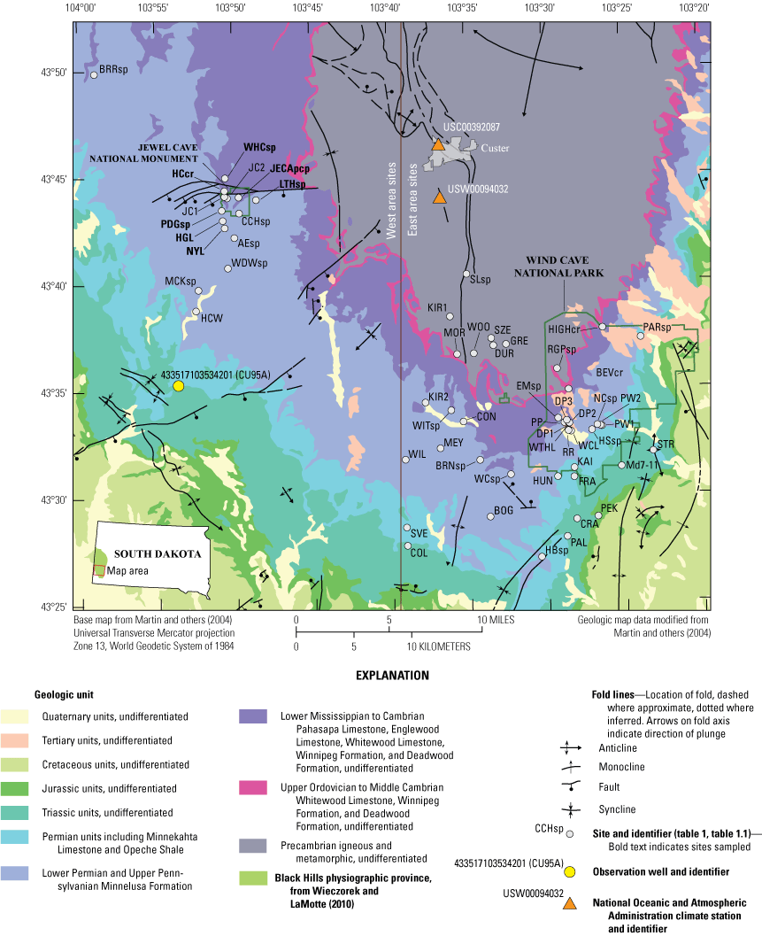
The study area with geologic units and structures from Martin and others (2004), sites where data were collected at Jewel Cave National Monument, southwestern South Dakota, and data from previous investigations included in analysis.
Jewel Cave was the first cave to be designated as a national monument in the United States in 1908 and was administered by the U.S. Forest Service until 1933 when the National Park Service (NPS) became steward (KellerLynn, 2009). Cave exploration has uncovered that Jewel Cave is currently (2022) the third longest mapped cave worldwide at 209.32 mi (NPS, 2021). Barometric pressure studies (Conn, 1966; Pflitsch and others, 2010) at the monument have indicated that Jewel Cave is much larger than what is currently mapped, and cave exploration is currently ongoing. It is estimated that more than 55 percent of the mapped cave lies outside of the monument’s boundaries (fig. 1) under the Black Hills National Forest (NPS, 2021), and future exploration may increase this number as new passageways are mapped in Jewel Cave.
In 2015, cavers exploring an unmapped part of Jewel Cave discovered the first subterranean water body (“cave lake”) that was later named Hourglass Lake. Various other cave lakes have been found at Jewel Cave since the discovery of Hourglass Lake. Cave lakes also were previously discovered at Wind Cave National Park about 20 mi southeast of Jewel Cave National Monument (fig. 1). Cave lakes in Jewel Cave and Wind Cave are considered to represent the water table of the Madison aquifer because the elevation of cave lakes in both caves was similar to the elevation of water levels in nearby wells completed in the Madison aquifer (Long and others, 2012; Long and others, 2019). Water-chemistry sampling at cave lakes in Jewel Cave and Wind Cave indicated hydraulic connection between cave lakes and regional groundwater flow in the Madison aquifer because cave lake water was chemically similar to groundwater from nearby wells completed in the Madison aquifer (Long and Valder, 2011; Long and others, 2012; Long and others, 2019).
The discovery of cave lakes at Jewel Cave added additional responsibilities and challenges for NPS staff to protect and conserve natural resources above and below the land surface. The Jewel Cave National Monument Foundation Document (NPS, 2016) identified Jewel Cave as a “fundamental resource” that “includes the entire cave system and its features, including developed, undeveloped, and as yet undiscovered areas; the cave environment itself, including air flow, water flow, temperature, and scenery; subterranean lakes; and the overlying karst landscape and its geophysical features.” Various cave lakes have been discovered in Jewel Cave, but only two lakes were sampled for water chemistry and instrumented with equipment to measure water levels. Sampling and instrumenting additional cave lakes provides additional insight on hydrogeological processes and relations among cave lakes and other water bodies. A more complete understanding of the Jewel Cave groundwater system is important for equipping NPS managers with the information to better understand and protect subsurface resources as cave discoveries continue.
Purpose and Scope
The purposes of this report are to describe data collection and analysis methods and to infer hydrogeologic characteristics of Hourglass and New Years Lakes within and near Jewel Cave National Monument, southwestern South Dakota. The approach for this study included comparing water-level data collected from Hourglass and New Years Lakes to historical climate data and applying multivariate statistical analyses to evaluate water-chemistry data collected during this study and from previous investigations. Discrete water-level measurements and continuous water-level data from March 2018 to April 2021 and October 2018 to April 2021 at Hourglass and New Years Lakes, respectively, were used in this study. Water-chemistry data from the southern Black Hills and Wind Cave National Monument (fig. 1) were included to build on findings from previous investigations and evaluate Jewel Cave within the larger context that includes both cave systems. Observations from this study were compared to findings from previous investigations and hydrogeologic models to infer hydrogeologic characteristics of Hourglass and New Years Lakes.
Previous Investigations
Previous investigations have described the geologic setting, stratigraphy, and lithologic composition of geologic units in the Black Hills area (Darton and Paige, 1925; Lisenbee and DeWitt, 1993) and have mapped the distribution of geologic structures and geologic units (fig. 1; Martin and others, 2004; Redden and DeWitt, 2008). Investigations from Carter and others (2001) and Carter and others (2003) determined the availability of groundwater in the Black Hills and estimated recharge and hydraulic properties for many of the major (regional) and minor aquifers. Dyer (1961), Deal (1962), Braddock (1963), Fagnan (2009), and Wiles (2013) have discussed the origin of Jewel Cave and the distribution of geologic units within and near Jewel Cave National Monument.
Recharge mechanisms and hydraulic properties of the Madison Limestone and Minnelusa Formation within and near Jewel Cave were investigated by Alexander and others (1989), M.E. Wiles (South Dakota School of Mines and Technology, unpub. data, 1992), and Driscoll and others (2002). Alexander and others (1989) examined recharge to Jewel Cave by conducting dye tracer tests (Wilson and others, 1986). Dye tracer tests consisted of pouring rhodamine water tracer dye in parking lots and septic systems in Jewel Cave National Monument and sampling drip sites within the cave for the presence of the dye. Dye was first recovered about 8 days after insertion, and recovery continued intermittently with variable dye concentrations throughout the yearlong study. Cave lakes were not yet discovered in Jewel Cave when dye tracer tests were conducted by Alexander and others (1989) and the drip sites where dye was recovered were at a higher elevation in the cave than at the cave lakes. M.E. Wiles (South Dakota School of Mines and Technology, unpub. data, 1992) observed that drip sites in Jewel Cave were located where an impermeable unit in the Minnelusa Formation is absent, indicating that groundwater in the Minnelusa aquifer can drain into the underlying Madison aquifer and has sufficient storage capacity to supply drip sites year-round. Driscoll and others (2002) determined the Madison and Minnelusa aquifers in the Black Hills receive appreciable recharge from streamflow losses and precipitation on the outcrops.
Other previous investigations pertaining to the scope of this study were conducted by Long and Valder (2011), Long and others (2012), Anderson and others (2019), and Long and others (2019). Long and Valder (2011) and Long and others (2012, 2019) used multivariate statistical analyses—including principal component analysis (PCA) and cluster analysis—to examine water-chemistry data collected from streams, springs, wells, and cave lakes. Water-quality data collected in various studies established baseline water quality for many sites, which included physical properties (pH, temperature, and specific conductance), major ions, arsenic, strontium, uranium, stable isotopes of oxygen and hydrogen, and radiogenic isotopes of strontium and uranium. The purpose of water-quality data collection was to better understand the newly discovered cave lakes in Jewel Cave and Wind Cave by comparing the cave-lake water to different sources of water in the Black Hills. Five hydrogeologic domains were identified by Long and others (2019) using PCA and cluster analysis and grouped based on similar water-quality characteristics. Samples from cave lakes in Jewel Cave grouped with samples from nearby Madison aquifer wells, which, combined with similar elevations between cave lakes in Jewel Cave and groundwater in nearby observation wells completed in the Madison aquifer, led Long and others (2019) to conclude that cave lakes in Jewel Cave, as well as Wind Cave, were connected to regional groundwater flow in the Madison aquifer.
Anderson and others (2019) prepared a generalized potentiometric map of the Madison aquifer near Jewel Cave National Monument based on water-level data from 24 observation wells completed in the Madison aquifer and 4 cave lakes. Previous investigations focused on preparing potentiometric surfaces of the Madison aquifer in the Black Hills (Strobel and others, 2000; McKaskey, 2013) did not use water-level data from cave lakes because these lakes had not yet been discovered. Before discovery of cave lakes in Jewel Cave, previous investigations had speculated groundwater in the cave was 50 ft below most of the known cave (NPS, 1994). Anderson and others (2019) also evaluated historical and current groundwater recharge to the Madison aquifer near Jewel Cave based on hydrographs of wells and water-level data from Hourglass Lake. While evaluating hydrograph fluctuations, Anderson and others (2019) documented statistical correlation between water levels at Hourglass Lake and cumulative daily precipitation from a nearby climate station. Correlation between water levels at Hourglass Lake and cumulative daily precipitation was attributed to recharge from precipitation on Madison Limestone outcrops. Another observation was that water levels at Hourglass Lake began increasing before cumulative daily precipitation, which was likely from early spring snowmelt contributing to recharge.
Methods of Water-Level and Water-Chemistry Data Collection
Data-collection methods for this study included (1) compiling water-level data from the NPS and previous investigations, (2) collecting water-level data from monitoring equipment in Hourglass and New Years Lakes, (3) compiling water-chemistry data within the study area from previous investigations, and (4) collecting water samples from April to August 2021. Water-level and water-chemistry data from previous investigations were downloaded from the NWIS database (USGS, 2022a). Data collected during this study included water-level measurements computed from pressure transducer (Cunningham and Schalk, 2011) data from two cave lakes and nine water samples collected from seven sampling sites in and around Jewel Cave National Monument (fig. 1; USGS, 2022a).
Water-Level Data Collection
Water-level data compiled during this study included discrete water levels measured by NPS staff and continuous water-level data measured with pressure transducers. The NPS provided the USGS with discrete water-level elevation measurements for 2 cave lakes that were collected as part of routine trips into the cave (USGS, 2022a). Water-level elevation measurements by NPS staff are performed using in-cave surveys starting from a benchmark of known elevation outside the cave. Discrete water-level measurements have been collected 11 times at Hourglass Lake by NPS staff since 2015, and 4 times at New Years Lake since 2017. Pressure transducers were installed in Hourglass Lake (HGL; USGS site 434258103504201; fig. 1) on March 11, 2018, and in New Years Lake (NYL; USGS site 434238103503501) on October 5, 2018. Water-level data from March 2018 to April 2021 were uploaded to the NWIS database (USGS, 2022a) and will be focus of analysis presented in this report.
Pressure transducers used in this study were unvented Solinst Levelogger LT F15/M5 Model 3001 electronic transducers with a manufacturer accuracy of plus or minus (±) 3 cm (0.01 ft; https://www.solinst.com/). Pressure transducers were unvented, which means that they required separate barometers to convert pressure data measured by the transducer to water-level data by compensating for atmospheric pressure. The barometers were Solinst Barologger LT F15/M5 Model 3001 electronic barometers with a manufacturer accuracy of ± 0.05 kilopascal (kPa; 0.007 pound per square inch; psi; https://www.solinst.com/). Both the pressure transducers and barometers were programmed to record continuously at 1-hour intervals at the start of each hour. NPS staff suspended the pressure transducers from cave ceilings using fishing line and submersed the transducers from 1 to 8 ft below the water surface. Barometers were placed or suspended above the water surface to prevent water damage from rising water levels. Water-level data from pressure transducers were corrected for atmospheric pressure recorded by barologgers using Levelogger Software version 4.6.1 (https://www.solinst.com/).
Continuous water-level data collected at Hourglass and New Years Lakes from 2018 to 2021 were measured using an hourly sampling rate from two transducers. Hourly pressure data measured with the transducers were converted to a height of water above the transducer by compensating for atmospheric pressure recorded by a nearby barometer. The hourly water heights were converted to relative water-level changes by subtracting each hourly measurement from the first measurement when the transducer was installed. The relative hourly water-level changes were added to the water-level elevation recorded by NPS staff when the transducer was installed to calculate water-level elevation for each hourly measurement. The accuracy of the calculated water-level elevations was evaluated by calculating the difference between the calculated water-level elevation on April 16, 2021, and water-level elevation measured by NPS on the same day when the pressure transducer was retrieved. The difference between the calculated water-level elevations on April 16, 2021 (4,694.6 ft at Hourglass and 4,617.0 ft at New Years Lake) and the NPS measured water-level elevations (4,694.5 ft at Hourglass and 4,616.9 ft at New Years Lake) was 0.1 ft. The difference was assumed to be caused by instrument drift, and a time-proportional correction was applied to the recorded water-level differences so that the estimated water elevations were within the accuracy of the discrete measurements (0.1 ft).
Major Ion and Stable Isotope Sample Collection
Water-chemistry data analyzed and presented in this report included samples from previous investigations (Long and Valder, 2011; Long and others, 2012, 2019) and samples collected as part of this study. Water-chemistry data from previous investigations were downloaded from the NWIS database (USGS, 2022a) by selecting only sites with the same chemical constituents and physical property data as the samples collected during this study, including major ions and stable isotopes of oxygen (oxygen-18, δ18O) and hydrogen (deuterium, δ2H). The list of sites with the physical properties and chemical constituents used in analysis is presented in table 1.2 in appendix 1. Sites with multiple samples were condensed by computing the mean of all available samples in the NWIS database (USGS, 2022a).
Nine water samples were collected from April to August 2021 at 7 sites and analyzed for 12 constituents (table 1). Sites sampled included one stream, three springs, two cave lakes, and one rain collector. Water samples were collected as grab samples using methods described in U.S. Geological Survey (variously dated). Sampling procedures and the constituents analyzed varied by site. Physical properties of sampled water—dissolved oxygen, pH, specific conductance, water temperature, and turbidity—were measured by USGS personnel using a multiparameter sonde (Xylem EXO1) at spring and stream sites in the field before sample collection; however, these physical properties were not measured at rain collector and cave lake sites where NPS personnel collected samples. Water samples from spring, stream, and cave lake sites were analyzed for stable isotopes and major ions. Precipitation samples from the rain collector site were analyzed for stable isotopes and not major ions because the concentration of major ions in precipitation is commonly low and predictable in small geographic areas (Rinella and Miller, 1988). Rain collectors used for precipitation sampling were “ball-in-funnel” type (Michelsen and others, 2018), installed at one site (JECApcp; USGS site 434404103494001) by USGS personnel, and fixed about 2 ft above the land surface in an unobstructed area.
Table 1.
Summary of site information, including site number, site name, short name, location, elevation, and number of samples collected within or near Jewel Cave National Monument, southwestern South Dakota, 2021.[USGS, U.S. Geological Survey; NAD 83, North American Datum of 1983; NAVD 88, North American Vertical Datum of 1988; SD, South Dakota]
All water samples were analyzed for stable isotopes δ18O and δ2H. Stable isotope samples were collected using 60-milliliter (mL) glass bottles with Polyseal caps and sent for laboratory analysis at the USGS Reston Stable Isotope Laboratory in Reston, Virginia. The laboratory methods used to determine stable isotope ratios are described by Révész and Coplen (2008a, 2008b). Samples analyzed for major ions were collected using a 125- or 250-mL polyethylene bottle rinsed and filled with a sample passed through a 0.45-micrometer pore size filter. Major ion samples were analyzed by the USGS National Water Quality Laboratory in Lakewood, Colorado, using methods described by Fishman and Friedman (1989), Fishman (1993), and Garbarino and others (2006).
Methods of Data Analysis
Data analysis methods used in this study included (1) qualitative comparison of hydrographs to climate data, (2) stable isotopic analysis through comparison with standards and among samples, (3) principal component analysis (PCA) of water-chemistry data, and (4) cluster analysis of PCA results. Hydrograph analysis included discrete water-level elevation measurements from NPS staff and continuous water-level data downloaded from the NWIS database (USGS, 2022a). Stable isotopic analysis included only data from sites within 15 mi of Jewel Cave National Monument (fig. 1) because relations among sites in and around Wind Cave National Monument were not the focus of this study and these relations were determined in previous investigations (Long and Valder, 2011; Long and others, 2012, 2019). PCA and cluster analysis included data from previous investigations (Long and Valder, 2011; Long and others, 2012, 2019) downloaded from the NWIS database (USGS, 2022a). The list of sites used in PCA and cluster analysis, including physical properties and chemical constituents, are listed in tables 1.1 and 1.2 in appendix 1.
Hydrograph Analysis
Hydrograph analysis involved comparing water-level changes among Hourglass and New Years Lakes and by comparing water-level measurements at each cave lake to climate data. Hydrographs of Hourglass and New Years Lakes were compared using continuous water-level data from October 2018 to April 2021 by calculating the elevation difference between the cave lakes and by qualitatively comparing water-level change differences among the cave lakes. Additionally, annual water-level elevation range and annual water-level change were estimated at Hourglass and New Years Lakes from 2018 to 2021 when pressure transducers were installed. Annual water-level elevation range was calculated by calculating the difference between each year’s maximum water-level elevation and minimum water-level elevation. Annual water-level change was calculated by subtracting water-level elevation on January 1 from water-level elevation on December 31 of the same year. When water-level data were not available for an entire year at Hourglass and New Years Lakes, the earliest and latest available water-level data were used instead to calculate the annual water-level change. The range of available water-level data at Hourglass Lake was from March 11, 2018, to April 16, 2021. The range of available data at New Years Lake was from March 12, 2018, to November 21, 2018, and from April 7, 2019, to April 16, 2021.
Hydrographs of Hourglass and New Years Lakes also were compared to precipitation and snow depth data obtained from the Custer, S.D. (USC00392087) and Custer County Airport, S.D. US (USW00094032) National Oceanic and Atmospheric Administration (NOAA) climate stations (fig. 1; NOAA, 2021a, 2021b). Daily observations from the Custer County Airport, S.D. US (USW00094032) climate station were substituted for missing daily observation data at the Custer, S.D. (USC00392087) climate station to provide a more complete dataset. Daily precipitation observations from Custer, S.D. (USC00392087) were cumulatively summed for each calendar year from 2015 to 2021 and were compared to annual normal precipitation totals from 1991 to 2020 at the Custer, S.D. climate station. Climate normals are means of climatological measurements spanning three decades and include temperature, precipitation, snowfall, and other measurements (NOAA, 2022). Daily snow depth observations were obtained from the Custer, S.D. (USC00392087) and were used to evaluate the effect of winter and spring snowmelt on water levels.
A separate analysis involved obtaining monthly precipitation observations from 2015 to 2021 to evaluate how each month from 2015 to 2021 compared to monthly normal precipitation totals from 1991 to 2020 (NOAA, 2021b). Monthly precipitation observations were obtained from the Custer, S.D. climate station, except where missing data from the Custer, S.D. climate station had to be supplemented with data obtained from the Custer Co Airport, S.D. US (USW00094032) climate station (fig. 1; NOAA, 2021a). Monthly normal precipitation from 1991 to 2020 were obtained from the Custer, S.D. climate station (NOAA, 2021b). The difference between monthly observations and monthly normals (departure from normal value) and the cumulative monthly difference (cumulative departure from normal) are plotted in figure 2.
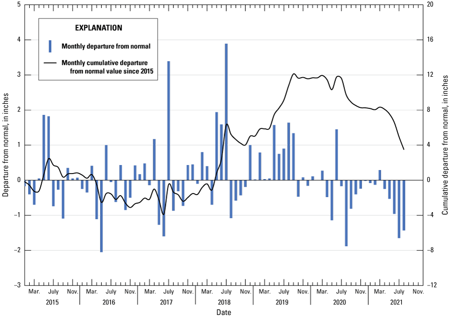
Monthly departure and cumulative departures from normal for precipitation from 2015 to 2021 from the Custer, S.D. (USC00392087) and Custer County Airport, S.D. US (USW00094032) climate stations. See figure 1 for station locations.
Stable Isotopic Analysis
Hydrogeological studies commonly use stable isotopes of abundant elements that are present naturally in the environment, such as hydrogen, carbon, or oxygen, to estimate water age, recharge processes, and groundwater-flow paths. Stable isotopes of hydrogen and oxygen are used as flow-path tracers because these isotopes are found naturally in groundwater, and meteoric weather processes can modify their composition (Clark and Fritz, 1997). Stable isotope analysis of a water sample compares ratios of heavier to lighter isotopes to a standard isotope ratio of known composition (Clark and Fritz, 1997). The result is reported in delta (δ) notation in parts per thousand (‰) calculated using equation 1 (Kendall and Caldwell, 1998):
whereA positive value of δ indicates the sampled isotope ratio is higher than the standard, and a negative value of δ indicates the sampled ratio is lower than the standard (Kendall and Caldwell, 1998). Stable isotope ratios of oxygen (18O/16O) and hydrogen (2H/1H) were measured for water samples collected at one stream, three springs, two cave lakes, and one rain collector for this study. Stable isotope data were converted to δ notation using equation 1 and the Vienna Standard Mean Ocean Water and Standard Light Antarctic Precipitation standards (Révész and Coplen, 2008a, 2008b). The notations δ18O and δ2H are used in this report to describe the ratios of heavy to light isotopes of oxygen and hydrogen, respectively.
The δ18O and δ2H data from this study and data from previous investigations in and around Jewel Cave (“West area” sites in table 1.1; fig. 1) were plotted based on a method described by Muir and Coplen (1981). The global meteoric water line (GMWL) from Craig (1961) was plotted with the sample data to compare the stable isotopic composition of samples to the global stable isotopic composition of precipitation. Stable isotope ratios of local precipitation samples deviated from the GMWL and were plotted as the local meteoric water line (LMWL). Linear regression was used to determine a LMWL by relating δ2H to δ18O for precipitation samples. Stable isotope samples were plotted in stable isotope plots. No samples were enriched (positive δ2H and δ18O values) relative to the standards used to calculate stable isotopes ratios—indicated by all samples plotting below the origin on stable isotope plots (fig. 3); however, some samples plotted closer to the origin than other samples. Samples plotting closer to the origin in stable isotope plots are heavier (more enriched in heavy isotopes) than samples with more negative δ18O and δ2H values (lighter—more depleted in heavy isotopes) that plot further below the origin (fig. 3).
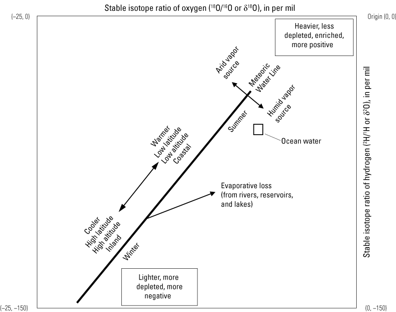
Schematic of the effects of hydrologic processes on the oxygen and hydrogen isotopic composition of water. Modified from Medler and Eldridge (2021) and University of Arizona (2020).
Ocean waters are considered to have heavy stable isotope compositions, and as precipitation that originates from ocean evaporation moves inland, it becomes lighter in isotopes as the heavier isotopes preferentially fall to the surface during rainfall (USGS, 2004). Generally, summer rains are heavier (more positive) than lighter winter rains (more negative). Similarly, precipitation from cooler, high latitude, high altitude, and inland sources is lighter than precipitation from warmer, low latitude, low altitude, coastal areas (University of Arizona, 2020). Shallow groundwater stable isotope values are similar to precipitation values, but evaporation, transpiration, and fractionation may alter the stable isotope ratios as the water moves downward toward the saturation zone (USGS, 2004). Additionally, evaporative loss from rivers, reservoirs, and lakes changes the isotopic composition of water, causing it to become heavier (University of Arizona, 2020).
Principal Component Analysis
PCA is a multivariate technique that tests for linear relations among variables in a dataset (Helsel and others, 2020). The PCA technique is performed by linearly transforming the original dataset into new axes, called principal components, that are linear combinations of all the input variables. The principal components responsible for the most variance—principal components one and two—are used to plot multidimensional data in two dimensions so data patterns, clusters, and groupings can be observed and interpreted (Long and Valder, 2011). Additional details and mathematical derivations of PCA are provided in Davis (2002). Python programming language (Rossum and Drake, 2011) was used to implement the PCA technique.
The PCA technique was performed using physical property and chemical constituent data collected for this study and from previous investigations (Long and Valder, 2011; Long and others, 2012, 2019). Data from previous investigations were downloaded from the USGS NWIS database (USGS, 2022a). Additional sites from other investigations assisted in the interpretation of relations among sites within a larger area in the southern Black Hills and improved PCA analysis by increasing the number of observations that have been found to produce a more stable result (MacCallum and others, 1999). Water-chemistry data from other studies were collected from streams, springs, wells, and cave lakes in the southern Black Hills near Jewel Cave National Monument and Wind Cave National Park (fig. 1). Aquifers for groundwater sites were designated in the USGS NWIS database and included the White River, Minnelusa, Madison, and undifferentiated Precambrian igneous and metamorphic aquifers. The naming convention of sites shared between this analysis and that of Long and others (2019) were kept the same for consistency. Sites sampled as part of this study not included (New Years Lake; Hell Canyon Creek) in the analysis by Long and others (2019) adhered to a similar naming convention given in tables 1 and 1.1. Additionally, similar to Long and others (2019), all sites east of the WIL site (south-central area of fig. 1) are referred to as the “East area,” whereas all sites west of the WIL site are referred to as the “West area.”
The number of variables used in PCA analysis was limited to physical property and chemical constituent data shared by all datasets (previously collected data and new data collected during this study) and included specific conductance, pH, carbon dioxide (CO2), hardness (as CaCO3), calcium (Ca), magnesium (Mg), sodium (Na), chloride (Cl), sulfate (SO4), silica (Si), arsenic (As), δ2H, and δ18O. Sites excluding any of the aforementioned physical properties and chemical constituents were excluded from PCA analysis because the method does not allow for missing values. Physical property and chemical constituent data were normalized, by setting the mean of each variable to zero, and standardized, by setting the standard deviation of each variable to one, before performing PCA to ensure that the distribution of the dataset was independent of measurement units (Davis, 2002).
Water-chemistry data were compiled for 63 total sites in the study area. The mean of each potential variable was computed for sites with more than one sample to reduce the effect of repeat samples on the PCA results. Additionally, the water-chemistry data for the 63 sites were inspected for outliers and certain physical properties and chemical constituents that could affect PCA results. Sites were excluded from PCA if chloride and sulfate concentrations exceeded 100 and 350 milligrams per liter, respectively, to avoid including treated groundwater from wells and sites with elevated ion concentrations from road salts. A total of 8 sites were removed based on the specified criteria, including Prairie Dog Spring (PDGsp) and four other sites from Long and others (2012). Long and others (2019) noticed that PDGsp was elevated by road salts applied during winter. The sodium and percent sodium variables were removed because they explained less than 1 percent of variance in the dataset. In total, 55 observations and 12 variables were used in the PCA analysis (table 1.2).
Principal component biplots were created to visualize the results on principal component axes one and two. Biplots are PCA plots with vectors, called loading lines that relate variance and correlation of the variables. Variance is represented by the magnitude of the vector, with larger vectors indicating larger variance, whereas correlation is represented by the direction of the vector, with opposite direction vectors indicating negative correlation (Jolliffe, 2002). Individual data points that plot close to loading lines have above-mean values for that loading line variable; conversely, data points that plot opposite of loading lines have lower than normal values for that loading line variable (Jolliffe, 2002).
Cluster Analysis
Cluster analysis is a method of assigning data points to groups, called clusters, based on similarities (Long and Valder, 2011). The cluster analysis method selected for this study was the k-means procedure because of its simplicity and frequent use in hydrological studies (Long and Valder, 2011; Masoud, 2014; Marín Celestino and others, 2018). The k-means procedure involves iteratively finding the minimum Euclidean distance between a manually selected number of cluster centroids, k, and an observation, n (Davis, 2002). Iterations continue until the location of each k is optimized and every observation is assigned to a specific cluster.
In this study, the k-means procedure was used to determine clusters for the PCA results of water-chemistry data collected during this study and from Long and others (2012, 2019). The purpose of using the k-means procedure was to statistically group sampling sites without introducing statistical bias, such as site type or spatial location. The number of clusters for the k-means procedure was determined using scree plots (Jolliffe, 2002). Scree plots are developed by plotting the number of cluster groups in numerical order (x-axis) against their respective sum of squared distances of samples to the nearest cluster centroid (y-axis). The optimal number of clusters from the k-means procedure can be determined by observing the “break point” in scree plots. The “break point” is the sharp change in slope (steep to nearly flat) of the scree plot curve that marks where increasing the number of clusters is no longer beneficial to the k-means procedure. After selecting the number of clusters, the k-means procedure was computed using 10 runs at 300 iterations per run (a total of 3,000 iterations) for data plotted in principal component axes one and two. The k-means procedure settings were chosen because the cluster results did not improve with increased runs and iterations. The Python programming language (Rossum and Drake, 2011) was used to perform the k-means procedure in this study.
Analysis of Water-Level Data
Water-level data were analyzed by (1) comparing hydrographs of Hourglass and New Years Lakes and (2) interpreting water-level changes from Hourglass and New Years Lakes compared to precipitation and snow depth data from the nearby USC00392087 and USW00094032 climate stations (fig. 1). Cave lake hydrographs were compared to precipitation and snowfall data to build on observations from Anderson and others (2019) at Hourglass Lake and describe new observations at New Years Lake. Anderson and others (2019) observed a 41-day delay between water-level increases at Hourglass Lake and increasing cumulative precipitation. The 41-day delay was confirmed using new data collected during this study and the delay was attributed to time required for recharged water from direct infiltration of precipitation and (or) streamflow losses on outcrops of the Madison aquifer to reach cave lakes. Water-level data from Hourglass and New Years Lakes can be accessed using the USGS NWIS database (USGS, 2022a).
Hydrograph Comparisons and Annual Water-Level Observations of Hourglass and New Years Lakes
Hydrographs of Hourglass and New Years Lakes are shown in figure 4 and include discrete and continuous water-level data. The water-level elevation of Hourglass Lake was consistently higher than New Years Lake (fig. 4) as expected because Hourglass Lake is in a higher elevation part of Jewel Cave. The elevation difference between Hourglass and New Years Lakes ranged from 61 to 93.5 ft, with mean and median differences of 70 and 71 ft, respectively. The range of elevation difference (32.5 ft) and water-level change dissimilarities between hydrographs of Hourglass and New Years Lakes (fig. 4) were unexpected because the lakes are separated by about 0.4 mi at the land surface and are within the same geologic formation. Hourglass Lake displayed small, gradual water-level changes with elevations ranging from 4,684.3 to 4,695.2 ft (an elevation range of 10.9 ft) from October 2015 to April 2021. New Years Lake displayed relatively large and rapid water-level changes (compared to Hourglass Lake) with elevations ranging from 4,590.9 to 4,629.5 ft (an elevation range of 38.6 ft) from January 2017 to April 2021 (fig. 4). The larger elevation range at New Years Lake—combined with its relatively more dynamic water level increases and decreases—varied the elevation difference between New Years and Hourglass Lakes.
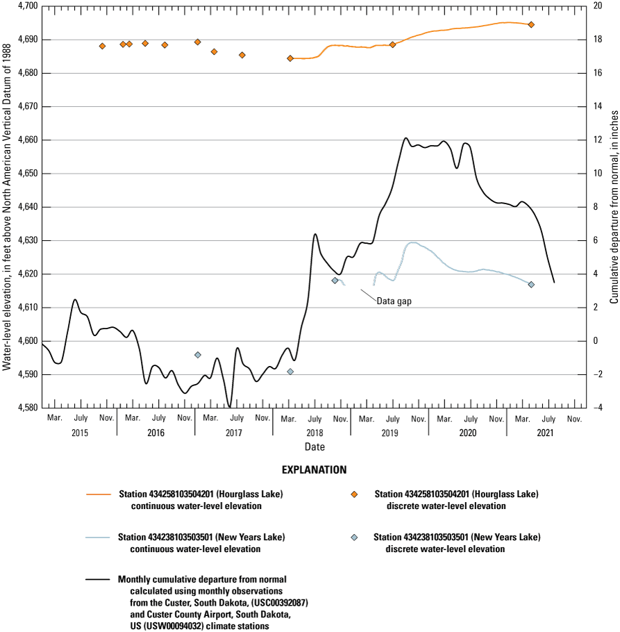
Water-level elevation hydrographs for Hourglass and New Years Cave Lakes, Jewel Cave National Monument, southwestern South Dakota, including discrete and continuous water-level measurements plotted with monthly cumulative departure from normal from the Custer, S.D. (USC00392087) and Custer County Airport, S.D. US (USW00094032) climate stations. See figure 1 for station locations.
At Hourglass Lake, annual water-level elevation ranges were 4.1 and 4.8 ft in 2018 and 2019, respectively, and decreased to 2.7 and 0.6 ft in 2020 and 2021, respectively (table 2). New Years Lake displayed a similar trend where water-level elevation ranges were largest in 2018 (27.5 ft) and 2019 (12.8 ft) and smallest in 2020 (7.1 ft) and 2021 (2.8 ft; table 2); however, annual water-level elevation ranges at New Years Lake were between 2.6 and 6.7 times greater than Hourglass Lake (table 2). Annual water-level changes at Hourglass Lake showed the overall water level increased from 2018 to 2020 (table 2; fig. 4). In 2021, water levels decreased by 0.6 ft at Hourglass Lake (table 2). Annual water-level changes at New Years Lake were similar to Hourglass Lake where water levels increased in 2018 and 2019 and decreased in 2021, except water levels decreased in 2020 at New Years Lake (table 2). Additionally, annual water-level changes at New Years Lake were between 2.3 and 7.4 times greater than Hourglass Lake (table 2).
Table 2.
Water-level elevation range and annual water-level change from 2018 to 2021 when pressure transducers were installed in Hourglass Lake and New Years Lake, Jewel Cave National Monument, southwestern South Dakota.[NAVD 88, North American Vertical Datum of 1988; NPS, National Park Service]
Calculated by subtracting the minimum water-level elevation from the maximum water-level elevation for each year.
Calculated by subtracting the water-level elevation on December 31 by the water-level elevation of January 1 of each year. Positive values indicate the water level increased and negative values indicate the water level decreased.
Hourglass Lake Hydrograph Compared to Precipitation and Snow Depth
Discrete water-level measurements at Hourglass Lake from mid October 2015 to late December 2016 were compared to precipitation and snow depth datasets to explain water-level changes (fig. 5). Discrete water-level measurements could not be interpreted on a monthly basis with precipitation and snow depth datasets because the measurements were separated by 1 to 22 months; however, some annual interpretations were made using the available data. Annual precipitation in 2015 (21.48 in.) was slightly greater than annual normal precipitation (20.66 in; fig. 5), and cumulative departure from normal, as shown in figure 2, indicates above normal precipitation conditions (wet) until April 2016. The water level of Hourglass Lake increased by 0.8 ft from mid October 2015 to late April 2016 during wet conditions. Annual precipitation in 2016 (17.13 in.) was about 3 in. below annual normal precipitation (fig. 5), and cumulative departure from normal, as shown in figure 2, indicates below normal precipitation conditions (dry) starting in April 2016 and continuing through December 2016. The water level of Hourglass Lake decreased by 0.5 ft from late April to late July 2016 during dry conditions; however, the water level increased by 0.9 ft from late July to late December 2016 while still under dry conditions. The water-level increase from July to December 2016 could result from snowmelt in December; daily snow depth data from December 2016 (fig. 5; NOAA, 2021a) indicated snow accumulations of 6.0 in. and 7.0 in. from two snowfall events that gradually melted in the 2-week period before the December 2016 water-level measurement—indicated by the decreasing snowpack during that time (fig. 5).
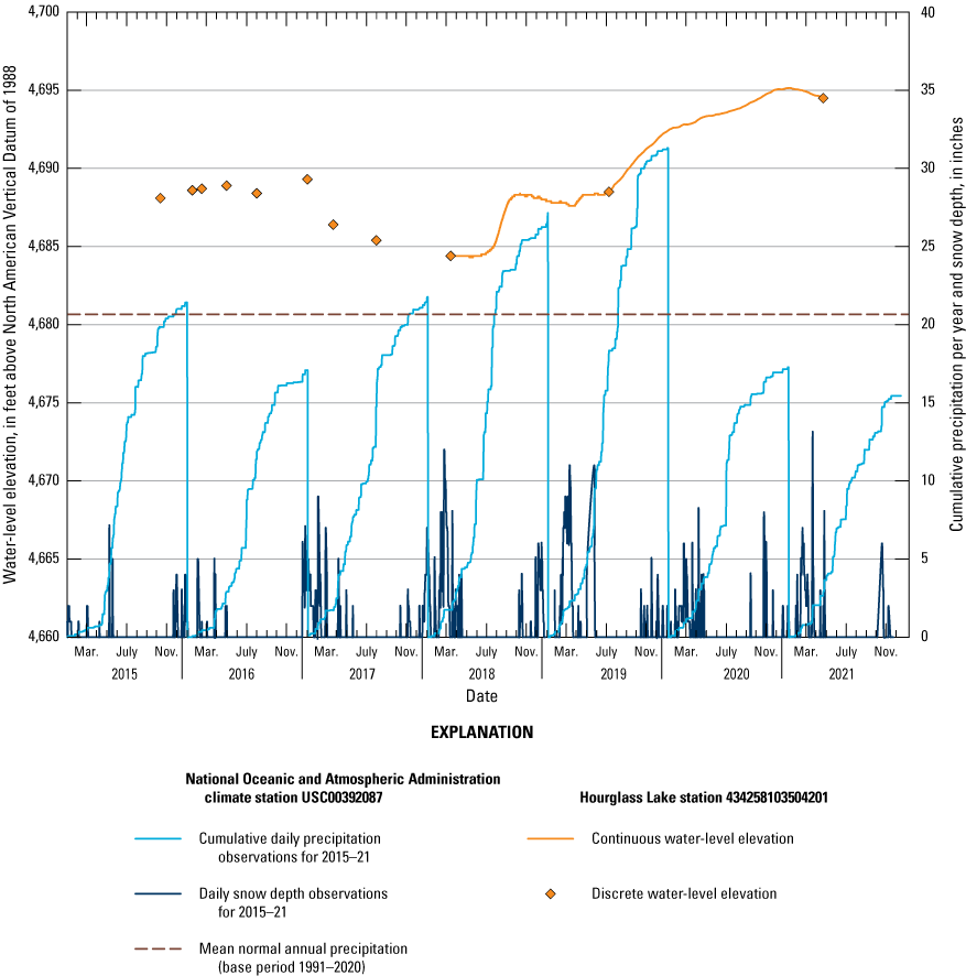
Water-level elevation hydrograph for Hourglass Lake, Jewel Cave National Monument, southwestern South Dakota, including discrete and continuous water-level measurements plotted with cumulative annual precipitation and snow depth. See figure 1 for station locations.
In 2017, discrete water-level measurements indicated water levels in Hourglass Lake were decreasing despite above normal annual precipitation (21.83 in.; fig. 5). Six months in 2017 were above normal with the largest departures from normal in July (3.39 in.), June (−1.60 in.), and May (−1.27 in.; fig. 2). Cumulative departure from normal remained negative for the early part of 2017, and the water level at Hourglass Lake correspondingly decreased during the same time. Decreasing water levels continued until March 2018 (fig. 5) while monthly precipitation was above normal for all but 1 month (January 2018) from November 2017 to March 2018 (fig. 2). Cumulative departure from normal (fig. 2) indicates the period of above normal precipitation from November 2017 to March 2018 only slightly increased the cumulative total because the departures from normal were less than 0.5 in. for all but 1 month (0.8 in. in February 2018; fig. 2).
After installing a pressure transducer in March 2018 in Hourglass Lake, the water level was relatively constant until mid-June 2018 when the water level increased by 4.1 ft and peaked in late September 2018 (fig. 5). Increasing water levels at Hourglass Lake likely resulted from a combination of spring snowmelt (fig. 5) followed by above normal spring and early summer precipitation in 2018 (fig. 2). Above normal precipitation fell in February and March 2018 as a mixture of snow and rain (figs. 3 and 5). The longest period of snowpack was from February 4, 2018, to March 8, 2018, where depths ranged from 1.0 in. to 12.0 in. (fig. 5; NOAA, 2021a). Various other snowfall events resulted in March and April 2018, but the snow melted completely within 1 week after each event (fig. 5; NOAA, 2021a). Precipitation in April 2018 was below normal but was followed by above normal precipitation for 3 consecutive months (fig. 2). Cumulative departure from normal shown in figure 2 increased from −1.12 in. below normal in April 2018 to 6.30 in. above normal in July 2018—meaning that from May to July 2018, 7.42 in. more precipitation fell than normal. Additionally, the largest increase in cumulative annual precipitation for 2018 (fig. 5) was from early April 2018 to August 2018; precipitation totaled 20.42 in. from April to August 2018—or about 75 percent of the annual total precipitation of 2018 (27.19 in.; NOAA, 2021a) and 99 percent of the annual normal precipitation (20.66 in.; NOAA, 2021b).
Water-level changes in Hourglass Lake from late September 2018 to late June 2019 were evaluated using precipitation and snow depth datasets. Dry conditions from August 2018 to November 2018—shown by decreasing cumulative departure from normal in figure 2—initially caused the 0.7 ft water-level decline in Hourglass Lake from late September 2018 to late March 2019 (fig. 5); however, water levels continued declining despite above normal precipitation from December 2018 to March 2019 (fig. 2). Continued decline of water levels until March 2019 correlated with cumulative departure from normal indicated in figure 2; the increase in cumulative departure from normal from November 2018 to March 2019 was smaller than the decrease in cumulative departure from normal from July to November 2018—indicating that the overall cumulative departure from normal from July 2018 to March 2019 was below normal. Additionally, precipitation falling in February and March 2018 may not have affected water levels in Hourglass Lake because low temperatures prevented snow melt from February 6, 2019, to March 17, 2019, with snow depths ranging from 1.0 to 11.0 in. (fig. 5). Increasing temperatures in March 2019 began melting snow accumulations from February 2019 and shortly after water levels in Hourglass Lake increased by 0.7 ft until mid-April 2019 (fig. 5). Water levels in Hourglass Lake remained relatively constant from mid-April to late June 2019 (fig. 5) as precipitation was 0.03 and 0.05 in. above normal in March and April 2019, respectively (fig. 2).
Water levels in Hourglass Lake increased by 6.9 ft from late June 2019 to early January 2021 (fig. 5) in response to above normal precipitation from May to December 2019 (fig. 2). Cumulative departure from normal indicated in figure 2 peaked in September 2019 after increasing by 6.2 in. from unusually high summer (May–September) precipitation. Cumulative departure from normal remained above normal and water levels in Hourglass Lake increased despite relatively dry conditions from October to December 2019 (figs. 3 and 5). The effect of dry conditions in fall and winter 2019 was observed when the rate of water-level increase slowed beginning in mid-January 2020 (fig. 5). Annual precipitation in 2020 (17.32 in.) was 3.3 in. lower than annual normal precipitation (20.66 in.); however, water levels in Hourglass Lake increased in 2020 at the slower rate of water-level increase until peaking in January 2021. The rate of water-level increase in 2020 varied slightly (fig. 5). These increases likely resulted from winter or spring snowmelt (increasing rate) and dry summer or fall conditions in 2020 (decreasing rate; fig. 2).
Water levels in Hourglass Lake decreased by 0.7 ft from early January 2021 to mid-April 2021 (fig. 5). Dry conditions from late 2020 continued in 2021 and likely caused water levels in Hourglass Lake to decline. Additionally, the water level at Hourglass Lake did not increase from spring snowmelt in March or April 2021, similar to the increase in previous years. Snow depth data from fall 2020 and winter 2021 show more temporally dispersed snowfall events and a smaller winter snowpack in February and March 2021 that melted completely by early March 2021 (fig. 5). As of November 2021, the annual precipitation of 2021 (13.57 in.) was 7.1 in. below annual normal precipitation. Additionally, cumulative departure from normal indicated in figure 2 decreased by 3.6 in. from July 2020 to February 2021.
New Years Lake Hydrograph Compared to Precipitation and Snow Depth
The New Years Lake hydrograph was compared to the same precipitation and snow depth datasets as the Hourglass Lake hydrograph described in the previous section to evaluate water-level changes (fig. 6). Water levels in New Years Lake declined by 5.0 ft from January 2017 to March 2018 despite above normal precipitation in 2017 (21.83 in.; fig. 6) and increasing cumulative departure from normal from January 2017 to March 2018 (fig. 2). The 5.0 ft water-level decline likely was caused by a deficit in precipitation, as indicated in figure 2, when cumulative departure from normal fell below 0 in April 2016 and remained negative throughout 2017 and early 2018. The precipitation deficit from January 1, 2016, to December 31, 2017, was calculated by first determining the annual departure from normal (difference between cumulative annual precipitation and annual normal precipitation) for 2016 and 2017, and second calculating the difference between annual departure from normal for 2016 (3.53 in. below normal) and 2017 (1.77 in. above normal; fig. 2). The precipitation deficit was 1.76 in. below normal from January 1, 2016, to December 31, 2017.
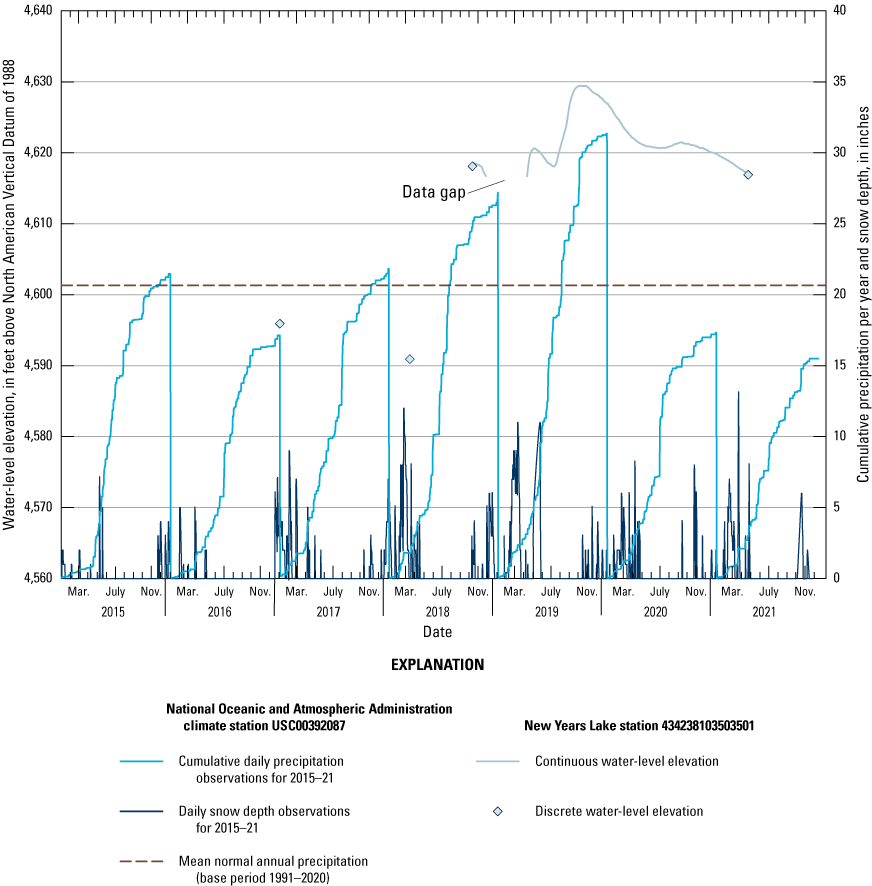
Water-level elevation hydrographs for New Years Lake, Jewel Cave National Monument, southwestern, South Dakota, including discrete and continuous water-level measurements plotted with cumulative annual precipitation and snow depth. See figure 1 for station locations.
The water level of New Years Lake increased by 27.5 ft from March 2018 to October 2018 during a period of above normal precipitation (fig. 6). Annual precipitation in 2018 (27.19 in.) was 6.53 in. greater than annual normal precipitation (20.66 in.; fig. 2). Additionally, precipitation from May to July 2018 was 7.42 in. greater than normal (fig. 2). The water level of New Years Lake likely began increasing soon after spring snowmelt in March or April 2018 and continued increasing from May to July 2018 during above normal precipitation (fig. 2). A pressure transducer was installed in New Years Lake on October 7, 2018, shortly before a water-level elevation peak on October 14, 2018 (fig. 6). The largest water-level elevation peak in 2018 may have been during the above normal precipitation period from May to July 2018 rather than on October 14, 2018; however, no water-level data were collected between March 12, 2018, and October 6, 2018, to confirm a larger water-level peak before October 14, 2018. Water levels in New Years Lake declined after October 14, 2018, during a period of below normal precipitation from August to November 2018 (fig. 2) until the water level decreased below the level of the transducer on November 21, 2018, and no data were recorded (fig. 6). The transducer in New Years Lake began recording water levels again beginning on April 7, 2019.
Water levels in New Years Lake began increasing sometime before April 7, 2019, and the increase likely coincided with spring snowmelt. Departure from normal monthly precipitation (fig. 2) indicates that 0.79 in. more precipitation fell in February 2019 than normal in the form of snowfall that accumulated until mid-March 2019 (fig. 6). Snow depth data (fig. 6) indicated a relatively large snowpack starting in February 2019 and fully melted by mid-March 2019. The water level of New Years Lake peaked in early May 2019, and soon after the water level decreased by 2.5 ft until early July 2019 (fig. 6), despite above normal precipitation falling in the area from March to June 2019 (fig. 2). Departure from normal was less than 0.05 in. for March and April 2019 and as a result cumulative departure from normal showed minimal increase from March and April 2019 (fig. 2). Water-level decline at New Years Lake from May to July could result from the return to normal precipitation conditions following above normal conditions; water released by melting of above normal winter snowfall falling over a relatively short time (1–2 months) compared to sporadic near normal precipitation in March and April 2019 (fig. 6).
The water level of New Years Lake fluctuated in response to climate-related events from July 2019 to August 2020. The water level of New Years Lake increased by 11.3 ft from early July 2019 to early October 2019 (fig. 6). Annual precipitation in 2019 was 10.73 in. above annual normal precipitation and cumulative departure from normal (fig. 2) increased from 5.91 in. above normal in April 2019 to 12.11 in. above normal in September 2018, indicating that 6.2 in. more precipitation fell in May to September 2018 than normal. The water level of New Years Lake increased in response to above normal summer precipitation in 2019 until peaking in early October 2019 (fig. 6). The water-level peak in early October 2019 was followed by a water-level decline that persisted until early July 2020 (fig. 6); however, the rate of water-level decline fluctuated in response to precipitation. The first noticeable change in the rate of water-level decline was in January 2020 when the rate of decline increased after 3 months of near or below normal precipitation (fig. 2). The next noticeable water-level change was in March 2020 when the rate of water-level decline decreased—likely in response to spring snowmelt in February and March 2020—and continued decreasing until early July 2020 (fig. 6). The water level of New Years Lake increased by 0.7 ft from early July to late August 2020 (fig. 6) after above normal precipitation in June 2020 and near normal precipitation in July 2020 (fig. 2). Additionally, the start of water-level increase in early July 2020 was less than 1 week after the last week of June 2020 where a total of 4.2 in. of rainfall fell (fig. 6). This total is 0.77 in. greater than the monthly normal precipitation measured in June 2020 (3.43 in.) and about 24 percent of the annual precipitation in 2020 (17.32 in.; fig. 6).
The water level of New Years Lake decreased from August 2020 to April 2021 during dry conditions (fig. 6). Annual precipitation in 2020 and 2021 were below annual normal precipitation (fig. 6), and departure from normal (fig. 2) indicated below normal precipitation for all but one month (March 2021) from July 2020 to April 2021. The period of below normal precipitation from July 2020 to April 2021 resulted in decreasing water levels in New Years Lake and, unlike previous years, the effect of spring snowmelt did not affect water levels in spring 2021 (fig. 6); however, the effects of spring snowmelt on water levels in New Years Lake may be after the last recorded water-level measurement on April 16, 2021.
Analysis of Water-Chemistry Data
Analysis of water-chemistry data was split into three sections for results of stable isotope analysis, PCA, and cluster analysis. Each section discusses observations from data analysis that provided insight on the hydrogeologic characteristics of the Madison Limestone and Minnelusa Formation. Hydrogeologic characteristics were evaluated mostly for sites within and near Jewel Cave National Monument because it was the primary focus of this report; however, observations from data analysis for sites within and near Wind Cave National Park were discussed for comparison with sites within and near Jewel Cave National Monument and to build on previous findings from previous investigations (Long and others, 2012, 2019).
Stable Isotopic Analysis
Stable isotope results were analyzed by (1) creating a local meteoric water line (LMWL) from precipitation samples collected during this study, (2) comparing stable isotope values from the study area to global meteoric values established by Craig (1961), and (3) comparing stable isotope values among sites to evaluate possible recharge characteristics.
Comparison with Global Meteoric Waters
The δ2H and δ18O values from samples collected during this study and other investigations (Long and others, 2012, 2019) were plotted with the global meteoric water line (GMWL) defined by Craig (1961; fig. 7). All samples plotted below the GMWL; therefore, a LMWL was calculated for the study area (fig. 7). The LMWL for the study area from samples collected in June 2021 is given in the equation below as
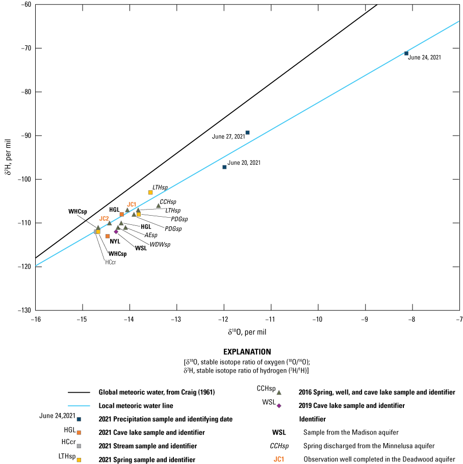
Stable isotope plot of water samples collected during this study and water samples collected by Long and others (2012, 2019) in Jewel Cave National Monument, southwestern South Dakota. See figure 1 for station locations. See tables 1.1 and 1.2 for site identifier description and stable isotope data used in analysis.
The slope and y-intercept of the LMWL were less than the GMWL and as a result the LMWL plotted below the GMWL (fig. 7). Putman and others (2019) observed the LMWL at arid and snowy sites, similar to the study area, often displayed higher slopes and intercepts relative to the GMWL. The deviation from trends observed by Putman and others (2019) may result from the LMWL not accurately representing the δ2H and δ18O values of precipitation in the study area. The natural variation of δ2H and δ18O values in precipitation likely was not captured from the three precipitation samples collected during this study because all three samples were collected during the same month and year (June 2021). Putman and others (2019) also discussed the sensitivity of developing a LMWL and determined the length of record needed to calculate a LMWL depended on the timescale of the processes of interest, such as recharge to an aquifer. Therefore, the LMWL for the study area likely is not an accurate representation of the average δ2H and δ18O values of precipitation in the study area; however, the LMWL may be useful for comparison of samples from other sites with precipitation samples collected during the same time period.
All stable isotope samples were depleted in heavy isotopes compared with the GMWL (more negative δ2H and δ18O values) and indicated a greater degree of evaporation from environmental factors, such as latitude, continental position (near coasts versus far inland), and altitude (Dansgaard, 1964; Rozanski and others, 1993). Medler and Eldridge (2021) provide a summary of the effect of latitude, continental position, and altitude on isotopic composition of precipitation. The most notable effects on the δ2H and δ18O compositions in the study area were from the latitude and continental effects because the study area is at a high latitude (between 43- and 44-degrees north latitude) and near the center of the North American continent. The great distance from low latitudes and coastlines to the study area (hundreds of miles) likely resulted in greater depletion of heavy isotopes for precipitation samples relative to studies at low latitudes or closer to coastlines (Dansgaard, 1964; Gat and Gonfiantini, 1981). The altitude effect was not observed for samples in the study area likely because the altitude difference among all sampled sites is only about 400 ft (table 1).
Streams, Wells, and Cave Lakes
Samples from one stream, two wells, and three cave lakes plotted either on or below the LMWL (fig. 7) and indicated generally greater depletion (more negative values) of heavy isotopes relative to precipitation and some spring samples. The Hell Canyon Creek (HCcr) sample from 2021 displayed the greatest depletion in heavy isotopes of all samples (fig. 7) and was considered anomalous because precipitation, generally enriched in heavy isotopes, was expected to increase the concentration of heavy isotopes in the stream. Springflow from West Hell Canyon Spring (WHCsp) is from the Madison aquifer and groundwater flows directly into HCcr upstream of the HCcr sampling site (fig. 1). Discharge from the Madison aquifer at WHCsp (fig. 7) appears to strongly affect the isotopic composition of HCcr. Samples from wells completed in the Deadwood aquifer (JC1 and JC2) in 2016 plotted close to the LMWL and had varying stable isotopic composition (fig. 7). Jewel Cave well 2 (JC2) was more depleted than Jewel Cave well 1 (JC1) despite the wells being less than 1,000 ft apart and both samples collected on the same day in 2016 (fig. 7). The stable isotopic composition difference between groundwater samples from the two wells completed in the Deadwood aquifer (JC1 and JC2) was not further examined because it was not the focus of this study. Samples from cave lakes—Hourglass, New Years, and Wellspring Lakes—had intermediate stable isotopic composition and were depleted and enriched compared to precipitation samples and samples from HCcr and WHCsp, respectively (fig. 7).
The depleted δ2H and δ18O values of groundwater samples—combined with the stable isotopic variation among samples from the same aquifer—in the stable isotope plot of the study area (fig. 7) provided insight on recharge mechanisms. Groundwater samples from the Deadwood aquifer (JC1 and JC2) and Madison aquifer (HGL, NYL, WSL, and WHCsp) were depleted in heavy isotopes compared to precipitation samples. Evaporation cannot explain the depleted groundwater samples because evaporation preferentially removes lighter isotopes and leaves behind heavier isotopes (Rozanski and others, 1993). Isotopic compositions typically do not change after precipitation has infiltrated into the ground (Gat, 1971; Naus and others, 2001); therefore, some other source or process was responsible for the depleted groundwater samples.
Gat (1971) provided four explanations that could account for groundwater samples being depleted in heavy isotopes. The first explanation is both aquifers contain large fractions of older water from past climates characterized by colder temperatures and snow containing lighter, more depleted waters, similar to the isotopic composition of snow and ice from modern Arctic and Antarctic environments (Gat, 1971; Rozanski and others, 1993). Age dating of water from the Madison aquifer using tritium (Naus and others, 2001; Rahn, 2018) indicated groundwater near recharge sources is newer and more like modern precipitation, whereas groundwater at greater distances from recharge areas is older and more like past precipitation. The second explanation is heavy rainfall, which generally is depleted in heavy isotopes, provides recharge to aquifers in the study area. The study area typically does not receive steady heavy rainfall; however, Vogel and Van Urk (1975) and Rehm and others (1982) determined that heavy rainfall was an important source of recharge for aquifers in semiarid regions. The third explanation is that snowfall and snowmelt are primary recharge sources for aquifers. Tian and others (2018) observed depleted δ2H and δ18O values in snowfall relative to spring, summer, and fall precipitation. The fourth explanation is that recharge resulted at a higher elevation where heavy isotopes are often more depleted than at lower elevations. Less than 10 mi from the study area the elevation increases to more than 7,000 ft above NGVD 88.
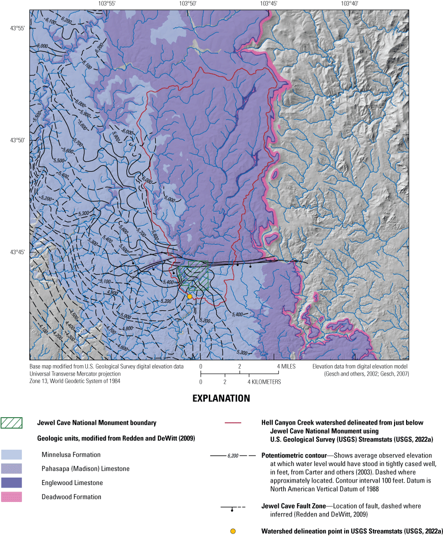
The first explanation from Gat (1971) likely does not apply to the Madison aquifer in the study area because Jewel Cave is near the recharge area for the Madison aquifer and karstic aquifers, such as the Madison aquifer, usually can be recharged quickly. All samples plot near the LMWL, and recharge areas (outcrops of Madison Limestone shown in figure 8; Redden and DeWitt, 2008) for the aquifer are near the study area—indicating aquifers in the study area are recharged from recent meteoric sources. A key component of the recharge in the study area is from karst features in the Madison Limestone, such as sinkholes and caves, that can recharge the aquifer relatively quickly compared to non-karstic aquifers. Karst features increase the capacity of the Madison aquifer to accept recharge and, in areas of outcrop of the Madison aquifer, water from precipitation and streams can be lost entirely to the Madison aquifer (Greene, 1997; Driscoll and others, 2002). The Hell Canyon Creek watershed delineated at a point downstream (south) of Jewel Cave National Monument is composed of about 80 percent of Madison Limestone outcrop (USGS, 2022b; Redden and DeWitt, 2008; fig. 8), and streamflow in the watershed could be recharging the Madison aquifer, in addition to recharge from direct infiltration of precipitation.
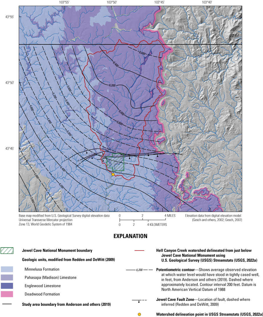
Generalized potentiometric contour map of the Madison aquifer from Anderson and others (2019) within and near Jewel Cave National Monument, South Dakota, with Hell Canyon Creek, the delineated Hell Canyon Creek watershed, and outcrops of the Deadwood Formation, Englewood Formation, Madison Limestone, and Minnelusa Formation.
A combination of the latter three explanations from Gat (1971) best account for heavy isotope depletion observed in the Madison aquifer underlying the study area. Recharge to the Madison aquifer in the study area likely is from large precipitation events and spring snowmelt. The study area does not receive steady heavy rainfall; however, the infrequent large precipitation events likely overcome evapotranspiration and would explain the generally depleted isotope values from groundwater samples. Recharge from snowmelt also may contribute to the depletion of heavy isotopes in the Madison aquifer. Climate normal data from 1991 to 2020 shows the study area receives about 57.9 in. of snow per year (NOAA, 2021b). Winter and spring snowmelt could contribute to recharge in the study area when evapotranspiration rates are lower than summer rates (Clark and Fritz, 1997). Large amounts of water released during spring snowmelt can cause normally dry streams, such as Hell Canyon Creek, to flow. Streamflow in Hell Canyon Creek following spring snowmelt could lose all or part of its flow to sinkholes in areas of Madison Limestone outcrop. The location or presence of streamflow loss zones along Hell Canyon Creek is unknown and streamflow data from streamgages upstream and downstream of Jewel Cave National Monument do not overlap to indicate the presence of streamflow losses.
The depletion of heavy isotopes for groundwater samples at Jewel Cave also could be from recharge at higher elevations. The elevation of the Hell Canyon Creek watershed generally decreases from northeast to southwest and ranges from 5,050 ft to 7,170 ft (USGS, 2022b). A generalized potentiometric map from Anderson and others (2019) shows groundwater flow in the Madison aquifer generally follows topography—indicating groundwater in the Madison aquifer flows from higher elevations in the northeastern part of the Hell Canyon Creek watershed toward the study area to the southeast (fig. 8). The effect of the Jewel Cave Fault Zone (fig. 8)—with an estimated vertical offset ranging from 100 (Darton and Paige, 1925) to 300 ft (NPS, 1994)—on groundwater flow in the Madison aquifer is unknown (Dyer, 1961). If the Jewel Cave Fault zone disrupts regional groundwater flow in the Madison aquifer to the cave lakes, then the depleted isotopic signature of the cave lakes could be explained by streamflow losses along Hell Canyon Creek. The isotopic signature of water from Hell Canyon Creek and its source from West Hell Canyon Spring also were depleted in heavy isotopes similar to Hourglass and New Years Lakes (fig. 7).
Springs Discharging from the Minnelusa Aquifer
Samples from springs discharging from the Minnelusa aquifer were qualitatively assessed to evaluate water composition using the stable isotope plot (fig. 7). The δ2H and δ18O values of springs discharging from the Minnelusa aquifer in the Minnelusa Formation generally were intermediate and plotted close to the LWML between groundwater samples from the Madison aquifer and precipitation samples. The intermediate composition of springs discharging from the Minnelusa aquifer indicated a mixture of groundwater and precipitation; however, the contribution from groundwater (more depleted in heavy isotopes) and precipitation (more enriched in heavy isotopes) varied for each spring. Stable isotopic composition was qualitatively assessed by observing the plotting positions of each site relative to other sites. Samples from A&E Spring (AEsp) and Water Draw Spring (WDWsp) plotted closer to depleted groundwater samples from cave lakes, whereas samples from Lithograph Spring (LTHsp), Chokecherry Spring (CCHsp), and Prairie Dog Spring (PDGsp) were more enriched in heavy isotopes and plotted closer to precipitation samples (fig. 7).
The variability of δ2H and δ18O values from springs with more than one sample was investigated using the stable isotope plot (fig. 7). Springs with more than one sample were Lithograph Spring (LTHsp) and Prairie Dog Spring (PDGsp). The stable isotopic composition of LTHsp changed from being more depleted in May 2016 to more enriched in August 2021. The stable isotopic composition of PDGsp remained relatively consistent between samples collected in May 2016 and August 2021. The variance or lack thereof in δ2H and δ18O values at LTHsp and PDGsp likely resulted because of changes in the contribution and type of precipitation falling shortly before sample collection. The contribution of groundwater or precipitation to LTHsp likely was related to (1) the elapsed time between precipitation events and sample collection, and (2) the residence time of infiltrated precipitation before spring discharge. Spring samples collected soon after precipitation events with similar stable isotopic composition as precipitation would indicate a shorter residence time (fast groundwater movement or short flowpaths) of infiltrated precipitation in the aquifer. Conversely, spring samples collected soon after precipitation events with more depleted stable isotopic composition would indicate longer residence time (slow groundwater movement or long flowpaths) of infiltrated precipitation in the aquifer that had not yet reached the spring. Infiltrated precipitation mixed with depleted groundwater, however, could potentially obscure the δ2H and δ18O values of infiltrated precipitation. A long residence time also may explain variable δ2H and δ18O values as water discharging from springs on each collection date could be water recharged during different times (spring snowmelt or summer rains). Stable isotope data collected from additional recharge sources (snowmelt and streams close to springs) and more frequently at springs could potentially be used to estimate residence time of water sources at each spring.
The intermediate δ2H and δ18O values of samples from springs discharging from the Minnelusa aquifer—combined with the stable isotopic variation among spring samples—in the stable isotope plot of the study area (fig. 7) provided insight on recharge mechanisms to the Minnelusa aquifer. The principles of conservation of stable isotopic composition for infiltrated precipitation (Naus and others, 2001; Gat, 1971) and depletion of heavy isotopes in spring samples compared to precipitation (Gat, 1971) also apply to the Minnelusa aquifer. A combination of the second and third explanations provided by Gat (1971) best account for heavy isotope depletion in the Minnelusa aquifer in the study area. The fourth explanation by Gat (1971)—recharge from high-elevation precipitation—is unlikely because higher elevation recharge areas immediately east of the study area are only about 200 ft higher in elevation than the surrounding areas (fig. 9). All spring samples plot near the LMWL and recharge areas for the Minnelusa aquifer are near the study area—indicating recharge to the Minnelusa aquifer is from recent meteoric sources. Recharge to the Minnelusa aquifer is primarily from precipitation on outcrops and streamflow losses; however, recharge from streamflow losses to the Minnelusa aquifer generally is less than to the Madison aquifer (Carter and others, 2003). In the study area, outcrop of the Minnelusa aquifer is mostly south of the Jewel Cave Fault Zone (Redden and DeWitt, 2008; fig. 9). The Hell Canyon Creek watershed is composed of about 20 percent of Minnelusa Formation outcrop (Redden and DeWitt, 2008; fig. 9), and precipitation or streamflow in the watershed could be lost to the Minnelusa aquifer.
Generalized potentiometric contour map of the Minnelusa aquifer from Carter and others (2003) within and near Jewel Cave National Monument, South Dakota, with Hell Canyon Creek, the delineated Hell Canyon Creek watershed, and outcrops of the Deadwood Formation, Englewood Formation, Madison Limestone, and Minnelusa Formation.
A combination of recharge from heavy rainfall, snowmelt, and aquifer residence time could explain depletion of heavy isotopes in samples from springs discharging from the Minnelusa aquifer. Samples from A&E Spring (AEsp) and Water Draw Spring (WDWsp) were collected in May 2016, so effects from spring snowmelt depleted in heavy isotopes could explain why those samples plot closer to groundwater samples. Effects of different precipitation types was apparent for samples from Lithograph Spring (LTHsp) because the sample collected in May 2016 was more depleted in heavy isotopes compared to the sample collected in August 2021 (fig. 7). The LTHsp sample collected in August 2021 likely was affected by enriched summer precipitation, which could indicate shorter aquifer residence time (fast groundwater movement or short flowpaths). Conversely, samples collected in May 2016 and August 2021 at Prairie Dog Spring (PDGsp) did not vary appreciably in stable isotope content. The lack of stable isotope variation at PDGsp could indicate a consistent groundwater source and (or) longer residence time of water in the aquifer resulting from either slower groundwater flow or longer flowpaths. The sample collected in May 2016 at Chokecherry Spring (CCHsp; fig. 7) was considered an anomaly because it was more enriched in heavy isotopes than all other samples. The enriched CCHsp sample could indicate its stable isotopic composition was affected by precipitation falling shortly before sample collection. Additional stable isotope and precipitation data would be required to better understand stable isotope variations and aquifer residence time at springs in the study area.
Another possible explanation for the depletion of heavy isotopes in samples from spring discharging from the Minnelusa aquifer could be from mixing with water from the Madison aquifer. Groundwater from the Madison aquifer was shown to be depleted in heavy isotopes (fig. 7) and mixing between the two aquifers would produce an overall depleted sample; however, hydraulic connection between the Minnelusa and Madison aquifers is not well defined (Carter and others, 2003). It is possible that the hydraulic connection between the Minnelusa and Madison aquifers is present along geologic structures, such as the Jewel Cave Fault Zone, where structure offset has juxtaposed the two units (fig. 9). The stable isotopic composition of samples from HGL—the cave lake sampled closest to the Jewel Cave Fault Zone—is similar to springs discharging from the Minnelusa aquifer, but additional data are needed to determine possible mixing between the two aquifers.
Site Groupings and Water Sources from Principal Component Analysis
The PCA method was used to create a biplot of water-chemistry data from this study and other studies (Naus and others, 2001; Long and others, 2012, 2019; fig. 10). The combined sum of principal components one and two explained 55.3 percent of the total variance in the dataset. Principal component three explained 14.3 percent of the total variance. Multiple variables were responsible for groupings along principal component axes one and two. Separation and grouping along principal component axis one were from a combination of specific conductance, hardness, ions (calcium, magnesium, chloride, and sulfate), and stable isotopes of oxygen and hydrogen. Loading lines for specific conductance, hardness, and ions displayed varying degrees of positive correlation, but all variables had positive loading on principal component one—shown by the loading lines plotting along the positive part of the x-axis (fig. 10). Conversely, loading lines for δ18O, δ2H, arsenic, silica, and pH had negative loading on principal component one (fig. 10). The δ18O, δ2H, and silica variables displayed positive correlation to each other and negative correlation to specific conductance, hardness, and ions—indicated by the nearly 180-degree angle between loading lines. The δ18O and δ2H variables were expected to contribute to groupings because the stable isotope plot (fig. 7) showed strong positive linear correlation. Additionally, the δ18O, δ2H, and silica variables showed almost no correlation to the pH and carbon dioxide variables—shown by the approximately 90-degree angle between loading lines (fig. 10). Separation and grouping along principal component axis two were from the pH, silica, and carbon dioxide variables.
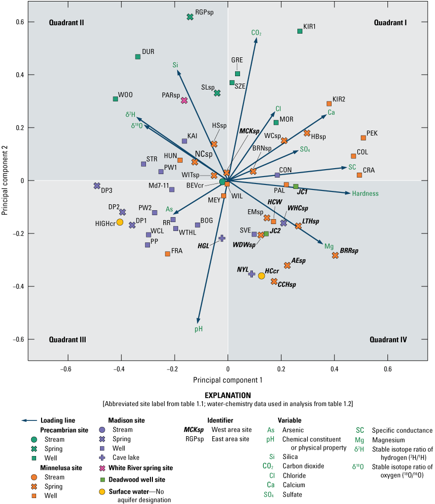
Principal component analysis biplot of water-chemistry data used in this study with loading lines for each variable label. See figure 1 for station locations. See tables 1.1 and 1.2 for site identifier description and the complete list of water-chemistry data used in analysis.
The plotting positions of sites in the PCA biplot show groupings based on location, aquifer, and the type of site (fig. 10). Sampling sites were identified by color and symbol for each aquifer and site type, respectively, where appropriate to make clear the relations among aquifers in the southern Black Hills (fig. 10). Precambrian aquifer sites (fig. 10) plotted mostly in upper parts of quadrants I and II—indicating lower pH and specific conductance, and higher concentrations of carbon dioxide. Williamson and Carter (2001) also noticed lower pH and specific conductance values, and higher carbon dioxide concentrations in groundwater from Precambrian aquifers compared to the Madison and Minnelusa aquifers. Most Madison aquifer sites (fig. 10) from the East area (fig. 1) plotted in the upper part of quadrant III with other sites plotting in quadrants I, II, and IV. Minnelusa aquifer sites (fig. 10) from the East area were scattered among all four quadrants but plotted mostly in quadrants I and II. Minnelusa aquifer sites were distinguishable from Madison aquifer sites in the East area because of their higher ion concentration, specific conductance, and hardness values. Williamson and Carter (2001) also observed that groundwater from the Minnelusa aquifer generally had higher ion concentrations (especially the calcium and sulfate ions) and greater specific conductance and hardness values than groundwater from the Madison aquifer.
Groundwater and surface-water sites from the West area (fig. 1) displayed distinctive water chemistry and plotted away from most samples from the East area with the exception Hourglass Lake (HGL), Mackenzie Spring (MCKsp), and Jewel Cave Well 1 (JC1; fig. 10). All groundwater samples from aquifer sites from the West area had intermediate ion concentrations and relatively lower δ18O and δ2H values compared to other samples from the East area; however, these samples from the West area had distinctively high magnesium concentration, and high hardness, pH, and specific conductance values that created separation along the y-axis (fig. 10). HGL and MCKsp both plotted near the y-axis of the PCA biplot between Madison aquifer sites from the East and West areas because of their higher δ18O and δ2H values and lower ion concentration, specific conductance, and hardness values (fig. 10). Some well and spring sites from the East area (fig. 10) were chemically similar to West area sites and plotted in quadrant I; however, East area sites in quadrant I are not immediately hydrologically connected to the West area because of the large distance (miles) between the areas (fig. 1). The higher ion concentration, and specific conductance, and hardness values for East area sites in quadrant I were likely caused by the evolution of groundwater from dissolution of aquifer material as it travels downgradient in the aquifer (fig. 1). Williamson and Carter (2001) determined ion concentrations, and specific conductance, and hardness values increase in the Minnelusa and Madison aquifers with increasing well depth and with distance from outcrop areas. For example, the COL, CRA, PEK, HBsp, and PAL sites in quadrant I are all downgradient of recharge areas further west (fig. 1) and all had higher ion concentration, and specific conductance and hardness values than sites closer to recharge areas.
The plotting positions of sites displayed in figure 10 from the West area were used to determine differences in water chemistry among the Deadwood, Madison, and Minnelusa aquifers. A similar analysis could be conducted on sites from the East area; however, that analysis is outside the scope of this study. Groundwater samples from Deadwood aquifer sites (JC1 and JC2) had similar water chemistry as Minnelusa aquifer sites (fig. 10); however, the water chemistry of Jewel Cave well 1 (JC1) and Jewel Cave well 2 (JC2) differed appreciably. The sample from JC1 had higher ion concentrations commonly associated with salts (sodium, calcium, magnesium, and chloride). Groundwater from the Madison aquifer generally had the lowest ion concentration, and specific conductance and hardness values in the West area (fig. 10). Additionally, water chemistry of cave lake sites notably differed; HGL plotted closer to Madison aquifer sites from the East area, whereas New Years Lake (NYL) plotted closer to Hell Canyon Creek (HCcr) and Minnelusa aquifer springs (fig. 10). West Hell Canyon Spring (WHCsp)—upgradient from cave lake sites—also differed from cave lake samples because WHCsp had higher ion concentration, and specific conductance and hardness values. The different water chemistry at WHCsp could result from the dissolution of aquifer materials during groundwater flow that increase ion concentrations and specific conductance (Williamson and Carter, 2001). Groundwater samples from Minnelusa aquifer sites displayed the greatest water-chemistry variation among the three aquifers, but generally had the highest ion concentration, and specific conductance and hardness values in the West area (fig. 10).
Cluster Assignments and Water Sources from Cluster Analysis
The k-means cluster procedure was applied to the PCA results shown in figure 10 to statistically group sites (fig. 11). Sampling sites were grouped into five categories based on cluster assignments from the k-means procedure (fig. 11; table 3). Group 1 included samples from Precambrian aquifer springs and wells and one White River aquifer sample. Group 2 mostly consisted of samples from the Madison aquifer in the East area (fig. 1). Group 3 consisted mostly of samples from springs and wells completed in the Minnelusa aquifer in the East area. Group 4 included mostly samples from the West area. Group 5 consisted of springs and wells completed in the Minnelusa and Precambrian aquifers from the East area with high ion concentrations and specific conductance and hardness values.
Table 3.
Summary of cluster analysis results listing groups, sampling site short names, location, and aquifer from the k-means cluster procedure applied to principal component analysis results.[--, no aquifer designation]
| Group number | Short name1 | Location (fig. 1) |
Site type | Aquifer |
|---|---|---|---|---|
| 1 | RGPsp | East | Spring | Precambrian |
| SLsp | West | Spring | Precambrian | |
| GRE | East | Well | Precambrian | |
| SZE | East | Well | Precambrian | |
| WOO | East | Well | Precambrian | |
| DUR | East | Well | Precambrian | |
| PARsp | East | Spring | White River | |
| 2 | FRA | East | Well | Minnelusa |
| HIGHcr | East | Surface water | -- | |
| Md7-11 | East | Well | Madison | |
| BOG | East | Well | Madison | |
| STR | East | Well | Madison | |
| PW1 | East | Well | Madison | |
| PW2 | East | Well | Madison | |
| WTHL | East | Cave lake | Madison | |
| WCL | East | Cave lake | Madison | |
| PP | East | Cave feature | Madison | |
| RR | East | Cave feature | Madison | |
| DP1 | East | Drip site | Madison | |
| DP2 | East | Drip site | Madison | |
| DP3 | East | Drip site | Madison | |
| 3 | BEVcr | East | Surface water | -- |
| KAI | East | Well | Madison | |
| NCsp | East | Spring | Minnelusa | |
| HSsp | East | Spring | Minnelusa | |
| WITsp | East | Spring | Minnelusa | |
| BRNsp | East | Spring | Minnelusa | |
| MEY | East | Well | Minnelusa | |
| HUN | East | Well | Minnelusa | |
| WIL | East | Well | Minnelusa | |
| MCKsp | West | Spring | Minnelusa | |
| 4 | NYL | West | Cave lake | Madison |
| HGL | West | Cave lake | Madison | |
| WHCsp | West | Spring | Madison | |
| WDWsp | West | Spring | Minnelusa | |
| LTHsp | West | Spring | Minnelusa | |
| AEsp | West | Spring | Minnelusa | |
| CCHsp | West | Spring | Minnelusa | |
| BRRsp | West | Spring | Minnelusa | |
| HCW | West | Well | Minnelusa | |
| JC1 | West | Well | Deadwood | |
| JC2 | West | Well | Deadwood | |
| SVE | East | Well | Madison | |
| CON | East | Well | Madison | |
| HCcr | West | Surface water | -- | |
| PAL | East | Well | Minnelusa | |
| EMsp | East | Spring | Minnelusa | |
| 5 | KIR1 | East | Well | Precambrian |
| MOR | East | Well | Precambrian | |
| KIR2 | East | Well | Minnelusa | |
| PEK | East | Well | Minnelusa | |
| COL | East | Well | Minnelusa | |
| CRA | East | Well | Minnelusa | |
| WCsp | East | Spring | Minnelusa | |
| HBsp | East | Spring | Minnelusa |
Short name from either table 1 or Long and others (2019).
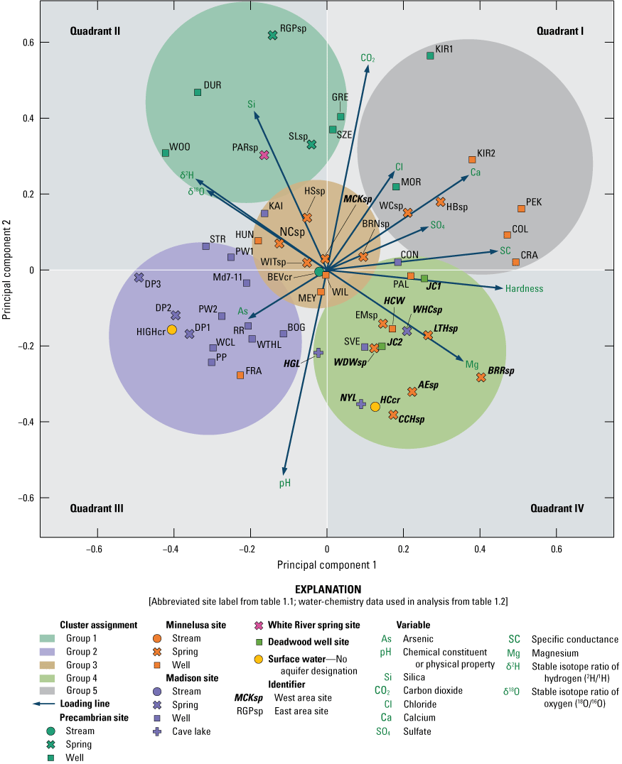
The k-means cluster procedure applied to the principal component analysis biplot (displayed in fig. 10) of water-chemistry data with colors symbolizing the five cluster assignment groups. See figure 1 for station locations. See tables 1.1 and 1.2 for site identifier description and the complete list of water-chemistry data used in analysis.
The k-means cluster procedure grouped samples into clusters sharing similar physical property, chemical constituent, and stable isotope values that were used to identify relations among sites from different aquifers in the East and West areas (fig. 1). Group 1 included only sites from the Precambrian aquifer in the East area (table 3); however, other Precambrian aquifer sites in group 5 (KIR1 and MOR; fig. 11) were not included in group one. Precambrian aquifer sites not included in group 1 were from well sites with water chemistry more similar to the chemistry of the Minnelusa aquifer (group 3). Groundwater from the Minnelusa aquifer could not affect water chemistry for Precambrian aquifer sites excluded from group 1 because all the collected samples were upgradient and isolated from the Minnelusa aquifer outcrop (fig. 1). Possible explanations for Precambrian aquifer sites excluded from group 1 could be from well treatment or elevated ion concentrations from road salts that would increase specific conductance values.
All well sites in group 2 were from the East area (fig. 1) and 12 of 14 of the sites were wells completed in the Madison aquifer (table 3). Separation of sites in the East area from sites in the West area can be explained by the altitude effect (Dansgaard, 1964; Rozanski and others, 1993) because the surface elevation of sites in the East area is about 1,400 ft lower than sites in the West area. As expected, the lower elevation East area well sites had higher δ18O and δ2H values (enriched with heavy isotopes) than the higher elevation West area sites. The FRA site was the only Minnelusa aquifer site in group 2 (fig. 1; table 3), and the PCA and cluster analysis results indicated that this well could be completed in the Madison aquifer rather than the Minnelusa aquifer as indicated in NWIS (USGS, 2022a). The FRA site did not have a drillers log with lithologic information in the South Dakota Department of Agriculture and Natural Resources (2022) database; however, the well depth of the FRA site was 440 ft, as available from NWIS (USGS, 2022a), and nearby wells with drillers logs indicated the depth to Madison Limestone is about 690 ft. Therefore, the FRA well likely is completed in the Minnelusa aquifer, but groundwater from this well has similar water chemistry as the underlying Madison aquifer. Separation of group 2 from other sites in the East area was from a combination of higher arsenic concentrations and lower ion concentrations, and specific conductance and hardness values than other sites (fig. 11).
Group 3 consisted of 10 sites with 1 from surface water, 1 from the Madison aquifer, and 8 from the Minnelusa aquifer (table 3). Additionally, 9 of the 10 sites in group 3 were from the East area and other was from the West area (table 3). Group 5 was similar to group 3; group 5 consisted of 8 sites from the East area with 2 from the Precambrian aquifer and 6 from the Minnelusa aquifer. Differences between sites completed in the Minnelusa aquifer in groups 3 and 5 likely were related to proximity to recharge areas as compared to other sites. Sites in group 3 often were closer to recharge areas of Minnelusa aquifer outcrop, whereas group 5 included mostly well sites further downgradient and at deeper well depths (fig. 1; table 3).
The KAI site (fig. 1) was the only site in group 3 completed in the Madison aquifer (table 3). The water chemistry of the KAI site was similar to the Minnelusa aquifer—indicating the KAI well could be completed in either the Minnelusa aquifer or both in the Minnelusa and Madison aquifers. The KAI site did not have a drillers log with lithologic information in the South Dakota Department of Agriculture and Natural Resources (2022) database; however, the well depth of the KAI site was 780 ft as obtained from NWIS (USGS, 2022a). Nearby wells with drillers logs indicated that the depth to the Madison Limestone is about 690 ft; therefore, the well probably is completed at least partially in the Madison aquifer and could be partially completed in the Minnelusa aquifer depending on the position and length of the screened (open) interval.
Group 4 contained 16 sites with 2 from the Deadwood aquifer, 5 from the Madison aquifer, 8 from the Minnelusa aquifer, and 1 surface-water site. Additionally, 12 of the 16 sites contained in group 4 were from the West area, and the other 4 were from the East area (table 3). As previously discussed, sites in group 4 differed from other sites because of their low δ18O and δ2H values (depleted) and high ion concentrations, and specific conductance and hardness values. The higher elevation of West area sites in group 4 compared with sites contained in other groups likely caused the lower δ18O and δ2H values (Dansgaard, 1964; Rozanski and others, 1993). Anomalies in group 4 from the East area included two wells completed in the Madison aquifer (CON and SVE), one spring discharging from the Minnelusa aquifer (Elk Mountain Spring; EMsp), and one well completed in the Minnelusa aquifer (PAL; fig. 11). Inclusion of the CON and SVE sites in group 4 could result from longer residence times in the Madison aquifer or groundwater mixing with the Minnelusa aquifer. Elk Mountain Spring (EMsp) and the PAL well were included in group 4 because of abnormally high magnesium concentrations and hardness values.
Relation among Hourglass and New Years Lakes, Possible Recharge Mechanisms, and Susceptibility
Relations between Hourglass (HGL) and New Years (NYL) Lakes were evaluated using hydrograph analyses, PCA results, and cluster analysis groupings. Hydrographs of the HGL (fig. 5) and NYL (fig. 6) showed different responses to precipitation events; HGL displayed smaller, delayed water-level changes in response to precipitation compared to NYL (figs. 5 and 6). Water-level changes at HGL were similar to water-level changes at a well completed in the Madison aquifer (433517103534201; CU-95A) about 9 mi south (fig. 12; USGS, 2022a; South Dakota Geological Survey [SDGS], 2022). Peak water levels at CU-95A were measured about from 4 to 8 months later than peak water levels at HGL. Water-level changes at NYL were not similar to HGL or CU-95A (fig. 13).
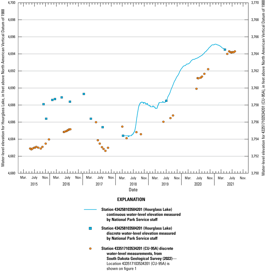
Hydrograph of Hourglass Lake plotted with water-level elevation data from well 433517103534201 (CU-95A), Jewel Cave National Monument, southwestern South Dakota (USGS, 2022a; South Dakota Geological Survey, 2022). See figure 1 for well location.
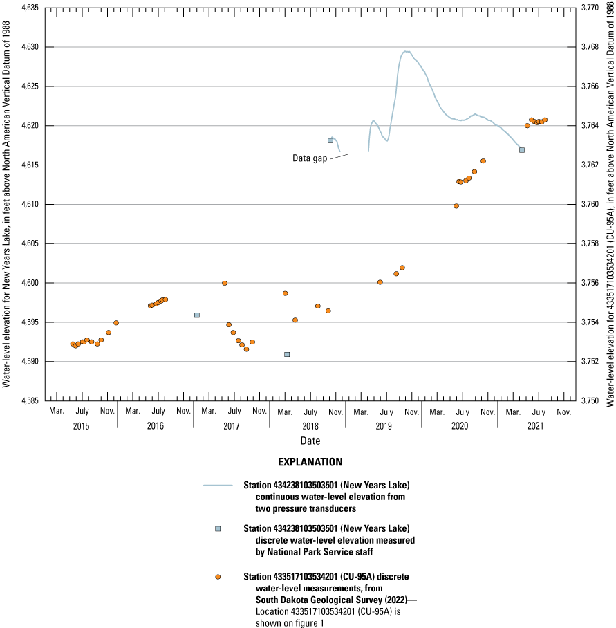
Hydrograph of New Years Lake plotted with water-level elevation data from well 433517103534201 (CU-95A), Jewel Cave National Monument, southwestern South Dakota (USGS, 2022a; South Dakota Geological Survey, 2022). See figure 1 for well location.
Anderson and others (2019) also noticed similarities between the HGL hydrograph and hydrographs of other wells completed in the Madison aquifer and included water-level elevations from cave lakes in preparation of a generalized potentiometric surface of the Madison aquifer in the Jewel Cave area. HGL and NYL, therefore, were assumed to be connected with the regional Madison aquifer because no evidence was available to suggest otherwise. Water-level change similarities between HGL and 433517103534201 (fig. 12) indicated that HGL is recharged similar to the regional Madison aquifer along outcrops to the north (fig. 8); conversely, differences between NYL and CU-95A (fig. 13) indicated a more direct connection to local recharge rather than solely from outcrops recharging the regional Madison aquifer.
Initially, the geometry of the cave passages in which HGL and NYL are contained was thought to contribute to the differences in water-level changes between HGL and NYL. For example, the water-level increase in a small passageway would be greater than the increase in a larger passageway if the same volume of water was added to both passageways. The actual geometry of the cave passageways containing HGL and NYL is unknown because NPS staff cannot access the submerged passageways; however, the mapped passageways containing HGL and NYL were used as a proxy for the actual geometry of the passageways. The larger mapped cave passageway containing NYL indicated larger water-level changes than the smaller cave passageway containing HGL (Dan Austin, NPS, written commun., December 2021); therefore, passageway geometry was not considered a factor contributing to water-level change differences between the two cave lakes. Possible explanations for water-level change differences between HGL and NYL could be (1) varying recharge rates, (2) different sources of recharge, or (3) varying discharge rates. The following sections discuss the water-level and water-chemistry data used to determine possible recharge sources to HGL and NYL.
Hourglass Lake
Water-chemistry data—evaluated using PCA and cluster analyses—highlighted differences between Hourglass and New Years Lakes that suggested different recharge mechanisms. PCA and k-means cluster analysis results showed that Hourglass Lake (HGL) grouped with Madison aquifer sites from the West area (fig. 1) but plotted away from other sites in group 4 (figs. 10 and 1) because it was more enriched in heavy isotopes and had lower concentrations of ions than other sites from the West area. Water chemistry of HGL was more similar chemically to precipitation (enriched in heavy isotopes with low ion concentrations) than other West area sites—indicating recharge to the lake results quickly because its water chemistry was less affected by evaporation and (or) dissolution of aquifer materials than other West area sites. Additionally, the water chemistry of HGL was noticeably different than West Hell Canyon Spring (WHCsp; figs. 10 and 11) that likely receives its recharged water from the high elevation Madison Limestone outcrops in the northern part of the study area (fig. 8). The difference in water chemistry between HGL and other Madison aquifer sites in the West area—combined with differences between hydrographs of HGL and NYL—indicates that HGL is recharged at a different rate and from a different or additional source(s) than other Madison aquifer sites in the West area.
Taylor and Greene (2008) provided a conceptual model of karst aquifers showing multiple recharge sources (fig. 14) that were used to hypothesize recharge mechanisms for Hourglass Lake. Recharge sources were differentiated in terms of residence time and the amount of water contributed to the aquifer. Taylor and Greene (2008) provided descriptions of each type of recharge source that will be briefly discussed here. In general, autogenic recharge and allogenic recharge are defined as precipitation falling on karstic and nonkarstic terrane, respectively (Gunn, 1983). The amount and timing of the precipitation determines whether the recharge is considered concentrated or diffuse (Gunn, 1983). Concentrated autogenic recharge (fig. 14) primarily is from filling of sinkhole depressions by surface runoff processes that can be either rapidly drained by swallets or relatively slowly through percolation of soil and other deposits. Diffuse autogenic recharge (fig. 14) from infiltration of water through soils overlying karstic terrane is the most common type of recharge to karst aquifers. Concentrated allogenic recharge (fig. 14) to karst aquifers is water contributed by sinking or losing streams originating as normal gaining streams in non-karstic terrain. Diffuse allogenic recharge (fig. 14) can be groundwater contributed from non-karstic aquifers, but more commonly is water that drains through vertical or near-vertical conduits in the unsaturated (vadose) zone where karstic rocks are overlain by non-soluble caprocks, such as sandstone.
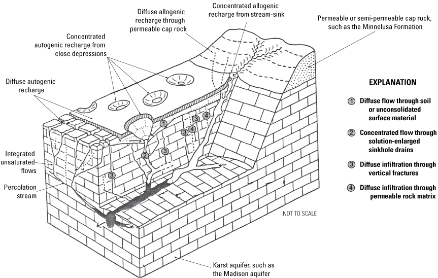
Block diagram of a karst basin with various types of recharge sources (modified by Taylor and Greene, 2008 and originally from Gunn, 1986). Descriptions of each type of recharge are provided in Taylor and Greene (2008). Underground conduits shown as solid black represent groundwater in the karst aquifer.
Recharge to HGL likely is a mix of various recharge sources, with the dominant recharge sources likely diffuse allogenic recharge through the Minnelusa Formation (including the Minnelusa aquifer and semiconfining units) and diffuse autogenic recharge in areas of Madison Limestone outcrop (fig. 14). Another possible recharge source could be streamflow losses (concentrated allogenic recharge from stream-sink; fig. 14). The Madison Limestone containing HGL is overlain by about 300–400 ft of the Minnelusa Formation, and its water chemistry was more similar to precipitation than other Madison aquifer sites—indicating the largest fraction of recharged water likely is from quickly infiltrated precipitation or streamflow losses. Dye tracer tests from Alexander and others (1989) indicated precipitation falling on the land surface above the cave infiltrates through the Minnelusa Formation and into Jewel Cave. The relatively quick recovery of dye 8 days after dye insertion may have been through vertical or near-vertical fractures connecting the Madison and Minnelusa aquifers, whereas the intermittent and reoccurring recovery of dye 1 year after insertion may be caused by slow vertical draining of the Minnelusa aquifer into the Madison aquifer.
Diffuse allogenic recharge also can explain water-chemistry similarities between HGL and precipitation. Some fraction of infiltrated precipitation would reach HGL quickly through vertical or near-vertical conduits, and its water chemistry would be similar to precipitation because of its short residence time in the Minnelusa aquifer. The other fraction of infiltrated precipitation would drain through the Minnelusa aquifer slower than water passing through vertical or near-vertical conduits, and its water chemistry would contain higher concentrations of ions and have higher specific conductance and hardness values. Another source of water supplying cave lakes could be groundwater flowing from outcrop recharge areas, such as those north of Jewel Cave (fig. 8), to Jewel Cave, which likely would have higher ion concentrations, and greater specific conductance and hardness values than recently infiltrated precipitation. Additionally, diffuse allogenic recharge can explain the relatively slow response between water levels in HGL and precipitation. Vertical or near-vertical conduits extending through the Minnelusa Formation (including the Minnelusa aquifer) can transport a certain quantity of water that may be small compared to the volume of water in HGL, so water levels would slowly change at HGL. Water-level increases at HGL during dry periods, such as in 2020–21 (figs. 3 and 5), could be related to the relatively slow downward vertical movement of water through the Minnelusa Formation (including the Minnelusa aquifer and the unsaturated zone of the Madison Limestone.
New Years Lake
PCA and k-means cluster analysis results showed New Years Lake (NYL) grouped with sites from the West area and plotted closest to Hell Canyon Creek (HCcr; figs. 10 and 11). Similar water chemistry between NYL and HCcr suggests that NYL may receive recharge from streamflow losses. HCcr is an intermittent stream that flows during wet conditions when springs in Hell Canyon, such as West Hell Canyon Spring (WHCsp), supply enough water to overcome evapotranspiration and streamflow losses to either the Madison or Minnelusa aquifers (NPS, 1994). Cumulative monthly departure from normal (fig. 2) indicates wet conditions throughout the study area from May 2018 to August 2021 and HCcr was flowing during sample collection in August 2021. Streamflow in HCcr is not currently monitored so the duration of streamflow is unknown. Water chemistry of HCcr likely was affected by the water chemistry of springs discharging into it. WHCsp discharges into HCcr; however, PCA analysis shows that WHCsp and HCcr plot away from each other (fig. 10) despite having similar stable isotope compositions (fig. 7) because the carbon dioxide concentration, and specific conductance and hardness values at WHCsp were noticeably higher than HCcr. Water chemistry of HCcr was distinguishable from WHCsp because HCcr received water from a variety of sources, including surface runoff and springs discharging from the Madison and Minnelusa aquifers.
Differences between NYL hydrograph and hydrographs of HGL and CU-95A indicated a different recharge source for NYL. Water-chemistry data indicated similarities between NYL and HCcr; however, comparisons between streamflow from HCcr and water levels at NYL could not be made because streamflow data were not measured during the period of water-level data collection at NYL. Greene and others (1999), Hortness and Driscoll (1998), and Carter and others (2001) compared streamflow data to water levels in wells for other streams in other parts of the Black Hills and noticed correlation between streamflow losses and water levels in the Madison aquifer.
It is unknown if HCcr was flowing during the entire period of water-level data collection at NYL evaluated from 2018 to 2021. Additionally, peak streamflow in HCcr likely would not coincide with peak water levels in NYL because of the time necessary for streamflow losses to recharge the lake. Therefore, a time delay between streamflow losses and water levels would be expected. Another consideration when comparing water-level changes at NYL to streamflow is the difficulty of differentiating recharge from streamflow losses compared to infiltrated precipitation because streamflow increases with increasing precipitation. Water-chemistry and hydrograph similarities between NYL and surface water indicated a possible connection to surface water in the study area, although additional data collection is required to further define the relation between increasing water levels and streamflow losses.
Streamflow loss zones along HCcr have not been mapped but their presence in the Jewel Cave area has been speculated by other studies (Dyer, 1961; NPS, 1994). Dyer (1961) postulated the Jewel Cave Fault Zone (fig. 8) could capture streamflow and (or) shallow groundwater in alluvial deposits in Hell Canyon; however, no evidence was provided to confirm this possibility. NPS (1994) discussed how streamflow in the Jewel Cave area could be affected by exposures of Madison Limestone and, to a lesser extent, the Minnelusa Formation because the porous nature of the substrate could capture streamflow and precipitation. A geologic map of the Jewel Cave area shows outcrops of Madison Limestone along HCcr south of the Jewel Cave Fault Zone (fig. 8). It is possible that the Jewel Cave Fault Zone, some other unnamed structure, or outcrops of Madison Limestone and Minnelusa Formation along HCcr could capture streamflow and (or) shallow groundwater and provide recharge to the Madison aquifer near NYL. The potential relation between streamflow in HCcr and water levels at NYL would be clearer if additional streamflow and water-level data were collected simultaneously.
Water-level changes and water-chemistry data supported the possibility that NYL is recharged by concentrated allogenic recharge (streamflow losses) along HCcr (fig. 14). NYL is overlain by the Minnelusa Formation and its mean water level is about 650 ft below land surface; therefore, a natural conduit connecting HCcr to NYL would have to be fairly large and continuous to quickly transport water from the surface to the cave. A crack in the cave ceiling with water discharging into NYL was observed by NPS staff (Dan Austin, NPS, written commun., December 2021). NPS staff also noted horizontal displacement along the crack that was estimated at about 1 ft (Dan Austin, NPS, written commun., December 2021). The aperture (width of the opening) of the crack was not measured; however, displacement in the cave ceiling indicated the crack was a fault. The fault observed in the cave ceiling above NYL was named “Delmars Fault” by NPS staff and little is known about its extent. It is possible that Delmars Fault is extensive and could provide a natural conduit for direct recharge from HCcr to NYL.
When HCcr is not flowing, the dominant recharge source to NYL probably changes from concentrated allogenic recharge (streamflow losses) to a combination of diffuse allogenic and autogenic recharge (fig. 14). Diffuse allogenic recharge likely results where the Minnelusa Formation overlies the Madison Limestone and would be similar to recharge at Hourglass Lake. Diffuse autogenic recharge likely results either where the Madison Limestone is exposed at the land surface or where alluvial deposits in Hell Canyon directly overlie Madison Limestone south of the Jewel Cave Fault Zone (fig. 8). Diffuse allogenic and autogenic recharge both likely contribute to recharging NYL when HCcr is flowing; however, contributions from diffuse allogenic and autogenic recharge likely are smaller with greater travel time to NYL because of slower vertical flow through the Minnelusa Formation and the unsaturated zone in the upper part of the Madison aquifer.
Susceptibility of Hourglass and New Years Lakes
Susceptibility of Hourglass and New Years Lakes from human-related activities at the land surface can be addressed qualitatively using observations from previous studies and the recharge mechanisms interpreted from the results of this study. Dye tracer tests (Alexander and others, 1989) demonstrated that dyed water inserted at the land surface passed through a septic system and entered Jewel Cave in 8 days. The dye was recovered for over 1 year after the tests began. Additionally, recharge mechanisms discussed in the previous section indicate that Hourglass and New Years Lakes are possibly well-connected to surface processes. Water-level and water-chemistry data from Hourglass and New Years Lakes indicated similarities to atmospheric water sourced from direct infiltration of precipitation and potential streamflow losses along Hell Canyon Creek. Therefore, human-related activities at recharge areas for the Madison and Minnelusa aquifers or in Hell Canyon could potentially affect the water chemistry of cave lakes in Jewel Cave. The theorized connection between Hell Canyon Creek and New Years Lake to recharge sources indicates the water chemistry of New Years Lake likely would be affected before Hourglass Lake; however, the water chemistry of Hourglass Lake could remain affected for a longer time period than New Years Lake because of its complex recharge mechanisms and likely connection to the Minnelusa aquifer. Observations from Alexander and others (1989), M.E. Wiles (South Dakota School of Mines and Technology, unpub. data, 1992), Anderson and others (2019), and from this study indicated recharge to Jewel Cave is complex and takes place on various timescales that are affected temporally by precipitation patterns and spatially by hydrologic connection with the overlying Minnelusa aquifer.
Data and Method Limitations
Various limitations affected the completeness of data collected during this study. Water-level data presented in this report were intermittent before pressure transducers were installed and when the water level fell below the transducer at New Years Lake (NYL) from November 21, 2018, to April 7, 2019. Complete hydrographs at Hourglass (HGL) and NYLs would provide a more complete analysis of relations among precipitation, snow depth, and water levels in Jewel Cave. Another data limitation for water-level analysis was that streamflow, spring discharge, and discharge from the Delmars Fault in the ceiling of NYL were not available during water-level monitoring of HGL and NYL. Measurements of streamflow and discharge from springs and the Delmars Fault could be used to better define relations between water-level changes at cave lakes and potential recharge sources. Water-level analysis also was limited by the distance between climate stations and Jewel Cave National Monument. Precipitation and snow depth data from climate station about 10 mi away from cave lakes were used for comparison, which could be inaccurate because weather patterns are spatially variable in the Black Hills.
Limitations for water-chemistry data included the lack of replicate samples and the small number of samples collected at each site. Replicate samples are used to evaluate variability in analytical results for two or more samples that should be chemically identical if not for potential sources of contamination, such as from sampling equipment. Obtaining a replicate sample would provide additional confidence that the water-chemistry data collected during this study accurately represented the true chemistry of sampled sites. The small number of water samples collected at sampling sites during the study restricted the ability to compare samples across multiple years and determine how water chemistry changes. Routine sampling of sites within and near Jewel Cave National Monument would allow for a time-series analysis of possible water-chemistry changes.
Method limitations included assumptions necessary to complete water-level analysis. Assumptions for water-level analysis included the accuracy of surveys that determined the elevation of cave lakes and the transducers installed in cave lakes accurately measured water-level changes. Surveys by NPS staff established the elevation of cave lakes, and additional work completed by a cooperative effort between the USGS and NPS accurately measured the true elevation of a reference point used for cave surveys. The accuracy of pressure transducers likely was affected by the length of time the instruments were installed in HGL and NYL. Instrument drift is a concern for all electronic instruments, and the uncertainty of measurements generally increases with time because of environmental factors, such as temperature and pressure. Water-level data from transducers were corrected for instrument drift using a time-proportional correction; however, uncertainty in measurements by the transducer still may result. Another assumption for water-level analysis was that groundwater in Jewel Cave is hydraulically connected to the regional Madison aquifer. Other studies have determined that water-level elevations of cave lakes in the Black Hills are similar to water-level elevations of wells completed in the Madison aquifer. Jewel Cave National Monument is near the recharge zones for the regional Madison and Minnelusa aquifers, but geologic structures such as the Jewel Cave Fault Zone or the complex nature of caves, could isolate groundwater in Jewel Cave from the regional Madison aquifer, resulting in water-level changes affected by water sources other than solely precipitation.
Assumptions for water-chemistry data were related to sampling techniques, as well as the type and number of physical properties and chemical constituents analyzed. Field methods used to collect samples followed instruction provided by USGS (variously dated); however, sampling at cave lakes is logistically difficult and requires altering some standard field methods used to collect water samples. The concentrations of ions and stable isotopes were assumed to not be affected by evaporation, which could alter the isotopic concentration of the sample. Evaporation likely was not an appreciable factor for samples collected at cave lakes because of their depth of about 650 ft below land surface. Another assumption was the physical properties and chemical constituents used in this study would be able to distinguish sites based on water-chemistry differences. The physical property and chemical constituents analyzed for this study were similar to previous studies by Long and others (2012, 2019); however, the previous studies sampled for metals and other isotopes not included in this study. Including additional physical properties, chemical constituents, and isotopes could improve the results of PCA and k-means cluster analyses, which also could change interpretations of recharge sources to HGL and NYL.
Summary
In 2015, cavers exploring an unmapped part of Jewel Cave in southwestern South Dakota discovered the first subterranean water body (“cave lake”) that was later named Hourglass Lake. Cave lakes in Jewel Cave and Wind Cave are considered to represent the water table of the Madison aquifer because the elevation of cave lakes in both Jewel and Wind Caves was similar to the elevation of water levels in nearby wells completed in the Madison aquifer. The discovery of cave lakes at Jewel Cave National Monument resulted in additional responsibilities and challenges for the National Park Service (NPS) staff to protect and conserve natural resources above and below the land surface. The U.S. Geological Survey (USGS), in cooperation with the NPS, collected water-level and water-chemistry data within and near Jewel Cave to better understand groundwater interactions in Jewel Cave and to evaluate recharge characteristics to cave lakes in the Jewel Cave recharge area. The approach for this study included comparing water-level data collected from two cave lakes to historical climate data and application of multivariate statistical analyses to evaluate water samples collected during this study and from previous investigations.
Data collection within and near Jewel Cave included monitoring water levels in two cave lakes and collecting 9 water samples from 7 sites. Pressure transducers and barometers were used to continuously record water-level and barometric-pressure data, respectively, from Hourglass and New Years cave lakes. Water-level elevation measurements at Hourglass and New Years Lakes were compared to daily observations, annual normal, monthly observations, and monthly normal climate data obtained from the closest climate stations. Nine water samples were collected intermittently from April to August 2021 at 7 sites and analyzed for 12 constituents. Physical properties of sampled water—dissolved oxygen, pH, specific conductance, water temperature, and turbidity—were measured by USGS personnel at spring and stream sites in the field before sample collection; however, these properties were not measured at rain collector and cave lake sites where NPS personnel collected samples. Water samples from spring, stream, and cave lake sites were analyzed for stable isotopes and major ions. All water samples were analyzed for stable isotopes of oxygen (oxygen-18 [δ18O]) and hydrogen (deuterium [δ2H]).
Water-level data were analyzed through (1) comparison of hydrographs of Hourglass and New Years Lakes and (2) interpretation of water-level changes from Hourglass and New Years Lakes compared to precipitation and snow depth data from the nearby climate stations. Hydrographs from Hourglass Lake and New Years Lake were compared because of noticeable differences between the two cave lakes. Hourglass Lake displayed small, gradual water-level changes with elevations ranging from 4,684.3 to 4,695.2 feet (ft) (an elevation range of 10.9 ft) from October 2015 to April 2021. New Years Lake displayed relatively large and rapid water-level changes with elevations ranging from 4,590.9 to 4,629.5 ft (an elevation range of 38.6 ft) from January 2017 to April 2021. Cave lake hydrographs were compared to precipitation and snowfall data to build on observations from a previous investigation at Hourglass Lake.
Stable isotope data were analyzed by (1) creating a local meteoric water line from precipitation samples collected during this study, (2) comparing stable isotope values from the study area to global meteoric values established by a previous investigation, and (3) comparing stable isotope values among sites to evaluate possible recharge characteristics. The slope and y-intercept of the local meteoric water line (LMWL) were dampened compared to the global meteoric water line (GMWL), and as a result the LMWL line plotted below the GMWL. All stable isotope samples were depleted in heavy isotopes (more negative δ2H and δ18O values) and indicated a greater degree of evaporation from environmental factors, such as latitude, continental position, and altitude (elevation above the North American Vertical Datum of 1988). All samples plot near the LMWL and recharge areas for aquifers are near the study area—indicating that both aquifers are recharged from recent meteoric sources. Recharge to the Madison aquifer in the study area likely is from large precipitation events and spring snowmelt. Heavy rainfall usually does not fall across the study area; however, the infrequent sustained precipitation events likely overcome evapotranspiration and would explain the generally depleted isotope values from groundwater samples. Recharge from snowmelt also may contribute to the depletion of heavy isotopes in the Deadwood and Madison aquifers. Large amounts of water released during spring snowmelt can cause normally dry streams, such as Hell Canyon Creek, to flow steadily. Streamflow in Hell Canyon Creek following spring snowmelt could lose all or part of its flow to sinkholes in areas of Madison Limestone outcrop.
Relations between Hourglass and New Years Lakes were evaluated based on hydrograph observations, principal component analysis (PCA) results, and cluster analysis groupings. Hydrographs of Hourglass and New Years Lakes displayed different responses to climate; Hourglass Lake displayed smaller, delayed water-level changes in response to precipitation compared to New Years Lake. Additionally, water-level changes at Hourglass Lake were similar to water-level changes at a well completed in the Madison aquifer about 9 miles south of Jewel Cave. Water-level changes at New Years Lake showed almost no similarities to water-level changes at the well completed in the Madison aquifer. Initially, the geometry of the cave passages in which Hourglass and New Years Lakes are contained was thought to contribute to the differences in water-level changes between Hourglass and New Years Lakes. This cave geometry hypothesis was later dismissed because the larger cave passageway containing New Years Lake showed larger water-level changes than the smaller cave passageway containing Hourglass Lake. A possible explanation for water-level change differences between Hourglass and New Years Lakes could be different recharge rates and (or) different sources of recharge.
The dominant recharge source for Hourglass Lake probably is diffuse allogenic recharge through the Minnelusa Formation. Dye tracer tests from a previous study indicated precipitation falling on the land surface above the cave infiltrates through the Minnelusa Formation that includes the Minnelusa aquifer and into Jewel Cave. The relatively quick recovery 8 days after dye insertion may have been through vertical or near-vertical fractures connecting the Madison and Minnelusa aquifers, whereas the intermittent and reoccurring recovery of dye 1 year after insertion may be caused by slow (months to years) vertical draining of the Minnelusa aquifer into the Madison aquifer. Diffuse allogenic recharge also can explain water-chemistry similarities between Hourglass Lake and precipitation in PCA and k-means cluster analysis results. Some fraction of infiltrated precipitation would reach Hourglass Lake quickly (hours to days) through vertical or near-vertical conduits, and its water chemistry would be similar to precipitation because of its short residence time in the Minnelusa Formation. The other fraction of infiltrated precipitation would drain through the Minnelusa Formation and Minnelusa aquifer slower than water passing through vertical or near-vertical conduits and its water chemistry would contain higher concentrations of ions and have higher specific conductance and hardness values. Additionally, diffuse allogenic recharge can explain the relatively slow response between water levels in Hourglass Lake and precipitation. Vertical or near-vertical conduits in the Minnelusa Formation can transport a certain quantity of water in the aquifer that may be small compared to the volume of water in Hourglass Lake—so water-level changes would result slowly at Hourglass Lake.
Water-level changes and water-chemistry data indicated New Years Lake is recharged by concentrated allogenic recharge (streamflow losses) along Hell Canyon Creek. PCA and k-means cluster analysis results showed New Years Lake grouped with sites from the West area part of the study area; however, New Years lake plotted closest to Hell Canyon Creek. New Years Lake is overlain by the Minnelusa Formation, and the mean water level of New Years Lake is about 650 ft below land surface; therefore, a natural conduit connecting Hell Canyon Creek to New Years Lake would have to be fairly large and continuous to quickly transport water from the surface to the cave. A fault observed in the cave ceiling above New Years Lake by NPS staff could provide a natural conduit for direct recharge from Hell Canyon Creek to New Years Lake if the fault is extensive. When Hell Canyon Creek is not flowing, the dominant recharge source to New Years Lake probably changes from concentrated allogenic recharge (streamflow losses) to a combination of diffuse allogenic and autogenic recharge.
References Cited
Alexander, E.C., Davis, M.A., and Alexander, S.C., 1989, Hydrologic study of Jewel Cave and Wind Cave—Final report: University of Minnesota Report 0645–5647, Contract CX–1200–S– A047, 196 p., accessed October 2022 at https://doi.org/10.13001/uwnpsrc.1987.2651.
Anderson, T.M., Eldridge, W.G., Valder, J.F., and Wiles, M., 2019, Generalized potentiometric-surface map and groundwater flow directions in the Madison aquifer near Jewel Cave National Monument, South Dakota: U.S. Geological Survey Scientific Investigations Report 2019–5098, 16 p., accessed January 2022 at https://doi.org/10.3133/sir20195098.
Braddock, W.A, 1963, The geology of the Jewel Cave SW quadrangle, South Dakota, and its bearing on the origin of the uranium deposits in the southern Black Hills: U.S. Geological Survey Bulletin 1063–G, 197 p., 3 plates, accessed January 2022 at https://doi.org/10.3133/b1063G.
Carter, J.M., Driscoll, D.G., and Foster Sawyer, J., 2003, Ground-water resources in the Black Hills area, South Dakota: U.S. Geological Survey Water-Resources Investigations Report 2003–4049, 36 p., accessed January 2022 at https://doi.org/10.3133/wri034049.
Carter, J.M., Driscoll, D.G., and Hamade, G.R., 2001, Estimated recharge to the Madison and Minnelusa aquifers in the Black Hills area, South Dakota and Wyoming, water years 1931–98: U.S. Geological Survey Water-Resources Investigations Report 00–4278, 66 p., accessed January 2022 at https://doi.org/10.3133/wri004278.
Craig, H., 1961, Isotopic variations in meteoric waters: Science, v. 133, no. 3465, p. 1702–1703, accessed January 2022 at https://doi.org/10.1126/science.133.3465.1702.
Cunningham, W.L., and Schalk, C.W., comps., 2011, Groundwater technical procedures of the U.S. Geological Survey: U.S. Geological Survey Techniques and Methods, book 1, chap. A1, 151 p., accessed August 2022 at https://pubs.usgs.gov/tm/1a1/.
Dansgaard, W., 1964, Stable isotopes in precipitation: Tellus, v. 16, no. 4, p. 436–537, accessed January 2022 at https://doi.org/10.3402/tellusa.v16i4.8993.
Darton, N.H., and Paige, S., 1925, Central Black Hills folio, South Dakota; U.S. Geological Survey Folios of the Geologic Atlas 219, 34 p., 7 plates, accessed January 2022 at https://doi.org/10.3133/gf219.
Driscoll, D.G., and Carter, J.M., 2001, Hydrologic conditions and budgets in the Black Hills area of South Dakota, through water year 1998: U.S. Geological Survey Water-Resources Investigations Report 01–4226, 143 p., accessed January 2022 at https://doi.org/10.3133/wri014226.
Driscoll, D.G., Carter, J.M., Williamson, J., and Putnam, L., 2002, Hydrology of the Black Hills area, South Dakota: U.S. Geological Survey Water-Resources Investigations Report 2002–4094, 150 p., accessed January 2022 at https://doi.org/10.3133/wri024094.
Dyer, C.F., 1961, Geology and occurrence of ground water at Jewel Cave National Monument South Dakota: U.S. Geological Survey Water-Supply Paper 1475–D, p. 139–157, accessed January 2022 at https://doi.org/10.3133/wsp1475D.
Fagnan, B.A., 2009, Geologic map of the Jewel Cave Quadrangle, South Dakota; South Dakota Department of Environment and Natural Resources 7.5 minute series geologic quadrangle map 9: accessed January 2022 at http://www.sdgs.usd.edu/pubs/pdf/GQ24K-09_20100225.pdf.
Fishman, M.J., 1993, Methods of analysis by the U.S. Geological Survey National Water Quality Laboratory—Determination of inorganic and organic constituents in water and fluvial sediments: U.S. Geological Survey Open-File Report 93–125, 217 p., accessed January 2022 at https://doi.org/10.3133/ofr93125.
Fishman, M.J., and Friedman, L.C., 1989, Methods for determination of inorganic substances in water and fluvial sediments: U.S. Geological Survey Techniques of Water Resources Investigations, book 5, chap. A1, 545 p., accessed January 2022 at https://doi.org/10.3133/twri05A1.
Garbarino, J.R., Kanagy, L.K., and Cree, M.E., 2006, Determination of elements in natural-water, biota, sediment and soil samples using collision/reaction cell inductively coupled plasma-mass spectrometry: U.S. Geological Survey Techniques and Methods, book 5, chap. B1, 88 p., accessed January 2022 at https://pubs.usgs.gov/tm/2006/tm5b1/.
Gat, J.R., 1971, Comments on the stable isotope method in regional groundwater investigations: Water Resources Research, v. 7, no. 4, p. 980–993, accessed January 2022 at https://doi.org/10.1029/WR007i004p00980.
Gat, J.R., and Gonfiantini, R., 1981, Stable isotope hydrology—Deuterium and oxygen-18 in the water cycle: International Atomic Energy Agency Technical Report Series No. 210, 339 p., accessed January 2022 at https://inis.iaea.org/search/search.aspx?orig_q=RN:13677657.
Greene, E.A., 1997, Tracing recharge from sinking streams over spatial dimensions of kilometers in a karst aquifer: Ground Water, v. 35, no. 5, p. 898–904, accessed January 2022 at https://doi.org/10.1111/j.1745-6584.1997.tb00159.x.
Greene, E.A., Shapiro, A.M., and Carter, J.M., 1999, Hydrogeologic characterization of the Minnelusa and Madison aquifers near Spearfish, South Dakota: U.S. Geological Survey Water-Resources Investigation Report 98–4156, 64 p., accessed January 2022 at https://doi.org/10.3133/wri984156.
Gunn, J., 1983, Point-recharge of limestone aquifers—A model from New Zealand karst: Journal of Hydrology, v. 61, p. 19–29., accessed November 2022 at https://doi.org/10.1016/0022-1694(83)90232-9.
Helsel, D.R., Hirsch, R.M., Ryberg, K.R., Archfield, S.A., and Gilroy, E.J., 2020, Statistical methods in water resources: U.S. Geological Survey Techniques and Methods, book 4, chap. A3, 458 p., accessed January 2022 at https://doi.org/10.3133/tm4A3.
Hortness, J.E., and Driscoll, D.G., 1998, Streamflow losses in the Black Hills of western South Dakota: U.S. Geological Survey Water-Resources Investigations Report 98–4116, 99 p., accessed January 2022 at https://doi.org/10.3133/wri984116.
KellerLynn, K., 2009, Jewel Cave National Monument geologic resources inventory report: Natural Resource Report NPS/NRPC/GRD/NRR—2009/084, National Park Service, Denver, Colorado, accessed January 2022 at http://npshistory.com/publications/jeca/nrr-2009-084.pdf.
Long, A.J., and Valder, J.F., 2011, Multivariate analyses with end-member mixing to characterize groundwater flow—Wind Cave and associated aquifers: Journal of Hydrology, v. 409, no. 1-2, p. 315–327, accessed January 2022 at https://doi.org/10.1016/j.jhydrol.2011.08.028.
Long, A.J., Ohms, M.J., and McKaskey, J.D.R.G., 2012, Groundwater flow, quality (2007–2010), and mixing in the Wind Cave National Park Area, South Dakota: U.S. Geological Survey Scientific Investigations Report 2011–5235, 50 p., accessed January 2022 at https://doi.org/10.3133/sir20115235.
Long, A.J., Paces, J.B., and Eldridge, W.G., 2019, Multivariate analysis of hydrochemical data for Jewel Cave, Wind Cave, and surrounding areas: Fort Collins, Colo., National Park Service, Natural Resource Report NPS/JECA/NRR– 2019/1883, 54 p., accessed January 2022 at https://irma.nps.gov/DataStore/DownloadFile/620542.
MacCallum, R.C., Widaman, K.F., Zhang, S., and Hong, S., 1999, Sample size in factor analysis: Psychological Methods, v. 4, no. 1, p. 84–99. [Also available at https://doi.org/10.1037/1082-989X.4.1.84.]
Marín Celestino, A.E., Martinez Cruz, D.A., Otazo Sanchez, E.M., Reyes, F.G., and Soto, D.V., 2018, Groundwater quality assessment—An improved approach to k-means clustering, principal component analysis and spatial analysis—A case study: Water, v. 10, 21 p., accessed January 2022 at https://doi.org/10.3390/w10040437.
Martin, J.E., Sawyer, J.F., Fahrenbach, M.D., Tomhave, D.W., and Schulz, L.D., 2004, Geologic map of South Dakota: South Dakota Geological Survey General Map G–10, accessed March 2021 at http://www.sdgs.usd.edu/pubs/pdf/G-10.pdf.
Masoud, A.A., 2014, Groundwater quality assessment of the shallow aquifers west of the Nile Delta (Egypt) using multivariate statistical and geostatistical techniques: Journal of African Earth Sciences, v. 95, p. 123–137, accessed January 2022 at https://doi.org/10.1016/j.jafrearsci.2014.03.006.
McKaskey, J.D.R.G., 2013, Hydrogeologic framework for the Madison and Minnelusa Aquifers in the Black Hills area: South Dakota School of Mines & Technology, Master’s Thesis, 56 p., accessed October 2022 at https://media.sd.gov/danr/powertech/wmb/McKaskey_Thesis.2013.05.10.pdf.
Medler, C.J., and Eldridge, W.G., 2021, Spring types and contributing aquifers from water-chemistry and multivariate statistical analyses for seeps and springs in Theodore Roosevelt National Park, North Dakota, 2018: U.S. Geological Survey Scientific Investigations Report 2020–5121, 48 p., accessed January 2022 at https://doi.org/10.3133/sir20205121.
Michelsen, N., van Geldern, R., Roßmann, Y., Bauer, I., Schulz, S., Barth, J.A.C., and Schüth, C., 2018, Comparison of precipitation collectors used in isotope hydrology: Chemical Geology, v. 488, p. 171–179, accessed January 2022 at https://doi.org/10.1016/j.chemgeo.2018.04.032.
Muir, K.S., and Coplen, T.B., 1981, Tracing ground-water movement by using the stable isotopes of oxygen and hydrogen, Upper Penitencia Creek Alluvial Fan, Santa Clara Valley, California: U.S. Geological Survey Water-Supply Paper 2075, 18 p., accessed January 2022 at https://doi.org/10.3133/wsp2075.
National Oceanic and Atmospheric Administration [NOAA], 2021a, Climate data online: National Oceanic and Atmospheric Administration web page, accessed December 2021 at https://www.ncdc.noaa.gov/cdo-web/.
National Oceanic and Atmospheric Administration [NOAA], 2021b, Climate normal: National Oceanic and Atmospheric Administration web page, accessed December 2021 at https://www.ncei.noaa.gov/products/land-based-station/us-climate-normals.
National Oceanic and Atmospheric Administration [NOAA], 2022, Climate normal: National Oceanic and Atmospheric Administration web page, accessed January 2022 at https://www.ncdc.noaa.gov/data-access/land-based-station-data/landbased-datasets/climate-normals.
National Park Service [NPS], 1994, Jewel Cave National Monument water resources scoping report: National Park Service Technical Report NPS-94/36, 42 p., accessed December 2021 at https://irma.nps.gov/DataStore/DownloadFile/460889.
National Park Service [NPS], 2016, Jewel Cave National Monument Foundation Document: Denver, Colorado, National Park Service, accessed January 2022 at http://npshistory.com/publications/foundation-documents/jeca-fd-overview.pdf.
National Park Service [NPS], 2021, Cave exploration: National Park Service web page, accessed January 2022 at https://www.nps.gov/jeca/learn/nature/caveexploration.htm#:~:text=At%20more%20than%20200%20miles,longest%20cave%20in%20the%20world.
Naus, C.A., Driscoll, D.G., and Carter, J.M., 2001, Geochemistry of the Madison and Minnelusa aquifers in the Black Hills area, South Dakota; U.S. Geological Survey Water-Resources Investigations Report 2001–4129, 118 p., accessed January 2022 at https://doi.org/10.3133/wri014129.
Palmer, A.N., Palmer, M.V., and Paces, J.B., 2016, Geologic history of the Black Hills caves, South Dakota: Geological Society of America Special Paper, v. 516, p. 87–101, accessed January 2022 at https://doi.org/10.1130/2015.2516(07).
Pflitsch, A., Wiles, M., Horrocks, R., Piasecki, J., and Ringeis, J., 2010, Dynamic climatologic processes of barometric cave systems using the example of Jewel Cave and Wind Cave in South Dakota, USA: Acta Carsologica, v. 39, no. 3, p. 449–462, accessed January 2022 at https://doi.org/10.3986/ac.v39i3.75.
Putman, A.L., Fiorella, R.P., Bowen, G.J., and Cai, Z., 2019, A global perspective on Local Meteoric Water Lines—Meta-analytic insight into fundamental controls and practical constraints: Water Resources Research, v. 55, no. 8, p. 6896–6910, accessed December 2021 at https://doi.org/10.1029/2019WR025181.
Rahn, P.H., 2018, Tritium and Carbon-14 in the Madison Limestone Aquifer: South Dakota Academy of Science, v. 97, p. 155–164, accessed December 2021 at https://www.sdaos.org/wp-content/uploads/pdfs/2018/18-155.pdf.
Redden, J.A., and DeWitt, E., 2008, Maps showing geology, structure, and geophysics of the central Black Hills, South Dakota: U.S. Geological Survey Scientific Investigations Map 2777, 44 p. pamphlet, 2 sheets, accessed January 2022 at https://doi.org/10.3133/sim2777.
Rehm, B.W., Moran, S.R., and Groenewold, G.H., 1982, Natural groundwater recharge in an upland area of central North Dakota, U.S.A: Journal of Hydrology (Amsterdam), v. 59, no. 3–4, p. 293–314, accessed January 2022 at https://doi.org/10.1016/0022-1694(82)90093-2.
Révész, K., and Coplen, T.B., 2008a, Determination of the δ(18O/16O) of water—RSIL lab code 489, in Révész, K., and Coplen, T.B., eds., Methods of the Reston Stable Isotope Laboratory: U.S. Geological Survey Techniques and Methods, book 10, chap. C2, 28 p., accessed January 2022 at https://doi.org/10.3133/tm10C2.
Révész, K., and Coplen, T.B., 2008b, Determination of the δ(2H/1H) of water—RSIL lab code 1574, in Révész, K., and Coplen, T.B., eds., Methods of the Reston Stable Isotope Laboratory: U.S. Geological Survey Techniques and Methods, book 10, chap. C1, 27 p., accessed January 2022 at https://doi.org/10.3133/tm10C1.
Rinella, J.F., and Miller, T.L., 1988, Distribution and variability of precipitation chemistry in the conterminous United States, January through December 1983: U.S. Geological Survey Open-File Report 87–558, 241 p., accessed January 2022 at https://doi.org/10.3133/ofr87558.
Rozanski, K., Araguas-Araguas, L., and Gonfiantini, R., 1993, Isotopic patterns in modern global precipitation—Climate change in continental isotopic records: Geophysical Monograph, v. 78, p. 1–36, accessed January 2022 at https://doi.org/10.1029/GM078p0001.
South Dakota Department of Agriculture and Natural Resources, 2022, Water well completion reports: accessed March 2022 at https://apps.sd.gov/nr68welllogs/.
South Dakota Geological Survey, 2022, Observation well database; South Dakota Geological Survey, accessed January 2022 at https://apps.sd.gov/NR69obswell/default.aspx.
Strobel, M.L., Galloway, J.M., Hamade, G.R., and Jarrell, G.L., 2000, Potentiometric surface of the Madison aquifer in the Black Hills area, South Dakota: U.S. Geological Survey Hydrologic Atlas 745–D, 1 map, accessed January 2022 at https://doi.org/10.3133/ha745D.
Strobel, M.L., Jarrell, G.J., Sawyer, J.F., Schleicher, J.R., and Fahrenbach, M.D., 1999, Distribution of hydrogeologic units in the Black Hills area, South Dakota: U.S. Geological Survey Hydrologic Investigations Atlas HA-743, 3 sheets, scale 1:100,000, accessed January 2022 at https://doi.org/10.3133/ha743.
University of Arizona, 2020, Isotopes: Sustainability of Semi-Arid Hydrology and Riparian Areas web page, accessed April 2020 at http://web.sahra.arizona.edu/programs/isotopes/oxygen.html.
Taylor, C.J., and Greene, E.A., 2008, Hydrogeologic characterization and methods used in the investigation of karst hydrology, chap. 3 of Rosenberry, D.O., and LaBaugh, J.W., eds., Field techniques for estimating water flues between surface water and ground water: U.S. Geological Survey Techniques and Methods, book 4, chap. D2, 114 p., accessed January 2022 at https://doi.org/10.3133/tm4D2.
Tian, C., Wang, L., Kaseke, K.F., and Bird, B.W., 2018, Stable isotope compositions (δ2H, δ18O and δ17O) of rainfall and snowfall in the central United States: Scientific Reports, v. 8, no. 1, p. 6712–6727, accessed January 2022 at https://doi.org/10.1038/s41598-018-25102-7.
U.S. Geological Survey [USGS], 2004, Resources on isotopes—Periodic table—Hydrogen: U.S. Geological Survey web page, accessed August 2022 at https://wwwrcamnl.wr.usgs.gov/isoig/period/h_iig.html.
U.S. Geological Survey [USGS], 2022a, USGS water data for the Nation: U.S. Geological Survey National Water Information System database, accessed January 2022 at https://doi.org/10.5066/F7P55KJN.
U.S. Geological Survey [USGS], 2022b, StreamStats: U.S. Geological Survey digital data, accessed August 2022 at https://streamstats.usgs.gov/ss/.
U.S. Geological Survey [USGS], variously dated, National field manual for the collection of water-quality data: U.S. Geological Survey Techniques of Water-Resources Investigations, book 9, chaps. A1–A10, accessed January 2022 at https://www.usgs.gov/mission-areas/waterresources/science/national-field-manual-collection-waterquality-data-nfm?qt-science_center_objects=0#qt-scienc e_center_objects.
Vogel, J.C., and Van Urk, H., 1975, Isotopic composition of groundwater in semi-arid regions of southern Africa: Journal of Hydrology (Amsterdam), v. 25, no. 1–2, p. 23–36, accessed January 2022 at https://doi.org/10.1016/0022-1694(75)90036-0.
Wieczorek, M., and LaMotte, A.E., 2010, Attributes for MRB_E2RF1 catchments by major river basins in the conterminous United States—Physiographic provinces: U.S. Geological Survey Data Series 491–18, accessed March 2022 at https://doi.org/10.3133/dds49118.
Wiles, M.E., 2013, Paleohydrology and the origin of Jewel Cave: 20th National Cave and Karst Management Symposium, University of South Florida, accessed February 2022 at https://digital.lib.usf.edu/SFS0053695/00001.
Williamson, J.E., and Carter, J.M., 2001, Water-quality characteristics in the Black Hills area, South Dakota: U.S. Geological Survey Water-Resources Investigations Report 2001–4194, 196 p., accessed January 2022 at https://doi.org/10.3133/wri20014194.
Wilson, J.F., Cobb, E.D., and Kilpatrick, F.A., 1986, Fluorometric procedures for dye tracing: U.S. Geological Survey Techniques of Water-Resources Investigations 03-A12, 34 p., accessed August 2022 at https://doi.org/10.3133/twri03A12.
Appendix 1. Sites used in Principal Component Analysis
Table 1.1.
List of sites used in principal component analysis with site information, Jewel Cave National Monument, southwestern South Dakota, obtained from the National Water Information System (U.S. Geological Survey, 2022).[NWIS, National Water Information System; --, no aquifer designation]
Site name from table 1 or Long and others (2019).
Designated based on sites east and west of the WIL site in figure 1.
Table 1.2.
List of sites used in principal component analysis with physical property and chemical constituent data, Jewel Cave National Monument, southwestern South Dakota, obtained from the National Water Information System (USGS, 2022).[mS/cm at 25°C, microSiemen per centimeter at 25 degrees Celsius; mg/L, milligram per liter; µg/L, microgram per liter; stable isotopes of hydrogen (δ2H/δ1H) and oxygen (δ18O/δ16O), unfiltered, in per mil; CO2, carbon dioxide; Ca, calcium; Mg, magnesium; Cl, chloride; SO4, sulfate; Si, silica; As, arsenic]
| Short name (table 1.1)1 | Number of samples2 | Physical parameters3 | Chemical constituents3 | ||||||||||
|---|---|---|---|---|---|---|---|---|---|---|---|---|---|
| Specific conductance (mS/cm at 25°C) |
pH (standard units) |
Hardness4 (mg/L) |
CO2 (mg/L) |
Ca (mg/L) |
Mg (mg/L) |
Cl (mg/L) |
SO4 (mg/L) |
Si (mg/L) |
As (µg/L) |
δ2H/δ1H (per mil) |
δ18O/δ16O (per mil) |
||
| BEVcr | 4 | 530 | 8.0 | 282 | 4.8 | 72.9 | 24.2 | 18.5 | 37.2 | 15.9 | 4.0 | −91 | −12.05 |
| HBsp | 7 | 693 | 7.2 | 269 | 29.6 | 65.7 | 25.5 | 45.7 | 69.0 | 18.1 | 6.4 | −114 | −15.03 |
| COL | 1 | 760 | 7.2 | 418 | 30.0 | 99.2 | 41.5 | 2.8 | 201.0 | 11.1 | 4.5 | −101 | −13.08 |
| PAL | 2 | 581 | 7.1 | 280 | 35.0 | 63.1 | 29.7 | 15.9 | 61.9 | 10.3 | 10.5 | −109 | −14.34 |
| SVE | 2 | 454 | 7.5 | 241 | 20.0 | 52.5 | 26.5 | 1.9 | 8.9 | 12.3 | 3.9 | −115 | −15.15 |
| CRA | 1 | 809 | 7.4 | 446 | 15.0 | 101.0 | 46.9 | 2.7 | 276.0 | 9.0 | 10.1 | −93 | −12.27 |
| PEK | 1 | 786 | 7.0 | 382 | 38.0 | 90.6 | 37.8 | 16.0 | 198.0 | 12.5 | 6.1 | −107 | −14.16 |
| BOG | 3 | 451 | 7.6 | 226 | 10.8 | 42.2 | 29.3 | 2.4 | 10.2 | 12.5 | 12.1 | −98 | −12.76 |
| FRA | 1 | 434 | 7.9 | 206 | 5.3 | 47.2 | 21.3 | 3.3 | 32.9 | 9.0 | 37.1 | −92 | −12.08 |
| HUN | 5 | 411 | 7.3 | 200 | 21.0 | 50.6 | 17.8 | 5.8 | 17.5 | 15.2 | 7.2 | −92 | −12.18 |
| WCsp | 2 | 689 | 7.1 | 391 | 60.0 | 67.8 | 53.9 | 3.8 | 19.5 | 13.9 | 12.0 | −95 | −12.40 |
| KAI | 2 | 424 | 7.1 | 204 | 29.0 | 51.1 | 18.5 | 5.6 | 16.4 | 15.6 | 7.0 | −91 | −12.24 |
| Md7-11 | 2 | 407 | 7.5 | 176 | 12.3 | 40.2 | 18.3 | 6.2 | 23.8 | 12.4 | 2.1 | −89 | −11.96 |
| BRNsp | 1 | 568 | 7.1 | 321 | 47.0 | 59.0 | 42.2 | 3.6 | 20.5 | 11.4 | 16.9 | −98 | −12.73 |
| WIL | 1 | 479 | 7.2 | 255 | 30.0 | 53.0 | 29.8 | 7.1 | 22.7 | 14.0 | 18.7 | −104 | −13.32 |
| STR | 7 | 346 | 7.4 | 158 | 16.7 | 39.9 | 14.2 | 2.5 | 11.2 | 16.6 | 8.8 | −88 | −11.85 |
| MEY | 1 | 495 | 7.4 | 267 | 19.0 | 55.8 | 30.9 | 9.3 | 29.0 | 13.4 | 18.5 | −99 | −12.88 |
| HSsp | 1 | 575 | 7.1 | 230 | 34.0 | 72.8 | 11.8 | 3.6 | 9.8 | 14.1 | 19.5 | −96 | −12.63 |
| WCL | 2 | 349 | 8.0 | 170 | 2.9 | 35.8 | 19.5 | 4.3 | 9.4 | 13.1 | 14.6 | −91 | −12.12 |
| WTHL | 2 | 419 | 7.9 | 219 | 5.8 | 45.4 | 25.6 | 3.0 | 7.2 | 12.6 | 12.7 | −91 | −12.11 |
| PP | 1 | 331 | 8.1 | 168 | 2.6 | 34.4 | 19.8 | 3.1 | 6.6 | 12.6 | 13.1 | −92 | −12.25 |
| RR | 1 | 435 | 7.8 | 211 | 6.1 | 43.2 | 25.1 | 3.0 | 6.8 | 13.4 | 12.6 | −91 | −12.12 |
| DP1 | 2 | 367 | 8.1 | 161 | 2.9 | 34.6 | 18.0 | 10.2 | 22.0 | 16.8 | 33.3 | −91 | −12.29 |
| DP2 | 3 | 333 | 8.1 | 168 | 2.8 | 42.5 | 15.1 | 6.3 | 15.2 | 17.3 | 30.2 | −87 | −11.82 |
| DP3 | 3 | 285 | 7.9 | 127 | 5.4 | 37.7 | 8.1 | 1.2 | 7.4 | 19.4 | 24.8 | −84 | −11.57 |
| PW1 | 2 | 385 | 7.5 | 180 | 13.5 | 46.2 | 15.6 | 5.2 | 18.1 | 16.1 | 8.7 | −90 | −11.98 |
| PW2 | 2 | 565 | 7.8 | 120 | 8.4 | 25.8 | 13.6 | 18.8 | 41.1 | 11.3 | 24.9 | −88 | −11.86 |
| NCsp | 1 | 409 | 7.2 | 214 | 26.0 | 75.0 | 6.5 | 2.4 | 7.1 | 12.3 | 16.9 | −96 | −12.55 |
| CON | 2 | 666 | 7.5 | 327 | 25.3 | 75.9 | 33.5 | 12.8 | 31.6 | 12.8 | 5.0 | −99 | −12.94 |
| EMsp | 2 | 656 | 7.4 | 374 | 28.0 | 47.9 | 61.8 | 2.0 | 20.4 | 11.2 | 15.3 | −96 | −12.48 |
| KIR2 | 1 | 771 | 7.2 | 394 | 41.0 | 107.0 | 30.9 | 41.1 | 24.1 | 12.9 | 3.0 | −97 | −12.83 |
| RGPsp | 2 | 372 | 6.5 | 187 | 113.0 | 55.3 | 11.9 | 1.9 | 19.7 | 17.2 | 2.0 | −90 | −12.16 |
| WITsp | 2 | 528 | 7.2 | 235 | 27.0 | 55.4 | 23.4 | 5.3 | 24.4 | 8.7 | 4.5 | −91 | −11.62 |
| MOR | 1 | 774 | 7.0 | 440 | 76.0 | 47.3 | 78.2 | 8.1 | 22.1 | 18.8 | 35.2 | −92 | −11.95 |
| WOO | 1 | 196 | 6.5 | 91 | 41.0 | 24.8 | 7.1 | 4.6 | 27.1 | 17.3 | 12.7 | −87 | −11.99 |
| DUR | 1 | 299 | 6.7 | 139 | 54.0 | 43.1 | 7.6 | 3.8 | 14.4 | 22.9 | 5.7 | −88 | −12.00 |
| GRE | 1 | 564 | 7.0 | 265 | 38.0 | 75.9 | 18.2 | 28.8 | 36.7 | 19.7 | 2.6 | −93 | −12.38 |
| PARsp | 1 | 607 | 7.2 | 230 | 32.0 | 61.8 | 18.4 | 5.2 | 8.4 | 21.0 | 11.1 | −88 | −11.10 |
| SZE | 1 | 523 | 7.0 | 258 | 43.0 | 77.0 | 15.9 | 15.1 | 40.5 | 19.4 | 1.9 | −94 | −12.63 |
| HIGHcr | 5 | 298 | 8.7 | 134 | 1.3 | 41.2 | 7.6 | 3.3 | 14.4 | 18.3 | 3.2 | −88 | −11.85 |
| KIR1 | 1 | 718 | 6.9 | 319 | 62.0 | 88.3 | 24.0 | 53.8 | 40.6 | 19.3 | 1.8 | −98 | −12.84 |
| SLsp | 2 | 319 | 6.5 | 147 | 79.0 | 44.8 | 8.5 | 3.1 | 26.7 | 17.3 | 0.8 | −112 | −14.91 |
| HCW | 1 | 501 | 7.4 | 280 | 18.0 | 67.2 | 27.2 | 4.1 | 29.3 | 11.6 | 4.5 | −114 | −14.56 |
| MCKsp | 3 | 481 | 7.3 | 237 | 22.0 | 75.0 | 12.0 | 6.5 | 14.0 | 14.0 | 13.0 | −103 | −13.46 |
| WDWsp | 4 | 528.5 | 7.6 | 283 | 14.0 | 54.0 | 36.0 | 5.5 | 13.4 | 13.3 | 6.4 | −112 | −14.30 |
| AEsp | 1 | 614 | 7.8 | 357 | 10.0 | 46.3 | 58.5 | 6.6 | 24.0 | 12.7 | 9.0 | −111 | −14.09 |
| NYL | 1 | 490 | 7.8 | 268 | 8.3 | 38.9 | 41.5 | 4.8 | 14.0 | 11.4 | 7.6 | −113 | −14.47 |
| HGL | 2 | 398 | 7.5 | 224 | 14.0 | 36.2 | 32.3 | 3.2 | 9.2 | 12.8 | 4.8 | −109 | −14.18 |
| CCHsp | 1 | 594 | 8.1 | 358 | 5.5 | 47.4 | 58.1 | 4.9 | 20.0 | 11.1 | 6.6 | −106 | −13.39 |
| LTHsp | 2 | 669 | 7.9 | 407 | 13.9 | 69.5 | 56.6 | 3.8 | 19.9 | 16.1 | 4.9 | −105 | −13.69 |
| JC1 | 1 | 590 | 7.5 | 305 | 16.0 | 63.5 | 35.5 | 51.3 | 6.9 | 11.3 | 0.9 | −107 | −14.05 |
| JC2 | 1 | 499 | 7.5 | 294 | 17.0 | 59.4 | 35.3 | 1.9 | 4.7 | 11.6 | 1.9 | −110 | −14.43 |
| HCcr | 1 | 490 | 8.1 | 268 | 8.3 | 59.6 | 37.2 | 1.3 | 5.2 | 11.4 | 1.6 | −112 | −14.71 |
| WHCsp | 2 | 522.5 | 7.4 | 312 | 29.0 | 63.1 | 37.4 | 1.2 | 5.2 | 10.6 | 1.6 | −112 | −14.67 |
| BRRsp | 3 | 780 | 7.7 | 420 | 16.0 | 56.0 | 68.0 | 6.8 | 19.0 | 14.0 | 7.0 | −115 | −14.67 |
Site name from table 1.1 or Long and others (2019).
The number of samples available in the National Water Information System database that were used to calculate mean values of physical properties and chemical constituents. Samples were collected between March 31, 1994, and August 31, 2021.
Mean value calculated for each physical property and chemical constituent for sites with more than one sample. The number of samples used to compute the mean values for some physical properties and chemical constituents sometimes was less than the total number of samples at each site because not all samples were tested for the same physical properties or chemical constituents. For example, the mean values of all physical properties and chemical constituents at the BEVcr site were computed using two of the four samples, except for the δ2H/δ1H and δ18O/δ16O variables that were represented in all four samples.
References Cited
Long, A.J., Paces, J.B., and Eldridge, W.G., 2019, Multivariate analysis of hydrochemical data for Jewel Cave, Wind Cave, and surrounding areas: Fort Collins, Colo., National Park Service, Natural Resource Report NPS/JECA/NRR– 2019/1883, 54 p., accessed January 2022 at https://irma.nps.gov/DataStore/DownloadFile/620542.
U.S. Geological Survey, 2022, USGS water data for the Nation: U.S. Geological Survey National Water Information System database, accessed January 2022 at https://doi.org/10.5066/F7P55KJN.
Conversion Factors
U.S. customary units to International System of Units
Temperature in degrees Celsius (°C) may be converted to degrees Fahrenheit (°F) as follows: °F = (1.8 × °C) + 32.
Temperature in degrees Fahrenheit (°F) may be converted to degrees Celsius (°C) as follows: °C = (°F – 32) / 1.8.
Datum
Vertical coordinate information is referenced to the North American Vertical Datum of 1988 (NAVD 88).
Horizontal coordinate information is referenced to the North American Datum of 1983 (NAD 83).
Altitude, as used in this report, refers to distance above the vertical datum.
Supplemental Information
Specific conductance is given in microsiemens per centimeter at 25 degrees Celsius (µS/cm at 25 °C).
Concentrations of chemical constituents in water are given in either milligrams per liter (mg/L) or micrograms per liter (µg/L).
Stable isotope ratios of oxygen (18O/16O) and hydrogen (2H/1H) are shown in delta (δ) notation as δ18O and δ2H, in parts per thousand (‰).
For more information about this publication, contact:
Director, USGS Dakota Water Science Center
821 East Interstate Avenue, Bismarck, ND 58503
1608 Mountain View Road, Rapid City, SD 57702
605–394–3200
For additional information, visit: https://www.usgs.gov/centers/dakota-water
Publishing support provided by the
Rolla Publishing Service Center
Disclaimers
Any use of trade, firm, or product names is for descriptive purposes only and does not imply endorsement by the U.S. Government.
Although this information product, for the most part, is in the public domain, it also may contain copyrighted materials as noted in the text. Permission to reproduce copyrighted items must be secured from the copyright owner.
Suggested Citation
Medler, C.J., 2022, Hydrogeologic characteristics of Hourglass and New Years Cave Lakes at Jewel Cave National Monument, South Dakota, from water-level and water-chemistry data, 2015–21: U.S. Geological Survey Scientific Investigations Report 2022–5108, 47 p., https://doi.org/10.3133/sir20225108.
ISSN: 2328-0328 (online)
Study Area
| Publication type | Report |
|---|---|
| Publication Subtype | USGS Numbered Series |
| Title | Hydrogeologic characteristics of Hourglass and New Years Cave Lakes at Jewel Cave National Monument, South Dakota, from water-level and water-chemistry data, 2015–21 |
| Series title | Scientific Investigations Report |
| Series number | 2022-5108 |
| DOI | 10.3133/sir20225108 |
| Publication Date | December 19, 2022 |
| Year Published | 2022 |
| Language | English |
| Publisher | U.S. Geological Survey |
| Publisher location | Reston, VA |
| Contributing office(s) | Dakota Water Science Center |
| Description | Report: viii, 47 p.; Dataset |
| Country | United States |
| State | South Dakota |
| Other Geospatial | Jewel Cave National Monument |
| Online Only (Y/N) | Y |