

Status and Understanding of Groundwater Quality in the Redding–Red Bluff Shallow Aquifer Study Unit, 2019: California GAMA Priority Basin Project
Links
- Document: Report (18 MB pdf) , HTML , XML
- Data Release: USGS data release - Potential explanatory variables for groundwater quality in the Redding–Red Bluff shallow aquifer assessment study unit, 2018–2019—California GAMA Priority Basin Project
- NGMDB Index Page: National Geologic Map Database Index Page (html)
- Download citation as: RIS | Dublin Core
Acknowledgments
Most of the funding for the work was provided by the California State Water Resources Control Board. Additional funding was provided by the U.S. Geological Survey Cooperative Matching Funds. This report is a product of the California State Water Resources Control Board Groundwater Ambient Monitoring and Assessment Program Priority Basin Project. We especially thank the site owners and water purveyors for granting access to wells, allowing the U.S. Geological Survey to collect samples from their sites. For consistent presentation of results from the California Groundwater Ambient Monitoring and Assessment Program Priority Basin Project (GAMA-PBP), parts of this report were written following a previously developed template.
Abstract
Groundwater quality in the north Sacramento Valley (NSV) was studied in the Redding–Red Bluff shallow aquifer study unit (referred to as the NSV shallow aquifer or NSV-SA) as part of the Priority Basin Project (PBP) of the California Groundwater Ambient Monitoring and Assessment (GAMA) Program. The study unit is in Shasta and Tehama Counties and included two physiographic study areas: (1) the Redding area to the north and (2) the Red Bluff area to the south. The study was focused on groundwater resources used for domestic drinking-water supply, which are mostly drawn from shallower parts of aquifer systems than those of groundwater resources used for public drinking-water supply in the same area. This assessment characterized the quality of ambient groundwater in the aquifer before filtration or treatment, rather than the quality of drinking water delivered to the tap.
The water-quality evaluation in this study has three components: (1) a status assessment, which characterized the quality of the groundwater resources used for domestic supply for 2018–19, in reference to state and national benchmarks; (2) an understanding assessment, which evaluated the natural and human factors potentially affecting water quality in those resources; and (3) a comparison between the groundwater resources used for domestic supply and those used for public supply in the region.
The status assessment was based on data collected from 50 sites sampled by the U.S. Geological Survey for the GAMA-PBP in 2018–19. To provide context for the measured concentrations of groundwater constituents compared to U.S. Environmental Protection Agency and California State Water Resources Control Board Division of Drinking Water regulatory and non-regulatory benchmarks for drinking-water quality, relative concentrations (RCs) of groundwater constituents were calculated as the concentration in a sample divided by the respective benchmark. Health-based benchmarks include regulatory and non-regulatory human-health benchmarks such as a maximum contaminant level, notification level, or health-based screening level. Aesthetic-based benchmarks are regulatory or non-regulatory non-health-based benchmarks that can affect the color or taste of water. A grid-based method was used to estimate the proportions of the groundwater resources used for domestic drinking wells that have water-quality constituents below (low), approaching (moderate, greater than half the benchmark), or above (high) benchmark concentrations. This method provides statistically unbiased results at the study-area scale and permits comparisons to other GAMA-PBP study areas.
In the NSV-SA, inorganic constituents with health-based benchmarks were detected at high RCs in 6 percent of the groundwater resources used for domestic drinking-water wells, and inorganic constituents with aesthetic-based benchmarks were detected at high RCs in 4 percent of the domestic drinking-water wells. The inorganic constituents detected at high RCs were barium, chloride, hexavalent chromium, iron, manganese, strontium, and total dissolved solids (TDS). Organic constituents with health-based benchmarks were not detected at high RCs in any domestic drinking-water wells. Of the 148 organic constituents analyzed, 8 constituents were detected, and only 1 constituent, chloroform, was detected in more than 10 percent of the sampled wells.
Natural and anthropogenic factors that could affect the groundwater quality were evaluated using results from statistical testing of associations between constituent concentrations and potential explanatory variables. Depth of wells, groundwater age (modern, mixed, or premodern), redox class (oxic or anoxic), aquifer lithology (sedimentary, volcanic), percentage of land use/land cover types in a 500-meter radius, pH, and dissolved oxygen concentrations were the explanatory variables that best explained the distribution patterns of most of the inorganic constituents. Chromium and hexavalent chromium were elevated (moderate or high RC) in oxic, premodern (recharged prior to 1952) groundwater with pH >7.5. Concentrations of chromium and hexavalent chromium were positively correlated to depth and percent natural land cover and negatively correlated to percent urban and agricultural land use. Concentrations of manganese were higher in samples from sites with anoxic redox conditions and were negatively correlated to total chromium and hexavalent chromium. Arsenic was positively correlated with pH and negatively correlated to percent modern carbon and distance from geothermal sites. Nitrate concentrations were higher in modern, oxic groundwater, were positively correlated to agricultural land use, and were negatively correlated to depth.
The NSV-SA water-quality results were compared to those of the GAMA-PBP north Sacramento Valley public-supply aquifer study unit (referred to as the NSV public aquifer or NSV-PA). The NSV-PA was sampled in 2007 and covered most of the same area as the NSV-SA but focused on the deeper public-supply aquifer system (115–450 feet (ft) below land-surface datum compared to 80–338 ft). Comparison of the NSV-PA to the NSV-SA showed overall similar water-quality conditions across the overlapping parts of the study units. The proportion of wells with modern and premodern groundwater did not differ significantly between the two study units despite significantly deeper public-supply wells. As a category, trace elements were measured at elevated concentrations in higher proportions in the NSV-SA, but differences in the proportions of elevated concentrations were not significant for any individual trace metal constituents between the study units or study areas. Chromium was observed at moderate concentrations only in the NSV-SA, likely because more domestic wells are west of the Sacramento River where concentrations of chromium in the soil are higher. Organic constituents and perchlorate were detected in samples from a greater proportion of the NSV-PA compared to the NSV-SA despite the shallower depths of drinking water supplies in the NSV-SA; however, these differences were not significant for organic constituents. Despite slight differences in the proportions of inorganic and organic constituents between the study units, groundwater quality throughout the north Sacramento Valley, overall, had low concentrations of water-quality constituents relative to water-quality standards or benchmarks.
Introduction
Groundwater contributes drinking water to more than 30 million Californians and can supply up to half of the water used for public and domestic drinking-water supply in some parts of the State (California Department of Water Resources, 2020). To better understand the quality of ambient groundwater in aquifers used for drinking-water supply and to establish a baseline groundwater-quality monitoring program, the California State Water Resources Control Board (SWRCB), in collaboration with the U.S. Geological Survey (USGS) and Lawrence Livermore National Laboratory, implemented the Groundwater Ambient Monitoring and Assessment (GAMA) Program (https://www.waterboards.ca.gov/gama/). The SWRCB started the GAMA Program in 2000 in response to legislative mandates (State of California, 1999, 2001a).
The program has two active projects: (1) the GAMA Priority Basin Project (GAMA-PBP), carried out by the USGS (https://ca.water.usgs.gov/gama/) and (2) the SWRCB GAMA project. The State Board program operates and maintains the GAMA online Groundwater Information System (California State Water Resources Control Board, 2020, https://gamagroundwater.waterboards.ca.gov/gama/gamamap/public/) and provides the public with other tools for analyzing groundwater quality (https://www.waterboards.ca.gov/water_issues/programs/gama/online_tools.html). The GAMA-PBP was initiated in response to the Groundwater Quality Monitoring Act of 2001 to assess and monitor the quality of groundwater used for drinking in California, to help identify and understand risks to groundwater resources better, and to increase the availability of information about groundwater quality to the public (State of California, 2001b). For the GAMA-PBP, the USGS, in collaboration with the SWRCB, developed a monitoring plan to assess groundwater basins by statistically reliable sampling approaches (Belitz and others, 2003).
From 2004 through 2012, the GAMA-PBP assessed water quality for groundwater resources used for drinking water in more than 95 percent of the groundwater resources used for public supply statewide (Belitz and others, 2015). The distribution of wells listed in the State of California’s database of public-supply wells was used to identify and prioritize groundwater basins and other areas to be assessed for water quality. Groundwater from public-supply wells serves an estimated 25 percent of the population in Shasta and Tehama Counties and total withdrawals are estimated at 17 million gallons (gal) per day (Dieter and Maupin, 2017). In 2012, the GAMA-PBP began water-quality assessments of groundwater resources typically used for private domestic and small system drinking-water supplies. Previously, the SWRCB’s GAMA Domestic Well Project sampled private domestic wells on a voluntary, first-come, first-served basis between 2002 and 2011.
Shallow aquifers are the primary source of drinking water supplies to domestic and small systems in most GAMA-PBP study units (U.S. Geological Survey, 2018). For the phase of the GAMA-PBP that focused on groundwater resources used by the domestic and small systems supplies, a different method of prioritization was used because no statewide database of domestic or small-system wells was available from which to identify areas for sampling. For the shallow aquifer assessment, California was divided into 938 groundwater units corresponding to the 463 alluvial groundwater basins defined by the California Department of Water Resources (CDWR) and 475 areas outside of basins (referred to as “highlands areas”; Johnson and Belitz, 2014). The groundwater units were prioritized for sampling based on the number and density of households relying on domestic wells estimated from U.S. Census data (U.S. Census Bureau, 1992) and water-use and well-location information compiled from well-completion reports submitted to the CDWR (Johnson and Belitz, 2014). In the north Sacramento Valley (NSV), 18.4 percent of the population, or more than 17,000 households, use a domestic-water supply and, in 2015, withdrew a total of 3.22-million gal per day (Dieter and Maupin, 2017). Groundwater units were grouped into comparable study units from the public-supply well assessment to facilitate comparison of groundwater quality in the groundwater resources used by domestic wells assessed in this second phase of the GAMA-PBP to the part of aquifer system assessed in the first phase.
The Redding–Red Bluff shallow aquifer study unit (referred to as NSV shallow aquifer or NSV-SA) was the ninth study unit assessed in the second phase of the GAMA-PBP. The NSV-SA is in the northern Central Valley hydrogeologic province (described by Belitz and others, 2003; fig. 1) and includes the Redding study area and Red Bluff study area. The NSV-SA encompasses the entirety of the area included in the GAMA-PBP assessment of groundwater resources used for public drinking water in the north Sacramento Valley, as defined by Bennett and others (2009), but also includes wells in the more rural region on the western side of the valley that was not covered by the public-supply well assessment.
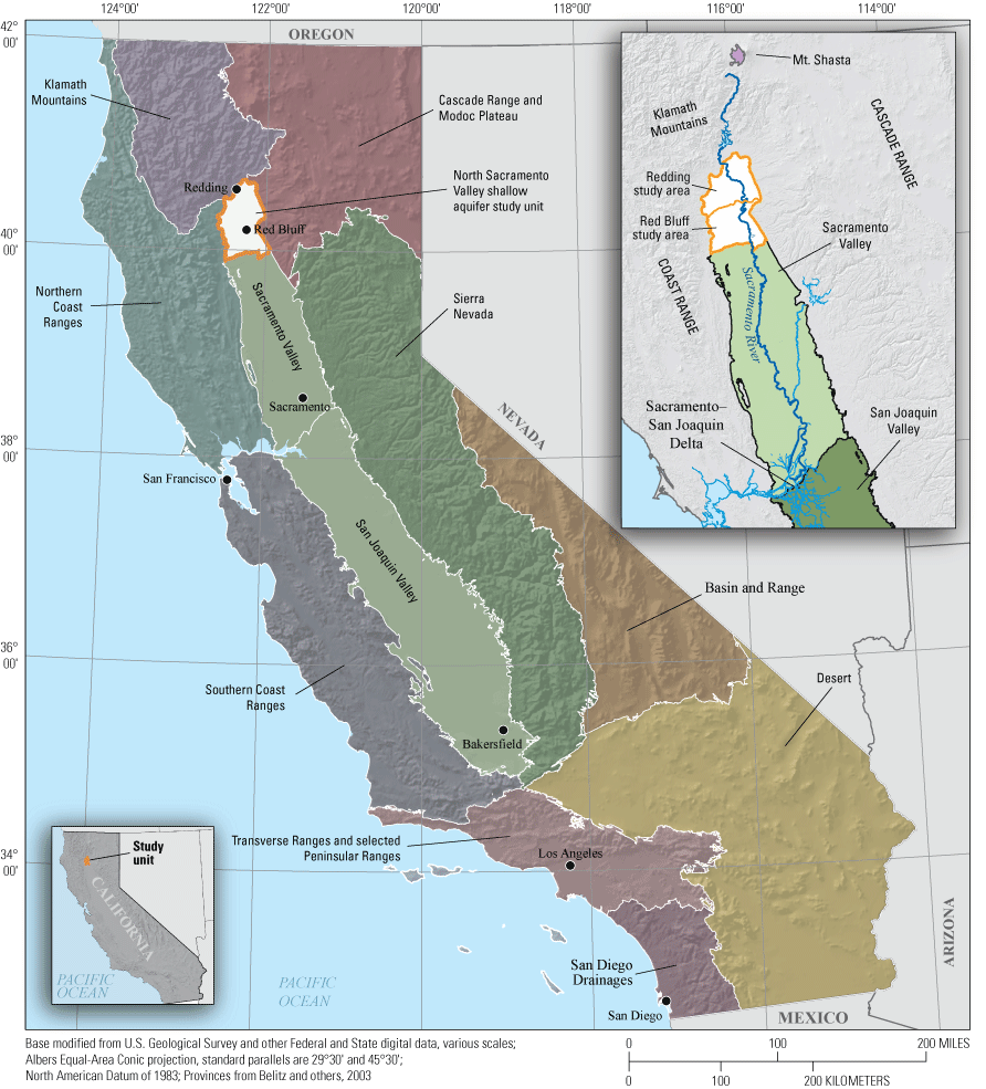
Hydrogeologic provinces of California and the location of the Redding–Red Bluff shallow aquifer study unit, California Groundwater Ambient Monitoring and Assessment Program Priority Basin Project, 2018–19 (adapted from Belitz and others, 2003).
The GAMA-PBP was designed to evaluate the ambient groundwater quality in aquifers used for drinking-water supply, identify natural and human factors likely affecting groundwater quality, and monitor changes in groundwater quality. These three objectives were modeled after those of the USGS National Water-Quality Assessment (NAWQA) Project (Hirsch and others, 1988). The sample collection protocols used in this study were designed to obtain representative samples of ambient groundwater (Belitz and others, 2003, 2010, 2015; Shelton and others, 2020). The quality of groundwater can differ from the quality of drinking water because water chemistry can change as a result of contact with plumbing systems or the atmosphere or because of treatment, disinfection, or blending with water from other sources.
The assessments in this report apply to the depth zone in the aquifer system containing groundwater resources used for domestic-water supply. In many groundwater basins, domestic and small system wells typically are shallower than public-supply wells; thus, the depth zone tapped by domestic and small-system wells typically corresponds to the shallow aquifer system, but this is not always true in every groundwater basin (Burow and others, 2008; Bennett, 2018). This separation of source water for domestic and public supply can be less distinct in some groundwater basins and in areas outside of groundwater basins.
Purpose and Scope
This USGS Scientific Investigations Report (SIR) is comparable to other USGS SIRs written for the GAMA-PBP study units and is the second in a series of reports presenting the water-quality data collected in the NSV-SA (Shelton and others, 2020). Reports addressing the status, understanding, and trends of the water-quality assessments done as part of the GAMA-PBP are available from the USGS (https://webapps.usgs.gov/gama/products/products.html) and the SWRCB (https://www.waterboards.ca.gov/water_issues/programs/gama/). This report provides (1) a description of the hydrogeologic setting of the NSV-SA, (2) a status assessment of the groundwater quality in the resources used for domestic wells of the NSV-SA in 2018–19, (3) an understanding assessment to identify natural and anthropogenic factors that could be affecting groundwater quality, and (4) a comparison between the quality of groundwater in the groundwater resources used by domestic wells and the quality of groundwater resources used for public drinking water. Temporal trends in groundwater quality in the domestic and public-supply aquifer systems are not discussed in this report.
The status assessment was designed to provide a statistically representative characterization of groundwater resources used for domestic drinking water at the study-area scale for December 2018 to April 2019. This report describes methods used to design the sampling network for the status assessment and estimate aquifer-scale proportions for constituents (Belitz and others, 2010). Aquifer-scale proportion is defined as the areal proportion of the groundwater resource having water of defined quality (Belitz and others, 2010). Water-quality data from 50 wells sampled by USGS-GAMA for the NSV-SA were used for the status assessment (fig. 2; Shelton and others, 2020). Aquifer-scale proportions for constituents and classes of constituents were computed for the NSV-SA as a whole and separately for the two study areas in the study unit (Redding and Red Bluff) by using a stratified-random sampling design (the USGS grid method) based on a 50-cell, approximately 50-square-kilometer (km2) equal-area grid covering the study unit (fig. 2; Belitz and others, 2010; Shelton and others, 202074).
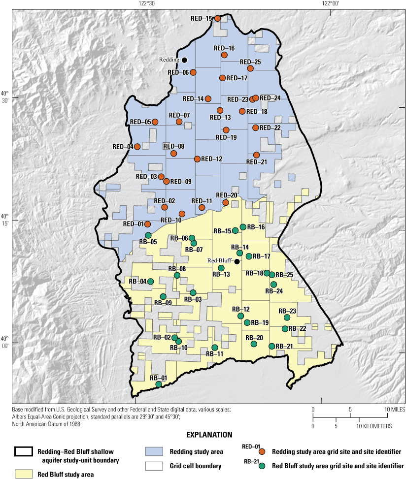
Locations of grid cells and groundwater grid sites sampled in the Redding and Red Bluff study areas for the Redding–Red Bluff shallow aquifer study unit, California Groundwater Ambient Monitoring and Assessment Program Priority Basin Project, 2018–19. Locations and site information for grid wells reported in Shelton and others (2020).
To provide context, the water-quality data discussed in this report were compared to California and Federal regulatory and non-regulatory benchmarks for treated drinking water delivered by public water systems (Toccalino and others 2014; California State Water Resources Control Board, 2015a; U.S. Environmental Protection Agency, 2016). The State of California does not regulate the quality of drinking water provided by domestic wells. The status of water quality reported herein is for ambient, untreated groundwater resources in domestic wells of the study unit.
The evaluation of natural and human factors affecting groundwater quality in the study unit is based primarily on relations between groundwater quality and potential explanatory variables. The following potential explanatory variables were evaluated: aquifer lithology, land use, hydrologic conditions, depth, elevation, aridity, groundwater age, geochemical conditions, underground storage tank (UST) density, and septic tank density. The relations were examined with statistical tests and graphical analyses. The results of the analyses are discussed in the context of the hydrogeologic and geographic setting of the study unit to support the observed associations. Results also are discussed in relation to other water-quality assessments in the region and differences observed between the studies are addressed (California State Water Resources Control Board, 2009; Central Valley Regional Water Quality Control Board, 2016).
To investigate the differences between groundwater resources used for domestic drinking water and those used for public drinking-water supply, statistical comparisons were made between groundwater-quality results from the NSV-SA (domestic drinking-water sources) samples and results obtained by the GAMA-PBP sampling of the north Sacramento Valley public-supply aquifer study unit (NSV-PA; public drinking-water sources) in 2007 (Bennett and others, 2009, 2011). Direct comparisons between the two study units were made after evaluating and adjusting for subtle differences in the designs of each study unit (discussed in the "Comparison of Domestic and Public-Supply Aquifer Systems" section). Variances in numerous study-unit characteristics, including explanatory variables and the results of water-quality analyses in each study unit, were identified and discussed at study-unit and study-area scales.
Hydrogeologic Setting
The Sacramento Valley is the northern section of California’s Central Valley between Redding at the base of the Klamath Mountains and north of the Sacramento–San Joaquin Delta (fig. 1). The Sacramento Valley has a Mediterranean-type climate characterized by hot, dry summers and cool, wet winters (Western Regional Climate Center, 2020). The average annual rainfalls in Redding and Red Bluff are 89 and 61 centimeters (cm), respectively, with about 90 percent of the precipitation falling from October through April (U.S. Department of Commerce National Climatic Data Center, 2020). Typical precipitation from May through September is less than 2.5 cm. The Sacramento River, California’s largest river, begins its course in the headwaters near Mount Shasta north of the study unit and meanders south through the study unit (fig. 1).
Numerous perennial and ephemeral streams flow from the mountain ranges surrounding the Sacramento Valley, across the valley floor, and into the Sacramento River. Streams originating on the western side of the Sacramento Valley are mostly ephemeral and most streams flowing from the eastern side are perennial. Some of the notable streams flowing from the western side of the valley in the northern part of the Sacramento Valley are Cottonwood Creek, Reeds Creek, Elder Creek, and Thomes Creek (fig. 3). Notable creeks flowing from the eastern side of the valley are Battle Creek, Antelope Creek, Mill Creek, and Deer Creek (fig. 3).
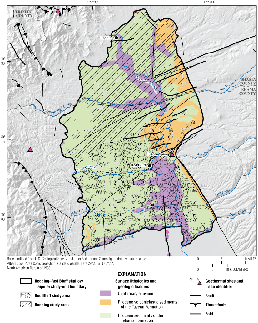
Generalized surface lithologies and geologic features adapted from Saucedo and others (2000) for the Redding–Red Bluff shallow aquifer study unit, California Groundwater Ambient Monitoring and Assessment Program Priority Basin Project, 2018–19.
The Redding–Red Bluff study unit covers an area of approximately 3,100 km2, in parts of Shasta and Tehama Counties, in the northern Sacramento Valley of California (figs. 1, 3). The study unit is divided into two study areas: (1) the Redding study area and (2) the Red Bluff study area. The Redding study area covers approximately 1,550 km2 and includes the CDWR-defined Redding Area groundwater basin and six subbasins: Enterprise, Millville, Anderson, South Battle Creek, Rosewood, and Bowman subbasins (California Department of Water Resources, 2003; California Department of Water Resources, 2022). Three mountain ranges border the Redding study area—the southernmost extension of the Cascade Range along the eastern edge, the northern Coast Ranges, a series of folded and faulted parallel ridges and valleys trending to the west, and the Klamath Mountains to the north (fig. 1). The Red Bluff study area covers approximately 1,500 km2 and includes the northernmost section of the CDWR-defined Sacramento Valley groundwater basin and five subbasins: Bend, Red Bluff, Antelope, Dye Creek, and Los Molinos subbasins (California Department of Water Resources, 2003; California Department of Water Resources, 202216). The Red Bluff study area is bounded to the east by the southern Cascade Range, to the west by the Coast Ranges, and to the south by Thomes Creek and Deer Creek (figs. 1, 3). The Red Bluff arch is a geological feature at the northern boundary of the Red Bluff study area that hydrologically separates the Redding and Sacramento Valley groundwater basins (California Department of Water Resources, 2003; California Department of Water Resources, 2014).
The Sacramento valley is an elongated, asymmetrical, structural basin that contains marine and non-marine sediments up to 8 km thick (California Department of Water Resources, 2014). A relatively thin layer of primarily mid- to late-Pliocene to Holocene continental sediments contains the fresh groundwater used for drinking water. These freshwater-bearing sediments are derived from the surrounding mountain ranges and constitute a mix of marine, continental, and volcanic sediments. Marine sediments are derived from the Coast Ranges, whereas the continental and volcanic sediments are derived from the Cascade Range. These aquifers overlie saline-water-saturated marine sediments that were deposited during the Mesozoic and early Cenozoic eras (Pierce, 1983; California Department of Water Resources, 2014). The depth to the base of freshwater (groundwater with a total dissolved solids concentration <3,000 milligrams per liter [mg/L]) in the Sacramento Valley generally occurs at less than 750 meters (m) below land surface (California Department of Water Resources, 2014; Heberger and Donnelly, 2015).
Although the groundwater basins are divided north and south, aquifer lithology is primarily divided east and west by the Sacramento River. Groundwater is in the heterogeneous gravel and sand layers of the Tehama and Tuscan Formations and in the shallower alluvial layers (California Department of Water Resources, 2014). The general pattern of groundwater flow is from the northern end of the Sacramento Valley toward the Sacramento–San Joaquin Delta and from the margins of the valley toward the Sacramento River (California Department of Water Resources, 2014).
The Pliocene Tuscan Formation is the primary water-bearing unit in the eastern part of the northern Sacramento Valley. It is an important sedimentary unit composed of volcaniclastic sediments deposited from the Cascade Range that yields relatively large quantities of water to wells in the Sacramento Valley and Redding groundwater basins (California Department of Water Resources, 2014). The Tuscan Formation crops out to the northeast of Red Bluff and then dips into the subsurface southwestward, where it intermingles with the Tehama Formation (fig. 3).
The Pliocene Tehama Formation crops out along the western margin of the Sacramento Valley and Redding groundwater basins and dips eastward beneath the Quaternary alluvium deposits in the center of the Sacramento Valley, where it intermingles with the Tuscan Formation (California Department of Water Resources, 2014). The Tehama Formation is derived from the Coast Ranges to the west and is composed of unconsolidated to moderately consolidated coarse- and fine-grained sediments with thin lenses of gravel and sand (California Department of Water Resources, 2014). The average thickness of the Tehama Formation is approximately 600 m, and the lower part of the Tehama Formation contains saline groundwater (California Department of Water Resources, 2014). The younger Quaternary alluvium deposits overlie the Tehama Formation along the Sacramento River and other minor creeks. These alluvial deposits primarily are composed of sands and gravels derived from the Coast Ranges. Overall, the Tehama Formation and the overlying Quaternary alluvial deposits produce variable amounts of water to wells (California Department of Water Resources, 2014).
Methods
The GAMA-PBP framework applies quantitative and statistical methods for the status assessment, understanding assessment, and comparison between the shallow aquifer and public supply. The methods used to collect and analyze groundwater samples and quality-control results are described by Shelton and others (2020). The methods used for compiling data for the potential explanatory variables are described in appendix 1 and a U.S. Geological Survey data release (Harkness, 2022){ label needed for book-app[@id='a1'] }.
Status Assessment
The status assessment was designed to quantitatively summarize groundwater quality of the groundwater resources used for domestic drinking-water wells of the Redding–Red Bluff study unit (NSV-SA) and Redding and Red Bluff study areas. This section describes the methods used for (1) defining groundwater quality, (2) assembling the data used for the assessment, (3) selecting constituents for evaluation, and (4) calculating aquifer-scale proportions.
Groundwater Quality Defined Relative to Water-Quality Benchmarks Concentrations
In this study, groundwater-quality data are presented as relative concentrations (RCs), which are defined as the ratio between the concentration measured in a groundwater sample to the concentration of a constituent’s regulatory or non-regulatory benchmark. The use of RCs is similar to the approaches used by previous studies to place the concentrations of constituents in groundwater in a toxicological context (Toccalino and Norman, 2006; Rowe and others, 2007). This approach allows for a quantitative definition of water quality that meets the standards for safe drinking water (U.S. Environmental Protection Agency, 1986; Toccalino and others, 2004).
The use of RCs allows comparison on a single scale for constituents that can be present at a wide range of concentrations. When the sample concentration is greater than the benchmark concentration, the RC has a value greater than 1.0. The RCs can only be computed for constituents with water-quality benchmarks; therefore, constituents without water-quality benchmarks are not included in the status assessment. Additionally, the RCs account for thresholds related to toxicological effects from individual constituents and does not include the additive effects of multi-constituents exceeding threshold values.
Regulatory and non-regulatory benchmarks are used to set quality standards for treated water that is served to the consumer by public water-supply systems. However, these standards are not applied to untreated groundwater in domestic wells. To provide some context for the results in this assessment, concentrations of constituents measured in the untreated groundwater were compared to benchmarks established by the U.S. Environmental Protection Agency (EPA), SWRCB Division of Drinking Water (DDW), and USGS. The benchmarks used for each constituent were selected in the following order of priority:
-
1. Regulatory, health-based levels established by the DDW and the EPA: California State Water Resources Control Board Division of Drinking Water maximum contaminant level (CA-MCL), the U.S. Environmental Protection Agency maximum contaminant level (US-MCL), and the U.S. Environmental Protection Agency action levels (US-AL; California State Water Resources Control Board, 2015a; U.S. Environmental Protection Agency, 2016). If the CA-MCL and US-MCL are the same value, the benchmark is called US-MCL. If the CA-MCL is lower than the US-MCL or no US-MCL exists, the benchmark is called CA-MCL.
-
2. For constituents lacking maximum contaminant levels (MCLs), aesthetic-based levels were established as secondary maximum contaminant levels (SMCLs) by the California State Water Resources Control Board (CA-SMCL) or the U.S. Environmental Protection Agency secondary maximum contaminant level (US-SMCL; California State Water Resources Control Board, 2015a). The salinity indicators chloride, sulfate, and total dissolved solids (TDS) have recommended and upper CA-SMCLs, and the values for the upper levels were used as water-quality benchmarks in this report; pH does not have a US-MCL or CA-SMCL value but does have a US-SMCL value.
-
3. For constituents with neither MCL nor SMCL benchmarks, non-regulatory, health-based levels established by the USGS, EPA, and DDW were used as benchmarks. These benchmarks included the California State Water Resources Control Board Division of Drinking Water response levels (CA-RL) and California State Water Resources Control Board Division of Drinking Water notification levels (CA-NL), U.S. Environmental Protection Agency lifetime health advisory levels (US-HAL), and USGS health-based screening levels (HBSL; U.S Environmental Protection Agency, 2012; Toccalino and others, 2014; California State Water Resources Control Board, 2015a). The priority order for non-regulatory, health-based benchmarks is as follows:
-
a. CA-RL or the US-HAL, whichever is lower.
-
b. US-HAL if no CA-RL exists.
-
c. USGS HBSL. A constituent may have a non-cancer or cancer HBSL or both, and the cancer HBSLs are given as ranges corresponding to the 10−4 to 10−6 risk levels. The lowest HBSL is used as the benchmark, with the exception of hexavalent chromium. For hexavalent chromium, the highest non-cancer HBSL value of 20 micrograms per liter (µg/L) is used. The lowest cancer HBSL value of 0.04 microgram per liter (µg/L) for hexavalent chromium is below the detection level for the analytical method. The HBSLs for lithium and cobalt were not used in this study because they are based on toxicity data from the EPA Provision Peer-Reviewed Toxicity Value program (https://www.epa.gov/pprtv/provisional-peer-reviewed-toxicity-values-pprtvs-assessments).
-
For constituents with multiple types of benchmarks, this hierarchy might not result in selection of the benchmark with the lowest concentration. Additional information on the types of benchmarks and listings of the benchmarks for all constituents analyzed are provided by Shelton and others (2020).
For ease of discussion, RCs for inorganic constituents (trace elements, nutrients, radionuclides, and constituents with SMCL benchmarks) and organic constituents were classified in “low,” “moderate,” and “high” categories. The RC values greater than 1.0 were defined as “high” for all constituents, RC values greater than 0.5 and less than or equal to 1.0 were defined as “moderate,” and RC values less than or equal to 0.5 were defined as “low” for inorganic constituents; two exceptions were boron (B) and vanadium (V), which have moderate/low RC threshold values of 0.16 and 0.1, respectively. The benchmarks for B and V are based on using second priority benchmarks (CA-NL) for the moderate/lower thresholds.
For organic constituents and perchlorate, RC values greater than 0.1 and less than or equal to 1.0 were defined as “moderate,” and RC values less than or equal to 0.1 were defined as “low.” Although more complex classifications could be devised based on the properties of individual constituents and the multiple available benchmarks, use of a single moderate/low threshold value for each of the two major groups of constituents provided a consistent objective criterion for distinguishing constituents present at moderate concentrations. The boundary between low and moderate RCs is not intended to indicate the presence of contamination from anthropogenic sources.
Dataset Used for Status Assessment
Groundwater-quality data used for the status assessment came from sites sampled by the USGS for the GAMA-PBP (fig. 2). Detailed descriptions of the methods used to identify sites for sampling and assign site identifiers are given in Shelton and others (2020). Briefly, the NSV-SA was divided into two study areas: (1) Redding and (2) Red Bluff. Each study area was divided into equal-area grid cells (Scott, 1990) so that 25–44 km2 cells comprised the Redding study area and 25–49 km2 cells comprised the Red Bluff study area (fig. 2). In each cell, one groundwater well was randomly selected to represent the groundwater resources used for domestic supply. Sample sites for each grid cell were selected from lists of domestic-supply wells compiled using information obtained from the CDWR well completion report database (California Department of Water Resources, 2018; Shelton and others, 2020). Field crews went door-to-door to obtain permission to sample domestic-supply wells from the target list, beginning with the well nearest to a randomly selected location in the grid cell to ensure random selection of sites. The USGS sampled 1 domestic-supply well in each of the 50 grid cells, referred to in this report as a USGS grid site. The USGS grid sites were named with an alphanumeric GAMA identification consisting of the prefix “S-NSV-Red” or “S-NSV-RB” (indicating Redding or Red Bluff study areas, respectively) and a number reflecting the order of sample collection (Shelton and others, 2020).
Samples collected from all sites were analyzed for 231 constituents (table 1; Shelton and others, 2020). Water-quality data collected by USGS-GAMA are tabulated in Shelton and others (2020) and are available from the GAMA Groundwater Information System (California State Water Resources Control Board, 2020) and the USGS National Water Information System (NWIS; U.S. Geological Survey, 2020).
Table 1.
Summary of water-quality constituent groups and numbers of constituents sampled for each constituent group by the U.S. Geological Survey (USGS) in the Redding–Red Bluff Aquifer study unit, California Groundwater Ambient Monitoring and Assessment Program Priority Basin Project, 2018–19.[Unless otherwise noted, constituent analyses were performed at the USGS National Water Quality Laboratory, Denver, Colorado. Abbreviations: C, carbon; H, hydrogen; O, oxygen; δ, delta notation, indicating the isotopic enrichment or depletion of a sample relative to a standard of known composition]
Selection of Constituents for Discussion
Aquifer-scale proportions were calculated and presented for the 12 constituents that were present at high or moderate RCs in samples from the 50 USGS grid sites (table 2). Aquifer-scale proportion results also are presented for chloroform because it had a detection frequency of greater than 10 percent in samples from the USGS grid sites (table 2). An additional 35 inorganic constituents, 1 constituent of special interest, and 7 organic constituents were detected but either do not have drinking-water quality benchmarks or were only detected at low RCs (table 2). Constituents that were only detected at low RCs in the study unit were not included in the aquifer scale proportion calculations. Of the 231 constituents analyzed in samples collected for the NSV-SA, 161 were not detected in any of the samples (Shelton and others, 2020).
Table 2.
Benchmark type and value for inorganic and organic constituents detected in samples from grid sites in the Redding–Red Bluff shallow aquifer study unit, California Groundwater Ambient Monitoring and Assessment Program Priority Basin Project, 2018–19.[Relative concentration (RC) is defined as the measured value divided by the benchmark value. For high RC, value is greater than 1.0 (for inorganic and organic constituents); moderate RC, value is less than or equal to 1.0 and greater than 0.5 (for inorganic constituents) or 0.1 (for organic constituents); low RC, value is less than or equal to 0.5 (for inorganic constituents) or 0.1 (for organic constituents). Benchmark types: Regulatory, health-based benchmarks: CA-MCL, California State Water Resources Control Board Division of Drinking Water (DDW) maximum contaminant level; US-MCL, U.S. Environmental Protection Agency (EPA) maximum contaminant level; US-AL, EPA action level. Non-regulatory health-based benchmarks: US-HAL, EPA lifetime health advisory level; HBSL, U.S. Geological Survey (USGS) Health Based Screening Level; CA-NL, DDW notification level; CA-RL, DDW response level. Non-regulatory aesthetic-based benchmarks: CA-SMCL, DDW secondary maximum contaminant level. Abbreviations: µg/L, microgram per liter; —, not applicable; mg/L, milligram per liter; pCi/L, picocuries per liter; C, carbon; H, hydrogen; O, oxygen; δ, delta notation, indicating the isotopic enrichment or depletion of a sample relative to a standard of known composition]
Maximum contaminant level benchmarks are listed as US-MCL when the US-MCL and CA-MCL are identical and as CA-MCL when the CA-MCL is lower than the MCL-US or no US-MCL exists. Sources of benchmarks: CA-MCL, California State Water Resources Control Board (2015a); US-MCL, U.S. Environmental Protection Agency (2012); CA-NL, California State Water Resources Control Board (2015a); Proposed US-MCL, CA-SMCL, California State Water Resources Control Board (2015a); HBSL, Toccalino and others (2014).
Chloroform is the only constituent within the volatile organic compound class to have been detected in more than 10 percent of the samples collected.
US-MCL benchmark for trihalomethanes is for the sum of chloroform, bromodichloromethane, dibromochloromethane, and bromoform.
Calculation of Aquifer-Scale Proportions
A grid-based statistical approach (Belitz and others, 2010) was used to calculate the areal proportions of the groundwater resources used by domestic drinking-water wells in the NSV-SA with high, moderate, and low RCs of constituents (eq. 2):
whereis the high-RC aquifer-scale proportion for the study area,
is the number of cells in the study area represented by a site having a high RC for the constituent, and
is the number of cells in the study area having a site with data (including non-detections) for the constituent (this varied as some sites did not have data for all constituents).
High-RC aquifer-scale proportions for the whole study unit were calculated as an area-weighted combination of the aquifer-scale proportions for the two study areas (eq. 2):
whereis the area-weighted high-RC aquifer-scale proportion for the two study areas in the NSV-SA study unit,
Σ
is the summation operator,
is the fraction of the study-unit gridded area occupied by each study area, and
is the high-RC aquifer-scale proportion for each study area.
Moderate- and low-RC aquifer-scale proportions for the study unit were calculated in the same manner as high-RC aquifer-scale proportions. The detection frequencies for organic constituents in samples from the USGS grid sites were calculated for each study area as area-weighted detection frequencies. The detection frequency in each study area was calculated by using equation 1 with replaced by the number of samples with detections, and then the detection frequency for the study unit as a whole was calculated by using equation 2 after making the corresponding replacement. Lower and upper confidence intervals for aquifer-scale proportions were computed by using the Jeffreys interval for the binomial distribution using the binom program in the R statistical program package DescTools (Brown and others, 2001; Belitz and others, 2010; RStudio Team, 2021; Signorell, 202175). For nonzero proportions, the confidence interval is computed as a two‐sided interval; for zero values, a one‐sided interval is computed.
For ease of discussion, these proportions are referred to as “high-RC,” “moderate-RC,” and “low-RC” aquifer-scale proportions. Aquifer-scale proportions were calculated for each study area and for the entire study unit. Aquifer-scale proportions were calculated for individual constituents and for groups of related individual constituents, referred to as “constituent classes.” Aquifer-scale proportions for constituent classes were calculated using the maximum RC for any constituent in the class to represent the class for each site. For example, a site having a high RC for arsenic, moderate RC for fluoride, and low RCs for molybdenum, boron, selenium, and other trace elements would be counted as having a high RC for the class of trace elements with health-based benchmarks.
Understanding Assessment
In the understanding assessment, the physical and chemical processes that could be affecting water quality were identified by examining relations between water quality and potential explanatory variables. The GAMA-PBP uses statistical tests of associations between potential explanatory variables and water-quality conditions to identify potential relations between water quality and various natural and human-induced processes in a study unit. Methods used for the understanding assessment included (1) selecting constituents for additional evaluation and (2) applying statistical tests of relations between potential explanatory variables and selected groundwater-quality constituents.
Selection of Constituents
A subset of constituents that were present at high or moderate RCs in samples from the 50 USGS grid sites (table 2) were selected for additional evaluation in the understanding assessment. This subset consisted of (1) individual constituents present at moderate or high RCs in greater than 2 percent of the groundwater resource used for domestic supply and (2) organic constituent classes detected at any concentration in greater than 10 percent of the resource. Use of these criteria resulted in selection of five inorganic constituents (arsenic, chromium, iron, manganese, and nitrate), one organic constituent class (chloroform), and one special-interest constituent (hexavalent chromium; table 2).
Statistical Analysis
All statistical analyses were done in the R statistical environment (RStudio Team, 2021) consistent with Helsel and others (2020). Nonparametric statistical tests were used to test the significance of correlations among potential explanatory variables and between water-quality constituents and potential explanatory variables. Nonparametric statistics are robust techniques that do not require the data to follow a distribution and are minimally affected by outliers (Helsel and others, 2020). The probability value (p) used for hypothesis testing for this report, unless otherwise noted, was compared to a level of significance (α) of 5 percent (α=0.05) to evaluate whether the relation was statistically significant (p less than α).
Three different statistical tests were used because the set of potential explanatory variables included categorical and continuous variables. Groundwater-age, oxidation-reduction (redox) class, groundwater lithology, and study area were treated as categorical variables. Land-use proportion, septic-tank density, UST density, aridity index, elevation, well depth, depth to top of screened or open interval, pH, and dissolved oxygen (DO) were treated as continuous variables.
-
• Concentrations of water-quality constituents were treated as continuous variables. Correlations between continuous variables were evaluated using the Spearman’s rank-correlation test (ρ; or rho) to calculate the rank-order correlation coefficient and to determine whether the correlation was significant (p less than α). Spearman’s rho was calculated using the cor.test function in R.
-
• The Wilcoxon rank-sum test was used when comparing two categories of explanatory variables such as redox class and study area (R function wilcox.test; RStudio Team, 2021); the Kruskal-Wallis and Dunn’s tests were used when comparing more than two categories of explanatory variables, such as groundwater age, land cover/land use, or aquifer lithology (R functions kruskal.test and posthoc.kruskal.dunn.test; RStudio Team, 2021). The null hypothesis for these tests is that the distributions of the continuous response variables do not significantly differ between or among categorical explanatory variables.
-
• Relations among categorical variables were evaluated using contingency tables. For contingency table analysis, the data are recorded as a matrix of counts using the prop.table function in R (RStudio Team, 2021). One variable is assigned to the columns and the other to the rows. The statistical test for independence compares the observed counts to the counts expected if the two variables are independent, and statistical significance is determined by comparing the test statistic (1–α) to the quantile of a chi-square distribution using Fisher’s exact test (R function fisher.test, RStudio Team, 2021), which is recommended for small sample sizes (less than 1,000; Helsel and others, 2020). If the contingency table test detected a significant difference between the observed counts and the expected counts, then the matrix cell, or cells, contributing the most to the difference was identified by comparing the magnitudes of the components of the test statistic (Helsel and others, 2020). Contingency tables were used mostly to compare the proportion of samples with high, moderate, and low RCs among different explanatory variables.
Comparison Between the Redding–Red Bluff Shallow Aquifer Study Unit and North Sacramento Valley Public-Supply Study Unit
Groundwater quality results were compared between the two study units to identify differences in water quality of groundwater resources used for domestic and public supply. Variations in the explanatory variables between the NSV-SA and NSV-PA were explored using contingency table comparisons to identify potential drivers of water-quality differences between the groundwater resources used for domestic and public drinking water supplies. Multiple nonparametric comparison tests, Kruskal-Wallis rank-sum test, and Dunn’s tests from the R statistical program (RStudio Team, 2021) were used to evaluate relations among categorical and continuous explanatory variables, including well depth, groundwater age and redox class, primary aquifer lithology, and land use or land cover. Geochemical differences between the study units were further evaluated using Piper diagrams (Piper, 1944) of the major ion proportions (R function transform_piper_dater; https://rpubs.com/gavan_mcgrath/PiperTrilinear), which identified the major geochemical processes that influence the chemical composition of the groundwater resources.
Aquifer-scale proportions of groundwater resources with high, moderate, and low RCs and categorical explanatory variables (groundwater age, redox class, aquifer lithology, land use/land cover) for the study units and study areas were tested using contingency tables and Fisher exact tests (2 by 2; R function fisher.test; RStudio Team, 2021). The significance level (p-value) used when testing these differences was based on a threshold value (α) of 10 percent (α=0.1). As already noted, if the test statistic p was less than α, the relation was considered statistically significant. If the test statistic p was greater than α, the relation was not considered statistically significant. A threshold value for significance of 0.1 was used for the study unit comparison to allow discussion of differences that would have been defined as not significant relative to the threshold value of 0.05 used for the rest of this study. The contingency tables were constructed to compare to frequency of sites with high or moderate RCs against those with low RCs and to compare sites with high RCs against those with low or moderate RCs. These tests were run for the constituent classes and for individual constituents.
Using the framework established in the status and understanding assessments of the NSV-PA and NSV-SA, constituents selected for additional evaluation were the focus of the comparison between the study units with respect to groundwater quality. Individual constituent aquifer-scale proportions and proportions of constituent groups by class presented for the NSV-SA were recalculated for the comparison analysis with the NSV-PA. Adjustment was necessary to prevent sites outside of the area of comparison from being included in the comparison of the two study units. Less than half of the wells in the NSV-SA study unit extent overlapped with the NSV-PA extent, but all the NSV-PA wells were within the NSV-SA study unit extent. A more even set of wells for statistical comparison between the two study units was achieved when sites from the NSV-SA within a 3-km distance of the NSV-PA extent were included in the analysis. The distance of 3 km was chosen because this was the buffer distance around public-supply wells used to create the NSV-PA study unit extent (Bennett and others, 2009).
Not all inorganic or organic constituents were sampled in both the NSV-SA and NSV-PA, so some constituents at high or moderate RCs in one study unit were not included in the comparison. Relative concentrations and aquifer-scale proportions presented in Bennett and others (2011) for the NSV-PA were recalculated to ensure that the same water-quality benchmarks were applied for both study units. Benchmark threshold levels for some constituents and the relative hierarchy among benchmarks changed since the NSV-PA analysis in 2007. For example, in the NSV-SA, the boron concentrations were compared to the US-HAL of 6,000 µg/L (Toccalino and others, 2014). In the NSV-PA, concentrations of boron were compared to the CA-NL of 1,000 µg/L (California State Water Resources Control Board, 2016). For a consistent comparison of RCs, benchmark thresholds and the benchmark hierarchy used for the 2018–19 NSV-SA sampling results were used for study-unit comparisons. Lastly, reporting levels for organic and special-interest constituents were re-evaluated if a constituent’s reporting level changed between 2007 and 2019; constituent non-detections were re-censored at the higher of the two reporting levels.
Potential Explanatory Variables
Characteristics of the aquifer system used for domestic drinking-water supplies are described using explanatory-variable data compiled for the 50 sites sampled for the USGS-GAMA for the study unit. The methods used for assigning values for each of the explanatory variables to the 50 sites sampled for the USGS-GAMA in the NSV-SA are described in appendix 1 and Harkness (2022). The potential explanatory variables examined in the NSV-SA are frequently correlated to one another. Correlations among explanatory variables can support interpretations of processes affecting groundwater quality. Therefore, statistical correlations were evaluated to determine differences or similarities among potential explanatory variables such as aquifer lithology, land use, hydrologic conditions, well depth, groundwater age, and geochemical conditions. Results of relations among explanatory variables are presented in tables 3 and 4.
Table 3.
Summary of Spearman’s rho (ρ) rank correlation test results for selected potential explanatory variables at grid wells, Redding–Red Bluff shallow aquifer study unit, California Groundwater Ambient Monitoring and Assessment Program Priority Basin Project, 2018–19.[Tabled values of rho are shown for statistically significant tests (p-value <0.05). Abbreviations: —, not applicable; ns, Spearman’s test indicates no significant correlation between variables; USTs, underground storage tanks; positive values, significant positive correlation; negative values, significant negative correlation]
Table 4.
Comparison of statistically significant (p-value<0.05) differences in median values between explanatory variables, study area, and select inorganic and organic constituents, Redding–Red Bluff shallow aquifer study unit, California Groundwater Ambient Monitoring and Assessment Program Priority Basin Project, 2018–19.[Relation of median values in categorical groups tested for differences using Kruskal-Wallis and Wilcoxon rank sum test and the posthoc Dunn's test for multiple comparisons. The p-values were calculated using the Kruskal-Wallis or Wilcoxon test; if significant, then Dunn's test was used to determine which differences were significant. Greater than symbol (>) indicates that the median value for left variable is greater than the median value for the right variable; for example, “Pre>Mod” for well depth means the following: the well depth values from premodern-age class sites are significantly greater than well-depth values from modern-age class sites. Categorical groups: Groundwater age class: Mix, mixed (modern and premodern); Mod, modern; Pre, premodern. Aquifer lithology: Q, Quaternary alluvium; QPc, sediment of the Tehama Formation. Study area: Red, Redding; RB, Red Bluff. Other abbreviations: vs, versus; UST, underground storage tank; >, greater than; ns, test indicated no significant differences between the sample groups]
Aquifer Lithology
To examine broad relations between aquifer lithology and groundwater quality, the various geologic units of the NSV-SA, as represented on the state geologic map (Saucedo and others, 2000), were grouped into three general rock types: (1) sediments of the Tehama Formation, (2) volcanoclastic sediments of the Tuscan Formation, and (3) Quaternary alluvium in the floodplains of the Sacramento River (fig. 3; appendix 1; Harkness, 2022).
The lithology of the Redding and Red Bluff study areas is composed primarily of sedimentary deposits of the Tuscan and Tehama Formations or Quaternary alluvial sediments that host the freshwater aquifers, with limited Quaternary pyroclastic volcanic rocks that crop out in the east (fig. 3). Three of the grid sites were in the Tuscan Formation, but all other sites were in the sedimentary deposits of the Sacramento Valley, so the statistical comparison was between the two predominant sedimentary lithologies: marine and continental sediments of the Tehama Formation and the Quaternary alluvium along the Sacramento River (fig. 3). Wells in the Tehama Formation sediments were significantly deeper than wells in the Quaternary alluvium (p=0.004; table 4).
Land Use and Land Cover
Land use and land cover was generalized into three categories: (1) natural (unused), (2) urban, and (3) agricultural (fig. 4; appendix 1; Harkness, 2022). Percentages of the three categories were calculated for the study unit, study areas, and for a circular area, with a radius of 500 m around each USGS grid site (Johnson and Belitz, 2009). As of 2012, land use in the NSV-SA was 67-percent natural, 14-percent urban, and 19-percent agricultural (fig. 5A; Falcone, 2015). Land use in the Redding study area was classified as 64-percent natural, 22-percent urban, and 14-percent agricultural, whereas land use in the Red Bluff study area was 71-percent natural, 5-percent urban, and 24-percent agricultural (fig. 5B).
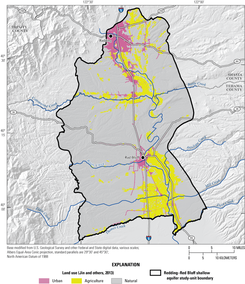
Generalized land use and land cover in 2011, adapted from Jin and others (2013), in the Redding–Red Bluff shallow aquifer study unit, California Groundwater Ambient Monitoring and Assessment Program Priority Basin Project, 2018–19.
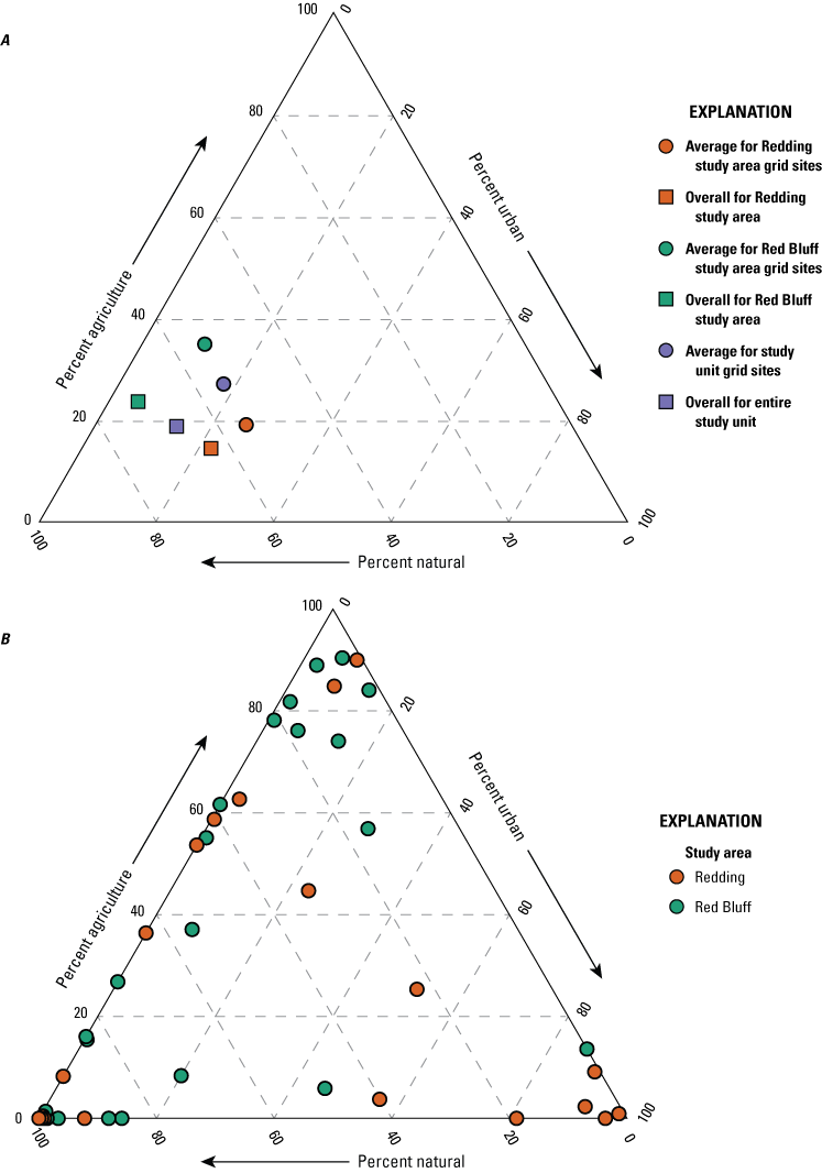
Land use and land cover in 2011, adapted from Jin and others (2013), in the Redding–Red Bluff shallow aquifer study unit, California Groundwater Ambient Monitoring and Assessment Program Priority Basin Project: A, overall land-use composition of the study unit and study areas, 2018–19; and B, percentages of urban, agricultural, and natural land within a 500-meter radius around individual grid wells.
Like the overall study-unit composition, land use in the buffered areas surrounding the USGS grid sites was primarily classified as natural (fig. 4). On average, in the study unit, urban and agricultural land use in the buffered areas (18 and 27 percent, respectively) was greater than in the overall study unit and natural land use was less (55 percent on average), indicating that more drinking-water wells were located near population centers. Around individual grid sites, land use ranged from 0 to 98-percent urban and 0 to 90-percent agriculture, with 20 of 50 sites (12 in the Red Bluff study area) surrounded by greater than 20-percent agricultural land use and 12 of 50 sites (8 in the Redding study area) surrounded by greater than 20-percent urban land use (fig. 5B). The primary crops grown in Shasta County are alfalfa, hay, rice, walnuts, and wheat, whereas agriculture in Tehama County is dominated by tree nuts (almonds, pecans, pistachios, walnuts), olives, and prunes (California Department of Pesticide Regulation, 2017).
Septic tanks and USTs are markers of urban areas or areas with higher populations, as shown by the strong positive correlation of septic tanks and UST densities in the NSV-SA with urban (ρ=0.68, p<0.0001, and ρ=0.41, p=0.003, respectively) and agricultural land use (ρ=0.31, p<0.027, septic tank density only) and negative correlation with natural land use (ρ= −0.67, p<0.0001 and ρ= −0.50, p<0.001; table 3). The average densities of USTs and septic tanks near a groundwater site can be indicators of potential sources of anthropogenic contaminants near the land surface. The density of USTs around grid sites ranged from 0 to about 2.5 tanks per square kilometer (tanks/km2), and the median density was 0.02 tanks/km2. A description of how the Thiessen polygon method (Thiessen, 1911) was used to calculate UST density is included in appendix 1 and Harkness (2022). The density of septic tanks around grid sites ranged from 0 to nearly 72 tanks/km2, and the median density was 5.0 tanks/km2.
Differences in land use were significant between the sediments of the Tehama Formation that dominates the region and the Quaternary alluvium. The Quaternary alluvium aquifer lithology had a higher average percentage of agricultural land use and a lower average percentage of natural land use and the differences between aquifer lithologies were significant (p=<0.001 and p<0.001, respectively; table 4). This relation indicates that agricultural land uses are preferentially located near the Sacramento River and smaller creeks because low-relief landforms favor such development, and the alluvial soil is typically more suitable for agriculture. This relation is further demonstrated by a higher density of septic tanks in areas with Quaternary alluvium lithology because development is denser along the river and the difference between aquifer lithologies is statistically significant (p=0.004; table 4).
Hydrologic Conditions
Hydrologic conditions were represented by elevation and aridity index at each groundwater site (appendix 1; Harkness, 2022; Shelton and others, 2020). Land-surface elevations referenced to the North American Vertical Datum of 1988 (NAVD 88) in the NSV-SA ranged from about 200 ft at the southernmost extent of the Sacramento River to more than 1,000 ft in the west, with the Redding study area at higher elevation than the Red Bluff study area (Shelton and others, 2020). Sampled groundwater sites were at elevations ranging from 233 to 914 ft above NAVD 88 (Shelton and others, 2020).
The climate in the study unit is typical of the Central Valley in California, with warm, dry summers and cold, wet winters (U.S. Department of Commerce National Climatic Data Center, 2020). The National Climatic Data Center station in Red Bluff, California, reported an average annual temperature of 17.0 degrees Celsius (°C) and an average annual precipitation of 62.2 cm in 2018. In contrast, Redding, California, which is in the north end of the study unit, had an average annual temperature of 16.8 degrees °C and average annual precipitation of 87.9 cm in 2018. This general decrease in precipitation from north to south is due to the rain-shadow effect of the mountain ranges in the study unit and prevailing winter weather patterns (U.S. Department of Commerce National Climatic Data Center, 2020).
Aridity index was used as an indicator of climate. Aridity index is defined as average annual precipitation divided by average annual potential evapotranspiration and is identical to the United Nations Educational, Scientific and Cultural Organization Aridity Index (United Nations Educational, Scientific and Cultural Organization, 1977; United Nations Environment Programme, 1997). Typically, conditions are wetter at higher elevations because of orographic effects, and the aridity index was positively correlated to elevation in the NSV-SA (ρ = 0.61, p-value <0.0001; table 3). Aridity-index values at sampled USGS grid sites ranged from 0.49 to 1.00 (Harkness, 2022). Of the 50 sites sampled in the NSV-SA, 21 sites (42 percent) had an aridity index in the humid or wet category (aridity index>0.65), as defined by the United Nations Environment Programme (1997), with only two sites having aridity-index values less than 0.50 (semiarid; Harkness, 2022).
All 21 of the sites with an aridity index in the humid or wet category were in the Redding study area, whereas the Red Bluff study area is drier, and encompasses the two semiarid groundwater sites. Sites in the sediments of the Tehama Formation had significantly greater aridity-index values and elevations than sites in the Quaternary alluvium aquifer lithology (p=0.002 and p<0.001, respectively; table 4); however, this is an example of correlation between two explanatory variables that is unrelated to direct causation. That is, aridity-index values are directly correlated to elevation (table 3), and the Quaternary alluvium found along the Sacramento River is at a relatively lower elevation. The aridity index also is negatively correlated to agricultural land use because agriculture in the region is concentrated along the low-lying Sacramento River (table 3).
Depth and Groundwater Age Characteristics
Well-depth information was available for all 50 wells sampled (appendix 1; Shelton and others, 2020). When compared, no differences were significant between well depths and depths to top of open or screened interval for USGS grid wells in the Redding study area and the Red Bluff study area (p=0.884; table 4; fig. 6). Depths of USGS grid wells ranged from 64 to 528 ft below land-surface datum; the median well depth was 157 ft (fig. 6; Shelton and others, 2020). Depths to the top of the screened or open interval ranged from 49 to 528 ft, with a median of 148 ft. The screened- or open-interval length ranged from 0 to 57 ft, with a median of 0 ft, which indicates that many (52 percent) of the wells in the study unit are open at the bottom of the well rather than screened over an interval (Shelton and others, 2020).
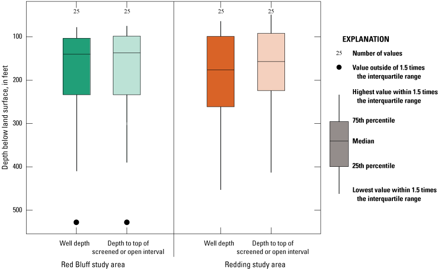
Well depth and depth to top of screened or open interval in feet below land-surface datum for grid wells in the Redding–Red Bluff shallow aquifer study unit, California Groundwater Ambient Monitoring and Assessment Program Priority Basin Project, 2018–19. The differences in well depths and depth to the top of open or screened interval were not significantly different between the study areas (p=0.8843 and p=0.8385, respectively).
Groundwater age refers to the length of time that the water has resided in the aquifer system, which is the amount of time elapsed since the water was last in contact with the atmosphere at recharge. Groundwater samples were assigned to groundwater-age classes based on the tritium (3H) and carbon-14 (14C) activities in the samples (see “Groundwater Age” section in appendix 1 and Harkness [2022]). Samples from 13 sites were classified as modern water (recharged after 1952; Schlosser and others, 1988; Lindsey and others, 2019), samples from 20 sites were classified as mixed (having a component of modern and premodern water), and samples from 17 sites were classified as premodern water (recharged prior to 1952).
Groundwater age typically increases with well depth and with depth to the top of the open or screened interval. Modern groundwater came from wells with significantly shallower depths and depths to the top of the open or screened interval than premodern groundwater (p<0.001 and p<0.001, respectively; fig. 7; table 4). Wells were deeper and groundwater ages older in the sediments of the Tehama Formation, and these wells had a greater proportion of mixed and premodern groundwater compared to the shallower wells with younger aged groundwater completed in the Quaternary alluvium along the river (Kruskal-Wallace test p=0.004 and contingency table test p=0.004; tables 4 and 5). Agricultural land use and septic-tank density were higher for wells with modern groundwater due to higher development along the Sacramento River where the wells are shallower and the differences between modern and premodern groundwater were statistically significant (p=0.013 and p=0.003, respectively; table 4). Percent natural land use and elevation were higher for wells with premodern groundwater in the more rural northern and western parts of the study unit and the differences between premodern and modern groundwater were statistically significant (p=0.003 and p=0.023, respectively; table 4).
Table 5.
Contingency table matrix counts for categorical variables groundwater age, aquifer lithology, redox conditions, or study area, Redding–Red Bluff Shallow Aquifer study unit, California Groundwater Ambient Monitoring and Assessment Program Priority Basin Project, 2018–19.[Fisher's exact test compares the observed counts to the counts expected if the two variables are independent, and statistical significance is determined by comparing the test statistic (p-value <0.1) to the quantile of a chi-square distribution using a one-sided Fisher’s exact test (Helsel and others, 2020). If the contingency table test detected a significant difference between the observed counts and the expected counts, then the matrix cell, or cells, contributing the most to the difference was identified by comparing the magnitudes of the components of the test statistic (Helsel and others, 2020). Abbreviation: SA, study area]
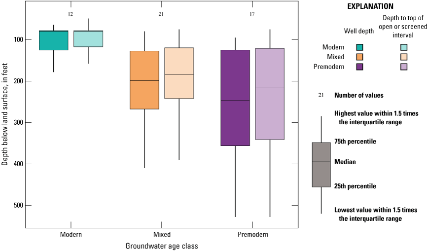
Well depth and depth to top of open or screened interval for grid wells classified as modern, mixed, or premodern in age in the Redding–Red Bluff shallow aquifer study unit, California Groundwater Ambient Monitoring and Assessment Program Priority Basin Project, 2018–19.
Geochemical Conditions
Oxidation-reduction (redox) conditions for the 50 sites sampled by GAMA-PBP were classified using the redox classification framework of McMahon and Chapelle (2008) and Jurgens and others (2009; appendix 1; Harkness, 2022). Groundwater redox conditions were predominantly oxic (47 of 50 sites). The proportion of anoxic groundwater was higher in premodern groundwater wells and the proportion of wells with oxic groundwater was higher in wells with mixed and modern groundwater, which is consistent with loss of oxygen as the groundwater residence time increases (contingency table test p=0.013; table 5). Dissolved oxygen (DO) concentrations were higher in samples from sites in the sediments of the Tehama Formation than in samples from sites in the Quaternary alluvium and the difference is statistically significant (p=0.045; table 4). DO was negatively correlated to agricultural land use (table 3) centered along the Sacramento River (fig. 4). A negative correlation for DO and agricultural land use likely indicates anoxic groundwater conditions in wells located in alluvial deposits near the Sacramento River. Low DO concentrations in these wells could be a result from a combination of groundwater age and sedimentology (higher dissolved organic carbon in the alluvial sediments).
Among all samples, values for pH ranged from 6.4 to 8.4 (Harkness, 2022); pH values were significantly positively correlated to well depth (table 3) and significantly greater in groundwater from mixed and premodern wells (table 4). One possible explanation for the high pH values in the mixed and premodern groundwater is the higher bicarbonate and alkalinity concentrations in these samples due to interactions with the aquifer sediments as the groundwater moves farther along the groundwater flow path. The percentage of natural land use was positively correlated to pH (table 3) because deeper wells with premodern groundwater and alkaline chemistry primarily occur in natural land-use areas. In contrast, the percent urban land use, density of septic tanks, and density of USTs all were negatively correlated to pH (table 3) because younger, more acidic groundwater is found closer to the Sacramento River where there is more development.
Status and Understanding of Groundwater Quality in the Shallow Aquifer System
The discussion of results for the status and understanding assessments is divided into three parts: (1) inorganic constituents, (2) organic and special-interest constituents, and (3) microbial indicators. Each part begins with a survey of the number of constituents that were detected at any concentration compared to the number of constituents analyzed and includes a graphical summary of the RCs of constituents detected in groundwater samples from the grid sites. Aquifer-scale proportions are then presented for constituent classes and the individual constituents that were present at moderate or high RCs. Finally, results of statistical tests for relations between water-quality constituents and potential explanatory variables are presented for the individual constituents and constituent classes that met additional criteria based on RCs for inorganic and detection frequencies for organic constituents and microbial indicators.
Inorganic Constituents
Most inorganic constituents are naturally present in groundwater, although their concentrations can be influenced by human activities (Hem, 1985). Of the 50 inorganic constituents analyzed by the USGS-GAMA, 46 were detected in groundwater in the NSV-SA (Shelton and others, 2020). Of these 46 constituents, 26 had regulatory or non-regulatory health-based benchmarks, 8 had non-regulatory, aesthetic-based benchmarks, and 12 did not have established benchmarks (table 2). The constituents without benchmarks are major or minor ions that are present in nearly all groundwater (table 2).
Of the 26 inorganic constituents that had regulatory and non-regulatory health-based benchmarks, 8 were detected at moderate or high RCs in the grid sites. These constituents included the trace elements arsenic, barium, boron, chromium, and strontium; the nutrient nitrate; the radionuclide gross alpha (a measure of radioactivity in water); and the special-interest constituent hexavalent chromium (table 2; figs. 8, 9A–C). The four inorganic constituents with aesthetic-based secondary maximum contaminant level (SMCL) benchmarks detected at moderate or high RCs in the grid sites were chloride, iron, manganese, and total dissolved solids (TDS; table 2; figs. 8, 9D). Previous investigations of domestic well-water quality in Tehama County (California State Water Resources Control Board, 2009) and the Shasta-Tehama sub-watershed (Central Valley Regional Water Quality Control Board, 2016) also observed moderate and high concentrations of nitrate, TDS, arsenic, boron, chromium, iron, and manganese. Five constituents—arsenic, chromium, hexavalent chromium, manganese, and nitrate—were selected for further evaluation in the understanding assessment because they were present at high or moderate RCs in greater than 2 percent of the groundwater resources used by domestic drinking-water wells (table 6).
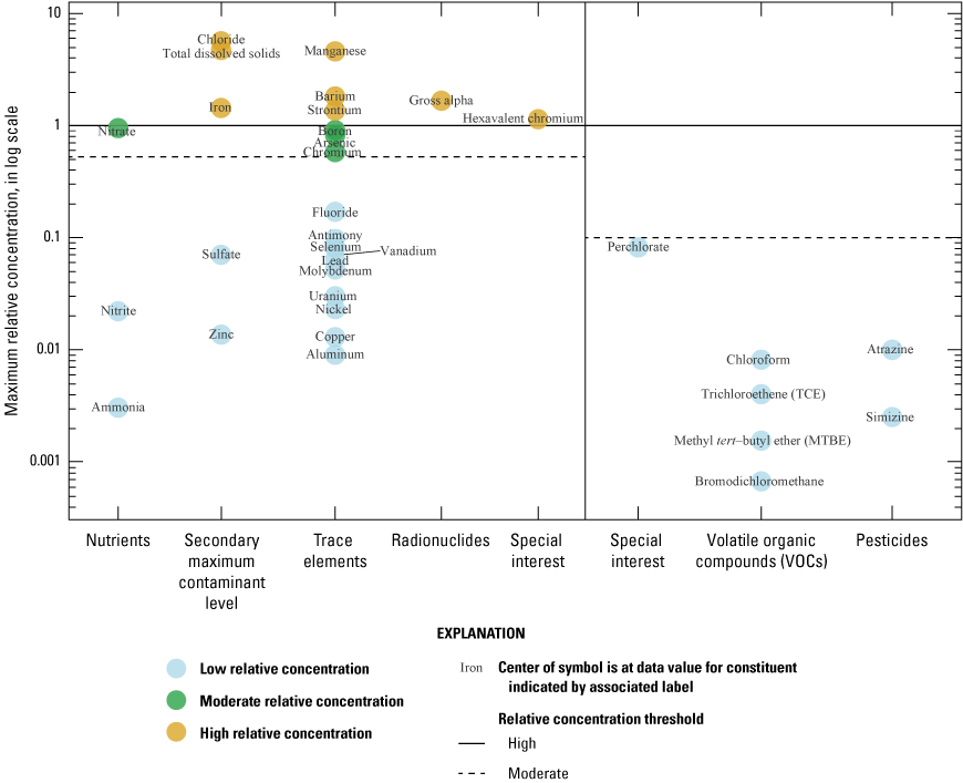
Maximum relative concentrations for constituents detected in grid wells by type of constituent, Redding–Red Bluff shallow aquifer study unit California Groundwater Ambient Monitoring and Assessment Program Priority Basin Project, 2018–19.
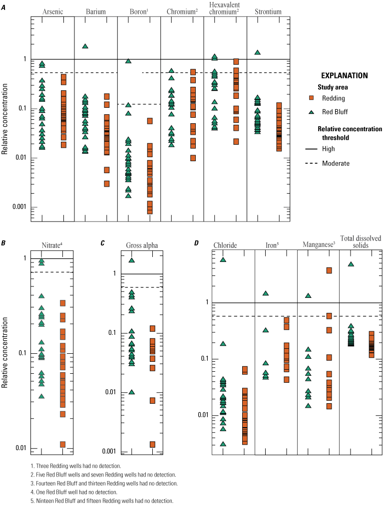
Relative concentrations of selected constituent classes in grid wells, Redding–Red Bluff shallow aquifer study unit, California Groundwater Ambient Monitoring and Assessment Program Priority Basin Project: A, trace elements; B, nutrients; C, radionuclides; and D, inorganic constituents (with nonregulatory aesthetic-based benchmarks), 2018–19.
Table 6.
Summary of aquifer-scale proportions for high and moderate relative concentrations of constituents selected for additional evaluation in the understanding assessment, Redding–Red Bluff shallow aquifer study unit, California Groundwater Ambient Monitoring and Assessment Program Priority Basin Project, 2018–19.[Grid-based aquifer-scale proportions are based on samples collected by the U.S. Geological Survey from 50 grid sites (one sample per grid cell) during December 2018 to April 2019. Relative concentration (RC) categories: high RC, value greater than 1.0 (for inorganic and organic constituents); moderate RC, value less than or equal to 1.0 and greater than 0.5 (for inorganic constituents) or 0.1 (for organic constituents); low RC, value less than or equal to 0.5 (for inorganic constituents) or 0.1 (for organic constituents). Inorganic constituents include trace metals, special interest constituents, and inorganic constituents with aesthetic-based benchmarks; organic constituents include volatile organic compounds and pesticides; see table 2 for benchmark details. Confidence intervals3 are given as lower limit and upper limit. Abbreviation: CI, confidence interval]
Study unit grid-based aquifer scale proportions are the area-weighted combination of the aquifer-scale proportions for the component study areas.
Study area aquifer-scale proportions are presented prior to area-weighted averaging used to calculate the study unit grid-based aquifer-scale proportion.
Based on Jeffreys interval for the binomial distribution (Brown and others, 2001).
Inorganic constituents with human-health benchmarks (nutrients, radionuclides, and trace elements) had high RCs in 6 percent of the groundwater resources used by domestic wells in the NSV-SA and moderate RCs in 18 percent of the NSV-SA (table 7). Inorganic constituents having aesthetic-based benchmarks had high and moderate RCs in 4 and 2 percent, respectively, of the groundwater resources used by domestic wells in the NS-SA (table 7).
Table 7.
Summary of aquifer-scale proportions for inorganic constituent classes with health-based and aesthetic-based benchmarks, organic and special-interest constituent classes with health-based benchmarks, and microbial indicator constituents, Redding–Red Bluff shallow aquifer study unit California Groundwater Ambient Monitoring and Assessment Program Priority Basin Project, 2018–19.[Relative concentration (RC) categories: high RC, value greater than 1.0 (for inorganic and organic constituents); moderate RC, value less than or equal to 1.0 and greater than 0.5 (for inorganic constituents) or 0.1 (for organic constituents); low RC, value less than or equal to 0.5 (for inorganic constituents) or 0.1 (for organic constituents). Inorganic constituents include trace metals, special-interest constituents and inorganic constituents with aesthetic-based benchmarks; organic constituents include volatile organic compounds and pesticides; detection, concentration of constituent was above the reporting limit]
Groundwater can be grouped in a few distinct water types based on the relative proportions of major ions measured in the samples. Samples with the same water types have likely undergone similar processes that affected the major ion profile and the presence of constituents that are concerning for human health. For example, in the NSV-SA, two major water types are observed. In modern and mixed-aged groundwater, primarily in the Red Bluff study area, calcium and magnesium are the dominant cations and sulfate and chloride are the dominant anions (fig. 10). This type of water is typical of younger groundwater that has interacted with marine rocks during recharge. Younger, typically fresh water (less than 1000 mg/L dissolved solids concentration) with a calcium-magnesium water type are recently recharged and can have higher concentrations of anthropogenic compounds, including nutrients, perchlorate, and organics that are present at the surface and brought into the aquifer during recharge.
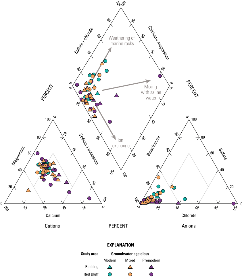
Relative ionic composition, water types, and groundwater age classifications for grid wells in the Redding–Red Bluff shallow aquifer study unit, California Groundwater Ambient Monitoring and Assessment (GAMA) Program Priority Basin Project, 2018–19.
The second water type is a sodium-bicarbonate water that is predominant in older, premodern groundwater that has undergone extensive ion exchange due to interactions with aquifer materials (fig. 10). The increased contact time allows for exchange of calcium for sodium on the surface of the aquifer matrix that results in sodium-dominated, premodern groundwater (fig. 10). The longer interactions with aquifer materials could allow for the accumulation of naturally occurring constituents, and higher salinities and concentrations of trace elements are found in sodium-bicarbonate water types.
A third water type was observed in a single sample, RB-01, in the southwesternmost part of the Red Bluff study area (fig. 2). The groundwater in this well has a sodium-chloride water type that is found in groundwater derived from seawater. This water type has been found in old, deep saline groundwater throughout California and can migrate into shallower, fresh-water aquifers used for drinking water though natural pathways such as faults and fractures in the subsurface (Kang and Jackson, 2016).
Trace Elements
Trace elements with health-based benchmarks had high and moderate RCs (for one or more constituents) in 6 and 14 percent, respectively, of the groundwater resources used by domestic wells (table 7). The proportion of the groundwater resources used by domestic wells in the Red Bluff study area with high RCs of trace elements (12 percent) was greater than the corresponding proportion of the Redding study area (0 percent). Barium, hexavalent chromium, and strontium were present at high RCs in samples from the Red Bluff study area (fig. 9A). Moderate RCs of arsenic, boron, chromium, and hexavalent chromium were reported in the Red Bluff study area, and moderate RCs of chromium and hexavalent chromium were reported in the Redding study area (table 6; fig. 9A).
Arsenic
Arsenic is a semi-metallic element that has been associated with increased cancer risk and non-cancerous effects, including skin damage and circulatory problems (U.S. Environmental Protection Agency, 2001). Natural sources of arsenic in groundwater include dissolution of arsenic-bearing minerals, desorption of arsenic from mineral surfaces, and mixing with hydrothermal fluids (Welch and others, 2000; Smedley and Kinniburgh, 2002). Potential anthropogenic sources of arsenic can include copper ore smelting, coal combustion, arsenical pesticides, wood preservatives, and dissolution of natural arsenic-bearing minerals from mining activities (Smedley and Kinniburgh, 2002; Welch and Stollenwerk, 2003). In an aqueous environment, arsenic occurs as an oxyanion in either the oxidized form, arsenate (As(VI)), or the reduced form, arsenite (As(III)). The reduced form, As(III), is more mobile under ambient conditions and potentially more toxic. The redox conditions and pH determine the dominance aqueous species in each well (Smedley and Kinniburgh, 2002).
The US-MCL was lowered from 50 to 10 µg/L in 2002 because of studies linking chronic exposure to arsenic concentrations between 10 µg/L and 50 µg/L in drinking water to increased incidence of cancer and other health risks (U.S. Environmental Protection Agency, 2001). An estimated 5 percent of groundwater resources used for domestic drinking water in the United States have high RCs of arsenic (greater than 10 µg/L; Ayotte and others, 2017, Focazio and others, 2000; Welch and others, 2000), and high concentrations of arsenic in groundwater resources used for drinking water are a worldwide concern (Smedley and Kinniburgh, 2002; Welch and others, 2006).
Arsenic was present at moderate RCs in 8 percent (table 6) of the groundwater resources used by domestic wells in the Red Bluff study area but was not found in the groundwater resources used by domestic drinking water wells in the Redding study area (table 6; fig. 9). As part of the SWRCB GAMA domestic well project, 223 wells were sampled in 2005 for water quality in Tehama County, which overlaps with parts of the Redding and Red Bluff study areas (California State Water Resources Control Board, 2009). During the SWRCB Tehama County study, private wells were sampled on a first-come, first-serve basis and the results from the program were collated at the county level, rather than at the basin level. The resulting well distribution in the SWRCB study is spatially biased and includes higher well densities near population centers. Of the wells sampled for the SWRCB Tehama County study, 157 wells were located within the current (2022) Red Bluff study area and 17 percent of those wells contained high arsenic concentrations (California State Water Resources Control Board, 2009). When reassessing the water-quality data from the SWRCB study using the areal proportion calculations from the GAMA-PBP domestic well assessment, 7 percent of the groundwater resources in the Red Bluff study area had high arsenic concentrations (Belitz and others, 2003; Belitz and others, 2010; Belitz and others, 2015). The differences between the well and area proportions reflect the clustering of wells sampled by the SWRCB study. The two wells with moderate arsenic values measured in the GAMA-PBP domestic well study (RB-16 and RB-22; fig. 2) were in areas where the SWRCB sampled 59–77 wells within a 5-km radius and those clusters included wells with high, moderate, and low arsenic—and were the only places the SWRCB sampling found high arsenic. The comparison of the two studies highlights that the GAMA-PBP grid-based method does not capture water-quality variations on a more local scale.
Previous studies of elevated arsenic in groundwater have identified two primary mechanisms for arsenic mobilization related to the observed conditions at sampled sites: (1) desorption from, or inhibition of sorption to, aquifer materials at elevated pH levels and (2) release of arsenic from dissolution of iron or manganese oxyhydroxides under iron- or manganese-reducing conditions (Smedley and Kinniburgh, 2002; Welch and others, 2006; Bennett and others, 20115). The first mechanism described requires pH values to be greater than 7.8, the level above which the primary arsenate species is relatively soluble (Smedley and Kinniburgh, 2002). The second mechanism requires low oxygen, anoxic conditions in which arsenic is released from oxyhydroxides as arsenite (As(III)). Moreover, arsenite release is enhanced by long contact and reaction times between groundwater and aquifer material (Smedley and Kinniburgh, 2002).
Elevated arsenic concentrations in anoxic groundwater from fine-grained sediment lithologies along the Sacramento River were observed in previous studies of the Sacramento Valley (Hull, 1984; Dawson, 2001; Bennett and others, 2011). Although the wells in the alluvium and volcanic lithologies along the river generally are shallower and contain younger groundwater, DO concentrations are relatively low indicating anoxic conditions that typically favor mobilization of arsenic in groundwater. However, low DO values do not appear to be the cause of arsenic along the river as arsenic was not correlated to DO values (table 8), and differences in arsenic concentrations between oxic and anoxic groundwaters were not significant. Additionally, arsenic was not correlated to iron or manganese, which would indicate that reductive dissolution of iron and manganese-oxyhydroxides is not the primary source of arsenic in the domestic wells of the NSV-SA (table 9).
Table 8.
Summary of Spearman’s rho (ρ) rank correlation test results for selected potential explanatory variables and water-quality constituents, Redding–Red Bluff shallow aquifer study unit, California Groundwater Ambient Monitoring and Assessment Program Priority Basin Project, 2018–19.[Tabled values of rho are shown for tests in which the variables were determined to be statistically significant (p-value <0.05). Abbreviations: ns, statistical test indicates no significant correlation between variables; positive values, significant positive correlation; negative values, significant negative correlation; USTs, underground storage tanks]
Table 9.
Summary of Spearman’s rho (ρ) rank correlation test results for selected water-quality constituents, Redding–Red Bluff shallow aquifer study unit, California Groundwater Ambient Monitoring and Assessment Program Priority Basin Project, 2018–19.[Tabled values of rho are shown for tests in which the variables were determined to be statistically significant (p-value <0.05). Abbreviations: —, not applicable; ns, Spearman’s test indicates no significant correlation between variables; positive values, significant positive correlation; negative values, significant negative correlation]
Arsenic concentrations had a positive correlation with pH (ρ=0.36, p=0.01) and a negative correlation to percent modern carbon (pmC; ρ= −0.43, p<0.0001) and tritium (ρ= −0.31, p<0.0001; table 8). Higher arsenic concentrations in older groundwater with higher pH are consistent with arsenic accumulation due to increased aquifer contact times and groundwater evolution. Older, premodern groundwater in the NSV-SA is associated with a sodium-bicarbonate water type that is indicative of exchange of ions over long residence times (fig. 10). In addition to allowing increased time for groundwater to interact with arsenic-rich materials, dissolved oxygen is consumed, and pH increases with groundwater age, creating conditions that promote arsenic mobilization.
One of the two sites with a moderate arsenic RC value, S9-RB-16, had a pH value greater than 7.8, was premodern, anoxic, and from the volcanic sediments of the Tuscan Formation in the eastern part of the study area (fig. 11A). The second site, S9-RB-22, was slightly acidic (pH=6.6) and had modern and oxic groundwater from the Quaternary alluvium. Groundwater samples with moderate RC values for arsenic were close to the Sacramento River. The presence of arsenic in alkaline, anoxic water and more acidic, oxic water indicates that more than one mechanism could be contributing to mobilization of arsenic in wells in the Sacramento River floodplain.
Hydrothermal waters can be a potential source of arsenic in some areas of the NSV-SA. Mineral solubility tends to increase with temperature, and thermal waters are often characterized as having elevated concentrations of trace elements like arsenic, boron, and fluoride (Hem, 1985). In the NSV-SA, arsenic concentrations were negatively correlated with the distance to the nearest geothermal site and the correlation was statistically significant, indicating that thermal water could be contributing arsenic to groundwater (table 8; fig. 11A).
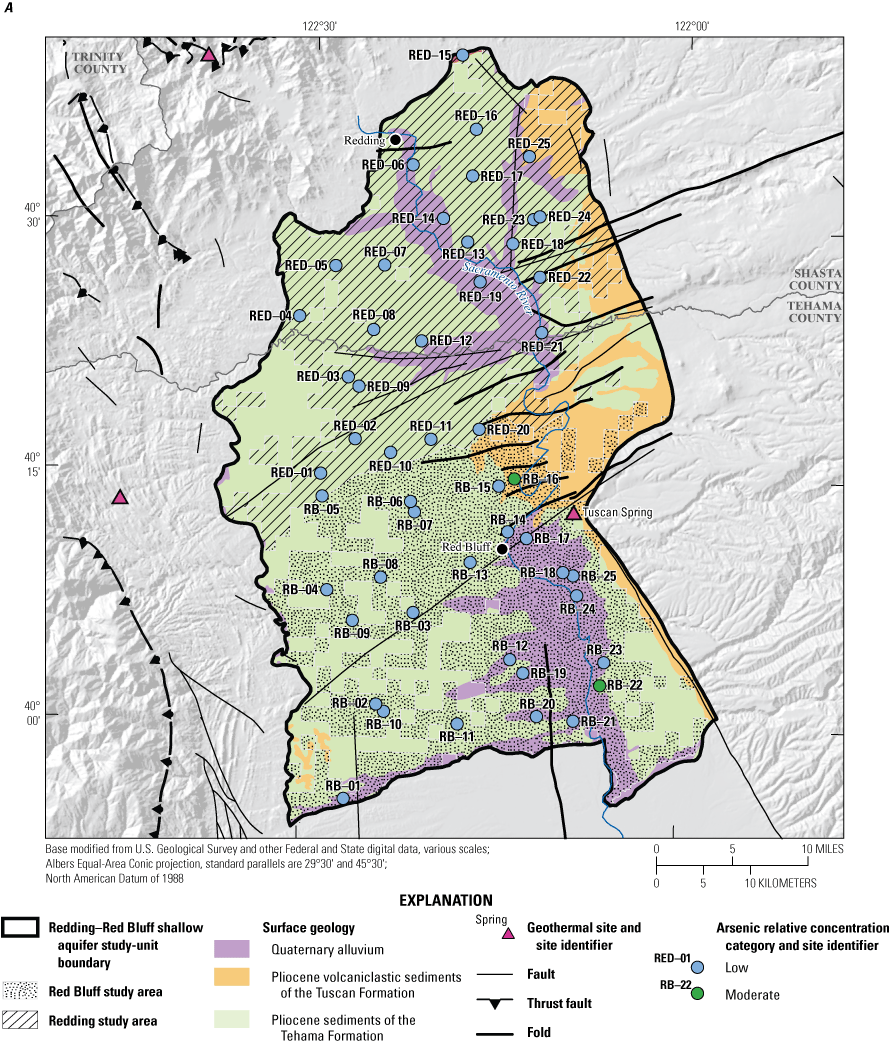
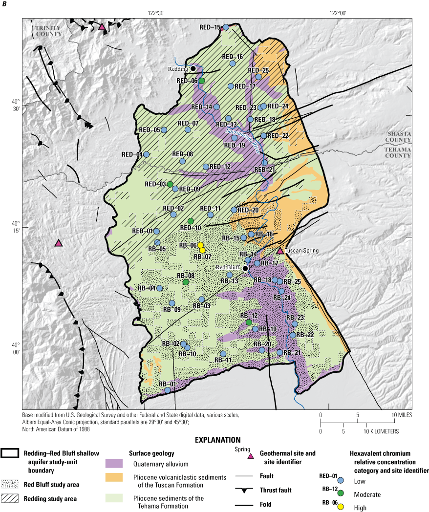
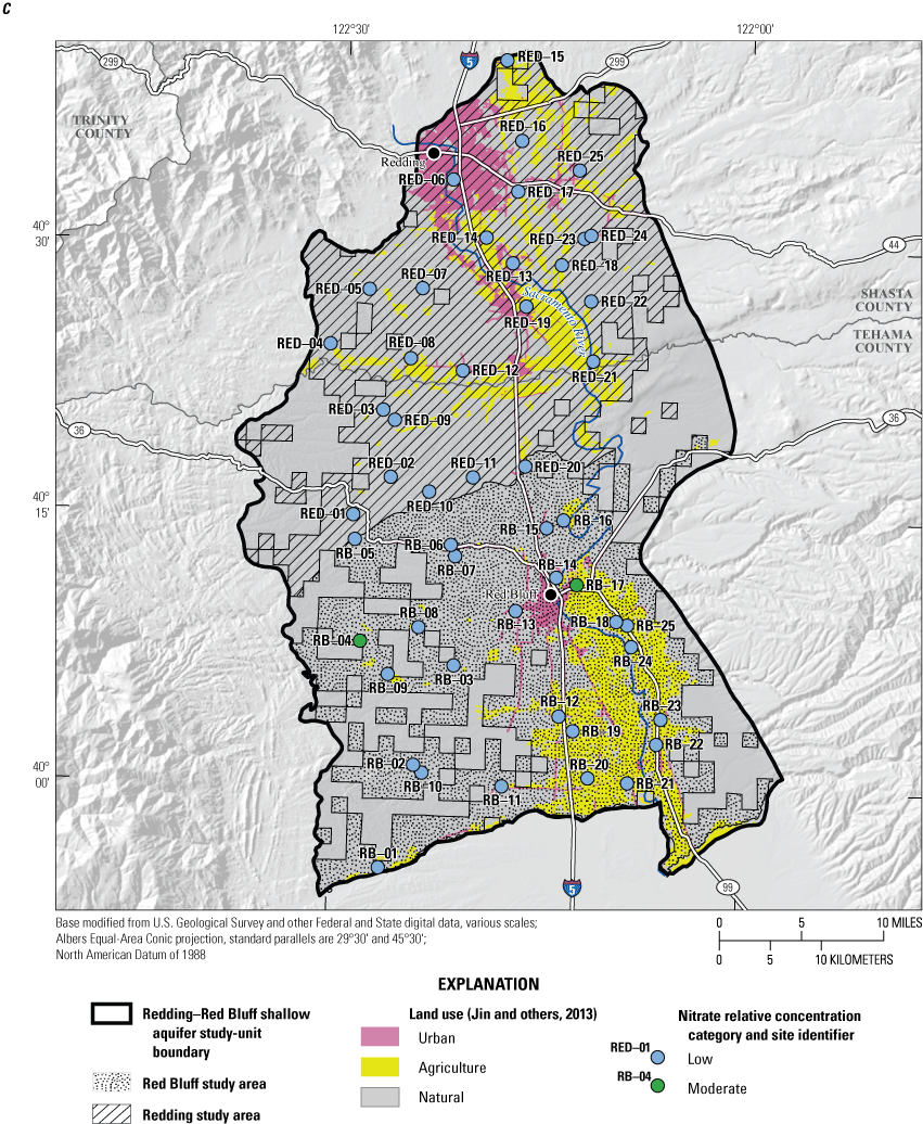
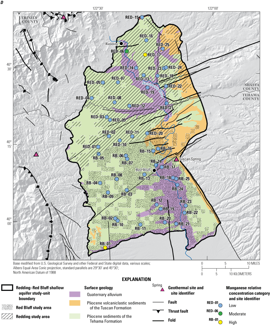
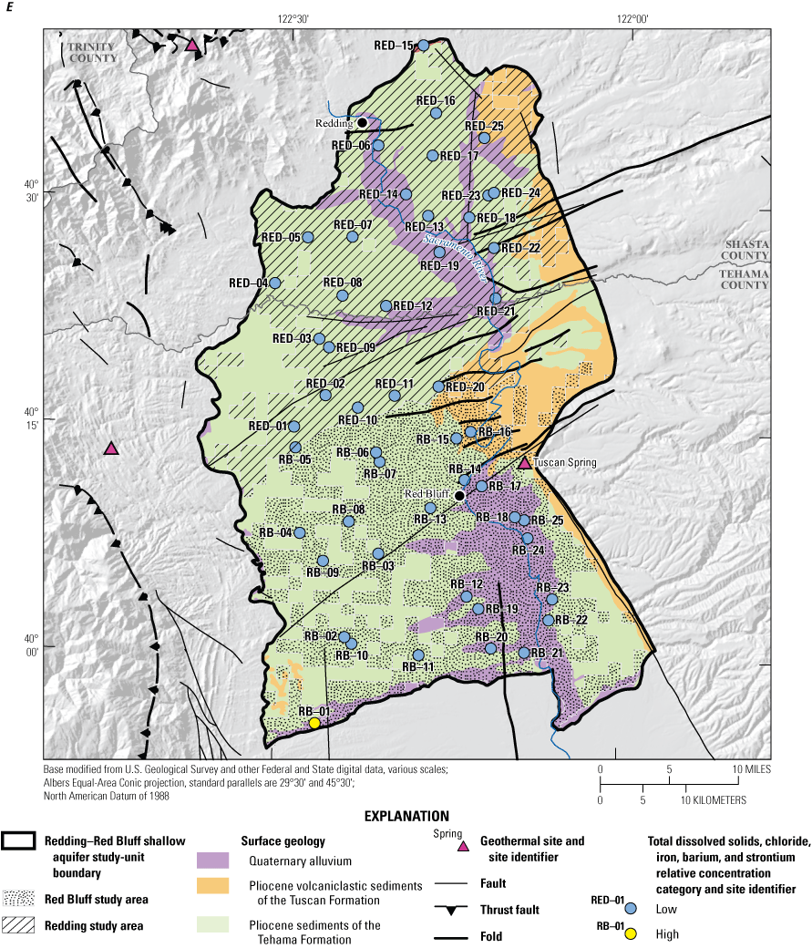
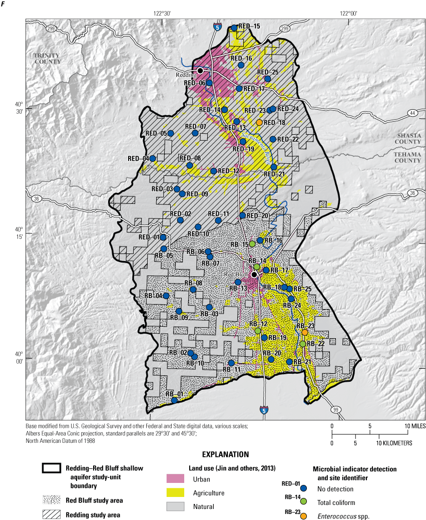
Relative concentrations of selected trace elements (A–D) and anthropogenic indicators (E–F) in grid wells, Redding–Red Bluff shallow aquifer study unit, California Groundwater Ambient Monitoring and Assessment Program Priority Basin Project, 2018–19: A, arsenic; B, hexavalent chromium; C, nitrate; D, manganese; E, total dissolved solids, chloride, iron, barium and strontium; and F, microbial indicators; relative concentration refers to a ratio of the measured concentration to water-quality benchmark concentration for the specified constituent.
Chromium
Chromium is an oxyanion-forming trace metal that exists in the aquatic environment in two forms: (1) as the reduced species trivalent chromium, and (2) as the oxidized form hexavalent chromium. Hexavalent chromium is more stable under oxic groundwater conditions and has higher solubility and mobility in natural waters than trivalent chromium (California State Water Resources Control Board, 2017). Natural sources of chromium in groundwater include dissolution of chromium bearing minerals associated particularly with ultramafic rocks, such as serpentinites found in ophiolite complexes (Oze and others, 2004, 2007; Izbicki and others, 2015; Hausladen and others, 2018). Hexavalent chromium is a common industrial contaminant, and the anti-corrosive properties of chromium make it a common chemical for use in metal plating, stainless-steel manufacturing, leather tanning, anticorrosion of industrial cooling waters, and wood preservative treatment.
The US-MCL for total chromium is 100 µg/L, and the CA-MCL for total chromium is 50 µg/L. Trivalent chromium is an essential nutrient and is considered to have very low health risks; however, hexavalent chromium is considered a health risk and carcinogen and can cause nausea, gastrointestinal distress, stomach ulcers, skin ulcers, allergic reactions, kidney and liver damage, reproductive problems, and lung and nasal cancer (U.S. Environmental Protection Agency, 2001; California State Water Resources Control Board, 2017). Hexavalent chromium detected in groundwater was widely presumed to be associated primarily with anthropogenic contamination, until more recent reports of the prevalence of naturally occurring hexavalent chromium (Hem, 1985, Izbicki and others, 2015; Hausladen and others, 2018). Hexavalent chromium is highly soluble and mobile in alkaline, oxic groundwater, and is often the dominant chromium species in more natural waters (Oze and others, 2004, 2007; Izbicki and others, 2015 Hausladen and others, 2018). A national MCL for hexavalent chromium has not been developed, but the USGS has an HBSL of 20 µg/L (Toccalino and others, 2014). California established an MCL of 10 µg/L for hexavalent chromium in 2014, but it was withdrawn in 2017 (California State Water Resources Control Board, 2017).
The Coast Ranges and Sierra Nevada contain known chromium-rich ultramafic units (Morrison and others, 2009, Manning and others, 2015, Izbicki and others, 2015 Hausladen and others, 2018). Samples of soil derived from the ultramafic rocks in the region contain up to 10,000 milligrams per kilogram (mg/kg) chromium, and sedimentary soils in the Sacramento Valley can contain up to 1,400 mg/kg chromium, particularly from the west side of the valley where there is a substantial contribution of chromium from ultramafic rocks in the Coast Ranges (Morrison and others, 2009). Valley sediments on the east side are primarily from the lower Cascade Range, which does not contain substantial ultramafic units compared to the Coast Ranges and parts of the northern Sierra Nevada (Manning and others, 2015).
Total chromium was present at moderate RCs in 4 percent of the groundwater resources used by domestic wells in the NSV-SA (table 6; fig. 9), and hexavalent chromium was present at high RCs in 4 percent and moderate RCs in 8 percent of the groundwater resources used by domestic wells (table 6; fig. 9). High RCs for hexavalent chromium were only found in the Red Bluff study area, but moderate RCs for total chromium and hexavalent chromium were found in 8 percent of groundwater resources in both study areas (table 6; fig. 9). Elevated total chromium and hexavalent chromium concentrations were measured in samples from wells in the valley west of the Sacramento River, where the chromium-rich mafic sediments from the Coast Ranges are incorporated into the sediments of the Tehama Formation (fig. 11B). Total chromium and hexavalent chromium were highly correlated (ρ=0.97, p<0.05; table 9) and hexavalent chromium is the dominant species (>75 percent) in most samples. About 80 percent of samples contained more than 90 percent of the total chromium as hexavalent chromium, which is consistent with previous studies that indicate hexavalent chromium is the dominant species of chromium in oxic groundwater (Oze and others, 2004, 2007; Izbicki and others, 2015 Hausladen and others, 2018). Hexavalent chromium was not reported in groundwater in the northern Sacramento Valley in previous domestic well studies, but total chromium was measured at elevated concentrations above the EPA-MCL in Tehama County (California State Water Resources Control Board, 2009). Similar to the GAMA-PBP Red Bluff study area, the moderate and high total chromium RC values reported for Tehama County occurred only in wells west of the Sacramento River and Red Bluff (California State Water Resources Control Board, 2009).
Total and hexavalent chromium concentrations were positively correlated to natural land-use percentage (table 8), likely due to chromium-rich minerals in the sediments of the Tehama Formation in the western side of the valley (Morrison and others, 2009; Manning and others, 2015; fig. 11B) where there is less urban and agricultural land use and wells have higher percentage of natural land cover (fig. 11B). Total chromium and hexavalent chromium concentrations were positively correlated to pH, DO, and well depth and negatively correlated to tritium and pmC (table 8). Total and hexavalent chromium were higher in oxic, premodern groundwater (p=0.007 and p=0.021, respectively; table 4; fig. 12). Studies in the Sacramento Valley and other parts of California have indicated that long residence times of oxygenated, alkaline (pH>8) groundwater promote mobilization of hexavalent chromium in groundwater (Izbicki and others, 2015; Manning and others, 2015). As groundwater age increases, weathering of primary silicate minerals increases groundwater pH, and hexavalent chromium desorption will occur in the more alkaline environment under persistent oxic conditions (Izbicki and others, 2015). This mechanism is consistent with the relations between pH (ρ=0.48, p<0.001), DO (ρ=0.32, p=0.024), tritium (ρ= −0.40, p=0.004), carbon-14 (ρ= −0.36, p=0.01) and hexavalent chromium concentrations observed in the NSV-SA (table 8).
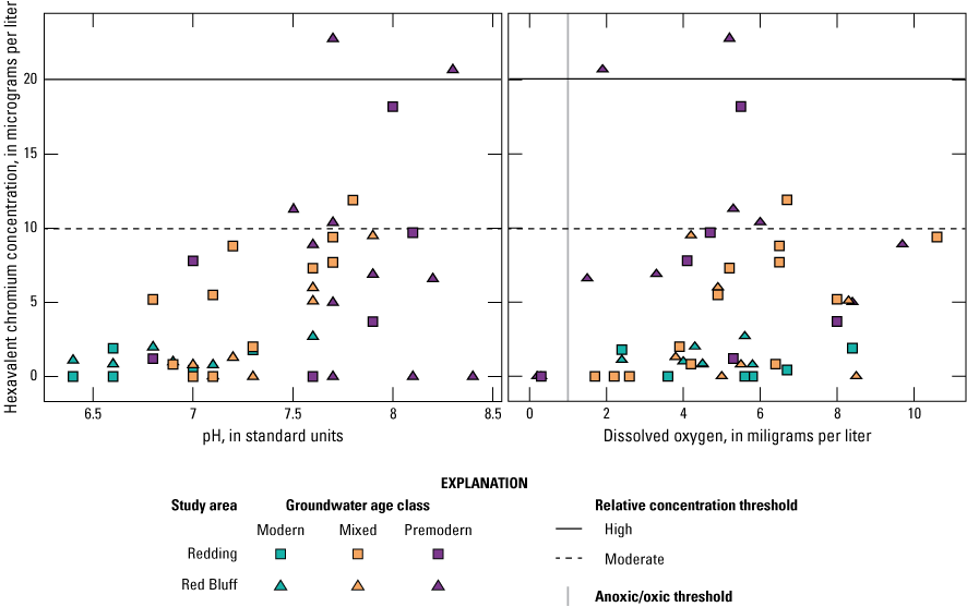
Relation of hexavalent chromium concentration to pH, dissolved oxygen, and groundwater age in grid wells, Redding–Red Bluff shallow aquifer study unit, California Groundwater Ambient Monitoring and Assessment Program Priority Basin Project, 2018–19. Relative concentration refers to a ratio of the measured concentration to water-quality benchmark concentration for the specified constituent.
In previous studies of hexavalent chromium occurrence in alluvial aquifers along the western side of the Central Valley, researchers hypothesized that irrigation return flow through a thick undersaturated zone can mobilize chromium in alluvial aquifers (Mills and others, 2011; Izbicki and others, 2015). Correlations between nitrate and hexavalent chromium concentrations in groundwater wells from the Sacramento Valley were used to support this hypothesis. However, in groundwater wells in the NSV-SA study unit, we did not observe a significant relation between total or hexavalent chromium and nitrate as observed in the other studies. Mills and others (2011) and Izbicki and others (2015) looked at the relation between chromium and nitrate in groundwater wells in the southwestern Sacramento Valley and in public-supply wells across California, respectively. In the NSV-SA, we sampled shallow, domestic wells only in the northern part of the Sacramento Valley, where hexavalent chromium concentrations were correlated with high natural land use and low agricultural land use areas. The results of the understanding assessment in the NSV-SA for hexavalent chromium supports long aquifer contact times with chromium-rich sediments as the primary mechanism driving the occurrence of high RCs in this part of the Sacramento Valley rather than irrigation return flow mobilizing chromium that has been observed in other parts of the Central Valley.
Nutrients
Nitrate in groundwater is the result of anthropogenic and natural sources; however, concentrations greater than 1.0 mg/L as nitrogen (relative concentration of 0.2) generally are considered to indicate the presence of nitrate from anthropogenic sources (Mueller and Helsel, 1996). Natural sources of nitrate in groundwater are nitrogen fixation from nitrogen gas, atmospheric deposition, animal waste, and dissolution of nitrogen-rich organic material in soils. Agricultural sources of nitrate include fertilizer application and livestock waste. Other anthropogenic sources include septic system discharge, leakage from municipal sewage lines, and additional atmospheric deposition of nitrogen oxides from the combustion of fossil fuels (Dubrovsky and others, 2010). Concentrations of nitrate in drinking water exceeding the 10 mg/L as nitrogen EPA-MCL can cause infant methemoglobinemia, also known as blue baby syndrome (U.S. Environmental Protection Agency, 2016).
Nitrate was the only nutrient present at moderate RCs and was found in 4 percent of groundwater resources used for domestic supply in the NSV (table 7; fig. 11C). These results are consistent with previous studies that demonstrated that nitrate concentrations are generally low in the Sacramento Valley but are more likely to be elevated near urban and agricultural areas (California State Water Resources Control Board, 2009; Central Valley Regional Water Quality Control Board, 2016). In a previous study of domestic wells in Tehama County, high concentrations of nitrate were observed in groundwater, but mostly concentrated in urban centers in the Red Bluff study area (California State Water Resources Control Board, 2009). These wells were sampled on a first-come, first-serve basis, and a higher density of wells was located around the urban centers where nitrate was more commonly found. The difference in the sampling method used in the Tehama County study and the equal-area grid cell method used by the GAMA-PBP may help explain why concentrations of nitrate exceeding the MCL were observed in wells in the SWRCB study, but not found in the GAMA-PBP study. The GAMA-PBP study included wells in the less populated regions of the study unit where nitrate concentrations are lower but sampled fewer wells in the developed parts of the study area where nitrate is more prevalent (fig. 11C).
Nitrate concentrations were significantly higher in samples from the Quaternary alluvium aquifer lithology than in samples from the Tehama Formation aquifer lithology (p=0.009, table 4). The moderate nitrate RCs were detected only in the Red Bluff study area, which has a higher proportion of wells in the alluvium than does the Redding study area (table 5). Both agricultural and urban areas are concentrated along the Sacramento River where there are alluvial deposits, and the percentage of agricultural land use was higher around wells in the Quaternary alluvium (table 4; fig. 11C). Negative correlations between concentrations of nitrate and the percentage of natural land use, the aridity index, elevation, and well depth were statistically significant and positive correlations between nitrate concentrations and tritium, pmC, percentage of urban and agricultural land use, UST density, and septic tank density were statistically significant (table 8). The agricultural and urban land-use areas are in the lower, more arid parts of the study area and the wells in the Quaternary alluvium are shallower and associated with more modern groundwater. Nitrate concentration increased with the percentage of urban and agricultural land use around a well and the correlation was statistically significant. Nitrate concentrations were higher in shallow, modern groundwater and the differences were statistically significant, which is consistent with recent inputs of nitrate to the groundwater resources used by domestic wells from anthropogenic activities such as irrigation-return water leaching nitrogen fertilizer or leaking of septic systems as the source of increased nitrate concentrations (Nolan and others, 2002; Landon and others, 2011).
Nitrate concentrations were also significantly positively correlated to perchlorate concentrations and significantly negatively correlated to iron concentrations (table 9). Perchlorate in groundwater typically is from similar natural or agricultural sources as nitrate because perchlorate is present in atmospheric deposition and found in some fertilizers, and both constituents are stable under oxic conditions (Dasgupta and others, 2005; Böhlke and others, 2009; Rajagopalan and others, 2009; Fram and Belitz, 2011). However, perchlorate concentrations are below the benchmark and not correlated to percent land use (table 8), indicating that perchlorate in the region is primarily naturally occurring. The negative correlation between nitrate and iron is related to redox conditions, with nitrate being the dominant species of dissolved nitrogen in oxic conditions and iron being released to groundwater in anoxic conditions.
Constituents with Secondary Maximum Contaminant Level Benchmarks
Constituents with aesthetic-based benchmarks that provide secondary maximum contaminant levels (SMCLs) had high RCs (for one or more inorganic constituents) in 4 percent of the groundwater resources used by domestic wells (table 7) and moderate RCs in 2 percent. Chloride, iron, manganese, and TDS were the constituents with high RCs in the study unit (table 6). Saline-water indicators such as chloride, sulfate, and TDS have recommended and upper CA-SMCL benchmarks. In this report, the upper CA-SMCL values are used for constituents with aesthetic-based benchmarks.
Manganese
Manganese is naturally present in most rock types and can be abundant in mafic and ultramafic igneous and metamorphic rocks (Homoncik and others, 2010). As a result of weathering processes, manganese can accumulate in aquifer sediments and is naturally present in most groundwater because of water-aquifer interactions (Homoncik and others, 2010). Manganese is redox sensitive and is present most commonly as hexavalent manganese in oxic conditions and divalent manganese in reducing conditions. The relative solubility of manganese is strongly influenced by oxidation-reduction (redox) conditions in the aquifer, with reduced divalent manganese more mobile in near-neutral pH groundwater (Groschen and others, 2008; Homoncik and others, 2010; DeSimone and others, 2014). In oxic conditions, hexavalent manganese and iron oxides precipitate and coat aquifer materials. The primary mechanism of manganese release to groundwater is the reductive dissolution of iron and manganese oxyhydroxides in anoxic conditions (Chapelle and others, 1995; McMahon and Chapelle, 2008; McMahon and others, 2019).
The comparison benchmark for manganese used in this study was the CA-SMCL of 50 µg/L (table 2). The HBSL for manganese is equal to the EPA lifetime health advisory level (US-HAL) of 300 µg/L and the CA-NL is 500 µg/L. The CA-SMCL is established at the concentration at which manganese can affect the aesthetic properties of water but has negligible adverse health effects. Chronic exposure of manganese at elevated concentrations has been associated with neurological effects in children, among other more minor health effects (U.S. Environmental Protection Agency, 2004; Wasserman and others, 2006).
Manganese was detected at high RCs in 4 percent of the groundwater resources used by domestic wells and at moderate RCs in 2 percent (table 6; fig. 11D). Manganese concentrations were detected at high RCs in two groundwater samples, one from each study area (figs. 9D, 11D). High manganese concentrations in the Sacramento Valley have been reported in previous studies, and manganese was detected at high concentrations in 8 percent of domestic wells sampled in the domestic well study in Tehama County, which is comparable to the GAMA-PBP study, considering the difference in sample methods (California State Water Resources Control Board, 2009). Manganese concentrations were significantly negatively correlated to DO concentrations (table 8); moreover, correlations were statistically significant for higher manganese concentrations in groundwater classified as anoxic than in groundwater classified as oxic (p<0.001; table 4; fig. 13). Anoxic conditions in groundwater persist when DO concentrations are less than 1 mg/L, per the criteria established in McMahon and Chapelle (2008; appendix 1; Harkness, 2022).
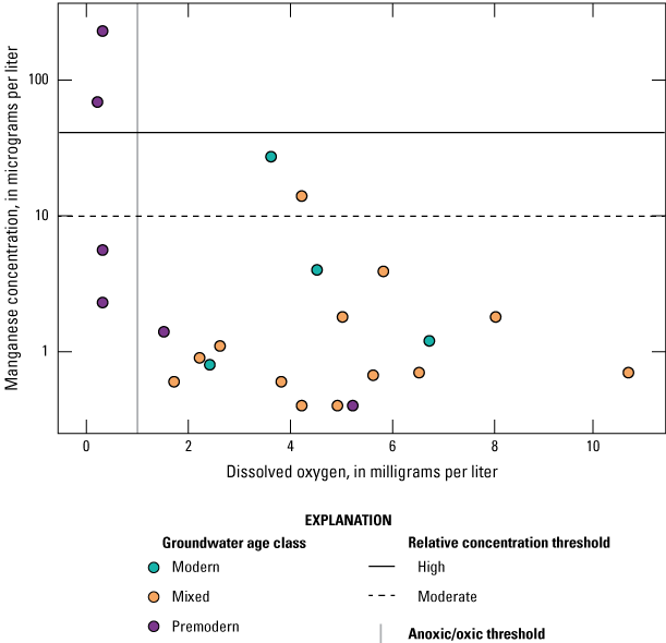
Relation of manganese concentration to dissolved oxygen concentration and groundwater age in grid wells, Redding–Red Bluff shallow aquifer study unit, California Groundwater Ambient Monitoring and Assessment Program Priority Basin Project, 2018–19. Relative concentration refers to a ratio of the measured concentration to water-quality benchmark concentration for the specified constituent.
The negative correlation with DO concentration is consistent with the redox processes controlling manganese solubility (fig. 13; Groschen and others, 2008; Homoncik and others, 2010; DeSimone and others, 2014). Manganese and iron concentrations are positively correlated, further supporting the release of manganese during reductive dissolution of manganese and iron oxides in the groundwater resources used by domestic wells in the study area (table 9). Arsenic also can be released to groundwater by the dissolution of iron and manganese oxides, but manganese is not correlated to arsenic (table 9). However, manganese is negatively correlated to chromium and hexavalent chromium. Manganese oxides have been shown to effectively oxidize chromium, resulting in the transformation of insoluble trivalent chromium to soluble hexavalent chromium (Eary and Rai, 1987; Oze and others, 2007; Hausladen and others, 2018). Manganese oxides from mafic-derived sediments could be oxidizing chromium in the oxic groundwater west of the Sacramento River; however, reducing conditions in the alluvial sediments along the river would mobilize manganese to the groundwater and reduce hexavalent chromium.
Saline-water Indicators
The high RCs of chloride, iron, and TDS, as well as the high and moderate RCs of the trace elements barium, boron, and strontium, were all measured in one sample collected from a grid site in the southwestern corner of the study unit (fig. 11E). The chemistry in this sample is consistent with mixing of saline water (TDS>1000 mg/L) from deeper formations into the shallow freshwater aquifer (figs. 10, 11E; Hull 1984; Kang and Jackson, 2016). This sample is from well RB-01 (fig. 2), which is located near the western fault systems that intersect in the southwestern most part of the study area (fig. 11E; Harwood and Helley, 1987); these faults could be conduits for deeper saline water to migrate upward into the freshwater aquifers the area. Although there is evidence this process influences the water quality in the study unit, it only affects a small (<2 percent) proportion of the groundwater resources used for the domestic well supply (table 7).
Organic and Special-Interest Constituents
The organic constituent classes assessed in this study were volatile organic compounds (VOCs) and pesticides (including degradates). Volatile organic compounds can be naturally present in groundwater associated with hydrocarbon (natural gas and oil) deposits, but their presence in groundwater in most areas outside oil and gas fields is related to anthropogenic sources (Gilliom and others, 2006; Zogorski and others, 2006; Rowe and others, 2007). Volatile organic compounds are characterized by their tendency to evaporate, and they generally persist longer in groundwater than in surface water because groundwater is more isolated from the atmosphere (Zogorski and others, 2006; Rowe and others, 2007). Volatile organic compounds can be present in paints, solvents, fuels, refrigerants, and fumigants or can be formed as byproducts of water disinfection (Zogorski and others, 2006; Rowe and others, 2007). Pesticides are used to control weeds, fungi, or insects in agricultural and urban settings and are entirely derived from anthropogenic applications at the land surface.
One or more organic constituents were detected in 8 of the 50 grid sites (16 percent) sampled in the study unit (Shelton and others, 2020). Of the 167 organic constituents analyzed, 8 were detected in at least 1 site in the NSV-SA (table 2). Of these eight constituents, six have regulatory health-based benchmarks (table 2). Organic constituents were not present at high or moderate RCs in groundwater resources used by domestic wells in the NSV-SA (table 6). The most common organic compounds detected were VOCs, primarily disinfection-byproducts, and the only organic constituent detected in greater than 10 percent of the grid-site samples was chloroform (table 2; fig. 14). Other VOCs detected include trichloroethylene (TCE), chlorodifluoromethane, bromodichloromethane, and methyl tert-butyl ether (MTBE). The detected pesticides were triazine herbicides atrazine and simazine and their degradation byproduct 2-chloro-4-isopropylamino-6-amino-s-triazine (table 2; fig. 14). Finding low levels of organic compounds, including VOCs and pesticides, in groundwater is consistent with other studies in the Redding–Red Bluff region that found no detections or only low concentrations of organic compounds in domestic wells (California State Water Resources Control Board, 2009; Central Valley Regional Water Quality Control Board, 2016). During the study in Tehama County, a different set of VOCs were detected, including acetone, the fumigant 1,3-dichloropropane, and the solvents 1,1,2-trichloroethane and 1,1,3-trichloro-1,2,2-trifluoroethane, but all detections that were at low concentrations were in less than 1 percent of sampled wells (California State Water Resources Control Board, 2009).
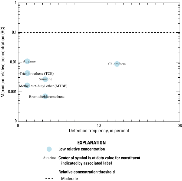
Detection frequency and maximum relative concentration of organic compounds detected in grid wells, Redding–Red Bluff shallow aquifer study unit, California Groundwater Ambient Monitoring and Assessment Program Priority Basin Project, 2018–19.
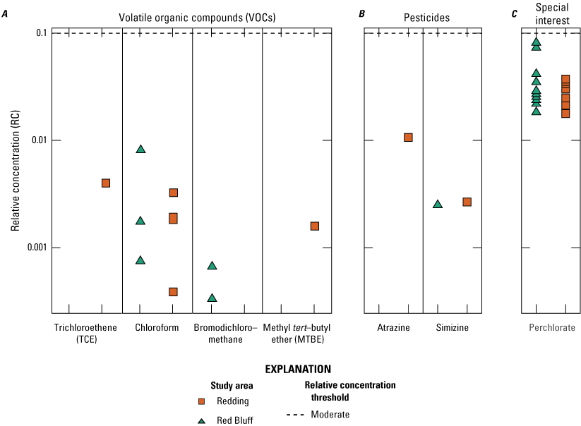
Relative concentrations of selected organic compounds and special-interest constituents in grid wells: A, volatile organic compounds; B, pesticides; and C, special-interest constituent perchlorate in the Redding–Red Bluff shallow aquifer study unit, California Groundwater Ambient Monitoring and Assessment Program Priority Basin Project, 2018–19.
The trihalomethane (THM) chloroform was the most commonly detected VOC in the NSV-SA, with a detection frequency of 12 percent (fig. 14), and detections were all at low RCs (fig. 15A). Chloroform is among the most detected VOCs in groundwater nationally (Zogorski and others, 2006). Chloroform is formed during wastewater treatment when chlorine is used for disinfection but can also form in groundwater when chlorine interacts with natural organic matter (Zogorski and others, 2006). Water used for household consumption from domestic wells is commonly disinfected with solutions that contain chlorine, called shock chlorination. Shock chlorination is a recommended procedure for the treatment of bacterial contamination and odor problems in domestic wells (Centers for Disease Control and Prevention and U.S. Department of Housing and Urban Development, 2006). In addition to disinfecting the water, the chlorine can react with organic matter to produce THMs and other chlorinated or brominated disinfection byproducts that can persist in the well.
Chloroform concentrations were higher in samples from wells with anoxic conditions and wells in the Quaternary alluvium and the differences between redox class and aquifer lithology were statistically significant (table 4). Concentrations of chloroform in the NSV-SA also were positively correlated to percent urban land use and UST density and negatively correlated to percent natural land use (table 8). The correlation between chloroform concentrations and urban land use or UST density could reflect a higher frequency of chlorination of domestic wells in densely populated areas. Domestic wells are more susceptible to contamination in urban areas and, therefore, more likely to be treated with chlorine than domestic wells in less populated areas. Municipal or public-supply wells also could leak disinfected water containing chloroform and other disinfection by-products to groundwater resources in the NSV-SA study unit (Ivahnenko and Zogorski, 2006). The higher chloroform concentrations in the alluvial aquifer are related to higher proportions of urban centers and development along the Sacramento River.
Perchlorate
Perchlorate is an inorganic salt with natural and anthropogenic sources. Perchlorate was considered a constituent of special interest when the GAMA-PBP began in 2001 (California State Water Resources Control Board, 2015b) and a CA-MCL for perchlorate of 6 µg/L became effective in October 2007 (California State Water Resources Control Board, 2015b). Even though perchlorate is a naturally present inorganic constituent, concentrations near or above the CA-MCL typically are derived from an anthropogenic source, such as fertilizers or industrial releases (California State Water Resources Control Board, 2015b). Perchlorate was detected in 50 percent of the groundwater resources used by domestic wells in the NSV-SA (fig. 15; Shelton and others, 2020). Perchlorate was detected more frequently in the Red Bluff study area (14 wells, 56 percent) than the Redding study area (11 wells, 44 percent; fig. 15; Shelton and others, 2020). All RCs of perchlorate were low (table 7; fig. 8). Perchlorate concentrations were positively correlated to TDS, nitrate, hexavalent chromium, and well depth. These relations, along with the low RCs, are consistent with a natural source of perchlorate in the groundwater resources of the NSV-SA.
Microbial Indicators
Microbes are ubiquitous and naturally occurring in the environment. Most of the microbes found in groundwater are harmless to humans; however, some microbes found in human and animal waste can be harmful when consumed in drinking water. The concentrations of these microbes typically are higher in surface waters, and microbes do not travel very far from the source through aquifer material. However, microbes may be introduced to wells through a “short-circuit pathway” such as improperly sealed casing or compromised well construction. The microbial indicators reported in this assessment were used to evaluate the potential for fecal contamination of water sources. Total coliforms, including Escherichia coli (E. coli), and Enterococcus spp. occur naturally in the digestive tracts of animals. In the NSV-SA, total coliforms were present in 8 percent of the groundwater resources used for domestic wells, and Enterococcus spp. were present in 4 percent of the groundwater resources used for domestic wells with total coliforms present (table 7). Escherichia coli bacteria are enumerated on samples that tested positive for total coliform bacteria but were not detected in any samples.
Enterococcus spp. were detected in 4 percent of the groundwater resources used for domestic wells in the Red Bluff and Redding study areas (table 7). Total coliforms were detected only in the Red Bluff study area, in about 16 percent of the groundwater resources used for domestic wells. Microbial indicators also were present in domestic wells sampled by the SWRCB in Tehama County, which includes parts of the Redding and Red Bluff study areas (California State Water Resources Control Board, 2009). Total coliforms were detected in 25 percent of domestic wells, and fecal coliforms were observed in 1 percent of wells in the county, mostly in domestic wells around Red Bluff, in the same locations where total coliforms were detected in the GAMA-PBP Red Bluff study area (California State Water Resources Control Board, 2009). Although the detection frequency of total coliforms was higher in the Tehama County study, it is likely related to higher densities of wells that were sampled in urban centers compared to the GAMA-PBP study because total coliforms are more likely to be present in domestic wells in densely populated areas with septic systems or agriculture.
The presence of microbial indicators provides information about surface contamination of groundwater wells. Wells with total coliform and Enterococcus spp. detections were in regions with agriculture and urban land use, and six of the eight wells with detections (including the two wells with detections of Enterococcus spp.) were shallow (<100 feet), indicating a relation between human activity and microbial contamination of wells (fig. 11F). However, relations between the microbial indicator detections and any of the inorganic or organic constituents associated with potential anthropogenic sources (nitrate, chloroform, or pesticides) were not statistically significant.
Comparison of Domestic and Public-Supply Aquifer Systems
In this section, we compare study-unit characteristics and results of groundwater-quality samples collected by the GAMA-PBP in the north Sacramento Valley public-supply aquifer study unit (NSV-PA; Bennett and others, 2009; Bennett and others, 2011) and the Redding–Red Bluff shallow aquifer (NSV-SA) study unit presented in this report and in Shelton and others (2020). The purpose of the comparison is to identify differences in the quality of groundwater between the part of the aquifer used for domestic and small system wells and the part of the aquifer used for public supply. In the original study, sites sampled in the NSV-PA were randomly selected from a list of wells in the DDW public-supply well database and were considered to be representative of the public-supply aquifer system or the part of the aquifer system most often used for public supply. In Bennett and others (2009), the study areas in the NSV-PA are the Redding and north Sacramento Valley, which overlap with the Redding and Red Bluff study areas in the NSV-SA. For ease of discussion, herein we refer to the “NSV-PA north Sacramento Valley study area” of Bennett and others (2009) as the “NSV-PA Red Bluff study area.” To eliminate any bias from regions where only domestic wells were sampled, only wells that were within a 3-km radius of the areas covered by the NSV-PA were included in the comparison (fig. 16; Bennett and others, 2009).
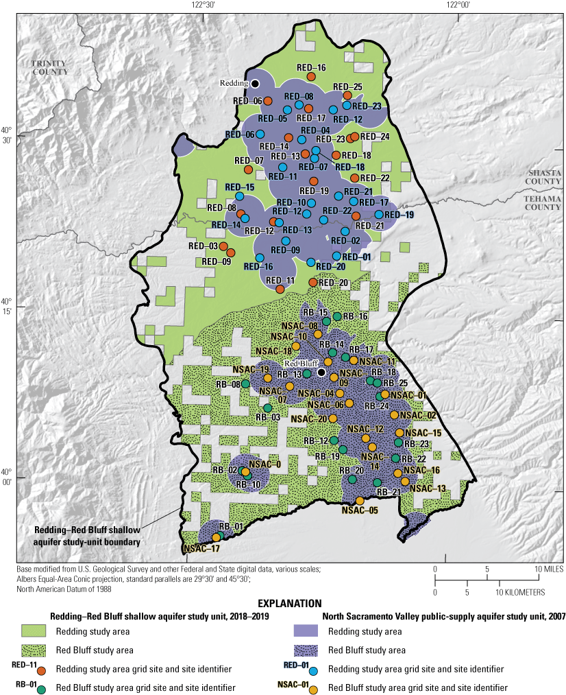
Extent of the north Sacramento Valley public-supply aquifer study unit sampled in 2007 and Redding–Red Bluff shallow aquifer study unit sampled 2018–19 for comparison of water quality in the groundwater resources used by public and domestic wells, California Groundwater Ambient Monitoring and Assessment Program Priority Basin Project.
Comparison of Study-Unit Characteristics
The NSV-PA and NSV-SA largely coincide areally (fig. 16); however, they represent different parts of the aquifer system vertically (fig. 17). The NSV-PA represents deeper groundwater primarily used for public supply, and the NSV-SA represents shallower groundwater primarily used for domestic supply. The differences in well depth between the NSV-PA and NSV-SA are statistically significant (p<0.0001; fig. 17). Additionally, the NSV-SA included the more rural western side of the valley that lacks public-supply wells, although wells that did not overlap with the extent of the NSV-PA were not included in the comparison. The differences between proportions of different land use and covers and aquifer lithologies around the public-supply and domestic wells used in the comparison were not statistically significant (p>0.1; figs. 18, 19).
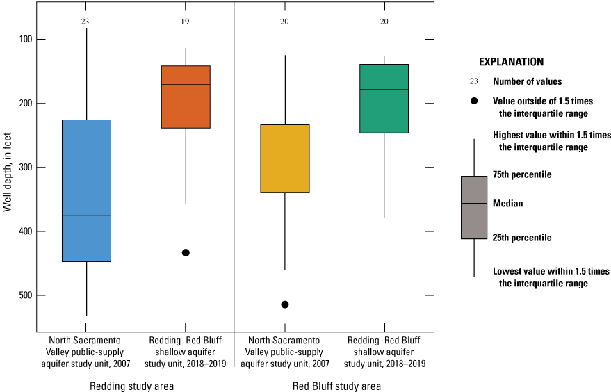
Grid well depths for the Red Bluff and Redding study areas in the north Sacramento Valley public-supply aquifer study unit in 2007 and Redding–Red Bluff shallow aquifer study unit in 2018–19, California Groundwater Ambient Monitoring and Assessment Program Priority Basin Project.
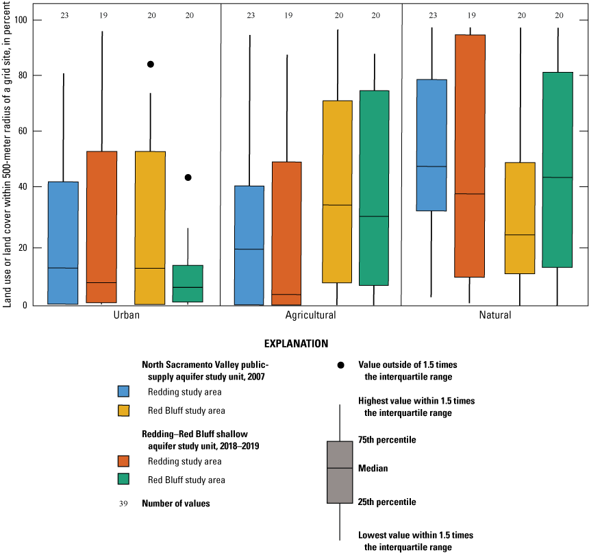
Land use or land-cover category percentages within a 500-meter radius around individual grid wells in the Red Bluff and Redding study areas, north Sacramento Valley public-supply aquifer study unit in 2007 and Redding–Red Bluff shallow aquifer study unit in 2018–19, California Groundwater Ambient Monitoring and Assessment Program Priority Basin Project.
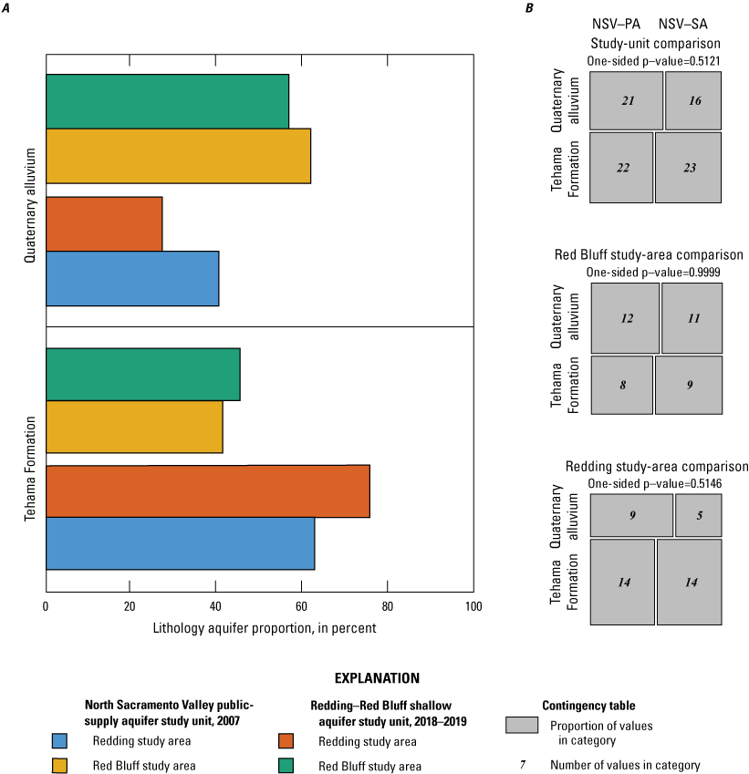
Surface lithology at grid well locations by study unit and study area: A, aquifer proportion by lithology; and B, proportion and number of grid wells by lithology, north Sacramento Valley public-supply aquifer study unit (NSV-PA) in 2007 and Redding–Red Bluff shallow aquifer study unit (NSV-SA) in 2018–19, California Groundwater Ambient Monitoring and Assessment Program Priority Basin Project. Fisher’s exact tests were used to determine the significance of the differences between the observed number of values (number of grid wells) in each category and the expected number of grid wells. A probability value (p-value) greater than 0.1 indicates the difference is not statistically significant.
Groundwater samples from the public-supply and domestic wells were geochemically similar at the study unit and study-area scales (figs. 20–22). The differences in dissolved oxygen concentrations and pH between the two study units were not statistically different (p=0.11 and p=0.35, respectively), and the difference in the proportion of wells in oxic or anoxic groundwater between the two study units was not statistically significant (fig. 20). The difference in proportion of wells with modern, mixed, and premodern aged groundwater and the distribution of tritium concentrations between the study units were not statistically difference (contingency table p=0.85 and Kruskal-Wallace rank sum test p=0.09, respectively; fig. 21). The same three water types were observed in the NSV-SA and NSV-PA: (1) a younger calcium-magnesium-sulfate-chloride water type found more commonly in the Red Bluff area, (2) an older or mixed sodium-bicarbonate type found in both areas, and (3) a sodium-chloride water type from mixing with deeper saline water (fig. 22). The overall water geochemistry in both study units was similar, indicating that water chemistry varies minimally with depth in the aquifer system.
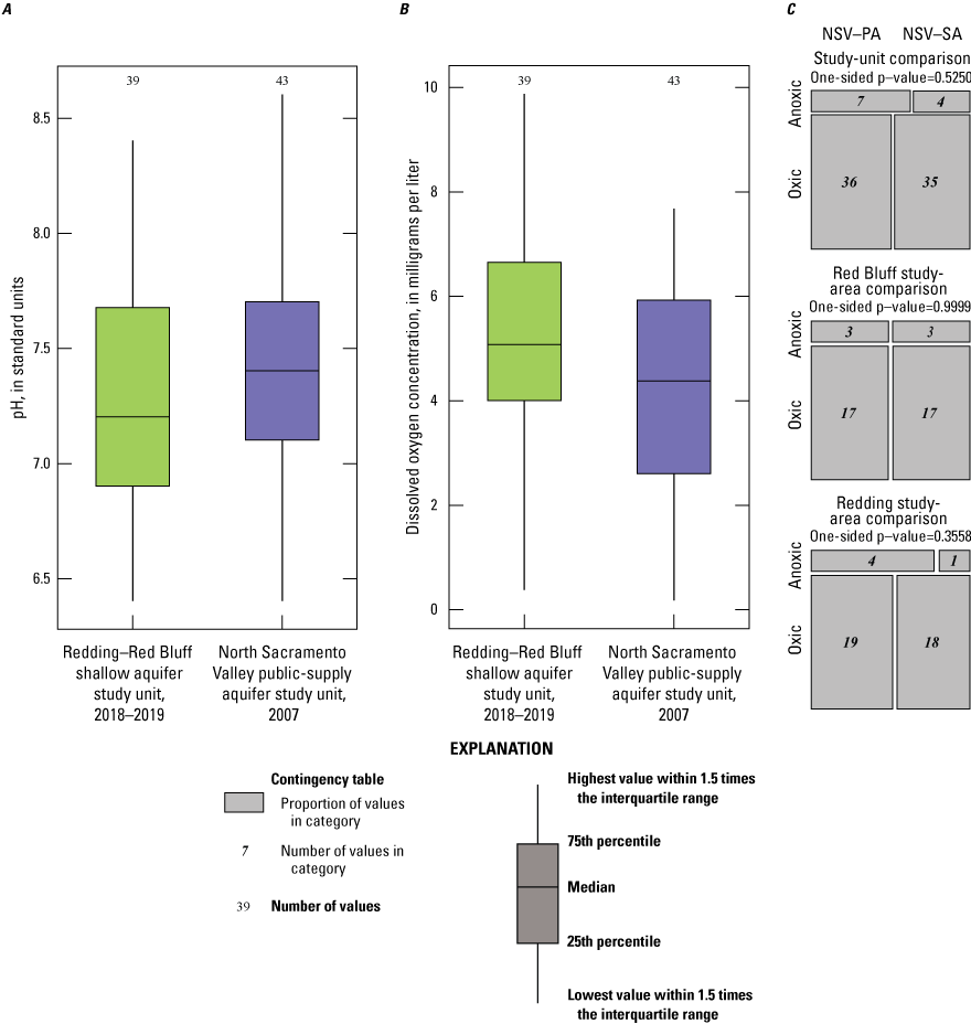
Constituent value, concentration, or redox condition in grid wells: A, pH value by study unit; B, dissolved oxygen concentration by study unit; and C, proportion and number of grid wells with oxic or anoxic groundwater by study unit and study area, north Sacramento Valley public-supply aquifer study unit (NSV-PA) in 2007, and Redding–Red Bluff shallow aquifer study unit (NSV-SA) in 2018–19, California Groundwater Ambient Monitoring and Assessment Program Priority Basin Project. Fisher’s exact tests were used to determine the significance of the differences between the observed number of values (number of grid wells) in each category and the expected number of grid wells. A probability value (p-value) greater than 0.1 indicates the difference is not statistically significant.
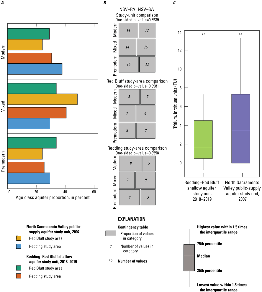
Groundwater age (modern, mixed, or premodern) or tritium concentration for grid wells by study unit and study area: A, aquifer proportion by groundwater age; B, proportion and number of grid wells by groundwater age; and C, tritium concentration (study unit only), north Sacramento Valley public-supply aquifer study unit (NSV-PA) in 2007 and the Redding–Red Bluff shallow aquifer study unit (NSV-SA) in 2018–19, California Groundwater Ambient Monitoring and Assessment Program Priority Basin Project. Fisher’s exact tests were used to determine the significance of the differences between the observed number of values (number of grid wells) in each category and the expected number of grid wells. A probability value (p-value) greater than 0.1 indicates the difference is not statistically significant.
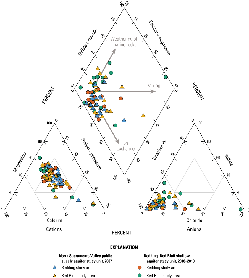
Groundwater chemical ionic composition and water type for grid wells in the north Sacramento Valley public-supply aquifer study unit in 2007 and Redding–Red Bluff shallow aquifer study unit in 2018–19, California Groundwater Ambient Monitoring and Assessment Program Priority Basin Project.
Comparison of Water Quality
Constituents selected for additional evaluation (table 6) were the focus of the groundwater-quality comparison between the study units. Manganese was the only inorganic constituent found at high RCs in both NSV-PA and NSV-SA study units. Hexavalent chromium was selected for further evaluation in the NSV-SA due to high RCs in more than 2 percent of the groundwater resource but was not included in the comparison analysis because it was not analyzed in the NSV-PA dataset. However, hexavalent chromium is typically the dominant chromium species in natural waters because it is the more mobile species, and total chromium can be used to estimate the concentration of hexavalent chromium in groundwater (Manning and others, 2015). Chloroform was the only organic constituent that was detected at a frequency greater than 10 percent in either study unit (Bennett and others 2009; Shelton and others, 2020). Neither chloroform nor any other organic constituents were found at high RCs in either study unit.
Inorganic Constituents
When comparing the NSV-PA and NSV-SA, higher proportions of high and moderate RCs for inorganic constituents (fig. 23) and trace metals (fig. 24) were observed in the groundwater resources used by domestic wells. These higher proportions also were demonstrated in differences between the individual study areas, except for total chromium, which was found at moderate concentrations only in the NSV-SA Redding study area. However, the difference in proportions of wells between the study units and study areas were not statistically significant for inorganic constituents (fig. 23) or trace metals (fig. 24), Although the difference is not significant, the higher occurrence of elevated trace metal concentrations in the NSV-SA likely is related to interactions of groundwater with sediments derived from the North Coast Ranges (fig. 1) west of the Sacramento River where there are more domestic wells and fewer public-supply wells. This observation is supported by the higher proportion of wells in the Tehama Formation and in areas with natural land use in the NSV-SA (figs. 18, 19).
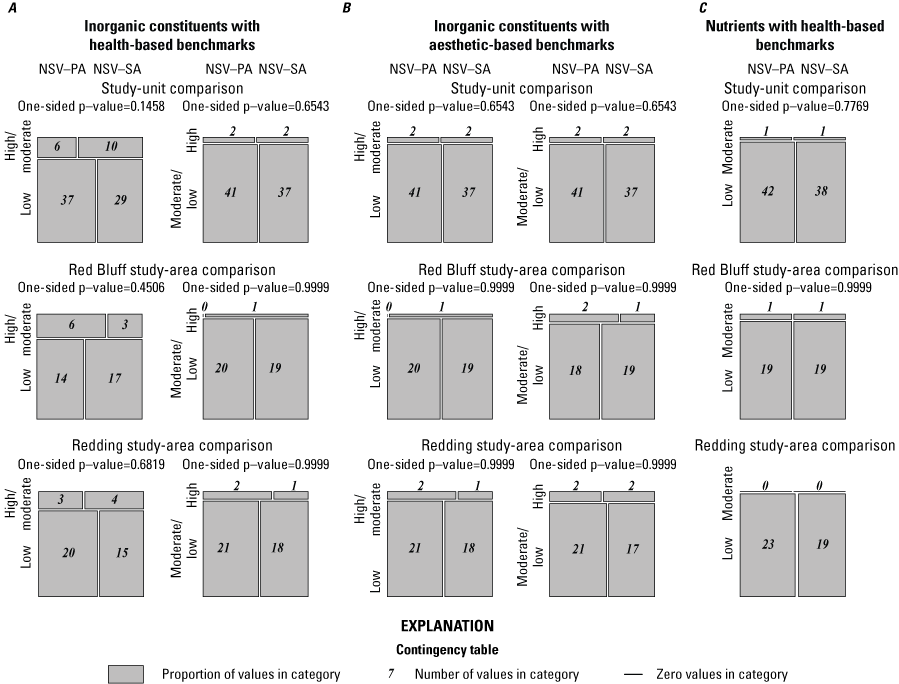
Proportion and number of grid wells with low, moderate, or high relative concentrations of inorganic constituents and nutrients by study unit and study area: A, inorganic constituents with health-based benchmarks; B, inorganic constituents with aesthetic-based benchmarks; and C, nutrients with health-based benchmarks, north Sacramento Valley public-supply aquifer study unit (NSV-PA) in 2007 and Redding–Red Bluff shallow aquifer study unit (NSV-SA) in 2018–19, California Groundwater Ambient Monitoring and Assessment Program Priority Basin Project. Fisher’s exact tests were used to determine the significance of the differences between the observed number of values (number of grid wells) in each category and the expected number of grid wells. A probability value (p-value) greater than 0.1 indicates the difference is not statistically significant. P-values are not shown for study units or study areas containing grid wells with no high or moderate RC value.
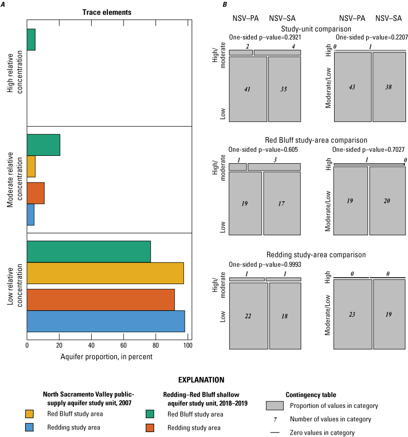
Low, moderate, or high relative concentration of trace elements with health-based benchmarks by study unit and study area: A, aquifer proportion; and B, proportion and number of grid wells, north Sacramento Valley public-supply aquifer (NSV-PA) in 2007 and the Redding–Red Bluff shallow aquifer (NSV-SA) study unit in 2018–19, California Groundwater Ambient Monitoring and Assessment Program Priority Basin Project. Fisher’s exact tests were used to determine the significance of the differences between the observed number of values (number of grid wells) in each category and the expected number of grid wells. A probability value (p-value) greater than 0.1 indicates the difference is not statistically significant. P-values are not shown for study units or study areas containing grid wells with no high or moderate RC value.
Manganese was the only trace element present at both high and moderate concentrations in the NSV-SA and NSV-PA; however, the difference in proportions of high or moderate RCs between the two study units was not statistically significant (figs. 25A–B). Total chromium was only found at moderate concentrations in 5 percent of the NSV-SA Redding study area, (figs. 25C–D). High and moderate RCs of total and hexavalent chromium were found in wells in the west side of the valley that did not overlap with the extent of the NSV-PA. Moderate levels of total chromium in the NSV-SA are not necessarily related to differences in depth of the groundwater resources used by the domestic and public-supply wells and could be related to locations of public-supply wells. Public-supply wells are primarily on the east and south side of the valley where there is less chromium-rich minerals in the aquifer sediments. However, the difference in number of grid wells located in each aquifer lithology between the study units was not statistically significant (fig. 19B).
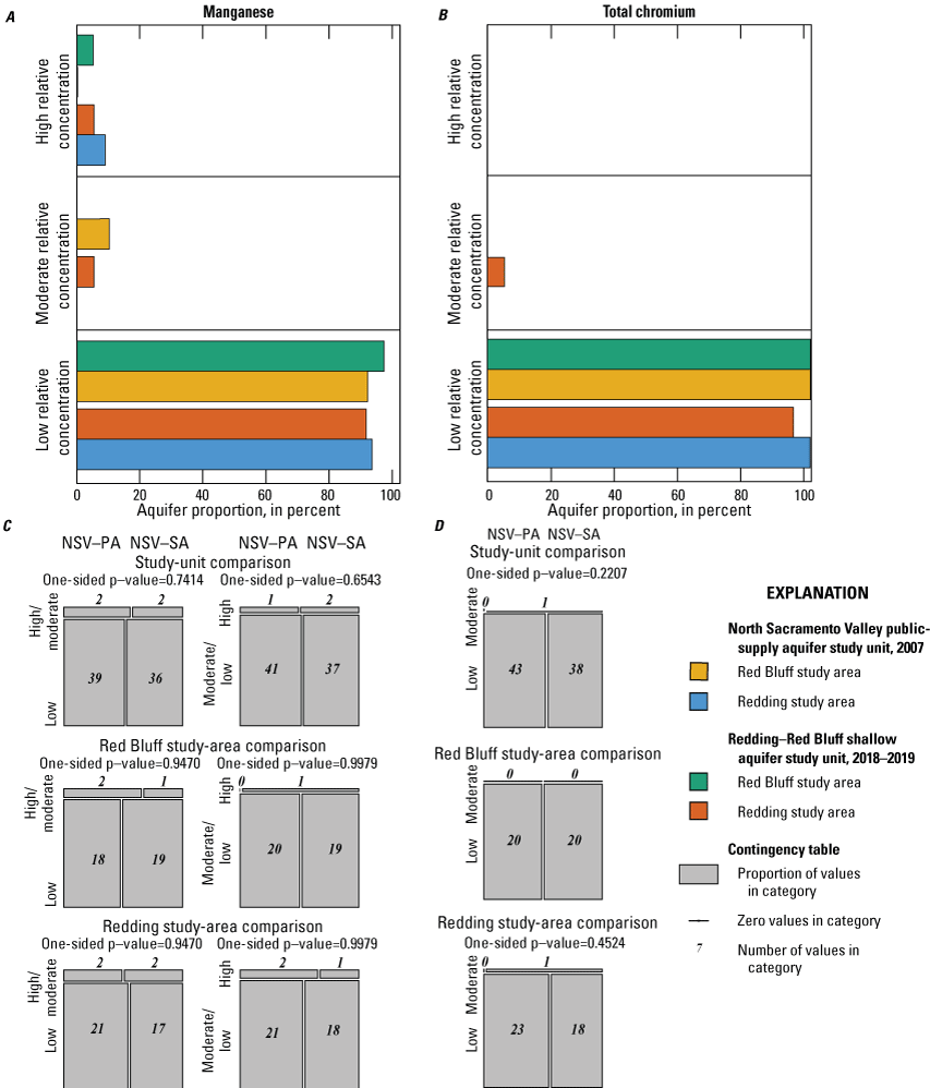
Low, moderate, or high relative concentration for manganese and total chromium by study unit and study area, A, aquifer proportion for manganese; B, aquifer proportion for total chromium; C, proportion and number of grid wells for manganese; and D, proportion and number of grid wells for total chromium, north Sacramento Valley public-supply aquifer (NSV-PA) in 2007 and the Redding–Red Bluff shallow aquifer (NSV-SA) study unit in 2018–19, California Groundwater Ambient Monitoring and Assessment Program Priority Basin Project. Fisher’s exact tests were used to determine the significance of the differences between the observed number of values (number of grid wells) in each category and the expected number of grid wells. A probability value (p-value) greater than 0.1 indicates the difference is not statistically significant. P-values are not shown for study units or study areas containing grid wells with no high or moderate RC value.
Organic Constituents and Perchlorate
Wells in the NSV-PA are significantly deeper than wells in the NSV-SA (fig. 17). The groundwater used by public wells in the NSV-PA is slightly older than groundwater resources used by domestic wells in the NSV-SA (fig. 21), and the older groundwater would be less likely to contain constituents from anthropogenic sources if flow paths and residence times are relatively long. However, differences in the proportions of wells in each groundwater age category between the two study units were not statistically significant (contingency table test p>0.1; fig. 21). The organic constituents were present in higher proportions in the NSV-PA than the NSV-SA (fig. 26). Organic constituents were present at concentrations greater than reporting levels in about 18 percent of the groundwater resources in the NSV-SA and 30 percent in the NSV-PA (fig. 26A, average no detections of about 82 and 70 percent, respectively). This pattern also was observed for differences between the individual study areas, with higher proportions of organic constituent detections in the NSV-PA study areas compared to the NSV-SA study areas; however, the difference in the proportions between the study units was not statistically significant (contingency table test p>0.1). The differences in proportions of the aquifer with detections of organic constituents between the Redding and Red Bluff study areas for either the NSV-SA or the NSV-PA study units was not significant (contingency table text p>0.1).
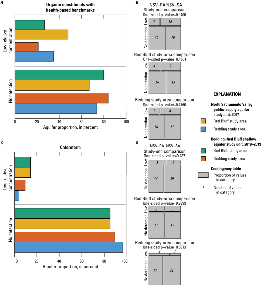
Non-detection or low relative concentration for organic constituents with a health-based benchmark and chloroform by study unit and study area: A, aquifer proportion for organic constituents; B, proportion and number of grid wells for organic constituents; C, aquifer proportion for chloroform; and D, proportion and number of grid wells for chloroform, north Sacramento Valley public-supply aquifer (NSV-PA) in 2007 and the Redding–Red Bluff shallow aquifer (NSV-SA) study unit in 2018–19, California Groundwater Ambient Monitoring and Assessment Program Priority Basin Project. Fisher’s exact tests were used to determine the significance of the differences between the observed number of values (number of grid wells) in each category and the expected number of grid wells. A probability value (p-value) greater than 0.1 indicates the difference is not statistically significant.
Disinfection by-products were detected in 15 percent of the area in the NSV-SA, but detection was lower at 9 percent of the area in the NSV-PA (fig. 27A); however, the difference was not significant (fig. 27B). Chloroform was the most common disinfection by-product detected in both study units and was found in all four study areas (Bennett and others, 2009; Shelton and others, 2020). The disinfection by-product nitrosodimethylamine (NDMA) was detected at moderate RCs in the NSV-PA Red Bluff study area but was not analyzed as part of the NSV-SA assessment; therefore, NDMA was not included in the comparison (Bennett and others, 2009). The presence of similar occurrences of trihalomethanes (including chloroform) and pesticides in both study units is consistent with the results of the geochemical and groundwater age comparisons showing that the groundwater resources used by the domestic and public-supply wells likely are not distinct. However, the slightly higher presence of chloroform detection in the Redding study area of the NSV-SA could be related to more wells in modern or mixed groundwater in the NSV-SA compared to the NSV-PA (fig. 21).
The difference in the proportion of pesticide detections between the study units was not statistically significant (fig. 27B). The herbicides, simazine and atrazine, were the most detected pesticides in both study units, and simazine was observed in all study areas (Bennett and others, 2009; Shelton and others, 2020). The herbicides were the most detected organic constituent class in the NSV-PA and were found in 16 percent of wells from the NSV-PA and 5 percent of the NSV-SA (fig. 27A). The difference in agricultural land use around grid wells between the two study units was not statistically significant, which may explain why proportions of pesticides are similar in the two study units (fig. 18). Simazine is among the Nation’s most detected pesticide compounds in groundwater (Gilliom and others, 2006). However, use of atrazine and simazine as herbicides has declined in California (California Department of Pesticide Regulation, 2017). Atrazine is more commonly used in Shasta County, and use of atrazine peaked in 1999, whereas simazine is used in Tehama County, and use of simazine peaked in 2006. Uses of simazine and atrazine have declined to less than 250 pounds per year (peak values were more than 10,000 pounds per year) in the last decade, so the higher proportions of these pesticides in the NSV-PA may have resulted from legacy contaminations through migration to deeper wells (California Department of Pesticide Regulation, 2017).
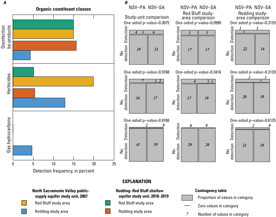
Non-detection and detection frequency for organic constituent classes (disinfection by-products, herbicides, and gas hydrocarbons) by study unit and study area: A, aquifer proportion; and B, proportion and number of grid wells, north Sacramento Valley public-supply aquifer (NSV-PA) in 2007 and the Redding–Red Bluff shallow aquifer (NSV-SA) study unit in 2018–19, California Groundwater Ambient Monitoring and Assessment Program Priority Basin Project. Fisher’s exact tests were used to determine the significance of the differences between the observed number of values (number of grid wells) in each category and the expected number of grid wells. A probability value (p-value) greater than 0.1 indicates the difference is not statistically significant. P-values are not shown for study units or study areas containing grid wells with no high or moderate RC value.
Perchlorate
Moderate RCs of perchlorate were detected in the NSV-PA Red Bluff study area but not the NSV-PA Redding study area or in either of the study areas in the NSV-SA (fig. 28). The application of imported fertilizers containing minor perchlorate impurities until the mid-1900s can leave residue in the unsaturated zone (Interstate Technology and Regulatory Council, 2005; U.S. Environmental Protection Agency Federal Facilities Restoration and Reuse Office, 2005; Dasgupta and others, 2005; Böhlke and others, 2009), and natural perchlorate salts also can accumulate in the unsaturated zone over time (U.S. Environmental Protection Agency Federal Facilities Restoration and Reuse Office, 2005; Rao and others, 2007; Fram and Belitz, 2011). These natural or fertilizer-based perchlorate salts can be remobilized by infiltrating irrigation water. The return-flow waters remobilizing perchlorate can contain detectable levels of pesticides and bring both perchlorate and pesticides into the groundwater. Pesticide detections were higher in the NSV-PA, with the higher proportions of wells with pesticide detections in the NSV-PA Red Bluff study area, which is consistent with influence from agricultural return flow and legacy pesticide use in the groundwater resources used for public supply. The co-occurrence of moderate perchlorate RCs with pesticide detections in the NSV-PA Red Bluff study area may be a result of agricultural activities and return-flow infiltration.
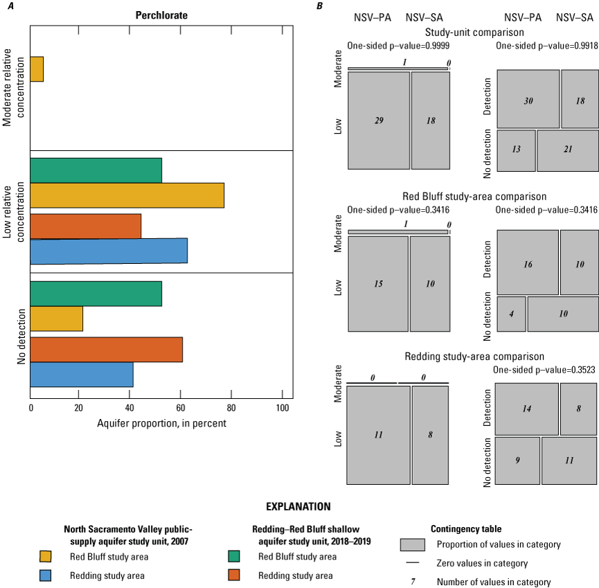
Non-detection, low, and moderate relative concentration for perchlorate by study unit and study area: A, aquifer proportion; and B, proportion and number of grid wells, north Sacramento Valley public-supply aquifer (NSV-PA) in 2007 and the Redding–Red Bluff shallow aquifer (NSV-SA) study unit in 2018–19, California Groundwater Ambient Monitoring and Assessment Program Priority Basin Project. Fisher’s exact tests were used to determine the significance of the differences between the observed number of values (number of grid wells) in each category and the expected number of grid wells. A probability value (p-value) greater than 0.1 indicates the difference is not statistically significant. P-values are not shown for study units or study areas containing grid wells with no high or moderate RC value.
Summary
Groundwater quality in the approximately 3,100 square kilometers (km2) Redding–Red Bluff shallow aquifer study unit (NSV-SA) was studied from 2018 to 2019 as part of the Priority Basin Project (PBP) of the Groundwater Ambient Monitoring and Assessment (GAMA) Program, in cooperation with the California State Water Resources Control Board (SWRCB). In this study, we analyzed untreated groundwater from domestic and small systems wells that draw, on average, from shallower depth intervals compared to nearby public-supply wells. The NSV-SA was selected for assessment because a large part of the population relies on domestic wells for drinking water compared to other parts of California.
The GAMA-PBP uses an equal-area grid-based method that allows for assessment of water quality across the whole extent of the groundwater resources used by the domestic supply in the study unit rather than the areas with high densities of wells. Concentrations of water-quality constituents are reported as relative concentrations (RCs) compared to an established national or state benchmark. The proportion of the groundwater resources in the NSV-SA with concentrations exceeding state or national water quality benchmarks (high RCs) was low compared to other study units in the Central Valley. The low occurrence of groundwater constituents of concern likely is related to the high proportions of natural land cover and low proportions of agriculture and urban areas, greater proportions of oxic groundwater conditions, and distinct sources of aquifer sediments compared to the rest of the Sacramento Valley.
Many oxyanions found in groundwater in California such as arsenic, vanadium, manganese, molybdenum, and chromium are derived from natural sources through interactions of groundwater with the host aquifer materials. Arsenic, vanadium, molybdenum, iron, and manganese are released to groundwater in low oxygen or anoxic environments. Dissolved-oxygen concentrations were lower in the Quaternary alluvial sediments than the sediments of the Tehama Formation. However, the groundwater in more than 90 percent of wells in the Redding–Red Bluff shallow aquifer study unit was oxic because of the restricted extent of the Sacramento River alluvial deposits in this part of the Sacramento Valley. The pervasiveness of oxic conditions in the northern regions of the Sacramento Valley limits the dissolution of trace elements that could pose risks to water quality in the groundwater resources used by domestic wells. Arsenic and manganese were negatively correlated with dissolved oxygen and, as a result, the areal proportions of high and moderate relative RCs exceeding the benchmark or half the benchmark, respectively, for manganese and arsenic were small, less than 5 percent.
The redox conditions and lithology of the NSV-SA that result in low concentrations of some trace elements contribute to the moderate and high cumulative RCs of total chromium and hexavalent chromium observed in about 12 percent of the groundwater resources in the NSV-SA. Hexavalent chromium, which makes up at least 75 percent of the total chromium measured in wells, is most stable under the oxic conditions prevalent throughout the study area. The sediments of the Pliocene Tehama Formation that dominate the aquifer lithology, particularly in the western side of the valley, are rich in chromium-based minerals derived from ultramafic units in the north Coast Ranges. The deeper wells and longer residence times for groundwater interacting with these sediments allows for accumulation of hexavalent chromium in the groundwater resources used for domestic wells in the NSV-SA.
Groundwater contaminants, such as nitrate and synthetic organic constituents, are usually released to groundwater because of human activities such as infiltration of fertilizer-affected irrigation water in agricultural areas and leaking septic systems for nitrate, and chemical spills in densely populated and industrialized areas for synthetic organic compounds. The land use cover in the NSV-SA is more than 65 percent natural, and the low urban and agricultural land use in the NSV-SA likely results in lower amounts of anthropogenic constituents released to groundwater. Wells assessed in the NSV-SA did not have high RCs of nitrate, and only 4 percent of measured wells had moderate RCs. Nitrate was positively correlated to underground storage tank density, septic tank density, and agricultural land use and also was statistically correlated to shallow (Quaternary sediments) and modern groundwater, which is consistent with an anthropogenic source of elevated nitrate. High or moderate RCs were not measured for any organic constituents in the groundwater wells assessed in the NSV-SA.
Organic constituents were detected in 16 percent of the groundwater resources used by domestic wells in the NSV-SA. Chloroform was the only organic constituent detected in more than 10 percent of sites sampled in the NSV-SA and was only detected at low RCs. Chloroform concentrations were positively correlated to urban land use and underground storage-tank density, which is consistent with anthropogenic releases of chloroform. The low RCs and levels of detections for organic constituents are consistent with the low percentage of developed land in the NSV-SA.
Comparison of the NSV-SA to the north Sacramento Valley public-supply aquifer study unit (NSV-PA) indicated that the groundwater resources used for domestic and public-supply wells were not significantly different. Although the public-supply wells were typically deeper, with longer screened intervals, characteristics like water type, age, and redox conditions were statistically indistinguishable with shallower domestic wells. Moreover, contingency table tests for inorganic and organic constituents did not identify statistically significant differences in measured high and moderate RCs for grid sites in the NSV-SA and NSV-PA study units or in the Redding and Red Bluff study areas within each study unit.
Comparisons at the study-unit and study-area scales showed higher proportions of high and moderate RCs for trace metals with health-based benchmarks in the NSV-SA than in the NSV-PA but this difference was only statistically significant at the study-unit scale. Higher concentrations of trace metals in the NSV-SA likely are related to domestic wells primarily occurring farther west of the Sacramento River where the groundwater is older, and the aquifer sediments are derived from the north Coast Ranges. Moderate total chromium RCs were only observed in the NSV-SA Redding study area; however, hexavalent chromium was not analyzed in the NSV-PA, so comparisons of hexavalent chromium could not be made between study units. The wells with high and moderate RCs of hexavalent chromium from the NSV-SA assessment were in the western part of the northern Sacramento Valley and did not overlap with the NSV-PA study unit. The public-supply wells are concentrated in the center and southern boundary of the northern Sacramento Valley, along the Sacramento River, where groundwater is not interacting with chromium-rich sediments from the north Coast Ranges.
For constituents included in analyses of both NSV-SA and NSV-PA study units, organic constituents were not detected at high or moderate RCs. The detection frequency of organic constituents at low RCs was higher in the NSV-PA (30 percent) than in the NSV-SA (18 percent), but this difference was not statistically significant. Trihalomethanes were the most detected organic constituent class in the NSV-SA. Chloroform was detected in more than 10 percent of samples from the NSV-SA and in 9 percent of the samples from the NSV-PA. Herbicides were the organic constituent class detected in more than 10 percent of the NSV-PA but were found in 5 percent of the NSV-SA; however, these differences were not statistically significant at the study unit or study-area scale.
Comparison of selected characteristics for the NSV-SA and NSV-PA study units indicated minimal distinction between the water quality of groundwater resources used by domestic and public-supply wells, despite the shallower depths of the domestic wells in the northern Sacramento Valley that is covered by the GAMA-PBP study units. The groundwater resources used by the public-supply wells have low RCs, low proportions of moderate and high RCs of constituents with health and aesthetic-based benchmarks, and low detections of organic constituents. The comparison assessment supported the results of the understanding assessment that the low agricultural and urban land use and oxic groundwater conditions in the region may limit contributions of anthropogenic and natural groundwater contaminants to the groundwater resources used for drinking water.
References Cited
Ayotte, J.D., Medalie, L., Qi, S.L., Backer, L.C., and Nolan, B.T., 2017, Estimating the high-arsenic domestic-well population in the conterminous United States: Environmental Science and Technology, v. 51, no. 21, p. 12443–12454, accessed January 9, 2020, at https://doi.org/10.1021/acs.est.7b02881.
Belitz, K., Dubrovsky, N.M., Burow, K., Jurgens, B., and Johnson, T.D., 2003, Framework for a ground-water quality monitoring and assessment program for California: U.S. Geological Survey Water Resources Investigations Report 2003–4166, 78 p., accessed November 8, 2019, at https://doi.org/10.3133/wri034166.
Belitz, K., Fram, M.S., and Johnson, T.D., 2015, Metrics for assessing the quality of groundwater used for public supply, CA, USA—Equivalent-population and area: Environmental Science and Technology, v. 49, no. 14, p. 8330–8338, accessed November 8, 2019, at https://doi.org/10.1021/acs.est.5b00265.
Belitz, K., Jurgens, B., Landon, M.K., Fram, M.S., and Johnson, T.D., 2010, Estimation of aquifer scale proportion using equal area grids—Assessment of regional scale groundwater quality: Water Resources Research, v. 46, no. 11, 14 p., accessed November 8, 2019, at https://doi.org/10.1029/2010WR009321.
Bennett, G.L.V., Fram, M.S., and Belitz, K., 2011, Status of groundwater quality in the southern, middle, and northern Sacramento Valley study units, 2005–08—California GAMA Priority Basin Project: U.S. Geological Survey Scientific Investigations Report 2011–5002, 119 p., accessed November 8, 2019, at https://doi.org/10.3133/sir20115002.
Bennett, G.L.V., 2018, Status and understanding of groundwater quality in the north San Francisco Bay Shallow Aquifer study unit, 2012—California GAMA Priority Basin Project (ver. 1.1): U.S. Geological Survey Scientific Investigations Report 2017–5051, 74 p., accessed November 18, 2020, at https://doi.org/10.3133/sir20175051.
Bennett, P.A., Bennett, G.L.V., and Belitz, K., 2009, Groundwater quality data for the northern Sacramento Valley, 2007—Results from the California GAMA Program: U.S. Geological Survey Data Series 452, 91 p., accessed November 18, 2020, at https://doi.org/10.3133/ds452.
Böhlke, J.K., Hatzinger, P.B., Sturchio, N.C., Gu, B.I.A., Abbene, I., and Mroczkowski, S.J., 2009, Atacama perchlorate as an agricultural contaminant in groundwater—Isotopic and chronologic evidence from Long Island, New York: Environmental Science and Technology, v. 43, no. 15, p. 5619–5625, January 11, 2021, at https://doi.org/10.1021/es9006433.
Brown, L.D., Cai, T.T., and DasGupta, A., 2001, Interval estimation for a binomial proportion: Statistical Science, v. 16, no. 2, p. 101–133, accessed November 18, 2020, at https://doi.org/10.1214/ss/1009213286.
Burow, K.R., Jurgens, B.C., Kauffman, L.J., Phillips, S.P., Dalgish, B.A., and Shelton, J.L., 2008, Simulations of ground-water flow and particle pathline analysis in the zone of contribution of a public-supply well in Modesto, eastern San Joaquin Valley, California: U.S. Geological Survey Scientific Investigations Report 2008–5035, 41 p., accessed March 6, 2020, at https://doi.org/10.3133/sir20085035.
California Department of Pesticide Regulation, 2017, Pesticide use reporting: California Department of Pesticide Regulation website, accessed November 18, 2020, at https://www.cdpr.ca.gov/docs/pur/purmain.htm.
California Department of Water Resources, 2003, California’s groundwater: California Department of Water Resources Bulletin 118, 246 p., accessed December 9, 2021, at https://water.ca.gov/Programs/Groundwater-Management/Bulletin-118.
California Department of Water Resources, 2014, Geology of the Northern Sacramento Valley: California Department of Water Resources, accessed November 18, 2020, at https://cawaterlibrary.net/wp-content/uploads/2017/05/Geology-of-the-Northern-Sacramento-Valley.pdf.
California Department of Water Resources, 2018, Online system for well completion reports: California Department of Water Resources website, accessed August 2018 at https://data.cnra.ca.gov/dataset/well-completion-reports.
California Department of Water Resources, 2020, Groundwater program: California Department of Water Resources website, accessed November 18, 2020, at https://water.ca.gov/Water-Basics/Groundwater.
California Department of Water Resources, 2022, Groundwater Basin Boundary Assessment Tool: California Department of Water Resources website, accessed August 9, 2022, at https://gis.water.ca.gov/app/bbat/.
California State Water Resources Control Board, 2009, GAMA Domestic Well Project groundwater quality data report, Tehama County focus area: California State Water Resources Control Board, 27 p., accessed January 11, 2021, at https://www.waterboards.ca.gov/water_issues/programs/gama/docs/tehama_focus_area_draft_datareport.pdf.
California State Water Resources Control Board, 2015a, California drinking water-related laws: California State Water Resources Control Board website, accessed November 18, 2020, at https://www.waterboards.ca.gov/drinking_water/certlic/drinkingwater/Lawbook.shtml.
California State Water Resources Control Board, 2015b, Perchlorate in drinking water: California State Water Resources Control Board website, accessed November 18, 2020, at https://www.waterboards.ca.gov/drinking_water/certlic/drinkingwater/Perchlorate.shtml.
California State Water Resources Control Board, 2016, A compilation of water quality goals, (17th ed.): State Water Resources Control Board, 47 p., accessed April 11, 2022, at https://www.waterboards.ca.gov/water_issues/programs/water_quality_goals/.
California State Water Resources Control Board, 2017, Groundwater information sheet—Hexavalent chromium: State Water Resources Control Board Division of Water Quality GAMA Program, 8 p., accessed November 18, 2020, at https://www.waterboards.ca.gov/water_issues/programs/gama/docs/coc_hexchromcr6.pdf.
California State Water Resources Control Board, 2020, Groundwater Information System: California State Water Resources Control Board website—GAMA Groundwater Information System and California Water Boards, accessed April 23, 2020, at https://gamagroundwater.waterboards.ca.gov/gama/gamamap/public/.
Central Valley Regional Water Quality Control Board, 2016, Groundwater quality assessment report: Northern California Water Association and Sacramento Valley Water Quality Coalition, 370 p., accessed November 18, 2020, at https://www.svwqc.org/wp-content/themes/svwqc-2015/docs/Groundwater-Quality-Assessment-Report-20160128.pdf.
Centers for Disease Control and Prevention and U.S. Department of Housing and Urban Development, 2006, Healthy housing reference manual: U.S. Department of Health and Human Services, 231 p., accessed April 12, 2022, at https://www.cdc.gov/nceh/publications/books/housing/housing_ref_manual_2012.pdf.
Chapelle, F.H., McMahon, P.B., Dubrovsky, N.M., Fuji, R.F., Oaksford, E.T., and Vroblesky, D.A., 1995, Deducing the distribution of terminal electron-accepting processes in hydrologically diverse groundwater systems: Water Resources Research, v. 31, no. 2, p. 359–371, accessed November 11, 2019, at https://doi.org/10.1029/94WR02525.
Dasgupta, P.K., Martinelango, P.K., Jackson, W.A., Anderson, T.A., Tian, K., Tock, R.W., and Rajogopalan, S., 2005, The origin of naturally occurring perchlorate—The role of atmospheric processes: Environmental Science & Technology, v. 39, no. 6, p. 1569–1575, accessed February 8, 2021, at https://doi.org/10.1021/es048612x.
Dawson, B.J., 2001, Shallow ground-water quality beneath rice areas in the Sacramento Valley, California, 1997: U.S. Geological Survey Water-Resources Investigations Report 2001–4000, 33 p., accessed November 18, 2020, at https://doi.org/10.3133/wri014000.
DeSimone, L.A., McMahon, P.B., and Rosen, M.R., 2014, The quality of our Nation’s waters—Water quality in principal aquifers of the United States, 1991–2010: U.S. Geological Survey Circular 1360, accessed November 18, 2020, at https://doi.org/10.3133/cir1360.
Dieter, C.A., and Maupin, M.A., 2017, Public supply and domestic water use in the United States, 2015: U.S. Geological Survey Open-File Report 2017–1131, 6 p., accessed August 8, 2022, at https://doi.org/10.3133/ofr20171131.
Dubrovsky, N.M., Burow, K.R., Clark, G.M., Gronberg, J.M., Hamilton, P.A., Hitt, K.J., Mueller, D.K., Munn, M.D., Nolan, B.T., Puckett, L.J., Rupert, M.G., Short, T.M., Spahr, N.E., Sprague, L.A., and Wilber, W.G., 2010, The quality of our Nation’s waters—Nutrients in the Nation’s streams and groundwater, 1992–2004: U.S. Geological Survey Circular 1350, 174 p., accessed November 18, 2020, at https://doi.org/10.3133/cir1350.
Eary, L.E., and Rai, D., 1987, Kinetics of chromium (III) oxidation to chromium (VI) by reaction with manganese dioxide: Environmental Science & Technology, v. 21, no. 12, p. 1187–1193., accessed on April 12, 2022, at https://doi.org/10.1021/es00165a005.
Falcone, J.A., 2015, U.S. conterminous wall-to-wall anthropogenic land use trends (NWALT), 1974–2012: U.S. Geological Survey Data Series 948, 33 p., plus appendixes 3–6 as separate files, accessed July 23, 2020, at https://doi.org/10.3133/ds948.
Focazio, M.J., Welch, A.H., Watkins, S.A., Helsel, D.R., and Horn, M.A., 2000, A retrospective analysis on the occurrence of arsenic in ground-water resources of the United States and limitations in drinking-water-supply characterizations: U.S. Geological Survey Water Resources Investigations Report 99–4279, 21 p., accessed November 18, 2020, at https://doi.org/10.3133/wri994279.
Fram, M.S., and Belitz, K., 2011, Probability of detecting perchlorate under natural conditions in deep groundwater in California and the southwestern United States: Environmental Science & Technology, v. 45, no. 4, p. 1271–1277, accessed February 8, 2021, at https://doi.org/10.1021/es103103p.
Gilliom, R.J., Barbash, J.E., Crawford, C.G., Hamilton, P.A., Martin, J.D., Nakagaki, N., Nowell, L.H., Scott, J.C., Stackelberg, P.E., Thelin, G.P., and Wolock, D.M., 2006, Pesticides in the Nation’s streams and ground water, 1992–2001: U.S. Geological Survey Circular 1291, 173 p., accessed November 18, 2020, at https://doi.org/10.3133/cir1291.
Groschen, G.E., Arnold, T., Morrow, W.S., and Warner, K.L., 2008, Occurrence and distribution of iron, manganese, and selected trace elements in ground water in the glacial aquifer system of the Northern United States: U.S. Geological Survey Scientific Investigations Report 2009–5006, 89 p., accessed November 18, 2020, at https://doi.org/10.3133/sir20095006.
Harkness, J.S., 2022, Potential explanatory variables for groundwater quality in the Redding–Red Bluff shallow aquifer assessment study unit, 2018–2019—California GAMA Priority Basin Project: U.S. Geological Survey data release, https://doi.org/10.5066/P9XQIWRU.
Harwood, D.S., and Helley, E.J., 1987, Late Cenozoic tectonism of the Sacramento Valley, California: U.S. Geological Survey Professional Paper 1359, 46 p., accessed November 18, 2020, at https://doi.org/10.3133/pp1359.
Hausladen, D.M., Alexander-Ozinskas, A., McClain, C., and Fendorf, S., 2018, Hexavalent chromium sources and distribution in California groundwater: Environmental Science & Technology, v. 52, no. 15, p. 8242–8251, accessed January 9, 2020, at https://doi.org/10.1021/acs.est.7b06627.
Heberger, M., and Donnelly, K., 2015, Oil, food, and water—Challenges and opportunities for California agriculture: Oakland, Calif., Pacific Institute, Technical Report, 65 p., accessed April 12, 2022, at https://pacinst.org/wp-content/uploads/2015/12/PI_OilFoodAndWater_-1.pdf.
Helsel, D.R., Hirsch, R.M., Ryberg, K.R., Archfield, S.A., and Gilroy, E.J., 2020, Statistical methods in water resources: U.S. Geological Survey Techniques and Methods book 4, chap. A3, 458 p., accessed May 27, 2020, at https://doi.org/10.3133/tm4a3.
Hem, J.D., 1985, Study and interpretation of the chemical characteristics of natural water (3d ed.): U.S. Geological Survey Water Supply Paper 2254, 263 p., accessed November 18, 2020, at https://doi.org/10.3133/wsp2254.
Hirsch, R.M., Alley, W.M., and Wilber, W.G., 1988, Concepts for a national water-quality assessment program: U.S. Geological Survey Circular 1021, 42 p. [Available at https://doi.org/10.3133/cir1021.]
Homoncik, S.C., MacDonald, A.M., Heal, K.V., Dochartaigh, B.É.Ó., and Ngwenya, B.T., 2010, Manganese concentrations in Scottish groundwater: Science of the Total Environment, v. 408, no. 12, p. 2467–2473, accessed April 12, 2020, at https://doi.org/10.1016/j.scitotenv.2010.02.017.
Hull, L.C., 1984, Geochemistry of ground water in the Sacramento Valley, California: U.S. Geological Survey Professional Paper 1401–B, 36 p., accessed November 18, 2020, at https://doi.org/10.3133/pp1401B.
Interstate Technology and Regulatory Council, 2005, Perchlorate—Overview of issues, status, and remedial options, PERCHLORATE-1: Washington, D.C., Interstate Technology and Regulatory Council, Perchlorate Team, accessed August 1, 2021, at http://www.itrcweb.org.
Ivahnenko, T., and Zogorski, J.S., 2006, Sources and occurrence of chloroform and other trihalomethanes in drinking-water supply wells in the United States, 1986–2001: U.S. Geological Survey Scientific Investigations Report 2006–5015, 13 p. [Available at https://doi.org/10.3133/sir20065015.]
Izbicki, J.A., Wright, M.T., Seymour, W.A., McCleskey, R.B., Fram, M.S., Belitz, K., and Esser, B.K., 2015, Cr (VI) occurrence and geochemistry in water from public-supply wells in California: Applied Geochemistry, v. 63, p. 203–217, accessed January 9, 2020, at https://doi.org/10.1016/j.apgeochem.2015.08.007.
Jin, S., Yang, L., Danielson, P., Homer, C., Fry, J., and Xian, G., 2013, A comprehensive change detection method for updating the National Land Cover Database to circa 2011: Remote Sensing of Environment, v. 132, p. 159–175, accessed November 18, 2020, at https://doi.org/10.1016/j.rse.2013.01.012.
Johnson, T.D., and Belitz, K., 2009, Assigning land use to supply wells for the statistical characterization of regional groundwater quality—Correlating urban land use and VOC occurrence: Journal of Hydrology, v. 370, p. 100–108, accessed November 8, 2019, at https://doi.org/10.1016/j.jhydrol.2009.02.056.
Johnson, T.D., and Belitz, K., 2014, California groundwater units: U.S. Geological Survey Data Series 796, 34 p., accessed November 8, 2019, at https://doi.org/10.3133/ds796.
Jurgens, B.C., McMahon, P.B., Chapelle, F.H., and Eberts, S.M., 2009, An Excel® workbook for identifying redox processes in ground water: U.S. Geological Survey Open-File Report 2009–1004, 8 p., November 18, 2020, at https://doi.org/10.3133/ofr20091004.
Kang, M., and Jackson, R.B., 2016, Salinity of deep groundwater in California—Water quantity, quality, and protection: Proceedings of the National Academy of Sciences, v. 113, no. 28, p. 7768–7773, accessed January 13, 2021, at https://doi.org/10.1073/pnas.1600400113.
Landon, M.K., Green, C.T., Belitz, K., Singleton, M.J., and Esser, B.K., 2011, Relations of hydrogeologic factors, groundwater reduction-oxidation conditions, and temporal and spatial distributions of nitrate, Central-Eastside San Joaquin Valley, California, USA: Hydrogeology Journal, v. 19, no. 6, p. 1203–1224, accessed November 8, 2019, at https://doi.org/10.1007/s10040-011-0750-1.
Lindsey, B.D., Jurgens, B.C., and Belitz, K., 2019, Tritium as an indicator of modern, mixed, and premodern groundwater age: U.S. Geological Survey Scientific Investigations Report 2019–5090, accessed November 8, 2019, at https://doi.org/10.3133/sir20195090.
Manning, A.H., Mills, C.T., Morrison, J.M., and Ball, L.B., 2015, Insights into controls on hexavalent chromium in groundwater provided by environmental tracers, Sacramento Valley, California, USA: Applied Geochemistry, v. 62, p. 186–199, accessed November 25, 2019, at https://doi.org/10.1016/j.apgeochem.2015.05.010.
McMahon, P.B., and Chapelle, F.H., 2008, Redox processes and water quality of selected principal aquifer systems: Groundwater, v. 46, no. 2, p. 259–271, accessed November 8, 2019, at https://doi.org/10.1111/j.1745-6584.2007.00385.x.
McMahon, P.B., Belitz, K., Reddy, J.E., and Johnson, T.D., 2019, Elevated manganese concentrations in United States groundwater—Role of land surface-soil-aquifer connections: Environmental Science and Technology, v. 53, no. 1, p. 29–38, accessed November 8, 2019, at https://doi.org/10.1021/acs.est.8b04055.
Mills, C.T., Morrison, J.M., Goldhaber, M.B., and Ellefsen, K.J., 2011, Chromium (VI) generation in vadose zone soils and alluvial sediments of the southwestern Sacramento Valley, California—A potential source of geogenic Cr(VI) to groundwater: Applied Geochemistry, v. 26, no. 8, p. 1488–1501, accessed January 21, 2020, at https://doi.org/10.1016/j.apgeochem.2011.05.023.
Morrison, J.M., Goldhaber, M.B., Lee, L., Holloway, J.M., Wanty, R.B., Wolf, R.E., and Ranville, J.F., 2009, A regional-scale study of chromium and nickel in soils of northern California, USA: Applied Geochemistry, v. 24, no. 8, p. 1500–1511, accessed January 21, 2020, at https://doi.org/10.1016/j.apgeochem.2009.04.027.
Mueller, D.K., and Helsel, D.R., 1996, Nutrients in the Nation’s waters—Too much of a good thing?: U.S. Geological Survey Circular 1136, 24 p., accessed January 29, 2021, at https://doi.org/10.3133/cir1136.
Nolan, B.T., Hitt, K.J., and Ruddy, B.C., 2002, Probability of nitrate contamination of recently recharged groundwaters in the conterminous United States: Environmental Science & Technology, v. 36, no. 10, p. 2138–2145, accessed January 9, 2020, at https://doi.org/10.1021/es0113854.
Oze, C., Fendorf, S., Bird, D.K., and Coleman, R.G., 2004, Chromium geochemistry of serpentine soils: International Geology Review, v. 46, no. 2, p. 97–126, accessed January 21, 2020, at https://doi.org/10.2747/0020-6814.46.2.97.
Oze, C., Bird, D.K., and Fendorf, S., 2007, Genesis of hexavalent chromium from natural sources in soil and groundwater: Proceedings of the National Academy of Sciences of the United States of America, v. 104, no. 16, p. 6544–6549, accessed January 21, 2020, at https://doi.org/10.1073/pnas.0701085104.
Pierce, M.J., 1983, Ground water in the Redding Basin, Shasta and Tehama counties, California: U.S. Geological Survey Water-Resources Investigations Report 83–4052, 41 p., accessed November 8, 2019, at https://doi.org/10.3133/wri834052.
Piper, A.M., 1944, A graphic procedure in the geochemical interpretation of water‐analyses: Eos, Transactions American Geophysical Union, v. 25, no. 6, p. 914–928, accessed November 18, 2020, at https://doi.org/10.1029/TR025i006p00914.
Rajagopalan, S., Anderson, T., Cox, S., Harvey, G., Cheng, Q., and Jackson, W.A., 2009, Perchlorate in wet deposition across North America: Environmental Science & Technology, v. 43, no. 3, p. 616–622, accessed January 9, 2021, at https://doi.org/10.1021/es801737u.
Rao, B., Anderson, T.A., Orris, G.J., Rainwater, K.A., Rajagopalan, S., Sandvig, R.M., Scanlon, B.R., Stonestrom, D.A., Walvoord, M.A., and Jackson, W.A., 2007, Widespread natural perchlorate in unsaturated zones of the southwest United States: Environmental Science & Technology, v. 41, no. 13, p. 4522–4528, accessed January 9, 2021, at https://doi.org/10.1021/es062853i.
Rowe, B.L., Toccalino, P.L., Moran, M.J., Zogorski, J.S., and Price, C.V., 2007, Occurrence and potential human-health relevance of volatile organic compounds in drinking water from domestic wells in the United States: Environmental Health Perspectives, v. 115, no. 11, p. 1539–1546, accessed November 18, 2020, at https://doi.org/10.1289/ehp.10253.
RStudio Team, 2021, RStudio: Boston, Mass., Integrated Development for R. RStudio, Inc., accessed June 3, 2021, at https://www.rstudio.com/.
Schlosser, P., Stute, M., Dörr, H., Sonntag, C., and Münnich, K.O., 1988, Tritium/3He dating of shallow groundwater: Earth and Planetary Science Letters, v. 89, no. 3–4, p. 353–362, accessed at November 8, 2019, at https://doi.org/10.1016/0012-821X(88)90122-7.
Scott, J.C., 1990, Computerized stratified random site-selection approaches for design of a ground-water-quality sampling network: U.S. Geological Survey Water-Resources Investigations Report 90–4101, 109 p., accessed November 18, 2020, at https://doi.org/10.3133/wri904101.
Shelton, J.L., Bennett, G.L., Watson, E., and Johnson, T.D., 2020, Groundwater-quality data in the Redding–Red Bluff shallow aquifer study unit, 2018–2019—Results from the California GAMA Priority Basin Project: U.S. Geological Survey data release, accessed April 23, 2020, at https://doi.org/10.5066/P9ZKAH3O.
Signorell, A., 2021, DescTools—Tools for descriptive statistics, R package software version 0.99.44, accessed November 2020 at https://cran.r-project.org/package=DescTools.
Smedley, P.L., and Kinniburgh, D.G., 2002, A review of the source, behaviour and distribution of arsenic in natural waters: Applied Geochemistry, v. 17, no. 5, p. 517–568, accessed November 18, 2020, at https://doi.org/10.1016/S0883-2927(02)00018-5.
State of California, 1999, Supplemental report of the 1999 Budget Act 1999–00 Fiscal Year, Item 3940-001-0001: State Water Resources Control Board, accessed November 18, 2020, at https://lao.ca.gov/1999/99-00_supp_rpt_lang.html.
State of California, 2001a, Assembly Bill No. 599, chapter 522: California Legislative Information, accessed November 18, 2020, at https://leginfo.legislature.ca.gov/faces/billTextClient.xhtml?bill_id=200120020AB599&search_keywords=Groundwater+Monitoring.
State of California, 2001b, Groundwater Monitoring Act of 2001—California Water Code, part 2.76, sections 10780–10782.3: California Legislative Information, accessed November 18, 2020, at https://leginfo.legislature.ca.gov/faces/codes_ displayText.xhtml?lawCode=WAT&division=6.&title=&part= 2.76.&chapter=&article=.
Thiessen, A.H., 1911, Precipitation averages for large areas: Monthly Weather Review, v. 39, no. 7, p. 1082–1084, accessed November 18, 2020, at https://doi.org/10.1175/1520-0493(1911)39%3C1082b:PAFLA%3E2.0.CO;2.
Toccalino, P.L., and Norman, J.E., 2006, Health-based screening levels to evaluate U.S. Geological Survey ground water quality data: Risk Analysis, v. 26, no. 5, p. 1339–1348, accessed November 18, 2020, at https://doi.org/10.1111/j.1539-6924.2006.00805.x.
Toccalino, P.L., Norman, J.E., Phillips, R.H., Kauffman, L.J., Stackelberg, P.E., Nowell, L.H., Krietzman, S.J., and Post, G.B., 2004, Application of health-based screening levels to ground-water quality data in a state-scale pilot effort: U.S. Geological Survey Scientific Investigations Report 2004–5174, 64 p., accessed November 18, 2020, at https://doi.org/10.3133/sir20045174.
Toccalino, P.L., Norman, J.E., and Schoephoester, K.M., 2014, Health-based screening levels for evaluating water-quality data: U.S. Geological Survey website, accessed November 18, 2020, at https://water.usgs.gov/nawqa/HBSL.
United Nations Educational, Scientific and Cultural Organization, 1977, Map of the world distribution of arid regions—Explanatory note: Paris, France, Man and the Biosphere (MAB) Technical Notes, v. 7, 54 p., accessed November 18, 2020, at https://unesdoc.unesco.org/ark:/48223/pf0000032661.
U.S. Census Bureau, 1992, Census of population and housing, 1990—Summary tape file 3A: Washington, D.C., U.S. Census Bureau, machine-readable data, accessed November 18, 2020, at https://www2.census.gov/census_1990/.
U.S. Department of Commerce National Climatic Data Center, 2020, Environmental data: U.S. Department of Commerce website, accessed November 18, 2020, at https://www.commerce.gov/data-and-reports/environmental-data.
U.S. Environmental Protection Agency, 1986, Guidelines for the health risk assessment of chemical mixtures: U.S. Environmental Protection Agency, EPA/630/R-98/002, 38 p., accessed November 18, 2020, at https://www.epa.gov/sites/default/files/2014-11/documents/chem_mix_1986.pdf.
U.S. Environmental Protection Agency, 2001, Technical Fact Sheet—Final rule for arsenic in drinking water: U.S. Environmental Protection Agency, accessed November 18, 2020, at https://nepis.epa.gov/Exe/ZyPdf.cgi?Dockey=20001XXE.txt.
U.S. Environmental Protection Agency, 2004, Drinking water health advisory for manganese: U.S. Environmental Protection Agency, EPA-822-R-04-003, 49 p., accessed November 18, 2020, at https://www.epa.gov/sites/default/files/2014-09/documents/support_cc1_magnese_dwreport_0.pdf.
U.S. Environmental Protection Agency, 2012, 2012 Edition of the drinking water standards and health advisories: U.S. Environmental Protection Agency, accessed November 18, 2020, at https://nepis.epa.gov/Exe/ZyPDF.cgi/P100N01H.PDF?Dockey=P100N01H.PDF.
U.S. Environmental Protection Agency, 2016, National primary drinking water regulations: Code of Federal Regulations, Title 40, Part 141, accessed November 18, 2020, at https://www.epa.gov/ground-water-and-drinking-water/national-primary-drinking-water-regulations.
U.S. Environmental Protection Agency Federal Facilities Restoration and Reuse Office , 2005, Perchlorate treatment technology update—Federal facilities forum issue paper: U.S. Environmental Protection Agency, EPA 542-R-05-015, accessed August 16, 2021, at https://www.epa.gov/remedytech/perchlorate-treatment-technology-update.
U.S. Geological Survey, 2018, California Groundwater Ambient Monitoring and Assessment (GAMA) Program Priority Basin Project—Shallow aquifer assessment: U.S. Geological Survey Fact Sheet 2012–3136, 2 p., accessed August 9, 2022, at https://doi.org/10.3133/fs20123136.
U.S. Geological Survey, 2020, USGS water data for the Nation: U.S. Geological Survey National Water Information System database, accessed April 23, 2020, at https://doi.org/10.5066/F7P55KJN.
Wasserman, G.A., Liu, X., Parvez, F., Ahsan, H., Levy, D., Factor-Litvak, P., Kline, J., van Geen, A., Slavkovich, V., Lolacono, N.J., Cheng, Z., Zheng, Y., and Graziano, J.H., 2006, Water manganese exposure and children’s intellectual function in Araihazar, Bangladesh: Environmental Health Perspectives, v. 114, no. 1, p. 124–129, accessed November 18, 2020, at https://doi.org/10.1289/ehp.8030.
Welch, A.H., Oremland, R.S., Davis, J.A., and Watkins, S.A., 2006, Arsenic in groundwater—A review of the current knowledge and relation to the CALFED solution area with recommendations for needed research: San Francisco Estuary and Watershed Science, v. 4, no. 2, article 4, 32 p., accessed November 18, 2020, at https://doi.org/10.15447/sfews.2006v4iss2art3.
Welch, A.H., Westjohn, D.B., Helsel, D.R., and Wanty, R.B., 2000, Arsenic in ground water of the United States—Occurrence and geochemistry: Groundwater, v. 38, no. 4, p. 589–604, accessed November 18, 2020, at https://doi.org/10.1111/j.1745-6584.2000.tb00251.x.
Western Regional Climate Center, 2020, Climate of California: Western Regional Climate Center website, accessed November 18, 2020, at http://www.wrcc.dri.edu/Climate/narrative_ca.php.
Zogorski, J.S., Carter, J.M., Ivahnenko, T., Lapham, W.W., Moran, M.J., Rowe, B.L., Squillace, P.J., and Toccalino, P.L., 2006, Volatile organic compounds in the Nation’s ground water and drinking-water supply wells: U.S. Geological Survey Circular 1292, 101 p., accessed November 18, 2020, at https://doi.org/10.3133/cir1292.
{ label needed for book-app[@id='a1'] }
Appendix 1. Attribution of Potential Explanatory Variables
Aquifer Lithology
Aquifer lithology for each well in the Redding–Red Bluff shallow aquifer study unit (NSV-SA) was classified into two broad categories (volcanic or sedimentary) from lithologic information available in well completion reports and from the California State geologic map and reported in a U.S. Geological Survey data release (California Department of Water Resources, 2018; Saucedo and others, 2000; Harkness, 2022). The sedimentary lithologies were further classified into two types: (1) Quaternary alluvium and (2) Pliocene sediment of the Tehama Formation (California Department of Water Resources, 2014). However, the state geologic map is composed of lithologic units exposed at the surface, which do not necessarily correspond to the lithologic units that host the groundwater tapped by the well. When both sources were available, the lithologic category at depth of the screened interval or well opening from the well completion report was used. If more than one type of lithology was intersected by the screened interval, the predominant category in the screened interval was used.
The three lithologic categories were (1) volcanic rocks and metavolcanic sediments that consist primarily of Tertiary and Quaternary rocks from the Cenozoic Era, including pyroclastic flows and mudflows from the southern Cascade Range and Tuscan Formation (California State geologic map units: Tvp; California Department of Water Resources, 2014); and sedimentary rocks that include rocks deposited during the Cenozoic Era, such as (2) marine and nonmarine sediments of the Tehama Formation (California State geologic map units: QPc) and (3) Quaternary alluvium deposits of nonmarine origin along the Sacramento River floodplain (California State geologic map units: Q; California Department of Water Resources, 2014). The volcanics were limited in extent to the easternmost part of the study unit, and for this reason, the understanding assessment evaluated differences only between the two sedimentary units that form the primary aquifers for domestic and public-supply wells—Quaternary alluvium deposits and sediments of the Tehama Formation, respectively.
Land Use
Land use in the NSV-SA was classified using the most recent U.S. conterminous wall-to-wall anthropogenic land-use trends (NWALT) product created by the U.S. Geological Survey (USGS) National Water Quality Assessment Program (Falcone, 2015). The NWALT dataset is a modified version of the National Land Cover Database (Jin and others, 2013) that consists of five 60-meter (m) geospatial rasters showing anthropogenic land use for the years 1974, 1982, 1992, 2002, and 2012, which correspond to the years of data collection for the U.S. Department of Agriculture (USDA) Census of Agriculture and National Resources Inventory (Falcone, 2015; U.S. Department of Agriculture, 2021). Rather than deriving land-use information from imagery, the NWALT dataset maps anthropogenic land-use changes from existing datasets, as described in more detail in Falcone (2015). The NWALT database is an updated version of the National Land Cover Dataset that incorporates (1) known changes in water bodies from reservoir construction or removal, (2) housing unit density changes, (3) regional mining/extraction trends, (4) timber and forestry activity; (5) changes in cultivated land, and (6) major conservation areas (Falcone, 2015). The resulting NWALT product includes 19 land-use classes. For this study, these 19 classes were aggregated into 3 principal land-use classes adequate for the purpose of characterizing general land use as urban, agricultural, or natural (Harkness, 2022). Proportions of urban, agricultural, and natural land uses for the study unit and for buffer areas within a radius of 500 m surrounding each site were calculated using a geographic information system, ArcGIS (version 9.2; Johnson and Belitz, 2009; Harkness, 2022113).
Underground Storage Tank and Septic Tank Densities
The density of underground storage tanks (UST) in the NSV-SA was calculated using a Thiessen polygon approach for spatial interpolation (Thiessen, 1911; Heywood and others, 1998), implemented using ArcGIS software and data from the State Water Resources Control Board (SWRCB) Groundwater Information System database of environmental-cleanup sites (California State Water Resources Control Board, 2007). Thiessen polygons were created with the UST in the center of the polygon, and the polygon edges were increased in all directions until they extended halfway to a neighboring UST (or until they reached the edge of the state). The resultant statewide map of Thiessen polygons attributes a uniquely shaped area to each UST. The NSV-SA groundwater sampling sites (grid sites) were then overlaid onto the Thiessen polygon map, and the grid site was assigned the UST density from the coincident Thiessen polygon (Harkness, 2022).
The mean density of septic tanks was calculated for each enumeration block of the housing census from the 1990 Census of Population and Housing (U.S. Census Bureau, 1992). The density of septic tanks around each NSV-SA grid site was then calculated from the area-weighted mean of the block densities of all enumeration blocks intersecting a 500-m buffer around the site location (Harkness, 2022).
Hydrologic Conditions
Elevation was determined at each well site in the NSV-SA from the USGS National Elevation Dataset (U.S. Geological Survey, 2006). The range of site land-surface elevations was large, ranging from a minimum of 233 feet (ft) to a maximum of 914 ft. Land-surface elevations are reported in feet relative to the North American Vertical Datum of 1988 (NAVD 88; Shelton and others, 2020).
The aridity index at each well site is defined as the ratio of average annual precipitation to average annual potential evapotranspiration (United Nations Educational, Scientific and Cultural Organization, 1977; United Nations Environment Programme, 1997129). Although we use the term aridity index, it is better conceptualized as a wetness index because higher values of the index correspond to wetter conditions. Index values less than 0.05 are defined as hyperarid, 0.05–0.20 as arid, 0.20–0.50 as semiarid, 0.50–0.65 as dry subhumid, 0.65–1.00 as humid, and greater than 1.00 as wet (United Nations Educational, Scientific and Cultural Organization, 1977; United Nations Environment Programme 1997).
Average annual precipitation for each site was determined from the geographic information system (GIS) map data for average annual precipitation from 1971 to 2000 (PRISM Climate Group, 2015). Average annual evapotranspiration for each site was extracted as a simple point estimate from an ESRI ArcGIS dataset modified from Flint and Flint (2007). The modification consisted of calibrating the modeled evapotranspiration values to the measured California Irrigation Management Information System reference evapotranspiration values (California Irrigation Management Information System, 2005). Computed aridity-index values are reported in Harkness (2022).
Well Construction
Well-construction data primarily were obtained from well completion reports filed with the California Department of Water Resources (2018). In some cases, well-construction data were obtained from ancillary records of site owners or the USGS National Water Information System database (U.S. Geological Survey, 2020). Well depths and depths to the top and bottom of the screened or open intervals are reported in Shelton and others (2020). Wells drilled in hard rock commonly do not have casings; the borehole is left open. For these wells, the top of the screened or open interval was defined as the base of the sanitary seal, and the bottom of the screened or open interval was defined as the depth of the borehole. A subset of wells in the study unit were constructed to extract water only at the bottom of the well, like a straw, instead of being screened at intervals throughout the borehole. For these wells, the top and bottom of the interval are defined as the depth of the borehole.
Groundwater Age
Groundwater-age dating evaluates the elapsed time since the groundwater was recharged into the aquifer system or the residence time of groundwater. Results for the age-dating tracers tritium (3H) and carbon-14 (14C) were used to classify groundwater ages into three categories: (1) modern, (2) mixed, and (3) premodern. Although more sophisticated lumped parameter models are available for analyzing age distributions of groundwater that incorporate mixing (Cook and Böhlke, 2000; Jurgens and others, 2012), use of these alternative models to characterize age mixtures was beyond the scope of this report. Classification into modern (recharged after 1952), mixed, and premodern (recharged before 1952) age categories was enough to provide an appropriate and useful characterization for the purposes of examining groundwater quality. Tritium concentration, percent modern carbon, and groundwater age classification are reported for each NSV-SA sample in Harkness (2022).
Tritium is a short-lived radioactive isotope of hydrogen with a half-life of 12.32 years (Lucas and Unterweger, 2000). Tritium enters the hydrologic cycle following precipitation of tritiated water. Although low levels of tritium are produced naturally in the atmosphere from the interaction of cosmogenic radiation with nitrogen, the tritium used to age-date modern groundwaters is anthropogenic, originated from aboveground nuclear explosions and the operation of nuclear reactors (Craig and Lal, 1961). Beginning in the early 1950s, above-ground nuclear explosions resulted in a large increase in the tritium concentration in precipitation, peaking in 1963 at tritium-activity values exceeding 1,000 tritium units (TU) in the northern hemisphere (Michel, 1989).
In the Sacramento Valley, most of the precipitation originates in the surrounding mountain ranges, where tritium activities can range from 5 TU in the Klamath Mountains to 12 TU in the Sierra Nevada (Harms and others, 2016). The Sacramento River, which aggregates precipitation from the mountain ranges and precipitation in the valley, has an average tritium value around 7.7 TU (Harms and others, 2016). Based on the decay equation for tritium (Cook and Böhlke, 2000; Jurgens and others, 2012), an initial tritium value of 7.7 TU would decay to 0.2 TU over a 67-year period (1952–2019). Tritium activity of less than 0.2 TU was interpreted for groundwater to have recharged the shallow aquifer in the NSV-SA primarily before 1952 (premodern). Based on an estimated tritium input curve, the minimum tritium activity in 2019 for groundwater recharged between 1952 and 2019 would be approximately 1 TU. Groundwater with tritium activity between 0.2 and 1 TU was inferred to represent a mixture of modern and premodern water (mixed). Tritium values greater than 1 TU occur in groundwater that was entirely recharged after 1952 (modern). However, in some cases, a mixture of modern and premodern can still produce a tritium value of 1 TU. In such a case, using a second age tracer such as carbon-14 (14C) can further distinguish between modern or mixed aged groundwater.
Carbon-14 is a longer-lived radiogenic ion formed in the atmosphere by the interaction of cosmic-ray neutrons with nitrogen atoms with a half-life of 5,730 years (Coplen, 1993). Carbon-14 atoms become incorporated into carbon dioxide and mixed throughout the atmosphere. Carbon dioxide enters the hydrologic cycle when it dissolves in precipitation and surface water in contact with the atmosphere. The total concentration of all dissolved inorganic carbon (DIC) species (carbonic acid, bicarbonates, and carbonates) typically is used for 14C dating of groundwater. The 14C content of groundwater can be used to estimate groundwater ages ranging from 1,000 to approximately 30,000 years before present because it indicates the extent of radioactive decay since the groundwater was last in contact with the atmosphere (in other words, recharged to the aquifer).
The 14C data are reported as percent modern (pM) or percent modern carbon (pmC). The 14C data for the NSV-SA in Shelton and others (2020) are reported in pM units as reported by the analyzing laboratory. The 14C data in pM units have been normalized for carbon isotopic fractionation based on a carbon isotope ratio (δ13C) value of −25 per million (per mil). The de-normalized 14C data in pmC units are used to determined age classification for wells in this report. Data were converted from pM to pmC using the following equation derived from Plummer and others (2004):
wherepmC
is the 14C value in units of normalized percent modern carbon;
pM
is the 14C value in non-normalized units of percent modern; and
δ13C
is the measured isotopic enrichment or depletion of 13C, in units per mil, in the sample’s DIC composition relative to the standard.
In this report, groundwater samples with 14C values ≤90 pmC were defined as “premodern” because the highest 14C value in the NSV-SA groundwater with tritium <0.27 TU was 90 pmC. Based on an estimated 14C input curve, the minimum 14C value for groundwater recharged between 1952 and 2019 was estimated as 99 pmC. Samples with 14C values between 85 and 99 pmC were interpreted to include water of mixed age, and samples with 14C values>99 could either be mixed or modern water. Values of pmC>100 percent are possible because atmospheric nuclear testing increased 14C concentrations above natural background levels (Coplen, 1993).
Geochemical Conditions
Geochemical conditions were described by oxidation-reduction (redox) characteristics and pH. Redox conditions influence the mobility of many organic and inorganic constituents in groundwater (McMahon and Chapelle, 2008). Along groundwater flow paths, redox conditions commonly proceed along a well-documented sequence of terminal electron acceptor processes (TEAP), where one TEAP typically dominates at a given location in the aquifer (Chapelle and others, 1995; Chapelle, 2001). The predominant TEAPs in order of decreasing oxygen availability are oxygen-reduction, nitrate-reduction, manganese-reduction, iron-reduction, sulfate-reduction, and methanogenesis. Groundwater samples can contain chemical species that indicate more than one active TEAP, often indicating mixing of waters from different redox zones upgradient of the site, mixing of waters from screened intervals across more than one redox zone, or spatial variability in microbial activity in the aquifer.
In this report, oxidation-reduction conditions were represented in two ways: (1) by dissolved oxygen (DO) concentrations and (2) by redox class. Dissolved oxygen concentrations were measured in the field at all NSV-SA wells (Shelton and others, 2020). Redox conditions were classified using ranges of DO, nitrate, manganese, and iron concentrations based on a modified version of the classification scheme of McMahon and Chapelle (2008) and Jurgens and others (2009) and reported in Harkness (2022). Groundwater was considered oxic if DO was ≥1.0 milligram per liter (mg/L) and anoxic if DO was <1 mg/L. Anoxic conditions were further classified as suboxic, nitrate-reducing, manganese reducing, or iron-reducing. Samples were classified as mixed if DO concentrations were ≥1 mg/L and the manganese or iron concentrations were greater than the thresholds for indicating manganese-reducing or iron-reducing conditions.
References Cited
California Irrigation Management Information System, 2005, California Irrigation Management Information System reference evapotranspiration zones: California Irrigation Management Information System website, accessed November 18, 2020, at http://wwwcimis.water.ca.gov/App_Themes/images/etozonemap.jpg.
California Department of Water Resources, 2014, Geology of the Northern Sacramento Valley: California Department of Water Resources, accessed August 1, 2020, at https://cawaterlibrary.net/wp-content/uploads/2017/05/Geology-of-the-Northern-Sacramento-Valley.pdf.
California Department of Water Resources, 2018, Online system for well completion reports: California Natural Resources Agency, accessed August 2018 at https://data.cnra.ca.gov/dataset/well-completion-reports.
California State Water Resources Control Board, 2007, Groundwater information system: GAMA Groundwater Information System and California Water Boards, accessed December 31, 2007, at https://gamagroundwater.waterboards.ca.gov/gama/gamamap/public/.
Chapelle, F.H., McMahon, P.B., Dubrovsky, N.M., Fuji, R.F., Oaksford, E.T., and Vroblesky, D.A., 1995, Deducing the distribution of terminal electron-accepting processes in hydrologically diverse groundwater systems: Water Resources Research, v. 31, no. 2, p. 359–371, accessed November 11, 2019, at https://doi.org/10.1029/94WR02525.
Cook, P.G., and Böhlke, J.K., 2000, Determining timescales for groundwater flow and solute transport, in Cook, P.G., and Herczeg, A., eds., Environmental tracers in subsurface hydrology: Boston, Mass., Springer, p. 1–30, accessed November 11, 2019, at https://doi.org/10.1007/978-1-4615-4557-6_1.
Craig, H., and Lal, D., 1961, The production rate of natural tritium: Tellus, v. 13, no. 1, p. 85–105, accessed November 18, 2020, at https://doi.org/10.3402/tellusa.v13i1.9430.
Falcone, J.A., 2015, U.S. conterminous wall-to-wall anthropogenic land use trends (NWALT), 1974–2012: U.S. Geological Survey Data Series 948, 33 p., plus appendixes 3–6 as separate files, accessed July 23, 2020, at https://doi.org/10.3133/ds948.
Flint, L.E., and Flint, A.L., 2007, Regional analysis of ground-water recharge, in Stonestrom, D.A., Constantz, Jim, Ferré, T.P.A., and Leake, S.A., eds., Ground-water recharge in the arid and semiarid southwestern United States: U.S. Geological Survey Professional Paper 1703–B, p. 29–60, accessed January 11, 2021, at https://doi.org/10.3133/pp1703B.
Harkness, J.S., 2022, Potential explanatory variables for groundwater quality in the Redding–Red Bluff Shallow Aquifer Assessment Study Unit, 2018–2019—California GAMA Priority Basin Project: U.S. Geological Survey data release, https://doi.org/10.3133/pp1703B.
Harms, P.A., Visser, A., Moran, J.E., and Esser, B.K., 2016, Distribution of tritium in precipitation and surface water in California: Amsterdam, Journal of Hydrology, v. 534, p. 63–72, accessed January 29, 2021, at https://doi.org/10.1016/j.jhydrol.2015.12.046.
Jin, S., Yang, L., Danielson, P., Homer, C., Fry, J., and Xian, G., 2013, A comprehensive change detection method for updating the National Land Cover Database to circa 2011: Remote Sensing of Environment, v. 132, p. 159–175, accessed November 18, 2020, at https://doi.org/10.1016/j.rse.2013.01.012.
Johnson, T.D., and Belitz, K., 2009, Assigning land use to supply wells for the statistical characterization of regional groundwater quality—Correlating urban land use and VOC occurrence: Journal of Hydrology, v. 370, nos. 1–4, p. 100–108, accessed November 8, 2020, at https://doi.org/10.1016/j.jhydrol.2009.02.056.
Jurgens, B.C., McMahon, P.B., Chapelle, F.H., and Eberts, S.M., 2009, An Excel® workbook for identifying redox processes in ground water: U.S. Geological Survey Open-File Report 2009–1004, 8 p., accessed November 18, 2020, at https://doi.org/10.3133/ofr20091004.
Jurgens, B.C., Böhlke, J.K., and Eberts, S.M., 2012, TracerLPM (version1)—An Excel® workbook for interpreting groundwater age distributions from environmental tracer data: U.S. Geological Survey Techniques and Methods book 4, chap. F3, 60 p., accessed November 18, 2020, at https://doi.org/10.3133/tm4F3.
Lucas, L.L., and Unterweger, M.P., 2000, Comprehensive review and critical evaluation of the half-life of tritium: Journal of Research of the National Institute of Standards and Technology, v. 105, no. 4, p. 541–549, accessed January 29, 2021, at https://doi.org/10.6028/jres.105.043.
McMahon, P.B., and Chapelle, F.H., 2008, Redox processes and water quality of selected principal aquifer systems: Groundwater, v. 46, no. 2, p. 29–271, accessed November 8, 2019, at https://doi.org/10.1111/j.1745-6584.2007.00385.x.
Michel, R.L., 1989, Tritium deposition in the continental United States, 1953–83: U.S. Geological Survey Water Resources Investigations Report 89–4072, 46 p., accessed January 29, 2021, at https://doi.org/10.3133/wri894072.
Plummer, L.N., Bexfield, L.M., Anderholm, S.K., Sanford, W.E., and Busenberg, E., 2004, Geochemical characterization of ground-water flow in the Santa Fe Group aquifer system, Middle Rio Grande Basin, New Mexico: U.S. Geological Survey Water-Resources Investigations Report 2003–4131, 395 p., accessed January 29, 2021, at https://doi.org/10.3133/wri034131.
PRISM Climate Group, 2015, United States average annual precipitation, maximum and minimum temperature, 1971–2010: Oregon State University, PRISM Climate Group website, accessed November 18, 2020, at https://prism.oregonstate.edu/normals/.
Shelton, J.L., Bennett, G.L., Watson, E., and Johnson, T.D., 2020, Groundwater-quality data in the Redding–Red Bluff shallow aquifer study unit, 2018–2019—Results from the California GAMA Priority Basin Project: U.S. Geological Survey data release, accessed April 23, 2020, at https://doi.org/10.5066/P9ZKAH3O.
Thiessen, A.H., 1911, Precipitation averages for large areas: Monthly Weather Review, v. 39, no. 7, p. 1082–1084, accessed November 18, 2020, at https://doi.org/10.1175/1520-0493(1911)39%3C1082b:PAFLA%3E2.0.CO;2.
United Nations Educational, Scientific and Cultural Organization, 1977, Map of the world distribution of arid regions—Explanatory note: Paris, France, United Nations Educational, Scientific and Cultural Organization, Man and the Biosphere (MAB) Technical Notes, v. 7, 54 p., accessed November 18, 2020, at https://unesdoc.unesco.org/ark:/48223/pf0000032661.
U.S. Census Bureau, 1992, Census of population and housing, 1990—Summary tape file 3A: Washington, D.C., U.S. Census Bureau, machine-readable data, accessed November 2020 at https://doi.org/10.3886/ICPSR09782.v1.
U.S. Department of Agriculture, 2021, U.S. Department of Agriculture—Census of agriculture web page: U.S. Department of Agriculture, accessed November 2021 at https://www.agcensus.usda.gov/.
U.S. Geological Survey, 2006, The National Map: U.S. Geological Survey database, assessed November 2007 at https://www.usgs.gov/programs/national-geospatial-program/national-map.
U.S. Geological Survey, 2020, USGS water data for the Nation: U.S. Geological Survey National Water Information System database: U.S. Geological Survey, accessed April 23, 2020, at https://doi.org/10.5066/F7P55KJN.
Conversion Factors
Datum
Vertical coordinate information is reported in feet referenced to North American Vertical Datum of 1988 (NAVD 88).
Horizontal coordinate information is referenced to the North American Datum of 1983 (NAD 83). Elevation, as used in this report, refers to distance above the vertical datum.
Supplemental Information
Well depths and water levels are reported in feet/inches. These values are stored in feet/inches in the USGS National Water Information System (NWIS; U.S. Geological Survey, 2020), and they are reported on NWIS Web in feet/inches (https://waterdata.usgs.gov/nwis/).
Concentrations of chemical constituents in water are given in either milligrams per liter (mg/L), micrograms per liter (µg/L), or nanograms per liter (ng/L). 1 milligram per liter is equivalent to 1 part per million (ppm); 1 microgram per liter is equivalent to 1 part per billion (ppb); 1 nanogram per liter (ng/L) is equivalent to 1 part per trillion (ppt); 1 per mil (‰) is equivalent to 1 part per thousand.
Activities for radioactive constituents in water are given in picocuries per liter (pCi/L).
Concentrations of tritium are presented in tritium units (TU). 1 TU equals 3.19 pCi/L.
Concentrations of carbon-14 (14C) are presented as percent modern carbon (pmC). A pmC of 100 is equivalent to the carbon-14 activity ratio in the sample being equal to the carbon-14 activity in the modern standard.
The density of underground storage tanks (UST) is given in number of tanks per square kilometer (tanks/km2).
Abbreviations
CA-MCL
California State Water Resources Control Board Division of Drinking Water maximum contaminant level
CA-NL
California State Water Resources Control Board Division of Drinking Water notification level
CA-RL
California State Water Resources Control Board Division of Drinking Water response level
CA-SMCL
California State Water Resources Control Board Division of Drinking Water secondary maximum contaminant level
CDWR
California Department of Water Resources
DDW
California State Water Resources Control Board Division of Drinking Water
DO
dissolved oxygen
EPA
U.S. Environmental Protection Agency
GAMA
Groundwater Ambient Monitoring and Assessment
GAMA-PBP
GAMA Priority Basin Project
HBSL
health-based screening level
MCL
maximum contaminant level
NAWQA
National Water Quality Assessment
NSV-PA
north Sacramento Valley public-supply aquifer study unit
NSV-SA
Redding–Red Bluff shallow aquifer study unit
p-value
probability value
pM
percent modern
pmC
percent modern carbon
RC
relative concentration
SWRCB
California State Water Resources Control Board
TDS
total dissolved solids
TEAP
terminal electron acceptor process
THM
trihalomethane
TU
tritium units
USGS
U.S. Geological Survey
US-AL
U.S. Environmental Protection Agency action level
US-HAL
U.S. Environmental Protection Agency lifetime health advisory level
US-MCL
U.S. Environmental Protection Agency maximum contaminant level
US-SMCL
U.S. Environmental Protection Agency secondary maximum contaminant level
UST
underground storage tank
VOC
volatile organic compound
α
Greek letter alpha representing the threshold value for level of significance used in statistical tests
ρ
Greek letter rho representing the test statistic from Spearman’s rank-order correlation test
For additional information, contact
NAWQA Science Team
U.S. Geological Survey
12201 Sunrise Valley Drive, MS 413
Reston, VA 20192–0002
Email: (gs-w_opp_nawqa_science_team@usgs.gov)
Publishing support provided by the U.S. Geological Survey
Science Publishing Network, Sacramento Publishing Service Center
Disclaimers
Any use of trade, firm, or product names is for descriptive purposes only and does not imply endorsement by the U.S. Government.
Although this information product, for the most part, is in the public domain, it also may contain copyrighted materials as noted in the text. Permission to reproduce copyrighted items must be secured from the copyright owner.
Suggested Citation
Harkness, J.S., 2023, Status and understanding of groundwater quality in the Redding–Red Bluff shallow aquifer study unit, 2019—California GAMA priority basin project: U.S. Geological Survey Scientific Investigations Report 2022–5127, 76 p., https://doi.org/10.3133/sir20225127.
ISSN: 2328-0328 (online)
Study Area
| Publication type | Report |
|---|---|
| Publication Subtype | USGS Numbered Series |
| Title | Status and understanding of groundwater quality in the Redding–Red Bluff shallow aquifer study unit, 2019—California GAMA priority basin project |
| Series title | Scientific Investigations Report |
| Series number | 2022-5127 |
| DOI | 10.3133/sir20225127 |
| Publication Date | February 09, 2023 |
| Year Published | 2023 |
| Language | English |
| Publisher | U.S. Geological Survey |
| Publisher location | Reston, VA |
| Contributing office(s) | California Water Science Center |
| Description | Report: xii, 76 p.; Data Release |
| Country | United States |
| State | California |
| Other Geospatial | Redding, Red Bluff |
| Online Only (Y/N) | Y |