

Salinity and Selenium Yield Maps Derived from Geostatistical Modeling in the Lower Gunnison River Basin, Western Colorado, 1992–2013
Links
- Document: Report (13.6 MB pdf) , HTML , XML
- Data Releases:
- USGS data release - Basin Characteristics and Salinity and Selenium Loads and Yields for Selected Subbasins in the Lower Gunnison River Basin, Western Colorado, 1992─2013
- USGS data release - USGS water data for the Nation: U.S. Geological Survey National Water Information System database
- NGMDB Index Page: National Geologic Map Database Index Page (html)
- Download citation as: RIS | Dublin Core
Abstract
Salinity is known to affect drinking-water supplies and damage irrigated agricultural lands. Selenium in high concentrations is harmful to fish and other wildlife. Land managers, water providers, and agricultural producers in the lower Gunnison River Basin in western Colorado expend resources mitigating the effects of these constituents. The U.S. Geological Survey revised existing salinity (total dissolved solids) and selenium models for the lower Gunnison River Basin in an attempt to better identify areas of greatest salinity and selenium yield. This effort developed maps of yields predicted from multiple linear regression (MLR) models for the lower Gunnison River Basin. The models included data for irrigation and nonirrigation seasons and two periods, 1992–2004 and 2005–13.
Concentrations of salinity and selenium and discharge measurements made at the time of sampling were used to compute loads for subbasins (component drainages of the larger lower Gunnison River Basin study area), which were adjusted for inflows and outflows of canal loads. Load regression equations were determined from explanatory basin characteristics that included physical properties, precipitation, land use and cover, surficial deposits (soil and unconsolidated geologic materials), and bedrock geology. Loads of salinity and selenium were converted to yields by using the subbasin drainage areas, and an empirical Bayesian kriging procedure was used to produce robust grids of yields for salinity and selenium.
Salinity yields ranged from 0.00667 to 6.564 tons per year per acre. The highest salinity yields, greater than about 5.0 tons per year per acre, are predicted on the western side of the Uncompahgre River upstream from Delta, Colorado, an area with a high density of irrigated land. The selenium yield map shows a similar pattern, but the highest yields are somewhat more confined to the eastern side of the lower Uncompahgre River and south of the Gunnison River near the confluence with the Uncompahgre River at Delta, Colorado. Selenium yields ranged from 2.6888 x 10⁻¹⁰ to 0.000445 pounds per day per acre. The highest predicted selenium yields, greater than 0.0003 pounds per day per acre, were in the area downstream from Montrose, Colorado, on the eastern side of the Uncompahgre River.
Introduction
Salinity is known to affect drinking-water supplies and damage irrigated agricultural lands. Selenium in high concentrations is harmful to fish and other wildlife (Butler and others, 1996; Lemly, 2002; Presser and Luoma, 2006; Tuttle and Grauch, 2009). Agricultural valleys in the lower Gunnison River Basin in western Colorado (fig. 1) tend to be located on geologic materials derived from marine shale (fig. 2) that have high salt and selenium content. Irrigation of the soils developed from this type of geology can mobilize salt and selenium (Duffy, 1984; Evangelou and others, 1984; Butler and others, 1991, 1996; Tuttle and Grauch, 2009; Leib and others, 2012).
Land managers, water providers, and agricultural producers expend resources mitigating the effects of salinity and selenium (dissolved selenium) on water quality in the lower Gunnison River Basin (Barnett, 2019; Ward and others, 2021). The terms “salt” and “salinity” are often used interchangeably. In this report, “salt” refers to the in situ occurrence of ions that compose geologic and soil materials; “salinity” refers to ions that have been solubilized in water. Salinity is often measured as total dissolved solids (TDS). The U.S. Environmental Protection Agency (EPA) has established a primary drinking-water standard for selenium of 50 micrograms per liter (μg/L) (EPA, 2003), and, in 1997, the State of Colorado established an aquatic-life standard for dissolved selenium of 4.6 μg/L (Colorado Department of Public Health and Environment, 2020). Current (2021) State of Colorado dissolved selenium aquatic-life standards are 18.4 μg/L for acute standards and 4.6 μg/L for chronic standards (Colorado Department of Public Health and Environment, 2020). Control projects, developed in response to the Colorado River Basin Salinity Control Act (1974) and administered by agencies such as the U.S. Department of the Interior Bureau of Reclamation (Reclamation) and the U.S. Department of Agriculture Natural Resources Conservation Service (NRCS), are implemented to reduce salinity levels in the Colorado River (Colorado River Basin Salinity Control Forum, 2020). Because of the close association of salt and selenium in marine shales, mitigation activities that reduce salinity yields can also prevent selenium from entering rivers and streams (Butler, 2001). These control projects include mitigation of salinity and selenium transport by minimizing seepage from irrigation canals and laterals as well as improving the efficiency of agricultural and residential irrigation practices.
Water-quality conditions of a river basin can be related to basin characteristics to assess sources of salinity and selenium and prioritize mitigation actions. Statistical regression modeling methods are frequently used to establish these relations. Leib and others (2012) used basin characteristics derived from geospatial data to develop multiple linear regression (MLR) models for estimating salinity and selenium loads in the lower Gunnison River Basin. Models have also been developed to inform the prioritization of mitigation projects. Linard (2013) refined the MLR models to estimate yields of salinity and selenium for the lower Gunnison River Basin by using geospatial basin characteristics. The use of yields (mass per time per unit of area) instead of loads was chosen to address collinearity of the explanatory variables and the weight of subbasin area as a predictor. The study produced salinity and selenium yield estimates for subbasins within the lower Gunnison River Basin and ranked each subbasin so that high-yield areas could be identified (Linard, 2013). A SPAtially Referenced Regressions on Watershed attributes (SPARROW) dissolved solids model (Schwarz and others, 2006) was implemented by Kenney and others (2009) by using water-quality data for water year 1991 and basin characteristics that were related to climate, land use, and geology for the Upper Colorado River Basin. The water year is defined as the 12-month period from October 1 through September 30, designated by the calendar year in which it ends. Resulting salinity load estimates underpredicted the computed salinity loads in the lower Gunnison River Basin downstream from the North Fork Gunnison River because of the absence of monitoring data on the North Fork Gunnison River. This result indicated additional data might improve those estimates. Miller and others (2017) updated the 1991 SPARROW model with data for water years 1984−2012, additional monitoring sites for model calibration (including sites on the North Fork Gunnison River), and basin attributes that were not available for the water year 1991 model. This effort allowed the model to better represent long-term average conditions rather than a single year estimate. Lastly, Nauman and others (2019) developed soil property and cover maps and used them along with the updated SPARROW model in a random forest regression approach to produce salinity yield maps for the Upper Colorado River Basin.
The U.S. Geological Survey (USGS), in cooperation with the Colorado Water Conservation Board and Reclamation, has refined the existing lower Gunnison River Basin salinity and selenium models developed by Linard (2013) in an attempt to better identify areas of greatest salinity and selenium yield. This effort is intended to provide a more accurate assessment of areas in the lower Gunnison River Basin with the highest salinity and selenium yields as well as provide more flexibility to assess yield information from user-defined areas (polygons). This study improves on and adds to previous efforts by including additional years of water-quality data (USGS, 2014b), as well as new geospatial data related to factors that influence salinity and selenium transport (Williams and others, 2023).
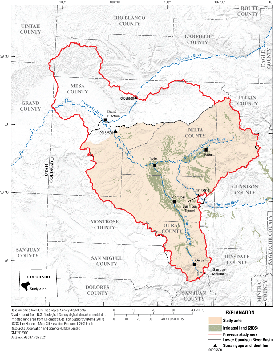
Irrigated land in the lower Gunnison River Basin study area. The previous study area used by Leib and others (2012) and Linard (2013) included Colorado River Basin drainages outside the lower Gunnison River Basin.
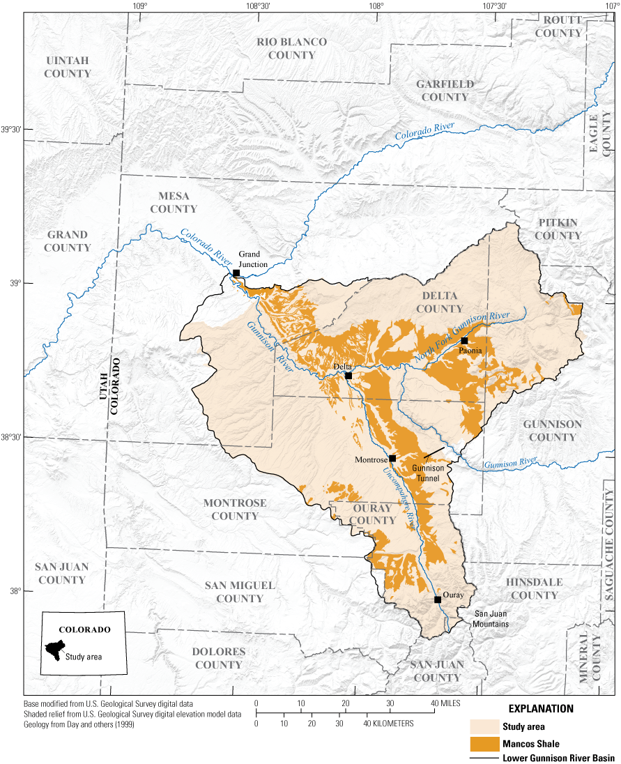
Cretaceous marine shale bedrock geology in the lower Gunnison River Basin study area.
Purpose and Scope
This report describes the statistical procedures, salinity and selenium water-quality data, and geospatial data used to develop MLR statistical models compiled to update those originally developed by Leib and others (2012) and Linard (2013). These new models estimate seasonal in-stream salinity and selenium loads within the lower Gunnison River Basin by using improved seasonal evaluations, additional years of data, and new geospatial data on land use, irrigation, and individual sewage disposal (ISD) system effluent. This report describes the MLR techniques, methods, and selection of basin characteristics, which differ from some procedures and characteristics used in previous studies. The objectives of this report are (1) to improve estimates of salinity and selenium loads by updating the regressions and incorporating new geospatial data from the lower Gunnison River Basin (and new statistical transformations of new variables and variables used in previous studies) and (2) to integrate into new MLR models water-quality data available for years since previous studies were completed. Descriptions of basin characteristics and load estimation techniques extensively reference methods described in previous reports (Leib and others, 2012; Linard, 2013). The reader may need to consult these reports for detailed procedures of computations and background on salinity and selenium science.
The spatial extent of the current study includes only drainages within the lower Gunnison River Basin, unlike Leib and others (2012) and Linard (2013), which included the Colorado River Basin drainages downstream from Cameo, Colorado (USGS streamgage 09095500), to the Utah-Colorado state line (fig. 1). This report groups water-quality and some geospatial data into two time periods (1992–2004 and 2005–13) and two seasons (irrigation, April–October; and nonirrigation, November–March). These changes help to reduce spatial variability and temporal complexity of the water-quality sample data. The estimates from the MLR models may help regulatory and land management agencies identify and prioritize areas in the lower Gunnison River Basin likely to yield more salinity and selenium than other areas.
Description of Study Area
The study area consists of the lower Gunnison River Basin downstream from the Gunnison Tunnel (USGS streamgage 09128000) to the Gunnison River near Grand Junction (USGS streamgage 09152500), near the confluence with the Colorado River at Grand Junction (fig. 1). The study area encompasses 803 square miles (mi2), and elevation ranges from 14,153 feet (ft) at the southern end of the lower Gunnison River Basin in the San Juan Mountains to 4,631 ft at the northern (downstream) end of the study area (USGS, 1999a, 2014a). Subbasins in the lower Gunnison River Basin study area range in size from 3.12 to 803 mi2 (USGS, 2014a).
Climate and hydrology may affect salinity and selenium yields in the study area. Precipitation is substantial in mountainous areas (greater than 30 or 40 inches of annual moisture in the highest peaks) and is predominantly in the form of snowfall. Low-elevation valleys are arid, with some areas receiving less than 10 inches of annual moisture (PRISM Climate Group, 2014). During the summer growing season (April–October), irrigation is necessary for many types of agriculture in the low-elevation areas. Reservoirs capture snowmelt primarily during the May–June period and release water at optimum times to augment natural discharge with agricultural diversion.
There are multiple natural and human sources of selenium and salinity to streams in the lower Gunnison River Basin. Salt- and selenium-bearing minerals, contained in soils and weathered bedrock (Mast and others, 2014), are weathered under favorable geochemical or physical conditions, making salt and selenium susceptible to transport as water migrates to streams by groundwater flow and surface-runoff pathways (Leib and others, 2012; Tuttle and others, 2014a, b). An extensive irrigation system moves water to the irrigated areas (fig. 1). Natural soil and vegetation in these areas were transformed in the early 1900s with the completion of several water-supply projects (Bureau of Reclamation, 2022). Other areas are not irrigated and retain more natural soil and native vegetation types. The multitude of irrigation infrastructure, diversion, and agricultural drains complicates the calculation of salinity and selenium loads in the lower Gunnison River Basin. In addition, residential development is mostly supported by ISD wastewater treatment systems, which add household wastewater (effluent) into the ground (Waller, 1994). Subsurface water is available to dissolve and transport salt (Rumsey and others, 2017) and associated selenium to surface waters (Butler and others, 1996).
Agricultural development is most intensive in valleys, which preferentially form in soils developed on the erodible Cretaceous Mancos Shale (fig. 2) (Leib and others, 2012). Because of the geomorphic setting and climate, crop growth on these marine shale areas of the lower Gunnison River Basin is not possible without irrigation. Quaternary surficial deposits and geologic units (Leib and others, 2012) also influence the yields of salinity and selenium and are described in the “Soil and Geology” section of this report.
Previous Investigations
Many previous studies have improved the understanding of salinity and selenium transport and geochemistry in western Colorado. Warner and others (1985) studied groundwater contributions to surface-water salinity loads in the Upper Colorado River Basin and found that the Uncompahgre River Basin was responsible for most of the salinity load in the lower Gunnison River Basin. Several studies were undertaken during the 1990s to investigate water-quality concerns related to irrigation. These studies involved characterization of groundwater, surface water, sediment, and biota and found that surface water was enriched with respect to selenium (Butler and others, 1991, 1996). Later work examined changes in salinity and selenium loads in response to canal leakage (Linard and others, 2017), irrigation system improvements (Butler, 2001), and land-use change (Mayo, 2008; Moore, 2011; Richards and Moore, 2015). Mast and others (2014) used laboratory leaching experiments and geochemical modeling to investigate selenium speciation and mobilization, concluding that selenium is released mainly through dissolution of soluble salts and gypsum found in soil and bedrock. Monitoring is ongoing in the lower Gunnison River Basin and other parts of western Colorado to improve understanding of salinity and selenium loading, source areas, and trends (Butler and Leib, 2002; Leib, 2008; Thomas and others, 2008; Mayo and Leib, 2012; Stevens and others, 2018; Henneberg, 2020). The installation of a 30-well monitoring network on the east side of the Uncompahgre River in the lower Gunnison River Basin has facilitated additional studies to characterize groundwater quality and groundwater-surface water interactions in the area (Mills and others, 2016; Thomas and others, 2019; Mast, 2021).
Building on the knowledge gained from previous studies, Leib and others (2012) and Linard (2013) used MLR models to better understand links between environmental characteristics and selenium and salinity loads and yields in the lower Gunnison River Basin. Basin characteristics used in the previous salinity and selenium regression models are listed in table 1. Leib and others (2012) analyzed salinity and selenium loading by computing loads at 231 locations having adequate water-quality concentration and discharge data and separating the data into irrigation (April–October) and nonirrigation (November–March) seasons. To delineate subbasins, pour points and stream networks were defined using the USGS National Hydrography Dataset (USGS, 1999b), which was corrected to topographic stream channel low points by using a digital elevation model, if necessary, where the stream network did not precisely align with terrain. The study area included Colorado River Basin drainages downstream from Cameo, Colorado, to the Utah-Colorado state line in addition to the lower Gunnison River Basin. The subbasin boundaries and a 10-meter digital elevation model were used as a mask in a geographic information system (GIS) to extract and calculate geospatial variables, such as elevation and land use, for each subbasin.
Table 1.
List of basin characteristics used for salinity (total dissolved solids) and selenium regression modeling in Leib and others (2012) and Linard (2013).[SI is the irrigation season (April–October) salinity model, SNI is the nonirrigation season (November–March) salinity model, SeI is the irrigation season selenium model, and SeNI is the nonirrigation season selenium model. Leib and others (2012) used the models to predict salinity and selenium loads; Linard (2013) used the models to predict yields. x, variable used in the model; —, not applicable; SSURGO, Soil Survey Geographic Database (U.S. Department of Agriculture, 1994)]
| Explanatory variable | Variable description | Characteristics combined for the explanatory variable | SI | SNI | SeI | SeNI |
|---|---|---|---|---|---|---|
| SA | Subbasin area | — | x | x | x | x |
| IM | Area of irrigated Mancos Shale | Irrigated area and Cretaceous marine shale (geologic subgroup 1.10 in Leib and others, 2012) | x | x | x | x |
| CAT | Wetted area of unlined irrigation canals | — | — | x | — | — |
| IT | Estimated amount of irrigation water applied | — | — | x | — | — |
| PI | Irrigation season precipitation | — | — | — | x | — |
| PNI | Nonirrigation season precipitation | — | — | — | — | x |
| Grp3.3 | Percentage of basin occupied by Quaternary alluvial deposits near streams | — | x | x | x | x |
| IM | Percentage of basin occupied by irrigated Mancos Shale | Irrigated area and Cretaceous marine shale (geologic subgroup 1.10 in Leib and others, 2012) | x | x | x | x |
| Clay2 | SSURGO mean percentage clay | — | x | — | — | x |
| Irr_land | Percentage of basin occupied by irrigated land | — | — | x | — | x |
| ffday2 | SSURGO mean frost-free days | — | — | x | — | — |
| sand2 | SSURGO mean percentage sand | — | — | x | — | — |
| elev | Mean subbasin elevation | — | — | x | — | — |
| aspect | Mean subbasin aspect | — | — | x | x | x |
| C.type1 | Percentage of small (1–100 cubic feet per second) canals in the subbasin | — | — | x | — | — |
| PIhires | High-resolution irrigation season mean precipitation | — | — | — | x | — |
| hzdepb2 | SSURGO mean soil depth | — | — | — | x | x |
| kwfact2 | SSURGO mean erodibility | — | — | — | x | x |
| slope | Mean subbasin slope | — | — | — | x | — |
| ETrev | Revised evapotranspiration from irrigated land | Evapotranspiration and irrigated area | — | — | x | — |
| Grp1.10 | Percentage of basin occupied by Mancos Shale | — | — | — | — | x |
| Grp3.2 | Percentage of basin occupied by the Mancos Shale and the Mesaverde, Wasatch, Green River, and Uinta Formations and Mancos Shale | — | — | — | — | x |
| ksat2 | SSURGO mean saturated hydraulic conductivity | — | — | — | — | x |
| resdepth2 | SSURGO mean depth to a restrictive layer | — | — | — | — | x |
Mean monthly precipitation was used to calculate mean irrigation and nonirrigation seasonal precipitation (Leib and others, 2012). Precipitation data were also used for computation of irrigation water application, which included the following variables: irrigation method, crop water need, crop consumptive use, growing season, and effective precipitation (Leib and others, 2012). The area of unlined canals in the irrigation network, a source of infiltration, was quantified.
Geology was important in the models because of the role rock units have as sources of salinity and selenium and their effects on geochemistry, the water table, leaching, and groundwater movement. Geologic units were classified into groups and subgroups by age, lithology, and unconsolidated deposit types (Leib and others, 2012). The estimates of final salinity and selenium load predictions were depicted graphically with 95-percent prediction intervals (Leib and others, 2012).
Linard (2013) analyzed salinity and selenium loading by computing yields at locations with adequate concentration and discharge data and separating the data into irrigation (April–October) and nonirrigation (November–March) seasons. Water quality was assessed in the same way as Leib and others (2012), but all data for the 231 sites were combined into a single period of analysis, water years 1989–2004. Differing from Leib and others (2012), salinity and selenium production were expressed in yields as tons per day per acre for salinity and pounds per day per acre for selenium. This calculation decreased the tendency of the models to estimate that large subbasins produce large loads, a potential bias (Linard, 2013).
Linard (2013) used some basin characteristics, such as precipitation, agricultural land use, geology, and soil properties, that were computed by Leib and others (2012). However, Linard (2013) used higher resolution elevation and precipitation data and soil properties with more detailed resolution than Leib and others (2012). Outcrop geology and projection of bedrock geology (bedrock beneath the surface of unconsolidated deposits) were used as grouped in Leib and others (2012) from geologic maps of the Grand Mesa, Uncompahgre, and Gunnison National Forests (Day and others, 1999) and Utah (Hintze and others, 2000). The Mancos Shale (geologic subgroup 1.10 from Leib and others, 2012), the Mancos Shale and the Late Cretaceous Mesaverde, early Tertiary Wasatch, Tertiary Green River, and Tertiary Uinta Formations (geologic subgroup 3.2 from Leib and others, 2012), and Quaternary alluvial deposits (geologic subgroup 3.3 from Leib and others, 2012) were used as variables in the regression modeling (Linard, 2013). Soil and unconsolidated deposits also were used extensively as basin characteristics. The soil properties were obtained from the Soil Survey Geographic Database (SSURGO) (U.S. Department of Agriculture, 1995) and, for areas lacking SSURGO soil property attributes, from the less precise State Soil Geographic Database (STATSGO) (U.S. Department of Agriculture, 1994).
Linard (2013) used MLR to produce irrigation and nonirrigation equations for salinity and selenium yield prediction by using basin characteristics as independent variables. Yield equations were then used to predict mean seasonal yields for 175, 12-digit Hydrologic Unit Code subbasins. The results were presented on maps by using color to emphasize subbasins having larger salinity and selenium yields (Linard, 2013). Irrigation season salinity yields ranged from 0.0001 to 0.03 tons per day per acre, and nonirrigation season salinity yields ranged from 0.0003 to 0.008 tons per day per acre. Irrigation season selenium yields ranged from 2.3x10⁻⁶ to 0.0007 pounds per day per acre, and nonirrigation season selenium yields ranged from 1.8x10⁻⁶ to 0.0005 pounds per day per acre.
Methods
The following sections describe the water quality and basin characteristics used in the current study. Water-quality data methods were the same as those used by Leib and others (2012) and Linard (2013). Unlike Leib and others (2012) and Linard (2013), the study area is restricted to the lower Gunnison River Basin.
Water-Quality Data
Water quality (salinity and selenium loads in this report) is the response variable in the MLR approach. Basin characteristics are the explanatory variables used for prediction of loads. Two seasons were defined for the loading analysis: April through October is the irrigation season, and November through March is the nonirrigation season. The irrigation season roughly defines the frost-free months at low elevations and corresponds to the application of irrigation water within the study area. Data were available in the National Water Information System (NWIS) database (USGS, 2014b) for two periods, 1992 through 2004 and 2005 through 2013. Separating the data into periods helped address potential issues of nonstationarity, the tendency for some basin characteristics to change variability ranges through time (Milly and others, 2008). The time periods for analysis were selected based on available water-quality and GIS data. Two time periods were used to account for land-use changes taking place between the two periods (for example, the conversion of agricultural land to urban land; Moore, 2011; Richards and Moore, 2015). Significant downward trends in salinity and selenium yields have been documented in the lower Gunnison River Basin through time (Richards and Moore, 2015; Henneberg, 2020, 2021). From 2013 to 2022, changes have occurred within the basin related to irrigation improvements, canal lining, and land-use conversion and are not well characterized by spatially robust sampling (Ward and others, 2021). For the period 1992–2004, there were 35 sites with salinity and discharge data for the irrigation season and 25 sites with data for the nonirrigation season. For the period 2005–13, 16 sites had salinity and discharge data for the irrigation season, and 16 sites had data for the nonirrigation season. For selenium in the period 1992–2004, there were 39 sites for the irrigation season and 34 sites for the nonirrigation season. For the period 2005–13, 22 sites had selenium and discharge data for the irrigation season, and 18 sites had data for the nonirrigation season. These periods considered in the current study are different from those described in the “Previous Investigations” section of this report. Site selection was based on the availability of sufficient salinity and selenium concentration data, availability of discharge data for those samples, and whether basins could be separated into smaller subbasins depending on the configuration of sites and canal inputs and outputs. A minimum of five samples per season was required for a site to be selected for an MLR model. The mean seasonal salinity and selenium water-quality data measured at each site were used to estimate load.
Salinity and selenium loads are computed by multiplying constituent concentrations by discharge measurements made at the time of sampling. Sample concentrations for salinity (TDS), selenium (dissolved selenium), and discharge measurements are available in the USGS NWIS database (USGS, 2014b) and can be retrieved using the site numbers in the USGS data release associated with this report (Williams and others, 2023). Daily load values for salinity in tons per day are calculated using the following equation (Leib, 2008):
whereL
is the daily constituent load, in tons per day;
C
is constituent concentration, in milligrams per liter;
Q
is discharge, in cubic feet per second; and
K
is the unit conversion constant, 0.0027.
Daily load values for selenium in pounds per day are calculated by using the following equation (Leib, 2008):
whereL
is constituent load, in pounds per day;
C
is constituent concentration, in micrograms per liter;
Q
is discharge, in cubic feet per second; and
K
is the unit conversion constant, 0.0054.
Due to the complexity of water imports, diversions, and the locations of sites with existing load information, final calculated loads were adjusted to avoid nesting of subbasins (overlap) and double counting of loads to ensure maximum model utility. In Linard (2013), some of the subbasins used to develop the models were nested. For the current study, avoiding nested basins provided more accurate load computations and reduced confusion regarding the load signal in large subbasins. The method for separating loads in basins with tributary load information was explained in detail in Leib and others (2012). For example, figure 3 is a simple schematic that shows how the use of available load information can create additional unnested subbasins for use in the regressions. In this example, a basin is partitioned for load calculations, and subbasin loads are adjusted such that inputs and outputs are accounted for. Ignoring the canal inputs (1a and 2a) and outputs (1b and 2b) for a moment, two subbasins define the drainages of two sites with available water-quality data. Site 1 is at the mouth of a tributary that is joined by another tributary just downstream. The two subbasins are defined as subbasin 1 (tan area in fig. 3), which is the drainage of the tributary sampled at site 1, and subbasin 2, which is the entire basin minus subbasin 1. Sites 1 and 2 have loads calculated from field sample constituent concentrations and discharges. With the water-quality data available for each site, the mean of all point loads (each load on a different date) is converted to annual or seasonal loads in this report. The load at site 1 (1T) is the calculated load averaged at the mouth of the tributary (tan area). The load at site 2 (2T), is calculated by taking the original load measured at site 2 and subtracting the load at site 1, leaving both subbasins with no overlapping contributing area and no loads counted twice.
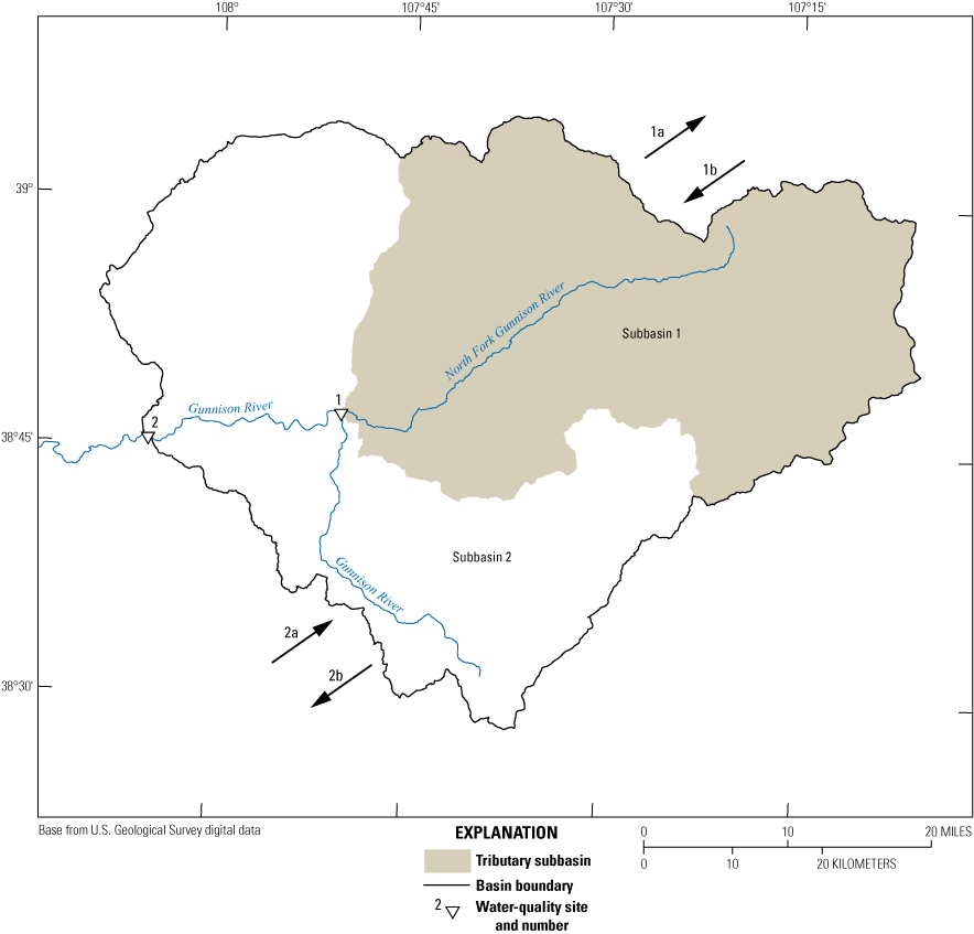
Flow routing for load calculations in a subbasin. Load input from canals is represented by 1a and 2a; load output from canals is represented by 1b and 2b. The adjusted basin load (1T and 2T) is computed by adding the canal load difference (for example, 1b−1a) to the load computed at the mouth of the stream (1 and 2) and, if applicable, subtracting the adjusted load for any nested basins.
A more complex situation commonly found in the irrigated parts of the lower Gunnison River Basin involves the irrigation network of canals and ditches, which moves loads from one subbasin to another (fig. 3). The load input from a canal, 1a, is computed the same way as a stream load entering a subbasin, and 1b is the load computed at the point that a canal leaves a subbasin. The difference of the two terms (output minus input) is added to or subtracted from the load of the subbasin traversed by the canal, depending on whether the canal loses or gains load. When the output from one subbasin continues into an adjacent subbasin, it becomes the input for that second subbasin and so on. The canal load difference (2b minus 2a) is added to the load at site 2, from which the load 1T is then subtracted. For example, consider a canal gaining load. If the measured loads are 15 pounds per day at the point where the canal enters the subbasin and 20 pounds per day at the point where the canal exits the subbasin, the canal gained 5 pounds per day of load. That gained load was generated within the subbasin and therefore is added to the overall load measured at the mouth of the stream. In the example (fig. 3), load 1T (equation 3), and load 2T (equation 4) are adjusted for canal mass balance. These adjusted load estimates were used in MLR analysis and are provided in the salinity and selenium attribute tables in the USGS data release associated with this report (Williams and others, 2023). The equations are as follows:
where1T
is the adjusted constituent load at site 1;
1
is the constituent load at site 1 calculated from field sample concentrations and discharge measurements;
1b
is constituent load transported out of subbasin 1 by canals; and
1a
is constituent load transported into subbasin 1 by canals.
2T
is the adjusted constituent load at site 2;
2
is the constituent load at site calculated from field sample concentrations and discharge measurements;
2b
is constituent load transported out of subbasin 2 by canals;
2a
is constituent load transported into subbasin 2 by canals; and
1T
is the adjusted constituent load at site 1.
Geospatial Data
Many basin characteristics were considered for MLR and prediction of salinity and selenium loads. Previous studies using basin characteristics for prediction of salinity and selenium loads or yields have identified many of the most significant classes of geospatial data that are important for consideration in MLR models. These basic types of data are discussed extensively in Leib and others (2012) and Linard (2013) and are summarized and referenced in the “Previous Investigations” section of this report. Basin characteristics used in the regressions in the current study belong to similar classes as those discussed in the earlier reports, and include physical characteristics, precipitation, land use, land cover, surficial deposits, and geologic units. New characteristics used in this study, such as a soil property related to selenium in soil and water derived from residential wastewater systems, were not considered in previous studies. These new characteristics are discussed in greater detail in the following sections. A GIS makes the use of the geospatial information described in the next sections of the report practical and efficient (Esri, 2016).
Subbasin Boundaries
Subbasins within the study area were selected for analysis if they met the criteria for water-quality load data (at least one site having at least five valid sets of paired concentration and discharge). Lists of subbasins were compiled for each season and analysis period, resulting in four combinations for salinity and four combinations for selenium. Subbasin polygons were delineated with GIS software (Esri, 2016) by using pourpoints (USGS, 2014a) located at the water-quality sites. A 10-meter digital elevation model (USGS, 1999a) was the base for delineation. Area (in acres) of the calibration subbasin is used to compute several basin characteristics, particularly those that represent a characteristic as a percentage of the subbasin area. For the GIS analysis, an Albers equal-area conic projection was used to minimize distortion bias when comparing subbasin areas. A digital elevation model was used to compute the mean elevations of subbasins, which were used in the calculations of irrigation water application.
Precipitation
Precipitation is an important component of some subbasin characteristics used in the MLR models, and precipitation that infiltrates below the root zone (effective precipitation) can be a major source of groundwater recharge. Water is a driver of salt and selenium transport because it dissolves minerals present in geologic and soil materials that contribute to salt and selenium loading. Natural settings and cultivated lands produce a portion of the loads that are, at the most basic level, mobilized by direct precipitation. The effective precipitation that becomes deep percolation groundwater has varying degrees of contact time with rock and soil and is primarily responsible for loading the water with salinity and selenium compounds. Deep percolation groundwater (from precipitation) may then discharge to local drainages for transport as surface water. Precipitation also may run off directly without deep percolation and pick up salt and selenium as it flows across rock or soil surfaces. In general, the potential for deep percolation or runoff increases with the amount, intensity, and duration of the precipitation (USGS, 2020).
The MLR models for salinity and selenium contain seasonal values for irrigation and nonirrigation seasons. The sum of monthly precipitation (PRISM Climate Group, 2014) for April–October represents precipitation for the irrigation season. The sum of monthly precipitation for November–March represents precipitation for the nonirrigation season.
Land Use and Land Cover
Subbasin characteristics related to agricultural and developed land use (including residential and urban or suburban land uses) were explored as explanatory variables of salinity and selenium loads. Water resources in the lower Gunnison River Basin have been developed extensively to facilitate irrigated agriculture through the construction of dams, canals, and irrigation ditches. Excess water not consumptively used by crops, removed by surface runoff, or evaporated infiltrates into soil and rock, then percolates and migrates along shallow and deep pathways as part of the groundwater flow system (Mayo, 2008; Thomas and others, 2019).
Colorado’s Decision Support Systems (2014) irrigated-lands dataset specifies crop type and irrigation method for each irrigated-lands area. The 1993 dataset was used to represent 1993−2004, and the 2005 dataset was used to represent 2005−13. Data that quantify the amounts of irrigation water applied are not directly available; however, by using the available geospatial data, these amounts can be estimated (Leib and others, 2012). The method for estimating amount of irrigation water applied (Broner and Schneekloth, 2003) is described in detail in Leib and others (2012). Briefly, the method involves computations using consumptive water use for each crop type (U.S. Department of Agriculture Natural Resources Conservation Service, 1988), efficiency of irrigation methods used (Waskom, 1994), length of growing season (National Climatic Data Center, 2005), and effective precipitation (precipitation that infiltrates to the root zone) (Leib and others, 2012). Irrigation water is also a source of groundwater recharge that seeps from canals, laterals, and ponds (Robinson and Rohwer, 1959). Irrigation channel data were provided by Reclamation (written commun., 2015; used to create input raster files that are provided in Williams and others [2023]), and pond area was determined using National Wetlands Inventory data (U.S. Fish and Wildlife Service, 2014).
Land uses other than irrigation were assessed for their value in improving MLRs for the prediction of salinity and selenium loads. Basin characteristics related to (1) acreage under cultivation, (2) intensity of development (U.S. Department of Agriculture, 2015), and (3) residential parcels outside municipal boundaries (related to ISD system effluent production) were useful in exploring correlations for regression modeling. The first two characteristics were available in the Cropland Data Layer for Colorado (U.S. Department of Agriculture, 2015). Acreage under cultivation is the total area of all crop agricultural lands, including nonirrigated parcels under dryland cultivation. The land-use data from the Cropland Data Layer for Colorado (U.S. Department of Agriculture, 2015) also include lands designated as developed with three levels of intensity: low, medium, and high.
Nonmunicipal residences (residential parcels outside municipal boundaries) that use ISD systems for wastewater treatment produce effluent that is potentially a direct source of recharge to groundwater and may contribute to salinity loads from dissolution of soil salts. Because the operation of an ISD system is designed such that effluent produced by the household is leached directly into the soil zone, there is a potential for salt to be mobilized from the unsaturated zone of the soil profile and underlying aquifers. The ISD system effluent produced per household was estimated by using residential parcel data from counties in the study area. County parcel data (Delta County, 2014; Gunnison County, 2014; Mesa County, 2014; Montrose County, 2014; Ouray County, 2014), as they existed at the time of analysis (2014), were used to identify residential locations outside municipal boundaries. These locations were subsequently checked for existing residential dwellings by using aerial imagery. Areas within municipal boundaries were assumed to be on municipal sewer systems and were excluded. Once identified, the centroid of each nonmunicipal residential parcel was used as the location of an ISD system. Municipal water-use data from 2003 to 2008 provided by the Tri-County Water Conservancy District (2010) were used to estimate volume of ISD system effluent. The mean water usage during January (when outdoor water use is at a minimum) was assumed to represent the monthly amount of water that goes into an ISD system leach field from a single household. The estimate for all customers on municipal water systems, 1,900 acre-feet per year (Tri-County Water Conservancy District, 2010), was converted to per capita household use, then multiplied by the number of nonmunicipal residential households assumed to be using ISD systems.
Soil and Geology
The association of salinity and selenium loading with Cretaceous marine shales was thoroughly discussed in Butler and others (1996), Leib and others (2012), and Linard (2013). Similarly, other geologic units in the study area also correlate with selenium and salinity, such as Cretaceous and Tertiary rock units, Quaternary unconsolidated deposits, selected glacial units, and sand and gravel lithologies (Warner and others, 1985; Leib and others, 2012). Because some geologic materials act as load sources and others facilitate transport of groundwater or act as barriers, many of the geologic units and combinations of geologic units described in Leib and others (2012, table 1) were promising candidates for explanatory variables.
The geology of bedrock parent material explains some of the variation in salinity and selenium loads in the lower Gunnison River Basin, but different soil types can form from weathering of the same bedrock. Numerous soil types have been mapped by the NRCS in the lower Gunnison River Basin and are available in the 1:24,000-scale SSURGO database (U.S. Department of Agriculture, 1995). Some soil properties are aggregates of other properties.
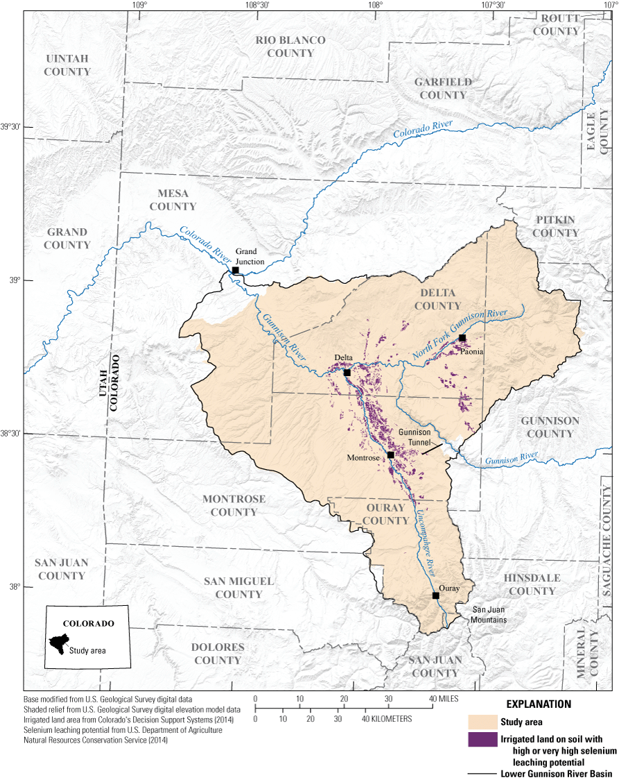
Irrigated land on soil with high or very high selenium leaching potential in the lower Gunnison River Basin study area. Selenium leaching potential is a Suitability and Limitation Rating dataset available from the Natural Resources Conservation Service Web Soil Survey (U.S. Department of Agriculture Natural Resources Conservation Service, 2014).
Some soils have a geochemical tendency to yield more selenium than other soil types (fig. 4). The Selenium Leaching Potential dataset available from the NRCS Web Soil Survey (U.S. Department of Agriculture Natural Resources Conservation Service, 2014) includes information from parts of the five counties of interest in the lower Gunnison River Basin: Delta, Gunnison, Mesa, Montrose, and Ouray. The interpretation criteria for selenium leaching potential are a set of soil and climate properties related to selenium leaching below the root zone (U.S. Department of Agriculture Natural Resources Conservation Service, 2014). The five soil and climate properties (parent material, soil pH, depth to bedrock, mean annual precipitation, and, if applicable, a water table index) were each assigned a numeric rating by the NRCS, and the ratings were aggregated into a single rating for each soil map polygon in SSURGO maps for the lower Gunnison River Basin (on a scale of 0.0 to 1.0, lowest risk to highest risk). The selenium leaching potential scale has thresholds of less than 0.20 for low, 0.21–0.60 for moderate, 0.61–0.80 for high, and greater than or equal to 0.81 for very high rating scale values assigned to soil polygons. Selenium leaching potential ratings and descriptions of the properties used to determine the ratings are available through the NRCS Web Soil Survey (U.S. Department of Agriculture Natural Resources Conservation Service, 2014).
Geostatistical Modeling
Estimated loads for salinity and selenium were modeled with MLR techniques by using geospatial basin characteristics (variables) available for the entire study area. Basin characteristics are surrogates meant to aid in the estimation of salinity and selenium loads. These surrogates may be related to processes, sources, land uses, and physical properties within the study area, and accuracy of the predictions of each equation may vary among subbasins. For the sites that had adequate water-quality data, subbasin boundaries and loads computed from monitoring data were used to calibrate the models (fig. 5). The zonal statistics tool in ArcMap (Esri, 2016) was used to aggregate data from raster grids of the geospatial variables for each calibration subbasin (detailed methods and calibration subbasins are provided in the USGS data release associated with this report; Williams and others, 2023). Many variables related to the primary types of characteristics already discussed were analyzed in a stepwise least-squares regression (Helsel and others, 2020) procedure conducted with scripts written in the R statistical programming language (R Core Team, 2017) to identify the strongest combinations of explanatory variables for salinity and selenium loads. Because two periods and two seasons were available for analysis, consideration was given for single season and two-part models separated into irrigation and nonirrigation seasons.
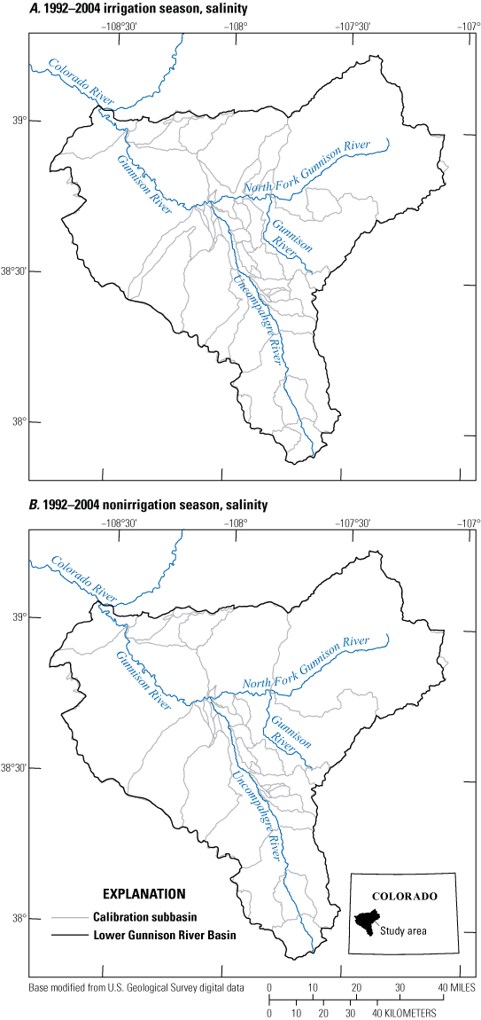
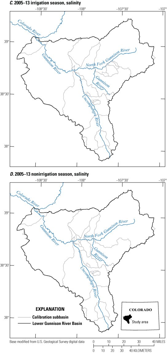
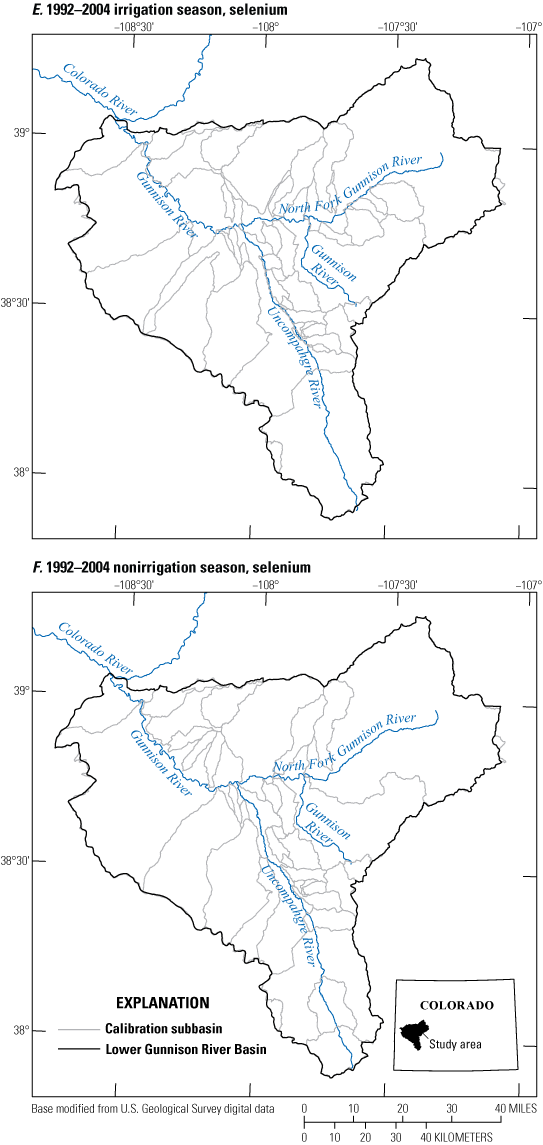
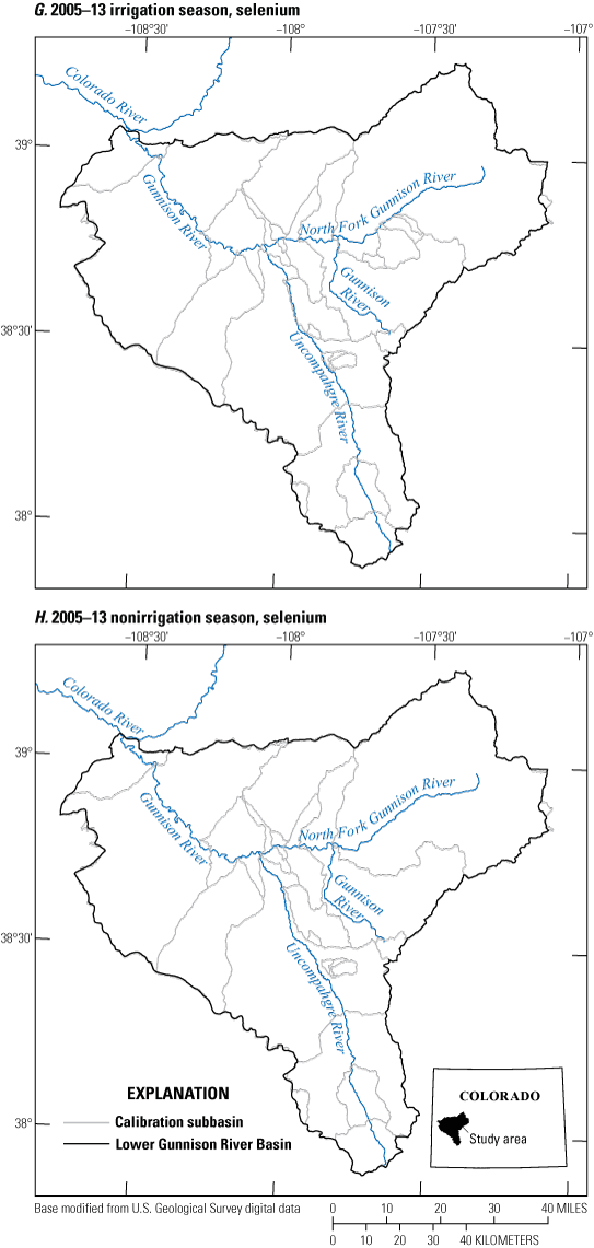
Calibration subbasins used to develop the salinity and selenium multiple linear regression models. Calibration data were separated into two time periods and two seasons. Salinity calibration subbasins are A, 1992–2004 irrigation season; B, 1992–2004 nonirrigation season; C, 2005–13 irrigation season; and D, 2005–13 nonirrigation season. Selenium calibration subbasins are E, 1992–2004 irrigation season; F, 1992–2004 nonirrigation season; G, 2005–13 irrigation season; and H, 2005–13 nonirrigation season.
Statistical procedures used in this study were similar to those described in Leib and others (2012). Variables with p-values greater than or equal to 0.05 were considered significant and were retained and included in the regression models. First, correlations between individual variables were considered to identify potential variables for the multivariate analysis. All combinations of variables were assessed by the statistical software, and variables were added to regressions by the R code until the maximum coefficients of determination (R2) were identified. Diagnostic plots were used to determine whether assumptions of MLR were met: homoscedasticity of residuals (linear variance of plotted residuals), normality of residuals (quantile-quantile plots), lack of outliers as indicated by a standardized residual less than 3 (residual divided by estimated standard error), and lack of high-leverage data points (plots of correlation of standardized residuals with high leverage).
Combinations of variables used in previous investigations and new variables computed for this study also were assessed based on adjusted R2 and prediction error sum of squares (PRESS) statistics (Helsel and others, 2020). Sometimes the best models did not have the top score for all three statistics, and other measures were used to determine the best final equations. Statistical significance of variables (p-values), diagnostic plots that indicated favorable residuals patterns such as constant variance (homoscedasticity), and normal distribution of residuals were used to qualify or disqualify candidate models or indicate if transformations of the data might be helpful (Helsel and others, 2020). Centering of some variables derived from basin characteristics (subtracting the value from the mean and dividing by the standard deviation) minimized multicollinearity (Iacobucci and others, 2016). Logarithm transformations were used in salinity models to optimize fit (Helsel and others, 2020). When logarithmic transformation was used, a bias correction factor was computed and added to the equation upon retransformation of logarithmic to linear space as detailed in Duan (1983). Some selenium variables were transformed by the square root to improve linearity. Square root transformation does not require a bias correction factor.
Candidate best-fit equations had adjusted R2 greater than 0.70 and p-values less than 0.05. Leverage and influence calculations were used to evaluate the effect of outliers on the regression. The leverage statistic was calculated to indicate whether a load associated with a site had high leverage, and the difference in fits (DFFITS) statistic was used to assess the influence (ability to bias the equation) of a high-leverage load site (Helsel and others, 2020). To check the independence of variables chosen for the equations, the collinearity between variables was evaluated using the variance inflation factor (VIF) statistic (Ott and Longnecker, 2001; Helsel and others, 2020). Generally, a VIF greater than 10 indicates a high degree of correlation (Helsel and others, 2020).
Empirical Bayesian Kriging
After the MLR models for salinity and selenium loads were finalized, yield predictions that are useful for interpretation purposes were computed using a raster data density map (cells). An empirical Bayesian kriging (EBK) procedure (Krivoruchko, 2012) was implemented in ArcMap (Esri, 2016) to produce a robust grid of yields for salinity and selenium. The study area was overlain by a grid of 12 layers of hexagonal polygons. The initial layer of polygons covering the study area was used to create a set of centroids (center points) for the net of polygons. Each salinity polygon had dimensions of 6,500 meters (m) on a side. From these center points another 11 layers of polygons were created by offsetting the center point by intervals of 3,250 m north−south and east−west around the initial polygon center point. Selenium polygon dimensions were 4,500 m on a side, and the center points were offset by 2,250 m (fig. 6). Hexagon dimensions were determined so that the grid resulted in overall loads that were consistent with long-term data for the study area. New polygons were created with each center point representing the centroid of each of the 11 new layers of polygons, each with the exact dimensions of the initial polygons. The polygons covered at least the entire study area (including a buffer around the study area) (figs. 7 and 8). The polygon layers were then used to calculate salinity and selenium loads by using the MLRs and the basin characteristics calculated for each individual polygon. Because salinity MLRs were for two seasons, the seasonal loads for irrigation and nonirrigation seasons were combined, weighted by the portion of the year of each season, to calculate the annual loads. The resulting load values were then converted to salinity yields in tons per year per acre and selenium yields in pounds per day per acre by using the area of the polygons.
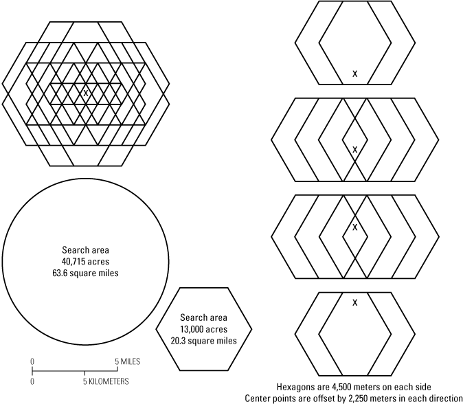
Hexagonal grid procedure used to create selenium yield raster. Different dimensions were used for the salinity hexagons, which were 6,500 meters on a side and were offset by 3,250 meters.
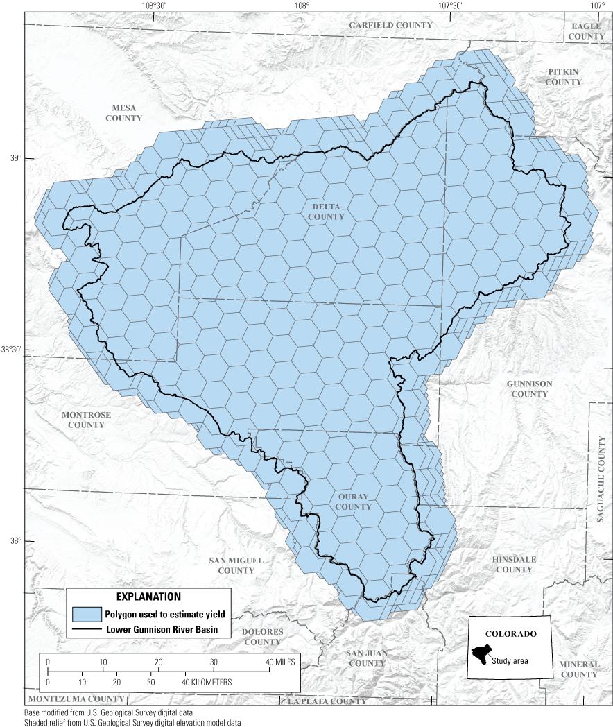
Single hexagonal grid layer overlaying the lower Gunnison River Basin study area with selenium yields in pounds per day per acre estimated by using basin characteristics for each polygon. Hexagonal grids are available in Williams and others (2023).
Example of 12 overlapping hexagonal grid layers overlaying the lower Gunnison River Basin study area for use in empirical Bayesian kriging (Krivoruchko, 2012). Hexagonal grids are available in Williams and others (2023).
The EBK tool in ArcMap Geostatistical Analyst (Esri, 2016) was used to average and smooth the overlapping polygon loads (fig. 8) and form a raster grid with 63.615-meter by 63.615-meter cells in the North American Datum of 1983 coordinate system and Albers projection. Specific model parameters entered for the EBK method are shown in table 2. EBK is a geostatistical interpolation method that automates difficult aspects of building a valid kriging model or, for this study, a raster yield prediction grid. Other kriging methods in ArcMap Geostatistical Analyst require users to manually adjust parameters, but EBK automatically computes parameters through subsetting and simulations (Krivoruchko, 2012). The method is processor intensive, but use of the semivariogram model type results in lower standard error of predictions compared to other kriging methods (Esri, 2016; Krivoruchko and Gribov, 2019).
Table 2.
Empirical Bayesian kriging method summary for salinity (total dissolved solids) and selenium yields in ArcMap (Esri, 2016).[—, not applicable]
Multiple Linear Regression Models
Basin characteristics chosen for best-fit equations, described in this section, are for use in salinity and selenium MLR models as noted (table 3) and described further in a U.S. Geological Survey data release (Williams and others, 2023).
Table 3.
Explanatory variables and methods of computation or extraction for salinity and selenium load-prediction multilinear regression models.[SI is the irrigation season (April–October) salinity model, SNI is the nonirrigation season (November–March) salinity model, and Se is the selenium model. The first column identifies the variables as “V” followed by a number indicating the order in the equation; for example, V1 is the first variable in the equation. Variable types are crop area physical characteristic (pc), precipitation (pr), irrigation (i), geology (g), soil property (s), canal area (c), pond area (po), developed land use (dev), individual sewage disposal (ISD) system effluent (sp), and crop area (ag). Elevation refers to distance above the North American Vertical Datum of 1988. GIS, geographic information system; z, standardized (centered) variable; x, specified method of computation or extraction was used; —, not applicable; log, logarithm; SQRT, square root]
| Variable in regression equation | Explanatory variable | Variable description | Transformation or centering | Method of computation or extraction | Type of variable | Regression coefficient | Variance inflation factor | |
|---|---|---|---|---|---|---|---|---|
| Sum | Geospatial mask (GIS) | |||||||
| V1 | PA11QA.Cat1 | Percentage of subbasin area occupied by Quaternary rock units, except basalt flows (geologic subgroup 3.3 in Leib and others, 2012) | z | x | x | g, pc | −0.3826 | 2.42 |
| V2 | R1 | Irrigation water applied to areas with Cretaceous marine shale geology (acre-feet) | z, log | — | x | i, g | 0.1274 | 2.26 |
| V3 | TSpctbIrrP | Sum of ISD system effluent, irrigation water applied, and mean effective precipitation | z, log | x | — | sp, i, pr | 0.4612 | 2.01 |
| V4 | PElev_MEAN | Mean elevation of subbasin (meters) | z | — | x | pc | 0.1112 | 2.86 |
| V5 | R9Pct | Percentage of subbasin area occupied by unlined irrigation channels on Quaternary rock units, except basalt flows (geologic subgroup 3.3 in Leib and others, 2012) | z | x | — | c, g, pc | 0.4294 | 2.85 |
| V6 | x | Percentage of subbasin area occupied by ancient alluvium, old glacial drift (pre-Bull Lake glaciation), old gravel and alluvium (pre-Bull Lake glaciation), gravel and alluvium of the Pinedale and Bull Lake glaciations, eolian deposits, and modern alluvium and terrace gravels (geologic subgroup 2.2 in Leib and others, 2012) | z, log | x | — | g, pc | 0.163 | 3.36 |
| SNI | ||||||||
| V1 | R12A | ISD system effluent infiltrated during the nonirrigation season (acre-feet) | z, log | x | — | se | 0.6122 | 2.11 |
| V2 | R17 | Area of ponds at elevations less than 1,820 meters (acres) | z, log | — | x | po, pc | 0.3802 | 1.6 |
| V3 | R14Pct | Percentage of subbasin area occupied by ponds | z, log | — | x | po, pc | −0.1699 | 1.5 |
| V4 | R13ASptcTerr | ISD system effluent infiltrated on Quaternary alluvium and terrace gravels (geologic subgroup 1.29 in Leib and others, 2012) during nonirrigation season (acre-feet) | z | — | x | sp, g | −0.1819 | 4.78 |
| V5 | R4 | Irrigated land area (acres) | z, log | x | — | i | −0.3274 | 6.45 |
| V6 | PAllQA.Cat.1 | Percentage of subbasin area occupied by Quaternary rock units, except basalt flows (geologic subgroup 3.3 in Leib and others, 2012) | z | — | x | g, pc | −0.2320 | 1.95 |
| V7 | PDevPct | Percentage of subbasin area classified as developed low intensity, developed medium intensity, or developed high intensity land use | z, log | — | x | dev, pc | 0.2276 | 1.33 |
| V8 | PGlacial.Cat.1 | Percentage of subbasin area occupied by Quaternary gravel and alluvium deposits of the Pinedale and Bull Lake glaciations (geologic subgroup 1.26 in Leib and others, 2012) | z | — | x | g, pc | 0.1753 | 2.28 |
| V1 | ACREFT | Irrigation water applied (acre-feet) | — | x | — | i | −0.00002898 | 11.84 |
| V2 | ACREFTSE1 | Irrigation water applied to soils with high to very high selenium leaching potential (acre-feet) | — | — | x | i, s | 0.00006544 | 5.36 |
| V3 | AgSum | Percentage of subbasin area with agricultural land use, all crop types | SQRT | x | — | ag | 0.177 | 3.34 |
| V4 | CanalAcres | Wetted area of unlined irrigation channels (acres) | SQRT | x | — | 0.06878 | 8.64 | |
| V5 | POLY_AREA | Subbasin area (acres) | SQRT | — | x | pc | 0.002286 | 7.76 |
| V6 | PondAcres | Wetted area of ponds (acres) | SQRT | x | — | po | 0.01234 | 3.33 |
| V7 | CDL122 | Percentage of subbasin area classified as developed low intensity land use | SQRT | x | — | dev | 0.5683 | 5.92 |
| V8 | CDL121 | Percentage of subbasin area classified as developed open space land use | SQRT | x | — | dev | −0.7469 | 8.77 |
Evaluating likely possible combinations of geospatial variables resulted in three MLR models that best estimated irrigation-season salinity load (SI), nonirrigation-season salinity load (SNI), and annual selenium load (Se) (tables 3 and 4, fig. 9). Different combinations of explanatory variables within the MLR analysis result in differences in the magnitude, and at times, the sign of the coefficients used when compared to independent correlations between each explanatory variable and the response variable.
Table 4.
Statistical values of the salinity and selenium load-prediction models.[R2, coefficient of determination; SI, salinity irrigation-season model; SNI, salinity nonirrigation-season model; Se, selenium model; <, less than; —, not applicable]
| Model | R2 | Prediction error sum of squares (PRESS) statistic | p-value | Bias correction factor (Duan, 1983) | Degrees of freedom | Standard error |
|---|---|---|---|---|---|---|
| SI | 0.89 | 3.11 | <0.0001 | 1.12 | 45 | 0.216 |
| SNI | 0.88 | 4.85 | <0.0001 | 1.15 | 32 | 0.295 |
| Se | 0.73 | 22.9 | <0.0001 | — | 104 | 0.416 |
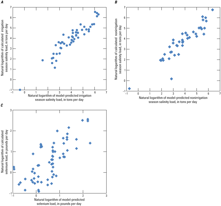
Relation of calculated loads to model-predicted loads for calibration basins. A, salinity irrigation season; B, salinity nonirrigation season; C, selenium.
Salinity Irrigation-Season Model
The six explanatory variables (V1–V6) used to estimate salinity load during the irrigation season (SI) were related to geology, irrigation, ISD system effluent, and basin physical characteristics (table 3). The equation takes the form:
whereSI
is the irrigation season salinity load in tons per day, and
Z
is the standardized (centered) value of the explanatory variable.
The values of the explanatory variables for the calibration subbasins used in the salinity irrigation-season MLR equation are provided in a shapefile attribute table in the USGS data release associated with this report (Williams and others, 2023). The combination of variables that predict irrigation-season salinity load includes both sources and transport pathways (table 3). Variable V2 represents irrigation water applied to Cretaceous marine shale geology, accounting for an important transport pathway (irrigation) and source (Cretaceous marine shale) of salinity in the study area. Other variables related to surficial deposits and geologic units are V1 (percentage of subbasin area occupied by Quaternary rock units, except basalt flows), V5 (percentage of subbasin area occupied by unlined irrigation channels on Quaternary rock units, except basalt flows), and V6 (percentage of subbasin area occupied by ancient alluvium, old glacial drift (pre-Bull Lake glaciation), old gravel and alluvium (pre-Bull Lake glaciation), gravel and alluvium of the Pinedale and Bull Lake glaciations, eolian deposits, and modern alluvium and terrace gravels. These variables are related to transport pathways because these geology types allow for subsurface infiltration and transport of water, which can lead to leaching of salt. Some geologic units are also sources of salt. Variable V3 is also related to leaching and a transport pathway of salt because ISD system effluent, irrigation water applied, and mean effective precipitation are major components of the water budget available for leaching salt below the root zone (Butler, 2001; Kanzer and Merritt, 2008). The method for estimating ISD system effluent is described in the “Land Use and Land Cover” section. Variable V4, mean subbasin elevation, is a physical characteristic that relates to transport pathways because elevation affects the amount of precipitation received.
Salinity Nonirrigation-Season Model
The eight explanatory variables (V1-V8) used to estimate salinity load during the nonirrigation season (SNI) were related to ISD system effluent, ponds, geology, irrigation, and developed land use (table 3). The equation takes the form
whereSNI
is the nonirrigation season salinity load in tons per day, and
Z
is the standardized (centered) value of the explanatory variable.
The variable values for calibration subbasins are provided in the shapefile attribute table in the associated USGS data release (Williams and others, 2023). Similar to the salinity irrigation-season model, several variables are related to geology (table 3). Variable V4 is the amount of ISD system effluent on Quaternary alluvium and terrace gravels, V6 is the percentage of subbasin area occupied by Quaternary rock units, except basalt flows, and V8 is the percentage of subbasin area occupied by Quaternary glacial gravel and alluvium. Because these deposit types facilitate infiltration and subsurface movement of water, the variables are related to transport pathways. Also related to transport pathways are variables V1 (ISD system effluent) and V5 (irrigated land area). Both ISD system effluent and irrigation water contribute to leaching and transport of salt. Two variables in the model are related to seepage from ponds and therefore transport pathways: V2, wetted area of ponds at elevations less than 1,820 meters above the North American Vertical Datum of 1988, and V3, percentage of subbasin area occupied by ponds. Ponds can be a source of salinity and water for leaching salt from soil. The remaining variable in the salinity nonirrigation-season model, V7, is the percentage of subbasin area with developed land use. This variable, related to transport pathways, is a basin characteristic that interacts with salinity loading dynamics and may demonstrate the effects of development that increases impervious surfaces, leading to increased runoff and decreased infiltration.
Selenium Model
The eight explanatory variables used to estimate selenium load (a single model, not separated for irrigation and nonirrigation seasons) were related to irrigation, soil properties, land use, and ponds (V1 through V8, table 3). The equation takes the form
whereThe variable values for calibration subbasins are provided in the shapefile attribute table in the associated USGS data release (Williams and others, 2023). Unlike the salinity models, the selenium model does not include variables that represent geologic units; however, the model does include a variable related to soil properties. Variable V2 is the amount of irrigation water applied to soils with high to very high selenium leaching potential. Selenium leaching potential is based on several criteria, including soil parent material (soils developed from Cretaceous marine shale are assigned higher ratings than those developed from other parent material; U.S. Department of Agriculture Natural Resources Conservation Service, 2014). Irrigation water is a transport pathway, and soil is a source of selenium. Variable V1 is similar and represents the amount of irrigation water applied. Two other variables in the model are related to irrigation: V3, percentage of subbasin area with agricultural land use, and V4, wetted area of unlined irrigation channels. Soils on agricultural land represent a source of selenium, and irrigation water (including water in unlined irrigation channels) is a transport pathway. The selenium model also includes a variable representing the wetted area of ponds (V6). Seepage from ponds can be a transport pathway for movement of selenium through deep percolation (Mayo, 2008). Variable V7 (percentage of subbasin area with developed low intensity land use) is related to transport pathways and is a basin characteristic that interacts with selenium vectors because impervious surfaces associated with development can affect runoff and infiltration. Additionally, developed areas tend to have more efficient irrigation systems than undeveloped areas, leading to reduced deep percolation and leaching of selenium in the soil profile (Mayo, 2008). Variable V8 (percentage of subbasin area with developed open space land use) is related to transport pathways because open space may be irrigated or have associated ponds that allow for infiltration and can lead to leaching and transport of selenium. Finally, variable V5 is the subbasin area. This variable is not a source or transport pathway of selenium but a basin characteristic that can influence or interact with selenium loading dynamics. In general, larger basins produce larger selenium loads; however, when using the fixed hexagonal grid for estimations, this variable acts as a constant, decreasing the magnitude of the y-axis intercept.
Salinity and Selenium Yield Maps
The salinity and selenium output datasets from the EBK procedure were raster yield prediction grids (salinity in tons per year per acre and selenium in pounds per day per acre) as georeferenced tag image file format (.tif) files, which are available in the USGS data release associated with this report (Williams and others, 2023). To produce yields that represent annual composites, irrigation and nonirrigation season salinity yields were combined, weighted by the portion of the year of each season. Prediction grids (figs. 10 and 11) present the modeling results and are classified by yield ranges. Linard (2013) presented the results of MLR models as maps depicting predicted salinity and selenium yields for selected subbasins in the study area. The raster grids produced by the current study are more detailed, providing yield values for each cell. With these grids, yields can be assessed for user-defined areas (polygons).
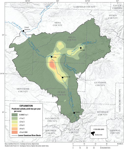
Predicted salinity yield in tons per year per acre in the lower Gunnison River Basin study area.
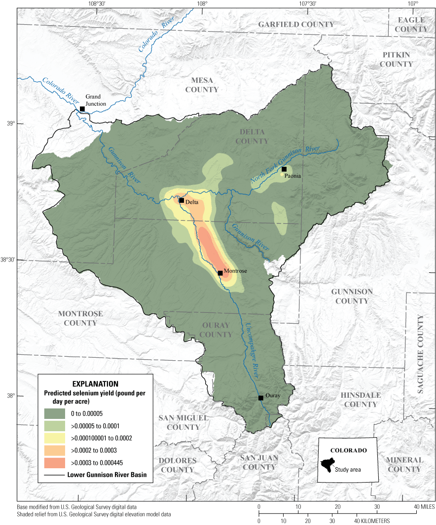
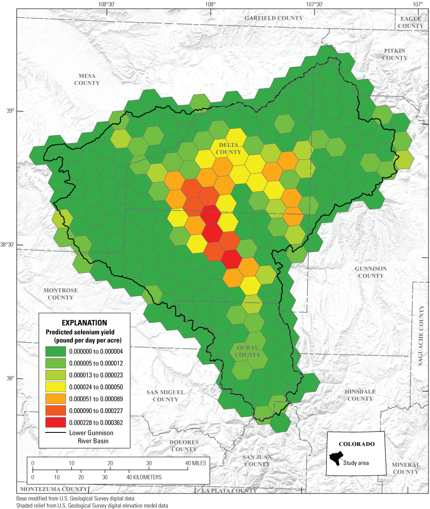
Predicted dissolved selenium yield in pounds per day per acre in the lower Gunnison River Basin study area.
The salinity map (fig. 10) indicates that the highest yields are predicted along the lower part of the Uncompahgre River Basin and the lower part of the Gunnison River upstream from Delta, Colorado, similar to the irrigated lands distribution (fig. 1). North of the main-stem Gunnison River and northeast of Delta and along the North Fork Gunnison River at and downstream from Paonia, Colorado, an area of low to moderate yields was predicted (both areas are irrigated [fig. 1] and associated with marine shales [fig. 2]). Salinity yields ranged from 0.00667 to 6.564 tons per year per acre. The highest salinity yields, greater than about 5.0 tons per year per acre, are predicted on the western side of the Uncompahgre River upstream from Delta (fig.10), an area with a high density of irrigated land (fig. 1).
The part of the basin that drains directly to the main-stem Gunnison River upstream from the confluence with the North Fork Gunnison River does not show high predicted yields (fig. 10) most likely because irrigation is not as common in the area, and because there are fewer drainages on marine shales that drain to this reach of the Gunnison. Adjacent to the lower part of the Uncompahgre River and the Gunnison River upstream from Delta are low-elevation irrigated areas, canals, residential land use (ISD system effluent), and Cretaceous marine shales (fig. 2), which are related to increases in salinity in the MLR models. The high predicted salinity yields do not extend substantially downstream from the confluence of the Gunnison and Uncompahgre Rivers at Delta (fig. 10).
The salinity yield map generally agrees with the salinity yield maps produced by Linard (2013); however, the Linard (2013) models predicted high salinity yields from a subbasin in the northwest part of the study area (hydrologic unit code 140200057503; see fig. 6 and appendix in Linard, 2013). The salinity yield map produced for the current study does not indicate high yields from this area.
The selenium yield map shows a similar pattern to salinity yields, with the highest yields along the lower half of the Uncompahgre River Basin and the lower part of the Gunnison River upstream from Delta, like the irrigated lands distribution (fig. 1). The highest selenium yields, however, are more confined to the eastern side of the lower Uncompahgre River and south of the Gunnison River near the confluence with the Uncompahgre River at Delta (fig. 11). These predicted higher selenium yield areas conform well to the areas of high selenium leaching potential (fig. 4). Selenium yields ranged from 2.6888 x 10⁻¹⁰ to 0.000445 pounds per day per acre. The highest predicted selenium yields, greater than 0.0003 pounds per day per acre, were in the area downstream from Montrose on the eastern side of the Uncompahgre River, unlike the area predicted for highest salinity yields, which was on the western side of the Uncompahgre Rive and closer to Delta (figs. 10 and 11). As with salinity yields, areas of slightly higher selenium yields were predicted north of the main-stem Gunnison River and northeast of Delta and along the North Fork Gunnison River at and downstream from Paonia (both areas are irrigated [fig. 1] and associated with marine shales [fig. 2]). The high predicted selenium yields do not extend substantially downstream from the confluence of the Gunnison and Uncompahgre Rivers at Delta (fig. 11), consistent with a finding of no substantial selenium loading to the Gunnison River in the reach downstream from Delta at low flow (Stevens and others, 2018).
As with salinity, the selenium yield map generally agrees with the maps produced by the Linard (2013) study. Linard (2013) predicted high selenium yields from a subbasin in the northwest part of the study area (hydrologic unit code 140200057503; see fig. 6 and appendix in Linard, 2013); however, the map produced for the current study does not indicate high selenium yields from this area. Additionally, the Linard (2013) nonirrigation season model did not predict higher selenium yields for the area at and downstream from Paonia. The irrigation season model did predict higher yields in that area, as did the map produced for the current study.
Verification of Salinity Yield
Verification of the salinity yield raster data was done to evaluate error or bias introduced into the prediction raster by the EBK process. Comparisons of yield residuals for 12 subbasin areas (fig.12) show that annual yields calculated from the prediction raster compare relatively well with yields derived from measured annual loads at USGS streamgages considered to be representative of those subbasins. The mean percentage error is −24.7 percent, and the median is 18.2 percent; percentage error ranged from −476 to 63.1 percent. The distribution of percentage error values may indicate that a positive bias exists, leading to predicted yields that are generally higher than observed yields (table 5). Additional field measurements, for example, measurements made during a synoptic study, could provide a better dataset to test model performance. Interbasin load transfers may account for some of the larger differences between predicted yield and measured yield, for example, the site Montrose Arroyo at East Niagara Street (table 5).
Table 5.
Summary of salinity yield verification results, 2005–13 (U.S. Geological Survey, 2014b).[Salinity yield residual is the difference between the yield computed from measured annual loads and the yield determined from the yield prediction raster. Residual percentage error is computed as the yield residual divided by the mean yield from load computation times 100. Site names from the National Water Information System database (USGS, 2014b) are abbreviated in this table. USGS, U.S. Geological Survey; ton/yr/acre, tons per year per acre; CO, Colorado; N, North; Rd, R, Road; St, street]
| USGS site name | USGS site number | Salinity yield from load computation (ton/yr/acre) | Salinity yield from prediction raster (ton/yr/acre) | Salinity yield residual (ton/yr/acre) | Salinity yield residual percentage error | Yield verification basin number (fig. 12) |
|---|---|---|---|---|---|---|
| Tongue Creek at Cory, CO | 09144200 | 0.191 | 0.649 | 0.458 | 39.9 | 1 |
| North Fork Gunnison River above mouth near Lazear, CO | 09136100 | 0.266 | 0.476 | 0.210 | 18.2 | 2 |
| Loutzenhizer Arroyo below N. River Rd. near Delta, CO | 383946107595301 | 1.76 | 1.61 | −0.147 | −12.8 | 3 |
| Gunnison River at Delta, CO | 09144250 | 0.339 | 0.708 | 0.369 | 32.1 | 4 |
| Montrose Arroyo at East Niagara St. | 382802107513301 | 7.76 | 2.29 | −5.47 | −476 | 5 |
| Montrose Arroyo at 6700 Rd. | 382711107500501 | 1.06 | 1.79 | 0.726 | 63.1 | 6 |
| Montrose Arroyo at 6750 and Ogden Roads | 382702107493701 | 0.434 | 0.966 | 0.532 | 46.2 | 7 |
| Gunnison River near Grand Junction, CO | 09152500 | 0.268 | 0.295 | 0.0267 | 2.32 | 8 |
| Uncompahgre River at Delta, CO | 09149500 | 0.540 | 1.06 | 0.522 | 45.4 | 9 |
| Uncompahgre River near Ridgway, CO | 09146200 | 0.545 | 0.499 | −0.0463 | −4.02 | 10 |
| Uncompahgre River at Colona, CO | 09147500 | 0.090 | 0.354 | 0.264 | 23.0 | 11 |
| Uncompahgre River near Ouray, CO | 09146020 | 0.570 | 0.457 | −0.113 | −9.83 | 12 |
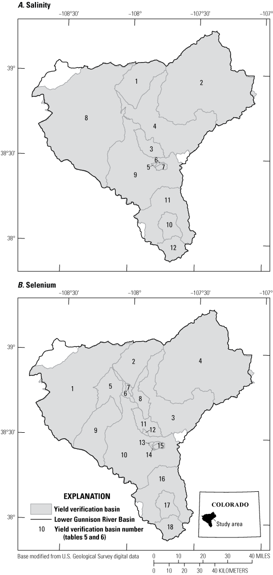
Subbasin areas used in A, salinity and B, selenium yield verification analysis. Yield verification basin numbers, subbasin information, and yield residuals are provided in tables 5 and 6.
Verification of Selenium Yield
Verification of the selenium yield raster data was done to evaluate error or bias introduced into the prediction raster by the EBK process. Comparisons of yield residuals for 18 subbasin areas (fig. 12) show that for most of the subbasin areas annual yields calculated from the prediction raster compare relatively well with yields derived from measured annual loads at USGS streamgages considered to be representative of those subbasins. The mean percentage error is −40.5 percent, and the median is 0.75 percent; percentage error ranged from −535 to 62.2 percent. The distribution of percentage error values may indicate that a negative bias exists, leading to predicted yields that are generally lower than observed yields (table 6). Additionally, targeted field assessments could provide a better test of model performance. Interbasin load transfers may account for some of the larger differences between predicted yield and measured yield.
Table 6.
Summary of dissolved selenium yield verification results, 2005–13 (U.S. Geological Survey, 2014b).[Selenium yield residual is the difference between the yield computed from measured annual loads and the yield determined from the yield prediction raster. Residual percentage error is computed as the yield residual divided by the mean yield from load computation times 100. Site names from the National Water Information System database (USGS, 2014b) are abbreviated in this table. USGS, U.S. Geological Survey; lb/yr/acre, pounds per year per acre; CO, Colorado; N, north; Rd, Road; St, Street]
| USGS site name | USGS site number | Selenium yield from load computation (lb/yr/acre) | Selenium yield from prediction raster (lb/yr/acre) | Selenium yield residual (lb/yr/acre) | Selenium yield residual percentage error | Yield verification basin number (fig. 12) |
|---|---|---|---|---|---|---|
| Gunnison River near Grand Junction, CO | 09152500 | 0.00370 | 8.59x10⁻⁴ | −2.84x10⁻³ | −5.88 | 1 |
| Tongue Creek at Cory, CO | 09144200 | 0.00185 | 4.36x10⁻³ | 2.51x10⁻³ | 5.20 | 2 |
| Gunnison River at 2200 Bridge at Austin, CO | 384624107570701 | 0.00582 | 5.38x10⁻³ | −4.37x10⁻⁴ | −0.91 | 3 |
| North Fork Gunnison River above mouth near Lazear, CO | 09136100 | 0.00144 | 0.00312 | 1.68 x10⁻³ | 3.47 | 4 |
| Gunnison River above Escalante Creek near Delta, CO | 384527108152701 | 0.0127 | 0.0176 | 4.95x10⁻³ | 10.3 | 5 |
| Gunnison River at Delta, CO | 09144250 | 0.0471 | 0.0503 | 0.00316 | 6.53 | 6 |
| Gunnison River above Hartland Ditch near North Delta, CO | 384617108022901 | 0.0426 | 0.0406 | −0.0020 | −4.2 | 7 |
| Gunnison River near Cory, CO | 09137500 | 0.0400 | 0.0294 | −0.0106 | −21.9 | 8 |
| Roubideau Creek at mouth near Delta, CO | 09150500 | 8.58 x10⁻⁴ | 2.98x10⁻³ | 2.12 x10⁻³ | 4.39 | 9 |
| Uncompahgre River at Delta, CO | 09149500 | 0.00140 | 0.0135 | 0.0121 | 25.1 | 10 |
| Loutzenhizer Arroyo below N. River Rd. near Delta, CO | 383946107595301 | 0.102 | 0.0646 | −0.037 | −77.5 | 11 |
| West tributary of Loutzenhizer Arroyo at Ida Rd. | 383250107540301 | 0.243 | 0.131 | −0.112 | −231 | 12 |
| Montrose Arroyo at East Niagara St. | 382802107513301 | 0.343 | 0.0847 | −0.258 | −535 | 13 |
| Montrose Arroyo at 6700 Rd. | 382711107500501 | 0.0133 | 0.0433 | 0.03000 | 62.2 | 14 |
| Montrose Arroyo at 6750 and Ogden Roads | 382702107493701 | 0.00709 | 0.0227 | 0.0156 | 32.3 | 15 |
| Uncompahgre River at Colona, CO | 09147500 | 8.09 x10⁻⁴ | 1.24x10⁻³ | 4.30 x10⁻⁴ | 0.89 | 16 |
| Uncompahgre River near Ridgway, CO | 09146200 | 0.00178 | 1.24x10⁻³ | −5.44 x10⁻⁴ | −1.13 | 17 |
| Uncompahgre River near Ouray, CO | 09146020 | 0.00160 | 1.24x10⁻³ | −3.64 x10⁻⁴ | −0.75 | 18 |
Summary
Land managers, water providers, and agricultural producers expend resources mitigating the effects of salinity (total dissolved solids) and selenium on water quality in the lower Gunnison River Basin in western Colorado. Salinity is known to affect drinking-water supplies and damage irrigated agricultural lands. Selenium in high concentrations is harmful to fish and other wildlife. Agricultural valleys in the lower Gunnison River Basin tend to be located on geologic materials derived from marine shale. Irrigation of those soils can mobilize salt and selenium.
The U.S. Geological Survey (USGS) revised existing salinity and selenium models for the lower Gunnison River Basin in an attempt to better identify areas of greatest salinity and selenium yield. This report describes the statistical procedures, salinity and selenium water-quality data, and geospatial data used to determine multiple linear regression (MLR) statistical models to estimate in-stream salinity and selenium loads for subbasins within the lower Gunnison River Basin. The MLR techniques, methods, and selection of basin characteristics differ from some procedures and characteristics used to create existing models for the lower Gunnison River Basin. The objectives of the current study were to (1) improve estimates of salinity and selenium loads by improving the regressions and geospatial data for the lower Gunnison River Basin with new variables (and new statistical transformations of new variables and variables used in previous studies) and (2) to integrate water-quality data available for years since previous studies were completed.
The water-quality and some geospatial data are grouped into two time periods (1992 through 2004 and 2005 through 2013) and two seasons (irrigation and nonirrigation). These changes can reduce spatial variability and temporal complexity of the data. The time periods for analysis were selected based on available water-quality and geographic information system data. Water quality (salinity and dissolved selenium loads in this report) is the response variable in the MLR approach. Basin characteristics are the explanatory variables used for prediction of salinity and dissolved selenium loads. Separating the data into two periods helped address potential issues of nonstationarity, the tendency for some basin characteristics to change variability ranges through time. The determination of loads required computations that include constituent concentrations and discharge measurements made at the time of sampling. Concentration and discharge data were obtained from the USGS National Water Information System database. Loads were assumed to be the mean of at least five concentration and discharge measurements both in subbasins and canals in a season.
Due to the complexity of water imports, diversions, and the locations of sites with existing load information, final calculated loads were adjusted to avoid nesting of subbasins (overlap) and to count loads only once. Avoiding nested basins is an approach not used in previous studies of the lower Gunnison River Basin and provided more accurate load computations and less confusion of the load signal in larger subbasins by separating out the overlap of areas. The procedure for separating nested subbasins involves subtracting the tributary load (the load in a subbasin encompassed within the drainage area of a larger subbasin) from the load computed for the larger subbasin, resulting in two separate subbasin drainages that do not count the same load twice. Canals are common in the study area and were part of the water budget accounting for the subbasins they cross. The load coming in across a subbasin boundary and the load leaving a subbasin are subtracted, and the difference is added to the basic subbasin load computation without canal influence.
Salinity and selenium loads were modeled with MLR techniques by using geospatial basin characteristics. Many basin characteristics were considered for MLR and prediction of salinity and selenium loads. Basin characteristics used in the regressions are related to physical properties of the subbasin, precipitation, land use and land cover, surficial deposits (soil and unconsolidated geologic materials), and bedrock geology. New characteristics used in this study, such as a soil property related to selenium in soil and water derived from residential wastewater systems, were not considered in previous studies. The variables were analyzed in a stepwise least-squares regression procedure to identify the strongest combinations of explanatory variables for salinity and selenium loads.
Combinations of variables were assessed based on adjusted R2 and prediction error sum of squares statistics. Sometimes the best models did not have the top score for all three statistics, and other measures were used to choose the best final equations. Statistical significance of variables (p-values), diagnostic plots that indicated favorable residuals patterns such as constant variance (homoscedasticity), and normal distribution of residuals were used to qualify or disqualify candidate models or indicate if transforms of the data might be helpful.
Evaluating all possible combinations of geospatial variables resulted in three MLR models that best estimated irrigation-season salinity load, nonirrigation-season salinity load, and annual selenium load. Loads of salinity and selenium were converted to yields by using the subbasin drainage areas, and an empirical Bayesian kriging (EBK) procedure was used to produce robust grids of yields for salinity and selenium. To produce yields that represent annual composites, irrigation and nonirrigation season salinity yields were summed.
The highest salinity yields are predicted along the lower part of the Uncompahgre River and the lower part of the Gunnison River upstream from Delta, Colorado, similar to the irrigated lands distribution. North of the main-stem Gunnison River and northeast of Delta and along the North Fork Gunnison River at and downstream from Paonia, Colorado, an area of low to moderate yields was predicted (both areas are irrigated and associated with marine shales). Salinity yields ranged from 0.00667 to 6.564 tons per year per acre. The highest salinity yields, greater than about 5.0 tons per year per acre, are predicted on the western side of the Uncompahgre River upstream from Delta, an area with a high density of irrigated land.
The selenium yield map was similar to the salinity yield map, but the highest predicted selenium yields were somewhat more confined to the eastern side of the lower Uncompahgre River and south of the Gunnison River near the confluence with the Uncompahgre River at Delta. Selenium yields ranged from 2.6888 x 10⁻¹⁰ to 0.000445 pounds per day per acre. The highest predicted yields, greater than 0.0003 pounds per day per acre, were in the area downstream from Montrose, Colorado, on the eastern side of the Uncompahgre River. As with salinity yields, areas of slightly higher selenium yields were predicted north of the main-stem Gunnison River and northeast of Delta and along the North Fork Gunnison River at and downstream from Paonia (both are irrigated areas associated with marine shales). These predicted higher selenium yield areas conform well to the areas of high selenium leaching potential.
The salinity and selenium yield maps generally agree with maps produced by the previous MLR models for the lower Gunnison River Basin. Verification of the salinity and selenium yield rasters was done to evaluate error or bias introduced into the prediction rasters by the EBK process. Comparisons of yield residuals for selected subbasin areas show that annual salinity and selenium yields calculated from the prediction raster compare relatively well with yields derived from measured annual loads at USGS streamgages considered to be representative of those subbasins. Additional field measurements, for example, measurements made during a synoptic study, could provide a better dataset to test model performance.. Interbasin load transfers may account for some of the larger differences between predicted yield and measured yield.
Acknowledgments
The authors extend thanks to the following U.S. Geological Survey employees who contributed data and analysis to this report: Ken Leib, Rod Richards, Judith Thomas, and Josh Linard.
References Cited
Barnett, D.A., 2019, Colorado River Basin Salinity Control Program briefing document: Bountiful, Utah, Colorado River Basin Salinity Control Forum, 4 p., accessed January 6, 2023, at https://coloradoriversalinity.org/docs/CRBSCP%20Briefing%20Document%202019-03-20.pdf.
Bureau of Reclamation, 2022, CRBSCP—Lower Gunnison Basin Unit—Title II: Bureau of Reclamation web page, accessed January 6, 2023, at https://www.usbr.gov/projects/index.php?id=343.
Butler, D.L., Krueger, R.P., Osmundson, B.C., Thompson, A.L., and McCall, S.K., 1991, Reconnaissance investigation of water quality, bottom sediment, and biota associated with irrigation drainage in the Gunnison and Uncompahgre River Basins and at Sweitzer Lake, west-central Colorado, 1988–89: U.S. Geological Survey Water-Resources Investigations Report 91–4103, 99 p. [https://doi.org/10.3133/wri914103.]
Butler, D.L., and Leib, K.J., 2002, Characterization of selenium in the lower Gunnison River Basin, Colorado, 1988−2000: U.S. Geological Survey Water-Resources Investigations Report 2002−4151, 26 p., accessed July 12, 2021, at https://doi.org/10.3133/wri024151.
Butler, D.L., Wright, W.G., Stewart, K.C., Osmundson, B.C., Krueger, R.P., and Crabtree, D.W., 1996, Detailed study of selenium and other constituents in water, bottom sediment, soil, alfalfa, and biota associated with irrigation drainage in the Uncompahgre Project area and in the Grand Valley, west-central Colorado, 1991–93: U.S. Geological Survey Water-Resources Investigations Report 96–4138, 136 p. [https://doi.org/10.3133/wri964138.]
Butler, D.L., 2001, Effects of piping irrigation laterals on selenium and salt loads, Montrose Arroyo Basin, western Colorado: U.S. Geological Survey Water-Resources Investigations Report 2001−4204, 14 p. [https://doi.org/10.3133/wri014204.]
Colorado’s Decision Support Systems, 2014, Division 4 irrigated lands geodatabase: Colorado’s Decision Support Systems vector digital data, accessed February 2015, at https://cdss.colorado.gov/gis-data/gis-data-by-category.
Colorado River Basin Salinity Control Forum, 2020, 2020 review—Water quality standards for salinity Colorado River system: Farmington, Utah, Colorado River Basin Salinity Control Forum, 32 p., accessed November 22, 2021, at https://coloradoriversalinity.org/docs/2020%20REVIEW%20-%20Final%20w%20appendices.pdf.
Day, W.C., Green, G.N., Knepper, D.H., Jr., and Phillips, R.C., 1999, Spatial geologic data model for the Gunnison, Grand Mesa, Uncompahgre National Forests mineral assessment area, southwestern Colorado and digital data for the Leadville, Montrose, Durango, and the Colorado parts of the Grand Junction, Moab, and Cortez 1° × 2° geologic maps: U.S. Geological Survey Open-File Report 99–427, accessed March 2014, at https://doi.org/10.3133/ofr99427.
Delta County, 2014, Interactive Delta County property information map: Delta County web page, accessed March 2014, at https://www.deltacounty.com/13/GIS.
Duan, N., 1983, Smearing estimate—A nonparametric retransformation method: Journal of the American Statistical Association, v. 78, no. 383, p. 605–610, accessed March 2014, at https://doi.org/10.1080/01621459.1983.10478017.
Duffy, C.J., 1984, Conceptual models of geologic and agricultural salt loads in streams of the Upper Colorado River Basin, in French, R.H., ed., Salinity in watercourses and reservoirs: Boston, Mass., Butterworth Publishers, Proceedings of the 1983 Symposium on State-of-the-Art Control of Salinity, p. 223–233.
Evangelou, V.P., Whittig, L.D., and Tanji, K.K., 1984, Dissolved mineral salts derived from Mancos Shale: Journal of Environmental Quality, v. 13, no. 1, p. 146–150, accessed March 2014, at https://doi.org/10.2134/jeq1984.00472425001300010027x.
Gunnison County, 2014, Interactive maps: Gunnison County web page, accessed March 2014, at https://www.gunnisoncounty.org/325/Map-Viewer.
Helsel, D.R., Hirsch, R.M., Ryberg, K.R., Archfield, S.A., and Gilroy, E.J., 2020, Statistical methods in water resources: U.S. Geological Survey Techniques and Methods, book 4, chapter A3, 458 p. [Supersedes USGS Techniques of Water-Resources Investigations, book 4, chapter A3, version 1.1.] [Also available at https://doi.org/10.3133/tm4A3.]
Henneberg, M.F., 2020, Assessment of dissolved-selenium concentrations and loads in the lower Gunnison River Basin, Colorado, as part of the Selenium Management Program, 2011−17: U.S. Geological Survey Open-File Report 2020–1078, 21 p., accessed July 12, 2021, at https://doi.org/10.3133/ofr20201078.
Henneberg, M.F., 2021, Dissolved-selenium concentrations and loads in the lower Gunnison River Basin, Colorado, as part of the Selenium Management Program: U.S. Geological Survey data release, accessed August 20, 2021, at https://doi.org/10.5066/P92UIS8X.
Hintze, L.F., Willis, G.C., Laes, D.Y.M., Sprinkel, D.A., and Brown, K.D., 2000, Digital geologic map of Utah: Department of Natural Resources, Utah Geological Survey, Map 179DM, scale 1:500,000, accessed February 14, 2011, at https://doi.org/10.34191/M-179DM.
Iacobucci, D., Schneider, M.J., Popovich, D.L., and Bakamitsos, G.A., 2016, Mean centering helps alleviate “micro” but not “macro” multicollinearity: Behavior Research Methods, v. 48, no. 4, p. 1308–1317, accessed March 2018, at https://doi.org/10.3758/s13428-015-0624-x.
Kanzer, D., and Merritt, D., 2008, The salinity control story of the Upper Colorado River Basin illustrated by case studies: 2nd International Salinity Forum, 4 p., accessed November 30, 2021, at http://www.riversimulator.org/Resources/Salinity/SalinityParadoxValley/SalinityControlStoryUCRBdanzer.pdf.
Krivoruchko, K., and Gribov, A., 2019, Evaluation of empirical Bayesian kriging: Spatial Statistics, v. 32, no. 100368, accessed August 24, 2021, at https://doi.org/10.1016/j.spasta.2019.100368.
Leib, K.J., 2008, Concentrations and loads of selenium in selected tributaries to the Colorado River in the Grand Valley, western Colorado, 2004−2006: U.S. Geological Survey Scientific Investigations Report 2008−5036, 36 p. [Also available at https://doi.org/10.3133/sir20085036.]
Leib, K.J., Linard, J.I., and Williams, C.A., 2012, Statistical relations of salt and selenium loads to geospatial characteristics of corresponding subbasins of the Colorado and Gunnison Rivers in Colorado: U.S. Geological Survey Scientific Investigations Report 2012–5003, 43 p. [Also available at https://doi.org/10.3133/sir20125003.]
Lemly, A.D., 2002, Selenium assessment in aquatic ecosystems—a guide for hazard evaluation and water quality criteria: New York, Springer-Verlag New York, Inc., 162 p. https://doi.org/10.1007/978-1-4613-0073-1
Linard, J.I., 2013, Ranking contributing areas of salt and selenium in the Lower Gunnison River Basin, Colorado, using multiple linear regression models: U.S. Geological Survey Scientific Investigations Report 2013–5075, 35 p. [Also available at https://doi.org/10.3133/sir20135075.]
Linard, J.I., McMahon, P.B., Arnold, L.R., and Thomas, J.C., 2017, Response of selenium concentrations in groundwater to seasonal canal leakage, lower Gunnison River Basin, Colorado, 2013: U.S. Geological Survey Scientific Investigations Report 2016–5047, 30 p., accessed July 12, 2021, at https://doi.org/10.3133/sir20165047.
Mast, M.A., 2021, Characterization of groundwater quality and discharge with emphasis on selenium in an irrigated agricultural drainage near Delta, Colorado, 2017–19: U.S. Geological Survey Scientific Investigations Report 2020–5132, 34 p. [Also available at https://doi.org/10.3133/sir20205132.]
Mast, M.A., Mills, T.J., Paschke, S.S., Keith, G., and Linard, J.I., 2014, Mobilization of selenium from the Mancos Shale and associated soils in the lower Uncompahgre River Basin, Colorado: Applied Geochemistry, v. 48, p. 16–27. [Also available at https://doi.org/10.1016/j.apgeochem.2014.06.024.]
Mayo, J.W., 2008, Estimating the effects of conversion of agricultural land to urban land on deep percolation of irrigation water in the Grand Valley, western Colorado: U.S. Geological Survey Scientific Investigations Report 2008–5086, 58 p. [Also available at https://doi.org/10.3133/sir20085086.]
Mayo, J.W., and Leib, K.J., 2012, Flow-adjusted trends in dissolved selenium load and concentration in the Gunnison and Colorado Rivers near Grand Junction, Colorado, water years 1986–2008: U.S. Geological Survey Scientific Investigations Report 2012–5088, 33 p., accessed July 12, 2021, at https://doi.org/10.3133/sir20125088.]
Mesa County, 2014, Mesa County GIS viewer: Mesa County web page accessed March 2014, at https://emap.mesacounty.us/viewer/.
Miller, M.P., Buto, S.G., Lambert, P.M., and Rumsey, C.A., 2017, Enhanced and updated spatially referenced statistical assessment of dissolved-solids load sources and transport in streams of the Upper Colorado River Basin: U.S. Geological Survey Scientific Investigations Report 2017–5009, 23 p., accessed June 28, 2021, at https://doi.org/10.3133/sir20175009.
Mills, T.J., Mast, M.A., Thomas, J., and Keith, G., 2016, Controls on selenium distribution and mobilization in an irrigated shallow groundwater system underlain by Mancos Shale, Uncompahgre River Basin, Colorado, USA: Science of the Total Environment, v. 566–567, p. 1621–1631, accessed July 12, 2021, at https://doi.org/10.1016/j.scitotenv.2016.06.063.
Milly, P.C.D., Betancourt, J., Falkenmark, M., Hirsch, R.M., Kundzewicz, Z.W., Lettenmaier, D.P., and Stouffer, R.J., 2008, Stationarity is dead—Whither water management?: Science, v. 319, no. 5863, p. 573–574. [Also available at https://doi.org/10.1126/science.1151915.]
Montrose County, 2014, Interactive maps: Montrose County web page, accessed March 2014, at https://www.montrosecounty.net/318/Interactive-Maps.
Moore, J.L., 2011, Characterization of salinity and selenium loading and land-use change in Montrose Arroyo, western Colorado, from 1992 to 2010: U.S. Geological Survey Scientific Investigations Report 2011–5106, 23 p., accessed July 12, 2021, at https://doi.org/10.3133/sir20115106.
Nauman, T.W., Ely, C.P., Miller, M.P., and Duniway, M.C., 2019, Salinity yield modeling of the Upper Colorado River Basin using 30-m resolution soil maps and random forests: Water Resources Research, v. 55, no. 6, p. 4954–4973, accessed July 6, 2021, at https://doi.org/10.1029/2018WR024054.
Ouray County, 2014, Ouray County EagleWeb: Ouray County web page, accessed March 2014 at https://ouraycountyassessor.org/assessor/web/.
Presser, T.S., and Luoma, S.N., 2006, Forecasting selenium discharges to the San Francisco Bay–Delta estuary—Ecological effects of a proposed San Luis Drain extension: U.S. Geological Survey Professional Paper 1646, 196 p. [Also available at https://doi.org/10.3133/pp1646.]
PRISM Climate Group, 2014, Monthly 30-year “normal” dataset covering the conterminous U.S., averaged over the climatological period 1981−2010: PRISM Climate Group, accessed 2014, at http://prism.oregonstate.edu.
R Core Team, 2017, R—A language and environment for statistical computing, version 3.4.1: Vienna, Austria, R Foundation for Statistical Computing software release, accessed June 2017, at https://www.R-project.org/.
Richards, R.J., and Moore, J.L., 2015, Characterization of streamflow, salinity, and selenium loading and land-use change in Montrose Arroyo, western Colorado, from 1992 to 2013: U.S. Geological Survey Scientific Investigations Report 2015–5039, 18 p., accessed July 12, 2021, at https://doi.org/10.3133/sir20155039.
Rumsey, C.A., Miller, M.P., Schwarz, G.E., Hirsch, R.M., and Susong, D.D., 2017, The role of baseflow in dissolved solids delivery to streams in the Upper Colorado River Basin: Hydrological Processes, v. 31, no. 26, p. 4705–4718. [Also available at https://doi.org/10.1002/hyp.11390.]
Stevens, M.R., Leib, K.J., Thomas, J.C., Bauch, N.J., and Richards, R.J., 2018, Streamflow and selenium loads during synoptic sampling of the Gunnison River and its tributaries near Delta, Colorado, November 2015: U.S. Geological Survey Scientific Investigations Report 2018–5029, 17 p. [Also available at https://doi.org/10.3133/sir20185029.]
Thomas, J.C., Leib, K.J., and Mayo, J.W., 2008, Analysis of dissolved selenium loading for selected sites in the Lower Gunnison River Basin, Colorado, 1978–2005: U.S. Geological Survey Scientific Investigations Report 2007–5287, 25 p. [Also available at https://doi.org/10.3133/sir20075287.]
Thomas, J.C., McMahon, P.B., and Arnold, L.R., 2019, Groundwater quality and hydrology with emphasis on selenium mobilization and transport in the lower Gunnison River Basin, Colorado, 2012–16: U.S. Geological Survey Scientific Investigations Report 2019–5029, 69 p., accessed July 12, 2021, at https://doi.org/10.3133/sir20195029.
Tuttle, M.L.W., Fahy, J.W., Elliott, J.G., Grauch, R.I., and Stillings, L.L., 2014a, Contaminants from Cretaceous black shale—I. Natural weathering processes controlling contaminant cycling in Mancos Shale, southwestern United States, with emphasis on salinity and selenium: Applied Geochemistry, v. 46, p. 57–71, [Also available at https://doi.org/10.1016/j.apgeochem.2013.12.010.]
Tuttle, M.L.W., Fahy, J.W., Elliott, J.G., Grauch, R.I., and Stillings, L.L., 2014b, Contaminants from Cretaceous black shale—II. Effect of geology, weathering, climate, and land use on salinity and selenium cycling, Mancos Shale landscapes, southwestern United States: Applied Geochemistry, v. 46, p. 72–84. [Also available at https://doi.org/10.1016/j.apgeochem.2013.12.011.]
Tuttle, M.L., and Grauch, R.I., 2009, Salinization of the upper Colorado River—Fingerprinting geologic salt sources: U.S. Geological Survey Scientific Investigations Report 2009–5072, 62 p. [Also available at https://doi.org/10.3133/sir20095072.]
U.S. Department of Agriculture Natural Resources Conservation Service, 2014, Conservation Service web soil survey: U.S. Department of Agriculture, accessed March 2014 at https://websoilsurvey.sc.egov.usda.gov/App/HomePage.htm.
U.S. Department of Agriculture, 2015, National cropland data layer, 2014: National Agricultural Statistics Service (NASS), accessed December 2015 at https://www.nass.usda.gov/Research_and_Science/Cropland/Release/.
U.S. Environmental Protection Agency [EPA], 2003, National primary drinking water standards: U.S. Environmental Protection Agency Office of Water Fact Sheet EPA 816-F-03-016, accessed March 2018 at https://www.epa.gov/safewater/contaminants/index.html.
U.S. Fish and Wildlife Service, 2014, National Wetlands Inventory: Washington, D.C., U.S. Fish and Wildlife Service vector digital data, accessed March 2014, at https://www.fws.gov/wetlands/index.html.
U.S. Geological Survey [USGS], 1999a, 1/3rd arc-second digital elevation models (DEMs)—USGS National Map 3DEP downloadable data collection: U.S. Geological Survey digital dataset, accessed March 2014, at https://catalog.data.gov/dataset/national-elevation-dataset-ned-1-3-arc-second-downloadable-data-collection-national-geospatial.
U.S. Geological Survey [USGS], 2014a, National hydrography dataset (NHD): U.S. Geological Survey digital data, accessed October 2014, at https://catalog.data.gov/dataset/usgs-national-hydrography-dataset-nhd-downloadable-data-collection-national-geospatial-data-as.
U.S. Geological Survey [USGS], 2014b, USGS water data for the Nation: U.S. Geological Survey National Water Information System database, accessed October 29, 2014, at https://doi.org/10.5066/F7P55KJN.
U.S. Geological Survey [USGS], 2020, Infiltration and the water cycle: U.S. Geological Survey web page, accessed October 2020, at https://www.usgs.gov/special-topic/water-science-school/science/infiltration-and-water-cycle?qt-science_center_objects=0#qt-science_center_objects.
Waller, R.M., 1994, Ground water and the rural homeowner: U.S. Geological Survey, Unnumbered Series, 38 p., accessed June 2019, at https://doi.org/10.3133/7000054.
Ward, J., McWhirter, L., Leib, K., Kanzer, D., and Funk, A., 2021, Selenium Management Program Gunnison River Basin 2020 annual progress report: Grand Junction, Colo., Bureau of Reclamation, 35 p., accessed January 6, 2022, at https://www.usbr.gov/uc/DocLibrary/Reports/SeleniumManagementProgram/20210800-SeleniumManagementProgram-2020Report-508-WCAO.pdf.
Williams, C.A., Gidley, R.G., and Stevens, M.R., 2023, Basin characteristics and salinity and selenium loads and yields for selected subbasins in the lower Gunnison River Basin, western Colorado, 1992–2013: U.S. Geological Survey data release, https://doi.org/10.5066/P9CW7Q1N.
Conversion Factors
U.S. customary units to International System of Units
Datum
Vertical coordinate information is referenced to the North American Vertical Datum of 1988 (NAVD88).
Horizontal coordinate information is referenced to the North American Datum of 1983 (NAD83).
Elevation, as used in this report, refers to distance above the vertical datum.
Supplemental Information
Concentrations of chemical constituents in water are given in either milligrams per liter (mg/L) or micrograms per liter (µg/L).
As used in this report, load relates the mass of a constituent for a specified unit of time. Load is specified for annual or seasonal time periods and reported as the mean in tons per day for salinity (total dissolved solids) and pounds per day for selenium.
As used in this report, yield is mass per time per unit of area. Yield of salinity (total dissolved solids) is in units of tons per year per acre, and selenium yield is in units of pounds per day per acre.
The water year is defined as the 12-month period from October 1 through September 30. The water year is designated by the calendar year in which it ends. Thus, the year ending September 30, 2014, is the “2014 water year.”
Abbreviations
EBK
empirical Bayesian kriging
EPA
U.S. Environmental Protection Agency
FWS
U.S. Fish and Wildlife Service
GIS
geographic information system
ISD
individual sewage disposal
MLR
multiple linear regression
NRCS
U.S. Department of Agriculture Natural Resources Conservation Service
Reclamation
Bureau of Reclamation
SPARROW
SPAtially Referenced Regressions on Watershed attributes
SSURGO
Soil Survey Geographic Database
TDS
total dissolved solids
USGS
U.S. Geological Survey
VIF
variance inflation factor
Publishing support provided by the Science Publishing Network,
Denver Publishing Service Center
For more information concerning the research in this report, contact the
Director, USGS Colorado Water Science Center
Box 25046, Mail Stop 415
Denver, CO 80225
(303) 236-6900
Or visit the Colorado Water Science Center website at
Disclaimers
Any use of trade, firm, or product names is for descriptive purposes only and does not imply endorsement by the U.S. Government.
Although this information product, for the most part, is in the public domain, it also may contain copyrighted materials as noted in the text. Permission to reproduce copyrighted items must be secured from the copyright owner.
Suggested Citation
Williams, C.A., Gidley, R.G., and Stevens, M.R., 2023, Salinity and selenium yield maps derived from geostatistical modeling in the lower Gunnison River Basin, western Colorado, 1992–2013: U.S. Geological Survey Scientific Investigations Report 2023–5013, 37 p., https://doi.org/10.3133/sir20235013.
ISSN: 2328-0328 (online)
Study Area
| Publication type | Report |
|---|---|
| Publication Subtype | USGS Numbered Series |
| Title | Salinity and selenium yield maps derived from geostatistical modeling in the lower Gunnison River Basin, western Colorado, 1992–2013 |
| Series title | Scientific Investigations Report |
| Series number | 2023-5013 |
| DOI | 10.3133/sir20235013 |
| Publication Date | April 05, 2023 |
| Year Published | 2023 |
| Language | English |
| Publisher | U.S. Geological Survey |
| Publisher location | Reston VA |
| Contributing office(s) | Colorado Water Science Center |
| Description | Report: vi, 37 p.; 2 Data Releases |
| Country | United States |
| State | Colorado |
| Other Geospatial | Lower Gunnison River basin |
| Online Only (Y/N) | Y |