

An Integrated Hydrologic Model to Support the Central Platte Natural Resources District Groundwater Management Plan, Central Nebraska
Links
- Document: Report (14.5 MB pdf) , HTML , XML
- Tables:
- Figures:
- Dataset: USGS National Water Information System database —USGS water data for the Nation
- Data Release: USGS data release - MODFLOW-One-Water model used to support the Central Platte Natural Resources District Groundwater Management Plan, central Nebraska
- NGMDB Index Page: National Geologic Map Database Index Page (html)
- Download citation as: RIS | Dublin Core
Acknowledgments
The authors express their gratitude to Brandi Flyr and Duane Woodward (retired) of the Central Platte Natural Resources District for their coordination and cooperation throughout the duration of this study that began in 2016. Their local knowledge of the study area was invaluable to the completion of the project.
The authors also recognize additional U.S. Geological Survey (USGS) scientists that contributed to the study: Benjamin Dietsch, Kellan Strauch, Brent Hall, Alec Weisser, and Chris Hobza from the USGS Nebraska Water Science Center; Mike Fienen from the USGS Upper Midwest Water Science Center for his invaluable help with the predictive uncertainty aspect of the study; and Joseph Richards from the USGS Central Midwest Water Science Center. This project would not have been possible without the Nebraska Natural Resources Commission Water Sustainability Fund and USGS Cooperative Matching Funds Program.
Abstract
The groundwater and surface-water supply of the Central Platte Natural Resources District supports a large agricultural economy from the High Plains aquifer and Platte River, respectively. This study provided the Central Platte Natural Resources District with an advanced numerical modeling tool to assist with the update of their Groundwater Management Plan.
An integrated hydrologic model, called the Central Platte Integrated Hydrologic Model, was constructed using the MODFLOW-One-Water Hydrologic Model code with the Newton solver. This code integrates climate, landscape, surface water, and groundwater-flow processes in a fully coupled approach. Model framework included 163 rows; 327 columns; 2,640 feet cell sides; and 3 vertical layers. A predevelopment model simulated steady-state hydrologic conditions prior to April 30, 1895, and a development period model discretized into 610 stress periods simulated transient hydrologic conditions from May 1, 1895, to December 31, 2016, using 170 biannual stress periods from 1895 to 1980, and monthly stress periods from May 1, 1980, to December 31, 2016.
Calibration of the Central Platte Integrated Hydrologic Model involved two phases: a manual adjustment of parameters, followed by the automated calibration completed using BeoPEST that was facilitated by the employment of the singular value decomposition-assist features of PEST that specified 50 super parameters assembled from the 435 adjustable parameters and Tikhonov regularization. The average absolute groundwater-level residuals for model layers one, two, and three were 6.1, 12.4, and 7.4 feet, respectively. Calibrated horizontal hydraulic conductivity was about 70, 32, and 35 feet per day for layers 1, 2, and 3, respectively. The largest development period inflow to groundwater was recharge from deep percolation past the root zone, averaging 1,122,257 acre-feet per year (2.7 inches per year), and the largest outflow was to irrigation wells, averaging 693,171 acre-feet per year (10.2 inches per year for the Central Platte Natural Resources District). Other substantial groundwater outflows included evapotranspiration and base flow. For the total development period, there was a net change in storage of −122,393 acre-feet per year (−0.3 inch per year).
The calibrated Central Platte Integrated Hydrologic Model was used to simulate eight different potential future climate and irrigation pumping conditions from January 1, 2017, to December 31, 2049. Simulated future groundwater levels within the Central Platte Natural Resources District varied significantly between scenarios and locally, from 13.8 feet below to 7.6 feet above baseline 1982 groundwater levels. Most areas exhibited groundwater-level declines for the drought scenarios and rises for the alternate irrigation scenarios. Changes in scenario groundwater levels correlated with the relations between farm net recharge and irrigation pumping. Linear “first order second moment” techniques indicated that the uncertainty in projected groundwater altitudes was reduced by 15.33 feet through model calibration.
Introduction
The Central Platte Natural Resources District (CPNRD; fig. 1A) is 1 of 23 Natural Resources Districts (NRDs) throughout Nebraska created by Nebraska Legislature (Nebraska Legislature, 1969) in 1969 with the goal of protecting its natural resources (Nebraska Association of Resources Districts, 2020). The NRDs are responsible for regulating groundwater use (University of Nebraska-Lincoln, 2020); the Nebraska Department of Natural Resources regulates surface-water use. The groundwater and surface-water supply of the CPNRD is one of its most valuable natural resources. Current beneficial water uses within the CPNRD include domestic and industrial water supply for a population of about 112,000; irrigation water supply for about 1 million acres; and minimum annual flows of more than 1 million acre-feet (acre-ft) of water in the Platte River for recreational and wildlife habitat use. The groundwater and surface-water supply supports an agricultural economy that generates more than $2 billion per year (U.S. Department of Agriculture, 2019). The CPNRD’s main groundwater management goal is “to assure an adequate supply of water for feasible and beneficial uses through proper management, conservation, development and utilization of the District’s water resources” (Central Platte Natural Resources District, 2019, p. 1).
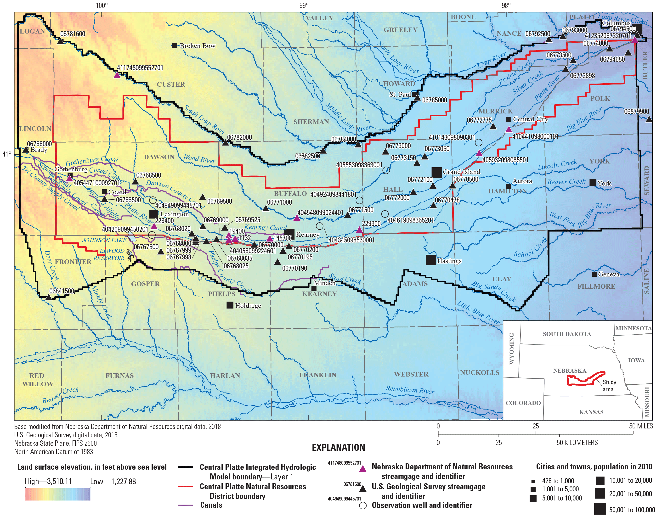
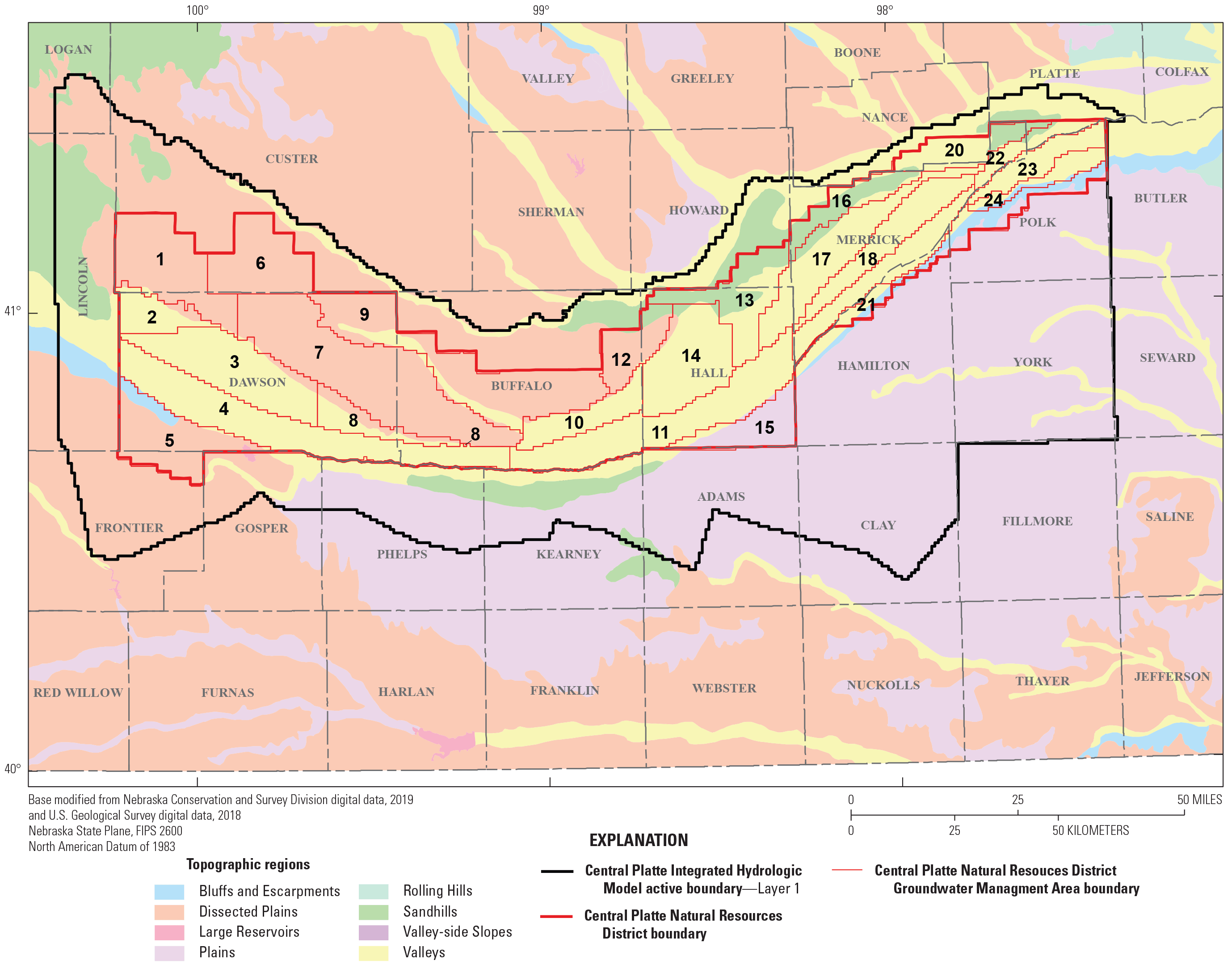
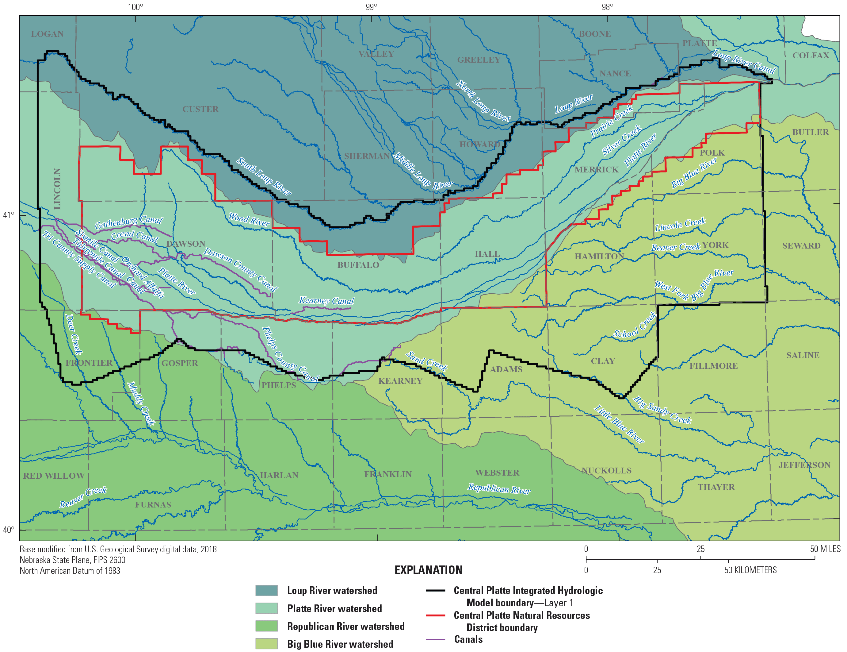
Map of the study area, the Central Platte Natural Resources District, central Nebraska. A, Central Platte Natural Resources District boundary, county boundaries, cities and towns by population, and major surface-water bodies. B, Central Platte Natural Resources District Groundwater Management Area boundaries, streams and canals simulated with the Streamflow Routing package, soil classification used in the Central Platte Integrated Hydrologic Model, and surface watersheds. C, Subregional watersheds in the study area.
Proper regulation of groundwater resources is necessary because during a normal growing season in the CPNRD, effective precipitation (the portion that does not immediately run off to a surface-water body) is usually less than the amount crops need to produce a robust harvest. For example, corn is estimated to need about 25 inches of water from May through September (Kranz and others, 2008), whereas effective precipitation in that time period is normally only about 10 to 15 inches, which leaves a net deficit of about 10 to 15 inches that generally must be met through irrigation. The CPNRD’s groundwater management strategy, which includes irrigation, is set in their Groundwater Management Plan (GMP), a requirement for each NRD determined by the Nebraska Groundwater Management and Protection Act (Nebraska Legislature, 2004) in 1982. The CPNRD’s GMP, initially adopted in 1987, specifies maximum acceptable declines (MADs) of 10 to 30 feet (ft) for 24 Groundwater Management Areas (GWMAs) across the CPNRD (fig. 1B), with the declines based on spring 1982 (approximately April 30, 1982) groundwater levels (Central Platte Natural Resources District, 2020a). The CPNRD monitors the groundwater-level declines and recovery across the 24 GWMAs each year to assess how the irrigation and climate stresses affect the groundwater resources. As specified in their GMP, if the groundwater levels decline to 50 percent of the MADs (5 and 15 ft, respectively, for each GWMA), phase II management would take effect, which triggers mandatory reductions in irrigated acres and establishment of spacing limits for new irrigation wells. Declines in groundwater levels to 70, 90, and 100 percent of the MADs for each GWMA would trigger phase III, IV, and V management, respectively, which include mandates of additional cutbacks in irrigated acreage and increased spacing limits for new wells (Central Platte Natural Resources District, 2020a).
To improve groundwater management and to better understand the effects of specific groundwater-management decisions on groundwater levels and streamflow, the CPNRD has been involved with ongoing groundwater-flow modeling efforts. The CPNRD’s initial and revised GMP rules and regulations were set using groundwater-flow models developed in the 1980s (Peckenpaugh and Dugan, 1983; Peckenpaugh and others, 1987). In 1998, the Platte River Cooperative Hydrology Study (COHYST; https://cohyst.nebraska.gov/) was initiated as a major component of a three-State (Colorado, Nebraska, and Wyoming) cooperative agreement with the U.S. Department of the Interior. COHYST was tasked to collect additional data and to create numerical groundwater-flow models for use in support of regulatory and management decisions. COHYST is a cooperative effort to improve the understanding of hydrological conditions of the Platte River upstream from Columbus, Nebraska, and to evaluate changes to current and proposed water uses in the Platte River Basin, including the part of the watershed within the CPNRD (fig. 1C). Three overlapping groundwater-flow models were originally developed for the eastern, central, western COHYST regions and are described in Peterson (2009), Carney (2008), and Luckey and Cannia (2006), respectively. Later groundwater-flow model updates combined the eastern and central model units into a single model as described in Cooperative Hydrology Study (2017). The CPNRD (and other NRDs with the Platte River) used the COHYST groundwater models to determine depletions to the Platte River from increases in groundwater use; these depletions were implemented as offset goals in their management plans.
The latest revision to the CPNRD’s GMP was the addition of the Integrated Management Plan in July 2009 (Central Platte Natural Resources District, 2020b). Recent updates to the CPNRD’s Integrated Management Plan were made using a groundwater-flow model developed for the COHYST (Cooperative Hydrology Study, 2017). The next planned revision to the CPNRD’s GMP and related rules and regulations is to use a groundwater-flow model with the latest and most comprehensive science available to support hydrologic water-budget management. An update of the GMP regulations will improve the CPNRD’s ability to protect and maintain sustainable groundwater resources in the area now and for future generations and will improve the phased management implementation used to specify when management or regulation of groundwater resources is necessary.
To update past numerical modeling efforts in the area, the U.S. Geological Survey (USGS), in cooperation with the CPNRD, developed a fully integrated hydrologic model. The model used the USGS modular finite difference flow model (MODFLOW)-based software called MODFLOW–One-Water Hydrologic Model (MF–OWHM; Boyce and others, 2020). The fully integrated hydrologic model of the Central Platte region of Nebraska, described in this report, will be referred to hereafter as the “Central Platte Integrated Hydrologic Model” (CPIHM).
MODFLOW–One-Water Hydrologic Model Theory and Approach
The MF–OWHM was developed to improve the simulation of the landscape, surface-water, and groundwater-flow processes in a fully integrated way to account for “all of the water everywhere and all of the time” (Hanson and others, 2014a, p. 1). The integration of climate, landscape, surface-water, and groundwater-flow processes in a fully coupled approach to hydrologic modeling simulates the natural feedbacks of a system within one numerical model. The MF–OWHM also includes specific features to simulate supply and demand driven agricultural processes, such as irrigation from canals or groundwater pumped from irrigation wells (Hanson and others, 2014a; Boyce and others, 2020). The MF–OWHM landscape processes integrate with the surface-water network through the routing of runoff to nearby streams and routing of canal diversions for irrigation to surface-water irrigated crops; the Farm process package (FMP) simulates the landscape features within the MF–OWHM (Hanson and others, 2014a; Boyce and others, 2020) (fig. 2). The MF–OWHM landscape processes connect to the groundwater through passing of the deep percolation as recharge to the water table and evapotranspiration of groundwater (ETg) via root uptake (fig. 2).
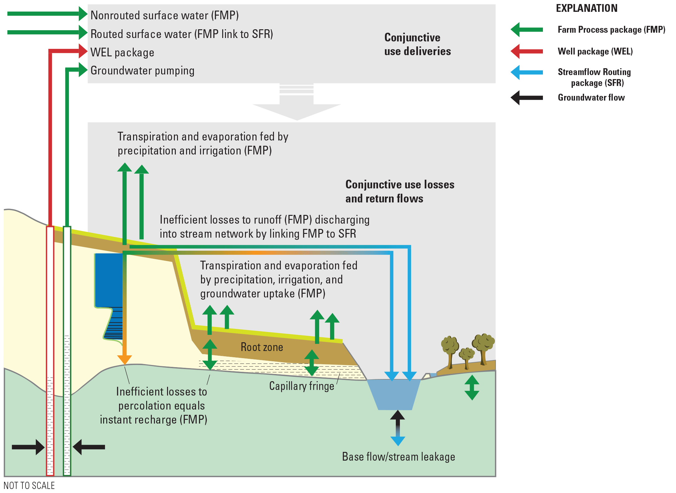
Schematic representation of components simulated by the Farm Process package in the modular finite difference flow model (MODFLOW) One-Water Hydrologic Model for the Central Platte Integrated Hydrologic Model (modified from Schmid and Hanson, 2009).
Landscape processes simulated by the FMP within the MF–OWHM include evaporation and transpiration of precipitation (Ep and Tp), evaporation and transpiration of irrigation water (Ei and Ti), surface water applied to the landscape as irrigation, groundwater applied to the landscape as irrigation, deep percolation past the root zone, and runoff (or overland flow). Within the supply and demand framework of the MF–OWHM, the supply refers to the sources of water to the landscape such as precipitation and groundwater withdrawals or surface-water deliveries for irrigation; demand refers to components of the landscape that require a water supply such as crop consumptive use or evapotranspiration (ET). The MF–OWHM also tracks the hybrid components of evaporation and transpiration of groundwater (Eg and Tg) within FMP because the Eg and Tg occur as a result of crop types specified in FMP, but Eg and Tg are not included in the calculation of the landscape budget because the water source is groundwater. A comprehensive mathematical and theoretical description of the MF–OWHM and FMP underpinnings is in the MF–OWHM and FMP documentation (Hanson and others, 2014a; Boyce and others, 2020). The key inputs to the FMP are discussed in the “Landscape Inputs and Configuration (Farm Process)” section of this report.
The MF–OWHM first calculates the crop water demand (CWD) as the product of input reference evapotranspiration (ETref) and crop coefficients (Kc); therefore, water demand on the landscape is driven by the requirements for ET. After calculation of the CWD, the MF–OWHM finds a water supply to meet the demand. The MF–OWHM determines the supply of water based on availability at a specific location. Potential water supply to meet CWD can include natural supply such as precipitation and or root uptake of groundwater for nonirrigated land uses or crops, anthropogenic supply such as surface-water deliveries from irrigation canals or groundwater pumping from irrigation wells for irrigated crops, or a combination of all four (fig. 2). For nonirrigated crops and land uses, the actual evapotranspiration (AET) is a function of the naturally available water supply and the CWD in which AET is curtailed if CWD is greater than the naturally available water supply. Additionally, any surplus naturally available water supply not used to meet the CWD either becomes runoff to a nearby stream or deep percolation past the root zone and is passed to the unsaturated zone, if present in the simulation, or becomes recharge to the groundwater system. Surface-water deliveries from irrigation canals or groundwater pumping from irrigation wells are only selected as water supply options within the MF–OWHM if crops are user-designated to receive irrigation water supply. For irrigated crops, the MF–OWHM calculates a crop irrigation requirement (CIR) based on the supply deficit between the CWD and the natural water supply available to the crop. The final irrigation amount applied to the crop accounts for irrigation efficiencies in addition to the CIR. The AET for irrigated crops is then the function of the final irrigation amount applied and the CWD (Hanson and others, 2014a; Boyce and others, 2020).
Previous Studies
The CPNRD area has been the subject of many hydrologic studies that include investigations of numerical models, recharge, geology and hydrogeology, land use, and crop water use since the late 1890s, as outlined in Peterson (2009). The earliest studies were a comprehensive description of the Great Plains geology and groundwater, including the CPNRD region of Nebraska (Darton, 1898, 1905). Numerical groundwater-flow models have been a part of several studies in the region within the CPNRD since the 1970s (Lappala and others, 1979; Peckenpaugh and Dugan, 1983; Peckenpaugh and others, 1987). Additionally, the development of groundwater-flow models has been the focus of COHYST since its inception in 1998 (Cooperative Hydrology Study, 2017). The first three COHYST groundwater-flow models were developed for three geographic regions, called model units, within COHYST—the eastern model unit, which contains the CPNRD (Peterson, 2009); the central model unit (Carney, 2008); and the western model unit (Luckey and Cannia, 2006). COHYST–2010 is the latest model developed as a part of COHYST and is a combined soil-water balance, surface water, and groundwater-flow model of the eastern and central model units (Cooperative Hydrology Study, 2017). In support of the COHYST groundwater-flow models, a COHYST study by Cannia and others (2006) included a detailed hydrogeologic study of the surface-water and groundwater resources in the Platte River Basin. Recent studies within the CPNRD include the collection of geophysical logs to delineate stratigraphic units by Anderson and others (2009) and an assessment by Exner and others (2010) of the response of nitrate in groundwater to management practices in the CPNRD. Irons and others (2012) compared surface nuclear magnetic resonance data to results from aquifer tests completed in the CPNRD, Steele and others (2014) used several methods to determine recharge and water movement through the unsaturated zone underlying several land-use types in the CPNRD, and Lauffenburger and others (2018) used a model to forecast recharge under different future climate scenarios. An airborne electromagnetic survey was completed in the CPNRD and adjacent Twin Platte Natural Resources District to develop a 3-dimensional hydrogeologic framework of the area (Cannia and others, 2017). A groundwater-flow model of the Northern High Plains aquifer, which included the CPNRD, was developed by Peterson and others (2016), and was used to simulate the effects of alternate climate and land use on groundwater conditions from 2009 through 2049 (Peterson and others, 2020).
Purpose and Scope
The purpose of this report is to document and describe the construction, calibration, and results of the CPIHM, a numerical fully integrated hydrologic model used to simulate the CPNRD hydrologic system. The scope of the study included the development of the numerical model to simulate all important hydrologic processes from the onset of surface-water irrigation in 1895 to the end of 2016 and forecasted groundwater conditions based on eight future scenarios with varying climate and limits on irrigation from 2017 through 2049. This study builds upon previous work to provide a current (2023) hydrologic model as a tool to support science-based integrated water management in the CPNRD. To meet the objective of this study, the analyses provided information about potential future water availability and changes in groundwater levels for each scenario with respect to the baseline 1982 groundwater levels and MADs that can be used by the CPNRD to update their GMP, as described in this report. Because of extensive use of groundwater and surface water for irrigation in the study area and the lack of metered irrigation pumping data for most wells throughout the development period (1895 to 2016), the MF–OWHM was selected as the best modeling code for simulating the entire hydrologic system.
Study Area Description
The study area is focused around the CPNRD, which includes parts of 10 counties in central Nebraska and a total area of 2,136,304 acres (fig. 1A). The total population of the CPNRD is 137,966, with Grand Island and Kearney being the most populous cities with 48,520 and 30,787 people, respectively (U.S. Census Bureau, 2012). The city of Columbus, with a population of about 21,000, is just outside the northeastern border of the study area (fig. 1A). The main hydrologic features are the Platte River (fig. 1A), which flows from west to east for about 205 miles, and the High Plains aquifer, which underlies the entire study area with saturated thicknesses ranging from about 50 to 550 ft (McGuire and others, 2012).
Crop production drives the local economy; from 2015 to 2017, the study area contained parts or all of four of the five counties with the highest corn production in the State (U.S. Department of Agriculture, 2019). As of 2005, the study area (Central Platte Integrated Hydrologic Model boundary-layer 1; fig. 1A) contained about 2.17 million acres of irrigated cropland, of which about 1 million irrigated acres were in the CPNRD (Center for Advanced Land Management Information Technologies, 2010). An extensive network of canals diverts water from the Platte River to surface-water irrigators in Buffalo, Dawson, Kearney, and Phelps Counties (fig. 1A). The remaining 936,000 acres are supplied by groundwater irrigation from the underlying High Plains aquifer. In addition, in some areas the water table is near enough to the crop root zone for crops to actively transpire groundwater, which reduces the net irrigation requirement in that area because less irrigation water would need to be supplied. As the water table continues to rise, actual crop ET may be reduced and eventually approach zero owing to anoxia conditions in crops that are not tolerant to waterlogging.
Physiography
The entire study area lies within the Great Plains physiographic province (Fenneman, 1931). Several subdivisions of the Great Plains province are present within the study area and can be differentiated by topographic regions that include the Bluffs and Escarpments, Dissected Plains, Plains, Sandhills, and Valleys (fig. 1B; Conservation and Survey Division, 2019). The Dissected Plains (also known as the Dissected Loess Plains) is present in portions of Buffalo, Custer, Dawson, Frontier, Gosper, Lincoln, and Logan Counties (fig. 1B) and are characterized by level to rolling hills and loess bluffs that grade into the Platte River valley to the south and east (Weaver and Bruner, 1948). Areas of considerable relief with hills of 100 ft or more were created by wind and stream erosion and produced the dissected nature of the loess deposits (Weaver and Bruner, 1948). The Dissected Plains in Frontier and Gosper counties feature deeply incised canyons and flat uplands known as “tablelands.” The dominant soil type is silt that includes the Holdrege Silt Loam and Colby Silt Loam (Weaver and Bruner, 1948; University of Nebraska-Lincoln, 2018). The Plains region located in portions of Adams, Clay, Gosper, Hall, Hamilton, Howard, Kearney, Phelps, Polk, and York counties is characterized by gently rolling hills with less relief than the Dissected Plains. The Sandhills region is present primarily in outlying portions of the main Sandhills region in portions of Buffalo, Hall, Howard, Kearney, Lincoln, Merrick, and Phelps counties (fig. 1B). The Valleys region is primarily located along the Platte River valley lowlands in portions of Buffalo, Hall, Howard, Kearney, Lincoln, Merrick, and Phelps counties (fig. 1B). The Valley lowlands are typically flood-plain areas and have minimal topographic relief with an eastward slope of 6 to 8 ft per mile (Peterson, 2009; fig. 1A–B).
Climate
The climate in the study area transitions from subhumid continental classification in the east, specified in Köppen (1936), to dry subhumid continental classification in the western part of the study area (Conservation and Survey Division, 1998); that is, annual precipitation decreases westward throughout the study area. The climate is characterized by warm and humid summers and cold and windy winters. The 30-year (1981 to 2010) average annual climate normal for precipitation is 29.12 inches at Columbus; 25.23 inches at Kearney; and 23.71 inches at Gothenburg (fig. 1A) (National Climatic Data Center, 2019). The 30-year (1981 to 2010) average climate normal for summer minimum and maximum temperatures is 63.5 and 74.3 degrees Fahrenheit (°F) at Columbus; 60.3 and 72.4 °F at Kearney; and 60.4 and 72.9 °F at Gothenburg (National Climatic Data Center, 2019). The 30-year (1981 to 2010) average climate normal for winter minimum and maximum temperature is 15.7 and 25.1 °F at Columbus; 14.9 and 26.2 °F at Kearney; and 16.0 and 27.9 °F at Gothenburg (National Climatic Data Center, 2019).
Reference ET (ETref) was measured at University of Nebraska-Lincoln Extension field sites at Clay Center, Nebr. (not shown) located in the center of Clay County and in North Platte, Nebr. (not shown), about 25 miles west of Brady from 1983 through 2003 (fig. 1A; Irmak and Skaggs, 2011). Average annual ETref at Clay Center was 61.7 inches and 62.4 inches for North Platte, which is substantially higher in the study area than average annual precipitation (24.3 inches) and is typical for the subhumid climate classifications. Average monthly ETref rates exceed precipitation rates throughout the year measured at locations near Clay Center and North Platte (Irmak and Skaggs, 2011; National Climatic Data Center, 2019). Average annual AET rates for a period between 2000 and 2009 are about 24.8 inches in the study area (Szilágyi and Kovacs, 2010). However, local AET values generally exceed precipitation by as much as 130 percent for areas with widespread irrigation of crops, whereas areas with natural vegetation generally exhibit less AET compared to precipitation (Szilágyi and Kovacs, 2010). Further, AET is generally lower in the eastern part of the study area than the western area for natural vegetation while irrigated crops exhibit similar AET values across the study area (Szilágyi and Kovacs, 2010).
Land Use, Crop Coefficients, and Water Use
Land use and water use in the study area are linked and are important characteristics of the supply and demand driven hydrologic system. Prior to the Civil War (1861 to 1865), the primary land uses in Nebraska were range, pasture, and grass (Hiller and others, 2009). The adoption of the Homestead Act in 1862, the end of the Civil War in 1865, and Nebraska’s statehood in 1867 encouraged settlers to move westward into the study area. In 1895, total cropland area was about 90 percent of 2005 total cropland area (Hiller and others, 2009). Since the mid-1960s, crop diversity in Nebraska decreased, and cropland is now dominated by corn and soybeans (Hiller and others, 2009).
The primary land use since the 1890s has been cultivated crops such as corn, soybeans, and winter wheat. By 1895, canals were developed to deliver surface water for crop irrigation to areas in Buffalo, Dawson, Phelps, and Kearney counties (Hiller and others, 2009; Peterson, 2009). The first irrigation wells were drilled and began pumping groundwater from the alluvial aquifer along the Platte River around 1900 (Nebraska Department of Natural Resources, 2017). Most irrigated land prior to 1940 was irrigated with surface water from canals diverted onto fields using flood irrigation techniques, but after 1940, with improvements in well-drilling technology and later the invention of the more efficient center-pivot irrigation systems, groundwater-irrigated land increased as dryland crops were converted to irrigated cropland. Since 1940, about 29,000 irrigation wells have been drilled in the study area, with most drilled between 1955 and 1990 (fig. 3; Nebraska Department of Natural Resources, 2017). In 2016, the density of irrigation wells in the study area was 3.8 wells per square mile; because of this high density, the CPNRD does not allow the drilling of new irrigation wells or development of new irrigated acres unless other irrigation wells or acres are retired (Central Platte Natural Resources District, 2019). Some irrigators have surface-water rights and groundwater wells for irrigation; the irrigated land that receives water from surface water and groundwater is described as “commingled.” Irrigators with commingled land primarily use their surface-water right and may supplement with groundwater from wells when necessary.
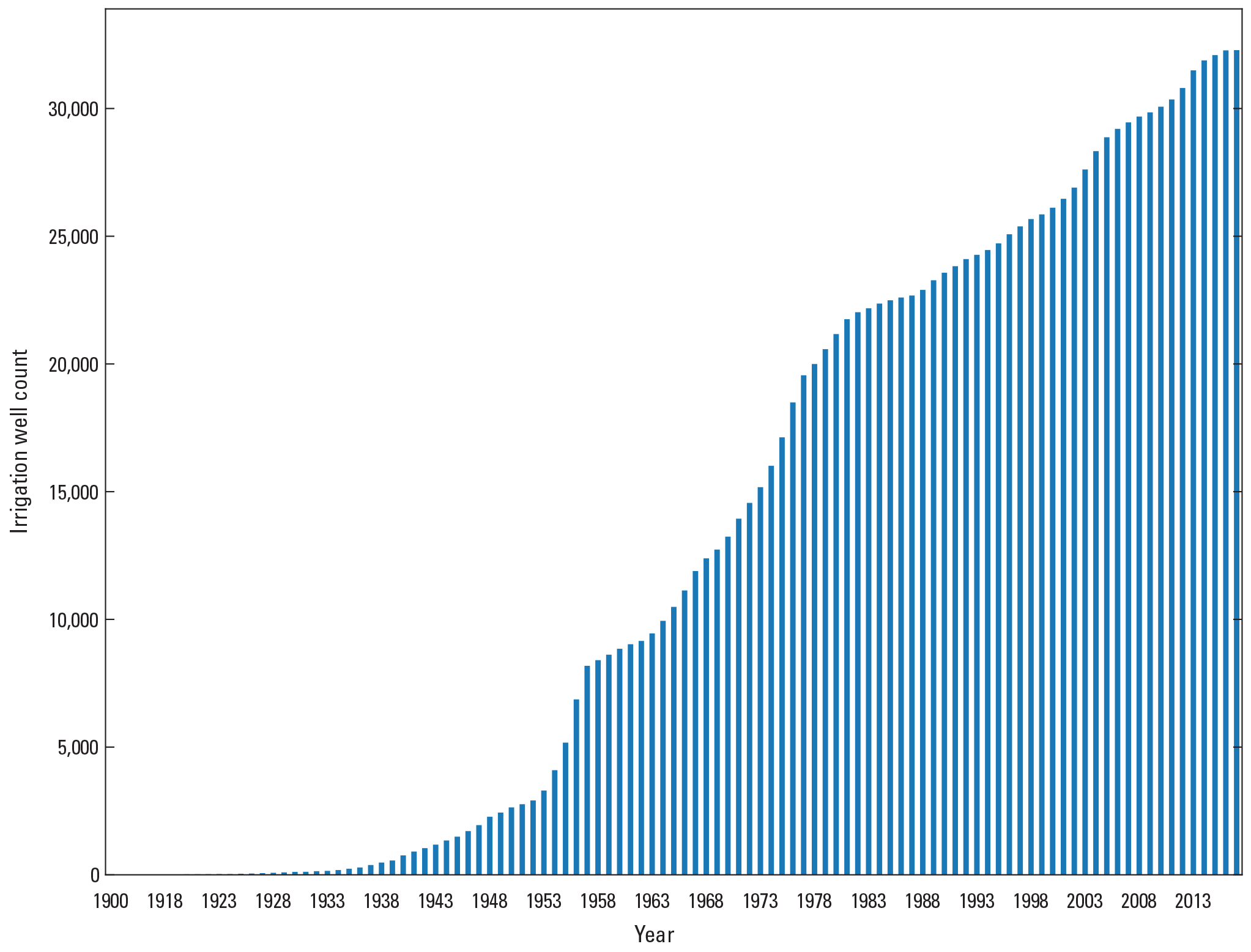
Irrigation well development in the study area from 1900 to 2016 (Nebraska Department of Natural Resources, 2017).
Within the study area, long-term land use data were available from the Cooperative Hydrology Study (2017). These data indicate that by 1950, land use in the study area was about 53 percent pasture (2,632,858 acres), 29 percent dry cropland (1,658,659 acres), 13 percent other uses (406,679 acres), and 5 percent irrigated cropland (227,884 acres; Cooperative Hydrology Study, 2017). The other land uses include open water, urban, riparian forest and wetlands, and roads. Between 1950 and 2016, dry cropland and pasture were converted to irrigated land supplied by groundwater wells. In 2016, the distribution was 47 percent irrigated land with 43 percent irrigated by groundwater (2,289,189 acres), 39 percent pasture (1,926,600 acres), 10 percent dry cropland (495,197 acres), and 4 percent other uses (215,094 acres; Cooperative Hydrology Study, 2017; fig. 4A, B). The development of irrigated cropland from 1950 to 2005 has taken place primarily from Buffalo County in the central part of the study area to Polk and York Counties in the eastern part of the study area (fig. 4B).
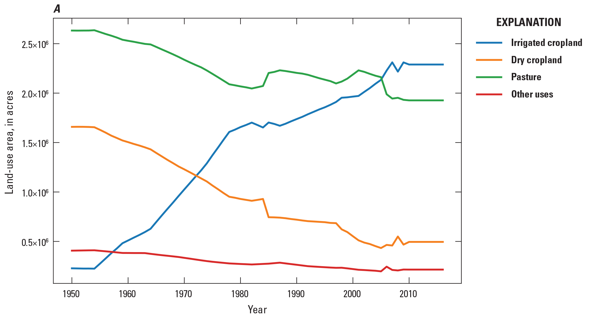

Land-use distribution within the study area, central Nebraska. A, Trends of irrigated cropland, dry cropland, pasture, and other uses, from 1950 through 2016. B, Groundwater irrigated cropland, dry cropland and pasture, and surface water irrigated cropland from 1950, 1985, and 2005 (this figure is a layered .pdf).
Crop coefficients (Kc), which are properties ascribed to plants and used to estimate AET, vary depending on land use or crop type. Allen and others (1998) reported Kc values for the two most common land uses, rangeland and corn, that vary from 0.15 to 1.05 and 0.15 to 1.20 for different parts of the growing season cycle. Crops typically are irrigated between May and September each year based on planting dates and harvesting dates from the U.S. Department of Agriculture (1997 and 2016). Further, the largest amounts of irrigation typically occur in July and August when there is the most difference between ETref and precipitation. The fraction of AET that comes from plant transpiration also varies across a single year, much like Kc values. For example, AET during the nongrowing season is predominantly from the evaporation because plants are absent or dormant. Alternately, AET is predominantly transpiration during the middle of the growing season when leaf area index is largest, and more plant surface area is available to transpire.
The primary water use has evolved since the late 1800s from surface-water irrigation to groundwater irrigation. In the late 1890s, surface water for irrigation was the primary water use by way of several canals (Peterson, 2009; fig. 1A). Groundwater irrigation development prior to 1940 was limited to about 760 wells (fig. 3) that irrigated about 158,000 acres. Based on 5-year water use survey data, groundwater irrigation became the primary water use after 1950, and from 1985 to 2015 the total groundwater withdrawals for irrigation were 480 to 840 million gallons per day (Mgal/d) or about 75 to 93 percent of the total water use in the Buffalo, Dawson, Hall, and Merrick counties (U.S. Geological Survey, 2017; fig. 5). Prior to the development of center-pivot irrigation systems in the early 1950s, groundwater pumped for irrigation was applied using less efficient flood irrigation methods. Flood irrigation efficiency prior to 1940 was assumed to be 50 percent (Irmak and others, 2011).
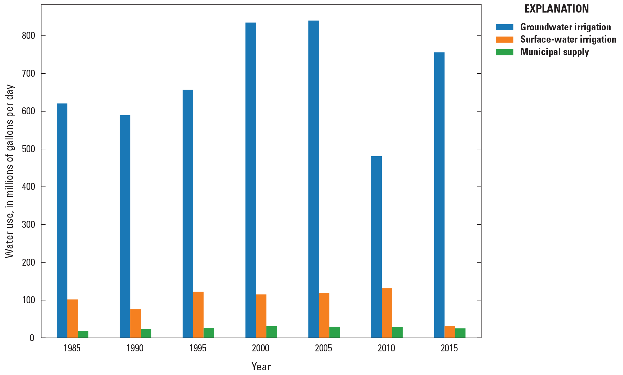
Primary annual water uses in Buffalo, Dawson, Hall, Merrick counties (U.S. Geological Survey, 2017).
Groundwater use for irrigation within the study area is affected by precipitation; irrigation withdrawals are generally higher during years of lower-than-average precipitation and less in years of higher-than-average precipitation. For example, the reduction in groundwater use for irrigation in 2010 can be attributed to an increase in precipitation compared to other years. Surface water used for irrigation accounted for about 32 to 132 Mgal/d or about 2 to 20 percent of total use (fig. 5). All public supply is from groundwater, and those withdrawals accounted for about 19 to 31 Mgal/d or about 3 to 5 percent of total withdrawals (fig. 5). In 2016, the primary water use in the study area was groundwater for irrigation and the secondary water use was groundwater used for public supply (Dieter and others, 2018).
Surface Water
The surface-water network consists of man-made irrigation canals and natural streams generally flowing west to east for five subregional watersheds: the Big Blue, Little Blue, Loup, Platte, and Republican Rivers (fig. 1C). The Platte River watershed is the primary watershed that constitutes the central region and includes the major streams such as the Platte River, Wood River, and Prairie Creek (fig. 1C). The Platte River flows eastward through the study area from Brady, Nebr., in the west through Kearney, Nebr., and Grand Island, Nebr., in the central region, before flowing out of the study area a few miles east of Duncan, Nebr. (not shown) (fig. 1A). The Platte River has the largest average annual flows in the study area. The mean annual streamflow at the Platte River near Duncan, Nebr. (USGS streamgage 06774000) is 1,420 cubic feet per second (ft3/s) for the period of record from 1895 to 2016 (U.S. Geological Survey, 2017). The Platte River is a braided stream often with two or three main channels for much if its path through the study area (Alexander and others, 2013). The South Loup and Loup Rivers flow along the northern boundary of the study area and have more tributaries draining from the north than in the study area (fig. 1C). The CPNRD boundary is approximately coincident with the Platte River watershed between Gothenburg, Nebr., and Columbus, Nebr. (fig. 1A). The Big Blue watershed is in the eastern part of the study area and includes Big Blue River and minor streams such as the Lincoln Creek and the West Fork of the Big Blue River (fig. 1C). The southern part of the study area includes the Little Blue River watershed in the east, which is drained by minor streams such as Cottonwood Creek (not shown) and Big Sandy Creek, and the Republican River watershed in the southwest, which includes minor streams such as Deer Creek and Muddy Creek (fig. 1C). Streams that flow out of the study area include the Platte River near Columbus, Nebr.; the Big Blue River in eastern Polk County; and Lincoln Creek and Beaver Creek in eastern York County (fig. 1C). Muddy Creek and Deer Creek flow out of the study area in Frontier County (fig. 1C). The spatial location of each stream was derived from the National Hydrography Dataset (McKay and others, 2012).
Some reaches of streams leak stream water into the groundwater system, primarily in the central and eastern region (Peterson and Carney, 2002). Stream leakage depends on stream physical properties such as vertical hydraulic conductivity of the streambed, streambed thickness, channel width, and the hydraulic gradient between the stream stage and the groundwater. Calibrated vertical streambed hydraulic conductivity from groundwater-flow models developed in Peterson (2009) and Peterson and others (2016) ranged from 0.1 to 10 feet per day (ft/d). Data were unavailable to define streambed thickness; therefore, streambed thickness was assumed to be a uniform constant value of 3 ft for all streams. Stream channel widths were defined using recent areal satellite imagery from Google Earth (Google, 2018). Streambed hydraulic conductivity was also assumed to be related to the predominant soil type in that location because streams in the study area are shallow and generally do not cut into bedrock, except in the southwestern part of the study area (fig. 1B).
A network of eight canals divert surface water from the Platte River for irrigation. The earliest canals began diverting water in 1895 and include Cozad Canal, Dawson County Canal, Gothenburg Canal, Kearney Canal, Orchard-Alfalfa Canal, and Sixmile Canal (fig. 1C). Elm Creek Canal (not shown) and Thirtymile Canal began diverting water from the Platte River in 1932 and 1928, respectively (fig. 1C). By 1940, the eight canals (Cozad Canal, Dawson County Canal, Orchard-Alfalfa Canal, Gothenburg Canal, Sixmile Canal, Kearney Canal, Thirtymile Canal, and Elm Creek Canal) were operating in the CPNRD with the water rights to divert an estimated 200,000 acre-feet per year (acre-ft/yr) (Peckenpaugh and others, 1987; Nebraska Department of Natural Resources, 2019), which is similar to the estimated annual diversion of 193,000 acre-feet in recent years; diversion amounts can vary slightly from year to year (Peterson, 2009). After 1940, the Central Nebraska Public Power and Irrigation District (CNPPID) constructed the Tri-County and Phelps Canals, which diverted surface water from the Platte River west of the study area but had about 130,000 acre-feet leakage through the canal and lateral beds within the study area each year (Peterson, 2009). An estimated 40 percent of the diverted water to the CPNRD canals, about 80,000 acre-ft/yr, leaks through the canal and lateral beds and recharges the aquifer (Peterson, 2009; Peterson and others, 2016). The annual leakage has contributed to increases in base flow of the Platte River and some tributaries in the area (Peckenpaugh and others, 1987). Two reservoirs, Johnson Lake and Elwood Reservoir, built in 1941 and 1974, respectively, exhibit stages above the water table in the area and leak water to the underlying aquifer (Central Nebraska Public Power and Irrigation District, 2019). Hydraulic head values for Johnson Lake and Elwood Reservoir were determined using the mean lake/reservoir stage for each stress period after construction (Central Nebraska Public Power and Irrigation District, 2019).
Hydrogeology and Groundwater
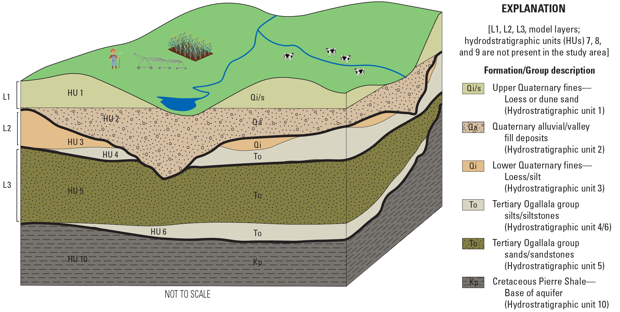
The Northern High Plains aquifer is a part of the High Plains aquifer (Peterson and others, 2016) and constitutes the primary groundwater aquifer in the study area. The geologic units in the study area consist of Quaternary-age valley-fill deposits, dune sand, loess, and alluvium, and Tertiary-age Ogallala Formation silt and sandstone (Gutentag and others, 1984). The most recent units are the Holocene-age valley-fill deposits located in stream valleys that consist of coarser materials such as sands and gravels, and the wind-blown dune sand deposits present in isolated parts of the study area (fig. 6). The wind-blown Pleistocene loess deposits are present throughout the study area and contain silt and fine-grained sands and clays. Pleistocene alluvial deposits, commonly referred to as “Paleo-channels,” also are present throughout the study area as stream deposits that consist of sands and gravels. The geologic units with similar hydraulic properties such as water storage and permeability were grouped into hydrostratigraphic units (HUs) and described in Cannia and others (2006) for incorporation into groundwater-flow models developed in Luckey and Cannia (2006), Carney (2008), and Peterson (2009). The spatial distribution of HUs in the study area is presented as a fence diagram in figure 36 of Cannia and others (2006).
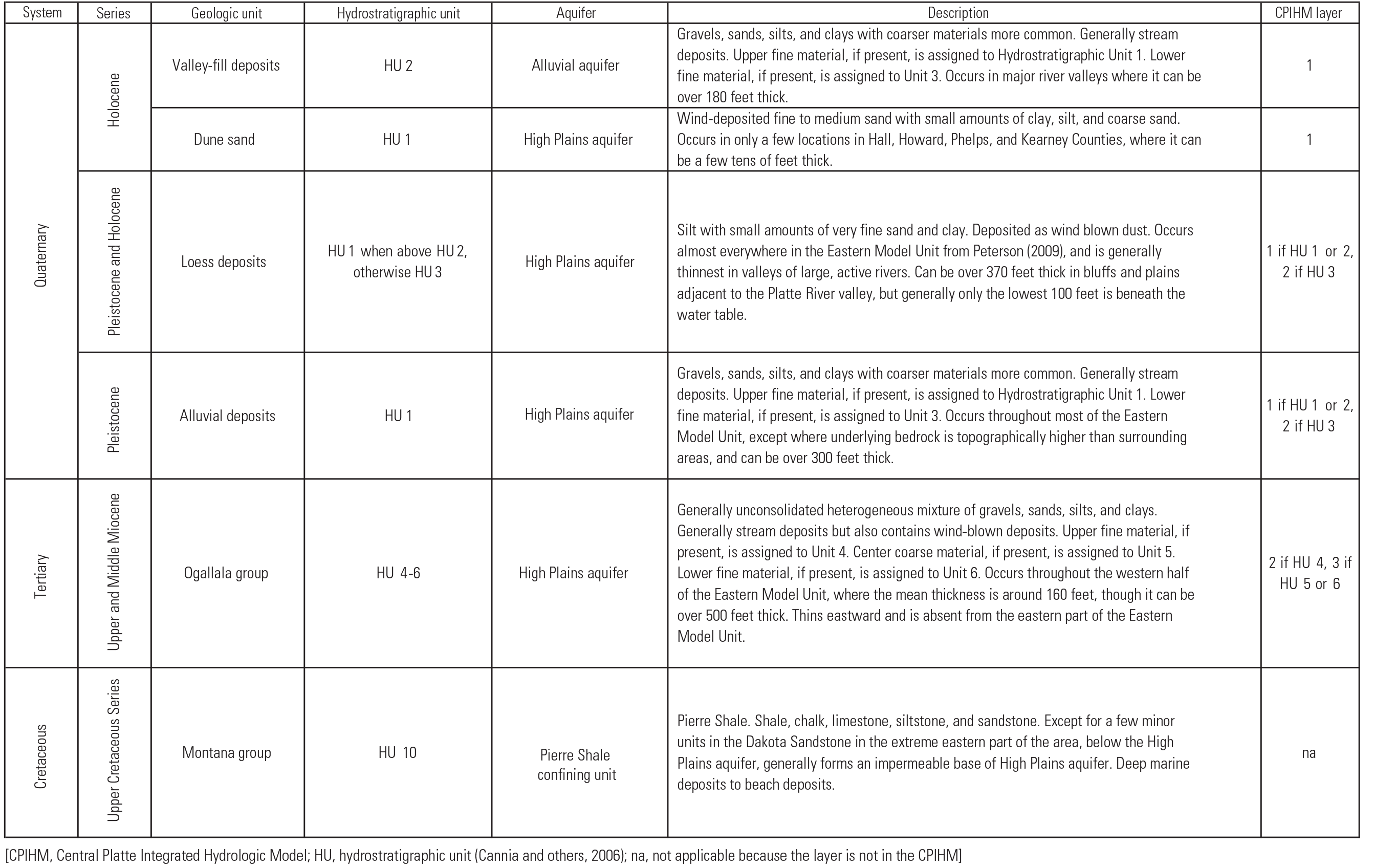
Generalized section of geologic units, hydrostratigraphic units delineated by Cannia and others (2006) (modified from Peterson, 2009), aquifers present in the study area, and the model layers for the Central Platte Integrated Hydrologic Model.
The Ogallala Formation is the principal geologic unit that forms the Northern High Plains aquifer (Gutentag and others, 1984). The Northern High Plains aquifer is the primary aquifer in the study area, is hydrologically connected to the Quaternary-age alluvial aquifers, and includes the Quaternary-age deposits and Tertiary-age Ogallala Formation (Cannia and others, 2006). The study area contains HUs 1–6 from Cannia and others (2006), where HUs 1 and 2 consist of Quaternary-age valley-fill, loess deposits, and alluvial aquifers; HUs 3 and 4 consist of the finer grained and less permeable Quaternary-age loess deposits and Upper-Tertiary-age portions of the Ogallala Formation; and HUs 5 and 6 consist of the sands, sandstones, silts, and gravels of the Ogallala Formation. Although HUs 3 and 4 are less permeable deposits, they are not confining units between coarser HUs 1 and 2 and HUs 5 and 6; therefore, each of the six HUs are hydrologically connected within the study area. The base of the Northern High Plains aquifer in the study area is the Cretaceous-age Pierre Shale, which is HU 10 (fig. 6). The Nebraska portion of the Northern High Plains aquifer has exhibited a loss of 6 million acre-feet of recoverable storage from predevelopment to 2015 (McGuire, 2017). The Northern High Plains aquifer serves as the source for all groundwater irrigation and public supply wells in the study area.
The groundwater is characterized by west to east regional groundwater flow (Peterson and others, 2016). Within each watershed in the study area, consistent with the regional flow system, groundwater typically flows west to east and either flows out of the study area on the eastern edge or discharges as base flow to streams. Locally, groundwater flows toward streams in the western portion of the study area where steams are gaining flow from groundwater, and groundwater flows away from streams in the central and eastern portions of the study area where streams are losing flow to groundwater. Groundwater discharge to streams, referred to as “base flow,” is a component of flow in most streams but not all reaches. Base flow is affected by pumping of wells near streams (Kollet and Zlotnik, 2003).
Aquifer properties, particularly horizontal hydraulic conductivity (Kh) and specific yield (Sy) have been evaluated in previous studies. Houston and others (2013) estimated Kh and Sy at test holes in the Northern High Plains aquifer, using lithologic logs to interpret Kh and Sy for vertical intervals of the aquifer. Peterson (2009) included the calibrated Kh for HUs 1 through 6; HUs 1 and 2 had Kh values of about 10 and 155 ft/d, respectively (table 1; table 3 in Peterson, 2009). The intervals representing HUs 3 and 4 consisted of predominantly silt. These two HUs had similar Kh of about 8 ft/d and acted as a semiconfining unit for most of the study area (Peterson, 2009). The average Kh for the interval representing HUs 5 and 6 was about 33 and 10 ft/d, respectively (Peterson, 2009).
Table 1.
Horizontal hydraulic conductivity and specific yield estimates for the Central Platte Integrated Hydrologic Model by hydrostratigraphic unit and model layer/group and derived from Peterson (2009) and Houston and others (2013).[HU, hydrostratigraphic unit; <, less than]
Value from Peterson (2009) are averages across coincident hydrostratigraphic units of the calibrated model.
Mean Kh estimates for test holes were highest for the interval representing HUs 1 and 2 at 66.6 ft/d (table 1; Houston and others, 2013). Mean Kh for the intervals representing HUs 3–6 were similar; however, the range in Kh for the upper of these intervals was from less than 1 to 325 ft/d and for the lower interval from about 5.6 to 67.7 ft/d, indicating that the lower interval sediments are much more homogeneous than the interval representing HUs 3 and 4 (table 1). Sy values were similar to the average Sy for the Northern High Plains aquifer of about 0.15 (table 1; Houston and others, 2013; McGuire, 2017).
Additionally, recharge rates to groundwater through the unsaturated zone ranged from 0.2 to 10 inches per year (in/yr) based on values measured across the CPNRD on irrigated land, dryland, and rangeland (Steele and others, 2014). Calibrated recharge simulated in Peterson (2009) had a range of about 1 to 7 in/yr (see fig. 16 and table 9 from Peterson, 2009). Calibrated recharge simulated in Peterson and others (2016) had a range of about 2 to 5 in/yr (see fig. 20B from Peterson and others, 2016).
Integrated Hydrologic Model
This section of the report describes the conceptual model of the hydrologic system, construction, and calibration of the CPIHM; results of the calibration; and scenario results of the CPIHM. The CPIHM is a numerical integrated hydrologic model developed for the CPNRD using a MODFLOW-based groundwater modeling software called MF–OWHM (Boyce and others, 2020). The MF–OWHM is a fully coupled (or fully integrated) landscape, surface water, and groundwater-flow model, which makes it a hydrologic-flow model in addition to a groundwater-flow model.
Conceptual Model of the Hydrologic System
The conceptual model of a hydrologic system is a schematic of the water cycle for a given study area that identifies and describes sources, sinks, and reservoirs of water in that system. The three main hydrologic subsystems represented in the conceptual model were the landscape water, surface water, and groundwater. The interface of each subsystem is a hydrologic boundary. Each subsystem consists of components that represent sources, sinks, and reservoirs of water. A source of water is the addition of water to a subsystem (hereafter referred to as “inflows”). A sink of water is the discharge or removal of water from a sub-system (hereafter referred to as “outflows”). Reservoirs represent water stored in a subsystem that is not an inflow or outflow. This conceptual model, to the extent possible, also describes the approximate magnitude of the reservoirs and fluxes of water for each component of the hydrologic system (referred to as “water budgets”), which creates a blueprint for construction of the numerically based computer model. After characterization of the inflows and outflows, the conceptual model becomes the framework for the accurate construction and development of the numerical hydrologic-flow model. The three subsystem components of the numeric model (climate and landscape, surface water, and groundwater) are conceptualized and described below. Conceptual descriptions include calculated fluxes representing the interaction between the subsystems and internal flows within the subsystems.
The conceptual flux estimates presented in this section of the report are based on previous studies in or near the area as described in this section and the "Previous Studies" section of this report, adapted to the 4,926,071-acre CPIHM active domain (fig. 1A). Conceptual flux estimates are presented for two time periods to represent the major periods of groundwater development: the period prior to widespread groundwater irrigation development (approximately 1940), and a recent period (approximately 2011 to 2016; tables 2 and 3). There was a wide range of values for ET and groundwater irrigation pumping because of the lack of available data to accurately characterize component values or a large uncertainty in the available published data or studies. The understanding of uncertainty and error in the conceptual estimates was applied in the development and calibration of the CPIHM.
Table 2.
Conceptual flux estimates for pre-1940 and recent development (2011–16) periods for the landscape subsystem fluxes of evapotranspiration of precipitation and irrigation water for the Central Platte Integrated Hydrologic Model.[nc, not calculated because there were not enough data available; negative flux values indicate outflows from the respective subsystem; positive flux values indicate inflows to the respective subsystem]
| Period | Area (acres) |
Irrigation wells | Evapotranspiration of precipitation and irrigation water | Evapotranspiration of precipitation and irrigation water range | Irrigation wells range | Evapotranspiration references |
|---|---|---|---|---|---|---|
| Pre-1940 | 4,926,071 | 263,000 | −8,600,000 | nc | 263,000–203,000 | Irmak (2014), Kranz and others (2008) |
| 2011–16 | 4,926,071 | 1,800,000 | −9,500,000 | −8,800,000 to −11,000,000 | 1,980,000–2,160,000 | Irmak (2014), Kranz and others (2008) |
Table 3.
Conceptual flux estimates for pre-1940 and recent development (2011–16) periods for the groundwater subsystem fluxes of outflows to irrigation wells for the Central Platte Integrated Hydrologic Model.[AET, actual evapotranspiration]
| Period | Area (acres) |
Outflow to irrigation wells | Irrigation wells range | Irrigation description |
|---|---|---|---|---|
| Pre-1940 | 4,926,071 | −263,000 | −286,000 to −203,000 | Irrigated acres in 1950 multiplied by average irrigation depth of 10 inches per year based on difference between growing season precipitation and irrigated corn AET. The range was based on efficiency between 50 and 65 percent (Peterson, 2009; Irmak and others, 2011). |
| 2011–16 | 4,926,071 | −1,990,000 | −1,990,000 to −2,190,000 | Irrigated acres in 2011–16 multiplied by average irrigation depth of 10 inches per year based on difference between growing season precipitation and irrigated corn AET. The range was based on efficiency between 80 and 90 percent (Peterson, 2009; Irmak and others, 2011). |
Climate and Landscape Components
The landscape in the study area includes land-use characteristics such as crop type, ET characteristics for each crop type, soil types, and surface-water characteristics. The landscape is characterized by an extensive surface-water network that includes major streams as described in the “Surface Water” section of this report. The climate and landscape water subsystems include inflows from precipitation; root uptake; inflows from surface-water deliveries or groundwater used for irrigation, runoff, and deep percolation past the root zone; and outflows of ET (broken down by source of water).
Precipitation is the largest inflow to the landscape, although locally the inflows from irrigation can exceed precipitation, particularly in drought conditions. Most surface-water deliveries occur to meet irrigation demands between May and September (table 1.1). Outflows from the landscape subsystem include ETp, ET of irrigation water, ETg that passes through the landscape, deep percolation past the root zone, and runoff of precipitation to streams. ET of irrigation water is generally the largest outflow from the landscape subsystem. Measured annual AET rates varied based on land cover and precipitation. Rangeland had the highest rates of AET that range from 22 to 36 in/yr depending on precipitation and location (Irmak, 2014). Regional irrigated and dry cropland annual AET rates were about 21.6 and 16.8 in/yr, respectively (Irmak, 2014). The AET of irrigated corn, the predominant crop in the study area, was 25.9 in/yr based on nearby measurements (Kranz and others, 2008). Based on average AET rates and land use reported by the Cooperative Hydrology Study (2017), the estimated annual volume of total AET of precipitation and irrigation was about −8,600,000 acre-feet for pre-1940 and about −9,500,000 acre-feet for the recent development period (2011–16; table 2). The uncertainty associated with these estimates was difficult to quantify owing to the lack of AET rates available for all land uses within the study area and the lack of an uncertainty assessment in the mentioned studies. The range of AET for the recent development period (2011–16), was about −8,800,000 to −11,000,000 acre-ft/yr based on the range of irrigated corn AET and rangeland AET in Kranz and others (2008), Irmak (2014), and Cooperative Hydrology Study (2017). The ET of irrigation water is conceptually difficult to estimate because precipitation and irrigation occur on the same area across similar time periods; therefore, the landscape ET component in table 2 combines ETp and ET of irrigation water sources.
Deep percolation past the root zone (often referred to as recharge) in the study area has been estimated at 0.2 to 2.1 in/yr below rangeland (that is, pasture), 2.7 to 6.3 in/yr below groundwater-irrigated cropland, 10 in/yr below surface-water irrigated cropland, and 0.5 to 2.5 in/yr below dry cropland (Steele and others, 2014). Additionally, recharge in the study area that occurs as leakage from the unlined irrigation canals can exceed 10 in/yr (Peterson and others, 2016). The highest recharge rates in areas without canal influence were about 4 to 6 in/yr in the flat, densely groundwater-irrigated cropland in the Platte River valley (Peterson and others, 2016).
Surface-Water Components
Surface-water inflows include streamflow that enters the study area, groundwater that discharges through the streambed as base flow, and runoff. Outflows include leakage of stream water into the underlying aquifer and outflows of streamflow where streams exit the study area. Runoff from precipitation was estimated for the study area using base flow separation techniques in the USGS Groundwater Toolbox (table 4; Barlow and others, 2014; 2017) from streamgage data for the Platte River, Prairie Creek, Silver Creek, and Wood River (table 4; fig. 1A). Streamgages were present at locations of major stream inflows and outflows in the study area for most or all of the development period, which provided adequate data to estimate the gaged flows in and out of the surface-water system. Minor streams that flowed into the study area that were ungaged along the Loup River boundary streams were estimated with flows of about 5 ft3/s for the entire period of interest based on stream width from aerial imagery and an assumed depth of 1 ft. The largest gaged inflows are at the North Loup River near St. Paul, Nebr. (USGS streamgage 06790500; fig. 1A), which has an average discharge of 853 ft3/s for the period of record 1928 to 2016 (U.S. Geological Survey, 2017). However, the Loup River system is a boundary stream; the largest gaged inflows for a nonboundary stream are at the Platte River at Brady, Nebr. (USGS and Nebraska Department of Natural Resources [NeDNR] streamgage 06766000; fig. 1A) with an average total inflow of about 746 ft3/s for the period from 1939 to 2016 (table 4). The largest outflows are at the Platte River about 5 miles downstream from the Platte River near Duncan, Nebr. (USGS streamgage 06774000: fig. 1A), which has an average discharge of 1,742 ft3/s for the period from 1939 to 2016 (U.S. Geological Survey, 2017). For the pregroundwater irrigation development period (pre-1940), total flow into the study area at the Platte River at Brady, Nebr. (USGS streamgage 06766000) was about 1,541 ft3/s. The outflow at the Platte River near Duncan, Nebr. (USGS streamgage 06774000) for the pre-1940 period was about 1,620 ft3/s; the overland flow portion of total streamflow was estimated to be an outflow of about 497 ft3/s (about 360,000 acre-ft/yr or 1 inch) within the Platte River watershed, based on values obtained from Cooperative Hydrology Study (2017). For the recent period (2011 to 2016), total streamflow and runoff at the Platte River at Brady, Nebr. (USGS streamgage 06766000) were about 1,102 ft3/s and 427 ft3/s, respectively. Recent period (2011–16) total streamflow and runoff at the Platte River near Duncan, Nebr. (USGS streamgage 06774000) were about 2,495 and 884 ft3/s, respectively (table 4). Runoff was estimated to be an outflow of about 460,000 acre-ft/yr (about 635 ft3/s or 1.11 inches) within the Platte River watershed, which contributes to the runoff at the Platte River near Duncan, Nebr. (USGS streamgage 06774000) based on values obtained from Cooperative Hydrology Study (2017; fig. 1A).
Table 4.
Average base flow, runoff, and total streamflow for primary U.S. Geological Survey National Water Information System streamgages in the study area, central Nebraska.[ID, identification; MM, month; DD, day; YYYY, year; NE, Nebraska; --, no data; NA, not available]
| Site ID | Site name | Period of record (MM/DD/YYYY) |
Flows, in cubic feet per second | Data source | ||
|---|---|---|---|---|---|---|
| Average baseflow | Average runoff | Average total flow | ||||
| 06766500 | Platte River near Cozad, NE | 10/1/1940–9/29/1991 | 328 | 347 | 674 | U.S. Geological Survey (2017) |
| 06770000 | Platte River near Odessa, NE | 10/1/1938–9/29/1991 | 1,002 | 479 | 1,487 | U.S. Geological Survey (2017) |
| 06770200 | Platte River near Kearney, NE | 1/27/1982–12/31/2016 | 1,080 | 718 | 1,797 | U.S. Geological Survey (2017) |
| 06770500 | Platte River near Grand Island, NE | 4/1/1934–12/31/2016 | 820 | 713 | 1,532 | U.S. Geological Survey (2017) |
| 06773050 | Prairie Creek near Ovina, NE | 5/30/1991–9/30/1999 | 6 | 11 | 18 | U.S. Geological Survey (2017) |
| 06773150 | Silver Creek at Ovina, NE | 5/31/1991–9/29/1995 | 3 | 7 | 11 | U.S. Geological Survey (2017) |
| 06773500 | Prairie Creek near Silver Creek, NE | 9/30/2001–1/1/2020 | 15 | 22 | 37 | U.S. Geological Survey (2017) |
| 06766000 | Platte River at Brady, NE | 3/1/1939–12/31/2016 | 347 | 394 | 746 | Nebraska Department of Natural Resources (2019), U.S. Geological Survey (2017) |
| 06774000 | Platte River near Duncan, NE | 10/25/1928–12/31/2016 | 923 | 813 | 1,742 | Nebraska Department of Natural Resources (2019), U.S. Geological Survey (2017) |
| 06768000 | Platte River near Overton, NE | 10/1/1930–12/31/2016 | 905 | 652 | 1,560 | U.S. Geological Survey (2017) |
| 06771000 | Wood River near Grand Island, NE | 3/1/2006–11/30/2011 | 18 | 19 | 37 | U.S. Geological Survey (2017) |
| 06766500 | Platte River near Cozad, NE | -- | -- | -- | -- | NA |
| 06770000 | Platte River near Odessa, NE | 10/1/1938–12/31/1939 | 1 | 145 | 1,108 | U.S. Geological Survey (2017) |
| 06770200 | Platte River near Kearney, NE | -- | -- | -- | -- | NA |
| 06770500 | Platte River near Grand Island, NE | 7/1/1934–12/31/1939 | 215 | 702 | 922 | U.S. Geological Survey (2017) |
| 06773050 | Prairie Creek near Ovina, NE | -- | -- | -- | -- | NA |
| 06773150 | Silver Creek at Ovina, NE | -- | -- | -- | -- | NA |
| 06773500 | Prairie Creek near Silver Creek, NE | -- | -- | -- | -- | NA |
| 06766000 | Platte River at Brady, NE | 3/1/1939–12/31/1939 | 570 | 474 | 1,541 | Nebraska Department of Natural Resources (2019), U.S. Geological Survey (2017) |
| 06774000 | Platte River near Duncan, NE | 11/1/1928–12/31/1939 | 649 | 962 | 1,620 | Nebraska Department of Natural Resources (2019), U.S. Geological Survey (2017) |
| 06768000 | Platte River near Overton, NE | 10/1/1930–12/31/1939 | 608 | 833 | 1,470 | U.S. Geological Survey (2017) |
| 06771000 | Wood River near Grand Island, NE | -- | -- | -- | -- | NA |
| 06766500 | Platte River near Cozad, NE | -- | -- | -- | -- | NA |
| 06770000 | Platte River near Odessa, NE | -- | -- | -- | -- | NA |
| 06770200 | Platte River near Kearney, NE | 1/1/2011–12/31/2016 | 1,441 | 801 | 2,243 | U.S. Geological Survey (2017) |
| 06770500 | Platte River near Grand Island, NE | 1/1/2011–12/31/2016 | 1,547 | 744 | 2,291 | U.S. Geological Survey (2017) |
| 06773050 | Prairie Creek near Ovina, NE | -- | -- | -- | -- | NA |
| 06773150 | Silver Creek at Ovina, NE | -- | -- | -- | -- | NA |
| 06773500 | Prairie Creek near Silver Creek, NE | 1/1/2011–12/31/2016 | 7 | 11 | 18 | U.S. Geological Survey (2017) |
| 06766000 | Platte River at Brady, NE | 1/1/2011–12/31/2016 | 675 | 427 | 1,102 | Nebraska Department of Natural Resources (2019), U.S. Geological Survey (2017) |
| 06774000 | Platte River near Duncan, NE | 1/1/2011–12/31/2016 | 1,611 | 884 | 2,495 | Nebraska Department of Natural Resources (2019), U.S. Geological Survey (2017) |
| 06768000 | Platte River near Overton, NE | 1/1/2011–12/31/2016 | 1,449 | 856 | 2,306 | U.S. Geological Survey (2017) |
| 06771000 | Wood River near Grand Island, NE | 1/1/2011–11/30/2011 | 15 | 15 | 30 | U.S. Geological Survey (2017) |
Groundwater Components
Inflows to the groundwater-flow system include recharge from the landscape subsystem deep percolation component, recharge as canal leakage from the CPNRD and CNPPID canal systems, stream leakage, and cross-boundary flow into the active model area. Recharge rates are described in the “Climate and Landscape Components” section of this report. Outflows from the groundwater-flow system include cross-boundary flow out of the active model area, discharge to streams as base flow, withdrawals from irrigation wells, withdrawals from municipal wells, and ETg. Transient changes in groundwater inflows and outflows are balanced by increases or decreases of groundwater in storage. When inflows are greater than outflows, aquifer storage increases (rise in groundwater levels), and when inflows are less than outflows, aquifer storage decreases (decline in groundwater levels).
Groundwater-flow subsystem components as annual inflows on the left-hand side and annual outflows on the right-hand side are presented in equation 1:
(1)
lake leakage
is the water that leaks through a lakebed and becomes groundwater recharge,
flow from adjacent zones
is the cross-boundary inflow of groundwater to the study area,
recharge
is the deep percolation of landscape water to the groundwater-flow system,
canal leakage
is the water that leaks through a canal bed and becomes groundwater recharge,
stream leakage
is the water that leaks through the streambed and becomes groundwater recharge,
releases from groundwater storage
is the release of groundwater from storage into the groundwater-flow system,
base flow
is the discharge of groundwater to streams,
groundwater evapotranspiration
is the discharge of groundwater via root uptake as transpiration or as the evaporation of groundwater,
discharge to lakes
is the discharge of groundwater to lakes,
irrigation wells
is the groundwater withdrawals via pumping of irrigation wells,
production wells
is the groundwater withdrawals via pumping of production wells,
flow to adjacent zones
is the cross-boundary outflow of groundwater from the study area, and
replenishment to groundwater storage
is the replenishment of groundwater storage resulting in groundwater-level increases.
Groundwater generally flowed into the active model area at the northwestern and southwestern boundary and flowed out along portions of the southwest and eastern boundaries during pre-irrigation development period of 1895 and throughout the irrigation development period after 1895 (fig. 7C). Data were not available at observation wells near the study area boundaries to estimate the amount of groundwater that flowed across the study area boundaries during the pre-irrigation period. Therefore, estimates of cross-boundary flow were derived using Darcy’s Law (Fetter, 2001), where hydraulic gradients were obtained from decadal groundwater levels simulated in Peterson and others (2016) and aquifer transmissivities (Kh and aquifer thickness) from Houston and others (2013) and Peterson and others (2016). Hydraulic conductivities across these boundaries were 16 to 158 ft/d, hydraulic gradients were 0.001 to 0.004, and aquifer thicknesses were about 142 to 588 ft (Houston and others 2013, Peterson and others 2016). These estimates of cross-boundary groundwater flow indicated that groundwater inflow for the pre-irrigation development period (about 1940) was about 50,000 acre-ft/yr and outflow was about 180,000 acre-ft/yr. These estimates of cross-boundary groundwater flow were assumed to be reasonable for the period prior to widespread groundwater irrigation development (about 1940) because withdrawals from the few active irrigation wells prior to 1940 were not enough to cause substantial declines in the water table at the boundaries of the study area and the decadal groundwater-level contours from Peterson and others (2016) showed little change across these boundaries for the April 30, 1940, and 1940s periods (see fig. 15 from Peterson and others, 2016). Estimates of groundwater-flow inflow to the study area for the recent period from 2011 to 2016 were about 50,000 acre-ft/yr and outflows were about 140,000 acre-ft/yr. The decrease in cross-boundary outflows is likely associated with the widespread increase in outflows to irrigation wells after 1940, which is indicated by the migration of groundwater-level contours eastward in some areas shown in the 1940s and 2000s decadal groundwater-level contours in Peterson and others (2016).
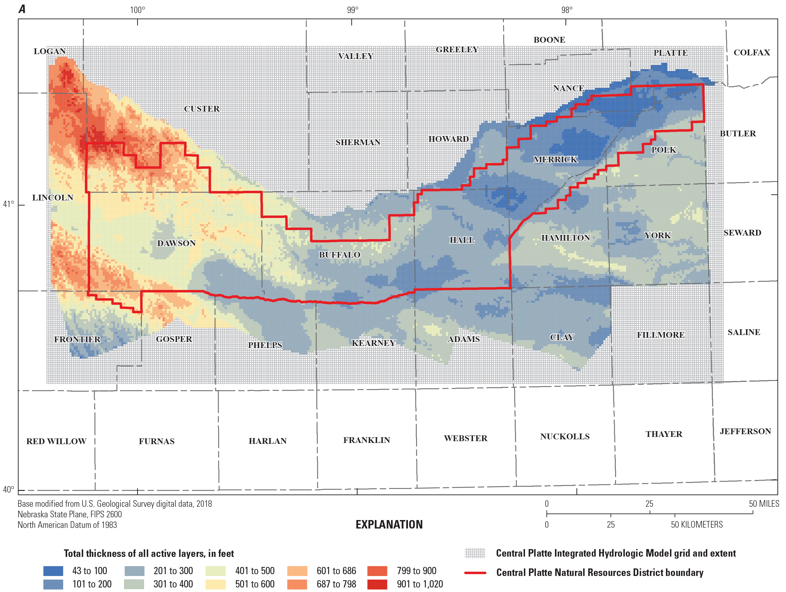
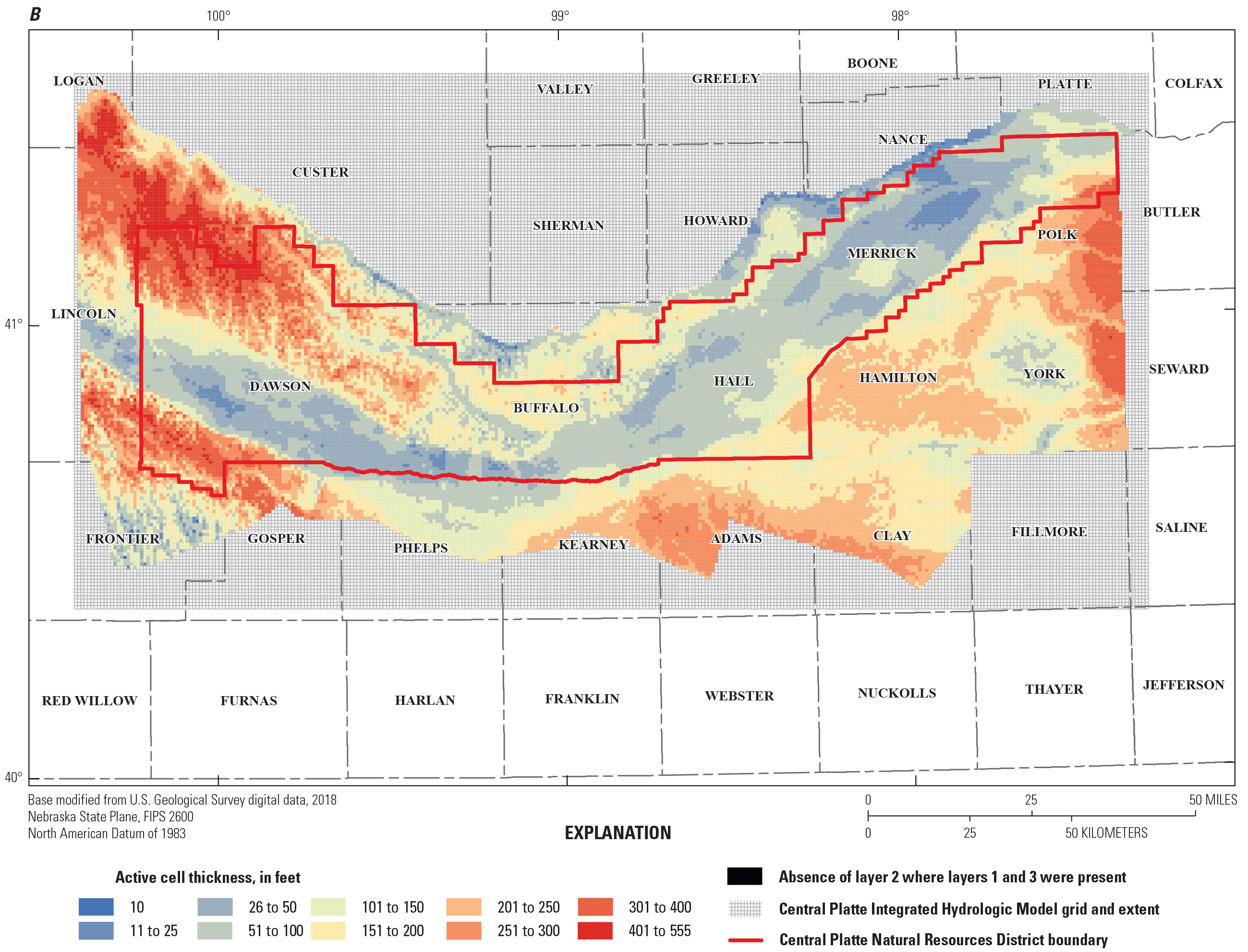
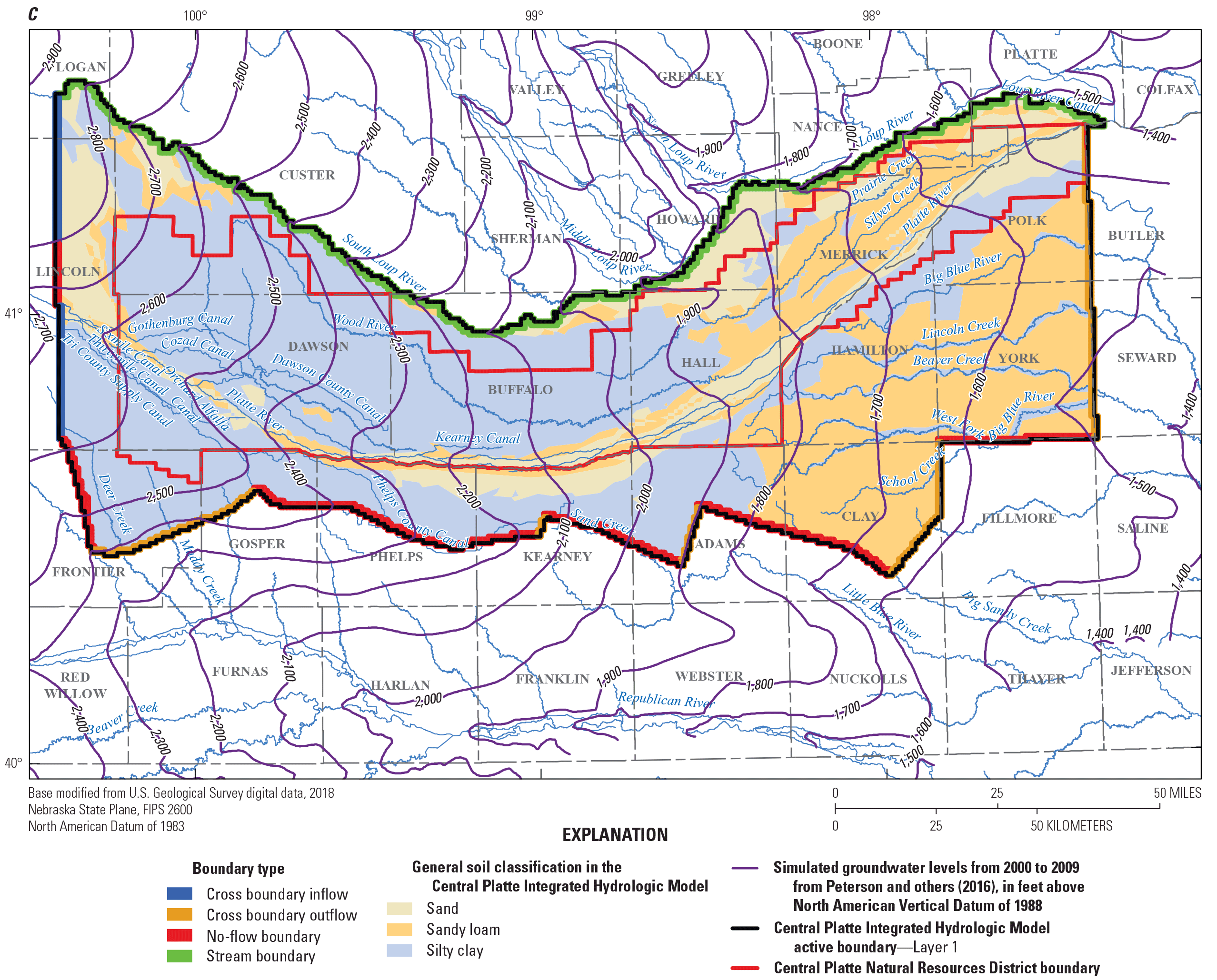
Map showing study area model structure, hydrologic boundaries, and conceptualized vertical layering. A, Orthogonal grid, active cells, and total cell thicknesses of the Central Platte Integrated Hydrologic Model. B, Orthogonal grid, active cells, and cell thicknesses of the Central Platte Integrated Hydrologic Model by layer (this figure is a layered .pdf). C, Simulated groundwater-level contours from 2000 to 2009 (Peterson and others, 2016) used to delineate groundwater-flow boundaries for this study and groundwater inflow, outflow, and no-flow boundaries.
The groundwater-flow system is connected to the surface-water system through stream-aquifer interaction. Water-table contour maps indicate groundwater levels were above adjacent stream surfaces in the western portion of the active study area, which results in a net outflow from the groundwater to streams (Summerside and others, 2001; fig. 7C). In the eastern portion of the study area, stream surfaces are generally higher than the adjacent groundwater levels, which results in a net inflow to the groundwater from streams (Summerside and others, 2001); for example, along the Platte River approximately between Cozad and Grand Island, Nebr. (fig. 1A).
The Platte River, the primary stream in the study area, is connected to the groundwater-flow system for the entire length that it flows through the study area (fig. 1A). Along some reaches, the groundwater-flow system discharges base flow to the Platte River, and along other reaches the groundwater-flow system receives inflows from the Platte River as stream leakage (Peterson and Carney, 2002). A groundwater discharge analysis in Peterson and Carney (2002) estimated base flow at several streamgages on the Platte River during the fall low-flow season: the average groundwater discharge as base flow was from −3.0 to 4.0 ft3/s per mile, where negative values indicate a losing reach of the stream. Estimated base flow at Platte River at Brady, Nebr., streamgage (USGS streamgage 06766000) was about 675 ft3/s for the recent development period and 570 ft3/s for the pre-1940 period (table 3). Estimated base flow at Platte River near Duncan, Nebr. (USGS streamgage 06774000) was estimated to be about 1,611 ft3/s for the recent development period and 649 ft3/s for the pre-1940 period (table 3).
Recharge (analogous to deep percolation from the landscape subsystem) is the primary inflow to the groundwater-flow system for the pre-1940 and recent development periods. Recharge rates are highest on irrigated lands and lowest on rangeland (see deep percolation values described in the “Climate and Landscape Components” section of this report and based on measured values from Steele and others, 2014). Stream leakage is also estimated to be a substantial inflow to the groundwater along “losing” stream reaches of the Platte River between Overton (not shown) and Grand Island, Nebr. (fig. 1A). Although groundwater irrigation is the primary groundwater outflow and is typically associated with groundwater-level declines, localized increases in groundwater storage changes for the recent development period from inflows such as canal leakage and decreased outflows to groundwater ET have contributed to a small increase in storage prior to 1940 (McGuire, 2017). The increase in groundwater levels because of canal leakage has been monitored in the study area and has a local influence on the water table that does not reflect groundwater levels in other areas that do not have canal leakage inflows each year (U.S. Geological Survey, 2017).
The increase in irrigated cropland and irrigation well development has resulted in a substantial increase in outflows from groundwater irrigation wells since the 1940s (Peterson, 2009; Peterson and others, 2016). Based on a consumptive use deficit (when available precipitation is less than the amount required for a crop to fully transpire) of about 10 inches per growing season for corn, the dominant crop type, an estimated 20 inches of water was required to be pumped during an average climate year to irrigate about 158,000 acres of cropland (pre-1940 land use) for an estimated annual volume pumped of 263,000 acre-feet (table 3; Irmak and others, 2011). Estimated ranges of groundwater irrigation in table 3 are based on the range of efficiency appropriate for the time period based on values in Irmak and others (2011). Prior to the development of center pivots in the 1950s, flood or furrow irrigation was the common technique to apply groundwater pumped for irrigation, and these efficiencies had a range of 50 to 65 percent. By 2016, the number of irrigation wells was about 32,000 (fig. 3; Nebraska Department of Natural Resources, 2017) and irrigation efficiency improved with development of center-pivot technology; 80 percent of groundwater irrigation is delivered by sprinklers in Nebraska, of which most are more efficient center pivots (Irmak and others, 2011; Johnson and others, 2011). The average rate of groundwater irrigation application decreased to about 10 to 11 in/yr, but with the increase in acreage to about 2,169,000 acres of cropland, the annual estimated volume pumped increased to about 1,990,000 acre-feet (table 3). With the development of irrigation technology, such as the Low Energy Precise Application, the efficiency of groundwater pumping improved to as much as 90 percent (Irmak and others, 2011). Metered data for irrigation pumping were unavailable for more than 99 percent of irrigation wells in the CPNRD, and irrigation technology data such as traditional sprinkler or Low Energy Precise Application were also not available. Lack of these data also contributed to the uncertainty of the conceptual estimates of groundwater irrigation.
Integrated Hydrologic-Flow Model Construction
An integrated hydrologic model was constructed using the MF–OWHM software (version 2.0.1; Boyce and others, 2020). The MF–OWHM is a comprehensive version of the MODFLOW suite of groundwater-flow simulators because it is a fully integrated simulator of the landscape, surface water, and groundwater-flow system. The MF–OWHM, as described in this report, is a MODFLOW-2005 based code and therefore includes the standard MODFLOW-2005 inputs and configuration (Harbaugh, 2005) and the Newton solver (MODFLOW–NWT; Niswonger and others, 2011). The CPIHM utilized the MODFLOW–NWT (MODFLOW–NWT, ver. 2.0.0; Niswonger and others, 2011) solver because it allowed for the solution of nonlinear groundwater flow associated with the drying and rewetting of model cells in unconfined conditions without permanently deactivating those dry cells. The layers simulated in the CPIHM were thin in some areas and some cells of the model went dry under stressed conditions. The models associated with this report are available as a USGS data release (Traylor, 2023).
The CPIHM was run for three different time periods: a predevelopment period (steady state), a period representing the start and development of irrigation in the study area (the development period), and a forecast period representing possible future scenarios of pumping and changes in the groundwater (table 5). A list of processes simulated in the CPIHM and associated MF–OWHM packages and the process used to simulate those processes is provided in table 5 and 6.
Table 5.
Central Platte Integrated Hydrologic Model spatial and physical characteristics.[—Left][FMP, Farm Process Package; GHB, General Head Boundary package; NWT, Newton Solver Package; RCH, Recharge Package; SFR, Streamflow Routing Package; UPW, Upstream weighting package; WEL, Well Package; --,not simulated because that feature was not present in the model]
Table 6.
Central Platte Integrated Hydrologic Model temporal characteristics.[na, not available]
Boundary Conditions
A combination of groundwater divides, surface-water features, and available input data extents were used to define the “active” domain and the boundary conditions simulated by the CPIHM around the CPNRD focus area. Simulated groundwater contours from the Northern High Plains groundwater-flow model (Peterson and others, 2016) were the principal source of information on the location of the western and southern hydrologic boundaries surrounding the CPNRD (fig. 7B). The western areal boundary of the study area was selected as the region extending north from central Frontier County through Brady, Nebr. (fig. 1A) to the South Loup River in southeastern Logan County about 10 miles upstream from South Loup River at Arnold, Nebr. (USGS streamgage 06781600, fig. 1A). Based on average decadal groundwater contours from Peterson and others (2016), groundwater flows into the study area across the northern and southern portions of the western boundary for this study, except for a region just north of the Platte River near Brady, Nebr., where the groundwater flows south into the Platte River, and the region in Frontier County where groundwater flows approximately southeast and creates a no-flow groundwater boundary (fig. 15 from Peterson and others, 2016; fig. 7C).
The South Loup River was chosen as the northern boundary of the CPIHM, west of the confluence of the Loup River (fig. 7C). The Loup River forms the northern boundary of the study area to its confluence with the Platte River in Platte County (fig. 7C). Hydrologically, the northern boundary that includes the South Loup and Loup Rivers is a mapped groundwater divide and creates a no-flow groundwater boundary (Peterson, 2009). Groundwater flows across much of the eastern boundary of the study area in Clay, York, and Polk Counties (fig. 7C). The northern and eastern boundaries are coincident with the boundaries from models in Peterson (2009) and Cooperative Hydrology Study (2017).
The southern boundary extended from the groundwater divide west of Deer Creek in Frontier County through central Gosper, Phelps, and Kearney Counties, then along the Big Sandy Creek in Clay County (fig. 7C). The southern boundary of the model approximately follows the groundwater divide created by a groundwater mound under the CNPPID canal system in central Gosper, Phelps, and Kearney Counties that is a result of persistent leakage recharge from the canals (fig. 7C). The southern boundary contains areas where groundwater flows east or southeast out of the study area or flows parallel to the model boundary and creates a no-flow groundwater boundary (fig. 7C). Vertical boundaries of the active domain of the CPIHM were the land surface as the upper boundary and top of the Pierre Shale as a no-flow lower boundary (HU 10 from Cannia and others, 2006; Peterson, 2009; Peterson and others, 2016).
Layering Scheme
The vertical discretization of the CPIHM, between the vertical boundaries (land surface and Pierre Shale), was defined by the HUs described in Cannia and others (2006) where present in the study area. The six HUs (HUs 1–6) present in the study area were combined into three hydrologically similar groups based on permeability, geologic age, and spatial relation to reduce the number of vertical layers that would need to be represented in the CPIHM (fig. 8). HUs 1 and 2 were combined into numerical model layer 1, HUs 3 and 4 were combined into numerical model layer 2, and HUs 5 and 6 were combined into numerical model layer 3 (fig. 8). Hydrologic connection remained between all three layers after grouping (figs. 6 and 8). Model layer 1 is the Quaternary alluvium and loess from HUs 1 and 2. Group 1 is present everywhere in the study area with an average thickness of 163 ft and a range from less than 10 ft in parts of the Platte River valley to greater than 500 ft in parts of Dawson and Custer counties (figs. 7B, 8). The alluvium and loess typically consisted of gravels, sands, and silts. Model layer 2 combined the lower Quaternary and upper Tertiary Silt identified in Cannia and others (2006) as HUs 3 and 4. There were a few areas in the central and eastern portion of the study area where these units were absent (Cannia and others, 2006). Group 2 is thicker toward the east with an average thickness of 57 ft and a range from less than 10 ft in the west and central areas to 300 ft in the eastern portion of the study area.
Model layer 3 is the Ogallala Formation identified in Cannia and others (2006) as HUs 5 and 6. Group 3 also incorporated airborne electromagnetic data from Cannia and others (2017) that were used to refine the aquifer base. The Ogallala Formation consists of sands, silts, and clays at various intervals. The Ogallala Formation is present in the western and central portions of the study area and thins eastward with an average thickness of 242 ft and ranges from less than 10 ft in the eastern portions to 500 ft in the western portions of the study area (figs. 7B, 8).
Conceptual diagram showing the hydrostratigraphic units from Cannia and others (2006) that were used to create the layering scheme for the Central Platte Integrated Hydrologic Model.
Spatial and Temporal Discretization
The CPIHM was spatially discretized into a grid of orthogonal blocks, called cells, horizontally and vertically. The orthogonal grid consisted of 163 rows and 327 columns with horizontal cell sides of 2,640 ft by 2,640 ft (0.5 mile by 0.5 mile or 160 acres) (table 5). The CPIHM was vertically discretized into three layers of varying spatial extents and thickness according to the hydrogeology and aquifer characteristics described in the “Study Area Description” and “Layering Scheme” sections of this report. The CPIHM includes 159,903 total cells (fig. 7A) where model layers 1, 2, and 3 include 30,788 active cells; 30,009 active cells; and 17,712 active cells, respectively. Based on the hydrostratigraphic data, layer 1 (Quaternary-age alluvial and loess deposits) was present, and therefore active, throughout the study area (fig. 7A). Layer 2 was active throughout most of the study area but was absent in some parts of the central and eastern model domain. The absence of layer 2 where layers 1 and 3 were present appeared as “holes” in the model grid and will be referred to as such throughout the report. Layer 3 was present in the west and central model domain and thinned out to the east (fig. 7A). MODFLOW–NWT cannot simulate discontinuous layers such as the absence of layer 2 at the “holes”; inactive cells are simulated as no-flow boundaries. Most of the layer 2 holes have layers 1 and 3 present and hydrologically connected. To simulate this hydrologic connection in the CPIHM, cells in the layer 2 holes were activated and given an artificial layer thickness of 5 ft with a hydraulic conductivity equal to the average of layers 1 and 3, and anisotropy was set to a 1:1 ratio to permit vertical flow in the artificial layer 2 (shown as “layer 2 holes” on fig. 7B).
The predevelopment model was run as a 500,000,000-day transient stress period to ensure that an approximate groundwater storage equilibrium was reached (table 6). The groundwater levels generated by the predevelopment model were used as the initial groundwater levels for the development model. The predevelopment model approximated average steady-state groundwater conditions prior to the construction of canals for surface-water irrigation and wells for groundwater irrigation.
The CPIHM development period was temporally discretized into 610 stress periods to simulate transient conditions from May 1, 1895, to December 31, 2016 (table 6). The transient simulation start date was selected as May 1, 1895, because it was coincident with the first documented surface-water diversions for irrigation in the CPIHM active domain. Also, two previous groundwater-flow models that included the CPIHM domain began transient simulations in 1895 to account for the onset of surface-water diversions for irrigation (Peterson, 2009; Peterson and others, 2016). The first 170 stress periods of the development model were discretized into periods of time that reflected the typical irrigation season from May 1 to September 30 and nonirrigation season from October 1 to April 30, with 2-week time steps and were meant to provide a reasonable starting point for the period of interest (April 1, 1982, to December 31, 2016; table 6). Stress periods 171 to 610, from May 1, 1980, to December 31, 2016, were discretized into monthly time periods to improve the temporal resolution of outputs generated for the period of interest, after April 1, 1982, again with 2-week time steps (table 6). Temporal resolution was increased after May 1980 to monthly stress periods to meet the objectives of the study and to facilitate comparison of simulated groundwater levels from different months within an irrigation season with the CPNRD’s baseline groundwater levels from the spring of 1982. The CPIHM scenario period was temporally discretized into 396 stress periods to simulate transient conditions from January 1, 2017, to December 31, 2049 (table 6). Stress periods were discretized into monthly time periods with 2-week time steps to maintain the temporal resolution with the development period model (table 6).
Landscape Inputs and Configuration (Farm Process)
Landscape inputs are necessary for simulation of landscape processes within the MF–OWHM, as outlined in the “MODFLOW–One-Water Hydrologic Model Theory and Approach” section of this report (fig. 2). Landscape properties specified within the FMP for this study included land surface altitude, soil types, ETref, precipitation, land use and crop types, Kc, irrigation flags, root depths and pressures, fractions of transpiration (FTRs), fractions of evaporation from irrigation (FEI), fractions of inefficient losses to surface water from precipitation (FIESWP), and fractions of inefficient losses to surface water from irrigation (FIESWI). Surface-water supply sources and routing, the irrigation supply well information, and the water accounting units were specified within the FMP. The water accounting units are referred to hereafter as “water-balance subregions” (WBSs) (Hanson and others, 2014a; Boyce and others, 2020). The WBSs were delineated for the CPIHM based on subregional watersheds, surface-water irrigation zones, groundwater irrigation zones, CPNRD GWMAs, and other natural resource district boundaries. In total, there are 212 WBSs in the CPIHM (Traylor, 2023). The 212 WBSs were combined into 24 “supergroup” zones to facilitate analysis of the water budgets for areas of interest within the CPIHM (fig. 9). The 24 GWMAs within the CPNRD were used to define the supergroups (fig. 9). Hereafter, the term “GWMA” will be used to reference results pertaining to the supergroups.
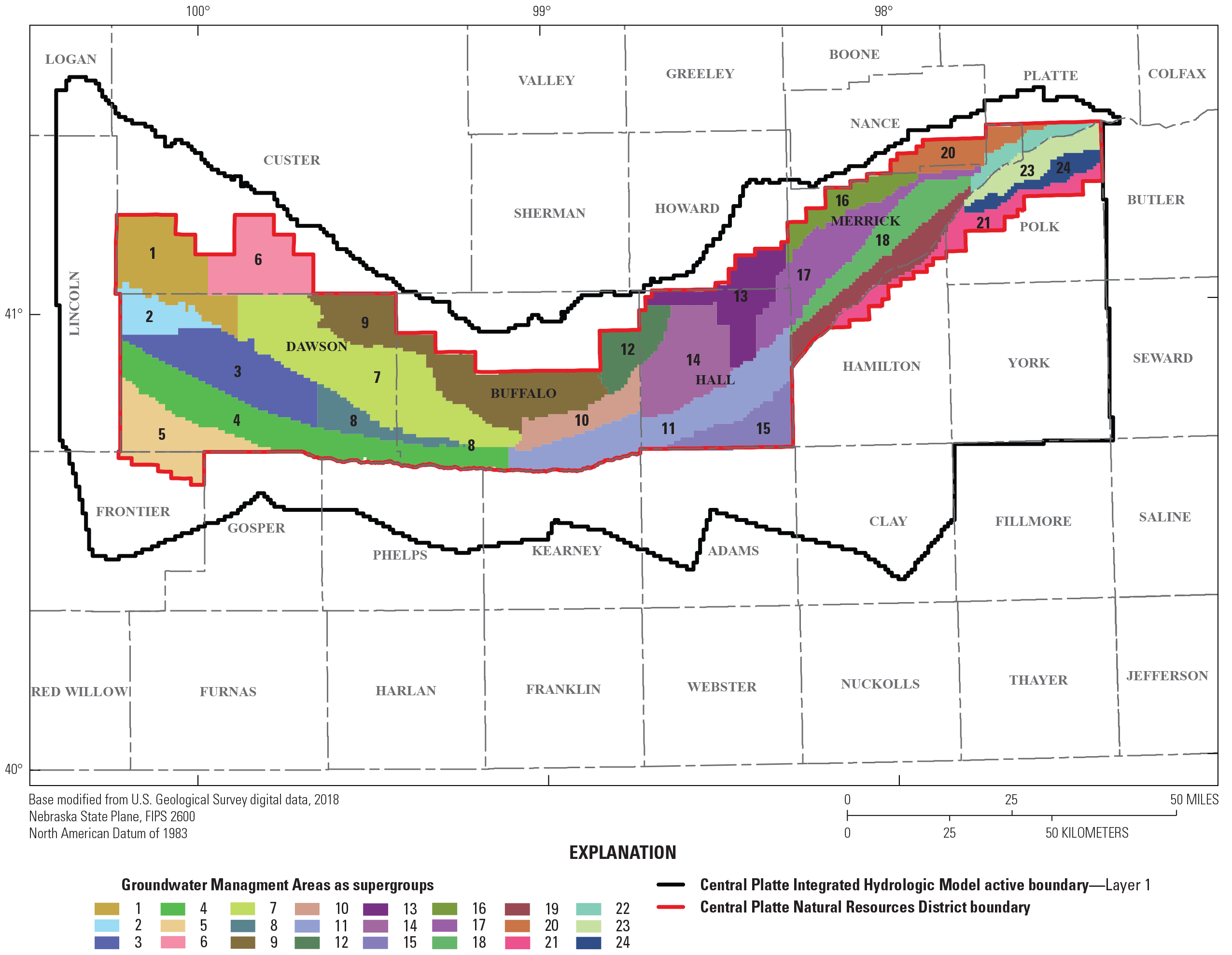
Supergroups (Central Platte Natural Resource District’s 24 Groundwater Management Areas) defined for the Central Platte Integrated Hydrologic Model. This is a layered .pdf; turn off supergroups layer for easier viewing of the 212 water balance subregions.
The land surface altitude dataset was created using a combination of 1- and 2-meter (m) light detection and ranging (lidar) digital elevation model datasets from the Nebraska Department of Natural Resources (2018) and a 10-m digital elevation model dataset from the U.S. Geological Survey (2018) and resampled to CPIHM model cell size. The precipitation (PPT) and ETref datasets used in the CPIHM were developed for each cell and stress period, generated from interpolation of climate data at as many as 77 weather stations in the COHYST area (Cooperative Hydrology Study (2017, p. 5–9), then clipped to the study area. The PPT and ETref datasets were constructed using the same weather stations and methods described in Cooperative Hydrology Study (2017), which included data from 1950 to 2013. Outside of the 1950 to 2013 period, climate datasets were obtained from the High Plains Regional Climate Center (2018) for each weather station included in the Cooperative Hydrology Study (2017) (fig. 10A, B).
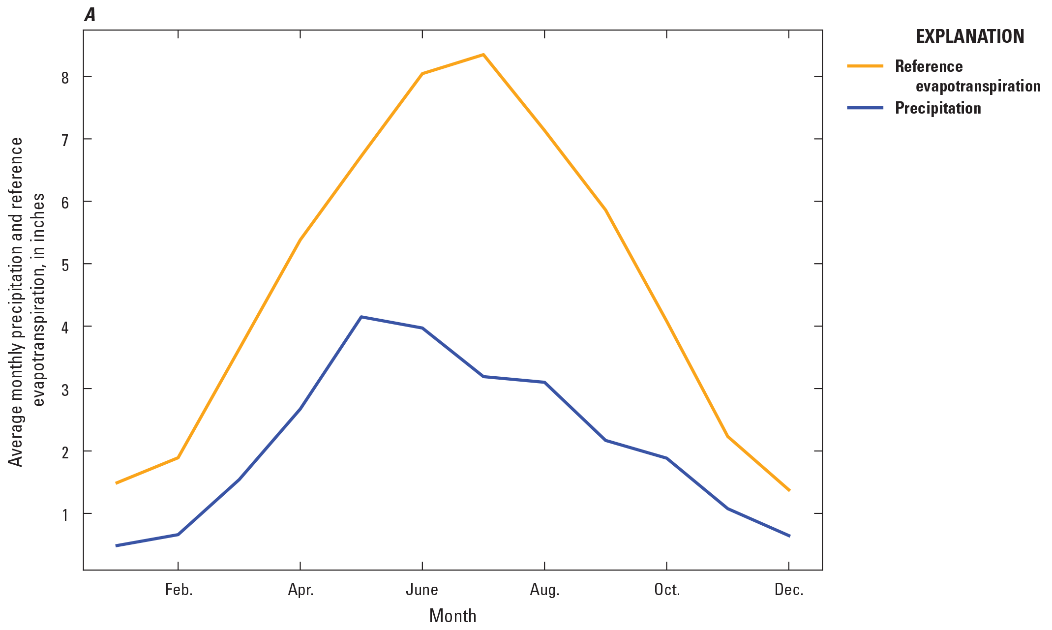
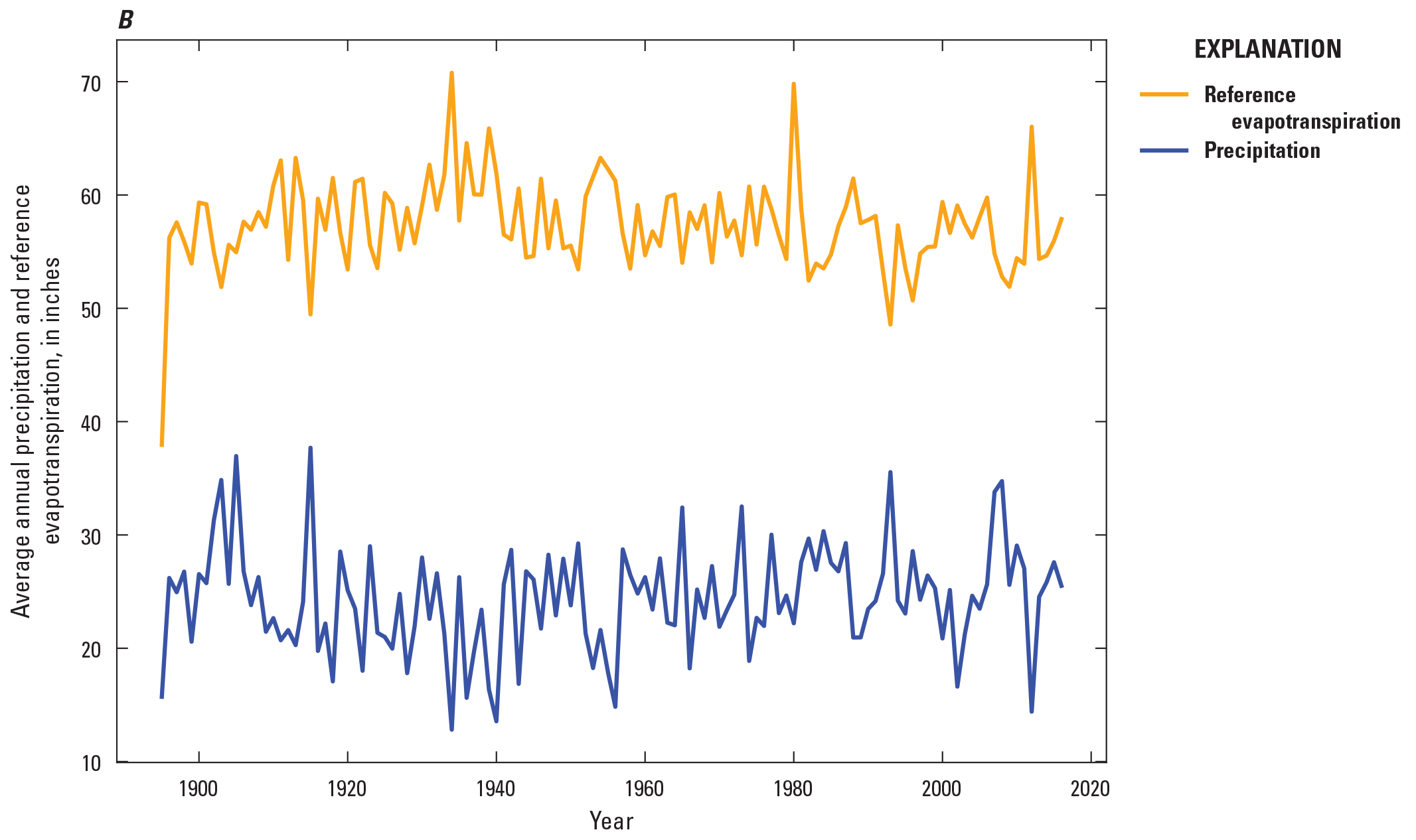
Plot of average precipitation and potential evapotranspiration for the Central Platte Integrated Hydrologic Model. A, Monthly post May 1980 model development period. B, Annual development period (1895 to 2016).
The Cooperative Hydrology Study (2017) land-use dataset specified multiple crop types per model cell in acres, and these values were converted to fractions of model cell area for use in the CPIHM (Traylor, 2023). For example, if crop type “groundwater-irrigated corn” in a specific cell was 64 acres, then the fraction used in the CPIHM cell dataset was 0.4 (for 160-acre cells). The distribution of land uses for 1982 and 2005 is shown in figure 1.1 (Dappen and others, 2007; also see figure 4-D-1 from Cooperative Hydrology Study, 2017). Soil types were grouped into sand, sandy loam, and silty clay based on classifications from a geographic information system soil dataset in University of Nebraska-Lincoln (2018) (fig. 7B). The land-use datasets were derived from those used in Cooperative Hydrology Study (2017) and included Cooperative Hydrology Study (2017) irrigated and dryland crop types for 1950 to 2013 partitioned into commingled irrigated, dryland uses, groundwater irrigated cropland, and surface-water irrigated cropland (table 7). The Cooperative Hydrology Study (2017) crop type “other” was then split into urban, roads, open water, and riparian forest and wetlands using the National Land Cover Database datasets to identify locations of those separate land uses (table 7) (Yang and others, 2018). The 1950 land-use dataset was used for 1895 to 1950, which was an acceptable approximation based on Hiller and others (2009), and the 2013 dataset was repeated from 2014 to 2016.
Table 7.
Land uses as crop types with crop numbers, crop short name, crop full name, and the source of water to meet water demand for each crop used in the Central Platte Integrated Hydrologic Model.The Kc values were specified for each crop type and stress period and interpolated and scaled to the various stress period lengths. When possible, daily Kc values were calculated following the methods used in the Cooperative Hydrology Study (2017). Additionally, the out-of-season value for cropland used in Cooperative Hydrology Study (2017) was used to represent fallow land and open water during the winter season, which was specified as November 15 to March 15. Monthly riparian forest Kc values from Hall and Rus (2013) were used for forest values. Published Kc values, planting dates, and crop growth period lengths were taken for all other land-use types from Allen and others (1998). Daily Kc values were calculated for all land uses by interpolating between the planting dates and growth stage dates. Monthly Kc values were then obtained by averaging the daily rates for the given month. Additional sources for Kc values from the Nebraska Agricultural Water Management Network (2018) were compared to the previously mentioned monthly Kc values and, where possible, were adjusted as needed to align with published values. Kc values assigned to each land use and stress period are available in the model archive associated with this report (Traylor, 2023)
Each land use was flagged for irrigation or no irrigation (dryland) for each stress period. Additionally, this “irrigation flag” included the irrigation efficiency type for the land use referenced from the separate “on-farm efficiency” (OFE) input table that specifies the irrigation efficiency as a fraction of the irrigation water pumped that is used by the crops (Boyce and others, 2020). Irrigation flags were designated for each commingled, groundwater, and surface-water crop type for potential irrigation stress periods (that is, May through September for irrigated crop types except winter wheat, which was flagged for potential irrigation from March to October). Irrigation efficiencies were specified in the development period model as 0.7, 0.55, and 0.8 for commingled, surface-water irrigated, and groundwater irrigated crops in the bi-annual irrigation stress periods from 1895 to 1980, respectively; and 0.72, 0.65, and 0.9 for commingled, surface-water irrigated, and groundwater irrigated crops in the monthly irrigation stress periods from May 1980 to December 2016, respectively, based on values from Irmak and others (2011).
Fractions of transpiration (FTRs) and FEI were assigned for each crop type. FTRs and FEI for common crop types like corn were derived from models that predicted corn transpiration and ET (Kimball and others, 2016). FTRs and FEI for winter wheat were derived from a study in China (Kang and others, 2003) and Nebraska (Irmak and others, 2016). Root depths for each land use ranged from 1 to 15 ft and were obtained from Irmak and Rudnick (2014) and U.S. Department of Agriculture (2016). Root pressure values as depths were obtained from table 7 in Hanson and others (2014b). The FIESWP and FIESWI values were chosen based on values of similar parameters within Cooperative Hydrology Study (2017). The runoff calculated by FIESWP or FIESWI was routed to a nearby stream cell specified in the semirouted returns feature of FMP.
The development model simulated the proliferation of groundwater irrigation wells in the study area. The irrigation wells that supply the CIR for each groundwater-irrigated crop were specified in the “farm wells” block within the FMP. Each irrigation well was assigned a pumping location in the model grid (layer, row, and column designation; fig. 11) and a WBS to which the well may supply water in addition to a maximum pumping rate. Farm wells that intersected stream cells were removed to improve model stability. Irrigation well start and end dates were based on construction dates and decommission dates in the well database (Nebraska Department of Natural Resources, 2017). Surface-water deliveries from canal diversions were specified as an available source of water for 36 WBSs (156–189, 211, and 212) because they were coincident with the surface-water irrigated acres. The amount of surface deliveries available each stress period depended on the diversion amount from the streamflow routing network to the canals (Nebraska Department of Natural Resources, 2019).
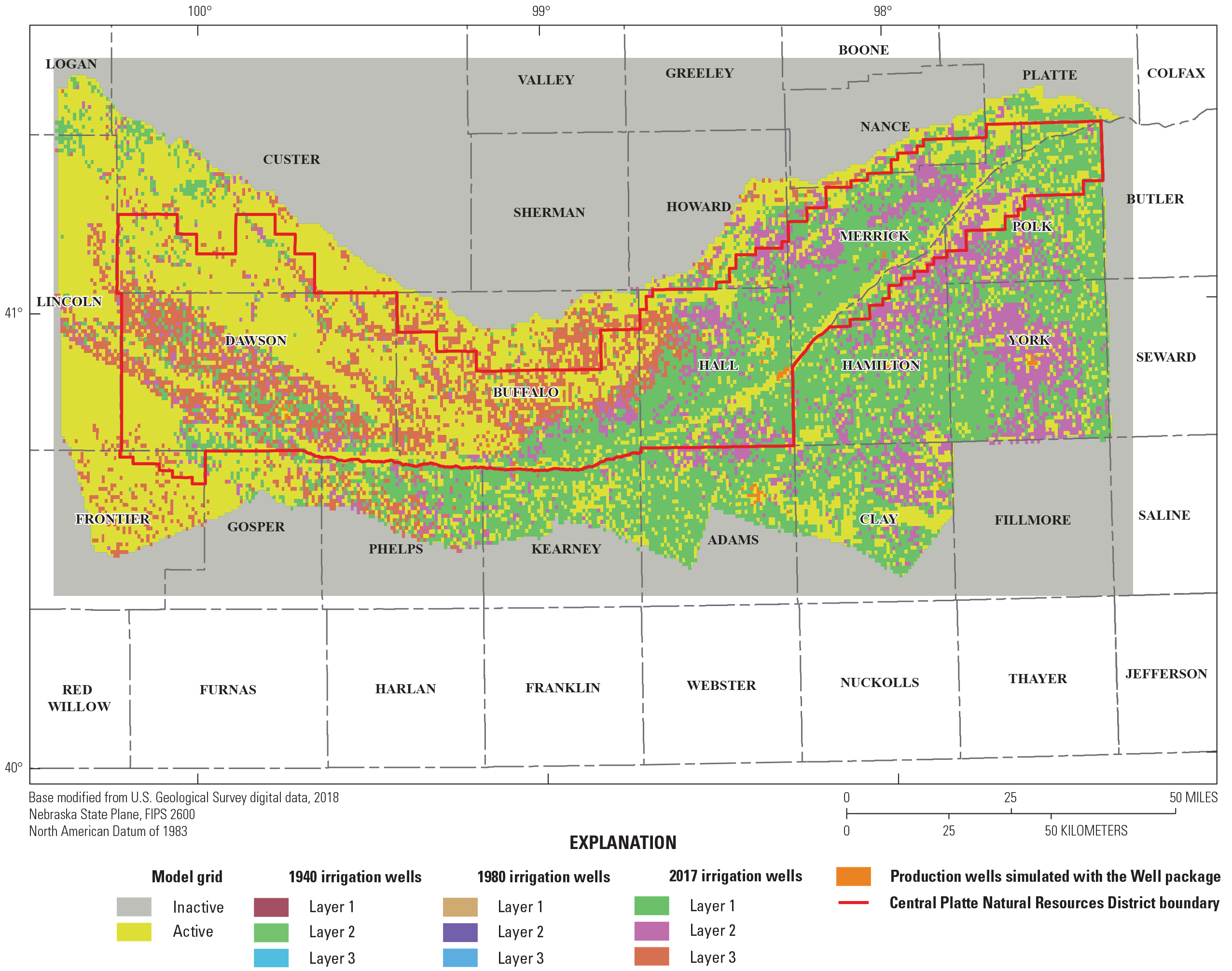
Irrigation well locations in the development Central Platte Integrated Hydrologic Model by layer prior to January 1, 1940; January 1, 1980; and January 1, 2017; production wells as cells simulated in the model (this figure is a layered .pdf).
MODFLOW Inputs and Configuration
MF–OWHM utilization of the Newton solver for the CPIHM required the use of the Upstream Weighting package (Niswonger and others, 2011), including hydraulic properties such as Kh, anisotropy, Sy, and specific storage (Ss) for each model layer. The precalibration initial values for the hydraulic properties are described in the “Hydrogeology and Groundwater” section. In an unconfined system, Sy is a more influential property than Ss because it quantifies 3 or 4 orders of magnitude more water. Further, assignment of a single Ss value across all active cells for each layer was a technique taken from the Northern High Plains aquifer model calibration from Peterson and others (2016). The aquifer storage (Ss and Sy), Kh, and anisotropy values were adjusted during the calibration process.
The General-Head Boundary package (GHB; Harbaugh and others, 2000) simulated inflow and outflow of groundwater across boundaries of the active model (640 cells) and the interaction of Johnson Lake and Elwood Reservoir with the groundwater-flow system (31 cells; fig. 1A; table 5). The GHB is a head-dependent flux boundary that requires a specified hydraulic head and conductance for each GHB designated cell. The flux between a GHB and adjacent cell is the product of the GHB cell conductance and the difference in hydraulic heads between the GHB cell and the adjacent cell. The conceptual model of groundwater flow (in the “Boundary Conditions” section of the report) indicated that there was lateral groundwater flow into the model domain along some portions of the western model boundary and lateral outflow along some southern and eastern portions of the model based on simulated groundwater-level contours from Peterson and others (2016) (fig. 7B). The GHB cells were assigned for these inflow and outflow edges of the model (fig. 12). The hydraulic head values were determined using a combination of rasterized decadal average groundwater levels from Peterson and others (2016) and interpolated heads from measured groundwater-level data at observation wells coincident or near boundary cells. Initial GHB heads were extracted from the rasterized grids of the decadal groundwater-level contours from Peterson and others (2016) and checked against measured groundwater levels when available (U.S. Geological Survey, 2017). For differences greater than 5 ft, GHB head values were specified by extracting values from raster grids interpolated from the measured data near boundary cells. Hydraulic conductance along the boundaries were estimated based on local aquifer properties and layer thicknesses (Peterson, 2009; Houston and others, 2013). Lake and reservoir stage data were used to specify the GHB heads for both reservoirs. Lake GHB conductance was manually adjusted such that the simulated groundwater levels below the lakes were similar to the measured groundwater levels from a nearby observation well (USGS 404046099504501) located on the southern shore of Johnson Lake (U.S. Geological Survey, 2017). Because of the proximity of Elwood Reservoir to Johnson Lake, the GHB conductance used for Elwood Reservoir was the same as that defined for Johnson Lake.
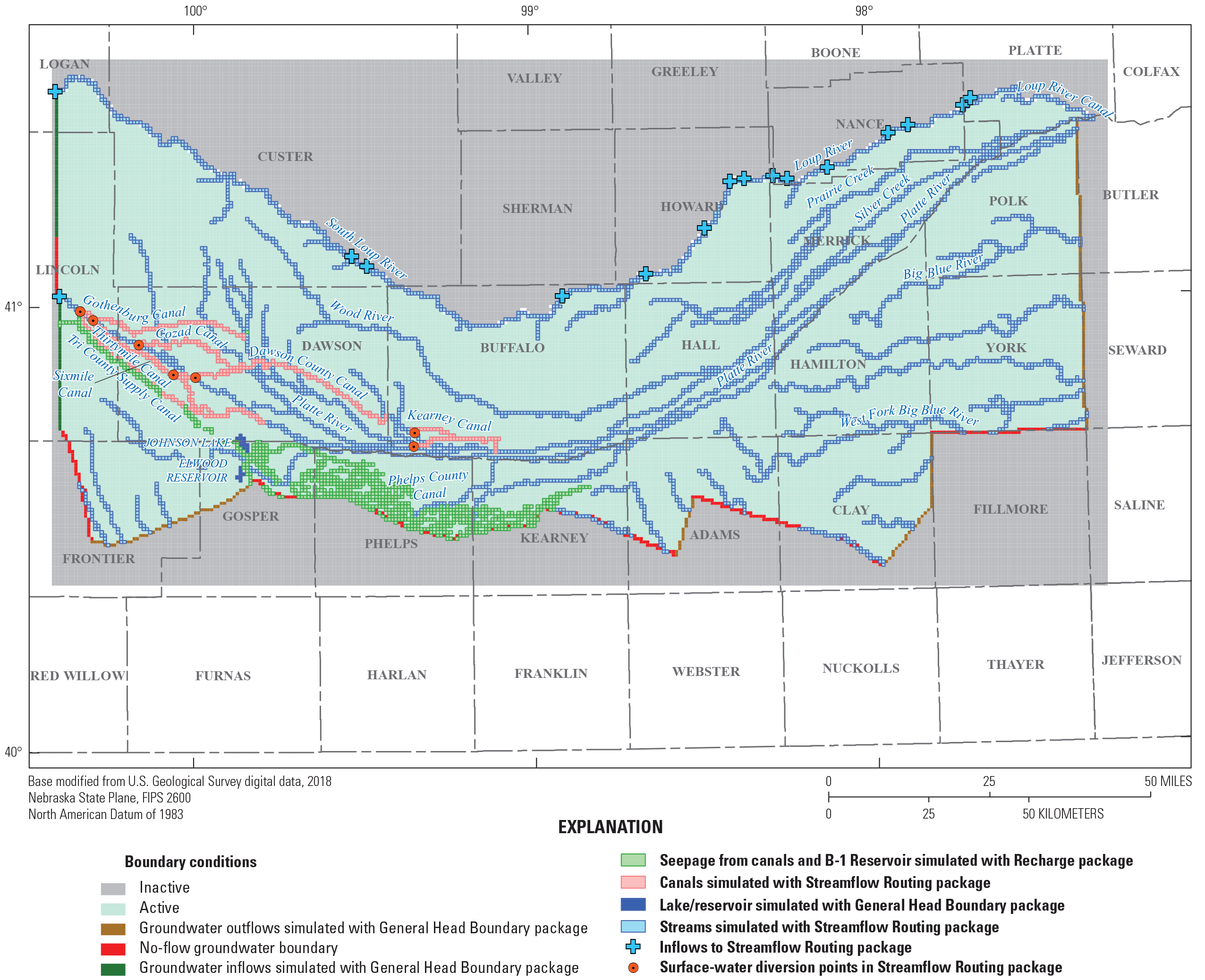
Boundary conditions of Central Platte Integrated Hydrologic Model.
The Streamflow Routing package (SFR; Niswonger and Prudic, 2005) simulated the flow and routing of surface water in streams and canals and their interaction with the landscape and groundwater-flow system within the study area and along the northern boundary. The SFR is a head-dependent flux boundary that interacts with the groundwater-flow system of each designated SFR cell based on the relation among the stage of the stream, streambed conductance, and the hydraulic head of the aquifer. Flow of water between the SFR and the groundwater-flow system is dictated by the conductance, which is the product of the hydraulic conductivity of the streambed and the area of the stream channel, divided by the streambed thickness. The SFR network included 4,318 cells, or reaches, and 219 segments, which are a group of reaches with uniform hydraulic properties, to represent major streams such as the Platte River, South Loup River, Middle Loup River (not shown), Loup River, Wood River, Prairie Creek, Big Blue River, and the perennial reaches of their perennial tributaries (fig. 12). The upper perennial reaches of the tributaries included in the SFR network were determined based on density of streams using geographic information system techniques and assessment of satellite imagery to identify segments of streams that interact with the groundwater based on identification of a wet channel and identification of vegetation along the stream that is assumed to be supported by groundwater. Flows and stage are calculated with the SFR as the difference among inflows from upstream reaches; runoff; tributaries; groundwater discharge to the reach as base flow; and outflows to downstream reaches, canal diversions, and leakage into the aquifer. The SFR simulated stream depth using Manning’s equation and assumed a rectangular channel (Niswonger and Prudic, 2005). Therefore, physical stream properties such as vertical hydraulic conductivity of the streambed, stream width, streambed roughness coefficient, and streambed thickness were specified for each segment. The Gage package (Merritt and Konikow, 2000) was used to extract time series of simulated streamflow for some SFR reaches for calibration to measured flow data.
Canals within the CPNRD focus area, and their associated diversions from the Platte River, were simulated with the SFR (fig. 12). The SFR simulated the routing of diverted streamflow into Cozad, Dawson, Gothenburg, Kearney, Orchard-Alfalfa, Sixmile, and Thirtymile canals (Nebraska Department of Natural Resources, 2019). Stress period averaged canal diversion values were created from daily diversions data available from the Nebraska Department of Natural Resources (2019) and were input to the SFR (table 1.1). Note that the CNPPID canal system located south of the Platte River was not simulated with the SFR. The leakage of diverted water through the canal beds of the CNPPID canals was simulated with the Recharge package (Harbaugh and others, 2000), wherein these recharge rates were estimated using change in groundwater-level values from measured groundwater-level hydrographs near the canals and mean Sy values of the aquifer. Additionally, the Recharge package was used to simulate the leakage from B-1 Reservoir in Dawson County (fig. 12); recharge rates were calculated based on the difference between reservoir inflow and evaporation data to estimate leakage through the lakebed of about 85 percent of inflows (Nebraska Department of Natural Resources, 2019).
Groundwater withdrawals for municipal supply (fig. 11) were simulated using the Well package (Harbaugh and others, 2000). The municipal well spatial and temporal information were obtained from the NeDNR Registered Well Database (Nebraska Department of Natural Resources, 2018). Well depths were used to determine the model layer from which the wells were pumped, and construction dates were used to determine the first active stress period of each well. Withdrawal rates were estimated for wells in communities or time periods without withdrawal data using withdrawal data from municipalities with similar populations. A total of 198 municipal wells were simulated (fig. 11). Municipal wells are hereafter referred to as production wells.
Calibration Approach
This section of the report describes the two-phase approach to calibration of the CPIHM. The combined predevelopment and development period transient models were used together to calibrate the CPIHM, and the calibrated inputs were then used in the forecast model. The CPIHM was linked to the Parameter Estimation (PEST) software (Doherty, 2005), which uses numerical inversion methods to adjust select model inputs, known as “calibration parameters,” to improve the fit between measured data, known as “calibration targets,” and their simulated equivalent outputs to constrain the range of reasonable parameter values. A two-phased calibration was used, which involved manual adjustment and fixing of some calibration parameters followed by the automated calibration, discussed in more detail in the “Two-Phase Calibration Approach” section of this report. This two-phase approach to calibration was also employed for the numerical MF–OWHM developed in Hanson and others (2018).
The CPIHM was calibrated to minimize the PEST objective function (Φ), which is the sum of squared weighted residuals between calibration targets and simulated equivalent outputs (Doherty, 2005), calculated using equation 3:
wheren
is the number of calibration targets,
w
is the weight applied to the calibration targets, and
r
is residual, as the difference between time and space equivalent calibration targets and simulated values.
In a normal PEST run, PEST requires one model run per adjustable parameter to determine the sensitivity of that parameter to the simulated model outputs equivalent to each observation. The Jacobian matrix (a matrix of parameter sensitivities to observations as derivatives) is recalculated for each iteration of the calibration process (Doherty, 2015). The CPIHM calibration was facilitated by the employment of the singular value decomposition-assist (SVDA) feature of PEST, where PEST uses the information in the first Jacobian matrix to recombine the adjustable parameters into grouped “superparameters.” Fifty superparameters were established based on the most sensitive parameters in the Jacobian matrix. After the establishment of superparameters, only the most sensitive superparameters are estimated, and the less sensitive superparameters can remain fixed. In future iterations, PEST only requires one model run per adjustable superparameter to calculate a new Jacobian matrix. Therefore, SVDA facilitated the calibration process by reducing the number of parameters that PEST can adjust and thus reducing the number of model runs required for the calculation of the Jacobian matrix in subsequent PEST iterations (Doherty and Hunt, 2010). The automated PEST calibration was further facilitated by a parallel computing version of PEST called BeoPEST (Schreuder, 2009; Doherty and others, 2010a) and deployed on a cluster of machines by way of the open source, high throughput, workload management software HTCondor (Condor Team, 2012).
Calibration Parameters
A total of 740 parameters were specified for the predevelopment and development CPIHM within six parameter groups, and 435 of those parameters were adjustable during the automated calibration process (table 8). Parameterization (the specification of model inputs as calibration variables, or parameters that PEST may adjust) was based on prior data availability, local knowledge, and uncertainty in their values. In environmental modeling, there is usually a lack of available data to quantify model inputs for every model cell and stress period. The parameterization scheme (that is, the structure and number of parameters used to represent the unknown natural-system input values of a model) is an important aspect of modeling because it can have a substantial effect on the ability of a model to gain information from the calibration dataset and appropriately simulate the natural system (Fienen and others, 2010). The parameter value and its imposed lower and upper bounds represent the reasonable range of values or the precalibration (prior) uncertainty of the model input, based on prior knowledge of the system (Fienen and others, 2010). Excluding a model input from the adjustable parameter set, either as a “fixed” parameter or excluding it entirely from the PEST framework, equates to “hard coding” the model input and is similar to saying that model input is known with 100-percent certainty, which is highly unlikely in complex environmental models. However, the model may be insensitive to some model inputs, which cause far smaller effects on model outputs than other inputs. Although some parameters may be insensitive to the calibration process because they may not gain information from the calibration dataset, they can still cause changes in scenario results, which is an important consideration when specifying parameters. Additionally, some model inputs can be well constrained (less uncertainty) because they may have ample data to specify an acceptable value that produces acceptable model results, whereas others may be poorly constrained (more uncertainty) and require more freedom during calibration to find optimal values.
Table 8.
Description of parameters by group that includes count and whether adjustable or fixed during automated calibration.[Ss, specific storage; Sy, specific yield; WBS, water-balance subregion; FTR, fraction of transpiration; FEI, fraction of evaporation from irrigation; OFE, on-farm efficiency; Kh, horizontal hydraulic conductivity; ET, evapotranspiration]
Calibration parameters were combined into groups defined as aquifer storage properties (aqprops), streamflow routing properties (sfrprops), farm or landscape properties (farmprops), pilot points for Kh (pilotpts), climate properties (climprops), and pilot points for aquifer anisotropy (apilotpts; table 8). As will be described in the “Two-Phase Calibration Approach” section, certain parameters were fixed to improve model stability, prevent spurious parameter values, and better simulate ET. After several calibration attempts, 305 of the 740 parameters were converted to nonadjustable or “fixed” parameters within the PEST framework so the final calibration used 435 adjustable parameters. The groups farmprops, aqprops, and climprops were all fixed for the final calibration, whereas the calibration treated the sfrprops, pilotpts, and apilotpts as adjustable.
Fixed Parameters for Final Calibration
The 305 parameters in the farmprops, aqprops, and climprops groups were fixed for the final calibration to combat overfitting, improve model stability, and improve the efficacy of the simulated water-budget results with the conceptual model water budget. The aquifer storage properties (aqprops) group of parameters included six fixed parameters for aquifer Sy and Ss values. Sy was parameterized with one multiplier for each layer and Ss values were specified as a single value for each layer. Initial Sy values were interpolated from test hole data in Houston and others (2013) (table 1) and were like values used in the COHYST model (Peterson, 2009). The three Ss parameters were fixed using literature values (Domenico and Schwartz, 1990) during the initial hand-calibration. Initial precalibration Ss values for model layers 1, 2, and 3 were at 2.4e-4, 9.4e-5, and 2.0e-4, respectively. The water-table layer, layer 1, used Sy to calculate storage, and layers 2 and 3, which were saturated for every stress period, used the Ss term. Lower and upper bounds for Sy multipliers were specified according to the range of values estimated from test hole data by Houston and others (2013; table 1).
The farm or landscape properties (farmprops) group of parameters included 273 fixed parameters for irrigation well maximum capacity scale factors, FIESWP, FIESWI, FTR, FEI, root depths, and on-farm efficiencies (table 1.2). A total of 170 parameters were defined as irrigation well maximum-capacity scale factors, which adjust the pumping capacity of the wells, for each WBS that had a designated supply from irrigation wells. The remaining 42 of the 212 WBSs were supplied irrigation by surface-water deliveries. The maximum pumping capacity was specified based on values of well yield reported in well construction logs (Nebraska Department of Natural Resources, 2018). Well yield values recorded in the logs typically represent the results of an initial well test completed immediately after construction and reported by the drillers; these values are often rounded numbers and contain some uncertainty; however, they were relatively insensitive parameters during preliminary calibration runs (table 1.3). Therefore, the well capacity scale factors were set as adjustable parameters for preliminary calibration runs but were later fixed at their initial scale factor of 1.0 for the final calibration.
The 18 FIESWI parameters, one for each irrigated crop type, were fixed for the final calibration. These parameters controlled the fraction of runoff of applied irrigation water that does not infiltrate but runs off to streams. The initial values were set between 0.001 and 0.01 because in Nebraska it is illegal to allow irrigation water pumped to run off the field (Nebraska Legislature, 2014). The 32 FIESWP parameters, one for each crop type, were fixed parameters for the final calibration. The FIESWP parameters partitioned available precipitation into runoff to streams or deep percolation past the root zone that became recharge to the water table. Initial values were set at 0.4 for most crops, like fractions of runoff in Cooperative Hydrology Study (2017), with lower and upper bounds of 0.01 and 1.0. The open water crop type land use that represents the portion of a model cell covered by open water from a stream or lake was specified an initial FIESWP value of 0.999 because precipitation that falls on this portion of the cell contributes to streamflow immediately. Similarly, the dryland urban and dryland roads crop types were specified an initial FIESWP value of 0.99 because their impervious surfaces promote runoff rather than recharge. Conversely, the dryland riparian forest and wetlands crop type was specified with an initial FIESWP value of 0.2 because the shallow water table and saturated soil of the wetlands or riparian areas promoted recharge.
A total of 14 FTR scale factors were fixed for the final calibration. FTR scale factors were parameterized by length of the stress period (irrigation season, nonirrigation season, monthly) (see table 1.2 for parameter description). The FTR scale factor parameter allowed PEST to adjust the amount of transpiration that constituted ET while maintaining the input FTR values relevant for each crop type. The FTR scale factors were specified an initial value of 1.0. Like the FTR scale factors, the FEI inputs were fixed for the final calibration. The nine FEI scale factor parameters were specified for stress periods with irrigation (irrigation season and March to September monthly stress periods). Initial values were 1.0 for each FEI scale factor. Root depth adjustable parameters were specified for 26 crop types in the model and set as fixed parameters for the final calibration. Their initial values were based on published values from Irmak and Rudnick (2014) and U.S. Department of Agriculture (2016). Four of the root depths for fallow land were not specified as parameters because fallow land does not have plants or roots; therefore, those root depths were hard coded as input values of 0 ft.
A total of six OFEs, one parameter for each of the three types of irrigation efficiencies (commingled, groundwater, and surface water), one for pre-1980 “early period” efficiencies, and one for post-1980 “recent” efficiencies, were specified to allow the model to simulate the improvement of irrigation technology and irrigation efficiency with time. However, these parameters were fixed for the final calibration at their initial values of 0.72 and 0.7 for early and recent period commingled efficiencies, respectively; 0.55 and 0.65 for early and recent period surface-water efficiencies, respectively; and 0.8 and 0.9 for early and recent period groundwater efficiencies, respectively (table 1.2).
The climate properties (climprops) parameters (table 1.2) included 15 ETref scale factors specified by stress period type like the FTR and FEI scale factors, except one additional ETref scale factor was parameterized for the predevelopment CPIHM. The ETref scale factors parameters were multipliers on the input ETref up or down to account for uncertainty in those datasets. All 15 of the ETref scale factors were fixed for the final calibration at values of 1.12 for the predevelopment CPIHM; 1.56 for the irrigation season stress periods and 1.0 for the nonirrigation season stress periods of the development-period CPIHM; and 1.0 for the January, February, March, April, September, October, November, and December stress periods, respectively, and 1.15, 1.20, 1.30, and 1.30 for the May, June, July, and August stress periods, respectively, for the development-period CPIHM.
Adjustable Parameters for Final Calibration
The streamflow routing properties (sfrprops) group of parameters included 11 adjustable parameters for vertical hydraulic conductivity of streambed (Ksb). Ksb parameters were defined for the lower and upper portion of each SFR reach and “tied” in PEST so that the Ksb remained the same for each SFR segment and did not change for reaches within a segment. Unique Ksb parameters were defined for natural streams according to soil class used in the CPIHM and for each canal simulated with the SFR (soil classification in fig. 1B; parameters in fig. 13). Initial values for calibration of Ksb for natural streams were set to less than 2 ft/d and canal Ksb values were set between 1 and 10 ft/d based on manual trial-and-error testing prior to automated calibration through which model stability was improved. The lower and upper bound were set to 0.001 and 15 ft/d, respectively, which is the acceptable range for the study area based on values from Peterson and others (2016).
Vertical hydraulic conductivity and Kh for each model cell was specified using interpolation between pilot points (see Doherty and others, 2010b). Vertical hydraulic conductivities were set using anisotropy ratios, also interpolated between pilot points. The pilot points for Kh (pilotpts) were specified as adjustable parameters to adequately represent the spatial heterogeneity of Kh across each model layer without needing to adjust Kh for each active model cell. A total of 124 pilot points were used: 49 for layer 1, 48 for layer 2, and 27 for layer 3 (fig. 13). In this study, pilot points were generated using the FloPy python module (Bakker and others, 2016), interpolation factors were generated using the “ppk2fac” PEST Groundwater Data Utility (Doherty 2018), and model input arrays generated from interpolation between the pilot points used the PyEmu module (White and others, 2016). The pilot point distribution was based on the presence of an active extent of each model layer. Pilot point density was chosen as one pilot point for every 25 active model cells. Pilot points within a few cells of a stream or general head boundary were manually moved away from the boundary to avoid the influence of boundary conditions. For this study, the vertical interval estimates of Kh from Houston and others (2013) were assigned to aquifer intervals that aligned with the HUs from Cannia and others (2006) and that correspond to the model layers (table 1). Initial values for individual pilot points were selected by extracting Kh values from two-dimensional arrays generated through interpolation of test hole data in Houston and others (2013) and summarized in table 1 (table 1 is a summary of the test hole data, not the interpolated grids used to extract the values).
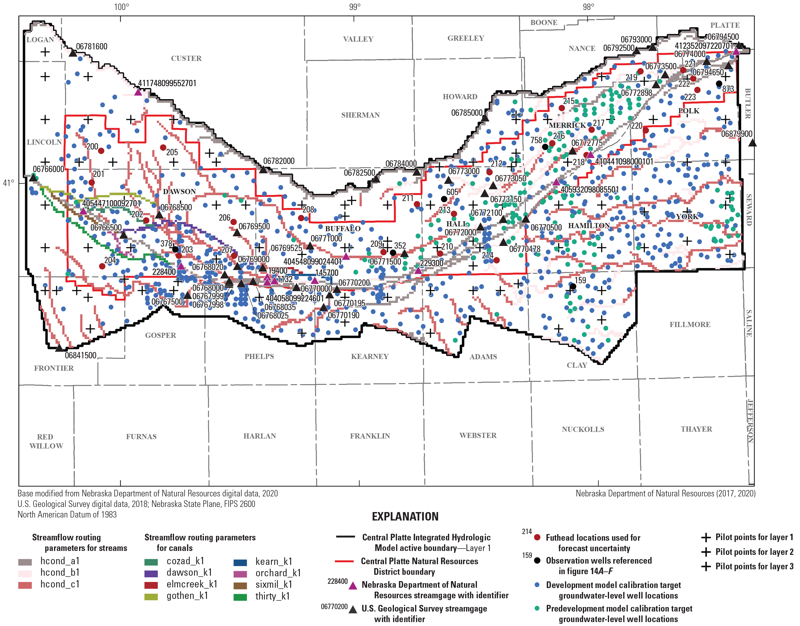
Locations of the observation wells, streamgages, and pilot points used during the calibration of the predevelopment (pre-May 1, 1895) and development (post May 1, 1895) Central Platte Integrated Hydrologic Model in addition to the well locations for observation wells in figure 14A–F. This is a layered .pdf.
The pilot points for aquifer anisotropy (apilotpts) were specified for the same locations as the Kh pilot points (fig. 13). Initial values for model layer 1 anisotropy pilot points were specified as 10:1 ratio (Kh:Kv) in accord with published values in Domenico and Schwartz (1990) for unconsolidated sands, silts, and clays of alluvial aquifers (Cannia and others, 2006). Layer 2 anisotropy at pilot points was specified as 20:1 because of the finer grained and lower Kh values of silts reported for that layer (Cannia and others, 2006). Layer 3 anisotropy at pilot points were specified as 10:1 ratio for sandstones (Domenico and Schwartz, 1990; Houston and others, 2013). Horizontal anisotropy was not simulated in the CPIHM.
Regularization of Parameters
Tikhonov regularization was employed in the CPIHM calibration process for the adjustable parameters to reduce the likeliness of overfitting during the automated calibration process (Doherty, 2015). Regularization is a mathematical preconditioning method that allows for a unique solution to an ill-posed inversion problem (many more parameters than observations) in which there is correlation between parameters (Doherty, 2015). Regularization allows for the PEST to use “prior information” or expert knowledge of the parameterized inputs as the initial preferred values unless the calibration target dataset can provide enough information to warrant deviation from those initial preferred parameter values during the calibration process (Doherty, 2015). PEST includes a weight to regularized parameters and tracks a regularized PEST objective function (Φr) that is added to the Φ from calibration target residuals (Doherty, 2015). Therefore, PEST imposes a penalty on the Φ if a regularized parameter deviates from its initial value. PEST will only deviate regularized parameters from their initial values if Φr contribution to Φ is less than the reduction in the Φ that would occur with improved fit to the calibration targets (Doherty, 2015). Regularization weights were manually adjusted from the default value of 1.0 to provide additional guidance to PEST based on the prior information.
The trial-and-error calibration demonstrated that the CPIHM adequately simulated ETp, ETg, recharge, and irrigation from wells in comparison to the conceptual flux estimates for recent years (2011–16) under the fixed climate and landscape parameter scheme (simulated values for the landscape subsystem, mentioned in this section, are presented in the “Predevelopment and Development Period Simulated Results and Water Budgets” section of this report). The comparison between the conceptual flux values (presented in tables 2 and 3 and the “Conceptual Model of the Hydrologic System” section of this report) and the manual trial-and-error calibration values verified that initial trial-and-error estimated landscape and climate parameters were acceptable values and the CPIHM accurately simulated CWD. The preliminary fit between calibration targets and their simulated equivalent values was acceptable for some stress periods and locations, whereas simulated values for other stress periods and locations exhibited some bias. This prior information gained about the CPIHM was transferred to PEST by lowering the weights of the groundwater-flow parameters to 0.5, which encouraged PEST to adjust the groundwater-flow parameters to improve the calibration.
Calibration Targets
Calibration targets are measured or estimated values assumed to represent conditions of the hydrologic system at the time of their measurement, with a degree of uncertainty that is based principally on measurement or estimation error. Calibration targets can be single measurements in time or a time series that represents the temporal behavior of the hydrologic system. PEST allows calibration targets to be clustered into groups where the contribution of each group to Φ can be assessed. The CPIHM had the following observation groups specified in PEST (table 9): development period average streamflows per stress period processed from daily average measured streamflows from USGS National Water Information System (NWIS) streamgages (nwisflow), development period average streamflows per stress period processed from daily average measured streamflows from the NeDNR streamgages (dnrflow), average streamflow differences between streamgages (sflowdiff), predevelopment model average streamflows per stress period processed from daily average measured streamflows from the USGS NWIS streamgages (ssflow), Predevelopment model average streamflow differences per stress period processed from daily average measured streamflows from the USGS NWIS streamgages (ssflowdiff), predevelopment model average groundwater levels processed from measured pre-1950 groundwater-levels in NWIS (sswls), development period measured groundwater-levels from USGS NWIS (realwls), development period differences in measured groundwater levels between stress periods (realdif), and development period measured groundwater-levels across transects of the Platte River, collected by the CPNRD (realwlst). Two sets of observation points were included that did not involve actual measurements but were used in the analysis of the calibrated model: scenario period “potential” observations that can be used for dataworth analysis (potheads), and scenario period “future” observations used in the predictive uncertainty analysis, located at the geometric center of each Groundwater Management Area (futheads) that were incorporated for the predictive uncertainty analyses (table 9). The calibration was not affected by any observation targets in the potheads or futheads groups because they were zero weighted. The CPIHM contained 40,711 weighted calibration targets.
Table 9.
Description of calibration targets in the Central Platte Integrated Hydrologic Model for the groundwater-level and surface-water observation groups.[USGS, U.S. Geological Survey; NWIS, National Water Information System; CPNRD, Central Platte Natural Resources District; NeDNR, Nebraska Department of Natural Resources]
| Observation group | Count | Description of observation group |
|---|---|---|
| realwls | 10,746 | Development period measured groundwater-levels from USGS NWIS (U.S. Geological Survey, 2017). |
| realwlst | 8,916 | Development period measured groundwater-levels across transects of the Platte River, collected by the CPNRD. |
| sswls | 189 | Predevelopment model average groundwater levels processed from measured pre-1950 groundwater-levels in NWIS. |
| realdif | 9,848 | Development period differences in measured groundwater levels between stress periods. |
| potheads1 | 12,973 | Scenario period “potential” observations that can be used for dataworth analysis. |
| futheads1 | 24 | Scenario period “future” observations used in the predictive uncertainty analysis, located at the geometric center of each Groundwater Management Area. |
| dnrflow | 2,886 | Development period average streamflows per stress period processed from daily average measured streamflows from the NeDNR streamgages. |
| nwisflow | 7,589 | Development period average streamflows per stress period processed from daily average measured streamflows from the USGS NWIS streamgages. |
| ssflow | 2 | Predevelopment model average streamflows per stress period processed from daily average measured streamflows from the USGS NWIS streamgages. |
| sflowdiff | 534 | Development period model average streamflows differences per stress period processed from daily average measured streamflows from the USGS NWIS streamgages. |
| ssflowdiff | 1 | Predevelopment model average streamflows differences per stress period processed from daily average measured streamflows from the USGS NWIS streamgages. |
Table 10.
Description of calibration targets in the Central Platte Integrated Hydrologic Model for the counts of groundwater-level calibration targets by layer.Groundwater Levels
The CPIHM was calibrated to groundwater levels for the predevelopment and development models. The predevelopment model was calibrated to 189 estimated groundwater levels at 189 observation wells as the average of measured groundwater levels prior to January 1, 1950, and assigned to the sswls observation group (table 9; fig. 13). The development model was calibrated to 19,662 measured groundwater-level observations at 963 observation wells obtained from the NWIS database (U.S. Geological Survey, 2017) and 9,848 groundwater-level differences, which were second-order observations calculated as the difference between a measured groundwater level at a single location from one stress period to the next, to ensure the model matched changes in groundwater levels in addition to the absolute groundwater level (table 9). A total of 16,840 groundwater-level observations at 725 wells completed in layer 1; 1,065 groundwater-level observations at 125 wells completed in layer 2; and 1,759 groundwater-level observations at 113 wells completed in layer 3 (table 10). Although wells were distributed across the model area, a total of 859 wells had less than 10 observations and 68 wells had 100 or more observations (fig. 13). Western regions of the active model area in Custer, Frontier, and Lincoln Counties had very few observations (fig. 13). About 95 percent of the groundwater-level observations were measured after 1980 (fig. 14); therefore, the calibration incurred a bias toward the post-1980 period. This bias was desirable because one objective of the study was to use the model results to update the CPNRD’s GMP, which compared current management and MADs to 1982 groundwater levels. Consequently, the natural bias built into the model calibration (because most observations were measured after 1980) allowed PEST to focus on adjusting parameters to match observations in the post-1980 period. All groundwater-level calibration targets and locations are available in the model archive associated with this report (Traylor, 2023).
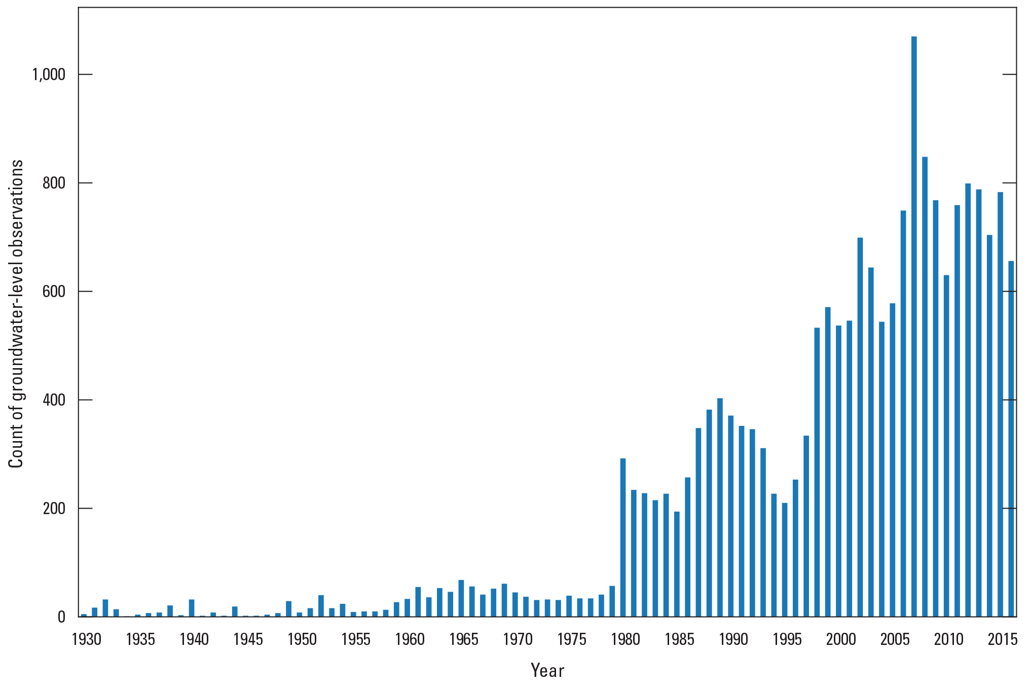
Count of groundwater-level observations used to calibrate the Central Platte Integrated Hydrologic Model for the development model.
Streamflows
The CPIHM included streamflow and streamflow difference calibration targets for the predevelopment and development period models. Streamflow targets at streamgages provided the calibration with information on absolute streamflow values. Streamflow difference targets provided additional calibration information to allow the model to reasonably match streamflows between streamgages, more accurately simulate the stream-aquifer interaction, and reduce the correlation between simulated flows of upstream and downstream locations so their potential bias at one location was not passed to another location.
Two streamflow targets were used to calibrate the predevelopment CPIHM streamflows at the Platte River near Overton, Nebr., and Platte River near Duncan, Nebr., streamgages (USGS streamgages 06768000 and 06774000, respectively), and a single streamflow difference was calculated for the predevelopment model between the same streamgages on the Platte River (fig. 13). Measured streamflow data did not exist for the predevelopment period (prior to May 1, 1895); therefore, the ssflow observations were the average of pre-1940 streamflows for the Platte River near Overton, Nebr., and Platte River near Duncan, Nebr., streamgages (fig. 13).
The CPIHM was calibrated to 10,475 stress-period-averaged streamflows calculated from measured daily values at a combination of 53 NWIS and Nebraska Department of Natural Resources streamgages (U.S. Geological Survey, 2017; Nebraska Department of Natural Resources, 2019) for the development model (fig. 13). An additional 534 streamflow differences were calculated between the Platte River near Overton, Nebr., and Platte River near Duncan, Nebr., streamgages on the Platte River for the development model (fig. 13).
Streamflow calibration targets were spatially distributed throughout the streams of the active model area (fig. 13). The Platte River Basin had 19 streamgages and the Loup River Basin, which included the South Loup, Middle Loup, and Loup Rivers, had eight streamgages. Streamflow calibration targets at streamgages downstream from the Loup River Power Canal diversion at Genoa, Nebr. (not shown), were reduced by the diversion amount because the diversion was not simulated in the model. Further, the Johnson Power Canal (not shown) return to the Platte River return (west of Kearney, Nebr., fig. 1A) was not simulated; therefore, Platte River calibration targets downstream from the return point were reduced by the amount of the returns. All streamflow calibration targets and streamgage locations are available in the model archive associated with this report (Traylor, 2023).
Weighting Scheme for Calibration Targets
Weights were applied to the calibration targets to capture their uncertainty, starting with an error-based weighting scheme, then adjusting the weights to balance each observation group’s contribution to Φ. Error-based weighting of the calibration targets was applied to each target based on measurement uncertainty associated with each measurement type (Hill and Tiedeman, 2007). Error-based weighting also kept PEST from being overaffected by targets with the largest magnitudes and different units. The attempts of PEST to minimize Φ are affected by the number and magnitude of the residuals in each observation group; groups with higher magnitudes or a greater number of targets have more effect on Φ than groups with smaller or fewer targets. For example, a streamflow residual of 10 ft3/s (864,000 cubic feet per day, in model units) is three orders of magnitude larger than a groundwater-level residual of 200 ft, and when weighted equally, PEST would be more affected by the streamflow residual and become insensitive to hydrologic signal represented by the groundwater-level residual. Error-based weights for each observation were calculated using equation 4:
wherew
is the error-based weight applied to the observation, and
σ
is the measurement uncertainty of the observation.
Measurement uncertainty varied by observation target group. The measured streamflows from USGS streamgages were assigned an uncertainty of 5 percent of their average flow for the period of record, which correlated to the 95-percent confidence interval that is typical for a “Good” rating for USGS streamgage measurements. The measured streamflows from NeDNR streamgages were assigned an uncertainty of 25 percent. Measured groundwater-level observations (realwls) were assigned an uncertainty of 10 ft. This reflects the uncertainty in the grid cell altitude in which the well is located (the error in resampling a 32.8-ft digital elevation model dataset to the CPIHM cell size of 2,640 ft). Initial weights for the measured groundwater-level observation groups (realwls, realdif, realwlst, and sswls) used the error-based scheme, but were adjusted during the calibration process to increase their contribution to Φ. The final weighting scheme used during calibration reflected the CPNRD’s planned use of the CPIHM to assess MADs in each GWMA, whereby smaller residuals for groundwater levels within the CPNRD were prioritized. Therefore, weights for the measured groundwater levels and groundwater-level differences were increased by about 40 percent for those measurements within the CPNRD boundary. Weights were increased for the sswls, ssflowdif, and ssflow to have a more balanced contribution to Φ for these observation groups.
The streamflow calibration targets were initially weighted using the error-based weighting method (Hill and Tiedeman, 2007). The calibration targets measured along the Loup River system were weighted about 75 percent lower than other targets because the Loup River system was the northern boundary of the active model area, and the hydrologic system to the north of the Loup River system that contributed base flow and runoff to those streams was not simulated in the CPIHM.
Two-Phase Calibration Approach
Calibration of the CPIHM involved two phases: a manual adjustment of parameters, followed by the automated calibration using BeoPEST. The two-phase calibration approach was adopted after several attempts to calibrate the CPIHM in a fully automated fashion because many of the adjustable parameters produced unrealistic results and resulted in significant model instability. Landscape parameters and some groundwater parameters were fixed to improve model stability during calibration, prevent spurious calibration results, and better match the conceptual estimates of landscape ET. The conceptual landscape ET estimates were based on measured data or calibrated outputs of previously developed models, which provided a blueprint for acceptable ranges of parameter values and outputs of ET and groundwater irrigation, for the CPIHM.
An assessment of parameter sensitivities to observations using a matrix of sensitivities, known as a Jacobian matrix, from a preliminary automated calibration attempt with all parameters set as adjustable, showed that the growing season ETref scale factors and Sy multipliers were some of the most sensitive (table 1.3). Preliminary automated calibration runs revealed that PEST preferred to adjust the Sy multipliers beyond acceptable ranges, even with heavy regularization weights applied, and as a result the multipliers were converted to fixed parameters before subsequent calibration. Further, the storage parameters were fixed in the calibration of layers 2–5 for the Eastern Model Unit groundwater-flow model from Peterson (2009) and the single layer Northern High Plains aquifer model from Peterson and others (2016); both models included the model domain for this study and used the same input test hole data derived from Houston and others (2013). This assessment of parameter sensitivities and methods from previous studies led to the implementation of the two-phase calibration approach that included the fixing of landscape and aquifer storage parameters to reasonable values based on available data.
In the initial manual adjustment phase, parameters were adjusted within the PEST framework to improve the fit between calibration targets and their simulated equivalent values. This phase focused on adjusting the growing season ETref scale factors to improve the CPIHM’s simulation of landscape ET and irrigation pumping throughout the development period model to values that were similar to the conceptual ET values and irrigation pumping from table 2. Model outputs were postprocessed to produce annual values of those ET and irrigation fluxes, and the recent 5 years of the simulated outputs (2011–16) were compared to the conceptual values from table 3. As mentioned in the “Fixed Parameters for the Final Calibration” section of this report, the ETref scale factors required adjustment from their 1.0 values that were standard for the other scale manually adjusted factors. The unadjusted average annual inputs of ETref shown in figure 10B were about 57 inches, which was about 7 to 8 percent less than the measured values from Irmak and Skaggs (2011). Consequently, initial manual trial and error testing indicated that simulated total AET (which is directly controlled by the ETref, and therefore the ETref scale factors) for all crop types was too low compared to the conceptual model water-budget values. Additionally, the undersimulated AET was responsible for the undersimulation of groundwater withdrawals for irrigation compared to available data and conceptual model values described in the “Conceptual Model of the Hydrologic System” section of this report, because lower ET corresponded to lower CIR. Initial automated calibration runs, with ETref scale factor parameters set as adjustable, showed that they were highly sensitive parameters as PEST preferentially adjusted them and they hit their upper bounds when the upper limit was set to even an unrealistic 3.0 (3.0 equates to a 3 times multiplier on ETref). Trial-and-error manual adjustment was used to determine the best initial values of each ETref scale factor to combat overfitting and maintain agreement with the conceptual model landscape ET.
After manual calibration, when the simulated recent water-budget fluxes were in accord with the conceptual model values, the final set of input parameter values obtained from the manual calibration were set as the initial parameter values for the automated PEST calibration. Therefore, initial parameter values at the beginning of the automated calibration phase were derived from a combination of local knowledge of the study area, information accrued from other scientific studies of the study area or similar hydrologic settings, and information gained about the CPIHM during the manual calibration phase. To honor these initial parameter values and their information and to keep PEST from deviating too far from the initial values, Tikhonov regularization was applied during the automated calibration, also described in “Regularization of Parameters” section of this report (Doherty and Hunt, 2010; Doherty, 201531).
Calibration Results
This section of the report describes the results of the CPIHM calibration and includes an assessment of fit among the calibration targets and their simulated equivalent values, presentation of the final “best” calibrated parameter values, and parameter sensitivity and identifiability analyses. Calibration results provide an indication of a model’s ability to simulate the dynamics of the hydrologic system and reproduce outputs that are in accord with the conceptual model of the hydrologic system and measured or observed data. Additionally, the final contribution to Φ shows how the observation groups affected the automated calibration process. Additional calibration statistics and plots of measured compared to simulated values are available in appendix 2.
Comparison of Calibration Targets to Simulated Equivalent Values
The comparison of calibration targets to their simulated equivalent values is an assessment of the fit between measured or observed data such as groundwater levels and streamflows with corresponding simulated values produced by the CPIHM. During the calibration process, PEST compared the calibration targets to corresponding simulated values and calculated the difference between the observation targets and simulated equivalent values, which for the remainder of the report will be referred to as the “residual.” A positive residual indicates an underestimation of simulated values by the CPIHM and a negative residual indicates an overestimation of simulated values by the CPIHM. The Gage package extracted the simulated streamflows from SFR reaches coincident with the location of the 53 streamgages for comparison to the streamflow calibration targets. The mod2obs PEST utility was used to extract the corresponding simulated groundwater levels for comparison to the calibration target groundwater levels (Doherty, 2018).
Groundwater Levels
The calibrated predevelopment CPIHM groundwater levels displayed an adequate fit to the calibration targets for the sswls observation group with an average absolute residual of 8.2 ft (table 11). Therefore, the predevelopment CPIHM provided acceptable initial conditions for the transient development-period CPIHM. Spatial trends in the calibrated sswls included an overestimation north of the Platte River and an underestimation south and east of the Platte River and minimal bias along the Platte River and Wood River from west to east (fig. 15). The calibrated development CPIHM groundwater levels displayed an adequate fit to the calibration targets for the realwls and realwlst observation groups, with average absolute residuals of 9.6 and 2.8 ft, respectively (figs. 15, 16A, and 2.3; table 11). The combined realwls and realwlst average absolute groundwater-level residuals for model layers 1, 2, and 3 were 6.1, 12.4, and 7.4 ft, respectively (table 11) for the whole development-phase model, which indicated that the CPIHM adequately simulated the groundwater levels for each layer. The fit between the measured and simulated groundwater levels in the realwls and realwlst groups was somewhat better within the CPNRD area after May 1, 1980, because the calibration of the CPIHM focused on the minimization of groundwater-level residuals for this area and period. This improvement in fit occurred mostly in layers 1 and 2 for the CPIHM and within the CPNRD; layer 3 exhibited an absolute residual that was larger (7.6 ft for the CPIHM and 7.5 ft for the CPNRD) after May 1, 1980, compared to the absolute residual for all time periods (7.4 ft for the CPIHM and 7.3 ft for the CPNRD); however, the difference was about 0.1 ft (table 12). The combined realwls and realwlst CPNRD average absolute groundwater-level residuals after May 1, 1980, for model layers 1, 2, and 3 were 4.0, 10.7, and 7.5 ft, respectively (table 12). Further, the calibrated development CPIHM groundwater levels displayed an adequate fit to the calibration targets for the realdif observation group with average absolute residuals of 1.2 ft and a standard deviation of 2.8 ft (table 11). These residuals indicated that the development-period CPIHM captured the transient nature of the groundwater-subsystem as groundwater-levels changed.
Table 11.
Calibration results statistics for the groundwater-level and streamflow observation groups of the Central Platte Integrated Hydrologic Model.[<, less than; >, greater than; --, could not calculate a value]
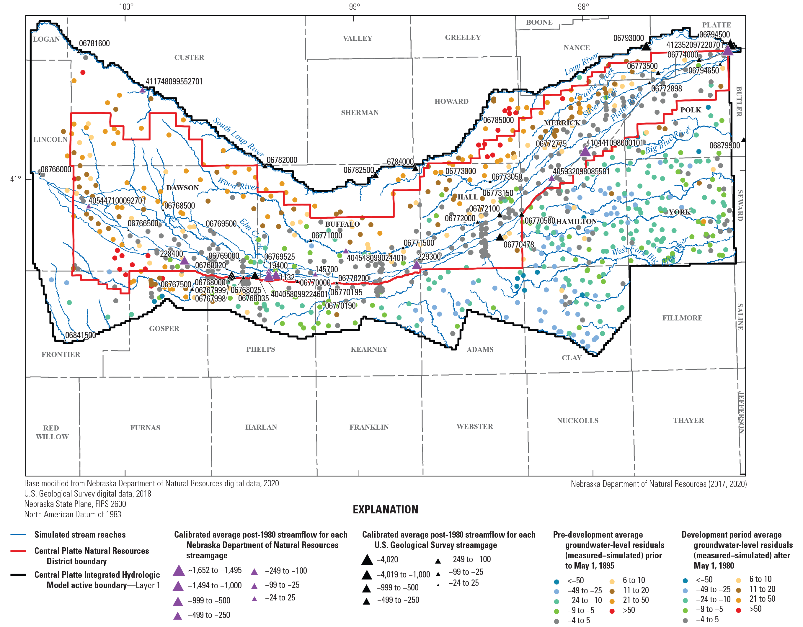
Spatial distribution of the average groundwater-level and streamflow residuals for the sswls, realwls, nwisflow, and dnrflow observation groups for the calibrated Central Platte Integrated Hydrologic Model.
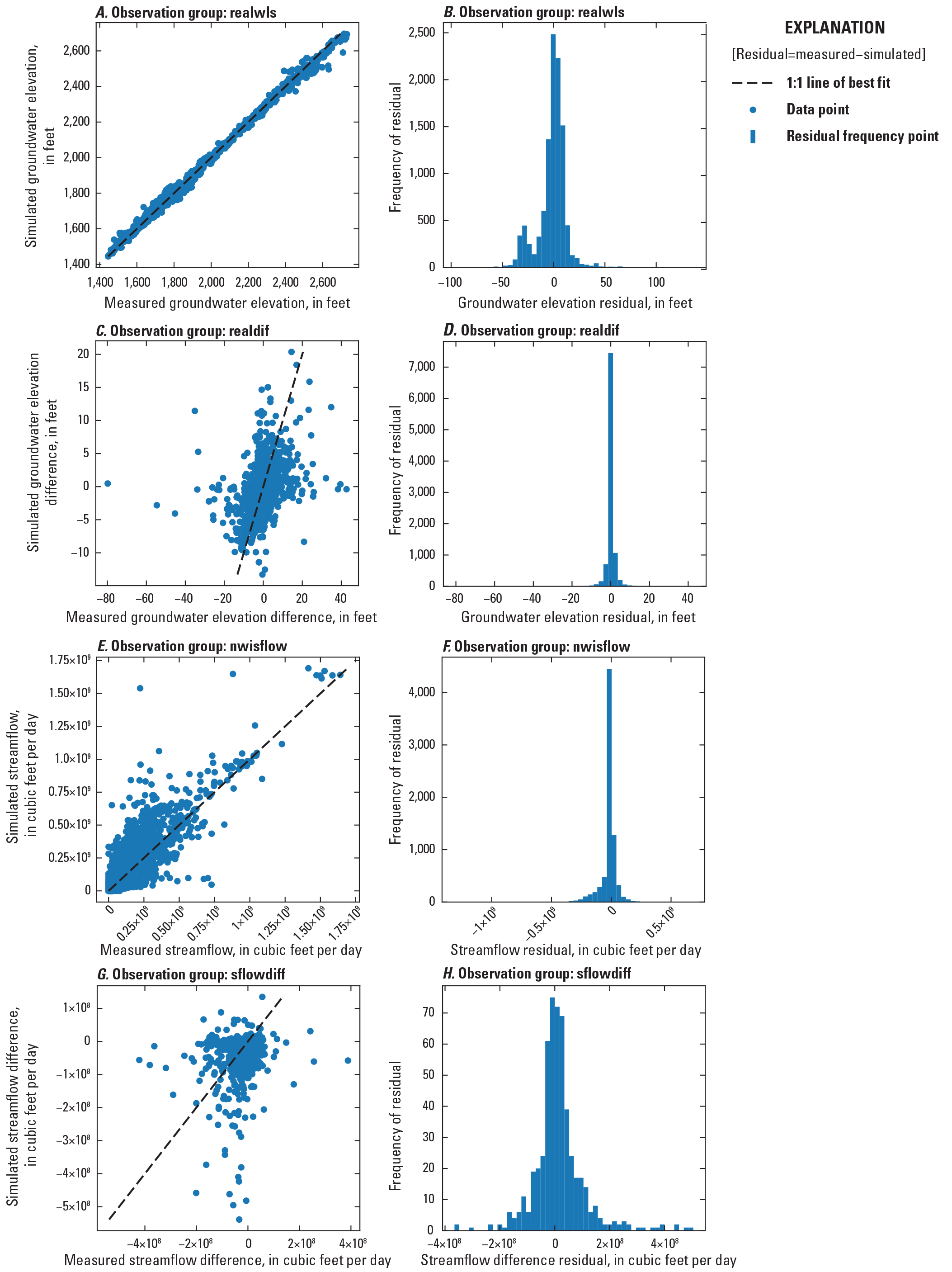
Calibration plots that include measured compared to simulated plots and residual value distribution histograms by observation group. A, Plot of measured compared to simulated values for the realwls observation group. B, Residual value distributions for the realwls observation group. C, Plot of measured compared to simulated values for the realdif observation group. D, Residual value distributions for the realdif observation group. E, Plot of measured compared to simulated values for the nwisflow observation group. F, Residual value distributions for the nwisflow observation group. G, Plot of measured compared to simulated values for the sflowdiff observation group. H, Residual value distributions for the sflowdiff observation group.
Table 12.
Average simulated groundwater levels and their residuals by layer in the Central Platte Integrated Hydrologic Model domain and the Central Platte Natural Resources District domain for the entire development model period (May 1, 1895, to December 31, 2016) and post-May 1, 1980.[CPIHM, Central Platte Integrated Hydrologic Model; CPNRD, Central; Platte Natural Resources District]
The calibrated groundwater-level residuals after May 1, 1980, exhibited spatial bias throughout the CPIHM domain. The average groundwater-level residuals at observation wells south of the Platte River were mostly negative, which indicated that the CPIHM overestimated the groundwater levels in this region; some residuals in this region exhibited a large bias of greater than 25 ft (fig. 15), including well 159 (fig. 17A). The average groundwater-level residuals at observation wells north of the Platte River were mostly positive, which indicated that the CPIHM underestimated the groundwater levels in this region (fig. 15), including well 352 (fig. 17B). Some of these wells were within the CPNRD boundary, particularly in Dawson, Buffalo, Hall, Howard, and Nance counties (fig. 15). The residuals along the Platte River were generally less than 5 ft (figs. 15 and 17C–F). Most of the residuals for observation wells that were overestimated by the CPIHM were located to the south and east of the Platte River outside the CPNRD boundary, particularly in Frontier, Gosper, Phelps, Kearney, Adams, Clay, Hamilton, and York Counties; because of their locations outside the CPNRD, they were weighted lower than the observations inside the CPNRD boundary, which caused them to have less effect on the Φ during the calibration. Therefore, PEST did not try to improve the fit for calibration targets outside the CPNRD boundary as much as the targets inside the CPNRD. Greater variability in groundwater levels outside of the Platte River Valley topographic region was also expected because of more dynamic terrain and depth to water in the Valley-side Slopes, Dissected Plains, and Sandhills topographic regions compared to the Valley region of the Platte River (fig. 1B). Additional comparisons of measured and simulated groundwater altitudes at other locations used in the model calibration process are available in the USGS data release associated with this report (Traylor, 2023).
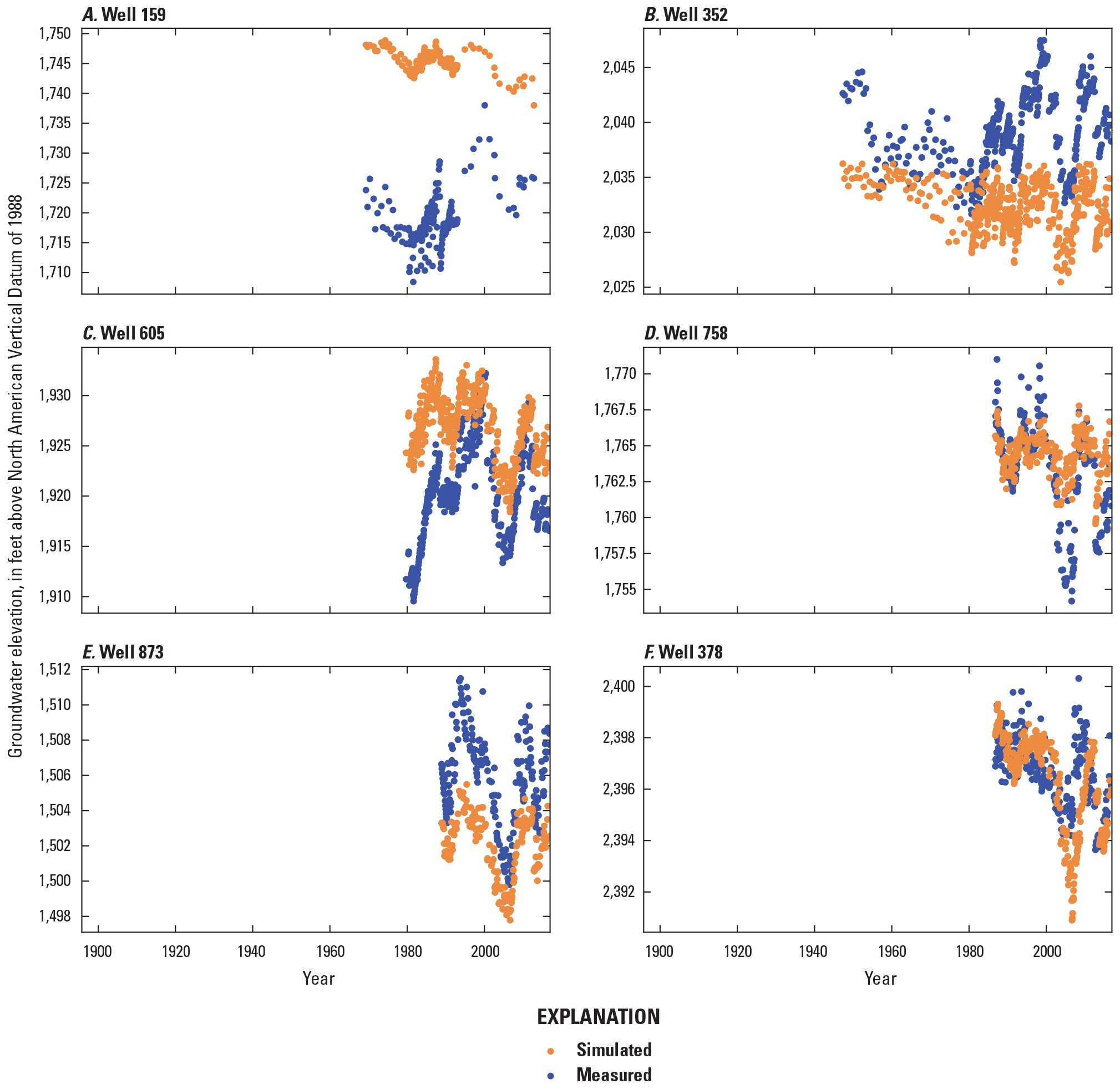
Measured and simulated groundwater-levels at observation wells in the Central Platte Integrated Hydrologic Model. A, Observation well 159. B, Observation well 352. C, Observation well 605. D, Observation well 758. E, Observation well 873. F, Observation well 378. Locations of observation wells shown on figure 13.
Streamflows
The calibrated predevelopment CPIHM undersimulated streamflow by 2,230 ft3/s for the ssflow observation group (table 11). However, given that (1) the ssflow observations were more uncertain than measured streamflows because they were estimated based on measured flows between 1930 and 1940, (2) the simulated predevelopment groundwater levels exhibited an adequate fit to the sswls observations, and (3) streamflow is a more dynamic observation than groundwater levels, and (4) major inflows to the Platte River are a transient input for the development CPIHM, the marginal fit to the ssflow observations still resulted in an adequate calibration for the development-period model. Most of the calibrated development-period CPIHM streamflows displayed a passable fit to the calibration targets (fig. 16E–H). Calibration targets from the nwisflow group exhibited a coefficient of determination of 0.776 with their simulated equivalent values. The nwisflow group exhibited a minor positive bias in their residuals, which indicated that the CPIHM oversimulated streamflows. The CPIHM accurately simulated the flows along the Platte River, including the outflow point of the Platte River near Duncan, Nebr. (fig. 18), streamgage (USGS streamgage 06774000; fig. 1A), which was important for the efficacy of the water balance during the simulation. The largest bias in flow along the Platte River occurred at splits in the complex braided network of channels such as a north and south channel at the Platte River near Overton North Channel, Nebr. (USGS streamgage 06767998) and the Platte River near Overton South Channel, Nebr. (USGS streamgage 06767999): residuals were −961 and −108 ft3/s, respectively (fig. 15). However, the single channel Platte River near Overton, Nebr. (USGS streamgage 06768000) residual was only −31 ft3/s (fig. 15). These residuals were expected because the model was not designed to simulate all the local complexities of a braided channel system such as Platte River; rather it was designed to simulate the primary channels of the Platte River and other streams in the study area. Further, the dnrflow residuals for the development-period CPIHM exhibited a large overestimation of flows on the Platte River streamgages, which was expected because these observations were weighted low in the calibration and consequently the parameters in PEST were not as sensitive to these observations compared to the nwisflow group. Additional comparisons of measured and simulated streamflow at 53 streamgages used in the model calibration process are available in the USGS data release associated with this report (Traylor, 2023).
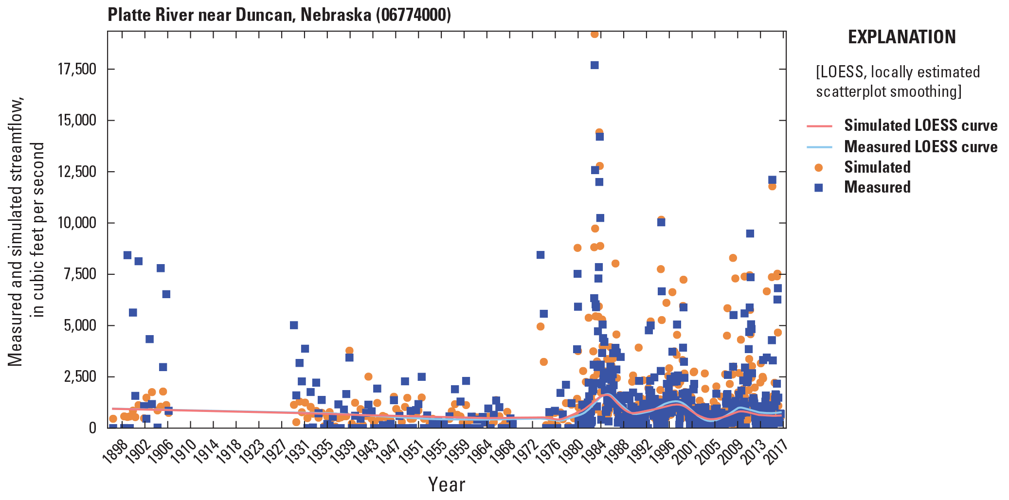
Measured compared to simulated streamflow and their respective locally estimated scatterplot smoothing (LOESS) line at the Platte River near Duncan, Nebraska, streamgage (U.S. Geological Survey streamgage 06774000) in the Central Platte Integrated Hydrologic Model.
The final phi distribution by observation group is presented in figure 19. The observation group with the largest contribution to Φ was from the nwisflow group (26.2 percent), followed by the realdif (24.2 percent) and realwls (19.9 percent) groups (fig. 19). The primary calibration focused on reducing the residuals of the realwls, realdif, and nwisflow groups more than other groups; therefore, the final Φ distribution, where the top three were nwisflow, realdif, and realwls, reflects the purpose of the study objectives.
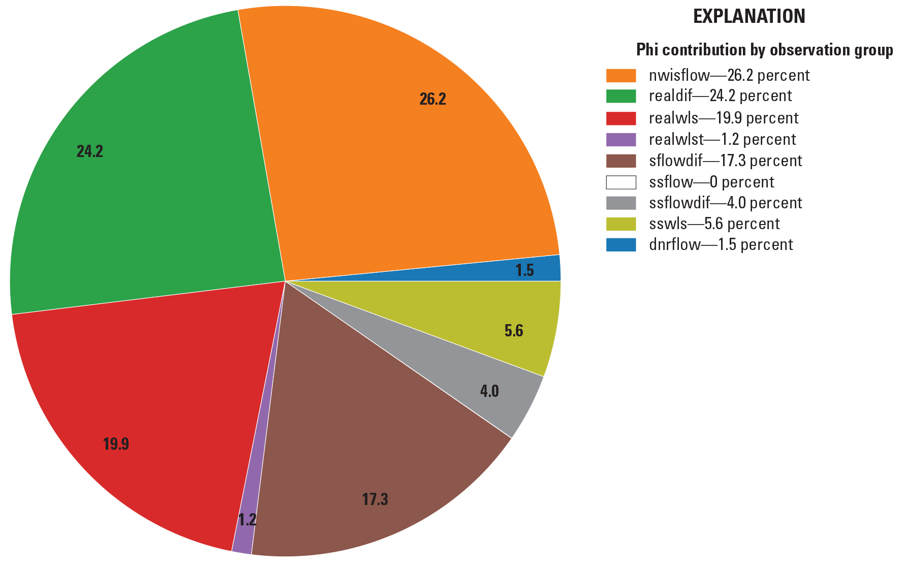
Distribution of phi values by observation group for the calibrated Central Platte Integrated Hydrologic Model.
Calibrated Parameters
This section of the report describes the final calibrated values for the automated values of the 435 adjustable parameters in the six parameter groups for the CPIHM. The following sections will provide a summary of the final calibrated parameter values and a comparison to the initial parameter values to illustrate how the calibration changed the parameter values to improve the fit between the calibration targets and their simulated equivalent values. The summaries will focus on the hydraulic parameters contained in the core MODFLOW–NWT functionality of the CPIHM because the landscape and climate parameters contained in the FMP functionality of the CPIHM were fixed before the automated calibration process. A sensitivity analysis also summarizes which parameters had the largest effect on the model outputs, and parameter identifiability indicates how well the calibration target dataset informed the parameters, which is discussed in the next section of the report.
Calibrated Groundwater-Flow Parameters
Calibrated Kh estimated at pilot points (fig. 13) and interpolated to the model grid kept the general trends and magnitude of the initially estimated hydraulic conductivity described in Houston and others (2013). The calibrated average Kh for layers 1, 2, and 3 were about 70, 32, and 35 ft/d, respectively (table 13). These numbers are all slightly higher (within 5 ft/d) than the initial starting values (table 1). Calibrated layer 1 Kh was generally less than 50 ft/d in the western region and more than 50 ft/d in the eastern region of the CPIHM (fig. 20A). Calibrated layer 2 Kh was generally less than 50 ft/d in almost all regions of the CPIHM except for the northeast corner where some Kh values were greater than 200 ft/d (fig. 20B); calibrated values greater than 200 ft/d were also simulated in the coincident COHYST model region in Peterson (2009). Calibrated layer 3 Kh was generally less than 40 ft/d in almost all regions of the CPIHM except for a west-central region where some Kh values were greater than 100 ft/d (fig. 20C). The highest Kh values for each layer were distributed around pilot points that had high initial values and were not outside the range of reasonable values for that layer; the high Kh values agreed with the test hole data from Houston and others (2013).
Table 13.
Calibrated adjustable parameter summaries of the minimum, average, and maximum calibrated (posterior) values for pilot points and model grid.[A, Soil group A; B, soil group B; C, soil group C; na, not applicable]
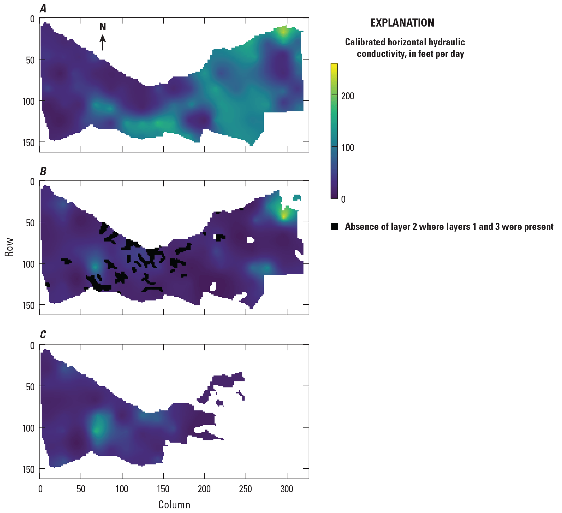
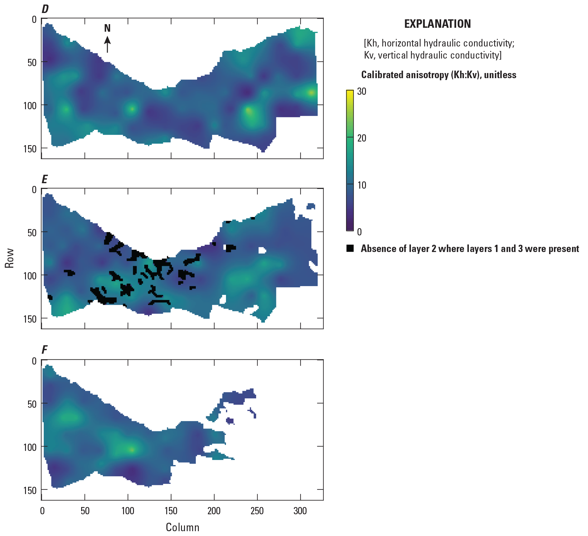
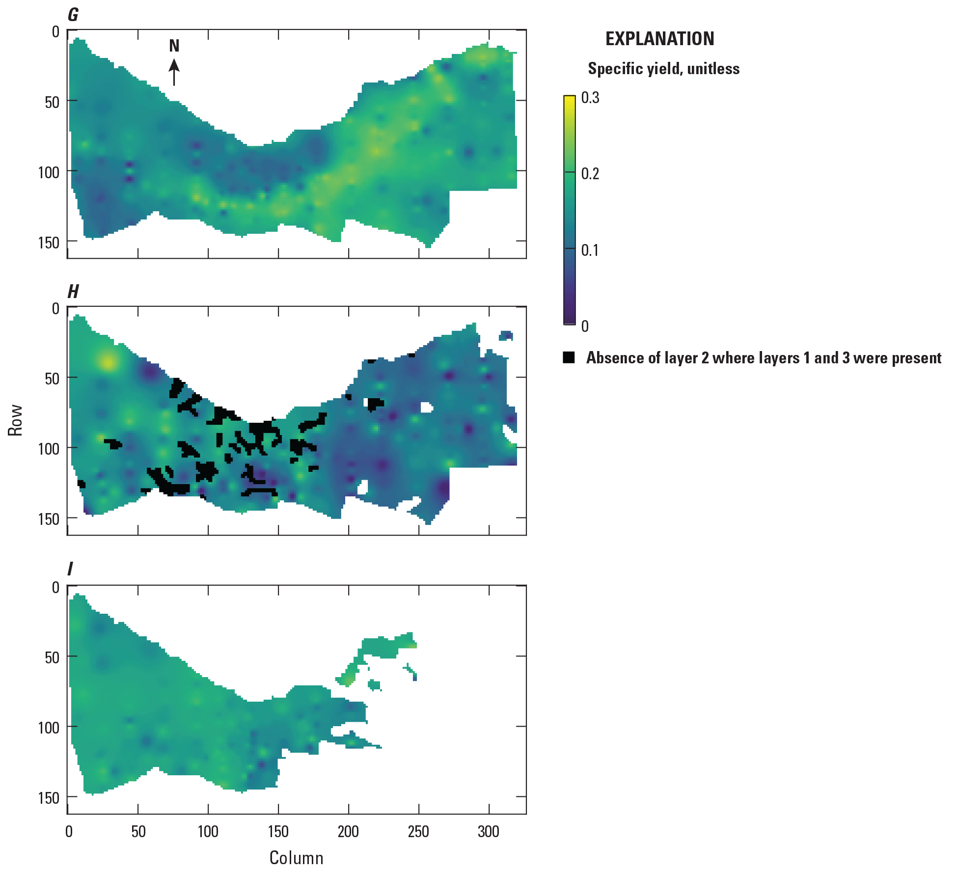
Central Platte Integrated Hydrologic Model calibrated aquifer properties for each layer. A, Horizontal hydraulic conductivity for layer 1. B, Horizontal hydraulic conductivity for layer 2. C, Horizontal hydraulic conductivity for layer 3. D, Anisotropy for layer 1. E, Anisotropy for layer 2. F, Anisotropy for layer 3. G, Input specific yield for layer 1. H, Input specific yield for layer 2. I, Input specific yield for layer 3.
Calibrated anisotropy, the ratio of horizontal to vertical hydraulic conductivity (Kh:Kv) estimated at pilot points (fig. 13) and interpolated to the model grid remained in the general range of acceptable values for each layer. The average vertical anisotropy for layers 1, 2, and 3 were 9.73, 9.86, and 9.99, respectively, which were equated to vertical hydraulic conductivity values for all layers (between 0.33 and 31.70 ft/d), and the calibrated average vertical hydraulic conductivity for layers 1, 2, and 3 were 7.86, 3.41, and 3.60 ft/d, respectively (table 13). Calibrated layer 1 vertical hydraulic conductivity was between less than 7 ft/d in most of the western CPIHM domain and primarily between 7 and 20 ft/d in the southern and eastern domain (fig. 20D). Layer 2 vertical hydraulic conductivity was less than 10 ft/d for most of the CPIHM domain (fig. 20E). Calibrated layer 2 vertical hydraulic conductivity increased from the initial values in much of the central and southern CPIHM domain where it was present and generally decreased in the northern and eastern regions (fig. 20E). Calibrated layer 3 vertical hydraulic conductivity remained near initial values for most of the CPIHM domain except for two areas in the west where values were greater than about 10 ft/d (fig. 20F). The Sy, which was fixed during calibration, is shown in figure 20G–I.
Parameter Sensitivity and Identifiability
The automated calibration process includes the calculation of the sensitivity of simulated observations to model parameters, where sensitivity is the change in simulated observation divided by the change in a model parameter; PEST records sensitivities of simulated observations to each parameter in the Jacobian matrix (Doherty, 2005). Parameter sensitivities were extracted from the Jacobian matrix file written by PEST and composite parameter sensitivities were analyzed from the sensitivity file, also written by PEST, and are available in the model archive (Traylor, 2023). Parameter sensitivities can provide some insight into parameters that were most impactful during the calibration process. The parameter sensitivities were assessed by parameter group and the most sensitive group was the anisotropy pilot points (apilotpts) with an average composite sensitivity of 0.351. The Kh pilot points (pilotpts) group had a slightly smaller average sensitivity of 0.342. The streambed hydraulic conductivity group (sfrprops) was the least sensitive parameter group. The apilopts group and, to a slightly less extent, pilotpts were the most sensitive because the anisotropy parameters affected the magnitude of vertical flow in the development model. The present gradient between the layers where average simulated groundwater levels were lowest in layer 2 (table 12) coupled with the large amount of groundwater irrigation wells that pumped in the development model (more than 20,000 by 1980; fig. 3), affected the vertical flow dynamics and the groundwater levels in the transient system.
Parameter sensitivities for the final Jacobian matrix used for calibration, with fixed landscape parameters, were low compared to an assessment of parameter sensitivity with all parameters set as adjustable (fig. 21A and table 1.3). In the Jacobian matrix, calculated with all parameters set to adjustable, July and August development period ETref scale factor parameters were the most sensitive and, during preliminary calibration runs, exhibited large deviations from initial values that affected AET, deep percolation (recharge to the water table), and irrigation pumping (table 1.3). The Sy multiplier for layer 1 was also one of the most sensitive parameters (12 of 740) that deviated from reasonable values during preliminary calibration runs (table 1.3). The parameter sensitivities under the fixed scheme influenced the forecast uncertainties and are described in the “Forecast Uncertainty Analysis” section of this report.
Parameter sensitivities are one metric that can be useful in understanding the parameter behavior during calibration. In complex environmental models such as the CPIHM, parameters are often correlated because there are far fewer observations than parameters, which can limit the ability for PEST to fully resolve some or all parameters with a unique solution during calibration. Quantification of how PEST is able to resolve unique parameter values is known as “parameter identifiability.” Parameter identifiability was assessed and provided insight into the information gained by each parameter from the calibration targets dataset during the calibration process and how well each parameter was uniquely estimated and correlated with other parameters (Doherty and Hunt, 2009; Doherty, 2015). Parameter identifiability was analyzed using pyEMU, an open-source Python module that offers a suite of tools to interrogate PEST files and analyze uncertainty (White and others, 2016). Identifiability values ranged from zero to one, where a value of one represented a parameter that could be uniquely resolved based on the information in the calibration target dataset; any error associated with the parameter was a result of noise or uncertainty in the calibration targets. Conversely, an identifiability of zero represented a parameter that gained no information from the calibration target dataset and did not cause a change to the residuals that were calculated at the calibration targets. Identifiability values between zero and one indicate that the parameter gained some information from the calibration targets during the calibration, but it also shares some information gained by the calibration target dataset with other parameters and cannot be uniquely solved (Doherty, 2015).
Overall, the pilot points for Kh parameters were the most identifiable as a group given the spatial distribution of the pilot points throughout the model domain and the number of observations in the calibration targets dataset. Individually, the most identifiable parameters in the CPIHM were the hcond_a2 (SFR vertical hydraulic conductivity of the streambed for soil type A), l2hkpp78 (layer 2 Kh at pilot point 78), and l3hkpp23 (layer 3 Kh at pilot point 23; fig. 21B), which were located downgradient of many groundwater-level observations that informed the groundwater-flow direction and reaction to stresses throughout the simulation period. Parameter hcond_a2 exhibited a low sensitivity of about 0.74 and was not in the top 50 most sensitive parameters shown in figure 21A. Whereas it could be the most uniquely solved in the calibration (highest identifiability, shown in figure 21B), the low sensitivity indicated that it did not have a substantial impact on the calibration. The high identifiability of parameter hcond_a2 is likely because it was one of the parameters that spanned much of the model domain and could gain information from observations at many of the 53 streamgage observation locations also distributed across the model domain. Conversely, parameter l2hkpp78 exhibited a high sensitivity of about 1.54 (second most sensitive parameter), which, coupled with its high identifiability, indicated that it was more uniquely solvable and impactful to the calibration than other parameters except hcond_a2. Parameter l3hkpp23 exhibited a very low sensitivity of about 0.10 (332nd most sensitive parameters out of the 435 parameters); however, its identifiability indicated that it was more uniquely solvable than most parameters, but it was not particularly impactful to the calibration (fig. 21A–B).
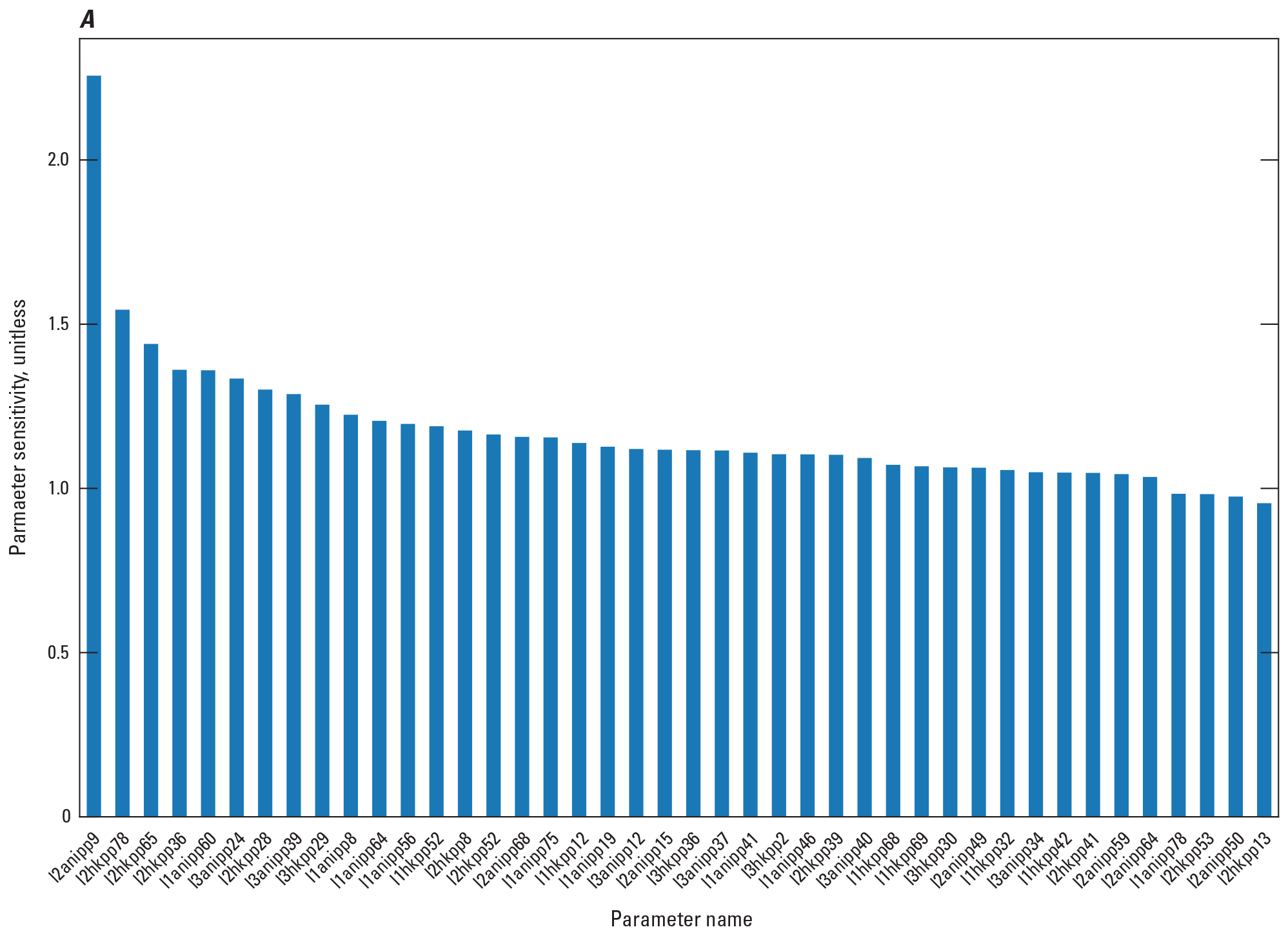
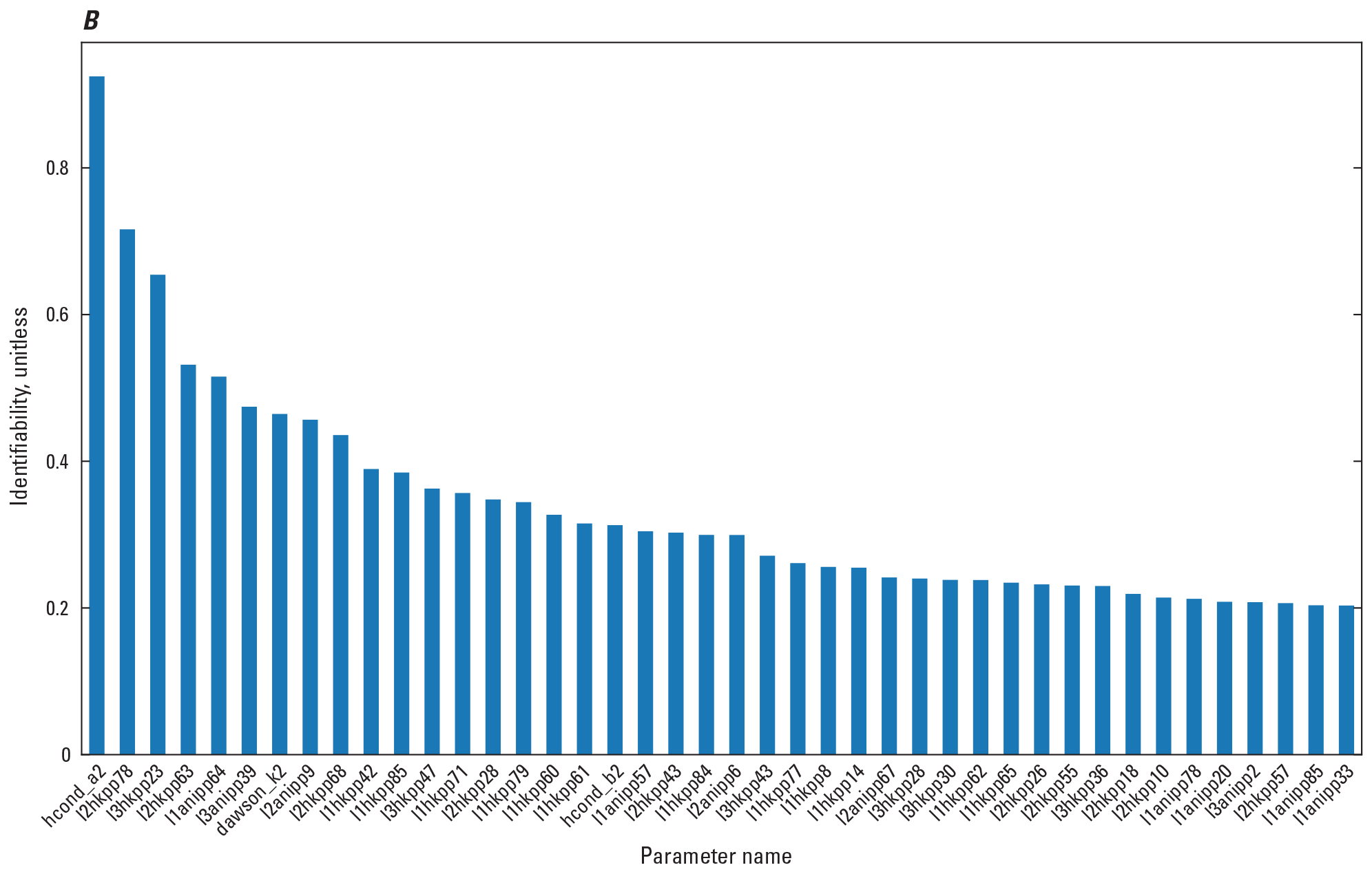
Sensitivity and identifiability of Central Platte Integrated Hydrologic Model Parameters. A, Sensitivity of the 42 most sensitive parameters. B, Identifiability for the 42 most identifiable parameters.
Predevelopment and Development Period Simulated Results and Water Budgets
This section of the report describes the simulated landscape and groundwater-flow budgets for the CPIHM predevelopment (April 30, 1895) and development model (May 1, 1895, to December 31, 2016) and for the recent development period (January 1, 2011, to December 31, 2016). The accurate simulation of water-budget components is important to the efficacy of the model to simulate historical results and minimize or understand the bias that can transfer to the scenario results. Additionally, landscape and groundwater-flow budgets for the development model are described for the 24 GWMAs, as well as the CPNRD area, and the entire model area (called the “CPIHM domain”), which were made by grouping the 212 WBSs into larger areas of interest, in the CPIHM (fig. 9). Calculation of total inflows and outflows for the landscape budget does not include the hybrid Eg and Tg, as described in the “MODFLOW–One-Water Hydrologic Model Theory and Approach” section of this report. Also, where applicable, groundwater-flow budget components are expressed as net values, or the difference between inflows and outflows, for each component. Additional simulated budget details are available in appendix 3.
Landscape Water Budgets for the Central Platte Integrated Hydrological Model Domain
The calibrated predevelopment CPIHM produced landscape water-budget inflows and outflows that were meant to approximate the average conditions prior to surface-water and groundwater irrigation development and to provide reasonable initial conditions for the development CPIHM. Precipitation was the only inflow to the landscape subsystem with an average annual flux of 10,937,662 acre-ft/yr (26.6 inches). Total outflows were distributed among Ep, Tp, Ei, Ti, deep percolation, and runoff. The primary outflow was Ep with an average annual flux of about 6,362,644 acre-ft/yr (58 percent of the outflows). The sum of Ep and Tp, evapotranspiration of precipitation (ETp), accounted for 97 percent of the outflows from the landscape subsystem with an average annual flux of 10,577,561 acre-ft/yr (25.8 inches). The average annual flux for deep percolation and runoff were 91,687 acre-ft/yr (0.22 inches) and 268,414 acre-ft/yr (0.65 inches), respectively (Traylor, 2023).
The calibrated development CPIHM produced landscape water-budget inflows and outflows that maintained the general trends and magnitudes similar to the conceptual understanding of the landscape water subsystem (fig. 22; table 14). Total inflows to the landscape, prior to groundwater irrigation development, were largely from precipitation, with minor amounts from surface-water deliveries for irrigation. The average annual flux of precipitation was 9,978,276 acre-ft/yr (24.3 inches if spread equally across the model domain), or about 93 percent of the inflows to the landscape for the development period (May 1, 1895, to December 31, 2016) (table 14). The average annual total outflows from the landscape during the development period were 10,709,293 acre-ft/yr and the primary outflows were to Tp (4,184,162 acre-ft/yr) and Ep (3,751,102 acre-ft/yr); ETp accounted for about 80 percent of the outflows from the landscape at 7,935,263 acre-ft/yr (table 14 shows Ep and Tp). Compared to the estimates for evapotranspiration of irrigation plus precipitation for the CPIHM in table 2, which ranged from 8,600,000 to 11,000,000 acre-ft/yr, the sum of all evaporation and transpiration columns in table 14 total 8,554,930 acre-ft/yr. Deep percolation (recharge to the water table) and runoff were also substantial outflows from the landscape across the development period (1895–2016) with average annual fluxes of 1,122,257 (about 2.7 inches) and 1,032,106 (about 2.5 inches) acre-ft/yr, respectively (table 14). Further, the deep percolation values on irrigated land and dry cropland simulated by the CPIHM were in accord with recharge measurements from Steele and others (2014) and the overall average annual deep percolation of about 2.7 inches is within the ranges simulated by the models in Peterson (2009) and Peterson and others (2016) for this study area.
Table 14.
Average annual Central Platte Integrated Hydrologic Model landscape budgets for the landscape development period (1895–2016) and landscape recent development period (2011–16).[CPIHM, Central Platte Integrated Hydrologic Model; CPNRD, Central Platte Natural Resources District; GWMA, Groundwater Management Area]
Table 15.
Average annual Central Platte Integrated Hydrologic Model groundwater budgets for the groundwater development period (1895–2016).[—Left][GWMA, Groundwater Management Area; CPNRD, Central Platte Natural Resources District; CPIHM, Central Platte Integrated Hydrologic Model; --, not applicable]
Table 16.
Average annual Central Platte Integrated Hydrologic Model groundwater budgets for the groundwater recent development period (2011–16).[—Left][GWMA, Groundwater Management Area; CPNRD, Central Platte Natural Resources District; CPIHM, Central Platte Integrated Hydrologic Model; --, not applicable]
Temporal trends in the landscape budget were marked by the onset of widespread groundwater irrigation that was responsible for the increase in total inflows to the landscape during the development period; average annual total inflows for 1895–2016 and 2011–16 were 10,709,293 and 12,084,641 acre-ft/yr (table 14). The increase in total inflows led to an increase in total outflows primarily through an increase in deep percolation and ET of irrigation water (sum of Ei and Ti) (fig. 22). The ETp declined after about 1960; however, total landscape-derived ET, the ETp and irrigation water (sum of Ep, Ei, Tp, and Ti), exhibited less than a 2-percent increase in the recent development period (2011 to 2016) compared to the pre-1940 development period (fig. 23). The landscape water budgets for the development CPIHM were similar from 1895 to about 1960 whereby the budget was primarily affected by inflows from annual precipitation and outflows to ET of that precipitation. After about 1960, the increase in groundwater irrigation for crops added additional outflows as ET of the irrigation water (fig. 22, 23). The large increase in irrigation after 1960 was the primary cause of the increase in deep percolation from about 660,000 acre-ft/yr (1895–1960 average) to about 1,700,000 acre-ft/yr (1961–2016 average; fig. 22). Another factor that contributed to the substantial increase in deep percolation was a 7-percent increase in average precipitation after 1960.
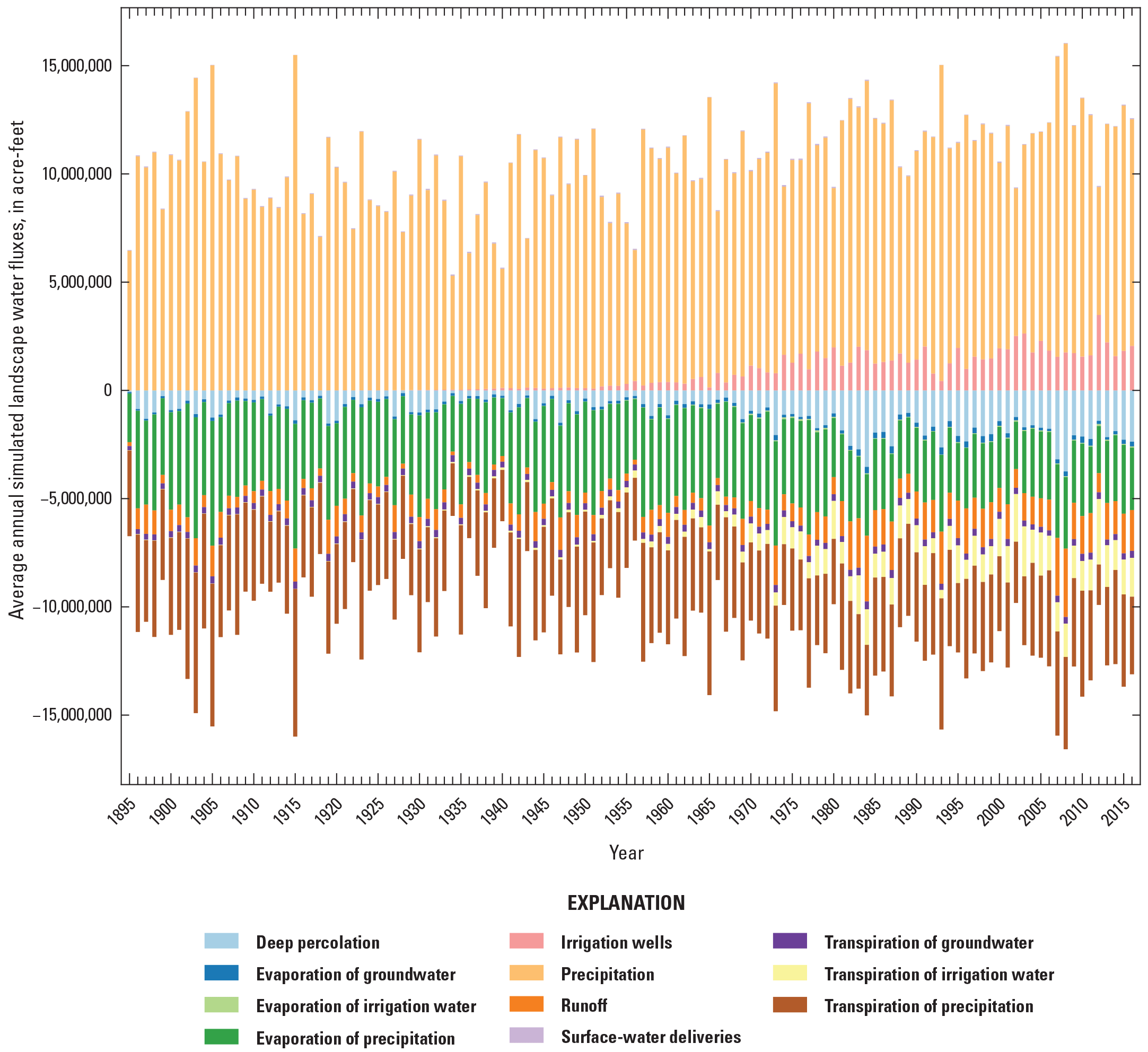
Simulated annual landscape water-budget volumes for the development period Central Platte Integrated Hydrologic Model (1895–2016).
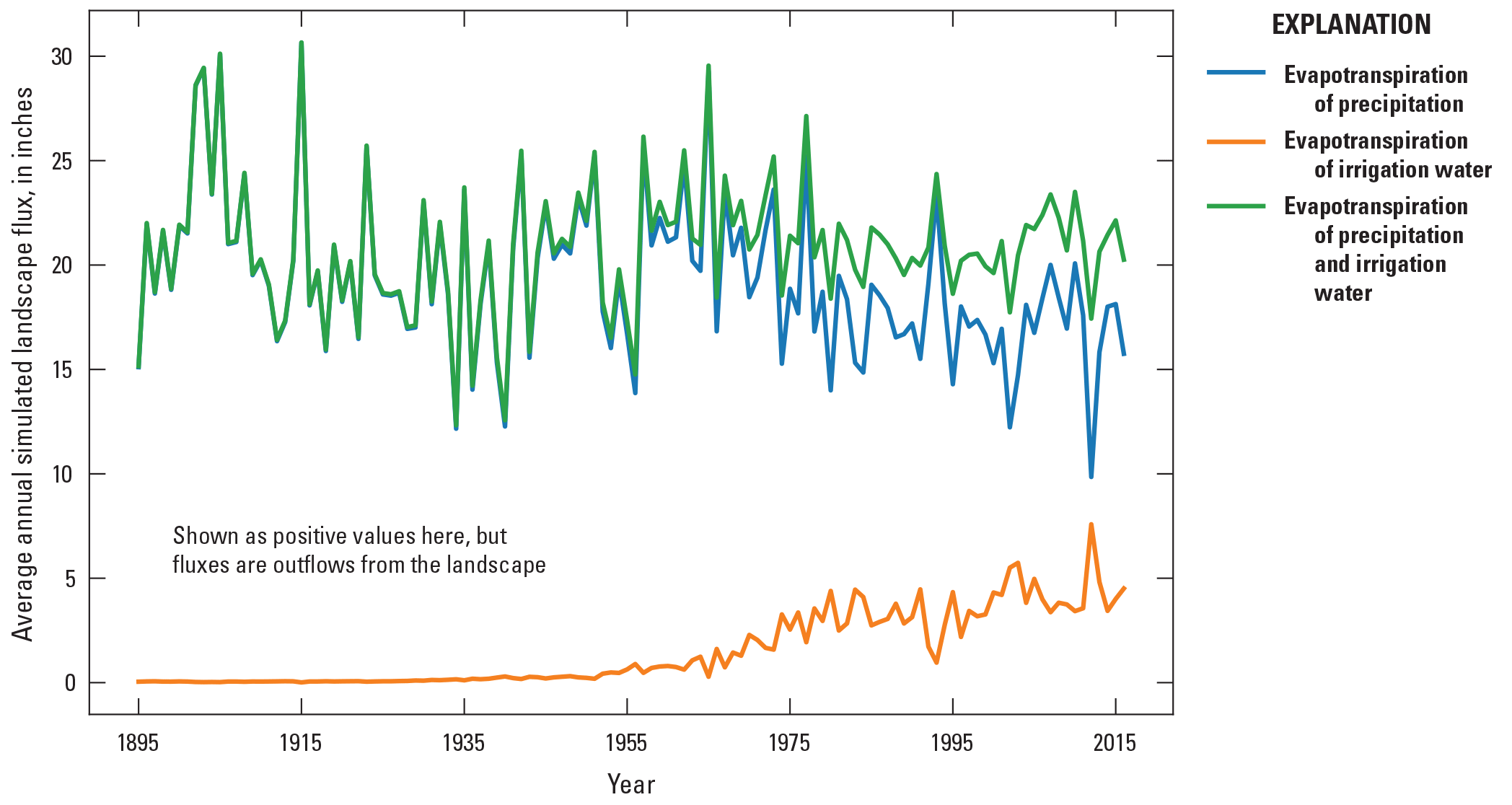
Simulated average annual evapotranspiration of precipitation, evapotranspiration of irrigation water, and evapotranspiration of precipitation and irrigation water for the calibrated Central Platte Integrated Hydrologic Model.
In the last 5 years of the development model simulation (2011–16), the average annual volume of total landscape ET, which included ET of precipitation and irrigation water sources, was 8,420,099 acre-ft/yr, about 11 percent less than the conceptual model estimate of 9,500,000 acre-ft/yr for the same time period but only 4.5 percent less than the estimated range of uncertainty for ET from the conceptual estimates in table 2 (table 14). The average deep percolation and runoff volumes simulated for the last 5 years of the development period (2011–16) were 2,056,936 and 1,607,607 acre-ft/yr, respectively. Monthly trends from 1980–2016 indicated that the largest rates of deep percolation occurred in the spring (April and May) when precipitation was highest, and ETp was relatively low compared to peak growing season (July) ET (fig. 24).
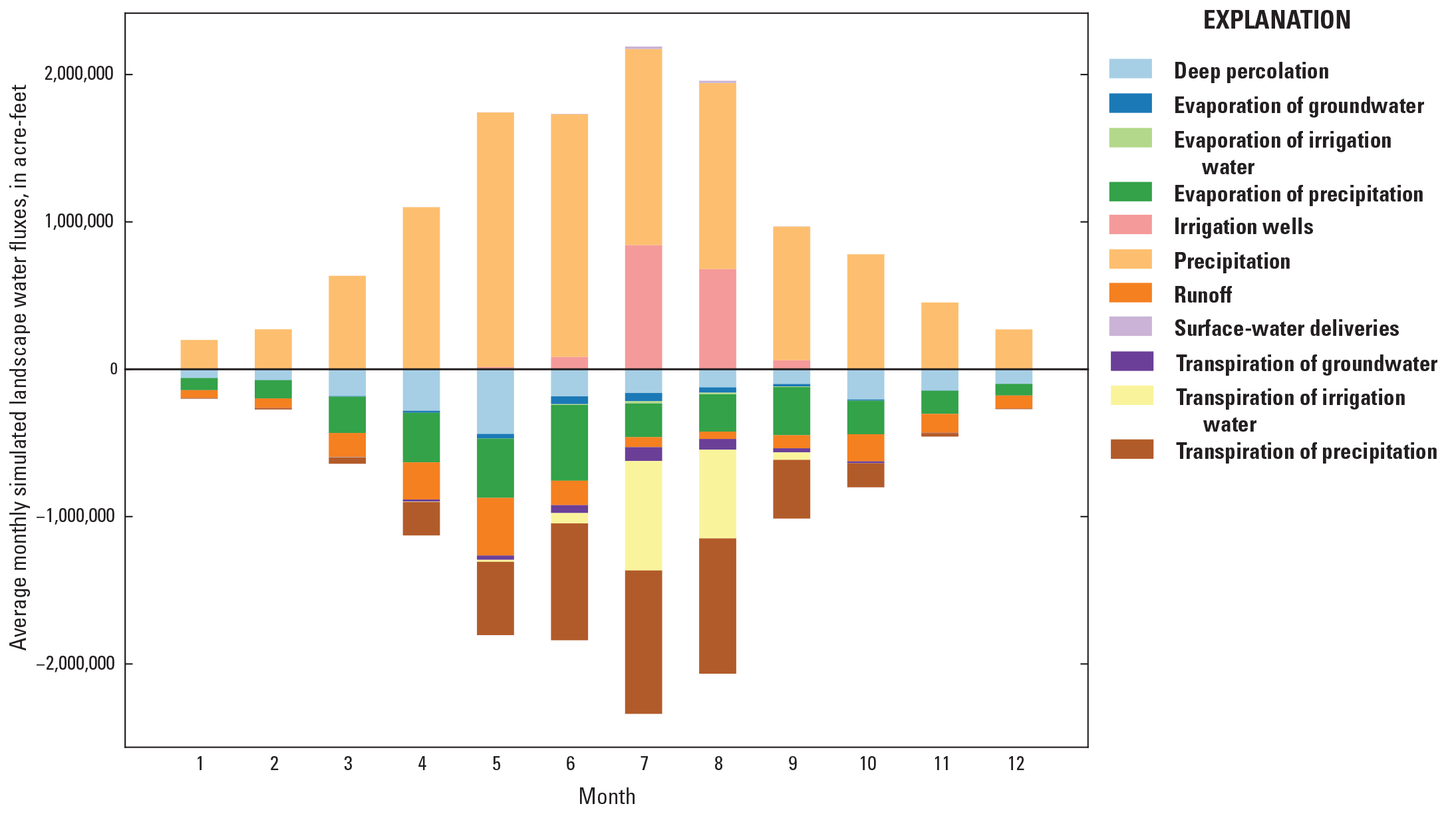
Simulated average monthly landscape water-budget volumes for the calibrated development period Central Platte Integrated Hydrologic Model (May 1, 1980–December 31, 2016).
The manually calibrated development period average annual ETref increased from 57.4 to 74.5 inches, a 30-percent increase from the precalibrated ETref (fig. 25). The reduction in ETref after 1980 is a result of different scale factors applied to the bi-annual and monthly stress periods to account for monthly dynamics in ET; however, this reduction was not present in the annual simulated total landscape ET, which increased by less than 2 percent for the development period owing to an increase in ET from irrigation water, as stated previously in the discussion of temporal trends (figs. 22, 23). The average monthly ETref increased 13-percent from the precalibrated ETref, for May through September (fig. 26, 10B). The increase in ETref was necessary because it led to an increase in the CWD for all crop types and increased the CIR for irrigated crops to values that were similar to conceptual estimates of total landscape ET and groundwater irrigation pumping.
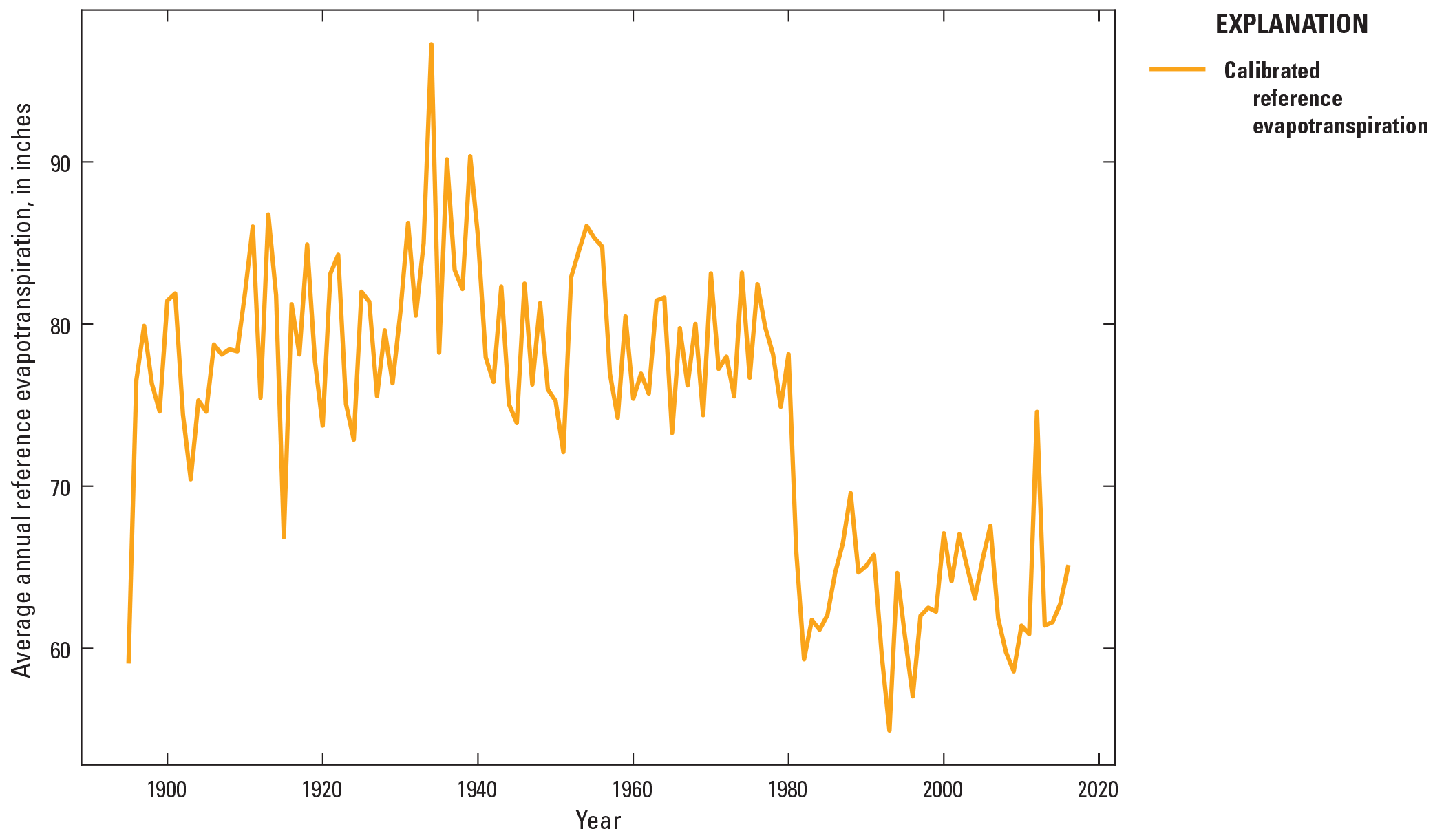
Simulated average annual reference evapotranspiration for the calibrated Central Platte Integrated Hydrologic Model.
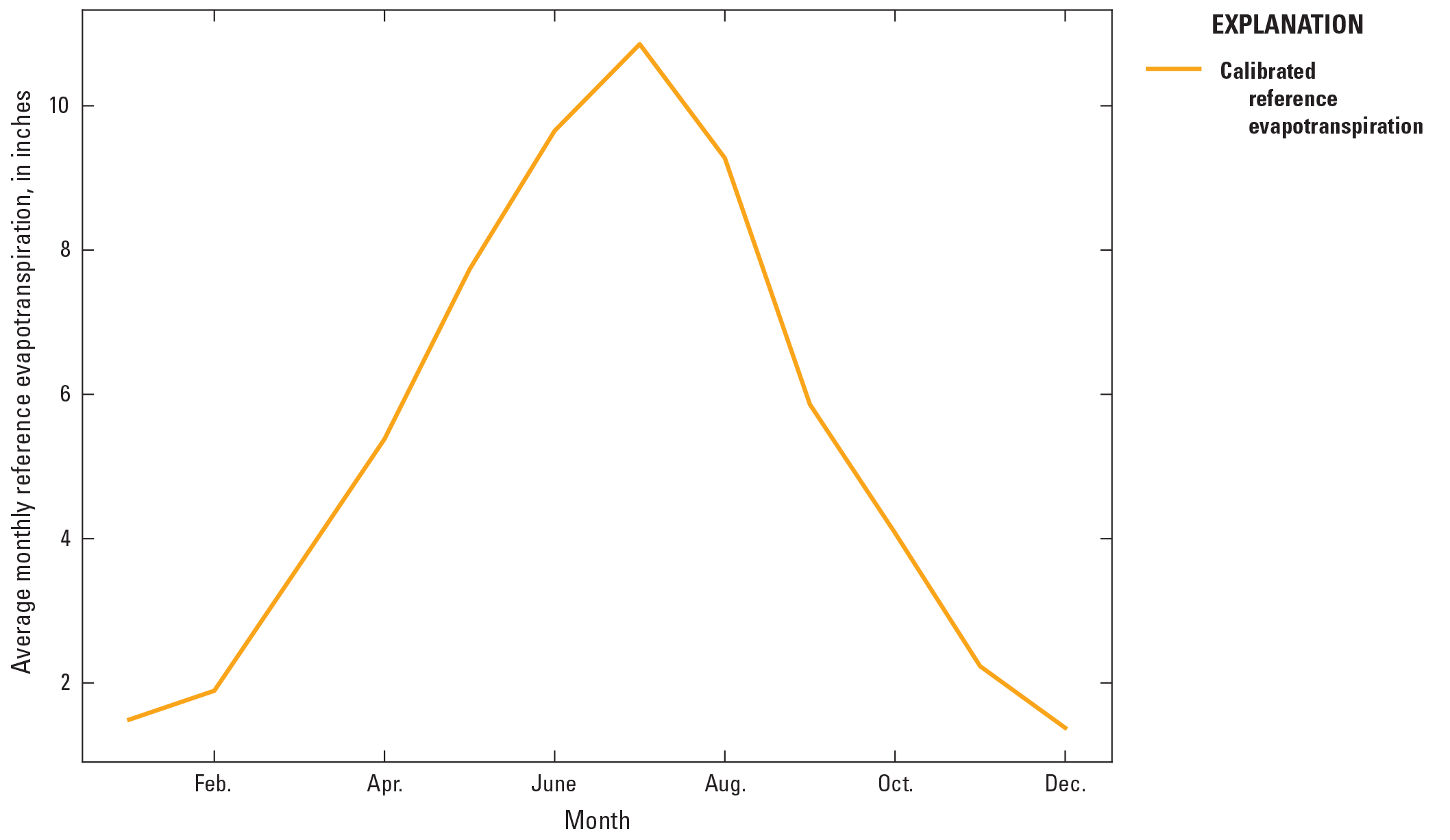
Simulated average monthly reference evapotranspiration for the calibrated Central Platte Integrated Hydrologic Model.
Although some simulated landscape flow components such as irrigation pumping and ET were a little different than conceptual estimates, they still represented the conceptual model within expected uncertainty. The landscape budget simulated by the CPIHM can be considered a more precise representation of the landscape water budget than the conceptual flux estimates from table 2, because the conceptual estimates are uncertain, but also because the simulated budgets are calibrated and reconciled with simulated groundwater flow.
Landscape Water Budgets for Groundwater Management Areas and Other Domains
Simulated landscape water budgets were assessed for each GWMA and the CPNRD (table 14). The budgets for each GWMA and the CPNRD were similar to the CPIHM budget and were characterized by primary inflows from precipitation and large outflows to ET. Deep percolation was affected by three factors: precipitation; the amount of irrigation water from irrigation wells or surface-water deliveries; and ETg, which was linked to the depth of the water table. Like the CPIHM domain, GWMAs with large irrigation volumes per acre, such as GWMA 3 and 14 (fig. 9), also exhibited large volumes of recharge per acre (table 14, table 3.1). Similarly, GWMAs with large fluxes of precipitation (in the eastern region of the CPIHM) and shallow water tables with large fluxes of ETg, such as GWMAs 19, 22, and 23, also exhibited the large recharge volumes per acre (table 14, table 3.1). GWMAs 1, 6, and 7 exhibited the smallest deep percolation (recharge) volumes per acre because they were in the western region of the CPIHM with less precipitation and less irrigation (fig. 9; table 14, table 3.1). Larger amounts of deep percolation occurred on irrigated lands compared to dryland in the CPNRD (fig. 27). The average annual rates of deep percolation on irrigated land after 1980 (about 5.1 inches) were double the amount on nonirrigated land (about 2.4 inches), and both were within the ranges measured in Steele and others (2014). Further, the relation among precipitation, irrigation, and deep percolation was evident during years of extreme climate conditions. For example, deep percolation on irrigated and nonirrigated cropland was greater than the amount of irrigation pumpage in 1993 because it was the wettest year between 1981 and 2016 (fig. 27). As a result, the CIR was minimal and there was surplus precipitation that went to deep percolation. Conversely, 2002 and 2012 exhibited large irrigation pumpage and little recharge because these were severe drought years. CIR for the severe drought years was very high and there was minimal precipitation available for recharge (fig. 27).
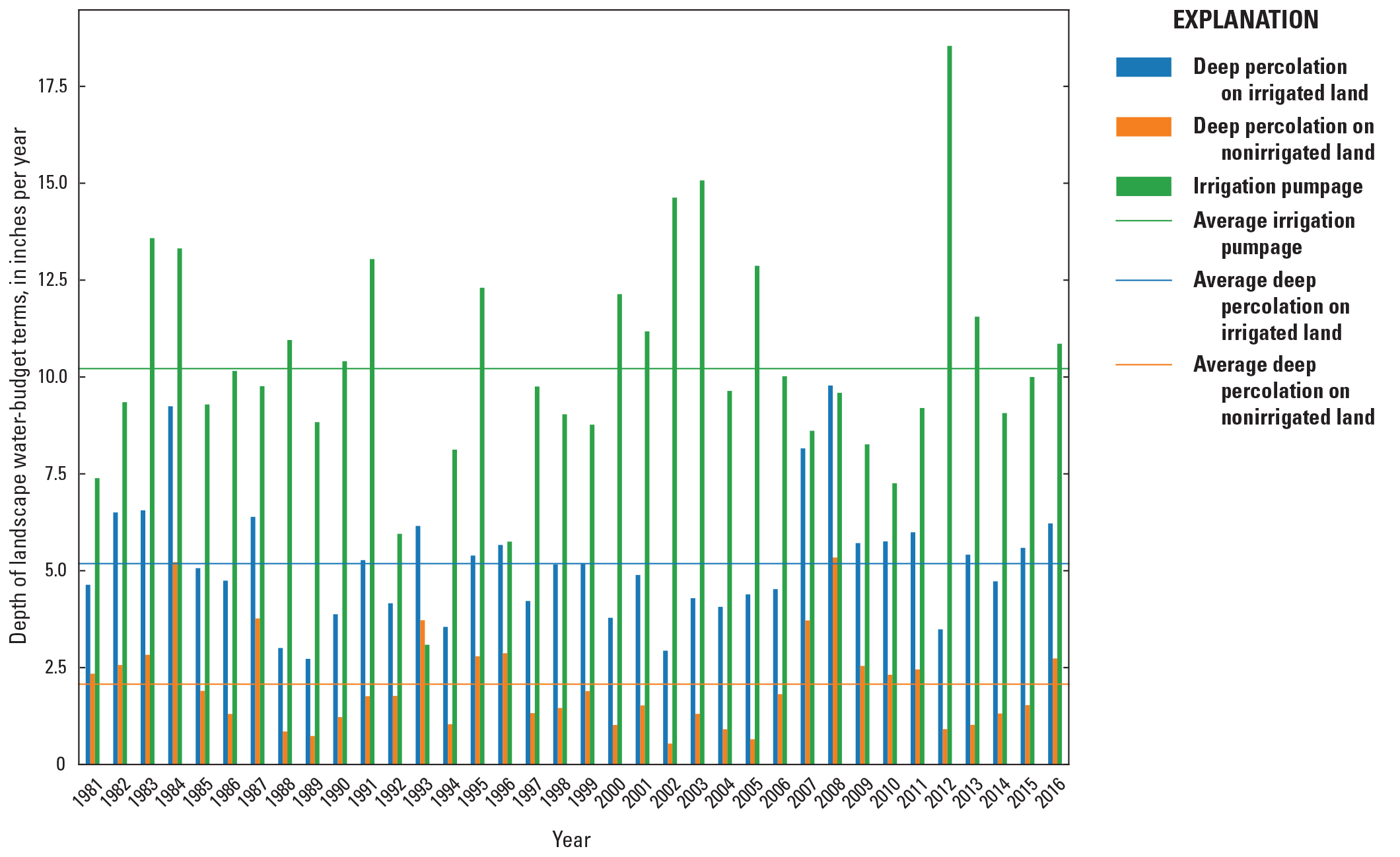
Average annual depths of water applied to the landscape by irrigation wells and deep percolation on irrigated land and nonirrigated land in the Central Platte Natural Resources District supergroup for the Central Platte Integrated Hydrologic Model.
Groundwater-Flow Budgets for the Central Platte Integrated Hydrologic Model Domain
The calibrated predevelopment CPIHM produced groundwater-budget inflows and outflows that were meant to approximate the average conditions prior to surface-water and groundwater irrigation development and to provide reasonable initial conditions for the development CPIHM. Total inflows and outflows were about 193,669,000 and 194,105,766 acre-ft/yr, respectively. Approximate steady-state conditions were achieved whereby the change in groundwater storage across the 500,000,000-day transient stress period was −572 acre-ft/yr. Stream leakage was the primary inflow to the groundwater subsystem, with a flux of 144,885,246 acre-ft/yr (75 percent of total inflows). Inflows to the study area across model boundaries accounted for 18 percent of total inflows and recharge from deep percolation accounted for 7 percent of total inflows. The primary outflow was to ETg, which constituted 53 percent of total outflows. Discharge of groundwater to streams as base flow constituted 33 percent of total outflows, and outflows across model boundaries accounted for 14 percent of total outflows (Traylor, 2023).
The calibrated development CPIHM produced groundwater-flow budget inflows and outflows that reflected the transient conditions simulated in the development period model (table 15, 16). The largest inflow component was recharge (analogous to deep percolation from the landscape), with an average development period (May 1, 1895, to December 31, 2016) annual volume of 1,122,257 acre-ft/yr (table 15). Stream leakage (602,318 acre-ft/yr) was another major annual inflow, which indicated that the stream system in the CPIHM was an important contributor to the groundwater-flow system (table 15). The largest outflows were to irrigation wells (693,171 acre-ft/yr). Changes in groundwater storage were substantial during the development period; the replenishment of groundwater storage was −985,912 acre-ft/yr and releases from groundwater storage were 863,519 acre-ft/yr. The large releases from storage (groundwater-level declines) began to make a substantial impact on the groundwater-flow budget after about 1960 owing to the increase in groundwater pumping for irrigation (fig. 28A). The net storage changes were driven primarily by the relation between outflows to irrigation wells and farm net recharge each year; farm net recharge is the difference between recharge from deep percolation and ETg (fig. 28B). Generally, groundwater levels increased when outflows to irrigation wells were less than farm net recharge (fig. 28B). The replenishment of storage came from a combination of groundwater flowing into the study area, recharge (deep percolation), and stream leakage (fig. 28C, shown as positive values of net streams). Prior to widespread irrigation development (about 1940), recharge was the primary source of water to replenish storage for most average and wet years. During dry periods, stream leakage became the dominant source of water to replenish storage (fig. 28C). After 1980, the average annual releases from groundwater storage were similar to those from recharge at about 1,957,000 acre-ft/yr and 1,941,000 acre-ft/yr, respectively. On average, the increase in outflows to irrigation wells were generally supported by increases in recharge throughout the development period except in dry years (for example, 2002, 2012) when farm net recharge was much less than outflows to irrigation wells. After 1980, even in dry years inflows from farm net recharge were generally greater than net streams (fig. 28D). Net replenishment to storage (negative net storage; groundwater-level rise) generally occurred during wet years or when the absolute magnitude of farm net recharge was greater than the absolute magnitude of irrigation wells (fig. 28B). Also, after 1980, the average annual depth (where depth represents a water-budget component expressed in terms of volume per area) of groundwater pumped by irrigation wells was 10.8 inches (1,698,000 acre-ft/yr), which was similar to the conceptual estimated depth of 10 inches (1,800,000 acre-ft/yr) from table 3 (fig. 27).
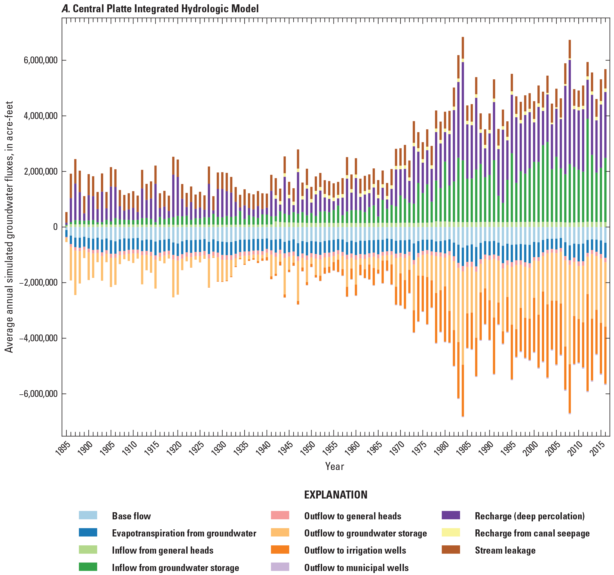
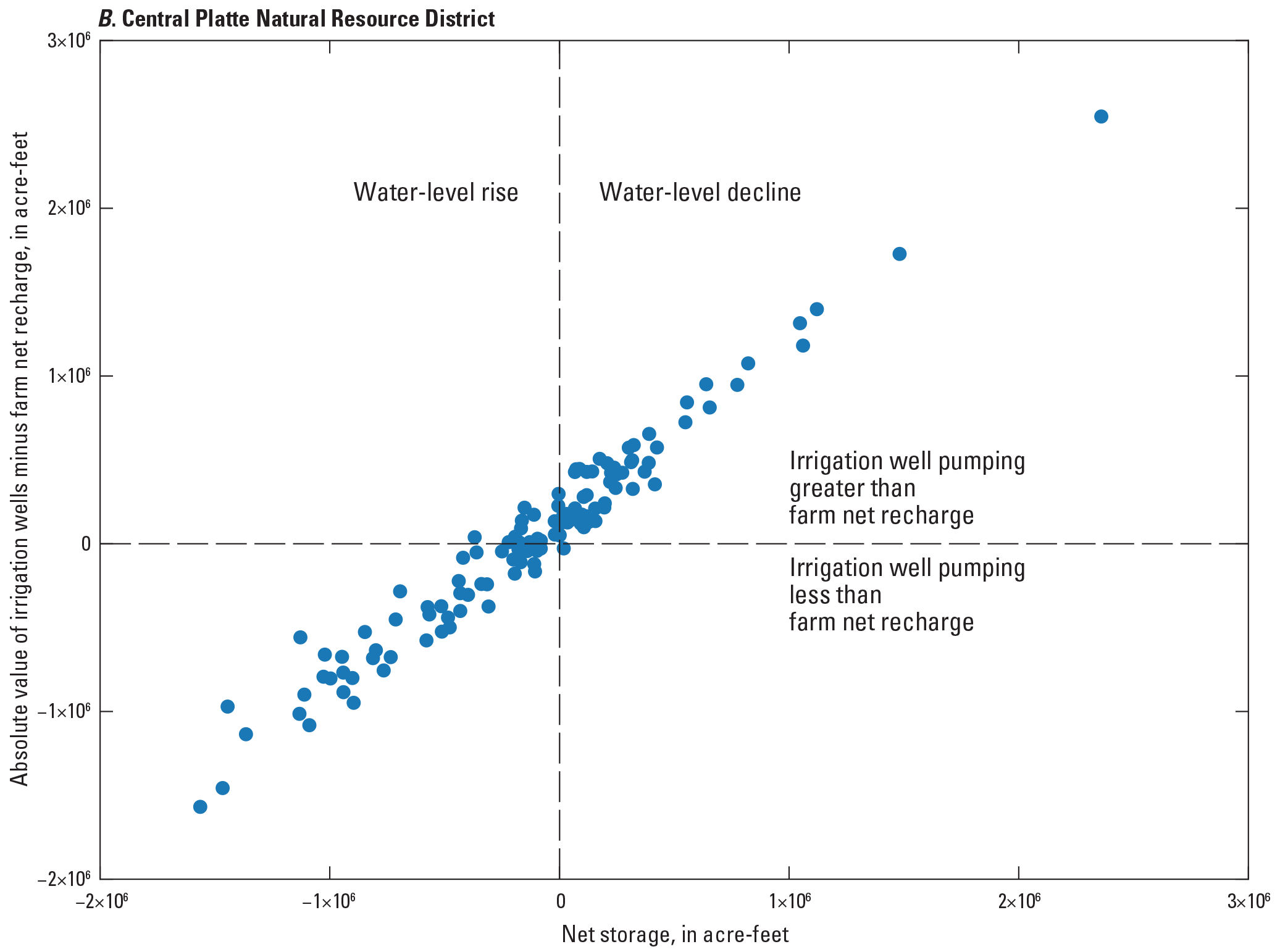
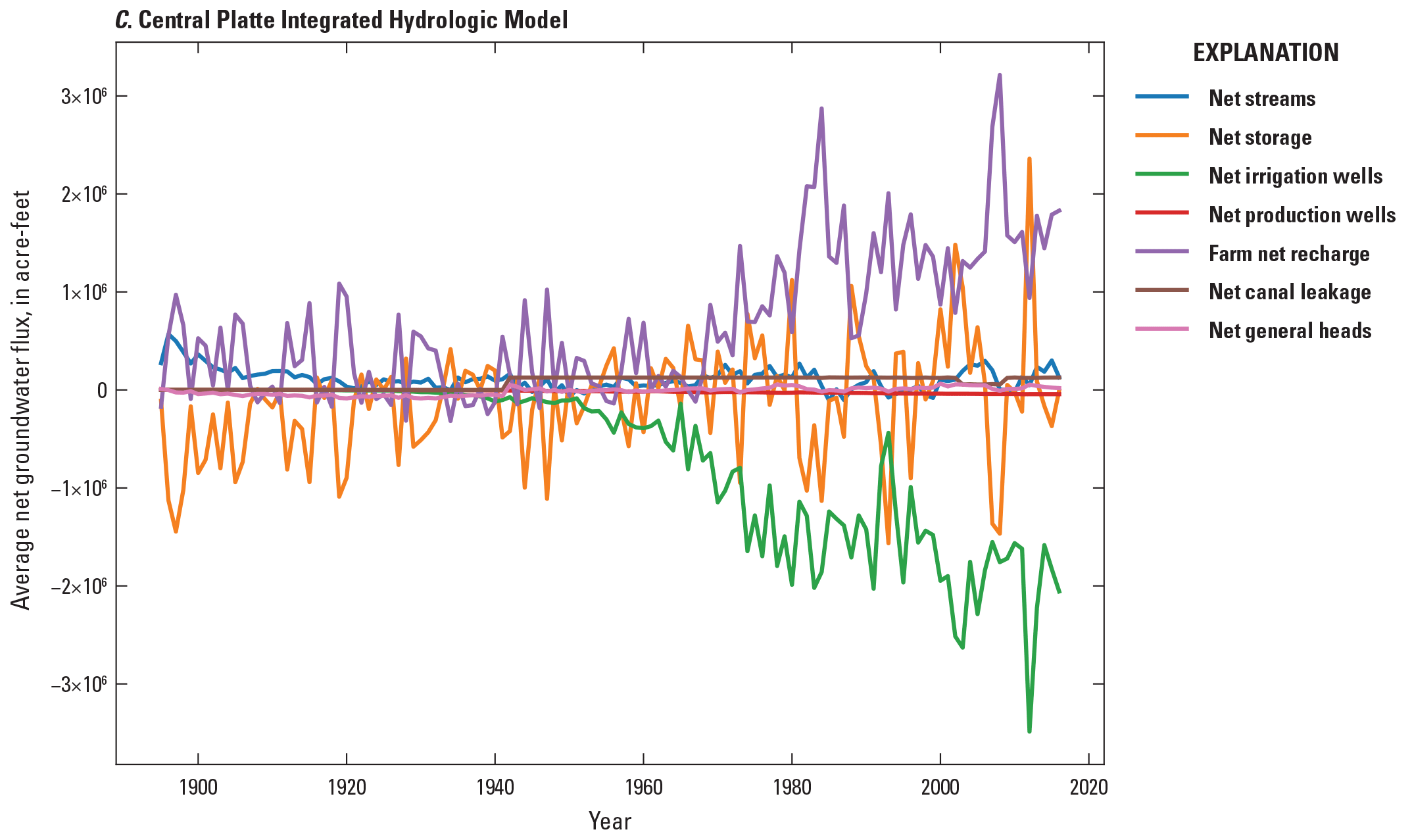
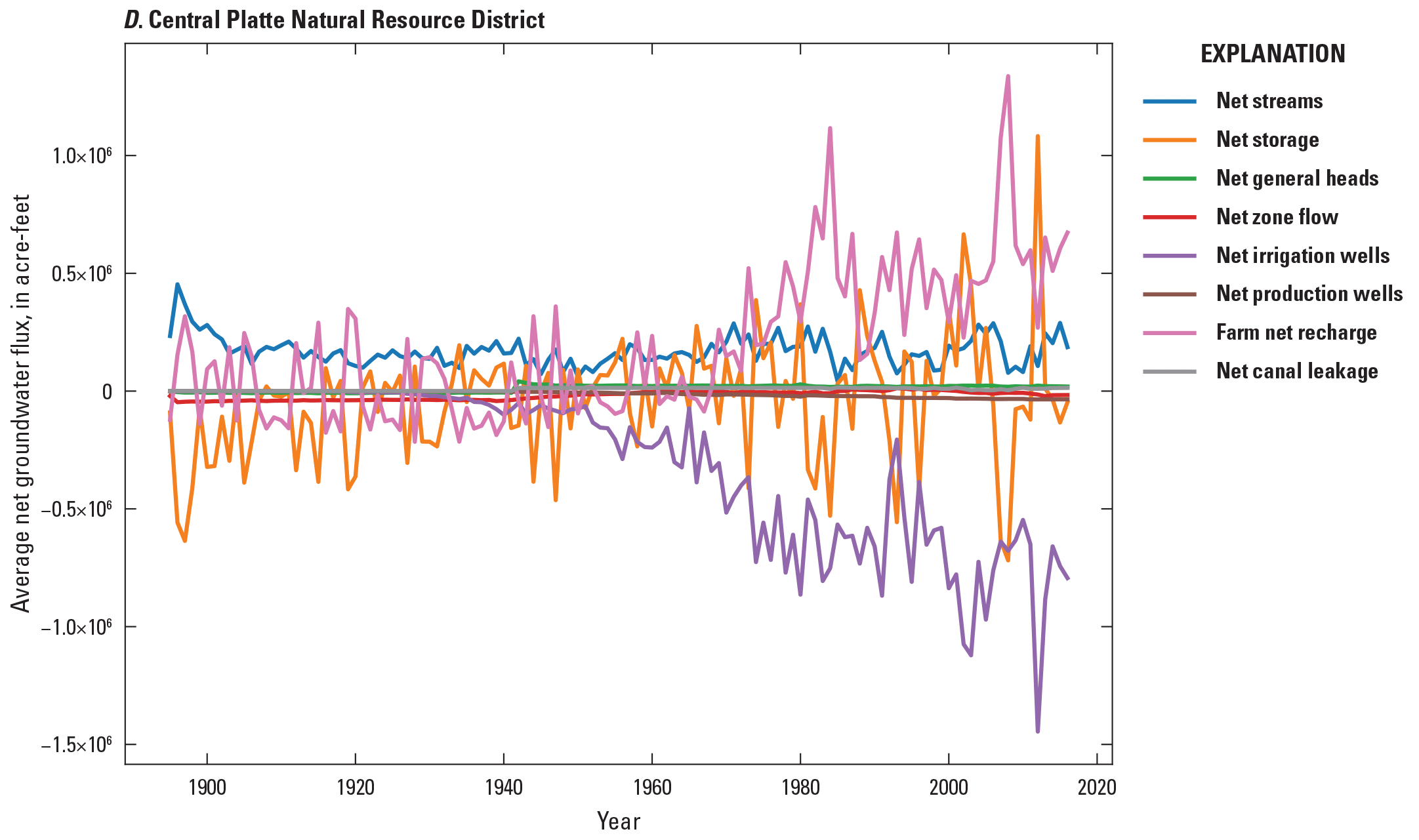
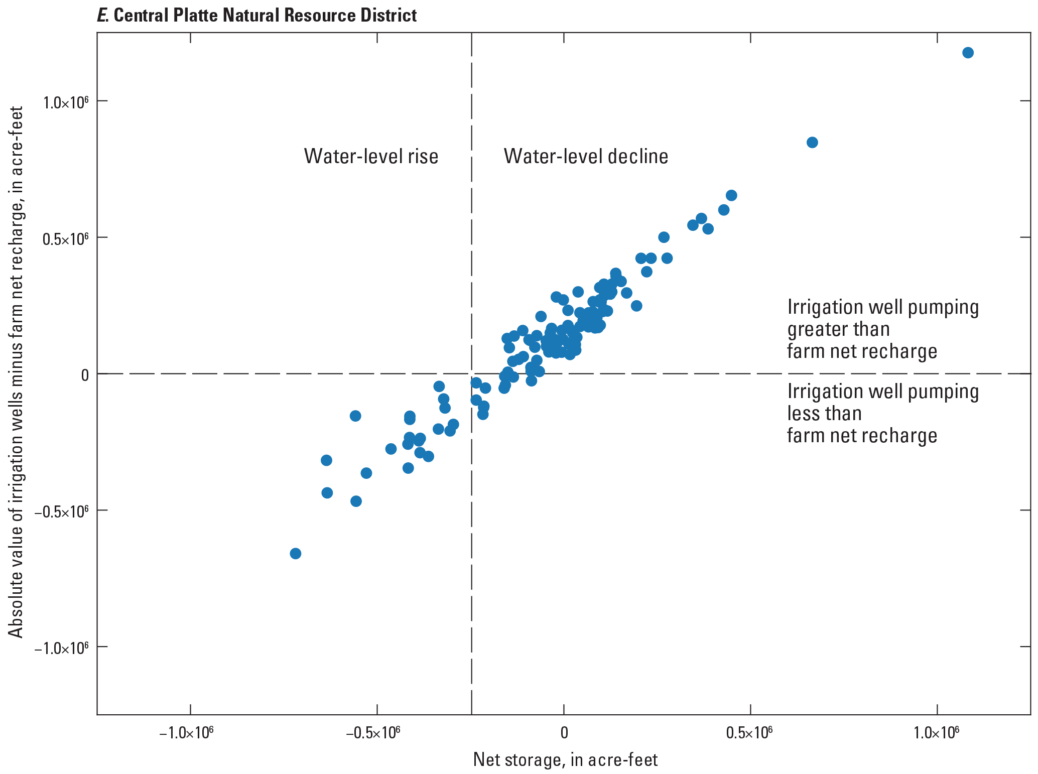
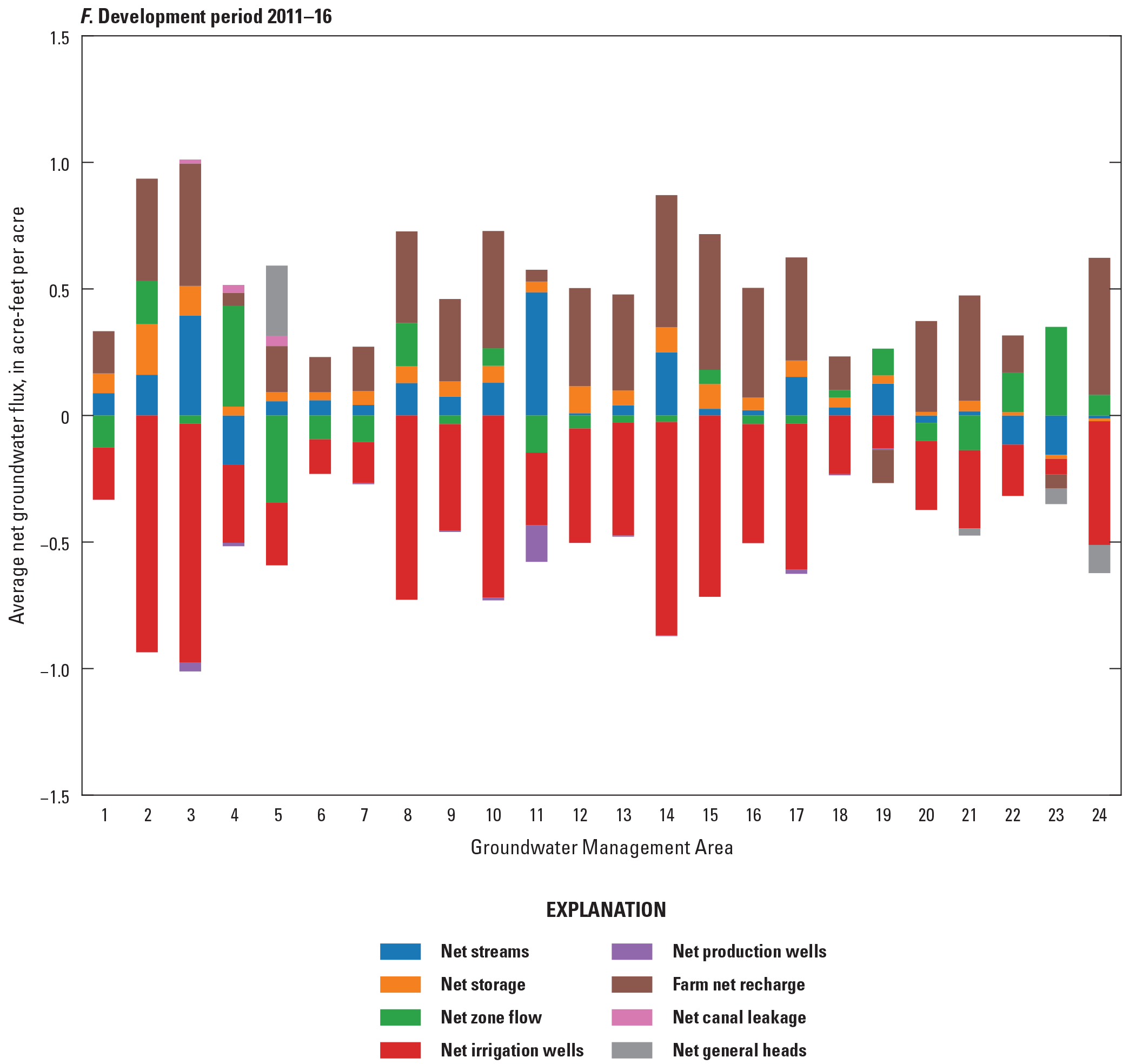
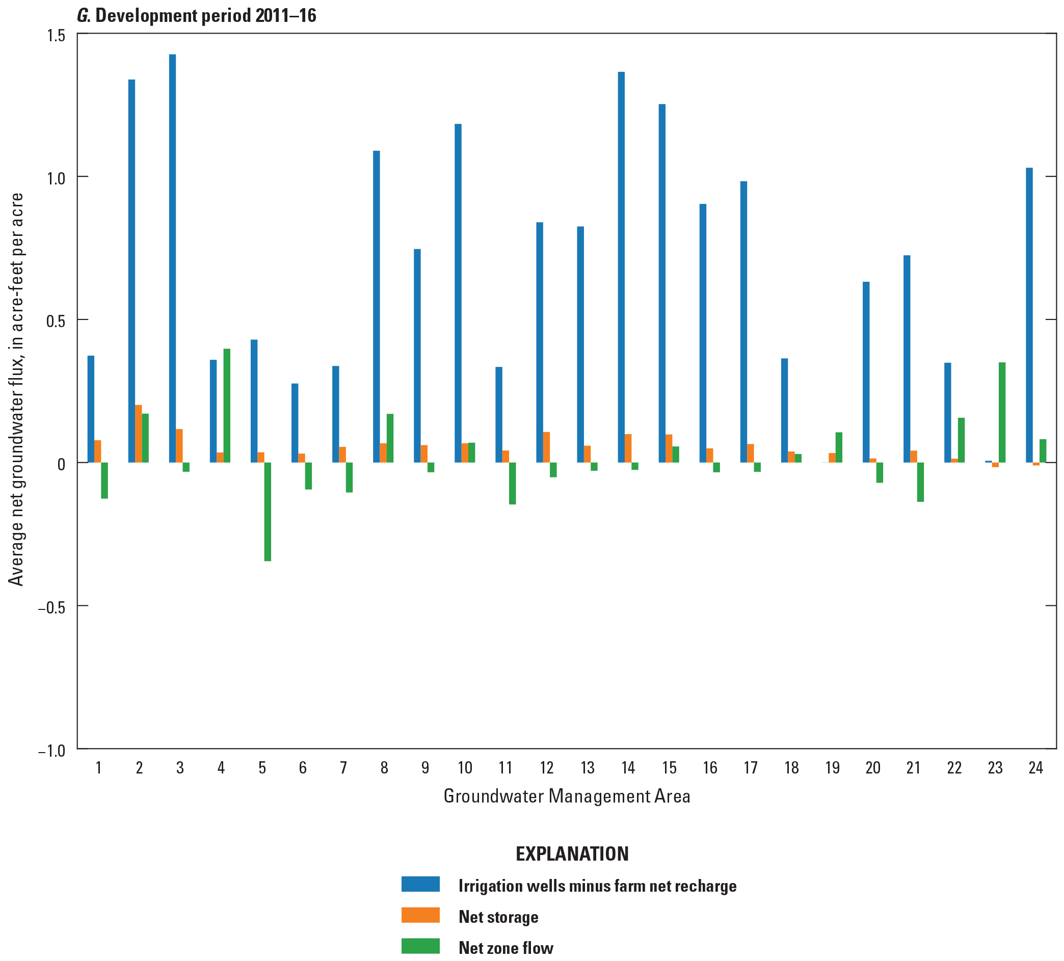
Simulated development period annual groundwater-flow budget components. A, Inflows and outflows by volume. B, Difference between the absolute value of outflows to irrigation wells and farm net recharge. C, Net components by volume for the Central Platte Integrated Hydrologic Model domain. D, Net components, for the Central Platte Natural Resource District. E, Difference between the absolute value of outflows to irrigation wells and farm net recharge for the Central Platte Natural Resource District. F, Net components by volumetric rate for the recent development period (2011–16) by Groundwater Management Area. G, Net volumetric rates for the difference between the absolute value of outflows to irrigation wells and farm net recharge, net storage, and net zone flow for the recent development period (2011–16) by Groundwater Management Area in the Central Platte Integrated Hydrologic Model.
The monthly trend in the simulated groundwater-flow budgets was typical of systems with large amounts of groundwater-irrigated cropland and characterized by large irrigation demands during the growing season. Monthly trends were assessed for the 1981 to 2016 period when the development model stress periods lengths changed to monthly (table 6). Recharge was the largest average monthly inflow from October to June (fig. 29). The largest volumes of recharge occurred in April, May, and October when groundwater pumping to irrigation wells was minimal or absent and precipitation was relatively high (fig. 29). The highest average monthly precipitation in the CPIHM was in June, but there was less recharge compared to April and May because the high landscape ET (1,306,656 acre-ft/yr) removed much of the precipitation that would have otherwise become recharge to the water table. The lowest volumes of recharge occurred in driest months of December, January, and February (fig. 29). The largest inflows to the groundwater-flow system during the 2 months with the highest irrigation (July and August) were caused by the release of groundwater from storage that supported the groundwater pumping during that time; the replenishment to storage occurred primarily during April, May, and October when recharge was highest (fig. 29). The average volume of water pumped for irrigation during July (814,815 acre-ft/yr) was more than twice as large as any other outflows for any month (replenishment to groundwater storage in May: −428,771 acre-ft/yr) (fig. 29).
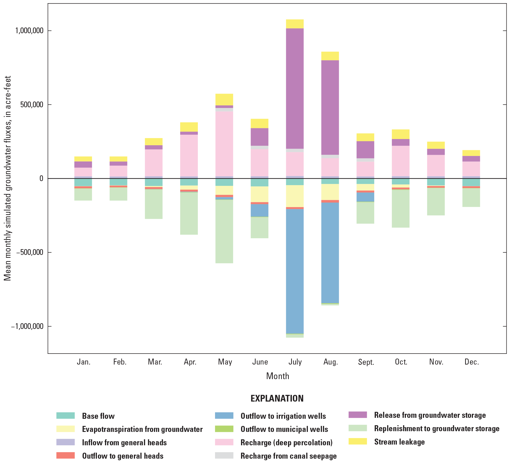
Simulated average monthly groundwater-flow budget from 1981 to 2016 of the development period Central Platte Integrated Hydrologic Model.
Groundwater-Flow Budgets for the Groundwater Management Areas and Other Domains
Individual simulated groundwater-flow budgets were assessed for each GWMA and the CPNRD for the development CPIHM. The budgets for each area were similar to the CPIHM budget, which is characterized by the largest inflows of recharge, largest outflows to irrigation wells, and large fluxes to and from groundwater storage (table 15). Other major inflows to many GWMAs and the CPNRD were the groundwater flows from adjacent zones upgradient and stream leakage (table 15). The spatial orientation of the CPNRD and the 24 GWMAs within the CPNRD along the Platte River corridor, perpendicular to the regional west to east direction of groundwater flow, caused most of the GWMAs to exhibit substantial inflows of groundwater from adjacent zones upgradient and outflows to adjacent downgradient zones (table 15). In the CPNRD, prior to 1960, the primary inflow was from streams and after 1960 the primary inflow was farm net recharge (recharge from deep percolation minus ETg) (fig. 28D). Like the CPIHM, the relation between outflows to irrigation wells and farm net recharge was the primary driver of net changes to storage within the CPNRD later in the development period; net replenishment to storage (groundwater-level rise) generally occurred when the difference between the absolute value of irrigation wells and farm net recharge was small (less than 270,000 acre-ft/yr). These results indicated that the groundwater was under more stress when irrigation pumping was high or recharge was low (fig. 28E). Net flow to and from the CPNRD (net zone flow) was a net outflow for 106 of the 122 years simulated in the development period and indicated that the loss of groundwater within the CPNRD may be attributed to a combination ETg, base flow, and outflow to irrigation wells (fig. 28D).
For the recent development period (2011–16), groundwater wells were the largest outflow for 21 of the 24 GWMAs, indicating that irrigation pumping is the dominant stress on most regions of the CPNRD. GWMAs 5, 19, and 23 were dominated by outflows of net zone flow, farm net recharge, and net streams, respectively, rather than irrigation pumping (fig. 28F, table 3.6). On average, changes in storage were driven by outflows to irrigation wells and farm net recharge for most GWMAs (fig. 28F, outflows are negative net values). Generally, GWMAs that exhibited net release to storage (groundwater-level decline) from 2011 to 2016 had larger imbalances between the magnitude of irrigation and farm net recharge, which indicated that recharge increases owing to pumping in these areas were less substantial and not enough to support those levels of pumping during that time period (fig. 28F, G). Further, the GWMAs that had smaller outflows to irrigation wells, coupled with low amounts of recharge, but exhibited net releases from storage (groundwater-level declines) generally had larger net outflows to adjacent zones, which indicated that net zone flow was an important contributor to the stability of the groundwater-flow system for these GWMAs (for example, GWMAs 1, 5, 6, 7; fig. 28G). Inflows from adjacent zones were larger than recharge (deep percolation) in 15 of the 24 GWMAs; however, net zone flow was less than zero (a net outflow) for 14 of 24 GWMAs, which indicated that more groundwater leaves a zone than enters (fig. 28F, table 15). For example, GWMAs 20 and 21 exhibited net releases from storage (positive net storage) despite having more net inflows from farm net recharge than irrigation pumping because they had substantial net outflows to adjacent zones (as negative net zones) (fig. 28F). The source of inflows to a GWMA was important in understanding the stability of the groundwater-flow system. The stability of the groundwater-flow system for each GWMA is influenced by activities and stresses within that area, such as pumping and recharge, but also the activities in GWMAs upgradient. Declines in an upgradient GWMA can cause less inflow of groundwater to the adjacent downgradient GWMAs even if the activities and stresses in the downgradient GWMA remain constant. If a GWMA receives more inflows from adjacent zones than other inflows, the groundwater-flow system of the GWMA is more influenced on activities upgradient. GWMAs 4, 8, 21, 23, and 24 each have greater than double the volume of inflows from adjacent zones compared to recharge (deep percolation) and are examples of areas that are more influenced by activities upgradient (table 15).
Scenario Simulated Groundwater Levels and Water Budgets Results
The CPIHM simulated the effects of eight different potential future climate and irrigation pumping scenarios on the landscape and groundwater-flow systems for 396 monthly stress periods from January 1, 2017, to December 31, 2049 (table 5 and 6). Initial conditions for each of the eight scenarios were specified using the simulated groundwater levels from the final stress period of the development-period CPIHM (stress period 610, with end date of December 31, 2016). The primary input datasets for each scenario were selected from the post-1980 development-period CPIHM to use realistic climate inputs of precipitation and ETref, land-use input, and stream inflows to the SFR network (table 17). The climate and streamflow inputs were selected as the year with climate and streamflow that most closely matched the monthly average for a moderately dry, very dry, or average condition. The averages were calculated from post-1980 monthly time series of precipitation and stream inflows used in the development-period CPIHM for a given condition. The monthly average for each condition was then compared to the post-1980 monthly time series of precipitation and stream inflows used in the development-period CPIHM where the year of data with the lowest coefficient of determination (R2) to the monthly average determined the best match to the calculated average monthly average for a given condition. For example, to select an “average” year of precipitation data that was most representative of the typical month for a year of “average” precipitation, all “average” years of precipitation (40th to 60th percentile) post-1980 were averaged together to create an “average year month” dataset for comparison. The precipitation dataset from 1999 had the lowest R2, indicating the January to December 1999 precipitation was most representative of the average monthly trend of an “average” year of precipitation. Drought years were also selected based on the intensity of the drought. The 3-year drought was an intense drought with total annual precipitation less than the 25th percentile post-1980, and the 10-year drought was a moderate drought with total annual precipitation between the 25th and 40th percentile post-1980. As with the “average” year selection, the moderate drought year was selected based on the month R2 comparison to the “moderate drought year monthly trend.” The intense 3-year drought was chosen based on recent familiarity with the 2012 drought. The climate input selected was from 1999 for average conditions, from 2012 for a 3-year drought, from 2013 for a 10-year drought, from 2013 for a mid-growing season drought, and from 1997 for an early growing season drought (table 17). Stream inflows specified were primarily the average year of 1991 inflows, considered average with respect to stream inflows, or the 2002 and 2003 inflows, considered dry years with respect to inflows, although 2003 inflows were less than 2002 owing to decreased releases in 2003 from Lake McConaughy (not shown), located about 70 miles upstream from the study area (table 17). Other model inputs such as GHB flow or crop parameters were held constant at their end of development period values for the entire scenario period. The 2016 land-use dataset was repeated each year for all scenario models. The differences in climate, land use, and stream inflows for each scenario are summarized in table 17. Input datasets varied by time period within each scenario and are denoted by “Input I,” “Input II,” and “Input III” in table 17. Additional plots of simulated groundwater levels for each scenario by GWMA are available in appendix 5.
Table 17.
Summary of the main input datasets that include a scenario name, description of each scenario, climate inputs, land-use inputs, and stream inflow inputs for each scenario simulated with the Central Platte Integrated Hydrologic Model.[AVG, average; --, not applicable]
The CPIHM that simulated average conditions was called the “FutBase” model; the monthly precipitation and ETref datasets for 1999 were repeated for each year of the FutBase model, as were the 1991 SFR inflows (table 17). The four drought scenarios simulated were (1) a short and intense 3-year drought (“Futdrought3yr”); (2) a long, moderate 10-year drought (“Futdrought10yr”); (3) a mid-growing-season drought from June to September each year of the scenario (“Futdroughtjun2sep”); and (4) an early growing-season drought from March to May each year of the scenario (“Futdroughtmar2may”) (table 11). The three irrigation scenarios that simulated limits on groundwater irrigation were (1) an annual 7-inch depth limit (“Futirr7in”), (2) an annual 9-inch depth limit (“Futirr9in”), and (3) an annual 10-inch depth limit (“Futirr10in”). The depth limits on irrigation pumping were specified as monthly depths in the FMP’s ALLOTMENT block using the GROUNDWATER feature (Boyce and others, 2020).
The simulated groundwater levels for each CPIHM scenario were compared to the baseline 1982 (April 30, 1982) average groundwater levels simulated by the development model (referred to hereafter as the “baseline 1982 gwlevels”). The comparison was calculated as the difference between the simulated average groundwater levels at the end of each scenario (December 31, 2049) and the baseline 1982 gwlevels by supergroup (table 12). Negative values indicated that the simulated average groundwater levels at the end of the scenario period (December 31, 2049) were below the baseline 1982 gwlevels and positive values indicated that the simulated average groundwater levels at the end of the scenario period were above the baseline 1982 gwlevels (table 18). The average groundwater levels simulated by the CPIHM for each scenario were also compared to the predrought (December 31, 2016) groundwater levels and the baseline 1982 gwlevels at three time periods (December 31, 2019; December 31, 2026; and December 31, 2049) for each GWMA, the CPNRD, and the CPIHM (table 19).
Table 18.
Change in simulated groundwater-level between baseline 1982 (April 30, 1982) average groundwater levels and the final stress period (December 31, 2049) for each scenario by supergroup in the Central Platte Integrated Hydrologic Model.[GWMA, Groundwater Management Area; NAVD 88, North American Vertical Datum of 1988; CPNRD, Central Platte Natural Resources District; CPIHM, Central Platte Integrated Hydrologic Model]
Forecast names defined in table 17.
Table 19.
Average simulated groundwater-level changes from baseline 1982 groundwater levels (April 30, 1982) and prescenario groundwater levels (December 31, 2016) to December 31, 2019; December 31, 2026; and December 31, 2049, by Groundwater Management Area, Central Platte Natural Resource District domain, and the Central Platte Integrated Hydrologic Model.[GWMA, Groundwater Management Area; NAVD 88, North American Vertical Datum of 1988; WL, water level; CPNRD, Central Platte Natural Resources District; CPIHM, Central Platte Integrated Hydrologic Model]
Forecast names defined in table 17.
Base Scenario Simulated Results
The FutBase scenario results provided a reference point for the effects of average climate conditions on the landscape and groundwater-flow systems that may be compared to results from other scenarios simulated by the CPIHM. By the end of the scenario, the groundwater levels for 12 GWMAs were 0.2 to 10.0 ft below their levels at the beginning of the scenario and 12 GWMAs exhibited groundwater levels that were 0.2 to 6.7 ft above their levels at the beginning of the scenario (table 19). Many of the GWMAs in the western portion of the CPNRD exhibited groundwater levels that were below the beginning of the scenario levels, which indicated that the groundwater-flow system was still stressed enough by the balance between irrigation pumping and farm net recharge under average climate conditions to cause a net release from storage (table 19).
The landscape water budget for the FutBase model was like the average conditions from the development model, characterized by large inflows from precipitation and large outflows of ET of precipitation, which was expected because of the recycling of the “average” condition datasets from the development model. Lower total ET values generally occurred in the more densely irrigated and wetter supergroups, where wetter areas in the eastern portion of the model had lower ETref values (except GWMAs 2 and 3), which resulted in greater values of deep percolation for 22 of the 25 supergroups and the CPIHM domain; GWMAs 2 and 3 contain canals that increased ET and deep percolation in the drier conditions of the western region (table 20). GWMAs 1, 5, 6, and 7 did not follow this pattern because they were in the drier western region of the CPIHM and had less irrigated land where ETref rates were higher and removed a higher percentage of precipitation from the landscape (table 20).
Table 20.
Average landscape water-budget component results for each scenario (January 1, 2017, to December 31, 2049) by Groundwater Management Area, Central Platte Natural Resource District domain, and the Central Platte Integrated Hydrologic Model.[GWMA, Groundwater Management Area; CPNRD, Central Platte Natural Resources District; CPIHM, Central Platte Integrated Hydrologic Model]
Forecast names defined in table 17.
The groundwater-flow budget for the FutBase model exhibited similar trends to the average conditions from the development model marked by large inflows from recharge (deep percolation) and large outflows to irrigation wells (table 21). The positive net change in groundwater storage for the CPIHM indicated that on average there was a net release from storage (corresponding to groundwater-level declines). Of the GWMAs, 10 exhibited negative average annual net changes in storage (rise in groundwater level) and were generally located in the central and eastern region of the CPIHM domain. Average annual groundwater irrigation pumping depth was 9.3 inches for the CPNRD (table 22). GWMA 6 had the largest average annual irrigation depth of 15.1 inches and GWMA 23 had the lowest depth of 0.7 inch. These irrigation pumping depths were about 1 inch lower than the average development period irrigation pumping depths, which indicated that overall, the pumping stress for the FutBase scenario across the CPIHM was slightly less than the average from the development period.
Table 21.
Average groundwater-flow budget component results for each scenario (January 1, 2017 to December 31, 2049) of the Central Platte Integrated Hydrologic Model by supergroup.[GWMA, Groundwater Management Area; --, not applicable; CPNRD, Central Platte Natural Resources District; CPIHM, Central Platte Integrated Hydrologic Model]]
Forecast names defined in table 17.
Table 22.
Average annual depths of irrigation withdrawals for each scenario, the difference from the irrigation limit for the Futirr7in, Futirr9in, and Futirr10in scenarios, and the difference between the FutBase scenario irrigation withdrawal and the scenario limit, by supergroup/Groundwater Management Area.[—Left][GWMA, Groundwater Management Area]
Alternate Irrigation Pumping Scenario Simulated Results
Three alternative irrigation pumping scenarios (called the Futirr7in, Futirr9in, and Futirr10in scenarios) limited annual groundwater withdrawals to depths of 7, 9, and 10 inches, respectively, under average climate and stream inflow conditions (table 17). The limits on irrigation were imposed as a depth for each month of the irrigation season (May to September) by scaling the average monthly trend simulated by the development model from 1981 to 2016 to the desired annual scenario limit. For each alternative groundwater pumping scenario, an irrigation well could pump less than the monthly limit, but not more, if that met the CIR. Results from these scenario simulations highlighted GWMAs with the most limited groundwater supply in the CPIHM.
The average outflows to irrigation wells, as depth, for each alternate pumping scenario were compared to the average outflows to irrigation wells for the FutBase scenario CPIHM for each GWMA to understand which areas had limited groundwater supply under the same average climate and stream inflow conditions (table 22). A positive value represented a higher FutBase scenario average than the scenario pumping cap limit and indicated a supply limited groundwater area in which a limit on irrigation pumping caused an irrigation deficit where the CWD was not met from irrigation (referred to hereafter as a “deficit irrigation state”; table 22); conversely a negative value represented a lower FutBase scenario average than the scenario pumping cap limit and indicated a supply surplus groundwater area in which a limit on irrigation pumping did not restrict the ET of the crop (referred to hereafter as a “surplus irrigation state”).
The groundwater levels for each alternate irrigation pumping limit scenario approached a new dynamic equilibrium compared to those of the development period and the FutBase scenario (table 19). By the end of the forecast period, the groundwater levels increased 0.0 to 24.8 ft from their prescenario levels for most GWMAs; only GWMAs 6, 22, and 23 exhibited groundwater levels that were lower than their initial scenario levels and baseline 1982 gwlevels, but these GWMAs also exhibited groundwater-level declines for the FutBase scenario. GWMAs 2 and 9 had the largest rise in groundwater levels, which indicated that the aquifer in this area was more responsive to the limits on irrigation pumping than other GWMAs and that the development period irrigation had a more substantial impact on the aquifer than for other GWMAs (table 18). Conversely, GWMAs 19 and 23 were the least responsive to limits on irrigation pumping because their difference in pumping from the irrigation limits was largest, indicating they required less pumping in average conditions to meet their CIR; the balance between their average irrigation rate and other stresses such as recharge throughout the development period was much less than the limits imposed by the cap on irrigation (table 18, 22). Generally, groundwater levels for GWMAs that did not exhibit a substantial change owing to limits on irrigation correlate to areas with less irrigation and net inflows from adjacent zones (table 20).
Across all three of these forecasts, the drier western region GWMAs (GWMAs 1, 2, 5, and 6) were also the regions that were most groundwater supply limited. The number of GWMAs that were in a deficit irrigation state also decreased as the irrigation cap increased (table 22). For all three alternate pumping forecasts, GMWAs 19 and 23 exhibited the highest surplus irrigation state where the average irrigation difference for the FutBase scenario was 6.3, 8.3, and 9.3 inches, which is less than the Futirr7in, Futirr9in, and Futirr10in scenario pumping limits because their irrigation requirements were small when compared to other GWMAs and they exhibited substantial net inflow from adjacent zones (table 22). Conversely, for all three alternate pumping scenarios, GMWA 6 exhibited the highest deficit irrigation state where the average irrigation for the FutBase scenario was 8.1, 6.1, and 5.1 inches, which is greater than the Futirr7in, Futirr9in, and Futirr10in scenario pumping limits because it had one of the lowest rates of farm net recharge and lacked other inflows such as net inflows from adjacent zones and limited net inflow from streams (table 22).
Alternate Climate Scenario Simulated Results
Four alternate climate scenarios simulated various lengths of drier than average climate and stream inflow conditions. A 3-year intense drought, called “Futdrought3yr,” was simulated from the beginning of the scenario model period (January 1, 2017) to December 31, 2019 (Input I in table 17), and was followed by average climate and stream inflow conditions simulated from January 1, 2020, to the end of the scenario model period (December 31, 2049) (Input II in table 17). A 10-year moderate drought, called “Futdrought10yr,” was simulated from the beginning of the scenario model period to December 31, 2026 (Input I in table 17), and was followed by average climate and stream inflow conditions simulated from January 1, 2027, to the end of the scenario model period (December 31, 2049) (Input II in table 17). In addition, the 10-year drought precipitation was reduced by 11 percent using a multiplier of 0.89 applied to the precipitation input file because locally the precipitation for several GWMAs was greater in the drought year compared to the average year even though precipitation was less than average across the CPIHM. A mid-growing season drought, called “Futdroughtjun2sep,” was simulated for each year of the scenario model period (2017 to 2049). Within each year, average monthly climate and stream inflow conditions were simulated from January to May (Input I, table 17) and October to December (Input III, table 17) and a moderate drought was simulated from June to September (Input II, table 17). An early growing season drought, called “Futdroughtmar2may,” simulated each year of the scenario model period (2017 to 2049). Within each year, average monthly climate and stream inflow conditions were simulated from January to February (Input I, table 17) and June to December (Input III, table 17), and a moderate drought was simulated from March to May (Input II, table 17).
3-Year Drought Scenario Results
The Futdrought3yr scenario average groundwater levels decreased during the drought and ended below their predrought levels for all GWMAs and the CPNRD (table 19). GWMA 6 exhibited the least amount of drawdown during the 3-year drought period (2.4 ft) and GWMA 3 exhibited the most amount of drawdown during the 3-year drought period (13.7 ft) (table 19). GWMAs 3, 14, and 17 had the largest declines during the drought (January 1, 2017, to December 31, 2019) because they had larger outflows to irrigation wells than other areas. GWMA 2 also exhibited large declines during the drought (11.9 ft) owing to having the third highest rate of outflows to irrigation wells and the lowest amount of recharge to the water table by area of any GWMA (table 21). By the end of the forecast, the groundwater levels fully recovered (equal to or above their predrought levels) for 10 GWMAs, whereas the groundwater levels for the other 14 GWMAs, CPNRD, and CPIHM did not recover to their predrought levels. Groundwater levels in GWMA 1 exhibited the largest drawdown from their predrought (January 1, 2017) levels at 13.4 ft, and GWMA 10 exhibited groundwater levels that recovered most compared to their predrought levels at 5.4 ft. Groundwater levels did not recover for GWMAs 1 and 6 after the end of the drought; instead, they continued to decline by 9.1 and 7.0 ft, respectively, until the end of the scenario period owing to a combination of net outflows to adjacent zones, low farm net recharge rates, and large CIR during drought and average conditions compared to other GWMAs (table 19). These continued declines postdrought indicated that areas with large CIR and low rates of recharge (large difference in irrigation and recharge) that are similar to average conditions are more vulnerable to severe droughts (fig. 30A). GWMAs 10, 14, 17, and 18 recovered the most after the end of the drought because they had more sources of water to replenish storage, such as larger farm net recharge, net inflows from adjacent zones, or net inflows from streams (figs. 30B, 5.10). Five GWMAs (11, 18, 19, 22, and 23) exhibited average annual recharge rates on irrigated land that were greater than the rates of groundwater irrigation; GWMA 23 exhibited the largest difference of 8 inches more recharge than irrigation and had other sources of water to draw from, which included large net inflows from adjacent zones and connection to streams (fig. 30C). GWMA 23 also exhibited fewer declines in groundwater levels at the end of the drought (3.0 ft), which indicated that these areas are more resilient to severe droughts and do not have the lasting effects like some of the heavily irrigated areas in the drier western region (table 19).
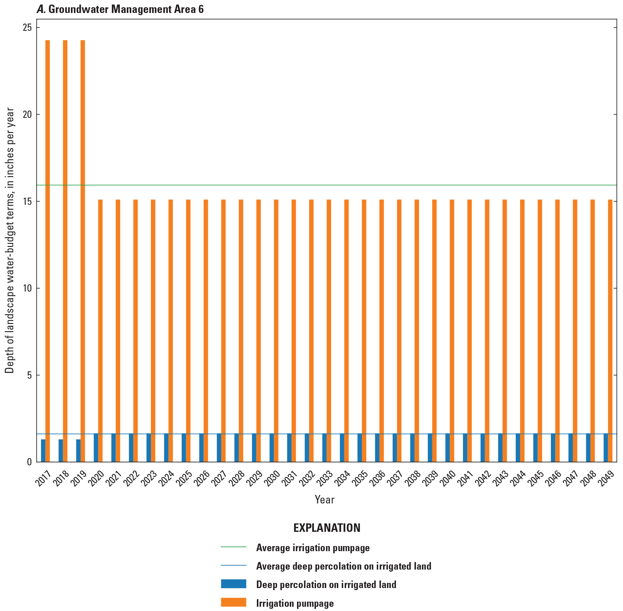
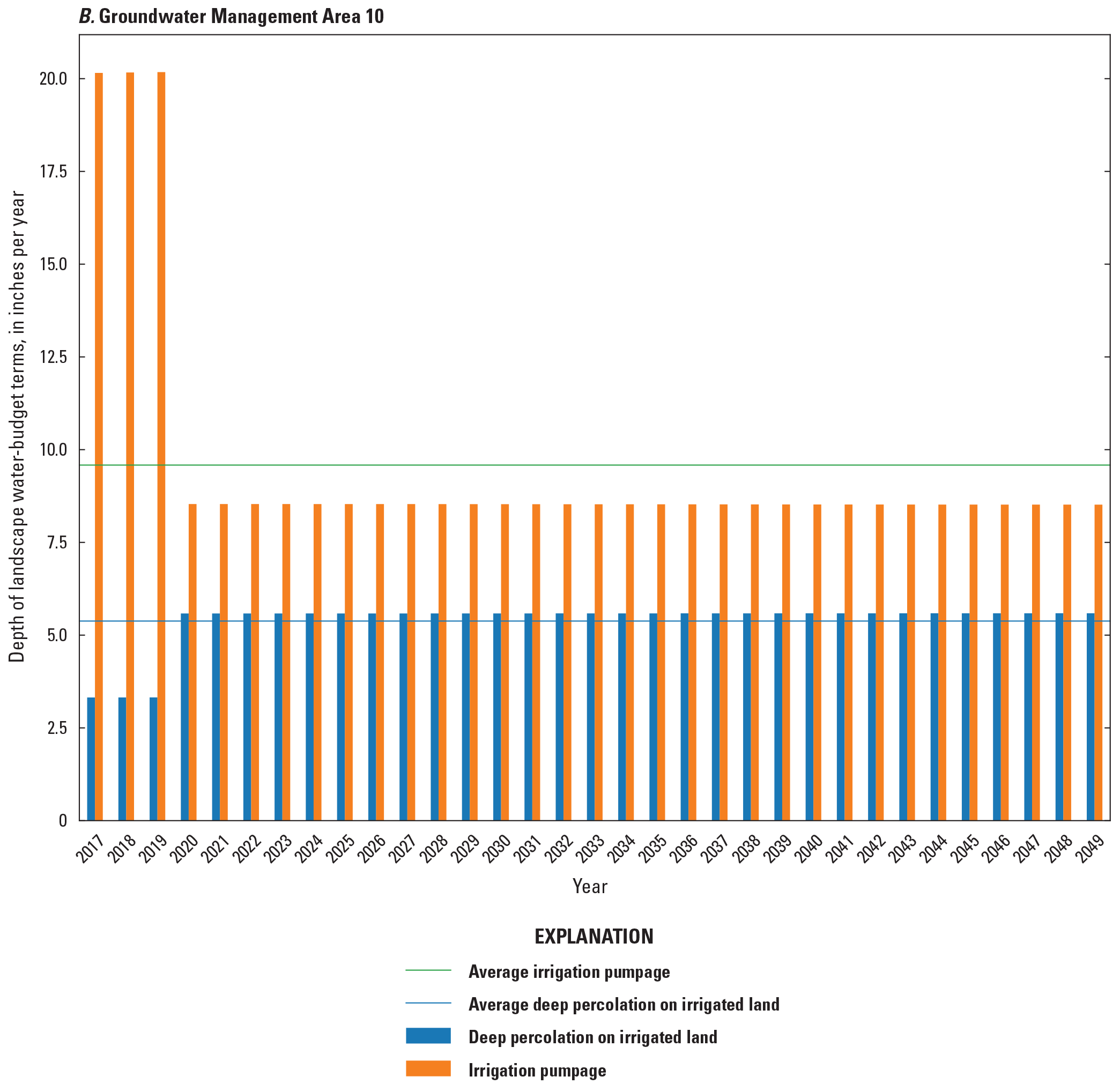
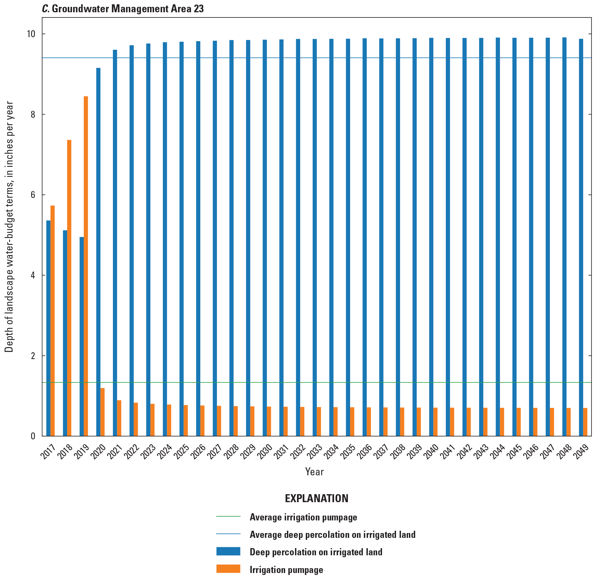
Drought3yr scenario simulated average annual groundwater irrigation pumping and recharge on irrigated land depths for the Central Platte Integrated Hydrologic Model. A, Groundwater Management Area (GWMA) 6. B, GWMA 10. C, GWMA 23.
10-Year Drought Scenario Results
The average groundwater levels simulated in the Futdrought10yr scenario were below levels for the FutBase scenario for most GWMAs (table 19). After 3 years of the moderate drought (December 31, 2019), average groundwater levels were below their predrought levels for 23 GWMAs and the CPNRD and CPIHM supergroups (table 19). Only GWMA 20 exhibited groundwater levels above predrought levels (0.6 ft) after 3 years of moderate drought. These results indicated that, in general, the moderate drought was more stressful on the groundwater-flow system across the study area compared to conditions at the beginning of the forecast. Compared to the 3-year intense drought, the average groundwater levels were 5.0 ft higher for the CPNRD and all 24 GWMAs exhibited higher groundwater levels in the same period (table 19).
At the end of the 10-year drought (December 31, 2026), average groundwater levels were below their predrought levels for 23 GWMAs and the CPNRD and CPIHM (table 19). Only GWMA 20 exhibited groundwater levels above their predrought levels (1.0 ft); this GWMA exhibited a decrease in outflows to irrigation wells for the 10-year moderate drought compared to the recent development period owing to an increase in precipitation compared to the recent development period (2011–16), which reduced the primary outflow from groundwater, indicating that this GWMA’s groundwater was more stressed in the development period compared to other GWMAs (table 22). By the end of the scenario (December 31, 2049), with average climate and stream inflow conditions simulated from January 1, 2027, to December 31, 2049, the groundwater levels fully recovered (equal to or above their predrought levels) for 10 GWMAs, whereas groundwater levels for the other 15 GWMAs, CPNRD, and CPIHM were below their predrought levels. Groundwater levels in GWMA 1 exhibited the largest drawdown from their predrought (December 3, 2016) levels at 13.9 ft, and GWMA 10 exhibited groundwater levels that recovered most compared to their predrought levels at 5.1 ft. Groundwater levels did not recover for seven GWMAs (1, 6, 13, 16, 20, 22, and 23) after the end of the drought; instead, they continued to decline by 0.1 to 6.6 ft, respectively, until the end of 2049 (table 19).
Outflows to irrigation wells, inflows to recharge, and the difference between irrigation and recharge on irrigated land affected the recovery of groundwater levels by the end of the forecast. GWMAs that exhibited the largest differences between irrigation depths and recharge depths on irrigated land (GWMAs 1, 6, and 13) did not recover at the end of the 10-year drought; instead, they continued to decline between 1.1 and 6.6 ft (table 19). GWMAs 1 and 6 were in the drier western region of the CPIHM where recharge was lowest compared to other regions and did not vary much from drought to average conditions, and GWMA 13 also exhibited a minimal difference in recharge during drought and average conditions (table 21). These GWMAs exhibited declines throughout the FutBase forecast, and their net outflows to irrigation wells were similar for the 10-year moderate drought and FutBase forecasts, which indicated that the groundwater-flow system in these areas was stressed enough under average conditions to illicit net releases from storage (table 22, fig. 5.11).
GWMAs that exhibited the most recharge (14, 15, and 24) also exhibited moderate differences between irrigation and recharge on irrigated land, which resulted in moderate recoveries (tables 19 and 21). GWMAs that recovered the most after the end of the 10-year moderate drought exhibited the smallest difference between irrigation and recharge on irrigated land (GWMAs 9 and 12). These GWMAs also exhibited farm net recharge rates that were similar to net outflows to irrigation wells and low net flow to or from adjacent zones, which indicated that recharge supported irrigation pumping, and there were minimal other outflows. These GWMAs were located in the central region of the CPIHM where irrigation pumping increased enough during the drought to cause declines, and after the drought ended, pumping was reduced enough and recharge was high enough to allow the system to recover, which indicated the groundwater-flow system was more responsive to changes in climate than other regions (table 19). Further, the five GWMAs (11, 18, 19, 22, and 23) that exhibited more recharge on irrigated land than outflows to irrigation wells and exhibited small differences between net irrigation wells and farm net recharge were generally in the wetter eastern region of the CPIHM; recharge and irrigation amounts were also similar between the drought and average conditions, which indicated that those GWMAs were less stressed than other GWMAs for the conditions simulated by the Futdrought10yr forecast and that storage was replenished primarily through net inflows from recharge.
Mid-Growing Season Drought Scenario Results
The average groundwater levels simulated by the CPIHM for the Futdroughtjun2sep (mid-growing season drought) scenario were below levels for the FutBase scenario for all GWMAs and the CPNRD and CPIHM (table 19). After 3 years of a mid-growing season drought (January 1, 2017, to December 31, 2019, with each June through September simulated as drought conditions), average groundwater levels were 0.9 to 4.9 ft below their predrought levels for all 24 GWMAs. GWMA 2 exhibited second largest declines (3.8 ft) after 3 years. By December 31, 2026, with mid-growing season drought conditions simulated from January 1, 2017, to December 31, 2026, all 24 GWMAs exhibited groundwater levels 1.6 to 12.9 ft below the predrought groundwater levels (December 31, 2016). These results indicated that a mid-growing season drought bookended by average climate and stream inflow conditions for January through May and October through December caused groundwater-level declines across all regions of the CPIHM (table 19). GWMAs 2, 3, and 15 exhibited the largest declines (11.6, 12.9, and 8.5 ft, respectively) during the 10-year period (January 1, 2017, to December 31, 2026) and GWMAs 4 and 22 exhibited the lowest declines (1.6 and 1.6 ft, respectively) (table 19).
By the end of the scenario (December 31, 2049), with mid-growing season drought conditions simulated from January 1, 2017, to December 31, 2049, all 24 GWMAs exhibited groundwater levels that were 2.0 to 30.6 ft below their initial predrought scenario levels. These results indicated that groundwater levels in all regions of the CPIHM continued to decline below their predrought levels each year of the scenario. The drier western GWMAs 1, 2, and 3 exhibited the largest declines (23.1, 30.6, and 28.3 ft, respectively) and GWMAs 4 and 22 exhibited the lowest declines (2.7 and 2.0 ft, respectively) (table 19). By the end of the scenario, 13 GWMAs exhibited declines of greater than 10 ft and six GWMAs exhibited declines of greater than 20 ft. The GWMAs that exhibited the largest declines in groundwater levels across the entire scenario period were generally in the western region (GWMAs 1, 2, and 3) and received less recharge compared to the GWMAs in the wetter eastern region, or they were in the most heavily irrigated regions (GWMAs 14 and 15) with high outflow rates to irrigation wells (table 21).
Early Growing Season Drought Scenario Results
The average groundwater levels simulated by the CPIHM for the Futdroughtmar2may (early growing season drought) scenario were below FutBase scenario levels for all GWMAs and the CPNRD and the CPIHM (table 19). After 3 years of an early growing season drought (January 1, 2017, to December 31, 2019, with each March through May simulated as drought conditions), average groundwater levels for all 24 GWMAs were below their predrought levels. By December 31, 2026, all 24 GWMAs exhibited continued declines in groundwater levels 0.9 to 9.9 ft below the predrought groundwater levels (December 31, 2016), which indicated that an early growing season drought bookended by average climate and stream inflow conditions for January through February and June through December caused groundwater-level declines across all regions of the CPIHM (table 19). By the end of the scenario (December 31, 2049), all 24 GWMAs exhibited further groundwater-level declines of 1.4 to 27.0 ft below their initial predrought scenario levels. GWMAs 2 and 12 exhibited the largest total declines (25.5 and 27.0 ft, respectively) for the entire forecast and GWMAs 4 and 22 exhibited the lowest declines (1.4 and 1.4 ft, respectively) (table 19). The GWMAs that exhibited the largest declines in groundwater levels across the entire forecast period were generally in the western region (GWMA 1 and 2) and received less recharge compared to the GWMAs in the wetter eastern region, or they were in the most heavily irrigated regions (GWMAs 12, 13, and 14) with the high rates of outflows to irrigation wells (table 21, fig. 5.12).
Comparison Between Early Growing Season and Mid-Growing Season Drought Scenarios
Comparison between the average change in groundwater levels across the scenario period for the early growing season and mid-growing season drought scenario indicated two general trends for the GWMAs in the CPNRD: 16 GWMAs exhibited 0.3 to 14.8 ft greater declines in groundwater levels by the end of the scenario period for the mid-growing season drought scenario, and 8 GWMAs exhibited 0.1 to 9.1 ft greater declines for the early growing season drought; GWMA 14 exhibited the same change in groundwater levels (−20.1) for both scenarios, which indicated that an early and mid-growing season drought had the same effect on the system (table 19). The GWMAs that exhibited larger declines for the early growing season drought (GWMAs 5, 12, 13, 16, 17, 18, 19, and 21) also had smaller net outflows to irrigation wells compared to the mid-growing season drought, but the groundwater levels declined because there was also less farm net recharge. These results indicated that for these GWMAs, less precipitation and recharge during spring (March to May) had a larger effect on net storage than irrigation wells. Conversely, the GWMAs that exhibited larger declines in groundwater levels for the mid-growing season drought had larger net outflows to irrigation wells but were also accompanied by larger farm net recharge. Despite the larger values of farm net recharge compared to other GWMAs, the increased outflows to irrigation wells in response to less precipitation and recharge in the summer months was the major stress that caused the larger declines in groundwater levels for the mid-growing season drought (table 19, figs. 5.12 and 5.13).
Scenario Differences Between Irrigation and Recharge from Deep Percolation
In all scenarios, outflows to irrigation wells, recharge from deep percolation, and farm net recharge were key components of the groundwater-flow system that influenced changes in storage and groundwater levels. Annual relations between inflows to recharge from deep percolation and outflows to irrigation wells exhibited two general trends among GWMAs related to location and climate. Outflows to irrigation wells in the drier central and western region GWMAs (GWMAs 1–16) exhibited approximately constant outflows to irrigation wells for each scenario, except the 3- and 10-year droughts, which were marked by substantial increases in pumping for most GWMAs during the drought periods and shown for GWMA 2 in figure 31A. Additionally, outflows to irrigation wells for these western and central region GWMAs were higher for the mid-growing season drought (futdroughtjun2sep) because there was less precipitation to support ETp, which resulted in a larger CIR that was met through increased pumping during the peak irrigation season (fig. 31A). Conversely, outflows to irrigation for the early season drought were similar to the FutBase scenario, because the drought occurred from March to May, which were not peak irrigation months (fig. 31A). During the peak irrigation season (June to September), the FutBase and early season drought scenarios had similar CIR, resulting in similar outflows to irrigation for each season (fig. 31A).
The wetter eastern region (GWMAs 17–24), with shallower water tables and larger outflows to ETg, generally exhibited a gradual increase in outflows to irrigation wells and annual inflows from recharge that indicated the seasonal climatic stresses had a lasting effect on the irrigation pumping as groundwater levels and ETg declined as crop roots were less able to reach the water table and shown for GWMA 18 in figure 31B. Outflows to irrigation wells increased for the duration of each drought period compared to the FutBase scenario owing to a decrease in precipitation and recharge and an increase in CWD and CIR (fig. 31B). Like the western and central region GWMAs, the outflows to irrigation wells were larger for the mid-growing season drought (futdroughtjun2sep) as there was less precipitation to support ETp during the peak irrigation season resulting in a larger CIR met by pumping from irrigation wells (fig. 31B). Further, annual recharge was larger in the mid-growing season drought scenario because recharge occurred more during the spring months when CWD and CIR were lower. The increase in recharge throughout the scenario period resulted from the increase in irrigation, which led to an increase in inefficient irrigation water that became recharge. Conversely, for the western and central region GWMAs, the early growing season drought (futdroughtmar2may) exhibited outflows to irrigation that were larger than the FutBase scenario because the reduced recharge from March to May also caused a reduction in the mid-growing season ETg (crops roots had less access to the water table that did not receive typical spring recharge) (fig. 31B). For readers interested in additional detail, irrigation pumping for each scenario by GWMA is provided in the model archive (Traylor, 2023).
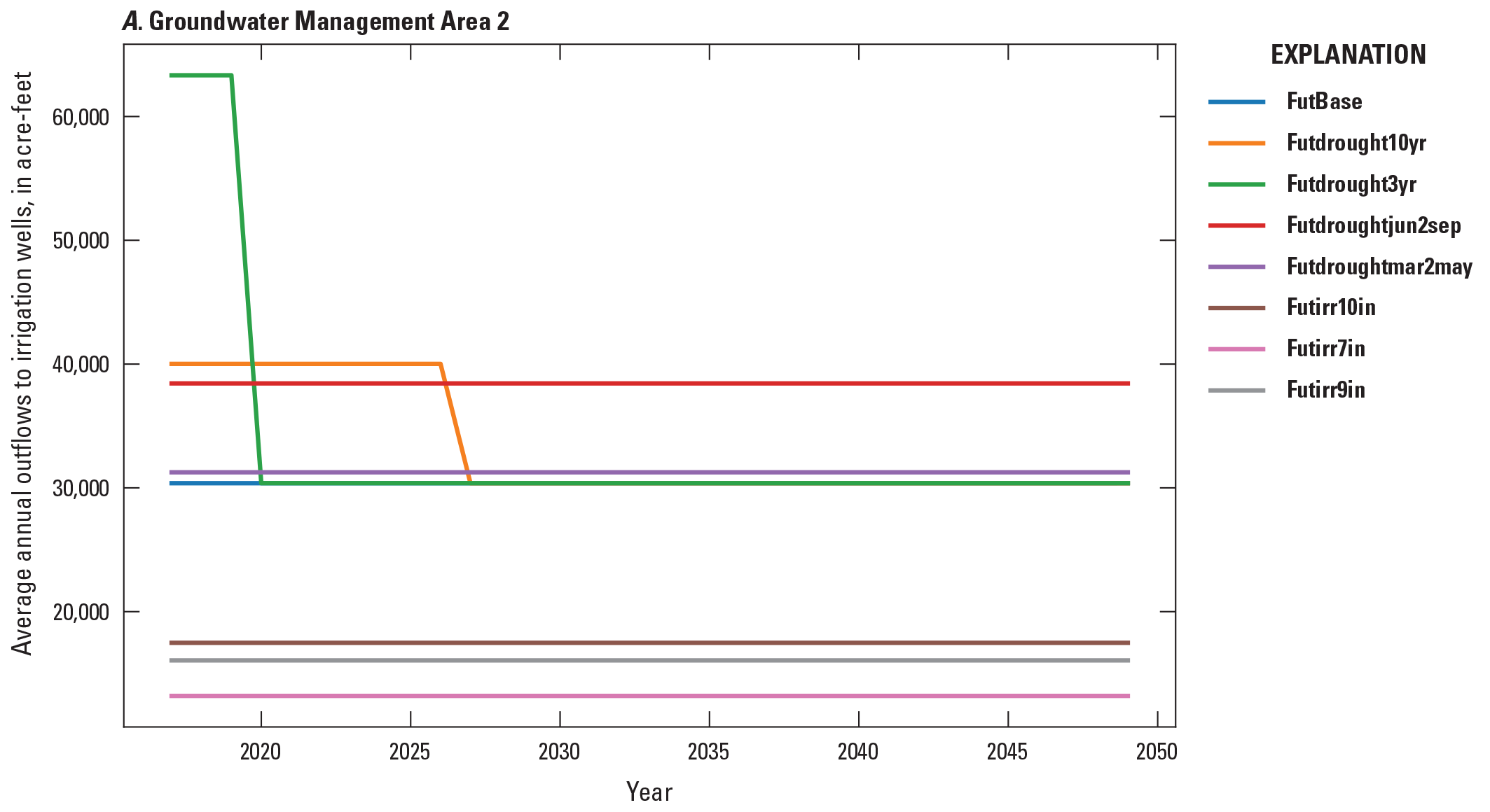
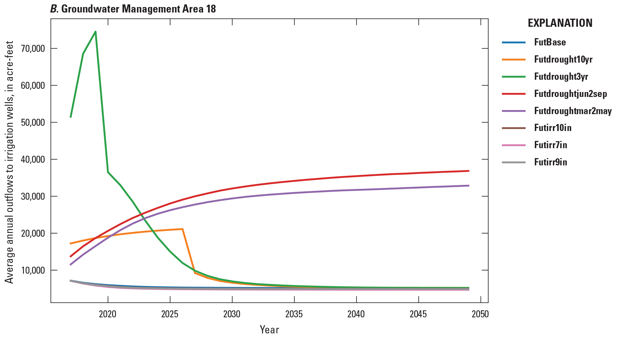
Plot of average annual outflows to irrigation wells for each scenario. A, Groundwater Management Area 2. B, Groundwater Management Area 18.
Inflows to recharge from deep percolation in the drier western and central GWMAs (1–16) generally exhibited constant annual recharge throughout the simulation period for each scenario (fig. 32A). GWMA 2 exhibits a typical trend where a large reduction in recharge occurs in the 3-year drought scenario and a moderate reduction in recharge for the 10-year drought scenario, each followed by an increase to match the FutBase postdrought recharge (fig. 32A). Further, the increase in irrigation also increased recharge from deep percolation as seen in the comparison between the alternate irrigation scenarios where the 10-inch alternate pumping scenario (Futirr10in) exhibited the highest annual recharge, and the 7-inch alternate pumping scenario (Futirr7in) exhibited the lowest annual recharge (fig. 32A). Also, the FutBase scenario, with identical climate to the alternate irrigation scenarios, exhibited larger irrigation and recharge than the 10-inch alternate pumping scenario. Irrigation efficiency was constant for different irrigation amounts and therefore the increases in recharge for the highest irrigation limits were because of more inefficient losses of irrigation water applied to crops compared to the lower irrigation limit scenarios.
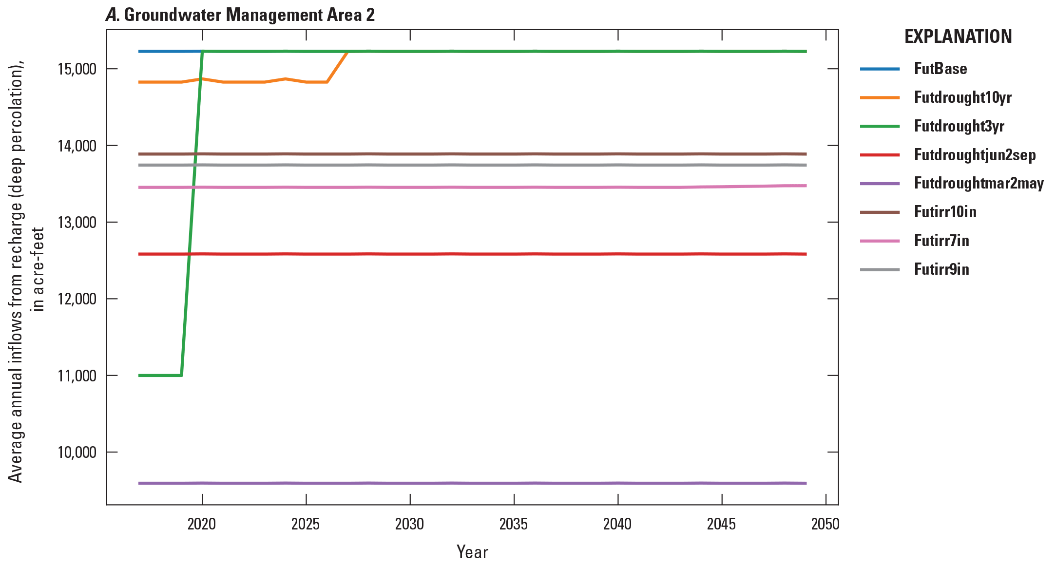
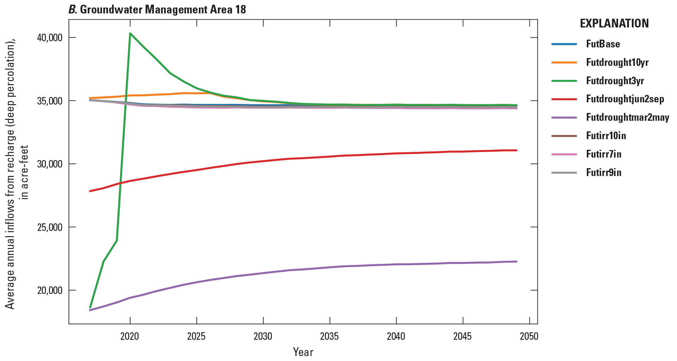
Plots of average annual recharge from deep percolation for each scenario. A, Groundwater Management Area 2. B, Groundwater Management Area 18.
Inflows to recharge from deep percolation in the wetter eastern GWMAs (17–24) exhibited a general increase because of an increase in irrigation pumping for the drought scenarios and a decrease because of a decrease in pumping for the alternate pumping scenarios that resulted from a change in inefficient losses of irrigation water (fig. 32B). The drought scenarios required a higher CIR each year that necessitated more irrigation pumping during the drought months and years; for the 3-year and 10-year drought scenarios, the postdrought average conditions caused a reduction of CIR and outflows to irrigation wells, which led to a reduction in recharge from deep percolation back to average amounts exhibited by the FutBase scenario (fig. 32B). The seasonal droughts indicated that the amount of precipitation that occurred in the spring months was a major contributor to total annual recharge; annual recharge was larger for the mid-growing season drought compared to the early growing season drought (fig. 32B). The recharge figures for each scenario for the other GWMAs are available in the model archive associated with this report (Traylor, 2023).
Comparison of Simulated Groundwater Levels to Maximum Acceptable Declines
The current CPNRD GMP specifies MADs for each GWMA (described in the “Introduction” section of this report). In this section of the report, simulated groundwater levels for each scenario were compared to the baseline 1982 gwlevels and MADs for each GWMA to assess the effect of the scenario stresses on current management thresholds set by the CPNRD (appendix 5). In general, by the end of the scenario period (December 31, 2049) for the FutBase, Futirr7in, Futirr9in, and Futirr10in scenarios, most GWMAs exhibited an increase in groundwater levels above their baseline 1982 gwlevels with seasonal irrigation related drawdowns that never approached the MAD during any period of the scenario (appendix 5). Only GWMA 6 exhibited groundwater-level declines for the FutBase and alternate irrigation scenarios owing to small inflow rates of farm net recharge and stream leakage and relatively large zone outflow. The declines for those scenarios indicated that the groundwater in GWMA 6 was not in a dynamic equilibrium with average climate and irrigation pumping conditions prior to the scenario period (fig. 5.5). Groundwater levels declined for all GWMAs during drought periods; groundwater levels continued to decline for some GWMAs postdrought, whereas other GWMAs recovered from droughts. GWMAs 2, 3, 8, and 12–17 exhibited groundwater levels that declined below their MADs for at least one scenario (fig. 33A, B; appendix 5).
For the FutBase scenario, most (21 of 25) GWMAs exhibited groundwater levels at the beginning of the forecast that were less than 5 ft from the baseline 1982 gwlevels (table 19). Deviations occurred because of dynamic climate and water use between April 1982 and December 2016. Twelve GWMAs exhibited groundwater levels from 0.2 to 13.7 ft below the baseline 1982 gwlevels at the end of the FutBase scenario (table 19). None of the GWMA exhibited declines in groundwater levels for the FutBase scenario that were below the MADs (appendix 5). GWMA 9 exhibited simulated groundwater levels 7.3 ft above the baseline 1982 gwlevels, which was attributed to the drier conditions from 1971 to 1982 and lower average deep percolation during that period (about 39,400 acre-ft/yr) in the development model compared to the FutBase model deep percolation of (66,107 acre-ft/yr). Additionally, recent development period net outflow to irrigation wells for GWMA 9 was greater than for the FutBase forecast, which contributed to less stress on the groundwater-flow system during the FutBase forecast (tables 14 and 20). The largest difference from the baseline 1982 gwlevels was in GWMA 2 (13.7 ft below baseline 1982 gwlevels), which was attributed to less irrigation pumping and more recharge owing to wetter conditions in 1981 and 1982 compared to those simulated in the FutBase model; the CPNRD supergroup average groundwater levels were 0.2 ft below the baseline 1982 gwlevels, which indicated that overall, the groundwater-flow system in the CPNRD was similar to levels in 1982 (table 19).
For the Futdrought3yr scenario, groundwater levels at the end of the scenario were 0.1 to 18.4 ft below the baseline 1982 gwlevels for 16 GWMAs (table 19). Groundwater levels exceeded the MAD by 0.3 and 0.1 ft, respectively, for GWMAs 2 and 14 by the end of the 3-year drought (September 2019); GWMA 15 was 0.1 ft above the MAD by that time (fig. 5.13). These areas were characterized by a high demand for groundwater to irrigate crops that was met by large rates of irrigation pumping and small rates of stream leakage that could not recharge the aquifer during extended drought conditions and led to the simulated larger declines in groundwater levels during the 3-year severe drought (table 4.18).
For the Futdrought10yr scenario, groundwater levels at the end of the scenario were 0.4 to 18.5 ft below the baseline 1982 gwlevels for 14 GWMAs (table 19). Groundwater levels did not exceed the MAD for any GWMA throughout the scenario (appendix 5). After 3 years of the moderate drought (December 31, 2019), average groundwater levels for 17 GWMAs and the CPNRD and CPIHM were below the baseline 1982 gwlevels. At the end of the 10-year drought (December 31, 2026), average groundwater levels for 19 GWMAs and the CPNRD and CPIHM were below the baseline 1982 gwlevels. GWMA 2 exhibited an average groundwater level more than 10 ft below the baseline 1982 gwlevels because of high outflows from irrigation wells and less recharge compared to many other GWMAs (10.7 ft; table 19).
For the mid-growing season drought scenario (Futdroughtjun2sep), all 24 GWMAs exhibited groundwater levels that ranged from 2.1 to 38.8 ft below the baseline 1982 gwlevels (table 19) by the end of the scenario (December 31, 2049), with mid-growing season drought conditions simulated from January 1, 2017, to December 31, 2049. After 3 years of a mid-growing season drought (January 1, 2017, to December 31, 2019, with each June through September simulated as drought conditions), average groundwater levels for 21 GWMAs were 0.1 to 12 ft below the baseline 1982 gwlevels (table 19). GWMA 2 exhibited the largest average groundwater-level difference from the baseline 1982 gwlevels at −12 ft. Five GWMAs (GWMAs 2, 3, 8, 13, 14, and 15) exhibited groundwater levels below their MADs by the end of the scenario (see appendix 5 figures for each GWMA). Each of these GWMAs were characterized by large irrigation pumping rates and small rates of stream leakage compared to other GWMAs, which had less irrigation pumping or more stream leakage that recharged the aquifer (table 4.20).
For the early growing season drought scenario (Futdroughtmar2may), all 24 GWMAs exhibited groundwater levels that ranged from 1.5 to 33.7 ft below the baseline 1982 gwlevels (table 19) by the end of the scenario (December 31, 2049), with early growing season drought conditions simulated from January 1, 2017, to December 31, 2049. After 3 years of a mid-growing season drought (January 1, 2017, to December 31, 2019, with each June through September simulated as drought conditions), average groundwater levels for 21 GWMAs were 0.1 to 12 ft below the baseline 1982 gwlevels (table 19). GWMA 2 exhibited the largest average groundwater-level difference from the baseline 1982 gwlevels at −11.2 ft. Five GWMAs (GWMAs 2, 12, 13, 14, 15, 16, and 17) exhibited groundwater levels below their MADs by the end of the scenario (see appendix 5 figures for each GWMA). Like the GWMAs for the other drought scenarios, each GWMA that exhibited groundwater-level declines below their MADs were characterized by large irrigation pumping rates and small rates of stream leakage, which was an indication that stream leakage supplies recharge to the aquifer during dry periods and reduces the impact of irrigation pumping on the aquifer (table 4.21).
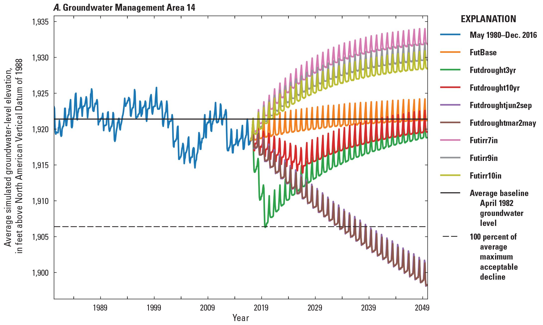
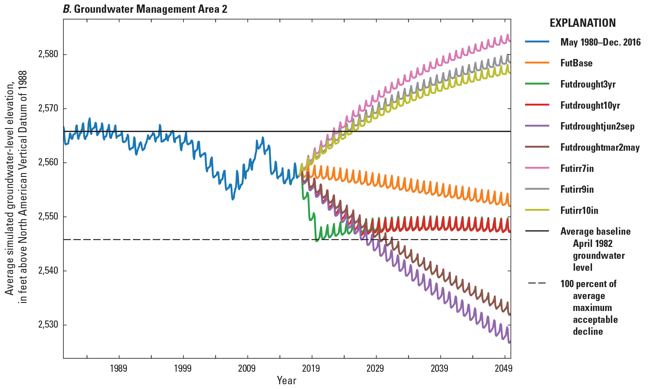
Simulated groundwater levels from May 1980 to December 2016 development period and January 2017 to December 2049 scenario period for the Central Platte Integrated Hydrologic Model. A, Groundwater Management Area 14. B, Groundwater Management Area 2.
Forecast Uncertainty Analysis
In a complex hydrologic model, the calibrated parameter set can be varied by large amounts and still generate similar model results with a similar objective function value (Anderson and others, 2015). Thus, the final calibrated parameter set calculated in the “Calibration Results” section can be viewed as a single set of parameters from an entire range. This parameter nonuniqueness can generate a range of reasonable outputs or results of a scenario, which can be thought of as the forecast uncertainty. Quantification of the forecast uncertainty can improve the understanding of the usefulness of the model. A large forecast uncertainty can correspond to a wider range of simulated model results, such as groundwater levels at the end of a scenario period, whereas a small forecast uncertainty can correspond to less variation in the same simulated groundwater level at the end of a scenario.
Forecast uncertainty was assessed for this study using the linear “first order second moment” uncertainty analysis techniques within the PEST++GLM code to generate an ensemble of 500 combinations of parameters (realizations) for a Monte Carlo analysis. A comprehensive description of this process, including its theoretical and mathematical underpinnings, can be found in the PEST++GLM documentation (White and others, 2019). The analysis was executed on the Denali supercomputer (U.S. Geological Survey, 2020).
Forecast uncertainty was evaluated for 24 theoretical future groundwater altitudes (futheads200 to futheads223) in the FutBase scenario, corresponding to end of scenario (December 31, 2049) groundwater altitudes at the center of GWMAs 1 to 24 (table 23). Uncertainty in the forecasted groundwater altitude at each location (fig. 13) was reduced from an average of 15.47 ft prior to the model calibration to 0.14 ft after the model calibration (posterior; table 23). Therefore, prior to model calibration, using acceptable ranges of input parameter values, the average standard deviation of a simulated groundwater altitude for the FutBase scenario of the CPIHM was 15.47 ft and post calibration standard deviation was 0.14 ft. Groundwater levels in GWMAs 2, 14, and 15 exhibited the highest reduction in uncertainty as indicated by the percentage change in standard deviation. These GWMAs contained more groundwater-level calibration targets than were in GWMAs 6, 17, and 20, which exhibited the lowest reduction in forecast uncertainty, because more observations in a region provide more information to parameters during the calibration process (fig. 13; Doherty, 2015). The large reduction in forecast uncertainty for all regions in the CPIHM was mainly a product of the fixed landscape parameters, particularly the ETref scale factors, which exhibited a large uncertainty and sensitivity during preliminary calibrations, and the relatively small sensitivities of the remaining adjustable parameters during the final calibration process (Kh, aquifer anisotropy, and streamed vertical hydraulic conductivity), discussed in the “Parameter Sensitivity and Identifiability” section of this report.
Table 23.
Summary of FutBase scenario uncertainty for each potential observation in each Groundwater Management Area.[GWMA, Groundwater Management Area; --, not applicable]
Assumptions and Limitations
The CPIHM was constructed to simulate the important hydrologic processes for the CPNRD. The calibration results indicated agreement between calibration targets and simulated equivalents, the results were deemed adequate, and the spatial and temporal resolutions of the CPIHM were appropriate to simulate and characterize landscape water and groundwater flow in the CPNRD and semiregional scale processes. Nonetheless, limitations exist with respect to applying the CPIHM for purposes beyond those for which it was designed. For example, local hydrologic processes may not have been represented or were combined with more regional processes; ephemeral channels were not simulated in this model and runoff that flows to these channels during precipitation events was instead routed directly to the closest perennial stream. The seasonal temporal discretization of the development CPIHM for stress periods 1 to 170 and monthly from 171 to 610 only allows the model to simulate the prevailing average conditions each month. Consequently, this model should not be used to study any hydrologic processes with less than a 1-month duration, such as the peak flows of streams during daily precipitation events (for example, thunderstorms) that produce heavy rainfall in a few minutes or hours. Model cell size limits the characterization of hydrologic properties and features to greater than or equal to a single model cell (160 acres) and includes land use, which was specified using fractions of a cell, but the total effect on the hydrologic system was the combination of each land-use fraction within a cell. Any properties of features less than 160 acres were effectively combined with other features. The CPIHM simulated landscape and groundwater hydrologic processes and did not simulate the soil moisture changes or processes in the unsaturated zone. Therefore, the CPIHM should not be used to assess the effects of hydrologic stresses on soil moisture or the unsaturated zone. Additionally, the CPIHM does not include porosity of aquifer layers and should not be used to conduct a particle travel time analysis without the implementation of porosity values.
The CPIHM should not be used to assess the impacts of stresses on total streamflow and base flow for the South Loup River, Middle Loup River, and Loup River. These streams interact with the groundwater-flow system and surface-water system to the north, but the region north of these streams was not simulated in the CPIHM because that was not within the scope of the study; the Loup River system was simulated as a boundary condition for the CPIHM. Therefore, the simulated flows for these streams did not include groundwater (base flow) and surface-water (run off) contributions from the north side because that was not included in the CPIHM. The CPIHM should not be used to assess the impacts of stresses on total streamflow and base flow for other boundary streams that include Sand Creek in Adams County, Big Sandy Creek in Clay County, and School Creek in Clay and York Counties.
The CPIHM should not be used to assess groundwater levels, streamflow, or impacts to either of those features from irrigation, climate change, or other stresses outside of the boundary of the CPNRD. The objective of the study and focus area of the model development and the calibration was the CPNRD. Physical properties, such as Kh and anisotropy, were adjusted during calibration to preferentially improve the fit between measured data and simulated equivalent values inside the CPNRD, and weighting of the groundwater-level calibration targets was larger for targets inside the CPNRD. Aquifer storage properties (Sy and Ss) of each model layer were not adjusted during calibration, but simulated groundwater-level hydrographs compared to high resolution temporal data from figure 17 showed that the amplitudes of measured and simulated groundwater levels were very similar, which indicated that the input storage values were accurate; however, local refinement of the storage properties and a different calibration parameter scheme may further improve the fit between the measured and simulated groundwater levels. Spatial bias in the groundwater-level residuals, as documented in this report, did not affect the ability of the CPIHM to meet the objectives of the study, particularly with respect to assessment of the scenario stresses on MADs because they were relative to simulated values for the baseline 1982 gwlevels and simulated end of development period (December 31, 2016) groundwater levels. The bias in the groundwater levels does affect the ability of the CPIHM to simulate absolute groundwater-level altitudes in the northern and southern regions of the model domain at the edges of the CPNRD boundary.
The conveyance and routing of surface water for the CNPPID canals was not simulated by the CPIHM; only leakage losses from the CNPPID canals were simulated. In addition to the CNPPID canals residing outside the CPNRD focus area, the CPIHM should not be used to assess the impact of Phelps County Supply Canal on the hydrologic system. The scenarios simulated by the CPIHM were theoretical and provided information on general hydrologic trends in each GWMA under different potential future conditions in a transient system. The scenarios analyzed with CPIHM were not intended to predict future climate.
The landscape parameters were not well constrained during preliminary calibration attempts because there were no calibration target datasets with adequate spatial or temporal coverage available to constrain inputs such as ETref, FTR, irrigation efficiencies, runoff, or recharge. Therefore, as discussed in the “Parameter Sensitivity and Identifiability” and “Forecast Uncertainty Analysis” sections of this report, the fixing of landscape parameters introduced a low bias in the uncertainty of model results. Although the simulated model results were in agreement with the conceptual understanding of the hydrologic system and the results presented in this report are acceptable with respect to the calibration targets and the conceptual understanding of the study area processes, the fixing of the landscape parameters limited the flexibility of the model during the calibration process. A calibration with all landscape parameters set as “adjustable” and accompanied by additional calibration targets to provide information and constrain the adjustable landscape parameters may have resulted in PEST finding a different combination of acceptable parameter values. A predictive uncertainty was performed and demonstrated that simulated groundwater levels in the CPNRD area have a very small predictive uncertainty related to the fixing of some of the most sensitive parameters such as the ETref scale factors, but the uncertainty in other model outputs or in groundwater levels outside of the CPNRD was not evaluated.
Potential Topics for Additional Study
Data collection and monitoring are essential for informing construction and calibration of hydrologic models, as well as assessment of results. A data-worth analysis may quantify the worth of new data collected and how the data would improve the calibration, such as new observations at existing sites, new observations at new sites, and new types of observations. A data-worth analysis may also quantify the impact of removal of observations on the calibration. Such information could be used to select new locations for data collection or removal of data collection sites if necessary. The unsaturated zone was not simulated in the CPIHM because it was not critical to the study objectives or model calibration and results within the CPNRD. A study to simulate the unsaturated zone in the CPIHM using the Unsaturated Zone Flow (UZF) package could be used to assess rejected infiltration and attenuation of deep percolation recharge past the root zone to the water table (Niswonger and others, 2006). Recent feature updates to the MF–OWHM code allow the FMP and the UZF package to be linked so that FMP-calculated deep percolation is passed as an inflow to UZF, as an infiltration rate, and is used as unsaturated flow (Boyce and others, 2020).
The scenarios simulated by the CPIHM provide information on the response of the hydrologic system to selected potential future climate and irrigation pumping conditions. Additional studies of the effects of other future climate conditions on recharge, runoff, ET, groundwater storage, stream leakage, and saturated thickness and availability would likely improve the understanding of the response of the system to those potential scenarios. For example, simulation of potential scenarios that include continuous warmer and drier conditions and continuous colder and wetter conditions on the hydrologic system in the CPIHM could improve the understanding of the response of the hydrologic system to a wider variety of potential future climate change conditions. This approach was used in a groundwater-flow model of the Northern High Plains aquifer to evaluate hydrologic responses induced by potential future conditions from downscaled global climate models (Peterson and others, 2020).
The MF–OWHM contains functionality to simulate more complex surface-water features. The simulations of the irrigation canals in the CPIHM used constant surface-water diversions from a year that matched climate trends. A study to simulate alternative surface-water diversions to canals could likely improve the understanding of those potential changes on the hydrologic-flow system. Additional scenarios to assess managed aquifer recharge using canals or new reservoirs may also quantify the impact of such practices on the hydrologic-flow system.
The CPIHM simulated subregional stresses, but localized stresses and their impact on the hydrologic system could be simulated and studied with an inset hydrologic-flow model within the CPNRD using a finer spatial resolution within the regional CPIHM domain that would produce higher resolution outputs. Additionally, the CPIHM could be linked to an economic model to create a full decision support system that may inform management decisions on economic factors or vice versa. Water-quality and particle tracking could be the focus of an additional study if permeability inputs were specified, which might allow for accurate simulation of particle paths and travel times. Water-quality data, such as age dating, might be useful to corroborate transit and residence times within the aquifer and possibly improve the understanding of water sources to streams and irrigation wells.
The complexity of a fully integrated model like the CPIHM would benefit from an increase in parameterization to better capture the unknowns and uncertainty in model inputs and allow for more flexibility for these model inputs during the calibration process. An increase in the number of adjustable parameters would improve the CPIHM’s ability to simulate the natural system and provide a more robust characterization of scenario uncertainty. The latest advancements in the PEST++ suite of calibration software includes the iterative ensemble smoother (PESTPP–IES) code, which was not available at the time of model development and calibration. PESTPP–IES can accommodate millions of parameters without the prohibitive increase in computational burden that is required for calculation of the derivatives of parameters to observations (Jacobian sensitivity matrix) when using traditional PEST and BeoPEST codes. Further, the addition of observations such as AET, recharge, and metered pumping as calibration targets to constrain landscape parameters also might improve the calibration of the CPIHM with respect to the landscape processes that influence recharge to the groundwater system. Additional AET observations from Reitz and others (2017) may improve the ability of PEST to constrain the ETref scale factors in an automated calibration rather than manual adjustments.
Summary
The Central Platte Natural Resources District (CPNRD) is responsible for regulating groundwater use of the district. The groundwater and surface-water supply of the CPNRD is one of its most valuable natural resources and supports an agricultural economy that generates more than $2 billion per year. The CPNRD’s main groundwater quantity management goal is the utilization of its water resources through proper management and conservation to ensure an adequate supply for feasible and beneficial uses. State law requires the CPNRD to develop a Groundwater Management Plan. The CPNRD’s initial Groundwater Management Plan was adopted in 1987. The CPNRD Groundwater Management Plan specifies maximum acceptable declines of 10 to 30 feet for 24 Groundwater Management Areas (GWMAs) across the CPNRD, with the declines based on spring 1982 (approximately April 30, 1982) groundwater levels. The CPNRD management strategy has employed advanced numerical flow models since the creation of their first Groundwater Management Plan, initially adopted in 1987. The purpose of this report is to document and describe the construction, calibration, and results of a numerical fully integrated hydrologic model using the U.S. Geological Survey MODFLOW-based software called MODFLOW–One-Water Hydrologic Model code that simulated the CPNRD hydrologic system under past development conditions from 1895 to 2016 and eight future scenarios simulated from 2017 to 2049. Results of the potential future scenarios are described in this report along with information about potential future water availability and changes in groundwater levels for each scenario with respect to the baseline 1982 groundwater levels, and maximum acceptable declines, that can be used by the CPNRD to update their Groundwater Management Plan.
The study area was focused around the CPNRD, which includes parts of 10 counties in central Nebraska and a total area of 2,136,304 acres. The main hydrologic features are the Platte River, which flows from west to east for about 205 miles, and the High Plains aquifer, which underlies the entire study area with saturated thicknesses ranging from about 50 to 550 feet. There are about 1 million irrigated acres of cropland in the CPNRD and 936,000 acres are supplied by pumping groundwater from the underlying High Plains aquifer. An extensive network of canals diverts water from the Platte River to surface-water irrigators in Buffalo, Dawson, Kearney, and Phelps Counties. The geologic units in the study area consist of Quaternary-age valley-fill, dune sand, loess, and alluvium; and Tertiary-age Ogallala Formation silt and sandstone. The Ogallala Formation is the principal geologic unit that forms the Northern High Plains aquifer, which includes the hydrologically connected Quaternary-age alluvial aquifers. The contact between the Ogallala Formation and underlying Pierre Shale, which is not hydrologically connected to the Ogallala Formation, represents the base of the Northern High Plains aquifer. Regional groundwater-flow directions are generally from west to east but can vary locally. The groundwater-flow system is connected to streams where groundwater receives inflows from stream leakage or outflows as base flow to streams.
An integrated hydrologic model, called the Central Platte Integrated Hydrologic Model (CPIHM), was constructed using the MODFLOW–One-Water Hydrologic Model code and used the Newton solver. The MODFLOW–One-Water Hydrologic Model integrates climate, landscape, surface water, and groundwater-flow processes in a fully coupled approach to hydrologic modeling that simulates the natural feedbacks of a system. The CPIHM consisted of 163 rows and 327 columns with horizontal cell sides of 2,640 feet by 2,640 feet and was vertically discretized into three layers of varying spatial extents and thickness according to the hydrogeology and aquifer. Layers 1, 2, and 3 represented the Quaternary-age valley-fill, loess deposits, and alluvial aquifers; Quaternary-age loess deposits and Upper-Tertiary-age portions of the Ogallala Formation; and the Tertiary -age Ogallala Formation. The CPIHM included two models: a pre irrigation development model that represented a steady-state equilibrium prior to April 30, 1895, and a development period model that was temporally discretized into 610 stress periods to simulate transient conditions from May 1, 1895, to December 31, 2016. There were 212 water accounting units, called water-balance subregions, delineated for use in the Farm Process package, which were merged into the 24 GWMAs as “supergroups” to present results.
Calibration of the CPIHM involved two phases: a manual adjustment of parameters, followed by the automated calibration using BeoPEST. During the automated calibration phase, 435 parameters were adjusted to improve the fit between 40,711 streamflow and groundwater-level observations and their simulated equivalent values at 53 streamgages and 963 observation well locations. Additionally, the automated calibration was facilitated by the employment of the singular value decomposition-assist features of the Parameter Estimates (PEST) software that specified 50 super parameters and Tikhonov regularization. The average absolute groundwater-level residuals for model layers 1, 2, and 3 were 6.1, 12.4, and 7.4 feet, respectively, and after 1980 were 4.0, 10.7, and 7.5 feet, respectively, which indicated that the CPIHM adequately simulated the groundwater levels for each layer. Calibrated horizontal hydraulic conductivity values estimated at pilot points and interpolated to the model grid were about 70, 32, and 35 feet per day for layers 1, 2, and 3, respectively, which were similar to values from previous studies.
Simulated landscape water budgets for the calibrated development model maintained the general trends and magnitudes expected from the conceptual understanding of the landscape water subsystem. The largest inflow component was precipitation with an average development period (May 1, 1895, to December 31, 2016) annual volume of 9,978,276 acre-feet per year (acre-ft/yr) (24.3 inches if spread equally across the model domain). The largest outflow from the landscape was evapotranspiration of precipitation at an average annual flux of 7,935,263 acre-ft/yr (19.3 inches). In the last 5 years of the development model simulation (2011–16), the average annual volume of total evapotranspiration, which included evapotranspiration of precipitation and irrigation water sources, was 8,420,099 acre-ft/yr (20.5 inches). For the groundwater budget, the largest inflow component was recharge (analogous to deep percolation from the landscape), with an average development period annual volume of 1,122,257 acre-ft/yr (2.7 inches). The largest groundwater outflows were to irrigation wells at an average annual volume of 693,171 acre-ft/yr (10.2 inches for the CPNRD). For the total development period, there was a net replenishment to groundwater storage of −122,393 acre-ft/yr (−0.3 inches per year). For the recent groundwater budget (2011–16), the average annual releases from groundwater storage were like those from recharge from deep percolation at about 2,326,871 acre-ft/yr (5.7 inches) and 2,056,936 acre-ft/yr (5.0 inches), respectively, because irrigation wells received most of their 2,132,994 acre-ft/yr of groundwater pumped from storage; however, recovery during the nonirrigation season included replenishment to storage of −2,045,430 acre-ft/yr. After 1980, average monthly recharge was the largest inflow from October to June. The largest volumes of recharge occurred in April, May, and October when evapotranspiration and groundwater pumping to irrigation wells was minimal or inactive and precipitation was relatively high.
The CPIHM simulated the effects of eight different potential future climate and irrigation pumping conditions that included one base scenario, three alternative irrigation scenarios, and four drought scenarios. The scenario simulation period included 396 monthly stress periods from January 1, 2017, to December 31, 2049. A base scenario simulated average climate conditions of precipitation and potential evapotranspiration, the four drought scenarios included the simulation of an intense 3-year drought, a moderate 10-year drought, a mid-growing season drought from June to September each year, and an early growing season drought from March to May each year. The three alternate irrigation scenarios included the simulation of an annual 7-inch depth limit on groundwater pumped, an annual 9-inch depth limit on groundwater pumped, and an annual 10-inch depth limit on groundwater pumped. The simulated groundwater levels for each scenario were compared to the baseline 1982 (April 30, 1982) average groundwater levels simulated by the development model, the groundwater levels simulated at the end of the development period (December 31, 2016), and the maximum acceptable decline groundwater-level elevation for each GWMA.
Base scenario average groundwater levels for the CPNRD were 0.2 foot below the baseline 1982 groundwater level and 0.3 foot below the prescenario (December 31, 2016) groundwater level by the end of the scenario period (December 31, 2049). Additionally, the average annual groundwater irrigation pumping depths were 9.3 inches for the CPNRD. Alternate irrigation pumping scenario average groundwater levels were 7.6, 6.1, and 5.4 feet above the baseline 1982 groundwater levels for the 7-inch, 9-inch, and 10-inch pumping scenarios, respectively, at the end of the scenario period for the CPNRD. Additionally, average CPNRD groundwater levels at the end of the scenario period (December 31, 2049) were 7.5, 6.0, and 5.3 feet above their prescenario (December 31, 2016) groundwater levels for the 7-inch, 9-inch, and 10-inch pumping scenarios, respectively. Across all three of these forecasts, the drier western region GWMAs that required the highest average outflows to irrigation for the FutBase scenario were also the regions that were most groundwater supply limited. In general, the amount of pumping varied by GWMA which indicated that a limit on irrigation pumping had a variable effect on the groundwater-flow system depending on the local stresses specific to each GWMA. GMWAs 19 and 23 exhibited the highest surplus irrigation state because their irrigation requirements were very small when compared to other GWMAs and they exhibited substantial net inflow from adjacent zones. Conversely, GMWA 6 exhibited the highest deficit irrigation state because it had one of the lowest rates of farm net recharge and lacked other sources of water such as net inflows from adjacent zones and limited net inflow from streams to offset outflows to irrigation wells.
The 3-year intense drought scenario average groundwater levels for the CPNRD were 1.7 feet below the baseline 1982 groundwater-level and 1.8 feet below the prescenario (December 31, 2016) groundwater level by the end of the scenario period (December 31, 2049). The average annual groundwater irrigation pumping depths were 10.2 inches for the CPNRD. The 10-year moderate drought scenario average groundwater levels for the CPNRD were 2.0 feet below the baseline 1982 groundwater-level and 2.1 feet below the prescenario (December 31, 2016) groundwater level by the end of the scenario period. Additionally, the average annual groundwater irrigation pumping depths were 10.0 inches for the CPNRD. GWMAs that exhibited more recharge and lower irrigation rates exhibited groundwater levels that generally recovered to predrought levels, whereas GWMAs with less recharge and higher irrigation rates exhibited groundwater levels that continued to decline postdrought.
The early growing season drought scenario average groundwater levels for the CPNRD were 11 feet below the baseline 1982 groundwater level and 11.1 feet below the prescenario (December 31, 2016) groundwater level by the end of the scenario period (December 31, 2049). Additionally, the average annual groundwater irrigation pumping depths were 9.7 inches for the CPNRD. The mid-growing season drought scenario average groundwater levels for the CPNRD were 13.8 feet below the baseline 1982 groundwater level and 13.9 feet below the prescenario (December 31, 2016) groundwater level by the end of the scenario period (December 31, 2049). Additionally, the average annual groundwater irrigation pumping depths were 11.7 inches for the CPNRD. Overall, there were two general trends in groundwater levels by the end of the scenario period: 16 GWMAs exhibited greater declines for the mid-growing season drought scenario and eight GWMAs exhibited greater declines for the early growing season drought scenario. The GWMAs that exhibited larger declines for the early growing season drought were affected by less net farm recharge, which indicated that less precipitation and recharge during spring (March to May) had a larger effect on net storage than irrigation well pumping. Conversely, the GWMAs that exhibited greater declines in groundwater levels for the mid-growing season drought were affected more by larger outflows to irrigation wells.
With respect to the maximum acceptable declines in groundwater-levels, in general, by the end of the scenario period (December 31, 2049) for the Base scenario, 7-inch, 9-inch, and 10-inch pumping scenarios, most GWMAs exhibited an increase in groundwater levels above their baseline 1982 groundwater levels with seasonal irrigation related drawdowns that never approached the maximum acceptable declines during any period of the scenario. In general, the 3-year drought scenario had a larger effect on groundwater levels compared to the 10-year drought scenario for some GWMAs, such as GWMA 2 where groundwater levels did not recover above their maximum acceptable declines even after 30 years of average climate and stream inflow conditions. In contrast, groundwater levels did not decline below the maximum acceptable declines in GWMA 2 for the 10-year drought scenario, although postdrought recovery was similar to the recovery from the 3-year drought scenario.
Forecast uncertainty was assessed for this study using the linear “first order second moment” uncertainty analysis techniques within the PEST++GLM code. Forecast uncertainty was evaluated for 24 theoretical future groundwater altitudes in the base scenario, corresponding to end of scenario (December 31, 2049) groundwater altitudes at the center of each of the 24 GWMAs. Uncertainty in the forecasted groundwater altitude at each location was reduced from an average of about 15.47 feet prior to the model calibration to 0.14 foot after the model calibration (posterior). The large reduction in forecast uncertainty for all regions in the CPIHM was primarily attributed to the fixed landscape parameters, particularly the reference evapotranspiration scale factors; local uncertainty differences between GWMAs were because of different amounts of observations that informed the calibration in those areas.
References Cited
Alexander, J.S., Schultze, D.M., and Zelt, R.B., 2013, Emergent sandbar dynamics in the lower Platte River in eastern Nebraska—Methods and results of pilot study, 2011: U.S. Geological Survey Scientific Investigations Report 2013–5031, 42 p. with appendixes., accessed September 1, 2020, at https://doi.org/10.3133/sir20135031.
Allen, R.G., Pereira, L.S., Raes, D., and Smith, M., 1998, Crop evapotranspiration—Guidelines for computing crop requirements: Rome, Italy, United Nations Food and Agriculture Organization, Irrigation and Drainage Paper no. 56, 300 p. [Also available at https://www.researchgate.net/publication/235704197_Crop_evapotranspiration-Guidelines_for_computing_crop_water_requirements-FAO_Irrigation_and_drainag e_paper_56.]
Anderson, J.A., Morin, R.H., Cannia, J.C., and Williams, J.H., 2009, Geophysical log analysis of selected test holes and wells in the High Plains aquifer, Central Platte River basin, Nebraska: U.S. Geological Survey Scientific Investigations Report2009–5033, 16 p. [Also available at https://doi.org/10.3133/sir20095033.]
Bakker, M., Post, V., Langevin, C.D., Hughes, J.D., White, J.T., Starn, J.J., and Fienen, M.N., 2016, Scripting MODFLOW model development using Python and FloPy: Ground Water, v. 54, no. 5, p. 733–739. [Also available at https://doi.org/10.1111/gwat.12413.
Barlow, P.M., Cunningham, W.L., Zhai, T., and Gray, M., 2014, U.S. Geological Survey Groundwater Toolbox, a graphical and mapping interface for analysis of hydrologic data (version 1.0)—User guide for estimation of base flow, runoff, and groundwater recharge from streamflow data: U.S. Geological Survey Techniques and Methods, book 3, chap. B10, 27 p. [Also available at https://doi.org/10.3133/tm3B10.]
Barlow, P.M., Cunningham, W.L., Zhai, T., and Gray, M., 2017, U.S. Geological Survey Groundwater Toolbox version 1.3.1, a graphical and mapping interface for analysis of hydrologic data: U.S. Geological Survey software release, accessed May 26, 2017, at https://doi.org/10.5066/F7R78C9G.
Boyce, S.E., Hanson, R.T., Ferguson, I., Schmid, W., Henson, W., Reimann, T., Mehl, S.M., and Earll, M.M., 2020, One-Water Hydrologic Flow Model—A MODFLOW based conjunctive-use simulation software: U.S. Geological Survey Techniques and Methods, book 6, chap. A60, 435 p., accessed September 2020 at https://doi.org/10.3133/tm6A60.
Cannia, J.C., Woodward, D.W., and Cast, L., 2006. Cooperative hydrology study hydrostratigraphic units and aquifer characterization report: Cooperative Hydrology Study, 91 p., accessed September 1, 2017, at http://cohyst.nebraska.gov/document/dc012hydro_aquifer_022406.pdf.
Cannia, J.C., Abraham, J.D., and Asch, T.H., 2017, Hydrogeologic framework of selected areas in the Twin Platte and Central Platte Natural Resources Districts: Aqua Geo Frameworks, accessed September 1, 2020, at https://www.dropbox.com/s/re4rzd96e7g8t55/TPNRD-CPNRD_AEM_Hydrogeologic_Report_AGF_28Dec2017_v1.pdf?dl=0.
Carney, C.P., 2008, Groundwater flow model of the eastern model unit of the Nebraska Cooperative Hydrology Study (COHYST) area: Cooperative Hydrology Study Technical Committee, 80 p., accessed September 1, 2017, at http://cohyst.nebraska.gov/adobe/dc012CMU_GFMR_081224.pdf.
Center for Advanced Land Management Information Technologies, 2010, 2005 Land use mapping: Lincoln, University of Nebraska-Lincoln Center for Advanced Land Management Information Technologies, accessed February 1, 2019, at http://www.calmit.unl.edu/2005landuse.
Central Nebraska Public Power and Irrigation District, 2019, Reservoir/river data: accessed March 15, 2019, at https://www.cnppid.com/wp-content/uploads/2016/06/lakeRiverData.html.
Central Platte Natural Resources District, 2019, Groundwater Quantity Management Program: accessed September 1, 2019, at http://cpnrd.org/groundwater-quantity/.
Central Platte Natural Resources District, 2020a, Groundwater management plan rules and regulations: Central Platte Natural Resources District, 68 p., accessed September 1, 2020, at http://cpnrd.org/wp-content/uploads/2018/10/GWMP-RR-September2018.pdf.
Central Platte Natural Resources District, 2020b, Integrated management plan jointly developed by the Central Platte Natural Resources District and the Nebraska Department of Natural Resources: Central Platte Natural Resources District, 102 p., accessed September 1, 2020, at http://cpnrd.org/wp-content/uploads/2019/12/CPNRD-IMP-final.pdf.
Cooperative Hydrology Study, 2017, COHYST 2010—A total water budget approach to integrated water management in the Platte River Nebraska—2017 documentation of revised integrated model: Cooperative Hydrology Study, 1795 p., accessed June 2017 at https://cohyst.nebraska.gov/#md.
Conservation and Survey Division, 2019, Topographic regions—Geology related GIS data: Institute of Agriculture and Natural Resources, University of Nebraska-Lincoln, , accessed February 15, 2019, at http://snr.unl.edu/data/geographygis/geology.aspx.
Dappen, P., Ratcliffe, I., and Robbins, C., 2007, Delineation of 2005 land use patterns for the State of Nebraska Department of Natural Resources: University of Nebraska-Lincoln Center for Advanced Land Management Information Technologies, 80 p., accessed February 1, 2018, at https://calmit.unl.edu/pdf/2005_Landuse_FinalReport.pdf.
Darton, N.H., 1898, Underground waters of a portion of southeastern Nebraska: U.S. Geological Survey Water Supply and Irrigation Paper 12, 56 p., accessed September 1, 2019, at https://doi.org/10.3133/wsp12.
Darton, N.H., 1905, Preliminary report on the geology and underground water resources of the central Great Plains. U.S. Geological Survey Professional Paper 32, 433 p., accessed September 1, 2019, at https://doi.org/10.3133/pp32.
Dieter, C.A., Maupin, M.A., Caldwell, R.R., Harris, M.A., Ivahnenko, T.I., Lovelace, J.K., Barber, N.L., and Linsey, K.S., 2018, Estimated use of water in the United States in 2015: U.S. Geological Survey Circular 1441, 65 p. [Supersedes USGS Open-File Report 2017–1131], accessed September 2019 at https://doi.org/10.3133/cir1441.
Doherty, J.E., 2005, PEST, model independent parameter estimation—User manual (5th ed.): Brisbane, Australia, Watermark Numerical Computing, accessed July 26, 2011, at https://pesthomepage.org/.
Doherty, J.E., Hunt, R.J., and Tonkin, M.J., 2010a, Approaches to highly parameterized inversion: A guide to using PEST for model-parameter and predictive-uncertainty analysis: U.S. Geological Survey Scientific Investigations Report 2010–5211, 71 p. [Also available at https://doi.org/10.3133/sir20105211.]
Doherty, J.E., 2018, PEST Programs—Groundwater utilities: accessed January 2018 at https://pesthomepage.org/programs.
Doherty, J., and Hunt, R.J., 2009, Two statistics for evaluating parameter identifiability and error reduction: Journal of Hydrology, v. 366, no. 1-4, p. 119–127. [Also available at https://doi.org/10.1016/j.jhydrol.2008.12.018.]
Doherty, J.E., and Hunt, R.J., 2010, Approaches to highly parameterized inversion—A guide to using PEST for groundwater-model calibration: U.S. Geological Survey Scientific Investigations Report2010–5169, 59 p. [Also available at https://doi.org/10.3133/sir20105169.]
Exner, M.E., Perea-Estrada, H., and Spalding, R.F., 2010, Long-term response of groundwater nitrate concentrations to management regulations in Nebraska’s Central Platte Valley: The Scientific World Journal, v. 10, p. 286–297. [Also available at https://doi.org/10.1100/tsw.2010.25.]
Fienen, M.N., Doherty, J.E., Hunt, R.J., and Reeves, H.W., 2010, Using prediction uncertainty analysis to design hydrologic monitoring networks—Example applications from the Great Lakes water availability pilot project: U.S. Geological Survey Scientific Investigations Report2010–5159, 44 p. [Also available at https://doi.org/10.3133/sir20105159.]
Gutentag, E.D., Heimes, F.J., Krothe, N.C., Luckey, R.R., and Weeks, J.B., 1984, Geohydrology of the High Plains aquifer in parts of Colorado, Kansas, Nebraska, New Mexico, Oklahoma, South Dakota, Texas, and Wyoming: U.S. Geological Survey Professional Paper1400–B, 63 p. [Also available at https://doi.org/10.3133/pp1400B.]
Hall, B.M., and Rus, D.L., 2013, Comparison of water consumption in two riparian vegetation communities along the central Platte River, Nebraska, 2008–09 and 2011: U.S. Geological Survey Scientific Investigations Report 2013–5203, 28 p., accessed September 1, 2018, at https://doi.org/10.3133/sir20135203.
Hanson, R.T., Boyce, S.E., Schmid, W., Hughes, J.D., Mehl, S.M., and Leake, S.A., Maddock, T., III, and Niswonger, R.G., 2014a, One-Water Hydrologic Flow Model (MODFLOW–OWHM): U.S. Geological Survey Techniques and Methods, book 6, chap. A51, 120 p., accessed November 2016 at https://doi.org/10.3133/tm6A51.
Hanson, R.T., Schmid, W., Faunt, C.C., Lear, J., and Lockwood, B., 2014b, Integrated hydrologic model of Pajaro Valley, Santa Cruz and Monterey Counties, California: U.S. Geological Survey Scientific Investigations Report 2014–5111, 166 p., accessed November 2017 at https://doi.org/10.3133/sir20145111.
Hanson, R.T., Ritchie, A.B., Boyce, S.E., Ferguson, I., Galanter, A.E., Flint, L.E., and Henson, W.R., 2018, Rio Grande transboundary integrated hydrologic model and water-availability analysis, New Mexico and Texas, United States, and Northern Chihuahua, Mexico: U.S Geological Survey Open-File Report 2018–1091, 185 p., accessed September 2020 Year at https://doi.org/10.3133/ofr20181091.
Harbaugh, A.W., 2005, MODFLOW-2005—The U.S. Geological Survey modular ground-water model—The Ground-Water Flow Process: U.S. Geological Survey Techniques and Methods, book 6, chap. A16, [variously paged]. [Also available at https://doi.org/10.3133/tm6A16.]
Harbaugh, A.W., Banta, E.R., Hill, M.C., and McDonald, M.G., 2000, MODFLOW–2000, the U.S. Geological Survey modular ground-water model—User guide to modularization concepts and the ground-water flow process: U.S. Geological Survey Open-File Report00–92, 121 p. [Also available at https://doi.org/10.3133/ofr200092.]
High Plains Regional Climate Center, 2018, National Weather Service surface observations and automated weather data network data: Lincoln, Nebr., University of Nebraska, digital data, accessed May 11, 2018, at http://www.hprcc.unl.edu.
Hill, M.C., and Tiedeman, C.R., 2007, Effective groundwater model calibration—With analysis of data, sensitivities, predictions, and uncertainty: New York, Wiley and Sons, 455 p. [Also available at https://doi.org/10.1002/0470041080.]
Hiller, T.L., Powell, J.A., McCoy, T.D., and Lusk, J.J., 2009, Long-term agricultural land-use trends in Nebraska, 1866–2007: Great Plains Research, v. 19, p. 225–237. [Also available at https://digitalcommons.unl.edu/cgi/viewcontent.cgi?article=1348&context=natrespapers.]
Houston, N.A., Gonzales-Bradford, S.L., Flynn, A.T., Qi, S.L., Peterson, S.M., Stanton, J.S., Ryter, D.W., Sohl, T.L., and Senay, G.B., 2013, Geodatabase compilation of hydrogeologic, remote sensing, and water-budget-component data for the High Plains aquifer, 2011: U.S. Geological Survey Data Series777, 12 p. [Also available at https://doi.org/10.3133/ds777.]
Irmak, S., 2014, Potential reference and actual evapotranspiration trends across the U.S. High Plains in relation to irrigation development and climate change: University of Nebraska-Lincoln Extension, EC712, 12 p. [Also available at https://extensionpublications.unl.edu/assets/pdf/ec712.pdf.]
Irmak, S., Odhiambo, L.O., Krnaz, W.L., and Eisenhauer, D.E., 2011, Irrigation efficiency and uniformity, and crop water use efficiency: University of Nebraska-Lincoln Extension, EC732, 8 p. [Also available at https://digitalcommons.unl.edu/biosysengfacpub/451/.]
Irmak, S., and Rudnick, D.R., 2014, Corn soil-water extraction and effective rooting depth in a silt-loam soil: University of Nebraska-Lincoln Extension, NebGuide G2245, accessed September 1, 2019, at https://extensionpublications.unl.edu/assets/pdf/g2245.pdf.
Irmak, S. and Skaggs, K.E., 2011, Variability of reference evapotranspiration across Nebraska: University of Nebraska-Lincoln Extension, EC 733, 6 p. [Also available at https://extensionpublications.unl.edu/assets/pdf/ec733.pdf.]
Irmak, S., Sharma, V., and Koffi, D., 2016 Winter wheat (Triticum aestivum L.) evapotranspiration (crop water use) and crop coefficients: University of Nebraska-Lincoln-Extension, EC3005, accessed September 1, 2019, at https://extensionpublications.unl.edu/assets/pdf/ec3005.pdf.
Irons, T.P., Hobza, C.M., Steele, G.V., Abraham, J.D., Cannia, J.C., and Woodward, D.D., 2012, Quantification of aquifer properties with surface nuclear magnetic resonance in the Platte River valley, central Nebraska, using a novel inversion method: U.S. Geological Survey Scientific Investigations Report2012–5189, 50 p. [Also available at https://doi.org/10.3133/sir20125189.]
Johnson, B., Thompson, C., Giri, A., and Van NewKirk, S., 2011, Nebraska irrigation fact sheet: University of Nebraska-Lincoln, Department of Agricultural Economics, Report no. 190, 6 p., accessed April 2021 at https://agecon.unl.edu/a9fcd902-4da9-4c3f-9e04-c8b56a9b22c7.pdf.
Kang, S., Gu, B., Du, T., and Zhang, J., 2003, Crop coefficient and ration of transpiration to evapotranspiration of winter wheat and maize in a semi-humid region: Agricultural Water Management, v. 59, no. 3, p. 239–254. [Also available at https://doi.org/10.1016/S0378-3774(02)00150-6.]
Kimball, B., Boote, K., Hatfield, J., Ahuja, L.R., Stockle, C., Archontoulis, S.V., Baron, C., Basso, B., Bertuzzi, P., Chen, M., Constantin, J., Derying, D., Dumont, B., Durand, J.-L., Ewert, F., Gaiser, T., Gayler, S., Griffis, T., Hoffmann, M., Jiang, Q., Kim, S.-H., Lizaso, J., Mouin, S., Nendel, C., Parker, P., Palosuo, T., Priesack, E., Zhiming Qi, Z., Srivastava, A., Stella, T., Tao, F., Thorp, K., Timlin, D., Twine, T., Webber, H., Willaume, M., and Williams, K., 2016, Prediction of evapotranspiration and yields of maize—An inter-comparison among 29 maize models: Phoenix, Arizona, ASA-CSSA-SSSA annual meeting, November 6–9, 2016, 4 p. [Also available at https://www.researchgate.net/publication/347439031_Prediction_of_Evapotranspiration_and_Yields_of_Maize_Phase_1_and_2_of_an_Inter-Comparison_Among_42_ Maize_Models_and_Future_Plans.]
Kollet, S.F., and Zlotnik, V.A., 2003, Stream depletion predictions using pumping test data from a heterogeneous stream–aquifer system (a case study from the Great Plains, USA): Journal of Hydrology, v. 281, no. 1-2, p. 96–114, accessed September 1, 2020, at https://doi.org/10.1016/S0022-1694(03)00203-8.
Kranz, W.L., Irmak, S., van Donk, S.J., Yonts, C.D., and Martin, D.L., 2008, Irrigation management for corn: University of Nebraska-Lincoln Extension, Institute of Agriculture and Natural Resources, NebGuide G1850, 4 p. [Also available at https://extensionpublications.unl.edu/assets/html/g1850/build/g1850.htm.]
Lappala, E.G., Emery, P.A., and Otradovsky, F.J., 1979. Simulated changes in ground-water levels and streamflow resulting from future development (1970 to 2020) in the Platte River basin: U.S. Geological Survey Water-Resources Investigations Report 79–26, 82 p., accessed September 1, 2018, at https://doi.org/10.3133/wri7926.
Lauffenburger, Z.H., Gurdak, J.J., Hobza, C., and Woodward, D., 2018, Irrigated agriculture and future climate change effects on groundwater recharge, northern High Plains aquifer, USA: Agricultural Water Management, v. 204, 69–80 p., accessed September 1, 2019, at https://digitalcommons.unl.edu/cgi/viewcontent.cgi?article=2094&context=usgsstaffpub.
Luckey, R.R., and Cannia, J.C., 2006, Groundwater flow model of the western model unit of the Nebraska Cooperative Hydrology Study (COHYST) area: Cooperative Hydrology Study Technical Committee, p. 63, accessed September 1, 2017, at http://cohyst.nebraska.gov/adobe/dc012WMU_GFMR_060519.pdf.
McKay, L., Bondelid, T., Dewald, T., Johnston, J., Moore, R., and Rea, A., 2012, NHDPlus Version 2—User guide: Horizon Systems Corporation Web page, accessed November 15, 2014, at http://www.horizon-systems.com/NHDPlus/NHDPlusV2_documentation.php.
McGuire, V.L., 2017, Water-level and recoverable water in storage changes, High Plains aquifer, predevelopment to 2015 and 2013–15: U.S. Geological Survey Scientific Investigations Report 2017–5040, 14 p., accessed February 2019 at https://doi.org/10.3133/sir20175040.
McGuire, V.L., Lund, K.D., and Densmore, B.K., 2012, Saturated thickness and water in storage in the High Plains aquifer, 2009, and water-level changes and changes in water in storage in the High Plains aquifer, 1980 to 1995, 1995 to 2000, 2000 to 2005, and 2005 to 2009: U.S. Geological Survey Scientific Investigations Report 2012–5177, 28 p., accessed February 1, 2019, at https://doi.org/10.3133/sir20125177.
National Climatic Data Center, 2019, Climate data online, weather observation station daily summaries: Asheville, N.C., National Climatic Data Center, digital data, accessed April 2, 2019, at https://www.ncdc.noaa.gov/cdo-web/.
Nebraska Association of Resources Districts, 2020, Natural Resources District information: accessed September 1, 2020, at https://www.nrdnet.org/nrds/about-nrds.
Nebraska Department of Natural Resources, 2017, Registered groundwater wells data retrieval: Nebraska Department of Natural Resources digital data, accessed May 1, 2017, at https://nednr.nebraska.gov/dynamic/Wells/Wells.
Nebraska Department of Natural Resources, 2018, Digital elevation model data retrieval: Nebraska Department of Natural Resources digital data, accessed September 1, 2018, at ftp://dnrftp.dnr.ne.gov/Pub/data/dems
Nebraska Department of Natural Resources, 2019, Stream gaging data retrieval: Nebraska Department of Natural Resources digital data, accessed March 15, 2019, at https://nednr.nebraska.gov/RealTime/.
Nebraska Department of Natural Resources, 2020, County Boundaries retrieval: Nebraska Department of Natural Resources digital data, accessed January 2, 2020, at https://www.nebraskamap.gov/datasets/county-boundaries/explore?location=41.467718%2C-99.634627%2C7.73
Nebraska Legislature, 1969, Legislative Bill 1357—Combine Nebraska's 154 special purpose entities into 24 Natural Resources Districts by July, 1972: accessed September 1, 2020, at https://www.nrdnet.org/news/01-04-2022/natural-resources-districts-reflect-50-years.
Nebraska Legislature, 2004, Legislative Bill 962—Ground water management plan; Nebraska Legislature, Statute 46-709, accessed September 1, 2020, at https://www.nebraskalegislature.gov/laws/statutes.php?statute=46-709.
Nebraska Legislature, 2014, Legislative Bill 513—Action to control or prevent runoff of water; natural resources district; rules and regulations; power to issue cease and desist orders; notice; hearing., Nebraska Legislature, Statute 46-708, accessed September 1, 2020, at https://www.nebraskalegislature.gov/laws/statutes.php?statute=46-708.
Nebraska Agricultural Water Management Network, 2018, Growth stage charts: University of Nebraska-Lincoln. [Also available at https://nawmn.unl.edu/GrowthStageData.]
Niswonger, R.G., Panday, S., and Ibaraki, M., 2011, MODFLOW–NWT, a Newton formulation for MODFLOW–2005: U.S. Geological Survey Techniques and Methods, book 6, chap. A37, 44 p. [Also available at https://doi.org/10.3133/tm6A37.]
Niswonger, R.G., and Prudic, D.E., 2005, Documentation of the Streamflow-Routing (SFR2) Package to include unsaturated flow beneath streams—A modification to SFR1: U.S. Geological Survey Techniques and Methods, book 6, chap. A13, 47 p. [Also available at https://doi.org/10.3133/tm6A13.]
Niswonger, R.G., Prudic, D.E., and Regan, R.S., 2006, Documentation of the Unsaturated-Zone Flow (UZF1) Package for modeling unsaturated flow between the land surface and the water table with MODFLOW-2005: U.S. Geological Survey Techniques and Methods, book6, chap. A19, 62 p. [Also available at https://doi.org/10.3133/tm6A19.]
Peckenpaugh, J.M., and Dugan, J.T., 1983, Hydrology of parts of the Central Platte and Lower Loup Natural Resources Districts, Nebraska: U.S. Geological Survey Water-Resources Investigations Report83–4219, 125 p. [Also available at https://pubs.usgs.gov/wri/1983/4219/report.pdf.]
Peckenpaugh, J.M., Dugan, J.T., Kern, R.A., and Schroeder, W.J., 1987, Hydrogeology of the Tri-Basin and parts of the Lower Republican and Central Platte Natural Resources Districts, Nebraska: U.S. Geological Survey Water-Resources Investigations Report87–4176, 117 p. [Also available at https://pubs.usgs.gov/wri/1987/4176/report.pdf.]
Peterson, S.M., 2009, Groundwater flow model of the eastern model unit of the Nebraska Cooperative Hydrology Study (COHYST) area: Lincoln, Nebraska Department of Natural Resources, 80 p., accessed June 21, 2010, at http://cohyst.dnr.ne.gov/adobe/dc012EMU_GFMR_090507.pdf.
Peterson, S.M., and Carney, C.P., 2002, Estimated groundwater discharge to streams from the High Plains Aquifer in the Eastern Model Unit of the COHYST study area for the period prior to major groundwater irrigation: Cooperative Hydrology Study, 25 p., accessed September 1, 2018, at http://cohyst.nebraska.gov/adobe/dc012EMU_baseflw_02.pdf.
Peterson, S.M., Flynn, A.T., and Traylor, J.P., 2016, Groundwater-flow model of the northern High Plains aquifer in Colorado, Kansas, Nebraska, South Dakota, and Wyoming: U.S. Geological Survey Scientific Investigations Report 2016–5153, 88 p., accessed December 3, 2019, at https://doi.org/10.3133/sir20165153.
Peterson, S.M., Traylor, J.P., and Guira, M., 2020, MODFLOW–NWT groundwater flow model used to evaluate groundwater availability with five forecast scenarios in the Northern High Plains aquifer in Colorado, Kansas, Nebraska, South Dakota, and Wyoming: U.S. Geological Survey data release, accessed September 2020 at https://doi.org/10.5066/P92UNY4F.
Reitz, M., Sanford, W.E., Senay, G.B., and Cazenas, J., 2017, Annual estimates of recharge, quick-flow runoff, and evapotranspiration for the contiguous U.S. using empirical regression equations: Journal of the American Water Resources Association, v. 53, no. 4, p. 961–983, accessed April 2022 at https://onlinelibrary.wiley.com/doi/10.1111/1752-1688.12546.
Schmid, W., and Hanson, R.T., 2009, The farm process version 2 (FMP2) for MODFLOW-2005—Modifications and upgrades to FMP1: U.S. Geological Survey Techniques and Methods, book 6, chap. A32, 102 p. [Also available at http://doi.org/10.3133/tm6A32.]
Schreuder, W.A., 2009, BeoPEST programmer’s documentation: Principia Mathematica, Inc., v. 1, 12 p., accessed September 2019 at https://www.prinmath.com/pest/BeoPESTprog.pdf
Steele, G.V., Gurdak, J.J., and Hobza, C.M., 2014, Water movement through the unsaturated zone of the High Plains Aquifer in the Central Platte Natural Resources District, Nebraska, 2008–12: U.S. Geological Survey Scientific Investigations Report 2014–5008, 51 p., plus tables and app., accessed September 2020 at https://doi.org/10.3133/sir20145008.
Szilágyi, J., and Kovacs, A., 2010, Complementary-relationship-based evapotranspiration mapping (CREMAP) technique for Hungary: Periodica Polytechnica, Civil Engineering, v. 54, no. 2, p. 95–100. [Also available athttps://doi.org/10.3311/pp.ci.2010-2.04.]
Traylor, J.P., 2023, MODFLOW-One-Water model used to support the Central Platte Natural Resources District Groundwater Management Plan, central Nebraska: U.S. Geological Survey data release, accessed March 2023 at https://doi.org/10.5066/P9G3Q5XK.
University of Nebraska-Lincoln, 2018, Soils of Nebraska: University of Nebraska-Lincoln School of Natural Resources Soil GIS Data, accessed September 1, 2018, at http://snr.unl.edu/data/geographygis/soil.aspx.
University of Nebraska-Lincoln, 2020, Regulations and policies: Natural Resources Districts, Institute of Agriculture and Natural Resources, UNL Water, 1 p., accessed September 1, 2020, at https://water.unl.edu/article/agricultural-irrigation/regulations-policies.
U.S. Census Bureau, 2012, Nebraska—2010—Summary population and housing characteristics: U.S. Census Bureau, access September 1, 2018, at https://www.census.gov/prod/cen2010/cph-1-29.pdf.
U.S. Department of Agriculture, 1997, Usual planting and harvesting dates for U.S. field crops—December 1997: National Agriculture Statistics Service Handbook 628, 51 p., accessed November 2018 at https://downloads.usda.library.cornell.edu/usda-esmis/files/vm40xr56k/9p290c614/kw52jb531/planting-12-05-1997.pdf.]
U.S. Department of Agriculture, 2016, Irrigation guide, Part 652: accessed November 2018 at https://www.nrcs.usda.gov/Internet/FSE_DOCUMENTS/nrcs141p2_017640.pdf.
U.S. Department of Agriculture, 2019, Quick stats: National Agricultural Statistics Service, accessed on February 1, 2019, at https://quickstats.nass.usda.gov/results/5F332E2C-25E0-3DF5-B0A1-76ECCC3B8660.
U.S. Geological Survey, 2017, USGS water data for the Nation: U.S. Geological Survey National Water Information System database, accessed January 2017 at https://doi.org/10.5066/F7P55KJN.
U.S. Geological Survey, 2018, National Elevation Dataset: U.S. Geological Survey, accessed September 1, 2018, at https://ned.usgs.gov/.
U.S. Geological Survey, 2020, Advanced research computing—USGS Denali Supercomputer: U.S. Geological Survey, accessed September 2020 at https://doi.org/10.5066/P9PSW367.
Weaver, J.E., and Bruner, W.E., 1948, Prairies and pastures of the Dissected Loess Plains of central Nebraska: Ecological Monographs, v. 18, no. 4, p. 507–549, accessed February 2019 at https://doi.org/10.2307/1948587.
White, J.T., Fienen, M.N., Doherty, J.E., 2016, pyEMU—A python framework for environmental model uncertainty analysis, version .07: U.S. Geological Survey software release, accessed October 2018 at https://doi.org/10.5066/F75D8Q01.
White, J.T., Welter, D., and Doherty, J.E., 2019, PEST++, ver. 4.2.1: 180 p., accessed March 1, 2020, at https://github.com/usgs/pestpp/tree/master/documentation.
Yang, L., Jin, S., Danielson, P., Homer, C., Gass, L., Bender, S.M., Case, A., Costello, C., Dewitz, J., Fry, J., Funk, M., Grannemann, B., Liknes, G.S., Rigge, M., and Xian, G., 2018, A new generation of the United States National Land Cover Database—Requirements, research priorities, design, and implementation strategies: ISPRS Journal of Photogrammetry and Remote Sensing, v. 146, p. 108–123, accessed September 1, 2018, at https://doi.org/10.1016/j.isprsjprs.2018.09.006.
Appendix 1. Canal Diversions, Final Farm Process Parameter Values, and Preliminary Parameter Sensitivities
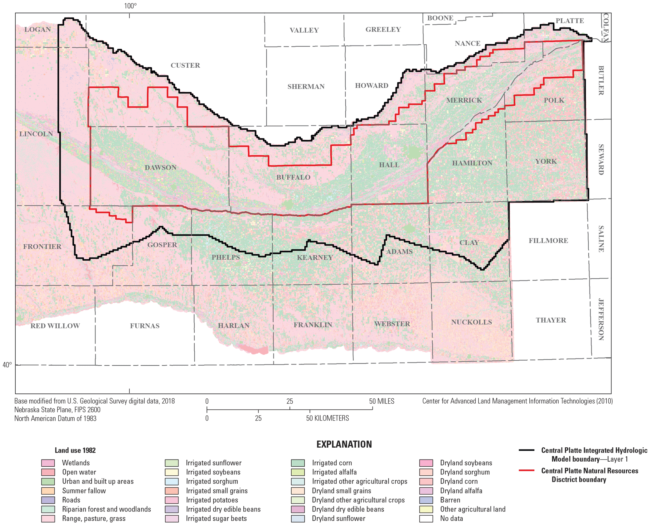
Distribution of land uses for 1982.
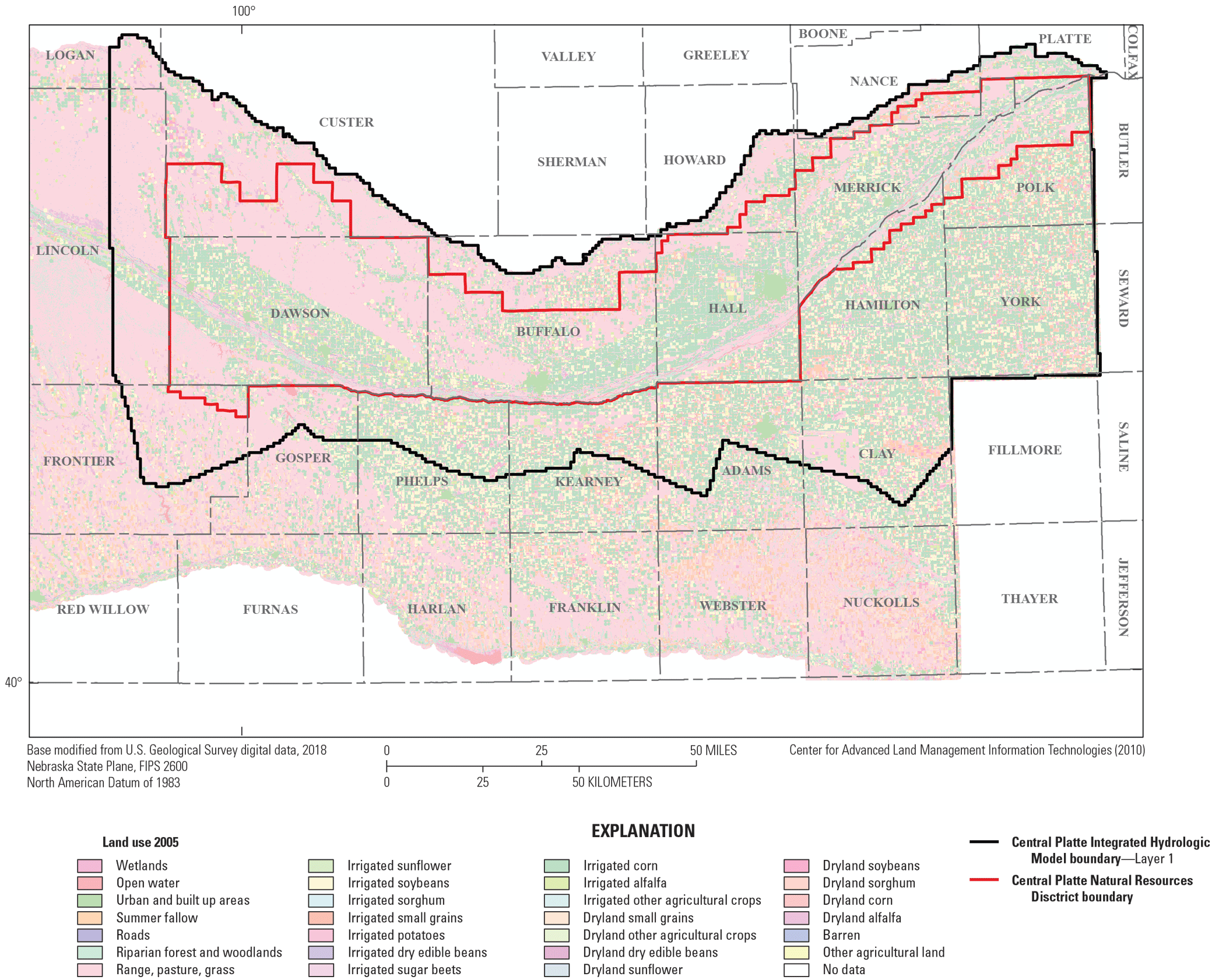
Distribution of land uses for 2005.
References Cited
Traylor, J.P., 2023, MODFLOW-One-Water model used to support the Central Platte Natural Resources District Groundwater Management Plan, central Nebraska: U.S. Geological Survey data release, accessed March 2023 at https://doi.org/10.5066/P9G3Q5XK.
Appendix 2. Additional Calibration Statistics that Include Measured and Simulated Plots and Residual Value Distribution Histograms by Observation Group
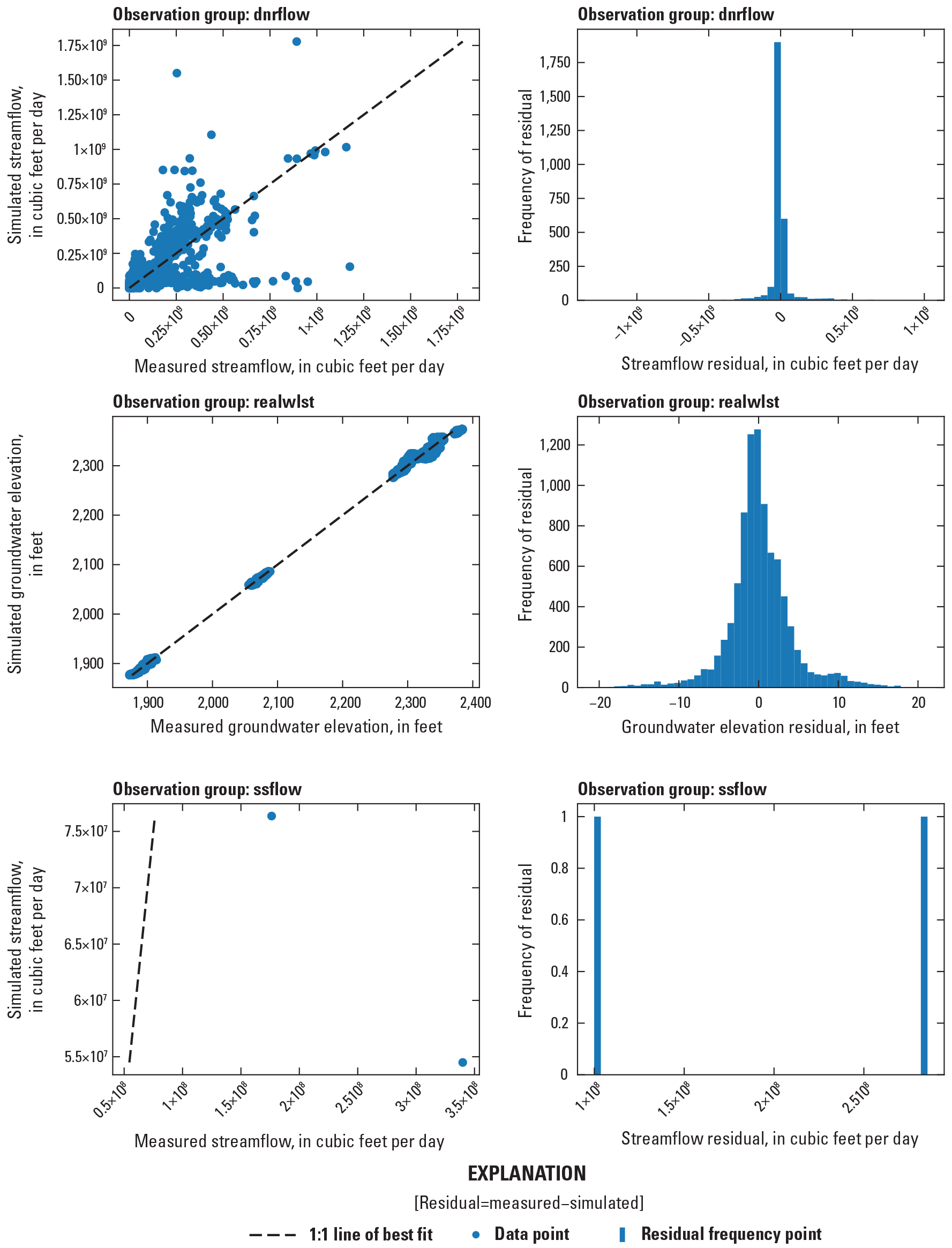
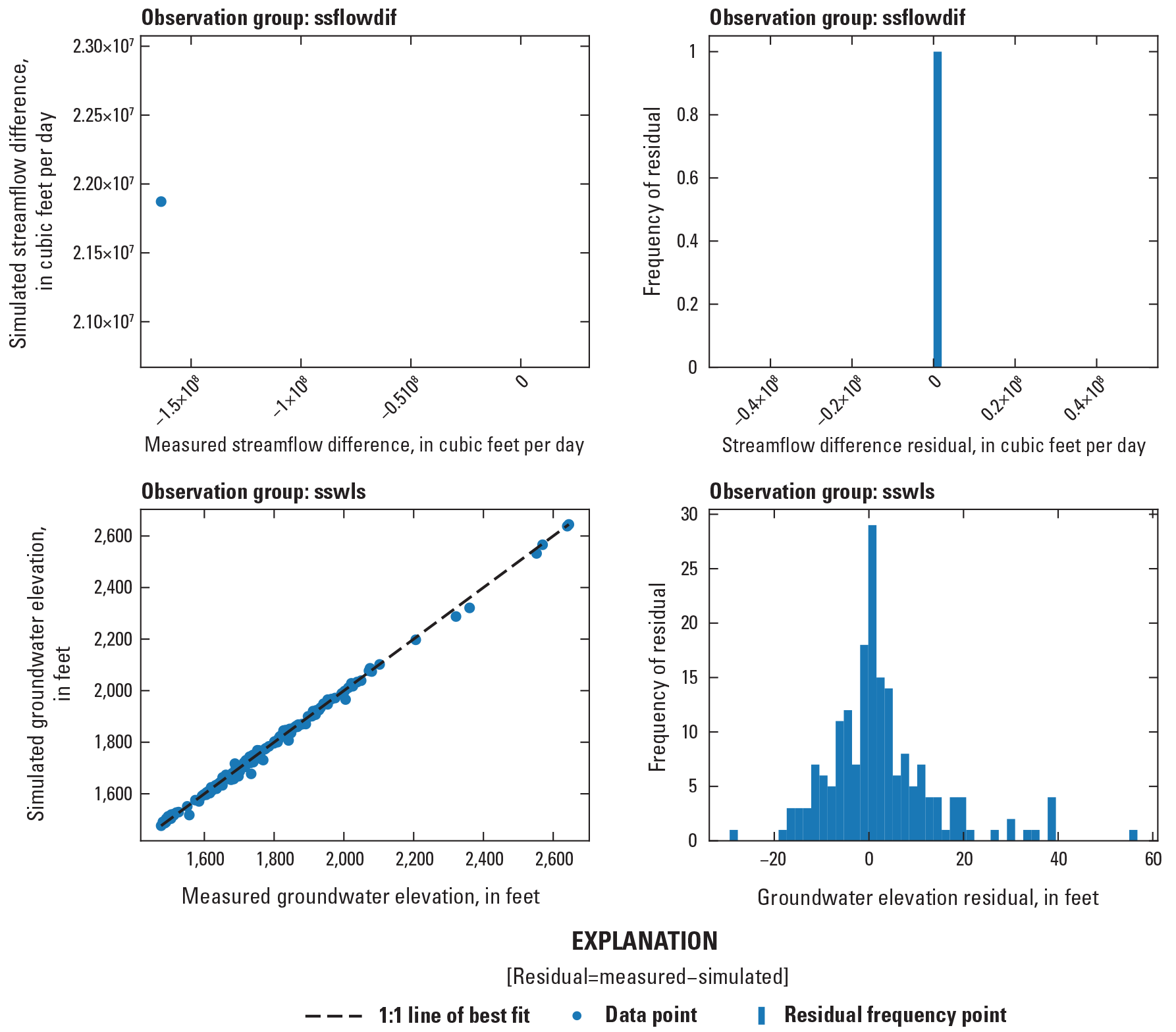
Plot of measured compared to simulated values and residual values distributions for observation groups (see table 9 for observation group definitions).
Appendix 3. Additional Average Landscape Water and Groundwater-Flow Budget Tables for the Development Period Central Platte Integrated Hydrologic Model and Groundwater Management Areas as Volumetric Rates and Net Volumetric Rates
Appendix 4. Additional Average Landscape Water and Groundwater-Flow Budget Tables for Each Scenario of the Central Platte Integrated Hydrologic Model by Groundwater Management Area as Area Normalized Volumetric Rates and Net Volumetric Rates
Appendix 5. Additional Simulated Groundwater-Levels for Each Scenario and Groundwater Management Area
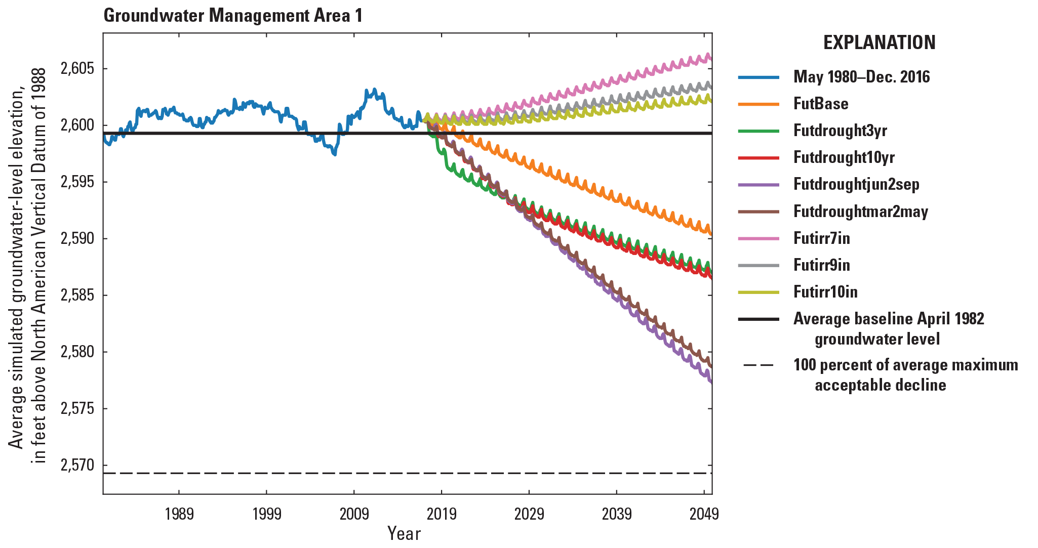
Simulated groundwater levels from May 1980 to December 2016 development period and January 2017 to December 2049 scenario period for the Central Platte Integrated Hydrologic Model in Groundwater Management Area 1.
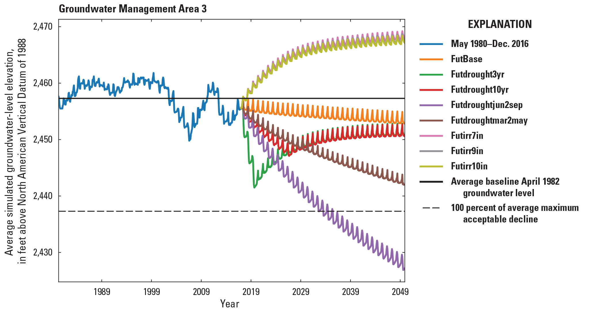
Simulated groundwater levels from May 1980 to December 2016 development period and January 2017 to December 2049 scenario period for the Central Platte Integrated Hydrologic Model in Groundwater Management Area 3.
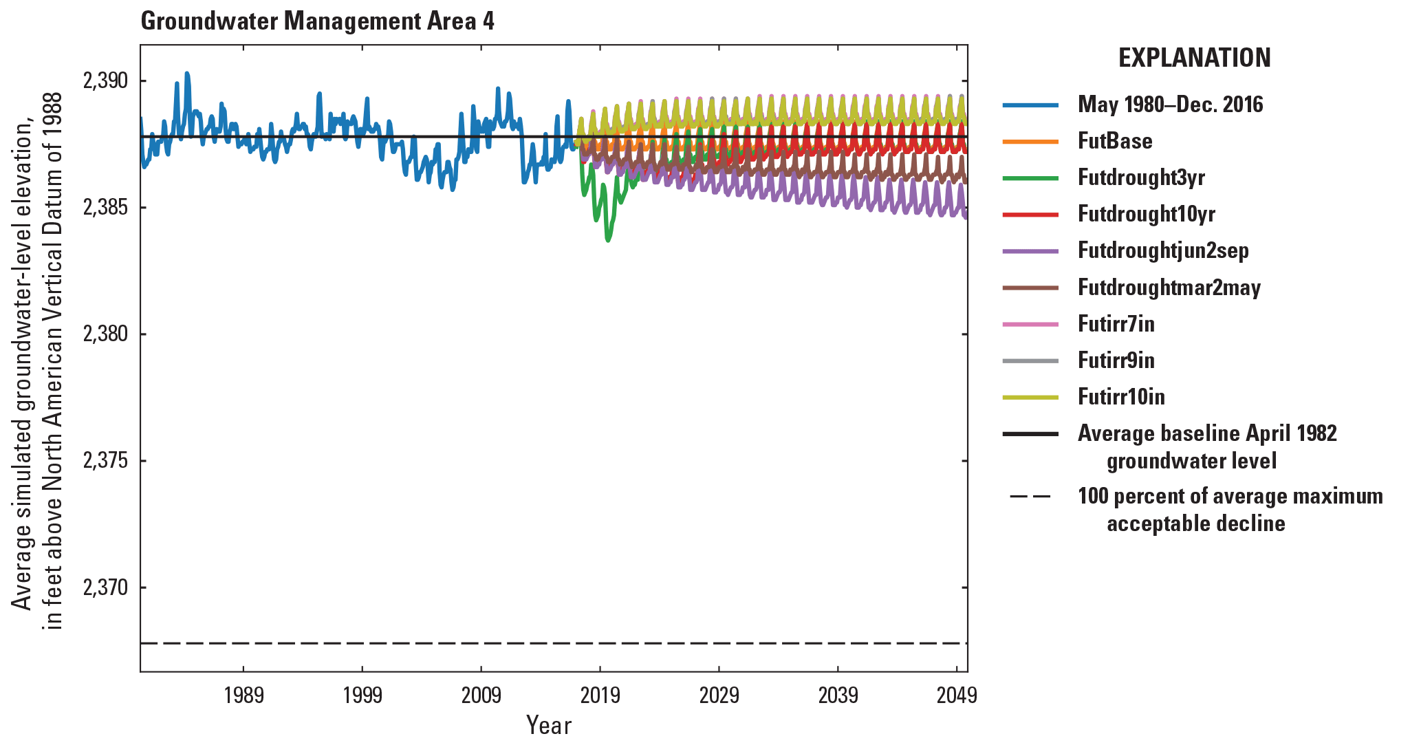
Simulated groundwater levels from May 1980 to December 2016 development period and January 2017 to December 2049 scenario period for the Central Platte Integrated Hydrologic Model in Groundwater Management Area 4.
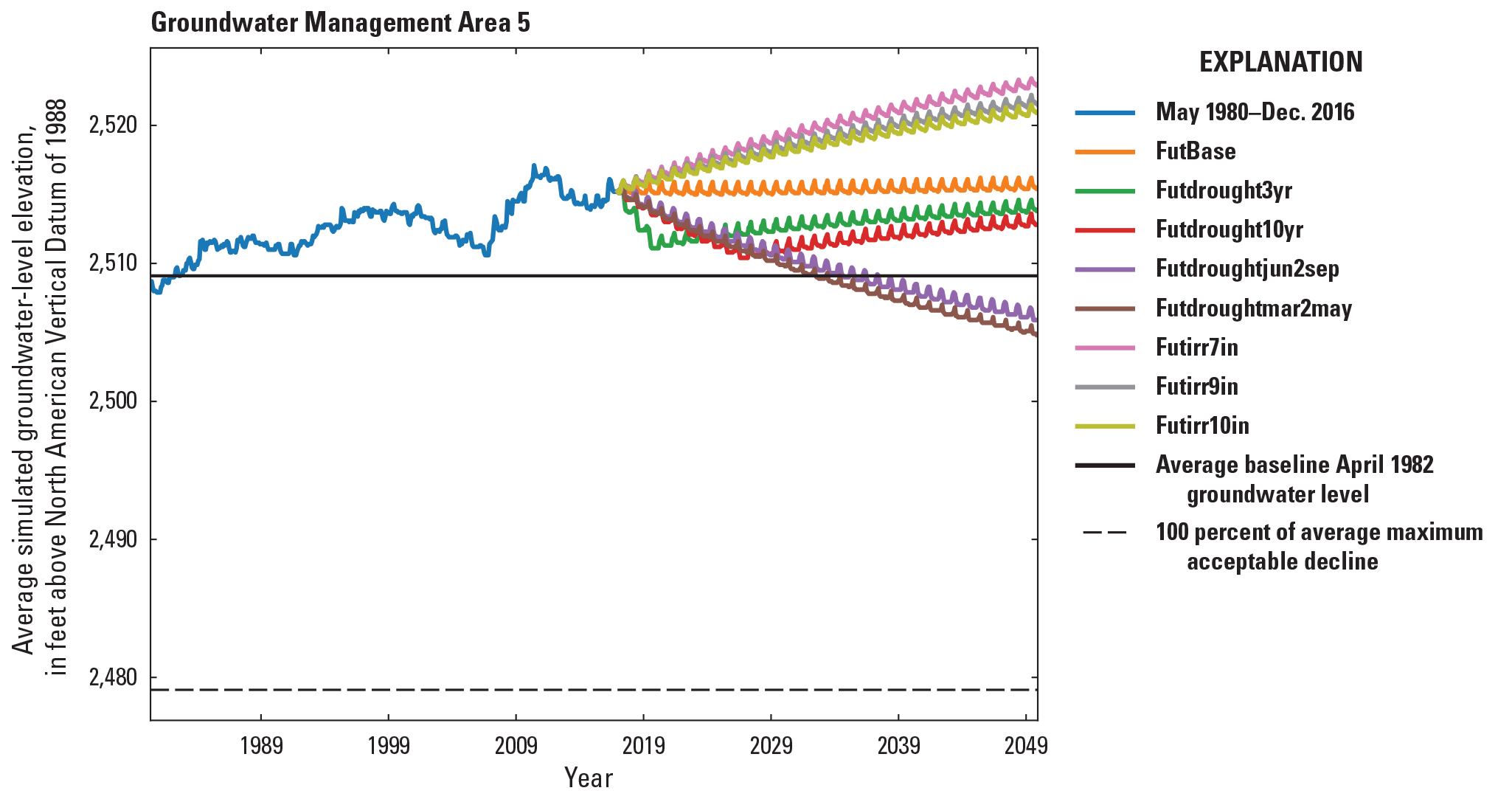
Simulated groundwater levels from May 1980 to December 2016 development period and January 2017 to December 2049 scenario period for the Central Platte Integrated Hydrologic Model in Groundwater Management Area 5.
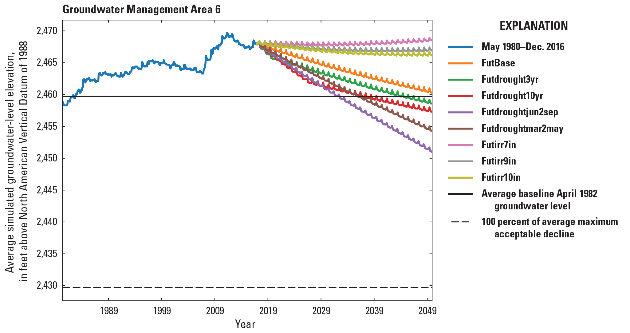
Simulated groundwater levels from May 1980 to December 2016 development period and January 2017 to December 2049 scenario period for the Central Platte Integrated Hydrologic Model in Groundwater Management Area 6.

Simulated groundwater levels from May 1980 to December 2016 development period and January 2017 to December 2049 scenario period for the Central Platte Integrated Hydrologic Model in Groundwater Management Area 7.
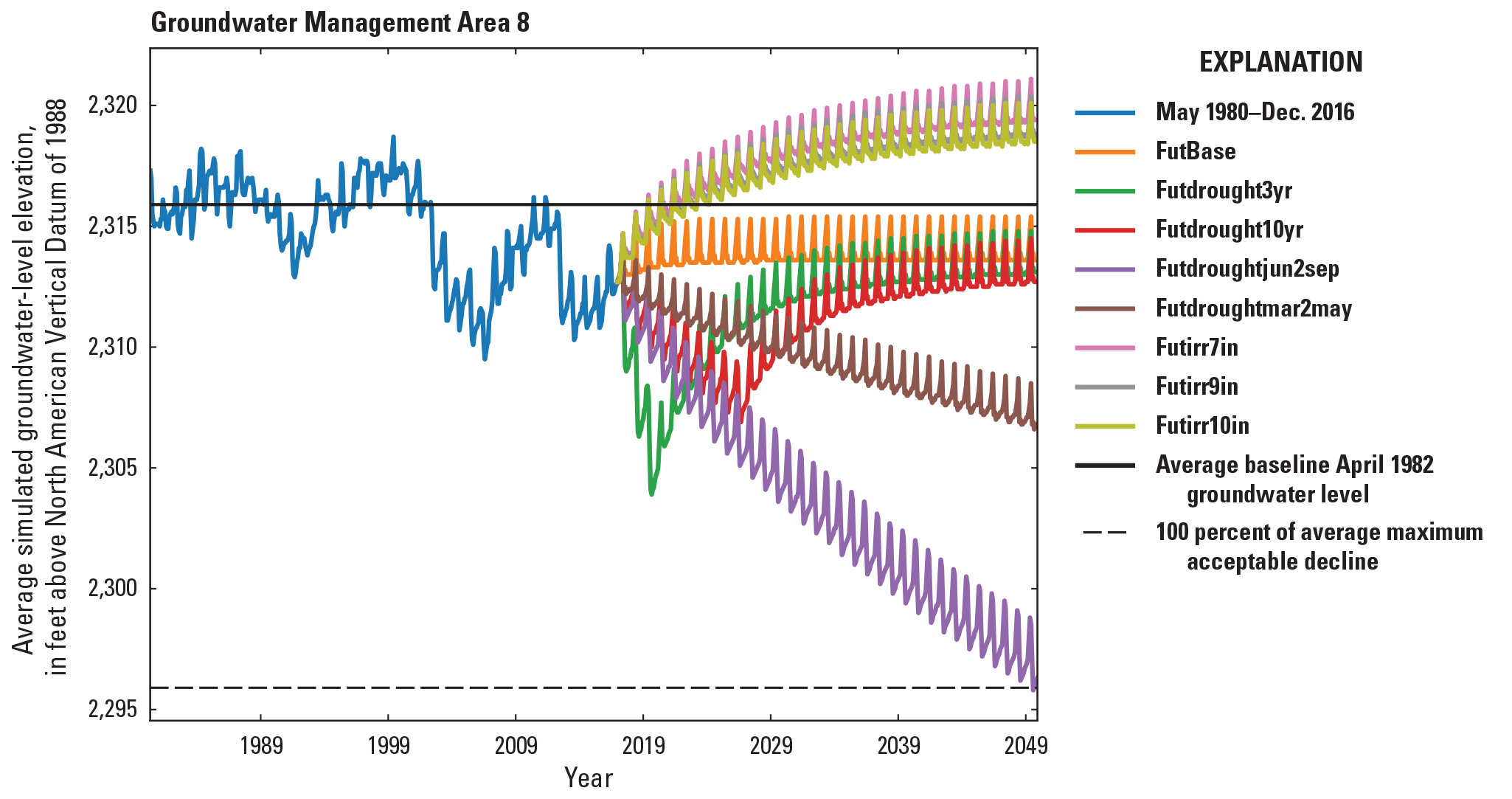
Simulated groundwater levels from May 1980 to December 2016 development period and January 2017 to December 2049 scenario period for the Central Platte Integrated Hydrologic Model in Groundwater Management Area 8.
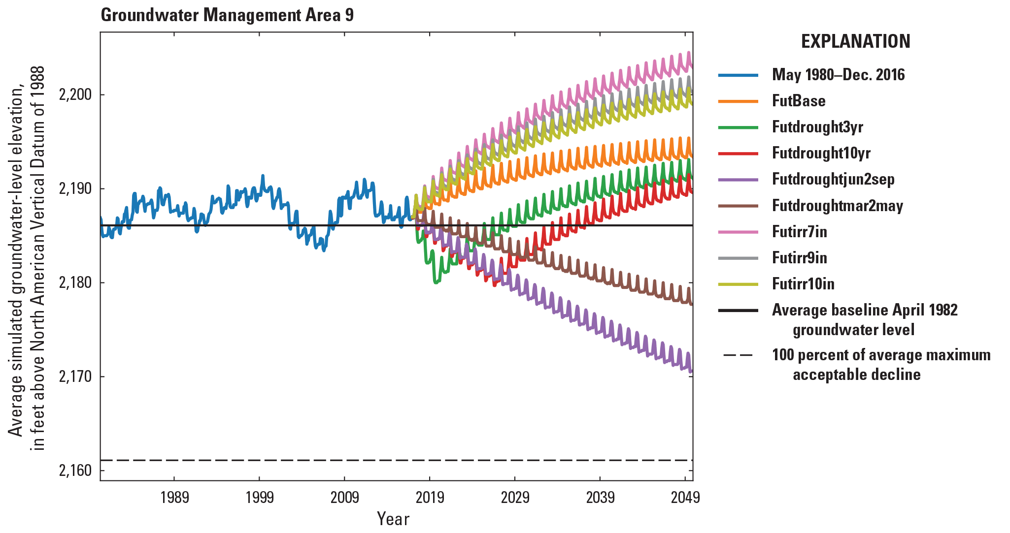
Simulated groundwater levels from May 1980 to December 2016 development period and January 2017 to December 2049 scenario period for the Central Platte Integrated Hydrologic Model in Groundwater Management Area 9.
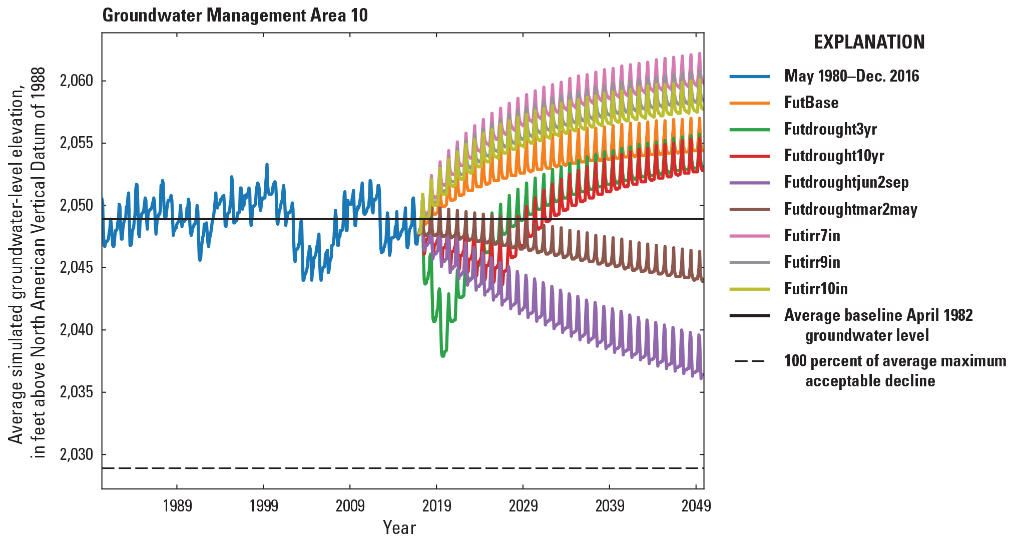
Simulated groundwater levels from May 1980 to December 2016 development period and January 2017 to December 2049 scenario period for the Central Platte Integrated Hydrologic Model in Groundwater Management Area 10.
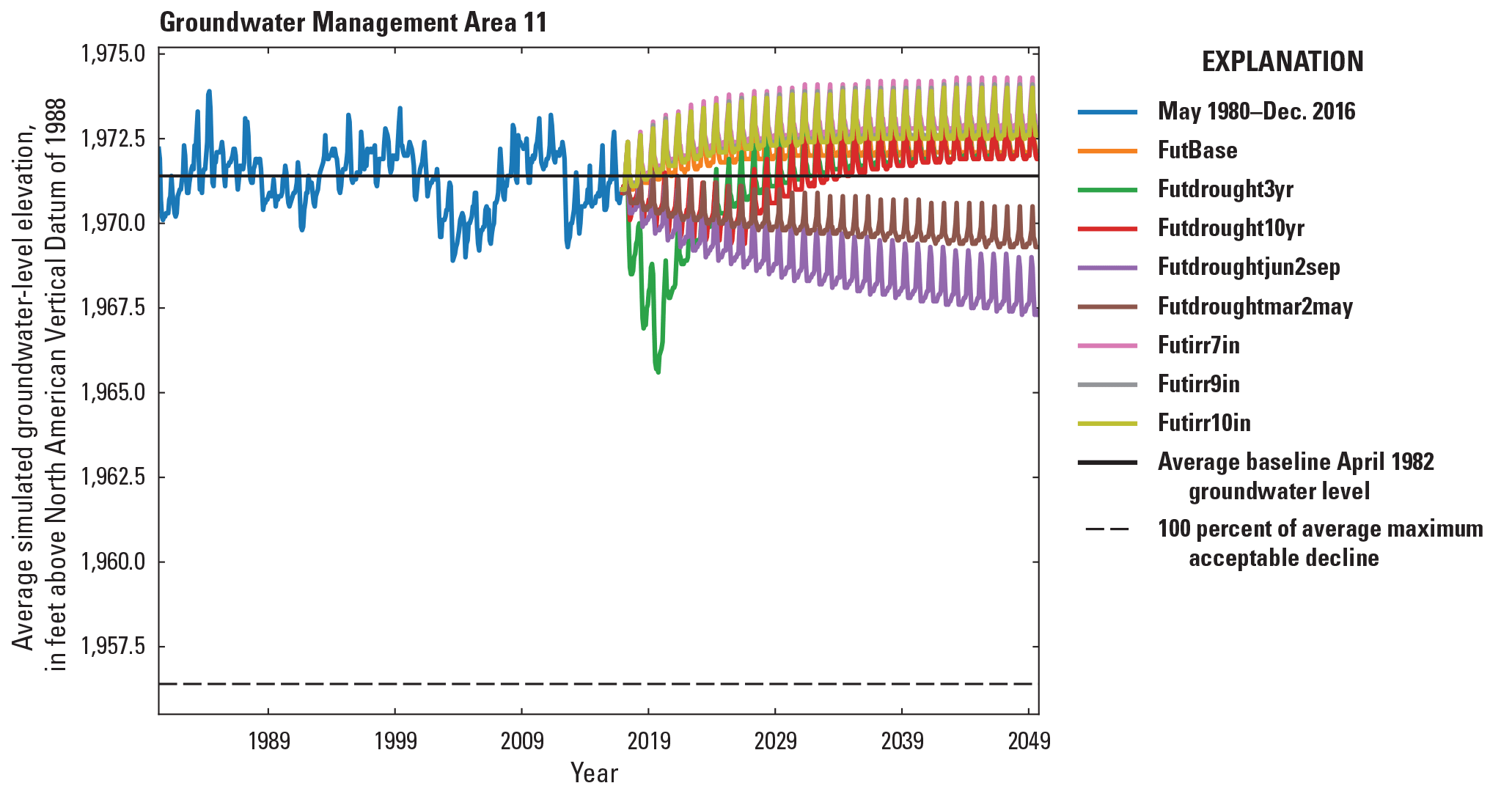
Simulated groundwater levels from May 1980 to December 2016 development period and January 2017 to December 2049 scenario period for the Central Platte Integrated Hydrologic Model in Groundwater Management Area 11.
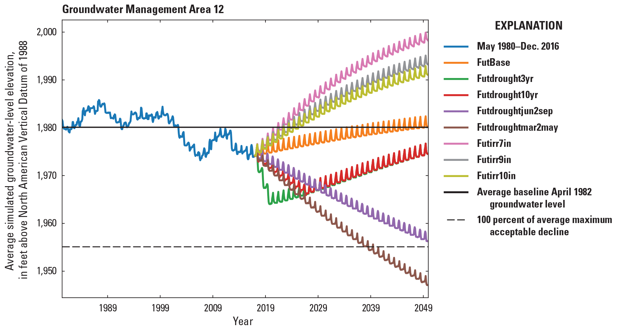
Simulated groundwater levels from May 1980 to December 2016 development period and January 2017 to December 2049 scenario period for the Central Platte Integrated Hydrologic Model in Groundwater Management Area 12.
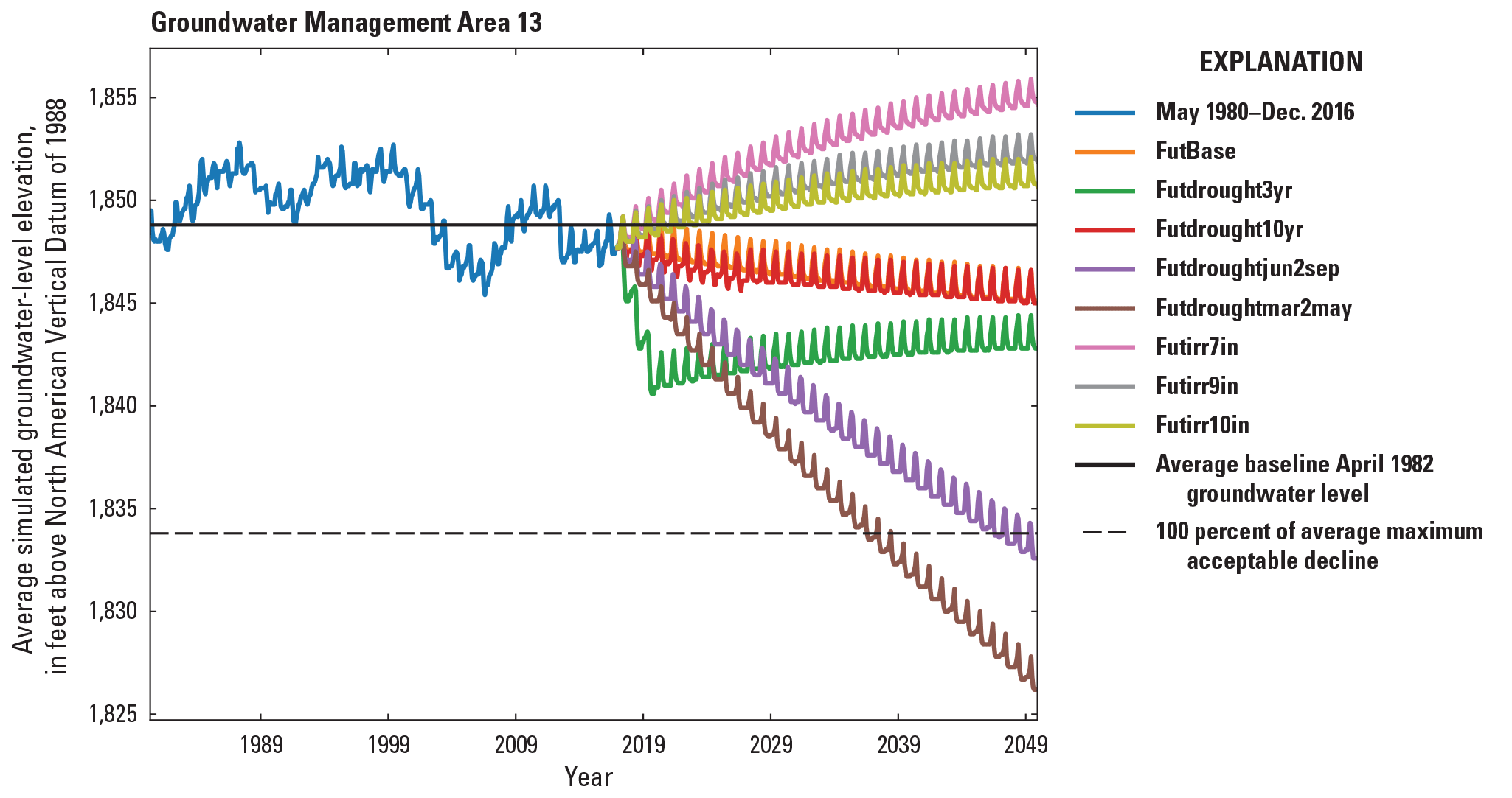
Simulated groundwater levels from May 1980 to December 2016 development period and January 2017 to December 2049 scenario period for the Central Platte Integrated Hydrologic Model in Groundwater Management Area 13.
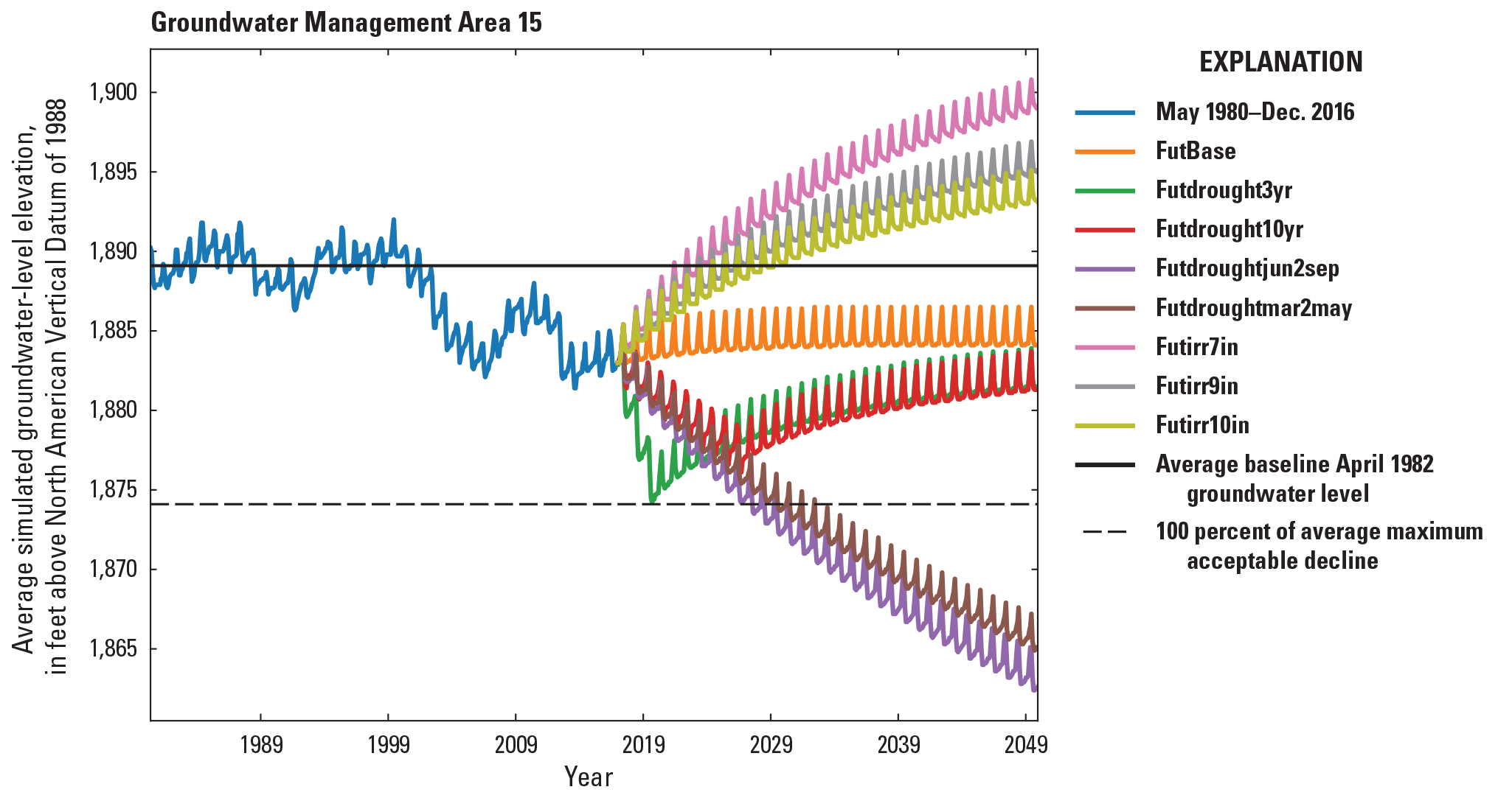
Simulated groundwater levels from May 1980 to December 2016 development period and January 2017 to December 2049 scenario period for the Central Platte Integrated Hydrologic Model in Groundwater Management Area 15.
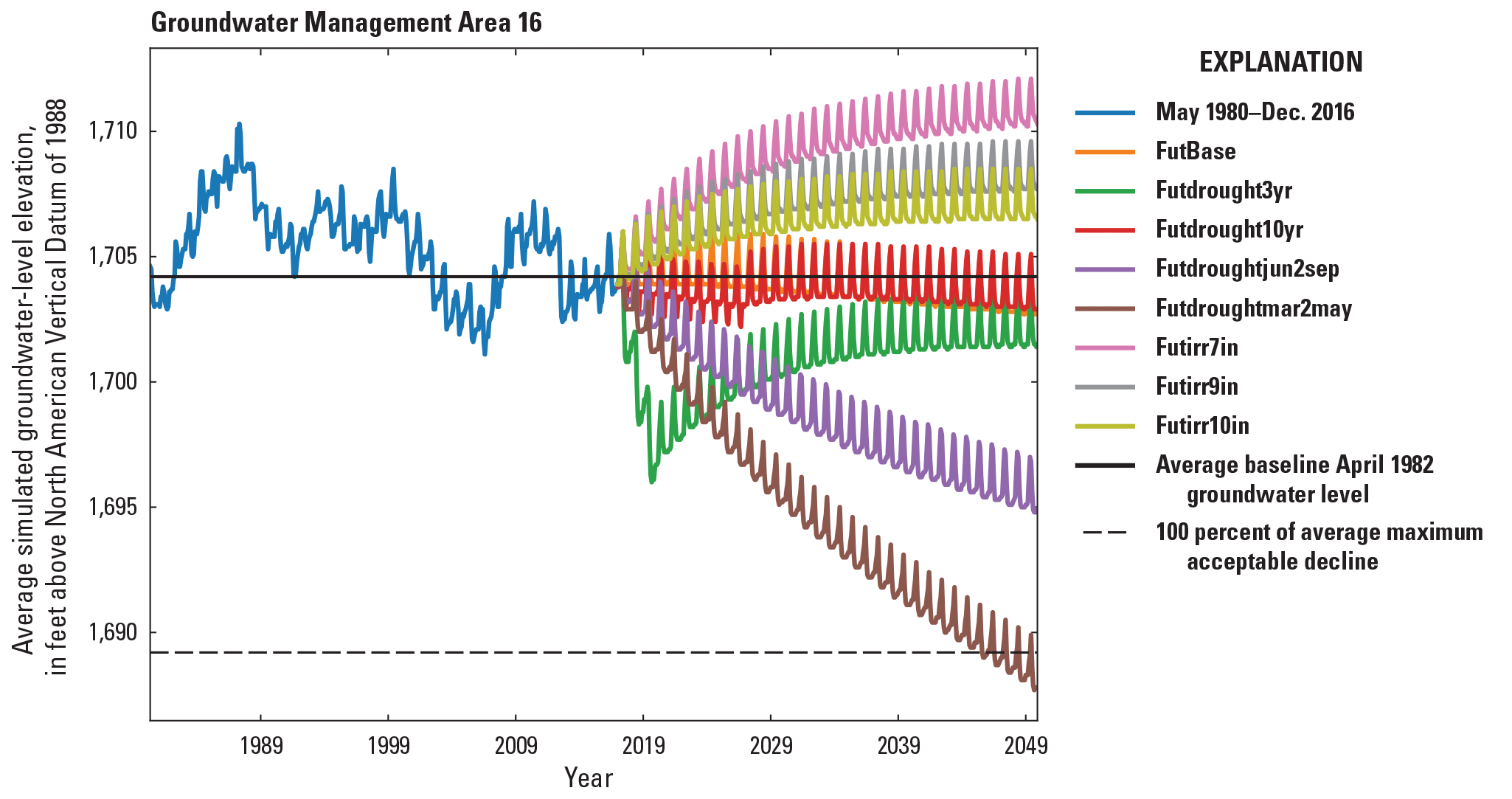
Simulated groundwater levels from May 1980 to December 2016 development period and January 2017 to December 2049 scenario period for the Central Platte Integrated Hydrologic Model in Groundwater Management Area 16.
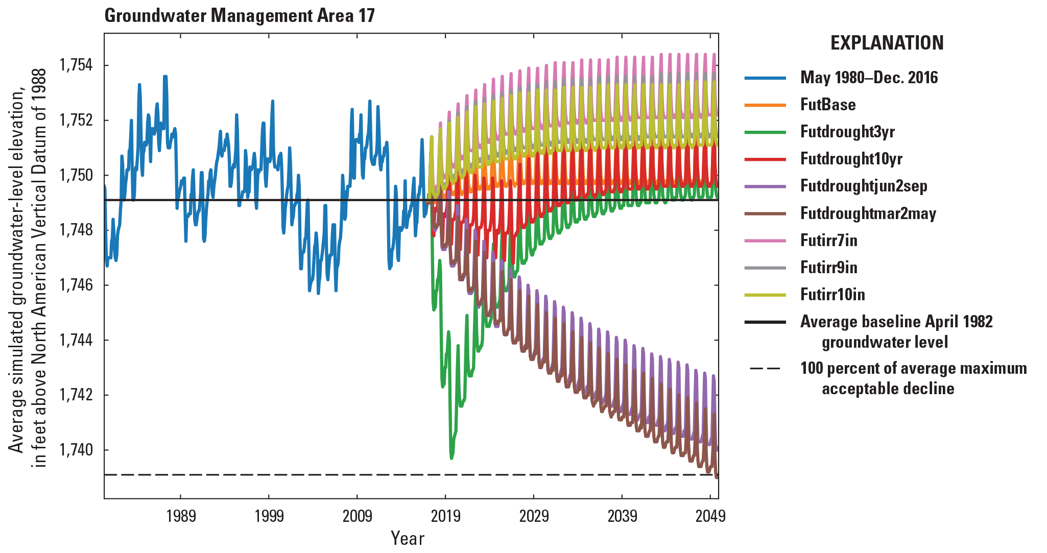
Simulated groundwater levels from May 1980 to December 2016 development period and January 2017 to December 2049 scenario period for the Central Platte Integrated Hydrologic Model in Groundwater Management Area 17.
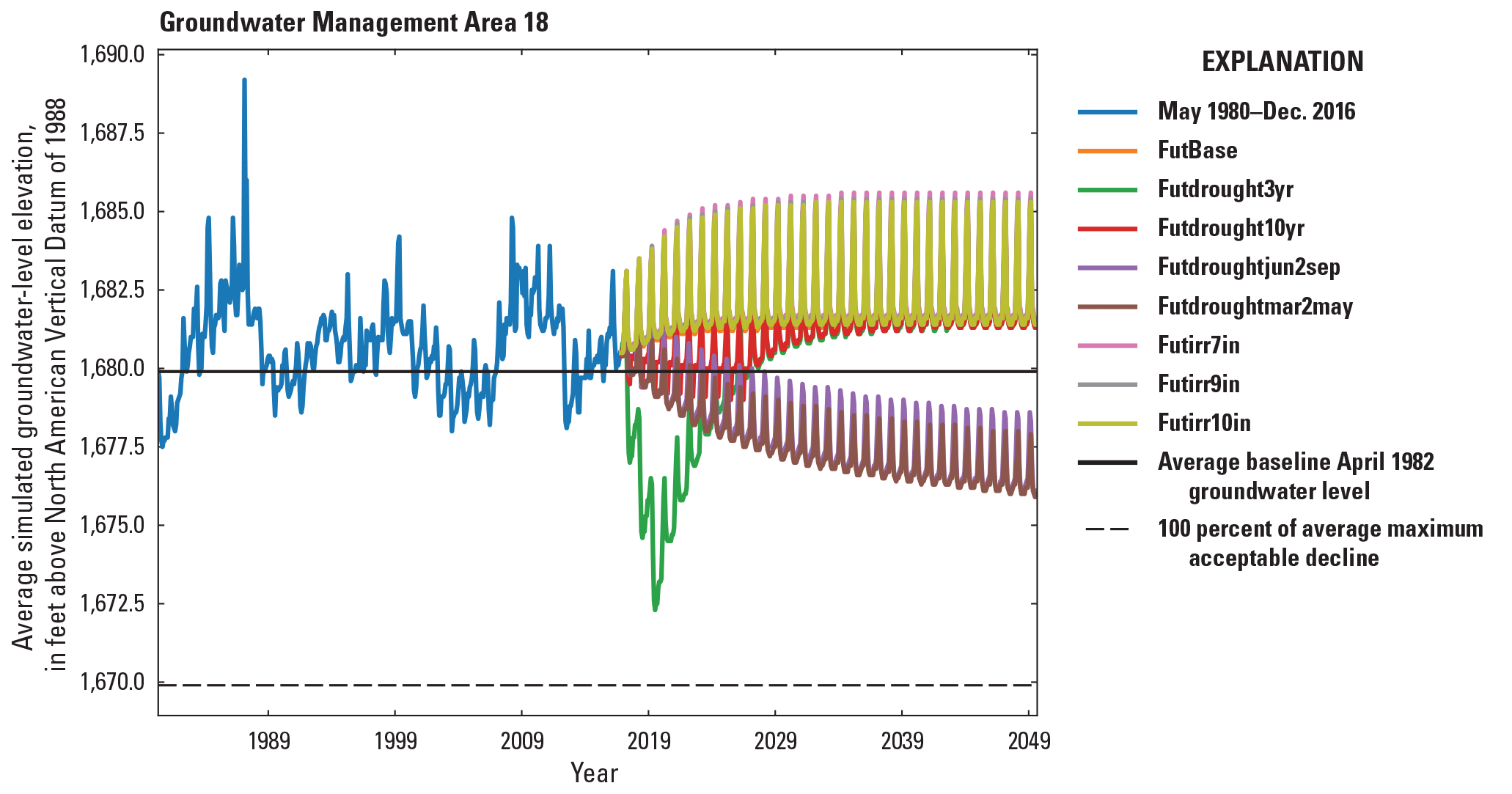
Simulated groundwater levels from May 1980 to December 2016 development period and January 2017 to December 2049 scenario period for the Central Platte Integrated Hydrologic Model in Groundwater Management Area 18.
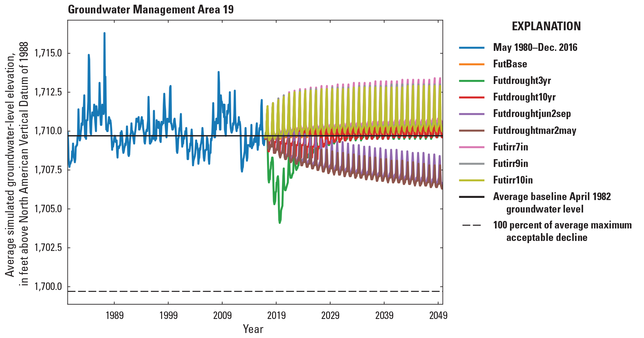
Simulated groundwater levels from May 1980 to December 2016 development period and January 2017 to December 2049 scenario period for the Central Platte Integrated Hydrologic Model in Groundwater Management Area 19.
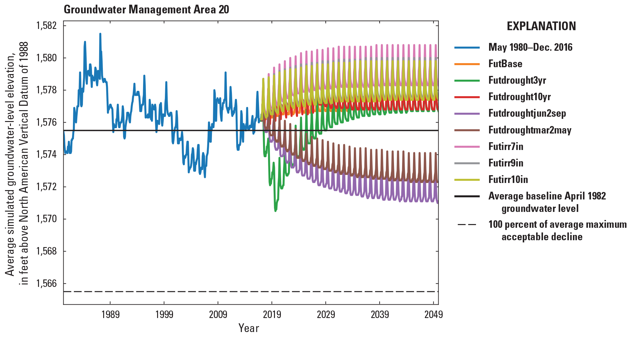
Simulated groundwater levels from May 1980 to December 2016 development period and January 2017 to December 2049 scenario period for the Central Platte Integrated Hydrologic Model in Groundwater Management Area 20.
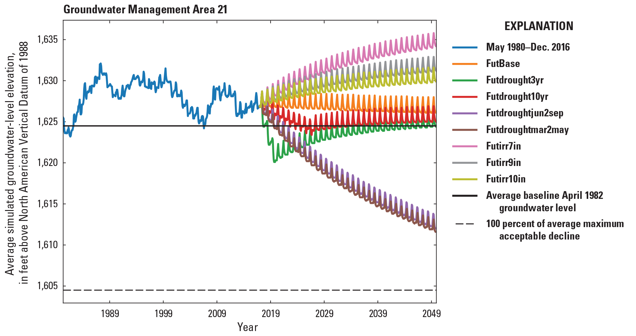
Simulated groundwater levels from May 1980 to December 2016 development period and January 2017 to December 2049 scenario period for the Central Platte Integrated Hydrologic Model in Groundwater Management Area 21.
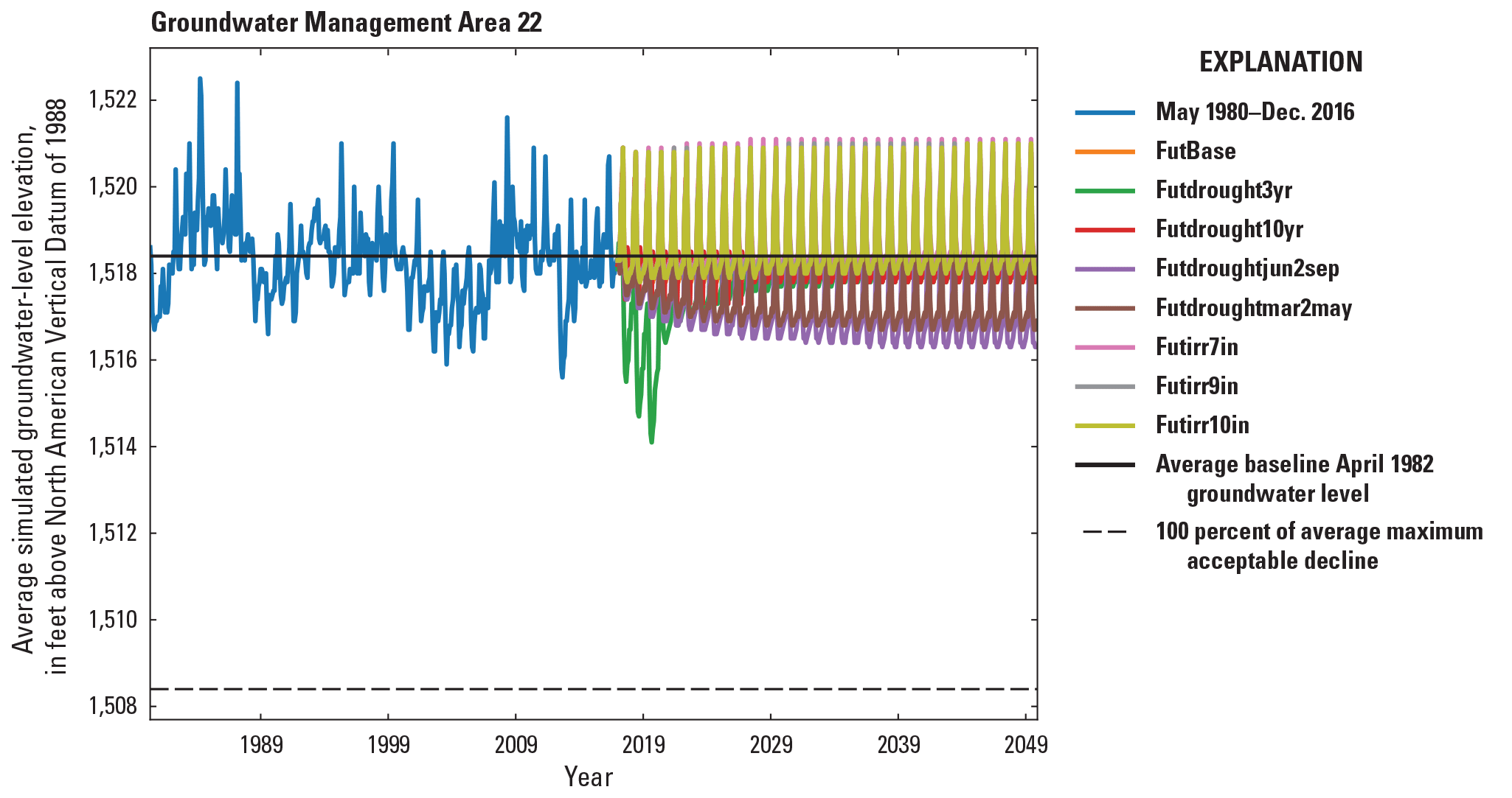
Simulated groundwater levels from May 1980 to December 2016 development period and January 2017 to December 2049 scenario period for the Central Platte Integrated Hydrologic Model in Groundwater Management Area 22.
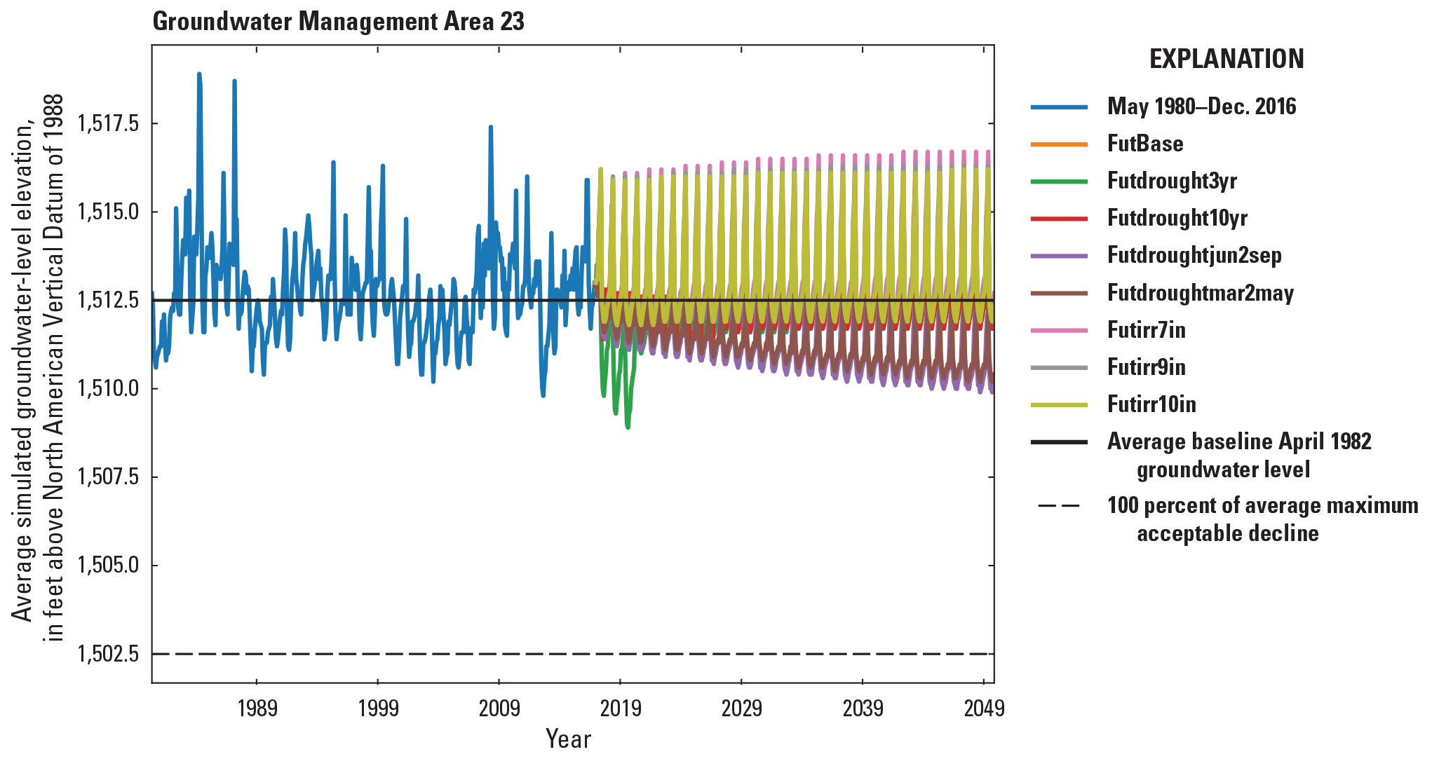
Simulated groundwater levels from May 1980 to December 2016 development period and January 2017 to December 2049 scenario period for the Central Platte Integrated Hydrologic Model in Groundwater Management Area 23.
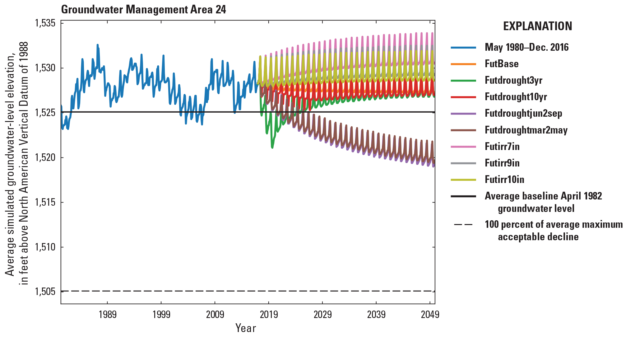
Simulated groundwater levels from May 1980 to December 2016 development period and January 2017 to December 2049 scenario period for the Central Platte Integrated Hydrologic Model in Groundwater Management Area 24.
Conversion Factors
U.S. customary units to International System of Units
Temperature in degrees Celsius (°C) may be converted to degrees Fahrenheit (°F) as follows: °F = (1.8 × °C) + 32.
Temperature in degrees Fahrenheit (°F) may be converted to degrees Celsius (°C) as follows: °C = (°F – 32) / 1.8.
Datum
Vertical coordinate information is referenced to the North American Vertical Datum of 1988 (NAVD 88).
Horizontal coordinate information is referenced to the North American Datum of 1983 (NAD 83).
Altitude, as used in this report, refers to distance above the vertical datum.
Abbreviations
AET
actual evapotranspiration
baseline 1982 gwlevels
baseline April 30, 1982, groundwater altitudes simulated by the development Central Platte Integrated Hydrologic Model
CIR
crop irrigation requirement
CNPPID
Central Nebraska Public Power and Irrigation District
COHYST
Cooperative Hydrology Study
CPIHM
Central Platte Integrated Hydrologic Model
CPNRD
Central Platte Natural Resources District
CWD
crop water demand
Eg
evaporation of groundwater
Ei
evaporation of irrigation water
Ep
evaporation of precipitation
ET
evapotranspiration
ETg
evapotranspiration of groundwater
ETp
evapotranspiration of precipitation
ETref
reference evapotranspiration
FEI
fraction of evaporation from irrigation
FIESWI
fraction of inefficient losses to surface water from irrigation
FIESWP
fraction of inefficient losses to surface water from precipitation
FMP
Farm Process package
FTR
fraction of transpiration
FutBase
base scenario
Futdrought3yr
3-year drought scenario
Futdrought10yr
10-year drought scenario
Futdroughtjun2sep
mid-growing season drought scenario
Futdroughtmar2may
early growing season drought scenario
Futirr7in
scenario limiting annual groundwater irrigation pumping to 7 inches
Futirr9in
scenario limiting annual groundwater irrigation pumping to 9 inches
Futirr10in
scenario limiting annual groundwater irrigation pumping to 10 inches
GHB
General Head Boundary package
GMP
Groundwater Management Plan
GWMA
Groundwater Management Area
HU
hydrostratigraphic unit
Kc
crop coefficient
Kh
horizontal hydraulic conductivity
Ksb
vertical hydraulic conductivity of streambed
lidar
light detection and ranging
MAD
maximum acceptable decline
MF–OWHM
MODFLOW–One-Water Hydrologic Model
MODFLOW
modular finite-difference flow model
MODFLOW–NWT
modular finite-difference flow model with Newton solver
n
number of calibration targets
NeDNR
Nebraska Department of Natural Resources
NRD
Natural Resource District
NWIS
National Water Information System
OFE
on-farm efficiency
PEST
Parameter ESTimation
PET
potential evapotranspiration
Φ
phi, the PEST objective function
Φr
regularization phi, a part of the PEST objective function
PPT
precipitation
r
residual, as the difference between time and space equivalent measured and simulated values.
R2
coefficient of determination
SFR
Streamflow Routing package
Ss
specific storage
SVDA
singular value decomposition-assist
Sy
specific yield
Tg
transpiration of groundwater
Ti
transpiration of irrigation water
Tp
transpiration of precipitation
USGS
U.S. Geological Survey
UZF
Unsaturated Zone Flow package
w
weight applied to the observation
WBS
water-balance subregion
For more information about this publication, contact:
Director, USGS Nebraska Water Science Center
5231 South 19th Street
Lincoln, NE 68512
402–328–4100
For additional information, visit: https://www.usgs.gov/centers/ne-water
Publishing support provided by the
Rolla Publishing Service Center
Disclaimers
Any use of trade, firm, or product names is for descriptive purposes only and does not imply endorsement by the U.S. Government.
Although this information product, for the most part, is in the public domain, it also may contain copyrighted materials as noted in the text. Permission to reproduce copyrighted items must be secured from the copyright owner.
Suggested Citation
Traylor, J.P., Guira, M., and Peterson, S.M., 2023, An integrated hydrologic model to support the Central Platte Natural Resources District Groundwater Management Plan, central Nebraska: U.S. Geological Survey Scientific Investigations Report 2023–5024, 143 p., https://doi.org/10.3133/sir20235024.
ISSN: 2328-0328 (online)
Study Area
| Publication type | Report |
|---|---|
| Publication Subtype | USGS Numbered Series |
| Title | An integrated hydrologic model to support the Central Platte Natural Resources District Groundwater Management Plan, central Nebraska |
| Series title | Scientific Investigations Report |
| Series number | 2023-5024 |
| DOI | 10.3133/sir20235024 |
| Publication Date | April 20, 2023 |
| Year Published | 2023 |
| Language | English |
| Publisher | U.S. Geological Survey |
| Publisher location | Reston, VA |
| Contributing office(s) | Nebraska Water Science Center |
| Description | Report: xii, 143 p.; 2 Tables; Data Release; Dataset; 3 Figures: 11.00 x 8.50 inches |
| Country | United States |
| State | Nebraska |
| Other Geospatial | Platte River |
| Online Only (Y/N) | Y |
| Additional Online Files (Y/N) | Y |