

Trends in Environmental, Anthropogenic, and Water-Quality Characteristics in the Upper White River Basin, Indiana
Links
- Document: Report (5.05 MB pdf) , HTML , XML
- Related Work: Fact Sheet 2023–3009 - Potential Drivers of Change in Fluxes of Nutrients and Total Suspended Solids in the Upper White River Basin, Indiana, Water Years 1997–2019
- Data Release: USGS data release - Model data archive—Trends in selected environmental, anthropogenic, and water-quality characteristics in the upper White River Basin, Indiana, 1991–2020
- NGMDB Index Page: National Geologic Map Database Index Page (html)
- Download citation as: RIS | Dublin Core
Acknowledgments
The author would like to thank the agencies and agency personnel who provided the water-quality and streamflow data. The author would also like to thank Cassie Hauswald (The Nature Conservancy), Nancy Baker (U.S Geological Survey), and Jeremy Weber (U.S Geological Survey) for their advice and assistance.
Abstract
The U.S. Geological Survey (USGS), in cooperation with The Nature Conservancy, undertook a study to update and extend results from a previous study (Koltun, 2019, https://doi.org/10.3133/sir20195119), using data from 3 additional years and newer estimation methods. Koltun (2019) assessed trends in streamflow, precipitation, and estimated annual mean concentrations and flux of nitrate plus nitrite, total Kjeldahl nitrogen, total phosphorus, and total suspended solids (TSS) for USGS streamflow gages on the upper White River at Muncie, near Nora, and near Centerton, Indiana. Annual mean and maximum daily streamflows had statistically significant upward trends at all study gages between water years 1978 and 2020. An abrupt increase in streamflow occurred around water year 2001. Annual total precipitation at the Indianapolis International Airport increased between calendar years 1932 and 2020 at an average rate of 0.089 inches per year.
The current study assessed the magnitude, direction, and likelihood of change in flow-normalized concentrations and flux of TSS, total phosphorus, nitrate plus nitrite, and total Kjeldahl nitrogen between water years 1997 and 2019. With two exceptions, concentration and flux changes that were statistically significant in Koltun (2019, https://doi.org/10.3133/sir20195119), which reported changes between water years 1997 and 2017, still have the same statistically significant change directions. The reliability of the current trend result for TSS is uncertain because of a large gap in the TSS record for the Centerton gage.
For each constituent, spatial patterns were examined in the sampled distribution of nutrient and TSS concentration data from 20 mainstem, tributary, and distributary locations in the upper White River Basin. The largest median concentrations of TSS, total phosphorus, and total Kjeldahl nitrogen were associated with mainstem upper White River sites downstream from Indianapolis. The median total phosphorus and total Kjeldahl nitrogen concentrations were elevated relative to bracketing upstream/downstream mainstem sites at the upper White River site immediately downstream from Muncie.
Data on several anthropogenic factors that could influence the concentrations and fluxes of nutrients and TSS were gathered and analyzed to better understand the factors’ spatial and temporal variations. Those anthropogenic factors included population, land cover, cropping and operational tillage practices, fertilizer application, and upgrades to wastewater treatment systems and delivery processes.
Introduction
The White River, in Indiana, is the largest tributary to the Wabash River, and the upper White River has been identified as a major contributor of nutrients from agricultural and urban sources (Robertson and Saad, 2013; Robertson and others, 2009). The U.S. Geological Survey (USGS) and The Nature Conservancy previously collaborated on a study (Koltun, 2019) to evaluate trends in streamflow and the concentrations and flux of nutrients and total suspended solids (TSS) at three study gages (at Muncie, near Nora, and near Centerton, Indiana) on the upper White River. In the context of contaminant transport, the term “flux” refers to the rate of mass transport. Koltun (2019) used USGS streamflow data, and water-quality data collected by the USGS and several state and local agencies, from water years 1992 to 2017, to identify several instances of statistically significant temporal trends in streamflows and likely temporal trends in flow-normalized concentrations and fluxes of TSS and nutrients. Water years are from October to September and are designated by the calendar year in which they end. The current study objectives were to (1) update the previous analyses using data collected through the 2020 water year, (2) use newly developed analytical techniques to compute more accurate annual mean concentration and flux estimates, and (3) compile and examine ancillary datasets on anthropogenic factors to better understand factors that might influence trends in the data.
Description of Study Area
The study area comprises the upper White River hydrologic unit (05120201) (hereafter referred to as the “upper White River Basin”), located predominantly in central and east-central Indiana (fig. 1). The upper White River Basin drains an area of approximately 2,718 square miles (mi2) and contains all or part of 16 counties that, in 2020, included 7 of the 20 most populated cities in Indiana (Indianapolis, Carmel, Fishers, Muncie, Noblesville, Greenwood, and Anderson) (STATS Indiana, 2022). Indianapolis was the most populated city in Indiana, with a 2020 population estimated at more than 887,600 and a population of more than 2,111,000 in the Indianapolis metro area that includes Indianapolis, Carmel, and Anderson, Indiana (STATS Indiana, 2022).
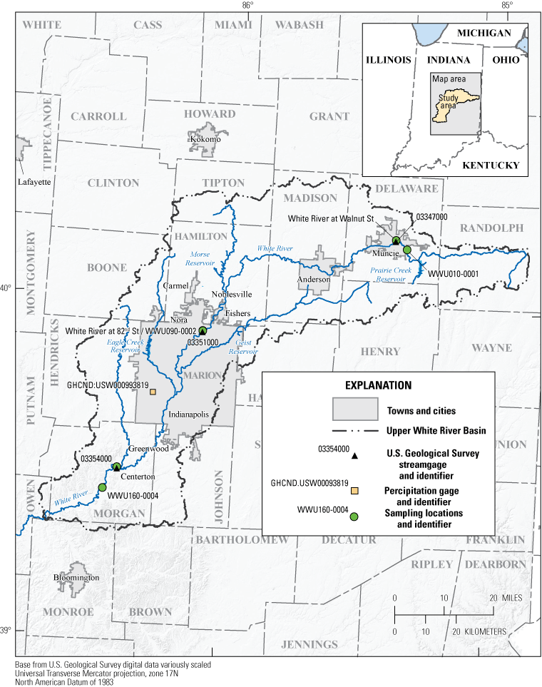
Map of study area, showing gages, and sampling locations.
There are more than 2,180 miles (mi) of streams (Tedesco and others, 2005) and four water-supply reservoirs (Eagle Creek, Geist, Morse, and Prairie Creek Reservoirs) in the upper White River Basin. Although Eagle Creek Reservoir has been used for water supply for the City of Indianapolis since 1976, the reservoir was developed primarily for flood control (Tedesco and others, 2005).
The drainage area upstream from the study gages is predominantly within the Tipton Till Plain physiographic region, with a small northerly part of the drainage area lying in the Bluffton Till Plain physiographic region. The Till Plains were formed by continental glaciation during the last Ice Age and consequently have low topographic relief. The Till Plains have a covering of glacial till and outwash material composed of 100 to 200 feet of silty clay till interspersed with thin (5 to 10 feet) layers of sand and gravel (Tedesco and others, 2011). Till Plain soils have attracted widespread agricultural land use but tend to have low infiltration rates so that tile drains are commonly installed to improve drainage and reduce surface runoff.
Based on an analysis of land-cover data from the 2019 National Land Cover Database (Dewitz and U.S. Geological Survey, 2021), the dominant land cover in the upper White River Basin was agricultural (constituting approximately 55.6 percent of the basin) followed by developed (29.5 percent) and forested (13.3 percent) land covers. In general, agricultural land cover in the upper White River Basin decreased as a percentage of the drainage area from the headwaters in Randolph County to downstream locations on the White River. Those decreases in agricultural land cover were predominantly offset by increases in developed land covers.
Central Indiana has a humid-continental climate characterized by distinct summer and winter seasons, large annual temperature changes, and highly variable weather patterns (Tedesco and others, 2005). For the period 1991–2020, the average annual temperature and precipitation for Indianapolis was 53.7 degrees Fahrenheit and 42.62 inches, respectively (National Oceanic and Atmospheric Administration, 2022). According to Widhalm and others (2018), Indiana has warmed, and average precipitation has increased since 1895, with more precipitation falling in heavy downpours.
Purpose and Scope
The purpose of this study is to estimate annual mean concentrations and fluxes of nutrients (nitrate plus nitrite, total Kjeldahl nitrogen, and total phosphorus) and total suspended solids (TSS) at three streamgage locations on the upper White River, and to assess temporal trends in concentration, flux, streamflow, and precipitation. The estimates and trend results in this report update and extend results from a previous study (Koltun, 2019) using three additional years of data and newer estimation methods. Nutrient and TSS concentration data from several sampling locations in the upper White River Basin were used to look for spatial patterns in their sampling distributions. In addition, a variety of anthropogenic factors that could influence the concentrations and flux of nutrients and TSS were examined to better understand their spatial and temporal variations. The analyses are based on water-quality data collected in water years 1992–2020 by Federal, State, and local agencies; and streamflow data collected by the USGS.
Methods
The sources of data used for analysis, as well as quality-control procedures and assumptions, are described in the following sections. Methods used to estimate concentrations and flux, to assess trends, and to assess spatial patterns in the statistical distributions of measured nutrient and TSS concentration data are described. Finally, a brief description is given of the method used to facilitate comparison of water-quality trend results with temporal variations in anthropogenic factors.
Streamflow and Water-Quality Data Sources
The following agencies collected water-quality data used in the analyses:
-
• U.S. Geological Survey
-
• Indiana Department of Environmental Management (IDEM)
-
• Citizens Energy Group (CEG)
-
• Muncie Sanitary District, Bureau of Water Quality
-
• Indianapolis Department of Public Works
-
• nitrate plus nitrite (reported as nitrogen [as N]),
-
• total Kjeldahl nitrogen (as N),
-
• total phosphorus (reported as phosphorus [as P]), and
-
• total suspended solids.
Water-quality data collected at the sampling sites were paired with streamflow data measured at the study gages to estimate annual mean concentrations and fluxes, and to evaluate temporal trends in concentration and flux. Nutrient and sediment data are instantaneous concentrations but were treated as daily mean concentrations in the analyses. Table 1 lists water-quality sampling site locations, the agencies whose data were used for those sites, and the study gages that were paired with the sampling sites. Water-quality results were paired with daily mean streamflow data measured at one of the study gages if (1) there were no known nutrient or sediment inputs between the study gage and sampling site that would likely cause the concentrations measured at the sampling sites to be unrepresentative of concentrations at the study gage, and (2) there was less than 10 percent difference between the drainage areas at the sampling site and the study gage. The only parameter and site combination that might not have met those criteria was TSS for the study gage near Centerton, Indiana. IDEM’s site WWU160-0004 was the only sampling site near the Centerton study gage where TSS data were collected. There were three facilities, all non-publicly owned treatment works that discharged to the White River between the gage and the IDEM sampling site, which reported TSS concentrations as part of their permit requirements. Two of the facilities were classified as minor dischargers. The third facility was classified as a major discharger for non-contact cooling water; however, the facility was required to sample for TSS in storm-water runoff. It is not known whether discharges from those facilities resulted in appreciable changes in concentrations measured at the sampling site relative to concentrations at the gage; however, concentrations of TSS measured at the sampling site were assumed to be representative of concentrations at the gage.
Table 1.
Streamflow gages and associated water-quality sampling sites.[USGS, U.S. Geological Survey; NAD 83, North American Datum of 1983; mi2, square miles; IDEM, Indiana Department of Environmental Management; IDPW, Indianapolis Department of Public Works; MBWQ, Muncie Sanitary District, Bureau of Water Quality; St, street; CEG, Citizens Energy Group]
Ideally, the same analytical period would be used for all sites for a given water-quality constituent to help facilitate comparisons between sites. To do so would have severely limited the analytical period for some constituents. For most constituents, there were suitable data to facilitate analysis of the 29-year period extending from water years 1992 to 2020 (calendar years 1991 to 2020); however, because of unavailability of sample data for part of that period, shorter analytical periods were necessary for total Kjeldahl nitrogen at the Muncie and Centerton gages and TSS at the Centerton gage (table 2).
Table 2.
Analysis periods and numbers of observations used for analyses of total suspended solids and nutrient constituents associated with streamgages on the White River at Muncie, near Nora, and near Centerton, Indiana.[USGS, U.S. Geological Survey; TSS, total suspended solids; TP, total phosphorus as phosphorus; NOx, nitrate plus nitrite as nitrogen; TKN, total Kjeldahl nitrogen as nitrogen]
Data were retrieved on July 15, 2021, from the National Water Quality Monitoring Council’s Water Quality Portal (https://www.waterqualitydata.us) for evaluating how distributions of sampled nutrient and TSS concentrations varied across sites within the upper White River Basin. The Water Quality Portal includes data from the USGS National Water Information System and from the U.S. Environmental Protection Agency’s Water Quality Exchange (formerly the STORET database) which in turn contains data from more than 400 State, Federal, Tribal, and local agencies. Data from the Water Quality Portal were from the Indiana IDEM, Indiana STORET, or the USGS Indiana Water Science Center. Data retrieved from the Water Quality Portal were filtered for water years 1992–2020, and there was some overlap with the dataset used to estimate concentrations and fluxes, and to evaluate trends. Data from multiple collecting agencies were combined if more than one agency collected water-quality data for a particular constituent at the same location.
Most agencies collect dip or grab samples (samples collected by filling an open container held beneath the surface of the water), whereas other agencies (such as the USGS) frequently collect samples using depth and (or) width integrating techniques and isokinetic samplers intended to produce concentrations that are more representative of a flow-weighted mean (Edwards and Glysson, 1999; U.S. Geological Survey, 2006). To use all available water-quality data, analytical results from samples collected by all agencies were treated as flow-weighted mean concentrations.
Data Quality
Many agencies perform internal quality-control (QC) checks of the water-quality data they produce. Some agencies (for example, the USGS and CEG) document the results of their QC checks in their databases. The water-quality data from the various agencies initially were assumed to be valid unless there was indication that a result was rejected because of QC (or other) issues.
Many constituents (such as sediment and total phosphorus) transported in runoff tend to increase in concentration with increasing streamflow; however, concentrations of constituents not strongly associated with runoff might decrease because of dilution. In either case, a pattern of either increasing or decreasing concentration with increasing streamflow is common. The relation between streamflow and pollutant concentrations typically is not strictly monotonic; concentrations for a given streamflow vary over time because of a variety of factors. Even with that variability, concentrations associated with a given streamflow typically tend to scatter within a limited range. Values that plot far away from the majority of the data in scatter plots are referred to as “outliers.”
Transport plots are scatter plots in which streamflow is on the x-axis and concentration (or flux) is on the y-axis (Glysson, 1987). Rudimentary quality-control screening of the data was done by creating transport plots for each constituent and examining them for outliers (values that plot far away from the rest of the data). Outliers were subsequently evaluated to determine whether they were likely erroneous and should be omitted from the dataset. That evaluation resulted in removal of water-quality results for constituents associated with station 03351000 (the gage near Nora) for a single day (January 27, 1994) and one TSS result associated with station 03354000 (the gage near Centerton) on May 13, 1996. All other water-quality results were retained. Constituent-specific arithmetic mean concentrations were substituted for individually measured concentrations if more than one sample was collected on the same day.
Concentration and Flux Estimation and Trends
Weighted Regressions on Time, Discharge and Season (WRTDS) as implemented in the Exploration and Graphics for RivEr Trends (EGRET) package (version 3.0.6; Hirsch and DeCicco, 2015) was used to estimate and assess temporal trends in annual mean concentrations and fluxes of nutrients and TSS. The WRTDS Kalman filter method (WRTDS-K) was used to estimate concentrations and flux. WRTDS-K makes the estimates of concentration equal to the measured values on sampled days and uses a first-order autoregressive model to account for the autocorrelation structure of model residuals for computing estimates for unsampled days (Zhang and Hirsch, 2019). WRTDS-K provides generally better daily estimates of concentration and flux (Zhang and Hirsch, 2019) than the base WRTDS method used in the earlier Upper White River analyses by Koltun (2019). The WRTDS-K analyses done for this study used the default values for the number of iterations and the lag-one autocorrelation value (rho). The WRTDS-K method was used only to obtain estimates of annual mean concentration and flux. The base WRTDS estimation method was used for evaluating trends.
The EGRET package was used to evaluate whether streamflow characteristics changed over time. EGRET analyses of long-term changes in streamflow characteristics are based on time-series smoothing methods pioneered by Cleveland (1979) and Cleveland and Devlin (1988). EGRET performs locally weighted scatterplot smoothing (LOWESS) on annual streamflow statistics (relevant to low, high, and mean streamflows) to produce plots that show patterns of change over time spans of about a decade or more (see Hirsch and others [2010] for details on the LOWESS method). LOWESS plots were also used to evaluate trends in annual precipitation totals.
Quantile-Kendall plots were prepared for each study gage. A Quantile-Kendall plot is a scatter plot of streamflow non-exceedance probability versus the trend slope for streamflows associated with that probability calculated with a Mann-Kendall trend test (Mann, 1945), expressed in percentage change per year. Larger non-exceedance probabilities are associated with larger streamflows and smaller nonexceedance probabilities are associated with smaller streamflows. Each point in the plot is color coded according to the p-value for a test of the null hypothesis that the trend slope is zero. All hypothesis tests in this study were based on an alpha level of 0.05.
In addition to LOWESS-based assessments of trend in streamflow statistics, two tests for nonstationarity in streamflow were performed. Nonstationarity is a condition in which the probability distribution of some process changes with time. Pettitt tests (Pettitt, 1979) were used to identify step trends in the natural logarithms of water-year annual streamflow statistics. Step trends differ from gradual trends in that they are abrupt, therefore step trends are not easily addressed with tools such as flow normalization in WRTDS (Hirsch and others, 2010). The null hypothesis for the Pettitt test is that there are no step trends in the time series (in other words, the observations are independent and identically distributed); whereas the alternative hypothesis is that there is at least one step trend in the time series. The Mann-Kendall test (Mann, 1945) was used to test for the presence of more gradual monotonic (unidirectional) trends in the natural logarithms of water-year annual streamflow statistics and calendar year precipitation totals. The Mann-Kendall trend test does not assume the shape of the trend (for example, whether the shape is linear), but instead tests whether values tend to increase or decrease overall. The null hypothesis for the Mann-Kendall test is no trend in the series. Sen’s slope (Sen, 1968) (the median of the slopes of all lines through pairs of points) computed the median linear rate of change in the natural logarithms of water-year annual streamflow statistics. The Pettitt and Mann-Kendall tests and Sen’s slope computations were done using the trend package (Pohlert, 2018) in R (R Core Team, 2017).
The WRTDS-K model calculates the expected value of concentration as a function of streamflow and time. The form of each WRTDS-K model (Hirsch and others, 2010) is:
whereln()
is the natural logarithm,
ci
is the constituent concentration on day i,
ti
is time (in years) on day i,
Qi
is the daily mean streamflow on day i,
sin()
is the sine function,
cos()
is the cosine function,
is the nth fitted coefficient on day i,
zi
is the standardized model residual on day i, and
is the fitted value of the conditional standard deviation of the model error on day i.
WRTDS accommodates water-quality results that are left censored or interval censored. Left-censored results are less than some value and interval-censored results are less than one value, but greater than another value. There were some left-censored results in the water-quality data reported by the various agencies, but none that were interval censored. Reporting of censored data differed by agency. For example, the Indiana Department of Environmental Management reported a laboratory result and a laboratory reporting limit. If the result they obtained was less than the laboratory reporting limit, then they reported the result as -1. By comparison, the USGS reported a left-censored value with a “less than” remark code (<) and a result value equal to the laboratory reporting limit. Each agency’s convention for reporting censored data was considered when creating input files in the format required for left-censored data in WRTDS.
The concentration and flux of a constituent can be strongly influenced by the time history of associated streamflow conditions. It can be unclear whether a year-to-year decrease in flux of a constituent is primarily because of changes in streamflow conditions or decreases in concentrations of the constituent associated with a given range of streamflows. For accurate information about temporal changes to a watershed’s constituent transport characteristics, it is crucial to remove the effects of year-to-year variation in streamflow without removing the influences associated with seasonal and long-term trends in streamflow. The method used to accomplish this in WRTDS is referred to by Hirsch and DeCicco (2015) as “flow normalization.” The flow-normalized concentration and flow-normalized flux on a given day are calculated as:
and wheret
is a single day at a point in the record (T),
is the flow-normalized concentration on day t,
is the flow-normalized flux on day t,
n
is the number of years in the record,
is the set of days in the record for the calendar day t
is the set of daily streamflows on days Ti,
is the estimated concentration on day t and streamflow ,
k
is a units conversion factor.
For complex statistical methods (such as the smoothing procedure applied in WRTDS), it generally is not feasible to calculate the uncertainty of results using simple mathematical expressions (such as those that apply to ordinary least-squares regression). Instead, bootstrapping is a common approach to describing the uncertainty of more complex analyses (Hirsch and others, 2015). Consequently, trends in flow-normalized concentrations and flux were evaluated by use of the WRTDS Bootstrap Test (WBT) contained in the EGRETci R package (version 2.0.4; Hirsch and others, 2015). The WBT uses a random sampling procedure with replacement to create multiple subsets of measured concentrations from the original dataset. Flow-normalized annual concentrations and fluxes are then calculated from each subset. Results from model iterations are used to estimate (1) the uncertainty of the flow-normalized annual values of concentration and flux and (2) the level of significance of changes in flow-normalized annual values between selected water years. Hirsch and others (2015) adopted the definitions shown in table 3 to describe the degree of statistical support that the dataset and WBT results provide regarding the likelihood associated with a direction of change over time. Because trends can be upward or downward, table 3 lists alternate descriptions depending on whether describing the likelihood of an upward or downward trend. For example, if an upward trend is “highly likely” that also means that a downward trend is “highly unlikely.”
Table 3.
Categorical definitions of the likelihood of trends for the Weighted Regressions on Time, Discharge and Season Bootstrap Test as a function of , the posterior mean estimate of the probability of an upward trend (after Hirsch and others, 2015).[≥, greater than or equal to; ≤, less than or equal to; <, less than; >, greater than]
In the WRTDS analysis, a one-way level of significance of 0.05 was chosen to identify a statistically significant trend. Consequently, a trend categorized as “highly likely” is statistically significant. Analyses discussed in this report were completed using RStudio version 1.1.463, R version 3.6.1, EGRET version 3.0.6 and EGRETci version 2.0.4. The R code used to perform the WRTDS analyses can be downloaded from ScienceBase (Koltun, 2023).
Assessment of Spatial Patterns in Sampling Distributions of Nutrients and Total Suspended Solids
Spatial patterns in the sampling distributions of nutrient and TSS concentrations were assessed by comparing boxplots of concentrations measured at selected sites in the upper White River Basin. Data retrieved from the Water Quality Portal were filtered to include only those data for sites that had 50 or more observations of total Kjeldahl nitrogen, total phosphorus, or TSS, and 10 or more observations of nitrate plus nitrite. The minimum threshold of 50 observations was a tradeoff between having (1) sufficient observations to produce representative sample distributions and (2) a large and spatially distributed set of sites to compare. The lower minimum threshold for sites with nitrate plus nitrite data was because no site had more than 11 observations and only observations from July, 2019 to July, 2020 were in the Water Quality Portal. Because of the smaller number of observations of nitrate plus nitrite, there is increased potential for sample distributions to be uncharacteristic of their parent populations (because of sampling error) than the other constituents; therefore there is more uncertainty when comparing distribution characteristics between sites.
Evaluation of Potentially Influential Anthropogenic Factors
Data were gathered from a variety of sources on anthropogenic factors that could influence the concentrations and fluxes of nutrients and TSS in the upper White River. The data were processed to compute time series of summary results for the upper White River hydrologic unit or sub-drainages corresponding to the intervening drainage areas at the study gages. Plots illustrating how the factors varied as a function of time were constructed to facilitate visual comparisons with water-quality trend results.
Results
Several analyses were done to better understand the transport of nutrients and TSS in the upper White River in Indiana. Those analyses include: (1) an assessment of temporal trends in streamflow and precipitation, (2) estimation of annual mean concentrations and flux of nutrients and TSS, (3) analysis of changes in the mean concentrations and fluxes of nutrients and TSS between water years 1997 and 2020, and (4) analysis of spatial patterns in the sample distributions of nutrients and TSS concentrations. Results from these analyses are discussed in the following sections.
Temporal Trends in Streamflow and Precipitation
Temporal trends in streamflows between water years 1978 and 2020 at the study gages were assessed using EGRET and using Mann-Kendall and Pettitt tests. Only streamflow records after the 1977 water year were used for trend analyses to avoid changes in streamflows associated with the adoption of Eagle Creek Reservoir as a water supply for the City of Indianapolis in 1976. Without exception, the annual maximum, mean, and median daily streamflows and the annual minimum 7-day average streamflows (hereafter referred to as the “annual 7-day minimum streamflows”) showed indications of temporal trend in the EGRET analyses (figs. 2–4).
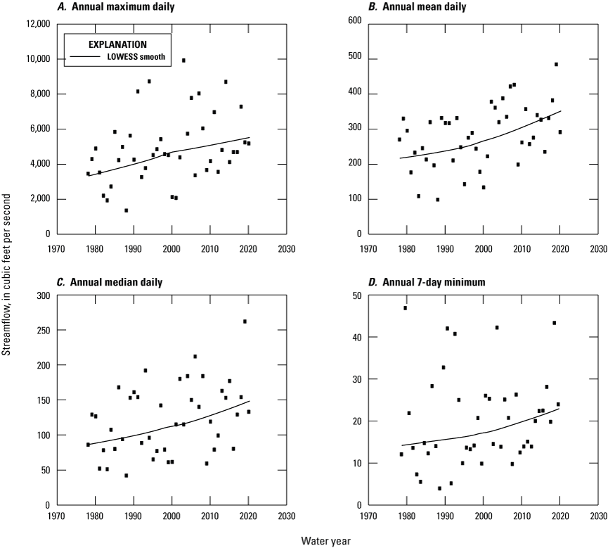
Scatter plots of the A, annual maximum daily, B, annual mean daily, C, annual median daily, and D, annual 7-day minimum streamflow values for the White River at Muncie, Indiana, water years 1978 to 2020 (locally weighted scatterplot smooth lines shown on scatter plots).
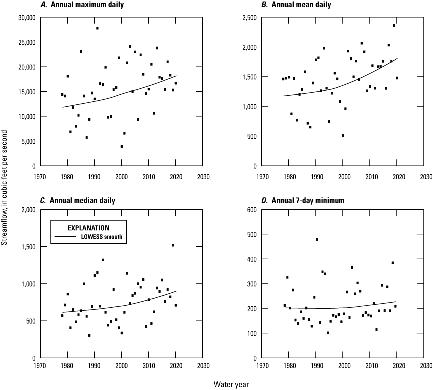
Scatter plots of the A, annual maximum daily, B, annual mean daily, C, annual median daily, and D, annual 7-day minimum streamflow values for the White River near Nora, Indiana, water years 1978 to 2020 (locally weighted scatterplot smooth lines shown on scatter plots).
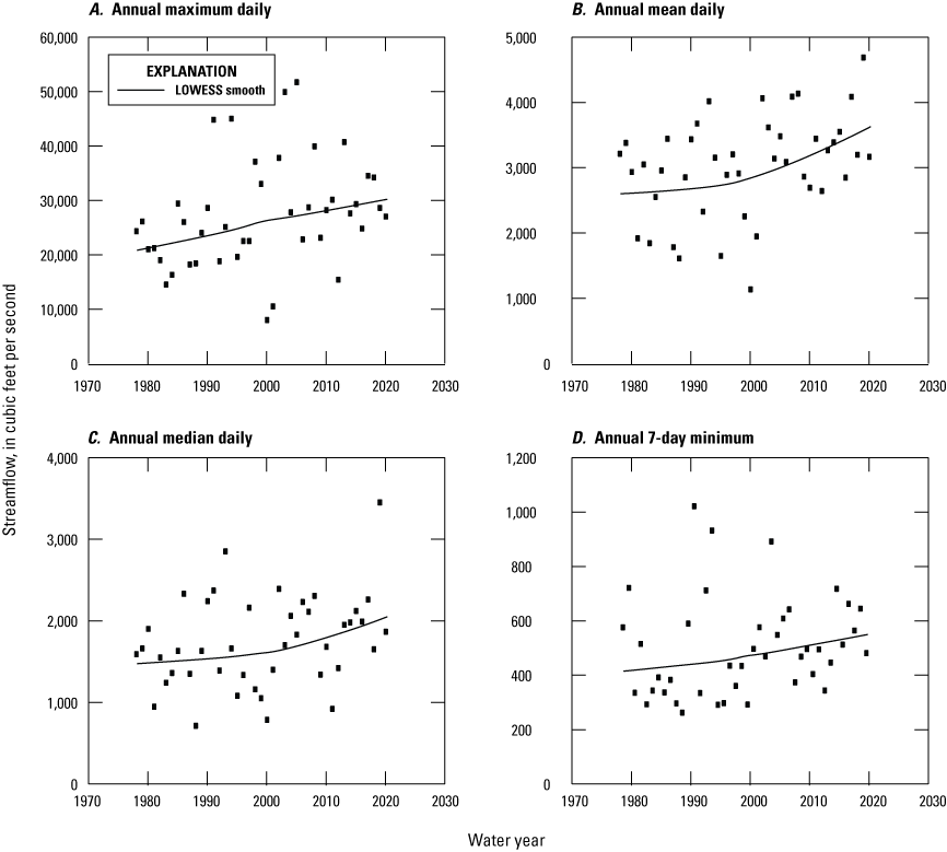
Scatter plots of the A, annual maximum daily, B, annual mean daily, C, annual median daily streamflows, and D, annual 7-day minimum streamflow values for the White River near Centerton, Indiana, water years 1978 to 2020 (locally weighted scatterplot smooth lines shown on scatter plots).
The positive tau (Kendall's nonparametric correlation coefficient) values from the Mann-Kendall analyses indicated that the streamflow statistics at all study gages generally trended upward over time between water years 1978 and 2020 (table 4). However, only trends for annual mean and maximum daily streamflows were statistically significant for all study gages (table 4).
Table 4.
Results of Mann-Kendall analyses for trends in streamflow statistics for streamgages on the White River at Muncie, near Nora, and near Centerton, Indiana, water years 1978–2020.[Bolded values are statistically significant; USGS, U.S. Geological Survey; tau, Kendall's nonparametric correlation coefficient; p-value, probability of obtaining the observed results, assuming that the null hypothesis is true; Sen’s slope reported in average log of streamflow (in cubic feet per second) units]
Like the Mann-Kendall tests, the quantile-Kendall plots (figs. 5–7) indicated upward temporal trends in streamflow and which parts of the streamflow regime in which non-zero trend slopes are most likely. Very low streamflows (non-exceedance probabilities less than about 0.05) and mid-range and larger streamflows (non-exceedance probabilities greater than about 0.5) showed the greatest likelihood of non-zero trend slopes at the study gages at Muncie and near Nora. Similar results were found for the study gage near Centerton; however, there were weaker indications of significant trend in a small part of the streamflow quantiles greater than about 0.5. At the three study gages, streamflows in the third quartile of non-exceedance probabilities (between 0.5 and 0.75) had positive trend slopes with most quantiles showing high likelihood of temporal trend (p-values less than or equal to 0.05).
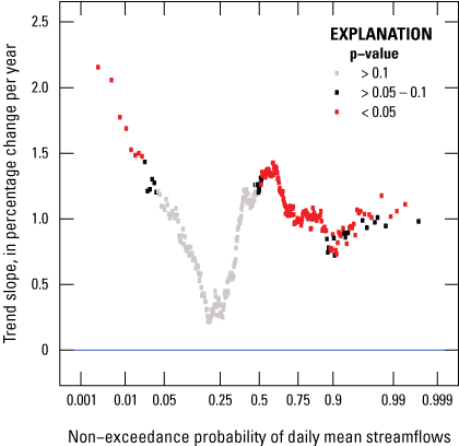
Quantile-Kendall plot showing magnitude and likelihood of temporal trend in streamflows for the White River at Muncie, Indiana, based on daily streamflow data for water years 1978–2020.
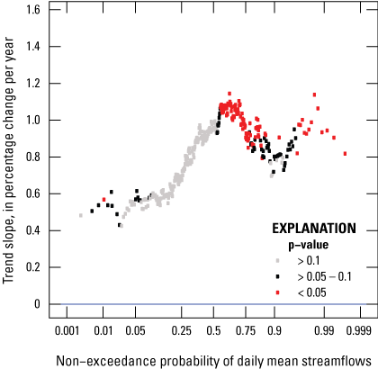
Quantile-Kendall plot showing magnitude and likelihood of temporal trend in streamflows for the White River near Nora, Indiana, based on daily streamflow data for water years 1978–2020.
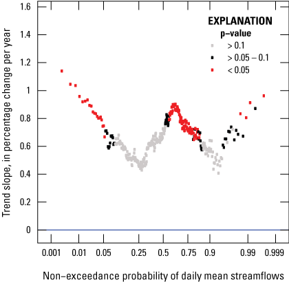
Quantile-Kendall plot showing magnitude and likelihood of temporal trend in streamflows for the White River near Centerton, Indiana, based on daily streamflow data for water years 1978–2020.
The Pettitt tests indicated that a step trend (abrupt change) occurred in annual mean daily streamflows at each of the study gages between water years 1978 and 2020 (table 5), and that the step trends most likely occurred at each gage around water year 2001. Other statistically significant step trends were indicated for the annual maximum daily streamflows at the gages near Nora and Centerton, and the annual median daily streamflow at the gage at Muncie. No statistically significant step trend was indicated for the annual 7-day minimum streamflows at the study gages (table 5); however, the Pettitt test is less effective at detecting changes in extremes than changes in means or medians (Mallakpour and Villarini, 2016). For statistically significant step trends, the water year change point was consistently 2001. The step trend in streamflows adds uncertainty to the interpretation of trends in the WRTDS analysis near the year of the step trend (in this case, water year 2001). That uncertainty decreases as you move further away in time from the year of the step trend.
Table 5.
Results of Pettitt tests for step trends in streamflow statistics for streamgages on the White River at Muncie, near Nora, and near Centerton, Indiana, water years 1978–2020.[Bolded values are statistically significant; USGS, U.S. Geological Survey; U*, Pettitt test statistic; p-value, probability value; na, not applicable]
To assess whether trends in streamflow might be related to changes in precipitation, a Mann-Kendall analysis was done using annual precipitation measured at the Indianapolis International Airport (network ID GHCND: USW00093819) between calendar years 1932 and 2020. That analysis indicated a weak but statistically significant upward trend (tau=0.20, p=0.005) in annual precipitation with a Sen’s slope of 0.089 inches per year. Consequently, though not definitive, this weak trend supports a hypothesis that upward trends in streamflows resulted (at least in part) from the upward trend in precipitation. LOWESS smooth lines fit through the annual precipitation totals measured at the Indianapolis International Airport (fig. 8) and annual mean streamflows measured at the White River near Nora gage (03351000) (fig. 9) indicate that precipitation and streamflow began trending upward more rapidly in the mid to late 1970s.
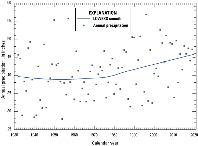
Scatter plot with LOWESS smooth line of annual precipitation totals measured at the Indianapolis International Airport for calendar years 1932–2020.
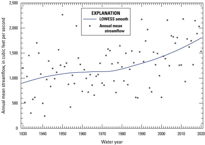
Scatter plot with LOWESS smooth line of annual mean streamflows measured at the White River near Nora, Indiana gage (03351000) for water years 1930–2020.
Evidence of the step trend in annual mean daily streamflow identified in the Pettitt tests for the gage near Nora (table 5) can be seen in figure 9. Annual mean daily streamflows less than about 1,000 cubic feet per second (ft3/s) occurred in approximately 39 percent of the years during water years 1931–2000. However, during water years 2001–20, the annual mean daily streamflow exceeded 1,000 ft3/s in all but one year.
Estimated Mean Concentrations and Flux of Sediment and Nutrients
Water-quality data were collected for a wide range of streamflows and in all months. The medians and interquartile ranges of streamflows at the study gages on the days when samples were collected were similar to those for the entire analytical period at the gage; however, streamflows at the study gages did not range as high as streamflows for the analytical period. Streamflows on sample dates included nearly the entire range of streamflows for the gage near Nora; however, there were fewer samples from high flow days at the Muncie and near Centerton gages. The absence of sample data at very high flows adds uncertainty because computation of concentrations and fluxes on those days requires extrapolation.
Water year annual mean daily concentrations and fluxes estimated with WRTDS (with and without flow normalization) are in tables 6–9 for TSS, total phosphorus, nitrate plus nitrite, and total Kjeldahl nitrogen. Confidence limits for the estimates have been omitted from tables 6–9; however, the annual mean concentration and flux estimates (from the WRTDS-K method) and their 90 percent confidence limits are available for download (Koltun, 2023). Estimates from the WRTDS-K method tended to be of equal or smaller magnitude than estimates from the base WRTDS method. For example, cumulative loads of total phosphorus for water years 1992–2020 computed with the WRTDS-K method at the three study gages ranged from about 90.1 to 96.9 percent of loads for the same period computed with the WRTDS base method.
Table 6.
Annual estimates of mean daily concentrations and flux (with and without flow normalization) of total suspended solids for streamgages on the White River at Muncie, near Nora, and near Centerton, Indiana, water years 1992–2020.[USGS, U.S. Geological Survey; ft3/s, cubic foot per second; mg/L, milligram per liter; FN, flow-normalized; t/yr, short ton per year; nd, no data]
Table 7.
Annual estimates of mean daily concentrations and flux (with and without flow normalization) of total phosphorus (as phosphorus) for streamgages on the White River at Muncie, near Nora, and near Centerton, Indiana, water years 1992–2020.[USGS, U.S. Geological Survey; ft3/s, cubic foot per second; mg/L, milligram per liter; FN, flow-normalized; lb/yr, pound per year]
Table 8.
Annual estimates of mean daily concentrations and flux (with and without flow normalization) of nitrate plus nitrite (as nitrogen) for streamgages on the White River at Muncie, near Nora, and near Centerton, Indiana, water years 1992–2020.[USGS, U.S. Geological Survey; ft3/s, cubic foot per second; mg/L, milligram per liter; FN, flow-normalized; lb/yr, pound per year]
Table 9.
Annual estimates of mean daily concentrations and flux (with and without flow normalization) of total Kjeldahl nitrogen (as nitrogen) for streamgages on the White River at Muncie, near Nora, and near Centerton, Indiana, water years 1992–2020.[USGS, U.S. Geological Survey; ft3/s, cubic foot per second; mg/L, milligram per liter; FN, flow normalized; lb/yr, pound per year; nd, no data]
To facilitate comparisons between gage locations, analytical-period and mean-annual loads and yields (load divided by drainage area) are summarized for the longest periods of concurrent record of each constituent at the three study gages (tables 10–11). Analytical-period and mean-annual loads of each of the constituents increased sequentially from the most upstream gage at Muncie to the most downstream gage near Centerton. Yields did not consistently follow the same pattern as loads. In this case, the largest analytical-period and mean-annual yields of TSS and total phosphorus were at the most upstream gage at Muncie, but the largest yields of nitrate plus nitrite were at the most downstream gage near Centerton. It is common for yields of nonpoint constituents in streams to decrease in a downstream direction because stream channel and land surface gradients typically decrease, and there is more opportunity for constituent losses (Koltun, 2019). The two most upstream gages had about equal total Kjeldahl nitrogen yields that were each about 13 percent larger than the yield of total Kjeldahl nitrogen at the most downstream gage.
Table 10.
Estimated analytical period loads and yields of total suspended solids, total phosphorus, nitrate plus nitrite, and total Kjeldahl nitrogen at streamgages on the White River at Muncie, near Nora, and near Centerton, Indiana.[Muncie, White River at Muncie, Indiana (U.S. Geological Survey station 03347000); Nora, White River near Nora, Indiana (U.S. Geological Survey station 03351000); Centerton, White River near Centerton, Indiana (U.S. Geological Survey station 03354000); TSS, total suspended solids; t, short ton; t/mi2, short ton per square mile; TP, total phosphorus as phosphorus; lb, pound; lb/mi2, pound per square mile; NOx, nitrate plus nitrite as nitrogen; TKN, total Kjeldahl nitrogen as nitrogen]
Table 11.
Estimated mean annual loads and yields of total suspended solids, total phosphorus, nitrate plus nitrite, and total Kjeldahl nitrogen at streamgages on the White River at Muncie, near Nora, and near Centerton, Indiana.[Muncie, White River at Muncie, Indiana (U.S. Geological Survey station 03347000); Nora, White River near Nora, Indiana (U.S. Geological Survey station 03351000); Centerton, White River near Centerton, Indiana (U.S. Geological Survey station 03354000); TSS, total suspended solids; t, short ton; t/mi2, short ton per square mile; TP, total phosphorus as phosphorus; lb, pound; lb/mi2, pound per square mile; NOx, nitrate plus nitrite as nitrogen; TKN, total Kjeldahl nitrogen as nitrogen]
Changes and Trends in Flow-Normalized Concentration and Flux
Table 12 lists WBT results that show the magnitude, direction, and likelihood of change in flow-normalized concentrations and flux of TSS, total phosphorus, nitrate plus nitrite, and total Kjeldahl nitrogen between water years 1997 and 2019. A similar analysis previously examined changes between 1997 and 2017 (Koltun, 2019). Differences in results between the two analyses reflect the addition of 2 years of data as well as using a more recent end year (2019) to compare against 1997. With two exceptions, concentration and flux changes that were statistically significant in Koltun (2019) showed the same statistically significant change direction. The first exception was nitrate plus nitrite concentration at the White River at Muncie, Indiana, which showed a downward change; however, the likelihood of change decreased from “highly likely” to “likely.” The second exception was for the White River near Centerton, Indiana, which previously showed a “highly likely” downward change in TSS concentration but now shows an upward change classified as “as likely as not.” Because TSS concentration data were not collected at or near the gage near Centerton between water years 2008 and 2017, the previous study’s change results for that constituent were based on data collected only between water years 1992 and 2007. Results from the current study include sample results from water years 2018–20 because sampling for TSS was restarted at the gage near Centerton in water year 2018. This shift in change direction demonstrates the degree to which perceived trends in concentration and flux are a function of the endpoints chosen for comparison. To provide a more temporally continuous picture of trends, plots were constructed showing flow-normalized annual mean concentrations and fluxes of nutrients and TSS as a function of time (figs. 10–13). The flow-normalization process attempts to remove the effects of interannual variation in streamflow on annual mean concentrations and fluxes so that trends driven by changes in the relation between streamflow and concentration are more apparent, whereas the WRTDS-K estimate includes the effects of changes in the streamflow-concentration relation and year-to-year changes in streamflow. Consequently, in a given year, the annual flow-normalized values can differ appreciably from annual mean concentrations and fluxes estimated with the WRTDS-K method (figs. 10–13). Uncertainties associated with the flow-normalized annual mean concentration and flux estimates vary over time; however, confidence intervals for the estimates have been omitted from the plots to facilitate comparisons of temporal trends between study gages.
Table 12.
Weighted Regressions on Time, Discharge, and Season bootstrap test results for estimated change in flow-normalized concentrations and flux of total suspended solids, total phosphorus, nitrate plus nitrite, and total Kjeldahl nitrogen from water year 1997 to water year 2019 for gages on the White River at Muncie, near Nora, and near Centerton, Indiana.[Bolded numbers are statistically significant; FN, flow normalized; mg/L, milligram per liter; USGS, U.S. Geological Survey; TSS, total suspended solids; tn/yr, short ton per year; TP, total phosphorus as phosphorus; lb/yr, pound per year; Nox, nitrate plus nitrite as nitrogen; TKN, total Kjeldahl nitrogen as nitrogen; ALAN, as likely as not; L, likely; VL, very likely; HL, highly likely]
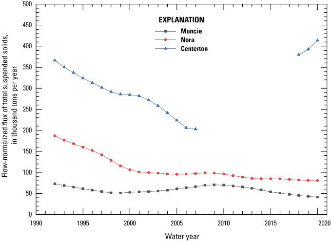
Scatter plot of flow-normalized annual flux of total suspended solids at gages on the White River at Muncie, near Nora, and near Centerton, Indiana, water years 1992–2020.
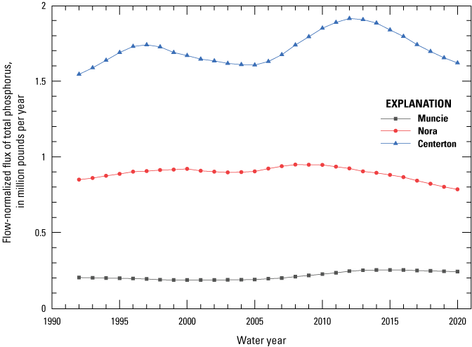
Scatter plot of flow-normalized annual flux of total phosphorus (as phosphorus) at gages on the White River at Muncie, near Nora, and near Centerton, Indiana, water years 1992–2020.
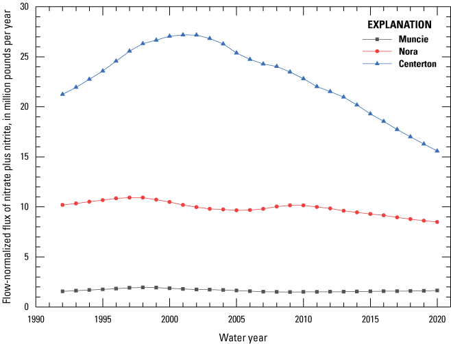
Scatter plot of flow-normalized annual flux nitrate plus nitrite (as nitrogen) at gages on the White River at Muncie, near Nora, and near Centerton, Indiana, water years 1992–2020.
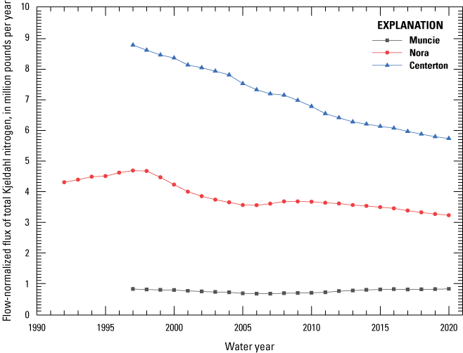
Scatter plot of flow-normalized annual flux of total Kjeldahl nitrogen (as nitrogen) at gages on the White River at Muncie, near Nora, and near Centerton, Indiana, water years 1992–2020.
Flow-normalized annual fluxes increased at the study gages from upstream to downstream (downstream order) during all years in the study period (figs. 10–13). In the period between 2010 and 2020, flow-normalized nutrient fluxes at the gage near Centerton showed some of the most rapid decreases of the three study gages. Flow-normalized nutrient fluxes at the gage near Nora also decreased (albeit less rapidly) over the same period; however, they increased some at the Muncie gage. Flow-normalized TSS fluxes at the gages at Muncie and near Nora (fig. 10) also decreased between 2010 and 2020. At the gage near Centerton, flow-normalized TSS flux was not reported for water years 2008–17 because of lack of sample data; however, flow-normalized TSS fluxes computed for water years 2018–20 are larger than the values computed for water years 1992–2017 and more than 4 times larger than corresponding water-year flux at the gage at Nora (fig. 10). This increase might be an artifact of the large sampled data gap (2008–2017), therefore the 2018–20 flow-normalized flux results for TSS at the gage near Centerton and the related change-analysis results might be misleading. Because of the weighting schemes used in WRTDS, TSS trend and flux results for 2018–20 for the gage near Centerton are more strongly influenced by data collected during 2018–20 than the trend and flux results for the period preceding the data gap (1992–2007). Hirsch and DeCicco (2015) discuss issues that can arise when using WRTDS with datasets that have large data gaps.
Annual flow-normalized concentrations did not increase or decrease consistently in downstream order at the study gages over the study period (figs. 14–17). Flow-normalized concentrations of nutrients were always larger for the gages near Nora and Centerton than for the gage at Muncie. Flow-normalized concentrations of TSS were not consistently larger at one site than at the others. The gage near Nora was the only site where flow-normalized concentrations of a constituent (TSS) consistently decreased over the analytical period.

Scatter plot of flow-normalized annual mean concentration of total suspended solids at gages on the White River at Muncie, near Nora, and near Centerton, Indiana, water years 1992–2020.
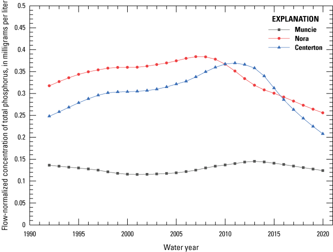
Scatter plot of flow-normalized annual mean concentration of total phosphorus (as phosphorus) at gages on the White River at Muncie, near Nora, and near Centerton, Indiana, water years 1992–2020.
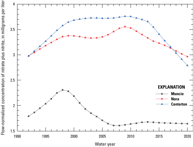
Scatter plot of flow-normalized annual mean concentration of nitrate plus nitrite (as nitrogen) at gages on the White River at Muncie, near Nora, and near Centerton, Indiana, water years 1992–2020.
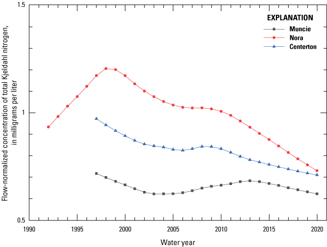
Scatter plot of flow-normalized annual mean concentration of total Kjeldahl nitrogen (as nitrogen) at gages on the White River at Muncie, near Nora, and near Centerton, Indiana, water years 1992–2020.
The WRTDS-K and flow-normalized annual mean concentrations are time-weighted means and consequently are influenced by the most frequent hydrologic conditions, which tend to be closer to median streamflow conditions than the larger magnitude mean-streamflow or high-streamflow conditions. Fluxes, on the other hand, tend to be more heavily influenced by conditions that occur during high-streamflow periods. These computational differences can cause counterintuitive outcomes in which concentrations are decreasing over time while fluxes are increasing, or in which concentrations are increasing over time while fluxes are decreasing.
Spatial Patterns in Sampling Distributions of Nutrients and Total Suspended Solids
Figures 18–21 show boxplots depicting the distributions of sampled concentrations of nutrients and TSS at 20 mainstem, tributary, and distributary water-quality sampling locations in the upper White River Basin (table 13; fig. 22). Sampling locations designated A–I are on the mainstem of the upper White River, and sampling locations designated J–T are on other waterways in the upper White River Basin. If a boxplot for a sampling location is not in a figure for a given constituent, the sampling location did not meet the minimum observation criteria for that constituent.
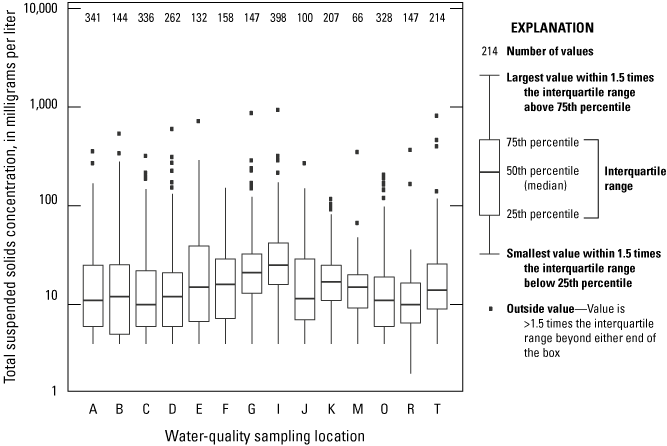
Boxplots of total suspended solids concentrations at sampling locations (table 13) in the upper White River Basin, water years 1992–2020.
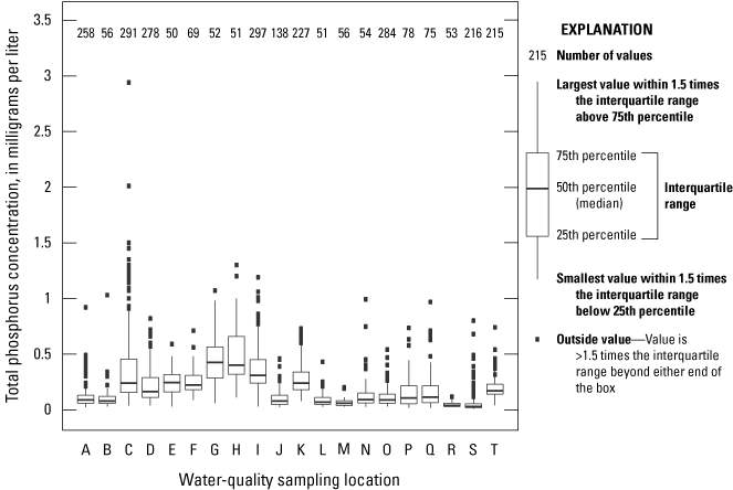
Boxplots of total phosphorus (as phosphorus) concentrations at sampling locations (table 13) in the upper White River Basin, water years 1992–2020.
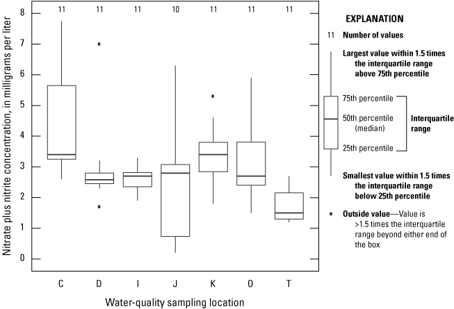
Boxplots of nitrate plus nitrite (as nitrogen) concentrations at sampling locations (table 13) in the upper White River Basin, water years 2019–20.
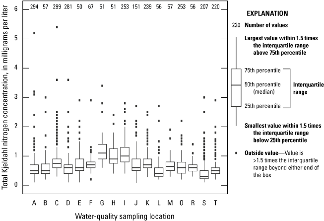
Boxplots of total Kjeldahl nitrogen (as nitrogen) concentrations at sampling locations (table 13) in the upper White River Basin, water years 1991–2020.
Table 13.
Information on Water Quality Portal sampling locations whose data were used to evaluate spatial patterns in nutrient and total suspended solids concentration distributions (see figure 22 for map).[ID, identification; WQP, Water Quality Portal; INSTOR, Indiana STORET; USGS, U.S. Geological Survey; nd, not determined]
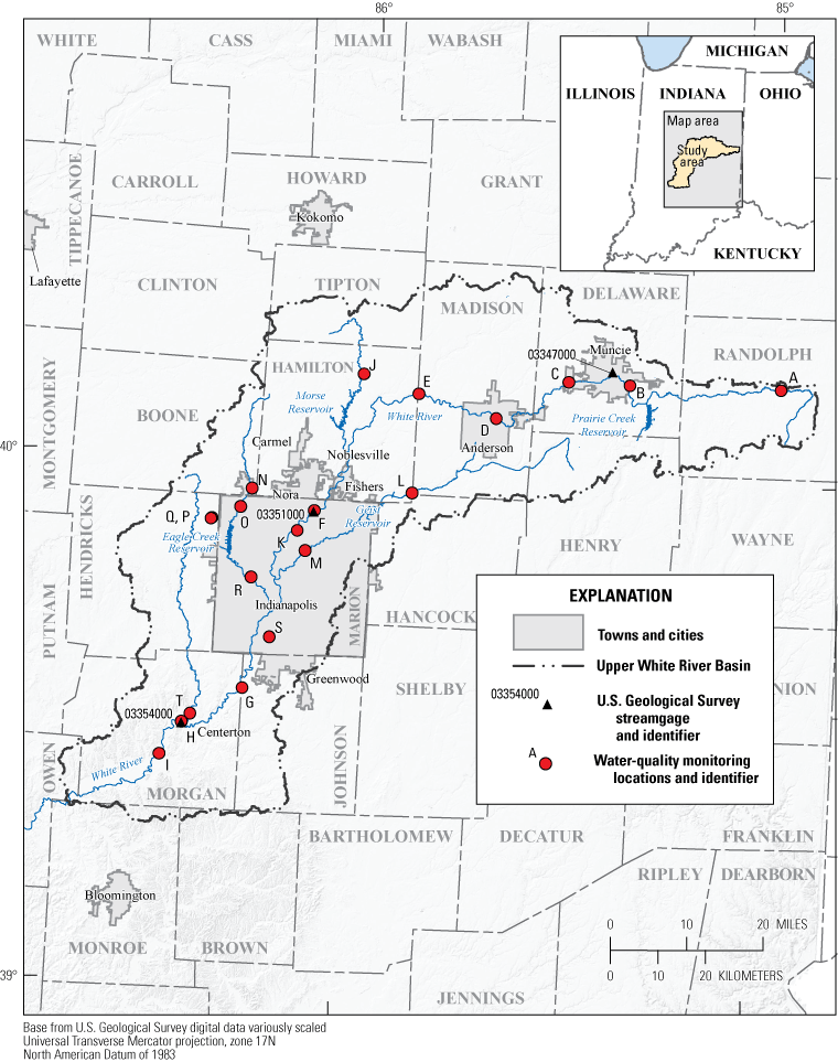
Map of water-quality sampling locations whose data were used to evaluate spatial patterns in nutrient and total suspended solids concentration distributions (see table 13 for information).
One pattern in figures 18–19 and 21 is that the largest median concentrations of TSS, total phosphorus, and total Kjeldahl nitrogen were associated with mainstem upper White River sampling locations downstream from Indianapolis (sites G–I). Another pattern is that median total phosphorus, and total Kjeldahl nitrogen concentrations at the upper White River site immediately downstream from Muncie (site C) were elevated relative to bracketing upstream/downstream mainstem sampling locations. Location C also had one of the highest median nitrate plus nitrite concentrations and the highest concentrations of total phosphorus, total Kjeldahl nitrogen, and nitrate plus nitrite of all sampling locations.
The median concentrations of all constituents at the Indianapolis Waterway Canal sampling location (K) were larger than at the other non-mainstem sites. In contrast, the Little Buck Creek sampling location (S) had the lowest median concentrations of total phosphorus, and total Kjeldahl nitrogen compared to other locations. Except for the Indianapolis Waterway Canal sampling location (K), median concentrations of nutrients and TSS at non-mainstem upper White River sampling locations generally had magnitudes in the same range or smaller than the mainstem upper White River locations. The canal was originally intended to be part of a transportation corridor, which was never completed because of insufficient funding. The canal was later repurposed to convey water from the White River to a downtown water treatment plant.
Most of the Water Quality Portal sampling locations had no associated streamflow data; consequently, interpretation of concentration data alone is impeded by a lack of hydrologic context. For example, boxplots of concentrations measured during predominantly low to medium streamflows might look very different if concentrations were measured for the full range of streamflows. This variable relation between streamflow concentration was illustrated by Koltun (2019) with the “U” or check-mark-shaped transport plots for total phosphorus, nitrate plus nitrite, and total Kjeldahl nitrogen for the study gages near Nora and near Centerton. Without associated flow data, there is no way to determine whether differences in the distributions of concentrations measured at different sites might be because of sampling strategy versus other factors.
Potentially Influential Anthropogenic Factors
There are a variety of anthropogenic factors that could influence the concentrations and fluxes of nutrients and TSS in the upper White River Basin. Factors related to population, land cover, cropping practices and operational tillage, fertilizer application, and upgrades to wastewater treatment systems and delivery processes were examined to better understand their spatial and (or) temporal variations. Time series of the factors were compared with trend results to determine if there are correlations.
Population
The relationship between human populations and water resources is complex. Human populations can affect a variety of hydrologic and environmental characteristics through the way they modify and (or) manage the land and water resources. Census data were obtained for 1990–2020 for the Indianapolis and Muncie metro areas and the City of Anderson, Indiana (STATS Indiana, 2022), the three most populated city/metro areas in the upper White River Basin. Figure 23 shows that the population of the Indianapolis metro area increased rapidly at a uniform rate between 1990 and 2020, while populations in the City of Anderson (which is part of the Indianapolis metro area) and the Muncie metro area decreased slightly. Between 1990 and 2020, the population increase in the Indianapolis metro area far exceeded the population decrease in the Muncie metro area.
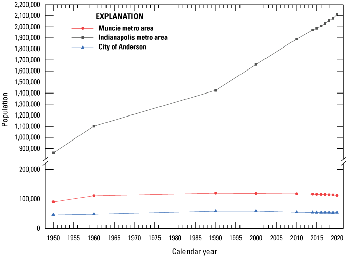
Plot of population for the City of Anderson and the Muncie and Indianapolis, Indiana metro areas, calendar years 1950–2020.
Land Cover
Changing land cover could change the hydrology and water chemistry of streams draining the affected areas. Changes in hydrology and water chemistry can result from (1) how quickly and how much water runs off land surfaces in each land-cover category, as well as (2) the quantity and wash-off/transport characteristics of contaminants associated with the various land covers.
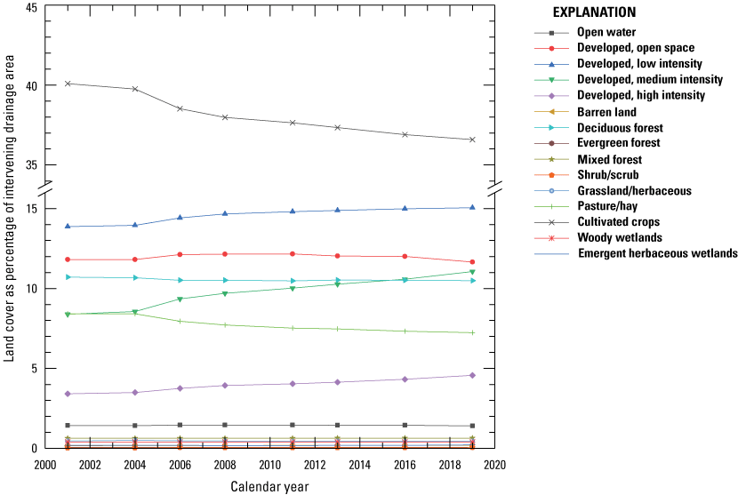
Land-cover characteristics for the period 2001–19 were computed from data in the National Land Cover Database (Dewitz and U.S. Geological Survey, 2021) for the intervening land areas draining to the study gages. The percentages of the upper White River Basin in the intervening areas draining to the study gages at Muncie, near Nora, and near Centerton are about 8.9, 36.0, and 45.1 percent, respectively. About 10 percent of the upper White River Basin drainage is downstream from the gage near Centerton. Because the gage at Muncie is the most upstream study gage, its intervening land area includes the entire headwater drainage upstream from the gage. Land-cover characteristics in the drainage to the gage at Muncie changed little during the 2001–19 period (fig. 24). More than 73 percent of the area draining to the Muncie gage was classified as cultivated crops, with deciduous forest as the second largest land-cover category at about 8.5 percent of the area. Some land-cover characteristics in the drainage between the gage at Muncie and the gage near Nora changed slightly during the 2001–19 period (figs. 25–26). Cultivated crops decreased from about 68.2 percent to 66.8 percent of the area, whereas developed land covers cumulatively increased from about 18.6 to 20.6 percent of the area over the same period.
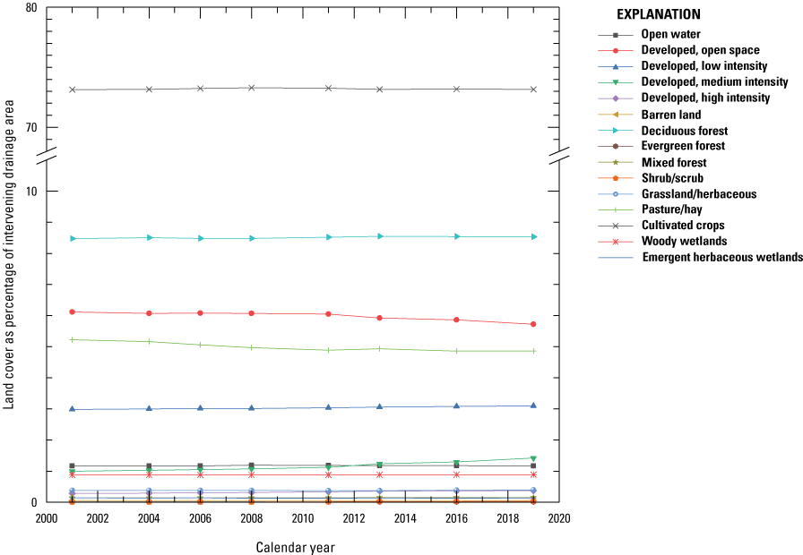
Plot of land cover as a percentage of intervening drainage area for the White River at Muncie, Indiana, calendar years 2001–19.
Plot of land cover as a percentage of intervening drainage area for the White River near Nora, Indiana, calendar years 2001–19.
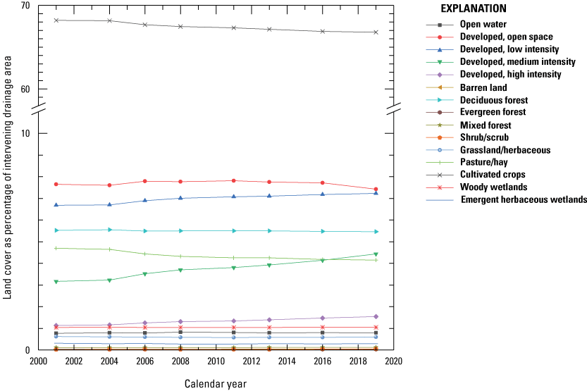
Plot of land cover as a percentage of intervening drainage area for the White River near Centerton, Indiana, calendar years 2001–19.
Land-cover characteristics in the drainage between the gage near Nora and the gage near Centerton (fig. 26) were different in character than those for the other two gages and showed noticeable changes in some land-cover categories during the 2001–19 period. In general, the intervening drainage between the gages near Nora and Centerton had smaller percentages of cultivated crops and larger percentages of developed land cover than the intervening areas of the other two study gages. Cultivated crops in the intervening drainage between the gages near Nora and Centerton decreased from about 40.1 to 36.6 percent of the area during the 2001–19 period and developed land covers cumulatively increased from about 37.5 and 42.3 percent of the area. Pasture and hay also decreased from about 8.4 to 7.2 percent of the area.
Crops and Operational Tillage
In a landscape with predominantly agricultural land uses, the delivery of nutrients and other contaminants to streams and lakes might be influenced by the amount and type of crops that are grown, use of winter cover crops, crop rotation, and tillage practices. For example, a recent analysis of data from midwestern streams indicated that yields and flow-weighted mean concentrations of nitrate from areas of soybean cultivation were larger than from areas of corn cultivation on an equal percentage-of-area basis (Piske, 2019). Rotational planting of corn and soybeans is common in the Midwest, which lets farmers use less nitrogen fertilizer for growing corn, as compared to continuous corn production. The use of less fertilizer, in turn, reduces the risk of having large amounts of land-applied fertilizer available for transport by runoff during storms. Winter cover crops and no-till/reduced-till practices reduce erosion by wind and water (Snapp and others, 2005) by binding and (or) covering the soil, which also helps prevent nutrients and other contaminants from running off agricultural lands.
Crop cover percentages for the period 2007–20 were computed from the U.S. Department of Agriculture (2021) Cropland Data Layers for the intervening land areas draining to the study gages. In most years during 2007–20, soybeans, followed by corn, constituted the largest crop percentages in the intervening drainage areas to the study gages (figs. 27–29). Other agricultural land covers constituted much smaller percentages except for in the intervening drainage area to the gage near Centerton, where grass/pasture percentages nearly equaled corn and soybeans until 2013, and steadily decreased afterward (fig. 29). Grass/pasture percentages steadily decreased over the entire 2007–20 period in the intervening drainage areas to the gages at Muncie and near Nora. The lines representing corn and soybean percentages intertwined over time in almost a mirror-image fashion (figs. 27–29), reflecting the influence of corn-soybean crop rotation. Central Indiana received nearly 19 inches of precipitation in the spring 2019, exceeding normal precipitation by almost 6 inches (Hill, 2019), which resulted in larger areas than typical left fallow/idle in 2019 (figs. 27–29).
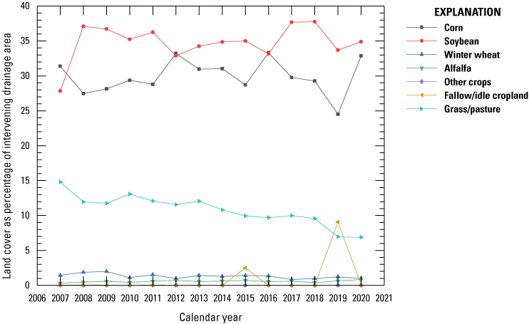
Plot of crop land cover as a percentage of intervening drainage area for the White River at Muncie, Indiana, calendar years 2007–20.
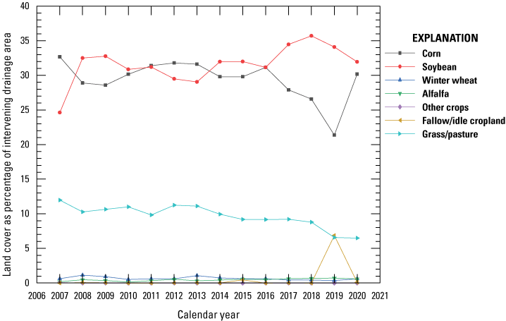
Plot of crop land cover as a percentage of intervening drainage area for the White River near Nora, Indiana, calendar years 2007–20.
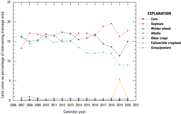
Plot of crop land cover as a percentage of intervening drainage area for the White River near Centerton, Indiana, calendar years 2007–20.
Operational Tillage Information System data (Conservation Technology Information Center, 2021) on tillage practices and winter crop cover were obtained for the upper White River Basin. Figures 30–32 show percentages of crops within the upper White River Basin that were no-tilled (plant residue cover of more than 30 percent for all crops other than corn, for which the residue cover is more than 50 percent), reduced tilled (plant residue cover of 16–30 percent for all crops other than corn, for which there is a reduced tillage category with a larger residue of 31–50 percent) and conventionally tilled (plant residue cover 0–15 percent), respectively, prior to planting the next crop. There were considerable year-to-year variations in the percentages of previously planted crops in the three tillage categories and no discernable consistent upward or downward trends. In most instances, the annual percentages of each previously planted crops that were no-tilled were larger than the corresponding percentages conventionally tilled. Crops previously planted in corn or soybeans generally had larger percentages of reduced till than no-till treatment whereas the opposite was true for small grain crops.
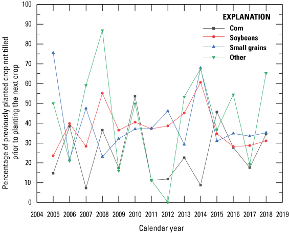
Plot of percentage of indicated crops within the upper White River Basin (hydrologic unit 05120201) that were not tilled prior to planting the next crop, 2005–18.
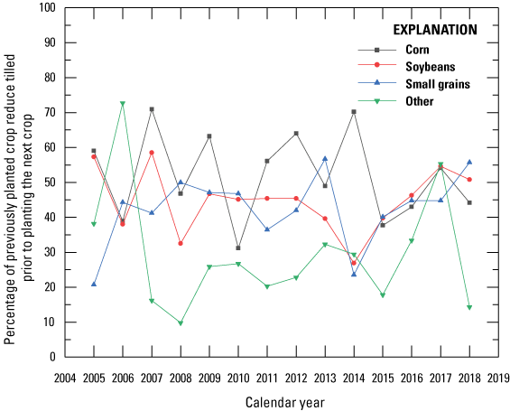
Plot of percentage of indicated crops within the upper White River Basin (hydrologic unit 05120201) that were reduce tilled prior to planting the next crop, 2005–18.
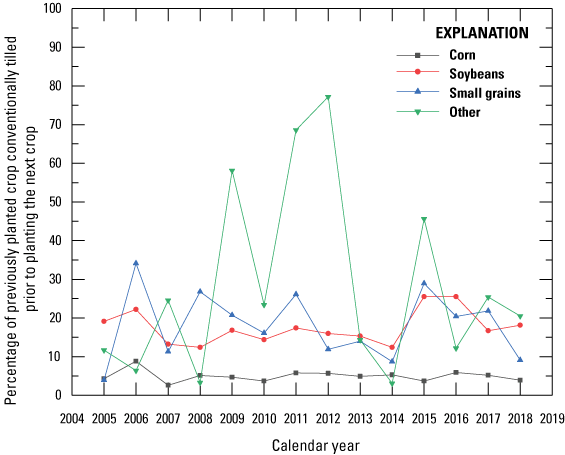
Plot of percentage of indicated crops within the upper White River Basin (hydrologic unit 05120201) that were conventionally tilled prior to planting the next crop, 2005–18.
The percentages of corn, soybeans, and small grain crops within the upper White River Basin for which a cover crop was planted during the following winter were plotted as a function of time (figs. 33–35). The percentage of winter cover crops that were planted following planting of corn varied irregularly over time between 2005 and 2018, and the percentage was typically small (totaling less than 1.5 percent) (fig. 33).
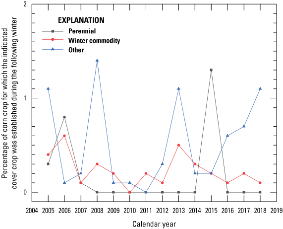
Plot of percentage of corn crop within the upper White River Basin (hydrologic unit 05120201) for which the indicated cover crop was planted during the following winter, calendar years 2005–18.
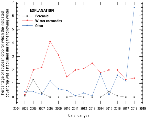
Plot of percentage of soybean crop within the upper White River Basin (hydrologic unit 05120201) for which the indicated cover crop was planted during the following winter, calendar years 2005–18.
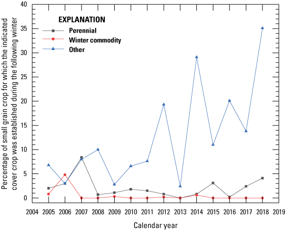
Plot of percentage of small grain crop within the upper White River Basin (hydrologic unit 05120201) for which the indicated cover crop was planted during the following winter, calendar years 2005–18.
The percentage of winter cover crops planted following planting soybeans was larger than for corn, with winter commodity crops (for example, winter wheat) typically being the most common (fig. 34). Percentages of winter commodity cover crops planted following soybeans have been trending downward since about 2008, other cover crops (cereal rye for example) have been trending upward since about 2013, and percentages of perennial cover crops have remained small (typically less than 0.1 percent) and mostly unchanged over time (fig. 34).
The percentage of winter cover crops established following planting small grain crops was larger than for corn or soybeans, with cover crops other than winter commodity or perennial being the most common (fig. 35). The percentages of winter commodity and perennial cover crops remained mostly steady over the period 2005–18; however, there was an upward trend in the percentage of other winter cover crops planted. For example, the average percentage of other winter cover crops planted following small grain crops during 2005–11 was 6.8 but that average increased to about 18.7 percent during 2012–18. Small grain crops averaged only about 1 percent of the area of the upper White River Basin planted in row crops during 2012–18, so changes in winter cover crop practices are unlikely to have appreciably influenced nutrient and TSS transport at a hydrologic unit scale.
Fertilizer Application
Land-applied commercial fertilizers and manure might become a source of water pollution if they are used in excess, they are washed off the land surface, or they enter an aquifer before they are taken up by plants. Fertilizer application estimates were derived from county-level data reported by Falcone (2021a). Falcone (2021b) described the process by which the county-level estimates were made at 5-year increments between 1987 and 2017.
Nutrient mass estimates from commercial fertilizers and manure were summed for 13 of the 16 counties constituting the upper White River Basin. Brown, Monroe, and Owen counties were omitted from the sums because the upper White River Basin only includes small parts of those counties. Figure 36 shows the estimated mass of nutrients applied as farm and non-farm commercial fertilizers (includes commercial fertilizers applied to lawns and other non-farm urban and suburban green spaces) or manure as a function of time during the period 1987–2017. Farm-applied commercial fertilizer was the largest source of nitrogen and phosphorus. Manure was the next largest source followed by non-farm commercial fertilizer. The estimated masses of farm-applied nitrogen and phosphorus from commercial fertilizers were larger than from manure (the second largest source of applied nitrogen and phosphorus) on an annual basis by factors of at least 5.4 and 3.2, respectively.
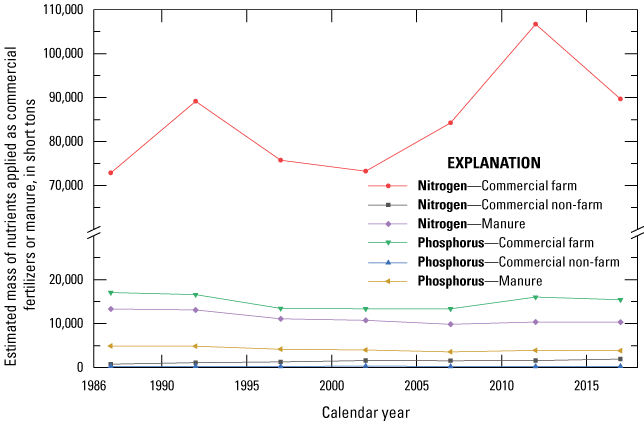
Plot of estimated total mass of nutrients applied as commercial fertilizers and manure during the period 1987–2017 summed for Boone, Clinton, Delaware, Hamilton, Hancock, Hendricks, Henry, Johnson, Madison, Morgan, Randolph, and Tipton Counties, Indiana.
The estimated masses of nitrogen and phosphorus applied as manure seem to have gradually trended downward between 1987 and 2017, whereas nitrogen and phosphorus masses from non-farm commercial fertilizers gradually trended upward (fig. 36). The remaining fertilizer sources did not show indication of temporal trend. The estimated mass of nitrogen from farm-applied commercial fertilizers did not change monotonically between 1987 and 2017; however, the most recent three estimates (for 2007, 2012, and 2017) were larger than estimates for earlier years except 1992.
Upgrades to Wastewater Treatment Systems and Delivery Processes
Nutrients and TSS are discharged in treated municipal wastewater and combined sewer overflows (CSOs). These discharges might constitute a substantial part of the nutrient and TSS flux in the receiving stream under some flow conditions. The mass of nutrients and TSS contributed depends on the level of treatment of the wastewater and the volume of wastewater discharged. Consequently, even though CSO discharge volumes are small compared to the volume of treated wastewater, the mass of nutrients and TSS discharged from CSOs are large because the CSO discharge contains a mixture of untreated sewage and stormwater. Improving wastewater treatment and eliminating or reducing CSOs are two ways of reducing the mass of nutrients and TSS delivered to the river.
The two largest population centers in the upper White River Basin (Indianapolis and Muncie, Indiana) provided lists of changes to their wastewater treatment systems or delivery processes between 1992 and 2020 that likely had an appreciable effect on nutrient and (or) TSS loadings to the White River. The earliest reported change to wastewater treatment in Indianapolis was in November 2002 and in Muncie in September 2016 (fig. 37). Changes identified as most impactful for reducing nutrient and (or) TSS loadings in Muncie occurred in 2018 when CSO with a discharge between 100 and 200 million gallons per year was separated so that untreated sewage was no longer discharged to the river (Rick Conrad, Director, Muncie Sanitary District Bureau of Water Quality, written commun., 2021). Changes identified as most impactful for reducing nutrient and (or) TSS loadings in Indianapolis occurred after 2011, including (1) the treatment improvements in December 2012 and April 2017 and (2) the completion of the Deep Rock and Eagle Creek tunnels in March 2018 (Olivia Hawbaker, Project Manager, Citizens Energy Group, written commun., 2021).
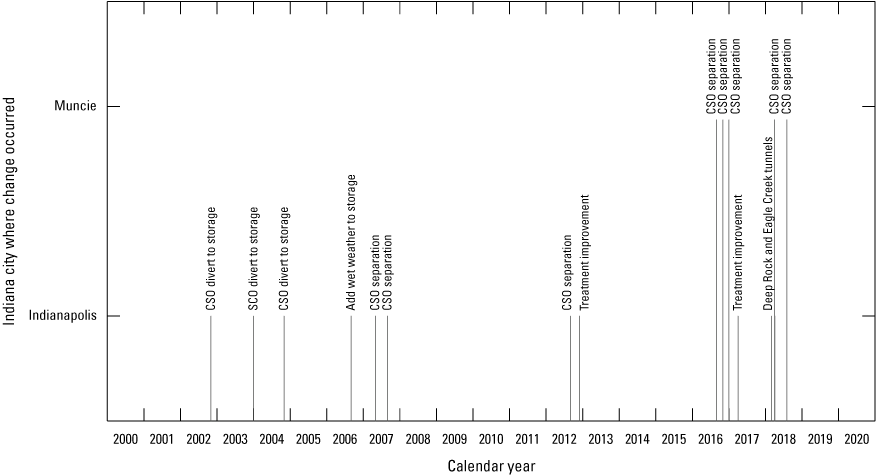
Timeline of selected changes to wastewater treatment systems and delivery processes implemented in Indianapolis and Muncie, Indiana, between 2000 and 2020. CSO, combined sewer overflow(s).
Discussion
It is difficult to causatively associate trends in flow-normalized flux with the anthropogenic factors examined in this study because many factors changed over time. The character and periods associated with temporally monotonic trends varied between constituents and between gage locations. In addition, the periods of available data for the anthropogenic factors varied by factor. The following discussion of trends is based on slopes of the annual flow-normalized flux curves (figs. 10–13) without accounting for uncertainty in individual flux estimates. Flow-normalized fluxes are used because they reduce or eliminate the effects of year-to-year variation in flux caused by changing streamflow. A downward trend is indicated when fluxes are monotonically decreasing over an extended period, and an upward trend is indicated when fluxes are monotonically increasing over an extended period. Of the three study gages, annual flow-normalized fluxes at the gage near Centerton showed the largest changes and had the most distinct inflection points in the trend plots during the period between water years 2002 and 2020. Consequently, results for the gage near Centerton will be used to illustrate the complexity of assessing the cause(s) of trends.
Downward trends in flow-normalized fluxes of total Kjeldahl nitrogen at the gage near Centerton started in water year 1997 (the first year of available data), and a downward trend in the flow-normalized flux of nitrate plus nitrite started around 2001. The only anthropogenic factors examined that had data from at least 1992 were population, fertilizer applications, and wastewater treatment system and delivery process improvements. Population monotonically increased in the upper White River Basin between 1992 and 2020 as did the mass of nitrogen and phosphorus applied as commercial fertilizer in non-farm settings. The masses of nitrogen and phosphorus applied as manure decreased over the same period and were considerably larger in magnitude than masses from non-farm commercial sources. The increasing population might have led to increased nutrients delivery to streams through treated wastewater and through runoff of nutrients from commercial fertilizers applied to lawns and other green spaces associated with population centers; however, those increases might have been offset or reversed by the decreases in nutrients applied as manure.
There were two local maxima in the curve for flow-normalized flux of total phosphorus followed by periods of downward trend at the gage near Centerton (fig. 11): the first was in water year 1997 and the second was in water year 2012 (the year when the first of the treatment improvements identified as most impactful were made in Indianapolis). The downward trend in flow-normalized total phosphorus flux beginning in 2012 could be related (at least in part) to the treatment improvements; however, the slopes of the curves for flow-normalized flux of nitrate plus nitrite and total Kjeldahl nitrogen did not noticeably change around 2012. Consequently, if the treatment improvements were responsible for the decrease in flow-normalized flux of total phosphorus beginning in 2012, those same improvements did not have an observable effect on the flow-normalized flux of nitrate plus nitrite or total Kjeldahl nitrogen. Without further investigation into the nature of the treatment improvements, it is impossible to say whether the improvements could have resulted in the observed outcomes.
Determining causation of trends in TSS and nutrient fluxes is complex and was not a goal of this study. The study objectives were (1) to evaluate trends in fluxes and concentrations of TSS and nutrients and (2) to provide spatial and temporal information on a variety of factors that could influence those trends. There were no obvious triggers for the flux trends. Consequently, further study may help to understand the causes of water-quality trends. This study provides a foundation for future studies addressing causation of trends.
Summary
In cooperation with The Nature Conservancy, the U.S. Geological Survey (USGS) undertook a study to estimate and assess trends in annual mean concentrations and flux of nitrate plus nitrite, total Kjeldahl nitrogen, total phosphorus, and total suspended solids (TSS) at three USGS streamgages (at Muncie, near Nora, and near Centerton, Indiana) on the upper White River. The estimates and trends presented in this report update and extend results from Koltun (2019), using three additional years of data and newer estimation methods. In addition, nutrient and TSS concentration data from sampling locations in the upper White River Basin were examined for spatial patterns in their sampling distributions and several anthropogenic factors that could influence the concentrations and flux of nutrients and TSS were explored to better understand their spatial and temporal variations. There were enough data for most water-quality constituents to analyze the 29-year period extending from water years 1992 to 2020; however, shorter analytical periods were necessary in some cases
Trends in streamflows at the study gages between water years 1978 and 2020 were assessed using the Exploration and Graphics for RivEr Trends (EGRET) package, and Mann-Kendall and Pettitt tests. Mann-Kendall trend tests indicated the annual maximum, mean, and median daily streamflows and the annual 7-day minimum streamflows generally trended upward with time between water years 1978 and 2020 at each of the study gages; however, only the trends for annual mean and maximum daily streamflows were statistically significant for all study gages at a 0.05 level. Pettitt tests indicated statistically significant step trends in annual mean daily streamflows occurring around water year 2001 at each of the study gages. Statistically significant step trends in annual maximum daily streamflows at the gages near Nora and Centerton and annual median daily streamflows at the gage at Muncie also occurred around 2001.
A Mann-Kendall trend test of annual precipitation totals measured at the Indianapolis International Airport between calendar years 1932 and 2020 indicated a statistically significant upward trend in annual precipitation (increasing at an average rate of 0.089 inches per year). That result supports the hypothesis that upward trends in streamflows resulted (at least in part) from an upward trend in precipitation. LOWESS smooth lines of the annual precipitation totals at the Indianapolis International Airport and annual mean streamflows at the upper White River gage near Nora indicated that precipitation and streamflows began trending upward more rapidly in the mid to late 1970s.
The Weighted Regressions on Time, Discharge and Season (WRTDS) function in EGRET was used to estimate annual water-year mean daily concentrations and fluxes of nutrients and TSS, as well as to estimate concentrations and fluxes that were normalized to remove the influence of year-to-year variation in streamflow. The WRTDS-Kalman Filter method (WRTDS-K) was used to estimate annual water year mean daily concentrations and fluxes instead of the WRTDS base method previously used by Koltun (2019). Estimates made with the WRTDS-K method are generally more accurate and generally were of equal or smaller magnitude than estimates made with the base WRTDS method. The WRTDS base method was used to estimate flow-normalized concentrations and fluxes.
Analytical period and average annual loads and yields of each constituent were estimated for their longest periods of concurrent record at the three gages. Loads of each of the constituents increased sequentially from the most upstream gage to the most downstream gage; however, the same was not true for yields. The largest yields of TSS and total phosphorus were at the most upstream gage (at Muncie); whereas the largest yield of nitrate plus nitrite was at the most downstream gage (near Centerton). The yield of total Kjeldahl nitrogen was smaller at the most downstream study gage and was larger at the two upstream gages which had about equal yields.
Annual flow-normalized fluxes increased at the study gages in downstream order during all years in the study period (water years 1992–2020); however, the same was not true for annual flow-normalized concentrations. Flow-normalized concentrations of nutrients were consistently larger at the gages near Nora and Centerton than at Muncie; however, there was no spatially consistent order to the magnitudes of the annual flow-normalized concentrations of TSS over the study period.
Temporal trends in the annual flow-normalized fluxes of nitrate plus nitrite and total Kjeldahl nitrogen were similar to each other at a given gage. The shorter sampling periods for total Kjeldahl nitrogen at the gages at Muncie and near Centerton adds uncertainty to comparisons; however, it seems that flow-normalized flux of nitrate plus nitrite and total Kjeldahl nitrogen at the gages near Nora and Centerton generally have been declining since the early 2000s, with the rate of decrease being larger at the gage near Centerton than at the other two study gages. The flow-normalized flux of nitrate plus nitrite and total Kjeldahl nitrogen at the Muncie gage decreased initially but rose between water years 2006 and 2008. As of water year 2020, annual flow-normalized fluxes of total phosphorus decreased since about water year 2008 at the gage near Nora, since about water year 2012 at the gage near Centerton, and since about water year 2013 at the Muncie gage. The largest magnitude and rate of decrease of the annual flow-normalized flux of total phosphorus at the study gages in the post water year 2011 period occurred at the gage near Centerton.
Annual flow-normalized flux of TSS decreased rapidly at the gage near Centerton between water years 1992 and 2007. Decreases also occurred at the gages at Muncie and near Nora during part of that same period but were less rapid. A gap in TSS sampling at the gage near Centerton lends uncertainty to the interpretation of trend and change results for that gage.
WRTDS bootstrap tests were used to assess the magnitude, direction, and likelihood of changes in annual flow-normalized concentrations and flux of TSS, total phosphorus, nitrate plus nitrite, and total Kjeldahl nitrogen at the study gages between water years 1997 and 2019. With two exceptions, concentration and flux changes that were statistically significant in Koltun (2019) showed the same statistically significant change direction. The only case in which the indicated change direction switched was at the gage near Centerton which previously showed a “highly likely” downward change in TSS concentration and now shows an upward change classified as “as likely as not.” The other exception was for nitrate plus nitrite concentration at the White River at Muncie, Indiana, that still showed a downward change; however, the likelihood of change decreased from “highly likely” to” likely.”
Boxplots of concentration data retrieved from the National Water Quality Monitoring Council’s Water Quality Portal (https://www.waterqualitydata.us) for water-quality sampling locations in the upper White River Basin showed that (1) the largest median concentrations of TSS, total phosphorus, and total Kjeldahl nitrogen were associated with mainstem upper White River sampling locations downstream from Indianapolis and (2) that median total phosphorus and total Kjeldahl nitrogen concentrations at the upper White River sampling location immediately downstream from Muncie were elevated relative to bracketing mainstem sampling locations. The practical effect of these observations on TSS and (or) nutrient flux is uncertain because there was no information on associated streamflow rates for most of the sites to permit computations of flux.
Several anthropogenic factors were examined to better understand their spatial and (or) temporal variations. These factors included information on population, land cover, cropping practices and operational tillage, fertilizer application, and upgrades to wastewater treatment systems and delivery processes.
-
• Population increased appreciably in the Indianapolis metro area (which includes Indianapolis, Carmel, and Anderson, Indiana) in the last 20 years while it decreased in the Muncie metro area and the City of Anderson. The population increase in the Indianapolis metro area exceeded the population decrease in the Muncie metro area.
-
• Land-cover characteristics (as defined in the USGS National Land Cover Database [Dewitz and U.S. Geological Survey, 2021]) in the drainage to the Muncie gage have remained mostly unchanged over time; however, the intervening areas draining to the gages near Nora and Centerton had noticeable decreases in the percentages of cultivated crops and pasture/hay coupled with increases in low- and medium-intensity developed lands.
-
• Areas classified as grass/pasture (as defined in the U.S. Department of Agriculture [2021] Cropland Data Layers [for 2007–20]) decreased over time as percentages of the intervening areas draining to the study gages. The percentages of areas planted in corn and soybeans were larger than for other crops in the intervening drainages to the gages at Muncie and near Nora. The same was nearly true for the gage near Centerton; however, areas classified as grass/pasture were of similar magnitude (percentagewise) to corn and soybeans in 2007 (the first year of available data) before decreasing in subsequent years.
-
• The percentages of areas planted in corn and soybeans generally decreased in downstream order at the study gages, with the largest decreases occurring in the intervening area between the gages near Nora and Centerton.
-
• A large single-year spike in the percentages of areas classified as fallow/idle cropland occurred in 2019. That spike was attributed to wet spring conditions that impeded planting.
-
• There were appreciable year-to-year variations in the percentages of corn, soybean, small grain, and other crops planted in the upper White River Basin that were subsequently no-tilled, reduce-tilled, or conventionally tilled (as defined in the Operational Tillage Information System [Conservation Technology Information Center, 2021]) prior to planting the next crop, with no visually discernable indications of consistent upward or downward trends. In most years, the annual percentage of each crop that was subsequently no tilled was larger than the corresponding percentage that was conventionally tilled. Corn or soybean crops generally had larger percentages of subsequent reduce- till than no-till treatment whereas the opposite was true for small grain crops.
-
• The percentages of winter cover crops (as defined in the Operational Tillage Information System) planted following planting corn varied in an irregular fashion over time between 2005 and 2018 and were typically small (less than 1.5 percent).
-
• The percentages of winter cover crops established following planting soybeans was consistently larger than following the planting of corn, with winter commodity crops being the most common cover. Percentages of winter commodity cover crops following planting soybeans have been trending downward since about 2008, whereas percentages of perennial cover crops have remained small (less than 0.1 percent) and mostly unchanged over time between 2005 and 2018 while percentages of other cover crops have been trending upward since about 2013.
-
• The percentage of winter cover crops established following planting small grain crops was larger than following planting corn or soybeans, with cover crops other than winter commodity or perennial being the most common. The percentages of winter commodity and perennial cover crops remained mostly steady over time (2005–18); however, there was an upward trend in the percentage of other winter cover crops planted following planting small grain crops.
-
• Estimates of the masses of nitrogen and phosphorus from commercial fertilizers and manure reported by Falcone (2021a) were summed for 13 of the 16 counties constituting the upper White River Basin. Farm-applied commercial fertilizer was the largest source of nitrogen and phosphorus. Manure was the next largest source, followed by non-farm commercial fertilizer.
-
• The estimated masses of nitrogen and phosphorus applied as manure gradually trended downward between 1987 and 2017, while nitrogen mass from non-farm commercial fertilizers gradually trended upward. The estimated mass of nitrogen from farm-applied commercial fertilizers did not change in a monotonic fashion between 1987 and 2017; however, the most recent three estimates (for 2007, 2012, and 2017) were larger than estimates for earlier years except 1992. No other fertilizer source showed strong visual indications of temporal trend.
-
• Indianapolis and Muncie, Indiana, provided information on changes to their wastewater treatment systems and delivery processes between 1992 and 2020 that potentially had an appreciable impact on nutrient and (or) TSS loadings to the White River. The earliest reported changes were in Indianapolis in November 2002 and in Muncie in September 2016. The changes identified as likely being most impactful for reducing nutrient and (or) TSS loadings occurred after 2011.
References Cited
Cleveland, W.S., 1979, Robust locally weighted regression and smoothing scatterplots: Journal of the American Statistical Association, v. 74, no. 368, p. 829–836. [Also available at https://doi.org/10.1080/01621459.1979.10481038.]
Cleveland, W.S., and Devlin, S.J., 1988, Locally weighted regression—An approach to regression analysis by local fitting: Journal of the American Statistical Association, v. 83, no. 403, p. 596–610. [Also available at https://doi.org/10.1080/01621459.1988.10478639.]
Conservation Technology Information Center, 2021, Operational tillage information system: Conservation Technology Information Center database, accessed October 9, 2021, at https://ctic.org/optis_tabular_query.
Dewitz, J., and U.S. Geological Survey, 2021, National Land Cover Database (NLCD) 2019 Products (ver. 2.0, June 2021): U.S. Geological Survey data release, accessed February 21, 2022, at https://doi.org/10.5066/P9KZCM54.
Edwards, T.K., and Glysson, G.D., 1999, Field methods for measurement of fluvial sediment: U.S. Geological Survey Techniques of Water-Resources Investigations, book 3, chap. C2, 89 p. [Also available at https://doi.org/10.3133/twri03C2.]
Falcone, J.A., 2021a, Tabular county-level nitrogen and phosphorus estimates from fertilizer and manure for approximately 5-year periods from 1950 to 2017: U.S. Geological Survey data release, accessed February 23, 2022, at https://doi.org/10.5066/P9VSQN3C.
Falcone, J.A., 2021b, Estimates of county-level nitrogen and phosphorus from fertilizer and manure from 1950 through 2017 in the conterminous United States: U.S. Geological Survey Open-File Report 2020–1153, 20 p., accessed February 23.2022, at https://doi.org/10.3133/ofr20201153.
Glysson, G.D., 1987, Sediment-transport curves: U.S. Geological Survey Open-File Report87–218, 47 p. [Also available at https://doi.org/10.3133/ofr87218.]
Hirsch, R.M., Moyer, D.L., and Archfield, S.A., 2010, Weighted Regressions on Time, Discharge, and Season (WRTDS), with an application to Chesapeake Bay River inputs: Journal of the American Water Resources Association, v. 46, no. 5, p. 857–880, accessed April 8, 2021, at https://doi.org/10.1111/j.1752-1688.2010.00482.x.
Hirsch, R.M., and DeCicco, L.A., 2015, User guide to Exploration and Graphics for RivEr Trends (EGRET) and dataRetrieval—R packages for hydrologic data (ver. 2.0, February 2015): U.S. Geological Survey Techniques and Methods, book 4, chap. A10, 93 p., accessed April 8, 2021, at https://doi.org/10.3133/tm4A10.
Hirsch, R.M., Archfield, S.A., and DeCicco, L.A., 2015, A bootstrap method for estimating uncertainty of water quality trends: Environmental Modelling & Software, v. 73, p. 148–166, accessed April 8, 2021, at https://doi.org/10.1016/j.envsoft.2015.07.017.
Hill, C., 2019, Did it rain a lot this spring in Indianapolis? The answer is yes—and no. Here's why: IndyStar, June 25, 2019, accessed July 24, 2019, at https://www.indystar.com/story/weather/indianapolis/2019/06/25/indianapolis-weather-how-spring-rain-compares-to-past-years/1526543001/.
Koltun, G.F., 2019, Trends in streamflow and concentrations and flux of nutrients and total suspended solids in the upper White River at Muncie, near Nora, and near Centerton, Indiana: U.S. Geological Survey Scientific Investigations Report2019–5119, 34 p. [Also available at https://doi.org/10.3133/sir20195119.]
Koltun, G.F., 2023, Model data archive—Trends in selected environmental, anthropogenic, and water-quality characteristics in the upper White River Basin, Indiana, 1991–2020: U.S. Geological Survey data release, https://doi.org/10.5066/P9O6C9L3.
Mallakpour, I. and Villarini, G., 2016, A simulation study to examine the sensitivity of the Pettitt test to detect abrupt changes in mean: Hydrological Sciences Journal, v. 61no. 2, p. 245–254, accessed September 22, 2021, at https://doi.org/10.1080/02626667.2015.1008482.
Mann, H.B., 1945, Nonparametric tests against trend: Econometrica, v. 13, no. 3, p. 245–259, accessed September 22, 2021, at https://doi.org/10.2307/1907187.
National Oceanic and Atmospheric Administration, 2022, Climate at a glance—Statewide time series: National Oceanic and Atmospheric Administration database, accessed April 4, 2022, at https://www.ncdc.noaa.gov/cag/statewide/time-series/33.
Pettitt, A.N., 1979, A non-parametric approach to the change-point problem: Journal of the Royal Statistical Society—Series C, Applied Statistics, v. 28, no. 2, p. 126–135. [Also available at https://doi.org/10.2307/2346729.]
Piske, J.T., 2019, Nitrate concentrations in streams as a function of crop cover in midwestern agricultural watersheds—Assessing the role of corn and soybeans: Illinois State University, Master’s thesis, 56 p., accessed February 3, 2022, at https://ir.library.illinoisstate.edu/etd/1108.
Pohlert, T., 2018, Trend—Non-parametric trend tests and change-point detection, R package version 1.1.1: Comprehensive R Archive Network website, accessed February 1, 2019, at http://CRAN.R-project.org/package=trend.
R Core Team, 2017, R—A language and environment for statistical computing (version 3.6.1): Vienna, Austria, R Foundation for Statistical Computing website, accessed July 22, 2020, at https://www.R-project.org/.
Robertson, D.M., Schwarz, G.E., Saad, D.A., and Alexander, R.B., 2009, Incorporating uncertainty into the ranking of SPARROW model nutrient yields from Mississippi/Atchafalaya River Basin watersheds: Journal of the American Water Resources Association, v. 45, no. 2, p. 534–549. [Also available at https://doi.org/10.1111/j.1752-1688.2009.00310.x.]
Robertson, D.M., and Saad, D.A., 2013, SPARROW models used to understand nutrient sources in the Mississippi/Atchafalaya River Basin: Journal of Environmental Quality, v. 42, no. 5, p. 1422–1440, accessed September 28, 2021, at https://doi.org/10.2134/jeq2013.02.0066.
Sen, P.K., 1968, Estimates of the regression coefficient based on Kendall’s tau: Journal of the American Statistical Association, v. 63, no. 324, p. 1379–1389. [Also available at https://doi.org/10.1080/01621459.1968.10480934.]
STATS Indiana, 2022, Population estimates for Indiana's incorporated places—2010–2020: State of Indiana database, accessed February 10, 2022, at https://www.stats.indiana.edu/topic/population.asp.
Snapp, S.S., Swinton, S.M., Labarta, R., Mutch, D., Black, J.R., Leep, R., Nyiraneza, J., and O’Neil, K., 2005, Evaluating cover crops for benefits, costs and performance within cropping system niches: Agronomy Journal, v. 97, no. 1, p. 322–332, accessed October 5, 2021, at https://doi.org/10.2134/agronj2005.0322a.
Tedesco, L.P., Pascual, D.L., Shrake, L.K., Hall, R.E., Casey, L.R., Vidon, P.G.F., Hernly, F.V., Salazar, K.A., and Barr, R.C., 2005, Eagle Creek Watershed Management Plan—An integrated approach to improved water quality: Indianapolis, Indiana, Indiana University—Purdue University Indianapolis, Center for Earth and Environmental Science Publication 2005-07, 182 p., accessed December 4, 2018, at https://www.in.gov/idem/nps/files/wmp_eaglecreek_98-002.pdf. [Also available at https://ourwaterways.org/wp-content/uploads/2019/08/Eagle-Creek-Watershed-Plan.pdf.]
Tedesco, L.P., Hoffman, J., Bihl, L., Hall, B.E., Barr, R.C., and Stouder, M., 2011, Upper White River Watershed Regional Watershed Assessment and Planning Report: Indianapolis, Indiana, Indiana University—Purdue University Indianapolis, Center for Earth and Environmental Science, 350 p., accessed December 4, 2018, at https://thewhiteriveralliance.org/wp-content/uploads/2018/08/Upper-White-River-Watershed-Regional-Plan.pdf.
U.S. Department of Agriculture, 2021, National Agricultural Statistics Service cropland data layers—2007–2020: U.S. Department of Agriculture database, accessed September 15, 2021, at https://www.nass.usda.gov/Research_and_Science/Cropland/Release/.
U.S. Geological Survey, 2006, Collection of water samples (ver. 2.0, September, 2006): U.S. Geological Survey Techniques of Water-Resources Investigations, book 9, chap. A4, 166 p., accessed April 4, 2022, at https://doi.org/10.3133/twri09A4.
Widhalm, M., Hamlet, A., Byun, K., Robeson, S., Baldwin, M., Staten, P., Chiu, C., Coleman, J., Hall, B., Hoogewind, K., Huber, M., Kieu, C., Yoo, J., and Dukes, J.S., 2018, Indiana’s past & future climate—A report from the Indiana climate change impacts assessment: West Lafayette, Indiana, Purdue Climate Change Research Center, Purdue University, accessed September 27, 2021, at https://doi.org/10.5703/1288284316634.
Zhang, Q., and Hirsch, R.M., 2019, River water-quality concentration and flux estimation can be improved by accounting for serial correlation through an autoregressive model: Water Resources Research, v. 55, no. 11, p. 9705–9723, accessed December 01, 2019, https://doi.org/10.1029/2019WR025338.
Conversion Factors
U.S. customary units to International System of Units
Temperature in degrees Fahrenheit (°F) may be converted to degrees Celsius (°C) as follows:
°C = (°F – 32) / 1.8.
Supplemental Information
Concentrations of chemical constituents in water are in milligrams per liter (mg/L).
A water year is the period from October 1 to September 30 and is designated by the year in which it ends; for example, water year 2020 was from October 1, 2019, to September 30, 2020.
Unless stated otherwise, references to years in this report refer to calendar years.
Abbreviations
CEG
Citizens Energy Group
CSO
combined sewer overflows
EGRET
Exploration and Graphics for RivEr Trends
IDEM
Indiana Department of Environmental Management
IDPW
Indiana Department of Public Works
LOWESS
locally weighted scatterplot smoothing
MBWQ
Muncie Sanitary District, Bureau of Water Quality
NOx
nitrate plus nitrite
QC
quality control
TSS
total suspended solids
USGS
United States Geological Survey
WBT
WRTDS bootstrap tests
WRTDS
Weighted Regressions on Time, Discharge, and Season
WRTDS-K
WRTDS Kalman-filter method
For more information about this report, contact:
Director, Ohio-Kentucky-Indiana Water Science Center
U.S. Geological Survey
5957 Lakeside Blvd.
Indianapolis, IN 46278-1996
or visit our website at
https://www.usgs.gov/centers/oki-water
Publishing support provided by the Tacoma and Reston Publishing Service Centers
Disclaimers
Any use of trade, firm, or product names is for descriptive purposes only and does not imply endorsement by the U.S. Government.
Although this information product, for the most part, is in the public domain, it also may contain copyrighted materials as noted in the text. Permission to reproduce copyrighted items must be secured from the copyright owner.
Suggested Citation
Koltun, G.F., 2023, Trends in environmental, anthropogenic, and water-quality characteristics in the upper White River Basin, Indiana: U.S. Geological Survey Scientific Investigations Report 2023–5025, 46 p., https://doi.org/10.3133/sir20235025.
ISSN: 2328-0328 (online)
Study Area
| Publication type | Report |
|---|---|
| Publication Subtype | USGS Numbered Series |
| Title | Trends in environmental, anthropogenic, and water-quality characteristics in the upper White River Basin, Indiana |
| Series title | Scientific Investigations Report |
| Series number | 2023-5025 |
| DOI | 10.3133/sir20235025 |
| Publication Date | April 14, 2023 |
| Year Published | 2023 |
| Language | English |
| Publisher | U.S. Geological Survey |
| Publisher location | Reston, VA |
| Contributing office(s) | Ohio-Kentucky-Indiana Water Science Center |
| Description | Report: x, 46 p.; Data Release |
| Country | United States |
| State | Indiana |
| Other Geospatial | Upper White River Basin |
| Online Only (Y/N) | Y |
| Additional Online Files (Y/N) | N |