
Evaluating Drivers of Hydrology, Water Quality, and Benthic Macroinvertebrates in Streams of Fairfax County, Virginia, 2007–18
Links
- Document: Report (24.1 MB pdf) , HTML , XML
- Data Release: USGS data release - Climate, landscape, and water-quality metrics for selected watersheds in Fairfax County, Virginia, 2007–2018
- NGMDB Index Page: National Geologic Map Database Index Page (html)
- Download citation as: RIS | Dublin Core
Acknowledgments
Ecologists with the Fairfax County Department of Public Works and Environmental Services, primarily Shannon Curtis, Joe Sanchirico, Chris Ruck, and Jon Witt, contributed greatly to this study. Their program coordination, field expertise, and scientific insights have been critical to the success of this effort and will continue to be relied upon in future study years. Staff at the Fairfax County Environmental Services Laboratory performed the nutrient analyses for most samples collected; their work is sincerely appreciated. Many U.S. Geological Survey (USGS) staff have contributed to the design, operation, and interpretation of this study since its inception in 2007. These combined efforts have produced years of consistent data collection and foundational knowledge that greatly benefited this report. Technical reviews by Doug Chambers of the USGS and Jonathan Duncan of the Pennsylvania State University strengthened this report and are greatly appreciated. The authors also thank Kaycee Faunce of the USGS for helping identify and communicate the findings of this research.
Abstract
In 2007, the U.S. Geological Survey partnered with Fairfax County, Virginia, to establish a long-term water-resources monitoring program to evaluate the hydrology, water quality, and ecology of Fairfax County streams and the watershed-scale effects of management practices. Fairfax County uses a variety of management practices, policies, and programs to protect and restore its water resources, but the effects of such strategies are not well understood. This report used streamflow, water-quality, and ecological monitoring data collected from 20 Fairfax County watersheds from 2007 through 2018 to assess the effects of management practices, landscape factors, and climatic conditions on observed nutrient, sediment, salinity, and benthic-macroinvertebrate community responses.
Urbanization, climatic variability, and an increase in management practices occurred within Fairfax County during the study period. Impervious cover, housing units, wastewater infrastructure, and (or) stormwater infrastructure increased in most study watersheds. Climatic conditions varied among study years; countywide estimates of average-annual air temperature differed by about 3 degrees Celsius, and total precipitation ranged from about 34 to 63 inches per year. The effects of the management practices, implemented to reduce nitrogen, phosphorus, and (or) sediment loads, are considered in this study. These management practices primarily consist of stormwater retrofits and stream restorations; however, stream restorations account for most of the financial investment and expected load reductions. Management practices were implemented in half of the study watersheds, and most practices were installed and reductions credited late in the study period.
Changes in hydrologic response during storm events were evaluated over the study period because many management practices that were implemented were designed to achieve nutrient and sediment reductions by slowing or intercepting runoff. The average number and length of storm events was mostly unchanged throughout the monitoring network. Four watersheds with 10 years of streamflow data showed a mixture of trends in stormflow peak, volume, and rate-of-change. Event-mean nutrient and sediment concentrations from these watersheds were evaluated during storm events and generally showed increases in total phosphorus (TP) and suspended sediment and reductions or no changes in total nitrogen (TN).
Landscape inputs of nitrogen and phosphorus and the percentage of inputs delivered to streams were estimated for the study watersheds. Estimated phosphorus from fertilizer and nitrogen from atmospheric deposition represented large nutrient inputs in most watersheds; amounts of other nonpoint sources varied based on land use. Estimated nitrogen inputs declined throughout Fairfax County and in most study watersheds from 2008 through 2018; in comparison, phosphorus input changes were relatively small. Most nonpoint-nutrient inputs were retained on the landscape and did not reach streams, with slightly more nitrogen retention than phosphorus, on average. Retention rates were lower for years with more precipitation and streamflow. After adjusting for streamflow, TN and TP loads were generally higher for years with more nutrient inputs. Calculated as a function of flow-adjusted loads, TP retention declined at most stations from 2009 through 2018, in comparison, TN retention was relatively unchanged.
Landscape and climatic conditions affected spatial differences and changes in Fairfax County stream conditions from 2009 through 2018. TN concentrations were higher and increases over time were larger in watersheds with elevated septic-system density. TP concentrations were higher in watersheds with more turfgrass; concentrations were lower, but had larger increases over time, in watersheds with deeper soils. Suspended-sediment concentrations were higher in watersheds with greater stream densities. Specific conductance was higher in watersheds with more developed land use and shallower soils. Benthic-macroinvertebrate index of biotic integrity (IBI) scores were lower in watersheds with high road density and had larger increases over time in bigger, more developed watersheds. Annual variability in TN and TP concentrations and benthic-macroinvertebrate IBI scores was affected by precipitation; annual variability in suspended sediment concentrations and specific conductance was affected by air temperature.
After accounting for influences from landscape and climatic conditions, expected management-practice effects were not consistently observed in monitored stream responses. These effects were assessed by comparing expected management-practice load reductions with the timing, direction, and magnitude of changes in storm-event hydrology, nutrient and sediment loads, median-annual water-quality conditions, and benthic-macroinvertebrate IBI scores. An important consideration for future investigations of management-practice effects is how to control for water-quality and ecological variability caused by geologic properties, the urban environment, precipitation, and (or) air temperature. The interpretation of management-practice effects in this report was likely influenced by a combination of factors, including (1) the amount, timing, and location of management-practice implementation; (2) unmeasured landscape and climatic factors; (3) uncertain management-practice expectations; (4) hydrologic variability; and (5) analytical assumptions. Through continued data-collection efforts, particularly after management practices have been completed, many of these factors may become less influential in the future.
Introduction
The prevalence of degraded water quality and ecological health in urban streams has been widely documented (Feminella and Walsh, 2005; Kaushal and others, 2015; Lenat and Crawford, 1994; Meyer and others, 2005; Paul and Meyer, 2001; Roy and others, 2003), but explanations of changing conditions over time often are unavailable. A mixture of improving and degrading water-quality and ecological trends in urban streams has been described in recent years (Aulenbach and others, 2017; Giorgino and others, 2018; Majcher and others, 2018; Miller and others, 2012). These trends are likely affected by a combination of factors, including changes to the landscape and climatic conditions. As urban areas continue to expand (Terando and others, 2014) and the climate becomes increasingly dynamic (Wuebbles and others, 2017), risks to the water quality and ecological health of urban streams are likely to increase (Van Metre and others, 2019). Watershed managers are attempting to mitigate these risks and restore the quality of urban streams by using a variety of management practices, programs, and policies (Bernhardt and others, 2005; McPhillips and Matsler, 2018); these strategies could be improved through a better understanding of the drivers of water-quality and ecological response.
The ability of management practices to treat stormwater runoff, modify stream environments to reduce nutrients and sediments, or improve ecological health is uncertain. Load reductions have been observed from practices that treat a large enough volume of runoff to alter hydrologic response (Koch and others, 2014; Vogel and Moore, 2016); however, load reductions are less apparent from practices designed to lower solute or particulate concentrations (Jefferson and others, 2017; Li and others, 2017). Stream restorations have been shown to reduce nitrogen, phosphorus, and sediment in streams (Kaushal and others, 2008b; Lammers and Bledsoe, 2017; Reisinger and others, 2019); however, these effects differ with land use (Newcomer Johnson and others, 2016), practice age (McMillan and others, 2014; McMillan and Noe, 2017), time of year (Sudduth and others, 2011), and flow condition (Filoso and Palmer, 2011). Compared to nutrient and sediment reductions, the ability of stream restorations to restore biological diversity is less commonly documented (Bernhardt and Palmer, 2011; Palmer and others, 2010; Stranko and others, 2012). The effects of stormwater treatment and stream-restoration practices are most commonly described from modeling studies rather than studies that evaluate effects based on monitored responses (Lintern and others, 2020). The combined effects of multiple practices and interactions with landscape and climatic conditions are poorly understood at larger spatial scales (Jefferson and others, 2017). Few studies are designed to identify how these integrative management-practice effects relate to monitored nutrient, sediment, and biotic responses, despite such information offering opportunities to guide ongoing and future watershed-management strategies (Li and others, 2017).
Fairfax County, Virginia, uses a variety of management strategies to protect and restore its water resources (Stormwater Planning Division, 2018), while facing pressures from continued population growth (Han and others, 2018) and climatic changes (Moglen and Rios Vidal, 2014). Many Fairfax County streams show symptoms of urbanization, with some conditions improving over time and some continuing to degrade (Jastram, 2014; Porter and others, 2020b; Stormwater Planning Division, 2018). Information about the drivers of these changing conditions and the ability of management practices to improve them is needed to guide ongoing and future management activities within the county.
The U.S. Geological Survey (USGS) partnered with Fairfax County in 2007 to establish a long-term water-resources monitoring program for selected Fairfax County streams. This study is designed to document the current hydrologic, water-quality, and ecological conditions of Fairfax County streams, evaluate how conditions are changing over time, and describe the effect of management practices as a driver of such changes. Some of these objectives have been addressed in previous USGS reports, including a “baseline” characterization of streams after 5 years of data collection (Jastram, 2014) and an assessment of trends after 10 years of data collection (Porter and others, 2020b). This report builds on those previous reports to describe how landscape factors, management practices, and climatic conditions affect water-quality and ecological responses observed through 2018. The interpretations of this report are expected to be explored in greater detail as this study continues in future years, and specific areas of research will be targeted to address Fairfax County’s management needs.
Purpose and Scope
The purpose of this report is to identify drivers of spatial differences and temporal changes in the water-quality and ecological conditions of Fairfax County streams to inform watershed-management activities. This objective was addressed through the following questions, which also serve as report section titles:
-
• How did landscape and climatic conditions change?
-
• What water-quality management practices were used?
-
• How did hydrology and water quality vary during storm events?
-
• How did water-quality loads relate to nutrient inputs and management practices?
-
• What factors affected water-quality and benthic-macroinvertebrate responses?
-
• Were management-practice effects observed?
Analyses and interpretations of responses observed from a 20-station monitoring network from 2007 through 2018 are primarily used in this report. Total nitrogen (TN), total phosphorus (TP), suspended sediment (SS), specific conductance (SC), and benthic-macroinvertebrate index of biotic integrity (IBI) scores are the primary response variables of interest. These variables are used to represent ecosystem health and are the focus of many ongoing management efforts within Fairfax County. Management-practice implementation during the study period is summarized and analyzed in relation to observed conditions. Effects of urbanization, climatic conditions, and physical watershed properties are also considered to offer a comprehensive interpretation about water-quality and ecological responses in Fairfax County streams.
Description of Study Area
Fairfax County is a 395 square-mile (mi2) jurisdiction in northern Virginia (fig. 1). The county borders the Potomac River to the north and east, Bull Run and the Occoquan River to the south, and Loudon County to the northwest. Parts of the eastern boundary are shared with Arlington County, the city of Falls Church, and the city of Alexandria. Fairfax County surrounds the incorporated city of Fairfax.
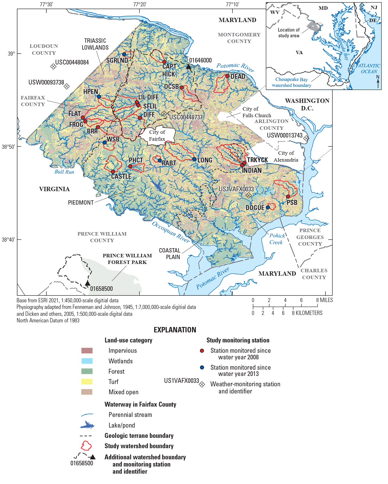
Map showing monitoring stations and study watersheds in Fairfax County, Virginia. Study watershed station names are defined in table 1. Land-use category data is from the Chesapeake Bay Program Office (2018).
Fairfax County is Virginia’s most populous jurisdiction, home to about 1.2 million people (Han and others, 2018). Land use in the county is predominately residential- most housing units are single-family homes. A sanitary-sewer network, separate from the stormwater system, services most of Fairfax County’s population; about 100 million gallons of wastewater are treated daily at five treatment plants (Fairfax County, 2021). Areas of lower-density development, commonly along a north-south gradient in the center of the county, primarily treat wastewater with onsite septic systems and have private well water.
Fairfax County contains three distinct geologic terranes: sedimentary rocks in the Triassic Lowlands, crystalline rocks in the Piedmont, and a mixture of sands and clays in the Coastal Plain (Froelich and Zenone, 1985a). These first two geologic terranes co-occur within sections of the Piedmont physiographic province: the Piedmont lowlands and uplands, respectively. Geologic terranes have distinct impacts on water quantity and quality (properties that vary based on rock type and structure), soil depth, and overburden thickness (weathered material that includes soil, residuum, saprolite, and non-consolidated sediments) (Froelich and Zenone, 1985b). Streams draining the Triassic Lowlands, also known as Mesozoic Basins, can have the highest dissolved-solids concentrations in the county during low-flow conditions (Larson, 1978). This highly mineralized water, predominantly consisting of calcium bicarbonate, likely results from soluble geologic materials (Froelich and Zenone, 1985b). Triassic Lowland lithology is characterized by shallow, fractured bedrock and thin overburden features, which results in very low groundwater storage and stream base flow (Mohler and Hagan, 1981). This lithology generally enables streams to be in direct hydraulic connection with the water table and may increase the susceptibility of surface-water contamination relative to Piedmont and Coastal Plain streams (Froelich and Zenone, 1985b).
About 1,600 miles (mi) of streams in Fairfax County, perennial and intermittent, range in size from small first-order headwater streams to larger, fourth-order streams. All surface water from Fairfax County eventually drains to the Potomac River. Fairfax County streams are intertwined with a stormwater drainage network that includes about 2,400 mi of conveyance pipes and channels and thousands of storm structures, all typically designed to convey rainwater from land surfaces to streams, ponds, and rivers (Stormwater Planning Division, 2018). Most Fairfax County streams are immediately bordered by undeveloped land resulting from zoning designations, protection by county parkland, or other development restrictions. Most upland areas contain a mixture of developed land and impervious cover that can cause water-quality and biotic impairment. Areas of older development, generally in eastern Fairfax County, may be more at risk for water-quality and biotic impairment because they received less riparian protection than areas of newer development. In 2017, biological data collected and analyzed by Fairfax County ecologists indicated that about 75 percent of Fairfax County streams are in fair to very-poor ecological condition (Stormwater Planning Division, 2018).
Methods of Investigation
Interpretations in this report are primarily derived from data collected from stream monitoring stations that represent 20 watersheds in Fairfax County (table 1). These data were analyzed to evaluate how patterns in streamflow, benthic-macroinvertebrate communities, and water quality relate to landscape and climatic conditions. These analyses were limited by the spatial and temporal resolution of observed data, the uncertainty in predictor datasets, and the uncertainty in analytical results. Combined, these limitations may overcome or confound an ability to identify causes of water-quality responses. Care has been taken throughout this report to acknowledge these limitations and minimize their influence.
Table 1.
Description of the 20 study watersheds in Fairfax County, Virginia.[mi2, square mile; Va., Virginia]
Study Design
A 14-station monitoring network, established in 2007, provided measurements of streamflow, water quality, and benthic macroinvertebrates. An additional six stations were added to the network in 2012 and 2013. Monitored locations are referred to as “stations” or “watersheds” throughout this report. All study watersheds had an area less than 6 mi2 and were selected to represent land uses, infrastructure, and physical settings common to Fairfax County (Jastram, 2014). Based on the desire to identify and understand management-practice effects on water-quality response, Fairfax County directed management-practice investments towards the study watersheds, when possible.
The 20-station network consists of “intensive” and “trend” monitoring stations (table 1). Monthly water-quality samples, 5-minute water-level measurements, and annual benthic-macroinvertebrate samples were collected at all stations. Targeted high-flow water-quality samples and 15-minute water-quality and streamflow measurements were only collected at the five intensive-monitoring stations, which are a representative subset of the 20-station network in terms of land use and physical setting.
Data Collection, Sampling, and Laboratory Analysis
A brief summary of the data collection, sampling, and laboratory analyses related to this study is discussed in the following paragraphs. Unless otherwise noted, all data are available from the USGS National Water Information System (U.S. Geological Survey, 2023), and all data were collected since the date of station establishment (table 1). Annual periods in this report typically refer to calendar years; a “water year,” from October 1 to September 30 was used for selected analyses and interpretations. Water years 2008 and 2013, when stations were established (table 1), correspond to data-collection activities beginning in October of 2007 and 2012, respectively.
Continuous data were collected from the five intensive-monitoring stations. These data included 5-minute measurements of streamflow and 15-minute measurements of water temperature (WT), SC, pH, dissolved oxygen (DO), and turbidity (TB). The operation and maintenance of continuous water-quality monitors were conducted by USGS staff in accordance with published procedures (Wagner, 2006). Standard USGS methods for computing real-time streamflow using stage-discharge relations were used (Rantz, 1982). Continuous water-level data were collected every 15-minutes from the trend stations following standard methods (Rantz, 1982).
Discrete water-quality samples were collected monthly at all stations, typically as a grab sample from the centroid of streamflow, in accordance with USGS methods (U.S. Geological Survey, variously dated). Some monthly samples were timed to capture stormflow responses during the most recent five study years. Storm-targeted samples were collected during the entire study at the five intensive-monitoring stations using an automated refrigerated sampler. Laboratory analyses of discrete water-quality samples were conducted by the Fairfax County Environmental Services Laboratory and the USGS Kentucky Sediment Laboratory. All samples were analyzed for concentrations of TN, TP, common dissolved and particulate nitrogen and phosphorus forms, and SS.
Benthic-macroinvertebrate samples were collected annually in March or April by Fairfax County staff. Annual samples collected from 14 stations from 2008 through 2017 were analyzed in this report. Eight samples collected during this period were excluded from analysis because of the impacts of construction or inconsistencies in the sample sorting process. Samples were collected using a semi-quantitative multi-habitat method in accordance with standard operating procedures (Fairfax County, 2019) based on the U.S. Environmental Protection Agency’s Rapid Bioassessment Protocol (Barbour and others, 1999). Benthic-macroinvertebrate data are available online (Porter and others, 2020a).
Compilation of Predictor Datasets
Many datasets were assembled to describe hypothesized water-quality drivers, hereafter referred to as “predictors” or “predictor variables.” These data represent some of the most commonly described water-quality drivers but are not a complete accounting of all landscape and climatic features affecting instream response. Some predictors, such as those representing soil characteristics and hydrogeomorphic setting, are time invariant, that is, their estimated values are not expected to differ over the study period (table 2). Other predictors, such as those that represent climate, land use, and stormwater infrastructure, are time varying, that is, they have differing values among years and, typically, among watersheds (table 3). When possible, predictor data were assembled to reflect annual conditions from 2008 through 2018. Unless otherwise noted, all datasets were assembled to represent the spatial scale of Fairfax County and each of the 20 study watersheds. Multiple sources were used to assemble predictor data, and many datasets were provided directly by Fairfax County. All predictor datasets described in the following paragraphs are available online (Webber and others, 2022).
Table 2.
Description of time-invariant predictor variables used to describe hypothesized water-quality drivers in Fairfax County, Virginia.Table 3.
Description of time-varying predictor variables used to describe hypothesized water-quality drivers in Fairfax County, Virginia.[>, greater than; <, less than]
Time-invariant measures of physical setting include elevation data (U.S. Geological Survey, 2017), geologic terranes (Froelich and Zenone, 1985a), and soils data (Wieczorek, 2014; Wieczorek and LaMotte, 2010). The length of streams classified as perennial or intermittent were summarized from Fairfax County spatial information.
Measures of phosphorus geochemistry reflect naturally occurring phosphorus concentrations in geologic formations and soils. Phosphorus concentrations contributed to streams from geologic materials were reported by Nardi (2014). Phosphorus soil concentrations were derived from data reported by Terziotti (2019).
Median-annual values of streamflow, WT, SC, pH, DO, and TB were summarized from data collected with monthly water-quality samples. These median-annual values may not be an accurate characterization of year-round stream conditions, as monthly samples were typically collected during daytime, base-flow conditions.
Precipitation and air-temperature metrics were summarized from annual data reported by weather-monitoring stations proximal to Fairfax County (fig. 1). Air-temperature metrics reflect average-annual conditions reported from Dulles (USW00093738) and Reagan (USW00013743) airport-weather stations, near the western and eastern boundaries of Fairfax County, respectively. Precipitation metrics were averaged from annual values reported by three additional weather stations (WFO STERLING, USC00448084; FRANCONIA 1.3 SSE US1VAFX0033; and VIENNA, USC00448737). Average-annual temperature data were retrieved from the National Oceanic and Atmospheric Administration (2021). Additional measures of temperature and all precipitation data were retrieved from the Climdex HadEX3 dataset (Donat and others, 2013). Precipitation and air temperature varied among years and were represented as spatially averaged annual values for Fairfax County and the study watersheds. This representation may misrepresent climatic variability among watersheds because spatial precipitation variability is typically higher than that of temperature (Donat and others, 2013).
Annual estimates of landscape conditions (impervious surfaces, turf grass, forested land, wetlands, and water) were derived from 1-meter data from 2013 (Chesapeake Bay Program Office, 2018) and time-varying information reported by the Chesapeake Bay Program (Chesapeake Bay Program, 2020). The Chesapeake Bay Program provides annual estimates of land cover at spatial scales referred to as land-river segments. Fairfax County comprises 19 land-river segments, 7 of which contain the 20 study watersheds. This study assigned annual land-cover values to each watershed by combining the known 2013 land cover with changes in land cover reported by land-river segments.
Annual estimates of developed and forested land conditions were derived from the 2016 National Land Cover Database (Dewitz, 2019). This product contains land-use estimates at 30-meter resolution for multiple years during the study period: 2008, 2011, 2013, and 2016. Annual estimates were linearly interpolated between and beyond these years as needed to complete the 2008 through 2018 record.
The total length of roads was summarized from data provided by Fairfax County (Fairfax County, 2022). These data were used to represent the length of local roads, major roads, interstates, and ramps. Roadway data were available only for 2011, 2015, 2017, and 2020.
The number of housing units were estimated from published Fairfax County demographic reports (Han and others, 2018) and tax-parcel data. The number of single and multifamily housing units was summarized from these data. Annual tax-parcel data provided by Fairfax County show location-specific housing data (Fairfax County, 2022).
Attributes that represent wastewater collection networks were summarized from data provided by Fairfax County (Fairfax County, 2022). Measures of the sanitary-sewer network include total pipe length and percent rehabilitated by routine-maintenance activities. Rehabilitation efforts typically included relining or resealing of pipes to extend their life. The number of septic systems was quantified. Septic systems were classified as either conventional systems (those with traditional drain fields) or alternative systems (those that were built with mechanisms to achieve greater drain-field nitrogen reductions). The location of each system and the date it was constructed can be determined from the data provided by Fairfax County, but the data do not identify when systems were deactivated or removed; therefore, the number of systems in any given year may be overestimated.
Attributes that represent Fairfax County’s stormwater infrastructure were summarized from data provided by Fairfax County (Fairfax County, 2022). These data represent structures and facilities primarily designed to control flooding and include the length of stormwater pipes, the number and surface area of wet and dry ponds, and the number of stormwater facilities.
Information about management practices was provided by Fairfax County (Fairfax County, 2022). This report considered practices completed during the study period that were designed to achieve water-quality benefits and were credited for nutrient and (or) sediment load reductions by the Chesapeake Bay Program. A variety of practice types was used, and the types were categorized as channel restorations or detention-based and infiltration-based stormwater retrofits (table 4). Predictor variables were calculated to represent the cumulative credited mass of TN, TP, and total suspended solids (TSS) reduced by management practices (table 5). This representation of management practices assumes that the full effects of each practice occurred immediately upon completion, that reductions persisted over time, and that the effects of multiple practices were additive. These assumptions are uncertain, and it is very possible that true management-practice effects follow complex, non-linear trajectories that vary based on practice type, maintenance, and watershed setting (Jefferson and others, 2017). Hypothetical changes in load that could result from a management practice installed in 2011 with a credited 100-pound (lb) load reduction illustrate these multiple potential responses (fig. 2). The simplest pattern, “response 1,” reduces loads by the full credited amount upon practice completion, and that reduction persists over time. Alternatively, “response 2” may take multiple years after practice completion to reach credited reductions. In “response 3,” reductions become less effective with age. A further complication is that loads may increase during practice construction but then exceed the credited reductions at some point in the future, as shown in “response 4.” The complexity of management practice responses likely increases when multiple practices are installed in a watershed that each follow different load-reduction trajectories.
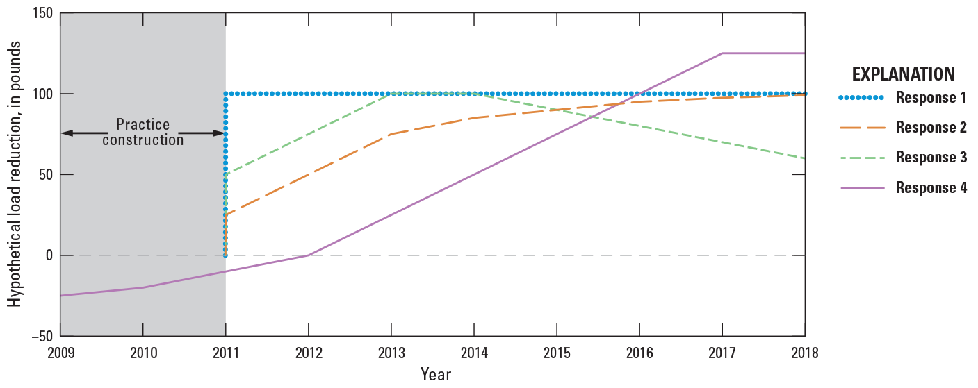
Graph showing hypothetical nutrient or sediment load reduction to a management practice completed in 2011.
Table 5.
Description of time-varying predictor variables used to represent credited management-practice load reductions in Fairfax County, Virginia.Estimation of Nitrogen and Phosphorus Inputs
Annual estimates of nitrogen and phosphorus applied from anthropogenic sources or contributed by natural processes, referred to as “inputs,” were derived for Fairfax County and the study watersheds from 2008 through 2018 from predictor datasets or regional models (table 6). Urban and suburban watersheds contain many point- and nonpoint-nitrogen/phosphorus inputs, which complicates a thorough inventory (Ator, 2019; Fissore and others, 2011; Hobbie and others, 2017; Kaushal and others, 2011). This report summarizes as many inputs as could be reasonably defined from available data. Estimated inputs include point-sources, fertilizer applications, pet waste, atmospheric deposition (nitrogen only), septic-system effluent (nitrogen only), and contributions from geologic sources (phosphorus only). Estimated nitrogen and phosphorus inputs are described in the following paragraphs and are available online (Webber and others, 2022).
Table 6.
Description of predictor variables representing nitrogen and phosphorus inputs and a brief description of predictor derivation.Point sources are direct inputs of nitrogen and phosphorus into surface waters. Annual point-source load data reported by the Chesapeake Bay Program were summarized and represent permitted industrial and municipal wastewater discharges. There are no permitted wastewater discharges in the study watersheds (Porter and others, 2020b).
Input estimates of atmospheric nitrogen deposition were derived from National Atmospheric Deposition Program estimates of total deposition (Schwede and Lear, 2014). TN deposition, which represents the combined fraction of reactive nitrogen delivered by wet and dry processes, is estimated annually by 4-square kilometer grids using a combination of monitoring and modeling data (Schwede and Lear, 2014). Annual estimates of total, wet, and dry nitrogen deposition were extracted from these grids for Fairfax County and applied to the study watersheds. A data-aggregation method, which preserves temporal changes but assumes no spatial variability among watersheds, was selected because of uncertainties in the National Atmospheric Deposition Program data.
Inputs of inorganic nitrogen and phosphorus from urban fertilizer applications were derived from Chesapeake Bay Program estimates (Chesapeake Bay Program, 2020). These estimates are based on fertilizer sales data reported by the Association of American Plant Food Control Officials, which are scaled to State geographies and used to calculate a fertilizer-application rate based on turf-grass area. Uncertainties in these estimates should be considered, as sales data may not reflect applications and rarely differentiate between sales of farm versus non-farm fertilizer. Notably, the steps to convert raw data into annual estimates results in a single urban fertilizer turfgrass application rate for each State. From 2008 through 2018, this rate ranged from 19.2 to 21.1 lb of nitrogen and from 3.9 to 4.1 lb of phosphorus per acre of turfgrass for all counties in Virginia.
Pet waste, defined in this report as the mass of nitrogen and phosphorus from dog urine and feces, represents a watershed nutrient input when it is not sent to a landfill or wastewater-treatment facility. An annual per-household pet waste input of 1.38 lb of nitrogen and 0.18 lb of phosphorus was used, based on values reported by Hobbie and others (2017) and methods used by Fissore and others (2011). These values and methods considered dog metabolism rates, dog feces pickup rates, and the percentage of homes owning a dog. Dog metabolism estimates were derived from the nutritional content of dog food and average dog weights (Baker and others, 2007). This pet-waste estimate assumes that 60 percent of dog owners pick up their pet’s waste (Swann, 1999) and that 32 percent of households own a dog: a dog ownership rate similar to previous work in Fairfax County (Moyer and Hyer, 2003). Annual pet waste inputs for nitrogen and phosphorus were scaled to Fairfax County and the study watersheds from 2008 through 2018 based on total number of housing units.
Septic-system input is defined as the nitrogen load leaving the septic drain field. Copying estimates used by the Chesapeake Bay Program (2020), a total of 29.7 lb of nitrogen per conventional septic system was calculated based on a per capita septic load of 11 lb of nitrogen per year and 2.7 persons per system. Because estimates of nitrogen removal from alternative systems vary (Carey and others, 2013), an average reduction of 50 percent was used in this study. Based on an estimated septic discharge of about 74 gallons per person per day, conventional septic-systems discharge an estimated 49 milligrams per liter (mg/L) of nitrogen in wastewater, which is within the range of commonly reported septic effluent concentrations (Carey and others, 2013). These loading rates were used with the spatial data of septic-system locations to estimate annual septic-system inputs for Fairfax County and the study watersheds.
Bedrock can contain large reservoirs of phosphorus and, although most is insoluble and does not readily move to streams, mineral dissolution can contribute to instream phosphorus loads (Denver and others, 2010). This study estimated phosphorus load delivered to streams by mineral erosion using a model developed to quantify phosphorus sources in the northeastern United States (Ator, 2019). Unlike the previously described nutrient sources, this estimated phosphorus load does not vary among years and reflects a load delivered to streams rather than the landscape.
Statistical Analysis of Streamflow, Water Quality, and Benthic-Macroinvertebrate Data
Multiple analytical methods were used to characterize observed streamflow, water-quality, and benthic-macroinvertebrate data and to associate them with predictor datasets. Some common statistical techniques were applied following recommended approaches for water-resource data (Helsel and others, 2020) and are briefly introduced in the text. For most analyses, p-values are reported and were used to assess the statistical significance of results based on an alpha value of greater than or equal to (≤) 0.05. Spearman’s rho or Pearson’s correlation coefficient (r) was used to assess monotonic or linear correlations among datasets, respectively. Three more complex analytical approaches are described in the following sections.
Identification and Analysis of Storm Events
Storm events were extracted from about 10 years of 15-minute stage data at 14 monitoring stations to evaluate hydrologic, nutrient, and sediment conditions during storms. This effort expands on work by Porter and others (2020b), in which hydrologic and water-quality responses were characterized during all flow conditions. Streamflow data are commonly used to extract stormflow hydrographs for the purpose of event-based analyses (Blume and others, 2007; Hopkins and others, 2020), and such methods are well established (Eckhardt, 2005; Nathan and McMahon, 1990; Sloto and Crouse, 1996); however, stage data, which measure water level above an arbitrary datum, were used in this report because continuous streamflow data were not available at all stations.
Before extracting storm events, data were adjusted to correct two issues unique to stage data that would have reduced the accuracy of results: shifting channel geomorphology and diel patterns evident during low flows in some watersheds. The first issue results from changes in channel geomorphology that are common in small urban watersheds and can cause gradual drifts or, after storms, sudden shifts in stage that may not reflect changes in streamflow. Records were corrected for such channel instability by subtracting the ith observation from a 5-day sliding minimum value. The second issue, diel waves in the dry weather stage data, was likely caused by variability in barometric pressures and (or) effects of evapotranspiration (Bond and others, 2002; Schwab and others, 2016). Because these fluctuations were not indicative of storm conditions, the diurnal signal was removed by applying a smoothing filter that replaced the ith value with an average of the previous 24 hours, representing 96-unit values. These adjusted data were used only for storm extractions, not for subsequent calculations of storm-event metrics.
Storm events were first extracted from the adjusted data as periods when stage exceeded a local minimum, a technique based on approaches used by Nathan and McMahon (1990). The following modifications were made to this published method: minima of 3-day nonoverlapping windows were computed for the entire study period and values less than 1.05 times the outer values (representing values between each minima) were located to serve as turning points. The timeseries was then computed by connecting all minima values. Next, storm events with a maximum stage range less than 0.5 foot were removed because these periods typically represented non-storm related fluctuations in water level. Finally, storms with multiple peaks were removed to avoid bias in several event-based metrics.
Multiple metrics were calculated to represent the number, duration, hydrologic characteristics, and water-quality conditions of extracted storm events. Holistically, these metrics provide insight into how each watershed transforms precipitation into event-based runoff. Rising- and falling-limb duration was calculated as the time from the beginning of a storm to peak stage, and from peak stage to the end of a storm, respectively. Measures of duration were the only characterization of storms made from stage data at all 14 stations. Three additional measures of storm-event hydrology were calculated using streamflow data at four intensive-monitoring stations. The magnitude of each event (“peak”) describes the peak streamflow volume normalized by watershed area. The volume of stormflow (“volume”) describes the area-normalized amount of total streamflow delivered during the event. The rate of streamflow change during the rising limb (“rise rate”) describes peak streamflow divided by the rising duration. Event-mean concentrations (EMCs) of TN, TP, and SS were calculated for each storm event at the four intensive-monitoring stations as the storm-event constituent load divided by the total storm-event streamflow volume. Unlike constituent loads, which are a function of concentration and runoff volume, EMCs represent the average flow-weighted water-quality concentrations during a storm event. These metrics commonly are used to assess the quality of stormwater runoff, exceedance of water-quality standards, and the efficacy of management-practice treatment and prevention processes (Maniquiz and others, 2010; U.S. Environmental Protection Agency, 2002).
Trends over time in all storm-event metrics were evaluated by a Mann-Kendall test, and the magnitude of trend was summarized from the slope of a Theil-Sen line, a non-parametric approach that is commonly used in environmental statistics and was used in previous Fairfax County water-quality analyses (Helsel and others, 2020; Porter and others, 2020b). Trends in the number and duration of extracted storm events represent conditions from 14 stations from August 2009 through March 2018, whereas trends in storm-event metrics derived from streamflow and water-quality data represent conditions from four intensive-monitoring stations from water years 2009 through 2017. Trends were not adjusted for precipitation because spatially explicit, sub-daily precipitation data were not available to this study. All analyses were conducted in R v.4.0.3 (R Core Team, 2020).
Computation and Analysis of Water-Quality Loads
Nutrient and SS loads describe the total mass of material delivered downstream from a monitoring station over a period of time. Annual loads are often of interest because they are commonly used for regulatory purposes (Fairfax County, 2017) and to quantify expected nutrient and sediment management-practice effects. TN, TP, and SS loads were reported for the five intensive-monitoring stations from 2009 through 2018 using published surrogate regression models (Porter and others, 2020b) following previously documented methods (Jastram and others, 2009; Jastram, 2014; Rasmussen and others, 2008). These models quantify a fixed relation between observed nutrient and sediment concentrations and measurements available at sub-daily time steps, such as streamflow, WT, TB, and time of year. After estimating a continuous time-series of concentrations, loads were calculated by multiplying modeled concentrations by measured streamflow. Additional analyses based on these loads are described below.
Base-flow nitrogen, phosphorus, and sediment loads describe the amount of material transported past a station during non-storm-event hydrologic conditions. Many methods can be used to identify base flow (Raffensperger and others, 2017); the general intent of these methods is to separate the amount of streamflow associated with groundwater discharge from surface-water runoff (referred to as quickflow). This report used the “BaseflowSeparation” function within the EcoHydRology R package to define base flow and quickflow; a method used in related urban-stormwater research (Hopkins and others, 2020). This method uses an automated approach to identify base flow from a station hydrograph, with the separation of base flow and quickflow dependent on a digital filtering parameter (Duncan, 2019). A three-pass filtering parameter of 0.975 was selected for all stations after visually inspecting hydrograph separation results from a range of recommended values. Base-flow nutrient and sediment loads were then calculated by multiplying modeled concentrations by the proportion of streamflow delivered during base flow.
Trends in nutrient and sediment loads over time were calculated to describe how water-quality conditions changed from 2009 through 2018 in four intensive-monitoring stations. Nutrient and sediment loads in Fairfax County streams are heavily affected by hydrologic conditions (Jastram, 2014; Porter and others, 2020b); therefore, trends in load were calculated by a non-parametric method that removes variability associated with streamflow (Helsel and others, 2020). The resulting trends are likely more closely associated with effects from landscape activities, including the role of management practices. For each station, monthly nutrient and sediment loads were computed using surrogate regression models and regressed against total monthly streamflow using a LOESS smooth relation. Trends in the residuals of these relations were calculated with a Mann-Kendall test, which describes patterns in monthly load after adjusting for streamflow. Trend magnitude was determined from the slope of a Thiel-Sen line, and monthly residual values were retransformed into units of mass. These results are referred to as “flow-adjusted loads” throughout the report. A non-parametric test recommended for water-quality datasets was used to determine the timing and significance of a change point in the distribution of monthly flow-adjusted loads (Helsel and others, 2020; Pettitt, 1979).
Nitrogen and phosphorus retention rates describe the percentage of nutrient inputs in a watershed that are not delivered to streams. Annual retention rates of nitrogen and phosphorus were calculated for the intensive-monitoring stations as the difference between estimated inputs, reflecting the sum of all nonpoint sources and calculated loads. Retention rates are low when most nutrient inputs in a watershed are delivered to streams, which typically occurs during high-streamflow years, as these conditions generate large loads. Therefore, changes in nutrient retention over time are explored as a function of computed loads and flow-adjusted loads.
Linear Mixed-Effect Models
Spatial and temporal relations between water-quality responses and watershed predictors were evaluated using linear mixed-effect (LME) models. In particular, LME models permitted management-practice effects to be evaluated after accounting for climatic and landscape factors: a critical step to identify the effects of management practices on water-quality and ecological responses. Linear mixed-effect models, also known as multilevel models or hierarchical models, are an extension of ordinary least-squares regression and are useful for datasets with a nested structure, where data within groups are more similar than data between groups. Such datasets violate ordinary least-squares assumptions of independence and, without accounting for their nested structure, other models can produce Type I errors (incorrect rejection of a null hypothesis) and biased parameter estimates (Peugh, 2010). LME models allow researchers to explore the effect of variables on differences within groups (referred to as level-1 variance) and on differences between groups (referred to as level-2 variance). Longitudinal studies, where repeat observations are collected from multiple groups over time, are often analyzed using LME models to understand changes within and between groups (Grimm and others, 2016). Similar methods have been used to characterize conditions affecting biological communities (Wenger and others, 2016; Xu and others, 2010) and water-quality conditions (Flint and McDowell, 2015; Funes and others, 2018; Goyette and others, 2019; Li and others, 2013).
LME models were used to evaluate how annual predictor variables related to annual measures of TN, TP, SS, SC, and benthic-macroinvertebrate IBI scores collected from 14 watersheds over a 10-year period. Watersheds were used to define the grouping structure of each LME model. For TN, TP, SS, and SC, relations between predictors and responses were evaluated from 2009 through 2018 using median-annual values summarized from monthly samples. Median-annual values allow for joint consideration of data collected across 14 watersheds, a comparison against annual predictor data, and a reduction of the influence of samples collected during stormflow conditions. For IBI scores, models were built using 132 samples collected annually across 14 watersheds from 2008 through 2017. As samples were collected during March or April of each year, models were built to relate annual IBI scores with predictors representing conditions in the year before sample collection. For landscape predictors in 2007, the 2008 value was used under the assumption that no change occurred over the 2007–08 period. All models were built using original units of measurement, that is, mg/L for TN, TP, and SS; microsiemens per centimeter (µS/cm) at 25 degrees Celsius (°C) for SC; and points for IBI scores.
LME models, described in equations 1–6, were used in this study to (1) partition the overall variability of each response variable to within-watershed and between-watershed variability, and (2) account for both sources of variability to the maximum extent possible using explanatory data. For example, TN concentrations from 2009 through 2018 varied annually within a watershed (the variability of observations about a watershed-specific regression line), and regression intercepts and slopes differed between watersheds (fig. 3). A model for this partitioning, described in equations 1–3, is referred to as a linear-growth model (Grimm and others, 2016). The “level-1” equation (eq. 1) in the model specifies a watershed-specific intercept (, eq. 1) as the sum of two “level-2” components: an overall fixed-effect constant (eq.2)and a watershed-specific random effect (eq. 2) watershed-specific slopes (, eq. 1) were specified similarly (eq. 3). The fixed effects and can be interpreted as the overall average response value at time zero and the overall average linear rate-of-change over time, respectively, whereas the random effects reflect watershed-specific deviations from the corresponding fixed effect. The linear-growth model in equations 1–3 includes six estimated parameters: estimates of the fixed-effect intercept ( and slope (), variance of the random intercept () and slope (), variance of the residuals (), and the covariance between the random intercept and slope. Collectively, the random intercept, random slope, and residual variance in the linear-growth model (eqs. 1–3) represent the unaccounted-for variability of all observations about the fixed-effect population intercept and slope.

Graphs showing median-annual total nitrogen concentrations in A, CAPT HICK and B, CASTLE study watersheds in Fairfax County, Virginia, from 2009 through 2018; lines describe sources of variability. Study watershed station names are defined in table 1.
is the repeatedly measured variable at time t for individual i,
is the random intercept, or predicted score for individual i when t=0,
is the sample-level mean for the intercept,
is the deviation of individual i from the sample mean intercept,
is the random slope, or rate-of-change, for individual i for a one-unit change in t,
is the sample-level mean for the slope,
is the deviation of individual i from the sample mean slope,
is a centered-time term, and
is the time-specific residual score.
The second objective of using LME models, as outlined in the previous paragraph, is achieved by augmenting the linear-growth model with explanatory covariates that reduce one or more of these three variance components in a manner that improves, or at least does not degrade, the fit to the observed data. Equations 4–6 describe a linear-growth model with capacity to include predictors as fixed effects that can vary over time, space, or both (table 2, table 3, table 5, and table 6), while retaining the same random-effect structure as the linear-growth model with no covariates, as described in equations 1–3. Time-invariant predictors, for example watershed area, have no influence over the variability of individual observations about a watershed-specific regression line; they only can affect between-watershed differences in slope and intercept. Thus, such variables and their corresponding coefficients (notated as though and through , respectively) can only appear in equations 5 (intercept; x=1) and 6 (slope; x=2), which are level-2 equations; the benefit of their inclusion is evidenced by the reduction in random slope and intercept variances. Time-varying predictors vary over time and, potentially, space. Those that vary over time but not space can affect within-watershed variability over time but not between-watershed differences in slope and intercept. These variables, which exclusively represent county-wide climatic predictors in this study, appear only in equation 4 (level-1), notated as with corresponding coefficients . The benefit of the inclusion of time-varying predictors would be evidenced in a reduction of residual variance in the models.
Several predictors vary over space and time. For example, the percentage of impervious cover has generally increased in the Captain Hickory Run at Route 681 near Great Falls, Va. (CAPT HICK) and Castle Creek at Newman Road at Clifton, Va. (CASTLE) watersheds from 2009 through 2018, but impervious cover in CAPT HICK remained consistently higher than in CASTLE over this 10-year period (fig. 4). To isolate their effects on random variance components, such predictors were decomposed following recommended centering techniques (Enders and Tofighi, 2007; Grimm and others, 2016; Hoffman and Stawski, 2009). In brief, raw predictor values were split into two separate components. First, time-invariant average levels of the predictor were computed for each watershed, then centered relative to the overall population mean, such that the mean of the watershed averages was zero. Second, the watershed-specific values of the predictor over time were centered relative to each watershed’s mean value, such that the average in each watershed was zero (fig. 4); hereafter, the former component is referred to as “grand-mean” centered, and the latter as “watershed-mean” centered. Time-invariant predictors were centered only to their grand-mean; time-varying predictors were centered to their grand-mean and watershed-mean. Grand-mean-centered components of time-invariant predictor and time-varying predictor variables, included through the level-2 slope and intercept equations (eqs. 5 and 6), have the capacity to reduce random intercept and slope variances. Watershed-mean time-varying predictor components (eq. 4) have the capacity to reduce residual variance.
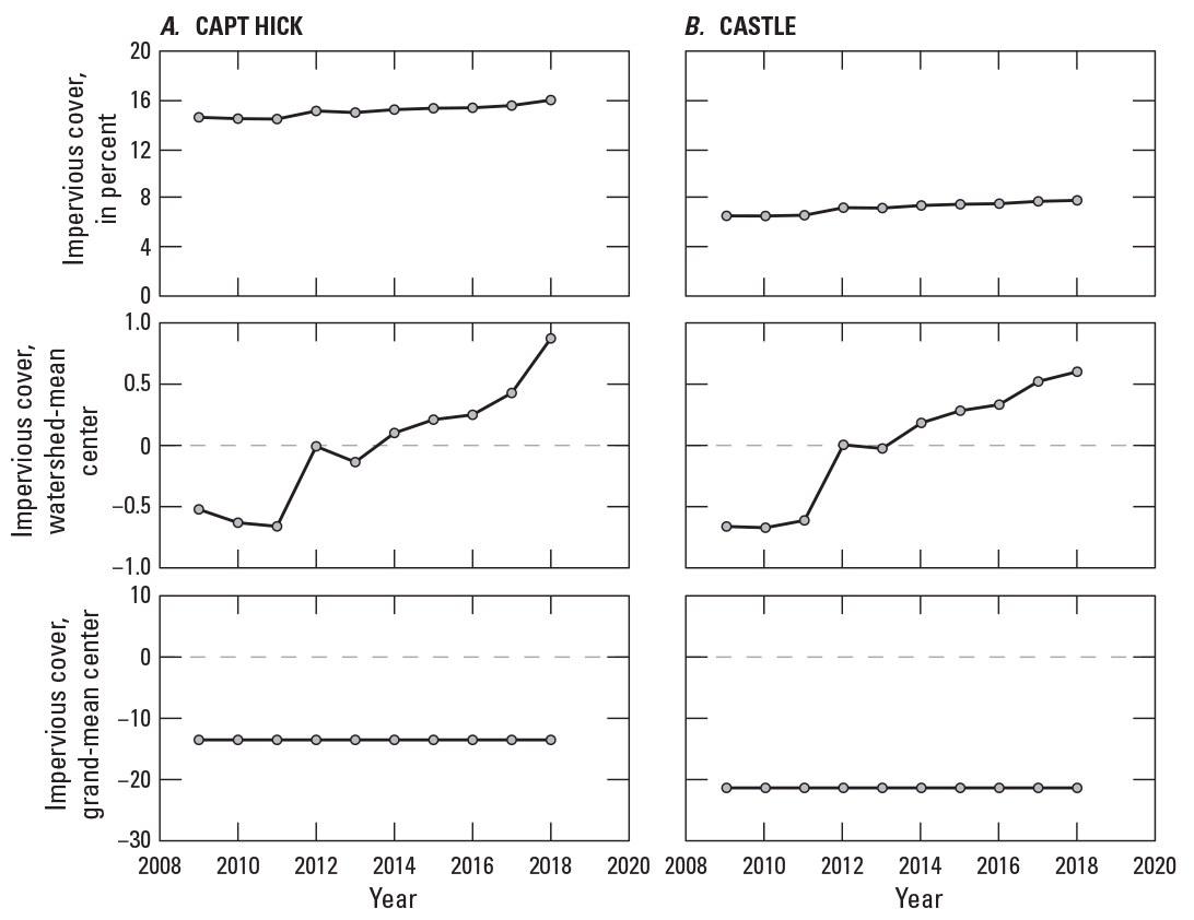
Graphs showing impervious cover in A, CAPT HICK and B, CASTLE study watersheds in Fairfax County, Virginia, from 2009 through 2018 and representations of how this term is centered for use in linear mixed-effect models. Study watershed station names are defined in table 1.
is the repeatedly measured variable at time t for individual i,
is the random intercept, or predicted score for individual i when t=0,
is the sample-level mean for the intercept,
is the relation between time-invariant predictors ( and individual-level intercept,
is the deviation of individual i from the sample mean intercept,
is the random slope, or rate-of-change for individual i for a one-unit change in t,
is the sample-level mean for the slope,
is the relation between time-invariant predictors ( and individual-level slope,
is the deviation of individual i from the sample-mean slope,
is the effect of time-varying covariates ,
are time-varying predictors, 1-f, at time t for individual i,
are the time-invariant predictors, 1-c, for individual i,
is a centered-time term, and
is the time-specific residual score.
The overarching goal of modeling water-quality responses with these additional parameters is to identify relations among watershed predictors and response variables. Specifically, models were constructed to address the following three relations: (1) predictors and average responses between watersheds, (2) predictors and the linear rate-of-change in responses between watersheds over the study period, and (3) annual changes in predictors and responses within watersheds over the study period. Except where the random-effect variance-covariance matrix converged to a perfectly linear relation (referred to as a singularity error in LME-model literature) and required simplification, all models were fit following recommendations advising the use of a maximal random-effect structure (Barr and others, 2013) and used a random intercept and random-linear relation with time for each watershed.
A combination of predictor variables was selected for consideration in LME models, largely guided by the evaluation of individual predictor-response relations and by applying professional judgement guided by previous Fairfax County studies (Hyer and others, 2016; Jastram, 2014; Porter and others, 2020b). After appropriate centering and decomposition, all possible combinations of selected predictors were modeled. Models that resulted in the largest variance reduction with the fewest additional parameters were prioritized because the linear-growth model described in equations 1–3 already contains six parameters for a response dataset of about 140 observations. Likelihood-ratio tests and model Akaike information criterion (AIC; Akaike, 1974) were used in model comparisons to determine the value of an added predictor. The usefulness of a predictor was also evaluated by examining the 95-percent confidence intervals of a coefficient to ensure that these ranges do not include zero. For all selected models, standardized coefficients are reported following methods described in Hoffman (2015) to determine the relative-effect size of predictors on modeled responses. Conditional and marginal R2 values are reported for selected models and respectively describe the proportion of total variance explained by fixed and random effects and by only fixed effects (Nakagawa and others, 2017). Tables used to evaluate relations between predictor and response variables and guide the selection of LME models are contained in appendix 1. Tables and figures that support the interpretation of selected and alternative LME models are contained in appendix 2.
Uncertainties and limitations of the predictor and response datasets affect the identification and interpretation of predictor-response relations. Except for climatic and water-quality data, most predictor data represent little change or a linear rate-of-change over the 10-year period; therefore, they do not help to explain the interannual differences in responses within watersheds. Therefore, temperature, precipitation, and water-quality terms, such as WT and DO, may be preferentially selected in LME models for their unique ability to reduce within-watershed variances. Causal links between response variables and annual measures of climate and water quality may exist, but the inclusion of these terms might be affected by the limited temporal accuracy of other predictor datasets.
Limitations of the LME model analysis also affect the identification and interpretation of predictor-response relations. This study did not consider every possible combination of predictors, predictor interactive effects, alternative random-effect structures, or models that may offer additional insights. LME models evaluate the strength of linear predictor-response relations and likely underrepresent non-linear patterns that may be present in the data. Strong correlations among predictors challenge the ability of LME models to identify the most influential predictors of a given response. It is convenient to discuss the interpretation of a single model; however, alternative models with similar performance often exist and are acknowledged in this report. Finally, the legacy effects of a predictor may heavily influence contemporary water-quality responses, but, generally, were not considered.
All LME model development was performed in R v.4.0.3 (R Core Team, 2020) using the “lme4” package (Bates and others, 2015). Standardized model coefficients were produced with the “standardize_parameters” function in the “effectsize” package (Ben-Shachar and others, 2020).
How did Landscape and Climatic Conditions Change?
Urban activities and climatic conditions interact with physical watershed properties to affect water-quality and ecological responses in Fairfax County streams. Patterns and changes in these predictors (table 3) from 2008 through 2018 were summarized and are described in the following paragraphs. In general, the monitoring network reflected a gradient of urban/suburban conditions, and the study period captured interannual climatic differences and an expansion of the built environment. Fairfax County’s population increased by about 10 percent, or 100,000 people (Han and others, 2018), requiring new homes, roads, and infrastructure to manage additional stormwater and wastewater (fig. 5 and 6). Some form of urbanization, characterized as an expansion of impervious surfaces, housing units, wastewater infrastructure, and/or stormwater infrastructure, occurred in all study watersheds throughout the study period (tables 7 and 8). Rates of urbanization during the study period generally were smaller than the increases in population and housing that occurred throughout Fairfax County in previous decades (fig. 5).

Graph showing observed and forecasted trends in the population and number of housing units in Fairfax County, Virginia, from 1970 through 2045. Population and housing unit estimates from Han and others (2018).

Aerial imagery showing selected areas in the A, DIFF; B, BRR; and C, PSB study watersheds in Fairfax County, Virginia, from 2009 and 2019. Study watershed station names are defined in table 1. Aerial imagery provided by Fairfax County (2022).
Table 7.
Summary of selected land-use and land-cover properties in 20 study watersheds and Fairfax County, including values in 2008 and the change in values from 2008 through 2018.[Station names are defined in table 1; predictor names are defined in table 3. %, percent]
Table 8.
Summary of selected housing, wastewater, and stormwater properties in 20 study watersheds and Fairfax County, including values in 2008 and the change in values from 2008 through 2018.[Station names are defined in table 1; predictor names are defined in table 3. n/mi2, number per square mile; mi/mi2, mile per square mile]
Countywide annual measures of air temperature and precipitation varied from 2008 through 2018. Total-annual precipitation ranged from 33.6 inches (in.) in 2012 to 62.6 in. in 2018 (fig. 7). The wettest years were associated with many heavy and very heavy rainfall days, defined by Donat and others (2013) as days receiving more than about 0.4 and 0.8 in. of precipitation, respectively (see predictors R10D and R20D in table 3). Average-annual air temperature ranged from 12.9 °C in 2014 to 15.4 °C in 2012 (fig. 7). Years with warmer average temperatures were generally associated with higher maximum- and minimum-annual temperatures, fewer frost days, and more summer days (see predictors TXx, TNn, FD, and SU in table 3).
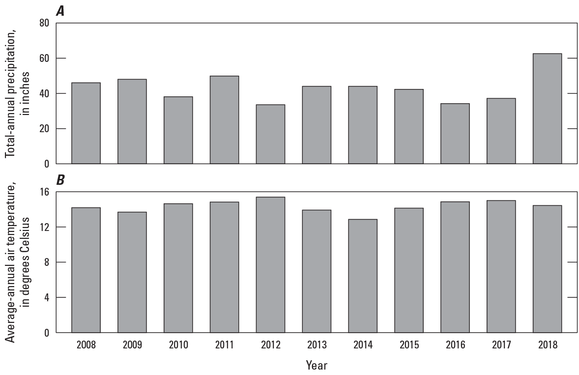
Bar graphs showing A, total-annual precipitation and B, average-annual air temperature in Fairfax County, Virginia, from 2008 through 2018.
Most measures of urban activity were related to one another (fig. 8). In general, more developed study watersheds contained greater amounts of impervious land and turfgrass cover and had higher densities of roadways, housing units, and stormwater and sanitary-sewer infrastructure. Lesser-developed study watersheds had more forested land and the highest septic-system densities. Landscape characteristics in 2008 (tables 7 and 8), were used in a hierarchical cluster analysis to classify the study watersheds into 1 of 3 groups (table 9). The intensity of development and impervious land cover increased from groups 1 to 3. The most high-density residential and commercial land uses were in group three watersheds: Old Courthouse Spring Branch near Vienna, Va. (OCSB) and Big Rocky Run at Stringfellow Road near Chantilly, Va. (BRR) (Jastram, 2014). The most open and low-density residential land and the greatest septic-system densities were in group one watersheds (CASTLE; Popes Head Creek Tributary near Fairfax Station, Va. [PHCT]; Little Difficult Run near Vienna, Va. [LIL DIFF]; CAPT HICK; and South Fork Little Difficult Run above mouth near Vienna, Va. [SFLIL]). The remaining 13 study watersheds in group two were mostly residential and had a level of urbanization common to Fairfax County.

Graphs showing the relations among selected predictors for 20 study watersheds in Fairfax County, Virginia, in 2013. Study watershed station names are defined in table 1.
Table 9.
Description of study watershed groups identified by a hierarchical cluster analysis.[Station names are identified in table 1]
Developed land, areas that contain a mixture of constructed materials and vegetation (mostly in the form of lawn grasses), covered about 56 percent of Fairfax County in 2008 and increased by about 1 percentage point, or 4.5 mi2, through 2018 (table 7). Most of the increase came from forested areas, which represented about 36 percent of Fairfax County in 2008 and 35.2 percent in 2018. On average, the study watersheds contained about 68 percent developed land in 2008, with a minimum value of 32 percent in LIL DIFF and a maximum value of 88 percent in BRR. Developed land increased in most study watersheds through 2018. Increases were as much as 2.2 percentage points (Rabbit Branch Tributary above Lake Royal near Burke, Va. [RABT], increased from 77.9 percent to 80.1 percent). Forested land in 2008 ranged from 9 percent in BRR to 62 percent in LIL DIFF and decreased in nearly all study watersheds through 2018.
Additional information about developed land was characterized from turfgrass and impervious coverage. Turfgrass covered about 31 percent of Fairfax County in 2008 and increased by about 2 percentage points, or 8.4 mi2, through 2018 (table 7). Turfgrass cover in 2008 in the study watersheds ranged from 22 percent in LIL DIFF to 49 percent in Horsepen Run above Horsepen Run Tributary near Herndon, Va. (HPEN), representing an average value of 38 percent. Turfgrass increased in all study watersheds by an average of 2.2 percentage points. Impervious cover represented about 21 percent of all land use in Fairfax County in 2008 and increased by about 2 percentage points, or 7.6 mi2, through 2018 (table 7). Impervious cover in 2008 in the study watersheds ranged from 6 percent in CASTLE to 50 percent in OCSB, representing an average value of 26 percent. Impervious cover increased in all study watersheds by an average of about 2.1 percentage points through 2018.
The 4,700 mi of roads in Fairfax County in 2011 increased by 100 mi, or about 2 percent, through 2017. About 72 percent of Fairfax County’s roadway length is local roads, but local road increases only represented about 28 percent of the total increases from 2011 through 2017; interstates, ramps, and major roadway length increased by 72 mi. Study watersheds with the most impervious cover had the highest roadway density and, in all watersheds, local roads represented most of the total roadway length. Total roadway length increased in most study watersheds from 2011 through 2017 by about 1.5 percent.
About 26,500 new housing units were added in Fairfax County from 2008 through 2018, an increase of 6.8 percent, mostly from the construction of multifamily homes such as apartments, condominiums, and townhouses. Total housing in 2008 in the study watersheds ranged from about 140 housing units per square mile in CASTLE to 2,700 housing units per square mile in BRR (table 8); more impervious watersheds typically have a higher housing density in the form of multifamily homes (fig. 8). The number of housing units increased in most study watersheds; the largest increases of about 741 and 367 units per square mile took place in OCSB and Difficult Run above Fox Lake near Fairfax, Va. (DIFF), respectively.
Most wastewater generated in Fairfax County is conveyed by a sanitary-sewer network to wastewater-treatment plants. The gravity sewers and force mains network in 2008 consisted of about 3,300 mi but expanded by about 2 percent, about 67 mi per square mile, through 2018 (table 8). Fairfax County has an inspection, maintenance, and cleaning program for their sanitary-sewer network. Hundreds of sewer miles are cleaned each year to prevent backups and overflows; backups and overflows have occurred about once per 100 miles of sewer over the past 5 years, a rate below established standards (Fairfax County, 2021). Most of the wastewater generated in 14 of the 20 study watersheds is conveyed by the sanitary-sewer network, but the other study watersheds are served entirely or mostly by septic systems (table 8). In these 14 study watersheds, the average sanitary-sewer line density was 14.3 mi per square mile; higher densities were in more impervious watersheds (fig. 8). The sanitary-sewer network expanded in most of these watersheds throughout the period by an average of about 0.8 mi per square mile or 1.2 percent.
Wastewater not conveyed by the sanitary-sewer network is treated by septic systems; residential parts of Fairfax County with low amounts of impervious cover typically use septic systems (fig. 8). About 20,100 septic systems were in Fairfax County in 2008, which increased by nearly 3 systems per square mile, or 6 percent, through 2018 (table 8). About half of these additions were alternative systems, those that were built with mechanisms to achieve greater reductions of nitrogen in drain fields, although such systems represented a small fraction of total Fairfax County septic systems. Almost every study watershed has septic systems, but only six study watersheds service all or most wastewater using septic systems (table 8). The density of septic systems in these 6 watersheds in 2008 ranged from about 115 systems per square mile in CASTLE to 490 systems per square mile in SFLIL. The number of septic systems increased in these 6 study watersheds through 2018: the largest changes being 22.4 systems per mi2 or a 5.3-percent increase in CAPT HICK and 15.8 systems per square mile or 7.6-percent increase in DIFF.
The Fairfax County stormwater network is designed to route runoff from impervious surfaces to streams and waterways to minimize flooding, pollution, and sediment erosion. The county performs routine inspections and maintenance of this network, which results in the replacement or renewal of pipes and the clearing and cleaning of stormwater structures (Stormwater Planning Division, 2018). In 2008, the stormwater network consisted of about 2,640 mi of pipes, most of which are maintained by Fairfax County. About 35 mi of stormwater pipes, 1.3 percent of the existing total, were added to the county through 2018. The 2008 density of stormwater pipes in the study watersheds ranged from about 0.1 mi of pipe per square mile in CASTLE to 16.7 mi of pipe per square mile in OCSB: a gradient consistent with the amount of impervious cover in each watershed (fig. 8). This stormwater pipe network increased slightly in most study watersheds (table 8).
What Water-Quality Management Practices were Used?
Fairfax County uses a variety of management strategies to protect and restore its water resources. Most of this responsibility is addressed by the county’s stormwater-management program, but many county programs also contribute to positive water-resource outcomes. The Fairfax County stormwater-management program pursues its goals of protecting property, health, and safety and improving the environment for public benefit through various policies, programs, and projects. A comprehensive stormwater regulation establishes guidelines for peak-flow volumes and water-quality criteria, which includes specific requirements for areas of new development and redevelopment. Programs to monitor and assess water resources are designed to characterize conditions, identify issues in local water bodies, and inform management strategies. Programs to inspect and maintain stormwater conveyance structures and facilities help ensure that the stormwater network is functioning as designed. Stormwater projects include non-structural components, such as educational and outreach efforts that are used to engage the public in resource protection, and structural projects, such as upgrades to the stormwater network, flood mitigation projects, stream stabilization projects, and projects designed to improve water quality. Structural stormwater projects that qualified for nitrogen, phosphorus, and (or) sediment load-reduction credits by the Chesapeake Bay Program are hereafter referred to as “management practices.” Structural projects not credited with load reductions and the effects of stormwater policies, programs, and non-structural elements are still expected to affect water-quality conditions; however, their combined effects are difficult to quantify and are not directly considered in this report.
Management Practices in Fairfax County
There were 245 management practices completed in Fairfax County from 2009 through 2018, representing a total investment of about 87 million dollars (table 10). Cumulatively, these practices treated runoff from about 47 mi2 of land and were credited with reductions of about 33,000 lb of nitrogen, 8,300 lb of phosphorus, and 1,600 tons of sediment (fig. 9). These cumulative values represent the additive credits from multiple practices completed over time, assuming that credited load reductions from all practices persist from year to year. Fairfax County has prioritized stormwater management for decades, but the crediting of nutrient and sediment load reductions associated with management practices by the Chesapeake Bay Program did not start until 2009 in response to local and regional total maximum daily load regulations. Because the programmatic elements of funding, planning, and construction of practices can take multiple years, most Fairfax County management practices were installed towards the end of the study period (fig. 10). Management practices are associated with many important benefits beyond credited nutrient reductions, including aesthetic improvements, enhanced recreational opportunities, removal of invasive vegetation, and educational benefits (Kenney and others, 2012), but these services were not the focus of this report.
Table 10.
Cumulative number, area treated, total cost, and credited load reductions of management-practice types completed in Fairfax County from 2009 through 2018.[mi2, square mile; TN, total nitrogen; lb, pound; TP, total phosphorus; TSS, total suspended solids]
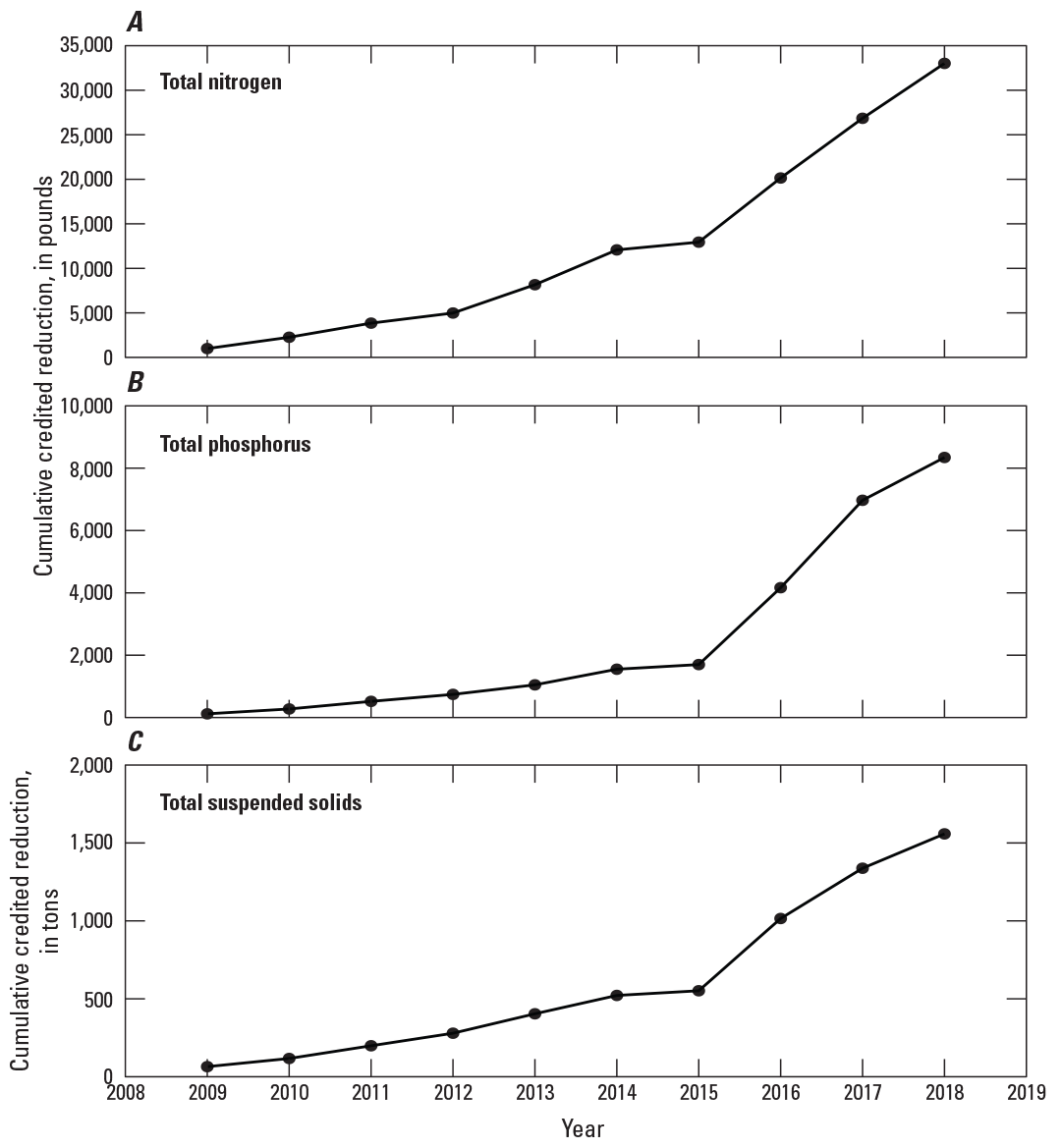
Graphs showing the cumulative credited reduction of A, total nitrogen; B, total phosphorus; and C, total suspended solids for Fairfax County management practices completed from 2009 through 2018.
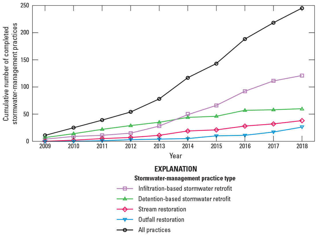
Graph showing the cumulative number of stormwater-management practices in Fairfax County, Virginia, from 2009 through 2018.
Fairfax County management practices were broadly classified as stormwater retrofits or channel-restoration practices (table 4). Detention-based stormwater retrofits comprise a suite of practices that reduce nitrogen, phosphorus, and (or) sediment loads through physical or biochemical processes by capturing stormwater runoff in temporary storage areas (Chesapeake Bay Program, 2018). Detention-based stormwater retrofits tend to be near surface waters and are designed to achieve load reductions through filtering or settling. Examples of detention-based stormwater retrofits include wetlands, ponds, and filtering practices, which represent traditional approaches to stormwater management; however, these types of retrofits are challenging to install in areas with existing development because of space limitations (National Research Council, 2009), which has led to the construction of some detention-based retrofits on rooftops or in underground facilities in recent years. Infiltration-based stormwater retrofits are in upland areas and achieve load reductions by enhancing infiltration and evapotranspiration. The most commonly used infiltration-based practices in Fairfax County includes bioretention areas, permeable pavement, and areas of land-use conversion. Land-use conversion generally consists of managed pervious or impervious area being changed to a native grassland or forested area. About twice as many infiltration-based retrofits were installed in Fairfax County than detention-based retrofits, but detention-based retrofits were credited with about four times more nitrogen and phosphorus load reduction and about eight times more sediment load reduction than infiltration-based retrofits (table 10). Larger reduction credits are typically assigned to detention-based practices because they treat more watershed area than infiltration-based practices. Constraints on available land for detention-based practices and the ability of infiltration-based practices to address multiple components of the hydrologic cycle (Jefferson and others, 2017) help explain the distribution of Fairfax County’s investment during the study period.
Channel restorations represent a large component of Fairfax County’s management-practice portfolio and include outfall restorations and stream restorations. Outfalls represent the discharge point where stormwater enters a water body, and their restoration primarily focuses on achieving sediment reductions by repairing and controlling bank erosion. Twenty-six outfall restorations were completed in Fairfax County and were credited with about 80 tons of sediment reduction and hundreds of pounds of nitrogen and phosphorus reduction (table 10). Stream restorations achieve water-quality load reductions by retaining sediment and attached nutrients in stable stream channels and floodplains that would otherwise be eroded downstream and by increasing biological nitrogen removal through instream processing, floodplain retention, or vegetative uptake (Chesapeake Bay Program, 2018). Fairfax County uses natural channel designs in their stream restorations, which modifies the pattern, profile, and dimensions of a disturbed stream section to achieve a more stable, natural form. Stream restorations can require intensive onsite construction, including hydrologic reconnection of the channel to the historical floodplain. Fairfax County uses these opportunities to also improve the surrounding floodplain conditions by planting native trees and vegetation in riparian areas, removing invasive species, and rehabilitating trails or walkways. Nearly 11 mi of streams were restored in Fairfax County from 2009 through 2018, representing 38 practices and investments of about 46 million dollars (table 10). Stream restorations represented about half of the dollars spent on all management practices and accounted for more than 70 percent of all credited nitrogen, phosphorus, and sediment reductions in Fairfax County (table 10). Based on reductions credited by the Chesapeake Bay Program, the average cost per pound removal rate of stream restorations is lower than outfall restorations, stormwater retrofits, and other treatment methods. Additionally, Fairfax County’s strategy of using stream restorations as a primary stormwater-management tool is influenced by the amount of streams on public land. Fairfax County’s land is mostly privately owned; however, many miles of stream channel are protected on park or county land and are, therefore, good candidates for restoration projects.
Management Practices in the Study Watersheds
Fifty-nine management practices were constructed in 10 of the 20 study watersheds from 2009 through 2018, 7 of these watersheds have been monitored since 2008 (table 11). Investments in these watersheds have been a focus of Fairfax County’s stormwater-management program because an overlap between management and monitoring offers opportunities to evaluate the credited load reductions against water-quality and ecological responses. The 20 study watersheds represent only 10 percent of the county’s land area but received 26 percent of all management-practice investments. Furthermore, three of the study watersheds with the largest cumulative credited TN, TP, and TSS reductions are intensive-monitoring stations that have been studied since 2008: DIFF, Flatlick Branch above Frog Branch at Chantilly, Va. (FLAT), and Dead Run at Whann Avenue near McLean, Va. (DEAD). Ten of the twenty study watersheds received no management-practice investments, offering an opportunity to compare water-quality responses between watersheds with and without management practices.
Table 11.
Cumulative number, cost, and credited load reductions of management practices completed in 10 study watersheds from 2009 through 2018.[Station names are defined in table 1. mi2, square mile; TN, total nitrogen; lb/mi2, pound per square mile; TP, total phosphorus; TSS, total suspended solids; ton/mi2, tons per square mile]
The number of completed management practices increased over time in each study watershed, but the timing, number, and type of practices and credited reductions differed among watersheds (fig. 11, fig. 12, and fig. 13). In general, most practices were completed toward the end of the study period. Only 15 of the 59 practices in study watersheds were completed from 2009 through 2013; an additional 44 practices were completed in the following 5 years. Of the 10 watersheds with at least 1 management practice, 4 (Indian Run at Bren Mar Drive at Alexandria, Va. [INDIAN], Dogue Creek Tributary at Woodley Drive at Mount Vernon, Va., Long Branch near Annandale, Va., and Turkeycock Run at Edsall Road at Alexandria, VA) had no practices installed during the first 5 years.
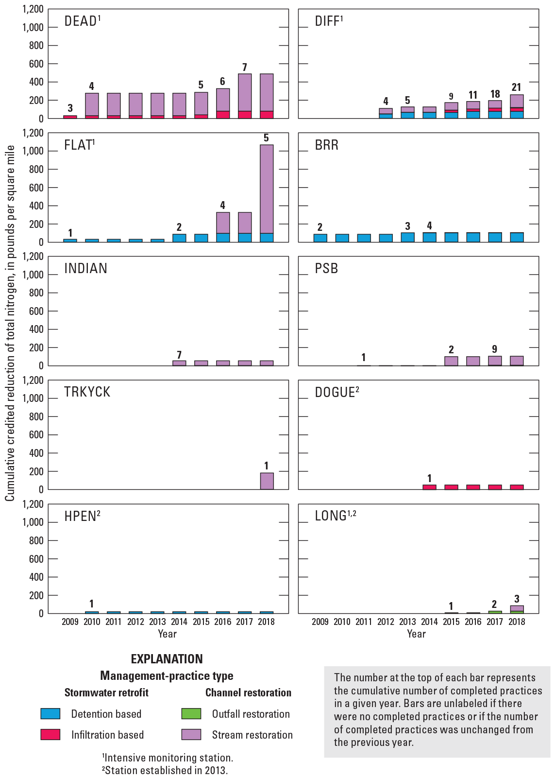
Bar graphs showing the cumulative credited reductions of total nitrogen from management practices completed in 10 study watersheds in Fairfax County, Virginia, from 2009 through 2018. Study watershed station names are defined in table 1.
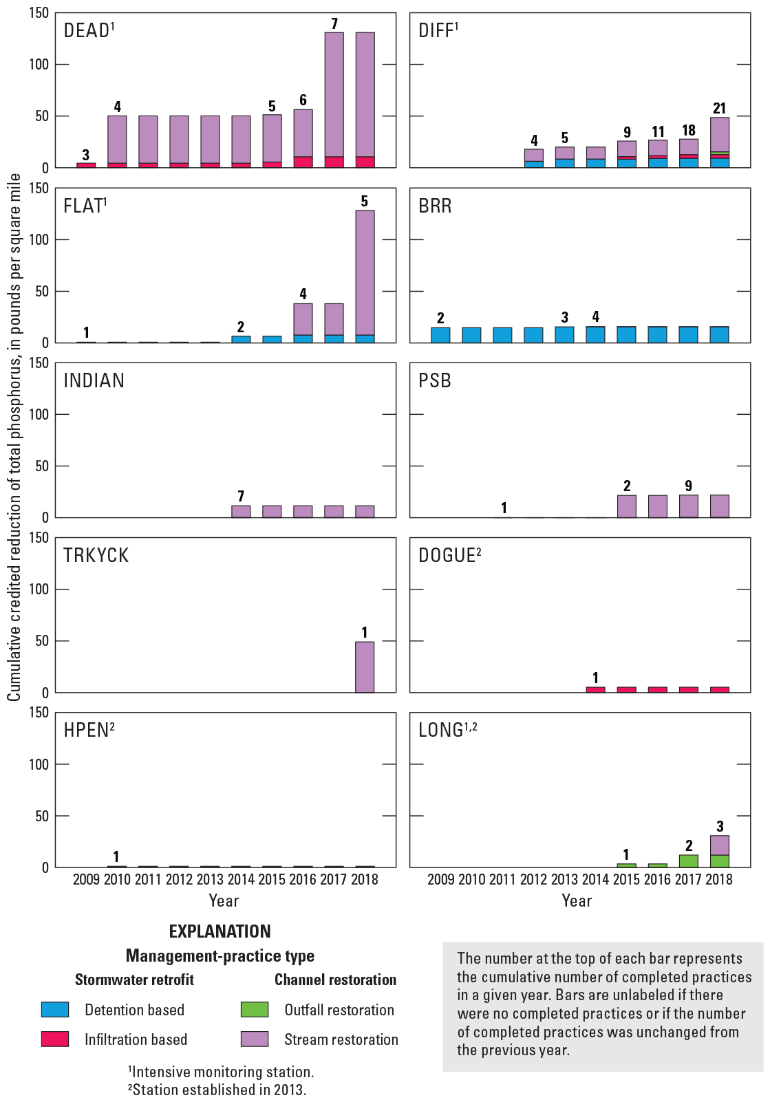
Bar graphs showing the cumulative credited reductions of total phosphorus from management practices completed in 10 study watersheds in Fairfax County, Virginia, from 2009 through 2018. Study watershed station names are defined in table 1.
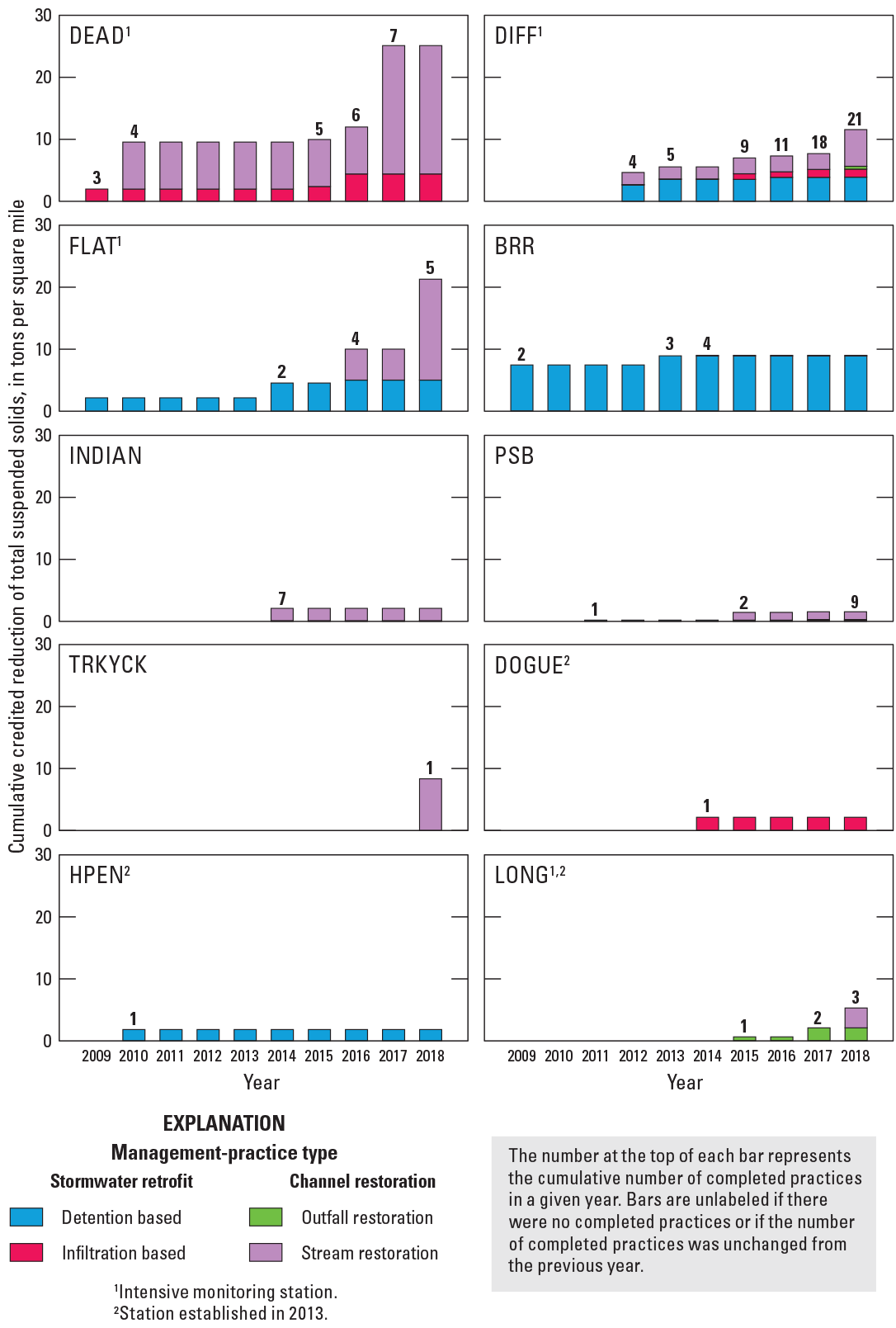
Bar graphs showing the cumulative credited reductions of total suspended solids from management practices completed in 10 study watersheds in Fairfax County, Virginia, from 2009 through 2018. Study watershed station names are defined in table 1.
At least one stream restoration was completed in seven study watersheds. Stream restorations accounted for most of the total credited TN, TP, and TSS reductions in these watersheds (table 12). Stream restorations were typically in the upper reaches of each watershed, away from the monitoring stations at the watersheds’ outlets, exceptions being at FLAT and INDIAN. About 6,000 ft of stream was restored in FLAT as part of restorations completed in 2016 and 2018 (table 13). The 2016 restoration, Flatlick Phase I, restored about 2,000 ft of stream and was about 3,000 ft upstream from the monitoring station; the 2018 restoration, Flatlick Phase II, restored about 4,000 ft of stream and included the monitoring station reach. A previously restored stream section in INDIAN was stabilized in 2014 (table 13), and bioretention cells were constructed along this stream reach. The INDIAN monitoring station is at the downstream extent of this stream reach.
Table 12.
Number of completed stream restoration and non-stream restoration management practices and the percentage of all management-practice load reduction credited to stream restorations in 10 study watersheds from 2009 through 2018.[Station names are defined in table 1. TN, total nitrogen; TP, total phosphorus; TSS, total suspended solids; %, percent]
Table 13.
Summary of stream restorations in seven study watersheds in Fairfax County, Virginia, from 2009 through 2018, including project name, year completed, restored stream length, and credited load reduction.[Station names are defined in table 1. ft, foot; TN, total nitrogen; lb/yr, pound per year; TP, total phosphorus; TSS, total suspended solids; tons/yr, ton per year]
Stormwater-retrofit practices, represented by infiltration-based and detention-based practices, were installed in eight study watersheds and treated less than 8 percent of watershed area in each study watershed (table 14). Infiltration-based practices were constructed in six study watersheds and detention-based practices were constructed in five study watersheds (table 14). Infiltration-based retrofit practices were especially numerous in DIFF, where 12 such practices were constructed, represented by permeable pavement, bioretention areas, dry swales, vegetated roofs, rainwater harvesting, and land-use conversion to a pollinator meadow. Infiltration-based practices typically were installed in spatially clustered groups throughout each watershed. In DIFF, most infiltration-based practices were completed on the Fairfax County Government Center campus in 2017. Likewise, in Paul Spring Branch above North Branch near Gum Springs, Va. (PSB), all seven infiltration-based practices were completed at an elementary school in 2017.
Table 14.
Summary of stormwater-retrofit practices in 10 study watersheds in Fairfax County, Virginia, from 2009 through 2018, including number of practices and percentage of watershed area treated.[Station names are defined in table 1. mi2, square mile; %, percent]
How did Hydrology and Water Quality Vary During Storm Events?
Hydrologic responses and nutrient and sediment EMCs were evaluated during storm events to assess how conditions varied among watersheds and over time. This work expands on the analysis of streamflow by Porter and others (2020b), which provides a thorough characterization of hydrologic conditions observed in the study watersheds. Interpretations from that report highlight the importance of storm conditions on hydrologic and water-quality responses and the need for an analysis focused only on storm events, as most streamflow occurs as stormflow and storm events deliver most of the nutrient and sediment load to streams. The analysis described below may help identify effects of management practices designed to attenuate stormflow runoff. Management practices are often designed to achieve nutrient and sediment load reductions by lowering the quantity of stormwater runoff and altering the shape of the hydrograph, benefits that have been observed in similar watershed settings (Jefferson and others, 2017).
Differences Among Study Watersheds
The average number of annual storm events differed among watersheds from August 2009 through March 2018. The average number of storm events per year ranged from about 12 in CASTLE to 40 in OCSB, averaging 22 annual storm events across all 14 watersheds. The average number of annual storm events was higher in watersheds with more impervious surfaces (fig. 14), likely because impervious surfaces quickly convert precipitation to runoff (Booth and Jackson, 1997; O’Driscoll and others, 2010; Paul and Meyer, 2001). A hydrograph’s rising-limb duration is affected by runoff generation and was shorter in watersheds with more impervious cover because such watersheds provide less opportunity to slow runoff through evaporation, transpiration, and infiltration (fig. 14). Median rising-limb duration ranged from 1.8 hours in DEAD to 4.8 hours in CASTLE. Falling-limb duration is affected by the storage and release of runoff and was strongly correlated with watershed area; median values ranged from 9.8 hours in DEAD to 35.9 hours in DIFF (fig. 14). Larger watersheds can store more water than smaller watersheds, and they have longer stream networks that can increase the amount of time it takes stormflow to be delivered to a downstream monitoring station.
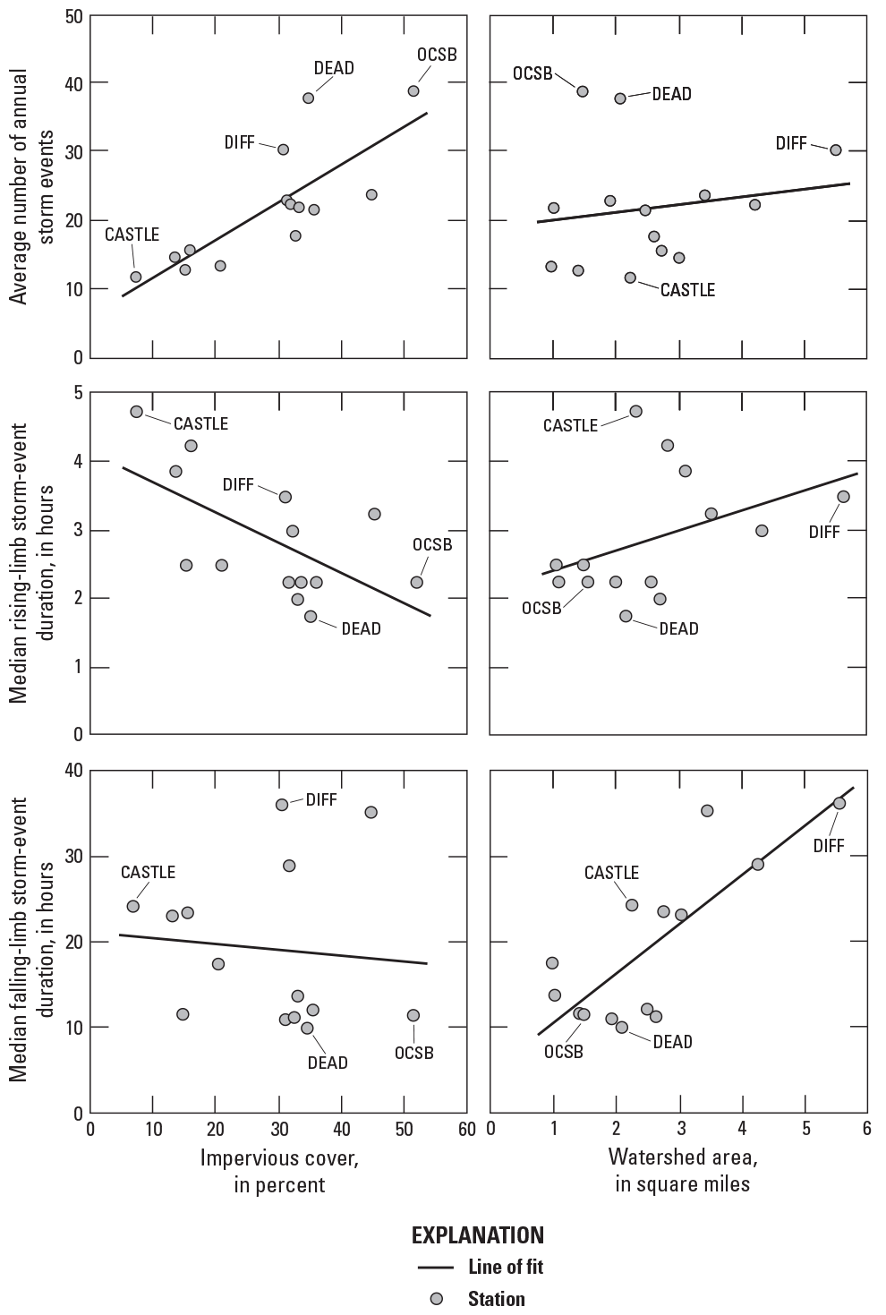
Graphs showing the relations of median duration and average-annual number of storm events to watershed area and percentage impervious cover in 14 study watersheds in Fairfax County, Virginia, from August 2009 through March 2018. Study watershed station names are defined in table 1.
In general, differences in storm-event hydrology among the four intensive-monitoring watersheds were similar to differences in annual hydrology described by Porter and others (2020b). Normalized by watershed area, the median stormflow peak and rising-limb rate-of-change was highest at DEAD (table 15), the most impervious intensive-monitoring watershed. The area-normalized median volume of streamflow during storm events was highest in FLAT and DIFF, the largest intensive-monitoring watersheds.
Table 15.
Summary of the number of storm events, median storm-event hydrologic metrics, and median event-mean concentrations in four study watersheds in Fairfax County, Virginia, from water years 2009 through 2017.[Station names are defined in table 1. ft3/mi2, cubic foot per square mile; [ft3/s]/mi2, cubic foot per second per square mile; [[ft3/s]/hr]/mi2, cubic foot per second per hour per square mile; mg/L, milligram per liter]
EMCs representing flow-weighted average concentrations that occurred during storm events, were generally higher than concentrations observed during non-storm conditions and differed among the four intensive-monitoring watersheds (table 15). The EMCs of TP and SS were strongly correlated with larger, flashier storm events, whereas the EMCs of TN were less affected by storm hydrology (table 16), likely because particulate material represents a larger fraction of TP and SS concentrations than TN. The median TN and TP EMCs were highest at SFLIL and lowest at DIFF. The median SS EMC was about twice as high at SFLIL than other stations. Impervious cover is lower at SFLIL than the other intensive-monitoring stations, which likely limits the frequency of smaller, short-duration storm events and explains why the watershed had the fewest storm events over the period of record (table 15). The absence of these smaller events may increase the storage of in-channel or near-channel sediment, which is delivered during large storm events, resulting in high SS and TP EMCs (Porter and others, 2020b). Differences in rates of streambank erosion or changing stream channel geomorphology may also contribute to these high concentrations but were not directly evaluated in this study.
Table 16.
Correlations between storm-event hydrologic responses and event-mean concentrations in four study watersheds in Fairfax County, Virginia, from water years 2009 through 2017.[Station names are defined in table 1]
Relations with Season and Time
Seasonal variability was apparent by the number and duration of storm events as a result of seasonal climatic patterns. At most stations, summer months had more storm events on average than other seasons of the year, but the storm events were of a shorter duration (fig. 15). Such hydrologic responses likely resulted from intense short-duration precipitation events, which are more common during periods of warm air temperature (Allen and Ingram, 2002; Trenberth and others, 2003). Seasonal variation in the number of storms differed by station and may be affected by the urban environment. Watersheds with high amounts of impervious cover, such as DEAD, had more summertime storm-event responses than those with lower impervious cover, such as SFLIL, likely because impervious surfaces provide an efficient route for the runoff of short-duration precipitation events to streams (O’Driscoll and others, 2010). Extreme precipitation events, representing short-duration, very high-intensity precipitation, occur most frequently in summer months (Janssen and others, 2016), have become more common in recent years (Wuebbles and others, 2017), and pose a substantial risk for flooding in urban areas as flood-control infrastructure may not adequately handle such events (Sridhar and others, 2019). Similarly, management practices designed to attenuate runoff and reduce nutrients and sediment may perform less efficiently during extreme precipitation events (Hopkins and others, 2020; Loperfido and others, 2014). These patterns highlight the importance of considering seasonal differences in storm-event hydrology as part of stormwater-management planning.
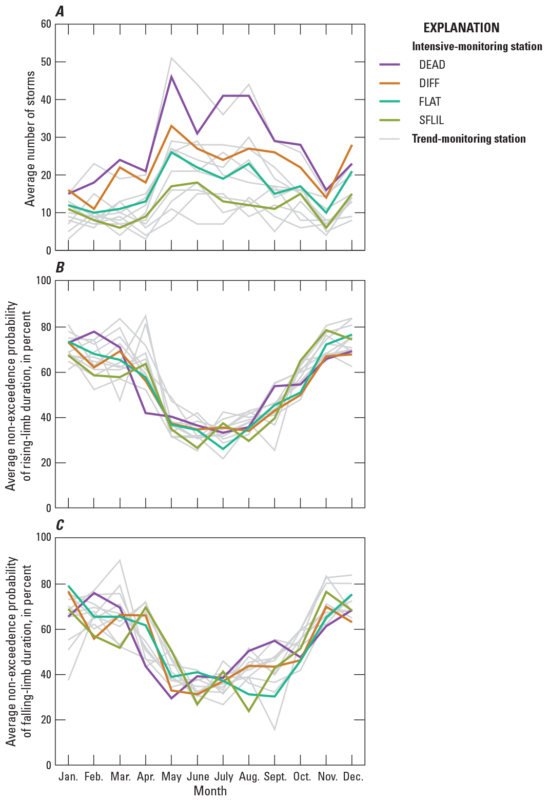
Graphs showing the A, average number of storm events and the B and C, non-exceedance probabilities of rising- and falling-limb duration for months in 14 study watersheds in Fairfax County, Virginia, from August 2009 through March 2018. Study watershed station names are defined in table 1. Jan., January; Feb., February; Mar., March; Apr., April; Aug., August; Sept., September; Oct., October; Nov., November; Dec., December.
Median EMCs of TN, TP, and SS varied by month, reflecting seasonal differences in biochemical processes and hydrologic responses (fig. 16). Median TN EMCs typically were highest in early spring and declined through the growing season, a pattern consistent with effects of biological processing and similar to the seasonal response of nitrogen previously documented in Fairfax County streams (Jastram, 2014; Porter and others, 2020b). The highest TP EMCs were commonly observed in summer months, likely a result of frequent, short-duration summer storm events (fig. 15). Although storm-event TP concentrations were mostly represented by particulate material, elevated TP concentrations have been observed in Fairfax County streams during non-storm conditions in warmer months. Such patterns likely result from temperature-dependent processes that release phosphorus from sediments to streams and from biological processing (Porter and others, 2020b; Dodds, 2003). Similar to TP, SS EMCs were typically highest in some summer months, again highlighting how intense short-duration storm events can mobilize large amounts of particulate material to streams.
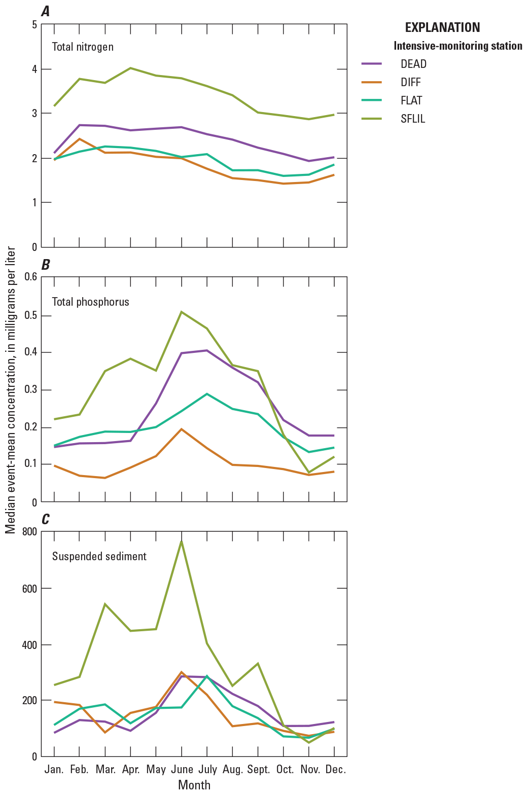
Graphs showing the median monthly event-mean concentration of A, total nitrogen; B, total phosphorus; and C, suspended sediment in four study watersheds in Fairfax County, Virginia, from water years 2009 through 2018. Study watershed station names are defined in table 1. Jan., January; Feb., February; Mar., March; Apr., April; Aug., August; Sept., September; Oct., October; Nov., November; Dec., December.
The number of storm events in each watershed varied from 2010 through 2017 (fig. 17). Normalized by the average-annual number of storm events across the 14-station network, changes in the number of annual storms would suggest that a station is experiencing a storm-event hydrologic response more or less frequently. The number of interannual storms events varied in each watershed, but only the change in PSB, a decrease of about two storms per year, represented a statistically significant linear trend (p-value ≤0.05), though such information should be treated with caution because results are based only on eight annual observations per watershed.
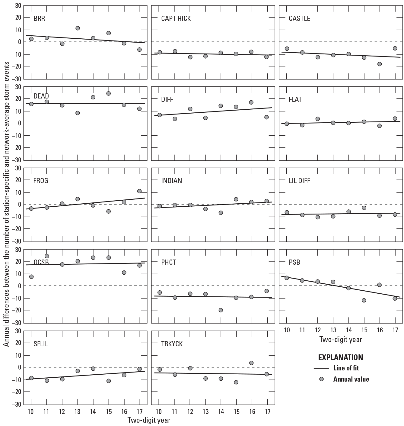
Graphs showing the number of annual storm events in 14 study watersheds in Fairfax County, Virginia, relative to the annual average value across all study watersheds, from 2010 through 2017. Study watershed station names are defined in table 1.
Changes in the duration of storm events were small at most stations from August 2009 through March 2018. Trends in rising- and falling-limb duration were based on 100 to 350 storm events in each watershed, and only 2 watersheds had a significant linear trend (p-value ≤0.05). The duration of the falling limb decreased at BRR and PHCT by about 100 minutes per year (fig. 18). Shorter falling-limb durations indicate that storm peaks return to base flow more quickly, which may result from changes in landscape and (or) climatic conditions. However, storm-event durations did not change in most watersheds, despite a general expansion of urban activities during the study period (table 7 and table 8).
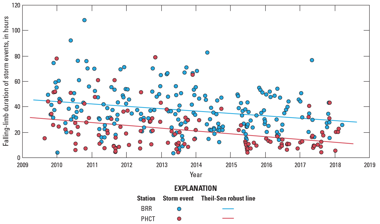
Graph showing the falling-limb duration of storm events in two study watersheds in Fairfax County, Virginia, from August 2009 through March 2018. Study watershed station names are defined in table 1.
Changes in storm-event streamflow metrics at four intensive-monitoring stations from water years 2009 through 2017 generally indicate that hydrologic conditions improved at DIFF and SFLIL and degraded at DEAD and FLAT (fig. 19). Normalized by watershed area, storm events in DEAD and FLAT tended to generate higher peak flows and had a faster rising-limb rate of streamflow change than DIFF or SFLIL (table 15). Both metrics increased over time in DEAD and FLAT, indicating that storm events had higher peak flows and reached peak streamflow more quickly in later years in these watersheds. Changes in streamflow volume during storm events were generally consistent with changes in peak flow, though no change in streamflow volume occurred in FLAT and SFLIL. The hydrologic changes in DIFF are consistent with the desired effect of many management practices: a reduction in peak flows and a lower streamflow rate-of-change. Many management practices were installed in DIFF during the study period (table 11); however, similar hydrologic improvements occurred in SFLIL, an adjacent watershed with no reported practice implementation during the study period. Changes in storm-event hydrology were likely affected by a variety of factors, including urban activities and climatic conditions (Bell and others, 2016; Paul and Meyer, 2001; Willems and others, 2012). Impervious cover expanded in all watersheds, but the expected hydrologic effects of such changes, increased stormflow peaks and streamflow rate of change, were only observed in DEAD and FLAT. Increased impervious cover may have had a smaller impact on hydrologic responses in DIFF and SFLIL because overall impervious area in these watersheds was smaller than DEAD and FLAT (table 7).
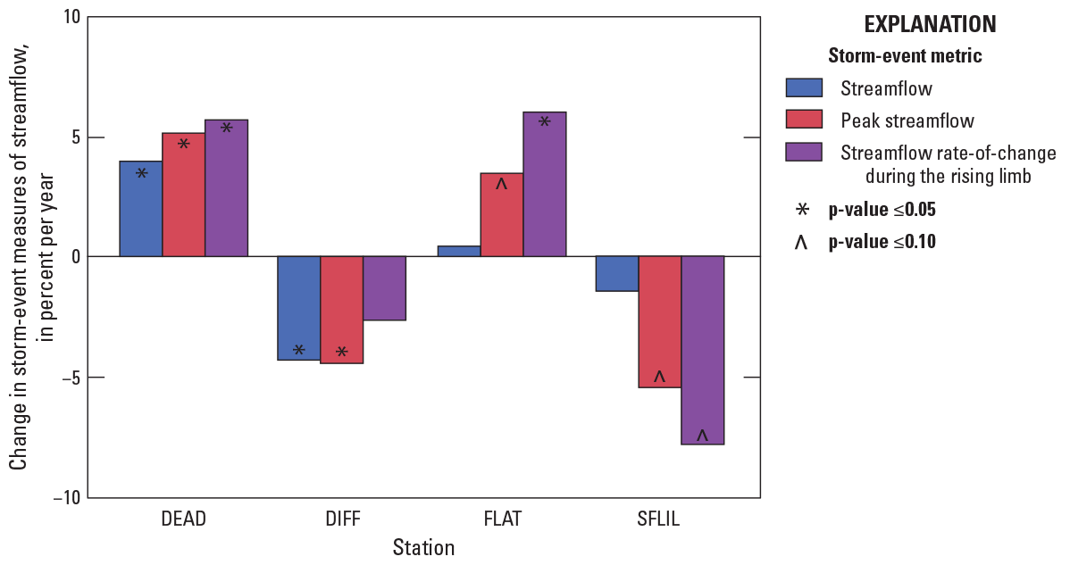
Graph showing the change in storm-event streamflow metrics in four study watersheds in Fairfax County, Virginia, from water years 2009 through 2017. Study watershed station names are defined in table 1.
Changes in EMCs of TN, TP, and SS from water years 2009 through 2017 were similar among the four intensive-monitoring stations (fig. 20), despite the previously described differences in storm-event hydrologic changes. In addition to the effects of rainfall volume and intensity, which may have varied between watersheds, EMCs were likely affected by differences in impervious cover among the watersheds (Perera and others, 2021). The EMC of TN decreased at FLAT by about 2 percent per year and was unchanged in other watersheds. Despite faster and larger storm events in FLAT and DEAD over the period of record (fig. 19), the nitrogen concentrations in storm-event runoff did not increase. At SFLIL and DIFF, reduced storm peaks and slower streamflow rates of change also resulted in no TN changes over the period of record. The lack of TN change at SFLIL is in contrast to increasing TN concentrations previously documented there over a similar period during non-storm conditions (Porter and others, 2020b), likely highlighting an increase in groundwater nitrate during lower flows that is less influential during storm conditions. Correlations between TN EMCs and streamflow metrics support the lack of consistency between changes in hydrology and concentration, as larger and faster storm events were generally not associated with higher TN concentrations (table 16).
The EMC of TP increased by 4–8 percent per year in all watersheds except FLAT (fig. 20). The TP increases in DEAD, where SS also increased, may be driven by the larger and flashier storm-event hydrologic responses observed in this watershed (fig. 19). In all watersheds, EMCs of TP and SS increased in relation to increased storm-event streamflow, faster rise rates, and higher peak flows (table 16)—characteristics that increase the transport of particulate materials (Edwards and Owens, 1991). TP and SS have a weaker relation to storm-event hydrology at FLAT than at DEAD, so the larger and flashier storm-event hydrologic responses in FLAT did not result in TP or SS increases. TP and SS may be less susceptible to larger and faster storms in FLAT than DEAD, because FLAT has shallower, flatter, and wider stream valleys (Porter and others, 2020b). The lower stormflow peaks and rate-of-change at DIFF and SFLIL were associated with no changes in SS EMC and increases in TP EMC (fig. 20). These patterns indicate that, although storm-event peak flows and rate of streamflow change declined over the period of record, storm events contained higher TP concentrations in later years. Particulate material represents the largest fraction of TP during storm events, but the increased release of phosphorus stored in soils and the decreased retention of phosphorus inputs in the landscape can affect the availability of dissolved phosphorus in streams and may contribute to these changing conditions.
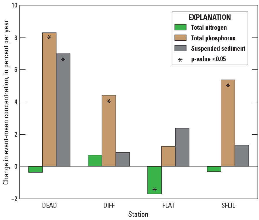
Bar graph showing changes in event-mean concentrations of total nitrogen, total phosphorus, and suspended sediment during storm events in four study watersheds in Fairfax County, Virginia, from water years 2009 through 2017. Study watershed station names are defined in table 1.
How did Water-Quality Loads Relate to Nutrient Inputs and Management Practices?
Effective management strategies target the most important sources of nutrients and control how material is delivered from the landscape to streams, information that often is uncertain and difficult to quantify in urban landscapes. Although point-source discharges are often well-controlled and documented, nonpoint-urban sources are diverse, particularly difficult to estimate, and less understood (Ator, 2019; Carpenter and others, 1998; Walsh and others, 2005). Not all watershed nutrient inputs reach streams. The relation between nutrient inputs and loads delivered to streams can be described as watershed nutrient retention, higher rates of retention are associated with lower loads and a greater proportion of inputs stored within or permanently removed from a watershed (Caraco and others, 2003; Hobbie and others, 2017). Nutrient retention rates are affected by a variety of physical watershed properties urban activities, and seasonal, hydrologic, ecological, and climatic conditions; lower retention rates in urban watersheds were commonly associated with areas of high impervious cover (Baron and others, 2013; Bratt and others, 2017; Groffman and others, 2004; Hobbie and others, 2017; Pfeifer and Bennett, 2011; Wollheim and others, 2005).
Nutrient Inputs
Nitrogen and phosphorus inputs were estimated for Fairfax County and the 20 study watersheds as the combination of point-source discharges, atmospheric deposition of nitrogen, fertilizer, pet waste, septic effluent, and weathering of phosphorus-bearing geologic materials (table 6). Potential nutrient inputs not represented in this study include atmospheric phosphorus inputs, septic phosphorus inputs, sanitary-sewer line exfiltration, wildlife waste, and agricultural inputs of manure and fertilizer. These inputs were not possible to quantify from available data, have uncertain influences on urban nutrient budgets, and (or) were assumed to represent minor inputs in Fairfax County.
Nitrogen and phosphorus inputs in Fairfax County were mostly nonpoint sources, but contributions of nonpoint inputs varied among the 20 study watersheds (fig. 21). At the county scale, nitrogen atmospheric deposition and phosphorus fertilizer represented the single largest inputs (30 percent and 60 percent of all inputs in 2013, respectively). In the study watersheds, fertilizer was commonly the largest phosphorus input, whereas the largest nitrogen inputs were a combination of atmospheric deposition, pet waste, fertilizer, or septic effluent. The distribution of inputs reflects urban activities. Septic inputs were typically largest in the least developed watersheds, pet waste inputs were typically largest in the most impervious watersheds caused by high housing-unit densities, and fertilizer inputs were typically largest in watersheds with low- to medium-density residential land use because of high turfgrass cover. Collectively, most of the nitrogen and phosphorus inputs in Fairfax County and the study watersheds were contributed from the household landscape: a finding observed in similar urban watersheds (Hobbie and others, 2017).
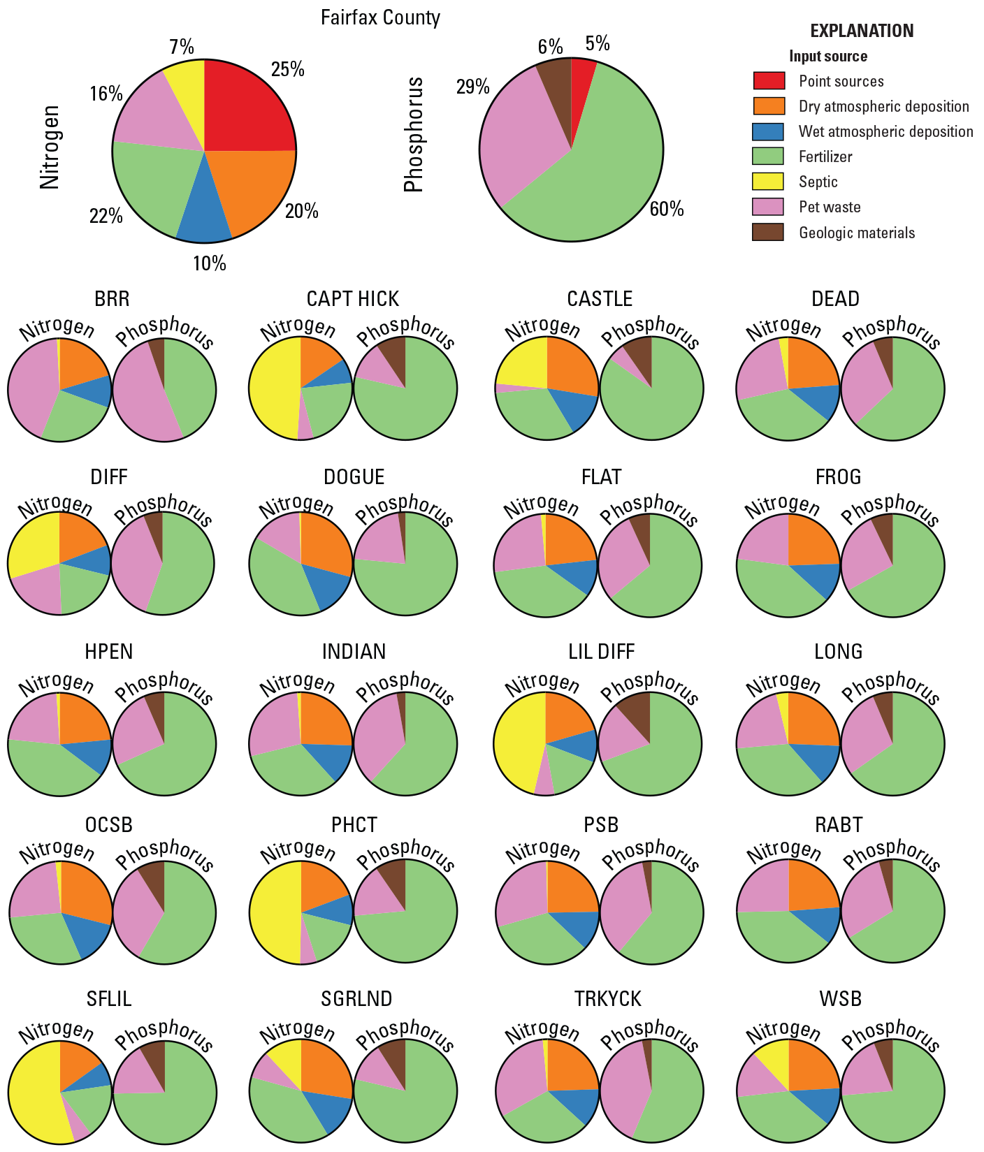
Pie charts showing nitrogen and phosphorus inputs in 2013 in Fairfax County, Virginia and the 20 study watersheds. Study watershed station names are defined in table 1. %, percent.
Nitrogen inputs in Fairfax County and most study watersheds declined from 2008 through 2018, in comparison, phosphorus inputs were relatively unchanged. Nitrogen declines equal to or greater than 1.5 pounds per acre were observed in half of the study watersheds as a result of atmospheric deposition declines (fig. 22A and fig. 23A). In general, pet waste, fertilizer, and septic effluent nitrogen sources did not decline. Nitrogen inputs increased in DIFF and OCSB because of increases in turfgrass cover, housing units, and septic systems (table 7 and table 8). Without the benefit of atmospheric reductions, phosphorus inputs increased slightly in six study watersheds or remained otherwise unchanged (fig. 22B and fig. 23B).
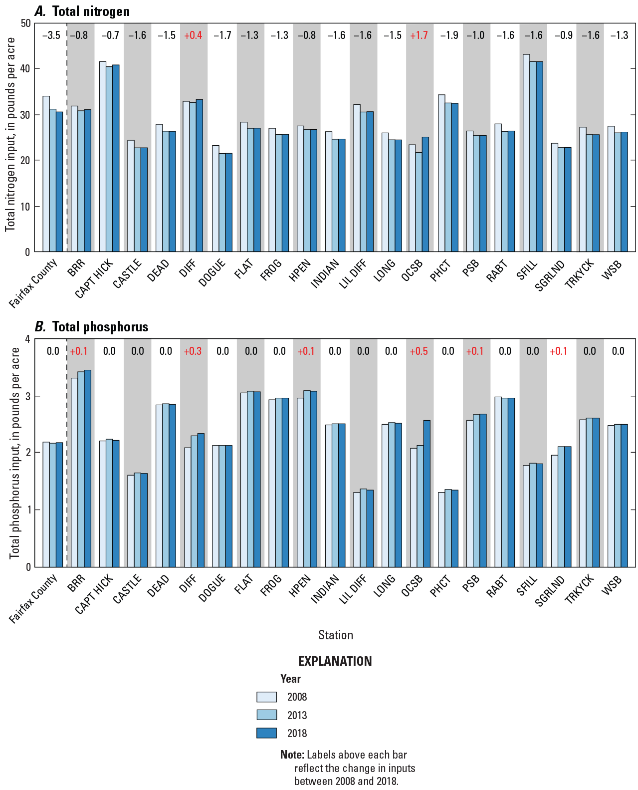
Bar graphs showing A, total nitrogen and B, total phosphorus inputs in 2008, 2013, and 2018 in Fairfax County, Virginia, and the 20 study watersheds. Study watershed station names are defined in table 1.
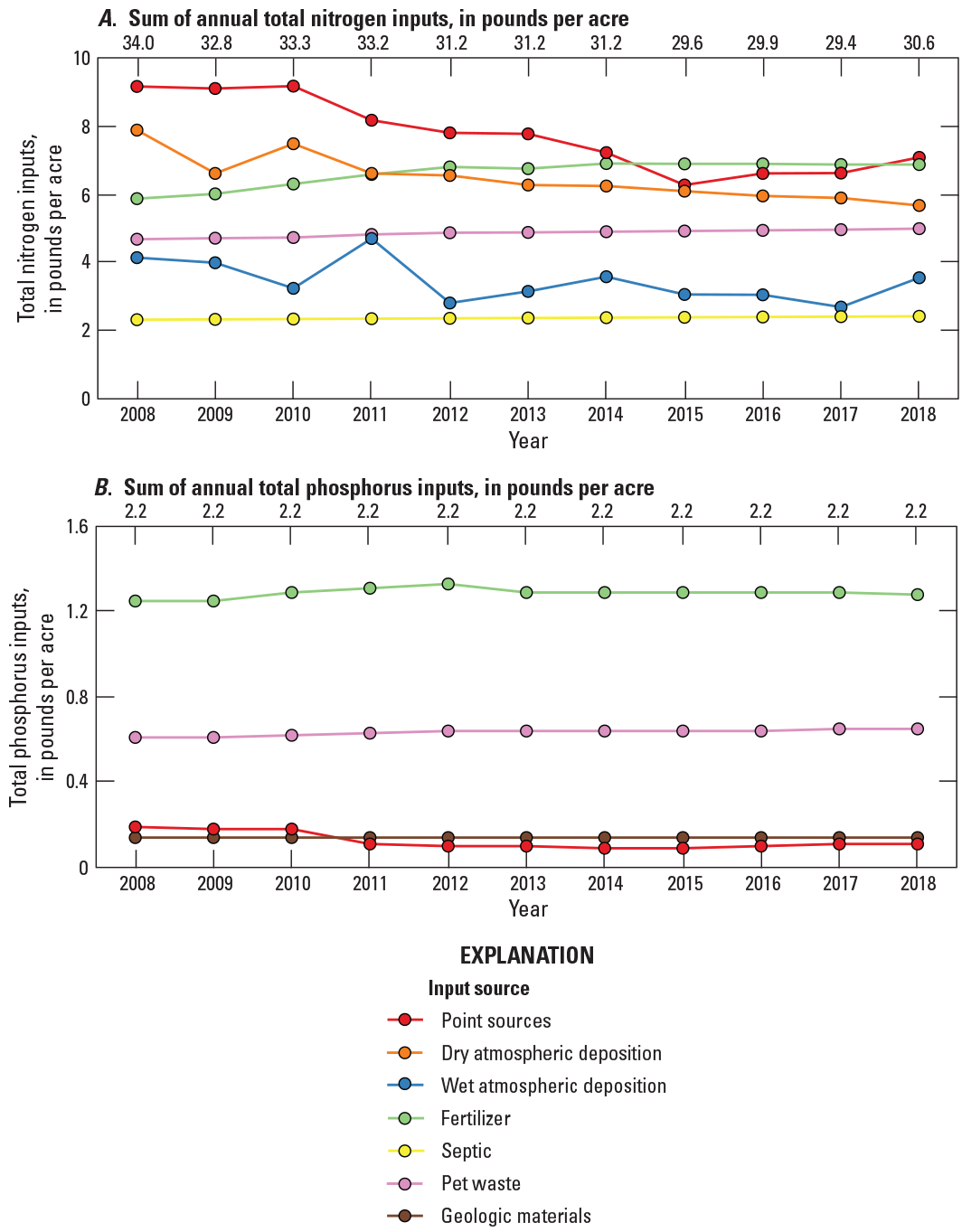
Graphs showing A, total nitrogen and B, total phosphorus inputs by source in Fairfax County, Virginia, from 2008 through 2018.
Point-source discharges from wastewater-treatment plants and other municipal/industrial sources are important nutrient inputs because their loads are delivered directly to streams. Point sources can represent a large fraction of urban nutrient budgets, but their loads have generally declined over time as a result of facility improvements, which has improved water-quality throughout the Chesapeake Bay watershed (Boynton and others, 2008; Lyerly and others, 2014) and within Fairfax County (Jones, 2020). Point sources reported for all of Fairfax County include major wastewater-treatment plant discharges from Blue Plains, Noman M. Cole Pollution Control Plant, and Upper Occoquan Sewage Authority, which discharge to the Potomac River, Pohick Creek, and Bull Run, respectively (fig. 1). Point-source inputs in Fairfax County represented about 25 percent of all nitrogen and 5 percent of all phosphorus inputs (fig. 21) and declined over the study period (fig. 23). There are no point-source discharges in the study watersheds.
Total atmospheric deposition (wet plus dry fractions) was the largest Fairfax County nitrogen input (30 percent of all inputs in 2013) and one of the largest nitrogen inputs in most study watersheds, ranging between 23 percent and 44 percent of all inputs in 2013 (fig. 21). These estimates are similar to the estimates from other urban study areas (Groffman and others, 2004; Hobbie and others, 2017; Kaushal and others, 2011; Wollheim and others, 2005). Most atmospheric nitrogen in Fairfax County is contributed by dry depositional processes, a fraction that can be elevated in urban areas from sources including powerplants and vehicles (Walker and others, 2019). Such local dry deposition is difficult to capture in regional monitoring networks, often resulting in an underestimation of dry nitrogen deposition in urban areas (Bettez and Groffman, 2013). Most forms of atmospheric nitrogen have declined in recent decades as a result of Clean Air Act Amendments (Burns and others, 2021); however, dry ammonia deposition from vehicle sources has likely increased (Bettez and Groffman, 2013). The contribution of atmospheric nitrogen to urban streams can be highest during stormflows and lowest during base flow (Kaushal and others, 2011), a pattern observed in Fairfax County’s Difficult Run watershed (Hyer and others, 2016). Atmospheric contributions, however, are not always dominant during stormflows, suggesting a complex relation likely affected by precipitation intensity, seasonality, and other nonpoint sources (Burns and others, 2009).
Fertilizer was the largest phosphorus input and one of the largest nitrogen inputs in Fairfax County (60 percent and 22 percent of all inputs in 2013, respectively), was a large input in many study watersheds (fig. 21) and increased during the study period in areas where turfgrass cover expanded (table 7). Fertilizer is a large nitrogen input in many urban watersheds (Groffman and others, 2004; Kaushal and others, 2011; Wollheim and others, 2005), and although elevated phosphorus concentrations have been associated with fertilizer use (Garn, 2002; King and others, 2007), more recent estimates of phosphorus fertilizer inputs are lower in some urban areas because of legislative changes (Hobbie and others, 2017). As of 2014, most fertilizers sold for residential use in Virginia do not contain phosphorus (Harper, 2011); however, the effect of this action was not reflected in the data available for this study. Nutrient loads can be elevated in streams draining fertilized areas, particularly during storms that follow applications of fertilizer, but properly maintained turfgrass can efficiently retain fertilizer inputs and minimize surface and leaching losses to streams (Bachman and others, 2016; Carey and others, 2013). In general, fertilizer can be retained at higher rates than other applications that bypass zones of denitrification, such as wastewater inputs (Kaushal and others, 2011).
Septic systems represented a small fraction of nitrogen inputs in Fairfax County and most study watersheds but was among the largest input in the least developed watersheds that lacked extensive sanitary-sewer networks (fig. 21). For example, in SFLIL, CAPT HICK, PHCT, and LIL DIFF, all lacking extensive sanitary-sewer networks, nitrogen from onsite septic systems represented about 50 percent of all nitrogen inputs, a figure broadly consistent with findings elsewhere (Burns and others, 2005; Kaushal and others, 2006; Kaushal and others, 2011; Valiela and others, 1997; Wollheim and others, 2005). Previous water-quality investigations in Fairfax County identified a positive relation between septic-system density and base-flow nitrate concentrations, with nitrate isotopes highlighting the dominance of septic effluent during base-flow conditions (Hyer and others, 2016; Porter and others, 2020b). Septic inputs do not represent septic-system failures, but the discharge from functioning systems, which remove only about 10–44 percent of TN from wastewater (Carey and others, 2013). More recently, septic systems are being built with enhanced nitrogen removal capabilities, but as most septic systems in Fairfax County were installed more than 30 years ago, these alternative systems are not common. Septic system inputs have increased slightly over the study period because of the addition of new systems (table 8). Nitrogen removal from septic effluent occurs through denitrification, a process that has been demonstrated in field settings (Aravena and Robertson, 1998; Kaushal and others, 2011), but rates are highly dependent on local conditions; systems placed in close proximity to streams and watersheds with high water tables are associated with more nitrogen delivery to streams (Carey and others, 2013; Ye and others, 2017). Nitrogen delivery rates may also increase as systems age, and older systems are associated with greater rates of failure (Valiela and others, 1997). Combined, these factors result in varying rates of nitrogen retention—some septic-system nitrogen delivery rates are similar to those of row-crop production (Carey and others, 2013). Exfiltration of wastewater from sanitary-sewer lines is difficult to quantify and was not represented in this study; however, wastewater leaks can be common in urban areas (Amick and Burgess, 2000; Fenz and others, 2005; Kaushal and others, 2011).
Pet waste represented 16 percent of all nitrogen and 29 percent of all phosphorus inputs in Fairfax County in 2013, was the largest nutrient input in some of the most urbanized Fairfax County watersheds (fig. 21), and increased during the study period with the number of housing units (table 8). Nitrogen and phosphorus inputs in OCSB increased primarily because of the larger estimated pet populations accompanying the new multifamily housing units that were added to the watershed in 2018 (fig. 22). Pet waste has been identified as an important nutrient input in other urban watersheds (Baker and others, 2001; Hobbie and others, 2017), but often is not considered as part of nutrient budgets (Groffman and others, 2004; Wollheim and others, 2005).
Phosphorus from geological materials contributed a small amount of phosphorus loads to Fairfax County and most study watershed streams, relative to other phosphorus inputs (fig. 21). This source reflects the dissolution of naturally occurring mineral phosphorus that has the potential to reach streams, a process influenced by certain dissolved elements, stream acidity, oxidizing or reducing conditions, and mineral erosion rates (Denver and others, 2010).
Water-Quality Loads and Nutrient Retention
Nutrient and sediment loads at the intensive-monitoring stations were higher during years of more streamflow. Loads are referred to throughout this section as a “yield” when normalized by watershed area, which promotes comparison across stations. From 2009 through 2018, relations between TN yield and streamflow were similar among stations (fig. 24A), and changes in TP yield per unit streamflow were larger at DEAD and SFLIL than DIFF or FLAT (fig. 24B). SS had similar patterns as TP (fig. 24C). SS and TP patterns may be related to rates of streambank erosion, which can be a dominant spatially varying sediment source in urban watersheds (Cashman and others, 2018; Noe and others, 2020). Broad, flat stream valleys are common in FLAT and may reduce the mobilization of sediment during stormflow events, comparatively, SFLIL may have more available sediment stored in floodplains and in-channel deposits that is mobilized during large stormflow events (Porter and others, 2020b).
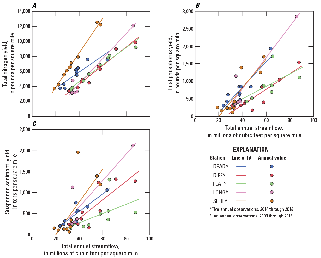
Graphs showing the relations of A, total nitrogen; B, total phosphorus; and C, suspended-sediment yields to total annual streamflow in five study watersheds in Fairfax County, Virginia. Study watershed station names are defined in table 1.
Because nutrient loads are closely tied to streamflow conditions, so too are nutrient retention rates; the lowest annual retention rates are typically observed during years with the most precipitation (fig. 25). Changes in annual TP retention were generally larger than that of TN, reflecting the strong association between streamflow, particulate material, and phosphorus loads. For TP, all watersheds except FLAT had a negative retention rate during the wettest study year, because more TP load was exported to streams than applied to the landscape in 2018. Phosphorus inputs can be stored in watershed soils for many years and, along with sediment mobilization, can greatly affect loads in streams (Fanelli and others, 2019; Kleinman and others, 2019). Sediment can be stored in a watershed for days to millennia before being delivered downstream, and shorter residence times are more common for in-channel sediments compared with floodplain or upland sediments (Noe and others, 2020). These patterns are a reminder that nutrient loads and retention rates are influenced by current and historical inputs (Chang and others, 2021; Kleinman, 2017; Van Meter and others, 2017).
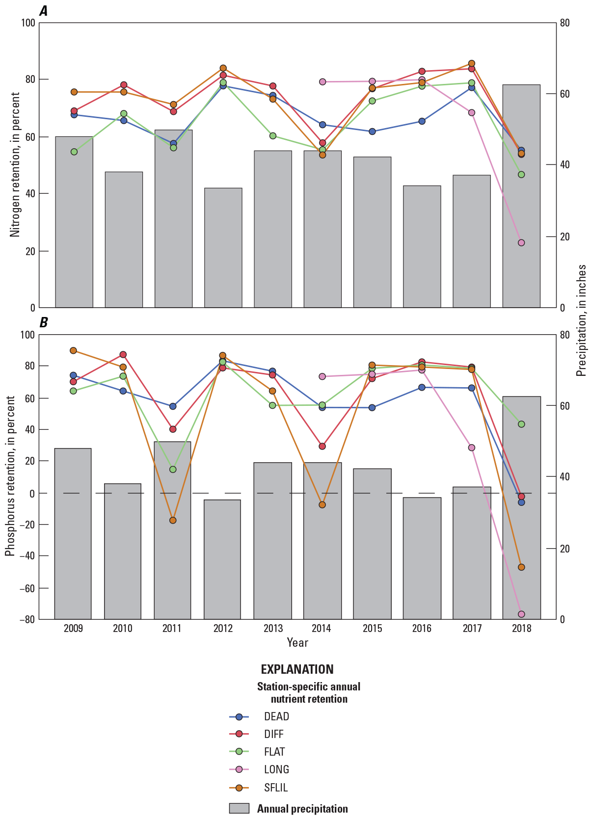
Graphs showing A, nitrogen and B, phosphorus retention and annual precipitation in five study watersheds in Fairfax County, Virginia, from 2009 through 2018. Study watershed station names are defined in table 1.
Average-annual nutrient yields and retention rates differed among the intensive-monitoring stations from 2009 through 2018 (table 17). Average TN and TP yields were lowest at DIFF (5,660 and 568 pounds per square mile per year [lb/mi2/yr], respectively). The highest average TN yield occurred at SFLIL (7,259 lb/mi2/yr), and the highest average TP yield occurred at DEAD (756 lb/mi2/yr). Base-flow nutrient loads reflect the delivery of nutrients in non-storm conditions, presumably through groundwater for TN and from pathways, including the release of soil-bound material, for TP. Average TN retention rates varied from 65.0 percent in FLAT to 73.1 percent in DIFF, values consistent with previous studies (Groffman and others, 2004; Hobbie and others, 2017; Kaushal and others, 2011; Wollheim and others, 2005). Average TP retention rates varied from 48.7 percent in SFLIL to 62.8 percent in FLAT. The slightly greater tendency for TN retention, relative to TP, has been observed in other studies and is likely related to the efficient delivery of phosphorus through surface-water pathways versus the slower delivery of nitrogen through groundwater (Boardman and others, 2019; Hobbie and others, 2017). Retention of TN and TP inputs at base flow was lowest in FLAT (83.5 and 90.7 percent, respectively), which may be related to shorter groundwater flow paths and a lower phosphorus soil storage capacity in this shallow-soil watershed in the fractured bedrock of the Triassic Lowlands. Previous studies have documented an inverse relation between nutrient retention and impervious cover in urban areas (Wollheim and others, 2005), a relation that was not apparent in these five watersheds.
Table 17.
Average yield, load from base flow, and retention of total nitrogen and total phosphorus from 2009 through 2018 in four study watersheds in Fairfax County, Virginia.[Station names are defined in table 1. TN, total nitrogen; TP, total phosphorus; lb/mi2/yr, pound per square mile]
After minimizing variability associated with streamflow, trends in water-quality yields from 2009 through 2018 may better reflect the effects of landscape activities, including the role of management practices. Flow-adjusted TN yields declined at DEAD and FLAT by between 850 and 1,000 lb/mi2 over the 10-year study period, decreases of about 2 percent per year (fig. 26 and table 18). Flow-adjusted TP yields increased at DEAD, DIFF, and SFLIL by between 120 and 260 lb/mi2 over the 10-year period, increases of about 8 or 9 percent per year. Flow-adjusted SS yields increased at DEAD by about 120 tons per square mile over the 10-year period, a change of 8 percent per year. No other trends were significant at p-value ≤0.05.
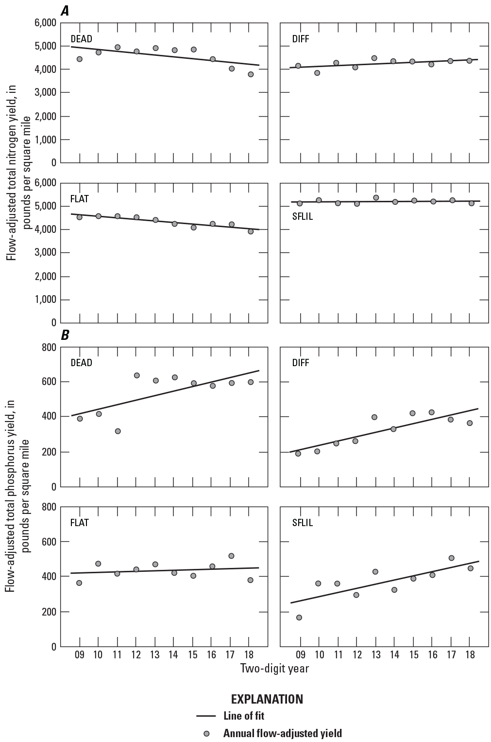

Graphs showing annual flow-adjusted A, total nitrogen; B, total phosphorus; and C, suspended-sediment yields in four study watersheds in Fairfax County, Virginia, from 2009 through 2018. Study watershed station names are defined in table 1.
Table 18.
Trends in total nitrogen, total phosphorus, and suspended-sediment flow-adjusted yields in four study watersheds in Fairfax County, Virginia, from 2009 through 2018.[Station names are defined in table 1. lb/mi2, pound per square mile; TN, total nitrogen; <, less than; TP, total phosphorus; SS, suspended sediment; ton/mi2, ton per square mile]
Changes in flow-adjusted nutrient loads result from differing amounts of nitrogen and phosphorus inputs and (or) differing rates of nutrient retention. Correlations between annual nutrient inputs and flow-adjusted loads from 2009 through 2018 were positive at all stations except SFLIL, indicating that flow-adjusted loads were higher in years with more inputs in all but this station (table 19). The strength of these correlations varied among stations, but was generally more positive for TN than TP, suggesting that flow-adjusted TN loads may be more strongly affected by changes in inputs than TP. Weak and (or) negative correlations between inputs and flow-adjusted loads may result from nitrogen storage in groundwater, phosphorus storage in soil, and sediment storage in floodplains and channels; these storage types are associated with lag times that often exceed annual timescales (Kleinman, 2017; Van Meter and others, 2017). After adjusting for streamflow, TN and TP loads had negative correlations with rates of nutrient retention, reflecting a pattern of higher loads in years with lower retention rates. These correlations were stronger for TP than TN at all stations; annual variability in flow-adjusted TP loads is highly dependent on the amount of phosphorus stored in and released from a watershed.
Table 19.
Correlations between annual flow-adjusted nutrient loads, nutrient inputs, and nutrient retention in four study watersheds in Fairfax County, Virginia, from 2009 through 2018.[Station names are defined in table 1. r, correlation coefficient; TN, total nitrogen; TP, total phosphorus; <, less than]
After adjusting for streamflow, annual TP retention declined from 2009 through 2018 at most stations, in comparison, annual TN retention was relatively unchanged (fig. 27). TN retention was stable in DIFF and SFLIL but increased in FLAT and DEAD: patterns that corresponded with changes in yield in each watershed (fig. 26). TP retention declined in all watersheds except FLAT, corresponding with increases in TP loads in DEAD, DIFF and SFLIL (fig. 26).
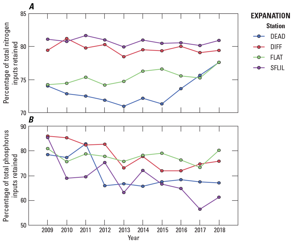
Graphs showing the percentage of annual A, total nitrogen and B, total phosphorus inputs retained in four study watersheds in Fairfax County, Virginia, from 2009 through 2018. Input retention is calculated using flow-adjusted loads. Study watershed station names are defined in table 1.
Water-Quality Loads and Management Practices
Credited management-practice effects were not apparent in annual nutrient and sediment loads calculated for the intensive-monitoring stations from 2009 through 2018. The cumulative reductions of TN, TP, and SS credited to management practices represented less than 10 percent of the 10-year median load at all stations in most years (fig. 28). Credited reductions represented the highest percentage of loads in recent years when several stream restoration practices were completed (table 13). Annual changes in flow-adjusted yields typically differed from credited reductions. From 2009 through 2018, changes in yield credited to management-practice reductions were always negative, whereas flow-adjusted yields followed more complex trajectories (fig. 29). Compared to other stations, SFLIL, a station where no management practices were installed, had relatively small changes in flow-adjusted TN yields. Flow-adjusted TN yields were higher in 2018 than 2009 in DIFF by about 200 lb/mi2, despite credited reductions of about 260 lb/mi2. Flow-adjusted TN yields were lower in 2018 than 2009 in DEAD and FLAT; changes at FLAT were relatively well aligned with credited TN management-practice reductions. Flow-adjusted TP and SS yields were higher in 2018 than 2009 at all stations, despite credited management-practice reductions. At most stations, increases in TP and SS flow-adjusted yields were much larger than credited practice reductions.
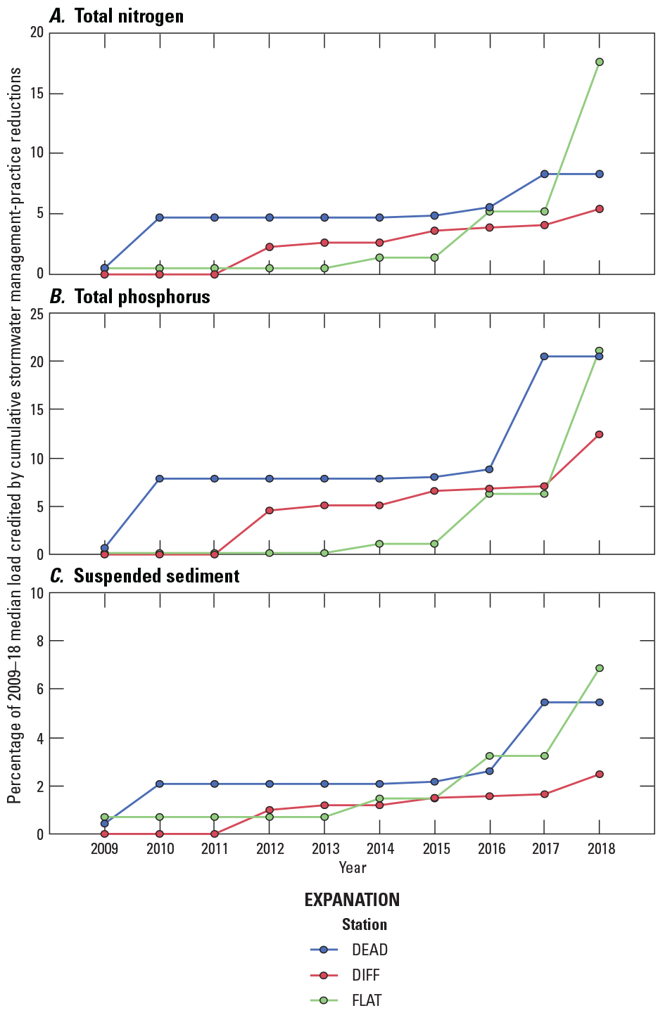
Graphs showing the percentage of median A, total nitrogen; B, total phosphorus; and C, suspended-sediment load credited by cumulative stormwater management-practice reductions in three study watersheds in Fairfax County, Virginia, from 2009 through 2018. Study watershed station names are defined in table 1.

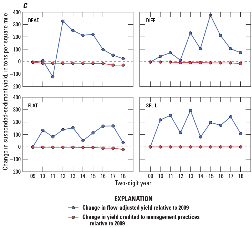
Graphs showing changes in A, total nitrogen; B, total phosphorus; and C, suspended-sediment flow-adjusted yields and credited management-practice reductions in four study watersheds in Fairfax County, Virginia, from 2009 through 2018. Study watershed station names are defined in table 1.
Monthly flow-adjusted yields from 2009 through 2018 did not consistently align with the timing of management-practice implementation. The distribution of monthly flow-adjusted TN yields was lower at DEAD after 2015 and FLAT after 2012 (fig. 30): a significant change point detected by a non-parametric test (p-value ≤0.05). Management practices were not clearly the driver of these lower yields, because most practices were installed after the detected change points. A significant trend or change point was not identified at SFLIL or DIFF for flow-adjusted TN yields, and many management practices were installed in DIFF from 2012 through 2018. Flow-adjusted TP yields increased at DEAD, DIFF, and SFLIL (table 18), and monthly flow-adjusted yields increased at DEAD and DIFF after 2012 (fig. 31). Flow-adjusted SS yields increased in DEAD (table 18), and a higher distribution of values was observed after 2012 (fig. 32). Trends and changes in TP and SS flow-adjusted yields were not clearly related to the timing of management-practice completion.
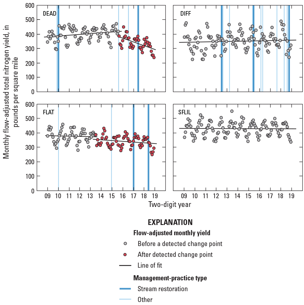
Graphs showing monthly flow-adjusted total nitrogen yields with detected change points from a non-parametric analysis and the timing of completed management practices in four study watersheds in Fairfax County, Virginia, from 2009 through 2018. Study watershed station names are defined in table 1.
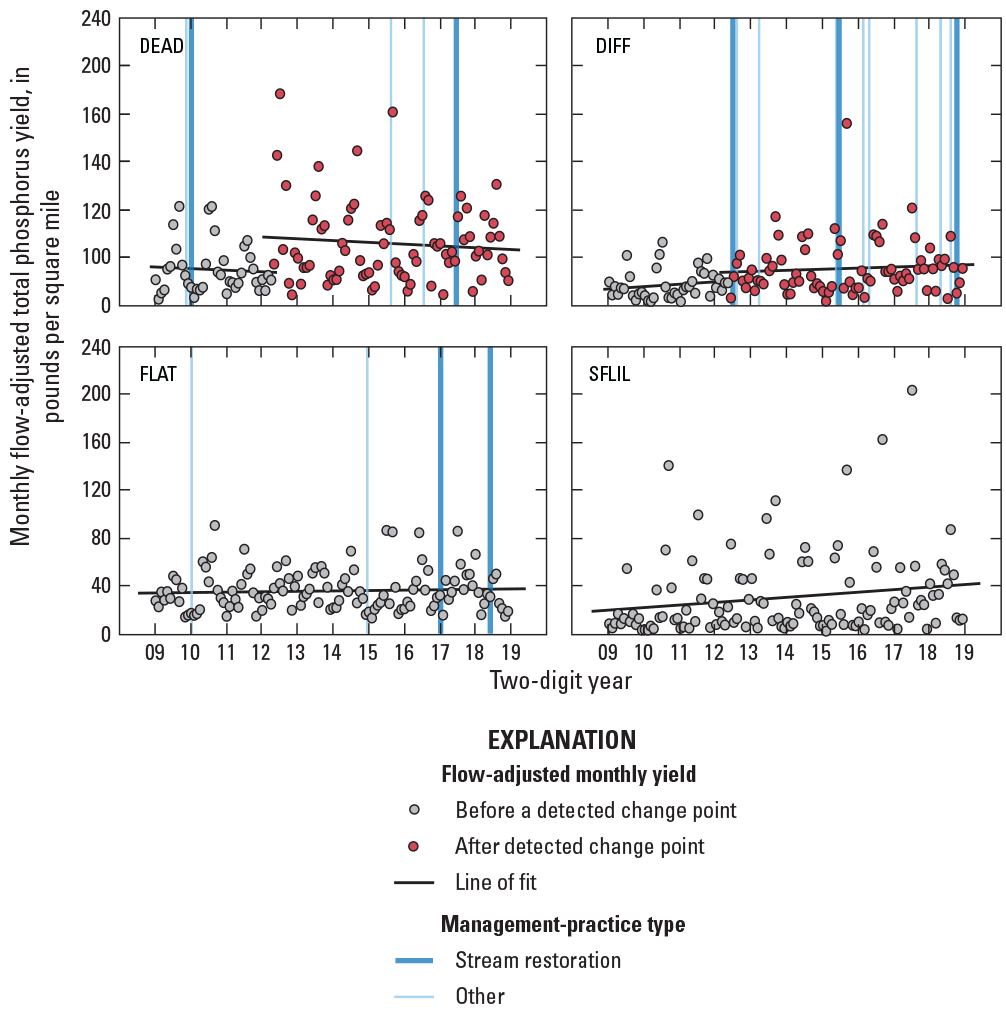
Graphs showing monthly flow-adjusted total phosphorus yields with detected change points from a non-parametric analysis and the timing of completed management practices in four study watersheds in Fairfax County, Virginia, from 2009 through 2018. Study watershed Station names are defined in table 1.
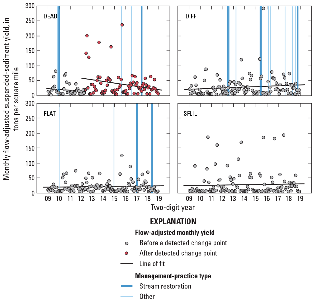
Graphs showing monthly flow-adjusted suspended-sediment yields with detected change points from a non-parametric analysis and the timing of completed management practices in four study watersheds in Fairfax County, Virginia, from 2009 through 2018. Study watershed station names are defined in table 1.
What Factors Affected Water-Quality and Benthic-Macroinvertebrate Responses?
A better understanding of the factors affecting water-quality and ecological responses in Fairfax County streams is needed to inform watershed-management strategies. To meet this objective, the following sections describe how TN, TP, SS, SC, and benthic-macroinvertebrate IBI scores differ among study watersheds, vary over the study period, and relate to landscape and climatic conditions. Median-annual water-quality values are described in the following sections, which represent temporal responses that are consistent with trends reported by Porter and others (2020b) for a similar period. Although the monthly water-quality samples represented a range of hydrologic conditions commonly observed across Fairfax County, they do not represent the highest streamflow conditions; therefore, spatial and temporal patterns of median-annual concentrations differ from annual loads (fig. 33).
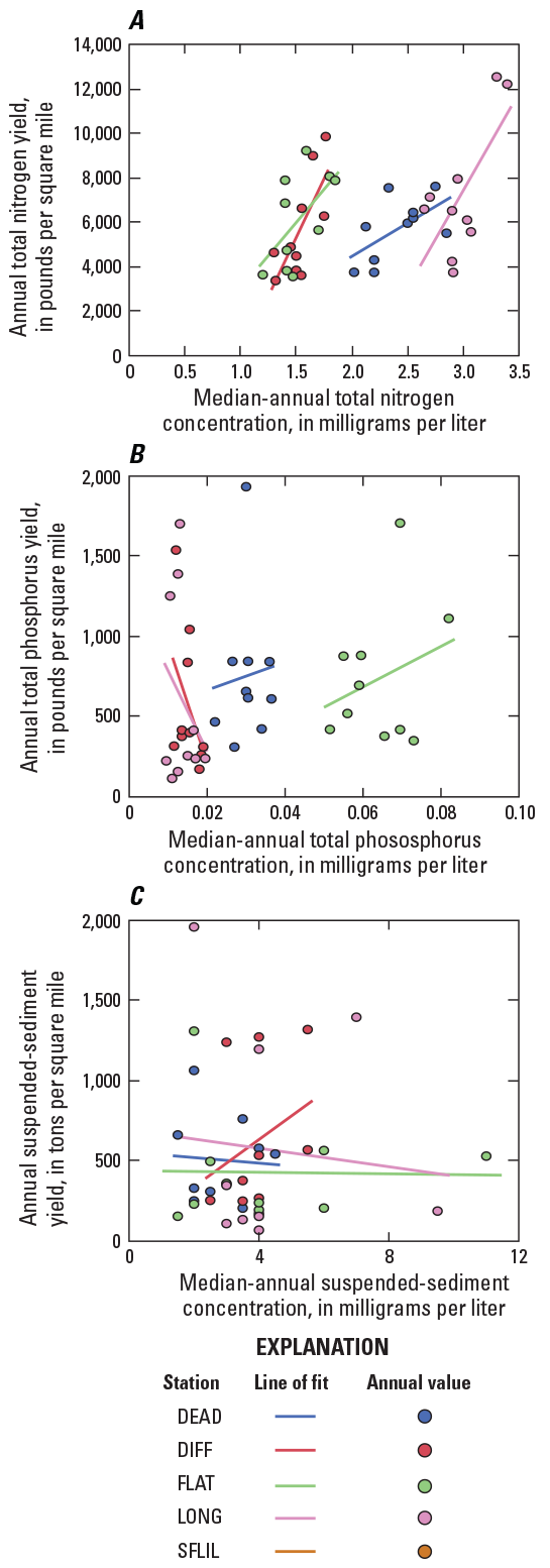
Graphs showing relations of median-annual concentrations to annual yields for A, total nitrogen; B, total phosphorus; and C, suspended sediment in four study watersheds in Fairfax County, Virginia, from 2009 through 2018. Study watershed station names are defined in table 1.
Nitrogen
Nitrogen is an essential nutrient for plant and animal growth, but, in excess quantities, can contribute to a range of negative ecosystem outcomes that harm biotic communities (Conley and others, 2009; Howarth and Paerl, 2008). Many urban and suburban streams have elevated nitrogen levels, and, while nitrogen reductions have been achieved from wastewater treatment-plant improvements, many streams still suffer from nonpoint inputs and pressures of continued urban growth (Paul and Meyer, 2001). The delivery of nitrogen to urban streams is controlled by multiple factors; understanding these factors requires a better understanding of nitrogen sources and nitrogen biogeochemical transformations to inform stormwater-management strategies (Yang and Lusk, 2018).
Patterns of Observed Responses
TN concentrations differed among study watersheds, varied seasonally, and were strongly related to streamflow (Porter and others, 2020b). Median-annual TN concentrations below about 2 mg/L typically occurred in most watersheds, but concentrations above 3 mg/L were observed in CAPT HICK and SFLIL (fig. 34). More than 90 percent of the TN in the monthly samples was typically dissolved nitrogen, mostly nitrate. Concentrations of TN and nitrate were commonly lower in warmer months than cooler months, likely reflecting nitrate loss through plant uptake and denitrification. TN concentrations typically increased with streamflow, whereas nitrate concentrations decreased (fig. 35). Higher stormflow TN concentrations likely result from surface-water runoff that carries leaves, grass clippings, woody debris, dry atmospheric nitrogen deposition, and other materials containing particulate forms of nitrogen to streams.

Boxplots showing the median-annual total nitrogen concentrations of 20 study watersheds in Fairfax County, Virginia. Study watershed station names are defined in table 1.
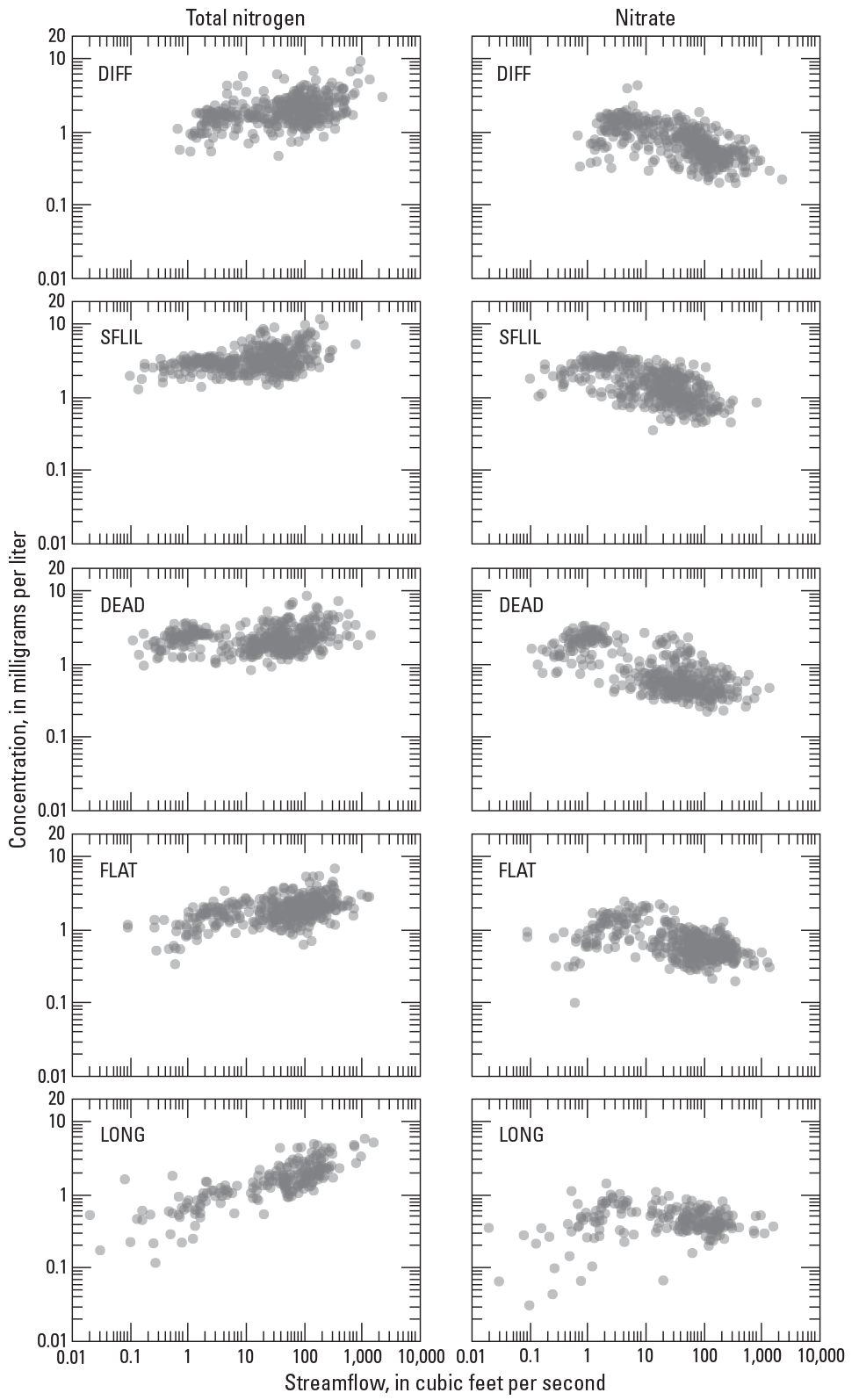
Graphs showing the relations of streamflow to total nitrogen and nitrate concentrations measured in five study watersheds in Fairfax County, Virginia. Study watershed station names are defined in table 1.
Nitrogen-concentration trends were evaluated using monthly water-quality samples collected from April 2008 through March 2018 to describe how conditions changed over time in 14 watersheds with 10 years of data, analyses, and interpretations originally conducted by Porter and others (2020b; table 20). After adjusting for streamflow, TN concentrations declined in 5, increased in 1, and had no trend in the remaining 8 watersheds. No network-wide trend in TN was detected with a regional Seasonal-Kendall analysis. TN decreases ranged from about −2 percent to −4 percent per year; the largest 10-year decline of about 0.5 mg/L was in DEAD. The TN increase in SFLIL represented a change of about 2 percent per year, or an increase of about 0.6 mg/L. The increase in this watershed is notable as SFLIL had higher average nitrogen concentrations relative to the rest of the monitoring network. At all stations, TN trends were greatly affected by nitrate concentrations. Nitrate decreased network-wide by -1.3 percent per year. Flow-adjusted nitrate concentrations increased only in SFLIL and CAPT HICK (by 3 percent and 1 percent per year, respectively): the two watersheds with the highest average nitrate concentrations. Nitrate decreases occurred in four watersheds; the largest percentage of decrease was −6 percent in BRR, and the largest total decrease was −0.6 mg/L in DEAD.
Table 20.
Flow-adjusted total nitrogen and nitrate concentration trends in 14 study watersheds in Fairfax County, Virginia, from March 2008 through April 2018.[Station names are defined in table 1. mg/L, milligram per liter; %, percent]
Between-watershed differences in median-annual TN concentrations were typically larger than year-to-year changes within watersheds (fig. 34). These two sources of variability, representing spatial differences among study watersheds and temporal differences from 2009 through 2018, were described by a linear-growth model (table 21). This model indicated that the average TN concentration across all watersheds in 2009 was 1.92 mg/L and that the linear rate-of-change could not be differentiated from zero. Random-effect variances describe a dataset where group-level variance (0.929), representing between-watershed differences in intercept, accounted for most total model variance (0.961). The variances representing TN change over time, differences in between-watershed slope (0.001) and within-watershed annual changes (0.031), were small. The median-annual TN changes that occurred from 2009 through 2018 included TN decreases in DEAD and increases in SFLIL (fig. 36). The AIC of the linear-growth model (12.06) was compared against models that included additional predictors; more parsimonious models reduced the random-effect variances.
Table 21.
Results of the total nitrogen linear-growth model, including fixed-effect estimates, 95-percent confidence intervals, random-effect variances, and the model’s Akaike information criterion.[The linear-growth model is defined in equations 1–3. AIC, Akaike information criterion]
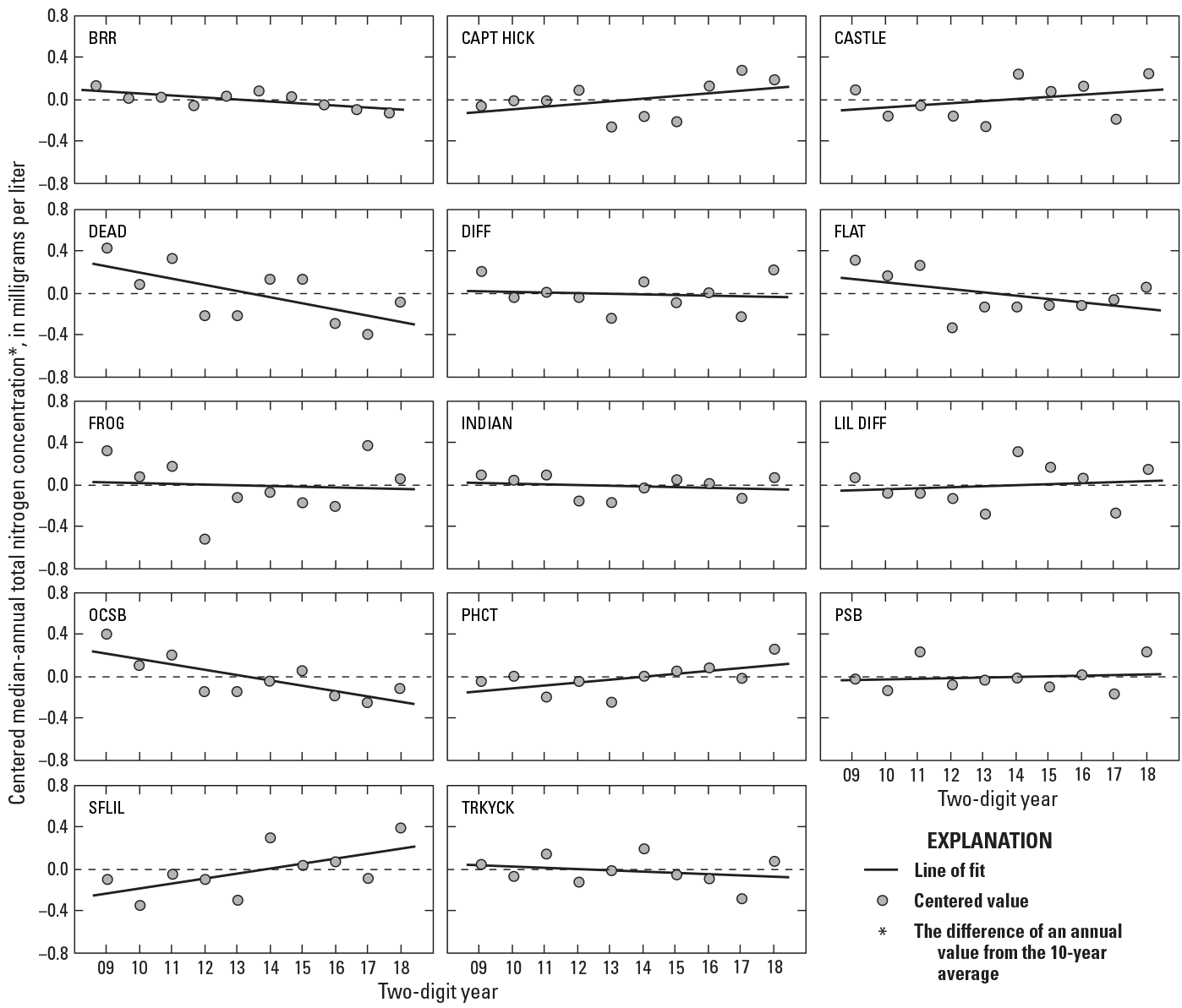
Graphs showing centered values of median-annual total nitrogen and nitrate concentrations in 14 study watersheds in Fairfax County, Virginia, from 2009 through 2018. Study watershed station names are defined in table 1.
Relations to Predictor Variables
Between-watershed TN differences were likely affected by a combination of human and natural factors, patterns that were explored by comparing average predictor values to TN concentrations from 2014 through 2018 at 20 study watersheds (app. 1, table 1.1). Septic-system density (SEPTIC DEN, r=0.74; fig. 37A), the estimated nitrogen input from septic systems (N SEPTIC, r=0.74), the sum of all nitrogen inputs (N TOT IN, r=0.66) and the length of sanitary-sewer lines (SAN SEWER LEN, r=−0.62) had the strongest correlations with TN, suggesting that between-watershed TN differences may be related to wastewater infrastructure. Septic-system effluent is likely an important factor in some watersheds with the highest TN concentrations, an influence previously discussed in this report, in previous Fairfax County studies (Hyer and others, 2016; Porter and others, 2020b), and in related water-quality investigations (Burns and others, 2005; Kaushal and others, 2006; Kaushal and others, 2011; Valiela and others, 1997; Wollheim and others, 2005). Negative correlations between TN and predictors such as impervious cover (IMP, r=−0.48; fig. 37B), developed land use (DEV ALL, r=−0.47), roadway length (TOT ROAD, r=−0.54), housing units (TOT HU, r=−0.57), and the amount of stormwater infrastructure (PIPE LEN, r=−0.52) demonstrate that more urbanized watersheds had lower average TN concentrations. Such conditions may occur because these watersheds contained the largest amount of infrastructure to control stormwater runoff, had the smallest fraction of wastewater served by septic systems, or otherwise limited the sources or delivery of nitrogen to streams.

Graphs showing relations of A, septic-system density and B, impervious cover to total nitrogen concentrations in 20 study watersheds in Fairfax County, Virginia; all values represent average conditions from 2014 through 2018. Study watershed station names are defined in table 1.
Denitrification, the permanent removal of nitrogen through conversion to atmospheric gas, can represent a dominant nitrogen loss term in mid-Atlantic watersheds (Van Breemen and others, 2002) and may affect between-watershed differences in TN concentrations. Considering this process, the inverse relation between TN and urbanization seems unusual, because more impervious watersheds commonly deliver increased amounts of water through surface runoff and limit opportunities for denitrification and other microbial pathways that affect nitrogen availability and mobility (Burgin and Hamilton, 2007). Similar rates of denitrification can occur, however, in urban areas as in lesser developed watersheds; urban denitrification rates are strongly affected by near-stream environments such as floodplains and detention basins (Groffman and Crawford, 2003). Therefore, even in highly impervious watersheds, denitrification opportunities exist if riparian zones allow for infiltration and hyporheic exchange, an important process in Fairfax County where many stream valleys are designated as park land and are afforded protection from urban development. Denitrification potential is often greatest in areas with saturated soils, abundant organic matter, and warmer stream and air temperatures (Bowden, 1987; Burgin and Hamilton, 2007; Pilegaard, 2013). Correlations among predictors representing these features and median TN concentrations offered mixed evidence for the role of denitrification (app. 1, table 1.1). These patterns cannot be used to discount the importance of denitrification because denitrification rates are highly variable in urban areas (Groffman and Crawford, 2003) and predictor data used to summarize soil properties do not represent spatial variability within a watershed or throughout soil horizons.
Some temporally averaged measures of wastewater and urbanization were related to the 2009 through 2018 percentage change in median-annual TN concentrations (app. 1, table 1.2). Average impervious cover had the strongest correlation to TN percentage change (IMP, r=−0.84; fig. 38A), indicating that declines in TN concentration were larger in more impervious watersheds. Conversely, the correlation of TN to septic-system density (SEPTIC DEN, r=0.70; fig. 38B) showed that concentration increases were larger in watersheds primarily served by septic systems. Responses at OCSB and SFLIL demonstrated these patterns. OCSB, one of the most impervious watersheds, was served by a sanitary-sewer network and had a TN decline of about 3 percent per year. In contrast to these stations, SFLIL had a smaller amount of impervious cover and a high density of septic systems and had a TN increase of about 2 percent per year.
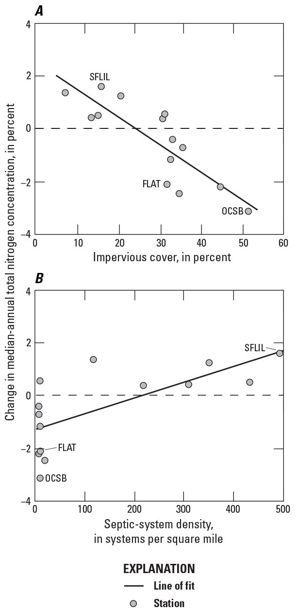
Graphs showing relations of A, impervious cover and B, septic-system density (values represent averages from 2009 through 2018) to changes in median-annual total nitrogen concentrations from 2009 through 2018 in 14 study watersheds in Fairfax County, Virginia. Study watershed station names are defined in table 1.
Correlations between annual measures of urbanization and median-annual TN concentrations from 2009 through 2018 varied by watershed; most predictors had no consistent relation to TN changes over time (app. 1, table 1.3). For example, impervious cover increased in OCSB and SFLIL from 2009 through 2018, but TN concentrations declined in OCSB (r=−0.71) and increased in SFLIL (r=0.68). Annual changes in the number of septic systems were not correlated with TN changes at most watersheds (SEPTIC DEN, median r=0.00); however, most watersheds were predominantly served by sanitary sewers, and septic-system increases may affect TN concentrations only in watersheds with elevated septic-system density. Median TN concentrations and the number of septic systems increased in SFLIL and CAPT HICK from 2009 through 2018, watersheds with hundreds of septic systems per square mile (table 8), resulting in positive correlations (r=0.63 and r=0.33, respectively). However, increased septic effluent contributed by new systems may not be the primary driver of increased TN concentrations in these watersheds because fewer than 30 new systems were installed in each watershed over the 10-year period. Not to discount the potentially important relations between septic systems and TN, it is possible that stream conditions were responding to past changes in septic infrastructure, nitrogen removal rates have declined in aging systems, or that effluent was delivered to streams more efficiently.
Annual changes in some spatially averaged climatic predictors were correlated with annual changes in median TN concentration across the 14 watersheds (app. 1, table 1.3). Years with more total precipitation and, a related measure, more days with total precipitation greater than or equal to about 0.4 in. (hereafter referred to as “heavy rainfall days”), were associated with higher annual TN concentrations in most watersheds. Thirteen of the fourteen watersheds had a positive correlation between TN and heavy rainfall days (R10D, median r=0.54), and only CAPT HICK had a negative relation (fig. 39). Years with more heavy rainfall produced more storm responses and stormwater runoff, hydrologic conditions that can produce elevated TN concentrations (fig. 35) and can result in the lowest retention of nitrogen inputs on the landscape (fig. 25). These patterns, which are similar to patterns reported from other small urban watersheds (Kaushal and others, 2008a), may reflect increased delivery of stored nitrogen to streams from soils and groundwater or the influence of atmospheric deposition, a nitrogen input that was higher in wetter years. Annual changes in atmospheric deposition had a positive relation with annual changes in TN concentration in most watersheds. Correlations were stronger with wet deposition (N WET DEPO, median r=0.50; fig. 39) than total deposition, which includes the dry deposition fraction (N TOT DEPO, median r=0.35). Atmospheric deposition can be an important nitrogen input in urban watersheds, especially during high-flow events that deliver surface runoff to streams (Kaushal and others, 2011): a process previously documented at Fairfax County streams (Hyer and others, 2016).
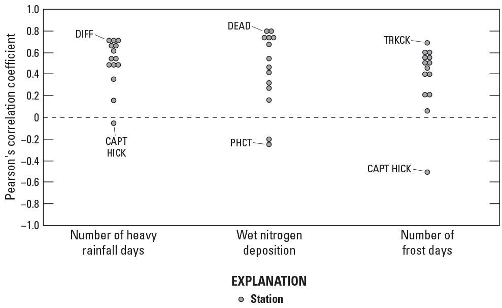
Graph showing Pearson’s correlation coefficients for relations between median-annual total nitrogen concentrations and selected predictors in 14 study watersheds in Fairfax County, Virginia. Correlations represent annual values from 2009 through 2018. Study watershed station names are defined in table 1.
Years with higher average air temperature had lower median TN concentrations in most watersheds (AIR TEMP, median r=−0.31; app. 1, table 1.3). This association was also in some measures of temperature extremes, where colder temperatures during the coldest night of the year (TNn, median r=−0.45) and more frost days per year (FD, median r=0.47) were correlated with lower median TN concentrations. Thirteen of fourteen watersheds had a positive correlation between the number of frost days and TN, but only CAPT HICK had a negative correlation (fig. 39). The unique negative correlation at CAPT HICK between annual TN and annual climatic predictors suggests that drivers of TN concentration in this watershed may differ from others in the monitoring network. Relations between warmer air temperature and lower TN concentrations are consistent with effects of denitrification (Pilegaard, 2013) and are similar to relations between air temperature and flow-normalized total nitrogen load reported for streams throughout the Chesapeake Bay watershed (Chanat and Yang, 2018).
Explanation of Variability
Based on the information described above, six predictors were included in LME models to describe the spatiotemporal variability of median-annual TN concentrations: (1) median-annual streamflow, (2) number of heavy rainfall days, (3) number of frost days, (4) impervious cover, (5) wet atmospheric nitrogen deposition, and (6) septic-system density. Median-annual streamflow was used to evaluate whether median-annual TN was affected by varying flow conditions because varying flow conditions can mask the role of other factors. Combined with the six parameters of the linear-growth model, all possible model combinations of the six additional predictors were considered. Models with the lowest AIC included a similar combination of terms and performed similarly (app. 2, table 2.1).
Many similarly performing models described the spatiotemporal variability of median-annual TN concentrations at the 14 study watersheds from 2009 through 2018, but interpretations from a single model can help inform watershed management. A 9-parameter model that included fixed-effect terms for the number of heavy rainfall days and septic-system density was the simplest model form among the top-performing models; more complex models did not offer a substantial improvement over this combination of predictors (app. 2, fig. 2.1). With the exception of a fixed effect to represent the linear rate of TN change over time, the slope term included in all models, the 95-percent confidence intervals of all fixed-effect parameters in the selected model did not include zero, suggesting an interpretable positive or negative effect on TN (table 22).
Table 22.
Results of a total nitrogen linear mixed-effect model selected for interpretation, including 95-percent confidence intervals, fixed-effect estimates, random-effect variances, and the model’s Akaike information criterion.[Linear mixed-effect models are described in equations 4–6. Predictors are described in table 3. b3, the effect of a predictor on within-watershed variability; b1, the effect of a predictor on between-watershed intercept differences; b2, the effect of a predictor on between-watershed slope differences; R2, coefficient of determination; AIC, Akaike information criterion]
The fixed-effect terms in the selected model explained 58 percent of the spatiotemporal variability in median-annual TN concentration (table 22). Compared to the linear-growth model (table 21), the selected model explained an additional 30 percent of the annual within-watershed variance, an additional 49 percent of the between-watershed intercept variance, and an additional 79 percent of the between-watershed slope variance. Observed and predicted responses plotted against time were used to visually assess the selected model’s performance in each watershed (app. 2, fig. 2.2). The selected model residuals for most stations appear evenly distributed around zero in most years: an improvement compared with predictions from the linear-growth model (fig. 40). The distribution of residuals around zero in the linear growth model is related to extremes in the annual record of heavy rainfall days (fig. 41A).
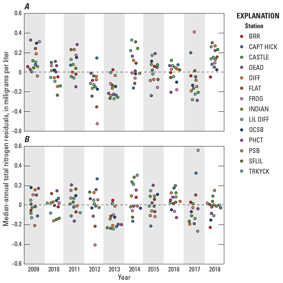
Graphs showing model residuals from A, the total nitrogen linear-growth model and B, the selected total nitrogen linear mixed-effect model in 14 study watersheds in Fairfax County, Virginia, from 2009 through 2018. Study watershed station names are defined in table 1.
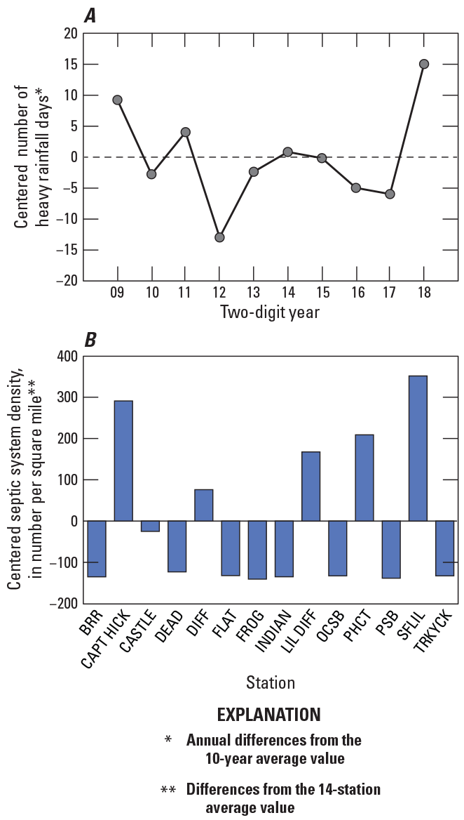
Graphs showing centered parameters used in the selected total nitrogen linear mixed-effect model: A, the number of heavy rainfall days from 2009 through 2018 and B, septic-system density in 14 study watersheds in Fairfax County, Virginia. Study watershed station names are defined in table 1.
The selected model estimated two effects of septic-system density on median-annual TN concentrations. In watersheds with above average septic-system densities (1) concentrations were higher than average and (2) concentration increases from 2009 through 2018 were larger. These effects are consistent with the observed relations between septic-system density and median-annual TN concentrations (fig. 37A and fig. 38B). The influence of septic systems on differences in TN concentration between watersheds has been reported in Fairfax County streams (Hyer and others, 2016; Porter and others, 2020b), but their potential effect on concentration changes over time has not been previously explored. The number of septic systems generally increased over time in each study watershed, but annual changes in septic density were not a predictor of median-annual TN concentrations. A few hypotheses can be deduced from these patterns: (1) TN concentrations are responding to the expansion of septic infrastructure that occurred in previous years, (2) TN concentrations are responding to changes in the delivery of groundwater concentrations of septic effluent, and (or) (3) TN concentrations are responding to changes in other landscape or climatic drivers, which are co-located or processed differently in areas with high septic-system density.
The selected model estimated that, on average, median-annual TN concentrations were higher during years with more heavy rainfall days (table 22), consistent with observed patterns in most watersheds (fig. 39). The annual number of heavy rainfall days was the only modeled effect that caused estimated values to deviate from a perfectly straight line (app. 2, fig. 2.2). The number of heavy rainfall days may affect annual TN concentrations in Fairfax County streams for a variety of reasons. First, it should be noted that relations between TN and the number of heavy rainfall days were similar to TN and average-annual precipitation (PRCP; app. 1, table 1.3), so, more broadly, precipitation may be an important driver of TN concentrations. Wetter years may deliver more nitrogen to streams because of (1) the direct runoff of inputs from the landscape, (2) the flushing of inputs that were previously stored in soils or groundwater, and (or) (3) changes in biogeochemical processes that limit removal rates of nitrogen. TN concentrations were typically higher during elevated streamflow (fig. 35), but it is unlikely that the modeled precipitation effect reflects the effect of direct runoff, because the model was built from samples mostly collected during non-storm conditions. An additional driver of TN during wet years is the increased delivery of atmospheric nitrogen. Annual relations between TN and wet atmospheric nitrogen deposition were similar to the annual relations between TN and the number of heavy rainfall days (fig. 39), and many alternative models included an effect for wet-nitrogen deposition (app. 2, table 2.1).
Management-Practice Effects
Stormwater-retrofit and channel-restoration practices to reduce nitrogen were installed in seven study watersheds from 2009 through 2018 and, normalized by watershed area, are expected to lower TN yields by tens to thousands of pounds. These credited reductions do not coincide with decreases in median-annual TN concentrations in most study watersheds (fig. 42). Credited TN reductions were considered as a predictor of median-annual TN concentrations in the previously described LME model to assess their potential effect on observed conditions, relative to other environmental and anthropogenic drivers. Specifically, the model considered the annual effect of cumulative TN reductions on differences in median-annual TN concentrations from 2009 through 2018 in 14 watersheds. A model including the effect of credited management-practice TN reductions did not reduce the AIC of the previously described model (–47.25 compared to –48.89), and the coefficient was not significantly different from zero (table 23).
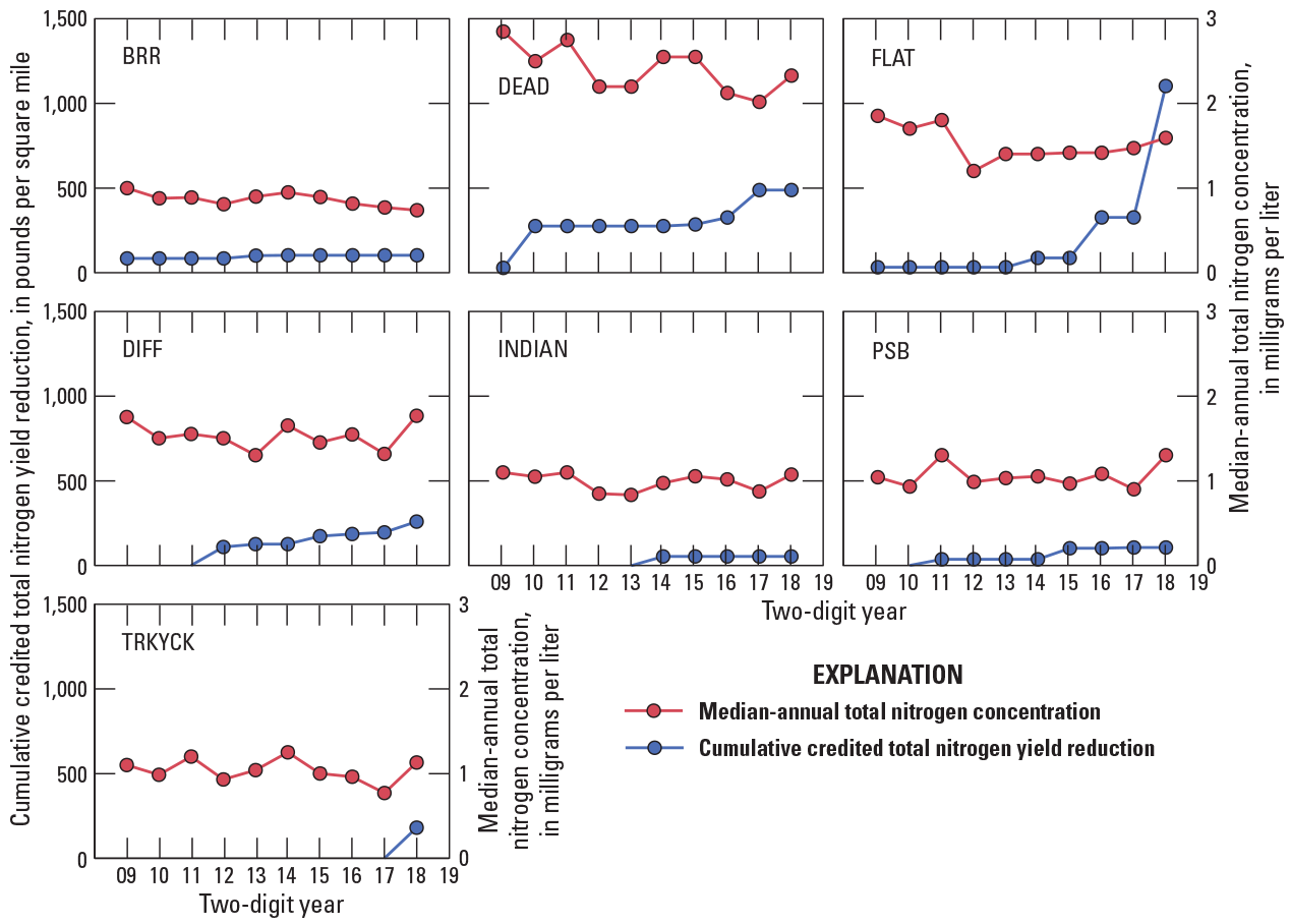
Graphs showing the cumulative credited total nitrogen yield reductions from management practices and median-annual total nitrogen concentrations in seven study watersheds in Fairfax County, Virginia, from 2009 through 2018. Study watershed station names are defined in table 1.
Table 23.
Results of a total nitrogen linear mixed-effect model with credited management-practice total nitrogen reductions, including 95-percent confidence intervals, fixed-effect estimates, random-effect variances, and the model’s Akaike information criterion.[Linear mixed-effect models are described in equations 4–6. Predictors are described in tables 3 and 5. b3, the effect of a predictor on within-watershed variability; b1, the effect of a predictor on between-watershed intercept differences; b2, the effect of a predictor on between-watershed slope differences; R2, coefficient of determination; AIC, Akaike information criterion]
Phosphorus
Phosphorus is an essential nutrient for plant and animal growth but, in excess quantities, can contribute to a range of negative ecosystem outcomes that harm biotic communities (Conley and others, 2009; Howarth and Paerl, 2008). Many urban and suburban streams have elevated phosphorus levels, and although nutrient reductions have been achieved by wastewater-treatment plant improvements, many streams still suffer from effects of nonpoint inputs and pressures of continued urban growth (Paul and Meyer, 2001). The delivery of phosphorus to urban streams is controlled by multiple factors; understanding these factors requires a better understanding of phosphorus sources and phosphorus biogeochemical transformations to inform stormwater-management strategies (Yang and Lusk, 2018).
Patterns of Observed Responses
TP concentrations, a measure of all dissolved and particulate phosphorus forms in the water column, differed among study watersheds, varied seasonally, and were strongly related to streamflow (Porter and others, 2020b). Median-annual TP concentrations were typically below about 0.03 mg/L in most watersheds, and concentrations as much as 0.06 mg/L were commonly observed in FLAT and Frog Branch above Flatlick Branch at Chantilly, Va. (FROG) (fig. 43). Dissolved phosphorus, predominately in the bioavailable form of orthophosphate, represented most of the non-storm TP concentration in most of the watersheds. Higher orthophosphate concentrations were observed in some streams during warmer months, likely because of temperature-dependent processes that affect the solubility of phosphorus minerals and the desorption of orthophosphate from sediments (Duan and others, 2012). Despite a similar seasonal pattern and range of WT observed at all stations, seasonal differences in orthophosphate were largest in FROG, FLAT, and HPEN (fig. 44). TP concentrations at all stations were highest during high flows because the increased delivery of sediment carries more phosphorus (fig. 45).
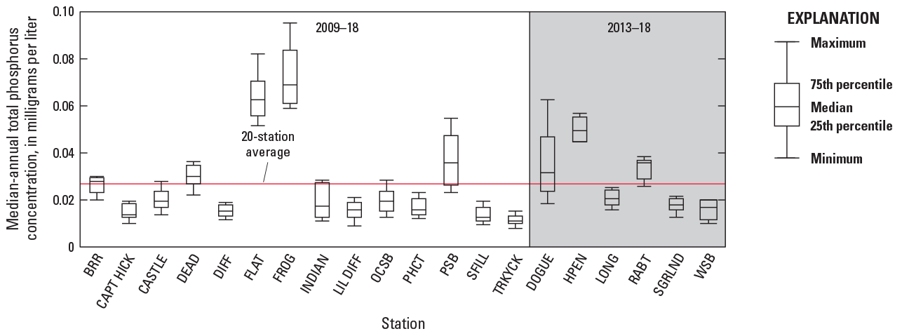
Boxplots showing the median-annual total phosphorus concentrations of 20 study watersheds in Fairfax County, Virginia. Study watershed station names are defined in table 1.
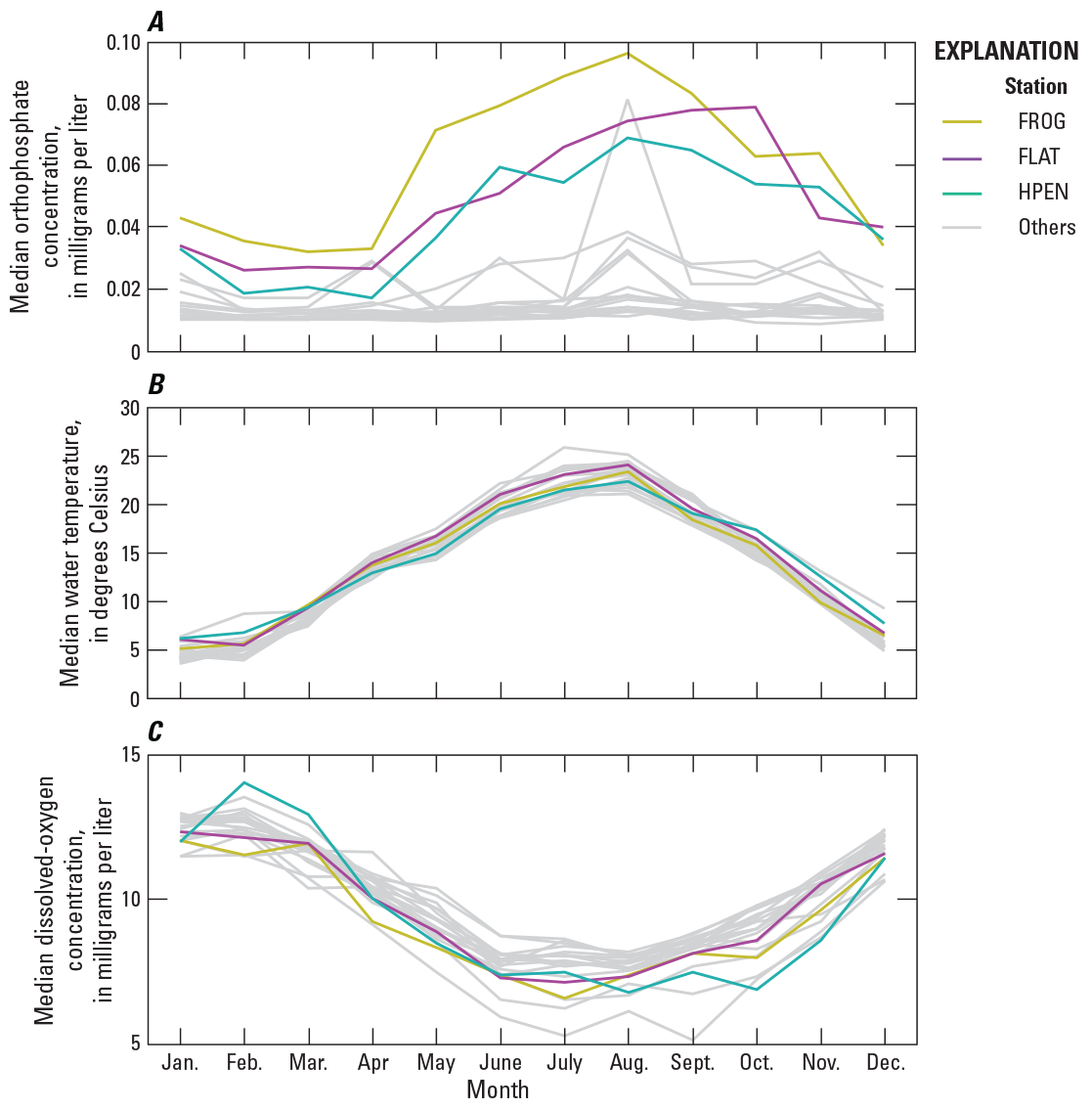
Graphs showing A, median orthophosphate concentrations; B, median water temperature, and C; median dissolved-oxygen concentrations by month in 20 study watersheds in Fairfax County, Virginia. Study watershed station names are defined in table 1. Jan., January; Feb., February; Mar., March; Apr., April; Aug., August; Sept., September; Oct., October; Nov., November; Dec., December.
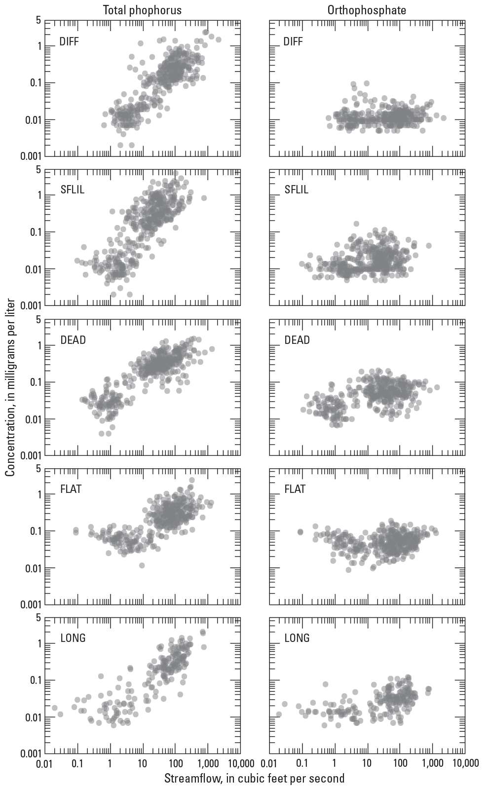
Graphs showing the relations of streamflow to total phosphorus and orthophosphate concentrations in five study watersheds in Fairfax County, Virginia. Study watershed station names are defined in table 1.
Phosphorus concentration trends were evaluated using monthly water-quality samples collected from April 2008 through March 2018 to describe how conditions changed over time in 14 watersheds with 10 years of data, analyses and interpretations originally conducted by Porter and others (2020b; table 24). After adjusting for streamflow, TP concentrations increased in 4, declined in 1, and had no trend in 9 watersheds. A network-wide increasing TP trend of 0.008 mg/L, an increase of 3.9 percent over the 10-year period, was determined by a regional Seasonal-Kendall analysis. The largest TP concentration increases of about 0.02 mg/L occurred in INDIAN and PSB. The only significant decrease occurred in FROG, a decline of about 0.04 mg/L. That decline is notable because this watershed typically had the highest median annual TP concentrations in the monitoring network (fig. 43). At stations other than FLAT, changes in TP were consistent with changes in orthophosphate (table 24). In FLAT, increases in TP at the end of the study period were likely caused by increases in particulate material and coincided with the completion of a stream restoration near the monitoring station (Porter and others, 2020b; fig. 46).
Table 24.
Flow-adjusted total phosphorus and orthophosphate concentration trends in 14 study watersheds in Fairfax County, Virginia, from March 2008 through April 2018.[Station names are defined in table 1. mg/L, milligram per liter; %, percent]
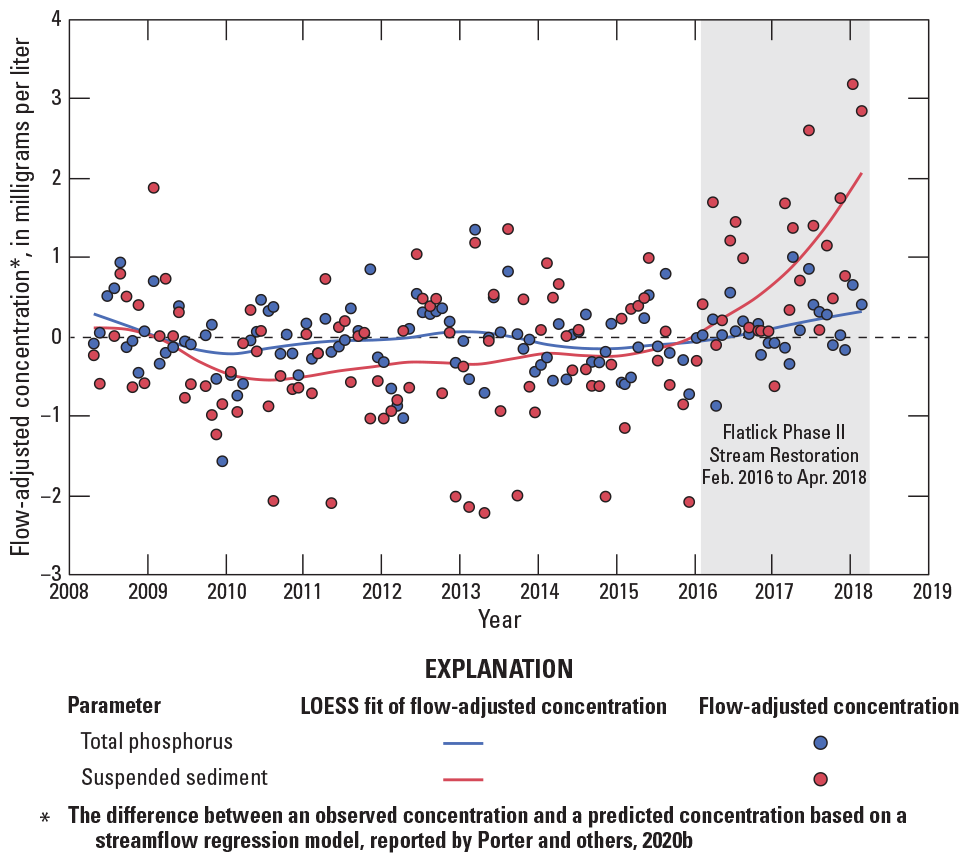
Graph showing flow-adjusted total phosphorus and suspended-sediment concentrations in Flatlick Branch above Frog Branch at Chantilly, Virginia, from April 2008 through March 2018. Feb., February; Apr., April.
Between-watershed differences in median-annual TP concentrations were typically larger than year-to-year changes within watersheds (fig. 43). These two sources of variability, representing spatial differences among study watersheds and temporal differences from 2009 through 2018, were described by a linear-growth model (table 25). The TP linear-growth model, and all subsequent TP LME models, represent TP concentrations multiplied by a factor of 100, which allows fixed- and random-effect estimates to be interpreted using fewer decimal places. The TP linear-growth model indicated that the average TP concentration across all watersheds in 2009 was 0.025 mg/L and that the linear rate-of-change could not be differentiated from zero. Random-effect variances describe a dataset where group-level variance (3.700), representing between-watershed differences in intercept, accounted for most of the total model variance (4.059). Variances representing TP change over time, differences in between-watershed slope (0.004) and within-watershed annual changes (0.355), were small. The median-annual TP and orthophosphate changes that occurred from 2009 through 2018 included large declines in FROG and smaller increases in most other watersheds (fig. 47). Changes in orthophosphate were consistent with changes in TP in all watersheds except FLAT, suggesting that changes in particulate phosphorus may have affected TP trends in this watershed. The AIC of the linear-growth model (335.42) was compared against models that included additional predictors; more parsimonious models reduced the between- and within-watershed random-effect variances.
Table 25.
Results of the total phosphorus linear-growth model, including fixed-effect estimates, 95-percent confidence intervals, random-effect variances, and the model’s Akaike information criterion.[The linear-growth model is defined in equations 1–3. AIC, Akaike information criterion]
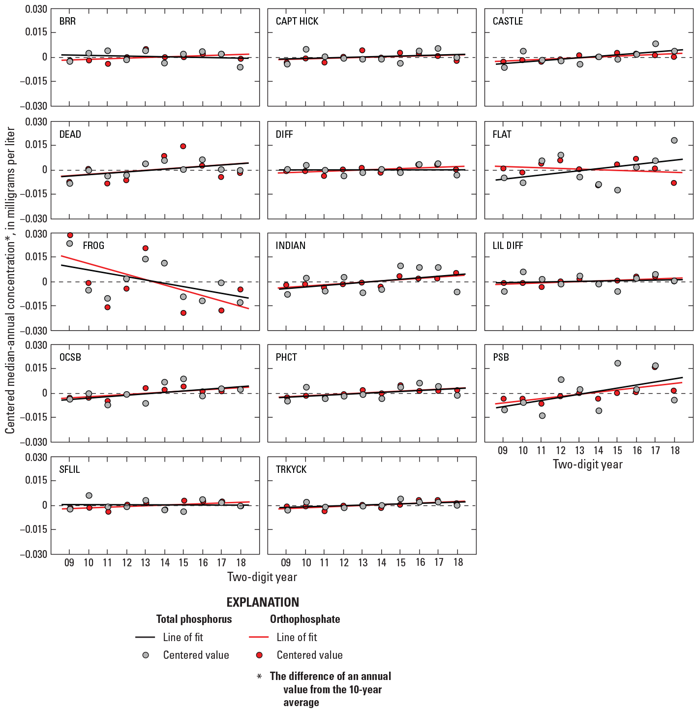
Graphs showing centered values of median-annual total phosphorus and orthophosphate concentrations in 14 study watersheds in Fairfax County, Virginia, from 2009 through 2018. Study watershed station names are defined in table 1.
Relations to Predictor Variables
Between-watershed TP differences were likely affected by a combination of human and natural factors; patterns that were explored by comparing average predictor values and TP concentrations from 2014 through 2018 at 20 study watersheds (app. 1, table 1.4). The percentage of a watershed within the Triassic Lowlands (TRIASSIC, r=0.75) had the strongest correlation with TP: a pattern previously observed and reported (Jastram, 2014; Porter and others, 2020b). Aside from differences in sediment transport, likely to be a minor influence on these median-annual TP concentrations, TP concentrations may be higher in Triassic Lowland streams for one or a combination of reasons: (1) they contain more nonpoint-phosphorus inputs, (2) they contain more naturally occurring phosphorus minerals that are contributed to streams as dissolved phosphorus through dissolution pathways, and (or) (3) their geologic, ecological, or water-quality properties result in greater rates of dissolved phosphorus mobilization to streams. Some evidence for this last point can be drawn from the previous discussion of nutrient input retention rates in the five intensive-monitoring stations, where FLAT had a slightly lower percentage of nitrogen and phosphorus inputs retained during base-flow conditions than SFLIL, DEAD, or DIFF (table 17).
Phosphorus concentrations may be higher in Triassic Lowland watersheds because of contributions from phosphorus-bearing minerals to streams. Phosphorus is naturally occurring in many minerals, most commonly in apatite and feldspars, and although most of this material is insoluble and not delivered to streams, the weathering of phosphorus-bearing minerals can contribute to elevated phosphorus concentrations in streams (Denver and others, 2010). Fairfax County streams in the Triassic Lowlands have higher naturally occurring dissolved solid concentrations, likely contributed by soluble carbonate minerals (Larson, 1978); however, the phosphorus content of these minerals is uncertain. Not all weathered phosphorus reaches streams because inorganic dissolved phosphorus can quickly attach to surfaces of other solids (“adsorption”), be converted to organic material (“immobilization”), or form complexes with metal compounds (“precipitation”; Denver and others, 2010). These complex biogeochemical interactions are reversible and variable across space and time based on local soil and environmental conditions.
Estimates of naturally occurring phosphorus contributions to streams can be made from data that describe concentrations of bed-sediment samples collected from small, undeveloped watersheds (Nardi, 2014). Phosphorus concentrations estimated from these data are highest in the Triassic Lowland study watersheds (FLAT, FROG, HPEN, and Sugarland Run Tributary below Crayton Road near Herndon, Va. [SGRLND]) and some Piedmont watersheds and lowest in the Coastal Plain (fig. 48A). An alternative representation of mineral phosphorus contributions is available from data that describe phosphorus concentrations in A and C soil horizons (Terziotti, 2019). Soil phosphorus concentrations estimated by these data do not differ by geologic terrane (fig. 48B). Estimates of bed-sediment and soil phosphorus concentrations were not strongly correlated with between-watershed differences in median-annual TP concentrations (app. 1, table 1.4; P GEOL, r=0.39; P SOIL A, r=0.24; and P SOIL C, r=−0.08).
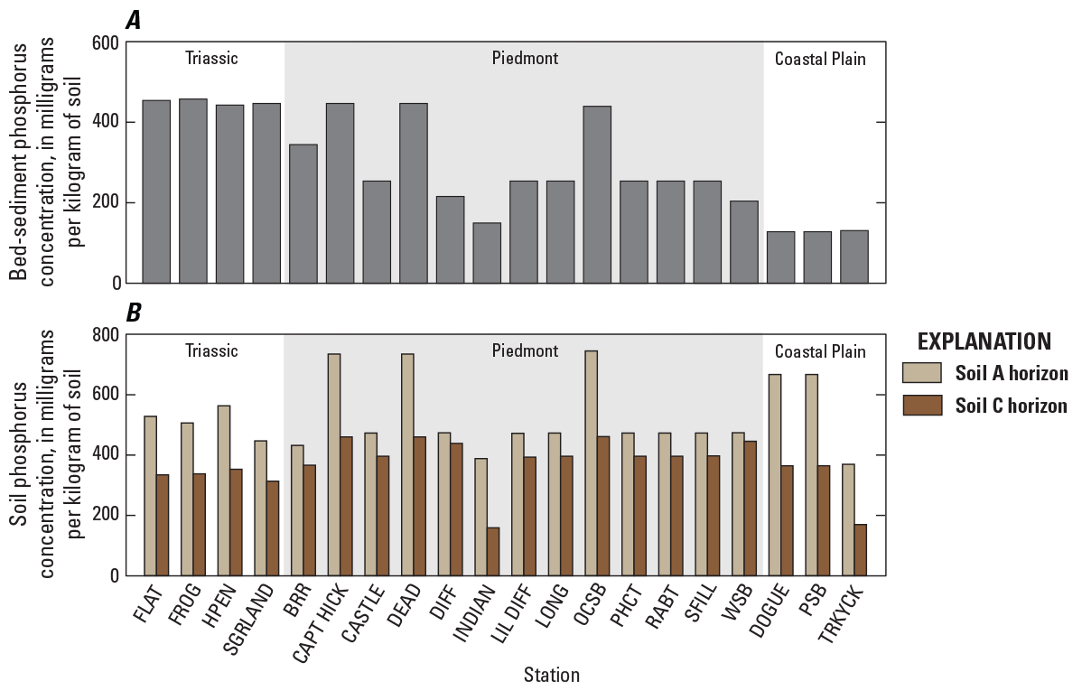
Bar graphs showing estimated A, bed-sediment phosphorus concentrations and B, soil phosphorus concentrations in 20 study watersheds in Fairfax County, Virginia. Study watershed station names are defined in table 1. Bed-sediment phosphorus concentrations are from Nardi (2014). Soil phosphorus concentrations are from Terziotti (2019).
Historical water-quality samples offered additional insights about the contribution of phosphorus from natural or anthropogenic sources. Water-quality samples were collected from 49 Fairfax County streams during a period of low flow in August 1977 (Larson, 1978). Fairfax County’s population and number of housing units has more than doubled since the late 1970s (fig. 5; Han and others, 2018), so these water-quality samples may reflect lower urban impacts. Orthophosphate concentrations in the historical data were lower than concentrations measured in August of the current study (fig. 49). Four of the five orthophosphate concentrations collected in 1977 from Triassic Lowland watersheds were below 0.02 mg/L, and one sample had a concentration of 0.08 mg/L, a value similar to conditions in FLAT, FROG, and HPEN during the study period. No stations in the current study were sampled in 1977, but a concentration below the 0.01 mg/L detection limit was measured in 1977 from a station on Flatlick Branch (USGS station ID 01656900), about 400 ft downstream from the current FLAT monitoring station. Compared with higher concentrations in FLAT during the study period, this historical concentration suggests that orthophosphate concentrations may have increased in FLAT because of human-derived inputs in addition to possible contributions from natural-mineral dissolution.
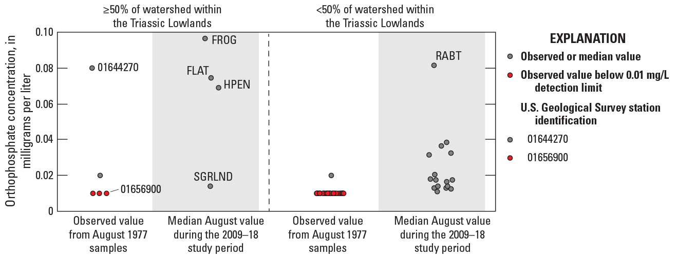
Graph showing orthophosphate concentrations measured in Fairfax County streams in August of 1977 and in 20 study watersheds in Fairfax County, Virginia, from 2009 through 2018. Orthophosphate concentration measurements in 1977 are from Larson (1978). Study watershed station names are defined in table 1. %, percent; mg/L, milligrams per liter.
The shallow soils and fractured bedrock common in Triassic Lowland watersheds may offer fewer opportunities for the retention of phosphorus in the soil and allow nonpoint-phosphorus inputs to reach streams quickly and efficiently. Compared to Piedmont watersheds with thicker soil layers, Triassic Lowland watersheds have shallow fractured bedrock that is poorly buffered from surface inputs (Froelich and Zenone, 1985b). In the Triassic Lowland study watersheds (FLAT, FROG, HPEN, and SGRLND), the average soil depth was about 45 in., compared with about 60 in. in other watersheds (table 26). Soil depth had a strong negative correlation with between-watershed, median-annual TP concentrations (app. 1, table 1.4; SOIL DEPTH, r=−0.70; fig. 50A).
Table 26.
Summary of average watershed soil depth, sand content, organic matter content, and cation-exchange capacity in 20 study watersheds in Fairfax County, Virginia.[Station names are defined in table 1, predictor names are defined in table 2]
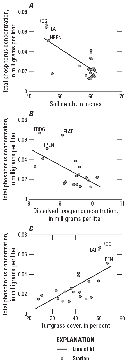
Graphs showing relations of A, soil depth; B, dissolved-oxygen concentration; and C, turfgrass cover to total phosphorus concentrations in 20 study watersheds in Fairfax County, Virginia; all values represent average conditions from 2014 through 2018. Study watershed station names are defined in table 1.
Some additional properties that describe physical soil structure and soil chemical composition were related to between-watershed differences in median-annual TP concentrations (app. 1, table 1.4) and may represent conditions that promote the mobilization of phosphorus to groundwater and streams. Phosphorus concentrations in streams can be high in areas with sandy soils because these areas have low phosphorus adsorption rates (Withers and Jarvie, 2008). The negative correlation of median-annual TP concentrations and soil sand content (SAND, r=−0.71), however, suggests that sand content, which is lowest in Triassic Lowland watersheds (table 26), may not be a driver of between-watershed TP differences. Watershed soils containing aluminum and iron can increase phosphorus retention, because dissolved phosphorus binds and forms insoluble complexes with these ions (Borggaard and others, 2004; Denver and others, 2010). Stream concentrations of aluminum and iron were not measured during the study period, but historical samples collected in Fairfax County between 1954 and 1979 (Froelich and Zenone, 1985b) indicate that some Triassic Lowland watersheds have lower dissolved iron groundwater concentrations than Piedmont or Coastal Plain watersheds (fig. 51). Watersheds in the Triassic Lowlands contained more soil organic matter than other study watersheds (table 26), a property that can increase dissolved phosphorus availability (Deb and Datta, 1967; Nziguheba and others, 1998; Yang and others, 2019; Ye and others, 2006). Despite this influence, differences in soil organic matter percentage were not correlated with between-watershed differences in median-annual TP concentrations (OM, r=0.26).
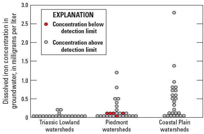
Plot of dissolved iron concentrations in groundwater collected from Fairfax County wells from 1954 through 1979. Dissolved iron concentrations are from Froelich and Zenone (1985b).
The capacity of soils to retain water may affect phosphorus retention in multiple ways. Fluctuations between wet and dry conditions can increase rates of phosphorus leaching from soils (Kinsman-Costello and others, 2016; Young and Ross, 2001); lower rates of leaching are typically associated with soils that have slower water transport times (Djodjic and others, 2004). Soils that remain saturated and form reducing conditions, however, can increase the leaching of phosphorus bound to iron (Shenker and others, 2005; Willett, 1989). Properties that describe the storage and retention of soil water were correlated with between-watershed differences in average-annual TP concentrations (app. 1, table 1.4). TP concentrations were typically higher in watersheds with higher soil field capacities (FC, r=0.70), lower rates of vertical hydraulic conductivity (KV, r=−0.74), and lower amounts of plant-available water (AWC, r=−0.67). Triassic Lowland watersheds generally had the highest FC and the lowest AWC and KV values of all study watersheds.
Biogeochemical transformations of phosphorus between soluble and insoluble forms affect phosphorus delivery to streams and are influenced by WT, DO, stream acidity, and microbial communities. Median-annual TP concentrations were higher in streams with higher WT at the time of sample collection (WT, r=0.52). This relation is consistent with studies demonstrating that temperature affects the release of phosphorus from sediment and that biotic processes enhance phosphorus availability (Duan and others, 2012; Duan and Kaushal, 2013; Withers and Jarvie, 2008). Median TP concentrations were higher in streams with lower median DO concentrations at the time of sample collection (DO, r=–0.61; fig. 50B). This relation may be related to the previously described relation between TP and WT because warmer water contains less DO. However, differences in oxidizing or reducing conditions can also affect phosphorus availability, with lower DO concentrations favoring phosphorus release from sediments (Duan and others, 2012; Withers and Jarvie, 2008). The range of DO concentrations commonly observed in Fairfax County streams reflects oxic conditions (fig. 44C), but steep declines in DO can occur within some shallow streambeds (House, 2003), resulting in lower DO concentrations in groundwater than surface water (Denver and others, 2010). Even temporary anoxic conditions that develop near the sediment surface can increase the release of phosphorus from sediments (James and Barko, 2004). Phosphorus availability can also change through pH-dependent processes, but the correlation between median-annual TP concentrations and pH values was not significant (pH, r=0.18).
The phosphorus input of fertilizer was positively correlated with between-watershed differences in median-annual TP concentrations (P FERT, r=0.65). Properly maintained turfgrass can efficiently retain fertilizer inputs, but fertilizer leaching and delivery to streams can occur in response to over applications or applications that precede storm events (Bachman and others, 2016). Phosphorus loading to streams can also increase after years of fertilizer applications that result in phosphorus-saturated soils, which describe soils without available phosphorus-bonding sites (Soldat and Petrovic, 2008). Phosphorus inputs from turfgrass fertilizer may have declined in recent years because of legislative restrictions on the sale of most residential fertilizers containing phosphorus (Harper, 2011), but it can take years to reverse the effects of phosphorus-saturated soils (Kleinman and others, 2011; Sharpley and others, 2013).
Turfgrass area also was positively correlated to median-annual TP concentrations (TURF, r=0.65; fig. 50C) and had the same correlation as fertilizer inputs, because amounts of applied fertilizer were derived directly from the turfgrass cover. Phosphorus inputs may be underrepresented in FLAT if total fertilizer applications are higher on golf courses than residential lawns, because a 200-acre golf course is within the watershed about 2 mi upstream from the monitoring station. Nutrient export from golf courses, however, can be highly variable and, like other managed turfgrass systems, is dependent on proper application and irrigation practices (Bock and Easton, 2020). In addition to representing phosphorus-fertilizer applications, the correlation between median-annual TP concentrations and turfgrass cover may result from other nonpoint inputs of phosphorus associated with residential activities. Sanitary-sewer densities were higher in watersheds with more turfgrass and were correlated with between-watershed differences in median-annual TP concentration (SAN SEWER LEN, r=0.53). Sanitary-sewer leaks in urban areas can deliver nutrients to streams (Kaushal and others, 2011), but their contributions are difficult to quantify (Amick and Burgess, 2000; Fenz and others, 2005) and may be less common in Fairfax County, which has a very low rate of reported sanitary-sewer overflows and backups (Fairfax County, 2021).
Some physical watershed properties were correlated with the 2009 through 2018 percentage change of median-annual TP concentrations (app. 1, table 1.5), which may describe the effects of phosphorus being stored and released from soils. Larger TP increases occurred in watersheds with lower soil cation-exchange capacities (CEC, r=−0.67; fig. 52A), which measures ability of a soil to hold positively charged ions. Watersheds in the Triassic Lowlands had the highest cation-exchange capacities (table 26) because these soils contained higher amounts of organic material, silts, and clays that contribute to negatively charged soil structures. Therefore, larger TP increases occurred in watersheds with more sandy soils (SAND, r=0.59) and less organic matter (OM, r=−0.60). The positive relation between TP percentage change and average soil depth (SOIL DEPTH, r=0.55; fig. 52B) would have been much stronger but for the TP increase that occurred in FLAT.
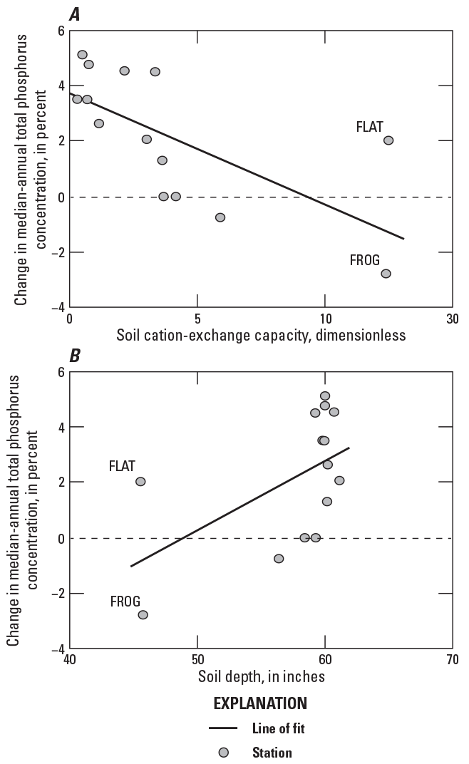
Graphs showing relations of A, soil cation-exchange capacity and B, soil depth (values represent averages from 2009 through 2018) to changes in median-annual total phosphorus concentrations from 2009 through 2018 in 14 study watersheds in Fairfax County, Virginia. Study watershed station names are defined in table 1.
Annual climatic conditions were correlated with changes in median TP concentrations from 2009 through 2018 (app. 1, table 1.6; and fig. 53). Median TP concentrations were higher in warmer years (AIR TEMP, median r=0.38) and in years with less precipitation (PRCP, median r=−0.33) in most watersheds. The relation with air temperature is consistent with the previously described effects of temperature-dependent phosphorus releases, driven by abiotic and biotic processes. The inverse relation between TP and annual precipitation may be driven by phosphorus geochemical transformations. Although years with more precipitation produce many storm events that can deliver high phosphorus concentrations to streams through sediment runoff and erosion, the phosphorus concentrations considered here are reflective of base-flow conditions and are not likely affected by such processes. Under these longer-term low-flow conditions, differences in TP concentration may be affected by differences in precipitation, as streambed sediments wet and dry and cycle between anoxic and oxic conditions. Although the net effect of these processes on phosphorus mobilization are difficult to predict (Kinsman-Costello and others, 2016), the release of phosphorus from organic matter through microbial mineralization can increase when anoxic sediments are dried (Baldwin and Mitchell, 2000; Dieter and others, 2015). Conversely, dry years and oxic conditions may be associated with the increased storage of phosphorus in bed sediments and lower stream concentrations of phosphorus (House, 2003).
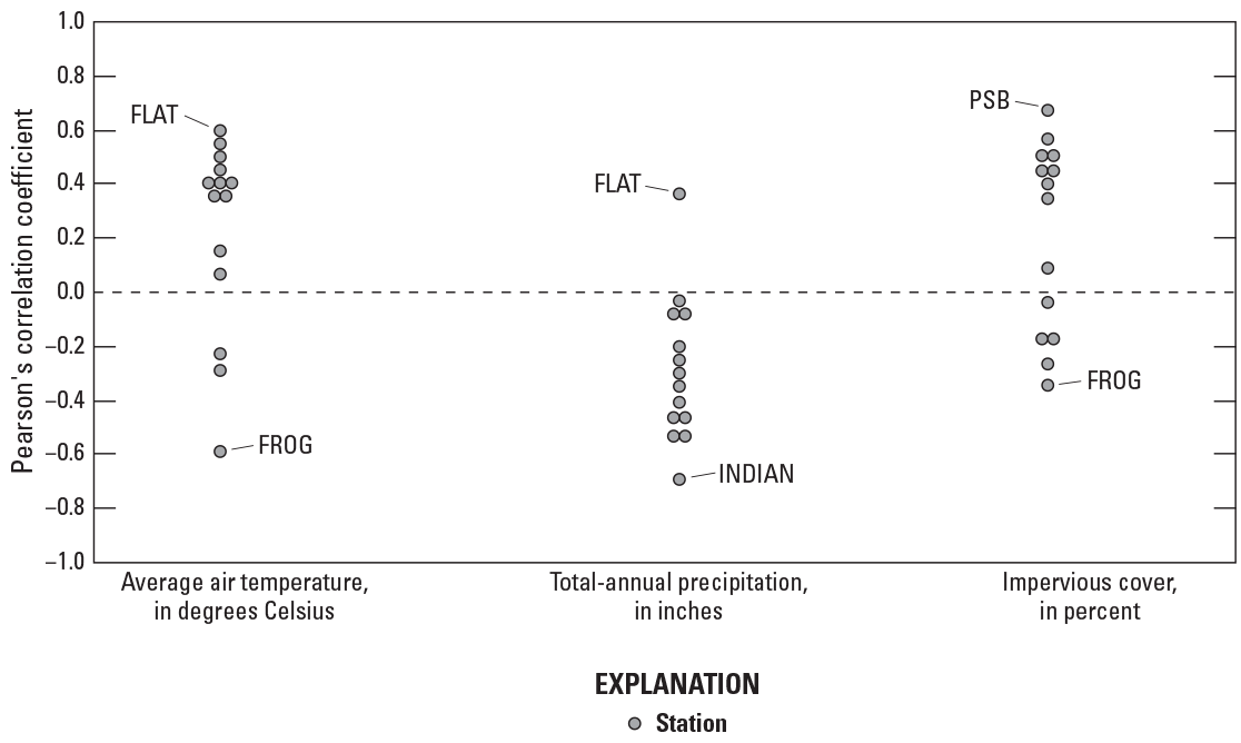
Graph showing Pearson’s correlation coefficients for relations between median-annual total phosphorus concentrations and selected predictors in 14 study watersheds in Fairfax County, Virginia. Correlations represent annual values from 2009 through 2018. Study watershed station names are defined in table 1.
Annual changes in some measures of urban land use were correlated with changes in median-annual TP concentrations from 2009 through 2018 (app. 1, table 1.6). Increases in the amount of impervious cover were associated with higher TP concentrations (IMP, median r=0.37; fig. 53) in most watersheds. Increased impervious cover may account for increased applications of phosphorus inputs, more efficient delivery of phosphorus inputs to streams, or effects of salinization on phosphorus mobilization. Stream salinity, measured as SC, was higher in the more impervious study watersheds, and large pulses of SC were observed during some winter storm events, which was consistent with the effects of road-salt application (Porter and others, 2020b). SC increased in the study watersheds over the past 10 years (Porter and others, 2020b); these increases can mobilize phosphorus (along with other cations and nutrients) to urban streams through various ion-exchange and biogeochemical pathways (Duan and Kaushal, 2015; Haq and others, 2018). Sodium, a common component of road salt, can preferentially displace some trivalent and divalent cations, including aluminum, iron, and calcium (Amrhein and others, 1992; Shanley, 1994), which commonly bind with phosphorus to form insoluble compounds. The stability of these phosphate complexes decreases with increasing salinity and can result in higher dissolved phosphorus concentrations in streams (Duan and Kaushal, 2015; Haq and others, 2018). Watersheds with low soil cation-exchange capacities, where TP concentration increases were largest (fig. 52A), may be more susceptible to these ion-exchange processes. The correlations between median-annual SC and median-annual TP concentrations were inconsistent across the study watersheds (app. 1, table 1.6), suggesting that potential salinization effects on phosphorus mobilization are locally variable, poorly represented by median-annual conditions, offset by other predictors, affected by salinity in previous years, or not strongly influential.
Explanation of Variability
Based on the information described above, seven predictors were included in LME models to describe the spatiotemporal variability of median-annual TP concentrations: (1) total-annual precipitation, (2) average-annual air temperature, (3) DO, (4) soil depth, (5) bed-sediment phosphorus concentrations, (6) impervious cover, and (7) turfgrass cover. Combined with the six parameters of the linear-growth model, all possible model combinations of the seven additional predictors were considered. Models with the lowest AIC included a similar combination of terms and performed similarly (app. 2, table 2.2). This model-building process was repeated after excluding FLAT because the phosphorus increases in this watershed were unique; the structure of top-performing models was similar to those including FLAT.
Many similarly performing models described the spatiotemporal variability of median-annual TP concentrations in the 14 study watersheds from 2009 through 2018, but interpretations from a single model can help inform watershed management. An 11-parameter model was selected for interpretation after considering the results of models with and without FLAT and the most likely factors that may be influencing TP concentrations. This model included fixed-effect terms for total-annual precipitation, soil depth, stream DO concentration, and turfgrass cover (table 27). Alternative models with the same or fewer parameters had similar AIC values, but the inclusion of more parameters did not offer meaningful improvements in model performance (app. 2, fig. 2.3). The 95-percent confidence interval of all model coefficients, except the effect of soil depth on the linear rate of TP change over time (SOIL DEPTH, b2), did not include zero. The effect of soil depth on the linear rate of TP change over time was consistently identified in models that did not include FLAT and was therefore included in the selected model of 14 watersheds. Additional predictors not included during initial model development were iteratively considered but did not improve the selected model’s performance. These predictors included effects of median-annual streamflow, cation-exchange capacity, organic matter, available water capacity, WT, SC, and the number of dry stormwater ponds.
Table 27.
Results of a total phosphorus linear mixed-effect model selected for interpretation, including 95-percent confidence intervals, fixed-effect estimates, random-effect variances, and the model’s Akaike information criterion.[Linear mixed-effect models are described in equations 4–6. Predictors are described in tables 2 and 3. b3, the effect of a predictor on within-watershed variability; b1, the effect of a predictor on between-watershed intercept differences; b2, the effect of a predictor on between-watershed slope differences; R2, coefficient of determination; AIC, Akaike information criterion]
The fixed-effect terms in the selected model explained 85 percent of the spatiotemporal variability in median-annual TP concentrations (table 27). Compared to the linear-growth model (table 25), the selected model explained an additional 96 percent of the between-watershed intercept variance, an additional 8 percent of the annual within-watershed variance, and an additional 29 percent of the between-watershed slope variance. Observed and predicted responses plotted against time were used to visually assess the selected model’s performance in each watershed (app. 2, fig. 2.4). Notably, the model did not accurately estimate the increase in TP concentrations in FLAT that occurred towards the end of the study period. The selected model residuals for most stations were evenly distributed around zero in most years: an improvement compared with predictions from the linear-growth model (fig. 54).
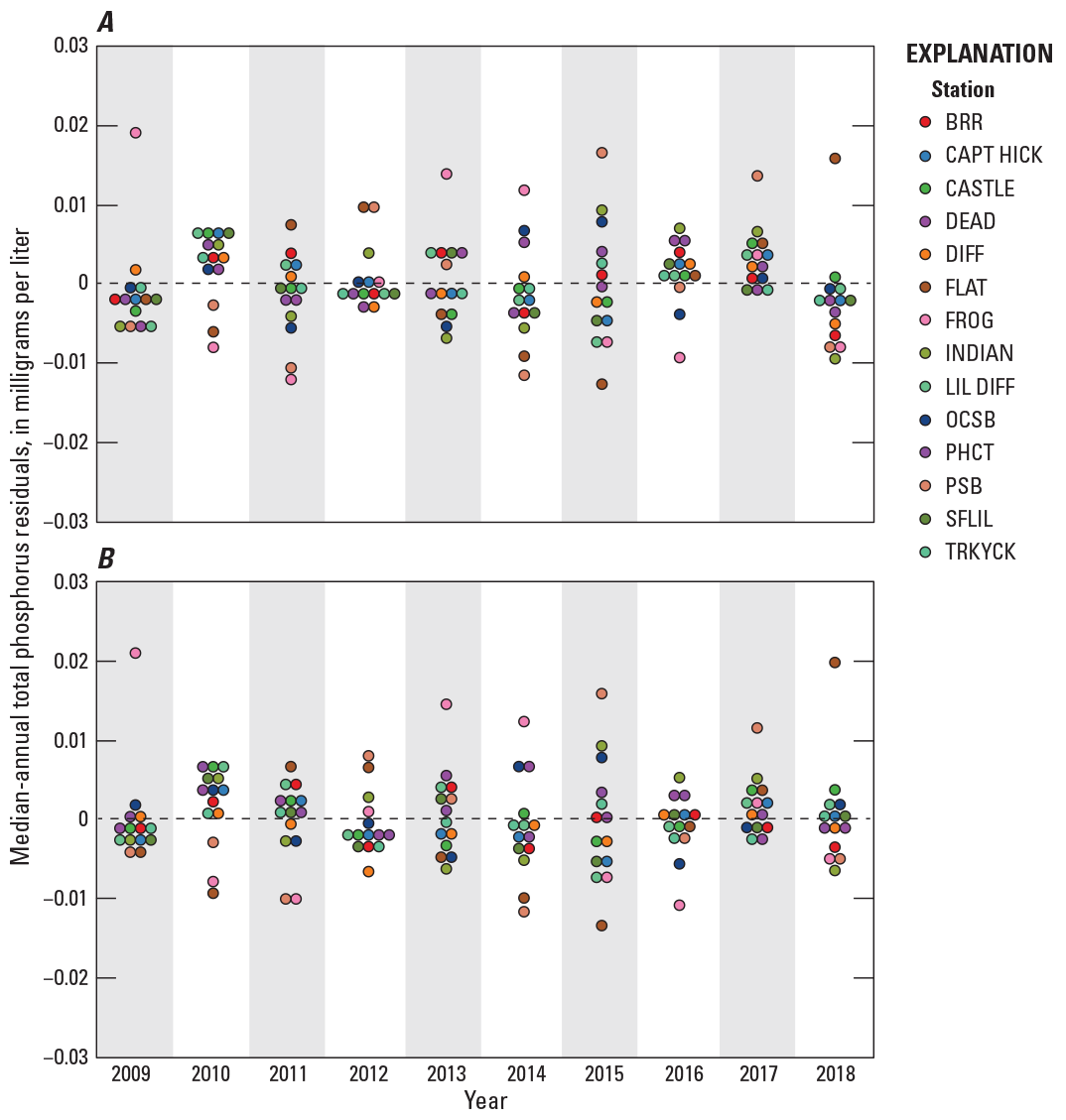
Graphs showing model residuals from A, the total phosphorus linear-growth model and B, the selected total phosphorus linear mixed-effect model in 14 study watersheds in Fairfax County, Virginia, from 2009 through 2018. Study watershed station names are defined in table 1.
The fixed effects in the selected model describe the average effect of average-annual precipitation, soil depth, turfgrass cover, and stream DO concentration on median-annual TP concentrations in 14 watersheds (table 27): predictors that vary over space and time (fig. 55). The largest model effect sizes corresponded to effects of soil depth; watersheds with deeper soils had lower TP concentrations (SOIL DEPTH b1, −0.77) and a more positive TP increase from 2009 through 2018 (SOIL DEPTH b2, 0.31). Watersheds with higher average DO concentrations and lower average turfgrass cover were associated with lower TP concentrations. The effect of annual precipitation on TP changes within watersheds over time (PRCP b3, −0.23) was similar in magnitude to that of the model slope (Year b3, 0.23), highlighting that, on average, TP concentrations were higher in years with less precipitation and in later years of the study period. The positive slope coefficient suggests that TP increases may be affected by additional factors not represented in the model. Annual precipitation was the only modeled effect that caused estimated values to deviate from a perfectly straight line (app. 2, fig. 2.4). The interpretation of these terms was similar to a model of 13 study watersheds that excluded FLAT (app. 2, table 2.3).
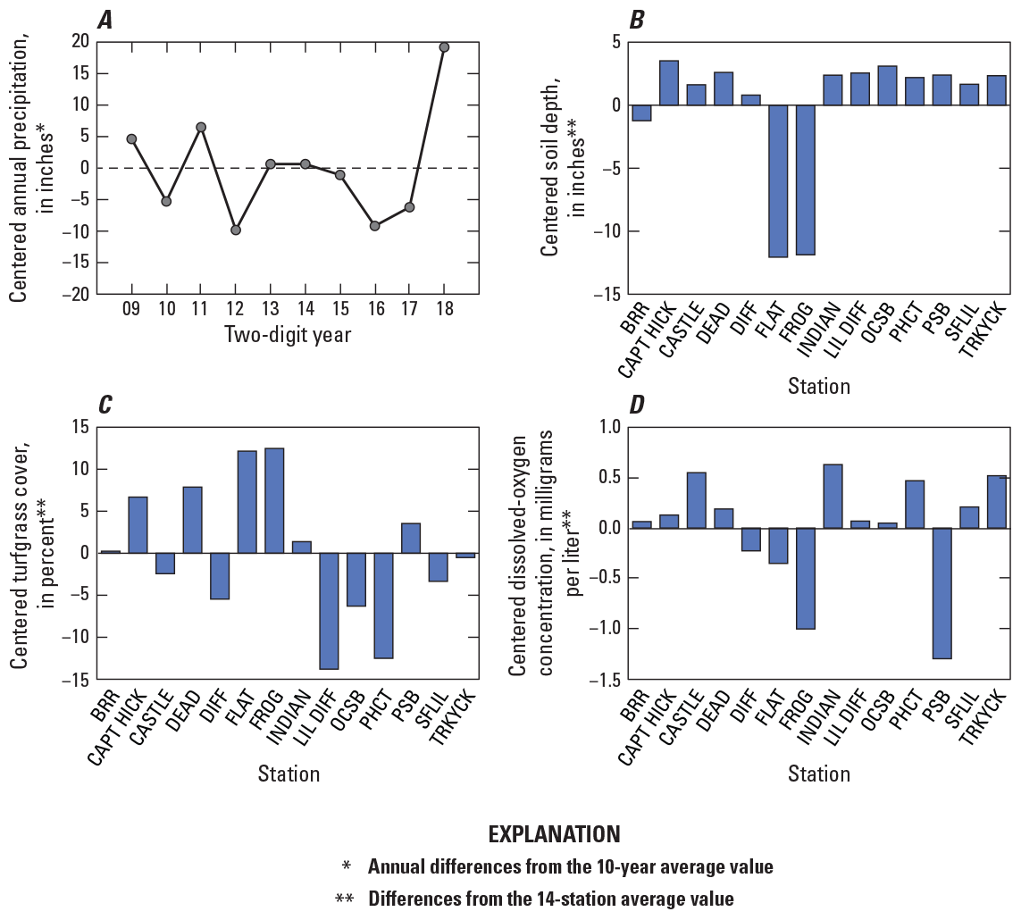
Graphs showing centered parameters used in the selected total phosphorus linear mixed-effect model: A, annual precipitation from 2009 through 2018; B, soil depth; C, turfgrass cover; and D, dissolved-oxygen concentrations in 14 study watersheds in Fairfax County, Virginia. Study watershed station names are defined in table 1.
The modeled effects of soil depth, turfgrass cover, DO concentration, and annual precipitation may be better understood by considering the retention of phosphorus on the landscape and phosphorus inputs. The modeled effect of turfgrass cover may suggest that phosphorus concentrations are higher in watersheds that receive more fertilizer applications. The modeled effects of soil depth describe lower average phosphorus concentrations that increased more positively over time in watersheds with deeper soils. Because deeper soils may store more phosphorus, changes in TP over time in Fairfax County streams may be affected by the retention or release of soil-bound phosphorus. The storage and release of phosphorus in a watershed is also controlled by environmental conditions such as temperature, DO, acidity, wetness, and microbial communities (House, 2003; Withers and Jarvie, 2008). The selected model identified two such effects: that TP concentrations were lower in watersheds with higher stream DO concentrations and that years with less precipitation were associated with higher TP concentrations. Lower DO concentrations can produce anoxic conditions that favor phosphorus release from sediments (Duan and others, 2012; Withers and Jarvie, 2008). The association between annual changes in precipitation and TP concentrations may be explained by the mineralization of organic matter, which is expected to occur more readily in drier conditions, releasing dissolved phosphorus from soils (Baldwin and Mitchell, 2000; Dieter and others, 2015). However, the net effect of precipitation on phosphorus mobilization is difficult to predict (Kinsman-Costello and others, 2016) and these effects are likely overwhelmed by the delivery of particulate phosphorus to streams during high-flow events. The positive slope term (Year b3) suggests that the modeled landscape and climatic factors do not completely account for an average increase in TP concentrations from 2009 through 2018.
Management-Practice Effects
Stormwater-retrofit and channel-restoration practices to reduce phosphorus were installed in seven study watersheds from 2009 through 2018 and, normalized by watershed area, were expected to lower TP yields by tens to hundreds of pounds. Despite the credited reductions, median annual TP concentrations typically did not decrease in these watersheds (fig. 56). Credited TP reductions were considered as a predictor of median-annual TP concentrations in the previously described LME model to assess their potential effect on observed conditions, relative to other environmental and anthropogenic drivers. Specifically, the model considered the annual effect of cumulative TP reductions on differences in median-annual TP concentrations from 2009 through 2018 in 14 watersheds. The AIC of a model including TP reductions credited to management practices was nearly 10 units lower than the previously described model (table 28). The modeled effect of management practices was positive, suggesting that credited reductions increase stream phosphorus concentrations; however, this relation was heavily affected by patterns in FLAT. Among the seven watersheds with credited phosphorus reductions, the modeled relation between phosphorus concentrations and credited reductions can be best seen at FLAT, where increases in credited TP reductions coincided with increases in median TP concentrations from 2016 through 2018 (fig. 56). After removing FLAT and refitting the model to 13 study watersheds, the credited phosphorus reduction term did not improve the modeled representation of TP concentrations (AIC of 247.16 versus 245.21 in a simpler model; app. 2, table 2.3), and the term was not significantly different from zero (app. 2, table 2.4).
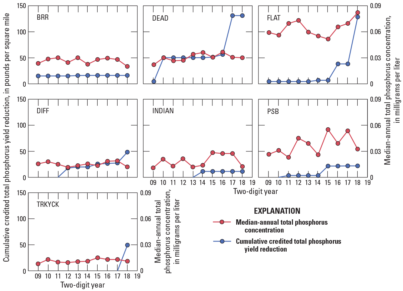
Graphs showing the cumulative credited total phosphorus yield reductions from management practices and median-annual total phosphorus concentrations in seven study watersheds in Fairfax County, Virginia, from 2009 through 2018. Study watershed station names are defined in table 1.
Table 28.
Results of a total phosphorus linear mixed-effect model with credited management-practice total phosphorus reductions, including 95-percent confidence intervals and fixed-effect estimates, random-effect variances, and the model’s Akaike information criterion.[Linear mixed-effect models are described in equations 4–6. Predictors are described in tables 2, 3, and table 5. b3, the effect of a predictor on within-watershed variability; b1, the effect of a predictor on between-watershed intercept differences; b2, the effect of a predictor on between-watershed slope differences; R2, coefficient of determination; AIC, Akaike information criterion]
The modeled effect of management practices on median-annual TP concentrations in FLAT may have been related to the construction of a stream-restoration practice immediately upstream from the monitoring station (fig. 46). Stream restorations that stabilize streambanks may offer some of the best opportunities to reduce phosphorus (Lammers and Bledsoe, 2017), but their construction may cause a short-term increase in particulate water-quality conditions. Construction sites are one of the largest contributors of sediment to surface waters in urban areas (U.S. Environmental Protection Agency, 2005); however, proper sediment and erosion controls can limit the impact of construction on downstream water quality (Houser and Pruess, 2009). Minimal water-quality effects have been associated with construction projects in larger river systems (Colangelo and Jones, 2005; Jastram and others, 2015), and water-quality impacts from the construction of other Fairfax County stream restorations (table 13) were not apparent in the monitoring data, including a stream restoration completed farther upstream from the FLAT monitoring station in 2016. These patterns may suggest that particulate material mobilized during construction is stored in-channel or in floodplains before being delivered downstream. Additionally, changes in flow-adjusted TP loads at FLAT did not show an increase during the 2016–18 period (fig. 31), suggesting that potential construction impacts were not influential during high streamflow conditions, which generate the most TP load.
Sediment
Sediment is naturally occurring in urban and suburban streams but can be in quantities that are harmful to stream biota (Paul and Meyer, 2001). Excess sediment in urban and suburban streams commonly results from streambank erosion or the delivery of upland material: sources that vary over time and space with stream size, climatic conditions, and land-use activity (Noe and others, 2020). Enhanced knowledge about sediment sources, lag times, and the effects of natural setting are needed to inform stormwater-management strategies because the efficacy of such strategies vary across watershed scale and land use (Noe and others, 2020).
Patterns of Observed Responses
SS concentrations differed among study watersheds, varied seasonally, and were strongly related to streamflow (Porter and others, 2020b). Median-annual SS concentrations below about 10 mg/L were commonly observed (fig. 57), though concentrations quickly increased by multiple orders of magnitude during stormflow events (fig. 58). SS concentrations and their relation to streamflow are influenced by a combination of factors that affect how quickly runoff enters streams, how much sediment is delivered from streambanks or upland sources, and how in-channel sediment is stored and remobilized. In general, most high streamflow SS concentrations in Fairfax County consist of fine materials, such as silts and clays (Porter and others, 2020b) that originate from stream banks (Cashman and others, 2018). Summer months were typically associated with more frequent and higher-intensity storm events (fig. 15), which result in greater SS concentrations and loads (Porter and others, 2020b).
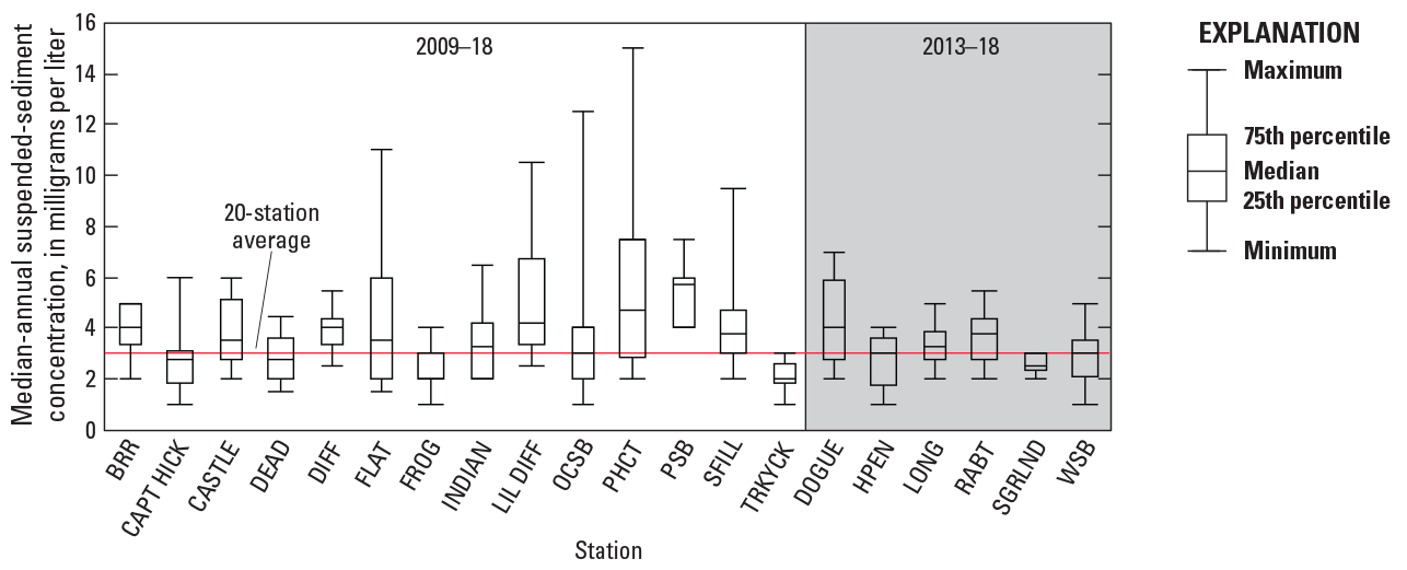
Boxplots showing the median-annual suspended-sediment concentrations of 20 study watersheds in Fairfax County, Virginia. Study watershed station names are defined in table 1.
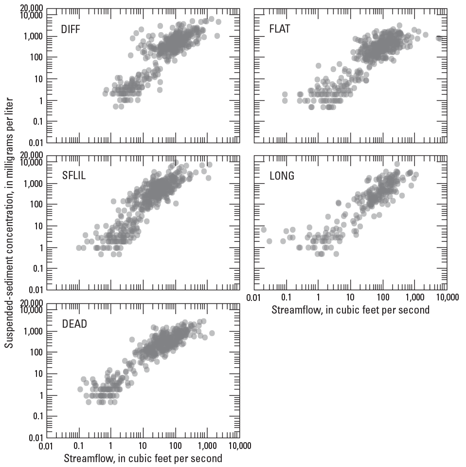
Graphs showing the relations of streamflow to suspended-sediment concentration measured in five study watersheds in Fairfax County, Virginia. Study watershed station names are defined in table 1.
SS concentration trends were evaluated using monthly water-quality samples collected from April 2008 through March 2018 to describe how conditions changed over time in 14 watersheds with 10 years of data, analyses, and interpretations originally conducted by Porter and others (2020b; table 29). After adjusting for streamflow, SS concentrations increased in FLAT and INDIAN, decreased in BRR, and had no trend in the remaining 11 watersheds. No network-wide trend in SS concentrations was detected. The increases in FLAT occurred from 2016 through 2018 and were consistent with a period of stream-restoration construction immediately upstream from the monitoring station (fig. 46).
Table 29.
Flow-adjusted suspended-sediment concentration trends in 14 study watersheds in Fairfax County, Virginia, from March 2008 through April 2018.[Station names are defined in table 1. mg/L, milligram per liter; %, percent]
Within any watershed and year, a large range of SS concentrations was observed because the monthly samples were collected during a range of streamflow conditions; however, median-annual values removed most of this variability (fig. 57). Between- and within-watershed differences in median-annual SS concentrations, representing spatial differences among study watersheds and temporal differences from 2009 through 2018, were described by a linear-growth model (table 30). This model indicated that the average SS concentration across all watersheds in 2009 was 3.67 mg/L and that the linear rate-of-change could not be differentiated from zero. Random-effect variances describe a dataset where within-watershed annual changes (3.898) represented most of the total model variance (4.437). Group-level variance (0.534), representing between-watershed differences in intercept and differences in between-watershed slope (0.005), was small. Interannual differences in median-annual SS concentration were larger than the linear rate-of-change over time in most watersheds (fig. 59). The AIC of the linear-growth model (615.02) was compared against models that included additional predictors; more parsimonious models reduced the between- and within-watershed random-effect variances.
Table 30.
Results of the suspended-sediment linear-growth model, including fixed-effect estimates, 95-percent confidence intervals, random-effect variances, and the model’s Akaike information criterion.[The linear-growth model is defined in equations 1–3. AIC, Akaike information criterion]
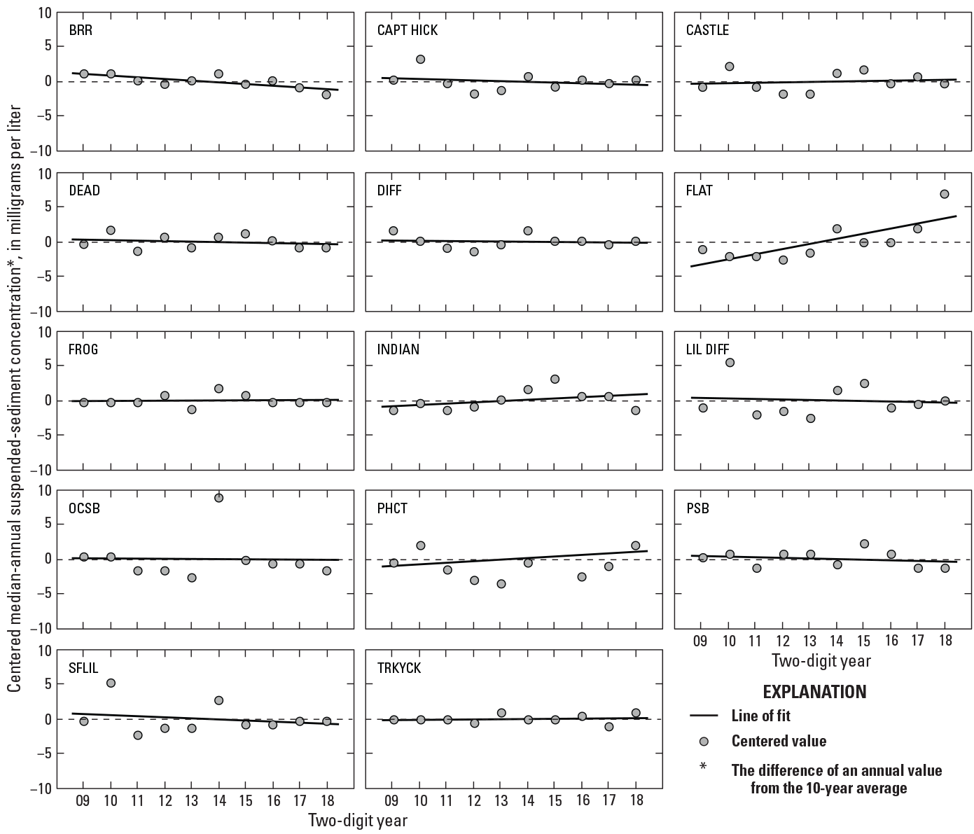
Graphs showing centered values of median-annual suspended-sediment concentration in 14 study watersheds in Fairfax County, Virginia, from 2009 through 2018. Study watershed station names are defined in table 1.
Relations to Predictor Variables
Between-watershed SS differences were likely affected by a combination of human and natural factors, patterns that were explored by comparing average predictor values and SS concentrations at 20 study watersheds from 2014 through 2018 (app. 1, table 1.7). Most predictors had weak relations or no relations with between-watershed SS differences, likely because the spatial variability of median-annual SS concentrations was small (fig. 57). Average TB conditions during the time of water-quality sample collection had the strongest correlation with SS (TURB, r=0.80; fig. 60A): an expected and well-documented pattern (Jastram and others, 2009; Porter and others, 2020b).
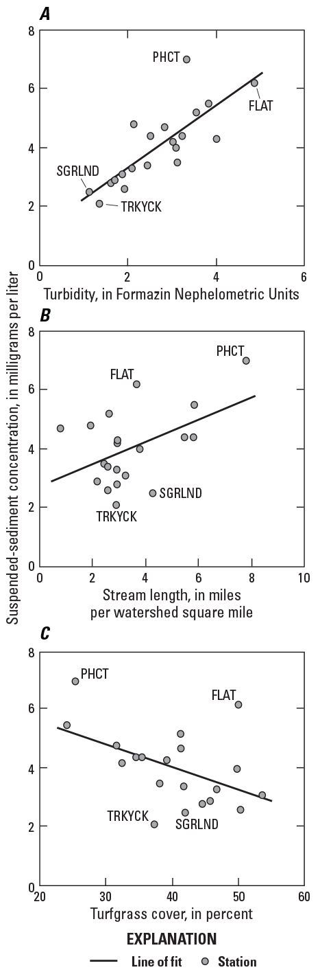
Graphs showing relations of A, turbidity; B, stream length; and C, turfgrass cover to suspended-sediment concentrations in 20 study watersheds in Fairfax County, Virginia; all values represent average conditions from 2014 through 2018. Study watershed station names are defined in table 1.
Between-watershed differences in median-annual SS concentrations were positively correlated with stream density, reflecting the length of perennial and non-perennial streams normalized by watershed area (TOTSTREAM, r=0.48; fig. 60B). Watersheds with a higher stream density may have more sinuous stream channels, more opportunities for stream-bank erosion and bed-sediment remobilization, and a faster pathway for particulate material in stormwater runoff to be delivered downstream. The length of streams in small Piedmont watersheds has previously been identified as an important predictor of SS loads throughout the Chesapeake Bay watershed (Brakebill and others, 2010). Greater rates of stream-bank erosion and floodplain deposition have been associated with more sinuous stream channels in Fairfax County streams (Gellis and others, 2017; Schenk and others, 2013).
Sediment sources vary over time and space based on local conditions. Stream banks can represent an important sediment source in mid-Atlantic urban watersheds and are typically a dominant source of sediment in first- and second-order streams (Devereux and others, 2010; Donovan and others, 2015; Noe and others, 2020). In Difficult Run, Fairfax County’s largest watershed (fig. 1), bank-derived sediment is the dominant source during storm events and accounts for most of the SS load (Cashman and others, 2018; Gellis and others, 2017). Much of this bank-derived material represents legacy sediment, that is, sediment that accumulated in the floodplains and channel beds during the colonial period in the 17th to 19th centuries (Noe and others, 2020). Legacy sediment accounts for most of the current bank height in Difficult Run and likely represents a substantial fraction of eroded material transported by Fairfax County streams (Hupp and others, 2013). Bank-derived sediment can be remobilized from in-channel storage, but most material is contributed from the erosion of stream banks (Cashman and others, 2018).
Changing stream-channel shapes and the lateral migration of stream banks can be an important erosional process in urban watersheds (Donovan and others, 2015) and occurs throughout Difficult Run, particularly in response to large storm events (Gellis and others, 2017; Hupp and others, 2013). Urbanization and expanded impervious cover can increase the delivery of stormwater runoff to streams, hydrologic changes that can cause stream-channel widening, migration, and incision (Paul and Meyer, 2001). The historical streamflow record and patterns of sediment erosion and deposition in Difficult Run indicate that such stream-channel changes are likely occurring, and that the watershed is not in geomorphic equilibrium (Hupp and others, 2013). Rates of stream-bank erosion or aggradation, the deposition of sediment along stream banks, vary throughout Difficult Run (Gellis and others, 2017). Difficult Run headwaters are typically erosional and downstream reaches are typically net depositional (Hupp and others, 2013). Patterns in Difficult Run may be indicative of the geomorphic changes occurring in other Fairfax County streams.
Changes in stream geometry were not directly measured in this study, but stream-channel dynamics can be partly represented from the maintenance of real-time streamflow records computed from the relation of water level to measured streamflow (Messinger and Burgholzer, 2018). As the stream channel changes shape, so too does the relation between water level and streamflow, which requires the development of a new streamflow rating curve (Nolan and others, 2005; Turnipseed and Sauer, 2010). From 2008 to 2019, 3 to 6 new rating curves were established at the intensive-monitoring stations. The most changes occurred in DEAD and the fewest in SFLIL, corresponding with differences in watershed impervious cover (table 7) and storm-event hydrologic responses (table 15). Over this same period, only one new rating curve was developed for a nearby headwater stream that drains mostly forested land in Prince William Forest Park and is considered a reference watershed for Fairfax County ecological assessments: South Fork Quantico Creek near Independent Hill, Va. (fig. 1; USGS station ID: 01658500).
Between-watershed differences in median-annual SS concentration were correlated with watershed turfgrass cover (TURF, r=−0.49; fig. 60C). Turfgrass cover may affect how much sediment reaches streams from upland sources by slowing stormwater runoff velocities and increasing infiltration rates, resulting in less sediment loss to streams (Gross and others, 1990; Krenitsky and others, 1998). These benefits can increase as turfgrass density increases (Easton and Petrovic, 2004).
Correlations between watershed predictors and the 2009 through 2018 percentage change in median-annual SS concentrations (app. 1, table 1.8) were influenced by the large SS increase in FLAT. After removing FLAT and reassessing these relations, stronger correlations were identified with stream-bank height (r=0.49), watershed slope (r=0.54), and wet stormwater detention ponds (r=−0.57; fig. 61). Correlations with stream-bank height and watershed slope suggest that median-annual SS concentration increases were larger over the study period in watersheds with taller stream banks and steeper slopes. Both metrics may affect sediment supply and storage: taller stream banks provide more opportunities for erosion and steeper slopes affect the delivery of upland material to streams. Conversely, watersheds with a greater area of wet stormwater detention ponds had a more negative SS rate-of-change over the 10-year period. Wet stormwater detention ponds are permanent pools of water designed to reduce nutrient and sediment loads in downstream receiving waters through chemical processes, the physical settling of particulate material, and attenuating stormflows. Stormwater detention ponds can reduce sediment concentrations and loads in many urban and suburban settings (Hossain and others, 2005; Krajewski and others, 2017; Marsalek and others, 2002), including Fairfax County (Schwartz and others, 2017), though effects can be highly variable.
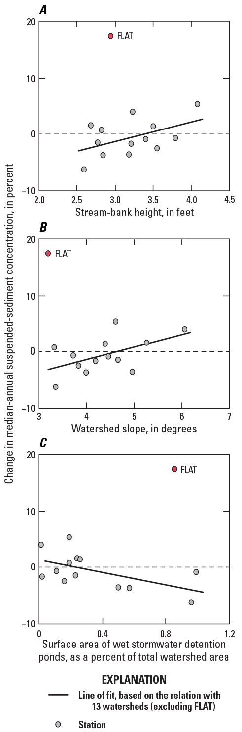
Graphs showing relations of A, stream-bank height; B, watershed slope; and C, surface area of wet stormwater detention ponds (values represent averages from 2009 through 2018) to changes in median-annual suspended-sediment concentrations in 14 study watersheds in Fairfax County, Virginia, from 2009 through 2018. Study watershed station names are defined in table 1.
Annual differences in median SS concentration were correlated with measures of stream TB (TB, median r=0.75; app. 1, table 1.9; fig. 62), an expected relation because SS increases light scatter and reduces water clarity. Stream turbidity measured at the time of sample collection was correlated with DO; lower DO concentrations were typical during periods of elevated TB. Therefore, DO was not likely a factor influencing sediment delivery to streams, despite a correlation between annual changes in DO and SS concentrations (DO, median r=−0.44).
Median-annual SS concentrations were higher during years with colder minimum air temperatures in most watersheds (TNn, median r=−0.38; app. 1, table 1.9; fig. 62), which typically occurred in January or February (fig. 63). The pattern of colder years having higher SS concentrations may be related to freeze-thaw processes, which have been hypothesized as a driver of elevated spring-time concentrations in Fairfax County streams (Porter and others, 2020b). Previous studies have documented high stream-bank erosion rates during the winter and that frost is one of the strongest predictors of stream-bank erosion (Lawler, 1986; Wolman, 1959; Wynn and others, 2008). Soil water expands when frozen, trapping sediment within ice crystals and weakening the cohesive structure of a stream bank. When frozen soil water melts, sediment stored within the ice is carried downstream and the loosened stream bank is more susceptible to erosion during a subsequent stormflow event (Lawler, 1986). Colder minimum temperatures have been associated with greater rates of erosion because these conditions likely result in more widespread frost conditions (Stott, 1997). More frequent freeze-thaw conditions may occur in urban watersheds because stormwater runoff is typically warmer than stream temperatures (Paul and Meyer, 2001; Walsh and others, 2005) and, in recent years, as climatic extremes became more prevalent (Inamdar and others, 2018). Stream banks contributed to a higher percentage of SS concentrations during the spring in Difficult Run, possibly as a result of freeze-thaw processes (Cashman and others, 2018); however, the effect of frost on stream-bank erosion can be overshadowed by large storm events (Gellis and others, 2017).
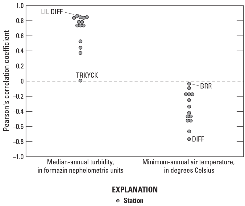
Graph showing Pearson’s correlation coefficients for relations between median-annual suspended sediment concentrations and selected predictors in 14 study watersheds in Fairfax County, Virginia. Correlations represent annual values from 2009 through 2018. Study watershed station names are defined in table 1.
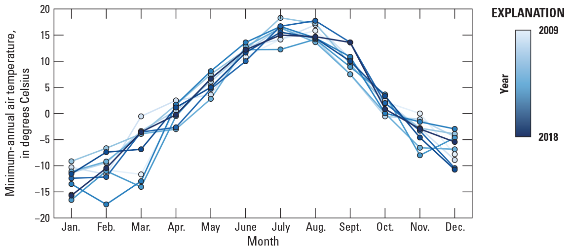
Graph showing minimum-annual air temperature of Fairfax County, Virginia, by month from 2009 through 2018. Study watershed station names are defined in table 1. Jan., January; Feb., February; Mar., March; Apr., April; Aug., August; Sept., September; Oct., October; Nov., November; Dec., December.
Explanation of Variability
Based on the information described above, seven predictors were included in LME models to describe the spatiotemporal variability of median-annual SS concentrations: (1) median-annual streamflow, (2) minimum-annual air temperature, (3) stream density, (4) turfgrass cover, (5) stream-bank height, (6) watershed slope, and (7) the area of wet stormwater detention ponds. Median-annual streamflow was considered to evaluate whether median-annual SS was affected by varying flow conditions because varying flow conditions can mask the role of other factors. Combined with the six parameters of the linear-growth model, all possible model combinations of the seven additional predictors were considered. Models with the lowest AIC had common terms and performed similarly (app. 2, table 2.5). This model-building process was repeated after excluding FLAT because the SS increases in that watershed were unique; the structure of the top-performing models was similar to those including FLAT.
Many similarly performing models described the spatiotemporal variability of median-annual SS concentrations in the 14 study watersheds from 2009 through 2018, but interpretations from a single model can help inform watershed management. An 8-parameter model was selected for interpretation after assessing model-performance metrics and considering the interpretations of previous studies on sediment sources and transport in Fairfax County (Cashman and others, 2018; Gellis and others, 2017; Hupp and others, 2013; Schenk and others, 2013). This model included fixed-effect terms for minimum-annual air temperature and stream density (table 31). In models that included and excluded FLAT, this 8-parameter model had one of the lowest AIC values, and the inclusion of additional terms did not greatly improve the representation of SS concentration variability (app. 2, fig. 2.5). This model was selected over an alternative 8-parameter model with similar AIC that replaced stream density with turfgrass cover. Although turfgrass can slow stormwater runoff and reduce sediment delivery to streams (Gross and others, 1990; Krenitsky and others, 1998), stream-bank erosion is an important sediment source in Fairfax County (Cashman and others, 2018; Gellis and others, 2017) and may be related to stream density. The effect of streamflow on interannual SS concentration variability was identified in many of the best-performing models (app. 2, table 2.5), but was not significant when combined with minimum-annual air temperature and stream density.
Table 31.
Results of a suspended-sediment linear mixed-effect model selected for interpretation, including 95-percent confidence intervals, fixed-effect estimates, random-effect variances, and the model’s Akaike information criterion.[Linear mixed-effect models are described in equations 4–6. Predictors are described in tables 2 and 3. b3, the effect of a predictor on within-watershed variability; b1, the effect of a predictor on between-watershed intercept differences; R2, coefficient of determination; AIC, Akaike information criterion]
The fixed-effect terms in the selected model explained 19 percent of the spatiotemporal variability in median-annual SS concentrations (table 31). Because between-watershed SS concentrations were similar (fig. 57), most of this predictive ability was assessed against within-watershed SS concentration variability. Compared to the linear-growth model (table 30), the effect of minimum-annual air temperature in the selected model explained an additional 15 percent of the within-watershed variability in median-annual SS concentrations. Observed and predicted responses plotted against time were used to visually assess the selected model’s performance in each watershed (app. 2, fig. 2.6). Notably, the model did not accurately estimate elevated SS concentrations that occurred in some watersheds and years (for example, OCSB in 2014 and PHCT in 2015). These years had higher median concentrations because most monthly samples were collected during stormflow conditions. Also, the model did not track the increase in SS that occurred in FLAT towards the end of the study period. The selected model residuals for most stations were evenly distributed around zero in most years: an improvement compared with predictions from the linear-growth model, although there are some large under-predictions, likely affected by samples collected during stormflow conditions (fig. 64). Patterns of over- or under-prediction in the linear-growth model appear similar to patterns of years when minimum-annual air temperature was high or low (fig. 65A).
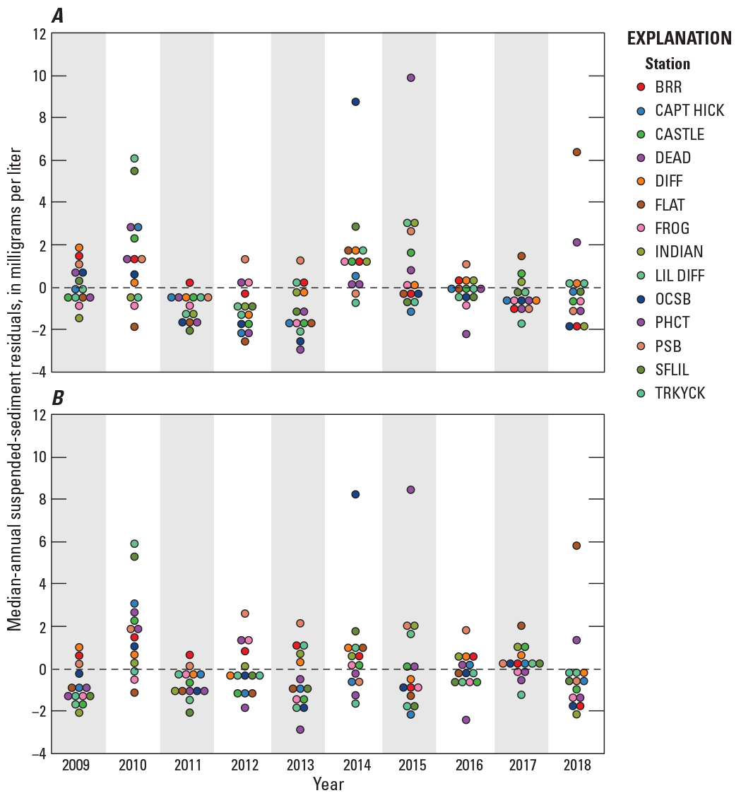
Graphs showing model residuals from A, the suspended-sediment linear-growth model and B, the selected suspended-sediment linear mixed-effect model in 14 study watersheds in Fairfax County, Virginia, from 2009 through 2018. Study watershed station names are defined in table 1.
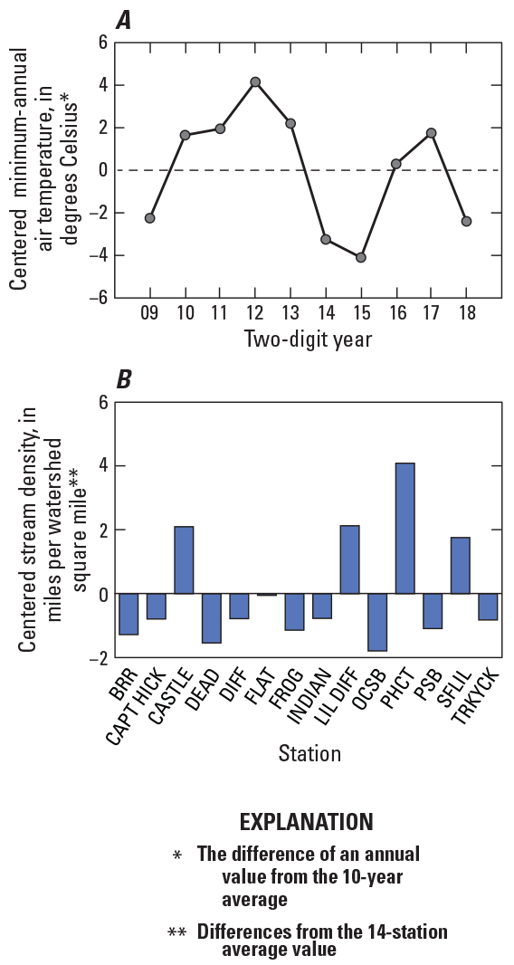
Graphs showing centered parameters used in the selected suspended-sediment linear mixed-effect model: A, minimum-annual air temperature from 2009 through 2018, and B, stream density in 14 study watersheds in Fairfax County, Virginia. Study watershed station names are defined in table 1.
The fixed effects in the selected model describe the average effect of minimum-annual air temperature and stream density on median-annual SS concentrations in 14 watersheds (table 31): predictors that varied over space and time (fig. 65). The largest effect size in the model corresponded to stream density: stations with a greater length of perennial and nonperennial streams per watershed area had higher SS concentrations (TOT STREAM, b1, 0.74, table 31). The negative coefficient of minimum-annual air temperature explains that SS concentrations were higher in years with colder minimum temperatures. On average, a 2.7-degree decrease in minimum air temperature was associated with a 0.7 mg/L median-annual SS concentration increase. Minimum-annual air temperature was the only modeled effect that caused estimated values to deviate from a perfectly straight line (app. 2, fig. 2.6). The interpretation of these terms was similar to a model of 13 study watersheds that excluded FLAT (app. 2, table 2.6).
The modeled effects of stream density and minimum-annual air temperature may be understood by considering how SS concentrations are affected by physical watershed properties and climatic conditions. Watersheds with a greater stream density may have higher SS concentrations because they have more sinuous stream channels with erosive stream banks, more opportunities for bed-sediment remobilization, and (or) a more efficient pathway for particulate material in stormwater runoff to be delivered downstream. Previous research has documented that bank erosion intensity increases with stream sinuosity in Difficult Run (Hupp and others, 2013), that stream banks are important as a source of sediment in Fairfax County streams, and that lateral streambank migration has erosional effects (Cashman and others, 2018; Gellis and others, 2017; Hupp and others, 2013). The modeled effect of higher SS concentrations in colder years may be related to freeze-thaw processes that increase stream-bank erosion rates. Previously, such effects have been hypothesized to explain differences in seasonal SS conditions in Fairfax County streams (Cashman and others, 2018; Porter and others, 2020b).
Management-Practice Effects
Stormwater-retrofit and channel-restoration practices to reduce sediment were installed in seven study watersheds from 2009 through 2018 and, normalized by watershed area, were expected to lower TSS yields by thousands of pounds. These credited reductions did not coincide with decreases in median-annual SS concentrations in most study watersheds (fig. 66). Credited TSS reductions were considered as a predictor of median-annual SS concentrations in the previously described LME model to assess their potential effect on observed conditions, relative to other environmental and anthropogenic drivers. Specifically, the model considered the annual effect of cumulative TSS reductions on differences in median-annual SS concentrations from 2009 through 2018 in 14 watersheds. The AIC of a model including TSS reductions credited to management practices was about 2.5 units lower than the previously described model (table 32). The modeled effect of management practices was positive, suggesting that credited reductions increase stream SS concentrations; however, this relation was heavily affected by patterns in FLAT. Among the seven watersheds with credited sediment reductions, the modeled relation between sediment concentrations and credited reductions can be best seen at FLAT, where increases in credited sediment reductions coincided with increases in median SS concentrations from 2016 through 2018 (fig. 66). After removing FLAT and refitting the model to 13 study watersheds, the credited sediment reduction term did not improve the modeled representation of SS concentrations (AIC of 546.10 versus 544.10 in a simpler model; app. 2, table 2.6) and was not significantly different from zero (app. 2, table 2.7). These models suggest that the positive relation between SS concentrations and credited sediment reductions is caused by responses at FLAT, a finding similar to the previously described relation between TP and management-practice effects, where sediment may have been mobilized during stream restoration construction.
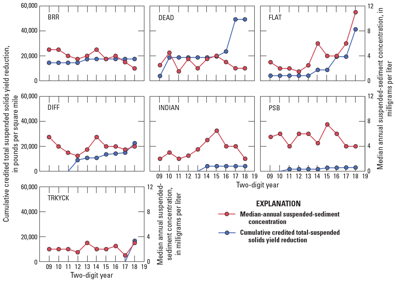
Graphs showing the cumulative credited total suspended solids yield reduction from management practices and median-annual suspended sediment concentrations in seven study watersheds in Fairfax County, Virginia, from 2009 through 2018. Study watershed station names are defined in table 1.
Table 32.
Results of a suspended-sediment linear mixed-effect model with credited management-practice total suspended solids reductions, including 95-percent confidence intervals, fixed-effect estimates, random-effect variances, and the model’s Akaike information criterion.[Linear mixed-effect models are described in equations 4–6. Predictors are described in tables 2, 3, and 5. b3, the effect of a predictor on within-watershed variability; b1, the effect of a predictor on between-watershed intercept differences; R2, coefficient of determination; AIC, Akaike information criterion]
Specific Conductance
Specific conductance (SC) of a stream or river represents the amount of positively and negatively charged ions, referred to as cations and anions, respectively, in solution (Hem, 1985). Many of these ions are naturally occurring and reach streams through the weathering of geologic materials; however, high concentrations in some urban and suburban streams can result from human activities (Paul and Meyer, 2001). The increasing SC of streams and rivers, termed freshwater salinization, is associated with a range of negative outcomes, including lethal and sub-lethal effects for biota, threats to public drinking supply, and degradation of the built environment (Kaushal and others, 2005; Kaushal and others, 2017; Kaushal and others, 2018). Managing these impacts often entails addressing winter maintenance activities to remove or reduce ice on impervious surfaces (Interstate Commission on the Potomac River Basin, 2020) and is a priority for Fairfax County.
Patterns of Observed Responses
SC differed between study watersheds, varied seasonally, and was strongly related to streamflow (Porter and others, 2020b). Median-annual SC values below about 400 µS/cm commonly were observed in most watersheds (fig. 67). The ionic composition of Fairfax County streams is primarily influenced by the solubility of naturally occurring geologic materials and urban activities that add salts to the environment and (or) affect their delivery to streams (Larson, 1978; Porter and others, 2020b). CASTLE, LIL DIFF, and SFLIL had the lowest amounts of developed land among the study watersheds (table 7). Median-annual SC values in these three watersheds were typically lower than watersheds with more extensive impervious cover or more soluble geologic materials. Low-ionic strength rainwater often dilutes SC during storm events. However, runoff can carry salts from the landscape that cause large SC spikes, most commonly observed during winter months and associated with roadway deicing and (or) anti-icing chemicals (fig. 68).
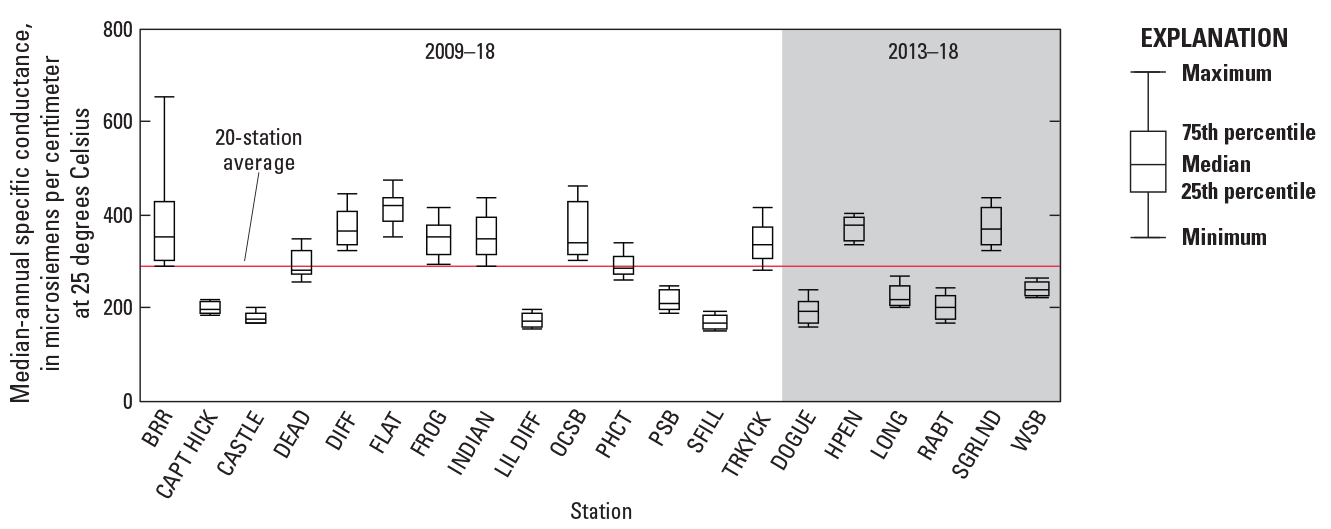
Boxplots showing the median-annual specific conductance of 20 study watersheds in Fairfax County, Virginia. Study watershed station names are defined in table 1.
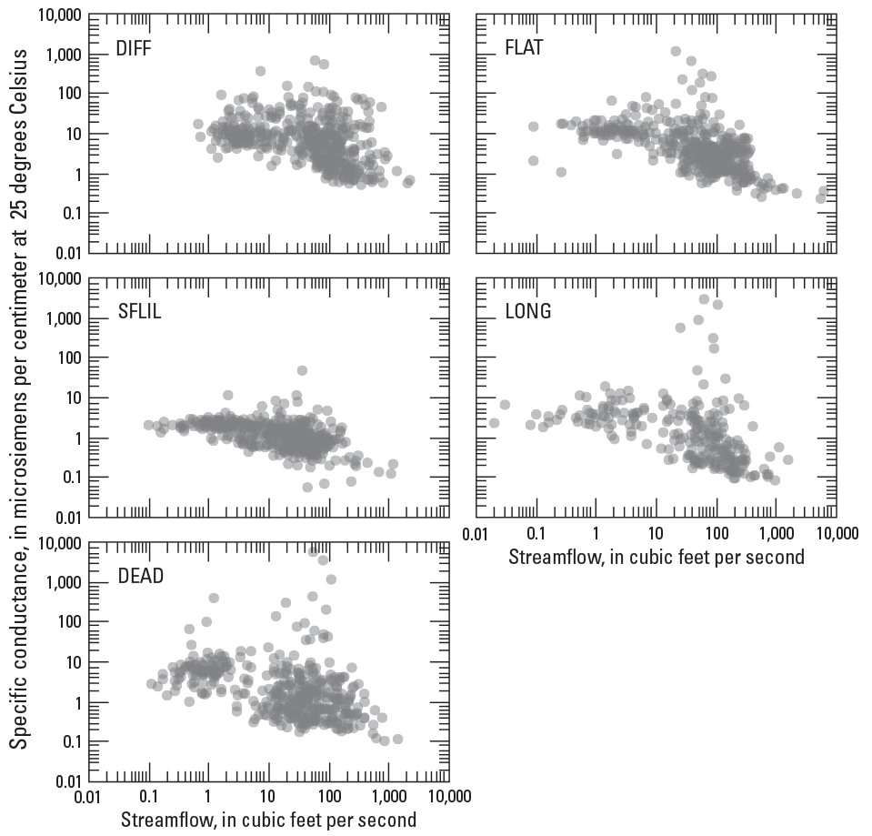
Graphs showing the relations of streamflow to specific conductance as measured in five study watersheds in Fairfax County, Virginia. Study watershed station names are defined in table 1.
SC trends were evaluated using monthly water-quality samples collected from April 2008 through March 2018 to describe how conditions changed over time in 14 watersheds with 10 years of data, analyses and interpretations originally conducted by Porter and others (2020b; table 33). After adjusting for streamflow, SC increased in 10 watersheds and throughout the network by 2.3 percent per year, as determined by a regional Seasonal-Kendall analysis. The largest annual SC percentage increase of 3.6 percent occurred in INDIAN, and the smallest increase of 1.1 percent occurred in FLAT. In most watersheds, the largest SC increases typically occurred during spring and fall months: a possible indication that ions are stored in the watershed and delivered to streams after their initial application to the landscape (Porter and others, 2020b).
Table 33.
Flow-adjusted specific conductance trends in 14 study watersheds in Fairfax County, Virginia, from March 2008 through April 2018.[Station names are defined in table 1. mg/L, milligram per liter; %, percent]
SC and major cations and anions were analyzed in water-quality samples collected from Fairfax County streams during base-flow conditions in August of 1977 (Larson, 1978) and can be used to assess how surface-water chemistry has changed over a multi-decadal period. These historical samples were compared to base-flow samples collected during summer months (June–August) between 2011 and 2018 at a station within Difficult Run (n=22 samples, USGS station ID 01646000, fig. 1). On average, calcium and bicarbonate were the most prevalent ions in the historical samples, whereas sodium and chloride were the most prevalent ions in the recent samples from Difficult Run (fig. 69). The recent samples from Difficult Run had significantly higher measures of SC, sodium, and chloride than the historical samples (p-value ≤0.05, as determined through a Kruskal-Wallis test; fig. 70). Average-annual SC values measured at Difficult Run from 1979 through 2018 show that salinity has increased steadily over time; average-annual SC values nearly tripled over this multi-decadal period (fig. 71).
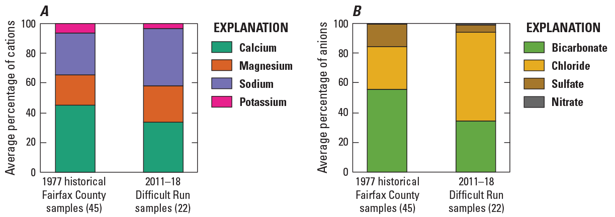
Bar graphs showing average A, cation and B, anion composition from samples collected throughout Fairfax County, Virginia, watersheds in 1977 and from the Difficult Run near Great Falls, Virginia, monitoring station from 2011 through 2018. Ion concentration measurements in 1977 are from Larson (1978).
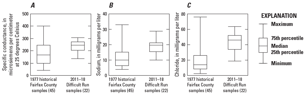
Boxplots showing A, specific conductance; B, sodium; and C, chloride measurements in historical samples collected from Fairfax County, Virginia, watersheds in 1977 and from the Difficult Run near Great Falls, Virginia, monitoring station from 2011 through 2018. Specific conductance measurements in 1977 are from Larson (1978).

Graph showing the average-annual specific conductance of samples collected from the Difficult Run near Great Falls, Virginia, monitoring station from 1979 through 2018.
Between-watershed differences in median-annual SC were typically larger than year-to-year changes within watersheds (fig. 67). These two sources of variability, representing spatial differences among study watersheds and temporal differences from 2009 through 2018, were described by a fixed-growth model (table 34). The fixed-growth model differs from a linear-growth model because the fixed-growth model excludes a random-effect slope term ( in eq. 1). The random-effect slope term was removed because most watersheds had a similar rate of SC increase over the 10-year period (fig. 72), resulting in a singularity condition caused by a random-effect variance component being reduced to nearly zero. The fixed-growth model indicated that the average SC value across all watersheds in 2009 was 263 µS/cm and that all watersheds had an average SC increase of about 6.9 µS/cm per year. The AIC of the fixed-growth model (1,482.4) was compared against models that included additional predictors; more parsimonious models reduced the between- and within-watershed random-effect variances.
Table 34.
Results of the specific conductance fixed-growth model, including fixed-effect estimates, 95-percent confidence intervals, random-effect variances, and the model’s Akaike information criterion.[The linear-growth model is defined in equations 1–3. AIC, Akaike information criterion]

Graphs showing centered values of median-annual specific conductance in 14 study watersheds in Fairfax County, Virginia, from 2009 through 2018. Study watershed station names are defined in table 1.
Relations to Predictor Variables
Between-watershed SC differences were likely affected by a combination of human and natural factors, patterns that were explored by comparing average predictor and SC values from 2014 through 2018 at 20 study watersheds (app. 1, table 1.10). Median SC was typically higher in watersheds with higher median streamflow, WT, and pH. Watersheds that have higher median streamflow and WT may receive more runoff than watersheds with lower streamflow and WT. Runoff can carry elevated ion concentrations, contributing to higher median SC. The strongest correlation of median SC was with pH (pH, r=0.64; fig. 73A), where watersheds with higher pH typically had higher SC. This relation may be explained by associations between waters with high-ionic strength and increases in alkalinity. Just as the runoff of salts from impervious surfaces raises stream salinity, weathering of the built environment can contribute ions such as calcium and bicarbonate that raise stream alkalinity (Kaushal and others, 2017). As stream alkalinity increases, the concentration of hydrogen ions in solution decreases, and streams become less acidic. Increases in alkalinity and pH have been observed in many urban settings and are associated with the runoff from, and the weathering of, impervious materials (Kaushal and others, 2013; Kaushal and others, 2017). Based on these previous studies, a causal link between SC and pH in Fairfax County streams is likely, but pH is not likely the driver of higher SC conditions.
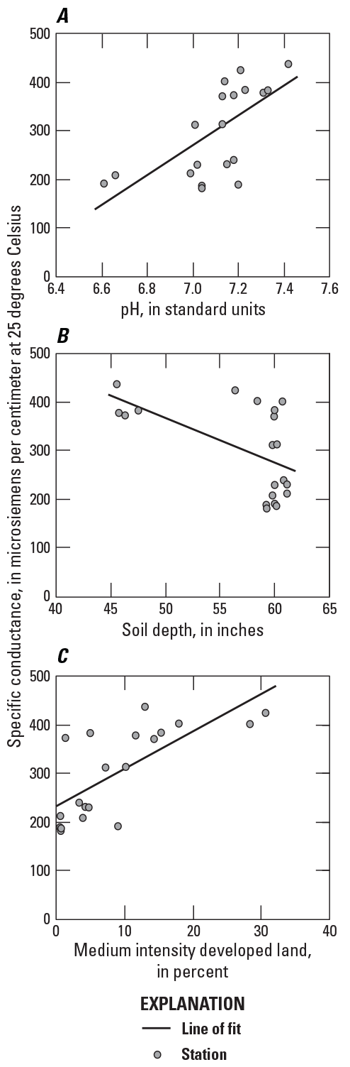
Graphs showing relations of A, pH; B, soil depth; and C, medium intensity developed land to specific conductance in 20 study watersheds in Fairfax County, Virginia; all values represent average conditions from 2014 through 2018.
Many watershed predictors that describe geologic properties were correlated to between-watershed SC differences, including soil depth, cation-exchange capacity, and organic matter (app. 1, table 1.10). A strong correlation with soil depth (SOIL DEPTH, r=−0.56; fig. 73B) indicates higher SC values in watersheds with more shallow soils. This correlation highlights the higher SC values in Triassic Lowland watersheds (FLAT, FROG, HPEN, SGRLND, and BRR; fig. 67). The Triassic Lowlands contain some of the most soluble bedrock materials underlying Fairfax County streams, and these areas have the highest natural concentration of dissolved minerals in stream water, commonly as calcium, magnesium, and bicarbonate (Larson, 1978). Additionally, SC in some Triassic Lowland watersheds may be affected by the susceptibility of groundwater to surface-water contamination caused by shallow, permeable soils (Froelich and Zenone, 1985b).
Many predictors that describe urban-landscape activities were correlated to between-watershed SC differences. In general, watersheds with more impervious land use, more roadways, higher housing densities, and more wastewater and stormwater infrastructure had higher SC values (app. 1, table 1.10). Many of these relations have been previously documented in Fairfax County streams (Jastram and others, 2009; Porter and others, 2020b) and in other urban/suburban watersheds (House and others, 1993; Paul and Meyer, 2001; Walsh and others, 2005). The percentage of watershed classified as medium intensity developed land, which describes areas with a mixture of constructed and vegetated land cover and most commonly includes single-family housing units (Homer and others, 2015), was most strongly correlated with between-watershed SC differences (DEV MED, r=0.73; fig. 73C). SC may be highest in such areas because of the opportunity for numerous salinity sources, including wastewater, fertilizer, and roadway chemicals, to reach streams through groundwater and surface-water pathways.
Watersheds with more impervious cover tended to have a slightly higher density of stormwater detention ponds; features that were positively correlated with between-watershed SC differences (N DRY POND, r=0.62). This correlation suggests that median SC values were higher in watersheds with more stormwater detention ponds, facilities constructed to manage stormwater runoff and improve water-quality conditions. Although these correlations do not demonstrate causality, previous research has found higher year-round sodium and chloride concentrations in streams and groundwater that are draining stormwater detention ponds (Snodgrass and others, 2017), and that some stormwater detention ponds may be ineffective at reducing stream salinity levels (Minnesota Groundwater Association, 2020).
Some physical watershed properties associated with the Triassic Lowlands were correlated with the 2009 through 2018 median-annual SC percentage change, including sand content, cation-exchange capacity, and soil depth (SOIL DEPTH, r=0.62; app. 1, table 1.11; fig. 74A). In general, these correlations reflect the smaller SC increases in FLAT and FROG from 2009 through 2018, relative to other watersheds. Larger SC increases tended to occur in watersheds with less turfgrass and more high intensity developed land (DEV HIGH, r =0.60; fig. 74B), representing areas with near complete impervious cover, such as apartment complexes or commercial/industrial land uses (Homer and others, 2015). Larger SC increases were also associated with watersheds that had a higher density of roadways classified as interstates and ramps (INT ROAD, r=0.68; fig. 74C). These correlations may be attributed to the role of de-icing and anti-icing roadway salts. Interstates can be large road-salt sources (Cooper and others, 2014), possibly because they receive more salt applications than local roads.
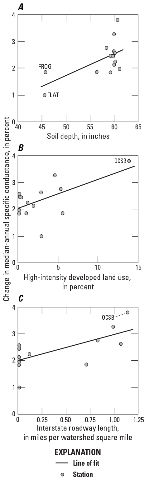
Graphs showing relations of A, soil depth; B, high-intensity developed land use; and C, interstate roadway length (values represent averages from 2009 through 2018) to changes in median-annual specific conductance in 14 study watersheds in Fairfax County, Virginia, from 2009 through 2018. Study watershed station names are defined in table 1.
All 14 watersheds had a negative correlation between changes in median-annual SC and changes in minimum-annual air temperature; in other words, higher SC values were observed in years with colder minimum temperatures (TNn, median r=−0.44; app. 1, table 1.12; fig. 75). January or February had the coldest air temperatures of each year (fig. 63). This correlation was weakest at CASTLE, one of the least developed watersheds. The correlation between changes in median-annual SC and changes in minimum-annual air temperature may correspond to the amount of anti-icing and (or) de-icing chemicals used in a given year. A variety of winter maintenance strategies are used to prevent or remove ice from impervious surfaces, including the use of chloride-based compounds (Fay and others, 2015). Sodium chloride is a commonly used anti-icing and de-icing agent because it is less expensive than other chemicals and can be applied in granular form (as rock salt or liquid brine); however, its effectiveness decreases at colder temperatures (Vignisdottir and others, 2019). Magnesium chloride and calcium chloride compounds are more effective under extremely cold temperatures, but higher application rates of all salt-based compounds are still required during lower temperatures (Vignisdottir and others, 2019). Additionally, precipitation events in colder years likely produce more freezing conditions that require salt treatments. As the association between freshwater salinity and road salts have been clearly demonstrated in a variety of urban areas (Cooper and others, 2014; Daley and others, 2009; Kaushal and others, 2005; Kaushal and others, 2018), the observed relations between annual temperature and SC may be driven by differences in application rates or the frequency of de-icing and anti-icing salt use.
All 14 watersheds had a positive correlation between changes in median-annual SC and changes in the percentage of impervious cover (IMP, median r=0.61; app. 1, table 1.12; fig. 75). Impervious cover expanded and median SC values increased in all watersheds from 2009 through 2018, and many predictors related to impervious cover had similar patterns (app. 1, table 1.12). Relations between urban expansion and increased stream salinity have been widely documented and are related to a combination of point and nonpoint sources (Corsi and others, 2015; Daley and others, 2009; Kaushal and others, 2018). Although changes in impervious cover were small in most watersheds over the study period, increases in freshwater salinity have been documented in urban areas during periods of stable-land cover (Bird and others, 2018). Water-quality conditions can take years to stabilize after urban growth, therefore, the multiple decades of rapid urbanization in Fairfax County (fig. 5) may still affect present-day stream conditions.
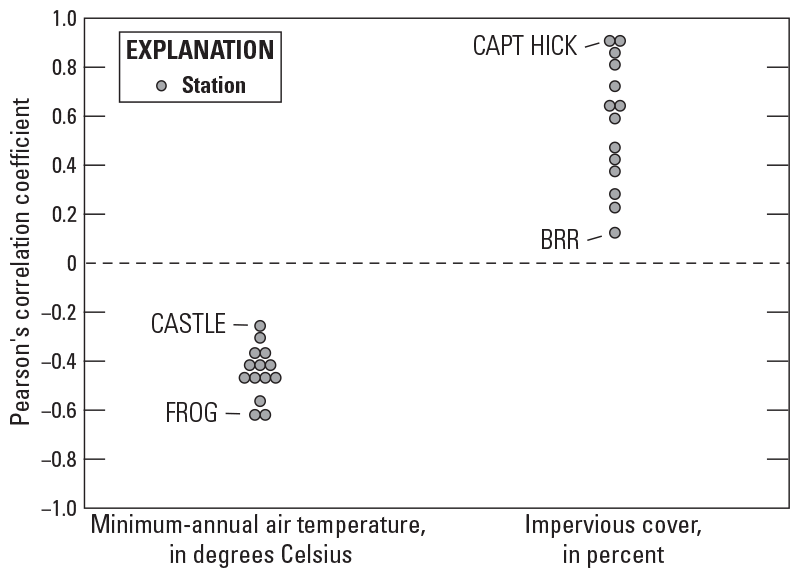
Graph showing Pearson’s correlation coefficients for relations between median-annual specific conductance and selected predictors in 14 study watersheds in Fairfax County, Virginia. Correlations represent annual values from 2009 through 2018. Study watershed station names are defined in table 1.
Explanation of Variability
Based on the information described above, six predictors were included in LME models to describe the spatiotemporal variability of median-annual SC: (1) median-annual streamflow, (2) minimum-annual air temperature, (3) soil depth, (4) impervious cover, (5) medium intensity developed land and (6) interstate roadway length. Median-annual streamflow was considered to evaluate whether median-annual SC was affected by varying flow conditions, because varying flow conditions can mask the role of other factors. Combined with the four estimated parameters in the fixed-growth model, all possible model combinations of the additional six predictors were considered. Models with the lowest AIC included a similar combination of terms and performed similarly (app. 2, table 2.8). Lower SC values were associated with years of higher impervious cover in many of the top-performing models, a relation not supported by observed patterns (fig. 75) and likely caused by the strong correlation between impervious cover and year, the slope term included in all models. The model selection process was repeated after removing the fixed effect of year, thereby accounting for potential multicollinearity issues, to evaluate the effects of time-varying watershed predictors on annual SC differences.
Many similarly performing models described the spatiotemporal variability of median-annual SC from 14 watersheds from 2009 through 2018, but interpretations from a single combination of predictors can help inform watershed management. A 7-parameter model was selected for interpretation after assessing model-performance metrics and considering likely factors of SC response identified in other urban studies. This model included fixed-effect terms for minimum-annual air temperature, medium intensity developed land, and soil depth (table 35). Models with more predictors generally did not explain greater amounts of SC variability and often included a within-watershed effect of impervious cover: a term highly correlated with the model slope term (app. 2, fig. 2.7). An alternative model, where the fixed effect of year was replaced with medium intensity developed land, performed similarly well (app. 2, table 2.9).
Table 35.
Results of a specific conductance linear mixed-effect model selected for interpretation, including 95-percent confidence intervals, fixed-effect estimates, random-effect variances, and the model’s Akaike information criterion.[Linear mixed-effect models are described in equations 4–6. Predictors are described in tables 2 and 3. b3, the effect of a predictor on within-watershed variability; b1, the effect of a predictor on between-watershed intercept differences; R2, coefficient of determination; AIC, Akaike information criterion]
The fixed-effect terms in the selected model explained 74 percent of the spatiotemporal variability in SC (table 35). Compared to the fixed-growth model (table 34), the fixed effects in the selected model explained an additional 85 percent of the between-watershed intercept variance and an additional 10 percent of the annual within-watershed variance. The additional variance explained by this latter component, representing interannual SC differences, was small because some of the within-watershed SC variance was already explained by the slope term in the fixed-growth model (Year, b3). Observed and predicted responses plotted against time were used to visually assess the selected model’s performance in each watershed (app. 2, fig. 2.8). The selected model residuals were an improvement over the fixed-growth model, but selected years still had some over or under predictions (fig. 76).
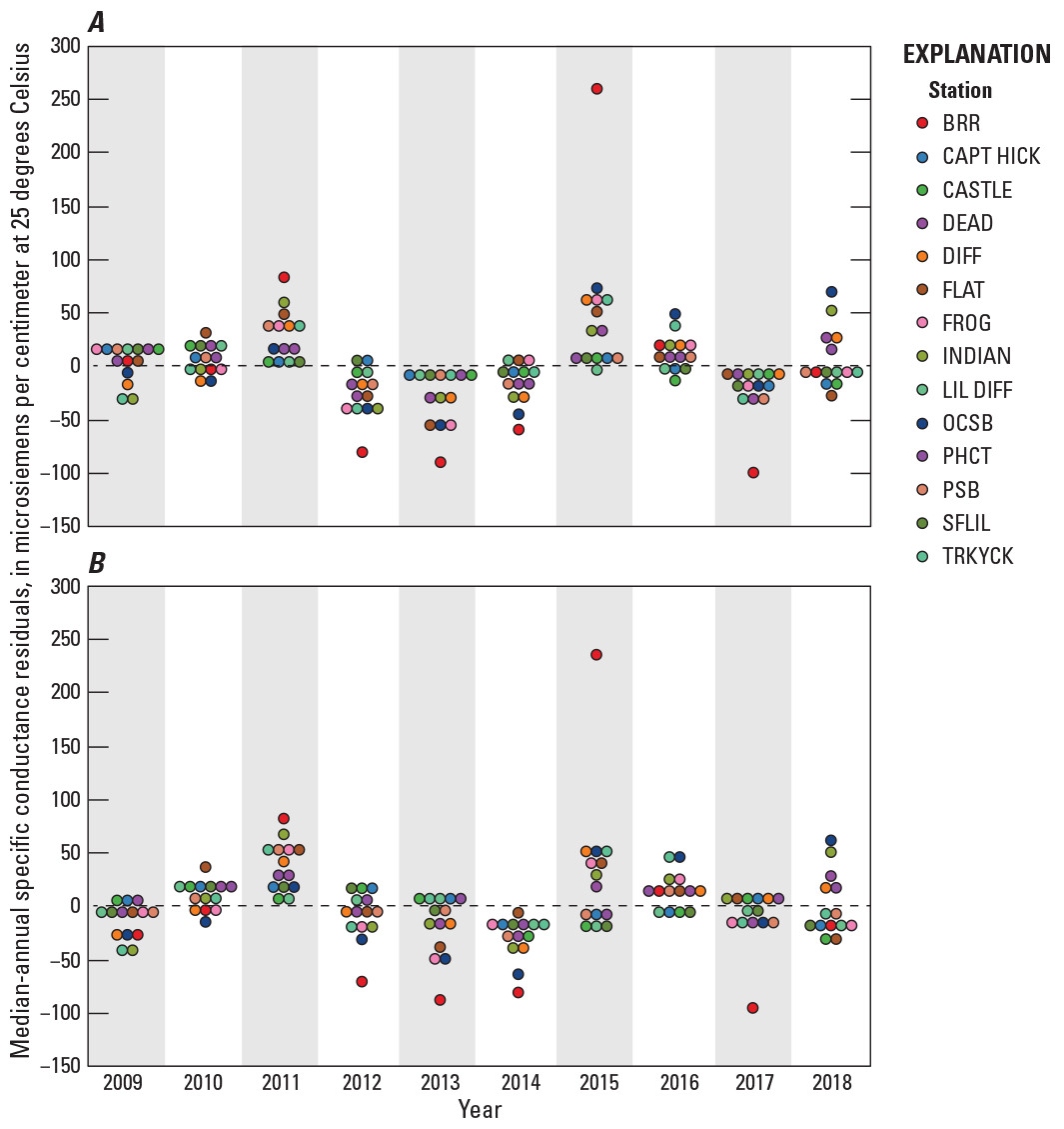
Graphs showing model residuals from A, the specific conductance fixed-growth model and B, the selected specific conductance linear mixed-effect model in 14 study watersheds in Fairfax County, Virginia, from 2009 through 2018. Study watershed station names are defined in table 1.
The fixed-effect coefficients in the selected model describe the average effect of minimum-annual air temperature, soil depth, and medium intensity developed land on median-annual SC values in 14 watersheds (table 35): predictors that vary over space and time (fig. 77). The largest effect size in the model corresponded to the effect of medium intensity developed land: watersheds with more developed land had higher SC values (DEVMI b1, 0.79). This effect was larger than that of soil depth (ROCKH b1, −0.39), which indicated that watersheds with shallower soils had higher average SC values. The model slope (Year b3, 0.38) and minimum-annual air temperature (TNn b3, −0.27) terms described effects influencing interannual SC differences. These terms indicated that, on average, SC increased over time and was higher in years with colder minimum-annual air temperatures. Minimum-annual air temperature was the only modeled effect that causes estimated values to deviate from a perfectly straight line (app. 2, fig. 2.8). An alternative model that replaced the fixed effect of year with medium intensity developed land related increases in SC to increases in developed land (DEVMI b3, 0.36; app. 2, table 2.9).
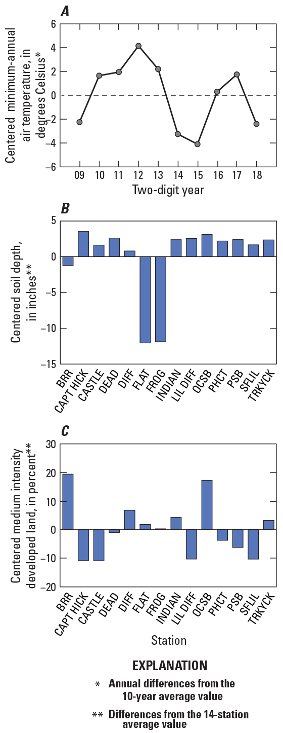
Graphs showing centered parameters used in the selected specific conductance linear mixed-effect model: A, minimum-annual air temperature from 2009 through 2018; B, soil depth; and C, medium intensity developed land in 14 study watersheds in Fairfax County, Virginia. Study watershed station names are defined in table 1.
The modeled effects of developed land use, soil depth, and air temperature suggest that variability of SC in Fairfax County streams was related to physical watershed setting and human activities. On average, SC was higher in watersheds that had shallower soils and more medium-intensity developed land. The modeled effect of soil depth likely represents (1) the lower capacity of watersheds with shallow soils to trap and retain landscape-applied salts, and (or) (2) the greater amount of geologic materials delivered to streams through natural weathering. Relations between urban infrastructure and SC have previously been documented in Fairfax County streams (Jastram, 2014; Porter and others, 2020b) and in other urban/suburban watersheds (House and others, 1993; Paul and Meyer, 2001; Walsh and others, 2005). The modeled effect of annual air temperature suggests that SC values were higher in years with colder minimum air temperatures. As the effectiveness of de-icing and anti-icing salts decreases with temperature (Vignisdottir and others, 2019) and freezing precipitation events become more common, years with very cold temperatures likely receive more salt applications. The positive slope term (Year b3) suggests that, on average, SC increased from 2009 through 2018, though these effects may be accounted for by increases in developed land.
Benthic Macroinvertebrates
Primarily because of their relatively immobile nature, freshwater benthic communities are well-studied indicators of stream ecosystem health (Rosenberg and Resh, 1993; Bonada and others, 2006; Buss and others, 2014). Fairfax County’s IBI is a composite index assembled from component metrics quantifying abundance, diversity, feeding traits, habitat requirement, and pollution tolerance of benthic organisms including insects, oligochaetes (aquatic worms), crustaceans, mollusks, and gastropods (snails). Adapted from work designed for regional application (Barbour and others, 1999), the county’s IBI considers a slightly different set of component metrics for streams lying in the Atlantic Coastal Plain, relative to those lying on Piedmont of Triassic lithology (Fairfax County, 2019; table 36). Index of biotic integrity scores are assigned based on the statistical distribution of component metrics in streams under evaluation relative to corresponding distributions in reference streams. By design, scores range from 0 to 100, with lower scores representing poorer health and conditions that are least similar to reference conditions. Flashy hydrologic responses, elevated stream temperatures, and increased sediment and nutrient loads are some common stressors in urban streams that cause benthic community impairment (Statzner and Beche, 2010; Nõges and others, 2016; Gieswein and others, 2017; Waite and others, 2021). A better understanding of why IBI scores differ among watersheds and change over time can help inform Fairfax County’s stormwater-management strategies, many of which are designed to improve stream ecological conditions by mitigating urban stressors.
Table 36.
Component metrics of Fairfax County’s benthic-macroinvertebrate index of biotic integrity score (Fairfax County, 2019).[EPT, Ephemeroptera, Plecoptera, and Trichoptera]
Patterns of Observed Responses
IBI scores varied appreciably between watersheds, in terms of average level and rate-of-change from 2008 through 2017 (fig. 78). In 2009, when samples were available from all 14 stations, IBI scores were lowest in BRR, INDIAN, and DEAD and highest in OCSB, LIL DIFF, and CASTLE. Among these last three, IBI scores in CASTLE were appreciably higher than in the other two, and no annual scores in CASTLE were rated lower than “good.” Trends in IBI scores were evaluated to describe how conditions changed over time in 14 watersheds, analyses and interpretations originally conducted by Porter and others (2020b; table 37). Four watersheds (BRR, DIFF, FLAT, and SFLIL) had a significant increase in IBI score, and the 14-station network had an average-annual increase of 1.8 points. These changes, indicating an improvement in benthic-macroinvertebrate community structure, can be observed in the upward trajectory of IBI scores in most study watersheds (fig. 78). Increased IBI scores from 2008 through 2017 primarily resulted from increases in taxon/group abundance (quantified as percentage composition), though increases in some measures of group taxa richness were also observed. The relative abundance of the most numerically dominant taxon or group in the sample, referred to as percentage dominance, is a component IBI metric for Piedmont streams that decreased in most stations, reflecting improved ecological conditions. The strongest upward IBI trend was at FLAT, where scores improved by about six points per year. In most stations, IBI scores in 2017 were at least one qualitative rating higher (for example, “fair” to “good”) than the first year that samples were collected. In general, average-annual rates of change were more variable in watersheds with lower IBI scores in 2009, whereas smaller increases occurred in watersheds with higher IBI scores in 2009 (fig. 79). These relations also suggest potential differences in response based on the amount of impervious cover in a watershed, an observation that will be discussed in more detail in the follow paragraphs.
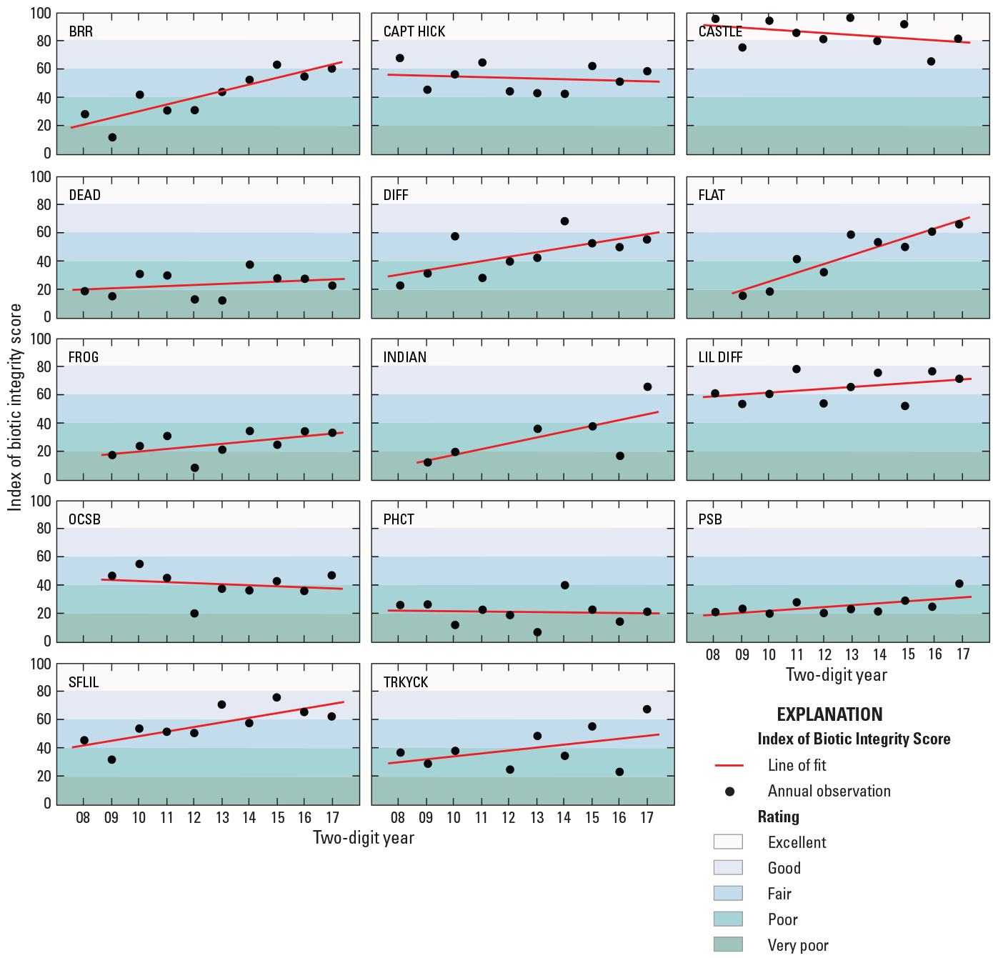
Graphs showing annual index of biotic integrity scores measured in 14 study watersheds in Fairfax County, Virginia, from 2008 through 2017. Study watershed station names are defined in table 1.
Table 37.
Average-annual changes in index of biotic integrity scores for 14 study watersheds in Fairfax County, Virginia.[Station names are defined in table 1. IBI, benthic-macroinvertebrate index of biotic integrity]
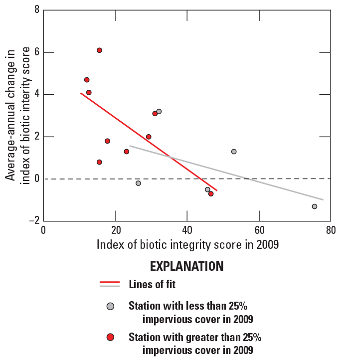
Graph showing the relation of index of biotic integrity scores in 2009 to the average-annual change in index of biotic integrity score, grouped by watershed impervious cover in 2009 above and below 25 percent. %, percent.
Variability in IBI scores between watersheds from 2008 through 2017 was quantified by fitting a linear-growth model to annual observations from the 14 watersheds (table 38). The fixed intercept and slope for the pooled data indicated a network average IBI score of 34.2 in 2008 and an increase of 1.72 points per year. The random-effect variances indicated that roughly 80 percent of total IBI score variance was represented by between-watershed differences in intercept, and only 20 percent was represented by between-watershed differences in slope and within-watershed year-to-year changes. The AIC of the linear-growth model (1,056.1), along with reductions in the three unexplained variance components, were the bases for evaluating the influences of watershed predictors on IBI scores.
Table 38.
Results of the index of biotic integrity linear-growth model, including fixed-effect estimates, 95-percent confidence intervals, random-effect variances, and the model’s Akaike information criterion.[The linear-growth model is defined in equations 1–3. AIC, Akaike information criterion]
Relations to Predictor Variables
The influences of human and natural factors on changes in IBI scores from 2008 through 2017 and between-watershed differences in IBI scores were evaluated by iteratively augmenting the linear-growth model with each watershed predictor (app. 1, table 1.13 and table 1.14). In these and all subsequent LME models, IBI scores were related to predictors representing conditions in the year before sampling because benthic-macroinvertebrate samples were collected annually in the early spring. This process was repeated to model conditions in 2010 through 2017 because, after lagging predictor values by 1 year, median-annual water-quality parameters (Q, WT, SC, PH, DO, and TB; table 3) were not available from all stations in 2008 or 2009. Median-annual water-quality parameters offered little ability to explain spatiotemporal IBI score variability because they did not substantially reduce the AIC of a linear-growth model representing this 8-year period. Seven predictors (defined in table 2 and table 3) reduced the AIC of the linear-growth model by nine or more units (fig. 80), a threshold selected based on the distribution of reductions observed across all predictors.
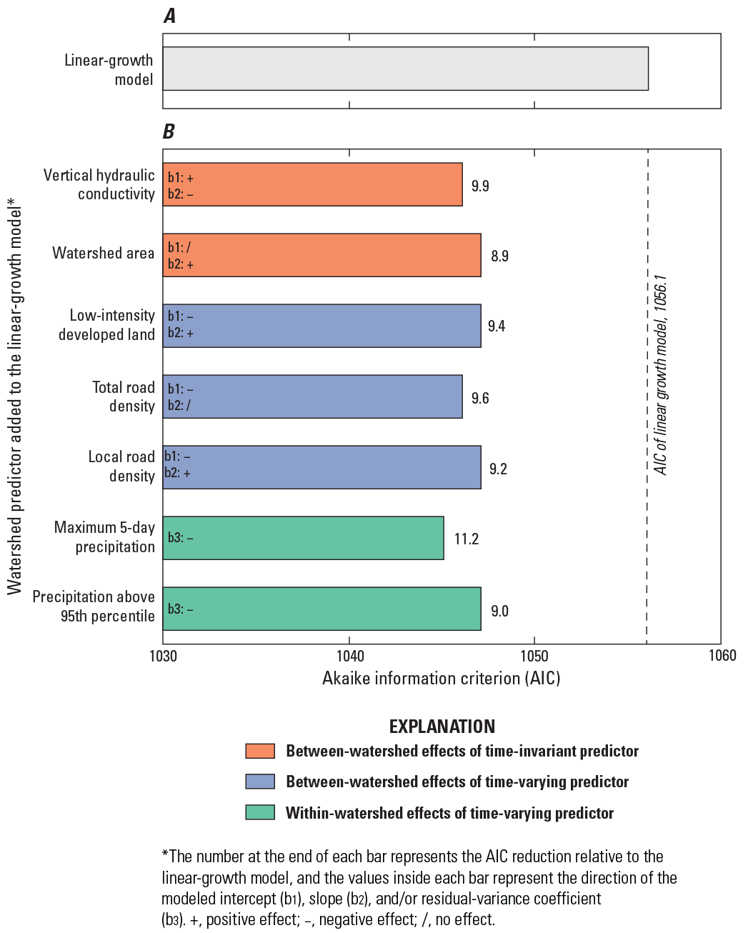
Graphs showing A, the Akaike information criterion of the index of biotic integrity linear-growth model and B, reductions in Akaike information criterion relative to the linear-growth model for selected predictor models.
A model with maximum annual 5-day rainfall reduced the AIC of the linear-growth model by about 11 points, the largest such reduction (Rx5D; fig. 80B). A related heavy rainfall indicator, R95P, reduced AIC by about 9 points. Maximum annual 5-day rainfall ranged from between about 3 to 9 in. from 2008 through 2017 and generally declined over time (fig. 81A). Except for PHCT, correlations between Rx5D and IBI scores across the 14 watersheds ranged from about –0.2 to –0.7 (fig. 81B); that is, lower IBI scores were typically observed in years following high Rx5D values, a relation that was strongest at FROG (fig. 81C). In contrast, at PHCT, prior-year Rx5D was a poor predictor of IBI scores, having a correlation coefficient of about 0.3 (fig. 81D). This distribution of correlations did not appear to be influenced by the amount of impervious cover in a watershed. Effects of antecedent flow on stream invertebrate assemblages are well-documented (Biggs and others, 2005; Greenwood and Booker, 2015; Zuellig and Carlisle, 2019). Using a nationwide set of 51 sites sampled repeatedly from 2002 through 2012, Zuellig and Carlisle (2019) found it necessary to consider sampling day-of-year, antecedent streamflow, and variability in antecedent streamflow when interpreting trends in multi-metric indices of stream ecological condition. The percent numerical representation of the single most dominant taxon is one component of the county’s IBI, and increasing dominance acts to decrease IBI (Fairfax County, 2019). It is plausible that bed disturbance associated with extreme flows might favor, for example, dominance of taxa capable of rapid colonization and reproduction, thereby reducing IBI scores. Such disturbances, however, can act in different directions depending on metric and time scale, emphasizing the importance of jointly considering a suite of covariates (Greenwood and Booker, 2015; Zuellig and Carlisle, 2019).
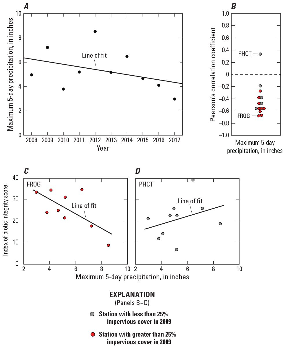
Graphs showing A, maximum-annual 5-day rainfall from 2008 through 2017; B, correlations for 14 study watersheds in Fairfax County, Virginia, between maximum-annual 5-day rainfall and benthic index of biotic integrity scores from 2008 through 2017; and relations of maximum-annual 5-day rainfall to index of biotic integrity scores at C, FROG and D, PHCT. Study watershed station names are defined in table 1. %, percent.
Watershed average vertical hydraulic conductivity (KV), which describes the vertical infiltration rate of water through fully saturated soils, decreased the AIC of the linear-growth model by about 10 units (fig. 80B). In general, higher KV values are in watersheds with more permeable soils that allow water to move up and down the soil profile with relative ease. Study watersheds with higher KV values had, on average, higher IBI scores in 2009 and lower annual rates of change from 2008 through 2017 (fig. 82A). Average KV was typically higher in less-developed watersheds (table 39), indicating (1) that regions of the county with lower soil infiltration rates had preferentially more development, (2) that extreme impervious cover influenced measurement of soil infiltration rates, or (3) that the correlation between KV and development was spurious. Although observed relations and the AIC reduction of a model including KV suggested that this soil property was an important static predictor of IBI scores, it is likely that this predictor is not causative of IBI score differences. The association between KV and IBI scores may simply result from correlations between KV and various measures of development.
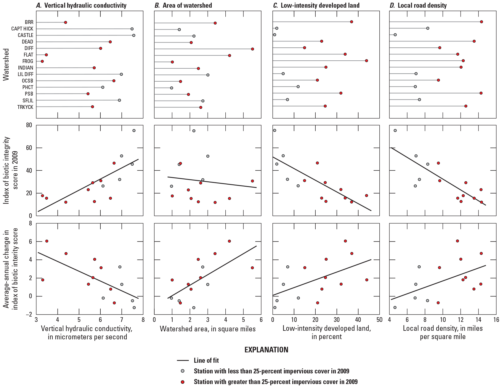
Graphs showing relations of index of biotic integrity scores to the watershed average values of A, vertical hydraulic conductivity; B, area of watershed; C, low-intensity developed land; and D, local road density. Study watershed station names are defined in table 1.
Table 39.
Spearman’s rho correlations between five watershed-average predictor variables.[Predictors are defined in tables 2 and 3. —, no correlation result shown]
Watershed area decreased the AIC of the linear-growth model by about nine units (fig. 80B). Watershed area did not affect between-watershed IBI differences in 2009, but larger watersheds tended to have larger average-annual rates-of-change from 2008 through 2017 (fig. 82B). In contrast to KV, watershed area had little correlation with the degree of urban development (table 39). The positive relation between watershed area and the rate of IBI change over time is consistent with the findings of Schmidt and others (2019), who found, but did not account for, a positive indirect relation between watershed area and IBI in midwestern streams. Walker and others (2021) found a relation between watershed area and IBI in a randomized sample of Maryland streams; however, the sign of this relation differed between two sampling periods separated by 20 years. The importance of watershed area on changing IBI scores may be related to well-established watershed hydraulic geometry relations, dictating differing non-linear rates of increase in channel characteristics such as width, depth, and velocity with increasing contributing area. Lotspeich (2009) reported such relations based on bank-full channel dimensions measured in 17 undeveloped watersheds ranging in area from 0.3 to 111 mi2 in the Virginia Piedmont. Those results indicate that bank-full bed shear stress, proportional to the product of depth and water-surface slope, increases with watershed area, likely decreasing bed stability. This suggests that all else equal, the same runoff-producing rainfall depth falling on two watersheds of differing size will result in more stressful benthic habitat conditions at the outlet of the larger watershed. Thus, more steeply improving IBI slopes in larger watersheds between 2008 and 2017 could reflect a differential response to the county-wide decreasing trend in maximum 5-day rainfall (fig. 81A). Additionally, larger watersheds may contain more diverse habitats, offering refuge for a greater variety of benthic macroinvertebrates (Allan and others, 2021). With less intense rainfall, IBI scores may respond quicker in these larger watersheds as benthic macroinvertebrates recolonize the stream from upstream reaches.
Predictors representing the 2008 through 2017 average value of road density (TOT RD, LOC RD) and low intensity development (DEV LI) reduced the AIC of the linear-growth model by about 9 or 10 units (fig. 80B). Watersheds having higher average values of these predictors, which were correlated with one another (table 39), tended to have lower IBI scores in 2009 and, for DEV LI and LOC RD, more rapid improvement over time (fig. 82C and D). The relation between higher measures of development and lower IBI scores has been previously documented (Paul and Meyer, 2001); however, the effect of development on changing IBI scores over time is less well understood. Although speculative, more rapid improvement of IBI in areas with greater road density may also represent a greater response to decreasing intense rainfall between 2008 and 2017.
Explanation of Variability
All possible combinations of LME models using the 7 previously described predictor variables (fig. 80B) were considered, resulting in models with 6 to 18 parameters. The difference in AIC between the highest-ranking model and the 30th-highest-ranking model was only four AIC units (app. 2, table 2.10), a small degree of distinction relative to the reductions observed when the predictors were considered individually (fig. 80B). This similarity in performance likely results from the strong correlations among considered predictor variables (table 39).
A 12-parameter model, which had the lowest AIC of all modeled combinations, was initially selected for interpretation (app. 2, fig. 2.9). As was the case for many of the best-performing models, this model indicated a singularity condition caused by the random-effect slope variance being reduced to nearly zero. Therefore, the random slope component was removed from the selected model, reducing the number of parameters by 2 (slope variance and slope-intercept covariance), resulting in a 10-parameter model (table 40). This model represents eight fixed effects plus random intercept and residual estimates of variance and has an AIC of 1,015.3, a reduction of just over 40 points relative to the linear-growth model (table 38). The model incorporates the effects of KV and AREA on between-watershed differences in intercept and slope, TOT_RD on between-watershed differences in intercept, and Rx5D accounting for year-to-year within-watershed variability; only the latter predictor enables estimated IBI scores to deviate from a linear regression line (app. 2, fig. 2.10). These predictors reduced the between-watershed unexplained variance in IBI score by about 68 percent relative to the linear-growth model and also reduced within-watershed residual variance by 10 percent. This 10-parameter model reduced the year-to-year mean residuals, relative to the linear-growth model, but was generally less effective in reducing the largest individual residuals in any year (fig. 83).
Table 40.
Results of an index of biotic integrity linear mixed-effect model selected for interpretation, including 95-percent confidence intervals, fixed-effect estimates, random-effect variances, and the model’s Akaike information criterion.[Linear mixed-effect models are described in equations 4–6. Predictors are described in tables 2 and 3. b3, the effect of a predictor on within-watershed variability; b1, the effect of a predictor on between-watershed intercept differences; b2, the effect of a predictor on between-watershed slope differences; R2, coefficient of determination; AIC, Akaike information criterion]
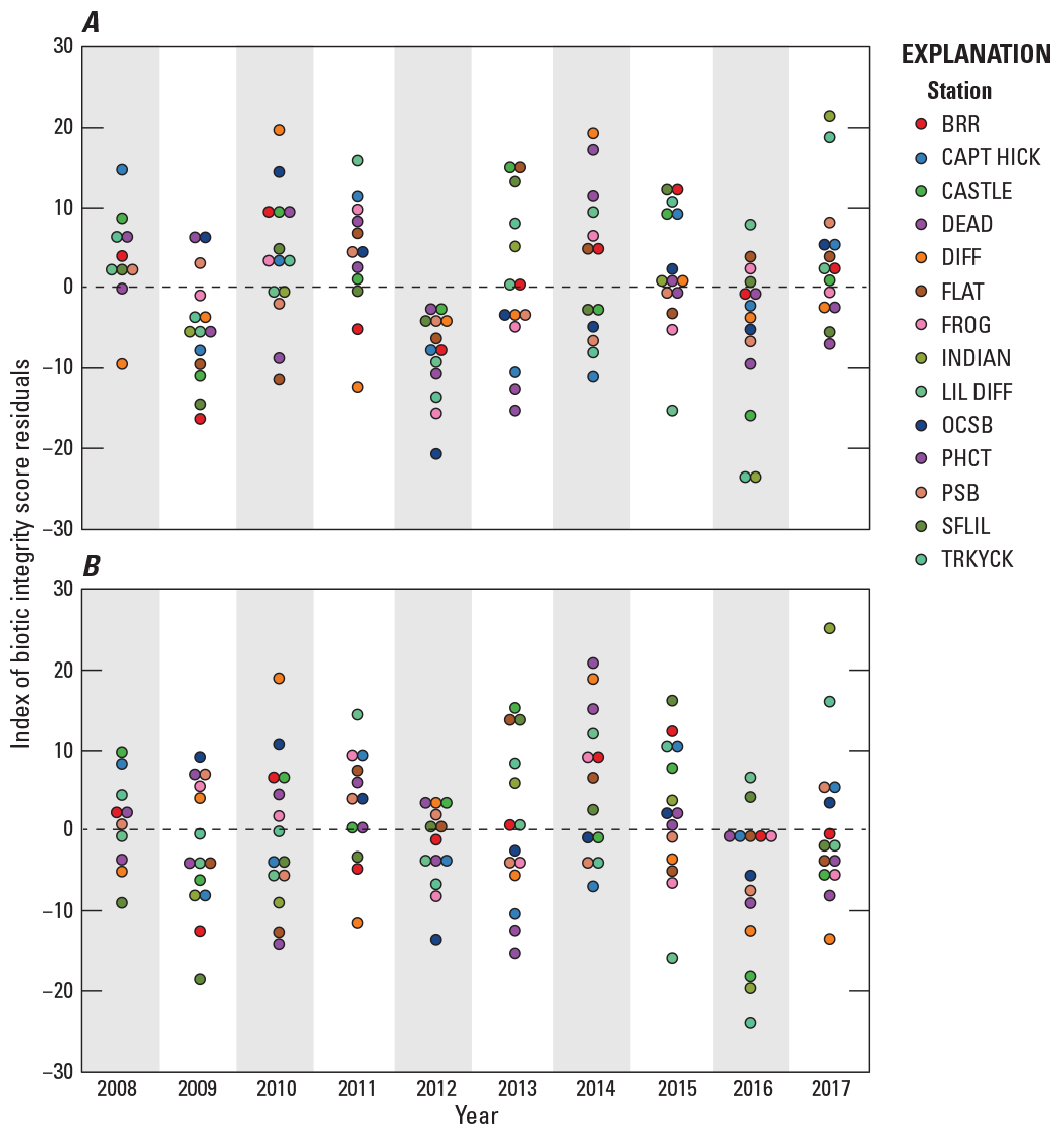
Graph showing model residuals from A, the index of biotic integrity linear-growth model and B, the selected index of biotic integrity linear mixed-effect model in 14 study watersheds in Fairfax County, Virginia, from 2008 through 2017. Study watershed station names are defined in table 1.
Arithmetic signs, showing standardized model coefficients in the selected model (table 40), are consistent with the observed relations between predictors and IBI scores (fig. 81B and fig. 82). The largest effect size in the model corresponded to the effect of TOT_RD, indicating that watersheds with higher roadway densities had lower average IBI scores (TOT_RD b1, −0.63). A similar effect was described by vertical hydraulic conductivity. Watersheds with higher KV values, which occurred in less urbanized areas, had higher average IBI scores (KV b1, 0.58). A modeled effect of this predictor also influenced the IBI rate-of-change, indicating that IBI scores had smaller improvements in watersheds with higher KV (KV b2, −0.52). This effect has the same magnitude but opposite sign as watershed area; on average, IBI scores had larger improvements in larger watersheds (AREA b2, 0.52). These effects are essentially independent because of the weak correlation between KV and AREA (table 39). The standardized estimate for Rx5D, −0.27, indicates that an increase in Rx5D of one standard deviation, about 1.7 in. of precipitation, from one year to the next, was associated with a decrease of roughly 2.5 IBI points. All else equal, if the increase in Rx5D between 2 consecutive years was extreme, such as 4 standard deviations (6.7 in.), IBI would be lowered by about 10 units, plausibly sufficient to lower IBI from one 20-unit-wide qualitative stream-condition description to another (fig. 78). The positive coefficient of the model’s slope term (Year b3, 0.30) highlights an average increase in IBI scores over time that was unaccounted for by the model’s fixed effects.
These interpretations are challenged by the limitations and uncertainties of using IBI scores to summarize ecological changes. Because it is a composite of roughly 10 simpler metrics quantifying abundance, taxa richness, and pollution tolerance of diverse taxonomic or functional groups, IBI may be influenced by different factors in different watersheds in such a way that prediction of its aggregate space-time behavior is possible in only the most general terms. Moreover, the ability of IBI scores to represent county-wide drivers of ecological change is challenged by differing component metrics for streams in the Piedmont and Coastal Plain. More consistent and interpretable models might result by considering only one of these components or even the abundance or richness of a single taxon or group. Additionally, the observed trends in IBI scores may suggest a subtle bias in responsiveness to changing conditions, because improvement in scores over time is more attainable for watersheds with more degraded initial conditions. Few precedents exist for interpreting drivers of ecological change over space and time using data such as those examined here, highlighting the importance of ongoing monitoring and research.
Management-Practice Effects
The model selected for interpretation was augmented, one predictor at a time, by three time-varying predictors representing values of cumulative management-practice credits for TN, TP, and TSS. In no case did the inclusion of a predictor improve model AIC (table 41). These results do not unequivocally rule out the possibility that one or more of these predictors improved instream ecological conditions as measured by IBI. Any improvements, however, were either not well represented by the cumulative credits time series, or improvements are manifesting (or have manifested) along a non-linear or time-lagged trajectory not readily represented in a LME framework.
Table 41.
Results of index of biotic integrity linear-mixed effect models with credited management-practice effects, including management-practice fixed-effect estimates, 95-percent confidence intervals, and the model Akaike information criteria.[Predictor variables are described in table 5. AIC, Akaike information criterion; dAIC, difference in AIC relative to the AIC of the selected linear mixed-effect model (1,015.3; table 40)]
Were Management-Practice Effects Observed?
Previous studies have identified and described a variety of management-practice effects in urban or suburban watersheds, insights that guided analysis of conditions within Fairfax County. Stormwater-retrofit practices and stream restorations can improve some specific water-quality conditions, but effects often vary by practice type, location, age, watershed setting, and dissolved and particulate response variables (Jefferson and others, 2017; Lammers and Bledsoe, 2017; McMillan and others, 2014; Newcomer Johnson and others, 2016). Effects of infiltration- and detention-based stormwater retrofits are most commonly detected if practices treat a large enough fraction of runoff from impervious surfaces to alter hydrologic responses (Jefferson and others, 2017; Li and others, 2017). Stream restorations are being used with increased frequency in urban areas, and monitoring to quantify water-quality responses continues to be needed (Bernhardt and others, 2005; Kenney and others, 2012; Lammers and Bledsoe, 2017). For nitrogen, restored reaches are associated with higher nitrate uptake and denitrification rates (Filoso and Palmer, 2011; Kaushal and others, 2008b; Reisinger and others, 2019), but these effects vary by flow condition, watershed impervious cover, restoration age, season, and practice location (McMillan and others, 2014; McMillan and Noe, 2017; Newcomer Johnson and others, 2016; Sudduth and others, 2011). For phosphorus, restorations that stabilize streambanks may offer the greatest potential to reduce loads (Lammers and Bledsoe, 2017). Although stream restorations often improve measures of physical habitat, their ability to restore biological diversity is more uncertain (Bernhardt and Palmer, 2011; Palmer and others, 2010; Stranko and others, 2012). In general, the watershed-scale effects of management practices are not well understood (Jefferson and others, 2017), and few studies are designed to identify how management-practice effects relate to monitored stream conditions, despite such studies offering some of the best opportunities to guide watershed-management strategies (Li and others, 2017).
Summary of Management-Practice Effects
Expected management-practice effects were not consistently observed in monitored stream responses. Management-practice effects may be most apparent at the intensive monitoring stations because watersheds with these stations received the most water-quality monitoring and generally had more management-practice investment than other study watersheds (table 11). All intensive-monitoring stations other than SFLIL received at least one management practice; the greatest number of practices were installed in DIFF. Most of the practice implementation in DIFF was as stormwater-retrofit practices, though these practices treated only 5 percent of watershed area (table 14). Stream restorations represented most of the credited TN, TP, and TSS load reductions in the intensive-monitoring stations (table 12), and most of these practices were completed from 2015 through 2018 (table 13). Stream restorations were completed near the FLAT monitoring station, but further upstream of monitoring stations in other intensive-monitoring watersheds (fig. 84).
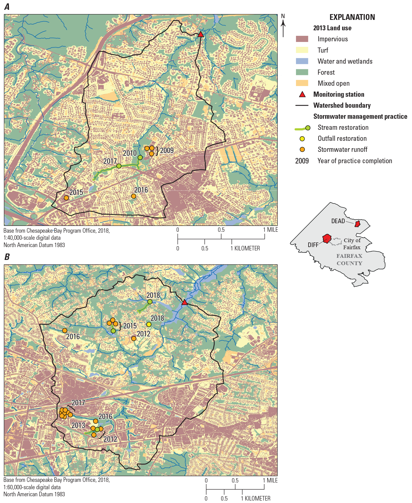
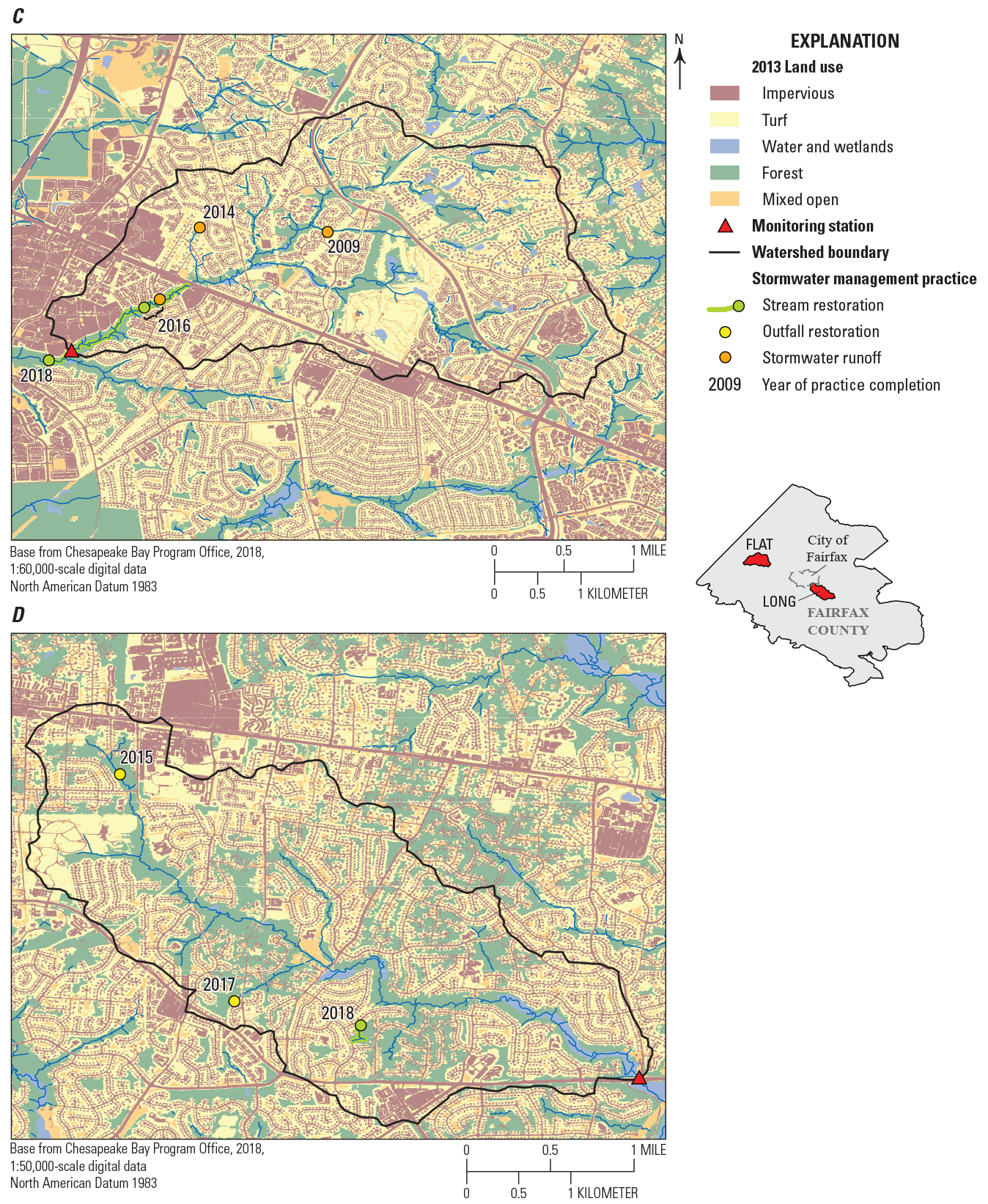
Maps showing the A, DEAD; B, DIFF; C, FLAT; and D, LONG study watersheds in Fairfax County, Virginia, and the land-use categorization; monitoring station locations; watershed boundaries; and the location, type, and completion year of stormwater management practices. Study watershed station names are defined in table 1.
Management-practice effects in the intensive-monitoring stations might be evident through changes in hydrology, but a relation between streamflow trends and management practices was not identified. Stormwater-retrofit practices that treat a large enough fraction of stormwater runoff and stream restorations that reconnect floodplains can alter the magnitude and timing of streamflow responses (Doll and others, 2020; Hopkins and others, 2020; Jefferson and others, 2017; Li and others, 2017). Changes in mean daily streamflow from 2008 through 2018 were mostly non-significant in DEAD, DIFF, SFLIL, and FLAT (Porter and others, 2020b), but trends during storm events revealed more nuanced patterns. The average number and duration of storm events were unchanged over time at these stations, yet stormflow hydrologic conditions generally improved in DIFF and SFLIL and degraded in DEAD and FLAT from water years 2009 through 2017 (fig. 19). During storm events, decreasing trends in streamflow volume, peak, and rising-limb rate-of-change occurred in DIFF and SFLIL. Management practices were installed in DIFF from 2012 through 2018 (fig. 11) and could produce these hydrologic changes during storm events. These effects being caused by management practices, however, are uncertain, as similar streamflow changes occurred in SFLIL (fig. 19), a watershed neighboring DIFF that had no management-practice implementation. Furthermore, increasing streamflow volume, peak, and rising-limb rate-of-change occurred in DEAD and FLAT during storm events (fig. 19): watersheds where many management practices were installed.
Changes in nutrient and sediment loads calculated at four intensive-monitoring stations from 2009 through 2018 did not clearly align with the timing of management-practice installation or the magnitude of credited reductions. On average, credited management-practice reductions represented less than 10 percent of the TN, TP, and SS loads at all stations in most years (fig. 28). Credited management-practice reductions occurred throughout the study period, but changes in annual flow-adjusted loads followed more complex trajectories (fig. 29). Flow-adjusted TN loads decreased at DEAD and FLAT and had no trend at SFLIL or DIFF; trends did not decrease in flow-adjusted TP or SS loads over the 10-year period (table 18). Similar to changes in annual conditions, patterns in monthly flow-adjusted loads were not clearly aligned with the timing of management-practice installation (fig. 30, fig. 31, and fig. 32).
The average credited effect of management practices across the 14-station network was not related to TN, TP, or SS concentration reductions or benthic-macroinvertebrate IBI score improvements from 2009 through 2018. These relations were assessed after accounting for climatic and landscape factors; a critical step in identifying the causal influences of management practices on water-quality and ecological responses. For all response variables, a single LME model was selected to represent the spatiotemporal effects of annual watershed and (or) climatic predictors. The selected models were refit after adding a term representing credited management-practice load reductions. The performance of models with and without this management-practice term was compared; an improvement in model performance would suggest that the management-practice effect helped explain the year-to-year variability in responses across all 14 study watersheds. Though such an improvement was not detected, the models demonstrated that management-practice effects may only be apparent after controlling for constituent-specific landscape and climatic conditions such as wastewater infrastructure, soil depth, precipitation, and air temperature.
Expected effects of some stream restoration practices may be temporarily offset by construction disturbances. The LME models suggested that elevated TP and SS concentrations in FLAT from 2016 through 2018 may have been related to the construction of a stream restoration practice. These concentration increases (fig. 46) were likely influenced by the close proximity of the practice to the FLAT monitoring station (fig. 84B) and did not appear to affect TP or SS loads (fig. 31 and fig. 32). A stream restoration completed in 2016 farther upstream in the FLAT watershed did not result in particulate water-quality impacts, and effects of other stream restorations completed during the study period were not observed. The longer-term, post-construction effects of stream restoration practices in FLAT and other watersheds can be evaluated in future years with continued data collection.
Considerations for Evaluating Management-Practice Effects
An inability to associate anticipated management-practice effects with water-quality monitoring data has been documented across a gradient of watershed and landscape settings (Lintern and others, 2020). This inability is commonly attributed to inaccurate estimates of management-practice effectiveness, nutrient and sediment response lag times, offsetting watershed factors, inadequate monitoring, non-optimal practice selection or location, and post-implementation practice failure (Ator and others, 2020; Lintern and others, 2020; Meals and others, 2010). These challenges were carefully considered in the design of this study and may become less influential in future years; however, the following factors likely affected the interpretation of management-practice effects in this report.
1. Amount, timing, and location of practice implementation.
-
• Management-practice effects are challenging to detect when practices treat a small watershed area, have a limited amount of post-construction monitoring, and are installed far upstream from monitoring stations. Management practices credited with TN, TP, and TSS reductions were completed in 10 of the 20 study watersheds from 2009 through 2018 (table 11). Stormwater-retrofit practices may most effectively reduce loads when they treat enough runoff to alter hydrologic conditions (Jefferson and others, 2017; Li and others, 2017); however, such practices treated less than eight percent of watershed area in each study watershed (table 14). Most credited reductions were associated with stream restorations, but many of these practices were completed late in the study period (table 13). Nutrient and sediment load reductions may not occur immediately after stream-restoration installation (McMillan and others, 2014), and it can take years to overcome the influences of groundwater nitrogen and soil phosphorus concentrations (Chang and others, 2021; Kleinman and others, 2019).
2. Unmeasured landscape and climatic factors.
-
• Changes in urban activities, climatic conditions, and the effects of physical watershed setting may reduce management-practice effectiveness or offset expected benefits. This study accounted for these challenges by modeling management-practice effects after accounting for influences from many factors that represent hypothetical drivers of water quality and benthic-macroinvertebrate community condition (table 2, table 3, and table 5). Interpretations in this report may be limited by unmeasured landscape and climatic factors and (or) the ability of available data to accurately represent conditions within watersheds and changes over time.
3. Uncertain management-practice expectations.
-
• Expected management-practice performance is often derived from expert opinion, but a large amount of uncertainty is associated with these assumptions (Koch and others, 2015). Management-practice effects likely follow complex, non-linear timelines that vary based on practice type, maintenance, and watershed setting (Jefferson and others, 2017). This study considered these various trajectories and evaluated water-quality and ecological responses against management-practice effects that maximized credited reductions (fig. 2).
4. Effects of hydrologic variability.
-
• Changes in streamflow influence water-quality and benthic-macroinvertebrate responses and should be considered when evaluating management-practice effects. In many Fairfax County watersheds, stormflow runoff is quickly routed to streams, resulting in fast and large streamflow responses (Porter and others, 2020b). Such hydrologic responses deliver most of the nutrient and sediment load to Fairfax County streams (Porter and others, 2020b) and can exceed the treatment capacity of stream restorations and stormwater retrofits (Doll and others, 2020; Jefferson and others, 2017). This study accounted for effects of hydrologic variability by comparing management-practice expectations against streamflow-normalized loads and by considering streamflow in models of water-quality and benthic-macroinvertebrate response.
5. Analytical assumptions.
-
• LME models were used to evaluate management-practice effects after accounting for landscape and climatic conditions. Specifically, LME models addressed if credited management-practice effects helped explain the annual variability of median water-quality conditions or benthic-macroinvertebrate IBI scores in 14 watersheds over a recent 10-year period. This approach was designed to identify an aggregate management-practice effect, which may mask an ability to identify practice effects in individual watersheds. Additionally, models represented linear changes over time, which may not capture observations that follow nonlinear trajectories.
Future Directions
Interpretations in this report about the effects of landscape and climatic conditions on water-quality and ecological responses in Fairfax County streams can inform future data-collection and analysis efforts. In partnership with Fairfax County, data-collection efforts from the Fairfax County monitoring network are expected to continue, along with efforts to better understand how and why conditions are changing over time. Continued analysis and exploration of the following topics, suggested by the initial interpretations in this report, could better inform watershed management in future years:
-
• The watershed-scale effects of management practices after additional years of post-restoration monitoring.
-
• The effects of temperature and precipitation on water-quality and ecological responses, specifically the roles of nitrogen and phosphorus biogeochemical transformations, sediment erosion freeze-thaw processes, and winter weather management strategies.
-
• The role of septic systems on increasing nitrogen trends over time, specifically whether these effects are caused by additional systems, aging infrastructure, or changing rates of groundwater nitrogen delivery to streams.
-
• The drivers of elevated phosphorus concentrations in Triassic Lowland watersheds, which may result from the natural dissolution of phosphorus-bearing minerals, the limited ability of these watersheds to retain phosphorus inputs within the landscape, or other anthropogenic effects.
-
• Factors affecting phosphorus retention on the landscape, including the effect of salinization on soil phosphorus mobilization; changes in phosphorus retention appear to have caused an increase in phosphorus concentrations and loads in many study watersheds.
-
• The influence of human activities and natural watershed setting on salinization, which could be explored in future years through analysis of major-ion concentration data, added to the intensive-monitoring stations in 2020.
-
• The effects of lateral stream migration and other geomorphic changes on stream-bank erosion rates and suspended-sediment conditions.
-
• The effects of urbanization on changing ecological responses over time, which could be explored by modeling non-composite benthic-macroinvertebrate response variables, characterizing stream habitat conditions, and (or) considering fall benthic-macroinvertebrate sampling data that have been recently added to the monitoring network.
These and other future research topics could be evaluated and advanced in collaboration with Fairfax County to identify questions most relevant to management needs. Future analyses and publications are expected to explore selected research topics in greater detail than the initial interpretations in this report. The process of identifying priority research topics, leveraging results from the monitoring network, and communicating detailed interpretations could provide more timely scientific information to guide Fairfax County’s management activities.
Summary
In 2007, the U.S. Geological Survey partnered with Fairfax County, Virginia, to establish a long-term water-resources monitoring program to evaluate the hydrology, water-quality, and ecology of Fairfax County streams and management-practice effects. Fairfax County uses a variety of management practices and policies to protect and restore water resources, but the watershed-scale effects of such strategies are not well understood. This report used streamflow, water-quality, and ecological monitoring data collected from 2007 through 2018 from 20 Fairfax County watersheds to assess the effects management practices, landscape factors, and climatic conditions had on observed nutrient, sediment, salinity, and benthic-macroinvertebrate community responses. This report expanded on the interpretations of previous U.S. Geological Survey reports that characterized Fairfax County stream conditions after 5 (Jastram and others, 2009) and 10 years (Porter and others, 2020b) of data collection.
Fairfax County experienced urban growth and climatic variability during the study period. Fairfax County’s population increased, resulting in the construction of new homes, roads, and stormwater and wastewater infrastructure. Increases in urban land were observed throughout many of the study watersheds, typically resulting from the conversion of previously wooded areas. Climatic conditions varied among study years; countywide estimates of average-annual air temperature differed by about 3 degrees Celsius and total precipitation ranged from about 34 to 63 inches per year.
Fairfax County’s investment in management strategies designed to protect and restore water resources increased during the study period. The county uses a variety of programs, policies, and practices to improve water resources, and this study focused on management practices credited with reducing nitrogen, phosphorus, and (or) sediment loads. These practices primarily included stormwater retrofits and stream restorations: stream restorations accounted for most of the financial investment and credited load reductions. There were 245 management practices completed in Fairfax County from 2009 through 2018, representing a total investment of about 87 million dollars. Cumulatively, these practices treat about 47 square miles and were credited with reductions of about 33,000 pounds of nitrogen, 8,300 pounds of phosphorus, and 1,600 tons of sediment. These cumulative values represent the additive credits reduced from multiple practices completed over time, where credited load reductions from all practices persist from year to year. Management practices were completed in half of the study watersheds; most practices were installed and most reductions were credited late in the study period.
Hydrologic responses during storm events were evaluated because many management practices are designed to achieve nutrient and sediment reductions by slowing or intercepting runoff. Watersheds with more impervious surfaces had more frequent and shorter-duration storm events. Summertime stormflow events were more frequent in watersheds with more impervious surfaces because impervious surfaces provide the runoff of short-duration precipitation events an efficient route to streams. The average number and length of stormflow events was mostly unchanged throughout the monitoring network over time, but some changes in stormflow peak, volume, and rate-of-change were observed over time in the four intensive-monitoring stations. These measures generally degraded in Dead Run at Whann Avenue near McLean, Virginia (Va.) (DEAD), and Flatlick Branch above Frog Branch at Chantilly, Va. (FLAT), but improved at Difficult Run above Fox Lake near Fairfax, Va. (DIFF), and South Fork Little Difficult Run above mouth near Vienna, Va. (SFLIL). Event-mean nutrient and sediment concentrations were measured during storm events and had similar trends over time across these four stations, showing increases in total phosphorus (TP) and suspended sediment (SS) and reductions or no changes in total nitrogen (TN).
Nitrogen and phosphorus loads in Fairfax County streams are affected by the amount of nutrients added to the landscape and the proportion of these inputs that reach streams. Estimated phosphorus from fertilizer and nitrogen from atmospheric deposition represented large nutrient inputs in many streams; amounts of other nonpoint inputs varied based on land use. For example, septic-system effluent was the largest nitrogen input in a few study watersheds without sanitary-sewer infrastructure. Estimated inputs of nitrogen declined throughout Fairfax County and most study watersheds during the study period as a result of atmospheric deposition reductions; in comparison, phosphorus inputs were relatively unchanged. Most nonpoint-nutrient inputs did not reach streams, and slightly more nitrogen was retained on the landscape than phosphorus, on average. These retention rates were lower in years with more precipitation and streamflow. After adjusting for streamflow effects, TN and TP loads were generally higher in years with greater nutrient inputs. Calculated as a function of these flow-adjusted loads, TP retention declined during the study period and, comparatively, TN retention was relatively unchanged.
Landscape conditions affected the average spatial differences and temporal changes in water-quality and ecological conditions of Fairfax County streams. These conditions were identified and described using linear mixed-effect models based on annual measures of TN, TP, and SS concentration, specific conductance (SC), and benthic-macroinvertebrate index of biotic integrity (IBI) scores. In general, among the 14 study watersheds, spatial differences in these response variables were larger than temporal changes observed from 2009 through 2018. For all response variables, many predictor combinations explained a similar amount of variability; however, a single model was selected for interpretation. Selected models typically explained a large amount of response variability between watersheds and a relatively smaller amount of variability in responses over time. TN concentrations were higher and had larger increases over the study period in watersheds with high septic-system density. TP concentrations were higher in watersheds with more turfgrass, shallower soils, and (or) with lower stream dissolved oxygen concentrations. TP concentration increases over the study period were largest in watersheds with deeper soils. Because deeper soils may store more phosphorus, changes in TP over time in Fairfax County streams may be affected by the retention or release of soil-bound phosphorus. Suspended-sediment concentrations were higher in watersheds with greater stream densities, likely highlighting the importance of stream banks as a source of sediment. SC was highest in watersheds with shallower soils and more developed land use. These relations suggest that SC may be affected by human activities, the capacity of watersheds to store salt inputs, and natural-mineral dissolution rates. Benthic-macroinvertebrate IBI scores were lower in watersheds with high road density and had larger increases over time in bigger, more developed watersheds. Year-to-year variability in water-quality and benthic-macroinvertebrate IBI scores was affected by annual climatic patterns. Changes in TN and TP concentrations and benthic-macroinvertebrate IBI scores over time were associated with differences in annual precipitation, whereas changes in SS concentrations and SC over time were associated with differences in annual air temperature. These relations suggest that surface-water runoff, nitrogen and phosphorus biogeochemical transformations, contributions of atmospheric nitrogen, freeze-thaw processes that increase stream-bank sediment erosion rates, and effects of winter weather management may be important processes to consider when evaluating Fairfax County stream conditions.
Expected management-practice effects were not consistently observed in the monitored data. Changes in the amount and timing of streamflow generated during storm events did not clearly align with management-practice implementation. Changes in calculated nutrient and sediment loads generally did not correspond to the timing of management-practice installation or the magnitude of credited reductions. After controlling for landscape and climatic conditions, the average credited effect of management practices across the monitoring network was not related to TN, TP, or SS concentration reductions or benthic-macroinvertebrate IBI score improvements from 2009 through 2018. An important consideration for future investigations of management-practice effects is how to control for water-quality and ecological variability caused by geologic properties, the urban environment, precipitation, and (or) air temperature. The interpretation of management-practice effects in this report was likely affected by a combination of factors, including (1) the amount, timing, and location of management-practice implementation; (2) unmeasured landscape and climatic factors; (3) uncertain management-practice expectations; (4) effects of hydrologic variability; and (5) analytical assumptions. Through continued data-collection efforts, particularly after management practices have been completed, many of these challenges may become less influential in the future.
References Cited
Akaike, H., 1974, A new look at the statistical model identification: IEEE Transactions on Automatic Control, v. 19, no. 6, p. 716–723, accessed January 2022 at https://doi.org/10.1109/TAC.1974.1100705.
Allan, J.D., Castillo, M.M., and Capps, K.A., 2021, Stream Ecology—Structure and function of running waters (3d ed.): Cham, Switzerland, Springer Nature Switzerland AG, p. 45–73, accessed August 2022 at https://doi.org/10.1007/978-3-030-61286-3.
Allen, M.R., and Ingram, W.J., 2002, Constraints on future changes in climate and the hydrologic cycle: Nature, v. 419, no. 6903, p. 228–232, accessed October 2021 at https://doi.org/10.1038/nature01092.
Amick, R.S., and Burgess, E.H., 2000, Exfiltration in sewer systems 600/R-01/034 (NTIS PB2003-103053): Cincinnati, Ohio, U.S. Environmental Protection Agency, 34 p., accessed August 2021 at https://cfpub.epa.gov/si/si_public_record_report.cfm?Lab=NRMRL&dirEntryId=99137.
Amrhein, C., Strong, J.E., and Mosher, P.A., 1992, Effect of deicing salts on metal and organic matter mobilization in roadside soils: Environmental Science & Technology, v. 26, no. 4, p. 703–709, accessed October 2021 at https://doi.org/10.1021/es00028a006.
Aravena, R., and Robertson, W.D., 1998, Use of multiple isotope tracers to evaluate denitrification in ground water—Study of nitrate from a large-flux septic system plume: Ground Water, v. 36, no. 6, p. 975–982, accessed August 2021 at https://doi.org/10.1111/j.1745-6584.1998.tb02104.x.
Ator, S.W., 2019, Spatially referenced models of streamflow and nitrogen, phosphorus, and suspended-sediment loads in streams of the northeastern United States: U.S. Geological Survey Scientific Investigations Report 2019–5118, 57 p., accessed March 2021 at https://doi.org/10.3133/sir20195118.
Ator, S.W., Blomquist, J.D., Webber, J.S., and Chanat, J.G., 2020, Factors driving nutrient trends in streams of the Chesapeake Bay watershed: Journal of Environmental Quality, v. 49, no. 4, p. 812–834, accessed August 2021 at https://doi.org/10.1002/jeq2.20101.
Aulenbach, B.T., Joiner, J.K., and Painter, J.A., 2017, Hydrology and water quality in 13 watersheds in Gwinnett County, Georgia, 2001–15: U.S. Geological Survey Scientific Investigations Report 2017–5012, 82 p., accessed August 2021, at https://doi.org/10.3133/sir20175012.
Bachman, M., Inamdar, S., Barton, S., Duke, J.M., Tallamy, D., and Bruck, J., 2016, A comparative assessment of runoff nitrogen from turf, forest, meadow, and mixed landuse watersheds: Journal of the American Water Resources Association, v. 52, no. 2, p. 397–408, accessed July 2021 at https://doi.org/10.1111/1752-1688.12395.
Baker, L.A., Hartzheim, P.M., Hobbie, S.E., King, J.Y., and Nelson, K.C., 2007, Effect of consumption choices on fluxes of carbon, nitrogen and phosphorus through households: Urban Ecosystems, v. 10, p. 97–117, accessed March 2021 at https://doi.org/10.1007/s11252-006-0014-3.
Baker, L.A., Hope, D., Xu, Y., Edmonds, J., and Lauver, L., 2001, Nitrogen balance for the central Arizona–Phoenix ecosystem: UrbanEcosystems, v. 4, p. 582–602, accessed March 2021 at https://doi.org/10.1007/s10021-001-0031-2.
Baldwin, D.S., and Mitchell, A.M., 2000, The effects of drying and re-flooding on the sediment and soil nutrient dynamics of lowland river–floodplain systems—A synthesis: Regulated Rivers, v. 16, no. 5, p. 457–467, accessed October 2021 at https://doi.org/10.1002/1099-1646(200009/10)16:5<457::AID-RRR597>3.0.CO;2-B.
Barbour, M.T., Gerritsen, J., Snyder, B.D., and Stribling, J.B., 1999, Rapid bioassessment protocols for use in streams and wadeable rivers—Periphyton, benthic macroinvertebrates, and fish (2d ed.), EPA 841-B-99-002: Washington, D.C., U.S. Environmental Protection Agency, Office of Water, 337 p., accessed August 2021 at https://www3.epa.gov/region1/npdes/merrimackstation/pdfs/ar/AR-1164.pdf.
Baron, J.S., Hall, E.K., Nolan, B.T., Finlay, J.C., Bernhardt, E.S., Harrison, J.A., Chan, F., and Boyer, E.W., 2013, The interactive effects of excess reactive nitrogen and climate change on aquatic ecosystems and water resources of the United States: Biogeochemistry, v. 114, p. 71–92, accessed August 2021 at https://doi.org/10.1007/s10533-012-9788-y.
Barr, D.J., Levy, R., Scheepers, C., and Tily, H.J., 2013, Random effects structure for confirmatory hypothesis testing—Keep it maximal: Journal of Memory and Language, v. 68, no. 3, p. 255–278, accessed May 2021 at https://doi.org/10.1016/j.jml.2012.11.001.
Bates, D., Mächler, M., Bolker, B., and Walker, S., 2015, Fitting linear mixed-effects models using lme4: Journal of Statistical Software, v. 67, no. 1, p. 1–48, accessed May 2021 at https://doi.org/10.18637/jss.v067.i01.
Bazinet, N.L., Gilbert, B.M., and Wallace, A.M., 2010, A comparison of urbanization effects on stream benthic macroinvertebrates and water chemistry in an urban and an urbanizing basin in Southern Ontario, Canada—Water: Qualitative Research Journal, v. 45, no. 3, p. 327–341, accessed July 2021 at https://doi.org/10.2166/wqrj.2010.035.
Bell, C.D., McMillan, S.K., Clinton, S.M., and Jefferson, A.J., 2016, Hydrologic response to stormwater control measures in urban watersheds: Journal of Hydrology, v. 541, pt. B, p. 1488–1500, accessed October 2021 at https://doi.org/10.1016/j.jhydrol.2016.08.049.
Ben-Shachar, M.S., Lüdecke, D., and Makowski, D., 2020, effectsize—Estimation of effect size indices and standardized parameters: Journal of Open Source Software, v. 5, no. 56, article 2815, 7 p., accessed January 2022 at https://doi.org/10.21105/joss.02815.
Bernhardt, E.S., Palmer, M.A., Allan, J.D., Alexander, G., Barnas, K., Brooks, S., Carr, J., Clayton, S., Dahm, C., Follstad-Shah, J., Galat, D., Gloss, S., Goodwin, P., Hart, D., Hassett, B., Jenkinson, R., Katz, S., Kondolf, G.M., Lake, P.S., Lave, R., Meyer, J.L., O’Donnell, T.K., Pagano, L., Powell, B., and Sudduth, E., 2005, Synthesizing U.S. river restoration efforts: Science, v. 308, no. 5722, p. 636–637, accessed October 2021 at https://doi.org/10.1126/science.1109769.
Bernhardt, E.S., and Palmer, M.A., 2011, River restoration—The fuzzy logic of repairing reaches to reverse catchment scale degradation: Ecological Applications, v. 21, no. 6, p. 1926–1931, accessed October 2021 at https://doi.org/10.1890/10-1574.1.
Bettez, N.D., and Groffman, P.M., 2013, Nitrogen deposition in and near an urban ecosystem: Environmental Science & Technology, v. 47, no. 11, p. 6047–6051, accessed October 2021 at https://doi.org/10.1021/es400664b.
Biggs, B.J.F., Nikora, V.I., and Snelder, T.H., 2005, Linking scales of flow variability to lotic ecosystem structure and function: River Research and Applications, v. 21, no. 2–3, p. 283–298, accessed February 2022 at https://doi.org/10.1002/rra.847.
Bird, D.L., Groffman, P.M., Salice, C.J., and Moore, J., 2018, Steady-state land cover but non-steady-state major ion chemistry in urban streams: Environmental Science & Technology, v. 52, no. 22, p. 13015–13026, accessed November 2021 at https://doi.org/10.1021/acs.est.8b03587.
Blume, T., Zehe, E., and Bronstert, A., 2007, Rainfall—Runoff response, event-based runoff coefficients and hydrograph separation: Hydrological Sciences Journal, v. 52, no. 5, p. 843–862, accessed October 2021 at https://doi.org/10.1623/hysj.52.5.843.
Boardman, E., Danesh-Yazdi, M., Foufoula-Georgiou, E., Dolph, C.L., and Finlay, J.C., 2019, Fertilizer, landscape features and climate regulate phosphorus retention and river export in diverse Midwestern watersheds: Biogeochemistry, v. 146, no. 3, p. 293–309, accessed August 2021 at https://doi.org/10.1007/s10533-019-00623-z.
Bock, E.M., and Easton, Z.M., 2020, Export of nitrogen and phosphorus from golf courses—A review: Journal of Environmental Management, v. 255, 109817, accessed May 2022 at https://doi.org/10.1016/j.jenvman.2019.109817.
Bonada, N., Prat, N., Resh, V.H., and Statzner, B., 2006, Developments in aquatic insect biomonitoring—A comparative analysis of recent approaches: Annual Review of Entomology, v. 51, no. 1, p. 495–523, accessed February 2022 at https://doi.org/10.1146/annurev.ento.51.110104.151124.
Bond, B.J., Jones, J.A., Moore, G., Phillips, N., Post, D., and McDonnell, J.J., 2002, The zone of vegetation influence on baseflow revealed by diel patterns of streamflow and vegetation water use in a headwater basin: Hydrological Processes, v. 16, no. 8, p. 1671–1677, accessed May 2022 at https://doi.org/10.1002/hyp.5022.
Booth, D.B., and Jackson, C.R., 1997, Urbanization of aquatic systems—Degradation thresholds, stormwater detection, and the limits of mitigation: Journal of the American Water Resources Association, v. 33, no. 5, p. 1077–1090, accessed January 2022 at https://doi.org/10.1111/j.1752-1688.1997.tb04126.x.
Borggaard, O.K., Szilas, C., Gimsing, A.L., and Rasmussen, L.H., 2004, Estimation of soil phosphate adsorption capacity by means of a pedotransfer function: Geoderma, v. 118, no. 1-2, p. 55–61, accessed October 2021 at https://doi.org/10.1016/S0016-7061(03)00183-6.
Bowden, W.B., 1987, The biogeochemistry of nitrogen in freshwater wetlands: Biogeochemistry, v. 4, no. 3, p. 313–348, accessed September 2021 at https://doi.org/10.1007/BF02187373.
Boynton, W.R., Hagy, J.D., Cornwell, J.C., Kemp, W.M., Greene, S.M., Owens, M.S., Baker, J.E., and Larsen, R.K., 2008, Nutrient budgets and management actions in the Patuxent River estuary, Maryland: Estuaries and Coasts, v. 31, no. 4, p. 623–651, accessed January 2022 at https://doi.org/10.1007/s12237-008-9052-9.
Brakebill, J.W., Ator, S.W., and Schwarz, G.E., 2010, Sources of suspended-sediment flux in streams of the Chesapeake Bay watershed—A regional application of the SPARROW model: Journal of the American Water Resources Association, v. 46, no. 4, p. 757–776, accessed August 2021 at https://doi.org/10.1111/j.1752-1688.2010.00450.x.
Bratt, A.R., Finlay, J.C., Hobbie, S.E., Janke, B.D., Worm, A.C., and Kemmitt, K.L., 2017, Contribution of leaf litter to nutrient export during winter months in an urban residential watershed: Environmental Science & Technology, v. 51, no. 6, p. 3138–3147, accessed August 2021 at https://doi.org/10.1021/acs.est.6b06299.
Burgin, A.J., and Hamilton, S.K., 2007, Have we overemphasized the role of denitrification in aquatic ecosystems? A review of nitrate removal pathways: Frontiers in Ecology and the Environment, v. 5, no. 2, p. 89–96, accessed September 2021 at https://doi.org/10.1890/1540-9295(2007)5[89:HWOTRO]2.0.CO;2.
Burns, D., Vitvar, T., McDonnell, J., Hassett, J., Duncan, J., and Kendall, C., 2005, Effects of suburban development on runoff generation in the Croton River basin, New York, USA: Journal of Hydrology, v. 311, no. 1, p. 266–281, accessed March 2021 at https://doi.org/10.1016/j.jhydrol.2005.01.022.
Burns, D.A., Bhatt, G., Linker, L.C., Bash, J.O., Capel, P.D., and Shenk, G.W., 2021, Atmospheric nitrogen deposition in the Chesapeake Bay watershed—A history of change: Atmospheric Environment, v. 251, 118277, accessed August 2021 at https://doi.org/10.1016/j.atmosenv.2021.118277.
Burns, D.A., Boyer, E.W., Elliott, E.M., and Kendall, C., 2009, Sources and transformations of nitrate from streams draining varying land uses—Evidence from dual isotope analysis: Journal of Environmental Quality, v. 38, no. 3, p. 1149–1159, accessed August 2021 at https://doi.org/10.2134/jeq2008.0371.
Buss, D.F., Carlisle, D.M., Chon, T.-S., Culp, J., Harding, J.S., Keizer-Vlek, H.E., Robinson, W.A., Strachan, S., Thirion, C., and Hughes, R.M., 2014, Stream biomonitoring using macroinvertebrates around the globe—A comparison of large-scale programs: Environmental Monitoring and Assessment, v. 187, article 4132, 12 p., accessed February 2022 at https://doi.org/10.1007/s10661-014-4132-8.
Caraco, N.F., Cole, J.J., Likens, G.E., Lovett, G.E., and Weathers, K.C., 2003, Variation in NO3 export from flowing waters of vastly different sizes—Does one model fit all?: Ecosystems (New York, N.Y.), v. 6, no. 4, p. 344–352, accessed August 2021 at https://doi.org/10.1007/s10021-002-0120-x.
Carey, R.O., Hochmuth, G.J., Martinez, C.J., Boyer, T.H., Dukes, M.D., Toor, G.S., and Cisar, J.L., 2013, Evaluating nutrient impacts in urban watersheds—Challenges and research opportunities: Environmental Pollution, v. 173, p. 138–149, accessed January 2022 at https://doi.org/10.1016/j.envpol.2012.10.004.
Carpenter, S.R., Caraco, N.F., Correll, D.L., Howarth, R.W., Sharpley, A.N., and Smith, V.H., 1998, Nonpoint pollution of surface waters with phosphorus and nitrogen: Ecological Applications, v. 8, no. 3, p. 559–568, accessed August 2021 at https://doi.org/10.1890/1051-0761(1998)008[0559:NPOSWW]2.0.CO;2.
Cashman, M.J., Gellis, A., Sanisaca, L.G., Noe, G.B., Cogliandro, V., and Baker, A., 2018, Bank-derived material dominates fluvial sediment in a suburban Chesapeake Bay watershed: River Research and Applications, v. 34, no. 8, p. 1032–1044, accessed January 2022 at https://doi.org/10.1002/rra.3325.
Chanat, J.G., and Yang, G., 2018, Exploring drivers of regional water-quality change using differential spatially referenced regression—A pilot study in the Chesapeake Bay watershed: Water Resources Research, v. 54, no. 10, p. 8120–8145, accessed August 2022 at https://doi.org/10.1029/2017WR022403.
Chang, S.Y., Zhang, Q., Byrnes, D.K., Basu, N.B., and Van Meter, K.J., 2021, Chesapeake legacies—The importance of legacy nitrogen to improving Chesapeake Bay water quality: Environmental Research Letters, v. 16, no. 8, p. 1–18, accessed August 2022 at https://doi.org/10.1088/1748-9326/ac0d7b.
Chesapeake Bay Program, 2018, Chesapeake Bay Program quick reference guide for best management practices: nonpoint source best management practices to reduce nitrogen, phosphorus and sediment loads to the Chesapeake Bay and its local waters CBP/TRS-323-18: Annapolis, Md., Chesapeake Bay Program office, 120 p., accessed October 2021 at https://www.chesapeakebay.net/what/publications/quick_reference_guide_for_best_management_practices_bmps.
Chesapeake Bay Program, 2020, Chesapeake Assessment and Scenario Tool Version 2019: Chesapeake Bay Program Office, accessed July 1, 2021, at https://cast.chesapeakebay.net/.
Chesapeake Bay Program Office, 2018, High-resolution land cover data for Chesapeake Bay watershed counties: Chesapeake Conservancy web page, accessed July 1, 2021, at https://www.chesapeakeconservancy.org/conservation-innovation-center/high-resolution-data/lulc-data-project-2022/.
Colangelo, D.J., and Jones, B.L., 2005, Phase I of the Kissimmee River restoration project, Florida, USA—Impacts of construction on water quality: Environmental Monitoring and Assessment, v. 102, no. 1, p. 139–158, accessed October 2021 at https://doi.org/10.1007/s10661-005-6017-3.
Conley, D.J., Pearl, H.W., Howarth, R.W., Boesch, D.F., Seitzinger, S.P., Havens, K.E., Lancelot, C., and Likens, G.E., 2009, Controlling eutrophication—Nitrogen and phosphorus: Science, v. 323, no. 5917, p. 1014–1015, accessed January 2022 at https://doi.org/10.1126/science.1167755.
Cooper, C.A., Mayer, P.M., and Faulkner, B.R., 2014, Effects of road salts on groundwater and surface water dynamics of sodium and chloride in an urban restored stream: Biogeochemistry, v. 121, p. 149–166, accessed November 2021 at https://doi.org/10.1007/s10533-014-9968-z.
Corsi, S.R., DeCicco, L.A., Lutz, M.A., and Hirsch, R.M., 2015, River chloride trends in snow-affected urban watersheds—Increasing concentrations outpace urban growth rate and are common among all seasons: Science of the Total Environment, v. 508, p. 488–497, accessed January 2020 at https://doi.org/10.1016/j.scitotenv.2014.12.012.
Daley, M.L., Potter, J.D., and McDowell, W.H., 2009, Salinization of urbanizing New Hampshire streams and groundwater—Effects of road salt and hydrologic variability: Journal of the North American Benthological Society, v. 28, no. 4, p. 929–940, accessed June 2020 at https://doi.org/10.1899/09-052.1.
Deb, D.L., and Datta, N.P., 1967, Effect of associating anions on phosphorus retention in soil: Plant and Soil, v. 26, no. 2, p. 303–316, accessed October 2021 at https://doi.org/10.1007/BF01880180.
Denver, J.M., Cravotta, C.A., III, Ator, S.W., and Lindsey, B.D., 2010, Contributions of phosphorus from groundwater to streams in the Piedmont, Blue Ridge, and Valley and Ridge physiographic provinces, eastern United States: U.S. Geological Survey Scientific Investigations Report 2010–5176, 38 p., accessed January 2022 at https://doi.org/10.3133/sir20105176.
Devereux, O.H., Prestegaard, K.L., Needelman, B.A., and Gellis, A.C., 2010, Suspended-sediment sources in an urban watershed, Northeast Branch Anacostia River, Maryland: Hydrological Processes, v. 24, no. 11, p. 1391–1403, accessed October 2021 at https://doi.org/10.1002/hyp.7604.
Dewitz, J., 2019, National Land Cover Database 2016 products: U.S. Geological Survey data release, January 2022 at https://doi.org/10.5066/P96HHBIE.
Dicken, C.L., Nicholson, S.W., Horton, J.D., Kinney, S.A., Gunther, G., Foose, M.P., and Mueller, J.A.L., 2005, Preliminary integrated geologic map databases for the United States: Delaware, Maryland, New York, Pennsylvania, and Virginia: U.S. Geological Survey Open-File Report 2005–1325, accessed March 2022 at https://pubs.er.usgs.gov/publication/ofr20051325.
Dieter, D., Herzog, C., and Hupfer, M., 2015, Effects of drying on phosphorus uptake in re-flooded lake sediments: Environmental Science and Pollution Research International, v. 22, p. 17065–17081, accessed October 2021 https://doi.org/10.1007/s11356-015-4904-x.
Djodjic, F., Börling, K., and Bergström, L., 2004, Phosphorus leaching in relation to soil type and soil phosphorus content: Journal of Environmental Quality, v. 33, no. 2, p. 678–684, accessed January 2022 at https://doi.org/10.2134/jeq2004.6780.
Dodds, W.K., 2003, The role of periphyton in phosphorus retention in shallow freshwater aquatic systems: Journal of Phycology, v. 39, no. 5, p. 840–849, accessed May 2022 at https://doi.org/10.1046/j.1529-8817.2003.02081.x.
Doll, B.A., Kurki-Fox, J.J., Page, J.L., Nelson, N.G., and Johnson, J.P., 2020, Flood flow frequency analysis to estimate potential floodplain nitrogen treatment during overbank flow events in urban stream restoration projects: Water, v. 12, no. 6, article 1568, 14 p., accessed May 2022 at https://doi.org/10.3390/w12061568.
Donat, M.G., Alexander, L.V., Yang, H., Durre, I., Vose, R., Dunn, R.J.H., Willett, K.M., Aguilar, E., Brunet, M., Caesar, J., Hewitson, B., Jack, C., Klein Tank, A.M.G., Kruger, A.C., Marengo, J., Peterson, T.C., Renom, M., Oria Rojas, C., Rusticucci, M., Salinger, J., Elrayah, A.S., Sekele, S.S., Srivastava, A.K., Trewin, B., Villarroel, C., Vincent, L.A., Zhai, P., Zhang, X., and Kitching, S., 2013, Updated analyses of temperature and precipitation extreme indices since the beginning of the twentieth century—The HadEX2 dataset: Journal of Geophysical Research, D, Atmospheres, v. 118, no. 5, p. 2098–2118, accessed July 2021 at https://doi.org/10.1002/jgrd.50150.
Donovan, M., Miller, A., Baker, M., and Gellis, A., 2015, Sediment contributions from floodplains and legacy sediments to Piedmont streams of Baltimore County, Maryland: Geomorphology, v. 235, p. 88–105, accessed October 2021 at https://doi.org/10.1016/j.geomorph.2015.01.025.
Duan, S., and Kaushal, S.S., 2015, Salinization alters fluxes of bioreactive elements from stream ecosystems across land use: Biogeosciences, v. 12, no. 23, p. 7331–7347, accessed June 2021 at https://doi.org/10.5194/bg-12-7331-2015.
Duan, S.-W., and Kaushal, S.S., 2013, Warming increases carbon and nutrient fluxes from sediments in streams across land use: Biogeosciences, v. 10, no. 2, p. 1193–1207, accessed January 2022 at https://doi.org/10.5194/bg-10-1193-2013.
Duan, S., Kaushal, S.S., Groffman, P.M., Band, L.E., and Belt, K.T., 2012, Phosphorus export across an urban to rural gradient in the Chesapeake Bay watershed: Journal of Geophysical Research—Biogeosciences, v. 117, no. G1 article G01025, 12 p., accessed January 2022 at https://doi.org/10.1029/2011JG001782.
Duncan, H.P., 2019, Baseflow separation—A practical approach: Journal of Hydrology, v. 575, p. 308–313, accessed January 2022 at https://doi.org/10.1016/j.jhydrol.2019.05.040.
Easton, Z.M., and Petrovic, A.M., 2004, Fertilizer source effect on ground and surface water quality in drainage from turfgrass: Journal of Environmental Quality, v. 33, no. 2, p. 645–655, accessed January 2022 at https://doi.org/10.2134/jeq2004.6450.
Eckhardt, K., 2005, How to construct recursive digital filters for baseflow separation: Hydrological Processes, v. 19, no. 2, p. 507–515, accessed October 2021 at https://doi.org/10.1002/hyp.5675.
Edwards, W.M., and Owens, L.B., 1991, Large storm effects on total soil erosion: Journal of Soil and Water Conservation, v. 46, no. 1, p. 75–78, accessed September 2021 https://www.jswconline.org/content/46/1/75.short.
Enders, C.K., and Tofighi, D., 2007, Centering predictor variables in cross-sectional multilevel models—A new look at an old issue: Psychological Methods, v. 12, no. 2, p. 121–138, accessed January 2022 at https://doi.org/10.1037/1082-989X.12.2.121.
Fairfax County, 2017, Fairfax County Chesapeake Bay total maximum daily load action plan, accessed January 7, 2022, at https://www.fairfaxcounty.gov/publicworks/sites/publicworks/files/assets/documents/chesapeake-bay-tmdl_0.pdf.
Fairfax County, 2019, Department of Public Works and Environmental Services policies and procedures—Stormwater Division comprehensive aquatic monitoring program standard operating procedures: Fairfax County Public Works and Environmental Services web page, accessed January 7, 2022, at https://www.fairfaxcounty.gov/publicworks/sites/publicworks/files/assets/documents/pdf/publications/stream_assessment_sop.pdf.
Fairfax County, 2021, Final sewer system certification report for fiscal year ended June 30, 2020, accessed August 6, 2021, at https://www.fairfaxcounty.gov/publicworks/sites/publicworks/files/Assets/Documents/sewer_certification_report_1.pdf.
Fairfax County, 2022, GIS data: Fairfax County, Va., web page, accessed October 1, 2022, at https://www.fairfaxcounty.gov/maps/gis-data.
Fanelli, R.M., Blomquist, J.D., and Hirsch, R.M., 2019, Point sources and agricultural practices control spatial-temporal patterns of orthophosphate in tributaries to Chesapeake Bay: Science of the Total Environment, v. 652, p. 422–433, accessed January 2022 at https://doi.org/10.1016/j.scitotenv.2018.10.062.
Fay, L., Veneziano, D., Muthumani, A., Shi, X., Kroon, A., Falero, C., Janson, M., and Peterson, S., 2015, Benefit-cost of various winter maintenance strategies: St. Paul, Minn., Western Transportation Institute, accessed January 10, 2022, at https://clearroads.org/download/final-report-19/.
Feminella, J.W., and Walsh, C.J., 2005, Urbanization and stream ecology—An introduction to the series: Journal of the North American Benthological Society, v. 24, no. 3, p. 585–587, accessed August 2021 at https://doi.org/10.1899/0887-3593(2005)024[0585:UASEAI]2.0.CO;2.
Fenz, R., Blaschke, A.P., Clara, M., Kroiss, H., Mascher, D., and Zessner, M., 2005, Monitoring of carbamazepine concentrations in wastewater and groundwater to quantify sewer leakage: Water Science and Technology, v. 52, no. 5, p. 205–213, accessed November 2020 at https://doi.org/10.2166/wst.2005.0135.
Filoso, S., and Palmer, M.A., 2011, Assessing stream restoration effectiveness at reducing nitrogen export to downstream waters: Ecological Applications, v. 21, no. 6, p. 1989–2006, accessed July 2021 at https://doi.org/10.1890/10-0854.1.
Fissore, C., Baker, L.A., Hobbie, S.E., King, J.Y., McFadden, J.P., Nelson, K.C., and Jakobsdottir, I., 2011, Carbon, nitrogen, and phosphorus fluxes in household ecosystems in the Minneapolis-Saint Paul, Minnesota, urban region: Ecological Applications, v. 21, no. 3, p. 619–639, accessed November 2020 at https://doi.org/10.1890/10-0386.1.
Flint, S.A., and McDowell, W.H., 2015, Effects of headwater wetlands on dissolved nitrogen and dissolved organic carbon concentrations in a suburban New Hampshire watershed: Freshwater Science, v. 34, no. 2, p. 456–471, accessed June 2021 at https://doi.org/10.1086/680985.
Froelich, A.J., and Zenone, C., 1985a, Maps showing geologic terrane, drainage basins, overburden, and low flow of streams in Fairfax County and vicinity, Virginia: U.S. Geological Survey IMAP 1534, 1 sheet, scale 1:24000, accessed March 2021 at https://pubs.er.usgs.gov/publication/i1534.
Froelich, A.J., and Zenone, C., 1985b, The relation of water quality to geology and land use changes in Fairfax County and vicinity, Virginia: U.S. Geological Survey IMAP 1561, 1 sheet, scale 1:480000, accessed March 2021 at https://pubs.er.usgs.gov/publication/i1561.
Funes, A., Martínez, F.J., Álvarez-Manzaneda, I., Conde-Porcuna, J.M., de Vicente, J., Guerrero, F., and de Vicente, I., 2018, Determining major factors controlling phosphorus removal by promising adsorbents used for lake restoration—A linear mixed model approach: Water Research, v. 141, p. 377–386, accessed January 2022 at https://doi.org/10.1016/j.watres.2018.05.029.
Garn, H.S., 2002, Effects of lawn fertilizer on nutrient concentration in runoff from lakeshore lawns, Lauderdale Lakes, Wisconsin: U.S. Geological Survey Water-Resources Investigations Report 2002–4130, 6 p., accessed January 2022 at https://doi.org/10.3133/wri024130.
Gellis, A.C., Myers, M.K., Noe, G.B., Hupp, C.R., Schenk, E.R., and Myers, L., 2017, Storms, channel changes, and a sediment budget for an urban-suburban stream, Difficult Run, Virginia, USA: Geomorphology, v. 278, p. 128–148, accessed August 2021 at https://doi.org/10.1016/j.geomorph.2016.10.031.
Gieswein, A., Hering, D., and Feld, C.K., 2017, Additive effects prevail—The response of biota to multiple stressors in an intensively monitored watershed: Science of the Total Environment, v. 593–594, p. 27–35, accessed February 2022 at https://doi.org/10.1016/j.scitotenv.2017.03.116.
Giorgino, M.J., Cuffney, T.F., Harden, S.L., and Feaster, T.D., 2018, Trends in water quality of selected streams and reservoirs used for water supply in the Triangle area of North Carolina, 1989–2013: U.S. Geological Survey Scientific Investigations Report 2018–5077, 67 p., accessed January 2022 at https://doi.org/10.3133/sir20185077.
Goyette, J.-O., Bennett, E.M., and Maranger, R., 2019, Differential influence of landscape features and climate on nitrogen and phosphorus transport throughout the watershed: Biogeochemistry, v. 142, no. 1, p. 155–174, accessed June 2021 at https://doi.org/10.1007/s10533-018-0526-y.
Greenwood, M.J., and Booker, D.J., 2015, The influence of antecedent floods on aquatic invertebrate diversity, abundance and community composition: Ecohydrology, v. 8, no. 2, p. 188–203, accessed February 2022 at https://doi.org/10.1002/eco.1499.
Groffman, P.M., and Crawford, M.K., 2003, Denitrification potential in urban riparian zones: Journal of Environmental Quality, v. 32, no. 3, p. 1144–1149, accessed January 2022 at https://doi.org/10.2134/jeq2003.1144.
Groffman, P.M., Law, N.L., Belt, K.T., Band, L.E., and Fisher, G.T., 2004, Nitrogen fluxes and retention in urban watershed ecosystems: Ecosystems, v. 7, p. 393–403, accessed January 2022 at https://doi.org/10.1007/s10021-003-0039-x.
Gross, C.M., Angle, J.S., and Welterlen, M.S., 1990, Nutrient and sediment losses from turfgrass: Journal of Environmental Quality, v. 19, no. 4, p. 663–668, accessed October 2021 at https://doi.org/10.2134/jeq1990.00472425001900040006x.
Han, X., Hovland, E., and Khaja, F., 2018, Demographic reports 2018—County of Fairfax, Virginia: Fairfax, Va., Department of Management and Budget, prepared by Economic, Demographic, and Statistical Research, 10 chap. (I–X) [variously paged], accessed August 6, 2021, at https://www.fairfaxcounty.gov/demographics/sites/demographics/files/Assets/DemographicReports/fullrpt2018.pdf.
Haq, S., Kaushal, S.S., and Duan, S., 2018, Episodic salinization and freshwater salinization syndrome mobilize base cations, carbon, and nutrients to streams across urban regions: Biogeochemistry, v. 141, p. 463–486, accessed April 2020 at https://doi.org/10.1007/s10533-018-0514-2.
Harper, S., 2011, Bill banning phosphorus from lawns soon to be law: The Virginian Pilot website, accessed July 28, 2021, at pilotonline.com at https://www.pilotonline.com/government/virginia/article_52dd1cf6-3929-56a5-b415-90c3ef505139.html.
Helsel, D.R., Hirsch, R.M., Ryberg, K.R., Archfield, S.A., and Gilroy, E.J., 2020, Statistical methods in water resources: U.S. Geological Survey Techniques and Methods, book 4, chap. A3, 484 p., accessed September 2020 at https://doi.org/10.3133/tm4A3. [Techniques and Methods 4-A3 supersedes Techniques of Water-Resources Investigations, book 4, chapter A3, version 1.1.]
Hem, J.D., 1985, Study and interpretation of the chemical characteristics of natural water: U.S. Geological Survey Water-Supply Paper, v. 2254, 263 p., accessed June 2020 at https://pubs.usgs.gov/wsp/wsp2254/.
Hobbie, S.E., Finlay, J.C., Janke, B.D., Nidzgorski, D.A., Millet, D.B., and Baker, L.A., 2017, Contrasting nitrogen and phosphorus budgets in urban watersheds and implications for managing urban water pollution: Proceedings of the National Academy of Sciences of the United States of America, v. 114, no. 16, p. 4177–4182, accessed October 2020 at https://doi.org/10.1073/pnas.1618536114.
Hoffman, L., 2015, Longitudinal analysis—Modeling within-person fluctuation and change: New York, Routledge, 654 p., accessed August 2021 at https://doi.org/10.4324/9781315744094.
Hoffman, L., and Stawski, R.S., 2009, Persons as contexts—Evaluating between-person and within-person effects in longitudinal analysis: Research in Human Development, v. 6, no. 2–3, p. 97–120, accessed January 2021 at https://doi.org/10.1080/15427600902911189.
Homer, C.G., Dewitz, J., Yang, L., Jin, S., Danielson, P., Xian, G.Z., Coulston, J., Herold, N., Wickham, J., and Megown, K., 2015, Completion of the 2011 National Land Cover Database for the conterminous United States–Representing a decade of land cover change information: Photogrammetric Engineering and Remote Sensing, v. 81, p. 345–354, accessed August 2020 at https://cfpub.epa.gov/si/si_public_record_report.cfm?Lab=NERL&dirEntryId=309950.
Hopkins, K.G., Bhaskar, A.S., Woznicki, S.A., and Fanelli, R.M., 2020, Changes in event-based streamflow magnitude and timing after suburban development with infiltration-based stormwater management: Hydrological Processes, v. 34, no. 2, p. 387–403, accessed May 2020 at https://doi.org/10.1002/hyp.13593.
Hossain, M.A., Alam, M., Yonge, D.R., and Dutta, P., 2005, Efficiency and flow regime of a highway stormwater detention pond in Washington, USA: Water, Air, and Soil Pollution, v. 164, p. 79–89, accessed January 2022 at https://doi.org/10.1007/s11270-005-2250-1.
House, W.A., 2003, Geochemical cycling of phosphorus in rivers: Applied Geochemistry, v. 18, no. 5, p. 739–748, accessed October 2021 at https://doi.org/10.1016/S0883-2927(02)00158-0.
House, M.A., Ellis, J.B., Herricks, E.E., Hvitved-Jacobsen, T., Seager, J., Lijklema, L., Aalderink, H., and Clifforde, I.T., 1993, Urban drainage—Impacts on receiving water quality: Water Science and Technology, v. 27, no. 12, p. 117–158, accessed January 2022 at https://doi.org/10.2166/wst.1993.0293.
Houser, D.L., and Pruess, H., 2009, The effects of construction on water quality—A case study of the culverting of Abram Creek: Environmental Monitoring and Assessment, v. 155, no. 1, p. 431–442, accessed October 2021 at https://doi.org/10.1007/s10661-008-0445-9.
Howarth, R., and Paerl, H.W., 2008, Coastal marine eutrophication—Control of both nitrogen and phosphorus is necessary: Proceedings of the National Academy of Sciences of the United States of America, v. 105, no. 49, p. E103, accessed January 2022 at https://doi.org/10.1073/pnas.0807266106.
Hupp, C.R., Noe, G.B., Schenk, E.R., and Benthem, A.J., 2013, Recent and historic sediment dynamics along Difficult Run, a suburban Virginia Piedmont stream: Geomorphology, v. 180–181, p. 156–169, accessed April 2020 at https://doi.org/10.1016/j.geomorph.2012.10.007.
Hyer, K.E., Denver, J.M., Langland, M.J., Webber, J.S., Böhlke, J.K., Hively, W.D., and Clune, J.W., 2016, Spatial and temporal variation of stream chemistry associated with contrasting geology and land-use patterns in the Chesapeake Bay watershed—Summary of results from Smith Creek, Virginia; Upper Chester River, Maryland; Conewago Creek, Pennsylvania; and Difficult Run, Virginia, 2010–2013: U.S. Geological Survey Scientific Investigations Report 2016–5093, 211 p., accessed January 2020 at https://doi.org/10.3133/sir20165093.
Inamdar, S., Johnson, E., Rowland, R., Warner, D., Walter, R., and Merritts, D., 2018, Freeze–thaw processes and intense rainfall—The one-two punch for high sediment and nutrient loads from mid-Atlantic watersheds: Biogeochemistry, v. 141, no. 3, p. 333–349, accessed October 2021 at https://doi.org/10.1007/s10533-017-0417-7.
Interstate Commission on the Potomac River Basin, 2020, Virginia Salt Management Strategy—A toolkit to reduce the environmental impacts of winter maintenance practices, 402 p., accessed January 10, 2022, at https://www.novaregion.org/DocumentCenter/View/13054.
James, W.F., and Barko, J.W., 2004, Diffusive fluxes and equilibrium processes in relation to phosphorus dynamics in the Upper Mississippi River: River Research and Applications, v. 20, no. 4, p. 473–484, accessed October 2021 at https://doi.org/10.1002/rra.761.
Janssen, E., Sriver, R.L., Wuebbles, D.J., and Kunkel, K.E., 2016, Seasonal and regional variations in extreme precipitation event frequency using CMIP5: Geophysical Research Letters, v. 43, no. 10, p. 5385–5393, accessed October 2021 at https://doi.org/10.1002/2016GL069151.
Jastram, J.D., 2014, Streamflow, water quality, and aquatic macroinvertebrates of selected streams in Fairfax County, Virginia, 2007-12: U.S. Geological Survey Scientific Investigations Report 2014–5073, 82 p., accessed January 2020 at https://doi.org/10.3133/sir20145073.
Jastram, J.D., Krstolic, J.L., Moyer, D.L., and Hyer, K.E., 2015, Fluvial geomorphology and suspended-sediment transport during construction of the Roanoke River Flood Reduction Project in Roanoke, Virginia, 2005–2012: U.S. Geological Survey Scientific Investigations Report 2015–5111, 53 p., accessed August 2021 at https://doi.org/10.3133/sir20155111.
Jastram, J.D., Moyer, D.L., and Hyer, K.E., 2009, A comparison of turbidity-based and streamflow-based estimates of suspended-sediment concentrations in three Chesapeake Bay tributaries: U.S. Geological Survey Scientific Investigations Report 2009–5165, 37 p., accessed May 2020 at https://doi.org/10.3133/sir20095165.
Jefferson, A.J., Bhaskar, A.S., Hopkins, K.G., Fanelli, R., Avellaneda, P.M., and McMillan, S.K., 2017, Stormwater management network effectiveness and implications for urban watershed function—A critical review: Hydrological Processes, v. 31, no. 23, p. 4056–4080, accessed August 2021 at https://doi.org/10.1002/hyp.11347.
Jones, R.C., 2020, Recovery of a tidal freshwater embayment from eutrophication—A multidecadal study: Estuaries and Coasts, v. 43, p. 1318–1334, accessed January 2020 at https://doi.org/10.1007/s12237-020-00730-3.
Kaushal, S.S., Duan, S., Doody, T.R., Haq, S., Smith, R.M., Newcomer Johnson, T.A., Newcomb, K.D., Gorman, J., Bowman, N., Mayer, P.M., Wood, K.L., Belt, K.T., and Stack, W.P., 2017, Human-accelerated weathering increases salinization, major ions, and alkalinization in fresh water across land use: Applied Geochemistry, v. 83, p. 121–135, accessed October 2021 at https://doi.org/10.1016/j.apgeochem.2017.02.006.
Kaushal, S.S., Groffman, P.M., Band, L.E., Elliott, E.M., Shields, C.A., and Kendall, C., 2011, Tracking nonpoint source nitrogen pollution in human-impacted watersheds: Environmental Science & Technology, v. 45, no. 19, p. 8225–8232, accessed July 2021 at https://doi.org/10.1021/es200779e.
Kaushal, S.S., Groffman, P.M., Band, L.E., Shields, C.A., Morgan, R.P., Palmer, M.A., Belt, K.T., Swan, C.M., Findlay, S.E.G., and Fisher, G.T., 2008a, Interaction between urbanization and climate variability amplifies watershed nitrate export in Maryland: Environmental Science & Technology, v. 42, no. 16, p. 5872–5878, accessed July 2021 at https://doi.org/10.1021/es800264f.
Kaushal, S.S., Groffman, P.M., Likens, G.E., Belt, K.T., Stack, W.P., Kelly, V.R., Band, L.E., and Fisher, G.T., 2005, Increased salinization of fresh water in the northeastern United States: Proceedings of the National Academy of Sciences of the United States of America, v. 102, no. 38, p. 13517–13520, accessed July 2021 at https://doi.org/10.1073/pnas.0506414102.
Kaushal, S.S., Groffman, P.M., Mayer, P.M., Striz, E., and Gold, A.J., 2008b, Effects of stream restoration on denitrification in an urbanizing watershed: Ecological Applications, v. 18, no. 3, p. 789–804, accessed October 2021 at https://doi.org/10.1890/07-1159.1.
Kaushal, S.S., Lewis, W.M., Jr., and McCutchan, J.H., Jr., 2006, Land use change and nitrogen enrichment of a Rocky Mountain watershed: Ecological Applications, v. 16, no. 1, p. 299–312, accessed August 2021 at https://doi.org/10.1890/05-0134.
Kaushal, S.S., Likens, G.E., Pace, M.L., Utz, R.M., Haq, S., Gorman, J., and Grese, M., 2018, Freshwater salinization syndrome on a continental scale: Proceedings of the National Academy of Sciences of the United States of America, v. 115, no. 4, p. E574–E583, accessed June 2021 at https://doi.org/10.1073/pnas.1711234115.
Kaushal, S.S., Likens, G.E., Utz, R.M., Pace, M.L., Grese, M., and Yepsen, M., 2013, Increased river alkalinization in the Eastern U.S: Environmental Science & Technology, v. 47, no. 18, p. 10302–10311, accessed October 2021 at https://doi.org/10.1021/es401046s.
Kaushal, S.S., McDowell, W.H., Wollheim, W.M., Johnson, T.A.N., Mayer, P.M., Belt, K.T., and Pennino, M.J., 2015, Urban evolution—The role of water: Water (Basel), v. 7, no. 8, p. 4063–4087, accessed June 2021 at https://doi.org/10.3390/w7084063.
Kenney, M.A., Wilcock, P.R., Hobbs, B.F., Flores, N.E., and Martínez, D.C., 2012, Is urban stream restoration worth it?: Journal of the American Water Resources Association, v. 48, no. 3, p. 603–615, accessed October 2022 at https://doi.org/10.1111/j.1752-1688.2011.00635.x.
King, K.W., Balogh, J.C., and Harmel, R.D., 2007, Nutrient flux in storm water runoff and baseflow from managed turf: Environmental Pollution, v. 150, no. 3, p. 321–328, accessed August 2021 at https://doi.org/10.1016/j.envpol.2007.01.038.
Kinsman-Costello, L.E., Hamilton, S.K., O’Brien, J.M., and Lennon, J.T., 2016, Phosphorus release from the drying and reflooding of diverse shallow sediments: Biogeochemistry, v. 130, no. 1, p. 159–176, accessed January 2021 at https://doi.org/10.1007/s10533-016-0250-4.
Kleinman, P.J.A., 2017, The persistent environmental relevance of soil phosphorus sorption saturation: Current Pollution Reports, v. 3, no. 2, p. 141–150, accessed March 2021 at https://doi.org/10.1007/s40726-017-0058-4.
Kleinman, P.J.A., Fanelli, R.M., Hirsch, R.M., Buda, A.R., Easton, Z.M., Wainger, L.A., Brosch, C., Lowenfish, M., Collick, A.S., Shirmohammadi, A., Boomer, K., Hubbart, J.A., Bryant, R.B., and Shenk, G.W., 2019, Phosphorus and the Chesapeake Bay—Lingering issues and emerging concerns for agriculture: Journal of Environmental Quality, v. 48, no. 5, p. 1191–1203, accessed August 2020 at https://doi.org/10.2134/jeq2019.03.0112.
Kleinman, P.J.A., Sharpley, A.N., Buda, A.R., McDowell, R.W., and Allen, A.L., 2011, Soil controls of phosphorus in runoff—Management barriers and opportunities: Canadian Journal of Soil Science, v. 91, no. 3, p. 329–338, accessed March 2021 at https://doi.org/10.4141/cjss09106.
Koch, B.J., Febria, C.M., Cooke, R.M., Hosen, J.D., Baker, M.E., Colson, A.R., Filoso, S., Hayhoe, K., Loperfido, J.V., Stoner, A.M.K., and Palmer, M.A., 2015, Suburban watershed nitrogen retention—Estimating the effectiveness of stormwater management structures: Elementa, v. 3, no. 000063, p. 1–18, accessed January 2022 at https://doi.org/10.12952/journal.elementa.000063.
Koch, B.J., Febria, C.M., Gevrey, M., Wainger, L.A., and Palmer, M.A., 2014, Nitrogen removal by stormwater management structures—A data synthesis: Journal of the American Water Resources Association, v. 50, no. 6, p. 1594–1607, accessed August 2021 at https://doi.org/10.1111/jawr.12223.
Krajewski, A., Sikorska, A.E., and Kazimierz, B., 2017, Modeling suspended sediment concentration in the stormwater outflow from a small detention pond: Journal of Environmental Engineering, v. 143, no. 10, article 5017005. 11 p., accessed October 2021 at https://doi.org/10.1061/(ASCE)EE.1943-7870.0001258.
Krenitsky, E.C., Carroll, M.J., Hill, R.L., and Krouse, J.M., 1998, Runoff and sediment losses from natural and man-made erosion control materials: Crop Science, v. 38, no. 4, p. 1042–1046, accessed January 2022 at https://doi.org/10.2135/cropsci1998.0011183X003800040026x.
Lammers, R.W., and Bledsoe, B.P., 2017, What role does stream restoration play in nutrient management?: Critical Reviews in Environmental Science and Technology, v. 47, no. 6, p. 335–371, accessed March 2021 at https://doi.org/10.1080/10643389.2017.1318618.
Larson, J.D., 1978, Chemical composition of streams during low flow—Fairfax County, Virginia: U.S. Geological Survey Open File Report 78–719, 31 p., 1 pls., accessed June 2020 at https://doi.org/10.3133/ofr78719.
Lawler, D.M., 1986, River bank erosion and the influence of frost—A statistical examination: Transactions of the Institute of British Geographers, v. 11, no. 2, p. 227–242, accessed June 2021 at https://doi.org/10.2307/622008.
Lenat, D.R., and Crawford, J.K., 1994, Effects of land use on water quality and aquatic biota of three North Carolina Piedmont streams: Hydrobiologia, v. 294, no. 3, p. 185–199, accessed January 2022 at https://doi.org/10.1007/BF00021291.
Li, C., Fletcher, T.D., Duncan, H.P., and Burns, M.J., 2017, Can stormwater control measures restore altered urban flow regimes at the catchment scale?: Journal of Hydrology, v. 549, p. 631–653, accessed August 2021 at https://doi.org/10.1016/j.jhydrol.2017.03.037.
Li, X., Xia, Y., Li, Y., Kana, T.M., Kimura, S.D., Saito, M., and Yan, X., 2013, Sediment denitrification in waterways in a rice-paddy-dominated watershed in eastern China: Journal of Soils and Sediments, v. 13, no. 4, p. 783–792, accessed June 2021 at https://doi.org/10.1007/s11368-013-0651-0.
Lintern, A., McPhillips, L., Winfrey, B., Duncan, J., and Grady, C., 2020, Best management practices for diffuse nutrient pollution—Wicked problems across urban and agricultural watersheds: Environmental Science & Technology, v. 54, no. 15, p. 9159–9174, accessed December 2021 at https://doi.org/10.1021/acs.est.9b07511.
Loperfido, J.V., Noe, G.B., Jarnagin, S.T., and Hogan, D.M., 2014, Effects of distributed and centralized stormwater best management practices and land cover on urban stream hydrology at the catchment scale: Journal of Hydrology, v. 519, no. pt. C, p. 2584–2595, accessed August 2021 at https://doi.org/10.1016/j.jhydrol.2014.07.007.
Lotspeich, R.R., 2009, Regional curves of bankfull channel geometry for non-urban streams in the Piedmont Physiographic Province, Virginia: U.S. Geological Survey Scientific Investigations Report 2009–5206, 51 p., October 2021 at https://pubs.usgs.gov/sir/2009/5206/pdf/sir2009-5206.pdf.
Lyerly, C.M., Hernandez Cordero, A.L., Foreman, K.L., Phillips, S.W., and Dennison, W.C., eds., 2014, New Insights—Science-based evidence of water quality improvements, challenges, and opportunities in the Chesapeake: Chesapeake Bay Program, University of Maryland Center of Environmental Science, and U.S. Geological Survey, 52 p., accessed June 2020 at https://ian.umces.edu/site/assets/files/11070/new-insights-science-based-evidence-of-water-quality-improvements-challenges-and-opportunities-in-the-ch esapeake.pdf.
Majcher, E.H., Woytowitz, E.L., Alexander, R.J., and Groffman, P.M., 2018, Factors affecting long-term trends in surface-water quality in the Gwynns Falls watershed, Baltimore City and County, Maryland, 1998–2016: U.S. Geological Survey Open-File Report 2018-1038, 27 p., accessed August 2021 at https://doi.org/10.3133/ofr20181038.
Maniquiz, M.C., Choi, J., Lee, S., Cho, H.J., and Kim, L.-H., 2010, Appropriate methods in determining the event mean concentration and pollutant removal efficiency of a best management practice: Environmental Engineering Research, v. 15, no. 4, p. 215–223, accessed July 2021 at https://doi.org/10.4491/eer.2010.15.4.215.
Marsalek, J., Rochfort, Q., Grapentine, L., and Brownlee, B., 2002, Assessment of stormwater impacts on an urban stream with a detention pond: Water Science and Technology, v. 45, no. 3, p. 255–263, accessed August 2021 at https://doi.org/10.2166/wst.2002.0086.
McMillan, S.K., and Noe, G.B., 2017, Increasing floodplain connectivity through urban stream restoration increases nutrient and sediment retention: Ecological Engineering, v. 108, p. 284–295, accessed December 2021 at https://doi.org/10.1016/j.ecoleng.2017.08.006.
McMillan, S.K., Tuttle, A.K., Jennings, G.D., and Gardner, A., 2014, Influence of restoration age and riparian vegetation on reach-scale nutrient retention in restored urban streams: Journal of the American Water Resources Association, v. 50, no. 3, p. 626–638, accessed January 2022 at https://doi.org/10.1111/jawr.12205.
McPhillips, L.E., and Matsler, A.M., 2018, Temporal evolution of green stormwater infrastructure strategies in three US cities: Frontiers in Built Environment, v. 4, article 26, 14 p., accessed June 2021 at https://doi.org/10.3389/fbuil.2018.00026.
Meals, D.W., Dressing, S.A., and Davenport, T.E., 2010, Lag time in water quality response to best management practices—A review: Journal of Environmental Quality, v. 39, no. 1, p. 85–96, accessed January 2022 at https://doi.org/10.2134/jeq2009.0108.
Messinger, T., and Burgholzer, R.W., 2018, Rating stability, and frequency and magnitude of shifts, for streamgages in Virginia through water year 2013: U.S. Geological Survey Scientific Investigations Report 2017–5137, 91 p., 5 pls., 5 tables, 4 app., accessed August 2021 at https://doi.org/10.3133/sir20175137.
Meyer, J.L., Paul, M.J., and Taulbee, W.K., 2005, Stream ecosystem function in urbanizing landscapes: Journal of the North American Benthological Society, v. 24, no. 3, p. 602–612, accessed May 2020 at https://doi.org/10.1899/04-021.1.
Miller, M.P., Kennen, J.G., Mabe, J.A., and Mize, S.V., 2012, Temporal trends in algae, benthic invertebrate, and fish assemblages in streams and rivers draining basins of varying land use in the south-central United States, 1993–2007: Hydrobiologia, v. 684, no. 1, p. 15–33, accessed August 2021 at https://doi.org/10.1007/s10750-011-0950-7.
Minnesota Groundwater Association, 2020, Impacts of stormwater infiltration on chloride in Minnesota groundwater: Minnesota Ground Water Association White Paper 04, 65 p., accessed January 10, 2022, at https://www.mgwa.org/documents/whitepapers/impacts_of_stormwater_infiltration_on_chloride_in_minnesota_groundwater.pdf.
Moglen, G.E., and Rios Vidal, G.E., 2014, Climate change and storm water infrastructure in the Mid-Atlantic region—Design mismatch coming?: Journal of Hydrologic Engineering, v. 19, no. 11, 04014026, accessed August 2021 at https://doi.org/10.1061/(ASCE)HE.1943-5584.0000967.
Mohler, E.H., and Hagan, G.F., 1981, Low flow of streams in Fairfax County, Virginia: U.S. Geological Survey Open File Report 81–63, 30 p., 1 pl., accessed May 2021 at https://doi.org/10.3133/ofr8163.
Moyer, D.L., and Hyer, K.E., 2003, Use of the hydrological simulation program-FORTRAN and bacterial source tracking for development of the fecal coliform total maximum daily load for Accotink Creek, Fairfax County, Virginia: U.S. Geological Survey Water-Resources Investigations Report 2003–4160, 67.p., accessed July 2021 at https://doi.org/10.3133/wri034160.
Nakagawa, S., Johnson, P.C.D., and Schielzeth, H., 2017, The coefficient of determination R2 and intra-class correlation coefficient from generalized linear mixed-effects models revisited and expanded: Journal of the Royal Society, Interface, v. 14, no. 134, 20170213, accessed June 2021 at https://doi.org/10.1098/rsif.2017.0213.
Nardi, M., 2014, Watershed potential to contribute phosphorus from geologic materials to receiving streams, conterminous United States: U.S. Geological Survey digital raster dataset, accessed August 2020 at https://water.usgs.gov/GIS/metadata/usgswrd/XML/pmapnatl.xml.
Nathan, R.J., and McMahon, T.A., 1990, Evaluation of automated techniques for base flow and recession analyses: Water Resources Research, v. 26, no. 7, p. 1465–1473, accessed May 2021 at https://doi.org/10.1029/WR026i007p01465.
National Atmospheric Deposition Program, 2020, Total deposition maps: National Atmospheric Depositional Program web page, accessed August 1, 2021, at https://nadp.slh.wisc.edu/committees/tdep/.
National Oceanic and Atmospheric Administration, National Centers for Environmental Information 2021, Climate at a Glance: City Time Series, accessed January 7, 2022, at https://www.ncdc.noaa.gov/cag/.
National Research Council, 2009, Urban stormwater management in the United States: Washing, D.C., National Academies Press, 598 p., accessed January 10, 2022, at https://www.nap.edu/catalog/12465/urban-stormwater-management-in-the-united-states.
Newcomer Johnson, T.A., Kaushal, S.S., Mayer, P.M., Smith, R.M., and Sivirichi, G.M., 2016, Nutrient retention in restored streams and rivers—A global review and synthesis: Water v. 8, no. 4, 28 p., accessed August 2021 at https://doi.org/10.3390/w8040116.
Noe, G.B., Cashman, M.J., Skalak, K., Gellis, A., Hopkins, K.G., Moyer, D., Webber, J., Benthem, A., Maloney, K., Brakebill, J., Sekellick, A., Langland, M., Zhang, Q., Shenk, G., Keisman, J., and Hupp, C., 2020, Sediment dynamics and implications for management—State of the science from long-term research in the Chesapeake Bay watershed, USA: WIREs Water, v. 7, no. 4, article e1454, 28 p., accessed April 2021 at https://doi.org/10.1002/wat2.1454.
Nõges, P., Argillier, C., Borja, Á., Garmendia, J.M., Hanganu, J., Kodeš, V., Pletterbauer, F., Sagouis, A., and Birk, S., 2016, Quantified biotic and abiotic responses to multiple stress in freshwater, marine and ground waters: Science of the Total Environment, v. 540, p. 43–52, accessed October 2021 at https://doi.org/10.1016/j.scitotenv.2015.06.045.
Nolan, K.M., Bohman, L., Stamey, T., and Firda, G., 2005, Stage-discharge relations—basic concepts: U.S. Geological Survey Scientific Investigations Report 2005–5028, 32 p., accessed March 2021 at https://doi.org/10.3133/sir20055028.
Nziguheba, G., Palm, C.A., Buresh, R.J., and Smithson, P.C., 1998, Soil phosphorus fractions and adsorption as affected by organic and inorganic sources: Plant and Soil, v. 198, no. 2, p. 159–168, accessed January 2022 at https://doi.org/10.1023/A:1004389704235.
O’Driscoll, M., Clinton, S., Jefferson, A., Manda, A., and McMillan, S., 2010, Urbanization effects on watershed hydrology and in-stream processes in the southern United States: Water (Basel), v. 2, no. 3, p. 605–648, accessed June 2021 at https://doi.org/10.3390/w2030605.
Palmer, M.A., Menninger, H.L., and Bernhardt, E.S., 2010, River restoration, habitat heterogeneity and biodiversity—A failure of theory or practice?: Freshwater Biology, v. 55, suppl. 1, p. 205–222, accessed August 2021 at https://doi.org/10.1111/j.1365-2427.2009.02372.x.
Paul, M.J., and Meyer, J.L., 2001, Streams in the urban landscape: Annual Review of Ecology and Systematics, v. 32, no. 1, p. 333–365, accessed April 2020 at https://doi.org/10.1146/annurev.ecolsys.32.081501.114040.
Perera, T., McGree, J., Egodawatta, P., Jinadasa, K.B.S.N., and Goonetilleke, A., 2021, Catchment based estimation of pollutant event mean concentration and implications for first flush assessment: Journal of Environmental Management, v. 279, article 111737, 9 p., accessed December 2021 at https://doi.org/10.1016/j.jenvman.2020.111737.
Pettitt, A.N., 1979, A non-parametric approach to the change-point problem: Journal of the Royal Statistical Society. Series C, v. 28, no. 2, p. 126–135, accessed May 2021 at https://doi.org/10.2307/2346729.
Peugh, J.L., 2010, A practical guide to multilevel modeling: Journal of School Psychology, v. 48, no. 1, p. 85–112, accessed October 2020 at https://doi.org/10.1016/j.jsp.2009.09.002.
Pfeifer, L.R., and Bennett, E.M., 2011, Environmental and social predictors of phosphorus in urban streams on the island of Montréal, Québec: Urban Ecosystems, v. 14, p. 485–499, accessed July 2021 at https://doi.org/10.1007/s11252-011-0160-0.
Pilegaard, K., 2013, Processes regulating nitric oxide emissions from soils: Philosophical Transactions of the Royal Society of London. Series B, Biological Sciences, v. 368, no. 1621, article 20130126, 8 p., accessed October 2021 at https://doi.org/10.1098/rstb.2013.0126.
Porter, A.J., Webber, J.S., Witt, J.W., and Jastram, J.D., 2020a, Inputs and selected outputs used to assess spatial and temporal patterns in streamflow, water chemistry, and aquatic macroinvertebrates of selected streams in Fairfax County, Virginia, 2007-2018: U.S. Geological Survey data release, accessed October 2021 at https://doi.org/10.5066/P95S9RFV.
Porter, A.J., Webber, J.S., Witt, J.W., and Jastram, J.D., 2020b, Spatial and temporal patterns in streamflow, water chemistry, and aquatic macroinvertebrates of selected streams in Fairfax County, Virginia, 2007–18: U.S. Geological Survey Scientific Investigations Report 2020–5061, 106 p., accessed October 2021 at https://doi.org/10.3133/sir20205061.
R Core Team, 2020, R—A language and environment for statistical computing. R Foundation for Statistical Computing software release, accessed January 14, 2020, at https://www.R-project.org/.
Raffensperger, J.P., Baker, A.C., Blomquist, J.D., and Hopple, J.A., 2017, Optimal hydrograph separation using a recursive digital filter constrained by chemical mass balance, with application to selected Chesapeake Bay watersheds: U.S. Geological Survey Scientific Investigations Report 2017–5034, 51 p., accessed July 2021 at https://doi.org/10.3133/sir20175034.
Rantz, S.E., 1982, Measurement and computation of streamflow: U.S. Geological Survey Water-Supply Paper, v. 2175, 283 p., accessed May 2020 at https://doi.org/10.3133/wsp2175.
Rasmussen, T.J., Lee, C.J., and Ziegler, A.C., 2008, Estimation of constituent concentrations, loads, and yields in streams of Johnson County, Northeast Kansas, using continuous water-quality monitoring and regression models, October 2002 through December 2006: U.S. Geological Survey Scientific Investigations Report 2008–5014, p. 104, accessed June 2021 at https://doi.org/10.3133/sir20085014.
Reisinger, A.J., Doody, T.R., Groffman, P.M., Kaushal, S.S., and Rosi, E.J., 2019, Seeing the light—Urban stream restoration affects stream metabolism and nitrate uptake via changes in canopy cover: Ecological Applications, v. 29, no. 6, article e01941, p. 1172–1186, accessed October 2021 at https://doi.org/10.1002/eap.1941.
Roy, A.H., Rosemond, A.D., Paul, M.J., Leigh, D.S., and Wallace, J.B., 2003, Stream macroinvertebrate response to catchment urbanisation (Georgia, U.S.A.): Freshwater Biology, v. 48, no. 2, p. 329–346, accessed October 2021 at https://doi.org/10.1046/j.1365-2427.2003.00979.x.
Schenk, E.R., Hupp, C.R., Gellis, A., and Noe, G., 2013, Developing a new stream metric for comparing stream function using a bank–floodplain sediment budget—A case study of three Piedmont streams: Earth Surface Processes and Landforms, v. 38, no. 8, p. 771–784, accessed August 2021 at https://doi.org/10.1002/esp.3314.
Schmidt, T.S., Van Metre, P.C., and Carlisle, D.M., 2019, Linking the agricultural landscape of the midwest to stream health with structural equation modeling: Environmental Science & Technology, v. 53, no. 1, p. 452–462, accessed June 2021 at https://doi.org/10.1021/acs.est.8b04381.
Schwab, M., Klaus, J., Pfister, L., and Weiler, M., 2016, Diel discharge cycles explained through viscosity fluctuations in riparian inflow: Water Resources Research, v. 52, no. 11, p. 8744–8755, accessed August 2021 at https://doi.org/10.1002/2016WR018626.
Schwartz, D., Sample, D.J., and Grizzard, T.J., 2017, Evaluating the performance of a retrofitted stormwater wet pond for treatment of urban runoff: Environmental Monitoring and Assessment, v. 189, no. 6, article 256, 19 p., accessed October 2021 at https://doi.org/10.1007/s10661-017-5930-6.
Schwede, D.B., and Lear, G.G., 2014, A novel hybrid approach for estimating total deposition in the United States: Atmospheric Environment, v. 92, p. 207–220, accessed March 2021 at https://doi.org/10.1016/j.atmosenv.2014.04.008.
Shanley, J.B., 1994, Effects of ion exchange on stream solute fluxes in a basin receiving highway deicing salts: Journal of Environmental Quality, v. 23, no. 5, p. 977–986, accessed October 2021 at https://doi.org/10.2134/jeq1994.00472425002300050019x.
Sharpley, A., Jarvie, H.P., Buda, A., May, L., Spears, B., and Kleinman, P., 2013, Phosphorus legacy—Overcoming the effects of past management practices to mitigate future water quality impairment: Journal of Environmental Quality, v. 42, no. 5, p. 1308–1326, accessed August 2021 at https://doi.org/10.2134/jeq2013.03.0098.
Shenker, M., Seitelbach, S., Brand, S., Haim, A., and Litaor, M.I., 2005, Redox reactions and phosphorus release in re-flooded soils of an altered wetland: European Journal of Soil Science, v. 56, no. 4, p., accessed June 2021, at 515–525 at https://doi.org/10.1111/j.1365-2389.2004.00692.x.
Sloto, R.A., and Crouse, M.Y., 1996, HYSEP—A computer program for streamflow hydrograph separation and analysis: U.S. Geological Survey Water-Resources Investigations Report 96–4040, 46 p., accessed May 2020 at https://doi.org/10.3133/wri964040.
Snodgrass, J.W., Moore, J., Lev, S.M., Casey, R.E., Ownby, D.R., Flora, R.F., and Izzo, G., 2017, Influence of modern stormwater management practices on transport of road salt to surface waters: Environmental Science & Technology, v. 51, no. 8, p. 4165–4172, accessed March 2021 at https://doi.org/10.1021/acs.est.6b03107.
Soldat, D.J., and Petrovic, A.M., 2008, The fate and transport of phosphorus in turfgrass ecosystems: Crop Science, v. 48, no. 6, p. 2051–2065, accessed June 2021 at https://doi.org/10.2135/cropsci2008.03.0134.
Sridhar, V., Modi, P., Billah, M.M., Valayamkunnath, P., and Goodall, J.L., 2019, Precipitation extremes and flood frequency in a changing climate in southeastern Virginia: Journal of the American Water Resources Association, v. 55, no. 4, p. 780–799, accessed August 2021 at https://doi.org/10.1111/1752-1688.12752.
Statzner, B., and Beche, L.A., 2010, Can biological invertebrate traits resolve effects of multiple stressors on running water ecosystems?: Freshwater Biology, v. 55, no. s1, p. 80–119, accessed January 2022 at https://doi.org/10.1111/j.1365-2427.2009.02369.x.
Stormwater Planning Division, 2018, 2018 Fairfax County stormwater status report: Fairfax County, Va., Department of Public Works and Environmental Services, accessed August 6, 2021, at https://wcmtrain.fairfaxcounty.gov/publicworks/sites/publicworks/files/assets/documents/pdf/reports/2018-stormwater-status-report.pdf.
Stott, T., 1997, A comparison of stream bank erosion processes on forested and moorland streams in the Balquhidder Catchments, central Scotland: Earth Surface Processes and Landforms, v. 22, no. 4, p. 383–399, accessed May 2021 at https://doi.org/10.1002/(SICI)1096-9837(199704)22:4<383::AID-ESP695>3.0.CO;2-4.
Stranko, S.A., Hilderbrand, R.H., and Palmer, M.A., 2012, Comparing the fish and benthic macroinvertebrate diversity of restored urban streams to reference streams: Restoration Ecology, v. 20, no. 6, p. 747–755, accessed August 2021 at https://doi.org/10.1111/j.1526-100X.2011.00824.x.
Sudduth, E.B., Hassett, B.A., Cada, P., and Bernhardt, E.S., 2011, Testing the field of dreams hypothesis—Functional responses to urbanization and restoration in stream ecosystems: Ecological Applications, v. 21, no. 6, p. 1972–1988, accessed August 2021 at https://doi.org/10.1890/10-0653.1.
Swann, C., 1999, A survey of residential nutrient behaviors in the Chesapeake Bay: Chesapeake Research Consortium, prepared by Center for Watershed Protection, Ellicott City, Md., 112 p., accessed April 2021 at https://cfpub.epa.gov/npstbx/files/UNEP_all.pdf.
Terando, A.J., Costanza, J., Belyea, C., Dunn, R.R., McKerrow, A., and Collazo, J.A., 2014, The southern megalopolis—Using the past to predict the future of urban sprawl in the southeast United States PLoS One, v. 9, no. 7, article e102261, 8 p., accessed June 2021 at https://doi.org/10.1371/journal.pone.0102261.
Terziotti, S., 2019, Distribution of phosphorus in soils and aggregated within geologic mapping units, conterminous United States: U.S. Geological Survey data release, accessed May 2020 at https://doi.org/10.5066/P918DF1E.
Toor, G.S., Lusk, M., and Obreza, T., 2011, Onsite sewage treatment and disposal systems—Nitrogen SL348/2011: EDIS, v. 2011, no. 4, 6 p., IFAS Extension, University of Florida website, accessed January 2022 at https://edis.ifas.ufl.edu/publication/SS550.
Trenberth, K., Dai, A., Rasmussen, R.M., and Parsons, D.B., 2003, The changing character of precipitation: Bulletin of the American Meteorological Society, v. 84, no. 9, p. 1205–1217, accessed July 2021 at https://doi.org/10.1175/BAMS-84-9-1205.
Turnipseed, D.P., and Sauer, V.B., 2010, Discharge measurements at gaging stations: U.S. Geological Survey Techniques and Methods, book 3, chap. A8, 87 p., accessed March 2020 at https://doi.org/10.3133/tm3A8. [Supersedes USGS Techniques of Water-Resources Investigations 3A-8, 1969, “Discharge measurements at gaging stations,” by T.J. Buchanan and W.P. Somers, available at https://pubs.usgs.gov/twri/twri3a8/, and supplements USGS Water-Supply Paper 2175, volume 1, 1982, “Measurement and computation of streamflow: Measurement of stage and discharge,” by S.E. Rantz and others, available at https://pubs.usgs.gov/wsp/wsp2175/.]
U.S. Environmental Protection Agency, 2002, Urban stormwater best management practices performance monitoring—A guidance manual for meeting the national stormwater best management practices database requirements: Environmental Protection Agency (EPA-821-B-02-001), prepared by GeoSyntec Consultants, Urban Drainage and Flood Control District, and Urban Water Resources Research Council of the American Society of Civil Engineers, 216 p., accessed January 2021 at https://www3.epa.gov/npdes/pubs/montcomplete.pdf.
U.S. Environmental Protection Agency, 2005, National management measures to control nonpoint source pollution from urban areas, EPA-841-B-05-004: Washington, D.C., Office of Water, accessed October 2021 at https://www.epa.gov/sites/default/files/2015-09/documents/urban_guidance_0.pdf.
U.S. Geological Survey, 2017, 1/3rd arc-second digital elevation models—USGS national map 3DEP downloadable data collection: U.S. Geological Survey data release, accessed June 2021 at https://www.sciencebase.gov/catalog/item/4f70aa9fe4b058caae3f8de5.
U.S. Geological Survey, 2023, USGS water data for the Nation: U.S. Geological Survey National Water Information System database, accessed January 2023 at https://doi.org/10.5066/F7P55KJN.
Valiela, I., Collins, G., Kremer, J., Lajtha, K., Geist, M., Seely, B., Brawley, J., and Sham, C.H., 1997, Nitrogen loading from coastal watersheds to receiving estuaries—New method and application: Ecological Applications, v. 7, no. 2, p. 358–380, accessed August 2021 at https://doi.org/10.1890/1051-0761(1997)007[0358:NLFCWT]2.0.CO;2.
Van Breemen, N., Boyer, E.W., Goodale, C.L., Jaworski, N.A., Paustian, K., Seitzinger, S.P., Lajtha, K., Mayer, B., van Dam, D., Howarth, R.W., Nadelhoffer, K.J., Eve, M., and Billen, G., 2002, Where did all the nitrogen go? Fate of nitrogen inputs to large watersheds in the northeastern U.S: Biogeochemistry, v. 57, no. 1, p. 267–293, accessed May 2021 at https://doi.org/10.1023/A:1015775225913.
Van Meter, K.J., Basu, N.B., and Van Cappellen, P., 2017, Two centuries of nitrogen dynamics—Legacy sources and sinks in the Mississippi and Susquehanna River Basins: Global Biogeochemical Cycles, v. 31, no. 1, p. 2–23, accessed October 2021 at https://doi.org/10.1002/2016GB005498.
Van Metre, P.C., Waite, I.R., Qi, S., Mahler, B., Terando, A., Wieczorek, M., Meador, M., Bradley, P., Journey, C., Schmidt, T., and Carlisle, D., 2019, Projected urban growth in the southeastern USA puts small streams at risk: PLoS One, v. 14, no. 10, article e0222714, 17 p., accessed August 2021 at https://doi.org/10.1371/journal.pone.0222714.
Vignisdottir, H.R., Ebrahimi, B., Booto, G.K., O’Born, R., Brattebø, H., Wallbaum, H., and Bohne, R.A., 2019, A review of environmental impacts of winter road maintenance: Cold Regions Science and Technology, v. 158, p. 143–153, accessed June 2021 at https://doi.org/10.1016/j.coldregions.2018.10.013.
Vogel, J.R., and Moore, T.L., 2016, Urban stormwater characterization, control, and treatment: Water Environment Research, v. 88, no. 10, p. 1918–1950, accessed August 2021 at https://doi.org/10.2175/106143016X14696400495938.
Wagner, R.J., Boulger, R.W., Oblinger, C.J., Smith, B.A., 2006, Guidelines and standard procedures for continuous water-quality monitors station operation, record computation, and data reporting: U.S. Geological Survey Techniques and Methods 1–D3, 51 p., accessed March 2020 at https://doi.org/10.3133/tm1D3.
Waite, I.R., Van Metre, P.C., Moran, P.W., Konrad, C.P., Nowell, L.H., Meador, M.R., Munn, M.D., Schmidt, T.S., Gellis, A.C., Carlisle, D.M., Bradley, P.M., and Mahler, B.J., 2021, Multiple in-stream stressors degrade biological assemblages in five U.S. regions: Science of the Total Environment, v. 800, article 149350, 16 p., accessed January 2022 at https://doi.org/10.1016/j.scitotenv.2021.149350.
Walker, R.H., Ashton, M.J., Cashman, M.J., Fanelli, R.M., Krause, K.P., Noe, G.B., and Maloney, K.O., 2021, Time marches on, but do the causal pathways driving instream habitat and biology remain consistent?: Science of the Total Environment, v. 789, article 147985, 14 p., accessed June 2021 at https://doi.org/10.1016/j.scitotenv.2021.147985.
Walker, J.T., Beachley, G.M., Amos, H.M., Baron, J.S., Bash, J., Baumgardner, R., Bell, M.D., Benedict, K.B., Chen, X., Clow, D.W., Cole, A., Coughlin, J.G., Cruz, K., Daly, R.W., Decina, S.M., Elliott, E.M., Fenn, M.E., Ganzeveld, L., Gebhart, K., Isil, S.S., Kerschner, B.M., Larson, R.S., Lavery, T., Lear, G.G., and Macy, T., Mast, M.A., Mishoe, K., Morris, K.H., Padgett, P.E., Pouyat, R.V., Puchalski, M., Pye, H.O.T., Read, A.W., Rhodes, M.F., Rogers, C.M., Saylor, R., Scheffe, R, Schichtel, B.A., Schwede, D.B., Sectone, G.A., Sive, B.C., Templer, P.H., Thompson, T., Tong, D., Wetherbee, G.A., Whitlow, T.H., Wu, Z, Yu, Z., Zhang, L.,2019, Science needs for continued development of total nitrogen deposition budgets in the United States, 601/R-19/001: Washington, D.C., U.S. Environmental Protection Agency, accessed August 2021 at https://cfpub.epa.gov/si/si_public_file_download.cfm?p_download_id=539934&Lab=CEMM.
Walsh, C.J., Roy, A.H., Feminella, J.W., Cottingham, P.D., Groffman, P.M., and Morgan, R.P., II, 2005, The urban stream syndrome—Current knowledge and the search for a cure: Journal of the North American Benthological Society, v. 24, no. 3, p. 706–723, accessed June 2021 at https://doi.org/10.1899/04-028.1.
Webber, J.S., Chanat, J.G., Porter, A.J., and Jastram, J.D., 2022, Climate, landscape, and water-quality metrics for selected watersheds in Fairfax County, Virginia, 2007–2018: U.S. Geological Survey data release, accessed August 2022 at https://doi.org/10.5066/P9FW7KLH.
Wenger, A.S., Whinney, J., Taylor, B., and Kroon, F., 2016, The impact of individual and combined abiotic factors on daily otolith growth in a coral reef fish: Scientific Reports, v. 6, no. 1, article 28875, 10 p., accessed June 2021 at https://doi.org/10.1038/srep28875.
Wieczorek, M., 2014, Area- and depth- weighted averages of selected SSURGO variables for the conterminous United States and District of Columbia: U.S. Geological Survey Data Series, v. 866, accessed April 2020 at https://doi.org/10.3133/ds866.
Wieczorek, M., and LaMotte, A.E., 2010, Attributes for NHDPlus catchments (Version 1.1) for the conterminous United States—STATSGO soil characteristics: U.S. Geological Survey Data Series 490–26, accessed May 2020 at https://pubs.er.usgs.gov/publication/dds49026.
Willems, P., Arnbjerg-Nielsen, K., Olsson, J., and Nguyen, V.T.V., 2012, Climate change impact assessment on urban rainfall extremes and urban drainage—Methods and shortcomings: Atmospheric Research, v. 103, p. 106–118, accessed July 2021 at https://doi.org/10.1016/j.atmosres.2011.04.003.
Willett, I.R., 1989, Causes and prediction of changes in extractable phosphorus during flooding: Australian Journal of Soil Research, v. 27, no. 1, p. 45–54, accessed August 2021 at https://doi.org/10.1071/SR9890045.
Withers, P.J.A., and Jarvie, H.P., 2008, Delivery and cycling of phosphorus in rivers—A review: Science of the Total Environment, v. 400, no. 1–3, p. 379–395, accessed October 2021 at https://doi.org/10.1016/j.scitotenv.2008.08.002.
Wollheim, W.M., Pellerin, B.A., Vörösmarty, C.J., and Hopkinson, C.S., 2005, N retention in urbanizing headwater catchments: Ecosystems, v. 8, p. 871–884, accessed August 2021 at https://doi.org/10.1007/s10021-005-0178-3.
Wolman, M.G., 1959, Factors influencing erosion of a cohesive river bank: American Journal of Science, v. 257, no. 3, p. 204–216, accessed June 2021 at https://doi.org/10.2475/ajs.257.3.204.
Wuebbles, D.J., Fahey, D.W., Hibbard, K.A., Dokken, D.J., Stewart, B.C., and Maycock, T.K., eds., 2017, Climate science special report—Fourth national climate assessment, volume I: Washington DC, U.S. Global Change Research Program, 470 p., accessed August 2021 at https://doi.org/10.7930/J0J964J6.
Wynn, T.M., Henderson, M.B., and Vaughan, D.H., 2008, Changes in streambank erodibility and critical shear stress due to subaerial processes along a headwater stream, southwestern Virginia, USA: Geomorphology, v. 97, no. 3, p. 260–273, accessed October 2021 at https://doi.org/10.1016/j.geomorph.2007.08.010.
Xu, C., Letcher, B.H., and Nislow, K.H., 2010, Context-specific influence of water temperature on brook trout growth rates in the field: Freshwater Biology, v. 55, no. 11, p. 2253–2264, accessed January 2022 at https://doi.org/10.1111/j.1365-2427.2010.02430.x.
Yang, X., Chen, X., and Yang, X., 2019, Effect of organic matter on phosphorus adsorption and desorption in a black soil from Northeast China: Soil & Tillage Research, v. 187, p. 85–91, accessed July 2021 at https://doi.org/10.1016/j.still.2018.11.016.
Yang, Y.-Y., and Lusk, M.G., 2018, Nutrients in urban stormwater runoff—Current state of the science and potential mitigation options: Current Pollution Reports, v. 4, no. 2, p. 112–127, accessed August 2021 at https://doi.org/10.1007/s40726-018-0087-7.
Ye, H., Chen, F., Sheng, Y., Sheng, G., and Fu, J., 2006, Adsorption of phosphate from aqueous solution onto modified palygorskites: Separation and Purification Technology, v. 50, no. 3, p. 283–290, accessed October 2021 at https://doi.org/10.1016/j.seppur.2005.12.004.
Ye, M., Sun, H., and Hallas, K., 2017, Numerical estimation of nitrogen load from septic systems to surface water bodies in St. Lucie River and Estuary Basin, Florida: Environmental Earth Sciences, v. 76, article 32, 14p., accessed March 2021 at https://doi.org/10.1007/s12665-016-6358-y.
Young, E.O., and Ross, D.S., 2001, Phosphate release from seasonally flooded soils—A laboratory microcosm study: Journal of Environmental Quality, v. 30, no. 1, p. 91–101, accessed July 2021 at https://doi.org/10.2134/jeq2001.30191x.
Zuellig, R.E., and Carlisle, D.M., 2019, Effects of antecedent streamflow and sample timing on trend assessments of fish, invertebrate, and diatom communities: Journal of the American Water Resources Association, v. 55, no. 1, p. 102–115, accessed January 2022 at https://doi.org/10.1111/1752-1688.12706.
Appendix 1. Results of Tests to Evaluate Relations Between Predictor and Response Variables
Supporting Materials for Total Nitrogen
Table 1.1.
Summary of correlations between average-annual total nitrogen concentrations and average-annual predictor variables in 20 study watersheds in Fairfax County, Virginia, representing conditions from 2014 through 2018.[Predictors are described in tables 2, 3, 5, and 6. r, correlation coefficient; <, less than; NA., no correlation available]
Table 1.2.
Summary of correlations between the 2009 through 2018 percentage change in median-annual total nitrogen concentrations and average predictor variables from 2009 through 2018 in 14 study watersheds in Fairfax County, Virginia.[Predictors are described in tables 2, 3, 5, and 6; r, correlation coefficient; <, less than; NA., no correlation available]
Table 1.3.
Summary of correlations between median-annual total nitrogen concentrations and annual predictor variables from 2009 through 2018 in 14 study watersheds in Fairfax County, Virginia.[Predictors are described in tables 3, 5, and 6. r, correlation coefficient]
Supporting Materials for Total Phosphorus
Table 1.4.
Summary of correlations between average-annual total phosphorus concentrations and average-annual predictor variables in 20 study watersheds in Fairfax County, Virginia, representing conditions from 2014 through 2018.[Predictors are described in tables 2, 3, 5, and 6. r, correlation coefficient; <, less than; NA., no correlation available]
Table 1.5.
Summary of correlations between the 2009 through 2018 percentage change in median-annual total phosphorus concentrations and average predictor variables from 2009 through 2018 in 14 study watersheds in Fairfax County, Virginia.[Predictors are described in tables 2, 3, 5, and 6. r, correlation coefficient; NA., no correlation available]
Table 1.6.
Summary of correlations between median-annual total phosphorus concentrations and annual predictor variables from 2009 through 2018 in 14 study watersheds in Fairfax County, Virginia.[Predictors are described in tables 3, 5, and 6. r, correlation coefficient]
Supporting Materials for Suspended Sediment
Table 1.7.
Summary of correlations between average-annual suspended-sediment concentrations and average-annual predictor variables in 20 study watersheds in Fairfax County, Virginia, representing conditions from 2014 through 2018.[Predictors are described in tables 2, 3, and 5. r, correlation coefficient; <, less than]
Table 1.8.
Summary of correlations between the 2009 through 2018 percentage change in median-annual suspended-sediment concentrations and average predictor variables from 2009 through 2018 in 14 study watersheds in Fairfax County, Virginia.[Predictors are described in tables 2, 3, and 5. r, correlation coefficient]
Table 1.9.
Summary of correlations between median-annual suspended-sediment concentrations and annual predictor variables from 2009 through 2018 in 14 study watersheds in Fairfax County, Virginia.[Predictors are described in tables 3, 5, and 6. r, correlation coefficient]
Supporting Materials for Specific Conductance
Table 1.10.
Summary of correlations between average-annual specific conductance and average-annual predictor variables in 20 study watersheds in Fairfax County, Virginia, representing conditions from 2009 through to 2018.[Predictors are described in tables 2 and 3. r, correlation coefficient; <, less than]
Table 1.11.
Summary of correlations between the 2009 through 2018 percentage change in median-annual specific conductance and average predictor variables from 2009 through 2018 in 14 study watersheds in Fairfax County, Virginia.[Predictors are described in tables 2 and 3. r, correlation coefficient]
Table 1.12.
Summary of correlations between median-annual specific conductance and annual predictor variables from 2009 through 2018 in 14 study watersheds in Fairfax County, Virginia.[Predictors are described in table 3. r, correlation coefficient]
Supporting Materials for Index of Biotic Integrity
Table 1.13.
Summary of results for index of biotic integrity linear mixed-effect models, incorporating individual predictors as slope and intercept terms for 14 study watersheds in Fairfax County, Virginia, from 2008 through 2017.[Predictors are described in tables 2 and 3. AIC, Akaike information criterion]
Values indicate a reduction in AIC of at least 8 relative to a linear-growth model with no co-variates (AIC=1056.1; table 38).
Table 1.14.
Summary of results for index of biotic integrity linear mixed-effect models, incorporating individual predictors as slope, intercept, and time-varying terms for 14 study watersheds in Fairfax County, Virginia, from 2008 through 2017.[Predictors are described in table 3. AIC, Akaike information criterion; NA., model failed to converge]
Values indicate a reduction in AIC of at least 8 relative to a linear-growth model with no co-variates (AIC=1056.1; table 38).
Appendix 2. Supporting Linear Mixed-Effect Model Development and Evaluation
Supporting Materials for Total Nitrogen Models
Table 2.1.
Summary of the top 30 linear mixed-effect model forms ranked by Akaike information criterion to describe the spatiotemporal variability in median-annual total nitrogen concentrations from 2009 through 2018 in 14 study watersheds in Fairfax County, Virginia.[Predictors are described in tables 3 and 6. Param, number of model parameters; AIC, Akaike information criterion; dAIC, difference in Akaike information criterion from model number 1; b3, the effect of a predictor on within-watershed variability; b1, the effect of a predictor on between-watershed intercept differences; b2, the effect of a predictor on between-watershed slope differences; +, a positive model coefficient; −, a negative model coefficient; X, an excluded model coefficient]
Graph showing the relation of Akaike information criterion to number of model parameters for all possible total nitrogen linear mixed-effect model combinations.
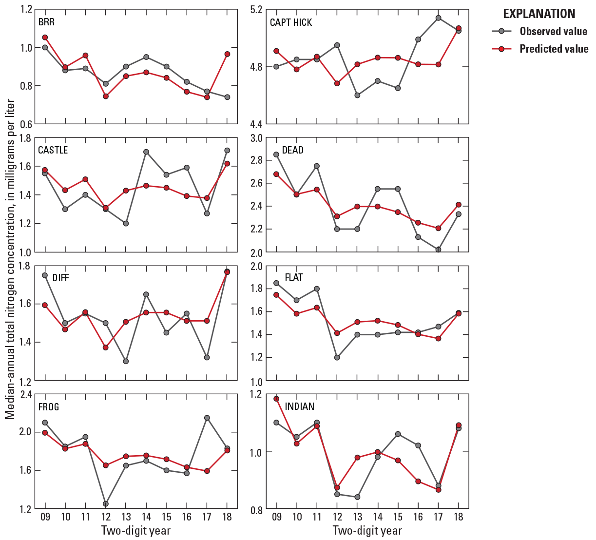

Graphs showing observed and predicted median-annual total nitrogen concentrations in 14 study watersheds in Fairfax County, Virginia, from 2009 through 2018. Study watershed station names are defined in table 1.
Supporting Materials for Total Phosphorus Models
Table 2.2.
Summary of the top 30 linear mixed-effect model forms ranked by Akaike information criterion to describe the spatiotemporal variability in median-annual total phosphorus concentrations from 2009 through 2018 in 14 study watersheds in Fairfax County, Virginia.[Predictors are described in tables 2, 3, and 6. Param, number of model parameters; AIC, Akaike information criterion; dAIC, difference in Akaike information criterion from model number 1; b3, the effect of a predictor on within-watershed variability; b1, the effect of a predictor on between-watershed intercept differences; b2, the effect of a predictor on between-watershed slope differences; −, a negative model coefficient; +, a positive model coefficient; X, an excluded model coefficient]
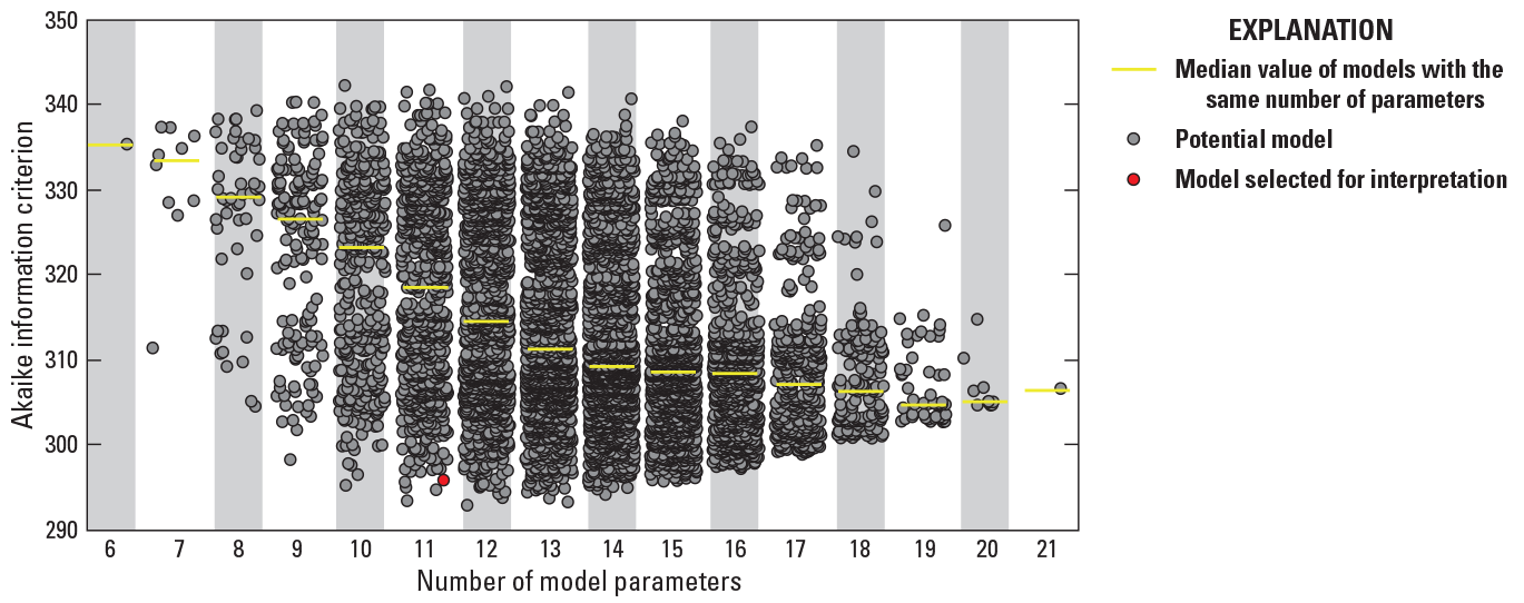
Graph showing the relation of Akaike information criterion to number of model parameters for all possible total phosphorus linear mixed-effect model combinations.

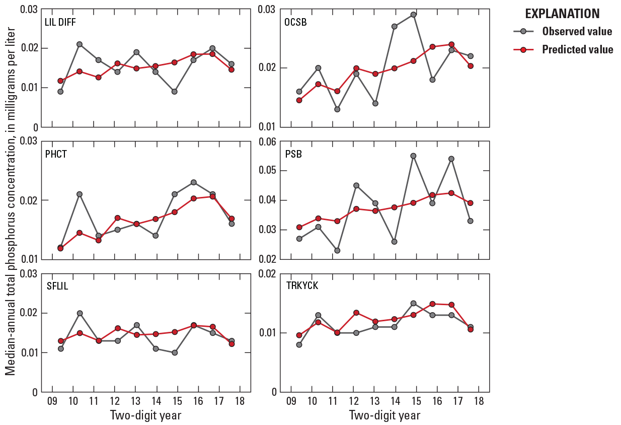
Graphs showing observed and predicted median-annual total phosphorus concentrations in 14 study watersheds in Fairfax County, Virginia, from 2009 through 2018. Study watershed station names are defined in table 1.
Table 2.3.
Results of a total phosphorus linear mixed-effect model where Flatlick Branch above Frog Branch at Chantilly, Virginia (FLAT), is excluded, including 95-percent confidence intervals and fixed-effect estimates, random-effect variances, and the model’s Akaike information criterion.[Linear mixed-effect models are described in equations 4–6. Predictors are described in tables 2 and 3. b3, the effect of a predictor on within-watershed variability; b1, the effect of a predictor on between-watershed intercept differences; b2, the effect of a predictor on between-watershed slope differences; R2, coefficient of determination; AIC, Akaike information criterion]
Table 2.4.
Results of a total phosphorus linear mixed-effect model with credited management-practice total phosphorus reductions when Flatlick Branch above Frog Branch at Chantilly, Virginia (FLAT), is excluded, including fixed-effect estimates and 95-percent confidence intervals, random-effect variances, and the model’s Akaike information criterion.[Linear mixed-effect models are described in equations 4–6. Predictors are described in tables 2, 3, and 5. b3, the effect of a predictor on within-watershed variability; b1, the effect of a predictor on between-watershed intercept differences; b2, the effect of a predictor on between-watershed slope differences; R2, coefficient of determination; AIC, Akaike information criterion]
Supporting Materials for Suspended-Sediment Models
Table 2.5.
Summary of the top 30 linear mixed-effect model forms, ranked by Akaike information criterion, to describe the spatiotemporal variability in median-annual suspended-sediment concentrations from 2009 through 2018 in 14 study watersheds.[Predictors are described in tables 2 and 3. Param, number of model parameters; AIC, Akaike information criterion; dAIC, difference in Akaike information criterion from model number 1; b3, the effect of a predictor on within-watershed variability; b1, the effect of a predictor on between-watershed intercept differences; b2, the effect of a predictor on between-watershed slope differences; +, a positive model coefficient; −, a negative model coefficient; X, an excluded model coefficient]
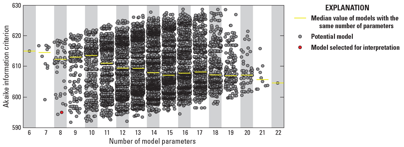
Graph showing the relation of Akaike information criterion to number of model parameters for all possible suspended-sediment linear mixed-effect model combinations.
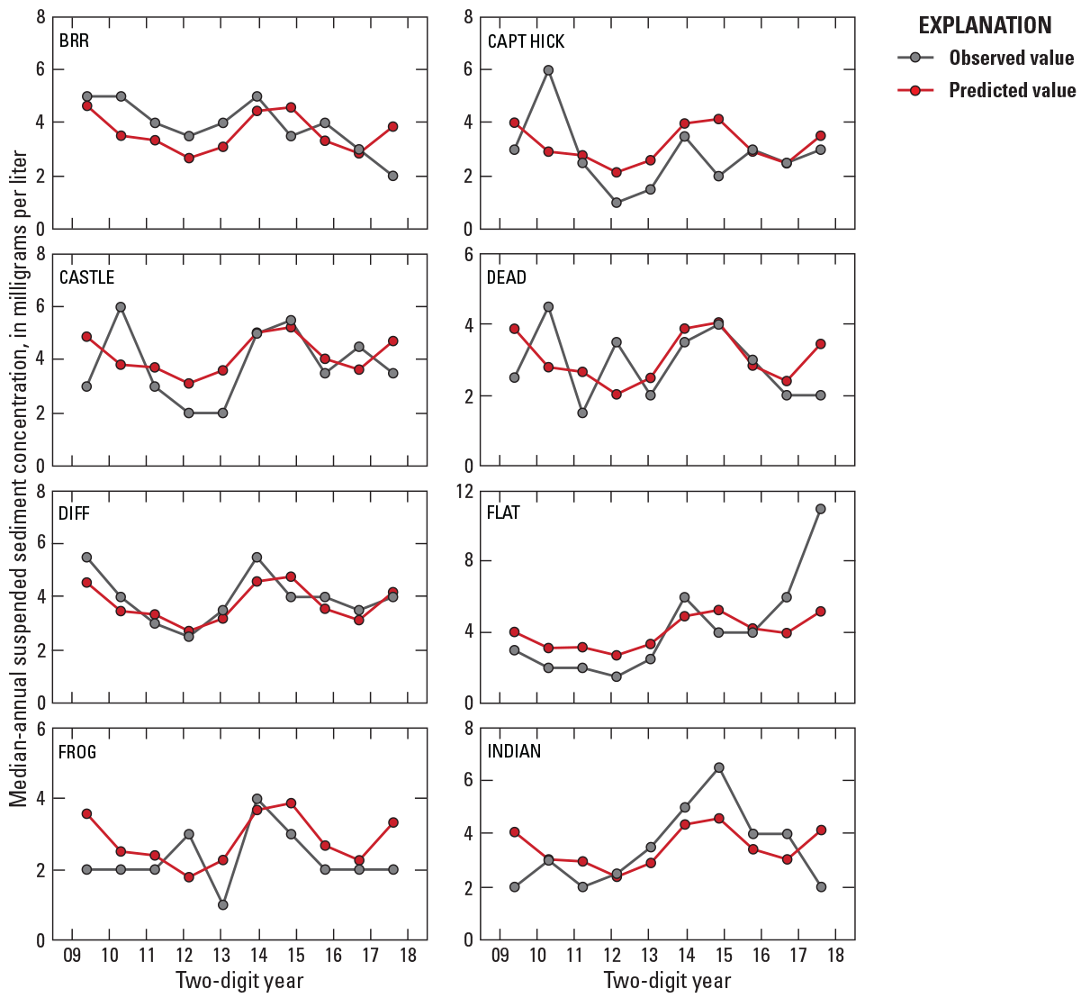
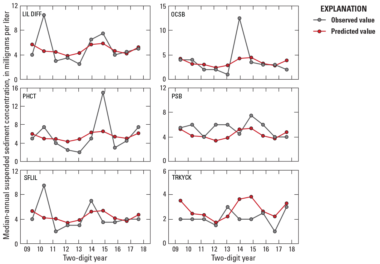
Graphs showing observed and predicted median-annual suspended-sediment concentrations in 14 study watersheds in Fairfax County, Virginia, from 2009 through 2018. Study watershed station names are defined in table 1.
Table 2.6.
Results of a suspended-sediment linear mixed-effect model where Flatlick Branch above Frog Branch at Chantilly, Virginia (FLAT), is excluded, including fixed-effect estimates and 95-percent confidence intervals, random-effect variances, and the model’s Akaike information criterion.[Linear mixed-effect models are described in equations 4–6. Predictors are described in tables 2 and 3. b3, the effect of a predictor on within-watershed variability; b1, the effect of a predictor on between-watershed intercept differences; R2, coefficient of determination; AIC, Akaike information criterion]
Table 2.7.
Results of a suspended-sediment linear mixed-effect model with credited management-practice total suspended solids reductions where Flatlick Branch above Frog Branch at Chantilly, Virginia (FLAT), is excluded, including fixed-effect estimates and 95-percent confidence intervals, random-effect variances, and the model’s Akaike information criterion.[Linear mixed-effect models are described in equations 4-6. Predictors are described in tables 2, 3, and 5. b3, the effect of a predictor on within-watershed variability; b1, the effect of a predictor on between-watershed intercept differences; R2, coefficient of determination; AIC, Akaike information criterion]
Supporting Materials for Specific Conductance Models
Table 2.8.
Summary of the top 30 linear mixed-effect model forms, ranked by Akaike information criterion, to describe the spatiotemporal variability in median-annual specific conductance from 2009 through 2018 in 14 study watersheds in Fairfax County, Virginia.[Predictors are described in tables 2 and 3. Param, number of model parameters; AIC, Akaike information criterion; dAIC, difference in Akaike information criterion from model number 1; b3, the effect of a predictor on within-watershed variability; b1, the effect of a predictor on between-watershed intercept differences; b2, the effect of a predictor on between-watershed slope differences; +, a positive model coefficient; −, a negative model coefficient; X, an excluded model coefficient]
Table 2.9.
Results of a specific conductance linear mixed-effect model without the fixed effect of year, including fixed-effect estimates and 95-percent confidence intervals, random-effect variances, and the model’s Akaike information criterion.[Linear mixed-effect models are described in equations 4–6. Predictors are described in tables 2 and 3. b3, the effect of a predictor on within-watershed variability; b1, the effect of a predictor on between-watershed intercept differences; R2, coefficient of determination; AIC, Akaike information criterion]
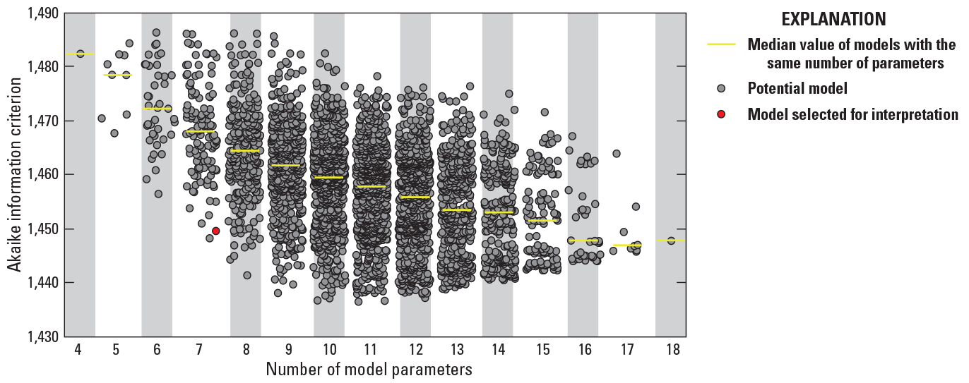
Graph showing the relation of Akaike information criterion to number of model parameters for all possible specific conductance linear mixed-effect model combinations.

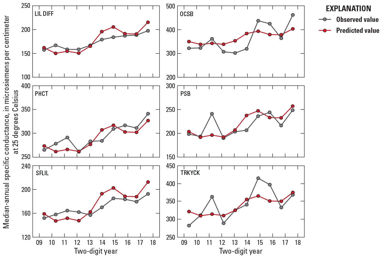
Graphs showing observed and predicted median-annual specific conductance in 14 study watersheds in Fairfax County, Virginia, from 2009 through 2018. Study watershed station names are defined in table 1.
Supporting Materials for Index of Biotic Integrity Models
Table 2.10.
Summary of the top 30 linear mixed-effect model forms, ranked by Akaike information criterion, to describe the spatiotemporal variability in median-annual index of biotic integrity scores from 2008 through 2017 in 14 study watersheds.[Predictors are described in tables 2 and 3. Param, number of model parameters; AIC, Akaike information criterion; dAIC, difference in Akaike information criterion from model number 1; b1, the effect of a predictor on between-watershed intercept differences; b2, the effect of a predictor on between-watershed slope differences; b3, the effect of a predictor on within-watershed variability; +, a positive model coefficient; −, a negative model coefficient; X, an excluded model coefficient]

Graph showing the relation of Akaike information criterion to number of model parameters for all possible index of biotic integrity score linear mixed-effect model combinations.


Graphs showing observed and predicted index of biotic integrity scores in 14 study watersheds in Fairfax County, Virginia, from 2008 through 2017. Study watershed station names are defined in table 1.
Conversion Factors
U.S. customary units to International System of Units
Temperature in degrees Celsius (°C) may be converted to degrees Fahrenheit (°F) as follows:
°F = (1.8 × °C) + 32.
Temperature in degrees Fahrenheit (°F) may be converted to degrees Celsius (°C) as follows:
°C = (°F – 32) / 1.8.
Datum
Horizontal coordinate information is referenced to the North American Datum of 1983 (NAD 83).
Altitude, as used in this report, refers to distance above the vertical datum.
Supplemental Information
Specific conductance is given in microsiemens per centimeter at 25 degrees Celsius (µS/cm at 25 °C).
Concentrations of chemical constituents in water are given in milligrams per liter (mg/L).
For additional information contact:
Director, Virginia and West Virginia Water Science Center
U.S. Geological Survey
1730 East Parham Road
Richmond, VA 23228
Publishing support provided by the Reston and West Trenton Publishing Service Centers
Disclaimers
Any use of trade, firm, or product names is for descriptive purposes only and does not imply endorsement by the U.S. Government.
Although this information product, for the most part, is in the public domain, it also may contain copyrighted materials as noted in the text. Permission to reproduce copyrighted items must be secured from the copyright owner.
Suggested Citation
Webber, J.S., Chanat, J.G., Porter, A.J., and Jastram, J.D., 2023, Evaluating drivers of hydrology, water quality, and benthic macroinvertebrates in streams of Fairfax County, Virginia, 2007–18: U.S. Geological Survey Scientific Investigations Report 2023–5027, 198 p., https://doi.org/10.3133/sir20235027.
ISSN: 2328-0328 (online)
ISSN: 2328-031X (print)
Study Area
| Publication type | Report |
|---|---|
| Publication Subtype | USGS Numbered Series |
| Title | Evaluating drivers of hydrology, water quality, and benthic macroinvertebrates in streams of Fairfax County, Virginia, 2007–18 |
| Series title | Scientific Investigations Report |
| Series number | 2023-5027 |
| ISBN | 978-1-4113-4516-4 |
| DOI | 10.3133/sir20235027 |
| Publication Date | May 18, 2023 |
| Year Published | 2023 |
| Language | English |
| Publisher | U.S. Geological Survey |
| Publisher location | Reston, VA |
| Contributing office(s) | Virginia and West Virginia Water Science Center |
| Description | Report: xv, 198 p.; Data Release |
| Country | United States |
| State | Virginia |
| County | Fairfax County |
| Online Only (Y/N) | N |
| Additional Online Files (Y/N) | N |