

Hydrology, Water-Quality, and Watershed Characteristics in 15 Watersheds in Gwinnett County, Georgia, Water Years 2002–20
Links
- Document: Report (4.76 MB pdf) , HTML , XML
- Dataset: USGS water data for the Nation—U.S. Geological Survey National Water Information System database
- Data Release: U.S. Geological Survey data release—Watershed characteristics and streamwater constituent load data, models, and estimates for 15 watersheds in Gwinnett County, Georgia, 2000-2021
- NGMDB Index Page: National Geologic Map Database Index Page (html)
- Download citation as: RIS | Dublin Core
Acknowledgments
Funding for this work was provided by the Gwinnett County Department of Water Resources and by U.S. Geological Survey (USGS) Cooperative Matching Funds. The authors wish to thank personnel of Gwinnett County Department of Water Resources for their long-term commitment to improved data and understanding of water quality in the watersheds in their county. We thank Gwinnett Country Departments of Water Resources, Public Utilities, and Planning and Development for providing unpublished data that were used in this report. At the time of publication, data were not available from Gwinnett County Departments of Water Resources, Public Utilities, and Planning and Development owing to proprietary interest or sensitivity concerns. This report is possible because of the field data-collection efforts and analytical expertise of the USGS South Atlantic Water Science Center Data Section personnel. USGS technical reviewers Mandy Stone and Lee Bodkin, specialist reviewer Anthony Gotvald, and supervisory reviewer Daniel Calhoun provided thoughtful reviews that much improved this report.
Abstract
The U.S. Geological Survey, in cooperation with Gwinnett County Department of Water Resources, established the Long-Term Trend Monitoring program in 1996 to monitor and analyze the hydrologic and water-quality conditions in Gwinnett County, Georgia. Gwinnett County is a suburban to urban area northeast of the city of Atlanta in north-central Georgia. The monitoring program currently consists of 15 watersheds ranging in size from 1.3 to about 161 square miles. This report synthesizes watershed characteristics and hydrologic and water-quality monitoring data collected for water years (WYs) 2002–20.
The 15 study watersheds were characterized for land-surface elevations, average land-surface slopes, septic densities, sanitary sewer densities, and detention pond areas. Temporal patterns in watershed characteristics were determined for land cover (2001–19), percent imperviousness (2000–20), population density (2000–20), and building density (1950–2022). In 2001, most of the watersheds had at least 45 percent of their land cover composed of developed land cover groups, and by 2019, at least 59 percent of each watershed was developed. Land cover changes occurred most rapidly between 2004 and 2008 at most watersheds. Percent imperviousness in the study watersheds varied substantially and ranged from 14.75 to 55.13 percent in 2019.
Precipitation and runoff were quantified at all study watersheds for WYs 2002–20, and the hydrologic cycle was evaluated both annually and seasonally. Several 1-year or longer droughts occurred during this period. Study area precipitation averaged 51.5 inches per year and runoff averaged 22.5 inches per year. Variations in annual runoff were largely determined by annual precipitation but were also dependent upon watershed storage. Runoff varied seasonally because of high evapotranspiration rates in the summer and changes in base flow associated with seasonal changes in watershed storage. Fifty-one percent of runoff in the study area occurred as base flow. Watersheds with higher imperviousness had higher stormflows because of increased surface runoff and lower base flows because of reduced infiltration that recharges watershed storage.
Turbidity, water temperature, and specific conductance were continuously measured at each study site. These constituents varied seasonally, diurnally, and with streamflow. A minimum of two base-flow and six stormflow samples were collected per year at each watershed and were analyzed for 21 water-quality constituents (water temperature, laboratory specific conductance, pH, and turbidity, biochemical and chemical oxygen demand, suspended sediments, nutrients, base cations, trace metals, and total dissolved solids). Concentrations of most particulate constituents were approximately one-half or more orders of magnitude higher in stormflow samples than in base-flow samples. Total copper and zinc stormflow concentrations exceeded the national recommended aquatic life criteria for acute conditions to varying degrees.
Annual loads and yields were estimated for 12 constituents (which include suspended sediments, nutrients, base cations, trace metals, and total dissolved solids) using a surrogate regression model approach and the Beale load estimator. Loads were typically higher for years with higher runoff. The proportional range of annual loads for total suspended solids, suspended-sediment concentrations, total phosphorus, and total lead, however, were 3.2 to 4.8 times larger than for annual runoff. Higher-than-expected annual sediment loads occurred in the years that also had some of the highest peak flows during the period, indicating that large storms are responsible for much of the sediment transport. Large development projects in proximity to streams also were related to years with high sediment loads. Yields from the Crooked Creek and North Fork Peachtree Creek watersheds were typically among the highest for 8 of the 12 constituents. These watersheds had the two highest amounts of developed medium plus high intensity land cover and the two highest percentages of imperviousness. Moderate to strong correlations were identified between seven of the constituent yields and the percentage of developed medium and high intensity land cover groups. Temporal trends in concentrations and loads were identified for 140 of the 300 possible watershed-time period-constituent combinations. There were substantially more negative than positive temporal trends identified during WYs 2003–10, whereas the number of negative and positive temporal trends were similar during WYs 2010–20. Measures of sediment transport had the most negative temporal trends. A few watersheds had consistent trends across several constituents; however, these trends did not appear to be associated with temporal changes in development or imperviousness.
This study provides a thorough assessment of watershed characteristics, hydrology, and water-quality conditions and trends for the 15 study watersheds and can be used to identify possible factors that affect runoff and water quality and determine changes in water-quality conditions. Watershed managers can use these data and analyses to inform management decisions regarding the designated uses of streams, minimization of flooding, protection of aquatic habitats, and optimization of the effectiveness of best management practices.
Introduction
Stream-water quantity and quality serve as an integrated measure of the effects of all inputs and processes within a watershed (Semkin and others, 1994; Likens, 2001). Stream runoff is controlled by weather and climate; drainage characteristics such as density, network configuration, channel morphology, and land-surface slopes (Liu and others, 2006); subsurface characteristics of soils, regolith, and bedrock such as their geometries and hydraulic conductivities; vegetative cover (Leopold, 1968); and land use. Outflowing stream-water quality reflects the cumulative effects of the complex interactions of multiple inputs, processes, and activities within the watershed, both spatially and temporally (MacDonald, 2000; Landers and others, 2007). These sources, processes, and activities include atmospheric inputs of precipitation and dry deposition (Smith and Alexander, 1983), inputs of point and nonpoint source contaminants, changes in land use, uptake of nutrients in plants (Reid and Hayes, 2003), biogeochemical processes within the unsaturated and saturated zones of the soils and bedrock, and biochemical processes within the stream itself. Reliable temporal measures of estimated constituent loads may help determine whether water quality is changing. These quantified changes can be used to assess the effects of climate, land use, point and nonpoint source contaminants, and the effectiveness of watershed-based mitigation strategies, such as best management practices (BMPs), on water quality.
Urbanization, particularly the associated increases in impervious area, has been shown to have a substantial effect on rainfall-runoff relations (Leopold, 1968; Hollis, 1975; Ogden and others, 2011) and stream-water quality (Schueler, 1994; Schueler and others, 2009). Impervious areas include buildings and transportation infrastructure such as roads, parking lots, and sidewalks. Some of the more important effects of increased impervious area on hydrology (Jacobson, 2011) include increased storm runoff and flood flows (Leopold, 1968); increased storm flashiness, with higher peak stormflow responses having a shorter duration (Seaburn, 1969; Graf, 1977) and a decreased lag time between precipitation and peak streamflow (Espey and others, 1966); increased recurrence interval of floods, particularly for smaller floods (Hollis, 1975; Konrad, 2003); and decreased rainfall infiltration and groundwater recharge rates that result in lower stream base flow (Simmons and Reynolds, 1982; Rose and Peters, 2001). Many studies have also shown that urbanization’s effects on streamflow characteristics decrease the biological richness of streams (Paul and Meyer, 2001; Gregory and Calhoun, 2007; DeGasperi and others, 2009; Richards and others, 2010) and that native stream biota are best adapted to natural, unimpaired streamflows (Poff and others, 1997; Richter and others, 1996, 1998; Carlisle and others, 2019). More frequent and higher magnitude flooding can also increase erosion and transport of land-surface and stream sediments (Trimble, 1997) and associated contaminants, as well as alter stream-channel stability. Stormwater BMPs, also known as stormwater management controls, are used to reduce and mitigate the effects of urban development and land use on stream hydrology and water quality. The effectiveness of BMPs has been assessed in many studies, and BMPs have been shown to decrease flood peak streamflows (for example, Soong and others, 2009; Gebert and others, 2012; Hopkins and others, 2020), decrease sediment and nutrient loads (for example, Park and others, 1994; Inamdar and others, 2001), and increase infiltration (for example, Ku and others, 1992).
The effects of urbanization on stream runoff and water quality have been extensively studied in the Atlanta, Georgia, metropolitan area and throughout the Piedmont physiographic province in the southeastern United States. A study of streamflow trends in eight watersheds in the Atlanta metropolitan area over a 20-year period indicated that streamflow flashiness and the frequencies of high-flow days increased in watersheds with the largest increases in development, and watersheds that were already substantially developed had decreasing streamflow (Diem and others, 2018). In a study of flash flooding in nine urban watersheds in the Atlanta area, data indicated that flood response was dependent on a combination of basin size, drainage network characteristics, the spatial distribution of land use, and water storage in soils and stormwater detention ponds (Wright and others, 2012). An analysis of the effects of urban development patterns on streamflow in the so-called Charlanta Megaregion (defined as the area from Charlotte, North Carolina, to Atlanta, Ga.) indicated that higher occurrences of both high and low flows were associated with watersheds having higher percentages of impervious areas within their riparian buffers and those having greater contiguously developed open space land cover (Debbage and Shepherd, 2018). This study also indicated that the frequency of high flows in watersheds increased with the amount of impervious areas clustered in source areas. Rose and Peters (2001) found that groundwater levels declined in two wells in Atlanta during 1958–1996 because of decreased groundwater recharge in urban watersheds. In an assessment of the effects of direct inflow and infiltration (seepage) into sanitary sewers in four watersheds near Atlanta, Pangle and others (2022) quantified infiltration into sewer conveyances paralleling streams ranging from 0 to 20 percent of the flow in the adjacent stream and concluded that streamflows could be enhanced substantially if infiltration was abated.
A long-term water-quality monitoring network’s data for the city of Atlanta indicated that elevated concentrations of chloride and trace metals likely resulted from chlorinated combined sewer overflows, deicing salts, and washoff from impervious surfaces (Peters, 2009). Stream-water loads estimated for this network indicated that at least 90 percent of suspended-sediment loads and loads of sediment-related constituents occurred during stormflow conditions (Horowitz, 2009). A previous study of the watersheds included in this current report similarly found that most of the annual suspended-sediment load was transported by the few largest storms of the year (Joiner and others, 2014). Horowitz (2009) indicated that for small, flashy Atlanta watersheds, loads calculated using a daily time step substantially underestimated loads and that greater accuracy required time steps as short as 2–3 hours. A study to determine the physical, chemical, and biological responses of streams to urbanization from 30 wadeable streams near Atlanta found that specific conductance (SC), chloride, sulfate, and pesticides increased with increasing urban land use and that algal, invertebrate, and fish communities exhibited statistically significant changes with urbanization (Gregory and Calhoun, 2007). A study of the effects of urbanization on macroinvertebrates in Piedmont streams in Georgia indicated that urbanization negatively affected macroinvertebrate biomass and community structure (Sterling and others, 2016). The U.S. Geological Survey (USGS) Southeastern Stream Quality Assessment of 76 wadeable streams in the Piedmont ecoregion of the southeastern United States documented that urban streams were nitrogen-nutrient enriched, but total phosphorus concentrations in Atlanta streams were lower than concentrations in streams in reference watersheds (Journey and others, 2018). A study of BMP implementation effects on detention pond sediment capture that included watersheds from this report showed that BMPs reduced stormflow peaks and runoff; however, the improvements in water quality were less apparent (Aulenbach and others, 2017b).
A similar monitoring program to the one in this study was initiated in 2012 in adjacent DeKalb County, Ga., and consists of 15 study watersheds with similar range of drainage areas. Results of analyses from the two county programs were compared for an overlapping period between October 2013 and September 2015 (Aulenbach and others; 2022). The Gwinnett County watersheds had higher amounts of base-flow runoff and lower runoff ratios than the DeKalb County watersheds for watersheds with the same percentages of imperviousness, indicating that BMP implementation to mitigate the effects of imperviousness might be more effective in the more recently developed Gwinnett County watersheds. Watershed yields were also compared between the adjacent county programs and, although the two studies had overlapping constituent concentration ranges, 6 of the 10 constituents compared (total suspended solids, total and dissolved phosphorus, total organic carbon, total lead, and total zinc) had significantly higher average watershed yields in the DeKalb County study.
Intensive, long-term streamflow and water-quality monitoring combined with watershed characterization are essential for quantifying land use, point- and nonpoint-source discharges, and management practice effects on surface water (water quantity, flow characteristics, and water quality). In 1996, the USGS in cooperation with Gwinnett County Department of Water Resources, established a comprehensive long-term watershed monitoring program in which consistently collected, high-quality water-quantity and water-quality data were collected to determine the status and trends in stream runoff and water quality. In addition, these data were related to watershed characteristics to better understand factors that affect runoff and water quality. Watershed managers can use these data and analyses to make informed management decisions to maintain the designated uses of streams, minimize flooding, protect aquatic habitats, and optimize the effectiveness of BMPs.
Purpose and Scope
The purpose of this report is to summarize and present analyses of watershed characteristics and hydrologic and water-quality data collected as part of the USGS-Gwinnett County Long-Term Trend Monitoring (LTTM) program for 15 watersheds for water years (WYs) 2002–20. This report is an update to and continuation of the reports by Landers and others (2007) in which data for the original six watersheds were presented and analyzed during WYs 1997–2003; Joiner and others (2014) in which data for 12 watersheds were presented and analyzed during WYs 2004–09; Landers (2013) in which data are presented only for total suspended solids (TSS) during 1996–2009, including two additional watersheds that are not part of the LTTM program; and Aulenbach and others (2017a) in which data for 13 watersheds were presented and analyzed during WYs 2001–15. The specific goals of this report are to
-
• quantify watershed characteristics of the 15 study watersheds, including topography, land-surface slopes, land cover (2001–19), impervious area (2000–20), population density (2000–20), building density (1950–2020), and water infrastructure;
-
• quantify hydrologic variables (precipitation, evapotranspiration, and runoff) during WYs 2002–20 and relate them to climatic conditions and watershed characteristics;
-
• summarize watershed continuously measured physicochemical constituents (sonde turbidity, water temperature, and sonde specific conductance [sonde SC]) for select watersheds, time periods, and hydrologic conditions;
-
• summarize watershed discrete base-flow and stormflow stream sample water-quality data (SC, biochemical oxygen demand [BOD], chemical oxygen demand [COD], pH, turbidity, TSS, suspended-sediment concentration [SSC], total nitrogen [TN], total nitrate plus nitrite [NO3+NO2], total ammonia plus organic nitrogen [TKN], dissolved ammonia [NH3], total phosphorus [TP], dissolved phosphorus [DP], total organic carbon [TOC], total calcium [Ca], total magnesium [Mg], total copper [TCu], total lead [TPb], total zinc [TZn], total dissolved solids [TDS]) for WYs 2003–20 and relate these data to watershed characteristics; and
-
• compute annual loads and yields for WYs 2003–20 for 12 constituents (TSS, SSC, TN, NO3+NO2, TP, DP, TOC, Ca, Mg, TPb, TZn, and TDS) for 13 of the 15 study watersheds, relate loads and yields to hydrologic conditions and watershed characteristics, and determine trends in concentrations and loads and relate these to trends in watershed characteristics.
Description of Study Area
Gwinnett County, which encompasses about 437 square miles (mi2), is a suburban to urban area northeast of the city of Atlanta located in north-central Georgia (fig. 1). The county is in the Piedmont physiographic province, which is a hilly plateau region located between the Blue Ridge and Coastal Plain Provinces. The geology of the county is a mixture of complex and varied metamorphic rocks, predominantly granitic gneisses along with substantial extents of biotitic gneisses, mica schists, amphibolites, and metagraywackes (USGS, 2022a). Watersheds in Gwinnett County are composed predominantly of first- to fourth-order streams that drain into the Chattahoochee, Ocmulgee, and Oconee Rivers. The lower reach of the Yellow River, including the sites in this study near Snellville and near Lithonia, is a fifth-order stream (USGS, 2022b). The Chattahoochee River Basin is part of the Apalachicola-Chattahoochee-Flint River Basin, and the Ocmulgee and Oconee River Basins are part of the larger Ocmulgee-Oconee-Altamaha River Basin. The Eastern Continental Divide runs approximately northeast-southwest across the northwestern side of the county and separates drainages that flow into the Gulf of Mexico (Chattahoochee River) from those that flow into the Atlantic Ocean (Ocmulgee and Oconee Rivers; fig. 1).
Study Design and Methods
Fifteen watersheds were monitored as part of the USGS-Gwinnett County LTTM program (fig. 1). Physiographic, climatic, and hydrologic settings, along with topographic and land-use attributes, were used to characterize the watersheds. Stage (water level), streamflow, turbidity, water temperature, and specific conductance were measured continuously (15-minute intervals) at the watershed outlets (stream sampling sites). A typical multiparameter stream monitoring site is shown in figure 2. Precipitation was monitored at 35 locations throughout the study area, including the 15 stream sampling sites. Water-quality samples were collected seasonally during base flow and stormflow events and were measured or analyzed for 21 water-quality constituents. Watershed annual stream-water loads and yields and their confidence intervals were estimated for 12 water-quality constituents using a regression-model approach and the Beale ratio estimator. All stage, streamflow, precipitation, and continuous and sample water-quality data used in this study are available on the USGS National Water Information System (NWIS) database at https://waterdata.usgs.gov and can be obtained by using the USGS site numbers listed in table 1 (USGS, 2021d).
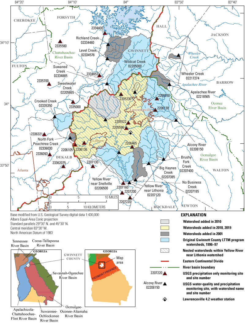
Location of the study area and the 15 monitored watersheds and U.S. Geological Survey (USGS) streamflow, water-quality, and precipitation monitoring sites, Gwinnett County, Georgia. Hydrography from National Hydrography Dataset (USGS, 2021a). LTTM, Long Term Trend Monitoring.
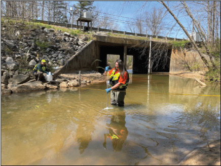
Sarah Chamblee (center) and Jonathan Jason (left) collecting a base-flow sample using a U.S. Geological Survey (USGS) DH-81 manual sampler and a multiple vertical integrating technique at the Gwinnett County Long-Term Trend Monitoring program multiparameter stream monitoring site, Richland Creek at Suwanee Dam Road, near Buford, Georgia, March 29, 2022 (USGS site number 02334480). Photograph by Andrew E. Knaak, USGS.
Table 1.
Fifteen U.S. Geological Survey (USGS) water-quantity and water-quality monitoring sites included in the USGS-Gwinnett County long-term monitoring program.[Drainage areas for each site are from StreamStats (https://streamstats.usgs.gov; USGS, 2021c); Ga., Georgia; nr, near]
| USGS site number (fig. 1; USGS, 2021d) |
Site name | Site/watershed name used in this report | Date when streamflow monitoring was established | Date when water-quality sampling was established | Drainage area (square miles) |
|---|---|---|---|---|---|
| 02205000 | Wildcat Creek near Lawrenceville, Ga. | Wildcat Creek | October 2019 | April 2019 | 11.29 |
| 02205865 | Sweetwater Creek at Club Drive near Lilburn, Ga. | Sweetwater Creek | March 2010 | March 2010 | 120.98 |
| 02206500 | Yellow River near Snellville, Ga. | Yellow River near Snellville | January 2018 | March 2019 | 1136.06 |
| 02207120 | Yellow River at Ga 124, near Lithonia, Ga. | Yellow River near Lithonia | September 2001 | April 1996 | 161.41 |
| 02207185 | No Business Creek at Lee Road, below Snellville, Ga. | No Business Creek | March 2001 | March 2001 | 10.06 |
| 02207385 | Big Haynes Creek at Lenora Road, near Snellville, Ga. | Big Haynes Creek | March 2001 | June 1996 | 17.26 |
| 02207400 | Brushy Fork Creek at Beaver Road, nr Loganville, Ga. | Brushy Fork Creek | March 2001 | June 1996 | 8.18 |
| 02208150 | Alcovy River at New Hope Road, near Grayson, Ga. | Alcovy River | April 2001 | June 1997 | 30.80 |
| 02217274 | Wheeler Creek at Bill Cheek Road, near Auburn, Ga. | Wheeler Creek | July 2001 | July 2001 | 1.31 |
| 02218565 | Apalachee River at Fence Road, near Dacula, Ga. | Apalachee River | August 2001 | July 2001 | 5.65 |
| 02334480 | Richland Creek at Suwanee Dam Road, near Buford, Ga. | Richland Creek | June 2001 | July 2001 | 9.37 |
| 02334578 | Level Creek at Suwanee Dam Road, near Suwanee, Ga. | Level Creek | June 2001 | July 2001 | 5.06 |
| 02334885 | Suwanee Creek at Suwanee, Ga. | Suwanee Creek | October 1984 | September 1996 | 47.09 |
| 02335350 | Crooked Creek near Norcross, Ga. | Crooked Creek | April 2001 | March 1996 | 8.87 |
| 02336030 | North Fork Peachtree Creek at Graves Rd, near Doraville, Ga. | North Fork Peachtree Creek | July 2001 | June 2001 | 1.53 |
Watershed Monitoring Site Selection
The 15 monitored watersheds in the Gwinnett County LTTM program are listed in table 1. Monitoring was established at six sites in 1996 and 1997 and at an additional six sites in 2001. Three additional sites were added to the monitoring program between 2010 and 2019: Sweetwater Creek (2010); Yellow River near Snellville (2018); and Wildcat Creek (2019). Eight of the watersheds are in the Ocmulgee River Basin, two are in the Oconee River Basin, and five are in the Chattahoochee River Basin (fig. 1). Wildcat Creek, Sweetwater Creek, and Yellow River near Snellville watersheds are subbasins “nested” within the drainage area of the Yellow River near Lithonia watershed. Watersheds were selected for this monitoring program to encompass diverse basin characteristics and land use for evaluating streamflow quantity and quality characteristics, while also ensuring sufficient spatial coverage of the county area. The specific monitoring site locations were selected on the basis of the suitability for hydrologic instrumentation and personnel safety.
The watershed drainage areas were delineated and quantified using StreamStats (https://streamstats.usgs.gov; USGS, 2021c; table 1). The watershed drainage areas span two orders of magnitude: the smallest is 1.29 mi2 (Wildcat Creek watershed) and the largest is about 161 mi2 (Yellow River near Lithonia watershed). The study watersheds cover an area of about 307 mi2, of which 300 mi2 lie within Gwinnett County, composing 68 percent of the county’s extent. Small portions of the Yellow River near Snellville, Yellow River near Lithonia, and Crooked Creek watersheds are located in DeKalb County and a portion of the Suwanee Creek watershed lies within Hall County.
Watershed Characteristics
Land-surface elevations within Gwinnett County were determined from a 5-foot (ft) grid resolution lidar-derived digital elevation model (DEM) representing the year 2015 (Gwinnett County Department of Public Utilities, unpub. data, 2016). The Gwinnett County DEM included portions of adjacent DeKalb and Hall Counties and drainage areas within the Crooked Creek and Suwanee Creek watersheds but did not include all drainage areas within the two Yellow River watersheds. Land-surface elevations for the remainder of the Yellow River watersheds were determined from a DeKalb County DEM downloaded from the USGS 3D Elevation Program (3DEP; USGS, 2017) at a 1/3-arc-second resolution (approximately a 34-ft or 10-meter [m] grid), which was mosaiced with the Gwinnett County DEM. Land-surface slopes were derived from the elevations by using geographic information system (GIS) software functions. GIS analyses in this report were done using the ArcGIS Pro, version 2.9.2 software (Esri, 2021), except for delineating the watershed drainage areas within StreamStats.
Land cover data were obtained from the National Land Cover Database (NLCD) 2019 dataset (USGS, 2021b; Homer and others, 2015) and included eight datasets from 2001, 2004, 2006, 2008, 2011, 2013, 2016, and 2019 analyzed using a consistent approach to assess land cover changes. The NLCD dataset is derived from Landsat imagery and has a grid size of 30 m. The datasets contained 14 land cover classes that were combined into 8 land cover groups to simplify the presentation of watershed land cover characteristics (table 2).
Table 2.
Summary of the land cover classification system in this study.[National Land Cover Database (NLCD) land cover classes, values, and descriptions are from the from the National Land Cover Database 2019 (U.S. Geological Survey [USGS], 2021b). <, less than; >, greater than]
Impervious area was determined from detailed countywide impervious area datasets developed to support the Gwinnett County stormwater utility (Gwinnett County Department of Public Utilities, unpub. data, 2022). The datasets have a 1-m2 grid size created by digitizing polygons of impervious surfaces from 1:1,200-scale aerial photography. The dataset was first created in 2000 and was updated in 2005, 2006, and 2008–20 annually using new aerial photography. Impervious areas were assigned to one of five land cover categories: transportation, buildings, recreation, structures, and utilities (table 3). Impervious areas by land cover category were determined for the 15 study watersheds for each year available. Impervious areas within a 200-ft stream buffer from the high resolution 1:24,000-scale National Hydrography Dataset flowlines (USGS, 2021a) were calculated for 2019 for all watersheds to evaluate whether this would be a more useful variable for explaining variations in watershed hydrologic metrics and water quality than watershed imperviousness. The imperviousness within the stream buffer is more likely connected to the stream and storm drainage network, which reflects the effective impervious area of a watershed (directly connected impervious area; Shuster and others, 2005). Effective impervious area is considered a better metric than overall watershed imperviousness in determining the influence of imperviousness on storm runoff but is difficult to delineate because of the complex routing of water, particularly in urban watersheds.
Table 3.
Land cover categories for impervious areas and example land covers.[Gwinnett County Department of Public Utilities, unpub. data, 2022]
Septic and sanitary sewer density within the study area was determined from wastewater infrastructure data obtained from Gwinnett County Department of Water Resources and represents infrastructure as of August 2021 (Gwinnett County Department of Water Resources, unpub. data, 2021). Septic density was calculated as the number of septic systems divided by the watershed drainage area. Sanitary sewer density was calculated as the total miles of sewer pipe divided by the watershed drainage area.
Detention pond locations and construction characteristics were determined from the Gwinnett County Department of Planning and Development database and represent detention ponds as of August 2021 (Gwinnett County Department of Planning and Development, unpub. data, 2021). The dataset represents detention ponds that Gwinnett County has jurisdiction for overseeing maintenance, areas within unincorporated Gwinnett County, and the City of Lilburn. This limited data analysis because watershed detention pond data within city limits were not available, and such areas are where detention ponds are expected to be used extensively.
The average building construction year for each watershed was calculated as the average of year built for all parcels in the watershed. Building construction dates and parcel boundaries were determined from the Gwinnett County Cadastral database (Gwinnett County Information Technology Services, 2021). Building construction dates were then matched to the parcels using their assigned property identification number. Building construction years were able to be determined for 99.6 percent of the parcels within the study watersheds.
The impervious area, septic, sanitary sewer, detention pond, and parcel data provided by Gwinnett County were determined only for areas within the county. Small portions of four study watersheds extend outside of the county boundary (Yellow River near Snellville, Yellow River near Lithonia, Suwanee Creek, and Crooked Creek watersheds). For these basins, imperviousness, septic and sewer densities, and average building construction years were extrapolated from the areas within Gwinnett County.
An analysis was conducted to compare watersheds delineated with StreamStats to drainage basins delineated with a higher resolution DEM and the stormwater pipe network. The stormwater pipe network within Gwinnett County as of August 2021 (Gwinnett County Department of Water Resources, unpub. data, 2021) and a 5-ft grid resolution lidar-derived DEM representing the year 2015 were obtained from Gwinnett County. The stormwater pipe coverage and DEM were used to delineate drainage basins for each site that included potential diversions through the stormwater network. Stormwater pipes outside of Gwinnett County were not included in the analysis. The Whitebox Tools (v1.4.0) FillBurn tool was used to burn the stormwater pipe network into the original DEM and the breach depressions least cost path tool (distance = 10 and fill = True) was used to breach obstructions and to fill any remaining unbreached depressions. An eight direction (d8) flow pointer and accumulation raster were used to delineate the stormwater drainage area for each site. The stormwater drainage area incorporates areas where stormwater pipes could divert water across drainage divides.
Population density within the study area was determined for 2000, 2010, and 2020 from the decadal U.S. Census and for 2012 and 2017 from the American Community Survey 5-year estimates of 2010–14 and 2015–19 block group data, respectively (U.S. Census Bureau, 2022). The temporal resolution of the 5-year population estimates is less accurate than that of the decadal census because data are compiled over a 5-year period. These 5-year estimates, however, are the most reliable interim population estimates for analyzing very small populations, such as in the smaller watersheds in this study, because data are collected for all areas and have the largest sample size of the interim 1-, 3-, and 5-year American Community Survey estimates. For this analysis, the representative date was set to the median of the 5-year period. Watershed population densities were calculated from census block group data, which is the smallest geographic unit for which the census provides data. Block group size varies with population density, and each group generally contains between 600 and 3,000 people, with an optimum size of 1,500 people. Population density within each watershed was determined by clipping the census block group data by the watershed boundaries and area-weighting the block group population density data within each watershed. This methodology assumes that population density is uniform throughout the census block. Even though population density is not always uniform, this approach is expected to reasonably estimate the population density of the watersheds, particularly in areas where the block group sizes are small or when blocks are predominantly within a single watershed. Population estimates may be less precise for smaller study watersheds, and inconsistent population patterns can result when census blocks groups are redefined.
Surface-Water Monitoring
Streamflow was continuously measured at the outlets of the 15 monitored watersheds. The periods of record vary by site (table 1). Standard USGS protocols were used for measuring streamflow, which include measuring stream stage (water-surface elevation), making discharge measurements, developing and maintaining a stage-discharge relation (rating curve), computing streamflow, and estimating periods of missing streamflow (Sauer and Turnipseed, 2010; Turnipseed and Sauer, 2010). Stage was recorded every 15 minutes to the nearest 0.01 ft and discharge was calculated using a site-specific stage-discharge relation.
Daily average streamflow from each watershed was separated into base-flow and stormflow (quick flow) components by hydrograph separation. Hydrograph separations were done by using the Web-based Hydrograph Analysis Tool (WHAT; further details at https://engineering.purdue.edu/~what/; Lim and others, 2005). The simple local minimum method was used, a method that does not require any model parameter fitting. Base flow was used as an explanatory variable in concentration models used to estimate stream-water constituent loads. Base flow and base-flow index (the proportion of base flow to total flow) were also used as indicators of groundwater recharge and the relative degree of storm runoff, and relations of these indicators with watershed characteristics were explored.
A Xylem YSI continuous, multiparameter water-quality monitor was installed at each site (originally model 6-series sondes with sites converting to EXO sondes starting in late 2018) and was equipped with turbidity (sonde turbidity; 6136 and EXO turbidity smart sensors were used for model 6-series and EXO sondes, respectively), water temperature, and SC (sonde SC) sensors (table 4). Water-quality monitors were installed adjacent to the streambank because of logistical concerns; however, routinely collected depth-integrated, equal-width-increment (EWI) and geometric mean samples indicated that stream water quality was consistently within 3 percent or 2 degrees Celsius (°C) of the water-quality monitor readings. These water-quality monitors were maintained, and sensor records were checked, corrected, or shifted following the quality-assurance and quality-control procedures outlined in Wagner and others (2006). During continuous water-quality record review, data determined to be of poor quality were removed from the record and unlike with stage data were not estimated, resulting in data gaps in the continuous record. Continuous water-quality data are available in the NWIS database (https://waterdata.usgs.gov/nwis/uv/?referred_module=qw; USGS, 2021d) by using the USGS site numbers listed in table 1.
Table 4.
Water-quality constituents measured and analyzed for samples collected in streams in Gwinnett County, Georgia, units of measure, and predominant laboratory reporting limits.[USGS, U.S. Geological Survey; na, not applicable; °C, degree Celsius; μS/cm at 25 °C, microsiemens per centimeter at 25 degrees Celsius; <, less than; mg/L, milligram per liter; NTU, nephelometric turbidity units; FNU, Formazin Nephelometric Units; N, nitrogen; P, phosphorus; C, carbon; μg/L, microgram per liter]
Reporting methods for high continuous turbidity values in the NWIS database have changed over time, because early in the monitoring study, unit values were used for reporting derived daily values such as median, minimum, and maximum turbidities and were not intended to be used in other analyses. Furthermore, right censoring levels of high turbidities changed over time, with two levels used prior to WY 2006, greater than (>) 2,200 and >1,100 Formazin Nephelometric Units (FNU) (depending on year), whereas >1,100 FNU was used thereafter. Before WY 2006, high unit-value turbidites above 2,200 FNU were retained, in WYs 2006–07, unit values were censored above 2,200 FNU, and after that, values were censored somewhat above 1,100 FNU. Although turbidities were infrequently above the censored levels, a large portion of annual loads of the predominantly particulate constituents can occur during these short periods of high turbidities (and streamflows). We used the magnitude of the unit value turbidities as reported in the NWIS database. This could possibly bias loads and induce trends during the WY 2003–10 period. An assessment of sediment-related constituents that used turbidity as a surrogate is detailed in the results.
Discrete water-quality samples were collected at each study site during base-flow and stormflow conditions to encompass the range of water-quality concentrations across hydrologic condition and season. For the purposes of sampling, the year was divided into two seasonal groupings—“summer” (May through October) and “winter” (November through April). A minimum of one base-flow sample and three stormflow-composited samples were collected in each season for a minimum of eight samples per year.
Base-flow samples were collected with a USGS DH–81 manual sampler and mostly depth-integrated EWI (stream velocities >1.5 ft per second) and multiple vertical (stream velocities less than or equal to [≤] 1.5 ft per second) integrating techniques to ensure a representative sample, as outlined in the “National Field Manual for the Collection of Water-Quality Data” (USGS, variously dated). Base-flow samples were collected after no more than 0.1 inch (in.) of precipitation had fallen during the previous 72 hours.
Stormflow samples were collected using ISCO refrigerated samplers with flow controllers (models 6712FR and Avalanche) that pump water from a designated point in the stream in accordance with USGS field methods protocols (Ward and Harr, 1990; Edwards and Glysson, 1999; USGS, variously dated). Automatic samplers were programmed to pump up to 24 half-liter aliquots into a single composite sample, and the individual aliquots were collected each time a specified volume of water flowed by the site (constant volume, time proportional to flow volume increment protocol; EPA, 1992) such that the sample is representative of the water-quality variations that occurred during the storm. The sampler pacing volume was set prior to each sampling event to sample throughout the duration of the storm hydrograph. This volume is determined from the storm’s expected runoff response, which is based on predictions of the storm’s precipitation amounts, durations, and intensities and the watershed antecedent wetness conditions. Stormflow sampling protocols required event precipitation to be a minimum of 0.3 in., with a minimum of 72 hours required between events. The samples were refrigerated in the automatic sampler at about 4 °C and were retrieved from the sampler within 24 hours of the end of an event. Periodic concurrent EWI and automatic samples were collected to ensure that the automatic point sample was representative of the entire stream cross section.
Base-flow and stormflow EWI and multiple vertical samples were measured for field water temperature, sonde SC, sonde pH, and sonde turbidity (table 4) using a calibrated sonde. Storm-composite samples were measured for laboratory SC, pH, and turbidity using a sonde at the USGS South Atlantic Water Science Center laboratory from a churn used to ensure each water-quality subsample was representative. Laboratory turbidity was measured from the subsample first, before sediment had time to settle out, whereas laboratory SC and pH were measured after readings stabilized. Base-flow and stormflow samples were processed and preserved following USGS field methods (USGS, variously dated). Samples were analyzed for SSC at the USGS Kentucky Sediment Laboratory in Louisville, Kentucky. Samples were analyzed for an additional 15 water-quality constituents (table 4) at the USGS-contracted RTI Laboratories in Livonia, Michigan. TN was calculated as the sum of NO3+NO2 and TKN. Units of measurement, predominant laboratory reporting limits (LRLs), and the percentages of left censored concentrations for each constituent are listed in table 4. A left censored value occurs when a concentration is below its LRL and is indicated by a remark code of “<” (less than) with its concentration set to the LRL. The LRLs for some constituents vary depending upon the use of laboratory sample dilutions and analytical performance. Analytical methods are listed in table 5. Discrete water-quality data are available in the NWIS database (https://nwis.waterdata.usgs.gov/usa/nwis/qwdata; USGS, 2021d) by using the site numbers listed in table 1.
Table 5.
Summary of analytical methods used to quantify water-quality constituent concentrations of samples in streams in Gwinnett County, Georgia.[EPA, U.S. Environmental Protection Agency; °C, degree Celsius]
| Constituent | Method | Reference |
|---|---|---|
| Laboratory specific conductance | Standard Method1 2510 B: Conductivity, laboratory method | American Public Health Association (2018a) |
| Biochemical oxygen demand | Standard Method1 5210 B: 5-day biochemical oxygen demand test | American Public Health Association (2018d) |
| Chemical oxygen demand | EPA Method 410.4, Revision 2.0: The determination of chemical oxygen demand by semi-automated colorimetry | EPA (1993f) |
| Laboratory pH | Standard Method1 4500-H+ B: pH value, electrometric method | American Public Health Association (2018c) |
| Laboratory turbidity | EPA Method 180.1: Determination of turbidity by nephelometry | EPA (1993a) |
| Total suspended solids | Standard Method1 2540 D: Total suspended solids dried at 103–105 °C | American Public Health Association (2018b) |
| Suspended-sediment concentration | Standard Test Method2 D3977-97 (2002) | American Society for Testing and Materials (2000) |
| Total nitrate plus nitrite | EPA Method 353.2, Revision 2.0: Determination of nitrate-nitrite nitrogen by automated colorimetry | EPA (1993d) |
| Total ammonia plus organic nitrogen | EPA Method 351.2, Revision 2.0: Determination of total Kjeldahl nitrogen by semi-automated colorimetry | EPA (1993c) |
| Dissolved ammonia | EPA Method 350.1, Revision 2.0: Determination of ammonia nitrogen by semi-automated colorimetry | EPA (1993b) |
| Total phosphorus; dissolved phosphorus | EPA Method 365.1, Revision 2.0: Determination of phosphorus by semi-automated colorimetry | EPA (1993e) |
| Total organic carbon | Standard Method1 SM5310B: High-temperature combustion method | American Public Health Association (2018e) |
| Total calcium and magnesium | EPA Method 200.7: Determination of metals and trace elements in waters and wastes by inductively coupled plasma–atomic emission spectrometry | EPA (1994a) |
| Total lead, zinc, and copper | EPA Method 200.8: Determination of trace elements in waters and wastes by inductively coupled plasma-mass spectrometry | EPA (1994b) |
| Total dissolved solids | Standard Method1 2540 C: Total dissolved solids dried at 180 °C | American Public Health Association (2018b) |
Some samples had substantially larger censoring levels than a constituent’s predominant LRL and many of its uncensored concentrations (table 6). These high-censored concentrations were excluded from all analyses. Including these high-censored concentrations in the summary of the water-quality data would have altered the constituent concentration distributions. Retaining data with unusually large left censoring levels caused poor model fits using USGS Load Estimator software (LOADEST; Runkel and others, 2004) and frequently prevented the software from producing a load estimate. Additionally, including these high-censored concentrations for estimating loads using the Beale Ratio Estimator (BRE) would likely result in overestimates; however, only six BRE models had high-censored concentrations that required removing. Some constituents with high-censored concentrations were the result of the laboratory periodically having a higher laboratory reporting limit. This was the case for DP (WYs 2003–07 and 2019–20), Ca (WY 2018), and Mg (WY 2018). Most of the high-censored concentrations for TOC, TPb, and TZn were for samples that had low TSS concentrations, and the higher laboratory reporting limit was likely the result of having insufficient sediment to accurately analyze these similarly low concentration constituents. Excluding these sample results likely had little effect on LOADEST estimated loads because enough other concentrations were available when TSS was low to sufficiently fit the concentration relation, and most of the estimated load occurs during periods represented by the higher end of the concentration relation.
Table 6.
Summary of high-censored values removed from analysis, water years 2003–20.[A total of 2,379 samples were collected. mg/L, milligram per liter; P, phosphorus; C, carbon; μg/L, microgram per liter; <, less than]
Concentrations of suspended organic and inorganic particles in surface waters were quantified in this study by using SSC and TSS. The SSC analytical method is considered to produce more consistent results than the TSS method because of its larger sample size; however, the TSS method is often the method adopted for regulatory monitoring. Furthermore, Gray and others (2000) indicated that SSC tends to exceed TSS when sand-sized materials (diameters >0.062 millimeter [mm]) are greater than 25 percent of the sediment dry weight.
Field water-quality blank and replicate samples were collected and analyzed following USGS protocols (Mueller and others, 2015; USGS, variously dated). Field blanks were used to identify possible contamination from sampling equipment and methodology. Replicates were used to assess the precision, accuracy, and representativeness of sampling methodology. Replicate sample pairs included storm-composite samples collected from automatic samplers, manually collected samples, and samples collected using mixed sampling approaches, although all types of replicate pairs were analyzed as one group. RTI Laboratories participates in the USGS Standard Reference Samples (https://bqs.usgs.gov/srs) round-robin quality-assurance program to test for interlaboratory method validation. A quality assessment summary of the quality assurance and quality control samples is provided in appendix 1.
Precipitation
Precipitation was measured and recorded at each site at 15-minute intervals using calibrated tipping bucket rain gages that measure precipitation in 0.01-in. increments. The rain gages were routinely cleaned and calibrated per USGS protocols (USGS, 2009). Precipitation was measured at 35 USGS precipitation monitoring sites; of these, 15 are collocated with the study sites and the remaining 20 are standalone sites within or adjacent to the study area (fig. 1; table 7). Precipitation data can be accessed from the NWIS database (https://nwis.waterdata.usgs.gov/nwis/sw, USGS, 2021d) using the site numbers in table 7. These sites are distributed throughout the study area and represent precipitation within the 15 watersheds. Daily precipitation within each watershed was approximated by averaging all available daily precipitation values within the watershed boundary and within a circular area centered on the watershed centroid with a radius defined as the distance between the watershed centroid and its outlet plus 1 mile (mi). In addition, precipitation values from sites outside this circle but within a concentric radius extending an additional 4 mi were weighted by an inverse distance squared approach (Shepard, 1968) in which the distance used for weighting was the distance from the watershed centroid minus the distance from the centroid to the watershed outlet, in miles. In cases where no sites with data were available within this outer radius, the 5-mi restriction was dropped to allow precipitation to be estimated from more distant sites. This occurred in 0.14 percent of the site and day combinations. Precipitation data were not available at all 35 sites for every day of the study period; many sites were added later in the study period, and occasional equipment malfunction or poor data quality resulted in data gaps. Precipitation estimates likely improved over time as additional rain gages were installed during the study period.
Table 7.
U.S. Geological Survey (USGS) precipitation monitoring sites included in the study, including dates monitoring was established.[Dates are in month/day/year format. Ga, Georgia; nr, near; Rd, road; R, river; Trib, tributary; Dr, drive; Mtn, mountain; Cr, creek; Mi, mile; Us, upstream; Fy, ferry, N.F., North Fork; N Fk, North Fork; Trb, tributary; Crk, creek]
| USGS site number (fig. 1; USGS, 2021d) |
Site name | Date when precipitation monitoring was established |
|---|---|---|
| 02205000 | Wildcat Creek near Lawrenceville, Ga1 | 10/04/2001 |
| 02205230 | Wolf Creek Tributary at Dean Road, nr Suwanee, Ga | 02/13/2020 |
| 02205522 | Pew Creek at Patterson Rd, near Lawrenceville, Ga | 03/28/2003 |
| 02205596 | Yellow R Trib at Plantation Rd, nr Lawrenceville, Ga | 03/13/2020 |
| 02205865 | Sweetwater Creek at Club Drive near Lilburn, Ga1 | 02/26/2010 |
| 02206105 | Jackson Creek at Angels Lane, near Lilburn, Ga | 03/11/2020 |
| 02206136 | Jackson Creek Trib 1 at Williams Rd, nr Lilburn, Ga | 03/10/2020 |
| 02206465 | Watson Creek Trib 2, Tanglewood Dr, Snellville, Ga | 03/12/2020 |
| 02206500 | Yellow River near Snellville, Ga1 | 12/20/2017 |
| 02207120 | Yellow River at Ga 124, near Lithonia, Ga1 | 04/26/1996 |
| 02207130 | Stone Mtn Cr at Silver Hill Rd, near Stone Mtn, Ga | 03/05/2013 |
| 02207160 | Stone Mountain Creek at Ga 124, near Lithonia, Ga | 09/30/2013 |
| 02207185 | No Business Creek at Lee Road, below Snellville, Ga1 | 03/01/2001 |
| 02207200 | Swift Creek near Lithonia, Ga | 11/02/2012 |
| 02207220 | Yellow River at Pleasant Hill Road, nr Lithonia, Ga | 11/27/2002 |
| 02207385 | Big Haynes Creek at Lenora Road, nr Snellville, Ga1 | 10/05/1998 |
| 02207400 | Brushy Fork Creek at Beaver Road, nr Loganville, Ga1 | 11/11/1998 |
| 02208050 | Alcovy River near Lawrenceville, Ga | 08/06/2003 |
| 02208130 | Shoal Creek at Paper Mill Rd, nr Lawrenceville, Ga | 10/01/2005 |
| 02208150 | Alcovy River at New Hope Road, near Grayson, Ga1 | 01/01/1999 |
| 02217274 | Wheeler Creek at Bill Cheek Road, near Auburn, Ga1 | 06/30/2001 |
| 02218565 | Apalachee River at Fence Road, near Dacula, Ga1 | 08/22/2001 |
| 02334400 | Lake Sidney Lanier near Buford, Ga | 06/29/2007 |
| 02334480 | Richland Creek at Suwanee Dam Road, near Buford, Ga1 | 05/17/2001 |
| 02334578 | Level Creek at Suwanee Dam Road, near Suwanee, Ga1 | 05/10/2001 |
| 02334653 | Chattahoochee R 0.76 Mi Us McGinnis Fy Suwanee Ga | 09/30/2010 |
| 02334885 | Suwanee Creek at Suwanee, Ga1 | 10/01/1996 |
| 02335000 | Chattahoochee River near Norcross, Ga | 06/29/2002 |
| 02335350 | Crooked Creek near Norcross, Ga | 03/23/2001 |
| 02335580 | Big Creek at Ga 9, near Cumming, Ga | 03/13/2007 |
| 02335700 | Big Creek near Alpharetta, Ga | 04/18/2002 |
| 02336030 | N.F. Peachtree Creek at Graves Rd, nr Doraville, Ga1 | 06/09/2001 |
| 02336093 | N Fk Peachtree Cr Trb at Dresden Dr, nr Atlanta, Ga | 12/23/2014 |
| 023362075 | Burnt Fork Creek at Montreal Rd, near Tucker, Ga | 12/24/2014 |
| 02336321 | Trib To Nancy Crk at Peachford Dr, nr Dunwoody, Ga | 12/23/2014 |
Precipitation was not recorded at any of the USGS rain gages on 4 days because the rain gages were not designed to measure frozen precipitation and were excluded from the data records because of inaccuracies in measurements. Missing data for these days were determined from an average of the “rain, melted snow, etc.” data from weather stations that are in the National Oceanic and Atmospheric Administration (NOAA), National Centers for Environmental Information (https://www.ncei.noaa.gov) database and are located in and adjacent to Gwinnett County (station identifications: US1GADK0001, US1GAGW0008, US1GAGW0016, US1GAGW0017, US1GAGW0033, US1GAGW0040, US1GAGW0052, and US1GAWL0001). All watersheds were assigned the same value (February 14, 2014 = 0.677 in., December 8, 2017 = 0.004 in., December 9, 2017 = 1.109 in., and December 10, 2017 = 0.021 in.).
Potential Evapotranspiration
Monthly potential evapotranspiration for Gwinnett County was derived from the Climatic Research Unit Time-Series, a high resolution 0.5 degree (°) by 0.5° gridded climate dataset (University of East Anglia Climatic Research Unit and others, 2021). Potential evapotranspiration data were downloaded and summarized for the period 2001–20. The centroid of Gwinnett County was near the corner of four grids, so potential evapotranspiration was calculated as the average from these grids with centers at lat. 34.25° N, long. 84.25° W; lat. 34.25° N, long. 83.75° W; lat. 33.75˚ N, long. 84.25° W; and lat. 33.75° N, long. 83.75° W to encompass the entire county. The Climate Research Unit potential evapotranspiration values were calculated using the method used in the Food and Agricultural Organization grass reference evapotranspiration equation (Ekström and others, 2007) using data derived from daily and subdaily gridded values of daily mean, minimum, and maximum air temperature; vapor pressure; and cloud cover. Although these potential evapotranspiration rates are for grass, which are generally not representative of the land cover in the Gwinnett County study area, evapotranspiration rates are expected to reasonably reflect the magnitude of seasonal variations.
Runoff Metrics
Several stream runoff metrics were used in this study to characterize aspects of the study area hydrologic cycle. Runoff herein refers to streamflow (channel runoff) as opposed to land surface runoff. The runoff ratio (runoff coefficient or water yield) is the portion of precipitation that results in runoff (runoff divided by precipitation). Daily average streamflow was separated into base-flow and stormflow components for each watershed by hydrograph separation. This was done to estimate base flow, which was used to calculate the base-flow index (BFI) of each watershed and used as a predictor variable within the load estimation regression models. The BFI is the long-term proportion of the base-flow component of runoff, whereas the remainder represents stormflow runoff. Hydrograph separations were done on daily average streamflow by using WHAT (Lim and others, 2005). The simple local minimum method was used, which required no parameters to be fit.
To test for significant differences in precipitation and the various runoff metrics between watersheds or months, a paired comparison using the Student’s t-test was used. Results from the test are summarized on the plots of these variables using a connecting letters report. Values that do not share the same letter are significantly different (significance [alpha] level of 0.05). Letters were generally ordered on the basis of the magnitude of values, from largest to smallest, starting with A.
Stream-Water Constituent Load Estimation
Loads were estimated on a WY basis for 13 watersheds and for 12 constituents: TSS, SSC, TN, NO2+NO3, TP, DP, TOC, Ca, Mg, TPb, TZn, and TDS. Loads were estimated at 12 watersheds for WYs 2003–20 and were estimated at the Sweetwater Creek watershed for WYs 2011–20 because monitoring started later. Loads were not estimated for the two more recently established monitoring watersheds, Wildcat Creek and Yellow River near Snellville (table 1), because an insufficient number of samples were collected through WY 2020 to estimate loads. For some constituents (DP, TOC, Ca, Mg, TPb, and TZn), load estimates started later than WY 2003 depending on when the constituent was routinely sampled and analyzed for each watershed. Loads were estimated by using one of two methods, depending on the strength of a site’s constituent “flow-turbidity” concentration-model relation. A regression-model method using the USGS LOADEST software (Runkel and others, 2004) was used if the constituent had a moderate to strong concentration-model relation (model-adjusted coefficient of determination [R2] greater than or equal to [≥] 0.20), whereas the Beale ratio estimator was used if the constituent had a weak concentration-model relation (model-adjusted R2 <0.20).
Regression-Model Load Estimation Methods
Constituent load, often referred to as “mass flux,” is the mass of chemical solutes or sediment transported past a point in a stream during a specified period. Constituent load is the product of constituent concentration and streamflow summed over time. Whereas streamflow can readily be measured in a nearly continuous manner, constituent concentration typically is measured less frequently because of the time, effort, and analytical expense. For this reason, loads typically must be estimated, for which a variety of approaches can be used. The regression-model method (Johnson, 1979; Crawford, 1991; Cohn and others, 1992) is an appropriate approach for water-quality constituents having moderate to strong relations with other concomitant continuous or nearly continuous measured explanatory variables, such as streamflow, season, and surrogate variables (Aulenbach and others, 2016). In the regression-model approach, the concentration model predicts the expected average concentration response to the combination of conditions described by the explanatory variables. Loads can then be calculated directly from measured streamflow and model estimated concentration at a sufficiently small time step to ensure accuracy. Surrogate variables, such as turbidity, water temperature, and SC can improve concentration model estimates because they often reflect chemically or physically related temporal variations in constituent concentrations better than empirically related explanatory variables such as streamflow.
Methods for regression model development and load computations are described in detail in Aulenbach and others (2017a, 2022). The regression-model load estimation method was modified to incorporate the use of storm-composite samples for this study following Landers and others (2007). This modification reduced the potential bias in load estimates during above base-flow conditions that results from treating storm composite sample average concentrations and flows as instantaneous values in the concentration-streamflow relation used in the regression model approach. In the modified approach, concentrations are modeled and loads are estimated using a predetermined computational time step representative of a typical storm duration. This approach has been refined in recent Gwinnett County analyses (Joiner and others, 2014; Aulenbach and others, 2017a) and for an analysis in adjacent DeKalb County, Ga. (Aulenbach and others, 2022). Base-flow discrete samples can be reasonably incorporated into the storm-composite concentration–streamflow relation because concentrations and streamflow do not change rapidly during base-flow conditions such that they are also representative of the longer time step. This methodology has some limitations because the computational time steps do not always properly reflect the stormflow periods. An assessment of the time-step approach indicated that load estimates could be biased, particularly in situations where the concentration-streamflow and concentration-turbidity model relations are not linear (Aulenbach and others, 2022, appendix 4). The modified time-step approach is more appropriate than estimating instantaneous concentrations from a concentration-streamflow relation developed from storm-composite samples.
The computational time step was determined for each site from the durations of its storm-composite water-quality samples because the sample chemistry reflects those durations. The time steps were determined from the average of the 25th and 75th percentiles of the storm-sample durations to better reflect the positively skewed distribution of durations. A factor of 24 hours (3, 4, 6, 8, 12, or 24 hours) nearest the calculated storm duration was selected as the time step for each site to prevent load estimates from being split across days.
Loads were estimated by using the USGS LOADEST software (Runkel and others, 2004) with the adjusted maximum likelihood estimates (AMLE) algorithm (Cohn, 1988; Cohn and others, 1989, 1992). The AMLE approach appropriately addresses censored water-quality data—concentrations that are below the laboratory analytical detection limit—such that load estimates have negligible bias (Cohn and others, 1992). The AMLE approach also applies a correction factor to account for retransformation bias of a logarithmic model transformed back to linear space (Ferguson, 1986) to provide a “nearly unbiased” estimate of load (Cohn, 1988). The TIBCO Spotfire S+ statistical software (TIBCO Software, Inc., 2008) implementation of the LOADEST computer code was used in this analysis.
An 11-parameter regression model was developed for estimating loads in LOADEST, and this has the form of the natural logarithm of load as a function of variables including streamflow, base flow, turbidity, season, and time:
whereL
is load and is the product of concentration and streamflow, in pounds per day;
a0 ... a10
are fitted parameter coefficients;
S
is the time-step average of the indicator variable that indicates the flow condition, 0 for base flow and 1 for stormflow;
Q
is the time-step average streamflow, in cubic feet per second;
Qb
is daily base flow, in cubic feet per second;
T
is the time-step average turbidity, in Formazin Nephelometric Units;
θ
is 2πdoy/365.25, where doy is day of year; and
time
is centered time, in decimal years.
Equation 1 is referred to as the “concentration model” for the purposes of this report. Loads were modeled in logarithmic space and models used logarithmic transformations of streamflow and turbidities, which linearized model relations and improved the model error distributions.
The variables in equation 1 were included in the models on the basis of their ability to explain some of the variations in constituent concentrations. Concentrations commonly vary with streamflow, Q, and sediment-related constituent concentrations typically increase with increasing Q because of particle suspension when stream velocities are higher (enhancement), whereas other constituents exhibit decreasing concentrations with increasing Q because of increased contributions of more dilute storm runoff (dilution). The daily base-flow variable, Qb, captures the effects of variability in hydrologic wetness status of a watershed on water quality. This variable, Qb, was calculated from the hydrograph separation of daily average streamflow as previously described. Continuously measured turbidity is commonly used as a surrogate for sediment (Rasmussen and others, 2009) and predominantly particulate-bound constituent concentration computation, and its use as a surrogate the current study improved load estimates of particulate-related constituents. Seasonality in constituent concentrations could be caused by changes in watershed inputs, biogeochemical processes, and variations in hydrologic conditions and was modeled using sine and cosine functions of day of year. Long-term trends in constituent concentrations were modeled using a second-order polynomial of time. If the stepwise regression only selected the time-square term, the linear time term was added to the model because LOADEST always fits a linear term when the second-order polynomial function is selected.
The flow condition indicator variable, S, allows for separate model intercept, streamflow, and turbidity parameter coefficients to be fit for base-flow and stormflow conditions. For the streams in this study, S was set to stormflow conditions (S=1) when turbidities were >20 FNU. For the streams in this study, turbidities were much less than 20 FNU during base-flow conditions, were typically >20 FNU during stormflow conditions, and were infrequently near 20 FNU (generally only during transitions between base-flow and stormflow conditions). If turbidity data were missing, then streamflow was used to determine stormflow conditions. The streamflow-stormflow condition cutoff was calculated for each watershed as the average streamflow of all unit-value turbidities between 18 and 22 FNU on a monthly basis because the relation between turbidity and streamflow varied by watershed and season.
The explanatory variables streamflow and turbidity were determined for the samples in the model calibration datasets by extrapolating the 15-minute streamflows and in situ sonde turbidities for the sample collection time. Storm-composite sample streamflows and turbidities were calculated as the average of their values at the time of aliquot collection by the automatic sampler. If continuous sonde turbidity data were missing during sample collection, the laboratory turbidity was substituted to allow the sample to be used in model calibration. Laboratory turbidities were substituted for about 21 percent of the samples.
The optimal set of model terms included in equation 1 was determined with an ordinary least-squares fitting approach using a forward stepwise regression and the corrected Akaike Information Criterion (AICc; Akaike, 1974; Burnham and Anderson, 2002). The model-term selection process was done in the JMP statistical data analysis software, version 16.1.0 (SAS Institute, Inc., 1989–2021) because LOADEST does not include a process for selecting the optimal set of model terms. The JMP software does not include an algorithm to handle censored concentrations, so one-half of the LRL was used as the concentration for these values in the model fitting process (Helsel, 1990; EPA, 1991). The streamflow parameter, Q, was set to always be included in the stepwise regression because it is a mandatory explanatory variable in the LOADEST model. The seasonal sine and cosine model terms worked as a single variable and as such were both included in a model even if only one term was deemed significant in the model fit. The selected stepwise regression-model terms were then used in LOADEST to fit the model coefficients using the AMLE algorithm, which properly incorporates censored values.
A streamflow-only model was developed to estimate loads when concomitant continuous turbidity data were missing. The model that contains turbidity term(s) is referred to as the “flow-turbidity model,” and the model without turbidity is referred to as the “flow-only model.” Flow-turbidity models were not available for all constituent-watershed combinations because model turbidity terms were sometimes not statistically significant. Annual loads were calculated by summing the computational time-step estimates of load for the flow-turbidity model while substituting the loads from the flow-only model when turbidity was missing for that time step.
The model calibration datasets were split into two time periods, WYs 2003–10 and 2010–20, to better allow for temporal changes in the model parameter fits and improve the ability to detect trends while still having a sufficient number of concentrations for fitting the models (Aulenbach, 2013). WY 2010 was selected as the split year because it divided the load estimation period into about two equal periods while avoiding starting or ending a period during a drought. The beginning and ending years of these two calibration periods had similar conditions with above average precipitation. Both calibration periods, however, did include periodic droughts. Loads for WY 2010 were compared for consistency and averaged to provide a single load estimate for that year.
A model residual analysis was conducted to ensure that models generated load estimates that were not biased. Residuals are the difference between the observed and predicted loads and represent the unexplained variance (error) in the model. Residuals were examined to ensure that the errors in the models were random (identically distributed) when plotted versus observed load and the model’s explanatory variables (streamflow, turbidity, and day of year). Residual distributions were also assessed for normality using the Turnbull-Weiss normality test statistic (Turnbull and Weiss, 1978) and from normal quantile plots of normalized residuals. A specific example of how models were assessed from LOADEST model output is available in Aulenbach and others (2022, appendix 3).
An outlier analysis was performed during the fitting process to determine outlier concentrations that had high influence and leverage on the fit of the concentration relation (Helsel and others, 2020). These outliers were not necessarily in error but may represent some condition that occurs infrequently and were removed from the model calibration dataset in order to not affect model predictions. The limited sampling, however, does not allow the frequency of uncommon ephemeral conditions to be accurately known. Excluding these outliers helps ensure the load estimates represent the normal range of conditions. Outlier analysis focused on the 12 constituents for which loads were estimated, although gross outliers observed for other constituents were also identified. Outlier values are presented in the water-quality summaries but were excluded from the concentration comparisons between base-flow and stormflow conditions (shown later). Outliers were identified as concentrations that greatly deviated from any observed relations with the explanatory variables used in the models (lnQ, lnT, and doy) and versus concentrations of other constituents where there is a relation. Outliers were also identified during the model fitting procedure in LOADEST from output plots of model residual concentrations versus explanatory variables, which reflect model deviations while accounting for the effects of all model explanatory variables at once. Outliers were also identified in LOADEST using the Grubbs and Beck outlier test criteria (Grubbs and Beck, 1972).
When calculating load, if a computational time step was missing average streamflow, the daily average streamflow value was substituted for the time steps for that day to prevent missing load estimates and ensure that the daily amount of runoff is properly represented in the load estimates. Daily average streamflow substitutions were infrequent (about 5.3 percent of streamflow record for the study period; shown later); particularly in recent years because streamflow unit values are selectively estimated using established protocols to prevent data gaps. To compare loads from differently sized watersheds, load was divided by watershed area to determine yield, which is the load per unit area.
Regression-Model Load Uncertainty Estimates
Quantifying the uncertainty in the load estimates is an important step in assessing whether differences in load are significant. The uncertainty bounds are also a guide to the magnitude of change that is required for a trend to be detected. Uncertainties in the load estimates arise from the accuracy and precision of streamflow measurements, water-quality sample representativeness, laboratory analytical measurements, and load estimation calculations. Horowitz (2003) indicated that suspended-sediment load uncertainties of less than or equal to 15–20 percent should be considered relatively accurate for small to large rivers and for load estimates reported at quarterly or longer intervals. Uncertainty for dissolved constituents can be more precise if the model explains a large portion of the variance in the data and (or) variance in the data is small (Aulenbach and others, 2016). Reported uncertainties in LOADEST-estimated annual loads and yields are based on the standard error of the prediction calculated in LOADEST. The standard error of the prediction represents the variability attributed to parameter uncertainty of the model calibration and the effects of random error. The uncertainties reflect how well the load estimation regression model fits the observed values of the explanatory variables during the estimation period. The standard error of the prediction uncertainty range reflects the 95-pecent confidence interval, indicating values are expected to be within this range 95 percent of the time, which is equivalent to a range of ±1.96 standard errors, assuming a normal probability distribution.
To help assess whether loads, yields, and average annual concentrations are significantly different from each other, both spatially and temporally, connecting letters are provided on the summary plots for these variables (shown later). Significant differences are evident when confidence intervals do not overlap; however, significant differences cannot always readily be determined from confidence intervals on plots when there is a partial overlap in confidence intervals. Goldstein and Healy (1995) indicated that values were significantly different at a significance (alpha) level of 0.05 when confidence intervals of 1.39 standard errors (about 83-percent confidence intervals) do not overlap. Confidence intervals of this size were calculated from the data’s 95-percent confidence intervals, assuming a normal distribution in errors, and overlaps were assessed to generate a connecting letters report. Values that do not share the same letter are significantly different. Letters were generally ordered on the basis of the magnitude of values, from smallest to largest, starting with A. Connecting letters were only determined for values estimated from LOADEST, because loads estimated using the Beale ratio estimator did not have uncertainty bounds calculated for them.
Uncertainty estimates were complicated by the fact that some load estimates were a combination of loads from the flow-only and flow-turbidity models. The annual uncertainty in loads of the combined models was estimated by weighting the annual uncertainty of the two models by the fraction of annual runoff each of the models contributed to the annual load. The lower (CI95%Lower) and upper (CI95%Upper) 95-percent confidence intervals were estimated by using equations 2 and 3, respectively.
whereL
is load;
RF
is the annual runoff fraction for that model’s load;
Total
is combined amount from flow-turbidity and flow-only models; and
QT and Q
represent the flow-turbidity and flow-only models, respectively.
Uncertainties for the combined study area and for individual watersheds for the entire study period were calculated by combining the uncertainties from the annual loads. These uncertainties were combined by adding them in quadrature (that is, squaring, adding, then taking the square root of), which is an appropriate method for combining errors from multiple values (Kirchner, 2001).
Beale Ratio Estimator Methods
The BRE is a commonly used ratio estimator approach in which an average sample-estimated load is scaled by its ratio of the annual average and sample average streamflows (Beale, 1962). The BRE statistically outperformed other averaging and regression-model-based approaches for constituents that do not have a strong concentration-streamflow relation (Dolan and others, 1981) and is a well-suited load estimation approach for studies that have few discrete concentration samples (Quilbé and others, 2006).
The BRE was used to estimate loads for constituents whose concentration models had R2 <0.2 (on the basis of the forward stepwise regression concentration-model fit) and, therefore, did not warrant using a regression-based load estimation approach (Aulenbach and others, 2016). If both flow-only and flow-turbidity models were fit for a constituent, the criterion to use BRE was based on the flow-turbidity model R2. In the BRE method, first the average sample-estimated load is adjusted by the ratio of the average annual flow and the sample average annual flow. This load is then corrected for bias by multiplying it by a factor that accounts for the covariance (correlation) between the flow and load values (Beale, 1962). This approach is an unbiased estimator of load when samples are collected randomly. Sampling in this study targeted a minimum of one base-flow and three stormflow samples per 6-month season, so sampling does not represent a fully random approach. BRE loads were estimated on an annual basis by using only the samples collected from that year. Sample stratification by flow or season, which is often used in the BRE approach, was not done because of the small number of samples collected per year. Estimates of uncertainty were not reported for loads using the BRE approach because calculations of error were poor when using small numbers of samples such as those documented herein.
Trends in Constituent Concentrations and Loads
Temporal trends in constituent concentrations and loads were determined from the long-term trend explanatory variables of the flow-only load estimation regression models. Trends were not based on the flow-turbidity models because these include the surrogate variable turbidity, which can effectively incorporate and predict any temporal changes in concentrations. Trends were modeled as a function of a second-order polynomial of time, in decimal years of the sample dates, which were then centered to remove collinearity between linear and squared terms. The model coefficients of the trend terms were determined with LOADEST using the AMLE approach. The AMLE routine in LOADEST is equivalent to the Tobit test for censored data in the USGS ESTREND program (Schertz and others, 1991), which is a parametric maximum likelihood estimation using a censored Tobit regression-based approach that is adjusted to provide unbiased parameter estimates (Cohn, 1988). A parametric approach can better quantify trends than a nonparametric statistical approach; however, parametric approaches are sensitive to outliers and require the model residuals to have equal variance and be normally distributed. Statistical checks and outlier removal were done for these models as part of the load estimation process. The other model explanatory variables in the flow-only models, such as streamflow and season, remove (that is, normalize for) the effects of flow, season, and climate on concentrations such that the trends are fit by using what is referred to as “flow- and season-adjusted concentrations.” Because the trends are fit in logarithmic space, they are expressed in percent change per unit time and the parameter estimates are applicable to both trends in concentrations and loads.
Trends were determined separately for the WY 2003–10 and WY 2010–20 periods, which allowed for more flexibility in fitting patterns in trends than if they were determined for the WY 2003–20 period. The significance of the trend terms was determined on the basis of whether the terms were included in the models developed from the stepwise regression. This test for significance of the trend terms, however, was not ideal for models where the frequency of censored values was >5 percent (Schertz and others, 1991), as the stepwise regression could not explicitly handle censored values; alternatively, those values were set to one-half their detection limit. In many cases, only one trend term was selected by stepwise regression. If the linear time term was not significant, a change in concentration or load from the beginning to the end of the model period was deemed not significant. LOADEST, however, requires the linear time term to be automatically fit when the second-order polynomial trend option is selected. In this situation, the fit of the trend was shown using the fit of both trend terms, but a remark was included with reported trends to indicate that there was not a significant long-term linear trend. To better examine how concentrations and loads varied across the two discrete periods, the trend lines were adjusted so that they similarly plotted at zero at decimal year 2010.25, which does not affect the predicted precent changes in trends.
Watershed Relations Among Watershed Characteristics, Runoff Metrics, and Yields
Relations between selected variables across the study watersheds were determined to better understand interactions between various runoff metrics and identify possible effects of watershed characteristics on runoff metrics and constituent yields. Relations do not necessarily indicate cause and effect. Similarities can be incidental or the result of a common third variable, and relations can be obscured because of the complex interactions among multiple variables, including some that have not been assessed. Linear relations were quantified by using the Pearson product-moment correlation coefficient (r). Correlation coefficients can vary from −1 to 1, with values near zero indicating low correlation and values near ±1 indicating high correlation. The strengths of the correlations are qualified herein on the basis of the magnitude of r as very weak to none (<0.3), weak (≥0.3 to <0.5), moderate (≥0.5 to <0.7), strong (≥0.7 to <0.9), and very strong (≥0.9).
Watershed Characteristics
Watershed characteristics were quantified for the 15 study watersheds, including drainage areas, land-surface elevations, land-surface slopes, land cover, percentage of impervious areas, population densities, septic densities, sanitary sewer densities, and detention pond locations. Watershed characteristics such as geology, drainage networks, land-surface elevations and slopes, and land cover affect surface-water quantity and quality. Higher proportions of impervious area associated with urbanization often result in increased storm runoff and decreased base flow. Watershed characteristics are later compared to watershed runoff characteristics and water quality and provide insight into possible reasons for variations in runoff and water quality between watersheds.
Topography
Land-surface topography affects hydrology and water quality because it defines basin drainage networks that generate and transport stream runoff. Steeper land-surface slopes are associated with higher surface runoff and erosion, and land-surface elevations and configurations can affect the distribution of precipitation. Land-surface elevations within the study area range from 558 ft (Yellow River near Snellville and Yellow River near Lithonia watersheds) to 1,288 ft (Suwanee Creek watershed) above the North American Vertical Datum of 1988 (NAVD 88; table 8). The low point in the two Yellow River watersheds represents the bottom of a quarry near the western edge of these basins. The streamgage datums at the outlets of these watersheds are 801.1 ft above NAVD 88 for Yellow River near Snellville and 719.5 ft above NAVD 88 for Yellow River near Lithonia. Average land-surface elevations for the watersheds range from 929 ft (No Business Creek watershed) to 1,094 ft (Suwanee Creek watershed) above NAVD 88. Watersheds with higher average elevations are generally in the northern half of the county and in the smaller basins along the Eastern Continental Divide. The elevation span for individual watersheds ranges between 153 ft (North Fork Peachtree Creek watershed) and 487 ft (Yellow River near Lithonia watershed on the basis of the datum at the watershed outlet, excluding quarry elevations). The watershed elevation range is generally larger for watersheds with larger drainage areas.
Table 8.
Physical characteristics for 15 watersheds in Gwinnett County, Georgia.[NAVD 88, North American Vertical Datum of 1988]
Land-surface slopes average 7.74 percent in the study area (table 8). Average land-surface slopes are lowest for the Brushy Fork Creek (4.18 percent), Big Haynes Creek (6.11 percent), and North Fork Peachtree Creek (5.41 percent) watersheds. Average land-surface slopes are highest for the Richland Creek (12.54 percent), and Suwanee Creek (9.03 percent) watersheds, which are located in the northern part of the county where elevations are also higher.
Stormwater Drainage Areas
Stormwater drainage areas were determined for the 15 study watersheds and compared to the StreamStats watersheds defined by the surface topography to assess whether stormwater pipe networks substantially altered the drainage areas. Stormwater pipe networks affect the movement of water within urban watersheds, providing opportunities for runoff to cross drainage divides. The StreamStats and the stormwater drainage areas were similar for most watersheds (table 8). For the study area, the drainage area defined by stormwater was 1.7 mi2 (0.6 percent) larger than that defined by StreamStats. Large differences between these watershed boundaries are located in the Suwanee Creek and Wheeler Creek watersheds (fig. 3). The Suwanee Creek stormwater basin had a larger drainage area (an additional 1.3 mi2, 2.7 percent) than the StreamStats basin because it included a tributary upstream from the monitoring site that drains to a large wetland. The StreamStats watershed has this tributary draining outside of the basin, whereas the stormwater basin includes this tributary. The Wheeler Creek stormwater drainage area was slightly smaller (0.02 mi2) than the StreamStats watershed because it excluded part of the eastern portion of the watershed where stormwater pipes divert water out of the watershed.
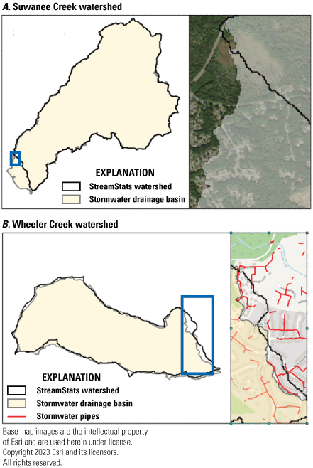
Examples of differences between StreamStats and stormwater drainage basin boundaries for the A, Suwannee Creek watershed and B, Wheeler Creek watershed, Gwinnett County, Georgia. Areas in blue boxes on basin maps on left are expanded in maps on right to show detail.
The stormwater pipe networks in Gwinnett County are gravity drained, and discharge to streams and stormwater drainage follows the surface drainage closely. The StreamStats basins were used to define the basin boundaries in analyses herein because differences in the basin areas were not substantial. The determination of the stormwater drainage areas had uncertainties because of uncertainties in the exact locations of the stormwater network pipes and the assumption that the intakes and outlets of pipes are at the same elevations as determined from the DEM. Some uncertainty was reduced by using a high-resolution DEM, but small errors possibly can result in large changes in basin drainages.
Land Cover and Imperviousness
Land cover and imperviousness are presented for the period 2000–20 in figure 4 with a discussion of conditions in 2019 here followed by a discussion of temporal changes. In 2019, the study area was dominated by developed land covers (72.3 percent), which consisted of 26.8-percent low intensity, 17.1-percent medium intensity, 7.47-percent high intensity, and 21.0-percent open space land cover groups (table 9, fig. 4). Watershed developed land coverages ranged from 59.2 percent in the Wheeler Creek watershed to 95.8 percent in the North Fork Peachtree Creek watershed. Percent developed land coverages were also low in the Richland Creek watershed (60.9 percent) and high in the Wildcat Creek (87.1 percent), Sweetwater Creek (82.8 percent), and Crooked Creek (85.6 percent) watersheds. The predominant type of developed land cover varied by watershed.
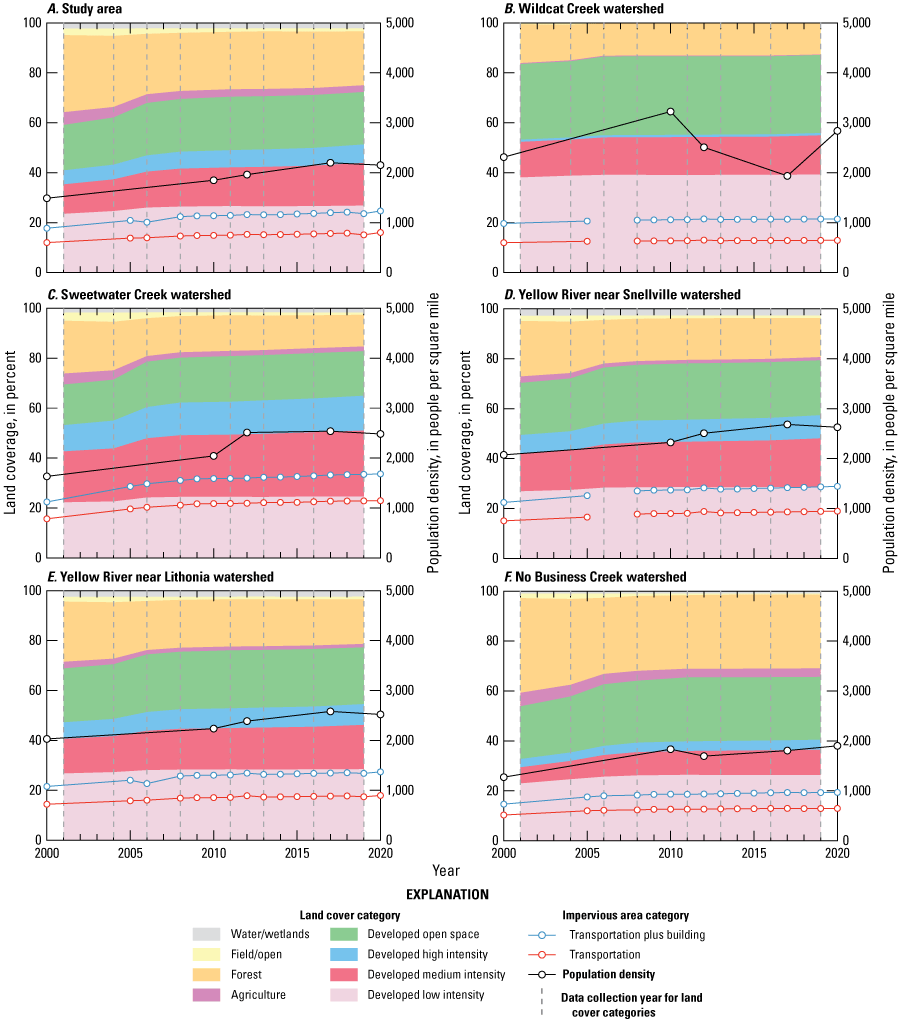
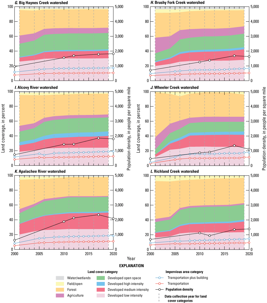
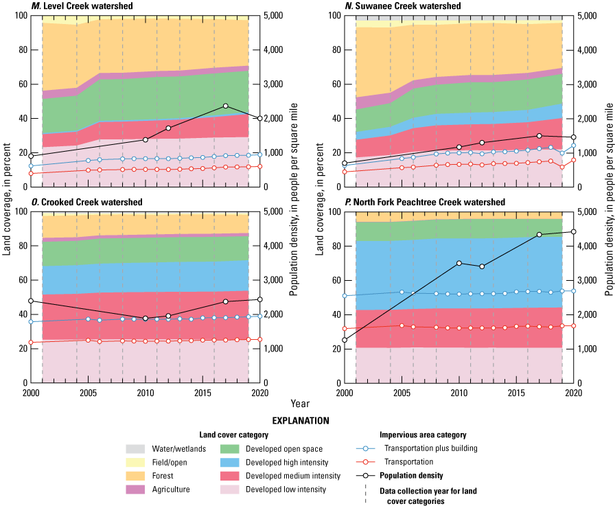
Percentage of each land cover group (table 2), impervious area category (table 3), and population density within the study area and within each of the 15 monitored watersheds, Gwinnett County, Georgia. Land cover data are derived from the National Land Cover Database 2019 (U.S. Geological Survey [USGS], 2021b). Impervious area data are from Gwinnett County Department of Public Utilities (unpub. data, 2022). Population density data are from U.S. Census Bureau (2022).
Table 9.
Land cover group percentages in 15 watersheds in Gwinnett County, Georgia, 2019.[Land cover groups are described in table 2. All values are percentages unless otherwise noted. Land cover data are derived from the National Land Cover Database 2019 (U.S. Geological Survey [USGS], 2021b). Parcel data are from Gwinnett County Information Technology Services, 2021. na, not available]
The developed low intensity and open space groups were strongly correlated between watersheds (r = 0.808) and the developed medium and high intensity groups were moderately correlated between watersheds (r = 0.620; table 10), indicating that these pairs of development groups are commonly associated with each other. The percentage of watershed developed land covers were strongly associated with the percentages in their developed medium plus high intensity land cover (r = 0.773), indicating that these two land cover groups define much of the variability observed in the percentage of developed land cover within these watersheds. This is apparent as the watersheds with the three highest percentages of developed medium plus high intensity land cover have three of the four highest sum percentages of developed land-use groups. The Wildcat Creek watershed also had a high percentage of developed land cover (87.1 percent); however, most of this was low intensity and open space (70.5 percent). The Wildcat Creek watershed is a small catchment and only represents 0.41 percent of the study area.
Table 10.
Pearson product-moment correlations between select watershed land cover groups and impervious fractional areas for 2019 between the 15 study watersheds.[Land cover groups are described in table 2. Land cover data are derived from the National Land Cover Database 2019 (U.S. Geological Survey [USGS], 2021b). 2019 Impervious area data are from Gwinnett County land coverage data, Gwinnett County Department of Public Utilities (unpub. data, 2022). Values in bold are significant at probability (p)-value less than or equal to 0.05; vs., versus; ft, foot]
In 2019, forest composed a substantial portion of the study area (21.6 percent) whereas agriculture, field/open, and water/wetlands land cover groups composed smaller portions (2.66, 1.21, and 2.22 percent, respectively; table 9). The percentage of the forest land cover group was highest in the Richland Creek watershed (34.1 precent). Seven of the 15 watersheds had forested land coverages greater than 25 percent. The North Fork Peachtree Creek watershed was the most heavily developed and had 3.94-percent forested land cover. Agriculture land coverage was highest in the Brushy Fork Creek watershed (9.96 percent) and was also high in the Big Haynes Creek (7.11 percent) and Wheeler Creek (6.82 percent) watersheds. The field/open land cover group percentage was highest in the Wheeler Creek watershed (3.71 percent), whereas the water/wetlands land cover group percentage was highest in the Brushy Fork Creek watershed (3.37 percent). The predominance of developed land-use types and lack of large proportions of forests, agricultural lands, and parks are typical of well-developed suburban and urban areas.
In 2001, most of the watersheds had at least 45 percent of their land cover composed of developed land cover groups (fig. 4). The only exceptions were Wheeler Creek, Brushy Fork Creek, and Richland Creek watersheds, consisting of 21.7-, 37.0-, and 37.0-percent developed land cover, respectively. By 2019, at least 59 percent of each watershed was developed. Developed land coverage groups in the study area increased between 2001 and 2019 by 13.2 percent, with the largest increase being for the developed medium intensity group (5.2 percent) and the smallest increase being for the developed high intensity group (1.9 percent; table 11). These increases were balanced mostly by decreases in the forest group (–9.2 percent) but also by smaller decreases of –2.4, –1.4, and –0.1 percent in the agriculture, field/open, and water/wetland groups, respectively. Land cover decreases were particularly high for forest for the Wheeler Creek watershed (–30.8 percent) and for agriculture for the Brushy Fork Creek (–11.2 percent) and Wheeler Creek (–9.9 percent) watersheds. Land cover changes occurred most rapidly between 2004 and 2008 at most watersheds (fig. 4). Land cover changes were most rapid at the Wheeler Creek watershed during 2001–04 (fig. 4J) and most rapid at the Apalachee Creek watershed during 2001–06 (fig. 4K). Only small changes occurred in land-use groups at the Crooked Creek (fig. 4O) and North Fork Peachtree Creek (fig. 4P) watersheds during 2001–19. These watersheds are located closer to the city of Atlanta than the other watersheds and were well developed much earlier.
Table 11.
Changes in land cover groups, 2001–19, and changes in impervious areas, 2000–20, in 15 watersheds in Gwinnett County, Georgia.[Land cover groups are described in table 2. Land cover types for impervious areas are listed in table 3. All values are percentages. Land cover data are derived from the National Land Cover Database 2019 (U.S. Geological Survey [USGS], 2021b). Impervious area data are from Gwinnett County Department of Public Utilities, unpub. data, 2022]
In 2019, impervious areas covered about 24.9 percent of the study area (table 12). Imperviousness in the study watersheds ranged from about 14.8 percent in the Richland Creek watershed to about 55.1 percent in the North Fork Peachtree Creek watershed. The latter watershed not only had the highest percentage of developed medium and high intensity land cover (64.7 percent), but also the lowest percentage of developed low intensity and open space land cover (31.1 percent). Imperviousness was also high in the Sweetwater Creek (34.9 percent) and Crooked Creek (40.0 percent) watersheds. Imperviousness was classified mostly as transportation (60.8 percent) and building (34.2 percent), and these two classes were very strongly correlated across study watersheds (r = 0.961, table 10). Imperviousness within the 200-ft stream buffer for the study area was about 11.2 percent, about 55 percent less than within the watershed area. Imperviousness was likely lower within the stream buffer because of less development in the stream floodplains and no development within the stream channel. The amount of imperviousness within the 200-ft stream buffer within a watershed was very strongly correlated with the overall imperviousness of the watershed (r = 0.954, table 10).
Table 12.
Impervious area percentages in 15 watersheds in Gwinnett County, Georgia, 2019.[Impervious area land cover types are listed in table 3. All values are percentages. Impervious area data are from Gwinnett County Department of Public Utilities (unpub. data, 2022)]
The imperviousness of a watershed reflects the proportions of various land cover groups within the watershed because each land cover group can have a distinct range of imperviousness. Imperviousness is part of the classification used for the developed land cover groups (table 2). This is evident in the variability in watershed imperviousness being significantly correlated to the watershed variability in the percentage of the more extensive land cover groups: very strongly correlated with developed high intensity land cover (r = 0.949), strongly correlated with developed medium intensity land cover (r = 0.726), and strongly inversely correlated with the forest land cover (r = –0.870; table 10, for 2019).
Changes in imperviousness from 2000 to 2020 are shown in figure 4. Imperviousness data were only available for transportation and building land cover categories for 2000, so changes in imperviousness were quantified using the sum of these categories. Both categories, however, represented about 95 percent of imperviousness. Imperviousness increased by 6.9 percent for the study area during 2000–20, and increases occurred at all 15 watersheds over this period (table 11, transportation plus buildings). The largest percentage change occurred in the Wheeler Creek watershed (13.4 percent) and changes exceeding 10 percent also occurred in the Sweetwater Creek, Apalachee River, and Suwanee Creek watersheds (11.2, 10.4, and 11.7 percent, respectively). Of the study watersheds, the Wheeler Creek watershed had some of the largest decreases in forest and agriculture land covers, which have low imperviousness. The smallest percent change occurred at the Wildcat Creek watershed (1.8 percent) and changes were also small at the Crooked Creek and North Fork Peachtree Creek watersheds (3.2 and 2.8 percent, respectively; table 11, transportation plus buildings). The smaller changes in imperviousness at these three watersheds were consistent with similarly small changes in land cover group percentages from 2001 to 2019 (fig. 4B, O, P). The more rapid increases in watershed imperviousness occurred before 2008 and appear to coincide with increases in various developed land cover groups and decreases in forest and sometimes agriculture land cover groups.
Long-term development in the study watersheds can be observed from temporal changes in watershed building densities (fig. 5). Although much of the development occurred before the 2002–20 study period, development continued throughout the study period. Increases in building densities of more than 250 buildings per mi2 occurred in the Brushy Fork Creek, Wheeler Creek, Apalachee River, and Richland Creek watersheds. Although Crooked Creek and North Fork Peachtree Creek watersheds had lower building densities (fig. 5N, O), these watersheds had larger areas of developed high intensity land cover (fig. 4O, P), which include larger buildings such as multifamily housing and office buildings (table 2). Average parcel build year ranged from 1980 for the North Fork Peachtree Creek watershed to 2002 for the Wheeler Creek watershed (table 9).
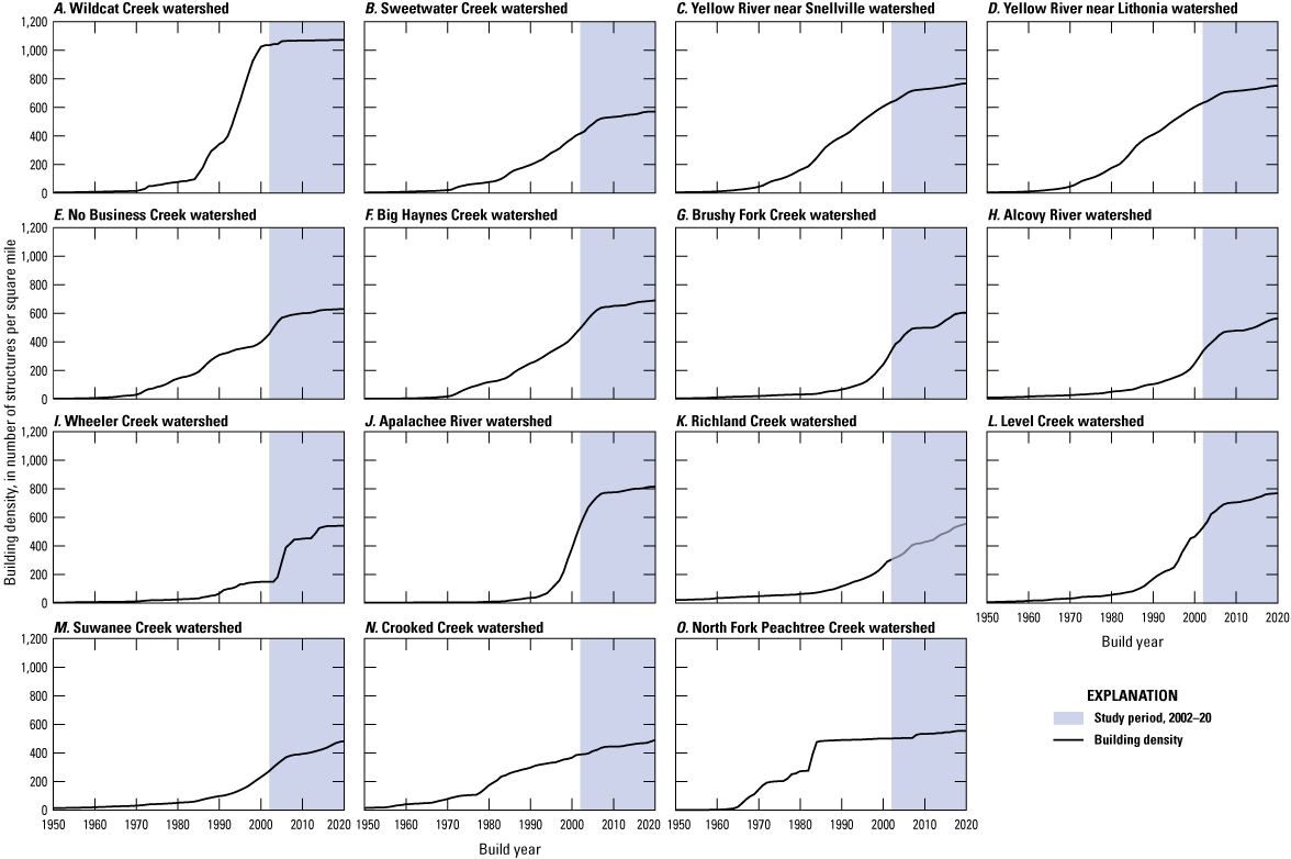
Watershed building density from 1950 to 2020, based on parcel build date, in 15 watersheds in Gwinnett County, Georgia. Parcel data are from Gwinnett County Information Technology Services (2021).
Population
Population density in the study area averaged 1,489 people per mi2 in 2000 and 2,152 people per mi2 in 2020, a 45-percent increase. Population density was highest in areas along the Interstate 85 corridor, particularly in its southwestern portion closer to the city of Atlanta, whereas spatial associations between areas with high population densities and areas within city boundaries were less apparent (fig. 6). In 2020, population densities were highest in the North Fork Peachtree Creek watershed (4,424 people per mi2) and were also high in the Wildcat Creek, Sweetwater Creek, Yellow River near Snellville, Yellow River near Lithonia, and Crooked Creek watersheds, all greater than 2,400 people per mi2. Population densities were low in the Wheeler Creek, Richland Creek, and Suwanee Creek watersheds, all less than 1,500 people per mi2 in 2020. Some of the population density estimates appeared to be temporarily inconsistent; for example, the change in population for the Wildcat Creek watershed (fig. 4B) was likely an artifact of a change in the census block group area combined with the small watershed drainage area. The decadal census estimates are expected to be more accurate than the interim 5-year estimates. Higher population densities were found in watersheds with higher percentages of developed medium and high intensity land covers and lower percentages of agriculture and forest land cover groups, as indicated in figure 4 and by the significant moderate to strong correlations between three of these watershed land cover groups for 2019 and population densities for 2020 (table 13).
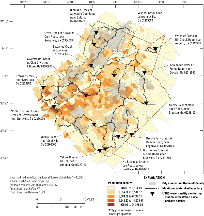
Population density for the area of the 15 monitored watersheds and Gwinnett County, Georgia, 2017. Data are from 2020 decadal census, U.S. Census Bureau (2022). USGS, U.S. Geological Survey.
Table 13.
Pearson product-moment correlations between select watershed land cover groups for 2019 and population densities for 2020 between the 15 study watersheds, Gwinnett County, Georgia.[Land cover groups are described in table 2. The 2019 land cover data are derived from the National Land Cover Database 2019 (U.S. Geological Survey [USGS], 2021b). The 2020 population values are from 2020 decadal census block group data, U.S. Census Bureau (2022). Values in bold are significant at probability (p)-value less than or equal to 0.05; vs., versus; <, less than]
The highest increase in population density between 2000 and 2020 was in the North Fork Peachtree Creek watershed, with an increase of 3,159 people per mi2, a 250-percent increase (fig. 4P). Large increases in population density also occurred during this period at the Alcovy River, Apalachee River, and Level Creek watersheds, all of which had increases of greater than 1,000 people per mi2 (fig. 4I, K, M, respectively). Watershed increases in population density over the period are reflected in increases in the developed medium intensity land cover group and, to a lesser extent, increases in the developed high intensity land cover group. The timing of the increases between population density and land cover group changes do not match as well. Temporal resolution is lower in the population density estimates, and the 5-year estimates are temporally less precise than the decadal census data. Population changed little between 2000 and 2020 in the Crooked Creek watershed and this was reflected in little change in the land cover groups (fig. 4O). The large increase in population density in the North Fork Peachtree Creek watershed was not reflected in changes in the land cover groups (fig. 4P), likely because much of the watershed area was already in developed medium to high intensity land cover groups by 2000.
Water Infrastructure
Gwinnett County receives most of its water from two raw water intakes in Lake Lanier, located outside of the study watersheds. This is supplemented with water from wells in the city of Lawrenceville. Gwinnett County residents are served by onsite residential septic systems or publicly operated water reclamation facilities (WRFs). Gwinnett County operates three WRFs, the F. Wayne Hill WRF that discharges to Lake Lanier, the Crooked Creek WRF that discharges to the Chattahoochee River, and the Yellow River WRF that discharges to the Yellow River. The Yellow River WRF is located about 3 mi upstream from the Yellow River near Snellville site, such that the facility discharge contributes to flows at the Yellow River near Snellville and Yellow River near Lithonia sites. The Yellow River WRF mostly services areas within the Yellow River watersheds.
Septic density averaged 164.5 systems per mi2 in the study area (table 14). Septic densities were generally highest in the southern parts of the county, which includes older development. Watershed septic densities ranged from 3.9 systems per mi2 in the North Fork Peachtree Creek watershed to 296.1 systems per mi2 in the Wildcat Creek watershed. Septic densities were highest in the Wildcat Creek, No Business Creek, Big Haynes Creek, and Yellow River near Lithonia watersheds, which all had septic densities greater than 200 systems per mi2.
Table 14.
Summary of water infrastructure in 15 watersheds in Gwinnett County, Georgia, August 2021.[Septic and sanitary sewer data are from Gwinnett County Department of Water Resources (unpub. data, 2021)]
Sewer density averaged 7.77 mi of sewer pipe per mi2 (table 14). Sewer densities were generally highest in the western and central parts of the county. Watershed sewer densities ranged from 5.57 to 11.00 mi of sewer pipe per mi2. Sewer densities were lowest in the Wheeler Creek, Richland Creek, and Suwanee Creek watersheds. Sewer densities were highest in the Crooked Creek and North Fork Peachtree Creek watersheds, with sewer densities greater than 10 mi of sanitary sewer pipe per mi2.
All watersheds have a mix of septic and sewer infrastructure (table 14; fig. 7). Watersheds with the highest sewer densities had the lowest septic densities because residents in the Crooked Creek and North Fork Peachtree Creek watersheds have most of their wastewater routed offsite to a WRF. These two watersheds had the highest percentages of developed medium and high intensity land covers (fig. 4O, P). The site with the highest septic density, Wildcat Creek, had a sewer density similar to the study-wide average, indicating a mix of onsite and offsite wastewater treatment.
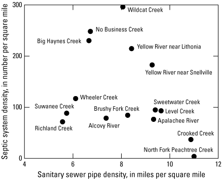
Septic system and sanitary sewer pipe density in 15 watersheds in Gwinnett County, Georgia, August 2021. Septic and sanitary sewer data are from Gwinnett County Department of Water Resources, (unpub. data, 2021).
The locations of detention ponds in unincorporated Gwinnett County and the City of Lilburn are shown in figure 8. Detention ponds are used widely throughout the study area, with 1,881 ponds from this dataset located within the study watersheds. Detention ponds designed to delay peak flows and ponds constructed in Gwinnett County since 2001 are designed to detain water from a 1-year return interval storm for a 24-hour period. The county also adopted water-quality protection design requirements in 2001 for new detention ponds that implement vegetation and higher pond outlets to retain sediment (Aulenbach and others, 2017b).
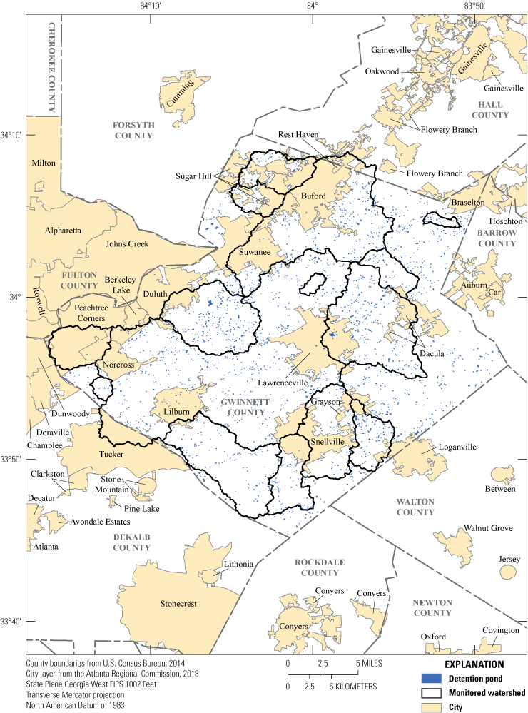
Locations of detention ponds in unincorporated Gwinnett County and City of Lilburn, Georgia, August 2021. Detention pond data are from Gwinnett County Department of Water Resources (unpub. data, 2021).
Water Budget
The effects of climate, watershed characteristics, and land use on the hydrologic cycle of the 15 study watersheds were assessed by evaluating several components of the water budget and comparing these to watershed attributes. Water budget components include precipitation, stream runoff, evapotranspiration, and groundwater inflows, outflows, and changes in storage. Precipitation and runoff were measured for each study watershed. These data were used to compute annual and monthly average precipitation and runoff; to calculate runoff ratios, base-flow runoff, and the BFI; and to estimate long-term actual evapotranspiration. Estimates of potential evapotranspiration are also presented.
Climate
Gwinnett County has a humid, subtropical climate characterized by warm, humid summers and cool, wet winters. Average monthly air temperatures ranged from 42.3 degrees Fahrenheit (°F) in January to 79.6 °F in July (based on the 30-year average during 1991–2020 for the nearby NOAA Atlanta Peachtree Airport station USW00053863 [National Oceanic and Atmospheric Administration, 2021]). Average annual precipitation at the Lawrenceville 4.2 SW station (US1GAGW0016) for the same period was 53.53 inches per year (in/yr), with higher precipitation in the winter (4.80 inches per month [in/mo], January–March) and summer (4.68 in/mo, July–September) and lower precipitation in the spring (4.19 in/mo, April–June) and fall (4.17 in/mo, October–December). Winter rainstorms are characterized by long duration and spatially widespread frontal systems. In contrast, spring and summer rainstorms are characterized by short duration, often unevenly spatially distributed, intense convective thunderstorms.
Weekly estimates of drought severity in Gwinnett County during the study period, as classified by the U.S. Drought Monitor (2021), are presented in figure 9. The U.S. Drought Monitor classifies drought by using a combination of meteorological, hydrologic, and agricultural drought characteristics. Gwinnett County has undergone reoccurring droughts during the study period, with 1-year or longer droughts in 2002, 2007–08, 2011–12, and 2016–17. This is evident from sustained values above 150 for the drought severity and coverage index (fig. 9B), which is indicative of at least half the county area having at least moderate drought conditions.
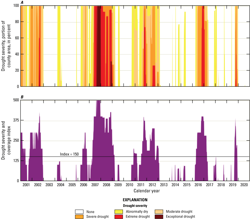
Weekly A, drought severity as a percentage of county area and, B, drought severity and coverage index in Gwinnett County, Georgia, for calendar years 2001–20. Modified from U.S. Drought Monitor (2021).
Precipitation, Evapotranspiration, and Runoff
Precipitation, as determined from the USGS precipitation monitoring sites (fig. 1; table 7), averaged 51.5 in/yr for the study area (fig. 10A) for WYs 2002–20; averages for these sites are near the long-term average of 53.53 in/yr reported at the NOAA Lawrenceville 4.2 SW weather station (1991–2020; National Oceanic and Atmospheric Administration, 2021; fig. 1). Annual precipitation was variable, with study area precipitation ranging from 35.1 in. (WY 2007) to 72.5 in. (WY 2003). Precipitation was below average (less than 46.9 in.), for 7 water years, namely WYs 2002, 2006–08, 2011–12, and 2014, which corresponded to drought periods previously mentioned (fig. 9); precipitation was above average (greater than 56.2 in.), for 7 water years, namely WYs 2003, 2005, 2009–10, 2013, and 2019–20.
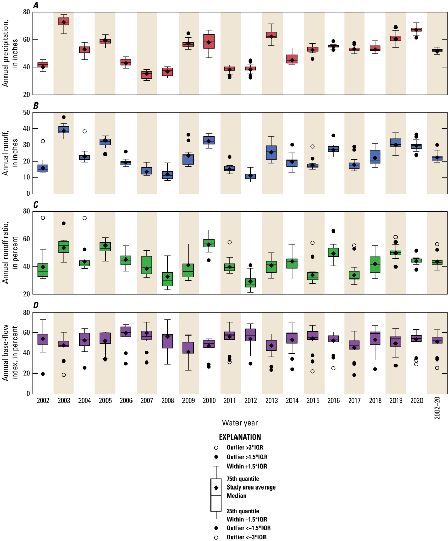
Boxplots showing the variability in annual A, precipitation, B, runoff, C, runoff ratio, and D, base-flow index for 13 of the monitored watersheds in Gwinnett County, Georgia, for water years 2002–20. Annual values for the Sweetwater Creek watershed are available only for water years 2011–20. Wildcat Creek and Yellow River near Snellville watersheds are not included. IQR, interquartile range; >, greater than; <, less than.
The spatial variability of precipitation between study watersheds was small relative to the large interannual variability in precipitation (fig. 11). Average annual precipitation ranged from 49.5 in. (Brushy Fork Creek watershed) to 54.5 in. (Level Creek watershed). No differences in average annual precipitation for this period were significant between watersheds as indicated by the same letter in figure 11. Variability in spatial patterns in precipitation can be caused by factors such as topography (McCrary, 2011), the variable distribution of precipitation from convective thunderstorms, and proximity and orientation to urban heat islands (Bornstein and Lin, 2000; Dixon and Mote, 2003; Mote and others, 2007; Shem and Shepherd, 2009). Long-term precipitation variability between watersheds may have been small because of the similar ranges in watershed elevation (table 8) and the similar position of the study watersheds adjacent to but not downwind of Atlanta (prevailing wind direction is from the west and northwest).
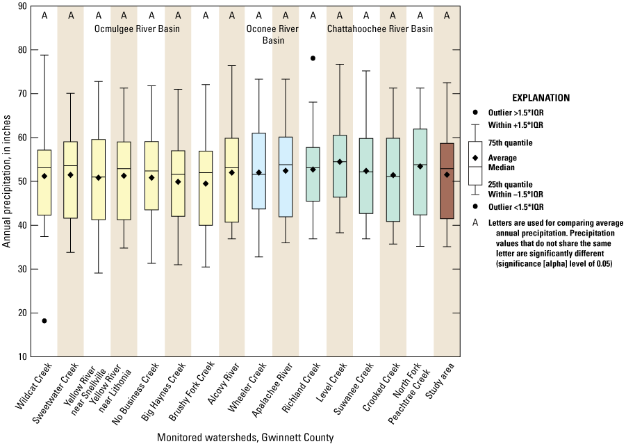
Boxplots showing the annual variability in precipitation for the 15 monitored watersheds and for the study area, Gwinnett County, Georgia, for water years 2002–20. Student’s t-test was used to compare average annual precipitation using a significance (alpha) level of 0.05; however, none of the differences were significant as indicated by the same letter for each watershed or study area. IQR, interquartile range.
Average monthly precipitation for the study period and area ranged from 3.41 in. for October to 5.26 in. for December (fig. 12A). Precipitation did not have a strong seasonal pattern, whereas interannual variability in monthly precipitation was large. The only significant differences identified in monthly precipitation were that July and December were higher than in October.
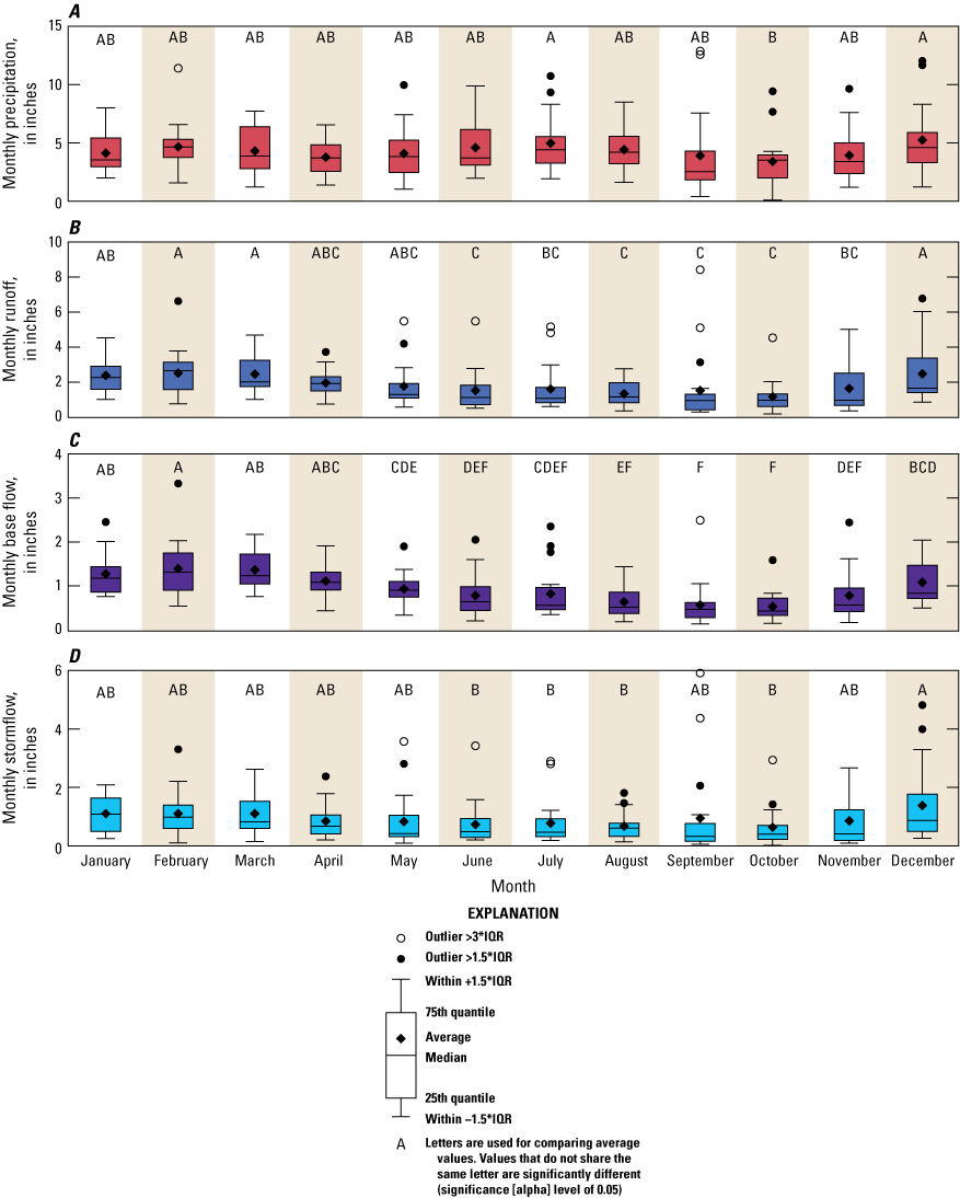
Boxplots showing annual variability in four monthly hydrologic variables, A, precipitation, B, runoff, C, base flow, and D, stormflow, for the study area, Gwinnett County, Georgia, for water years 2002–20. Significant differences between averages were determined from Student’s t-test with a significance (alpha) level of 0.05. IQR, interquartile range; >, greater than.
Average annual potential evapotranspiration was calculated as 45.8 in. for the WY 2002–20 period and ranged annually from 40.6 in. (WY 2003) to 48.9 in. (WY 2016). The study area had a dryness index (potential evapotranspiration/precipitation) of 0.89, which indicates energy-limited conditions for the overall period. Average annual actual evapotranspiration for this period was 29.1 in., based on the long-term difference between precipitation and runoff and assuming that the net changes in storage over this period were negligible. Actual evapotranspiration was 63.4 percent of potential evapotranspiration, indicating that climatic water deficits (Stephenson, 1990, 1998) occurred frequently where insufficient water was available to fully support potential evapotranspiration. Actual evapotranspiration represented about 56.4 percent of precipitation, which is consistent with a map that indicated average annual evapotranspiration accounted for 50–59 percent of the annual precipitation in the study area on the basis of climate and land cover data (Sanford and Selnick, 2013, p. 228).
Average monthly potential evapotranspiration varied substantially and ranged from 1.95 in. for December to 5.64 in. for June (fig. 13). Potential evapotranspiration was highest in the summer because of seasonally high air temperature and solar radiation that provide the energy for evapotranspiration. High potential evapotranspiration rates exceed precipitation rates in the summer (fig. 12A), resulting in water-limited conditions that can lead to water deficits and reduced plant transpiration caused by a lack of available water for uptake.
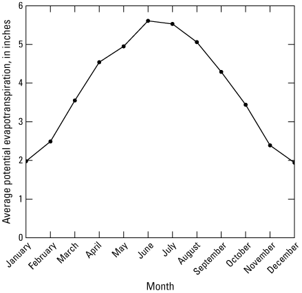
Average monthly potential evapotranspiration (PET) for calendar years 2001–20. PET values were compiled from Climatic Research Unit Time-Series (University of East Anglia Climatic Research Unit and others, 2021). IQR, interquartile range; >, greater than; <, less than; ≤, less than or equal to.
Runoff is largely controlled by various components of the water budget—the amount of precipitation and evapotranspiration and changes in watershed storage (soil water and groundwater). Runoff is also affected by basin characteristics such as land use, impervious area, vegetation, soil types, drainage area, basin shape, drainage network patterns, topography (land-surface slopes), and the presence of lakes and reservoirs. Watershed water budgets are complicated by water management infrastructure and activities that supply, remove, and redistribute water into, out of, within, and between watersheds.
Average annual runoff for the study area for 2002–20 was 22.5 in. and annual average runoff ranged from 11.1 in. for WY 2012 to 38.7 in. for WY 2003 (fig. 10B). Variations in annual runoff were largely related to annual precipitation (r = 0.91; fig. 10A). Watershed storage and evapotranspiration, however, also affected annual runoff. For example, during the droughts in WYs 2007–08 and 2011–12, runoff was lower in WY 2012 (fig. 10B) and runoff ratios were lower in WYs 2008 and 2012 (fig. 10C), the second year of each drought, despite precipitation being similar during all 4 years. These patterns were likely the result of runoff being sustained from storage during the first year of each drought, whereas storage was more depleted during the second year of each drought, resulting in lower runoff and runoff ratios. The role of storage can also be observed when the hydrologic system is wetting up. For example, following the 2007–08 drought, runoff and runoff ratios were lower in WY 2009 than in WY 2010 despite having had similar amounts of precipitation. In WY 2009, a substantial portion of precipitation recharged storage depleted during the drought, whereas in WY 2010, precipitation resulted in more runoff because storage had been replenished. The seasonal effects of evapotranspiration on runoff can be observed from WYs 2015 to 2018, which had similar amounts of precipitation (ranging from 52.3 to 54.6 in.). WY 2016 had higher runoff and runoff ratios than the other 3 years because much more precipitation occurred during the dormant season in WY 2016 (November–February, 31.6 in.) compared to the other 3 years (ranging from 13.3 to 16.7 in.). A larger portion of precipitation contributes to runoff in the dormant season than the growing season because evapotranspiration is substantially lower during the dormant season (fig. 13).
Annual average runoff was highest at the Sweetwater Creek, Crooked Creek, and North Fork Peachtree Creek watersheds (fig. 14), which also are the three watersheds with imperviousness greater than 30 percent in 2019 (fig. 4C, O, P, table 12). Annual average runoff was similar between the other watersheds. The variability in annual runoff between watersheds was small relative to the interannual variability of each.
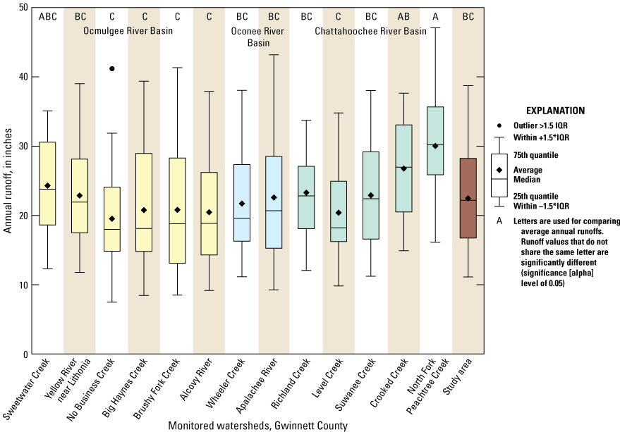
Boxplots showing the annual runoff for 13 of the monitored watersheds and the study area, Gwinnett County, Georgia, water years 2002–20 (Sweetwater Creek watershed, water years 2011–20). Significant differences between average annual runoff values were determined from Student’s t-test with a significance (alpha) level of 0.05. IQR, interquartile range; >, greater than.
Runoff from the two Yellow River watersheds includes discharge from the Yellow River WRF. Annual facility discharges for 2019, 2020, and 2021 were reported as 15.21, 16.71, and 15.07 million gallons per day (Heather Gacek, Gwinnett County Department of Water Resources, written commun., March 23, 2022). Comparing the 3-year average WRF discharge (24.2 cubic feet per second [ft3/s]) to average streamflow at Yellow River near Lithonia for WYs 2002–20 (271.7 ft3/s) indicates that WRF discharge likely constitutes about 9 percent of streamflow at that site. Furthermore, base flow at Yellow River near Lithonia can drop below 100 ft3/s during the summer such that WRF discharge could constitute upwards of 25 percent of streamflow during these conditions.
Monthly runoff had a substantial seasonal pattern while exhibiting high interannual variability (fig. 12B). Study area average monthly runoff was highest in February (2.52 in.) and was lowest in October (1.18 in.), when average monthly precipitation was also lowest (fig. 12A). Average monthly runoff typically was significantly higher during December through March, when hydrologic conditions are wet, than during June through November, when hydrologic conditions are dry. Runoff is expected to be higher when hydrologic conditions are wet because base flow is higher, storm runoff response is larger because of the flow system being more hydrologically connected, and less water is necessary to replenish watershed storage. The seasonality in hydrologic conditions was caused by the seasonal effects of evapotranspiration (fig. 13) on the water cycle.
The runoff ratio is the proportion of precipitation that occurs as stream runoff. The average runoff ratio was 43.6 percent for the period WYs 2002–20 for the study area (fig. 10C). Annual runoff ratios ranged from 29.1 percent in WY 2012, the second year of a 2-year drought (figs. 9 and 10A), to 55.8 percent in WY 2010. The runoff ratio was particularly high in WY 2010 as a result of high runoff (fig. 10B) because (1) it was unusually wet at the beginning of the water year such that storage did not need to be recharged and resulted in unusually high amounts of runoff early in the dormant season, (2) conditions were hydrologically wet because of above average precipitation (fig. 10A), and (3) precipitation was distributed such that a higher than normal proportion occurred during the dormant season when evapotranspiration was low.
Differences in annual runoff ratios between watersheds (fig. 15) largely reflected the differences observed for annual runoff (fig. 14), because precipitation was relatively similar across these watersheds (fig. 11). Average annual runoff ratios were highest at the Crooked Creek and North Fork Peachtree Creek watersheds and were lowest at the No Business Creek and Level Creek watersheds.
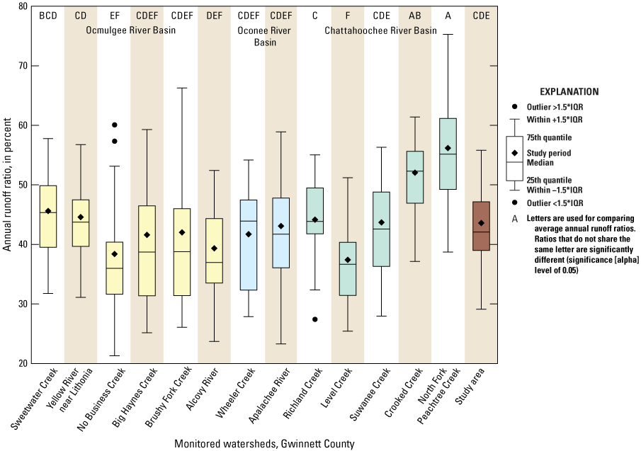
Boxplots showing the annual runoff ratio for 13 of the monitored watersheds and the study area, Gwinnett County, Georgia, water years 2002–20 (Sweetwater Creek watershed, water years 2011–20). Significant differences between average annual runoff ratios were determined from Student’s t-test with a significance (alpha) level of 0.05. IQR, interquartile range; >, greater than; <, less than.
The monthly average runoff ratio had a strong seasonal pattern, with a substantially larger proportion of precipitation contributing to runoff during January through April relative to the rest of the year (fig. 16). The runoff ratio was highest in January (57.8 percent) and lowest in July (30.2 percent) for the period WYs 2002–20 for the study area. Seasonal patterns in runoff ratios largely reflect the seasonality in runoff (fig. 12B). The seasonal pattern in the runoff ratio results from the large seasonal variations in evapotranspiration, but timing is altered by watershed storage. Although evapotranspiration is relatively low by October (fig. 13), runoff ratios progressively increase from October to January as watershed storage is first replenished before more runoff is generated. Although evapotranspiration is relatively high by April, runoff ratios are still high in April and May, supported by high base flows derived from watershed storages recharged during the dormant season. Although runoff ratios still exhibit a seasonal pattern at the Crooked Creek and North Fork Peachtree Creek watersheds, runoff ratios in the summer and fall are much higher and do not follow the same pattern as those for the other watersheds. These two watersheds have much higher percentages of imperviousness than the other watersheds (40.0 and 55.1 percent, respectively, as indicated by 2019 data; table 12), and this likely results in a higher proportion of surface runoff to streams even during seasonally dry hydrologic conditions in the summer and fall.
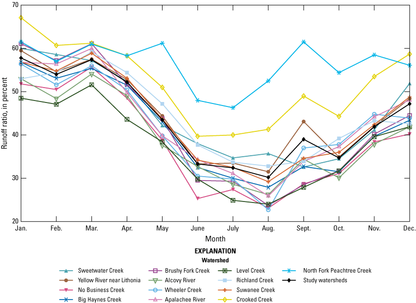
Monthly runoff ratio for 13 of the monitored watersheds and the study area, Gwinnett County, Georgia, water years 2002–20 (Sweetwater Creek watershed, water years 2011–20).
Average annual base-flow runoff for period WYs 2002–20 for the study area was 11.5 in. (fig. 17) and ranged from 7.7 in. at the North Fork Peachtree Creek watershed to 14.6 in. at the Richland Creek watershed. Average annual base-flow runoff was highest at the Big Haynes Creek and Richland Creek watersheds. These watersheds had two of the three lowest percentages of imperviousness in 2019: 18.1 percent for the Big Haynes Creek watershed and 14.8 percent for Richland Creek watershed (fig. 4G, L; table 12). Average annual base-flow runoff was lowest at the Sweetwater Creek, Crooked Creek, and North Fork Peachtree Creek watersheds, which had the three highest percentages of imperviousness in 2019 (fig. 4C, O, P; table 12). These observations highlight the effect of impervious areas on reducing infiltration and recharge to watershed storage.
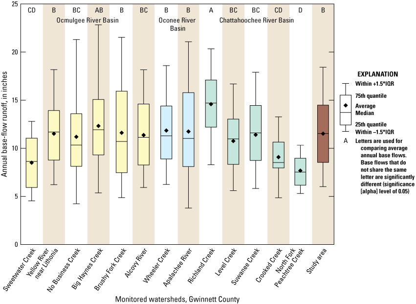
Boxplots showing the annual base-flow runoff for 13 of the monitored watersheds and the study area, Gwinnett County, Georgia, water years 2002–20 (Sweetwater Creek watershed, water years 2011–20). Significant differences between average annual base flows were determined from Student’s t-test with a significance (alpha) level of 0.05. IQR, interquartile range.
Monthly average base-flow runoff exhibited a strong seasonal pattern (figs. 12C and 18), reflecting the effect of the seasonality in watershed storage levels. Watershed storage typically was depleted during the growing season because of high evapotranspiration and was replenished during the first part of the dormant season when evapotranspiration was low (fig. 13). Base flow for the study area for WYs 2002–20 was nearly twice as high during January through March (1.36 in/mo) as it was during June through October (0.71 in/mo).
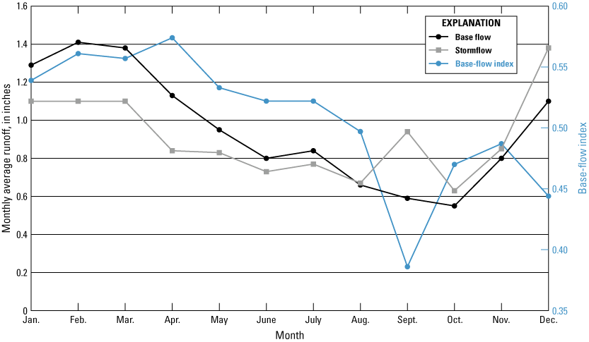
Monthly average base-flow runoff and stormflow runoff and the base-flow index (BFI) for the study area in Gwinnett County, Georgia, water years 2002–20.
Annual stormflow runoff varied similarly to annual precipitation (r = 0.92; fig. 10A). Stormflow runoff varied substantially between watersheds. Average annual stormflow runoff amounts were highest from the North Fork Peachtree Creek watershed and were also high at Sweetwater Creek and Crooked Creek watersheds (fig. 19), whose imperviousness exceeded 30 percent (fig. 4C, O, P; table 12). Average annual stormflow runoff amounts were lowest at the No Business Creek watershed, although several other watersheds were not statistically different. Average monthly stormflow runoff was moderately correlated with average monthly precipitation (r = 0.50; fig. 12A, D), with the lack of a stronger relation likely owing to the important role that wetness conditions contribute to generating stormflow.
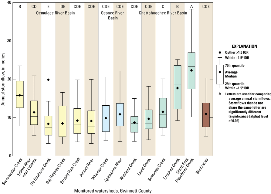
Boxplots showing the annual stormflow runoff for 13 of the monitored watersheds and the study area, Gwinnett County, Georgia, water years 2002–20 (Sweetwater Creek watershed, water years 2011–20). Significant differences between average annual stormflows were determined from Student’s t-test with a significance (alpha) level of 0.05. IQR, interquartile range; >, greater than.
The BFI for the study area was 0.51 for the period WYs 2002–20, indicating that 51 percent of runoff occurred as base flow and the remainder occurred as stormflow. The low proportion of base-flow runoff in most of the watersheds is indicative of urban streams affected by impervious areas. The BFI captures the relative proportions of base-flow and stormflow runoff, which can affect water quality when base-flow and stormflow runoff are chemically distinct. BFIs varied annually and were higher in years with less precipitation (r = –0.65), particularly for years with below average precipitation (WYs 2002, 2006–08, 2011–12, and 2014; fig. 12A, D). The higher annual BFIs for years with below average precipitation were likely the combination of lower stormflow runoffs along with base flows composing a larger proportion of runoff.
The WY 2002–20 BFI was highest at the Richland Creek (0.63) watershed and was also high at the No Business Creek (0.57) and Big Haynes Creek (0.59) watersheds (fig. 20). These watersheds had relatively low percentages of impervious area (<21 percent in 2019; fig. 4F, G, L; table 12). The lowest WY 2002–20 BFI was at the North Fork Peachtree Creek watershed (0.26), and BFIs were also low at the Sweetwater Creek (0.35; WYs 2011–20) and Crooked Creek (0.34) watersheds. These three watersheds had the three highest percentages of impervious areas (fig. 4C, O, P; table 12). The BFI hydrologic metric is more sensitive to the specific effects of impervious area than for the base-flow and stormflow runoff metrics because although base-flow and stormflow response can vary independently or conversely with some watershed characteristics, imperviousness increases stormflow runoff and decreases infiltration and therefore base-flow runoff, resulting in a compounding effect on the BFI metric.
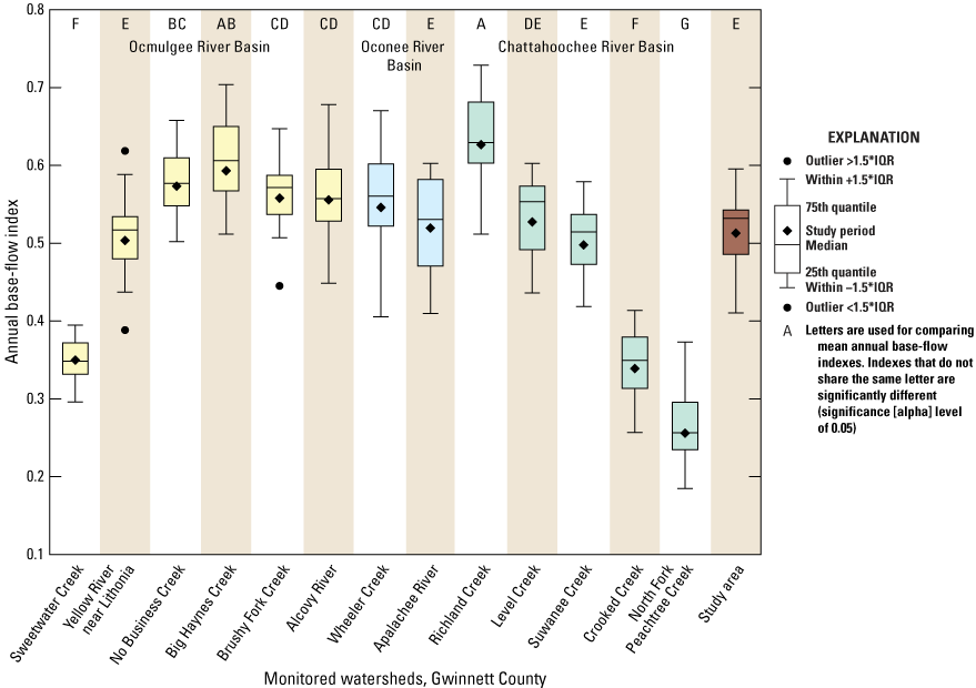
Boxplots showing the annual base-flow index for 13 of the monitored watersheds and the study area, Gwinnett County, Georgia, water years 2002–20 (Sweetwater Creek watershed, water years 2011–20). Significant differences between average annual base-flow index values were determined from Student’s t-test with a significance (alpha) level of 0.05. IQR, interquartile range; >, greater than; <, less than.
Study period monthly BFIs varied seasonally, with higher BFIs from January through April and lower BFIs from August through December (fig. 21). Monthly BFIs for the study area for WYs 2002–20 ranged from 0.39 in September to 0.57 in April. Monthly BFI was moderately correlated with average monthly base-flow runoff for the study area (r = 0.67), indicating the role that seasonality in watershed storage plays on BFI. The BFIs for the Sweetwater Creek, Crooked Creek, and North Fork Peachtree Creek watersheds were substantially lower and had weaker seasonality, consistent with the expected effects of high imperviousness where flows are more controlled by surface runoff processes than seasonal variations in watershed storage.
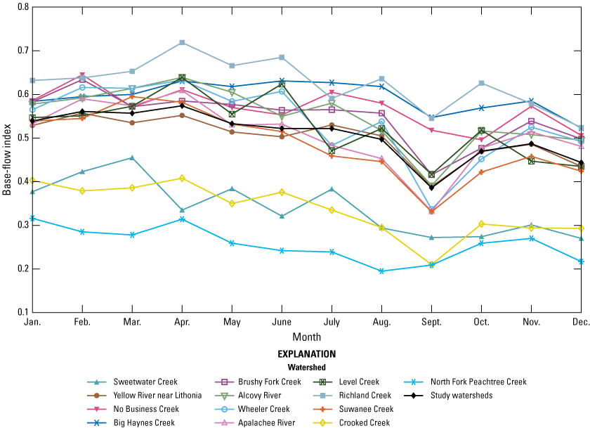
Monthly base-flow index for 13 of the monitored watersheds and the study area, Gwinnett County, Georgia, water years 2002–20 (Sweetwater Creek watershed, water years 2011–20).
Relations Between Runoff Metrics and Watershed Characteristics
Correlations between watershed characteristics and runoff metrics were evaluated to determine whether relations exist between these variables (table 15). Runoff metrics included precipitation, runoff, the runoff ratio, base-flow runoff, stormflow runoff, and the BFI. Watershed characteristics included average land-surface slope, basin area, and imperviousness for 2019 for watershed areas and within 200-ft stream buffers. The imperviousness variables were significantly correlated with most of the runoff metrics, whereas none of the other watershed characteristics had significant correlations with any of the runoff metrics. The significant intercorrelations between runoff metrics were expected because many of these metrics are interrelated.
Table 15.
Pearson product-moment correlation coefficients between watershed characteristics and runoff metrics for 15 monitored watersheds in Gwinnett County, Georgia, water years 2002–20 (Sweetwater Creek watershed, water years 2011–20).[Statistically significant Pearson product-moment correlation coefficients in bold font (significance (alpha) level of 0.05). na, not applicable; ft, foot; —, result not listed for duplicative combination]
Watershed storm runoff had a very strong correlation with watershed imperviousness (r = 0.977; fig. 22A), similar to what has been well documented in many urban studies (Leopold, 1968; Hollis, 1975; Ogden and others, 2011). The relation indicated that stormflow runoff was about twice as high for watersheds with 50-percent imperviousness than those with 20-percent imperviousness. The watershed runoff ratio had a strong correlation with watershed imperviousness (r = 0.882; fig. 22B). Watershed base-flow runoff had a strong inverse correlation with watershed imperviousness (r = –0.871; fig. 22C). The relation indicated that base-flow runoff was about 30 percent lower for watersheds with 50-percent imperviousness than with 20-percent imperviousness. Watershed BFI had a very strong inverse correlation with watershed imperviousness (r = –0.958; fig. 22D). The base-flow runoff and BFI relations reflect how impervious cover reduces infiltration and limits watershed storage, thereby decreasing base-flow runoff (Simmons and Reynolds, 1982). These four runoff metrics were similarly correlated with the amount of imperviousness within the watershed and within the 200-ft stream buffer.
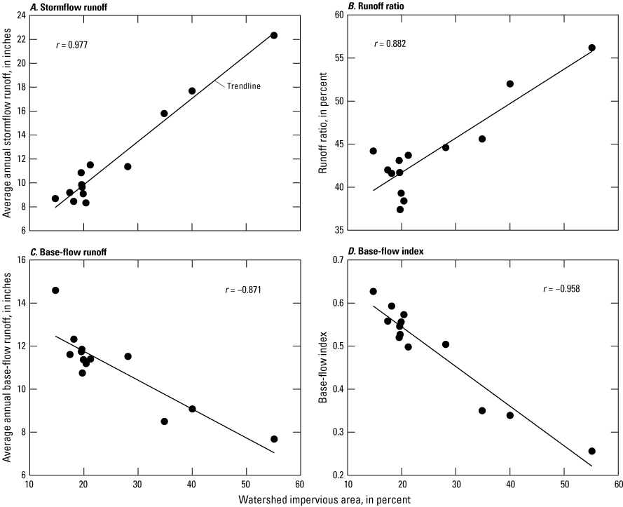
A, Stormflow runoff, B, runoff ratio, C, base-flow runoff, and D, base-flow index versus watershed imperviousness in 2019 for 13 of the watersheds in Gwinnett County, Georgia. Runoff metrics are for water years 2002–20 (Sweetwater Creek watershed, water years 2011–20). r, Pearson product-moment correlation coefficient.
Surface-Water Quality
Surface-water quality was assessed from in situ water-quality monitors, base-flow samples, and storm-composite samples. An example evaluation of the in situ data at four sites was used to illustrate how water-quality conditions can vary seasonally, diurnally, and during storms. Base-flow and stormflow sample concentrations are presented using boxplots by site to illustrate their variability and to enable comparisons. Water-quality standards are presented to provide context to the observed concentrations.
In Situ Water-Quality Monitoring
Continuous sonde turbidity, water temperature, and SC were measured in situ at the 15 USGS water-quality monitoring sites in the study area (table 1) at 15-minute intervals. An evaluation of how these constituents vary temporally is presented from four sites that represent a range of study catchment drainage areas. The in situ measurements show how water quality varies seasonally, diurnally, and during storms, which cannot easily be observed from the discrete base-flow and storm-composite samples. Example in situ data are shown for water year 2019, for a 3-day base-flow period, and for a large storm (figs. 23, 24, and 25; precipitation for the large storm ranged from 3.03 in. at the Richland Creek site to 4.77 in. at the Apalachee Creek site). The water-quality variations in the example data do not reflect the full range of patterns observed because patterns vary with location, storm dynamics, and season.
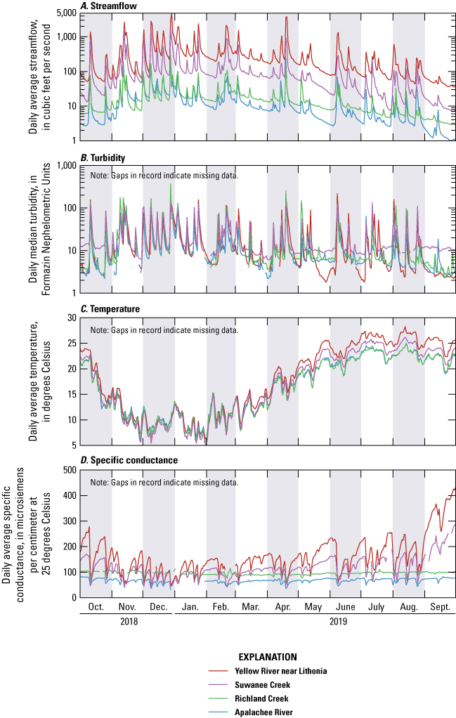
Streamflow and in situ water-quality monitoring data from the Yellow River near Lithonia, Suwanee Creek, Richland Creek, and Apalachee River sites (U.S. Geological Survey sites 02207120, 02334885, 02334480, and 02218565, respectively) showing seasonal variations for water year 2019. A, Daily average streamflow, B, daily median turbidity, C, daily average temperature, and D, daily average specific conductance. Data are from U.S. Geological Survey (USGS, 2021d).
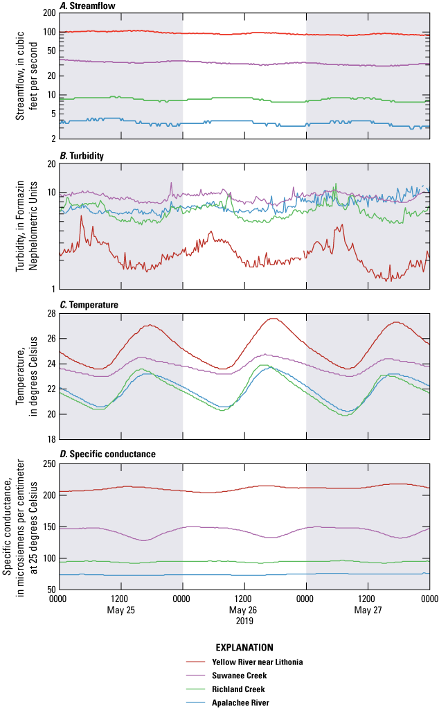
Streamflow and in situ water-quality monitoring data from the Yellow River near Lithonia, Suwanee Creek, Richland Creek, and Apalachee River sites (U.S. Geological Survey sites 02207120, 02334885, 02334480, and 02218565, respectively) showing diurnal variations, May 25–27, 2019. A, Streamflow, B, turbidity, C, temperature, and D, specific conductance. Times are in eastern standard time. Data are from U.S. Geological Survey (USGS, 2021d).
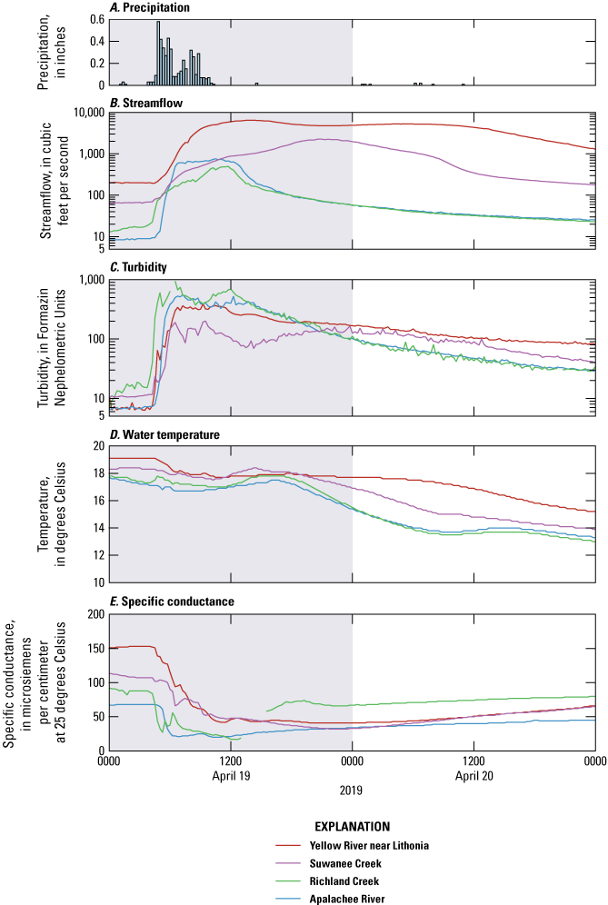
Precipitation, streamflow, and in situ water-quality monitoring data from the Yellow River near Lithonia, Suwanee Creek, Richland Creek, and Apalachee River sites (U.S. Geological Survey sites 02207120, 02334885, 02334480, and 02218565, respectively) showing response to a storm on April 19, 2019. A, Precipitation (at Yellow River near Lithonia; 4.76 inches total), B, streamflow, C, turbidity, D, temperature, and E, specific conductance. Times are in eastern standard time. Data are from U.S. Geological Survey (USGS, 2021d).
Turbidity is a measure of water cloudiness or opacity and is the result of the amount and type of suspended and dissolved matter in the water, including sediment, litter, and organic matter such as algae, microorganisms, and plant debris (Anderson, 2005). Turbidity is commonly used as a surrogate for suspended sediment (Jastram and others, 2009; Rasmussen and others, 2009). High turbidities were associated with storms (fig. 23A, B), as would be expected because the higher streamflow velocities and energy available during stormflow mobilize particulates. Seasonal changes in baseline turbidity corresponded to seasonal changes in base flow at three of the sites, whereas baseline conditions at the Suwanee Creek site were relatively constant year round. During the summer, turbidity exhibited diurnal patterns during base-flow conditions, with lower values from midday to early evening (fig. 24B) that corresponded to times of lower streamflows at three of the sites (fig. 24A). The diurnal pattern in turbidity, however, was substantially out of sync with the diurnal pattern in streamflow at the Yellow River near Lithonia site.
Turbidity increased during storms, but the increase did not exactly coincide with the increase in streamflow (fig. 25B, C). In the example large storm, turbidity peaked before the initial streamflow peak. Subsequent further increases in streamflow at the Suwanee Creek and Richland Creek sites did not result in higher turbidities, and the extended period of high streamflows at the Yellow River near Lithonia site corresponded to decreasing turbidities. Lower turbidities observed later in this storm may reflect (1) less sediment transport after an initial washoff and transport of sediments deposited on land surfaces and in the streambed since the last large storm, (2) contributions of streamflow from a larger contributing area from distant upstream drainages that reflect lower streamflow velocities and sediment transport compared to the beginning of the storm, and (3) contributions of water delayed from detention ponds that are designed to retain sediment.
Water temperature regulates the rate of chemical and biological reactions and determines the maximum amount of dissolved oxygen saturation. The temperature regime also determines the types of aquatic life a stream can support. Water temperature varied seasonally (fig. 23C) and diurnally (fig. 24C) because of the effects of air temperature and solar radiation. Temperature changed with inputs of storm runoff (fig. 25D), which can increase or decrease temperature depending upon the seasonal differences in temperature between base flow and storm runoff; with storm runoff temperature being affected by the temperature of precipitation and the surfaces from which precipitation runs off.
SC is a measure of water’s capacity to conduct an electrical current and is related to the concentration of dissolved ions in water (Hem, 1982). The proportional increase in SC with higher amounts of dissolved constituents varies by constituent and is affected by interactions between constituents (for example, Visconti and others, 2010). Base-flow SC increased with decreasing streamflow, reflecting larger contributions of waters with longer transit times that have had more time to dissolve more constituents (fig. 23A, D) and possibly other seasonal changes in water quality associated with biochemical cycles. SC also decreased with increasing streamflow during stormflow conditions (figs. 23A, D, and 25B, E) indicating that, overall, dissolved constituents tended to dilute because of contributions of more dilute storm runoff. During base-flow conditions, SC exhibited diurnal patterns, with higher SC observed in the morning at three of the sites and higher SC observed in the afternoon or evening at the Yellow River near Lithonia site (fig. 24D).
Base-Flow and Stormflow Water Quality
Boxplots were used to summarize the statistical distribution of concentrations for 20 water-quality constituents, and concentrations were separated by base-flow and stormflow conditions, depending on when samples were collected (fig. 26; table 4). Significant differences between watershed base-flow and stormflow sample concentration distributions were determined using the nonparametric Mann-Whitney U test (also called the Wilcox rank-sum test) with a significance (alpha) level of 0.05. The predominant reporting limit for each constituent is indicated on the plots as a guide because values that were censored are not indicated on the plots. In the following descriptions, concentration ranges refer to the approximate range within the whiskers of the box-and-whisker plots.
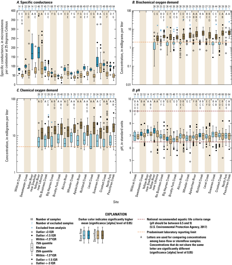
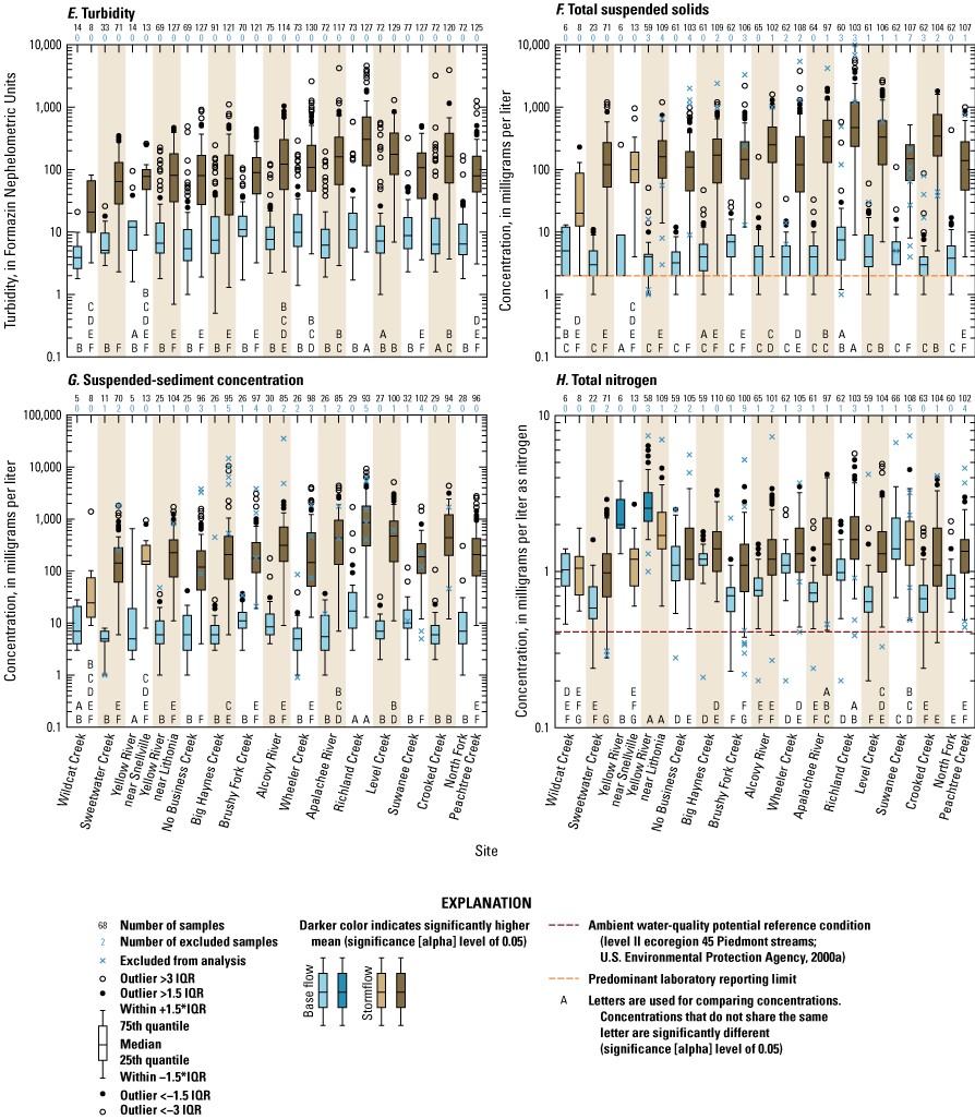
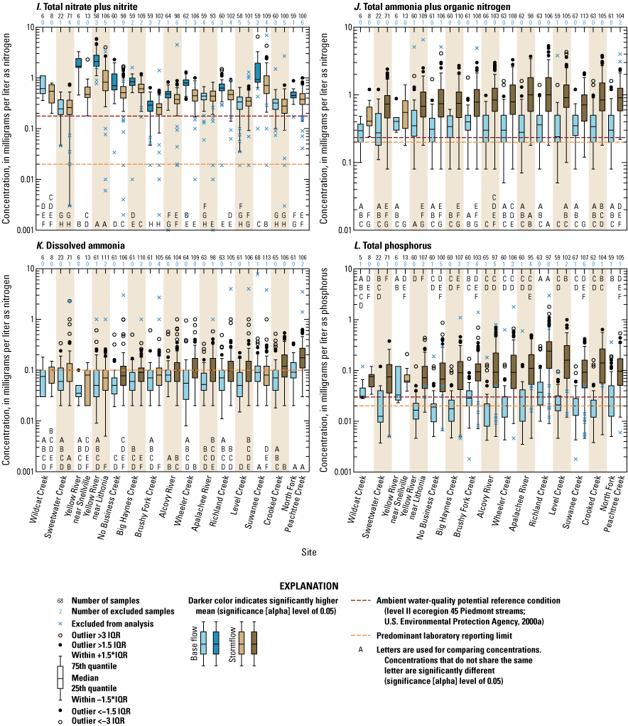
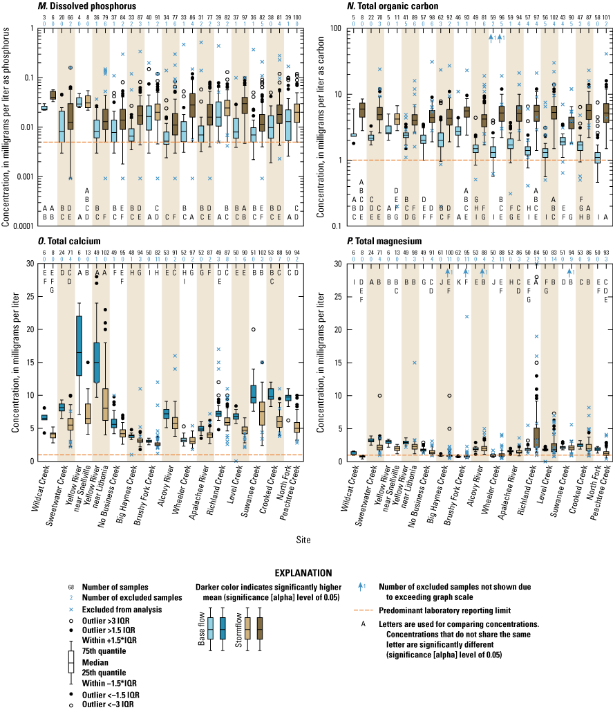
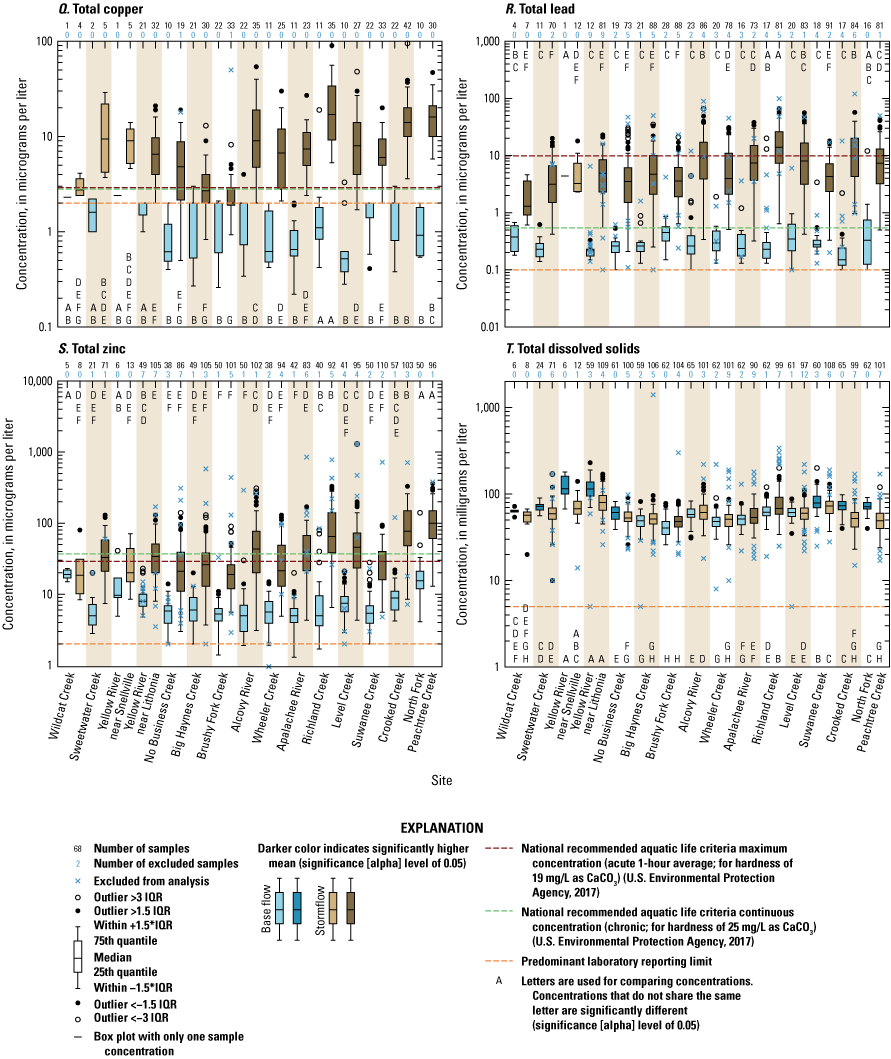
Boxplots showing base-flow and stormflow sample concentration magnitudes at 15 monitored watersheds in Gwinnett County, Georgia, water years 2003–20. Significant difference between base-flow and stormflow sample concentration distributions determined from Mann-Whitney U test with a significance (alpha) level of 0.05. Significant difference between mean watershed concentrations determined from Student’s t-test with a significance level of 0.05. IQR, interquartile range; mg/L, milligrams per liter; CaCO3, calcium carbonate. Data are from U.S. Geological Survey (USGS, 2021d).
Interpreting Water-Quality Standards
Various types of water-quality standards have been adopted for constituents that are considered toxic or detrimental at high concentrations, such as trace metals and nutrients. These standards have been included on figure 26 to provide context to the observed sample concentrations. Criteria often include a time element such that the concentration of a single sample above a criterion does not necessarily indicate a criterion exceedance.
The U.S. Environmental Protection Agency (EPA, 2017) has determined national recommended aquatic life ambient water-quality criteria for toxic chemicals and conditions. Georgia has adopted these water-quality standards to comply with the Clean Water Act (EPA, 2015). These criteria represent the highest constituent concentration that is not expected to pose a significant risk to the majority of species in a given environment or that will ensure that a water body is free from certain negative conditions (EPA, 2017). Criteria were determined for acute and chronic conditions, where acute is for a short period of time (1-hour average) and chronic is for an extended period of time (4-day average), for which aquatic life can be exposed without deleterious effects. For pH, the acute aquatic life criteria require that pH values be between 6.5 and 9. The criteria for total lead, total zinc, and total copper are dependent on the hardness of the water. The median hardness values for samples collected in this study were about 19 milligrams per liter as calcium carbonate (CaCO3) for the stormflow samples and 25 milligrams per liter as CaCO3 for the base-flow samples on the basis of calcium (Ca) and magnesium (Mg) concentrations from samples collected for this study (fig. 26O, P) and assuming that these concentrations were mostly in dissolved form. The trace metals criteria presented in figure 26Q–S were calculated by using the freshwater acute and chronic formulas. These criteria should be used only as a guide for possible exceedance of water-quality standards, because (1) chronic and acute criteria have defined time-period requirements that individual samples do not necessarily comply with, and (2) the criteria presented were not calculated from individual sample hardness.
The EPA (2000) has published recommendations for establishing ambient water-quality criteria for nutrients in rivers and streams in nutrient ecoregion IX, level III ecoregion 45 (Piedmont), which includes Gwinnett County, Ga. Reference conditions, which represent pristine or minimally impacted waters, can be used as a basis for developing nutrient criteria. These reference values are indicated on figure 26H, I, J, L for total nitrogen (N), total nitrate plus nitrite (NO3+NO2), total ammonia plus organic nitrogen (total Kjeldahl nitrogen [TKN]), and total phosphorus (P), respectively.
SC ranged from about 45 to 270 microsiemens per centimeter at 25 degrees Celsius (µS/cm at 25 °C) in base-flow samples and from about 10 to 210 µS/cm in stormflow samples (fig. 26A). The three sites with the highest SC values under both base-flow and stormflow conditions (Yellow River near Snellville, Yellow River near Lithonia, and Suwanee Creek) have the three largest drainage areas. The two Yellow River sites may also be showing elevated values because of discharge from the upstream Yellow River WRF, and this would likely be more evident during base-flow conditions when discharge constitutes a larger proportion of streamflow. SC values were significantly lower in stormflow samples than in base-flow samples for all sites, with site mean stormflow SC ranging from 47 to 82 percent of site mean base-flow SC. This pattern reflects the contributions of more dilute stormflow to base flow. Base flow and sites with larger drainage areas had higher conductivities, likely because of higher concentrations of weathering constituents associated with longer contact times with geologic materials (Maher, 2010, 2011). Sites with higher base-flow SC generally also had higher stormflow SC (r = 0.88 between site base-flow and stormflow SCs).
Biochemical oxygen demand (BOD) is the amount of dissolved oxygen needed by aerobic organisms to break down the amount of organic material in a sample over a specific time period (5 days) and water temperature (20 °C) and is an indication of the degree of organic pollution in surface waters. BOD represents the potential consumption of oxygen by microbial respiration, whereas the actual rate of consumption depends on several factors, including water temperature, pH, microorganisms present, and types of organic material. BOD concentrations ranged from 0.1 to 3 milligrams per liter (mg/L) (of oxygen consumed) in base-flow samples and from 1.5 to 15 mg/L in stormflow samples (fig. 26B). Concentrations of BOD were significantly higher in stormflow samples than in base-flow samples at all sites. Stormflow BOD was highest at the Apalachee River, Richland Creek, Crooked Creek, and North Fork Peachtree Creek sites.
Chemical oxygen demand (COD) is the amount of oxygen needed to fully oxidize organic compounds to carbon dioxide and is a measure of oxidizable contaminants in surface waters. COD represents the potential consumption of oxygen by chemical oxidation. COD concentrations ranged from about 4 to 20 mg/L (of oxygen consumed) in base-flow samples and from about 4 to 30 mg/L in stormflow samples (fig. 26C). Concentrations of COD were significantly higher in stormflow samples than in base-flow samples at all sites. Higher stormflow COD concentrations were more frequently observed at the Apalachee River, Level Creek, Crooked Creek, and North Fork Peachtree sites than at the other sites, but mean concentrations were not significantly higher than at several other sites.
pH ranged from about 5.3 to 8.1 across all sites (fig. 26D), reflecting somewhat acidic to neutral acid-base conditions. Ranges were generally similar among sites but were highest for Sweetwater Creek, Yellow River near Snellville, Yellow River near Lithonia, and Suwanee Creek. pH values were similar between base-flow and stormflow samples except at the Sweetwater Creek, Yellow River near Snellville, Yellow River near Lithonia, Big Haynes Creek, and Richland Creek sites, where mean pH values were significantly higher during base-flow conditions than during stormflow conditions. Several sites had pH values below the acute national recommended aquatic life criterion of 6.5 (EPA, 2017), and this occurred most frequently during stormflow conditions.
Turbidity ranged from about 0.5 to 40 FNU in base-flow samples and from about 1 to 1,000 FNU in stormflow samples across all sites (fig. 26E). Stormflow turbidities were about greater than or equal to one order of magnitude higher than base-flow turbidities for all sites except Wildcat Creek, which may be the result of the limited number of storm samples because of the more recent initiation of this site. The range in turbidity during stormflows was similar across sites and was highest at the Richland Creek site, whose watershed has the highest average basin slope.
Sediment accounts for more water-quality impairments than any other contaminant in the United States (EPA, 2003). Excess sediment in surface waters can disrupt aquatic habitats; reduce aquatic plant growth; reduce fish populations; fill storm drains, catch basins, and reservoirs; and increase the cost of water treatment. Total suspended sediment (TSS) concentrations ranged from about 1 to 20 mg/L in base-flow samples and from about 2 to 2,500 mg/L in stormflow samples (fig. 26F). Suspended sediment concentration (SSC) concentrations ranged from about 1 to 50 mg/L in base-flow samples (excluding high values from Yellow River at Snellville) and from about 5 to 4,000 mg/L (fig. 26G). SSC stormflow concentrations were somewhat higher than TSS stormflow concentrations. The ranges of sediment (both TSS and SSC) concentrations were similar among sites within base-flow and stormflow groupings. Sediment concentrations in stormflow samples were between one and two orders of magnitude higher than in base-flow samples for most sites. Stormflow sediment concentrations at Wildcat Creek and Yellow River near Snellville were not significantly higher than their base-flow concentrations, but this was likely the result of the high variability in concentrations and the low number of samples collected so far at these newly initiated sites. Sediment stormflow concentrations were highest at the Richland Creek site. The sites with higher SSC versus TSS concentrations likely transport higher proportions of coarser sand-sized sediment, because TSS concentrations typically underrepresent actual suspended sediments when sediments contain more than 25-percent sand because of its analytical methodology (Gray and others, 2000; Landers, 2013).
Nutrients, such as nitrogen and phosphorus, are necessary for growth of aquatic plants. However, excess nutrients can lead to eutrophication, inducing excessive growth of algae and reductions in dissolved oxygen levels that can be detrimental to the health and survival of aquatic organisms. Total nitrogen (TN) concentrations ranged from about 0.2 to 4 mg/L as N (fig. 26H). Mean TN concentrations were significantly higher in stormflow samples than in base-flow samples at 11 sites. Mean TN concentrations were significantly higher in base-flow samples at the two Yellow River sites. Mean TN concentrations were not significantly different between base-flow and stormflow samples at the Wildcat Creek and Suwanee Creek sites. Mean base-flow TN concentrations were highest at the two Yellow River sites, and the highest mean stormflow concentrations were observed at the Yellow River near Lithonia, Apalachee River, Richland Creek, and Suwanee Creek sites. TN concentrations usually (about 92 percent of samples) exceeded the ambient water-quality potential reference condition of 0.411 mg/L as N (EPA, 2000).
Total nitrate plus nitrite (NO3+NO2) concentrations ranged from about 0.04 to 4 mg/L as N in base-flow samples and from nondetection (<0.02 mg/L as N) to 2.5 mg/L as N in stormflow samples (fig. 26I). Mean concentrations in base-flow samples were significantly higher than in stormflow samples from 10 of the 15 sites, indicating dilution during stormflow, whereas the other sites had similar mean concentrations in base-flow and stormflow samples. Base-flow NO3+NO2 concentrations were highest at the Yellow River near Snellville, Yellow River near Lithonia, and Suwanee Creek sites, which have the three largest drainage areas in the study. Mean NO3+NO2 concentrations were lowest in both base-flow and stormflow samples at the Sweetwater Creek, Brushy Fork Creek, Level Creek, and Crooked Creek sites. NO3+NO2 concentrations were mostly above the ambient water-quality potential reference condition of 0.177 mg/L as N (EPA, 2000). Higher-than-ambient NO3+NO2 concentrations are consistent with the findings of Journey and others (2018) for urban streams in the southeastern United States.
Total ammonia plus organic nitrogen (total Kjeldahl nitrogen [TKN]) concentrations ranged from nondetection (<0.2 mg/L as N) to 1 mg/L as N in base-flow samples and from nondetection to 3 mg/L as N in stormflow samples (fig. 26J). TKN concentrations were significantly higher in stormflow samples than in base-flow samples from 13 of the sites. During stormflow conditions, concentrations of TKN were higher than NO3+NO2, indicating that TKN is the predominant component of TN during these conditions. Concentrations usually (about 85 percent of samples) exceeded the ambient water-quality potential reference condition of 0.234 mg/L as N (EPA, 2000). Dissolved ammonia (NH3) concentrations ranged from about 0.005 to 0.5 mg/L as N (fig. 26K). The lower NH3 concentrations relative to TKN indicate that the predominant component of TKN is typically the relatively recalcitrant organic portion. NH3 concentrations were significantly higher in stormflow samples than in base-flow samples for nine of the sites.
Base-flow total phosphorus (TP) concentrations ranged from nondetection (<0.005 mg/L as P) to 0.1 mg/L as P (fig. 26L). TP concentrations ranged from nondetection (<0.005 mg/L as P) to 0.7 mg/L as P in stormflow samples and were typically about one-half to one order of magnitude higher than in base-flow samples. Mean TP concentrations were significantly higher in stormflow samples than in base-flow samples at all sites except Yellow River near Snellville. This reflects the predominantly particulate form and sediment-related nature of TP. Base-flow TP concentrations were typically near or below the ambient water-quality potential reference condition of 0.030 mg/L as P (EPA, 2000). This is somewhat consistent with the findings of Journey and others (2018) that TP concentrations were below the ambient levels for wadeable urban streams in the Atlanta area. Concentrations in stormflow samples were mostly above this reference condition. TP concentrations were infrequently greater than 0.1 mg/L as P in base-flow samples, which is the threshold at which TP concentrations are able to support nuisance levels of algal production in flowing waters (EPA, 2000). Dissolved phosphorus (DP) concentrations ranged from nondetection (<0.005 mg/L as P) to about 0.09 mg/L as P (fig. 26M). At 11 sites, mean DP stormflow concentrations were significantly higher than base-flow concentrations, whereas the difference between base-flow and stormflow concentrations at the other four sites was not significant.
Total organic carbon (TOC) represents the amount of organic matter in water and is an indication of organic pollution and is related to BOD and COD. TOC concentrations ranged from about 0.5 to 6 mg/L as carbon (C) in base-flow samples and from 1.5 to 12 mg/L as C in stormflow samples (fig. 26N). Stormflow sample TOC was significantly higher at 14 of the sites and was more similar among sites than the concentrations in base-flow samples and about one-half an order of magnitude higher than in base-flow samples. Storm samples collected at 13 sites on November 29 or 30, 2016, had some of the highest TOC concentrations (ranging from 11 to 41 mg/L) and were excluded from analysis. Similarly high TOC concentrations were observed for the same dates in adjacent DeKalb County (Aulenbach and others, 2022) and were likely a result of TOC contributions from wildfire ash (Earl and Blinn, 2003; Bodí and others, 2014) that occurred in October and November in northern Georgia and the adjacent mountains of Tennessee and North Carolina as the result of a flash drought. Smoke from these fires was observed in the study area, and the stormflow samples collected represent the first storm with appreciable rainfall in about 2 months.
Total calcium (Ca) and total magnesium (Mg) concentrations are used to calculate water hardness, which is used in calculating aquatic organisms’ toxicity criteria for various dissolved metals in freshwater. Ca concentrations ranged from about 2 to 23 mg/L (fig. 26O), and Mg concentrations ranged from about 0.5 to 9 mg/L (fig. 26P). Mean concentrations were significantly higher in base-flow samples than in stormflow samples at 14 and 8 of the sites for Ca and Mg, respectively, indicating the effects of dilution during stormflow conditions. Mean Mg concentrations were higher at four sites during stormflow conditions, namely Brushy Fork Creek, Wheeler Creek, Richland Creek, and Level Creek. Mean Ca concentrations were highest at the Yellow River near Snellville, Yellow River near Lithonia, Suwanee Creek, and Crooked Creek sites for base-flow and stormflow samples. Mean Mg concentrations were highest at the Sweetwater Creek, Yellow River near Snellville, and Yellow River near Lithonia sites for base-flow samples and at Richland Creek for stormflow samples. Watershed differences in Ca and Mg concentrations likely reflect their bedrock geologies, and higher concentrations in the larger watersheds could be due to contributions of groundwater with long travel times, allowing for more chemical dissolution.
Heavy metals, such as lead, zinc, and copper, can be toxic to aquatic organisms at elevated concentrations. Total copper (TCu), total lead (TPb), and total zinc (TZn) are similar in that their concentrations are much higher in stormflows than in base flows, because increases in their particulate forms are associated with elevated sediment transport during storms. TCu concentrations ranged from about 0.2 to 3 micrograms per liter (µg/L) in base-flow samples and from 0.8 to 55 µg/L in stormflow samples (fig. 26Q). TPb concentrations ranged from about 0.1 to 1.5 µg/L in base-flow samples and from about 0.2 to 50 µg/L in stormflow samples (fig. 26R). TZn concentrations ranged from about 1.5 to 30 µg/L in base-flow samples and from about 3 to 300 µg/L in stormflow samples (fig. 26S). TCu, TPb, and TZn concentrations were typically about one order of magnitude higher in stormflow samples than in base-flow samples. Only one significant difference was detected for the Wildcat Creek and Yellow River near Snellville sites, but significance testing lacked power because few samples were analyzed for these newly initiated sites. Base-flow TPb concentrations were similar among sites, but base-flow TZn and TCu concentrations differed substantially between sites. During stormflow, the relative magnitudes and variance in concentrations between TPb, TZn, and TCu were similar among sites. Mean stormflow TCu concentration was highest at the Richland Creek site and concentrations were also relatively high at the Crooked Creek and North Fork Peachtree Creek sites. Mean stormflow TPb concentration was highest at the Richland Creek site and concentrations were also relatively high at the Alcovy River, Level Creek, and Crooked Creek sites. Mean stormflow TZn concentration was highest at the North Fork Peachtree Creek site and concentrations were also relatively high at the Alcovy River, Richland Creek, Level Creek, and Crooked Creek sites.
Concentrations of TCu, TPb, and TZn in stormflow and base-flow samples exceeded the national recommended aquatic life criteria for chronic and acute conditions (EPA, 2017) to varying degrees (fig. 26Q, R, S). TCu concentrations in base-flow samples rarely exceeded the chronic criterion (2.9 µg/L for a hardness of 25 mg/L as CaCO3), and this was mostly by concentrations designated as high outliers. TCu concentrations in stormflow samples exceeded its acute criterion (2.9 µg/L for a hardness of 19 mg/L as CaCO3) often, and the median concentrations in stormflow samples were higher than the criterion at all sites except Wildcat Creek, Big Haynes Creek, and Brushy Fork Creek. TPb concentrations infrequently exceeded the Pb criteria, with the 75th quantile of concentrations in base-flow samples exceeding the chronic criterion (0.54 µg/L) at four of the sites, and the median of concentrations in stormflow samples exceeded the acute criterion (9.9 µg/L) at one site, Richland Creek. The TZn criteria were unusual in that the chronic criterion (37 µg/L) was higher than the acute criterion (29 µg/L) because of the differences in base-flow and stormflow hardnesses. In this case, the lower acute criterion should be used for both sample types. Very few base-flow TZn concentrations exceeded this criterion; however, median concentrations in stormwater samples exceeded this criterion at eight sites.
Total dissolved solids (TDS) concentrations ranged from about 30 to 200 mg/L in base-flow samples and from about 25 to 150 mg/L in stormflow samples (fig. 26T). Mean concentrations were significantly higher in base-flow samples at seven of the sites, were significantly higher in stormflow samples at three sites (Brushy Fork Creek, Apalachee River, and Richland Creek), and were similar between base-flow and stormflow samples at five sites. The differences in TDS concentrations between sites were consistent with the patterns observed for the similar constituent SC (fig. 26A, T). SC patterns between mean base-flow and stormflow concentrations, however, differed from TDS in that SC concentrations were significantly higher in base-flow samples at all sites. TDS likely is a better constituent for determining overall enhancement or dilution of dissolved constituents during stormflow conditions because it is a direct determination of the dissolved material. The U.S. Environmental Protection Agency (EPA; 2020) has established TDS as a drinking water standard with a secondary maximum contaminant level of 500 mg/L, because high concentrations of TDS can be an indicator of elevated levels of other contaminants. TDS concentrations did not exceed the secondary maximum contaminant level during this study.
Constituent Loads and Yields
Annual constituent loads were estimated using the regression-model method and the Beale ratio estimator (BRE) for 13 of the study watersheds for the period WYs 2003–20. The samples and regression models used for estimating loads were summarized. Annual constituent loads and average concentrations were evaluated for the study area and a more detailed analysis of TSS and SSC loads was done for each watershed. Watershed constituent yields were compared for the WY 2010–20 period. Trends in constituent concentrations and loads were evaluated for the WY 2003–10 and 2010–20 periods. Variations in loads, yields, and trends in loads were related to variations in runoff, climate, and watershed characteristics.
Datasets and results related to load estimation are provided in a companion data release (Aulenbach and others, 2023). These components include (1) daily stream base flows determined from hydrograph separation; (2) outlier concentrations removed from load estimation datasets, including explanations for removal; (3) water-quality data used for LOADEST model calibration and BRE load estimation; (4) LOADEST models including model statistics, model coefficients, and LOADEST model output files used in model assessment; (5) time-step data used for LOADEST load estimation; and (6) annual loads, annual average concentrations, and yields and associated uncertainty estimates.
Calibration Samples and Outliers
LOADEST regression models were fit by using an average of 75.6 samples per model and ranged from 25 to 95 samples. Most constituents had few censored values except for TN (13.7 percent) and TP (9.4 percent; table 16). The outlier analysis identified 817 concentrations as outliers that were excluded from the calibration datasets (3.6 percent). The outliers removed varied by constituent and ranged from 2.1 percent (TSS) to 6.3 percent (TPb). About 51 percent of outliers were identified as high concentrations. About 75 percent of outliers were from samples that represented storm conditions, whereas only about 60 percent of the samples in this study were collected during storms, indicating that outliers were removed more frequently from samples collected during storms.
Table 16.
Summary of sample concentrations used for calibrating load regression models by constituent for 13 of the monitored watersheds in Gwinnett County, Georgia.[Includes number and percentage of outliers removed and censored values]
Outliers have an undue effect on the concentration model fits because model parameters are fit by minimizing the least squared errors in the relation such that outliers have a greater influence than nonoutliers on the model fit and thus can result in biased load estimates. However, a high percentage of outliers indicates that these unusual conditions are not so infrequent. If a high percentage of outliers removed from the model calibration dataset are predominately high or low, the fitted concentration model will likely under- or over-predict loads, respectively. By removing outliers from the model fits, load estimates represent the normal range of conditions observed.
Load Modeling
Loads were estimated for 12 constituents at 13 of the study watersheds with sufficiently long datasets and for the two periods, WYs 2003–10 and 2010–20 (Sweetwater Creek watershed loads are only available for period WYs 2011–20). This process yielded 300 sets of loads and 25 sets of loads per constituent. Of these, 274 sets of loads were estimated by using LOADEST (table 17) and 26 (8.7 percent) were estimated by using the BRE. The BRE was used when constituents had weak concentration relations and occurred for the following five constituents (the number of watershed and model period combinations is in parentheses): TN (5), NO3+NO2 (3), DP (4), Mg (3), and TDS (11).
Table 17.
Summary of U.S. Geological Survey load estimator software (LOADEST) model statistics and parameter by constituent and model type for 13 monitored watersheds in Gwinnett County with load estimates, water years 2003–20 (Sweetwater Creek, water years 2011–20).[Residual variance in natural logarithmic units. R2, coefficient of determination; Q, flow-only model; QT, flow-turbidity model; na, not applicable; TSS, total suspended solids; SSC, suspended-sediment concentration; TN, total nitrogen; NO3+NO2, total nitrate plus nitrite; TP, total phosphorus; DP, dissolved phosphorus; TOC, total organic carbon; Ca, total calcium; Mg, total magnesium; TPb, total lead; TZn, total zinc; TDS, total dissolved solids. Number of model parameters includes mandatory model intercept and streamflow parameters. Seasonal terms count as one parameter]
For loads estimated with LOADEST, 214 (78.1 percent) used flow-only and flow-turbidity models, and 60 (21.9 percent) only used flow-only models because turbidity was not a significant explanatory variable (table 17). Constituents that less frequently included turbidity as an explanatory variable are predominantly in a dissolved phase and include the following (the percentage of LOADEST method loads with flow-turbidity models is in parentheses): NO3+NO2 (55), DP (29), Ca (36), Mg (77), and TDS (50). The flow-turbidity models generally had lower residual variances than their corresponding flow-only models, with lower variances indicating more precise model predictions. Average residual variances were 22.6 percent lower for flow-turbidity models than their paired flow-only models. Turbidity data were available for 79.9 percent of the time steps (ranging from 71.3 to 88.2 percent, by watershed), indicating that the preferred flow-turbidity models were predominantly used (table 18). The percentage of runoff corresponding to periods with turbidity data were fairly similar to the frequency of turbidity data for most watersheds, which indicates that turbidity data were distributed similarly to runoff data. This alleviates the concern that turbidity data might be preferentially missing during the highest flow conditions when most of the particulate constituent transport occurs and results in a more frequent reliance on the less precise flow-only models for estimating loads during these conditions.
Table 18.
Summary of load estimation computational time steps, the frequency of turbidity data availability including the portion of runoff and load representation, the occurrence of stormflow conditions, the frequency of daily streamflow substitutions, and the frequency of streamflow exceedance of their calibration dataset maximum streamflow from the 13 monitored watersheds in Gwinnett County, Georgia, with load estimates, water years 2003–20 (Sweetwater Creek, water years 2011–20).[na, not applicable; S, indicator variable where S = 1 represents stormflow conditions]
The residual variance reflects the uncertainty in the load estimates and can be used to compare errors across constituents because they vary relative to percent error. Residual variances were lowest for NO3+NO2, TOC, Ca, Mg, and TDS (table 17); these are predominantly dissolved-phase constituents that had smaller ranges in observed concentrations (fig. 26). Residual variances were highest for TSS, SSC, TP, and DP (table 17).
The flow-only models included an average of 5.1 parameters (5.4 parameters in cases with paired flow-turbidity models), whereas the flow-turbidity models included an average of 5.9 parameters (table 17). The additional two possible model parameters in the flow-turbidity models often resulted in the replacement of other model parameters selected in the flow-only models, thus indicating that turbidity was a better explanatory variable. Of the nonmandatory model parameters, the frequency of inclusion in the models from most to least were season (66 percent), stormflow intercept (50 percent), daily base flow (49 percent), time trend parameter(s) (47 percent), and streamflow during base-flow conditions (46 percent). In models that had trend parameters, 72 percent of the models had a time-squared parameter. In the flow-turbidity models, both turbidity parameters were included in 26 percent of the models, only the turbidity parameter for all flow conditions was included in 42 percent of the models, and only the turbidity parameter for stormflow conditions was included in 32 percent of the models. The inclusion of each model parameter in a moderate percentage of the models indicates their utility in explaining the variations in constituent concentrations.
The occurrence of stormflow conditions, as indicated by the turbidity >20 FNU criterion, varied by watershed, with the lowest frequency at the Suwanee Creek (12.2 percent), Wheeler Creek (12.3 percent), and No Business Creek (12.5 percent) watersheds and the highest frequency at the Richland Creek watershed (32.7 percent; table 18). The much higher frequency of stormflow conditions at the Richland Creek watershed may be partially related to its high basin slope (12.54 percent; table 8), which could be related to more surface runoff and steeper stream channels with higher stream velocities that may have sustained higher turbidities longer than at all other watersheds. The percentage of time as stormflow was not significantly correlated to watershed drainage area (r = 0.273) or BFI (r = 0.413), as might have been expected.
Watershed load estimation computational time steps ranged from 4 to 12 hours (table 18). Time steps were determined differently than in the previous analysis (Aulenbach and others, 2017a), and time steps herein were the same length for seven watersheds, shorter for four watersheds, and longer for two watersheds. Time-step length and watershed drainage area were strongly correlated (r = 0.710, p-value = 0.007), whereas time-step length and stormflow occurrence were not significantly correlated (r = −0.136). The time step is longer for larger watersheds because of the integration of runoff over a larger area with longer and more varied traveltimes to the watershed outlet as well as the attenuation of the storm hydrograph as the runoff travels downstream, which lengthens the hydrograph response time with respect to the duration of precipitation.
The percentage of time that daily average streamflow was substituted into time steps with missing unit-value streamflows was 5.3 percent and varied by watershed from 1.0 to 18.5 percent (table 18). Substitutions were particularly high for the Crooked Creek (12.8 percent) and No Business Creek (18.5 percent) watersheds. Loads estimated on days with substitutions in which streamflows varied greatly could be biased, particularly for constituents in which concentrations vary greatly with streamflow and for watersheds with shorter time-step intervals. Missing unit-value streamflow record periods are infrequent in the second half of the study period because missing periods are selectively estimated using established protocols (USGS, 2010), whereas in the early part of the study period only daily average streamflow was estimated for data gaps (Rantz and others, 1982). Time-step average streamflows rarely exceeded the range of flows included in the calibration dataset, with exceedances occurring between 0 to 0.21 percent of the time by watershed (table 18), indicating that load models were infrequently extrapolated. All LOADEST models were evaluated for goodness of fit using statistical tests and model residual analyses. Statistical reports of these analyses for each model are available in a companion data release (Aulenbach and others, 2023).
Annual Loads for Study Watersheds
The annual loads for the study area (table 19) were calculated from the sum of the non-nested watersheds’ annual loads for WYs 2003–20. Average annual SSC loads were about 41 percent higher than average TSS loads, although the annual minimum and maximum loads were quite similar. Average annual NO3+NO2 loads were 63.3 percent of average annual TN loads, indicating that the larger part of TN is made up of the NO3+NO2 fraction. Average annual DP loads were 20.8 percent of average annual TP load (WYs 2006–20) indicating that the phosphorous in TP was predominantly in the particulate phase.
Table 19.
Average and range in annual constituent loads and runoff for the study area in Gwinnett County, Georgia, water years 2003–20.[CI, confidence interval; na, not applicable; %, percent]
Confidence intervals are provided for all loads estimated using the regression-model approach. TSS, SSC, TP, and TPb, had high levels of uncertainties, whereas TN, NO3+NO2, TOC, Ca, Mg, and TDS had low levels of uncertainties and exhibited less interannual variability (fig. 27A–G). The ability to discern significant differences in load between years and identify trends is dependent upon the amount of uncertainty.
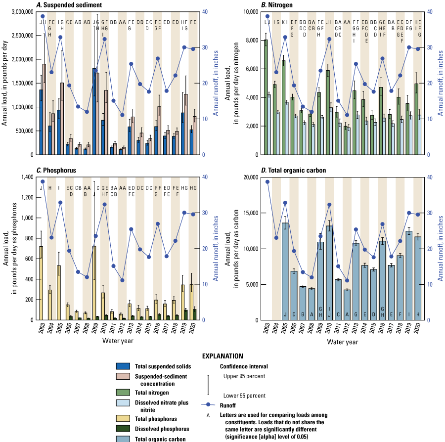
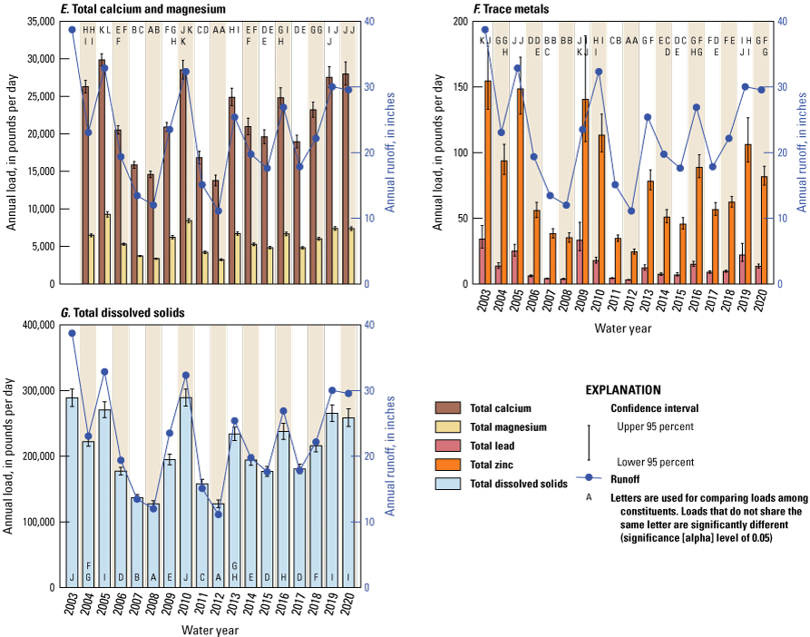
Annual runoff and annual loads of A, suspended sediment, B, nitrogen, C, phosphorus, D, total organic carbon, E, total calcium and magnesium, F, trace metals, and G, total dissolved solids for the Gwinnett County, Georgia, study area, water years 2003–20. ≤, less than or equal to.
Annual loads generally varied with variations in annual runoff (fig. 27A–G). Annual loads were lowest for all constituents in WY 2012 (table 19), which was the second year of a 2-year drought (fig. 9) and had the lowest runoff during the study period (fig. 10B). The year with the highest annual loads varied by constituent (WYs 2003, 2005, 2009, 2010, and 2020). These years all had above average precipitation (fig. 10A) and all years had above average runoff, except WY 2009 for which runoff was near average (fig. 10B).
Annual loads were also influenced by how constituent concentrations change with streamflow (fig. 26A–T). Annual average concentration, the annual load divided by annual runoff, is used to remove the effects of variations in the quantity of runoff to distinguish variations in concentrations (fig. 28A–G). TSS, SSC, TP, DP, TPb, and TZn annual average concentrations were positively related to annual runoff, whereas NO3+NO2, Ca, and TDS concentrations were inversely related to annual runoff. No relations were clear between TN, TOC, and Mg annual average concentrations and annual runoff. The load-runoff range ratio, defined as the ratio of a constituent’s ratio of maximum and minimum annual loads relative to the ratio of the maximum and minimum annual runoff for the same period, is an indication of how much the relations between concentrations and streamflow affect variations in annual loads (table 19). TSS, SSC, TP, and TPb had load-runoff range ratios between 3.2 and 4.8, indicating that the range in annual loads was 3.2–4.8 times larger than the range in runoff. DP and TZn also had proportionally larger ranges in annual loads than for annual runoff but were not as extreme (load-runoff range ratios of 1.8). TN, TOC, and Mg annual load ranges were similar to runoff (load-runoff range ratios 0.8–1.2). NO3+NO2, Ca, and TDS load-runoff range ratios were between 0.6 and 0.7, indicating the range in annual loads was smaller than the range in runoff. These lower ratios result from dilution during stormflow (fig. 26I, O, T) and higher proportions of stormflow during wet years (lower base-flow indices; fig. 10B, D).
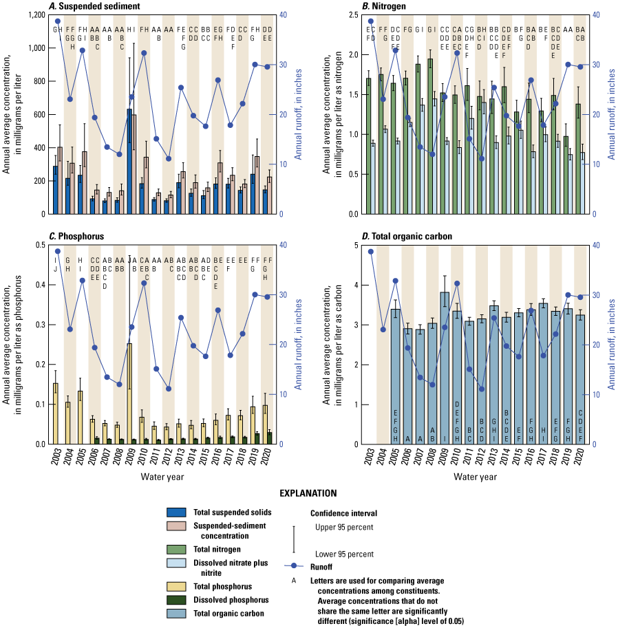
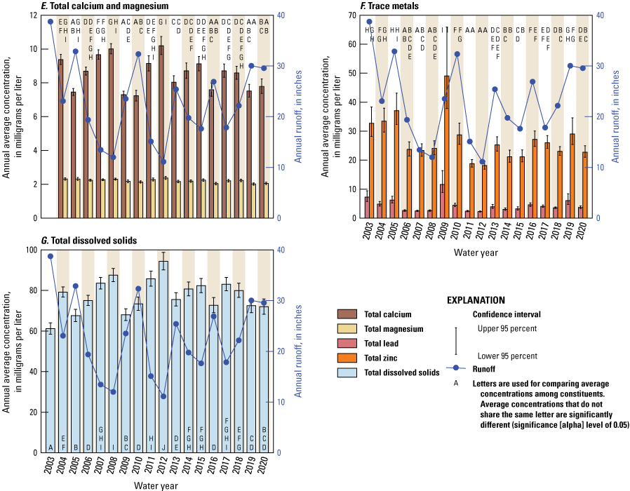
Annual runoff and annual average concentrations of A, suspended sediment, B, nitrogen, C, phosphorus, D, total organic carbon, E, total calcium and magnesium, F, trace metals, and G, total dissolved solids for the Gwinnett County, Georgia, study area, water years 2003–20. ≤, less than or equal to.
There were some deviations from the general patterns observed between annual loads, average concentrations, and runoff. For example, runoff was substantially higher in WY 2010 than in WY 2009, whereas TSS, TP, and TPb loads were higher in WY 2009, and SSC and TZn loads were similar between WYs 2009 and 2010 (fig. 27A, C, F). The annual average concentrations were higher in WY 2009 than in WY 2010 for all five constituents, which deviated from the usual positive relation between concentration and runoff (fig. 28A, C, F). This period followed the 2007–08 drought and may indicate a flushing of particulate materials that built up during the drought, a period with low runoff. Another example of deviations from the usual concentration-runoff relation occurred in WYs 2019–20. Those 2 years had similar, above average amounts of runoff, whereas TSS, SSC, TPb, and TZn loads and average concentrations were significantly higher in WY 2019, and TN loads and average concentrations were significantly higher in WY 2020 (figs. 27A, B, F, and 28A, B, F).
Annual suspended sediment loads were evaluated in more detail to provide insights into sources and transport processes at each watershed because excess sediment is a particular concern in Gwinnett County streams. Supply- and transport-limited behaviors and flushing responses were assessed. A sediment supply-limited behavior is when stream channel transport capacity exceeds incoming sediment, resulting in stream channel erosion. A sediment transport-limited behavior is when stream channel cannot sufficiently transport incoming sediment, resulting in stream channel aggradation. A flushing response is defined here as when sediment builds up in the watershed during dry years and is subsequently flushed when conditions become wet.
To determine if watersheds have a supply-limited or transport-limited behavior, two periods with multiple years of wet hydrologic conditions were examined: WYs 2003–05, for which runoffs in WYs 2003 and 2005 were above average and runoff in WY 2004 was near normal, and WYs 2019–20, for which runoffs were above average. At eight of the watersheds, annual TSS and SSC loads varied similarly with annual runoff, indicating that the amount of sediment transported was dependent upon the amount of runoff to move sediment downstream (transport limited; Sweetwater Creek, Yellow River near Lithonia, Big Haynes Creek, Brushy Fork Creek, Richland Creek, Suwanee Creek, Crooked Creek, and North Fork Peachtree Creek watersheds; fig. 29A, B, D, E, I, K, L, M). TSS and SSC loads from the Apalachee River watershed exhibited a supply-limited behavior as loads were much lower during the last year of both periods (WYs 2003–05, 2019–20), indicating the stream was running out of available sediment to transport (fig. 29H). The remaining four watersheds exhibited mixed behaviors. TSS and SSC loads from the No Business Creek, Alcovy River, and Level Creek watersheds mimicked annual runoff during WYs 2003–05, consistent with transport-limited behavior, whereas loads were much lower in WY 2020 than in WY2019 when annual runoffs were similar, consistent with supply-limited behavior (fig. 29C, F, J).
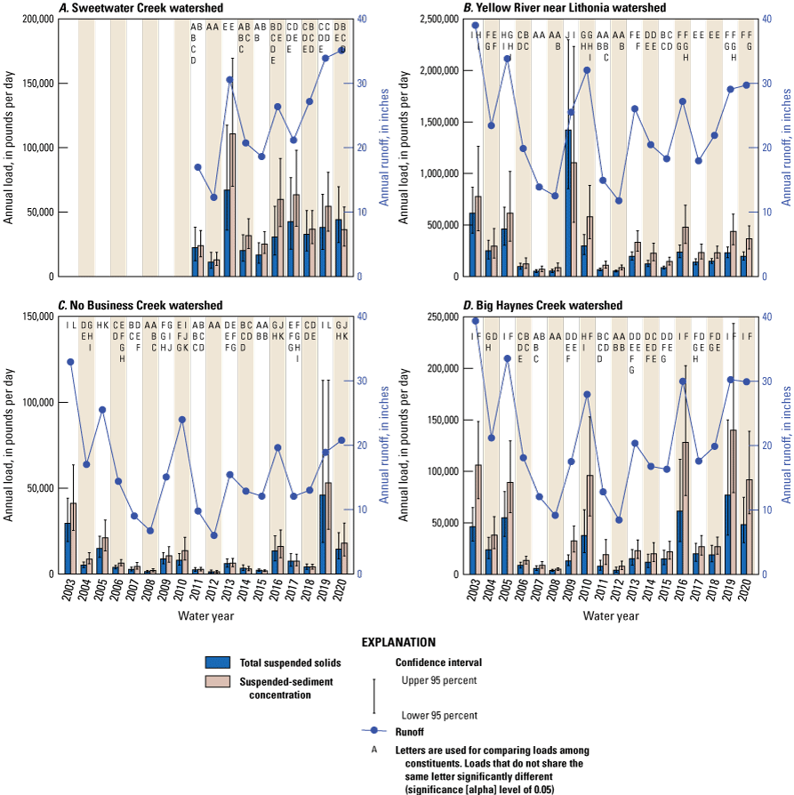
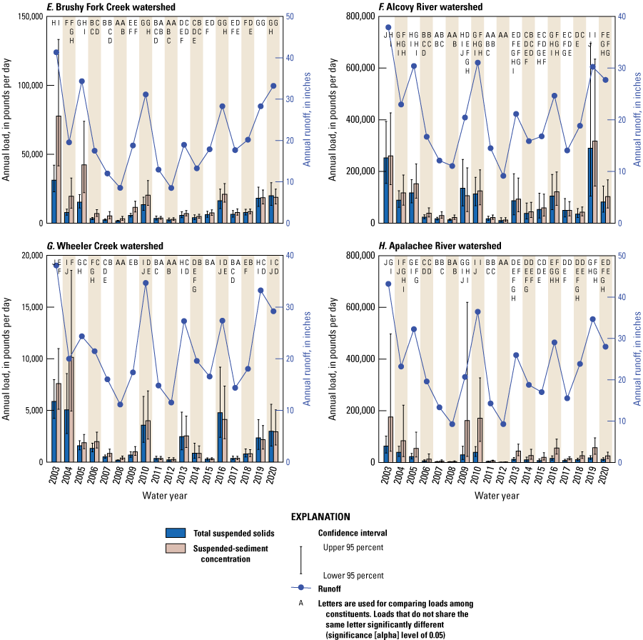
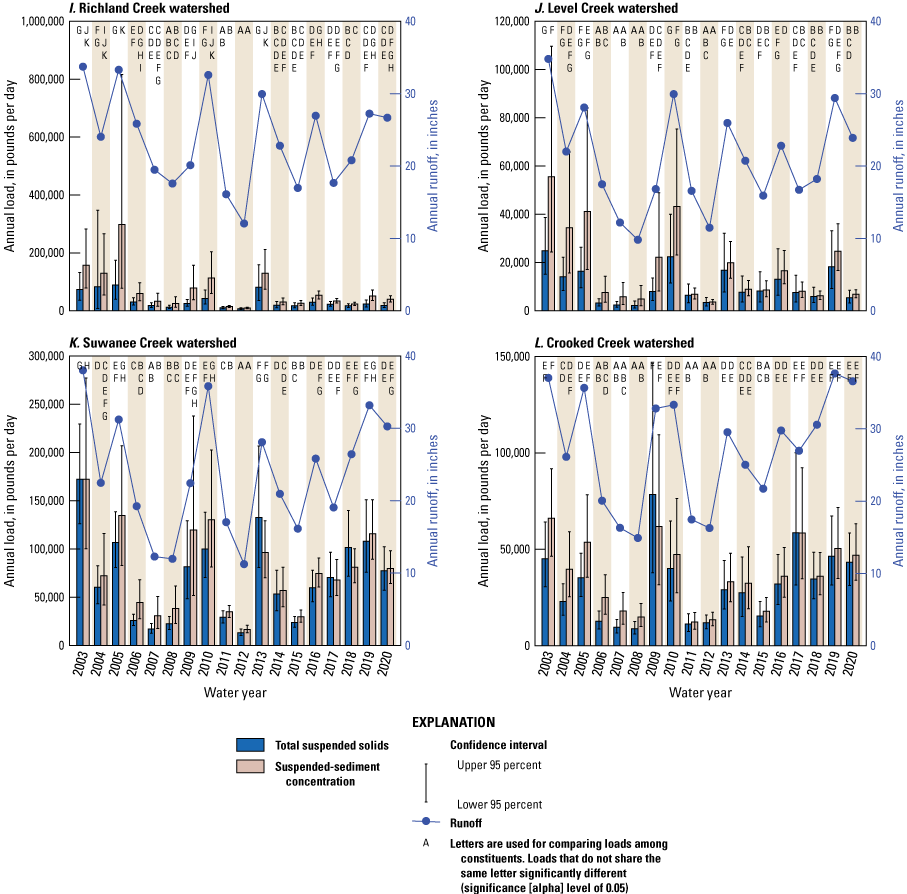
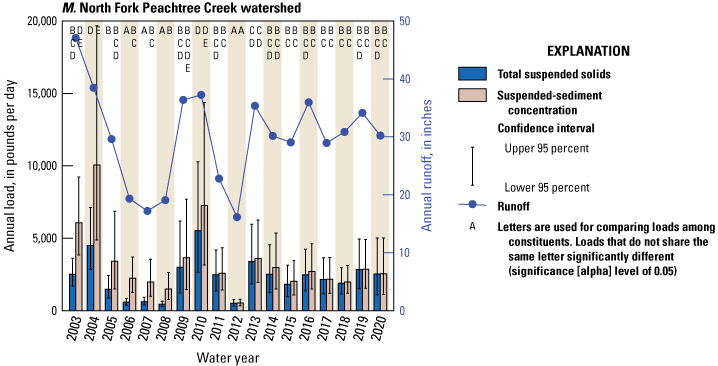
Annual sediment loads for 13 of the monitored watersheds in Gwinnett County, Georgia, water years 2003–20 (Sweetwater Creek watershed, water years 2011–20). ≤, less than or equal to.
To determine whether sediment builds up during drier years and is then flushed when hydrologic conditions wet up, WYs 2009–10 were examined. These 2 years followed a 2-year drought period with below average runoff. WY 2009 had average runoff (except at the Crooked Creek and North Fork Creek watersheds where runoff was above average) and WY 2010 had above average runoff. Annual TSS and SSC loads varied similarly to annual runoff at Big Haynes Creek, Brushy Fork Creek, Wheeler Creek, Suwanee Creek, and North Fork Peachtree Creek watersheds, indicating a transport-limited behavior with no evidence of a substantial flush of sediment (fig. 29D, E, G, J, K, M). TSS and SSC loads from the Yellow River near Lithonia and Crooked Creek watersheds were higher in WY 2009, when hydrologic conditions were wetting up, than in WY 2010 when runoff was above average, indicating a sediment flush (fig. 29B, L). Four watersheds had similar TSS and SSC loads in WYs 2009–10, whereas annual runoff was substantially higher in WY 2010, indicating that some of the loads in WY 2009 may represent the flushing of built-up sediment (No Business Creek, Alcovy River, Apalachee River, and Richland Creek watersheds; fig. 29C, F, H, I), although these flushes were not as substantial as those for the Yellow River near Lithonia and Crooked Creek watersheds.
The variation of annual TSS and SSC loads versus annual runoff at each watershed was also examined. Although there was a linear relation between sediment and runoff for most years, almost every watershed exhibited years where either SSC or both TSS and SSC loads were much higher than expected from the annual sediment-runoff relation (fig. 30). Eleven watershed-WY combinations were identified as having both high TSS and SSC loads, and 22 watershed-WY combinations had higher-than-expected SSC loads (table 20). From previous analyses of these watersheds (Joiner and others, 2014), it was shown that most of the annual suspended sediment load was transported by the few largest storms of the year. Investigating this further, the annual peak flows were retrieved from NWIS database (USGS, 2021d) for the period WYs 2003–20, and WYs of the maximum peak flow and WYs that had peak flows >70 percent of the maximum peak flow were compiled for each watershed. Thirty-three years were identified, which represented 15 percent of the years with peak flow data available (233 years). Of the 32 years with high sediment loads and available peak flow data, 8 years had the maximum peak flow for the period and 10 years had peak flows >70 percent of the maximum peak flows, indicating that 56 percent of the years with higher-than-expected sediment loads also had some of the highest peak flows. Furthermore, the majority of the higher-than-expected sediment years occurred only for SSC (22 of 33 occurrences), which is indicative of more coarse-grained sediments that require higher stream velocities for transport. These observations indicate that higher-than-expected annual sediment loads are frequently the result of one or more large storms that occurred during those years. Other years with higher-than-expected sediment loads could be associated with large discrete streambank failures, which likely occur more frequently during large storm events and wet hydrologic conditions but can occur during any year (Simon and others, 2000).
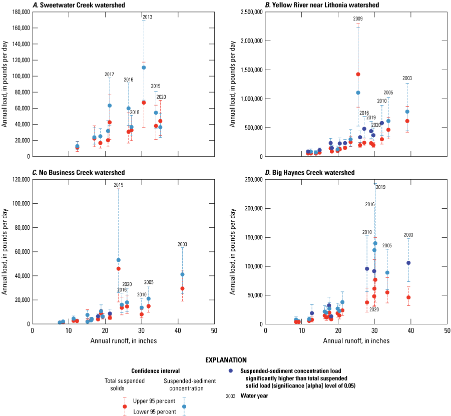
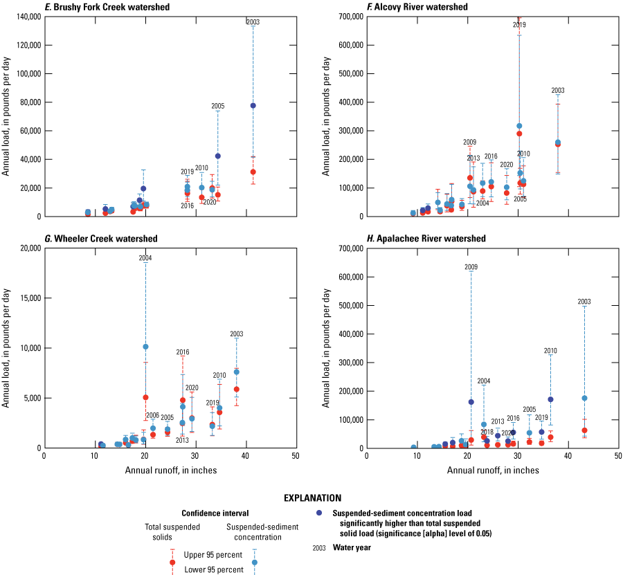
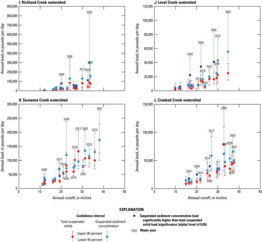
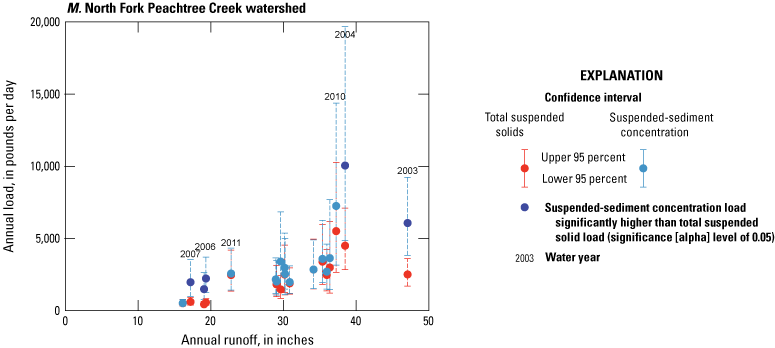
Annual total suspended solids and suspended sediment loads versus annual runoff for 13 of the monitored watersheds in Gwinnett County, Georgia, water years 2003–20 (Sweetwater Creek watershed, water years 2011–20). Water year is indicated for select years. >, greater than.
Table 20.
Compilation of water years when annual total suspended solid and suspended sediment concentration loads were higher than expected for their annual runoff for 13 of the watersheds in Gwinnett County, Georgia, water years 2003–20.[Water years with high peak flows are noted. TSS, total suspended solids; SSC, suspended-sediment concentration; >, greater than, —, no water years with sediment loads higher-than-expected for their annual runoff identified]
Higher-than-expected sediment loads can also be associated with discrete activities within a watershed. Joiner and others (2014) indicated that the high TSS and SSC yields at the Richland Creek watershed in WY 2005 was associated with construction of a large Gwinnett County park adjacent to the stream during that timeframe. Our analysis was consistent with this interpretation because WY 2005 SSC loads were higher than expected even though peak runoff was not particularly high that year (fig. 30I; table 20). The Wheeler Creek watershed exhibited higher-than-expected TSS and SSC loads in WY 2004 and higher-than-expected SSC loads in WY 2003 (fig. 30G; table 20). These loads were the highest observed loads for the period, although these were not statistically different than sediment loads from WYs 2010 and 2016, years with above average runoff (fig. 29G). High sediment loads in WYs 2003–04 were associated with years having high peak flows (>70 percent of the maximum peak flow for the period; table 20); however, the loads stood out as deviating higher than loads in WY 2010, which contained the maximum peak flow for the period, when plotting versus annual runoff. The building density increased rapidly between WYs 2004 and 2006 (fig. 5I), the most rapid density increase observed for any watershed over the 1950–2020 period. Aerial photography from April 2002 indicated a large area of land being prepared for building two schools that opened in August 2004 adjacent to Wheeler Creek in the upstream portion of its watershed. Near this same area, aerial photography from November 2005 shows a partially built housing development adjacent to Wheeler Creek. The high sediment loads in WYs 2003–04 were possibly caused by a combination of sediment from this development activity and high peak streamflows that occurred during this period.
Watershed Constituent Yields
Constituent yields—loads per unit area—are summarized for 12 constituents, by watershed, for the period WYs 2010–20 in figure 31. This 11-year period allows for more consistent comparison with the Sweetwater Creek watershed, which only had yields available for WYs 2011–20. Substantial differences in yields are discussed herein. The TSS yield was highest at the Crooked Creek watershed, and yields at the Alcovy River and Richland Creek watersheds were similarly high (fig. 31A). TSS yields were similarly low at the Sweetwater Creek, Yellow River near Lithonia, No Business Creek, Big Haynes Creek, Brushy Fork Creek, Wheeler Creek, and Suwanee Creek watersheds. The SCC yield was highest at the Apalachee River watershed and was similar to the yield at the Richland Creek watershed. The SSC yield was also high at the Crooked Creek watershed. The Richland Creek watershed has the steepest basin slope of the study watersheds, whereas the Crooked Creek watershed has the second highest imperviousness. SSC yields were significantly higher than TSS yields at the Yellow River near Lithonia, Big Haynes Creek, Apalachee River, and Richland Creek watersheds, whereas SSC and TSS yields were similar at the remaining watersheds. SSC loads, however, have been observed to be substantially greater than TSS loads within individual years at most watersheds, as indicated by the higher SSC loads at nine of the watersheds for years noted in table 20. Sediment in watersheds with higher SSC yields than other watersheds likely had a greater proportion of sand-sized material (Gray and others, 2000).
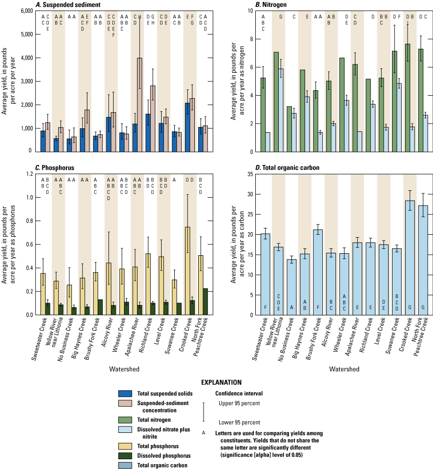
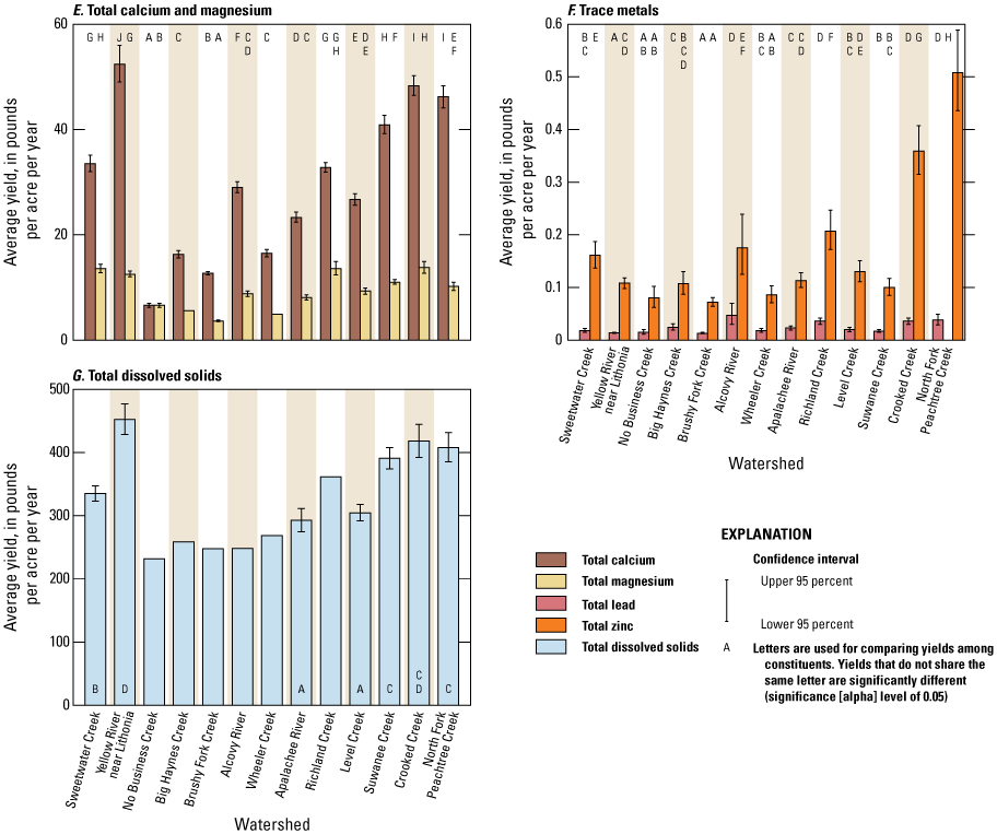
Annual yields of A, suspended sediment, B, nitrogen, C, phosphorus, D, total organic carbon, E, total calcium and magnesium, F, trace metals, and G, total dissolved solids for 13 monitored watersheds in Gwinnett County, Georgia, water years 2010–20 (Sweetwater Creek watershed, water years 2011–20). ≤, less than or equal to.
Variability in TN yields was not large between watersheds (fig. 31B). TN yields were highest in the Yellow River near Lithonia, Wheeler Creek, Apalachee River, Suwanee Creek, Crooked Creek, and North Fork Peachtree Creek watersheds. The TN yield was lowest in the No Business Creek watershed. The NO3+NO2 yield was highest in the Yellow River near Lithonia watershed and was also high in the Suwanee Creek watershed. NO3+NO2 yields were low in the Sweetwater Creek, Brushy Fork Creek, and Apalachee River watersheds. The ratio of NO3+NO2 to TN yields at the Yellow River near Lithonia watershed for the WY 2010–20 period was 0.83, substantially higher than all other watersheds except for the No Business Creek watershed that had a ratio of 0.85. This high ratio indicates an additional and (or) different source of NO3+NO2 in the Yellow River near Lithonia watershed. Nitrogen yields may have been higher at the Yellow River near Lithonia watershed because of contributions of nitrogen in discharge from the Yellow River WRF. Although the facility reduces the concentration of nitrogen, some residual nitrogen in facility effluent is possible, whereas the discharge from the facility represents about 9 percent of runoff from this watershed.
The TP yield was highest at the Crooked Creek watershed and was statistically similar to yields at the Alcovy River, Richland Creek, Level Creek, and North Fork Peachtree Creek watersheds (fig. 31C). Many watersheds had similarly low TP yields. The DP yield was highest at the North Fork Peachtree Creek watershed. TOC yields were highest in the Crooked Creek and North Fork Peachtree Creek watersheds (fig. 31D). TOC yields were also high in the Sweetwater Creek and Brushy Fork Creek watersheds. The other remaining watersheds had similar TOC yields.
The Ca yield was highest at the Yellow River near Lithonia watershed and yields were also high for the Crooked Creek and North Fork Peachtree Creek watersheds (fig. 31E). The Ca yield was lowest at the No Business Creek watershed. Mg yields were highest at the Sweetwater Creek, Yellow River near Lithonia, Richland Creek, and Crooked Creek watersheds and lowest at the Brushy Fork Creek watershed.
TPb yields were highest at the Alcovy River, Richland Creek, Crooked Creek, and North Fork Peachtree Creek watersheds (fig. 31F). TPb yields were lowest at the Yellow River near Lithonia, No Business Creek, and Brushy Fork watersheds. The TZn yield was highest at the North Fork Peachtree Creek watershed and yields were also high in the Sweetwater Creek, Alcovy River, Richland Creek, and Crooked Creek watersheds. TZn yields were lowest at the No Business Creek, Brushy Fork, and Wheeler Creek watersheds.
The TDS yield was highest at the Yellow River near Lithonia watershed and was statistically similar to the yield at the Crooked Creek watershed (fig. 31G). TDS yields were also high at Suwanee Creek and North Fork Peachtree Creek watersheds. TDS yields were similarly low at the No Business Creek, Big Haynes Creek, Brushy Fork Creek, Alcovy River, and Wheeler Creek watersheds.
Relations Between Watershed Constituent Yields and Watershed Characteristics
Correlations between watershed constituent yields and watershed characteristics can provide insights about sources and transport of constituents. Correlations were explored for select watershed characteristics where relations might be expected. Constituent yields were compared to developed low, medium, and high intensity land cover groups, as these are expected to have related effects on water quality. The highest significant correlation is likely the most relevant relation, as the developed medium and high intensity land cover groups were moderately correlated with each other across watersheds (r = 0.620; table 10). Weaker inverse relations with yield may reflect incidental relations. For example, weak inverse relations between yields and developed low intensity groups may reflect the strong correlation of yields with developed high intensity groups along with the moderate inverse correlation between developed low and high intensity groups (r = –0.529). TOC yields had a significant strong correlation and TN, Ca, Mg, TZn, and TDS yields had significant moderate correlations with the developed medium intensity group (table 21). DP, TOC, and TZn yields had significant strong correlations and Ca had a significant moderate relation with the developed high intensity group. A moderate correlation was found between Ca and impervious area within the 200-ft stream buffer (r = 0.689), which could be caused by concrete dissolution along streams near roads, bridges, paths, and sidewalks. Correlations were strong between DP, TOC, and TZn with imperviousness and with impervious area within the 200-ft stream buffer. These constituent yields, however, were among the highest for DP and the highest for TOC and TZn in the Crooked Creek and North Fork Peachtree Creek watersheds (fig. 31C, D, F), and these watersheds also had the two highest levels of imperviousness (table 12) and developed high intensity land cover (fig. 4O, P; table 10). Despite the strong correlations, multiple relations make it difficult to discern whether the variations in these yields between watersheds might be related to activities associated with their land cover types, imperviousness, or a combination of both.
Table 21.
Pearson product-moment correlation coefficients between constituent yields for water years 2010–20 and select watershed characteristics across 13 of the study watersheds in Gwinnett County, Georgia.[Watershed characteristics include land cover percentages for 2016, impervious areas for 2019, and water infrastructure. Statistically significant Pearson product-moment correlation coefficients are in bold font (significance (alpha) level of 0.05). ft, foot]
NO3+NO2 yields were compared to watershed septic densities in order to identify whether the inadequate performance of septic systems might substantially affect stream water NO3+NO2 concentrations. An insignificant, weak correlation was found between these variables (r = 0.491; table 21). After excluding the Yellow River near Lithonia watershed from the calculations because of the possible influence of the WRF effluent on NO3+NO2 yields, the correlation was even weaker (r = 0.317). This may be an indication that septic systems are generally well maintained or that there may be other more important factors that affect the variability in NO3+NO2 yields between watersheds.
Trends in Water Quality
Long-term trends in constituent concentrations and loads were determined for the 12 constituents and 13 watersheds with load estimates for the same two periods used for calibrating the loads, WYs 2003–10 and 2010–20. Trends were fit using quadratic time terms in the flow-only concentration regression models used in estimating loads such that the effects of streamflow, season, and climate are removed. Significant temporal patterns were indicated by the inclusion of the trend terms in the stepwise regression.
To illustrate how model time trend terms fit temporal changes in concentrations, TSS trendlines and TSS model residuals that have not been detrended by excluding turbidity and trend model terms are shown in figure 32. The scatter in the model residuals represents the unexplained variance, and a trend must be sufficiently large relative to this scatter to be identified as significant. Of the 25 watershed-model period combinations, 12 trends were identified: 1 linear trend and 11 quadratic trends. Of these quadratic trends, three did not have significant linear time terms. This finding indicates that even though a significant temporal pattern was identified, the change from the beginning to the end of the period was not significantly different. Eight periods had significant negative trends and one period had a significant positive trend. Trends varied between the two periods at most watersheds except for North Fork Peachtree Creek, where trends were negative during both periods, and four watersheds had no trends during both periods. The largest significant linear trend for TSS was for the Wheeler Creek watershed for the WY 2003–10 period, –13.9 percent per year (fig. 32G). The high loads at the beginning of this period, as previously noted, appeared to be associated with construction in proximity to the creek (figs. 29G and 30G, table 20).
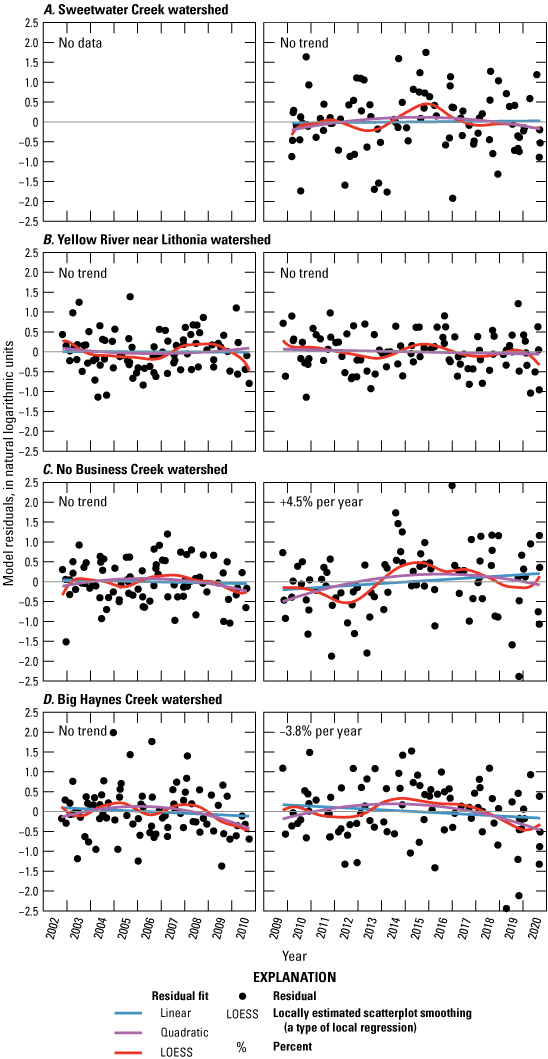
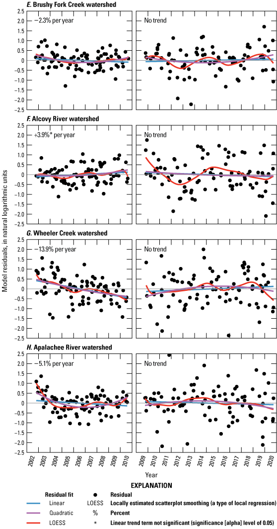
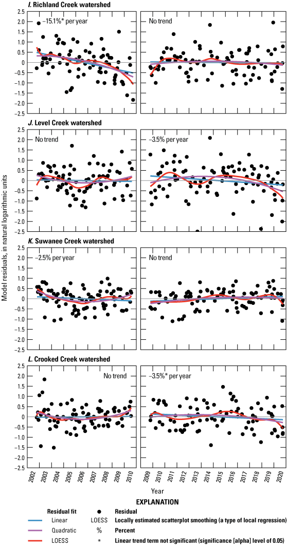
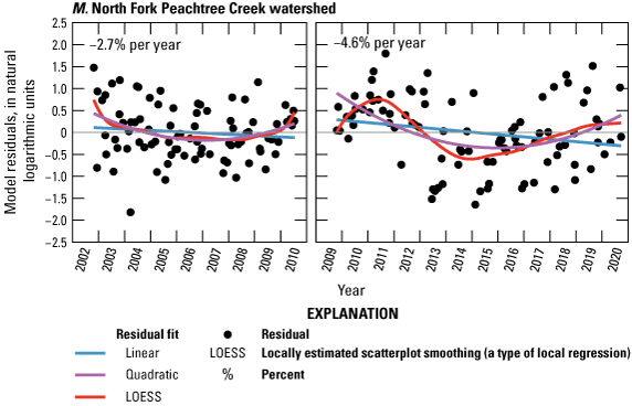
Model residuals and trendlines of the residual fits to total suspended solid regression models fit without trend terms for the two periods water years 2003–10 and 2010–20 for 13 monitored watersheds in Gwinnett County, Georgia.
Trends are summarized by constituent in table 22 and significant trendlines are visually displayed in figure 33. Time trends were identified for 140 of the 300 possible watershed-time period-constituent combinations. Many trends exhibited large variations over their periods while having little net change from their beginnings to ends. Ninety-eight of the trends had a significant linear trend term, of which 57 trends were negative and 41 were positive. The WY 2003–10 period had more negative trends and the WY 2010–20 period had more positive trends. TSS and SSC had the largest net number of negative trends, seven and six, respectively. Mg and TZn had four and three more net negative trends, respectively. TDS exhibited the most net positive trends with seven positive trends and two negative trends. Other constituents had similar numbers of positive and negative trends.
Table 22.
Summary of significant trends in concentrations and loads by water-quality constituent from 13 of the study watersheds in Gwinnett County, Georgia, for the water years 2003–10 and 2010–20 model calibration periods.[All numbers are counts of occurrences. 2d, second]
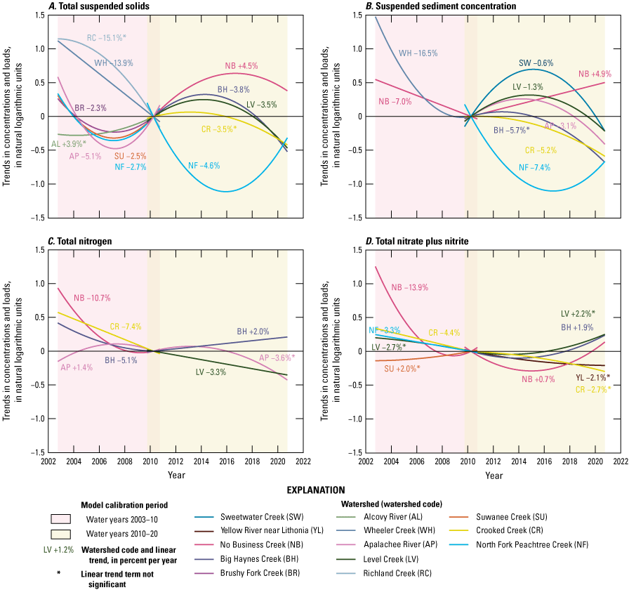
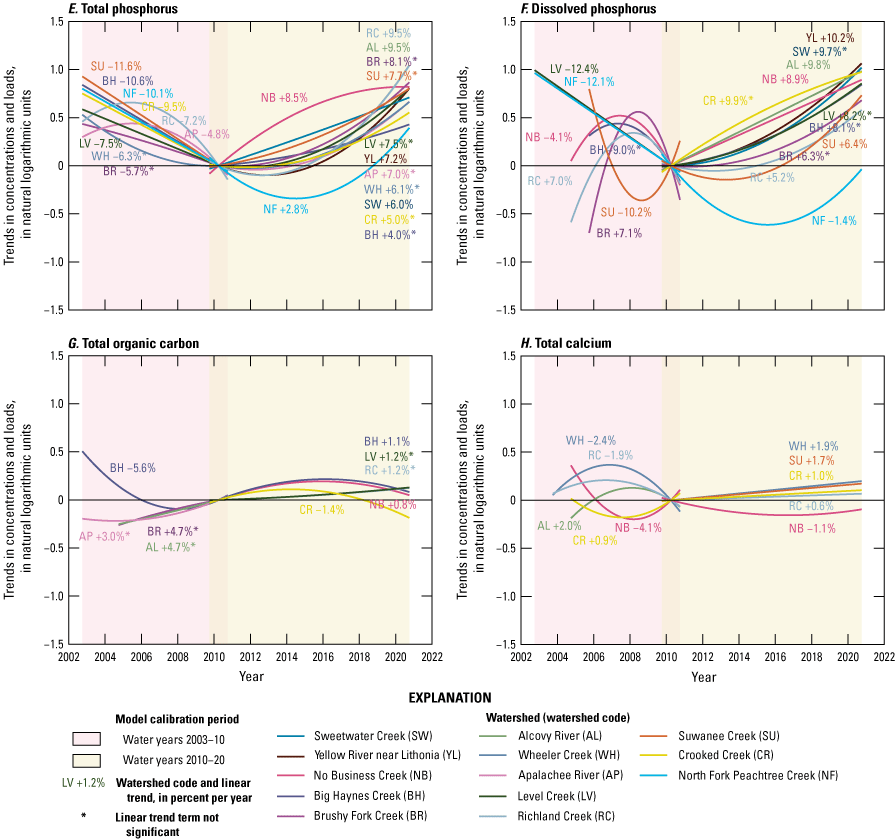
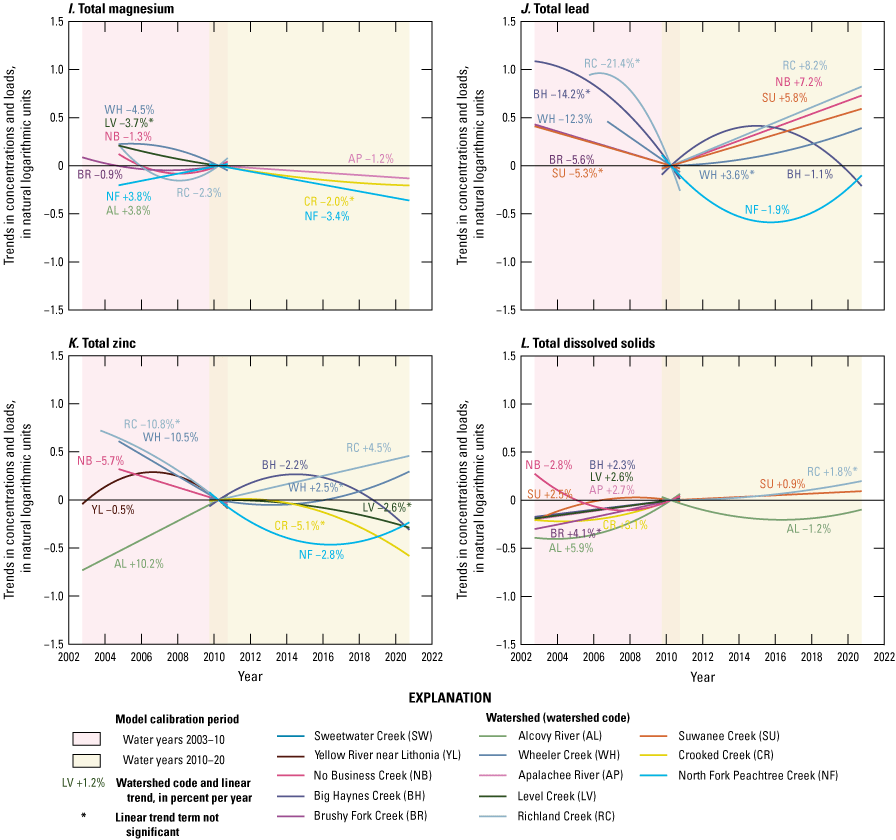
Trendlines for concentrations and loads for the two periods water years 2003–10 and 2010–20 for A, total suspended solids, B, suspended sediment concentration, C, total nitrogen, D, total nitrate plus nitrite, E, total phosphorus, F, dissolved phosphorus, G, total organic carbon, H, total calcium, I, total magnesium, J, total lead, K, total zinc, and L, total dissolved solids for 13 monitored watersheds in Gwinnett County, Georgia. Trendlines are only shown for trends that were significant in the concentration regression models.
TP and DP had the most trends, with many negative trends during WYs 2003–10 and positive trends during WYs 2010–20 (fig. 33E, F). Upon further evaluation of the TP and DP concentration data, however, these trends appear to be artifacts of variations in laboratory reporting limits. During the period November 2005 to December 2018, the laboratory reported concentrations were below the typical reporting limits of around 0.02 mg/L as P. Accurately reported lower concentrations should improve the precision of load estimates because LOADEST normally must estimate the distribution of concentrations below the reporting limit. The period of lower reported concentrations, however, resulted in lower load estimates during this period. The trend terms adjusted for these differences, resulting in the negative and positive trends for the WY 2003–10 and 2010–20 periods, respectively. In these cases, and for these constituents, trends should be disregarded. The only trends that should be considered representative of real changes in loads are at the Big Haynes Creek, Brushy Fork Creek, and Suwanee Creek watersheds for DP for the WY 2003–10 period, because these loads were only calculated for WYs 2006–10, a period that had consistent reporting limits. After excluding the trend results from TP and DP that were influenced by changes in laboratory reporting levels, many more trends were negative than positive during WY 2003–10, whereas the number of negative and positive trends were now similar during WY 2010–20 (table 22).
Trends in concentrations and loads are summarized by watershed in table 23. TP and DP trends that were the result of the changes in the laboratory reporting level are not discussed here and were reported separately in table 23. It is expected that trends for a particular watershed and period might be similar because several constituents have similar sources and transport mechanisms that could be similarly affected. The No Business Creek watershed had seven negative trends during WYs 2003–10 followed by five positive trends during WYs 2010–20. The Wheeler Creek watershed had six negative trends and the Alcovy River had four positive trends during WYs 2003–10. The North Fork Peachtree Creek watershed had five negative trends during WYs 2010–20. Otherwise, no other watersheds had more than three trends in any one direction during each period. Many watersheds exhibited their greatest degree of land cover change within the study period during 2004–08 (fig. 4) and few trends were positive during the WY 2003–10 period. The only evidence of a relation with land cover change was for the Wheeler Creek watershed, where development increased abruptly during the 2001–04 period (fig. 4J). The six negative trends in this watershed during WYs 2003–10 (TSS, SSC, Ca, Mg, TPb, and TZn) appear to be from decreases caused by the effects of development early in the period as opposed to the presence of additional developed land cover later in the study period.
Table 23.
Summary of significant trends in concentrations and loads by study watershed for 12 water-quality constituents, Gwinnett County, Georgia, for model calibration periods water years 2003–10 and 2010–20.[All numbers are counts of occurrences. Counts of trend results from total and dissolved phosphorus that were influenced by changes in laboratory reporting levels are reported separately in parentheses. 2d, second]
Assessment of Changes in Continuous Turbidity Reporting on Loads and Trends
The effects of higher uncensored continuous turbidity values present during WYs 2003–07 on loads and trends were assessed for TSS, SSC, TP, TPb, and TZn, predominantly particulate constituents that frequently utilized turbidity as an explanatory variable (table 17). Although more trends were negative than positive for these constituents for the WY 2003–10 period (table 22), negative trends across most constituents occurred only for the Richland Creek and Wheeler Creek watersheds (fig. 33; not all negative trends were significant). The TSS model residuals do not show a consistent drop between WYs 2003–07 and WYs 2008–10, except possibly at the Apalachee River and Suwannee Creek watersheds (fig. 32). Years with higher-than-expected TSS and SSC loads were identified within WYs 2003–05, corresponding to the period with the highest uncensored continuous turbidity values (table 20). Loads were higher than expected for nine of the watersheds for at least one of these years, but only at the Level Creek watershed for all 3 years, and loads were higher than expected mostly for only SSC. WYs 2003 and 2005, however, had above average precipitation (fig. 10) and many of the higher-than-expected TSS and SSC loads in WYs 2003–05 were associated with the occurrence of high peak flows (8 of 15 cases). The lack of consistent decreases in particulate related constituent concentrations and loads during WYs 2003–10 for most watersheds and the lack of consistently higher-than-expected annual loads in WYs 2003–05 and for both TSS and SSC indicates that any effects of the use of higher uncensored turbidity values early in the study on loads and trends were minor.
Discussion
The state of understanding of processes affecting changes in annual sediment loads in the study watersheds is reviewed along with discussion of the usefulness of various analytical approaches and the utility of turbidity as a surrogate explanatory variable to capture these changes. Relations between changes in stream water quality and watershed characteristics are reviewed, and factors that make it difficult to identify relations are discussed. Future avenues for analyses of sediment transport and for identifying factors that affect stream water quality are provided.
Sediment Transport
This study has the benefit of a long-term data record that allows for a variety of conditions to be examined, including various climate sequences with multiple cycles that allow for the identification and verification of various processes and relations. The long record also improves the opportunity to identify infrequent events that may have large effects on sediment loads but only for short durations. The analysis of annual sediment loads over multiyear periods allows for the assessment of supply- and transport-limited behaviors and flushing responses after droughts on an annual timescale. Most watersheds appear to be transport-limited except for the Apalachee River watershed, which appears to be long-term source limited (fig. 29). Four other watersheds exhibited mixed conditions. Two watersheds, Yellow River near Lithonia and Crooked Creek, had substantial flushing responses and four other watersheds exhibited a less pronounced degree of flushing.
Examining annual sediment loads with respect to annual runoff was also informative (fig. 30). The relation between higher-than-expected TSS and SSC annual loads (based on their annual runoff) and years containing the highest peak flows (table 20) points to the importance of the few largest storms each year in transporting sediment in these watersheds and indicates that the variability in annual loads cannot be ascertained from annual runoff alone. Differences in responses between TSS and SSC loads also provide insights to sources and transport mechanisms because SSC better reflects coarser, sand-sized materials (Gray and others, 2000). Two years with higher-than-expected annual sediment loads appeared to be related to development projects in the vicinity of streams, indicating that these activities can have substantial effects on stream water quality. Because high sediment transport is related to high annual runoff and occurs during years containing the highest peak flows, meeting particulate-based constituent water-quality regulatory standards for loads may be more difficult to achieve in years that have higher than average periods of rainfall.
The effects of years with higher-than-expected annual TSS and SSC loads relative to their annual runoffs (figs. 29 and 30) were not addressed for the related particulate constituents. A precursory analysis of some of these years indicated that for years with both high TSS and SSC, TPb loads increased nearly proportionally with sediment, whereas TZn loads increased but not to the same degree. TP and TOC had less substantial or consistent changes with respect to sediment. In years where only SSC (and not TSS) was higher than expected, increases in TPb and TZn were proportionally less than the increases in SSC and were more comparable to the increases in TSS. Between-year variability in these relations was common. These observations indicate that the additional sediment transported during the years with higher-than-expected sediment loads differed in composition, possibly indicating sediment came from different sources, or in the case of just higher SSC (and not TSS) loads, more coarse-grained associated sediment was transported during the storm events that had the highest peak flows.
The use of sonde turbidity as a surrogate for suspended sediment in the load estimation regression models was crucial in enabling the identification of temporal deviations in sediment transport behavior with streamflow because turbidity tracks these variations. Streamflow-only based concentration models do not describe as much variability in suspended sediment concentrations as the turbidity-based models because the flow-only models do not capture the dynamic changes in sediment concentrations unrelated to streamflow. When sonde turbidity data are not available, the relegated approach is to predict sediment concentrations as the average streamflow response for the calibration period. Furthermore, without the context of turbidity, many high concentrations in sediment samples would likely appear as outliers when modeling versus streamflow. This also points to the importance of prioritizing event sampling across the range of hydrologic events and conditions to better define the relation between constituent concentration and turbidity such that the models can properly predict loads to these infrequent events that transport substantial amounts of sediment and sediment-associated loads.
Future work could include evaluating transport during the largest storms to determine patterns and variability. This could be used to better assess whether changes in annual sediment loads were the result of that year’s occurrence of larger storms (relative to those of other years) or other factors. Evaluations of large storm events could also be used to accurately identify short-term characteristics of sediment transport such as supply- and transport-limitation and flushing. Measuring the distribution of coarse- to fine-grained particulates in suspended sediment samples to determine how they vary with concentration and streamflow could provide insights into the sources and transport of sediment. Insights regarding sediment transport processes can also be used to evaluate best management practices that aim to reduce sediment and sediment-bound constituent loads. More research could be directed toward evaluating whether the higher-than-expected annual sediment loads with respect to annual runoff were the result of high peak flow events or activities within the watersheds. Records of development in watersheds along with historical aerial photography could be utilized, and attributes such as proximity to streams could be useful in assessing potential effects.
Water-Quality Trends and Relating Trends to Urban Development
Correlations were evident between watershed characteristics and hydrology (for example, watershed imperviousness versus runoff metrics, fig. 22); however, relations between watershed characteristics and water quality were less pronounced (table 21). Explaining differences in water quality between watersheds is often difficult because water quality reflects the combined effects of many factors, including but not limited to watershed characteristics, hydrologic and biogeochemical processes, and land-use changes (MacDonald, 2000; Landers and others, 2007), several of which are rarely measured at a level of resolution that allows meaningful statistical comparisons. Effects from discrete point sources within specific watersheds can also be confounding. Temporal changes in watershed BMP implementation and water infrastructure can also affect stream water quality, and the analysis herein only contains a limited assessment of these types of characteristics, such as septic densities and detention pond implementation (figs. 7 and 8, table 14). These factors make determining relations between water-quality trends and changes in watershed characteristics difficult to quantify. Temporal patterns in watershed characteristics were determined for each watershed for eight land cover groups, degree of imperviousness, population density (fig. 4, table 11), and building density (fig. 5) for the study period. There were few relations between these patterns and trends in concentrations and loads (fig. 33) despite the large changes in these characteristics over the study period. In the Wheeler Creek watershed, an early period of rapid land-use change, as indicated by the large increases in the developed land cover groups during 2001–04 (fig. 4J) and the abrupt increase in building densities during 2004-06 (fig. 5I), likely resulted in the negative trends noted for TSS, SSC, Ca, Mg, TPb, and TZn during WYs 2003–10 (fig. 33). If indeed true, this finding indicates that discrete perturbations within a watershed can have substantial effects in addition to any effects of land cover changes with respect to water-quality constituent concentrations and loads.
The difficulty in accurately estimating loads and determining trends is confounded by several factors. The study area experienced recurring drought and wetter than average periods (figs. 9 and 10), which can cause the concentration relations used to estimate loads to vary and result in large variabilities in annual loads (fig. 27, table 19). Attempts were made to minimize the effects of climate on loads and trends in loads by including base flow as an explanatory variable in the concentration models to capture the effects of wetness conditions. To further minimize other potential artifacts, the model calibration periods also started and ended during years having similar hydrologic conditions, namely WYs 2003, 2010, and 2020, which all had above average runoff. Beyond climatic effects on modeling approaches, the role of the largest storms on particulate transport (table 20), the potential short-term effects of land-use change, and punctuated events such as mass streambank failures, add additional variability to loads. Considering all of this variability, analyses covering extended periods of time are often necessary to be able to accurately quantify trends in water quality.
The use of sonde-based turbidity as a surrogate explanatory variable allows for the detection of water-quality responses over shorter time scales. The near continuous sonde water-quality measurements are invaluable because fully sampling every storm would be resource intensive. Turbidity was a particularly useful surrogate for the particulates and particulate-associated constituents, TSS, SSC, TN, TP, TOC, TPb, and TZn (table 17). Constituent relations are naturally stronger specifically for the sediment variables because the other constituents make up only a variable proportion of sediment. The relation between sediment concentration and turbidity is also affected by changes in sediment material and particle-size distributions. For constituents in which surrogate explanatory variables do not accurately explain the variability in concentrations, the models utilized herein rely on the trend terms to predict changes in concentrations and loads. This approach only describes gross temporal shifts in concentrations, however, because these trend terms are not equipped to model discrete and short-term changes in concentrations and loads.
Future work could include a quantitative temporal analysis of detention pond implementation in the watersheds, assuming that data could be obtained from areas within city limits. This analysis could assess the effectiveness of this widely implemented BMP on storm runoff and water quality. Future quantitative approaches to the modeling of these watersheds could include a more comprehensive determination of factors that characterize our complex understanding of water quality. This determination likely would involve multivariate ordination techniques, such as a principal component analyses, that can identify the simultaneous effects of multiple factors. With sufficient data, machine learning techniques could also contribute to these goals. These approaches could allow for the identification of the most influential variables to more effectively explain the temporal variations in stream water quality and assist in the determination of the most effective strategies for potential mitigation.
Summary
The U.S. Geological Survey (USGS), in cooperation with Gwinnett County Department of Water Resources, established the Long-Term Trend Monitoring (LTTM) program in 1996 to monitor and analyze the hydrologic and water-quality conditions in Gwinnett County, Georgia. Gwinnett County is a suburban to urban area northeast of the city of Atlanta, located in north-central Georgia within the Piedmont physiographic province. The LTTM program currently consists of 15 watersheds within the Chattahoochee, Ocmulgee, and Oconee River Basins encompassing ranges of land cover types and sizes (1.3 to 161 square miles). The purpose of this report is to summarize and present analysis of watershed characteristics and hydrologic and water-quality monitoring data collected for water years (WYs) 2002–20, and this report updates the previously published report for the most recent 5 years of data collected. This study of Gwinnett County streams provides a thorough assessment of watershed characteristics, hydrology, and water quality of 15 watersheds. These results improve the understanding of relations among these various aspects of water resources that can then be utilized to identify and mitigate current or future challenges to the hydrology and water quality of these urban and suburban watersheds.
Watershed characteristics, including land-surface elevations, average land-surface slopes, septic densities, sanitary sewer densities, and detention pond locations were characterized for 15 study watersheds. Temporal patterns in watershed characteristics were determined for land cover (2001–19), percent imperviousness (2000–20), population density (2000–20), and building density (1950–2020). Watershed average land-surface slopes ranged from 4.18 to 12.54 percent. The predominant land cover groups in the study area as of 2019 were developed low intensity (26.8 percent), forest (21.6 percent), developed open space (21.0 percent), developed medium intensity (17.1 percent), and developed high intensity (7.47 percent). By 2001, most of the watersheds had at least 45 percent of their land cover composed of developed land cover groups; by 2019, at least 59 percent of each watershed was developed. Land cover changes occurred most rapidly between 2004 and 2008 at most watersheds. Percent imperviousness in the study watersheds ranged from 14.75 to 55.13 percent. The Crooked Creek and North Fork Peachtree Creek watersheds had the highest percentages of developed medium plus high intensity land cover and imperviousness. Population density in the study area averaged 1,489 people per square mile in 2000 and 2,152 people per square mile in 2020. The use of septic versus sanitary sewers was variable within the watersheds.
The study watersheds were continuously monitored for water level (stage), streamflow, and precipitation. Precipitation and runoff were determined at all watersheds for WYs 2002–20, and the hydrologic cycle was evaluated both annually and seasonally. Gwinnett County has undergone reoccurring droughts during this period. In the study area, precipitation averaged 51.5 inches per year (in/yr) and runoff averaged 22.5 in/yr. Actual evapotranspiration was calculated and averaged about 29.0 in/yr assuming no net changes in watershed storage over the period. Variations in annual runoff were largely determined by annual precipitation, but the effects of base-flow contributions from watershed storage and replenishment of watershed storage after droughts were also evident. Runoff varied seasonally and was typically higher during December through March than during June through November. These seasonal patterns resulted from (1) higher base flows caused by increases in watershed storage and higher storm runoff during wetter hydrologic conditions during the dormant season (October through March) and (2) high evapotranspiration and decreases in base flows caused by decreases in watershed storage during the growing season (April through September). Fifty-one percent of runoff occurred as base flow and the remainder occurred as stormflow.
The percentage of impervious area within the watersheds had a large effect on hydrology. Watersheds with higher imperviousness had higher amounts of storm runoff (r = 0.977) and lower amounts of base-flow runoff (r = –0.871). This finding indicates that imperviousness results in more surface runoff and less infiltration to recharge watershed storage that supports base flows.
The study watersheds were continuously monitored for water-quality properties (water temperature, specific conductance [SC], and turbidity). A minimum of eight stream-water samples were collected at each watershed every year to characterize variations in water quality, both hydrologically and seasonally, and included two samples collected during base-flow conditions and six samples collected during storm events. Samples were analyzed for 20 water-quality constituents: water temperature, SC, biochemical oxygen demand (BOD), chemical oxygen demand (COD), pH, turbidity, total suspended solids (TSS), suspended-sediment concentration (SSC), total nitrate plus nitrite (NO3+NO2), total ammonia plus organic nitrogen (TKN), dissolved ammonia (NH3), total phosphorus (TP), dissolved phosphorus (DP), total organic carbon (TOC), total calcium (Ca), total magnesium (Mg), total copper (TCu), total lead (TPb), total zinc (TZn), and total dissolved solids (TDS). Total nitrogen (TN) was calculated from the summation of NO3+NO2 and TKN.
Seasonal, diurnal, and storm-related variations were observed in the continuously monitored water-quality data. Turbidity was positively related to streamflow but was not completely in sync with streamflow during stormflow conditions. Temperature varied seasonally, diurnally, and with storm runoff. SC decreased as streamflow increased during stormflow conditions, indicating that dissolved constituents were typically more dilute during storms. SC increased with decreasing base flow, reflecting larger contributions of waters with longer transit times, and exhibited diurnal patterns.
Sample-based concentrations of water-quality constituents were compared by watershed and by hydrologic condition (base flow and stormflow). Concentrations were about one-half or more orders of magnitude higher in stormflow samples than in base-flow samples for TSS, SSC, TP, TCu, TPb, and TZn and were also significantly higher in stormflow samples at most watersheds for BOD, COD, turbidity, TN, TKN, TP, and TOC. Concentrations were significantly higher in base-flow samples at most watersheds for SC and Ca, whereas differences in base flow and stormflow for the other constituents varied by watershed. TN, NO3+NO2, and storm sample TP concentrations were mostly above the U.S. Environmental Protection Agency established ambient water-quality potential reference conditions, whereas TP concentrations in base-flow samples were near or below the reference condition. TCu, TPb, and TZn concentrations in base flow infrequently exceeded the national recommended aquatic life criteria for chronic conditions; however, TCu and TZn stormflow concentrations exceeded the acute criteria to varying degrees.
Stream-water loads and yields were estimated for 12 constituents (TSS, SSC, TN, NO3+NO2, TP, DP, TOC, Ca, Mg, TPb, TZn, and TDS) for WYs 2003–20. A regression-model method was used for constituents that had a moderate to strong concentration-model relation; otherwise, the Beale ratio estimator was used. Concentrations were fit to the explanatory variables streamflow, base flow, season, time, and turbidity using a forward stepwise multiple linear regression. The load estimation methodology was modified by using a time-step approach that accommodated incorporation of storm-composited samples into the concentration–streamflow relations. Loads and their uncertainties were estimated by using the USGS load estimator (LOADEST) software.
Patterns in annual constituent loads were positively related to variations in annual runoff. The proportional range of annual loads for SSC, TSS, TP, and TPb, however, were 3.2 to 4.8 times larger than the proportional range in annual runoff, indicating that an increase in annual runoff can result in a several times larger increase in annual load. DP and TZn also had proportionally larger ranges in loads but the differences were not as extreme. TSS, SSC, TP, and TPb loads had high levels of uncertainties, whereas TN, NO3+NO2, TOC, Ca, Mg, and TDS had low levels of uncertainties and exhibited less interannual variability. Most watersheds appear to have transport-limited conditions on an annual timeframe, whereas the Apalachee River watershed had a long-term supply-limited condition and four other watersheds exhibited mixed behaviors. The Yellow River near Lithonia and Crooked Creek watersheds exhibited substantial flushing of sediment that accumulated during the 2007–08 drought, and four other watersheds also exhibited lesser amounts of flushing. Annual TSS and SSC loads were plotted versus annual runoff for each watershed and 33 instances where TSS and SSC or SSC loads were well above the typical relation between annual load and annual runoff were inventoried. Of these instances, 56 percent of the years also had some of the highest peak flows during the period. This observation illustrates the importance of large stormflow events in determining annual sediment transport and indicates that incorporating approaches to mitigate the effects of these events would be helpful in sediment management. Two instances of high annual sediment loads appear to be associated with construction projects adjacent to the stream channel during those years.
TSS yields were highest in the Alcovy River, Richland Creek, and Crooked Creek watersheds, whereas SSC yields were highest in the Apalachee River and Richland Creek watersheds. Constituent yields were typically among the highest in the Crooked Creek and North Fork Peachtree Creek watersheds for TN, TP, DP, TOC, Ca, TPb, TZn, and TDS. These watersheds had the two highest amounts of developed medium plus high intensity land cover and two highest percentages of imperviousness. The Yellow River near Lithonia watershed had the highest yields in NO3+NO2, Ca, and TDS. Ca and TDS yields may reflect the longer water residence times of this large watershed, and NO3+NO2 yields may be affected by effluent from the Yellow River water reclamation facility. Moderate to strong correlations were identified between TN, TP, TOC, Ca, Mg, TZn, and TDS yields and the percentage developed medium and high intensity land cover groups.
Temporal trends in concentrations and loads were identified for 140 of the 300 possible watershed-time period-constituent combinations. Many more trends were identified as negative than positive during WYs 2003–10, whereas the number of negative and positive trends were similar during WYs 2010–20 (after removing trends that were the artifacts of changes in TP and DP reporting limits). TSS and SSC had the largest net number of negative trends, seven and six, respectively. Mg and TZn had four and three net negative trends, respectively, and TDS had five net positive trends. Consistent trends for multiple water-quality constituents were observed at the No Business Creek (seven negative trends during WYs 2003–10 and five positive trends during WYs 2010–20), Alcovy River (four positive trends during WYs 2003–10), Wheeler Creek (six negative trends during WYs 2003–10), and the North Fork Peachtree Creek (five negative trends during WYs 2010–20) watersheds. Trends did not appear to be associated with temporal changes in development or imperviousness. The negative trends observed for the Wheeler Creek watershed during WYs 2003–10, however, appear to be the result of high yields at the beginning of this period and were possibly associated with development of schools and a housing development adjacent to Wheeler Creek and the observed rapid increase in the land cover groups related to development during 2001–04.
References Cited
Akaike, H., 1974, A new look at the statistical model identification: IEEE Transactions on Automatic Control, v. 19, no. 6, p. 716–723, accessed July 11, 2020, at https://doi.org/10.1109/TAC.1974.1100705.
American Public Health Association, 2018a, 2510 Conductivity—Standard methods—For the examination of water and wastewater (2017): American Public Health Association web page, accessed July 11, 2020, at https://www.standardmethods.org/doi/10.2105/SMWW.2882.027.
American Public Health Association, 2018b, 2540 Solids—Standard methods—For the examination of water and wastewater (2017): American Public Health Association web page, accessed July 11, 2020, at https://www.standardmethods.org/doi/10.2105/SMWW.2882.030.
American Public Health Association, 2018c, 4500-H+ pH value—Standard methods—For the examination of water and wastewater (2017): American Public Health Association web page, accessed July 11, 2020, at https://www.standardmethods.org/doi/10.2105/SMWW.2882.082.
American Public Health Association, 2018d, 5210 Biochemical oxygen demand (BOD)— Standard methods—For the examination of water and wastewater: American Public Health Association web page, accessed July 11, 2020, at https://www.standardmethods.org/doi/10.2105/SMWW.2882.102.
American Public Health Association, 2018e, 5310 Total organic carbon (TOC)— Standard methods—For the examination of water and wastewater (2017): American Public Health Association web page, accessed July 11, 2020, at https://www.standardmethods.org/doi/10.2105/SMWW.2882.104.
Anderson, C.W., 2005, Turbidity: U.S. Geological Survey Techniques of Water-Resources Investigations, book 9, chap. A6, section 6.7, 55 p., accessed July 11, 2020, at https://doi.org/10.3133/twri09A6.7.
Aulenbach, B.T., 2013, Improving regression-model-based streamwater constituent load estimates derived from serially correlated data: Journal of Hydrology, v. 503, p. 55–66, accessed July 11, 2020, at https://doi.org/10.1016/j.jhydrol.2013.09.001.
Aulenbach, B.T., Burns, D.A., Shanley, J.B., Yanai, R.D., Bae, K., Wild, A.D., Yang, Y., and Yi, D., 2016, Approaches to stream solute load estimation for solutes with varying dynamics from five diverse small watersheds: Ecosphere, v. 7, no. 6, article e01298, 22 p., accessed July 11, 2020, at https://doi.org/10.1002/ecs2.1298.
Aulenbach, B.T., Henley, J.C., and Hopkins, K.G., 2023, Watershed characteristics and streamwater constituent load data, models, and estimates for 15 watersheds in Gwinnett County, Georgia, 2000–2020: U.S. Geological Survey data release, https://doi.org/10.5066/P9G8HZTY.
Aulenbach, B.T., Joiner, J.K., and Painter, J.A., 2017a, Hydrology and water quality in 13 watersheds in Gwinnett County, Georgia, 2001–15: U.S. Geological Survey Scientific Investigations Report 2017–5012, 82 p., accessed July 11, 2020, at https://doi.org/10.3133/sir20175012.
Aulenbach, B.T., Kolb, K., Joiner, J.K., and Knaak, A.E., 2022, Hydrology and water quality in 15 watersheds in DeKalb County, Georgia, 2012–16: U.S. Geological Survey Scientific Investigations Report 2021–5126, 105 p., accessed January 7, 2022, at https://doi.org/10.3133/sir20215126.
Aulenbach, B.T., Landers, M.N., Musser, J.W., and Painter, J.A., 2017b, Effects of impervious area and BMP implementation and design on storm runoff and water quality in eight small watersheds: Journal of the American Water Resources Association, v. 53, no. 2, p. 382–399, accessed July 11, 2020, at https://doi.org/10.1111/1752-1688.12501.
Bodí, M.B., Martin, D.A., Balfour, V.N., Santín, C., Doerr, S.H., Pereira, P., Cerdà, A., and Mataix-Solera, J., 2014, Wildland fire ash—Production, composition and eco-hydro-geomorphic effects: Earth-Science Reviews, v. 130, p. 103–127, accessed June 26, 2020, at https://doi.org/10.1016/j.earscirev.2013.12.007.
Bornstein, R., and Lin, Q., 2000, Urban heat islands and summertime convective thunderstorms in Atlanta—Three case studies: Atmospheric Environment, v. 34, no. 3, p. 507–516, accessed July 11, 2020, at https://doi.org/10.1016/S1352-2310(99)00374-X.
Carlisle, D.M., Wolock, D.M., Konrad, C.P., McCabe, G.J., Eng, K., Grantham, T.E, and Mahler, B., 2019, Flow modification in the Nation’s streams and rivers: U.S. Geological Survey Circular 1461, 75 p., accessed May 9, 2022, at https://doi.org/10.3133/cir1461.
Cohn, T.A., 1988, Adjusted maximum likelihood estimation of the moments of lognormal populations from type I censored samples: U.S. Geological Survey Open-File Report 88–350, 34 p., accessed July 11, 2020, at https://doi.org/10.3133/ofr88350.
Cohn, T.A., Caulder, D.L., Gilroy, E.J., Zynjuk, L.D., and Summers, R.M., 1992, The validity of a simple statistical model for estimating fluvial constituent loads—An empirical study involving nutrient loads entering Chesapeake Bay: Water Resources Research, v. 28, no. 9, p. 2353–2363, accessed July 11, 2020, at https://doi.org/10.1029/92WR01008.
Cohn, T.A., DeLong, L.L., Gilroy, E.J., Hirsch, R.M., and Wells, D.K., 1989, Estimating constituent loads: Water Resources Research, v. 25, no. 5, p. 937–942, accessed July 11, 2020, at https://doi.org/10.1029/WR025i005p00937.
Crawford, C.G., 1991, Estimation of suspended-sediment rating curves and mean suspended-sediment loads: Journal of Hydrology, v. 129, no. 1–4, p. 331–348, accessed July 11, 2020, at https://doi.org/10.1016/0022-1694(91)90057-O.
Debbage, N., and Shepherd, J.M., 2018, The influence of urban development patterns on streamflow characteristics in the Charlanta megaregion: Water Resources Research, v. 54, no. 5, p. 3728–3747, accessed July 11, 2020, at https://doi.org/10.1029/2017WR021594.
DeGasperi, C.L., Berge, H.B., Whiting, K.R., Burkey, J.J., Cassin, J.L., and Fuerstenberg, R.R., 2009, Linking hydrologic alteration to biological impairment in urbanizing streams of the Puget Lowland, Washington, USA: Journal of the American Water Resources Association, v. 45, no. 2, p. 512–533, accessed July 11, 2020, at https://doi.org/10.1111/j.1752-1688.2009.00306.x.
Diem, J.E., Hill, T.C., and Milligan, R.A., 2018, Diverse multi-decadal changes in streamflow within a rapidly urbanizing region: Journal of Hydrology, v. 556, p. 61–71, accessed July 11, 2020, at https://doi.org/10.1016/j.jhydrol.2017.10.026.
Dixon, P.G., and Mote, T.L., 2003, Patterns and causes of Atlanta’s urban heat island–Initiated precipitation: Journal of Applied Meteorology, v. 42, no. 9, p. 1273–1284, accessed July 11, 2020, at https://doi.org/10.1175/1520-0450(2003)042<1273:PACOAU>2.0.CO;2.
Dolan, D.M., Yui, A.K., and Geist, R.D., 1981, Evaluation of river load estimation methods for total phosphorus: Journal of Great Lakes Research, v. 7, no. 3, p. 207–214, accessed July 11, 2020, at https://doi.org/10.1016/S0380-1330(81)72047-1.
Earl, S.R., and Blinn, D.W., 2003, Effects of wildfire ash on water chemistry and biota in south-western U.S.A. streams: Freshwater Biology, v. 48, no. 6, p. 1015–1030, accessed June 16, 2020, at https://doi.org/10.1046/j.1365-2427.2003.01066.x.
Edwards, T.K., and Glysson, G.D., 1999, Field methods for measurement of fluvial sediment: U.S. Geological Survey Techniques of Water-Resources Investigations, book 3, chap. C2, 89 p., accessed May 29, 2022, at https://doi.org/10.3133/twri03C2.
Ekström, M., Jones, P.D., Fowler, H.J., Lenderink, G., Buishand, T.A., and Conway, D., 2007, Regional climate model data used within the SWURVE project 1—Projected changes in seasonal patterns and estimation of PET: Hydrology and Earth System Sciences Discussions, European Geosciences Union, v. 11, no. 3, p. 1069–1083, accessed April 4, 2022, at https://doi.org/10.5194/hess-11-1069-2007.
Espey, W.H., Morgan, C.W., and Masch, F.D., 1966, Study of some effects of urbanization on storm runoff from a small watershed: Texas Water Development Board Report 23, 110 p., accessed November 1, 2019, at https://repositories.lib.utexas.edu/handle/2152/64863.
Esri, 2021, ArcGIS Pro (ver. 2.9.2): Esri website, accessed May 19, 2022, at https://www.esri.com/en-us/arcgis/products/arcgis-pro/overview.
Ferguson, R.I., 1986, River loads underestimated by rating curves: Water Resources Research, v. 22, no. 1, p. 74–76, accessed April 20, 2020, at https://doi.org/10.1029/WR022i001p00074.
Gebert, W.A., Rose, W.J., and Garn, H.S., 2012, Evaluation of the effects of Middleton’s stormwater-management activities on streamflow and water-quality characteristics of Pheasant Branch, Dane County, Wisconsin 1975–2008: U.S. Geological Survey Scientific Investigations Report 2012–5014, 27 p., 2 app., accessed July 11, 2020, at https://doi.org/10.3133/sir20125014.
Goldstein, H., and Healy, M.J.R., 1995, The graphical presentation of a collection of means: Journal of the Royal Statistical Society, Series A (Statistics in Society), v. 158, no. 1, p. 175–177, accessed July 11, 2020, at https://doi.org/10.2307/2983411.
Graf, W.L., 1977, Network characteristics in suburbanizing streams: Water Resources Research, v. 13, no. 2, p. 459–463, accessed July 11, 2020, at https://doi.org/10.1029/WR013i002p00459.
Gray, J.R., Glysson, G.D., Turcios, L.M., and Schwarz, G.E., 2000, Comparability of suspended-sediment concentration and total suspended solids data: U.S. Geological Survey Water-Resources Investigations Report 2000–4191, 20 p., accessed July 11, 2020, at https://doi.org/10.3133/wri004191.
Gregory, M.B., and Calhoun, D.L., 2007, Physical, chemical, and biological responses of streams to increasing watershed urbanization in the Piedmont Ecoregion of Georgia and Alabama, 2003, chap. B of Effects of urbanization on stream ecosystems in six metropolitan areas of the United States: U.S. Geological Survey Scientific Investigations Report 2006–5101–B, 104 p., accessed July 11, 2020, at https://doi.org/10.3133/sir20065101B.
Grubbs, F.E., and Beck, G., 1972, Extension of sample sizes and percentage points for significance tests of outlying observations: Technometrics, v. 14, no. 4, p. 847–854, accessed May 10, 2022, at https://doi.org/10.1080/00401706.1972.10488981.
Gwinnett County Information Technology Services, 2021, Cadstral data (October 2021): Gwinnett County Government web page, accessed December 2021 at https://www.gwinnettcounty.com/web/gwinnett/departments/informationtechnologyservices/geographicinformationsystems/gisdataandmapsales/-/mapsales/produ ct/GIS_SET-1.
Helsel, D.R., 1990, Less than obvious—Statistical treatment of data below the detection limit: Environmental Science & Technology, v. 24, no. 12, p. 1766–1774, accessed August 3, 2020, at https://doi.org/10.1021/es00082a001.
Helsel, D.R., Hirsch, R.M., Ryberg, K.R., Archfield, S.A., and Gilroy, E.J., 2020, Statistical methods in water resources: U.S. Geological Survey Techniques and Methods, book 4, chap. A3, 458 p., accessed March 5, 2021, at https://doi.org/10.3133/tm4a3. [Supersedes USGS Techniques of Water-Resources Investigations, book 4, chap. A3, version 1.1.]
Hem, J.D., 1982, Conductance—A collective measure of dissolved ions, in Minear, R.A., and Keith, L.H., eds., Water analysis, volume 1—Inorganic species, part 1: Orlando, Fla., Academic Press, p. 137–161, accessed May 20, 2022, at https://doi.org/10.1016/B978-0-12-498301-4.50009-8.
Hollis, G.E., 1975, The effect of urbanization on floods of different recurrence intervals: Water Resources Research, v. 11, no. 3, p. 431–435, accessed July 11, 2020, at https://doi.org/10.1029/WR011i003p00431.
Homer, C.G., Dewitz, J.A., Yang, L., Jin, S., Danielson, P., Xian, G., Coulston, J., Herold, N.D., Wickham, J.D., and Megown, K., 2015, Completion of the 2011 National Land Cover Database for the conterminous United States—Representing a decade of land cover change information: Photogrammetric Engineering and Remote Sensing, v. 81, no. 5, p. 345–354, accessed March 14, 2023, at https://www.sciencedirect.com/science/article/abs/pii/S0099111215301002.
Hopkins, K.G., Bhaskar, A.S., Woznicki, S.A., and Fanelli, R.M., 2020, Changes in event‐based streamflow magnitude and timing after suburban development with infiltration‐based stormwater management: Hydrological Processes, v. 34, no. 2, p. 387–403, accessed September 28, 2020, at https://doi.org/10.1002/hyp.13593.
Horowitz, A.J., 2003, An evaluation of sediment rating curves for estimating suspended sediment concentrations for subsequent flux calculations: Hydrological Processes, v. 17, no. 17, p. 3387–3409, accessed July 11, 2020, at https://doi.org/10.1002/hyp.1299.
Horowitz, A.J., 2009, Monitoring suspended sediments and associated chemical constituents in urban environments—Lessons from the City of Atlanta, Georgia, USA Water Quality Monitoring Program: Journal of Soils and Sediments, v. 9, no. 4, p. 342–363, accessed July 11, 2020, at https://doi.org/10.1007/s11368-009-0092-y.
Inamdar, S.P., Mostaghimi, S., McClellan, P.W., and Brannan, K.M., 2001, BMP impacts on sediment and nutrient yields from an agricultural watershed in the coastal plain region: Transactions of the ASAE, American Society of Agricultural Engineers, v. 44, no. 5, p. 1191–1200, accessed July 11, 2020, at https://doi.org/10.13031/2013.6449.
Jacobson, C.R., 2011, Identification and quantification of the hydrological impacts of imperviousness in urban catchments—A review: Journal of Environmental Management, v. 92, no. 6, p. 1438–1448, accessed July 11, 2020, at https://doi.org/10.1016/j.jenvman.2011.01.018.
Jastram, J.D., Moyer, D.L., and Hyer, K.E., 2009, A comparison of turbidity-based and streamflow-based estimates of suspended-sediment concentrations in three Chesapeake Bay tributaries: U.S. Geological Survey Scientific Investigations Report 2009–5165, 37 p., accessed October 20, 2020, at https://doi.org/10.3133/sir20095165.
Johnson, A.H., 1979, Estimating solute transport in streams from grab samples: Water Resources Research, v. 15, no. 5, p. 1224–1228, accessed July 11, 2020, at https://doi.org/10.1029/WR015i005p01224.
Joiner, J.K., Aulenbach, B.T., and Landers, M.N., 2014, Watershed characteristics and water-quality trends and loads in 12 watersheds in Gwinnett County, Georgia: U.S. Geological Survey Scientific Investigations Report 2014–5141, 79 p., accessed July 11, 2020, at https://doi.org/10.3133/sir20145141.
Journey, C.A., Van Metre, P.C., Waite, I.R., Clark, J.M., Button, D.T., Nakagaki, N., Qi, S.L., Munn, M.D., and Bradley, P.M., 2018, Nutrient enrichment in wadeable urban streams in the Piedmont Ecoregion of the Southeastern United States: Heliyon, v. 4, no. 11, article e00904, 24 p., accessed July 11, 2020, at https://doi.org/10.1016/j.heliyon.2018.e00904.
Kirchner, J., 2001, Data analysis toolkit #5—Uncertainty analysis and error propagation: Berkeley, Calif., University of California, Analysis of Environmental Data Course, 8 p., accessed January 17, 2017, at http://seismo.berkeley.edu/~kirchner/eps_120/Toolkits/Toolkit_05.pdf.
Konrad, C.P., 2003, Effects of urban development on floods: U.S. Geological Survey Fact Sheet 076–03, 4 p., accessed September 28, 2020, at https://doi.org/10.3133/fs07603.
Ku, H.F.H., Hagelin, N.W., and Buxton, H.T., 1992, Effects of urban storm-runoff control on ground-water recharge in Nassau County, New York: Ground Water, v. 30, no. 4, p. 507–514, accessed July 11, 2020, at https://doi.org/10.1111/j.1745-6584.1992.tb01526.x.
Landers, M.N., 2013, Total suspended solids concentrations and yields for water-quality monitoring stations in Gwinnett County, Georgia, 1996–2009: U.S. Geological Survey Open-File Report 2013–1145, 10 p., accessed July 11, 2020, at https://doi.org/10.3133/ofr20131145.
Landers, M.N., Ankcorn, P.D., and McFadden, K.W., 2007, Watershed effects on streamflow quantity and quality in six watersheds of Gwinnett County, Georgia: U.S. Geological Survey Scientific Investigations Report 2007–5132, 62 p., accessed July 11, 2020, at https://doi.org/10.3133/sir20075132.
Leopold, L.B., 1968, Hydrology for urban land planning—A guidebook on the hydrologic effects of urban land use: U.S. Geological Survey Circular 554, 18 p., accessed July 11, 2020, at https://doi.org/10.3133/cir554.
Likens, G.E., 2001, Biogeochemistry, the watershed approach—Some uses and limitations: Marine and Freshwater Research, v. 52, no. 1, p. 5–12, accessed July 11, 2020, at https://doi.org/10.1071/MF99188.
Lim, K.J., Engel, B.A., Tang, Z., Choi, J., Kim, K.-S., Muthukrishnan, S., and Tripathy, D., 2005, Automated Web GIS based Hydrograph Analysis Tool, WHAT: Journal of the American Water Resources Association, v. 41, no. 6, p. 1407–1416, accessed July 11, 2020, at https://doi.org/10.1111/j.1752-1688.2005.tb03808.x.
Liu, Y.B., Gebremeskel, S., De Smedt, F., Hoffmann, L., and Pfister, L., 2006, Predicting storm runoff from different land-use classes using a geographical information system-based distributed model: Hydrological Processes, v. 20, no. 3, p. 533–548, accessed July 11, 2020, at https://doi.org/10.1002/hyp.5920.
MacDonald, L.H., 2000, Evaluating and managing cumulative effects—Process and constraints: Environmental Management, v. 26, no. 3, p. 299–315, accessed July 11, 2020, at https://doi.org/10.1007/s002670010088.
Maher, K., 2010, The dependence of chemical weathering rates on fluid residence time: Earth and Planetary Science Letters, v. 294, no. 1–2, p. 101–110, accessed July 11, 2020, at https://doi.org/10.1016/j.epsl.2010.03.010.
Maher, K., 2011, The role of fluid residence time and topographic scales in determining chemical fluxes from landscapes: Earth and Planetary Science Letters, v. 312, no. 1–2, p. 48–58, accessed July 11, 2020, at https://doi.org/10.1016/j.epsl.2011.09.040.
McCrary, M., 2011, Effects of topography on North Georgia (Atlanta, GA)—Severe weather and tornadoes: The Weather Prediction, the Ultimate Weather Education Website web page, accessed July 12, 2011, at http://www.theweatherprediction.com/weatherpapers/122/index.html.
Mote, T.L., Lacke, M.C., and Shepherd, J.M., 2007, Radar signatures of the urban effect on precipitation distribution—A case study for Atlanta, Georgia: Geophysical Research Letters, v. 34, no. 20, L20710, accessed July 11, 2020, at https://doi.org/10.1029/2007GL031903.
Mueller, D.K., Schertz, T.L., Martin, J.D., and Sandstrom, M.W., 2015, Design, analysis, and interpretation of field quality-control data for water-sampling projects: U.S. Geological Survey Techniques and Methods, book 4, chap. C4, 54 p., accessed January 4, 2021, at https://doi.org/10.3133/tm4C4.
National Oceanic and Atmospheric Administration, 2021, 1991–2020 U.S. climate normals for Atlanta DeKalb Peachtree Airport, Georgia, United States: National Centers for Environmental Information web page, accessed October 18, 2021, at https://www.ncdc.noaa.gov/oa/ncdc.html.
Ogden, F.L., Pradhan, N.R., Downer, C.W., and Zahner, J.A., 2011, Relative importance of impervious area, drainage density, width function, and subsurface storm drainage on flood runoff from an urbanized catchment: Water Resources Research, v. 47, no. 12, accessed July 11, 2020, at https://doi.org/10.1029/2011WR010550.
Pangle, L.A., Diem, J.E., Milligan, R., Adams, E., and Murray, A., 2022, Contextualizing inflow and infiltration within the streamflow regime of urban watersheds: Water Resources Research, v. 58, no. 1, e2021WR030406, 19 p., accessed April 3, 2022, at https://doi.org/10.1029/2021WR030406.
Park, S.W., Mostaghimi, S., Cooke, R.A., and McClellan, P.W., 1994, BMP impacts on watershed runoff, sediment, and nutrient yields: Journal of the American Water Resources Association, v. 30, no. 6, p. 1011–1023, accessed July 11, 2020, at https://doi.org/10.1111/j.1752-1688.1994.tb03349.x.
Paul, M.J., and Meyer, J.L., 2001, Streams in the urban landscape: Annual Review of Ecology and Systematics, v. 32, no. 1, p. 333–365, accessed May 9, 2022, at https://doi.org/10.1146/annurev.ecolsys.32.081501.114040.
Peters, N.E., 2009, Effects of urbanization on stream water quality in the City of Atlanta, Georgia, USA: Hydrological Processes, v. 23, no. 20, p. 2860–2878, accessed July 11, 2020, at https://doi.org/10.1002/hyp.7373.
Poff, N.L., Allan, J.D., Bain, M.B., Karr, J.R., Prestegaard, K.L., Richter, B.D., Sparks, R.E., and Stromberg, J.C., 1997, The Natural Flow Regime—A paradigm for river conservation and restoration: Bioscience, v. 47, no. 11, p. 769–784, accessed July 11, 2020, at https://doi.org/10.2307/1313099.
Quilbé, R., Rousseau, A.N., Duchemin, M., Poulin, A., Gangbazo, G., and Villeneuve, J.-P., 2006, Selecting a calculation method to estimate sediment and nutrient loads in streams—Application to the Beaurivage River (Québec, Canada): Journal of Hydrology, v. 326, no. 1–4, p. 295–310, accessed July 11, 2020, at https://doi.org/10.1016/j.jhydrol.2005.11.008.
Rantz, S.E., and others, 1982, Measurement and computation of streamflow—Volume 2, Computation of discharge: U.S. Geological Survey Water-Supply Paper 2175, 373 p., accessed July 11, 2020, at https://doi.org/10.3133/wsp2175.
Rasmussen, P.P., Gray, J.R., Glysson, G.D., and Ziegler, A.C., 2009, Guidelines and procedures for computing time-series suspended-sediment concentrations and loads from in-stream turbidity-sensor and streamflow data: U.S. Geological Survey Techniques and Methods, book 3, chap. C4, 52 p., accessed October 20, 2020, at https://doi.org/10.3133/tm3C4.
Reid, R., and Hayes, J., 2003, Mechanisms and control of nutrient uptake in plants: International Review of Cytology, v. 229, p. 73–114, accessed July 11, 2020, at https://doi.org/10.1016/S0074-7696(03)29003-3.
Richards, K.D., Scudder, B.C., Fitzpatrick, F.A., Steuer, J.J., Bell, A.H., Peppler, M.C., Stewart, J.S., and Harris, M.A., 2010, Effects of urbanization on stream ecosystems along an agriculture-to-urban land-use gradient, Milwaukee to Green Bay, Wisconsin, 2003–2004: U.S. Geological Survey Scientific Investigations Report 2006–5101–E, 210 p., accessed July 11, 2020, at https://doi.org/10.3133/sir20065101E.
Richter, B.D., Baumgartner, J.V., Braun, D.P., and Powell, J., 1998, A spatial assessment of hydrologic alteration within a river network: Regulated Rivers, v. 14, no. 4, p. 329–340, accessed July 11, 2020, at https://doi.org/10.1002/(SICI)1099-1646(199807/08)14:4<329::AID-RRR505>3.0.CO;2-E.
Richter, B.D., Baumgartner, J.V., Powell, J., and Braun, D.P., 1996, A method for assessing hydrologic alteration within ecosystems: Conservation Biology, v. 10, no. 4, p. 1163–1174, accessed July 11, 2020, at https://doi.org/10.1046/j.1523-1739.1996.10041163.x.
Rose, S., and Peters, N.E., 2001, Effects of urbanization on streamflow in the Atlanta area (Georgia, USA)—A comparative hydrological approach: Hydrological Processes, v. 15, no. 8, p. 1441–1457, accessed July 11, 2020, at https://doi.org/10.1002/hyp.218.
Runkel, R.L., Crawford, C.G., and Cohn, T.A., 2004, Load estimator (LOADEST)—A FORTRAN program for estimating constituent loads in streams and rivers: U.S. Geological Survey Techniques and Methods, book 4, chap. A5, 69 p., accessed July 11, 2020, at https://doi.org/10.3133/tm4A5.
Sanford, W.E., and Selnick, D.L., 2013, Estimation of evapotranspiration across the conterminous United States using a regression with climate and land-cover data: Journal of the American Water Resources Association, v. 49, no. 1, p. 217–230, accessed July 11, 2020, at https://doi.org/10.1111/jawr.12010.
SAS Institute, Inc., 1989–2021, JMP (ver. 16.1.0): Cary, North Carolina, SAS Institute software release, accessed November 25, 2022, at https://www.jmp.com/content/jmp/en_us/home.html/.
Sauer, V.B., and Turnipseed, D.P., 2010, Stage measurement at gaging stations: U.S. Geological Survey Techniques and Methods, book 3, chap. A7, 45 p., accessed May 24, 2022, at https://doi.org/10.3133/tm3A7.
Schertz, T.L, Alexander, R.B., and Ohe, D.J., 1991, The computer program estimate trend (ESTREND), a system for the detection of trends in water-quality data: U.S. Geological Survey Water-Resources Investigations Report 91–4040, 63 p., accessed January 20, 2022, at https://doi.org/10.3133/wri914040.
Schueler, T., 1994, The importance of imperviousness: Watershed Protection Techniques, v. 1, no. 3, p. 100–111, accessed July 11, 2020, at https://scc.wa.gov/wp-content/uploads/2015/06/The-Importance-of-Imperviousness_Schueler_2000.pdf.
Schueler, T.R., Fraley-McNeal, L., and Cappiella, K., 2009, Is impervious cover still important?—Review of recent research: Journal of Hydrologic Engineering, v. 14, no. 4, p. 309–315, accessed July 11, 2020, at https://doi.org/10.1061/(ASCE)1084-0699(2009)14:4(309).
Seaburn, G.E., 1969, Effects of urban development on direct run-off to East Meadow Brook, Nassau County, New York: U.S. Geological Survey Professional Paper 627–B, 14 p., accessed July 11, 2020, at https://doi.org/10.3133/pp627B.
Semkin, R.G., Jefferies, D.S., and Clair, T.A., 1994, Hydrochemical methods and relationships for study of stream output from small catchments, chap. 7 of Moldan, B., and Černy, J., eds., Biogeochemistry of small catchments—A tool for environmental research: New York, Wiley, p. 163–187, accessed July 11, 2020, at https://www.semanticscholar.org/paper/Hydrochemical-Methods-and-Relationships-for-Study-Semkin-Jeffries/4afbcf5bda13ac4e80a45f4d04f56d58ad9ce3d7.
Shem, W., and Shepherd, M., 2009, On the impact of urbanization on summertime thunderstorms in Atlanta—Two numerical model case studies: Atmospheric Research, v. 92, no. 2, p. 172–189, accessed July 11, 2020, at https://doi.org/10.1016/j.atmosres.2008.09.013.
Shepard, D., 1968, A two-dimensional interpolation function for irregularly-spaced data in ACM '68, 23rd Annual Association for Computing Machinery national meeting, August 27–29, 1968 [Proceedings]: New York, Association for Computing Machinery, p. 517–524, accessed September 28, 2020, at https://doi.org/10.1145/800186.810616.
Shuster, W.D., Bonta, J., Thurston, H., Warnemuende, E., and Smith, D.R., 2005, Impacts of impervious surface on watershed hydrology—A review: Urban Water Journal, v. 2, no. 4, p. 263–275, accessed May 12, 2022, at https://doi.org/10.1080/15730620500386529.
Simmons, D.L., and Reynolds, R.J., 1982, Effects of urbanization on baseflow of selected south-shore streams, Long Island, New York: Journal of the American Water Resources Association, v. 18, no. 5, p. 797–805, accessed July 11, 2020, at https://doi.org/10.1111/j.1752-1688.1982.tb00075.x.
Simon, A., Curini, A., Darby, S.E., and Langendoen, E.J., 2000, Bank and near bank processes in an incised channel: Geomorphology, v. 35, no. 3–4, p. 193–217, accessed May 24, 2022, at https://doi.org/10.1016/S0169-555X(00)00036-2.
Smith, R.A., and Alexander, R.B., 1983, Evidence for acid-precipitation-induced trends in stream chemistry at hydrologic bench-mark stations: U.S. Geological Survey Circular 910, 12 p., accessed July 11, 2020, at https://doi.org/10.3133/cir910.
Soong, D.T., Murphy, E.A., and Straub, T.D., 2009, Effect of detention basin release rates on flood flows—Application of a model to the Blackberry Creek Watershed in Kane County, Illinois: U.S. Geological Survey Scientific Investigations Report 2009–5106, 33 p., accessed July 11, 2020, at https://doi.org/10.3133/sir20095106.
Stephenson, N.L., 1990, Climatic control of vegetation distribution—The role of the water balance: American Naturalist, v. 135, no. 5, p. 649–670, accessed July 11, 2020, at https://doi.org/10.1086/285067.
Stephenson, N.L., 1998, Actual evapotranspiration and deficit—Biologically meaningful correlates of vegetation distribution across spatial scales: Journal of Biogeography, v. 25, no. 5, p. 855–870, accessed July 11, 2020, at https://doi.org/10.1046/j.1365-2699.1998.00233.x.
Sterling, J.L., Rosemond, A.D., and Wenger, S.J., 2016, Watershed urbanization affects macroinvertebrate community structure and reduces biomass through similar pathways in Piedmont streams, Georgia, USA: Freshwater Science, v. 35, no. 2, p. 676–688, accessed July 11, 2020, at https://doi.org/10.1086/686614.
TIBCO Software, Inc., 2008, TIBCO Spotfire S+ (ver. 8.1 for Microsoft Windows): TIBCO Software, Inc., software release, accessed May 19, 2022, at https://www.tibco.com.
Trimble, S.W., 1997, Contribution of stream channel erosion to sediment yield from an urbanizing watershed: Science, v. 278, no. 5342, p. 1442–1444, accessed July 11, 2020, at https://doi.org/10.1126/science.278.5342.1442.
Turnbull, B.W., and Weiss, L., 1978, A likelihood ratio statistic for testing goodness of fit with randomly censored data: Biometrics, v. 34, no. 3, p. 367–375, accessed July 11, 2020, at https://doi.org/10.2307/2530599.
Turnipseed, D.P., and Sauer, V.B., 2010, Discharge measurements at gaging stations: U.S. Geological Survey Techniques and Methods, book 3, chap. A8, 87 p., accessed May 24, 2022, at https://doi.org/10.3133/tm3A8.
University of East Anglia Climatic Research Unit, Harris, I.C., Jones, P.D., and Osborn, T., 2021, CRU TS4.05—Climatic Research Unit (CRU) Time-Series (TS) version 4.05 of high-resolution gridded data of month-by-month variation in climate (Jan. 1901–Dec. 2020): NERC EDS Centre for Environmental Data Analysis database, accessed March 15, 2022, at https://catalogue.ceda.ac.uk/uuid/c26a65020a5e4b80b20018f148556681.
U.S. Census Bureau, 2022, American community survey 5-year estimates block group and decadal census data: U.S. Census Bureau web page, accessed March 2022 at https://www.census.gov/geo/maps-data/data/tiger-data.html.
U.S. Drought Monitor, 2021, U.S. drought monitor time series graph for DeKalb County, Georgia: National Drought Mitigation Center web page, accessed October 18, 2021, at https://droughtmonitor.unl.edu/DmData/Timeseries.aspx.
U.S. Environmental Protection Agency [EPA], 1991, Chemical concentration data near the detection limit: U.S. Environmental Protection Agency, EPA 903–8–91–001, 4 p., accessed August 3, 2020, at https://nepis.epa.gov/Exe/ZyPURL.cgi?Dockey=9100S9OP.txt.
U.S. Environmental Protection Agency [EPA], 1992, NPDES storm water sampling guidance document: U.S. Environmental Protection Agency, EPA 833–8–92–001, 123 p., accessed November 21, 2019, at https://nepis.epa.gov/Exe/ZyPURL.cgi?Dockey=P1002YY0.txt.
U.S. Environmental Protection Agency [EPA], 1993a, Method 180.1—Determination of turbidity by nephelometry: U.S. Environmental Protection Agency, 10 p., accessed November 21, 2019, at https://www.epa.gov/sites/production/files/2015-08/documents/method_180-1_1993.pdf.
U.S. Environmental Protection Agency [EPA], 1993b, Method 350.1, revision 2.0—Determination of ammonia nitrogen by semi-automated colorimetry: U.S. Environmental Protection Agency, 14 p., accessed November 21, 2019, at https://www.epa.gov/sites/production/files/2015-08/documents/method_350-1_1993.pdf.
U.S. Environmental Protection Agency [EPA], 1993c, Method 351.2, revision 2.0—Determination of total Kjeldahl nitrogen by semi-automated colorimetry: U.S. Environmental Protection Agency, 15 p., accessed November 21, 2019, at https://www.epa.gov/sites/production/files/2015-08/documents/method_351-2_1993.pdf.
U.S. Environmental Protection Agency [EPA], 1993d, Method 353.2, revision 2.0—Determination of nitrate-nitrite nitrogen by automated colorimetry: U.S. Environmental Protection Agency, 14 p., accessed July 11, 2020, at https://www.uvm.edu/bwrl/lab_docs/protocols/353.2_Nitrate_by_cadmium_reduction_(EPA_1993).pdf.
U.S. Environmental Protection Agency [EPA], 1993e, Method 365.1, revision 2.0—Determination of phosphorus by semi-automated colorimetry: U.S. Environmental Protection Agency, 15 p., accessed November 21, 2019, at https://www.epa.gov/sites/production/files/2015-08/documents/method_365-1_1993.pdf.
U.S. Environmental Protection Agency [EPA], 1993f, Method 410.4, revision 2.0—The determination of chemical oxygen demand by semi-automated colorimetry: U.S. Environmental Protection Agency, 11 p., accessed November 21, 2019, at https://www.epa.gov/sites/production/files/2015-08/documents/method_410-4_1993.pdf.
U.S. Environmental Protection Agency [EPA], 1994a, Method 200.7, revision 4.4—Determination of metals and trace elements in waters and wastes by inductively coupled plasma–atomic emission spectrometry: U.S. Environmental Protection Agency, 58 p., accessed November 21, 2019, at https://www.epa.gov/sites/production/files/2015-08/documents/method_200-7_rev_4-4_1994.pdf.
U.S. Environmental Protection Agency [EPA], 1994b, Method 200.8, revision 5.4—Determination of trace elements in waters and wastes by inductively coupled plasma–mass spectrometry: U.S. Environmental Protection Agency, 57 p., accessed November 21, 2019, at https://www.epa.gov/sites/production/files/2015-08/documents/method_200-8_rev_5-4_1994.pdf.
U.S. Environmental Protection Agency [EPA], 2000, Nutrient criteria technical guidance manual—Rivers and streams: U.S. Environmental Protection Agency, EPA–822–B–00–002, 253 p., accessed June 21, 2012, at https://water.epa.gov/scitech/swguidance/standards/criteria/nutrients/rivers/index.cfm.
U.S. Environmental Protection Agency [EPA], 2003, Strategy for water quality standards and criteria—Setting priorities to strengthen the foundation for protecting and restoring the Nation’s waters: U.S. Environmental Protection Agency, Office of Water (4305T), EPA–823–R–03–010, 48 p., accessed May 12, 2020, at https://www.iwa-network.org/filemanager-uploads/WQ_Compendium/Database/Future_analysis/089.pdf.
U.S. Environmental Protection Agency [EPA], 2015, Rule 391–3–6.03—Water use classifications and water quality standards [Georgia, 2016]: U.S. Environmental Protection Agency, 53 p., accessed April 20, 2020, at https://www.epa.gov/sites/production/files/2014-12/documents/gawqs.pdf.
U.S. Environmental Protection Agency [EPA], 2017, Causal Analysis/Diagnosis Decision Information System (CADDIS), volume 2—Dissolved oxygen: U.S. Environmental Protection Agency, Office of Research and Development, accessed May 11, 2020, at https://www.epa.gov/caddis-vol2/caddis-volume-2-sources-stressors-responses-dissolved-oxygen.
U.S. Environmental Protection Agency [EPA], 2020, Secondary drinking water standards—Guidance for nuisance chemicals: U.S. Environmental Protection Agency web page, accessed July 11, 2020, at https://www.epa.gov/sdwa/secondary-drinking-water-standards-guidance-nuisance-chemicals.
U.S. Geological Survey [USGS], 2009, Collection, quality assurance, and presentation of precipitation data (revised December 2009): Office of Surface Water Technical Memorandum No. 2006.01, 29 p., accessed January 6, 2021, at https://water.usgs.gov/admin/memo/SW/OSW_2006-01_Revised_02122010.pdf.
U.S. Geological Survey [USGS], 2010, Continuous records processing of all water time series data: U.S. Geological Survey Water Resources Discipline Policy Memorandum 2010.02, accessed October 26, 2021, at https://water.usgs.gov/water-resources/memos/memo.php?id=3306.
U.S. Geological Survey [USGS], 2017, 3D Elevation Program (3DEP): U.S. Geological Survey software release, accessed December 2017 at https://www.usgs.gov/core-science-systems/ngp/3dep.
U.S. Geological Survey [USGS], 2021a, National Hydrography Dataset: U.S. Geological Survey database, accessed September 23, 2021, at https://www.usgs.gov/core-science-systems/ngp/national-hydrography/access-national-hydrography-products.
U.S. Geological Survey, [USGS] 2021b, National Land Cover Database (NLCD) 2019 land cover (CONUS): Multi-Resolution Land Characteristics Consortium database, accessed December 2021, at https://www.mrlc.gov/data/nlcd-2019-land-cover-conus.
U.S. Geological Survey [USGS], 2021c, StreamStats—Streamflow statistics and spatial analysis tools for water-resources applications: U.S. Geological Survey web page, accessed January 5, 2021, at https://streamstats.usgs.gov.
U.S. Geological Survey [USGS], 2021d, USGS water data for the Nation: U.S. Geological Survey National Water Information System database, accessed May 24, 2021 at https://doi.org/10.5066/F7P55KJN.
U.S. Geological Survey [USGS], 2022a, Geologic units by geographic area (State [Georgia], County [Gwinnett]): U.S. Geological Survey mineral resources spatial data web page, accessed March 22, 2022, at https://mrdata.usgs.gov/geology/state/geog-units.html.
U.S. Geological Survey, [USGS] 2022b, NHDPlus High Resolution: U.S. Geological Survey National Hydrography database, accessed March 22, 2022, at https://www.usgs.gov/national-hydrography/nhdplus-high-resolution.
U.S. Geological Survey [USGS], [variously dated], National field manual for the collection of water-quality data: U.S. Geological Survey Techniques and Methods, book 9, chap. A0–A10, variously paged, accessed February 5, 2022, at https://www.usgs.gov/mission-areas/water-resources/science/national-field-manual-collection-water-quality-data-nfm?qt-science_center_objects=0#qt-scie nce_center_objects.
Visconti, F., De Paz, J.M., and Rubio, J.L., 2010, An empirical equation to calculate soil solution electrical conductivity at 25˚C from major ion concentrations: European Journal of Soil Science, v. 61, no. 6, p. 980–993, accessed May 20, 2022, at https://doi.org/10.1111/j.1365-2389.2010.01284.x.
Wagner, R.J., Boulger, R.W., Jr., Oblinger, C.J., and Smith, B.A., 2006, Guidelines and standard procedures for continuous water-quality monitors—Station operation, record computation, and data reporting: U.S. Geological Survey Techniques and Methods, book 1, chap. D3, 51 p., 8 attachments, accessed July 11, 2020, at https://doi.org/10.3133/tm1D3.
Ward, J.R., and Harr, C.A., eds., 1990, Methods for collection and processing of surface-water and bed- material samples for physical and chemical analyses: U.S. Geological Survey Open-File Report 90–140, p. 71, accessed May 29, 2022, at https://doi.org/10.3133/ofr90140.
Wright, D.B., Smith, J.A., Villarini, G., and Baeck, M.L., 2012, Hydroclimatology of flash flooding in Atlanta: Water Resources Research, v. 48, no. 4, 14 p., accessed July 11, 2020, at https://doi.org/10.1029/2011WR011371.
Appendix 1. Quality Assurance, Quality Control, and Quality Assessment Summary
Table 1.1.
Summary of replicate comparisons for 19 constituents from 431 paired samples collected in streams in Gwinnett County, Georgia.[Samples collected between January 10, 2000, and January 24, 2020. na, not applicable]
Table 1.2.
Summary of the stream-water sampling-field blank sample results for 18 constituents for the Gwinnett County, Georgia, study.[Results are summarized for 335 samples collected between March 23, 2000, and August 19, 2020. μS/cm at 25 °C, microsiemens per centimeter at 25 degrees Celsius; <, less than; mg/L, milligram per liter; na, not applicable; FNU, Formazin Nephelometric Units; N, nitrogen; P, phosphorus; C, carbon; μg/L, microgram per liter]
Table 1.3.
Summary of U.S. Geological Survey Standard Reference Sample (SRS; https://bqs.usgs.gov/srs/) Project quality-control samples run by RTI Laboratories used in this study.[RTI Laboratories SRS results are identified by SRS lab number 568. Results are for 12 constituents for the period fall 2014–fall 2020 (number of sample rounds = 12). The number of laboratories participating varied by sample type and sample round: 6–40 for major, 5–55 for nutrient (high), and 27–44 for trace sample types]
Conversion Factors
U.S. customary units to International System of Units
Temperature in degrees Celsius (°C) may be converted to degrees Fahrenheit (°F) as follows: °F = (1.8 × °C) + 32.
Temperature in degrees Fahrenheit (°F) may be converted to degrees Celsius (°C) as follows: °C = (°F – 32) / 1.8.
Datums
Vertical coordinate information is referenced to the North American Vertical Datum of 1988 (NAVD 88).
Horizontal coordinate information is referenced to the North American Datum of 1983 (NAD 83).
Elevation, as used in this report, refers to distance above the vertical datum.
Supplemental Information
Specific conductance is given in microsiemens per centimeter at 25 degrees Celsius (µS/cm at 25 °C).
Concentrations of chemical constituents in water are given in either milligrams per liter (mg/L) or micrograms per liter (µg/L).
A water year is the period from October 1 to September 30 and is designated by the year in which the period ends.
Abbreviations
3DEP
3D Elevation Program
AICc
corrected Akaike Information Criterion
AMLE
adjusted maximum likelihood estimate
BFI
base-flow index
BMPs
best management practices
BOD
biochemical oxygen demand
BRE
Beale ratio estimator
Ca
total calcium
CaCO3
calcium carbonate
COD
chemical oxygen demand
CSO
combined sewer overflow
DEM
digital elevation model
DO
dissolved oxygen
DOC
dissolved organic carbon
DP
dissolved phosphorus
EPA
U.S. Environmental Protection Agency
EWI
equal-width increment
FIB
fecal indicator bacteria
FNU
Formazin Nephelometric Units
LOADEST
Load Estimator software
LRL
laboratory reporting limit
LTTM
Long-Term Trend Monitoring
Mg
total magnesium
NH3
dissolved ammonia
NLCD
National Land Cover Database
NO3+NO2
total nitrate plus nitrite
NOAA
National Oceanic and Atmospheric Administration
NWIS
National Water Information System
p-value
probability value
r
Pearson product-moment correlation coefficient
R2
coefficient of determination
RMSE
root-mean-square error
RPD
relative percent difference
SC
specific conductance
SSC
suspended-sediment concentration
TCu
total copper
TDS
total dissolved solids
TKN
total Kjeldahl nitrogen (total ammonia plus organic nitrogen)
TMDL
total maximum daily load
TN
total nitrogen
TOC
total organic carbon
TP
total phosphorus
TPb
total lead
TSS
total suspended solids
TZn
total zinc
USGS
U.S. Geological Survey
WHAT
Web-based Hydrograph Analysis Tool
WRF
water reclamation facility
WY
water year
>
greater than
≥
greater than or equal to
<
less than
≤
less than or equal to
For more information about this publication, contact
Director, South Atlantic Water Science Center
U.S. Geological Survey
1770 Corporate Drive, Suite 500
Norcross, GA 30093
For additional information, visit
https://www.usgs.gov/centers/sawsc
Publishing support provided by
Lafayette Publishing Service Center
Disclaimers
Any use of trade, firm, or product names is for descriptive purposes only and does not imply endorsement by the U.S. Government.
Although this information product, for the most part, is in the public domain, it also may contain copyrighted materials as noted in the text. Permission to reproduce copyrighted items must be secured from the copyright owner.
Suggested Citation
Aulenbach, B.T., Henley, J.C., and Hopkins, K.G., 2023, Hydrology, water-quality, and watershed characteristics in 15 watersheds in Gwinnett County, Georgia, water years 2002–20: U.S. Geological Survey Scientific Investigations Report 2023–5035, 106 p., https://doi.org/10.3133/sir20235035.
ISSN: 2328-0328 (online)
ISSN: 2328-031X (print)
Study Area
| Publication type | Report |
|---|---|
| Publication Subtype | USGS Numbered Series |
| Title | Hydrology, water-quality, and watershed characteristics in 15 watersheds in Gwinnett County, Georgia, water years 2002–20 |
| Series title | Scientific Investigations Report |
| Series number | 2023-5035 |
| ISBN | 978-1-4113-4517-1 |
| DOI | 10.3133/sir20235035 |
| Publication Date | April 20, 2023 |
| Year Published | 2023 |
| Language | English |
| Publisher | U.S. Geological Survey |
| Publisher location | Reston, VA |
| Contributing office(s) | South Atlantic Water Science Center |
| Description | Report: xii, 106 p; Data Release; Dataset |
| Country | United States |
| State | Georgia |
| County | Gwinnett County |
| Online Only (Y/N) | N |