Simulation of Future Streamflow and Irrigation Demand Based on Climate and Urban Growth Projections in the Cape Fear and Pee Dee River Basins, North Carolina and South Carolina, 2055–65
Links
- Document: Report (12.8 MB pdf) , HTML , XML
- Data Releases:
- USGS Data Release—Soil and Water Assessment Tool (SWAT) models for the Cape Fear River Basin used to simulate future streamflow and irrigation demand based on climate and urban growth projections
- USGS Data Release—Soil and Water Assessment Tool (SWAT) models for the Pee Dee River Basin used to simulate future streamflow and irrigation demand based on climate and urban growth projections
- NGMDB Index Page: National Geologic Map Database Index Page (html)
- Download citation as: RIS | Dublin Core
Acknowledgments
This study was done as part of the Coastal Carolinas Focus Area Study, which was funded by the U.S. Geological Survey (USGS) Water Availability and Use Science Program. The authors thank Chad Wagner, USGS, for his guidance in the modeling process. Additionally, the authors thank those who reviewed the report for their thoughtful comments.
Abstract
Water resources in the coastal region of North Carolina and South Carolina (Coastal Carolinas) are currently under stress from competing ecological and societal needs. Projected changes in climate and population are expected to place even more stress on water resources in the region. The Coastal Carolinas Focus Area Study was initiated by the U.S. Geological Survey Water Availability and Use Science Program’s National Water Census to investigate these stressors and their effects on water resources for the Coastal Carolinas. As part of that study, the Soil and Water Assessment Tool (SWAT) model was used to investigate future streamflow and irrigation demand under six scenarios for the Cape Fear and Pee Dee River Basins, which flow through the Coastal Carolinas and into the Atlantic Ocean.
For each river basin, historical (2000 through 2014) Soil and Water Assessment Tool models were minimally calibrated, and future (2055 through 2065) scenario models were developed based on three alternative global climate models, two alternative urban growth projections, and water-use projections that correspond to each global climate model and urban growth projection pair. The river basins were delineated into 2,928 and 5,678 subbasins for the Cape Fear and Pee Dee, respectively, each approximately 2.6 square miles (mi2) in size. The best available water-use and wastewater discharge data were used for historical model calibration. The models simulated monthly mean streamflow with median Nash-Sutcliffe efficiency values of 0.53 (n = 36) and 0.61 (n = 33) in the Cape Fear and Pee Dee River Basins, respectively. Average percent bias was −4.8 percent for the Cape Fear River Basin and −1.2 percent for the Pee Dee River Basin. Catchments for streamgages chosen for model calibration that were small (less than 100 mi2) to medium (100–1,000 mi2) in area tended to perform better than larger catchments (greater than 1,000 mi2).
Historical models were used to develop future model scenarios by replacing historical weather, land-use, and water-use input datasets with projected datasets. One small, gaged catchment was selected to illustrate how the models can be used to evaluate the relative differences in simulated streamflow resulting from alternative global climate models and urban growth projections. For the selected catchment, future climate projections had a much greater influence on simulated streamflow than urban growth projections. Simulated cumulative monthly mean streamflow results for this catchment differed by 26 percent under alternative global climate models and differed by 2.4 percent under alternative urban growth projections.
Irrigation demand was modeled for subbasins with cropland. Simulated differences in irrigation demand were more pronounced and widespread across the model domain under the alternative future climate scenarios compared to alternative urban growth scenarios.
The calibrated and future scenario models have the capability to run on a daily time step and simulate streamflow and irrigation demand for thousands of small subbasins in the Cape Fear and Pee Dee River Basins. The models and underlying datasets enable future analyses for large and small areas within the basins.
Introduction
Projected changes in climate and population are predicted to place significant stress on water resources in the southeastern United States as competition from societal and ecological needs increase (Terando and others, 2014). The Coastal Carolinas Focus Area Study was initiated as part of the U.S. Geological Survey (USGS) Water Availability and Use Science Program’s National Water Census (NWC) to investigate stressors and potential effects from increasing water demand in river basins draining to the coastal region of North Carolina and South Carolina, hereinafter referred to as the “Coastal Carolinas.” The objective of the NWC was to develop scientific and technical information to support decision making concerning water use and availability.
Water resources in the Coastal Carolinas are currently under stress from competing ecological and societal needs. Permanent and tourist population growth and urbanization are expected to increase water demand, and future global climate models (GCMs) have varying projections of precipitation and air temperature. Reliable tools are needed to predict future water availability. These tools should be able to evaluate a suite of future scenarios in land use, climate, population growth, and water demand to help determine the sustainability of water resources in the region. Some work has been done in this area. Sanchez and others (2020a) estimated that total developed land area in North and South Carolina will increase by 39 percent from 2010 to 2065 under current development patterns. Water demand was estimated to increase by 37–383 percent during the same period, depending on different climate and urbanization scenarios (Sanchez and others, 2020a). Suttles and others (2018) found that the combined effect of climate and land-use projections increased runoff and decreased base flow in the Pee Dee River Basin. Also, for the Pee Dee River Basin, Saia and others (2020) coupled Soil and Water Assessment Tool (SWAT) model output with risk management techniques to identify vulnerable communities. This study expands on the current knowledge and predictive capability for the area.
Two SWAT models were developed for the Cape Fear and Pee Dee River Basins to investigate two important factors of water availability: streamflow and irrigation demand. SWAT is a well-established, basin-scale, watershed process model with the capability of simulating growth. Irrigation is an important factor for this study because it is typically an uncertain component of water use (Foster and others, 2020). The models were calibrated for the period 2000 through 2014 using annual water use data compiled by Gonthier and Painter (2020), and future scenario models were developed for the period 2055 through 2065. Scenario models incorporated two alternative urban growth projections, downscaled output from three GCMs, and corresponding water-use projections (Sanchez and others, 2018, 2020b). The scenario models provide streamflow simulations at daily and monthly time steps for subbasins approximately 2.6 square miles (mi2) in area. These models open many lines of investigation for future modeling and analysis and are available online (Gurley and others, 2023a, b) to support future investigations of streamflow, irrigation demand, and water availability in the Cape Fear and Pee Dee River Basins.
Purpose and Scope
The purpose of this report is to (1) document the SWAT model development, calibration, and application to future scenarios, and (2) draw initial conclusions on differences in streamflow and irrigation demand in the Cape Fear and Pee Dee River Basins based on predictions of climate, urban growth, and corresponding water demand projections. The paucity of comprehensive, historical water-use data did not support separate model calibration and validation periods. Likewise, the availability of water-use projections for future scenario modeling was also limited. Specifically, water-use data for historical modeling included water consumption and wastewater discharge, but water-use projections only included consumption. For this reason, the model results for the different future scenarios were compared to each other, but they were not compared to the modeled historical conditions.
Study Area
The Cape Fear and Pee Dee River Basins are major drainages in the South Atlantic region of the United States, together draining approximately 27,172 mi2, representing 39 percent of North Carolina and 25 percent of South Carolina. Headwaters begin in the mountainous Blue Ridge Physiographic Province and flow across the Piedmont and Coastal Plain Physiographic Provinces to the Atlantic Ocean. The Cape Fear River is fed by several important tributaries including the Haw, Deep, and Northeast Cape Fear Rivers. The main stem of the Pee Dee River in South Carolina originates from the Yadkin River in North Carolina. Major tributaries in the Pee Dee River Basin include the Black, Lynches, Little Pee Dee, and Waccamaw Rivers (fig. 1).
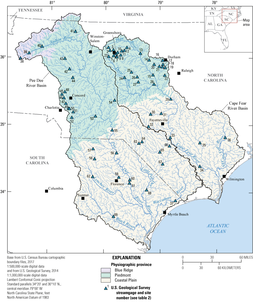
Locations of the Cape Fear and Pee Dee River Basins in North Carolina, South Carolina, and Virginia, physiographic provinces based on U.S. Environmental Protection Agency (2013) Level III Ecoregions, modeled stream network, and U.S. Geological Survey streamgages used for calibration of the Soil and Water Assessment Tool models for the two river basins.
Predominant land-use classes in the Cape Fear and Pee Dee River Basins include woody wetlands, deciduous forest, evergreen forest, and cultivated crops (table 1) (Homer and others, 2015). The basins are located between the cities of Raleigh, North Carolina, and Columbia, South Carolina, and include 10 percent developed area. Major urban areas include Charlotte, Concord, Winston-Salem, Greensboro, Durham, Raleigh, Fayetteville, and Wilmington, North Carolina, and Sumter, Florence, and Myrtle Beach, South Carolina. Precipitation ranges from 40 to 60 inches per year. Mean annual temperature ranges from 57 to 64 degrees Fahrenheit (PRISM Climate Group, 2015a, b).
Table 1.
Land-use summary for the Cape Fear and Pee Dee River Basins, North Carolina and South Carolina.[Based on the 2011 National Land Cover Database (NLCD) for the conterminous United States (Homer and others, 2015). The four “Developed” classes were combined into a single urban land-use class for the purposes of this study]
Methods
Modeling Approach
The SWAT model is a well-established, basin-scale, watershed process model that is used worldwide (Arnold and others, 1998). SWAT was originally developed by the Agricultural Research Service of the U.S. Department of Agriculture as a tool for assessing water-resource and nonpoint-source pollution problems (Arnold and others, 1998). The SWAT model was selected for this study because it was designed to simulate management effects on streamflow in gaged and ungaged watersheds (Gassman and others, 2007). The model can simulate changes in irrigation demand resulting from changing climate, water-use demand, or land use. The ArcGIS extension for SWAT (ArcSWAT), version 2012.10_4.19, was used with ArcGIS 10.4.1 (Esri, Redlands, Calif.) for model development.
Data Used for Model Input and Calibration
For the historical calibration time period (2000 through 2014), input data included daily streamflow at locations throughout the model basins, weather data such as daily precipitation and temperature, and the best available water-use data. Geospatial data layers needed for model framework development included land use, soil, digital elevation, and hydrography. For the future scenario time period (2055 through 2065), GCMs, urban growth projections, and water demand projections were used.
Streamflow Data
The modeling approach required daily mean streamflow data from streamgages, also referred to as “stations” within this report, located at the outlet of catchments with natural to near-natural streamflow conditions (i.e., no to minimal disturbance from urbanization, agriculture, diversions, or regulation). The use of the term “catchment” in this report refers to the area of land that drains streams and rainfall to the location of a gaging station. The Geospatial Attributes of Gages for Evaluating Streamflow (GAGES-II) (Falcone, 2011) dataset, a dataset that was developed from a hydrologic analysis of streamgages across the United States, was used to evaluate catchment hydrologic disturbance. All gaging stations in the GAGES-II dataset that were in the study area were considered for calibration. Gaging stations were eliminated for use in calibration under the following conditions: (1) the station streamflow data period of record was outside the model calibration time period (2000–2014), (2) the station experienced tidal influence, or (3) the station was proximal to and influenced by reservoir or dam operations. Sixty-nine stations were selected for calibration, 36 in the Cape Fear River Basin and 33 in the Pee Dee River Basin (fig. 1; table 2). GAGES-II hydrologic-disturbance scores for the selected stations ranged from 7 to 29, where 7 represented a station at the outlet of a catchment that was minimally disturbed and mostly forested, and 29 represented a station in a catchment that was more disturbed and urbanized. Completely avoiding use of stations with some hydrologic disturbance was impossible due to development in the Cape Fear and Pee Dee River Basins.
Table 2.
U.S. Geological Survey streamgages used for calibration of the Soil and Water Assessment Tool models for the Cape Fear and Pee Dee River Basins, North Carolina and South Carolina.[USGS, U.S. Geological Survey; GAGES-II, Geospatial Attributes of Gages for Evaluating Streamflow (Falcone, 2011); mi2, square mile; SWAT, Soil and Water Assessment Tool; NSE, Nash-Sutcliffe efficiency; PBIAS, percent bias]
| Site number (fig. 1) |
USGS station number | USGS station name | GAGES-II hydrologic-disturbance score (Falcone, 2011) | Catchment area (mi2) |
SWAT model calibration results | |
|---|---|---|---|---|---|---|
| NSE | PBIAS | |||||
| 1 | 02093800 | Reedy Fork near Oak Ridge, N.C. | 16 | 20.6 | 0.38 | −28.7 |
| 2 | 02093877 | Brush Creek at Muirfield Road at Greensboro, N.C. | 17 | 5.3 | 0.44 | −38.7 |
| 3 | 0209399200 | Horsepen Creek at U.S. Highway 220 near Greensboro, N.C. | 18 | 15.9 | 0.67 | −12.2 |
| 4 | 02094500 | Reedy Fork near Gibsonville, N.C. | 23 | 131.5 | 0.67 | −9.7 |
| 5 | 02094659 | South Buffalo Creek near Pomona, N.C. | 21 | 7.4 | 0.66 | −11.0 |
| 6 | 02094770 | South Buffalo Creek at U.S. Highway 220 at Greensboro, N.C. | 21 | 15.6 | 0.49 | −1.50 |
| 7 | 02094775 | Ryan Creek below U.S. Highway 220 at Greensboro, N.C. | 21 | 3.8 | 0.56 | 16.8 |
| 8 | 02095000 | South Buffalo Creek near Greensboro, N.C. | 20 | 34.3 | 0.66 | −15.2 |
| 9 | 02095181 | North Buffalo Creek at Westover Terrace at Greensboro, N.C. | 22 | 9.6 | 0.30 | 26.3 |
| 10 | 02095271 | North Buffalo Creek at Church Street at Greensboro, N.C. | 22 | 14.6 | 0.67 | 7.30 |
| 11 | 02095500 | North Buffalo Creek near Greensboro, N.C. | 23 | 37.1 | 0.61 | 4.50 |
| 12 | 0209553650 | Buffalo Creek at Secondary Road 2819 near McLeansville, N.C. | 23 | 88.7 | 0.69 | −13.2 |
| 13 | 02096500 | Haw River at Haw River, N.C. | 27 | 603.0 | 0.65 | −30.8 |
| 14 | 02096846 | Cane Creek near Orange Grove, N.C. | 10 | 7.6 | 0.30 | −25.2 |
| 15 | 02096960 | Haw River near Bynum, N.C. | 23 | 1,273.3 | 0.60 | −33.4 |
| 16 | 0209722970 | Sandy Creek at Cornwallis Road near Durham, N.C. | 16 | 4.7 | 0.63 | 22.0 |
| 17 | 02097280 | Third Fork Creek at Woodcroft Parkway near Blands, N.C. | 21 | 14.8 | 0.42 | 45.1 |
| 18 | 02097314 | New Hope Creek near Blands, N.C. | 22 | 76.2 | 0.53 | 7.20 |
| 19 | 0209741955 | Northeast Creek at Secondary Road 1100 near Genlee, N.C. | 24 | 21.1 | 0.52 | −2.80 |
| 20 | 02097464 | Morgan Creek near White Cross, N.C. | 13 | 8.3 | 0.29 | −15.3 |
| 21 | 02097517 | Morgan Creek near Chapel Hill, N.C. | 23 | 41.3 | 0.22 | 35.6 |
| 22 | 0209782609 | White Oak Creek at mouth near Green Level, N.C. | 16 | 12.0 | 0.49 | 17.5 |
| 23 | 02099000 | East Fork Deep River near High Point, N.C. | 19 | 14.5 | 0.44 | −32.6 |
| 24 | 02100500 | Deep River at Ramseur, N.C. | 25 | 355.4 | 0.63 | −22.5 |
| 25 | 0210166029 | Rocky River at Secondary Road 1300 near Crutchfield Crossroads, N.C. | 17 | 7.6 | 0.67 | −18.2 |
| 26 | 02101726 | Rocky River at U.S. Highway 64 near Siler City, N.C. | 17 | 68.9 | 0.67 | −12.2 |
| 27 | 02101800 | Tick Creek near Mount Vernon Springs, N.C. | 14 | 15.3 | 0.30 | 59.4 |
| 28 | 02102000 | Deep River at Moncure, N.C. | 21 | 1,444.0 | 0.51 | −36.2 |
| 29 | 02102500 | Cape Fear River at Lillington, N.C. | 25 | 3,473.1 | 0.57 | −24.8 |
| 30 | 02102908 | Flat Creek near Inverness, N.C. | 7 | 7.6 | −0.23 | 2.40 |
| 31 | 02103000 | Little River at Manchester, N.C. | 23 | 345.7 | 0.76 | 3.20 |
| 32 | 02104220 | Rockfish Creek at Raeford, N.C. | 11 | 93.4 | −0.98 | 2.40 |
| 33 | 02105500 | Cape Fear River at William O. Huske Lock near Tar Heel, N.C. | 25 | 4,861.8 | 0.58 | −28.6 |
| 34 | 02105769 | Cape Fear River at Lock #1 near Kelly, N.C. | 24 | 5,274.0 | 0.51 | −36.1 |
| 35 | 02106500 | Black River near Tomahawk, N.C. | 16 | 679.3 | 0.50 | 3.10 |
| 36 | 02108000 | Northeast Cape Fear River near Chinquapin, N.C. | 14 | 606.0 | 0.52 | 23.5 |
| 37 | 02110500 | Waccamaw River near Longs, S.C. | 16 | 1,122.9 | 0.43 | 33.9 |
| 38 | 02111000 | Yadkin River at Patterson, N.C. | 8 | 28.6 | 0.69 | −16.9 |
| 39 | 02111180 | Elk Creek at Elkville, N.C. | 9 | 50.8 | 0.78 | −6.20 |
| 40 | 02111500 | Reddies River at North Wilkesboro, N.C. | 15 | 90.2 | 0.17 | 33.0 |
| 41 | 02113850 | Ararat River at Ararat, N.C. | 23 | 230.4 | 0.50 | 4.40 |
| 42 | 02118000 | South Yadkin River near Mocksville, N.C. | 15 | 305.0 | 0.71 | −11.0 |
| 43 | 02118500 | Hunting Creek near Harmony, N.C. | 12 | 154.6 | 0.67 | −20.7 |
| 44 | 02120780 | Second Creek near Barber, N.C. | 23 | 117.7 | 0.61 | −33.0 |
| 45 | 0212393300 | West Branch Rocky River below mouth of South Prong River near Cornelius, N.C. | 18 | 20.9 | 0.80 | 5.80 |
| 46 | 02124080 | Clarke Creek near Harrisburg, N.C. | 19 | 22.0 | 0.74 | 12.1 |
| 47 | 0212414900 | Mallard Creek below Stony Creek near Harrisburg, N.C. | 27 | 35.7 | 0.77 | −12.1 |
| 48 | 0212419274 | Coddle Creek at Secondary Road 1612 near Davidson, N.C. | 15 | 22.8 | 0.60 | −10.4 |
| 49 | 0212430293 | Reedy Creek below I-485 near Pine Ridge, N.C. | 22 | 12.5 | 0.71 | 4.00 |
| 50 | 0212430653 | McKee Creek at Secondary Road 2804 near Wilgrove, N.C. | 20 | 5.8 | 0.78 | 20.1 |
| 51 | 0212466000 | Clear Creek at Secondary Road 3181 near Mint Hill, N.C. | 19 | 11.4 | 0.72 | −0.200 |
| 52 | 0212467595 | Goose Creek at Secondary Road 1525 near Indian Trail, N.C. | 20 | 11.1 | 0.72 | −0.400 |
| 53 | 02126000 | Rocky River near Norwood, N.C. | 26 | 1,238.3 | 0.73 | −23.6 |
| 54 | 02128000 | Little River near Star, N.C. | 12 | 105.6 | −0.01 | −68.7 |
| 55 | 02129000 | Pee Dee River near Rockingham, N.C. | 24 | 6,881.1 | 0.61 | −31.1 |
| 56 | 02130561 | Pee Dee River near Bennettsville, S.C. | 26 | 7,778.9 | 0.67 | −24.2 |
| 57 | 02130840 | Black Creek below Chesterfield, S.C. | 12 | 51.1 | 0.74 | 17.8 |
| 58 | 02130900 | Black Creek near McBee, S.C. | 12 | 114.0 | 0.49 | −16.3 |
| 59 | 02130980 | Black Creek near Quinby, S.C. | 29 | 439.2 | −0.35 | 17.3 |
| 60 | 02131000 | Pee Dee River at Pee Dee, S.C. | 29 | 8,819.1 | 0.63 | −24.8 |
| 61 | 02131010 | Pee Dee River below Pee Dee, S.C. | 27 | 8,882.5 | 0.62 | −26.7 |
| 62 | 02131500 | Lynches River near Bishopville, S.C. | 20 | 664.3 | 0.58 | 13.1 |
| 63 | 02132320 | Big Shoe Heel Creek near Laurinburg, N.C. | 20 | 81.8 | 0.36 | 4.30 |
| 64 | 02133624 | Lumber River near Maxton, N.C. | 23 | 365.3 | 0.45 | −26.1 |
| 65 | 02134170 | Lumber River at Lumberton, N.C. | 25 | 712.5 | 0.61 | −11.9 |
| 66 | 02134480 | Big Swamp near Tar Heel, N.C. | 16 | 222.9 | 0.25 | 34.8 |
| 67 | 02134500 | Lumber River at Boardman, N.C. | 24 | 1,228.4 | 0.51 | −0.800 |
| 68 | 02135000 | Little Pee Dee River at Galivants Ferry, S.C. | 23 | 2,801.6 | 0.47 | 13.4 |
| 69 | 02136000 | Black River at Kingstree, S.C. | 17 | 1,239.9 | −0.71 | 110.3 |
Streamgages chosen for model calibration were well distributed throughout the study area, with the three physiographic provinces in the study area represented. Most stations (44) were in the Piedmont, 24 were in the Coastal Plain, and 1 was in the Blue Ridge (fig. 1). Catchment areas of streamgages ranged from 3.8 to 8,882.5 mi2. Daily mean streamflow values from the selected stations were obtained from the USGS National Water Information System (https://doi.org/10.5066/F7P55KJN; USGS, 2018).
Climate and Weather Data
Weather data for calibrating the SWAT model included daily precipitation, minimum and maximum daily temperature, relative humidity, solar radiation, and wind speed. Historical daily precipitation and temperature data from gridMET were used for the calibration time period (2000–2014) (https://www.climatologylab.org/gridmet.html; Abatzoglou, 2011). The gridMET dataset is a 4-kilometer gridded surface of meteorological data available from 1979 to the present. Daily relative humidity, solar radiation, and wind speed were calculated within the SWAT model by using a built-in weather generator. The model generated the additional weather parameters by using historical data and trends collected from surrounding National Weather Service stations (Neitsch and others, 2005).
For the future scenario models, forecasted daily precipitation and temperature data were obtained by using the multivariate adaptive constructed analogs version 2 datasets that were trained using the gridMET observational data (MACAv2-METDATA) (https://climate.northwestknowledge.net/MACA/index.php; Abatzoglou, 2011; Abatzoglou and Brown, 2012). Multivariate adaptive constructed analogs version 2 (MACAv2) is a statistical downscaling method (Abatzoglou and Brown, 2012) that was applied to the Coupled Model Intercomparison Project 5 (CMIP5) GCMs (Taylor and others, 2012). The MACAv2-METDATA datasets are compatible with gridMET historical data because they are statistically downscaled and trained using gridMET data. Three GCMs were selected for future scenario modeling based on findings from Gray (2019) to represent relatively dry, central, and wet future climate: (1) inmcm4, (2) MRI-CGCM3, and (3) NorESM1-M, respectively. For these GCMs, the representative concentration pathway of 8.5 was selected. This representative concentration pathway represents future climate based on status quo conditions (CoastAdapt, 2020).
Water-Use Data
A primary objective of this study was to evaluate future scenarios of water availability. For this reason, water-use data were needed for the SWAT modeling. The USGS compiles and publishes water-use data every 5 years. The compilations summarize water demand from various sectors, including public water supply, industrial water use, irrigation for cropland, and irrigation for golf courses. In this study, water-use data from the 2005, 2010, and 2015 compilations were used (Kenny and others, 2009; Maupin and others, 2014; Dieter and others, 2018). Information from all sectors were aggregated into one total water-use value per subbasin. U.S. Environmental Protection Agency data from facilities permitted to discharge wastewater into streams (EPA, 2016) were also compiled for the study area and aggregated by subbasin. Together, water-use and discharge data were summed at an annual time step, resulting in 379 subbasins with water demand ranging from 1,618 to −382 million gallons per day (Mgal/d) for the Cape Fear River Basin, and 753 subbasins with water demand ranging from 345 to −816 Mgal/d for the Pee Dee River Basin (Gonthier and Painter, 2020). A negative water demand represents water discharged to the subbasin.
Water-use projections modeled by Sanchez and others (2020a) were used in the SWAT future scenarios. Sanchez and others (2020a) used estimated future population, urban growth pattern, and climate to predict scenarios of future water use. The water-use projections included domestic and industrial supply; they did not include agricultural water use nor water use for golf course irrigation. Projected water-use values were divided into surface-water and groundwater sources based on historical distributions. This process involved quantifying the percentage withdrawal by source (groundwater or surface water) during the reference year 2011 and assumed the same withdrawal distribution for future projections.
Land-Use Data and Urban Growth Projections
The SWAT model is a spatially explicit surface water model that uses spatial data as inputs, including land use, soil, elevation, and hydrography. Historical land-use data were derived from the 2011 National Land Cover Database (Homer and others, 2015). Fourteen of the land-use classes in that database are in the study area (table 1). Developed land-use classes (developed open space, low intensity, medium intensity, and high intensity) were combined to form a single urban land-use class that was consistent with the framework for urban growth projections. Hence, 11 land-use classes were modeled.
Urban growth projections were modeled following methods by Sanchez and others (2020a) and used for SWAT scenario modeling. The projections were obtained using North Carolina State University FUTure Urban-Regional Environment Simulation (FUTURES) model (Meentemeyer and others, 2013; Petrasova and others, 2016) to develop two alternative urban growth projections: a “status quo” scenario in which historical urban growth patterns were continued into the future to 2065; and an “urban infill” scenario in which infill and clustering urbanization patterns were adopted moving forward into the future to 2065. The resultant land use raster for the year 2065 from the “status quo” and “urban infill” scenarios were used for the SWAT future scenarios (example shown in fig. 2). Projected water demands generally were higher for the status quo scenario than for the urban infill scenario (Sanchez and others, 2020a).
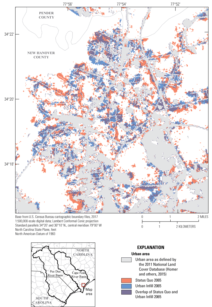
Two projected urban growth patterns (1) status quo, 2065, and (2) urban infill, 2065 for a selected area in northern New Hanover County, within the Cape Fear River Basin in North Carolina. The status quo projection uses historical urban growth patterns that are carried through the future, and the urban infill projection uses infill and clustering urbanization patterns that are carried through the future.
Soil Data
Data from the Natural Resources Conservation Service State Soil Geographic (STATSGO2) dataset (Natural Resources Conservation Service, undated) were used for SWAT modeling. There were 294 soil types in the Cape Fear River Basin and 463 soil types in the Pee Dee River Basin. Soils generally range from sandy and siliceous in the Coastal Plain Physiographic Province to fine, loamy and kaolinitic in the Piedmont Physiographic Province (Natural Resources Conservation Service, undated).
Configuration of Historical Models for Calibration (2000 Through 2014)
Two SWAT models were developed in parallel for the Cape Fear and Pee Dee River Basins. DEMs, coupled with the National Hydrography Dataset, were used to delineate the basins into approximately 2.6-mi2 subbasins. A total of 2,928 and 5,678 subbasins were delineated for the Cape Fear and Pee Dee River Basins, respectively. Subbasins range in area from 6.5×10⁻⁵ to 20 mi2 in the Cape Fear River Basin (median = 2.6 mi2) and from 6.9×10⁻⁵ to 32 mi2 in the Pee Dee River Basin (median = 2.6 mi2) (fig. 3).
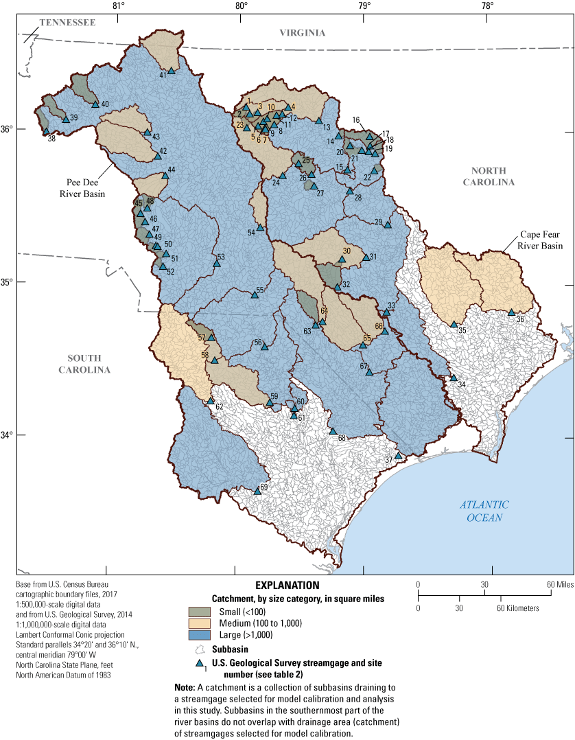
Delineation of the Cape Fear and Pee Dee River Basins, subbasins, and catchments as used in the Soil and Water Assessment Tool models.
The SWAT subbasins were further subdivided into hydrologic response units (HRUs) which represent unique combinations of land-use class, slope class, and soil type. Eleven land-use classes were used for HRU definition, as described in table 1 and the section entitled “Land-Use Data and Urban Growth Projections.” All developed land areas were maintained during creation of HRUs. Other land-use classes making up a small proportion of a subbasin were subject to consolidation to help limit the number of HRUs per subbasin. HRUs therefore represent the most predominant land-use classes. Two slope classes (0 to 2 percent slope and greater than 2 percent) were defined as proxy to mimic the ecohydrologic differences between the Coastal Plain and Piedmont Physiographic Provinces, respectively, that prevail throughout the Cape Fear and Pee Dee River Basins. All STATSGO2 soil types were used for HRU development. These methods resulted in the development of 13,596 HRUs for the Cape Fear River Basin and 25,013 HRUs for the Pee Dee River Basin.
Net water use, defined as water consumed minus water discharged in a subbasin, was incorporated into the model by using the “point source” feature in SWAT. A single net water use value was assigned per subbasin.
Irrigation demand was modeled with the “management practices” feature in SWAT. Specifically, auto-irrigation was enabled to quantify irrigation demand as a function of plant stress. Plant stress data were compiled for more than 70 plant species into a SWAT database with various sources (Arnold and others, 2012). Because of the complexity of the models, large study area, and number of crops present, however, generic agricultural and agricultural management operations were set to defaults similar to corn or tobacco plant species. This setting was implemented only for HRUs with agricultural (row crop) land use in catchments with irrigation exceeding 80 Mgal/d, based on data from the 2005 Water-Use Census (Kenny and others, 2009). With a few exceptions, modeled irrigation demands were located primarily in the Coastal Plain Physiographic Province.
Model Calibration, Uncertainty, and Limitations
Calibration
The models were calibrated for the time period 2000 through 2014 to daily observed streamflow at 69 stations in the study area (fig. 1; table 2). The models were minimally calibrated, meaning no sophisticated algorithms were used to find the best fit for parameters. Parameters were adjusted one at a time based on knowledge of the system (table 3), including information from a groundwater model that has been completed for the same study area (B.G. Campbell, USGS, written commun., 2017). A Muskingum channel routing algorithm was applied in which reach storage is defined by the difference between inflow to and outflow from the reach (Carter and Godfrey, 1960).
Table 3.
Parameters modified during calibration of the Soil and Water Assessment Tool model.[m3/m3, cubic meter per cubic meter; mm H2O, millimeters of water; mm H2O/mm soil, millimeters of water per millimeters of soil]
Modification to Coastal Plain Physiographic Province only (B.G. Campbell, U.S. Geological Survey, written commun., 2017).
Modification to Piedmont Physiographic Province only (Arnold and others, 2012).
Modification to soil 664823 (Nason-Herndon-Helena-Georgeville-Appling) only (Natural Resources Conservation Service, undated). This soil occurs in the Piedmont Physiographic Province and represents a small area of the Cape Fear (9 percent) and Pee Dee (2 percent) River Basins. This sandy soil type was modified to represent a soil with clay-content typically found in the Piedmont.
Model output was evaluated based on a monthly time step by calculating the Nash-Sutcliffe efficiency (NSE) coefficient and percent bias (PBIAS).
wheren
is an integer representing the greatest time step;
t
is time;
is the observed streamflow at time t;
is the simulated streamflow at time t; and
is the observed mean streamflow at time t.
The NSE describes the relative magnitude of residual variance; in other words, the NSE describes how well the simulated versus observed streamflow matches the 1:1 line (Nash and Sutcliffe, 1970). An NSE of 1 indicates a perfect match of simulated versus observed streamflow. The PBIAS describes the average tendency of simulated streamflow to be larger or smaller than observed streamflow. Values greater than 0.5 for NSE (Moriasi and others, 2007; Harmel and others, 2018) and plus or minus 25 percent for PBIAS were considered successful calibration criteria. Results were further categorized by performance rating as suggested by Moriasi and others (2007) (table 4).
Table 4.
Nash-Sutcliffe efficiency (NSE) and percent bias (PBIAS) performance ratings for streamflow models with a monthly time step (Moriasi and others, 2007).[<, less than; ≤, less than or equal to; ±, plus or minus; ≥, greater than or equal to]
Uncertainty and Limitations
All models inherently have some degree of uncertainty and limitations. It is important to understand some of the key limitations that introduce uncertainty in these models. One of the most important limitations is calibrating a “natural” streamflow model, such as the SWAT model. All streamgages used for model calibration have at least some degree of hydrologic disturbance, making a perfect calibration impossible. Average hydrologic disturbance was 19.4 for streamgages in the Cape Fear River Basin and 19.7 for streamgages in the Pee Dee River Basin, suggesting that even when the least hydrologically disturbed stations are selected for calibration, moderate levels of disturbance, which are unavoidable, may cause model fit problems. This presents a calibration challenge that is not unique to this study (Hunt and García, 2014).
Additionally, the flat and swampy physiographic characteristics of the Coastal Plain make this region challenging to model. The SWAT model delineates streams based on gridded DEMs input into the model. As a result of this process, generally flat, topographic areas may be misrepresented if subtle small features controlling hydrography are not captured due to the resolution of the DEM. Flow patterns in these lowlands are complex and historically have not been well-represented by the SWAT stream delineation algorithm; however, improvements in the representation of flat areas have been made to the SWAT model over the years, particularly because the model was originally intended to represent flat, agricultural areas (Gassman and others, 2007).
Configuration of Scenario Models to Investigate Future Streamflow and Irrigation Demand (2055 Through 2065)
Six Cape Fear River Basin and six Pee Dee River Basin scenarios were developed by configuring stand-alone SWAT models that used the same calibration parameters but different forcing data, specifically, forecasted weather data based on GCMs, projected urban growth, and associated water demand projections (table 5). Subbasin delineation was maintained for all 12 scenarios. HRUs were re-created based on the 2065 status quo and urban infill urban growth projections. Six water demand projections were incorporated based on each GCM-urban growth projection pair. Management settings remained the same, and auto-irrigation was applied to all agricultural land. In summary, the six scenarios incorporate either status quo or urban infill urban growth projections, and either the dry, central, or wet GCM.
Table 5.
The six scenarios developed for use in the Soil and Water Assessment Tool models to simulate future streamflow and irrigation demand for the Cape Fear and Pee Dee River Basins, North Carolina and South Carolina.[GCM, global climate model]
| GCM (Abatzoglou and Brown, 2012; Taylor and others, 2012) |
Urban growth projection | |
|---|---|---|
| Status quo | Urban infill | |
| Inmcm4 (dry) | scenario 1 | scenario 4 |
| MRI-CGCM3 (central) | scenario 2 | scenario 5 |
| NorESM1-M (wet) | scenario 3 | scenario 6 |
Results and Discussion
Model Performance (2000 Through 2014)
The Cape Fear and Pee Dee River Basin SWAT models accurately simulate monthly streamflow at several USGS streamgages across the study area. The models simulated monthly mean streamflow with median Nash-Sutcliffe efficiency values of 0.53 (n = 36) and 0.61 (n = 33) in the Cape Fear and Pee Dee River Basins, respectively (fig. 4). Of the 69 streamgages used to calibrate these models, 46 of them (66 percent) were considered to have an accurate (satisfactory or better; table 4) representation. Of the 36 streamgages in the Cape Fear River Basin, NSE values were greater than 0.5 for 23 (64 percent) of them. Of the 33 streamgages in the Pee Dee River Basin, NSE values were greater than 0.5 for 23 (68 percent) of them. PBIAS values ranged from −39 to 59 percent with a mean of −4.8 percent for streamgages in the Cape Fear River Basin. PBIAS values ranged from −69 to 110 percent with a mean of −1.2 percent for streamgages in the Pee Dee River Basin. These mean PBIAS values are very good (within the ‘very good’ criteria of plus or minus 10 percent; table 4), although monthly hydrographs depict slight underprediction for some stations (figs. 5, 6).
![Figure 4. Performance ratings range from unsatisfactory to very good for goodness-of-fit
metrics (Nash-Sutcliffe efficiency [NSE] and percent bias [PBIAS]) at streamgages
in the Cape Fear and Pee Dee River Basins](https://pubs.usgs.gov/sir/2023/5036/images/sir20235036_fig04.png)
Goodness-of-fit metrics (Nash-Sutcliffe efficiency [NSE] and percent bias [PBIAS]) at streamgages in the Cape Fear and Pee Dee River Basins based on performance ratings suggested by Moriasi and others (2007) for streamflow models.
The best performing stations (15 stations with NSE values greater than or equal to 0.65 and PBIAS values within plus or minus 15 percent) had small to medium-sized catchments predominantly in the Piedmont Physiographic Province (table 2; figs. 1 and 4). Catchments were categorized as small (less than 100 mi2), medium (100 to 1,000 mi2), or large (greater than 1,000 mi2) in area. Hydrologic-disturbance scores ranged from 9 to 27 (table 2) for these 15 streamgages. Overall, model performance was not strongly related to hydrologic disturbance at gage locations.
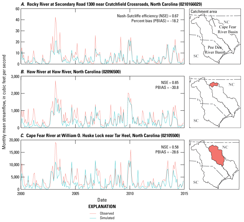
Monthly mean observed and simulated streamflow for the calibration period, 2000 through 2014, at streamgages in the Cape Fear River Basin with A, small (Rocky River at Secondary Road 1300 near Crutchfield Crossroads, North Carolina), B, medium (Haw River at Haw River, North Carolina), and C, large (Cape Fear River at William O. Huske Lock near Tar Heel, North Carolina) catchment areas.
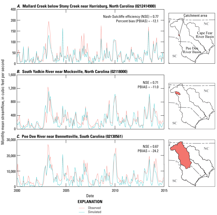
Monthly mean observed and simulated streamflow for the calibration period, 2000 through 2014, at streamgages in the Pee Dee River Basin with A, small (Mallard Creek below Stony Creek near Harrisburg, North Carolina), B, medium (South Yadkin River near Mocksville, North Carolina), and C, large (Pee Dee River near Bennettsville, South Carolina) catchment areas.
Scenario Modeling (2055 Through 2065): Differences in Streamflow and Irrigation Demand
Differences in Streamflow
Climate and urban growth projections incorporated into model scenarios have a direct effect on simulated streamflow. Model scenarios cannot be directly compared to historical, calibrated models because future projections are limited in scope and availability. Specifically, available wastewater discharge data were used for the historical calibration, but no wastewater discharge projections were available for future model scenario development. Model scenario simulations, however, were compared to each other.
The USGS gage, Mallard Creek below Stony Creek near Harrisburg, North Carolina (0212414900, site number 47; fig. 1; table 2), was selected to illustrate some differences in simulated streamflow among model scenarios. This streamgage has a small catchment of 35.7 mi2. Simulated streamflow differences for this catchment are not representative of the entire modeled domain. However, a similar evaluation is possible for any location in the model (Gurley and others, 2023a, b).
Differences in streamflow related to potential climate changes are illustrated by comparing results from scenarios 1, 2, and 3 (fig. 7). Scenarios 1, 2 and 3 incorporate weather data from the inmcm4 (dry), MRI-CGCM3 (central), and NorESM1-M (wet) GCMs, respectively (table 5). An important consideration for this group of GCMs is that the dry, central, and wet designations do not indicate the relative dryness or wetness of weather projected on a given day in the future; instead, the designations indicate the overall model tendency for dryness or wetness when compared with other GCMs. In this same manner, streamflow values simulated in scenario 1 are not necessarily lower than those simulated in scenarios 2 and 3; the highest streamflow values are not necessarily simulated in scenario 3 (fig. 7A).
Maximum monthly mean streamflow ranged from 0 to 385 cubic feet per second (ft3/s) across model scenarios 1, 2, and 3 for the Mallard Creek streamgage. Scenarios 1 and 2 had similar maximum monthly mean streamflow values (217 and 225 ft3/s, respectively), and scenario 3 had the greatest value (385 ft3/s). Cumulative monthly mean streamflow across the three scenarios ranged by 760 ft3/s, a 26-percent difference (fig. 7B). By the end of the simulation period, scenario 3 had the greatest cumulative monthly mean streamflow, followed by scenario 2 and then scenario 1.
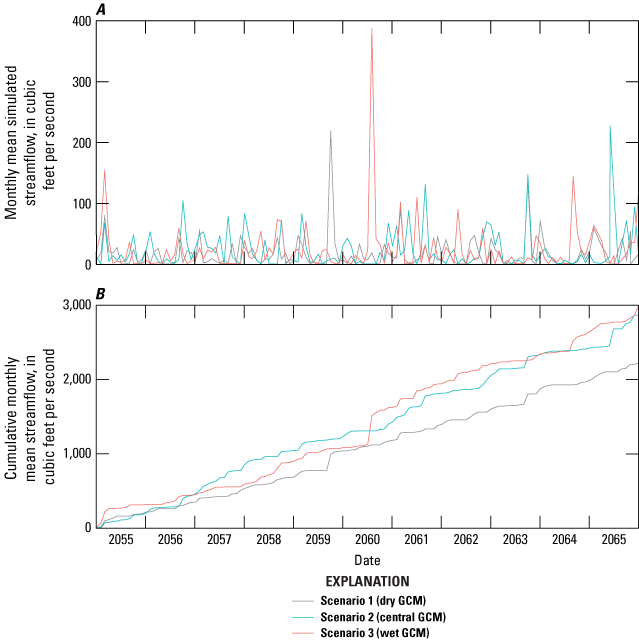
A, Monthly mean simulated streamflow and B, cumulative monthly mean simulated streamflow during the period from 2055 through 2065 at Mallard Creek below Stony Creek near Harrisburg, North Carolina (0212414900), resulting from scenarios 1, 2, and 3 which incorporate alternative weather forecasts based on three global climate models (GCMs).
To evaluate differences in streamflow simulations that result from the use of alternative urban growth projections, scenarios 2 and 5 were compared (fig. 8). Scenario 2 incorporates the status quo urban growth pattern which is consistent with historical patterns, and scenario 5 incorporates the urban infill urban growth pattern where clustering patterns in urbanization are implemented (table 5). Differences in simulated monthly mean streamflow between the two scenarios were relatively minor and ranged from 0 to 2.2 ft3/s (fig. 8A–B). Cumulative monthly mean streamflow for these scenarios diverged by only 73 ft3/s, a 2.4-percent difference (fig. 8C). These results indicate only a small difference in simulated streamflow at the streamgage when interchanging the two urban growth patterns for the catchment.
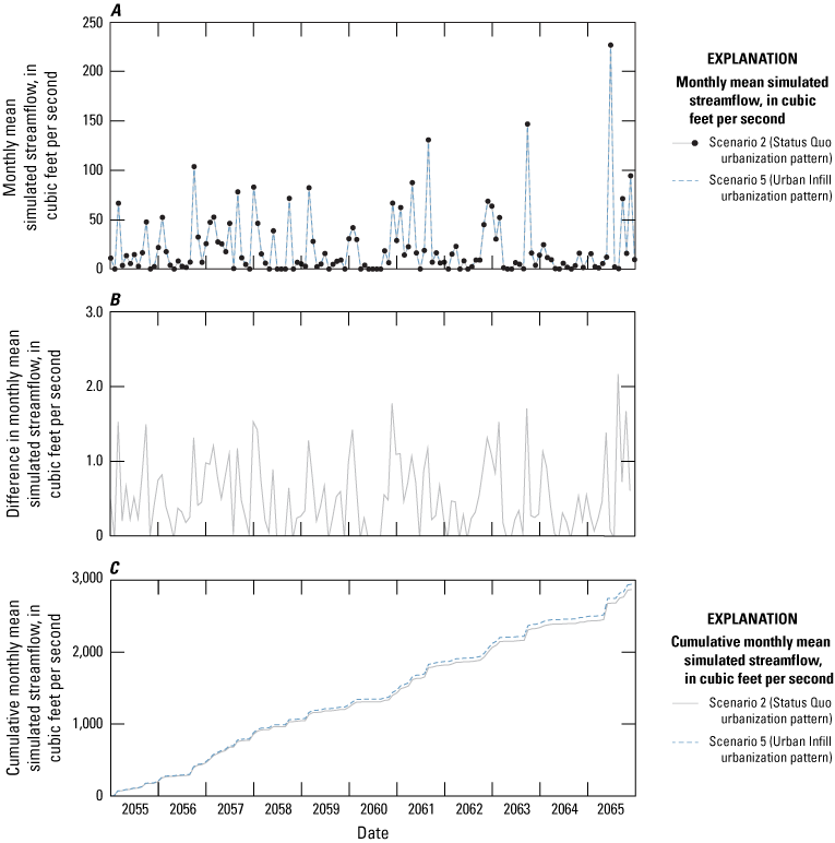
A, Monthly mean simulated streamflow for scenarios 2 and 5 which incorporate alternative urban growth projections, B, difference in monthly mean simulated streamflow between scenarios 2 and 5, and C, cumulative monthly mean simulated streamflow for scenarios 2 and 5 during the period from 2055 through 2065 at Mallard Creek below Stony Creek near Harrisburg, North Carolina (0212414900).
Irrigation Demand
Irrigation demand refers to the quantity of water required for plant growth, less the available water in the environment. Changes in average annual irrigation demand resulting from changing climate and urban growth were simulated for the period 2055 through 2065. Among all six future scenarios, irrigation demand ranged from 0 to 6.0 Mgal/d per subbasin.
Overall, the use of alternative GCMs had a larger and more widespread influence on simulated irrigation demand than the use of alternative urban growth projections. Irrigation demand differences resulting from weather simulations (precipitation and temperature) from alternative GCMs were evaluated based on scenarios 1–3. The difference for each subbasin was calculated by using the highest and lowest average annual irrigation demand values among the three model scenarios. Average annual irrigation demand resulting from these scenarios differed by 0 to 198.8 percent among subbasins (fig. 9). The median difference in annual irrigation demand for subbasins requiring irrigation of agricultural land was 40 percent. No single GCM consistently simulated the highest irrigation demand, a result that illustrates how weather predictions (precipitation and temperature) not only vary by model but also vary in intensity spatially.
Irrigation demand differences resulting from using status quo or urban infill urban growth projections were evaluated based on scenarios 2 and 5. Average annual irrigation demand resulting from these alternative scenarios differed by 0 to 164.2 percent among subbasins (fig. 10), however the median difference was only 0.96 percent.
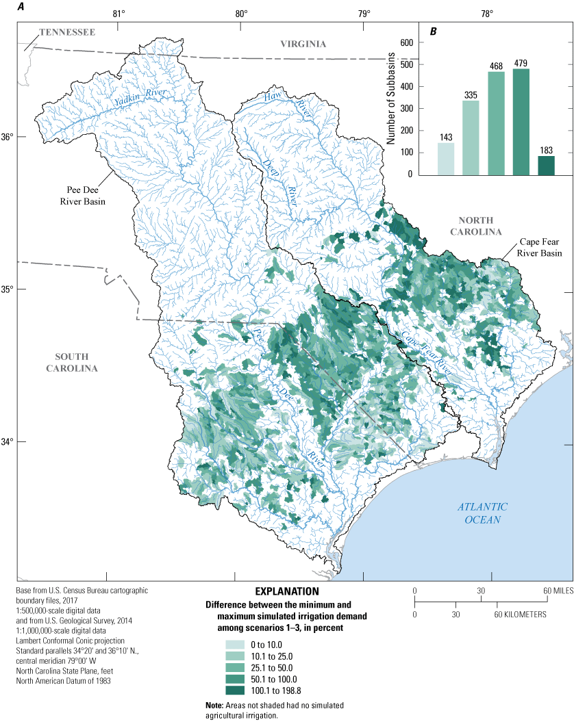
A, The difference between the minimum and maximum simulated irrigation demand among scenarios 1–3 which incorporate alternative global climate models during the period from 2055 through 2065, and B, the number of subbasins with those ranges of differences.
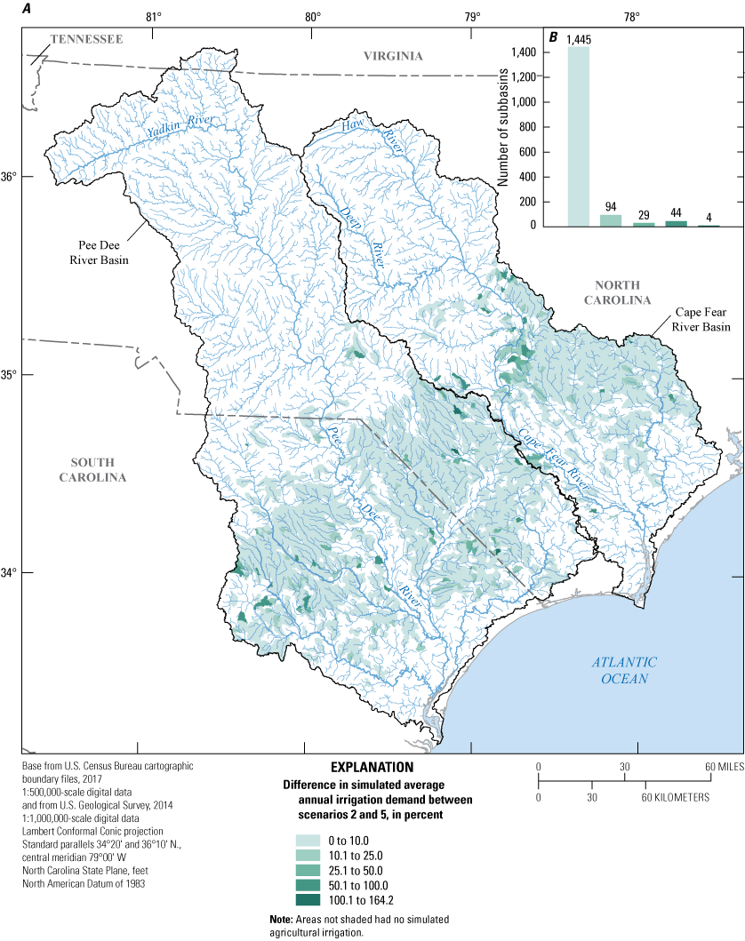
A, The difference in simulated average annual irrigation demand by subbasin during the period from 2055 through 2065 resulting from scenarios 2 and 5 which are alternative urban growth projections, and B, the number of subbasins with those ranges of differences.
Conclusions
The Coastal Carolinas Focus Area Study, part of the U.S. Geological Survey (USGS) Water Availability and Use Science Program’s National Water Census, was initiated to investigate stressors and potential effects from increasing water demand in river basins in the southeastern United States. As part of the Coastal Carolinas Focus Area Study of the USGS, Soil and Water Assessment Tool (SWAT) models were developed for the Cape Fear and Pee Dee River Basins with the purpose of investigating streamflow and irrigation demand, two important factors that impact water availability. A historical model for each river basin was calibrated, and six future scenario models for each river basin were developed based on that basin’s historical model.
The models were calibrated for the time period 2000 through 2014 by using the best available water-use and discharge data. The models simulated monthly mean streamflow with median Nash-Sutcliffe efficiency values of 0.53 and 0.61 in the Cape Fear and Pee Dee River Basins, respectively. Average percent bias was −4.8 percent for the Cape Fear River Basin and −1.2 percent for the Pee Dee River Basin. Streamgages draining catchments that were small (less than 100 square miles [mi2]) to medium (100–1,000 mi2) in size tended to perform better than larger catchments (greater than 1,000 mi2).
Future scenario models incorporated three alternative global climate models (GCMs): inmcm4, representing a relatively dry climate; MRI-CGCM3, representing a relatively central climate; and NorESM1-M, representing a relatively wet climate. Two alternative urban growth projections that implement different urbanization patterns were also incorporated into future scenario models: a status quo projection where urbanization patterns follow historical sprawling trends and an urban infill projection where urbanization patterns tend to cluster and infill where urbanization already exists.
Higher streamflow differences were simulated in response to alternative GCMs rather than alternative urban growth projections. Simulated cumulative monthly mean streamflow results for a selected small illustrative catchment differed by 26 percent under alternative GCMs and differed by 2.4 percent under alternative urban growth projections.
For subbasins with cropland, irrigation demand was simulated based on plant stress. Like the streamflow results, alternative GCMs had a stronger influence on irrigation demand than alternative urban growth projections. Among subbasins, irrigation demand differed by a median of 40 percent depending on the GCM, compared to approximately 1 percent depending on the urban growth alternative.
For this study, calibrated models were developed as a tool for investigating differences in future streamflow and irrigation demand under different scenarios. Calibrated and future scenario models have the capability to run on a daily time step and simulate streamflow and irrigation demand for thousands of small subbasins. The models enable a wide variety of investigations for large and small areas within the Cape Fear and Pee Dee River Basins that extend beyond those described in this report.
References Cited
Abatzoglou, J.T., 2011, Development of gridded surface meteorological data for ecological applications and modelling: International Journal of Climatology, v. 33, no. 1, p. 121–131, https://doi.org/10.1002/joc.3413.
Abatzoglou, J.T., and Brown, T.J., 2012, A comparison of statistical downscaling methods suited for wildfire applications: International Journal of Climatology, v. 32, no. 5, p. 772–780, https://doi.org/10.1002/joc.2312.
Arnold, J.G., Kiniry, J.R., Srinivasan, R., Williams, J.R., Haney, E.B., and Neitsch, S.L., 2012, Soil and Water Assessment Tool, input/output documentation, version 2012: Texas Water Resources Institute, TR-439, accessed September 19, 2022, at https://swat.tamu.edu/media/69296/swat-io-documentation-2012.pdf.
Carter, R.W., and Godfrey, R.G., 1960, Storage and flood routing, Manual of hydrology—Part 3. Flood-flow techniques: U.S. Geological Survey Water-Supply Paper 1543–B, accessed September 19, 2022, at https://doi.org/10.3133/wsp1543B.
CoastAdapt, 2020, What are the RCPs? accessed September 19, 2022, at https://coastadapt.com.au/sites/default/files/infographics/15-117-NCCARFINFOGRAPHICS-01-UPLOADED-WEB%2827Feb%29.pdf.
Falcone, J., 2011, GAGES-II—Geospatial Attributes of Gages for Evaluating Streamflow: U.S. Geological Survey dataset, accessed September 19, 2022, at https://doi.org/10.3133/70046617.
Foster, T., Mieno, T., and Brozović, N., 2020, Satellite-based monitoring of irrigation water use—Assessing measurement errors and their implications for agricultural water management policy: Water Resources Research, v. 56, no. 11, accessed January 10, 2023, at https://doi.org/10.1029/2020WR028378.
Gassman, P.W., Reyes, M.R., Green, C.H., and Arnold, J.G., 2007, The Soil and Water Assessment Tool—Historical development, applications, and future research directions: Transactions of the American Society of Agricultural and Biological Engineers, v. 50, no. 4, p. 1211–1250, accessed September 22, 2022, at https://doi.org/10.13031/2013.23637.
Gonthier, G.J., and Painter, J.A., 2020, Estimated use of water for Coastal Carolinas Focus Area Study: U.S. Geological Survey data release, https://doi.org/10.5066/P9PSFJYB.
Gray, G.M.E., 2019, Ensemble creation of downscaled climate projections in the Southeast: Raleigh, N.C., North Carolina State University, Master of Science thesis, 151 p., accessed September 20, 2022, at https://repository.lib.ncsu.edu/bitstream/handle/1840.20/36425/etd.pdf?sequence=1.
Gurley, L.N., García, A.M., and Pfiefle, C.M., 2023a, Soil and Water Assessment Tool (SWAT) models for the Cape Fear River Basin used to simulate future streamflow and irrigation demand based on climate and urban growth projections: U.S. Geological Survey data release, https://doi.org/10.5066/P98PVDBW.
Gurley, L.N., García, A.M., and Pfiefle, C.M., 2023b, Soil and Water Assessment Tool (SWAT) models for the Pee Dee River Basin used to simulate future streamflow and irrigation demand based on climate and urban growth projections: U.S. Geological Survey data release, https://doi.org/10.5066/P951VE5P.
Homer, C.G., Dewitz, J., Yang, L., Jin, S., Danielson, P., Xian, G., Coulston, J., Herold, N., Wickham, J., and Megown, K., 2015, Completion of the 2011 National Land Cover Database for the conterminous United States—Representing a decade of land cover change information: Photogrammetric Engineering & Remote Sensing, v. 81, p. 345–353.
Hunt, A.M., and García, A.M., 2014, Simulation of natural flows in major river basins in Alabama: U.S. Geological Survey Scientific Investigations Report 2014–5021, 32 p., accessed September 20, 2022, at https://doi.org/10.3133/sir20145021.
Meentemeyer, R.K., Tang, W., Dorning, M.A., Vogler, J.B., Cunniffe, N.J., and Shoemaker, D.A., 2013, FUTURES—Multilevel simulations of emerging urban–rural landscape structure using a stochastic patch-growing algorithm: Annals of the Association of American Geographers, v. 103, no. 4, p. 785–807, accessed September 20, 2022, at https://doi.org/10.1080/00045608.2012.707591.
Nash, J.E., and Sutcliffe, J.V., 1970, River flow forecasting through conceptual models, part 1—A discussion of principles: Journal of Hydrology, v. 10, no. 3, p. 282–290, accessed September 20, 2022, at https://doi.org/10.1016/0022-1694(70)90255-6.
Natural Resources Conservation Service, undated, U.S. General Soil Map (STATSGO2), accessed January 10, 2020, at https://sdmdataaccess.sc.egov.usda.gov.
Neitsch, S.L., Arnold, J.G., Kiniry, J.R., and Williams, J.R., 2005, Soil and Water Assessment Tool theoretical documentation: 476 p., accessed September 22, 2022, at https://swat.tamu.edu/media/1292/SWAT2005theory.pdf.
Petrasova, A., Petras, V., Van Berkel, D., Harmon, B.A., Mitasova, H., and Meentemeyer, R.K., 2016, Open source approach to urban growth simulation: The International Archives of the Photogrammetry, Remote Sensing and Spatial Information Sciences, v. XLI-B7, p. 953–959, accessed September 20, 2022, at https://doi.org/10.5194/isprsarchives-XLI-B7-953-2016.
PRISM Climate Group, 2015a, 30-yr normal precipitation, annual; period, 1981–2010, accessed January 10, 2020, at http://www.prism.oregonstate.edu/normals/.
PRISM Climate Group, 2015b, 30-yr normal mean temperature, annual; period, 1981–2010, accessed January 10, 2020, at http://www.prism.oregonstate.edu/normals/.
Saia, S.M., Suttles, K.M., Cutts, B.B., Emanuel, R.E., Martin, K.L., Wear, D.N., Coulston, J.W., and Vose, J.M., 2020, Applying climate change risk management tools to integrate streamflow projections and social vulnerability: Ecosystems, v. 23, no. 1, p. 67–83, accessed September 20, 2022, at https://doi.org/10.1007/s10021-019-00387-5.
Sanchez, G.M., Smith, J.W., Terando, A., Sun, G., and Meentemeyer, R.K., 2018, Spatial patterns of development drive water use: Water Resources Research, v. 54, no. 3, p. 1633–1649, accessed September 20, 2022, at https://agupubs.onlinelibrary.wiley.com/doi/10.1002/2017WR021730.
Sanchez, G.M., Terando, A., Smith, J.W., García, A.M., Wagner, C.R., and Meentemeyer, R.K., 2020a, Forecasting water demand across a rapidly urbanizing region: Science of the Total Environment, v. 730, article 139050, accessed September 20, 2022, at https://doi.org/10.1016/j.scitotenv.2020.139050.
Sanchez, G.M., Terando, A., Smith, J.W., García, A.M., Wagner, C.R., and Meentemeyer, R.K., 2020b, Land-use and water demand projections (2012 to 2065) under different scenarios of environmental change for North Carolina, South Carolina, and coastal Georgia: U.S. Geological Survey data release, https://doi.org/10.5066/P95PTP5G.
Suttles, K.M., Singh, N.K., Vose, J.M., Martin, K.L., Emanuel, R.E., Coulston, J.W., Saia, S.M., and Crump, M.T., 2018, Assessment of hydrologic vulnerability to urbanization and climate change in a rapidly changing watershed in the Southeast U.S.: Science of the Total Environment, v. 645, p. 806–816.
Taylor, K.E., Stouffer, R.J., Meehl, G.A., 2012, An overview of CMIP5 and the experiment design: Bulletin of the American Meteorological Society, v. 93, no. 4, p. 485–498, https://doi.org/10.1175/BAMS-D-11-00094.1.
Terando, A.J., Costanza, J., Belyea, C., Dunn, R.R., McKerrow, A., and Collazo, J.A., 2014, The southern megalopolis—Using the past to predict the future of urban sprawl in the Southeast U.S.: PLoS ONE, v. 9, no. 7, article e102261, accessed September 20, 2022, at https://doi.org/10.1371/journal.pone.0102261.
U.S. Environmental Protection Agency [EPA], 2013, Level III Ecoregions of the conterminous United States, accessed March 30, 2023, at https://www.epa.gov/eco-research/level-iii-and-iv-ecoregions-continental-united-states.
U.S. Environmental Protection Agency [EPA], 2016, ICIS-NPDES Permit Limit and Discharge Monitoring Report (DMR) datasets, accessed April 16–18, 2016, at https://echo.epa.gov/tools/data-downloads/icis-npdes-dmr-and-limit-data-set.
U.S. Geological Survey [USGS], 2016a, 3D Elevation Program 1-arc second resolution digital elevation model, accessed July 2016 at https://www.usgs.gov/the-national-map-data-delivery.
U.S. Geological Survey [USGS], 2016b, USGS National Hydrography Dataset best resolution for Hydrologic Unit 3, accessed July 2016 at https://www.usgs.gov/national-hydrography/access-national-hydrography-products.
U.S. Geological Survey [USGS], 2018, USGS water data for the Nation: U.S. Geological Survey National Water Information System database, accessed August 24, 2018, at https://doi.org/10.5066/F7P55KJN.
Conversion Factors
U.S. customary units to International System of Units
International System of Units to U.S. customary units
Temperature in degrees Fahrenheit (°F) may be converted to degrees Celsius (°C) as follows:
°C = (°F – 32) / 1.8.
Abbreviations
CMIP5
Coupled Model Intercomparison Project 5
DEM
digital elevation model
GAGES-II
Geospatial Attributes of Gages for Evaluating Streamflow
GCM
global climate model
HRU
hydrologic response unit
MACAv2
multivariate adaptive constructed analogs
NSE
Nash-Sutcliffe efficiency
NWC
National Water Census
PBIAS
percent bias
STATSGO2
U.S. General Soil Map
SWAT
Soil and Water Assessment Tool
USGS
U.S. Geological Survey
For more information about this publication, contact
Director, South Atlantic Water Science Center
U.S. Geological Survey
1770 Corporate Drive, Suite 500
Norcross, GA 30093
For additional information, visit
https://www.usgs.gov/centers/sa-water
Publishing support provided by
Lafayette Publishing Service Center
Disclaimers
Any use of trade, firm, or product names is for descriptive purposes only and does not imply endorsement by the U.S. Government.
Although this information product, for the most part, is in the public domain, it also may contain copyrighted materials as noted in the text. Permission to reproduce copyrighted items must be secured from the copyright owner.
Suggested Citation
Gurley, L.N., García, A.M., Pfeifle, C.A., and Sanchez, G.M., 2023, Simulation of future streamflow and irrigation demand based on climate and urban growth projections in the Cape Fear and Pee Dee River Basins, North Carolina and South Carolina, 2055–65: U.S. Geological Survey Scientific Investigations Report 2023–5036, 23 p., https://doi.org/10.3133/sir20235036.
ISSN: 2328-0328 (online)
Study Area
| Publication type | Report |
|---|---|
| Publication Subtype | USGS Numbered Series |
| Title | Simulation of future streamflow and irrigation demand based on climate and urban growth projections in the Cape Fear and Pee Dee River Basins, North Carolina and South Carolina, 2055–65 |
| Series title | Scientific Investigations Report |
| Series number | 2023-5036 |
| DOI | 10.3133/sir20235036 |
| Publication Date | June 21, 2023 |
| Year Published | 2023 |
| Language | English |
| Publisher | U.S. Geological Survey |
| Publisher location | Reston, VA |
| Contributing office(s) | South Atlantic Water Science Center |
| Description | Report: viii, 23 p.; 2 Data Releases |
| Country | United States |
| State | North Carolina, South Carolina |
| Other Geospatial | Cape Fear and Pee Dee River Basins |
| Online Only (Y/N) | Y |


