

Automated Construction of Streamflow-Routing Networks for MODFLOW—Application in the Mississippi Embayment Region
Links
- Document: Report (46.2 MB pdf) , HTML , XML
- Related Works:
- SIR 2023–5080 —Updated estimates of water budget components for the Mississippi embayment region using a Soil-Water-Balance model, 2000–2020
- SIR 2023–5100 —Simulating groundwater flow in the Mississippi Alluvial Plain with a focus on the Mississippi Delta
- Dataset: USGS National Water Information System database —USGS water data for the Nation
- Data Releases:
- USGS data release - Waterborne resistivity inverted models, Mississippi Alluvial Plain, 2016–2018
- USGS data release - National-scale grid to support regional groundwater availability studies and a national hydrogeologic database
- USGS data release - Datasets used to map the potentiometric surface, Mississippi River Valley alluvial aquifer, spring 2020
- USGS data release - MODFLOW–6 models of the Mississippi embayment (MERAS 3) and Mississippi Delta
- Download citation as: RIS | Dublin Core
Acknowledgments
Thanks to Megan Haserodt (U.S. Geological Survey) for compiling channel width and substrate information from the National Water Information System database and for producing the Manning’s roughness coefficient estimates from channel substrate. Thanks also to Wesley Henson and Mike Fienen (U.S. Geological Survey) for their thoughtful review comments that greatly improved the manuscript.
Funding was provided by the Mississippi Alluvial Plain Regional Water Availability Study through the U.S. Geological Survey Water Availability and Use Science Program.
Abstract
In humid regions with dense stream networks, surface water exerts a fundamental control on the water levels and flow directions of shallow groundwater. Understanding interactions between groundwater and surface water is critical for managing groundwater resources and groundwater-dependent ecosystems. Representing streams in groundwater models has historically been arduous and error prone. In recent years, however, all the information needed to numerically describe stream boundary conditions for a model area has become readily available online, as have robust open-source software tools for translating that information to a model grid. The SFRmaker Python package leverages geospatial capabilities in the scientific Python ecosystem to robustly automate the production of input to the Streamflow-Routing (SFR) Package of MODFLOW from the National Hydrography Dataset Plus or other hydrography data. This report documents an application of SFRmaker to automate production of SFR Package input for groundwater models within the Mississippi Embayment Regional Aquifer Study area. SFR package input was developed in three steps: (1) preprocessing to develop a single set of grid-independent flowlines from National Hydrography Dataset Plus version 2 data; (2) setting up the SFR package from the preprocessed flowlines, and (3) correcting streambed top elevations after an initial model run. Separating the hydrography preprocessing from the construction of SFR package input was advantageous in that it minimized the need to repeat computationally expensive geoprocessing (thereby speeding model construction) and also allowed for the curation of a single set of grid-independent SFR input data that can be used for any MODFLOW model within the study area.
Introduction
In humid regions with dense stream networks, surface water exerts a fundamental control on the water levels and flow directions of shallow groundwater. In the absence of consumptive pumping, most groundwater discharges to surface water features such as streams, lakes, and wetlands. By removing groundwater from the system, consumptive pumping captures flows that would otherwise discharge to surface water. From a pumping perspective, flow captured from surface water reduces the amount of water pumped from aquifer storage, thereby buffering declines in groundwater levels from pumping (Theis, 1940; Leake and others, 2010; Feinstein and others, 2016; Fienen and others, 2017; Barlow and others, 2018). Understanding interactions between groundwater and surface water is therefore critical for managing groundwater resources and surface water ecosystems, which can be adversely affected even when groundwater pumping is small compared to the overall water budget (Acreman and Ferguson, 2010; Richter and others, 2012; Watson and others, 2014; Bradbury and others, 2017).
Representing streams in groundwater models has historically been arduous and error prone, requiring many manual geoprocessing operations or even hand digitizing of features. Software support for automating stream network creation and visualization has been limited, making realistic and accurate representation of streams difficult, especially for large models. In humid regions, a model area might have thousands of perennial streams. As a result, many regional groundwater models in the past have limited the representation of surface water to only include the largest streams (Clark and Hart, 2009; Campbell and Coes, 2010). Limiting the density of surface water boundaries comes at a cost: too few discharge points can result in the simulation of unrealistically high water-table elevations or, when the model output is fit to head observations, parameter compensation and unrealistically high hydraulic conductivity values (Feinstein and others, 2006; Feinstein and others, 2010, p. 73; White and others, 2014).
Boundary conditions representing streams in numerical models are typically derived from geographic information system (GIS) line vector features representing either mapped hydrography (for example, the National Hydrography Dataset; U.S. Geological Survey [USGS], 2018a) or flow accumulation across a smoothed digital elevation model (DEM; Gardner and others, 2018). The latter approach is best suited to montane areas where topographic flow paths towards channels are well defined but may still require some manual intervention in flat, low-lying areas (Gardner and others, 2018). In recent years, hydrography and elevation datasets having all the information needed to numerically describe stream boundary conditions for a model area have become readily available in online datasets such as the National Hydrography Dataset Plus (NHDPlus; McKay and others, 2012; Moore and others, 2019). In the same period, capabilities, robustness, and availability of open-source software tools for processing those data and aligning them with the model grid have grown substantially. The SFRmaker package (Leaf and others, 2021a, b36) uses geospatial capabilities in the scientific Python ecosystem (for example, Harris and others, 2020) to robustly automate the production of input to the Streamflow-Routing (SFR) package in MODFLOW from NHDPlus or other hydrography data.
This report documents an application of SFRmaker to automate the production of SFR package input for the Mississippi Embayment regional aquifer study (MERAS) 3 model and other groundwater models within the MERAS extent. Three steps in developing an SFR package are described: (1) preprocessing to produce a single set of grid-independent flowlines from NHDPlus version 2 files for six major drainage basins; (2) setting up the MODFLOW SFR package from the preprocessed flowlines, and (3) correcting streambed top elevations after an initial model run. The SFRmaker source code and online documentation are available at the SFRmaker GitHub page (https://github.com/DOI-USGS/sfrmaker; Leaf and others, 2021a, b36); the MERAS 3 application, including input files and the relevant scripts are available in a companion data release (Leaf and others, 2023a).
Study Area
The Mississippi Embayment region is a historical bay of the Gulf of Mexico that extends southward from the present-day confluence of the Ohio and Mississippi Rivers to the Gulf coast. The Embayment was formed by crustal down warping that began during the Cretaceous period (Saucier, 1994; Van Arsdale and Cox, 2007) and led to the subsequent accumulation of sedimentary deposits that compose the MERAS. The Mississippi Alluvial Plain (abbreviated “MAP” in associated products; for example, Alhassan and others, 2019) is a broad, nearly flat region within the Mississippi Embayment that encompasses the historical floodplain of the Mississippi and Ohio Rivers (Woods and others, 2004; fig. 1). The Quaternary alluvial sediments that underlie the Mississippi Alluvial Plain, and overly the older Tertiary deposits of the MERAS, compose the Mississippi River alluvial aquifer.
Fertile soils, a long growing season, and abundant water resources make the Mississippi Alluvial Plain ideal for agriculture, which lead to its conversion from historical wetlands and hardwood forest to primarily cropland today. Although annual rainfall averages more than 50 inches, evapotranspiration is also high, and the timing and quantity of precipitation are not always sufficient to meet crop demand (Barlow and Clark, 2011; Reba and others, 2017). As a result, the more than $6 billion agricultural industry in the alluvial plain relies heavily on groundwater (Alhassan and others, 2019). Increasing irrigation withdrawals from the underlying Mississippi River alluvial aquifer have led to some of the most severe declines in groundwater levels in the United States, creating concerns about the future sustainability of the Mississippi River alluvial aquifer resource (Barlow and Clark, 2011; Konikow, 2013).
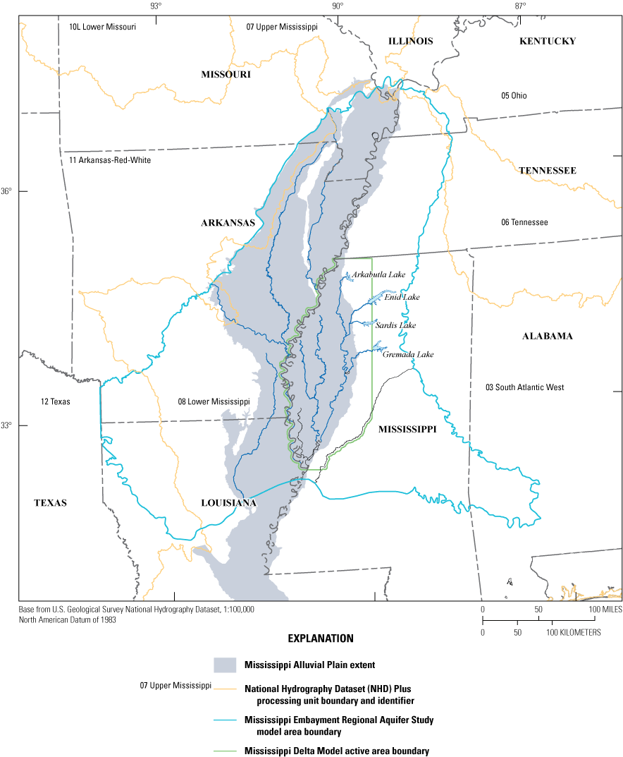
Mississippi Embayment Regional Aquifer Study model area with National Hydrography Dataset Plus vector processing units and the Mississippi Alluvial Plain region.
The USGS’s Mississippi Alluvial Plain Regional Water Availability Study (called the “MAP project”) focuses on quantifying groundwater resources in the Mississippi Alluvial Plain and the response of groundwater resources to development (USGS, 2018b). An important component of the MAP project is automating groundwater model construction or updates to rapidly answer management questions about groundwater sustainability throughout the alluvial plain (Leaf and others, 2023b). Robust, automated creation of SFR Package input to realistically represent the many mapped streams in the alluvial plain is an essential part of the rapid model construction.
Methods
Groundwater Flow Models
Initial numerical modeling efforts in the MAP project focused on updating previous versions of the MERAS model (Clark and Hart, 2009; Clark and others, 2013; Haugh and others, 2020; fig. 1) and also focused on water management in the Mississippi Delta. The MERAS–NWT model (Hunt and others, 2021) retained the same spatial discretization (1-mile cells) and biannual timesteps as MERAS 2 (Clark and others, 2013; Haugh and others, 2020) but implemented the Newton-Raphson solver in MODFLOW–NWT (Niswonger and others, 2011) to better represent aquifer storage and the nonlinear effects of a changing water table. The MERAS 3 model (Leaf and others, 2023b) simulates the same area as previous versions (fig. 1) but with a smaller 1-kilometer (km) horizontal discretization (Clark and others, 2018), simplified vertical discretization of three layers, monthly timesteps, and the Newton-Raphson solver in MODFLOW 6 (Langevin and others, 2017). The primary goal of MERAS 3 is to provide boundary conditions for more-detailed inset models within the Mississippi Alluvial Plain, such as the Mississippi Delta model described by Leaf and others (2023b; fig. 1). The MERAS–NWT, MERAS 3, and the Mississippi Delta models used the workflow and revised stream network described in this report.
The MERAS 3 model grid consists of 666 rows and 634 columns of uniform, 1-km square cells that encompass the Mississippi Alluvial Plain region and the surrounding Tertiary deposits of the East and West Gulf Coastal Plains (Mississippi Embayment region; fig. 1). Three model layers represent the entire sequence of Tertiary deposits above the Midway confining unit, which is believed to form a laterally continuous basal no-flow boundary across the bulk of the embayment (Clark and Hart, 2009). MERAS–NWT and previous versions were constructed in the MODFLOW–2005 framework (Harbaugh, 2005), which includes MODFLOW–NWT (Niswonger and others, 2011). Like previous versions that used the SFR2 Package (Niswonger and Prudic, 2005; Prudic and others, 2004), the MERAS 3 model represents streams using the SFR Package in MODFLOW 6 (Langevin and others, 2017). Representing streams in MERAS 2 and earlier versions was however limited to only 43 major streams across the Mississippi Embayment, out of thousands of mapped streams (fig. 2). In this report, “SFR2” refers specifically to the MODFLOW–2005 package (code module) described by Niswonger and Prudic (2005); “SFR” is used more generally as an acronym for streamflow routing. “SFR Package” refers generally to the SFR component of MODFLOW (for example, SFR2 or the SFR Package in MODFLOW 6); “SFR package” refers to input datasets to those code modules (that is, for a specific groundwater model).
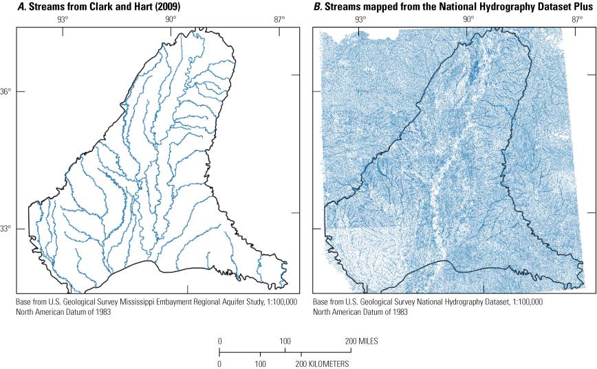
Streams in and near the Mississippi Embayment Regional Aquifer Study model area. A; from Clark and Hart (2009). B, mapped from the National Hydrography Dataset Plus.
Streamflow-Routing Package for MODFLOW
The SFR package allows a MODFLOW simulation to include stream-aquifer interactions that are constrained by the amount of water available in the stream channel. Streams are included in the finite-difference simulation as reaches that represent the part of the stream contained in a model computational cell. A mass balance is solved for each reach:
whereQinspecified
is an inflow rate specified to a stream,
Qtrb
is inflow from upstream reaches,
Qro
is overland runoff entering the cell,
Qppt
is precipitation falling directly on the stream reach,
Qgwin
is groundwater discharge to the stream (negative from the perspective of the groundwater system, which loses water when the stream gains),
Qsro
is outflow routed to downstream reaches,
Qdiv
is diverted outflows,
Qet
is evapotranspiration from a stream reach, and
Qgwout
is discharge from the stream to the aquifer.
y
is the stream depth (or height of water column above the streambed),
Q
is the stream discharge,
n
is Manning’s roughness coefficient,
C
is a constant for unit conversion (1.0 for units of cubic meters per second or 1.486 for units of cubic feet per second),
w
is the width of the stream channel, and
S0
is the slope of the stream channel.
Qgw
is the volumetric flow rate between a stream reach and the aquifer,
Kv
is the vertical hydraulic conductivity of the streambed,
w
is the representative width of the stream channel,
L
is the length of stream channel represented by the reach,
m
is the thickness of the streambed deposits,
hs
is stream stage (y plus streambed elevation), and
ha
is the head in the aquifer.
When stream stage is greater than the head in the aquifer, leakage from the stream to groundwater occurs but is limited by the amount of available water determined by equations 1–3. For example, if the stream is dry, then no leakage is simulated. A key advantage to using equation 4 instead of specifying stage a priori is that simulated stages generally reflect the quantity of water available in the streambed. Depletion of water in the stream channel from leakage to the aquifer will cause stage to decrease, thereby lessening the gradient between the stream and aquifer (when heads are above the streambed bottom). Similarly, groundwater discharge causes stage to rise, also leading to a decrease in gradient and a dampening of leakage. Fixed stream stages can result in unrealistic leakage rates and abrupt transitions between gaining and losing conditions that produce oscillations in the conjunctive solution between the stream reach and the groundwater system.
Equations 1–5 are solved iteratively with the groundwater flow solution until fluxes between the two solutions agree within a specified convergence criterion. The result is a solution for stream-aquifer interactions and streamflow in each reach. Simulated streamflow at a given point on the network represents the cumulative effect of all interactions between groundwater and surface water upstream from that point and can be directly compared to measured total flows if surface runoff (Qro) is sufficiently well known. If Qro is neglected, simulated streamflow can be directly compared to estimates of stream base flow (the groundwater component of streamflow).
Source Data
The NHDPlus version 2 dataset was used as the basis for the SFR packages described here. The dataset includes “flowline” features that describe the locations and geometry of streams throughout the United States at a 1:100,000 scale resolution, and attribute tables with supporting information. The flowlines are encoded as linestrings (linear features defined by vectors of points) in the shapefile format (Esri, 1998). The attribute tables are encoded in the dbf format (Esri, 1998) and include information such as routing connections between flowlines, minimum and maximum elevations, and the total length of stream channels upstream from each flowline (arbolate sum). The flowlines are the product of several decades of hydrographic mapping that originated with the 1:100,000-scale USGS topographic map series (Moore and Dewald, 2016). Attribute data are associated with flowlines via common identifier numbers (COMIDs). Flowline data and associated attribute tables are distributed by drainage area; 26 drainage areas cover the continental United States. More details are available from McKay and others (2012) and the project website (https://www.epa.gov/waterdata/get-nhdplus-national-hydrography-dataset-plus-data).
Elevation and routing information from NHDPlus were refined using the most recent DEMs for the Mississippi Alluvial Plain region, many of which were derived from lidar surveys (USGS, 2018c). The lidar-based DEMs represent a significant advance over previous elevation data in the level of detail they provide about small-scale topographic features and the current state of the stream network in the alluvial plain.
Widths for large streams, where available, were obtained from the North American River Width Database (NARWidth version 0.1; Allen and Pavelsky, 2015). NARWidth contains continuous estimates of channel width derived from Landsat imagery for North American streams larger than 30 meters wide (Allen and Pavelsky, 2015).
Overview of Workflow
The automated workflow for producing an SFR package is shown in figure 3. The “Preprocessing,” “SFR package creation,” and “update streambed tops” boxes each represent a separate Python script that in turn calls various code modules listed in the figure. For example, in the preprocessing step, functions from the SFRmaker Preprocessing module are called. The Python scripts are customizable for a specific application, whereas the code modules are general to the procedures described in this report. The code modules described here are contained within SFRmaker (Leaf and others, 2021a, b36; more online documentation is available at the SFRmaker GitHub page: https://github.com/DOI-USGS/sfrmaker). Scripts for the MERAS 3 application and additional details about the workflow are available in the companion data release (Leaf and others, 2023a).
A set of flowlines that are independent of any finite difference grid forms the basis for the SFR package. NHDPlus data can be input directly to SFRmaker, or the Preprocessing module can be used to create input hydrography that is customized to a study area. The Preprocessing module is designed to cull the NHDPlus data to a specified study area, reduce the stream density to a desired level, address issues with routing and channel elevation in the NHDPlus data, and improve representation of channel widths for large streams. The Preprocessing module ultimately outputs a single shapefile containing most of the information needed to generate an SFR package on a finite difference grid within the area covered by the shapefile.
Much of the preprocessing is time intensive and requires working with large datasets, including the drainage areas shown in figure 1 (which cover a sizeable part of the continental United States) and many DEM tiles within the MERAS footprint. With a separate preprocessing step (before building the model or the SFR package), these data and routines only need to be handled once for the MERAS study area, which greatly speeds up and simplifies the subsequent creation of SFR packages.
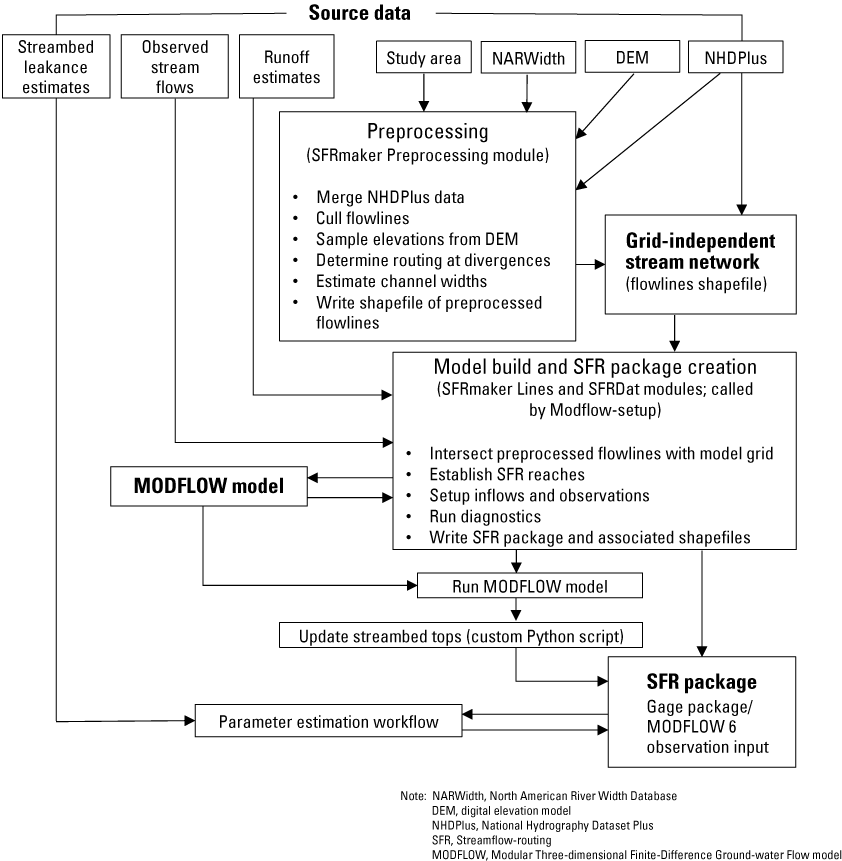
Workflow for generating a Streamflow-Routing (SFR) package. The basis for the SFR package is a set of flowlines (vector data independent of any model grid) and supporting attribute data. National Hydrography Dataset data can be used directly or preprocessed to better represent a specific study area, scale, and (or) modeling goals. The preprocessing routine is designed to reduce the source hydrography data to a desired density of streams; improve routing, elevations, and channel widths; and translate the source data into a format amenable to SFR input creation. A single shapefile is written containing all the information needed to generate an SFR package for a model grid within the study area. The SFR package creation script writes SFR2 or MODFLOW 6 SFR input. Often, streambed tops derived from a digital elevation model reflect the water surface instead of the actual streambed. A third script takes simulated depths from a MODFLOW run and subtracts them from the initial set of streambed tops, resulting in simulated stages that better reflect the water surface.
Preprocessing
This section describes the processes done within the preprocessing script (“Preprocessing” box in figure 3; “preprocess_flowlines.py” in Leaf and others, 2023a), except for channel width estimation, which is described in the “Stream Reach Properties” section.
Merging and Culling the NHDPlus Flowlines
The Mississippi Embayment region intersects six major drainage basins (vector processing units in the NHDPlus), including most of the Lower Mississippi Basin (08) and small parts of surrounding basins (fig. 1). The mapped flowlines within each basin include many more streams than are desirable to simulate in a large regional groundwater model with a coarse resolution. Within the Mississippi Alluvial Plain, most of the mapped headwater streams are ephemeral, flowing only during precipitation or periods of high water. Inspection of the hydrography overlain on satellite imagery suggested that many other mapped streams no longer exist because of land use changes; therefore, the first part of preprocessing was to merge the flowline and associated attribute data from the various drainage basins and cull the dataset to only include a reasonable density of flowlines representing the current stream network within the model area. The term “reasonable” is subjective but in this case represents a balance between including all flowlines that potentially receive groundwater discharge for at least several months of the year and maintaining a workable stream network size for the model solution and coarse grid discretization.
A Python function (cull_flowlines() in the SFRmaker Preprocessing module) was developed to perform the above tasks for a set of NHDPlus files and a polygon shapefile of the active area of the MODFLOW grid. The function outputs a single set of flowlines for the model domain and three associated attribute files (following the structure of NHDPlus version 2):
-
• The “value added attribute” (VAA) file, which contains arbolate sums.
-
• The “PlusFlow” file, which contains routing connections.
-
• The “elevslope” file, which contains minimum and maximum elevations for each flowline.
Arbolate sum was selected as a numeric criterion for limiting stream density because it is continuous (unlike stream order) and more easily obtainable than drainage area, especially in the flat terrains of the Mississippi Alluvial Plain region. The NHDPlus flowlines were culled at various arbolate sums ranging from 4 to 30 km and overlain on satellite imagery. Flowlines in headwater areas were visually inspected at various locations around the model area for correspondence with wet channel conditions. Although this method is qualitative and depends on the time of year the satellite imagery was taken, it can provide an approximate sense for the range of appropriate arbolate sum thresholds. A threshold of 20 km was selected, meaning that streams with less than 20 km of upstream channel were excluded. From the remaining streams longer than 20 km, those identified in NHDPlus as intermittent, and with arbolate sums less than 50 km, were also culled. This resulted in a handful of isolated perennial streams that no longer had downstream connections. Inspecting these streams against satellite imagery suggested them to be minor, especially at a 1-mile or 1-km grid resolution. The isolated streams were also culled. The remaining stream network includes about 24 percent of the flowline features mapped in NHDPlus within the MERAS region (fig. 4).
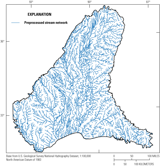
Streams included in the preprocessed stream network.
Elevations and Routing at Divergences
The second part of the preprocessing focused on recasting the NHDPlus data to a format readily convertible to SFR Package input while maintaining the model grid-independent structure of the flowline features. A key part of the preprocessing was handling divergences in the stream network, where flow is routed to two or more distributaries. Many distributaries are mapped throughout the Mississippi Alluvial Plain region, but most of these features are either nonexistent or only carry flow intermittently during high water events. Although distributaries in NHDPlus are classified into “main” or “minor” paths at divergences, inspection against the satellite imagery and the most recent, lidar-based DEMs for the region (USGS, 2018c) suggested that the NHDPlus classifications are often inaccurate. The steps described below are illustrated graphically in figure 5, which shows an example location on the Quiver River near Sunflower, Mississippi. The following steps were taken to identify the main channel at each divergence:
-
• A 50-meter buffer polygon was drawn around each flowline feature. A flat end-cap was used so that only areas perpendicular to the flowlines were included in each buffer.
-
• Zonal statistics for the lidar-based DEM elevations within each buffer polygon were computed using the rasterstats Python package (Perry, 2017). The 10th percentile elevation was selected as a metric for discriminating between the main channel and minor distributaries. Lower elevation percentiles would be more likely to represent areas of overlap between the buffers for the main channel and minor distributaries (resulting in minor distributary elevations that are similar to the main channel), whereas higher elevation percentiles might miss the lowest parts of the main channel or even represent parts of the channel banks instead.
-
• At each divergence, the distributary with the lowest 10th percentile elevation was assumed to be the main channel.
Comparison of the sampled DEM elevations with the NHDPlus elevation attribute data revealed a high bias in many of the attribute elevations, especially near diversions. This may be a result of the upstream smoothing process described by McKay and others (2012, p. 123) when it encounters distributaries of unequal elevations such as the example shown in figure 5. To remedy this issue, the 10th percentile elevations obtained from the buffer zonal statistics were assigned to each flowline and then smoothed in the downstream direction to ensure that no flowlines had negative (uphill) streambed slopes.
Finally, routing connections to minor distributaries were removed, and arbolate sums were recomputed for the entire stream network with arbolate sums at minor distributaries starting at zero. In this way, the minor distributaries are treated like headwater streams in that they will only receive flow if the water table is greater than their assigned elevation; otherwise, they are simulated as dry and are not part of the groundwater model solution. Like headwater streams, the first 20 km of minor distributaries were trimmed from the stream network, based on inspection of satellite imagery that revealed most of them to be nonexistent or dry (fig. 5).
The above steps were implemented in the preprocess_nhdplus() function in the SFRmaker Preprocessing module, which reads the culled files produced by cull_flowlines() (or a single set of native NHDPlus version 2 files) and outputs a single shapefile with the preprocessed flowlines and attribute information including routing, channel width (described in the “Stream Reach Properties” section), and elevations. The shapefile is designed to provide a basis for an SFR package on any finite difference grid within the MERAS area.
Creation of Stream Reaches
This section describes translation of the vector-based dataset produced in the preprocessing step to a finite difference grid and SFR package reaches (“SFR package creation” box in figure 3; “setup_meras3-3layer.py” in Leaf and others, 2023a). SFRmaker can do this step independently with or without an existing model (Leaf and others, 2021a, b36), or in the context of automated model construction with the Modflow-setup Python package (Leaf and Fienen, 2022). In the MERAS 3 application, Modflow-setup was used to create the SFR Package input in tandem with the other MODFLOW input. Within the Modflow-setup workflow, SFRmaker reads the preprocessed flowlines from step 1, and optionally other information about stream inflows, observations, and surface water runoff. An SFR package file and several shapefiles for visualizing the SFR package in a GIS environment are produced along with the MODFLOW input files.
Intersecting the Flowlines with the Model Grid
SFRmaker develops reaches by breaking the preprocessed flowlines at the model grid cell boundaries, resulting in a flowline fragment (reach) for each intersection between a flowline and a model grid cell (fig. 5a). An r-tree spatial index (Gillies, 2017) is used to speed the testing of intersections between model grid cells and flowlines. The shapely package (Gillies and others, 2017) is used to create the reaches from their parent flowlines. By default, reaches less than 5 percent of a model cell length (50 meters for 1-km cells) are discarded. The remaining reaches are grouped into segments corresponding to their parent flowlines. Stream segments are numbered sequentially with the numbering always increasing in the downstream direction (Prudic and others, 2004). Segments are routed using the attribute information developed in the preprocessing step; reaches are routed (numbered) based on geographic proximity of their end vertices (accounting for discarded reaches). Attribute information from the preprocessed flowlines is transferred to the grid-based reaches by recording the index position of model grid cells intersecting each flowline. This type of operation, where attribute information is transferred from one vector-based feature to another based on location, is often referred to as a spatial join.
Handling of Colocated Reaches
Even with the arbolate sum thresholds described in the preprocessing step, the high stream density in the Mississippi Embayment region resulted in many instances of model cells containing multiple reaches (fig. 5 shows an example). Although the SFR package is capable of computing flows between multiple colocated stream reaches and a model cell representing the groundwater flow solution, having many colocated reaches places an additional burden on the model solver and also greatly increases the size of the SFR package, which in turn slows file input and output. There is little utility in carrying these features in the model solution: all computations for a model cell are performed at the cell center, meaning the spatial component of the interactions between colocated reaches and the groundwater flow solution cannot be resolved. In other words, the level of detail that can be represented in an SFR package is limited by the model grid size. Meaningful representation of colocated streams requires refining the grid so that they are no longer colocated.
To address this issue, a “sparse” version of the SFR package was created with only one reach in each model cell. In each cell, the dominant reach (likely to carry the most flow) was identified based on the largest arbolate sum computed in the preprocessing step. The conductance term (KvwL/m in eq. 5) was then summed for all reaches within the cell and applied to the dominant reach by increasing the hydraulic conductivity value (Kv; eq. 6). Minor reaches were then removed so that each cell contained no more than one reach, with a conductance value that represented all the original reaches. Routing connections between successive dominant reaches were established using a directed graph of the original reach connections. The one_reach_per_cell option in SFRmaker and Modflow-setup allows this “sparse reach” option to be turned on or off.
whereCi
is the conductance for a colocated reach, equal to KvwL/m;
md, wd, Ld
are the streambed thickness, width, and length, respectively, of the dominant reach; and
n
is the number of colocated reaches.
If values of 1 are assumed for Kv and m, equation 6 reduces to a dimensionless scaling factor (eq. 7) that can be applied to any values of leakance (Kv/m) assigned to an SFR reach. This allows leakance to be updated while maintaining the relative differences in total reach area between model cells that originally contained multiple reaches.
Example Location on the Quiver River
Figure 5 illustrates the preprocessing steps described in the “Preprocessing” section for an example location on the Quiver River west of Greenwood, Miss. Figure 5A shows the original flowlines from NHDPlus overlain on recent satellite imagery. The white numbers indicate the 10th percentile elevations sampled from the lidar-based DEM (in feet above sea level) within a 50-meter buffer of the flowlines. Inspection of the flowlines, air photo, and a shaded relief of the DEM (fig. 5B) suggests that the Quiver River historically followed a meander bend to the west (elevation of 102.27 feet) but now takes a more direct, possibly dredged cutoff (elevation of 97.39 feet). The historical meander bend is coded as the main channel in NHDPlus, but the cutoff was selected instead in the preprocessing based on a lower elevation of 97.39 feet. Inspection of the satellite imagery clearly confirms the cutoff to be the main channel. Other tributaries shown in figure 5A are mapped across what are now aquaculture ponds (green rectangles; for example, the tributary with an elevation of 105.74 feet) or row-crop fields (light brown rectangles).
Figure 5B shows the stream network after removal of flowlines with arbolate sums less than 20 km and intermittent flowlines with arbolate sums less than 50 km, overlain on a shaded relief of the DEM. The remaining (blue) lines all represent streams that are visible in the satellite imagery and DEM. The solid blue lines illustrate the dominant reach in each model cell (with the highest arbolate sum); the dashed lines illustrate minor reaches that are colocated. The red arrows illustrate routing connections between reaches as MODFLOW sees them in the “sparse” version of the SFR package. The connections extend between the centers of the finite difference cells (where all calculations are made) and only occur between successive dominant reaches. The existence of the intervening minor reaches is implied, but they are not included in the SFR package. The physical footprints of the streams in each cell (length and width; including colocated reaches) are represented implicitly via streambed hydraulic conductivity in the leakance term, as described in the “Handling of Colocated Reaches” section. A potential downside of this approach is that flux targets on minor reaches may not have simulated flows that are directly equivalent. However, the large scale and coarse discretization of the model preclude accurate simulation of these smaller streams.
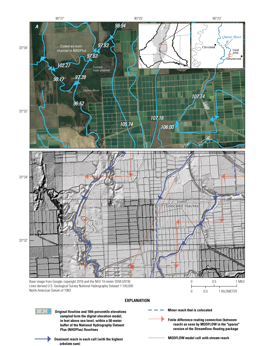
Flowline preprocessing and stream reach consolidation. A, Original flowlines from the National Hydrography Dataset Plus overlain on recent satellite imagery. Inspection of the flowlines, air photo, and a shaded relief of the digital elevation model (DEM) in B suggest that the Quiver River historically followed a meander bend to the west (elevation=102.27 feet) but now takes a more direct, possibly dredged cutoff to the south (elevation=97.39 feet). B, Stream network after removal of flowlines with arbolate sums less than 20 kilometers (km), and intermittent flowlines with arbolate sums less than 50 km, overlain on a shaded relief of the DEM. The non-existent flowlines have been removed, and the remaining (blue) lines represent streams that are visible in the satellite imagery and DEM. The connections shown (red lines) extend between the centers of the finite difference cells (where all calculations are made), and only occur between successive dominant reaches.
Stream Reach Properties
This section describes how stream reach property inputs to the SFR Package were derived.
Estimation of Reach Widths with Field Measurements
Stream channel widths were estimated for individual flowlines during the preprocessing step (preprocess_nhdplus() function) and applied to SFR reaches later by mapping COMIDs to reach numbers. Two methods were used to estimate channel widths for flowlines. In the first method, widths were estimated from field measurements based on their arbolate sum. In the second method, widths were sampled onto the flowlines directly from the NARWidth database (Allen and Pavelsky, 2015). The two methods were compared, and preference was given to the second method where data were available.
Field measurements of channel width recorded by USGS personnel during streamflow measurements were obtained from the National Water Information System (NWIS; USGS, 2022) for sites throughout the Mississippi Embayment region, in the period after 1970. The NWIS database includes base flow and flood measurements. Widths associated with the latter often greatly exceed the width of the stream channel during typical base flow conditions. To determine if a width measurement was made during base flow conditions, base flow periods were identified at the closest streamgage with a continuous record: an index station. Tenth percentile flows (Q90; equaled or exceeded 90 percent of the time) were computed for each index station. Width measurements were considered to be representative of base flow when the ratio between the measured flow at the index station and the index station Q90 (Q:Q90) was less than two. For locations with more than one base flow channel width measurement, the measured widths were averaged.
Each width measurement was located on the stream network developed in the preprocessing step and assigned an arbolate sum value. A power-law relation between arbolate sum and width was then developed via a curve fitting analysis, similar to Feinstein and others (2010, p. 266). Figure 6 shows the best-fit line through the log-transformed data.
Although figure 6 shows a clear relation between stream channel width and arbolate sum, considerable scatter about the best-fit line illustrates the amount of heterogeneity in channel width caused by other geomorphic factors. Additionally, streamgages are typically located in areas where the channel is straight and stable and near bridges and other artificial structures. Therefore, the measured channel widths shown in figure 6 may be biased low compared to actual widths throughout the stream network (Park, 1977; Allen and Pavelsky, 2015).
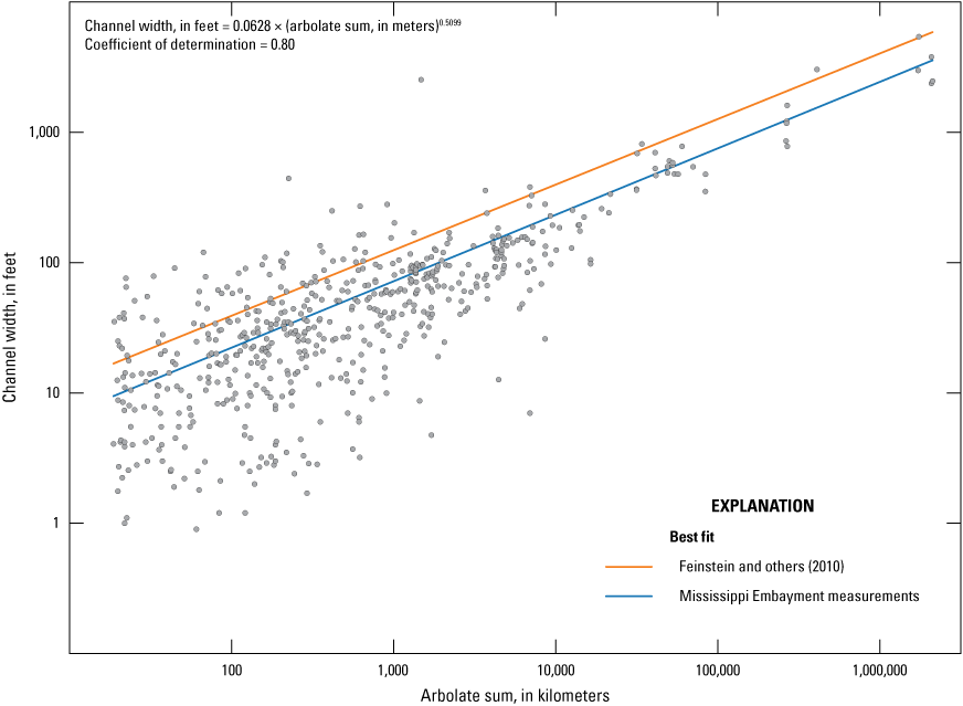
The relation between measured stream channel widths and arbolate sum.
Estimation of Reach Widths from Remote Sensing Data
Widths from NARWidth were sampled onto the stream network by performing a spatial join based on the intersection of the NARWidth line features with 1-km buffer polygons around the preprocessed flowlines. To avoid erroneous overlap between mainstem NARWidth estimates and minor tributaries, flowlines with arbolate sums less than 500 km only received widths from NARWidth lines with at least 50 percent of their length inside of the 1-km buffer.
In addition to the channel widths estimated from the power law relation described above, NARWidth values were also assigned to flowlines where available. Figure 7 provides a comparison of widths from the two sources. The major rivers originating outside of the model area (Mississippi, Ohio, White, and other rivers) are visible in the clusters of points at similar arbolate sum width estimates. The drainage areas for these streams lie mostly outside of the model domain, resulting in large arbolate sums at their inflow points, and relatively small increases in arbolate sum (and therefore small increases in estimated width) as they cross the model domain (except for confluences of major rivers, where there are large step changes in arbolate sum). In other words, the clusters of points representing the largest streams in figure 7 mostly reflect the size of contributing drainage areas upstream from the model domain.
Substantial scatter in the NARWidth values for the largest streams illustrates the wide variability in width along large rivers attributable to natural geomorphic and anthropogenic factors (control structures, dredging, etc.). Arbolate sum-based width estimates, which increase monotonically downstream, cannot capture this variability. The largest scatter is at reservoirs (blue points) along the periphery of the MERAS model domain—features that vary widely in width but have low arbolate sums due to their upstream positions in the stream network.
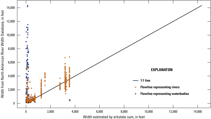
Stream channel widths from the North American River Width Database (NARWidth) compared to widths estimated from arbolate sums. The blue points with a large amount of scatter represent reservoirs that vary widely in width but have low arbolate sums. The clusters of orange points at width values of greater than 1,000 feet represent the largest streams that originate outside of the Mississippi Embayment. Arbolate sums for these streams are high where they enter the model, mostly reflecting drainage outside of the Mississippi Embayment Regional Aquifer Study area; increase in arbolate sums for these streams within the Mississippi Embayment is comparatively minor. Substantial scatter in the NARWidth values for the largest streams illustrates the wide variability in width along large rivers because of natural geomorphic and other human-made factors (control structures, dredging, and so on).
Smaller widths falling below the 1:1 line indicate a low bias in the arbolate sum-based widths relative to NARWidth. This bias is consistent with channel widths (which form the basis for the arbolate sum estimates) measured at streamgages where the channel is narrower than average and under base flow conditions, whereas the NARWidth estimates represent mean flows. Comparing measured channel widths with NARWidth estimates for the same locations indicates the NARWidth estimates to be about 32 percent higher on average but otherwise have good correspondence (fig. 8).
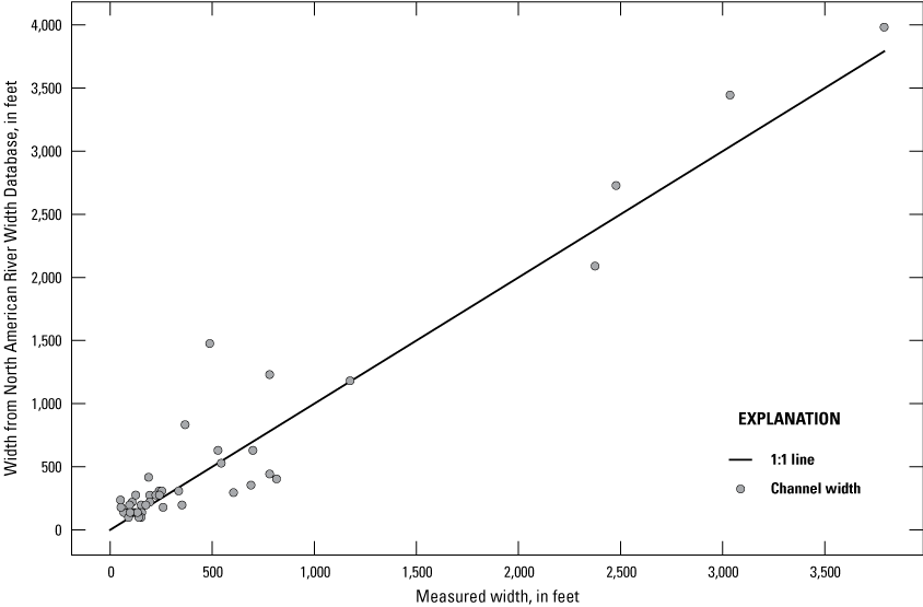
Measured channel widths compared to the North American River Width Database estimates.
Manning’s Roughness
The USGS streamflow measurement dataset used for the width estimation was also evaluated for Manning’s roughness coefficient (n). Two approaches were used: direct estimation of n from streambed bottom material type; and back calculation of n from recorded discharge, channel geometry, and an estimated slope obtained from the flowline preprocessing.
In the first approach, a representative n for each stream in the Mississippi Embayment region was estimated using channel bottom material reported by USGS personnel during streamflow measurements. Channel bottom material categories for streamflow measurements are ledge—bedrock—artificial, cobble—boulders, gravel, sand, and silt/mud. Each bottom material was assigned a representative n using the following equation (Arcement and Schneider 1989):
wherenb
is the base value for straight, uniform smooth channel in natural materials with values that change based on the bottom material,
n1
is a correction factor for the effect of surface irregularities,
n2
is a value for variations in shape and size of the channel cross section,
n3
is a value for obstructions,
n4
is a value for vegetation and flow conditions, and
m
is a correction factor for meandering of the channel.
Values for nb were estimated (table 1) for each bottom material category using the ranges listed in table 1 in Arcement and Schneider (1989) for various types of channel bottoms. Values for n1, n2, n3, and n4 were estimated (table 2) using table 2 in Arcement and Schneider (1989) and assuming:
-
• a minor degree of irregularity (carefully dredged channels in good condition but having slightly eroded or scoured side slopes),
-
• occasionally alternating channel cross sections (large and small cross sections alternate occasionally, or the main flow occasionally shifts from side to side),
-
• minor obstruction effects (obstructions occupy less than 15 percent of the cross-sectional area),
-
• a small amount of vegetation, and
-
• a medium amount of meandering.
Table 1.
Base values of Manning’s roughness coefficient for the bottom sediment categories.[Data are summarized from Arcement and Schneider (1989), table 1]
| Sediment category | nb (eq. 8) |
|---|---|
| Ledge—bedrock—artificial | 0.025 |
| Cobble—boulder | 0.040 |
| Gravel | 0.031 |
| Sand | 0.022 |
| Silt/mud | 0.012 |
Table 2.
Values of correction factors for the bottom sediment categories.[Data are summarized from Arcement and Schneider (1989), table 2]
| Variable (eq. 8) | Value |
|---|---|
| n1 | 0.0030 |
| n2 | 0.0030 |
| n3 | 0.0050 |
| n4 | 0.0060 |
| m | 1.15 |
Table 3.
Estimated base values of Manning’s roughness coefficients for the bottom sediment categories.[Data are summarized from Leaf and others (2023a)]
| Sediment category | nb (eq. 8) |
|---|---|
| Ledge—bedrock—artificial | 0.048 |
| Cobble—boulder | 0.065 |
| Gravel | 0.055 |
| Sand | 0.045 |
| Silt/mud | 0.033 |
An n was calculated for each measurement location that had at least one measurement where sediment type was reported. Locations with multiple measurements where the bottom material was reported were each assigned an n, and an average of all values was used to estimate a single n for that location.
In the second approach, equation 4 was rearranged to solve for n:
Channel area recorded in the streamflow measurement dataset was divided by the recorded channel width (w) to get an average depth (y); the slope term (S0) was estimated using the minimum and maximum smoothed elevations for the flowline associated with the streamflow measurement. Figure 9 compares the populations of roughness estimates from the two methods. The distribution of values from the first approach highlights the inherent difficulty in precisely describing the physical factors that contribute to n, an empirical parameter that is probably best estimated from actual flow observations (the second method). However, general agreement between the mean values from the two approaches, and the population densities about the means suggests that the default value of 0.037 used in SFRmaker (and the SFR packages described here) is appropriate for the MERAS region.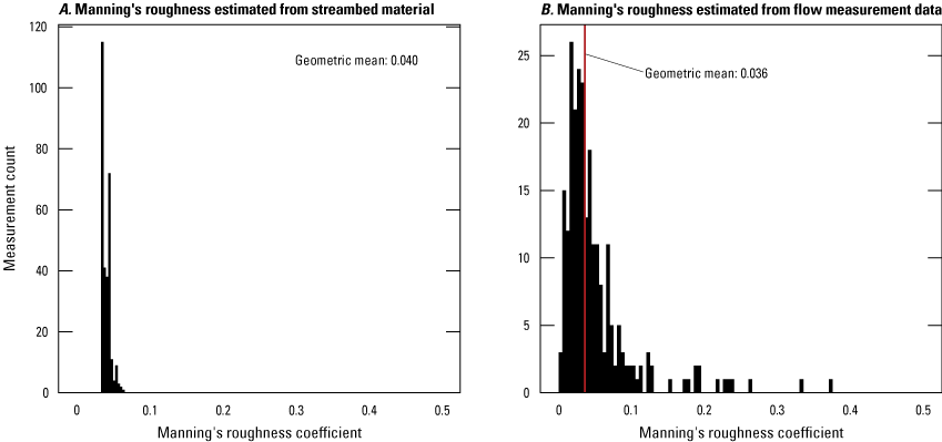
Estimated Manning’s roughness coefficients for streams in the Mississippi Embayment Regional Aquifer Study area.
Length, Streambed Elevation, and Slope
SFRmaker computes reach lengths from the respective flowline fragments (linestring geometries) using the shapely package. The preprocess_nhdplus() function assigns initial streambed top elevations from the smoothed segment end elevations developed in the preprocessing by linear interpolation to the reach mid-points. Optionally, SFRmaker can also sample minimum elevations from a DEM while creating the stream reaches (typically at a higher resolution than the flowlines; Leaf and others, 2021a, b36); this can be advantageous for finer grid resolutions but was not deemed necessary here. In subsequent development of the SFR reaches, SFRmaker computes streambed slopes as the forward differences of the initial streambed tops. A minimum slope of 0.00001 was enforced to prevent excessive stream depths (eq. 4). Compared to the default value of 0.0001 in SFRmaker, a minimum slope of 0.00001 resulted in improved matches of stream stage on the lowest gradient streams in the Mississippi Delta and is also consistent with the low stream gradients present throughout the Mississippi Alluvial Plain (Leaf and others, 2023b).
Stream Depth
DEMs can be problematic for assigning streambed elevations because the DEM often represents the water surface instead of the streambed. In that case, stream depths computed by equation 4 will be added to the water surface elevation, resulting in unrealistically high simulated stages and, often, simulated leakage out of streams that is not actually occurring.
Equation 4, which does not consider continuity of energy between stream reaches, can also produce inaccurate stream depths, especially when reach properties are averaged over large areas or consolidated from multiple streams. Because streambed elevations are not considered in equation 4, computed depths can result in stages that rise in the downstream direction. These effects are most problematic for the largest streams, which can have the largest computed depths.
To address the above issues with stage, the MERAS 3 model was run once with the initial streambed top elevations to get an estimate of stream depth for each reach. Average depths from the initial run across all stress periods were then subtracted from the original streambed tops to get a revised set of streambed tops. This resulted in computed stages in subsequent runs that were generally close to the original streambed top elevations, which are more representative of actual stages. This step was performed by a third Python script (“adjust_sfr_streambed_tops_set_stages.py” in Leaf and others, 2023a) that reads SFR Package output from the model solution and writes a new SFR package with updated streambed tops.
Streambed Kv and Thickness
Although the SFR Package allows for input of both Kv and thickness (m), these parameters are often not well understood at the scale of the model, and simulation of interactions between groundwater and surface water often lump them together conceptually into a resistance (m/Kv; units of days) or leakance (Kv/m; units of days−1) term that describes the total resistance to flow between the aquifer and a surface water body. Initial leakance values for the SFR packages described here were derived from the results of waterborne electrical resistivity surveys of streams in the MERAS region (Killian, 2018; Adams and others, 2019). The results of Adams and others (2019) consist of depth-integrated estimates of streambed Kv (see Killian, 2018 for methodology) and the total survey depth (the thickness of sediments contributing to the Kv values) at point locations along the surveyed streams. Leakance values were computed from these data at each survey point. The population of leakance estimates is shown in figure 10.
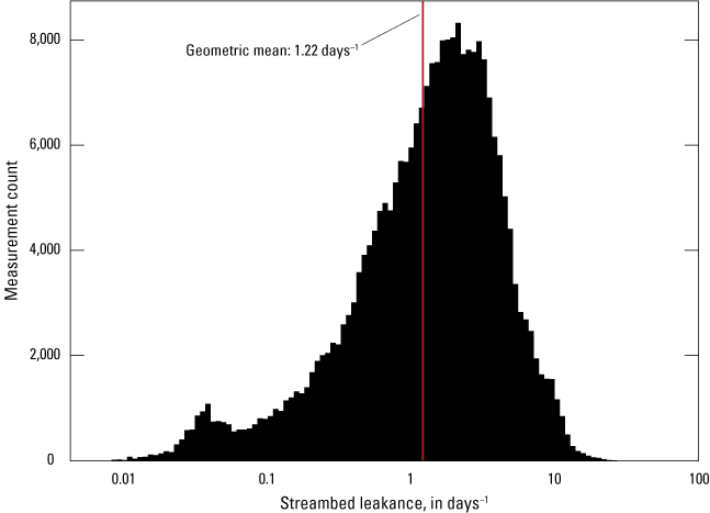
Streambed leakance values for the Mississippi Embayment Regional Aquifer Study region derived from the surveys of Adams and others (2019).
The point estimates of leakance within each model grid cell were identified using a spatial index and the geometric mean computed for each cell (fig. 11). Kv was then assigned to the SFR reaches by multiplying the mean leakances by the area factors from equation 7, assuming a uniform streambed thickness of 1 foot for all SFR reaches. SFR reaches with no leakance estimates were assigned the geometric mean for the whole Adams and others (2019) dataset of 1.22 days−1. The initial Kv values were assigned in the parameter estimation setup for the MERAS 3 and Mississippi Delta models (“setup_parameters.py” script in Leaf and others, 2023a) and then subsequently adjusted in the parameter estimation (Leaf and others, 2023b).
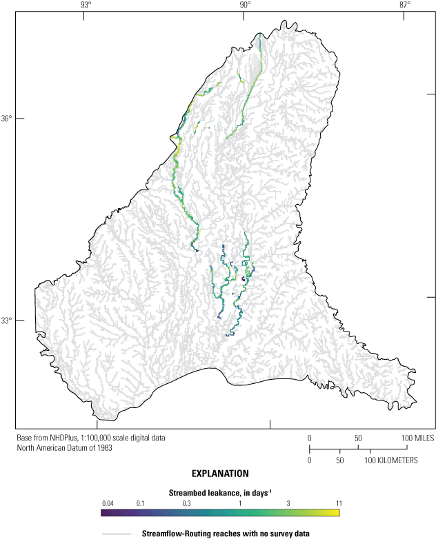
Streambed leakance values derived from the surveys of Adams and others (2019).
Specified Inflows to the Stream Network and Streamflow Observations
The MERAS model domain receives many surface water inflows from the greater Mississippi watershed. Partial streamgage records were available for five sites near the model perimeter. Additionally, streamflow was specified at the outlets of the four flood control reservoirs that feed the Tallahatchie/Yazoo River system in the Mississippi Delta (Arkabutla, Enid, Sardis, and Grenada Lakes; Tim Rodgers, U.S. Army Corps of Engineers, written commun., March 19, 2020; fig. 1). Remaining inflows for 136 additional ungaged streams and missing flows at gaged locations dating back to July 2000 were estimated using a statistical model based on the random forest method (Dietsch and others, 2023). The random forest model compares variables including monthly precipitation, minimum and maximum temperature, evapotranspiration, catchment elevations, and geology with monthly total flow and base flow values at gaged sites throughout the Mississippi Embayment and surrounding region; and then makes predictions of monthly total flows and base flows at ungaged locations and times. A description of the random forest model is in Dietsch and others (2023). Locations of inflows to the SFR network are shown in figure 12. SFRmaker automates the process of assigning inflows to SFR reaches using NHDPlus COMIDs and proximity to the reach linestrings as grid-independent references, allowing for changes in the stream network or the application of inflows to inset models with minimal additional labor. The same process is used to locate flow or stage observations within the SFR network.
Surface Water Runoff
Comparing simulated and observed streamflow and stages, and a large runoff component in the surface water balance, indicated a need to simulate total streamflow to adequately represent surface-water availability and groundwater/surface water gradients (Leaf and others, 2023b). Total streamflow was simulated by specifying monthly mean estimates of surface water runoff from the Soil-Water-Balance code (SWB; Westenbroek and others, 2018) simulation of Nielsen and Westenbroek (2023). Gridded daily runoff output from the SWB simulation (including the “runoff” and “rejected net infiltration” variables) was aggregated to monthly mean values and NHDPlus catchment polygons (which each correspond to a COMID and a flowline) using the swb_runoff_to_csv() function in the SFRmaker Preprocessing module. swb_runoff_to_csv() produces a table of transient runoff totals for each COMID, which was then input to Modflow-setup and SFRmaker during the model build step (fig. 3). By retaining the NHDPlus COMID associated with each stream reach, SFRmaker can map runoff totals from the catchment polygons to stream reaches. Monthly runoff totals were apportioned evenly among the reaches associated with each catchment.
Diagnostics and SFR Package Input
After developing reach and segment input, a FloPy ModflowSfr2 package object is created (Bakker and others, 2016, 2022). A series of diagnostics in the FloPy SFR module are then run, including checks for the following:
SFRmaker can then produce either a MODFLOW–2005 (SFR2) or MODFLOW–6-style SFR input file, and input to the MODFLOW Gage Package or MODFLOW–6 observation utility.Visualization
After creating SFR reaches, SFRmaker can also write shapefiles of the following:
-
• The reach linestrings with model row/column, segment, reach, streambed top, original COMID, and other attribute information to facilitate rapid querying of the SFR network. Association of the reach linestrings with segment and reach numbering also allows for model output such as streamflow and stream/aquifer interactions to be easily visualized with GIS software.
-
• SFR reach data with model cell polygons as features.
-
• Linestring features depicting routing connections between reaches.
-
• Point features depicting inlets where flows are entering the model through the SFR network and outlets where flows are leaving the model through the SFR network.
Results and Discussion
In the case of the MERAS–NWT model, the above procedure with the “sparse reaches” option resulted in an SFR package with 25,635 reaches grouped into 15,095 segments, compared to 57,295 reaches and 28,281 segments for an “all reaches” version. In total, 107 reaches had streambed elevations more than 0.01 foot above the model top; 65 reaches exceeded the model top by more than 1 foot. Streambed elevations above the model top can occur when model cells are sufficiently large to encompass a low-lying area and an adjacent area of higher ground with a dominant stream reach. With coarse cell sizes, some model top violations are typically unavoidable. The FloPy diagnostics also identified 795 (3 percent) reach connections that were nonadjacent (defined as greater than the diagonal distance across a model cell). These represent routing connections that pass through minor reaches that were dropped from the SFR network (red lines in fig. 5B). Such connections are expected in the “sparse reaches” conceptualization, which only retains a single reach in each model cell. All other diagnostic checks passed.
Initial testing and comparison of model output from an early version of MERAS–NWT suggested that the “sparse reaches” approach produces sufficiently similar results to the “all reaches” version but has less artificial cycling of water between SFR reaches, and therefore is a valid and even preferable approach for the modeling goals. Net mass balance results for the “sparse reaches” and “all reaches” versions of the SFR Package were similar to within 1.2 percent after 137 years of simulation. However, the “all reaches” version simulated about four times the stream leakage of the “sparse” version (and an additional quantity of groundwater discharge to streams to match), indicating spurious cycling of water between colocated reaches. The numerical solution for the “all reaches” version was also more unstable, taking 40 percent longer to solve. Based on these results, and the efficiency of managing a smaller SFR package, the sparse option was used for the SFR packages described here. Modeling questions that are sensitive to the local partitioning of flows between competing tributaries may require construction of an inset model at a finer grid resolution.
MODFLOW Model Solution
Figure 12 shows total streamflows from the MERAS 3 model solution at the end of stress period 121 (October 1, 2016), which represents seasonal dry conditions. A general increase in simulated streamflow (as darkening shades of blue) can be observed with distance along the SFR network, providing additional visual confirmation that continuity in the stream network is being properly simulated.
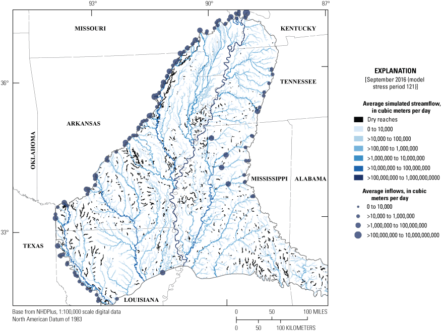
Total streamflows simulated by the Mississippi Embayment Regional Aquifer Study 3 model at the end of stress period 121 (October 1, 2016) and specified inflows to the stream network. Darkening shades of blue illustrate the simulated accumulation of streamflow with distance along the stream network.
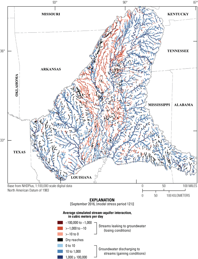
Simulated stream-aquifer interactions from the Mississippi Embayment Regional Aquifer Study 3 model at the end of stress period 121 (October 1, 2016).
Figure 13 shows simulated interactions between streams and groundwater for the same period (stress period 121; October 1, 2016). The effects of groundwater depletion within the Mississippi Alluvial Plain are apparent in the red cells showing leakage out of the stream network, and black cells indicating dry stream reaches. Groundwater discharge to streams is generally greatest during dry periods, when stream stages are lower than groundwater levels; in wet periods when stream stages are high, most streams in the alluvial plain leak (Leaf and others, 2023b). Stream leakage constitutes an import source of water to the Mississippi River Valley alluvial aquifer: 20.6 percent of net inflows in the MERAS 3 model for 2010–19 (Leaf and others, 2023b). The effects of stream leakage can be observed as high spots of reduced groundwater depletion near major rivers (Clark and others, 2011; McGuire and others, 2021; Leaf and others, 2023b).
Limitations
SFR packages produced by the workflow described here, like any component of a groundwater flow model, are greatly simplified representations of complex natural systems. Simplification is necessary because it is not possible to know everything about a real stream network, and the level of detail that can be included in a model is limited by available computing resources. SFR packages produced by this workflow are limited by simplifying assumptions in the MODFLOW SFR Package formulation (Prudic and others, 2004), in the model application (in this case, the conceptual model and structure of the MERAS–NWT, MERAS 3, and Mississippi Delta models), and in SFR package construction workflow itself.
Limitations of the Automated Workflow
The limitations described in the following subsections are inherent to the workflow described in this report.
Source Hydrography
Figure 5 and the accompanying text highlight some of the deficiencies in the 1:100,000 scale resolution NHDPlus hydrography data for the Mississippi Embayment region and the general challenge of accurately mapping streams in a relatively flat, highly altered landscape where land use and natural geomorphic processes continue to change the stream network. NHDPlus High Resolution (Moore and others, 2019) offers similar functionality to NHDPlus version 2 at a 1:24,000 resolution, albeit at the cost of managing appreciably more files and data. The workflow described in this report could be used with NHDPlus High Resolution hydrography to produce an improved SFR network. This would most benefit inset models at resolutions that are fine enough to incorporate the additional detail.
Similarly, in other regions, improved hydrography may be available, including hydrography generated via flow accumulation on a DEM (Gardner and others, 2018). Regardless of the source, hydrography input to the SFR package creation step (fig. 3) must include information on routing. The user must supply this information if using hydrography not from NHDPlus. Future developments may relax some of these requirements. For example, routing connections could be developed from flowline start/end proximity.
Limitations of the Preprocessing Approach
The preprocessing methods described in this report are intended to reduce the source hydrography, which in this application contained many streams that no longer exist or are dry under low-flow conditions, into input that is tractable for a numerical solution covering a large area. A primary goal was to automate this process to facilitate future updates to the MERAS 3 model and the creation of inset models with minimal additional labor. Limiting stream density using an arbolate sum criterion based on ad hoc comparison to satellite imagery may result in areas within the model domain where streams are under or overrepresented. Inset models focusing on smaller streams within the network have the most potential to be affected by this shortcoming and should be checked accordingly. The arbolate sum thresholds in the preprocessing routine can be adjusted to increase or decrease the number of streams represented.
Similarly, divergences may be present where the main channel was not correctly identified. Important locations in the model should be checked by the user. A “known connections” input argument to the preprocess_nhdplus() function allows routing connections to be specified manually by the user.
Finally, the preprocessed hydrography produced by the SFRmaker preprocessing module can be edited manually in a GIS environment to correct any remaining deficiencies before building the SFR package. This can greatly facilitate rapid edits to the SFR package throughout a modeling project.
Effects of Stream Reach Consolidation
Use of the “sparse” option on a coarse model grid can result in many reaches that are only implicitly represented in connections between subsequent dominant reaches. For example, a tributary to a major stream would not have any representation (and therefore no groundwater exchange) within any cells that also include the major stream. Streamgages on the tributary within these cells therefore do not have an exact output equivalent from the model. Observed flows at such locations can only be compared to the closest upstream or downstream reach that is in the model. This problem can be eliminated by selecting a grid discretization fine enough to represent the streams of interest. Coarse regional models such as MERAS 3 are generally unsuitable for representing small streams in detail.
The stream reach consolidation described by equations 6 and 7 also violates the conceptual model for computing stream depth (eq. 4). Reaches representing multiple streams have leakance values that represent groundwater inflows or outflows for all consolidated reaches but widths and slopes that only represent the dominant reach. Some of these reaches may have simulated depths (and therefore stages) that are unrealistic. This effect was mitigated by subtracting stream depths from an initial model run from the original streambed top elevations (resulting in simulated stages that are close to the water surface elevations obtained from DEMs).
Limitations Associated with the MERAS 3 Model
The MERAS 3 application of the workflow described in this report is intended to accurately represent the effects of streams on the Mississippi River alluvial aquifer at a level of detail appropriate to the regional scale and 1-km model grid resolution. Limitations inherent to this application, but not necessarily to the automated SFR construction or MODFLOW SFR Package formulation, are discussed below.
Model Spatial and Temporal Resolution
Although more detail is available from the lidar-based DEM, waterborne resistivity surveys, and other data, the coarse grid resolution of the MERAS model only allows for a single property value to be assigned to each SFR reach representing streams within that square kilometer grid cell. At many SFR reaches, property values represent more than one physical stream. Figure 5 illustrates this reduction in detail graphically, both in terms of the consolidation of streams and streambed elevations. The outcome of this simplification is that although the model solution may adequately capture groundwater flow patterns and the overall water balance at a regional scale, the details of interactions between groundwater and surface water at scales smaller than a few grid cells cannot be resolved. This includes heterogeneity in these interactions within each model cell and the effects of pumping wells near streams. Similarly, hydrologic events occurring at scales of less than a calendar month cannot be accurately represented (Leaf and others, 2023b).
Effects of Setting Streambed Tops Using Depths Estimated from an Initial Model Run
Initial streambed top elevations derived from the lidar-based DEM were adjusted by subtracting stream depths simulated from an initial model run. Ideally, this produces simulated stream stages (streambed top plus simulated depth) that are close to the DEM elevations and that vary smoothly in space, as irregularities in simulated depths created by equation 4, are canceled in the subtraction. However, if large temporal variations in stage are simulated, the depths used to adjust streambed top need to be chosen carefully, or another method of setting streambed top might be preferable. Incorporation of stage observations can help ensure that stream stages are well represented (Leaf and others, 2023b).
Limitations Associated with the MODFLOW SFR Formulation
Although the MODFLOW SFR Package simulates continuity in flow throughout the stream network, continuity of energy is not considered. Stream stage is computed independently at each reach based on the mass balance for that reach (eq. 4). Hydraulic gradients within the stream channel and the effects of momentum are not considered. Therefore, simulated stages may rise in the downstream direction. This effect was mostly mitigated in the MERAS 3 application by subtracting stream depths from an initial model run from the original streambed top elevations. Other important limitations of the SFR formulation are discussed by Prudic and others (2004) and Langevin and others (2017).
Summary
This report and the associated data release demonstrate an approach for rapid, automated creation of MODFLOW Streamflow-Routing Package input through an application for a large, multi-State area with a relatively dense, complex stream network. The two-step approach of creating a grid-independent SFR dataset and then applying it to a particular model grid is designed to facilitate the use of other grids or inset models within a study area, and rapid updating of groundwater models. Although much of the preprocessing effort was developed to address challenges specific to the mapped hydrography for the Mississippi Embayment and the coarse discretization of the Mississippi Embayment Regional Aquifer Study model, the overall approach is applicable to other areas. The SFRmaker Preprocessing module can be useful to any project encompassing multiple National Hydrography Dataset Plus drainage basins; or, where the hydrography is too dense, contains distributaries or requires custom editing before creating Streamflow-Routing package input.
References Cited
Acreman, M.C., and Ferguson, A.J.D., 2010, Environmental flows and the European Water Framework Directive: Freshwater Biology, v. 55, no. 1, p. 32–48. [Also available at https://doi.org/10.1111/j.1365-2427.2009.02181.x.]
Adams, R.F., Miller, B.V., and Kress, W.H., 2019, Waterborne Resistivity Inverted Models, Mississippi Alluvial Plain, 2016-2018: U.S. Geological Survey data release, accessed April 1, 2023, at https://doi.org/10.5066/P9WQPRFB.
Alhassan, M., Lawrence, C., Richardson, S., and Pindilli, E.J., 2019, The Mississippi Alluvial Plain aquifers—An engine for economic activity: U.S. Geological Survey Fact Sheet 2019–3003, 4 p., accessed April 1, 2023, at https://doi.org/10.3133/fs20193003.
Allen, G.H., and Pavelsky, T.M., 2015, Patterns of river width and surface area revealed by the satellite-derived North American River Width data set: Geophysical Research Letters, v. 42, no. 2, p. 395–402. [Also available at https://doi.org/10.1002/2014GL062764.]
Arcement, G.J., and Schneider, V.R., 1989, Guide for selecting Manning’s roughness coefficients for natural channels and flood plains: U.S. Geological Survey Water-Supply Paper 2339, accessed January 18, 2018, at https://doi.org/10.3133/wsp2339.
Bakker, M., Post, V., Hughes, J.D., Langevin, C.D., White, J.T., Leaf, A.T., Paulinski, S.R., Bellino, J.C., Morway, E.D., Toews, M.W., Larsen, J.D., Fienen, M.N., Starn, J.J., and Brakenhoff, D., 2022, FloPy version 3.3.7—Release candidate: U.S. Geological Survey software release, v. 15, accessed April 1, 2023, at https://doi.org/10.5066/F7BK19FH.
Bakker, M., Post, V., Langevin, C.D., Hughes, J.D., White, J.T., Starn, J.J., and Fienen, M.N., 2016, Scripting MODFLOW model development using Python and FloPy: Groundwater, v. 54, no. 5, p. 733–739. [Also available at https://doi.org/10.1111/gwat.12413.]
Barlow, J.R.B., and Clark, B.R., 2011, Simulation of water-use conservation scenarios for the Mississippi Delta using an existing regional groundwater flow model: U.S. Geological Survey Scientific Investigations Report 2011–5019, 14 p., accessed April 1, 2023, at https://doi.org/10.3133/sir20115019.
Barlow, P.M., Leake, S.A., and Fienen, M.N., 2018, Capture versus capture zones—Clarifying terminology related to sources of water to wells: Groundwater, v. 56, no. 5, p. 694–704. [Also available at https://doi.org/10.1111/gwat.12661.]
Bradbury, K.R., Fienen, M.N., Kniffin, M.L., Krause, J.J., Westenbroek, S.M., Leaf, A.T., and Barlow, P.M., 2017, A groundwater flow model for the Little Plover River Basin in Wisconsin’s Central Sands: Wisconsin Geological and Natural History Survey Bulletin 111, 82 p., accessed April 1, 2023, at https://water.usgs.gov/GIS/dsdl/gwmodels/WGNHS2017-LittlePlover/WGNHS2017_B111-report.pdf.
Campbell, B.G., and Coes, A.L., eds., 2010, Groundwater availability in the Atlantic Coastal Plain of North and South Carolina: U.S. Geological Survey Professional Paper 1773, 241 p., 7 pls., accessed April 1, 2023, at https://pubs.usgs.gov/pp/1773/.
Clark, B.R., Barlow, P.M., Peterson, S.M., Hughes, J.D., Reeves, H.W., and Viger, R.J., 2018, National-scale grid to support regional groundwater availability studies and a national hydrogeologic database: U.S. Geological Survey data release, accessed April 1, 2023, at https://doi.org/10.5066/F7P84B24.
Clark, B.R., and Hart, R.M., 2009, The Mississippi Embayment Regional Aquifer Study (MERAS)—Documentation of a groundwater-flow model constructed to assess water availability in the Mississippi Embayment: U.S. Geological Survey Scientific Investigations Report 2009–5172, 61 p., accessed April 1, 2023, at https://doi.org/10.3133/sir20095172.
Clark, B.R., Hart, R.M., and Gurdak, J.J., 2011, Groundwater availability of the Mississippi embayment: U.S. Geological Survey Professional Paper 1785, 62p., accessed April 1, 2023, at https://pubs.usgs.gov/pp/1785/.
Clark, B.R., Westerman, D.A., and Fugitt, D.T., 2013, Enhancements to the Mississippi Embayment Regional Aquifer Study (MERAS) groundwater-flow model and simulations of sustainable water-level scenarios: U.S. Geological Survey Scientific Investigations Report 2013–5161, 29 p., accessed April 1, 2023, at https://doi.org/10.3133/sir20135161.
Dietsch, B.J., Asquith, W.H., Breaker, B.K., Westenbroek, S.M., and Kress, W.H., 2023, Simulation of monthly mean and monthly base flow of streamflow using random forests for the Mississippi River Alluvial Plain, 1901 to 2018: U.S. Geological Survey Scientific Investigations Report 2022–5079, 17 p., accessed March 2023 at https://doi.org/10.3133/sir20225079.
Esri, 1998, Esri shapefile technical description: Esri, 34p., accessed March 28, 2019, at https://www.esri.com/library/whitepapers/pdfs/shapefile.pdf.
Fienen, M.N., Bradbury, K.R., Kniffin, M., and Barlow, P.M., 2017, Depletion mapping and constrained optimization to support managing groundwater extraction: Groundwater, v. 56, no. 1, p. 18–31. [Also available at https://doi.org/10.1111/gwat.12536.]
Feinstein, D.T., Fienen, M.N., Reeves, H.W., and Langevin, C.D., 2016, A semi‐structured MODFLOW‐USG model to evaluate local water sources to wells for decision support: Groundwater, v. 54, no. 4, p. 532–544. [Also available at https://doi.org/10.1111/gwat.12389.]
Feinstein, D.T., Hunt, R.J., and Reeves, H.W., 2010, Regional groundwater-flow model of the Lake Michigan Basin in support of Great Lakes Basin water availability and use studies: U.S. Geological Survey Scientific Investigations Report 2010–5109, 379 p., accessed April 1, 2023, at https://doi.org/10.3133/sir20105109.
Gardner, M.A., Morton, C.G., Huntington, J.L., Niswonger, R.G., and Henson, W.R., 2018, Input data processing tools for the integrated hydrologic model GSFLOW: Environmental Modelling & Software, v. 109, p. 41–53. [Also available at https://doi.org/10.1016/j.envsoft.2018.07.020.]
Gillies, S., 2017, Rtree (ver. 0.8): Anaconda, Inc., web page, accessed July 5, 2017, at https://anaconda.org/conda-forge/rtree.
Gillies, S., Bierbaum, A., Lautaportti, K., and Tonnhofer, O., 2017, Shapely (ver. 1.5): Anaconda, Inc., web page, accessed July 5, 2017, at https://doi.org/10.5281/zenodo.5597138. [Also available at https://anaconda.org/conda-forge/shapely.]
Harbaugh, A.W., 2005, MODFLOW-2005—The U.S. Geological Survey modular ground-water model—The ground-water flow process: U.S. Geological Survey Techniques and Methods, book 6, chap. A16, variously paged. [Also available at https://doi.org/10.3133/tm6A16.]
Harris, C.R., Millman, K.J., van der Walt, S.J., Gommers, R., Virtanen, P., Cournapeau, D., Wieser, E., Taylor, J., Berg, S., Smith, N.J., Kern, R., Picus, M., Hoyer, S., van Kerkwijk, M.H., Brett, M., Haldane, A., del Río, J.F., Wiebe, M., Peterson, P., Gérard-Marchant, P., Sheppard, K., Reddy, T., Weckesser, W., Abbasi, H., Gohlke, C., and Oliphant, T.E., 2020, Array programming with NumPy: Nature, v. 585, no. 7825, p. 357–362. [Also available at https://doi.org/10.1038/s41586-020-2649-2.]
Haugh, C.J., Killian, C.D., and Barlow, J.R.B., 2020, Simulation of water-management scenarios for the Mississippi Delta: U.S. Geological Survey Scientific Investigations Report 2019–5116, 15 p. [Also available at https://doi.org/10.3133/sir20195116.]
Hunt, R.J., White, J.T., Duncan, L.L., Haugh, C.J., and Doherty, J., 2021, Evaluating lower computational burden approaches for calibration of large environmental models: Groundwater, v. 59, no. 6, p. 788–798. [Also available at https://doi.org/10.1111/gwat.13106.]
Killian, C., 2018, Characterizing spatial and temporal changes and driving factors of groundwater and surface-water interactions within the Mississippi portion of the Mississippi Alluvial Plain: Theses and Dissertations, v. 1044, accessed April 1, 2023, at https://scholarsjunction.msstate.edu/td/1044/.
Konikow, L.F., 2013, Groundwater depletion in the United States (1900–2008): U.S. Geological Survey Scientific Investigations Report 2013–5079, 63 p., accessed April 1, 2023, at https://pubs.usgs.gov/sir/2013/5079.
Langevin, C.D., Hughes, J.D., Banta, E.R., Niswonger, R.G., Panday, S., and Provost, A.M., 2017, Documentation for the MODFLOW 6 Groundwater Flow Model: U.S. Geological Survey Techniques and Methods, book 6, chap. A55, 197 p., accessed April 1, 2023, at https://doi.org/10.3133/tm6A55.
Leaf, A.T., Duncan, L.L., and Haugh, C.J., 2023a, Modflow-6 models of the Mississippi embayment (MERAS 3) and Mississippi Delta: U.S. Geological Survey data release, https://doi.org/10.5066/P971LPOB.
Leaf, A.T., Duncan, L.L., Haugh, C.J., Hunt, R.J., and Rigby, J.R., 2023b, Simulation of groundwater flow in the Mississippi Alluvial Plain with a focus on the Mississippi Delta: U.S. Geological Survey Scientific Investigations Report 2023–5100, 143 p., https://doi.org/10.3133/sir20235100.
Leaf, A.T., and Fienen, M.N., 2022, Modflow-setup—Robust automation of groundwater model construction: Frontiers in Earth Science, v. 10, no. 903965, 11 p., accessed April 1, 2023, at https://doi.org/10.3389/feart.2022.903965.
Leaf, A.T., Fienen, M.N., and Reeves, H.W., 2021a, SFRmaker (ver. 0.7.1): U.S. Geological Survey software release, accessed April 1, 2023, at https://doi.org/10.5066/P9U2T031.
Leaf, A.T., Fienen, M.N., and Reeves, H.W., 2021b, SFRmaker and Linesink-Maker—Rapid construction of streamflow routing networks from hydrography data: Ground Water, v. 59, no. 5, p. 761–771, accessed August 2023 at https://doi.org/10.1111/gwat.13095.
Leake, S.A., Reeves, H.W., and Dickinson, J.E., 2010, A new capture fraction method to map how pumpage affects surface water flow: Groundwater, v. 48, no. 5, p. 690–700. [Also available at https://doi.org/10.1111/j.1745-6584.2010.00701.x.]
McGuire, V.L., Seanor, R.C., Asquith, W.H., Strauch, K.R., Nottmeier, A.M., Thomas, J.C., Tollett, R.W., and Kress, W.H., 2021, Datasets used to map the potentiometric surface, Mississippi River Valley alluvial aquifer, spring 2020: U.S. Geological Survey data release, accessed April 1, 2023, at https://doi.org/10.5066/P9CXDIPL.
McKay, L., Bondelid, T., Dewald, T., Johnston, J., Moore, R., and Rea, A., 2012, NHDPlus version 2—User guide (data model version 2.1): U.S. Environmental Protection Agency, accessed January 3, 2023, at https://www.epa.gov/waterdata/basic-information.
Moore, R.B., and Dewald, T.G., 2016, The road to NHDPlus—Advancements in digital stream networks and associated catchments: Journal of the American Water Resources Association, v. 52, no. 4, p. 890–900. [Also available at https://doi.org/10.1111/1752-1688.12389.]
Moore, R.B., McKay, L.D., Rea, A.H., Bondelid, T.R., Price, C.V., Dewald, T.G., and Johnston, C.M., 2019, User's guide for the national hydrography dataset plus (NHDPlus) high resolution: U.S. Geological Survey Open-File Report 2019–1096, 66 p., accessed April 1, 2023, at https://doi.org/10.3133/ofr20191096.
Nielsen, M.G., and Westenbroek, S.M., 2023, Updated estimates of water budget components for the Mississippi embayment region using a Soil-Water-Balance model, 2000–2020: U.S. Geological Survey Scientific Investigations Report 2023–5080, 58 p., https://doi.org/10.3133/sir20235080.
Niswonger, R.G., Panday, S., and Ibaraki, M., 2011, MODFLOW-NWT—A Newton formulation for MODFLOW-2005: U.S. Geological Survey Techniques and Methods, book 6, chap. A37, 44 p., accessed April 1, 2023, at https://doi.org/10.3133/tm6A37.
Niswonger, R.G., and Prudic, D.E., 2005, Documentation of the Streamflow-Routing (SFR2) Package to include unsaturated flow beneath streams—A modification to SFR1: U.S. Geological Survey Techniques and Methods, book 6, chap. A13, 50 p., accessed April 1, 2023, at https://doi.org/10.3133/tm6A13.
Park, C.C., 1977, World-wide variations in hydraulic geometry exponents of stream channels—An analysis and some observations: Journal of Hydrology, v. 33, no. 1–2, p. 133–146. [Also available at https://doi.org/10.1016/0022-1694(77)90103-2.]
Perry, M., 2017, Rasterstats (ver. 0.12): Anaconda, Inc., web page, accessed July 5, 2017, at https://conda-forge.org/.
Prudic, D.E., Konikow, L.F., and Banta, E.R., 2004, A new Streamflow-Routing (SFR1) Package to simulate stream-aquifer interaction with MODFLOW–2000: U.S. Geological Survey Open–File Report 2004–1042, 95 p., accessed April 1, 2023, at https://doi.org/10.3133/ofr20041042.
Reba, M., Massey, J., Adviento‐Borbe, M., Leslie, D., Yaeger, M., Anders, M., and Farris, J., 2017, Aquifer Depletion in the Lower Mississippi River Basin—Challenges and Solutions: Journal of Contemporary Water Research & Education, v. 162, no. 1, p. 128–139. [Also available at https://doi.org/10.1111/j.1936-704X.2017.03264.x.]
Richter, B.D., Davis, M.M., Apse, C., and Konrad, C., 2012, A presumptive standard for environmental flow protection: River Research and Applications, v. 28, no. 8, p. 1312–1321. [Also available at https://doi.org/10.1002/rra.1511.]
Saucier, R.T., 1994, Geomorphology and Quaternary geologic history of the Lower Mississippi Valley vol. I: U.S. Army Corps of Engineers Waterways Experiment Station, 400 p. [Also available at https://biotech.law.lsu.edu/climate/mississippi/sausier/sausier.htm.]
U.S. Geological Survey [USGS], 2018a, National Hydrography Dataset: U.S. Geological Survey web page, accessed September 19, 2018, at https://www.usgs.gov/national-hydrography/national-hydrography-dataset.
U.S. Geological Survey [USGS], 2018b, Mississippi Alluvial Plain project website: U.S. Geological Survey web page, accessed August 16, 2018, at https://www2.usgs.gov/water/lowermississippigulf/map/index.html.
U.S. Geological Survey [USGS], 2018c, 3D Elevation Program data: U.S. Geological Survey web page, accessed September 19, 2018, at https://apps.nationalmap.gov/downloader.
U.S. Geological Survey [USGS], 2022, USGS water data for the Nation: U.S. Geological Survey National Water Information System database, accessed December 2022 at https://doi.org/10.5066/F7P55KJN.
Van Arsdale, R.B., and Cox, R.T., 2007, The Mississippi’s curious origins: Scientific American, v. 296, no. 1, p. 76–82. [Also available at https://doi.org/10.1038/scientificamerican0107-76.]
Watson, K.A., Mayer, A.S., and Reeves, H.W., 2014, Groundwater availability as constrained by hydrogeology and environmental flows: Groundwater, v. 52, no. 2, p. 225–238. [Also available at https://doi.org/10.1111/gwat.12050.]
Westenbroek, S.M., Engott, J.A., Kelson, V.A., and Hunt, R.J., 2018, SWB version 2.0—A Soil-Water-Balance code for estimating net infiltration and other water-budget components: U.S. Geological Survey Techniques and Methods, book 6, chap. A59, 118 p., accessed October 2018 at https://doi.org/10.3133/tm6A59.
White, J.T., Doherty, J.E., and Hughes, J.D., 2014, Quantifying the predictive consequences of model error with linear subspace analysis: Water Resources Research, v. 50, no. 2, p. 1152–1173. [Also available at https://doi.org/10.1002/2013WR014767.]
Woods, A.J., Foti, T.L., Chapman, S.S., Omernik, J.M., Wise, J.A., Murray, E.O., Prior, W.L., Pagan, J.B., Jr., Comstock, J.A., and Radford, M., 2004, Ecoregions of Arkansas (color poster with map, descriptive text, summary tables, and photographs): U.S. Geological Survey poster, scale 1:1,000,000, accessed August 16, 2018, at https://www.epa.gov/eco-research/ecoregion-download-files-state-region-6.
Conversion Factors
U.S. customary units to International System of Units
Datum
Vertical coordinate information is referenced to the North American Vertical Datum of 1988 (NAVD 88).
Horizontal coordinate information is referenced to the North American Datum of 1983 (NAD 83).
Abbreviations
COMID
common identifier number
DEM
digital elevation model
GIS
geographic information system
lidar
light detection and ranging
MERAS
Mississippi Embayment Regional Aquifer Study
n
Manning’s roughness coefficient
NARWidth
North American River Width Database
NHDPlus
National Hydrography Dataset Plus
SFR
Streamflow-Routing
SFR2
Streamflow-Routing Package (for MODFLOW), version 2
USGS
U.S. Geological Survey
For more information about this publication, contact:
Director, USGS Upper Midwest Water Science Center
1 Gifford Pinchot Drive
Madison, WI 53726
For additional information, visit: https://www.usgs.gov/centers/uppermidwest-water-science-center
Publishing support provided by the Rolla Publishing Service Center
Disclaimers
Any use of trade, firm, or product names is for descriptive purposes only and does not imply endorsement by the U.S. Government.
Although this information product, for the most part, is in the public domain, it also may contain copyrighted materials as noted in the text. Permission to reproduce copyrighted items must be secured from the copyright owner.
Suggested Citation
Leaf, A.T., 2023, Automated construction of Streamflow-Routing networks for MODFLOW—Application in the Mississippi Embayment region: U.S. Geological Survey Scientific Investigations Report 2023–5051, 28 p., https://doi.org/10.3133/sir20235051.
ISSN: 2328-0328 (online)
Study Area
| Publication type | Report |
|---|---|
| Publication Subtype | USGS Numbered Series |
| Title | Automated construction of Streamflow-Routing networks for MODFLOW—Application in the Mississippi Embayment region |
| Series title | Scientific Investigations Report |
| Series number | 2023-5051 |
| DOI | 10.3133/sir20235051 |
| Publication Date | December 22, 2023 |
| Year Published | 2023 |
| Language | English |
| Publisher | U.S. Geological Survey |
| Publisher location | Reston, VA |
| Contributing office(s) | Upper Midwest Water Science Center |
| Description | Report: vii, 28 p.; 4 Data Releases; Dataset |
| Country | United States |
| Other Geospatial | Mississippi Embayment Region |
| Online Only (Y/N) | Y |
| Additional Online Files (Y/N) | N |