

Regression Equations for Estimating the 4-Day, 3-Year Low-Flow Frequency and Adjusted Harmonic Mean Streamflow at Ungaged Sites for Unregulated, Perennial Streams in New Mexico
Links
- Document: Report (1.23 MB pdf) , HTML , XML
- Data Releases:
- USGS StreamStats - Streamflow statistics and spatial analysis tools for water-resources applications
- USGS water data for the Nation - U.S. Geological Survey National Water Information System database
- NGMDB Index Page: National Geologic Map Database Index Page (html)
- Download citation as: RIS | Dublin Core
Acknowledgments
This study was supported by the New Mexico Environment Department Surface Water Quality Bureau. The authors would like to thank the many U.S. Geological Survey hydrologic technicians who collected streamflow data and ensured it was of high quality, and Michael Kohn for sharing his knowledge of southern Colorado streamgages. The authors also wish to express their gratitude to William Asquith and William Farmer for their continued support and guidance.
Abstract
The Federal Clean Water Act stipulates that States adopt water-quality standards to protect and enhance the quality of water in those States and to protect water quality through the creation of planning documents and discharge permits. Critical low-flow values, including the 4-day, 3-year low-flow frequency (4Q3) and harmonic mean streamflows, are necessary for developing those planning documents and permits. The U.S. Geological Survey computed the 4Q3 and adjusted harmonic mean streamflows using data from 96 streamgages on perennial streams, and regression equations were developed for the estimation of these parameters at ungaged, perennial streams in the State of New Mexico using weighted least-squares regression and readily accessed basin and climatic characteristics. Six equations were developed for the 4Q3 statistic, and five equations were developed for the adjusted harmonic mean statistic. Separate equations were developed for sites located in basins with mean elevations equal to or greater than 8,000 feet above the National Geodetic Vertical Datum of 1929 (except where noted as the North American Vertical Datum of 1988), as well as for sites on streams that are tributary to the San Juan River. Pseudo R-squared values ranged from 0.53 to 0.87 (4Q3) and adjusted R-squared values ranged from 0.69 to 0.89 (adjusted harmonic mean). For sites in basins with mean elevations of less than 8,000 feet above the National Geodetic Vertical Datum of 1929 (except where noted as the North American Vertical Datum of 1988), equations were developed based on contributing drainage area size. Drainage area, mean basin elevation, basinwide mean annual precipitation, and mean basin slope were found to have relations to the 4Q3; drainage area, mean basin elevation, basinwide mean annual precipitation, mean basin slope, and mean basinwide precipitation for the winter period, defined as the months of October through April, were found to have relations to the adjusted harmonic mean. Comparison to previous 4Q3 regression equations using fit statistics indicate an overall improvement in performance.
Introduction
The State of New Mexico is required under the New Mexico Water Quality Act (New Mexico Water Quality Control Commission, 2020a) and the Federal Clean Water Act (33.U.S.C. §1251 et seq.) to adopt water-quality standards that are consistent with and serve the purposes of those acts, including protecting the public and enhancing the quality of water (New Mexico Water Quality Standards Section 11). Critical low-flow values, including the 4-day, 3-year low-flow frequency (4Q3) and harmonic mean streamflows, are necessary for developing planning documents and point-source discharge permits by the New Mexico Environment Department (NMED).
The 4Q3 streamflow is the minimum 4-consecutive-day mean streamflow that has a recurrence interval of 3 years in a perennial stream (fig. 1). Harmonic mean annual streamflow, referred to hereafter as “harmonic mean streamflow,” is computed as the number of daily mean streamflow values divided by the sum of the reciprocals of the daily mean streamflows for perennial streams. Harmonic mean streamflow is generally smaller than the corresponding arithmetic mean streamflow and gives greater weights to low daily mean streamflows (Straub, 2001). This statistic is used because exposure concentration of contaminants in streams can be greater on days with low streamflow and, therefore, proportionally more detrimental than on days with higher streamflows. Because reciprocals of streamflows are used in the equation for harmonic mean, a value of zero for daily mean streamflow cannot be handled directly by the formula. To account for the zero values for daily mean streamflow encountered in New Mexico streams for some days, this study incorporated the use of an adjusted harmonic mean. The adjusted harmonic mean accounts for zero-flow values by multiplying the harmonic mean for the nonzero daily mean streamflows by the ratio of the number of nonzero daily mean streamflows to the total number of daily mean streamflows in the period of record analyzed.
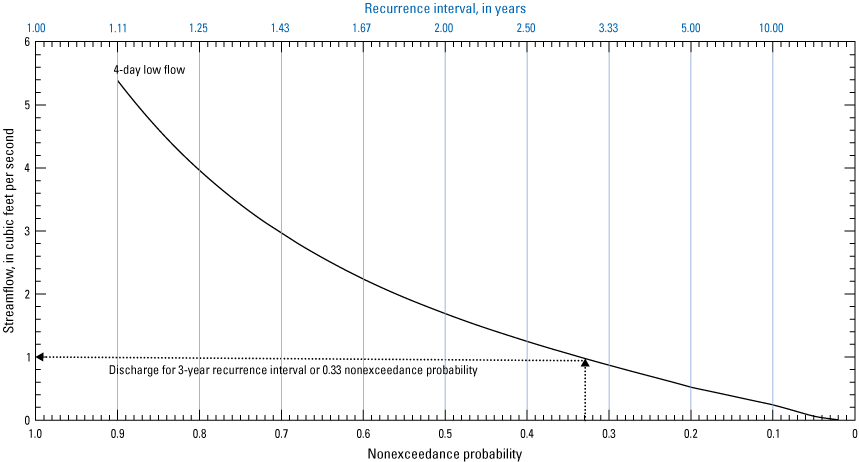
Four-day low-flow frequency curve for streamflow-gaging station 07215500 Mora River at La Cueva, New Mexico (adapted from Waltemeyer, 2002, fig. 2).
Efficient and science-based techniques for estimating these low-flow statistics could support the State of New Mexico in its decision-making and regulatory processes related to water resources. Values of 4Q3 and adjusted harmonic mean can be computed directly for locations where there are streamflow gages (streamgages) and at least 10 years of unregulated and perennial record using streamflow statistics applications. For locations where streamgage data are not available, regional regression equations are used to compute 4Q3 and adjusted harmonic mean streamflow values. Regionalization, a process using statistical regression analysis, provides a relation for efficiently transferring information from a group of streamgages in a region to ungaged sites in the same region (Farmer and others, 2019). The regional regression equations for 4Q3 streamflow were last developed nearly 20 years ago using streamflow data from the late 1990s and precipitation data from 1961 to 1990 (Waltemeyer, 2002), whereas regional regression equations for harmonic mean streamflow previously have not been developed for New Mexico streams. The present study was conducted by the U.S. Geological Survey (USGS), in cooperation with the New Mexico Environment Department, to provide a statewide set of regional equations that can be used to estimate 4Q3 and adjusted harmonic mean streamflow at ungaged locations on unregulated, perennial streams in New Mexico. Calculations of 4Q3 low-flow and adjusted harmonic mean streamflow using the latest period of record for streamgages in New Mexico are used for the development of these regional regression equations. These equations are intended for incorporation into the New Mexico StreamStats application (Ries and others, 2017).
This report documents the regression equations used to estimate the 4-day, 3-year low-flow frequency and adjusted harmonic mean streamflow at ungaged sites for unregulated, perennial streams in New Mexico.
Equation Notation Used in This Report
There are two categories of equations included in this report. General equations that were used to support the study are identified by number in the order that they appear in the text. The regional regression equations that were developed are identified by a prefix indicating which streamflow statistic the equation is associated with. For example, the regression equation used to compute the 4Q3 for a location at or above an elevation of 8,000 ft is identified herein as “4Q3-1a,” whereas the regression equation used to compute the adjusted harmonic mean streamflow for a location at or above an elevation of 8,000 ft is identified herein as “AHM-1a.”
Basin characteristic abbreviations used in this report are shortened from those used in the StreamStats application for simplicity. A crosswalk of abbreviations of basin characteristics used in this report is located in the front matter of this report.
Flow statistics in this report are referred to as “calculated,” “computed,” and “estimated.” Calculated flow statistics are those that have been determined using published software, in this case, SWToolbox (Kiang and others, 2018). Computed flow statistics have been determined using the regional regression equations developed in this study. Estimated flow statistics refer to those determined using previously published regression equations (that is, Waltemeyer [2002]).
Description of Study Area
The State of New Mexico is a large and geographically heterogeneous area encompassing 122,580 square miles (mi2) (Keyes, 1906), making it the fifth largest State in the United States (fig. 2). The physiography of the State is complex and includes a wide variety of landforms, including mountains, valleys, mesas, and plains. While generally arid, variations in elevation and latitude result in a wide range of average precipitation, precipitation type (snow and rain), temperature, and evapotranspiration rates throughout the State.
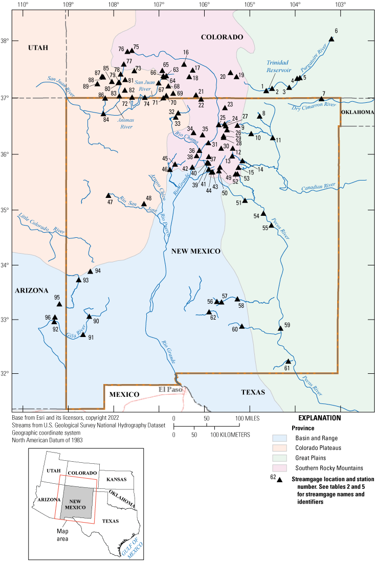
Study area, including locations of streamgages used in this study.
New Mexico is bisected by the Rio Grande and associated rift basin and includes parts of four distinct physiographic provinces: the Great Plains, Basin and Range, Colorado Plateaus, and Southern Rocky Mountains (Fenneman and Johnson, 1946). Each province has characteristic landforms, flora, fauna, and climate. Elevation in the State ranges from 2,800 ft to over 13,000 feet (ft). Average annual precipitation in the State ranges from less than 10 inches (in.) at lower elevations to more than 20 in. at higher elevations. In general, the State receives 40–70 percent of its precipitation as a result of a seasonal monsoon (July–September), during which high pressure systems develop east of the State and draw moisture from the Gulf of Mexico into the study area (National Weather Service, 2021). The precipitation events resulting from this are often of relatively short duration and limited in areal extent. In high elevation mountainous areas, winter precipitation accounts for the majority of the annual runoff (New Mexico Interstate Stream Commission, 2018), and streams sourced there often experience peak streamflow during spring runoff of snowmelt.
The climatic year (April 1–March 31), as opposed to the water year (October 1–September 30), was used for this low-flow frequency analysis. The climatic year is named after the year in which it begins; for example, climatic year 2021 begins April 1, 2021, and ends on March 31, 2022. Streamflows in the study area are typically lowest in winter and early spring, prior to runoff from snowmelt.
Previous Investigations
Low-flow frequency equations have been developed for many States, particularly in the eastern part of the Nation (Eash and Barnes, 2017; Ries and Friesz, 2000). Fewer such equations have been developed for States in the western part of the Nation, although they have been developed in some form for Colorado (Capesius and Stephens, 2009), Idaho (Hortness, 2006), and Oregon (Risley and others, 2008).
In New Mexico, Borland (1970) developed low-flow statistic regression equations for New Mexico streams using 64 streamgages with periods of record of at least 10 years. These equations were generally considered to have high standard errors of estimate and would presumably have benefitted from longer periods of record and a larger geographical distribution of streamgages.
Waltemeyer (2002) developed two regression equations to estimate the 4Q3 low-flow frequency statistic in New Mexico. The study used data from 50 streamgages, and two regression equations were developed, one for general statewide use and one for those watersheds with mean basin elevations above 7,500 ft.
Methods for Regionalization of Low-Flow Statistics
The development of regression equations to estimate selected low-flow statistics in New Mexico generally followed three steps. The first step was to develop a dataset, which included trend and redundancy analyses as a part of streamgage selection. The second step was to compute selected low-flow statistics and basin characteristics. The third and final step was the iterative process of computing and refining regression equations for the selected streamflow statistics, including classification of streamgages into subgroups.
Dataset Development
The selection of an appropriate set of streamgages for use in low-flow regression is foundational to generating streamflow statistics that are representative of stream systems for which the regression equations will be applied. Numerous basin characteristics must be considered along with the relations and possible redundancies between streamgages.
Streamflow data used in this report were compiled for 411 active and inactive streamgages located in New Mexico and the adjacent States of Colorado, Oklahoma, Arizona, and Texas. This initial set of 411 streamgages included those within New Mexico and in 8-digit hydrologic unit code areas of adjoining States that extend into or originate in New Mexico (Seaber and others, 1987). Streamgages on unregulated, perennial streams with at least 10 years of streamflow data were targeted. Daily mean streamflows recorded through the 2018 climate year for the active streamgages and for the entire period of record for the currently inactive streamgages were downloaded from the USGS National Water Information System (NWIS) database (USGS, 2021). Additional assessment of the initial 411 streamgages included screening for streamflow classification of “perennial,” screening for streamflow regulation, screening for redundancy between streamgages, and screening for streamflow trends with time. The screening methods applied for this study are discussed in this section. Regulation of streamflow determinations were made by technicians servicing those streamgages and were based on the percentage of flow retained or diverted; these decisions were made on a case-by-case basis and varied somewhat on the basis of professional judgement.
Perennial Streamflow Classification
The perennial status of a stream was determined using information from the National Hydrography Dataset (NHD) (USGS, 2018; Moore and others, 2019), evaluations by NMED using their “Hydrology Protocol” (New Mexico Water Quality Control Commission, 2020b), and an evaluation of percentage of zero-flow days. New Mexico’s Water Quality Standards define a surface water as perennial when “the water body typically contains water throughout the year and rarely experiences dry periods” (New Mexico Water Quality Control Commission, 2020a, p. 4). Therefore, streamgages with recorded daily mean flows of zero were not precluded from inclusion in this study. The NMED “Hydrology Protocol” was considered to be a more robust method for use in New Mexico, as the protocol uses on-the-ground methods and was therefore given preference over NHD evaluations. NMED uses a standardized method for classifying streams as perennial, intermittent, or ephemeral as described in their “Hydrology Protocol,” which is published as part of NMED’s “Statewide Water Quality Management Plan and Continuing Planning Process” (New Mexico Water Quality Control Commission, 2020b). In locations where these determinations had been made, NMED’s stream classifications were used. Finally, streamgages having 10 percent or more zero-flow days over the entirety of the record were disqualified from inclusion on the basis that they were not perennial.
Streamflow Regulation
Manipulation of streamflow (streamflow regulation) is prevalent in New Mexico and has been practiced in some form since at least the late 16th century (Natural Resources Conservation Service, undated). The most common types of streamflow regulation in New Mexico are diversions for and returns from irrigation or other uses, and storage in and releases from on- and offstream impoundments (dams and reservoirs). The USGS in New Mexico identifies annual streamflow peaks affected by some degree of regulation. The degrees of regulation are grouped into two broad categories.
The first category (NWIS discharge code 6; USGS, 2021), “Discharge affected by Regulation or Diversion,” is applied to each year in the streamgage record that streamflow regulation is known to have occurred and considered to be either complete or substantial (increasing or decreasing flow by more than 15 percent). Years in which streamflow records were impacted by regulation are typically not included in the development of streamflow statistics. In this study, streamgages with peak flows identified as being regulated (NWIS discharge code 6) were not included for the period over which they were regulated. Streamflow record at these streamgages was included, however, for the period of the record prior to any regulation. For example, if there were streamgage records for several decades prior to the installation of a dam, those years would have been included in this study.
The other category of regulation (NWIS discharge code 5; USGS, 2021), “Discharge affected to unknown degree by Regulation or Diversion,” is applied for each year that discharge is affected by an unknown, slight, or partial (less than 15 percent) degree by regulation or diversion. Streamgages with streamflow affected by unknown regulation (NWIS discharge code 5) were considered if stream regulation was not present for the entirety of the record. With these sites, a trend analysis was conducted for the entire period of record to determine if the degree of regulation was detectible. If no trend was detected, the regulation was determined to be inconsequential and the streamgage was retained. If the entire record was coded with “unknown regulation,” the streamgage was not included because there was no way to evaluate the degree of regulation at that site.
Redundancy
Streams may have multiple streamgages on the same channel located sequentially in close proximity, leading to watersheds that are nested, occasionally with watersheds that vary in size and shape only by small slivers. Other pairs of streamgages, although in different watersheds, are in close geographic proximity and share similar hydrologic responses and characteristics such that they represent the same hydrologic setting. Streamgages and correlating watersheds were therefore examined together for redundancy between streamgages in order to avoid overrepresentation of a particular hydrologic setting, which could result in the generation of cross correlation of flow conditions in the model violating the model assumption that individual streamflow values are independent of each other (Veilleux, 2009). Streamflow records were not checked for redundancy. The contributing drainage areas and the distance between basin centroids were compared for every possible pair of streamgages to determine that a specific hydrologic setting was not represented through more than a single streamgage. When basin pairs had proximity values (measured as the distance from each basin centroid) of less than 0.5 mile and area ratios less than five, the streamgages were considered redundant and one of the streamgages was removed from the study. The decision of which of the two streamgages to keep was based on several factors including the size of the contributing drainage area, whether the basins were nested, and the number of redundant pairings a streamgage was identified in. When determining which streamgage to retain, preference was given to streamgages with smaller drainage areas and longer periods of record. Streamgages with smaller contributing drainage areas are likely more representative of the sites at which the regression equations will be used. Streamgages with longer continuous records are preferable because long-term system behavior is key to developing useful low-flow regression equations.
Streamflow Trends With Time
An effort was made to ensure that the streamgage period of record used for each streamgage in this study was representative of modern conditions. In streamflow frequency analyses, there is an assumption that annual low flows, in this case the annual minimum 4-consecutive-day average streamflow, are independent and stationary over time; therefore, trends in streamflow with time could introduce bias into the analysis. The longest period of record representative of modern conditions for each streamgage was evaluated using the Kendall Tau statistic, which computes the monotonic relation between streamflow and time (Helsel and others, 2020), in this case, the 4Q3 and climatic years. To find the longest continuous streamflow record with no significant monotonic trend, each streamgage was first analyzed using the entire period of record. If the entire period of record did not show a significant (p-value greater than or equal to 0.05) Kendall Tau, the entire record was used to determine the low-flow statistics (Kiang and others, 2018). If the Kendall Tau statistic was deemed significant (p-value less than or equal to 0.05), the period of record was shortened in steps, removing the earliest period of the streamgage record in 5-year intervals, and recomputing the Kendall Tau statistic each time until there was no longer any evidence of a statistically significant trend. The resulting continuous streamflow record was assumed to be representative of modern conditions and used to compute low-flow statistics for that streamgage. No annual values were computed for those years that contained missing records. Although years with missing data were not included in the study, missing data did not prevent the inclusion of streamgages from the study. Streamgages were included for consideration in the study if there were at least 10 years of continuous or noncontinuous record with no missing data.
Low-Flow Statistics
The USGS has established standard methods for estimating low-flow statistics, which were computed by climate year (April 1–March 31). With a few exceptions, streamflows in New Mexico are generally at their lowest in the late summer and early fall and highest in the spring, although monsoonal events can influence this (USGS, 2021). By placing the timeframe of the lowest expected streamflows wholly within the time period analyzed, rather than near the beginning or end of it, the annual flow statistic for each year was anticipated to be as independent of hydrologic conditions in adjacent years as possible, thereby producing flow statistics for each year that were not influenced by data from other years.
SWToolbox
SWToolbox is a program developed by USGS (Kiang and others, 2018) that combines streamflow analysis methods from USGS “SWSTAT” software (https://water.usgs.gov/water-resources/legacy-software/) and U.S. Environmental Protection Agency (EPA) program DFLOW (EPA, 1986). The program is primarily used for the computation of critical low-flow statistics. The main analyses that SWToolbox performs are the computation of hydrologic frequency statistics, computation of statistically significant flows of interest to resource managers and other stakeholders (that is, 4Q3 and adjusted harmonic mean), and computation of flow-duration curves (Searcy, 1959) and hydrographs.
4Q3
The 4Q3 flow statistic is an example of an n-day low-flow statistic, which is the annual minimum, mean streamflows for a specific period of days in an annual period with a recurrence interval of a given number of years. For example, the 4Q3 is the 4-day minimum flow with a recurrence interval of 3 years. In the case of determining specific low-flow frequencies, n-day frequency analysis is used to estimate the probability that streamflow at a specific location will not exceed a specified flow level in any given year. The 4Q3 statistic was calculated for the longest period of record without a monotonic trend for each streamgage using the Integrated Design Flow (IDF) plug-in in SWToolbox. In SW Toolbox, the computed n-day flows for the period of analysis are fit to a log-Pearson type III (LP3) distribution (see Asquith and others [2017]).
In datasets containing daily mean flows with a value of zero, the log transformation that is needed to fit the LP3 distribution is not possible. In this case, the LP3 distribution is fit to the nonzero members of the time series. In records containing daily mean flow values of zero, a conditional probability adjustment is made to account for zero-flow days in the record and to compute an unconditional nonexceedance probability that includes the possibility of zero flows. The unconditional probabilities are then used to define the frequency curve (Kiang and others, 2018). This process allows for the possibility of nonzero 4Q3s in streams having some number of daily mean flow values of zero.
Adjusted Harmonic Mean
The adjusted harmonic mean statistic of the daily mean streamflow was calculated for the longest period of record without a monotonic trend for each streamgage using the IDF plug-in in SWToolbox. Harmonic mean is the reciprocal of the arithmetic mean of the reciprocals of a dataset (eq. 1). The harmonic mean is always the least, or most conservative, of the commonly used means, except when all values in the dataset are equal. The harmonic mean minimizes the impact of large outliers while emphasizing small outliers:
whereQh
is the harmonic mean;
Ni
is the number of observations; and
Qi
is the daily mean discharge streamflow value, in cubic feet per second, for the ith day.
Because traditional harmonic means cannot be calculated with zeroes in the dataset—including zero-flow data results in a nonnumber—an adjusted harmonic mean can be calculated that considers the proportion of zero-flow days. Generally, the adjusted harmonic mean is considered to be the more conservative value, as it considers days of zero flow, and the unadjusted harmonic mean on a stream with zero-flow days may actually result in a higher harmonic mean than that calculated for a nearby similar stream with no zero-flow days. However, Martin and Ruhl (1993) suggested that this is not necessarily true and that the treatment of the zero-flow days, whether they are removed or replaced, may substantially impact the computed value.
The adjustment made to harmonic mean is the harmonic mean multiplied by the proportion of zero-flow days in the record. This method is the same as is used by the EPA in early versions of the computer program DFLOW (Rossman, 1990). The current version of DFLOW available in SWToolbox does not include this correction (Kiang and others, 2018). Zero-flow days are not equivalent to days with missing flow data. At the time of this publication, NMED used adjusted harmonic mean to support computations of permit requirements and thus, a regression equation of the adjusted harmonic mean is presented here (eq. 2), based on output from the IDF plug-in of SWToolbox:
whereRegression Equation Development
A regression equation is, fundamentally, a way to describe the relation between a response variable and explanatory variables (Helsel and others, 2020). The focus of this study is to provide equations that predict the value of the chosen low-flow statistic using data readily available for the watershed in question by finding the strongest relations between the low-flow statistic and known basin (watershed) characteristics. The process of developing the regression equations is described in the following sections. All low-flow data necessary to develop the regression models were generated using SWToolbox and all watershed characteristic data were generated using StreamStats.
Exploratory Basin Analysis
Basin characteristic information for each streamgage was generated using StreamStats (USGS, 2020). The list of basin characteristics generated and examined for correlation with the low-flow statistics is available in StreamStats. Exploratory data analysis was completed using statistical techniques. Individual basin characteristics were plotted against the flow statistics of interest, directly and with log transformations, to evaluate which characteristics had the most linear relations with the 4Q3 and adjusted harmonic mean. The datasets were examined as a whole, as well as divided into several different subregions, in an effort to maximize correlations. Basin characteristics with the highest correlation to a flow statistic were identified for possible inclusion in the regression equations. The basin characteristics were also investigated for cross correlation (for example, winter precipitation and January precipitation) by plotting individual basin characteristics against each other.
Regionalization/Regional Analysis
Models, including regression models, are developed for specific conditions and domains using datasets representing domain conditions. For example, the regression equations in this report were developed for the State of New Mexico using streamgages in watersheds that exist in whole or in part within the State. Although regression models incorporating data from the entire domain of interest can be productive, it is likely that model fit will be improved by refining the domain into subregions through a process called regionalization. Subregions may be based on spatial conditions, temporal conditions, or other conditions associated with the dataset. During the exploratory phase of this study, the streamgage network was assessed as a whole, then as subsets based on latitude, longitude, elevation, and drainage area. The results were used to inform the development of the final regression equations.
Regression Analysis
Regression analysis is a statistical technique used to describe and quantify relations between two or more variables. Variables are generally described as being either explanatory (independent) variables or response (dependent) variables. Regression can be used to predict the response variable using quantified relation to explanatory variables (Farmer and others, 2019). The technique of quantifying a relation between two variables by calculating a straight line is known as linear regression (Helsel and others, 2020). Alternatively, multiple linear regression can be used to evaluate the relations of a response variable to two or more explanatory variables and describes a plane or hyperplane rather than a straight line (Helsel and others, 2020). The general multiple linear regression model is denoted as follows:
wherey
is the response variable,
β0
is the intercept,
β1
is the slope coefficient for the first explanatory variable,
x1
is the first explanatory variable,
β2
is the slope coefficient for the second explanatory variable,
x2
is the second explanatory variable,
βk
is the slope coefficient for the kth explanatory variable,
xi
is the ith explanatory variable, and
ε
is the remaining unexplained noise in the data (error).
Least squares is a method of regression estimation that approximates relations between the response and explanatory variables that minimizes the variance by minimizing the vertical distance between each data point and the line of regression. The variance is the sum of the squares of the errors for all observations, thus least squares (Farmer and others, 2019; Helsel and others, 2020). Common techniques using least-squares regression as their basis include ordinary least squares (OLS), weighted least squares (WLS), and general least squares (GLS). WLS was used in this study and is discussed in more detail below.
WLS is a refinement of basic least-squares regression that accounts for nonuniform uncertainties in observations of the response variable, in this case typically because of differences in the length of streamflow record used to compute streamflow statistics (Farmer and others, 2019). WLS can be used when the conditions required for OLS regression are not met. For example, input accuracies may include differences in the reliability or accuracy of streamflow data at different streamgages because of differences in periods of record or differences in flow regimes at the streamgage sites. Nonconstant variance of residuals (heteroscedasticity) resulting from presence in a “flashy” basin or other possible causes, also causes concern when using OLS. WLS allows more emphasis to be placed on streamgages that are considered more reliable, either due to length of period of record or because of minimal variance. WLS is typically the appropriate regression type to use for low-flow frequency studies unless cross correlation between sites is large (K. Eng, USGS, written commun., 2023). In this case, WLS was used for both low-flow regression analyses with weighting based on streamgage record length.
The Weighted-Multiple-Linear Regression Program software (WREG) was developed by the USGS to facilitate multiple linear regression for surface-water statistics. WREG was initially developed in 2009 (Eng and others, 2009) and was recently updated (Farmer, 2021) using R programming language (version 4.1.3; R Core Team, 2022). WREG provides for OLS, WLS, and GLS regressions. WREG is used primarily for frequency flow statistics, and thus was used only for the 4Q3 regressions and not for adjusted harmonic mean. Regression equations for adjusted harmonic mean were developed using the linear model function in base R (version 4.1.3, R Core Team, 2022). This function is used to fit linear models and can be used to develop multiple regressions and also returns an analysis of variance.
Degrees of Freedom
Degrees of freedom is a statistical concept that refers to the number of independent values in a dataset that can vary as parameters are estimated through regression analysis (Helsel and others, 2020). Generally, the number of degrees of freedom is related to the number of independent values less the number of parameters that are being estimated, although more complexity exists depending on the statistical analysis being performed (Eisenhauer, 2008).
When performing regression analysis, the R-squared (or pseudo R-squared) statistic is generally used as a metric to judge how well a predictive model fits the dataset. An R-squared value approaching one is generally desired (Helsel and others, 2020), but there is the potential to overfit a model in the effort to increase the R-squared value. Overfitting occurs when the model becomes too complex and begins to describe random error in the dataset rather than the relations between variables either as a result of using more explanatory terms or more complex approaches than required. When this happens, the regression model is less generalizable and is less likely to fit samples outside of the modeled dataset (Hawkins, 2004).
Logarithmic Transformation and Bias Correction Adjustment
With linear regression, several assumptions are made, which include a symmetrical distribution of data, linear relations of variables, and homoscedastic (randomly distributed but similar variance) errors (Helsel and others, 2020). If the original dataset does not adequately meet these assumptions, it may be possible to transform the data in such a way to meet them. Transformations may include raising a variable to a power, log transformation of the variable, or otherwise changing the scale of the variable. Logarithmic transformation, such as natural log, is commonly used in hydrology and may be used on both the explanatory and response variables. However, transforming the response variable of a regression equation logarithmically will produce equations with outputs in transformed units, requiring retransformation back to the original units (Helsel and others, 2020).
A logarithmic equation may be expressed in terms of the untransformed response variable by simply retransforming, or back transforming, to normal space via antilog. However, there are implications to consider when retransforming, which are discussed at length in Beauchamp and Olson (1973). When appropriately transformed, the response values will be normally distributed; thus, the mean and median will be approximately equal. After simple retransformation of the response variable from log space to normal space, the mean will be greater than the median and similarly impact variance of the model (Finney, 1941). In transformed regressions, the regression line estimates the mean response of the response variable, but the resulting equation estimates the median response of the response variable. When retransformed from log space, the resulting distribution of the response variable will be skewed to the right and follow a log-normal distribution as the largest values of the transformed response variable are compressed at the upper end of the logarithmic scale (Beauchamp and Olson, 1973). If the mean response is sought, rather than the median, then a bias correction must be applied (Helsel and others, 2020).
For the objectives and intended use of the regression equations outlined in this study, the median is appropriate. However, it is possible that an end user may wish to use these equations to develop cumulative estimates of loading. If this is sought, then the conditional mean is needed, rather than the median value (Helsel and others, 2020).
There are multiple ways to estimate an adjustment to compensate for the bias introduced by retransformation. The parametric or maximum likelihood estimate (MLE) requires that (1) residuals in the log-transformed units are normal, and (2) the coefficients of the regression model are known without error, a condition that is rarely or never met in a natural system (Helsel and others, 2020). When the dataset is large and the standard error of the regression is small, the MLE can be a very good approximation of the needed bias correction. When the dataset is small or the standard error is large, the MLE is likely to overcompensate the bias correction (Helsel and others, 2020). Alternatively, the nonparametric, or Duan smearing, estimate only requires an assumption that the residuals are independent and homoscedastic. The smearing estimate is based on the concept that the residuals of the regression are equally likely and retransforms those residuals from the transformed units into the original units and then computes their mean. The produced mean is the bias-correction factor that is then multiplied by the uncorrected y-value (Duan, 1983). Additionally, the Duan smearing estimate can be used to correct bias when retransforming any type of transformation—it is not limited to the use of log retransformation (Helsel and others, 2020). The Duan smearing bias correction estimate has been included in this report to be used if needed.
Regression Equations to Estimate Low Flow at Ungaged Sites
Final Dataset Assembly
Of the original set of 411 streamgages, 159 streamgages were removed because they were crest-stage gages, which record only peak flows and do not record daily streamflow data. Forty-eight streamgages were disqualified from the study, because the streams they monitored did not meet the NMED “Hydrology Protocol” requirements (New Mexico Water Quality Control Commission, 2020b) to be considered a perennial stream or were classified as intermittent in the NHD (USGS, 2018).
The redundancy screening revealed 114 pairs of streamgages that had potential for redundancy on the basis of proximity and similarity of basin areas. The redundancy analysis included 42 pairs of nested basins. Because of the nature of nested basins in subsequent downstream streamgages on a single stream, certain streamgages appeared in numerous redundant streamgage pairs. In these cases, the streamgage that occurred in the highest number of redundant pairs was removed in order to keep as many other streamgages as possible. Basin areas were also considered because it is preferrable to have the greatest variability of basin areas included in the study as possible; priority was therefore given to the streamgage with the smaller drainage area, because smaller contributing drainage areas are likely more representative of the ungaged sites at which the regression equations will be used. In a small number of streamgage pairs, both streamgages were kept despite meeting the screening guidelines. For example, pairs that were located in or near mountainous terrain were considered for difference in topography and possible differences in precipitation pattern. As a result of the redundancy analysis, an additional 26 streamgages were removed from the study.
An additional 25 streamgages were removed because they had greater than 10 percent of zero-flow days in the useable record. Eleven streamgages were removed because they had a 4Q3 of zero or not a number (NaN), as computed using the IDF application in SWToolbox.
Years with missing data were not included in the study, and missing data mostly did not disallow the inclusion of streamgages from the study. The exception to this was the 17 streamgages removed from the study because of their having less than 10 years of record after subtracting any missing years of record.
Nineteen streamgages were removed from the dataset because they were identified as partially regulated (NWIS discharge code 5—“Discharge affected to unknown degree by Regulation or Diversion”) for the entire period of record and so the degree of regulation could not be ascertained. Two streamgages that were identified as partially regulated for a portion of their periods of record were removed from the dataset because there were trends identified during the period of record indicating regulation was likely impacting the low flow at those streamgages. An accounting of the number of streamgages removed from the dataset is provided in table 1.
Table 1.
Accounting of streamgages removed from the dataset.[No., number; NMED, New Mexico Environment Department; 4Q3, 4-day, 3-year low-flow frequency streamflow; NaN, not a number; NWIS, National Water Information System; WREG, Weighted-Multiple-Linear Regression Program software]
Trend Analysis Findings
After consideration for perennial status (minimum of zero-flow days), length of streamflow record, minimum periods of missing streamflow record, and possible redundancy with other streamgages, the remaining gages were analyzed for trends. Trend analyses on the remaining streamgages generally showed minimal changes in streamflow with time. Thirty-two streamgages had Kendall Tau values that were considered significant (p-values less than 0.05) and indicative of change with time for some portion of their streamgage record. In order to keep the streamflow record that was most reflective of current conditions, we kept the longest period of record starting with the present values and moving toward the past with no trend. This assessment resulted in the loss of 277 total years of streamflow record across 21 streamgages (fig. 3), as well as the removal of 7 streamgages from the dataset. The minimum number of years of record removed from any streamgage was 1 year and the maximum number was 56 years.
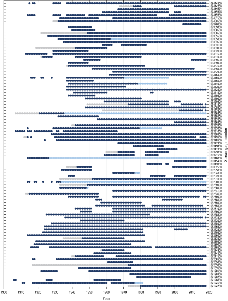
Period of record used for low-flow analysis (dark blue), years dropped from analysis because of evidence of trend with time (light gray), and years dropped from analysis because of regulation (light blue) for each streamgage included in the study.
Miscellaneous Streamgage Determination
Several streamgages had stream low-flow values that were outliers, as identified by the WREG leverage value (Eng and others, 2009), and merited closer scrutiny. Streamgage 07126500 was not coded as being regulated, but visual investigation of the aerial photo clearly indicated a large diversion structure upstream of the streamgage. Subsequent inquiries revealed that streamflow at the streamgage is affected by operation of the Trinidad Reservoir, and the stream is possibly dry for months at a time. This streamgage was therefore removed from the study. Streamgages 9365500, 09363500, and 09371000 were also outliers with respect to the leverage value during regression analysis, but further investigation of these sites did not produce any obvious factors that might explain the difference in flow values, so they were retained in the study.
Evaluation of streamflow records based on period of record, missing years of record, perennial status, and redundancy resulted in the removal of 315 streamgages, or approximately 77 percent of the streamgage records initially considered for inclusion in this study. The number of streamgages excluded from the dataset for each justification and (or) reason are presented in table 1. Streamgages may fit into multiple categories, but removal was performed in a stepwise manner; thus, only one reason was identified for each streamgage. The remaining set of streamflow records included in this study from 96 streamgages should be considered a current representation of perennial streams in and near New Mexico.
Low-Flow Statistics
The low-flow statistics computed for the 96 streamgages using the IDF plug-in in SWToolbox are listed in table 2. The 4Q3 flow statistics ranged from 0.03 to 324.21 cubic feet per second (ft3/s) and adjusted harmonic mean flow statistics ranged from 0.12 to 871.14 ft3/s. To ensure that the adjustment made to the harmonic mean was consistent, the adjusted harmonic mean for each streamgage was computed using both the IDF and DFLOW plug-ins of SWToolbox and the two values were compared. DFLOW documentation was not sufficient to determine how and if adjusted or unadjusted harmonic mean was computed. Because NMED uses adjusted harmonic mean in its surface-water discharge permitting, the IDF output was used.
Table 2.
Calculated low-flow statistics for study streamgages.[Streamflow data used to calculate the low-flow statistics are available from U.S. Geological Survey (USGS, 2021). no., number; 4Q3, 4-day, 3-year low-flow frequency streamflow, in cubic feet per second; AHM, adjusted harmonic mean streamflow, in cubic feet per second; CO, Colorado; R, River; nr, near; NM, New Mexico; C, Creek; ab, above; Ft., Fort; Nat. Mon., National Monument; Res, Reservoir; bl, below; Cr, Creek; EF, East Fork; Spgs., Springs; WF, West Fork; AZ, Arizona]
Basin Characteristics
Sixty-five basin characteristics (including latitude and longitude at the basin pour point) were available for analyses for each of the streamgages included in this study. These basin characteristics were computed using the USGS StreamStats tool (Ries and others, 2017). Plots of each of these basin characteristics against flow statistics showed likely correlation among the following basin characteristics for both 4Q3 and adjusted harmonic mean: drainage area, in square miles; winter precipitation (from October to April), in inches; average basin slope (unitless); average annual precipitation, in inches; and mean basin elevation, in feet. Drainage area ranged from 10.6 to 15,600 mi2, winter precipitation ranged from 4.27 to 29.24 in., average basin slope ranged from 0.03 to 0.54, annual precipitation ranged from 13.23 to 43.16 in., and mean basin elevation ranged from 4,470 to 11,900 ft. (table 3).
Table 3.
Basin and climatic characteristics used in regression equation development.[No., number; DA, drainage area, in square miles; E, mean basin elevation, in feet above the National Geodetic Vertical Datum of 1929; P, mean annual basinwide precipitation, in inches; WP, mean basinwide precipitation for the winter period (from October to April), in inches; S, mean basin slope, unitless; 4Q3, 4-day, 3-year low-flow frequency streamflow; AHM, adjusted harmonic mean streamflow]
Regression Equations
For this study, regression equations for 4Q3 and adjusted harmonic mean flow were regionalized by elevation and drainage area and are listed in tables 4 and 5 along with their pseudo or adjusted R-squared values and associated error. Regionalization based on mean basin elevation provided the results with the lowest residuals and the highest adjusted R-squared values. Locations in the San Juan River and tributary watersheds with mean basin elevation equal to or greater than 8,000 ft were put into a separate region. Tables 6 and 7 list the 96 streamgages used in the study with their computed and predicted flow statistics for comparison. When basin conditions meet several equation conditions, see the section titled “Suggested Uses and Application of Regression Equations.”
Table 4.
Regional 4-day, 3-year low-flow frequency streamflow (4Q3) equations using weighted least-squares regression.[No. number; pseudo R2, pseudo coefficient of determination; E, mean basin elevation, in feet above the National Geodetic Vertical Datum of 1929; ft, foot; DA, drainage area, in square miles; tribs, tributaries; P, mean annual basinwide precipitation, in inches; WP, mean basinwide precipitation for the winter period (from October to April), in inches; S, mean basin slope; ≥, greater than or equal to; <, less than; >, greater than]
Table 5.
Regional adjusted harmonic mean (AHM) streamflow equations using weighted least-squares regression.[No., number; adjusted R2, adjusted coefficient of determination; E, mean basin elevation, in feet above the National Geodetic Vertical Datum of 1929; DA, drainage area, in square miles; tribs, tributaries; P, basinwide mean annual precipitation, in inches; WP, mean basinwide precipitation for the winter period (from October to April), in inches; <, less than; >, greater than; ≥, greater than or equal to]
Table 6.
Calculated and predicted 4-day, 3-year low-flow frequency (4Q3) streamflow values (in cubic feet per second) and relevant basin characteristics for each streamgage used in regression analysis.[Basin characteristics are available from the U.S. Geological Survey StreamStats application (USGS, 2021); calculated 4Q3 values were generated using the IDF plug-in in SWToolbox (Kiang and others, 2018). no., number; USGS, U.S. Geological Survey; DA, drainage area, in square miles; E, mean basin elevation in feet above the National Geodetic Vertical Datum of 1929, except when noted as North American Vertical Datum of 1988 (NAVD 88); P, basinwide mean annual precipitation, in inches; S, mean basin slope; WP, mean basinwide precipitation for the winter period (from October to April), in inches; CO, Colorado; NA, not applicable; R, River; nr, near; NM, New Mexico; C, Creek; ab, above; Ft., Fort; Nat. Mon., National Monument; Res, Reservoir; bl, below; Cr, Creek; EF, East Fork; Spgs., Springs; WF, West Fork; AZ, Arizona]
Table 7.
Calculated and predicted adjusted harmonic mean (AHM) streamflow values (in cubic feet per second) and relevant basin characteristics for each streamgage used in regression analysis.[Basin characteristics are available from the U.S. Geological Survey StreamStats application (USGS, 2021); calculated AHM values were generated using the IDF plug-in in SWToolbox (Kiang and others, 2018). no., number; USGS, U.S. Geological Survey; DA, drainage area, in square miles; E, mean basin elevation, in feet above the National Geodetic Vertical Datum of 1929, except when noted as North American Vertical Datum of 1988 (NAVD 88); P, basinwide mean annual precipitation, in inches; WP, mean basinwide precipitation for the winter period (from October to April), in inches; CO, Colorado; NA, not applicable; R, River; nr, near; NM, New Mexico; C, Creek; ab, above; Ft., Fort; Nat. Mon., National Monument; Res, Reservoir; bl, below; Cr, Creek; EF, East Fork; Spgs., Springs; WF, West Fork; AZ, Arizona]
Suggested Uses and Application of Regression Equations
The regression equations presented herein can be used to estimate adjusted harmonic mean and 4Q3 flow values at ungaged stream locations throughout the State of New Mexico. Regression equations specific to the magnitude of the basin areas were intentionally created with overlapping area-based bins. The overlapping bins were helpful in computing the regression equations because they allowed for larger populations for each set of regressions. Hydrologic judgement and knowledge about an area will be helpful in deciding which of the applicable equations is best for that location or if it is preferable to solve multiple applicable equations and then apply a weighting value to each for an integrated value. The general procedures for estimation of adjusted harmonic mean and 4Q3 flow values are illustrated in this section.
When solving for either 4Q3 or adjusted harmonic mean flow statistics for basins with average basin elevations equal to or greater than 8,000 ft, the equations designed for high elevation basins will produce satisfactory results for the majority of basins, particularly those specific to the portion of the San Juan Subregion that lies in the study area. When solving 4Q3 or adjusted harmonic mean for basins with average elevations of less than 8,000 ft, the equation should be selected on the basis of the basin area. For those basins whose areas fall into more than one basin-area region, results can be computed for both applicable basin-area regions and then weighted inversely proportional to the root mean square error (for 4Q3) or residual standard error (for adjusted harmonic mean) for each applicable region to produce estimates that would be more reliable than the results from either individual method.
For 4Q3, the equation for weighing computed values is as follows:
whereQweighted
is the weighted streamflow value,
RMSEx
is the root mean square error for the chosen equation,
Qeqnx
is the streamflow computed from the chosen equation,
eqn n
is the first chosen equation, and
eqn n1
is the second chosen equation.
For adjusted harmonic mean, the equation for weighing computed values is as follows:
whereExample Solutions
Example 1: Solving 4Q3 for a tributary to the Rio Grande with a drainage area of 60 mi2 and an average basin elevation of 9,200 ft.—In this example, because the average basin elevation is greater than 8,000 ft but the basin is not a tributary to the San Juan River, the best results will be obtained by using the statewide equation for basins having average elevations equal to or greater than 8,000 ft (eq. 4Q3-1a) as follows:
Example 2: Solving adjusted harmonic mean for a basin with a drainage area of 250 mi2, an average basin elevation of 6,800 ft, and annual precipitation of 22.5 in.—Because the average basin elevation in this example is less than 8,000 ft, the high-elevation equations cannot be used. The user must instead select the appropriate basin area equations. The basin area of 250 mi2 is included in the range for two different basin area equations, equations AHM-2 and AHM-3, which represent the drainage areas that are less than 300 mi2 and drainage areas between 200 and 1,000 mi2. Each of the two applicable equations will be solved and then they will be combined and weighted using standard errors according to equation 5
Solution: Equation AHM-2
Solution: Equation AHM-3
Weighting using equation 5 and an RSE of 4.94 ft3/s for equation AHM-2 and an RSE of 5.32 ft3/s for equation AHM-3:
Discussion and Limitations of Use
Regression equations for those basins having average elevations equal to or greater than 8,000 ft consistently performed better than total-state equations based on basin area. Those streamgages in basins with average elevations equal to or greater than 8,000 ft that were also in the portion of the San Juan Subregion that lies in the study area performed even better than the statewide aggregation of streamgages with average basin elevations equal to or greater than 8,000 ft.
The basin area regionalized groupings with the least error are the grouping with basin areas less than 75 mi2 for 4Q3 prediction and basin areas less than 300 mi2 for adjusted harmonic mean prediction, likely because these groupings included the largest number of streamgages in regression analysis. Pseudo R-squared values ranged from 0.53 to 0.87 for the set of 4Q3 regression equations, with the lowest value associated with the DA>1,000 mi2 region, which included the fewest number of streamgages in the dataset as well as covering the largest range of drainage area. Adjusted R-squared values for the set of adjusted harmonic mean regression equations ranged from 0.69 (DA<300 mi2) to 0.89 (E ≥ 8,000 ft, San Juan and tribs). Regression equations should only be used for those basins whose characteristic variables fall in the range of those used in the generation of the regression equations (table 3). Applications of regression equations for basins outside of the range used for the regression analysis should be thought of as having questionable reliability.
Comparison With Previous Regression Equations
Adjusted harmonic mean equations have not previously been published for the State of New Mexico. Prior to this study, the most recent set of regression equations used to estimate 4Q3 at ungaged, perennial, unregulated streams in New Mexico were presented in Waltemeyer (2002). Two equations were developed by Waltemeyer (2002) using 50 streamgages: an equation for sites representing basins with mean elevations greater than 7,500 ft, termed “mountainous,” and an equation for the State below 7,500 ft. The equations presented in this report were based on a larger population of streamgages and an additional 20 years of potential record than were included in Waltemeyer (2002). A comparison of basin and climate characteristics used in this study and Waltemeyer (2002) are outlined in table 8. Despite the larger population and longer period of record, errors associated with 4Q3 regression equations for some populations exceeded 500 percent. High standard errors of estimate have been noted in similar studies in arid regions and may reflect the extreme variability in conditions that affect streamflow in New Mexico (Thomas and others, 1997).
Table 8.
Comparison of basin and climate characteristics used in Waltemeyer (2002) and this study.[DA, contributing drainage area, in square miles; E, mean basin elevation in feet above the National Geodetic Vertical Datum of 1929; P, mean annual basinwide precipitation, in inches; WP, mean basinwide precipitation for the winter period (from October to April), in inches; S, mean basin slope, in feet over feet]
| Study parameter | Waltemeyer (2002) | This study |
|---|---|---|
| Number of streamgages | 50 | 96 |
| High elevation gages | 40 | 67 |
| DA | 1.62–5,900 | 10.6–15,600 |
| E | 3,730–11,100 | 4,470–11,900 |
| P | Not used | 13.23–43.16 |
| WP | 3.89–19.42 | 4.27–29.24 |
| S | 0.025–0.517 | 0.03–0.54 |
The Waltemeyer (2002) mountainous equation was developed using 40 streamgages, had an R-squared value of 0.66, and a root mean squared error (RMSE) of 94 percent. The statewide equation in the same study was developed using 50 streamgages, 40 of which were also used in the mountainous assessment, had an R-squared value of 0.48, and an RMSE of 126 percent. In comparison, this study incorporated 96 streamgages, 67 of which were considered for high-elevation equation development. Details of the regression errors, fit statistics, and number of streamgages are provided in table 9. The two studies used two different versions of the coefficient of determination, with this study using the R2pseudo because of the use of the WLS regression method. The R2pseudo metric is based on the variability in the dependent variables explained by the regression (Farmer and others, 2019). Waltemeyer (2002) presents the R2 metric for the two equations, which potentially overstates the fits of the models because it does not adjust for the number of independent variables used in the regressions.
Table 9.
Regression and error summary of Waltemeyer (2002) and this study.[n, number of streamgages; R2, coefficient of determination; Pseudo R2, pseudo coefficient of determination; RMSE, root mean square error, in percent; NA, not applicable; E, mean basin elevation in feet (ft) above National Geodetic Vertical Datum of 1929; eq., equation; tribs, tributaries; DA, contributing drainage area, in square miles; ≥, greater than or equal to; <, less than; >, greater than]
| Descriptor | n | R2 | Pseudo R2 | RMSE |
|---|---|---|---|---|
| Statewide | 50 | 0.48 | NA | 126 |
| Mountainous | 40 | 0.66 | NA | 94 |
| E ≥ 8,000 ft (eq. 1a) | 44 | NA | 0.72 | 86 |
| E ≥ 8,000 ft, San Juan and tribs (eq. 1b) | 23 | NA | 0.87 | 76 |
| DA<75 (eq. 2) | 39 | NA | 0.75 | 80 |
| 70<DA<250 (eq. 3) | 23 | NA | 0.66 | 295 |
| 200<DA<2,000 (eq. 4) | 26 | NA | 0.67 | 176 |
| DA>1,000 (eq. 5) | 16 | NA | 0.53 | 341 |
The Pseudo R2 of equations 4Q3-1a and 4Q3-1b, for sites with a mean basin elevation equal to or greater than 8,000 ft, are higher than the R2 value of Waltemeyer’s mountainous equation for sites located with mean basin elevations equal to or greater than 7,500 ft, and the corresponding RMSE values are lower for this study’s equations 4Q3-1a and 4Q3-1b.
Waltemeyer (2002) developed a single equation to apply to all sites in New Mexico below 7,500 ft elevation, whereas this study developed four equations based on the drainage area basin characteristic. Although subdividing the streamgages into multiple groupings has resulted in a larger RMSE in three of the four new equations, all have a Pseudo R2 value equal to or larger than the R2 values presented in Waltemeyer (2002). The RMSE measures the average magnitude of error, and the errors, in this case residuals, are squared before they are averaged. As such, higher errors have more influence on the RMSE.
An effort was made to compare the performance of Waltemeyer’s mountainous regions equation and this study’s high elevation 4Q3 equations, as these are the most directly comparable equations. The estimated 4Q3 values from Waltemeyer (2002) and this study were compared both visually and statistically against the computed 4Q3 values from this study. Basin characteristics from this dataset were used in this comparison analysis. Because Waltemeyer developed the mountainous equation using streamgages with mean basin elevations equal to or greater than 7,500-ft elevation, as opposed to those with mean basin elevation equal to or greater than 8,000 ft as used in this study, only sites representing a mean basin elevation at or above 8,000 ft were included in this comparison, for a total of 66 sites. Results from this study’s equations 4Q3-1a and 4Q3-1b were combined for the purposes of this comparison analysis.
The distributions of the calculated 4Q3, the Waltemeyer mountainous 4Q3 estimates, and this study’s high elevation 4Q3 estimates are shown in figure 4. Whereas the medians and first quartile of the three populations are similar, the third quartile of the Waltemeyer (2002) data indicates a general overestimation of 4Q3 when compared to the calculated value, although the Waltemeyer (2002) outliers on the upper end of the y-axis are generally lower than the computed outliers and this study’s outliers. The interquartile ranges of the three populations quantify this visual difference and are listed in table 10.
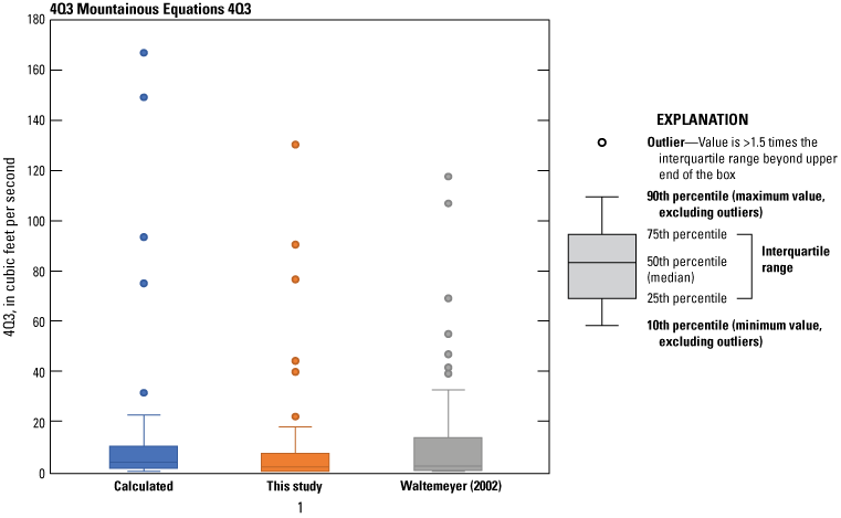
Differences between the computed and estimated 4-day, 3-year low-flow frequency (4Q3) streamflow values for high elevation, mountainous streamgages.
Table 10.
Median and interquartile range of 4-day, 3-year low-flow frequency (4Q3) streamflow populations of mountainous (Waltemeyer, 2002) and high-elevation (calculated 4Q3 and this study) locations.| Streamflow population | Median | Interquartile range |
|---|---|---|
| Calculated 4Q3 | 3.76 | 8.68 |
| Waltemeyer (2002) | 2.98 | 23.78 |
| This study | 3.17 | 9.16 |
Based on the above analysis, the high-elevation equations in this study (eqs. 4Q3-1a and 4Q3-1b) represent an improved estimation for 4Q3 on ungaged, perennial streams in New Mexico over the Waltemeyer (2002) estimates. It should be noted again that this study’s high-elevation equation development used data from substantially more streamgages than were available to Waltemeyer (2002) and longer available streamflow periods of record, as much as 20 years.
Summary
The State of New Mexico is required by the New Mexico Water Quality Act and the Federal Clean Water Act to adopt water-quality standards to protect and enhance the quality of water and to protect water quality through the creation of planning documents and discharge permits. The U.S. Geological Survey calculated the 4-day, 3-year low-flow frequency (4Q3) and adjusted harmonic mean streamflows at 96 streamgages on perennial streams in New Mexico and adjacent States, and developed regression equations to estimate these parameters at ungaged, perennial streams using the weighted least-squares method. Basin and climatic characteristics used in equation development were obtained from StreamStats. Six equations were developed for the estimation of the 4Q3 statistic, and five equations were developed for the estimation of the adjusted harmonic mean statistic. Regionalization of regression based on mean basin elevation provided the equations with the lowest residuals and the highest adjusted R2 values, and locations in the San Juan River watershed, including tributaries to the San Juan River, with mean basin elevations equal to or greater than 8,000 feet above the National Geodetic Vertical Datum of 1929 (except where noted as the North American Vertical Datum of 1988) grouped into a single, separate region. For sites with mean basin elevations less than 8,000 feet above the National Geodetic Vertical Datum of 1929 (except where noted as the North American Vertical Datum of 1988), equations for both low-flow statistics were developed based on drainage area size. Drainage area, mean basin elevation, basinwide mean annual precipitation, mean basin slope, and mean basinwide precipitation for the winter period were found to have relations to the 4Q3; drainage area, mean basin elevation, basinwide mean annual precipitation, and mean basinwide precipitation for the winter period were found to have relations to the adjusted harmonic mean. Pseudo R2 values ranged from 0.53 to 0.87 (4Q3) and from 0.69 to 0.89 (adjusted harmonic mean). Regression equations developed for drainage-area based regions were intentionally designed to have overlapping drainage area ranges, and a process of solving multiple applicable equations and applying a weight to each value before integrating for a single value was described. A visual and statistical comparison to previous high elevation 4Q3 regression equations was performed and indicated an improvement in performance over those presented in an earlier study, with the note that the population of streamgages and length of record were expanded with this study. The interquartile ranges of the calculated 4Q3s, regressed values from an earlier study, and regressed values from this study indicate that this study’s high-elevation regressed 4Q3s compare more favorably to the calculated 4Q3s.
References Cited
Asquith, W.H., Kiang, J.E., and Cohn, T.A., 2017, Application of at-site peak-streamflow frequency analyses for very low annual exceedance probabilities: U.S. Geological Survey Scientific Investigation Report 2017–5038, 93 p., accessed June 15, 2022, at https://doi.org/10.3133/sir20175038.
Borland, J.P., 1970, A proposed streamflow-data program for New Mexico: U.S. Geological Survey Open-File Report 70–35, 71 p., accessed April 3, 2023, at https://doi.org/10.3133/ofr7035.
Capesius, J.P., and Stephens, V.C., 2009, Regional regression equations for estimation of natural streamflow statistics in Colorado: Reston, Va., U.S. Geological Survey Scientific Investigations Report 2009–5136, 46 p., accessed April 3, 2023, at https://doi.org/10.3133/sir20095136.
Eash, D.A., and Barnes, K.K., 2017, Methods for estimating selected low-flow frequency statistics and harmonic mean flows for streams in Iowa (ver. 1.1, November 2017): U.S. Geological Survey Scientific Investigations Report 2012–5171, 99 p., accessed October 10, 2019, at https://doi.org/10.3133/sir20125171.
Eisenhauer, J.G., 2008, Degrees of freedom: Teaching Statistics, v. 30, no. 3, p. 75–78, accessed August 18, 2022, at https://doi.org/10.1111/j.1467-9639.2008.00324.x.
Eng, K., Chen, Y.-Y., and Kiang, J.E., 2009, User’s guide to the weighted-multiple-linear-regression program (WREG, ver. 1.0): U.S. Geological Survey Techniques and Methods, book 4, chap. A8, 21 p. [Also available at https://pubs.usgs.gov/tm/tm4a8.]
Farmer, W.H., 2021, R package WREG—Weighted least squares regression for streamflow frequency statistics: Reston, Va., U.S. Geological Survey software release, accessed June 16, 2022, at https://doi.org/10.5066/P9ZCGLI1.
Farmer, W.H., Kiang, J.E., Feaster, T.D., and Eng, K., 2019, Regionalization of surface-water statistics using multiple linear regression (ver. 1.1, February 2021): U.S. Geological Survey Techniques and Methods, book 4, chap. A12, 40 p., accessed April 3, 2023, at https://doi.org/10.3133/tm4A12.
Fenneman, N.M., and Johnson, D.W., 1946, Physical divisions of the United States: Washington, D.C., U.S. Geological Survey, 1 sheet, scale 1:7,000,000, accessed April 3, 2023, at https://doi.org/10.3133/70207506.
Hawkins, D.M., 2004, The problem of overfitting: Journal of Chemical Information and Computer Sciences, v. 44, no. 1, p. 1–12, accessed September 1, 2022, at https://doi.org/10.1021/ci0342472.
Helsel, D.R., Hirsch, R.M., Ryberg, K.R., Archfield, S.A., and Gilroy, E.J., 2020, Statistical methods in water resources: U.S. Geological Survey Techniques and Methods, book 4, chap. A3, 458 p., accessed October 29, 2020, at https://doi.org/10.3133/tm4A3.
Hortness, J.E., 2006, Estimating low-flow frequency statistics for unregulated streams in Idaho: U.S. Geological Survey Scientific Investigations Report 2006–5035, 40 p., accessed May 14, 2020, at https://doi.org/10.3133/sir20065035.
Keyes, C.R., 1906, Physiography of New Mexico: The Journal of Geography, v. 5, no. 6, p. 251–256, accessed April 7, 2023, at https://doi.org/10.1080/00221340608986127.
Kiang, J.E., Flynn, K.M., Zhai, T., Hummel, P., and Granato, G., 2018, SWToolbox—A surface-water tool-box for statistical analysis of streamflow time series: U.S. Geological Survey Techniques and Methods, book 4, chap. A11, 33 p., accessed October 10, 2019, at https://doi.org/10.3133/tm4A11.
Martin, G.R., and Ruhl, K.J., 1993, Regionalization of harmonic-mean streamflows in Kentucky: U.S. Geological Survey Water-Resources Investigations Report 92–4173, 47 p., accessed December 1, 2021, at https://doi.org/10.3133/wri924173.
Moore, R.B., McKay, L.D., Rea, A.H., Bondelid, T.R., Price, C.V., Dewald, T.G., and Johnston, C.M., 2019, User’s guide for the national hydrography dataset plus (NHDPlus) high resolution: U.S. Geological Survey Open-File Report 2019–1096, 66 p., accessed April 3, 2023, at https://doi.org/10.3133/ofr20191096.
National Weather Service, 2021, North American monsoon highlights: National Weather Service web page, accessed December 23, 2021, at https://www.weather.gov/abq/northamericanmonsoon-intro.
Natural Resources Conservation Service, [undated], The history of the Acequia—Interview with Patrick Jaramillo, former New Mexico Acequia Association, Outreach for USDA programs: Natural Resources Conservation Service, accessed August 6, 2021, at https://docslib.org/doc/9322931/acequia-association-outreach-for-usda-programs.
New Mexico Interstate Stream Commission, 2018, New Mexico State Water Plan: New Mexico Interstate Stream Commission web page, accessed August 18, 2022, at https://www.ose.state.nm.us/Planning/swp.php.
New Mexico Water Quality Control Commission, 2020a, Standards for interstate and intrastate surface waters: New Mexico Administrative Code, title 20, chap. 6, pt. 4, accessed June 30, 2022, at https://www.env.nm.gov/surface-water-quality/wp-content/uploads/sites/18/2022/05/2022-04-23-SRCA-20.6.4-NMAC-FINAL.pdf.
New Mexico Water Quality Control Commission, 2020b, Statewide Water Quality Management Plan and Continuing Planning Process: New Mexico Water Quality Control Commission web page, accessed September 16, 2020, at https://www.env.nm.gov/surface-water-quality/wqmp-cpp/.
Ries, K.G., and Friesz, P.J., 2000, Methods for estimating low-flow statistics for Massachusetts streams: U.S. Geological Survey Water-Resources Investigations Report 00–4135, 81 p., accessed October 10, 2019, at https://pubs.usgs.gov/wri/wri004135/.
Ries, K.G., III, Newson, J.K., Smith, M.J., Guthrie, J.D., Steeves, P.A., Haluska, T.L., Kolb, K.R., Thompson, R.F., Santoro, R.D., and Vraga, H.W., 2017, StreamStats, version 4: U.S. Geological Survey Fact Sheet 2017–3046, 4 p., accessed April 3, 2023, at https://doi.org/10.3133/fs20173046. [Supersedes USGS Fact Sheet 2008–3067.]
Risley, J., Stonewall, A.J., and Haluska, T., 2008, Estimating flow-duration and low-flow frequency statistics for unregulated streams in Oregon: U.S. Geological Survey Scientific Investigations Report 2008–5126, 23 p., accessed May 14, 2020, at https://doi.org/10.3133/sir20085126.
Rossman, L.A., 1990, DFLOW user’s manual: U.S. Environmental Protection Agency, 26 p., accessed August 3, 2022, at https://nepis.epa.gov.
Seaber, P.R., Kapinos, F.P., and Knapp, G.L., 1987, Hydrologic unit maps: U.S. Geological Survey Water-Supply Paper 2294, 63 p., 1 pl., accessed March 9, 2021, at https://pubs.usgs.gov/wsp/wsp2294/.
Searcy, J.K., 1959, Flow-duration curves: U.S. Geological Survey Water Supply Paper 1542–A, 33 p., accessed June 15, 2022, at https://doi.org/10.3133/wsp1542A.
Thomas, B.E., Hjalmarson, H.W., and Waltemeyer, S.D., 1997, Methods for estimating magnitude and frequency of floods in the southwestern United States: U.S. Geological Survey Water-Supply Paper 2433, 205 p., accessed July 21, 2021, at https://doi.org/10.3133/wsp2433.
U.S. Geological Survey [USGS], 2020, StreamStats—Streamflow statistics and spatial analysis tools for water-resources applications: U.S. Geological Survey website, accessed March 2019 at http://streamstats.usgs.gov.
U.S. Geological Survey [USGS], 2021, USGS water data for the Nation: U.S. Geological Survey National Water Information System database, accessed September 21, 2021, at https://doi.org/10.5066/F7P55KJN.
Waltemeyer, S.D., 2002, Analysis of the magnitude and frequency of the 4-day annual low flow and regression equations for estimating the 4-day, 3-year low-flow frequency at ungaged sites on unregulated streams in New Mexico: U.S. Geological Survey Water-Resources Investigations Report 2001–4271, 22 p., accessed October 10, 2019, at https://doi.org/10.3133/wri014271.
Supplemental Information
Basin characteristics used in regional regression equations in this report are correlated to basin characteristics available in the StreamStats web application. For brevity and ease of use, basin characteristic identifiers were chosen for this report that are shortened forms of the StreamStats identifiers they represent, as shown in the following key.
Datum
Vertical coordinate information is referenced to the National Geodetic Vertical Datum of 1929 (NGVD 29), except where noted as North American Vertical Datum of 1988 (NAVD 88).
Horizontal coordinate information is referenced to the North American Datum 1927 (NAD 27), except where noted as North American Datum of 1983 (NAD 83).
Elevation, as used in this report, refers to distance above the vertical datum.
Abbreviations
4Q3
4-day, 3-year low-flow frequency
EPA
U.S. Environmental Protection Agency
GLS
general least squares
IDF
Integrated Design Flow
LP3
log-Pearson type III
MLE
maximum likelihood estimate
NHD
National Hydrography Dataset
NMED
New Mexico Environment Department
NWIS
National Water Information System
OLS
ordinary least squares
RMSE
root mean square error
USGS
U.S. Geological Survey
WLS
weighted least squares
For more information about this publication, contact
Director, New Mexico Water Science Center
U.S. Geological Survey
6700 Edith Blvd. NE
Albuquerque, NM 87113
For additional information, visit
https://www.usgs.gov/centers/nm-water
Publishing support provided by
Lafayette Publishing Service Center
Disclaimers
Any use of trade, firm, or product names is for descriptive purposes only and does not imply endorsement by the U.S. Government.
Although this information product, for the most part, is in the public domain, it also may contain copyrighted materials as noted in the text. Permission to reproduce copyrighted items must be secured from the copyright owner.
Suggested Citation
Bell, M.T., and Tillery, A.C., 2023, Regression equations for estimating the 4-day, 3-year low-flow frequency and adjusted harmonic mean streamflow at ungaged sites for unregulated, perennial streams in New Mexico: U.S. Geological Survey Scientific Investigations Report 2023–5058, 31 p., https://doi.org/10.3133/sir20235058.
ISSN: 2328-0328 (online)
Study Area
| Publication type | Report |
|---|---|
| Publication Subtype | USGS Numbered Series |
| Title | Regression equations for estimating the 4-day, 3-year low-flow frequency and adjusted harmonic mean streamflow at ungaged sites for unregulated, perennial streams in New Mexico |
| Series title | Scientific Investigations Report |
| Series number | 2023-5058 |
| DOI | 10.3133/sir20235058 |
| Publication Date | September 26, 2023 |
| Year Published | 2023 |
| Language | English |
| Publisher | U.S. Geological Survey |
| Publisher location | Reston, VA |
| Contributing office(s) | New Mexico Water Science Center |
| Description | Report: viii, 31 p.; 2 Data Releases |
| Country | United States |
| State | New Mexico |
| Online Only (Y/N) | Y |