

Introduction and Methods of Analysis for Peak Streamflow Trends and Their Relation to Changes in Climate in Illinois, Iowa, Michigan, Minnesota, Missouri, Montana, North Dakota, South Dakota, and Wisconsin
Links
- Document: Report (44.2 MB pdf) , HTML , XML
- Larger Work: This publication is Chapter A of Peak streamflow trends and their relation to changes in climate in Illinois, Iowa, Michigan, Minnesota, Missouri, Montana, North Dakota, South Dakota, and Wisconsin
- Dataset: USGS National Water Information System database —USGS water data for the Nation
- Data Release: USGS data release - Peak streamflow data, climate data, and results from investigating hydroclimatic trends and climate change effects on peak streamflow in the Central United States, 1920–2020
- NGMDB Index Page: National Geologic Map Database Index Page (html)
- Download citation as: RIS | Dublin Core
Acknowledgments
Funding for this project was provided by the Transportation Pooled Fund-5(460) project in cooperation with the following State agencies: Illinois Department of Transportation, Iowa Department of Transportation, Michigan Department of Transportation, Minnesota Department of Transportation, Missouri Department of Transportation, Montana Department of Natural Resources and Conservation, North Dakota Department of Water Resources, South Dakota Department of Transportation, and Wisconsin Department of Transportation.
Abstract
Flood-frequency analysis, also called peak-flow frequency or flood-flow frequency analysis, is essential to water resources management applications including critical structure design and floodplain mapping. Federal guidelines for doing flood-frequency analyses are presented in a U.S. Geological Survey Techniques and Methods Report known as Bulletin 17C. A basic assumption within Bulletin 17C is that for drainage basins without major hydrologic alterations, statistical properties of the distribution of annual peak streamflows (peak flows) are stationary; that is, the mean, variance, and skew are constant. The stationarity assumption has been widely accepted within the flood-frequency community; however, a better understanding of long-term climatic persistence and concerns about potential climate change and land-use change has caused a reexamination of the stationarity assumption. Flood-frequency analyses that do not incorporate observed trends and abrupt changes may result in a poor representation of the true flood risk. Bulletin 17C does not offer guidance for incorporating nonstationarities when estimating floods, and it describes a need for studies that incorporate changing climate or basin characteristics. In response to this need and a history of concern regarding nonstationarity peak flows in the region, this study was done by the U.S. Geological Survey, in cooperation with the Departments of Transportation of Illinois, Iowa, Michigan, Minnesota, Missouri, South Dakota, and Wisconsin; the Montana Department of Natural Resources and Conservation; and the North Dakota Department of Water Resources, to assess potential nonstationarity in peak flows in the north-central United States.
This chapter summarizes the methods used to detect hydroclimatic changes in peak-flow data in the study region. A wide range of analyses and statistical approaches are applied to document the primary mechanisms controlling floods and characterize temporal changes in hydroclimatic variables and peak flow. Four periods were selected for analysis of peak flow, daily streamflow, and climate data. The periods are (1) a 100-year period, 1921–2020; (2) a 75-year period, 1946–2020; (3) a 50-year period, 1971–2020; and (4) a 30-year period, 1991–2020. The climate data consist of monthly time series estimates of temperature, precipitation, potential evapotranspiration, actual evapotranspiration, snowfall, soil moisture storage, snow water equivalent, and runoff on a 3.1-mile by 3.1-mile grid for the conterminous United States.
Statistical and graphical analyses were used to investigate potential changes in hydrology and climate. The starting point for these analyses was the initial data analysis of peak flow described in Bulletin 17C, which includes plotting the peak flow and checking for autocorrelation, monotonic trends, and changes points. Analyses were added to examine additional features in the data. To examine potential causal drivers of changes, the climate data were analyzed graphically and statistically. Results are provided in a U.S. Geological Survey data release. The study limitations are documented for users of the results.
Introduction
Flood-frequency analysis is essential to water resources management applications including critical structure design (for example, bridges and culverts) and floodplain mapping. Standardized Federal guidelines for doing flood-frequency analyses are presented in a U.S. Geological Survey (USGS) Techniques and Methods Report known as Bulletin 17C (B17C; chap. 5 of sec. B, “Surface Water,” book 4, “Hydrologic Analysis and Interpretation”) (England and others, 2019). A basic assumption within B17C is that for drainage basins without major hydrologic alterations (for example, regulation, diversion, and urbanization), statistical properties of the distribution of peak flows are stationary; that is, the mean, variance, and skew are constant (or stationary). From the onset of the USGS streamgaging program through most of the 20th century, the stationarity assumption was widely accepted within the flood-frequency community; however, a better understanding of climatic persistence (extended periods of relatively wet or relatively dry conditions) and concerns about potential climate change and land-use change have caused a reexamination of the stationarity assumption (Milly and others, 2008; Lins and Cohn, 2011; Stedinger and Griffis, 2011; Koutsoyiannis and Montanari, 2015; Serinaldi and Kilsby, 2015).
Nonstationarity is a statistical property of a peak-flow series such that the long-term distributional properties (the mean, variance, or skew) change one or more times either gradually or abruptly. Individual nonstationarities may be attributed to one source (for example, flow regulation, land-use change, or climate) but often are the result of a mixture of the sources (Vogel and others, 2011), which makes detection and attribution of nonstationarities challenging (Barth and others, 2022). Nonstationarity in peak flow can manifest as a monotonic trend in peak flows through time (Hodgkins and others, 2019) or as an abrupt change in the central tendency (mean or median), variability, or skew of peak flows (Ryberg and others, 2020a). Neglecting trends and abrupt changes in flood-frequency analysis may result in a poor representation of the true flood risk. B17C does not offer guidance on how to incorporate nonstationarities when estimating floods and further identifies a need for additional flood-frequency studies that incorporate changing climate or basin characteristics into the analysis (England and others, 2019).
In response to a history of concern regarding nonstationarity in peak flows in the region, a study was done by the USGS, in cooperation with the Departments of Transportation of Illinois, Iowa, Michigan, Minnesota, Missouri, South Dakota, and Wisconsin; the Montana Department of Natural Resources and Conservation; and the North Dakota Department of Water Resources, to assess potential nonstationarity in peak flows in the north-central United States. The study area considered consists of nine states that form a diverse region with complex variability in topography and climate (fig. 1). The range in elevation, longitude, and latitude results in a variety of climate conditions that affect the magnitude and timing of peak flows. Figure 1 shows that parts of the study area have contributing drainage area in Canada and in States that were not part of the study; however, the topography, land use, and climate of those areas outside the study affect the flows analyzed.
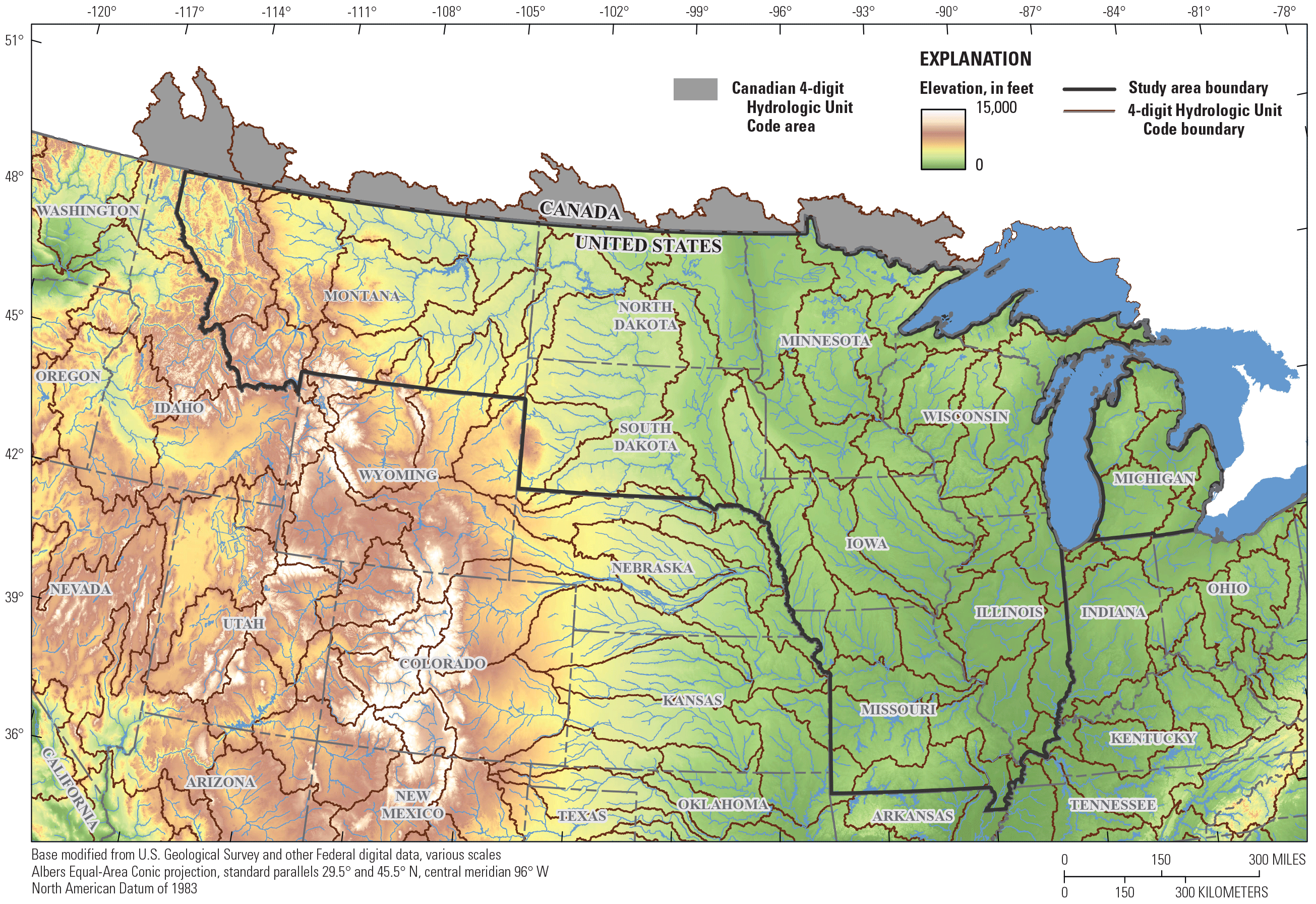
Topography and hydrography of the study area in the north-central United States.
Background
Hydroclimatology “was defined by Langbein (1967) as the study of the influence of climate upon the waters of the land” (Wendland, 1987, p. 497). Precipitation, evapotranspiration, and imbalances between them are the hydroclimate. Along with physical characteristics like soils and topography, the hydroclimate underlies floods and droughts (Shelton, 2008). The hydroclimatology in the study area is complex, and primary climatic drivers are highly variable among different peak-flow regimes. In some areas, peak-flow regimes are clearly dominated by snowmelt with relatively minor representation of rainfall events outside of the snowmelt period (Ryberg and others, 2016). Conversely, in other areas, peak-flow regimes are strongly affected by rainfall during or outside of the snowmelt period (Ryberg and others, 2016). Well-documented temporal changes in peak-flow distributions in the study area potentially violate the assumption of stationarity (Pederson and others, 2011; Hirsch and Ryberg, 2012; Mallakpour and Villarini, 2015; Archfield and others, 2016; Ryberg and others, 2016, 2020a98; Villarini, 2016; Dudley and others, 2017). Additionally, distinct contrasts in hydroclimatic patterns (that is, areas with large downward rainfall trends and areas with large upward trends) within the region (Sando and others, 2022), combined with rural and urban land-use changes (Juckem and others, 2008; Schilling and others, 2008, 2010103; Hejazi and Markus, 2009; Yang and others, 2013; Villarini and Strong, 2014; Over and others, 2016; Ahiablame and others, 2017; Falcone and others, 2018), make the multi-State region an ideal area for investigating potential nonstationary flood-frequency methodologies.
The Pacific, Atlantic (including the Gulf of Mexico), and Arctic Oceans (not shown) are the primary sources of atmospheric moisture to the study area (Bryson and Hare, 1974; Wendland and Bryson, 1981; Hirschboeck, 1991). The source and magnitude of water from precipitation differ spatially and temporally with the seasons because of changes in the prevailing winds (Hirschboeck, 1991). In the fall and winter, dominant moisture sources also include air masses over the north-central and eastern United States (Hirschboeck, 1991). The source, magnitude, and shifts in atmospheric moisture, in turn, affect the timing, magnitude, seasonality, and duration of peak flows (Archfield and others, 2016; Dickinson and others, 2019).
Previous studies have identified hydroclimatic changes that affect streamflow in the study area (Ryberg and others, 2014; Mallakpour and Villarini, 2015; Griffin and Friedman, 2017; Ivancic and Shaw, 2017; Levin and Holtschlag, 2022; Sando and others, 2022) including gradual changes in streamflow, precipitation, or temperature and more abrupt hydroclimatic shifts. These regional hydroclimatic changes (mainly increases or decreases in precipitation) have been identified as primary drivers of some peak flow nonstationarities in the study area (Levin and Holtschlag, 2022; Sando and others, 2022). Previous trend studies have generally shown an abrupt change along a northwest-southeast transect, with downward peak-flow trends in the western part of the study area, including Montana, and the western parts of North and South Dakota, and upward trends in eastern North and South Dakota, Minnesota, Iowa, Illinois, and Missouri (Hirsch and Ryberg, 2012; Peterson and others, 2013; Georgakakos and others, 2014; Norton and others, 2014; Ryberg and others, 2016, 2020a98; Hodgkins and others, 2017; Norton and others, 2022). The broad regional extent, abrupt transition, and large magnitudes of trends in the study area support the hypothesis that the trends may be caused by long-term (on the order of decades) persistence and regional hydroclimatic shifts (Vecchia, 2008; Ryberg and others, 2014; Razavi and others, 2015; Kolars and others, 2016). Long-term persistence refers to clustered wet and dry periods that induce serial correlation into the peak-flow series at lags of greater than 1 year. This long-term persistence also is referred to as memory, long-range dependence, or the Hurst phenomenon (Koutsoyiannis and Montanari, 2007; Ryberg and others, 2020b).
Other documented changes in streamflow characteristics within the study area during the last 30 years show spatial and temporal differences in the timing, magnitude, and frequency of streamflows. Olsen and others (1999) examined the relation between climatic indices and the distribution of flood flows in the upper Mississippi River and lower Missouri River. They state that global climate patterns were not primary drivers of variation in flood peaks in the 1950–96 data period. McCabe and Wolock (2002) documented change points in minimum and median daily streamflow at selected U.S. streamgages; significant increases began in 1971 at sites primarily east of 100 degrees west longitude. There is a tendency toward decreased snowpacks and earlier snowmelt runoff in mountainous areas of Montana (Pederson and others, 2011) and a general tendency toward earlier snowmelt-dominated flood peaks for much of the northern part of the study area (Ryberg and others, 2016). Other studies have indicated a more gradual tendency toward decreases in annual streamflow in Montana and Wyoming (Norton and others, 2014) and increases in monthly, seasonal, and annual streamflow in eastern North and South Dakota along with parts of Iowa and Missouri within the Missouri River Basin (Norton and others, 2014; Hoogestraat and Stamm, 2015). Mallakpour and Villarini (2015) analyzed changes in flood characteristics in the central United States (14 States: North Dakota, South Dakota, Nebraska, Kansas, Missouri, Iowa, Minnesota, Wisconsin, Illinois, West Virginia, Kentucky, Ohio, Indiana, and Michigan) during 1962–2011. They reported an increase in the frequency rather than magnitude of flooding and related these changes to changes in seasonal rainfall and temperature. More specifically, the frequency of flooding increased for much of the study area except for northern Minnesota, Wisconsin, and Michigan; Virginia and West Virginia; and western parts of Nebraska and Kansas (Mallakpour and Villarini, 2015). Analysis of temporal changes in streamflows for the 1912–2011 period (Wise and others, 2018) indicated decreases in snowpack and streamflows in the Upper Missouri River Basin including areas in Montana, North Dakota, and South Dakota, whereas streamflows in the Lower Missouri River Basin states, including Iowa and Missouri, increased during the same period.
Trends in peak flows resulting from factors other than hydroclimatology (such as land-use change or changes in agricultural practices) are also possible and may exist simultaneously with hydroclimatic changes, complicating the task of attributing these trends just to hydroclimatic changes. This study is limited in scope to hydroclimate. Those interested in other factors can consult Sando and others (2022) and Levin and Holtschlag (2022).
This chapter summarizes the methods used to detect hydroclimatic changes in peak-flow data in the study region. Evaluating hydroclimatological changes is a way of evaluating shifts in the hydrologic cycle, so a wide range of analyses and statistical approaches are applied to document the primary mechanisms controlling floods and characterize temporal changes in peak flow, daily flow, and climatic data. These analyses will provide the foundation in the region for addressing nonstationarities in observed peak flows.
Purpose and Scope
The purpose of this chapter is to document the methods used for the second task of the Transportation Pooled Fund (TPF) study TPF 5(460), which is to characterize the effects of natural hydroclimatic shifts and potential climate change on peak flows in the region. The scope of the TPF study is to evaluate the combined effects of multidecadal climatic persistence, gradual and abrupt climate change, and limited aspects of land-use change on flood-frequency analyses in the States of Illinois, Iowa, Michigan, Minnesota, Missouri, Montana, North Dakota, South Dakota, and Wisconsin. In this evaluation, peak flow, daily streamflow, and model-simulated gridded climatic data were examined for trends, change points, and other statistical properties indicative of changing climatic and environmental conditions. The TPF study is intended to provide a framework for addressing potential nonstationarity issues in flood-frequency updates that are commonly done by the USGS in cooperation with other agencies throughout the Nation. The scope of this chapter is to provide an introduction and describe the methods used to complete the second task of TPF 5(460).
Description of Study Area
The study area encompasses nine states with complex topography (fig. 1) and climate as described earlier. The physical characteristics of temperature, precipitation, and soils provide a basic understanding of this complexity. The next three figures describe these characteristics and are followed by two systems of description that integrate these characteristics and other information.
Figure 2 depicts the temperature in the region from the climate normals dataset from National Oceanic and Atmospheric Administration (NOAA) National Centers for Environmental Information (2022b). Climate normals represent the average annual temperature during the previous 30-year normal period, 1991 through 2020 (NOAA National Centers for Environmental Information, 2022b). For illustration purposes, the average temperature is classed by 5-degree increments, and the classes show a north-south gradation. Figure 3 depicts precipitation normals from the same climate normals dataset. This time, the classes represent 5-inch (in.) increments. In contrast to temperature, figure 3 shows an east-west gradation with more precipitation in the eastern parts of the study area. Precipitation class rotation to the east results from typical transport patterns for moisture coming from the Gulf of Mexico (Hirschboeck, 1991).
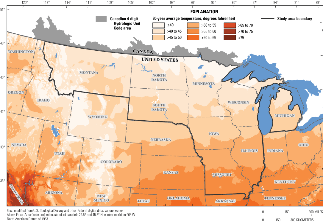
Average annual temperature for the 30-year period from 1991 through 2020 for the study area, north-central United States.
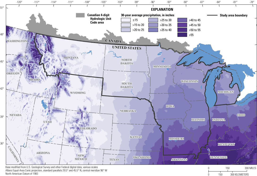
Average annual precipitation for the 30-year period from 1991 to 2020 for the study area, north-central United States.
Underpinning this complexity in topography and climate is soil. Soil characteristics affect runoff and land use and are one reason a given amount of rain does not produce the same amount of runoff everywhere. Soil characteristics can differ on a small, field scale; however, generalizations can be made about dominant soil conditions and runoff from rainfall using hydrologic soil groups (fig. 4).
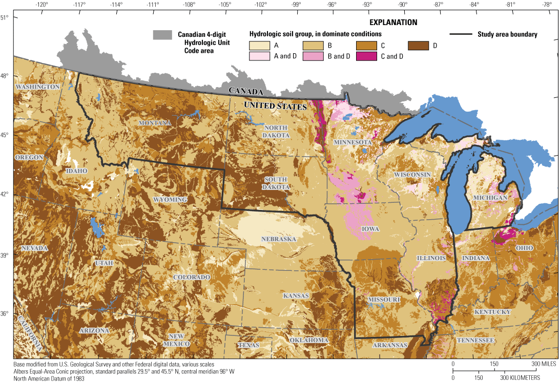
Dominant hydrologic soil groups across the study area, north-central United States.
Group A soils (fig. 4) have low runoff potential when thoroughly wetted because water is transmitted freely through the soil. These soils are typically characterized by having less than 10 percent clay and more than 90 percent sand or gravel (U.S. Department of Agriculture Natural Resources Conservation Service, 2009). Group B soils (fig. 4) have moderately low runoff potential when thoroughly wetted because water transmission through the soil is generally unimpeded. These soils are typically characterized by having 10–20 percent clay and 50–90 percent sand (U.S. Department of Agriculture Natural Resources Conservation Service, 2009). Group C soils (fig. 4) have moderately high runoff potential when thoroughly wetted because water transmission through the soil is somewhat restricted. These soils are typically characterized by 20–40 percent clay and less than 50 percent sand with loam soil in the remainder (U.S. Department of Agriculture Natural Resources Conservation Service, 2009). Group D soils (fig. 4) have high runoff potential when thoroughly wetted as water movement through the soil is restricted or very restricted. These soils are typically characterized by greater than 40 percent clay and less than 50 percent sand (U.S. Department of Agriculture Natural Resources Conservation Service, 2009).
There are also dual hydrologic soil groups (fig. 4) based on the presence of the water table within 24 in. of the surface. If these soils are adequately drained, then a dual hydrologic soil group can be used (U.S. Department of Agriculture Natural Resources Conservation Service, 2009). Dual hydrologic soil groups in our study area include A/D, B/D, and C/D. The first letter refers to the drained condition and the second to the undrained condition. These indicate that the soils may functionally move from the D group (high runoff potential) to the A (low runoff potential), B (moderately low runoff potential), or C (moderately high runoff potential) group. The dual hydrologic soil groups are in shades of pink to distinguish them from the other soil groups (in shades of brown). The pink areas have a water table within 24 in. of the surface, and the darker the shade of pink, the higher the amount of clay in the soil (fig. 4). The study of the presence and effect of drainage in these areas is beyond the scope of this report.
Two systems of description that integrate topography, climate, soil, and other information are ecoregions and classifications of areas by land cover. Because of the variations in temperature, precipitation, soils, and other characteristics, the study area encompasses varied ecoregions (fig. 5). Ecoregions are defined by the type, quality, and quantity of environmental resources including geology, landforms, soils, vegetation, climate, land use, wildlife, and hydrology (U.S. Environmental Protection Agency, 2022). These ecoregions can be useful in describing differences in hydrologic response across the study area. There are four levels of ecoregions and level III ecoregions were chosen to describe this study area because they work well at a regional scale (level IV ecoregions would be too specific for this study and levels I and II would be too broad; U.S. Environmental Protection Agency, 2021).
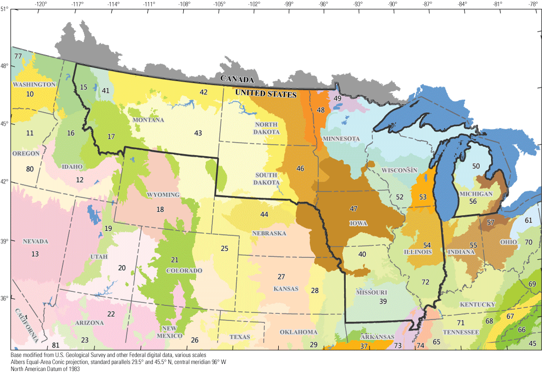
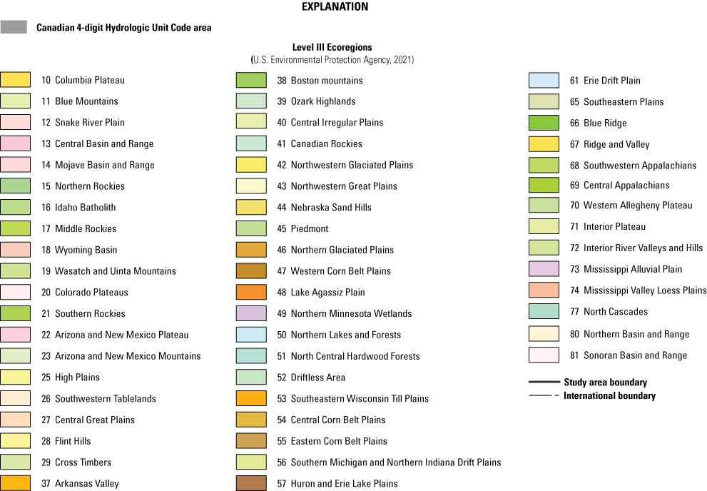
Level III ecoregions (U.S. Environmental Protection Agency, 2021) of the study area, north-central United States.
The following paragraphs describe the level III ecoregions in a west-to-east, north-to-south fashion. Their groupings in level I and level II ecoregions (not shown on map) help describe their overall characteristics. There are too many level III ecoregions to describe in detail, but users of this study’s results may benefit from comparing the results to their ecoregions of interest.
The western most level III ecoregions are mountainous regions: 15 (Northern Rockies), 17 (Middle Rockies), and 41 (Canadian Rockies). These are part of the level I ecoregion Northwestern Forested Mountains (Commission for Environmental Cooperation, undated a) and are all part of the level II ecoregion Western Cordillera (Commission for Environmental Cooperation, undated b). These level III ecoregions have many similarities, but the climate and vegetation of the Northern Rockies and Canadian Rockies are affected by maritime air masses whereas the Middle Rockies are not (U.S. Environmental Protection Agency, 2013).
A small part of ecoregion 18 (Wyoming Basin) extends into the study area. It is part of the level I North American Deserts and level II Cold Deserts (Commission for Environmental Cooperation, undated a, b). This level III ecoregion is an intermontane basin dominated by grasslands and shrubs, with hills and low mountains (U.S. Environmental Protection Agency, 2013).
Ecoregions 25 (High Plains), 40 (Central Irregular Plains), 42 (Northwestern Glaciated Plains), 43 (Northwestern Great Plains), 44 (Nebraska Sand Hills), 46 (Northern Glaciated Plains), 47 (Western Corn Belt Plains), and 48 (Lake Agassiz Plain) are all part of the level I Great Plains ecoregion (Commission for Environmental Cooperation, undated a). At level II, they can be grouped into the West-Central, Semi-Arid Prairies (25, 42, 43, and 44) and the Temperate Prairies (40, 46, 47, and 48; Commission for Environmental Cooperation, undated b). As the names suggest, these areas differ in terms of precipitation and temperature regimes that affect agricultural practices in the regions (see also figs. 2 and 3). Notably, ecoregion 42 represents the western and southwestern limits of the last glaciation, and this ecoregion is referred to as the Prairie Pothole region because of the depressional wetlands formed by the melting of sediment-laden ice at the glacial margin (Bluemle and Biek, undated; U.S. Environmental Protection Agency, 2013).
Ecoregions 49 (Northern Minnesota Wetlands) and 50 (Northern Lakes and Forests) are part of the level I Northern Forests ecoregion (Commission for Environmental Cooperation, undated a) in an area described as the Mixed Wood Shield (Commission for Environmental Cooperation, undated b). Both ecoregions are forested and lack the agricultural production of ecoregions to the south (U.S. Environmental Protection Agency, 2013).
Ecoregions 39 (Ozark Highlands), 51 (North Central Hardwood Forests), 52 (Driftless Area), 53 (Southeastern Wisconsin Till Plains), 54 (Central Corn Belt Plains), 55 (Eastern Corn Belt Plains), 56 (Southern Michigan and Northern Indiana Drift Plain), 57 (Huron and Erie Lake Plains), 71 (Interior Plateau), 72 (Interior River Valleys and Hills), 73 (Mississippi Alluvial Plain), and 74 (Mississippi Valley Loess Plains) are part of ecoregion level I Eastern Temperate Forests (Commission for Environmental Cooperation, undated a; U.S. Environmental Protection Agency, 2013). Ecoregion 39 is in the Ozark, Ouachita-Appalachian Forests; ecoregions 51, 52, and 45 are in the level II ecoregion Mixed Wood Plains; ecoregions 53, 54, 55, and 56, and 57 are in the Central USA Plains; ecoregions 71, 72, and 74 are in the Southeastern USA Plains; and ecoregion 73 is in the Mississippi Alluvial and Southeast USA Coastal Plains (Commission for Environmental Cooperation, undated b). These ecoregions are diverse in landforms and agriculture; however, as their level I association and figures 2 and 3 suggest, these ecoregions are more forested with more moisture than the Great Plains to the west and are warmer than the Northern Forests.
Land cover (fig. 6) is affected by temperature, precipitation, and soils (figs. 2–4) and is related to ecoregions (fig. 5). The National Land Cover Database (Dewitz, 2019) shows the evergreen forests of the study area’s western edge, which give way to shrub/scrub, herbaceous, and cultivated crops areas, with cultivated crops extending to the eastern edge of the study area. The northeastern part of the study area has mixed forest and woody wetlands, whereas the southernmost parts show hay/pasture and deciduous forest. Developed areas do lie within the study area, but they represent a small part.
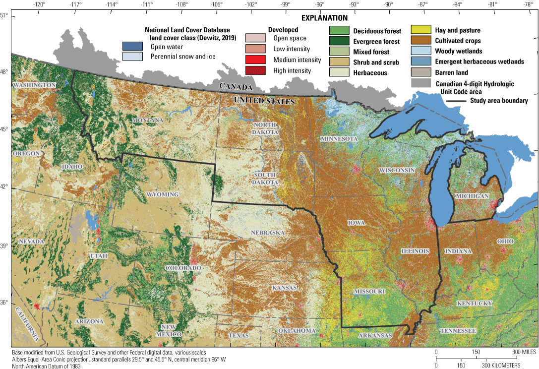
Land cover classes in the study area, north-central United States.
Data Selection
The following sections document the selection of streamgages with observed peak and daily streamflow data appropriate for the study of hydroclimatic variability as well as screening criteria for completeness. The climate dataset and processing of the data are also described.
Site Selection and Annual Peak Streamflow and Daily Streamflow Data
Peak-flow data were retrieved from the USGS National Water Information System database (USGS, 2021). Sites with an end date before October 1, 2018, were eliminated from consideration. Peak flows that occurred before water year 1921 were also eliminated (water year is a continuous 12-month period, from October 1 to September 30, and is identified by the year in which it ends). Peak flows with the following qualification codes were removed from the dataset: a maximum daily mean value (not an instantaneous peak; peak-qualification code 1); streamflow affected by dam failure (code 3); an uncertain peak value (streamflow known to be less than or greater than an indicated value; codes 4 and 8); discharge affected by regulation or diversion (code 6); recorded peaks outside of the systematic record (historical peak; code 7); or any part of the date of occurrence is unknown or not exact (codes A and B; (see Ryberg and others [2017] for more detailed descriptions of qualification codes).
Four analysis periods were selected: (1) a 100-year period, 1921–2020; (2) a 75-year period, 1946–2020; (3) a 50-year period, 1971–2020; and (4) a 30-year period, 1991–2020. Each period was required to have a peak in the first or second water year and have at least 80 percent completeness to be used for our study; for example, for a site to be used in our 75-year trend period, it would need a peak in 1946 or 1947 and 60 peaks total. Sites that did not meet the criteria were eliminated from further consideration.
All sites were evaluated for regulation using a dimensionless dam-impact metric indexed to the National Hydrography Dataset (NHD) that quantifies the degree of regulation of a given reach and is intended to aid in understanding how peak flows may be affected by reservoir storage in the upstream river network (Wieczorek and others, 2021).
The metric is a function of the upstream reservoir storage, 30-year average annual precipitation, the upstream drainage area, and the drainage area of the dam(s) (Wieczorek and others, 2021). Reservoir storage was retrieved from the U.S. Army Corps of Engineer’s National Inventory of Dams (U.S. Army Corps of Engineers, 2018), and the storage values used are the maximum National Inventory of Dams storage, which represents the maximum amount of storage each dam can hold. The NHD flowline corresponding to each streamgage was identified using data from Hayes and others (2021), a streamgage location dataset that indexed streamgages to the NHDPlus V2.1. Streamgages were then matched to the NHD flowline and corresponding dam-impact metric in the dam-impact dataset. A dam-impact-metric threshold of 0.1 was used to identify “regulated” stations. This threshold is based on metric ranges provided in Wieczorek and others (2021) combined with information from an independent analysis of site water years with peak code 6 values. Sites with a decadal dam-impact metric that met or exceeded the 0.1 threshold at any point in the streamgage’s active period of record were excluded from analysis. Further details on the method used here to identify regulated streamflows are available in Marti and Ryberg (2023).
Climate Data
Output from a monthly water-balance model (MWBM; McCabe and Wolock, 2011b) for the period 1900–2020 is available in Wieczorek and others (2022). These data comprise monthly time series estimates of temperature, precipitation, potential evapotranspiration, actual evapotranspiration, snowfall, soil moisture storage, snow water equivalent, and runoff on a 3.1-mile by 3.1-mile grid for the conterminous United States. The temperature and precipitation values were obtained from the NOAA Monthly U.S. Climate Gridded Dataset (Vose and others, 2015). The NOAA Monthly U.S. Climate Gridded Dataset is based on station data from the Global Historical Climatology Network-Daily dataset (Menne and others, 2012), which was corrected and gridded using climatologically aided interpolation to a latitude-longitude grid at a nominal spacing of 5 miles (Vose and others, 2014). The remaining monthly time series were computed using the MWBM.
The MWBM is a water-accounting model that estimates water storage in the snowpack and in the soil and the fluxes into, between, and from those stores at a monthly time step. These fluxes consist of precipitation (which is partitioned between rain and snow depending on the temperature), snowmelt, evaporation (as driven by potential evapotranspiration, which is modeled as a function of the temperature and latitude), and runoff (McCabe and Wolock, 2011b). The model has six parameters of which all but one (the soil-moisture storage capacity) were taken as spatially constant as described in McCabe and Wolock (2011b). None of the parameters differ in time; as a result, all nonstationarity in the model results arises from the effects of the input temperature and precipitation, and no attempt was made to model the effects of urbanization or any other type of land-use change.
Methods
The following sections describe the statistical methods used to analyze peak flow, daily streamflow, and climate data. The starting point for these analyses was the initial data analysis of peak flow described in B17C (app. 4 of England and others, 2019). Analyses were added to examine additional features in the data (such as seasonality) and to examine potential causal drivers of change. The open-source environment for statistical analysis and graphics R (R Core Team, 2021) was used to perform the analyses and generate associated graphics. The code, text documentation, and numerical and graphical outputs were combined in R Markdown documents. R Markdown documents are reproducible “notebook interfaces” that combine code, narrative, and graphics (RStudio, 2020). These R Markdown documents are in an associated data release (Marti and others, 2024) and can be consulted as the descriptions of the methods are read. Examples are also shown in subsequent state chapters, such as Levin (2024).
Statistical Analysis of Annual Peak Streamflow
Bulletin 17C describes initial data analysis to determine if the peak-flow series is stationary or nonstationary (England and others, 2019). A stationary series meets the statistical assumptions of flood-frequency analysis as described in B17C, whereas a nonstationary series has one or more violations of the assumptions. A primary assumption is that the peak-flow data for a given site are independent and identically distributed (England and others, 2019). Bulletin 17C recommends doing initial data analysis that includes the following: plotting the data, checking for autocorrelation, and checking for trends and shifts. The following sections describe the analyses performed to check for autocorrelation, monotonic (gradual) trends, and change points (abrupt shifts in the distribution). In addition to the initial data analysis described in B17C, quantile regression was done as well as trend analysis of the timing of peak flow. The statistical significance level used for these analyses was 0.05.
Autocorrelation
Autocorrelation was explored using function “acf” in R (R Core Team, 2021), the rank von Neumann test for lag-1 autocorrelation (Bartels, 1982; von Neumann and others, 1941), and the Hurst exponent coefficient (Hurst, 1951). The acf function computes and plots estimates of the autocorrelation (see the data release for these plots; Marti and others, 2024). This provides estimates of short- and long-term persistence and incorporates a hypothesis test. The null distribution of the serial correlation coefficient may be affected by departures from normality in the underlying process (Cox, 1966); therefore, a nonparametric test for randomness was used because the normality of the underlying process is in doubt (Bartels, 1982). The nonparametric test used was the rank von Neumann test for lag-1 autocorrelation (Bartels, 1982; von Neumann and others, 1941), which investigated short-term persistence. This test is implemented in the “EnvStats” package for R (Millard, 2013).
The Hurst exponent coefficient was calculated using the “reservoir” package for R (Turner and Galelli, 2016). This coefficient, H, is a measure of long-term persistence or the Hurst phenomenon (Hurst, 1951). An H less than 0.5 is mathematically possible but does not have as physical interpretation. If H is approximately equal to 0.5, the data are random with zero correlation at nonzero lags and the series can be analyzed with classical statistical techniques (Beran, 1994; Hamed, 2008; Koutsoyiannis, 2003; Koutsoyiannis, 2006; Villarini, 2016). An H greater than 0.5 indicates the autocorrelation function has a slow decay compared to short memory processes, such as an autoregressive or autoregressive-moving mean, and that modified statistics should be used to adjust for a scaled stochastic process (Hamed, 2008). Such persistence can be natural; however, Villarini and others (2009) showed that H can be sensitive to anthropogenic changes. Attribution requires additional data to investigate the mechanisms generating the persistence, and these data are not always available.
Monotonic Trends
To assess statistical significance, a nonparametric test based on Kendall’s tau (Kendall, 1938) was used to examine the presence of a monotonic trend. The trend line was plotted using the Theil-Sen estimator (Sen, 1968; Theil, 1992) for the slope and the Conover equation (Conover, 1999) for the intercept. The confidence interval for the slope uses Gilbert’s modification of the Theil-Sen method (Gilbert, 1987). In the absence of autocorrelation, peak-flow series were analyzed for trends using the “kendallTrendTest” function in the R package “EnvStats” (Millard, 2013). For sites with autocorrelation, a method that adjusts for autocorrelation was used. The method selected compares favorably to other methods in Ryberg and others (2020b) and is used by others in hydrologic research such as in the R package Flow Analysis Summary Statistics Tool for R (known as fasstr; Goetz and Schwarz, 2020). The function “zyp.trend.vector” with method argument equal to “yuepilon” in the “zyp” package (Bronaugh and Werner, 2013) performs a modified Mann-Kendall test for trend that first detrends the series then uses the estimated lag-one autocorrelation coefficient of the detrended series to remove, or prewhiten, the serial correlation; the estimated trend is then added back and the Mann-Kendall Trend test is applied (Önöz and Bayazit, 2012; Yue and others, 2002).
Change Points
Change points are abrupt changes (sometimes called step trends) in the mean, median, variance, scale, or general distribution of a series. Numerous change-point methods have been developed and are available in R. The Pettitt test is a nonparametric method that finds a single change point in the distribution of a series (Pettitt, 1979; Pohlert, 2020) and reports a p-value for a determination of significance. The Pettitt test is frequently used in hydrology and has been shown to have a lower false positive rate than some other common methods (Ryberg and others, 2020a). Change points were detected using the Pettitt test implemented in the R package “trend” (Pohlert, 2020). The Mood test is another nonparametric change-point method that finds a single abrupt change in the scale (or spread) of a series (Mood, 1954). The implementation of the test used here is from the R package “cpm” (Ross, 2015, 202091). Because the Mood test is based on a test statistic, one would assume there would be an associated p-value; however, the implementation of the test in “cpm” does not return a p-value. Based on the default settings of the function used, the change points returned do have a p-value less than 0.05; therefore, the change points in variance can be judged based on the same level of significance as used for the other statistical tests.
Quantile Regression
In the statistical literature, “quantile regression” strictly refers to the estimation of conditional quantiles (for example, the median) of a predictand as a function of one or more predictors (Koenker, 2005). The estimation of conditional quantiles is in contradistinction to least squares regression, which estimates the conditional mean of the predictand. In this analysis, two estimates of conditional quantiles are presented: one which uses strict quantile regression and the other which uses an application of locally weighted scatterplot smoothing (loess; Cleveland, 1979; Cleveland and McGill, 1984; Helsel and others, 2020). The strict quantile regression application estimates linear (straight line) trends conditioned to prevent crossing of the lines (He, 1997). Quantile regression was implemented using the “Qtools” R package (Geraci, 2016) and provides estimates of the 10, 25, 50, 75, and 90 percent quantiles, along with the trend slopes and their standard errors. The loess application provides smooth (locally quadratic) lines that correspond to the 12.5, 25, 50, 75, and 87.5 percent quantiles. The 50 percent quantile (median) line is the standard output of a loess analysis. The 25 and 75 percent quantiles are estimated using what are called upper and lower smooths (Cleveland and McGill, 1984; Helsel and others, 2020, chap. 10), which are created by applying the loess algorithm to the upper and lower residuals of the median smooth. Then, in turn, the 12.5 and 87.5 percent quantile smooths are computed as lower and upper smooths of the lower and upper residuals of the 25 and 75 percent lines, respectively. Although the loess lines do not provide trend slopes and their standard errors, loess lines are much more sensitive to changes in the relation of the peak flows versus time and thus provide useful visual information. These quantile trend estimates were applied to the log10-transformed and the untransformed peak-flow data series. In the case of the linear quantile trends for the log10-transformed-peak-flow data, the normalized derivative of peak flow with time is:
where The units of the normalized derivative are those of the peak-flow normalized trend, that is, years−1.Peak-Flow Timing Analysis
This analysis plots the timing (day of water year) of each peak in the period of record to identify potential shifts in the timing of floods. The magnitude of each peak is shown by changing the size and color of the marker used for each peak. An additional plot is produced which shows the frequency with which peaks occurred for each day of the water year.
Peak flows can come from more than one streamflow-generating process. For streams that are snowmelt dominated, the peak of the year comes in the spring; for other streams that are dominated by summer rain, the peaks occur in the summer; and others have peaks occurring in snowmelt periods and in periods of summer or fall rain. To assess change in timing from these two separate processes, an automated process (similar to that used in Ryberg and others, 2016) was developed to detect a breakpoint in the frequency of peaks and classify the peaks into those occurring early (snowmelt peaks) and those occurring later (rain-generated peaks). The density and the turnpoints functions of the R package “pastecs” (Grosjean and Ibanez, 2018) were used to provide a smoothed representation of the frequency of peaks on days of the water year and to identify turning points in the slope. The minimum turning point in spring and summer was used to divide the peak flow into an early and a late period. A monotonic trend was calculated for the day of the water year for all peaks. This trend is depicted by a black solid line (if not statistically significant) and a solid red line (if statistically significant [p less than 0.05]). Monotonic trends were then calculated for the two periods unless a period had less than 10 observations. The trends for one or both periods are depicted by black dashed lines (if not statistically significant) and red dashed lines (if statistically significant). The magnitude of the trend line’s slope and associated p-value is saved for each streamgage and compiled in a table for further analysis (such as spatial pattern of peak-flow timing). All plots were created in R using the “ggplot2” package (Wickham, 2016).
Statistical Analysis of Daily Streamflow
This project is focused on peak flow; however, examining daily mean streamflow (daily streamflow), particularly at the higher end of the streamflow regime, may contribute to understanding the processes behind changes in peak flow. The following analyses were performed on daily streamflow series for sites selected to meet completeness criteria for peak flow. Some sites selected for peak-flow analysis may not have daily streamflow (such as crest stage gages) and, therefore, do not have the daily streamflow analyses.
Regime Plot
The regime plot is generated using the R package “FlowScreen” (Dierauer and others, 2017; Dierauer and Whitfield, 2019). The plot depicts the minimum, maximum, mean, and 10th and 90th percentiles of daily streamflow for the period of analysis. This provides a comprehensive visual summary of the flow regime although the plot does assume stationarity during the period of analysis. The regime plot assumes that the mean for a particular day is constant through the long term; however, change points and monotonic trends may indicate that the mean is gradually changing or subject to an abrupt change. For example, the mean streamflow for June 1 before 1993 might be higher than the mean of the series after 1993.
Raster-Seasonality Plot
In these plots, daily streamflow data are presented as raster (gridded) data. The y-axis represents the water year with the most recent water year at the top. The x-axis represents the day of the water year with the last day of a water year (September 30th) on the right-hand-side. The daily streamflow values are then represented as gridded data with day-of-water year and water year providing the grid. The color of streamflow is graduated so that the highest flows are in blue, and the lowest flows are tan. Flows of 0 cubic feet per second are represented as white grid cells. The streamflow data are logarithmically transformed because of the wide range of values at many sites. Logarithmic transformation better visualizes differences given practical limits on the number of colors one can effectively display.
Center of Volume Analysis
The center of volume (COV) is the date by which half of the streamflow for a water year has passed a streamgage. In this analysis we calculated COV and calculated the date by which 25 percent of the total annual streamflow volume and 75 percent of the annual streamflow volume have been reached. We also calculated the duration, in days, between the point at which 25 and 75 percent of annual streamflow volume have been reached. The metrics are calculated using the R package “FlowScreen” (Dierauer and others, 2017; Dierauer and Whitfield, 2019), a Mann-Kendall Trend analysis is then done for each metric using the R package “EnvStats” (Millard, 2013), and then the annual metrics and the overall trends are plotted.
Changes in COV and timing of peaks are of interest to those trying to understand changes in hydrologic regimes. One advantage of examining peak timing of COV is that peaks are available at more streamgage locations than are long-term records of daily streamflow. Some have used COV as an indicator of changes in streamflow timing related to climate and hypothesized that changes may be related to changes in temperature (Hodgkins and Dudley, 2006); however, Whitfield (2013) stated that COV was originally developed as a measure of land-use effects and that it is affected by several factors other than temperature, particularly total runoff. Whitfield (2013) suggested avoiding using COV as an indicator of snowmelt timing; therefore, interpretation of the results should be considered with other information about changing precipitation and land use.
Peaks-Over-Threshold Analysis
A partial-duration flood series is a list of all flows (such as flood peaks) that exceed a chosen base stage or discharge regardless of the number of peaks occurring in a year. Also called basic-stage flood series or floods above a base (England and others, 2019; Langbein and Iseri, 1960), a peaks-over-threshold (POT) approach uses the partial-duration flood series of daily mean flows above some threshold to estimate the magnitude and frequency of floods (Lang and others, 1999). Because of a lack of general guidelines for setting a threshold for the floods above a base, the POT approach tends to be underused compared to, for example, analyses that use annual maximum floods based on water year. The primary challenge with the POT approach is meeting the independence criteria between candidate daily flood events. Two different approaches have historically been used for a threshold selection criterion: one based on a physical criterion (such as out of bank) or a second based on a purely mathematical and statistical approach (Lang and others, 1999). Recent studies that have evaluated changes in magnitude and frequency of POTs across conterminous United States have used threshold criteria approaches based on physical and statistical metrics to define the independence between two events (Archfield and others, 2016; Barth and others, 2018). In this study, we use the approach described in Barth and others (2018) to perform a POT analysis where, on average, there are two events per year (POT2) and four events per year (POT4), with no more than one event in a time window defined as |log10(drainage area)+5 days|.
Statistical Analysis of Climate Data
Monthly spatially averaged time series for each MWBM variable in each study basin were created in this analysis. The first step in this process was to geographically delineate the basin. Basins were generated with StreamStats Version 4 (Ries and others, 2017) using hydro-enforced digital elevation models (various resolutions) and using 1:100,000 or 1:24,000 or better streams data (Barnhart and others, 2020). For streamgages in States where StreamStats was not available (Michigan, Nebraska, and Wyoming), the “NLDI Flowtools” package (Hopkins, 2021) for Python (Python Software Foundation, 2021) was used (where NLDI stands for network-linked data index). “NLDI Flowtools” base data are 1:100,000 (medium resolution) national hydrography data and USGS 30-meter hydro-enforced digital elevation models. All streamgage basins generated by StreamStats or “NLDI Flowtools” were checked against USGS National Water Information System reported drainage areas (USGS, 2021). Streamgage basins with a greater than 5-percent difference in drainage area were visually checked to ensure the basin boundaries followed hydrologic principles outlined in Rea and Skinner (2012).
Time series for each of the eight MWBM variables were computed for each basin by averaging the values at the grid points within the basin unless the basin contained no grid points. If there were no grid points in the basin, the values at the grid point nearest to the centroid of the basins were used. Because MWBM data are only available within the United States, the average is computed only for the area inside the United States. The fraction of each basin that is within the United States is recorded for the analyst to consider in interpreting the climatic results.
R Markdown documents (one for each basin) were produced to illustrate the properties of the climate data, especially their trends and their relations to the observed peak, monthly, and annual streamflow. The analyses, quantitative results, and plots described in this section may be viewed in an associated data release (Marti and others, 2024). Analyses of the observed monthly and annual streamflow from each basin were included where and when such data were available. Limits to the number of missing streamflow values were set as follows: a required yearly total of at least 335 daily values; a required monthly total of at least 25 days; a required 3-month seasonal total of at least 2 months; and, to compute a trend, at least 10 annual values are needed. If the limits to the missing data were exceeded, the corresponding month, season, year, or trend was considered missing. Throughout the climate data analysis, the observed streamflow in cubic feet per second is converted to depth in inches per month or year by dividing by the drainage area that was determined as part of the basin delineation.
To visually indicate departures from linear fits, loess curves (Cleveland and others, 1992), computed using the loess function of the R “stats” package, are included in the plots in all the plot groups. Statistics of the fitted lines shown in the climate plots are provided in a table with one row per basin for use in comparing the climate results among basins (Marti and others, 2024).
Comparing Modeled Runoff and Observed Streamflow
The first group of plots compares the model-simulated runoff (hereafter, “runoff”) and observed streamflow (hereafter, “streamflow”) where available. Linear trends in time of water year-total runoff and streamflow are computed based on ordinary least squares (OLS) regression. Linear trends in runoff and streamflow in the month with the maximum value each water year are also computed based on OLS regression. There are also scatterplots between the observed and model-simulated values and the associated Pearson correlation and the root mean-square error of the runoff as a streamflow predictor. These plots and their associated statistics allow evaluation of the accuracy of the modeled runoff as a predictor of the observed streamflow. The modeled runoff only includes the effects of climatic variation and assumes rural land use, so differences from observed streamflow may arise from the effects of urbanization and other land-use change.
Comparing Peak Flows with Modeled Runoff and Observed Streamflow
The second group of plots presents an analysis of the peak flows as a function of the observed and model-simulated runoff. There is a plot of the linear peak-flow trend computed by OLS regression for reference then four scatterplots, which present linear OLS. These scatterplots indicate the predictability of the peak flows as a function of the water year-total streamflow (where available), of the water year-total runoff, of the maximum monthly streamflow (where available), and of the maximum monthly runoff. The predictability of the peak flows by these four quantities is characterized by the coefficient of determination (R2) and root mean-square error.
Annual Time Series Plots
The third group of plots presents time trends computed by OLS regression values of the eight MWBM variables and certain ratios of these variables. For fluxes, water-year totals are used, and for temperature and storage variables, water-year averages are used. The ratios presented consist of the annual ratios of runoff to precipitation, streamflow to precipitation, actual evapotranspiration to potential evapotranspiration, and snowfall to rainfall precipitation. Also presented in this group of plots are annual time series of the maximum and minimum monthly soil storage and maximum monthly snowpack.
Relations Between Runoff and Precipitation
The fourth group of plots presents analyses of the relations between runoff and precipitation, and, where streamflow data are available, between streamflow and precipitation. These analyses are presented because precipitation is the primary driver of hydrology. Two types of plots are used, one a scatterplot of runoff or streamflow as a function of precipitation at a water year time step (in part, to eliminate the effects of within-year snowpack storage variations) and the other a double-mass curve. This double-mass curve is a plot of cumulative runoff or streamflow against cumulative precipitation. Although Searcy and others (1960) cautioned against use of double-mass curves for this purpose, preferring to plot streamflow predicted by a precipitation-runoff relation obtained by other means, double-mass curves have been widely used in streamflow analysis (Zhao and others, 2017; Sando and others, 2022) in this form to infer changes in precipitation-runoff relations. In these double-mass curve plots, a line is further fit to the double-mass curves from the origin to the end of the curve. The slope of the curve is the long-term average runoff ratio (the fraction of precipitation that became runoff). To help visualize changes in the runoff ratio, differences from the long-term runoff ratio line are also plotted.
Raster-Seasonality Plots
The fifth group of plots is a set of monthly raster plots, one for each of the eight MWBM variables and observed streamflow. These plots allow for quick visual identification of flow patterns and trends within and between water years.
Monthly Boxplots
The sixth group of plots is a set of monthly boxplots. These plots are provided for the eight MWBM variables and observed streamflow and indicate the average and variability of the within-year (seasonal) cycle of the variables. Such plots are used to understand the interplay of changes in processes governing the hydrology between the seasons (see, for example, Weingartner and others, 2013).
Seasonal Trend Plots
The seventh group of plots presents trends in seasonal values of the 8 MWBM variables and observed runoff. Four seasons are used. They are defined as “SON” (September, October, and November), “DJF” (December, January, and February), “MAM” (March, April, and May), and “JJA” (June, July, and August) and correspond to meteorological fall, winter, spring, and summer, respectively, in the temperate Northern Hemisphere (NOAA National Centers for Environmental Information, 2022a). Trend lines were fit in arithmetic space using OLS regression; however, the y-axes of the plots (except for those of temperature) are square root-transformed, so visually the lines may be curved.
Budyko Plots
The eighth and final group of plots presents two versions of the Budyko curve (Budyko, 1974) for the basin and corresponding time series. The first version is the standard Budyko curve, which is constructed by plotting the ratio of actual evapotranspiration to precipitation against the ratio of potential evapotranspiration to precipitation. The Budyko curve is useful because it couples the water and energy cycles and can be used to analyze long-term hydroclimatology (Hobbins and Huntington, 2016). Here, the actual and potential evapotranspiration are model simulated. To provide a version of the Budyko curve based on observations, a second version of the Budyko curve is plotted in which the actual evapotranspiration is estimated as precipitation minus the observed streamflow. The data used in both versions of the Budyko curve are water year totals. To assess trends in the quantities used for the standard Budyko curve, two additional plots are provided, showing time trends in the ratio of actual evapotranspiration to precipitation and in the ratio of potential evapotranspiration to precipitation.
Presentation of Statistical Significance
For all statistical hypothesis tests, the p-values are reported in the associated data release (Marti and others, 2024). When the results of statistical tests for trends are mapped, the trends are presented using a likelihood approach which was proposed by Hirsch and others (2015) as an alternative to simply reporting significant trends with an arbitrary cutoff point. Trend likelihood values were determined using the p-value reported by each test using the equation: trend likelihood=1−(p-value/2). When the trend is “likely upward” or “likely downward,” the trend likelihood value associated with the trend is between 0.85 and 1.0; that is, the chance of the trend occurring in the specified direction is at least 85 out of 100. When the trend is “somewhat likely upward” or “somewhat likely downward,” the trend likelihood value associated with the trend is between 0.70 and 0.85; that is, the chance of the trend occurring in the specified direction is between 70 and 85 out of 100. When the trend is “about as likely as not,” the trend likelihood value associated with the trend is less than 0.70; that is, the chance of the trend being either upward or downward is less than 70 out of 100. Consider a trend in which peak flow increased with a likelihood value of 0.80 (p-value=0.40). Using traditional hypothesis testing and a traditional p-value cutoff of either 0.05 or 0.01, the trend would be reported as nonsignificant. Using likelihood, the trend would be reported instead as “somewhat likely upward” (USGS, 2017). Traditional hypothesis testing could lead to a potentially false sense of no trend because it is interpreted as there being no proof of a trend. The likelihood approach shows instead that it is somewhat likely that a trend has occurred, providing more information for decision makers. Likelihood values have been used to present national water-quality trends (Oelsner and others, 2017; U.S. Geological Survey, 2017; Ryberg and others, 2020c), trends in indices of climate extremes (Ryberg and Chanat, 2022), and trends in ecological metrics (Zuellig and Carlisle, 2019).
Results
This chapter describes the methods used to analyze the data but does not make inferences regarding the results. The results are summarized in R Markdown documents and are available in a USGS data release (Marti and others, 2024) along with comma-separated values (csv) files with the numerical results. Careful statistical analyses of multiple aspects of the data cannot completely replace detailed knowledge of the conditions affecting streams or stream reaches; therefore, study limitations are provided below for consideration when making inferences from the results. In addition, some of the sites in this study were the subject of a recent study (Ryberg, 2022) that attributed changes in peak flow to one or more potential causal mechanisms. In particular, chapters C and D of the USGS Professional Paper documenting the previous study provide attributions for most of the sites in this nine-State study (Levin and Holtschlag, 2022; Sando and others, 2022).
Study Limitations
The spatial distribution and drainage basin size of streamgages used may skew results. The spatial distribution of streamgages has been informed by the location of feasible gaging sites and flood forecasting, water supply, and other specific needs. In the long-term, this spatial distribution does not reflect an ideal distribution of sites to answer questions about the effects of climate and land-use change. In addition, the longest term streamgages tend to represent large basins.
There is a tradeoff between a spatial distribution more representative of conditions across the study area and the use of long-term streamgages to study climate; therefore, we used 100-, 75-, 50-, and 30-year trend periods. The short-term (30-year) trend may differ markedly from the longer-term patterns.
The lack of comprehensive information on regulation, diversion, and depletions makes site selection a challenge when investigating questions about climate effects on peak flow. A data-informed approach to regulation was used for the selection of sites in this study; however, there are known limitations to the available data. The approach and limitations are described in Marti and Ryberg (2023).
The seasonal analyses in this report have been done without regard for the circular nature of the underlying data; therefore, the resulting statistics (medians and trends of peak flow and COV) may be misleading when the data being considered have values near the end or the beginning of the water year (that is, in September and October). Such data values are more common in the peak-flow data than in the COV data.
Analyses of daily streamflow include sites with periods of missing record, as initial gage selection was based on criteria for appropriateness and completeness of peak-flow data. In some cases, this means the COV analysis and the POT analysis may not fully represent the hydrologic regime during the entire period of analysis. Users may consult the data release (Marti and others, 2024) to assess sites individually.
We used methods to detect nonstationarities that are gradual (monotonic trends, Mann-Kendall test for trend, and Theil-Sen slope) and abrupt (Pettitt test for changes in the median, Mood test for changes in scale). Gradual detection methods look at the entire record to assess the significance of change and determine if there is a trend. Abrupt methods look for specific points in the series when there is a significant change in a selected statistic; however, the true type of nonstationarity detected by a gradual or abrupt method may be unclear (Rougé and others, 2013). For instance, an abrupt method may identify the center of a gradual linear trend as a change point. Similarly, a gradual method may identify a trend when the data series exhibits a change point. Whether a series contains a change point, a monotonic trend, or both, such features are a violation of the stationarity assumption for flood-frequency analysis (Ryberg and others, 2020b).
The climate analyses rely on modeled data; therefore, the modeled streamflow does not match the actual streamflow. Depending on the degree of divergence, the mismatch can make it challenging to interpret the analyses of the various pieces of the water balance and to ascertain which components contribute most to the error; however, if the trend in modeled streamflow is in the same direction as the trend in actual streamflow, we assumed that the water-balance components were estimated with reasonable accuracy. See McCabe and Wolock (2011a) for more discussion on sources of error in the water-balance model.
Furthermore, the model parameters used to simulate the modeled streamflow and the related hydrologic states such as soil moisture are unchanging in time and assume rural land use; therefore, the model output does not include the effects of urbanization and other land-use change. In addition, the climate data (observed and modeled) are at a monthly time step. As a result, these data do not provide information on changes in climate at shorter time steps (for example, changes in daily precipitation intensity) that may be important for peak flows under certain conditions (Ivancic and Shaw, 2015; Sharma and others, 2018).
Summary
Flood-frequency analysis is essential to water resources management applications, including critical structure design and floodplain mapping. Federal guidelines for doing flood-frequency analyses are presented in a U.S. Geological Survey (USGS) Techniques and Methods report, Bulletin 17C. A basic assumption within Bulletin 17C is that for basins without major hydrologic alterations, statistical properties of the distribution of annual peak streamflows (peak flows) are stationary; that is the mean, variance, and skew are constant, otherwise known as stationary. The stationarity assumption has been widely accepted within the flood-frequency community; however, a better understanding of climatic persistence (extended periods of relatively wet or relatively dry conditions) as well as concerns about potential climate change and land-use change have caused the stationarity assumption to be reexamined. Flood-frequency analyses that do not incorporate observed trends and abrupt changes may result in a poor representation of the true flood risk. Bulletin 17C does not offer guidance on how to incorporate nonstationarities when estimating floods, and it describes a need for additional flood-frequency studies that incorporate changing climate or basin characteristics. In response to a history of concern regarding nonstationarity in peak flows in the region, this study was done by the USGS, in cooperation with the Departments of Transportation of Illinois, Iowa, Michigan, Minnesota, Missouri, South Dakota, and Wisconsin, the Montana Department of Natural Resources and Conservation, and the North Dakota Department of Water Resources, to assess potential nonstationarity in peak flows in the north-central United States. The study area considered consists of nine states that form a diverse region with complex variability in topography and climate.
This chapter summarizes the methods used to detect hydroclimatic changes in peak-flow data in the study region. Peak-flow data were retrieved for all streamgages from each State from USGS National Water Information System database. Individual peak flow values were screened for appropriateness for studying hydroclimatic variability by using their associated qualification codes. Four periods were selected: (1) a 100-year period, 1921–2020; (2) a 75-year period, 1946–2020; (3) a 50-year period, 1971–2020; and (4) a 30-year period, 1991–2020. Sites were further screened to meet completeness criteria and for regulation, and sites deemed regulated were removed from the study.
The temperature and precipitation values were obtained from the National Oceanic and Atmospheric Administration Monthly U.S. Climate Gridded Dataset. The remaining monthly time series were computed from a monthly water-balance model for 1900–2020. These data comprise monthly time series estimates of temperature, precipitation, potential evapotranspiration, actual evapotranspiration, snowfall, soil moisture storage, snow water equivalent, and runoff on a 3.1-mile by 3.1-mile grid for the conterminous United States.
An array of statistical and graphical analyses was used to investigate peak flow, daily streamflow, and climate data. The starting point for these analyses was the initial data analysis of peak flow described in Bulletin 17C, which included plotting the peak flow and checking for autocorrelation, monotonic trends, and changes points. Additional analyses were added to examine further nuances in the data, including quantile regression and peak-flow timing for analysis, as well as raster-seasonality plots and center of volume analysis of the daily streamflow data. To examine potential causal drivers of changes, the climate data were analyzed graphically and statistically by comparing modeled runoff to observed streamflow, calculating trends in climate metrices, examining relations between runoff and precipitation, and plotting additional summaries of the data. Results are provided in a USGS data release. The study limitations are documented for users of the results.
References Cited
Ahiablame, L., Sheshukov, A.Y., Rahmani, V., and Moriasi, D., 2017, Annual baseflow variations as influenced by climate variability and agricultural land use change in the Missouri River Basin: Journal of Hydrology, v. 551, no. 1, p. 188–202. [Also available at https://doi.org/10.1016/j.jhydrol.2017.05.055.]
Archfield, S.A., Hirsch, R.M., Viglione, A., and Blöschl, G., 2016, Fragmented patterns of flood change across the United States: Geophysical Research Letters, v. 43, no. 19, p. 10232–10239. [Also available at https://doi.org/10.1002/2016GL070590.]
Barnhart, T.B., Smith, M., Rea, A., Kolb, K., Steeves, P., and McCarthy, P., 2020, StreamStats data preparation tools (ver. 4): U.S. Geological Survey software release, accessed June 1, 2022, at https://code.usgs.gov/StreamStats/data-preparation/datapreptools.
Bartels, R., 1982, The rank version of von Neumann’s ratio test for randomness: Journal of the American Statistical Association, v. 77, no. 377, p. 40–46. [Also available at https://doi.org/10.1080/01621459.1982.10477764.]
Barth, N.A., Ryberg, K.R., Gregory, A., and Blum, A.G., 2022, Introduction to attribution of monotonic trends and change points in peak streamflow across the conterminous United States using a multiple working hypotheses framework, 1941–2015 and 1966–2015, chap. A of Ryberg, K.R., ed., Attribution of monotonic trends and change points in peak streamflow across the conterminous United States using a multiple working hypotheses framework, 1941–2015 and 1966–2015: U.S. Geological Survey Professional Paper 1869, p. A1–A29, accessed October 4, 2022, at https://doi.org/10.3133/pp1869.
Barth, N.A., Villarini, G., and White, K., 2018, Contribution of eastern North Pacific tropical cyclones and their remnants on flooding in the western United States: International Journal of Climatology, v. 38, no. 14, p. 5441–5446, accessed December 21, 2022, https://onlinelibrary.wiley.com/doi/10.1002/joc.5735.
Bluemle, J., and Biek, B., undated, No ordinary plain—North Dakota’s physiography and landforms: North Dakota Geological Survey web page, North Dakota Note 1, accessed October 3, 2022, at https://www.dmr.nd.gov/ndgs/ndnotes/ndn1.asp.
Bronaugh, D., and Werner, A., 2013, zyp—Zhang + Yue-Pilon trends package (ver. 0.10-1): CRAN digital data, accessed July 30, 2021, at https://CRAN.R-project.org/package=zyp.
Cleveland, W.S., 1979, Robust locally weighted regression and smoothing scatterplots: Journal of the American Statistical Association, v. 74, no. 368, p. 829–836. [Also available at https://doi.org/10.1080/01621459.1979.10481038.]
Cleveland, W.S., Grosse, E., and Shyu, W.M., 1992, Local regression models, chap. 8 of Chambers, J.M., and Hastie, T.J., eds., Statistical models in S: Boca Raton, Fla., Chapman & Hall/CRC, p. 309–376. [Also available at https://doi.org/10.1201/9780203738535.]
Cleveland, W.S., and McGill, R., 1984, Graphical perception—Theory, experimentation, and application to the development of graphical methods: Journal of the American Statistical Association, v. 79, no. 387, p. 531–554. [Also available at https://doi.org/10.1080/01621459.1984.10478080.]
Commission for Environmental Cooperation, undated a, Ecological regions of North America level I: Commission for Environmental Cooperation, 1 sheet, accessed October 3, 2022, at https://gaftp.epa.gov/EPADataCommons/ORD/Ecoregions/cec_na/NA_LEVEL_I.pdf.
Commission for Environmental Cooperation, undated b, Ecological regions of North America level I–II: Commission for Environmental Cooperation, 1 sheet, accessed October 3, 2022, at https://gaftp.epa.gov/EPADataCommons/ORD/Ecoregions/cec_na/NA_LEVEL_II.pdf.
Cox, D.R., 1966, The null distribution of the first serial correlation coefficient: Biometrika, v. 53, nos. 3–4, p. 623–626. [Also available at https://doi.org/10.1093/biomet/53.3-4.623.]
Dewitz, J., 2019, National Land Cover Database (NLCD) 2016 products (ver. 2.0, July 2020): U.S. Geological Survey data release, accessed October 3, 2022, at https://doi.org/10.5066/P96HHBIE.
Dickinson, J.E., Harden, T.M., and McCabe, G.J., 2019, Seasonality of climatic drivers of flood variability in the conterminous United States: Scientific Reports, v. 9, no. 1, art. 15321, 10 p. [Also available at https://doi.org/10.1038/s41598-019-51722-8.]
Dierauer, J., and Whitfield, P., 2019, FlowScreen—Daily streamflow trend and change point screening (ver. 1.2.6): CRAN digital data, accessed July 15, 2021, at https://CRAN.R-project.org/package=FlowScreen.
Dierauer, J.R., Whitfield, P.H., and Allen, D.M., 2017, Assessing the suitability of hydrometric data for trend analysis—The ‘FlowScreen’ package for R: Canadian Water Resources Journal, v. 42, no. 3, p. 269–275. [Also available at https://doi.org/10.1080/07011784.2017.1290553.]
Dudley, R.W., Hodgkins, G.A., McHale, M.R., Kolian, M.J., and Renard, B., 2017, Trends in snowmelt-related streamflow timing in the conterminous United States: Journal of Hydrology, v. 547, no. 4, p. 208–221. [Also available at https://doi.org/10.1016/j.jhydrol.2017.01.051.]
England, J.F., Jr., Cohn, T.A., Faber, B.A., Stedinger, J.R., Thomas, W.O., Jr., Veilleux, A.G., Kiang, J.E., and Mason, R.R., Jr., 2019, Guidelines for determining flood flow frequency—Bulletin 17C (ver. 1.1, May 2019): U.S. Geological Survey Techniques and Methods, book 4, chap. B5, 148 p., accessed May 5, 2022, at https://doi.org/10.3133/tm4B5.
Falcone, J.A., Murphy, J.C., and Sprague, L.A., 2018, Regional patterns of anthropogenic influences on streams and rivers in the conterminous United States, from the early 1970s to 2012: Journal of Land Use Science, v. 13, no. 6, p. 585–614. [Also available at https://doi.org/10.1080/1747423X.2019.1590473.]
Georgakakos, A., Fleming, P., Dettinger, M., Peters-Lidard, C., Richmond, T.C., Reckhow, K., White, K., and Yates, D., 2014, Water resources, chap. 3 of Melillo, J.M., Richmond, T.C., and Yohe, G.W., eds., Climate change impacts in the United States—The Third National Climate Assessment: Washington, D.C., U.S. Government Printing Office, U.S. Global Change Research Program, p. 69–112.
Geraci, M., 2016, Qtools—A collection of models and tools for quantile inference: The R Journal, v. 8, no. 2, p. 117–138. [Also available at https://doi.org/10.32614/RJ-2016-037.]
Goetz, J., and Schwarz, C.J., 2020, fasstr—Analyze, summarize, and visualize daily streamflow data (ver. 0.3.2): CRAN digital data, accessed February 21, 2021, at https://CRAN.R-project.org/package=fasstr.
Griffin, E.R., and Friedman, J.M., 2017, Decreased runoff response to precipitation, Little Missouri River Basin, northern Great Plains, USA: Journal of the American Water Resources Association, v. 53, no. 3, p. 576–592. [Also available at https://doi.org/10.1111/1752-1688.12517.]
Grosjean, P., and Ibanez, F., 2018, pastecs—Package for analysis of space-time ecological series (ver. 1.3.21): CRAN digital data, accessed October 26, 2021, at https://CRAN.R-project.org/package=pastecs.
Hamed, K.H., 2008, Trend detection in hydrologic data—The Mann-Kendall trend test under the scaling hypothesis: Journal of Hydrology, v. 349, nos. 3–4, p. 350–363. [Also available at https://doi.org/10.1016/j.jhydrol.2007.11.009.]
Hayes, L., Chase, K.J., Wieczorek, M.E., and Jackson, S.E., 2021, USGS streamgages in the conterminous United States indexed to NHDPlus v2.1 flowlines to support Streamgage Watershed InforMation (SWIM), 2021: U.S. Geological Survey data release, accessed January 18, 2022, at https://doi.org/10.5066/P9J5CK2Y.
He, X., 1997, Quantile curves without crossing: The American Statistician, v. 51, no. 2, p. 186–192. [Also available at https://doi.org/10.1080/00031305.1997.10473959.]
Hejazi, M., and Markus, M., 2009, Impacts of urbanization and climate variability on floods in northeastern Illinois: Journal of Hydrologic Engineering, v. 14, no. 6, p. 606–616. [Also available at https://doi.org/10.1061/(ASCE)HE.1943-5584.0000020.]
Helsel, D.R., Hirsch, R.M., Ryberg, K.R., Archfield, S.A., and Gilroy, E.J., 2020, Statistical methods in water resources: U.S. Geological Survey Techniques and Methods, book 4, chap. A3, 458 p., accessed October 26, 2021, at https://doi.org/10.3133/tm4A3.
Hirsch, R.M., Archfield, S.A., and De Cicco, L.A., 2015, A bootstrap method for estimating uncertainty of water quality trends: Environmental Modelling & Software, v. 73, p. 148–166. [Also available at https://doi.org/10.1016/j.envsoft.2015.07.017.]
Hirsch, R.M., and Ryberg, K.R., 2012, Has the magnitude of floods across the USA changed with global CO2 levels?: Hydrological Sciences Journal, v. 57, no. 1, p. 1–9. [Also available at https://doi.org/10.1080/02626667.2011.621895.]
Hirschboeck, K.K., 1991, Hydrology of floods and droughts—Climate and floods, in Paulson, R.W., Chase, E.B., Roberts, R.S., and Moody, D.W., comps., National water summary 1988–89—Hydrologic events and floods and droughts: U.S. Geological Survey Water Supply Paper 2375, p. 67–88. [Also available at https://doi.org/10.3133/wsp2375.]
Hodgkins, G.A., and Dudley, R.W., 2006, Changes in the timing of winter–spring streamflows in eastern North America, 1913–2002: Geophysical Research Letters, v. 33, no. 6, art. L06402, 5 p. [Also available at https://doi.org/10.1029/2005GL025593.]
Hodgkins, G.A., Dudley, R.W., Archfield, S.A., and Renard, B., 2019, Effects of climate, regulation, and urbanization on historical flood trends in the United States: Journal of Hydrology, v. 573, p. 697–709. [Also available at https://doi.org/10.1016/j.jhydrol.2019.03.102.]
Hodgkins, G.A., Whitfield, P.H., Burn, D.H., Hannaford, J., Renard, B., Stahl, K., Fleig, A.K., Madsen, H., Mediero, L., Korhonen, J., Murphy, C., and Wilson, D., 2017, Climate-driven variability in the occurrence of major floods across North America and Europe: Journal of Hydrology, v. 552, p. 704–717. [Also available at https://doi.org/10.1016/j.jhydrol.2017.07.027.]
Hoogestraat, G.K., and Stamm, J.F., 2015, Climate and streamflow characteristics for selected streamgages in eastern South Dakota, water years 1945–2013: U.S. Geological Survey Scientific Investigations Report 2015–5146, 35 p., accessed July 30, 2021, at https://doi.org/10.3133/sir20155146.
Hopkins, A., 2021, nldi-flowtools: U.S. Geological Survey digital data, accessed December 9, 2021, at https://code.usgs.gov/wma/nhgf/toolsteam/nldi-flowtools.
Hurst, H.E., 1951, Long-term storage capacity of reservoirs: Transactions of the American Society of Civil Engineers, v. 116, no. 1, p. 770–799. [Also available at https://doi.org/10.1061/TACEAT.0006518.]
Ivancic, T.J., and Shaw, S.B., 2015, Examining why trends in very heavy precipitation should not be mistaken for trends in very high river discharge: Climatic Change, v. 133, no. 4, p. 681–693. [Also available at https://doi.org/10.1007/s10584-015-1476-1.]
Ivancic, T.J., and Shaw, S.B., 2017, Identifying spatial clustering in change points of streamflow across the contiguous U.S. between 1945 and 2009: Geophysical Research Letters, v. 44, no. 5, p. 2445–2453. [Also available at https://doi.org/10.1002/2016GL072444.]
Juckem, P.F., Hunt, R.J., Anderson, M.P., and Robertson, D.M., 2008, Effects of climate and land management change on streamflow in the driftless area of Wisconsin: Journal of Hydrology, v. 355, no. 1–4, p. 123–130. [Also available at https://doi.org/10.1016/j.jhydrol.2008.03.010.]
Kendall, M.G., 1938, A new measure of rank correlation: Biometrika, v. 30, no. 1/2, p. 81–93. [Also available at https://doi.org/10.2307/2332226.]
Koenker, R., 2005, Quantile regression—Econometric society monographs: Cambridge, Cambridge University Press, 366 p. [Also available at https://doi.org/10.1017/CBO9780511754098.]
Kolars, K.A., Vecchia, A.V., and Ryberg, K.R., 2016, Stochastic model for simulating Souris River Basin precipitation, evapotranspiration, and natural streamflow: U.S. Geological Survey Scientific Investigations Report 2015–5185, 55 p., accessed April 19, 2016, at https://doi.org/10.3133/sir20155185.
Koutsoyiannis, D., 2006, Nonstationarity versus scaling in hydrology: Journal of Hydrology, v. 324, no. 1–4, p. 239–254. [Also available at https://doi.org/10.1016/j.jhydrol.2005.09.022.]
Koutsoyiannis, D., and Montanari, A., 2007, Statistical analysis of hydroclimatic time series—Uncertainty and insights: Water Resources Research, v. 43, no. 5, art. W05429, 9 p. [Also available at https://doi.org/10.1029/2006WR005592.]
Koutsoyiannis, D., and Montanari, A., 2015, Negligent killing of scientific concepts—The stationarity case: Hydrological Sciences Journal, v. 60, no. 7–8, p. 1174–1183. [Also available at https://doi.org/10.1080/02626667.2014.959959.]
Lang, M., Ouarda, T.B.M.J., and Bobée, B., 1999, Towards operational guidelines for over-threshold modeling: Journal of Hydrology, v. 225, nos. 3–4, p. 103–117. [Also available at https://doi.org/10.1016/S0022-1694(99)00167-5.]
Langbein, W.B., and Iseri, K.T., 1960, General introduction and hydrologic definitions: U.S. Geological Survey Water Supply Paper 1541–A, 29 p., accessed May 5, 2022, at https://doi.org/10.3133/wsp1541A.
Levin, S.B., 2024, Peak streamflow trends in Wisconsin and their relation to changes in climate, water years 1921–2020, chap. J of Ryberg, K.R., comp., Peak streamflow trends and their relation to changes in climate in Illinois, Iowa, Michigan, Minnesota, Missouri, Montana, North Dakota, South Dakota, and Wisconsin: U.S. Geological Survey Scientific Investigations Report 2023–5064, 49 p., https://doi.org/10.3133/sir20235064J.
Levin, S.B., and Holtschlag, D.J., 2022, Attribution of monotonic trends and change points in peak streamflow in the Midwest region of the United States, 1941–2015 and 1966–2015, chap. D of Ryberg, K.R., ed., Attribution of monotonic trends and change points in peak streamflow across the conterminous United States using a multiple working hypotheses framework, 1941–2015 and 1966–2015: U.S. Geological Survey Professional Paper 1869, p. D1–D22, accessed October 3, 2022, at https://doi.org/10.3133/pp1869.
Lins, H.F., and Cohn, T.A., 2011, Stationarity—Wanted dead or alive?: Journal of the American Water Resources Association, v. 47, no. 3, p. 475–480. [Also available at https://doi.org/10.1111/j.1752-1688.2011.00542.x.]
Mallakpour, I., and Villarini, G., 2015, The changing nature of flooding across the central United States: Nature Climate Change, v. 5, no. 3, p. 250–254. [Also available at https://doi.org/10.1038/nclimate2516.]
Marti, M.K., and Ryberg, K.R., 2023, Method for identification of reservoir regulation within U.S. Geological Survey streamgage basins in the Central United States using a decadal dam impact metric: U.S. Geological Survey Open-File Report 2023–1034, 15 p., accessed June 16, 2023, at https://doi.org/10.3133/ofr20231034.
Marti, M.K., Wavra, H.N., Over, T.M., Ryberg, K.R., Podzorski, H.L., and Chen, Y.R., 2024, Peak streamflow data, climate data, and results from investigating hydroclimatic trends and climate change effects on peak streamflow in the Central United States, 1920–2020: U.S. Geological Survey data release, https://doi.org/10.5066/P9R71WWZ.
McCabe, G.J., and Wolock, D.M., 2002, A step increase in streamflow in the conterminous United States: Geophysical Research Letters, v. 29, no. 24, p. 38-1–38-4. [Also available at https://doi.org/10.1029/2002GL015999.]
McCabe, G.J., and Wolock, D.M., 2011a, Century-scale variability in global annual runoff examined using a water balance model: International Journal of Climatology, v. 31, no. 12, p. 1739–1748. [Also available at https://doi.org/10.1002/joc.2198.]
McCabe, G.J., and Wolock, D.M., 2011b, Independent effects of temperature and precipitation on modeled runoff in the conterminous United States: Water Resources Research, v. 47, no. 11, art. W11522, 11 p. [Also available at https://doi.org/10.1029/2011WR010630.]
Menne, M.J., Durre, I., Vose, R.S., Gleason, B.E., and Houston, T.G., 2012, An overview of the global historical climatology network-daily database: Journal of Atmospheric and Oceanic Technology, v. 29, no. 7, p. 897–910. [Also available at https://doi.org/10.1175/JTECH-D-11-00103.1.]
Millard, S.P., 2013, EnvStats—An R package for environmental statistics: New York, Springer, 307 p. [Also available at https://doi.org/10.1007/978-1-4614-8456-1.]
Milly, P.C.D., Betancourt, J., Falkenmark, M., Hirsch, R.M., Kundzewicz, Z.W., Lettenmaier, D.P., and Stouffer, R.J., 2008, Stationarity is dead—Whither water management?: Science, v. 319, no. 5863, p. 573–574. [Also available at https://doi.org/10.1126/science.1151915.]
Mood, A.M., 1954, On the asymptotic efficiency of certain nonparametric two-sample tests: Annals of Mathematical Statistics, v. 25, no. 3, p. 514–522. [Also available at https://doi.org/10.1214/aoms/1177728719.]
National Oceanic and Atmospheric Administration [NOAA] National Centers for Environmental Information, 2022a, Meteorological versus astronomical seasons: National Oceanic Atmospheric Administration National Centers for Environmental Information web page, accessed May 23, 2022, at https://www.ncei.noaa.gov/news/meteorological-versus-astronomical-seasons.
National Oceanic Atmospheric Administration [NOAA] National Centers for Environmental Information, 2022b, U.S. climate normals: National Oceanic Atmospheric Administration National Centers for Environmental Information web page, accessed December 1, 2022, at https://www.ncei.noaa.gov/products/land-based-station/us-climate-normals#:~:text=NCEI%20generates%20the%20official%20U.S.%20normals%20every%2010,of%20 decadal%20normals%20first%20produced%20in%20the%201950s.
Norton, P.A., Anderson, M.T., and Stamm, J.F., 2014, Trends in annual, seasonal, and monthly streamflow characteristics at 227 streamgages in the Missouri River watershed, water years 1960–2011: U.S. Geological Survey Scientific Investigations Report 2014–5053, 128 p., accessed June 21, 2021, at https://doi.org/10.3133/sir20145053.
Norton, P.A., Delzer, G.C., Valder, J.F., Tatge, W.S., and Ryberg, K.R., 2022, Assessment of streamflow trends in the eastern Dakotas, water years 1960–2019: U.S. Geological Survey Scientific Investigations Report 2022–5055, 11 p., accessed October 3, 2022, at https://doi.org/10.3133/sir20225055.
Oelsner, G.P., Sprague, L.A., Murphy, J.C., Zuellig, R.E., Johnson, H.M., Ryberg, K.R., Falcone, J.A., Stets, E.G., Vecchia, A.V., Riskin, M.L., De Cicco, L.A., Mills, T.J., and Farmer, W.H., 2017, Water-quality trends in the Nation’s rivers and streams, 1972–2012—Data preparation, statistical methods, and trend results (ver. 2.0, October 2017): U.S. Geological Survey Scientific Investigations Report 2017–5006, 136 p., accessed March 15, 2022, at https://doi.org/10.3133/sir20175006.
Olsen, J.R., Stedinger, J.R., Matalas, N.C., and Stakhiv, E.Z., 1999, Climate variability and flood frequency estimation for the Upper Mississippi and Lower Missouri Rivers: Journal of the American Water Resources Association, v. 35, no. 6, p. 1509–1523. [Also available at https://doi.org/10.1111/j.1752-1688.1999.tb04234.x.]
Önöz, B., and Bayazit, M., 2012, Block bootstrap for Mann-Kendall trend test of serially dependent data: Hydrological Processes, v. 26, no. 23, p. 3552–3560. [Also available at https://doi.org/10.1002/hyp.8438.]
Over, T.M., Saito, R.J., and Soong, D.T., 2016, Adjusting annual maximum peak discharges at selected stations in northeastern Illinois for changes in land-use conditions: U.S. Geological Survey Scientific Investigations Report 2016–5049, 33 p., accessed December 22, 2020, at https://doi.org/10.3133/sir20165049.
Pederson, G.T., Gray, S.T., Ault, T., Marsh, W., Fagre, D.B., Bunn, A.G., Woodhouse, C.A., and Graumlich, L.J., 2011, Climatic controls on the snowmelt hydrology of the northern Rocky Mountains: Journal of Climate, v. 24, no. 6, p. 1666–1687. [Also available at https://doi.org/10.1175/2010JCLI3729.1.]
Peterson, T.C., Heim, R.R., Jr., Hirsch, R., Kaiser, D.P., Brooks, H., Diffenbaugh, N.S., Dole, R.M., Giovannettone, J.P., Guirguis, K., Karl, T.R., Katz, R.W., Kunkel, K., Lettenmaier, D., McCabe, G.J., Paciorek, C.J., Ryberg, K.R., Schubert, S., Silva, V.B.S., Stewart, B.C., Vecchia, A.V., Villarini, G., Vose, R.S., Walsh, J., Wehner, M., Wolock, D., Wolter, K., Woodhouse, C.A., and Wuebbles, D., 2013, Monitoring and understanding changes in heat waves, cold waves, floods, and droughts in the United States—State of knowledge: Bulletin of the American Meteorological Society, v. 94, no. 6, p. 821–834. [Also available at https://doi.org/10.1175/BAMS-D-12-00066.1.]
Pettitt, A.N., 1979, A non-parametric approach to the change-point problem: Journal of the Royal Statistical Society. Series C (Applied Statistics), v. 28, no. 2, p. 126–135. [Also available at https://doi.org/10.2307/2346729.]
Pohlert, T., 2020, trend—Non-parametric trend tests and change-point detection (ver. 1.1.2): CRAN digital data, accessed July 29, 2022, at https://CRAN.R-project.org/package=trend.
Python Software Foundation, 2021, Python: Python Software Foundation web page, accessed June 1, 2022, at https://www.python.org/.
R Core Team, 2021, R—A language and environment for statistical computing: R Foundation for Statistical Computing website, accessed February 21, 2021, at http://www.R-project.org.
Razavi, S., Elshorbagy, A., Wheater, H., and Sauchyn, D., 2015, Toward understanding nonstationarity in climate and hydrology through tree ring proxy records: Water Resources Research, v. 51, no. 3, p. 1813–1830. [Also available at https://doi.org/10.1002/2014WR015696.]
Rea, A., and Skinner, K.D., 2012, Geospatial datasets for watershed delineation and characterization used in the Hawaii StreamStats web application: U.S. Geological Survey Data Series 680, 12 p., accessed June 1, 2022, at https://doi.org/10.3133/ds680.
Ries, K.G., III, Newson, J.K., Smith, M.J., Guthrie, J.D., Steeves, P.A., Haluska, T., Kolb, K.R., Thompson, R.F., Santoro, R.D., and Vraga, H.W., 2017, StreamStats, version 4: U.S. Geological Survey Fact Sheet 2017–3046, 4 p., accessed June 1, 2022, at https://doi.org/10.3133/fs20173046.
Ross, G.J., 2015, Parametric and nonparametric sequential change detection in R—The cpm package: Journal of Statistical Software, v. 66, no. 3, p. 1–20. [Also available at https://doi.org/10.18637/jss.v066.i03.]
Ross, G.J., 2020, cpm—Sequential and batch change detection using parametric and nonparametric methods (ver. 2.3): CRAN digital data, accessed July 30, 2021, at http://CRAN.R-project.org/package=cpm.
Rougé, C., Ge, Y., and Cai, X., 2013, Detecting gradual and abrupt changes in hydrological records: Advances in Water Resources, v. 53, no. 5863, p. 33–44. [Also available at https://doi.org/10.1016/j.advwatres.2012.09.008.]
RStudio, 2020, R Markdown: RStudio web page, accessed December 1, 2022, at https://rmarkdown.rstudio.com/.
Ryberg, K.R., 2022, Attribution of monotonic trends and change points in peak streamflow across the conterminous United States using a multiple working hypotheses framework, 1941–2015 and 1966–2015: U.S. Geological Survey Professional Paper 1869, [variously paged], accessed January 2023 at https://doi.org/10.3133/pp1869.
Ryberg, K.R., Akyüz, F.A., Wiche, G.J., and Lin, W., 2016, Changes in seasonality and timing of peak streamflow in snow and semi-arid climates of the north-central United States, 1910–2012: Hydrological Processes, v. 30, no. 8, p. 1208–1218. [Also available at https://doi.org/10.1002/hyp.10693.]
Ryberg, K.R., and Chanat, J.G., 2022, Climate extremes as drivers of surface-water-quality trends in the United States: Science of the Total Environment, v. 809, art. 152165, 12 p. [Also available at https://doi.org/10.1016/j.scitotenv.2021.152165.]
Ryberg, K.R., Goree, B.B., Williams-Sether, T., and Mason, R.R., Jr., 2017, The U.S. Geological Survey peak-flow file data verification project, 2008–16: U.S. Geological Survey Scientific Investigations Report 2017–5119, 63 p., accessed November 6, 2017, at https://doi.org/10.3133/sir20175119.
Ryberg, K.R., Hodgkins, G.A., and Dudley, R.W., 2020a, Change points in annual peak streamflows—Method comparisons and historical change points in the United States: Journal of Hydrology, v. 583, art. 124307, 13 p. [Also available at https://doi.org/10.1016/j.jhydrol.2019.124307.]
Ryberg, K.R., Kolars, K.A., Kiang, J.E., and Carr, M.L., 2020b, Flood-frequency estimation for very low annual exceedance probabilities using historical, paleoflood, and regional information with consideration of nonstationarity: U.S. Geological Survey Scientific Investigations Report 2020–5065, 89 p., accessed June 14, 2021, at https://doi.org/10.3133/sir20205065.
Ryberg, K.R., Lin, W., and Vecchia, A.V., 2014, Impact of climate variability on runoff in the north-central United States: Journal of Hydrologic Engineering, v. 19, no. 1, p. 148–158. [Also available at https://doi.org/10.1061/(ASCE)HE.1943-5584.0000775.]
Ryberg, K.R., Stone, W.W., and Baker, N.T., 2020c, Causal factors for pesticide trends in streams of the United States—Atrazine and deethylatrazine: Journal of Environmental Quality, v. 49, no. 1, p. 152–162. [Also available at https://doi.org/10.1002/jeq2.20045.]
Sando, R., Sando, S.K., Ryberg, K.R., and Chase, K.J., 2022, Attribution of monotonic trends and change points in peak streamflow in the Upper Plains region of the United States, 1941–2015 and 1966–2015, chap. C of Ryberg, K.R., ed., Attribution of monotonic trends and change points in peak streamflow across the conterminous United States using a multiple working hypotheses framework,1941–2015 and 1966–2015: U.S. Geological Survey Professional Paper 1869, p. C1–C36, accessed October 4, 2022, at https://doi.org/10.3133/pp1869.
Schilling, K.E., Chan, K.-S., Liu, H., and Zhang, Y.-K., 2010, Quantifying the effect of land use land cover change on increasing discharge in the Upper Mississippi River: Journal of Hydrology, v. 387, no. 3–4, p. 343–345. [Also available at https://doi.org/10.1016/j.jhydrol.2010.04.019.]
Schilling, K.E., Jha, M.K., Zhang, Y.-K., Gassman, P.W., and Wolter, C.F., 2008, Impact of land use and land cover change on the water balance of a large agricultural watershed—Historical effects and future directions: Water Resources Research, v. 44, no. 7, art. W00A09, 12 p. [Also available at https://doi.org/10.1029/2007WR006644.]
Searcy, J.K., Hardison, C.H., and Langbein, W.B., 1960, Double-mass curves, with a section fitting curves to cyclic data: U.S. Geological Survey Water-Supply Paper 1541–B, p. 31–66, accessed May 23, 2022, at https://doi.org/10.3133/wsp1541B.
Sen, P.K., 1968, Estimates of the regression coefficient based on Kendall’s tau: Journal of the American Statistical Association, v. 63, no. 324, p. 1379–1389. [Also available at https://doi.org/10.1080/01621459.1968.10480934.]
Serinaldi, F., and Kilsby, C.G., 2015, Stationarity is undead—Uncertainty dominates the distribution of extremes: Advances in Water Resources, v. 77, p. 17–36. [Also available at https://doi.org/10.1016/j.advwatres.2014.12.013.]
Sharma, A., Wasko, C., and Lettenmaier, D.P., 2018, If precipitation extremes are increasing, why aren’t floods?: Water Resources Research, v. 54, no. 11, p. 8545–8551. [Also available at https://doi.org/10.1029/2018WR023749.]
Shelton, M.L., 2008, Hydroclimatology—Perspectives and applications: Cambridge, Cambridge University Press, 440 p. [Also available at https://doi.org/10.1017/CBO9780511754746.]
Stedinger, J.R., and Griffis, V.W., 2011, Getting from here to where? Flood frequency analysis and climate: Journal of the American Water Resources Association, v. 47, no. 3, p. 506–513. [Also available at https://doi.org/10.1111/j.1752-1688.2011.00545.x.]
Theil, H., 1992, A rank-invariant method of linear and polynomial regression analysis, in Raj, B., and Koerts, J., eds., Henri Theil’s contributions to economics and econometrics: Dordrecht, Springer, p. 345–381. [Also available at https://doi.org/10.1007/978-94-011-2546-8_20.]
Turner, S.W.D., and Galelli, S., 2016, Water supply sensitivity to climate change—An R package for implementing reservoir storage analysis in global and regional impact studies: Environmental Modelling & Software, v. 76, p. 13–19. [Also available at https://doi.org/10.1016/j.envsoft.2015.11.007.]
U.S. Army Corps of Engineers, 2018, National inventory of dams: U.S. Army Corps of Engineers web page, accessed November 12, 2021, at https://nid.usace.army.mil/ords/f?p=105:1.
U.S. Environmental Protection Agency, 2013, Primary distinguishing characteristics of level III ecoregions of the continental United States: U.S. Environmental Protection Agency, accessed October 3, 2022, at https://gaftp.epa.gov/EPADataCommons/ORD/Ecoregions/us/Eco_Level_III_descriptions.doc.
U.S. Environmental Protection Agency, 2021, Ecoregions of North America: U.S. Environmental Protection Agency digital data, accessed December 1, 2021, at https://www.epa.gov/eco-research/ecoregions-north-america.
U.S. Environmental Protection Agency, 2022, Ecoregions: U.S. Environmental Protection Agency web page, accessed October 3, 2022, at https://www.epa.gov/eco-research/ecoregions.
U.S. Geological Survey, 2017, Map interface user guide: U.S. Geological Survey database, accessed January 29, 2018, at https://nawqatrends.wim.usgs.gov/swtrends/.
U.S. Geological Survey, 2021, USGS water data for the Nation: U.S. Geological Survey National Water Information System database, accessed May 23, 2022, at https://doi.org/10.5066/F7P55KJN.
Vecchia, A.V., 2008, Climate simulation and flood risk analysis for 2008–40 for Devils Lake, North Dakota: U.S. Geological Survey Scientific Investigations Report 2008–5011, 28 p., accessed August 3, 2021, at https://doi.org/10.3133/sir20085011.
Villarini, G., 2016, On the seasonality of flooding across the continental United States: Advances in Water Resources, v. 87, no. 4, p. 80–91. [Also available at https://doi.org/10.1016/j.advwatres.2015.11.009.]
Villarini, G., Serinaldi, F., Smith, J.A., and Krajewski, W.F., 2009, On the stationarity of annual flood peaks in the continental United States during the 20th century: Water Resources Research, v. 45, no. 8, 17 p., accessed December 22, 2020, at https://doi.org/10.1029/2008WR007645.
Villarini, G., and Strong, A., 2014, Roles of climate and agricultural practices in discharge changes in an agricultural watershed in Iowa: Agriculture, Ecosystems and Environment, v. 188, p. 204–211. [Also available at https://doi.org/10.1016/j.agee.2014.02.036.]
Vogel, R.M., Yaindl, C., and Walter, M., 2011, Nonstationarity—Flood magnification and recurrence reduction factors in the United States: Journal of the American Water Resources Association, v. 47, no. 3, p. 464–474. [Also available at https://doi.org/10.1111/j.1752-1688.2011.00541.x.]
von Neumann, J., Kent, R.H., Bellinson, H.R., and Hart, B.I., 1941, The mean square successive difference: Annals of Mathematical Statistics, v. 12, no. 2, p. 153–162. [Also available at https://doi.org/10.1214/aoms/1177731746.]
Vose, R.S., Applequist, S., Squires, M., Durre, I., Menne, M.J., Williams, C.N., Fenimore, C., Gleason, K., and Arndt, D., 2014, Improved historical temperature and precipitation time series for U.S. climate divisions: Journal of Applied Meteorology and Climatology, v. 53, no. 5, p. 1232–1251. [Also available at https://doi.org/10.1175/JAMC-D-13-0248.1.]
Vose, R.S., Applequist, S., Squires, M., Durre, I., Menne, M.J., Williams, C.N., Fenimore, C., Gleason, K., and Arndt, D., 2015, Gridded 5km GHCN-daily temperature and precipitation dataset (Nclimgrid) (ver. 1): National Oceanic Atmospheric Administration National Centers for Environmental Information, accessed June 1, 2022, at https://doi.org/10.7289/V5SX6B56.
Weingartner, R., Blöschl, G., Hannah, D.M., Marks, D.G., Parajka, J., Pearson, C.S., Rogger, M., Salinas, J.L., Sauquet, E., Srikanthan, R., Thompson, S.E., and Viglione, A., 2013, Prediction of seasonal runoff in ungauged basins, chap. 6 of Blöschl, G., Sivapalan, M., Wagener, T., Viglione, A., and Savenije, H., eds., Runoff prediction in ungauged basins—Synthesis across processes, places and scales: Cambridge, Cambridge University Press, p. 102–134. [Also available at https://doi.org/10.1017/CBO9781139235761.009.]
Wendland, W.M., 1987, Hydroclimatology in Climatology—Encyclopedia of earth science: Boston, MA, Springer, p. 497–502, accessed April 26, 2003, at https://doi.org/10.1007/0-387-30749-4_90.
Wendland, W.M., and Bryson, R.A., 1981, Northern hemisphere airstream regions: Monthly Weather Review, v. 109, no. 2, p. 255–270. [Also available at https://doi.org/10.1175/1520-0493(1981)109<0255:NHAR>2.0.CO;2.]
Whitfield, P.H., 2013, Is ‘centre of volume’ a robust indicator of changes in snowmelt timing?: Hydrological Processes, v. 27, no. 18, p. 2691–2698. [Also available at https://doi.org/10.1002/hyp.9817.]
Wieczorek, M.E., Signell, R.P., McCabe, G.J., and Wolock, D.M., 2022, USGS monthly water balance model inputs and outputs for the conterminous United States, 1895–2020, based on ClimGrid data: U.S. Geological Survey data release, accessed April 26, 2022, at https://doi.org/10.5066/P9JTV1T6.
Wieczorek, M.E., Wolock, D.M., and McCarthy, P.M., 2021, Dam impact/disturbance metrics for the conterminous United States, 1800 to 2018: U.S. Geological Survey data release, accessed August, 31, 2021, at https://doi.org/10.5066/P92S9ZX6.
Wise, E.K., Woodhouse, C.A., McCabe, G.J., Pederson, G.T., and St-Jacques, J.-M., 2018, Hydroclimatology of the Missouri River basin: Journal of Hydrometeorology, v. 19, no. 1, p. 161–182. [Also available at https://doi.org/10.1175/JHM-D-17-0155.1.]
Yang, L., Smith, J.A., Wright, D.B., Baeck, M.L., Villarini, G., Tian, F., and Hu, H., 2013, Urbanization and climate change—An examination of nonstationarities in urban flooding: Journal of Hydrometeorology, v. 14, no. 6, p. 1791–1809. [Also available at https://doi.org/10.1175/JHM-D-12-095.1.]
Yue, S., Pilon, P., Phinney, B., and Cavadias, G., 2002, The influence of autocorrelation on the ability to detect trend in hydrological series: Hydrological Processes, v. 16, no. 9, p. 1807–1829. [Also available at https://doi.org/10.1002/hyp.1095.]
Zhao, Y., Zou, X., Liu, Q., Yao, Y., Li, Y., Wu, X., Wang, C., Yu, W., and Wang, T., 2017, Assessing natural and anthropogenic influences on water discharge and sediment load in the Yangtze River, China: Science of the Total Environment, v. 607–608, p. 920–932. [Also available at https://doi.org/10.1016/j.scitotenv.2017.07.002.]
Zuellig, R.E., and Carlisle, D.M., 2019, Effects of antecedent streamflow and sample timing on trend assessments of fish, invertebrate, and diatom communities: Journal of the American Water Resources Association, v. 55, no. 1, p. 102–115. [Also available at https://doi.org/10.1111/1752-1688.12706.]
Conversion Factors
U.S. customary units to International System of Units
Temperature in degrees Fahrenheit (°F) may be converted to degrees Celsius (°C) as follows:
°C = (°F – 32) / 1.8.
For more information about this publication, contact:
Director, USGS Dakota Water Science Center
821 East Interstate Avenue, Bismarck, ND 58503
1608 Mountain View Road, Rapid City, SD 57702
605–394–3200
For additional information, visit: https://www.usgs.gov/centers/dakota-water
Publishing support provided by the Rolla and Sacramento Publishing Service Centers
Disclaimers
Any use of trade, firm, or product names is for descriptive purposes only and does not imply endorsement by the U.S. Government.
Although this information product, for the most part, is in the public domain, it also may contain copyrighted materials as noted in the text. Permission to reproduce copyrighted items must be secured from the copyright owner.
Suggested Citation
Ryberg, K.R., Over, T.M., Levin, S.B., Heimann, D.C., Barth, N.A., Marti, M.K., O’Shea, P.S., Sanocki, C.A., Williams-Sether, T.J., Wavra, H.N., Sando, T.R., Sando, S.K., and Liu, M.S., 2024, Introduction and methods of analysis for peak streamflow trends and their relation to changes in climate in Illinois, Iowa, Michigan, Minnesota, Missouri, Montana, North Dakota, South Dakota, and Wisconsin, chap. A of Ryberg, K.R., comp., Peak streamflow trends and their relation to changes in climate in Illinois, Iowa, Michigan, Minnesota, Missouri, Montana, North Dakota, South Dakota, and Wisconsin: U.S. Geological Survey Scientific Investigations Report 2023–5064, 27 p., https://doi.org/10.3133/sir20235064A.
ISSN: 2328-0328 (online)
Study Area
| Publication type | Report |
|---|---|
| Publication Subtype | USGS Numbered Series |
| Title | Introduction and methods of analysis for peak streamflow trends and their relation to changes in climate in Illinois, Iowa, Michigan, Minnesota, Missouri, Montana, North Dakota, South Dakota, and Wisconsin |
| Series title | Scientific Investigations Report |
| Series number | 2023-5064 |
| Chapter | A |
| DOI | 10.3133/sir20235064A |
| Publication Date | January 25, 2024 |
| Year Published | 2024 |
| Language | English |
| Publisher | U.S. Geological Survey |
| Publisher location | Reston, VA |
| Contributing office(s) | Illinois Water Science Center, Minnesota Water Science Center, Dakota Water Science Center, Central Midwest Water Science Center, Upper Midwest Water Science Center |
| Description | Report: vi, 27 p.; Data Release; Dataset |
| Larger Work Type | Report |
| Larger Work Subtype | USGS Numbered Series |
| Larger Work Title | Peak Streamflow Trends and Their Relation to Changes in Climate in Illinois, Iowa, Michigan, Minnesota, Missouri, Montana, North Dakota, South Dakota, and Wisconsin |
| Country | United States |
| State | Iowa, Illinois, Michigan, Missouri, Minnesota, Montana, North Dakota, South Dakota, Wisconsin |
| Online Only (Y/N) | Y |
| Additional Online Files (Y/N) | N |