

Peak Streamflow Trends in Michigan and Their Relation to Changes in Climate, Water Years 1921–2020
Links
- Document: Report (19.6 MB pdf) , HTML , XML
- Larger Work: This publication is Chapter D of Peak streamflow trends and their relation to changes in climate in Illinois, Iowa, Michigan, Minnesota, Missouri, Montana, North Dakota, South Dakota, and Wisconsin
- Data Release: USGS data release - Peak streamflow data, climate data, and results from investigating hydroclimatic trends and climate change effects on peak streamflow in the Central United States, 1920–2020
- Download citation as: RIS | Dublin Core
Acknowledgments
Funding for this project was provided by the Transportation Pooled Fund–5(460) project, in cooperation with the following State agencies: the Illinois Department of Transportation, Iowa Department of Transportation, Michigan Department of Transportation, Minnesota Department of Transportation, Missouri Department of Transportation, Montana Department of Natural Resources and Conservation, North Dakota Department of Water Resources, South Dakota Department of Transportation, and Wisconsin Department of Transportation.
Several U.S. Geological Survey colleagues contributed to the methods and ideas used in this chapter, including Karen Ryberg, Harper Wavra, Chris Sanocki, Nancy Barth, Steve Sando, Roy Sando, Mackenzie Marti, and Padraic O’Shea.
Abstract
This study characterizes hydroclimatic variability and change in peak streamflow and daily streamflow in Michigan from water years 1921 through 2020. Four analysis periods were examined: the 100-year period from water year 1921 through 2020, the 75-year period from water year 1946 through 2020, the 50-year period from water year 1971 through 2020, and the 30-year period from water year 1991 through 2020. Peak streamflow and climate data were available at 4, 29, 50, and 30 streamgages in the 100-, 75-, 50-, and 30-year periods, respectively. Daily streamflow was available for 4, 29, 74, and 79 streamgages in the 100-, 75-, 50-, and 30-year periods, respectively.
Peak streamflow for each streamgage and analysis period was assessed for monotonic trends and change points. Trends in peak streamflow were predominantly upward, with some isolated downward trends throughout the southern half of Michigan for all four analysis periods. Trends in the Upper Peninsula were downward in 75- and 50-year analysis periods and upward or neutral in the 30-year period. Upward trends in peak flows were largely driven by increases in precipitation, which occurred at nearly every streamgage in all analysis periods, with the greatest magnitude trends in winter and spring in the 50- and 30-year periods.
Analyses using daily streamflow included tests for monotonic trends in annual and seasonal average streamflow, peaks over thresholds analysis, and center of volume analysis. Annual streamflow patterns were similar to peak-streamflow patterns, with primarily upward trends throughout the lower peninsula in all analysis periods, downward trends in the Upper Peninsula in the 75- and 50-year periods, and upward trends in the Upper Peninsula in the 30-year period. Seasonal trends in streamflow varied by analysis period and region. In the 30-year analysis period, upward streamflow trends in spring were likely from increases in winter and spring precipitation, whereas neutral and downward trends in fall and summer in the southern part of the State were due to increasing temperatures in fall and summer.
Introduction
Peak-flow frequency analysis is essential to water-resources management applications, including critical structure design (for example, bridges and culverts) and floodplain mapping. Standardized recommended guidelines for conducting peak-flow frequency analyses are presented in Bulletin 17C (England and others, 2019). A basic assumption within Bulletin 17C is that, for basins without major hydrologic alterations (for example, regulation, diversion, and urbanization), statistical properties of the distribution of annual peak flows are stationary (that is, the mean, variance, and skew are constant). Stationarity requires that all the data represent a consistent hydrologic regime within the same (albeit highly variable) fundamental climatic system. From the onset of the U.S. Geological Survey (USGS) streamgage program through much of the 20th century, the stationarity assumption was widely accepted within the flood-frequency community. However, in recent decades, better understanding of long-term climatic persistence (extended periods of wetter or drier than average conditions), as well as concerns about potential climate change and land-use change have caused the stationarity assumption to be reexamined (Milly and others, 2008; Lins and Cohn, 2011; Stedinger and Griffis, 2011; Koutsoyiannis and Montanari, 2015; Serinaldi and Kilsby, 2015).
Nonstationarity is a statistical property of a peak-flow series such that the long-term distributional properties (mean, variance, or skew) change one or more times either gradually or abruptly through time. Individual nonstationarities may be attributed to one source (for example, either flow regulation, land-use change, or climate) but often are the result of a mixture of the sources listed above (Vogel and others, 2011), making detection and attribution of nonstationarities challenging (Barth and others, 2022; Levin and Holtschlag, 2022; Sando and others, 2022). Nonstationarity in peak streamflow can manifest as a monotonic trend in peak flows over time (Hodgkins and others, 2019) or as an abrupt change in the central tendency (mean or median), variability, or skew of peak flows (Ryberg and others, 2020). Failure to incorporate observed nonstationarities into flood-frequency analysis may result in a poor representation of the true present-day flood risk. Bulletin 17C does not offer guidance on how to incorporate nonstationarities when estimating floods and identifies a need for additional flood-frequency studies that incorporate changing climate or basin characteristics into the analysis (England and others, 2018). Many nonstationary flood-frequency methods that have been proposed require statistical modeling of the streamflow nonstationarity (Villarini and others, 2009; Serago and Vogel, 2018), which requires that nonstationarity be characterized at site-specific and regional scales and reasonable causal mechanisms for these changes be understood.
Previous studies have identified hydroclimatic and land-use changes and the resultant nonstationarity in peak streamflow in the upper Midwest, including Michigan (Hodgkins and others, 2019; Levin and Holtschlag, 2022). This report is part of a larger study to document peak-flow nonstationarity and hydroclimatic changes across a nine-State region including Illinois, Iowa, Michigan, Minnesota, Missouri, Montana, North Dakota, South Dakota, and Wisconsin. The full scope of the project includes evaluating the combined effects of hydroclimatic and land-use change on flood-frequency analysis across the nine-State region. A wide range of statistical analyses characterizing changes in streamflow and climate were applied to characterize temporal changes in hydroclimatic variables and peak streamflow at streamgages across the nine-State region (Marti and others, 2023). These analyses are intended to provide the foundation for future studies to address nonstationarity in observed peak-flow and flood-frequency analysis.
This report summarizes the results in an associated USGS data release (Marti and others, 2023) for streamgages in the State of Michigan and identifies spatial and temporal patterns of changes in streamflow and climate across the State. This study was completed by the USGS in cooperation with the State Departments of Transportation of Illinois, Iowa, Michigan, Minnesota, Missouri, South Dakota, and Wisconsin; the Montana Department of Natural Resources and Conservation; and the North Dakota Department of Water Resources. This report was made possible by the Transportation Pooled Fund (TPF) Program, study number TPF 5(460).
Purpose and Scope
The purpose of this report is to characterize temporal and spatial patterns of nonstationarity in annual peak streamflows and hydroclimatology in Michigan. In this evaluation, annual peak streamflow, daily streamflow, and model-simulated gridded climatic data were examined for trends, change points, and other statistical properties indicative of changing climatic and environmental conditions. This study is intended to provide a foundation for addressing potential nonstationarity issues in flood-frequency updates that commonly are completed by the USGS in cooperation with other agencies throughout the Nation.
Description of Study Area
Flanked by four of the five Great Lakes, Michigan boasts 3,288 miles of freshwater shoreline, which is the longest in the United States (fig. 1). Michigan is divided into two peninsulas. The Upper Peninsula (UP) is bounded by Lake Superior to the north, Lakes Huron and Michigan to the south, Wisconsin to the west, and Canada to the east. The Lower Peninsula (LP) is bounded by Indiana and Ohio to the south, Lake Michigan to the west, and Canada, Lake Huron, and Lake Erie to the west. The two peninsulas have 40,175 square miles of inland lakes and streams that cover 41.5 percent of the land area, making Michigan one of the wettest States in the United States. Despite a dense stream network, most streams are rather small, the largest of which is the Saginaw River (not shown), which has a drainage area of approximately 6,250 square miles.
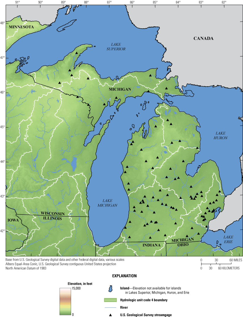
Elevation, hydrography, and U.S. Geological Survey streamgages used in this study in Michigan.
Climate
The Great Lakes play an important role affecting the climate and local weather patterns in Michigan. Water temperatures change more slowly than air temperatures. As air temperatures decline in the fall, warm water releases heat and moisture into the air, resulting in warmer falls and lake-effect precipitation downwind of the Great Lakes. Similarly in spring, cool or ice-covered water in the Great Lakes can result in cooler springs (Scott and Huff, 1996).
Michigan has a continental climate with cool to cold winters and warm to hot summers; however, the effect of the Great Lakes causes a more moderate and moist climate than other States at the same latitude, particularly along the coastal regions (Kunkel and others, 2022). The climatology of Michigan generally follows a north to south gradient, with the UP having the coldest annual temperatures and fewest frost-free days per year. Average annual temperatures in Michigan range from about 40 degrees Fahrenheit in the UP to 50 degrees Fahrenheit in the south (fig. 2).
Average annual precipitation in Michigan ranges from 40 to 50 inches (fig. 3), with the highest precipitation in the southwest. Seasonal rainfall is highest in the summer months. Average annual snowfall is 60 inches; however, this varies substantially from year to year and within the State. Effects of the Great Lakes on precipitation include increased cloud cover and precipitation downwind of the lakes during winter and decreased summertime rainfall downwind of the lakes (Scott and Huff, 1996). Coastal areas along the southern shore of Lake Superior in the UP and the eastern shore of Lake Michigan in the LP receive two to three times the winter snowfall than other areas of the State owing to lake-effect snowfall patterns.
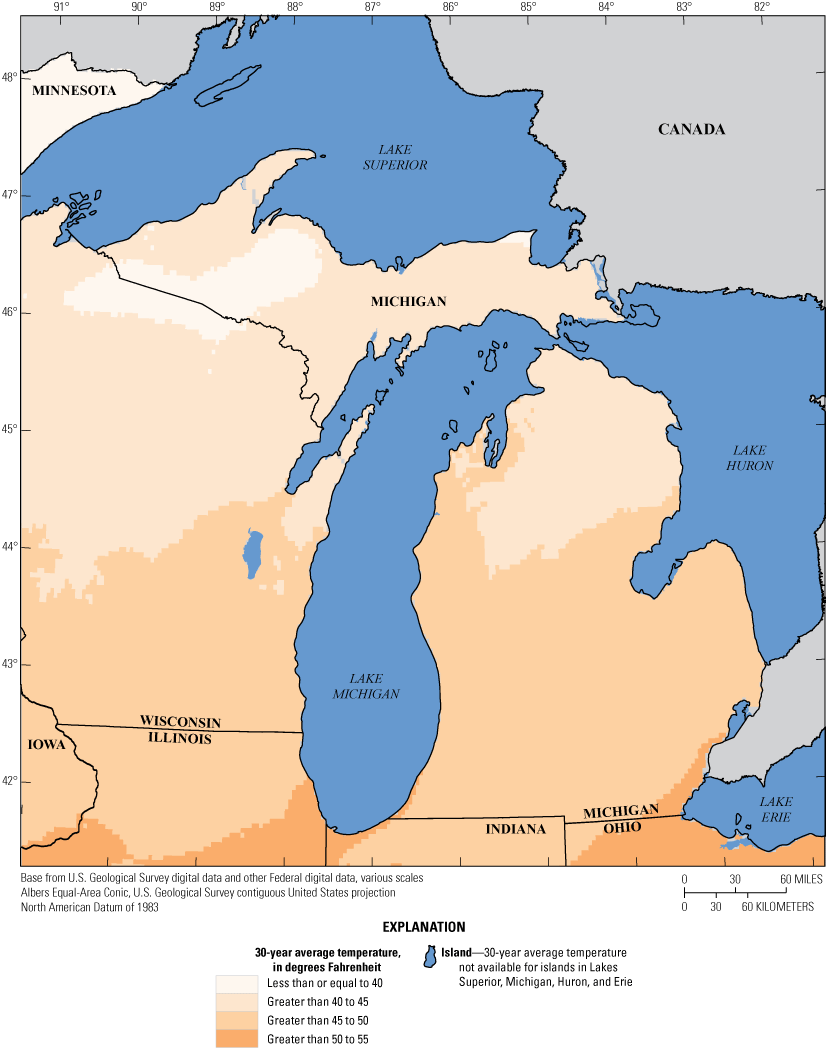
Average annual temperature for the 30-year period from 1991 to 2020 for Michigan (National Oceanic and Atmospheric Administration, 2022).
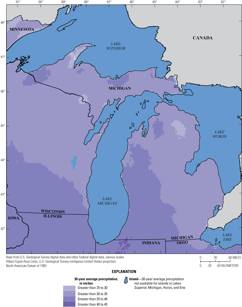
Average annual precipitation for the 30-year period from 1991 to 2020 for Michigan (National Oceanic and Atmospheric Administration, 2022).
Ecoregions
Ecoregions are areas of general similarity in ecosystems including ecological, climatic, physiographic, and geological aspects of the landscape (Omernik and Gallant, 1988; Omernik and Griffith, 2014). There are five different Level III ecoregions in Michigan (fig. 4). The Northern Lakes and Forests and the North Central Hardwood Forests ecoregions make up all of northern Michigan. The Northern Lakes and Forests ecoregion is the largest ecoregion in Michigan, encompassing all of the UP and most of the northern half of the LP. This region is characterized by sandy, nutrient poor soils; abundant wetlands; and primarily coniferous forests (figs. 5 and 6). The North Central Hardwood Forests are present in a small area of shoreline in the northwest portion of the LP. This ecoregion is characterized by steep sloping end moraines and drumlins as well as sand dunes along the lake shore (Omernik and Gallant, 1988; Omernik and Griffith, 2014).
The Southern Michigan/Northern Indiana Drift Plains, Huron/Erie Lake Plains, and the Eastern Corn Belt Plains make up southern Michigan. Most of the interior and western portion of Michigan is in the Southern Michigan/Northern Indiana Drift Plains ecoregion. This ecoregion has a diverse range of soils and abundant lakes and marshes. Land use in this region is a mix of agriculture, mixed forest, and urban land. Mixed forests and urban land cover are also found in this ecoregion. The Huron/Erie Lake Plains extends along the eastern coast of the LP. This region is characterized by fertile and nearly flat plains. Much of the original poorly drained soil (fig. 5) has been artificially drained to facilitate agriculture, which is the dominant land cover in this region. This ecoregion includes Detroit and the surrounding areas, which are the most urbanized (fig. 6) areas of Michigan. The Eastern Corn Belt Plains runs in a small strip extending from the southern border with Indiana northward between the Southern Michigan/Northern Indiana Drift Plains and the Huron/Erie Lake Plains. This ecoregion contains rolling till plains and end moraines with loamier and better drained soils (fig. 5) than those in the Huron/Erie Lake Plains ecoregion to the east (Omernik and Gallant, 1988; Omernik and Griffith, 2014).
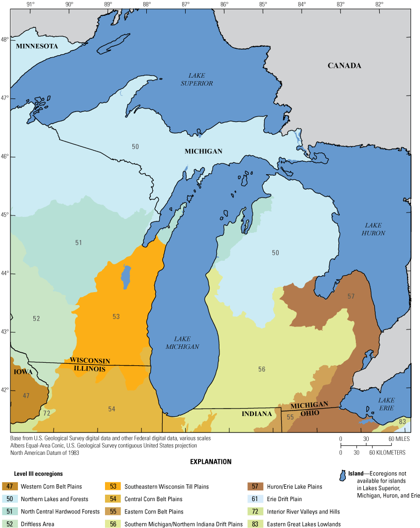
Level III Ecoregions of Michigan.
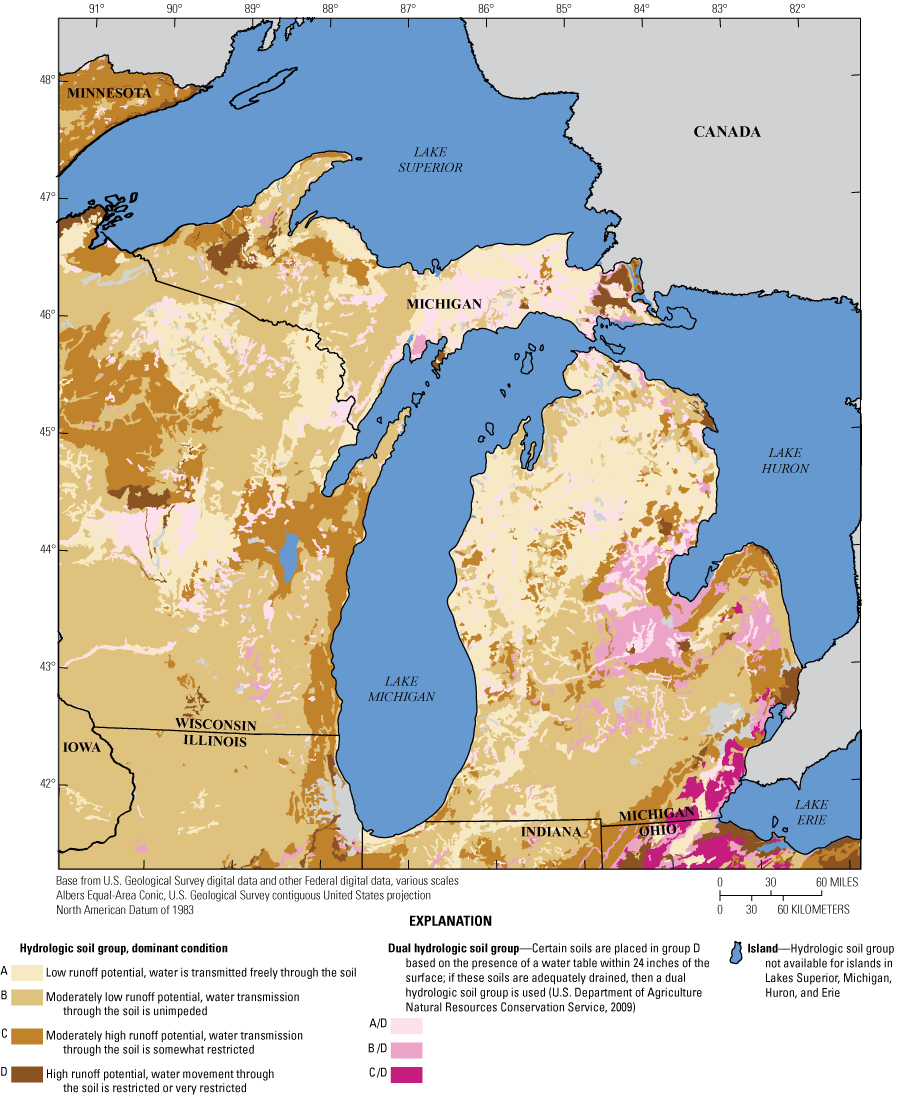
Dominant hydrologic soil groups of Michigan.
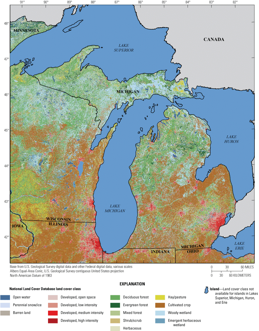
Land cover class of Michigan.
Brief History of U.S. Geological Survey Peak-Flow Data Collection in Michigan
Annual peak streamflow has been recorded in Michigan since the late 1800s. Based on data through water year 2021, there are 341 active or discontinued streamgage locations with 10 or more years of annual peak-streamflow measurements (U.S. Geological Survey, 2023). A water year is the period from October 1 to September 30 and is designated by the year in which it ends. Of these streamgages, 46 are standalone crest-stage gages (CSGs) and 301 are continuous streamgage operations. The two streamgages with the longest peak-flow record are on the Grand River at Lansing, Michigan (USGS streamgage 04113000) and the Grand River at Grand Rapids, Michigan (USGS streamgage 04119000), both of which have more than 120 annual peak-streamflow measurements, starting in water year 1901. Streamgages reporting annual peak streamflow per year are shown in figure 7. The number of continuous streamgages grew throughout the late 19th and early 20th centuries and reached a maximum of 316 streamgages in 1975. Early streamgages were operated primarily on large streams with drainage areas of roughly 1,000 square miles (fig. 8). Streamgages installed later in the 20th century focused on smaller and mid-sized basins with drainage areas on the order of 50 to several hundred square miles (fig. 8). Standalone CSG operations began in 1943, rapidly increased in number until the mid-1970s, and reached a maximum of 61 in 1975. Standalone CSGs are typically installed in smaller drainage basins less than 50 square miles. Standalone CSG usage decreased during the 1980s, and as of water year 2021, there were only four standalone CSGs in operation.
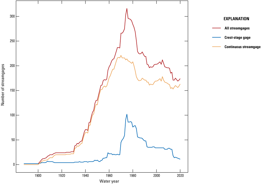
Number and type of U.S. Geological Survey streamgages reporting peak streamflow for water year 1880 through 2020 in Michigan.
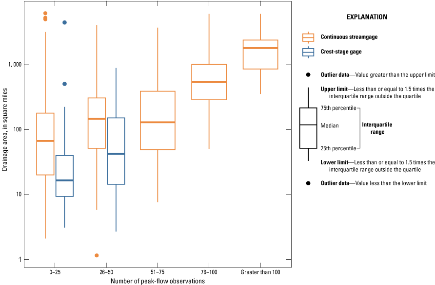
Drainage area distributions for continuous streamgages and crest stage gages in Michigan by length of record.
The history of streamgage operations is relevant to nonstationarity analyses because it provides information on the temporal distribution of the data available for evaluating nonstationarity. The temporal variability of streamgage data may represent a bias in the evaluation of nonstationarity in annual peak flows in Michigan because many streamgages on smaller basins do not have a long period of record for analysis. The trends and statistical characteristics of floods in larger basins with longer periods of record may not reflect those in smaller upstream areas.
Brief History of Statistical Analysis of Peak Streamflow and Nonstationarity
Holtschlag and Croskey (1984) estimated flood magnitudes for selected exceedance probabilities for 185 streamgages in Michigan using methods from Bulletin 17C (England and others, 2018) and data through water year 1982. These data were used to produce the first regional regression equations to estimate flood magnitudes at ungaged basins in Michigan. Veilleux and Wagner (2019) updated flood-frequency estimates using the expected moments algorithm as outlined in Bulletin 17C (England and others, 2018) for unregulated streamgages in the Great Lakes region, which included all of Michigan but did not update the regional regression equations for estimating floods at ungaged locations.
Nonstationarity in Michigan streamflow has been examined using several different methods including monotonic trend analysis, peaks over thresholds (POT), and identification of change points. Several studies have identified downward trends in peak streamflow in the UP and upward trends along the southern half of the LP (Mallakpour and Villarini, 2015; Rice and others, 2015; Hodgkins and others, 2019). Trends in mean annual streamflow follow largely the same spatial patterns as those for peak streamflows (Hodgkins and others, 2007; Johnston and Shmagin, 2008; Norton and others, 2019). The POT method uses time series of all daily mean streamflows that exceed a specified threshold, which may include more than one flood per year. POT analysis focuses on more frequent floods with magnitudes that may be less than the maximum annual flood and that can be of importance for scour and geomorphology (Slater and others, 2015). The choice of a threshold for POT analysis is subjective, however, a threshold equal to an average of two events per year (POT2) is commonly used. Increases in the frequency of POT2 events in Michigan’s LP were determined by Hodgkins and others (2019), Archfield and others (2016), and Mallakpour and Villarini (2015), with similar spatial patterns to trends in peak streamflows. Peak streamflow change points were identified in Michigan. Ivancic and Shaw (2017) identified spatial clusters of upward trends in unregulated streams in the LP, whereas Ryberg and others (2020) identified both downward and upward change points in Michigan in unregulated and regulated or urban streams.
Changes in streamflow in Michigan have been attributed to climate effects, regulation, and land-use change. Downward trends in annual streamflow in the UP correspond to a mix of neutral and downward trends in precipitation as well as neutral to upward trends in minimum summer temperatures, which could be affecting the evapotranspiration rates (Norton and others, 2019). Similarly, upward trends in the southern LP correspond to increases in precipitation and increases in spring minimum temperature, which may affect snowmelt dynamics (Hodgkins and others, 2007; Norton and others, 2019). Some areas of southern Michigan have undergone substantial urbanization during the last century. Urbanization is known to increase the magnitude and frequency of flood peaks (Moglen and Schwartz, 2006). In urban areas of southern Michigan, streamflow may be affected by both urbanization and precipitation, which make it difficult to assign a primary cause of streamflow change (Levin and Holtschlag, 2022)
Review of Research Relating to Climatic Variability and Change
Climate in Michigan is driven by large scale air masses from the Gulf of Mexico and from the Arctic and Pacific Northwest and is also affected by the Great Lakes. Streamflow in Michigan follows naturally cyclical patterns with persistent periods of lower than or higher than average streamflow over large spatial areas. This section discusses historical flood and drought periods across Michigan and the climatic forces that affect these large-scale streamflow patterns.
Historical Floods and Drought Periods in Michigan
Many Michigan rivers periodically flood, and several major floods have been recorded during the past 100 years. Flooding most often occurs in late winter or spring when rainfall combines with snowmelt on saturated or frozen soils that have little capacity for infiltration. Although documentation of floods prior to the 1900s is limited, there are references to several floods between 1840 and 1902 in the Grand River, Saginaw River, Kalamazoo River, and the Ontonagon River (not shown, Paulson and others, 1991). One of the first major floods on record in Michigan was the Grand River flood in March 1904 in the central and southern parts of the State. With flood stages 7 to 9 feet above present-day flood stage, peak streamflow from this flood is still considered the highest on record at Grand River at Lansing, Mich. (USGS streamgage 04113000) and the Grand River at Grand Rapids, Mich. (USGS streamgage 04119000) (Murphy, 1905; U.S. Geological Survey, 2023). Repeated floods in this river and at others across the State have led to the implementation of flood control structures in many communities. Other notable floods in Michigan occurred in April 1947, April 1960, April 1975, September 1986, and April 2013 (Paulson and others, 1991).
Although mild drought is common in Michigan, severe droughts are infrequent and are typically short in duration (Paulson and others, 1991). Several statewide droughts have occurred in Michigan in the past 100 years. Like much of the country, the extreme, extended drought in the 1930s is considered one of the worst in Michigan history. A second severe and extended drought during the period of record affected the entire State between 1960 and 1967 (Paulson and others, 1991). Mean annual streamflow for each year of record for Michigan streamgages in the study area is shown in figure 9. Mean annual streamflow is colored by the Z-score, which represents the number and direction of standard deviations away from the mean for each streamgage. Streamgages in figure 9 are ordered by latitude, with northernmost streamgages at the top. Periods of drier-than-average conditions spanning across many streamgages in Michigan can be seen in the 1930s, late 1970s, and much of the 2000s extending through 2013 for some southern streamgages, whereas periods of higher-than-average conditions can be seen at most streamgages during 1950–51, the mid-1970s, mid-1980s, 1990s, and 2016–20.
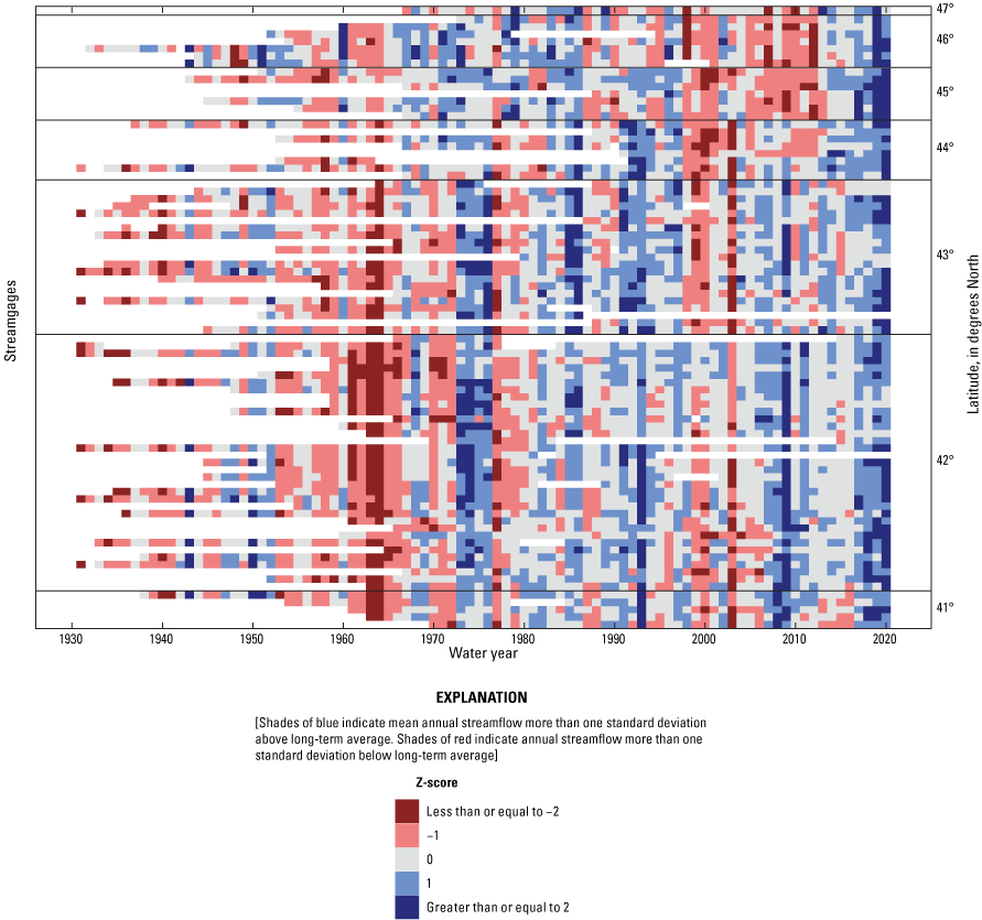
Mean annual streamflow, in standard deviations from the mean. Shades of blue indicate mean annual streamflow more than one standard deviation above long-term average. Shades of red indicate annual streamflow more than one standard deviation below long-term average.
Review of Evidence of Climatic Variability
Climate variability in the upper Midwest has been associated with large scale ocean-atmospheric oscillations that shift the configuration of the jet stream. El Niño–Southern Oscillation (ENSO) refers to the periodic warming of surface waters in the tropical Pacific Ocean and resulting disruptions in atmospheric air masses. In the negative phase (El Niño), ENSO pushes the jet stream northward, causing milder-than-average temperatures in Michigan, whereas in the positive phase (La Niña), warmer and wetter winter conditions have been noted in the upper Midwest. The effect of the ENSO cycle in Michigan may be strengthened or weakened by interactions with other ocean-atmospheric oscillations such as the Pacific Decadal Oscillation and Atlantic Multidecadal Oscillation, which have different cycle lengths (Budikova and others, 2021).
Climate in much of Michigan is affected by the water levels and ice coverage on the surrounding Great Lakes. By lowering the available moisture content above the surface of a lake, ice coverage can mitigate lake-effect snow events downwind of the Great Lakes in winter. Warmer winters throughout the Great Lakes region have contributed to a downward trend in ice cover on the Great Lakes since the 1970s (Wang and others, 2012; Mason and others, 201622). Additionally, change points in ice coverage across the great lakes have been noted, which may be controlled by the Arctic Oscillation and ENSO (El Niño) climate patterns (Wang and others, 2012). Declining ice on the Great Lakes can affect weather and climate patterns, particularly in downwind areas that experience more lake-effect snow or rainfall in years with lower ice coverage.
In recent decades, the climate in Michigan has been getting warmer and wetter. Annual temperature in Michigan increased nearly 3 degrees Fahrenheit since 1900, mostly in winter and spring (Frankson and others, 2022). Temperatures in the 2000s were higher than any other period on record. Precipitation was lowest in the 1930s and 1960s and has been increasing more recently. The wettest 5-year consecutive period was from 2015 to 2020 (Frankson and others, 2022). The frequency of high intensity precipitation has also increased in Michigan (Frankson and others, 2022). Increases in snowfall since the 1980s have also been observed in the UP and northern parts of the LP (Andresen and others, 2012).
Climate Effects on Flooding and Runoff
Flooding in Michigan is primarily observed in spring as a result of high precipitation and snowmelt and less frequently from high intensity summer storms. The amount of runoff from a specific precipitation event or from snowmelt can vary depending on antecedent soil moisture conditions and the amount of evaporation that occurs. Observed and projected changes in precipitation and temperature across Michigan have the potential to change the magnitude, timing, and seasonality of floods across the State.
Anticipated climate projections for Michigan include increases in temperature and precipitation during this century (Frankson and others, 2022). Additional climate projections include an increase in frost-free days and summer extremes (Andresen and others, 2012). Longer frost-free days and increased summer temperatures have the potential to change evapotranspiration and soil moisture, which are important factors in controlling daily runoff and streamflow. Additionally, warmer temperatures may affect the Great Lakes’ water levels and ice cover, which can increase lake-effect precipitation.
Precipitation is expected to increase in Michigan, although there is a higher degree of uncertainty with future precipitation than temperature (Frankson and others, 2022). Precipitation increases are most likely in winter and spring due to changes in temperature. The ratio of snow to total precipitation is expected to decrease (Byun and Hamlet, 2018; Frankson and others, 2022). Changes in snow storage could affect the timing and magnitudes of peak streamflows in Michigan and include earlier snowmelt-related peak streamflows (Byun and others, 2019).
Data and Methods
Statistical analyses of peak streamflow, annual streamflow, and climate metrics were performed for four periods: the 100-year period from water year 1921 through water year 2020, the 75-year period from water year 1946 through water year 2020, the 50-year period from water year 1971 through 2020, and the 30-year period from water year 1991 through 2020. Statistical analysis of peak streamflow consisted of evaluation of autocorrelation, monotonic trends, change points, quantile regression, and seasonality. Statistical analysis of daily streamflow consisted of an evaluation of streamflow seasonality, center of volume, and POT analysis. Methods used for each statistical analysis are described in Ryberg and others (2024), and results of all analyses for each streamgage were published in a USGS data release (Marti and others, 2023). This report summarizes the results in Marti and others (2023) and identifies spatial and temporal patterns in the results across Michigan.
Results of statistical tests are commonly assessed with a probability value (p-value), which is the probability of obtaining the observed results if the null hypothesis is true. Typically, a p-value between 0.01 and 0.1, chosen by the analyst, is used as the cutoff to categorize results as statistically significant. In this report, the trends are presented using a likelihood approach, which was proposed by Hirsch and others (2015) as an alternative to simply reporting significant trends with an arbitrary cutoff point. Trend likelihood values were determined using the p-value reported by each test using the equation trend likelihood=1−(p-value)/2. When the trend is “likely upward” or “likely downward,” the trend likelihood value associated with the trend is between 0.85 and 1.0; that is, the chance of the trend occurring in the specified direction is at least 85 out of 100. When the trend is “somewhat likely upward” or “somewhat likely downward,” the trend likelihood value associated with the trend is between 0.70 and 0.85—the chance of a trend occurring in the specified direction is between 70 and 85 out of 100. There is a greater chance that random variability at a streamgage could be identified as a “somewhat likely” trend using this method and a single streamgage with this category in a region with no other similar trends may warrant additional investigation. The utility of this less stringent trend categorization is in identifying broad regions of change, in which clusters of streamgages show similar trend directions that may go unnoticed if using traditional definitions of statistical significance. When the trend is “about as likely as not,” the trend likelihood value associated with the trend is less than 0.70—the chance of the trend being either upward or downward is less than 70 out of 100. Additional details are in Ryberg and others (2024).
Results of Streamflow and Climate Analyses
Peak-streamflow data were available at 4, 29, 79, and 89 streamgages in Michigan for the 100-, 75-, 50-, and 30-year analysis periods, respectively. Widespread changes in peak flow, daily streamflow, precipitation, and temperature were identified across Michigan during all four analysis periods. This section summarizes results of streamflow and climate analyses and describes spatial or temporal patterns in nonstationarity across the State. Results for streamflow or climate analyses at specific streamgages in Michigan are available in Marti and others (2023).
Annual Peak Streamflow
This section summarizes the results of analyses of peak streamflow in Michigan. Several types of nonstationarities in peak streamflow were detected in Michigan, including trends in the magnitude and timing, and change points. Analysis results were affected by the length of the period of analysis and the number of available streamgages. There were few streamgages in the 100-year period statewide and few streamgages in the UP and northern LP in the 75-year period, making it difficult to generalize results or identify spatial patterns of peak-flow changes in these areas of the State for these periods.
Monotonic Trends in Peak Streamflow
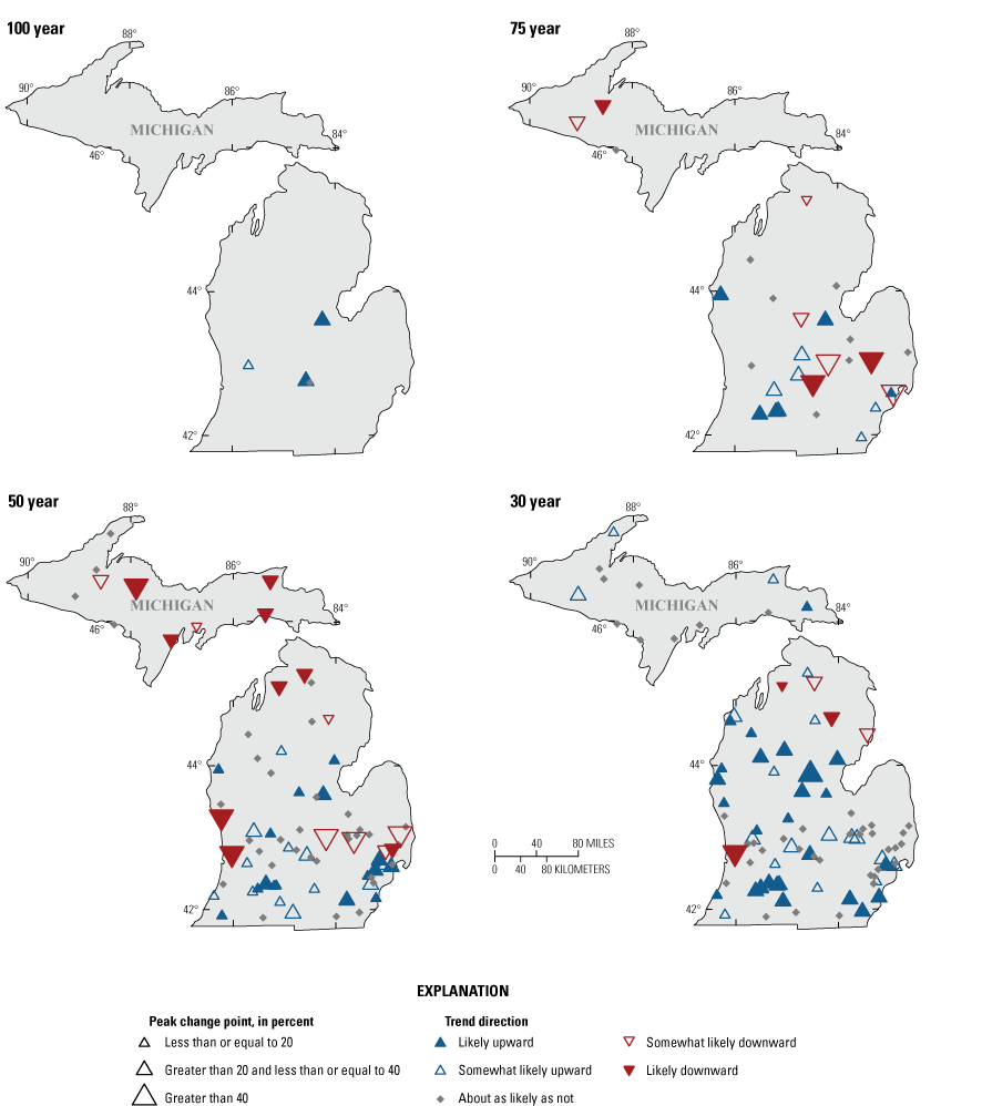
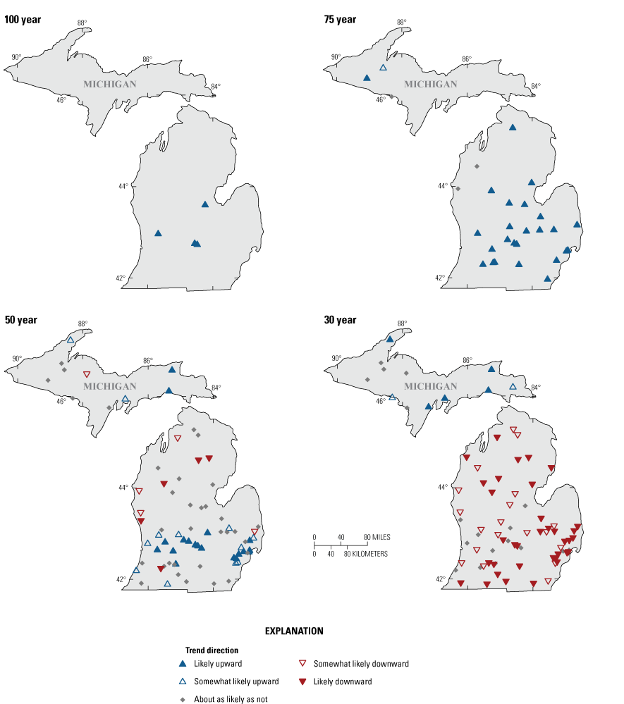
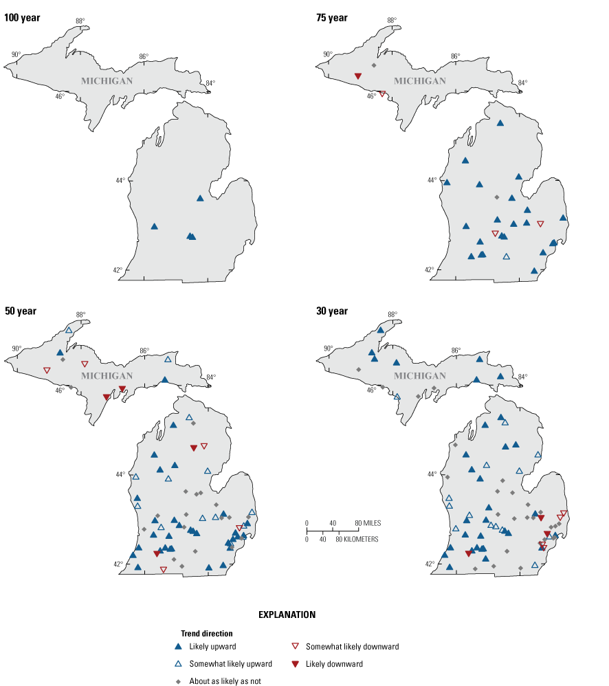
The Mann-Kendall test was used to identify the presence of a monotonic trend at streamgages for each analysis period as described in Ryberg and others (2024). A monotonic trend is one in which the direction of the trend does not reverse over time. Results of the Mann-Kendall analyses are shown in table 1 and figure 10. In the LP, trends were largely upward across all time periods, with isolated downward trends. The UP had downward trends at most streamgages in the 75- and 50-year periods, with no upward trends; however, in the 30-year period, trends in the UP were predominantly upward with no downward trends. The reversal in trend direction between time periods is indicative of nonmonotonic patterns in the peak streamflows. At many UP streamgages, peak streamflow exhibited a “U” shaped curve, with downward peak trends occurring until the mid-2000s and upward trends after that. Peak streamflow for specific streamgages available in Marti and others (2023).
Table 1.
Likelihood of monotonic trends, timing, and change points in peak streamflow at selected streamgages in Michigan for four analysis periods ending in water year 2020.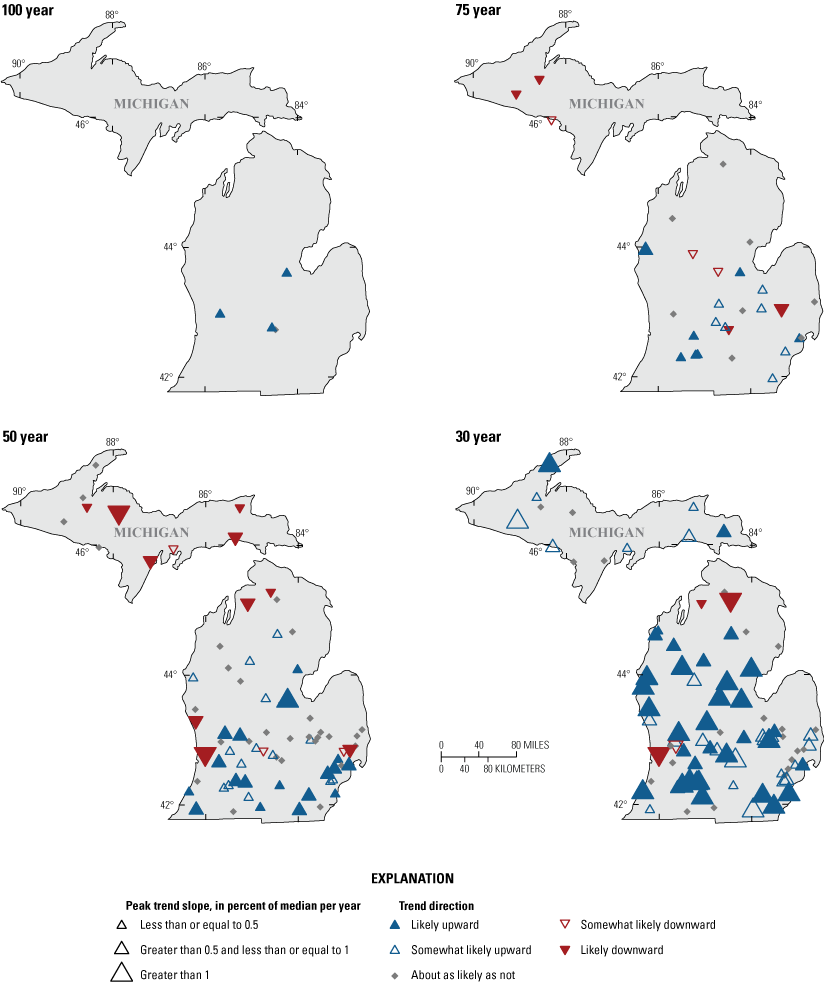
Likelihood and magnitude of peak-streamflow trends at selected U.S. Geological Survey streamgages in Michigan for four analysis periods ending in water year 2020.
To compare trend magnitudes across streams of different sizes, trend slopes were normalized by the median peak streamflow at the streamgage and converted to a percentage (fig. 10). The resulting percentage represents the yearly change in the median peak streamflow at the streamgage. For example, at a streamgage with an upward trend of 1 percent, the median peak streamflow would double during a 100-year period. Statewide, median trend magnitudes for streamgages with likely or somewhat likely trends were less than 0.5 percent per year for all analysis periods except the 30-year period, where median trends for likely and somewhat likely upward trends were 0.9 percent per year. Trend magnitudes were similar for both upward and downward trends.
Trends in Peak-Streamflow Timing
Snowmelt or rain-on-snow are the primary mechanisms for producing peak streamflows in Michigan, with occasional peak streamflows caused by summer rainstorms. Snowmelt typically peaks between March through May. The peak-flow timing analysis plots identify changes in the timing of annual peak streamflows at each streamgage (Marti and others, 2023). An example of a peak-flow timing analysis for Shiawassee River at Owosso, Mich. (USGS streamgage 04144500) is shown in figure 11A. A trend in these data indicates that annual peak streamflows are occurring later (upward trend) or earlier (downward trend) in the water year.
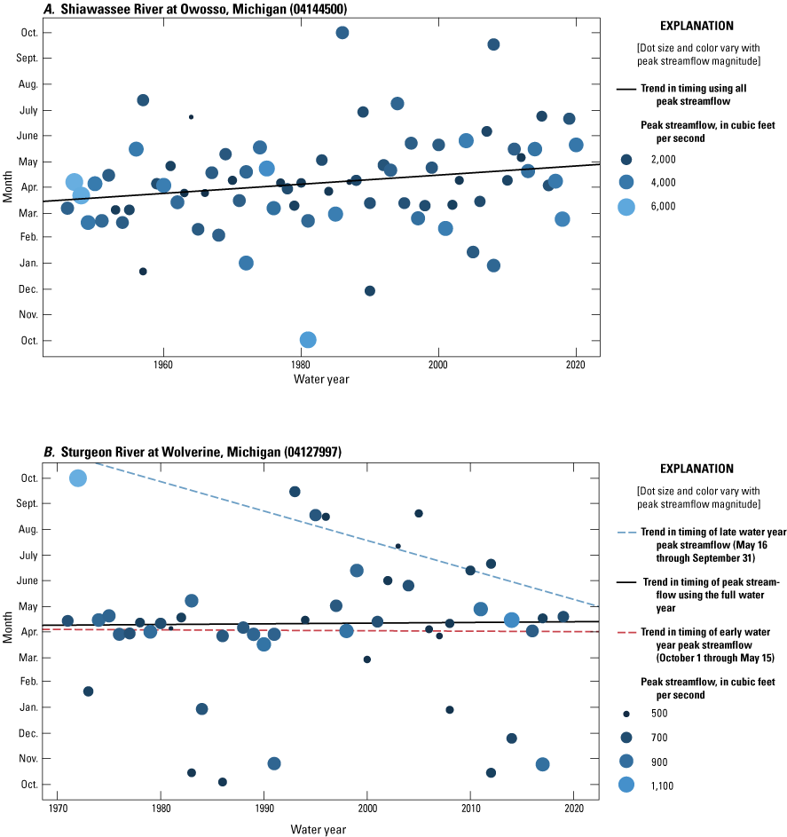
Peak-flow timing for U.S. Geological Survey (USGS) streamgages. A, Shiawassee River at Owosso, Michigan (USGS streamgage 04144500) for water years 1950 to 2020. B, Sturgeon River at Wolverine, Mich. (USGS streamgage 04127997) for water years 1991 to 2020.
Summary results of peak-flow timing trends for all time periods are shown in table 1 and figure 12. Trends in the timing of peak streamflows in Michigan showed some regional patterns, with upward trends primarily in the south and downward trends in the UP and along the northeastern side of the LP. In general, shifts in the timing of annual peak streamflow were greatest in the southern areas of Michigan. For streamgages with likely upward trends in peak-flow timing in the 75-year period, the occurrence of annual peak streamflow shifted an average of 23 days later in the spring during the time period.
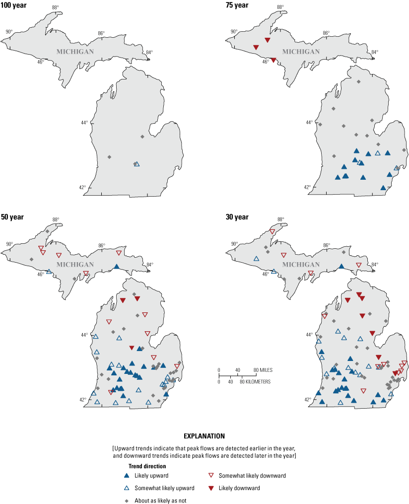
Likelihood of peak-streamflow timing trends at selected U.S. Geological Survey streamgages in Michigan for four analysis periods ending in water year 2020.
Some of the apparent downward trends in figure 12 in the 30- and 50-year periods may be caused by storms that occurred in October or November. Because the trend timing analysis uses a water year, October is considered the first month which plots at the bottom of the y-axis. Peak streamflows in October or November are low outliers in the timing analyses, which can affect the trend slope and cause a downward trend. A downward trend in peak-flow timing typically indicates that snowmelt-related spring peak streamflows are occurring earlier in the year over time. Peak streamflows in October or November may be contributing to apparent downward trends at some streamgages, although they are actually evidence of peak streamflows caused by high precipitation events occurring late in the year as opposed to spring snowmelt peaks occurring earlier in the year. If the plots were drawn using a calendar year, these October and November storms would be high outliers, leading to a neutral or upward trend. An example of this is shown in figure 11B for the Sturgeon River at Wolverine, Mich. (USGS streamgage 04127997). Downward trends at several streamgages in the northern LP seem to have been affected by this issue and the direction of the trend may be unreliable. Because of the potential effect of these outliers, plots of the peak-streamflow timing analysis, available in Marti and others (2023), should be examined for any streamgage of interest with a downward slope.
Change Points in Peak Streamflows
Change points are abrupt changes in the median, mean, or variance of a time series. The nonparametric Pettitt test was used to find change points in the median peak streamflow (Pettitt, 1979). Results of the tests for change points are shown in table 1 and figure 13. Magnitudes of change points are shown as a percent change in the median before and after the change point (fig. 13). As with tests for monotonic trends, the results of the change point analyses are presented in terms of statistical likelihood. Results in figure 13 and table 1 may differ slightly from individual streamgage analyses presented in Marti and others (2023), which do not use a likelihood approach and only show change points for streamgages when the p-value of the Pettitt test is less than or equal to 0.05.
Change point dates ranged from 1936 to 2016 (fig. 14). Downward change points occurred at individual streamgages throughout the period of record. Small clusters in which change points were present in more than one streamgage in a year occurred in 1952, 1976, and in the late 1990s. Upward change points were clustered in the early 1970s, mid-1980s, 1995, and multiple years after water year 2000.
Likelihood and magnitude of change points in median peak streamflow at selected U.S. Geological Survey streamgages in Michigan for four analysis periods ending in water year 2020.
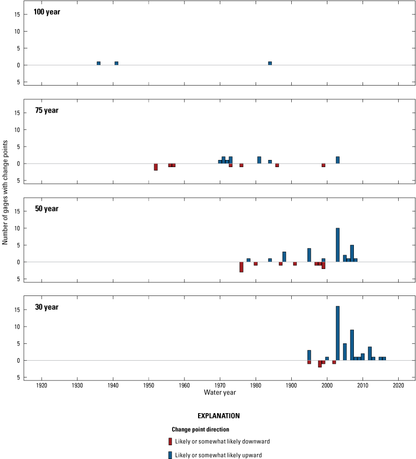
Dates of likely and somewhat likely change points in median peak streamflow at selected U.S. Geological Survey streamgages in Michigan for four analysis periods ending in water year 2020.
Daily Streamflow
This section summarizes the results of analyses of daily streamflow in Michigan. Daily streamflow data were available at 4, 29, 74, and 79 streamgages respectively for the 100-, 75-, 50-, and 30-year analysis periods. Daily streamflow is not available at every streamgage used in the peak-streamflow analyses because of the use of standalone CSGs in Michigan, which only record the annual peak streamflow. Changes in daily streamflow were examined using several different analyses including identification of seasonal and annual trends, raster seasonality plots, center of volume plots, and POT analysis, described in Ryberg and others (2024).
Trends in Mean Annual and Seasonal Streamflow
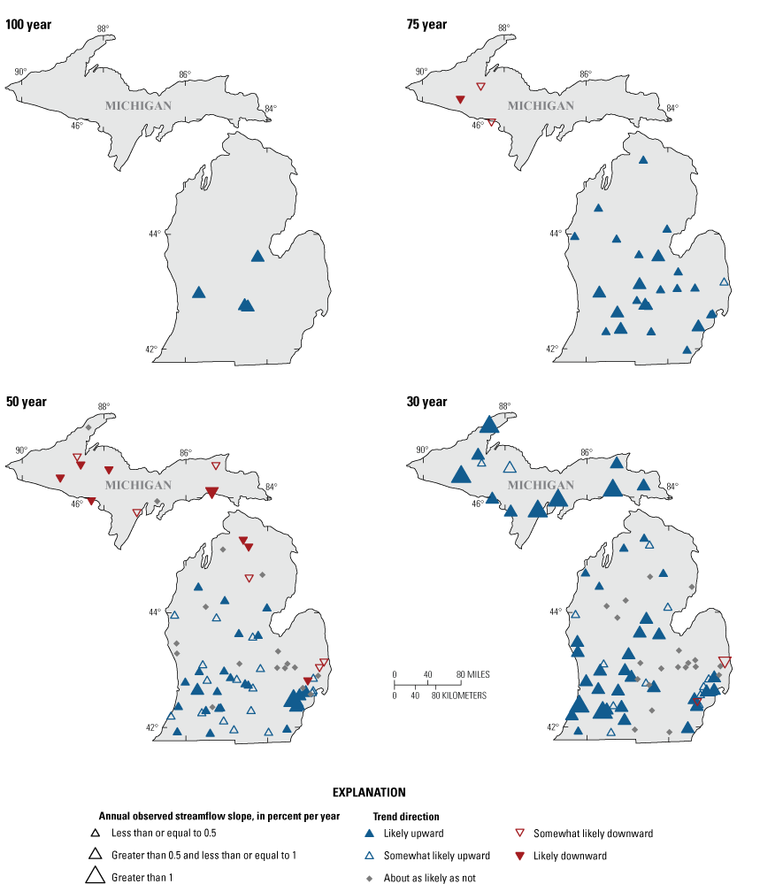
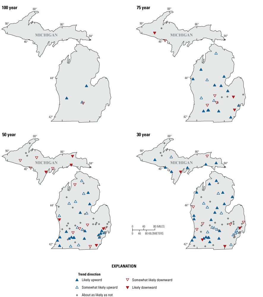
Seasonal mean streamflow was computed for spring (March through May), summer (June through August), fall (September through November), and winter (December through February). The likelihood of monotonic trends in annual streamflow is shown in table 2 and figure 15. Similar to trends in peak streamflow, trends in annual streamflow are predominantly upward. Downward trends were identified in the UP for the 75-year and 50-year period; however, all streamgages in the UP had likely or somewhat likely upward trends in the 30-year period. Median trend slopes were −0.12, −0.25, and 0.86 percent per year for the 75-, 50-, and 30-year trends, respectively, for streamgages in the UP; and 0.58, 0.43, 0.28, and 0.52 percent per year for the 100-, 75-, 50-, and 30-year trends, respectively, for streamgages in the LP.
Table 2.
Likelihood of monotonic trends in mean annual and daily streamflow, change points in peaks over threshold analyses, and trends in center of volume analyses (25th, 50th, and 75th percentile streamflows) at selected streamgages in Michigan for four analysis periods ending in water year 2020.[POT2, peaks over threshold with two events per year; POT4, peaks over threshold with four events per year; Q25, 25th percentile of annual streamflow volume; Q50, 50th percentile of annual streamflow volume; Q75, 75th percentile of annual streamflow volume]
Magnitude and likelihood of monotonic trends in mean annual streamflow at selected U.S. Geological Survey streamgages in Michigan for four analysis periods ending in water year 2020.
Seasonal streamflow trends are shown in figure 16. Seasonal trends are similar to annual trends for the 100- and 75-year periods, with predominantly downward trends in the UP and upward trends in the LP. Trend magnitudes were lowest during the spring in the LP and the fall in the UP for the 75-year period. Seasonal trends in the 50-year period were variable. Trends in the UP and northern LP were predominantly downward. In the LP, trends were predominantly upward in winter and summer and were a mix of upward, downward, and neutral (no trend) in fall and spring. There were some reversals of trend patterns in the 30-year period. The UP, which had mostly downward trends in the 75- and 50-year periods, had predominantly upward trends in the 30-year period. In the southeastern LP, which had primarily upward or neutral trends in the longer analysis periods, downward trends were identified in fall and summer in the 30-year analysis period. As with peak streamflows, a change in direction of the trends indicates a nonmonotonic, often “U” shaped pattern in the streamflow data.
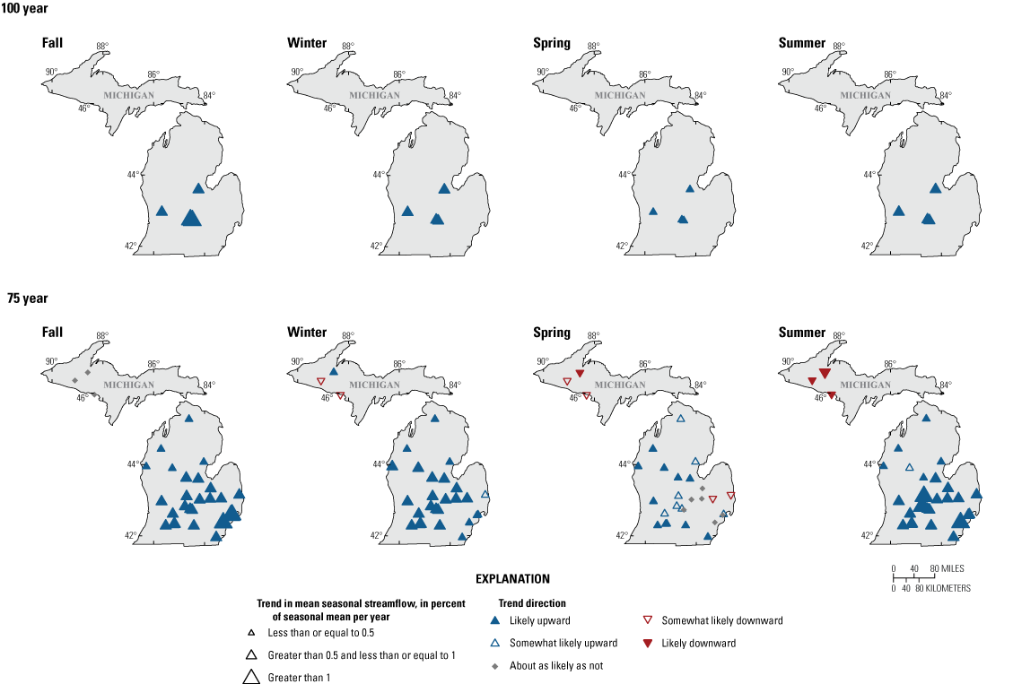
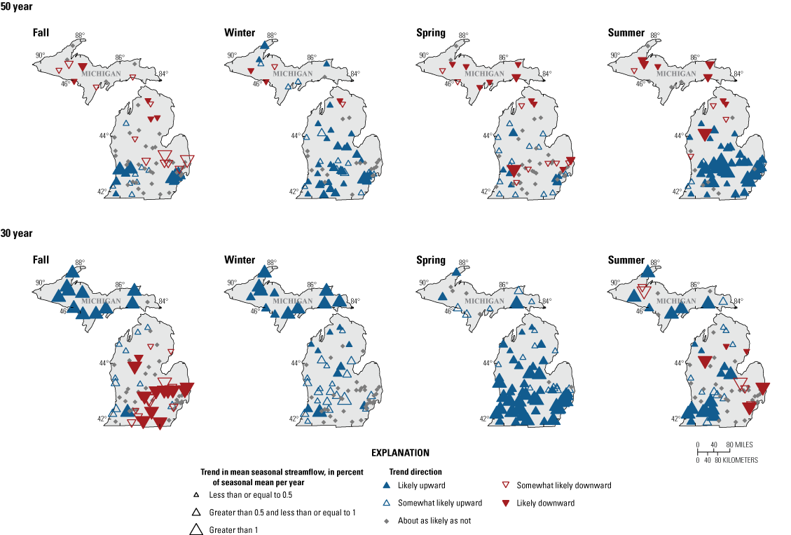
Likelihood and magnitude of monotonic trends in mean seasonal streamflow, in percent of seasonal mean per year for four analysis period ending in water year 2020 for selected U.S. Geological Survey streamgages in Michigan.
Raster Seasonality Plots
Raster seasonality plots show the mean daily streamflow for every day in the period of record (fig. 17A), colored by the magnitude of the streamflow, with day of the water year on the x-axis and water year on the y-axis. These plots provide a visual view of streamflow magnitudes across the water year for the entire period of record. Changes in the magnitude of streamflow can be seen in the color patterns in these plots. For example, figure 17A shows the raster seasonality plot for Grand River at Grand Rapids, Mich. (USGS streamgage 04119000). At the beginning of the period of record for this streamgage, the moderate and high streamflows (green and blue) typically occur between March and June, with periodic wet years in which higher flows occur in the late fall and winter. Starting in the late 1960s, the frequency of these high-magnitude flows increases during the early part of the water year, from October through February. Raster seasonality plots are a qualitative analysis and not easily summarized across the State; however, similar increases in daily streamflow during the fall and winter are evident at many southern Michigan streamgages. Raster seasonality plots for other streamgages available in Marti and others (2023). These changes in daily streamflow magnitude are not as apparent in the northern LP or the UP.
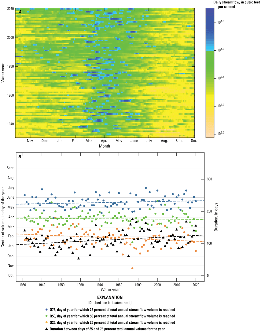
Analyses of daily streamflow for Grand River at Grand Rapids, Michigan (U.S. Geological Survey streamgage 04119000) for water years 1921 through 2020. A, Raster seasonality plot. B, Center of volume analysis.
Center of Volume Plots
The center of volume plots show the day of the year in which the 25th (Q25), 50th (Q50), and 75th (Q75) percentile of annual streamflow volume occurred as well as the duration of time between the occurrence of the Q25 and Q75 (COVdur) (fig. 17B). Linear trends in these values over time indicate a change in the distribution of streamflow timing throughout the year. Upward trends in the Q25, Q50, or Q75 indicate the dates at which these percentiles of annual streamflow volume occur are earlier in the water year, whereas a downward trend indicates a later occurrence. Trends in the COVdur indicate how evenly streamflow is distributed throughout the year. An upward trend in COVdur indicates that the annual volume of streamflow is becoming more evenly spread throughout the year, whereas a downward trend indicates that streamflows are becoming more concentrated in one season of the year.
The center of volume analysis for Grand River at Grand Rapids, Mich. (USGS streamgage 04119000) is shown in figure 17B. At this location, there are diverging trends for the Q25 and Q75 and an increasing trend in the COVdur. These trends are consistent with the increase in the magnitude of daily streamflows during fall and winter seen in the raster seasonality plot for the site (fig. 17A). The number of streamgages with likely or somewhat likely trends in the Q25, Q50, Q75, and COVdur is shown in table 2. Increasing trends in the duration between the 25th and 75th percentile of annual streamflow volume were detected at most streamgages in the 100- and 75-year periods (fig. 18). The 50-year period had a mix of upward, downward, and no likely trend in COVdur. Upward trends in this period were clustered in the southern half of the LP. Trends in COVdur in the 30-year period were primarily downward in the LP and upward or neutral in the UP. The change in direction of COVdur throughout much of the LP may be due to changes in seasonal streamflow during this period. Decreases in fall and summer streamflows and increases in spring streamflows during the 30-year period (fig. 16) result in more of the annual volume concentrated in a shorter amount of time, which result in a downward trend in COVdur.
Likelihood of monotonic trends in the duration between the 25th and 75th percentile of annual streamflow volume for selected U.S. Geological Survey streamgages in Michigan for four analysis periods.
Peaks Over Thresholds Analysis
Peaks over threshold (POT) analyses detect changes in the frequency of daily streamflow that exceed a set streamflow threshold. For a given threshold, the number of streamflow events that exceed the threshold is counted for each year as described in Ryberg and others (2024). Thresholds for the POT analyses in this study were set at the streamflow magnitude for which there is an average of two (POT2) and four (POT4) events per year. A POT analysis complements a traditional annual peak-flow flood-frequency analysis because it accounts for large flood-causing flows that may not be the peak of the year and can account for years with multiple floods in 1 year. Tests for change points in the number of events over the threshold were completed to identify increases or decreases in the frequency of these high POT2 and POT4 streamflow events. There was a mix of upward, downward, and neutral (no change points detected) results throughout the State. Spatial patterns in change point results were not evident except for a cluster of downward trends in the UP during the 50-year analysis period (fig. 19). The water years in which POT2 and POT4 change points occurred are shown in figure 20. In the 75-year period, change points are spread across the analysis, with small clusters of upward trends in several decades. In the 50- and 30-year periods, upward change points are more heavily concentrated after water year 2000.
Likelihood of change points in the annual frequency of streamflow events above a threshold for selected U.S. Geological Survey streamgages in Michigan for four analysis periods. A, Peaks over threshold for which there is an average of two events per year. B, Peaks over threshold for which there is an average of four events per year.
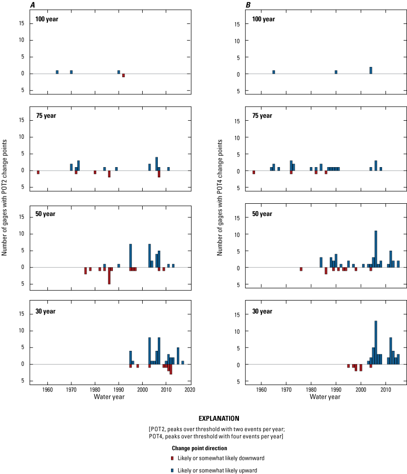
Water year of change points in the frequency of streamflow events for which there is an average of events per year for selected U.S. Geological Survey streamgages in Michigan for four analysis periods. A, Peaks over threshold with two events per year. B, Peaks over threshold with four events per year.
Climate
Gridded climate data from the monthly water balance model (Wieczorek and others, 2022), described previously, were averaged over streamgaged basins with available peak streamflow in the 100-, 75-, 50-, and 30-year analysis periods. Trends in annual and seasonal precipitation, and temperature were identified across Michigan during all four analysis periods. This section summarizes results of climate trend analyses and describes spatial and temporal patterns in these analyses across the State.
Precipitation
The likelihood and magnitude of annual precipitation trends are shown in figure 21 and table 3. Upward precipitation trends were prevalent across most of the State and all four analysis periods. Trend slopes increased substantially during the 30-year period, particularly in the UP. Median trend slopes in the LP ranged from 0.07 to 0.08 inch per year for the 100-, 75-, and 50-year periods in the LP and increased to 0.14 inch per year in the 30-year period. In the UP, median trend slopes were 0.01 and 0.02 inch per year in the 75- and 50-year periods and 0.22 inch per year in the 30-year period. The trend in precipitation at many UP streamgages was nonlinear, with a decrease in annual precipitation between water years 1990 and 2010 and a large increase after water year 2010. For example, figure 22 shows this pattern for the Sturgeon River near Sidnaw, Mich. (USGS streamgage 04040500). Because the 30-year analysis period begins during this low-precipitation period, the large slope magnitude during this period may not reflect longer-term changes in precipitation. Some LP streamgages also saw a decrease in precipitation during 1990–2020, although the decreases were less pronounced than at the UP streamgages and precipitation trends were generally more linear in the LP. Climate analyses results for individual streamgages are available in Marti and others (2023).
Table 3.
Likelihood of monotonic trends in annual and seasonal precipitation at selected streamgages in Michigan for four analysis periods ending in water year 2020.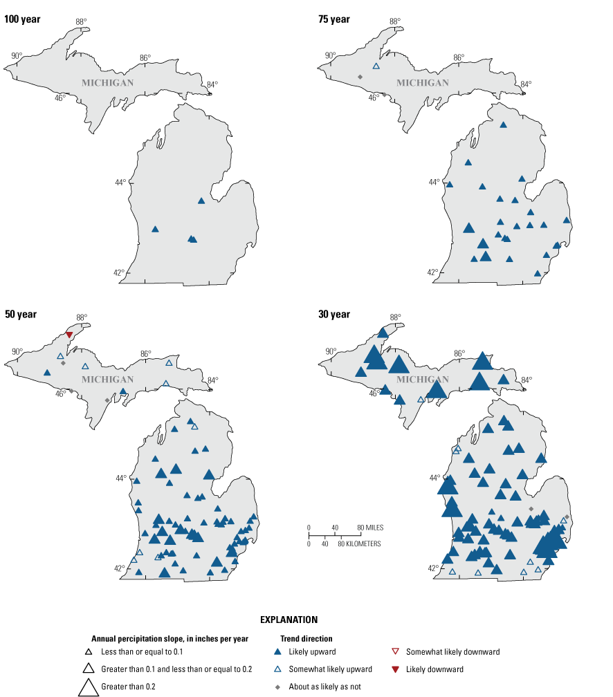
Magnitude and likelihood of monotonic trends in annual precipitation at selected U.S. Geological Survey streamgages in Michigan for four analysis periods ending in water year 2020.
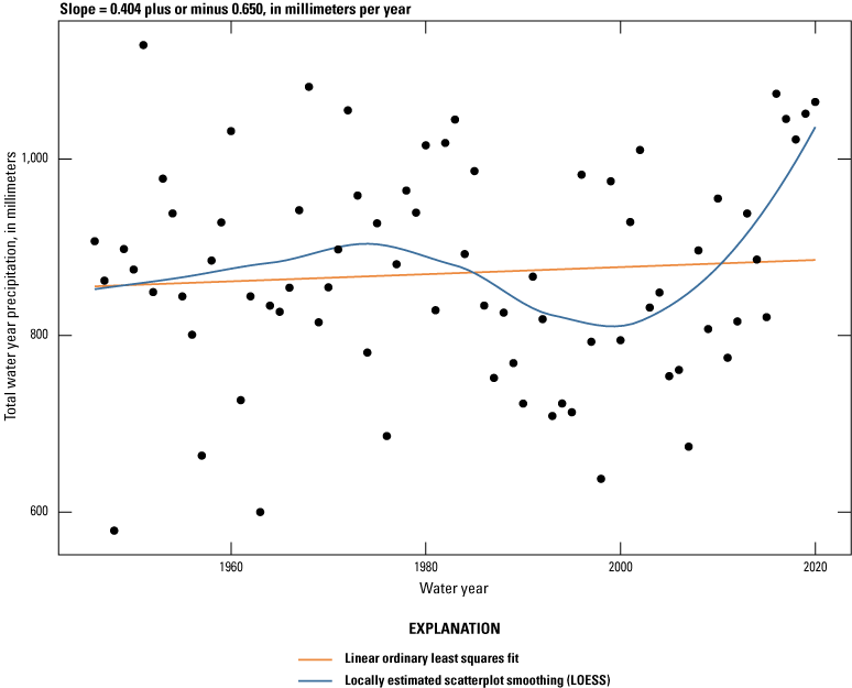
Annual precipitation for Sturgeon River near Sidnaw, Michigan (U.S. Geological Survey streamgage 04040500) from water years 1946 through 2020.
The likelihood and magnitude of seasonal precipitation trends are shown in figure 23 and table 3. Likely and somewhat likely upward seasonal precipitation trends were detected at most streamgages during the 100- and 75-year periods except for three streamgages in the UP, which had downward trends in the summer and no trend during the spring in the 75-year period. Relative trend magnitudes in these two analysis periods were generally less than 0.5 percent of the seasonal mean and there were only minor differences in trend magnitudes between seasons. During the 50- and 30-year periods, differences in seasonal trends were more evident, with spring and winter having a greater number of trends (between 89 and 97 percent of streamgages) compared to summer and fall (between 31 and 66 percent of streamgages). Trend magnitudes were largest in the 30-year period. In the UP, precipitation trends were upward in every season, whereas the LP had upward trends primarily in winter and spring. Summer precipitation trends during the 30-year period in the LP had a mix of upward trends in the southeastern area of the State, and a mix of neutral, weaker, and somewhat likely downward trends in the western and southern areas.
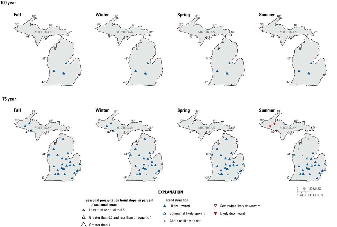
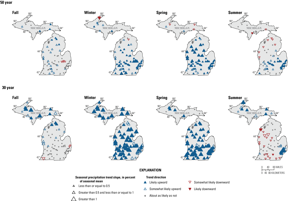
Likelihood of monotonic trends in seasonal precipitation at selected U.S. Geological Survey streamgages in Michigan for four analysis periods ending in water year 2020.
Temperature
Likely or somewhat likely upward trends in annual temperature were detected at every streamgage in the 100-, 75-, and 50-year analysis periods (fig. 24 and table 4). In the 30-year period, upward trends were detected at every streamgage in the LP and two streamgages in the UP. Other streamgages in the UP had no likely trend in the 30-year period. Statewide, median temperature trend slopes were 0.02 and 0.03 degree Fahrenheit per year in the 100- and 75-year analysis periods, respectively, and 0.5 degree per year in the 50- and 30-year analysis periods. Trends in annual temperature throughout the State were nonlinear, with neutral or downward trends through the early part of the 20th century until about the mid-1970s, when temperatures began to increase, as shown in figure 25 for Grand River at Lansing, Mich. (USGS streamgage 04113000). At some streamgages, particularly in the UP, this increase in temperature was accompanied by an increase in variability, as well which made it difficult to assess the presence of a trend in the short 30-year analysis period.
Table 4.
Likelihood of monotonic trends in annual and seasonal temperature at selected streamgages in Michigan for four analysis periods ending in water year 2020.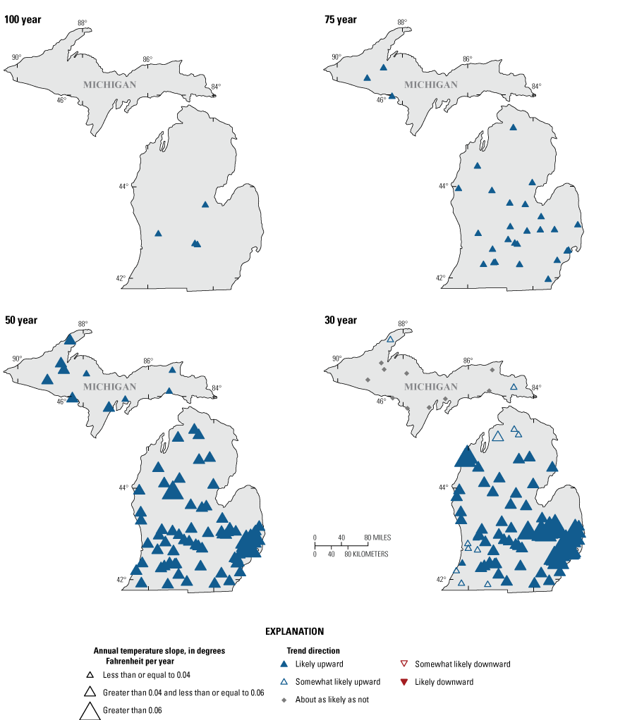
Likelihood and magnitude of monotonic trends in annual temperature at selected streamgages in Michigan for four analysis periods ending in water year 2020.
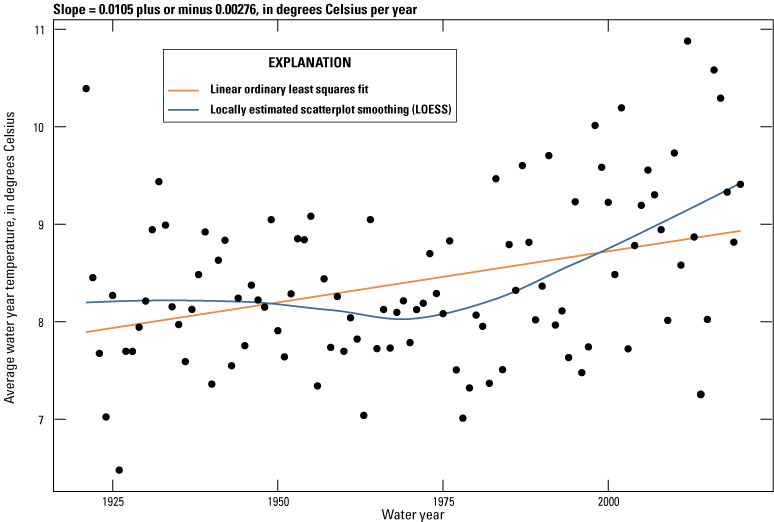
Annual temperature for Grand River at Lansing, Michigan (U.S. Geological Survey streamgage 04113000) from water year 1921 to 2020.
Seasonal mean temperature trends were greatest in the winter for the 75-year period, winter and fall in the 50-year period, and fall in the 30-year period (fig. 26). Few trends were detected in spring and winter during the 30-year period. As with precipitation and annual temperature, nonlinearities in the seasonal temperature trends can make the calculation of slope sensitive to the period of record, and high variability can mask trends in the shorter 30-year analysis period.
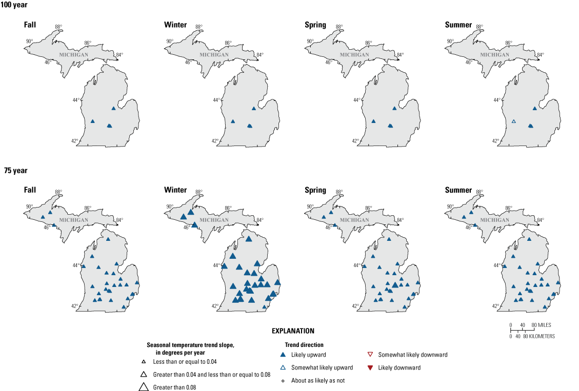
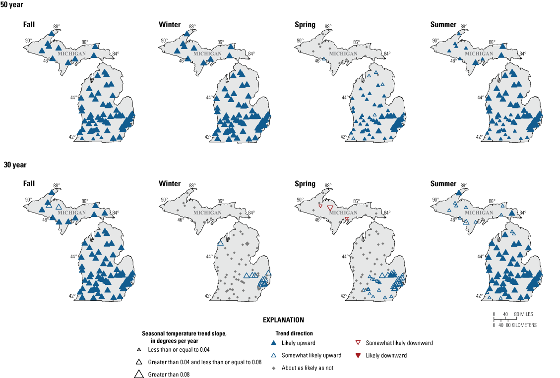
Likelihood and magnitude of monotonic trends in seasonal temperature at selected streamgages in Michigan for four analysis periods ending in water year 2020.
Trends in Modeled Water Balance Components
Although temperature and precipitation generally increased in Michigan during the past 100 years, there were differences in the seasonality, magnitude, and geographic extent of these changes. The water balance is largely driven by precipitation and temperature. Precipitation into a drainage basin may return to the atmosphere through evapotranspiration, be stored as soil moisture or groundwater, or run off as streamflow. Trends and nonstationarities in precipitation and temperature (and therefore evapotranspiration) have the potential to change the relative quantities of each of these water balance components and the interactions between them. Additionally, changes in seasonal temperature and precipitation can alter snowfall and snowmelt dynamics. Results from a monthly water balance model were used to explore the relative change in annual precipitation, potential evapotranspiration (PET), and streamflow. Modeled outputs include PET, actual evapotranspiration, snowfall, soil moisture, soil water equivalent, and runoff. A complete description of these data available in Ryberg and others (2024).
The ratio of PET to precipitation is an indication of overall “wetness” of a drainage basin, with low ratio values indicating wet and high values indicating dry. Trends in this ratio are indicators of the relative magnitudes of the increases in precipitation and temperature that were detected across the State. Trends in this ratio were mostly downward (fig. 27). Decreases in this ratio indicate that the rate of increase in precipitation was generally larger than the increase in PET from temperature increases and indicates generally “wetter” conditions at these locations, which is consistent with the upward trend patterns in mean annual streamflow.
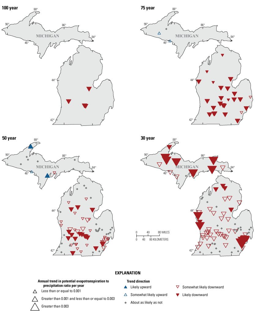
Magnitude and likelihood of the ratio of annual potential evapotranspiration and precipitation at selected U.S. Geological Survey streamgages in Michigan for four analysis periods ending in water year 2020.
Snowfall and snowmelt play an important part in the timing and magnitude of streamflow throughout Michigan. Increasing temperatures and precipitation during the fall through spring can change the amount of snowfall and the timing of snowmelt-related peak streamflows. Long-term trends in annual snowfall (50-, 75-, and 100-year analysis periods) showed downward or no trend throughout most of the State (table 5). Seasonal snowfall trends for these analysis periods had downward or no trend during the spring and fall but many upward trends in winter snowfall, which is consistent with seasonal temperature and precipitation increases in Michigan. Seasonal upward trends in precipitation were largest in winter and spring during these analysis periods. Temperature increased in all seasons during these periods, which could lead to more precipitation falling as rain instead of snow in fall and spring. In winter, despite upward temperature trends, it is still typically cold enough for most precipitation to fall as snow.
During the 30-year period, snowfall trends were primarily upward for annual and seasonal, with the largest magnitude trends in the UP (fig. 28). Seasonally, trends were seen primarily in the winter and some in spring, which is consistent with upward trends in precipitation during these seasons (fig. 28). Similar to precipitation trend magnitudes, the large magnitude of snowfall trends in the UP likely are due to decreased precipitation at these streamgages during the 1990s at the start of the 30-year analysis period and may not be representative of the longer-term conditions.
Table 5.
Likelihood of monotonic trends in annual and seasonal snowfall at selected streamgages in Michigan for four analysis periods ending in water year 2020.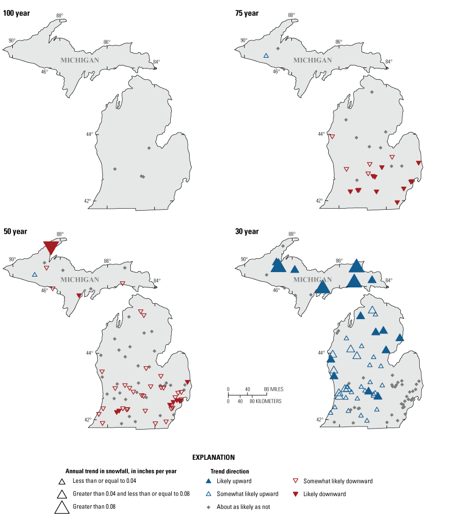
Likelihood and magnitude of monotonic trends in annual snowfall at selected streamgages in Michigan for four analysis periods ending in water year 2020.
Discussion and Implications for Flood-Frequency Analysis
Nonstationarity was identified in streamflow and climate data throughout Michigan in the past 100 years. Changes in precipitation seem to be driving many of the changes in annual and peak streamflow in Michigan. The patterns of annual and seasonal increases in precipitation (figs. 21 and 23) are generally consistent with changes in peak, annual, and seasonal streamflow (figs. 10, 15, and 16). Changes in temperature began in the late 1970s, with upward trends at most streamgages occurring between 1975 and 2020. In the LP, upward trends in temperature were primarily in fall and summer, whereas seasonal trends in precipitation were upward primarily in winter and spring. Upward trends in precipitation in winter and spring are consistent with the upward spring streamflow trends and upward peak streamflows, which typically occur in spring, whereas upward trends in temperature in fall and summer may be increasing evapotranspiration, leading to downward trends in fall and summer streamflow in the LP during this period. Upward trends in temperature have a less apparent effect on peak streamflow because temperature increases were largest during the fall and summer, whereas peak streamflow occurs more often in the spring.
The widespread prevalence of nonstationarity in peak streamflow in Michigan has important implications for flood-frequency analysis. The standard statistical methods used to estimate the flood magnitude for a given annual exceedance probability assume that the peak-streamflow time series are stationary and representative of a random process. The presence of a trend in peak streamflow time series is particularly problematic at streamgages with short periods of record because their peak streamflows may not be representative of the full range of peak-streamflow magnitudes and may result in a biased estimate of the flood magnitude. For example, Levin and Sanocki (2023) showed that flood discharge estimate for the 1-percent annual exceedance probability at a streamgage in Wisconsin varied by a factor of three when using a subset 20-year data record on a stream location with a trend in peak streamflow. Regression equations currently used to estimate flood magnitudes at ungaged streams in Michigan were last published in 1984 (Holtschlag and Croskey, 1984). Peak-streamflow data used to develop regional flood discharge equations in 1984 do not reflect the increasing peak streamflows detected in the last 30 years and cannot account for the nonstationarity observed in the streamflow record. As a result, using the old equations to estimate current (2023) peak streamflow in ungaged areas could lead to greater uncertainty than is reported in Holtschlag and Croskey (1984) and may lead to biased flood estimates.
Summary
Nonstationarity is a statistical property of annual peak streamflow time-series such that the long-term distributional properties (mean, variance, or skew) change one or more times either gradually or abruptly through time. Failure to incorporate observed nonstationarities into flood-frequency analysis may result in a poor representation of the true present-day flood risk. This report characterizes changes in annual peak streamflow, daily streamflow, and monthly precipitation and temperature in Michigan as part of a larger U.S. Geological Survey effort to characterize the effects of regional hydroclimatic shifts and changes in climate on streamflow across the Midwest. These analyses provide the foundation for ongoing studies to address nonstationarity in observed peak streamflow and flood-frequency analysis.
Streamflow and climate were analyzed using four analysis periods: the 100-year period from water year 1921 to 2020, the 75-year period from water year 1946 to 2020, the 50-year period from water year 1971 to 2020, and the 30-year period from water year1991 to 2020. A water year is the period from October 1 to September 30 and is designated by the year in which it ends. Peak streamflow was available for 4, 29, 50, and 30 streamgages in the 100-, 75-, 50-, and 30-year periods, respectively. Daily streamflow was available for 4, 29, 74, and 79 streamgages in the 100-, 75-, 50-, and 30-year periods, respectively. Additionally, trends in precipitation, temperature data, and estimated water budget components were examined as potential drivers of streamflow change.
Peak streamflows were assessed using monotonic trend detection using the Mann-Kendall test, as well as change point analysis during the four specified time periods. Trends and change points in peak streamflow were primarily upward in the Lower Peninsula (LP) across all time periods, with some isolated downward changes. In the Upper Peninsula (UP), trends and change points were downward for the 75- and 50-year time periods but upward or neutral for the 30-year period. Shifts in the timing of peak streamflows were identified with a shift towards later peaks in the southern half of the LP, and a shift towards earlier peaks in along the eastern and northern areas of the LP. For streamgages with likely upward trends in peak-flow timing in the 75-year period, the occurrence of annual peak streamflow shifted an average of 23 days later in the spring during the course of the analysis period.
A variety of analyses were used to assess changes in annual and seasonal streamflows, including the Mann-Kendall test to identify monotonic trends, raster seasonality plots to visualize changes in daily streamflow magnitude, center of volume analyses to identify changes in the timing of streamflow, and peaks over threshold analyses to identify changes in the frequency of high-magnitude streamflows. Annual streamflow trends resembled peak-flow trend patterns, with upward trends throughout the LP, downward trends in the UP in the 75- and 50-year periods, and upward trends in the 30-year period. Seasonal precipitation trends were primarily upward in the LP, with fall, winter, and summer trends being the largest in magnitude throughout the 75- and 50-year periods. In the 30-year period, downward fall precipitation trends were identified in the southeastern area of the LP.
Changes in climate during the periods of analysis point to wetter conditions overall and are likely driving increases in streamflow. Annual precipitation increased at nearly every streamgage in the study. Upward seasonal trends were largest in magnitude in winter and spring, particularly in the 30-year period. Precipitation at some UP streamgages was nonlinear, with decreases in precipitation between 1990 and 2010 and increasing afterwards. Because the 30-year analysis period begins during this low-precipitation period, the large slope magnitude during this period may not reflect longer-term changes in precipitation in the UP. Temperature increased statewide, with most temperature trends beginning in the mid-1970s. Temperature trends were generally strongest in fall and winter and weakest in the spring. Despite widespread increases in annual temperature, modeled potential evapotranspiration to precipitation ratios indicate an overall trend towards wetter conditions in Michigan.
References Cited
Andresen, J.A., Hilberg, S.D., and Kunkel, K.E., 2012, Historical climate and climate trends in the Midwestern United States, in Winkler, J.A., Andresen, J.A., Hatfield, J.L., Bidwell, D., and Brown, D., eds., Climate change in the Midwest—A synthesis report for the National Climate Assessment: Island Press, p. 8–36.
Archfield, S.A., Hirsch, R.M., Viglione, A., and Bloschl, G., 2016, Fragmented patterns of flood change across the United States: Geophysical Research Letters, v. 43, p. 10232–10239. [Also available at https://doi.org/10.1002/2016GL070590.]
Barth, N.A., Ryberg, K.R., Gregory, A., and Blum, A.G., 2022, Attribution of monotonic trends and change points in peak streamflow across the conterminous United States using a multiple working hypotheses framework,1941–2015 and 1966–2015, chap. A of Ryberg, K.R., ed., Attribution of monotonic trends and change points in peak streamflow across the conterminous United States using a multiple working hypotheses framework,1941–2015 and 1966–2015: U.S. Geological Survey Professional Paper 1869, p. A1–A29.
Budikova, D., Ford, T.W., and Wright, J.D., 2021, Characterizing winter season severity in the Midwest United States, part II—Interannual variability: International Journal of Climatology, v. 42, no. 6, p. 3499–3516. [Also available at https://doi.org/10.1002/joc.7429.]
Byun, K., and Hamlet, A.F., 2018, Projected changes in future climate over the Midwest and Great Lakes region using downscaled CMIP5 ensembles: International Journal of Climatology, v. 38, p. e531–e553. [Also available at https://doi.org/10.1002/joc.5388.]
Byun, K., Chiu, C., and Hamlet, A.F., 2019, Effects of 21st century climate change on seasonal flow regimes and hydrologic extremes over the Midwest and Great Lakes region of the US: Science of the Total Environment, v. 650, part 1, p. 1261–1277. [Also available at https://doi.org/10.1016/j.scitotenv.2018.09.063.]
England, J.F., Jr., Cohn, T.A., Faber, B.A., Stedinger, J.R., Thomas, W.O., Jr., Veilleux, A.G., Kiang, J.E., and Mason, R.R., Jr., 2018, Guidelines for determining flood flow frequency—Bulletin 17C (ver. 1.1, May 2019): U.S. Geological Survey Techniques and Methods, book 4, chap. B5, 148 p. [Also available at https://doi.org/10.3133/tm4B5.]
Hirsch, R.M., Archfield, S.A., and De Cicco, L.A., 2015, A bootstrap method for estimating uncertainty of water quality trends: Environmental Modelling & Software, v. 73, p. 148–166. [Also available at https://doi.org/10.1016/j.envsoft.2015.07.017.]
Hodgkins, G.A., Dudley, R.W., and Aichele, S.S., 2007, Historical changes in precipitation and streamflow in the U.S. Great Lakes Basin, 1915–2004: U.S. Geological Survey Scientific Investigations Report 2007–5118, 31 p. [Also available at https://doi.org/10.3133/sir20075118.]
Hodgkins, G.A., Dudley, R.W., Archfield, S.A., and Renard, B., 2019, Effects of climate, regulation, and urbanization on historical flood trends in the United States: Journal of Hydrology, v. 573, p. 697–709. [Also available at https://doi.org/10.1016/j.jhydrol.2019.03.102.]
Holtschlag, D.J., and Croskey, H.M., 1984, Statistical models for estimating flow characteristics of Michigan streams: U.S. Geological Survey Water-Resources Investigations Report 84–4207, 80 p. [Also available at https://doi.org/10.3133/wri844207.]
Ivancic, T.J., and Shaw, S.B., 2017, Identifying spatial clustering in change points of streamflow across the contiguous U.S. between 1945 and 2009: Geophysical Research Letters, v. 44, no. 5, p. 2445–2453. [Also available at https://doi.org/10.1002/2016GL072444.]
Johnston, C.A., and Shmagin, B.A., 2008, Regionalization, seasonality, and trends of streamflow in the U.S. Great Lakes Basin: Journal of Hydrology, v. 362, no. 1–2, p. 69–88. [Also available at https://doi.org/10.1016/j.jhydrol.2008.08.010.]
Koutsoyiannis, D., and Montanari, A., 2015, Negligent killing of scientific concepts—The stationarity case: Hydrological Sciences Journal, v. 60, no. 7–8, p. 1174–1183. [Also available at https://doi.org/10.1080/02626667.2014.959959.]
Kunkel, K.E., Frankson, R., Runkle, J., Champion, S.M., Stevens, L.E., Easterling, D.R., Stewart, B.C., McCarrick, A., and Lemery, C.R., eds., 2022, State climate summaries for the United States 2022: Silver Spring, Maryland, National Oceanic and Atmospheric Administration Technical Report NESDIS, [variously paged].
Levin, S.B., and Holtschlag, D.J., 2022, Attribution of monotonic trends and change points in peak streamflow in the Midwest Region of the United States, 1941–2015 and 1966–2015, chap. D of Ryberg, K.R., ed., Attribution of monotonic trends and change points in peak streamflow across the conterminous United States using a multiple working hypotheses framework,1941–2015 and 1966–2015: U.S. Geological Survey Professional Paper 1869, p. D1–D22.
Levin, S.B., and Sanocki, C.A., 2023, Estimating flood magnitude and frequency for unregulated streams in Wisconsin: U.S. Geological Survey Scientific Investigations Report 2022–5118, 25 p., accessed January 15, 2023, at https://doi.org/10.3133/sir20225118. [Supersedes Scientific Investigations Report 2016–5140.]
Lins, H.F., and Cohn, T.A., 2011, Stationarity—Wanted dead or alive?: Journal of the American Water Resources Association, v. 47, no. 3, p. 475–480. [Also available at https://doi.org/10.1111/j.1752-1688.2011.00542.x.]
Mallakpour, I., and Villarini, G., 2015, The changing nature of flooding across the central United States: Nature Climate Change, v. 5, no. 3, p. 250–254. [Also available at https://doi.org/10.1038/nclimate2516.]
Marti, M.K., Wavra, H.N., Over, T.M., Ryberg, K.R., Podzorski, H.L., and Chen, Y.R., 2023, Peak streamflow data, climate data, and results from investigating hydroclimatic trends and climate change effects on peak streamflow in the Central United States, 1921–2020: U.S. Geological Survey data release, accessed January 2023 at https://doi.org/10.5066/P9R71WWZ.
Mason, L.A., Riseng, C.M., Gronewold, A.D., Rutherford, E.S., Wang, J., Clites, A., Smith, S.D.P., and McIntyre, P.B., 2016, Fine-scale spatial variation in ice cover and surface temperature trends across the surface of the Laurentian Great Lakes: Climatic Change, v. 138, no. 1-2, p. 71–83. [Also available at https://doi.org/10.1007/s10584-016-1721-2.]
Milly, P.C.D., Betancourt, J., Falkenmark, M., Hirsch, R.M., Kundzewicz, Z.W., Lettenmaier, D.P., and Stouffer, R.J., 2008, Stationarity Is dead—Whither water management?: Science, v. 319, no. 5863, p. 573–574. [Also available at https://doi.org/10.1126/science.1151915.]
Moglen, G., and Schwartz, E., 2006, Methods for adjusting U.S. Geological Survey rural regression peak discharges in an urban setting, U.S. Geological Survey Scientific Investigations Report 2006-5270, 55.p [Also available at https://doi.org/10.3133/sir20065270.]
Murphy, E.C., 1905, Destructive floods in the United States in 1904: U.S. Geological Survey Water-Supply Paper, v. 147. [Also available at https://doi.org/10.3133/wsp147.]
National Oceanic and Atmospheric Administration, 2022, U.S. climate normals: National Oceanic and Atmospheric Administration, National Centers for Environmental Information database, accessed June 1, 2022, at https://www.ncei.noaa.gov/products/land-based-station/us-climate-normals.
Norton, P.A., Driscoll, D.G., and Carter, J.M., 2019, Climate, streamflow, and lake-level trends in the Great Lakes Basin of the United States and Canada, water years 1960–2015. U.S. Geological Survey Scientific Investigations Report 2019–5003, 47 p., [Also available at https://doi.org/10.3133/sir20195003.]
Omernik, J.M., and Griffith, G.E., 2014, Ecoregions of the conterminous United States—Evolution of a hierarchical spatial framework: Environmental Management, v. 54, no. 6, p. 1249–1266. [Also available at https://doi.org/10.1007/s00267-014-0364-1.]
Paulson, W.P., Chase, E.B., Roberts, R.S., and Moody, D.W., 1991, National water summary 1988–89—Hydrologic events and floods and droughts: U.S. Geological Survey Water-Supply Paper 2375, 591 p. [Also available at https://doi.org/10.3133/wsp2375.]
Rice, J.S., Emanuel, R.E., Vose, J.M., and Nelson, S.A.C., 2015, Continental U.S. streamflow trends from 1940 to 2009 and their relationships with watershed spatial characteristics: Water Resources Research, v. 51, no. 8, p. 6262–6275. [Also available at https://doi.org/10.1002/2014WR016367.]
Ryberg, K.R., Hodgkins, G.A., and Dudley, R.W., 2020, Change points in annual peak streamflows—Method comparisons and historical change points in the United States: Journal of Hydrology, v. 583, 124307, 13 p. [Also available at https://doi.org/10.1016/j.jhydrol.2019.124307.]
Ryberg, K.R., Over, T.M., Levin, S.B., Heimann, D.C., Barth, N.A., Marti, M.K., O’Shea, P.S., Sanocki, C.A., Williams-Sether, T.J., Wavra, H.N., Sando, T.R., Sando, S.K., and Liu, M.S., 2024, Introduction and methods of analysis for peak streamflow trends and their relation to changes in climate in Illinois, Iowa, Michigan, Minnesota, Missouri, Montana, North Dakota, South Dakota, and Wisconsin, chap. A of Ryberg, K.R., comp., Peak streamflow trends and their relation to changes in climate in Illinois, Iowa, Michigan, Minnesota, Missouri, Montana, North Dakota, South Dakota, and Wisconsin: U.S. Geological Survey Scientific Investigations Report 2023–5064, 27 p. [Also available at https://doi.org/10.3133/sir20235064A.]
Sando, R., Sando, S.K., Ryberg, K.R., and Chase, K.J., 2022, Attribution of monotonic trends and change points in peak streamflow in the Upper Plains Region of the United States, 1941–2015 and 1966–2015, chap. C of Ryberg, K.R., ed., Attribution of monotonic trends and change points in peak streamflow across the conterminous United States using a multiple working hypotheses framework,1941–2015 and 1966–2015: U.S. Geological Survey Professional Paper 1869, p. C1–C36.
Scott, R.W., and Huff, F.A., 1996, Impacts of the Great Lakes on regional climate conditions: Journal of Great Lakes Research, v. 22, no. 4, p. 845–863. [Also available at https://doi.org/10.1016/S0380-1330(96)71006-7.]
Serago, J., and Vogel, R., 2018, Parsimonious nonstationary flood frequency analysis: Advances in Water Resources, v. 112, no. 5, p. 1–16. [Also available at https://doi.org/10.1016/j.advwatres.2017.11.026.]
Serinaldi, F., and Kilsby, C.G., 2015, Stationarity is undead—Uncertainty dominates the distribution of extremes: Advances in Water Resources, v. 77, p. 17–36. [Also available at https://doi.org/10.1016/j.advwatres.2014.12.013.’
Slater, L.J., Singer, M.B., and Kirchner, J.W., 2015, Hydrologic versus geomorphic drivers of trends in flood hazard: Geophysical Research Letters, v. 42, no. 2, p. 370–376. [Also available at https://doi.org/10.1002/2014GL062482.]
Stedinger, J.R., and Griffis, V.W., 2011, Getting from here to where? Flood frequency analysis and climate: Journal of the American Water Resources Association, v. 47, no. 3, p. 506–513. [Also available at https://doi.org/10.1111/j.1752-1688.2011.00545.x.]
U.S. Geological Survey, 2023, USGS water data for the Nation: U.S. Geological Survey National Water Information System database, accessed August 25, 2023, at https://doi.org/10.5066/F7P55KJN.
Veilleux, A.G., and Wagner, D.M., 2019, Methods for estimating regional skewness of annual peak flows in parts of the Great Lakes and Ohio River Basins, based on data through water year 2013: U.S. Geological Survey Scientific Investigations Report 2019–5105, 26 p., accessed at [Also available at https://doi.org/10.3133/sir20195105.]
Villarini, G., Smith, J.A., Serinaldi, F., Bales, J., Bates, P.D., and Krajewski, W.F., 2009, Flood frequency analysis for nonstationary annual peak records in an urban drainage basin: Advances in Water Resources, v. 32, no. 8, p. 1255–1266. [Also available at https://doi.org/10.1016/j.advwatres.2009.05.003.]
Wang, J., Bai, X., Hu, H., Clites, A., Colton, M., and Lofgren, B., 2012, Temporal and spatial variability of Great Lakes ice cover 1973–2010: Journal of Climate, v. 25, no. 4, p. 1318–1329. [Also available at https://doi.org/10.1175/2011JCLI4066.1.]
Wieczorek, M.E., Signell, R.P., McCabe, G.J., and Wolock, D.M., 2022, USGS monthly water balance model inputs and outputs for the conterminous United States, 1895–2020, based on ClimGrid data: U.S. Geological Survey data release, accessed June 2022 at https://doi.org/10.5066/P9JTV1T6.
Conversion Factors
Supplemental Information
A water year is the period from October 1 to September 30 and is designated by the year in which it ends; for example, water year 2020 was from October 1, 2019, to September 30, 2020.
Abbreviations
COVdur
duration of time between the occurrence of the 25th percentile of annual streamflow and the 75th percentile of annual streamflow
CSG
crest-stage gage
EMA
expected moments algorithm
ENSO
El Niño–Southern Oscillation
LP
Lower Peninsula
MWBM
monthly water balance model
NWIS
National Water Information System
p-value
probability value
PET
potential evapotranspiration
POT
peaks over threshold
POT2
peaks over threshold with two events per year
POT4
peaks over threshold with four events per year
Q25
25th percentile of annual streamflow volume
Q50
50th percentile of annual streamflow volume
Q75
75th percentile of annual streamflow volume
UP
Upper Peninsula
USGS
U.S. Geological Survey
For more information about this publication, contact:
Director, USGS Upper Midwest Water Science Center
1 Gifford Pinchot Drive
Madison, WI 53726
For additional information, visit: https://www.usgs.gov/centers/upper-midwest-water-science-center
Publishing support provided by the
Rolla Publishing Service Center
Disclaimers
Any use of trade, firm, or product names is for descriptive purposes only and does not imply endorsement by the U.S. Government.
Although this information product, for the most part, is in the public domain, it also may contain copyrighted materials as noted in the text. Permission to reproduce copyrighted items must be secured from the copyright owner.
Suggested Citation
Levin, S.B., 2024, Peak streamflow trends in Michigan and their relation to changes in climate, water years 1921–2020, chap D of Ryberg, K.R. comp., Peak streamflow trends and their relation to changes in climate in Illinois, Iowa, Michigan, Minnesota, Missouri, Montana, North Dakota, South Dakota, and Wisconsin: U.S. Geological Survey Scientific Investigations Report 2023–5064, 49 p., https://doi.org/10.3133/sir20235064D.
ISSN: 2328-0328 (online)
Study Area
| Publication type | Report |
|---|---|
| Publication Subtype | USGS Numbered Series |
| Title | Peak streamflow trends in Michigan and their relation to changes in climate, water years 1921–2020 |
| Series title | Scientific Investigations Report |
| Series number | 2023-5064 |
| Chapter | D |
| DOI | 10.3133/sir20235064D |
| Publication Date | May 23, 2024 |
| Year Published | 2024 |
| Language | English |
| Publisher | U.S. Geological Survey |
| Publisher location | U.S. Geological Survey |
| Contributing office(s) | Upper Midwest Water Science Center |
| Description | Report: viii, 49 p., Data Release |
| Larger Work Type | Report |
| Larger Work Subtype | USGS Numbered Series |
| Larger Work Title | Peak Streamflow Trends and Their Relation to Changes in Climate in Illinois, Iowa, Michigan, Minnesota, Missouri, Montana, North Dakota, South Dakota, and Wisconsin |
| Country | United States |
| State | Michigan |
| Online Only (Y/N) | Y |