

Peak Streamflow Trends in North Dakota and Their Relation to Changes in Climate, Water Years 1921–2020
Links
- Document: Report (10 MB pdf) , HTML , XML
- Larger Work: This publication is Chapter H of Peak streamflow trends and their relation to changes in climate in Illinois, Iowa, Michigan, Minnesota, Missouri, Montana, North Dakota, South Dakota, and Wisconsin
- Dataset: USGS National Water Information System database - USGS water data for the Nation
- Data Releases:
- USGS data release - Peak streamflow data, climate data, and results from investigating hydroclimatic trends and climate change effects on peak streamflow in the Central United States, 1921–2020
- USGS data release - USGS monthly water balance model inputs and outputs for the conterminous United States, 1895–2020, based on ClimGrid data
- NGMDB Index Page: National Geologic Map Database Index Page (html)
- Download citation as: RIS | Dublin Core
Acknowledgments
Funding for this project was provided by the Transportation Pooled Fund-5(46) project, in cooperation with the following State agencies: Illinois Department of Transportation, Iowa Department of Transportation, Michigan Department of Transportation, Minnesota Department of Transportation, Missouri Department of Transportation, Montana Department of Natural Resources and Conservation, North Dakota Department of Water Resources, South Dakota Department of Transportation, and Wisconsin Department of Transportation.
Abstract
Standardized guidelines for completing flood-flow frequency analyses are presented in a U.S. Geological Survey Techniques and Methods report known as Bulletin 17C, https://doi.org/10.3133/tm4B5. In recent decades (since about 2000), a better understanding of long-term climatic persistence (periods of clustered floods or droughts, or wet or dry periods) and concerns about potential climate change and land-use change have caused a reexamination of the stationarity assumptions underlying methods in Bulletin 17C. Bulletin 17C does not offer guidance on incorporating nonstationarities and further identifies a need for flood-frequency studies that incorporate changing climate or basin characteristics. As part of that reexamination, a study of annual peak streamflow (peak flow) has begun in the Midwest. This chapter of the study summarizes how hydroclimatic variability affects peak flows in North Dakota.
In this analysis of peak flow, daily streamflow, and climate metrics, four periods were selected: (1) a 100-year period, 1921–2020; (2) a 75-year period, 1946–2020; (3) a 50-year period, 1971–2020; and (4) a 30-year period, 1991–2020. Output from a monthly water-balance model was used for the climate data. Statistical analysis of peak flow consisted of evaluations of autocorrelation, trends, and change points and was augmented with analyses of seasonality and daily streamflow. The long-term pattern of decreasing peak flow in the west and increasing peak flow in the east is a pattern of opposing signals on either side of the 100th meridian. Analyses indicate that a key factor in changing hydroclimatology is the increase in fall precipitation. The trends in soil moisture closely match the trends in annual precipitation. Nonstationary flood-frequency analysis necessitates detailed exploratory data analysis and additional data and information about climate, land use, and other factors. This study provides extensive exploratory analysis for peak flow, daily streamflow, and climate data for North Dakota, setting the stage for informed nonstationary flood-frequency analysis.
Introduction
Flood-flow frequency analysis (flood-frequency analysis) is essential to water-resources management applications, including critical structure design (for example, bridges and culverts) and floodplain mapping. Standardized recommended guidelines for completing flood-flow frequency analyses are presented in Bulletin 17C (England and others, 2018). A basic assumption within Bulletin 17C is that, for basins without major hydrologic alterations (for example, regulation, diversion, and urbanization), statistical properties of the distribution of annual peak streamflows (peak flows) are stationary; that is, the mean, variance, and skew of the population from which the peaks are observations are assumed constant. Stationarity requires that all the data represent a consistent hydrologic regime within the same, albeit highly variable, fundamental climatic system. From the onset of the U.S. Geological Survey (USGS) streamgaging program through much of the 20th century, the stationarity assumption was widely accepted within the flood-frequency community. However, in recent decades, better understanding of long-term climatic persistence (periods of clustered floods or droughts, or wet or dry periods compared to median streamflow at a particular site), as well as concerns about potential climate change and land-use change, have caused the stationarity assumption to be reexamined (Milly and others, 2008; Lins and Cohn, 2011; Stedinger and Griffis, 2011; Koutsoyiannis and Montanari, 2015; Serinaldi and Kilsby, 2015).
Nonstationarity is a statistical property of a peak-flow series such that the long-term distributional properties (the mean, variance, or skew) change one or more times either gradually or abruptly through time. Individual nonstationarities could be attributed to one driver (for example, either flow regulation, land-use change, or climate) but may be the result of a mixture of drivers (Vogel and others, 2011), making detection and attribution of nonstationarities challenging (Barth and others, 2022; Levin and Holtschlag, 2022; Sando and others, 2022). Nonstationarity in peak flow can manifest as a monotonic trend of gradually increasing or decreasing peak flows over time (Hodgkins and others, 2019) or as an abrupt change in the central tendency (mean or median), variability, or skew of peak flows (Ryberg and others, 2020a). Not incorporating observed trends into flood-frequency analysis can result in a poor representation of the true flood risk. Bulletin 17C does not offer guidance on how to incorporate nonstationarities when estimating floods and further identifies a need for additional flood-frequency studies that incorporate changing climate or basin characteristics into the analysis (England and others, 2018).
A study of nonstationarities in peak flows has begun in the Midwest (Illinois, Iowa, Michigan, Minnesota, Missouri, Montana, North Dakota, South Dakota, and Wisconsin; Marti and others, 2023). An introduction to the study and detailed descriptions of the methods of analysis are provided in chapter A (Ryberg and others, 2024) of this USGS Scientific Investigations Report (Ryberg, 2024a), entitled “Introduction and Methods of Analysis for Peak Streamflow Trends and Their Relation to Changes in Climate in Illinois, Iowa, Michigan, Minnesota, Missouri, Montana, North Dakota, South Dakota, and Wisconsin,” and hereafter referred to as “chapter A.”
The complex topography, hydrology, and climate of the study are described in chapter A. Peak-flow hydrology in the Midwest study area is also complex, and variability exists in the primary climatic drivers among various peak-flow regimes. In some areas, including North Dakota, peak-flow regimes are clearly dominated by snowmelt, with minor rainfall-generated peak flows (Ryberg and others, 2016a). Conversely, in other areas, peak-flow regimes also are strongly affected by rainfall events during or outside of the snowmelt period (Ryberg and others, 2016a). Additionally, distinct areas of contrasting hydroclimatic patterns (that is, areas with large downward rainfall trends and areas with large upward trends) within the region (Sando and others, 2022), combined with land-use changes (Ahiablame and others, 2017; Falcone and others, 2018), make North Dakota (and the Midwest, multistate study region) an ideal area for investigating potential nonstationary peak-flow frequency methodologies.
Previous regional and national studies have identified hydroclimatic changes that affect streamflow in North Dakota (Hirsch and Ryberg, 2012; Peterson and others, 2013; Norton and others, 2014, 2022; Ryberg and others, 2014, 2016a, 2020a; Hodgkins and others, 2019; Sando and others, 2022), including gradual changes in streamflow, precipitation, or temperature and more abrupt hydroclimatic shifts. Increases or decreases in precipitation have been attributed as major drivers of some nonstationarities in peak flows in North Dakota (Sando and others, 2022). Trends in peak flow in the region indicate an abrupt change with downward peak-flow trends in western parts of North Dakota and upward trends in eastern North Dakota (Peterson and others, 2013; Norton and others, 2014, 2022; Ryberg and others, 2016a, 2020a; Hodgkins and others, 2017, 2019). The broad regional extent, abrupt transition, and large magnitudes of trends in the study area support the hypothesis that the trends can be caused by long-term (decades) persistence and regional hydroclimatic shifts (Vecchia, 2008; Ryberg and others, 2014; Razavi and others, 2015; Kolars and others, 2016). In the context of North Dakota hydroclimatology, long-term persistence refers to clustered wet and dry periods that induce serial correlation into the peak-flow series at lags of more than 1 year. This long-term persistence is also referred to as “memory,” “long-range dependence,” or “the Hurst phenomenon” (Koutsoyiannis and Montanari, 2007; Ryberg and others, 2020b).
Other documented changes in streamflow characteristics within the study area in the last 30 years indicate spatial and temporal differences in the timing, magnitude, and frequency of streamflows. For example, a general tendency is toward earlier snowmelt-dominated peak flows for much of the northern part of the study area (Ryberg and others, 2016a). Other studies have noted a more gradual tendency toward decreases in annual streamflow in Montana and Wyoming (Norton and others, 2014) and increases in monthly, seasonal, and annual streamflow in eastern North and South Dakota (Norton and others, 2014; Hoogestraat and Stamm, 2015). McCabe and Wolock (2002) determined a change point in minimum and median daily streamflow at selected U.S. streamgages with substantial increases beginning in 1971 at sites primarily east of lat 100° W.
Analysis of temporal changes in streamflow for the 1912–2011 period (Wise and others, 2018) indicated decreases in snowpack and streamflow in the Upper Missouri River Basin, including areas in Montana, North Dakota, and South Dakota. Mallakpour and Villarini (2015) analyzed the 1962–2011 changes in flood characteristics in the central United States and reported an increase in the magnitude and frequency of flooding in eastern North Dakota at the annual scale, along with increases in frequency of heavy rainfall events. At the seasonal scale, the magnitude and frequency of flooding increased in summer and fall in eastern North Dakota, and widespread increases in the frequency of fall heavy rainfall events were observed. Increases in spring flooding were characterized by more increases in frequency than magnitude, and increases in winter flooding were characterized by increases in magnitude (Mallakpour and Villarini, 2015).
This chapter summarizes how hydroclimatic variability affects the temporal and spatial distributions of peak-flow data in the State of North Dakota. Trends in peak flows resulting from other factors, such as land-use change or changes in agricultural practices, are possible and could exist simultaneously with hydroclimatic changes, complicating the task of attributing these trends just to hydroclimatic changes. Numerous analyses and statistical approaches are applied to document the primary mechanisms controlling floods and characterize temporal changes in hydroclimatic variables and peak flow.
These analyses can be used to provide the foundation for future studies to evaluate, modify, or develop methods to address nonstationarities in observed peak flows in flood-frequency analysis. This study and resulting report were completed by the USGS in cooperation with the State Departments of Transportation of Illinois, Iowa, Michigan, Minnesota, Missouri, South Dakota, and Wisconsin; the Montana Department of Natural Resources and Conservation; and the North Dakota Department of Water Resources. This report was made possible by the Transportation Pooled Fund-5(460) project.
Purpose and Scope
The purpose of this report is to document the completion of the second task of the study, which is to characterize the effects of natural hydroclimatic shifts and potential climate change on peak flows in the State of North Dakota. The scope of this chapter is to evaluate the combined effects of multidecadal climatic persistence and gradual and abrupt climate change on peak-flow frequency analyses in the State of North Dakota. In this evaluation, peak flow, daily streamflow, and model-simulated gridded climatic data were examined for trends, change points, and other statistical properties indicative of changing climatic and environmental conditions. This study is intended to provide a framework for addressing potential nonstationarity issues in flood-frequency updates that commonly are completed by the USGS in cooperation with other agencies throughout the Nation.
The following sections describe the climatology, soils, and ecoregions of the study area; the history of peak-flow collection as it affects the data used in the analysis; history of the statistical analysis of peak flow and nonstationarity; a review of research relating to climate variability and change; the data used in this study; the study methods; and the results.
Description of Study Area
North Dakota lies in the center of North America (U.S. Geological Survey, undated b), and the topography is generally low relief (fig. 1). North Dakota is separated into two major drainage basins. The streamgages labeled 1–20 represent streams draining to Hudson Bay, Canada (not shown), and are part of the Souris-Red-Rainy water-resource region. The remainder of the labeled streamgages represent streams draining to the Gulf of America (not shown) and are part of the Missouri water-resource region (Seaber and others, 1987).
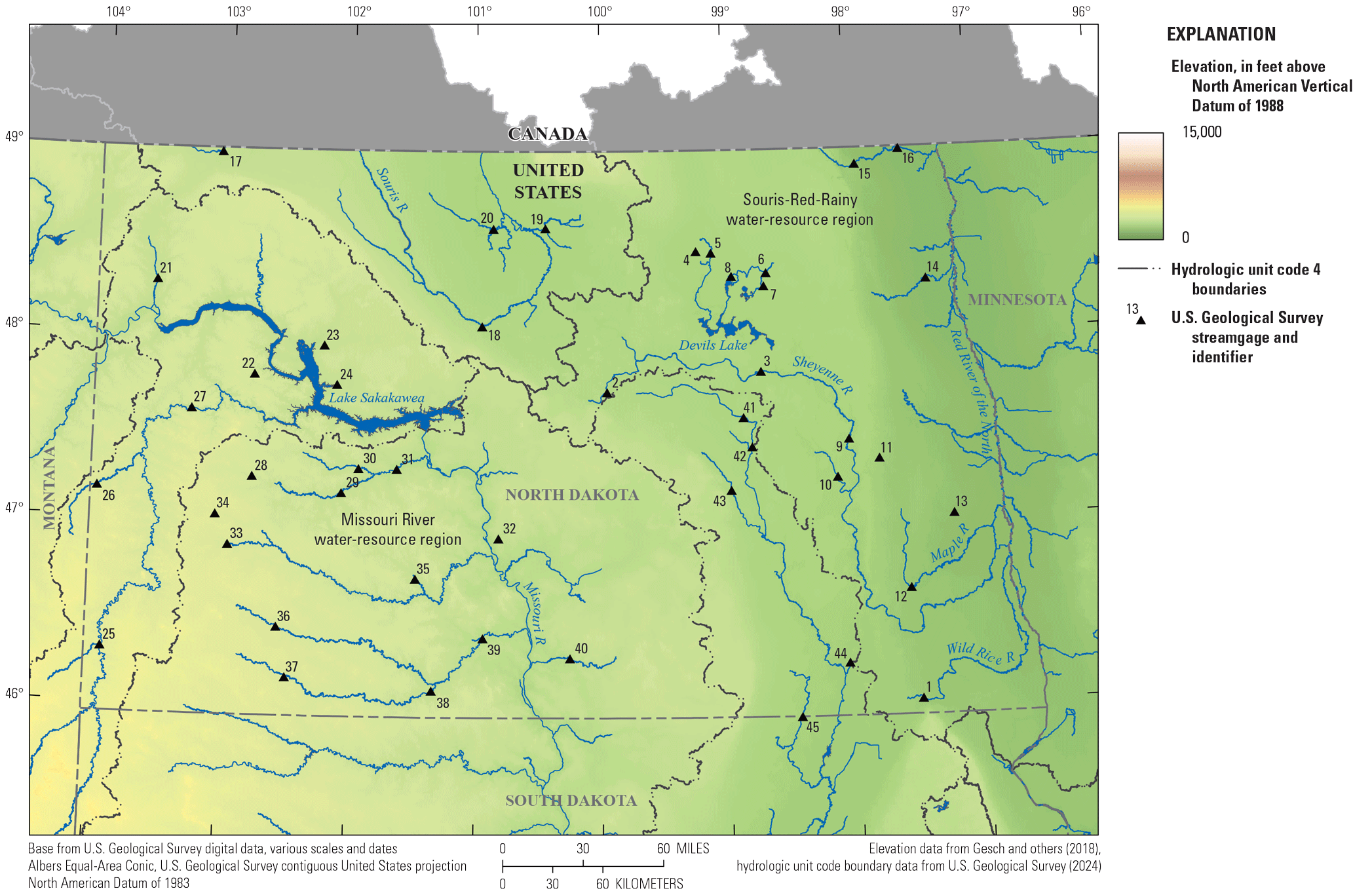
Map showing elevation, hydrography, and U.S. Geological Survey streamgages in North Dakota used in this study.
In the Souris-Red-Rainy water-resource region, floods are observed primarily during April and May and are caused by rapid spring snowmelt, which can be accompanied by rain (Ryberg and others, 2016a; U.S. Geological Survey, 2021). In the Missouri River water-resource region in North Dakota, floods are mainly associated with spring snowmelt or heavy summer rainfall (Ryberg and others, 2016a; U.S. Geological Survey, 2021). Timing of the snowmelt is critical for peak flow because the later snowmelt begins, the greater the risk for an accelerated melt and increased flooding because of elevated temperatures or spring rainfall (Enz, 2003). Precipitation, temperature, evapotranspiration (ET), and soils provide a basic understanding of the complexity of the State’s climate and hydrology. Ecoregions and land cover integrate these characteristics and other information to explain differences in hydrologic setting across the State.
Precipitation, Temperature, and Evapotranspiration
An east-west gradient in precipitation exists across North Dakota and the Northern Great Plains in general, as well as a north-south gradient in temperature (Knapp and others, 2023). In this transition zone, North Dakota’s climate has been highly variable. “Early explorers and settlers had the same complaints about weather as we do today: too dry, too wet, too cold, too hot, too windy” (Severson and Sieg, 2006, p. 37). In a more scientific manner, Thornthwaite (1941, p. 180) stated that “the Great Plains, so situated as to be inundated successively by moist and dry, cold and hot air masses, suffer meteorological excesses and in consequence experience large fluctuations in climate.”
The east-west divide represents a change from continental to semiarid climate between the 98th and 100th meridians. The 100th meridian has long been considered a dividing line from the international border with Canada to the international border with Mexico. John Wesley Powell stated:
“It is a well known fact that agriculture without irrigation is successfully carried on in the valley of the Red River of the North and in the southeastern portion of Dakota Territory. A much more extended series of rain gauge records than we now have is necessary before this line constituting the eastern boundary of the Arid Region can be well defined… but in a general way it may be represented by the one hundredth meridian… The limit of successful agriculture without irrigation has been set at 20 inches, that the extent of the Arid Region should by no means be exaggerated; but at 20 inches agriculture will not be uniformly successful from season to season. Many droughts will occur many seasons in a long series will be fruitless and it may be doubted whether on the whole agriculture will prove remunerative. On this point it is impossible to speak with certainty. A larger experience than the history of agriculture in the western portion of the United States affords is necessary to a final determination of the question” (Powell, 1879, p. 3).
Wallace Stegner reemphasized the 100th meridian as a dividing line when he published “Beyond the Hundredth Meridian—John Wesley Powell and the Second Opening of the West” (Stegner, 1954). This line of demarcation entered popular culture, not just in the United States, but in Canada as well, with the Canadian rock band The Tragically Hip recording “At the Hundredth Meridian,” a song that describes the crossroads between the Great Plains and the Canadian Shield, or eastern Canada and western Canada (The Tragically Hip, 1993; Holmes, 2015; Krajick, 2018).
More recent research has determined that this line of demarcation is real in terms of agriculture and population (more intense agriculture and human settlement east of the line) and that the line could be moving east with climate change (Krajick, 2018; Seager and others, 2018a, b). However, the 98th meridian has been used as the line of demarcation in the past (Webb, 1931), and it is incorrect to assume this line is fixed, especially considering the extreme natural climate variability in the Great Plains. Differences east and west of the 98th–100th zones have been evident as long as historians and scientists have been studying the Great Plains (Powell, 1879; Webb, 1931; Hirsch and Ryberg, 2012; Seager and others, 2018a, b; Norton and others, 2022; Sando and others, 2022; Knapp and others, 2023).
Annual average precipitation in North Dakota varies from year to year, and average annual precipitation from 1895 to 2020 ranges from less than 16 inches (in.) in the northwest to 24 in. in the southeast (Frankson and others, 2022). Because of the State’s northern latitude, winter storms can be accompanied by severe conditions, including heavy snows, high winds, and low wind chill temperatures; however, compared to other northern States, North Dakota receives less snowfall, 30–55 in. annually (Frankson and others, 2022). The probability of a blizzard occurring in any given year is greater than 50 percent for the State, one of the highest probabilities in the Nation (Frankson and others, 2022). Despite harsh winters, most of the State’s precipitation falls in late spring or early summer (Frankson and others, 2022). The wettest multiyear periods in the State were in the early 1940s, 1990s, and early 2010s; the driest periods were in the 1930s; and the frequency of extreme precipitation events of 2 in. or more has been greater than average since 1990 (Frankson and others, 2022). Average annual precipitation over the 30-year period of 1991 through 2020 is shown in figure 2.
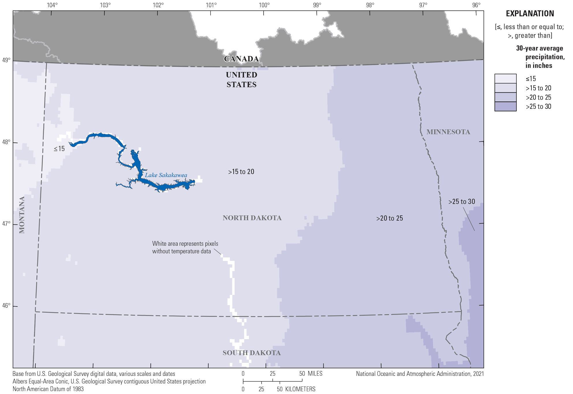
Map showing the average annual precipitation in North Dakota for the 30-year period, 1991—2020 (National Oceanic and Atmospheric Administration, 2021).
Numerous studies have identified a decadal-scale signal in precipitation in North America (10–20 years; Ault and St. George, 2010), in western North America (greater than a 7-year period; Cayan and others, 1998), in the United States (in fall precipitation with a period of 12 years; Small and Islam, 2008, 2009), in the Great Plains (Garbrecht and Rossel, 2002), and in the central United States (interdecadal variations of annual precipitation on 12- and 20-year time scales; Hu and others, 1998). Causal mechanisms generating this signal are not fully understood. Yang and others (2007) determined that September, October, and November precipitation values were strongly related to the Niño-3.4 sea-surface temperatures index on a 5.5–8.5-year timescale, where the Niño-3.4 sea-surface temperatures index considers temperature anomalies over a region between 5° N. and 5° S., 120° W. to 170° W. Precipitation increases have been reported in all seasons (Karl and Knight, 1998; Wang and others, 2009), and the largest changes were observed in fall (Garbrecht and Rossel, 2002; Small and Islam, 2008, 2009; Wang and others, 2009).
North Dakota is far from the temperature moderating effects of the oceans and as a result has one of the most variable temperature regimes in the United States (Frankson and others, 2022). Average (1991–2020) January temperatures range from 4 degrees Fahrenheit (°F) in the northeast to 18 °F in the southwest; average July temperatures range from 65 °F in the northeast to 72 °F in the south, and extreme temperatures of 100 °F are most prevalent in the southwestern and south-central areas (Frankson and others, 2022). Average annual temperature over the 30-year period of 1991 through 2020 is shown in figure 3.
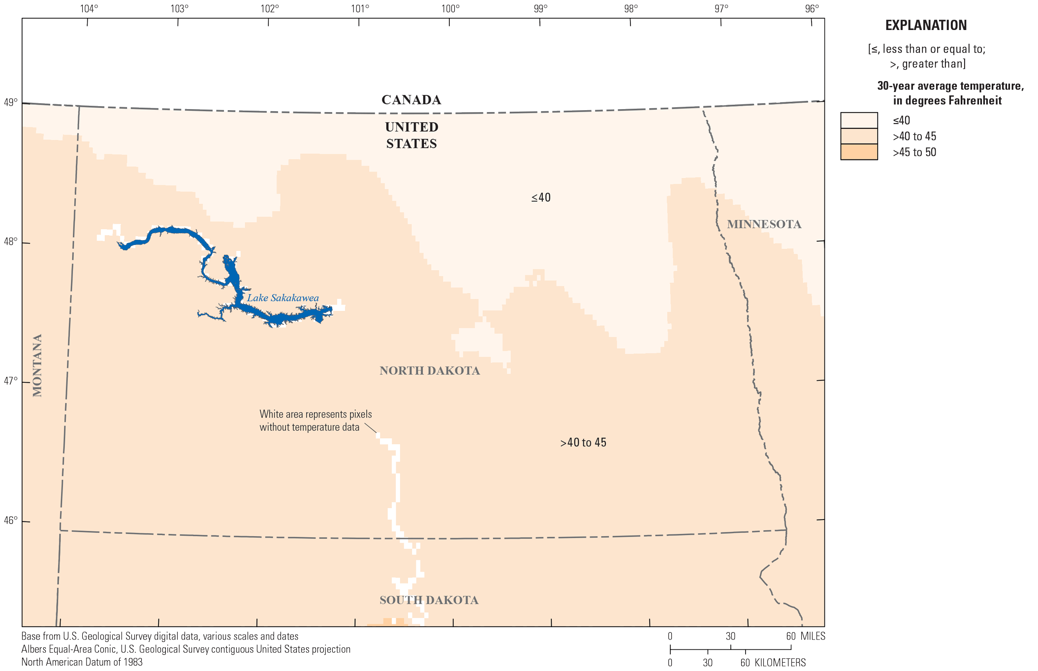
Map showing the average annual temperature in North Dakota for the 30-year period, 1991–2020 (National Oceanic and Atmospheric Administration, 2021).
Changes in temperature also exist in the region, but in a manner different from the changes in precipitation. Wang and others (2009) determined that the strongest U.S. surface air temperature warming in 1950–2000 was in the spring over the northwestern United States and the Northern Plains. North Dakota’s warming has been primarily in the winter and spring, with minimal warming in the summer months, a pattern like other States in the Great Plains and Midwest (Reidmiller and others, 2018; Frankson and others, 2022; Marvel and others, 2023). Since 1900, winter temperatures have risen by 4.5 °F per century, whereas summer temperatures have risen by 1.5 °F per century during the same period (Frankson and others, 2022). The period of 2000–20 has been one of the warmest recorded periods for North Dakota, and 2006, 2012, 2015, and 2016 are comparable to the heat of the Dust Bowl era in the 1930s (Frankson and others, 2022).
Water budgets provide a way to evaluate availability of water and balance the rate of change in water stored in an area against the rate at which water flows in and out of the area (Healy and others, 2007). After precipitation, the next key component of the water budget is ET (Hanson, 1991). ET is the sum of evaporation from the land surface and waterbodies plus transpiration from plants (Hanson, 1991; U.S. Geological Survey, 2018). On average, ET consumes about 70 percent of annual precipitation in the United States and more than 90 percent of the precipitation in the western and midwestern United States (Irmak, 2017). Weather conditions affect the evaporation from the land surface and plant transpiration. When net solar radiation increases, ET increases; when temperature increases, transpiration rates increase; when relative humidity increases around plants, transpiration decreases; increased wind increases evaporation and transpiration rates; and soil-moisture availability affects rates—when soils dry out, less moisture is evaporated and plants begin to senesce, transpiring less water (Hanson, 1991; U.S. Geological Survey, 2018). In North Dakota, potential evapotranspiration (PET) is greater in the west than the east, but actual ET depends on the moisture available during the year (Stoner and others, 1993). Increases in evaporation rates because of rising temperatures could increase the rate of soil-moisture loss and the intensity of naturally occurring droughts (Frankson and others, 2022).
Hydrologic Soil Groups
The dominant hydrologic soil groups, defined by the U.S. Department of Agriculture Natural Resources Conservation Service (2009), in North Dakota are shown in figure 4. The hydrologic soil groups are classified into four groups based on the soil’s runoff potential (U.S. Department of Agriculture Natural Resources Conservation Service, 2009, p. 7). Soil group A (isolated areas in northwestern, central, and southeastern North Dakota) has low runoff potential or high permeability. Soil group B (detected throughout North Dakota) has moderately low runoff potential or moderately high permeability. Soil group C (detected mainly in southwestern and eastern North Dakota) has moderately high runoff potential or moderately low permeability. Soil group D (detected mainly in southwestern and eastern North Dakota) has high runoff potential or low permeability because of high proportions of clay (greater than 40 percent; U.S. Department of Agriculture Natural Resources Conservation Service, 2009).
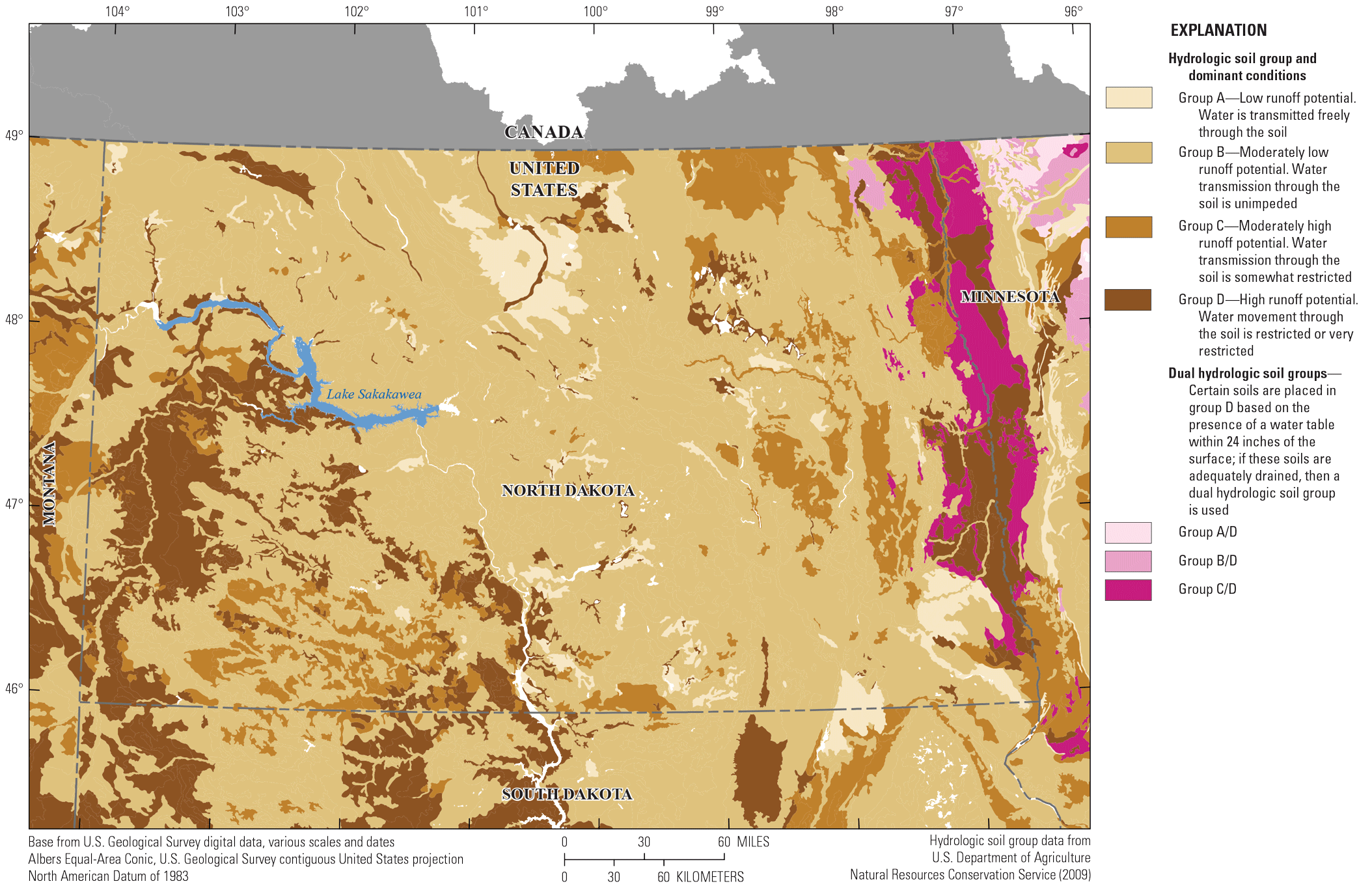
Map showing the dominant hydrologic soil groups in North Dakota (U.S. Department of Agriculture Natural Resources Conservation Service, 2009).
Some soils are categorized as dual hydrologic soil groups. These groups have two letters, such as the B/D group in northeastern North Dakota. The first letter applies when the drainage of the soil has been modified, and the second letter applies to the undrained or natural condition of the soil (U.S. Department of Agriculture Natural Resources Conservation Service, 2009). Following the convention of chapter A, the dual hydrologic soil groups are in shades of pink to distinguish them from the other soil groups (in shades of brown). The pink areas have a water table within 24 in. of the surface, and the darker the shade of pink, the higher the amount of clay in the soil.
Ecoregions and Land Cover
Ecoregions are areas of similar ecosystems in type, quality, and quantity of environmental resources. Five levels of ecoregions have been defined, and the levels are increasingly specific—level I separates North America into 15 regions, whereas level III distinguishes 182 regions (Wiken and others, 2011; U.S. Environmental Protection Agency, 2021; Commission for Environmental Cooperation, undated). Thus, higher levels are more ideal for State or local projects because they delineate finer variations in landscape, precipitation, or vegetation. North Dakota is categorized into four level III ecoregions (fig. 5). The level III ecoregions—the Northwestern Great Plains, Northwestern Glaciated Plains, Northern Glaciated Plains, and Lake Agassiz Plain—span the State with a north-south orientation, although they bend to conform to the shape of the Missouri River in the western and central regions of the State, which represents the boundary of the last glaciation (Bryce and others, undated).
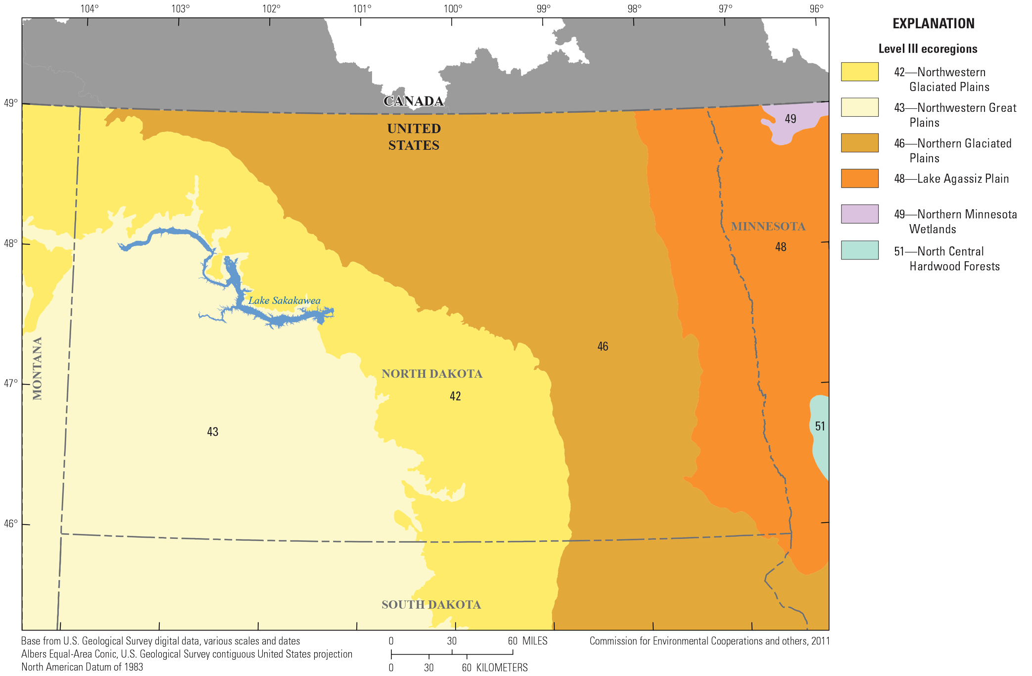
Map showing level III ecoregions of North Dakota (U.S. Environmental Protection Agency, 2013, 2021).
The Northwestern Great Plains, with some small areas of exception, lie in southwestern North Dakota (fig. 5). This area encompasses the Missouri Plateau and is semiarid with rolling plains and buttes and badlands (U.S. Environmental Protection Agency, 2013). Land use includes farming and cattle ranching; rain is a limiting factor in agriculture productivity (U.S. Environmental Protection Agency, 2013; Bryce and others, undated).
The Northwestern Glaciated Plains ecoregion (fig. 5) lies on the northern and eastern sides of the Missouri River and coincides with the extent of continental glaciation (U.S. Environmental Protection Agency, 2013). The topography is characterized by moraines (where moraines are glacial till, or sediments, deposited by glaciers; Molnia, 2004) and has a high concentration of wetlands and glacial potholes, semipermanent and seasonal wetlands known as prairie potholes (U.S. Environmental Protection Agency, 2013; Bryce and others, undated). The Northwestern Glaciated Plains are defined by a rise in elevation from the Northern Glaciated Plains to the east and mark the beginning of the Great Plains (Bryce and others, undated). Land-use in this ecoregion is split between the farming common in the Northern Glaciated Plains to the east and the cattle ranching and farming more prevalent on the Northwestern Great Plains to the west (Bryce and others, undated).
The Northern Glaciated Plains ecoregion (fig. 5) extends across most of the northern part of the State and southward between the Lake Agassiz Plain and Northwestern Great Plains ecoregions to the southern border of North Dakota and into South Dakota. The landscape in this region is composed of glacial drift, has flat to gently rolling topography, has a subhumid climate, and lies in the transition zone between the tall and shortgrass prairies (U.S. Environmental Protection Agency, 2013). Like the Lake Agassiz Plain to the east, the soil in this ecoregion is fertile, but because of climatic factors, agricultural productivity is more variable (Bryce and others, undated).
The easternmost ecoregion of North Dakota, the Lake Agassiz Plain (fig. 5), is composed of glacial till overlain by thick lacustrine sediment layers. Formed by the Glacial Lake Agassiz at the end of the last ice age, the region is extremely flat (Upham, 1895; U.S. Environmental Protection Agency, 2013). Although this ecoregion is a glacial lake plain, it is commonly called the Red River Valley. The flat land with lacustrine sediments has made this region agriculturally productive but prone to overland flooding, and much of the original tallgrass prairie has been converted to intensive agriculture (Bryce and others, undated).
The major land-cover classes in North Dakota are shown in figure 6. Cultivated crops, hay, and pasture are most common throughout the State. Forest cover (deciduous and mixed) is minimal and is detected in isolated areas. Herbaceous area is mainly in the western areas of the State. High intensity developed land is isolated to North Dakota’s largest cities and most notable on the eastern edge of the State.
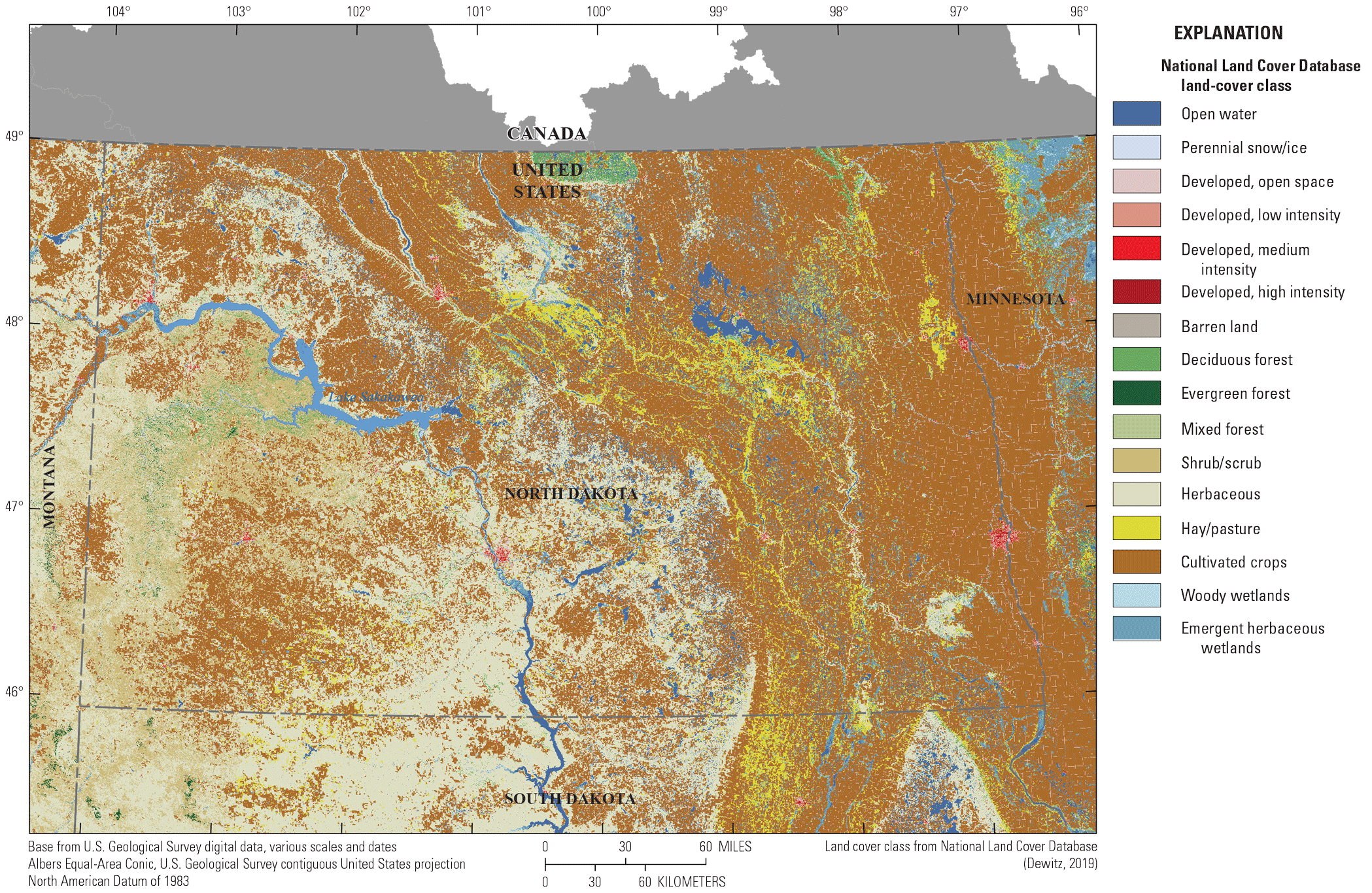
Map showing the land-cover classes of North Dakota (Dewitz, 2019).
History of U.S. Geological Survey Peak-Flow Data Collection in North Dakota
The streamflow program of the USGS in North Dakota has evolved through the years (fig. 7) as Federal, State, local, and Tribal interests in surface-water resources have increased and as funds for operating the streamgaging network have become available. The collection of systematic streamflow data began in 1882 when a streamgage was established on the Red River at Grand Forks (Crosby, 1970; Ryan, 1985). This was a stage gage; however, infrequent streamflow measurements were made for navigational purposes. The streamgage on the Missouri River at Bismarck, North Dakota, has a similarly long record but a more piecemeal approach in its early years. Daily gage height records from February 1881 to October 1882 and May 1886 to December 1899 were published by the Missouri River Commission, records from 1891 to 1928 were published in reports of the U.S. Weather Bureau, and the USGS started publishing records in 1904 and started recording daily streamflow in October 1927 (Hendricks, 1964).
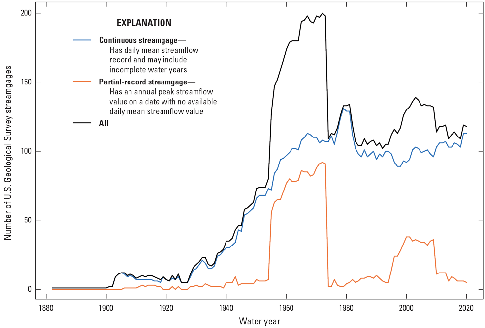
Graph showing number and type of U.S. Geological Survey streamgages in North Dakota with one or more annual peak-streamflow values from 1881 to 2020. Streamgages are identified as continuous or partial record. A subset of these streamgages was used in this report. [A water year is the period from October 1 to September 30 designated by the year in which it ends]
As a result of the disastrous flood in 1897 in the Red River Basin and the National Reclamation Act of 1902, the USGS, in cooperation with the State of North Dakota, established and operated streamgages starting in 1901 (Crosby, 1970). Additional interest was created with the signing of the U.S.-Canada Boundary Waters Treaty of 1909 and the first meeting of the International Joint Commission in 1912 (International Joint Commission, 2023). Eight streamgages were in operation in 1925 when State cooperation was discontinued, and only five federally operated streamgages were continued. State cooperation resumed in 1931, but funds were limited in 1934–38 during the Great Depression. However, the Rivers and Harbors Act of 1927 and the Flood Control Acts of 1928 and 1936 resulted in the U.S. Army Corps of Engineers supporting a large expansion of the streamgaging program (Crosby, 1970). When the North Dakota-South Dakota USGS office was created on October 16, 1944, 41 streamgages were in operation. Plans for the coordinated development of the waters of the Missouri River Basin, with respect to flood control, navigation, power, and irrigation, were formulated in 1943–44 by the U.S. Army Corps of Engineers, the Bureau of Reclamation, and the States in the basin. These plans resulted in a rapid increase in the streamgage program, and by 1947, 64 streamgages were in operation (Crosby, 1970). The number of streamgages grew steadily from the late 1940s until the late 1960s, and by 1969, 109 streamgages were in operation. During the 1970s, the USGS established 25 additional streamgages to monitor the quantity and quality of streamflow in drainage basins underlain by strippable lignite deposits (Haffield, 1981). By 1979, about 145 streamgages were in operation in North Dakota. During 1981–83, the number of streamgages in operation declined rapidly, and during 1984–87, the number declined slowly to about 110. The increase in the 1960s and 1970s, followed by a decline, was part of a national pattern of less funding available to meet Federal needs (U.S. Geological Survey, 1999). During 1987–2020, the number of streamgages in operation rose to about 135 (fig. 7), in part because of broader uses of streamflow data, including flood forecasting, regulation, intrastate compacts and international treaties, irrigation, public water supply, water-quality management, aquatic-habitat management, recreation, and other scientific and regulatory uses (U.S. Geological Survey, 1999). The National Streamflow Information Program, proposed in 1999 and now called the Federal Priority Streamgage (FPS) network, first allocated funds in 2000 to support streamgages meeting the Federal priorities of providing data for flood forecasting, compacts and decrees, water budgets, long-term changes, and water quality (Dillow and others, 2023). The FPS network funds about one-third of eligible streamgages nationwide (Dillow and others, 2023). In North Dakota, the streamgage network is funded by FPS, USGS Cooperative Matching Funds, and Federal, State, local, Tribal, and private entities.
The streamgages represented in figure 7 and used in this study represent continuous and partial-record gages. Streamgages identified as continuous have daily mean streamflow record and may include incomplete water years (the period from October 1 to September 30 designated by the year in which it ends). Streamgages identified as partial record have a peak-flow value on a date with no available daily mean streamflow value. Partial-record streamgages can be streamgages that are operated seasonally, such as sites that have little to no flow in the winter where the entire channel may freeze. Other partial-record streamgages can be crest-stage gages, which are low-cost devices used to estimate flood crests, and then indirect methods are used to estimate the peak flow (Rantz, 1982; U.S. Geological Survey, undated a). The crest-stage gages represent much of the increase in streamgages in North Dakota from the late 1950s to late 1970s.
History of Statistical Analysis of Peak Flow and Nonstationarity
Peak flows through 1934 were reported for three streamgages in North Dakota with more than 20 years of record by Jarvis and others (1936). Despite reviewing statistical and graphical peak-flow frequency analysis methods, Jarvis and others (1936) did not report peak-flow frequency estimates for the three streamgages in North Dakota. McCabe and Crosby (1959), in cooperation with the North Dakota State Highway Department and the South Dakota Department of Highways, used all data available through 1955 and completed a study of the magnitude and frequency of floods in North Dakota and South Dakota. Patterson (1966) used data through 1964, and Patterson and Gamble (1968) used data through 1961 to complete part of a series of reports on the magnitude and frequency of floods in the United States. Patterson (1966) and Patterson and Gamble (1968) presented regional relations based on average annual floods and selected basin characteristics for estimating peak-flow frequencies in the study area. Crosby (1970) included a limited analysis of magnitude and frequency of floods when he evaluated the streamflow data program for North Dakota. Crosby (1975), in cooperation with the North Dakota State Highway Department, used data available through 1973 to complete a study of the magnitude and frequency of floods for small drainage basins of 100 square miles or less. Miller and Frink (1984), in cooperation with the Upper Mississippi River Basin Commission Souris-Red-Rainy Regional Committee and the North Dakota State Water Commission, completed a study to determine whether any changes in flood response because of changes in land use could be documented for the Red River. Williams-Sether (1992), in cooperation with the North Dakota Department of Transportation, developed regional regression equations to estimate peak flows in North Dakota for selected recurrence intervals using data through 1988. Williams-Sether (2015), in cooperation with the North Dakota State Water Commission, the North Dakota Department of Transportation, the North Dakota Department of Health, the Red River Joint Water Resources Board, and the Devils Lake Basin Joint Water Resource Board, updated the regional regression equations of Williams-Sether (1992) for estimating the magnitude of peak flows in North Dakota for selected recurrence intervals using data through 2009.
Peak-flow changes in North Dakota have been documented in context with other gages across the north-central United States and the conterminous United States (Hirsch and Ryberg, 2012; Peterson and others, 2013; Ryberg and others, 2016a, 2020a; Dudley and others, 2018; Hodgkins and others, 2019). Hodgkins and others (2019) documented gradual changes in peak flow for water years 1916–2015, 1941–2015, and 1966–2015. The Red River and James River Basins demonstrate a spatially cohesive pattern of increasing peak flow (fig. 4 of Hodgkins and others [2019]), even at regulated sites (fig. 5B of Hodgkins and others [2019]), whereas western North Dakota was experiencing downward trends in streamflow. Ryberg and others (2020a) documented abrupt changes in the median peak flow for water years 1916–2015, 1941–2015, and 1966–2015 and detected the same pattern for North Dakota as Hodgkins and others (2019) discovered previously. Numerous abrupt changes in the 1990s (refer to animations in supplementary data 2 and 3 of Ryberg and others [2020a]), coincided with increasing precipitation and flooding in the eastern Dakotas (Macek-Rowland, 1997, 2001; Williams-Sether, 1999; Macek-Rowland and others, 2001a, b; Ryberg and others, 2007b; Vecchia, 2008).
The Third National Climate Assessment (Georgakakos and others, 2014) documented mostly increasing peak flow in the Midwest, with the largest trends in the Red River Basin, whereas west of the 100th meridian, most of the peak-flow trends were downward. The Fifth National Climate Assessment (Knapp and others, 2023) highlights the differences in peak-flow trends in eastern and western North Dakota and indicates that this pattern is consistent in the Northern Great Plains. Observed trends indicate that peak flow has decreased in the west, generally west of the 100th meridian, and increased in the east. With few exceptions, the eastern Dakotas have experienced increasing peak flow, whereas the western Dakotas, Montana, and Wyoming have experienced decreasing peak flow.
Review of Research Relating to Climatic Variability and Change
The Great Plains and Prairies have long been known for their extremely variable climate. The historian Walter Prescott Webb described the boundary between eastern timberlands and the grasslands as an “institutional fault” (Webb, 1931, p. 8), meaning a sharp break in ways of life that would require changes to traditional institutions. As a semiarid region, the Great Plains are “sometimes humid, sometimes desert, and sometimes a cross between the two” (Thornthwaite, 1941, p. 177). Although cold air and snow can make their way to the Southern Great Plains, the Northern Great Plains have the added challenge of sustained periods of cold, snow accumulation, and windchill. Because of these factors, the Great Plains have been described as too hot, too cold, too dry, and too wet (Severson and Sieg, 2006).
North Dakota’s climate is highly variable and experiences persistent periods of relatively wet or relatively dry conditions that change flood risk. Peak flows are one realization of the variable and changing climate. The USGS and others have been studying floods and droughts in this region for decades, and the past work provides a plethora of information that puts current conditions into long-term context.
Paleofloods and Historical Floods and Drought Periods in North Dakota
The study of flooding in what is now North Dakota starts at the end of the last glaciation when Glacial Lake Agassiz (Lake Agassiz) formed during retreat of the glaciers (Upham, 1895). Areal extent and volume of Lake Agassiz varied greatly, depending on the ice margin, overflow outlets, and isostatic (postglacial) rebound (Teller and Thorleifson, 1987); however, about one-fifth of Lake Agassiz existed in what is now the United States and the rest extended into Manitoba, Ontario, and Saskatchewan, Canada (Upham, 1895; Fisher and others, 2011). In the period of about 1.8 million years to 2004, 3 of 27 known freshwater floods with flows greater than 3.53 million cubic feet per second (ft3/s; 100,000 cubic meters per second [m3/s]) were associated with Lake Agassiz (O’Connor and Costa, 2004). Approximately 9,900 years before present, Lake Agassiz discharged to the lower Clearwater and Athabasca Rivers in Alberta, Canada, when the lake level overtopped a drainage divide near the Alberta-Saskatchewan border (Smith and Fisher, 1993). The discharge was estimated as 42.4 million to 84.8 million ft3/s (1,200,000–2,400,000 m3/s; Smith and Fisher, 1993; O’Connor and Costa, 2004). In the period between 129,000 and 11,700 years ago, water from Lake Agassiz began to flow east into the Great Lakes, and this discharge increased abruptly when a glacial dam failed; maximum flow was estimated as 7.06 million ft3/s (200,000 m3/s; Teller and Thorleifson, 1987; O’Connor and Costa, 2004). Also in the period between 129,000 and 11,700 years ago, another ice dam failure was detected through a southern outlet named “River Warren,” the valley of which is now occupied by Lake Traverse, Big Stone Lake, and the Minnesota River (Upham, 1895; O’Connor and Costa, 2004; Fisher and others, 2011). This resulted in a discharge estimated as 4.59 million ft3/s (130,000 m3/s; O’Connor and Costa, 2004).
Lake Agassiz has left a legacy that makes the eastern part of North Dakota especially flood prone. What is commonly referred to as the “Red River Valley” is the level III ecoregion designated as the “Lake Agassiz Plain.” Thick beds of Lake Agassiz sediments on top of glacial till create the extremely flat floor of the Lake Agassiz Plain (Wiken and others, 2011). The Red River transects the ecoregion from south to north, forming most of the North Dakota-Minnesota border. Rivers in this ecoregion are flood prone because a gentle slope (averaging 0.5 to 1.5 feet per mile for the Red River) inhibits channel flow and encourages overland flooding (Ryberg and others, 2007a). The northerly direction of flow is also a critical factor in the spring flooding when the southern (upstream) part of the river has thawed and the northern (downstream) part of the channel is still frozen (Ryberg and others, 2007a), leading to ice-jam flooding.
Climate is a crucial driver for past floods and droughts. North Dakota is susceptible to persistent periods of relatively wet and relatively dry conditions (Vecchia, 2008; Ryberg and others, 2014; Ryberg, 2015). These distinct periods of hydroclimatic persistence that lack an intermediate state (a state in which conditions persist at or near long-term average precipitation or temperature) are a characteristic of the north-central United States and southern Manitoba and Saskatchewan, Canada (Burn and Goel, 2001; St. George and Nielsen, 2002; Vecchia, 2008; Ryberg and others, 2014, 2016b; Razavi and others, 2015; Kolars and others, 2016). Wet and dry periods from about 1900 to 2020 are well documented, and data are readily available from agencies such as the USGS, the National Oceanic and Atmospheric Administration (NOAA), and Environment and Climate Change Canada; therefore, the following literature review, modified from Ryberg (2015), was done on past tree-ring, precipitation, and streamflow studies in the north-central United States that indicated periods of wet and dry conditions before 1900 (Carlyle, 1984; Rannie, 1998; Thorleifson and others, 1998; St. George and Nielsen, 2002, 2003; Brooks and others, 2003; Case and MacDonald, 2003; St. George and Rannie, 2003; Severson and Sieg, 2006; Lapp and others, 2013).
Wet and dry periods are visible in the sediments of Devils Lake (fig. 1), North Dakota, for the past 4,000 years (Bluemle, 1996), in tree rings and sediment cores in a 1,000-year reconstruction at the Waubay Lakes complex in northeastern South Dakota (not shown; Shapley and others, 2005), and in tree rings in the region for the past 300 years (Ryberg and others, 2016b). For most of North Dakota’s history, Devils Lake has been a closed basin (artificial outlets were completed in 2005 and 2012; North Dakota Department of Water Resources, 2024). However, Devils Lake has overflowed into Stump Lake and then through Tolna Coulee (not shown) and into the Sheyenne and Red Rivers (fig. 1) at least twice during the past 4,000 years. The last Devils Lake spill into the Sheyenne River was within the last 1,800 years (Wiche and others, 2000b). Because of the nature of the closed basin, the rise and fall of Devils Lake represents longer term wetting and drying periods, and a depiction of Devils Lake elevations in the last 4,000 years is shown in figure 8. Variations of figure 8 have been a useful means for depicting hydroclimatic variability in North Dakota for decades. The idea for the figure originated in the University of North Dakota dissertation of Edward Callender (1968; fig. 45, p. 248) and was based on the analysis of sediment cores for the lake. John Bluemle of the North Dakota Geological Survey refined the figure with additional data based on radio-carbon dating of soils (1991, fig. 7, p. 10). The North Dakota Department of Water Resources subsequently updated the figure (North Dakota Department of Water Resources, 2024).
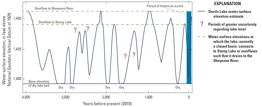
Graph showing estimates of Devils Lake water-surface elevation (National Geodetic Vertical Datum of 1929) over the last 4,000 years, based on sediment-core data (Callender, 1968) and radio-carbon dating of soils (Bluemle, 1991; graph modified from North Dakota Department of Water Resources [undated]).
The water level of Devils Lake fluctuates in response to climatic variability, and a rising or declining water level is the normal condition for Devils Lake rather than a stable water level (Wiche and others, 2000b). Annual evaporation varies from year to year, although not as much as surface-water inflow. Warm, dry periods increase lake evaporation and wet periods increase inflow and lake levels (Wiche and others, 2000b). Thus, Devils Lake elevations are a proxy for eastern North Dakota climate—as stated in the “State Geological Survey of North Dakota Sixth Biennial Report” in 1912, “lakes are as fickle as the weather, yet they approach climate in their constancy” (Simpson, 1912).
Numerous historical accounts also describe persistent wet and dry conditions and sudden shifts from one state to the other (Rannie, 1998; Severson and Sieg, 2006; Ryberg, 2015). The early 1700s (about 1703–21) had periods of drought or dry years in the Northern Great Plains and central North Dakota (Severson and Sieg, 2006). Lapp and others (2013) described 24 sustained drought episodes in northwestern Canadian prairies from 1472 through 2004 and determined that 1717–21 was the most intense drought. St. George and Nielsen (2003) documented floods on the upper Red River in 1726, 1727, and 1741. The period 1753–62 was dry in parts of the Northern Great Plains (Severson and Sieg, 2006). Using tree rings, St. George and Nielsen (2002) documented a severe drought in 1753 in southern Manitoba with annual precipitation estimated at more than two standard deviations less than the mean. There seems to have been a widespread regional drought in the 1750s to the early 1760s. Using tree rings, Meko (1982) detected a period of drought or dry years in the western Great Plains from 1753 to 1762 based on Pinus ponderosa (Ponderosa pine) in North Dakota, South Dakota, Nebraska, Wyoming, and Montana. Using tree rings, Lapp and others (2013) detected a sustained drought in the northwestern Great Plains from 1755 to 1761, and Stockton and Meko (1983) detected a major historical drought in the mid- to late 1750s in the Great Plains. Tree-ring analysis revealed a severe drought around 1800 in southern Manitoba and southeastern Saskatchewan (Ryberg, 2015). Thorleifson and others (1998, p. 191) described the period of 1792–1828 as one of “high variability; numerous floods and several drought episodes.”
From 1823 to 1828 and again in 1847–52, five successive high or very high runoff years were detected on the Red River (Thorleifson and others, 1998). The year 1849 stands out in Severson and Sieg (2006) as a very wet year, whereas 1852 had one of the largest floods on the Red River at Winnipeg and extreme flooding on the Assiniboine River (tributary to the Red River in Canada; Rannie, 2002; Government of Canada, 2013). St. George and Nielsen (2002) detected a pronounced wet interval in the 1850s in southern Manitoba. The Red River again experienced a large flood at Winnipeg in 1861 (Government of Canada, 2022). In 1897, the Fargo Forum and Daily Republican published an account of the 1861 flood saying, “That year the entire valley was flooded from Big Stone Lake to Winnipeg, more than 300 miles. There are but four men living in the valley now that witnessed the great flood of ’61 – the largest body of fresh water in the world at that time” (U.S. Geological Survey, 1952).
Case and MacDonald (2003) stated that tree-ring reconstructions of precipitation have also indicated drought during the mid-19th century in the southern Canadian Prairies, Rocky Mountain foothills, and Montane regions. Numerous studies report dry, drought, and (or) low streamflow conditions from about 1852 to about 1880 in the Red, Wild Rice, Sheyenne, Souris, and Missouri River Basins; the Great Plains; southern North Dakota; eastern North Dakota; and central North Dakota (Thorleifson and others, 1998; St. George and Nielsen, 2003; Severson and Sieg, 2006). Lapp and others (2013) described the 1858–72 drought as the “most severe and longest” of the 24 northwestern Canadian prairie droughts in their study.
The Great Plains experienced a major historical drought centered in the early 1860s, worse than 1930s (Stockton and Meko, 1983). In 1862, Samuel Bond, traveling with a wagon train between the Wild Rice and Sheyenne Rivers in eastern North Dakota (fig. 1), noted that the region was “somewhat dry and barren” (Severson and Sieg, 2006, p. 29). In 1863, soldiers with General Sibley described conditions that had worsened. A solider noted that the prairie had cracks so large “as to let one’s foot through” (Severson and Sieg, 2006, p. 29). When traveling from Lake Traverse to the Sheyenne River, another said that the roads were dry and dusty “the most so it has been for 20 years So say the inhabitant[s] of this Country. Scarcely any water and grass…” (Severson and Sieg, 2006, p. 29). A soldier with Sibley said on July 2 that “grasshoppers [are] going east. Some starving for want of a spear of grass which cannot be found on level land.” (Severson and Sieg, 2006, p. 29–30). Also in 1863, William Clandening, accompanying a wagon train from Fort Abercrombie to Lake Jessie (a stopping point for exploration parties in the 1800s and wagon trains on their way to Montana gold fields; State Historical Society of North Dakota, undated) and then to the Souris River said no water was in the Wild Rice or Maple Rivers (fig. 1)—only pools—both had had running water in 1862 (Severson and Sieg, 2006). Joseph Hamel, also with a wagon train, said near the Souris River, “The draught we had in Minnesota is prevalent this far. The prarie [prairie], on the whole, is very dry, burned by the sun. We find grass only on the bottom land and around lakes … many dry lakes” (Severson and Sieg, 2006, p. 30–31).
A shift from dry to wet existed, and historical photographs, newspaper accounts, historical gage height estimates, and instrumental records indicate floods in the Missouri, Red, and Souris River Basins in 1881 and 1882 (The Bismarck Tribune, 1881, 1882a, b; Ryberg, 2015; U.S. Geological Survey, 2022a, b, c, 2023; Digital Horizons, 2024). Severe flooding again was detected on the Red River in 1897 (U.S. Geological Survey, 1952, 2023). The first peak-flow value recorded for the Red River at Fargo, North Dakota, is from this flood, which was preceded by an “extremely severe” winter (U.S. Geological Survey, 1952).
Floods, droughts, and extended wet or dry periods from the scientific and historical accounts described earlier and from additional resources are characterized in tables 1–3. The extended wet and dry periods are corroborated by tree-ring records (refer to references in tables 1–3) and lake sediments from Devils Lake (Vecchia, 2008), indicating long-term climatic persistence in the interior of North America. The pre-1900 period ended with severe flooding in 1897 (fig. 9), which prompted more interest in streamgaging.
Table 1.
Wet and dry periods in the north-central United States from 1400 to 1799. Wet periods encompass those described in the reference material as wet, snowy, high runoff, or flood years. Dry periods encompass those described as dry, drought, low flow, low runoff, or sustained drought. Conditions identified as other may mention lack of floods, a flood that may not be extreme, or seasonally dry conditions—these periods may be useful historical notes describing nonextreme conditions (modified from Ryberg [2015]).[Bur oak refers to Quercus macrocarpa Michx. Ponderosa pine refers to Pinus ponderosa, ±, plus or minus; N. Dak., North Dakota; PDO, Pacific Decadal Oscillation; ENSO, El Niño Southern Oscillation; SD, South Dakota; NE, Nebraska; WY, Wyoming; MT, Montana; ~, about; --, no data or not applicable]
| Year(s) | Conditions | Region or basins | Notes | Sources |
|---|---|---|---|---|
| 1406–15 | Dry | Central North Dakota | Period of drought or dry years, Will (1946) used bur oak from Missouri River near Bismarck, N. Dak., to identify dry and wet years, could be off ±5 years | (Will, 1946; Severson and Sieg, 2006) |
| 1434–52 | Dry | Central North Dakota | Period of mostly drought or dry years, Will (1946) used bur oak from Missouri River near Bismarck, N. Dak., to identify dry and wet years, could be off ±5 years | (Will, 1946; Severson and Sieg, 2006) |
| 1471–1501 | Dry | Central North Dakota | Period of drought or dry years, Will (1946) used bur oak from Missouri River near Bismarck, N. Dak., to identify dry and wet years, could be off ±5 years | (Will, 1946; Severson and Sieg, 2006) |
| 1472–81 | Dry | Northwestern Great Plains, Canada | Positive PDO, high variance ENSO | (Lapp and others, 2013) |
| 1477 | Dry | Southern Manitoba | Annual precipitation estimated more than 2 standard deviations less than the mean | (St. George and Nielsen, 2002) |
| 1483–94 | Dry | Northwestern Great Plains, Canada | Positive PDO, high variance ENSO | (Lapp and others, 2013) |
| 1485 | Dry | Southern Manitoba | Annual precipitation estimated more than 2 standard deviations less than the mean | (St. George and Nielsen, 2002) |
| 1498–1508 | Dry | Northwestern Great Plains, Canada | Positive PDO, high variance ENSO | (Lapp and others, 2013) |
| 1505–18 | Dry | Central North Dakota | Period of drought or dry years, Will (1946) used bur oak from Missouri River near Bismarck, N. Dak., to identify dry and wet years, could be off ±5 years | (Will, 1946; Severson and Sieg, 2006) |
| 1510 | Wet | Red | Flood upper Red | (St. George and Nielsen, 2003) |
| 1512–18 | Dry | Northwestern Great Plains, Canada | Positive PDO, low variance ENSO | (Lapp and others, 2013) |
| 1525–31 | Dry | Central North Dakota | Period of drought or dry years, Will (1946) used bur oak from Missouri River near Bismarck, N. Dak., to identify dry and wet years, could be off ±5 years | (Will, 1946; Severson and Sieg, 2006) |
| 1538 | Wet | Red | Flood upper Red | (St. George and Nielsen, 2003) |
| 1539–53 | Dry | Central North Dakota | Period of drought or dry years, Will (1946) used bur oak from Missouri River near Bismarck, N. Dak., to identify dry and wet years, could be off ±5 years | (Will, 1946; Severson and Sieg, 2006) |
| 1556 | Dry | Southern Manitoba | Annual precipitation estimated more than 2 standard deviations less than the mean | (St. George and Nielsen, 2002) |
| 1559–70 | Dry | Northwestern Great Plains, Canada | Positive PDO, high variance ENSO | (Lapp and others, 2013) |
| 1562–76 | Dry | Central North Dakota | Period of drought or dry years, Will (1946) used bur oak from Missouri River near Bismarck, N. Dak., to identify dry and wet years, could be off ±5 years | (Will, 1946; Severson and Sieg, 2006) |
| 1576–83 | Dry | Northwestern Great Plains, Canada | Positive PDO, low variance ENSO | (Lapp and others, 2013) |
| 1576–96 | Dry | Central North Dakota | Period of wet years | (Will, 1946) |
| 1595 | Dry | Southern Manitoba | Annual precipitation estimated more than 2 standard deviations less than the mean | (St. George and Nielsen, 2002) |
| 1596–1611 | Dry | Central North Dakota | Period of drought or dry years, Will (1946) used bur oak from Missouri River near Bismarck, N. Dak., to identify dry and wet years, could be off ±5 years | (Will, 1946; Severson and Sieg, 2006) |
| 1612 | Dry | Southern Manitoba | Annual precipitation estimated more than 2 standard deviations less than the mean | (St. George and Nielsen, 2002) |
| 1618–23 | Dry | Northwestern Great Plains, Canada | Negative PDO, low variance ENSO | (Lapp and others, 2013) |
| 1623–27 | Dry | Central North Dakota | Period of drought or dry years, Will (1946) used bur oak from Missouri River near Bismarck, N. Dak., to identify dry and wet years, could be off ±5 years | (Will, 1946; Severson and Sieg, 2006) |
| 1626–30 | Dry | Northwestern Great Plains, Canada | Negative PDO, low variance ENSO | (Lapp and others, 2013) |
| 1633–49 | Dry | Central North Dakota | Period of drought or dry years, Will (1946) used bur oak from Missouri River near Bismarck, N. Dak., to identify dry and wet years, could be off ±5 years | (Will, 1946; Severson and Sieg, 2006) |
| 1644 | Dry | Southern Manitoba | Annual precipitation estimated more than 2 standard deviations less than the mean | (St. George and Nielsen, 2002) |
| 1645–54 | Dry | Northwestern Great Plains, Canada | Negative PDO, high variance ENSO | (Lapp and others, 2013) |
| 1646–54 | Dry | Northern Great Plains | Period of drought or dry years (Meko [1982], using Ponderosa pine in N. Dak., SD, NE, WY, MT) | (Severson and Sieg, 2006) |
| 1648–1746 | Other | Red | Interval without extreme flooding on lower Red | (St. George and Nielsen, 2003) |
| 1654–63 | Dry | Central North Dakota | Period of drought or dry years, Will (1946) used bur oak from Missouri River near Bismarck, N. Dak., to identify dry and wet years, could be off ±5 years | (Will, 1946; Severson and Sieg, 2006) |
| 1658 | Wet | Red | Flood upper Red | (St. George and Nielsen, 2003) |
| 1661 | Dry | Southern Manitoba | Annual precipitation estimated more than 2 standard deviations less than the mean | (St. George and Nielsen, 2002) |
| 1663–1702 | Wet | Central North Dakota | Longest wet period in Will’s (1946) record | (Will, 1946) |
| 1670–1775 | Dry | Red River | Less than normal precipitation detected ~2 years out of 3 | (St. George and Nielsen, 2002) |
| 1673 | Other | Missouri | First historical documentation of Missouri River flood at mouth, but not known whether this was typical or extreme; Louis Jolliet and Jacques Marquette journals; Marquette wrote “sailing quietly in clear and calm Water, we heard the noise of a rapid, into which we were about to run. I have seen nothing more dreadful. An accumulation of large and entire trees, branches, and floating islands, was issuing from The mouth of The river pekistanoul [Missouri], with such impetuosity that we could not without great danger risk passing through it. So great was the agitation that the water was very muddy, and could not become clear. Pekitanoul is a river of Considerable size, coming from the Northwest, from a great Distance; and it discharges into the Missisipi” (Marquette, unpaginated). | (Marquette, 1966) |
| 1682 | Wet | Red | Flood upper Red | (St. George and Nielsen, 2003) |
| 1682–88 | Dry | Northwestern Great Plains, Canada | Positive PDO, low variance ENSO | (Lapp and others, 2013) |
| 1701–8 | Dry | Northwestern Great Plains, Canada | Negative PDO, low variance ENSO | (Lapp and others, 2013) |
| 1703–12 | Dry | Northern Great Plains | Period of drought or dry years (Meko [1982], using Ponderosa pine in N. Dak., SD, NE, WY, MT) | (Severson and Sieg, 2006) |
| 1707–20 | Dry | Central North Dakota | Period of drought or dry years, Will (1946) used bur oak from Missouri River near Bismarck, N. Dak., to identify dry and wet years, could be off ±5 years | (Will, 1946; Severson and Sieg, 2006) |
| 1717–21 | Dry | Northwestern Great Plains, Canada | Positive PDO, high variance ENSO | (Lapp and others, 2013) |
| 1726 | Wet | Red | Flood upper Red | (St. George and Nielsen, 2003) |
| 1727 | Wet | Red | Flood upper Red | (St. George and Nielsen, 2003) |
| 1728–35 | Dry | Central North Dakota | Period of drought or dry years, Will (1946) used bur oak from Missouri River near Bismarck, N. Dak., to identify dry and wet years, could be off ±5 years | (Will, 1946; Severson and Sieg, 2006) |
| 1741 | Wet | Red | Flood upper Red | (St. George and Nielsen, 2003) |
| 1744–52 | Dry | Central North Dakota | Period of drought or dry years, Will (1946) used bur oak from Missouri River near Bismarck, N. Dak., to identify dry and wet years, could be off ±5 years | (Will, 1946; Severson and Sieg, 2006) |
| 1747 | Wet | Red | Extreme flood lower Red | (St. George and Nielsen, 2003) |
| 1747 | Wet | Red | Flood upper Red | (St. George and Nielsen, 2003) |
| Mid-1700s | Wet | Red | Increased flood frequency lower Red | (St. George and Nielsen, 2003) |
| 1752–86 | Other | Central North Dakota | Period of alternation between wet and dry years | (Will, 1946; Severson and Sieg, 2006) |
| 1753 | Dry | Southern Manitoba | Annual precipitation estimated more than 2 standard deviations less than the mean | (St. George and Nielsen, 2002) |
| 1753–62 | Dry | Northern Great Plains | Period of drought or dry years (Meko, 1982, using Ponderosa pine in N. Dak., SD, NE, WY, MT) | (Severson and Sieg, 2006) |
| 1755–61 | Dry | Northwestern Great Plains, Canada | Positive PDO, high variance ENSO | (Lapp and others, 2013) |
| Late 1750s | Dry | Great Plains | Major historical drought centered in the late 1750s, worse than 1930s | (Stockton and Meko, 1983, in Severson and Sieg, 2006) |
| 1762 | Wet | Red | Extreme flood lower Red | (St. George and Nielsen, 2003) |
| 1762 | Wet | Red | Flood upper Red | (St. George and Nielsen, 2003) |
| 1763–1825 | Other | Red | Interval without extreme flooding on lower Red | (St. George and Nielsen, 2003) |
| 1776 | Wet | Red River at Winnipeg | Large flood on the Red, likely larger than 1826 flood | (Simons and King, 1922; U.S. Geological Survey, 1952; Miller and Frink, 1984; Rannie, 1998; Severson and Sieg, 2006) |
| 1786–1802 | Wet | Central North Dakota | “[E]xtremely wet” | (Will, 1946) |
| 1790 | Wet | Red River at Winnipeg | “[G]eneral overflow occurred” (U.S. Geological Survey, 1952); mentioned by Native Americans (Rannie, 1998) | (Simons and King, 1922; Miller and Frink, 1984; Rannie, 1998) |
| 1791–1800 | Dry | Northwestern Great Plains, Canada | Positive PDO, high variance ENSO | (Lapp and others, 2013) |
| 1793–1828 | Other | Red | Period of “high variability; numerous floods and several drought episodes” | (Thorleifson and others, 1998) |
| 1795–96 | Dry | Red River and Assiniboine River | -- | (Rannie, 1998) |
| 1797–98 | Wet | Red River at Pembina | -- | (Rannie, 1998) |
| 1798–1806 | Wet | Red | Concentration of high runoff years; overbank at Pembina in 1798 | (Thorleifson and others, 1998) |
| Winter of 1799–1800 | Wet | Post at Assiniboine and Red confluence | Alexander Henry, the younger, described “extraordinary heavey [sic] fall of Snow” in early November, the rest of the season was “opend [sic] and mild,” excessively hot in April, followed by a 3 day snow storm, 3 feet of snow that melted quickly | (Severson and Sieg, 2006) |
Table 2.
Wet and dry periods in the north-central United States from 1800 to 1850. Wet periods encompass those described in the reference material as wet, snowy, high runoff, or flood years. Dry periods encompass those described as dry, drought, low flow, low runoff, or sustained drought. Conditions identified as other may mention lack of floods, a flood that may not be extreme, or seasonally dry conditions—these periods may be useful historical notes describing nonextreme conditions (modified from Ryberg [2015]).[Bur oak refers to Quercus macrocarpa Michx. Ponderosa pine refers to Pinus ponderosa, N. Dak., North Dakota; --, no data or not available; PDO, Pacific Decadal Oscillation; ENSO, El Niño Southern Oscillation; SD, South Dakota; NE, Nebraska; WY, Wyoming; MT, Montana; ±, plus or minus]
| Year(s) | Conditions | Region or basins | Notes | Sources |
|---|---|---|---|---|
| 1800 | Dry | Red River in N. Dak. | Alexander Henry, the younger, reported drought conditions in August | (Severson and Sieg, 2006, p. 27–28) |
| 1799–1800 | Dry | Assiniboine, Red, and Clearwater Rivers | -- | (Rannie, 1998) |
| 1800–1 | Wet | Red, Winnipeg, and Assiniboine Rivers | -- | (Rannie, 1998) |
| 1802–30 | Other | Central North Dakota | Will (1946); seven wet, seven dry years | (Severson and Sieg, 2006) |
| 1802–3 | Wet | Northern Red River | -- | (Rannie, 1998) |
| 1803–5 | Dry | Red | Period of successive low/very low runoff | (Thorleifson and others, 1998) |
| 1803–5 | Dry | Lake Superior to Missouri River region, including Assiniboine | -- | (Rannie, 1998) |
| 1804–5 | Dry | Assiniboine, Red, South Saskatchewan, Saskatchewan | “Drought was reported from the Upper Missouri in the west to Lake Nipigon in the east and low water retarded the progress of the canoe brigades throughout the area.” | (Kemp, 1982, p. 36) |
| 1805–6 | Wet | Red River | Heavy late winter snow | (Rannie, 1998) |
| 1808 | Wet | Pembina to the Missouri River via the Souris | Alexander Henry, the younger, described very wet conditions | (Severson and Sieg, 2006) |
| 1807–8 | Dry | Red River and Leech Lake, Minnesota | -- | (Rannie, 1998) |
| 1809 or 1811 | Wet | Red River at Pembina and South | “[G]eneral overflow occurred” (U.S. Geological Survey, 1952); some discrepancy with date, may have been 1811; 1811 “exceptionally large flood” (Rannie, 1998); did not include Assiniboine | (Simons and King, 1922; Miller and Frink, 1984; Rannie, 1998) |
| 1810–12 | Wet | Red River | -- | (Rannie, 1998) |
| 1811–15 | Wet | Red | Concentration of high runoff years | (Thorleifson and others, 1998) |
| 1811–15 | Dry | Northwestern Great Plains, Canada | Negative PDO, high variance ENSO | (Lapp and others, 2013) |
| 1812 | Wet | Souris | Flooding in May | (Rannie, 1998) |
| 1815 | Wet | Red River at Pembina, Assiniboine at Portage la Prairie | “[O]verflowing its banks to a considerable distance” in one account, but overall “difficult to access” (Rannie, 1998) | (Canada Department of Resources and Development, 1953b; Miller and Frink, 1984; Rannie, 1998) |
| 1814–15 | Wet | Assiniboine and Red Rivers | -- | (Rannie, 1998) |
| 1815–18 | Dry | Red | Period of successive low/very low runoff | (Thorleifson and others, 1998) |
| 1815–19 | Dry | Red River, Saskatchewan, South Saskatchewan, North Saskatchewan | “Meteorological droughts over the 1815 to 1819 period are well known from records of crop failure and grasshopper infestation at the Red River Settlement in southern Manitoba (Hope, 1938; Allsopp, 1977). During this period, journal reports of low streamflow are also frequent (Ball, 1992). As an example, Peter Fidler, an employee of the Hudson Bay Company at Brandon House, Manitoba (now Brandon), reported in 1819 that ‘all small creeks that flowed with plentiful streams all summer have entirely dried up, for these several years loaded craft could ascend up as high as the Elbow or Carlton House but these last 3 summers it was necessary to convey all the goods from the Forks by land in carts...’ (in Ball, 1992, p. 189 [p. 189 in the version Case and MacDonald (2003) cited, p. 201 in the version cited in this report]). Low flows during the same period on the Saskatchewan River are also frequently mentioned in Hudson’s Bay Company employee journals (Ball, 1992). The reconstruction of Saskatchewan River streamflow shows major hydrological drought events in 1815 and 1817; in fact, the single year drought of 1815 is the lowest flow of the full 325-year period. The South Saskatchewan River shows similarly low flows in 1815 and 1817. On the North Saskatchewan River, flows were near median levels in 1815 to 1818. However, a hydrological drought occurred in 1819. In general, for the 1815 to 1819 period, both the historical and tree ring data support the existence of hydrological drought.” | (Case and MacDonald, 2003, p. 713) |
| 1816–18 | Dry | Red, Assiniboine | -- | (Rannie, 1998) |
| 1817–26 | Dry | Northern Great Plains | Period of drought or dry years (Meko [1982], using Ponderosa pine in N. Dak., SD, NE, WY, MT) | (Severson and Sieg, 2006) |
| Early 1820s | Dry | Great Plains | Major historical drought centered in the early 1820s, worse than 1930s | (Stockton and Meko, 1983, in Severson and Sieg, 2006) |
| 1822–23 | Dry | Red, Saskatchewan, Minnesota Rivers | -- | -- |
| 1823 | Dry | Red River | Major Stephen Long described very dry conditions and mentioned the aftereffects of fires, Bois de Sioux and Marsh low or dry | (Severson and Sieg, 2006, p. 28–29) |
| 1823–28 | Wet | Red | Five successive high or very high runoff years | (Thorleifson and others, 1998) |
| 1823–28 | Wet | Red River, Assiniboine | -- | (Rannie, 1998) |
| 1824 | Wet | Red, Assiniboine | According to Rannie (1998), extremely wet summer but large flood cannot be confirmed | (Harrison and Bluemle, 1980; Miller and Frink, 1984; Rannie, 1998; Severson and Sieg, 2006) |
| 1825 | Wet | Red, Assiniboine | Substantial spring flooding and persistently high water levels in early fall in Red and Assiniboine Basins | (Harrison and Bluemle, 1980; Miller and Frink, 1984; Thorleifson and others, 1998; St. George and Rannie, 2003; Severson and Sieg, 2006) |
| 1826 | Wet | Red, Assiniboine | Records indicate that 1825–26 was not an exceptionally cold or snowy winter; however, deep snowpack near the Red River Settlement and throughout the southern basin was reported (Severson and Sieg, 2006). Cold, snowy April, late spring, abundant rainfall during rising phase, largest event since 1648; extreme flood on the lower Red; conditions in the Assiniboine seem to be as extreme as those in the Red Basin (Rannie, 1998); one of the greatest floods on the Red River at Winnipeg, before floodway; ice reached “extraordinary thickness” at Winnipeg (Rannie, 1998) | (U.S. Geological Survey, 1952; Miller and Frink, 1984120; Rannie, 1998; St. George and Nielsen, 2003; St. George and Rannie, 2003; Severson and Sieg, 2006; Environment and Climate Change Canada, 2013) |
| December 1826 | Wet | Pembina region | December 20, 1826, extremely severe blizzard, livestock lost, 33 people died | (Severson and Sieg, 2006, p. 35–36) |
| Late 1820s | Wet | Southern Manitoba | Pronounced wet interval | (St. George and Nielsen, 2002) |
| 1828–47 | Other | Red | Period of “stability and no floods when runoff seems to have fluctuated within the ‘normal’ range” | (Thorleifson and others, 1998) |
| 1833–34 | Dry | Red River | -- | (Rannie, 1998) |
| 1836–37 | Dry | Red River | -- | (Rannie, 1998) |
| 1836–51 | Dry | Central North Dakota | Period of drought or dry years, Will (1946) used bur oak from Missouri River near Bismarck, N. Dak., to identify dry and wet years, could be off ±5 years | (Will, 1946; Severson and Sieg, 2006) |
| 1842–47 | Dry | Northwestern Great Plains, Canada | Positive PDO, low variance ENSO | (Lapp and others, 2013) |
| 1844 | Wet | Missouri | Major flood on Missouri (location not specified) | (National Park Service, 2021) |
| 1847–52 | Wet | Red | Five successive high or very high runoff years | (Rannie, 1998; Thorleifson and others, 1998) |
| 1847–70 | Other | Red | Period of “frequently high runoff and several major floods, with one extreme drought in 1862–64” | (Thorleifson and others, 1998) |
| 1849 | Wet | Western Missouri, eastern Nebraska, and the Northern Great Plains; eastern North Dakota, Minnesota | One of the wettest years “Spring breakup of the Red River was exceptionally late, snow fell in the Red River Settlement on several days in late May, and widespread, heavy rainfall from June to August caused unusual and protracted flooding of the Red River and its tributaries” (Blair and Rannie, 1994, p. 3). “The year most often identified as being wet when encountered by explorers was 1849” (Severson and Sieg, 2006, p. 32–33). |
(Parker, 1964; Blair and Rannie, 1994, p. 3; Severson and Sieg, 2006, p. 32–33) |
| 1849 | Wet | Red, eastern North Dakota | Lieutenant John Pope accompanying Major Samuel Wood on a military mission from Fort Snelling to the Red, then up the Red to the Pembina, said “The heavy and incessant rain since the 4th of June had so saturated the prairies…I was informed by the guides that such a season had not been known for twenty years, and that they had never seen the country in such conditions before.” On July 15, the party reached the Sheyenne with Wood described as “much swollen… The Shayenne is a rapid turbid stream, and was at that time deep.” After a few days, they traveled cross country and said water was standing from “two inches to two feet deep almost the entire way… we reached the Maple river which Mr. Kittson had bridged; but the water being much higher now than when he crossed it, the bridge had disappeared… There had been such torrents of rain about this time, the little branches that ordinarily furnish barely a sufficiency of water… were now swimming… we arrived at Pembina [on August 1] and found the Red river and Pembina river with about twenty feet rise in them and overflowing their banks.” | (Severson and Sieg, 2006, p. 32–33) |
| 1849 | Wet | Red, eastern North Dakota | Another unknown sergeant on the march from the Sheyenne to the Maple described the water as 3 or 4 feet deep for a 4-mile stretch, from the Rush to the Goose he “crossed 4 miles of prairie covered with a foot and a half of water.” | (Severson and Sieg, 2006, p. 32–33) |
| 1849 | Wet | Red River at Pembina | Flooding in June, July, and August | (Rannie, 1998) |
| Mid-1800s | Wet | Red | Increased flood frequency in the lower Red River | (St. George and Nielsen, 2003) |
Table 3.
Wet and dry periods in the north-central United States from 1850 to 1897. Wet periods encompass those described in the reference material as wet, snowy, high runoff, or flood years. Dry periods encompass those described as dry, drought, low flow, low runoff, or sustained drought. Conditions identified as other may mention lack of floods, a flood that may not be extreme, or seasonally dry conditions—these periods may be useful historical notes describing nonextreme conditions (modified from Ryberg [2015]).[Bur oak refers to Quercus macrocarpa Michx. Ponderosa pine refers to Pinus ponderosa, PDO, Pacific Decadal Oscillation; ENSO, El Niño Southern Oscillation, --, no data or not available; N. Dak., North Dakota; SD, South Dakota; NE, Nebraska; WY, Wyoming; MT, Montana; ±, plus or minus]
| Year(s) | Conditions | Region or basins | Notes | Sources |
|---|---|---|---|---|
| 1850 | Wet | Red River at Pembina, Red Lake River in Minnesota | Flooding in June and July, a great deal of Minnesota flooded | (Rannie, 1998) |
| 1850s | Wet | Southern Manitoba | Pronounced wet interval | (St. George and Nielsen, 2002) |
| 1850–54 | Dry | Northwestern Great Plains, Canada | Positive PDO, low variance ENSO | (Lapp and others, 2013) |
| 1851 | Wet | Red River at Pembina | Summer, no farming done at Pembina in 1851 because of 1849, 1850, and 1851 floods (Rannie, 1998) | (Harrison and Bluemle, 1980; Miller and Frink, 1984; Rannie, 1998) |
| 1851–63 | Wet | Central North Dakota | -- | (Will, 1946) |
| 1852 | Wet | Red River, Assiniboine between Portage la Prairie and White Horse Plain | Extreme flood on the lower Red; conditions in the Assiniboine seem to be as extreme as those in the Red Basin; one of the greatest floods on the Red River at Winnipeg, before floodway | (U.S. Geological Survey, 1952; Canada Department of Resources and Development, 1953a; Anderson, 1966; Carlyle, 1984; Miller and Frink, 1984; Rannie, 1998; St. George and Nielsen, 2003; Environment and Climate Change Canada, 2013) |
| 1853 | Wet | Red River | “No farming was done in the Red River valley near Pembina due to the floods of this year and the previous two years” (Rannie, 1998) | (Harrison and Bluemle, 1980; Miller and Frink, 1984; Rannie, 1998) |
| Mid-1800s | Dry | Northern Great Plains, Southern Canadian Prairies, Rocky Mountain foothills | “There is ample historical documentation of meteorological drought during the mid-1800s across the northern Great Plains (e.g., Mock, 1991; Blair and Rannie, 1994). Tree ring reconstructions of precipitation have also indicated drought during the mid-19th Century in the southern Canadian Prairies (Sauchyn and Beaudoin, 1998), Rocky Mountain foothills (Case and MacDonald, 1995), and Montane regions (Watson and Luckman, 2001).” | (Case and MacDonald, 2003) |
| 1853–72 | Dry | Northern Great Plains | Period of drought or dry years (Meko, 1982, using Ponderosa pine in N. Dak., SD, NE, WY, MT) | (Severson and Sieg, 2006) |
| 1856–61 | Wet | Red | Concentration of high runoff years | (Thorleifson and others, 1998) |
| 1856–57 | Wet | Red River | -- | (Rannie, 1998) |
| 1857–58 | Dry | Red River | -- | (Rannie, 1998) |
| 1858–72 | Dry | Northwestern Great Plains, Canada | Positive PDO, high variance ENSO | (Lapp and others, 2013) |
| 1858–59 | Wet | Red River; Minnesota, upper Mississippi | -- | (Rannie, 1998) |
| 1860 | Wet | Red River | Began to be cited as a “flood year” by Upham, but Rannie determined a large flood in this year is unlikely (Rannie, 1998) | (Upham, 1895; Miller and Frink, 1984; Rannie, 1998) |
| 1861 | Wet | Red River | One of the greatest floods on the Red River at Winnipeg, before floodway | (U.S. Geological Survey, 1952; Canada Department of Resources and Development, 1953a; Anderson, 1966; Carlyle, 1984; Miller and Frink, 1984; Rannie, 1998; St. George and Nielsen, 2003; Environment and Climate Change Canada, 2013) |
| 1860–61 | Wet | Red River | -- | (Rannie, 1998) |
| 1861–64 | Dry | Red | Period of successive low/very low runoff | (Thorleifson and others, 1998) |
| Early 1860s | Dry | Great Plains | Major historical drought centered in the early 1860s, worse than 1930s | (Stockton and Meko, 1983, in Severson and Sieg, 2006) |
| 1862 | Dry | Between Wild Rice and Sheyenne Rivers | Samuel Bond, traveling with a wagon train, said region was “dry and barren” | (Severson and Sieg, 2006, p. 29) |
| 1861–64 | Dry | Red River, Assiniboine | -- | (Rannie, 1998) |
| 1862–1949 | Other | Red | Interval without extreme flooding on lower Red | (St. George and Nielsen, 2003) |
| 1862–64 | Dry | Red | Extreme drought | (Thorleifson and others, 1998) |
| 1863 | Dry | Lake Traverse to the Sheyenne River, Southern North Dakota | A soldier noted that the prairie had cracks so large “as to let one’s foot through.” A soldier with General Sibley said the roads were dry and dusty “the most so it has been for 20 years So say the inhabitant[s] of this Country. Scarcely any water and grass…” An anonymous soldier with Sibley said on July 2 that “grasshoppers [are] going east. Some starving for want of a spear of grass which cannot be found on level land.” |
(Severson and Sieg, 2006, p. 29–31) |
| 1863 | Dry | Lake Traverse to the Sheyenne River, Southern North Dakota | Rained when Sibley was on the Sheyenne River July 4, cavalry went out 50 miles to
see about grass. After July 18, by the time they reached Lake Jesse (https://history.nd.gov/historicsites/jessie/index.html) forage was better. William Clandening, accompanying a wagon train from Fort Abercrombie to Lake Jessie and then to the Souris River said no water was in the Wild Rice or Maple rivers—only pools (both had had running water in 1862). Joseph Hamel, also accompanying the wagon train, said near the Souris River, “The draught we had in Minnesota is prevalent this far. The prarie [prairie], on the whole, is very dry, burned by the sun. We find grass only on the bottom land and around lakes … many dry lakes.” |
(Severson and Sieg, 2006, p. 29–31) |
| 1863 | Other | Tewaukon Lake and the Sheyenne River | All diaries from Sibley’s command mention extreme heat in early July. July 3 “hot air strikes as if from an oven.” July 9 “it is one of the most uncomfortable days I ever saw in my life the wind is so hot that it will take a mans breath.” Followed by a sudden switch to cold temperatures | (Severson and Sieg, 2006, p. 34) |
| 1863–64 | Other | Eastern North Dakota | Hot midsummers with cold periods in late summer | (Severson and Sieg, 2006, p. 35) |
| 1864 | Other | Eastern North Dakota | Temperatures of 100 degrees Fahrenheit and greater in June, sudden switch to cold in late summer | (Severson and Sieg, 2006, p. 35) |
| 1865 | Other | Cannonball River, Devils Lake, Souris River, Forth Berthold on the Missouri | General Sully expedition, conditions described as dry with prairie pothole lakes drying out, Sheyenne, Souris, and James were not running, but difficult to determine if this was drought or normal late summer conditions. Missouri Coteau described in dismal terms by another member of the party. | (Severson and Sieg, 2006, p. 31) |
| 1869–70 | Wet | Red River | -- | (Rannie, 1998) |
| 1871 | Wet | Red River | -- | (U.S. Geological Survey, 1952; Miller and Frink, 1984; Rannie, 1998) |
| 1873 | Wet | Red River | -- | (U.S. Geological Survey, 1952; Miller and Frink, 1984; Rannie, 1998) |
| 1877–1900 | Dry | Central North Dakota | Period of drought or dry years, Will (1946) used bur oak from Missouri River near Bismarck, N. Dak., to identify dry and wet years; could have some wet years interspersed in period, could be off ±5 years | (Will, 1946; Severson and Sieg, 2006) |
| 1881 | Wet | Red, Missouri | At Grand Forks “all buildings on the bottom lands were washed away.” Very large flood
on Missouri at Bismarck; major flood on Missouri (location not specified) The April 1, 1881, Bismarck Tribune had the headline “Missouri’s Grand Bust—A Break-up That Wipes Out Previous Records” and reported ice chunks 36-inches thick. Notes on the flood also included the sentence, “there is a time in the affairs of man, which, if taken at the flood, leads on to the destruction of Mandan.” |
(The Bismarck Tribune, 1881; Ryberg, 2015, fig. 2.1.; National Park Service, 2021; U.S. Geological Survey, 2021) |
| 1882 | Wet | Red, Souris | One of the greatest floods on the Red River at Winnipeg, before floodway; large flood in North Dakota on Red; large, poorly documented flood on the Souris in North Dakota | (Environment and Climate Change Canada, 2013; U.S. Geological Survey, 2021) |
| 1889–97 | Dry | Northwestern Great Plains, Canada | Positive PDO, high variance ENSO | (Lapp and others, 2013) |
| 1892 | Wet | Red | One of the greatest floods on the Red River at Winnipeg, before floodway | (Severson and Sieg, 2006; Environment and Climate Change Canada, 2013) |
| 1892–1901 | Dry | Northern Great Plains | Period of drought or dry years (Meko [1982], using Ponderosa pine in N. Dak., SD, NE, WY, MT) | (Severson and Sieg, 2006) |
| Mid-1890s | Dry | Great Plains | Major historical drought centered in the mid-1890s | (Stockton and Meko, 1983, in Severson and Sieg, 2006) |
| 1897 | Wet | Red | One of the greatest floods on the Red River at Winnipeg, before floodway; Large flood in N. Dak. on the Red | (Environment and Climate Change Canada, 2013; Ryberg, 2015; U.S. Geological Survey, 2021) |
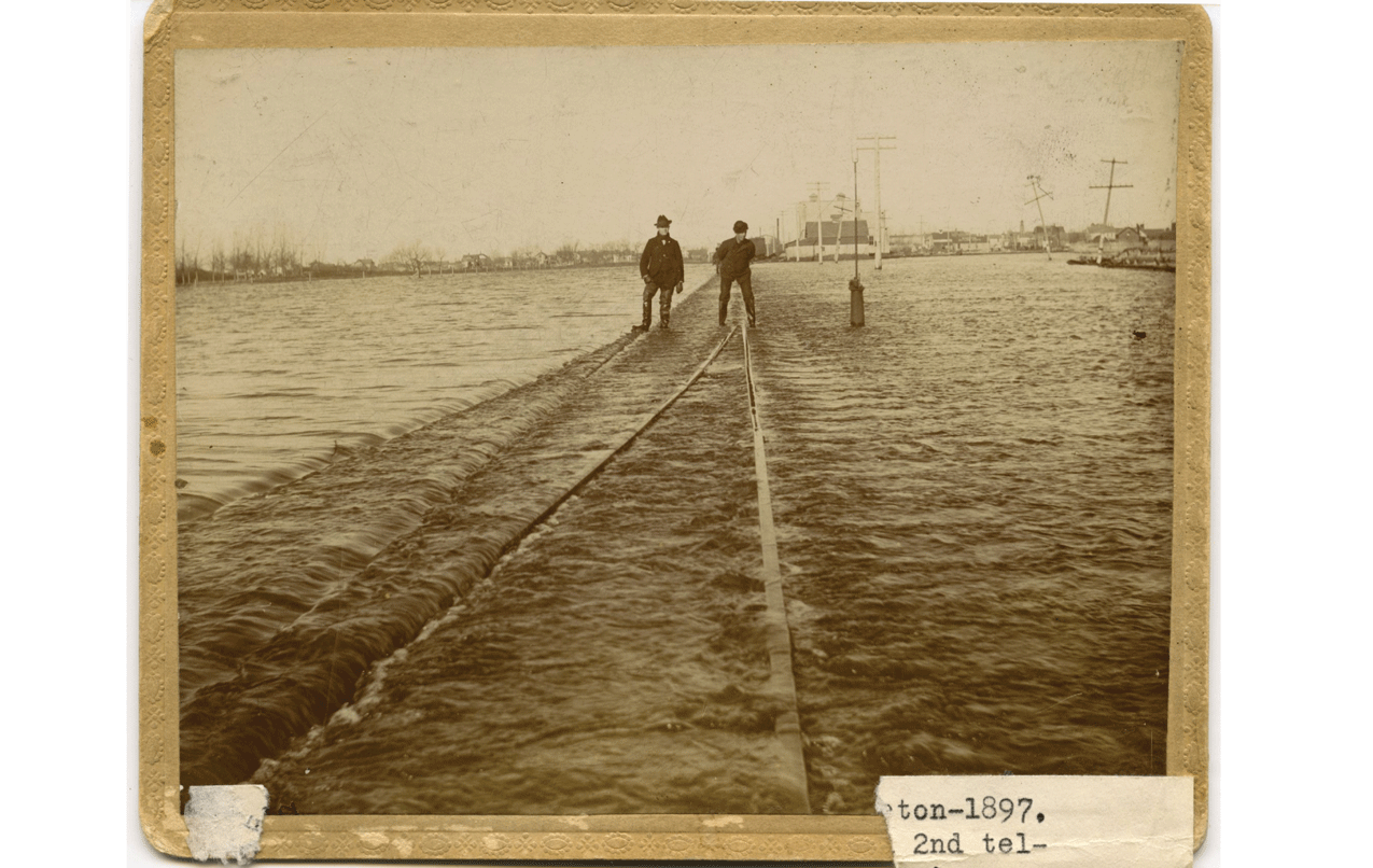
Photograph showing flood waters going over railroad tracks in Wahpeton, North Dakota, in 1897. The town of Wahpeton is visible in the background. The flood waters are the Bois de Sioux River, the Red River of the North, or both (photograph courtesy of Digital Horizons [North Dakota Memories Collection, North Dakota State Library]).
Review of More Recent Evidence of Climatic Variability and Change
Longer term studies of tree rings and sediment cores in the north-central United States and south-central Canada have borne out the sentiments of explorers, settlers, and scientists by indicating distinct periods of hydroclimatic persistence alternating between wet and dry periods (Will, 1946; Burn and Goel, 200123; St. George and Nielsen, 2002; Vecchia, 2008; Ryberg and others, 2014, 2016b; Razavi and others, 2015; Kolars and others, 2016). Will’s 1946 tree-ring study for North Dakota was summarized by H.L. Walster, director of the North Dakota Agricultural Experiment Station at the North Dakota Agricultural College (now North Dakota State University), as follows, North Dakota’s “recent [climatic] variability has occurred many times in the past centuries. It further establishes that relatively wet and relatively dry periods have not occurred according to any cyclic or rhythmic pattern” (Will, 1946, p. 24). In 2008, Vecchia published a study of lake levels for Devils Lake, North Dakota. He used sediment core data and stochastic simulation modeling, and the results are like those of Will’s tree-ring study.
“Although future precipitation is impossible to predict, paleoclimatic data and recent research on climate dynamics indicate that climatic conditions in the Devils Lake Basin in the distant past and the near future may consist of two equilibrium states: a dry state like 1950–79 and a wet state like 1980–2006. Existence of any intermediate states, or more extreme dry or wet states, is unlikely. The average duration of the wet states was estimated to be 30 years and the average duration of the dry states was estimated to be 120 years. However, the number of years left in the current wet period is highly random and it is not likely the current wet period will end anytime soon” (Vecchia, 2008, p. 21).
Large changes in runoff in the north-central United States have been detected during the past century; large declines in streamflow in the 1930s and a recovery in the 1940s were detected (Ryberg and others, 2014; Marti and others, 2024), and larger floods and increases in runoff had a tendency to happen in the 1970s and the 1990s (McCabe and Wolock, 2002; Ryberg and others, 2020a; Sando and others, 2022). A nonlinear water-balance analysis indicates that changes in precipitation and PET (that is, climate) explain most of the multidecadal spatial/temporal variability of runoff and flood magnitudes, and precipitation is the dominant driver (Ryberg and others, 2014). Historical changes in climate and runoff in the region seem to be more consistent with complex transient shifts in seasonal climatic conditions than with gradual climate change, although a part of the unexplained variability stems from land-use change (Ryberg and others, 2014).
Historically unprecedented flooding was detected in the Souris River Basin of Saskatchewan, North Dakota, and Manitoba in 2011 during a longer-term period of wet conditions in the basin (Nustad and others, 2016). Tree-ring chronologies and historical precipitation data were analyzed to develop regression models that can be used for predicting long-term variations of precipitation. The 12-year moving average precipitation was modeled in five subregions of the study area over three seasons (November–February, March–June, and July–October). Results indicate that precipitation varies on long-term (multidecadal) time scales of 16, 32, and 64 years. Past extended pluvial and drought events, which can vary with season and subregion, were highlighted by the models. Results indicate that the recent wet period could be a part of natural variability on a long time scale (Ryberg and others, 2016b). The transition for dry to wet was studied in the Souris River Basin of Saskatchewan, North Dakota, and Manitoba after a devastating flood event in 2011 (Kolars and others, 2016, 2019; Nustad and others, 2016). For the USGS streamgage Souris River above Minot, N. Dak. (05117500), the peak flow recorded in 2011 was more than twice that of any previously record peak flow and more than five times the estimated 100-year postregulation streamflow event (Nustad and others, 2016; U.S. Geological Survey, 2023). Analysis determined that “if the wet climate state continues during the next 10 years, there is about a 2-percent chance that there will be another flood like the 2011 flood (or greater). Past data indicates the wet climate state will revert to the dry climate state, but when that will happen is uncertain” (Nustad and others, 2016, p. 4).
Trend analysis of the Missouri River Basin over the period of 1960–2011 indicated that the western and the southern parts of the basin had downward trends in annual streamflow and the eastern part had upward trends in streamflow (Norton and others, 2014). The Missouri River Basin experienced flooding unprecedented in the regulated era in 2011 for some of the same reasons as the Souris River Basin. A combination of wet antecedent conditions with higher than average plains and mountain snowpack, much lower than average temperatures in February through April, and higher than normal precipitation beginning in May led to historical flooding in the Missouri River Basin in 2011. The U.S. Army Corps of Engineers 2011 annual report stated that record snowfalls were recorded across much of the plains of North and South Dakota in December 2010 with 29.0 in. in Watertown, South Dakota; 31.1 in. in Wheaton, S. Dak.; 33.0 in. in Sisseton, S. Dak.; and 35.3 in. in Williston, N. Dak. (U.S. Army Corps of Engineers, 2012). In addition, the report noted that much of eastern Montana and the Dakotas received 150 percent or more of their normal precipitation for the 3-month period ending on February 28, 2011. Snowfall totals in the plains from the 2010–11 season ranged from 112 to 362 percent of the climatological average. The State of Montana reported 300 percent of normal precipitation for the month of May with individual locations across the State setting new monthly rainfall records for May. Heavy rainfall continued into June with several monthly totals exceeding 200 percent of normal from Montana to northern Nebraska (U.S. Army Corps of Engineers, 2012).
In an assessment used to understand the extremes associated with the 2011 flooding, a NOAA report (Hoerling and others, 2013, p. 23) stated that “the factors immediately responsible for flooding were found to be a sequence of events that included antecedent wet conditions, a particularly cold and wet 2010–2011 winter that led to unusually high snow pack, and record setting rains in late spring. The latter condition was almost certainly the most critical in the meteorological sequence for understanding the historic proportion of Missouri Basin flooding that developed in late Spring 2011.” The report also stated that “the record Missouri Basin flooding event of 2011 was consistent with the physical response of basin runoff to a sequence of naturally occurring climate conditions” and that “that annual flow in the Upper Missouri Basin was found to be more volatile in recent decades compared to prior decades dating to 1898” (Hoerling and others, 2013, p. 24). A follow-up NOAA report indicated that “the increased frequency of high runoff years in the [Upper Missouri River Basin] UMRB in recent decades has been due to an increase in precipitation falling over the upper basin... and that an overall wetter climate has likely increased soil moisture in the UMRB, with the implication that more water-years in recent decades were initiated from moist antecedent land states” (Livneh and others, 2016, p. 31). Temperature has increased in the basin and could be reducing streamflow in some parts of the basin, but not extremes at the upper end of the distribution; however, future climate predictions and modeling indicate that temperature increases could result in greater declines in flows (Livneh and others, 2016).
In a report examining the causes of recent hydrologic extremes in the Upper Missouri River Basin, Livneh and others (2016) determined that increases in precipitation had increased runoff in recent decades. In the recent period of increased high runoff, 1975–2014 (as compared to 1895–1974), the largest increases in seasonal wetting have happened during the cold season (October–March). Regional wetting was strongest in the eastern one-third of upper basin and South Dakota, models were insensitive to recent increases in heavy daily rainfall, and recent temperature increases do not seem to be reducing extreme runoff events (Livneh and others, 2016).
Changes were also detected in the seasonality of peak flow (Ryberg and others, 2016a; Ye and others, 2017; Marti and others, 2024). Over climatologically and geographically similar regions in the north-central United States, logistic regression was used to model the odds of getting a summer/fall peak flow. When controlling for antecedent wet and dry conditions and geographical variations, the odds of summer/fall peak flows being detected have increased across the study area (Ryberg and others, 2016a). With respect to timing within the seasons, trend analysis determined that in northern parts of the study region, snowmelt/spring peak flows are happening earlier. The timing of snowmelt/spring peak flows in three regions in the northern part of the study area is earlier by 8.7–14.3 days (Ryberg and others, 2016a).
Trend methods are sensitive to periods of record because of the methodology—regression methods can be sensitive to outliers and values with high leverage or effect (Helsel and others, 2020)—and because of long-term persistence, especially at the beginning or end of the record, from naturally occurring quasi-periodic hydroclimatic processes (Cohn and Lins, 2005). Therefore, studies can report differing results. In addition, the data sources used affect the choice of analysis methods and the period of record studied. North Dakota and the surrounding region have a broad range of qualitative and quantitative information available for studying floods and droughts (tree-ring data, sediment cores, historical accounts, and instrumental data). Across data sources and analysis methods, some periods stand out for being particularly dry and having low flood risk or wet and having high flood risk. The paleo- and historical periods of dry and wet periods indicate that in the early 1700s, periods of drought were detected in the Northern Great Plains and central North Dakota with a 1717–21 drought worse than the 1930s drought (Lapp and others, 2013; Ryberg and others, 2016b). Beginning in the 1820s to about 1861, conditions seem to have been quite wet, and the largest flood in the last 350 years was on the Red River at Winnipeg in 1826 (St. George, 2010; Ryberg and others, 2020b). The year 1849 stands out in records documented by Severson and Sieg (2006) as a very wet year, whereas 1852 had one of the largest floods on the Red River at Winnipeg. Dry, drought, or low streamflow conditions were reported from about 1861 to about 1880 in most of what is now North Dakota. In the early 1880s, a shift from dry to wet was detected, and historical photographs (Ryberg, 2015) and instrumental records (U.S. Geological Survey, 2023) illustrate flooding. The 1930s standout in the instrumental record as a period of low streamflow and flood risk (U.S. Geological Survey, 2023; Marti and others, 2024). A statewide drought in the late 1980s to early 1990s had a particularly clear signal in decreased peak flow in western North Dakota (Sando and others, 2022). Conditions shifted to wetter conditions and increased peak flow, particularly in eastern North Dakota in 1993 (Ryberg and others, 2020a; Sando and others, 2022).
Future Climate and Flooding
Summer precipitation is projected to vary from no change under a lower climate-change effect scenario to 10–20 percent reductions under higher scenarios (Reidmiller and others, 2018). Conversely, projections indicate an increase in winter and spring precipitation levels by 20–30 percent of mean, which could potentially delay planting and result in loss of yield for North Dakota’s agricultural economy (Frankson and others, 2017, p. 4; Reidmiller and others, 2018). Under a higher climate-effect scenario, projections estimate a 50-percent increase in the frequency of 2-day heavy rainfall events by 2050. The amount of rain from single-day heavy events will increase by 8–10 percent (White and Arnold, 2015a; Reidmiller and others, 2018; where heavy was variously defined as the amount of precipitation falling in the heaviest 1 percent of events, the average amount of precipitation falling on the wettest day of the year, or 20-year 24-hour precipitation events). Despite projected increases in heavy rainfall, climate projections indicate less annual precipitation for the upper Missouri River region, and this precipitation will likely be concentrated within thunderstorms or other larger precipitation events (White and Arnold, 2015b, p. 26).
Projections indicate a minimum temperature increase of 2–4 °F by 2050, although this will likely be higher under the middle or higher climate change emission scenarios (Reidmiller and others, 2018). Days with minimum temperatures less than 28 °F are likely to decrease by 30 days or more per year by the middle of the century. Conversely, the probability for days with maximum temperatures higher than 90 °F is expected to increase—potentially affecting agriculture, energy production, human health, streamflow levels, snowmelt, and wildfire likelihood (Reidmiller and others, 2018). The overall warming trend is expected to lead to more intense summer heat waves and less intense winter cold waves (Frankson and others, 2017, p. 3). The gradual warming of the Northern Plains is expected to coincide with less snowpack and greater fluctuations in yearly water availability (Reidmiller and others, 2018). For the Missouri River Basin, Livneh and others (2016) noted that temperature could become a more key factor in runoff in the future, which could be happening at a smaller scale within the Missouri River Basin because of changes in rainfall-runoff response for the Little Missouri River of Wyoming, Montana, South Dakota, and North Dakota. For a given amount of rainfall, runoff has declined, and after extensive examination of water-use permits and other factors, Griffin and Friedman (2017) attributed this change to increasing temperature. Sando and others (2022) attributed similar patterns in the Little Missouri River and additional streams in southwestern North Dakota to changes in temperature and runoff decline noted by Griffin and Friedman (2017).
According to the Fifth National Climate Assessment, ET is expected to increase in North Dakota, along with increased temperatures, which contributes to increased drought risk (Knapp and others, 2023). Under an intermediate future climate scenario, the average of the driest 20 percent of projections of actual ET indicate that evaporation could decrease over most of the Great Plains, including all of North Dakota, except the extreme southeastern part of the State, because of low water availability to meet evaporative demand (Payton and others, 2023).
Average streamflow in the State is likely to decrease, but the effect of this decrease is unclear given the general increase in large precipitation events. The concentration of precipitation could lead to increased runoff, flooding, and subsequently, soil erosion and reduced water quality (Frankson and others, 2017); however, studies have determined conflicting predictions as to how changing rainfall will affect streamflow, especially in the Souris-Red-Rainy region (White and Arnold, 2015a, p. 33). In the Upper Missouri River Basin, Livneh and others (2016, p. 3) state that “analysis of predicted runoff statistics for the [Upper Missouri River Basin] UMRB based on the extension of those model simulations to the end of the 21st century, under assumption of aggressive carbon emissions (RCP8.5), reveals increased volatility in upper basin annual runoff from year-to-year owing to increases in both extreme high and low runoff events.” They noted that projected future change to a more volatile hydroclimate in the upper basin resembles recent observed trends (Livneh and others, 2016). Future predictions include that the Upper Missouri River Basin above the confluence of the Yellowstone River with the Missouri River in northwestern North Dakota will trend toward decreasing flows, reduction in the fraction of precipitation falling as snow, and warming spring temperatures (Wise and others, 2018). Future climate simulations indicate increasing frequency of drought and flooding in the upper Missouri River region (Badger and others, 2018).
The high degree of natural variability and uncertainty about future climate creates a challenge for predicting future flood risk and water availability. However, as drought risk increases, flood risk is predicted to increase. The Fifth National Climate Assessment also states that with 3.6–7.2 °F (2–4 degrees Celsius) of global warming, the Northern Great Plains would expect to have some of the highest increases in annual flooding damage costs in the conterminous United States (Knapp and others, 2023).
Data
Detailed descriptions of the compilation, screening, and processing of streamflow and climatic data used in the study are provided in chapter A. In brief, annual peak-flow data compiled for all streamgages from each State came from the USGS National Water Information System database (U.S. Geological Survey, 2023). Four periods were selected for analysis: (1) a 100-year period, 1921–2020; (2) a 75-year period, 1946–2020; (3) a 50-year period, 1971–2020; and (4) a 30-year period, 1991–2020. Each period was required to have a peak flow in the first or second water year of record and have at least 80-percent completeness to avoid large data gaps (80 percent of peak flows were quantified within the period). In addition, streamgages were screened for potential regulation by dams or water diversions using existing streamflow qualification codes within the USGS National Water Information System database and a dimensionless dam impact metric described in Marti and Ryberg (2023). Peak-flow data screening for North Dakota resulted in 2 streamgages in the 100-year period, 12 streamgages in the 75-year period, 33 streamgages in the 50-year period, and 44 streamgages in the 30-year period (Marti and others, 2024). For the 100-, 75-, 50-, and 30-year trend periods, 2, 33, 32, and 30 screened peak-flow streamgages with daily streamflow were available in North Dakota, respectively (Marti and others, 2024).
Notably, this screening of data based on qualification codes leaves out some USGS streamgages with lengthy periods of record in North Dakota, including the Missouri River at Bismarck and the Red River at Fargo and at Grand Forks. All these sites have peaks qualified with a code 6, meaning streamflow was affected by regulation or diversion (Ryberg and others, 2017). When examining the peak-flow values, the regulation effect is obvious for the Missouri River at Bismarck where peak flow declined substantially after the completion of the upstream Garrison Dam (U.S. Geological Survey, 2023). However, the regulation effect is not obvious for the Red River at Fargo or Grand Forks (U.S. Geological Survey, 2023), and in fact, the argument has been made in the past that the peaks for the Red River at Grand Forks are not regulated (Hirsch and Ryberg, 2012). For consistency in the larger nine-State study (Ryberg and others, 2024), the decision was made to interpret all peaks qualified with a code 6 as regulated.
Output from a monthly water-balance model (MWBM) for the period of 1900–2020 (Wieczorek and others, 2022) was used for the climate data in this study. The climate data consist of monthly time series estimates of temperature, precipitation, PET, actual ET, rainfall, snowfall, soil-moisture storage, snow water equivalent, and runoff on a 5-kilometer by 5-kilometer grid for the conterminous United States. The precipitation and temperature values are observed data obtained from the NClimGrid dataset (Vose and others, 2015). All other monthly time series are modeled output from the MWBM. Refer to chapter A and the associated USGS data release for additional information (Marti and others, 2024; Ryberg and others, 2024).
Methods
Methods used for each statistical analysis are described in greater detail in chapter A and are also briefly described in the data release that contains the results of all analyses (Marti and Ryberg, 2023; Marti and others, 2024). Graphical and statistical analyses of peak flow, daily streamflow, and climate metrics were completed for all four analysis periods. Statistical analysis of peak flow consisted of evaluation of autocorrelation, monotonic trends, change points, all recommended initial data analyses for flood-frequency analysis (England and others, 2018), and were augmented with quantile regression and analyses of seasonality. Statistical analysis of daily streamflow consisted of graphical and statistical evaluations of flow regime, seasonality, center of volume, and peaks-over-threshold (POT) analysis.
Results of statistical tests are commonly validated with a probability- (p-) value, which measures the probability of obtaining the observed results, assuming the null hypothesis is true. Typically, a p-value between 0.01 and 0.10, chosen by the analyst in advance, is used as the cutoff to categorize results as statistically significant. In this study, the trends are presented using a likelihood approach, which was proposed by Hirsch and others (2015) as an alternative to simply reporting significant trends with an arbitrary cutoff point. Trend likelihood values were calculated using the p-value reported by each test using the equation trend likelihood=1−(p-value/2). When the trend is “likely upward” or “likely downward,” the trend likelihood value associated with the trend is between 0.85 and 1.0; that is, the chance of the trend being in the specified direction is at least 85 out of 100. When the trend is “somewhat likely upward” or “somewhat likely downward,” the trend likelihood value associated with the trend is between 0.70 and 0.85; the chance of the trend being in the specified direction is between 70 and 85 out of 100. When the trend is “about as likely as not,” the trend likelihood value associated with the trend is less than 0.70; the chance of the trend being either upward or downward is less than 70 out of 100.
In the results that follow, presentations of trends on summary maps and in summary tables use the likelihood value because it facilitates determining spatial patterns in trend direction and likelihood. When using autocorrelation and discussing individual statistically significant results, the significance level used is 0.05. Most of the analysis methods used report a p-value, and those p-values are available in the results in the associated data release (Marti and others, 2024). Users of the results have the option to select their own significance level or likelihood values and parse the results in additional ways.
Results of Streamflow and Climate Analyses
This section summarizes results of peak flow, daily streamflow, and climatic analyses and describes spatial and temporal patterns in these analyses across North Dakota. Changes in peak flow, daily streamflow, annual and seasonal precipitation, annual temperature, ratio of annual PET and precipitation, ratio of annual snowfall to annual precipitation, and annual soil moisture were identified across the State of North Dakota in the 100-, 75-, 50-, and 30-year analysis periods. Detailed streamflow and climatic results for individual streamgages can be accessed in the form of R Markdown documents accompanying the associated data release (Marti and others, 2024). Study limitations are outlined in chapter A.
Annual Peak Streamflow
Peak flows were evaluated for 2, 12, 33, and 44 USGS streamgages in the 100-, 75-, 50-, and 30-year analysis periods in North Dakota, respectively. Site locations throughout the State in the four analysis periods are shown in figure 10A–D. Nonstationarity analyses of peak flow checked for autocorrelation, monotonic trends, change points, changes in seasonality, and changes in peak-flow quantiles were completed for each streamgage in each analysis period. Changes in peak flow varied across the State but indicated some consistency across the four analysis periods.
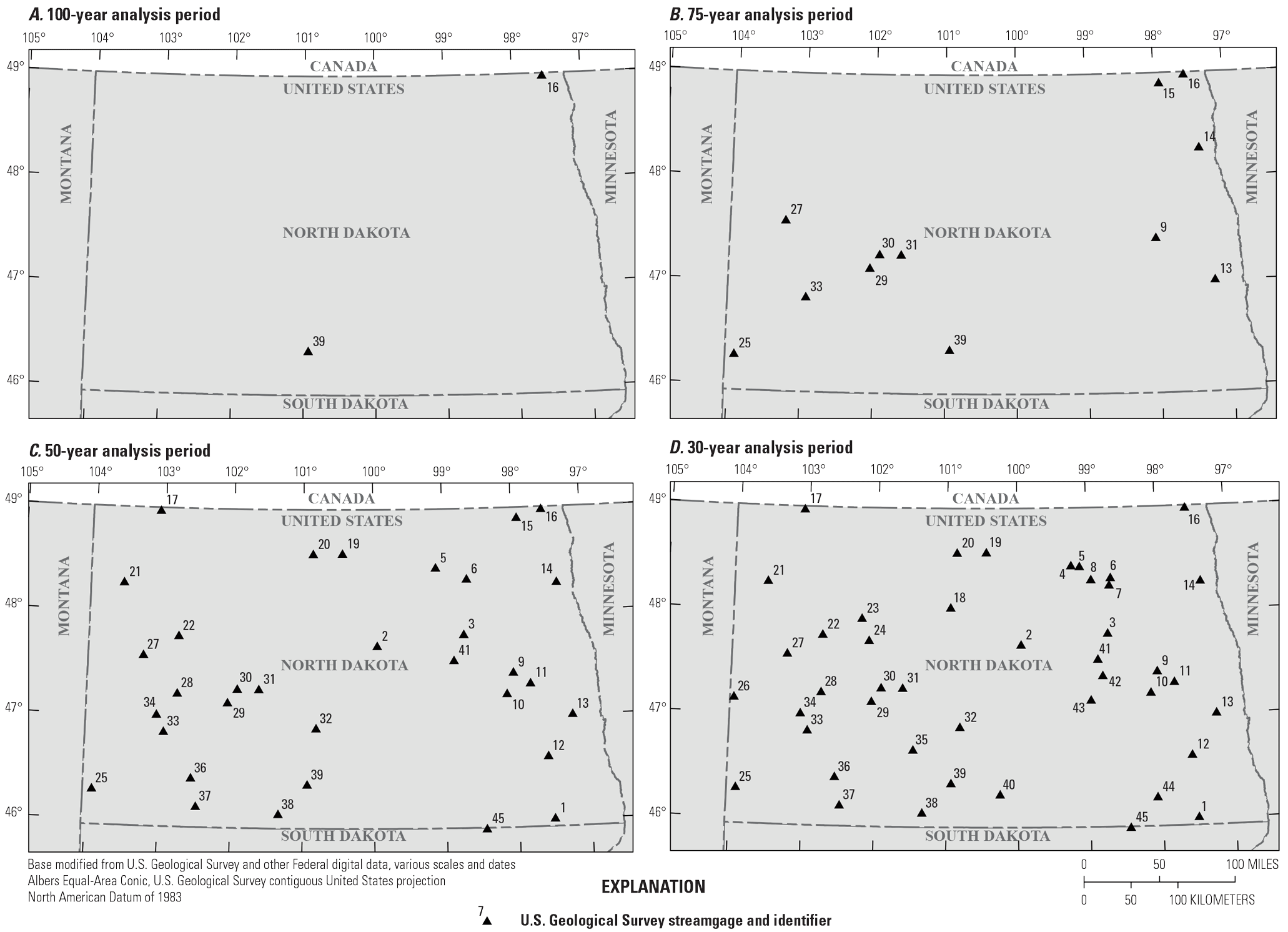
Maps showing locations and corresponding map numbers of U.S. Geological Survey streamgages in North Dakota for the (A) 100-year, (B) 75-year, (C) 50-year, and (D) 30-year analysis periods (1921–2020, 1946–2020, 1971–2020, and 1991–2020, respectively).
Autocorrelation
Autocorrelation, also called serial correlation, dependence, or persistence, is a state in which values in a time series are not random but are correlated with each other. Autocorrelation can be on short time scales, such as wet or dry periods of several years, or on much longer times scales because of persistent climatic forces. Autocorrelation violates the underlying assumptions of many statistical methods and can negatively affect flood-frequency analysis because it violates the assumption of independent, identically distributed data. One effect is that for a times series with autocorrelation, the analyst does not have as much independent data as the length of the record would imply. The Red River of the North in Canada was used as an example in a study that looked at flood frequency and the effect of autocorrelation. Burn and Goel (2001, p. 355) detected “persistence in the data series can lead to a slight increase in the expected flood magnitude for a given return period” and “persistence is shown to dramatically increase the uncertainty associated with estimated flood quantiles. The 117-year flood series for the Red River at Winnipeg is demonstrated to be equivalent to roughly 45 years of independent data.”
Two statistical tests for autocorrelation in peak flow were evaluated at streamgages for the four analysis periods. The rank von Neumann test for lag-1 autocorrelation was used to investigate short-term persistence, and the Hurt exponent was used to investigate long-term persistence. Details about these two tests are described in chapter A.
A peak-flow series can indicate persistence when high peak flows are followed by high peak flows or low peak flows are followed by low peak flows. Time series with persistence are nonstationary, which means that the data are not independent, random occurrences. Short-term persistence (rank von Neuman test for lag-1, p-value less than [<] 0.05) was detected at 3 streamgages, and long-term persistence (Hurst coefficient greater than 0.6) was detected at 12 streamgages in the four analysis periods (table 4, fig. 11A, B). Whether a streamgage indicated short- or long-term persistence was not dependent upon the size of the drainage area. Two streamgages in the 75- and 50-year analysis periods (USGS streamgages Wild Rice River near Rutland, North Dakota, [05051600], and Rush River at Amenia, North Dakota, [05060500], respectively) indicated evidence of short- and long-term persistence. In the 50-year analysis period, USGS streamgage 05051600 has short- and long-term persistence (fig. 11A, B). The peak-flow series is shown in figure 11A, and the autocorrelation plot is shown in figure 11B. The short-term persistence (rank von Neuman test) was statistically significant with a p-value of 0.018, and long-term persistence (Hurst exponent) has a value of 0.644, indicating that long-term persistence (autocorrelation at lags greater than 1) exists in the series of peak flow.
Table 4.
U.S. Geological Survey streamgages in the 100-, 75-, 50-, and 30-year analysis periods in North Dakota with short-term persistence and long-term persistence.[ID, identifier; mi2, square mile; --, no data or not available; drainage area from U.S. Geological Survey (2023)]
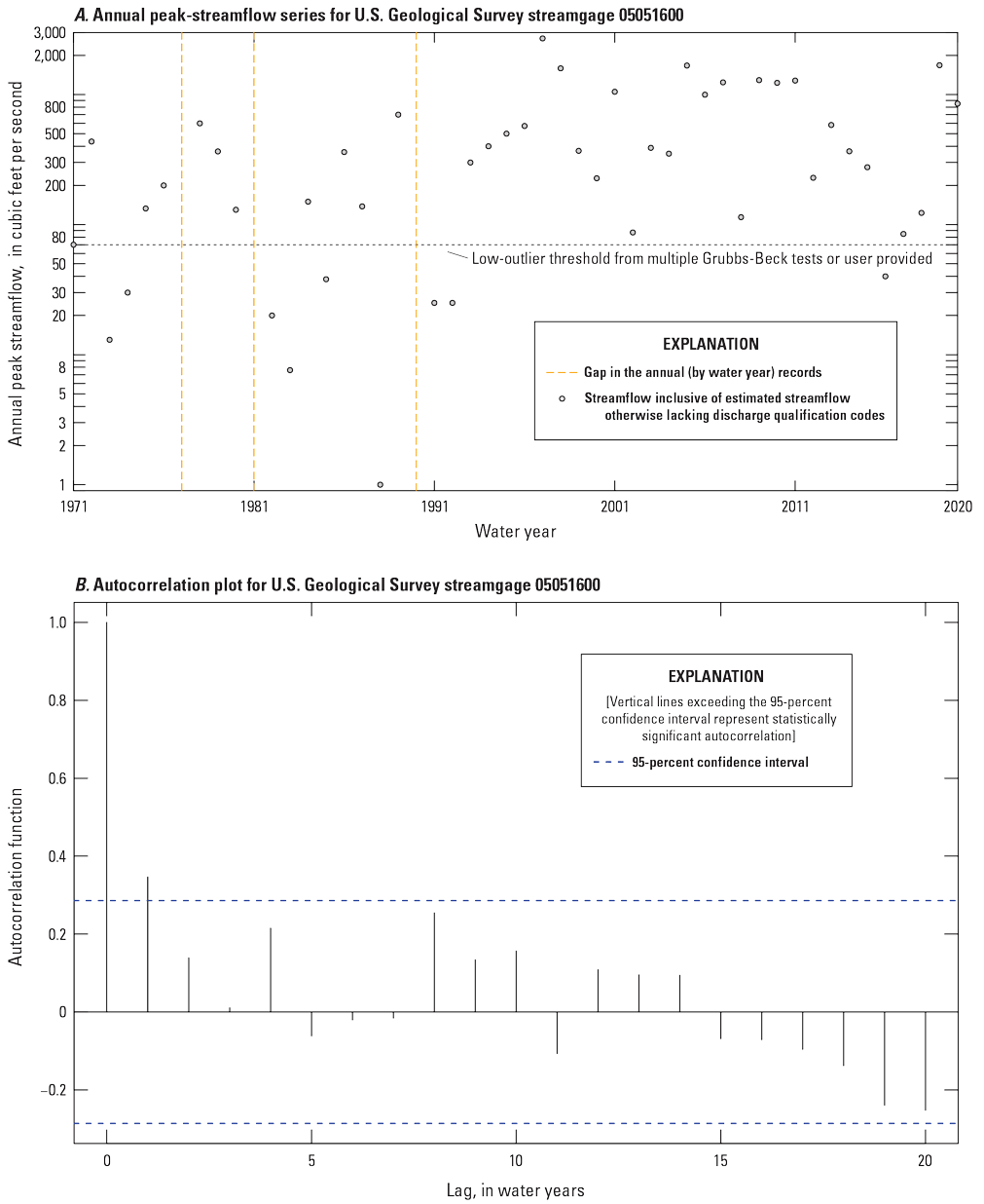
Graphs showing (A) annual peak-streamflow series and (B) autocorrelation plot for U.S. Geological Survey streamgage Wild Rice River near Rutland, North Dakota (05051600), in the 50-year analysis period (1971–2020). Data are from U.S. Geological Survey (2023). [A water year is the period from October 1 to September 30 designated by the year in which it ends]
Human interventions, such as land-use or land-cover change and construction of upstream dams, can result in a peak-flow series having a Hurst coefficient greater than 0.5 (Villarini and others, 2009a). Nonregulated sites were used in this study to control for some of these factors and, based on research on past climatic persistence described earlier in this chapter, the short-term and long-term persistence detected here is related to climate.
In a national study that included sites in North Dakota, Hodgkins and others (2019) detected statistically significant (p-value<0.05) lag-1 autocorrelation in 7.8 percent of 1,465 peak-flow series (that included regulated streams) for 1941–2015; therefore, autocorrelation was not a concern nationwide. The result was similar for North Dakota; however, analysis of Devils Lake and the Red River indicates that the region is subject to long-term climatic persistence. Analysis of naturalized peak flows for the Red River at James Avenue Pumping Station, Winnipeg, Manitoba, Canada, indicated statistically significant autocorrelation on the scale of 1 to 14 years (Ryberg and others, 2020b). The record was longer than 100 years (1892–2016), making it useful for detecting long-term persistence. Because the Red River at Winnipeg integrates streamflow from a substantial part of North Dakota, long-term persistence could be present to a greater extent than indicated and might be evident if streamgage records were longer.
Monotonic Trends
Monotonic trends are defined by a monotonic function that is always increasing or always decreasing (never changing sign), but the relation is not necessarily linear. The slope of the monotonic trends was determined using the Theil-Sen estimate, and the relation was tested for statistical significance using the Mann-Kendall test (Kendall, 1938; Sen, 1968; Theil, 1992; Helsel and others, 2020; Ryberg and others, 2024). This form of trend is nonparametric; that is, it does not have assumptions that the explanatory or response variables or the residuals can be approximated by a specific statistical distribution, although it has an assumption that the data are independent and identically distributed, and the distribution is possibly unknown (Hollander and others, 2014; Helsel and others, 2020). Nonparametric monotonic trends are more robust to outliers because the slope estimate is less affected by outliers than linear regression. For this reason, nonparametric monotonic trend methods are often a better choice for environmental data than trends based on linear regression. Because of the independence assumption, the autocorrelation results informed this analysis. If autocorrelation was not detected, then a Mann-Kendall test for trend in R (Millard, 2013) was used. If autocorrelation was detected, then a modified Mann-Kendall test for trend was completed (refer to chapter A).
An example of upward monotonic trend, hereafter referred to as a “trend,” in the peak flow at USGS streamgage Pembina River at Neche, North Dakota (05100000), in the 100-year analysis period is shown in figure 12A. The Theil-Sen slope and Mann-Kendall test for trend indicate a statistically significant upward trend at this site. An example of a downward trend in the peak flow at USGS streamgage Bear Den Creek near Mandaree, North Dakota (06332515), in the 50-year analysis period is shown in figure 12B. The Theil-Sen slope and Mann-Kendall test for trend indicate a statistically significant downward trend at this site.
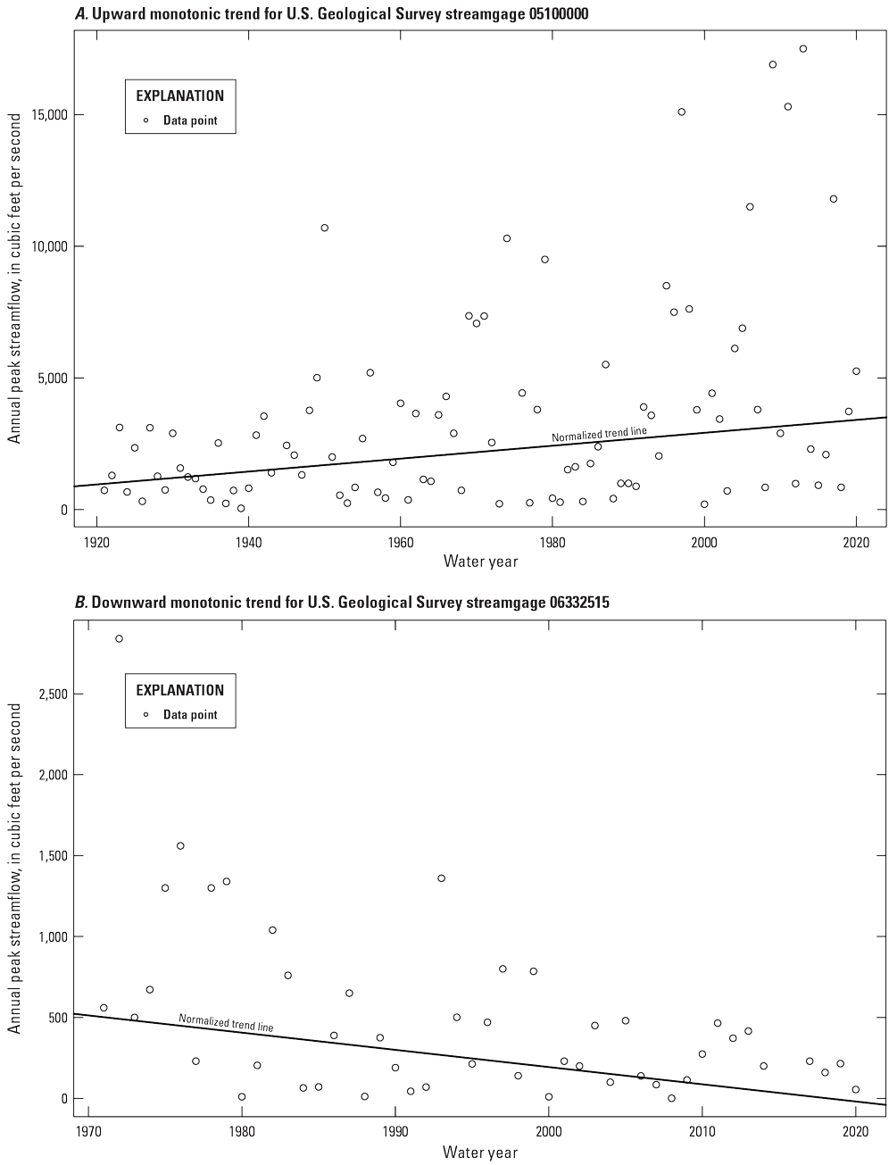
Graphs showing (A) upward monotonic trend for U.S. Geological Survey streamgage Pembina River at Neche, North Dakota (05100000), in the 100-year analysis period (1921–2020) and (B) downward monotonic trend for U.S. Geological Survey streamgage Bear Den Creek near Mandaree, North Dakota (06332515), in the 50-year analysis period, 1971–2020. Data are from U.S. Geological Survey (2023).
The percentage of streamgages per likelihood category of detected trends in the peak flow in each analysis period is listed in table 5. The likelihood and normalized magnitude of trends for the streamgages in each analysis period are shown in figure 13. In the 100-, 75-, and 50-year analysis periods, likely upward trends in peak flow generally were detected in the eastern part of the State, and slightly larger magnitudes were detected in the 50-year analysis period. In the 30-year analysis period, likely upward trends generally were detected in the western part of the State. Likely upward trend magnitudes were larger in the 30-year analysis period than those in the 100-, 75-, and 50-year analysis periods. Likely downward trends were detected in the western part of the State in the 75- and 50-year analysis periods and, in the northeast, in the 30-year analysis periods. The largest likely downward trend magnitude was detected in the 50-year analysis period, whereas the rest of the likely downward trend magnitudes remained about the same in the 75-, 50-, and 30-year analysis periods.
Table 5.
U.S. Geological Survey streamgages in the 100-, 75-, 50-, and 30-year analysis periods in North Dakota that indicated monotonic trends in annual peak streamflow.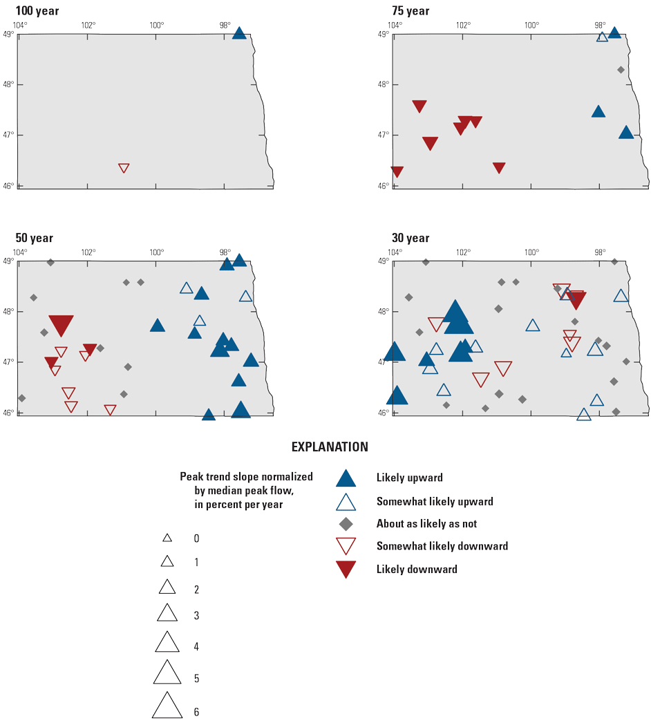
Maps showing likelihood and normalized magnitude of annual peak-streamflow monotonic trends for U.S. Geological Survey streamgages in the 100-, 75-, 50-, and 30-year analysis periods in North Dakota.
The long-term pattern (as determined in the 100-, 75-, and 50-year periods) of decreasing peak flow in the west and increasing peak flow in the east is a pattern of opposing signals on either side of the 100th meridian, and this pattern has been noted in the Third National Climate Assessment (water resources chapter, fig. 3.5, Georgakakos and others, 2014), the Fifth National Climate Assessment (Northern Great Plains chapter, fig. 25.4, Knapp and others, 2023), in other studies (Hirsch and Ryberg, 2012; Peterson and others, 2013; Hodgkins and others, 2019; Sando and others, 2022), and in the results for South Dakota presented in another chapter and the data release (Barth and Sando, 2024; Marti and others, 2024).
Many of the sites included here were used in an attribution study of changes in peak flow that indicated sites in eastern North Dakota with increased peak flow were also experiencing positive trends in annual precipitation (Ryberg, 2022; Sando and others, 2022). Eastern North Dakota and surrounding areas in Manitoba, Canada; Minnesota; and South Dakota have been extensively studied because of rising lake levels, increases in streamflow, and large, costly floods in Devils Lake, the Red River, the Souris River, and the James River Basins (Wiche, 1986; Macek-Rowland, 1997, 2001; Thorleifson and others, 1998; Wiche and others, 2000a, b, 2002; Burn and Goel, 2001; St. George and Nielsen, 2002, 2003; Vecchia, 2002, 2008, 2011; Brooks and others, 2003; Ryberg and others, 2007a, b, 2014, 2016a, b; Regorrah and Todhunter, 2008; Government of Canada, 2013; Gupta and others, 2015; Ryberg, 2015; Kolars and others, 2016, 2019; Nustad and others, 2016; Todhunter and Fietzek-DeVries, 2016; Todhunter and others, 2020; Van Hoy and others, 2020; Norton and others, 2022; Archambault and others, 2023; Atashi and others, 2023). Because of the supporting studies and the concurrent trends in precipitation that were identified in the attribution study, increasing long-term precipitation was recently attributed as the reason for nearly all the trends in peak flow in eastern North Dakota (Sando and others, 2022). Land-use and land-cover changes play a role, and numerous studies have attributed differing degrees of land-use effect on streamflow (Zhang and Schilling, 2006; Regorrah and Todhunter, 2008; Ryberg and others, 2014; Gupta and others, 2015; Todhunter and others, 2020). Increased magnitude of peak flow in recent years means that the exceedance probability of floods affecting infrastructure in eastern North Dakota could be increasing (Salas and Obeysekera, 2014), highlighting why advancements in flood-frequency analysis of nonstationary series would be beneficial.
In the attribution study, most streamgages in the Upper Plains with significant downward trends had nonsignificant positive trends in annual precipitation and significant positive trends in annual air temperature (Sando and others, 2022). The most common attribution for significant downward trends in western North Dakota was air temperature (Sando and others, 2022). Some streamgages in this area are in the USGS Hydro-Climatic Data Network 2009, which only includes streamgages that monitor drainage basins with minimal human alterations that are suitable for analyzing hydrologic nonstationarity caused by climatic changes (Lins, 2012). The inclusion of some of the streamgages in the USGS Hydro-Climatic Data Network 2009 provides additional support that the regional pattern could be caused by climatic changes. Air temperature as an attribution for trends is supported by other studies. In the Little Missouri River Basin of western North Dakota, Griffin and Friedman (2017) detected an increased winter and summer atmospheric evaporative demand in 1976–2012 when compared to 1939–75. Because atmospheric evaporative demand represents the potential amount of water transfer from land surface to the atmosphere, increases in winter and summer atmospheric evaporative demand are likely contributors to decreased runoff for a given amount of rain (Griffin and Friedman, 2017; Sando and others, 2022).
Griffin and Friedman (2017) determined that air temperature was the dominant cause of reduced runoff from rainfall. They also determined that surface‐water withdrawals in the Little Missouri River Basin had a noticeable effect on the hydrology in the area, although they accounted for less than 12 percent of the reduction in average annual streamflow volume. They detected no evidence of substantial streamflow reduction caused by groundwater pumping (Griffin and Friedman, 2017). The attribution study also analyzed data from the Bureau of Reclamation’s Missouri River Basin depletions database (Bureau of Reclamation, 2012). The database indicated some increases in depletions related to irrigated agriculture and surface-water public supply; however, depletions were not considered a primary attribution for downward trends in peak flow (Sando and others, 2022). Like eastern North Dakota, climate is the major driver of changes in western North Dakota, and land-use change is a secondary consideration. Long-term (periods greater than 30 years), downward trends in the magnitude of peak indicate that the exceedance probability of floods affecting infrastructure in western North Dakota could be decreasing (Salas and Obeysekera, 2014). As with the pattern of increasing magnitude in eastern North Dakota, this observation highlights the need for improved analysis methods for nonstationary series. However, these observed trends could change in the future, particularly if affected by low-frequency climatic variability driven by phenomena such as Pacific Decadal Oscillation and Atlantic Multidecadal Oscillation, and increased extreme precipitation events, even in areas that experience drying climates, will be complicating factors (Salas and Obeysekera, 2014; Knapp and others, 2023).
Change Points
Change points are abrupt changes in the median, mean, scale, or variance of a time series. Change points in the median and scale of the peak flow were evaluated in this study using two tests (the Pettitt and Mood tests), as described in chapter A. The Pettitt test finds a single change point in the distribution of a series and reports a p-value for a determination of statistical significance. The Mood test finds a single change in the scale, or spread, of a series. The p-values from the results were converted to likelihood values to provide the following tabular and graphical summaries. This likelihood approach, proposed by Hirsch and others (2015) as an alternative to simply reporting significant trends with an arbitrary cutoff point, facilitates mapping spatial patterns in the direction of change.
Change points in the median and scale of peak flows were detected at 11 of the 91 streamgages tested in the 4 analysis periods (table 6). Five of these streamgages had changes in the median and scale of peak flow. Also listed in table 6 are the year and direction of the median change points and the year of the scale change point. Most change points in the median were in a positive direction, the years of median change points ranged from 1972 to 2008, and most were detected in the early 1990s. The years of scale change points ranged from 1981 to 2012, and many change points were detected at a similar time to the change points in the median.
Table 6.
U.S. Geological Survey streamgages in the 100-, 75-, 50-, and 30-year analysis periods in North Dakota that indicated change points in the median or scale of annual peak streamflow.[ID, identifier; mi2, square mile; --, no data or not available]
The percentage of streamgages per likelihood category with change points in the median of peak flow for the 100-, 75-, 50-, and 30-year analysis periods is listed in table 7. The likelihood of change points in median peak flows is shown in figure 14. The spatial patterns in change points were like those for trends. Likely upward change points were detected in the east, and likely downward change points were detected in the west. In the 30-year analysis period, the patterns differ; likely upward change points were detected in the west, and mixed results were detected in the east.
Table 7.
Percentage of U.S. Geological Survey streamgages per likelihood category of median annual peak-streamflow change points in the 100-, 75-, 50-, and 30-year analysis periods in North Dakota.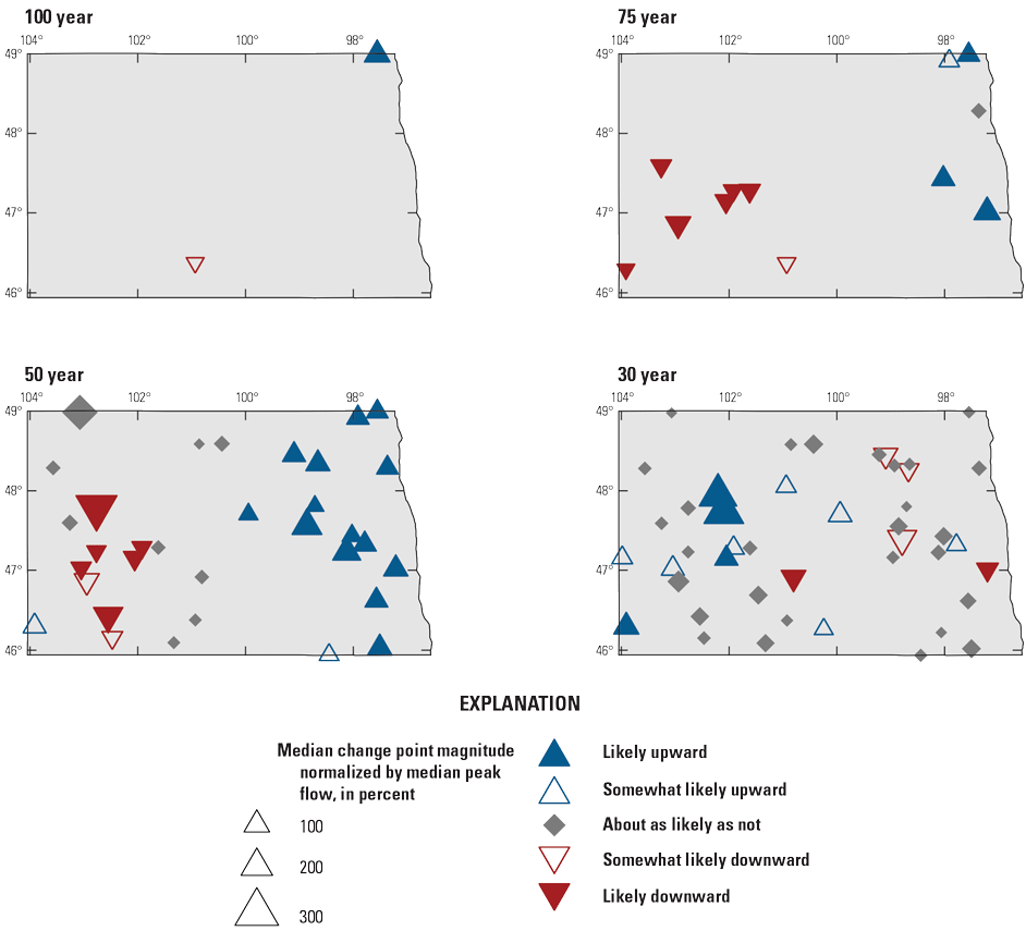
Maps showing likelihood of change points in the median annual peak streamflow for U.S. Geological Survey streamgages in the 100-, 75-, 50-, and 30-year analysis periods in North Dakota.
An example of change-point analysis for streamgage 05100000 is shown in figure 15. An upward change point in the median peak flow was identified in 1991 because the median flow for the period from 1992 to 2020 is larger than the median flow for the period from 1921 to 1991. A change point in the scale was identified in 1993 because the peak flows were less variable in scale before 1993 than after.
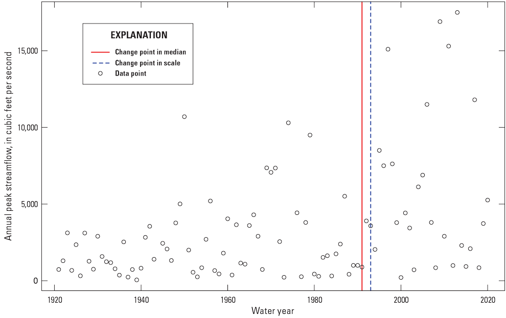
Graph showing change points of annual peak streamflow in the median and the scale at U.S. Geological Survey streamgage Pembina River at Neche, North Dakota (05100000), in the 100-year analysis period (1921–2020). Data are from U.S. Geological Survey (2023). [A water year is the period from October 1 to September 30 designated by the year in which it ends]
The attribution study discussed in the “Monotonic Trends” section also examined the change points in peak flow (Ryberg, 2022). In eastern North Dakota, change-point years were clustered around 1992, as they are in the results presented here, and have remarkably little variation around that year (Sando and others, 2022). The circa 1992 change point for eastern North Dakota is consistent with the findings of Williams-Sether (1999), who documented a sudden switch from drought to wet conditions in North Dakota around 1992–93 and the findings of Wiche and others (2000b) who determined that in the Devils Lake Basin of eastern North Dakota, unusually high precipitation amounts have been detected since the 1990s during May and June and again during the early fall. Excess moisture can carry over into the next year’s flood season (Ryberg and others, 2014), thereby priming basins in eastern North Dakota for increased runoff and flooding.
In western North Dakota, negative change points were attributed to decreases in precipitation, increases in temperature, and at one site, increases in depletions (Sando and others, 2022). Most change points in the attribution study were from 1972 to 1987 (in the 1970s for the 75-year period and in the 1980s for the 50-year period). The results are similar here (fig. 14). Sando and others (2022) determined the most common attribution for statistically significant change points in western North Dakota, and the trends, was air temperature, and the increases in evaporative demand and reduced runoff from rainfall were discussed in the “Monotonic Trends” section of this report. In the attribution study, three streamgages with significant change points for the 50-year period were attributed to long-term precipitation changes, and a drought was determined to be the most probable cause (Sando and others, 2022). The mean year of the change point for the three streamgages was 1987, and that coincided with a severe drought from 1988 to 1992 (Williams-Sether and others, 1994; Williams-Sether, 1999). The departure from normal monthly precipitation during 1988–92 for each climatic division in North Dakota and a substantial decline in precipitation starting in 1987 in some areas are shown in figure 2 of Williams-Sether and others (1994).
Annual Peak-Streamflow Timing Analysis
The peak-flow timing analysis, as described in chapter A, is used to identify potential shifts, earlier or later, in the timing of floods. Peaks were classified programmatically into an early period, usually representing snowmelt, and a later period, representing rain-generated peaks. An example of a density plot and peak-flow timing analysis at USGS streamgage 05051600 is shown in figure 16A and B. The density plot (fig. 16A) shows the frequency of occurrence of peak flows on days of the water year and illustrates a bimodal peak-flow occurrence. The earlier peak flows are likely snowmelt generated, and the later peak flows are rain generated. The dark red vertical line indicates that day 229 of the water year is a local minimum, or turning point, in the density function and is the breakpoint between the early and late periods for the timing analysis. The peak-flow timing analysis (fig. 16B) shows the magnitudes of each peak flow (circular marker size and color) and the trend lines of the peak flows in the early, later, and overall periods. The solid line is the trend for all peaks. The dotted lines are the trend lines for the early and late peaks (snowmelt or rain generated). Red lines indicate trends that are statistically significant with a p-value <0.05. The upward trend lines for this streamgage indicate that peak flow is happening later in the water year for the overall period, and this is driven by an increase in the 1990s in the occurrence of peaks after day 229 of the water year.
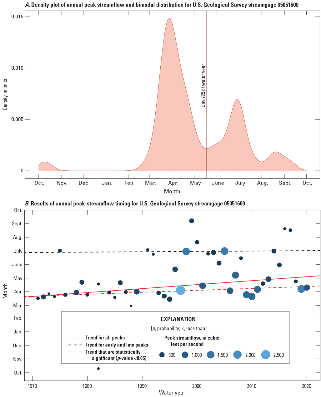
Graphs showing (A) the density plot of annual peak streamflows and the bimodal distribution, where day 229 of the water year (the period from October 1 to September 30 designated by the year in which it ends) represents a transition from the snowmelt (early) peaks to the rain-generated (late) peaks and (B) results of annual peak-streamflow timing analysis for U.S. Geological Survey streamgage Wild Rice River near Rutland, North Dakota (05051600), in the 50-year analysis period (1971–2020). Data are from U.S. Geological Survey (2023).
The percentage of streamgages per likelihood category for peak-flow timing trends in the 100-, 75-, 50-, and 30-year analysis periods for the complete, early, and late part of the water year is listed in table 8. The likelihood and magnitude of peak-flow timing trends for streamgages in the 100-, 75-, 50-, and 30-year analysis periods for the complete water year are shown in figure 17. Upward trends in the timing of peak flows were mainly in eastern part of North Dakota and were detected in the 100-, 75-, 50-, and 30-year analysis periods, indicating that peak flows are happening later in the year. Downward trends were mainly in the western part of North Dakota in the most recent 30-year analysis period, indicating that peak flows are happening earlier in the year. The trend magnitudes are largest in the 30-year analysis period compared to the longer analysis periods.
Table 8.
Percentage of U.S. Geological Survey streamgages per likelihood category of the annual peak-streamflow timing monotonic trends for the complete, early, and late parts of the water year in the 100-, 75-, 50-, and 30-year analysis periods in North Dakota.[A water year is the period from October 1 to September 30 designated by the year in which it ends. NA, no detection of early or late peak-streamflow timing]
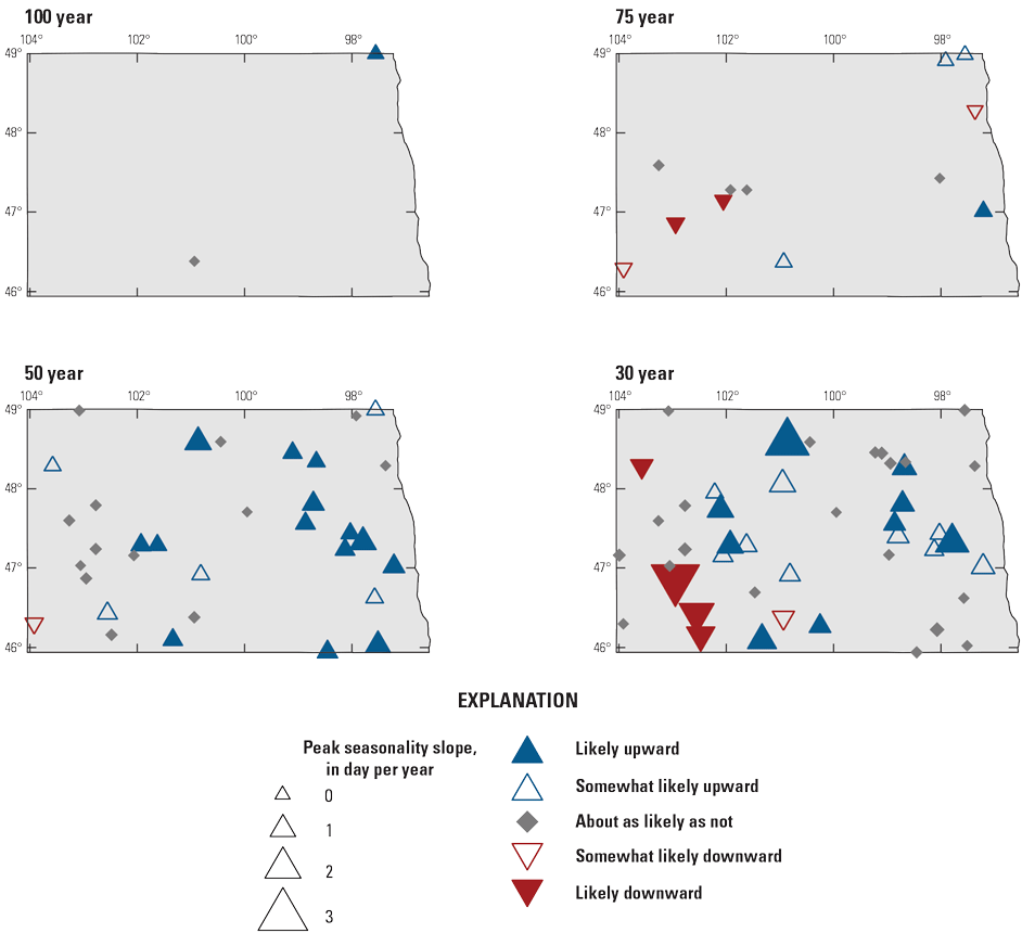
Maps showing likelihood and magnitude of annual peak-streamflow timing monotonic trends for the complete water year (the period from October 1 to September 30 designated by the year in which it ends) in the 100-, 75-, 50-, and 30-year analysis periods in North Dakota.
These changes were studied earlier in Ryberg and others (2016a), who determined that for all of North Dakota, snowmelt peak flows were tending to happen earlier, by 8.7–14.3 days, over a period of 1910–2012. The 75-year trend period has preponderance of somewhat likely or likely downward trends in the early part of the water year (table 8), also indicating likely earlier snowmelt peak flows; however, the pattern changes for shorter periods, indicating snowmelt/spring peak flows coming later (table 8). More late spring rain could be the cause of this pattern because North Dakota receives most of its precipitation in late spring and early summer, and although total annual precipitation is highly variable, it has been greater than average since 1990 (Frankson and others, 2022).
The 75-year trend period has a preponderance of somewhat likely or likely upward trends for the late part of the water year, indicating that trends are happening later in the water year. Based on Ryberg and others (2016a), this is affected by later summer/fall peak flows in eastern and northern North Dakota. They happened, on average, 5.2 days later over a period of 1910–2012. Fall streamflow has been higher in recent decades in these areas because of increases in fall precipitation; for example, November 4, 2009, streamflow for the Red River at Fargo, North Dakota, was the highest streamflow recorded for the month of November since measurements started in 1901 and was so high that the USGS put out a press release because high fall streamflow increases flood risk for the next spring (Ryberg and others, 2007a, 2016a). The November 4, 2009, daily streamflow value (7,900 ft3/s) is still the daily streamflow value record for November and fall streamflow has remained at values greater than typical historical conditions (U.S. Geological Survey, 2023).
The raster seasonality plots described in a subsequent section, “Raster Seasonality Plots,” and available in the data release for each streamgage in the study (Marti and others, 2024) can help in visualizing these changes. Those plots use daily streamflow and show increases in fall streamflow since 1993 in eastern North Dakota.
Daily Streamflow
To aid in understanding some of the patterns in peak flows, changes in daily streamflow were examined using analyses described in chapter A. The analyses include regime plots, raster seasonality plots, center of volume analysis, and POT analysis. Daily streamflow is not available at every streamgage that was examined for peak flows because some streamgages can have incomplete daily flow record or are crest-stage gages that only record peak flow. Regime plots, not discussed here, show the minimum, maximum, and mean and 10th and 90th percentiles of daily streamflow for a complete analysis period. These plots provide a visual summary of the flow regime for a streamgage and are available in the data release (Marti and others, 2024).
Raster Seasonality Plots
The raster seasonality plot, as described in chapter A, depicts gridded daily mean streamflow for every day in a period of record. The color of the daily mean streamflow is graduated with the larger flows in blue and the smaller flows in tan. Days with no daily mean streamflow are depicted as white. Raster seasonality plots for all streamgages analyzed are available in the data release (Marti and others, 2024). An example raster seasonality plot at USGS streamgage 05100000 in the 100-year analysis period in northeastern North Dakota is shown in figure 18. Larger flows (wetter conditions) are depicted with the blue coloring, and smaller flows (drier conditions) are depicted with the tan coloring. Before 1940, larger flows were measured between April and mid-July, and smaller flows were measured in August–November. Between 1940 and 1990, larger flows generally were measured between mid-March and about September. Larger flows started to be measured for most of the water year after 1990. Since about 1940 and after 2000, conditions at this streamgage have gradually become wetter as shown by the increase in green to blue coloring. Periodic drier conditions, shown by tan coloring, have not been detected since about 1990.
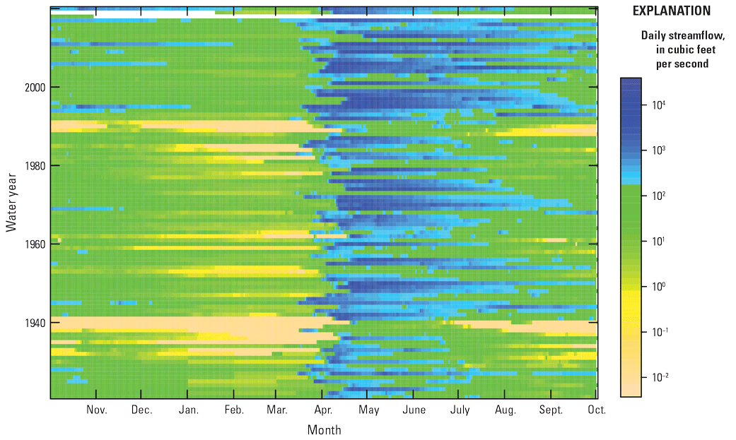
Raster seasonality plot showing daily mean streamflow for U.S. Geological Survey streamgage Pembina River at Neche, North Dakota (05100000), in the 100-year analysis period, 1921–2020. The scale is the base-10 logarithm of streamflow at this site. Data are from U.S. Geological Survey (2023).
Center of Volume Analysis
The center of volume analysis plot, as described in chapter A, depicts the date of the water year for which 25, 50, and 75 percent of the streamflow volume has passed a given streamgage. Monotonic trends in the percentiles can be an indicator of change in the streamflow over time. The center of volume analysis plots for streamgages in the study are available in the data release (Marti and others, 2024). Two example center of volume analysis plots in the 100-year analysis period are shown in figure 19A and B: the plot for USGS streamgage 05100000, in northeastern North Dakota, is shown in figure 19A, and the plot for USGS streamgage Cannonball River at Breien (06354000), in southwestern North Dakota, is shown in figure 19B. In figure 19A, no apparent trend was detected in the 25th (orange line) percentile, indicating that the date at which 25 percent of the total volume has passed has not changed. Upward trends in the 50th (green line) and 75th (blue line) percentiles indicate that the date at which 50 and 75 percent of the total volume has passed is getting later. In figure 19B, an apparent downward trend exists in the 25th, 50th, and 75th percentiles, indicating that the dates for the 25th, 50th, and 75th percentiles of the total volume are earlier in more recent years. The duration between the 25th and 75th percentile dates is shown as black triangles and is scaled to the y-axis on the right-hand side of the plots. An increase exists in the duration in figure 19B, indicating that the number of days between the 25th and 75th percentiles of flow volume is getting longer.
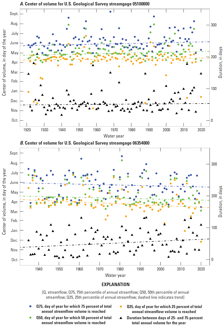
Graphs showing center of volume analysis for (A) U.S. Geological Survey streamgages Pembina River at Neche, North Dakota (05100000), and (B) Cannonball River at Breien, North Dakota (06354000), in the 100-year analysis period, 1921–2020. Data are from U.S. Geological Survey (2023).
Peaks-Over-Threshold Analysis
POT analysis, as described in chapter A, analyzes the frequency of occurrence for daily mean streamflows over a set threshold. For a given threshold, the number of times a streamflow exceeds the threshold is counted for each year. Meeting the independence criterion among candidate streamflows is the primary challenge with the POT analysis. Thresholds for the POT analyses in this study were set at the daily mean streamflow magnitude for which there is an average of two (POT2) and four (POT4) events per year. Tests for change points in the number of events over the threshold were completed to find increases or decreases in the frequency of the candidate streamflows. The results of change points in the frequency of POT2 for USGS streamgage 05051600 in the 50-year analysis period are shown in figure 20A and B. The daily mean streamflow times series (in gray) is shown in figure 20A. The daily mean streamflow magnitudes greater than the POT2 determined threshold (red line) are shown as blue (fig. 20A). Larger daily mean streamflows are more prevalent after about 1990. The detected change point (1992) in the frequency of mean daily streamflow greater than the POT2 threshold is shown in figure 20B.
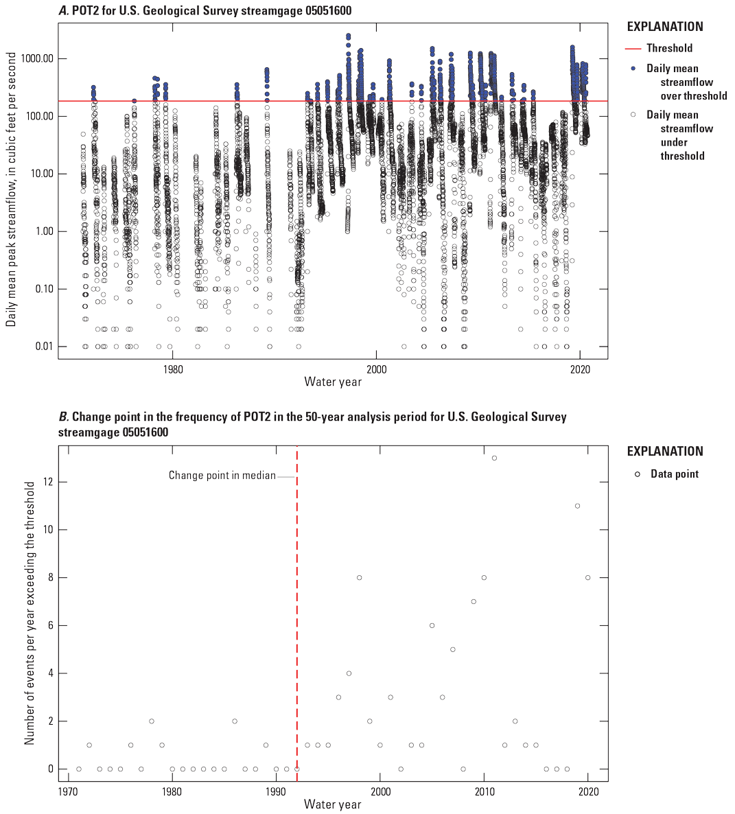
Graphs showing (A) peaks-over-threshold with an average of two daily mean streamflows per water year (POT2) and (B) the change point in the frequency of POT2 in the 50-year analysis period for U.S. Geological Survey streamgage Wild Rice River near Rutland, North Dakota (05051600). Data are from U.S. Geological Survey (2023). [A water year is the period from October 1 to September 30 designated by the year in which it ends]
The results of change points in the frequency of POT4 for USGS streamgage 05051600 in the 50-year analysis period are shown in figure 21A and B. The POT4 results are like those of the POT2, indicating larger and more frequent mean daily streamflows after the detected change point in 1992. The main difference between the POT2 and POT4 results is that the threshold is lower in the POT4 analysis than the POT2 analysis.
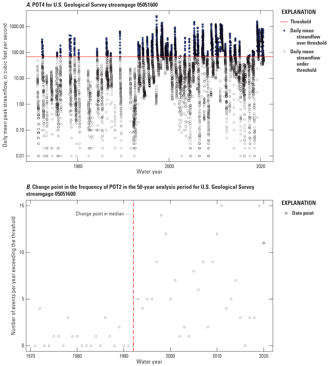
Graphs showing (A) peaks-over-threshold with an average of four daily mean streamflows per water year (POT4) and (B) the change point in the frequency of POT4 in the 50-year analysis period for U.S. Geological Survey streamgage Wild Rice River near Rutland, North Dakota (05051600). Data are from U.S. Geological Survey (2023). [A water year is the period from October 1 to September 30 designated by the year in which it ends]
The percentage of streamgages per likelihood category of detected change points in median frequency of POT2 and POT4 of daily mean streamflow in each analysis period is listed in tables 9 and 10, respectively. The likelihood of change points in the median frequency POT2 and POT4 for streamgages in the four analysis periods is shown in figures 22 and 23, respectively. Likely upward and somewhat likely upward changes are being detected in streamgages in the eastern areas of North Dakota in the 100-, 75-, and 50-year analysis periods. Likely downward and somewhat likely downward changes are being detected in streamgages in the western areas the 75- and 50-year analysis periods. Likely and somewhat likely upward and downward changes are being detected throughout North Dakota in the 30-year analysis period.
Table 9.
Percentage of U.S. Geological Survey streamgages per likelihood category of change points in the median of peaks-over-threshold with an average of two daily mean streamflows per water year in the 100-, 75-, 50-, and 30-year analysis periods in North Dakota.[A water year is the period from October 1 to September 30 designated by the year in which it ends; NA, the percentage of streamgages that did not have daily mean streamflow values]
Table 10.
Percentage of U.S. Geological Survey streamgages per likelihood category of change points in the median of peaks-over-threshold with an average of four daily mean streamflows per year in the 100-, 75-, 50-, and 30-year analysis periods in North Dakota.[NA, the percentage of streamgages that did not have daily mean streamflow values]
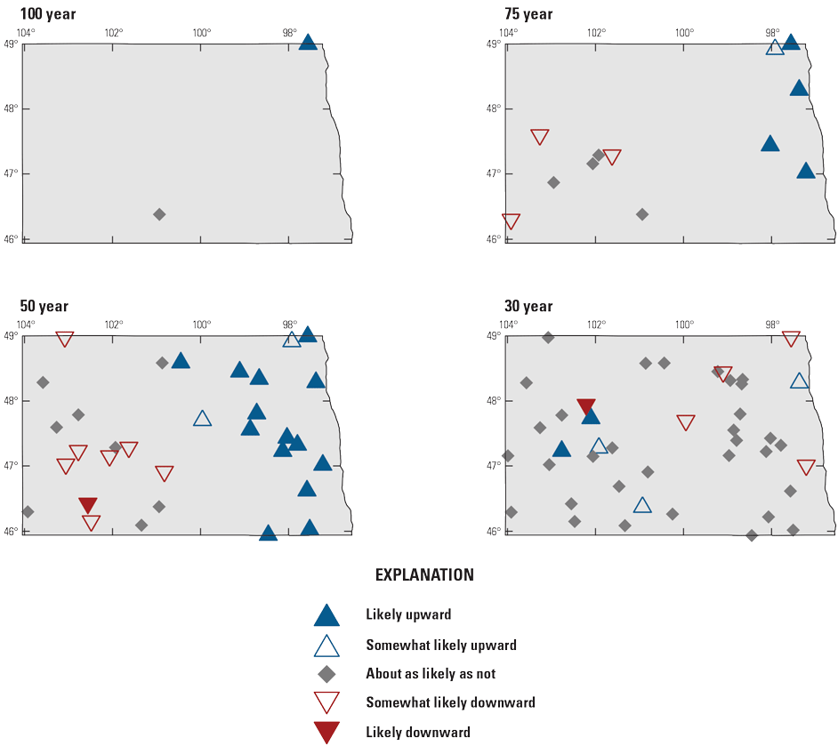
Maps showing likelihood of change points in the median peak-over-threshold with an average of two daily mean streamflows per year in the 100-, 75-, 50-, and 30-year analysis periods in North Dakota.
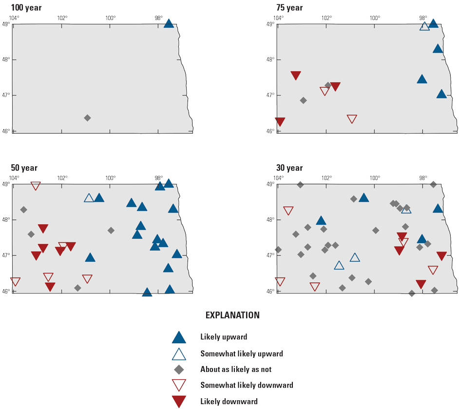
Maps showing likelihood of change points in the median peaks-over-threshold with an average of four daily mean streamflows per year in the 100-, 75-, 50-, and 30-year analysis periods in North Dakota.
Climate
The climate data analyzed in this study are described in greater detail in chapter A. As noted in chapter A, the precipitation and temperature data were derived from observed data from the NClimGrid dataset (Vose and others, 2014a, b), and the other climate metrics were modeled from the MWBM (McCabe and Wolock, 2011). All climate metrics presented in this section were averaged over the contributing drainage area for each streamgage to create basin-average values. Summaries of patterns in the climate metrics are presented for annual and seasonal precipitation, annual temperature, annual PET and precipitation ratio, annual snow and precipitation ratio, and annual soil moisture. Climate metric summaries for individual streamgages for the 100-, 75-, 50-, and 30-year analysis periods are presented in the associated data release (Marti and others, 2024).
Annual and Seasonal Precipitation
The percentage of streamgages in each likelihood category of detected trends in annual precipitation for each analysis period is listed in table 11. The likelihood and magnitude of annual precipitation trends in each analysis period are shown in figure 24. In the 100-, 75-, and 50-year analysis periods, most trends were upward, and the largest magnitudes were in the 50-year analysis period. In the 30-year analysis period, somewhat likely upward trends were detected in the west. Likely downward trends were detected in the southwest in the 50-year analysis period and in the northeast in the 30-year analysis period, and larger magnitudes were detected in the 30-year analysis period.
Table 11.
Percentage of U.S. Geological Survey streamgages per likelihood category of annual precipitation monotonic trends in the 100-, 75-, 50-, and 30-year analysis periods in North Dakota.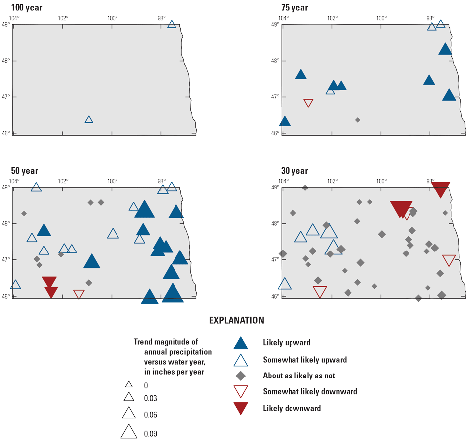
Maps showing likelihood and magnitude of monotonic trends in annual precipitation in the 100-, 75-, 50-, and 30-year analysis periods in North Dakota.
Annual precipitation totals may not be the best indicators of potential flooding because antecedent conditions, such as wet falls, and accumulated moisture over the winter contribute to runoff (Ryberg and others, 2007a, 2014; Gupta and others, 2015). Therefore, seasonal metrics of precipitation were also analyzed. The percentage of streamgages per likelihood category of seasonal precipitation trends in the 100-, 75-, 50-, and 30-year analysis periods is listed in table 12.
Table 12.
Percentage of U.S. Geological Survey streamgages per likelihood category of seasonal precipitation monotonic trends in the 100-, 75-, 50-, and 30-year analysis periods in North Dakota.The likelihood and magnitude of seasonal precipitation trends in each analysis period are shown in figure 25. During the winter season, likely upward trends were detected at most streamgages in 50- and 30-year analysis periods and were detected across the State. Likely downward trends were detected in all analysis periods and tended to be detected in the southwestern and northeastern areas of the State. During the spring season, likely upward trends were detected in all analysis periods, most in the western area of the State. Likely downward trends were detected mainly in the east in the 30-year analysis period. During the summer season, likely upward trends were detected in the 100-, 75-, and 50-year analysis periods in the eastern and northwestern to southeastern areas of the State. Likely downward trends were detected mainly in the southwest in the 75- and 50-year analysis periods and across the State in the 30-year analysis period. During the fall season, likely upward trends were detected in all analysis periods, and trend magnitudes were largest in the 30-year analysis period mainly in the northwestern and northern areas of the State. The significant seasonal increases in likely upward and likely downward trend magnitudes in the 30-year analysis period indicate that precipitation is increasing over much of the State during the fall season and decreasing across the State during the summer season. As discussed earlier in the peak-streamflow timing analysis and raster seasonality plots of daily streamflow, a key factor in change in North Dakota hydroclimatology is in the increase in fall precipitation, particularly in the most recent period, as shown in figure 25.
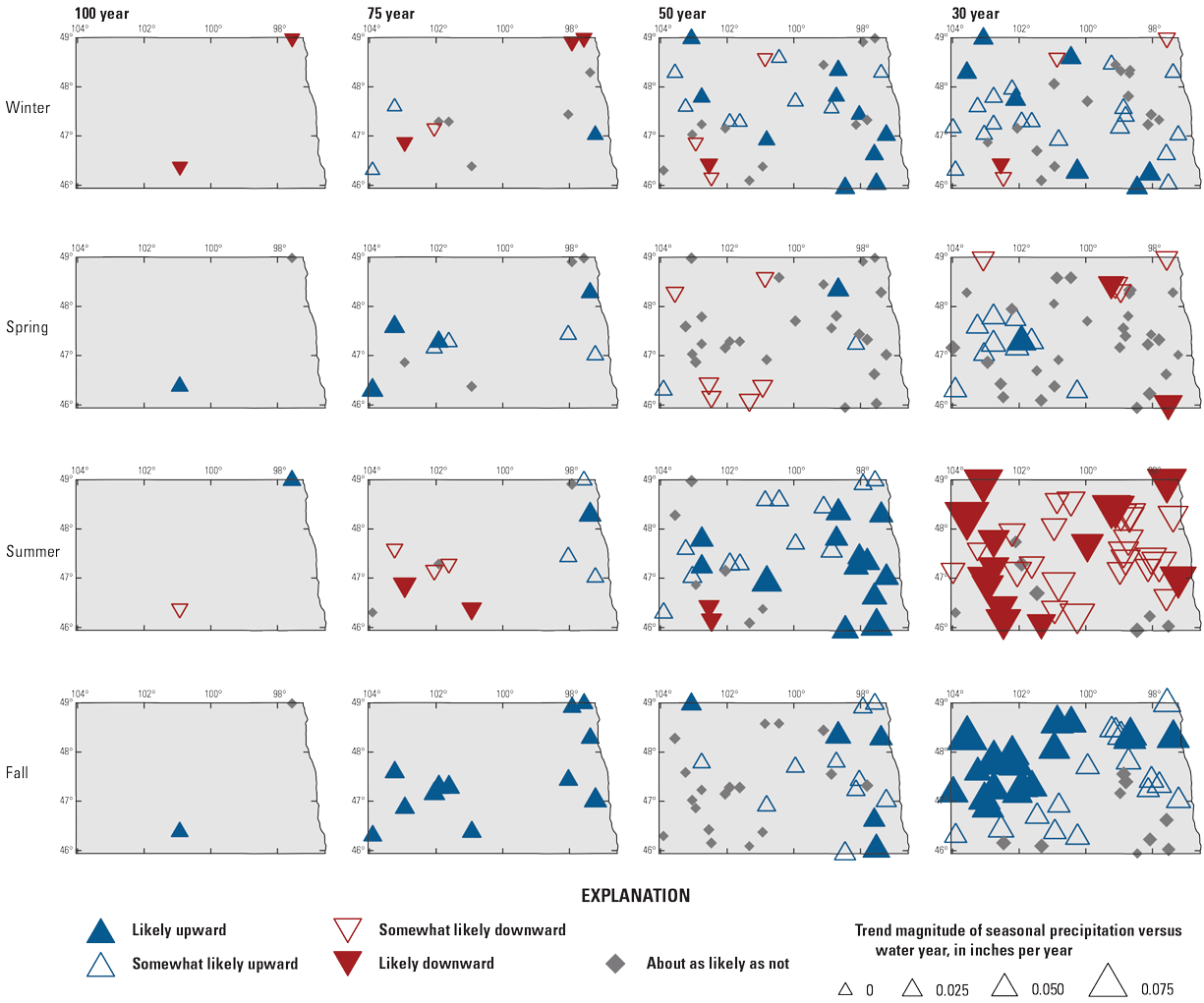
Maps showing likelihood and magnitude of seasonal precipitation monotonic trends in the 100-, 75-, 50-, and 30-year analysis periods in North Dakota.
Annual Temperature
The percentage of streamgages in each likelihood category of detected trends in annual temperature is listed in table 13, and the likelihood and magnitude of annual temperature trends are shown in figure 26. As noted in the earlier “Precipitation, Temperature, and Evapotranspiration” section, temperatures have risen across North Dakota. The trends in the 30-year period are somewhat likely upward (have less statistical significance). Given the high degree of variability in temperature, as described earlier, a large sample size is required to detect a trend; therefore, the 30-year results are reasonable statistically and indicate the temperature change is in one direction.
Table 13.
Percentage of U.S. Geological Survey streamgages per likelihood category of annual temperature monotonic trends in the 100-, 75-, 50-, and 30-year analysis periods in North Dakota.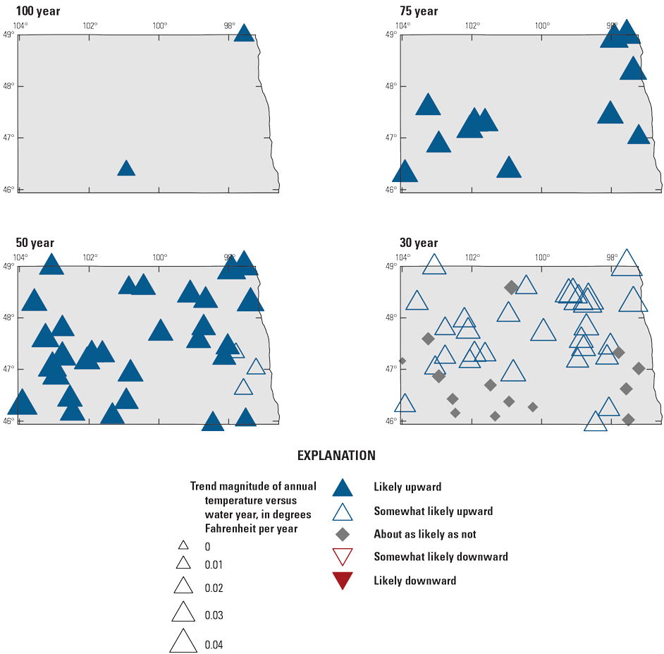
Maps showing likelihood and magnitude of annual temperature monotonic trends in the 100-, 75-, 50-, and 30-year analysis periods in North Dakota.
Annual Potential Evapotranspiration
The percentage of streamgages per likelihood category of trends in the ratio of PET and precipitation in the 100-, 75-, 50-, and 30-year analysis periods is listed in table 14. The likelihood and magnitude of trends in the ratio of annual PET and precipitation in the 100-, 75-, 50-, and 30-year analysis periods are shown in figure 27. Likely downward trends were detected mainly in the eastern area of the State in the 75- and 50-year analysis periods with magnitudes not substantially changing. Likely upward trends were detected in the southwestern area of the State in the 75- and 50-year analysis periods, and in the western and northeastern areas of the State in the 30-year analysis period. Trend magnitudes were larger in the 30-year analysis period. Likely upward trends indicate that annual PET (the numerator in the ratio) could be increasing or total annual precipitation (the denominator in the ratio) could be decreasing. Likewise, likely downward trends indicate that annual PET could be decreasing, or annual precipitation could be increasing.
Table 14.
Percentage of U.S. Geological Survey streamgages per likelihood category of monotonic trends in the ratio of annual potential evapotranspiration and precipitation in the 100-, 75-, 50-, and 30-year analysis periods in North Dakota.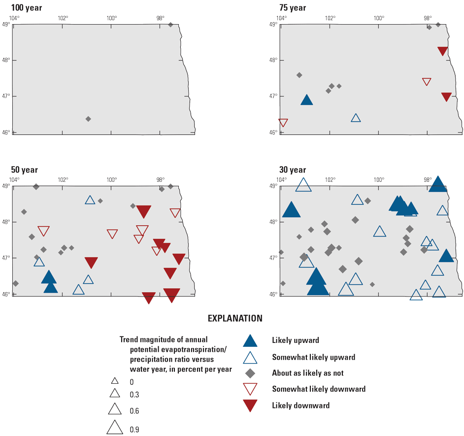
Maps showing likelihood and magnitude of monotonic trends in the ratio of annual potential evapotranspiration and precipitation in the 100-, 75-, 50-, and 30-year analysis periods in North Dakota.
Given the widespread increases in temperature (fig. 26), the upward trends in the ratio of annual PET to precipitation are indicative of the effect of increased temperature on PET. Annual precipitation indicated the largest and most frequent trends in the 50-year trend period were in eastern North Dakota (fig. 24), and that increase in precipitation results in the downward trends in the ratio of annual PET to precipitation in eastern North Dakota in the 50-year period (fig. 27).
Annual Snowfall
The percentage of streamgages per likelihood category of trends in the ratio of annual snowfall to annual precipitation in the 100-, 75-, 50-, and 30-year analysis periods is listed in table 15. The likelihood and magnitude of trends in the ratio of annual snowfall to annual precipitation each analysis period are shown in figure 28. Likely downward trends were detected throughout most of the State in the 100-, 75-, and 50-year analysis periods. These downward trends indicate that amounts of snowfall (the numerator in the ratio) have been decreasing and (or) the amounts of total annual precipitation (the denominator in the ratio) have been increasing during these analysis periods. Few trends were detected in the 30-year period, and the trends that were detected indicated likely upward and somewhat likely upward trends in the northwestern and south-central areas of the State.
Table 15.
Percentage of U.S. Geological Survey streamgages per likelihood category of monotonic trends in the ratio of annual snowfall and precipitation in the 100-, 75-, 50-, and 30-year analysis periods in North Dakota.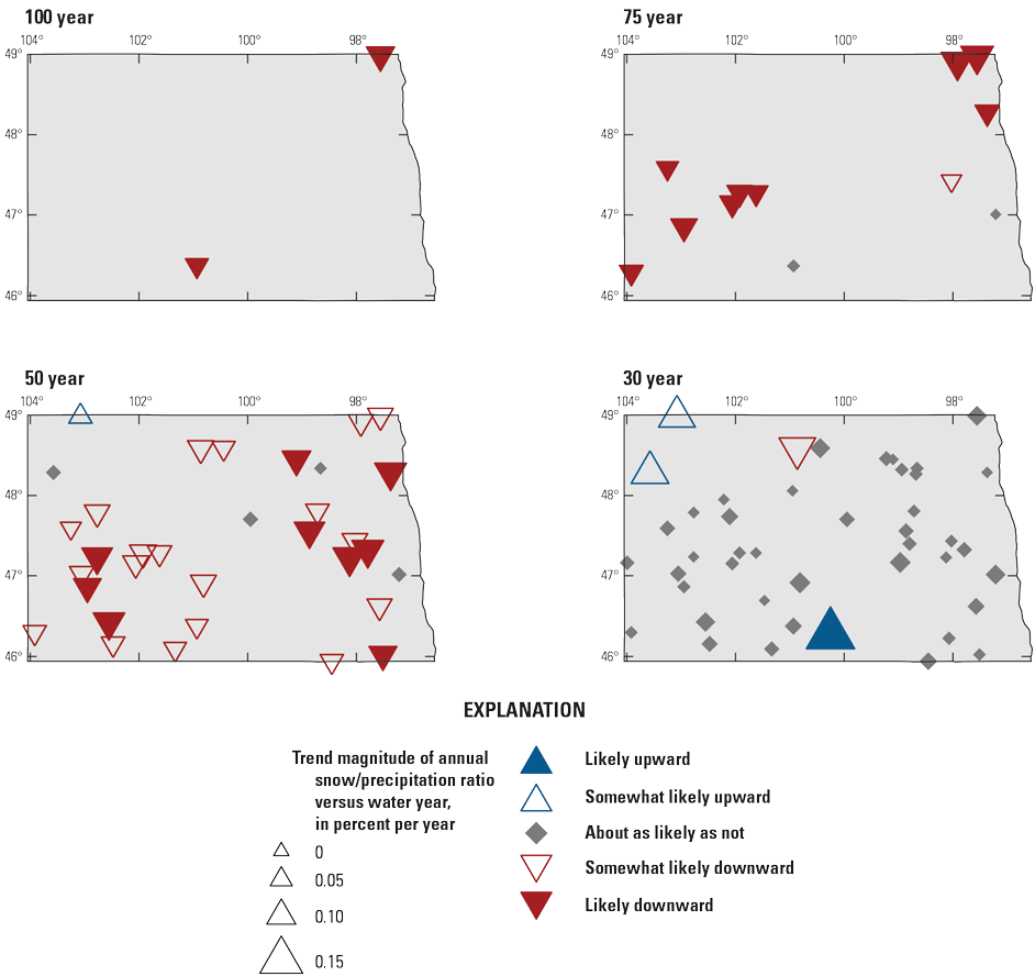
Maps showing likelihood and magnitude of monotonic trends in the ratio of annual snowfall and precipitation in the 100-, 75-, 50-, and 30-year analysis periods in North Dakota.
A decrease in snowfall or a decrease in the percentage of annual precipitation falling as snow could decrease the magnitude and frequency of snowmelt peaks and favor changes in flood regimes to a more bimodal distribution (fig. 16A), and more peaks would be generated by rain rather than accumulated snow. In an analysis of peak flow in the north-central United States, Ryberg and others (2016a) determined that the odds of peaks being in summer/fall, as opposed to peaks in spring/snowmelt, have increased.
Annual Soil Moisture
The percentage of streamgages per likelihood category of annual soil-moisture trends in the 100-, 75-, 50-, and 30-year analysis periods is listed in table 16. The likelihood and magnitude of annual soil-moisture trends in the 100-, 75-, 50-, and 30-year analysis periods are shown in figure 29. Likely upward trends were detected across the State in all analysis periods and were concentrated in the east in the 50-year analysis period and in the west in the 30-year analysis period. Likely downward trends were detected in the southwest in the 50-year analysis period (at one site) and in the northeast in the 30-year analysis period (two sites). Likely upward magnitudes increased slightly in the 50- and 30-year analysis periods. Likely downward magnitudes were largest in the 30-year analysis period. Likely upward trends indicate that annual soil moisture could be increasing because of increases in precipitation and decreases in PET and temperature. Likewise, likely downward trends indicate that annual soil moisture could be decreasing because of decreases in precipitation and increases in PET and temperature.
Table 16.
Percentage of U.S. Geological Survey streamgages per likelihood category of annual soil-moisture monotonic trends in the 100-, 75-, 50-, and 30-year analysis periods in North Dakota.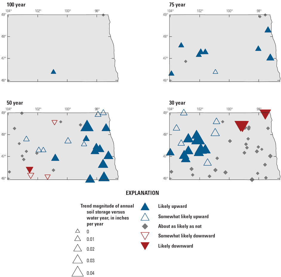
Maps showing likelihood and magnitude of annual soil-moisture monotonic trends in the 100-, 75-, 50-, and 30-year analysis periods in North Dakota.
The trends in soil moisture closely match the trends in annual precipitation (fig. 24). Saturated soils can carry over surplus moisture into the next year and play a substantial role in runoff and flood risk (Ryberg and others, 2007a, 2014; Knapp and others, 2023). In fact, modeling of high-flow events in the Upper Missouri River Basin indicates “acute runoff sensitivity to soil moisture in eastern sections of the basin” and wet antecedent soil conditions contributed to the extreme flood event of 2011 (Livneh and others, 2016, p. 3).
Synthesis of 50-Year Peak Streamflow and Climate Trends
The 50-year period is the period that balances the intersecting objectives of widespread spatial coverage for trends and the longest trend period possible. The pattern of monotonic (gradual) changes in peak flow in this period can be summarized as increased magnitude in the eastern half of the State and decreased magnitude in the western half of the State (fig. 13). For that same period, the ratio of annual snowfall to annual precipitation declined across the State. This pattern of decreased annual snowfall as a fraction of annual precipitation can be detected across the Northern Hemisphere; however, like in North Dakota, the resulting streamflow variation is complex (Han and others, 2024; Ryberg, 2024b).
Eastern parts of the State are in a snow climate (Köppen-Geiger classification system, major climate “snow”; Kottek and others, 2006) and typically have a pattern like that of figure 16, indicating that the highest frequency of occurrence of peak flow is in the spring, which is indicative of snowmelt (also refer to Ryberg and others, 2016a). Snowmelt peaks tend to be larger than rain-generated peaks (refer to figure 16 as an example and additional sites in the associated data release, Marti and others, 2024). However, in the eastern part of the State, flood magnitude increased, whereas snow as part of total precipitation declined. This can be explained by changes in annual and seasonal precipitation. In the 50-year trend period, annual precipitation increased (fig. 24); therefore, even if snow amounts held steady, the ratio of snow to total precipitation would still decline. In addition, summer and fall precipitation increased (fig. 25), but the ratio of annual PET and precipitation declined (fig. 27). Greater than normal precipitation in the fall and the resulting increase in soil moisture are factors that contribute to flooding in the eastern part of the State (Ryberg and others, 2007a), and increased soil moisture can be detected in the east (fig. 29). Moisture-surplus conditions carry over into the spring and can increase runoff and flood risk (Ryberg and others, 2014). Temperature and ET are important parts of the water balance as well, and results indicate that despite increased temperatures, the ratio of annual PET and precipitation has decreased (fig. 27), indicating that precipitation is a larger driver of observed peak-flow trends in the east than is temperature or ET. These results match those of Han and others (2024) for the Northern Hemisphere in that they determined that even though declining snowfall as a fraction of annual precipitation is often assumed to be related to changes in temperature, it is more closely related to changes in precipitation (Ryberg, 2024b).
For the western part of the State, annual and seasonal precipitation trends are mixed, temperature trends are upward, snowfall as a ratio of total precipitation is downward, and PET and snow moisture trends are mixed and have smaller magnitudes than the trends in the east. These factors combine to create conditions in which peak flow has declined. Central North Dakota is a transition zone to the arid climate on the western edge of the State (Köppen-Geiger classification system, major climate “arid”; Kottek and others, 2006), and in semiarid and arid basins, temperature plays a greater role in the water balance, as determined in a detailed study of the Little Missouri River of western North Dakota (Griffin and Friedman, 2017).
Uncertainty Monsters and Study Implications for Flood-Frequency Analysis
Nonstationary peak flows in North Dakota have implications for flood-frequency analysis. Flood-frequency analysis using current Federal guidance, Bulletin 17C (England and others, 2018), assumes that the peak-flow values used are independent and identically distributed. Trends, change points, and serial correlation are violations of these underlying assumptions. Peak-flow values are assumed to be representative of the population of interest, and changes in flooding regime seasonality and changes related to climate or land-use change violate this assumption. Despite the violations, when is standard flood-frequency analysis good enough? That is, how bad does a violation of one or more of the assumptions have to be (how large a change point for example) before one declares standard flood-frequency analysis results unacceptable? The current state of practice does not provide guidance on this. The numerous examples of assumption violations in North Dakota highlight that development of advanced flood-frequency analysis techniques is warranted.
Monsters as Metaphor for the Stationary-Nonstationary Choice
The choice of analysts and decision makers between stationary assumptions and analyses and nonstationary assumptions and analyses is commonly represented as a choice with mutually exclusive options, one of them having a great deal more uncertainty (in choice of methods, distributions, or explanatory variables). This binary choice itself is a source of uncertainty, and these kinds of mutually exclusive choices have been described as “uncertainty monsters.” In the metaphor of monsters, “a monster is understood as a phenomenon that at the same moment fits into two categories that were considered to be mutually excluding, such as knowledge versus ignorance, objective versus subjective, facts versus values, prediction versus speculation, science versus policy” (Van der Sluijs, 2005, p. 87). “In terms of philosophical pragmatism, a monster should be read as a so-called ‘problematic situation,’ a confusing situation in which a new phenomenon severely challenges our preliminary categories of judgment” (Smits, 2006, p. 501).
This metaphor of monsters for uncertainty has evolved from research on premodern ideas of technological doom and salvation (Douglas, 1975) to a monster theory of technology (Smits, 2002, 2006), to a monster theory of the science-policy interface (Van der Sluijs, 2005), to a metaphor for coping with uncertainty in flood-risk management (Knotters and others, 2024). The metaphor applies well to the flood-frequency analysis question of using stationary or nonstationary assumptions and methods.
Uncertainty monsters may be dealt with in six ways: “denial,” “exorcism,” “adaptation,” “embracement,” “assimilation,” or “anesthesia” (Smits, 2002, 2006; Van der Sluijs, 2005; Knotters and others, 202490). Monster denial could entail ignoring the problem, clinging to past investments (Bulletin 17C, England and others, 2018), or not reporting uncertainties. These actions might be described as the ostrich or Concorde effect or sunk cost fallacy (Knotters and others, 2024). Monster exorcism would entail reducing all uncertainties (get rid of the monster), but the theory predicts that this option is futile in the long run (Smits, 2002, 2006; Van der Sluijs, 2005). Climate science is an example of attempts to reduce uncertainties. As one source of uncertainty is addressed in climate models, science finds new complexities in a chaotic system (Van der Sluijs, 2005).
In monster adaptation, attempts are made to change the monster into something that better fits existing categories (Smits, 2002, 2006; Van der Sluijs, 2005). Again, climate science has been used as an example of this adaptation because, rather than reducing all the uncertainties, climate science has turned to scenarios (Van der Sluijs, 2005). Various scenarios are fed into models, and the choice is changed from best model and model parameters to a choice of what scenario is preferred or likely; the multiple results can cause new uncertainties. In flood-frequency analysis, one could generate multiple potential peak-flow series and produce multiple realizations of annual exceedance probabilities.
In monster assimilation, the mutually exclusive categories are rethought and the lack of a single truth is acknowledged (Smits, 2002, 2006; Van der Sluijs, 2005). Smits uses an example from medicine to describe the rethinking of mutually exclusive categories.
“… monster assimilation refers to a strategy of adapting not only the monster but also the cultural categories by which it is judged. An example from medical technology is the introduction of the notion of brain death. This notion came as an answer to the embarrassments about comatose patients and about organ transplantation in the late 1960s. At that time, many considered organ transplantation as a monstrous technology. One of its awkward qualities was the necessity to commit possible murder on a dying person in order to be able to use the organs. The medical professionals intervened by shifting the traditional definition of death as the definitive stopping of pulse and breathing to the definitive halt of brain activity” (Smits, 2006, p. 501).
In monster embracement, the complexities are fascinating, the uncertainties are to be pointed out to the detriment of a focus on the actual risk, and new methods are also embraced (Smits, 2002, 2006; Van der Sluijs, 2005). In monster anesthesia, consensus is key, and a panel or committee might decide the path forward, providing some psychological and organizational benefits, but the uncertainty remains (Knotters and others, 2024).
Knotters and others (2024) indicate that if the problem is well structured and simple, monster adaptation is the right choice. Statistical models can be applied, and uncertainties can be quantified. If a well-structured, complex problem exists, monster assimilation is the right choice. The uncertainties that can be quantified are quantified, the unquantifiable uncertainties are disclosed, and the uncertainties have a role in decision making (Knotters and others, 2024).
Implications for Flood-Frequency Analysis
Nonstationary flood-frequency analysis necessitates detailed exploratory data analysis and additional data and information about climate, land use, and other factors (Serinaldi and Kilsby, 2015). This study provides extensive exploratory analysis for peak flow and daily streamflow and climate data for North Dakota, setting the stage for informed nonstationary flood-frequency analysis. Attribution of the causes of nonstationarity is valuable because the driving mechanisms can be natural, such as long low-frequency climate signals; anthropogenic; or a mix (Khaliq and others, 2006; Vogel and others, 2011). One may be able to incorporate explanatory variables into a nonstationary model, and the types of models can depend on the distribution of or trends in the explanatory variable. An attribution study has been completed for streams in North Dakota (Sando and others, 2022), and that study informed this work and could be viewed in conjunction with the results here.
The many methodological choices for nonstationary flood-frequency analysis and the detailed additional analyses of explanatory data could become part of monster embracement if an analyst becomes overly enamored with the patterns in the data and the statistical intricacies of methods and overly focused on the minutiae of sources of uncertainty. However, the path through the data and methods may be one of monster assimilation, adaptation, or both. No one nonstationary flood-frequency analysis method is likely applicable to all studies, and multiple scenarios from multiple models and future estimates of peak flow may be useful in making design decisions.
Historical and paleoflood data can help place some nonstationarities in a broader context and improve flood-frequency analysis, and such data can represent floods from a different climate or different channel conditions and complicate flood-frequency analysis (Benito and others, 2004; Harden and others, 2011; Ryberg and others, 2020b). Bulletin 17C provided advancements for the inclusion of historical and paleoflood data (England and others, 2018), and these additional data can be used in a scenario approach (monster adaptation) to assess the fit of flood-frequency curves for rare floods (Ryberg and others, 2020b). This option is limited because historical and paleoflood data are available for a small subset of sites, and a comprehensive paleoflood study might require a team of geomorphologists, hydraulic modelers, hydrologists, and surveyors (Harden and others, 2021). Detailed analysis of past meteorological conditions is also essential and depends on reconstructions of data (Benito and others, 2004) that may be technically or cost prohibitive.
Numerous advanced techniques have been suggested (monster embracement; Cunderlik and Burn, 2003; Khaliq and others, 2006; Villarini and others, 2009b; Gilroy and McCuen, 2012; O’Brien and Burn, 2014; Machado and others, 2015; Tan and Gan, 2015; Debele and others, 2017; Luke and others, 2017; Razmi and others, 2017; Serago and Vogel, 2018; Yan and others, 2019; Hecht and Vogel, 2020; Vogel and Kroll, 2020; Awasthi and others, 2022; Hecht and others, 2022). Limited testing has determined that stationary analysis could still be preferred, and nonstationary models commonly are not an improvement, but the use of nonstationary models to update parameters for stationary models may be preferred for physically changing basins (Luke and others, 2017). This last possibility could be seen as monster assimilation: update the model parameters with new, current information and then use the stationary method, thereby blurring the stark stationary-nonstationary choice.
When embracing the monster, some of the suggested nonstationary methods are statistically complex, discouraging widespread adoption. In addition, when one goes outside the framework of Bulletin 17C, the method may require one to choose a different statistical distribution for the data or compare multiple distributions (Debele and others, 2017); this too is a discouragement to widespread adoption. A promising step toward addressing nonstationarity and assimilating the monster may be explaining the nonstationary behaver with an exogenous variable and then generating conditional mean, variance, and skew with which to complete stationary flood-frequency analysis (Khaliq and others, 2006; Serago and Vogel, 2018). Generalized additive models for location, scale, and shape (known as GAMLSS) can also incorporate explanatory variables and provide a flexible framework for modeling nonstationarities because they can model abrupt changes and trends (Villarini and others, 2009a, b; Machado and others, 2015). However, the flexibility comes with more choices for the analyst in terms of statistical distributions and explanatory variables.
Serially correlated, or dependent, peak flows violate the assumptions of conventional flood-frequency analysis. Several methods have been suggested to adjust for serial correlation, including decorrelation or prewhitening; modeling the short- and long-term persistence; or thinning the observations (Lettenmaier, 1976; Burn and Goel, 2001; Khaliq and others, 2006). One challenge is that serially correlated observations result in an effective record length that can be much shorter than the observed record length (Burn and Goel, 2001); therefore, thinning, or otherwise using fewer of the data in the series, results in small sample size problems (Khaliq and others, 2006).
The changes in seasonality and extended periods of high flow, as shown in raster plots, indicate that using only the annual maximum series, peak flow, leaves many floods out of the analysis. A POT approach would include multiple floods in some years (and none in others) that are greater than a particular threshold. A POT approach can have less bias for frequent floods, and using more of the data seems reasonable, making a POT approach seem like a way to have a well-structured and simple method, or monster adaptation. However, the POT approach has been underused mainly because of the challenge of selecting a threshold and a minimum separation time that ensure independent peaks that meet distributional assumptions and provide enough data for estimation of parameters (Khaliq and others, 2006; Pan and others, 2022).
Results of this study indicate that the patterns in nonstationarity have spatial or temporal cohesiveness, such as the opposing trends in North Dakota east and west of the 100th meridian and increases in peak flow in the 1990s in eastern North Dakota. These regional patterns can indicate linkages to low-frequency climate effects, such as El Niño-Southern Oscillation, Pacific Decadal Oscillation, North Atlantic Oscillation, or Atlantic Multidecadal Oscillation. Researchers have attempted to document these linkages, but they are complex given the varying time scales, differing seasonal patterns in precipitation and temperature, and their interactions (Wang and others, 2016; Dickinson and others, 2019; Collins and others, 2022). A panel regression model can incorporate explanatory variables that have fixed effects or vary across space and time and therefore could have a regional component (Khaliq and others, 2006; Ferreira and Ghimire, 2012; Over and others, 2016; Blum and others, 2020) and might be an example of monster assimilation. Modeling regional components of flood behavior can be particularly useful given short record lengths at some sites (Khaliq and others, 2006).
Some proposed methods can incorporate climate projections (such as Awasthi and others [2022]) and follow the monster adaptation approach of creating flood-risk scenarios. Parameters of a statistical distribution can be estimated using explanatory variables, such as rainfall and temperature. Once such a model is developed, projected precipitation and temperature could be used to project flood-frequency estimates under future climate scenarios. Awasthi and others (2022) developed a process to do this; however, they determined that model estimates were better in humid basins and did not work as well in arid basins. This finding is common in hydrologic modeling because rainfall runoff in arid and semiarid areas has a nonlinear relation; precipitation is more variable in space and time than in humid regions and hydrological processes differ (such as less base flow and more channel losses than in humid areas; Pilgrim and others, 1988; Jin and others, 2022). As determined by the natural state of Devils Lake being rising or falling and as described by Pilgrim and others (1988, p. 381), “arid zones (and especially semiarid zones) are often in a delicate hydrological balance. The whole nature of the hydrology (and hence values of model parameters) may be changed by a prolonged wet or dry sequence.”
Finally, if a causal mechanism for the nonstationarities cannot be identified, as is sometimes the case (Barth and others, 2022; Sando and others, 2022; York and others, 2022), a model other than the conventional stationary model introduces additional uncertainty (Serinaldi and Kilsby, 2015). When the cause of the nonstationarity is unknown, the stationary model can provide the best estimates provided uncertainty and other safety factors are taken into consideration (Serinaldi and Kilsby, 2015).
Summary
Flood-frequency analysis is essential to water-resources management applications, including critical structure design (for example, bridges and culverts) and floodplain mapping. Standardized guidelines for completing flood-flow frequency analyses are presented in a U.S. Geological Survey Techniques and Methods report known as Bulletin 17C, https://doi.org/10.3133/tm4B5. In recent decades, a better understanding of long-term climatic persistence (extended periods of relatively wet or relatively dry conditions) and concerns about potential climate change and land-use change have caused a reexamination of the stationarity assumptions underlying methods in Bulletin 17C. Not incorporating observed trends into flood-frequency analysis can result in a poor representation of the true flood risk. However, Bulletin 17C does not offer guidance on how to incorporate nonstationarities when estimating floods and further identifies a need for additional flood-frequency studies that incorporate changing climate or basin characteristics into the analysis.
As part of that reexamination, a study of nonstationarities in peak flows (trends, change points, and autocorrelation) has begun in the Midwest. This chapter of the study summarizes how hydroclimatic variability affects the temporal and spatial distributions of peak-flow data in the State of North Dakota. Because of North Dakota’s highly variable precipitation and temperature regimes, along with sensitivity to ET, and varying ecoregions, North Dakota is an ideal area for investigating potential nonstationary peak-flow frequency methodologies.
In this analysis of North Dakota peak flow, daily streamflow, and climate metrics, four periods were selected for analysis: (1) a 100-year period, 1921–2020; (2) a 75-year period, 1946–2020; (3) a 50-year period, 1971–2020; and (4) a 30-year period, 1991–2020. Streamgages were screened for potential regulation by dams or water diversions using existing streamflow qualification codes within the U.S. Geological Survey National Water Information System database and a dimensionless dam impact metric to focus on hydroclimatic variability. Output from a monthly water-balance model for 1900–2020 was used for the climate data in this study. Statistical analysis of peak flow consisted of evaluation of autocorrelation, trends, and change points—all recommended initial data analysis for Bulletin 17C flood-frequency analysis—and was augmented with analyses of seasonality. Statistical analysis of daily streamflow consisted of graphical and statistical evaluations of seasonality, center of volume, and peaks-over-threshold (POT) analysis.
The long-term pattern of decreasing peak flow in the west and increasing peak flow in the east is a pattern of opposing signals on either side of the 100th meridian, and this pattern has been observed in the Third National Climate Assessment, https://nca2014.globalchange.gov/highlights/report-findings/extreme-weather#intro-section, the Fifth National Climate Assessment, https://doi.org/10.7930/NCA5.2023.CH25, and in other studies. Past related work determined eastern North Dakota was experiencing increased peak flow and positive trends in annual precipitation and that most streamgages with significant downward trends had significant positive trends in annual air temperature.
Changes in daily streamflow were analyzed to improve understanding of some of the patterns in peak flows. Peak-flow timing analysis and raster seasonality plots of daily streamflow indicate that a key factor in change in North Dakota hydroclimatology is in the increase in fall precipitation, particularly in the most recent period. Trends in climate metrics indicate precipitation, temperature, and PET patterns that explain the patterns in peak flow and daily streamflow. The trends in soil moisture closely match the trends in annual precipitation.
Nonstationary peak flows in North Dakota, and their causes, have implications for flood-frequency analysis. The choice between stationary assumptions and analyses and nonstationary assumptions and analyses is commonly represented as a choice with mutually exclusive options, one of them having a great deal more uncertainty (in choice of methods, distributions, or explanatory variables). This binary choice itself is a source of uncertainty, and these kinds of mutually exclusive choices have been described metaphorically as “uncertainty monsters.”
Uncertainty monsters may be dealt with through “denial,” “exorcism,” “adaptation,” “embracement,” “assimilation,” or “anesthesia.” If we can structure the flood-frequency analysis problem well and in a straightforward way, monster adaptation may be the best option. Statistical models can be applied and uncertainties can be quantified. If we can structure the flood-frequency analysis problem well but with notable uncertainties, monster assimilation may be the best option. The uncertainties that can be quantified are, the unquantifiable uncertainties are disclosed, and the uncertainties have a role in decision making.
Nonstationary flood-frequency analysis necessitates detailed exploratory data analysis and additional data and information about climate, land use, and other factors. This study provides extensive exploratory analysis for peak flow, daily streamflow, and climate data for North Dakota, setting the stage for informed nonstationary flood-frequency analysis. Attribution of the causes of nonstationarity is valuable because the driving mechanisms can be natural, such as low-frequency climate signals; anthropogenic; or a mix. One may be able to incorporate explanatory variables into a nonstationary model, and the types of models may depend on the distribution of or trends in the explanatory variable. No one nonstationary flood-frequency analysis method is likely applicable in all situations, and multiple scenarios from multiple models and future estimates of peak flow may be useful in making design decisions.
Historical and paleoflood data can help place some nonstationarities in a broader context and improve flood-frequency analysis. When an analyst goes outside the framework of Bulletin 17C, the method may require one to choose a different statistical distribution for the data or compare multiple distributions, which can discourage widespread adoption. One promising step toward addressing nonstationarity and assimilating the uncertainty monster may be explaining the nonstationary behavior with an exogenous variable and then generating conditional mean, variance, and skew with which to complete stationary flood-frequency analysis. Generalized additive models for location, scale, and shape can also incorporate explanatory variables and provide a flexible framework for modeling nonstationarities because they can model abrupt changes and trends. The changes in seasonality and extended periods of high flow, as shown in raster plots, indicate that using only the annual maximum series of peak flow leaves numerous floods out of the analysis. A POT approach would include multiple floods in some years (and none in others) that are greater than a particular threshold. A POT approach can have less bias for frequent floods, but this approach has been underused mainly because of the challenge of selecting a threshold and a minimum separation time that ensure independent peaks that meet distributional assumptions and provide enough data for estimation of parameters.
Results of this study indicate that the patterns in nonstationarity have spatial cohesiveness or temporal cohesiveness, such as the opposing trends in North Dakota east and west of the 100th meridian and increases in peak flow in the 1990s in eastern North Dakota. These regional patterns may indicate linkages to low-frequency climate effects, such as El Niño-Southern Oscillation, Pacific Decadal Oscillation, North Atlantic Oscillation, or Atlantic Multidecadal Oscillation. Researchers have attempted to document these linkages, but they are complex given the varying time scales, differing seasonal patterns in precipitation and temperature, and their interactions. A panel regression model can incorporate explanatory variables that have fixed effects or vary across space and time and therefore could have a regional component. Some proposed methods to integrate climate change into flood-frequency analysis can incorporate climate projections and could be used to create scenarios.
Finally, if a mechanism for the nonstationarities cannot be identified, a model other than the conventional stationary model introduces additional uncertainty because the nonstationarity might be related to something other than climate change (such as land-use change). When the cause of the nonstationarity is unknown, the stationary model can provide the best estimates provided uncertainty and other safety factors are taken into consideration.
References Cited
Ahiablame, L., Sheshukov, A.Y., Rahmani, V., and Moriasi, D., 2017, Annual baseflow variations as influenced by climate variability and agricultural land use change in the Missouri River Basin: Journal of Hydrology, v. 551, p. 188–202. [Also available at https://doi.org/10.1016/j.jhydrol.2017.05.055.]
Anderson, D., 1966, Red River Flood—1852—An excerpt from Bishop David Anderson’s book notes of the Flood at Red River, 1852: Manitoba Pageant, v. 11, no. 3, unpaginated, accessed December 31, 2024, at http://www.mhs.mb.ca/docs/pageant/11/redriverflood1852.shtml.
Archambault, A.L., Mahmood, T.H., Todhunter, P.E., and Korom, S.F., 2023, Remotely sensed surface water variations during drought and deluge conditions in a Northern Great Plains terminal lake basin: Journal of Hydrology—Regional Studies, v. 47, article 101392, 19 p., accessed December 28, 2023, at https://doi.org/10.1016/j.ejrh.2023.101392.
Atashi, V., Mahmood, T.H., and Rasouli, K., 2023, Impacts of climatic variability on surface water area observed by remotely sensed imageries in the Red River Basin: Geocarto International, v. 38, no. 1, article 2209541, 21 p., accessed December 28, 2023, at https://doi.org/10.1080/10106049.2023.2209541.
Ault, T.R., and St. George, S., 2010, The magnitude of decadal and multidecadal variability in North American precipitation: Journal of Climate, v. 23, no. 4, p. 842–850. [Also available at https://doi.org/10.1175/2009JCLI3013.1.]
Awasthi, C., Archfield, S.A., Ryberg, K.R., Kiang, J.E., and Sankarasubramanian, A., 2022, Projecting flood frequency curves under near‐term climate change: Water Resources Research, v. 58, no. 8, article e2021WR031246, 21 p., accessed August 12, 2022, at https://doi.org/10.1029/2021WR031246.
Badger, A.M., Livneh, B., Hoerling, M.P., and Eischeid, J.K., 2018, Understanding the 2011 Upper Missouri River Basin floods in the context of a changing climate: Journal of Hydrology—Regional Studies, v. 19, p. 110–123. [Also available at https://doi.org/10.1016/j.ejrh.2018.08.004.]
Barth, N.A., and Sando, S.K., 2024, Peak streamflow trends in South Dakota and their relation to changes in climate, water years 1921–2020, chap. I of Ryberg, K.R., comp., Peak streamflow trends and their relation to changes in climate in Illinois, Iowa, Michigan, Minnesota, Missouri, Montana, North Dakota, South Dakota, and Wisconsin: U.S. Geological Survey Scientific Investigations Report 2023–5064, 70 p. [Also available at https://doi.org/10.3133/sir20235064I.]
Barth, N.A., Ryberg, K.R., Gregory, A., and Blum, A.G., 2022, Introduction to attribution of monotonic trends and change points in peak streamflow across the conterminous United States using a multiple working hypotheses framework, 1941–2015 and 1966–2015, chap. A of Ryberg, K.R., ed., Attribution of monotonic trends and change points in peak streamflow across the conterminous United States using a multiple working hypotheses framework, 1941–2015 and 1966–2015: U.S. Geological Survey Professional Paper 1869, p. A1–A29, accessed October 4, 2022, at https://doi.org/10.3133/pp1869.
Benito, G., Lang, M., Barriendos, M., Llasat, M.C., Francés, F., Ouarda, T., Thorndycraft, V., Enzel, Y., Bardossy, A., Coeur, D., and Bobée, B., 2004, Use of systematic, palaeoflood and historical data for the improvement of flood risk estimation—Review of scientific methods: Natural Hazards, v. 31, no. 3, p. 623–643. [Also available at https://doi.org/10.1023/B:NHAZ.0000024895.48463.eb.]
The Bismarck Tribune, 1881, Missouri’s grand bust—A break-up that wipes out previous records: The Bismarck Tribune, April 1, 1881, p. 1, accessed March 7, 2024, at https://chroniclingamerica.loc.gov/lccn/sn85042331/1881-04-01/ed-1/seq-1/.
The Bismarck Tribune, 1882a, Drowned Fargo: The Bismarck Tribune, April 14, 1882, p. 4, accessed March 7, 2024, at https://chroniclingamerica.loc.gov/lccn/sn85042331/1882-04-14/ed-1/seq-4/.
The Bismarck Tribune, 1882b, Furious floods at Fargo: The Bismarck Tribune, April 14, 1882, p. 7, accessed March 7, 2024, https://chroniclingamerica.loc.gov/lccn/sn85042331/1882-04-14/ed-1/seq-7/.
Bluemle, J.P., 1991, Radiocarbon dating of beaches and outlets of Devils Lake: North Dakota Geological Survey Miscellaneous Series no. 75, 10 p., accessed June 5, 2024, at https://www.dmr.nd.gov/ndgs/documents/Publication_List/pdf/MiscSeries/MS-75.pdf.
Bluemle, J.P., 1996, From the state geologist: North Dakota Geological Survey Newsletter, v. 23, no. 1, p. 1–2, accessed December 22, 2020, at https://www.dmr.nd.gov/ndgs/outofprint/NewsLetters/1996Spring.pdf.
Blum, A.G., Ferraro, P.J., Archfield, S.A., and Ryberg, K.R., 2020, Causal effect of impervious cover on annual flood magnitude for the United States: Geophysical Research Letters, v. 47, no. 5, article e2019GL086480, 10 p., accessed March 5, 2020, at https://doi.org/10.1029/2019GL086480.
Bryce, S.A., Omernik, J.M., Pater, D.E., Ulmer, M., Schaar, J., Freeouf, J., Johnson, R., Kuck, P., and Azevedo, S.H., [undated], Ecoregions of North Dakota and South Dakota: U.S. Environmental Protection Agency, scale 1:1,500,000, accessed December 1, 2021, at https://gaftp.epa.gov/EPADataCommons/ORD/Ecoregions/nd/ndsd_front.pdf.
Bureau of Reclamation, 2012, Missouri River Basin depletions database—Great Plains Region: Bureau of Reclamation, 97 p., accessed November 29, 2018, at https://www.usbr.gov/gp/dkao/naws/FSEIS/missouri_river_basin_depletions_database.pdf.
Burn, D.H., and Goel, N.K., 2001, Flood frequency analysis for the Red River at Winnipeg: Canadian Journal of Civil Engineering, v. 28, no. 3, p. 355–362. [Also available at https://doi.org/10.1139/l00-122.]
Callender, E., 1968, The postglacial sedimentology of Devils Lake, North Dakota: Grand Forks, N. Dak., University of North Dakota, Ph.D. dissertation, 312 p., accessed June 5, 2024, at https://commons.und.edu/theses/46/.
Canada Department of Resources and Development, 1953a, Appendix B—History of floods on the Red River, in Report on investigations into measures for the reduction of the flood hazard in the greater Winnipeg area: Water Resources Division, Engineering and Water Resources Branch, Ottawa, Ontario, Canada, 106 p.
Carlyle, W.J., 1984, Water in the Red River Valley of the North: Geographical Review, v. 74, no. 3, p. 331–358. [Also available at https://doi.org/10.2307/214943.]
Case, R.A., and MacDonald, G.M., 2003, Tree ring reconstructions of streamflow for three Canadian Prairie rivers: Journal of the American Water Resources Association, v. 39, no. 3, p. 703–716. [Also available at https://doi.org/10.1111/j.1752-1688.2003.tb03686.x.]
Cayan, D.R., Dettinger, M.D., Diaz, H.F., and Graham, N.E., 1998, Decadal variability of precipitation over western North America: Journal of Climate, v. 11, no. 12, p. 3148–3166. [Also available at https://doi.org/10.1175/1520-0442(1998)011<3148:DVOPOW>2.0.CO;2.]
Cohn, T.A., and Lins, H.F., 2005, Nature’s style—Naturally trendy: Geophysical Research Letters, v. 32, no. 23, 5 p. [Also available at https://doi.org/10.1029/2005GL024476.]
Collins, M.J., Hodgkins, G.A., Archfield, S.A., and Hirsch, R.M., 2022, The occurrence of large floods in the United States in the modern hydroclimate regime—Seasonality, trends, and large-scale climate associations: Water Resources Research, v. 58, no. 2, article e2021WR030480, 22 p., accessed March 17, 2023, at https://doi.org/10.1029/2021WR030480.
Commission for Environmental Cooperation, [undated], Ecological regions of North America—Level I: Commission for Environmental Cooperation, 1 sheet [scale not given], accessed October 3, 2022, at https://gaftp.epa.gov/EPADataCommons/ORD/Ecoregions/cec_na/NA_LEVEL_I.pdf.
Crosby, O.A., 1970, A proposed streamflow-data program for North Dakota: U.S. Geological Survey Open-File Report 70–91, 77 p., accessed July 11, 2022, at https://doi.org/10.3133/ofr7091.
Crosby, O.A., 1975, Magnitude and frequency of floods in small drainage basins in North Dakota: U.S. Geological Survey Water-Resources Investigations Report 19–75, 31 p., accessed June 15, 2021, at https://doi.org/10.3133/wri1975.
Cunderlik, J.M., and Burn, D.H., 2003, Non-stationary pooled flood frequency analysis: Journal of Hydrology, v. 276, no. 1–4, p. 210–223. [Also available at https://doi.org/10.1016/S0022-1694(03)00062-3.]
Debele, S.E., Strupczewski, W.G., and Bogdanowicz, E., 2017, A comparison of three approaches to non-stationary flood frequency analysis: Acta Geophysica, v. 65, no. 4, p. 863–883. [Also available at https://doi.org/10.1007/s11600-017-0071-4.]
Dewitz, J., 2019, National Land Cover Database (NLCD) 2016 products (ver. 2.0, July 2020): U.S. Geological Survey data release, accessed October 3, 2022, at https://doi.org/10.5066/P96HHBIE.
Dickinson, J.E., Harden, T.M., and McCabe, G.J., 2019, Seasonality of climatic drivers of flood variability in the conterminous United States: Scientific Reports, v. 9, no. 1, article 15321, 10 p., accessed February 17, 2022, at https://doi.org/10.1038/s41598-019-51722-8.
Digital Horizons, 2024, Digital horizons—Life on the Northern Plains: Digital Horizons web page, accessed March 7, 2024, at https://digitalhorizonsonline.org/.
Dillow, J.J.A., McCallum, B.E., and Angeroth, C.E., 2023, Re-prioritization of the U.S. Geological Survey Federal Priority Streamgage Network, 2022: U.S. Geological Survey Open-File Report 2023–1032, 7 p., accessed March 29, 2024, at https://doi.org/10.3133/ofr20231032.
Dudley, R.W., Archfield, S.A., Hodgkins, G.A., Renard, B., and Ryberg, K.R., 2018, Basin characteristics and peak-streamflow trends and change-points for 2,683 USGS streamgages in the conterminous U.S.: U.S. Geological Survey data release, accessed June 6, 2019, at https://doi.org/10.5066/P9AEGXY0.
England, J.F., Jr., Cohn, T.A., Faber, B.A., Stedinger, J.R., Thomas, W.O., Jr., Veilleux, A.G., Kiang, J.E., and Mason, R.R., Jr., 2018, Guidelines for determining flood flow frequency—Bulletin 17C (ver. 1.1, May 2019): U.S. Geological Survey Techniques and Methods, book 4, chap. B5, 148 p., accessed May 5, 2022, at https://doi.org/10.3133/tm4B5.
Environment and Climate Change Canada, 2013, Flooding events in Canada—Prairie provinces: Environment and Climate Change Canada web page, accessed March 22, 2024, at https://www.canada.ca/en/environment-climate-change/services/water-overview/quantity/floods/events-prairie-provinces.html.
Enz, J.W., 2003, North Dakota topographic, climatic, and agricultural overview: North Dakota State University, North Dakota Climate Office document, 3 p., accessed June 26, 2024, at https://www.ndsu.edu/fileadmin/ndsco/documents/ndclimate.pdf.
Falcone, J.A., Murphy, J.C., and Sprague, L.A., 2018, Regional patterns of anthropogenic influences on streams and rivers in the conterminous United States, from the early 1970s to 2012: Journal of Land Use Science, v. 13, no. 6, p. 585–614. [Also available at https://doi.org/10.1080/1747423X.2019.1590473.]
Ferreira, S., and Ghimire, R., 2012, Forest cover, socioeconomics, and reported flood frequency in developing countries: Water Resources Research, v. 48, no. 8, article WR011701, 13 p., accessed March 28, 2024, at https://doi.org/10.1029/2011WR011701.
Fisher, T.G., Lepper, K., Ashworth, A.C., and Hobbs, H.C., 2011, Southern outlet and basin of glacial Lake Agassiz, in Miller, J.D., Hudak, G.J., Wittkop, C., and McLaughlin, P.I., eds., Archean to Anthropocene—Field guides to the geology of the mid-continent of North America: Geological Society of America, p. 379–400. [Also available at https://doi.org/10.1130/2011.0024(17).]
Frankson, R., Kunkel, K.E., Stevens, L.E., Easterling, D.R., Shulski, M., and Akyüz, A., 2017, North Dakota state climate summary: National Oceanic and Atmospheric Administration Technical Report NESDIS 149–ND, 4 p., accessed June 24, 2021, at https://statesummaries.ncics.org/chapter/nd/.
Frankson, R., Kunkel, K.E., Stevens, L.E., Easterling, D.R., Shulski, M., Akyüz, A., Umphlett, N.A., and Stiles, C.J., 2022, North Dakota state climate summary 2022: National Oceanic and Atmospheric Administration/National Environmental Satellite, Data, and Information Service Technical Report NESDIS 150–ND, 5 p., accessed January 31, 2022, at https://statesummaries.ncics.org/chapter/nd/.
Garbrecht, J.D., and Rossel, F.E., 2002, Decade-scale precipitation increase in Great Plains at end of 20th century: Journal of Hydrologic Engineering, v. 7, no. 1, p. 64–75. [Also available at https://doi.org/10.1061/(ASCE)1084-0699(2002)7:1(64).]
Georgakakos, A., Fleming, P., Dettinger, M., Peters-Lidard, C., Richmond, T.C., Reckhow, K., White, K., and Yates, D., 2014, Water resources, chap. 3 of Melillo, J.M., Richmond, T.C., and Yohe, G.W., eds., Climate change impacts in the United States—The Third National Climate Assessment: Washington, D.C., U.S. Global Change Research Program, p. 69–112.
Gilroy, K.L., and McCuen, R.H., 2012, A nonstationary flood frequency analysis method to adjust for future climate change and urbanization: Journal of Hydrology, v. 414–415, p. 40–48. [Also available at https://doi.org/10.1016/j.jhydrol.2011.10.009.]
Government of Canada, 2013, Manitoba—Red River floods: Government of Canada web page, accessed July 11, 2022, at https://www.canada.ca/en/environment-climate-change/services/water-overview/quantity/floods/events-prairie-provinces.html#MB.
Government of Canada, 2022, Environment Canada streamflow data, 1860-: Government of Canada web page, accessed July 11, 2022, at https://open.canada.ca/data/en/dataset/d7601729-972d-41e6-b126-1d187641010f.
Griffin, E.R., and Friedman, J.M., 2017, Decreased runoff response to precipitation, Little Missouri River Basin, northern Great Plains, USA: Journal of the American Water Resources Association, v. 53, no. 3, p. 576–592. [Also available at https://doi.org/10.1111/1752-1688.12517.]
Gupta, S.C., Kessler, A.C., Brown, M.K., and Zvomuya, F., 2015, Climate and agricultural land use change impacts on streamflow in the upper midwestern United States: Water Resources Research, v. 51, no. 7, p. 5301–5317. [Also available at https://doi.org/10.1002/2015WR017323.]
Haffield, N.D., 1981, Statistical summaries of streamflow and water-quality data for streams of western North Dakota, 1977–80: U.S. Geological Survey Open-File Report 81–1066, 88 p., accessed July 11, 2022, at https://doi.org/10.3133/ofr811066.
Han, J., Liu, Z., Woods, R., McVicar, T.R., Yang, D., Wang, T., Hou, Y., Guo, Y., Li, C., and Yang, Y., 2024, Streamflow seasonality in a snow-dwindling world: Nature, v. 629, no. 8014, p. 1075–1081. [Also available at https://doi.org/10.1038/s41586-024-07299-y.]
Hanson, R.L., 1991, Evapotranspiration and droughts, in Paulson, R.W., Chase, E.B., Roberts, R.S., and Moody, D.W., comps., National water summary 1988–89—Hydrologic events and floods and droughts: Reston, Va., U.S. Geological Survey, p. 99–104, accessed December 23, 2023, at https://doi.org/10.3133/wsp2375.
Harden, T.M., O’Connor, J.E., Driscoll, D.G., and Stamm, J.F., 2011, Flood-frequency analyses from paleoflood investigations for Spring, Rapid, Boxelder, and Elk Creeks, Black Hills, western South Dakota: U.S. Geological Survey Scientific Investigations Report 2011–5131, 136 p., accessed September 30, 2016, at https://doi.org/10.3133/sir20115131.
Harden, T.M., Ryberg, K.R., O’Connor, J.E., Friedman, J.M., and Kiang, J.E., 2021, Historical and paleoflood analyses for probabilistic flood-hazard assessments—Approaches and review guidelines: U.S. Geological Survey Techniques and Methods, book 4, chap. B6, 91 p., accessed July 11, 2024, at https://doi.org/10.3133/tm4B6.
Healy, R.W., Winter, T.C., LaBaugh, J.W., and Franke, O.L., 2007, Water budgets—Foundations for effective water-resources and environmental management: U.S. Geological Survey Circular 1308, 90 p., accessed December 23, 2023, at https://doi.org/10.3133/cir1308.
Hecht, J.S., Barth, N.A., Ryberg, K.R., and Gregory, A.E., 2022, Simulation experiments comparing nonstationary design-flood adjustments based on observed annual peak flows in the conterminous United States: Journal of Hydrology X, v. 17, article 100115, 24 p., accessed May 4, 2023, at https://doi.org/10.1016/j.hydroa.2021.100115.
Hecht, J.S., and Vogel, R.M., 2020, Updating urban design floods for changes in central tendency and variability using regression: Advances in Water Resources, v. 136, article 103484, 14 p., accessed July 18, 2022, at https://doi.org/10.1016/j.advwatres.2019.103484.
Helsel, D.R., Hirsch, R.M., Ryberg, K.R., Archfield, S.A., and Gilroy, E.J., 2020, Statistical methods in water resources: U.S. Geological Survey Techniques and Methods, book 4, chap. A3, 458 p., accessed September 19, 2023, at https://doi.org/10.3133/tm4A3.
Hendricks, E.L., 1964, Compilation of records of surface waters of the United States, October 1950 to September 1960, part 6–A—Missouri River basin above Sioux City, Iowa: U.S. Geological Survey Water Supply Paper 1729, 507 p., 1 plate, accessed March 25, 2024, at https://doi.org/10.3133/wsp1729.
Hirsch, R.M., Archfield, S.A., and De Cicco, L.A., 2015, A bootstrap method for estimating uncertainty of water quality trends: Environmental Modelling & Software, v. 73, p. 148–166. [Also available at https://doi.org/10.1016/j.envsoft.2015.07.017.]
Hirsch, R.M., and Ryberg, K.R., 2012, Has the magnitude of floods across the USA changed with global CO2 levels?: Hydrological Sciences Journal, v. 57, no. 1, p. 1–9. [Also available at https://doi.org/10.1080/02626667.2011.621895.]
Hodgkins, G.A., Dudley, R.W., Archfield, S.A., and Renard, B., 2019, Effects of climate, regulation, and urbanization on historical flood trends in the United States: Journal of Hydrology, v. 573, p. 697–709. [Also available at https://doi.org/10.1016/j.jhydrol.2019.03.102.]
Hodgkins, G.A., Whitfield, P.H., Burn, D.H., Hannaford, J., Renard, B., Stahl, K., Fleig, A.K., Madsen, H., Mediero, L., Korhonen, J., Murphy, C., and Wilson, D., 2017, Climate-driven variability in the occurrence of major floods across North America and Europe: Journal of Hydrology, v. 552, p. 704–717. [Also available at https://doi.org/10.1016/j.jhydrol.2017.07.027.]
Hoerling, M., Eischeid, J., and Webb, R., 2013, Understanding and explaining climate extremes in the Missouri River Basin associated with the 2011 flooding: National Oceanic and Atmospheric Administration Climate Assessment Report, 28 p., accessed August 16, 2019, at https://psl.noaa.gov/csi/factsheets/pdf/noaa-mrb-climate-assessment-report.pdf.
Hoogestraat, G.K., and Stamm, J.F., 2015, Climate and streamflow characteristics for selected streamgages in eastern South Dakota, water years 1945–2013: U.S. Geological Survey Scientific Investigations Report 2015–5146, 48 p., accessed July 30, 2021, at https://doi.org/10.3133/sir20155146.
Hu, Q., Woodruff, C.M., and Mudrick, S.E., 1998, Interdecadal variations of annual precipitation in the central United States: Bulletin of the American Meteorological Society, v. 79, no. 2, p. 221–230. [Also available at https://doi.org/10.1175/1520-0477(1998)079<0221:IVOAPI>2.0.CO;2.]
International Joint Commission, 2023, History of the IJC: International Joint Commission web page, accessed March 25, 2024, at https://ijc.org/en/who/history.
Irmak, S., 2017, Evapotranspiration basics and estimating actual crop evapotranspiration from reference evapotranspiration and crop-specific coefficients: Nebraska Extension, 9 p., accessed February 15, 2022, at https://extensionpublications.unl.edu/assets/pdf/g1994.pdf.
Jarvis, C.S., and others, 1936, Floods in the United States—Magnitude and frequency: U.S. Geological Survey Water Supply Paper 771, 495 p., accessed October 26, 2021, at https://doi.org/10.3133/wsp771.
Jin, H., Rui, X., and Li, X., 2022, Analysing the performance of four hydrological models in a Chinese arid and semi-arid catchment: Sustainability (Basel), v. 14, no. 6, article 3677, 15 p., accessed March 7, 2024, at https://doi.org/10.3390/su14063677.
Karl, T.R., and Knight, R.W., 1998, Secular trends of precipitation amount, frequency, and intensity in the United States: Bulletin of the American Meteorological Society, v. 79, no. 2, p. 231–241. [Also available at https://doi.org/10.1175/1520-0477(1998)079<0231:STOPAF>2.0.CO;2.]
Kemp, D.D., 1982, The drought of 1804–1805 in central North America: Weather, v. 37, no. 2, p. 34–41. [Also available at https://doi.org/10.1002/j.1477-8696.1982.tb03543.x.]
Kendall, M.G., 1938, A new measure of rank correlation: Biometrika, v. 30, no. 1/2, p. 81–93. [Also available at https://doi.org/10.2307/2332226.]
Khaliq, M.N., Ouarda, T.B.M.J., Ondo, J.-C., Gachon, P., and Bobée, B., 2006, Frequency analysis of a sequence of dependent and/or non-stationary hydro-meteorological observations—A review: Journal of Hydrology, v. 329, no. 3–4, p. 534–552. [Also available at https://doi.org/10.1016/j.jhydrol.2006.03.004.]
Knapp, C.N., Kluck, D.R., Guntenspergen, G., Ahlering, M.A., Aimone, N.M., Bamzai-Dodson, A., Basche, A., Byron, R.G., Conroy-Ben, O., Haggerty, M.N., Haigh, T.R., Johnson, C., Mayes Boustead, B., Mueller, N.D., Ott, J.P., Paige, G.B., Ryberg, K.R., Schuurman, G.W., and Tangen, S.G., 2023, Northern Great Plains, chap. 25 of Crimmins, A.R., Avery, C.W., Easterling, D.R., Kunkel, K.E., Stewart, B.C., and Maycock, T.K., eds., Fifth National Climate Assessment: Washington, D.C., U.S. Global Change Research Program, 58 p.
Knotters, M., Bokhove, O., Lamb, R., and Poortvliet, P.M., 2024, How to cope with uncertainty monsters in flood risk management?: Cambridge Prisms—Water, v. 2, no. e6, 13 p., accessed March 26, 2024, at https://doi.org/10.1017/wat.2024.4.
Kolars, K.A., Vecchia, A.V., and Galloway, J.M., 2019, Stochastic model for simulating Souris River Basin regulated streamflow upstream from Minot, North Dakota: U.S. Geological Survey Scientific Investigations Report 2018–5155, 36 p., accessed December 22, 2023, at https://doi.org/10.3133/sir20185155.
Kolars, K.A., Vecchia, A.V., and Ryberg, K.R., 2016, Stochastic model for simulating Souris River Basin precipitation, evapotranspiration, and natural streamflow: U.S. Geological Survey Scientific Investigations Report 2015–5185, 55 p., accessed April 19, 2016, at https://doi.org/10.3133/sir20155185.
Kottek, M., Grieser, J., Beck, C., Rudolf, B., and Rubel, F., 2006, World map of the Köppen-Geiger climate classification updated: Meteorologische Zeitschrift (Berlin), v. 15, no. 3, p. 259–263. [Also available at https://doi.org/10.1127/0941-2948/2006/0130.]
Koutsoyiannis, D., and Montanari, A., 2007, Statistical analysis of hydroclimatic time series—Uncertainty and insights: Water Resources Research, v. 43, no. 5, article W05429, 9 p., accessed July 11, 2022, at https://doi.org/10.1029/2006WR005592.
Koutsoyiannis, D., and Montanari, A., 2015, Negligent killing of scientific concepts—The stationarity case: Hydrological Sciences Journal, v. 60, no. 7–8, p. 1174–1183. [Also available at https://doi.org/10.1080/02626667.2014.959959.]
Krajick, K., 2018, The 100th meridian, where the Great Plains begin, may be shifting: Columbia Climate School Climate, Earth, and Society, April 11, 2018, accessed December 7, 2021, at https://news.climate.columbia.edu/2018/04/11/the-100th-meridian-where-the-great-plains-used-to-begin-now-moving-east/.
Lapp, S.L., Jaques, J.-M.S., Sauchyn, D.J., and Vanstone, J.R., 2013, Forcing of hydroclimatic variability in the northwestern Great Plains since AD 1406: Quaternary Research, v. 310, p. 47–61. [Also available at https://doi.org/10.1016/j.quaint.2012.09.011.]
Lettenmaier, D.P., 1976, Detection of trends in water quality data from records with dependent observations: Water Resources Research, v. 12, no. 5, p. 1037–1046. [Also available at https://doi.org/10.1029/WR012i005p01037.]
Levin, S.B., and Holtschlag, D.J., 2022, Attribution of monotonic trends and change points in peak streamflow in the Midwest region of the United States, 1941–2015 and 1966–2015, chap. D of Ryberg, K.R., ed., Attribution of monotonic trends and change points in peak streamflow across the conterminous United States using a multiple working hypotheses framework, 1941–2015 and 1966–2015: U.S. Geological Survey Professional Paper 1869, p. D1–D22, accessed October 3, 2022, at https://doi.org/10.3133/pp1869.
Lins, H.F., 2012, USGS Hydro-Climatic Data Network 2009 (HCDN–2009): U.S. Geological Survey Fact Sheet 2012–3047, 4 p., accessed March 23, 2018, at https://doi.org/10.3133/fs20123047.
Lins, H.F., and Cohn, T.A., 2011, Stationarity—Wanted dead or alive?: Journal of the American Water Resources Association, v. 47, no. 3, p. 475–480. [Also available at https://doi.org/10.1111/j.1752-1688.2011.00542.x.]
Livneh, B., Hoerling, M., Badger, A., and Eischeid, J., 2016, Causes for hydrologic extremes in the upper Missouri River Basin: National Oceanic and Atmospheric Administration Climate Assessment Report, 36 p., accessed August 16, 2019, at https://www.esrl.noaa.gov/psd/csi/factsheets/pdf/mrb-climate-assessment-report-hydroextremes_2016.pdf.
Luke, A., Vrugt, J.A., AghaKouchak, A., Matthew, R., and Sanders, B.F., 2017, Predicting nonstationary flood frequencies—Evidence supports an updated stationarity thesis in the United States: Water Resources Research, v. 53, no. 7, p. 5469–5494. [Also available at https://doi.org/10.1002/2016WR019676.]
Macek-Rowland, K.M., 1997, 1997 floods in the Red River of the North and Missouri River basins in North Dakota and western Minnesota: U.S. Geological Survey Open-File Report 97–575, 8 p., accessed June 15, 2021, at https://doi.org/10.3133/ofr97575.
Macek-Rowland, K.M., 2001, 2001 floods in the Red River of the North basin in eastern North Dakota and western Minnesota: U.S. Geological Survey Open-File Report 2001–169, 8 p., accessed June 15, 2021, at https://doi.org/10.3133/ofr01169.
Macek-Rowland, K.M., Burr, M.J., and Mitton, G.B., 2001a, Peak discharges and flow volumes for streams in the Northern Plains, 1996–97: U.S. Geological Survey Circular 1185–B, 52 p., accessed June 15, 2021, at https://doi.org/10.3133/cir1185B.
Macek-Rowland, K.M., Burr, M.J., and Mitton, G.B., 2001b, Precipitation in the Northern Plains, September 1996 through April 1997: U.S. Geological Survey Circular 1185–A, 19 p., accessed June 15, 2021, at https://doi.org/10.3133/cir1185A.
Machado, M.J., Botero, B.A., López, J., Francés, F., Díez-Herrero, A., and Benito, G., 2015, Flood frequency analysis of historical flood data under stationary and non-stationary modelling: Hydrology and Earth System Sciences, v. 19, no. 6, p. 2561–2576. [Also available at https://doi.org/10.5194/hess-19-2561-2015.]
Mallakpour, I., and Villarini, G., 2015, The changing nature of flooding across the central United States: Nature Climate Change, v. 5, no. 3, p. 250–254. [Also available at https://doi.org/10.1038/nclimate2516.]
Marquette, J., 1966, Voyages of Marquette—Section 17th—Departure of the Father from the Illinois; Of the painted monsters which he saw upon the great River Misssisipi [sic]; of the River Pekitanout—Continuation of the voyage: The Jesuit Relations, v. 59, [unpaginated], accessed March 20, 2021, at https://titan.iwu.edu/%7Ematthews/marquett.html.
Marti, M.K., and Ryberg, K.R., 2023, Method for identification of reservoir regulation within U.S. Geological Survey streamgage basins in the central United States using a decadal dam impact metric: U.S. Geological Survey Open-File Report 2023–1034, 15 p., accessed March 31, 2022, at https://doi.org/10.3133/ofr20231034.
Marti, M.K., Wavra, H.N., Over, T.M., Ryberg, K.R., Podzorski, H.L., and Chen, Y.R., 2024, Peak streamflow data, climate data, and results from investigating hydroclimatic trends and climate change effects on peak streamflow in the Central United States, 1921–2020: U.S. Geological Survey data release, accessed January 25, 2024, at https://doi.org/10.5066/P9R71WWZ.
Marvel, K., Su, W., Delgado, R., Aarons, S., Chatterjee, A., Garcia, M.E., Hausfather, Z., Hayhoe, K., Hence, D.A., Jewett, E.B., Robel, A., Singh, D., Tripati, A., and Vose, R.S., 2023, Climate trends, chap. 2 of Crimmins, A.R., Avery, C.W., Easterling, D.R., Kunkel, K.E., Stewart, B.C., and Maycock, T.K., eds., Fifth National Climate Assessment: Washington, D.C., U.S. Global Change Research Program, 59 p.
McCabe, J.A., and Crosby, O.A., 1959, Floods in North and South Dakota—Frequency and magnitude: U.S. Geological Survey Open-File Report 59–80, 132 p., accessed June 15, 2021, at https://doi.org/10.3133/ofr5980.
McCabe, G.J., and Wolock, D.M., 2002, A step increase in streamflow in the conterminous United States: Geophysical Research Letters, v. 29, no. 24, article 2185, 4 p., accessed December 22, 2020, at https://doi.org/10.1029/2002GL015999.
McCabe, G.J., and Wolock, D.M., 2011, Independent effects of temperature and precipitation on modeled runoff in the conterminous United States: Water Resources Research, v. 47, no. 11, article W11522, 11 p., accessed July 30, 2021, at https://doi.org/10.1029/2011WR010630.
Miller, J.E., and Frink, D.L., 1984, Changes in flood response of the Red River of the North basin, North Dakota-Minnesota: U.S. Geological Survey Water Supply Paper 2243, 103 p., accessed June 15, 2021, at https://doi.org/10.3133/wsp2243.
Milly, P.C.D., Betancourt, J., Falkenmark, M., Hirsch, R.M., Kundzewicz, Z.W., Lettenmaier, D.P., and Stouffer, R.J., 2008, Stationarity is dead—Whither water management?: Science, v. 319, no. 5863, p. 573–574. [Also available at https://doi.org/10.1126/science.1151915.]
Molnia, B.F., 2004, Glossary of glacier terminology—A glossary providing the vocabulary necessary to understand the modern glacier environment: U.S. Geological Survey Open-File Report 2004–1216, [variously paged], accessed June 26, 2024, at https://doi.org/10.3133/ofr20041216.
National Oceanic and Atmospheric Administration, 2021, U.S. climate normals: National Oceanic and Atmospheric Administration National Centers for Environmental Information, accessed December 1, 2022, at https://www.ncei.noaa.gov/products/land-based-station/us-climate-normals.
National Park Service, 2021, Pick-Sloan Plan—Part one—The background: National Park Service web page, accessed March 22, 2024, at https://www.nps.gov/mnrr/learn/historyculture/pick-sloan-plan-part-one-the-background.htm.
North Dakota Department of Water Resources, 2024, Flood history & response—Devils Lake: Bismarck, N. Dak., North Dakota Department of Water Resources, 4 p., accessed April 2, 2024, at https://www.dwr.nd.gov/pdfs/dl_fact_sheet.pdf.
North Dakota Department of Water Resources, [undated], Devils Lake elevation graph (4,0000 years): Bismarck, N. Dak., North Dakota Department of Water Resources figure, 1 p., accessed February 28, 2024, at https://www.dwr.nd.gov/pdfs/4000_year_levels.pdf.
Norton, P.A., Anderson, M.T., and Stamm, J.F., 2014, Trends in annual, seasonal, and monthly streamflow characteristics at 227 streamgages in the Missouri River watershed, water years 1960–2011: U.S. Geological Survey Scientific Investigations Report 2014–5053, 138 p., accessed June 21, 2021, at https://doi.org/10.3133/sir20145053.
Norton, P.A., Delzer, G.C., Valder, J.F., Tatge, W.S., and Ryberg, K.R., 2022, Assessment of streamflow trends in the eastern Dakotas, water years 1960–2019: U.S. Geological Survey Scientific Investigations Report 2022–5055, 20 p., accessed October 3, 2022, at https://doi.org/10.3133/sir20225055.
Nustad, R.A., Kolars, K.A., Vecchia, A.V., and Ryberg, K.R., 2016, 2011 Souris River flood—Will it happen again?: U.S. Geological Survey Fact Sheet 2016–3073, 4 p., accessed June 14, 2022, at https://doi.org/10.3133/fs20163073.
O’Brien, N.L., and Burn, D.H., 2014, A nonstationary index-flood technique for estimating extreme quantiles for annual maximum streamflow: Journal of Hydrology, v. 519, p. 2040–2048. [Also available at https://doi.org/10.1016/j.jhydrol.2014.09.041.]
O’Connor, J.E., and Costa, J.E., 2004, The world’s largest floods, past and present—Their causes and magnitudes: U.S. Geological Survey Circular 1254, 13 p., accessed February 28, 2024, at https://doi.org/10.3133/cir1254.
Over, T.M., Saito, R.J., Veilleux, A.G., O’Shea, P.S., Sharpe, J.B., Soong, D.T., and Ishii, A.L., 2016, Estimation of peak discharge quantiles for selected annual exceedance probabilities in northeastern Illinois: U.S. Geological Survey Scientific Investigations Report 2016–5050, 50 p. with appendix, accessed July 27, 2022, at https://doi.org/10.3133/sir20165050.
Pan, X., Rahman, A., Haddad, K., and Ouarda, T.B.M.J., 2022, Peaks-over-threshold model in flood frequency analysis—A scoping review: Stochastic Environmental Research and Risk Assessment, v. 36, no. 9, p. 2419–2435. [Also available at https://doi.org/10.1007/s00477-022-02174-6.]
Patterson, J.L., 1966, Magnitude and frequency of floods in the United States—Part 6–A, Missouri River Basin above Sioux City, Iowa: U.S. Geological Survey Water-Supply Paper 1679, 471 p., accessed October 26, 2021, at https://doi.org/10.3133/wsp1679.
Patterson, J.L., and Gamble, C.R., 1968, Magnitude and frequency of floods in the United States, part 5, Hudson Bay and Upper Mississippi River Basins: U.S. Geological Survey Water-Supply Paper 1678, 546 p., accessed May 24, 2019, at https://doi.org/10.3133/wsp1678.
Payton, E.A., Pinson, A.O., Asefa, T., Condon, L.E., Dupigny-Giroux, L.-A.L., Harding, B.L., Kiang, J., Lee, D.H., McAfee, S.A., Pflug, J.M., Rangwala, I., Tanana, H.J., and Wright, D.B., 2023, Water, chap. 4 of Crimmins, A.R., Avery, C.W., Easterling, D.R., Kunkel, K.E., Stewart, B.C., and Maycock, T.K., eds., Fifth National Climate Assessment: Washington, D.C., U.S. Global Change Research Program, 46 p.
Peterson, T.C., Jr., Heim, R.R., Jr., Hirsch, R., Kaiser, D.P., Brooks, H., Diffenbaugh, N.S., Dole, R.M., Giovannettone, J.P., Guirguis, K., Karl, T.R., Katz, R.W., Kunkel, K., Lettenmaier, D., McCabe, G.J., Paciorek, C.J., Ryberg, K.R., Schubert, S., Silva, V.B.S., Stewart, B.C., Vecchia, A.V., Villarini, G., Vose, R.S., Walsh, J., Wehner, M., Wolock, D., Wolter, K., Woodhouse, C.A., and Wuebbles, D., 2013, Monitoring and understanding changes in heat waves, cold waves, floods, and droughts in the United States—State of knowledge: Bulletin of the American Meteorological Society, v. 94, no. 6, p. 821–834. [Also available at https://doi.org/10.1175/BAMS-D-12-00066.1.]
Pilgrim, D.H., Chapman, T.G., and Doran, D.G., 1988, Problems of rainfall-runoff modelling in arid and semiarid regions: Hydrological Sciences Journal, v. 33, no. 4, p. 379–400. [Also available at https://doi.org/10.1080/02626668809491261.]
Powell, J.W., 1879, Report on the lands of the arid region of the United States with a more detailed account of the land of Utah with maps: Washington, D.C., U.S. Government Printing Office, Monograph, 203 p., accessed December 7, 2021, at https://doi.org/10.3133/70039240.
Rannie, W.F., 1998, A survey of hydroclimate, flooding, and runoff in the Red River Basin prior to 1870: Geological Survey of Canada Open-File Report 3705, 189 p., accessed December 22, 2020, at https://digitalcollection.gov.mb.ca/awweb/pdfopener?smd=1&did=18421&md=1.
Rantz, S.E., 1982, Measurement and computation of streamflow—Measurement of stage and discharge: U.S. Geological Survey Water Supply Paper 2175, v. 1, 284 p., accessed June 27, 2024, at https://doi.org/10.3133/wsp2175.
Razavi, S., Elshorbagy, A., Wheater, H., and Sauchyn, D., 2015, Toward understanding nonstationarity in climate and hydrology through tree ring proxy records: Water Resources Research, v. 51, no. 3, p. 1813–1830. [Also available at https://doi.org/10.1002/2014WR015696.]
Razmi, A., Golian, S., and Zahmatkesh, Z., 2017, Non-stationary frequency analysis of extreme water level—Application of annual maximum series and peak-over threshold approaches: Water Resources Management, v. 31, no. 7, p. 2065–2083. [Also available at https://doi.org/10.1007/s11269-017-1619-4.]
Reidmiller, D.R., Avery, C.W., Easterling, D.R., Kunkel, K.E., Lewis, K.L.M., Maycock, T.K., and Stewart, B.C., 2018, Impacts, risks, and adaptation in the United States, v. 2 of The Fourth National Climate Assessment: U.S. Global Change Research Program, 1,526 p., accessed June 24, 2021, at https://nca2018.globalchange.gov/.
Ryan, G.L., 1985, Data uses and funding of the streamflow-gaging program in North Dakota: U.S. Geological Survey Open-File Report 85–349, 29 p., accessed July 11, 2022, at https://doi.org/10.3133/ofr85349.
Ryberg, K.R., 2015, The impact of climate variability on streamflow and water quality in the North Central United States: North Dakota State University, Ph.D. dissertation, 277 p., accessed February 28, 2024, at http://hdl.handle.net/10365/24809.
Ryberg, K.R., ed., 2022, Attribution of monotonic trends and change points in peak streamflow across the conterminous United States using a multiple working hypotheses framework, 1941–2015 and 1966–2015: U.S. Geological Survey Professional Paper 1869, 328 p., accessed November 29, 2022, at https://doi.org/10.3133/pp1869.
Ryberg, K.R., comp., 2024a, Peak streamflow trends and their relation to changes in climate in Illinois, Iowa, Michigan, Minnesota, Missouri, Montana, North Dakota, South Dakota, and Wisconsin: U.S. Geological Survey Scientific Investigations Report 2023–5064, [variously paged; 6 p.], accessed January 25, 2024, at https://doi.org/10.3133/sir20235064.
Ryberg, K.R., 2024b, Why snow is crucial for water supply—And what will happen when it becomes scarce: Nature, v. 609, no. 8014, p. 1013–1014. [Also available at https://doi.org/10.1038/d41586-024-01239-6.]
Ryberg, K.R., Akyüz, F.A., Wiche, G.J., and Lin, W., 2016a, Changes in seasonality and timing of peak streamflow in snow and semi-arid climates of the north-central United States, 1910–2012: Hydrological Processes, v. 30, no. 8, p. 1208–1218. [Also available at https://doi.org/10.1002/hyp.10693.]
Ryberg, K.R., Goree, B.B., Williams-Sether, T., and Mason Jr., R.R., 2017, The U.S. Geological Survey peak-flow file data verification project, 2008–16: U.S. Geological Survey Scientific Investigations Report 2017–5119, 76 p., accessed November 2, 2021, at https://doi.org/10.3133/sir20175119.
Ryberg, K.R., Hodgkins, G.A., and Dudley, R.W., 2020a, Change points in annual peak streamflows—Method comparisons and historical change points in the United States: Journal of Hydrology, v. 583, article 124307, 13 p., accessed June 14, 2021, at https://doi.org/10.1016/j.jhydrol.2019.124307.
Ryberg, K.R., Kolars, K.A., Kiang, J.E., and Carr, M.L., 2020b, Flood-frequency estimation for very low annual exceedance probabilities using historical, paleoflood, and regional information with consideration of nonstationarity: U.S. Geological Survey Scientific Investigations Report 2020–5065, 85 p., accessed June 14, 2021, at https://doi.org/10.3133/sir20205065.
Ryberg, K.R., Lin, W., and Vecchia, A.V., 2014, Impact of climate variability on runoff in the north-central United States: Journal of Hydrologic Engineering, v. 19, no. 1, p. 148–158. [Also available at https://doi.org/10.1061/(ASCE)HE.1943-5584.0000775.]
Ryberg, K.R., Macek-Rowland, K.M., Banse, T.A., and Wiche, G.J., 2007a, A history of flooding in the Red River Basin: U.S. Geological Survey General Information Product 55, 1 p., accessed June 14, 2021, at https://doi.org/10.3133/gip55.
Ryberg, K.R., Macek-Rowland, K.M., Wiche, G.J., and Klapprodt, L.A., 2007b, 10th anniversary of the 1997 Red River flood: U.S. Geological Survey General Information Product 49, 1 p., accessed June 15, 2021, at https://doi.org/10.3133/gip49.
Ryberg, K.R., Over, T.M., Levin, S.B., Heimann, D.C., Barth, N.A., Marti, M.K., O’Shea, P.S., Sanocki, C.A., Williams-Sether, T.J., Wavra, H.N., Sando, T.R., Sando, S.K., and Liu, M.S., 2024, Introduction and methods of analysis for peak streamflow trends and their relation to changes in climate in Illinois, Iowa, Michigan, Minnesota, Missouri, Montana, North Dakota, South Dakota, and Wisconsin, chap. A of Ryberg, K.R., comp., Peak streamflow trends and their relation to changes in climate in Illinois, Iowa, Michigan, Minnesota, Missouri, Montana, North Dakota, South Dakota, and Wisconsin: U.S. Geological Survey Scientific Investigations Report 2023–5064, 27 p., accessed January 25, 2024, at https://doi.org/10.3133/sir20235064A.
Ryberg, K.R., Vecchia, A.V., Akyüz, F.A., and Lin, W., 2016b, Tree-ring-based estimates of long-term seasonal precipitation in the Souris River Region of Saskatchewan, North Dakota and Manitoba: Canadian Water Resources Journal/Revue canadienne des ressources hydriques, v. 41, no. 3, p. 412–428. [Also available at https://doi.org/10.1080/07011784.2016.1164627.]
Salas, J.D., and Obeysekera, J., 2014, Revisiting the concepts of return period and risk for nonstationary hydrologic extreme events: Journal of Hydrologic Engineering, v. 19, no. 3, p. 554–568. [Also available at https://doi.org/10.1061/(ASCE)HE.1943-5584.0000820.]
Sando, R., Sando, S.K., Ryberg, K.R., and Chase, K.J., 2022, Attribution of monotonic trends and change points in peak streamflow in the Upper Plains region of the United States, 1941–2015 and 1966–2015, chap. C of Ryberg, K.R., ed., Attribution of monotonic trends and change points in peak streamflow across the conterminous United States using a multiple working hypotheses framework, 1941–2015 and 1966–2015: U.S. Geological Survey Professional Paper 1869, p. C1–C36, accessed October 4, 2022, at https://doi.org/10.3133/pp1869.
Sauchyn, D.J., and Beaudoin, A.B., 1998, Recent environmental change in the southwestern Canadian Plains: The Canadian Geographer/Geographe Canadien, v. 42, no. 4, p. 337–353. [Also available at https://doi.org/10.1111/j.1541-0064.1998.tb01350.x.]
Seaber, P.R., Kapinos, F.P., and Knapp, G.L., 1987, Hydrologic unit maps: U.S. Geological Survey Water Supply Paper 2294, 63 p., accessed March 25, 2024, at https://doi.org/10.3133/wsp2294.
Seager, R., Feldman, J., Lis, N., Ting, M., Williams, A.P., Nakamura, J., Liu, H., and Henderson, N., 2018a, Whither the 100th Meridian? The once and future physical and human geography of America’s arid–humid divide–Part II–The meridian moves east: Earth Interactions, v. 22, no. 5, 24 p. [Also available at https://doi.org/10.1175/EI-D-17-0012.1.]
Seager, R., Lis, N., Feldman, J., Ting, M., Williams, A.P., Nakamura, J., Liu, H., and Henderson, N., 2018b, Whither the 100th Meridian? The once and future physical and human geography of America’s arid–humid divide–Part I–The story so far: Earth Interactions, v. 22, no. 5, 22 p. [Also available at https://doi.org/10.1175/EI-D-17-0011.1.]
Sen, P.K., 1968, Estimates of the regression coefficient based on Kendall’s tau: Journal of the American Statistical Association, v. 63, no. 324, p. 1379–1389. [Also available at https://doi.org/10.1080/01621459.1968.10480934.]
Serago, J.M., and Vogel, R.M., 2018, Parsimonious nonstationary flood frequency analysis: Advances in Water Resources, v. 112, p. 1–16. [Also available at https://doi.org/10.1016/j.advwatres.2017.11.026.]
Serinaldi, F., and Kilsby, C.G., 2015, Stationarity is undead—Uncertainty dominates the distribution of extremes: Advances in Water Resources, v. 77, p. 17–36. [Also available at https://doi.org/10.1016/j.advwatres.2014.12.013.]
Shapley, M.D., Johnson, W.C., Engstrom, D.R., and Osterkamp, W.R., 2005, Late Holocene flooding and drought in the Northern Great Plains, reconstructed from tree rings, lake sediments and ancient shorelines: The Holocene, v. 15, no. 1, p. 29–41. [Also available at https://doi.org/10.1191/0959683605hl781rp.]
Simons, P.T., and King, F.V., 1922, Report on drainage and prevention of overflow in the valley of the Red River of the North: U.S. Department of Agriculture Bulletin no. 1017, 89 p., accessed March 22, 2024, at https://doi.org/10.5962/bhl.title.108837.
Small, D., and Islam, S., 2008, Low frequency variability in fall precipitation across the United States: Water Resources Research, v. 44, no. 4, 13 p. [Also available at https://doi.org/10.1029/2006WR005623.]
Small, D., and Islam, S., 2009, A synoptic view of trends and decadal variations in autumn precipitation across the United States from 1948 to 2004: Journal of Geophysical Research, v. 114, no. D10, 14 p. [Also available at https://doi.org/10.1029/2008JD011579.]
Smith, D.G., and Fisher, T.G., 1993, Glacial Lake Agassiz—The northwestern outlet and paleoflood: Geology, v. 21, no. 1, p. 9–12. [Also available at https://doi.org/10.1130/0091-7613(1993)021<0009:GLATNO>2.3.CO;2.]
Smits, M., 2006, Taming monsters—The cultural domestication of new technology: Technology in Society, v. 28, no. 4, p. 489–504. [Also available at https://doi.org/10.1016/j.techsoc.2006.09.008.]
St. George, S., 2010, Tree rings as paleoflood and paleostage indicators, in Stoffel, M., Bollschweiler, M., Butler, D.R., and Luckman, B.H. eds., Tree rings and natural hazards—A state-of-art: Springer Science+Business Media, New York, p. 233–239.https://doi.org/10.1007/978-90-481-8736-2_22
St. George, S., and Nielsen, E., 2002, Hydroclimatic change in southern Manitoba since AD 1409 inferred from tree rings: Quaternary Research, v. 58, no. 2, p. 103–111. [Also available at https://doi.org/10.1006/qres.2002.2343.]
St. George, S., and Nielsen, E., 2003, Palaeoflood records for the Red River, Manitoba, Canada, derived from anatomical tree-ring signatures: The Holocene, v. 13, no. 4, p. 547–555. [Also available at https://doi.org/10.1191/0959683603hl645rp.]
St. George, S., and Rannie, W.F., 2003, The causes, progression and magnitude of the 1826 Red River flood in Manitoba: Canadian Water Resources Journal, v. 28, no. 1, p. 99–120. [Also available at https://doi.org/10.4296/cwrj2801099.]
State Historical Society of North Dakota, [undated], Lake Jessie State Historic Site: State Historical Society of North Dakota web page, accessed June 26, 2024, at https://www.history.nd.gov/historicsites/jessie/index.html.
Stedinger, J.R., and Griffis, V.W., 2011, Getting from here to where? Flood frequency analysis and climate: Journal of the American Water Resources Association, v. 47, no. 3, p. 506–513. [Also available at https://doi.org/10.1111/j.1752-1688.2011.00545.x.]
Stockton, D.W., and Meko, D.M., 1983, Drought recurrence in the Great Plains reconstructed from long-term tree-ring records: Journal of Climate and Applied Meteorology, v. 22, no. 1, p. 17–29. [Also available at https://doi.org/10.1175/1520-0450(1983)022<0017:DRITGP>2.0.CO;2.]
Stoner, J.D., Lorenz, D.L., Wiche, G.J., and Goldstein, R.M., 1993, Red River of the North Basin, Minnesota, North Dakota, and South Dakota: Journal of the American Water Resources Association, v. 29, no. 4, p. 575–615. [Also available at https://doi.org/10.1111/j.1752-1688.1993.tb03229.x.]
Tan, X., and Gan, T.Y., 2015, Nonstationary analysis of annual maximum streamflow of Canada: Journal of Climate, v. 28, no. 5, p. 1788–1805. [Also available at https://doi.org/10.1175/JCLI-D-14-00538.1.]
Thorleifson, H., Brooks, G., Hanuta, I., Kroker, S., Matile, G., Nielsen, E., Prévost, C., and Rannie, W.F., 1998, Red River flooding—Evolutionary geomorphic trends and evidence for major floods in recent centuries (NTS 62H/W), in Geological Services, Report of Activities, 1988: Winnipeg, Manitoba, Manitoba Energy and Mines, p. 186–195.
Todhunter, P.E., and Fietzek-DeVries, R., 2016, Natural hydroclimatic forcing of historical lake volume fluctuations at Devils Lake, North Dakota (USA): Natural Hazards, v. 81, no. 3, p. 1515–1532. [Also available at https://doi.org/10.1007/s11069-015-2143-6.]
Todhunter, P.E., Jackson, C.C., and Mahmood, T.H., 2020, Streamflow partitioning using the Budyko framework in a northern glaciated watershed under drought to deluge conditions: Journal of Hydrology, v. 591, article 125569, 11 p., accessed December 28, 2023, at https://doi.org/10.1016/j.jhydrol.2020.125569.
Upham, W., 1895, The glacial lake Agassiz: U.S. Geological Survey Monograph 25, 658 p., accessed February 28, 2024, at https://doi.org/10.3133/m25.
U.S. Army Corps of Engineers, 2012, Tributary reservoir regulation activities—2011 annual report (October 2010–September 2011): U.S. Army Corps of Engineers Water Control and Water Quality Section Hydrologic Engineering Branch Engineering Division Omaha District, 321 p., accessed July 10, 2024, at https://usace.contentdm.oclc.org/digital/collection/p266001coll1/id/2817.
U.S. Environmental Protection Agency, 2013, Primary distinguishing characteristics of level III ecoregions of the continental United States: U.S. Environmental Protection Agency, 19 p., accessed March 25, 2024, at https://view.officeapps.live.com/op/view.aspx?src=https%3A%2F%2Fgaftp.epa.gov%2FEPADataCommons%2FORD%2FEcoregions%2Fus%2FEco_Level_III_descriptions.do c&wdOrigin=BROWSELINK.
U.S. Environmental Protection Agency, 2021, Ecoregions of North America: U.S. Environmental Protection Agency web page, accessed December 1, 2021, at https://www.epa.gov/eco-research/ecoregions-north-america.
U.S. Geological Survey, 1952, Floods of 1950 in the Red River of the North and Winnipeg River basins: U.S. Geological Survey Water Supply Paper 1137–B, 325 p., accessed June 15, 2021, at https://doi.org/10.3133/wsp1137B.
U.S. Geological Survey, 1999, Streamflow information for the next century—A plan for the National Streamflow Information Program of the U.S. Geological Survey: U.S. Geological Survey Open-File Report 99–456, 13 p., accessed March 29, 2024, at https://doi.org/10.3133/ofr99456.
U.S. Geological Survey, 2018, Evapotranspiration and the water cycle: U.S. Geological Survey web page, accessed February 15, 2022, at https://www.usgs.gov/special-topics/water-science-school/science/evapotranspiration-and-water-cycle.
U.S. Geological Survey, 2021, Peak streamflow for the Nation, in USGS water data for the Nation: U.S. Geological Survey National Water Information System database, accessed November 12, 2021, at https://doi.org/10.5066/F7P55KJN. [Peak streamflow information directly accessible at https://nwis.waterdata.usgs.gov/nwis/peak.]
U.S. Geological Survey, 2022a, Red River of the North at Fargo, North Dakota—110 years: U.S. Geological Survey web page, accessed July 11, 2022, at https://www.usgs.gov/centers/dakota-water-science-center/red-river-north-fargo-north-dakota-110-years.
U.S. Geological Survey, 2022b, Red River of the North at Grand Forks, North Dakota—129 years: U.S. Geological Survey web page, accessed July 11, 2022, at https://www.usgs.gov/centers/dakota-water-science-center/red-river-north-grand-forks-north-dakota-129-years.
U.S. Geological Survey, 2022c, Souris River above Minot, North Dakota—108 years: U.S. Geological Survey web page, accessed July 11, 2022, at https://www.usgs.gov/centers/dakota-water-science-center/souris-river-above-minot-north-dakota-108-years.
U.S. Geological Survey, 2023, USGS water data for the Nation: U.S. Geological Survey National Water Information System database, accessed December 22, 2023, at https://doi.org/10.5066/F7P55KJN.
U.S. Geological Survey, 2024, USGS Watershed Boundary Dataset (WBD)—National (published 20240910) FileGDB: U.S. Geological Survey digital data, accessed September 20, 2024, at https://www.sciencebase.gov/catalog/item/61fd7d49d34e622189cf3aab.
U.S. Geological Survey, [undated a], Crest gage—A quick way to measure river stage: U.S. Geological Survey web page, accessed June 26, 2024, at https://www.usgs.gov/special-topics/water-science-school/science/crest-gage-a-quick-way-measure-river-stage.
U.S. Geological Survey, [undated b], Geographic centers: U.S. Geological Survey web page, accessed March 25, 2024, at https://www.usgs.gov/educational-resources/geographic-centers.
Van der Sluijs, J., 2005, Uncertainty as a monster in the science–policy interface—Four coping strategies: Water Science and Technology, v. 52, no. 6, p. 87–92. [Also available at https://doi.org/10.2166/wst.2005.0155.]
Van Hoy, D.F., Mahmood, T.H., Todhunter, P.E., and Jeannotte, T.L., 2020, Mechanisms of cold region hydrologic change to recent wetting in a northern glaciated landscape: Water Resources Research, v. 56, no. 7, article e2019WR026932, 28 p., accessed December 28, 2023, at https://doi.org/10.2166/wst.2005.0155.
Vecchia, A.V., 2002, Simulation of a proposed emergency outlet from Devils Lake, North Dakota: U.S. Geological Survey Water-Resources Investigations Report 2002–4042, 129 p., accessed September 30, 2024, at https://doi.org/10.3133/wri024042.
Vecchia, A.V., 2008, Climate simulation and flood risk analysis for 2008–40 for Devils Lake, North Dakota: U.S. Geological Survey Scientific Investigations Report 2008–5011, 28 p., accessed August 3, 2021, at https://doi.org/10.3133/sir20085011.
Vecchia, A.V., 2011, Simulation of the effects of Devils Lake outlet alternatives on future lake levels and downstream water quality in the Sheyenne River and Red River of the North: U.S. Geological Survey Scientific Investigations Report 2011–5050, 50 p., accessed December 28, 2023, at https://doi.org/10.3133/sir20115050.
Villarini, G., Serinaldi, F., Smith, J.A., and Krajewski, W.F., 2009a, On the stationarity of annual flood peaks in the continental United States during the 20th century: Water Resources Research, v. 45, no. 8, p. 17. [Also available at https://doi.org/10.1029/2008WR007645.]
Villarini, G., Smith, J.A., Serinaldi, F., Bales, J., Bates, P.D., and Krajewski, W.F., 2009b, Flood frequency analysis for nonstationary annual peak records in an urban drainage basin: Advances in Water Resources, v. 32, no. 8, p. 1255–1266. [Also available at https://doi.org/10.1016/j.advwatres.2009.05.003.]
Vogel, R.M., and Kroll, C.N., 2020, A comparison of estimators of the conditional mean under non-stationary conditions: Advances in Water Resources, v. 143, article 103672, 10 p., accessed January 31, 2024, at https://doi.org/10.1016/j.advwatres.2020.103672.
Vogel, R.M., Yaindl, C., and Walter, M., 2011, Nonstationarity—Flood magnification and recurrence reduction factors in the United States: Journal of the American Water Resources Association, v. 47, no. 3, p. 464–474. [Also available at https://doi.org/10.1111/j.1752-1688.2011.00541.x.]
Vose, R.S., Applequist, S., Squires, M., Durre, I., Menne, M.J., Williams, C.N., Jr., Fenimore, C., Gleason, K., and Arndt, D., 2014a, Improved historical temperature and precipitation time series for U.S. climate divisions: Journal of Applied Meteorology and Climatology, v. 53, no. 5, p. 1232–1251. [Also available at https://doi.org/10.1175/JAMC-D-13-0248.1.]
Vose, R.S., Applequist, S., Squires, M., Durre, I., Menne, M.J., Williams, C.N., Jr., Fenimore, C., Gleason, K., and Arndt, D., 2014b, NOAA monthly U.S. climate gridded dataset (NClimGrid), version 1: National Oceanic and Atmospheric Administration digital data, accessed May 23, 2022, at https://www.ncei.noaa.gov/access/metadata/landing-page/bin/iso?id=gov.noaa.ncdc:C00332.
Vose, R.S., Applequist, S., Squires, M., Durre, I., Menne, M.J., Williams, C.N., Fenimore, C., Gleason, K., and Arndt, D., 2015, Gridded 5km GHCN-daily temperature and precipitation dataset: National Oceanic and Atmospheric Administration digital data, accessed July 30, 2021, at https://data.nodc.noaa.gov/cgi-bin/iso?id=gov.noaa.ncdc:C00332.
Wang, H., Schubert, S., Suarez, M., Chen, J., Hoerling, M., Kumar, A., and Pegion, P., 2009, Attribution of the seasonality and regionality in climate trends over the United States during 1950–2000: Journal of Climate, v. 22, no. 10, p. 2571–2590. [Also available at https://doi.org/10.1175/2008JCLI2359.1.]
Wang, R., Kumar, M., and Link, T.E., 2016, Potential trends in snowmelt-generated peak streamflows in a warming climate: Geophysical Research Letters, v. 43, no. 10, p. 5052–5059. [Also available at https://doi.org/10.1002/2016GL068935.]
Watson, E., and Luckman, B.H., 2001, Dendroclimatic reconstruction of precipitation for sites in the southern Canadian Rockies: The Holocene, v. 11, no. 2, p. 203–213. [Also available at https://doi.org/10.1191/095968301672475828.]
White, K.D., and Arnold, J.R., 2015a, Climate change and hydrology literature synthesis for the US Army Corps of Engineers missions in the United States—Souris, Red, and Rainy Rivers Region 09: U.S. Army Corps of Engineers CWTS–2015–10, 44 p., accessed June 25, 2021, at https://usace.contentdm.oclc.org/utils/getfile/collection/p266001coll1/id/6732.
White, K.D., and Arnold, J.R., 2015b, Recent US climate change and hydrology literature applicable to US Army Corps of Engineers missions—Missouri River Region 10: U.S. Army Corps of Engineers CWTS–2015–05, 36 p., accessed June 25, 2021, at https://usace.contentdm.oclc.org/utils/getfile/collection/p266001coll1/id/6737.
Wiche, G.J., 1986, Hydrologic and climatologic factors affecting water levels of Devils Lake, North Dakota: U.S. Geological Survey Water-Resources Investigations Report 86–4320, 62 p., accessed June 15, 2021, at https://doi.org/10.3133/wri864320.
Wiche, G.J., Guttormson, K.G., Robinson, S.M., Mitton, G.B., and Bramer, B.J., 2002, June 2002 floods in the Red River of the North basin in northeastern North Dakota and northwestern Minnesota: U.S. Geological Survey Open-File Report 2002–278, 8 p., accessed June 15, 2021, at https://doi.org/10.3133/ofr02278.
Wiche, G.J., Vecchia, A.V., Osborne, L., and Fay, J.T., 2000a, Climatology and potential effects of an emergency outlet, Devils Lake Basin, North Dakota: U.S. Geological Survey Fact Sheet 089–00, 4 p., accessed June 15, 2021, at https://doi.org/10.3133/fs08900.
Wiche, G.J., Vecchia, A.V., Osborne, L., Wood, C.M., and Fay, J.T., 2000b, Climatology, hydrology, and simulation of an emergency outlet, Devils Lake Basin, North Dakota: U.S. Geological Survey Water-Resources Investigations Report 2000–4174, 16 p., accessed June 14, 2021, at https://doi.org/10.3133/wri004174.
Wieczorek, M.E., Signell, R.P., McCabe, G.J., and Wolock, D.M., 2022, USGS monthly water balance model inputs and outputs for the conterminous United States, 1895–2020, based on ClimGrid data: U.S. Geological Survey data release, accessed April 26, 2022, at https://doi.org/10.5066/P9JTV1T6.
Wiken, E., Jimenez Nava, F., and Griffith, G., 2011, North American terrestrial ecoregions—Level III: Commission for Environmental Cooperation, 149 p., accessed February 28, 2024, at https://gaftp.epa.gov/EPADataCommons/ORD/Ecoregions/pubs/NA_TerrestrialEcoregionsLevel3_Final-2june11_CEC.pdf.
Will, G.F., 1946, Tree ring studies in North Dakota: North Dakota State University, Agricultural Experiment Station North Dakota Agricultural College Bulletin 338, 24 p., accessed July 11, 2022, at http://hdl.handle.net/10365/6892.
Williams-Sether, T., 1992, Techniques for estimating peak-flow frequency relations for North Dakota streams: U.S. Geological Survey Water-Resources Investigations Report 92–4020, 57 p., accessed June 15, 2021, at https://doi.org/10.3133/wri924020.
Williams-Sether, T., 1999, From dry to wet, 1988–97, North Dakota: U.S. Geological Survey Fact Sheet 075–99, 4 p., accessed June 6, 2016, at https://doi.org/10.3133/fs07599.
Williams-Sether, T., 2015, Regional regression equations to estimate peak-flow frequency at sites in North Dakota using data through 2009: U.S. Geological Survey Scientific Investigations Report 2015–5096, 12 p., accessed October 26, 2021, at https://doi.org/10.3133/sir20155096.
Williams-Sether, T., Macek-Rowland, K.M., and Emerson, D.G., 1994, Climatic and hydrologic aspects of the 1988–92 drought and the effect on people and resources of North Dakota: North Dakota State Water Commission, Water Resources Investigation 29, 57 p., accessed June 21, 2021, at https://www.swc.nd.gov/info_edu/reports_and_publications/pdfs/wr_investigations/wr29_report.pdf.
Wise, E.K., Woodhouse, C.A., McCabe, G.J., Pederson, G.T., and St-Jacques, J.-M., 2018, Hydroclimatology of the Missouri River Basin: Journal of Hydrometeorology, v. 19, no. 1, p. 161–182. [Also available at https://doi.org/10.1175/JHM-D-17-0155.1.]
Yan, L., Li, L., Yan, P., He, H., Li, J., and Lu, D., 2019, Nonstationary flood hazard analysis in response to climate change and population growth: Water (Basel), v. 11, no. 9, article 1811, 20 p., accessed July 18, 2022, at https://doi.org/10.3390/w11091811.
Yang, S., Ding, X., Zheng, D., and Li, Q., 2007, Depiction of the variations of Great Plains precipitation and its relationship with tropical central-eastern Pacific SST: Journal of Applied Meteorology and Climatology, v. 46, no. 136–153. [Also available at https://doi.org/10.1175/JAM2455.1.]
Ye, S., Li, H.-Y., Leung, L.R., Guo, J., Ran, Q., Demissie, Y., and Sivapalan, M., 2017, Understanding flood seasonality and its temporal shifts within the contiguous United States: Journal of Hydrometeorology, v. 18, no. 7, p. 1997–2009. [Also available at https://doi.org/10.1175/JHM-D-16-0207.1.]
York, B.C., Ryberg, K.R., Asquith, W.H., Chase, K.J., Dickinson, J.E., Dudley, R.W., Harden, T.M., Hodgkins, G.A., Holtschlag, D.J., Humberson, D.G., Konrad, C.P., Levin, S.B., Restivo, D.E., Sando, R., Sando, S.K., Swain, E.D., Tillery, A.C., and Totten, A.R., 2022, Attributions for nonstationary peak streamflow records across the conterminous United States, 1941–2015 and 1966–2015: U.S. Geological Survey data release, accessed February 7, 2022, at https://doi.org/10.5066/P9FOUVWG.
Zhang, Y.-K., and Schilling, K.E., 2006, Increasing streamflow and baseflow in Mississippi River since the 1940s—Effect of land use change: Journal of Hydrology, v. 324, no. 1–4, p. 412–422. [Also available at https://doi.org/10.1016/j.jhydrol.2005.09.033.]
Conversion Factors
U.S. customary units to International System of Units
Temperature in degrees Fahrenheit (°F) may be converted to degrees Celsius (°C) as follows:
°C = (°F – 32) / 1.8.
Datums
Vertical coordinate information is referenced to the National Geodetic Vertical Datum of 1929 (NGVD 29).
Horizontal coordinate information is referenced to the North American Datum of 1983 (NAD 83).
Supplemental Information
A water year is the period from October 1 to September 30 and is designated by the year in which it ends; for example, water year 2020 was from October 1, 2019, to September 30, 2020.
Abbreviations
<
less than
ET
evapotranspiration
FPS
Federal Priority Streamgage
MWBM
monthly water-balance model
NOAA
National Oceanic and Atmospheric Administration
p
probability
PET
potential evapotranspiration
POT
peaks over threshold
POT2
peaks over threshold with two events per year
POT4
peaks over threshold with four events per year
USGS
U.S. Geological Survey
For more information about this publication, contact:
Director, USGS Dakota Water Science Center
821 East Interstate Avenue, Bismarck, ND 58503
1608 Mountain View Road, Rapid City, SD 57702
605–394–3200
For additional information, visit: https://www.usgs.gov/centers/dakota-water
Publishing support provided by the
Rolla Publishing Service Center
Disclaimers
Any use of trade, firm, or product names is for descriptive purposes only and does not imply endorsement by the U.S. Government.
Although this information product, for the most part, is in the public domain, it also may contain copyrighted materials as noted in the text. Permission to reproduce copyrighted items must be secured from the copyright owner.
Suggested Citation
Ryberg, K.R., and Williams-Sether, T., 2025, Peak streamflow trends in North Dakota and their relation to changes in climate, water years 1921–2020, chap. H of Ryberg, K.R., comp., Peak streamflow trends and their relation to changes in climate in Illinois, Iowa, Michigan, Minnesota, Missouri, Montana, North Dakota, South Dakota, and Wisconsin: U.S. Geological Survey Scientific Investigations Report 2023–5064, 80 p., https://doi.org/10.3133/sir20235064H.
ISSN: 2328-0328 (online)
Study Area
| Publication type | Report |
|---|---|
| Publication Subtype | USGS Numbered Series |
| Title | Peak streamflow trends in North Dakota and their relation to changes in climate, water years 1921–2020 |
| Series title | Scientific Investigations Report |
| Series number | 2023-5064 |
| Chapter | H |
| DOI | 10.3133/sir20235064H |
| Publication Date | March 04, 2025 |
| Year Published | 2025 |
| Language | English |
| Publisher | U.S. Geological Survey |
| Publisher location | Reston, VA |
| Contributing office(s) | Dakota Water Science Center |
| Description | Report: ix, 80 p.; 2 Data Releases; 1 Dataset |
| Country | United States |
| State | North Dakota |
| Online Only (Y/N) | Y |
| Additional Online Files (Y/N) | N |