

Peak Streamflow Trends in Wisconsin and Their Relation to Changes in Climate, Water Years 1921–2020
Links
- Document: Report (16.9 MB pdf) , HTML , XML
- Larger Work: This publication is Chapter J of Peak streamflow trends and their relation to changes in climate in Illinois, Iowa, Michigan, Minnesota, Missouri, Montana, North Dakota, South Dakota, and Wisconsin
- Dataset: USGS National Water Information System database —USGS water data for the Nation
- Data Release: USGS data release - Peak streamflow data, climate data, and results from investigating hydroclimatic trends and climate change effects on peak streamflow in the Central United States, 1921–2020
- Download citation as: RIS | Dublin Core
Acknowledgments
Funding for this project was provided by the Transportation Pooled Fund TPF–5(460) project, in cooperation with the following State agencies: the Illinois Department of Transportation, Iowa Department of Transportation, Michigan Department of Transportation, Minnesota Department of Transportation, Missouri Department of Transportation, Montana Department of Natural Resources and Conservation, North Dakota Department of Water Resources, South Dakota Department of Transportation, and Wisconsin Department of Transportation.
Several U.S. Geological Survey colleagues contributed to the methods and ideas used in this chapter, including Karen Ryberg, Harper Wavra, Chris Sanocki, Nancy Barth, Steve Sando, Roy Sando, Mackenzie Marti, and Padraic O’Shea.
Abstract
This study characterizes hydroclimatic variability and change in peak streamflow and daily streamflow in Wisconsin from water years 1921 through 2020. Nonstationarity in peak streamflow in Wisconsin can include monotonic trends, change points, and autocorrelation. Spatial patterns of nonstationarity in peak streamflow, daily streamflow, and monthly precipitation, temperature, and snowfall were examined using four temporal periods. Upward trends in peak streamflow and daily streamflow were detected across the State, from around 1990 to 2020 and were likely predominantly driven by concurrent increases in precipitation and temperatures during this time. Earlier decreases in peak streamflow between the 1920s to the 1980s in the southern parts of the State were likely affected by nonclimate-related factors such as urbanization, water use, and land-use changes associated with agriculture.
Introduction
Peak-flow frequency analysis is essential to water-resources management applications, including critical structure design (for example, bridges and culverts) and floodplain mapping. Standardized recommended guidelines for peak-flow frequency analyses are presented in Bulletin 17C (England and others, 2018). A basic assumption within Bulletin 17C is that, for basins without major hydrologic alterations (for example, regulation, diversion, and urbanization), statistical properties of the distribution of annual peak streamflows are stationary; that is, the mean, variance, and skew are constant (England and others, 2018). Stationarity requires that all the data represent a consistent hydrologic regime within the same (albeit highly variable) fundamental climatic system. From the onset of the U.S. Geological Survey (USGS) streamgage program through much of the 20th century, the stationarity assumption was widely accepted within the flood-frequency community. However, in recent decades, better understanding of climatic persistence (extended periods of wet or relatively dry conditions), as well as concerns about potential climate change and land-use change, have caused the stationarity assumption to be reexamined (Milly and others, 2008; Lins and Cohn, 2011; Stedinger and Griffis, 2011; Koutsoyiannis and Montanari, 2015; Serinaldi and Kilsby, 2015).
Nonstationarity is a statistical property of a peak-flow series such that the long-term distributional properties (the mean, variance, or skew) change one or more times either gradually or abruptly through time. Individual nonstationarities may be attributed to one source (for example, either flow regulation, land-use change, or climate) but often are the result of a mixture of the sources listed previously (Vogel and others, 2011), making detection and attribution of nonstationarities challenging (Barth and others, 2022; Levin and Holtschlag, 2022; Sando and others, 2022). Nonstationarity in peak streamflow can manifest as a monotonic trend in peak streamflows over time (Hodgkins and others, 2019) or as an abrupt change in the central tendency (mean or median), variability, or skew of peak streamflows (Ryberg and others, 2020). Failure to incorporate observed nonstationarities into flood-frequency analysis may result in a poor representation of the true present-day flood risk. Bulletin 17C does not offer guidance on how to incorporate nonstationarities when estimating floods, and the authors identify a need for additional flood-frequency studies that incorporate changing climate or basin characteristics into the analysis (England and others, 2018).
Previous studies have identified hydroclimatic changes, land-use changes, and nonstationarity in peak streamflow in the Upper Midwest, including Wisconsin (Gyawali and others 2015; Hodgkins and others, 2019; Levin and Holtschlag, 2022). This report is part of a larger study to document peak-flow nonstationarity and hydroclimatic changes across a nine-State region consisting of Illinois, Iowa, Michigan, Minnesota, Missouri, Montana, North Dakota, South Dakota, and Wisconsin. The full scope of the project includes evaluating the combined effects of hydroclimatic and land-use changes on flood-frequency analysis across the nine-State region. A wide range of statistical analyses characterizing changes in streamflow and climate were applied to characterize temporal changes in hydroclimatic variables and peak streamflow at streamgages across the nine-State region (Marti and others, 2024). These analyses are intended to provide the foundation for future studies to address nonstationarity in observed peak-streamflow and flood-frequency analysis.
This report summarizes the results in an associated USGS data release (Marti and others, 2024) for streamgages in the State of Wisconsin and identifies spatial and temporal patterns of changes in streamflow and climate across the State. This study was completed by the USGS in cooperation with the State Departments of Transportation of Illinois, Iowa, Michigan, Minnesota, Missouri, South Dakota, and Wisconsin, the Montana Department of Natural Resources and Conservation, and the North Dakota Department of Water Resources. This report was made possible by the Transportation Pooled Fund Program, study number TPF–5(460).
Purpose and Scope
The purpose of this report is to characterize temporal and spatial patterns of nonstationarity in annual peak streamflows and hydroclimatology in Wisconsin. In this evaluation, annual peak streamflow, daily streamflow, and model-simulated gridded climatic data were examined for trends, change points, and other statistical properties indicative of changing climatic and environmental conditions. This study is intended to provide a foundation for addressing potential nonstationarity issues in flood-frequency updates that commonly are completed by the USGS in cooperation with other agencies throughout the Nation.
Description of Study Area
Between the St. Croix and Mississippi Rivers (not shown) to the west and Lake Michigan to the east, Wisconsin has more than 84,000 miles of rivers and contains a variety of geographic features (fig. 1). Drainage basins in much of the State contribute to river systems flowing southward or southwestward, which eventually flow into the Mississippi River. Watersheds in the northeastern and eastern side of the State flow into Lake Michigan, and a small part of the northernmost region of the State contains smaller rivers, which drain into Lake Superior (fig. 1).
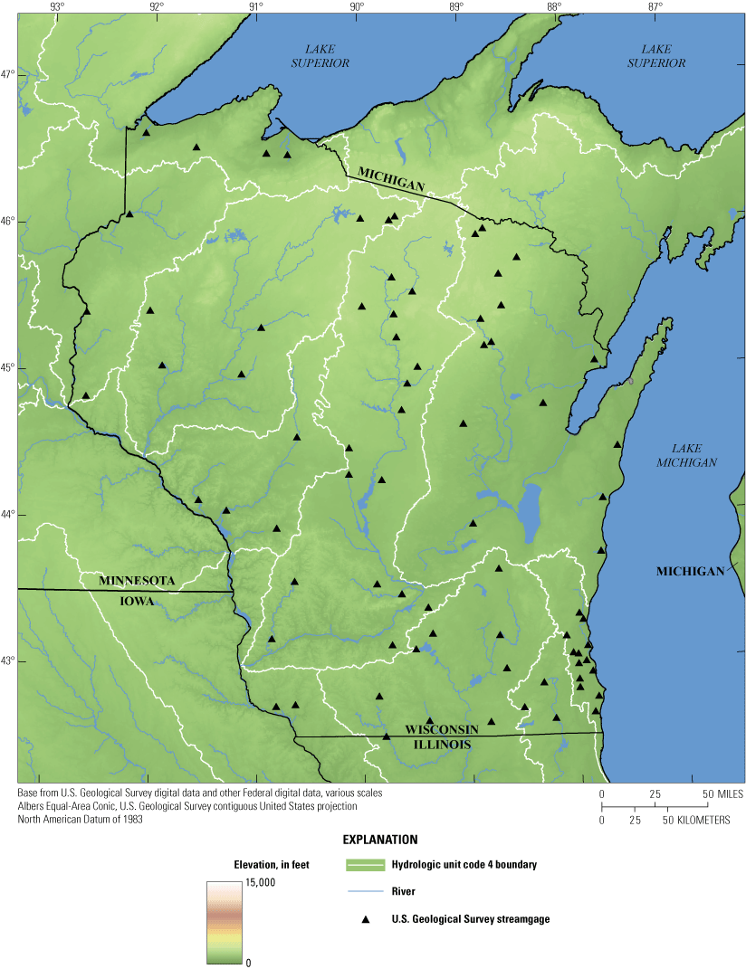
Elevation, hydrography, and U.S. Geological Survey streamgages used in this study in Wisconsin.
Climate
Wisconsin has a continental climate with warm humid summers and cold, snowy winters. The climatology of Wisconsin generally follows a north-south gradient with the northernmost regions having the coldest annual temperatures and fewest frost-free days per year. Average temperatures range from 39 degrees Fahrenheit in the north to 50 degrees Fahrenheit in the south (fig. 2). Wisconsin’s location in the interior of the continent makes it susceptible to large seasonal temperature variations. The convergence of cold artic air masses and warm, humid air masses from the Gulf of Mexico further increases this variation (Frankson and others, 2022). Summers are characterized by warm humid air from the Gulf of Mexico but are sometimes punctuated by intrusions of colder air from the north (Frankson and others, 2022).
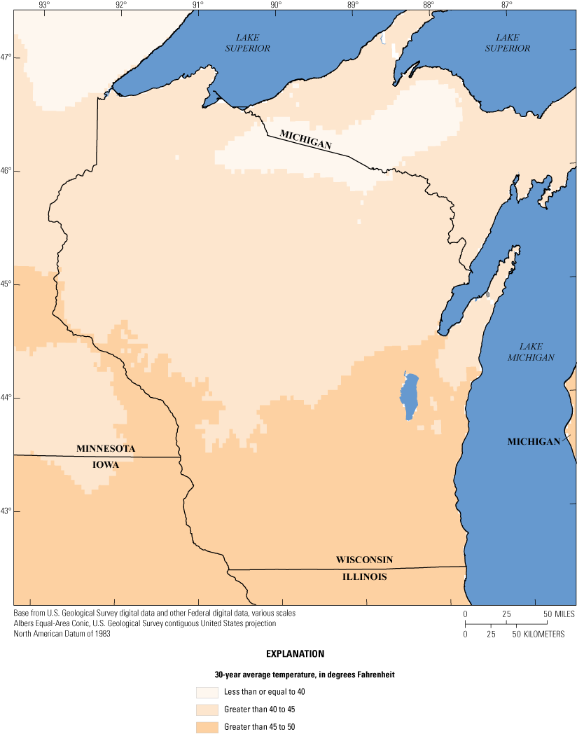
Average annual temperature for the 30-year period from 1991 to 2020 for Wisconsin.
Average precipitation ranges from roughly 30 to 38 inches per year, although annual precipitation rates can vary widely (fig. 3). Precipitation amounts vary on a roughly north-south gradient and are higher in the south. Most of the precipitation falls during the spring and summer. Average annual snowfall ranges from 30 inches (in.) in the south to more than 100 in. along the shore of Lake Superior.
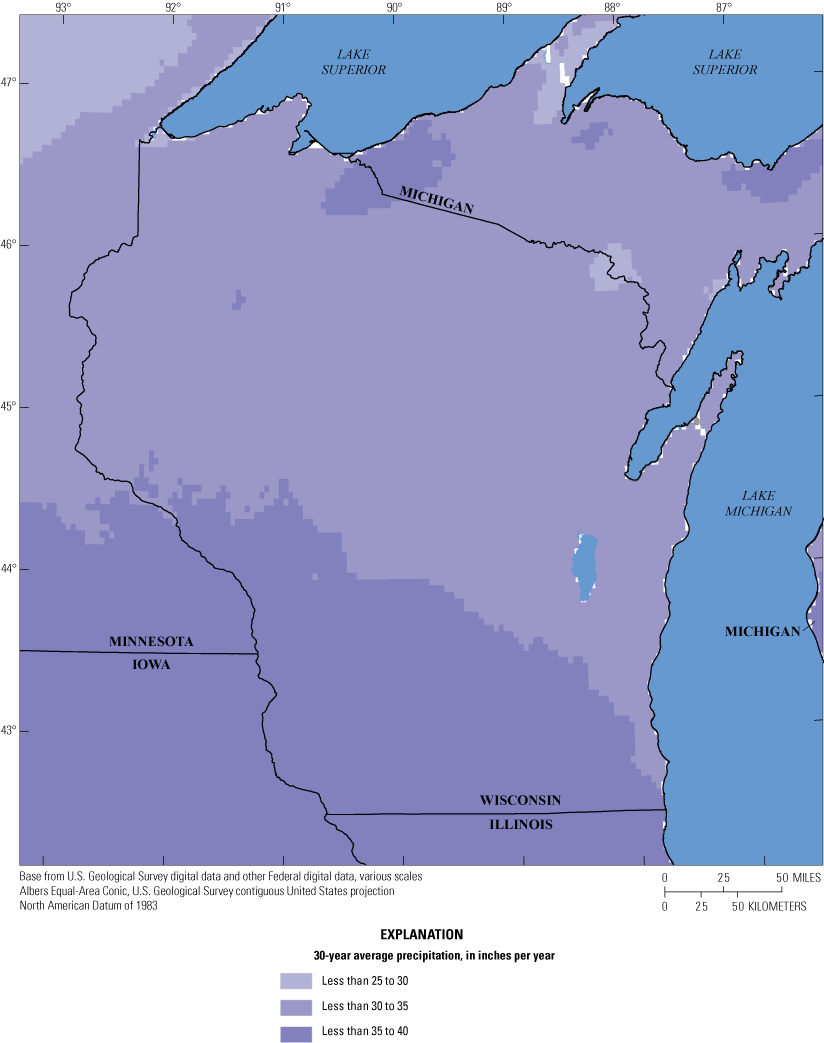
Average annual precipitation for the 30-year period from 1991 to 2020 for Wisconsin.
Ecoregions
Ecoregions are areas of general similarity in ecosystems including ecological, climatic, physiographic, and geological aspects of the landscape (Omernik and Griffith, 2014). The five level III ecoregions characterizing Wisconsin are shown in figure 4.
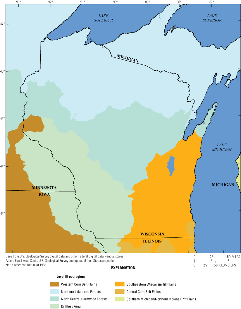
Level III ecoregions of Wisconsin.
The Northern Lakes and Forests (NLF) ecoregion runs across roughly the northernmost one-third of Wisconsin. This region consists of glaciated highland deposits and includes the headwater areas of several large river systems that drain into the Mississippi River, as well as drainage into Lake Superior. Soils here are a mixture of sand and loam (soil groups A and B; fig. 5) and are relatively nutrient poor compared to southern areas of the State (Omernik and others, 2000). The NLF ecoregion is heavily forested and has the highest proportion of lake area in the State (McDonald and others, 2012; Dewitz, 2019; fig. 6).
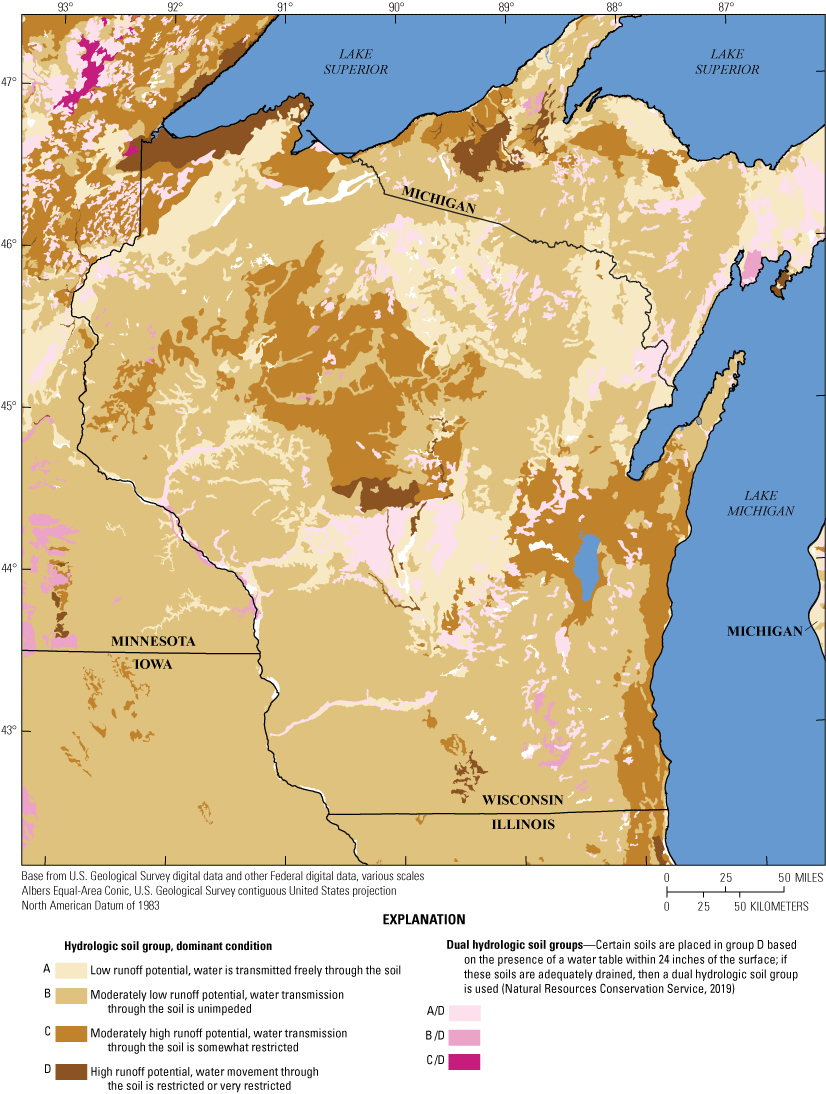
Dominant hydrologic soil groups in Wisconsin (Natural Resources Conservation Service, 2019).
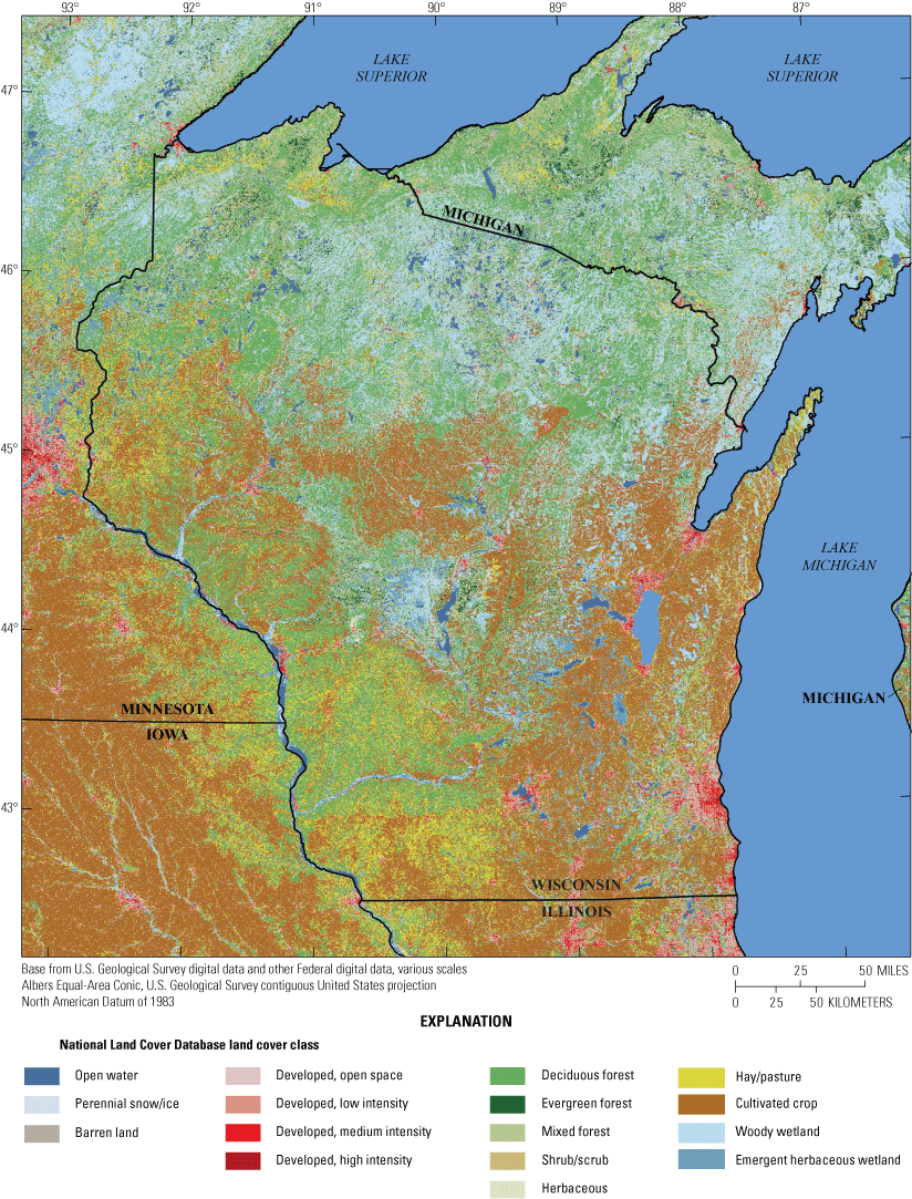
Land cover classes of Wisconsin (Dewitz, 2019).
The North Central Hardwood Forests (NCHF) ecoregion lies to the south of the NLF ecoregion and runs southeast to northwest across the State. A small section of the Western Corn Belt Plains ecoregion extends into Wisconsin, abutting the NCHF on the western side. The physiography of this region is characterized by glacial till plains and moraines. These regions are transitional between the heavily forested northern part of the State and the agricultural regions to the south and have a mixture of forested and agricultural land uses.
The Southeastern Wisconsin Till Plains ecoregion consists of glaciated, fertile ridges and lowlands and includes drainage into Lake Michigan and some south-flowing Mississippi River tributaries. Much of this region is agricultural, although Milwaukee and its suburbs are in the southeastern part of this region and consist of some of the most highly urbanized areas in the State (fig. 6).
The Driftless Area (DA) runs along the southwestern edge of Wisconsin. This region was not glaciated and is geomorphologically different from other areas of the State, with rugged hills and deep, steeply sloped river valleys. Karst geology in the DA, characterized by soluble bedrock, includes features such as caves, sinkholes, and losing streams (Potter, 2019). There are fewer lakes in this region and high groundwater recharge rates in the DA, which contribute to an abundance of cold-water streams with higher base flow than other ecoregions in the State (Potter, 2019). Land use is a mix of agriculture and forest (fig. 6).
Brief History of U.S. Geological Survey Peak-Streamflow Data Collection in Wisconsin
Annual peak streamflow has been recorded in Wisconsin since the late 1800s. Streamgages in Wisconsin include continuous streamgages, which report daily streamflow, and crest-stage gages (CSGs), which report only the annual peak streamflow. Based on data through water year 2020, there are 393 active or discontinued streamgage locations with 10 or more years of annual peak-streamflow measurements (U.S. Geological Survey, 2021). A water year (WY) is the period from October 1 to September 30 and is designated by the year in which it ends. The oldest continually operational USGS streamgage reporting annual peak streamflow is on the Chippewa River at Chippewa Falls, Wisconsin (05365500), which has annual peak-streamflow measurements for 132 years, for water years 1888 to 2020. Some streamgages have historical peak-streamflow data that predate the USGS streamgage record. The number of streamgages reporting annual peak streamflow per year is shown in figure 7. The number of continuous streamgages grew throughout the late 19th and early 20th century, reaching a maximum of 211 streamgages in 2013. Early streamgages were operated primarily on large streams with drainage areas of roughly 1,000 square miles (fig. 8). Streamgages installed later in the 20th century focused on smaller and midsized basins with drainage areas on the order of 50 to several hundred square miles (fig. 8). CSG operations began in 1958 and rapidly increased in number throughout the mid-20th century, reaching a maximum of 108 in 1974. CSGs are typically installed in smaller drainage basins of less than 50 square miles (fig. 8).
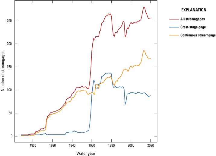
Number and type of U.S. Geological Survey streamgages reporting peak streamflow for water years 1880 through 2020 in Wisconsin.
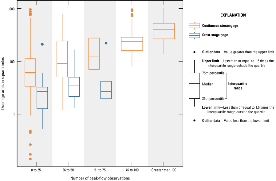
Drainage area distributions for continuous streamgages and crest-stage gages in Wisconsin by length of record.
The history of streamgage operations is relevant to nonstationarity analyses because it provides information on the temporal distribution of the data available for evaluating nonstationarity. The temporal variability of streamgage data may represent a bias in the evaluation of nonstationarity in annual peak streamflows in Wisconsin because many streamgages on smaller basins do not have a long period of record for analysis. The trends and statistical characteristics of floods in larger basins with longer periods of record may not reflect those in smaller upstream areas.
Brief History of Statistical Analysis of Peak Streamflow and Nonstationarity
USGS efforts to analyze peak-streamflow data in Wisconsin began in 1961 with the first flood-frequency estimates for streamgages estimated by hand-drawing the best visual fit for the flood-frequency relations and developing regression equations for ungaged areas (Ericson, 1961). After this first report, updates to Wisconsin flood-frequency estimates were published at roughly 10-year intervals using updated data and statistical techniques. Reports in 1971 and 1981 (Conger, 1971, 1981) introduced the use of the log-Pearson type III distribution to estimate flood frequency at gaged locations, in accordance with methods described in Bulletin 15 (U.S. Water Resources Council, 1967) and Bulletin 17A (U.S. Water Resources Council, 1977). Additional reports in 1992, 2003, and 2017 (Krug and others, 1992; Walker and Krug, 2003; Walker and others, 2017) updated flood-frequency estimates using statistical methods described in Bulletin 17B (Interagency Advisory Committee on Water Data, 1982), which outlined revised procedures for estimating skew, dealing with outliers, and computing confidence intervals. Most recently, new flood-frequency regions and equations have been developed (Levin and Sanocki, 2023) using the expected moments algorithm methodology as outlined in Bulletin 17C (England and others, 2018).
Downward monotonic trends and change points in peak streamflow have been documented throughout Wisconsin and are somewhat of a regional anomaly because primarily increasing peak streamflows have been detected in the surrounding States of Minnesota, Iowa, Illinois, and Indiana (Dudley and others, 2018; Hodgkins and others, 2019). The most substantial changes in streamflow were detected in the southern and southwestern parts (DA ecoregion) of Wisconsin. Several studies have documented downward trends in annual peak streamflows, accompanied by increasing trends in low flow or daily streamflow in southern Wisconsin (Potter, 1991; Gebert and Krug, 1996; Juckem and others, 2008; Splinter and others, 2015). Gyawali and others (2015) identified changes in the monthly streamflow patterns; the greatest increases were in summer months and decreases in spring monthly flows were detected in southern Wisconsin streamgages. In addition to monotonic trends, change points representing abrupt changes in streamflow over time have been detected in southern Wisconsin. Several studies have documented an increasing change point in mean annual and baseflow around 1970 (McCabe and Wolock, 2002; Juckem and others, 2008; Gyawali and others, 2015; Splinter and others, 2015), which corresponds to a concurrent change point in precipitation.
Attribution of the causal mechanisms of trends in DA ecoregion peak streamflows is complex, and the literature does not provide a clear consensus. Early studies did not show changes in precipitation or temperature that could explain the changes in streamflow and attributed streamflow trends to changes in agricultural practices (Potter, 1991; Gebert and Krug, 1996). Beginning in the 1930s, land management practices aiming to reduce erosion and improve soil quality began to be implemented across the region. Practices such as contour plowing, incorporation of crop residue into soil, crop rotation, conservation tillage, and the reduction of hillside grazing increase infiltration, which potentially explains increases in base flow and decreases in peak streamflows. Later studies have ascribed streamflow changes to a combination of increasing precipitation, temperature, and changes in agricultural practices (Gyawali and others, 2015; Gebert and others, 2016). Juckem and others (2008) note that the magnitude of the change in base flow was greater than could be expected from the change in precipitation and concluded that precipitation was the primary driver of changes in streamflow, but these changes were magnified by changes in land management of agricultural areas. Gyawali and others (2015) attribute increasing trends in base flow to precipitation but decreasing trends in peak streamflows to changes in agriculture.
Documented changes in streamflow in the northern forested areas of Wisconsin are less prevalent in the literature than in southern Wisconsin. Trends in annual peak streamflows in the northern forested areas of Wisconsin were not apparent in studies by Gebert and Krug (1996) and Gyawali and others (2015); however, upward trends in seasonal peak streamflows were detected by Gyawali and others (2015) who documented increases in winter peak streamflows, possibly because of increases in fall and winter temperature and winter rain. Others have identified decreasing change points in annual streamflow in several unregulated drainage basins in northern Wisconsin (Splinter and others, 2015; Ivancic and Shaw, 2017). These change points were detected later than those in the southern part of the State. Change point dates corresponding to decreasing precipitation ranged from 1987 to 2002.
Review of Research Relating to Climatic Variability and Change
Streamflow in Wisconsin follows natural cyclical patterns with persistent periods of lower than or higher than average streamflow over large spatial areas. These wet-dry cycles are associated with fluctuations in the position of the jet stream and large-scale ocean-atmospheric oscillations, which can alter temperature and precipitation patterns across the Upper Midwest. This section discusses historical flood and drought periods across Wisconsin and the climatic forces that affect these large-scale streamflow patterns.
Historical Floods and Drought Periods in Wisconsin
Periodic flooding has long been associated with Wisconsin rivers, and many historical floods have been documented before USGS streamgage data (table 1). The first known written account of a flood in Wisconsin was documented by early settlers in the village of Prairie du Chien in southwestern Wisconsin in 1785. Known as the “l’année des grandes eaux” (year of the great waters), flood waters from the Mississippi River damaged the village and many downstream settlements in Illinois and Missouri. Many rivers overflow their streambanks regularly and flood at roughly decadal frequencies (Wisconsin Historical Society, 2021). Repeated floods on many of these rivers led to the eventual implementation of flood control structures to protect nearby communities.
Table 1.
Floods reported for Wisconsin Rivers before U.S. Geological Survey streamgage records at those locations.[WI, Wisconsin]
| Date of flood | River basin or geographic region affected | Reference |
|---|---|---|
| April 1785 | Prairie du Chien, Mississippi River in southwestern Wisconsin | Wisconsin Historical Society, 2021 |
| 1838 | Wisconsin River at Portage, WI | Morton and others, 1948 |
| July 1845 | Wisconsin River at Portage, WI | Morton and others, 1948 |
| 1855 | Eau Claire, Chippewa and Eau Claire Rivers | Morton and others, 1948 |
| August 1870 | Eau Claire, Chippewa and Eau Claire Rivers | Morton and others, 1948 |
| June 1880 | Southern Wisconsin, including the Mississippi River, Black River, Wolf River, and Fox River | Wisconsin Historical Society, 2021 |
| September 1884 | Eau Claire, Chippewa and Eau Claire Rivers | Wisconsin Historical Society, 2021 |
| June 1899 | Bear Creek and La Crosse River at Sparta, WI | Morton and others, 1948 |
| October 1911 | Black River | Wisconsin Historical Society, 2021 |
| 1923 | Pecatonica River at Darlington, WI | Morton and others, 1948 |
| 1937 | Pecatonica River at Darlington, WI | Morton and others, 1948 |
| 1938 | Chippewa and Eau Claire Rivers, Eau Claire | Morton and others, 1948 |
| 1941 | Eau Claire, Chippewa and Eau Claire Rivers | Morton and others, 1948 |
| May 1943 | Bear Creek at Sparta, WI | Morton and others, 1948 |
Several statewide droughts have been detected in Wisconsin in the past 100 years. Like much of the country, extreme droughts in the 1930s are considered some of the worst in Wisconsin history. Additional climatic droughts have been detected throughout most of the State in 1948, 1977, 1988, and 2007 (National Integrated Drought Information System, 2022). Mean annual streamflow for each year of record for unregulated streamgages in Wisconsin is shown in figure 9. Mean annual streamflow is colored by the Z-score, which represents the number and direction of standard deviations away from the mean for each streamgage. Streamgages in figure 9 are grouped by ecoregion with northernmost streamgages at the top. Periods of drier-than-average conditions spanning across many streamgages in Wisconsin are documented throughout much of the early part of the record, from the 1930s through the 1960s, 1977, and the late 1980s/early 1990s, whereas periods of higher-than-average conditions are documented at most streamgages during the 1970s, mid-1980s, and the last decade between 2010 and 2020. Some regional differences in wet/dry streamflow patterns are evident. For example, the southern DA and Southeastern Wisconsin Till Plains ecoregions had primarily wetter than average conditions starting in 2008 through 2020, whereas in the northern NLF and NCHF ecoregions, conditions remained drier than average from the mid-2000s until roughly 2012 and did not enter wetter-than-average conditions until later in the 2010s.

Mean annual streamflow for selected unregulated streamgages in Wisconsin. Streamgages are grouped by ecoregion. Mean annual streamflow for each year is colored by the Z-score, which is the number and direction of standard deviations away from the mean for each streamgage. Shades of blue represent wetter than average conditions, and shades of red indicate drier than average conditions.
Review of Evidence of Climatic Variability
Wisconsin is near the convergence of warm moist air masses from the Gulf of Mexico and cold, dry arctic or Pacific air masses. The relative importance of the different airflow source regions varies with season and the configuration of the polar jet stream (Andresen and others, 2012). Climate variability in the Upper Midwest has been associated with large-scale ocean-atmospheric oscillations, which shift the configuration of the jet stream. Unlike coastal regions of the United States, which may be strongly affected by one or two ocean-atmospheric oscillations, Wisconsin sits roughly in the center of the continent and is affected weakly by several oscillations. The relative spatial scales, strength, and timing of these different cycles interact with each other to produce complex decadal-scale signals in climate variability (Andresen and others, 2012; Budikova and others, 2022).
El Niño-Southern Oscillation (ENSO) refers to the periodic warming of surface waters in the tropical Pacific Ocean and resulting disruptions in atmospheric air masses. In the negative phase (El Niño), ENSO pushes the jet stream northward, causing milder than average temperatures in Wisconsin, whereas in the positive phase (La Niña), warmer and wetter winter conditions have been noted in the Upper Midwest. The effect of the ENSO cycle in Wisconsin may be strengthened or weakened by interactions with other ocean-atmospheric oscillations such as the Pacific Decadal Oscillation and Atlantic Multidecadal Oscillation. Effects of El Niño on winter precipitation in the upper Mississippi Basin may be strengthened when El Niño occurs during the positive phase of the Pacific Decadal Oscillation and the Atlantic Multidecadal Oscillation (Enfield and others, 2001). Other atmospheric oscillations, such as the North Atlantic Oscillation and Pacific-North American pattern, and the Tropical Northern Hemispheric pattern have been weakly associated with winter temperatures and precipitation in the Upper Midwest (Budikova and others, 2022).
In recent decades, the climate in Wisconsin has been getting warmer and wetter; however, there is considerable spatial and seasonal variability in the observed climate changes. Statewide, the average temperature in Wisconsin has risen 2 degrees Fahrenheit since the start of the 20th century, and 2000–4 was the hottest 5-year period in recorded history (Frankson and others, 2022). Upward trends in mean annual temperature are the largest in northwestern and central Wisconsin, and most increases are during the winter and spring seasons. Summer and fall daily average maximum temperatures generally have not changed or have decreased slightly across the State, and the largest decreases are in the northeastern and southwestern corners of the State (Kucharik and others, 2010).
Increases in precipitation have also been observed across the State. Wisconsin has experienced unusually wet years in the last decade, and the highest 5-year average precipitation in the State fell from 2016 to 2020. The highest observed annual precipitation for Wisconsin fell in the year 2019. Additionally, 2018, 2016, and 2010 were the third, fourth, and fifth wettest years recorded in Wisconsin, respectively. The driest periods were in the 1890s, 1930s, and mid-1950s whereas the wettest periods were 1982–86 and 2016–20 (Frankson and others, 2022). Statewide average annual precipitation has increased by as much as 15 percent (White and Arnold, 2015), and the largest increases are in the west-central and south-central areas. Annual snowfall has also increased in Wisconsin since 1930 (Frankson and others, 2022). Seasonal precipitation trends varied across the State, and the largest increases in precipitation were in the fall for northwestern Wisconsin and summer for central Wisconsin. Decreases in summer precipitation were observed in northern Wisconsin.
Climate Effects on Flooding and Runoff
Flooding in Wisconsin is driven by spring snowmelt and summer storms. Extreme flooding in small or moderate drainage basins often results from intense summer storms rather than snowmelt because meltwater runoff accumulates slowly; however, in larger basins, slowly accumulating snowmelt from several tributaries can combine downstream to cause large floods (Knox, 2000). High antecedent soil moisture during the spring can exacerbate flooding from intense spring or early summer rainfall events. Annual peak streamflows tend to be larger when the rainfall during the previous year is greater than normal and lead to increased antecedent soil moisture at the start of the melting period (Knox, 2000).
Climate projections for Wisconsin include continued increases in temperature and precipitation during this century. Increased precipitation during the winter and spring is projected, whereas snowfall is expected to decrease because of increased temperatures (Frankson and others, 2022). The shifting dynamics of temperature and precipitation have the potential to change the frequency, magnitude, and (or) timing of floods and droughts in Wisconsin.
Data
A detailed description of the selection of data and streamgages for this study is described in Ryberg and others (2024). Annual peak-streamflow data compiled for all streamgages came from the USGS National Water Information System database (U.S. Geological Survey, 2021). Four periods were selected for analysis: (1) a 100-year period, water years 1921–2020; (2) a 75-year period, water years 1946–2020; (3) a 50-year period, water years 1971–2020; and (4) a 30-year period, water years 1991–2020. Streamgages included in the study have peak-streamflow data for at least 80 percent of the period of record and included peak streamflows in at least 1 of the first 2 years of record. Streamgages were screened for potential regulation by dams or water diversions using existing streamflow qualification codes within the National Water Information System database and a dam impact metric described in Marti and Ryberg (2023). Regulated streamgages identified by the screening process were removed from the study. Additional data quality screening resulted in the removal of one streamgage, Kinnickinnic River Tributary at River Falls, Wis. (05341900), because of poor peak-streamflow data quality during part of the record. Data screening resulted in 8 streamgages in the 100-year period, 24 streamgages in the 75-year period, 57 streamgages in the 50-year period, and 71 streamgages in the 30-year period in Wisconsin. Of these streamgages, 8, 24, 38, and 56 streamgages had daily streamflow for the 100-, 75-, 50-, and 30-year analysis periods, respectively.
The climate data used in this report were compiled for each drainage basin from the output of a monthly water balance model for the period of 1900–2020 (Wieczorek and others, 2022). These data consist of monthly time series estimates of temperature, precipitation, potential evapotranspiration (PET), actual evapotranspiration, rainfall, snowfall, soil moisture storage, snow water equivalent, and runoff on a 5-kilometer by 5-kilometer grid for the conterminous United States. The precipitation and temperature values are observed data obtained from the nCLIMGRID dataset (Vose and others, 2017). All other monthly time series are modeled outputs from the monthly water balance model. Further details are available in Ryberg and others (2024).
Methods
Statistical analyses of peak streamflow, annual streamflow, and climate metrics were completed for all four analysis periods. Statistical analysis of peak streamflow consisted of evaluation of autocorrelation, monotonic trends, change points, quantile regression, and seasonality. Statistical analysis of daily streamflow consisted of an evaluation of streamflow seasonality, center of volume, and peaks-over-threshold (POT) analysis. Methods used for each statistical analysis are described in Ryberg and others (2024), and results of all analyses for each streamgage were published in a USGS data release (Marti and others, 2024). This report summarizes the results in Marti and others (2024) and identifies spatial and temporal patterns in the results across Wisconsin.
Results of statistical tests are commonly validated with a probability value (p-value), which is the probability of obtaining the observed results, assuming the null hypothesis is true. Typically, a p-value between 0.01 and 0.1, chosen by the analyst, is used as the cutoff to categorize results as statistically significant. In this report, the trends are presented using a likelihood approach, which was proposed by Hirsch and others (2015) as an alternative to simply reporting significant trends with an arbitrary cutoff point. Trend likelihood values were determined using the p-value reported by each test using the equation trend likelihood=1−(p-value/2). When the trend is likely upward or likely downward, the trend likelihood value associated with the trend is between 0.85 and 1.0; that is, the chance of the trend being detected in the specified direction is at least 85 out of 100. When the trend is somewhat likely upward or somewhat likely downward, the trend likelihood value associated with the trend is between 0.70 and 0.85—the chance of the trend being detected in the specified direction is between 70 and 85 out of 100. When the trend is about as likely as not, the trend likelihood value associated with the trend is less than 0.70—the chance of the trend being either upward or downward is less than 70 out of 100. Additional details are available in Ryberg and others (2024).
Results of Streamflow and Climate Analyses
This section summarizes results of streamflow and climate analyses and describes spatial or temporal patterns in nonstationarity across the State. Widespread changes in peak streamflow, daily streamflow, precipitation, and temperature were identified across Wisconsin during all four analysis periods (100, 75, 50, and 30 years). Results for streamflow and climate analyses at specific streamgages in Wisconsin are available in Marti and others (2024).
Annual Peak Streamflow
Peak-streamflow data were available at 8, 24, 57, and 71 streamgages in Wisconsin for the 100-, 75-, 50-, and 30-year analysis periods, respectively. Several types of nonstationarities in peak streamflow were detected in Wisconsin, including trends in the magnitude and timing, change points, and autocorrelation. Analysis results were affected by the length of the period of analysis and the number of streamgages available. It is difficult to generalize results or identify spatial patterns of peak streamflow changes in the northern and eastern parts of the State for the 75- and 100-year periods because there are too few streamgages with long periods of record in these areas.
Monotonic Trends in Peak Streamflow
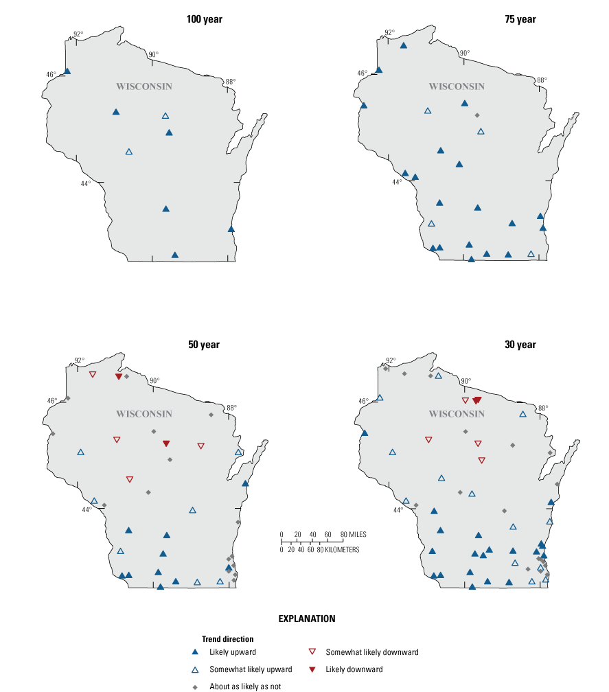
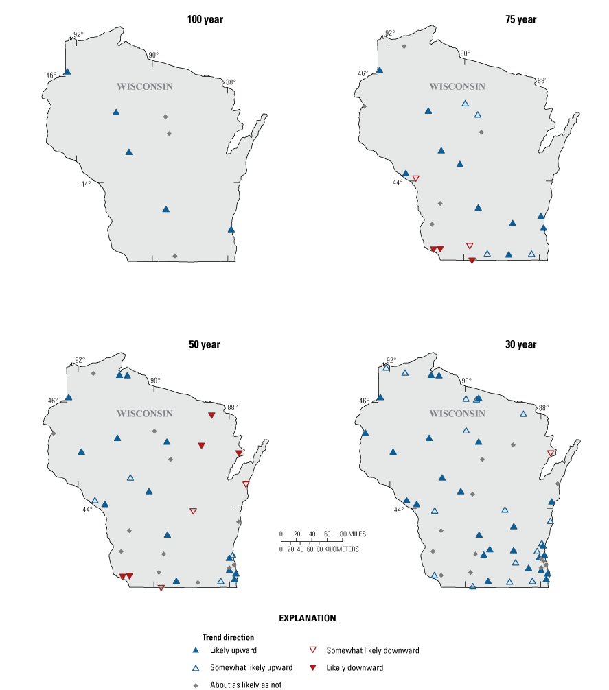
The Mann-Kendall test (Kendall, 1938) was used to identify the presence of a monotonic trend at streamgages for each analysis period as described in Ryberg and others (2024). A monotonic trend is one in which the direction of the trend does not reverse over time. Results of the Mann-Kendall analyses were inconsistent across analysis periods (table 2; fig. 10). In the 100- and 75-year periods, downward trends were detected primarily in central and southwestern Wisconsin and upward trends were detected in the southeastern corner of the State, near Milwaukee, as well as some upward trends in north-central Wisconsin. The 50-year analysis period has more than twice the number of streamgages as the 75-year period and includes many locations in northeastern Wisconsin, which were not represented in longer analysis periods. In this period, the mix of streamgages with upward, downward, or likely no trend throughout the State was nearly equal and spatial patterns were less apparent. Trends in the 30-year period were predominantly upward throughout the State. Notably, the DA ecoregion, which had primarily downward trends for the longer analysis periods, had no downward trends in the 30-year period and several upward or likely upward trends. In some cases, a large change point can affect the detection of a trend, leading to an improper identification of a trend when, in fact, a change point is in the data. Results of trend tests for specific streamgages of interest should be checked in Marti and others (2024) to determine if this is the case.
Table 2.
Likelihood of monotonic trends, timing, and change points in peak streamflow at selected streamgages in Wisconsin for four analysis periods.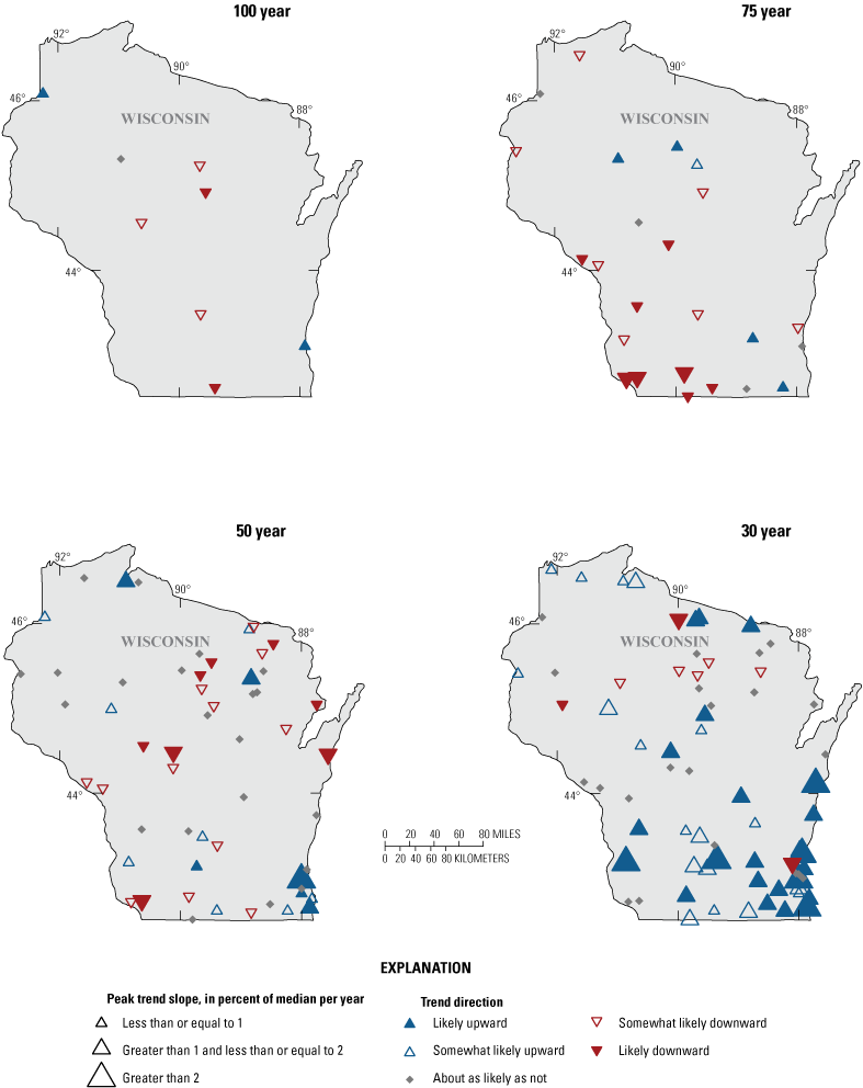
Likelihood and magnitude of peak-streamflow trends at selected U.S. Geological Survey streamgages in Wisconsin for four analysis periods ending in water year 2020.
To compare trend magnitudes across streams of different sizes, trend slopes were divided by the median peak streamflow and converted to a percentage (fig. 10). The resulting trend slope is a percentage of the median peak streamflow. For example, at a streamgage with an upward trend of 1 percent, the median peak streamflow would increase by 10 percent in 10 years and double over a 100-year period. Statewide, median trend magnitudes for streamgages with likely or somewhat likely trends were less than 1 percent per year for all analysis periods except the 30-year period where the median trend for likely and somewhat likely upward trends was 1.2 percent per year.
The transition from downward peak-streamflow trends in the 75-year period to upward trends in the 30-year period is indicative of a nonmonotonic peak-streamflow pattern that was detected at many streamgages.in the DA ecoregion. Streams in this ecoregion had decreasing peak streamflows until the 1980s, followed by a subsequent increase in peak streamflows starting around the year 2000. An example of the change in the direction of the trend in peak streamflows for USGS streamgage Sugar River near Brodhead, Wis. (05436500) is shown in figure 11A. Tests for trends are sensitive to the period of record and can be inconsistent when trends are nonmonotonic; for example, in the Sugar River, the test for a monotonic trend for the 100-year period is likely downward with a slope of −11.5 cubic feet per second (ft3/s) per year. The 30-year analysis period began at the end of a period of lower peak streamflows at this streamgage in 1990. In this period, the monotonic trend is upward with a slope of 26.5 ft3/s per year. The prevalence in nonmonotonic trends in peak streamflow in Wisconsin complicates the identification and comparison of trends across the State and can lead to inconsistent results depending on the period of record used for analysis.
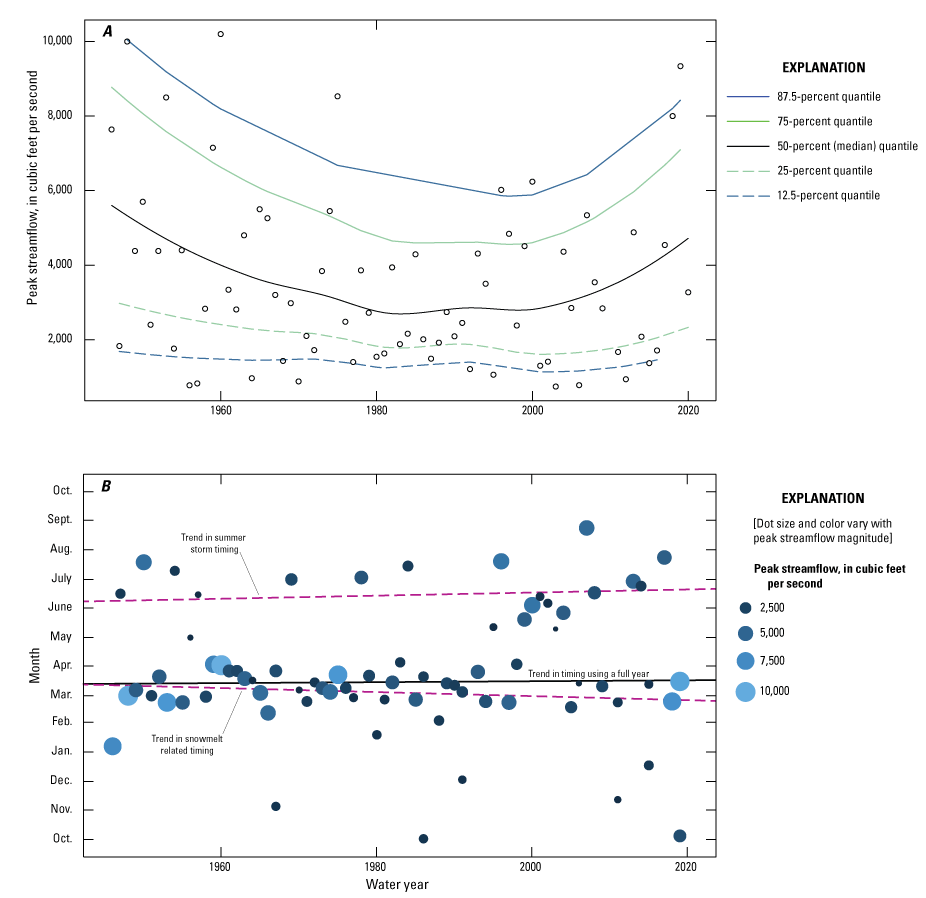
(A) Peak-streamflow quantiles and (B) peak-streamflow timing for U.S. Geological Survey streamgage Sugar River near Brodhead, Wisconsin (05436500), for the 75-year period of water years 1951 to 2020 (modified from Marti and others [2024]).
Trends in Peak-Streamflow Timing
The peak-streamflow timing analysis plots show the timing and magnitude of the annual peak streamflow with the water year on the x-axis and the Julian day of the water year on the y-axis (fig. 11B). The magnitude of each peak streamflow is shown by varying the marker size and color assigned for each annual peak. A trend in these data indicates that annual peak streamflows are later (upward trend) or earlier (downward trend) in the year. Snowmelt and summer rainstorms are the two primary mechanisms for producing peak streamflows in Wisconsin. Snowmelt peaks are typically from March through May, whereas peak streamflows caused by thunderstorms are in the summer, typically from June through September. Some streamgages demonstrate a strong bimodal temporal distribution of peak streamflows, and a clear distinction exists between the two causal mechanisms of peak flows, whereas for other streamgages, the distinction is not as obvious. The peak-flow timing analysis identifies trends in the overall timing of peak streamflows, and for bimodal streamgages, the analysis also identifies trends in early (snowmelt) and late (summer storm) peak-streamflow timing.
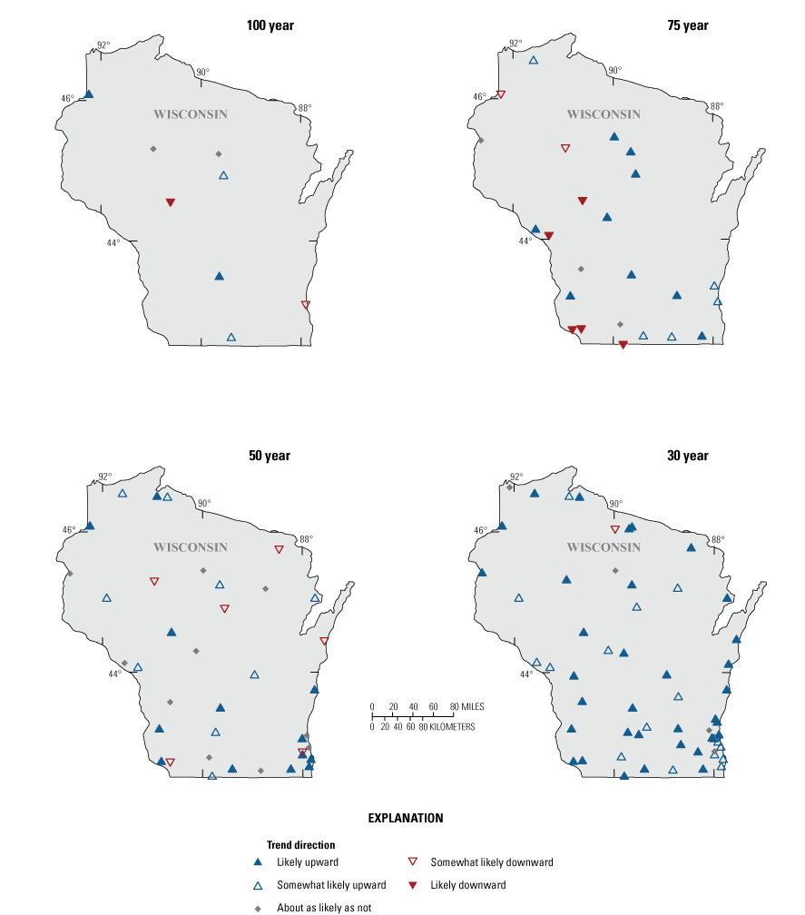
Trends in the timing of peak streamflows were primarily upward in the 100-, 75-, and 50-year periods, indicating that peak streamflows were occurring later in the year (fig. 12; table 2). As with the peak-streamflow magnitude trends, a change in direction in the timing trends of peak streamflows is apparent in the 30-year period compared to longer periods. This period had 24 likely or somewhat likely downward trends and 15 likely or somewhat likely upward trends. Some of the apparent downward trends in the 30-year period may be caused by storms that were detected in October. Because the trend timing analysis uses a water year, October is considered the first month that plots at the bottom of the y-axis. These large October peak streamflows are typically low outliers that have a greater effect on the trend slope in the shorter 30-year period. Large peaks in October may be contributing to downward trends at some streamgages, although they are really evidence of peak streamflows caused by summer storms occurring later than usual and should be considered part of an upward trend. Because of the potential effect of these outliers, summary results from the 30-year period should be used with caution, and plots of the peak-streamflow timing analysis, available in Marti and others (2024), should be examined for any streamgage of interest.
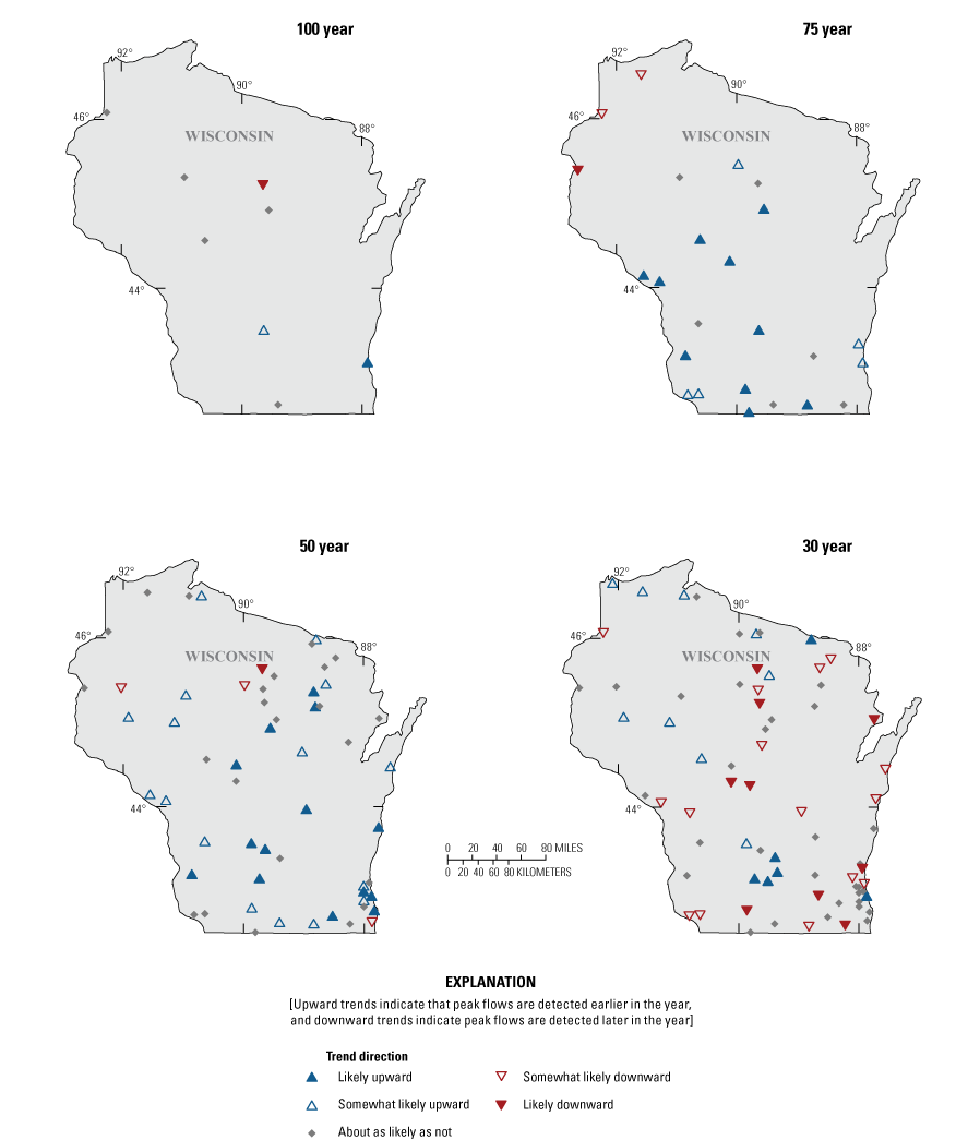
Likelihood of peak-streamflow timing trends at selected U.S. Geological Survey streamgages in Wisconsin for four analysis periods ending in water year 2020. Upward trends indicate that peak streamflows are detected earlier in the year, and downward trends indicate peak streamflows are detected later in the year.
The peak-streamflow timing analysis identifies gradual trends in the changes in peak-streamflow timing, but at many locations changes were more abrupt. Timing changes were often concurrent with changes in peak-streamflow magnitudes. The timing changes at USGS streamgage Sugar River near Brodhead, Wis. (05436500), are shown in figure 11B. For most of the period of record, peak streamflows primarily were detected in the spring, which is consistent with snowmelt-related floods. Around the year 2000, a shift in the timing of peak streamflows was observed, and a higher proportion of peak streamflows after the year 2000 were detected in the summer months and extending into October and November. This timing change was concurrent with the shift from decreasing to increasing peak streamflows at this streamgage.
Change Points in Peak Streamflows
Change points are abrupt median, mean, or variance time series changes. The nonparametric Pettitt test was used to find change points in the median peak streamflow (Pettitt, 1979). Change points test results are listed in table 2 and shown in figure 13. Change point magnitudes are shown as a percentage change in the median before and after the change point. As with tests for monotonic trends, the results of the change point analyses are presented in terms of statistical likelihood. Results (figure 14 and table 2) may differ slightly from individual streamgage analyses presented in Marti and others (2024), which do not use a likelihood approach and only show change points for streamgages when the p-value of the Pettitt test is less than or equal to 0.05.
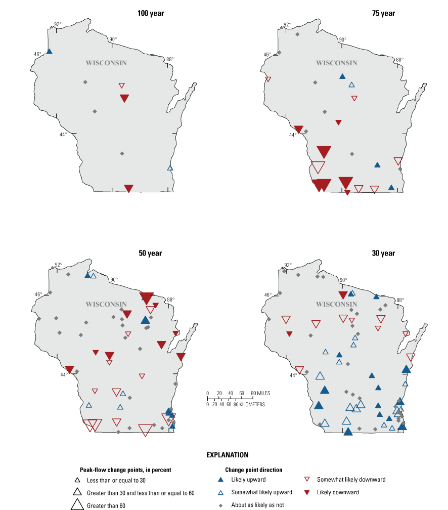
Likelihood and magnitude of change points in median peak streamflow at selected U.S. Geological Survey streamgages in Wisconsin for four analysis periods ending in water year 2020.
Dates of change points in median peak streamflow at selected U.S. Geological Survey streamgages in Wisconsin for four analysis periods ending in water year 2020.
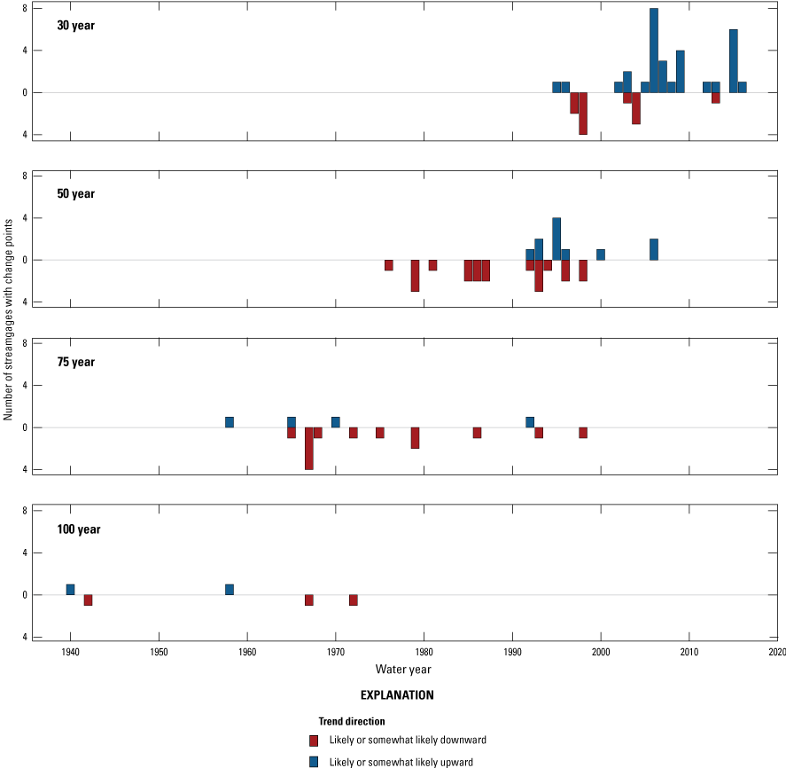
Spatial patterns in change points were similar to those for monotonic trends: longer periods of record indicate mostly downward changes, which are greatest in the southwestern DA, whereas changes in the 30-year period are mostly upward. Change points in the 100- and 75-year periods were primarily in the 1960s and 1970s (fig. 14). The largest change points during these periods were downward changes in the DA ecoregion. In the 50-year period, the largest downward change points were in the central and northeastern areas of Wisconsin during the late 1980s and 1990s. Upward change points were in the southeastern area around Milwaukee and at isolated streamgages in northern Wisconsin. Change points in the 30-year period were primarily upward for southern Wisconsin and were detected in the early 2000s.
Autocorrelation
Persistence is the tendency for one high (or low) annual peak-streamflow value to be followed by another high (or low) value instead of randomly varying in time. Persistence in peak streamflows can be caused by wet antecedent conditions from a previous wetter-than-average year extending into the spring. In this case, the high peak streamflows in the first “wet” year may be followed by high peak streamflows the next year because the antecedent soil moisture magnifies the spring floods. Long-term persistence refers to clustered wet and dry periods that induce serial correlation into the peak-streamflow series at lags of greater than 1 year. Short-term persistence refers to the presence of lag-1 autocorrelation (correlation between values that are one year apart) in the annual peak streamflow time series (see Ryberg and others, 2024).
Persistence in annual peak streamflows was investigated with respect to long- and short-term persistence. The rank von Neumann test for lag-1 autocorrelation (von Neumann and others, 1941) was used to identify the short-term persistence in peak streamflow time series. The Hurst coefficient (Hurst, 1951) is a measure of long-term persistence. Hurst coefficients range from 0 to 1, and values greater than 0.5 indicate long-term persistence (see Ryberg and others, 2024). An example of autocorrelation in peak streamflows at USGS streamgage Allen Creek Tributary near Alvin, Wis. (04059900; in northern Wisconsin), which has short-term persistence (rank von Neuman test p-value less than 0.001) and long-term persistence (Hurst coefficient of 0.715) during the 50-year period, is shown in figure 15B. In this small basin, the largest peak streamflows were from summer and early fall storms, whereas snowmelt-related peak streamflows in the spring are smaller in magnitude. Climate analyses for this streamgage (not shown; see Marti and others [2024]) indicate a decrease in summer and fall precipitation between 1990 and 2010, likely contributing to the strong persistence noted at this streamgage.
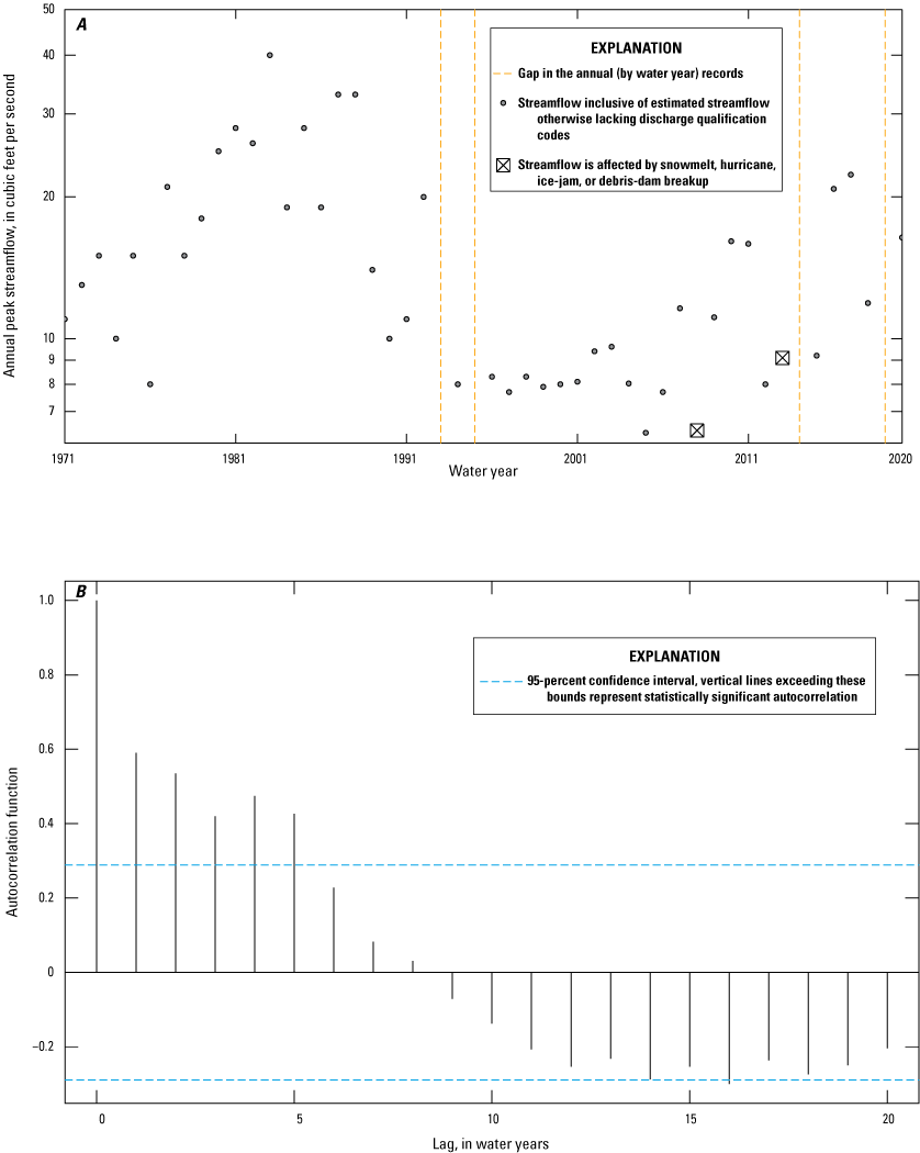
(A) Peak streamflow and (B) autocorrelation plot for U.S. Geological Survey streamgage Allen Creek Tributary near Alvin, Wisconsin (04059900), for the 50-year period of water years 1971 to 2020 (modified from Marti and others [2024]).
Streamgages at 17 locations showed evidence of short-term persistence (rank von Neuman test p-value less than 0.1) in at least one of the analysis periods. Streamgages at 24 locations had evidence of long-term persistence (Hurst coefficients greater than 0.60) in at least one analysis period, indicating evidence of long-term persistence. Streamgages demonstrating short-term and long-term persistence were detected throughout the State and across basins of different sizes and did not demonstrate any apparent spatial patterns.
Daily Streamflow
Daily streamflow data were available at 8, 24, 38, and 56 streamgages for the 100-, 75-, 50-, and 30-year analysis periods, respectively. Daily streamflow is not available at every streamgage used in the peak-streamflow analyses because of the prevalence of CSGs in Wisconsin. CSGs only record the annual peak streamflow. Changes in daily streamflow were examined using several analyses including identification of seasonal and annual trends in daily streamflow, raster seasonality plots, center of volume plots, and POT analysis, described in Ryberg and others (2024).
Trends in Mean Annual and Seasonal Streamflow
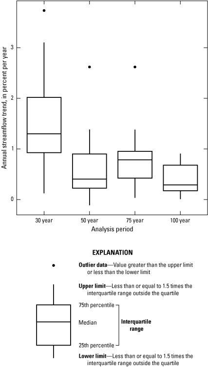
Trends in mean annual streamflow were likely or somewhat likely upward at most streamgages in the State for all four analysis periods (table 3). No downward trends were noted in any analysis period. Trend magnitudes in the 50-, 75-, and 100-year periods were generally less than 1 percent per year. Trend magnitudes in the 30-year period were higher and had a median upward trend of 1.3 percent per year, and roughly one-quarter of streamgages had trend magnitudes of 2 percent or higher (fig. 16).
Table 3.
Likelihood of monotonic trends in mean annual and seasonal streamflow, change points in peaks over thresholds, and trends in center of volume (25th, 50th, and 75th percentile streamflows) at selected streamgages in Wisconsin for four analysis periods ending in water year 2020.[POT2, peaks over threshold with two events per year; POT4, peaks over threshold with four events per year; Q25, 25th percentile of annual streamflow; Q50, 50th percentile of annual streamflow; Q75, 75th percentile of annual streamflow]
Magnitude of monotonic trends in mean annual streamflow at selected U.S. Geological Survey streamgages in Wisconsin for four analysis periods ending in water year 2020.
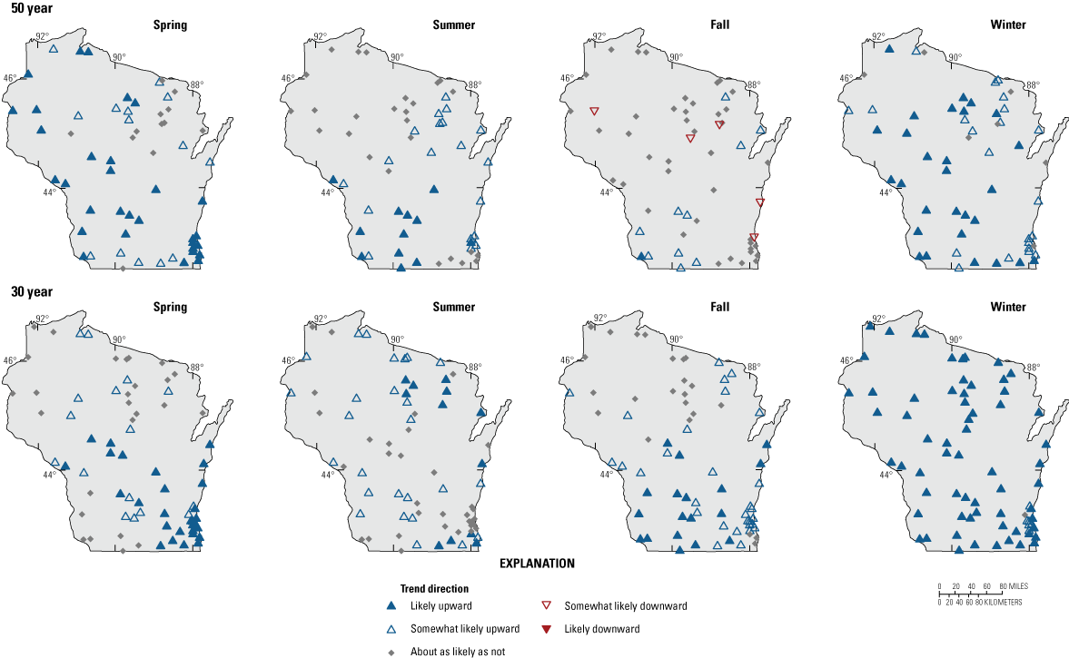
Seasonal streamflow trends are shown in figure 17. As with annual streamflow trends, seasonal trends were predominantly upward across all seasonal and analysis periods, and the largest trend magnitudes were in the 30-year period. In the southern half of the State, trends in seasonal streamflow were upward at nearly every streamgage in every season and analysis period. Streamgages in the northern half of the State had more variable seasonal trend results. The variability in seasonal trend likelihood and magnitudes across analysis periods is due to nonlinear or nonmonotonic trends at many streamgages. As with peak streamflow, changes in mean annual and seasonal streamflow were typically nonmonotonic, and many locations had unchanging or decreasing annual or seasonal streamflows during the early and mid-20th century and increases in the later part of the period.
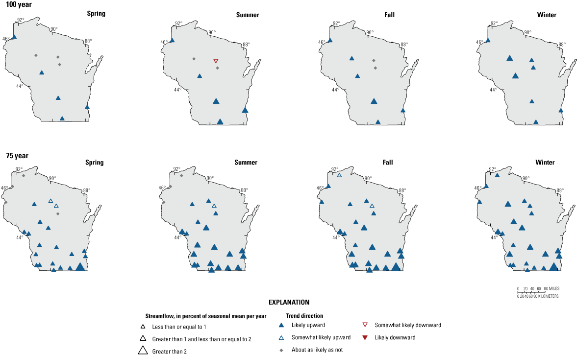
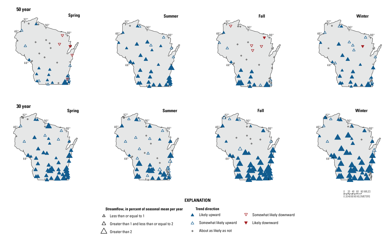
Magnitude and likelihood of monotonic trends in mean seasonal streamflow, in percent per year for four analysis periods ending in water year 2020.
Raster Seasonality Plots
Raster seasonality plots show the mean daily streamflow for every day in the period of record, colored by the magnitude of the streamflow, with day of the water year on the x-axis and water year on the y-axis (fig. 18A). These plots provide a visual view of streamflow magnitudes across the water year for the entire period of record. Changes in the magnitude of streamflow can be seen in the color patterns in these plots. For example, figure 18A shows the raster seasonality plot for USGS streamgage Sugar River near Brodhead, Wis. (05436500). At the beginning of the period of record for this streamgage, the moderate and high streamflows (green and blue) are typically between March and May. In the last 20 years of record, these same magnitude streamflows were detected throughout the year, and the lowest flows (tan and yellow), which were formerly common throughout the fall and winter, were rare. For the Sugar River near Brodhead streamgage, the increase in moderate and high flows around the year 2000 corresponds with increases in peak streamflow and changes in peak-streamflow timing shown in figure 11. The increase in daily streamflow magnitudes after the year 2000 indicates an increase in overall moisture conditions during seasons that were formerly dry. This increase in antecedent streamflows during summer storms may contribute to higher summer peak streamflows than would be expected under drier conditions. Raster seasonality plots are a qualitative analysis and not easily summarized across the State; however, similar increases in daily streamflow are evident at many southern Wisconsin streamgages (see Marti and others [2024] for raster plots at other streamgages). These changes in daily streamflow magnitude are not as apparent in central and northern streamgages.
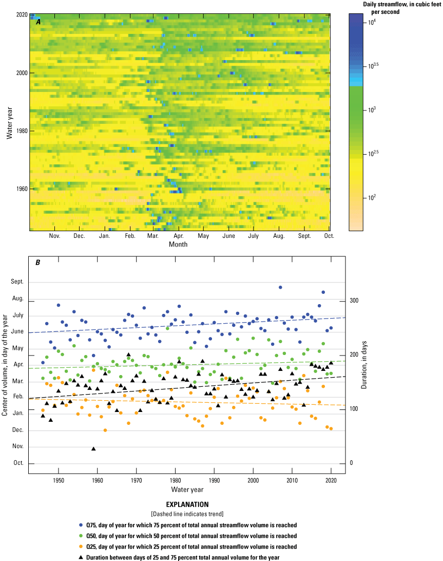
(A) Raster seasonality plot and (B) center of volume analysis for U.S. Geological Survey streamgage Sugar River near Brodhead, Wisconsin (05436500), for the 75-year period of water years 1946 to 2020 (modified from Marti and others [2024]).
Center of Volume Plots
The center of volume plots show the day of the year in which the 25th (Q25), 50th (Q50), and 75th (Q75) percentile of annual streamflow volume was detected. Linear trends in these percentile values over time indicate a change in the distribution of streamflow timing throughout the year. For example, figure 18B shows the center of volume analysis for USGS streamgage Sugar River near Brodhead, Wis. (05436500). At this location, a decrease in the Q25 indicates that the date at which 25 percent of the total annual volume of streamflow was detected has become earlier. A concurrent increase in the Q50 and Q75 indicates that the date at which 50 and 75 percent of the annual volume is detected is getting later. Essentially, the annual volume of streamflow has become spread out more evenly throughout the year, which is consistent with the increase in the magnitude of daily streamflows during summer, fall, and winter seen in the raster seasonality plot for the site (fig. 18A). The number of streamgages with likely or somewhat likely trends in the Q25, Q50, and Q75 and duration between the Q25 and Q75 are listed in table 3. Many streamgages across the State had upward trends in the duration between the Q25 and Q75 similar to Sugar River near Brodhead, indicating that the volume of annual streamflow is becoming more evenly spread throughout the year. Trends in the duration between the Q25 and Q75 were primarily upward in the southern ecoregions and had variable results in the northern half of the State (fig. 19).
Likelihood of monotonic trends in the duration between the 25th and 75th percentiles of annual streamflow volume for selected U.S. Geological Survey streamgages in Wisconsin for four analysis periods ending in water year 2020. Upward trends indicate the duration between the 25th and 75th percentiles of annual streamflow volume is getting longer, whereas downward trends indicate this duration is getting shorter.
Peaks-Over-Threshold Analysis
POT analyses detect changes in the frequency of daily streamflow that exceed a set streamflow threshold. For a given threshold, the number of streamflow events that exceed the threshold is counted for each water year as described in Ryberg and others (2024). Thresholds for the POT analyses in this study were set at the streamflow magnitude for which there is an average of two (POT2) and four (POT4) events per year. A POT analysis complements a traditional annual peak-streamflow flood-frequency analysis because it accounts for large flood-causing flows that may not be the peak of the year and can account for years with multiple floods.
Tests for change points in the number of events over the threshold were completed to identify increases or decreases in the frequency of these high POT2 and POT4 streamflow events. Change points were primarily upward for POT2 and POT4 for all four periods with isolated downward change points across the State (fig. 20). Downward change points were most common in the 1980s and 1990s (fig. 21). Many upward change points were detected after 2000. Although longer analysis periods do show upward change points as early as 1940, these earlier change points are spread more evenly through time and are less indicative of the regional scale changes seen in streamflows after 2000.
Likelihood of change points in the frequency of daily streamflow magnitude for which there is an average of (A) two events and (B) four events per year for selected streamgages in Wisconsin for four analysis periods ending in water year 2020.
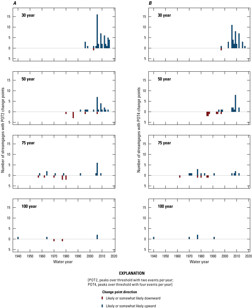
Dates of change points in the frequency of daily streamflow above a threshold for which there is (A) an average of two events and (B) an average of four events per year at selected streamgages in Wisconsin for four analysis periods ending in water year 2020.
Climate
Gridded climate data from the monthly water balance model (Wieczorek and others, 2022), described in the “Methods” section, were averaged over streamgaged drainage basins with available peak streamflow in the 100-, 75-, 50-, and 30-year analysis periods. Trends in annual and seasonal precipitation and temperature were identified across Wisconsin during all four analysis periods. This section summarizes results of climate trend analyses and describes spatial and temporal patterns in these analyses across the State.
Precipitation
The likelihood and magnitude of annual precipitation trends are shown in figure 22 and listed in table 4. Upward precipitation trends were prevalent across most of the State and all four analysis periods, except for the northwestern part of the State, which had fewer and weaker trends. Likely and somewhat likely precipitation trends were upward in each of the four analysis periods. No instances of downward trends in annual precipitation were detected. Median trend slopes for annual precipitation were largest in the 30-year period across the State, and within each analysis period, trend slopes were generally largest in the southern half of the State.
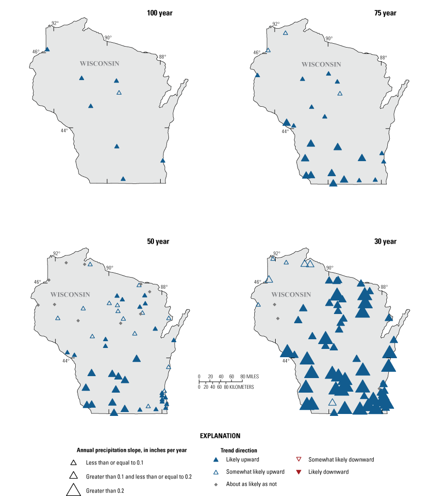
Magnitude and likelihood of monotonic trends in annual precipitation at selected U.S. Geological Survey streamgages in Wisconsin for four analysis periods ending in water year 2020.
Table 4.
Likelihood of monotonic trends in annual and seasonal precipitation at selected streamgages in Wisconsin for four analysis periods ending in water year 2020.Seasonal precipitation trends were most prevalent in winter and spring across all analysis periods (table 4; fig. 23). Upward winter precipitation trends were detected between 75 and 99 percent of streamgages, and upward spring trends were detected between 59 and 100 percent of streamgages across all four analysis periods. Trends in summer and fall were variable across analysis periods. Magnitudes of precipitation trends are shown in figure 24A and B in inches per year and as a relative percentage of the seasonal mean, respectively. Trend magnitudes increased in every season in the 30-year period compared to longer periods (fig. 24A). Average precipitation varies by season in Wisconsin; summer has the most precipitation (mean of 12.4 in. across all streamgages in this study), and winter has the least precipitation (mean of 3.9 in. across all streamgages in the study). Although winter trend magnitudes were generally equal to or less than trend magnitudes in other seasons (fig. 24A), winter trend magnitudes represent a larger relative increase in seasonal precipitation than other seasons because the average precipitation in winter is much lower than the other seasons.
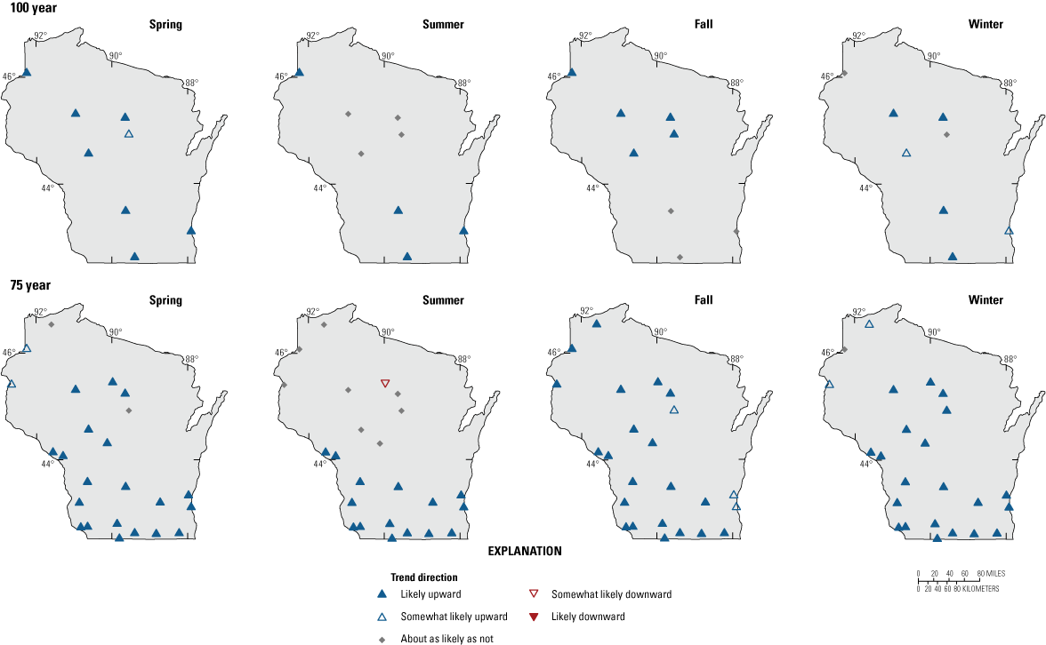
Likelihood of monotonic trends in seasonal precipitation at selected U.S. Geological Survey streamgages in Wisconsin for four analysis periods ending in water year 2020.
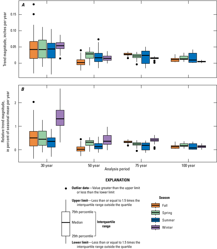
The distribution of trend magnitudes (A) in inches per year and (B) as the percentage of mean seasonal precipitation at selected U.S. Geological Survey streamgages in Wisconsin for four analysis periods ending in water year 2020.
Temperature
Likely upward trends in annual temperature were detected across every streamgage in the 100-, 75-, and 50-year periods (table 5). Fewer and weaker trends were detected in the latest 30-year period, particularly in the northern regions of the State. Temperature trends at most streamgages across the State were nonlinear, and at nearly all streamgages, mean annual temperature trends did not begin until the mid-1970s–80s. This typical trend pattern of annual and seasonal temperature at USGS streamgage Cedar Creek near Cedarburg, Wis. (04086500), for the 75-year analysis period is shown in figure 25A and B. The high amount of variability in annual temperatures after the year 2000 made detecting potential trends in the 30-year period difficult at many locations. Increases in annual temperature were largely driven by changes in winter temperature. Winter temperature changes were greater than the other seasons in the 100-, 75-, and 50-year periods (fig. 26) and, at most streamgages, showed the same pattern of rapid increase in winter temperatures during the 1980s and 1990s (fig. 25B). During the 30-year period, there were no trends in spring or winter, and the trend magnitudes in summer and fall were higher than other analysis periods. High variability in seasonal temperatures in winter and spring made it difficult to detect any trends during the 30-year period.
Table 5.
Likelihood of monotonic trends in annual and seasonal temperature at selected streamgages in Wisconsin for four analysis periods ending in water year 2020.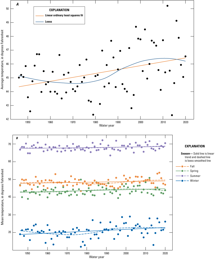
Annual mean temperature for U.S. Geological Survey streamgage Cedar Creek near Cedarburg, Wisconsin (04086500), for water years 1946 through 2020 (modified from Marti and others [2024]).
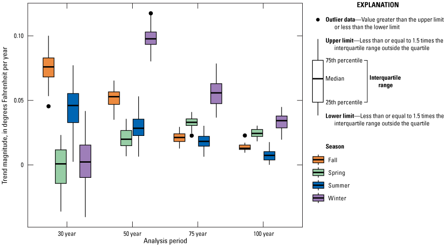
The distribution of seasonal trend slopes at selected U.S. Geological Survey streamgages in Wisconsin for four analysis periods ending in water year 2020.
Trends in Modeled Water Balance Components
Although temperature and precipitation generally increased in Wisconsin over the past 100 years, differences in the seasonality, magnitude, and geographic extent of these changes were detected. The water balance is largely driven by precipitation and temperature. Precipitation into a drainage basin may return to the atmosphere through evapotranspiration, be stored as soil moisture or groundwater, or run off later as streamflow. Trends and nonstationarities in precipitation and temperature (and therefore evapotranspiration) have the potential to change the relative quantities of each of these water balance components and the interactions between them. Additionally, changes in seasonal temperature and precipitation can alter snowfall and snowmelt dynamics. Results from a monthly water balance model were used to explore the relative change in annual precipitation, PET, and streamflow. Modeled outputs include PET, actual evapotranspiration, snowfall, soil moisture, soil water equivalent, and runoff (see Ryberg and others [2024] for complete description of these data).
The ratio of PET to precipitation is an indication of the overall “wetness” of a drainage basin; low ratio values indicate wet conditions, and high values indicate dry conditions. Trends in this ratio are indicators of the relative magnitudes of the increases in precipitation and temperature that were detected across the State. Trends in this ratio were mostly downward, primarily in the southern part of the State for the 100-, 75-, and 50-year periods and in the southern and northeastern areas of the State for the 30-year period (fig. 27). Decreases in this ratio indicate that the rate of increase in precipitation was generally larger than the increase in PET from temperature increases and indicate generally “wetter” conditions at these locations, which is consistent with the upward trend patterns in mean annual streamflow.
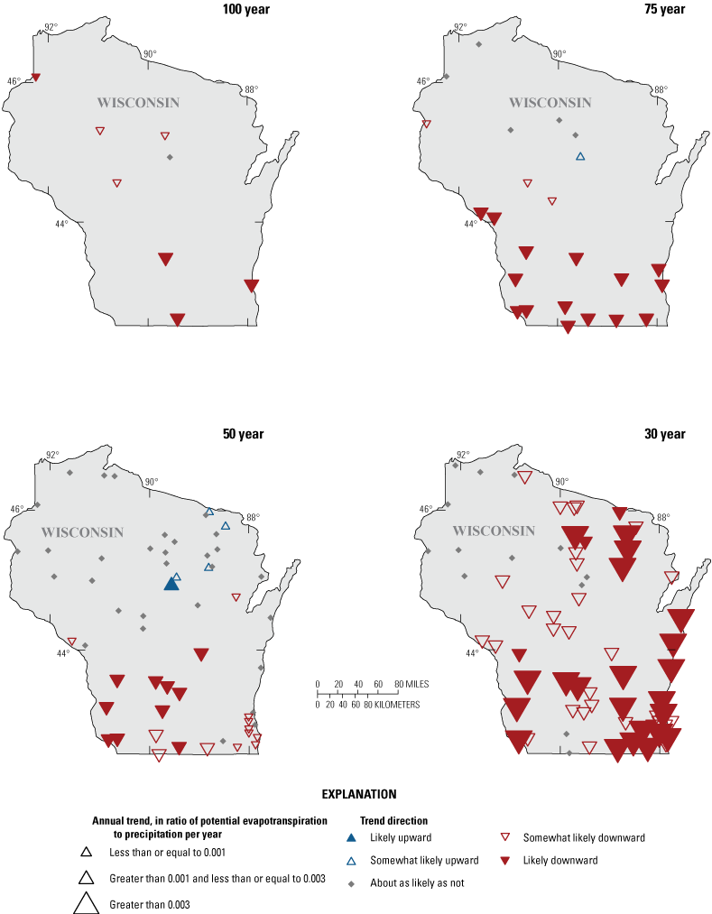
Magnitude and likelihood of the ratio of annual potential evapotranspiration and precipitation at selected U.S. Geological Survey streamgages in Wisconsin for four analysis periods ending in water year 2020.
Snowfall and snowmelt play an important part in the timing and magnitude of streamflow throughout much of Wisconsin. Increasing temperatures and precipitation during the fall through spring can change the amount of snowfall and the timing of snowmelt-related peak streamflows. Modeled annual snowfall trends were varied across analysis periods (table 6; fig. 28). Downward trends in annual snowfall in the 50-year period were detected at some northern and eastern streamgages and are consistent with the increased winter temperature and weaker precipitation trends during this period. Annual snowfall increased in central and northeastern Wisconsin in the 30-year period. Upward trends in the 30-year period are consistent with stabilizing winter temperatures and substantial upward winter precipitation trends during this period.
Table 6.
Likelihood of monotonic trends in annual and seasonal snowfall at selected U.S. Geological Survey streamgages in Wisconsin for four analysis periods ending in water year 2020.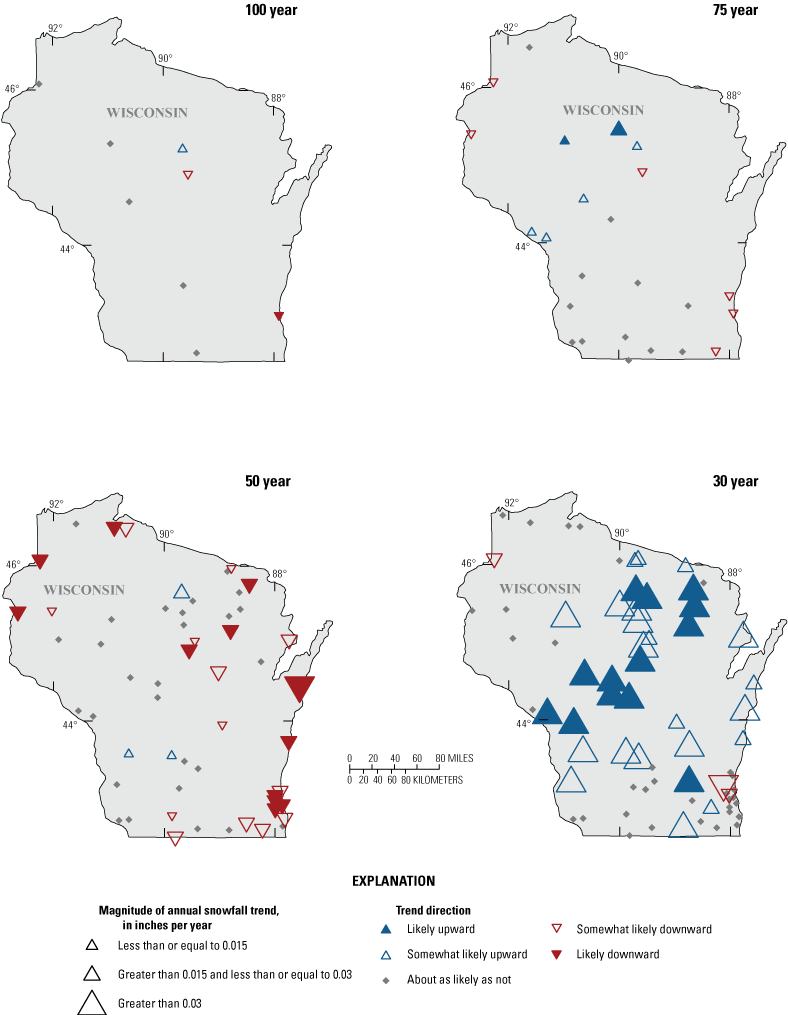
Magnitude and likelihood of monotonic trends in annual snowfall at selected U.S. Geological Survey streamgages in Wisconsin for four analysis periods ending in water year 2020.
Changes in the seasonality of snowfall were identified across the State, and trends in snowfall were primarily upward in the winter and downward in the spring and fall (table 6). Downward trends in snowfall during spring and fall are consistent with temperature increases in these months, which can cause more precipitation to fall as rain instead of snowfall. In winter, despite an upward trend in temperature, it was typically still cold enough for snow to form, and the general upward trend in precipitation in winter led to increases in snowfall.
Discussion and Implications for Flood-Frequency Analysis
Widespread nonstationarity was identified in streamflow and climate data throughout Wisconsin in the past 100 years. Changes in precipitation seem to be driving many of the changes in annual and peak streamflow in Wisconsin. The patterns of annual and seasonal increases in precipitation (figs. 22 and 23) are generally consistent with the patterns of annual and seasonal increases in annual streamflow (figs. 16 and 17). Increases in precipitation and annual streamflow were particularly large in the 30-year analysis period. During this period, increases in precipitation, particularly during fall and winter, led to wetter conditions and higher daily streamflows during normally low flow periods. This observation is consistent with results from the center of volume analyses and can be seen in the “greening” of the last 10 years of the raster streamflow analyses in the southern regions of the State, such as in figure 18A. Increases in precipitation in the 30-year period may be affecting peak-streamflow trends during this period as well. Precipitation increases, particularly in the fall in the DA ecoregion, are consistent with increasing peak-streamflow magnitudes and timing changes in peak streamflows as seen in figure 11A and B for Sugar River near Brodhead.
Trends in the climate data in this study do not explain the downward trends in peak streamflows in the 100- and 75-year periods. Despite increasing precipitation and daily streamflow, and decreasing PET/precipitation ratios indicating wetter conditions, peak streamflows decreased throughout much of the DA ecoregion before the year 2000. Other potential causes of decreases in peak streamflows such as urbanization and land-use changes associated with agricultural practices are beyond the scope of this study but have been indicated as potential causes of downward trends in peak streamflows by previous investigators (Gyawali and others, 2015; Gebert and others 2016; Levin and Holtschlag, 2022).
The widespread prevalence of nonstationarity in peak streamflow in Wisconsin has important implications for flood-frequency analysis. The statistical methods used to estimate the flood magnitude for a given annual exceedance probability assume that the peak-streamflow time series are stationary and representative of a random process. The presence of a trend in peak-streamflow time series is particularly problematic at streamgages with short periods of record because the peak streamflows during that period may not be representative of the full range of peak-streamflow magnitudes and may result in a biased estimate of the flood magnitude. For example, peak streamflows at Sugar River near Brodhead indicate a U-shaped trend (figure 11A). The estimated flood magnitude for the 1-percent annual exceedance probability for this streamgage for the period of record (from water year 1914 through water year 2020) is 15,970 ft3/s, with a 95 percent confidence interval of 12,680 to 22,500 (Levin and Sanocki, 2023). However, if only 20 years of data were available at this stream, the resulting estimated flood magnitude for the 1-percent annual exceedance probability could be as low as 8,700 ft3/s (confidence interval, 6,150 to 19,640 ft3/s) using data from 1975 through 1995) or as high as 24,400 ft3/s (confidence interval 15,680 to 58,020 ft3/s) using data from 1914 through 1934, a nearly threefold difference. Bulletin 17C recommends a minimum period of record of 10 years to compute the flood frequency at a streamgage (England and others, 2018). However, if a 10-year record was used in the DA ecoregion, which demonstrates widespread peak-streamflow trends, the short record length would lead to unreliable estimates of flood frequency.
In addition to biases in at-site flood-frequency analysis, nonstationarity in peak streamflow can complicate the development of regional flood-frequency equations used to estimate flood frequency at ungaged locations. Biases in estimates of flood-frequency magnitude at streamgages may propagate through regional regression equations. Additionally, in a region with widespread nonstationarity, there may not be enough streamgages with long periods of record (at least 50 years) with which to develop a regression equation, and the incorporation of flood-frequency estimates at streamgages with shorter records will introduce a high degree of variability or bias to the data underlying the regression equation. Biases and uncertainties in regional regression equations have implications in floodplain management, bridge and road construction, and other infrastructure projects that use these equations in their designs.
Summary
This report characterizes changes in annual peak streamflow and daily streamflow in Wisconsin as part of a larger U.S. Geological Survey effort to characterize the effects of regional hydroclimatic shifts and changes in climate on streamflow across the Midwest. Four analysis periods were examined: the 100-year period including water years 1921 through 2020, the 75-year period of water years 1946 through 2020, the 50-year period of water years 1971 through 2020, and the 30-year period of water years 1991 through 2020. Additionally, trends in gridded precipitation, temperature data, and estimated water budget components were examined as potential drivers of streamflow change.
Trends in peak streamflows varied spatially and temporally. Peak streamflows in the Driftless Area of Wisconsin decreased from 1920 through the 1980s but increased between 1990 and 2020. The change in direction of the trend around 1990 was accompanied by a change in the timing of peak streamflows, and peak streamflows became more common in the late summer and early fall. Peak streamflows in the southeastern corner of Wisconsin increased throughout most analysis periods. Trends in peak streamflows in the central and northern regions of Wisconsin were variable, and upward and downward trends were present. Change points were detected at many streamgages across the State and generally followed the same spatial patterns as those for monotonic trends.
Daily streamflow was used to examine trends in annual and seasonal streamflow. Annual streamflow increased across the State at most streamgages. Trend magnitudes for annual streamflow were largest in southern Wisconsin. Although upward trends were detected across all four analysis periods, trend magnitudes in all ecoregions increased markedly in the 30-year analysis period, and median seasonal trend magnitudes doubled or nearly doubled in most ecoregions.
Annual precipitation and temperature increased at streamgages across the State. Upward trends in precipitation were detected throughout the State and fewer trends were identified in the northwestern area of the State. Seasonal precipitation trends were more prevalent in winter and spring than in summer and fall. For all seasons, trend magnitudes in precipitation were larger in the most recent 30-year analysis period. Upward temperature trends were also identified at all streamgages in the study in the 100-, 75-, and 50-year periods and were largest during the winter. Trends were less prevalent during the 30-year period, when high variability in annual temperatures made trend detection more difficult.
Changes in climate over the periods of analysis point to wetter conditions overall and are likely driving increases in streamflow. Hydroclimatic trends may also be driving upward trends in peak streamflows from 1990 through 2020; however, they do not adequately explain the downward trends in peak streamflows between 1920 and 1980. In addition to hydroclimatic variability, other potential mechanisms can cause nonstationarity in peak streamflow, including effects of urbanization, water use, and land-use changes associated with agriculture.
References Cited
Andresen, J., Hilberg, S., and Kunkel, K., 2012, Historical climate and climate trends in the Midwestern USA, in Winkler, J., Andresen, J., Hatfield, J., Bidwell, D., and Brown, D., coordinators, U.S. National Climate Assessment Midwest technical input report: Great Lakes Integrated Sciences and Assessments Center, 18 p., accessed June 1, 2022, at http://glisa.msu.edu/docs/NCA/MTIT_Historical.pdf.
Barth, N.A., Ryberg, K.R., Gregory, A., and Blum, A.G., 2022, Introduction to attribution of monotonic trends and change points in peak streamflow across the conterminous United States using a multiple working hypotheses framework, 1941–2015 and 1966–2015, chap. A of Ryberg, K.R., ed., Attribution of monotonic trends and change points in peak streamflow across the conterminous United States using a multiple working hypotheses framework, 1941–2015 and 1966–2015: U.S. Geological Survey Professional Paper 1869, p. A1–A29, accessed June 1, 2022, at https://doi.org/10.3133/pp1869.
Budikova, D., Ford, T.W., and Wright, J.D., 2022, Characterizing winter season severity in the Midwest United States, part II—Interannual variability: International Journal of Climatology, v. 42, no. 6, p. 3499–3516. [Also available at https://doi.org/10.1002/joc.7429.]
Conger, D.H., 1971, Estimating magnitude and frequency of floods in Wisconsin: U.S. Geological Survey Open-File Report 71–76, 200 p. [Also available at https://doi.org/10.3133/ofr7176.]
Conger, D.H., 1981, Techniques for estimating magnitude and frequency of floods for Wisconsin streams: U.S. Geological Survey Open-File Report 80–1214, 116 p. [Also available at https://doi.org/10.3133/ofr801214.]
Dewitz, J., 2019, National Land Cover Database (NLCD) 2016 products (ver. 2.0, July 2020): U.S. Geological Survey data release, accessed June 1, 2022, at https://doi.org/10.5066/P96HHBIE.
Dudley, R.W., Archfield, S.A., Hodgkins, G.A., Renard, B., and Ryberg, K.R., 2018, Peak-streamflow trends and change-points and basin characteristics for 2,683 U.S. Geological Survey streamgages in the conterminous U.S. (ver. 3.0, April 2019): U.S. Geological Survey data release, accessed June 1, 2022, at https://doi.org/10.5066/P9AEGXY0.
Enfield, D.B., Mestas-Nuñez, A.M., and Trimble, P.J., 2001, The Atlantic Multidecadal Oscillation and its relation to rainfall and river flows in the continental U.S.: Geophysical Research Letters, v. 28, no. 10, p. 2077–2080. [Also available at https://doi.org/10.1029/2000GL012745.]
England, J.F., Jr., Cohn, T.A., Faber, B.A., Stedinger, J.R., Thomas, W.O., Jr., Veilleux, A.G., Kiang, J.E., and Mason, R.R., Jr., 2018, Guidelines for determining flood flow frequency—Bulletin 17C (ver. 1.1, May 2019): U.S. Geological Survey Techniques and Methods, book 4, chap. B5, 148 p. [Also available at https://doi.org/10.3133/tm4B5.]
Ericson, D.W., 1961, Floods in Wisconsin—Magnitude and frequency: U.S. Geological Survey Open-File Report 61–44, 109 p. [Also available at https://doi.org/10.3133/ofr6144.]
Frankson, R., Kunkel, K.E., Champion, S.M., and Sun, L., 2022, Wisconsin state climate summary: National Oceanic and Atmospheric Administration Technical Report NESDIS 150–WI, 6 p., accessed July 14, 2022, at https://statesummaries.ncics.org/chapter/wi/.
Gebert, W.A., Garn, H.S., and Rose, W.J., 2016, Changes in streamflow characteristics in Wisconsin as related to precipitation and land use (ver. 1.1, January 28, 2016): U.S. Geological Survey Scientific Investigations Report 2015–5140, 23 p., 1 appendix. [Also available at https://doi.org/10.3133/sir20155140.]
Gebert, W.A., and Krug, W.R., 1996, Streamflow trends in Wisconsin’s Driftless Area: Journal of the American Water Resources Association, v. 32, no. 4, p. 733–744. [Also available at https://doi.org/10.1111/j.1752-1688.1996.tb03470.x.]
Gyawali, R., Greb, S., and Block, P., 2015, Temporal changes in streamflow and attribution of changes to climate and landuse in Wisconsin watersheds: Journal of the American Water Resources Association, v. 51, no. 4, p. 1138–1152. [Also available at https://doi.org/10.1111/jawr.12290.]
Hirsch, R.M., Archfield, S.A., and De Cicco, L.A., 2015, A bootstrap method for estimating uncertainty of water quality trends: Environmental Modelling & Software, v. 73, p. 148–166. [Also available at https://doi.org/10.1016/j.envsoft.2015.07.017.]
Hodgkins, G.A., Dudley, R.W., Archfield, S.A., and Renard, B., 2019, Effects of climate, regulation, and urbanization on historical flood trends in the United States: Journal of Hydrology, v. 573, p. 697–709. [Also available at https://doi.org/10.1016/j.jhydrol.2019.03.102.]
Interagency Advisory Committee on Water Data, 1982, Guidelines for determining flood flow frequency: U.S. Geological Survey, Office of Water Data Coordination Bulletin 17B of the Hydrology Subcommittee, 194 p. [Also available at https://water.usgs.gov/osw/bulletin17b/dl_flow.pdf.]
Ivancic, T.J., and Shaw, S.B., 2017, Identifying spatial clustering in change points of streamflow across the contiguous U.S. between 1945 and 2009: Geophysical Research Letters, v. 44, no. 5, p. 2445–2453. [Also available at https://doi.org/10.1002/2016GL072444.]
Juckem, P.F., Hunt, R.J., Anderson, M.P., and Robertson, D.M., 2008, Effects of climate and land management change on streamflow in the Driftless Area of Wisconsin: Journal of Hydrology, v. 355, no. 1–4, p. 123–130. [Also available at https://doi.org/10.1016/j.jhydrol.2008.03.010.]
Kendall, M.G., 1938, A new measure of rank correlation: Biometrika, v. 30, no. 1/2, p. 81–93. [Also available at https://doi.org/10.2307/2332226.]
Knox, J.C., 2000, Sensitivity of modern and Holocene floods to climate change: Quaternary Science Reviews, v. 19, no. 1–5, p. 439–457. [Also available at https://doi.org/10.1016/S0277-3791(99)00074-8.]
Koutsoyiannis, D., and Montanari, A., 2015, Negligent killing of scientific concepts—The stationarity case: Hydrological Sciences Journal, v. 60, no. 7–8, p. 1174–1183. [Also available at https://doi.org/10.1080/02626667.2014.959959.]
Krug, W.R., Conger, D.H., and Gebert, W.A., 1992, Flood-frequency characteristics of Wisconsin streams: U.S. Geological Survey Water-Resources Investigations Report 91–4128, 185 p. [Also available at https://doi.org/10.3133/wri914128.]
Kucharik, C.J., Serbin, S.P., Vavrus, S., Hopkins, E.J., and Motew, M.M., 2010, Patterns of climate change across Wisconsin from 1950 to 2006: Physical Geography, v. 31, no. 1, p. 1–28. [Also available at https://doi.org/10.2747/0272-3646.31.1.1.]
Levin, S.B., and Holtschlag, D.J., 2022, Attribution of monotonic trends and change points in peak streamflow in the Midwest Region of the United States, 1941–2015 and 1966–2015, chap. D of Ryberg, K.R., ed., Attribution of monotonic trends and change points in peak streamflow across the conterminous United States using a multiple working hypotheses framework, 1941–2015 and 1966–2015: U.S. Geological Survey Professional Paper 1869, p. D1–D22, accessed December 1, 2022, at https://doi.org/10.3133/pp1869.
Levin, S.B., and Sanocki, C.A., 2023, Estimating flood magnitude and frequency for unregulated streams in Wisconsin: U.S. Geological Survey Scientific Investigations Report 2022–5118, 25 p., accessed January 15, 2023, at https://doi.org/10.3133/sir20225118. [Supersedes Scientific Investigations Report 2016–5140.]
Lins, H.F., and Cohn, T.A., 2011, Stationarity—Wanted dead or alive?: Journal of the American Water Resources Association, v. 47, no. 3, p. 475–480. [Also available at https://doi.org/10.1111/j.1752-1688.2011.00542.x.]
Marti, M.K., and Ryberg, K.R., 2023, Method for identification of reservoir regulation within U.S. Geological Survey streamgage basins in the Central United States using a decadal dam impact metric: U.S. Geological Survey Open-File Report 2023–1034, 15 p., accessed May 2023 at https://doi.org/10.3133/ofr20231034.
Marti, M.K., Wavra, H.N., Over, T.M., Ryberg, K.R., Podzorski, H.L., and Chen, Y.R., 2024, Peak streamflow data, climate data, and results from investigating hydroclimatic trends and climate change effects on peak streamflow in the Central United States, 1921–2020: U.S. Geological Survey data release, https://doi.org/10.5066/P9R71WWZ.
McCabe, G.J., and Wolock, D.M., 2002, A step increase in streamflow in the conterminous United States: Geophysical Research Letters, v. 29, no. 24, p. 38-1–38-4. [Also available at https://doi.org/10.1029/2002GL015999.]
McDonald, C.P., Rover, J.A., Stets, E.G., and Striegl, R.G., 2012, The regional abundance and size distribution of lakes and reservoirs in the United States and implications for estimates of global lake extent: Limnology and Oceanography, v. 57, no. 2, p. 597–606. [Also available at https://doi.org/10.4319/lo.2012.57.2.0597.]
Milly, P.C.D., Betancourt, J., Falkenmark, M., Hirsch, R.M., Kundzewicz, Z.W., Lettenmaier, D.P., and Stouffer, R.J., 2008, Stationarity is dead—Whither water management?: Science, v. 319, no. 5863, p. 573–574. [Also available at https://doi.org/10.1126/science.1151915.]
Morton, W.E., McArthur, A.D., and Neverman, P.F., 1948, The Wisconsin centennial story of disasters and other unfortunate events, 1848–1948: Wisconsin State Centennial Committee, 84 p. [Also available at https://www.wisconsinhistory.org/turningpoints/search.asp?id=1675.]
National Integrated Drought Information System, 2022, Drought in Wisconsin from 2000–present: National Integrated Drought Information System digital data, accessed June 29, 2022, at https://www.drought.gov/states/wisconsin#historical-conditions.
Natural Resources Conservation Service, 2019, Web Soil Survey: Natural Resources Conservation Service digital data, accessed June 3, 2019, at https://websoilsurvey.nrcs.usda.gov/app/.
Omernik, J.M., Chapman, S.S., Lillie, R.A., and Dumke, R.T., 2000, Ecoregions of Wisconsin: Transactions of the Wisconsin Academy of Sciences, Arts, and Letters, v. 88, p. 77–103. [Also available at https://images.library.wisc.edu/WI/EFacs/transactions/WT2000/reference/wi.wt2000.jmomernik.pdf.]
Omernik, J.M., and Griffith, G.E., 2014, Ecoregions of the conterminous United States—Evolution of a hierarchical spatial framework: Environmental Management, v. 54, no. 6, p. 1249–1266. [Also available at https://doi.org/10.1007/s00267-014-0364-1.]
Pettitt, A.N., 1979, A non-parametric approach to the change point problem: Journal of the Royal Statistical Society, Series C, Applied Statistics, v. 28, no. 2, p. 126–135. [Also available at https://doi.org/10.2307/2346729.]
Potter, K.W., 1991, Hydrological impacts of changing land management practices in a moderate-sized agricultural catchment: Water Resources Research, v. 27, no. 5, p. 845–855. [Also available at https://doi.org/10.1029/91WR00076.]
Potter, K.W., 2019, Hydrology of the Driftless Area, in Dauwalter, D.C., ed., A look back at Driftless Area science to plan for resiliency in an uncertain future: Special Publication of the 11th Annual Driftless Area Symposium, La Crosse, Wis., February 5–6, 2019, p. 15–19. [Also available at https://www.kiaptuwish.org/wp-content/uploads/2020/03/Special-Publication_DASymp_2019__Final.pdf.]
Ryberg, K.R., Hodgkins, G.A., and Dudley, R.W., 2020, Change points in annual peak streamflows—Method comparisons and historical change points in the United States: Journal of Hydrology, v. 583, art. 124307, 13 p. [Also available at https://doi.org/10.1016/j.jhydrol.2019.124307.]
Ryberg, K.R., Over, T.M., Levin, S.B., Heimann, D.C., Barth, N.A., Marti, M.S., O’Shea, P.S., Sanocki, C.A., Williams-Sether, T.J., Wavra, H.N., Sando, T.R., Sando, S.K., and Liu, M.S., 2024, Introduction and methods of analysis for peak streamflow trends and their relation to changes in climate in Illinois, Iowa, Michigan, Minnesota, Missouri, Montana, North Dakota, South Dakota, and Wisconsin, chap. A of Ryberg, K.R., comp., Peak streamflow trends and their relation to changes in climate in Illinois, Iowa, Michigan, Minnesota, Missouri, Montana, North Dakota, South Dakota, and Wisconsin: U.S. Geological Survey Scientific Investigations Report 2023–5064, 27 p., accessed January 2024 at https://doi.org/10.3133/sir20235064A.
Sando, R., Sando, S.K., Ryberg, K.R., and Chase, K.J., 2022, Attribution of monotonic trends and change points in peak streamflow in the Upper Plains Region of the United States, 1941–2015 and 1966–2015, chap. C of Ryberg, K.R., ed., Attribution of monotonic trends and change points in peak streamflow across the conterminous United States using a multiple working hypotheses framework, 1941–2015 and 1966–2015: U.S. Geological Survey Professional Paper 1869, p. C1–C36, accessed December 15, 2022, at https://doi.org/10.3133/pp1869.
Serinaldi, F., and Kilsby, C.G., 2015, Stationarity is undead—Uncertainty dominates the distribution of extremes: Advances in Water Resources, v. 77, p. 17–36. [Also available at https://doi.org/10.1016/j.advwatres.2014.12.013.]
Stedinger, J.R., and Griffis, V.W., 2011, Getting from here to where? Flood frequency analysis and climate: Journal of the American Water Resources Association, v. 47, no. 3, p. 506–513. [Also available at https://doi.org/10.1111/j.1752-1688.2011.00545.x.]
U.S. Geological Survey, 2021, USGS water data for the Nation: U.S. Geological Survey National Water Information System database, accessed July 14, 2021, at https://doi.org/10.5066/F7P55KJN.
Vogel, R.M., Yaindl, C., and Walter, M., 2011, Nonstationarity—Flood magnification and recurrence reduction factors in the United States: Journal of the American Water Resources Association, v. 47, no. 3, p. 464–474. [Also available at https://doi.org/10.1111/j.1752-1688.2011.00541.x.]
von Neumann, J., Kent, R.H., Bellinson, H.R., and Hart, B.I., 1941, The mean square successive difference: Annals of Mathematical Statistics, v. 12, no. 2, p. 153–162. [Also available at https://doi.org/10.1214/aoms/1177731746.]
Vose, R.S., Applequist, S., Squires, M., Durre, I., Menne, M.J., Williams, C.N., Jr., Fenimore, C., Gleason, K., and Arndt, D., 2017, Gridded 5km GHCN-daily temperature and precipitation dataset (nCLIMGRID), version 1: National Oceanic and Atmospheric Administration, National Centers for Environmental Information digital data, accessed June 1, 2022, at https://doi.org/10.7289/V5SX6B56.
Walker, J.F., and Krug, W.R., 2003, Flood-frequency characteristics of Wisconsin streams: U.S. Geological Survey Water-Resources Investigations Report 2003–4250, 37 p. [Also available at https://doi.org/10.3133/wri034250.]
Walker, J.F., Peppler, M.C., Danz, M.E., and Hubbard, L.E., 2017, Flood-frequency characteristics of Wisconsin streams (ver. 2.2, April 2020): U.S. Geological Survey Scientific Investigations Report 2016–5140, 33 p., 1 plate, 2 appendixes, accessed June 1, 2022, at https://doi.org/10.3133/sir20165140.
White, K.D., and Arnold, J.R., 2015, Recent US climate change and hydrology literature applicable to US Army Corps of Engineers missions—Great Lakes Region: Washington, D.C., U.S. Army Corps of Engineers Civil Works Technical Report CWTS–2015–07, 41 p., accessed June 1, 2022, at https://usace.contentdm.oclc.org/utils/getfile/collection/p266001coll1/id/6735.
Wieczorek, M.E., Signell, R.P., McCabe, G.J., and Wolock, D.M., 2022, USGS monthly water balance model inputs and outputs for the conterminous United States, 1895–2020, based on ClimGrid data: U.S. Geological Survey data release, accessed June 1, 2022, at https://doi.org/10.5066/P9JTV1T6.
Wisconsin Historical Society, 2021, Floods in Wisconsin: Wisconsin Historical Society web page, accessed July 2021 at https://www.wisconsinhistory.org/Records/Article/CS2507.
Conversion Factors
Supplemental Information
A water year is the period from October 1 to September 30 and is designated by the year in which it ends; for example, water year 2020 was from October 1, 2019, to September 30, 2020.
Abbreviations
CSG
crest-stage gage
DA
Driftless Area [ecoregion]
ENSO
El Niño-Southern Oscillation
NCHF
North Central Hardwood Forests [ecoregion]
NLF
Northern Lakes and Forests [ecoregion]
p-value
probability value
PET
potential evapotranspiration
POT
peaks over threshold
POT2
peaks over threshold with two events per year
POT4
peaks over threshold with four events per year
Q25
25th percentile of annual streamflow
Q50
50th percentile of annual streamflow
Q75
75th percentile of annual streamflow
USGS
U.S. Geological Survey
WY
water year
For more information about this publication, contact:
Director, USGS Upper Midwest Water Science Center
1 Gifford Pinchot Drive
Madison, WI 53726
For additional information, visit: https://www.usgs.gov/centers/upper-midwest-water-science-center
Publishing support provided by the
Rolla Publishing Service Center
Disclaimers
Any use of trade, firm, or product names is for descriptive purposes only and does not imply endorsement by the U.S. Government.
Although this information product, for the most part, is in the public domain, it also may contain copyrighted materials as noted in the text. Permission to reproduce copyrighted items must be secured from the copyright owner.
Suggested Citation
Levin, S.B., 2024, Peak streamflow trends in Wisconsin and their relation to changes in climate, water years 1921–2020, chap. J of Ryberg, K.R., comp., Peak streamflow trends and their relation to changes in climate in Illinois, Iowa, Michigan, Minnesota, Missouri, Montana, North Dakota, South Dakota, and Wisconsin: U.S. Geological Survey Scientific Investigations Report 2023–5064, 49 p., https://doi.org/10.3133/sir20235064J.
ISSN: 2328-0328 (online)
Study Area
| Publication type | Report |
|---|---|
| Publication Subtype | USGS Numbered Series |
| Title | Peak streamflow trends in Wisconsin and their relation to changes in climate, water years 1921–2020 |
| Series title | Scientific Investigations Report |
| Series number | 2023-5064 |
| Chapter | J |
| DOI | 10.3133/sir20235064J |
| Publication Date | January 25, 2024 |
| Year Published | 2024 |
| Language | English |
| Publisher | U.S. Geological Survey |
| Publisher location | Reston, VA |
| Contributing office(s) | Upper Midwest Water Science Center |
| Description | Report: ix, 49 p.; Data Release; Dataset |
| Country | United States |
| State | Wisconsin |
| Online Only (Y/N) | Y |
| Additional Online Files (Y/N) | N |