

Effects of Impoundments on Selected Flood-Frequency and Daily Mean Streamflow Characteristics in Georgia, South Carolina, and North Carolina
Links
- Document: Report (4 MB pdf) , HTML , XML
- Data Releases:
- NGMDB Index Page: National Geologic Map Database Index Page (html)
- Download citation as: RIS | Dublin Core
Acknowledgments
The authors acknowledge the longstanding partnership between the U.S. Geological Survey (USGS) and the South Carolina Department of Transportation (SCDOT). The foresight and leadership of engineers and management at the SCDOT have been vitally important to improving the understanding of water resources in South Carolina and the impacts that extreme events can have on highway infrastructure. The authors also would like to acknowledge Thomas Knight, SCDOT, for his support and guidance on this investigation.
The peak flow and daily mean flow data used in the analyses in this report were collected throughout Georgia, South Carolina, and North Carolina at streamgages operated in cooperation with a variety of Federal, State, and local agencies. The foresight of those cooperators in realizing the importance of long-term monitoring of streamflow is of paramount importance for investigations such as this. The authors also acknowledge the dedicated work of the USGS field-office staff in collecting, processing, and storing the peak flow and daily mean flow data necessary for the completion of this investigation.
Abstract
The U.S. Geological Survey (USGS) has a long history of working cooperatively with the South Carolina Department of Transportation to develop methods for estimating the magnitude and frequency of floods for rural and urban streams that have minimal to no regulation or tidal influence. As part of those previous investigations, flood-frequency estimates also have been generated for selected streamgages on regulated streams. This report assesses the effects of impoundments on flood-frequency characteristics by comparing annual exceedance probability (AEP) streamflows from pre- and post-regulated (before and after impoundment) periods at 18 long-term USGS streamgages, which is defined as a streamgage with 30 or more years of record, in Georgia, South Carolina, and North Carolina. For an assessment of how differences in such statistics can be influenced by period of record and hydrologic conditions captured in those records, which could be considered as natural variability, AEP streamflows at an additional 18 long-term USGS streamgages that represent unregulated conditions in those three States were computed and compared for the first and last half of those records.
Of the 18 long-term streamgages with pre- and post-regulated periods of record, 17 streamgages had both peak streamflows and daily mean streamflows available. To further assess how impoundments may influence a broader range of streamflow characteristics, The Nature Conservancy’s Indicators of Hydrologic Alteration software was used to compare selected streamflow characteristics generated from daily mean streamflows for pre- and post-regulated periods of record at 16 of those long-term streamgages. For comparison of the natural variability of such streamflow statistics, two periods of record (first half and last half) also were compared at 17 of the 18 long-term streamgages on unregulated streams. The remaining long-term streamgage on an unregulated stream included in this report had only annual peak streamflows and, therefore, was not included in the hydrologic alteration analysis.
In a separate USGS investigation completed in 2023, flood-frequency statistics for the 50-, 20-, 10-, 4-, 2-, 1-, 0.5-, and 0.2-percent AEP streamflows (also known as the 2-, 5-, 10-, 25-, 50-, 100-, 200-, and 500-year recurrence interval streamflows, respectively) were computed for 72 streamgages on regulated streams in Georgia, South Carolina, and North Carolina. Of those 72 streamgages, 29 streamgages were found to be redundant, which is a situation where the drainage basin of one streamgage is contained inside another (nested) and the two basins are of similar size. For the remaining 43 streamgages, 39 had basins where 75 percent or more of the drainage area was above the Fall Line. Those 39 streamgages were included in this investigation to develop regional regression equations that can be used to estimate the flood-frequency statistics at ungaged locations on regulated streams in Georgia, South Carolina, and North Carolina in which 75 percent or more of the drainage basin is located above the Fall Line. The flood-frequency regression equations are functions of drainage area and maximum storage index computed for upstream reservoirs.
Introduction
Reliable estimates of the magnitude and frequency of floods are essential for flood insurance studies, floodplain management, and the design of transportation and water-conveyance structures such as roads, bridges, culverts, dams, and levees. Federal, State, regional, and local officials rely on such estimates to effectively plan and manage land use and water resources, protect lives and property in flood-prone areas, and determine flood insurance rates. The U.S. Geological Survey (USGS) and the South Carolina Department of Transportation have a long history of working cooperatively to develop techniques for estimating the magnitude and frequency of floods for rural and urban streams that have minimal to no regulation or tidal influence (Whetstone, 1982a, b; Guimaraes and Bohman, 1991; Bohman, 1992; Feaster and Tasker, 2002; Feaster and Guimaraes, 2004; Feaster and others, 2009, 2014, 2023). The Federal guidelines for flood-frequency analyses at streamgaging stations (streamgages) were developed for basins where streamflows under flood conditions are not appreciably altered by regulation, basin changes, or hydrologic nonstationarities (England and others [2018], commonly referred to as “Bulletin 17C”). However, under certain conditions, it may be appropriate to apply those techniques at streamgages monitoring regulated streams. Factors that must be considered include the severity of the regulation, the length of record at the regulated streamgage for which the regulation patterns have been relatively stable, and whether the statistical distribution used in the Federal guidelines adequately fits the logarithms of the peak-streamflow data used in the analysis. Over the years, flood-frequency analyses have been done at selected streamgages on regulated streams in South Carolina (Conrads and others, 2008; Feaster and others, 2009), but there has not been a comprehensive report assessing the effects of regulation from impoundments on streamflow.
Streams are impounded for a variety of reasons such as flood control, water supply, irrigation, and hydroelectric power generation (Ruddy and Hitt, 1990). The effect of the regulation from those various impoundments on downstream streamflows also varies widely. For example, a water-supply reservoir may have little to no storage capacity for flood control and, consequently, not appreciably change the characteristics of downstream flood streamflows. Reservoirs for which the main function is hydroelectric power generation or flood control will tend to decrease flood streamflows and may increase low streamflows (Graf, 2006). The degree of regulation at USGS streamgages located downstream from impoundments often is assessed on more of a qualitative than quantitative basis (Asquith, 2001). For humid areas of the United States, Benson (1962) determined that a usable storage of less than 103 acre-feet per square mile (acre-ft/mi2) would generally affect peak streamflows by less than 10 percent and, therefore, used that level of usable storage as a limiting value for assuming that flood-frequency statistics were not substantially influenced by upstream regulation. Along with other assessment tools, the guidance from Benson (1962) related to the level of usable storage that generally starts appreciably affecting peak flows was used by Feaster and others (2023) to assess the potential degree of regulation of basins being monitored at streamgages downstream from impoundments. However, Feaster and others (2023) used the maximum storage, in acre-feet, from the U.S. Army Corps of Engineers National Inventory of Dams (NID) database (U.S. Army Corps of Engineers, 2020), which is defined as the total storage in a reservoir below the maximum attainable water-surface elevation, including any surcharge storage. Usable storage is defined as storage that is normally available for release from a reservoir below the maximum controllable water level and, therefore, excludes dead storage, which is the volume of water in a reservoir below the lowest controllable water level (Martin and Hanson, 1966). In many hydroelectric reservoirs, the dead storage tends to be a small part of the total storage.
Purpose and Scope
The purpose of this investigation was to assess the effects of impoundments on selected streamflow characteristics across the contiguous hydrologic regions in Georgia, South Carolina, and North Carolina as defined by Feaster and others (2009, 2014, 2023). Of particular interest to the South Carolina Department of Transportation are the effects that impoundments have on flood-frequency statistics for the 50-, 20-, 10-, 4-, 2-, 1-, 0.5-, and 0.2-percent annual exceedance probability (AEP) streamflows (also known as the 2-, 5-, 10-, 25-, 50-, 100-, 200-, and 500-year recurrence interval streamflows, respectively). Along with assessing changes in selected flood-frequency characteristics due to regulation from impoundments, other selected streamflow characteristics were assessed to gain a more complete understanding of impacts from regulation throughout the streamflow regime. As such, the report assesses the effects on low-streamflow characteristics, mean annual streamflow, the annual maximum streamflow, and the impacts on flow-duration statistics at selected USGS daily mean streamgages that have long-term periods of record collected during both pre- and post-regulated (before and after impoundment) streamflow conditions. The streamgages were selected based on a criterion of having at least 30 years of record in both the pre- and post-regulated periods. For an assessment of natural variability of such statistics based on period of record and hydrologic conditions captured in that record, streamflow records at selected long-term streamgages monitoring daily mean streamflows for unregulated conditions also were compared using the Indicators of Hydrologic Alteration (IHA) software developed by The Nature Conservancy (Richter and others, 1996) by analyzing the first and last half of the records. The IHA software also was used to compare selected streamflow characteristics from pre- and post-regulated long-term periods of record at USGS streamgages monitoring daily mean streamflow that had at least 30 years of record in each period. Most of the flood-frequency statistics included in this investigation were detailed in Feaster and others (2023) and are available from a USGS data release by Kolb and others (2023).
Description of Study Area
The study area includes all of Georgia, South Carolina, and North Carolina, covering an area of about 142,500 square miles (mi2) within seven U.S. Environmental Protection Agency (EPA) level III ecoregions—Southwestern Appalachians, Ridge and Valley, Blue Ridge, Piedmont, Southeastern Plains, Middle Atlantic Coastal Plain, and Southern Coastal Plain (fig. 1) (Omernik, 1987; Griffith and others, 2002; U.S. Environmental Protection Agency, 2022). The ecoregions represent areas of general similarity in ecosystems and in the type, quality, and quantity of environmental resources. The ecoregions provide a spatial framework for the research, assessment, management, and monitoring of ecosystems and ecosystem components. The ecoregions were determined from an analysis of the spatial patterns and the composition of biotic and abiotic phenomena that include geology, physiography, vegetation, climate, soils, land use, wildlife, and hydrology (Griffith and others, 2002). The Fall Line separates the higher elevation Southwestern Appalachians, Ridge and Valley, Blue Ridge, and Piedmont ecoregions from the low-lying Southeastern Plains, Middle Atlantic Coastal Plain, and Southern Coastal Plain ecoregions (Cooke, 1936; U.S. Environmental Protection Agency, 2022).
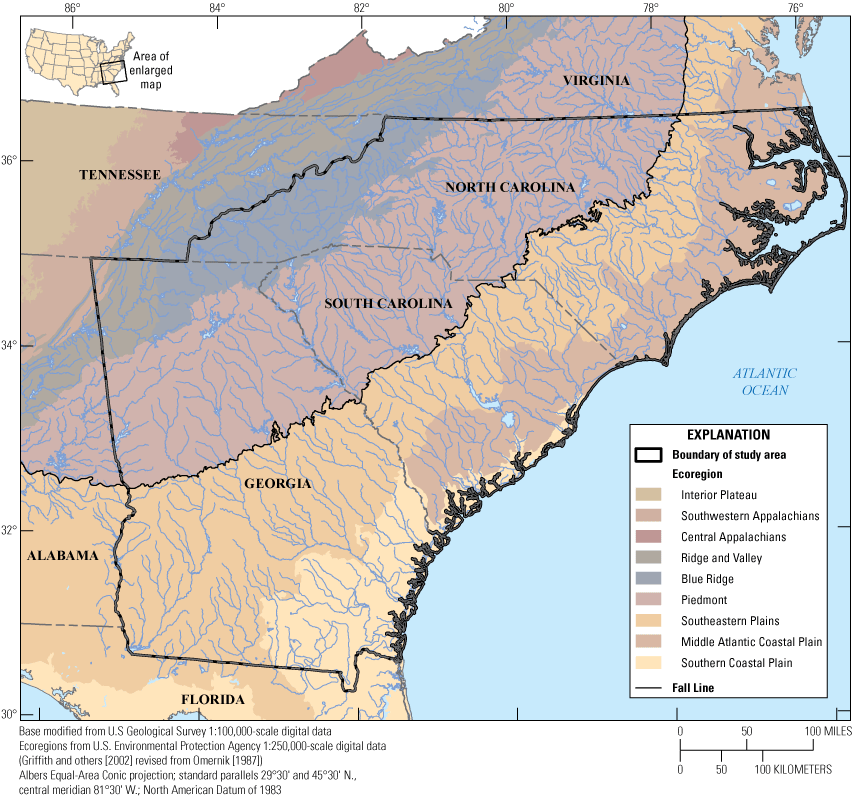
Study area and ecoregions in Georgia, South Carolina, and North Carolina and the surrounding States. Level III ecoregions are from U.S. Environmental Protection Agency (2022).
The Southwestern Appalachians ecoregion is composed of open, low mountains. The eastern boundary of this ecoregion, along the more abrupt escarpment where it meets the Ridge and Valley ecoregion, is relatively smooth and only slightly notched by small, eastward-flowing streams. The Ridge and Valley ecoregion is composed of roughly parallel ridges and valleys that have a variety of widths, heights, and geologic materials. Springs and caves are relatively numerous in this ecoregion, and present-day forests cover about 50 percent of the ecoregion. The Blue Ridge ecoregion varies from narrow ridges to hilly plateaus to more massive mountainous areas. The mostly forested slopes; high-gradient, cool, clear streams; and rugged terrain overlie primarily metamorphic rocks, with minor areas of igneous and sedimentary geology. The Piedmont ecoregion is composed of a transitional area between the mostly mountainous ecoregions of the Appalachian Mountains to the northwest and the relatively flat Coastal Plain to the southeast. The Piedmont ecoregion is a complex mosaic of metamorphic and igneous rocks of Precambrian and Paleozoic age, with moderately dissected irregular plains and some hills. The soils tend to be finer textured than in the Coastal Plain ecoregions to the south. Once largely cultivated, much of this ecoregion has reverted to pine and hardwood forests, with increasing conversion to urban and suburban land cover (Omernik, 1987).
The Southeastern Plains ecoregion is composed of irregular plains featuring a mixture of cropland, pasture, woodland, and forest. The sand, silt, and clay geology of this ecoregion contrasts with the older rocks of the Piedmont ecoregion. Elevations and relief are greater than in the Southern Coastal Plain ecoregion but generally are less than in much of the Piedmont ecoregion. Streams in this area have relatively low gradient and sandy bottoms. The Southern Coastal Plain ecoregion consists of mostly flat plains, but it is a heterogeneous ecoregion containing barrier islands, coastal lagoons, marshes, and swampy lowlands along the Gulf of Mexico and Atlantic coasts. This ecoregion is lower in elevation with less relief and wetter soils than the Southeastern Plains ecoregion. The Middle Atlantic Coastal Plain ecoregion consists of low-elevation flat plains and includes many swamps, marshes, and estuaries. The low terraces, marshes, dunes, barrier islands, and beaches are underlain by unconsolidated sediments. Poorly drained soils are common, and the ecoregion has a mix of coarse and finer textured soils compared to the mostly coarse soils in the majority of the Southeastern Plains ecoregion. The Middle Atlantic Coastal Plain ecoregion typically is lower, flatter, and more poorly drained than the Southern Coastal Plain ecoregion (Omernik, 1987).
Selection of Streamgages
Most of the flood-frequency statistics included in this report for streamgages having pre- and post-regulated periods of record were previously published in a USGS data release by Kolb and others (2023) as part of the rural flood-frequency investigation by Feaster and others (2023). Feaster and others (2023) published flood-frequency estimates for 72 streamgages on regulated streams in Georgia, South Carolina, and North Carolina that had 20 or more years of regulated peak streamflows. Those streamgages are the basis of the analyses included in this report (fig. 2). Feaster and others (2023) documented several tools that were used to assess the relative stability of regulation patterns based on the stability of the peak-streamflow patterns. From those assessments, the longest period of most recent peak streamflows determined to have relatively stable streamflow patterns was used in the flood-frequency analysis of the streamgages on regulated streams (table 8 from Kolb and others, 2023). For ease of reference, the map index numbers used in this report and the companion USGS data release (Musser and Feaster, 2023) match the map index numbers used by Feaster and others (2023) and Kolb and others (2023). Details on the regression analysis for the streamgages noted in figure 2 are provided later in this report.
The hydrologic regions used in Feaster and others (2023) also were used in this report and are based on the EPA level III and IV ecoregions (U.S. Environmental Protection Agency, 2022). Hydrologic region 1 is a combination of the Piedmont and Ridge and Valley ecoregions along with a small portion of the Southwestern Appalachians ecoregion in the northwest corner of Georgia (figs. 1 and 2). Hydrologic region 2 represents the Blue Ridge ecoregion. Hydrologic region 3 represents the EPA level IV ecoregion known as the Sand Hills. Hydrologic region 4 represents the remainder of the Coastal Plain, which is a combination of the Southeastern Plains, Middle Atlantic Coastal Plain, and Southern Coastal Plain ecoregions except for the lower Tifton Upland area, which represents hydrologic region 5.
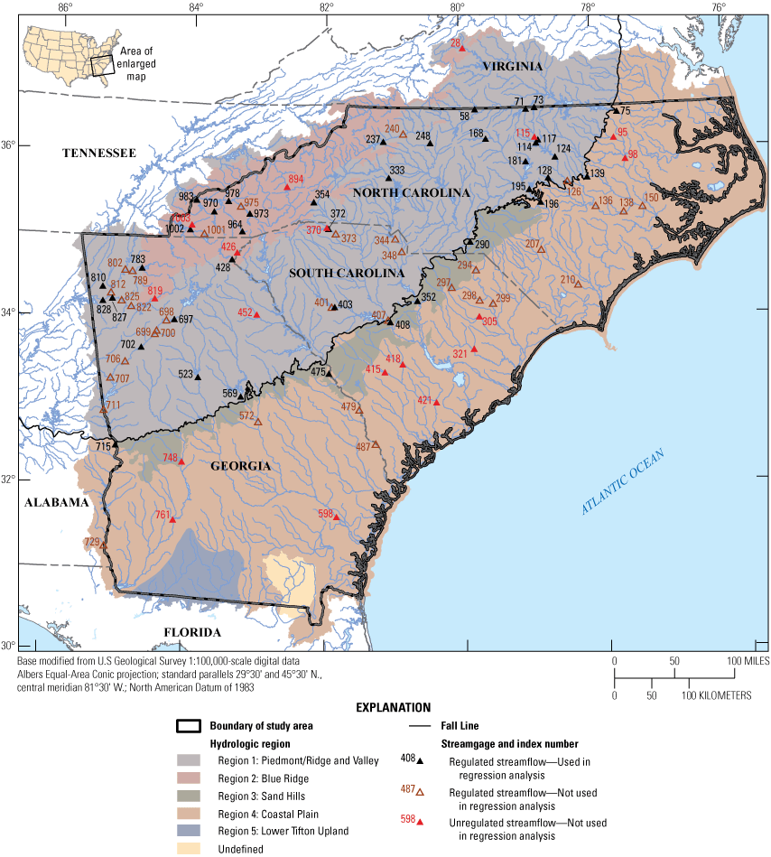
Study area, hydrologic regions, and locations of U.S. Geological Survey streamgages with unregulated or regulated streamflow conditions and with long-term periods of record compared for the flood-frequency analyses for Georgia, South Carolina, and North Carolina (hydrologic regions from Feaster and others, 2023; Fall Line from U.S. Environmental Protection Agency, 2022; streamgage locations from U.S. Geological Survey, 2021b).
Of the 72 streamgages on regulated streams from Feaster and others (2023) and Kolb and others (2023), 18 had at least 30 years of record in both the pre- and post-regulated periods (fig. 3) (table 1 from Musser and Feaster, 2023). Of those 18 streamgages, 17 had both daily mean and annual peak-streamflow data available with the remaining streamgage having only annual peak-streamflow data available. For comparison purposes, 18 streamgages on unregulated streams also are included in this report, for which streamflow statistics computed from the first half of the record were compared to those computed from the last half (fig. 4) (table 2 from Musser and Feaster, 2023). To be considered, both the first and last half of the records had to have at least 30 years of record. Of those 18 streamgages, 17 had both daily mean and annual peak streamflows available with the remaining streamgage having only annual peak streamflows available. The annual peak streamflows and daily mean streamflows used in this report were downloaded from the USGS National Water Information System (NWIS; U.S. Geological Survey, 2019, 2021b).
Flood-Frequency Estimates at Streamgage Locations
Flood-frequency estimates for the streamgages included in this report were completed using recommendations from “Guidelines for Determining Flood Flow Frequency—Bulletin 17C” (England and others, 2018). Bulletin 17C (B17C) recommends fitting the Pearson Type III distribution to the logarithms (LPIII) of annual peak streamflows. The LPIII distribution is a three-parameter distribution that requires estimates of the mean, the standard deviation, and the skew coefficient of logarithms of annual peak streamflow at a streamgage. While maintaining the moments-based approach of the Bulletin 17B procedures (Interagency Advisory Committee on Water Data, 1982), B17C introduces the expected moments algorithm (EMA; Cohn and others, 1997), an improved method-of-moments approach for fitting the LPIII distribution to the flood peaks that can accommodate interval estimates of peak streamflow, censored estimates of peak streamflow, and multiple thresholds of observation. B17C also includes a generalization of the Grubbs Beck low-outlier test (called the multiple Grubbs Beck test [Cohn and others, 2013]) that permits identification of multiple potentially influential low floods. Additionally, new methods for estimating regional skew and uncertainty (Veilleux and others, 2011) are provided in B17C. The EMA methodology in B17C has been incorporated into the USGS peak streamflow frequency analysis program, PeakFQ, version 7.4 (Flynn and others, 2006; Veilleux and others, 2014; U.S. Geological Survey, 2022), and was used to compute the AEP streamflows for streamgages in this investigation.
For streamgages on unregulated streams, there can be a relatively large uncertainty in the skew of the annual peak streamflows (England and others, 2018). As such, B17C recommends that the skew from the streamgage peak streamflows be weighted with a regional skew coefficient. As part of the update of rural flood-frequency statistics for streamgages in Georgia, South Carolina, and North Carolina, a regional skew analysis also was done (Feaster and others, 2023). The regional skew analysis resulted in a constant model with a regional skew coefficient of 0.048 with a mean square error of 0.092. The flood-frequency statistics included in this report for the streamgages on unregulated streams were computed by weighting this new regional skew with the skew of the streamgage peak streamflows.
Because the regional skew is estimated from unregulated rural streamflow data, it is not recommended that it be used when doing a flood-frequency analysis for regulated peak streamflows. For the regulated flood-frequency estimates included in this report, the analysis employed B17C methods by using the skew from the streamgage peak streamflows, also referred to as the “station skew.”
Most of the flood-frequency statistics included in this report for streamgages having pre- and post-regulated periods of record were previously published in a USGS data release by Kolb and others (2023) as part of the rural flood-frequency investigation by Feaster and others (2023). However, there were seven streamgages from Georgia that had at least 30 years of annual peak streamflows for both pre- and post-regulated periods of record for which only the post-regulated statistics were included in Feaster and others (2023). Those streamgages are 02223000 Oconee River at Milledgeville, Ga.; 02335000 Chattahoochee River near Norcross, Ga.; 02339500 Chattahoochee River at West Point, Ga.; 02383500 Coosawattee River near Pine Chapel, Ga.; 02387500 Oostanaula River at Resaca, Ga.; 02388500 Oostanaula River near Rome, Ga.; and 02395980 Etowah River at Georgia 1 Loop near Rome, Ga. The pre-regulated flood-frequency statistics for those seven streamgages are provided in table 3 from Musser and Feaster (2023).
Comparison of Pre- and Post-Regulated Annual Exceedance Probability Streamflow From Long-Term Streamgages
For the 18 streamgages with both pre- and post-regulated periods (table 1 from Musser and Feaster, 2023), the percentage change in the estimated 10-, 1-, and 0.2-percent AEP streamflows, which correspond to recurrence intervals of 10, 100, and 500 years, respectively, was computed (table 3 from Musser and Feaster, 2023). In general, percentage change represents the change in a value relative to the previous value and is computed as follows:
whereFor this comparison, y2 represents the AEP streamflow estimate from the post-regulated period, and y1 represents the AEP streamflow estimate from the pre-regulated period. A negative percentage change indicates a decrease in the AEP streamflow from the pre-regulated to post-regulated period, and a positive percentage change indicates an increase. On average, at the 18 streamgages analyzed, regulation decreased the 10-, 1-, and 0.2-percent AEP streamflow estimates by about 31 percent. For the 10-percent AEP streamflows, all estimates at the 18 streamgages decreased from the pre- to post-regulated period, ranging from 2.0 to 72.0 percent (table 3 from Musser and Feaster, 2023). The median decrease was 28.9 percent with a mean decrease of 32.3 percent. For the 1-percent AEP streamflows, the percentage change ranged from −78.0 to 22.4 percent with 02089000 Neuse River near Goldsboro, N.C., and 02105500 Cape Fear River at William O. Huske Lock near Tarheel, N.C., being the only streamgages with a positive percentage change (fig. 3). It is worth noting that the peak of record at 02089000 occurred in October 2016 because of Hurricane Matthew (Weaver and others, 2016) and that the peak of record and the second largest peak of record at 02105500 occurred in September 2018 and October 2016, respectively, because of Hurricane Florence (Feaster and others, 2018) and Hurricane Matthew (Weaver and others, 2016), respectively. The median percentage change and mean percentage change for the 1-percent AEP streamflows were −32.4 and −31.6 percent, respectively. For the 0.2-percent AEP streamflows, the percentage change ranged from −83.4 to 44.7 percent with the median and mean being −31.1 and −29.8 percent, respectively. Comparisons of the full range of the flood-frequency curves from the 50- to 0.2-percent AEP streamflows are shown on figure 3.
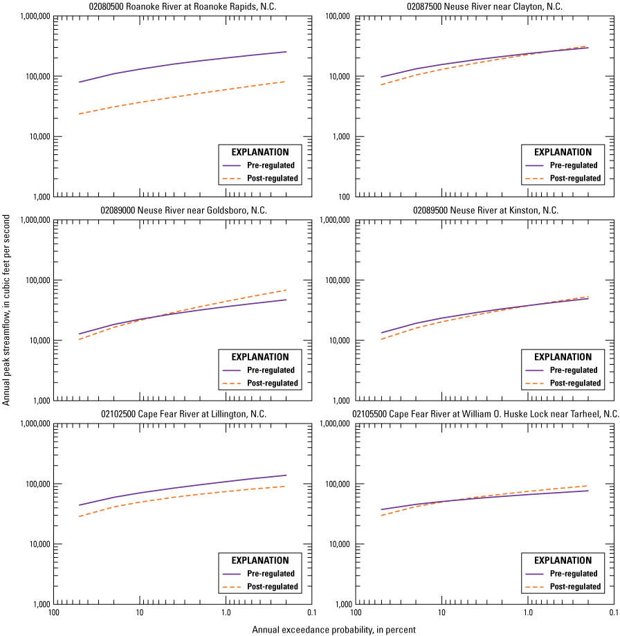
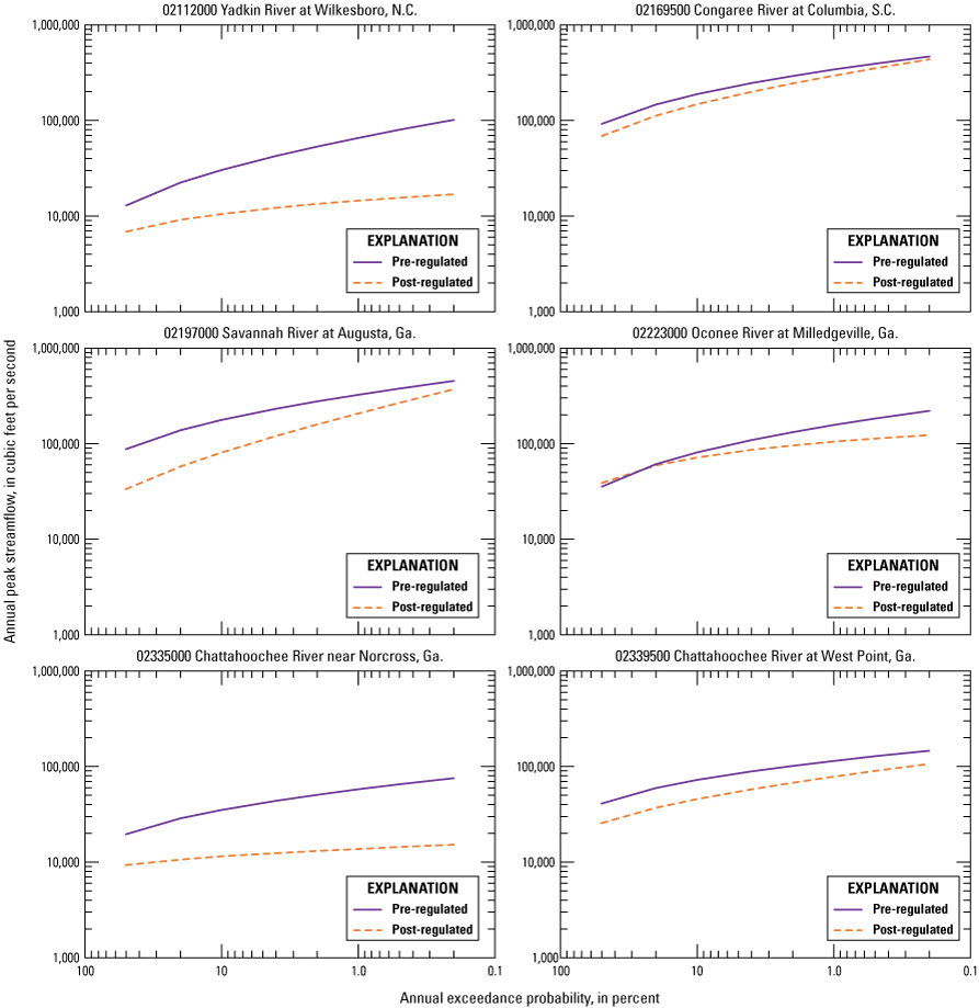
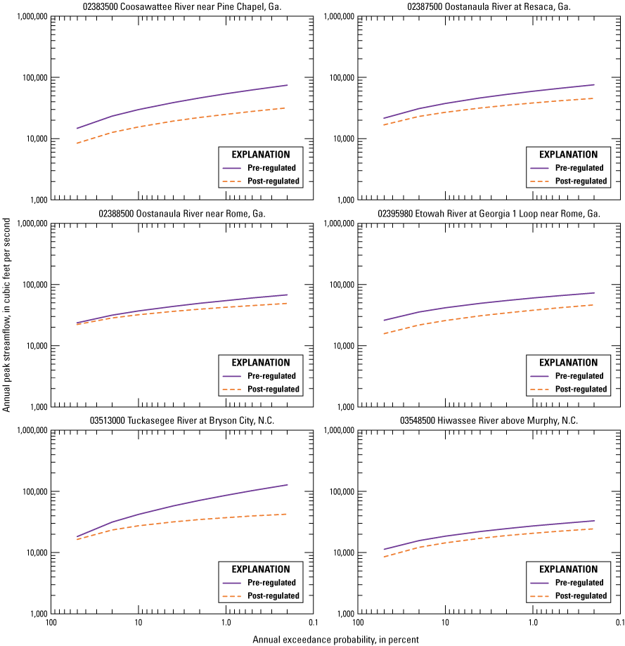
Flood-frequency curves of the annual exceedance probability streamflows for the pre- and post-regulated periods at 18 U.S. Geological Survey streamgages with long-term periods of record in Georgia, South Carolina, and North Carolina (streamflow data from U.S. Geological Survey, 2019).
Comparison of Annual Exceedance Probability Streamflows for Two Periods at Long-Term Streamgages on Unregulated Streams
The flood-frequency statistics computed for streamgages on unregulated streams are strongly influenced by period of record and hydrologic conditions captured in that record. This natural variability also will influence streamflow statistics computed at streamgages on regulated streams but with the added complexity of the influence from the regulation, which may enhance or even offset the natural variability in those data. Although the USGS typically designates streamgage records with 30 or more years as long term (U.S. Geological Survey, 2013), records of that length and much longer may still be too short to positively identify and quantify a real long-term change in the natural hydrologic regime (Riggs, 1985). As Lins and others (2010) noted, sometimes streamflow records of several decades may indicate a trend but, when viewed in the context of timeframes spanning many decades to centuries, may just be recognized as a short-term trend that is part of a much longer term oscillation (Stahle and Cleaveland, 1992). In their paper discussing trends in hydroclimatological data and long-term persistence, Cohn and Lins (2005, section “Discussion and Conclusions,” paragraph 27) noted that “… natural climatic excursions may be much larger than we imagine.”
To get a sense of how flood-frequency statistics have varied at unregulated USGS streamgages in Georgia, South Carolina, and North Carolina, the percentage change in the flood-frequency estimates for the 10-, 1-, and 0.2-percent AEP streamflows was computed for 18 streamgages monitoring unregulated streams by separating the record into two periods: first half of the record and last half of the record (fig. 4) (table 4 from Musser and Feaster, 2023). The record lengths analyzed ranged from 41 to 65 years for each half period with the average length being 52 years. For the 10-percent AEP streamflows, the percentage change ranged from −38.9 to 30.1 percent with a median of −9.8 percent and a mean of −8.6 percent. For the 1-percent AEP streamflows, the percentage change ranged from −48.1 to 57.0 percent with a median of −7.4 percent and a mean of −6.4 percent. For the 0.2-percent AEP streamflows, the percentage change ranged from −53.6 to 69.0 percent with a median of −9.5 percent and a mean of −5.0 percent. Comparisons of the full range of the flood-frequency curves from the 50- to 0.2-percent AEP streamflows are shown on figure 4.
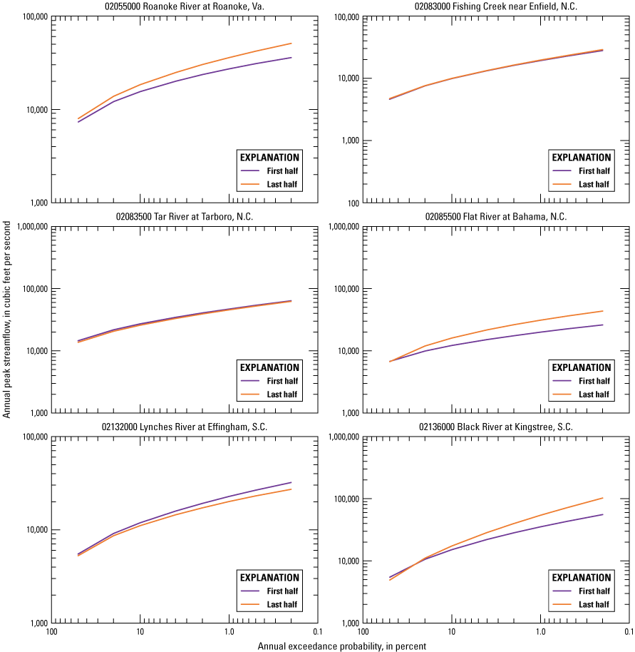
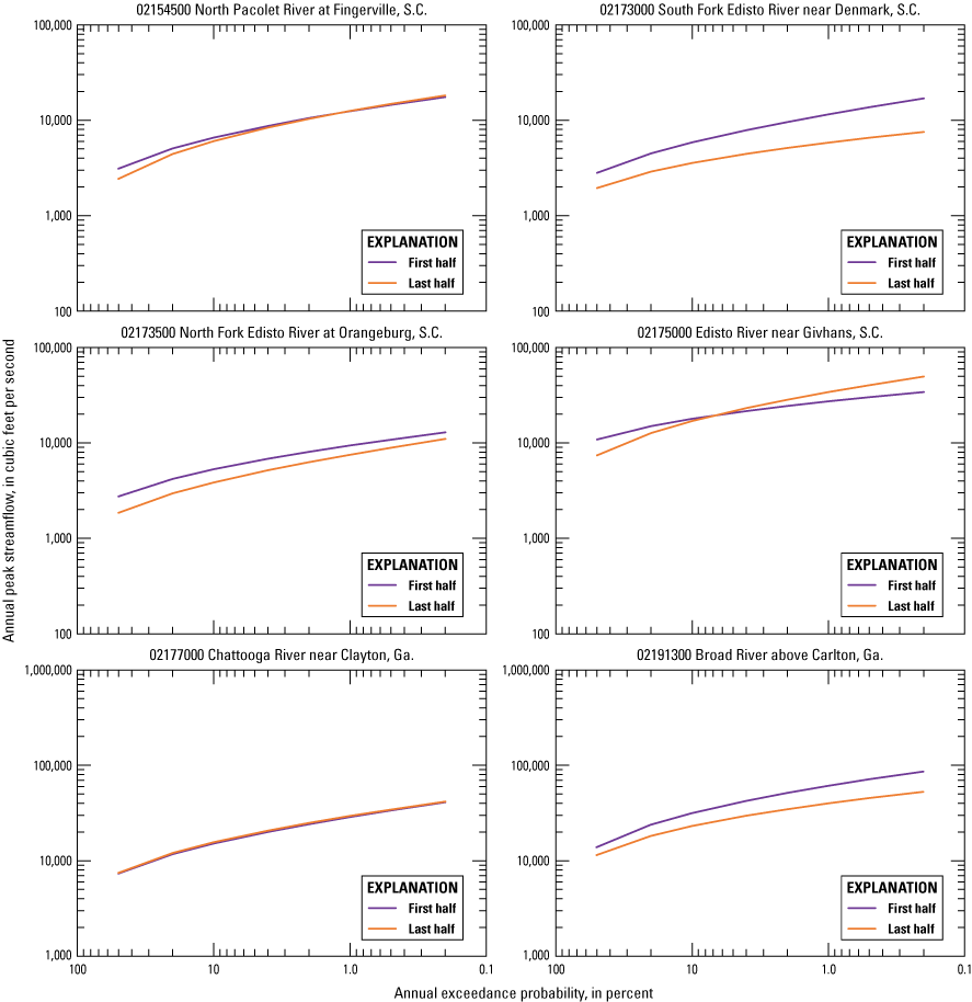
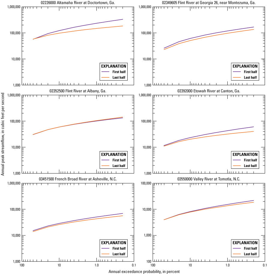
Annual exceedance probability flood-frequency curves from two periods (the first half and the last half) of long-term periods of record at 18 U.S. Geological Survey streamgages monitoring unregulated streams in Georgia, South Carolina, and North Carolina (streamflow data from U.S. Geological Survey, 2019; Virginia streamgage is included because it has a long-term record and the downstream basin extends into North Carolina).
Comparison of the Distribution of the Percentage Change in Annual Exceedance Probability Streamflows for Selected Streamgages Having Long-Term Pre- and Post-Regulated Periods of Record and at Selected Unregulated Streamgages Having Two Long-Term Periods of Record
To further explore the percentage change between the 10-, 1-, and 0.2-percent AEP streamflows for the two periods from the 18 USGS streamgages with pre- and post-regulated periods of record (tables 1 and 3 from Musser and Feaster, 2023), boxplots were generated and compared with the percentage change in those same AEP streamflows for two periods of record at 18 unregulated streamgages (tables 2 and 4 from Musser and Feaster, 2023) (fig. 5). This comparison provides insight into differences that might be attributed to natural variability. Boxplots provide an informative graphical display of the distribution of a dataset (Helsel and others, 2020). The line inside the box is the median. The box height is formed from the 25th and 75th percentiles (quartiles [Q] 1 and 3, respectively) of the dataset. The difference between Q3 and Q1 is the interquartile range (IQR). The IQR provides a visual of the variation (spread) of the dataset. The location of the median line in the box indicates the skewness. For a normally distributed dataset, the median and the mean are the same. Data points that are greater than or less than 1.5 times the IQR are considered outliers. If a dataset has no outliers, the end of the whiskers extending from the box represents the minimum and maximum data points of the dataset. For datasets that have outliers, the end of the whiskers represent the minimum or maximum data point of the dataset excluding the outliers.
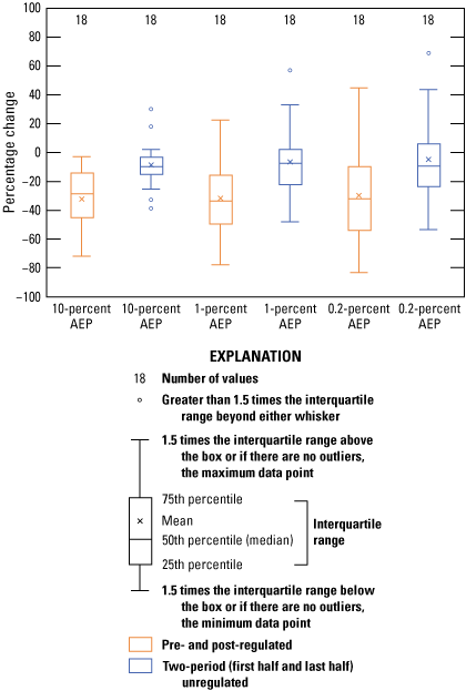
Distribution of the percentage change in the 10-, 1-, and 0.2-percent annual exceedance probability (AEP) streamflows for 18 U.S. Geological Survey streamgages that have both pre- and post-regulated long-term periods of record and for two long-term periods of record (the first half and the last half) at 18 U.S. Geological Survey streamgages monitoring unregulated streams in Georgia, South Carolina, and North Carolina (streamflow data from U.S. Geological Survey, 2019, 2021b).
In general, the boxplots of the percentage change in the 10-, 1-, and 0.2-percent AEP streamflows for the two periods from the 18 streamgages monitoring unregulated streams show a variability that tends to be more balanced between positive and negative changes as compared to the pre- and post-regulated AEP streamflows (fig. 5). In comparison, the interquartile percentage change from the pre- and post-regulated periods at the 18 streamgages was all in the negative range, thereby indicating that overall, those AEP streamflows were lower in the post-regulated period than in the pre-regulated period. The median percentage change for the 10-, 1-, and 0.2-percent AEP streamflows from the pre- and post-regulated periods was 19.1, 25.0, and 21.6 percentage points lower, respectively, than the median percentage change for those same AEP streamflows of the two periods from the streamgages monitoring unregulated streams (tables 3 and 4 from Musser and Feaster, 2023). It is also interesting to note that there was at least one outlier for each of the AEP streamflows from the comparison of two unregulated periods of record but no outliers from the comparisons of the pre- and post-regulated periods of record. As noted earlier, regulation of streamflows often decreases the highest streamflows and increases the lowest streamflows, thus reducing the extremes that are typically part of natural streamflow regimes and that may tend to show up as outliers (Williams and Wolman, 1984).
Analyses of Daily Mean Streamflow Using the Indicators of Hydrologic Alteration Software
To determine the effects of impoundments on a broader range of streamflow characteristics, The Nature Conservancy’s IHA software (Richter and others, 1996) was used to assess daily mean streamflow at streamgages monitoring unregulated and regulated streams. The IHA software can be used to characterize a large variety of streamflow characteristics from a single period of record or compare those characteristics from two or more periods of record. The software compares characteristics such as magnitude of streamflows, timing of annual extremes, and frequency and duration of high and low pulses (The Nature Conservancy, 2009). A pulse, which is defined as a daily mean streamflow above or below selected thresholds, can be set by the user. For the IHA analyses in this report, the default setting of the high and low pulse was used, which is the annual number of daily mean streamflows greater than the 75th percentile and less than the 25th percentile for the period of record analyzed, respectively. Pulse count is the number of pulses that exceed the selected thresholds within each year. Pulse duration is the number of days the pulses exceed the selected thresholds within each year.
Comparison of Percentage Change in Selected Pre- and Post-Regulated Daily Mean Streamflow Characteristics From Long-Term Streamgages
The IHA software (Richter and others, 1996) was used to analyze selected streamflow characteristics from the 16 USGS streamgages that had pre- and post-regulated daily mean streamflows (table 5 from Musser and Feaster, 2023). The streamflow characteristics analyzed were mean annual streamflow, 1-day maximum streamflow, 1- and 7-day minimum streamflows, low pulse count and duration, and high pulse count and duration. Other than the mean annual streamflow, the other streamflow characteristics were based on the median values for the period analyzed. The length of records available in the pre-regulated period ranged from 34 to 80 years. The length of records available in the post-regulated period ranged from 39 to 68 years. Of the 16 streamgages included in table 5 from Musser and Feaster (2023), 03513000 Tuckasegee River at Bryson City, N.C., had the lowest maximum storage index (193 acre-ft/mi2), and 02335000 Chattahoochee River near Norcross, Ga., had the highest (2,183 acre-ft/mi2). As compared to 03513000, which shows only minor differences between the pre- and post-regulated periods, the effects of regulation on the high and low streamflows at 02335000 are substantial, showing how regulation decreased the annual 1-day maximum streamflows and increased the annual 7-day minimum streamflows (figs. 6 and 7).
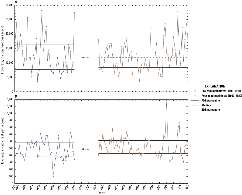
Annual A, 1-day maximum and B, 7-day minimum streamflows at U.S. Geological Survey streamgage 03513000 Tuckasegee River at Bryson City, North Carolina (streamflow data from U.S. Geological Survey, 2021b).
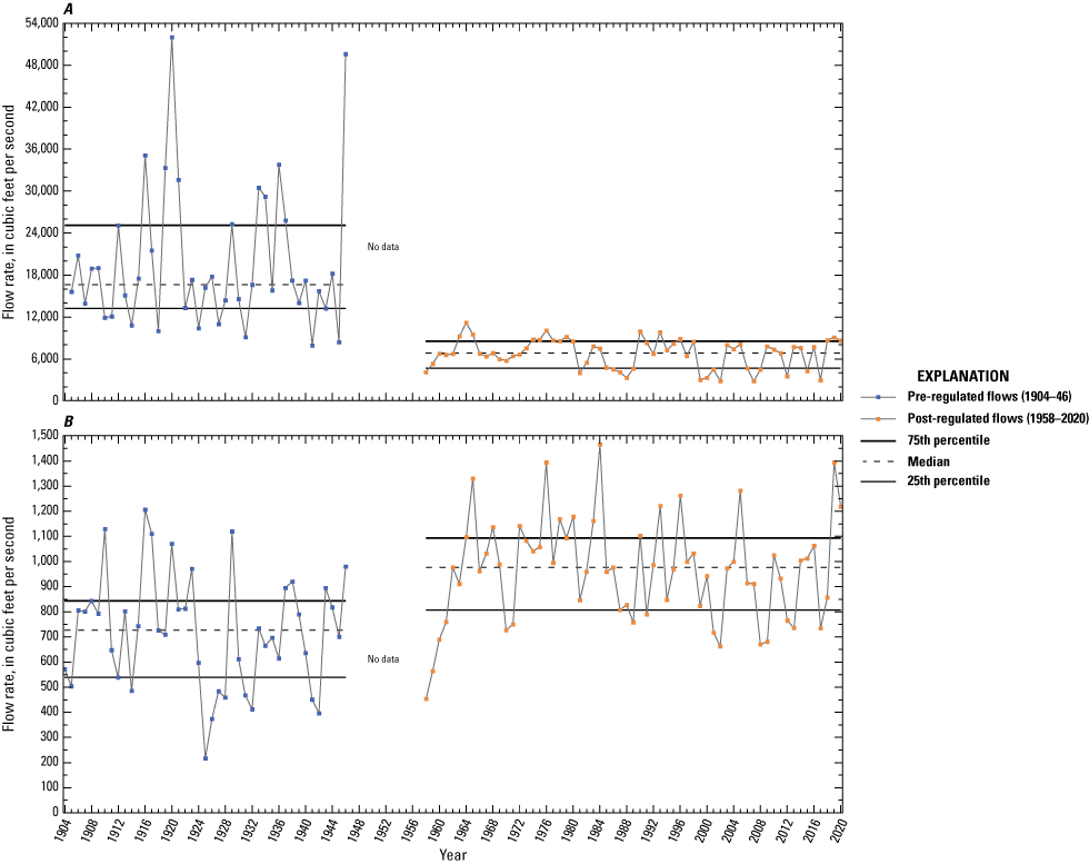
Annual A, 1-day maximum and B, 7-day minimum streamflows at U.S. Geological Survey streamgage 02335000 Chattahoochee River near Norcross, Georgia (streamflow data from U.S. Geological Survey, 2021b).
The percentage change in the mean annual streamflow from the pre- to post-regulated period ranged from −21.8 to 9.7 percent with a median of −0.9 percent and a mean of −1.4 percent (table 5 from Musser and Feaster, 2023). For the 1-day maximum streamflow, the percentage change ranged from −69.4 to 0.9 percent with a median of −24.4 percent and a mean of −28.2 percent. For the 1-day minimum streamflow, the percentage change ranged from −46.7 to 350 percent with a median of −4.8 percent and a mean of 29.7 percent. The percentage change for the 7-day minimum streamflow ranged from −48.2 to 166 percent with a median of 19.6 percent and a mean of 24.1 percent. These findings reflect conditions that are often found to occur from regulation; on average, the low streamflows increased, and the high streamflows decreased.
The percentage change in the low pulse count from the pre- to post-regulated period ranged from −93.5 to 400 percent with a median of 20.0 percent and a mean of 64.6 percent (table 5 from Musser and Feaster, 2023). The percentage change in the low pulse duration ranged from −75.0 to 60.0 percent with a median of −17.5 percent and a mean of −21.6 percent. For the high pulse count, the percentage change ranged from −35.7 to 65.4 percent with a median of −5.5 percent and a mean of 6.1 percent. The percentage change in the high pulse duration ranged from −50.0 to 100 percent with a median of 12.7 percent and a mean of 13.1 percent.
Comparison of Percentage Change in Daily Mean Streamflow Characteristics From Two Periods at Long-Term Streamgages Monitoring Unregulated Streams
To assess natural variability in selected daily mean streamflow characteristics based on period of record, the IHA software (Richter and others, 1996) was used to analyze two periods (first half and last half of the records) at 17 USGS streamgages monitoring unregulated streams (table 6 from Musser and Feaster, 2023). Like the IHA analysis of the pre- and post-regulated periods at 16 USGS streamgages (table 5 from Musser and Feaster, 2023), the streamflow characteristics analyzed were mean annual streamflow, 1-day maximum streamflow, 1- and 7-day minimum streamflows, low pulse count and duration, and high pulse count and duration. The length of records available in the two periods at the 17 streamgages monitoring unregulated streams ranged from 39 to 60 years.
The percentage change in the mean annual streamflow ranged from −19.0 to 28.3 percent with a median of −3.7 percent and a mean of −2.4 percent (table 6 from Musser and Feaster, 2023). For the 1-day maximum streamflow, the percentage change ranged from −37.3 to 22.9 percent with a median of −5.8 percent and a mean of −7.3 percent. The percentage change for the 1-day minimum streamflow ranged from −74.7 to 53.9 percent with a median of −20.4 percent and a mean of −19.5 percent. Changes in the 7-day minimum streamflow were similar with a range of −71.1 to 50.0 percent and a median and mean of −24.9 and −21.4 percent, respectively. The reduction in the mean of the 1- and 7-day minimum streamflows and 1-day maximum streamflows may reflect historical drought periods that have occurred in the Southeast over the last couple of decades (South Carolina Department of Natural Resources, 2004; Weaver, 2005; Gotvald, 2016; Feaster and Guimaraes, 2017) or other influences in the basins.
The percentage change in the low pulse count from the two periods at the streamgages monitoring unregulated streams ranged from −22.2 to 28.6 percent with a median of 0.0 percent and a mean of 1.0 percent indicating a relatively normal distribution (table 6 from Musser and Feaster, 2023). For the low pulse duration, the percentage change ranged from −23.1 to 61.9 percent with a median of 28.0 percent and a mean of 25.1 percent. For the high pulse count, the percentage change ranged from −29.4 to 33.3 percent with a median of −6.3 percent and a mean of −3.1 percent. The percentage change for the high pulse duration ranged from −16.7 to 50.0 percent with a median of 0.0 percent and a mean of 2.1 percent.
Comparison of the Distribution of the Percentage Change in Daily Mean Streamflow Characteristics From the Indicators of Hydrologic Alterations Analysis at Long-Term Streamgages
Boxplots of the percentage change in daily mean streamflow characteristics for pre- and post-regulated periods at the 16 USGS streamgages (table 5 from Musser and Feaster, 2023) were compared with boxplots of the percentage change in those same daily mean streamflow characteristics for the two periods at 17 USGS streamgages monitoring unregulated streams (table 6 from Musser and Feaster, 2023) (fig. 8). The boxplots of the percentage change in mean annual streamflow for two periods at the 17 streamgages monitoring unregulated streams show a well-balanced distribution of positive and negative values with the mean and median values being similar and just slightly less than zero. The boxplots for the percentage change in mean annual streamflow for the 16 streamgages with pre- and post-regulated record also show mean and median values that are similar and just slightly less than zero but with less variability.
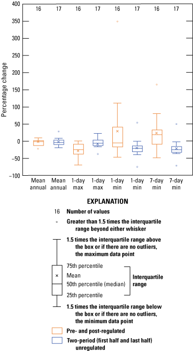
The distribution of the percentage change in the mean annual, 1-day maximum (max), and 1- and 7-day minimum (min) streamflows for 16 U.S. Geological Survey streamgages that have both pre- and post-regulated long-term periods of record and for two long-term periods of record (the first half and the last half) at 17 U.S. Geological Survey streamgages monitoring unregulated streams in Georgia, South Carolina, and North Carolina (streamflow data from U.S. Geological Survey, 2021b).
The boxplot for the percentage change in the 1-day maximum streamflows for the pre- and post-regulated periods was mostly in the negative range with the median and mean values being −24.4 and −28.2 percent, respectively (fig. 8), showing that the 1-day maximum streamflows tended to be lower for the post-regulated periods of record (table 5 from Musser and Feaster, 2023). As previously noted, this is consistent with the observation that regulation tends to reduce high streamflows. The boxplot of the percentage difference in the 1-day maximum streamflows for the two unregulated periods of record tends to be more balanced between both positive and negative percentages with the median and mean values being −5.8 and −7.3 percent, respectively (table 6 from Musser and Feaster, 2023).
Comparisons of the boxplots of the percentage change in the 1- and 7-day minimum streamflows for the pre- and post-regulated streamflows and the two periods of unregulated streamflows show that the percentage change of the pre- and post-regulated streamflows had a larger variability with the mean values both being positive, thereby suggesting (as previously noted) that, on average, the low streamflows for the post-regulated period tended to be higher than those for the unregulated periods (fig. 8).
For the low and high pulse counts and durations, boxplots were generated for the actual values instead of the percentage change (figs. 9A, B and 10A, B). The low pulse count from the pre-regulated period of record was somewhat like the two periods from the streamgages on unregulated streams, which show no substantial differences between the two periods, but with less variability (fig. 9A). The post-regulated period had a higher mean and median low pulse count and a much greater variability than the pre-regulated period and the two unregulated periods. Although not substantially different, the post-regulated low pulse duration had greater variability and a lower mean and median duration than the pre-regulated period (fig. 9B). The low pulse duration for the first half and last half of the streamgages monitoring unregulated streams had greater variability and higher means and medians than the pre- and post-regulated low pulse durations.
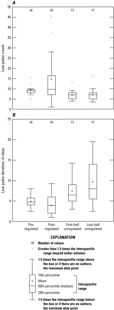
The distribution of A, the low pulse count and B, the low pulse duration for 16 U.S. Geological Survey streamgages that have pre- and post-regulated long-term periods of record and for two long-term periods of record (the first half and the last half) at 17 U.S. Geological Survey streamgages monitoring unregulated streams in Georgia, South Carolina, and North Carolina (streamflow data from U.S. Geological Survey, 2021b).
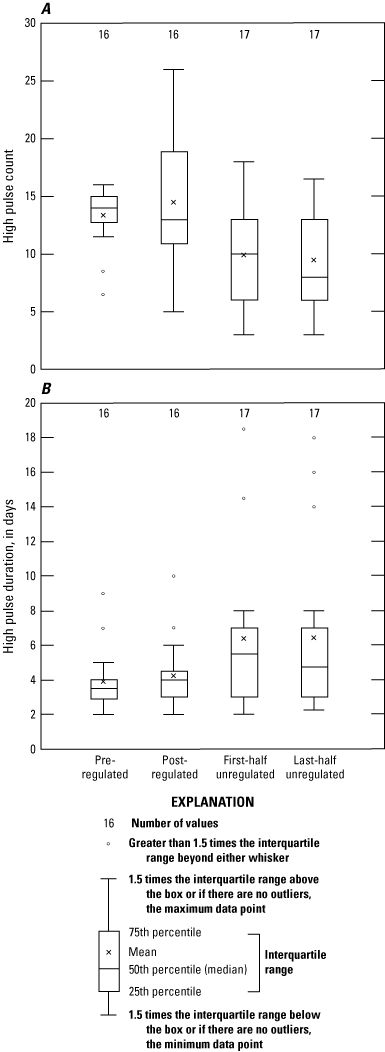
The distribution of A, the high pulse count and B, the high pulse duration for 16 U.S. Geological Survey streamgages that have pre- and post-regulated long-term periods of record and for two long-term periods of record (the first half and the last half) at 17 U.S. Geological Survey streamgages monitoring unregulated streams in Georgia, South Carolina, and North Carolina (streamflow data from U.S. Geological Survey, 2021b).
For the pre- and post-regulated periods at the 16 streamgages, the median values for the high pulse count were similar, but the post-regulated distribution of high pulse count had much greater variability (fig. 10A). Like the low pulse count (fig. 9A), the high pulse count for the first and last half of the record at the 17 streamgages monitoring unregulated streams was quite similar (fig. 10A). The pre- and post-regulated high pulse durations also were similar, with the post-regulated period having only slightly more variability than the pre-regulated period (fig. 10B). Like the high pulse count (fig. 10A), the distribution of the high pulse duration for the first and last half of the record at the 17 streamgages monitoring unregulated streams was similar (fig. 10B).
Comparison of Flow-Duration Curves
Flow-duration curves are cumulative frequency curves that show the percentage of time during which specified streamflows were equaled or exceeded during the period of record analyzed (Searcy, 1959). Flow-duration curves can be useful for understanding the broad range of streamflow characteristics of a gaged stream and can be useful for comparisons with other streams. Flow-duration curve data from the IHA analysis for the 17 USGS streamgages with pre- and post-regulated daily mean streamflow were used to generate flow-duration curves (table 1 from Musser and Feaster, 2023) (fig. 11). The flow-duration curves provide a graphical comparison of the effects of regulation throughout the full range of daily mean streamflows. For some of the streamgages, the extremes tend to show the greatest differences between the pre- and post-regulated periods of record, which as previously noted is a common occurrence for certain types of regulation.
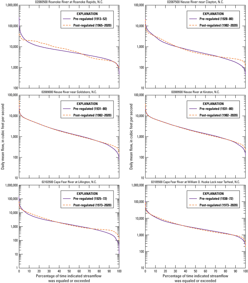
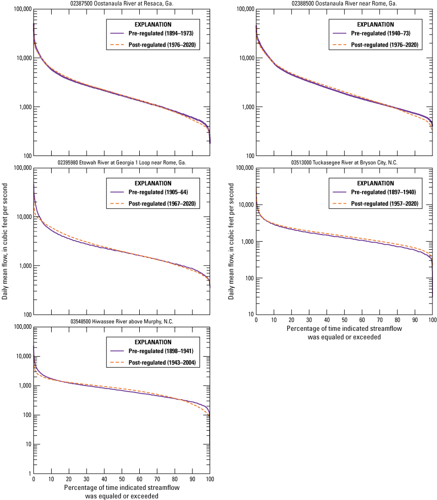
Flow-duration curve comparisons for pre- and post-regulated long-term periods of record at 17 U.S. Geological Survey streamgages in Georgia, South Carolina, and North Carolina (streamflow data from U.S. Geological Survey, 2021b).
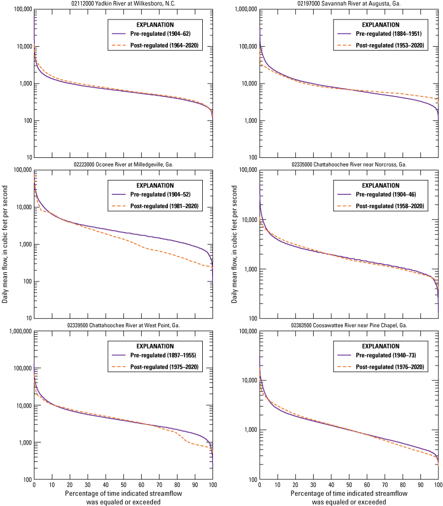
To gain an understanding of how flow-duration curves may differ based on period of record, a comparison of two periods at the 17 streamgages monitoring unregulated streams also was made (table 2 from Musser and Feaster, 2023) (fig. 12). For the streamgages monitoring unregulated streams, the flow-duration curves for the two periods tend to have similar shapes. The streamgages in the Edisto and Flint River Basins tend to show lower streamflows throughout much of the flow-duration curve for the last half of the records. This tendency could be due to the historical droughts captured in those records or other influences in the basins.
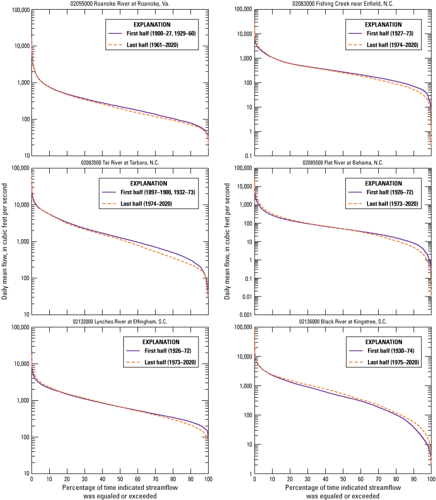
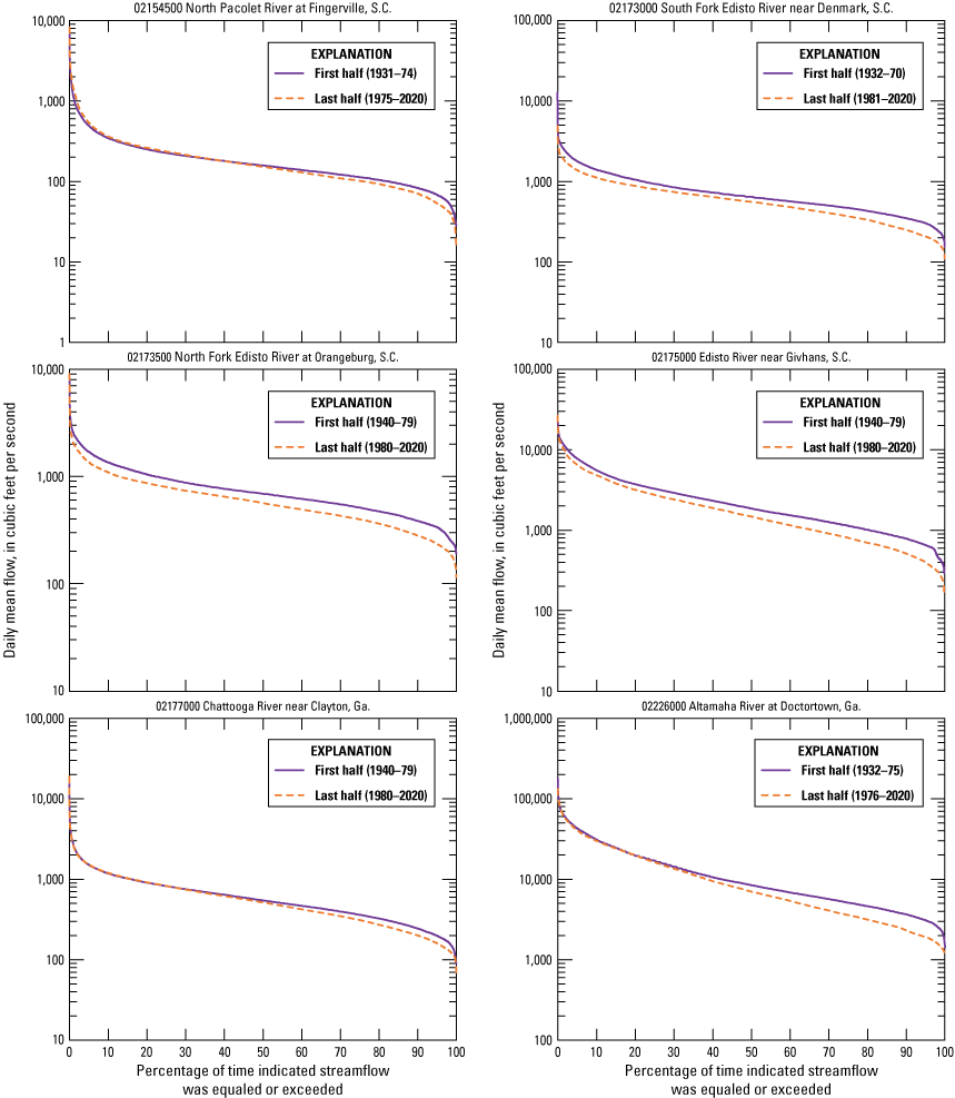
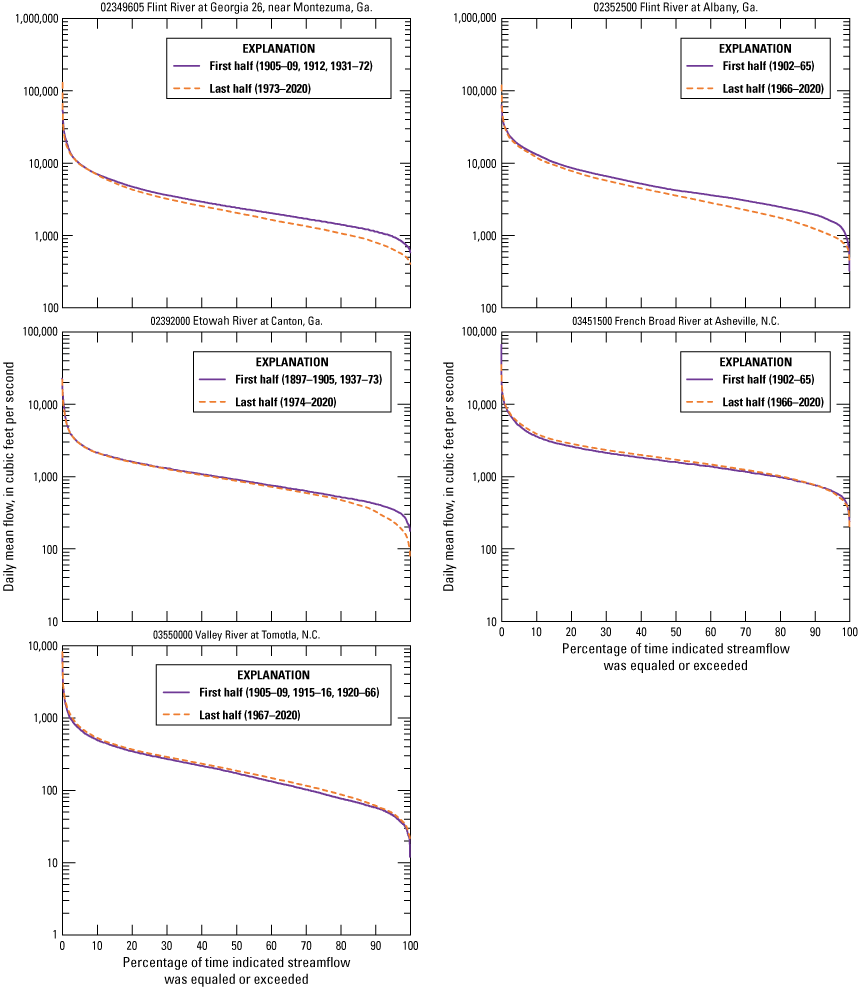
Flow-duration curve comparisons for two long-term periods of record (the first half and the last half) at 17 U.S. Geological Survey streamgages monitoring unregulated streams in Georgia, South Carolina, and North Carolina (streamflow data from U.S. Geological Survey, 2021b; Virginia streamgage is included because it has a long-term record and the downstream basin extends into North Carolina).
Flood-Frequency Estimates for Ungaged Locations on Regulated Streams
Regional regression analyses were used to develop a set of flood-frequency equations that can be used to estimate selected AEP streamflows at ungaged locations on regulated streams. The multiple linear regression analyses used standard USGS methods (Farmer and others, 2019) to relate the 50-, 20-, 10-, 4-, 2-, 1-, 0.5-, and 0.2-percent AEP streamflows computed from available records for streamgages monitoring regulated streams (U.S. Geological Survey, 2019) to selected basin characteristics.
The general model for an ordinary least squares (OLS) regression analysis is of the form
whereQP
is the response variable, which is the flood magnitude at a selected percent AEP;
A, B, and C
are explanatory (independent) variables; and
a, b, c, and d
are regression coefficients.
If the response and explanatory variables are logarithmically transformed, the regression model has the following line form:
where the variables are as previously defined in equation 2.The initial set of streamgages included in the analyses was the 72 streamgages on regulated streams for which AEP streamflows were computed by Feaster and others (2023) and is available in a USGS data release by Kolb and others (2023). An assessment for redundancy of the streamgages was made using procedures described in Feaster and others (2023). Redundancy occurs when the drainage basins of two streamgages are nested one within another and are similarly sized, leading to concurrent streamflow records. When this is the case, the two streamgages exhibit nearly the same hydrologic response to a given storm and, thus, effectively represent only one spatial observation (Gruber and Stedinger, 2008). From the redundancy analysis, 29 streamgages were found to be redundant and, therefore, were excluded from the regression analysis, thereby leaving 43 streamgages (table 7 from Musser and Feaster, 2023). For the remaining 43 streamgages, 39 had basins where 75 percent or more of the drainage area was located above the Fall Line. Those 39 streamgages were included in this investigation to develop regional regression equations that can be used to estimate the flood-frequency statistics at ungaged locations on regulated streams in Georgia, South Carolina, and North Carolina in which 75 percent or more of the drainage basin is located above the Fall Line (fig. 2).
Because there were not enough regulated streamgages in the regression analysis to properly represent basins draining predominately from below the Fall Line, the regression equations are applicable for only basins draining predominantly (75 percent or more) from above the Fall Line. It also should be noted that the 39 streamgages included in the regression analysis are considered rural streamgages for the purpose of this investigation.
Exploratory Regression Analysis
For the exploratory regression analysis, OLS regression techniques were used to determine the best regression models for all combinations of basin characteristics and testing of the two hydrologic regions above the Fall Line (fig. 2). In OLS regression, linear relations between the explanatory and response variables are necessary; thus, variables sometimes must be transformed to create linear relations. For example, the relation between arithmetic values of basin drainage area and AEP streamflow normally is curvilinear; however, the relation between the logarithms of drainage area and the logarithms of the AEP streamflows for selected probabilities (P-percent; for example, 50, 20, or 10 percent) normally is linear. Homoscedasticity (a constant variance in the response variable over the range of the explanatory variables) about the regression line and normality of the residuals are another assumption for OLS regression. Transformation of the AEP streamflow and the explanatory variables to logarithms often enhances the homoscedasticity of the data about the regression line. Homoscedasticity and normality of residuals were examined in residual plots. Additionally, residuals, which are the difference between the observed and predicted values, were mapped to assess the geographic distribution in the uncertainty of the predictions, which provides information on potential subregions that might reduce the uncertainty. This assessment of independent variables for percentage of drainage area from hydrologic regions 1 and 2 indicated that there was not a statistically significant difference between the two regions, and therefore, the regression analysis was done using a single region above the Fall Line.
Multicollinearity, which is a situation where two or more independent variables are highly correlated with strong linear dependence, was also assessed by the variance inflation factor (VIF). A VIF greater than 10 indicates highly correlated explanatory variables and warrants additional investigation (Montgomery and others, 2012), and a VIF less than 5 is preferred (Farmer and others, 2019). The VIF for the final variables included in the regression analysis was close to 1.
As part of the update of rural flood-frequency regional regression equations for Georgia, South Carolina, and North Carolina, Feaster and others (2023) tested 26 basin characteristics as potential explanatory variables. In that analysis, drainage area and percentage of hydrologic regions were included in the final regional regression equations. Based on that analysis, drainage area and percentage of hydrologic regions 1 and 2 were tested with a series of other characteristics related to impoundments in this investigation. The additional characteristics tested were
-
• Maximum storage, in acre-feet, which is defined as the total storage space in a reservoir below the maximum attainable water-surface elevation;
-
• Maximum storage index, in acre-feet per square mile, which was computed as the cumulative maximum storage from reservoirs upstream from the USGS streamgage divided by the drainage area at the streamgage;
-
• Surface area, in acres, of the reservoir at its normal retention level;
-
• Distance, in miles, from the streamgage to the first upstream reservoir; and
-
• Distance, in miles, from the streamgage to the last upstream reservoir.
The maximum storage and surface area were obtained from the U.S. Army Corps of Engineers (2020) NID database. The distance to the first and last upstream reservoirs was computed using Esri ArcMap (Esri, 2021). The ArcMap Utility Network Analyst tool “Find Path” was used to select segments of streamline from the National Hydrography Dataset (U.S. Geological Survey, 2021a) High Resolution layer NHDFlowline between a streamgage and a reservoir. The attribute values of LengthKM from the NHDFlowline layer were summed for these segments and converted to miles. The remaining distance along the selected streamline that extended downstream from the streamgage was then determined using the “Measure” tool and subtracted from the summed total distance.
All-possible-subsets regression methods were tested using the candidate explanatory variables related to impoundments along with drainage area, percentage of hydrologic regions 1 and 2, and a cross product of drainage area and percentage of hydrologic region 2, which was statistically significant in the rural regression equations from Feaster and others (2023). The final explanatory variables for the exploratory regression analysis were selected based on several factors, including (1) standard error of the estimate, (2) Mallow’s Cp statistic (Helsel and others, 2020), (3) statistical significance of the explanatory variables, (4) coefficient of determination (R2), and (5) ease of measurement of explanatory variables. Based on the OLS assessments of various groupings of explanatory variables and the criteria noted previously, a regression model including drainage area and maximum storage index was selected using only streamgages for which the basin drained 75 percent or more from above the Fall Line.
Final Regional Regression Equations
Generalized least squares (GLS) regression methods, as described by Stedinger and Tasker (1985, 1986), were used to determine the final regional P-percent AEP streamflow regression equations. The analysis was performed using R statistical software (R Core Team, 2020) with the R package WREG (a weighted least squares regression for streamflow frequency statistics program), version 3.0 (Farmer, 2021). Stedinger and Tasker (1985, 1986) found that GLS regression equations are more accurate and provide a better estimate of the accuracy of the equations than OLS regression equations when annual peak-streamflow records at streamgages are of different and widely varying lengths and when concurrent streamflows at different streamgages are correlated. GLS regression techniques give less weight to streamgages that have shorter periods of record than to streamgages with longer periods of record. Less weight also is given to streamgages where concurrent peak streamflows are correlated because of the geographic proximity with other streamgages (Hodgkins, 1999).
For both the OLS and GLS regression analyses, regression diagnostics were computed and reviewed to assess potential problems with the regression models. Along with reviewing the residuals in terms of being randomly distributed around zero and assessing the geographic distribution, regression diagnostics also were reviewed to assess high leverage and high influence. The leverage metric measures how unusual the values of independent variables at one streamgage are compared to the values of the same variables at all other streamgages. The influence metric indicates whether the data at a streamgage had a high influence on the estimated regression metric values (Eng and others, 2009; Farmer and others, 2019). A streamgage may have a high leverage metric indicating that its independent variables are substantially different from those at all other streamgages, but the same streamgage may not have a high influence on the regression metrics. Conversely, a streamgage with a high influence may not have a high leverage metric. Sometimes, measurement or transcription errors in reported values of some independent variables may produce high leverage or influence metrics. Streamgages with high influence or leverage were given additional review to determine if such errors had been made or if the streamgage should be excluded for other reasons. From those reviews, nothing was found to warrant removing any streamgages from the regression analyses. For the final regression analyses, 39 streamgages were included with the distribution by State shown in table 1 and figure 2.
Table 1.
Distribution by State of 39 U.S. Geological Survey streamgages included in the regional regression analyses for regulated streams in Georgia, South Carolina, and North Carolina.The final regression equations for estimating peak streamflows at the selected AEPs are listed in table 2. The equations allow for the computation of AEP streamflows for regulated rural basins that drain 75 percent or more from above the Fall Line. Figure 13 shows plots of the observed and predicted 10-, 1-, and 0.2-percent AEP streamflows and provides a visual of this uncertainty in the regression estimates, which is discussed in detail in the next section. Figure 13 also includes the observed and predicted estimates from the 24 streamgages that were not included in the regression analysis because the basin was found to be redundant but still had 75 percent or more of the basin drainage coming from above the Fall Line (table 7 from Musser and Feaster, 2023). The estimates from these 24 streamgages provide a cross validation of the regression model and show that, although they were not included in the regression analysis, the plot of the observed and predicted estimates from these 24 streamgages are well within the mix of the streamgages that were included in the regression analysis.
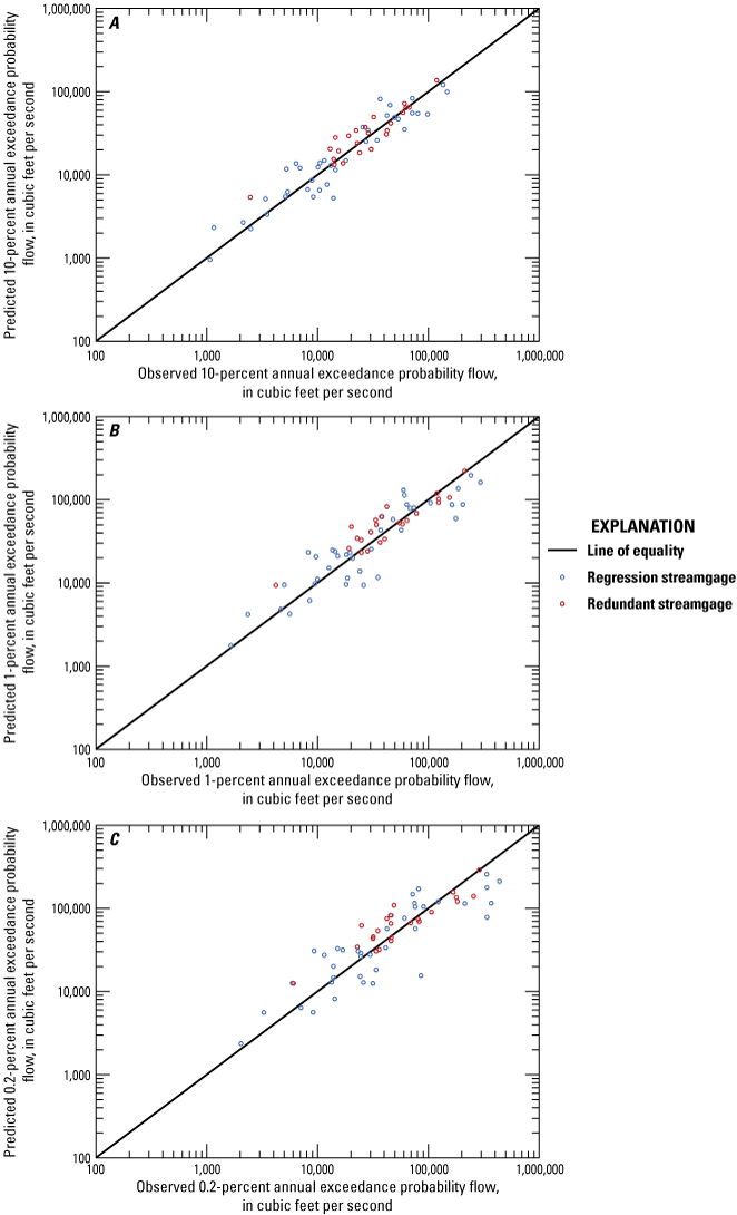
Comparisons of the observed and predicted A,10-, B, 1-, and C, 0.2-percent annual exceedance probability streamflows at streamgages on regulated streams in Georgia, South Carolina, and North Carolina that were included in the regression analysis for estimating peak streamflows at regulated rural basins or that were excluded from the regression analysis because of redundancy (streamflow data from Kolb and others, 2023).
Table 2.
Regional flood-frequency equations for estimating peak streamflows for regulated rural basins in Georgia, South Carolina, and North Carolina.[DA, drainage area in square miles; MSI, maximum storage index in acre-feet per square mile]
Accuracy and Limitations
Regression equations are statistical models that must be interpreted and applied within the limits of the data and with the understanding that the results are best-fit estimates with an associated scatter or variance. Uncertainty, or error, in the model (that is, differences between the predicted and observed values) can be examined to determine parameters that describe the accuracy of a regression equation, which depends on both the model error and the time-sampling error. Model error measures the ability of a set of explanatory variables to estimate the values of peak-streamflow characteristics calculated from the streamgage records used to develop the equation. The model error depends on the number and predictive power of the explanatory variables in a regression equation. Time-sampling error measures the ability of a finite number of streamgages with a finite number of recorded annual peak streamflows to describe the true characteristics of the entire peak-streamflow record for a streamgage. The time-sampling error depends on the number and record length of streamgages used in the analysis and decreases as the number of streamgages and record lengths increase. A measure of the uncertainty in a regression equation estimate for a site, i, is the variance of prediction, Vp,i. The Vp,i is the sum of the model error variance and time-sampling error variance and is computed using the following equation:
whereγ2
is the model error variance, in log units; and
MSEs,i
is the time-sampling mean square error for site i, in log units.
Assuming that the explanatory variables for the streamgages in a regression analysis are representative of all streamgages in the region, the average accuracy of prediction for a regression equation can be determined by computing the average variance of prediction, AVP, for n number of streamgages:
where the remaining variables are as previously defined in equation 4.A more traditional measure of the accuracy of P-percent AEP streamflow regression equations is the standard error of prediction, Sp, which is simply the square root of the variance of prediction. The average standard error of prediction for a regression equation can be computed in percent by using AVP, in log units, and the following transformation formula:
whereThe Sp,ave is a measure of the average uncertainty of the regression equations when predicting flood estimates for ungaged sites, which is the most common application of the regression equations. There is about a 68-percent probability that the true AEP streamflow at an ungaged location will be between plus or minus the Sp,ave of the regression estimate (Hodgkins, 1999).
A measure of the proportion of the variation in the response variable explained by the explanatory variables in OLS regressions is the coefficient of determination, R2 (Montgomery and others, 2012). For GLS regressions, a more appropriate performance metric than R2 is pseudo R2 described by Griffis and Stedinger (2007b). Unlike the R2 metric, pseudo R2 is based on the variability in the response variable explained by the regression after removing the effect of the time-sampling error. The pseudo R2 is computed using the following formula:
whereγ2(k)
is the model error variance from a GLS regression with k explanatory variables, and
γ2(0)
is the model error variance from a GLS regression with no explanatory variables.
Table 3.
Pseudo coefficient of determination (pseudo R2), average variance of prediction, and average standard error of prediction for the regional regression equations for regulated rural basins in Georgia, South Carolina, and North Carolina.Users of the regression models may be interested in a measure of uncertainty at a particular site as opposed to the uncertainty statistics based on streamgage data used to generate the regression models. One such measure of uncertainty at a particular ungaged site is the confidence interval of a prediction, or prediction interval. The prediction interval is the range that likely contains the streamflow characteristic for a new observation not included in the development of the regression equations. Tasker and Driver (1988) determined that a 100(1–α) prediction interval for the true value of a streamflow characteristic for an ungaged site from the regression equation can be computed as follows:
whereQ
is the streamflow characteristic for the ungaged site, and
C
is the confidence or prediction interval computed as
Z(α/2)
is the normal critical value at a particular alpha level α, which equals 0.05 for a 95-percent prediction interval, divided by 2 and is equal to 1.96 for an α of 0.05; and
Sp,i
is the standard error of prediction and is computed as
γ2
is the model error variance;
xi
is a row vector of variables logDA and logMSI for site i, augmented by a 1 as the first element;
U
is the covariance matrix for the regression coefficients; and
xi′
is the transpose of xi (Ludwig and Tasker, 1993).
Table 4.
Model error variance and covariance matrix values needed to determine 95-percent prediction intervals for the regression equations for regulated rural basins in Georgia, South Carolina, and North Carolina.[AEP, annual exceedance probability; γ2, model error variance; U, the covariance matrix; DA, drainage area in log square miles; MSI, maximum storage index in log acre-feet per square mile]
The following limitations should be recognized when using the final regional regression equations for regulated rural basins in Georgia, South Carolina, and North Carolina:
-
1. The regulated flood-frequency analyses computed at the USGS streamgages by Feaster and others (2023) used the most recent period of streamflow record showing relatively stable peak-streamflow patterns through water year 2019. Use of these flood-frequency statistics assumes similar future peak-streamflow patterns. If future peak-streamflow patterns are shown to have substantially changed, the use of the regulated flood-frequency statistics may not be warranted.
-
2. The methods are applicable to regulated rural basins draining 75 percent or more from above the Fall Line.
-
3. Applying the equations outside the range of the explanatory variables used to develop the regional regression equations (table 5) will produce results with unknown accuracy.
Table 5.
Ranges of drainage area and maximum storage index values used to develop the regression equations for regulated rural basins in Georgia, South Carolina, and North Carolina.[mi2, square mile; acre-ft/mi2, acre-foot per square mile]
The maximum storage for the individual reservoirs upstream from the streamgages included in the regulated rural regression analysis ranged from 185 acre-feet (acre-ft) to 3,820,000 acre-ft (U.S. Army Corps of Engineers, 2020). Of those reservoirs, 90 percent had a maximum storage greater than or equal to 5,220 acre-ft with the mean maximum storage being 328,000 acre-ft and the median being 40,600 acre-ft.
Comparison of Regulated Rural Flood-Frequency Estimates With Unregulated Rural Flood-Frequency Estimates
For the 10-, 1-, and 0.2-percent AEP streamflows, the at-site regulated flood-frequency estimates were compared with the regulated regression estimates by using the equations in table 2 and with the unregulated rural flood-frequency estimates from the regional regression equations from Feaster and others (2023). The comparisons were done using boxplots of the percentage change from the at-site regulated flood-frequency estimates for the 39 streamgages included in the regulated regression analysis to the regulated regression estimates and to the unregulated regression estimates for the same group of 39 streamgages (fig. 14). In general, the boxplots show that the regulated regression estimates better match the at-site regulated flood-frequency estimates than do the unregulated flood-frequency estimates. The median and mean percentage change shows that the unregulated flood-frequency estimates tend to overestimate the at-site regulated flood-frequency estimates and have greater variability than do the percentage change from the regulated regression estimates.
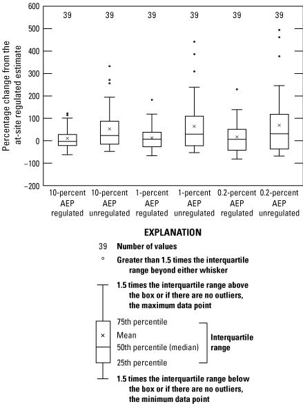
The distribution of the percentage change between the at-site regulated estimates and the regulated regression estimates and between the at-site regulated estimates and the unregulated regression estimates in the 10-, 1-, and 0.2-percent annual exceedance probability (AEP) streamflows at 39 U.S. Geological Survey streamgages in Georgia, South Carolina, and North Carolina (streamflow data from U.S. Geological Survey, 2019).
The percentage change between the at-site regulated estimates and regulated regression estimates for the 10-percent AEP streamflows ranged from −62 to 126 percent with a median and mean of −2.9 and 10 percent, respectively (fig. 14). The percentage change between the at-site regulated estimates and the unregulated regression estimates for the 10-percent AEP streamflow predictions ranged from −48 to 332 percent with a median and mean of 23 and 52 percent, respectively.
For the 1-percent AEP streamflows, the percentage change between the at-site regulated estimates and the regulated regression estimates ranged from −67 to 182 percent with a median and mean of 6.6 and 12 percent, respectively (fig. 14). The percentage change between the at-site regulated estimates and the unregulated regression estimates for the 1-percent AEP streamflows ranged from −53 to 442 percent with the median and mean being 28 and 62 percent, respectively.
For the 0.2-percent AEP streamflows, the percentage change between the at-site regulated estimates and the regulated regression estimates ranged from −82 to 229 percent with a median and mean of 5.8 and 15 percent, respectively (fig. 14). The percentage change between the at-site regulated estimates and the unregulated regression estimates for the 0.2-percent AEP streamflows ranged from −68 to 495 percent with a median and mean of 30 and 67 percent, respectively.
Figure 15 provides a visual comparison of the regulated regression flood-frequency curves and the unregulated regression flood-frequency curves for the 10-, 1-, and 0.2-percent AEP flows. The unregulated flood-frequency curves are from Feaster and others (2023) and assume that basins drain fully from hydrologic regions 1 and 2, which are the two hydrologic regions above the Fall Line (fig. 2). Because the regulated flood-frequency equations are functions of drainage area and maximum storage index (table 2), two curves are shown (fig. 15), with one holding the maximum storage index constant at the minimum value and the other holding the maximum storage index constant at the maximum value from the streamgages included in the regulated regression analysis (table 5). As can be seen, as the maximum storage index increases from the minimum to the maximum value included in the regression analysis, the flood-frequency estimates decrease (fig. 15). For the minimum value of the maximum storage index, the flood-frequency curve is more in the range of the unregulated curves. It should be noted that the regulated flood-frequency analysis includes 39 streamgages and the unregulated flood-frequency analysis for hydrologic regions 1 and 2 includes 352 and 113 streamgages, respectively, that drain 75 percent or more within one hydrologic region (table 1 from Kolb and others, 2023). Also, holding the maximum storage index at the minimum and maximum values is useful to provide a one-dimensional visual comparison; however, with the regulated regression being a function of two independent variables, the regression analysis is fitting a plane and not a linear curve within a range of maximum storage index values between the minimum and maximum values (table 5). As such, differences in unregulated regression curves and the regulated regression curve for the minimum value of the maximum storage index would be expected.
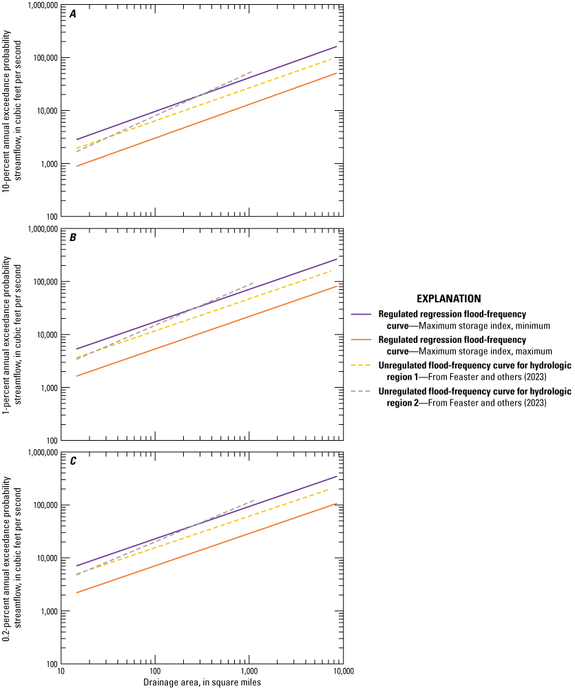
Regulated regression flood-frequency curves and unregulated flood-frequency curves for basins draining 75 percent or more from hydrologic regions above the Fall Line in Georgia, South Carolina, and North Carolina for the A, 10-, B, 1-, and C, 0.2-percent annual exceedance probability streamflows.
Application of Methods
B17C (England and others, 2018) provides methods for reducing the uncertainty of flood-frequency estimates by weighting the streamgage estimate with the regional regression estimate. The following sections describe the weighting process at a streamgage as well as a process for shifting the weighted estimate to an ungaged location on the same stream.
Estimation at a Streamgage
B17C (England and others, 2018) recommends that improved flood-frequency estimates for a streamgage can be obtained by combining (weighting) streamgage streamflow estimates determined from the LPIII analysis of the annual peak streamflows with streamflow estimates obtained for the streamgage from regression equations. Optimal weighted streamflow estimates can be obtained if the variance of prediction for each of the two estimates is known or can be estimated accurately. The variance of prediction can be thought of as a measure of the uncertainty in either the streamgage estimate or the regional regression results. If the two estimates can be assumed to be independent and are weighted in inverse proportion to the associated variances, the variance of the weighted estimate will be less than the variance of either of the independent estimates.
The variance from the EMA analyses at a streamgage is provided for each AEP estimate as part of the output in PeakFQ (table 13 from Musser and Feaster, 2023; U.S. Geological Survey, 2022). The variance from the streamgage analysis is related to the years of record, with long records tending to have a lower variance than short records. The variance of prediction from the regional regression equations is a function of the regression equations and the values of the independent variables used to develop the streamflow estimate from the regression equations. This variance generally increases as the values of the independent variables move further from the mean values of the independent variables. The average variance of prediction values for the regional regression equations used in this investigation are listed in table 3.
Once the variances have been computed, the two independent streamflow estimates can be weighted using the following equation:
whereQw(s)
is the weighted estimate of peak streamflow for any P-percent AEP for a streamgage, in cubic feet per second;
Vr(s)
is the variance of prediction at the streamgage derived from the applicable regional regression equations for the selected P-percent AEP, in log units, and can be obtained from the weighted least squares regression for streamflow frequency statistics program (Farmer, 2021) output. If the weighting is being done for a streamgage that was not included in the regression analysis, the average variance of prediction can be used from table 3;
Qs
is the estimate of peak streamflow at the streamgage from the LPIII analysis for the selected P-percent AEP, in cubic feet per second;
Vs
is the variance of prediction at the streamgage from the LPIII analysis for the selected P-percent AEP (table 13 from Musser and Feaster, 2023), in log units; and
Qr(s)
is the peak-streamflow estimate for the P-percent AEP at the streamgage derived from the applicable regional regression equations in table 2, in cubic feet per second.
For the 63 streamgages in Georgia, South Carolina, and North Carolina that drained 75 percent or more from above the Fall Line (table 13 from Musser and Feaster, 2023), the weighted streamflow estimates were computed using equation 11 with the variance from the at-site EMA analysis along with one of the following:
-
• The variance of prediction values at the streamgage (table 13 from Musser and Feaster, 2023), or
-
• The average variance of prediction (table 3) for the redundant streamgages that were not included in the regression analysis.
Confidence intervals for the weighted estimate also can be computed (England and others, 2018). The upper and lower 95-percent confidence intervals (95%CI) on the weighted AEP estimate can be computed as
where the remaining variables are as previously defined in equations 11 and 12.Example Application
An example of the application of the procedure described above is the following computation of the weighted 1-percent AEP streamflow for 02147020 Catawba River below Catawba, S.C. (map index number 348 in fig. 2 in this report and in table 7 from Musser and Feaster, 2023):
-
1. Obtain the streamgage estimate of the 1-percent AEP streamflow based on the systematic flood peaks (table 13 from Musser and Feaster, 2023) (Qs = 156,000 ft3/s);
-
2. Obtain drainage area and maximum storage index (table 7 from Musser and Feaster, 2023) (DA = 3,540 mi2 and maximum storage index = 326 acre-ft/mi2);
-
3. Compute the peak-streamflow estimate at the streamgage using the 1-percent AEP equation in table 2 (Qr(s) = 6,320 × (3,5400.609) × (326−0.384) = 99,308 ft3/s, which is rounded to the value 99,300 for Qr(s) for this streamgage [table 13 from Musser and Feaster, 2023]);
-
4. Obtain the variance of prediction for the LPIII streamgage estimate for the 1-percent AEP streamflow (table 13 from Musser and Feaster, 2023) (Vs = 0.0117);
-
5. Obtain the variance of prediction for the 1-percent AEP streamflow regression estimate (table 13 from Musser and Feaster, 2023) (Vr(s) = 0.0519);
-
6. Compute the weighted 1-percent AEP streamflow for the streamgage by using equation 11 (log Qw(s) = ((0.0519) (log 156,000) + (0.0117) (log 99,300)) / (0.0117 + 0.0519) = 5.157, and the base 10 antilog Qw(s) = 143,549 ft3/s, which is rounded to the value 144,000 ft3/s for Qw(s) for this streamgage).
-
7. Compute the weighted 1-percent AEP variance for the streamgage by using equation 12 (Vw(s) = (0.0117 × 0.0519) / (0.0117 + 0.0519) = 0.00955); and
-
8. Compute the 95-percent confidence interval by using equation 13
With respect to step 2 for an ungaged location, the drainage area can be obtained using the USGS StreamStats application, which is available at https://streamstats.usgs.gov/ss. The maximum storage index can be obtained by computing the cumulative maximum storage for reservoirs upstream from the site of interest. The first step in the process is to identify the upstream reservoirs. To identify the upstream reservoirs, the user can zoom to the site of interest using StreamStats. If the site is at a USGS streamgage, the user can zoom to the outlet of the basin by using the streamgage number. If the site is at an ungaged location, the user can search StreamStats by using the latitude and longitude or can find the site by zooming to the location on the StreamStats map. For USGS streamgages, users also can search by streamgage number by using the USGS NWIS (U.S. Geological Survey, 2019). From the StreamStats or NWIS map, users can zoom out and view upstream to determine the reservoirs in the basin of interest. For the example using 02147020, the upstream reservoirs are Lake Wylie in South Carolina and Mountain Island Lake, Lake Norman, Lookout Shoals Lake, Lake Hickory, Rhodhiss Lake, and Lake James in North Carolina. The maximum storage for these reservoirs is then obtained from the U.S. Army Corps of Engineers NID database (U.S. Army Corps of Engineers, 2020). The NID website has various tools available to search for dams. Users can also download the data by State as a comma-separated values file that can be opened in a spreadsheet. From the NID database, the maximum storage (in acre-feet) for the reservoirs upstream as previously listed was 246,435; 45,970; 414,100; 26,390; 127,500; 27,570; and 265,182, respectively. The cumulative total maximum storage is 1,153,147 acre-ft. The maximum storage index is computed by dividing the cumulative total maximum storage by the drainage area at the site of interest (1,153,147/3,540 = 326 acre-ft/mi2).
Estimation for an Ungaged Site Near a Streamgage
Sauer (1974) presented the following method to improve flood-frequency estimates for an ungaged site near a streamgage, on the same stream, that has 10 or more years of peak-streamflow record. To obtain a weighted peak-streamflow estimate for P-percent AEP at the ungaged site, Qw(u), the weighted streamflow estimates for an upstream or downstream streamgage, Qw(s), must first be determined by using equation 11. The weighted AEP estimate for the ungaged site, Qw(u), is then computed using the following equation:
whereQw(u)
is the weighted estimate of peak streamflow for the selected P-percent AEP at the ungaged site, in cubic feet per second;
ΔA
is the absolute value of the difference between the drainage areas for the streamgage (As) and the ungaged site (Au), in square miles;
A(s)
is the drainage area for the streamgage, in square miles;
Qw(s) and Qr(s)
are as previously defined in equation 11; and
Qr(u)
is the peak-streamflow estimate derived from the applicable regional regression equations in table 2 for the selected P-percent AEP at the ungaged site, in cubic feet per second.
Use of equation 14 gives full weight to the regression equation estimates when the drainage area for the ungaged site is equal to 0.5 or 1.5 times the drainage area for the streamgage and gives increasing weight to the streamgage estimates as the drainage area ratio approaches 1. The weighting procedure should not be applied when the drainage area ratio for the ungaged site and streamgage is less than 0.5 or greater than 1.5. For streamgages with large drainage areas, hydrologic judgement should be applied as to whether shifting the weighted estimate to the full limits of the drainage area ratio (0.5 or 1.5) is appropriate. In addition, all other limitations noted in the report should be adhered to as well.
Example Application
An example application of this procedure is the computation of the weighted 1-percent AEP streamflow for a hypothetical ungaged site on the Catawba River located downstream from USGS streamgage 02147020 Catawba River below Catawba, S.C., referred to in the previous section. The ungaged downstream location has a drainage area of 3,620 mi2. Because there are no major impoundments between 02147020 and the downstream location, the maximum storage index at the downstream location can be computed from the maximum storage index at 02147020 times the ratio of the drainage area at 02147020 and the downstream location:
-
1. Calculate the value of Qw(s) for the streamgage (see step 6 of example in previous example application in section “Estimation for an Ungaged Site Near a Streamgage,” Qw(s) = 144,000 ft3/s);
-
2. Obtain the drainage areas for both the gaged and ungaged sites (As = 3,540 mi2 and Au = 3,620 mi2);
-
3. Determine the maximum storage index for the ungaged site (326 × (3,540/3,620) = 319 acre-ft/mi2);
-
4. Compute Qr(u) for the ungaged site by using the 1-percent AEP equation in table 2 (Qr(u) = 6,320 × (3,6200.609) × (319−0.384) = 101,511 ft3/s, which is rounded to 102,000 for Qr(u) for this ungaged site);
-
5. Compute Qr(s) for the streamgage by using the 1-percent AEP equation in table 2 (see step 3 of example in previous example application subsection, Qr(s) = 99,300 ft3/s);
-
6. Compute ΔA, where ΔA = 3,620 − 3,540 = 80 mi2; and
-
7. Compute the weighted estimate for the ungaged site, Qw(u), by using equation 14 (Qw(u) = [((2 × 80) / 3,540) + ((1 – ((2 × 80) / 3,540)) × (144,000/99,300))] × 102,000 = 141,230 ft3/s (rounded to 141,000 ft3/s)).
For an ungaged site that is located between two streamgages on the same stream and whose drainage area is 75 percent or more from above the Fall Line, two streamflow estimates can be made using the methods and criteria outlined in this section. Hydrologic judgment may be necessary to determine which of the two estimates (or some interpolation thereof) is most appropriate. Other factors that might be considered when evaluating the two estimates include differences in the length of record for the two streamgages and the hydrologic conditions that existed during the data-collection period for each streamgage (for example, whether the time series represents a climatic period that was predominantly wet or dry).
Summary
Reliable estimates of the magnitude and frequency of floods are essential for flood insurance studies, floodplain management, and the design of transportation and water-conveyance structures such as roads, bridges, culverts, dams, and levees. Federal, State, regional, and local officials rely on such estimates to effectively plan and manage land use and water resources, protect lives and property in flood-prone areas, and determine flood insurance rates. The U.S. Geological Survey (USGS) and the South Carolina Department of Transportation have a long history of working cooperatively to develop techniques for estimating the magnitude and frequency of floods for rural and urban basins that have minimal to no regulation or tidal influence. The Federal guidelines for flood-frequency analyses at streamgaging stations (streamgages) were developed for basins where streamflows under flood conditions are not appreciably altered by regulation, basin changes, or long-term changes in the hydrologic system. However, under certain conditions, it may be appropriate to apply those techniques at streamgages on regulated streams. Over the years, flood-frequency analyses have been done at selected streamgages in Georgia, South Carolina, and North Carolina, but there has not been a comprehensive report assessing the effects of regulation from impoundments on streamflow until this investigation. The effect of an impoundment on downstream streamflows can vary widely based on the purpose and structure of the impoundment. The degree of regulation reflected at USGS streamgages located downstream from impoundments often is assessed more on a qualitative rather than quantitative basis. For humid areas of the United States, one USGS investigation determined that a usable storage of less than 103 acre-feet per square mile would generally affect peak streamflows by less than 10 percent.
The purpose of this investigation was to assess the effects of impoundments on peak streamflows and other selected streamflow characteristics. Streamgages from Georgia, South Carolina, and North Carolina with long-term periods of record (30 or more years) were included in the investigation. At 18 streamgages, annual exceedance probability (AEP) streamflows were compared for pre- and post-regulated (before and after impoundment) periods of record. For the 10-, 1- and 0.2-percent AEP streamflows, the average reduction in the streamflows from the pre- to post-regulated periods was about 31 percent. For the 10-percent AEP streamflows (10-year flood), the percentage change from the pre- to post-regulated periods ranged from 2.0 to 72.0 percent. For the 1-percent AEP streamflows (100-year flood), the percentage change from the pre- to post-regulated periods ranged from −78.0 to 22.4 percent. For the 0.2-percent AEP streamflows (500-year flood), the percentage change from the pre- to post-regulated periods ranged from −83.4 to 44.7 percent.
To get a sense of how flood-frequency statistics can vary based on analyzing different periods of record, the 10-, 1-, and 0.2-percent AEP streamflows were compared for two periods of record at 18 USGS streamgages monitoring unregulated streams. For the three AEP streamflow statistics, the average change was a reduction of 8.6, 6.4, and 5.0 percent, respectively. The ranges of change in the three AEP streamflow statistics from minimum to maximum percentage change were −38.9 to 30.1, −48.1 to 57.0, and −53.6 to 69.0 percent, respectively. These results provide some indication of the natural variability in the AEP streamflows at specific streamgage locations based on length of record and hydrologic conditions captured in those records. As compared to the percentage change from the pre- and post-regulated periods of record, the range of percentage changes between the two periods at the unregulated streamgages tends to be more balanced between the positive and negative percentage changes with average percentage changes that are much smaller than the average for the pre- and post-regulated AEP streamflow statistics.
To assess the effects of impoundments on a broader range of streamflow statistics, The Nature Conservancy’s Indicators of Hydrologic Alteration (IHA) software was used to assess a limited number of streamflow characteristics computed from daily mean streamflows. The IHA software was used to compare mean annual streamflow, 1-day maximum streamflow, 1- and 7-day minimum streamflows, low pulse count and duration, and high pulse count and duration for pre- and post-regulated periods of record at 16 streamgages. The length of records analyzed for the pre-regulated period ranged from 34 to 80 years. The length of records analyzed for the post-regulated period ranged from 39 to 68 years. The mean annual streamflows were relatively consistent for the pre- and post-regulated periods of record with the average percentage change being −1.4 percent with a range of −21.8 to 9.7 percent. The average change between the pre- and post-regulated 1-day maximum streamflows was −28.2 percent, which was close to the average reduction in the AEP streamflows. The average change in the 1- and 7-day minimum streamflows was an increase of 29.7 and 24.1 percent, respectively. These findings reflect conditions that are often found to occur from regulation; on average, the low streamflows increased and the high streamflows decreased.
To assess the natural variability in selected daily mean streamflow characteristics based on period of record and hydrologic conditions captured in those records, the IHA software was used to analyze long-term periods at 17 streamgages monitoring unregulated streams. The length of records in the two periods ranged from 39 to 60 years. The average percentage change in the mean annual streamflow for the two periods was −2.4 percent, which was similar to the percentage change in the mean annual streamflows the pre- and post-regulated periods of record. However, a comparison of boxplots showed that the variability in the mean annual streamflows was much less from the streamgages with pre- and post-regulated periods as compared to the two periods of record analyzed at the streamgages monitoring unregulated streams. The average percentage change in the 1-day maximum streamflows for the two periods of record was −7.3 percent. For the 1- and 7-day minimum streamflows, the average change between the two unregulated periods analyzed at the 17 streamgages was −19.5 and −21.4 percent, respectively. These results may reflect historical drought periods that have occurred in the Southeast over the last couple of decades or other influences in the basins.
In a separate USGS investigation completed in 2023, flood-frequency statistics were computed for 72 streamgages monitoring regulated streams in Georgia, South Carolina, and North Carolina. Of those 72 streamgages, 29 were found to be redundant, which is a situation where the drainage basin of one streamgage is contained inside another (nested) and the two basins are of similar size. For the remaining 43 streamgages, 39 had basins that drained 75 percent or more from above the Fall Line. Those 39 streamgages were used in this investigation to develop regression equations for the 50-, 20-, 10-, 4-, 2-, 1-, 0.5-, and 0.2-percent AEP streamflows. The independent variables in the equations were drainage area and maximum storage index from upstream reservoirs. The pseudo coefficient of determination statistics, which is based on the variability in the AEP streamflows explained by the regression equation after removing the time-sampling error, ranged from 77.9 to 92.6 percent. The average standard error of prediction, which is a measure of the average uncertainty of the regression equations when predicting flood estimates at ungaged locations, ranged from 40.0 to 70.3 percent. There were not enough streamgages monitoring regulated streams available to allow for development of similar equations in the Coastal Plain portion of the study area (below the Fall Line).
The at-site regulated flood-frequency estimates for the 10-, 1-, and 0.2-percent AEP streamflows were compared with the regulated regression and unregulated regression estimates for the 39 streamgages included in the regulated regression analysis. Boxplots of percentage change showed that the regulated regression estimates match the at-site regulated flood-frequency estimates better than do the unregulated flood-frequency estimates. The median and mean percentage change showed that the unregulated flood-frequency estimates tend to overestimate the at-site regulated flood-frequency estimates and have greater variability than do the percentage change from the regulated regression estimates. These comparisons suggest that in most instances when estimating flood-frequency statistics at an ungaged regulated location, using the regulated flood-frequency regression equations instead of the unregulated flood-frequency regression equations will provide a more accurate estimate.
Selected References
Asquith, W.H., 2001, Effects of regulation on L-moments of annual peak streamflow in Texas: U.S. Geological Survey Water-Resources Investigations Report 2001–4243, 66 p. [Also available at https://doi.org/10.3133/wri014243.]
Benson, M.A., 1962, Factors influencing the occurrence of floods in a humid region of diverse terrain: U.S. Geological Survey Water-Supply Paper 1580–B, 64 p. [Also available at https://doi.org/10.3133/wsp1580B.]
Bohman, L.R., 1992, Determination of flood hydrographs for streams in South Carolina—Volume 2. Estimation of peak-discharge frequency, runoff volumes, and flood hydrographs for urban watersheds: U.S. Geological Survey Techniques of Water-Resources Investigations Report 92–4040, 79 p. [Also available at https://doi.org/10.3133/wri924040.]
Cohn, T.A., England, J.F., Berenbrock, C.E., Mason, R.R., Stedinger, J.R., and Lamontagne, J.R., 2013, A generalized Grubbs-Beck test statistic for detecting multiple potentially influential low outliers in flood series: Water Resources Research, v. 49, no. 8, p. 5047–5058. [Also available at https://doi.org/10.1002/wrcr.20392.]
Cohn, T.A., Lane, W.L., and Baier, W.G., 1997, An algorithm for computing moments-based flood quantile estimates when historical flood information is available: Water Resources Research, v. 33, no. 9, p. 2089–2096. [Also available at https://doi.org/10.1029/97WR01640.]
Cohn, T.A., Lane, W.L., and Stedinger, J.R., 2001, Confidence intervals for expected moments algorithm flood quantile estimates: Water Resources Research, v. 37, no. 6, p. 1695–1706. [Also available at https://doi.org/10.1029/2001WR900016.]
Cohn, T.A., and Lins, H.F., 2005, Nature’s style—Naturally trendy: Geophysical Research Letters, v. 32, no. 23, L23402, 5 p. [Also available at https://doi.org/10.1029/2005GL024476.]
Conrads, P.A., Feaster, T.D., and Harrelson, L.G., 2008, The effects of the Saluda Dam on the surface water and ground-water hydrology of the Congaree National Park flood plain, South Carolina: U.S. Geological Survey Scientific Investigations Report 2008–5170, 58 p. [Also available at https://pubs.water.usgs.gov/sir2008-5170.]
Cooke, C.W., 1936, Geology of the Coastal Plain of South Carolina: U.S. Geological Survey Bulletin 867, 196 p. [Also available at https://pubs.er.usgs.gov/publication/b867.]
Eng, K., Chen, Y.-Y., and Kiang, J.E., 2009, User’s guide to the weighted-multiple-linear regression program (WREG version 1.0): U.S. Geological Survey Techniques and Methods, book 4, chap. A8, 21 p. [Also available at https://pubs.usgs.gov/tm/tm4a8.]
England, J.F., Jr., Cohn, T.A., Faber, B.A., Stedinger, J.R., Thomas, W.O., Jr., Veilleux, A.G., Kiang, J.E., and Mason, R.R., Jr., 2018, Guidelines for determining flood flow frequency—Bulletin 17C (ver. 1.1, May 2019): U.S. Geological Survey Techniques and Methods, book 4, chap. B5, 148 p. [Also available at https://doi.org/10.3133/tm4B5.]
Esri, 2021, ArcGIS Desktop (ver. 10.7.1): Esri ArcGIS Desktop web page, accessed January 12, 2021, at https://desktop.arcgis.com/en/.
Farmer, W.H., 2021, R package WREG—Weighted least squares regression for streamflow frequency statistics(ver. 3.0): U.S. Geological Survey software release, accessed April 14, 2021, at https://doi.org/10.5066/P9ZCGLI1.
Farmer, W.H., Kiang, J.E., Feaster, T.D., and Eng, K., 2019, Regionalization of surface-water statistics using multiple linear regression: U.S. Geological Survey Techniques and Methods, book 4, chap. A12, 40 p., accessed January 2020 at https://doi.org/10.3133/tm4A12.
Feaster, T.D., Gotvald, A.J., Musser, J.W., Weaver, J.C., and Kolb, K.R., 2023, Magnitude and frequency of floods for rural streams in Georgia, South Carolina, and North Carolina, 2017—Results: U.S. Geological Survey Scientific Investigations Report 2023–5006, 75 p. [Also available at https://doi.org/10.3133/sir20235006.]
Feaster, T.D., Gotvald, A.J., and Weaver, J.C., 2009, Magnitude and frequency of rural floods in the Southeastern United States, 2006—Volume 3, South Carolina: U.S. Geological Survey Scientific Investigations Report 2009–5156, 226 p. [Also available at https://pubs.usgs.gov/sir/2009/5156/.]
Feaster, T.D., Gotvald, A.J., and Weaver, J.C., 2014, Methods for estimating the magnitude and frequency of floods for urban and small, rural streams in Georgia, South Carolina, and North Carolina, 2011 (ver. 1.1, March 2014): U.S. Geological Survey Scientific Investigations Report 2014–5030, 104 p. [Also available at https://doi.org/10.3133/sir20145030.]
Feaster, T.D., and Guimaraes, W.B., 2004, Estimating the magnitude and frequency of floods in small urban streams in South Carolina, 2001: U.S. Geological Survey Scientific Investigations Report 2004–5030, 58 p. [Also available at https://pubs.usgs.gov/sir/2004/5030/.]
Feaster, T.D., and Guimaraes, W.B., 2017, Low-flow characteristics of streams in South Carolina: U.S. Geological Survey Open-File Report 2017–1110, 161 p. [Also available at https://doi.org/10.3133/ofr20171110.]
Feaster, T.D., and Tasker, G.D., 2002, Techniques for estimating the magnitude and frequency of floods in rural basins of South Carolina, 1999: U.S. Geological Survey Water- Resources Investigations Report 02–4140, 34 p. [Also available at https://pubs.usgs.gov/wri/wri024140/.]
Feaster, T.D., Weaver, J.C., Gotvald, A.J., and Kolb, K.R., 2018, Preliminary peak stage and streamflow data at selected U.S. Geological Survey streamgaging stations in North and South Carolina for flooding following Hurricane Florence, September 2018: U.S. Geological Survey Open-File Report 2018–1172, 36 p. [Also available at https://doi.org/10.3133/ofr20181172.]
Flynn, K.M., Kirby, W.H., and Hummel, P.R., 2006, User’s manual for program PeakFQ, annual flood-frequency analysis using Bulletin 17B guidelines: U.S. Geological Survey Techniques and Methods, book 4, chap. B4, 42 p. [Also available at https://pubs.usgs.gov/tm/2006/tm4b4/.]
Gotvald, A.J., 2016, Selected low-flow frequency statistics for continuous-record streamgages in Georgia, 2013: U.S. Geological Survey Scientific Investigations Report 2016–5037, 20 p. [Also available at https://doi.org/10.3133/sir20165037.]
Griffis, V.W., and Stedinger, J.R., 2007a, The LP3 distribution and its application in flood frequency analysis. II—Parameter estimation methods: Journal of Hydrologic Engineering, v. 12, no. 5, p. 492–500. [Also available at https://ascelibrary.org/doi/abs/10.1061/(ASCE)1084-0699(2007)12%3A5(492).]
Griffis, V.W., and Stedinger, J.R., 2007b, The use of GLS regression in regional hydrologic analyses: Journal of Hydrology, v. 344, nos. 1–2, p. 82–95. [Also available at https://doi.org/10.1016/j.jhydrol.2007.06.023.]
Griffith, G.E., Omernik, J.M., Comstock, J.A., Schafale, M.P., McNab, W.H., Lenat, D.R., MacPherson, T.F., Glover, J.B., and Shelburne, V.B., 2002, Ecoregions of North Carolina and South Carolina: Reston, Virginia, U.S. Geological Survey, color poster with map, descriptive text, summary tables, and photographs, map scale 1:1,500,00. [Also available at http://ecologicalregions.info/data/nc/ncsc_front.pdf.]
Gruber, A.M., and Stedinger, J.R., 2008, Models of LP3 regional skew, data selection and Bayesian GLS regression, in Babcock, R.W., Jr., and Walton, R., eds., World Environmental and Water Resources Congress, 2008, Honolulu, Hawaii, May 12–16, 2008 [Proceedings]: American Society of Civil Engineers, Paper 596, 10 p. [Also available at https://doi.org/10.1061/40976(316)563.]
Guimaraes, W.B., and Bohman, L.R., 1991, Techniques for estimating the magnitude and frequency of floods in South Carolina, 1988: U.S. Geological Survey Water-Resources Investigations Report 91–4157, 174 p. [Also available at https://doi.org/10.3133/wri914157.]
Helsel, D.R., Hirsch, R.M., Ryberg, K.R., Archfield, S.A., and Gilroy, E.J., 2020, Statistical methods in water resources: U.S. Geological Survey Techniques and Methods, book 4, chapter A3, 458 p. [Also available at https://doi.org/10.3133/tm4A3.] [Supersedes U.S. Geological Survey Techniques of Water-Resources Investigations, book 4, chapter A3, ver. 1.1.]
Hodgkins, G., 1999, Estimating the magnitude of peak flows for streams in Maine for selected recurrence intervals: U.S. Geological Survey Water-Resources Investigations Report 99–4008, 45 p. [Also available at https://doi.org/10.3133/wri994008.]
Interagency Advisory Committee on Water Data, 1982, Guidelines for determining flood flow frequency, Bulletin 17B of the Hydrology Subcommittee: U.S. Geological Survey, Office of Water Data Coordination, 28 p., 14 app., 1 pl. [Also available at https://water.usgs.gov/osw/bulletin17b/dl_flow.pdf.]
Kolb, K.R., Musser, J.W., Feaster, T.D, Gotvald, A.J., and Weaver, J.C., 2023, Supporting tables and hydrologic region boundaries for magnitude and frequency of floods for rural streams in Georgia, South Carolina, and North Carolina, 2017: U.S. Geological Survey data release, accessed April 29, 2023, at https://doi.org/10.5066/P9TSBPFS.
Lins, H.F., Hirsch, R.M., and Kiang, J., 2010, Water—The Nation’s fundamental climate issue—A white paper on the U.S. Geological Survey role and capabilities: U.S. Geological Survey Circular 1347, 9 p., accessed July 27, 2015, at https://pubs.usgs.gov/circ/1347/.
Ludwig, A.H., and Tasker, G.D., 1993, Regionalization of low-flow characteristics of Arkansas streams: U.S. Geological Survey Water-Resources Investigations Report 93–4013, 19 p. [Also available at https://doi.org/10.3133/wri934013.]
Martin, R.O.R., and Hanson, R.L., 1966, Reservoirs in the United States: U.S. Geological Survey Water-Supply Paper 1838, 115 p. [Also available at https://pubs.er.usgs.gov/publication/wsp1838.]
Musser, J.W., and Feaster, T.D., 2023, Tables and associated data for effects of impoundments on selected flood-frequency and daily mean streamflow characteristics in Georgia, South Carolina, and North Carolina: U.S. Geological Survey data release, https://doi.org/10.5066/P9Z93G0F.
Omernik, J.M., 1987, Ecoregions of the conterminous United States: Annals of the Association of American Geographers, v. 77, no. 1, p. 118–125, map scale 1:7,500,000. [Also available at https://doi.org/10.1111/j.1467-8306.1987.tb00149.x.]
R Core Team, 2020, R—A language and environment for statistical computing: Vienna, Austria, R Foundation for Statistical Computing website, accessed November 30, 2020, at https://www.R-project.org/.
Richter, B.D., Baumgartner, J.V., Powell, J., and Braun, D.P., 1996, A method for accessing hydrologic alteration within ecosystems: Conservation Biology, v. 10, no. 4, p. 1163–1174. [Also available at https://www.conservationgateway.org/Documents/1996.pdf.]
Ries, K.G., III, Newson, J.K., Smith, M.J., Guthrie, J.D., Steeves, P.A., Haluska, T.L., Kolb, K.R., Thompson, R.F., Santoro, R.D., and Vraga, H.W., 2017, StreamStats, version 4: U.S. Geological Survey Fact Sheet 2017–3046, 4 p., accessed February 27, 2018, at https://doi.org/10.3133/fs20173046. [Supersedes U.S. Geological Survey Fact Sheet 2008–3067.]
Ruddy, B.C., and Hitt, K.J., 1990, Summary of selected characteristics of large reservoirs in the United States and Puerto Rico, 1988: U.S. Geological Survey Open-File Report 90–163, 295 p. [Also available at https://doi.org/10.3133/ofr90163.]
Searcy, J.K., 1959, Flow-duration curves, manual of hydrology—Part 2. Low-flow techniques: U.S. Geological Survey Water-Supply Paper 1542–A, 33 p. [Also available at https://doi.org/10.3133/wsp1542A.]
South Carolina Department of Natural Resources, 2004, Hydrologic effects of the June 1998–August 2002 drought in South Carolina: South Carolina Department of Natural Resources, Land, Water, and Conservation Division, Water Resources Report 34, 49 p. [Also available at https://hydrology.dnr.sc.gov/pdfs/reports/Report%2034%20Drought.pdf.]
Stahle, D.W., and Cleaveland, M.K., 1992, Reconstruction and analysis of spring rainfall over the Southeastern U.S. for the past 1000 years: Bulletin of the American Meteorological Society, v. 73, no. 12, p. 1947–1961. [Also available at https://doi.org/10.1175/1520-0477(1992)073%3C1947:RAAOSR%3E2.0.CO;2.]
Stedinger, J.R., and Tasker, G.D., 1985, Regional hydrologic analysis—1. Ordinary, weighted, and generalized least squares compared: Water Resources Research, v. 21, no. 9, p. 1421–1432. [Also available at https://doi.org/10.1029/WR021i009p01421.]
Stedinger, J.R., and Tasker, G.D., 1986, Correction to “Regional hydrologic analysis—1. Ordinary, weighted, and generalized least squares compared”: Water Resources Research, v. 22, no. 5, p. 844. [Also available at https://doi.org/10.1029/WR022i005p00844.]
The Nature Conservancy, 2009, Indicators of hydrologic alteration, version 7.1, user’s manual: Smythe Scientific Software, 76 p. [Also available at https://www.conservationgateway.org/Documents/IHAV7.pdf.]
U.S. Army Corps of Engineers, 2020, National Inventory of Dams: U.S. Army Corps of Engineers database, accessed May 29, 2020, at https://nid.sec.usace.army.mil/.
U.S. Environmental Protection Agency, 2022, Level III and IV ecoregions of the continental United States: U.S. Environmental Protection Agency web page, accessed February 23, 2022, at https://www.epa.gov/eco-research/level-iii-and-iv-ecoregions-continental-united-states.
U.S. Geological Survey, 2013, Number of USGS streamgages through time: U.S. Geological Survey National Streamflow Information Program (NSIP) web page, accessed October 22, 2013, at https://water.usgs.gov/nsip/history1.html.
U.S. Geological Survey, 2019, USGS surface-water data for the Nation, in USGS water data for the Nation: U.S. Geological Survey National Water Information System database, accessed June 7, 2019, at https://doi.org/10.5066/F7P55KJN. [Surface-water data directly accessible at https://waterdata.usgs.gov/nwis/sw.]
U.S. Geological Survey, 2021a, National Hydrography Dataset: U.S. Geological Survey web page, accessed January 12, 2021, at https://www.usgs.gov/national-hydrography.
U.S. Geological Survey, 2021b, USGS surface-water data for the Nation, in USGS water data for the Nation: U.S. Geological Survey National Water Information System database, accessed May 7, 2021, at https://doi.org/10.5066/F7P55KJN. [Surface-water data directly accessible at https://waterdata.usgs.gov/nwis/sw.]
U.S. Geological Survey, 2022, PeakFQ (ver. 7.4): U.S. Geological Survey software release, accessed July 2022 at https://water.usgs.gov/software/PeakFQ/.
Veilleux, A.G., Cohn, T.A., Flynn, K.M., Mason, R.R., Jr., and Hummel, P.R., 2014, Estimating magnitude and frequency of floods using the Peak FQ 7.0 program: U.S. Geological Survey Fact Sheet 2013–3108, 2 p., accessed October 22, 2015, at https://doi.org/10.3133/fs20133108.
Veilleux, A.G., Stedinger, J.R., and Lamontagne, J.R., 2011, Bayesian WLS/GLS regression for regional skewness analysis for regions with large cross-correlations among flood flows, in World Environmental and Water Resources Congress 2011—Bearing Knowledge for Sustainability, Palm Springs, Calif., May 22–26, 2011 [Proceedings]: Palm Springs, Calif., American Society of Civil Engineers Environmental and Water Resources Institute, p. 2253–2263.
Weaver, J.C., 2005, The drought of 1998–2002 in North Carolina—Precipitation and hydrologic conditions: U.S. Geological Survey Scientific Investigations Report 2005–5053, 88 p. [Also available at https://doi.org/10.3133/sir20055053.]
Weaver, J.C., Feaster, T.D., and Robbins, J.C., 2016, Preliminary peak stage and streamflow data at selected streamgaging stations in North Carolina and South Carolina for flooding following Hurricane Matthew, October 2016: U.S. Geological Survey Open-File Report 2016–1205, 38 p. [Also available at https://doi.org/10.3133/ofr20161205.]
Whetstone, B.H., 1982a, Techniques for estimating magnitude and frequency of floods in South Carolina: U.S. Geological Survey Water-Resources Investigations Report 82–1, 78 p. [Also available at https://doi.org/10.3133/wri821.]
Whetstone, B.H., 1982b, Estimating magnitude of peak discharges for selected flood frequencies on small streams in South Carolina (1975): U.S. Geological Survey Open-File Report 82–337, 17 p. [Also available at https://doi.org/10.3133/ofr82337.]
Williams, G.P., and Wolman, M.G., 1984, Downstream effects of dams on alluvial rivers: U.S. Geological Survey Professional Paper 1286, 83 p. [Also available at https://doi.org/10.3133/pp1286.]
Abbreviations
AEP
annual exceedance probability
B17C
Bulletin 17C
EMA
expected moments algorithm
EPA
U.S. Environmental Protection Agency
GLS
generalized least squares
IHA
Indicators of Hydrologic Alteration
IQR
interquartile range
LPIII
log-Pearson Type III
NID
National Inventory of Dams
NWIS
National Water Information System
OLS
ordinary least squares
P-percent
probability percent
Q
quartile
R2
coefficient of determination
USGS
U.S. Geological Survey
VIF
variance inflation factor
For more information about this publication, contact
Director, South Atlantic Water Science Center
U.S. Geological Survey
1770 Corporate Drive, suite 500
Norcross, GA 30093
For additional information, visit
https://www.usgs.gov/centers/sawsc
Publishing support provided by
Lafayette Publishing Service Center
Disclaimers
Any use of trade, firm, or product names is for descriptive purposes only and does not imply endorsement by the U.S. Government.
Although this information product, for the most part, is in the public domain, it also may contain copyrighted materials as noted in the text. Permission to reproduce copyrighted items must be secured from the copyright owner.
Suggested Citation
Feaster, T.D., and Musser, J.W., 2023, Effects of impoundments on selected flood-frequency and daily mean streamflow characteristics in Georgia, South Carolina, and North Carolina: U.S. Geological Survey Scientific Investigations Report 2023–5065, 43 p., https://doi.org/10.3133/sir20235065.
ISSN: 2328-0328 (online)
Study Area
| Publication type | Report |
|---|---|
| Publication Subtype | USGS Numbered Series |
| Title | Effects of impoundments on selected flood-frequency and daily mean streamflow characteristics in Georgia, South Carolina, and North Carolina |
| Series title | Scientific Investigations Report |
| Series number | 2023-5065 |
| DOI | 10.3133/sir20235065 |
| Publication Date | August 11, 2023 |
| Year Published | 2023 |
| Language | English |
| Publisher | U.S. Geological Survey |
| Publisher location | Reston, VA |
| Contributing office(s) | South Atlantic Water Science Center |
| Description | Report: viii, 43 p.; 2 Data Releases |
| Country | United States |
| Other Geospatial | Georgia, North Carolina, South Carolina |
| Online Only (Y/N) | Y |