

Updates to the Regional Groundwater-Flow Model of the New Jersey Coastal Plain, 1980–2013
Links
- Document: Report (25.6 MB pdf) , HTML , XML
- Data Release: USGS data release - MODFLOW-2005 model used to simulate the regional groundwater flow system in the updated New Jersey Coastal Plain model, 1980-2013
- NGMDB Index Page: National Geologic Map Database Index Page (html)
- Download citation as: RIS | Dublin Core
Acknowledgments
This update of a previously published regional groundwater-flow model of the New Jersey Coastal Plain is derived directly from the published work of Mary Martin Chepiga (Martin, 1998) and Lois Voronin (Voronin, 2004) of the U.S. Geological Survey (USGS); the authors are grateful for their insights and their assistance in developing the updated model. Debra Buxton (USGS, retired) completed most of the work to build the three-dimensional hydrogeologic framework for the groundwater-flow model. Liam Kenefic (USGS) assisted with revisions of the framework. Technical reviews of the report and model by Eric Roman (New Jersey Geological and Water Survey) and Leon Kauffman and Paul Misut (USGS) improved the accuracy of the report. The verification by Wesley Zell (USGS) of the model data release accompanying this report is appreciated. The authors also appreciate the additional technical input from members of the New Jersey Geological and Water Survey, particularly Jeffrey Hoffman (New Jersey State Geologist) and Steven Domber.
Abstract
A 21-layer three-dimensional transient groundwater-flow model of the New Jersey Coastal Plain was developed and calibrated by the U.S. Geological Survey (USGS) in cooperation with the New Jersey Department of Environmental Protection to simulate groundwater-flow conditions during 1980–2013, incorporating average annual groundwater withdrawals and average annual groundwater recharge. This model is the third version of the New Jersey Coastal Plain regional groundwater-flow model that was initially developed as part of the USGS Regional Aquifer System Analysis (RASA) program. The model simulates groundwater flow in 11 aquifers and 10 intervening confining units of the New Jersey Coastal Plain to provide a regional overview of groundwater conditions. Averaged groundwater withdrawal data for 1980 to 2013 were used in the model. The 11 aquifers in New Jersey are, from shallowest to deepest, the Holly Beach water-bearing zone and the confined Cohansey aquifer in Cape May County; the Rio Grande water-bearing zone; the Atlantic City 800-foot sand; the Piney Point, Vincentown, and Wenonah-Mount Laurel aquifers; the Englishtown aquifer system; and the upper, middle, and lower aquifers of the Potomac-Raritan-Magothy (PRM) aquifer system.
The model was developed with the MODFLOW–2005 numerical code and the UCODE parameter estimation technique and calibrated using water-level and base-flow observations. A total of 3,453 water-level observations from 392 wells in New Jersey and 48 wells in Delaware from 1983 to 2013 were used in model calibration, which includes historical water-level trends for 29 wells in New Jersey during 1980–2013 presented in time-series hydrographs. In addition, derived observations also were included by calculating the vertical gradient at 33 pairs of nested observation wells in New Jersey, for a total of 210 observations. Changes in water levels over time were calculated for 134 wells in New Jersey and four wells in Delaware where water levels had varied substantially (approximately 10 ft) over the 30-year span of synoptic water-level measurements, for a total of 767 observations. A total of 1,485 base-flow observations in 47 surface-water basins in New Jersey from 1980 to 2013 were used in model calibration.
Updates to the groundwater-flow model include the conversion to a fully three-dimensional model from the previous quasi-three-dimensional model. The new model will allow for potential future uses such as particle tracking or simulation of variable-density groundwater flow that could not be accomplished with earlier versions of the model. Spatially and temporally variable recharge estimated by using a soil-water balance model resulted in a spatially and temporally finer discretization. The Rio Grande water-bearing zone was added to the model as an aquifer layer to refine estimates of simulated flow in Atlantic and Cape May Counties, New Jersey. Hydrogeologic parameters were updated to include the confining units in New Jersey and corresponding hydrogeologic units in Delaware and eastern Maryland.
The simulated water levels for the New Jersey Coastal Plain aquifers were compared to water-level measurements made during 1980–2013. The average residual for 4,243 water-level observations for New Jersey (simulated water levels minus measured water levels) is 1.5 feet. The simulated water-level contours for the confined aquifers for 2013 were compared to potentiometric surfaces produced from water levels measured during 2013. Simulated water levels generally matched the 2013 potentiometric surfaces of the confined aquifers in the areas of large withdrawals. Hydrographs of wells in the confined Coastal Plain aquifers of New Jersey show that simulated water levels generally match the magnitude and seasonal variation of the observed water levels. Hydrographs of base-flow for the 47 streamgaging stations in New Jersey indicate that most of the simulated and estimated data match reasonably well.
Groundwater withdrawals are an important resource for water supply, agricultural, industrial, and commercial needs in the New Jersey Coastal Plain. Groundwater withdrawals from the New Jersey Coastal Plain aquifers have resulted in persistent, regionally extensive cones of depression in the Englishtown aquifer system and Wenonah-Mount Laurel aquifer in Ocean and Monmouth Counties; Wenonah-Mount Laurel and upper, middle, and lower PRM aquifers in Camden County; and Atlantic City 800-foot sand in Atlantic County. Because hydrologic stresses and water-management needs change with time, periodic updates to the groundwater-flow model are required to provide current information about hydrologic conditions in the New Jersey Coastal Plain and to maintain its usefulness as a tool to manage water resources and develop water-resource strategies. The current updates will support the continued application of this model as a tool for evaluating the regional effects of changes in groundwater withdrawals and of current and potential future water-management strategies on groundwater levels in the New Jersey Coastal Plain.
Introduction
The U.S Geological Survey (USGS) Regional Aquifer System Analysis (RASA) program was begun in 1978 in response to a Congressional mandate to develop quantitative appraisals of the major groundwater systems of the United States (Martin, 1998). The initial New Jersey Coastal Plain groundwater-flow model, constructed by Martin (1998) as part of the New Jersey RASA program, was based on the hydrogeologic framework of the New Jersey Coastal Plain developed by Zapecza (1989). Martin (1998) adapted the hydrogeologic framework presented in Zapecza (1989) for the New Jersey RASA model and represented the Coastal Plain sediments as 10 aquifers and 9 intervening confining units. The RASA model of Martin (1998) was updated by Voronin (2004), who (1) rediscretized the model parameters with a finer cell size, (2) rediscretized stream cells to more accurately represent the streams, (3) used a spatially variable recharge rate based on results of USGS studies conducted in New Jersey since Martin (1998), and (4) updated groundwater-withdrawal data to 1998.
Since its original development, the New Jersey Coastal Plain groundwater-flow model has been used to evaluate the regional effects of groundwater withdrawals on water levels in the confined aquifers in the New Jersey Coastal Plain and as a tool to assess water-management strategies for the region. Studies conducted in New Jersey that have used the model to address water-supply management issues, depletion of streamflow from increased groundwater withdrawals, and continued declining water levels include Navoy (1994), Pope (2006), Watt and Voronin (2006), and Gordon (2007). In some studies (for example, Spitz and others, 2008; Spitz and DePaul, 2008), the regional effect of reducing or increasing groundwater withdrawals on water levels in Water Supply Critical Areas 1 and 2—two areas designated by the New Jersey Department of Environmental Protection (NJDEP) where excessive water use threatens the long-term sustainability of the water supply (fig. 1)—were evaluated. Critical Area 1, designated in 1985, encompasses parts of Middlesex, Monmouth, and Ocean Counties. Regulated aquifers in Critical Area 1 are, in order of increasing depth, the Wenonah-Mount Laurel aquifer, the Englishtown aquifer system, and the upper and middle Potomac-Raritan-Magothy (PRM) aquifers. To improve the management of groundwater resources of the PRM aquifer system in southwestern New Jersey, Critical Area 2 was designated in 1993. This management area encompasses Camden, most of Burlington and Gloucester, and parts of Atlantic, Cumberland, and Salem Counties. Regulated aquifers in Critical Area 2 are, in order of increasing depth, the upper, middle, and lower PRM aquifers.
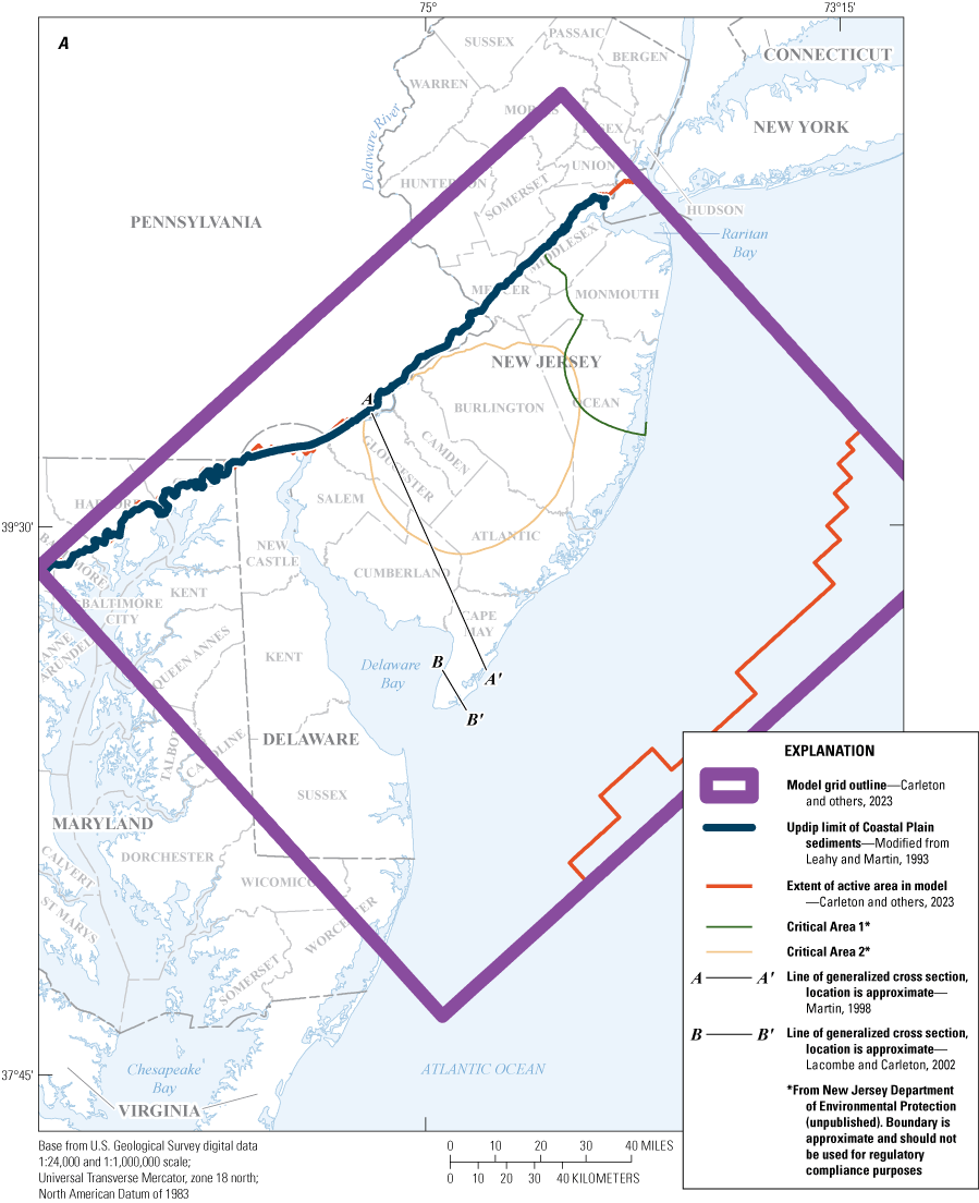
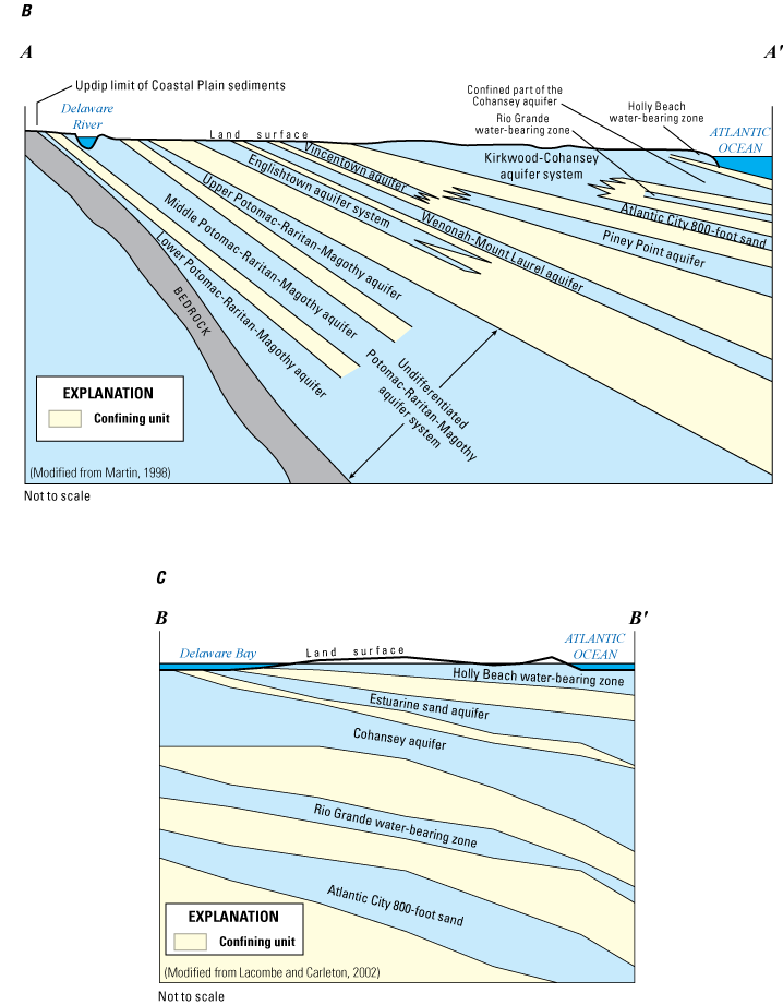
Map showing A, location of the study area, B, generalized hydrogeologic section A–A’ through the Coastal Plain of southern New Jersey, and C, generalized hydrogeologic section B–B’ through southern Cape May County, New Jersey.
To maintain the usefulness of the New Jersey Coastal Plain groundwater-flow model as a tool for managing water resources and developing water-resource strategies in light of changing hydrologic conditions, the USGS, in cooperation with the NJDEP, revised the model by updating the hydrogeologic framework, hydraulic parameters, and groundwater withdrawals. The updated hydrogeologic framework includes a three-dimensional framework of the New Jersey Coastal Plain that extends into Delaware and parts of eastern Maryland. These updates may result in (1) refined boundary flows for local models, (2) improved estimates of the simulated interaction between water levels in southwestern New Jersey and withdrawals in Delaware, (3) simulation of the unconfined Kirkwood-Cohansey aquifer system and confined Rio Grande water-bearing zone as model layers, and (4) the ability to conduct particle tracking to determine regional sources of flow and times of travel.
Purpose and Scope
This report describes the development and calibration of a numerical groundwater-flow model of the New Jersey Coastal Plain that extends into Delaware and parts of eastern Maryland. The model simulates transient regional groundwater conditions incorporating annual groundwater withdrawals and recharge from 1980 to 2013 and will be used to assess changes in water levels over the simulated period. The fully three-dimensional flow model described in this report is a 21-layer model that represents 11 aquifers and 10 intervening confining units in the New Jersey Coastal Plain. The groundwater-flow model is based on the USGS New Jersey RASA model (Martin, 1998), which was rediscretized in the late 1990s by Voronin (2004). These two previous quasi-three-dimensional models represented 10 aquifers in the New Jersey Coastal Plain but did not explicitly include the intervening confining units or the Rio Grande water-bearing zone. The confining units were previously represented as leakage by using a vertical leakance parameter. The model simulates the groundwater-flow system in the New Jersey Coastal Plain and offshore sediments that contain water with a chloride concentration less than 10,000 milligrams per liter (mg/L). Model design and input data, boundary conditions, and groundwater withdrawals used in the model calibration are described. The hydrogeologic parameters for each aquifer and confining unit, including the correlated units in Delaware and Maryland, also are discussed. A total of 3,453 annual water-level observations from 392 wells in New Jersey and 48 wells in Delaware from 1983 to 2013 were used in model calibration. Hydrographs of simulated and observed water levels in 29 observation wells and simulated and interpreted potentiometric surfaces for 2013 conditions are shown. Hydrographs of simulated and estimated annual base flows in 47 surface-water basins are presented. The calibration of the model, conducted by trail-and-error adjustment and by using UCODE (Poeter and others, 2014), is presented. Model parameter sensitivities and limitations are discussed. Estimates of recharge in New Jersey, applied to the groundwater-flow model by using a soil-water balance (SWB) code by Westenbroek and others (2010), is discussed in the appendix. The model archive for the groundwater-flow model described in this report contains the input and output files and the executable file needed to run the model (Carleton and others, 2023). Digital data describing the extents and thicknesses of the units of the updated hydrogeologic framework can be found in Carleton and others (2023).
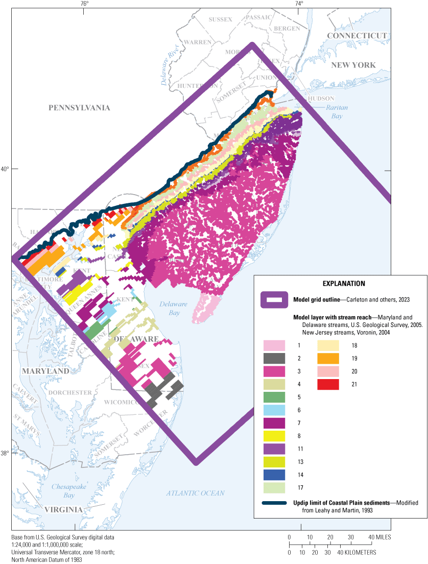
Location and Extent of the Model Area
The model area encompasses the Coastal Plain Physiographic Province of New Jersey and a small part of southeastern Pennsylvania, and parts of the Coastal Plain in Delaware and eastern Maryland (fig. 1). The model area covers approximately 16,537 square miles (mi2) and is bounded on the north and northwest by the updip limit of the Coastal Plain sediments (Fall Line), which separates the Coastal Plain sediments from the Piedmont Physiographic Province sediments; on the east and southeast by the Atlantic Ocean; and on the southwest by Delaware Bay, most of Delaware, and part of eastern Maryland. This investigation focused on the Counties of Atlantic, Burlington, Camden, Cape May, Cumberland, Gloucester, Monmouth, Ocean, Salem, and parts of Mercer and Middlesex in New Jersey, and includes New Castle, Kent, and most of Sussex Counties in Delaware and parts of Cecil, Kent, Queen Anne’s, Caroline, Wicomico, and Worcester Counties in Maryland. Topography in New Jersey is relatively flat; altitudes range from sea level along estuaries, bays, and the Atlantic Ocean to nearly 400 feet (ft) in northeastern Monmouth County, New Jersey.
Previous Investigations
Martin (1998), Pope and Gordon (1999), and Voronin (2004) describe simulated groundwater flow in the New Jersey Coastal Plain from a regional perspective. These three studies, along with other studies describing regional simulated flow in the New Jersey Coastal Plain or the North Atlantic Coastal Plain, are listed in table 1. Table 1 also includes regional studies completed in Critical Areas 1 and 2 and in the Atlantic City area of the New Jersey Coastal Plain.
Table 1.
Previous regional simulation studies conducted for the New Jersey Coastal Plain and Northern Atlantic Coastal Plain.[Northern Atlantic Coastal Plain includes Delaware and parts of Maryland, New Jersey, New York, North Carolina, and Virginia; Water Supply Critical Area 1 includes parts of Middlesex, Monmouth, and Ocean Counties in New Jersey; Water Supply Critical Area 2 includes Camden and parts of Atlantic, Burlington, Cumberland, Gloucester, Ocean and Salem Counties in New Jersey]
| Area of study | Simulated aquifers | Report name | Reference |
|---|---|---|---|
| Northern Atlantic Coastal Plain | Ten regional North Atlantic Coastal Plain aquifers | Geohydrology and simulation of ground-water flow in the Northern Atlantic Coastal Plain aquifer system | Leahy and Martin, 1993 |
| Water Supply Critical Area 1 in New Jersey | Upper and middle Potomac-Raritan-Magothy aquifers, Englishtown aquifer system, and Wenonah-Mount Laurel aquifer | Hydrogeology, simulation of regional ground-water flow, and saltwater intrusion, Potomac-Raritan-Magothy aquifer system, northern Coastal Plain of New Jersey | Pucci and others, 1994 |
| Water Supply Critical Area 2 in New Jersey | Upper, middle, and lower Potomac-Raritan-Magothy aquifers | Ground-water flow and future conditions in the Potomac-Raritan-Magothy Aquifer system, Camden area, New Jersey | Navoy and Carleton, 1995 |
| New Jersey Coastal Plain | Ten regional New Jersey Coastal Plain aquifers | Ground-water flow in the New Jersey Coastal Plain | Martin, 1998 |
| New Jersey Coastal Plain | Ten regional New Jersey Coastal Plain aquifers | Simulation of groundwater flow and movement of the freshwater-saltwater interface in the New Jersey Coastal Plain | Pope and Gordon, 1999 |
| Cape May and parts of Atlantic and Ocean Counties in New Jersey | Atlantic City 800-foot sand | Ground-water flow and quality in the Atlantic City 800-foot sand, New Jersey | McAuley and others, 2001 |
| New Jersey Coastal Plain | Ten regional New Jersey Coastal Plain aquifers | Documentation of revisions to the Regional Aquifer System Analysis model of the New Jersey Coastal Plain | Voronin, 2004 |
| Water Supply Critical Area 2 in New Jersey | Upper and middle Potomac-Raritan-Magothy aquifers, Englishtown aquifer system, and Wenonah-Mount Laurel aquifer | Recovery of ground-water levels from 1988 to 2003 and analysis of 2003 and full-allocation withdrawals in Critical Area 2, Southern New Jersey | Spitz and DePaul, 2008 |
| Water Supply Critical Area 1 in New Jersey | Upper and middle Potomac-Raritan-Magothy aquifers, Englishtown aquifer system, and Wenonah-Mount Laurel aquifer | Recovery of ground-water levels from 1988 to 2003 and analysis of potential water-supply management options in Critical Area 1, east-central New Jersey | Spitz and others, 2008 |
| Salem and Gloucester Counties in New Jersey | Upper, middle and lower Potomac-Raritan-Magothy aquifers, and Englishtown aquifer system | Simulated effects of allocated and projected 2025 withdrawals from the Potomac-Raritan-Magothy aquifer system, Gloucester and northeastern Salem Counties, New Jersey | Charles and others, 2011 |
| Atlantic, Burlington, Gloucester, Camden, Ocean, and Cape May Counties in New Jersey | Kirkwood-Cohansey aquifer system, Rio Grande water-bearing zone, and Atlantic City 800-foot sand | Simulated effects of alternative withdrawal strategies on groundwater flow in the Kirkwood-Cohansey aquifer system, the Rio Grande water-bearing zone, and the Atlantic City 800-foot sand in the Great Egg Harbor and Mullica River Basins, New Jersey | Pope and others, 2012 |
| Ocean and southern Monmouth Counties in New Jersey | Kirkwood-Cohansey aquifer system, Rio Grande water- bearing zone, Atlantic City 800-foot sand, Piney Point and Vincentown aquifers | Simulated effects of groundwater withdrawals from aquifers in Ocean County and vicinity, New Jersey | Cauller and others, 2016 |
| Northern Atlantic Coastal Plain | 19 regional North Atlantic Coastal Plain aquifers | Documentation of a groundwater flow model developed to assess groundwater availability in the Northern Atlantic Coastal Plain aquifer system from Long Island, New York, to North Carolina | Masterson and others, 2016a. |
In addition to the previous regional simulation studies listed in table 1, the rediscretized RASA model of the New Jersey Coastal Plain (Voronin, 2004) was used by Pope (2006) to simulate the effects of increased withdrawals from the Atlantic City 800-foot sand on water levels, by Watt and Voronin (2006) to simulate sources of water to wells in the Wenonah-Mount Laurel aquifer, and by Gordon (2007) to produce water budgets for confined aquifers in the New Jersey Coastal Plain under various withdrawal scenarios.
Eight synoptic water-level studies of the confined aquifers of the New Jersey Coastal Plain document water-level data and potentiometric-surface maps for those aquifers. Potentiometric-surface maps in these reports show water levels in the Coastal Plain at 5-year intervals from 1978 through 2013: 1978, Walker (1983); 1983, Eckel and Walker (1986); 1988, Rosman and others (1995); 1993 and 1998, Lacombe and Rosman (1997 and 2001, respectively); 2003, DePaul and others (2009); 2008, DePaul and Rosman (2015); and 2013, Gordon and others (2021).
Conceptual Hydrogeologic Model
The hydrogeologic framework of the New Jersey Coastal Plain is based on the hydrogeologic framework presented in Zapecza (1989). The framework consists of a southeastward-dipping and -thickening wedge of unconsolidated deposits of sand, silt, and clay of Cretaceous to Neogene age underlain by basement rocks and overlain by locally occurring Quaternary sediments (fig. 1). Coastal Plain sediments were deposited in various shelf, marginal marine, nearshore or coastal beach, and deltaic environments, the extent of which fluctuated in response to changes in sea level. Units composed of substantially less permeable sediments (predominantly clays and fine-grained silts) form the confining units, and coarser, more permeable sand and gravel units, which readily produce water, form the aquifers. These deposits are less than 50 ft thick along the updip limit of the Coastal Plain sediments (Fall Line) in New Jersey and thicken to more than 6,500 ft in southern Cape May County. Coastal Plain sediments generally strike northeast-southwest and dip gently from 10 to 60 feet per mile to the southeast (Zapecza, 1989); overlying Quaternary deposits are flat. The sediments composing the New Jersey Coastal Plain aquifers and confining units generally crop out near the Fall Line parallel to strike; the aquifer units generally transition into confined aquifers, except the Piney Point aquifer, which is confined throughout the study area. The aquifers and confining units in the New Jersey Coastal Plain range in age from Cretaceous to Quaternary (fig. 2).
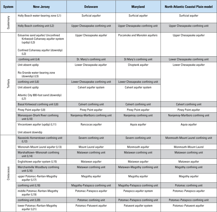
Hydrogeologic units for the New Jersey Coastal Plain, and the correlated hydrogeologic units in the New Jersey Coastal Plain groundwater-flow model of the Delaware and Maryland Coastal Plain and the regional hydrogeologic units in the North Atlantic Coastal Plain aquifer system. Unit names for New Jersey are from modified from Zapecza (1989). Unit names for Delaware are modified from Vroblesky and Fleck, (1991) and Masterson and others (2016b). Unit names for Maryland are modified from Andreasen and others (2013) and from Masterson and others (2016b). Units in Maryland are not the primary focus of this report. Unit names in the North Atlantic Coastal Plain groundwater-flow model are from Masterson and others (2016b). Letter and number in parentheses (for example, L1) in the New Jersey column is the model-layer designation in New Jersey, Delaware, and Maryland.
Figure 1 is a generalized hydrogeologic cross section through the New Jersey Coastal Plain; aquifers and confining units are shown in figure 2, which also shows the correlation of the corresponding units in Maryland and Delaware with those in New Jersey. Detailed discussions in Zapecza (1989) and Sugarman and others (2005) describe the hydrogeology of New Jersey; Vroblesky and Fleck (1991) describe the hydrogeology of Delaware; and Andreasen and others (2013) describe the hydrogeology of Maryland. In addition, the hydrogeology of Delaware, Maryland, and New Jersey is described in Trapp and Meisler (1992) and Masterson and others (2015).
Martin (1998) and Voronin (2004) adapted the hydrogeologic framework in Zapecza (1989) for use in the New Jersey RASA model and represented the Coastal Plain sediments as 10 major aquifers and 9 intervening confining units. In the RASA groundwater-flow models of Martin (1998) and Voronin (2004), the Atlantic City 800-foot sand and the Rio Grande water-bearing zone were simulated by using one aquifer layer. The downdip area of this model layer was referred to by Martin (1998) as the confined Kirkwood aquifer; the updip area of the model layer represents the lower part of the unconfined Kirkwood-Cohansey aquifer system. The model layer above the lower part of the unconfined Kirkwood-Cohansey aquifer system and the confined Kirkwood aquifer represents the unconfined upper Kirkwood-Cohansey aquifer system. Martin (1998) states that the Kirkwood-Cohansey aquifer system was subdivided into an upper and lower aquifer in updip areas to more accurately represent the vertical head distribution in the unconfined aquifer system and to provide a lateral connection between the confined Kirkwood aquifer and the lower Kirkwood-Cohansey aquifer. This framework also was used in the rediscretized RASA model of Voronin (2004).
The updated model described in this report represents aquifers and intervening confining units with a hydrogeologic framework of 21 layers—11 aquifers and 10 confining units. This representation includes the 10 aquifers simulated by Martin (1998) and Voronin (2004) as well as the Rio Grande water-bearing zone, which is represented as a separate aquifer layer to more accurately estimate flow in Atlantic and Cape May Counties, where this aquifer is used as a source of water. Each aquifer layer is represented in the fully three-dimensional groundwater-flow model by specifying its hydraulic parameters; confining units are simulated as layers by specifying their hydraulic parameters.
Only the freshwater parts of the aquifer (where the chloride concentration is less than 10,000 milligrams per liter (mg/L) are represented in this study. The locations of the 10,000-mg/L isochlors for selected aquifers in the New Jersey were obtained from simulation results from the New Jersey Coastal Plain SHARP (Essaid, 1990) model (Pope and Gordon, 1999). SHARP, a quasi-three-dimensional finite-difference model that can simulate freshwater and saltwater flow, was used by Pope and Gordon (1999) to simulate the groundwater-flow system in the New Jersey Coastal Plain, including the location and movement of the freshwater-saltwater interface. The simulated freshwater-saltwater interface was used to define the downdip limit of those aquifers and adjacent confining units where a downdip limit is not defined and is discussed further in the section on boundary conditions. The locations of the 10,000-mg/L isochlors for aquifers in Maryland and Delaware were determined from data published in Meisler (1989), Vroblesky and Fleck (1991), and Trapp and Meisler (1992).
Aquifer and Confining-Unit Characteristics
Below is a brief description of the hydrogeologic properties of the 21 model layers, including the corresponding units in Delaware and Maryland. Additional data on the hydraulic properties of the aquifers and confining units in the New Jersey Coastal Plain are summarized in Martin (1998). The hydrologic properties of the units in Maryland and Delaware were obtained primarily from the Maryland Geologic Survey (Andreasen and others, 2013) and also Masterson and others (2016a).
Estimates of hydraulic conductivity were also made for 3,621 wells in the New Jersey Coastal Plain from results of specific-capacity tests conducted with pumping rates of 250 gallons per minute (gal/min) for a minimum of 8 hours. These data are stored in the USGS National Water Information System (NWIS) database (U.S. Geological Survey, 2017). The transmissivity of the aquifer in the vicinity of these wells was estimated from specific-capacity data by using the Theis equation as presented in Heath (1983). The hydraulic conductivity for an aquifer at a well location was estimated from the calculated transmissivity value determined by using the length of the screened interval. The range of horizontal hydraulic conductivity estimated for the aquifers is summarized in table 2 and the well locations are shown in figure 3.
Table 2.
Horizontal hydraulic conductivities estimated from specific-capacity data for wells in selected aquifers in the New Jersey Coastal Plain.[ft/d, feet per day; PRM, Potomac-Raritan-Magothy]
Hydraulic conductivity for a well was estimated from specific-capacity data by using the equation in Heath (1983) which was used to calculate the transmissivity of the aquifer in the vicinity of the well. The transmissivity was then divided by the length of the screened interval of the well to yield the hydraulic conductivity. These data are stored in the U.S. Geological Survey National Water Information System (NWIS) database (U.S. Geological Survey, 2017).
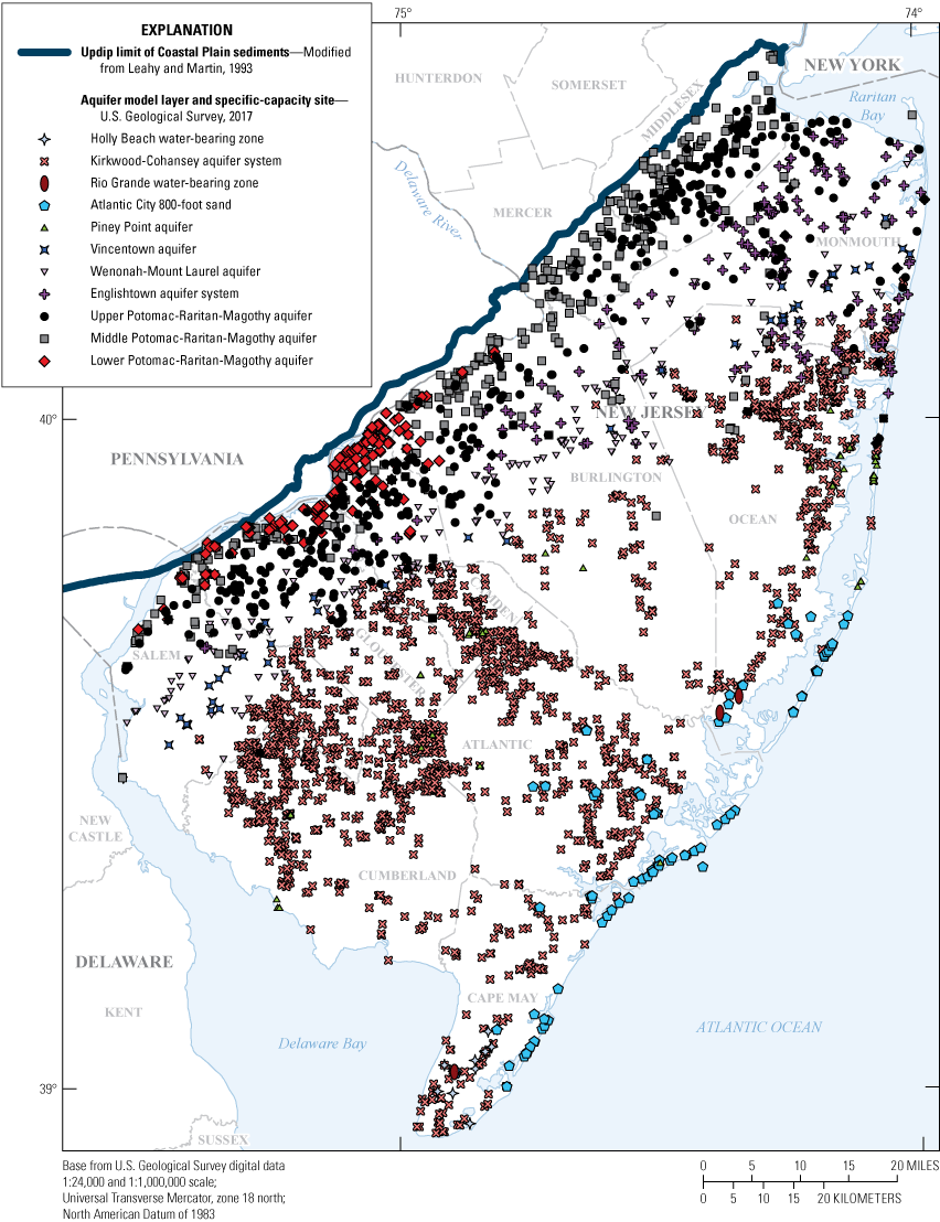
Map showing location of sites of specific-capacity tests, New Jersey Coastal Plain.
Horizontal hydraulic conductivity can vary spatially for each aquifer (fig. 3). Table 2 indicates the order-of-magnitude variability observed in the range of horizontal hydraulic conductivity for some aquifers. Ranges of horizontal hydraulic conductivity values for 11 aquifers in the New Jersey Coastal Plain (table 2) indicate that hydraulic conductivities are greatest at wells screened in the Kirkwood-Cohansey aquifer system and the upper, middle and lower Potomac-Raritan-Magothy aquifers. In addition to the specific-capacity data, the horizontal hydraulic conductivities of the aquifers, vertical hydraulic conductivities of the confining units, and aquifer storage coefficients from selected previously published groundwater-flow models of the New Jersey Coastal Plain are summarized in table 3.
Table 3.
Hydraulic properties of aquifers and confining units from selected groundwater-flow models in the New Jersey Coastal Plain.[PRM, Potomac-Raritan-Magothy; ft/d, feet per day; ft, feet; >, greater than; <, less than; —, no data]
| Aquifer | Model layer | Horizontal hydraulic conductivity (ft/d) | Thickness1 (ft) | Storage coefficient | Reference |
|---|---|---|---|---|---|
| Holly Beach water-bearing zone | 1 | 126–219 | 15–225 | 6.0×10⁻² | Spitz, 1998 |
| Unconfined Kirkwood-Cohansey aquifer system | 3 | 50–60 | 50–>400 | — | Pope and others, 2012 |
| Rio Grande water-bearing zone | 5 | 50 | >0–140 | — | Pope and others, 2012 |
| Atlantic City 800-foot sand | 7 | 50 | 40–200 | 1.1×10⁻⁵–1.0×10⁻⁴ | Pope and others, 2012; McAuley and others, 2001 |
| Piney Point | 9 | 23 | >0–>200 | 3.0×10⁻⁴ | Rush, 1968 |
| Vincentown | 11 | 20 | 20–>140 | — | Nicholson and Watt, 1997 |
| Wenonah-Mount Laurel | 13 | 13–19 | <25–>120 | 1.5×10⁻⁵–3.5×10⁻⁴ | Nemickas, 1976 |
| Englishtown aquifer system | 15 | 6–70 | 40–140 | — | Charles and others, 2011 |
| upper PRM | 17 | 18–90 | 50–>200 | 1.0×10⁻⁴ | Navoy and Carleton, 1995; Martin, 1998 |
| middle PRM | 19 | 7–90 | <50–>150 | 1.0×10⁻⁴ | Navoy and Carleton, 1995; Martin, 1998 |
| lower PRM | 21 | 15–150 | >0–250 | 1.0×10⁻⁴ | Charles and others, 2011; Martin, 1998 |
| Confining unit overlying the estuarine sand and confining unit overlying the confined Cohansey aquifer | 2 | 4.0×10⁻³ | 20–150 | — | Spitz, 1998 |
| Confining unit overlying the Rio Grande water-bearing zone | 4 | 1.00×10⁻⁵ | — | — | Pope and others, 2012 |
| Confining unit overlying the Atlantic City 800-foot sand | 6 | 1.0×10⁻⁵ | <100–>300 | — | Pope and others, 2012 |
| Composite confining unit2 | 8 | 1.0×10⁻⁵–1.4×10⁻⁵ | 3100 | — | McAuley and others, 2001 |
| Composite confining unit4 | 10 | 5.7×10⁻³ | <50–1,190 | — | Rosenau and others, 1969 |
| Composite confining unit5 | 12 | 5.6×10⁻² | 60–90 | — | Nichols, 1977 |
| Marshalltown-Wenonah | 14 | 1.5×10⁻⁵ | 20–>180 | — | Nichols, 1977 |
| Merchantville-Woodbury | 16 | 4.3×10⁻⁶–3.5×10⁻³ | 100–350 | — | Nichols, 1977; Pucci and others, 1994 |
| Confining unit between upper and middle PRM | 18 | 1.8×10⁻⁵–8.0×10⁻¹ | 50–>200 | — | Pucci and others, 1994; Charles and others, 2011 |
| Confining unit between middle and lower PRM | 20 | 2.1×10⁻⁵–1.7×10⁻¹ | >0–<50 | — | Charles and others, 2011. |
Thickness from Zapecza (1989), except for model layers 1 and 2 (Spitz, 1998), model layers 3 and 5 (Pope and others, 2012), and model layer 6 (McAuley and others, 2001).
Thickness in vicinity of Atlantic City, New Jersey, from McAuley and others (2001).
Martin (1998) referred to this part of the composite confining unit as the Navesink-Hornerstown confining unit.
Data on the hydraulic properties of confining units within the modeled area in New Jersey are limited, and most estimates of these hydraulic properties are primarily from the groundwater-flow-model studies listed in table 3. Data on the hydraulic properties of hydrogeologic units within the model area in Delaware and counties in eastern Maryland also are limited and are summarized in table 4. Data presented in table 4 are compiled from the literature of previous estimates of the hydraulic properties of aquifers and confining units within the Delaware and Maryland Coastal Plain and from Andreasen and others, 2013.
Table 4.
Summary of hydraulic properties of aquifers and confining units in Delaware and counties in eastern Maryland.[ft, feet; ft2/day, feet squared per day; ft/d, feet per day; —, no data]
Data from aquifer tests summarized in Andreasen and others (2013).
Values of transmissivity, horizontal hydraulic conductivity, and storage coefficient in Dugan and others (2008).
Average thickness of regional hydrogeologic units in the Northern Atlantic Coastal Plain aquifer system in Masterson and others (2016a).
Simulation of Groundwater Flow
Groundwater flow in the New Jersey Coastal Plain was simulated under transient conditions for the period 1980–2013. In this section, the previous versions of the New Jersey Coastal Plain models are described briefly, and the development of the three-dimensional groundwater-flow model, model calibration, simulation of groundwater flow, the sensitivity of model parameters to water levels and base flows, and model limitations are discussed.
Groundwater-Flow System
Groundwater flow in the New Jersey Coastal Plain is controlled by topography, the hydraulic properties of the sediments, and hydrologic stresses. Flow within the aquifers is predominantly horizontal, although some vertical flow exists. Hydraulic gradients in the confining units generally are vertical because the horizontal hydraulic conductivity is orders of magnitude less than that in the aquifers. The major source of recharge to the aquifers of the New Jersey Coastal Plain is infiltration of precipitation, although leakage from surface-water bodies, lateral flow from adjacent areas, and in confined aquifers, flow from downdip areas also occurs. Most of the groundwater recharge is discharged to nearby surface-water bodies; a smaller amount infiltrates through confining units to recharge the underlying confined aquifers. In addition to the water that discharges from the aquifers to surface-water bodies (streams that flow to the ocean and bays), some groundwater discharges directly to saltwater bodies as submarine groundwater discharge, or is removed by groundwater evapotranspiration, withdrawals from wells, and lateral flow to adjacent areas. Discharge areas in the New Jersey Coastal Plain include the Atlantic Ocean, Raritan Bay, Delaware River, Delaware Bay, and streams. Because groundwater withdrawals in some areas of the New Jersey Coastal Plain are substantial, large cones of depression developed in several aquifers, and recharge and discharge locations shifted. These changes in regional groundwater-flow patterns were investigated in the eight water-level synoptic studies completed for the New Jersey Coastal Plain in cooperation with the NJDEP and are listed in the “Previous Investigations” section of this report.
Design of Previous Models of the New Jersey Coastal Plain
The New Jersey RASA model (Martin, 1998) was developed in the 1980s from a modified version of the Trescott model code (Trescott, 1975). The grid spacing ranges from 6.25 to 9.375 mi2 in onshore areas to 47.5 mi2 in offshore areas. The model used a constant recharge rate of 20 inches per year (in/yr) and withdrawals averaged over time at pumping intervals from 1896–1980. The model was rediscretized in the 1990s (Voronin, 2004) with a smaller grid spacing, recharge based on water-budget equations that used base flow estimated from hydrograph separation of streamflow data for several surface-water basins in of the New Jersey Coastal Plain, and updated withdrawals to 1998, and was run in MODFLOW–96 (Harbaugh and McDonald, 1996). The grid spacing ranged from 0.25 to 0.31 mi2 in onshore areas to 3.16 mi2 in offshore areas. Martin (1998) and Voronin (2004) modeled the aquifers of the New Jersey Coastal Plain using a quasi-three-dimensional representation of the aquifers that represented the confining units by using a vertical leakance parameter (vertical hydraulic conductivity divided by thickness). Voronin (2004) simulated the aquifer system using a 10-layer model and simulated streams using the drain (DRN) and river (RIV) packages of MODFLOW–96 (Harbaugh and McDonald, 1996). Martin (1998) simulated the aquifer system and streams by using an 11-layer model in which the top layer was a constant-head layer that represented the streams. The major differences between the two previous versions of the New Jersey RASA model and the version described in this report are summarized in table 5. The development, design, and calibration of the model described in this report are discussed in the following sections.
Table 5.
Characteristics of three groundwater-flow models developed for the New Jersey Coastal Plain.[RASA, Regional Aquifer System Analysis; in/yr, inches per year; SWB, soil-water balance]
| Reference | Model computer code1 | Total model layers2 | Withdrawal conditions | Most recent water-level data used | Minimum cell size (square miles) | Boundary flows derived from: | Recharge to cells in New Jersey |
|---|---|---|---|---|---|---|---|
| Martin (1998) | Trescott (1975) | 11 | 1896–1980 | 1978 | 6.25 | Leahy and Martin (1993) | Constant of 20 in/yr |
| Voronin (2004) | MODFLOW–96 | 10 | 1968–1998 | 1998 | 0.25 | Leahy and Martin (1993)3 | 0.01–20 in/yr; varies by cell but not by year |
| Gordon and Carleton (2023) | MODFLOW–2005 | 21 | 41978–2013 | 2013 | 0.25 | Masterson and others (2016a) | Used SWB5 model to vary by cell and by year. |
Reference for MODFLOW–96 is Harbaugh and McDonald (1996); for MODFLOW–2005 is Harbaugh (2005).
The groundwater-flow models of Martin (1998) and Voronin (2004) are quasi-three-dimensional models. Confining units are not explicitly modeled but are simulated by a vertical leakance. The vertical leakance is calculated as the hydraulic conductivity divided by thickness.
Stress periods 1 through 3 are transitional stress periods in this model that generally correspond to the time periods 1970–76 and 1977–79, and 1980, respectively, to set antecedent conditions in the model. The withdrawal rates for these three time periods are based on a percentage of the average annual 1978–81 withdrawals in Voronin (2004).
The SWB model uses a soil-water-balance code (Westenbroek and others, 2010) for estimating an annual recharge for each year simulated in inches per year. The recharge rates for the time periods 1970–76 and 1977–79 (model stress periods 1 and 2), used to set antecedent conditions in the model, are based on a percentage of the 1980 average recharge.
Model Development
The three-dimensional groundwater-flow model developed to simulate the groundwater-flow system in the New Jersey Coastal Plain is based on the USGS computer program MODFLOW–2005 (Harbaugh and others, 2005). Updates to the two previous versions of the RASA model include (1) a 21-layer hydrogeologic framework that extends into Delaware and part of Maryland; (2) spatially variable recharge estimated by using the SWB model (Westenbroek and others, 2010); (3) updated hydraulic parameters to include the confining units in New Jersey and the hydrogeologic units in Delaware and eastern Maryland; (4) updated boundary flows from the groundwater-flow model of the North Atlantic Coastal Plain (NACP) (Masterson and others, 2016a); (5) groundwater-withdrawal data for 1980–2013 for the New Jersey Coastal Plain and for 1980–2010 for the modeled areas in Delaware and eastern Maryland; and (6) the Rio Grande water-bearing zone and the confining units above and below it, added as a model layer to refine the estimate of simulated flow in Atlantic and Cape May Counties, New Jersey. The updip part of model layer 5, where the Rio Grande water-bearing zone is absent (fig. 1), is represented in this model by a thin layer that allows for a hydraulic connection between the overlying and underlying model layers. The groundwater-flow model is used to (1) simulate current (2013) conditions of groundwater flow in the New Jersey Coastal Plain and the confined aquifers of Delaware, (2) improve the representation of the groundwater system of the New Jersey Coastal Plain, and (3) provide the NJDEP and other water managers with the information (Carleton and others, 2023) that can be used to calculate groundwater-budget components and evaluate water-resource management decisions.
Spatial and Temporal Discretization
The finite-difference grid for the numerical model consists of 145 rows, 245 columns, and 21 layers. The model grid size is variable, with a grid spacing of 0.25 mi2 (the smallest) in the northern and southwestern parts of the New Jersey Coastal Plain, 0.31 mi2 in the southeastern part of the Coastal Plain, and as much as 3.16 mi2 in the offshore areas. The model area is approximately 16,597 mi2 and extends from the Fall Line (fig. 1), which is the transition from the consolidated rocks of the upland Piedmont Physiographic Province to the unconsolidated sediments of the Coastal Plain Physiographic Province, to the approximate downdip and (or) freshwater-saltwater interface in each model layer. (The location and extent of the Fall Line in southeastern New York is not shown in figures.) The grid is oriented approximately parallel to the Fall Line and to the strike of the New Jersey Coastal Plain hydrogeologic units (Zapecza, 1989).
A schematic diagram of the model layers used to represent the hydrogeologic units in the New Jersey Coastal Plain and the corresponding hydrogeologic units in Delaware and eastern Maryland is shown in figure 4. Confining units are modeled as individual layers by assigning them appropriate hydrologic properties.
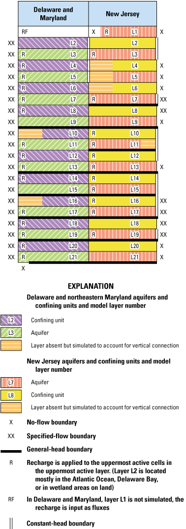
Schematic representation of aquifers, confining units and boundary conditions in the New Jersey Coastal Plain groundwater-flow model.
The model area extends vertically from the water table to consolidated bedrock and includes 11 distinct major aquifers and 10 confining units of the New Jersey Coastal Plain. The hydrogeologic framework described by Zapecza (1989) was revised for this study to improve the simulation of the groundwater-flow system. Extents of each model layer in Delaware and eastern Maryland are based on hydrogeologic data from Meisler (1989), Vroblesky and Fleck (1991) and Andreasen and others (2013). The hydrogeologic framework is described in more detail in the data release for this report (Carleton and others, 2023). This data release contains an ArcGIS shapefile containing the top, bottom, thickness, and extent of each layer in the model used to define the aquifers and confining units incorporated into the New Jersey Coastal Plain model (Carleton and others, 2023).
If a hydrogeologic layer does not extend across a given model layer in the MODFLOW-2005 finite-difference solution method but instead the hydrogeologic layer pinches out, but the model layer above and (or) below is an active area in the model, an area was created in the model layer with the limited extent to make that layer continuous with the above and (or) below layer, if needed, and was given a small thickness (1 foot or more). The hydraulic properties of the overlying model layer were assigned so that the layer would be continuous, thereby achieving a hydraulic connection between the layers above and below. For example, model layer 11 which represents the Vincentown aquifer, an aquifer with a small area, but the areas of the overlying and underlying layers extend beyond the area of the Vincentown aquifer, therefore an area is needed to simulate the flow from overlying aquifers to underlying aquifers to more accurately represent the vertical head distribution in the model layers (fig. 1). Additionally, in the updip area of the Piney Point aquifer (model layer 9) where the aquifer pinches out and does not outcrop, an area is needed to simulate the flow from overlying units to underlying units to more accurately represent the vertical head distribution in the model layers (fig. 1). The same is true for the updip area in model layer 5, which in the downdip area (fig. 1) represents the confined Rio Grande water-bearing zone, and the overlying and underlying confining units (model layers 4 and 6, respectively). In the updip parts of those three model layers, an area is needed to simulate the flow from the overlying model layer 3 to the underlying model layer 7 to more accurately represent the vertical connection in the model layers.
A total of 36 stress periods were simulated—1 steady-state period and 35 transient periods. Stress period 1 is steady-state and stress period 2 is transient and 3 years long. Stress periods 1 and 2 are transitional stress periods that generally correspond to 1970–76 and 1977–79, respectively. Stress periods 3 to 36 are 1 year long and generally represent the period 1980–2013.
Lateral and Lower Boundary Conditions
The model is bounded to the north and northwest and below by the contact between the unconsolidated Coastal Plain deposits and consolidated bedrock that underlies the Coastal Plain sediments. This boundary was represented numerically as a no-flow boundary condition. Lateral boundaries for each layer in the groundwater-flow model are shown in a generalized schematic diagram in figure 4. Although water may flow into the model area along the Fall Line between the subsurface fractured rock and the Coastal Plain sediments, this amount is assumed to be negligible and, therefore, is not considered in this report.
In the two previous New Jersey RASA groundwater-flow models (Martin, 1998; Voronin, 2004), the lateral boundaries in the northeast and southwest are specified-flux boundaries that originally were derived from a model of the NACP (Leahy and Martin, 1993). Some modifications were made to the boundary fluxes near Delaware Bay in the rediscretized RASA model (Voronin, 2004). The Leahy and Martin (1993) model area extended from Long Island, New York, to North Carolina and includes the New Jersey Coastal Plain. In the model described in this report, the lateral model boundaries in the northeast and southwest are specified-flux boundaries derived from the NACP aquifer system model (Masterson and others, 2016a), which also extends from Long Island, New York, to North Carolina, by using the MODFLOW Flow and Head Boundary (FHB) package (Leake and Lilly, 1997). Specified fluxes are applied in areas where the aquifers and confining units intersect the flow boundary. Flows from the NACP model (Masterson and others, 2016a) are incorporated into the FHB package for stress periods 1 through 32. Because the end of the NACP model simulation coincides with stress period 32 of the current New Jersey Coastal Plain model, fluxes for stress period 32 are repeated for stress periods 33 through 36. The FHB package is used to specify lateral boundary fluxes in each active cell along column 1 of the model grid, which traverses eastern Maryland and a small part of southwestern Delaware (fig. 1). Some active cells along column 1 where the flux was zero were not included in the FBH model file. Specified fluxes are also input in New Jersey using the FHB package along the northeastern edge of the active model area for some layers in column 245 for the offshore extent of layers 7 and 8 and in layers 16 to 19 for the offshore part of the upper and middle Potomac-Raritan-Magothy aquifers (layers 17 and 19), the Merchantville-Woodbury confining unit (layer 16), and the confining unit between the upper and middle Potomac-Raritan-Magothy aquifers (layer 18). The remaining layers have a no-flow or a constant-head boundary along northeastern limit of the model area (fig. 4).
The southeastern (downdip) boundary of the aquifers and confining-unit model layers in New Jersey, Delaware, and Maryland are simulated as no-flow boundaries except as described in the “General Head Boundary” section of this report. The downdip extents of the aquifers and confining-unit model layers in Delaware and Maryland are from Meisler (1989), Vroblesky and Fleck (1991), and Andreasen and others (2013). The southeastern downdip boundary of the aquifers and confining-unit layers in New Jersey are generally located at the downdip limit of freshwater in the aquifer (10,000 mg/L isochlor) determined by Pope and Gordon (1999). Pope and Gordon (1999) used the SHARP computer model (Essaid, 1990) to simulate the groundwater-flow system, including the location and movement of the freshwater-saltwater interface in nine aquifers and eight intervening confining units in the Coastal Plain. Although the interface position is not static in the model, the actual amount of movement cannot be quantified because of the model’s coarse cell size. Because the SHARP model is quasi-three-dimensional, the downdip limit of the 10,000-mg/L isochlor in those aquifers was assumed to be the same for the overlying confining unit. However, the Englishtown aquifer system and Vincentown aquifer are not continuous throughout the New Jersey Coastal Plain and contain freshwater throughout their confined extent in New Jersey. However, chloride concentrations exceeded 15,000 mg/L at an observation well in the Englishtown aquifer system in Sandy Hook in northeastern Monmouth County (DePaul and Rosman, 2015).
General Head Boundary
The General Head Boundary (GHB) package (McDonald and Harbaugh, 1988) was used to represent flow in the updip direction from limited parts of the downdip lateral boundaries of layers 7, 9, 11, 13, 15, 17, 19, and 21 (fig. 4). However, in model layer 11, the GHB boundary was used in New Jersey only. The GHB head is constant for all stress periods and is set to 0.0 ft (NAVD 88); no attempt was made to estimate the equivalent freshwater head where groundwater density is greater than that of freshwater. A single value of bed conductance of 1 square foot per second (ft2/s) was applied to all GHB cells.
The GHB boundaries were included to prevent the occurrence of unrealistically low heads downdip from withdrawals; because the boundaries are generally far from the withdrawals, they have only a minor effect on the overall flow system. In 2013, flow into the model from GHB cells is about 0.6 percent of the total flow budget.
Upper Boundary Conditions
The upper boundaries in the model represent the streams and recharge in onshore areas and the Delaware and Raritan Bays and Atlantic Ocean (fig. 1) in offshore areas. In offshore areas, the upper boundary is a constant freshwater equivalent water level specified by using the Time-Variant Specified-Head (CHD) package (Harbaugh, 2005) and is applied across the top active layer of model cells used to represent the Atlantic Ocean and the Delaware and Raritan Bays. CHD cells represent the outcrop of layers 2 through 5 in the Delaware Bay, the outcrop in layers 14 through 19 (excluding layer 18) in Raritan Bay, and the outcrop of layers 2, 3, 7, and 10 through 12 in the Atlantic Ocean (fig. 4).
Recharge
The Recharge (RCH) package of the USGS finite-difference groundwater model MODFLOW–2005 was used to apply recharge to the topmost active layer of each onshore model cell. This upper boundary is spatially variable recharge from precipitation estimated by using the Soil-Water Balance (SWB) model (Westenbroek and others, 2010). The SWB model is based on a modified Thornthwaite-Mather method (Thornthwaite and Mather, 1957) that incorporates spatially distributed land cover, soil properties, and daily climate data to produce a detailed spatial and temporal variability of recharge. SWB model-calculated recharge rates from 1980 to 2013 were used as the initial recharge values for New Jersey in the groundwater-flow model. The SWB model is described in appendix 1. Recharge was adjusted as part of the model parameter-estimation process to allow for more variability than that calculated by the SWB model and adjusted for comparison with base-flow estimates at various surface-water drainage basins in the New Jersey Coastal Plain. Average annual precipitation in southern New Jersey (Office of the New Jersey State Climatologist, 2021) during 1970–76 and 1977–79 were 1.23 and 1.31 times the 1980 annual average, respectively. Therefore, the recharge rates applied in model stress periods 1 (associated with 1970–76) and 2 (1977–79) are 1.23 and 1.31 times those applied in stress period 3 (1980). Stress periods 1 and 2 are used in the model to set antecedent conditions for the other years.
Because the surficial aquifer in Delaware and Maryland is not simulated, cell-by-cell vertical flows into or out of active cells in model layer 1 in Delaware and Maryland were calculated from the NACP model (Masterson and others, 2016a) and applied with the recharge.
Drain Package
The MODFLOW Drain package (DRN) is used to represent the rivers and streams in the model where groundwater flows (drains) out of the model area (fig. 5). The DRN package was used for continually gaining stream reaches in the New Jersey Coastal Plain which are not a source of groundwater recharge except on a localized scale (for example, upstream from a dam). Use of the DRN package allows for the representation of headwater reaches, where the streambed elevation may be above the water table in places, preventing simulated small streams from being a source of potentially unlimited volumes of water, as would be the case with the MODFLOW River package (RIV) (discussed below). The drain elevation is the average elevation of a stream or stream tributary in the topmost active layer in each onshore model cell. Streams in New Jersey are those used in the previous model version from Voronin (2004). Model cells containing streams in New Jersey were identified by intersecting the model-grid polygons with streams digitized from USGS 1:24,000-scale topographic maps. Streams in Maryland and Delaware were identified by intersecting the grid with NHDPlus (U.S. Geological Survey, 2005), a comprehensive geospatial dataset developed by the U.S. Environmental Protection Agency and the USGS.
Map showing location of stream cells in the model area, New Jersey Coastal Plain groundwater-flow model.
The elevations of drain boundaries are kept constant for all stress periods in the transient model. The drain elevations are long-term averages and do not include annual or seasonal variations. Seasonal variations cannot be considered when annual stress periods are used; neglecting the variation of average elevation from year to year is minor in the context of surface-water elevations averaged over model cells of 0.25 mi2 or larger.
The DRN package also requires specification of streambed conductance, an aggregate parameter that represents the product of the streambed hydraulic conductivity, the length of the stream reach, and the stream width divided by the streambed thickness. The same streambed conductance is applied to all drains and was adjusted during calibration.
River Package
The MODFLOW River package (RIV) package was used to represent the Delaware River (fig. 5). The RIV package (unlike the DRN package) allows the Delaware River to be a source of recharge to the aquifer near pumping centers. This is appropriate because the Delaware River carries substantial flow, is tidal in the simulated area, and can provide unlimited flow to the aquifer. The river stage is constant for all stress periods and increases from 0.0 ft (NAVD 88) at the southwestern extent of model river cells in Delaware Bay to 1.0 ft near Trenton by 0.1 ft in segments of approximately the same length. A single value of riverbed conductance was applied to all river cells, representing the product of the riverbed hydraulic conductivity, length, and width of the river reach in each model cell divided by riverbed thickness. Riverbed conductance was modified during model calibration.
Hydraulic Properties
The hydraulic properties hydraulic conductivity and storage coefficient are described in the “Hydraulic Properties of Aquifers and Confining Units” section near the beginning of this report. As previously mentioned, data for the hydraulic properties of confining units are limited. The hydraulic properties are specified by parameter zones within each layer that are assumed to have similar properties. The initial values are comparable with those from Martin (1998), Voronin (2004) and Masterson and others (2016a). During model calibration, the range of hydraulic properties shown in tables 2 and 3 were used to provide supplemental information for values in areas of New Jersey. The hydraulic conductivities and storage coefficients in table 4 were used to provide supplemental information for values in Delaware and Maryland. Hydraulic-conductivity and storage-coefficient parameters were adjusted manually and by using the parameter-estimation software UCODE-2014 (Poeter and others, 2014) during model calibration as needed to improve the model fit between observed data and simulated results.
Groundwater Withdrawals
Groundwater-withdrawal data for the New Jersey Coastal Plain were tabulated and mapped to assess the volume of water pumped from wells in each of the aquifers. These wells include those used for public supply, large-scale agricultural (irrigation), and commercial or industrial purposes. Withdrawals from small-capacity wells, such as those used for domestic supply, are not incorporated into the model. This is a limitation of the model in the outcrop areas of confined aquifers or the Kirkwood-Cohansey aquifer system in areas where a substantial number of domestic-supply wells are located, but domestic self-supply withdrawals do not make up a substantial part of the groundwater withdrawals. Statewide production from domestic wells accounts for about 3 percent of total withdrawals in New Jersey (New Jersey Department of Environmental Protection, 2017b).
Withdrawal data for 1980–1998 were obtained from Voronin (2004) and were reviewed for updates that may have been made since 2003, such as an update to an aquifer code or surveyed well location. Withdrawal data for 1999–2003 were obtained from data reported to the NJDEP. These data were quality reviewed and incorporated into a water-use database available in the data release accompanying this report (Carleton and others, 2023). This withdrawal information includes permitted data only—that is, only data from wells in which daily withdrawals meet or exceed 100,000 gallons for a period of more than 30 days in a consecutive 365-day period. Withdrawal data for 2004–13 were obtained from the NJWATr database developed by the USGS and maintained by the NJDEP to track water withdrawals, use, treatment, and discharge in New Jersey (New Jersey Department of Environmental Protection, 2017a). Total withdrawals from New Jersey Coastal Plain aquifers input to the model for 2004 to 2013 are shown in figure 6. The largest withdrawals occurred in the unconfined Kirkwood-Cohansey aquifer system, the Atlantic City 800-foot sand, and the upper, middle, and lower Potomac-Raritan-Magothy aquifers (model layers 3, 7, 17, 19, and 21).
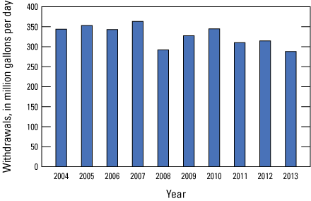
Graph showing estimated groundwater withdrawals from New Jersey Coastal Plain aquifers, 2004–13.
Annual withdrawal data for 1980–2013 for Delaware and Maryland were obtained from a dataset of pumping rates for 1980–2010 from the groundwater-flow model developed for a groundwater-availability study of the NACP by Masterson and others (2016a; Jack Monti, Jr., U.S. Geological Survey, written commun., 2014). Agricultural withdrawal data for Delaware and Maryland may be less complete and less well documented (Masterson and others, 2016a) than New Jersey agricultural withdrawals. Masterson and others (2016a) provide a detailed description of the methods used to tabulate and estimate groundwater withdrawals in their study. Withdrawals from the unconfined surficial aquifer in Delaware and Maryland were not included in the New Jersey Coastal Plain groundwater-flow model. The unconfined surficial aquifer in Delaware and eastern Maryland was not included in the model hydrogeologic framework because model layer 1 represents the Holly Beach water-bearing zone in Cape May County, New Jersey, which is not continuous into Delaware.
Stress periods 1 (steady-state) and 2 (transient) are transitional stress periods that generally correspond with 1970–76 and 1977–79, respectively. Stress periods 3 and 4 generally represent 1980 and 1981, respectively. Withdrawals for stress periods 1, 2, and 3 are 73, 86, and 93 percent, respectively, of those in stress period 4, and account for the estimated increase in withdrawals from 1970 to 1980. Withdrawals for stress period 4 generally are an average of 1978–81 withdrawals in Voronin (2004) and represent 1981 withdrawal rates in the groundwater-flow model. Average annual withdrawals were used in the model for stress periods 5 to 36, which are 1 year long, and the average annual withdrawals are equivalent to total annual withdrawals during each of these stress periods. Stress periods 5 through 36 represent each year from 1982 to 2013, respectively.
Model Sensitivity Analysis and Calibration
Model calibration was conducted using manual adjustments of parameters through trial and error and parameter estimation techniques. The UCODE-2014 (Poeter and others, 2014) was used to evaluate the sensitivity of parameters to improve the fit of simulation results to observation data and identify correlated parameters that may not be estimated separately. Parameter estimation is the process of determining which parameters can be statistically estimated and then varying those parameters to minimize the weighted least squares objective function (Hill and Tiedeman, 2007). The objective function measures this fit by quantitatively comparing simulated and observed values. This section of the report describes the observations, residuals, final parameter values, correlations between parameters, and parameter sensitivity achieved by the model calibration and the sensitivity of water levels and base flow to the model parameters.
Effective use of hydrogeologic data and observations to constrain a model is likely to produce a model that improves the accuracy of the representation of groundwater flow and, consequently, simulation results. The match of observed to simulated values is used to evaluate how well a model represents an actual system. The simulated and observed values compared for the New Jersey Coastal Plain groundwater-flow model are water-level altitudes (heads) and groundwater discharge (base flow) to gaged streams which involved the adjustment of model parameters so that residuals (the differences between simulated and observed water levels or base flows) are minimized. During calibration, initial model parameters, such as hydraulic conductivity and storage coefficient, are changed to minimize residuals. All observed and simulated water-level observations and simulated and estimated base-flow observations are available in the data release accompanying this report (Carleton and others, 2023).
Water-Level Observations
The model was calibrated by using water-level observations that include observations derived from selected water-level measurements described below. The water-level observations in New Jersey are a subset of measurements collected during the seven quinquennial New Jersey Coastal Plain water-level synoptic studies (1983, 1988, 1993, 1998, 2003, 2008, and 2013) and were selected to provide a spatial distribution in 10 of the simulated aquifers. The water-level synoptic studies did not include the unconfined Holly Beach water-bearing zone and the unconfined part of the Kirkwood-Cohansey aquifer system. Water levels in correlated aquifers in Delaware were obtained from the Delaware Geological Survey (Delaware Geological Survey, 2017). Most of the water levels were measured during October–December after large summer withdrawals had decreased but before water levels had recovered to those measured during spring, thereby representing an approximation of the annual average water level. Water levels were measured at least once during 1983–2013 in 392 wells in New Jersey and 48 wells in Delaware (fig. 7), yielding a total of 2,533 water-level observations in 440 wells. Hydraulic water levels at each well were calculated by subtracting the water level, in feet below land surface, from the land-surface altitude, in feet above the North American Vertical Datum of 1988 (NAVD 88); the result of this calculation is shown in this report as the water-level altitude.
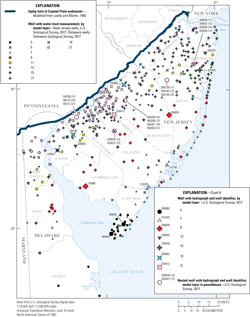
Map showing location of wells with measured water levels, New Jersey Coastal Plain.
Average annual water levels were calculated for 29 wells in New Jersey (fig. 7) where continuous water levels were measured: 19 wells with observations for every year during 1980–2013 and 10 wells with data for most of that period (average of 27 years). A total of 920 observations from the 29 wells were included in the model calibration; these data are shown in time-series hydrographs shown in this report in the “Calibration of Water Levels” section.
In addition to the water-level observations used in the model calibration, derived observations also were included by calculating the vertical gradient at nested observation wells in New Jersey. Vertical gradients were calculated for 33 pairs of nested wells, for a total of 210 observations. (Nested well pairs are wells that are near each other but are open to different aquifers.) For each sequential synoptic water-level measurement period, vertical gradients calculated by subtracting water levels in colocated wells screened in different aquifers provided information for calibrating the hydraulic conductivity of the confining units. By attempting to match the gradient across the confining unit, the parameter-estimation function improved the accuracy of the vertical-conductance value, for example, in a situation where simulated water levels in both aquifers were somewhat high but the gradient was exact. Also, the change in water level over time was calculated by subtracting water levels in selected wells in which measurements had been made in sequential water-level synoptic studies; the difference was used in calibrating storage in aquifers and confining units. Changes in water levels over time were calculated for 138 wells, 134 wells in New Jersey and four wells in Delaware, where water levels had varied substantially (approximately 10 ft) over the 30-year span of synoptic water-level measurements, for a total of 767 observations.
Water-level observations and vertical-gradient and change-over-time observations calculated from water-level measurements were all assigned the same weight, except for annual observations from the 29 wells with a continuous water-level recorder. Most water-level hydrographs for selected wells had 34 observations, whereas many synoptically measured wells had at most 7 observations; therefore, synoptic water-level observations and calculated observations were assigned a weight of 5, and hydrograph observations were assigned a weight of 1.1. Hill and Tiedeman (2007) describe methods for assigning weights on the basis of estimated error ranges so that observations with substantial potential errors exert a smaller effect on the parameter estimation function than the more accurate measurements do. This approach was not practical for the model in this study because water-level observations were collected under a wide range of conditions, often unknown. For example, some water-level measurements were made in wells with varying degrees of recent and nearby pumping, whereas others were made in unused wells known to be thousands of feet from current or recent withdrawals; still other water-level measurements were made at production wells that had been pumped as recently as 1 hour earlier. Attempting to quantify potential errors based on proximity in time or space to known and unknown withdrawals for synoptic water-level measurements conducted over a 30-year period was infeasible. Most land-surface-elevation estimates were determined from light detection and ranging (lidar) data considered to be accurate to within 2 ft, a modest error compared to the uncertainties related to proximal withdrawals at the time of measurement.
Base-Flow Observations
The New Jersey Coastal Plain model was calibrated by using a total of 1,485 estimates of base flow from 47 stream basins in New Jersey. The locations of the 47 basins are shown in figure 8. The surface-water basins were selected because of location and availability of data during the period 1980—2013. Annual base flow was calculated by using the hydrograph-separation technique PART in Barlow and others (2015) for each of the 21 continuous-record gaging stations for each year of record. For 26 partial-record gaging stations in the New Jersey Coastal Plain, an annual base flow was calculated by correlating manual low-flow measurements made at the partial-record stations with same-day flows at index stations by using the MOVE.1 program (Colarullo and others, 2018). Annual base-flow estimates for each of the 47 basins were averaged to obtain a period-of-record average base flow for each basin.
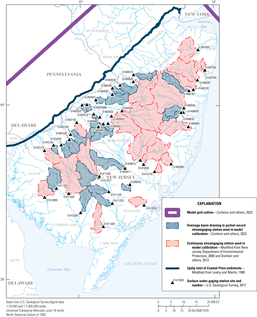
Map showing location of surface-water drainage basins with base-flow observations, New Jersey Coastal Plain.
Base-flow observations determined by using the PART hydrograph-separation technique in Barlow and others (2015) of continuous-record-station data were assigned a weight of 1.0. Observations determined from partial-record-station data correlated with measurements from continuous-record index stations were assigned a weight less than 1.0 based on the percent standard error of estimate (%SEE), which is the percent of unexplained variance relative to the value of the estimate. The %SEE is a better measure of uncertainty than the standard error of estimate (SEE) because it accounts for the proportional effect encountered in natural streamflow processes, where variance increases with flow (Amy McHugh, U.S. Geological Survey, written commun., 2020). Colarullo and others (2018) defined weights as the reciprocal of %SEE to lessen the weight of predictions made using MOVE.1 regressions that show a high degree of unexplained variability in flows and increase the weight of predictions made using regressions with a small amount of unexplained flow variability. The weights of measurements made at partial-record stations were set to a number less than 1.0 by dividing 4.5 by the squared average %SEE for each partial record station; resulting weights ranged from 0.95 to 0.22.
Model Parameters
A parameter is defined in this report as a single value assigned to a variable used in the finite-difference groundwater-flow equation at one or more model cells. The 422 parameters used in the model fall into seven categories: horizontal hydraulic conductivity (184 parameters), vertical hydraulic conductivity (184 parameters), storage coefficient (42 parameters), riverbed conductance (1 parameter), streambed conductance (1 parameter), general-head-boundary conductance (8 parameters), and recharge (2 parameter). The initial parameter values for several aquifers and confining units in New Jersey, Delaware, and eastern Maryland were changed during calibration to improve the match with observations and improve model results.
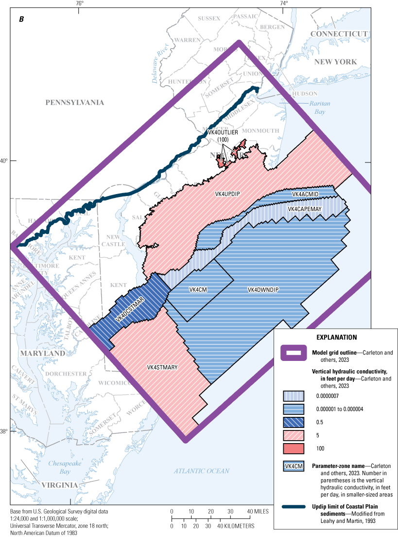
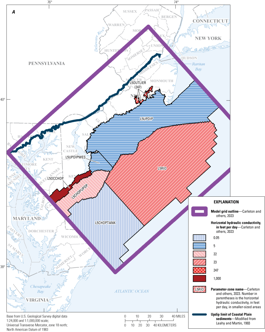
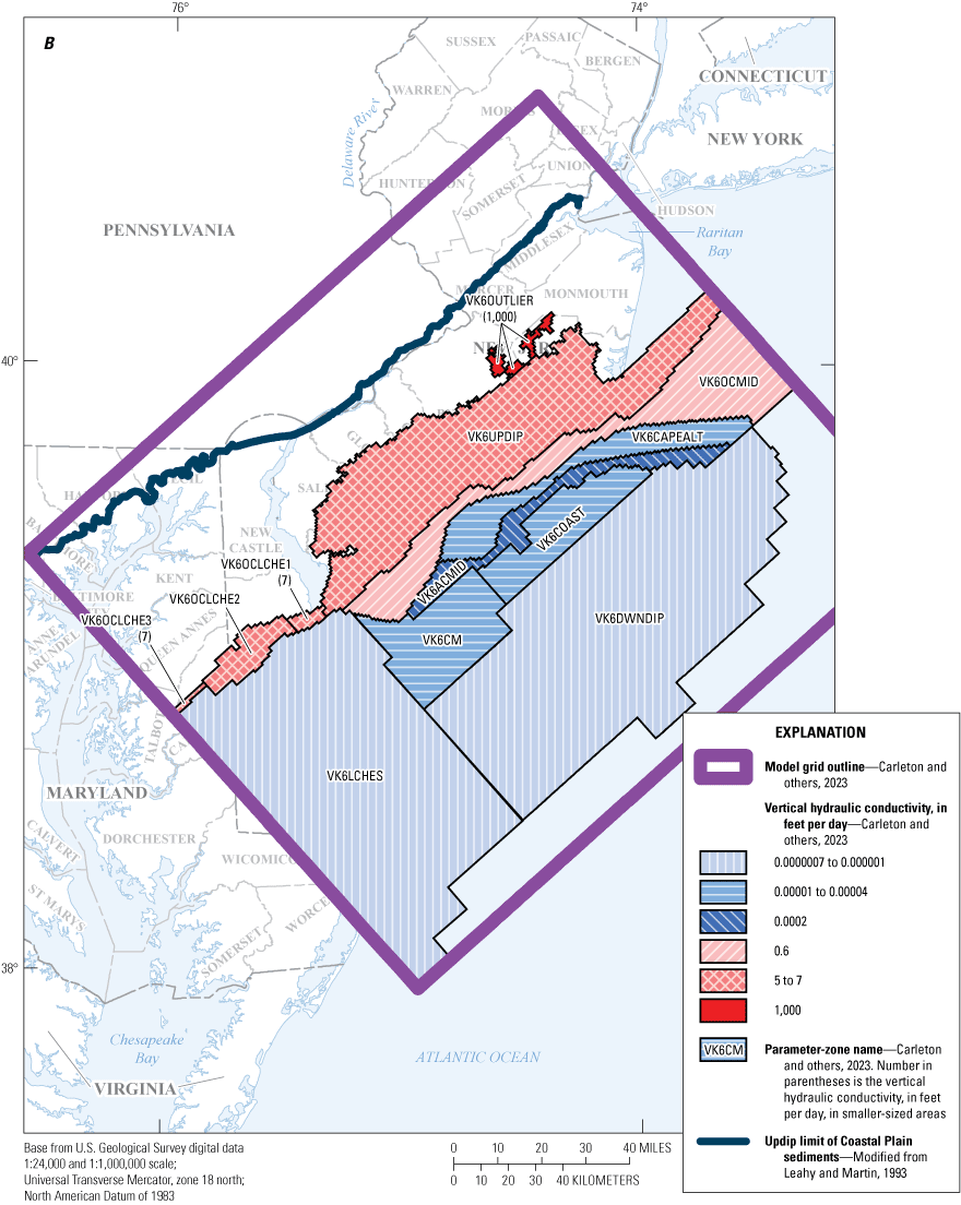
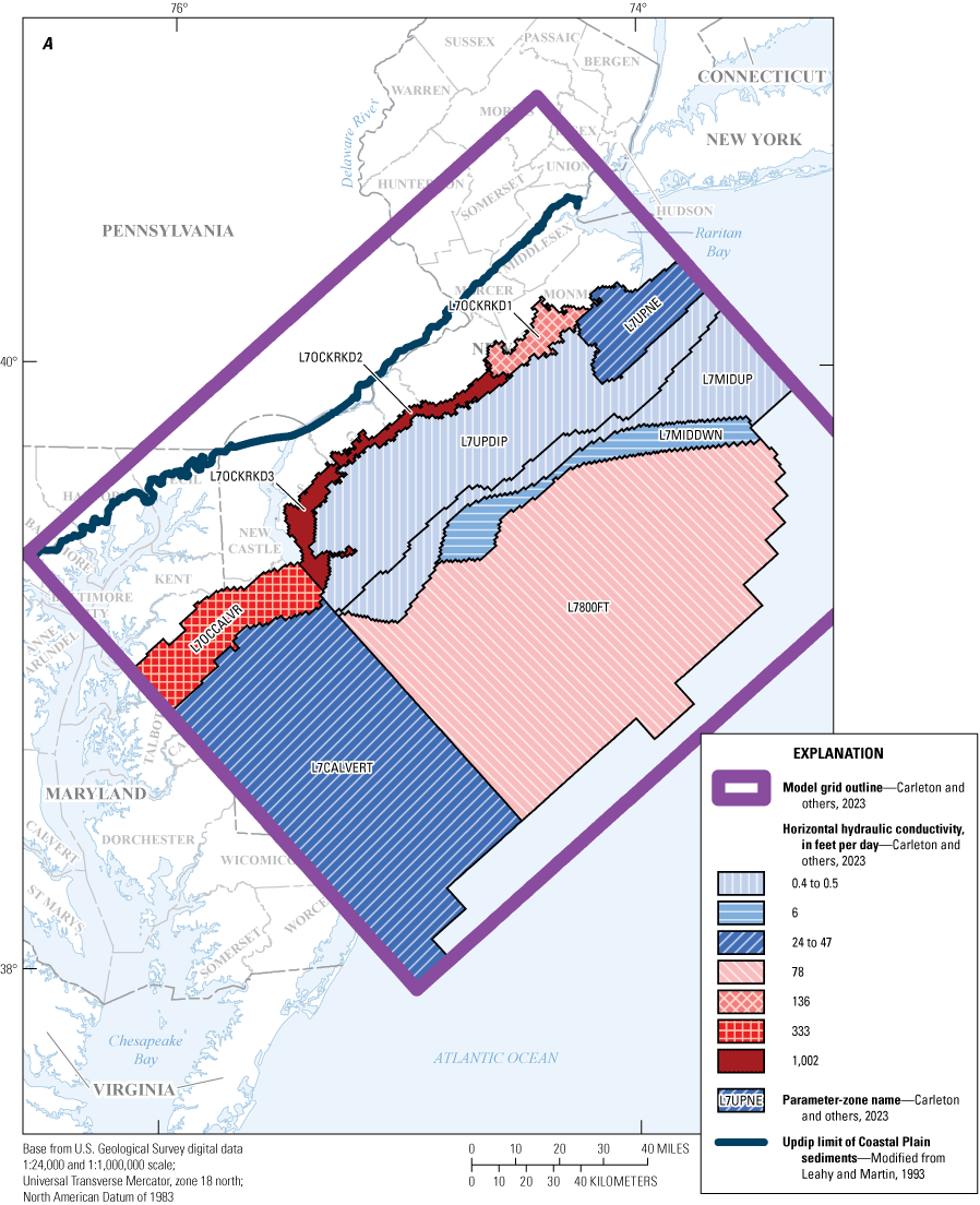
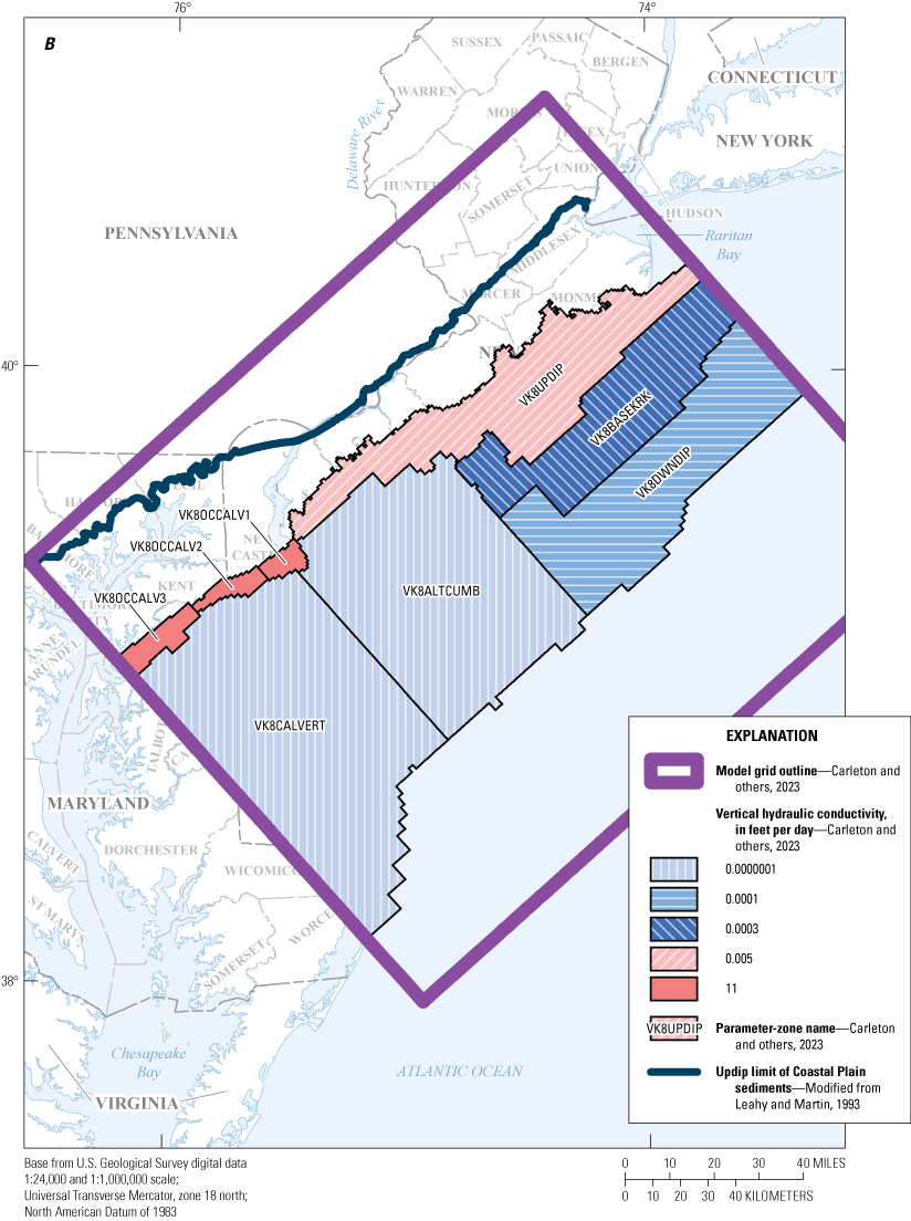
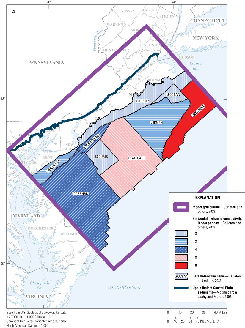
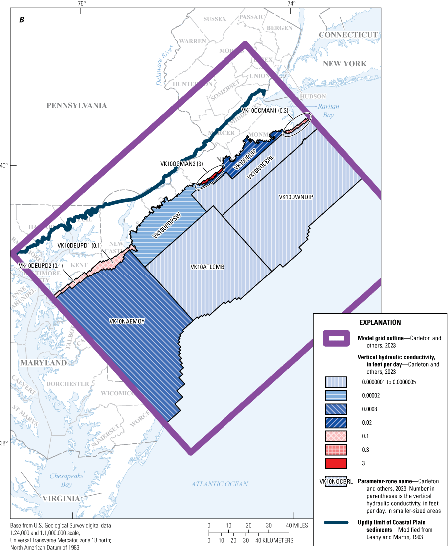
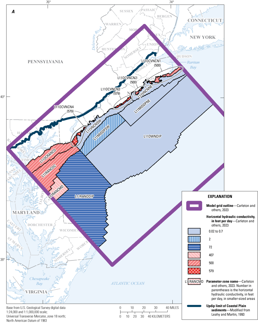
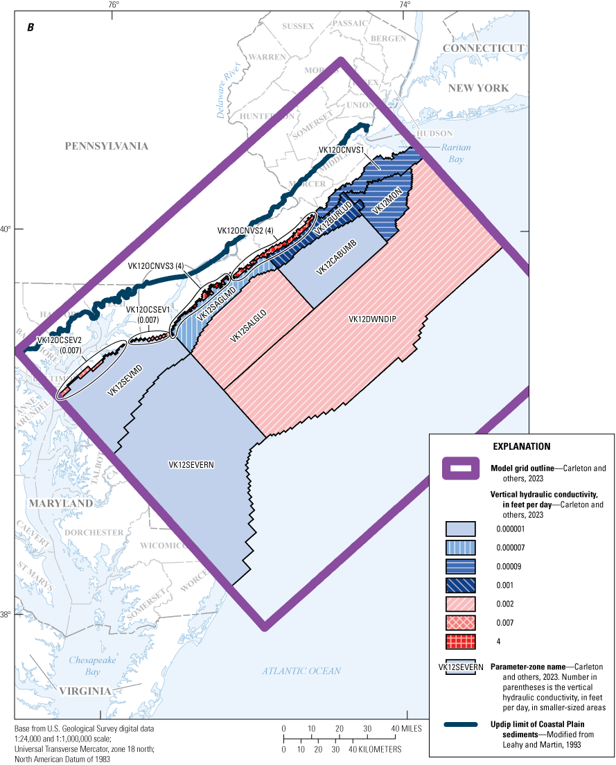
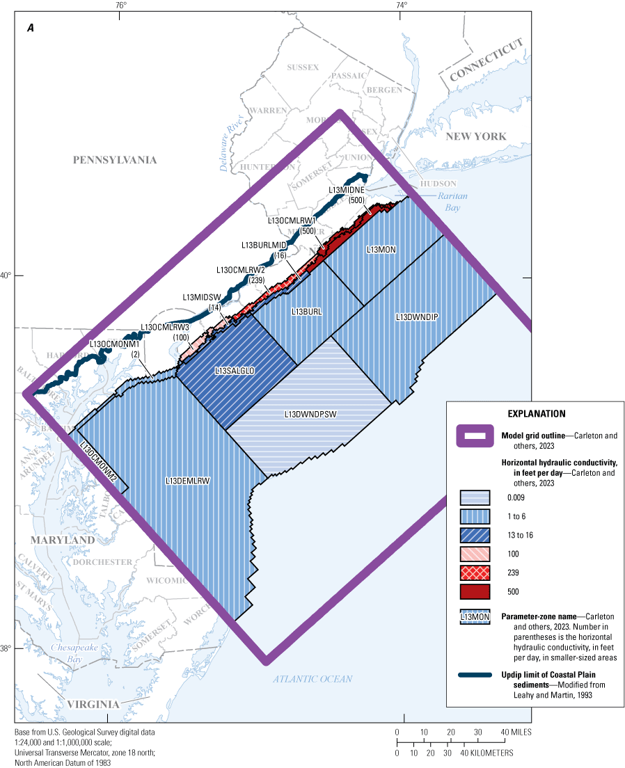
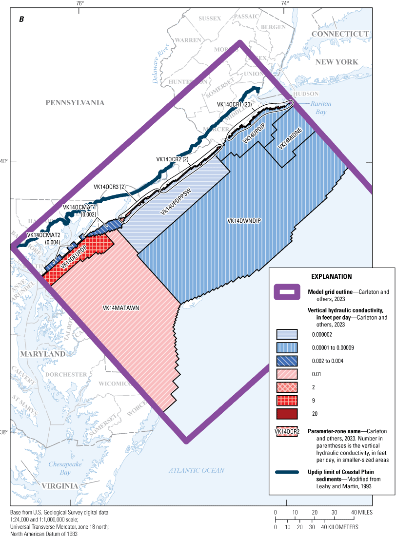
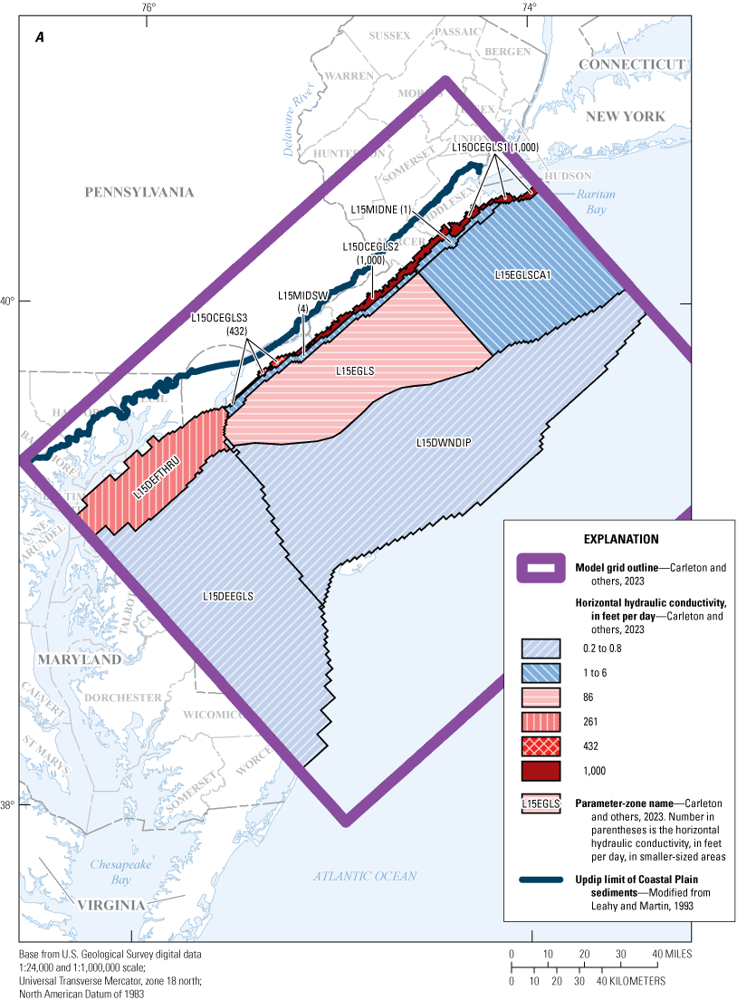
The final calibrated values for horizontal and vertical hydraulic conductivity and storage coefficients for aquifers and confining units are listed in tables 6 through 9. Table 6 lists the horizontal hydraulic conductivity (Kh) for the aquifer layers, table 7 lists the horizontal hydraulic conductivity for the confining-unit layers, and table 8 lists the vertical hydraulic conductivity (Kv) for the model layers. Table 9 lists the storage coefficients for each model layer. Parameter zones in each model layer were created using these values to allow for spatial variability of Kh and Kv. Several parameter zones were added or modified during model calibration. The conversion to a fully three-dimensional model framework and varied recharge resulted in the need for additional Kh parameter zones in the outcrop areas of all layers with updip outcrops following the strike of the hydrogeologic layers, corresponding to model layers 3 through 8 and 10 through 21. During the model calibration, some zones acquired a parameter value equal to or similar to that of an adjacent zone but remained a separate zone and was not incorporated into the adjacent zone. The ratio of horizontal to vertical hydraulic conductivity (Kh:Kv) was initially set to 10:1 for aquifers and 1:1 for confining units. Kh and Kv were adjusted independently during calibration; the sensitivity of Kv is low in most aquifer parameter zones and the sensitivity of Kh is low in most confining-unit parameter zones. The zones are designated by the parameters listed in tables 6 through 9. The location and extent of the Kh zones for the aquifers and Kv zones for the confining units are shown in figures 9 through 19. The parameter names for horizontal hydraulic conductivity for the confining units are zones with prefix “CU”. The location and extent of the horizontal hydraulic conductivity parameter zones for the confining units (table 7) are not shown in figures. The location and extent of the horizontal hydraulic conductivity parameter zones for the confining units coincide with the location and extent of the vertical hydraulic conductivity parameter zones (zones with prefix “VK”) for the confining units shown in figures 9B through 18B for those model layers.
Table 6.
Final horizontal hydraulic conductivity parameters for the aquifers in the calibrated New Jersey Coastal Plain groundwater-flow model.[The number of significant figures used is based on the magnitude of the parameter value. Parameter names and zones for horizontal hydraulic conductivity for aquifers are shown in figures 9A–19.]
Table 7.
Final horizontal hydraulic conductivity parameters for confining units in the calibrated New Jersey Coastal Plain groundwater-flow model.[The number of significant figures used is based on the magnitude of the parameter value.]
Table 8.
Final vertical hydraulic conductivity parameters in the calibrated New Jersey Coastal Plain groundwater-flow model.[The number of significant figures used is based on the magnitude of the parameter value. Parameter names and zones for vertical hydraulic conductivity for confining units are shown in figures 9B–18B.]
Table 9.
Final storage-coefficient parameters in the calibrated New Jersey Coastal Plain groundwater-flow model.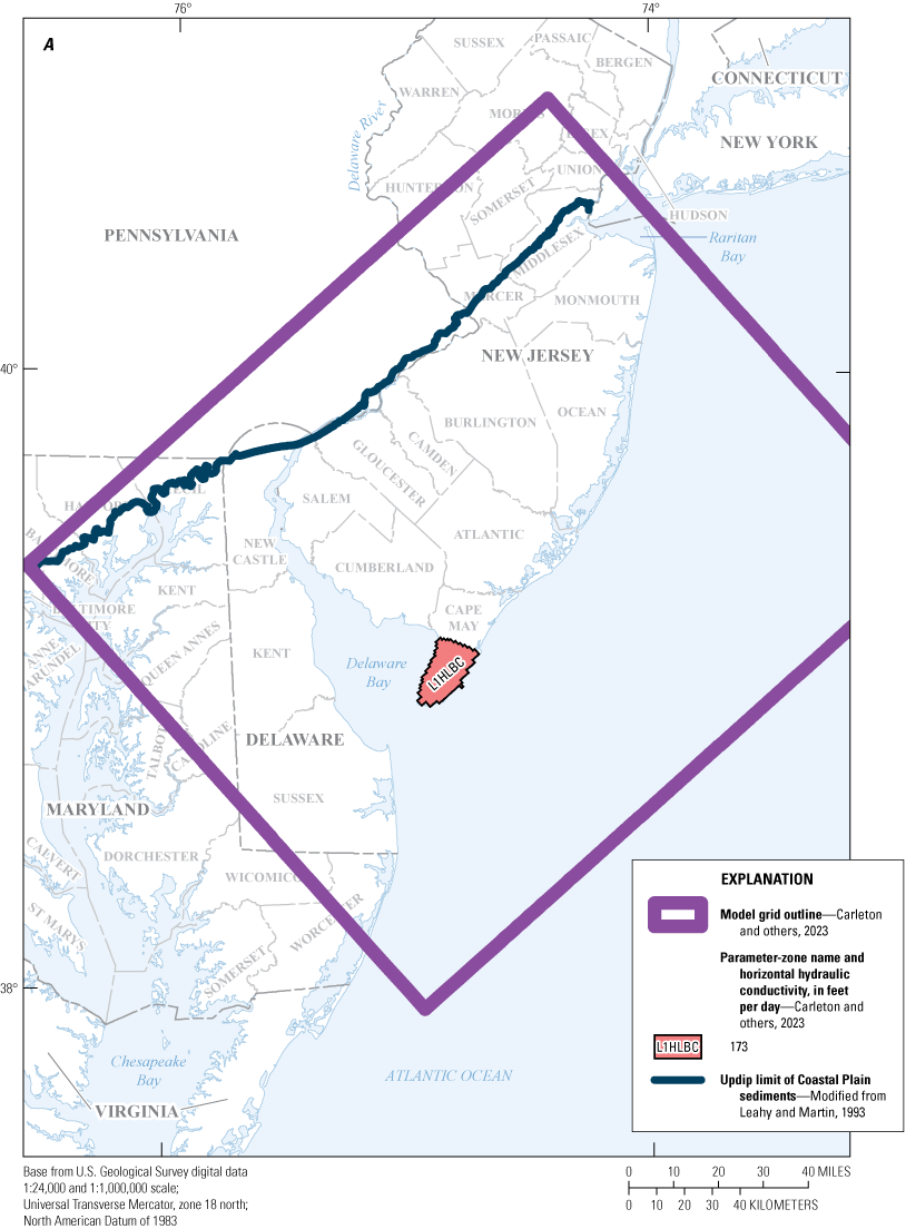
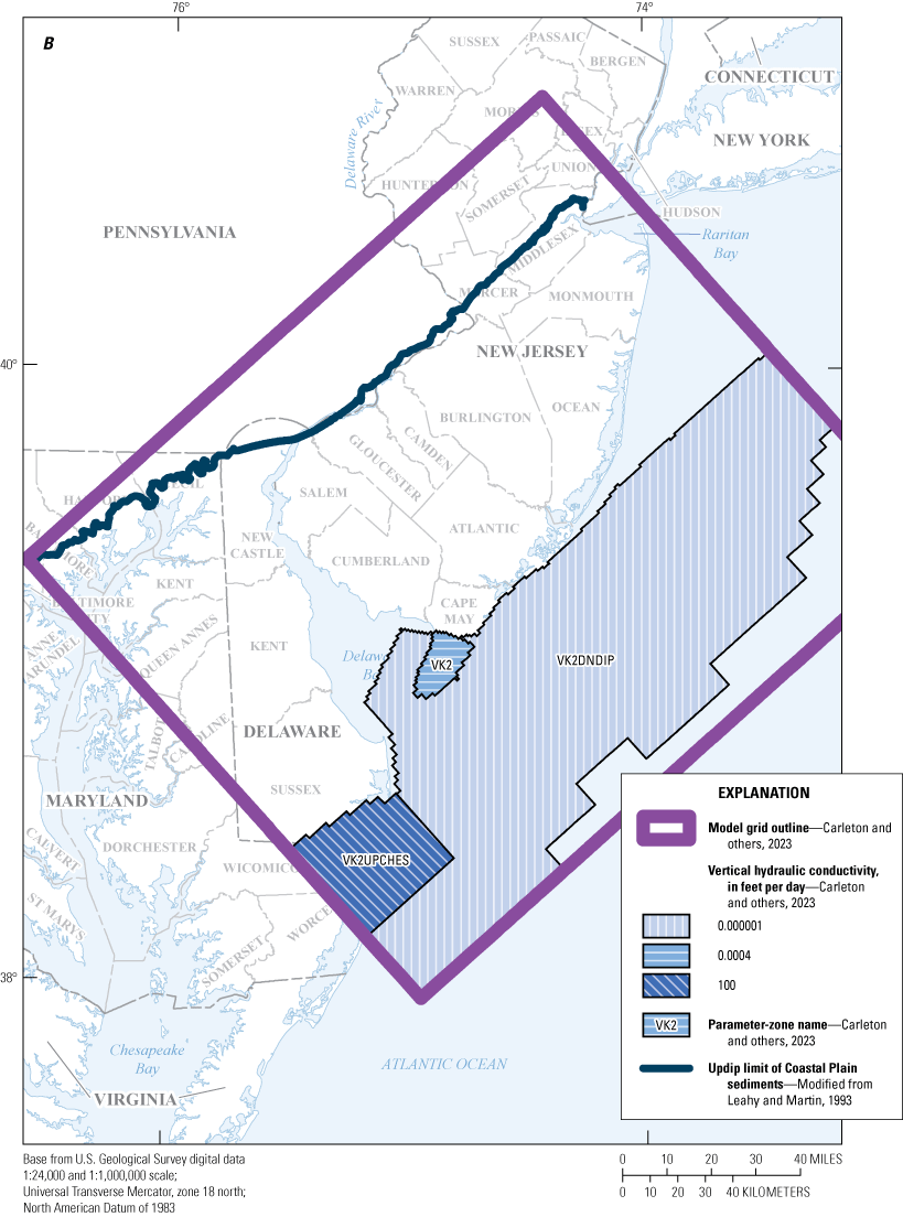
Maps showing A, horizontal hydraulic conductivity zones of model layer 1 and B, vertical hydraulic conductivity of model layer 2, in the New Jersey Coastal Plain groundwater-flow model.
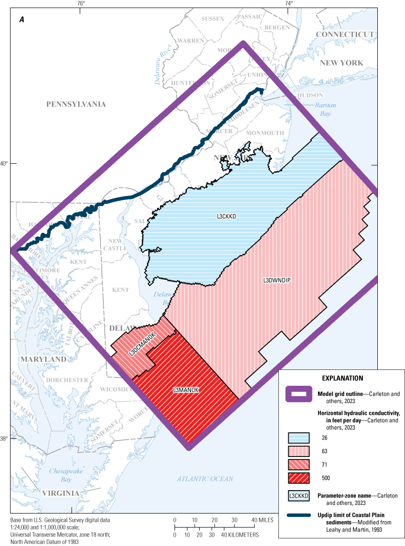
Maps showing A, horizontal hydraulic conductivity zones of model layer 3 and B, vertical hydraulic conductivity zones of model layer 4, in the New Jersey Coastal Plain groundwater-flow model.
Maps showing A, horizontal hydraulic conductivity zones of model layer 5 and B, vertical hydraulic conductivity zones of model layer 6, in the New Jersey Coastal Plain groundwater-flow model.
Maps showing A, horizontal hydraulic conductivity zones of model layer 7 and B, vertical hydraulic conductivity zones of model layer 8, in the New Jersey Coastal Plain groundwater-flow model.
Maps showing A, horizontal hydraulic conductivity zones of model layer 9 and B, vertical hydraulic conductivity zones of model layer 10, in the New Jersey Coastal Plain groundwater-flow model.
Maps showing A, horizontal hydraulic conductivity zones of model layer 11 and B, vertical hydraulic conductivity zones of model layer 12, in the New Jersey Coastal Plain groundwater-flow model.
Maps showing A, horizontal hydraulic conductivity zones of model layer 13 and B, vertical hydraulic conductivity zones of model layer 14, in the New Jersey Coastal Plain groundwater-flow model.
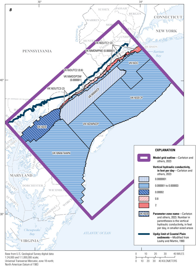
Maps showing A, horizontal hydraulic conductivity zones of model layer 15 and B, vertical hydraulic conductivity zones of model layer 16, in the New Jersey Coastal Plain groundwater-flow model.
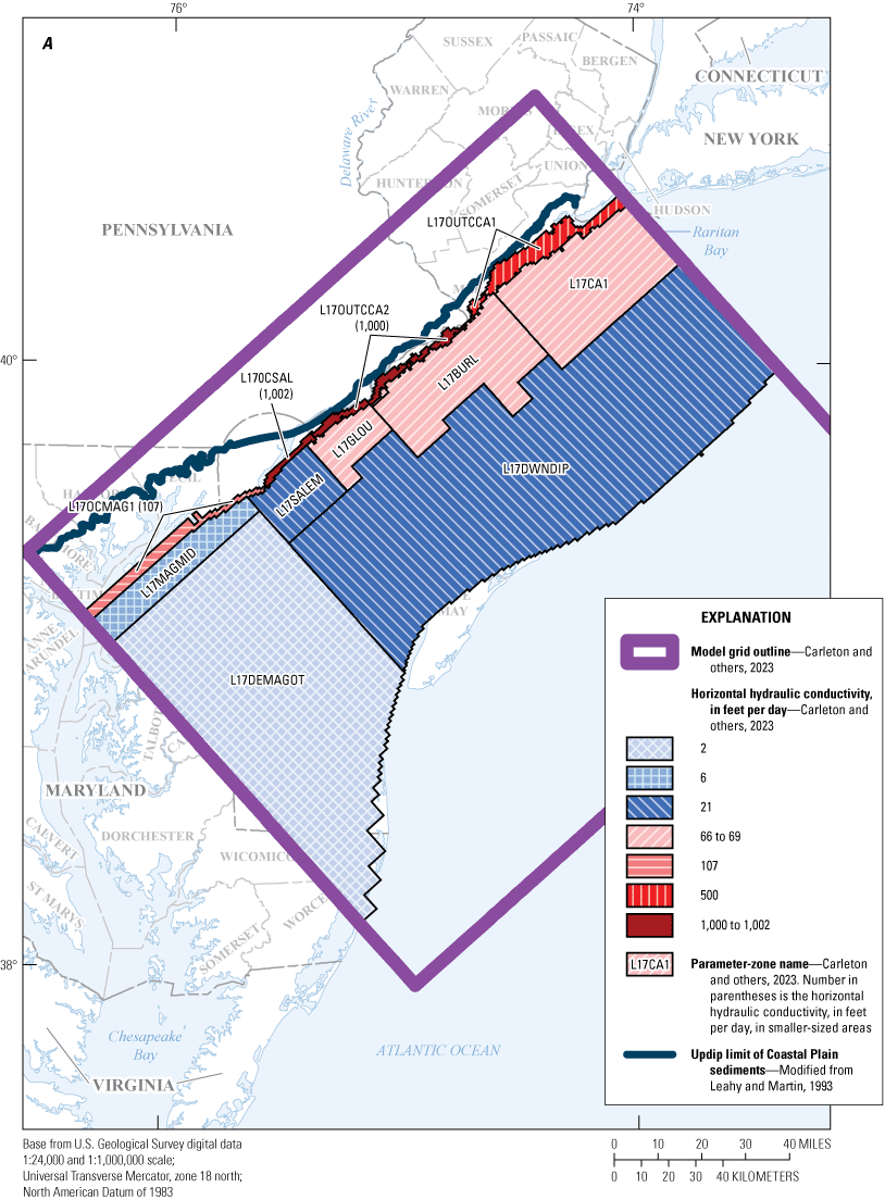
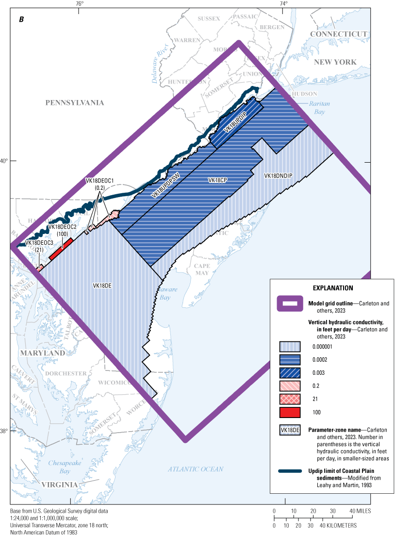
Maps showing A, horizontal hydraulic conductivity zones of model layer 17 and B, vertical hydraulic conductivity zones of model layer 18, in the New Jersey Coastal Plain groundwater-flow model.
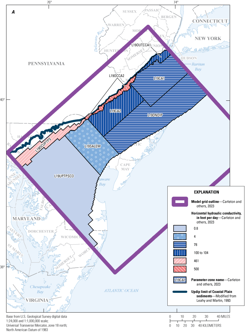
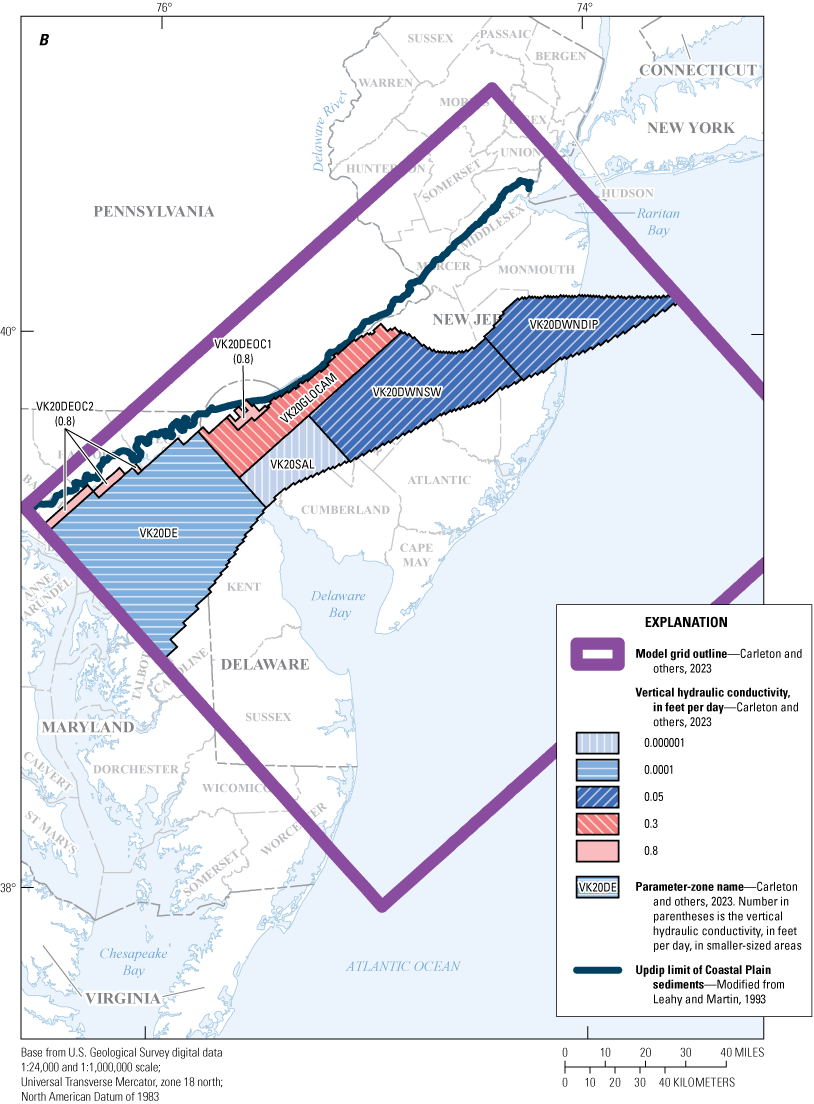
Maps showing A, horizontal hydraulic conductivity zones of model layer 19 and B, vertical hydraulic conductivity zones of model layer 20, in the New Jersey Coastal Plain groundwater-flow model.
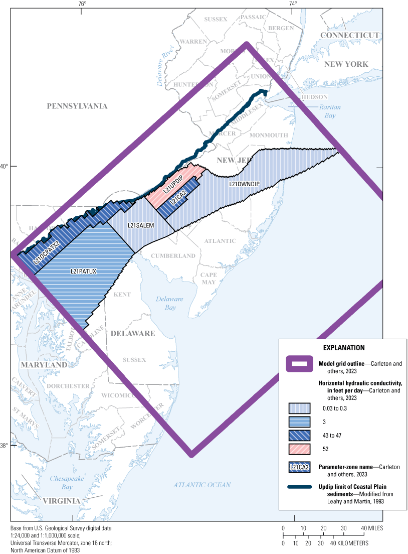
Map showing horizontal hydraulic conductivity zones of model layer 21 in the New Jersey Coastal Plain groundwater-flow model.
The final parameters for horizontal and vertical hydraulic conductivity were compared to the values shown in tables 2 and 3 of this report. Many of the parameter values of horizontal hydraulic conductivity, such as those for the confined aquifers and the Holly Beach water-bearing zone in New Jersey, fall within the ranges of the value for horizontal hydraulic conductivity shown in the tables 2 and 3 and also table 1 of Masterson and others (2016a). Some horizontal hydraulic conductivity assigned to the outcrop areas of certain model layers for aquifers were higher (greater than 500 ft/d, table 6) because those areas are thin and the higher value increased model stability in these areas but did not affect the flow farther downdip. Higher values of horizontal hydraulic conductivity were also assigned to the outcrop areas of some confining-unit model layers (table 7) for the same reason. Lower values of horizontal hydraulic conductivity (less than 1 ft/d) were assigned in downdip areas of some aquifers—for example model layer 11 which represents the Vincentown aquifer—because the model layer is not present downdip and the small horizontal hydraulic conductivity value allowed for the lateral connection between the updip and downdip parts of the model layer and (or) a vertical connection between the model layer with the overlying and underlying model layers.
The parameters for riverbed conductance for the Delaware River cells and for streambed conductance for drains cells each have a single value. Although hydrogeologic and stream-width data could be used to justify multiple parameters for these properties, these data were considered secondary to the calibration of the regional-scale Coastal Plain model. During model calibration, simulation results indicated the model was insensitive to the riverbed-conductance parameter. Additionally, the comparison of simulated to estimated base flows was reasonable when a single streambed-conductance parameter for drain cells was used; therefore, neither parameter was subdivided to represent smaller or local areas for the river or drain cells. This process is described further in the “Parameter Sensitivity and Correlation” and “Parameter Estimation and Residual Analysis” sections below.
Two parameters were used to vary the recharge rates in the model calibration. One parameter was used for New Jersey and another parameter was used for recharge in Delaware and Maryland. The recharge parameter for New Jersey is a multiplier applied equally to the recharge value estimated for each model cell by using the Soil-Water-Balance model (described in the “Recharge” section earlier in this report). The recharge parameter was increased from an initial value of 1.0 to a final value of 1.2 to provide a reasonable match between simulated and estimated base flow in the 47 New Jersey surface-water basins (fig. 8).
Parameter Sensitivity and Correlation
A sensitivity analysis of the calibrated model was conducted to evaluate the relative effects of the various parameters on the match between simulated and observed water levels and simulated and estimated base flows. The sensitivity analysis is used to identify which parameters in the model, when modified, improve model results. Parameters which are least sensitive, when modified, have little effect on model results. The sensitivity of model parameters was calculated by using the parameter-estimation software UCODE–2014 (Poeter and others, 2014). Parameter sensitivities were calculated two ways: by using base-flow observations only and by using water-level observations only. This section discusses composite scaled sensitivities (CSS) and parameter correlation coefficients. The CSS values show how sensitive water-level and base-flow observations in the model are to changes in each of the parameters.
According to composite-scaled sensitivity analysis, the parameters most sensitive to base-flow observations (excluding recharge) are primarily streambed conductance, horizontal hydraulic conductivity, and storage in zones in the outcrop areas of several model layers (fig. 20). Recharge is the dominant parameter with respect to base-flow observations, and the recharge multiplier parameter was adjusted manually such that average simulated base flow equaled the estimated base flow of the New Jersey Coastal Plain of about 16 inches per year (in/yr), a value determined from surficial-aquifer studies completed in surface-water basins in the New Jersey Coastal Plain during 1992–2003 (Watt and Johnson, 1992; Watt and others, 1994; Lacombe and Rosman, 1995; Johnson and Watt, 1996; Johnson and Charles, 1997; Charles and others, 2001; Watt and others, 2003; Gordon, 200418). The streambed-conductance parameter for the drains (DRN_Par1) is ranked the 4th most sensitive parameter to base-flow observations (fig. 20). As indicated above, there is only one parameter for streambed conductance and any change to that parameter is applied to all streams uniformly rather than to individual streams. When the streambed conductance was decreased, groundwater levels tended to increase but the location or timing of discharge to base flow did not necessarily change. The 21 most sensitive parameters (fig. 20) other than streambed conductance (DRN_Par1) are in, or laterally or vertically adjacent to, an outcrop area.
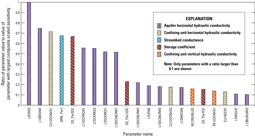
Graph showing composite scaled sensitivities of model parameters derived from base-flow observations for the New Jersey Coastal Plain groundwater-flow model.
Results of the CSS analysis indicate that the parameters most sensitive to water-level observations are recharge, and horizontal and vertical hydraulic conductivity (fig. 21); riverbed and general-head-boundary conductances are insensitive. Of the 27 most sensitive parameters (including the two recharge parameters (RCH_SWB and RchDeFlux), 19 (70 percent) are horizontal hydraulic conductivity, and 6 (22 percent) are vertical hydraulic conductivity.
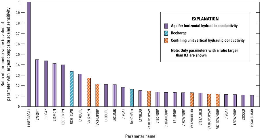
Graph showing composite scaled sensitivities of model parameters derived from water-level observations for the New Jersey Coastal Plain groundwater-flow model.
Six pairs of the 130 most sensitive horizontal and vertical hydraulic conductivity parameters are correlated when recharge is excluded and only head observations are included in the parameter estimation (fig. 22). Most of the correlations are between vertically adjacent zones (for example, layers 20 and 21 in Delaware (figs. 18B and 19)) or horizontal and vertical hydraulic conductivity of the same zone (for example, layer 11 in northwestern Ocean County and northeastern Burlington County (figs. 1424.)). Four of the six pairs are parameter zones in Delaware and three of the six pairs are parameter zones in outcrop areas. Although the parameters were correlated, each correlated parameter was allowed to be estimated separately. There is not sufficient water-level data in the parameter zones to resolve the negative correlation between the horizontal hydraulic conductivity and (or) vertical hydraulic conductivity of each of the correlated parameter pairs.
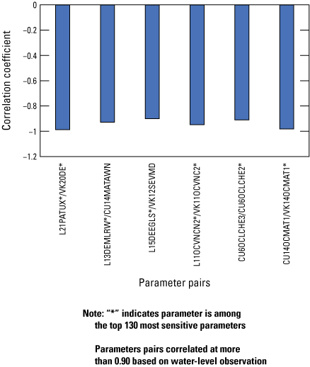
Graph showing model parameter pairs in the New Jersey Coastal Plain groundwater-flow model with greater than 90 percent correlation.
Parameter Estimation and Residual Analysis
The parameters used in the New Jersey Coastal Plain model were tested and adjusted in an iterative calibration process. Initial parameter-estimation runs with UCODE–2014 (Poeter and others, 2014) were conducted by using all observations (water-level and base-flow). Results indicated that matching water levels in the aquifers would be less likely if base-flow observations were included. The challenge of adjusting the weights of base-flow observations to avoid their having too little or too great an effect on water levels was judged to be not effective because of the single streambed parameter for drains and the relative coarseness of the representation of the stream network in the DRN package. Therefore, after some adjustments were made to sensitive parameters to obtain an initial optimal calibration with all observations, parameter-estimation runs were done by using only base-flow observations. The recharge multiplier had the greatest effect on simulated base flows; once the recharge multiplier was held constant, the model response was generally more sensitive to parameters in the outcrop areas of aquifers and confining units. Subsequent parameter-estimation runs were done by using only water-level observations. For these runs, the parameters that were sensitive to drain (base-flow) observations, but not to water-level observations, typically remained at the value determined in the previous parameter-estimation runs in which only drain observations were used.
The number of simulated and water-level observations from wells in New Jersey used in the NJCP groundwater-flow model each total 4,243. The total includes 2,361 water-level observations from 392 wells, 920 historical water-level trends for 29 wells during 1980–2013, 210 observations of vertical gradients in 33 pairs of nested wells, and 752 observations of changes in water levels over time calculated for 134 wells. When plotted against each other (fig. 23), these values are clustered around the 1:1 correlation line where the observed water levels have a range of 411 ft and more than 96 percent of the simulated water levels fall within +/− 10 percent of the total range during 1980–2013. The residuals (simulated minus observed water level) are within + or – 10 feet for 58 percent of the water-level observations for New Jersey, and within + or – 20 feet for 84 percent. The average water-level residual is 1.5 ft; the minimum; first, second, and third quartile; and maximum residuals are −127.4, −5.5, 1.6, 10.4, and 179.4 ft, respectively.
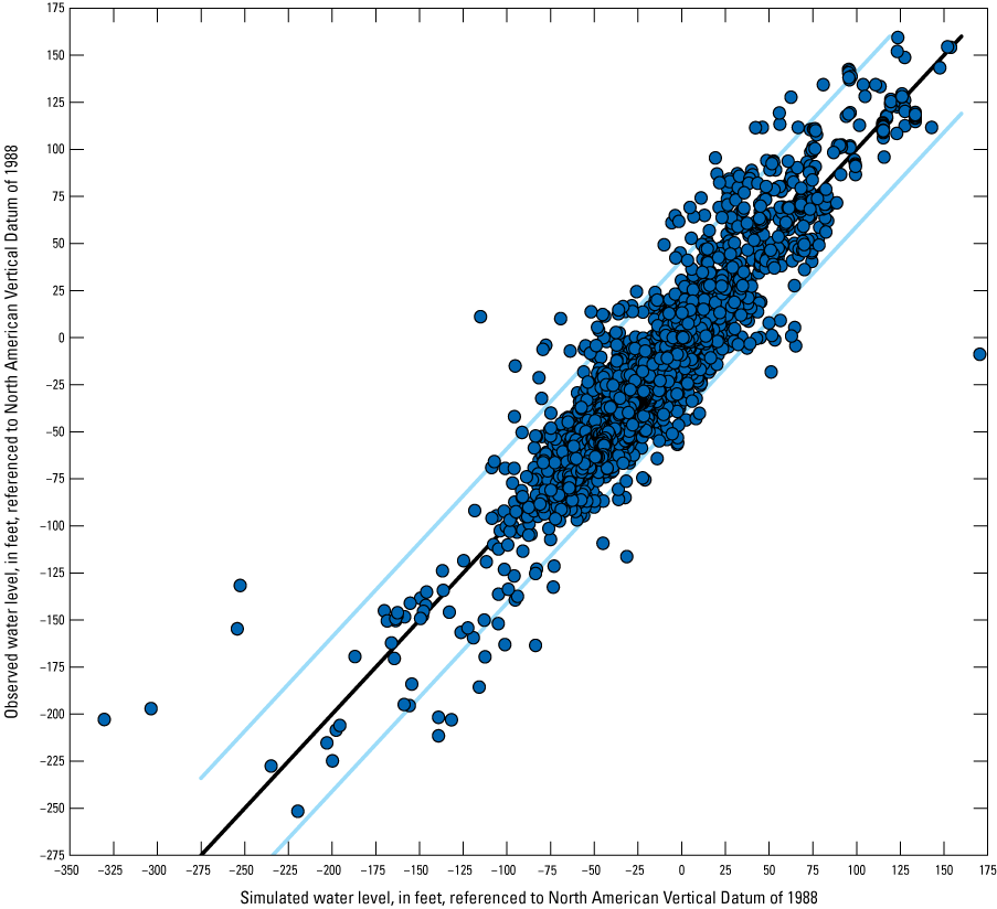
Graph showing simulated and observed water levels in wells in New Jersey used in calibration for the New Jersey Coastal Plain groundwater-flow model, 1980–2013.
Calibration of Stream Base Flows
The simulated average annual base flows and estimated annual average base flows for the period of record for 47 surface-water basins are shown in figure 24. Hydrographs of simulated average annual base flows at continuous- and partial-record gaging stations during the period of record available for 1980–2013 generally match estimated average annual base flows and are shown in figures 25 and 26, respectively. Although the annual variations are not well correlated and simulated flows are higher than estimated base flow in some basins and lower in others, the overall difference between simulated and estimated average base flow was reasonably matched for most basins (figs. 25 and 26).
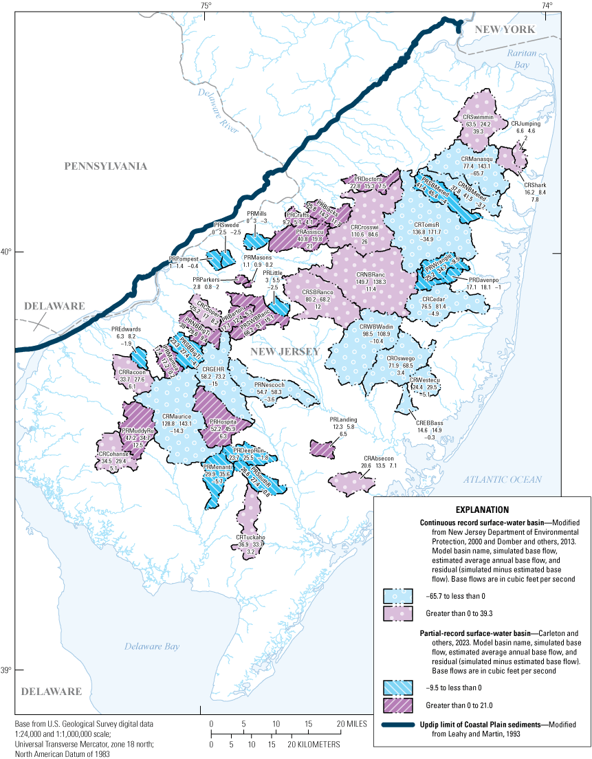
Map showing simulated average and estimated average annual base flow for the period of record for selected surface-water basins in the New Jersey Coastal Plain.
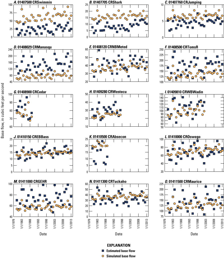
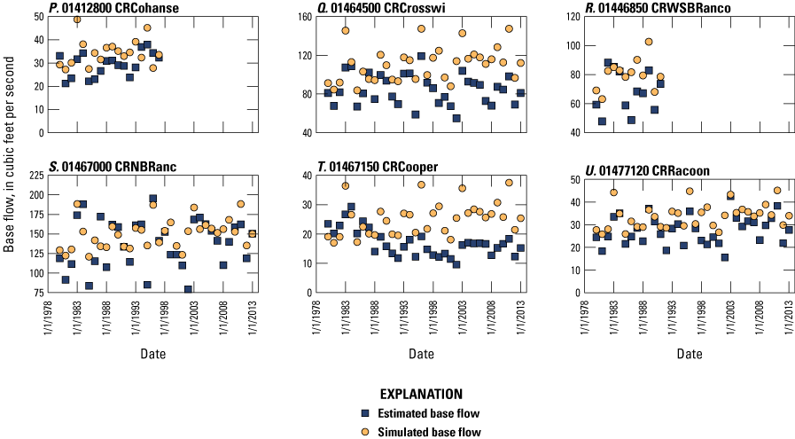
Hydrographs of simulated and estimated annual base flow for selected continuous-record gaging stations in the New Jersey Coastal Plain, 1980–2013.
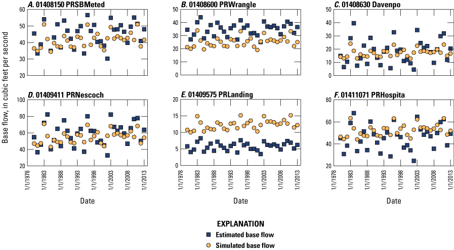
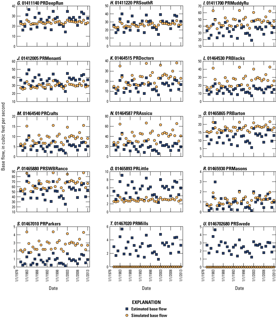
Hydrographs of simulated and estimated annual base flow for selected partial-record gaging stations in the New Jersey Coastal Plain, 1980–2013.
The residual (simulated average annual base flow minus estimated annual average base flow) for each of the 47 surface-water basins in New Jersey also is shown in table 10. Simulated average annual base flows in 37 of the 47 surface-water basins (79 percent) are within 50 percent of the estimated average annual base flows and simulated average base flows in 25 basins (53 percent) are within 25 percent. Estimated average annual base flow ranges from 0.8 to 171.7 cubic feet per second (ft3/s) and simulated average base flows range from 0.0 to 149.7 (ft3/s). The largest percent residuals in the table generally are associated with the small streamflows in basins with drainage areas 20 mi2 or less (7 of 20 surface-water basins (30 percent)). In some instances, simulated average base flow is lower than estimated base flow in the surface-water basins in updip basins (fig. 24), and simulated average base flow is higher than estimated base flow in adjacent downdip basins. For example, simulated average base flow at the Toms River continuous-record gaging station (01408500) is −34.9 ft3/s (20 percent) less than estimated average annual base flow, whereas simulated average base flow at gaging stations in the adjacent basin of Crosswicks Creek (01464500) is 26.0 ft3/s (31 percent), respectively, greater than the estimated value. Simulated base flow from this model and the previous RASA model (Voronin, 2004) are compared during model calibration to ensure that the level of calibration was maintained or improved. Voronin (2004) reports that simulated average base flows at the gaging stations at Toms River (01408500) and North Branch Rancocas Creek (0146700) are within about 10 percent of estimated values for 1926–96 and 1921–96, respectively. Simulated average base flows at Toms River (01408500) and North Branch Rancocas Creek (01467000) in this report are within −20 and 8 percent of estimated values, respectively, for 1980–2013. Similarly, Voronin (2004) reports that simulated average base flow of Raccoon Creek (01477120) is within 31 percent of the estimated value for 1966–92; simulated average base flow for this station in this report, however, is within 22 percent of that estimated for 1980–2013.
Table 10.
Simulated average and estimated average annual base flow for the period of record at selected continuous and partial-record streamflow-gaging stations in the New Jersey Coastal Plain.[ft3/s, cubic feet per second; NJ, New Jersey]
Calibration of Water Levels
During model calibration, simulated water levels were compared to water levels measured in the seven quinquennial New Jersey Coastal Plain synoptic studies conducted in 1983, 1988, 1993, 1998, 2003, 2008, and 2013 to ensure that the cones of depression and flow directions were simulated accurately. Discussion of simulated water levels in this report is limited to 2013 groundwater-flow conditions. Maps of the 2013 potentiometric surface for the confined aquifers in the New Jersey Coastal Plain (Cauller and Gordon, 2021) and the simulated water levels for the major aquifers in the New Jersey Coastal Plain and the confined aquifers in Delaware and residuals at wells measured in those aquifers in 2013 are shown in this section. As previously mentioned in the “Model Development” section, if the aquifer does not extend across a model layer in the MODFLOW-2005 finite difference solution method, but instead pinches out, the absent area of the aquifer is represented in the model by a thin layer that allows for the hydraulic connection between underlying and overlying model layers. These aquifers include the downdip areas of the Vincentown and lower PRM aquifers, and the Englishtown aquifer system, (model layers 11, 21, and 15, respectively), and the updip areas of the Rio Grande water-bearing zone, Atlantic 800-foot sand, and Piney Point aquifer (model layers 5, 7, and 9). Therefore, the simulated water levels for the part of a model layer representing the aquifer area only are shown on the figures for these aquifers. The residuals are the simulated water level minus the measured (observed) water level at the well and the root mean square error (RMSE) statistic of the residuals for each aquifer is computed. The RMSE is the standard deviation of the residuals. Hydrographs of water levels also were used to calibrate the model. The hydrographs were compared to simulation results from Voronin (2004) to ensure that the updated model maintained or improved the level of calibration achieved with the previous model.
Calibration of Water Levels in the Holly Beach Water-Bearing Zone
Simulated water-level contours in the Holly Beach water-bearing zone (model layer 1, Cape May County) are shown in figure 27. The Holly Beach water-bearing zone is a minor aquifer in New Jersey; the observed water levels shown in Lacombe and Carleton (2002) were used to visually compare to the simulated water-level contours.
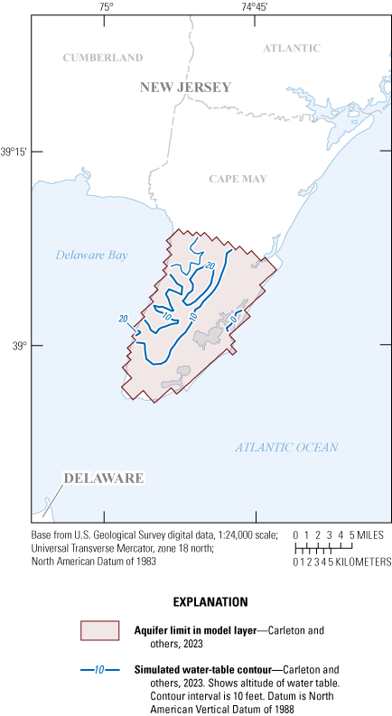
Map showing simulated water-level contours for the Holly Beach water-bearing zone, Cape May County, New Jersey, 2013.
Calibration of Water Levels in the Confined Cohansey Aquifer and Unconfined Kirkwood-Cohansey Aquifer System
Simulated water-level contours in the unconfined Kirkwood-Cohansey aquifer shown in the updip area of model layer 3 closely match the observed water-table contours in general direction and slope (fig. 28). The observed water-table contours are an aggregate of data from multiple surficial-aquifer studies in the following surface-water basins of the New Jersey Coastal Plain: Great Egg Harbor River Basin (Watt and Johnson, 1992); Toms River, Metedeconk River, and Kettle Creek Basins (Watt and others, 1994); upper Maurice River Basin (Lacombe and Rosman, 1995); Mullica River Basin (Johnson and Watt, 1996); Salem River and Raccoon, Oldmans, Alloway, and Stow Creek Basins (Johnson and Charles, 1997); and Rancocas, Crosswicks, Assunpink, Blacks, and Crafts Creek Basins (Watt and others, 2003). The aggregated (observed) water-table contours are shown only in the areas where a surficial-aquifer study was completed before 2004. In Cape May County, New Jersey, as well as in Sussex County, Delaware, groundwater is confined.
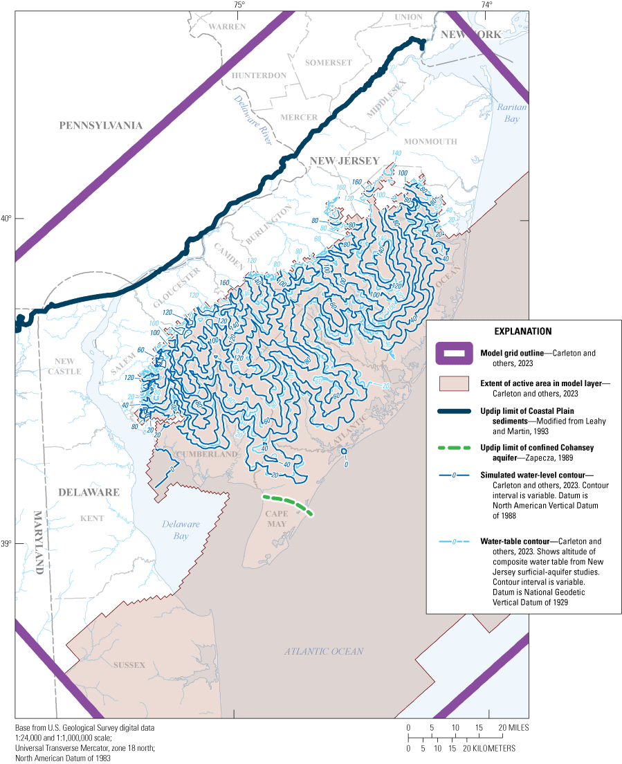
Map showing simulated and composite observed water-table contours for the unconfined Kirkwood-Cohansey aquifer system in New Jersey.
The updip limit of the confined Cohansey aquifer in Cape May County is shown in figure 29. The simulated water-level contours in the confined Cohansey aquifer in New Jersey and the potentiometric surface of the 2013 New Jersey Coastal Plain water-level synoptic study (Cauller and Gordon, 2021) for this aquifer also are shown in figure 29. Simulated water levels in the confined part of the Cohansey aquifer (model layer 3, Cape May County) generally match observed water levels (table 11). The average water-level residual (simulated minus observed) for 17 observation points in Cape May County for the confined Cohansey aquifer is −0.2 ft and the root mean square error (RMSE) is 3.3 ft. The simulated water levels for the Upper Chesapeake aquifer in Delaware and the average water-level residual for four wells measured in Delaware in 2013 (table 11) also are shown in figure 29.
Table 11.
Simulated and observed water-level observations and residuals for wells open to the confined Cohansey aquifer, Cape May County, New Jersey, and the Upper Chesapeake aquifer, Delaware, 2013.[USGS, U.S. Geological Survey; residual, simulated water level minus observed water level]
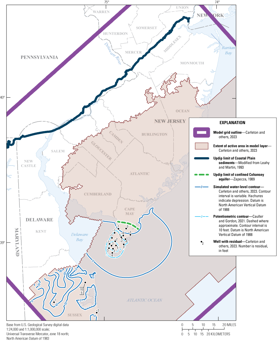
Map showing simulated water-level contours and 2013 potentiometric surface of, and residuals for selected wells in, the confined Cohansey aquifer, Cape May County, New Jersey, and simulated water-level contours for the Upper Chesapeake aquifer, Delaware.
The hydrographs of simulated and observed water levels for well 090049 (fig. 30) are similar, with minima, maxima, and averages for the observed water levels of –21, –8, and –13 ft, respectively, for the observed water levels and –19, –7, and –11 ft, respectively, for the simulated water levels. Simulated water levels are, on average, 2 ft greater than observed. The hydrographs of simulated and observed water levels for well 090080 in south-central Cape May County (fig. 31) are similar, with minima, maxima, and averages for the observed water levels of –11, –1, and –6 ft, respectively, for the observed water levels and –18, –0.5, and –8 ft, respectively, for the simulated water levels.
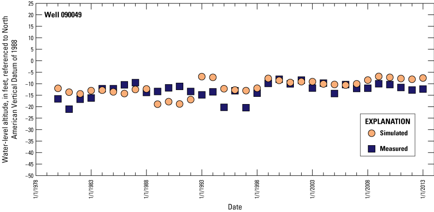
Hydrograph of simulated and observed water levels in well 090049 open to the confined Cohansey aquifer, New Jersey, 1980–2013.
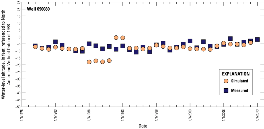
Hydrograph of simulated and observed water levels in well 090080 open to the confined Cohansey aquifer, New Jersey, 1980–2013.
Calibration of Water Levels in the Rio Grande Water-Bearing Zone
Simulated water-level contours and the potentiometric surface of the 2013 New Jersey Coastal Plain water-level synoptic study (Cauller and Gordon, 2021) in the Rio Grande water-bearing zone (model layer 5, parts of Ocean, Atlantic, and Cape May Counties) are shown in figure 32. The 2013 simulated water levels are an average 7 ft lower than the observed water levels at six wells in Cape May County and are 35 ft lower than the observed water levels at three wells in Ocean County. The simulated 2013 potentiometric contours indicate a cone of depression along the shoreline of Cape May and Atlantic Counties caused by drawdowns in the underlying Atlantic City 800-foot sand; a cone of depression also is observed in the simulated water-level contours. The differences between the simulated and observed water levels for 10 observation points in New Jersey are listed in table 12. The average water-level residual (simulated minus observed) for the 10 observation points (figs. 32 and 33) is −16 ft and the RMSE is 24 ft. The minimum; first, second, and third quartile; and maximum residuals are −45, −31, −13, 0, and 5 ft, respectively.
Table 12.
Simulated and observed water-level observations and residuals for wells open to the Rio Grande water-bearing zone, New Jersey, 2013.[USGS, U.S. Geological Survey; residual, simulated water level minus observed water level]
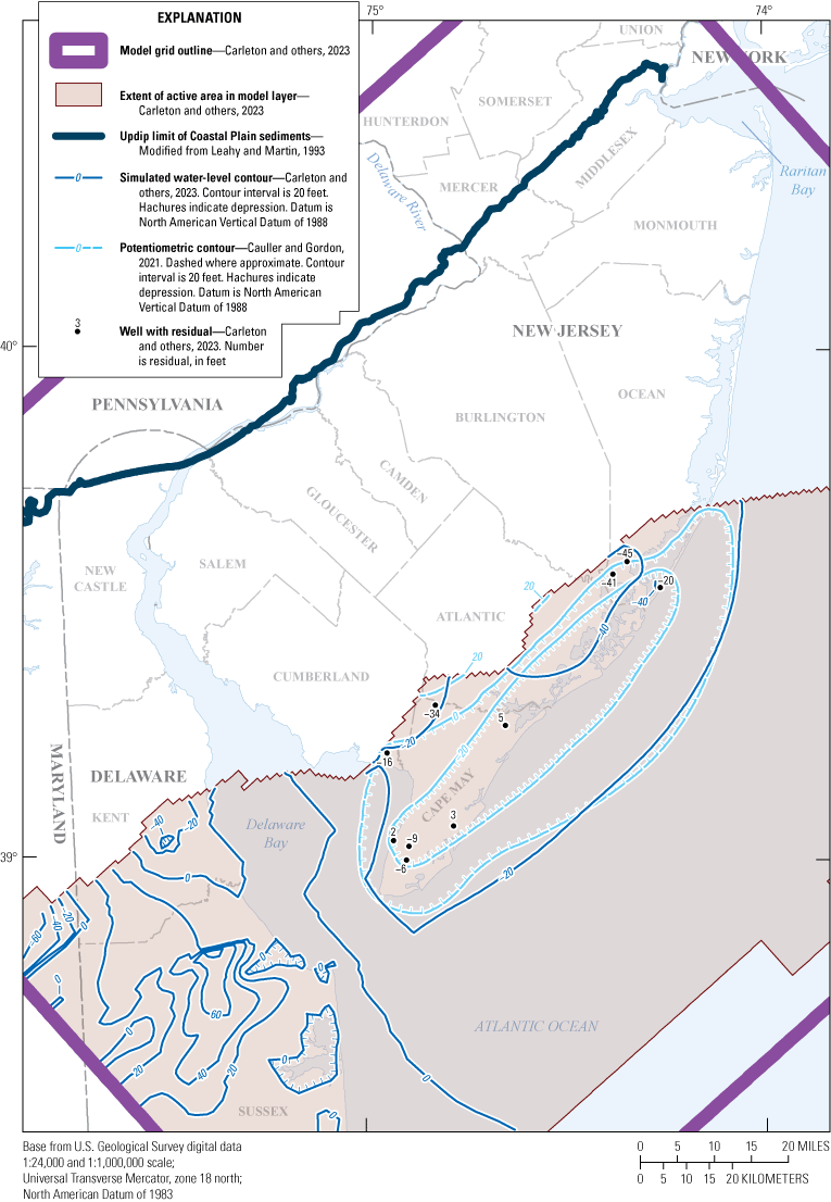
Map showing simulated water-level contours and 2013 potentiometric surface for, and residuals for selected wells in, the Rio Grande water-bearing zone, New Jersey and simulated water-level contours for the Lower Chesapeake aquifer, Delaware.
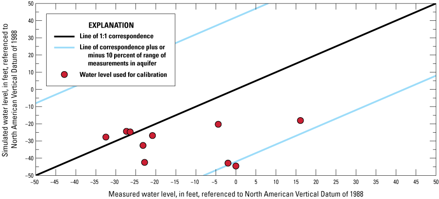
Graph showing simulated and observed water levels in wells open to the Rio Grande water-bearing zone, Cape May, Atlantic, and Ocean Counties, New Jersey, 2013.
Calibration of Water Levels in the Atlantic City 800-Foot Sand
Simulated water-level contours in the Atlantic City 800-foot sand (model layer 7, parts of Cape May, Atlantic, and Ocean Counties) generally match the 2013 potentiometric surface in coastal Atlantic and Cape May Counties (fig. 34). The simulated water-level contours are similar in shape to the 2013 potentiometric surface (Cauller and Gordon, 2021), although the gradient of the simulated contours is less steep than that of the water-level contours drawn from measurements made in updip central Atlantic County. The simulated water levels are within 10 ft of observed levels in 13 of 34 wells (38 percent) in New Jersey and within 15 ft of observed levels in 24 of 34 wells (71 percent) (figs. 34 and 35 and table 13). The 2013 simulated water levels are an average 8 ft higher than the observed water levels at 13 wells in Cape May County and are an average 13 ft lower than the observed water levels at 14 wells in Atlantic County. The simulated water levels are an average 11 ft lower than observed levels at 7 wells in Ocean County. The average water-level residual (simulated minus observed) for 34 wells in Cape May, Atlantic, and Ocean Counties is −4 ft and the RMSE is 21 ft. The minimum; first, second, and third quartile; and maximum residuals are −57, −12, 3, 12, and 17 ft, respectively. The simulated water levels for the Calvert aquifer system in Delaware and the average water-level residual for one well measured in Delaware in 2013 (table 13) also are shown in figure 34.
Table 13.
Simulated and observed water-level observations and residuals for wells open to the Atlantic City 800-foot sand, New Jersey, and the Calvert aquifer system, Delaware, 2013.[USGS, U.S. Geological Survey; residual, simulated water level minus observed water level]
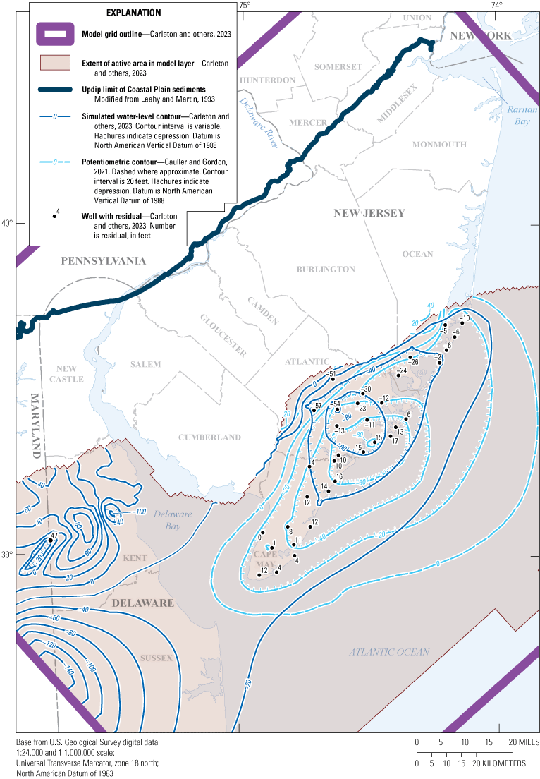
Map showing simulated water–level contours and 2013 potentiometric surface for, and residuals for selected wells in, the Atlantic City 800-foot sand, New Jersey, and the simulated water-level contours for, and residuals for a selected well in, the Calvert aquifer system, Delaware.
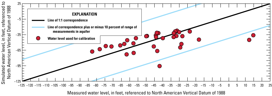
Graph showing simulated and observed water levels for wells open to the Atlantic City 800-foot sand, Cape May, Atlantic, and Ocean Counties, New Jersey, 2013.
The hydrographs of wells 010180 and 010578, in northeastern and southeastern Atlantic County, respectively (fig. 36), show the same trend and amplitude as the observed water levels, but the simulated water levels are, on average, 1 ft lower and 12 ft higher, respectively, than the observed. The hydrographs of simulated and observed water levels for well 010180 (fig. 36A) are similar, with minima, maxima, and average for the observed water levels of –57, –35, and –47 ft, respectively, for the observed water levels and –60, –36, and –48 ft, respectively, for the simulated water levels. The hydrographs of simulated and observed water levels for well 010158 (fig. 36B) are similar, with minima, maxima, and average for the observed water levels of –71, –49, and –60 ft, respectively, and –60, –38, and –48 ft, respectively, for the simulated water levels. The hydrograph for well 010578 (fig. 36B) shows simulated water levels that are closer to and more closely match the trend in the observed water levels than those simulated by Voronin (2004) for 1990–98.
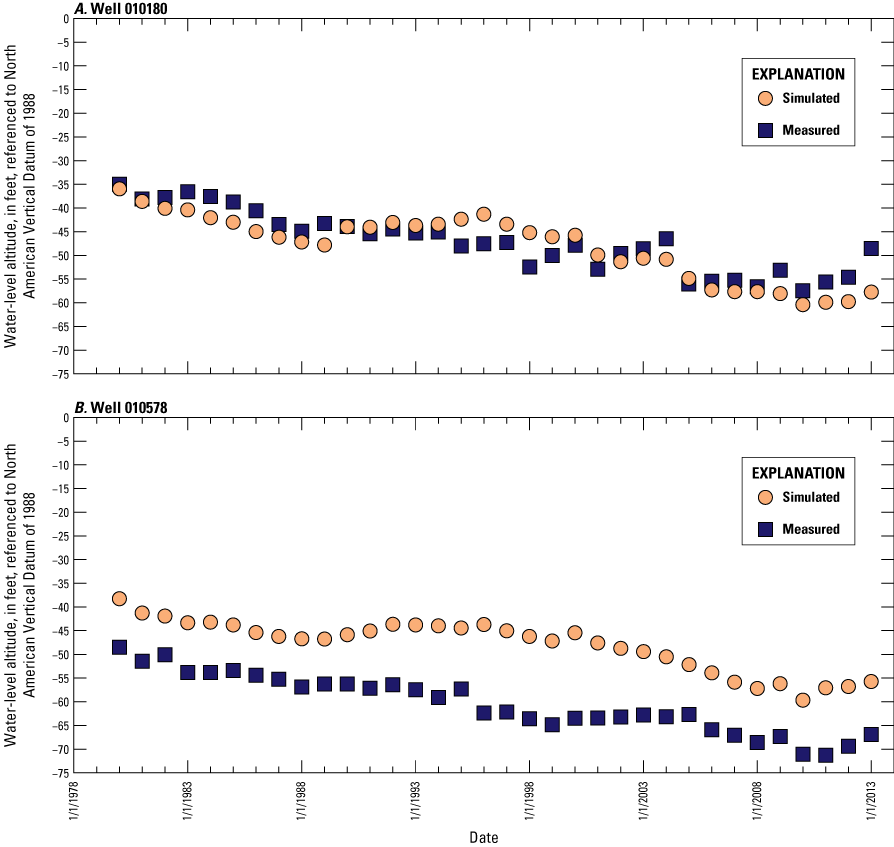
Hydrographs of simulated and observed water levels in wells A, 010180 and B, 010578, open to the Atlantic City 800-foot sand, New Jersey, 1980–2013.
Calibration of Water Levels in the Piney Point Aquifer
Simulated water-level contours in the Piney Point aquifer (model layer 9, parts of Monmouth, Ocean, Atlantic, Gloucester, Cumberland, and Salem Counties, New Jersey, and Kent County in Delaware) are generally similar in shape to the 2013 potentiometric surface (Cauller and Gordon, 2021) (fig. 37), including the contours defining cones of depression in Kent County in Delaware and Cumberland and Ocean Counties in New Jersey. The simulated water levels extend farther updip in Burlington and Ocean Counties than the 2013 potentiometric surface because the updip limit of the Piney Point aquifer in the new hydrogeologic framework used in this groundwater-flow model used new well information from that area which was not available at the time of the previous framework developed by Zapecza, (1989). However, the 2013 potentiometric surface used the updip limit of the Piney Point aquifer which was based on the earlier hydrogeologic framework presented in Zapecza, (1989) for that aquifer. Available Piney Point aquifer withdrawal data indicate anomalously low rates in 2004, 2008, and 2010, likely resulting from missing data for wells with reported withdrawals in other years. Therefore, the 2007 withdrawal rates were substituted for 2004, 2008, and 2010 withdrawals for wells with presumed missing data. The average water-level residuals (simulated minus observed) are shown in table 14 and figures 37 and 38 for 26 wells in New Jersey. The average water-level residual for 26 wells in Cumberland, Atlantic, Gloucester, Camden, Burlington, and Ocean Counties in New Jersey is 9 ft and the RMSE is 23 ft. The minimum; first, second, and third quartile; and maximum residuals are –22, –2, 4, 16, and 80 ft, respectively. The simulated water levels are within 10 ft of observed water levels for 14 of the 26 wells (54 percent) in New Jersey and within 20 ft of observed levels in 19 of 26 wells (73 percent) (figures 37 and 38 and table 14). The average water-level residuals also are shown in table 14 and figure 37 for four wells in Delaware.
Table 14.
Simulated and observed water-level observations and residuals for wells open to the Piney Point aquifer, New Jersey and Delaware, 2013.[USGS, U.S. Geological Survey; residual, simulated water level minus observed water level]
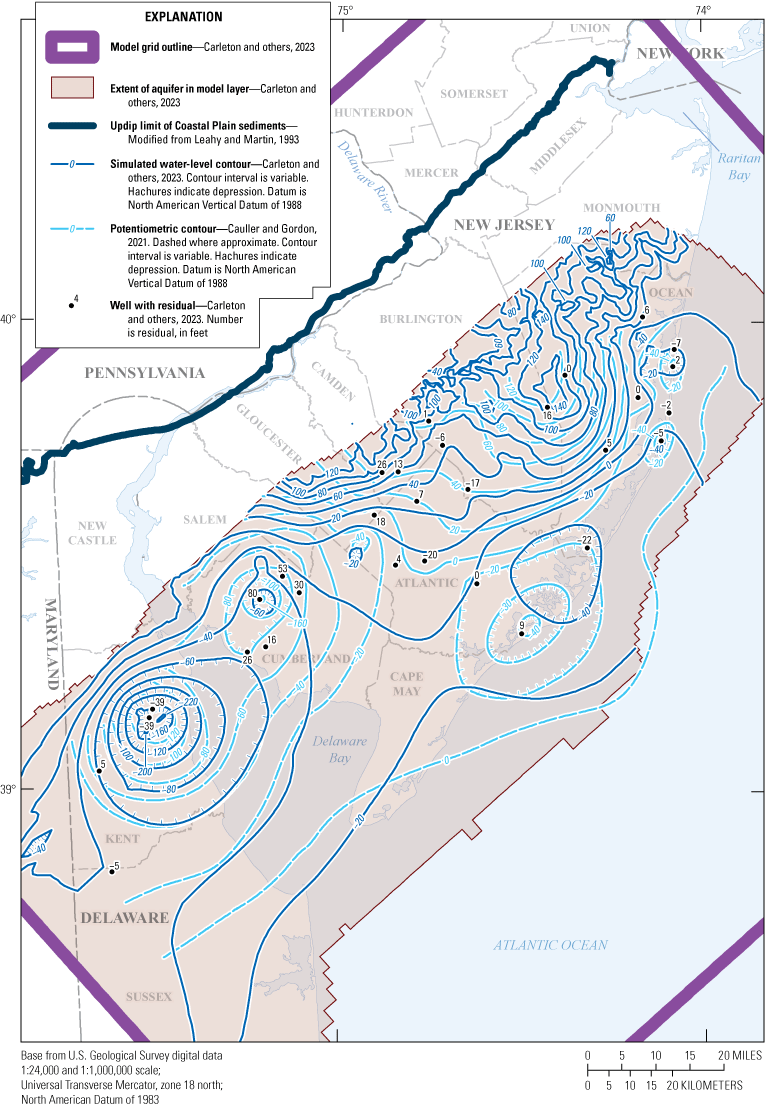
Map showing simulated water–level contours and the 2013 potentiometric surface for, and residuals for selected wells in, the Piney Point aquifer, New Jersey and Delaware.
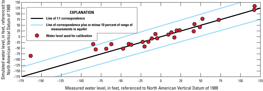
Graph showing simulated and observed water levels for selected wells open to the Piney Point aquifer, New Jersey and Delaware, 2013.
Hydrographs for two wells screened in the Piney Point aquifer are shown in figure 39. Simulated water levels in well 050676, located in an area in southeastern Burlington County where withdrawals are minimal, have the same flat trend but a smaller amplitude than observed water levels and are, on average, 16 ft greater than observed water levels (fig. 39A). The water levels simulated for this well by Voronin (2004) also show a smaller amplitude than observed water levels and are 5 to 10 ft lower than the observed water levels during 1980–98. The simulated water levels in well 110096 in Cumberland County have the same decreasing trend and amplitude as the observed water levels (associated with increased nearby withdrawals), but the simulated water levels are on average 9 ft greater than observed water levels (fig. 39B). The water levels simulated for this well by Voronin (2004) show a pattern similar to that of the simulated water levels shown in figure 39B for 1980–98.
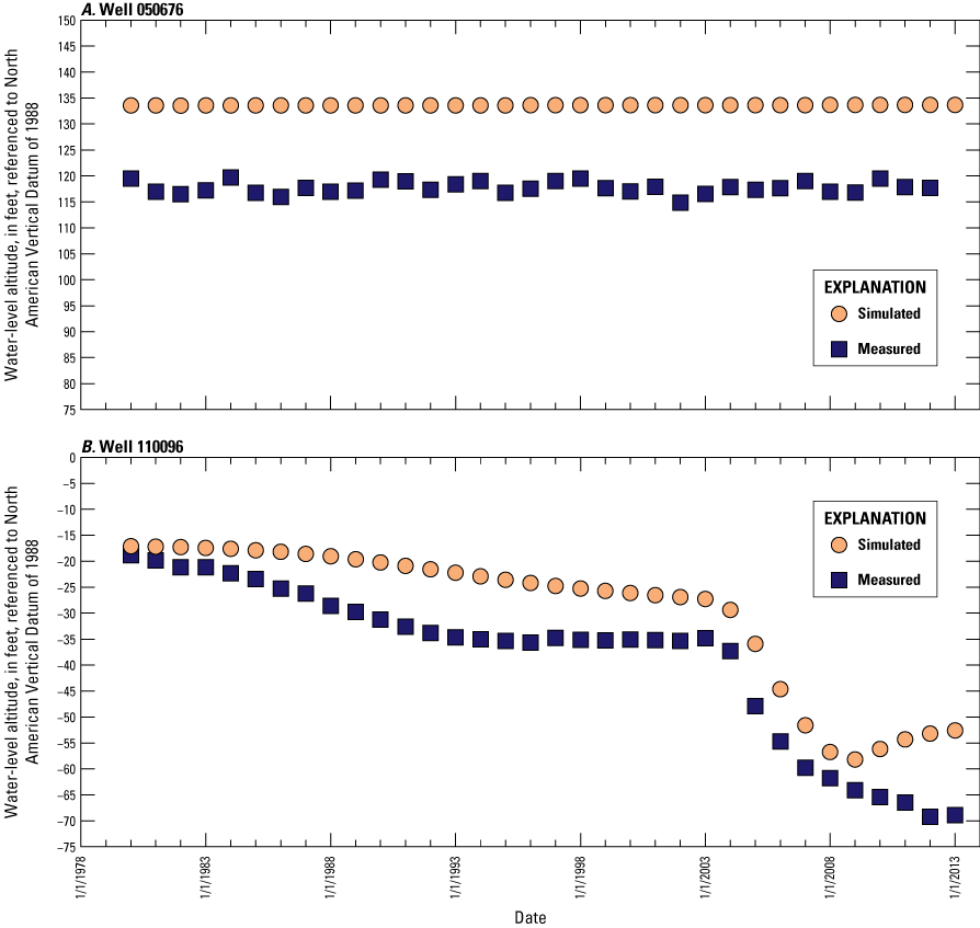
Hydrographs of simulated and observed water levels in wells A, 050676 and B, 110096, open to the Piney Point aquifer, New Jersey, 1980–2013.
Calibration of Water Levels in the Vincentown Aquifer
Simulated water level contours in the Vincentown aquifer (model layer 11, present primarily in Burlington, Gloucester, Monmouth, Ocean, and Salem Counties) generally match the 2013 potentiometric surface (Cauller and Gordon, 2021) (fig. 40). The differences between the simulated and observed water levels are shown in table 15 and in figures 40 and 41 for wells measured in New Jersey in 2013. The average water-level residual (simulated minus observed) for nine wells in Burlington, Gloucester, Monmouth, Ocean, and Salem Counties is −2 ft and the RMSE is 11 ft. The minimum; first, second, and third quartile; and maximum residuals are −9, −6, −2, 8, and 29 ft, respectively. The simulated water levels are within 10 ft of observed water levels for seven of the nine wells (89 percent) in New Jersey. The simulated water levels for the Rancocas aquifer in Delaware and the average water-level residual for one well measured in Delaware in 2013 (table 15) also are shown in figure 40.
Table 15.
Simulated and observed water-level observations and residuals for wells open to the Vincentown aquifer, New Jersey, and the Rancocas aquifer, Delaware, 2013.[USGS, U.S. Geological Survey; residual, simulated water level minus observed water level]
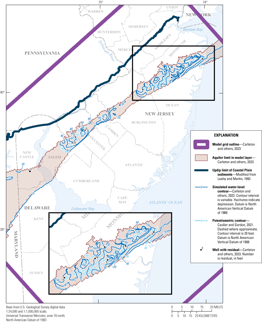
Map showing simulated water-level contours and the 2013 potentiometric surface for, and residuals for selected wells in, the Vincentown aquifer, New Jersey and the simulated water-level contours for, and residual for a selected well in, the Rancocas aquifer, Delaware.
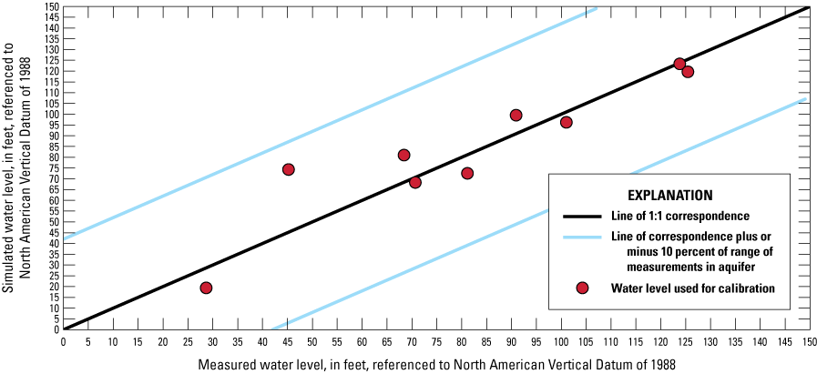
Graph showing simulated and observed water levels open to the Vincentown aquifer, New Jersey, 2013.
Hydrographs of simulated and observed water levels in wells 250636 and 290139 in Monmouth and Ocean Counties, respectively, show that simulated water levels are an average of 2 ft and about 3 ft lower than observed water levels, respectively, and have the same flat trend and similar amplitude (fig. 42). The hydrograph for well 290139 in Voronin (2004) is similar to the hydrograph shown in figure 42B for 1980–98, whereas the hydrograph for well 250636 (fig. 42A) in Voronin (2004) shows simulated water levels that are 20 to 25 ft lower than observed water levels during 1980–98.
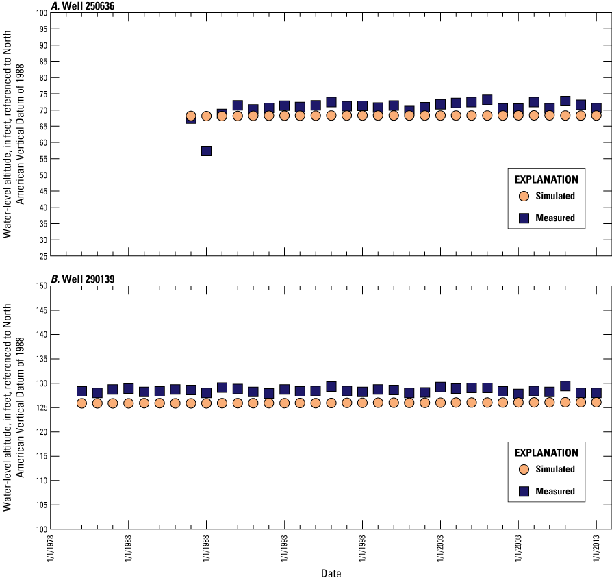
Hydrographs of simulated and observed water levels in wells, A, 250636, and B, 290139, open to the Vincentown aquifer, New Jersey, 1980–2013.
Calibration of Water Levels in the Wenonah-Mount Laurel Aquifer
Simulated water-level contours in the Wenonah-Mount Laurel aquifer (model layer 13, Monmouth, Ocean, Burlington, Camden, Gloucester, and Salem Counties) generally match the 2013 potentiometric surface (Cauller and Gordon, 2021), but the simulated water levels are lower in updip areas of Monmouth County and central Gloucester County (fig. 43). The simulated water-level contours generally are similar in shape to the 2013 potentiometric surface over much of the extent of the aquifer and the simulated water levels are within 10 or 20 ft of the water levels that were measured at the cones of depression associated with pumping centers in coastal Ocean and Monmouth Counties and western Burlington and central Camden Counties. The differences between the simulated and observed water levels for wells measured in New Jersey in 2013 are shown in table 16 and in figures 43 and 44. The average water-level residual (simulated minus observed) for 48 wells in Salem, Gloucester, Camden, Burlington, Ocean, and Monmouth Counties is −8 ft and the RMSE is 23 ft. The minimum; first, second, and third quartiles; and maximum residuals are –57, –23, –4, 7, and 55 ft, respectively. The simulated water levels are within 10 ft of observed water levels for 19 of the 48 wells (40 percent) and within 20 ft of observed water levels for 33 of the 48 wells (69 percent) in New Jersey. The simulated water levels for the Mount Laurel aquifer in Delaware and the average water-level residual for two wells measured in Delaware in 2013 (table 16) also are shown in figure 43.
Table 16.
Simulated and observed water-level observations and residuals for wells open to the Wenonah-Mount Laurel aquifer, New Jersey, and the Mount Laurel aquifer, Delaware, 2013.[USGS, U.S. Geological Survey; residual, simulated water level minus observed water level]
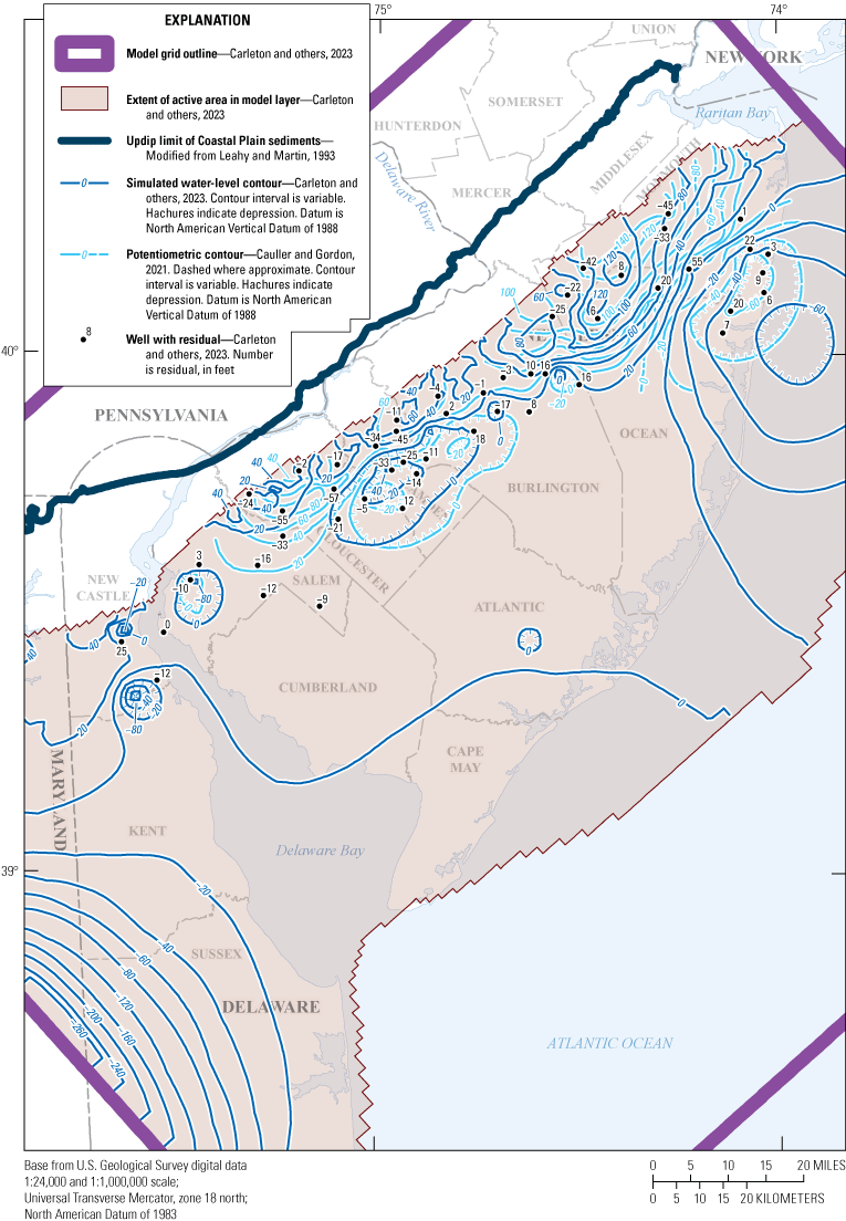
Map showing simulated water-level contours and the 2013 potentiometric surface for, and residuals for selected wells in, the Wenonah-Mount Laurel aquifer, New Jersey and simulated water-level contours for, and residuals for selected wells in, the Mount Laurel aquifer, Delaware.
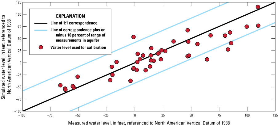
Graph showing simulated and observed water levels for selected wells open to the Wenonah-Mount Laurel aquifer, New Jersey, 2013.
The hydrographs of selected wells screened in the Wenonah-Mount Laurel aquifer are shown in figure 45. The hydrograph for well 070478 in Camden County indicates simulated water levels have a similar trend as observed water levels but a smaller amplitude and are lower from 1980 to 1992, but higher from 1993 to 2013, with an average difference of 8 ft (fig. 45A). These trends are also observed in the hydrograph shown in Voronin (2004) for this well during 1980–98. The hydrographs of simulated water levels for wells 250353 (fig. 45B) and 250637 (fig. 45C) in Monmouth County have the same trend and amplitude as observed water levels in those wells but with an average residual of 0.3 and 10 ft lower, respectively, than the observed water levels. Water levels in well 250353 simulated by Voronin (2004) show a smaller amplitude than the observed water levels, and the simulated water levels in well 250637 are about 10 ft lower than those observed during 1980–98. The hydrograph for well 290140 in Ocean County indicates that the simulated water levels have the same trend and amplitude as the observed water levels, and are, on average, within 3 ft of the observed water levels (fig. 45D). Simulated water levels in well 330020 in Salem County have the same trend and amplitude as observed water levels but are an average of 12 ft lower than them (fig. 45E).
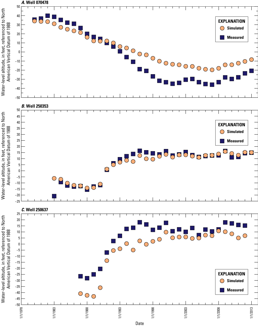
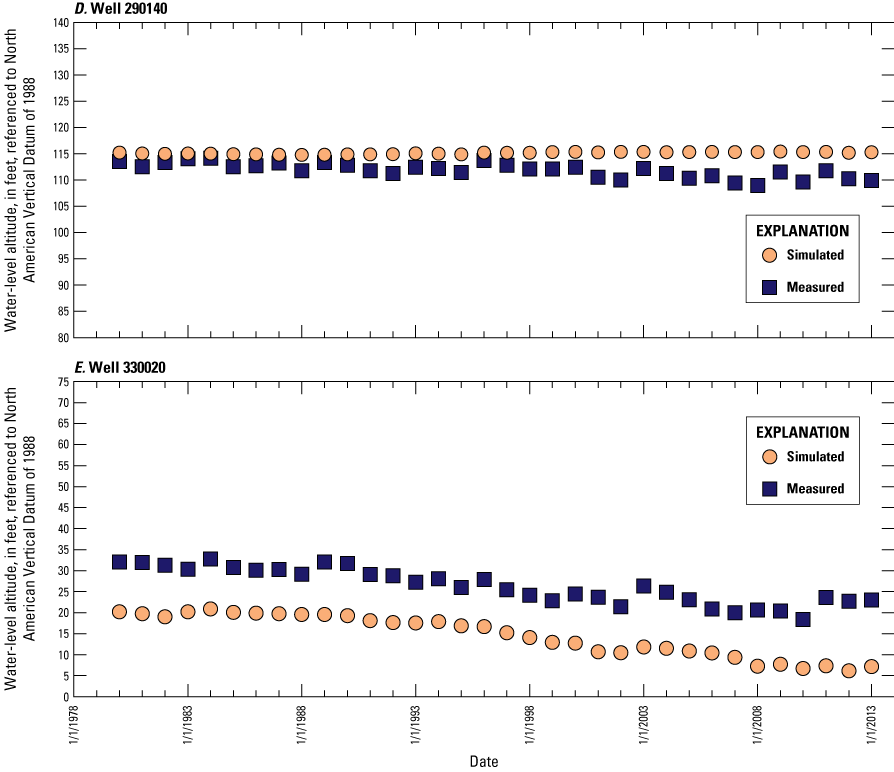
Hydrographs of simulated and observed water levels for wells A, 070478, B, 250353, C, 250637, D, 290140, and E, 330020, open to the Wenonah-Mount Laurel aquifer, New Jersey, 1980–2013.
Calibration of Water Levels in the Englishtown Aquifer System
Simulated water-level contours in the Englishtown aquifer system (model layer 15, Monmouth, Ocean, Burlington, Camden, Gloucester, and Salem Counties) generally match the 2013 potentiometric surface (Cauller and Gordon, 2021) but the simulated water levels are lower in parts of northern Camden and Burlington counties and near a pumping center in updip Monmouth County (fig. 46). The simulated contours and 2013 potentiometric surface generally have the same minima in the cones of depression in coastal southern Monmouth County and central northern Ocean County, but the cones differ in shape, partly as a result of simulated residuals and (or) of interpretation of the limited water-level data in areas used to develop the potentiometric contours. The differences between the simulated and observed water levels for wells measured in 2013 are shown in table 17 and figures 46 and 47. The average water-level residual (simulated minus observed) for 39 wells in New Jersey is −5 ft and the RMSE is 17 ft. The minimum; first, second, and third quartile; and maximum residuals are −41, −13, −1, 6, and 28 ft, respectively. The simulated water levels are within 10 ft of observed water levels for 23 of the 39 wells (59 percent) and within 15 ft of observed water levels for 29 of the 39 wells (74 percent) in New Jersey.
Table 17.
Simulated and observed water-level observations and residuals for wells open to the Englishtown aquifer system, New Jersey, 2013.[USGS, U.S. Geological Survey; residual, simulated water level minus observed water level]
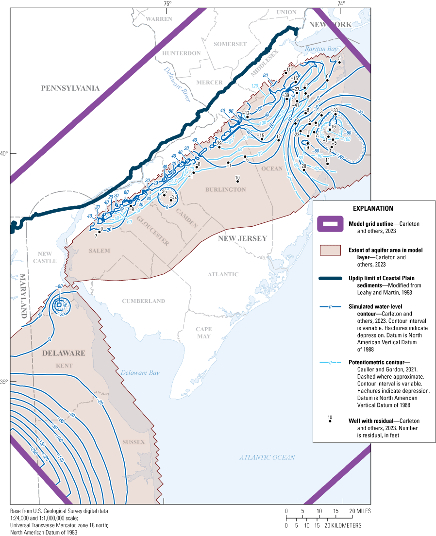
Map showing simulated water-level contours and 2013 potentiometric surface for, and residuals for selected wells in, the Englishtown aquifer system, New Jersey and simulated water-level contours for the Matawan aquifer, Delaware.
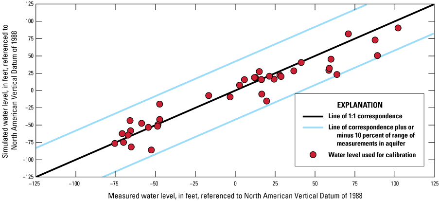
Graph showing simulated and observed water-levels for selected wells open to the Englishtown aquifer system, New Jersey, 2013.
The hydrographs of selected wells screened in the Englishtown aquifer system are shown in figure 48. The hydrograph for well 050259 in Burlington County shows that simulated water levels have the same trend and amplitude as observed water levels but are an average of 1 ft lower than observed water levels (fig. 48A). In comparison, the hydrograph in Voronin (2004) for well 050259 shows simulated water levels that are 5 to 10 ft higher than the observed water levels during 1980–98. The simulated water levels in the hydrographs for wells 250429 and 250638 in Monmouth County show the same trend of the recovering observed water levels in the 1990s and the amplitudes of the simulated water levels are similar to those of the observed water levels but are an average of –4 and –12 ft, respectively, lower than them (figs. 48B and 48C). In comparison, the hydrographs in Voronin (2004) for these two wells show simulated water levels that follow a similar pattern as those simulated by the current updated model but a smaller amplitude than observed water levels during 1980–98. Simulated water levels in well 290138 in Ocean County have the same trend and amplitude as observed water levels but are an average of 18 ft lower than them (fig. 48D). The hydrograph for this well in Voronin (2004) shows simulated water levels that are 10 to 15 ft higher than observed water levels during 1980–98.


Hydrographs of simulated and observed water levels in wells A, 050259, B, 250429, C, 250638, and D, 290138, open to the Englishtown aquifer system, New Jersey, 1980–2013.
Calibration of Water Levels in the Upper Potomac Raritan Magothy Aquifer
Simulated water-level contours in the upper Potomac-Raritan-Magothy aquifer (model layer 17, Middlesex, Mercer, Monmouth, Ocean, Burlington, Camden, Gloucester, and Salem Counties) closely match the 2013 potentiometric surface (Cauller and Gordon, 2021) (fig. 49). The simulated contours and 2013 potentiometric surface are similar in shape and the contours correspond well in the areas of the major cones of depression in central Camden and Ocean Counties. The differences (residuals) between the simulated and observed water levels for wells measured in New Jersey in 2013 are shown in table 18 and in figures 49 and 50. The average water-level residual for 88 wells in New Jersey is 9 ft and the RMSE is 14 ft. The minimum; first, second, and third quartile; and maximum residuals for New Jersey wells are −17, 2, 24, 15, and 35 ft, respectively. The simulated water levels are within 10 ft of observed water levels for 46 of the 88 wells (52 percent) and within 15 ft of observed water levels for 64 of the 88 wells (73 percent) in New Jersey. The simulated water levels for the Magothy aquifer in Delaware and the average water-level residual for four wells measured in Delaware in 2013 (table 18) also are shown in figure 49.
Table 18.
Simulated and observed water-level observations and residuals for wells open to the upper Potomac-Raritan-Magothy aquifer, New Jersey, and the Magothy aquifer, Delaware, 2013.[USGS, U.S. Geological Survey; residual, simulated water level minus observed water level]
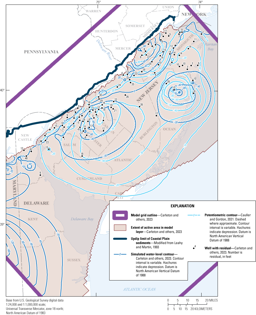
Map showing simulated water-level contours and 2013 potentiometric surface for, and residuals for selected wells in, the upper Potomac-Raritan-Magothy aquifer, New Jersey and simulated water-level contours for, and residuals for selected wells in, the Magothy aquifer, Delaware.
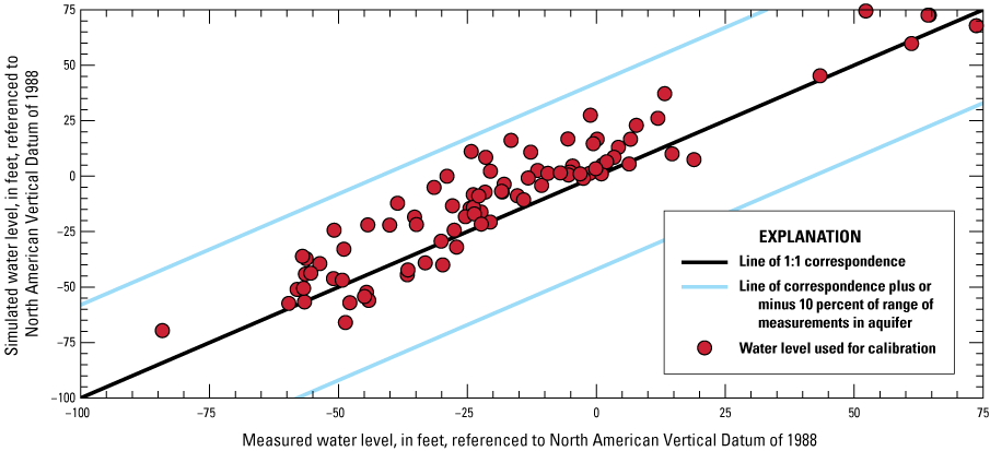
Graph showing simulated and observed water-levels for selected wells open to the upper Potomac-Raritan-Magothy aquifer, New Jersey, 2013.
The hydrographs of four selected wells screened in the upper Potomac-Raritan-Magothy aquifer are shown in figure 51. Simulated water levels in wells 050258, 070477, 150728, and 250639 in Burlington, Camden, Gloucester, and Monmouth Counties, respectively, have the same trend and amplitude as observed water levels but are an average of 24, 11, 11, and 6 ft higher than them, respectively. The hydrographs for these four wells in Voronin (2004) show simulated water levels in wells 050258, 070477, and 150728 that are 5 to 15, 15 to 25, and 5 to 10 ft higher, respectively, than the observed water levels during 1980–98; the hydrograph for well 290639 shows simulated water levels within 15 ft of observed water levels, but with smaller amplitude.


Hydrographs of simulated and observed water levels in wells A, 050258, B, 070477, C, 150728, and D, 250639, open to the upper Potomac-Raritan-Magothy aquifer, New Jersey, 1980–2013.
Calibration of Water Levels in the Middle Potomac-Raritan-Magothy Aquifer
Simulated water-level contours in the middle Potomac-Raritan-Magothy aquifer (model layer 19, Middlesex, Mercer, Monmouth, Ocean, Burlington, Camden, Gloucester, and Salem Counties) closely match the 2013 potentiometric surface (Cauller and Gordon, 2021) (fig. 52). The simulated contours and 2013 potentiometric surface are similar in shape and correspond well in the areas of the major cones of depression in central Camden County and north-central Ocean County. The differences between the simulated and observed water levels for wells measured in New Jersey in 2013 are shown in table 19 and in figures 52 and 53. The average water-level residual (simulated minus observed) for 73 wells in New Jersey is 1 ft and the RMSE is 9 ft. The minimum; first, second, and third quartile; and maximum residuals are −22, −4, −0.1, 7, and 24 ft, respectively. The simulated water levels are within 10 ft of observed water levels for 57 of the 73 wells (78 percent) and within 15 ft of observed water levels for 68 of the 73 wells (93 percent) in New Jersey. The simulated water levels for the Potomac-Patapsco aquifer in Delaware and the average water-level residual for three wells measured in Delaware in 2013 (table 19) also are shown in figure 52.
Table 19.
Simulated and observed water-level observations and residuals for wells open to the middle Potomac-Raritan-Magothy aquifer, New Jersey, and the Potomac-Patapsco aquifer, Delaware, 2013.[USGS, U.S. Geological Survey; residual, simulated water level minus observed water level]
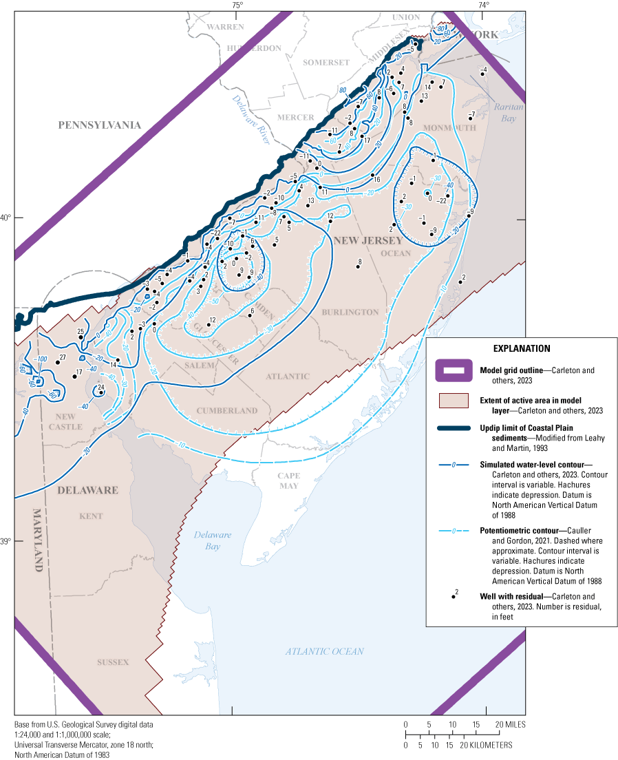
Map showing simulated water-level contours and the 2013 potentiometric surface for, and residuals for selected wells in, the middle Potomac-Raritan-Magothy aquifer, New Jersey, and the simulated water-level contours for, and residuals for selected wells in, the Potomac-Patapsco aquifer, Delaware.
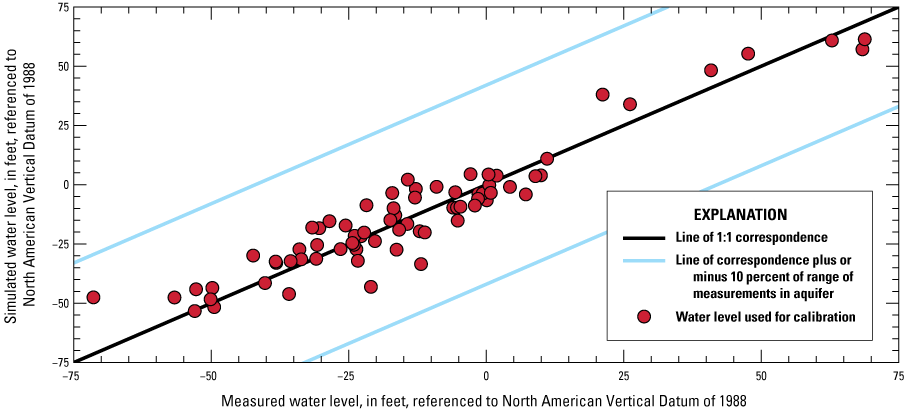
Graph showing simulated and observed water-levels for selected wells open to the middle Potomac-Raritan-Magothy aquifer, New Jersey, 2013.
The hydrographs of five wells screened in the Middle Potomac-Raritan-Magothy aquifer are shown in figure 54. The simulated water levels in wells 050063, 050261, 150713, 330187, and 330251, located in Burlington (2 wells), Gloucester (1 well), and Salem (2 wells) Counties, respectively, have the same trend and amplitude as the observed water levels but are an average of −5, 10, −5, 2, and 15 ft higher or lower, respectively, than them. In comparison, the hydrographs for wells 150713, 330187, and 330251 in Voronin (2004) show simulated water levels that are 0 to 5, 10 to 15, and 0 to 10 ft higher, respectively, than observed water levels during 1980–98, and simulated water levels in well 050261 that are 5 to 10 ft lower prior to 1984 and 5 to 10 ft higher during 1992–98 than observed water levels.
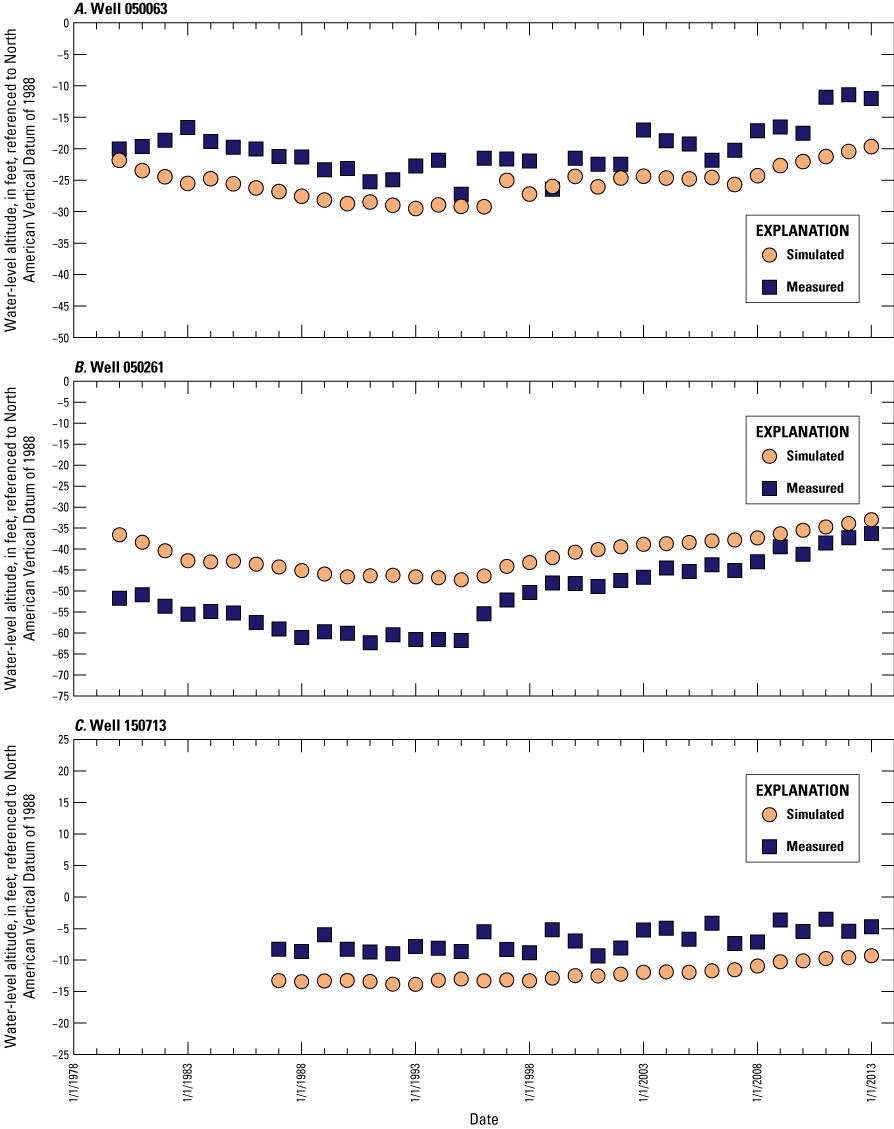
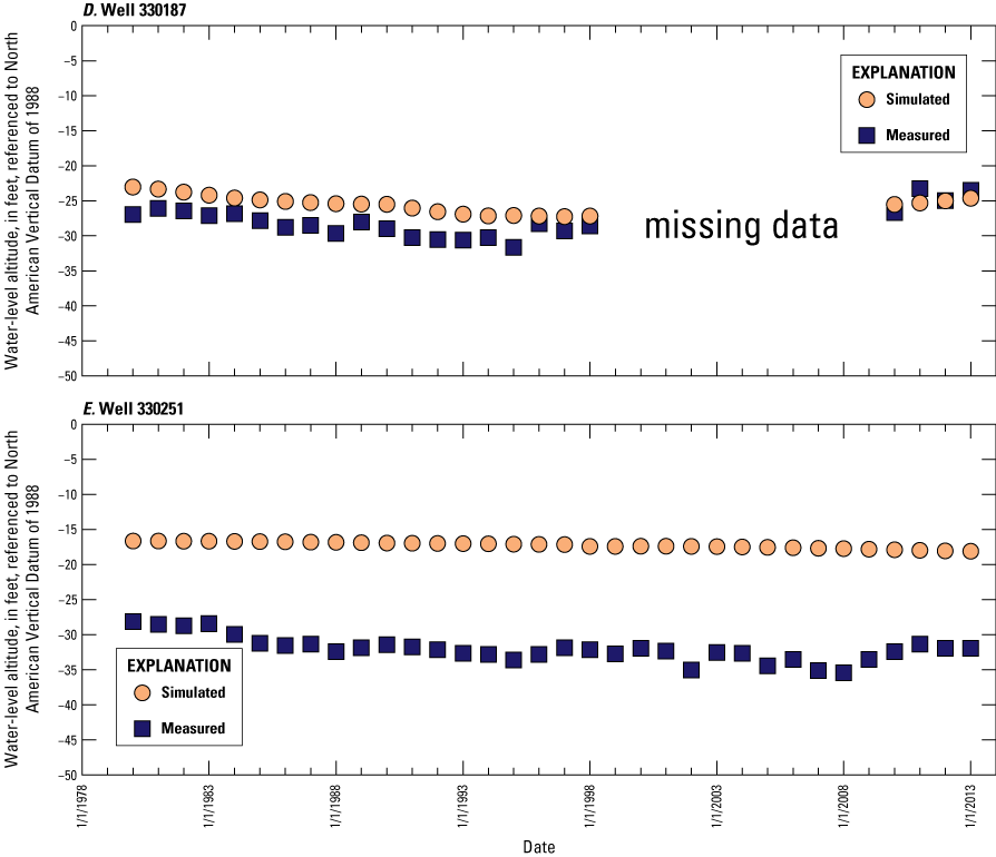
Hydrographs of simulated and observed water levels in wells A, 050063, B, 050261, C, 150713, D, 330187, and E, 330251, open to the middle Potomac-Raritan-Magothy aquifer, New Jersey, 1980–2013.
Calibration of Water Levels in the Lower Potomac-Raritan-Magothy Aquifer
Simulated water-level contours in the lower Potomac-Raritan-Magothy aquifer (model layer 21, Burlington, Camden, Gloucester, and Salem Counties) generally match the 2013 potentiometric surface (Cauller and Gordon, 2021) (fig. 55). The simulated water-level contours are similar in shape, and the location of the major cone of depression in central Camden County and the location of the major cone of depression in Salem County that results from withdrawals in Delaware, corresponds closely to the location of the two simulated cones of depression. The differences between the simulated and observed water levels for wells measured in New Jersey in 2013 are shown in table 20 and in figures 55 and 56. The average water-level residual (simulated minus observed) for 39 wells in New Jersey is −4 ft and the RMSE is 13 ft. The minimum; first, second, and third quartile; and maximum residuals are −25, −13, −3, 3, and 29 ft, respectively. The simulated water levels are within 10 ft of observed water levels for 25 of the 39 wells (64 percent) and within 15 ft of observed water levels for 31 of the 39 wells (79 percent) in New Jersey. The simulated water levels for the Potomac-Patuxent aquifer in Delaware and the average water-level residual for five wells measured in Delaware in 2013 (table 20) also are shown in figure 55.
Table 20.
Simulated and observed water-level observations and residuals for wells open to the lower Potomac-Raritan-Magothy aquifer, New Jersey, and the Potomac-Patuxent aquifer, Delaware, 2013.[USGS, U.S. Geological Survey; residual, simulated water level minus observed water level]
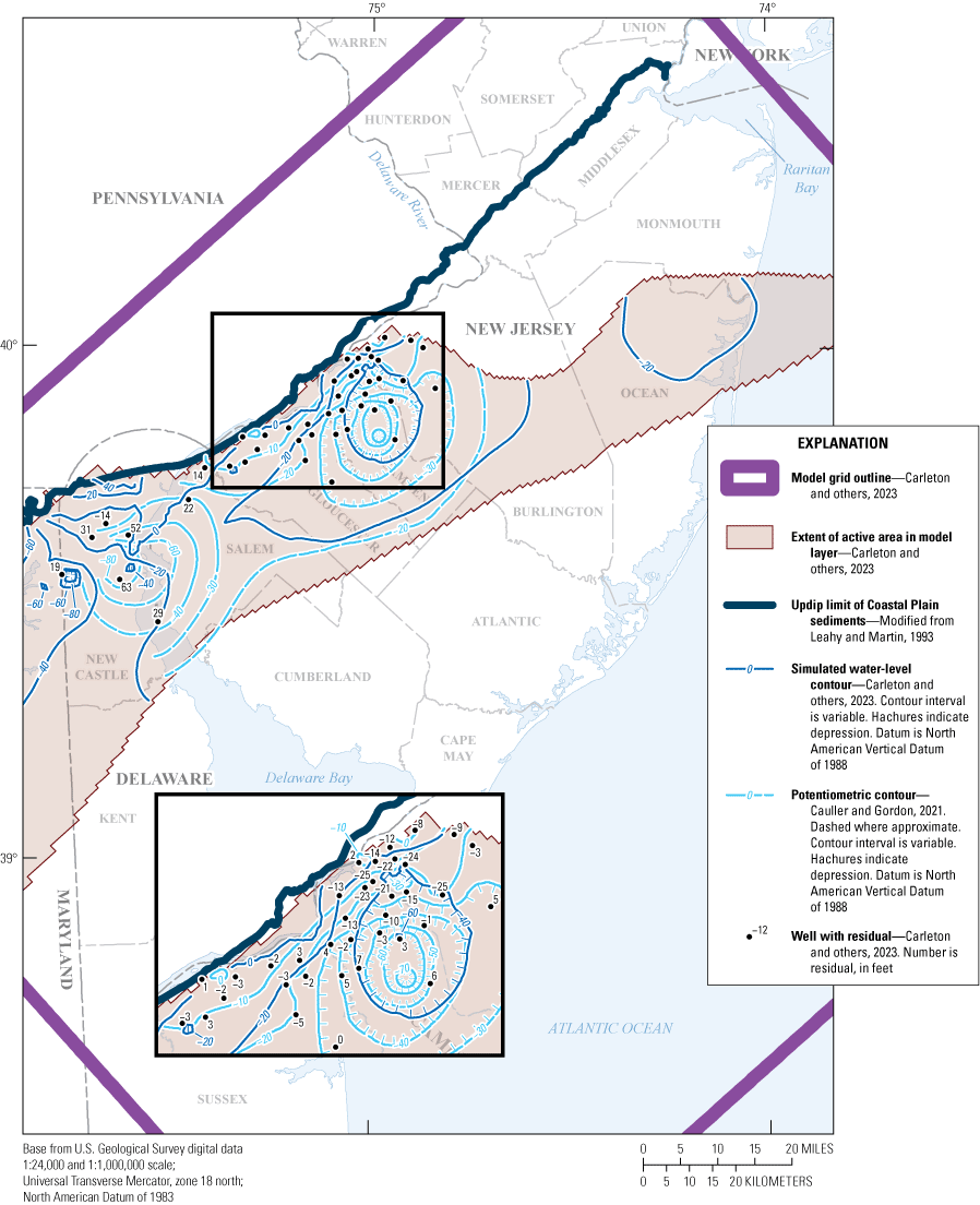
Map showing simulated water-level contours and the 2013 potentiometric surface for, and residuals for selected wells in, the lower Potomac-Raritan-Magothy aquifer, New Jersey and simulated water-level contours for, and residuals for selected wells in, and the Potomac-Patuxent aquifer, Delaware.
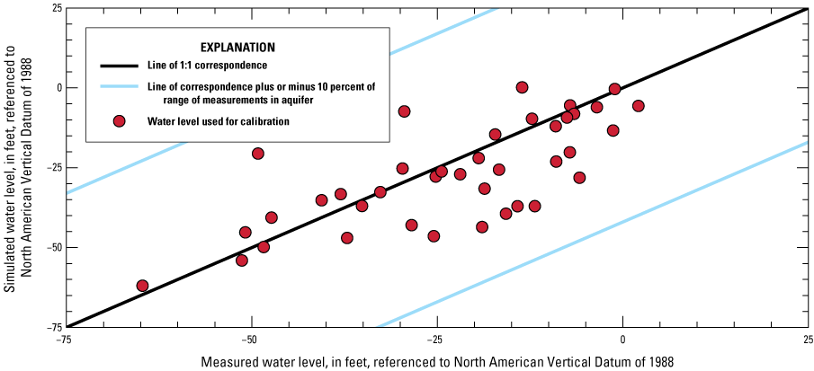
Graph showing simulated and observed water-levels for selected wells open to the lower Potomac-Raritan-Magothy aquifer, New Jersey, 2013.
The hydrographs of three selected wells screened in the Lower Potomac-Raritan-Magothy aquifer are shown in figure 57. Simulated water levels in wells 050262, 070412, and 150712, located in Burlington, Camden, and Gloucester Counties, respectively, have the same trend and amplitude as observed water levels and are an average of 10, 8, and −2 ft higher than observed water levels, respectively. The hydrograph for well 050262 in Voronin (2004) shows simulated water levels that range from 15 to 20 ft lower before 1984 and 0 ft to 10 ft higher during 1990–98 than observed water levels, and the hydrograph for well 150712 shows simulated water levels that are 5 to 10 ft higher than observed water levels during 1980–98.
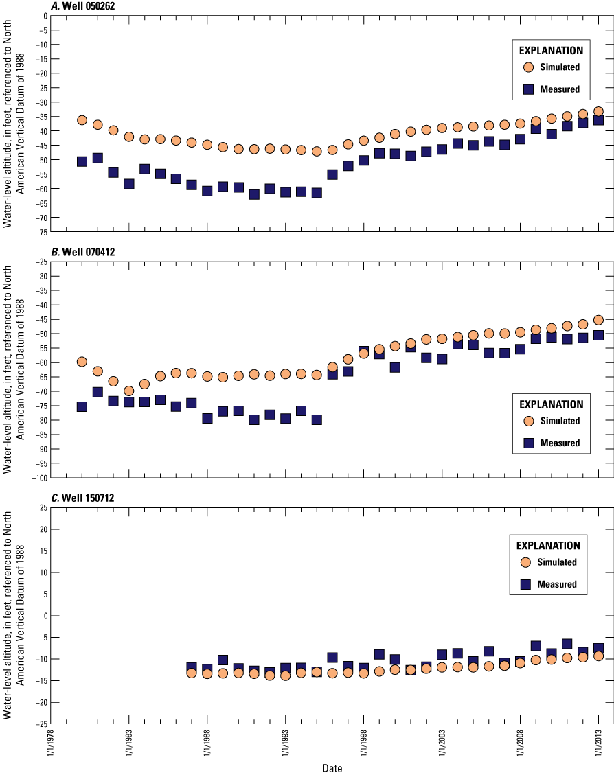
Hydrographs of simulated and observed water levels in wells A, 050262, B, 070412, and C, 150712, open to the lower Potomac-Raritan-Magothy aquifer, New Jersey, 1980–2013.
Average Simulated Water Levels in Critical Areas 1 and 2, 1980–2013
The State of New Jersey instituted a program in the late 1980s to reduce groundwater withdrawals in two designated Critical Areas in which water levels in certain aquifers used for water supply had declined substantially. Restrictions on groundwater withdrawals in Critical Area 2 apply only to the aquifers of the PRM aquifer system and were initiated in 1996. Critical Area 1 restrictions were implemented in 1989, however compliance by most purveyors was deferred until 1991 because access to alternate water supplies was not initially available. The potentiometric surface in 2013 indicates that water levels generally recovered in the Critical Areas during 1983–2013, particularly at the center of the regional cones of depression measured in the Critical Areas in 1983 (Gordon and others, 2021). Trends in the average simulated water levels and withdrawals for the period 1980–2013 are shown by aquifer in figures 58 and 59. Figure 58A shows the decrease in simulated groundwater withdrawals in Critical Area 1, generally after the mid-1990s, from the Englishtown aquifer system, Wenonah-Mount Laurel aquifer, and the upper and middle PRM aquifer and a general recovery in average simulated water levels (fig. 58B), particularly in the Englishtown aquifer system and the Wenonah-Mount Laurel aquifer, resulting from the decrease in groundwater withdrawals from those aquifers. The average simulated water levels in the upper PRM aquifer show a decline after 2004, however, the average simulated water levels show a recovery after 2010. Figure 59A shows a decrease in groundwater withdrawals from the upper, middle, and lower PRM aquifers in Critical Area 2 generally after 1996 and the subsequent recovery in average simulated water levels in those aquifers is shown in figure 59B. These figures show the withdrawal data in cubic feet per second (the units used for withdrawal data in the New Jersey Coastal Plain groundwater-flow model) together with the water levels simulated with the model for the Critical Area aquifers.
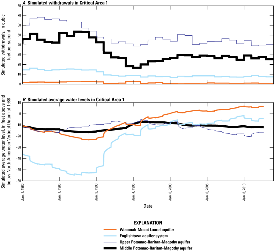
Graphs showing A, simulated withdrawals and B, simulated average water levels in Critical Area 1 for the Wenonah-Mount Laurel aquifer, Englishtown aquifer system, upper Potomac-Raritan-Magothy aquifer, and middle Potomac-Raritan-Magothy aquifer, New Jersey Coastal Plain, 1980–2013.
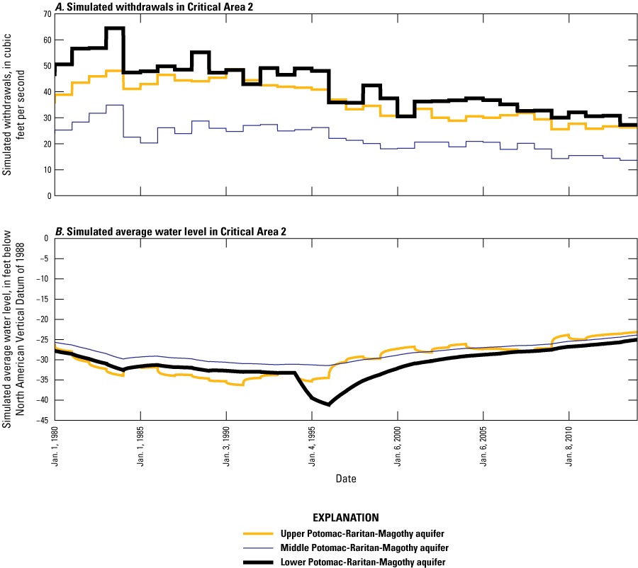
Graphs showing A, simulated withdrawals and B, simulated average water levels in Critical Area 2 for the upper Potomac-Raritan-Magothy aquifer, middle Potomac-Raritan-Magothy aquifer, and lower Potomac-Raritan-Magothy aquifer, New Jersey Coastal Plain, 1980–2013.
Model Limitations
The purpose of the New Jersey Coastal Plain groundwater-flow model is to represent the interactions of groundwater flow in and simulated water levels in 11 major aquifers in the groundwater-flow system of the New Jersey Coastal Plain. In the model, grid-cell dimensions are smaller in the onshore part of New Jersey than in offshore areas, Delaware, and Maryland. The smaller grid-cell dimensions were used to improve the accuracy of the flow simulation in the aquifers in New Jersey and are adequate for a regional representation of the groundwater-flow system. However, spatial and temporal discretization in the model require simplifications of the groundwater-flow system. Although detailed groundwater/surface-water interactions cannot be evaluated in some areas, the model cell size is adequate for a regional representation of streams in New Jersey. However, because land-surface elevation and hydraulic parameters are assigned values that represent an average over an entire model cell, they may not accurately represent parameters for the streams.
The model simulates the groundwater-flow system using average annual withdrawals and estimated annual recharge rates. The water-level calibration attempts to reproduce water levels measured in late fall of the seven quinquennial New Jersey Coastal Plain water-level synoptic studies (1983, 1988, 1993, 1998, 2003, 2008, and 2013) to represent an approximation of average annual water-level conditions. Water levels that result from seasonal variations in groundwater withdrawals or recharge rates are not simulated and this may introduce inaccuracies in matching observed and simulated water levels and base flows. Although permitted withdrawals from public-supply, industrial, commercial, and agricultural wells are simulated in the model, domestic-self supply wells are not included in the withdrawal dataset; these wells are typically open to the shallower aquifers, potentially affecting base flow to the simulated streams or water levels in the aquifers that crop out.
The unconfined surficial aquifer in Delaware and eastern Maryland was not included in the model hydrogeologic framework; however, the effects of withdrawals from the surficial aquifer are assumed to be controlled by local streams and not to affect water levels in New Jersey. Recharge to the surficial aquifer in this area was input as fluxes to the model layer. The model is based on a 21-layer hydrogeologic framework, because the framework used to represent the groundwater-flow system is regionalized, local clay units or heterogeneities that affect the groundwater-flow system may not represented.
Summary
The U.S. Geological Survey, in cooperation with the New Jersey Department of Environmental Protection, updated a previously published regional groundwater-flow model of the New Jersey Coastal Plain by incorporating a revised hydrogeologic framework of the New Jersey Coastal Plain and groundwater withdrawals from 1980 to 2013, updating groundwater recharge based on a soil-water balance budget, and extending the model into Delaware to address the effects of withdrawals from aquifers that extend into that state.
The three-dimensional transient groundwater-flow model was developed by using the numerical code MODFLOW–2005. The model was constructed by using hydrogeologic information about and estimated hydraulic properties of 11 separate aquifers and 10 intervening confining units to represent the groundwater-flow system. The finite-difference grid consists of 145 rows, 245 columns, and 21 layers. The model extends from the updip limit of the Coastal Plain sediments in New Jersey, Delaware, and Maryland, downdip to the boundary between freshwater and saltwater in each aquifer.
The model was calibrated by using the parameter-estimation code UCODE–2014 as well as manual calibration techniques. Seven categories of parameters were adjusted: horizontal and vertical hydraulic conductivity, storage coefficient, riverbed conductance for the Delaware River, streambed conductance for the other streams in the model area, general-head-boundary conductance, and recharge, resulting in a total of 422 parameters. Model calibration consisted of matching data for 1980 to 2013 that include 3,453 water levels measured during 1983–2013 in 440 wells in New Jersey and Delaware, which includes trends in water levels for 29 wells in New Jersey during 1980–2013 presented in time-series hydrographs, and historical base-flow measurements made during 1980–2013 in 47 surface-water basins in New Jersey. Observations of vertical gradients were calculated for 33 pairs of nested observation wells in New Jersey, for a total of 210 observations. Changes in water levels over time were calculated for 138 wells, 134 wells in New Jersey and four wells in Delaware, where water levels had varied substantially (approximately 10 ft) over the 30-year span of synoptic water-level measurements, for a total of 767 observations.
The simulated water levels for the New Jersey Coastal Plain aquifers were compared to water-level measurements made during 1980–2013. The average water-level residual (simulated minus observed water level) for 4,243 water-level observations for New Jersey is 1.5 ft. The simulated water-level contours for the confined aquifers for 2013 were compared to potentiometric surfaces produced from water levels measured during 2013. Simulated water levels generally matched the 2013 potentiometric surfaces of the confined aquifers in the areas of large withdrawals, most of the simulated water levels are within 10 to 15 ft of the observed water levels. Hydrographs of 29 wells in the New Jersey coastal Plain aquifers with long-term water level measurements from 1980 to 2013 show that simulated water levels reasonably match the magnitude and seasonal variation of the observed water levels. Hydrographs of base-flow for the 47 streamgaging stations indicate that most of the simulated and observed data match reasonably well.
The sensitivity of simulated water levels to the model parameters was calculated with UCODE-2014. Composite scaled sensitivities were calculated for the 422 parameters by using the water level and base-flow observations. Parameters most sensitive to water-level observations include recharge and horizontal hydraulic conductivity, and vertical hydraulic conductivity. Recharge is the dominant parameter with respect to base-flow observations, but streambed conductance, horizontal hydraulic conductivity and storage parameters are also sensitive in and near outcrop areas in some aquifers.
Several limitations are associated with the ability of the New Jersey Coastal Plain groundwater-flow model to simulate the regional groundwater-flow system of the New Jersey Coastal Plain. The model simulates the groundwater-flow system using average annual withdrawals and estimated annual recharge rates. Spatial discretization in the model requires simplifications of the groundwater-flow system that may prevent the model from representing smaller scale hydrologic features. Temporal discretization in the model may limit the accuracy of simulated water levels that result from seasonal variations in groundwater withdrawals or recharge rates that are not simulated, thereby introducing inaccuracies in matching observed and simulated water levels and base flows. Although the model is based on a 21-layer hydrogeologic framework, because the framework used to represent the groundwater-flow system is regionalized, local clay units or heterogeneities that affect the groundwater-flow system may not be represented.
The groundwater-flow model of the New Jersey Coastal Plain must be updated periodically to maintain its usefulness as a tool for managing water resources and evaluating water-resource-development alternatives because of changing hydrologic stresses, changing and increasingly complex water-management needs, and updated knowledge of hydrologic conditions. The conversion from a quasi- to a fully three-dimensional model will allow for potential future uses such as particle tracking and simulation of variable-density flow that were not possible with earlier versions of the model. The addition of annual recharge estimates derived by using the U.S. Geological Survey Soil-Water Balance model (SWB) resulted in a spatially and temporally finer discretization. These updates will support the application of this model as a tool to evaluate regional effects of changes in groundwater withdrawals on water levels and the effects of potential water-management strategies in the New Jersey Coastal Plain. This current revision further improves the accuracy of the model and enhances its usefulness for evaluating alternative water-management alternatives under recent conditions.
References Cited
Andreasen, D.C., Staley, A.W., and Achmad, G., 2013, Maryland Coastal Plain aquifer information system—Hydrogeologic framework: Maryland Geological Survey Open-File Report no. 12–02–20, 121 p. [Also available at http://www.mgs.md.gov/publications/report_pages/OFR_12-02-20.html.]
Barlow, P.M., Cunningham, W.L., Zhai, T., and Gray, M., 2015, U.S. Geological Survey groundwater toolbox, a graphical and mapping interface for analysis of hydrologic data (version 1.3.1)—User guide for estimation of base flow runoff, and groundwater recharge from streamflow data: U.S. Geological Survey Techniques and Methods, book 3, chap. B10, 27 p. [Also available at https://doi.org/10.3133/tm3B10.]
Carleton, G.B., Gordon, A.D., Kenefic, L.F., Watt, M.K., and Buxton, D.E., 2023, MODFLOW–2005 used to simulate the regional groundwater flow system in the updated New Jersey Coastal Plain model, 1980–2013: U.S. Geological Survey data release, https://doi.org/10.566/P9W6RXFC.
Cauller, S.J., and Gordon, A.D., 2021, Geospatial data representing wells open to, and 2013 potentiometric-surface contours of, the confined aquifers of the New Jersey Coastal Plain: U.S. Geological Survey data release, accessed February 11, 2021, at https://doi.org/10.5066/P9EKA147.
Cauller, S.J., Voronin, L.M., and Chepiga, M.M., 2016, Simulated effects of groundwater withdrawals from aquifers in Ocean County and vicinity, New Jersey: U.S. Geological Survey Scientific Investigations Report 2016–5035, 77 p., accessed November 11, 2017 at https://doi.org/10.3133/sir20165035.
Charles, E.G., Nawyn, J.P., Voronin, L.M., and Gordon, A.D., 2011, Simulated effects of allocated and projected 2025 withdrawals from the Potomac-Raritan-Magothy aquifer system, Gloucester and Northeastern Salem Counties, New Jersey: U.S. Geological Survey Scientific Investigations Report 2011–5033, 145 p.[Also available at https://doi.org/10.3133/sir20115033.]
Charles, E.G., Storck, D.A., and Clawges, R.M., 2001, Hydrology of the unconfined aquifer system, Maurice River area–Maurice and Cohansey River Basins, New Jersey, 1994–95: U.S. Geological Survey Water-Resources Investigations Report 01–4229, 5 pls. [Also available at https://doi.org/10.3133/wri014229.]
Colarullo, S.J., Sullivan, S.L., and McHugh, A.R., 2018, Implementation of MOVE.1, censored MOVE.1, and piecewise MOVE.1 low-flow regressions with applications at partial-record streamgaging stations in New Jersey: U.S. Geological Survey Open-File Report 2018–1089, 20 p., accessed September 12, 2022 at https://doi.org/10.3133/ofr20181089.
Delaware Geological Survey, 2017, Recent and historical groundwater level data: Delaware Geological Survey, accessed November 8, 2017, at https://www.dgs.udel.edu/sites/recent-and-historical-groundwater-level-data.html.
DePaul, V.T., and Rosman, R., 2015, Water-level conditions in the confined aquifers of the New Jersey Coastal Plain, 2008: U.S. Geological Survey Scientific Investigations Report 2013–5232, 107 p., 9 pls., accessed March 20, 2017, at https://doi.org/10.3133/sir20135232.
DePaul, V.T., Rosman, R., and Lacombe, P.J., 2009, Water-level conditions in selected confined aquifers of the New Jersey and Delaware Coastal Plain, 2003: U.S. Geological Survey Scientific Investigations Report 2008–5145, 123 p., 9 pls. [Also available at https://doi.org/10.3133/sir20085145.]
Domber, S., Snook, I., and Hoffman, J.L., 2013, Using the stream low flow margin method to assess water availability in New Jersey’s water-table-aquifer system, New Jersey Geological and Water Survey Technical Memorandum 13–3, 70 p. [Also available at https://dep.nj.gov/wp-content/uploads/njgs/reports/tmemo/tm13-3.pdf.]
Dugan, B.L., Neimeister, M.P., and Andres, A.S., 2008, Hydrogeologic framework of southern New Castle County: Delaware Geological Survey Open-File Report No. 49, 22 p., 3 pls. [Also available at https://www.dgs.udel.edu/publications/ofr49-hydrologeologic-framework-southern-new-castle-county.]
Eckel, J.A., and Walker, R.L., 1986, Water levels in major artesian aquifers of the New Jersey Coastal Plain, 1983: U.S. Geological Survey Water-Resources Investigations Report 86–4028, 62 p., 7 pls. [Also available at https://doi.org/10.3133/wri864028.]
Essaid, H.I., 1990, The computer model SHARP, a quasi-three-dimensional finite-difference model to simulate freshwater and saltwater flow in layered coastal aquifer systems: U.S. Geological Survey Water-Resources Investigations Report 90–4130, 181 p. [Also available at https://doi.org/10.3133/wri904130.]
Farlekas, G.M., 1979, Geohydrology and digital-simulation model of the Farrington aquifer in the northern Coastal Plain of New Jersey: U.S. Geological Survey Water-Resources Investigations Report 79–106, 55 p. [Also available at https://doi.org/10.3133/wri79106.]
Farlekas, G.M.., Nemickas, B., and Gill, H.E., 1983, Geology and ground-water resources of Camden County, New Jersey: U.S. Geological Survey Water-Resources Investigations Report 83–4029, 158 p. [Also available at https://doi.org/10.3133/wri834029.]
Gordon, A.D., 2004, Hydrology of the unconfined aquifer system, Forked River and Cedar, Oyster, Mill, Westecunk, and Tuckerton Creek Basins and adjacent basins in the southern Ocean County area, New Jersey, 1998–99: U.S. Geological Survey Water-Resources Investigations Report 03–4337, 5 pls. [Also available at https://doi.org/10.3133/wri034337.]
Gordon, A.D., 2007, Simulated effects of projected 2010 withdrawals on ground-water flow and water levels in the New Jersey Coastal Plain– A task of the New Jersey Water Supply Plan 2006 Revision: U.S. Geological Survey Scientific Investigations Report 2007–5134, 116 p. [Also available at https://doi.org/10.3133/sir20075134.]
Gordon, A.D., Carleton, G.B., and Rosman, R., 2021, Water-level conditions in the confined aquifers of the New Jersey Coastal Plain, 2013: U.S. Geological Survey Scientific Investigations Report 2019–5146, 104 p., 9 pls., accessed March 31, 2021 at https://doi.org/10.3133/sir20195146.
Harbaugh, A.W., 2005, MODFLOW–2005—The U.S. Geological Survey modular ground-water model—The ground-water flow process: U.S. Geological Survey Techniques and Methods, book 6, chap. A16 [variously paged]. [Also available at https://doi.org/10.3133/tm6A16.]
Harbaugh, A.W., and McDonald, M.G., 1996, User’s documentation for MODFLOW–96, an update to the U.S. Geological Survey modular finite-difference ground-water flow model: U.S. Geological Survey Open-File Report 96–485, 56 p. [Also available at https://doi.org/10.3133/ofr96485.]
Heath, R.C., 1983, Basic ground-water hydrology: U.S. Geological Survey Water-Supply Paper 2220, 86 p. [Also available at https://doi.org/10.3133/wsp2220.]
Johnson, M.L., and Charles, E.G., 1997, Hydrology of the unconfined aquifer system, Salem River Area—Salem River and Raccoon, Oldmans, Alloway, and Stow Creek Basins, New Jersey, 1993–94: U.S. Geological Survey Water-Resources Investigations Report 96–4195, 5 pls. [Also available at https://doi.org/10.3133/wri964195.]
Johnson, M.L., and Watt, M.K., 1996, Hydrology of the unconfined aquifer system, Mullica River basin, New Jersey, 1991–92: U.S. Geological Survey Water-Resources Investigations Report 94–4234, 6 sheets. [Also available at https://doi.org/10.3133/wri944234.]
Lacombe, P.J., and Carleton, G.B., 2002, Hydrogeologic framework, availability of water supplies, and saltwater intrusion, Cape May County, New Jersey: U.S. Geological Survey Water-Resources Investigations Report 01–4246, 151 p. [Also available at https://doi.org/10.3133/wri014246.]
Lacombe, P.J., and Rosman, R., 1995, Hydrology of the unconfined aquifer system in the upper Maurice River basin and adjacent areas in Gloucester County, New Jersey, 1986–87: U.S. Geological Survey Water-Resources Investigations Report 92–4128, 5 pls. [Also available at https://doi.org/10.3133/wri924128.]
Lacombe, P.J., and Rosman, R., 1997, Water levels in, extent of freshwater in, and water withdrawals from eight major confined aquifers, New Jersey Coastal Plain, 1993: U.S. Geological Survey Water-Resources Investigations Report 96–4206, 8 sheets. [Also available at https://doi.org/10.3133/wri964206.]
Lacombe, P.J., and Rosman, R., 2001, Water levels in, extent of freshwater in, and water withdrawals from ten confined aquifers, New Jersey and Delaware Coastal Plain, 1998: U.S. Geological Survey Water-Resources Investigations Report 00–4143, 10 sheets. [Also available at https://doi.org/10.3133/wri004143.]
Leahy, P.P., and Martin, M., 1993, Geohydrology and simulation of ground-water flow in the northern Atlantic Coastal Plain aquifer system: U.S. Geological Survey Professional Paper 1404–K, 81 p., 22 pls. [Also available at https://doi.org/10.3133/pp1404K.]
Leake, S.A., and Lilly, M.R., 1997, Documentation of a computer program (FHB1) for assignment of transient specified-flow and specified-head boundaries in applications of the modular finite-difference ground-water flow model (MODFLOW): U.S. Geological Survey Open-File Report 97–571, 50 p. [Also available at https://doi.org/10.3133/ofr97571.]
Martin, M., 1998, Ground-water flow in the New Jersey Coastal Plain: U.S. Geological Survey Professional Paper 1404–H, 146 p. [Also available at https://doi.org/10.3133/pp1404H.]
Masterson, J.P., Pope, J.P., Fienen, M.N., Monti, J., Jr., Nardi, M.R., and Finkelstein, J.S., 2016a, Documentation of a groundwater flow model developed to assess groundwater availability in the Northern Atlantic Coastal Plain aquifer system from Long Island, New York, to North Carolina: U.S. Geological Survey Scientific Investigations Report 2016–5076, 70 p., accessed January 31, 2020 at https://doi.org/10.3133/sir20165076.
Masterson, J.P., Pope, J.P., Fienen, M.N., Monti, J., Jr., Nardi, M.R., and Finkelstein, J.S., 2016b, Assessment of groundwater availability in the Northern Atlantic Coastal Plain aquifer system from Long Island, New York, to North Carolina: U.S. Geological Survey Professional Paper 1829, 76 p. [Also available at https://doi.org/10.3133/pp1829.]
Masterson, J.P., Pope, J.P., Monti, J., Jr., Nardi, M.R., Finkelstein, J.S., and McCoy, K.J., 2015, Hydrogeology and hydrogeologic conditions of the Northern Atlantic Coastal Plain aquifer system from Long Island, New York, to North Carolina: U.S. Geological Survey Scientific Investigations Report 2013–5133, ver. 1.1, 76 p. [Also available at https://doi.org/10.3133/sir20135133.]
McAuley, S.D., Barringer, J.L., Paulachok, G.N., Clark, J.S., and Zapecza, O.S., 2001, Ground-water flow and quality in the Atlantic City 800-foot sand, New Jersey: New Jersey Geological Survey Report GSR 41, 86 p. [Also available at https://doi.org/publication/70114185.]
McDonald, M.G., and Harbaugh, A.W., 1988, A modular three-dimensional finite-difference ground-water flow model: U.S. Geological Survey Techniques of Water-Resources Investigations, book 6, chap. A1, 586 p. [Also available athttp://https://doi.org/10.3133/twri06A1.]
Meisler, H., 1989, The occurrence and geochemistry of salty ground water in the northern Atlantic Coastal Plain: U.S. Geological Survey Professional Paper 1404–D, 51 p., 6 pls. [Also available at https://doi.org/10.3133/pp1404D.]
Navoy, A.S., 1994, Simulated effects of projected withdrawals from the Wenonah-Mount Laurel aquifer on ground-water levels in the Camden, New Jersey, area and vicinity: U.S. Geological Survey Water-Resources Investigations Report 92–4152, 22 p. [Also available at https://doi.org/10.3133/wri924152.]
New Jersey Department of Environmental Protection, 2000, NJDEP 11 Digit Hydrologic Unit Code delineations for New Jersey (DEPHUC11): accessed October 10, 2002, at http://www.state.nj.us/dep/gis/digidownload/zips/statewide/dephuc11.zip.
New Jersey Department of Environmental Protection, 2017a, New Jersey Water Supply Plan 2017–2022: 92 p., 8 app., accessed August 19, 2018, at https://www.state.nj.us/dep/watersupply/wsp.html.
New Jersey Department of Environmental Protection, 2017b, Water supply: Environmental Trends Report, 5 p., accessed February 23, 2020, at https://www.nj.gov/dep/dsr/trends/watersupply.pdf.
Office of the New Jersey State Climatologist, 2021, Monthly climate tables: New Jersey Climate Division 2 (South), accessed July 23, 2021, at http://climate.rutgers.edu/stateclim_v1/nclimdiv/index.php?stn=NJ02&elem=pcpn.
Poeter, E.P., Hill, M.C., Lu, D., Tiedeman, C.R., and Mehl, S., 2014, UCODE_2014, with new capabilities to define parameters unique to prediction, calculate weights using simulated values, estimate parameters with SVD, evaluate uncertainty with MCMC and more: Integrated Groundwater Modeling Center Report Number GWMI 2014–02, 172 p.
Pope, D.A., 2006, Simulation of proposed increases in ground-water withdrawals from the Atlantic City 800-foot sand, New Jersey Coastal Plain: U.S. Geological Survey Scientific Investigations Report 2006–5114, 17 p. [Also available at https://doi.org/10.3133/sir20065114.]
Pope, D.A., Carleton, G.B., Buxton, D.E., Walker, R.L., Shourds, J.L., and Reilly, P.A., 2012, Simulated effects of alternative withdrawal strategies on groundwater flow in the unconfined Kirkwood-Cohansey aquifer system, the Rio Grande water-bearing zone, and the Atlantic City 800-foot sand in the Great Egg Harbor and Mullica River Basins, New Jersey: U.S. Geological Survey Scientific Investigations Report 2012–5187, 139 p. [Also available at https://doi.org/10.3133/sir20125187.]
Pope, D.A., and Gordon, A.D., 1999, Simulation of groundwater flow and movement of the freshwater-saltwater interface in the New Jersey Coastal Plain: U.S. Geological Survey Water-Resources Investigations Report 98–4216, 159 p. [Also available at https://doi.org/10.3133/wri984216.]
Pucci, A.A., Jr., Pope, D.A., and Gronberg, J.M., 1994, Hydrogeology, simulation of ground-water flow and saltwater intrusion, Potomac-Raritan-Maggoty aquifer system, northern Coastal Plain of New Jersey: New Jersey Geological Survey Geological Survey Report 36, 206 p., 2 pls. [Also available at https://doi.org/publication/70159214.]
Rosman, R., Lacombe, P.J., and Storck, D.A., 1995, Water levels in the major artesian aquifers of the New Jersey Coastal Plain, 1988: U.S. Geological Survey Water-Resources Investigations Report 95–4060, 74 p., 8 pls. [Also available at https://doi.org/10.3133/wri954060.]
Spitz, F.J., 1998, Analysis of ground-water flow and saltwater encroachment in the shallow aquifer system of Cape May County, New Jersey: U.S. Geological Survey Water-Supply Paper 2490, 51 p. [Also available at https://doi.org/10.3133/wsp2490.]
Spitz, F.J., and DePaul, V.T., 2008, Recovery of ground-water levels from 1988 to 2003 and analysis of effects of 2003 and full-allocation withdrawals in Critical Area 2, southern New Jersey: U.S. Geological Survey Scientific Investigations Report 2008–5142, 29 p., accessed March 17, 2018, at https://doi.org/10.3133/sir20085142.
Spitz, F.J., Watt, M.K., and DePaul, V.T., 2008, Recovery of ground-water levels from 1988 to 2003 and analysis of potential water-supply management options in Critical Area 1, east-central New Jersey: U.S. Geological Survey Scientific Investigations Report 2007–5193, 40 p., accessed March 17, 2018, at https://doi.org/10.3133/sir20075193.
Trapp, H., Jr., and Meisler, H., 1992, The regional aquifer system underlying the Northern Atlantic Coastal Plain in parts of North Carolina, Virginia, Maryland, Delaware, New Jersey, and New York—Summary: U.S. Geological Survey Professional Paper 1404–A, 33 p., 11 pls. [Also available at https://doi.org/10.3133/pp1404A.]
Trescott, P.C., 1975, Documentation of finite-difference model for simulation of three-dimensional ground-water flow: U.S. Geological Survey Open-File Report 75–438, 103 p. [Also available at https://doi.org/10.3133/ofr75438.]
U.S. Geological Survey, 2005, National Hydrography Dataset Plus: U.S. Geological Survey database, accessed November 5, 2013, at https://www.usgs.gov/national-hydrography/nhdplus-high-resolution.
U.S. Geological Survey, 2017, U.S. Geological Survey water data for the Nation: U.S. Geological Survey National Water Information System database, accessed September 27, 2017, at https://doi.org/10.5066/F7P55KJN.
Voronin, L.M., 2004, Documentation of revisions to the regional aquifer system analysis model of the New Jersey Coastal Plain: U.S. Geological Survey Water-Resources Investigations Report 03–4268, 49 p., 1 pl., [Also available at https://doi.org/10.3133/wri034268.]
Vroblesky, D.A., and Fleck, W.B., 1991, Hydrogeologic framework of the Coastal Plain of Maryland, Delaware, and the District of Columbia: U.S. Geological Survey Professional Paper 1404–E, 45 p., 2 pls. [Also available at https://doi.org/10.3133/pp1404E.]
Walker, R.L., 1983, Evaluation of water levels in major aquifers of the New Jersey Coastal Plain, 1978: U.S. Geological Survey Water-Resources Investigations Report 82–4077, 56 p., 5 pls. [Also available at https://doi.org/10.3133/wri824077.]
Watt, M.K., and Johnson, M.L., 1992, Water resources of the unconfined aquifer system of the Great Egg Harbor River Basin, New Jersey, 1989–90: U.S. Geological Survey Water-Resources Investigations Report 91–4126, 5 pls. [Also available at https://doi.org/10.3133/wri914126.]
Watt, M.K., Johnson, M.L., and Lacombe, P.J., 1994, Hydrology of the unconfined aquifer system, Toms River, Metedeconk River, and Kettle Creek Basins, New Jersey, 1987–90: U.S. Geological Survey Water-Resources Investigations Report 93–4110, 5 sheets. [Also available at https://doi.org/10.3133/wri934110.]
Watt, M.K., Kane, A.C., Charles, E.G., and Storck, D.A., 2003, Hydrology of the unconfined aquifer system, Rancocas Creek area—Rancocas, Crosswicks, Assunpink, Blacks, and Crafts Creek Basins, New Jersey, 1996: U.S. Geological Survey Water-Resources Investigations Report 02–4280, 5 sheets. [Also available at https://doi.org/10.3133/wri024280.]
Watt, M.K., and Voronin, L.M., 2006, Sources of water to wells in updip areas of the Wenonah-Mount Laurel aquifer, Gloucester and Camden Counties, New Jersey, 2006: U.S. Geological Survey Scientific Investigations Report 2005-5250. [Also available at https://doi.org/10.3133/sir20055250.]
Westenbroek, S.M., Kelson, V.A., Dripps, W.R., Hunt, R.J., and Bradbury, K.R., 2010, SWB—A modified Thornthwaite-Mather soil-water-balance code for estimating groundwater recharge: U.S. Geological Survey Techniques and Methods, book 6, chap. A31, 59 p., accessed March 11, 2013, at https://doi.org/10.3133/tm6A31.
Zapecza, O.S., 1989, Hydrogeologic framework of the New Jersey Coastal Plain: U.S. Geological Survey Professional Paper 1404–B, 49 p., 24 pls. [Also available at https://doi.org/10.3133/pp1404B.]
Appendix 1. Soil-Water Balance Methodology
Introduction
Soil-water balance (SWB) models estimate potential groundwater recharge by simulating the physical process of the movement of water as it enters the soil and moves downward to the water table (Masterson and others, 2015). The method allocates the water from precipitation among surface runoff, evapotranspiration, and infiltration.
The SWB model used in this investigation to estimate recharge is based on a modified Thornthwaite-Mather (Thornthwaite and Mather, 1957) approach that incorporates spatially distributed land-use cover data, soils properties, and daily meteorological data and produces model output of detailed spatial and temporal variability of recharge and evapotranspiration across the study area (Westenbroek and others, 2010). The SWB model calculates the distribution of soil-water budget components by using gridded datasets for hydrologic soil groups, land-use classification, and available soil-water capacity. The SWB model also uses tabular daily precipitation and temperature data as input. The Thornthwaite and Mather (1957) method is used to estimate evapotranspiration in the SWB model. Land-cover classification, hydrologic soil group, available water capacity, evapotranspiration estimates, and daily precipitation and temperature are inputs to the SWB model used to calculate the water-budget components. Model output was generated for each year from 1980 to 2013.
The SWB model used to estimate recharge in this study consists of 108,240 grid cells equally spaced (at 0.62 miles (1 kilometer)) across a study area that includes the New Jersey Coastal Plain, Delaware, part of southeastern Pennsylvania, and the eastern part of Maryland (fig. 1.1). The grid consists of 328 rows and 330 columns and is oriented north-south.
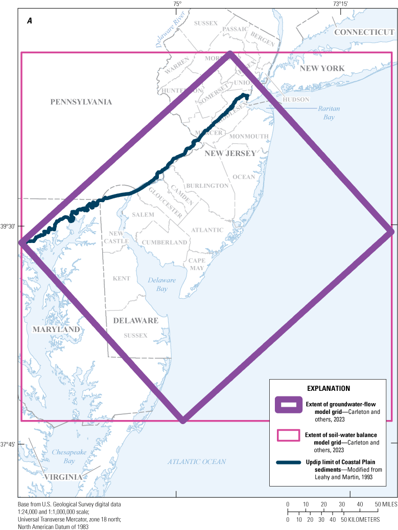
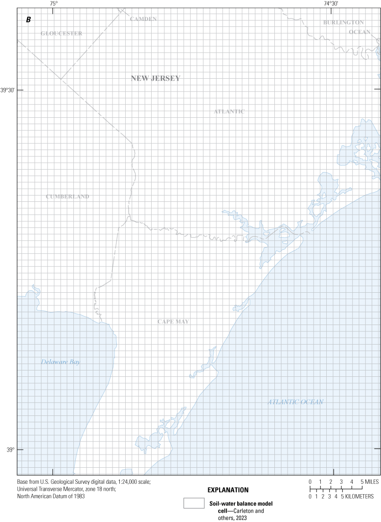
Maps showing A, location of soil-water balance (SWB) model grid for the New Jersey Coastal Plain groundwater-flow model study area; and B, Example of cells in the SWB model grid in Atlantic County, New Jersey.
Model Input Requirements
Meteorological data needed for the model include daily precipitation, minimum daily temperature, and maximum daily temperature. The SWB model also requires the following gridded dataset to calculate a cell-by-cell recharge: land-cover data, hydrologic soil group, and available water capacity. The gridded land-use and soils data were converted to ASCII format for use in the SWB model by using ArcGIS methods.
Daily Climate Data
Precipitation in inches and maximum and minimum temperature in degrees Fahrenheit were input for the years 1980 through 2013. The daily mean, maximum, and minimum air temperatures are used to determine whether precipitation takes the form of rain or snow. Daily minimum temperature, maximum temperature, and precipitation tabular data were obtained from the USGS Geo Data Portal (GDP) (U.S. Geological Survey Geo Data Portal, 2017) for the study area shown in the grid in figure 1.1. Mean annual precipitation for 1980 through 2013 ranged from 38.4 inches per year (in/yr) in 2001 to 63.4 in/yr in 2011, with an average of 48.4 in/yr. For comparison, mean annual precipitation for the area that encompasses the New Jersey Coastal Plain from 1980 through 2013 is 44.4 in/yr (Office of the New Jersey State Climatologist, 2021).
Land Cover
The SWB model requires land-cover data to calculate net recharge to the groundwater-flow system. Grids of land-cover classifications were developed from the National Land Cover Database (NLCD) for 1992, 2001, and 2011 (U.S. Geological Survey, 2008; 2014a; 2014b, respectively). The NLCD is a raster dataset with a spatial resolution of 30 meters (approximately 98.4 feet). Land-use cover in the study area in 1992 was primarily agricultural (32 percent), forest (27 percent), and developed (13 percent); in 2001, agricultural (27 percent), forest (22 percent), and developed (18 percent); and in 2011, agricultural (26 percent), forest (22 percent), and developed (19 percent) (U.S. Geological Survey, 2008; 2014a; and 2014b, respectively). The NLCD dataset includes 16 land-cover classifications for 2001 and 2011, and 13 land-cover classifications for 1992. The 1992 NLCD was used in the SWB program to estimate recharge for 1980 through 1999, the 2001 NLCD was used to estimate recharge from 2000 through 2006, and the 2011 NLCD was used to estimate recharge from 2007 to 2013. The 1992 land-cover classification codes for wetland and residential areas were modified in 2001; therefore, some modifications were made in wetland and residential areas to accommodate this code change. Figure 1.2 shows the land-cover classification for the New Jersey Coastal Plain and Delaware for 2011. Recharge is not calculated where the land-cover type of a cell has been identified as “Open_water_land_use” in the input control file or where the soil-water capacity is near zero (Westenbroek and others, 2010).
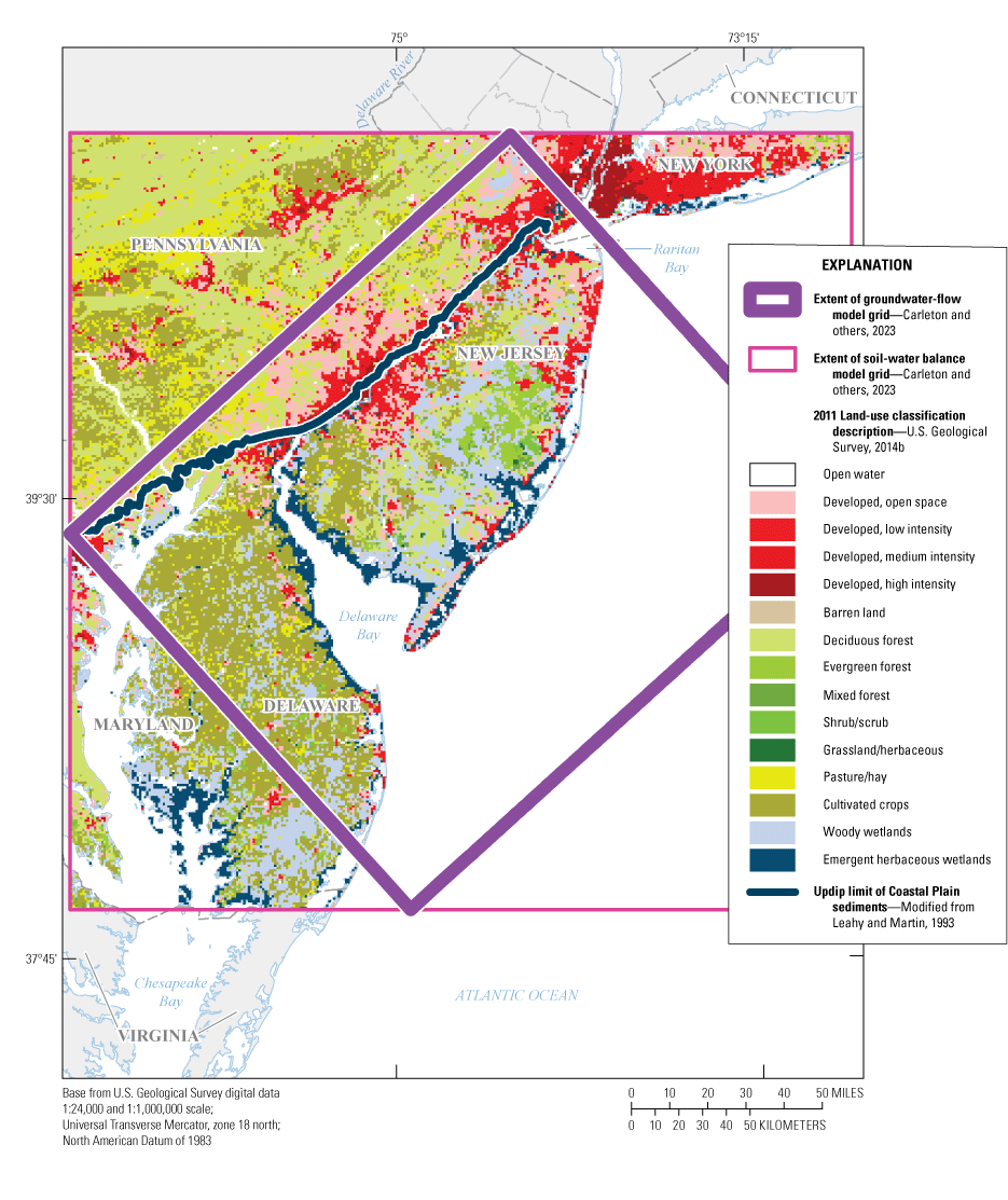
Maps showing land-use classification in New Jersey Coastal Plain groundwater-flow model study area, 2011.
Hydrologic Soil Groups
Soil data were obtained for each county in the study area from the Natural Resources Conservation Service (NRCS) Soil Survey Geographic (SSURGO) database (Natural Resources Conservation Service, 2014). The SSURGO digital maps at the county scale were merged and converted to a 1-kilometer-square (0.386 miles-square) grid. The data on hydrologic soils groups provided in the NRCS soil (SSURGO) datasets (Natural Resources Conservation Service, 2014) were used to define gridded datasets of hydrologic soils to be used as input to the SWB model. Hydrologic soils within the United States are classified in the U.S. Department of Agriculture NRCS National Engineering Handbook for Hydrology (Natural Resources Conservation Service, 2009) into four major groups. Each group is assigned a letter designation (A–D) that describes soils with similar physical and runoff characteristics. The designation focuses on the soil’s capacity for infiltration. Soils designated group A have a high capacity for infiltration (greater than 0.30 inch per hour (in/hr)) and low runoff potential, whereas those designated group D have low infiltration capacity (less than 0.05 in/hr) and high runoff potential (Cronshey and others, 1986). Group B soils have moderate infiltration capacity and low runoff potential and group C soils have low infiltration capacity and moderately high runoff potential. Most soils are group A in Burlington and Ocean Counties (in the Pineland Preservation area of New Jersey) and group B in the western part of the New Jersey Coastal Plain. The hydrologic soil groups in the SWB study area are shown in figure 1.3. In Delaware, group B is found primarily in the interior of the state and group C is found primarily in the northern and southern parts. Group D soils are found along streams and in coastal areas of New Jersey and Delaware (fig. 1.3). A hydrologic soil group category was assigned to every SWB model grid cell and the same values were used throughout the 1980-2013 time period.
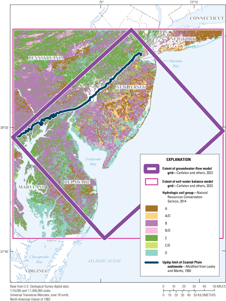
Map showing hydrologic soil groups in the New Jersey Coastal Plain groundwater-flow model study area.
Available Water Capacity
Available water capacity (AWC) is the amount of water that a soil can store that is available for use by plants (Natural Resources Conservation Service, 1998). An AWC value was assigned to every SWB model grid cell and these values were unchanged from 1980–2013. Estimated AWC values for 14 soil-texture groups are provided in Westenbroek and others (2010). These AWC values are expressed in units of inches of water per foot of soil thickness. The original source of these values is Thornthwaite and Mather (1957). The AWC grid input to the SWB model was created by assigning values from Westenbroek and others (2010) for each soil-texture group from the SSURGO soil-survey data (U.S. Department of Agriculture, 2014).
Lookup Tables
The SWB model requires two lookup tables to assign properties related to soils and land use to model cells. The first lookup table is used to assign, root-zone depths, runoff curve numbers, interception storage values, and maximum recharge to each combination of hydrologic soil group and land-use/land-cover type (Westenbroek and others, 2010). Root-zone depth is needed in the recharge calculation because of its effect on water flow and transpiration. Root-zone depth values, in feet, were modified from those determined for New Jersey by the NRCS (Natural Resources Conservation Service, 2007). The runoff-curve number is an empirical parameter developed by the U.S. Department of Agriculture Soil Conservation Service (SCS) (since 1994, the NRCS) that is used to estimate rainfall runoff or infiltration (Hjelmfelt, 1991). The SWB model applies runoff-curve numbers to the combination of hydrologic soil groups and land-cover types listed in the lookup table. Curve-number information was obtained primarily from the NRCS (Natural Resources Conservation Service, 2004).
Interception storage values represent water that is trapped by vegetation or evaporated from plant surfaces (Westenbroek and others, 2010). Precipitation must exceed interception for any water to reach the soil surface. Interception storage values in the SWB model are specified for each land-cover type and for growing and nongrowing (dormant) seasons. A value of 0.0835 was used for all land-cover types during the growing season except land-use types designated open water, barren land, and emergent herbaceous wetland land-cover types, which were assigned a value of zero (Tillman, 2015). Maximum daily recharge rates are used to limit the maximum amount of recharge in any cell to a reasonable value. Maximum recharge rates were input to the SWB model modified from values given in Westenbroek and others (2010).
The second lookup table is an extended version of the Thornthwaite-Mather soil-water retention tables that describe the ability of various soils to hold water (Thornthwaite and Mather, 1957). The ability of soil to hold water is strongly related to particle size; water molecules hold more tightly to clay than to coarse materials, such as sand. The soil-water retention tables are provided with the SWB model (Westenbroek and others, 2010).
Comparison of Recharge Estimates for New Jersey Coastal Plain Groundwater-Flow Models
In the Regional Aquifer System Analysis (RASA) model of the New Jersey Coastal Plain (Martin, 1998), a constant recharge rate of 20 in/yr was used. Recharge values in the rediscretized RASA model (Voronin, 2004) ranged from 0.01 in/yr in the outcrop areas of the confining units in updip areas to 20 in/yr in the outcrop areas of the unconfined Kirkwood-Cohansey aquifer system in downdip areas; however, recharge was not varied annually. The values used by Voronin (2004) were based on long-term averages reported in surficial-aquifer studies completed in the late 1980s to late 1990s in several surface-water basins in the New Jersey Coastal Plain as well as on regional estimates. The recharge rates reported in the surficial-aquifer studies ranged from 12.5 to 19.4 in/yr (Watt and Johnson, 1992; Watt and others, 1994; Lacombe and Rosman, 1995; Johnson and Watt, 1996; Johnson and Charles, 1997; Charles and others, 2001; Watt and others, 2003). These values were calculated by using water-budget equations determined for each individual New Jersey Coastal Plain basin studied, and do not incorporate land use or soil cover in the determination of the recharge estimates.
Because the recharge determined by using the SWB method is a function of land use, soil type, and AWC, estimated recharge varied spatially. Recharge also varied annually and was calculated for each year from 1980 through 2013. Results of the SWB model indicate that the average recharge rate in the study area varied from a minimum of 7.9 in/yr in 1985 to a maximum of 26.2 in/yr in 1996 and averaged 15.4 in/yr in the study area.
A SWB model also was developed for the North Atlantic Coastal Plain (NACP) groundwater-flow model for 2005–09 (Masterson and others, 2015). Results of the NACP SWB model indicate that the average recharge rate for the NACP study area varied from a minimum of 4.2 to a maximum of 37.6 in/yr, and averaged 13.9 in/yr, The SWB model developed for the New Jersey Coastal Plain (NJCP) groundwater-flow model simulated conditions over a longer annual period, 34 years (1980–2013), and the study area was smaller, occupying only part of the NACP study area. For example, the SWB program for the NJCP groundwater-flow model calculated an average groundwater recharge rate for 2013 of 15.3 in/yr, and recharge varied from a minimum of 5.8 to a maximum of 23.3 in/yr (fig. 1.4) for land-use categories not designated as a water body.
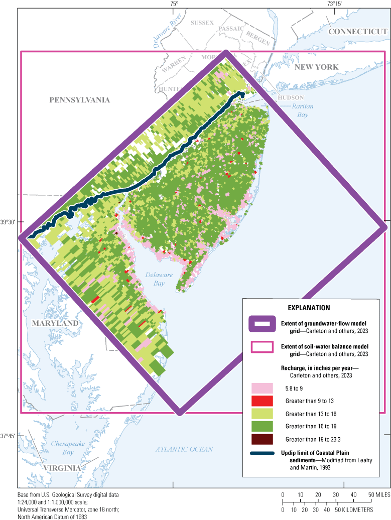
Maps showing recharge in the New Jersey Coastal Plain groundwater-flow model in 2013.
Limitations
The SWB method provides an improved understanding of the effects of climate, land use, and soil type on infiltration at the regional scale, but some uncertainties and limitations are acknowledged. Although recharge rates vary over the study area, the SWB model does not account for lag time. Recharge in the model is assumed to be instantaneous within the daily time step, whereas actual recharge is less rapid. Travel times to the water table are affected by infiltration capacity and root-zone dynamics at the time of recharge, as well as the amount of the recharge.
Maximum infiltration rates, root-zone depth, and curve-number values input to the first lookup table are subject to parameter uncertainties. In addition, parameters input to the SWB model are generalized across a model cell, although these parameters can vary locally across the model cell. This limitation may have resulted in a bias in gridded average weighted results for land use, soil, and precipitation in some areas.
Recharge was adjusted during model calibration (described in the Model Calibration section of this report) by using only one recharge parameter for New Jersey in the parameter-estimation calibration process. The use of only one parameter zone for New Jersey in the groundwater-flow model in this study likely affected the accuracy of recharge estimates in areas where local variations occur.
Recharge from wastewater return flow was not simulated in the SWB model. The omission of return flow may have affected estimates of recharge in areas of the NJCP with domestic wells where sewers are absent.
References Cited
Carleton, G.B., Gordon, A.D., Kenefic, L.F., Watt, M.K., and Buxton, D.E., 2023, MODFLOW–2005 used to simulate the regional groundwater flow system in the updated New Jersey Coastal Plain model, 1980–2013: U.S. Geological Survey data release, https://doi.org/10.566/P9W6RXFC.
Charles, E.G., Storck, D.A., and Clawges, R.M., 2001, Hydrology of the unconfined aquifer system, Maurice River area: Maurice and Cohansey River Basins, New Jersey, 1994–95: U.S. Geological Survey Water-Resources Investigations Report 01–4229, 5 pls. [Also available at https://doi.org/10.3133/wri014229.]
Cronshey, R., McCuen, R.H., Miller, N., Rawls, W., Robbins, S., and Woodward, D., 1986, Urban hydrology for small watersheds (2d ed.): U.S. Department of Agriculture Technical Release 55, accessed March 18, 2017, at https://www.nrcs.usda.gov/Internet/FSE_DOCUMENTS/stelprdb1044171.pdf.
Hjelmfelt, A.T., Jr., 1991, Investigation of the Curve Number Procedure: Journal of Hydraulic Engineering,, v. 117, no. 6, p. 725–737, accessed March 17, 2018, at https://doi.org/10.1061/(ASCE)0733-9429(1991)117:6(725).
Johnson, M.L., and Charles, E.G., 1997, Hydrogeology of the unconfined aquifer system, Salem River area—Salem River and Raccoon, Oldmans, Alloway, and Stow Creek Basins, New Jersey, 1993–94: U.S. Geological Survey Water-Resources Investigations Report 96–4195, 5 sheets. [Also available at https://doi.org/10.3133/wri964195.]
Johnson, M.L, and Watt, M.K., 1996, Hydrology of the unconfined aquifer system, Mullica River basin, New Jersey, 1991-92: U.S. Geological Survey Water-Resources Investigations Report 94–4234, 6 sheets. [Also available at https://doi.org/10.3133/wri944234.]
Lacombe, P.J., and Rosman, R., 1995, Hydrology of the unconfined aquifer system in the upper Maurice River Basin and adjacent areas in Gloucester County, New Jersey, 1986–87: U.S. Geological Survey Water-Resources Investigations Report 92–4128, 5 sheets. [Also available at https://doi.org/10.3133/wri924128.]
Leahy, P.P., and Martin, M., 1993, Geohydrology and simulation of ground-water flow in the northern Atlantic Coastal Plain aquifer system: U.S. Geological Survey Professional Paper 1404–K, 81 p., 22 pls. [Also available at https://doi.org/10.3133/pp1404K.]
Masterson, J.P., Pope, J.P., Monti, J., Jr., Nardi, M.R., Finkelstein, J.S., and McCoy, K.J., 2015, Hydrogeology and hydrogeologic conditions of the Northern Atlantic Coastal Plain aquifer system from Long Island, New York, to North Carolina: U.S. Geological Survey Scientific Investigations Report 2013–5133, ver. 1.1, 76 p. [Also available at https://doi.org/10.3133/sir20135133.]
Natural Resources Conservation Service, 1998, Soil quality resource concerns—Available water capacity: Soil Quality Information Sheet, 2 p., accessed August 17, 2018, at https://www.nrcs.usda.gov/Internet/FSE_DOCUMENTS/nrcs142p2_051279.pdf.
Natural Resources Conservation Service, 2004, Hydrologic soil-cover complexes: Natural Resources Conservation Service Part 630 Hydrology National Engineering Handbook, chap. 9, 14 p., accessed March 11, 2017, at https://directives.sc.egov.usda.gov/OpenNonWebContent.aspx?content=17758.wba.
Natural Resources Conservation Service, 2007, Root zone available water capacity map of New Jersey, 1 p., accessed March 3, 2017, at https://geospatial.wvu.edu/files/d/230555de-9177-4c7a-9a4b-4f9709a6b577/nj.pdf.
Natural Resources Conservation Service, 2009, Hydrologic soil groups: Natural Resources Conservation Service Part 630 Hydrology National Engineering Handbook, chap. 7, 13 p., accessed March 11, 2017, at https://directives.sc.egov.usda.gov/OpenNonWebContent.aspx?content=22526.wba.
Natural Resources Conservation Service, 2014, Web soil survey (WSS): accessed March 17, 2014, at https://websoilsurvey.nrcs.usda.gov/app/WebSoilSurvey.aspx.
Office of the State Climatologist, 2021, Monthly climate tables: New Jersey Climate Division 2 (South), accessed July 23, 2021, at http://climate.rutgers.edu/stateclim_v1/nclimdiv/index.php?stn=NJ02&elem=pcpn.
Tillman, F.D., 2015, Documentation of input datasets for the soil-water balance groundwater recharge model of the Upper Colorado River Basin: U.S. Geological Survey Open-File Report 2015–1160, 17 p., accessed March 18. 2017 at https://doi.org/10.3133/ofr20151160.
U.S. Geological Survey, 2008, National Land Cover Database (NLCD) 1992 land cover conterminous United States: U.S. Geological Survey Data Release, accessed March 2, 2017, at https://data.doi.gov/dataset/national-land-cover-database-nlcd-1992-land-cover-conterminous-united-states.
U.S. Geological Survey, 2014a, NLCD 2001 land cover (2011 ed.): accessed April 2, 2014, at https://www.mrlc.gov/data/nlcd-2001-land-cover-conus.
U.S. Geological Survey, 2014b, NLCD 2011 land cover (2011 ed., amended 2014) accessed November 3, 2014, at https://www.usgs.gov/media/images/nlcd-2011-land-cover-2011-edition-amended-2014.
U.S. Geological Survey Geo Data Portal, 2017, University of Idaho Daily Meteorological data for continental US: accessed November 29, 2017, at https://labs.waterdata.usgs.gov/gdp_web/client/#!catalog/gdp/dataset/54dd5df2e4b08de9379b38.
Voronin, L.M., 2004, Documentation of revisions to the regional aquifer system analysis model of the New Jersey Coastal Plain: U.S. Geological Survey Water-Resources Investigations Report 03–4268, 49 p., 1 pl., [Also available at https://doi.org/10.3133/wri034268.]
Watt, M.K., and Johnson, M.L., 1992, Water resources of the unconfined aquifer system of the Great Egg Harbor River Basin, New Jersey, 1989–90: U.S. Geological Survey Water-Resources Investigations Report 91–4126, 5 sheets. [Also available at https://doi.org/10.3133/wri914126.]
Watt, M.K., Johnson, M.L., and Lacombe, P.J., 1994, Hydrology of the unconfined aquifer system, Toms River, Metedeconk River, and Kettle Creek Basins, New Jersey, 1987–90: U.S. Geological Survey Water-Resources Investigations Report 93–4110, 5 sheets. [Also available at https://doi.org/10.3133/wri934110.]
Watt, M.K., Kane, A.C., Charles, E.G., and Storck, D.A., 2003, Hydrology of the unconfined aquifer system, Rancocas Creek area: Rancocas, Crosswicks, Assunpink, Blacks, and Crafts Creek Basins, New Jersey, 1996: U.S. Geological Survey Water-Resources Investigations Report 02–4280, 5 sheets. [Also available at https://doi.org/10.3133/wri024280.]
Westenbroek, S.M., Kelson, V.A., Dripps, W.R., Hunt, R.J., and Bradbury, K.R., 2010, SWB—A modified Thornthwaite-Mather soil-water-balance code for estimating groundwater recharge: U.S. Geological Survey Techniques and Methods, book 6, chap. A31, 59 p., accessed March 11, 2013, at https://doi.org/10.3133/tm6A31.
Conversion Factors
U.S. customary units to International System of Units
Datum
Vertical coordinate information is referenced to the North American Vertical Datum of 1988 (NAVD 88).
Horizontal coordinate information is referenced to the North American Datum of 1983 (NAD 83).
Altitude, as used in this report, refers to distance above the vertical datum.
Abbreviations
AWC
available water capacity
CHD
MODFLOW Time Variant Specified-Head package
DRN
MODFLOW Drain package
mg/L
milligram per liter (parts per million)
GIS
geographic information system
GWSI
Groundwater Site Inventory
NACP
Northern Atlantic Coastal Plain
NAD 83
North American Datum of 1983
NAVD 88
North American Vertical Datum of 1988
NJDEP
New Jersey Department of Environmental Protection
PRM
Potomac-Raritan-Magothy
RASA
Regional Aquifer System Analysis
RIV
MODFLOW River package
SWB
soil-water Balance
UCODE
universal inverse modeling computer code
USGS
U.S. Geological Survey
%SEE
percent standard error of estimate
For more information, contact:
Director, New Jersey Water Science Center
3450 Princeton Pike Suite 110,
Lawrenceville, New Jersey 08648
Or go to our website at https://www.usgs.gov/centers/new-jersey-water-science-center.
Publishing support provided by the Baltimore Publishing Service Center.
Disclaimers
Any use of trade, firm, or product names is for descriptive purposes only and does not imply endorsement by the U.S. Government.
Although this information product, for the most part, is in the public domain, it also may contain copyrighted materials as noted in the text. Permission to reproduce copyrighted items must be secured from the copyright owner.
Suggested Citation
Gordon, A.D., and Carleton, G.B., 2023, Updates to the regional groundwater-flow model of the New Jersey Coastal Plain, 1980–2013: U.S. Geological Survey Scientific Investigations Report 2023–5066, 116 p., https://doi.org/10.3133/sir20235066
ISSN: 2328-0328 (online)
Study Area
| Publication type | Report |
|---|---|
| Publication Subtype | USGS Numbered Series |
| Title | Updates to the regional groundwater-flow model of the New Jersey Coastal Plain, 1980–2013 |
| Series title | Scientific Investigations Report |
| Series number | 2023-5066 |
| DOI | 10.3133/sir20235066 |
| Publication Date | November 17, 2023 |
| Year Published | 2023 |
| Language | English |
| Publisher | U.S. Geological Survey |
| Publisher location | Reston, VA |
| Contributing office(s) | New Jersey Water Science Center |
| Description | Report: xii, 116 p.; Data Release |
| Country | United States |
| Other Geospatial | New Jersey Coastal Plain |
| Online Only (Y/N) | Y |
| Additional Online Files (Y/N) | N |