

Hydrogeology and Simulated Groundwater Availability in Reaches 3 and 4 of the Washita River Aquifer, Southern Oklahoma, 1980–2017
Links
- Document: Report (57.7 MB pdf) , HTML , XML
- Data Releases:
- NGMDB Index Page: National Geologic Map Database Index Page (html)
- Download citation as: RIS | Dublin Core
Acknowledgments
The project documented in this report was conducted in cooperation with the Oklahoma Water Resources Board (OWRB) as part of the U.S. Geological Survey (USGS) Water Availability and Use Science Program. The authors value the contributions of many OWRB and USGS staff that led to the successful completion of the project. The authors thank the OWRB for support on this project, especially Division Chief (Water Rights Administration Division) Christopher Neel and Technical Studies Manager (Water Rights Administration Division) Derrick Wagner, who provided hydrogeologic data and helped with defining study objectives and deliverables. The authors also thank Alan LePera and Byron Waltman, who assisted in collecting synoptic water-table-altitude measurements.
The authors express gratitude to USGS employees who performed data-collection activities in the field. Stephen Bradford, Kyle Cothren, Aaron Moyer, Kevin Smith, Steve Smith, and Adam Trevisan measured synoptic base flows during 2018. Leland Fuhrig and Kyle Rennell measured bedrock depths with the Geoprobe hydraulic profiling tool and collected synoptic water-table-altitude measurements. Derek Ryter contoured preliminary aquifer-base maps. In addition, Waylon Marler facilitated data entry to the USGS National Water Information System database. The authors also thank USGS employees Moussa Guira, Cory Russell, Chris Braun, and Martha Watt, who performed detailed technical reviews of this report and the accompanying model archive data release. The authors acknowledge and appreciate the professionalism, experience, and dedication of these helpful and resourceful colleagues.
Abstract
The 1973 Oklahoma Groundwater Law (Oklahoma Statutes §82–1020.5) requires that the Oklahoma Water Resources Board conduct hydrologic investigations of the State’s aquifers to determine the maximum annual yield for each groundwater basin. Because more than 20 years have elapsed since the final order was issued, the U.S. Geological Survey, in cooperation with the Oklahoma Water Resources Board, conducted an updated hydrologic investigation and evaluated the effects of potential groundwater withdrawals on groundwater flow and availability in reaches 3 and 4 of the Washita River aquifer in southern Oklahoma for a study period spanning 1980–2017. A hydrogeologic framework and conceptual model were developed to guide the construction and calibration of a numerical model of the Washita River aquifer. The numerical model was calibrated to water-table-altitude observations at selected wells, base-flow observations at selected U.S. Geological Survey streamgages, and the conceptual-model recharge.
Three types of groundwater-availability scenarios were run using the calibrated numerical model. These scenarios were used to (1) estimate equal-proportionate-share pumping rates, (2) quantify the potential effects of projected well withdrawals on groundwater storage over a 50-year period, and (3) simulate the potential effects of a hypothetical 10-year drought. With Washita River main-stem inflows, the 20-, 40-, and 50-year equal-proportionate-share pumping rates under normal recharge conditions were about 3.08 acre-feet per acre per year for reach 3 and about 3.80 acre-feet per acre per year for reach 4. Projected 50-year pumping scenarios were used to simulate the effects of modified well withdrawal rates. Because well withdrawals were less than 1 percent of the calibrated numerical-model water budget, changes to the well pumping rates had little effect on Washita River base flows and groundwater storage in the Washita River aquifer. A hypothetical 10-year drought scenario was used to simulate the potential effects of a prolonged period of reduced recharge on groundwater storage. Groundwater storage at the end of the drought period was 4.6 percent less than the groundwater storage of the calibrated numerical model at the end of the drought period.
Introduction
The 1973 Oklahoma Groundwater Law (Oklahoma Statutes §82–1020.5 [Oklahoma State Legislature, 2021b]) requires that the Oklahoma Water Resources Board (OWRB) conduct hydrologic investigations of the State’s aquifers (called groundwater basins in the statutes) to determine the maximum annual yield (MAY) for each groundwater basin. The MAY is defined as the total amount of fresh groundwater that can be annually withdrawn while ensuring a minimum 20-year life of that groundwater basin (OWRB, 2020). For alluvium and terrace groundwater basins, the life requirement is satisfied if, after 20 years of MAY withdrawals, 50 percent of the groundwater basin (hereinafter referred to as “aquifer”) retains a saturated thickness of at least 5 feet (ft) (OWRB, 2014). Although 20 years is the minimum period required by law, the OWRB can and often does consider management scenarios with longer periods. Once a MAY has been established, the amount of land owned or leased by a groundwater-use permit applicant determines the annual volume of water allocated to that groundwater-use permit applicant. The annual volume of groundwater allocated per acre of land is known as the equal-proportionate-share (EPS) pumping rate.
The OWRB issued a final order on November 13, 1990, that established the MAY (81,840 and 46,935 acre-feet per year [acre-ft/yr]) and EPS pumping rate (1.5 and 1.0 acre-foot per acre per year [(acre-ft/acre)/yr]) for reaches 3 and 4, respectively, of the Washita River aquifer in southern Oklahoma (OWRB, 2020). The MAY and EPS pumping rate were based on hydrologic investigations by Kent and others (1984) and Patterson (1984) that used a numerical groundwater-flow model (Trescott and others, 1976) to evaluate the effects of potential groundwater withdrawals on groundwater availability in the Washita River aquifer in southern Oklahoma. Every 20 years, the OWRB is statutorily required to update the hydrologic investigation on which the MAY and EPS were based. Because more than 20 years have elapsed since the final order was issued, the U.S. Geological Survey (USGS), in cooperation with the OWRB, conducted an updated hydrologic investigation and evaluated the effects of potential groundwater withdrawals on groundwater flow and availability in the Washita River aquifer of southern Oklahoma for a study period spanning 1980–2017.
Purpose and Scope
The purpose of this report is to describe a hydrologic investigation of the Washita River aquifer in southern Oklahoma. This description includes (1) an updated summary of the hydrogeology with a definition of the hydrogeologic framework (including an updated geographic extent) of the aquifer, (2) development of conceptual and calibrated numerical groundwater-flow models for the aquifer representing the 1980–2017 study period, and (3) results of simulations of groundwater-availability scenarios. The groundwater-availability scenarios use the calibrated numerical groundwater-flow model to (1) estimate the EPS pumping rate that ensures a minimum 20-, 40-, and 50-year life of the aquifer, (2) quantify the potential effects of projected well withdrawals on groundwater storage over a 50-year period, and (3) simulate the potential effects of a hypothetical (10-year) drought on groundwater storage. The calibrated numerical groundwater-flow model and groundwater-availability scenarios were archived and released in a USGS data release (Rogers and others, 2023).
The entire Washita River aquifer in Oklahoma consists of four administrative sections, or reaches, which are managed independently by the OWRB. Reach 1 extends from the Texas border to downstream from Foss Reservoir in western Oklahoma (fig. 1; Ellis and others, 2020), and reach 2 is hydraulically connected to and managed as part of the Rush Springs aquifer in western Oklahoma (fig. 1; Ellis, 2018a); both reach 1 and reach 2 are outside the scope of this report. The modeled area of this report is a 279.6-square-mile (mi2) (178,938-acre) subarea of the 411.5-mi2 extent of alluvium and terrace deposits (Heran and others, 2003; Miller and Stanley, 2004; Chang and Stanley, 2010; Stanley and Chang, 2012) of reaches 3 and 4 of the Washita River aquifer in southern Oklahoma (fig. 1). Reach 3 extends from near Anadarko, Okla., to Alex, Okla., and includes 113.6 mi2 (72,697 acres, or 40.6 percent) of the modeled area. Reach 4 extends from near Alex to south of Davis, Okla., and includes 166.0 mi2 (106,241 acres, or 59.4 percent) of the modeled area. The aquifer becomes narrow and thin in smaller tributary valleys, so this investigation focused on the main body of the aquifer along the Washita River main stem and selected large tributaries (modeled aquifer area, fig. 1). Though sometimes referred to as the “Washita River alluvial aquifer” (Schipper, 1983; OWRB, 2019b), the aquifer is referred to as the “Washita River aquifer” in this report because it consists not only of alluvium deposits but also of terrace and dune deposits. Selected sections in this report are modified from Ellis (2018a, b), Ellis and others (2020), and Smith and others (2021). Though the study areas are different, the organization and wording of this report are largely based on Smith and others (2021).
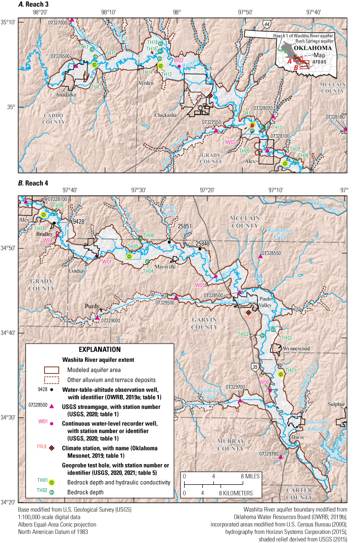
Selected data-collection stations in the study area and the extent of A, reach 3 and B, reach 4 of the Washita River aquifer, southern Oklahoma.
Description of Study Area
The Washita River aquifer is a long, narrow, unconfined aquifer that includes alluvium and terrace deposits of the Washita River and tributaries in Caddo, Grady, Garvin, McClain, and Murray Counties, Oklahoma (fig. 1). The Washita River is perennial in the study area except during the most extreme droughts as documented by historical USGS streamgaging records for the stream obtained from the USGS National Water Information System (NWIS) database (USGS, 2020; table 1). The Washita River generally flows from northwest to southeast for about 207 miles (mi) (Horizon Systems Corporation, 2015) in the study area. The largest tributaries in the study area are Little Washita River and Sugar, Rush, and Wildhorse Creeks (fig. 1). Many of the smaller tributaries to the Washita River in the study area are dammed by hundreds of Natural Resources Conservation Service (NRCS) floodwater-retarding structures (fig. 2), which were mostly built in the 1950s through 1970s (U.S. Army Corps of Engineers, 2021). Floodwater-retarding structures were designed to impound runoff from headwater catchments and slowly release it downstream with the purpose of reducing the frequency and magnitude of damaging flood flows on the Washita River main stem (Smith and Esralew, 2010). The Washita River main stem, however, is not dammed in the study area.
Table 1.
Selected data-collection stations in and near the Washita River aquifer study area, southern Oklahoma.[U.S. Geological Survey (USGS; 2020) data can be accessed using the 8- or 15-digit station number or other identifier. M/D/Y, month/day/year; NAVD 88, North American Vertical Datum of 1988; --, unknown or not applicable; SFR2, Streamflow-Routing package; SWB, Soil-Water Balance; WTF, water-table fluctuation method; OWRB, Oklahoma Water Resources Board]
| Station number or identifier (figs. 1 and 2) | Short name for station or other identifier | Station name | Latitude, in decimal degrees | Longitude, in decimal degrees | County | Period of record (may contain gaps) (M/D/Y) | Land-surface altitude, in feet above NAVD 88 | Well or hole depth, in feet | Contributing drainage area, in square miles | Use in numerical groundwater-flow model | |
|---|---|---|---|---|---|---|---|---|---|---|---|
| Begin | End | ||||||||||
| 07326500 | Anadarko gage | Washita River at Anadarko, Okla. | 35.0842 | −98.2434 | Caddo | 10/1/1963 | Present (2022) | -- | -- | 3,628 | SFR2 inflow |
| 07327000 | Gracemont gage | Sugar Creek near Gracemont, Okla. | 35.1751 | −98.2559 | Caddo | 10/1/1955 | 9/29/1974 | -- | -- | 208 | SFR2 inflow |
| 07327550 | Ninnekah gage | Little Washita River east of Ninnekah, Okla. | 34.9634 | −97.8995 | Grady | 2/24/1992 | 9/29/2005 | -- | -- | 232 | SFR2 inflow |
| 07328070 | -- | Winter Creek near Alex, Okla. | 34.9931 | −97.7614 | Grady | 10/1/1964 | 5/14/1987 | -- | -- | 33.0 | SFR2 inflow |
| 07328100 | Alex gage | Washita River at Alex, Okla. | 34.9259 | −97.7739 | Grady | 10/1/1964 | Present (2022) | -- | -- | 4,756 | Calibration |
| 07328180 | Criner gage | North Criner Creek near Criner, Okla. | 34.9715 | −97.5848 | McClain | 10/15/1993 | Present (2022) | -- | -- | 7.19 | SFR2 inflow |
| 07328500 | Pauls Valley gage | Washita River near Pauls Valley, Okla. | 34.7548 | −97.2514 | Garvin | 10/1/1961 | 12/8/2020 | -- | -- | 5,294 | Calibration |
| 07328550 | -- | Washington Creek near Pauls Valley, Okla. | 34.8259 | −97.2022 | Garvin | 7/3/1991 | 3/10/1994 | -- | -- | 7.56 | SFR2 inflow |
| 07329500 | Maysville gage | Rush Creek near Maysville, Okla. | 34.7434 | −97.4053 | Garvin | 10/1/1954 | 9/29/1976 | -- | -- | 206 | SFR2 inflow |
| 07329700 | Hoover gage | Wildhorse Creek near Hoover, Okla. | 34.5415 | −97.2472 | Garvin | 10/1/1969 | 6/30/2002 | -- | -- | 600 | SFR2 inflow |
| 07329780 | Davis gage | Honey Creek below Turner Falls near Davis, Okla. | 34.4318 | −97.1472 | Murray | 10/22/2004 | Present (2022) | -- | -- | 16.4 | SFR2 inflow |
| 07331000 | Dickson gage | Washita River near Dickson, Okla. | 34.2334 | −96.9758 | Carter | 10/1/1961 | Present (2022) | -- | -- | 7,160 | Calibration |
| CHIC | CHIC | Chickasha | 35.0324 | −97.9145 | Grady | 1/1/1994 | Present (2022) | 1,076 | -- | -- | Recharge (SWB, WTF) |
| PAUL | PAUL | Pauls Valley | 34.7155 | −97.2292 | Garvin | 1/1/1994 | Present (2022) | 955 | -- | -- | Recharge (SWB, WTF) |
| ANA | USC00340224 | ANADARKO, OK US | 35.0619 | −98.1988 | Caddo | 12/31/1892 | 11/29/2016 | 1,168 | -- | -- | Recharge (SWB) |
| ANA2 | US1OKCD0011 | ANADARKO 3.8 E, OK US | 35.0719 | −98.1769 | Caddo | 12/3/2010 | 3/4/2017 | 1,160 | Recharge (SWB) | ||
| ARD | USC00340292 | ARDMORE, OK US | 34.1773 | −97.1617 | Carter | 12/31/1900 | Present (2022) | 841 | -- | -- | Recharge (SWB) |
| CES | USC00341750 | CHICKASHA EXPERIMENTAL STATION, OK US | 35.0488 | −97.9158 | Grady | 5/31/1953 | Present (2022) | 1,085 | -- | -- | Recharge (SWB) |
| CNRA | USC00341745 | CHICKASAW NRA, OK US | 34.4967 | −96.9705 | Murray | 10/31/1978 | Present (2022) | 1,047 | -- | -- | Recharge (SWB) |
| COX | USC00342196 | COX CITY 2 NE, OK US | 34.7423 | −97.7038 | Grady | 9/30/1980 | 6/29/2012 | 1,232 | -- | -- | Recharge (SWB) |
| ELM | USC00342872 | ELMORE CITY 3 SW, OK US | 34.6100 | −97.4222 | Garvin | 7/9/1947 | Present (2022) | 1,020 | -- | -- | Recharge (SWB) |
| HEA | USC00344001 | HEALDTON 3 E, OK US | 34.2332 | −97.4202 | Carter | 12/31/1893 | Present (2022) | 902 | -- | -- | Recharge (SWB) |
| HEN | USC00344052 | HENNEPIN 5 N, OK US | 34.5797 | −97.3510 | Garvin | 8/31/1993 | Present (2022) | 966 | -- | -- | Recharge (SWB) |
| LIN | USC00345216 | LINDSAY 2 W, OK US | 34.8261 | −97.6386 | Garvin | 3/31/1938 | 3/30/2010 | 980 | -- | -- | Recharge (SWB) |
| MAD | USC00345468 | MADILL, OK US | 34.0919 | −96.7708 | Marshall | 11/30/1936 | Present (2022) | 770 | -- | -- | Recharge (SWB) |
| PAUX | USC00346931 | PAULS VALLEY 1 SSW MESONET, OK US | 34.7155 | −97.2292 | Garvin | 1/31/2009 | Present (2022) | 954 | -- | -- | Recharge (SWB) |
| PV4 | USC00346926 | PAULS VALLEY 4 WSW, OK US | 34.7253 | −97.2814 | Garvin | 12/31/1892 | 2/14/2011 | 940 | -- | -- | Recharge (SWB) |
| TIS | USC00348884 | TISHOMINGO NATIONAL WLR, OK US | 34.2070 | −96.6424 | Johnston | 11/30/1902 | Present (2022) | 664 | -- | -- | Recharge (SWB) |
| W01 | 344916097360001 | 04N-04W-15-ADA 1 W34001 | 34.8210 | −97.5999 | Garvin | 3/28/2018 | 6/12/2019 | 972.68 | 51.5 | -- | -- |
| W02 | 350514097593201 | 07N-08W-13 ADA 1 W34002 | 35.0874 | −97.9923 | Grady | 11/23/2016 | 6/12/2019 | 1,099.23 | 36.8 | -- | Recharge (WTF) |
| W03 | 345824097484201 | 06N-06W-22 DDA 1 W34003 | 34.9733 | −97.8116 | Grady | 11/23/2016 | 4/15/2019 | 1,044.56 | 62.8 | -- | -- |
| W04 | 345137097414501 | 05N-05W-35 DBB 1 W34004 | 34.8602 | −97.6957 | Grady | 7/2/2017 | 11/30/2017 | 999.84 | -- | -- | -- |
| W05 | 344704097183601 | 04N-01W-28 CDA 1 W34005 | 34.7846 | −97.3100 | Garvin | 11/22/2016 | 6/12/2019 | 905.43 | 32.6 | -- | Recharge (WTF) |
| W06 | 343341097102901 | 01N-01E-14 BBD 1 W34006 | 34.5613 | −97.1748 | Garvin | 4/6/2017 | 6/12/2019 | 823.34 | -- | -- | -- |
| 25848 | 345017097205701 | 04N-01W-07 BBD 1 | 34.8381 | −97.3495 | Garvin | 2/20/2001 | 1/26/2010 | 930 | -- | -- | Calibration |
| 25851 | 345102097252601 | 04N-02W-05 ADA 1 | 34.8506 | −97.4242 | Garvin | 2/20/2001 | 1/26/2010 | 942 | -- | -- | Calibration |
| 9428 | 345304097421301 | 05N-05W-26 BBB 1 | 34.8845 | −97.7039 | Grady | 3/10/1983 | 2/3/1993 | 1,010 | -- | -- | Calibration |
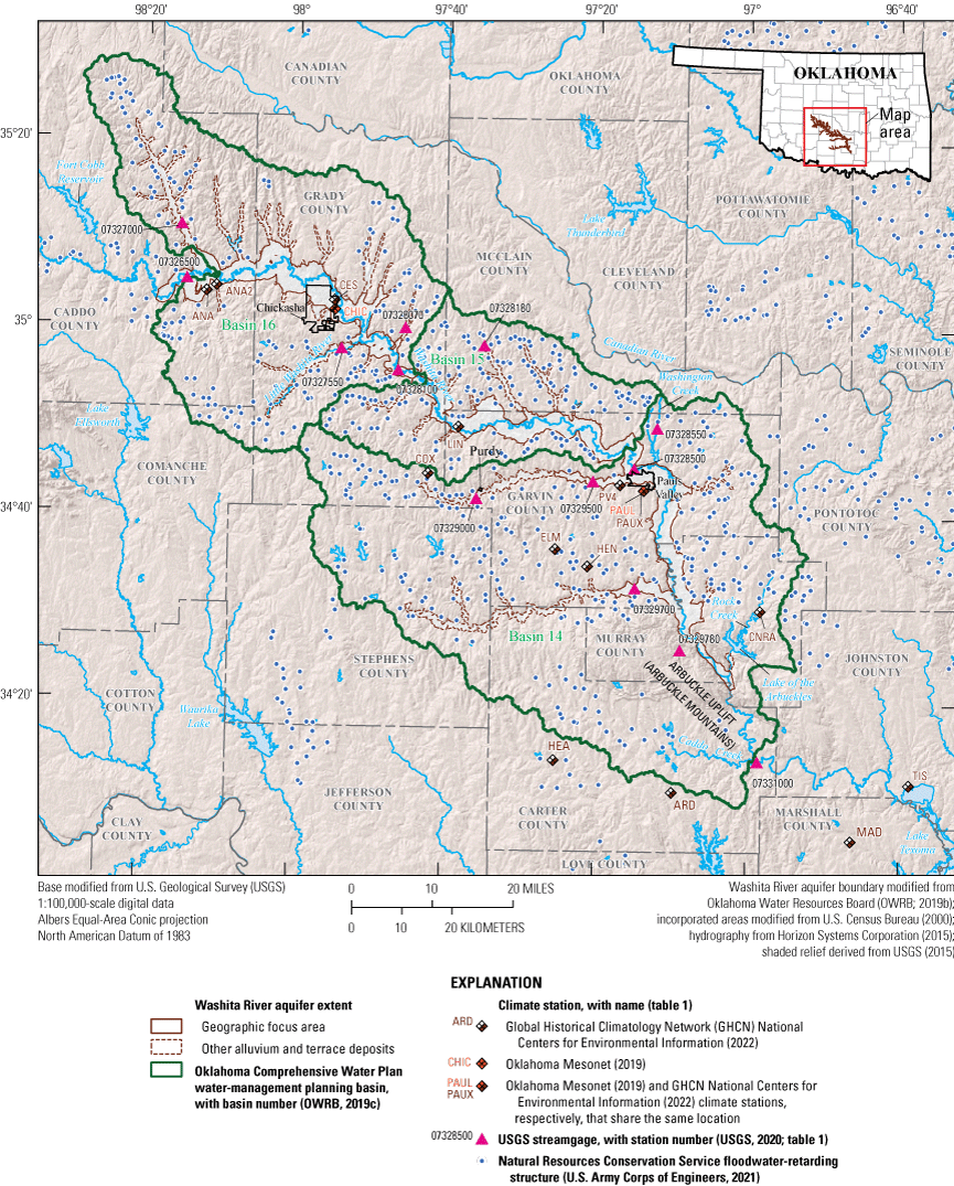
Selected data-collection stations and the major geographic and surface-water features in and near the Washita River aquifer study area, southern Oklahoma.
Land-cover data for the Washita River aquifer study area were obtained from the CropScape database (National Agricultural Statistics Service, 2019) (fig. 3), which includes land-cover characteristics at 30-meter (m) resolution for land overlying the Washita River aquifer for the 2010–17 period. During this period, land-cover type was primarily cropland (44.1 percent), grass or pasture (36.3 percent), forest and shrubland (9.3 percent), or developed (7.7 percent). Winter wheat was the major crop-cover type in the study area, accounting for 57.6 percent of cropland by area. Alfalfa or hay (22.0 percent) was the next largest crop-cover type by area. Corn and soybeans accounted for 7.5 and 6.6 percent of cropland by area, respectively. Cotton (1.3 percent) and fallow or idle cropland (1.2 percent) were the only other crop-cover types that accounted for more than 1 percent of cropland by area (fig. 3). Crop-cover types typically change in response to economic conditions and hydrologic factors, but the percentages of total cropland cover and individual crop types did not change substantially during the 2010–17 period.
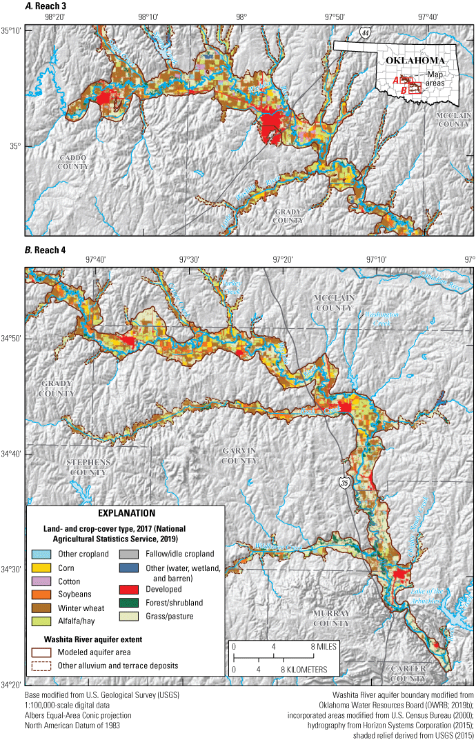
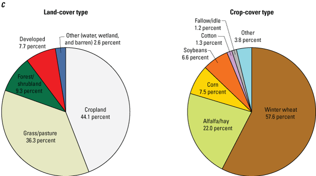
Land- and crop-cover types for land overlying A, reach 3, B, reach 4, and C, the study area of the Washita River aquifer, southern Oklahoma, 2010–17.
Climate Characteristics
The climate of the study area is classified as subhumid with generally southerly prevailing winds (Patterson, 1984). Historical data from selected climate stations in southern Oklahoma (Climate Division 8) have been quality assured and summarized monthly as part of the Global Historical Climatology Network (National Centers for Environmental Information, 2021). These data were used to calculate and graph annual and monthly temperature and precipitation statistics for the study area (fig. 4, table 2). A locally weighted scatterplot smoothing line (Cleveland, 1979) was used to delineate periods of below- and above-mean annual temperature and precipitation (fig. 4). The mean annual temperature during 1895–2020 was 62.2 degrees Fahrenheit (°F) (fig. 4, table 2), and the mean annual temperature differed by about 2 °F from northwest to southeast across the study area (Oklahoma Climatological Survey, 2021a, b). The mean annual precipitation during 1895–2020 was 38.0 inches per year (in/yr) (fig. 4, table 2), and the mean annual precipitation increased by about 7.5 in/yr from northwest to southeast across the study area (Oklahoma Climatological Survey, 2021a, b). The mean annual precipitation for the 1980–2017 study period was 40.1 in/yr (fig. 4, table 2). The 1981–2002 period was an unprecedented wet period in the available record; above-mean precipitation was recorded in 18 of these 22 years (82 percent of the years), contributing to a higher mean precipitation during the study period compared to the mean for the period of record (fig. 4A). May is typically the wettest month, and January is typically the driest month (fig. 5A).
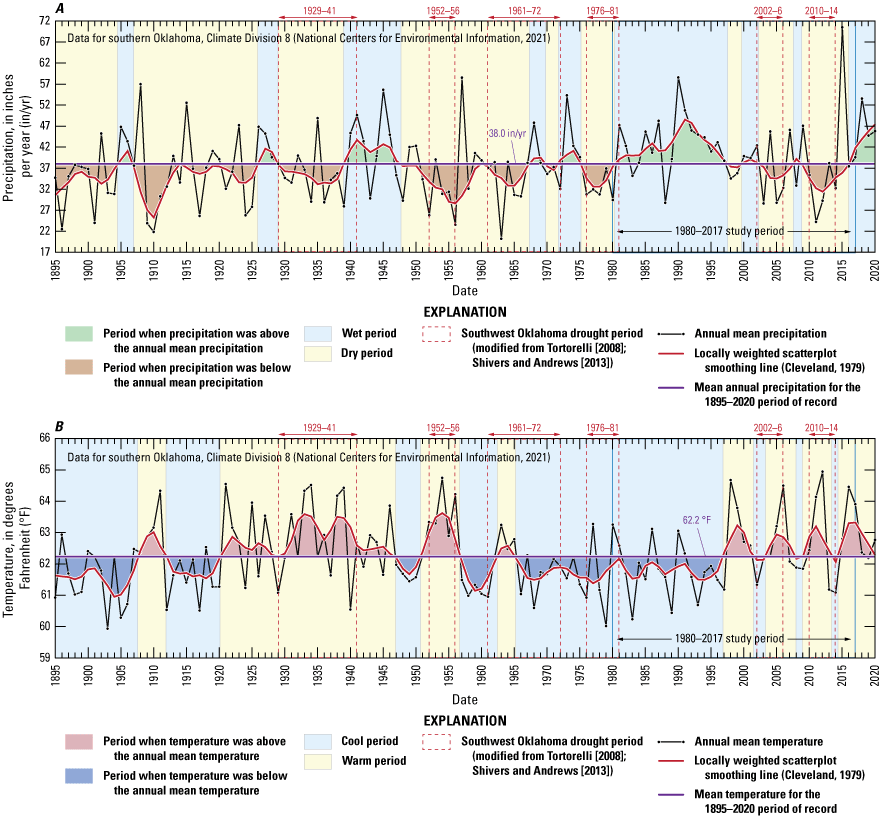
A, Precipitation and B, temperature, southern Oklahoma (Climate Division 8), 1895–2020 (National Centers for Environmental Information, 2021).
Table 2.
Mean annual precipitation and mean annual temperature for selected periods, southern Oklahoma, 1895–2020.[Reach and station locations shown on figures 1 and 2. --, data not available or not applicable]
| Region or location | Period | Number of years | Mean annual precipitation, in inches per year | Mean annual temperature, in degrees Fahrenheit |
|---|---|---|---|---|
| Southern Oklahoma (Climate Division 8; National Centers for Environmental Information, 2021) | 1895–2020 | 126 | 38.0 | 62.2 |
| 1895–1936 | 42 | 36.3 | 62.2 | |
| 1937–78 | 42 | 37.2 | 62.2 | |
| 1979–2020 | 42 | 40.5 | 62.3 | |
| 1980–2017 | 38 | 40.1 | 62.4 | |
| Reach 3 of the Washita River aquifer (Chickasha, Okla., station USC00341750; National Centers for Environmental Information, 2022) | 1980–2017 (missing daily values [1.3 percent of record] were assumed to equal the mean of available daily values) | 38 | 36.2 | -- |
| Reach 4 of the Washita River aquifer (Pauls Valley, Okla., stations USC00346926 and USC00346931; National Centers for Environmental Information, 2022) | 1980–2017 (missing daily values [3.3 percent of record] were assumed to equal the mean of available daily values) | 38 | 38.6 | -- |
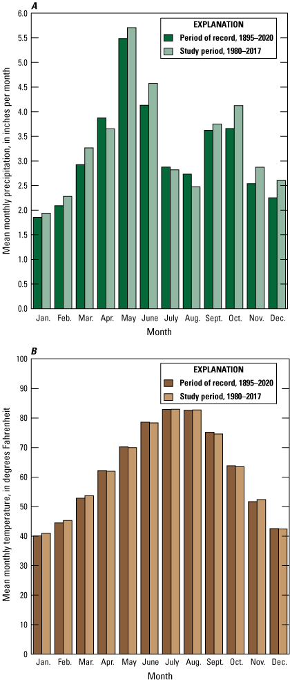
A, Mean monthly precipitation and B, mean monthly temperature, southern Oklahoma (Climate Division 8), 1895–2020 and 1980–2017 (National Centers for Environmental Information, 2021).
Multiyear to decadal droughts are common for the study area (fig. 4). The 1929–41 (Dust Bowl; Egan, 2006) and 1952–56 drought periods were among the most severe in Oklahoma in the 20th century; two shorter, less severe drought periods also occurred in the late 20th century during 1961–72 and 1976–81 (Tortorelli, 2008; Shivers and Andrews, 2013). The 21st century began with the 2002–6 and 2010–14 drought periods (Tortorelli, 2008; Shivers and Andrews, 2013). The most severe droughts on record developed from extended periods of below-mean precipitation paired with above-mean temperature.
Streamflow Characteristics and Trends
Daily streamflow data, with various and sometimes interrupted periods of record, were recorded at selected USGS streamgages in the study area (figs. 1 and 2) and summarized for the 1980–2017 study period (table 3). Streamflow measured at streamgages is the sum of runoff and base flow originating upstream; base flow is the component of streamflow that is supplied by the discharge of groundwater to streams (Barlow and Leake, 2012). For this report, streamflow-hydrograph data obtained from the NWIS database (USGS, 2020) were separated into runoff and base-flow components by using the standard Base-Flow Index code (Wahl and Wahl, 1995) in the USGS Groundwater Toolbox (Barlow and others, 2015). The Base-Flow Index code uses the minimum streamflow in a moving n-day window as a basis for hydrograph separation; for consistency, a 6-day window was used for all streamgages in this report. The 6-day window was selected by testing multiple n-day windows for the study period at USGS streamgage 07328100 Washita River at Alex, Okla. (hereinafter referred to as the “Alex gage”) and plotting the resulting mean base-flow percentage against n; a slope change was evident at 6 days. Base flow, as computed using this method, accounts for about 35–48 percent of annual streamflow for the period of record at streamgages on the Washita River main stem (table 3). This percentage, known as the base-flow index (BFI) (Wahl and Wahl, 1995; Barlow and others, 2015), generally increased over the period of record at streamgages on the Washita River (fig. 6A–D). When summarized annually using the Kendall (1938) tau test with the Theil-Sen (Sen, 1968) slope estimator and an alpha value of 0.0500 set as the significance level, the upward trends in the BFI were found to be statistically significant (probability value [p-value] = 0.0054) at USGS streamgage 07326500 Washita River at Anadarko, Okla. (hereinafter referred to as the “Anadarko gage”), statistically significant (p-value = 0.0248) at the Alex gage, statistically significant (p-value = 0.0000) at USGS streamgage 07328500 Washita River near Pauls Valley, Okla. (hereinafter referred to as the “Pauls Valley gage”), and statistically significant (p-value = 0.0083) at USGS streamgage 07331000 Washita River near Dickson, Okla. (hereinafter referred to as the “Dickson gage”). Upward trends in base flow (fig. 6A–D) were found to be not statistically significant (p-value = 0.0772) at the Anadarko gage, statistically significant (p-value = 0.0111) at the Alex gage, statistically significant (p-value = 0.0163) at the Pauls Valley gage, and statistically significant (p-value = 0.0177) at the Dickson gage. The overall pattern of upward trends in the BFI and base flow may have developed following the construction of more than 570 NRCS floodwater-retarding structures (dams; fig. 2) on tributaries of the Washita River within the study area. NRCS dam construction in this area began in 1948, peaked at 65 dams per year in 1963, greatly diminished to about 1 dam per year in the 1980s, and concluded in the early 1990s (U.S. Army Corps of Engineers, 2021). NRCS dams temporarily impound runoff and release it over several days with the purpose of reducing peak flows on the river main stem. The flows that are slowly and steadily released by these dams are indistinguishable from groundwater-derived base flows when they reach the main stem and are mostly classified as base flows by the Base-Flow Index code. Though most upward trends in the BFI and base flow were statistically significant for the streamgage periods of record, no statistically significant trends in base flow or BFI were detected for the 1980–2017 study period at streamgages on the Washita River main stem. One interpretation of the upward trends in the BFI and base flow for the period of record is that the construction of the floodwater-retarding structures caused a step change in apparent base flows in the Washita River.
Table 3.
Annual streamflow, base-flow, and base-flow index values for selected U.S. Geological Survey streamgages in and near the Washita River aquifer study area, southern Oklahoma, for the various periods of record, 1903–2020, and for the study period, 1980–2017.[Data from the U.S. Geological Survey (USGS) National Water Information System (USGS, 2020). Values computed by using the Base-Flow Index code (Wahl and Wahl, 1995) in the USGS Groundwater Toolbox (Barlow and others, 2015). Gage locations shown on figures 1 and 2. Gray shading indicates the data for the 1980–2017 study period. BFI, base-flow index; --, data not available or not applicable; POR, period of record]
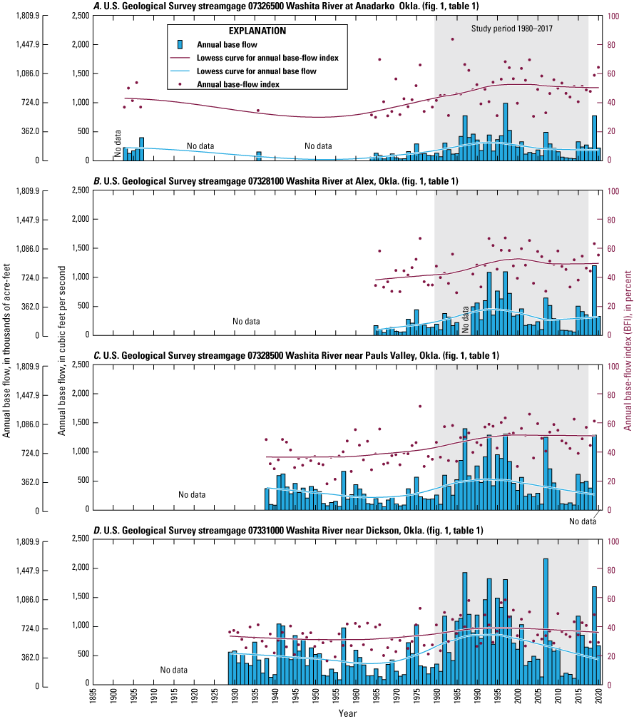
Annual base-flow and annual base-flow index values for U.S. Geological Survey streamgages A, 07326500 Washita River at Anadarko, Okla.; B, 07328100 Washita River at Alex, Okla.; C, 07328500 Washita River near Pauls Valley, Okla.; and D, 07331000 Washita River near Dickson, Okla., on the main stem of the Washita River in the Washita River aquifer study area, southern Oklahoma, for the various periods of record, 1903–2020 (U.S. Geological Survey, 2020). Lowess, locally weighted scatterplot smoothing.
Surface-water use in the Washita River aquifer study area consists of permitted diversions along the main stem of the Washita River and its associated tributaries (OWRB, 2019d). At the end of the study period (2017), 60 active, nontemporary permitted diversions on the Washita River main stem allowed for a maximum total withdrawal of 13,957 acre-ft/yr. All of those permitted diversions were for irrigation with the exception of three permitted diversions that were used for public supply, and all but 15 of those permitted diversions were in reach 3 of the Washita River aquifer. At the end of the study period (2017), 29 active, nontemporary permitted diversions on Washita River tributaries allowed for a maximum total withdrawal of 9,749 acre-ft/yr.
Groundwater Use
The OWRB permits and regulates groundwater use of more than 5 acre-ft/yr for domestic and agricultural purposes and groundwater use for irrigating more than 3 acres of land for growing gardens, orchards, or lawns in Oklahoma (Oklahoma Statutes §82–1020.1[2] [Oklahoma State Legislature, 2021a; OWRB, 2014]; Oklahoma Statutes §82–1020.3 [Oklahoma State Legislature, 2021c]). Groundwater-use data since 1980 are self-reported annually to the OWRB by permitted users (Christopher Neel, OWRB, written commun., 2019). In 2017, about 61 long-term temporary (regular) groundwater-use permits and about 66 prior-right groundwater-use permits were active for the Washita River aquifer (OWRB, 2019d). Each permit may be served by multiple wells that share the allocated groundwater use. Most groundwater-use permits for the Washita River aquifer were allocated for irrigation (38.0 percent) and public supply (61.4 percent), with some allocated for other uses (0.6 percent), including agricultural (nonirrigation); commercial; industrial; mining; power; recreation, fish, and wildlife; or uncategorized uses (figs. 7 and 8, table 4) (OWRB, 2019d; Rogers and others, 2023). Groundwater use for domestic supply (self-supplied directly to a home by a private well) was assumed to be a negligible part of the total groundwater use because the population of the land overlying the aquifer was predominantly rural or concentrated in cities supplied water by municipal or rural water districts. For the purposes of this report, all groundwater use was assumed to be consumptive use (that is, none of the groundwater that is withdrawn returns to the aquifer as recharge).
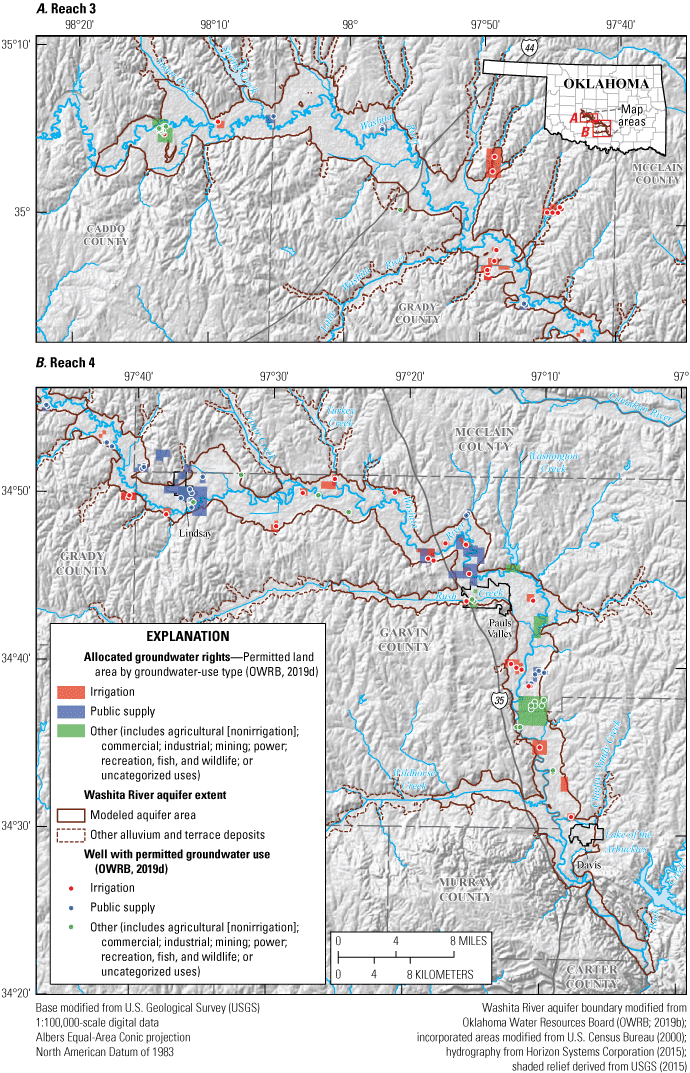
Land areas and wells permitted for groundwater use from A, reach 3 and B, reach 4 of the Washita River aquifer, southern Oklahoma, 2017.
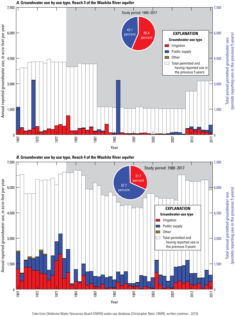
Annual reported and total annual permitted groundwater use by use type from A, reach 3 and B, reach 4 of the Washita River aquifer, southern Oklahoma, 1967–2017.
Table 4.
Annual reported groundwater use from reach 3 and reach 4 of the Washita River aquifer, southern Oklahoma, 1967–2017.[Permit-level reported groundwater-use data from the Oklahoma Water Resources Board (OWRB) were aggregated by groundwater-use type in this table (Rogers and others, 2023) owing to restrictions of proprietary interest and permit-holder anonymity; table excludes groundwater use of less than 5 acre-feet per year for domestic and agricultural purposes and groundwater use for irrigation of fewer than 3 acres of land for growing of gardens, orchards, or lawns (Oklahoma Statutes §82–1020.3; Oklahoma State Legislature, 2021c). All values are in units of acre-feet per year. Totals may not equal sum of components because of independent rounding. Gray shading indicates the data for the 1980–2017 study period]
Mean annual groundwater use for the 1980–2017 study period was 1,214.1 acre-ft/yr, which includes 745.8 acre-ft/yr (61.4 percent) for public supply and 461.8 acre-ft/yr (38.0 percent) for irrigation (table 4) (Rogers and others, 2023). Mean annual groundwater use for the period of record (1967–2017) was 1,590.7 acre-ft/yr, which includes 861.6 acre-ft/yr (54.2 percent) for irrigation and 709.7 acre-ft/yr (44.6 percent) for public supply (table 4) (Rogers and others, 2023). The decrease in groundwater use, particularly in irrigation groundwater use after 1980, is likely a result of the OWRB implementing changes in methods of groundwater-use reporting. Since 1980, the OWRB has required irrigation permit holders to estimate and annually report their groundwater use in terms of number of applications and number of inches of water applied (Christopher Neel, OWRB, written commun., 2019). Prior to 1980, however, inches of water applied during irrigation were not required to be reported. As a result, the OWRB adopted rules to estimate the number of inches of water applied for pre-1980 data on the basis of the number of water applications. This estimate results in what appears to be a step-change decrease in irrigation groundwater use after 1980 (fig. 8). In 2017, regular permits accounted for about 58 percent and prior-right permits accounted for about 42 percent of reported groundwater use from the Washita River aquifer (OWRB, 2019d).
Mean annual groundwater use for the 1980–2017 study period was 309.9 acre-ft/yr in reach 3 and 904.2 acre-ft/yr in reach 4 of the Washita River aquifer (table 4) (Rogers and others, 2023). Mean annual groundwater use for the period of record 1967–2017 was 406.7 acre-ft/yr in reach 3 and 1,184.0 acre-ft/yr in reach 4 of the Washita River aquifer (table 4) (Rogers and others, 2023). Groundwater-use permits for public supply were predominantly for wells near Lindsay, Okla., or Pauls Valley, Okla., in reach 4 of the Washita River aquifer, whereas groundwater-use permits for irrigation were for wells scattered throughout the Washita River aquifer (fig. 7). Reach 4 accounted for 74.5 percent of the groundwater use for the 1980–2017 study period and 74.4 percent of the groundwater use for the period of record 1967–2017.
Historical groundwater yields from wells completed in the Washita River aquifer generally decreased from northwest to southeast as the aquifer materials thin; groundwater yields of about 350 gallons per minute (gal/min) were reported near Lindsay and groundwater yields of about 200 gal/min were reported near Davis in the 1950s (Leonard and others, 1958). Driller-estimated groundwater-yield values, which have been mostly recorded since the 1980s, averaged about 70 gal/min; about 50 percent of the values recorded were greater than 25 gal/min (the median value), and about 9 percent of the values recorded were greater than 200 gal/min (OWRB, 2019a). Historical groundwater-yield values in the Washita River aquifer obtained from the NWIS database (USGS, 2020) averaged about 240 gal/min. The median groundwater-yield value was 175 gal/min, and a groundwater-yield value of 1,200 gal/min was reported at one well northwest of Pauls Valley (USGS station 344625097181001). These groundwater-yield statistics likely were biased high because high-yield irrigation and public-supply wells were the most common type of well to have measured discharges (USGS, 2020).
Hydrogeology of the Washita River Aquifer and Surrounding Units
The alluvium and terrace deposits of the Washita River aquifer mostly lie atop Permian-age bedrock units of the northwest-southeast trending Anadarko Basin syncline axis where it approaches the Arbuckle Uplift in southern Oklahoma (fig. 9). The Permian-age bedrock units are generally composed of shale, siltstone, and fine-grained sandstone that serve as boundaries in relation to the alluvium and terrace deposits of the Washita River aquifer (fig. 10). The Arbuckle Uplift deformed and exposed pre-Permian Paleozoic-age sedimentary and igneous units that form the Arbuckle Mountains in the southeastern part of the study area (fig. 9) (Reeds, 1927; Ye and others, 1996). Where they cross the Arbuckle Mountains, the alluvium and terrace deposits of the Washita River aquifer narrow and thin (Kent and others, 1984) and are no longer classified as a major aquifer by the OWRB. In the discussion herein, the geologic units of the study area are presented in reverse chronological order, which is the order in which the units are crossed by the Washita River (upstream to downstream).
Alluvium and Terrace Deposits
Alluvium and terrace deposits of Quaternary age are the principal water-bearing units of the Washita River aquifer (fig. 9). These deposits are made up of alluvial gravel, sand, silt, and clay (figs. 9 and 10; Leonard and others, 1958). Most terrace deposits are hydraulically connected to the valley-bottom alluvium, but some are hydraulically disconnected from the other terrace deposits and the valley-bottom alluvium and thus are unable to store water (Leonard and others, 1958). The disconnected terrace deposits are most evident north of Anadarko and northwest of Pauls Valley (fig. 9). The alluvium and terrace deposits are typically about 2–3 mi wide, but where the Washita River Valley constricts, those deposits are less than 1 mi wide (fig. 11). The Washita River Valley is narrowest where it approaches the Arbuckle Uplift (figs. 9 and 11E). In that area, the alluvium and terrace deposits are only about 0.25 mi wide, which the OWRB regards as the southern boundary of the Washita River aquifer (fig. 9; OWRB, 2019a).
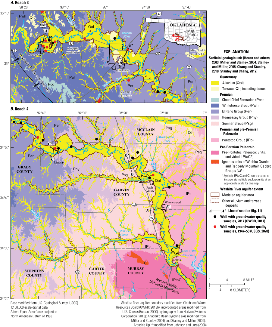
Surficial geologic units and major structural features in A, reach 3 and B, reach 4 of the Washita River aquifer study area, southern Oklahoma.
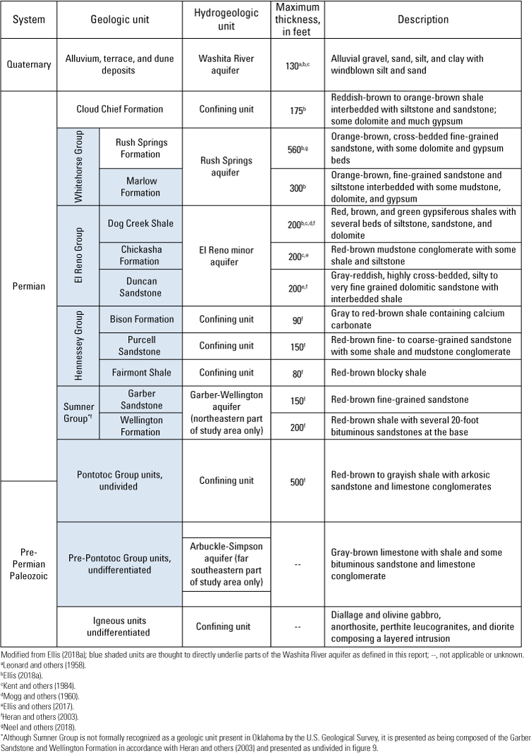
Stratigraphic descriptions of surficial geologic and hydrogeologic units of the Washita River aquifer study area, southern Oklahoma.
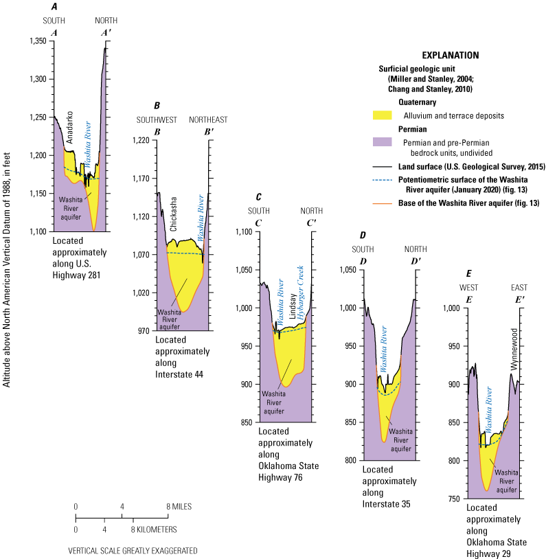
Hydrogeologic cross sections of the Washita River aquifer, southern Oklahoma, at various locations A–E (fig. 9) in the study area.
Bedrock Units
Bedrock units of Permian age underlie all of reach 3 (fig. 9A) and most of reach 4 (fig. 9B) of the Washita River aquifer. In the northwesternmost part of the aquifer, west of Anadarko, the Whitehorse Group directly underlies the geologic units that contain the Washita River aquifer (fig. 9). The Whitehorse Group consists of the Rush Springs Formation and the Marlow Formation (fig. 10) but is shown in figure 9 as an undivided unit. The Rush Springs Formation is described as orange-brown, cross-bedded fine-grained sandstone, with some dolomite and gypsum beds (Ellis, 2018a; Neel and others, 2018). The thickness of this geologic unit ranges between 186 and 560 ft in the study area (Ellis, 2018a). Stratigraphically below the Rush Springs Formation is the Marlow Formation, which consists of orange-brown, fine-grained sandstone and siltstone interbedded with mudstone, gypsum, and dolomite (Kent and others, 1984; Ellis, 2018a). The Marlow Formation directly underlies the Washita River aquifer near Anadarko and along Sugar Creek (Kent and others, 1984).
Beneath the White Horse Group is the Permian-age El Reno Group, which consists of the Dog Creek Shale, the Chickasha Formation, and the Duncan Sandstone (fig. 10) but is shown in figure 9 as an undivided unit (Heran and others, 2003). The Dog Creek Shale underlies the Washita River aquifer in the western part of Grady County and consists of red, brown, and green gypsiferous shales interbedded with siltstone, sandstone, and dolomite (Kent and others, 1984; Heran and others, 2003; Ellis, 2018a). The Dog Creek Shale has an estimated thickness of 200 ft and is described as having very low permeability (Mogg and others, 1960; Ellis, 2018a), which serves to limit downward flow in the Washita River aquifer. The Chickasha Formation and Duncan Sandstone make up the stratigraphically lower part of the El Reno Group. The Chickasha Formation is characterized as a red-brown mudstone conglomerate with some shale and siltstone and is estimated to be about 200 ft thick (Kent and others, 1984; Ellis and others, 2017). The Duncan Sandstone has a similar thickness to the Chickasha Formation and the Dog Creek Shale and is characterized as a light gray to reddish cross-bedded fine-grained sandstone interbedded with shale (Heran and others, 2003; Ellis and others, 2017). The Duncan Sandstone directly underlies the Washita River aquifer as reach 3 transitions to reach 4 (Heran and others, 2003). The units of the El Reno Group contain the El Reno minor aquifer in the study area.
The Permian-age Hennessey Group directly underlies the Washita River aquifer in the northern part of Garvin County (Kent and others, 1984; fig. 9). The Hennessey Group is made up of the Bison Formation, Purcell Sandstone, and Fairmont Shale (fig. 10) but is shown in figure 9 as an undivided unit. The Bison Formation, estimated to be 50–90 ft thick in the study area, makes up the upper part of the Hennessey Group and is characterized as gray to red-brown shale containing calcium carbonate (Heran and others, 2003). The Purcell Sandstone is a red-brown, fine- to coarse-grained sandstone with some shale and mudstone conglomerate (Heran and others, 2003). The Purcell Sandstone is about 90–150 ft thick in the study area and lies directly above the Fairmont Shale. The Fairmont Shale is similar in color to the Purcell Sandstone, characterized as red-brown and blocky. The Fairmont Shale thickness is 40–80 ft in the study area.
The Permian-age Sumner Group, which includes the Garber Sandstone and Wellington Formation, underlies the Washita River aquifer northwest of Pauls Valley (figs. 9 and 10). The Garber Sandstone is characterized as red-brown fine-grained sandstone with a thickness of about 100–150 ft in the study area (Heran and others, 2003). The Wellington Formation is composed of red-brown shale with several 20–30-ft bituminous sandstones at the base and a thickness of about 100–200 ft decreasing southeastward in the study area (Heran and others, 2003). The Garber Sandstone and Wellington Formation contain the Garber-Wellington aquifer (also known as the Central Oklahoma aquifer, Mashburn and others, 2013) in the northeastern part of the study area, where the Garber Sandstone and Wellington Formation are thicker and more permeable. However, the Garber Sandstone and Wellington Formation are not considered to be a major aquifer near the Washita River aquifer (Hart, 1974; Patterson, 1984).
Underlying the Sumner Group is the Pontotoc Group, a mostly Permian-age red-brown to grayish shale with arkosic sandstone and limestone conglomerates (fig. 10). The Pontotoc Group directly underlies the Washita River aquifer in reach 4 where it approaches the Arbuckle Mountains (fig. 9) and has a relative thickness of 300–500 ft in the study area (Heran and others, 2003). The Pontotoc Group is not sufficiently permeable to yield large quantities of water in most locations and is not considered to be a major water-bearing unit in the study area; however, well yields of 60 gal/min have been reported in a small area in southwestern Garvin County (Hart, 1974).
Pre-Permian Paleozoic-age units make up the Arbuckle Mountains and underlie the southeasternmost part of the Washita River aquifer (fig. 9). These units are composed of gray-brown limestone with shale and some bituminous sandstone and limestone conglomerate (fig. 10) and were greatly faulted and folded by the Arbuckle Uplift (Reeds, 1927; Ye and others, 1996). Some of the pre-Permian Paleozoic-age units form the Arbuckle-Simpson aquifer in southern Oklahoma. It is uncertain, however, whether that aquifer is in direct hydraulic connection with the Washita River aquifer as defined in this report. Igneous units (Wichita Granite and Raggedy Mountain Gabbro Groups [fig. 9], consisting of diallage and olivine gabbro, anorthosite, perthite leucogranites, and diorite composing a layered intrusion [fig. 10]) are present within the study area southwest of Davis; however, these igneous units are not in direct hydraulic connection with the Washita River aquifer.
Groundwater Quality
Groundwater-quality data were collected in the study area during July 28–August 25, 2014, by the OWRB (OWRB, 2017). Groundwater was sampled from 14 wells in the alluvium and terrace deposits of the Washita River aquifer study area (fig. 9; site information is available in Rogers and others [2023]) and analyzed for selected constituents including physical properties (pH, temperature, and specific conductance), major ions, nutrients, and trace metals. Total dissolved solids (TDS) concentrations in the groundwater samples ranged from 215 to 1,070 milligrams per liter (mg/L) with a median concentration of 523 mg/L and a mean concentration of 594 mg/L. The U.S. Environmental Protection Agency (2017) has established a secondary drinking water standard of 500 mg/L for TDS. The State of Oklahoma, however, acknowledges a beneficial domestic use for general use (class II) groundwater with TDS concentrations of less than 3,000 mg/L and limited use (class III) groundwater with TDS concentrations of 3,000–5,000 mg/L (OWRB, 2015). Specific conductance ranged from 316 to 1,879 microsiemens per centimeter at 25 degrees Celsius (µS/cm at 25 °C) with a median value of 955 µS/cm at 25 °C and a mean of 1,051 µS/cm at 25 °C. The hardness ranged from 142 to 1,470 mg/L; the median hardness value was 493 mg/L, and the mean hardness value was 553 mg/L. All groundwater samples were classified as hard water (hardness greater than 180 mg/L) except for two samples that were collected from terrace deposits of northern Garvin County, which had hardness values of 142 and 170 mg/L.
In addition to the groundwater-quality data collected in 2014 from 14 wells by the OWRB (OWRB, 2017), groundwater-quality data from 3 wells sampled during 1947–53 were obtained from the NWIS database (USGS, 2020) (fig. 9). Groundwater from those wells was analyzed for selected constituents including physical properties (pH, temperature, and specific conductance), major ions, and nutrients. TDS concentrations in the groundwater samples ranged from 432 to 7,960 mg/L with a median concentration of 716 mg/L and a mean concentration of 1,471 mg/L. Specific conductance ranged from 195 to 6,990 µS/cm at 25 °C with a median value of 1,120 µS/cm at 25 °C and a mean value of 2,115 µS/cm at 25 °C. The hardness ranged from 160 to 900 mg/L; the median value was 622 mg/L, and the mean value was 219 mg/L. All groundwater samples were classified as hard water except for two samples, which had hardness values of 160 and 180 mg/L, from western Grady County.
Major-ion groundwater-quality data were converted to units of milliequivalents per liter and excluded from further analysis if the difference in the cation-anion balance for the sample was greater than 10 percent; one sample was excluded from the OWRB (2017) data, and two samples were excluded from the USGS (2020) data. The data from the remaining 13 OWRB (2017) and 12 USGS (2020) samples were plotted on a Piper (1944) diagram for visualization of groundwater types and trends (fig. 12). The northern parts of the Washita River aquifer are adjacent to Permian-age bedrock transitioning in the southern parts to the Pontotoc Group, Permian and pre-Permian Paleozoic-age red-brown to grayish shale with arkosic sandstone and limestone conglomerates near the Arbuckle Mountains (figs. 9 and 10). The groundwater samples show a downgradient transition in anions from a sulfate-rich water to a bicarbonate-rich water (fig. 12). Bicarbonate dominates the anions, particularly in the downgradient samples, resulting in the calcium-magnesium bicarbonate water type for a majority of the samples. A calcium-magnesium sulfate-chloride water type was identified in seven of the samples. These samples occurred mostly in the northwestern part of the aquifer (fig. 9A), where interactions with the Permian-age bedrock contribute the sulfate anion through dissolution of gypsum beds (fig. 10).
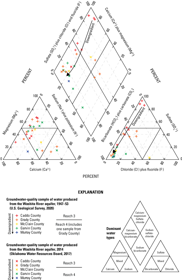
Groundwater-quality samples of water produced from the Washita River aquifer, 1947–53 and 2014, southern Oklahoma.
Hydrogeologic Framework of the Washita River Aquifer
A hydrogeologic framework is a three-dimensional representation of an aquifer and how that aquifer interfaces with surrounding geologic units at a scale that captures the regional controls on groundwater flow (Smith and others, 2021). The hydrogeologic framework for the alluvium and terrace deposits of the Washita River aquifer includes updated definitions of the three-dimensional aquifer extent and potentiometric surface, as well as a description of the hydraulic and textural properties of aquifer materials. The hydrogeologic framework was used in the construction of the numerical groundwater-flow model of the Washita River aquifer (Rogers and others, 2023) described in this report.
Aquifer Extent and Thickness
The geographic extent of the Washita River aquifer (fig. 1) was updated from the OWRB (2019b) by using information obtained from relatively new 1:100,000-scale geologic maps (Miller and Stanley, 2004; Chang and Stanley, 2010; Stanley and Chang, 2012). An older 1:250,000-scale geologic map (Heran and others, 2003) was used for a part of the aquifer near Chickasha, Okla., for which finer scale geologic maps were unavailable. Compared to the relatively coarse scale of the older 1:250,000-scale geologic map of the study area, the finer 1:100,000-scale geologic maps showed a narrower extent of the alluvium and terrace deposits that contain the aquifer, so the updated aquifer area presented in this report is smaller than previously documented.
Where present, the top of the Washita River aquifer was defined as the land-surface altitude obtained from a 10-m (horizontal resolution) digital elevation model (DEM) (USGS, 2015) with filled depressions. The altitude of the base of the Washita River aquifer, which was equivalent to the top of the bedrock, was contoured at a 50-ft interval from bedrock depths obtained from drillers’ lithologic logs, well-completion reports, and test-hole data (OWRB, 2019a; USGS, 2020) and direct-push test holes (fig. 13; USGS, 2020). For each of these data sources, the altitude of the base of the aquifer was calculated by subtracting the measured bedrock depth from the land-surface altitude. For consistency, the land-surface altitude was obtained from the 10-m DEM, even when the data source provided a land-surface altitude.
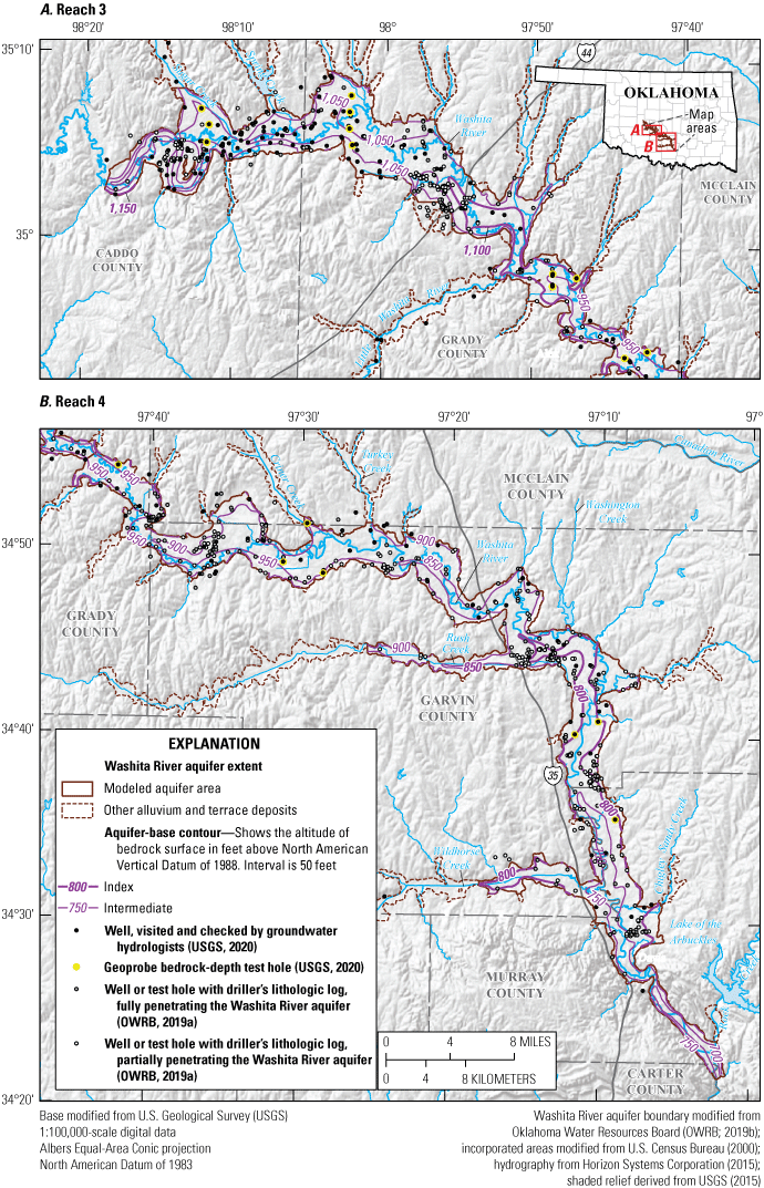
The altitude of the base in A, reach 3 and B, reach 4 of the Washita River aquifer, southern Oklahoma.
Selected wells and direct-push test holes in the Washita River aquifer were assumed to fully penetrate the aquifer (USGS, 2020; fig. 13), and their depths were assumed to be equal to the bedrock depth. Bedrock depths from these wells and test holes were given the highest priority because they had each been visited and checked by the authors of this report. Other wells and test holes included reports with drillers’ lithologic logs (OWRB, 2019a; fig. 13) that were searched for terms representing consolidated Permian-age bedrock units (such as “redbed” and “bedrock”). The altitude associated with the first occurrence of these terms in the logs was used as the altitude of the aquifer base. For logs that indicated that the well completely penetrated the Washita River aquifer (for example, the well log did not include a bedrock-related term), the altitude associated with the hole depth listed on the lithologic log was assumed to be the maximum (highest) possible altitude of the aquifer base at that location.
The mean thickness of alluvium and terrace deposits in the Washita River aquifer was about 54 ft, estimated by using the land-surface altitude and the aquifer-base altitude defined in this report. The mean thickness of alluvium and terrace deposits in reach 3 was about 56 ft and in reach 4 was about 53 ft.
Potentiometric Surface and Saturated Thickness
Potentiometric-surface maps show the altitude at which the water level would have stood in tightly cased wells at a specified time; the potentiometric surface is usually contoured or spatially interpolated from synoptic water-table-altitude measurements in many wells across an aquifer extent. Potentiometric-surface maps are used to indicate the general directions of groundwater flow in an aquifer. Groundwater generally flows perpendicular to potentiometric contours in the direction of decreasing contour altitudes (Freeze and Cherry, 1979).
In this report, the Washita River aquifer water table was assumed to be equivalent to the potentiometric surface because the aquifer is unconfined (Kent and others, 1984). The potentiometric surface for the Washita River aquifer was mapped by using groundwater-level measurements from selected wells and subtracting the measured depth to water from the land-surface altitude derived from a light detection and ranging (lidar) DEM (USGS, 2019). The selected wells were domestic and irrigation wells that were unused at the time of measurement. Methods described in Cunningham and Schalk (2011) were used to obtain groundwater-level measurements. A January 2020 potentiometric surface (fig. 14) for the Washita River aquifer was contoured primarily from synoptic groundwater-level altitudes measured during January 21–23, 2020, in 66 wells and supplemented with selected water-level altitudes measured mostly during February 2018 and December 1986–January 1987 in 24 wells (USGS, 2020; sites not listed in table 1; instead, site information is available in Rogers and others [2023]). Water-level altitudes measured in 2018 and 1986–87 were used to add control in areas where there was not a measurement in 2020. The mean saturated thickness of the Washita River aquifer was about 47 ft. The mean saturated thickness of reach 3 was about 50 ft and of reach 4 was about 45 ft (Rogers and others, 2023). Local flow in the Washita River aquifer was generally from topographically high areas toward the Washita River and major tributaries with regional flow in the aquifer generally from northwest to southeast (fig. 14).
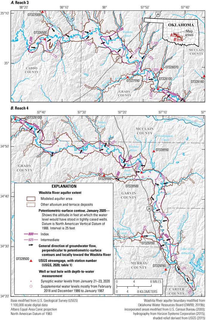
Potentiometric-surface contours and general direction of groundwater flow in A, reach 3 and B, reach 4 of the Washita River aquifer, southern Oklahoma, 2020.
Hydraulic and Storage Properties of Aquifer Materials
The distribution and variability of textural and hydraulic properties of aquifer materials, especially the horizontal hydraulic conductivity, were assumed to be the primary controls on groundwater flow in the Washita River aquifer. Multiple methods were used to estimate the range and central tendency of horizontal hydraulic conductivity values in the aquifer. These methods included in-place estimation in test holes, a multiwell aquifer test, and summary of data in drillers’ lithologic logs.
Horizontal Hydraulic Conductivity Estimated in Test Holes
A direct-push Geoprobe hydraulic profiling tool (HPT; Geoprobe Systems, 2015) was used at six Geoprobe test-hole sites (table 5, fig. 1) during June 24–July 15, 2021, to obtain in-place estimates of horizontal hydraulic conductivity by using the McCall (2010) method. This method can be used in the saturated zone to estimate horizontal hydraulic conductivity values between 0.1 and 150 feet per day (ft/d). During direct-push drilling, the HPT injects water into the aquifer material while logging electrical conductivity, injection pressure (corrected for hydrostatic gradient in the saturated zone), and injection flow rate at 0.05-ft depth intervals (Geoprobe Systems, 2015). The Direct Image Viewer (version 3.0) software package (Geoprobe Systems, 2020) was used to calculate discrete horizontal hydraulic conductivity values with depth by using the ratio of the injection flow rate and the hydrostatic-corrected injection pressure. The HPT test holes were drilled to a depth of refusal, which was assumed to be the bedrock contact. The 5,595 discrete (every 0.05 ft) HPT horizontal hydraulic conductivity measurements from all six test holes ranged from 0.1 to 89.0 ft/d (fig. 15) with a mean of 12.2 ft/d (table 5; USGS, 2021). These horizontal hydraulic conductivity data may be underestimated, though; small algal mats from the injection-water tank became entrained in the injection line during logging, which may have partially obstructed flow through the injection line, possibly increasing the measured injection pressure and making the aquifer appear less permeable. Progressive obstruction of the injection line may explain why the first two drilled test holes (TH11 and TH12, table 5, fig. 15A) had greater mean horizontal hydraulic conductivity measurements (22.1 and 26.7 ft/d, respectively) than did the others. Most of the HPT test holes showed generally decreasing electrical conductivity and generally increasing horizontal hydraulic conductivity with depth, indicating that the aquifer materials tend to fine upward from fine to medium sand to silt and clay (fig. 9.2 in Boggs [1995]).
Table 5.
Hydraulic properties calculated from Geoprobe hydraulic profiling tool logs at direct-push Geoprobe test holes in the Washita River aquifer, southern Oklahoma, 2020–21.[Data from U.S. Geological Survey (USGS; 2020, 2021). M/D/Y, month/day/year; NAVD 88, North American Vertical Datum of 1988; HPT, hydraulic profiling tool; Kh, horizontal hydraulic conductivity; --, not available or not applicable]
| Map name (fig. 1) | Field identifier | USGS station identifier | USGS site name | Latitude, in decimal degrees | Longitude, in decimal degrees | Reach | Drilling date (M/D/Y) | Land-surface altitude, in feet above NAVD 88 | Well or hole depth, in feet | HPT logging date (M/D/Y) | HPT depth, in feet below land surface | HPT depth to water, in feet below land surface | HPT mean Kh, in feet per day |
|---|---|---|---|---|---|---|---|---|---|---|---|---|---|
| TH01 | WYNNEWOOD3 | 343537097085801 | 02N-01E-36 DCC 1 | 34.5936 | −97.1494 | 4 | 10/5/2020 | 826 | 40.6 | 7/13/2021 | 33.2 | 3.4 | 5.7 |
| TH02 | PAULSVALLEY1 | 344011097114301 | 02N-01E-03 CCB 1 | 34.6697 | −97.1953 | 4 | 10/5/2020 | 864 | 48.6 | -- | -- | -- | -- |
| TH03 | PAULSVALLEY2 | 344053097101001 | 03N-01E-35 CDD 1 | 34.6814 | −97.1696 | 4 | 10/2/2020 | 851 | 46.6 | -- | -- | -- | -- |
| TH04 | LINDSAY3 | 344842097283401 | 04N-03W-23 AAA 1 | 34.8118 | −97.4762 | 4 | 9/11/2020 | 958 | 46.9 | -- | -- | -- | -- |
| TH05 | LINDSAY1 | 344916097311401 | 04N-03W-16 BDA 1 | 34.8212 | −97.5205 | 4 | 10/2/2020 | 961 | 63.2 | 7/14/2021 | 63.0 | 15.6 | 6.8 |
| TH06 | LINDSAY4 | 345122097294001 | 05N-03W-34 DDD 1 | 34.8562 | −97.4946 | 4 | 10/2/2020 | 956 | 74.1 | -- | -- | -- | -- |
| TH07 | BRADLEY1 | 345402097434901 | 05N-05W-16 DCB 1 | 34.9005 | −97.7302 | 4 | 10/6/2020 | 1,019 | 49.2 | 7/14/2021 | 48.5 | 4.3 | 7.1 |
| TH08 | BRADLEY3 | 345422097421801 | 05N-05W-14 CBB 1 | 34.9061 | −97.7051 | 4 | 10/9/2020 | 1,013 | 90.2 | -- | -- | -- | -- |
| TH09 | ALEX3 | 345749097484101 | 06N-06W-26 CBB 1 | 34.9637 | −97.8114 | 3 | 10/1/2020 | 1,038 | 59.2 | -- | -- | -- | -- |
| TH10 | ALEX2 | 345817097470602 | 06N-06W-24 DCC 2 | 34.9715 | −97.7849 | 3 | 10/1/2020 | 1,038 | 43.4 | -- | -- | -- | -- |
| TH11 | ALEX1 | 345829097484101 | 06N-06W-23 CCB 1 | 34.9748 | −97.8115 | 3 | 10/9/2020 | 1,043 | 57.5 | 6/28/2021 | 58.9 | 19.2 | 22.1 |
| TH12 | CHICKASHA2 | 350513098021301 | 07N-08W-10 CCD 1 | 35.0870 | −98.0369 | 3 | 10/1/2020 | 1,115 | 63.6 | 6/24/2021 | 63.6 | 2.8 | 26.7 |
| TH13 | ANADARKO2 | 350513098115501 | 07N-10W-12 DDD 1 | 35.0869 | −98.1987 | 3 | 10/8/2020 | 1,164 | 69.2 | 7/15/2021 | 68.5 | 7.4 | 4.8 |
| TH14 | CHICKASHA1 | 350606098022501 | 07N-08W-03 CCC 1 | 35.1017 | −98.0403 | 3 | 10/9/2020 | 1,123 | 49.3 | -- | -- | -- | -- |
| TH15 | ANADARKO1 | 350610098114701 | 07N-09W-06 CCC 1 | 35.1028 | −98.1965 | 3 | 10/8/2020 | 1,165 | 98.0 | -- | -- | -- | -- |
| TH16 | CHICKASHA3 | 350700098022501 | 07N-08W-04 AAA 1 | 35.1167 | −98.0403 | 3 | 10/1/2020 | 1,114 | 35.2 | -- | -- | -- | -- |
| TH17 | ANADARKO3 | 350701098121901 | 07N-10W-01 ABB 1 | 35.1170 | −98.2054 | 3 | 10/8/2020 | 1,172 | 92.7 | -- | -- | -- | -- |
| TH18 | CHICKASHA4 | 350753098022001 | 08N-08W-28 DDD 1 | 35.1314 | −98.0389 | 3 | 10/9/2020 | 1,117 | 47.3 | -- | -- | -- | -- |
| Mean | 55.9 | 8.8 | 12.2 |
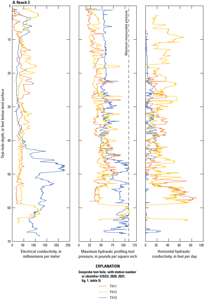
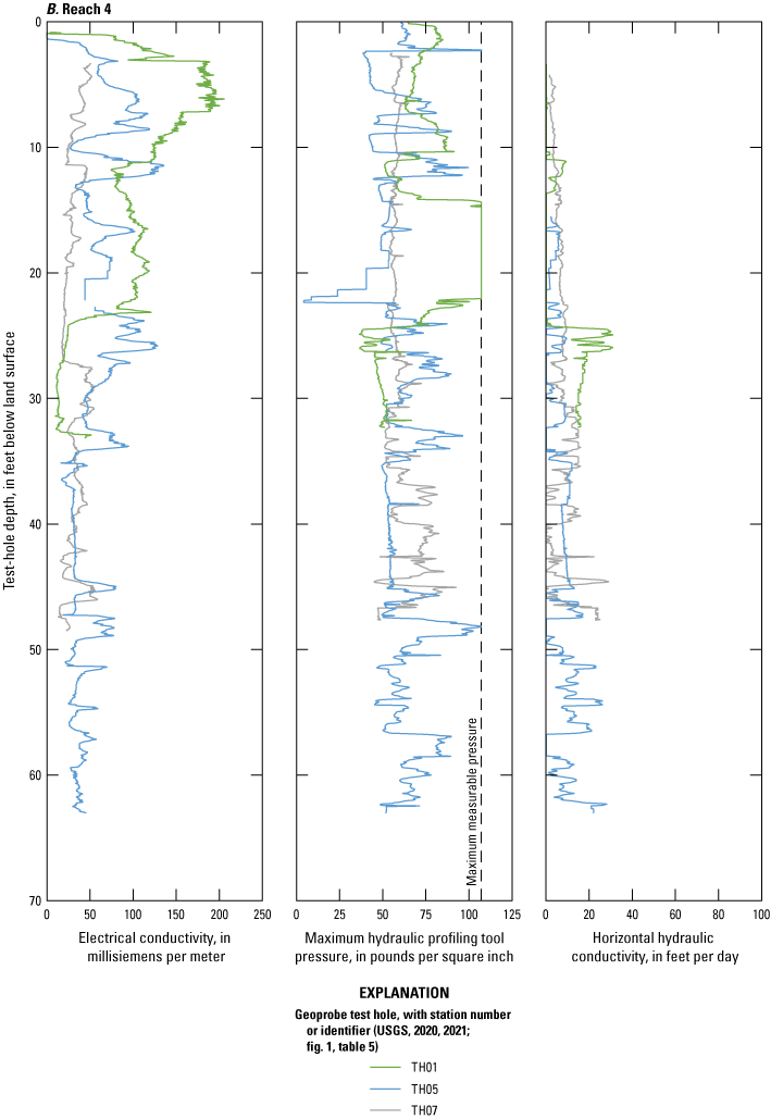
Logs of electrical conductivity, maximum hydraulic profiling tool pressures, and horizontal hydraulic conductivity (U.S. Geological Survey, 2021) from selected Geoprobe test holes (U.S. Geological Survey, 2020) in A, reach 3 and B, reach 4 of the Washita River aquifer, southern Oklahoma, June 24–July 15, 2021.
Horizontal Hydraulic Conductivity Estimated From a Multiwell Aquifer Test
Multiwell aquifer tests are the best method for estimating mean hydraulic and storage properties of aquifer materials over a small area (Stallman, 1971). Data for two unpublished multiwell aquifer tests were found in the USGS paper archives in Oklahoma City, Okla. A multiwell aquifer test in the terrace north of Chickasha was of short duration (24 hours) and failed to induce adequate drawdown in the observation wells (an unknown distance from the pumping well) at a pumping rate of about 60 gal/min (Davis, 1955); this test could not be used for this report. Another multiwell aquifer test, conducted just east of Pauls Valley on March 21–22, 1950, also was of short duration (24 hours) but induced a drawdown of about 7–8 ft in observation wells about 15–30 ft from a production well discharging about 90 gal/min (Rogers and others, 2023). Using the Cooper and Jacob (1946) method, this test yielded a transmissivity value of 922 feet squared per day (ft2/d) (6,900 gallons per day per foot). A horizontal hydraulic conductivity value of about 13 ft/d was calculated by dividing the transmissivity value by the 70 ft of pre-pumping saturated thickness at the aquifer-test site. A specific yield value of about 0.04 (dimensionless) also was calculated from the Pauls Valley multiwell aquifer test. The Pauls Valley multiwell aquifer test was not able to drain the presumed coarser and more porous material at the base of the aquifer, so the calculated transmissivity, horizontal hydraulic conductivity, and specific yield values are likely underestimated for the whole saturated thickness at the aquifer-test site. One short duration multiwell aquifer test is not sufficient to attribute hydraulic and storage properties for an entire aquifer. However, the Pauls Valley multiwell aquifer test is useful as a piece of evidence in characterizing groundwater flow and storage in the aquifer. The data and field notes relevant to the Pauls Valley multiwell aquifer test were scanned and included in the data release that accompanies this report (Rogers and others, 2023).
Horizontal Hydraulic Conductivity Estimated From Lithologic Logs
Drillers’ lithologic logs that penetrated at least 20 ft of the aquifer also were used to estimate the horizontal hydraulic conductivity of aquifer materials. Textural terms in each lithologic log (OWRB, 2019a) were standardized, categorized, and converted to percentage-coarse-material values by using the methods of Mashburn and others (2013). Lithologic logs included terms such as “gravel,” “sand,” “silt,” and “clay” to describe the texture of unconsolidated alluvium and terrace deposits of the Washita River aquifer; however, terms used for lithologic descriptions varied among drillers. To simplify and standardize the lithologic logs, lithologic descriptions of unconsolidated deposits were reclassified into five lithologic categories (clay, silt, fine to medium sand, coarse sand, and gravel) that were assumed to have ranges of percentage coarse material (0–20, 20–40, 40–60, 60–80, and 80–100 percent coarse material, respectively). The midpoint of each range (10, 30, 50, 70, or 90 percent coarse material, respectively) was then assigned to each lithologic depth interval. The percentage-coarse-material value for each lithologic log was computed as the thickness-weighted mean of percentage-coarse-material values assigned to the unconsolidated lithologic categories in the log. The theoretical maximum percentage-coarse-material value for any lithologic log was 90 percent (all gravel), and the theoretical minimum percentage-coarse-material value for any lithologic log was 10 percent (all clay). A total of 260 lithologic logs (OWRB, 2019a) were used for the percentage-coarse-material analysis, and at least 161 of those logs fully penetrated the aquifer. Layers of predominantly gravel were noted in about 20 percent of the lithologic logs analyzed, and clay layers were noted in almost 100 percent of the logs analyzed.
Ellis and others (2017) developed the following equation to characterize the relation between horizontal hydraulic conductivity and the percentage-coarse-material value:
whereKh
is the horizontal hydraulic conductivity, in feet per day; and
Ps
is the percentage-coarse-material value.
Equation 1 was used by Ellis and others (2017) to relate core-derived percentage-coarse-material values to horizontal hydraulic conductivity for alluvium and terrace deposits in the Canadian River aquifer of west-central Oklahoma; equation 1 is used in this report to estimate horizontal hydraulic conductivity values for lithologic logs in the Washita River aquifer. Lithologic-log horizontal hydraulic conductivity values of less than 0.1 ft/d were reassigned to that minimum value. The lithologic-log horizontal hydraulic conductivity values ranged from 0.1 to 90.1 ft/d with a mean of 32.9 ft/d.
Textural and Hydraulic Properties From Other Reports
Hemann (1985) measured horizontal hydraulic conductivity and specific yield values for core samples from reach 3 of the Washita River aquifer east of Anadarko by using a laboratory permeameter. The horizontal hydraulic conductivity measurements ranged from 0.1 to 184 ft/d and averaged about 23 ft/d. The specific yield measurements ranged from 0.03 to 0.22 and averaged about 0.10.
A hydrologic investigation and calibrated groundwater-flow model by Ellis (2018a, b) included simulations of groundwater flow in the alluvium and terrace deposits of the Washita River upgradient from and adjacent to the Washita River aquifer as described in this report. The Ellis (2018b) groundwater-flow model of the Rush Springs aquifer used calibrated horizontal hydraulic conductivity values that ranged from 60 to 90 ft/d for the most downgradient alluvium and terrace deposits, which are coincident with the upgradient extent of the study area for this report. The horizontal hydraulic conductivity values were comparable for the Washita River aquifer and Canadian River aquifer (fig. 43B in Ellis [2018a]). However, the Ellis (2018b) groundwater-flow model used calibrated specific yield values of 0.06–0.12 for the most downgradient Washita River alluvium and terrace deposits; those values were considerably less than the calibrated specific yield values (0.15–0.29) used for the most downgradient Canadian River alluvium and terrace deposits (fig. 46B in Ellis [2018a]). Ellis (2018a) related the difference in calibrated specific yield values to the textural difference in the source rocks eroded by (and contributing sediment to) the two streams; the Washita River alluvium and terrace deposits mostly originated from finer grained Permian-age sedimentary units in present-day Oklahoma, whereas the Canadian River alluvium and terrace deposits mostly originated from coarser grained Tertiary-age sedimentary units in present-day Oklahoma, Texas, and New Mexico (Hendricks, 1937).
The vertical anisotropy (ratio of horizontal to vertical hydraulic conductivity) and specific storage values have not been measured in the Washita River aquifer and were assumed to be comparable to those used in simulations of water availability in the nearby Salt Fork Red River aquifer (Smith and others, 2021), which used vertical anisotropy and specific storage values of 10.0 (dimensionless) and 1×10⁻⁵ inverse foot, respectively; these values were each within the range suggested by Domenico and Schwartz (1998) for unconsolidated aquifer materials like those of the Washita River aquifer.
Conceptual Groundwater-Flow Model
A conceptual groundwater-flow model is a simplified description (or diagram) of the major inflow and outflow sources (hydrologic boundaries) of a groundwater-flow system and includes a water-budget accounting of the estimated mean flows from those sources for a specified period. A conceptual groundwater-flow model (hereinafter referred to as the “conceptual model”) for the Washita River aquifer was developed to constrain the construction and calibration of a numerical groundwater-flow model (hereinafter referred to as the “numerical model”) for the aquifer. The conceptual-model water budget (table 6, fig. 16A) was used to estimate mean annual inflows to, and outflows from, the Washita River aquifer for the 1980–2017 study period and included a subaccounting of mean annual inflows and outflows for reach 3 (upgradient from the Alex gage) and reach 4 (downgradient from the Alex gage) (fig. 1). The conceptual-model (and numerical-model) aquifer area (modeled aquifer area, fig. 1) totaled 178,938 acres (table 6).
Table 6.
Conceptual-model water budget of estimated mean annual inflows and outflows for the Washita River aquifer, southern Oklahoma, 1980–2017.[All water-budget component values are in units of acre-feet per year. Totals may not equal sum of components because of independent rounding. Net streambed seepage, net lateral groundwater flow, and net change in groundwater storage represent the net effect of aquifer inflows and outflows. --, not quantified]
| Reach 3 | Reach 4 | Total | Percentage of water budget | Notes | ||
|---|---|---|---|---|---|---|
| Modeled area | in cells | 4,948 | 7,231 | 12,179 | -- | Reach 3 and reach 4 are upgradient and downgradient, respectively, from the vicinity of U.S. Geological Survey streamgage 07328100 Washita River at Alex, Okla. |
| in acres | 72,697 | 106,241 | 178,938 | -- | ||
| in percent | 40.6 | 59.4 | 100.0 | -- | ||
| Water-budget component | Recharge | 49,071 | 71,712 | 120,783 | 85.5 | 8.1 inches per year (table 7), or 20.2 percent of mean annual precipitation |
| Net lateral groundwater flow | 6,763 | 13,797 | 20,560 | 14.5 | Unknown; calculated as balance of water budget | |
| Total inflow | 55,835 | 85,509 | 141,344 | 100.0 | ||
| Water-budget component | Net streambed seepage | 49,041 | 75,130 | 124,171 | 87.8 | Estimated from base-flow data at streamgages (table 3) |
| Saturated-zone evapotranspiration | 6,484 | 9,476 | 15,960 | 11.3 | Estimated as 1.33 feet per year1 times 12,000 acres2 | |
| Net change in groundwater storage | -- | -- | -- | -- | Assumed to be a negligible part of water budget | |
| Well withdrawals | 310 | 903 | 1,213 | 0.9 | Calculated from Oklahoma Water Resources Board reported groundwater-use data (table 4) (Rogers and others, 2023) | |
| Total outflow | 55,835 | 85,509 | 141,344 | 100.0 | ||
Reduced slightly from an estimate of 1.46 feet per year by Ellis (2018a).
About 12,000 acres along the Washita River stream corridor were classified as wetland by the National Wetlands Inventory (U.S. Fish and Wildlife Service, 2014).
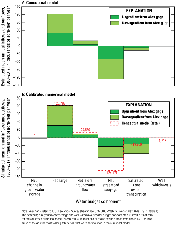
Estimated mean annual inflows and outflows by water-budget component for the A, conceptual model and B, calibrated numerical model of the Washita River aquifer, southern Oklahoma, 1980–2017.
Estimated mean annual flows to hydrologic boundaries of the conceptual model have varying levels of uncertainty. Where possible, those estimated flows were based on field measurements from the study area and study period. In cases where field measurements were unavailable or too difficult or expensive to obtain, estimated flows of the conceptual model were assumed to be analogous to those of published conceptual models from similar aquifers in Oklahoma (Ryter and Correll, 2016; Ellis and others, 2017, 2020; Smith and others, 2017, 2021; Ellis, 2018a). The “notes” section of table 6 summarizes data sources and assumptions used to construct the conceptual-model water budget for the Washita River aquifer.
Hydrologic Boundaries
Hydrologic boundaries in the conceptual model represent actual sources (inflows) and sinks (outflows) of water to and from the aquifer. Boundaries that act as both inflows and outflows may be referred to as “net inflows” or “net outflows” depending on which flow component dominates.
Recharge
Recharge is the predominant inflow to the Washita River aquifer. Recharge is defined in this report as the amount of precipitation that infiltrates from the land surface through the unsaturated zone and reaches the water table over a given time. This definition of recharge includes irrigation return flows to groundwater. Other processes such as stream seepage or lateral groundwater flow from adjacent hydrogeologic units are not considered recharge and are accounted for separately in the conceptual-model water budget. Recharge rates are controlled by many factors including precipitation rate, land-surface gradient, soil and sediment permeability, evapotranspiration rates, and vegetation cover type. Although recharge rates are difficult to measure because of high spatial and temporal variability, methods that include environmental tracers, physical measurements, streamflow-hydrograph techniques, and computer codes can be used to estimate recharge rates. For this report, a groundwater-hydrograph-based water-table fluctuation (WTF) method (Healy and Cook, 2002) was used to estimate localized recharge rates for 2017–19, and a code-based water-balance-estimation technique (Westenbroek and others, 2010) was used to estimate spatially distributed recharge rates for the 1980–2017 study period.
Water-Table Fluctuation Method
The WTF method was the primary method used to estimate recharge to the Washita River aquifer. The WTF method assumes that rises in groundwater levels in unconfined aquifers that occurred during a relatively short period (hours to a few days) can be attributed to recharge arriving at the saturation zone following a period of precipitation. This method is most appropriately applied to groundwater wells with shallow water tables and hydrographs that display sharp rises in groundwater levels after precipitation (Healy and Cook, 2002). The WTF method cannot account for a steady rate of recharge or recharge from sources other than precipitation. Annual recharge (R), in inches per year, was estimated by using the following equation:
whereSy
is the specific yield (dimensionless);
Δh
is the rise in groundwater-level altitude, in inches; and
Δt
is the change in time, in years.
Water-level hydrographs from three USGS continuous water-level recorder wells (W01, W02, and W05, table 1; USGS, 2020) were used to estimate annual recharge during 2017–19. W01 was located near Lindsay, W02 was located near Chickasha, and W05 was located near Pauls Valley (fig. 1). The water-level hydrographs from other continuous water-level recorder wells in the study area were not analyzed because they were affected by nearby pumping (in the case of W03, fig. 17A) or because they did not display sharp water-level rises (in the case of W04 and W06, fig. 17B). Annual precipitation data for the 2016–19 period of analysis were obtained from the Chickasha (CHIC) and Pauls Valley (PAUL) climate stations (fig. 1; Oklahoma Mesonet, 2019). Using the daily precipitation record from the nearest climate station and a specific yield of 0.10 from Hemann (1985), the annual recharge estimates for wells W02 and W05 in 2017 were 5.3 inches (in.; about 13.5 percent of the station annual precipitation) and 7.4 in. (about 18.5 percent of the station annual precipitation), respectively (table 7). The annual recharge estimates for wells W02 and W05 in 2018 were 9.0 in. (about 23.7 percent of the station annual precipitation) and 11.5 in. (about 22.8 percent of the station annual precipitation), respectively. In a year-long period from April 1, 2018, through March 31, 2019, the annual recharge estimate at well W01 was 10.3 in. (about 22.6 percent of the station annual precipitation). When those recharge estimates are normalized by the annual mean precipitation of 40.1 in/yr for the 1980–2017 study period and averaged, the resulting station-averaged mean annual recharge for 2017–19 in reach 3 and 4 of the Washita River aquifer was 8.1 in/yr (about 20.2 percent of mean annual precipitation for the 1980–2017 period). Multiplied by the 178,938-acre modeled area and unit converted, the WTF-calculated mean annual recharge for 2017–19 was 120,783 acre-ft/yr; this value was used as the conceptual-model recharge during 1980–2017 (table 6).
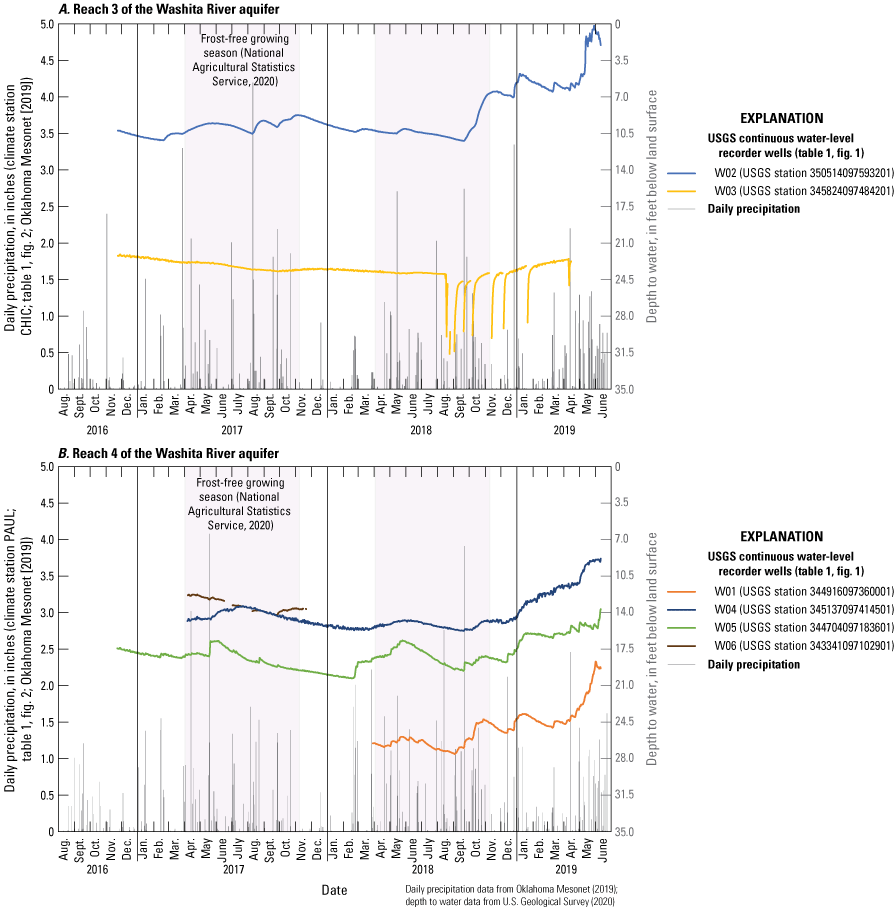
Daily precipitation and depth to water in U.S. Geological Survey (USGS) continuous water-level recorder wells completed in A, reach 3 and B, reach 4 of the Washita River aquifer, southern Oklahoma, August 2016–June 2019.
Table 7.
Summary of recharge amounts estimated using the water-table fluctuation method for the Washita River aquifer, southern Oklahoma, 2017–19.[Continuous water-level recorder wells W03 and W04 were not suitable for analysis with the water-table fluctuation method (Healy and Cook, 2002). Dates for the periods are in month-day-year (MM-DD-YYYY) format; --, data not available or not applicable]
| U.S. Geological Survey continuous water-level recorder well (fig. 1, table 1) | |||
|---|---|---|---|
| W02 | W01 | W05 | |
| Annual mean precipitation 1980–2017, in inches per year, southern Oklahoma, Climate Division 8 (National Centers for Environmental Information, 2021) | 40.1 | 40.1 | 40.1 |
| Climate station (fig. 2, table 1) | CHIC | PAUL | PAUL |
| Estimated specific yield | 0.10 | 0.10 | 0.10 |
| Station annual precipitation, in inches | 39.4 | -- | 40.1 |
| Sum of water-level rises, in feet | 4.4 | -- | 6.2 |
| Recharge, in inches per year | 5.3 | -- | 7.4 |
| Recharge, percent of annual precipitation | 13.5 | -- | 18.5 |
| Recharge, in inches per year, normalized to mean annual precipitation during 1980–2017 | 5.4 | -- | 7.4 |
| Station annual precipitation, in inches | 37.9 | -- | 50.5 |
| Sum of water-level rises, in feet | 7.5 | -- | 9.6 |
| Recharge, in inches per year | 9.0 | -- | 11.5 |
| Recharge, percent of annual precipitation | 23.7 | -- | 22.8 |
| Recharge, in inches per year, normalized to mean annual precipitation during 1980–2017 | 9.5 | -- | 9.2 |
| Station annual precipitation, in inches | -- | 45.5 | -- |
| Sum of water-level rises, in feet | -- | 8.6 | -- |
| Recharge, in inches per year | -- | 10.3 | -- |
| Recharge, percent of annual precipitation | -- | 22.6 | -- |
| Recharge, in inches per year, normalized to mean annual precipitation during 1980–2017 | -- | 9.0 | -- |
| Mean annual recharge during 2017–19, in inches per year, normalized to mean annual precipitation 1980–2017 | 8.1 | ||
Soil-Water-Balance Code
The Soil-Water-Balance code (SWB; Westenbroek and others, 2010) was used to estimate the amount and spatial distribution of daily groundwater recharge to the Washita River aquifer for each month of the 1980–2017 study period. SWB uses a modified Thornthwaite and Mather (1957) soil-water-balance method on a gridded data structure to compute the daily amount of infiltration (minus losses) that exceeds the storage capacity of the plant root zone. The soil-water-balance equation (modified from Westenbroek and others [2010]) has the form of the following equation:
whereR
is recharge, in inches per day;
P
is precipitation, in inches per day;
S
is snowmelt, in inches per day;
Ri
is surface runoff inflow, in inches per day;
Int
is plant interception, in inches per day;
Ro
is surface runoff outflow, in inches per day;
Pet
is potential evapotranspiration, in inches per day; and
ΔSm
is the change in soil moisture, in inches per day.
SWB requires climate and landscape characteristic data inputs including precipitation, temperature, soil-water storage capacity, hydrologic soil group, surface-water flow direction, and land-cover type (Westenbroek and others, 2010). Each of these inputs was assigned to a user-specified grid that was 600 by 500 cells of 800 by 800 ft each. The landscape inputs were assumed to remain constant during the study period, but climate data inputs varied daily. Daily climate data including precipitation and minimum and maximum air temperature were obtained for 14 selected climate stations (fig. 2, table 1; National Centers for Environmental Information, 2022) in and near the study area and gridded using inverse-distance-weighted (Esri, 2021b) interpolation. Accumulated snowmelt was added on the basis of the daily minimum and maximum air temperatures. Potential evapotranspiration was calculated by using the Hargreaves and Samani (1985) method for a reference latitude range of 34.5–35.4 degrees. Surface runoff was routed downslope by using a flow-direction grid derived from a 10-m DEM (USGS, 2015). Depressions in the DEM were filled by using the ArcGIS Fill tool (Esri, 2021a) to ensure correct routing of surface runoff and to eliminate areas of internal drainage that can result in unrealistically high amounts of recharge. Soil properties (soil-water storage capacity and hydrologic soil group) were derived from the Soil Survey Geographic database (NRCS, 2022), which is an inventory of generalized soil characteristics. Land-cover types (Fry and others, 2011; Multi-Resolution Land Characteristics Consortium, 2011; fig. 3) were used in conjunction with hydrologic soil groups to partition daily precipitation into plant interception (Int) and surface runoff (Ri and Ro) components and assign plant root-zone depths. The root-zone depths for grass/pasture and cropland (the dominant land-cover types for land overlying the aquifer; fig. 3) varied with soil texture but ranged from about 0.8 to 1.5 ft (40 percent of the values used by Westenbroek and others [2010] for permeable glacial deposits in Wisconsin). The soil-water storage capacity, analogous to specific yield in the saturated zone, multiplied by the root-zone depth determined the maximum volume of water available in the root zone. Changes in soil moisture (ΔSm) exceeding the soil-water storage capacity were assumed to be recharge (R) to the saturated zone. Larger root-zone depths resulted in increased evapotranspiration of water from the root zone and decreased recharge; smaller root-zone depths resulted in decreased evapotranspiration of water from the root zone and increased recharge. Recharge from irrigation was not simulated by SWB but was assumed to be negligible given the relatively small amount of irrigation groundwater use in the study area. The SWB model for the Washita River aquifer study area is included in Rogers and others (2023).
The SWB-estimated mean annual recharge for the 1980–2017 study period was about 4.9 in/yr, or about 12.2 percent of the mean annual precipitation of 40.1 in/yr during 1980–2017 (fig. 18A). The minimum and maximum SWB-estimated annual recharge values were about 1.1 in/yr in 2003 and 11.6 in/yr in 2015, respectively. Recharge efficiency (mean monthly recharge as a percentage of mean monthly precipitation) was greatest from November to February, when evapotranspiration was at a minimum; recharge in these months was greater than 20 percent of precipitation (fig. 18B). Recharge efficiency was lowest in July and August, when evapotranspiration was at a maximum; recharge in these months was less than 6 percent of precipitation. Spatially, mean annual recharge for the study period was greatest in areas of alluvium near the Washita River and tributaries (fig. 19). The SWB-estimated mean annual recharge generally increased from northwest to southeast in the Washita River aquifer; the mean annual recharge for reach 4 was about 14 percent greater than mean annual recharge for reach 3 of the Washita River aquifer. Increased recharge from reach 3 to reach 4 is correlated with increased precipitation from northwest to southeast in the study area (Oklahoma Climatological Survey, 2021a, b).
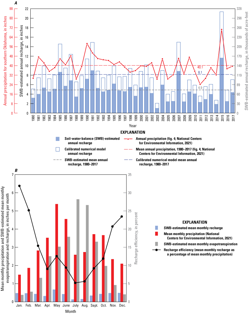
A, Annual precipitation with annual recharge estimated by using the Soil-Water-Balance code (Westenbroek and others, 2010) and B, mean monthly precipitation with mean monthly recharge and evapotranspiration estimated by using the Soil-Water-Balance code for the Washita River aquifer, southern Oklahoma, 1980–2017.
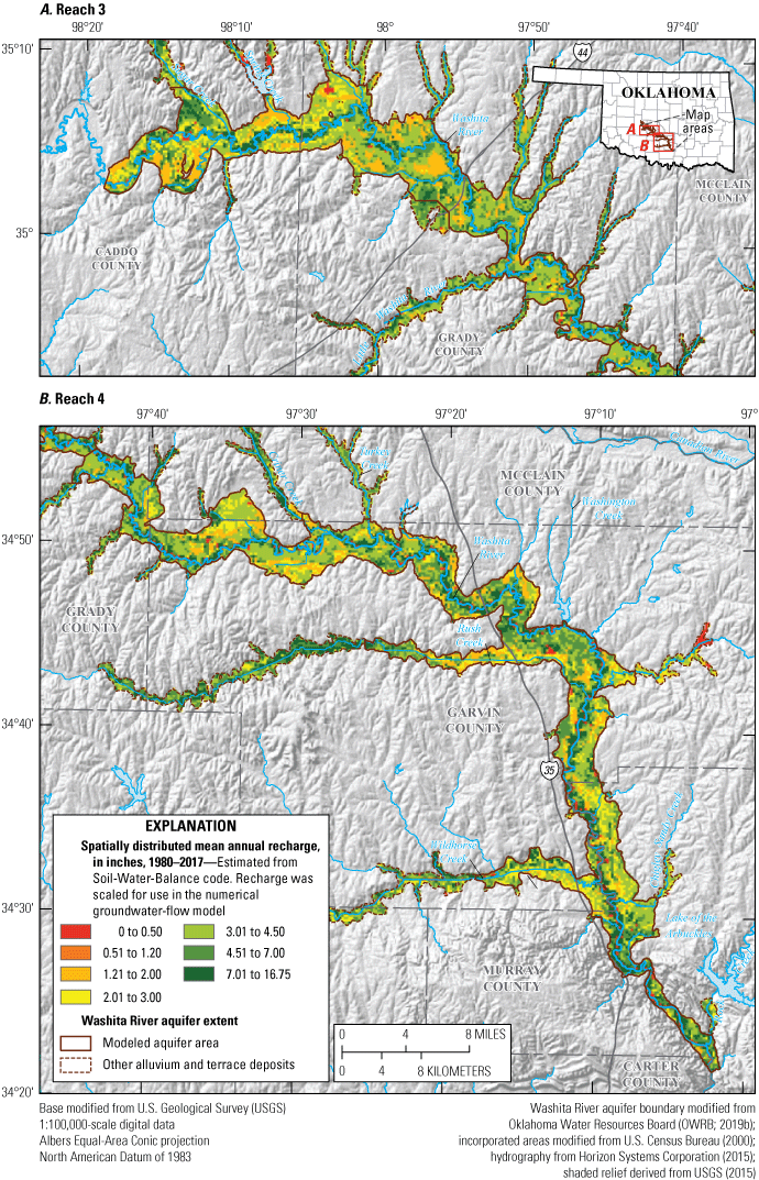
Mean annual recharge estimated by using the Soil-Water-Balance code (Westenbroek and others, 2010) in A, reach 3 and B, reach 4 of the Washita River aquifer, southern Oklahoma, 1980–2017.
Mean annual recharge rates estimated from SWB were compared to published estimates of mean annual recharge for the Washita River aquifer. Kent and others (1984) estimated a mean annual recharge of 3.72 in/yr, or about 12 percent of the mean annual precipitation of 32.2 in/yr during a 20-year study period (July 1, 1973–July 1, 1993). That estimate was applied across the entire Washita River aquifer in Oklahoma and included reaches that are outside the scope of this report. Schipper (1983) estimated a mean annual recharge of 3.17 in/yr, or about 13 percent of the mean annual precipitation (24.90 in/yr), during the same 20-year study period for a groundwater model of reach 1 of the Washita River aquifer (in western Oklahoma). Ellis and others (2020) estimated a mean annual recharge for reach 1 of the Washita River aquifer (in western Oklahoma) of 3.15 in/yr, or about 14 percent of the mean annual precipitation of 23 in/yr, during a 36-year study period (1980–2015). The mean annual recharge rate of 4.9 in/yr that was estimated by using SWB for the study area in this report is thus within the range of published estimates of recharge for the Washita River aquifer, particularly when calculated as a percentage of the applicable mean annual precipitation.
The SWB-estimated mean annual recharge was, however, about 40 percent less than the WTF-estimated mean annual recharge used for the conceptual model. SWB is a numerical model, and SWB-estimated recharge must, therefore, be checked against and calibrated to field-based measurements or estimates of recharge like those estimated using WTF. In other reports (Smith and others, 2017, 2021; Ellis, 2018a; Ellis and others, 2020), SWB-estimated recharge was calibrated by decreasing root-zone depths until the SWB-estimated mean annual recharge approximated the conceptual-model recharge. That method was also applied in this report to a point but was halted when the mean root-zone depths began to decrease to less than 1.2 ft. Additional adjustment of SWB-estimated recharge was accomplished during calibration of the numerical model as detailed in the “Numerical Groundwater-Flow Model” section of this report.
Saturated-Zone Evapotranspiration
Evapotranspiration is the process by which water is transferred to the atmosphere directly through evaporation and indirectly through plant transpiration; most evapotranspiration occurs at the land surface where precipitation pools as surface water or where it infiltrates the soil unsaturated zone and becomes available to plant root zones (Lubczynski, 2009). The surface-water and unsaturated-zone components of evapotranspiration were not considered to be a part of the conceptual model for the Washita River aquifer because they occur before infiltrating precipitation has reached the saturated zone to become groundwater recharge. An additional component of evapotranspiration, however, occurs in areas of the aquifer where the saturated zone intersects the plant root zone, most commonly in lower lying or wetland areas along streams (Lubczynski, 2009); this component of evapotranspiration (hereinafter referred to as “saturated-zone evapotranspiration”) was an important part of the conceptual-model water budget.
Rates of saturated-zone evapotranspiration are difficult to estimate over a large area such as the study area but are expected to be roughly proportional to (1) the area where the saturated zone intersects the plant root zone, (2) the mean depth to groundwater in that area during the growing season, and (3) the mean rate of transpiration associated with the assemblage of plants in that area. The area where the saturated zone intersects the plant root zone probably is small compared to the entire modeled area and is mostly confined to the typically perennial Washita River stream corridor. About 12,000 acres along the Washita River stream corridor were classified as wetland (land area with frequently saturated or flooded soils [Cowardin and others, 1979]) by the National Wetlands Inventory (U.S. Fish and Wildlife Service, 2014). The saturated-zone component of evapotranspiration was assumed to be active during the growing season (April–October [National Agricultural Statistics Service, 2020; Oklahoma Climatological Survey, 2020]), greatest annually in wet and hot years, and greatest monthly in early summer (Scholl and others, 2005) when precipitation and temperature typically exceed their mean annual values (fig. 5).
By using the assumptions described in the previous paragraph, groundwater outflow by saturated-zone evapotranspiration could be estimated from daily water-level fluctuation data at wells with shallow depths to water according to methods of White (1932). Wells with continuously measured groundwater-level data were not available during the study period in the study area, but gage-height data from the Anadarko, Alex, and Pauls Valley gages (fig. 1) indicated daily declines in stream stage during daylight hours in summer low-flow conditions. These daily declines in stream stage (with rebounds at night) indicated that saturated-zone evapotranspiration was an active process in the Washita River aquifer, but the declines were too small to be accurately measured from the gage-height data. For this reason, the White (1932) methods were not used. Instead, an annual saturated-zone evapotranspiration rate of at least 1.33 feet per year (table 6, reduced slightly from an estimate of 1.46 feet per year by Ellis [2018a]) was assumed to be appropriate for the Washita River aquifer. If about 12,000 acres of wetland area had similar cover and depths to water, this assumed rate would correspond to an annual saturated-zone evapotranspiration outflow of 15,960 acre-ft/yr (table 6). This estimated annual saturated-zone evapotranspiration outflow was allocated to reach 3 and reach 4 in proportion to modeled area instead of wetland area for simplicity and consistency with other calculated components of the conceptual model.
Streambed Seepage
Base flow can be measured directly in streams when the runoff component of streamflow is at or near zero cubic feet per second (Garner and Bills, 2012). When base-flow measurements are collected at multiple locations over a short span of time, they are called synoptic base-flow (seepage-run) measurements. These measurements can be used to calculate net streambed seepage and classify stream reaches as gaining (exhibiting an increase in base flow between the upstream and downstream endpoints of the reach) or losing (exhibiting a decrease in base flow between the upstream and downstream endpoints of the reach). Streambed seepage rates were calculated as the difference in measured base flows (adjusted for tributary inflows) divided by the stream reach length between measurement locations.
Synoptic base-flow measurements were collected by using the methods of Rantz and others (1982) during a period of minimal runoff on January 23, 2018. These measurements, along with data from active USGS streamgages, served to delineate tributary inflow and base-flow conditions across the aquifer in January 2018. Tributaries along the Washita River alluvium contributed base flows ranging from 0.21 to 32.3 cubic feet per second (ft3/s; fig. 20). Tributaries with unmeasured base flows, many of which were visually observed as having minimal or no flows, were assumed to contribute no base flows. The base-flow measurements on the Washita River main stem indicated that there were gaining and losing reaches of the stream. The greatest base-flow gain (12.6 cubic feet per second per mile) occurred over a 5-mi reach south of Davis, and the greatest base-flow loss (–4.8 cubic feet per second per mile) occurred over a 9-mi reach near Lindsay.
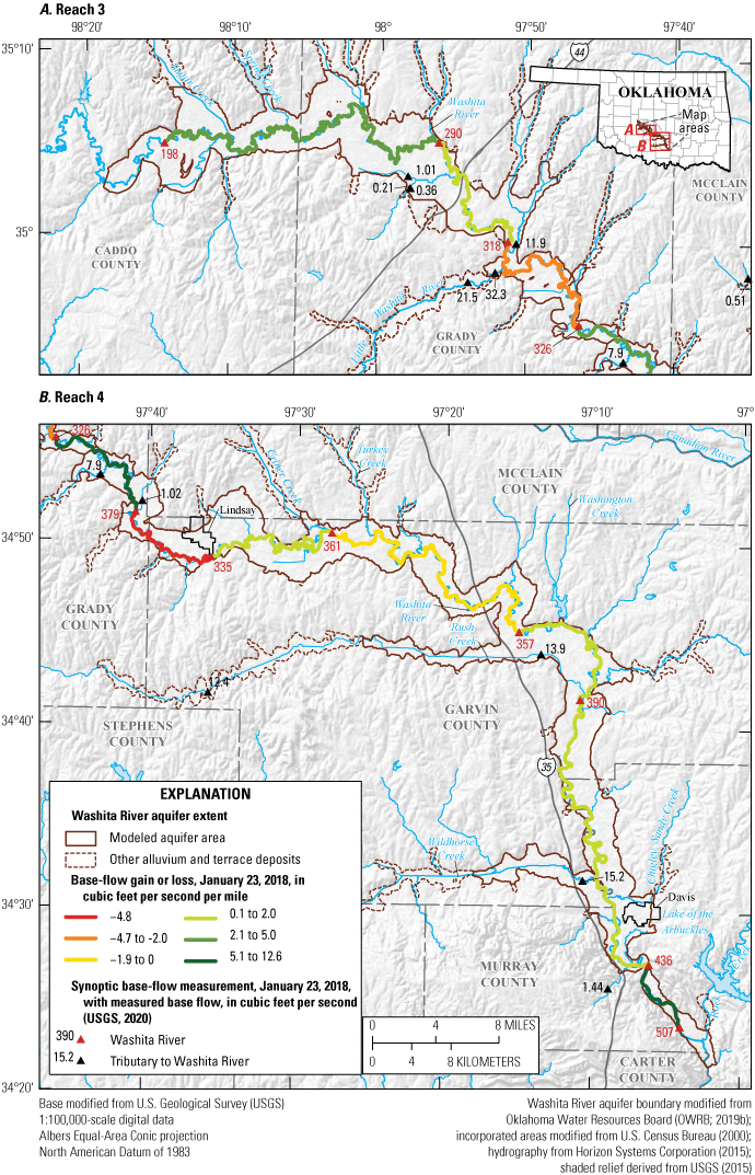
Synoptic streamflow (base-flow) measurements and estimated streambed seepage (base-flow gain or loss) in gaining and losing reaches of A, reach 3 and B, reach 4 of the Washita River aquifer, southern Oklahoma, January 23, 2018.
Net streambed seepage terms for the conceptual model were assumed to be net outflows from the aquifer and were estimated from mean annual base flows computed by using the Base-Flow Index code (Wahl and Wahl, 1995) in the USGS Groundwater Toolbox (Barlow and others, 2015) on selected streamgages in the study area. Net streambed seepage in reach 3 for the 1980–2017 study period (49,041 acre-ft/yr, table 6) was roughly estimated as the mean annual base flow at the Alex gage minus the mean annual base flows at the Anadarko gage and selected tributary streamgages: USGS streamgage 07327000 Sugar Creek near Gracemont, Okla.; USGS streamgage 07327550 Little Washita River east of Ninnekah, Okla.; and USGS streamgage 07328070 Winter Creek near Alex, Okla. (fig. 2, tables 1, 3; tributary base flows are summarized in Rogers and others [2023]). Net streambed seepage in reach 4 during 1980–2017 (75,130 acre-ft/yr, table 6) was estimated as the mean annual base flow at the downgradient end of the aquifer (estimated using data from the Dickson gage) minus the mean annual base flows at the Alex gage and tributary streamgages: USGS streamgage 07328180 North Criner Creek near Criner, Okla.; USGS streamgage 07329000 Rush Creek at Purdy, Okla.; USGS streamgage 07329700 Wildhorse Creek near Hoover, Okla.; and USGS streamgage 07329780 Honey Creek below Turner Falls near Davis, Okla. (fig. 2, tables 1, 3; tributary base flows are summarized in Rogers and others [2023]). When available, streamflow data from the 1980–2017 study period were used to estimate mean annual base flows for the conceptual model. Streamflow data from outside the study period were used to estimate mean annual base flows when other data were unavailable. The total net streambed seepage was 124,171 acre-ft/yr and accounted for 87.8 percent of total outflows in the conceptual-model water budget (table 6).
Well Withdrawals
Well withdrawals were assumed to equal the mean annual reported groundwater use for the 1980–2017 study period, or about 1,214 acre-ft/yr (table 4) (Rogers and others, 2023). About 74 percent of the well withdrawals for that period were from permitted wells in reach 4. Well withdrawals were greatest in dry and hot years because more water was required in those years to grow healthy crops. The altitude of the water table generally declines during dry and hot years (especially during extended droughts) and rises during wet and cool years (fig. 4). The degree to which the water table fluctuates annually at a location is related in part to the volume of nearby well withdrawals and the distribution (or concentration) of recharge near that location. No wells with annual water-level measurements made during 1980–2017 were available for the Washita River aquifer, so estimating net storage change in the aquifer was not possible. The net storage change of the Washita River aquifer was assumed to be a negligible component of the conceptual-model water budget.
Lateral Groundwater Flows
No data were available to estimate lateral groundwater flows (including vertical groundwater flows) across hydrogeologic units and political boundaries (administrative sections or reaches) of the Washita River aquifer. The lateral groundwater flows were from two assumed sources: (1) flow across the alluvium or intra-alluvial flow at the most upgradient and downgradient boundaries of the aquifer and (2) the exchange of groundwater between bedrock units and alluvium. Lateral groundwater flows from tributary alluvium and terrace deposits (those not considered to be part of the Washita River aquifer) were assumed to be a negligible part of the conceptual-model water budget. Net lateral flow was calculated as the difference between the aquifer inflows (recharge) and summed aquifer outflows (saturated-zone evapotranspiration, streambed seepage, and well withdrawals) and was used to balance the water budget. The net lateral flows for reach 3 and reach 4 of the Washita River aquifer accounted for 14.5 percent of the total inflows of the conceptual-model water budget (table 6). By comparison, net lateral flows accounted for 44 percent of the total inflows in the conceptual-model water budget for reach 1 of the Washita River aquifer (Ellis and others, 2020) and 65 percent of the total inflows in the conceptual-model water budget for the Canadian River alluvial aquifer (Ellis and others, 2017). Both of those alluvial aquifers, unlike the Washita River aquifer, were in contact with major bedrock aquifers. In the current study area, however, net lateral flows may be disproportionately greater in reach 4 than in reach 3 of the Washita River aquifer because the bedrock geologic units underlying reach 4 include the Garber Sandstone and Purcell Sandstone (members of the Sumner Group and Hennessey Group, respectively), which are among the coarsest lithologies in the study area (figs. 9 and 10).
Conceptual-Model Water Budget
The conceptual-model water budget (table 6) summarized mean water flows exchanged between each hydrologic boundary and the Washita River aquifer for the 1980–2017 study period. Components of the water budget were estimated from analyses of available data; however, where data were not available, assumptions were made by using published analogs as described in the “Hydrologic Boundaries” section. Recharge accounts for 85.5 percent of the conceptual-model inflows to the Washita River aquifer, and net streambed seepage accounts for 87.8 percent of the outflows from the Washita River aquifer. Net lateral groundwater flow (14.5 percent of inflows) and saturated-zone evapotranspiration (11.3 percent of outflows) were the only other components estimated to be greater than 5 percent of inflows or outflows. Well withdrawals accounted for less than 1 percent of conceptual-model water-budget outflows.
Numerical Groundwater-Flow Model
A finite-difference numerical model of the Washita River aquifer was constructed by using the USGS modular groundwater-flow model MODFLOW-2005 (Harbaugh, 2005) with the Newton formulation solver (MODFLOW-NWT, version 1.2.0; Niswonger and others, 2011) for improved solution of problems involving drying and rewetting. In the modular design of MODFLOW, each hydrologic boundary of the conceptual model, such as streambed seepage, recharge, or well withdrawals, is included as a boundary-condition package that, when activated, adds new inflow and outflow terms to the groundwater-flow equation being solved. Data inputs for each package are specified in machine-readable text files. Model space is discretized into cells, and the cell size is the finest resolution at which spatially varying properties (such as land-surface altitude or horizontal hydraulic conductivity) may be represented and varied. Model time is discretized into time steps within stress periods. The stress-period length is the finest resolution at which temporally varying inflows and outflows may be represented and varied, and the time-step length is the finest length of time for which model outputs may be written (Harbaugh, 2005). Selected numerical-model input values were adjusted to calibrate the model to available water-table-altitude and base-flow observations. The calibrated numerical groundwater-flow model inputs, outputs, metadata, directions for use, and ancillary data were published in a USGS data release (Rogers and others, 2023).
Spatial and Temporal Discretization
The model domain (fig. 21) of the Washita River aquifer was spatially discretized into 500 rows; 600 columns; 12,179 active cells measuring 800 by 800 ft each; and a single convertible layer (Harbaugh, 2005) based on the hydrogeologic framework described in this report. The cell size was chosen to minimize model-processing time while still representing the variability of properties being simulated. The chosen cell size also ensured that the narrowest part of the aquifer was represented by no fewer than three cells; model instability and water-level volatility often occur in narrow parts of the modeled area where groundwater flow is focused into fewer cells. The single convertible layer represented the undifferentiated Quaternary-age alluvium and terrace deposits with variable thickness determined from the hydrogeologic framework; the underlying bedrock was not represented as a layer. The altitude of the top of the aquifer was multiplied by 1.01 in the numerical model to prevent confined aquifer conditions that occur as a side effect of model discretization when the simulated water-table altitude exceeds the altitude of the top of the aquifer. This multiplier, which adds about 10 ft to the altitude of the top of the aquifer, has no effect on most parts of the model where the simulated water-table altitude is below the altitude of the top of the aquifer.
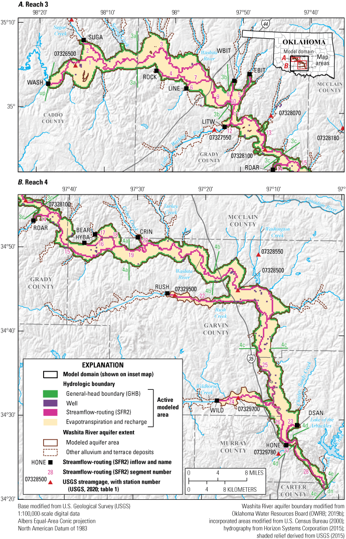
Model domain, active modeled area, hydrologic boundaries, and parameter zones for the numerical groundwater-flow model of A, reach 3 and B, reach 4 of the Washita River aquifer, southern Oklahoma.
The active modeled area (fig. 21) was initially derived from the Washita River aquifer extent (modified from OWRB [2019b]) as defined in the hydrogeologic framework of the Washita River aquifer. The active modeled area was expanded or contracted in some areas to ensure that each active cell was in connection with at least one other active cell. The active modeled area was further modified by inactivating some model cells in narrow areas along selected Washita River tributaries to improve model stability.
The numerical model was temporally discretized into 456 monthly transient stress periods (each with two time steps to improve model stability) representing the 1980–2017 study period (the numerical-modeling period [hereinafter referred to as the “modeling period”] coincides with the 1980–2017 study period). An initial steady-state stress period represented mean annual inflows to, and outflows from, the aquifer. The steady-state solution was used as the initial condition for subsequent transient stress periods, as well as some groundwater-availability scenarios. The numerical model was constructed by using length and time units of feet and days, respectively.
Simulation of Hydrologic Boundaries and Hydraulic Parameters
Hydrologic boundaries in the numerical model (fig. 21) define where and how water may enter or leave the model and include specified-flux and head-dependent boundaries (Harbaugh and others, 2000). Specified-flux boundaries were used to simulate recharge and well withdrawals. Head-dependent boundaries were used to simulate streambed seepage, saturated-zone evapotranspiration, and lateral groundwater flow exchanged with adjacent (upstream and downstream) alluvium and terrace deposits of the Washita River aquifer and with the surrounding bedrock units. When available, hydrologic data (along with data-based assumptions and analogs) were used to estimate or constrain precalibration model inputs for each hydrologic boundary.
Recharge and Distribution With the Soil-Water-Balance Code
Recharge to the Washita River aquifer was simulated using the Recharge package (Harbaugh and others, 2000). Recharge was spatially and temporally distributed for each month of the 1980–2017 study period by using outputs from SWB (Westenbroek and others, 2010). The SWB-output monthly recharge grids were converted to model units of feet per day and used as precalibration numerical-model inputs. These inputs were then scaled with multipliers during the numerical-model calibration to improve agreement between the simulated recharge rate and the conceptual-model recharge determined by the WTF method. The initial steady-state recharge-rate multiplier (rch001, table 8) of 1.66 was allowed to vary within about 3.0 percent (between 1.61 and 1.71); the initial transient recharge-rate multipliers (rch002–rch457, table 8) of 1.66 for each month in the period 1980–2017 were allowed to vary between 1.40 and 2.00 (Rogers and others, 2023). A narrow range was required for the steady-state recharge-rate multiplier to keep the numerical-model recharge closely aligned with the conceptual-model recharge.
Table 8.
Calibration parameters for the numerical groundwater-flow model of the Washita River aquifer, southern Oklahoma, 1980–2017.[A more detailed and longer version of this table is available in the associated data release (Rogers and others, 2023). GHB, general-head boundary; NAVD 88, North American Vertical Datum of 1988]
Lateral Groundwater Flows
Lateral groundwater flows between the general-head boundaries (GHBs) of the Washita River aquifer and the adjoining alluvium and terrace deposits and bedrock units were simulated by using the General-Head Boundary package (Harbaugh and others, 2000). The flow to or from a GHB is the product of the GHB conductance and the difference between the water-table altitude in the model cell and the specified GHB for that model cell. The GHB altitudes along the northwestern and southeastern model boundaries (where the aquifer is adjoined by the continuation of Washita River aquifer alluvium and terrace deposits) were estimated at about 1,200 and 740 ft, respectively, on the basis of the 2020 potentiometric surface of the aquifer (fig. 14). The altitudes specified for the GHBs remained constant throughout the simulation period. Lateral groundwater flows across the northwestern numerical-model boundary (“up,” fig. 21A) were likely net aquifer inflows, and lateral groundwater flows across the southeastern numerical-model boundary (“dn,” fig. 21B) were likely net aquifer outflows. For simplicity, GHBs simulating lateral groundwater flow exchange with the bedrock units (3a–3c and 4a–4e, fig. 21) were only assigned to model cells with side faces contacting those bedrock units; model cells that only contacted bedrock units through their bottom faces were not assigned a GHB. The GHB altitudes of those model cells were initially assigned an altitude 10 ft below land surface (assigned from a 10-m DEM [USGS, 2015]) and were allowed to vary in the range of 3–15 ft below land surface (ghd3a–ghd3c and ghd4a–ghd4e, table 8; Rogers and others, 2023). GHB conductance values were adjusted by zones during the numerical-model calibration and were allowed to vary in the range of 1,000–8,000 ft2/d for the contacts with adjoining alluvium and terrace deposits (ghcup and ghcdn, table 8; Rogers and others, 2023). GHB conductance values were allowed to vary in the range of 0.1–6,000 ft2/d for the bedrock contacts with the lower Hennessey Group and the Sumner Group, which included some of the coarsest bedrock lithologies (figs. 9 and 10) in the study area, and 0.1–2,000 ft2/d for the bedrock contacts with other units, which included generally finer bedrock lithologies (ghc3a–ghc3c and ghc4a–ghc4e, table 8; Rogers and others, 2023).
Streams
Selected named streams listed in the National Hydrography Dataset Plus (Horizon Systems Corporation, 2015) were simulated by using the Streamflow-Routing package, version 2 (SFR2) (Niswonger and Prudic, 2005). Only base flow was simulated in the SFR2 streams. Inflows for SFR2 stream cells included base flows routed from upstream segments, specified inflows (base flows) from tributary streams, and streambed seepage from the aquifer; outflows for SFR2 stream cells included base flows routed downstream and streambed seepage to the aquifer. SFR2 computes streambed seepage between the aquifer and the stream according to Darcy’s Law (Darcy, 1856; Bennett, 1976); the flow exchanged between the aquifer and the stream is the product of the streambed conductance and the difference between the water-table altitude and the stream stage, where the streambed conductance is the product of the hydraulic conductivity of the streambed sediments and the area of the stream channel divided by the streambed thickness. In SFR2, simulated base flows are calculated in each model cell and are routed downstream by segments, or group of cells with uniform hydraulic properties. Accumulated base flows are passed to the next downstream segment until flows are routed out of the active modeled area.
All SFR2 stream segments (1–28, fig. 21) were initially assigned a streambed thickness (sbb01–sbb28, table 8) of 2.0 ft and a streambed hydraulic conductivity (sbk01–sbk28, table 8) of 10.0 ft/d (based on Ryter and Correll [2016]; Ellis and others [2017]; Smith and others [2017, 2021]), but these properties were adjusted during calibration within ranges of 1.0–7.0 ft and 2.0–12.0 ft/d, respectively (Rogers and others, 2023). The streambed widths of stream segments (sbw01–sbw28, table 8) were estimated from aerial photographs (Microsoft Corporation, 2018) and ranged from about 40 to 600 ft (Rogers and others, 2023), gradually increasing downstream. The channel widths of some streams were increased to as much as 2.5 times the estimated values during calibration; increased stream widths resulted in decreased simulated stream stages and corresponding increases in the flow from the aquifer to the stream, allowing parts of the model to drain more efficiently. The streambed depth below land surface (sbd01–sbd28, table 8) was initially set to about 4.5–7.0 ft and was adjusted during calibration within the range of 1.0–8.0 ft (Rogers and others, 2023). The streambed depth was subtracted at model run time from the land-surface altitude as represented by a 10-m DEM (USGS, 2015). This streambed incision is necessary to compensate for lost spatial resolution of the stream channel (altitude averaging) caused by the large DEM cell size. When land-surface altitudes of actual features are represented by a DEM cell, the lowest altitudes (often stream channels) and highest altitudes (summits) are generalized to a single value—the mean land-surface altitude in the cell. The difference between the actual altitude of those features and the cell-averaged altitude depends on the local altitude relief and the cell size.
Monthly base-flow inflows at the boundary of the active modeled area were estimated for the Washita River (WASH), Sugar Creek (SUGA), Rock Hollow Creek (ROCK), Line Creek (LINE), West Bitter Creek (WBIT), East Bitter Creek (EBIT), Little Washita River (LITW), Roaring Creek (ROAR), Bear Creek (BEAR), Hybarger Creek (HYBA), Criner Creek (CRIN), Rush Creek (RUSH), Dry Sandy Creek (DSAN), Wildhorse Creek (WILD), and Honey Creek (HONE) (fig. 21). Streamgage records were used to estimate base-flow inflows where available (table 3). Where streamgage records were unavailable, the January 2018 synoptic streamflow (base-flow) measurements (fig. 20) were used to estimate some base-flow inflows. Base-flow inflows for some streams were estimated from streamgage records and base-flow measurements on similar streams nearby (USGS, 2020). Rock Creek, a relatively large tributary near the downgradient end of the model, was not simulated because it was dominated by periodic reservoir releases from Lake of the Arbuckles (fig. 21).
Saturated-Zone Evapotranspiration
Saturated-zone evapotranspiration was simulated by using the Evapotranspiration package (Harbaugh and others, 2000) and was expected to occur near streams and riparian wooded areas along the Washita River and perennial tributaries. Maximum rates of saturated-zone evapotranspiration were assumed to not exceed the difference between potential and actual evapotranspiration as computed by SWB; this assumption prevented the summed components of evapotranspiration from exceeding the potential evapotranspiration. Arrays representing the potential minus actual evapotranspiration for each monthly transient stress period (evtjan–evtdec, table 8) and the steady-state stress period (evtavg, table 8) were initially scaled by a factor of 0.6. During calibration, the scaling factors were allowed to vary independently in the range of 0.5–1.0 (Rogers and others, 2023). The evapotranspiration extinction (root-zone) depth (evtextd, table 8), or the depth below land surface at which the saturated zone becomes inaccessible to plants, was initially set at 1.0 ft in the active modeled area, which was consistent with the mean plant root-zone depth specified for grass/pasture and cropland (the dominant land-cover types, fig. 3) in SWB. During calibration, the evapotranspiration extinction depth was allowed to vary in the range of 0.8–1.2 ft. The saturated-zone evapotranspiration reference altitude (evttop, table 8) was initially set to the land-surface altitude of each cell but was adjusted during calibration by a multiplier that was allowed to vary in the range of 0.998–1.010. The narrow range on the reference altitude multiplier was necessary for model stability.
Well Withdrawals
Well withdrawals for the 1980–2017 study period were simulated by using the Well package (Harbaugh and others, 2000). Annual reported groundwater use for each permit was evenly distributed among all well locations recorded for that permit (OWRB, 2019d). In the case of permits for which there were no recorded wells, a single well was placed in the center of the land parcel recorded for the permit. Annual reported groundwater use was temporally split into model stress periods by using the mean monthly water demand distribution (fig. 22; OWRB, 2012a) from Oklahoma Comprehensive Water Plan water-management planning basins 14–16 (fig. 2; OWRB, 2019c). The monthly water demand for irrigation was greatest in the summer months; July–September accounted for about 76 percent of irrigation groundwater use (fig. 22). The monthly water demand for public supply also was greatest in the summer months; however, July–September only accounted for about 34 percent of public-supply groundwater use (fig. 22).
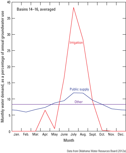
Monthly water demand by groundwater-use type for Oklahoma Comprehensive Water Plan water-management planning basins 14–16, averaged, Washita River aquifer, southern Oklahoma.
Storage and Hydraulic Properties
The Upstream Weighting package of MODFLOW-2005 (Niswonger and others, 2011) was used to represent storage and hydraulic properties of the Washita River aquifer. Initial storage and hydraulic property values were similar to those used in numerical models for other alluvial aquifers in Oklahoma (Ellis and others, 2017, 2020; Smith and others, 2017) and identical to those used in the numerical model for the Salt Fork Red River aquifer (Smith and others, 2021). The storage and hydraulic property values were adjusted during model calibration but were held spatially uniform and temporally constant through all stress periods in all simulations. The specific yield (sy3 and sy4, table 8) and specific storage (ss, table 8) of the Washita River aquifer were initially set as 0.10 (dimensionless) and 1×10⁻⁵ inverse foot, respectively. Horizontal hydraulic conductivity (hkpp001–hkpp146, table 8) was represented by using 146 pilot points (1–146, fig. 23; Doherty, 2010) placed at 12,800-ft intervals (1 at every 16th column and row) within a 10,560-ft buffer of the aquifer boundary. (Pilot points are regularly spaced control points used to support an interpolation of cell-based horizontal hydraulic conductivity values across an active modeled area.) The pilot points were assigned an initial horizontal hydraulic conductivity value of 20 ft/d and interpolated before each model run to create the horizontal hydraulic conductivity array read by the numerical model (Doherty, 2010). During calibration, pilot-point horizontal hydraulic conductivity values were allowed to vary independently between 10 and 100 ft/d (Rogers and others, 2023).
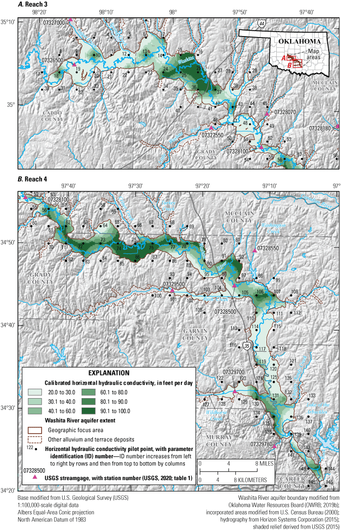
Horizontal hydraulic conductivity pilot points and calibrated horizontal hydraulic conductivity in A, reach 3 and B, reach 4 for the numerical groundwater-flow model of the Washita River aquifer, southern Oklahoma.
Solver Settings and Budget Percentage Discrepancies
Most of the settings for the Newton solver were unchanged from suggested input values (Winston, 2018), which were converted to model units of feet and days. The head tolerance was increased to 1.5×10⁻³ ft, and the flux tolerance was increased to 5.0×10⁴ cubic feet per day. These settings improved model stability while keeping the budget percentage discrepancies in the solution under 1.0 percent for all 457 stress periods; the largest budget percentage discrepancy (by absolute value) was about 0.16 percent in stress period 411 (Rogers and others, 2023).
Calibration
Model calibration is the process of systematically changing selected model input values (parameters) within limits to improve the fit between model-simulated data and observed data (calibration targets). The preferred calibration results (1) minimize the differences (residuals) between simulated and observed data and (2) conform to the predetermined conceptual model. The calibration process for the numerical model included both manual and automated adjustment of parameters. The manual calibration approach was primarily focused on aligning the numerical-model water budget, especially the recharge and streambed seepage components, to the conceptual-model water budget. The manual calibration also involved selected structural elements of the model, such as boundary elevations, that are not easily adjusted by automated calibration methods. The automated calibration approach was focused solely on minimizing residuals and used the PEST++ iterative ensemble smoother (White, 2018) to reduce run times associated with the calibration of highly parameterized models.
Calibration Targets
The suite of calibrated parameter values was evaluated on the basis of the minimization of an objective function that quantifies the difference between simulated and observed values included in the model (White, 2018). The objective function was calculated as the sum of squared weighted residuals for calibration targets in five observation groups: water-table-altitude observations, base-flow observations at the Alex gage, base-flow observations at the Pauls Valley gage, base-flow observations (estimated) at the downgradient end of the model, and the conceptual-model recharge rate (table 9). Observation weights were required to prevent calibration targets of any one observation group from dominating the objective function and, therefore, becoming the sole focus of parameter adjustments during automated calibration (Hill and Tiedeman, 2007; Doherty, 2010). The observation weights (1.0, 5.0 × 10⁻⁷, 1.7 × 10⁻⁷, 1.8 × 10⁻⁷, 2.5 × 10⁻² for water-table-altitude observations, base-flow observations at the Alex gage, base-flow observations at the Pauls Valley gage, base-flow observations [estimated] at the downgradient end of the model, and conceptual-model recharge rate, respectively) were uniform for all observations from the transient simulation within each observation group; the base-flow observations from the steady-state simulation were given increased weights (200 times greater) relative to the base-flow observations from the transient simulation. The observation weights were chosen so that, at the beginning of automated calibration (that is, precalibration), the observation groups accounted for 24.0, 10.5, 55.3, 10.2, and 0.0 percent of the objective function, respectively (table 9). This weighting scheme reflects an assumption that base-flow observations (totaling 76.0 percent of the objective function) are more important than water-table-altitude observations for the purpose of determining the parameter values that are most influential in estimating groundwater availability (the primary subject of this report) in an unconfined alluvial aquifer. Base flows are generally more sensitive to changes in specific yield than they are to changes in water-table altitudes. Water-table altitudes are generally more sensitive to changes in horizontal hydraulic conductivity than to changes in specific yield.
Table 9.
Components of the objective function for the automated calibration of the numerical groundwater-flow model of the Washita River aquifer, southern Oklahoma, 1980–2017.[Objective function is calculated as the sum of squared weighted residuals. SS, steady-state simulation; TR, transient simulation; Min, minimum; Max, maximum; RMSE, root-mean-square error; OWRB, Oklahoma Water Resources Board; USGS, U.S. Geological Survey; E, base-10 exponent (for example, 1.7E-07 means 1.7 × 10⁻⁷)]
| Observation group | Source1 | Number of observations | Weight multiplier | Precalibration residuals | Calibrated residuals | ||||||||||
|---|---|---|---|---|---|---|---|---|---|---|---|---|---|---|---|
| SS TR |
SS TR |
Min | Mean | Max | Interquartile range | RMSE | Objective function component (percent in parentheses) |
Min | Mean | Max | Interquartile range | RMSE | Objective function component (percent in parentheses) | ||
| Water-table altitude, in feet (headobs) | Water-table-altitude observations (OWRB, 2019a; USGS, 2020) | 63 130 |
2.0E+00 2.0E+00 |
−22.5 | −6.5 | 17.2 | 9.1 | 18.6 | 66,641 (24.0) |
−19.5 | −4.1 | 10.5 | 6.8 | 13.8 | 36,522 (24.9) |
| Base flow, in cubic feet per second (gageobs1) | Alex gage (USGS, 2020) | 1 432 |
1.0E-04 5.0E-07 |
−1,238.8 | 14.0 | 970.2 | 95.6 | 8.2 | 28,993 (10.5) |
−1,228.1 | −7.7 | 981.8 | 93.9 | 7.9 | 27,109 (18.5) |
| Base flow, in cubic feet per second (gageobs2) | Pauls Valley gage (USGS, 2020) | 1 456 |
3.4E-05 1.7E-07 |
−1,207.7 | 105.4 | 2,549.3 | 213.2 | 18.3 | 153,413 (55.3) |
−1,224.2 | 45.6 | 2,489.8 | 213.8 | 10.8 | 53,763 (36.6) |
| Base flow, in cubic feet per second (gageobs3) | Downgradient end of model; adjusted from Dickson gage (USGS, 2020) | 1 456 |
3.6E-05 1.8E-07 |
−1,457.2 | 8.8 | 4,952.7 | 234.1 | 7.9 | 28,231 (10.2) |
−1,433.3 | −8.8 | 4,932.0 | 234.1 | 8.0 | 29,173 (19.9) |
| Conceptual-model recharge, in acre-feet per year (budget) | Conceptual model (table 6) | 1 1 |
2.0E-02 2.0E-02 |
353.7 | 353.8 | 353.8 | 0.0 | 7.1 | 100.1 (0.0) |
−829.8 | −416.5 | −3.2 | 413.3 | 11.7 | 275.4 (0.2) |
| Total | 1,542 | Precalibration objective function: | 277,378 | Calibrated objective function: | 146,842 | ||||||||||
Water-Table-Altitude Observations
The Head Observation (HOB) package (Hill and others, 2000) was used to compare simulated water-table altitudes to observed water-table altitudes in the Washita River aquifer for the 1980–2017 modeling period. Observed water-table altitudes were calculated from depth-to-water measurements and the land-surface altitude obtained from a lidar DEM (USGS, 2019). For consistency, the land-surface altitude was obtained from the lidar DEM, even when the data source provided a land-surface altitude. Sites with water-table altitude observations were screened for location errors, and observations were filtered such that only one observation per cell per stress period was included in the HOB package. Only 130 water-table-altitude observations (OWRB, 2019a; USGS, 2020) from 63 wells were included for the transient simulation in the HOB package (fig. 24A). Water-table-altitude observations from the period 2018–20 were assigned to 2017 in the HOB package because few historical observations were available from the modeling period. Some water-table-altitude observations from the period 2018–20 were assigned to the same month and day in 2017, but a set of 51 synoptic water-table-altitude observations from January 2020 were assigned to the same day in December 2017. Water-table-altitude observations from the transient simulation were averaged by well to derive 63 calibration targets for the steady-state simulation because no water-table-altitude observations were available in 1980, at the beginning of the modeling period.
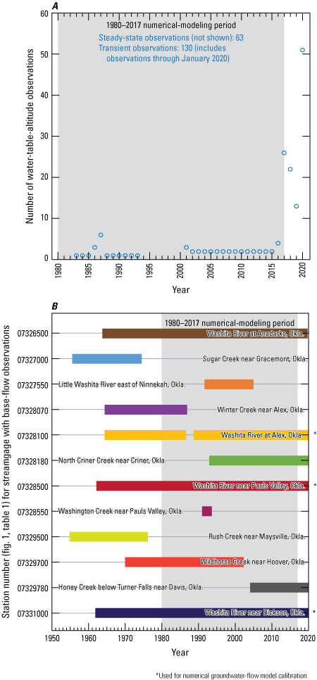
Temporal distribution of U.S. Geological Survey and Oklahoma Water Resources Board A, water-table-altitude observations and B, base-flow observations used for the numerical groundwater-flow model of the Washita River aquifer, southern Oklahoma.
Base-Flow Observations
Base-flow observations were available for the full modeling period (456 months) at the Pauls Valley gage on the Washita River and for most of the modeling period (432 months) at the Alex gage (fig. 24B) (USGS, 2020) on the Washita River within the modeled area (fig. 1). Base-flow observations also were available for the full modeling period (456 months) at the Dickson gage (fig. 24B) (USGS, 2020), which is downstream from the modeled area on the Washita River (fig. 2). Base-flow observations from the Dickson gage were decreased by 30 percent (to account for drainage that originated from the tributaries outside of the modeled area) and used as estimated base-flow observations for the Washita River at the downgradient end of the model. The monthly mean base flows for these three streamgages, accounting for 1,344 observations (table 9), were used as calibration targets for the transient simulation (Rogers and others, 2023). The mean annual base flows for the three streamgages (table 3), accounting for three observations (table 9), were used as calibration targets for the steady-state simulation. Base-flow observations from other selected streamgages were not used as calibration targets because they (1) were previously used to define inflows for SFR2 or (2) had periods of record that were too short to be representative of streamflow conditions during the modeling period.
Calibration Results
Calibration results were evaluated on the basis of the reduction of the objective function and the general fit of the calibrated numerical-model water budget to the predetermined conceptual-model water budget. Automated calibration reduced the calibrated objective function total by about 47 percent from the precalibration objective function (table 9). Most of that reduction resulted from reducing base-flow residuals at the Pauls Valley gage. Base-flow residuals for the Alex gage and the downgradient end of the model were mostly reduced during a round of manual calibration prior to calculation of the precalibration objective function.
Observation-Sensitivity Analysis
As part of the calibration process, an observation-sensitivity analysis was performed with the iterative parameter estimation software package PEST (Doherty, 2010) to identify which parameters were most effective (and most ineffective) at reducing the objective function. PEST is used to measure the changes in calibration-target residuals resulting from 1-percent changes in each parameter and records those changes in a Jacobian matrix with dimensions equal to the number of observations times the number of parameters (Doherty, 2010). Parameters with the greatest effects on calibration-target residuals have the greatest observation sensitivities (Rogers and others, 2023).
Parameters that were closely linked, either spatially or temporally, to observations typically had the greatest observation sensitivities in the numerical model. Parameters with the greatest observation sensitivities were the saturated-zone evapotranspiration reference altitude multiplier (evttop), the steady-state recharge-rate multiplier (rch001), the altitude of the upstream GHB (ghdup), the steady-state saturated-zone evapotranspiration-rate multiplier (evtavg), and the streambed depth for SFR2 zone 3 (sbd03) (Rogers and others, 2023; table 8). Horizontal hydraulic conductivity pilot points 15, 26, 71, 77, 78, 79, and 89 (hkpp015, hkpp026, hkpp071, hkpp077, hkpp078, hkpp079, and hkpp089) were the only horizontal hydraulic conductivity pilot points with sensitivities ranking in the top 100 (of 753 calibration parameters). The horizontal hydraulic conductivity pilot points with the highest ranking sensitivities were in parts of the aquifer with large spatial and temporal concentrations of water-table-altitude observations. The specific yield for reach 3 (sy3) and the specific yield for reach 4 (sy4) ranked 72 and 28 (of 753 calibration parameters), respectively. The steady-state recharge-rate multiplier parameter (rch001) determined how much recharge was applied in the steady-state simulation, which included about one-third of the water-table-altitude observations (Rogers and others, 2023). The specific yield parameters (sy3 and sy4) controlled the volume of water released (from storage) as streambed seepage to streams across the entire aquifer, which in turn partially controlled how much base flow was simulated in the Washita River at the Alex gage, Pauls Valley gage, and downgradient end of the model.
To graphically summarize the observation-sensitivity analysis, observation-group sensitivities were calculated as the weighted sum of the absolute Jacobian matrix output for each parameter group (fig. 25). Because recharge parameters and horizontal hydraulic conductivity parameters influence every cell in the model, those parameter groups had the greatest observation-group sensitivities. The storage parameter group, which included specific yield and specific storage parameters, had the least observation-group sensitivities.
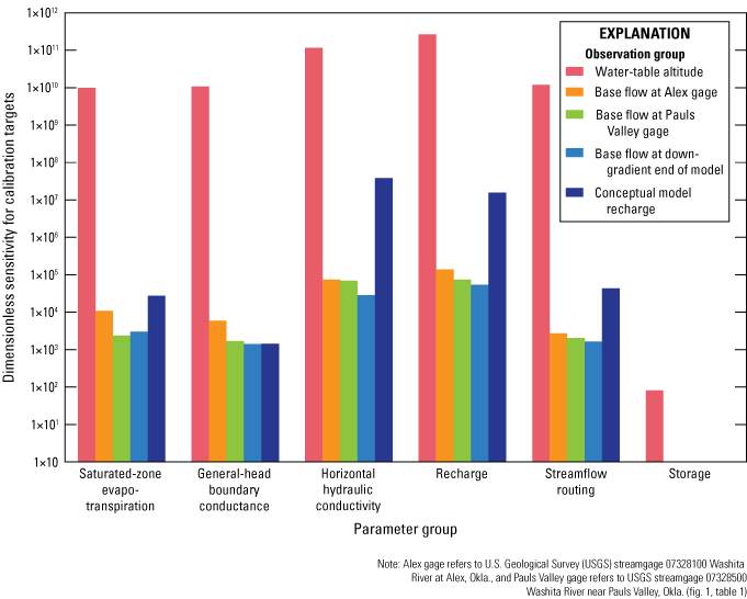
Observation-group sensitivity for calibration targets by parameter group in the numerical groundwater-flow model of the Washita River aquifer, southern Oklahoma, 1980–2017.
Calibrated Parameter Values
The calibrated parameter values (Rogers and others, 2023) selected for the numerical model were the combined result of manual and automated calibration approaches. Many of the calibrated parameter values were at the minimum or maximum bounds specified in the PEST control file (Rogers and others, 2023). Calibrated parameter values at bounds indicate that the objective function could likely be further reduced by expanding those bounds; doing so, however, would divert the numerical model further from the conceptual model or increase model instability. For the recharge parameter group (rch, table 8), 333 of 457 calibrated recharge-rate multiplier values were assigned to either the minimum or maximum bounds; 156 of those values were at the minimum bound (1.40), and 177 were at the maximum bound (2.00) (Rogers and others, 2023). For the horizontal hydraulic conductivity parameter group (hyd, table 8), 53 of 146 calibrated parameter (pilot point) values were assigned to either the minimum or maximum bounds; 15 of those values were at the minimum bound (10.0 ft/d), and 38 were at the maximum bound (100.0 ft/d) (Rogers and others, 2023). However, the minimum value interpolated in the calibrated horizontal hydraulic conductivity array was increased to 20.0 ft/d (fig. 23) to alleviate problems with flooding (cells with water levels above land surface) in low-lying areas; 32 of the calibrated parameter (pilot point) values were less than or equal to 20.0 ft/d. Most of the calibrated parameter values in the evapotranspiration group (evt, table 8) were at bounds, including the saturated-zone evapotranspiration extinction (root-zone) depth, the steady-state saturated-zone evapotranspiration-rate multiplier, and 7 of the 12 transient (monthly) saturated-zone evapotranspiration-rate multipliers. For the streamflow routing parameter group (sfr, table 8), all but 2 of the streambed hydraulic conductivity zone calibrated parameter values (sbk01–sbk28), all but 4 of the streambed thickness zone calibrated parameter values (sbb01–sbb28), all but 8 of the streambed depth zone calibrated parameter values (sbd01–sbd28), and all but 12 of the streambed width zone calibrated parameter values (sbw01–sbw28) were at bounds.
Comparison of Simulated and Observed Calibration Targets
Conforming to MODFLOW convention (Harbaugh, 2005), calibration-target residuals in this report were calculated as observed minus simulated values; positive residuals indicate lower simulated than observed values, and negative residuals indicate higher simulated than observed values. The mean calibrated residual for water-table-altitude observations was –4.1 ft (table 9), indicating that, on average, simulated water levels were slightly higher than observed water levels. The combined (steady-state and transient simulation) water-table-altitude root-mean-square error (RMSE) was 13.8 ft, and the interquartile range was 6.8 ft (table 9, fig. 26B).
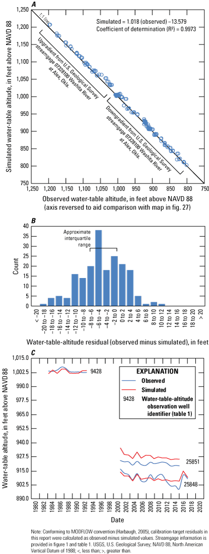
A, Relation between simulated and observed water-table altitudes, B, water-table-altitude residual distribution, and C, observed and simulated water-table altitudes for selected observation wells for the numerical groundwater-flow model of the Washita River aquifer, southern Oklahoma, 1980–2017.
The water-table-altitude residuals with the greatest magnitudes were associated with wells near Alex, in the downgradient part of reach 3 and the upgradient part of reach 4 of the Washita River aquifer (figs. 26A and 27). The residuals near Alex were mostly negative, indicating that simulated water-table altitudes were higher than observed water-table altitudes (fig. 27). In that part of the model, given the weights applied to observations in the objective function (table 9), there was a tradeoff between minimizing the water-table-altitude residuals and minimizing the base-flow residuals at the Alex streamgage.
Annual water-table-altitude observations representing more than 5 years were measured in three wells (9428, 25848, and 25851, table 1, figs. 26C and 27B; OWRB, 2019a; USGS, 2020). Well 9428 was in the upgradient part of reach 4 of the Washita River aquifer near Alex. Simulated water-table altitudes generally matched the magnitude and pattern of observed water-table altitudes in that well. Wells 25848 and 25851 were in reach 4 of the Washita River aquifer near Maysville, Okla. The simulated water-table altitudes for well 25848 were comparable in pattern but were less variable in magnitude than the observed water-table altitudes. The simulated water-table altitudes for well 25851 generally matched the pattern of but were about 6 ft higher than the observed water-table altitudes.
The mean calibrated residual for base-flow observations at the Alex gage was −7.7 ft3/s (table 9), indicating that, on average, simulated base flows were slightly higher than observed base flows. The combined (steady-state and transient simulations) Alex gage base-flow RMSE was 7.9 ft3/s, and the interquartile range of residuals was 93.9 ft3/s. The mean calibrated residual for base-flow observations at the Pauls Valley gage was 45.6 ft3/s (table 9), indicating that, on average, simulated base flows were lower than observed base flows. The combined Pauls Valley gage base-flow RMSE was 10.8 ft3/s, and the interquartile range of residuals was 213.8 ft3/s. The mean calibrated residual for base-flow observations at the downgradient end of the model was −8.8 ft3/s (table 9), indicating that, on average, simulated base flows were slightly higher than observed base flows. The combined base-flow RMSE at the downgradient end of the model was 8.0 ft3/s, and the interquartile range of residuals was 234.1 ft3/s. Although simulated base flows generally matched the pattern of observed base flows, they often failed to reach the high and low extremes (fig. 28). For example, the simulated base flows failed to reach the highest observed base flows in 2007 at the Pauls Valley gage and at the downgradient end of the model (fig. 28B, C). Likewise, the simulated base flows failed to reach the low (sometimes 0 ft3/s) observed base flows during the 2011–14 drought (fig. 4) at all locations on the Washita River, especially the downgradient end of the model (fig. 28). The failure to simulate extreme values in the observed data is typical of groundwater-flow models (Ellis and others, 2017; Smith and others, 2017, 2021) and probably results from numerical-model discretization, or the necessary simplification of spatially and temporally variable hydrologic processes that actually occur (Mandelbrot, 1983).
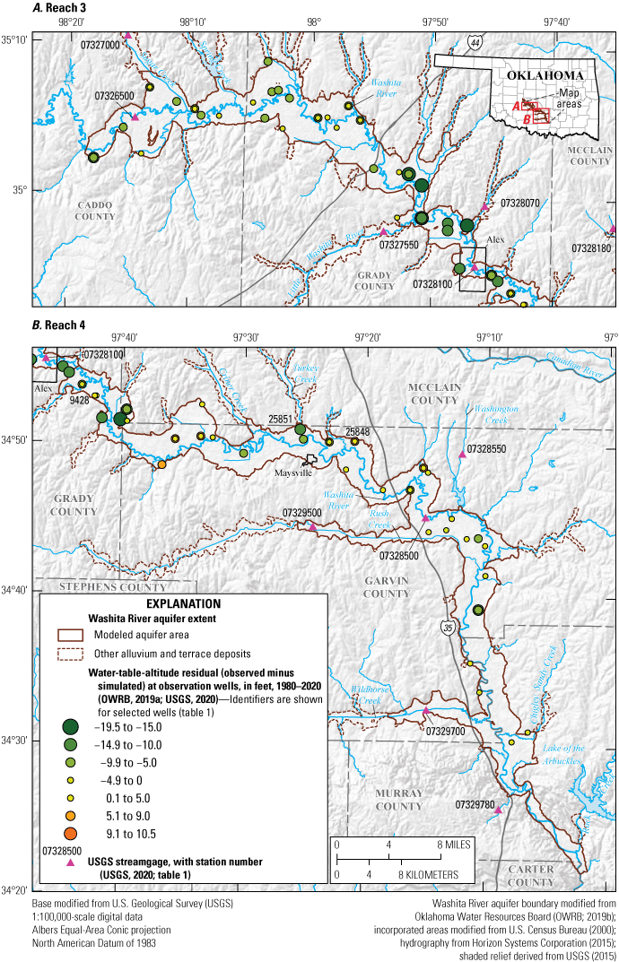
Water-table-altitude residuals at observation wells in A, reach 3 and B, reach 4 used to calibrate the numerical groundwater-flow model of the Washita River aquifer, southern Oklahoma, 1980–2017.
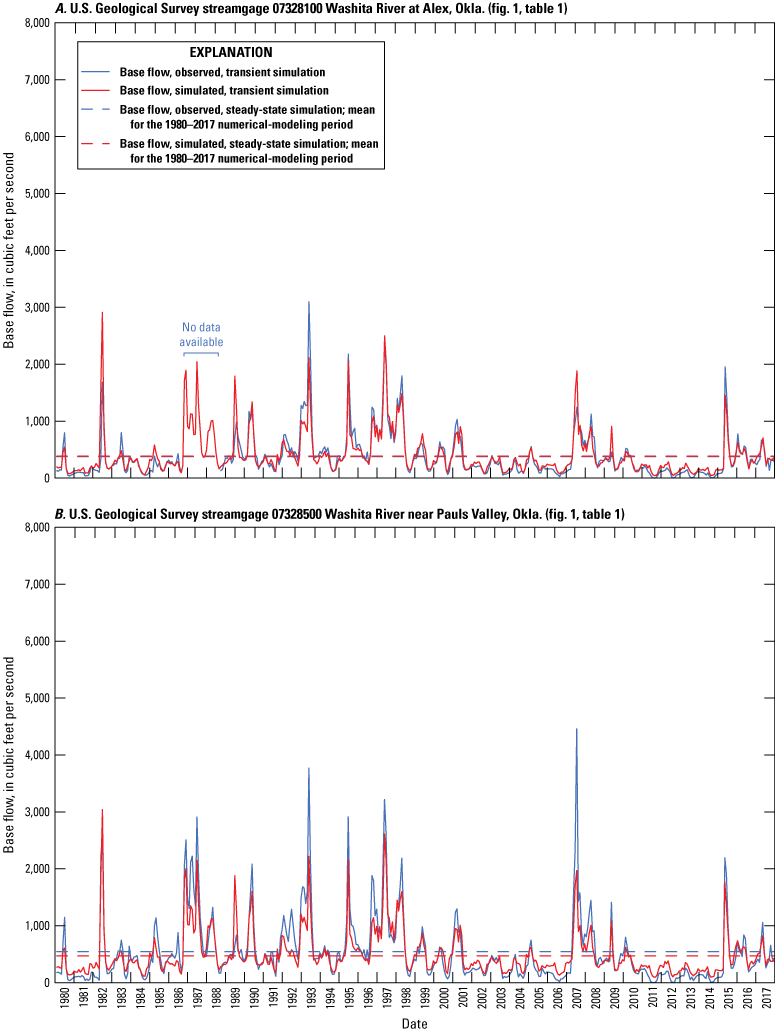
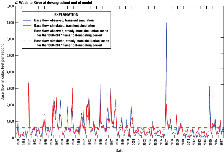
Observed base flow and simulated base flow at U.S. Geological Survey streamgages A, 07328100 Washita River at Alex, Okla., and B, 07328500 Washita River near Pauls Valley, Okla., and C, on the Washita River at the downgradient end of the model for the numerical groundwater-flow model of the Washita River aquifer, southern Oklahoma, 1980–2017.
Calibrated Numerical-Model Water Budget
The calibrated numerical-model water budget (table 10, fig. 16B) shows simulated mean annual inflows and outflows for the 1980–2017 modeling period; a subaccounting for reach 3 and reach 4 of the Washita River aquifer was computed by using the ZONEBUDGET utility (Harbaugh, 1990). Simulated recharge (121,613 acre-ft/yr) was the primary inflow for the calibrated numerical model and accounted for 88.9 percent of inflows in the water budget. Net lateral groundwater flow accounted for the other 11.1 percent of inflows. Net streambed seepage (54.3 percent of outflows in the water budget) was the largest outflow for the calibrated numerical model; saturated-zone evapotranspiration accounted for 43.5 percent, and well withdrawals accounted for 0.7 percent of outflows (table 10, fig. 16B). The inflow components of the calibrated numerical-model water budget compare well with those of the conceptual-model water budget (table 6, fig. 16). The saturated-zone evapotranspiration and net streambed seepage outflow components, however, differed substantially between the calibrated numerical-model and conceptual-model water budgets (table 6, fig 16). These components of the conceptual model, especially the saturated-zone evapotranspiration component, were poorly constrained by available field data. No field data were available to quantify saturated-zone evapotranspiration. The types of field activities required to effectively model saturated-zone evapotranspiration are expensive to conduct, and the resulting data are difficult to integrate at the scale of the study area. Historical base-flow observations at the downgradient end of the model were estimated from the Dickson gage, which included base-flow contributions from a relatively large tributary (Caddo Creek) and periodic releases from Lake of the Arbuckles (fig. 2); thus, the budgeted outflows for reach 4 were more poorly constrained than those for reach 3. The conceptual-model net streambed seepage also may be biased high because of the inclusion of some outflows from floodwater-retarding structures that could not be distinguished and separated from groundwater-derived base flows.
Table 10.
Calibrated numerical-model water budget of simulated mean annual inflows and outflows for the Washita River aquifer, southern Oklahoma, 1980–2017.[All values are in units of acre-feet per year; --, not applicable. Totals may not equal sum of components because of independent rounding. Net water-budget totals are calculated as the difference between outflow and inflow; negative values indicate outflow from the aquifer, and positive values indicate inflow to the aquifer. Net streambed seepage, net lateral groundwater flow, and net change in groundwater storage represent the net effect of aquifer inflows and outflows. Negative net change in groundwater storage indicates gain of groundwater storage to the aquifer, which is reported as an aquifer outflow in the numerical groundwater-flow model mass balance. Reach 3 and Reach 4 are upgradient and downgradient, respectively, from the vicinity of U.S. Geological Survey streamgage 07328100 Washita River at Alex, Okla. (fig. 1)]
Simulated annual net changes in groundwater storage reflect climatic trends during the 1980–2017 modeling period (fig. 29). Groundwater storage, for the purposes of this report, is the volume of water that would drain from the aquifer under gravity; this definition excludes the water that adheres to the aquifer matrix and water that remains locked in isolated or unconnected pore spaces. Simulated groundwater storage was calculated by multiplying the calibrated specific yield (Rogers and others, 2023) by the simulated saturated thickness of each active model cell (see section “Simulated Saturated Thickness and Groundwater Storage”). The cumulative net change in simulated groundwater storage (surplus or deficit), referenced to the simulated groundwater storage from the steady-state simulation (811,037 acre-feet [acre-ft]), was between −5 and 5 percent in most years. The greatest simulated groundwater storage surplus (10.8 percent) occurred in 2015 after a year of record recharge for the period 1980–2017. The greatest simulated groundwater storage deficit (−8.4 percent) occurred in 2016. The 2016 recharge was below but not exceptionally below the mean for the period 1980–2017; the recharge during 6 other years from 1980 to 2017 was less than the 2016 recharge. The large change in simulated groundwater storage from 2015 to 2016 could be explained by increased inflow from daily recharge received late in 2015 that was not fully discharged as streambed seepage and saturated-zone evapotranspiration until early in 2016. Whatever the cause, the occurrence of the greatest simulated groundwater storage surplus and deficit in consecutive years illustrates the potential for large changes in groundwater storage over short time frames in the study area; between 2015 and 2016, the simulated groundwater storage changed by about 155,000 acre-ft. The 2016 groundwater storage deficit was fully regained in 2017, and the transient simulation modeling period ended with a slight (0.4 percent) groundwater storage surplus as compared to the steady-state simulation (fig. 29).
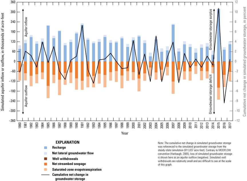
Simulated annual inflows, outflows, and cumulative net change in groundwater storage for the calibrated numerical groundwater-flow model of the Washita River aquifer, southern Oklahoma, 1980–2017.
Simulated Saturated Thickness and Groundwater Storage
The simulated saturated thickness of the Washita River aquifer was determined by subtracting the altitude of the aquifer base from the simulated water-table altitude at the end of the modeling period (2017). The simulated saturated thickness was more than 100 ft along the assumed paleochannel of the Washita River near Verden, Okla. (fig. 30). The simulated mean aquifer thickness (sum of saturated and unsaturated thicknesses) was 54.28 ft (Rogers and others, 2023), and the simulated mean saturated thickness was 47.12 ft (table 11). The simulated mean saturated thicknesses for reaches 3 and 4 were 50.03 and 45.13 ft, respectively (table 11). A simulated mean transmissivity of 2,276 ft2/d was calculated as the mean of the calibrated horizontal hydraulic conductivity multiplied by the saturated thickness of each cell; the simulated mean transmissivities for reaches 3 and 4 were 2,061 and 2,423 ft2/d, respectively. The simulated groundwater storage of the Washita River aquifer at the end of the modeling period (2017) was 869,053 acre-ft; 436,807 acre-ft (50.3 percent) of that total was in reach 3, and 432,247 acre-ft (49.7 percent) of that total was in reach 4 (table 11).
Table 11.
Simulated hydraulic properties, storage properties, and available groundwater in storage at the end of the numerical-modeling period for the Washita River aquifer, southern Oklahoma, 1980–2017.[Kh, horizontal hydraulic conductivity; E, base-10 exponent (for example, 1.65E-06 means 1.65×10⁻⁶)]
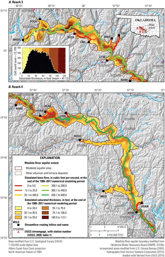
Simulated base flow and simulated saturated thickness in A, reach 3 and B, reach 4 at the end of the 1980–2017 numerical-modeling period for the calibrated numerical model of the Washita River aquifer, southern Oklahoma.
Groundwater-Availability Scenarios
Three types of groundwater-availability scenarios were run using the calibrated numerical model. These scenarios were used to (1) estimate the EPS pumping rate that ensures a minimum 20-, 40-, and 50-year life of the aquifer, (2) quantify the potential effects of projected well withdrawals on groundwater storage over a 50-year period, and (3) simulate the potential effects of a hypothetical 10-year drought on base flow and groundwater storage. The inputs and outputs for the groundwater-availability scenarios are available in Rogers and others (2023).
Equal-Proportionate-Share Pumping Rates
EPS scenarios for reaches 3 and 4 of the Washita River aquifer were run for periods of 20, 40, and 50 years. The 2017 simulated water table from the calibrated numerical model was used as the starting water table in each EPS scenario. Annual stress periods were used in these scenarios instead of monthly stress periods to simplify the analysis, improve model stability, and lessen run times. Model inputs for recharge, saturated-zone evapotranspiration, and most stream inflows to the active modeled area were configured as the means of each annual period used in the calibrated numerical model; stream inflows from the Alex gage were added for the Washita River at the boundary between reach 3 and reach 4 (which has no specified Washita River inflow in the calibrated numerical model) so that results from reach 3 and reach 4 could be compared. The General-Head Boundary package (Harbaugh and others, 2000) was disabled for the EPS scenarios to prevent the input of unrealistically high simulated flows from adjacent bedrock units. All simulated wells from the calibrated numerical model, including wells with prior-right permits, were discarded, and a hypothetical well was placed in each active cell (covering about 14.7 acres). The aquifer top multiplier was reduced to 1.00 for the EPS scenarios; these extreme pumping scenarios are sensitive to the aquifer top altitude because well pumping is automatically reduced when the ratio of saturated thickness to aquifer thickness (aquifer top minus aquifer base altitude) approaches zero. The adjustment of specified well pumping is necessary because the full pumping rate is not possible in cells with minimal saturated thickness. The MODFLOW-2005 Well package PHIRAMP variable (Niswonger and others, 2011), which specifies the ratio of saturated thickness to aquifer thickness at which to begin reducing pumping rates, was set to 0.05 (5 percent of aquifer thickness) for the EPS scenarios. Lower PHIRAMP settings were tested but caused model instability.
PEST++ (White and others, 2020), a software package for iterative parameter estimation, was used to determine the EPS pumping rate for the selected period (20, 40, or 50 years). In each PEST++ iteration, the hypothetical wells were assigned a uniform pumping rate for the selected period. If a saturated thickness of at least 5 ft was determined for more than 50 percent of the active cells at the end of an iteration, successive iterations with an increased uniform pumping rate were performed until a saturated thickness of less than 5 ft was determined for at least 50 percent of the cells.
The EPS pumping rates for reach 3 and reach 4 were computed independently, although they were simulated with the same model. The EPS scenarios were sensitive to the rate of Washita River main-stem inflows, which can be highly variable and would likely cease at full EPS development. Therefore, an alternate version of the EPS scenarios without the Washita River main-stem inflows was provided in this report for comparison. To account for potential climate variability, additional EPS scenarios were run with recharge increased and decreased by 10 percent.
PHIRAMP complicates the reporting of EPS pumping rates because the actual (reduced) EPS pumping rate is not uniform across cells and may be substantially less, on average, than the nominal EPS pumping rate specified in the Well package file (Harbaugh, 2005). The nominal and actual EPS pumping rates are provided in table 12, but only the actual EPS pumping rates are discussed in this section of the report. With Washita River main-stem inflows, the 20-, 40-, and 50-year EPS pumping rates under normal recharge conditions were about 3.08 (acre-ft/acre)/yr for reach 3 and about 3.80 (acre-ft/acre)/yr for reach 4 (table 12). Given the respective 72,697- and 106,241-acre modeled areas, these EPS pumping rates correspond to annual yields of about 224,000 acre-ft/yr for reach 3 and about 404,000 acre-ft/yr for reach 4. For the 20-, 40- and 50-year EPS scenarios with Washita River main-stem inflows, decreasing and increasing recharge by 10 percent resulted in a 1.5–2.0-percent change in the EPS pumping rate (table 12). Without Washita River main-stem inflows, the 20-year EPS pumping rate under normal recharge conditions was about 1.14 (acre-ft/acre)/yr for reach 3 and about 1.23 (acre-ft/acre)/yr for reach 4 (table 12). Without Washita River main-stem inflows, the 40- and 50-year EPS pumping rates under normal recharge conditions were about 1.13 (acre-ft/acre)/yr for reach 3 and about 1.23 (acre-ft/acre)/yr for reach 4 (table 12). Given the respective 72,697- and 106,241-acre modeled areas, these EPS pumping rates correspond to annual yields of about 82,000 acre-ft/yr for reach 3 and about 131,000 acre-ft/yr for reach 4. For the EPS scenarios without Washita River main-stem inflows, decreasing and increasing recharge by 10 percent resulted in about a 5.3–5.9-percent change in the EPS pumping rate (table 12).
Table 12.
Equal-proportionate-share (EPS) pumping rates for the calibrated numerical model of the Washita River aquifer, southern Oklahoma.[Results are from calibrated numerical model with no General-Head Boundary package (Harbaugh, 2005). All values are in units of acre-feet per acre per year]
| Nominal EPS pumping rate specified in the Well package (Harbaugh, 2005) file | Actual EPS pumping rate with reductions as a result of PHIRAMP (Niswonger and others, 2011) | |||||||||||
|---|---|---|---|---|---|---|---|---|---|---|---|---|
| Period (years) | With Washita River main-stem inflows | Without Washita River main-stem inflows | With Washita River main-stem inflows | Without Washita River main-stem inflows | ||||||||
| Recharge reduced by 10 percent | Normal recharge | Recharge increased by 10 percent | Recharge reduced by 10 percent | Normal recharge | Recharge increased by 10 percent | Recharge reduced by 10 percent | Normal recharge | Recharge increased by 10 percent | Recharge reduced by 10 percent | Normal recharge | Recharge increased by 10 percent | |
| 20 | 5.0882 | 5.1544 | 5.2257 | 1.5682 | 1.6354 | 1.6990 | 3.0245 | 3.0833 | 3.1441 | 1.0744 | 1.1353 | 1.1956 |
| 40 | 5.0882 | 5.1544 | 5.2257 | 1.5582 | 1.6241 | 1.6883 | 3.0245 | 3.0833 | 3.1441 | 1.0685 | 1.1293 | 1.1898 |
| 50 | 5.0882 | 5.1544 | 5.2257 | 1.5575 | 1.6241 | 1.6878 | 3.0245 | 3.0833 | 3.1441 | 1.0683 | 1.1293 | 1.1897 |
| 20 | 6.3533 | 6.4250 | 6.4840 | 1.6569 | 1.7343 | 1.8158 | 3.7364 | 3.8001 | 3.8588 | 1.1626 | 1.2336 | 1.3060 |
| 40 | 6.3533 | 6.4250 | 6.4840 | 1.6552 | 1.7314 | 1.8130 | 3.7364 | 3.8001 | 3.8588 | 1.1617 | 1.2328 | 1.3051 |
| 50 | 6.3533 | 6.4250 | 6.4840 | 1.6552 | 1.7314 | 1.8130 | 3.7364 | 3.8001 | 3.8588 | 1.1618 | 1.2327 | 1.3052 |
| 20 | 5.8393 | 5.9088 | 5.9728 | 1.6208 | 1.6941 | 1.7684 | 3.4472 | 3.5088 | 3.5684 | 1.1267 | 1.1937 | 1.2611 |
| 40 | 5.8393 | 5.9088 | 5.9728 | 1.6158 | 1.6878 | 1.7623 | 3.4472 | 3.5088 | 3.5684 | 1.1239 | 1.1907 | 1.2583 |
| 50 | 5.8393 | 5.9088 | 5.9728 | 1.6155 | 1.6878 | 1.7621 | 3.4472 | 3.5088 | 3.5684 | 1.1238 | 1.1907 | 1.2583 |
The EPS scenarios with Washita River main-stem inflows reached equilibrium (less than 0.1 percent annual change in storage) after 6 years, so the 20-, 40-, and 50-year scenarios were nearly identical (fig. 31A–C). At the end of all EPS scenarios, the simulated groundwater storage had decreased by about 59 percent, and simulated base flows on the Washita River at the Alex gage, the Pauls Valley gage, and the downgradient end of the model had all substantially decreased (fig. 31). The Washita River likely would be dry (0 ft3/s) at all locations if the mean main-stem and tributary base flows had not been supplied at the SFR2 inflow locations (figs. 31D–F and 32). After 20 years of EPS pumping, only areas along streams with specified SFR2 inflows retained more than 5 ft of saturated thickness (fig. 32); areas along those streams remained saturated because they received streambed seepage supplied by tributaries of the Washita River (SFR2 inflows).
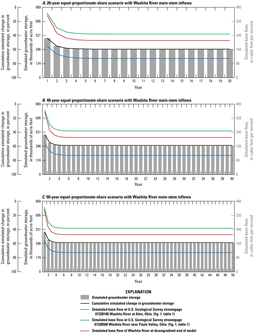
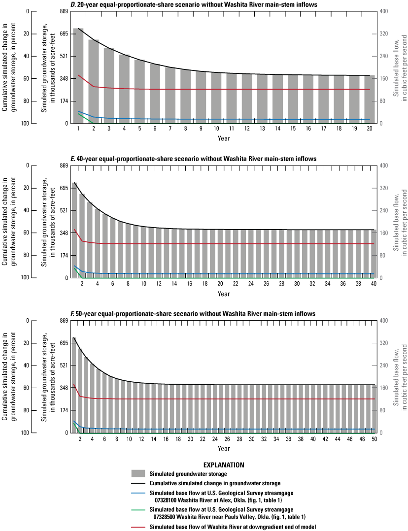
Changes in simulated base flow on the main stem of the Washita River and simulated groundwater storage in the Washita River aquifer, southern Oklahoma, during A, 20, B, 40, and C, 50 years of continuous equal-proportionate-share groundwater pumping with Washita River main-stem inflows and during D, 20, E, 40, and F, 50 years of continuous equal-proportionate-share groundwater pumping without Washita River main-stem inflows.
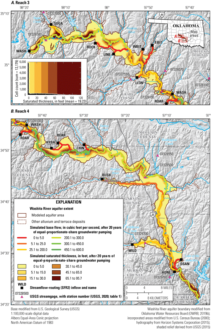
Simulated base flow and simulated saturated thickness in A, reach 3 and B, reach 4 after 20 years of continuous equal-proportionate-share groundwater pumping in the Washita River aquifer, southern Oklahoma.
The EPS pumping rates computed for the Washita River aquifer with Washita River main-stem inflows were higher than those computed for similar alluvial aquifers in Oklahoma (Ellis and others, 2017, 2020; Smith and others, 2017, 2021). Many hydrologic factors influence the EPS pumping rate, but one of the most important factors is the presence or absence of large areas of elevated terrace deposits. These areas of terrace deposits, which often have minimal saturated thickness as compared to alluvium deposits along the center of the river valley, quickly go dry at the beginning of the EPS scenarios. Because the Washita River aquifer as defined in this report includes few elevated terrace deposits, the saturated alluvium deposits along the center of the river valley must be drained to a greater degree with a greater EPS pumping rate to make half of the aquifer reach a saturated thickness of less than 5 ft.
With Washita River main-stem inflows, the actual EPS pumping rate for the Washita River aquifer (both reaches) stabilized at about 59 percent of the nominal EPS pumping rate (fig. 33A). Without Washita River main-stem inflows, the actual EPS pumping rate for the Washita River aquifer (both reaches) stabilized at about 71 percent of the nominal EPS pumping rate (fig. 33B).
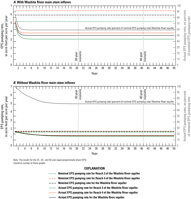
Nominal and actual equal-proportionate-share pumping rates for the Washita River aquifer, southern Oklahoma, A, with Washita River main-stem inflows and B, without Washita River main-stem inflows.
EPS scenarios represent an extreme theoretical construct in which the aquifer is fully developed with regularly spaced wells (one well per model cell, which is one well for every 14.7 acres of modeled area), with each well pumping at a high rate. This level of development is unlikely to occur, and these EPS scenarios bear no resemblance to the current (2022) level of development in the Washita River aquifer in terms of well distribution and pumping rates. Some parts of the aquifer may be more developed than others, but the current level of development in the aquifer as a whole is far smaller than the level of development simulated in the EPS scenarios. The total groundwater use for 2017 (1,402.1 acre-ft/yr, table 4) (Rogers and others, 2023), if divided by the modeled area (178,938 acres), is equivalent to an aquifer-averaged pumping rate of about 0.0078 (acre-ft/acre)/yr—less than 1 percent of the 20-year EPS pumping rate for the Washita River aquifer with or without Washita River main-stem inflows.
Projected 50-Year Pumping
Projected 50-year pumping scenarios were used to simulate the effects of modified well withdrawal rates on groundwater storage in the Washita River aquifer and base flows in the Washita River. Monthly stress periods were used in these scenarios. Well withdrawals in these scenarios, unlike in the EPS scenarios, used historical well withdrawal rates (or multipliers on historical well withdrawal rates) and historical well locations used in the transient simulation of the calibrated numerical model. The effects of modified well withdrawals were evaluated by quantifying differences in groundwater storage and base flow in four 50-year scenarios, which applied (1) no groundwater pumping, (2) 2017 pumping rates, (3) increasing demand pumping rates at simulated wells, and (4) mean pumping rates for the study period (1980–2017). The increasing demand pumping rates assumed a cumulative 45.7-percent increase (0.756-percent compounding annual increase) in pumping over 50 years based on 2010–60 demand projections for southern Oklahoma (OWRB, 2012b). Other model stresses were configured as the means of each monthly stress period from the calibrated numerical model, and the scenarios assumed that future climate conditions were comparable to the 1980–2017 study period. The simulated water table from the end of the calibrated numerical modeling period (2017) was used as the starting water table in each projected pumping scenario covering the period 2018–67.
Because well withdrawals were a small part (less than 1 percent) of the calibrated numerical-model water budget (table 10), changes to the well pumping rates had little effect on simulated Washita River base flows (fig. 34) and groundwater storage (table 13) in the Washita River aquifer. For convenience, all groundwater storage changes were referenced to the groundwater storage at the end of the 2017-pumping-rate scenario (876,165 acre-ft, table 13). Groundwater storage after 50 years with no pumping was 876,593 acre-ft, or 428 acre-ft (0.049 percent) greater than the groundwater storage at the end of the 2017-pumping-rate scenario; this groundwater storage increase is equivalent to a mean water-table-altitude increase of 0.023 ft. Groundwater storage at the end of the 50-year period with the increasing demand pumping rates was 876,030 acre-ft, or 135 acre-ft (0.015 percent) less than the storage at the end of the 2017-pumping-rate scenario; this groundwater storage decrease is equivalent to a mean water-table-altitude decline of 0.007 ft. Groundwater storage after 50 years of pumping at the mean rate for the study period (1980–2017) was 874,807 acre-ft, or 1,358 acre-ft (0.155 percent) less than the groundwater storage at the end of the 2017-pumping-rate scenario; this groundwater storage decrease is equivalent to a mean water-table-altitude decline of 0.074 ft. Though changes in groundwater storage were minimal, some cells near well boundaries showed increased development of simulated cones of depression. For example, local simulated drawdown in some cells was about 3 ft at the end of the 50-year period with the increasing demand pumping rates (Rogers and others, 2023).
Table 13.
Simulated changes in groundwater storage after 50 years of groundwater pumping at selected rates for the calibrated numerical model of the Washita River aquifer, southern Oklahoma, 2018–67.[Sy, specific yield]
| 50-year projected pumping scenario | Groundwater storage at end of 2017-pumping-rate scenario, in acre-feet | Groundwater storage at end of scenario, in acre-feet | Change in groundwater storage, in acre-feet | Change in groundwater storage, in percent | Mean change in water-table altitude, in feet (using mean calibrated Sy of 0.1022 [table 11]) |
|---|---|---|---|---|---|
| No pumping | 876,165 | 876,593 | 428 | 0.049 | 0.023 |
| 2017 pumping rate | 876,165 | 876,165 | 0 | 0.000 | 0.000 |
| Increasing demand pumping rate1 | 876,165 | 876,030 | −135 | −0.015 | −0.007 |
| Mean pumping rate, 1980–2017 | 876,165 | 874,807 | −1,358 | −0.155 | −0.074 |
The increasing demand pumping rate assumed a cumulative 45.7-percent increase (0.756-percent compounding annual increase) in pumping over 50 years based on 2010–60 demand projections for southern Oklahoma (Oklahoma Water Resources Board, 2012b).
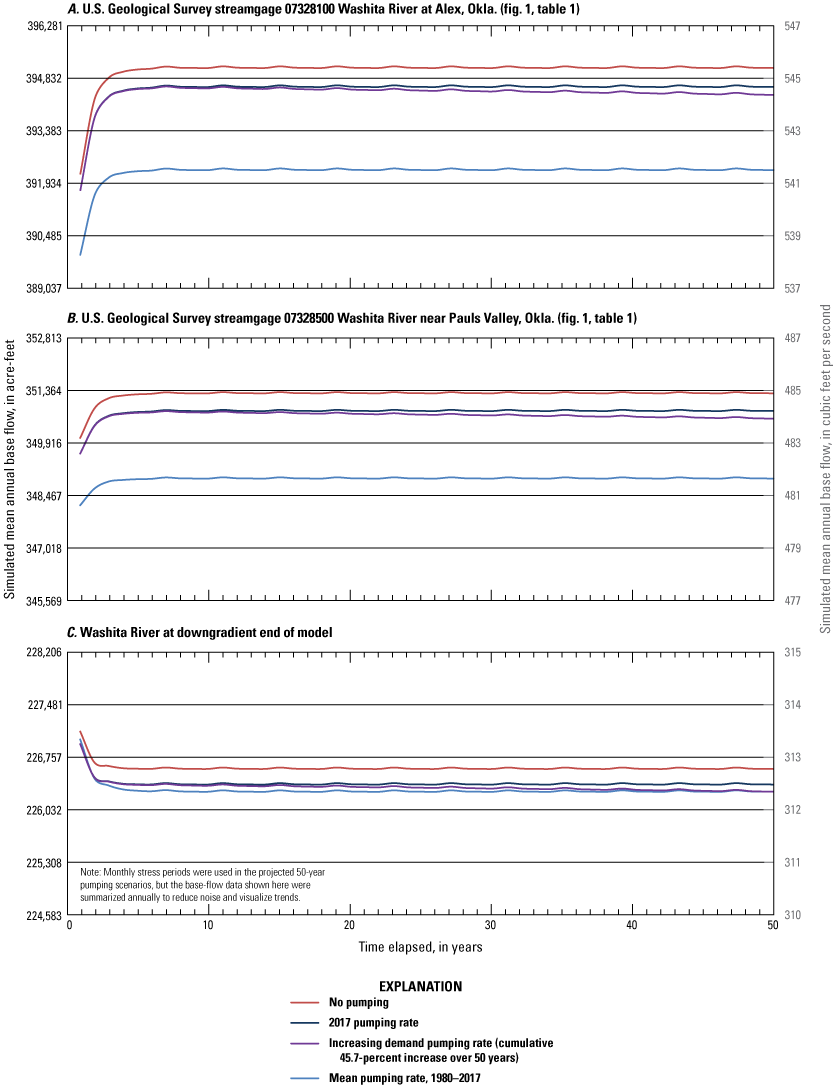
Simulated mean annual base flow at U.S. Geological Survey streamgages A, 07328100 Washita River at Alex, Okla., and B, 07328500 Washita River near Pauls Valley, Okla., and C, on the Washita River at the downgradient end of the model through 50 years of groundwater pumping at selected rates in the Washita River aquifer, southern Oklahoma, 2018–67.
Hypothetical 10-Year Drought
A hypothetical 10-year drought scenario was used to simulate the potential effects of a prolonged period of reduced recharge on groundwater storage. The period January 1993–December 2002 was chosen as the hypothetical drought period because it had a mean annual recharge rate (8.3 in/yr) similar to that of the 1980–2017 study period (8.1 in/yr, table 7). Drought effects were quantified by comparing the results of the drought scenario to those of the calibrated numerical model (no drought) at the end of the hypothetical drought period (2002). To simulate the hypothetical drought, recharge in the calibrated numerical model was reduced by 50 percent during the hypothetical drought period (1993–2002), and upstream inflows from the Washita River and simulated tributaries were reduced by 75 percent, which was comparable to the reduction in Washita River base flows at the Anadarko gage during the 2010–14 drought period (fig. 6A).
Simulated groundwater storage with drought at the end of the hypothetical 10-year drought period (stress period 277) was 826,141 acre-ft, which is 39,487 acre-ft (4.6 percent) less than the simulated groundwater storage of the calibrated numerical model (with no drought) at the end of the drought period (865,627 acre-ft, table 14, fig. 35). This decrease in simulated groundwater storage is equivalent to a mean water-table-altitude decline of 2.2 ft (table 14). The largest simulated water-table-altitude declines occurred in the terrace areas most upgradient from the Washita River (Rogers and others, 2023). The simulated saturated thickness of areas near the Washita River and major tributaries changed little during the hypothetical drought, but the simulated base flow in streams in those areas decreased rapidly. After 12 months of the hypothetical drought, simulated base flows in the Washita River at the Alex gage, Pauls Valley gage, and downgradient end of the model had all decreased by greater than 60 percent as compared to the calibrated numerical model (fig. 36). At the end of the hypothetical 10-year drought period (120 months), simulated base flows at the Alex gage, Pauls Valley gage, and downgradient end of the model had decreased by about 72, 68, and 71 percent, respectively (fig. 36). After the drought period, simulated base flows mostly recovered (returned to less than a 1-percent decrease in simulated base flow) after 2 years (fig. 36), but a groundwater storage deficit of about 1 percent remained until the end of the simulation (fig. 35).
Table 14.
Change in simulated groundwater storage after a hypothetical 10-year drought for the Washita River aquifer, southern Oklahoma, 1993–2002.[Sy, specific yield]
| Scenario | Groundwater storage of calibrated numerical model (with no drought) (2002), in acre-feet | Groundwater storage with drought at end of drought period (2002), in acre-feet | Change in groundwater storage, 1993–2002, in acre-feet | Change in groundwater storage, 1993–2002, in percent | Mean change in water-table altitude, in feet (using mean calibrated Sy of 0.1022 [table 11]) |
|---|---|---|---|---|---|
| Hypothetical 10-year drought | 865,627 | 826,141 | −39,487 | −4.6 | −2.2 |
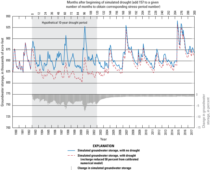
Simulated groundwater storage with drought, simulated groundwater storage with no drought, and changes in simulated groundwater storage resulting from a hypothetical 10-year drought (1993–2002) for the Washita River aquifer, southern Oklahoma, 1990–2017.
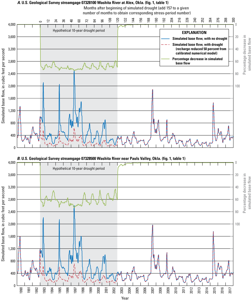
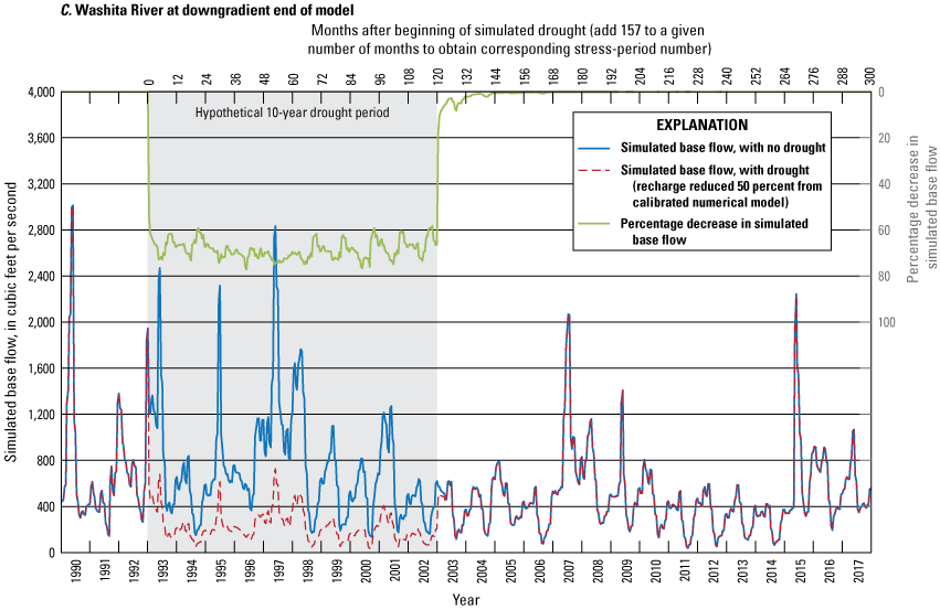
Simulated base flow with drought, simulated base flow with no drought, and changes in simulated base flow at U.S. Geological Survey streamgages A, 07328100 Washita River at Alex, Okla., and B, 07328500 Washita River near Pauls Valley, Okla., and C, on the Washita River at the downgradient end of the model resulting from a hypothetical 10-year drought (1993–2002) for the Washita River aquifer, southern Oklahoma, 1990–2017.
Model Limitations
Some assumptions and simplifications were necessary in the simulation of groundwater flow in the calibrated numerical model. The use of the MODFLOW code requires the assumptions that groundwater flows are governed by Darcy’s Law (Darcy, 1856), water is incompressible and of uniform density, and the aquifer hydrogeology can be simulated appropriately by the cell size and number of layers present. Computing and time limitations prevented the use of cell sizes that could better represent the true variability of the hydrogeologic characteristics of the Washita River aquifer; therefore, results generated by the model may be more applicable to a regional, rather than local, area. No water-table-altitude observations were available for the beginning of the modeling period (1980), so the steady-state simulation was calibrated to mean water-table-altitude observations from the transient period at each observation well. An uneven temporal distribution of water-table-altitude observations caused large data gaps in the calibration data (fig. 24A). Although the simulated water table in areas with fewer observations fell within an expected water-table-altitude range, more site-specific and local calibration-target data could facilitate a more detailed characterization of water-table conditions. Additionally, base-flow gain to the Washita River is based on the simulated water table and may not be accurately represented in locations where water-table-altitude observation data were relatively sparse.
The edges of most of the modeled area, including the bottoms of active cells, were simulated as no-flow boundaries. This practice is common in numerical-model simulations, but it is a simplification that, given the large number of cells involved, likely adds uncertainty to the results described in this report. The stream network used in the numerical model also is a simplification of the actual stream geometry and hydraulic properties. Refined measurement of the stream channel width and streambed conductivity at the local scale could improve the numerical-model calibration because these factors control the amount of streambed seepage exchange with the aquifer. The numerical model was calibrated primarily to base-flow estimates; therefore, collection of more streamflow data during other hydrologic conditions also could further reduce uncertainty in local-scale simulation results.
No streamflow data were available from the most downstream part of the study area, so data from a streamgage farther downstream were used to estimate streambed seepage. The conceptual-model net streambed seepage also may be biased high because of the inclusion of some outflows from floodwater-retarding structures that could not be distinguished and separated from groundwater-derived base flows. Similarly, no field data were available to quantify saturated-zone evapotranspiration. The types of field activities required to effectively model saturated-zone evapotranspiration are expensive to conduct, and the resulting data are difficult to integrate at the scale of the study area. Exact amounts of annual groundwater use are unknown because groundwater wells are not metered and reported groundwater-use data are based on estimates of varying quality submitted to the OWRB by permit holders. Additionally, groundwater use for domestic supply, though assumed to be relatively small, was not included in the numerical model.
Summary
The 1973 Oklahoma Groundwater Law (Oklahoma Statutes §82–1020.5) requires that the Oklahoma Water Resources Board (OWRB) conduct hydrologic investigations of the State’s aquifers to determine the maximum annual yield (MAY) for each groundwater basin. The MAY is defined as the total amount of fresh groundwater that can be annually withdrawn while allowing a minimum 20-year life of that groundwater basin. The annual volume of groundwater allocated per acre of land is known as the equal-proportionate-share (EPS) pumping rate. The OWRB issued a final order on November 13, 1990, that established the MAY (81,840 and 46,935 acre-feet per year [acre-ft/yr]) and EPS pumping rate (1.5 and 1.0 acre-foot per acre per year [(acre-ft/acre)/yr]) for reaches 3 and 4, respectively, of the Washita River aquifer in southern Oklahoma. Because more than 20 years have elapsed since the final order was issued, the U.S. Geological Survey (USGS), in cooperation with the OWRB, conducted an updated hydrologic investigation and evaluated the effects of potential groundwater withdrawals on groundwater flow and availability in the Washita River aquifer for a study period spanning 1980–2017. The modeled area of the Washita River aquifer includes 279.6 square miles (178,938 acres) of alluvium and terrace deposits in Caddo, Grady, Garvin, McClain, and Murray Counties. Reach 3 extends from near Anadarko, Okla., to Alex, Okla., and includes 113.6 square miles (72,697 acres, or 40.6 percent) of the modeled area. Reach 4 extends from near Alex to south of Davis, Okla., and includes 166.0 square miles (106,241 acres, or 59.4 percent) of the modeled area.
The purpose of this report is to describe a hydrologic investigation of the Washita River aquifer in southern Oklahoma. This description included (1) an updated summary of the hydrogeology with a definition of a hydrogeologic framework of the aquifer, (2) development of conceptual and calibrated numerical groundwater-flow models for the aquifer representing the 1980–2017 study period, and (3) results of simulations of groundwater-availability scenarios. The calibrated numerical groundwater-flow model and groundwater-availability scenarios were archived and released in a USGS data release.
A groundwater-hydrograph-based water-table fluctuation method was used to estimate localized recharge rates for 2017–19, and a code-based soil-water-balance estimation technique was used to estimate spatially distributed recharge rates for the period 1980–2017. Water-level hydrographs from three USGS continuous water-level recorder wells were used to estimate annual recharge for 2017–19. The resulting station-averaged mean annual recharge for 2017–19 was 8.1 inches per year, or about 20.2 percent of mean annual precipitation for the period 1980–2017. Multiplied by the 178,938-acre modeled area and unit converted, the calculated mean annual recharge for 2017–19 was 120,783 acre-ft/yr; this value was used for the conceptual-model recharge during 1980–2017.
The code-based soil-water-balance estimate of mean annual recharge for the 1980–2017 study period was about 4.9 inches per year, or about 12.2 percent of the mean annual precipitation. Spatially, mean annual recharge for the study period was greatest in areas of alluvium near the Washita River and tributaries. The code-estimated mean annual recharge generally increased from northwest to southeast in the Washita River aquifer; the mean annual recharge for reach 4 was about 14 percent greater than mean annual recharge for reach 3. Increased recharge from reach 3 to reach 4 is correlated with increased precipitation from northwest to southeast in the study area. The code-estimated mean annual recharge was about 40 percent less than the hydrograph-estimated mean annual recharge used for the conceptual model.
The numerical groundwater-flow model of the Washita River aquifer was constructed by using the USGS modular groundwater-flow model MODFLOW-2005 with the Newton formulation solver. The model was spatially discretized into 500 rows; 600 columns; 12,179 active cells measuring 800 by 800 feet (ft) each; and a single convertible layer based on the hydrogeologic framework. The model was temporally discretized into 456 monthly transient stress periods representing the 1980–2017 study period. An initial steady-state stress period represented mean annual inflows to and outflows from the aquifer and produced a solution that was used as the initial condition for subsequent transient stress periods and some groundwater-availability scenarios. The model was calibrated to water-table-altitude observations at selected wells, base-flow observations at selected USGS streamgages, and the conceptual-model recharge.
The simulated saturated thickness of the Washita River aquifer at the end of the modeling period (2017) was more than 100 ft near Verden, Okla. The mean aquifer thickness was 54.28 ft, and the mean saturated thickness was 47.12 ft. The mean saturated thicknesses for reaches 3 and 4, respectively, were 50.03 and 45.13 ft. A simulated mean transmissivity of 2,276 feet squared per day was calculated as the mean of the calibrated horizontal hydraulic conductivity multiplied by the saturated thickness of each cell; the simulated mean transmissivities for reaches 3 and 4, respectively, were 2,061 and 2,423 feet squared per day. The simulated groundwater storage of the Washita River aquifer at the end of the modeling period (2017) was 869,053 acre-feet (acre-ft); 436,807 acre-ft (50.3 percent) of that total was in reach 3, and 432,247 acre-ft (49.7 percent) of that total was in reach 4.
Three types of groundwater-availability scenarios were run using the calibrated numerical model. These scenarios were used to (1) estimate the EPS pumping rate that ensures a minimum 20-, 40-, and 50-year life of the aquifer, (2) quantify the potential effects of projected well withdrawals on groundwater storage over a 50-year period, and (3) simulate the potential effects of a hypothetical 10-year drought on base flow and groundwater storage. With Washita River main-stem inflows, the 20-, 40-, and 50-year EPS pumping rates under normal recharge conditions were about 3.08 (acre-ft/acre)/yr for reach 3 and about 3.80 (acre-ft/acre)/yr for reach 4. These EPS pumping rates correspond to annual yields of about 224,000 acre-ft/yr for reach 3 and about 404,000 acre-ft/yr for reach 4. For the 20-, 40- and 50-year year EPS scenarios with Washita River main-stem inflows, decreasing and increasing recharge by 10 percent resulted in a 1.5–2.0-percent change in the EPS pumping rate. Without Washita River main-stem inflows, the 20-year EPS pumping rate under normal recharge conditions was about 1.14 (acre-ft/acre)/yr for reach 3 and about 1.23 (acre-ft/acre)/yr for reach 4. Without Washita River main-stem inflows, the 40- and 50-year EPS pumping rates under normal recharge conditions were about 1.13 (acre-ft/acre)/yr for reach 3 and about 1.23 (acre-ft/acre)/yr for reach 4. These EPS pumping rates correspond to annual yields of about 82,000 acre-ft/yr for reach 3 and about 131,000 acre-ft/yr for reach 4. For the EPS scenarios without Washita River main-stem inflows, decreasing and increasing recharge by 10 percent resulted in about 5.3–5.9-percent change in the EPS pumping rate.
Projected 50-year pumping scenarios were used to simulate the effects of modified well withdrawal rates on groundwater storage in the Washita River aquifer and base flows in the Washita River. The effects of modified well withdrawals were evaluated by quantifying differences in groundwater storage and base flow in four 50-year scenarios, which applied (1) no groundwater pumping, (2) 2017 pumping rates, (3) increasing demand pumping rates at simulated wells, and (4) mean pumping rates for the study period (1980–2017). Because well withdrawals were a small part (less than 1 percent) of the calibrated numerical-model water budget, however, changes to the well pumping rates had little effect on simulated base flows in the Washita River and simulated groundwater storage in the Washita River aquifer.
A hypothetical 10-year drought scenario was used to simulate the potential effects of a prolonged period of reduced recharge on groundwater storage. The period January 1993–December 2002 was chosen as the hypothetical drought period. Drought effects were quantified by comparing the results of the drought scenario to those of the calibrated numerical model (no drought) at the end of the hypothetical drought period (2002). To simulate the hypothetical drought, recharge in the calibrated numerical model was reduced by 50 percent during the hypothetical drought period (1993–2002), and upstream inflows from the Washita River and simulated tributaries were reduced by 75 percent, which was comparable to the reduction in Washita River base flows at USGS streamgage 07326500 Washita River at Anadarko, Okla., during the 2010–14 drought period. Simulated groundwater storage with drought at the end of the hypothetical 10-year drought period was 826,141 acre-ft, or 39,487 acre-ft (4.6 percent) less than the groundwater storage of the calibrated numerical model (with no drought) at the end of the drought period. This decrease in groundwater storage is equivalent to a mean water-table-altitude decline of 2.2 ft. The largest water-table-altitude declines occurred in the terrace areas most upgradient from the Washita River. The saturated thickness of areas near the Washita River and major tributaries changed little during the hypothetical drought, but the simulated base flow in streams in those areas decreased rapidly. At the end of the hypothetical 10-year drought period, simulated base flows at USGS streamgage 07328100 Washita River at Alex, Okla., at USGS streamgage 07328500 Washita River near Pauls Valley, Okla., and at the downgradient end of the model had decreased by about 72, 68, and 71 percent, respectively. After the drought period, simulated base flows mostly recovered after 2 years, but a groundwater storage deficit of about 1 percent remained until the end of the simulation.
References Cited
Barlow, P.M., Cunningham, W.L., Zhai, T., and Gray, M., 2015, U.S. Geological Survey groundwater toolbox, a graphical and mapping interface for analysis of hydrologic data (version 1.0)—User guide for estimation of base flow, runoff, and groundwater recharge from streamflow data: U.S. Geological Survey Techniques and Methods, book 3, chap. B10, 27 p., accessed June 5, 2020, at https://doi.org/10.3133/tm3B10.
Barlow, P.M., and Leake, S.A., 2012, Streamflow depletion by wells—Understanding and managing the effects of groundwater pumping on streamflow: U.S. Geological Survey Circular 1376, 84 p., accessed June 5, 2020, at https://doi.org/10.3133/cir1376.
Bennett, G.D., 1976, Introduction to ground-water hydraulics, a programmed text for self-instruction: U.S. Geological Survey Techniques of Water-Resources Investigations, book 3, chap. B2, 172 p., accessed July 21, 2022, at https://doi.org/10.3133/twri03B2.
Chang, J.M., and Stanley, T.M., 2010, Geologic map of the Pauls Valley 30' X 60' quadrangle, Carter, Cleveland, Garvin, Grady, McClain, Murray, Pottawatomie, and Stephens Counties, Oklahoma: Oklahoma Geological Survey Geologic Quadrangle Map OGQ–81, scale 1:100,000, accessed August 4, 2022, at http://ogs.ou.edu/docs/OGQ/OGQ-81-color.pdf.
Cleveland, W., 1979, Robust locally weighted regression and smoothing scatterplots: Journal of the American Statistical Association, v. 74, no. 368, p. 829–836, accessed August 4, 2022, at https://doi.org/10.1080/01621459.1979.10481038.
Cooper, H.H., and Jacob, C.E., 1946, A generalized graphical method for evaluating formation constants and summarizing well field history: American Geophysical Union Transactions, v. 27, p. 526–534, accessed July 21, 2022, at https://agupubs.onlinelibrary.wiley.com/doi/abs/10.1029/TR027i004p00526.
Cowardin, L.M., Carter, V., Golet, F.C., and LaRoe, E.T., 1979, Classification of wetlands and deepwater habitats of the United States: Washington, D.C., U.S. Department of the Interior, U.S. Fish and Wildlife Service, FWS/OBS–79/31, 131 p., accessed July 21, 2022, at https://www.fws.gov/wetlands/documents/classification-of-wetlands-and-deepwater-habitats-of-the-united-states.pdf.
Cunningham, W.L., and Schalk, C.W., 2011, Groundwater technical procedures of the U.S. Geological Survey: U.S. Geological Survey Techniques and Methods, book 1, chap. A1, 151 p., accessed June 5, 2020, at https://doi.org/10.3133/tm1A1.
Davis, L.V., 1955, Geology and ground water resources of Grady and northern Stephens Counties, Oklahoma: Oklahoma Geological Survey Bulletin 73, 184 p., accessed July 22, 2022, at http://ogs.ou.edu/docs/bulletins/B73.pdf.
Doherty, J., 2010, PEST, version 17.05 model independent parameter estimation user manual (5th ed.): Brisbane, Australia, Watermark Numerical Computing, accessed August 3, 2022, at https://pesthomepage.org/programs.
Ellis, J.H., 2018a, Simulation of groundwater flow and analysis of projected water use for the Rush Springs aquifer, western Oklahoma: U.S. Geological Survey Scientific Investigations Report 2018–5136, 156 p., accessed March 1, 2019, at https://doi.org/10.3133/sir20185136.
Ellis, J.H., 2018b, MODFLOW model used in simulation of groundwater flow and analysis of projected water use for the Rush Springs aquifer, western Oklahoma: U.S. Geological Survey data release, accessed May 11, 2023, at https://doi.org/10.5066/F7Q52NXK.
Ellis, J.H., Mashburn, S.L., Graves, G.M., Peterson, S.M., Smith, S.J., Fuhrig, L.F., Wagner, D.L., and Sanford, J.E., 2017, Hydrogeology and simulation of groundwater flow and analysis of projected water use for the Canadian River alluvial aquifer, western and central Oklahoma: U.S. Geological Survey Scientific Investigations Report 2016–5180, 64 p., accessed August 2, 2022, at https://doi.org/10.3133/sir20165180.
Ellis, J.H., Ryter, D.W., Fuhrig, L.T., Spears, K.W., Mashburn, S.L., and Rogers, I.M.J., 2020, Hydrogeology, numerical simulation of groundwater flow, and effects of future water use and drought for reach 1 of the Washita River alluvial aquifer, Roger Mills and Custer Counties, western Oklahoma, 1980–2015: U.S. Geological Survey Scientific Investigations Report 2020–5118, 81 p., accessed August 3, 2022, at https://doi.org/10.3133/sir20205118.
Esri, 2021a, ArcGIS for desktop help—Fill tool: Esri web page, accessed May 6, 2021, at https://desktop.arcgis.com/en/arcmap/10.7/tools/spatial-analyst-toolbox/fill.htm.
Esri, 2021b, ArcGIS for desktop help—IDW tool: Esri web page, accessed May 6, 2021, at https://desktop.arcgis.com/en/arcmap/10.7/tools/spatial-analyst-toolbox/idw.htm.
Fry, J.A., Xian, G., Jin, S., Dewitz, J.A., Homer, C.G., Yang, L., Barnes, C.A., Herold, N.D., and Wickham, J.D., 2011, Completion of the 2006 National Land Cover Database for the conterminous United States: Photogrammetric Engineering and Remote Sensing, v. 77, no. 9, p. 858–864, accessed August 4, 2019, at https://pubs.er.usgs.gov/publication/70034549.
Garner, B.D., and Bills, D.J., 2012, Spatial and seasonal variability of base flow in the Verde Valley, central Arizona, 2007 and 2011: U.S. Geological Survey Scientific Investigations Report 2012–5192, 33 p., accessed August 4, 2022, at https://doi.org/10.3133/sir20125192.
Geoprobe Systems, 2015, Geoprobe hydraulic profiling tool (HPT) system, standard operating procedure: Salina, Kans., Kejr, Inc., Technical Bulletin MK3137, 22 p., accessed August 3, 2022, at https://geoprobe.com/literature/hpt-sop.
Geoprobe Systems, 2020, Direct Image Viewer user guide (rev. 2.0): Salina, Kans., Kejr, Inc., accessed July 31, 2020, at https://geoprobe.com/sites/default/files/storage/pdfs/DI%20Viewer%20User%20Guide%20Rev.2.0.pdf.
Harbaugh, A.W., 1990, A computer program for calculating subregional water budgets using results from the U.S. Geological Survey modular three-dimensional groundwater-flow model: U.S. Geological Survey Open-File Report 90–392, 46 p., accessed June 5, 2020, at https://doi.org/10.3133/ofr90392.
Harbaugh, A.W., 2005, MODFLOW-2005, the U.S. Geological Survey modular ground-water model—The ground-water flow process: U.S. Geological Survey Techniques and Methods, book 6, chap. A16, [variously paged]. [Also available at https://pubs.usgs.gov/tm/2005/tm6A16/PDF.htm.]
Harbaugh, A.W., Banta, E.R., Hill, M.C., and McDonald, M.G., 2000, MODFLOW-2000, the U.S. Geological Survey modular ground-water model—User guide to modularization concepts and the ground-water flow process: U.S. Geological Survey Open-File Report 2000–92, 121 p., accessed August 3, 2022, at https://doi.org/10.3133/ofr200092.
Hargreaves, G.H., and Samani, Z.A., 1985, Reference crop evapotranspiration from temperature: Applied Engineering in Agriculture, v. 1, no. 2, p. 96–99, accessed August 3, 2022, at https://doi.org/10.13031/2013.26773.
Hart, D.L., Jr., 1974, Reconnaissance of the water resources of the Ardmore and Sherman quadrangles, southern Oklahoma: Oklahoma Geological Survey Hydrologic Atlas 3, 4 sheets, scale 1:250,000, accessed August 3, 2022, at https://www.ou.edu/ogs/maps/hydrologicatlases.
Healy, R.W., and Cook, P.G., 2002, Using groundwater levels to estimate recharge: Hydrogeology Journal, v. 10, no. 1, p. 91–109, accessed August 3, 2022, at https://doi.org/10.1007/s10040-001-0178-0.
Hemann, M.R., 1985, Field evaluation of the relationships between transmissivity, permeability and particle size distribution in the Washita River alluvial aquifer, near Anadarko, Oklahoma: Oklahoma State University master’s thesis, 180 p., accessed August 3, 2022, at https://shareok.org/handle/11244/17261.
Hendricks, T.A., 1937, History of the Canadian River of Oklahoma as indicated by the Gerty Sand: Geological Society of America Bulletin, v. 48, no. 3, p. 365–372, accessed December 28, 2022, at https://doi.org/10.1130/GSAB-48-365.
Heran, W.D., Green, G.N., and Stoeser, D.B., 2003, A digital geologic map database for the State of Oklahoma: U.S. Geological Survey Open-File Report 03–247, 10 p., accessed August 3, 2022, at https://doi.org/10.3133/ofr03247.
Hill, M.C., Banta, E.R., Harbaugh, A.W., and Anderman, E.R., 2000, MODFLOW-2000, the U.S. Geological Survey modular ground-water model—User guide to the observation, sensitivity, and parameter-estimation processes and three post-processing programs: U.S. Geological Survey Open-File Report 00–184, 210 p., accessed June 5, 2020, at https://doi.org/10.3133/ofr00184.
Hill, M.C., and Tiedeman, C.R., 2007, Effective groundwater model calibration—With analysis of data, sensitivities, predictions, and uncertainty: New York, Wiley, 455 p., accessed August 3, 2022, at https://doi.org/10.1002/0470041080.
Horizon Systems Corporation, 2015, National Hydrography Dataset Plus (NHDPlus) version 1: Horizon Systems Corporation database, accessed August 3, 2022, at https://nhdplus.com/NHDPlus/.
Johnson, K.S., and Luza, K.V., 2008, Earth science and mineral resources of Oklahoma: Oklahoma Geological Survey Educational Publication 9, 21 p., accessed May 3, 2023, at http://ogs.ou.edu/docs/educationalpublications/EP9.pdf.
Kendall, M.G., 1938, A new measure of rank correlation: Biometrika, v. 30, nos. 1–2, p. 81–93, accessed August 3, 2022, at https://doi.org/10.1093/biomet/30.1-2.81.
Kent, D.C., Neafus, R.J., Patterson, J.W., Jr., and Schipper, M.R., 1984, Evaluation of aquifer performance and water supply capabilities of the Washita River alluvium in Oklahoma—Final report: Oklahoma Water Resources Board, prepared by University of Oklahoma, Department of Geology, 49 p., accessed August 3, 2022, at https://www.owrb.ok.gov/studies/reports/reports_pdf/WashitaRiverA&T.pdf.
Leonard, A.R., Davis, L.V., and Stacy, B.L., 1958, Ground water in the alluvial deposits of the Washita River and its tributaries in Oklahoma: U.S. Geological Survey Open File Report 58–63, 10 p., accessed August 3, 2022, at https://doi.org/10.3133/ofr5863.
Lubczynski, M.W., 2009, The hydrogeological role of trees in water-limited environments: Hydrogeology Journal, v. 17, no. 1, p. 247–259, accessed June 5, 2020, at https://doi.org/10.1007/s10040-008-0357-3.
Mandelbrot, B.B., 1983, The fractal geometry of nature: New York, W.H. Freeman, 468 p. [Also available at https://doi.org/10.1002/esp.3290080415.]
Mashburn, S.L., Ryter, D.W., Neel, C.R., Smith, S.J., and Correll, J.S., 2013, Hydrogeology and simulation of groundwater flow in the central Oklahoma (Garber-Wellington) aquifer, Oklahoma, 1987 to 2009, and simulation of available water in storage, 2010–2059 (ver. 2.0, October 2019): U.S. Geological Survey Scientific Investigations Report 2013–5219, 92 p., accessed June 5, 2020, at https://doi.org/10.3133/sir20135219.
McCall, W., 2010, Tech guide for calculation of estimated hydraulic conductivity (Est. K) log from HPT data: Salina, Kans., Kejr, Inc., 20 p., accessed August 3, 2022, at https://geoprobe.com/sites/default/files/pdfs/tech_guide_estk_v5_0_0.pdf.
Microsoft Corporation, 2018, Bing Maps imagery API: Microsoft web page, accessed May 11, 2023, at https://learn.microsoft.com/en-us/bingmaps/rest-services/imagery/.
Miller, G.W., and Stanley, T.M., 2004, Geologic map of the Anadarko 30' X 60' quadrangle, Caddo, Canadian, Custer, Grady, Kiowa and Washita Counties, Oklahoma: Oklahoma Geological Survey Geologic Quadrangle Map OGQ–58, scale 1:100,000, accessed December 4, 2015, at http://ogs.ou.edu/docs/OGQ/OGQ-58-color.pdf.
Mogg, J.L., Schoff, S.L., and Reed, E.W., 1960, Groundwater resources of Canadian County, Oklahoma: Oklahoma Geological Survey Bulletin 87, 112 p., accessed July 22, 2022, at http://ogs.ou.edu/docs/bulletins/B87.pdf.
Multi-Resolution Land Characteristics Consortium, 2011, National Land Cover Database 2006 (NLCD 2006): Multi-Resolution Land Characteristics Consortium database, accessed October 3, 2020, at https://www.mrlc.gov/data/nlcd-2006-land-cover-conus.
National Agricultural Statistics Service, 2019, CropScape—Cropland data layers, 2010–17: U.S. Department of Agriculture database, accessed June 30, 2019, at https://nassgeodata.gmu.edu/CropScape/.
National Agricultural Statistics Service, 2020, Oklahoma agricultural statistics 2020: National Agricultural Statistics Service and Oklahoma Department of Agriculture, Food and Forestry, Oklahoma Annual Statistical Bulletin 2020 edition, 84 p., accessed May 24, 2020, at https://www.nass.usda.gov/Statistics_by_State/Oklahoma/Publications/Annual_Statistical_Bulletin/ok-bulletin-2020-web.pdf.
National Centers for Environmental Information, 2021, Climate at a glance—Divisional time series: National Oceanic and Atmospheric Administration database, accessed July 20, 2021, at https://www.ncdc.noaa.gov/cag/divisional/time-series.
National Centers for Environmental Information, 2022, Daily observational data—GHCN daily: National Oceanic and Atmospheric Administration database, accessed August 3, 2022, at https://ncei.noaa.gov/maps/daily/.
Natural Resources Conservation Service [NRCS], 2022, Soil Survey Geographic database (SSURGO): U.S. Department of Agriculture database, accessed August 3, 2022, at https://www.nrcs.usda.gov/resources/data-and-reports/soil-survey-geographic-database-ssurgo.
Neel, C.R., Wagner, D.L., Correll, J.S., Sanford, J.E., Hernandez, J.R., Spears, K.W., and Waltman, P.B., 2018, Hydrologic investigation report of the Rush Springs aquifer in west-central Oklahoma, 2015: Oklahoma Water Resources Board Publication 2018–01, 73 p., accessed August 3, 2022, at https://www.owrb.ok.gov/reports/studies/RushSprings2015.pdf.
Niswonger, R.G., Panday, S., and Ibaraki, M., 2011, MODFLOW-NWT, a Newton formulation for MODFLOW-2005: U.S. Geological Survey Techniques and Methods, book 6, chap. A37, 44 p., accessed June 5, 2020, at https://doi.org/10.3133/tm6A37.
Niswonger, R.G., and Prudic, D.E., 2005, Documentation of the Streamflow-Routing (SFR2) package to include unsaturated flow beneath streams—A modification to SFR1: U.S. Geological Survey Techniques and Methods, book 6, chap. A13, 50 p., accessed June 5, 2020, at https://doi.org/10.3133/tm6A13.
Oklahoma Climatological Survey, 2020, Average length of growing season: Oklahoma Climatological Survey web page, accessed November 25, 2020, at http://climate.ok.gov/index.php/climate/map/average_length_of_growing_season/oklahoma_south-central_u.s.
Oklahoma Climatological Survey, 2021a, Caddo County climate summary: Oklahoma Climatological Survey web page, 1 p., accessed September 9, 2021, at https://climate.ok.gov/county_climate/Products/CountyPages/caddo.html.
Oklahoma Climatological Survey, 2021b, Murray County climate summary: Oklahoma Climatological Survey web page, 1 p., accessed September 9, 2021, at https://climate.ok.gov/county_climate/Products/CountyPages/murray.html.
Oklahoma Mesonet, 2019, Daily data retrieval: Oklahoma Mesonet web page, accessed May 2019 at https://www.mesonet.org/index.php/past_data/daily_data_retrieval.
Oklahoma State Legislature, 2021a, Definitions, chap. 1020, section 1 of Waters and water rights: Oklahoma Statutes, title 82, accessed October 19, 2021, at https://oksenate.gov/sites/default/files/2019-12/os82.pdf.
Oklahoma State Legislature, 2021b, Determination of maximum annual yield, chap. 1020, section 5 of Waters and water rights: Oklahoma Statutes, title 82, accessed October 19, 2021, at https://oksenate.gov/sites/default/files/2019-12/os82.pdf.
Oklahoma State Legislature, 2021c, Domestic use—Spacing of wells and waste, chap. 1020, section 3 of Waters and water rights: Oklahoma Statutes, title 82, accessed October 19, 2021, at https://oksenate.gov/sites/default/files/2019-12/os82.pdf.
Oklahoma Water Resources Board [OWRB], 2012a, Oklahoma Comprehensive Water Plan—Lower Washita Watershed Planning Region report (ver. 1.1, updated 2012): Oklahoma Water Resources Board, 111 p., accessed August 4, 2022, at https://www.owrb.ok.gov/supply/ocwp/pdf_ocwp/WaterPlanUpdate/regionalreports/OCWP_LowerWashita_Region_Report.pdf.
Oklahoma Water Resources Board [OWRB], 2012b, Oklahoma Comprehensive Water Plan—Executive report (updated 2012): Oklahoma Water Resources Board, 151 p., accessed August 4, 2022, at https://www.owrb.ok.gov/supply/ocwp/pdf_ocwp/WaterPlanUpdate/draftreports/OCWP%20Executive%20Rpt%20FINAL.pdf.
Oklahoma Water Resources Board [OWRB], 2014, Taking and use of groundwater, chap. 30 of Oklahoma Administrative Code: Oklahoma Administrative Code, title 785, 44 p., accessed August 3, 2022, at https://www.owrb.ok.gov/rules/pdf/current/Ch302019.pdf.
Oklahoma Water Resources Board [OWRB], 2015, Produced water reuse in Oklahoma—Regulatory considerations and references: Oklahoma Water Resources Board, 51 p., accessed June 2, 2022, at https://www.owrb.ok.gov/2060/PWWG/GWPC-Ok-Produced-Water-Project-Summary-Report.pdf.
Oklahoma Water Resources Board [OWRB], 2017, 2017 Oklahoma groundwater report—Beneficial Use Monitoring Program: Oklahoma Water Resources Board, 172 p., accessed July 5, 2020, at https://www.owrb.ok.gov/quality/monitoring/bump/pdf_bump/Reports/GMAP2017.pdf.
Oklahoma Water Resources Board [OWRB], 2019a, Interactive maps & GIS data: Oklahoma Water Resources Board database, accessed November 2019 at https://www.owrb.ok.gov/maps/index.php.
Oklahoma Water Resources Board [OWRB], 2019b, OWRB open data—Groundwater: Oklahoma Water Resources Board database, accessed November 2019 at https://home-owrb.opendata.arcgis.com/search?tags=groundwater.
Oklahoma Water Resources Board [OWRB], 2019c, OWRB open data—OCWP: Oklahoma Water Resources Board database, accessed November 2019 at https://home-owrb.opendata.arcgis.com/search?tags=OCWP.
Oklahoma Water Resources Board [OWRB], 2019d, OWRB open data—Water rights: Oklahoma Water Resources Board database, accessed November 2019 at https://home-owrb.opendata.arcgis.com/search?tags=rights.
Oklahoma Water Resources Board [OWRB], 2020, Maximum annual yield: Oklahoma Water Resources Board Fact Sheet, 2 p., accessed June 5, 2020, at https://www.owrb.ok.gov/about/about_pdf/Fact-MAY.pdf.
Patterson, J.W., Jr., 1984, Ground-water management model of the Washita River aquifer in Grady, McClain, Garvin, Murray, Carter, and Johnston Counties in south-central Oklahoma: Stillwater, Okla., Oklahoma State University master’s thesis, 285 p. [Also available at https://shareok.org/handle/11244/16079.]
Piper, A.M., 1944, A graphic procedure in the geochemical interpretation of water analyses: Transactions, American Geophysical Union, v. 25, no. 6, p. 914–928, accessed July 21, 2022, at https://doi.org/10.1029/TR025i006p00914.
Rantz, S.E., and others, 1982, Measurement and computation of streamflow—Volume 1. Measurement of stage and discharge: U.S. Geological Survey Water-Supply Paper 2175, 284 p., accessed June 5, 2020, at https://doi.org/10.3133/wsp2175.
Reeds, C.A., 1927, The Arbuckle Mountains, Oklahoma—The fossil collector’s happy hunting ground: Oklahoma Geological Survey, Circular No. 14, 15 p., accessed July 21, 2022, at http://ogs.ou.edu/docs/circulars/C14.pdf.
Rogers, I.M.J., Smith, S.J., Gammill, N.C., Gillard, N.J., Lockmiller, K.A., Fetkovich, E.J., Correll, J.S., and Hussey, S.P., 2023, MODFLOW-NWT model used in simulation of groundwater availability in reaches 3 and 4 of the Washita River aquifer, southern Oklahoma, 1980–2017: U.S. Geological Survey data release, https://doi.org/10.5066/P9UET694.
Ryter, D.W., and Correll, J.S., 2016, Hydrogeological framework, numerical simulation of groundwater flow, and effects of projected water use and drought for the Beaver-North Canadian River alluvial aquifer, northwestern Oklahoma (ver. 1.1, February 2016): U.S. Geological Survey Scientific Investigations Report 2015–5183, 63 p., accessed June 5, 2020, at https://doi.org/10.3133/sir20155183.
Schipper, M.R., 1983, Ground-water management model for the Washita River alluvial aquifer in Roger Mills and Custer Counties: Stillwater, Okla., Oklahoma State University master’s thesis, 147 p., accessed July 20, 2022, at https://shareok.org/handle/11244/16409.
Scholl, M., Christenson, S., Cozzarelli, I., Ferree, D., and Jaeshke, J., 2005, Recharge processes in an alluvial aquifer riparian zone, Norman Landfill, Norman, Oklahoma, 1998–2000: U.S. Geological Survey Scientific Investigations Report 2004–5238, 54 p., accessed July 5, 2020, at https://doi.org/10.3133/sir20045238.
Sen, P.K., 1968, Estimates of the regression coefficient based on Kendall’s tau: Journal of the American Statistical Association, v. 63, no. 324, p. 1379–1389, accessed August 4, 2022, at https://doi.org/10.1080/01621459.1968.10480934.
Shivers, M.J., and Andrews, W.J., 2013, Hydrologic drought of water year 2011 compared to four major drought periods of the 20th century in Oklahoma: U.S. Geological Survey Scientific Investigations Report 2013–5018, 52 p., accessed July 5, 2020, at https://doi.org/10.3133/sir20135018.
Smith, S.J., Ellis, J.H., Paizis, N.C., Becker, C.J., Wagner, D.L., Correll, J.S., and Hernandez, R.J., 2021, Hydrogeology and model-simulated groundwater availability in the Salt Fork Red River aquifer, southwestern Oklahoma, 1980–2015: U.S. Geological Survey Scientific Investigations Report 2021–5003, 85 p., accessed August 4, 2022, at https://doi.org/10.3133/sir20215003.
Smith, S.J., Ellis, J.H., Wagner, D.L., and Peterson, S.M., 2017, Hydrogeology and simulated groundwater flow and availability in the North Fork Red River aquifer, southwest Oklahoma, 1980–2013: U.S. Geological Survey Scientific Investigations Report 2017–5098, 107 p., accessed July 5, 2020, at https://doi.org/10.3133/sir20175098.
Smith, S.J., and Esralew, R.A., 2010, StreamStats in Oklahoma—Drainage-basin characteristics and peak-flow frequency statistics for ungaged streams: U.S. Geological Survey Scientific Investigations Report 2009–5255, 59 p., accessed July 5, 2020, at https://doi.org/10.3133/sir20095255.
Stallman, R.W., 1971, Aquifer-test design, observation, and data analysis: U.S. Geological Survey Techniques of Water-Resources Investigations, book 3, chap. B1, 26 p., accessed August 3, 2022, at https://doi.org/10.3133/twri03B1.
Stanley, T.M., and Chang, J.M., 2012, Geologic map of the Ardmore 30' X 60' quadrangle and the Oklahoma part of the Gainesville 30' X 30' quadrangle, Carter, Jefferson, Love, Murray, and Stephens Counties, Oklahoma: Oklahoma Geological Survey Geologic Quadrangle Map OGQ–86, scale 1:100,000, accessed August 3, 2022, at http://ogs.ou.edu/docs/OGQ/OGQ-86-color.pdf.
Thornthwaite, C.W., and Mather, J.R., 1957, Instructions and tables for computing potential evapotranspiration and the water balance: Centerton, N.J., Drexel Institute of Technology, Laboratory of Climatology, Publications in Climatology, v. 10, no. 3, p. 185–311, accessed July 21, 2022, at https://www.wrc.udel.edu/wp-content/publications/ThornthwaiteandMather1957Instructions_Tables_ComputingPotentialEvapotranspiration_Water%20Balance.pdf.
Tortorelli, R.L., 2008, Hydrologic drought of water year 2006 compared with four major drought periods of the 20th century in Oklahoma: U.S. Geological Survey Scientific Investigations Report 2008–5199, 46 p., accessed June 5, 2020, at https://doi.org/10.3133/sir20085199.
Trescott, P.A., Pinder, G.F., and Larson, S.P., 1976, Finite-difference model for aquifer simulation in two dimensions and results of numerical experiments: U.S. Geological Survey Techniques of Water Resources Investigations, book 7, chap. C1, 116 p., accessed July 21, 2022, at https://doi.org/10.3133/twri07C1.
U.S. Army Corps of Engineers, 2021, National Inventory of Dams: U.S. Army Corps of Engineers database, accessed April 23, 2021, at https://nid.sec.usace.army.mil/#/.
U.S. Census Bureau, 2000, TIGER/line shapefiles and TIGER/line files: U.S. Census Bureau database, accessed August 4, 2022, at https://www.census.gov/geo/maps-data/data/tiger-line.html.
U.S. Environmental Protection Agency, 2017, Drinking water regulations and contaminants: U.S. Environmental Protection Agency web page, accessed March 24, 2020, at https://www.epa.gov/dwregdev/drinking-water-regulations-and-contaminants.
U.S. Fish and Wildlife Service, 2014, National Wetlands Inventory—Download seamless wetlands data by State: U.S. Fish and Wildlife Service database, accessed March 28, 2014, at https://www.fws.gov/wetlands/Data/State-Downloads.html.
U.S. Geological Survey [USGS], 2015, National Elevation Dataset (NED) 1/3 arc-second DEM: U.S. Geological Survey database, accessed September 21, 2015, at https://apps.nationalmap.gov/downloader/#/10/34.77438352431586/-97.66967773437258/usgs_topo/elevation-products-three-dep/.
U.S. Geological Survey [USGS], 2019, National Elevation Dataset (NED) 1/9 arc-second DEM: U.S. Geological Survey database, accessed January 28, 2019, at https://apps.nationalmap.gov/downloader/#/10/34.77438352431586/-97.66967773437258/usgs_topo/elevation-products-three-dep/.
U.S. Geological Survey [USGS], 2020, USGS water data for Oklahoma, in USGS water data for the Nation: U.S. Geological Survey National Water Information System database, accessed January 2020 at https://doi.org/10.5066/F7P55KJN. [State water data directly accessible at https://waterdata.usgs.gov/ok/nwis/.]
U.S. Geological Survey [USGS], 2021, GeoLog Locator: U.S. Geological Survey web page, accessed July 13, 2021, at https://webapps.usgs.gov/GeoLogLocator/#!/search.
Wahl, K.L., and Wahl, T.L., 1995, Determining the flow of Comal Springs at New Braunfels, Texas, in Texas Water ‘95, a component conference of the First International Conference on Water Resources Engineering, San Antonio, Texas, August 16–17, 1995 [Proceedings]: American Society of Civil Engineers, p. 77–86.
Westenbroek, S.M., Kelson, V.A., Dripps, W.R., Hunt, R.J., and Bradbury, K.R., 2010, SWB—A modified Thornthwaite-Mather Soil-Water-Balance code for estimating groundwater recharge: U.S. Geological Survey Techniques and Methods, book 6, chap. A31, 60 p., accessed June 5, 2020, at https://doi.org/10.3133/tm6A31.
White, J.T., 2018, A model-independent iterative ensemble smoother for efficient history-matching and uncertainty quantification in very high dimensions: Environmental Modelling & Software, v. 109, p. 191–201, accessed June 5, 2020, at https://doi.org/10.1016/j.envsoft.2018.06.009.
White, W.N., 1932, A method of estimating ground-water supplies based on discharge by plants and evaporation from soil—Results of investigations in Escalante Valley, Utah: U.S. Geological Survey Water-Supply Paper 659–A, 105 p., accessed June 5, 2020, at https://doi.org/10.3133/wsp659A.
White, J.T., Hunt, R.J., Fienen, M.N., and Doherty, J.E., 2020, Approaches to highly parameterized inversion—PEST++ version 5, a software suite for parameter estimation, uncertainty analysis, management optimization and sensitivity analysis: U.S. Geological Survey Techniques and Methods, book 7, chap. C26, 51 p., accessed August 25, 2021, at https://doi.org/10.3133/tm7C26.
Winston, R.B., comp., 2018, Online guide to MODFLOW-NWT—Suggested input values for the NWT input file: U.S. Geological Survey web page, accessed November 2018 at https://water.usgs.gov/ogw/modflow-nwt/MODFLOW-NWT-Guide/index.html?suggested_input_values_for_the.htm.
Ye, H., Royden, L., Burchfiel, C., and Schuepbach, M., 1996, Late Paleozoic deformation of interior North America—The greater ancestral Rocky Mountains: American Association of Petroleum Geologists Bulletin, v. 80, no. 9, p. 1397–1432, accessed August 4, 2022, at https://doi.org/10.1306/64ED9A4C-1724-11D7-8645000102C1865D.
Conversion Factors
U.S. customary units to International System of Units
Temperature in degrees Celsius (°C) may be converted to degrees Fahrenheit (°F) as follows:
°F = (1.8 × °C) + 32.
Temperature in degrees Fahrenheit (°F) may be converted to degrees Celsius (°C) as follows:
°C = (°F – 32) / 1.8.
Datum
Vertical coordinate information is referenced to the North American Vertical Datum of 1988 (NAVD 88).
Horizontal coordinate information is referenced to the North American Datum of 1983 (NAD 83).
Altitude, as used in this report, refers to distance above the vertical datum.
Supplemental Information
Specific conductance is given in microsiemens per centimeter at 25 degrees Celsius (µS/cm at 25 °C).
Concentrations of chemical constituents in water are given in milligrams per liter (mg/L).
Abbreviations
BFI
base-flow index
DEM
digital elevation model
EPS
equal-proportionate-share
GHB
general-head boundary
HOB
Head Observation package
HPT
hydraulic profiling tool
lidar
light detection and ranging
MAY
maximum annual yield
NAVD 88
North American Vertical Datum of 1988
NRCS
Natural Resources Conservation Service
NWIS
National Water Information System
OWRB
Oklahoma Water Resources Board
p-value
probability value
RMSE
root-mean-square error
SFR2
Streamflow-Routing package, version 2
SWB
Soil-Water-Balance code
TDS
total dissolved solids
USGS
U.S. Geological Survey
WTF
water-table fluctuation
For more information about this publication, contact
Director, Oklahoma-Texas Water Science Center
U.S. Geological Survey
1505 Ferguson Lane
Austin, TX 78754–4501
For additional information, visit
https://www.usgs.gov/centers/ot-water
Publishing support provided by
Lafayette Publishing Service Center
Disclaimers
Any use of trade, firm, or product names is for descriptive purposes only and does not imply endorsement by the U.S. Government.
Although this information product, for the most part, is in the public domain, it also may contain copyrighted materials as noted in the text. Permission to reproduce copyrighted items must be secured from the copyright owner.
Suggested Citation
Rogers, I.M.J., Smith, S.J., Gammill, N.C., Gillard, N.J., Lockmiller, K.A., Fetkovich, E.J., Correll, J.S., and Hussey, S.P., 2023, Hydrogeology and simulated groundwater availability in reaches 3 and 4 of the Washita River aquifer, southern Oklahoma, 1980–2017: U.S. Geological Survey Scientific Investigations Report 2023–5072, 83 p., https://doi.org/10.3133/sir20235072.
ISSN: 2328-0328 (online)
Study Area
| Publication type | Report |
|---|---|
| Publication Subtype | USGS Numbered Series |
| Title | Hydrogeology and simulated groundwater availability in reaches 3 and 4 of the Washita River aquifer, southern Oklahoma, 1980–2017 |
| Series title | Scientific Investigations Report |
| Series number | 2023-5072 |
| DOI | 10.3133/sir20235072 |
| Publication Date | August 25, 2023 |
| Year Published | 2023 |
| Language | English |
| Publisher | U.S. Geological Survey |
| Publisher location | Reston, VA |
| Contributing office(s) | Oklahoma-Texas Water Science Center |
| Description | Report: xii, 83 p.; 2 Data Releases |
| Country | United States |
| State | Oklahoma |
| Other Geospatial | Washita River Aquifer |
| Online Only (Y/N) | Y |