

Potential Effects of Projected Pumping Scenarios on Future Water-Table Elevations Near Kirtland Air Force Base in Albuquerque, New Mexico
Links
- Document: Report (1.86 MB pdf) , HTML , XML
- Data Release: USGS data release—Modified multi-node well (MNW2) files used to simulate potential future (2016-2050) water-table elevation change near Kirtland Air Force Base in Albuquerque, New Mexico
- NGMDB Index Page: National Geologic Map Database Index Page (html)
- Download citation as: RIS | Dublin Core
Acknowledgments
The author would like to acknowledge the Air Force Civil Engineer Center for supporting this research, as well as the U.S. Geological Survey staff who contributed to this work.
Abstract
The U.S. Geological Survey, in cooperation with the Air Force Civil Engineer Center, simulated different groundwater pumping scenarios from 2016 to 2050 to determine the potential future changes in groundwater levels in areas around the Kirtland Air Force Base Bulk Fuels Facility and an ethylene dibromide (EDB) plume. Projections of water supply and demand created by the Albuquerque Bernalillo County Water Utility Authority were used to develop the future groundwater pumping scenarios used as inputs for a refined local-scale model within the updated Middle Rio Grande Basin regional model.
The simulated water-table elevations in model cells that contain the EDB plume in the medium demand and medium supply scenario rose 29 feet (ft) until 2035, then remained within 10 ft of that elevation through 2050, whereas the water-table elevations in the high demand and low supply scenario rose about 26 ft until 2035 and then decreased by more than 10 ft. Simulated water-table elevations in the low demand and high supply scenario continued to rise throughout most of the future simulation period and peaked at about 44 ft over the 2016 water-table elevation. All of the scenarios ended the future simulation period with higher simulated water-table elevations than at the beginning of the future simulation period. Simulations that represented the potentially highest and lowest volume of groundwater pumping near the EDB plume by adjusting the spatial distribution of pumping had similar simulated water-table elevations as the nonadjusted scenarios, with maximum water-table elevation changes that only differed by about 2 ft from the nonadjusted scenarios. Consideration should be taken when using these model results to inform decisions because the model results are subject to uncertainty from many different sources, including uncertainty in the future pumping scenarios as well as the model itself because of the simplification of the hydrogeologic system.
Introduction
The Albuquerque Bernalillo County Water Utility Authority (ABCWUA) began diverting surface water from the Rio Grande as part of the San Juan-Chama (SJC) Drinking Water Project in December 2008. Before the implementation of this alternate water source, the municipal water supply was largely groundwater pumped from the Santa Fe Group aquifer system. The use of the SJC surface water has generally increased since then, composing about 20 percent of the annual supply to Albuquerque, New Mexico, and the surrounding areas in 2009 and about 70 percent in 2019 (ABCWUA, 2016, 20203). Because of the increased use of surface water and conservation efforts to reduce per capita water use, groundwater withdrawals declined 67 percent between 2008 and 2016 (Galanter and Curry, 2019), resulting in rising groundwater levels throughout the aquifer system from 2008 until recent years (Falk and others, 2011; Powell and McKean, 2014; ABCWUA, 2016; Galanter and Curry, 2019; Jurney and Bell, 2021).
Although rising groundwater levels are indicative of a recovering aquifer, rising groundwater levels and changes in groundwater flow direction could also remobilize or redistribute the fuel-related contaminants present in soil, soil vapor, and groundwater at the water table as a result of a fuel spill containing ethylene dibromide (EDB) at the Kirtland Air Force Base (KAFB) Bulk Fuels Facility (BFF). Wells in the KAFB BFF groundwater monitoring well network were installed with well screens open across the water table in order to monitor and sample less dense fuel products floating on groundwater within the EDB plume. Some monitoring wells were replaced because the tops of their well screens had been submerged by the rising water table (U.S. Army Corps of Engineers, 2017). Understanding the potential changes to groundwater levels in the future and how changes in groundwater pumping can affect groundwater levels is important to provide guidance for well design and placement of well screens in the monitoring wells. The U.S. Geological Survey (USGS), in cooperation with the Air Force Civil Engineer Center, initiated a two-part study to (1) document and analyze the response of the water-table aquifer in the Albuquerque metropolitan area to decreased groundwater pumping (Flickinger and Mitchell, 2020) and (2) to simulate groundwater responses to possible future water-supply pumping scenarios using an existing groundwater-flow model.
Purpose and Scope
The purpose of this report is to present simulations of different groundwater pumping scenarios that are based on projections of supply and demand and designed to determine potential future changes in groundwater levels in areas around the KAFB BFF and the EDB plume. Specifically, the report documents simulations of three main scenarios that represent future groundwater pumping under low demand and high supply, medium demand and medium supply, and high demand and low supply projections. An existing groundwater-flow model that uses the USGS modular, transient, three-dimensional, finite-difference groundwater flow with localized grid refinement, version 2 (MODFLOW-LGR2) (Mehl and Hill, 2013) to iteratively couple a regional model of the Middle Rio Grande Basin (Bexfield and others, 2011) and a local-scale model of the area surrounding the EDB plume (Myers and Friesz, 2019) was selected to facilitate the simulation of the groundwater pumping scenarios. The report describes how scenario results were analyzed by extracting the water-table elevations at monitoring wells and the model cells that cover the extent of the EDB plume. Simulated water-table elevations are discussed in the context of observed water-table elevations and possible sources of uncertainty. The model files for the simulations that support the results and conclusions of this study are available from Flickinger (2023).
Study Area
Albuquerque is located in the Middle Rio Grande Basin (hereafter referred to as “the basin”), which encompasses the area along the Rio Grande between Cochiti Lake and San Acacia (Bartolino and Cole, 2002) (fig. 1). The SJC Drinking Water Project is a cross-basin diversion that moves water from tributaries of the San Juan River through a series of diversions, canals, and tunnels into a tributary of the Rio Chama, where the water flows into the Rio Grande upstream from Cochiti Lake. Tijeras Arroyo, an ephemeral stream that originates in the Manzanita and Sandia Mountains and discharges ephemeral water to the Rio Grande, is the primary drainage for the southeastern area of the city and KAFB (fig. 2). The reach of the Rio Grande that flows through Albuquerque generally loses water to the Santa Fe Group aquifer system (Rankin and others, 2016).

Locations of the Middle Rio Grande Basin, Middle Rio Grande Basin regional model, local-scale model, Albuquerque municipal limits, and Kirtland Air Force Base, New Mexico. Middle Rio Grande Basin boundary from Plummer and others (2004). Middle Rio Grande Basin regional model boundary modified from Bexfield and others (2011).

Locations of the local-scale model boundary, Kirtland Air Force Base (KAFB) Bulk Fuels Facility, ethylene dibromide plume (KAFB, 2022), faults (Connell, 2006), and locations of wells and well clusters. Extent of the local-scale model within the Middle Rio Grande Basin is shown on figure 1.
The Santa Fe Group aquifer system in the basin consists of the Santa Fe Group and the post-Santa Fe Group alluvial sediments that were deposited on top of the Santa Fe Group (Bartolino and Cole, 2002). Depending on location in the basin, the water table is either in the Santa Fe Group or the post-Santa Fe Group sediments. In the area surrounding the KAFB BFF (fig. 2), the water table is in the Santa Fe Group. The shallow part of the Santa Fe Group is generally considered to be an unconfined system, but interbedded fine-grained layers of the Santa Fe Group create semiconfined conditions at depth (Bexfield and others, 2012). Near the KAFB BFF, the semiconfined conditions and greater hydraulic pressures at depth lead to groundwater elevations in some wells screened at or near the water table being lower than the groundwater elevations in wells screened at greater depths by 25 feet (ft) or more (Bexfield and Anderholm, 2002). Variations in groundwater levels can also vary by the depth of the well within the Santa Fe Group aquifer system, with some nested monitoring wells indicating a greater groundwater level recovery in the deep piezometer compared to the lesser recovery at the shallow and middle piezometers, whereas other nested monitoring wells indicate similar trends of recovery for the shallow, middle, and deep piezometers (Jurney and Bell, 2021). However, the height of water level recovery is not necessarily related to the volume of water recovered, as the height depends on whether the part of the aquifer system being measured is confined or unconfined and the depths at which the pumping wells extracted water.
Recharge to the Santa Fe Group aquifer system in the basin occurs along stream channels, canals, and mountain fronts as well as from irrigation, septic fields, sewage systems, and subsurface groundwater inflow at the northern end of the basin (Myers and Friesz, 2019). Outflow from the Santa Fe Group aquifer system in the basin occurs through groundwater pumping, irrigation seepage to drains, riparian evapotranspiration, and subsurface groundwater outflow at the southern end of the basin.
Prior to extensive groundwater pumping in the Albuquerque area that began in the 1960s, subsurface flow entered the basin from the north, and groundwater east of the Rio Grande in Albuquerque flowed from north to south-southwest (Bexfield and Anderholm, 2002). After decades of groundwater pumping, the direction of groundwater flow near the KAFB BFF reversed flow from southwest to northeast (Powell and McKean, 2014; Rice and others, 2014; Myers and Friesz, 2019). By 2008, groundwater pumping had resulted in a decline of groundwater levels of 120 ft in southeast Albuquerque (Falk and others, 2011). After the SJC Drinking Water Project came online in 2008 and groundwater pumping decreased, groundwater levels began rising in the Santa Fe Group aquifer system (Myers and Friesz, 2019). The amount of surface water available can be limited by drought and other climatic factors. For example, the volume of water that passed through the outlet of the Azotea Tunnel used to transport SJC water from the San Juan River to the tributary of the Rio Chama was about 163,000 acre-feet (acre-ft) in 2017 and only 60,000 acre-ft in 2021 (Bureau of Reclamation, 2022). Water from the SJC Drinking Water Project provided 71 percent of all water distributed to customers in 2017 (ABCWUA, 2018), but in 2021, 74 percent of the potable water resources use was from groundwater and 26 percent was from SJC surface water (ABCWUA, 2022).
Previous Studies
Many previous studies have focused on the basin, including extensive overviews of the hydrogeology (Bartolino and Cole, 2002), development of the hydrogeologic framework (Hawley and Haase, 1992; Hawley and others, 1995), efforts to map and refine the stratigraphic nomenclature of the sedimentary facies and deposits as well as faults in the area (Connell and others, 1998; Connell, 2006, 2008), and a geochemical characterization of groundwater that resulted in a greater understanding of the groundwater recharge and groundwater flow (Plummer and others, 2004). The first version of the Middle Rio Grande Basin regional groundwater-flow model (MRGB regional model) was developed and used to simulate conditions from 1900 through 2000 (McAda and Barroll, 2002). The MRGB regional model was later refined and recalibrated to improve spatial discretization, add recharge from leaking municipal water systems, and extend the model period through 2008 (Bexfield and others, 2011). A local-scale model was created from the updated MRGB regional model to simulate groundwater flow near the EDB plume (Myers and Friesz, 2019).
Local-Scale Model
The local-scale model developed by Myers and Friesz (2019) was selected for use in this study because it combined the modifications and updates Bexfield and others (2011) made to the MRGB regional model (McAda and Barroll, 2002) with additional updates and refinement in the area of interest. The local-scale model uses the three-dimensional finite-difference numerical program MODFLOW-LGR2 (Mehl and Hill, 2013) to implement a fine-gridded local-scale model and the surrounding coarse-gridded MRGB regional model that are separate MODFLOW-2005 (Harbaugh, 2005) models with two-way iterative coupling for accurate simulation of heads and fluxes along the interface between the models. Model input and output files are available in the associated USGS data release (Friesz and Myers, 2019).
The local-scale model covers a 190-square-kilometer area in the vicinity of the EDB plume, with the domain extending 10 kilometers from west to east and 19 kilometers from north to south. The grid cell size in the MRGB regional model is 500 meters (about 1,640 ft), consistent with the Bexfield and others (2011) model, and the grid cell size in the local-scale model is 125 meters (about 410 ft) on each side. The top six layers of the Bexfield and others (2011) model were refined into 21 layers in the local-scale model, with layers 1, 2, and 3 remaining the same as in the Bexfield and others (2011) model and layers 4, 5, and 6 refined into 4, 8, and 6 separate layers, respectively. The modeling time periods for the MRGB regional and local-scale models are the same. The models represent predevelopment conditions using an initial steady-state stress period followed by 15 5-year stress periods (simulating 1900–74), 15 annual stress periods (simulating 1975–89), a short stress period (simulating January 1–March 15, 1990), and 84 stress periods that represent the irrigation seasons (March 16–October 31) and winter seasons (November 1–March 15) from March 16, 1990, through 2050.
In addition to the creation of the local-scale model, further changes were also made from the Bexfield and others (2011) updated MRGB regional model, including the following:
-
• extending the simulation period (the updated MRGB regional model period ended December 2008);
-
• replacing the Multi-Node Well version 1 (MNW1; Halford and Hanson, 2002) package with the Multi-Node Well version 2 (MNW2; Konikow and others, 2009) package;
-
• using the MNW2 package to simulate subsurface recharge from adjacent basins at the perimeter of the updated MRGB regional model instead of using the original MODFLOW Well package; and
-
• increasing the hydraulic conductivity values to better match the groundwater flow rate indicated by the EDB plume extent.
Methods
Pumping scenarios were used to represent various water supply and demand projections, and these scenarios were run in the local-scale model using modified MNW2 (well pumping) files. The simulation results were summarized to present a potential range of water-table elevations in areas of interest.
Pumping Scenarios
The pumping scenarios applied to the water supply wells in this study were based on supply and demand projections from the ABCWUA “Water 2120—Securing our Water Future” (Water 2120) report (ABCWUA, 2016). These scenarios can be summarized as follows:
-
• High demand and low supply: representing a future of rapid population growth while drought and climate change simultaneously reduce available supplies
-
• Medium demand and medium supply: representing a projected average amount of population growth and climate change
-
• Low demand and high supply: representing slow growth and high supply of water because of minimal effects of climate change
Demand Projections
The ABCWUA Water 2120 report bases the demand projections on three possibilities for population growth: 0.8, 1, and 1.2 percent growth for the low, medium, and high demands, respectively. These population projections were multiplied by the conservation goal of 135 gallons per capita per day (gpcd) to attain projections of total water demand, and the “outdoor” portion of the total water demand projections was adjusted for potential future changes in evapotranspiration by applying climate projections of temperature and precipitation to the monthly average reference evapotranspiration for Albuquerque. The conservation goal of 135 gpcd was reached in 2014, making it a conservative estimate for water use, especially because it is expected that population growth will be supported through new, more water-efficient buildings. Per capita water usage was 124 gallons per day in 2021, and the new conservation goal is to achieve 110 gpcd by 2037 (ABCWUA, 2022). The resulting total projected water demand in 2050 ranges from approximately 133,000 to 164,000 acre-ft in the low and high demand growth scenarios, respectively, compared to the approximately 99,000 acre-ft of water demand in 2014 (ABCWUA, 2016).
Supply Projections
The water supply for ABCWUA is composed of both surface water and groundwater. The surface-water supply comes from the SJC Drinking Water Project and native Rio Grande streamflow. Groundwater is pumped from the Santa Fe Group aquifer system at various water supply wells located throughout the city. The goal is to have the SJC Drinking Water Project supply 70–75 percent of all customer demand, but the ratio of groundwater to surface water from the SJC Drinking Water Project can vary from year to year depending on the availability of surface water (ABCWUA, 2018).
Surface Water
Projections of streamflow were developed by the Bureau of Reclamation (Bureau of Reclamation, 2011) using World Climate Research Program’s Coupled Model Intercomparison Project Phase 3 (CMIP3; Maurer and others, 2007). The CMIP3 global projections were downscaled using the bias correction and spatial disaggregation approach (Wood and others, 2002). The 112 climate projections were grouped into five “ensembles” by precipitation and temperature, and these grouped results were used to modify the historical record of temperature and precipitation data from 1951 to 1998 (ABCWUA, 2016). A scaling factor was applied to the precipitation records and an incremental adjustment was applied to the temperature records (Bureau of Reclamation, 2011). The modified records of temperature and precipitation data were used as input to the Variable Infiltration Capacity (VIC; Liang and others, 1994, 1996; Nijssen and others, 1997) model to simulate runoff and natural streamflows. Overall, the downscaled CMIP3 hydroclimate projections for the Rio Grande Basin indicate that a decrease in precipitation and an increase in temperature are expected through 2100, and the simulated streamflows indicate a decrease in runoff and streamflow in the Rio Grande Basin (Bureau of Reclamation, 2011). The simulated natural streamflows and altered climate records were used in the Upper Rio Grande Simulation Model (URGSiM; Roach and Tidwell, 2010), a monthly mass balance model that simulates groundwater and surface water of the Rio Grande Basin upstream from the Caballo Reservoir outlet, to obtain streamflow sequences in the context of current management practices and demands. These streamflow sequences were used to create the supply projections in the ABCWUA Water 2120 report (ABCWUA, 2016).
The low supply projection (using the hot-dry CMIP3 ensemble) reflects the average of the upper 25 percent of climate projections for temperature and precipitation change. The medium supply projection (using the central CMIP3 ensemble) reflects the central tendency of climate projections, using the climate projections that fall between 25 and 75 percent for temperature and precipitation change. Because the future surface-water supply is expected to be less than the historical surface-water supply and not to exceed the historical supply, the historical supply hydrologic sequence that includes the recent historical record from 1971 to 2014 was used to represent the high supply projection.
Based on these climate simulations performed by Reclamation, the projections for the SJC supply range from 75 to 100 percent of the ABCWUAs annual allocation of consumptive rights (48,200 acre-feet per year) (ABCWUA, 2016), with the low supply scenario at 75 percent, the medium supply scenario at 88 percent, and the high supply scenario at 100 percent. Historically, Heron Reservoir has been able to act as a buffer to the annual variability of surface-water supply, which is why the historical supply that is being used as the high supply projection is considered to be 100 percent of the consumptive rights. The potential future reductions to the native Rio Grande streamflows were also considered in the simulation of the surface-water supply. There is about a 22-percent decrease in average streamflow between the high supply and low supply projections for the Rio Grande (table 1).
Table 1.
Annual average and median Rio Grande streamflow projections for the projection period of 2015–20 (ABCWUA, 2016).[ft3/s, cubic foot per second]
Groundwater
Groundwater is expected to be less affected by climate change compared to the highly variable surface-water projections (ABCWUA, 2016). A small change in future recharge rates is possible, but the future groundwater supply is still considerably more reliable than the future surface-water supply. The amount of groundwater used to meet the total demand was determined as the difference between the projected demand and the projected surface-water supply (ABCWUA, 2016) and varies annually (fig. 3A).

A, Annual and, B, seasonal projected groundwater pumping totals for the Albuquerque Bernalillo County Water Utility Authority (ABCWUA) through 2050 for the three main scenarios: high demand and low supply; medium demand and medium supply; and low demand and high supply (ABCWUA, 2016).
Simulations and Analysis
The future simulation period for this study starts in 2016 to stay consistent with the projection period from the ABCWUA Water 2120 report, and the future period ends in 2050 as to not exceed the previously published simulation period of the local-scale model. The total annual groundwater pumping values from the ABCWUA Water 2120 report (ABCWUA, 2016) for this future simulation period were separated into summer (mid-March through October) and winter (November through mid-March) seasons using the seasonal percentages of annual pumping from historical pumping data as used in the original pumping projections from the local-scale model files (approximately 24 percent of the annual total occurring in the winter and 76 percent occurring in the summer) (Friesz and Myers, 2019). The calculated seasonal projected pumping totals were divided between the various ABCWUA water supply well locations using the seasonal fractions for each specific well from historical pumping data (data from November 2009 to October 2010) for the three main pumping scenarios (fig. 3B).
Pumping volumes vary between the municipal wells, and the variation is not consistent over time. Two additional scenarios were developed to adjust the spatial distribution of the groundwater pumping so it is focused either near the plume or away from the plume (referred to as the “adjusted distribution scenarios”). The Ridgecrest and Burton clusters of water supply wells were designated as “near the plume,” and all of the other wells were considered “away from the plume” (fig. 2). The spatial distribution of the seasonal projected pumping totals was based on the minimum and maximum values that represent the range of seasonal distributions from historical pumping data (data from 1988 to 2019). The highest proportion of historical seasonal pumping taking place near the plume in the winter was 7.06 percent in 2015 and in summer was 17.95 percent in 2017. The lowest proportion of seasonal pumping taking place near the plume in winter was 1.61 percent in 2017 and in the summer was 8.91 percent in 2015. Using historical data to determine the adjustments to the pumping distribution ensured that the pumping distributions were possible within the constraints of the water supply system and that the pumping distributions could potentially occur again in the future.
In addition to the ABCWUA water supply wells, there are water supply wells for KAFB and the U.S. Department of Veterans Affairs hospital included in the local-scale model. The projected pumping rates for these wells were constant in the different pumping scenarios used for this study and identical to the pumping values used in the local-scale model’s MNW2 file (Friesz and Myers, 2019). Seasonal pumping projections were supplied for the U.S. Department of Veterans Affairs hospital well, and the pumping at the KAFB wells was based on past pumping rates and held constant throughout the future simulation period (2016–50). There were not sufficient data to estimate how changes in demand could vary and affect the pumping at these wells.
The pumping scenarios were used to modify the MNW2 files of the local-scale model and the MRGB regional model. The MNW2 file for the local-scale model was also adjusted to remove an extra extraction well—used to simulate the pumping and treating of contaminated groundwater—from the model. The extra extraction well was added because the number and final locations of the extraction wells (fig. 2) had not been established at the time the model was built.
The results from the model simulations with the five pumping scenarios (low demand and high supply, medium demand and medium supply, high demand and low supply, an adjusted distribution of low demand and high supply, and an adjusted distribution of high demand and low supply) were analyzed using Python and the FloPy package (Bakker and others, 2016). Water-table elevations were obtained by processing the data and using the groundwater elevation from the topmost model layer with groundwater (nondry cell) for each model cell. The topmost nondry cell can vary between layers as the cells become dry and can then rewet throughout the simulation period. Time series plots of the water-table elevations were constructed for cells in areas of interest.
Results of Simulations
On average, simulated average water-table elevations increased in all supply and demand scenarios in model cells in which the EDB plume is located until about 2035 (fig. 4). After 2035, the simulated average water-table elevations from the low demand and high supply scenario continue to increase until almost 2050 (fig. 4). The peak change is about 44 ft above the water-table elevation at the beginning of the future simulation period and occurs in 2048, before the increase in water-table elevations slow and begin to plateau. For the medium demand and medium supply scenario, some variable simulated changes in average water-table elevations occurred after 2035, although they largely remained steady (fig. 4). Simulated average water-table elevations decreased from 2035 to 2050 for the high demand and low supply scenario (fig. 4). The simulated average water-table elevations for the medium demand and medium supply scenario peaked in 2035 approximately 29 ft higher than the water-table elevation at the beginning of the future simulation period, while the average water-table elevation results from the high demand and low supply scenario also peaked in 2035 about 26 ft higher than the lowest simulated water-table elevations (fig. 4). The adjusted distribution scenarios largely follow the pattern of the simulated water-table elevations from their associated main scenarios, with simulated maximum changes in average water-table elevations that differ by about 2 ft in the low demand and high supply scenario and approximately 2 ft in the high demand and low supply scenario (although the high demand and low supply adjusted distribution scenario can differ from the main high demand and low supply scenario by as much as 5 ft).

Time series of the simulated average water-table elevation change from initial head of the future simulation period (2016–50) in the model cells that contain the ethylene dibromide plume as of March 2021. The shaded area around the average water-table elevation change is bounded by the minimum and maximum water-table elevation change from the adjusted distribution scenarios.
The highest and lowest future simulated water-table elevations in the local-scale model are mapped in figure 5 for the area near the EDB plume, along with the simulated water-table elevations in 2050 at the end of the future simulation. The model stress periods in which the highest water-table elevations occurred, as noted in figure 5, are not the same for all three main scenarios. The water-table elevations for the low demand and high supply scenario continue to rise throughout most of the model period, and winter 2048 is the stress period with the highest water-table elevations in the model cells containing the EDB plume (fig. 5). The highest water-table elevations for the medium demand and medium supply and the high demand and low supply scenario occurred at the end of the summer 2035 stress period (fig. 5). The lowest water-table elevations occurred in the beginning of the future simulation period (summer 2016) for every scenario.

Future simulated water-table elevations for model stress periods with the highest and lowest overall water-table elevations, and the final stress period for the A, low demand and high supply scenario, for which the stress period with the highest overall water-table elevations is also the final stress period; B, medium demand and medium supply scenario; and C, high demand and low supply scenario.
“Sentinel wells” are located between the EDB plume and drinking water supply wells. The sentinel wells are intended to monitor movement of groundwater contamination and provide advanced warning of any movement of contamination toward the drinking water supply wells. The cells in which the sentinel wells are located have similar water-table elevation changes, as do the cells in which the EDB plume is located. The time series plots in figure 6 show that the simulated groundwater levels in the future simulation period continue to increase until 2035 in the medium demand and medium supply and high demand and low supply scenarios. In contrast, simulated groundwater levels continue to mostly increase throughout the whole future simulation period for the low demand and high supply scenario until they begin to plateau near the end of the future period at around 44–46 ft higher than the beginning of the future period. The simulated water-table elevations for the medium demand and medium supply scenario peaked approximately 29–31 ft higher than the water-table elevations at the beginning of the future period, and the simulated water-table elevations for the high demand and low supply scenario peaked approximately 26–28 ft higher than the water-table elevations at the beginning of the future period. The adjusted distribution scenarios had patterns similar to those for the associated main scenarios, with the adjusted low demand and high supply scenario simulated water-table elevations peaking about 2 ft higher than those for the main scenario and the adjusted high demand and low supply scenario simulated water-table elevations peaking about 2 ft lower than those for the main scenario. (However, the simulated water-table elevations in the future period from the high demand and low supply adjusted distribution can differ as much as about 5 ft from the high demand and low supply scenario.)

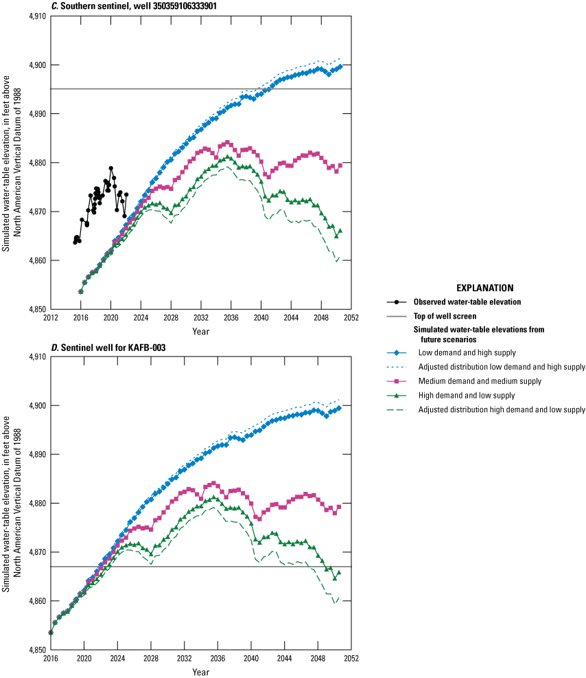
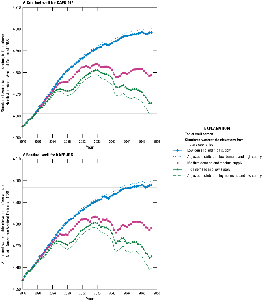
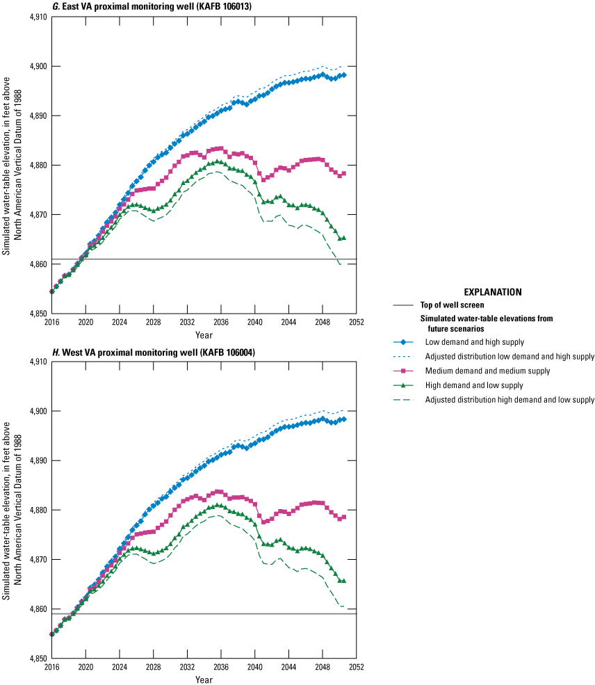
Time series of simulated water-table elevations in model cells that contain wells of interest for the future simulation period (2016–50). Sites are the water-table level screened wells at the following locations A, Cesar Chavez sentinel (USGS site no. 350359106335201), B, Southern sentinel (USGS site no. 350359106333901), C, Trumbull sentinel (USGS site no. 350408106335601), D, KAFB-003 sentinel (KAFB-106201), E, KAFB-015 sentinel (KAFB-106003), F, KAFB-016 sentinel (KAFB-106245), and G–H, the two U.S. Department of Veterans Affairs hospital proximal monitoring wells (KAFB-106013 and KAFB-106004). Observed water-table elevations are included for applicable U.S. Geological Survey sites (U.S. Geological Survey, 2022).
Potential Effects of Simulated Future Pumping
The ABCWUA considers the medium demand projection to be the most expected scenario on the basis of the information available, including recent and historical economic conditions and population growth, although it does not consider the scenario any more likely than the others (ABCWUA, 2016). However, it is possible that unexpected changes to population growth or water usage rates could result in the low or high demand projections. The high supply projection that uses the historical supply does not account for any future effects from climate change, but the streamflow projections derived from the climate projection output indicate that climate change will have some effect on the surface-water supply in the basin. Although the medium demand and medium supply scenario is considered the most expected scenario, using the three main scenarios that combine the different projections of demand and supply is necessary to understand the full range of potential effects on water-table elevations because of the variability involved.
Overall, the water-table elevations in the wells of interest and the model cells that contain the EDB plume continued to rise throughout the future simulation period for the low demand and high supply scenario until beginning to plateau at the end of the period. The water-table elevations rose until leveling off about 2035 with some variation for the medium demand and medium supply scenario, and the water-table elevations rose until about 2035 and then decreased for the high demand and low supply scenario. The pumping scenarios with adjusted spatial distribution of pumping had similar patterns of water-table elevation changes, with the peak water-table elevation change in the adjusted spatial distribution approximately 2 ft higher than that of the low demand and high supply scenario and the peak water-table elevation change in the adjusted distribution approximately 2 ft lower than that of the high demand and low supply scenario. These model results indicate that the spatial distribution of the pumping, even at the most extreme observed distributions in regard to production wells near the area of interest, is not likely to have a substantial effect on the water-table elevations near the EDB plume.
The groundwater elevations observed at the sentinel wells indicate that the water table rose steadily from 2014 to about 2020, similar to other wells in Albuquerque that had an increase in water table elevations starting around 2008 (Jurney and Bell, 2021). However, the groundwater elevation levels in the sentinel wells began to decline starting in 2020 (as shown for the sentinel wells in fig. 6) because more groundwater has been pumped from municipal wells in recent years. The simulated results based on the groundwater pumping projections do not indicate any leveling off or decreases in water-table elevations until 2035. It is possible that either the surface-water supply projections are not as extreme as the actual conditions that occurred in 2020–21, or it could be that the model is not as sensitive as the hydrogeologic system that it is trying to simulate. The simulated results prior to the observed water-table elevation decline also differ from the observed water-table elevations in the USGS sentinel wells, with the observed water-table elevations about 5–15 ft higher than the simulated water-table elevations until the observed values decrease and almost match the simulated values by 2022. This discrepancy should be considered when determining how these future model results are used to inform decisions.
Limitations to the model inputs should be considered in the interpretation of the model results. Although the groundwater pumping at the ABCWUA water supply wells was projected to estimate future supply and demand, the pumping at the KAFB wells was not truly projected, because the model used the same previously recorded pumping rates to populate the future pumping for 2016–50 as used in the publication of the local-scale model (Myers and Friesz, 2019). It is unlikely that the KAFB groundwater pumping will remain static throughout the next several decades. In addition, the ABCWUA groundwater pumping projections do not account for any improvements in water-use efficiency or implementation of water policies that could potentially decrease the gpcd. It is possible that future changes to the gpcd could impact the total water demand. The groundwater pumping projections also do not account for possible alternatives for supply that are discussed in the report (ABCWUA, 2016) including reuse, additional aquifer storage and recovery, stormwater capture, indirect potable reuse, and watershed management. The water supply and sources of the supply could be affected if any of these ideas are implemented in the future.
In addition to the uncertainty associated with the model inputs, there is also uncertainty associated with the model itself. Modeling is, of necessity, a simplification of the hydrogeologic system, and the simulated pumping is a simplification of the actual pumping stresses to the system. These simplifications lead to uncertainty in the model results. A detailed discussion of the local-scale model, the simplifications made, and some potential sources of uncertainty is provided in Myers and Friesz (2019). The uncertainty associated with the future simulated water-table elevations should be considered when using the results to inform decisions, and verification through continued monitoring of water-table elevations will continue to enhance understanding.
Summary
Groundwater levels throughout the Santa Fe Group aquifer system in Albuquerque, New Mexico, have been rising from 2008 up until recent years. Understanding the potential changes to groundwater levels in the future and how changes in groundwater pumping can affect these changes is important to inform well design and placement of well screens in the Kirtland Air Force Base Bulk Fuels Facility monitoring network. Several scenarios of varying water supply and demand were used to develop groundwater pumping projections to determine the potential future changes in water-table elevations in areas around the Kirtland Air Force Base Bulk Fuels Facility and the ethylene dibromide (EDB) plume. The groundwater pumping projections were used as input for the local-scale model of the MODFLOW-LGR2 version of the updated Middle Rio Grande Basin regional model.
The water-table elevations in the model domain rose in all scenarios until approximately 2035. Around that time, the simulated water table elevations in the medium demand and medium supply scenario both increased and decreased, whereas the water-table elevations began to steadily decline for the high demand and low supply scenario. Simulated water-table elevations continued to rise throughout the future simulation period in the low demand and high supply scenario. All of the scenarios ended the future simulation period with higher simulated water-table elevations than at the beginning of the future simulation period. Results indicate that the simulated future water-table elevations averaged from model cells that contain the EDB plume had a maximum increase of approximately 44, 29, and 26 feet over the 2016 water-table elevation at the beginning of the future simulation period in the pumping scenarios based on high supply and low demand, medium supply and medium demand, and low supply and high demand projections, respectively. Model cells at locations of wells of interest had similar maximum increases in water-table elevation during the future simulation period. The scenarios with adjusted spatial distribution that simulated the highest and lowest focus of groundwater pumping near the EDB plume had similar water-table elevations as the associated main scenarios, with water-table elevation changes that only differed by 2 feet from the nonadjusted scenarios.
The model results are subject to uncertainty from many different sources, including uncertainty in the model itself and uncertainty associated with the supply and demand projections used to create the future pumping scenarios. As such, consideration should be taken when using these model results to inform decisions.
References Cited
Albuquerque Bernalillo County Water Utility Authority [ABCWUA], 2016, Water 2120—Securing our water future. Volume 1—main text and appendices: Albuquerque Bernalillo County Water Utility Authority, 309 p., accessed June 15, 2020, at https://www.abcwua.org/wp-content/uploads/Your_Drinking_Water-PDFs/Water_2120_Volume_I.pdf.
Albuquerque Bernalillo County Water Utility Authority [ABCWUA], 2018, Annual information statement: Albuquerque Bernalillo County Water Utility Authority, 157 p., accessed April 4, 2022, at https://www.abcwua.org/wp-content/uploads/Finances_PDF/AIS__Final_3_30_18___W3172082x7A92D_.pdf.
Albuquerque Bernalillo County Water Utility Authority [ABCWUA], 2020, 2019 Water quality report: Albuquerque Bernalillo County Water Utility Authority, 6 p., accessed December 10, 2020, at https://www.abcwua.org/wp-content/uploads/Your_Drinking_Water-PDFs/2019_ABCWUA_Water_Quality_Report-1.pdf.
Albuquerque Bernalillo County Water Utility Authority [ABCWUA], 2022, Annual information statement: Albuquerque Bernalillo County Water Utility Authority, 189 p., accessed April 4, 2022, at https://www.abcwua.org/wp-content/uploads/2022/03/ABCWUA-AIS-2022-03.23.2022-FINAL.pdf.
Bakker, M., Post, V., Langevin, C.D., Hughes, J.D., White, J.T., Starn, J.J., and Fienen, M.N., 2016, Scripting MODFLOW model development using Python and FloPy: Ground Water, v. 54, no. 5, p. 733–739, accessed December 10, 2020, at https://doi.org/10.1111/gwat.12413.
Bartolino, J.R., and Cole, J.C., 2002, Groundwater resources of the Middle Rio Grande Basin, New Mexico: U.S. Geological Survey Circular 1222, 132 p., accessed August 3, 2021, at https://doi.org/10.3133/cir1222.
Bexfield, L.M., and Anderholm, S.K., 2002, Spatial patterns and temporal variability in water quality from City of Albuquerque drinking-water supply wells and piezometer nests, implications for the ground-water flow system: U.S. Geological Survey Water-Resources Investigations Report 01–4224, 101 p., accessed September 15, 2021, at https://doi.org/10.3133/wri014244.
Bexfield, L.M., Heywood, C.E., Kauffman, L.J., Rattray, G.W., and Vogler, E.T., 2011, Hydrogeologic setting and groundwater flow simulation of the Middle Rio Grande Basin regional study area, New Mexico, section 2 of Eberts, S.M., ed., Hydrologic settings and groundwater flow simulations for regional studies of the transport of anthropogenic and natural contaminants to public-supply wells—Studies begun in 2004: U.S. Geological Survey Professional Paper 1737–B, p. 2–1 to 2–61, accessed September 15, 2021, at https://doi.org/10.3133/pp1737B.
Bexfield, L.M., Jurgens, B.C., Crilley, D.M., and Christenson, S.C., 2012, Hydrogeology, water chemistry, and transport processes in the zone of contribution of a public-supply well in Albuquerque, New Mexico, 2007–9: U.S. Geological Survey Water-Resources Investigations Report 2011–5182, 114 p., accessed September 15, 2021, at https://doi.org/10.3133/sir20115182.
Bureau of Reclamation, 2011, West-wide climate risk assessments—Bias-corrected and spatially downscaled surface water projections: Denver, Colorado, U.S. Department of the Interior, Bureau of Reclamation Technical Services Center, Technical Memorandum No. 86–68210–2011–01, 138 p., accessed March 19, 2021, at https://www.usbr.gov/watersmart/docs/west-wide-climate-risk-assessments.pdf.
Bureau of Reclamation, 2022, HydroData—Hydrologic database: Bureau of Reclamation database, accessed August 10, 2022, at https://www.usbr.gov/uc/water/hydrodata/gage_data/site_map.html.
Connell, S.D., 2006, Preliminary geologic map of the Albuquerque-Rio Rancho metropolitan area and vicinity, Bernalillo and Sandoval Counties, New Mexico: New Mexico Bureau of Geology and Mineral Resources Open File Report 496, 2 plates, accessed August 3, 2021, at https://geoinfo.nmt.edu/publications/openfile/details.cfml?Volume=496.
Connell, S.D., 2008, Refinements to the stratigraphic nomenclature of the Santa Fe Group, northwestern Albuquerque Basin, New Mexico: New Mexico Geology, v. 30, no. 1, p. 14–35, 70, accessed August 3, 2021, at https://geoinfo.nmt.edu/publications/periodicals/nmg/30/n1/nmg_v30_n1_p14.pdf.
Connell, S.D., Allen, B.D., and Hawley, J.W., 1998, Subsurface stratigraphy of the Santa Fe Group from borehole geophysical logs, Albuquerque area, New Mexico: New Mexico Geology, v. 20, no. 1, p. 2–7, accessed August 3, 2021, at https://geoinfo.nmt.edu/publications/periodicals/nmg/20/n1/nmg_v20_n1_p2.pdf.
Falk, S.E., Bexfield, L.M., and Anderholm, S.K., 2011, Estimated 2008 groundwater potentiometric surface and predevelopment to 2008 water-level change in the Santa Fe Group aquifer system in the Albuquerque area, central New Mexico: U.S. Geological Survey Scientific Investigations Map 3162, 1 sheet, accessed September 15, 2021, at https://doi.org/10.3133/sim3162.
Flickinger, A.K., 2023, Modified multi-node well (MNW2) files used to simulate potential future (2016-2050) water-table elevation change near Kirtland Air Force Base in Albuquerque, New Mexico: U.S. Geological Survey data release, https://doi.org/10.5066/P9ENV9EN.
Flickinger, A.K., and Mitchell, A.C., 2020, Water-table elevation maps for 2008 and 2016 and water-table elevation changes in the aquifer system underlying eastern Albuquerque, New Mexico: U.S. Geological Survey Open-File Report 2020–1036, 9 p., accessed September 15, 2021 at https://doi.org/10.3133/ofr20201036.
Friesz, P.J., and Myers, N.C., 2019, MODFLOW–LGR2 groundwater-flow model used to delineate transient areas contributing recharge and zones of contribution to selected wells in the upper Santa Fe Group aquifer, southeastern Albuquerque, New Mexico: U.S. Geological Survey data release, accessed February 11, 2021, at https://doi.org/10.5066/F79P303S.
Galanter, A.E., and Curry, L.T.S., 2019, Estimated 2016 groundwater level and drawdown from predevelopment to 2016 in the Santa Fe Group aquifer system in the Albuquerque area, central New Mexico: U.S. Geological Survey Scientific Investigations Map 3433, 1 sheet, 13-p. pamphlet, accessed September 15, 2021, at https://doi.org/10.3133/sim3433.
Halford, K.J., and Hanson, R.T., 2002, User guide for the drawdown-limited, Multi-Node Well (MNW) package for the U.S. Geological Survey’s modular three-dimensional finite-difference ground-water flow model, versions MODFLOW–96 and MODFLOW–2000: U.S. Geological Survey Open-File Report 02–293, 33 p., accessed March 19, 2021, at https://doi.org/10.3133/ofr02293.
Harbaugh, A.W., 2005, MODFLOW–2005, the U.S. Geological Survey modular ground-water model—The ground-water flow process: U.S. Geological Survey Techniques and Methods, book 6, chap. A16, [variously paged], accessed March 19, 2021, at https://doi.org/10.3133/tm6A16.
Hawley, J.W., and Haase, C.S., 1992, Hydrogeologic framework of the northern Albuquerque Basin: Socorro, New Mexico, New Mexico Bureau of Mines and Mineral Resources Open-File Report 387, [variously paged], accessed August 3, 2021, at https://geoinfo.nmt.edu/publications/openfile/details.cfml?Volume=387.
Hawley, J.W., Haase, C.S., and Lozinsky, R.P., 1995, An underground view of the Albuquerque Basin, in Ortega Klett, C.T., ed., The water future of Albuquerque and the Middle Rio Grande Basin—Annual New Mexico Water Conference, 39th, Albuquerque, New Mexico, November 3–4, 1994, [Proceedings]: Las Cruces, New Mexico, New Mexico Water Resources Research Institute WRRI Report No. 290, p. 37–55.
Jurney, E.R., and Bell, M.T., 2021, Water-level data for the Albuquerque Basin and adjacent areas, central New Mexico, period of record through September 30, 2020: U.S. Geological Survey Data Series 1139, 40 p., accessed April 14, 2022, at https://doi.org/10.3133/ds1139.
Kirtland Air Force Base [KAFB], 2022, Periodic monitoring report—July–September 2021 for the Bulk Fuels Facility, solid waste management units ST–106/SS–111, Kirtland Air Force Base, New Mexico: Kirtland Air Force Base, USACE-Albuquerque District Contract No. W912PP20C0020, prepared by EA Engineering, Science, and Technology, Inc., PBC, Albuquerque, New Mexico, 232 p., accessed August 3, 2021, at https://cloud.env.nm.gov/waste/resources/_translator.php/NoP4Wd1EyorPC~sl~BWz~sl~H2+PXdCQEKefUZ80ilOeP6j2AO9W56nqHMNoYa5qQ6X4yyuPi+2PCkTygIMYH16+gNs1q EVx1ZU9STfIWlz4WPOfdZ1bUBMjybsq~sl~X+W+H6bcG.pdf.
Konikow, L.F., Hornberger, G.Z., Halford, K.J., and Hanson, R.T., 2009, Revised Multi-Node Well (MNW2) package for MODFLOW ground-water flow model: U.S. Geological Survey Techniques and Methods, book 6, chap. A30, 67 p., accessed March 19, 2021, at https://doi.org/10.3133/tm6A30.
Liang, X., Lettenmaier, D.P., Wood, E.F., and Burges, S.J., 1994, A simple hydrologically based model of land surface water and energy fluxes for general circulation models: Journal of Geophysical Research, v. 99, D7, p. 14415–14428, accessed March 19, 2021, at https://agupubs.onlinelibrary.wiley.com/doi/10.1029/94JD00483.
Liang, X., Wood, E.F., and Lettenmaier, D.P., 1996, Surface soil moisture parameterization of the VIC-2L model—Evaluation and modifications: Global and Planetary Change, v. 13, no. 1–4, p. 195–206, accessed March 19, 2021, at https://doi.org/10.1016/0921-8181(95)00046-1.
Maurer, E.P., Brekke, L., Pruitt, T., and Duffy, P.B., 2007, Fine-resolution climate projections enhance regional climate change impact studies: Eos (Washington, D.C.), v. 88, no. 47, p. 504, accessed March 19, 2021, at https://doi.org/10.1029/2007EO470006.
McAda, D.P., and Barroll, P., 2002, Simulation of groundwater flow in the Middle Rio Grande Basin between Cochiti and San Acacia, New Mexico: U.S. Geological Survey Water-Resources Investigations Report 02–4200, 81 p., accessed August 3, 2021, at https://doi.org/10.3133/wri20024200.
Mehl, S.W., and Hill, M.C., 2013, MODFLOW–LGR—Documentation of ghost node local grid refinement (LGR2) for multiple areas and the boundary flow and head (BFH2) package: U.S. Geological Survey Techniques and Methods, book 6, chap. A44, 43 p., accessed March 19, 2021, at https://doi.org/10.3133/tm6A44.
Myers, N.C., and Friesz, P.J., 2019, Hydrogeologic framework and delineation of transient areas contributing recharge and zones of contribution to selected wells in the upper Santa Fe Group aquifer, southeastern Albuquerque, New Mexico, 1900–2050: U.S. Geological Survey Scientific Investigations Report 2019–5052, 73 p., accessed February 11, 2021, at https://doi.org/10.3133/sir20195052.
Nijssen, B., Lettenmaier, D.P., Liang, X., Wetzel, S.W., and Wood, E.F., 1997, Streamflow simulation for continental-scale river basins: Shui Zi Yuan Yan Jiu, v. 33, p. 711–724, accessed March 19, 2021, at https://doi.org/10.1029/96WR03517.
Plummer, N.L., Bexfield, L.M., Anderholm, S.K., Sanford, W.E., and Busenberg, E., 2004, Geochemical characterization of ground-water flow in the Santa Fe Group aquifer system, Middle Rio Grande Basin, New Mexico: U.S. Geological Survey Water-Resources Investigations Report 03–4131, 395 p., accessed August 3, 2021, at https://doi.org/10.3133/wri034131.
Powell, R.I., and McKean, S.E., 2014, Estimated 2012 groundwater potentiometric surface and drawdown from predevelopment to 2012 in the Santa Fe Group aquifer system in the Albuquerque metropolitan area, central New Mexico: U.S. Geological Survey Scientific Investigations Map 3301, 1 sheet, accessed September 15, 2021, at https://doi.org/10.3133/sim3301.
Rankin, D.R., Oelsner, G.P., McCoy, K.J., Moret, G.J.M., Worthington, J.A., and Bandy-Baldwin, K.M., 2016, Groundwater hydrology and estimation of horizontal groundwater flux from the Rio Grande at selected locations in Albuquerque, New Mexico, 2009–10: U.S. Geological Survey Scientific Investigations Report 2016–5021, 89 p., accessed August 3, 2021, at https://doi.org/10.3133/sir20165021.
Rice, S., Oelsner, G., and Heywood, C., 2014, Simulated and measured water levels and estimated water-level changes in the Albuquerque area, central New Mexico, 1950–2012: U.S. Geological Survey Scientific Investigations Map 3305, 1 sheet, accessed September 15, 2021, at https://doi.org/10.3133/sim3305.
Roach, J., and Tidwell, V., 2010, Upper Rio Grande Simulation Model (URGSIM): U.S. Department of Energy, Office of Scientific and Technical Information software release, accessed August 3, 2021, at https://doi.org/10.11578/dc.20220414.70.
U.S. Army Corps of Engineers, 2017, RCRA facility investigation report, Bulk Fuels Facility release, solid waste management unit ST–106/SS–111, Kirtland Air Force Base, Albuquerque, New Mexico: U.S. Army Corps of Engineers, prepared by Sundance Consulting, Inc., January 2017, Albuquerque, New Mexico, [variously paged], accessed August 3, 2021, at https://hwbdocuments.env.nm.gov/Kirtland%20AFB/KAFB4479/KAFB4479.pdf.
U.S. Geological Survey, 2022, USGS water data for the Nation: U.S. Geological Survey National Water Information System database, accessed March 3, 2022, at http://dx.doi.org/10.5066/F7P55KJN.
Wood, A.W., Maurer, E.P., Kumar, A., and Lettenmaier, D.P., 2002, Long-range experimental hydrologic forecasting for the Eastern United States: Journal of Geophysical Research, v. 107, no. D20, article 4429, p. AAC1–1 to SOL8–10, accessed March 19, 2021, at https://doi.org/10.1029/2001JD000659.
Conversion Factors
U.S. customary units to International System of Units
International System of Units to U.S. customary units
Datums
Vertical coordinate information is referenced to the North American Vertical Datum of 1988 (NAVD 88).
Horizontal coordinate information is referenced to the North American Datum of 1983 (NAD 83).
Elevation, as used in this report, refers to distance above the vertical datum.
Abbreviations
ABCWUA
Albuquerque Bernalillo County Water Utility Authority
BFF
Bulk Fuels Facility
CMIP3
Coupled Model Intercomparison Project Phase 3
EDB
ethylene dibromide (also known as 1,2-dibromoethane)
KAFB
Kirtland Air Force Base
LGR2
localized grid refinement, version 2
MODFLOW
modular three-dimensional finite-difference groundwater flow model
MNW1
Multi-Node Well package, version 1
MNW2
Multi-Node Well package, version 2
SJC
San Juan-Chama
URGSIM
Upper Rio Grande Simulation Model
USGS
U.S. Geological Survey
VIC
Variable Infiltration Capacity
For more information about this publication, contact
Director, New Mexico Water Science Center
U.S. Geological Survey
6700 Edith Blvd. NE
Albuquerque, NM 87113
For additional information, visit
https://www.usgs.gov/centers/nm-water
Publishing support provided by
Lafayette Publishing Service Center
Disclaimers
Any use of trade, firm, or product names is for descriptive purposes only and does not imply endorsement by the U.S. Government.
Although this information product, for the most part, is in the public domain, it also may contain copyrighted materials as noted in the text. Permission to reproduce copyrighted items must be secured from the copyright owner.
Suggested Citation
Flickinger, A.K., 2023, Potential effects of projected pumping scenarios on future water-table elevations near Kirtland Air Force Base in Albuquerque, New Mexico: U.S. Geological Survey Scientific Investigations Report 2023–5075, 19 p., https://doi.org/10.3133/sir20235075.
ISSN: 2328-0328 (online)
Study Area
| Publication type | Report |
|---|---|
| Publication Subtype | USGS Numbered Series |
| Title | Potential effects of projected pumping scenarios on future water-table elevations near Kirtland Air Force Base in Albuquerque, New Mexico |
| Series title | Scientific Investigations Report |
| Series number | 2023-5075 |
| DOI | 10.3133/sir20235075 |
| Publication Date | July 10, 2023 |
| Year Published | 2023 |
| Language | English |
| Publisher | U.S. Geological Survey |
| Publisher location | Reston, VA |
| Contributing office(s) | New Mexico Water Science Center |
| Description | Report: viii, 20 p.; Data Release |
| Country | United States |
| State | New Mexico |
| Other Geospatial | Kirtland Air Force Base |
| Online Only (Y/N) | Y |