

Updated Estimates of Water Budget Components for the Mississippi Embayment Region Using a Soil-Water-Balance Model, 2000–2020
Links
- Document: Report (14.0 MB pdf) , HTML , XML
- Related Works:
- SIR 2023–5100 —Simulating groundwater flow in the Mississippi Alluvial Plain with a focus on the Mississippi Delta
- SIR 2023–5051 — Automated construction of Streamflow-Routing networks for MODFLOW—Application in the Mississippi Embayment region
- Dataset: USGS National Water Information System database —USGS water data for the Nation
- Data Release: USGS data release - Model archive and output files for net infiltration, runoff, and irrigation water use for the Mississippi Embayment Regional Aquifer System, 2000 to 2020, simulated with the Soil-Water-Balance model
- NGMDB Index Page: National Geologic Map Database Index Page (html)
- Download citation as: RIS | Dublin Core
Abstract
A Soil-Water-Balance (SWB) model for the Mississippi embayment region in Arkansas, Tennessee, Mississippi, and Louisiana was constructed and calibrated to gain insight into potential recharge patterns for the Mississippi River Valley alluvial aquifer, which has had substantial drawdown under intense pumping stress over the last several decades. An analysis of the net infiltration term from the SWB model combined with newly gathered airborne electromagnetic geophysical data on the surficial sediments in a calibrated modular three-dimensional finite-difference (MODFLOW 6) groundwater flow model of one area in the alluvial plain found that the distribution of net infiltration was significantly different from the recharge that gets to the water table through the complicated silt and clay stratigraphy of the unsaturated zone. The net infiltration of water through the rooting zone as simulated by SWB ranges from 5.7 to 12.3 inches per year in the alluvial plain part of the model domain, and is fairly evenly distributed within local areas. Recharge to the underlying aquifer is less and is much more focused in particular zones where the connectivity through the upper layers of the unsaturated zone above the water table is greater, indicating possible horizontal flow and perched water table conditions in the unsaturated zone. Runoff and net infiltration together account for 32 percent of the incoming precipitation overall and somewhat higher percentages in the alluvial plain area on an annual basis. These terms are much higher in the fall and winter than in the summer. Actual evapotranspiration accounts for between 62 and 72 percent on average of the annual precipitation but dominates all other terms in the summer months. Without irrigation, summertime net infiltration and runoff would be near zero in the crop-dominated alluvial plain area. The SWB model reproduced reported irrigation rates for corn, soybeans, rice, and cotton on an annual basis fairly well. The SWB model for the Mississippi embayment region was calibrated using more than 15,000 observations representing four parts of the calculated water budget: actual evapotranspiration, surface runoff, net infiltration, and irrigation. Using a Monte Carlo approach to determine the uncertainty in the model results stemming from the uncertainty in the model parameters used in the calibration, the uncertainty in the annual actual evapotranspiration values was around 5 percent, whereas the uncertainty in the irrigation, net infiltration, and runoff was around 20 percent.
Introduction
The Mississippi River Valley alluvial aquifer (U.S. Geological Survey [USGS], 2015), which lies underneath the Mississippi Alluvial Plain within the larger Mississippi embayment region (fig. 1), is one of the most heavily pumped aquifers in the United States (Lovelace and others, 2020). Pumping from this aquifer and underlying aquifers supplies water for the irrigation of crops, aquaculture, drinking water for urban areas, industrial supply, and other uses (Clark and others, 2011; Lovelace and others, 2020). The heavy use of this aquifer has caused substantial groundwater level declines in the alluvial plain of Arkansas and Mississippi, which has motivated a large number of hydrologic studies by the USGS aimed at understanding groundwater movement in the system of aquifers in the area and the potential effect of increasing or reducing pumping on groundwater supply and availability (Boswell and others, 1968; Cushing and others, 1970; Broom and Reed, 1973; Brahana and Mesko, 1988; Ackerman, 1989, 1996; Mahon and Ludwig, 1990; Sumner and Wasson, 1990; Arthur and Taylor, 1998; Arthur, 2001; Brahana and Broshears, 2001; Mahon and Poynter, 1993; McKee and Clark, 2003; Reed, 2003; Stanton and Clark, 2003; Kresse and Clark, 2008; Clark and Hart, 2009; Clark and others, 2011, 2013).
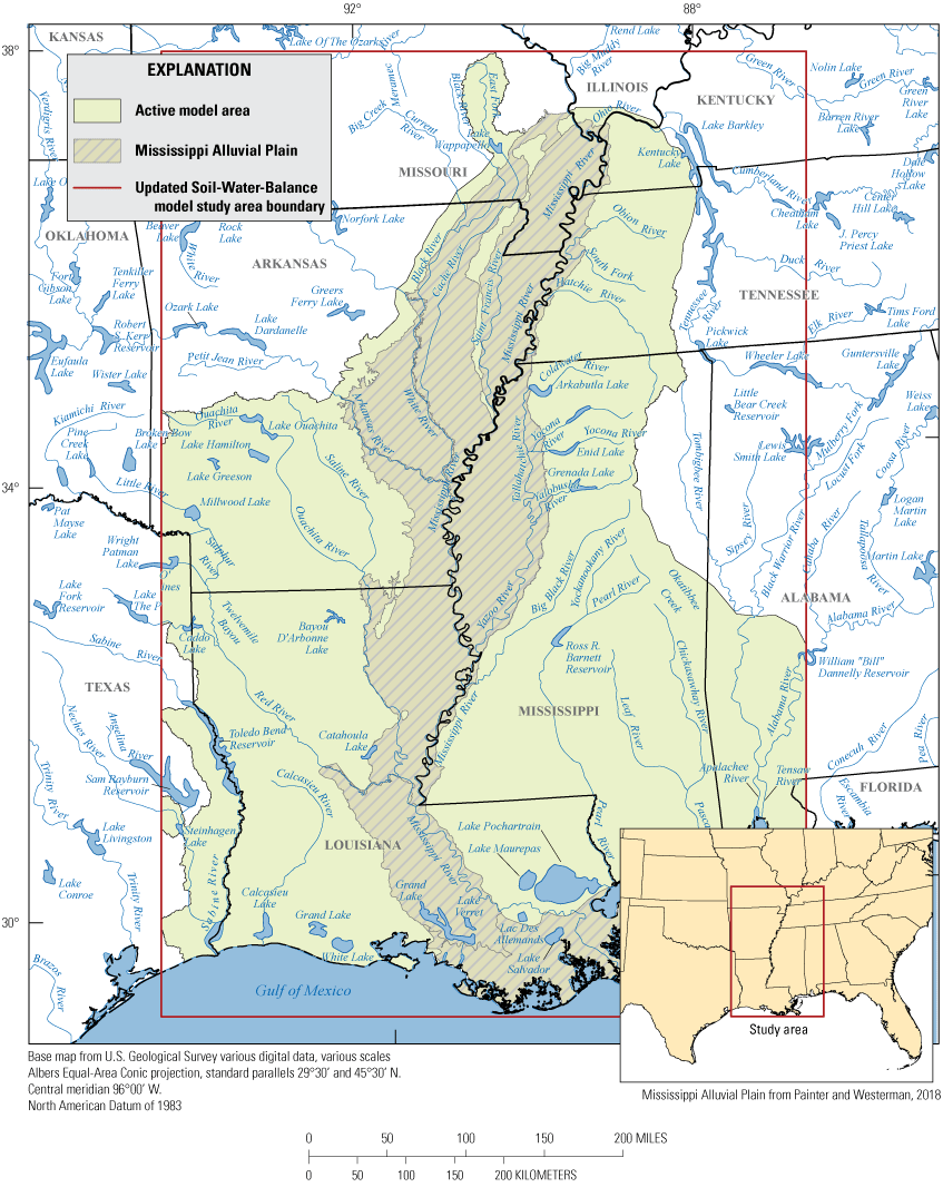
Updated Soil-Water-Balance model area and the Mississippi Alluvial Plain in the Mississippi embayment region.
The USGS’s Mississippi Alluvial Plain Regional Water-Availability Study (see Rigby and Kress, 2019) was envisioned to be a 5-year project from 2017 to 2021 that would bring fresh scientific approaches and would build on previous groundwater and water availability studies. The Mississippi Alluvial Plain project had two overall objectives: (1) to assess current and long-term water availability, and (2) to provide resource managers with a decision-support framework. One element of understanding water availability in the Mississippi embayment region and the smaller Mississippi Alluvial Plain was to determine an accurate water budget for the hydrologic system.
The USGS Soil-Water-Balance (SWB) model, version 2.0 (Westenbroek and others, 2010, 2018), simulated the various components of the water budget in the Mississippi embayment region (fig. 1). The SWB method uses daily inputs of temperature and precipitation, along with data on land use and soil information, to calculate daily estimates of the water budget components. The SWB model application for the study area was calibrated to surface-water flows at USGS streamgages, crop irrigation pumping rates from the surficial aquifer, satellite-derived estimates of evapotranspiration (ET) of water from the land surface, and net infiltration from base-flow separation analysis at USGS streamgages in the study area. For the purposes of the calibration, the net infiltration term is treated as potential recharge to compare to measurements of base flow in rivers and streams. The calibration method is similar to the methods described in Nielsen and Westenbroek (2019) and Westenbroek and others (2021) but adds crop irrigation data as a source of observation data.
Uncertainty in each of the components of the water budget were estimated using Monte-Carlo methods, in which model parameters are assumed to be normally distributed around the calibrated value, resulting in an output probability distribution for each water budget component. The primary application of these water budget estimates is to provide projections of net infiltration to new groundwater flow models (for example, Leaf and others, 2023); the combined models will support informed water use and agricultural policy in the region.
A preliminary version of the SWB model for the Mississippi embayment region and Mississippi Alluvial Plain (Westenbroek and others, 2021; fig. 2) covered a smaller geographic footprint, used older versions of input data, was not calibrated to as many independent variables, did not estimate uncertainty, and only modeled conditions through 2018.
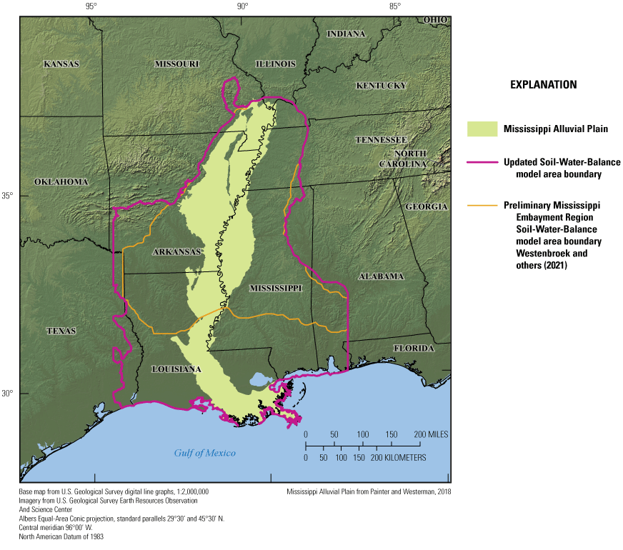
A comparison of preliminary and updated Soil-Water-Balance model areas for the Mississippi embayment region.
Note that the SWB modeled net infiltration values reported in this report are substantially different from groundwater recharge. The term “net infiltration” refers to water that infiltrates into the soil surface and escapes from the bottom of the root zone. “Groundwater recharge” refers to water that travels from the root zone, through the unsaturated zone, and then becomes groundwater when it meets the surface of the water table. These two quantities may differ greatly across the parts of the Mississippi Alluvial Plain study area where one or more clay layers are present between the bottom of the root zone and the top of the water table. These layers can trap water (become a “perched water table”) or cause water to move laterally for some distance before joining the water table. In addition, saturated soils caused by backwater flooding also cause substantial differences between the simulated and actual water budget components. The “Discussion” section of this report covers the implications of these differences.
The Mississippi Alluvial Plain area is divided into several generalized regions (fig. 3; Ladd and Travers, 2019). Four of the regions (St. Francis, Cache, Grand Prairie, and Boeuf) are primarily or partly in Arkansas; three are wholly or partly in Louisiana (Boeuf, Deltaic and Chenier Plains, and Atchafalaya), and three are wholly or partly in Mississippi (Boeuf, Delta, and Grand Prairie). The St. Francis Region also covers small parts of Tennessee, Kentucky, Illinois, and Missouri.
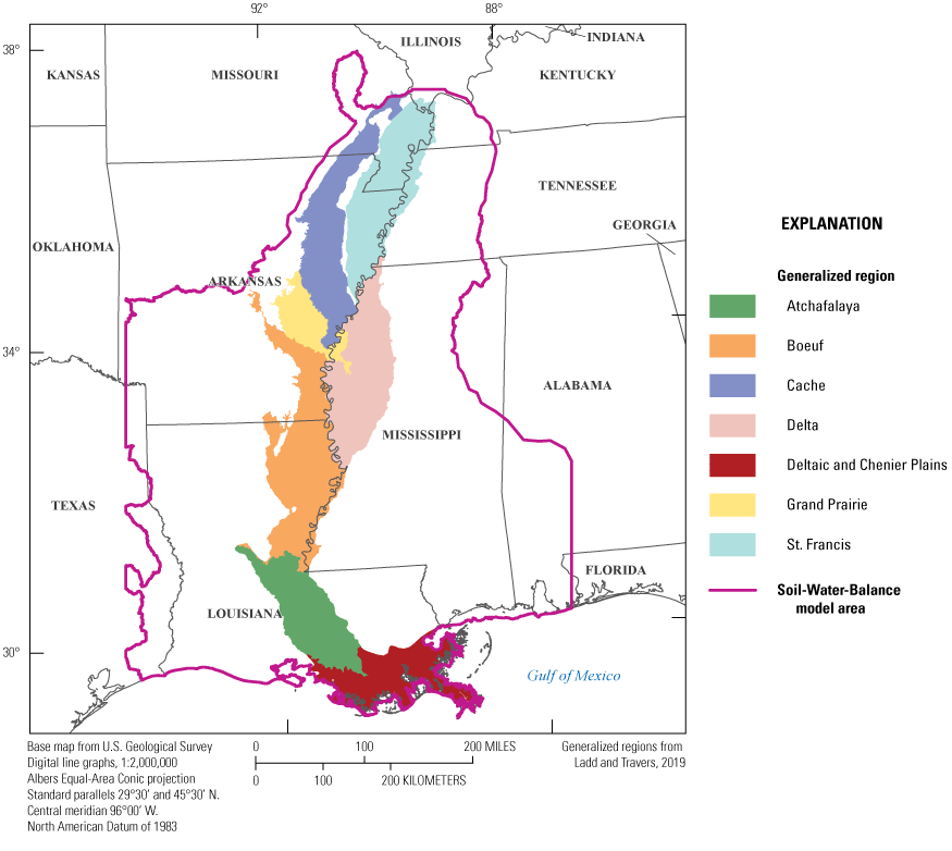
Generalized regions of the Mississippi Alluvial Plain.
The quaternary-age Mississippi River Valley alluvial plain aquifer is the shallowest of several overlapping aquifers in the region (Boswell and others, 1968; Cushing and others, 1970; Ackerman, 1996; Arthur and Taylor, 1998; Clark and others, 2011). An unconformity below the alluvial plain aquifer separates this unit from several Cretaceous- and Tertiary-age productive aquifers that are confined below the Mississippi Alluvial Plain but outcrop and are recharged in the uplands surrounding the alluvial plain (Cushing and others, 1970).
Previous Investigations
Many previous studies of the groundwater system included recharge as a part of the analysis, but few of them attempted to specifically quantify recharge in the study area, except as a calibration parameter for various groundwater flow model studies. Few studies investigated recharge rates in the uplands of the Mississippi embayment region outside of the Mississippi Alluvial Plain area.
Previous groundwater studies in the Mississippi Alluvial Plain area, primarily those using groundwater flow models to study the groundwater system, have suggested groundwater recharge rates for the alluvial plain that range from less than 1 inch per year to no greater than 5 inches per year (see, for example, Ackerman, 1989, 1996; Sumner and Wasson, 1990; Mahon and Poynter, 1993; Stanton and Clark, 2003; Clark and others, 2013; Killian and others, 2019; Gratzer and others, 2020; Wacaster, 2020). Pumping in the alluvial aquifer has drawn down the water table extensively, resulting in an induced increase in recharge over predevelopment rates (Ackerman, 1989, 1996). Wacaster (2020) compared recharge estimates from a chloride mass balance approach, a previous groundwater model (Mississippi Embayment Regional Aquifer Study; Clark and others, 2013), an empirical water budget approach (Reitz and Kress, 2019), and earlier versions of SWB model output (Westenbroek and others, 2021); these methods yielded median recharge values of 1.0, 1.4, 4.1, and 5.6 inches per year, respectively.
Purpose and Scope
The purpose of this report is to document the development and application of an SWB model used to simulate water budget components across the Mississippi embayment region from 2000 to 2020. This report includes sections discussing the following:
-
• Construction and calibration of a SWB model of the Mississippi embayment region
-
• Performance of the model calibration and comparison to observed values
-
• Seasonal and spatial variability of the estimates of irrigation, actual ET, net infiltration, and runoff
-
• Effect of irrigation on the growing season water budget
-
• Uncertainty in the estimates caused by uncertainty in model parameters, and
-
• A comparison of the net infiltration estimates and model-calibrated recharge in one subarea of the model.
Methods—Soil-Water-Balance Model Construction and Calibration
The SWB software package (Westenbroek and others, 2018) simulates net infiltration, actual ET, runoff, and other water budget components, driven by daily weather data and modified by soil and vegetation parameters and land use categories. Irrigation inputs to the land surface are computed by the model (based on the Food and Agriculture Organization of the United Nations Irrigation and Drainage Paper 56 [FAO56] method of determining crop water demand from Allen and others, 1998) and are combined with precipitation as water available for infiltration. Gross precipitation is reduced through interception of rain and snow by plant canopies. Water that is not captured by plant canopies is called net precipitation, and may either infiltrate into the soil or become runoff. Runoff of water is calculated by means of the Soil Conservation Service Curve Number method (Cronshey and others, 1986). Infiltrated water is added to the root zone, whereas water required for plant growth is taken away by the ET term. Water exceeding the soil’s moisture storage capacity is routed beneath the rooting zone as net infiltration dependent on the soil’s maximum recharge rate; any excess is routed to “rejected recharge” which is added to the runoff term. Evaporation of interception is included in the actual ET term and is not further discussed in this report.
Input Data
The SWB model for the Mississippi embayment region covers 252,400 square miles (653,700 square kilometers) and is gridded using a cell size of 1,000 meters (m; 989 rows by 661 columns; fig. 4). Gridded model input data includes daily precipitation, daily minimum and maximum temperature, hydrologic soil group, available water capacity of the soil, and land use. Each of these datasets are described below.
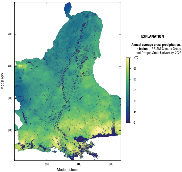
Annual average gross precipitation from PRISM datasets for the Mississippi embayment region Soil-Water-Balance model, 2000–20.
The climate inputs required for SWB were obtained from PRISM daily datasets (PRISM Climate Group and Oregon State University, 2022). Daily PRISM American Standard Code for Information Interchange (known as “ASCII”) grid files at a 4-kilometer cell size were reprocessed to 1,000 m for the model period and combined into a network Common Data Form (known as “netCDF”) format file for use in the SWB model. The annual average precipitation for the study area, which ranges from less than 50 to greater than 70 inches per year, is illustrated in figure 4.
The hydrologic soil groups (HSGs) and the available water capacity input grids are derived from the U.S. Department of Agriculture (USDA) Natural Resources Conservation Service gridded national soil survey geographic database (“gNATSGO”, Soil Survey Staff, 2019). The gNATSGO data for the top 150 centimeters were used in this study because many of the crops and land uses have rooting zones that extend that deep and beyond. The HSGs (USDA, 2007) used in the study include the four basic HSGs (A, B, C, and D) and the dual HSGs (A/D, B/D, and C/D; table 1; fig. 5). The available water capacity data for the top 150 centimeters are expressed in units of inches per foot of soil thickness. The HSG and available water capacity data are gridded representations of mapped soil unit polygons, and the values assigned by lookup tables relate the soil unit properties to the soil unit polygon distribution. The native dataset is rasterized at a 10-m resolution, which was resampled to 1,000 m for this study.
Table 1.
Hydrologic soil groups used in the Mississippi embayment region Soil-Water-Balance model.[Hydrologic soil group information is summarized from U.S. Department of Agriculture (2007). in/hr, inch per hour]
| Hydrologic soil group (fig. 5) | Description | Percentage of model area |
| A | Low runoff potential and high infiltration rates even when thoroughly wetted (infiltration rates greater than 0.30 in/hr). | 4.1 |
| B | Low to moderate runoff potential and moderate infiltration rates when thoroughly wetted (infiltration rates ranging from 0.15 to 0.30 in/hr). | 18.9 |
| C | Moderate to high runoff potential and low infiltration rates when thoroughly wetted (infiltration rates ranging from 0.05 to 0.15 in/hr). | 20.2 |
| D | High runoff potential; very low rate of water transmission (infiltration rates ranging from 0 to 0.05 in/hr). | 31.5 |
| A/D | Dual hydrologic soil group. “A” if the soil is drained; “D” if the soil is undrained. | 1.7 |
| B/D | Dual hydrologic soil group. “B” if the soil is drained; “D” if the soil is undrained. | 5.3 |
| C/D | Dual hydrologic soil group. “B” if the soil is drained; “D” if the soil is undrained. | 18.3 |
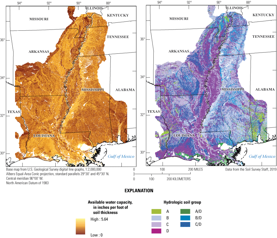
Available water capacity and hydrologic soil groups for the Mississippi embayment region Soil-Water-Balance model.
Land use data change annually and were sourced from the USDA National Agricultural Statistics Service Cropland Data Layer (CDL) (USDA National Agricultural Statistics Service, 2020) for 2008–20; these data were resampled for this study from the native 30-m cell size to 1,000 m by applying a majority filter. The CDL data contain classes for 127 possible land-use categories; in the study area, 45 crop types and 17 other land uses are represented (62 land use categories in total). Overall, 19 percent of the land is in cropland, 17 percent in other agricultural uses (pasture, fallow, etc.), 8 percent in wetlands (wetlands, open water, and aquaculture), 4 percent in urban areas, and 52 percent in forested land uses (including forested wetlands; fig. 6). The Mississippi Alluvial Plain is heavily dominated by cropland with abundant wetland forest areas around major rivers, and the upland is primarily forest with scattered cropland and urban areas (fig. 6). The CDL data do not cover the period from 2000 to 2007. To simulate a dynamic crop landscape for those years, the CDL data for 2010–17 were applied to 2000–7.
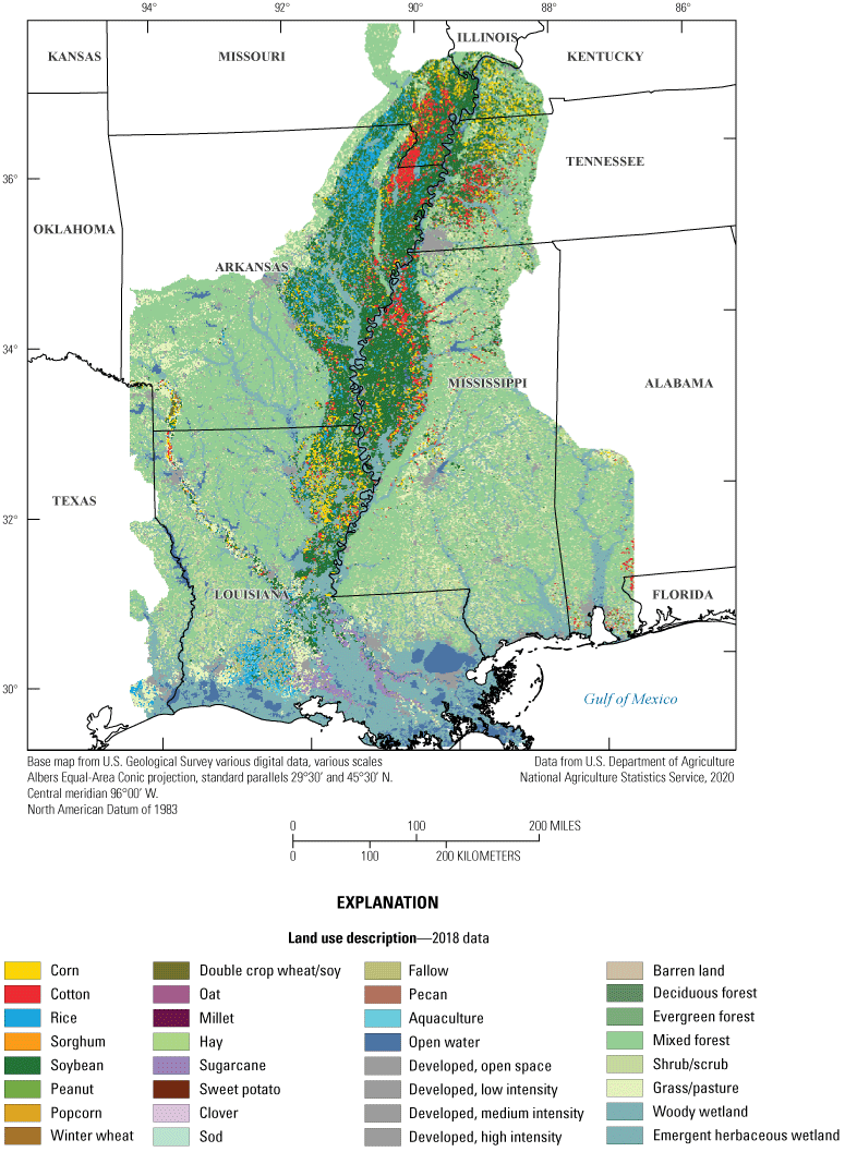
Land use distribution for the Mississippi embayment region Soil-Water-Balance model area, 2018.
To simulate irrigation application, the SWB model requires a mask of irrigated lands. For this study, an annual mask of irrigated lands was created using the LANID dataset (Xie and Lark, 2021), a Landsat-based irrigation classification (irrigated versus not irrigated) for the conterminous United States. The native 30-m grid was resampled to the SWB model’s 1,000-m grid by determining the percentage of 30-m LANID cells in each 1,000-m SWB cell that were irrigated. After a trial-and-error analysis, the irrigation status in the 1,000-m SWB cells was set to “irrigated” if greater than 40 percent of the 30-m LANID cells were irrigated to capture most irrigation in the study area. The LANID dataset covers 1997 through 2017. To simulate irrigation in the SWB model from 2018 to 2020, the 2017 irrigation mask was applied to the years after 2017.
Tabular Model Inputs
The SWB model for the Mississippi embayment region uses two lookup tables to calculate the water balance terms: a land-use lookup table and an irrigation lookup table, which was used for supporting ET calculations using the FAO56 ET method (Allen and others, 1998; Westenbroek and others, 2018). The FAO56 ET method gives much greater control over the ET simulation compared to the Thornthwaite-Mather method (Thornthwaite and Mather, 1957). The land-use lookup table contains values for runoff curve numbers, maximum daily recharge, and rooting depths for each combination of land use class and HSG in the model (an example is shown in table 2; the full table is included in the model archive for this study, Westenbroek and Nielsen, 2023). With 127 possible land-use classes and 7 HSGs, the Mississippi embayment region SWB model potentially has 889 different values for each of these categories (although many combinations of land use and HSG do not occur in the study area). Lookup values for interception change with land use and growing season and are also included in the SWB land-use lookup table. The irrigation land-use table (an example is shown in table 3; the full table is included in Westenbroek and Neilsen, 2023) includes plant growth settings such as crop coefficients (Kcb values for onset of growth, plant maturity, and senescence), growing-season lengths, bare soil evaporation settings for every land-use class, and irrigation application settings for irrigated crops.
Table 2.
Example land-use lookup table for runoff curve numbers, maximum recharge rate, interception, and rooting zone depths used by the Soil-Water-Balance model.[See descriptions of hydrologic soil groups (A, B, B/D, and C/D) in table 1 and U.S. Department of Agriculture (2007). in/d, inch per day; ft, foot]
In the lookup table used in the Mississippi Embayment Region simulations, this table has entries for all seven hydrologic soil groups, whereas groups C, D, and A/D are not included in this example table. See the model archive at https://doi.org/10.5066/P97KK17G for the full table (Westenbroek and Nielsen, 2023).
In the lookup table used in the Mississippi Embayment Region simulations, this table has entries for 127 land-use classes, whereas this example table omits classes 6–110. See the model archive at https://doi.org/10.5066/P97KK17G for the full table (Westenbroek and Nielsen, 2023).
Table 3.
Example irrigation lookup table for plant growth settings, bare soil evapotranspiration, and irrigation settings used by the Soil-Water-Balance model.—Left[See descriptions of hydrologic soil groups (A, B, B/D, and C/D) in table 1 and U.S. Department of Agriculture (2007). Dates are given in month/day. Kcb, transpiration crop coefficient; mid, middle; min, minimum; dev, deviation]
In the lookup table used in the Mississippi Embayment Region simulations, this table has entries for all seven hydrologic soil groups, whereas groups C, D, and A/D are not included in this example table. See the model archive at https://doi.org/10.5066/P97KK17G for the full table (Westenbroek and Nielsen, 2023).
In the lookup table used in the Mississippi Embayment Region simulations, this table has entries for 127 land-use classes, whereas this example table omits classes 6–110. See the model archive at https://doi.org/10.5066/P97KK17G for the full table (Westenbroek and Nielsen, 2023).
The CDL and HSG datasets were cross tabulated to determine how many model cells were covered by each unique combination of land use class and HSG. The model variables that pertain to the most abundant combinations of land use/crop type and HSG will have the most effect on the overall outcome of the model runs. The top (most abundant) 35 combinations of land use/crop type (2015 data) and HSG in the model area and in the Mississippi Alluvial Plain part of the model area are listed in table 4. Forests in HSGs B, C, D, and C/D (including forested wetlands) and soybeans in group D are the most abundant in the whole model area (table 4); soybeans in HSGs D, C, and C/D, forested wetlands in soil groups D and C/D, and rice on group D were the most abundant in the alluvial plain part of the model (table 4).
Table 4.
Most-abundant combinations of land use/crop types and hydrologic soil groups in 2015 in the Soil-Water Balance model area and the Mississippi Alluvial Plain.| Rank | Land use/crop type1 (fig. 6) | Hydrologic soil group2 (fig. 5) | Number of model cells | Percentage of total |
|---|---|---|---|---|
| 1 | Woody wetland | D | 26,061 | 6.6 |
| 2 | Evergreen forest | C | 23,563 | 6.0 |
| 3 | Soybeans | D | 22,789 | 5.8 |
| 4 | Evergreen forest | C/D | 19,354 | 4.9 |
| 5 | Evergreen forest | D | 18,959 | 4.8 |
| 6 | Evergreen forest | B | 18,660 | 4.7 |
| 7 | Deciduous forest | B | 18,204 | 4.6 |
| 8 | Woody wetlands | C/D | 14,586 | 3.7 |
| 9 | Deciduous forest | C | 11,941 | 3.0 |
| 10 | Woody wetland | C | 10,121 | 2.6 |
| 11 | Grassland/pasture | D | 9,714 | 2.5 |
| 12 | Grassland/pasture | C | 7,885 | 2.0 |
| 13 | Shrubland | B | 7,791 | 2.0 |
| 14 | Grassland/pasture | B | 7,489 | 1.9 |
| 15 | Deciduous forest | D | 6,693 | 1.7 |
| 16 | Shrubland | C | 6,537 | 1.7 |
| 17 | Soybean | C/D | 6,492 | 1.6 |
| 18 | Woody wetland | B | 6,417 | 1.6 |
| 19 | Grassland/pasture | C/D | 6,274 | 1.6 |
| 20 | Herbaceous wetland | D | 5,867 | 1.5 |
| 21 | Rice | D | 5,661 | 1.4 |
| 22 | Shrubland | C/D | 5,599 | 1.4 |
| 23 | Soybean | C | 5,391 | 1.4 |
| 24 | Evergreen forest | A | 5,322 | 1.4 |
| 25 | Deciduous forest | C/D | 5,072 | 1.3 |
| 26 | Shrubland | D | 4,833 | 1.2 |
| 27 | Woody wetlands | B/D | 4,732 | 1.2 |
| 28 | Soybean | B | 4,210 | 1.1 |
| 29 | Evergreen forest | B/D | 3,864 | 1.0 |
| 30 | Open water | D | 3,837 | 1.0 |
| 31 | Fallow/idle cropland | D | 3,789 | 1.0 |
| 32 | Corn | D | 3,751 | 1.0 |
| 33 | Herbaceous wetland | A/D | 3,593 | 0.9 |
| 34 | Mixed forest | B | 2,988 | 0.8 |
| 35 | Deciduous forest | B/D | 2,659 | 0.7 |
| 1 | Soybean | D | 21,129 | 25.7 |
| 2 | Woody wetland | D | 10,955 | 13.3 |
| 3 | Soybean | C/D | 5,379 | 6.5 |
| 4 | Soybean | C | 4,392 | 5.3 |
| 5 | Rice | D | 4,094 | 5.0 |
| 6 | Fallow/idle cropland | D | 2,797 | 3.4 |
| 7 | Woody wetlands | C/D | 2,797 | 3.4 |
| 8 | Soybeans | B | 2,718 | 3.3 |
| 9 | Woody wetlands | C | 1,958 | 2.4 |
| 10 | Corn | D | 1,738 | 2.1 |
| 11 | Soybeans | B/D | 1,385 | 1.7 |
| 12 | Rice | C/D | 1,039 | 1.3 |
| 13 | Woody wetlands | B | 1,020 | 1.2 |
| 14 | Corn | C | 987 | 1.2 |
| 15 | Open water | D | 979 | 1.2 |
| 16 | Sorghum | D | 932 | 1.1 |
| 17 | Fallow/idle cropland | C/D | 932 | 1.1 |
| 18 | Soybeans | A | 868 | 1.1 |
| 19 | Corn | B | 805 | 1.0 |
| 20 | Corn | C/D | 747 | 0.9 |
| 21 | Cotton | D | 721 | 0.9 |
| 22 | Developed/open space | D | 596 | 0.7 |
| 23 | Fallow/idle cropland | C | 576 | 0.7 |
| 24 | Cotton | C | 512 | 0.6 |
| 25 | Evergreen forest | C/D | 463 | 0.6 |
| 26 | Woody wetlands | A | 448 | 0.5 |
| 27 | Fallow/idle cropland | B | 430 | 0.5 |
| 28 | Double crop winter wheat/soybeans | D | 413 | 0.5 |
| 29 | Cotton | C/D | 412 | 0.5 |
| 30 | Cotton | B | 378 | 0.5 |
| 31 | Rice | C | 376 | 0.5 |
| 32 | Woody wetlands | B/D | 349 | 0.4 |
| 33 | Corn | B/D | 329 | 0.4 |
| 34 | Developed/open space | C/D | 317 | 0.4 |
| 35 | Developed/open space | C | 304 | 0.4 |
Model Calibration and Supporting Datasets
We calibrated the Mississippi embayment region SWB model using parameter estimation (Parameter ESTimation [PEST] software; Doherty, 2004; Doherty and Hunt, 2010), specifically the PEST++ software (White and others, 2020) with the Iterative Ensemble Smoother (IES). Parameters were primarily based on the lookup table variables for the most-abundant combinations of land use/crops and HSGs in the model domain. To reduce the predictive uncertainty of the model, a diverse set of calibration targets was used as described in Schilling and others (2019), representing the primary model outputs of interest: runoff, net infiltration, actual ET, and irrigation. Choosing appropriate observation data to use in the PEST–IES calibration workflow is crucial in ensuring that the model is calibrated to endpoints that matter to stakeholders and others. We took care to map the spatial and temporal scale of observation datasets to those matching the SWB model discretization.
One issue that is discussed throughout this report is that there is no method of observing groundwater recharge—we can only make estimates from other observations, and these estimates rely on assumptions made about the way in which net infiltration from the root zone becomes groundwater recharge at the water table. Base-flow separation techniques used to estimate groundwater recharge assume, amongst other things, that the interaction between the surficial aquifer and deeper aquifers is negligible, that bank storage is negligible, and that ET from wetlands, lakes, and other backwater is negligible (Halford and Mayer, 2000, Healy, 201028). We attempted to limit our “groundwater” observations to basins for which these assumptions apply but likely were not conservative enough in our attempts to cull the list of basins. This section discusses the workflow used to evaluate and process observations, as well as the process we used to choose model parameters to optimize using PEST–IES.
Observations
The Mississippi Alluvial Plain SWB model was calibrated using four sets of observation data. Using diverse sets of calibration targets can reduce the predictive uncertainty of hydrologic process models, such as groundwater flow models (Schilling and others, 2019), and should also improve the predictive uncertainty of this SWB model. Two of the sets were derived from USGS streamgages in the study area (U.S. Geological Survey, 2020): runoff and indirect estimates of recharge. Additional observation datasets included ET data from a conterminous United States-wide model based on remote sensing data (Reitz and others, 2017), and irrigation data from the USGS Aquaculture and Irrigation Water-Use Model (AIWUM; Wilson, 2021a, 2021b74). As previously noted, the SWB model does not directly simulate recharge. The net infiltration calculated by SWB is assumed for most of the study area to represent water that could become recharge; and, for the purposes of calibration, the net infiltration was treated as potential recharge.
Runoff and Recharge
Indirect estimates of groundwater recharge may be made by applying base-flow separation techniques to daily surface-water streamflow records (Healy, 2010). Base flow is often assumed to represent long-term discharge from groundwater, which should approximate groundwater recharge if ET from the water table is negligible, drainage to underlying aquifers is minimal, and the groundwater and surface-water watersheds are coincident (Healy, 2010). Those assumptions hold for the upland areas in the model domain; however, because of the low gradients, backwater conditions, and irrigation returns in the Mississippi Alluvial Plain, the method works only marginally well in the alluvial plain watersheds. The base-flow separation analysis separated base flow (net infiltration) from direct runoff, both of which were used as observations.
The streamgages used for base-flow separation were selected from a candidate list of 155 watersheds across the model domain, of which 81 had data for the period covered by the SWB model (U.S. Geological Survey 2020). Decadal flow-duration curve analysis (Asquith, 2011; Worland and others, 2019) helped to determine which watersheds had sustained base flow and would be good candidates for base-flow separation analysis and which had insufficient base flow to use for this kind of analysis. The streamgages with the best sustained base flow were all outside the alluvial plain; however, because the alluvial plain is of primary interest to the modeling effort, some streamgages within the alluvial plain were selected for use as well. After the screening exercise, 58 streamgages and their associated watersheds were selected for use in the observation dataset: 50 outside the alluvial plain and 8 within the alluvial plain (table 5; fig. 7). Backwater from slow-draining downstream water bodies can create very long peaks in the streamflow record that make the separation of direct runoff from base flow very difficult. Nevertheless, because of a lack of any other data to define the potential separation of base flow from direct runoff, these 8 watersheds in the alluvial plain were included in the calibration datasets nevertheless, but they were weighted less than the upland watersheds in the calibration (described in the section below on observation groups and weighting).
Table 5.
Streamgages and watersheds used to develop observations for the Soil-Water-Balance model.[Data are from the U.S. Geological Survey (USGS) National Water Information System database (USGS, 2020). AL, Alabama; MS, Mississippi; KY, Kentucky, TN, Tennessee; AR, Arkansas; LA, Louisiana; MO, Missouri]
| Watershed zone (fig. 7) | Site number | Site name | Watershed area, in square miles |
|---|---|---|---|
| 1 | 02469800 | Satilpa Creek near Coffeeville, AL | 163.2 |
| 2 | 02475500 | Chunky River near Chunky, MS | 369.0 |
| 3 | 02476500 | Sowashee Creek at Meridian, MS | 52.0 |
| 4 | 02483000 | Tuscolameta Creek at Walnut Grove, MS | 354.6 |
| 5 | 02484000 | Yockanookany River near Kosciusko, MS | 300.6 |
| 6 | 02484500 | Yockanookany River near Ofahoma, MS | 164.4 |
| 7 | 07024000 | Bayou De Chien near Clinton, KY | 67.9 |
| 8 | 07024500 | South Fork Obion River near Greenfield, TN | 379.5 |
| 9 | 07027720 | South Fork Forked Deer River near Owl City, TN | 766.5 |
| 10 | 07030392 | Wolf River at Lagrange, TN | 209.6 |
| 11 | 07030500 | Wolf River at Rossville, TN | 292.9 |
| 12 | 07031650 | Wolf River at Germantown, TN | 193.6 |
| 13 | 07077555 | Cache River near Cotton Plant, AR | 1,152.5 |
| 07077950 | Big Creek at Poplar Grove, AR | 447.6 | |
| 15 | 07274000 | Yocona River near Oxford, MS | 240.7 |
| 16 | 07280400 | Tillat oba Creek at Charleston, MS | 120.0 |
| 17 | 07287150 | Abiaca Creek near Seven Pines, MS | 95.4 |
| 18 | 07288280 | Big Sunflower River near Merigold, MS | 528.2 |
| 19 | 07288860 | Steele Bayou at Grace Road at Hopedale, MS | 68.7 |
| 20 | 07288847 | Steele Bayou near Glen Allan, MS | 322.7 |
| 21 | 07289350 | Big Black River at West, MS | 1,005.8 |
| 22 | 07289730 | Big Black River near Bentonia, MS | 1,302.9 |
| 23 | 07290000 | Big Black River near Bovina, MS | 436.4 |
| 24 | 07352000 | Saline Bayou near Lucky, LA | 148.2 |
| 25 | 07364133 | Bayou Bartholomew at Garrett Bridge, AR | 399.9 |
| 26 | 07364150 | Bayou Bartholomew near Mcgehee, AR | 192.6 |
| 27 | 07369680 | Bayou Macon at Eudora, AR | 476.2 |
| 28 | 02477000 | Chickasawhay River at Enterprise, MR | 496.5 |
| 29 | 07288500 | Big Sunflower River at Sunflower, MS | 234.9 |
| 30 | 02483500 | Pearl River near Lena, MS | 1,621.4 |
| 31 | 02467500 | Sucarnoochee River at Livingston AL | 607.8 |
| 32 | 02472000 | Leaf River near Collins, MS | 744.1 |
| 33 | 02472500 | Bouie Creek near Hattiesburg, MS | 305.0 |
| 34 | 02472850 | Okatoma Creek at Sanford, MS | 256.4 |
| 35 | 02479155 | Cypress Creek near Janice, MS | 53.0 |
| 36 | 02479560 | Escatawpa River near Agricola, MS | 562.0 |
| 37 | 02479945 | Big Creek at County Rd 63 near Wilmer, AL | 31.7 |
| 38 | 03611260 | Massac Creek near Paducah, KY | 13.3 |
| 39 | 07291000 | Homochitto River at Eddiceton, MS | 185.1 |
| 40 | 07292500 | Homochitto River at Rosetta, MS | 615.0 |
| 41 | 07359610 | Caddo River near Caddo Gap, AR | 132.1 |
| 42 | 07360200 | Little Missouri River near Langley, AR | 67.9 |
| 43 | 07373000 | Big Creek at Pollock, LA | 50.6 |
| 44 | 08013000 | Calcasieu River near Glenmora, LA | 499.5 |
| 45 | 08014500 | Whiskey Chitto Creek near Oberlin, LA | 503.9 |
| 46 | 08025500 | Bayou Toro near Toro, LA | 147.9 |
| 47 | 07340300 | Cossatot River near Vandervoort, AR | 89.0 |
| 48 | 02481000 | Biloxi River at Wortham, MS | 96.2 |
| 49 | 02481510 | Wolf River near Landon, MS | 309.1 |
| 50 | 07376500 | Natalbany River at Baptist, LA | 79.2 |
| 51 | 07375960 | Tickfaw River at Montpelier, LA | 131.3 |
| 52 | 07377000 | Amite River near Darlington, LA | 588.9 |
| 53 | 08029500 | Big Cow Ck near Newton, TX | 128.7 |
| 54 | 02479300 | Red Creek at Vestry, MS | 441.8 |
| 55 | 07043500 | Little River Ditch No. 1 near Morehouse, MO | 436.3 |
| 56 | 07362100 | Smackover Creek near Smackover, AR | 384.6 |
| 57 | 07376000 | Tickfaw River at Holden, LA | 30.9 |
| 58 | 07375800 | Tickfaw River at Liverpool, LA | 88.1 |
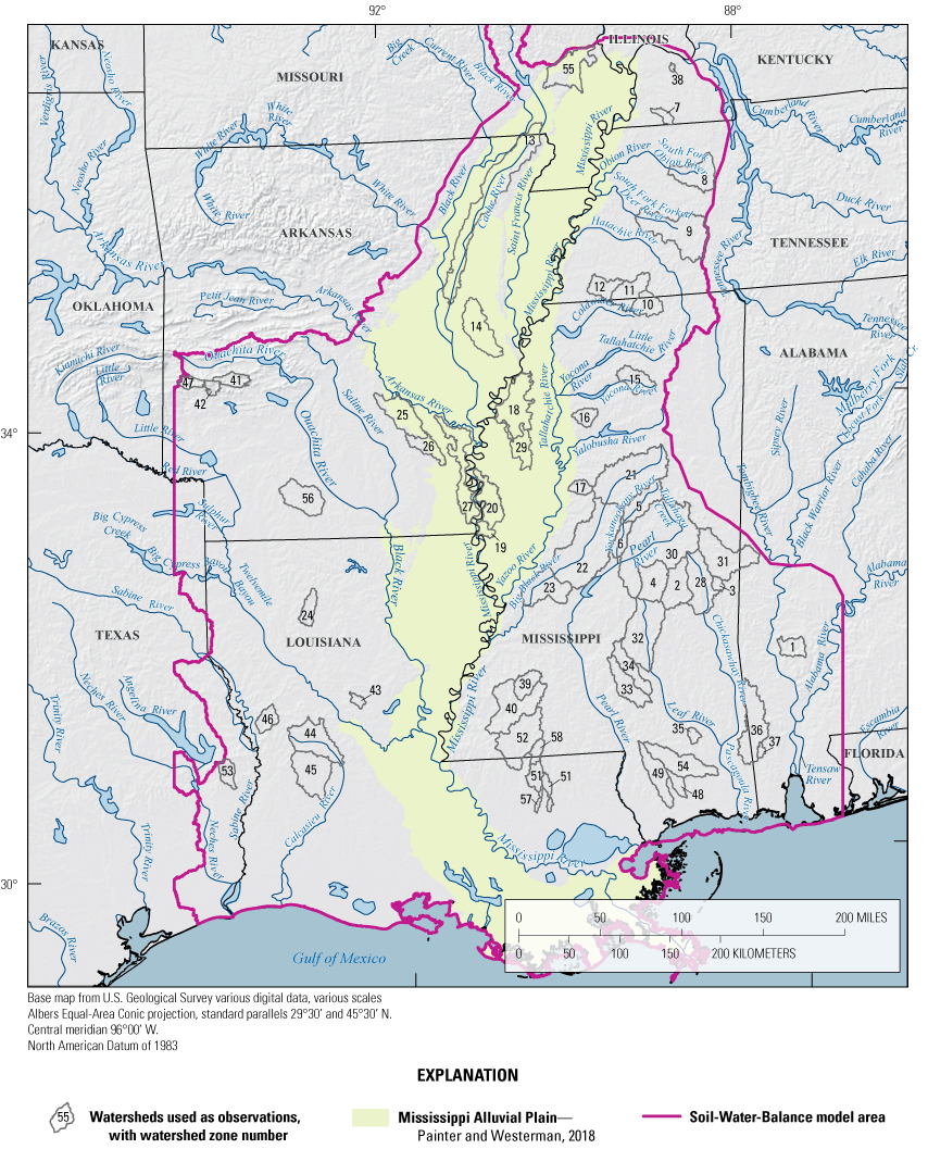
Watersheds used as observation zones for the calibration of the Soil-Water-Balance model.
The base-flow separation analysis was conducted using the USGS GW Toolbox computer program (Barlow and others, 2015). This program includes calculations of nine different base-flow separation techniques. An ensemble approach was used to derive an overall estimate of the base flow and direct runoff for each streamgage, using the median of all nine methods. The base-flow analysis was aggregated to monthly and annual summaries of direct runoff and base flow (a proxy for recharge) for each streamgage/watershed. An example showing six of the base-flow separation methods for the Homochitto River, Mississippi, for water year 2009 is shown in figure 8 to illustrate the methods used.
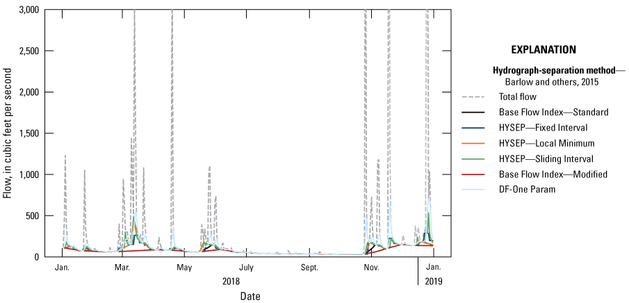
Example hydrograph of base flow and total flow for each of the base-flow separation methods, as produced by the U.S. Geological Survey Groundwater Toolbox code, for the Homochitto River at Eddiceton, Mississippi, water year 2009. HYSEP is a computer program for hydrograph separation, and DF-One Param is a one-parameter digital filter method; see Barlow and others (2015) for more descriptions of the base-flow separation methods used in this study.
Using the base-flow separation analysis, annual values of runoff and potential recharge observations for each watershed were calculated for every year from 2000 to 2018. Monthly values were calculated for 2003, 2007, 2009, 2011, and 2014, which represented a range of low and high flow years. Overall, 1,780 annual runoff and potential recharge observations and 5,983 monthly runoff and potential recharge observations were used as input to the calibration.
Simulated daily values of runoff and net infiltration were summed and tabulated for each contributing area associated with a streamgage over time periods consistent with observation data availability; these statistics were calculated for the calibration using the SWBSTATS2 utility (Westenbroek and others, 2018).
Evapotranspiration
The actual ET observations were developed for specific land uses in the model domain, using published actual ET estimates from a statistical relation between landscape variables and remotely sensed datasets of land surface temperatures (operational Simplified Surface Energy Balance [SSEbop] model), constrained by other water budget variables (Reitz and others, 2017). Using polygons derived from annual CDL grids for 2013, 2014, and 2015, the monthly total estimated ET values from Reitz and others (2017) were summed across each polygon to generate crop- and land use-specific ET observations to compare to the SWB simulated values. Monthly ET observations were generated for rice, corn, soybean, deciduous forest, evergreen forest, and wetland forest polygons. More than 4,900 monthly ET observations were used in the calibration. Daily values of model-generated actual ET output were processed with SWBSTATS2 software (Westenbroek and others, 2018) to yield monthly actual ET values that could be directly compared to the SSEbop values.
Crop Water Use (Irrigation)
The fourth set of observations used in the calibration came from a database of estimated monthly irrigation water use developed for the Mississippi Alluvial Plain during the growing season for 1999 to 2017 (the AIWUM model: Wilson, 2021b). This dataset is a raster-based estimate of water use for crops and aquaculture, developed using a machine-learning algorithm that analyzed reported withdrawals from the Mississippi Department of Environmental Quality (MDEQ) and the Yazoo Mississippi Delta Joint Water Management District. The raster data were aggregated by county for use as observations in the SWB model calibration. The SWB calibration used more than 3,000 of these monthly observations. Daily values of applied irrigation were processed with SWBSTATS2 software (Westenbroek and others, 2018) to generate monthly model-generated crop water-use estimates on a county wide basis. The range in monthly observed values for the entire set of runoff, base flow, ET, and irrigation is illustrated in figure 9.
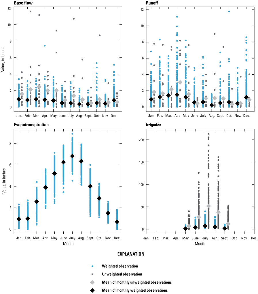
Weighted and unweighted monthly base-flow, runoff, evapotranspiration, and irrigation observations for the Soil-Water-Balance model.
Observation Groups and Weighting
“Observation groups” are used in the parameter estimation process to identify the category each observation belongs to; these categories are based on the type of observation and whether the observation represented an annual or monthly value. Base-flow (bf) and runoff (ro) observations were grouped into four categories or groups: bf_monthly, bf_annual, ro_monthly, and ro_annual. Actual evapotranspiration (aet) observations were all monthly, but the crop observations (aet-corn, aet-rice, and aet-soy) include only the growing season months, whereas the others (aet-dcd, aet-evr, and aet-wet), representing deciduous (dcd), evergreen (evr), and forested wetland (wet) observations include all 12 months. The monthly irrigation observations were grouped based on the State: irr_ark (Arkansas), irr_la (Louisiana), irr_miss (Mississippi), and irr_mo (Missouri). The irrigation observations for Kentucky and Tennessee from the AIWUM model dataset were dropped from the parameter estimation because they seemed to have values that were unrealistic and did not match similar values in the adjacent states. Altogether, 14 groups of observation values were used in the parameter estimation.
Weighting of the observations is needed for calibration because not all calibration targets are equally important or useful. Some calibration targets have more uncertainty than others, and some are more important than others for the model to simulate correctly. Therefore, calibration targets must be weighted for use in parameter estimation. Initial weights for each observation set were developed based on the range of measurement error (see Hill and Tiedeman, 2007), but the weights were adjusted during the calibration process so that the observation groups contributed appropriate amounts to the overall error between the weighted simulated versus observed values. Some of the observations were zero-weighted if further investigations into the observed value looked like it could be in error, was very uncertain, or was an unrealistic value for the SWB model to correctly simulate. The final weighting scheme for the observation set was arrived at by a combination of analysis of measurement error and the range in observed values, contributions of each parameter group to the overall objective function, and modeler best judgement (Anderson and others, 2015). Of the 17,091 observations assembled for the PEST calibration, 2,201 were given a weight of zero. The final weights assigned to each observation are included in the accompanying model data release (Westenbroek and Nielsen, 2023). An analysis of the model’s ability to simulate values in the observation dataset (prior data conflict) is discussed in the “PEST–IES Calibration” section of this report.
Model Parameters
As outlined above, the SWB (version 2.0) model calculations are controlled by the two input lookup tables: the land-use lookup table and the irrigation lookup table (Westenbroek and others, 2018). Any of the values in these lookup tables could be treated as a parameter in the PEST calibration, but only some of them control enough of the model output to make them sensitive to the parameter estimation process. Because the lookup tables are organized by combinations of land use and soil type, the lookup-table values that controlled model behavior for combinations of land use and soil type that were not covered by greater than about 1 percent of the model area were not treated as parameters in the calibration. Given the seven HSGs and 127 possible land use codes, there is the potential for more than 2,900 parameters in the land-use lookup table and more than 3,800 parameters in the irrigation lookup table, but constraining the parameters to combinations that represented more than about 1 percent of the model area resulted in 546 lookup table values being used as parameters. A complete listing and description of all potential SWB version 2.0 parameters (that is, lookup table values) are listed in appendix 3 of Westenbroek and others (2018).
Parameters were grouped according to how they are used in the model. Each parameter group used is listed in table 6, along with the type of parameter and associated lookup table of the parameter group in the SWB model and an example parameter name as used in the calibration. Each parameter must also be given a range of possible values that PEST can use in the parameter estimation, which are the upper and lower parameter bounds provided to PEST. The ranges of parameter values allowed for each were chosen based on literature values for the type of variable (such as plant rooting depths or Kcb values for a crop) and previous experience with SWB parameter estimation (Nielsen and Westenbroek, 2019; Fienen and others, 2022). During parameter estimation, the ability of PEST to modify the parameter value was turned on and off for various parameters, and some parameter values were tied by a statistical relation to the values of other parameters. The complete set of parameters, adjustability, and allowed range of values for the final calibration is presented in the accompanying USGS data release for this study (Westenbroek and Nielsen, 2023).
Table 6.
Soil-Water-Balance parameter groups used in parameter estimation of the model, the number of parameters, example parameter names, and example parameter bounds.[Data are summarized from Westenbroek and Nielsen (2023)]
PEST–IES Calibration
The latest available version of the PEST++ software (version 5, White and others, 2020) was used to perform the parameter estimation. PEST++ is built upon the well-established PEST model calibration approach (Doherty and Hunt, 2010, 2009; Doherty, 2004) and includes several different extensions for global sensitivity analysis and Monte Carlo parameter analysis. The IES algorithm was used to perform the calculations, which is a much less computationally intensive method than the traditional Gauss-Levenberg-Marquardt (GLM) method of performing calibration for highly parameterized models (White, 2018). The algorithm used in PEST–IES combines the capability of the GLM method to minimize a least-squares objective function and estimate a Jacobian matrix (White and others, 2020). The PEST–IES method draws an ensemble of possible parameter values using the parameter bounds specified for every parameter in the calibration, generating a large number of possible model parameter realizations (Monte Carlo analysis) from which to calculate parameter upgrades for each successive iteration of parameter estimates. The parameter bounds (upper and lower) are used to construct a 95-percent confidence interval around the preferred value (the initial parameter value), from which the ensemble set of parameter values are drawn for each iteration (for this calibration, an ensemble of 100 alternative parameter sets were used for each iteration). See White and others (2020) for additional detail on the use of PEST–IES.
The PEST–IES approach allows for the calculation of how well the model using current parameter values is able to simulate the observation values used in the calibration, considering their upper and lower bounds, and assuming the weights assigned represent the uncertainty in the observation values. This analysis was used to help identify areas of structural error in the model, improve parameter bounds, and identify observations that seemed to be unrealistic. This analysis was important because some of the observations, such as the irrigation estimates, were themselves model-derived (from the AIWUM model) and, upon closer inspection, were not always accurately estimated.
A python-based toolset called pyEMU (White and others, 2016) was used to help prepare the model input files and PEST–IES control files for the calibration. Several preprocessing and postprocessing python scripts were developed to assist in the calibration analysis, including a python script that converted the native model output from the SWBSTATS.exe software into simulated equivalents of the observation values. Although the use of PEST–IES for this highly parameterized model is less computationally intensive than traditional PEST approaches, it still required hundreds of parallel model runs for each estimation run. All the parameter estimation activity was run in a LINUX environment on the USGS Denali supercomputer (Falgout and others, 2022) at the Earth Resources Observation and Science data center in South Dakota. The coordination of all the parallel model runs was handled by the SLURM resource manager (Jette and Grondona, 2003) for job scheduling and management of communication between the PEST master and worker nodes. Postprocessing of run results was done locally on laptops running a Windows operating system. The results of each attempt at parameter estimation were used to modify the model and various input files until no further significant improvements in the objective function and observed-to-simulated value fits could be made.
Results and Discussion
The final base run from the calibration exercise provided us with the best-fit parameter values for the SWB model lookup table inputs. The final calibrated lookup tables and all the model inputs are in the model archive for this study (Westenbroek and Nielsen, 2023).
Model Fit to Observations
The best-fit model calibration obtained with the four sets of observation data yielded a model with an overall coefficient of determination (r2) of 0.84 and a standard error of 0.005 for the observations that were not zero weighted. The observations that compose the water budget output terms (actual ET, net infiltration, and runoff) are plotted against the simulated equivalents in figures 10A, 10B, and 10C, respectively. All three show an acceptable distribution along the 1:1 line. Coefficients of determination for each observation group separately are 0.89 for actual ET, 0.90 for net infiltration (potential recharge), 0.91 for runoff, and 0.68 for irrigation. The actual ET and runoff values have a small amount of skew in the residuals: in the case of the actual ET (fig. 10E), the model overpredicts the values when the monthly observed values are low (less than 2 inches), and in the case of the runoff (fig. 10G) the model slightly underpredicts when the observed values are greater than about 5 inches. The fit of the county-based total irrigation observed versus simulated values are much more scattered than the other observation groups (fig. 10D). The AIWUM irrigation model observations were determined using a variety of methods that varied from one State to another, and sometimes relied on estimates of irrigated acres that differed from the LANID irrigated acreages that was applied in the SWB model. This resulted in irrigation rates that were not always directly comparable.
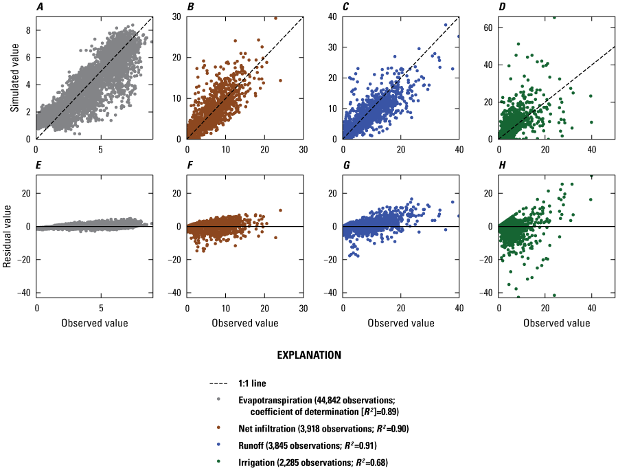
Overall model calibration results. Simulated versus observed values for, A, actual evapotranspiration; B, net infiltration; C, runoff; and, D, irrigation. Residuals versus observed values for, E, actual evapotranspiration; F, net infiltration; G, runoff; and H, irrigation.
A comparison of the annual simulated irrigation water requirement to reported and estimated irrigation for crops in the study area was used as a secondary evaluation of model performance for irrigation. Field-specific irrigation amounts were obtained from the MDEQ volunteer monitoring program (MDEQ, 2022). This program operates within the Delta Mississippi Alluvial Plain region, where major crops include corn, soybeans, cotton, and rice. The field data, which include irrigation rates and the crop type, were compared to the simulated irrigation amounts in SWB model cells where the field crop type matched the CDL crop type simulated by the SWB model. Data from the MDEQ volunteer monitoring program were available for 5 years of the SWB model period, 2014 to 2019. In the area where the data overlapped, the total annual irrigation from both datasets compared well. The graphs in figure 11 include the median irrigation rates for the MDEQ data compared to the median SWB estimates for each of the 5 years. The SWB-simulated values are close to the reported amounts for corn (about 6 inches per year), soybeans (about 6 inches per year), and rice (about 24 inches per year). The SWB-simulated values for cotton are a little bit higher than the reported data, overall.
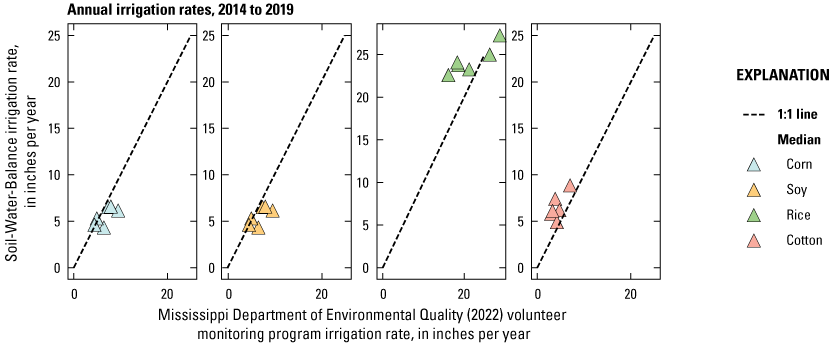
Soil-Water-Balance model simulated annual irrigation rates compared to measured data in Mississippi, 2014–19.
The term “prior-data conflict” is a model performance evaluation concept that encapsulates the idea that mismatches between observations and model output may be attributed to one of two things: inadequately characterized observation datasets, or implausibly parameterized or inappropriately constructed models. We used PEST++ to evaluate prior-data conflict for simulations made with SWB. Prior-data conflict analysis can show whether the model as conceptualized and constructed is capable of producing output consistent with observed values at all. The prior-data conflict analysis for the final calibration run indicated that 11 percent of the non-zero-weighted observations could not be simulated closely given the parameter bounds provided during the PEST–IES calibration and the given observation weights. The observation groups with the highest amount of prior-data conflict (observations with simulated values out of range) were crop ET observation groups (aet-rice, aet-soy, aet-corn), particularly during the month of April, and annual total base-flow and runoff observations. The forested ET observations (aet-evr, aet-dcd, and aet-wet) all had a relatively high amount of prior-data conflict for the winter months compared to the other observations.
The reasons for the prior-data conflict in the Mississippi embayment region SWB model may include issues related to the very nature of modeling itself, which is an imperfect attempt to use relatively simple mathematics to describe complex systems. In the case of the Mississippi embayment region SWB model, the SWB model consistently underestimates actual ET in the late summer and overestimates actual ET in the winter and early spring, as compared to the SSEbop estimated values of actual ET. Given the sparsity of reliable datasets for true measurements of actual ET at a given location, this could represent either an error in the SWB model algorithm or errors in the SSEbop estimated actual ET values themselves. The runoff and base-flow prior-data conflict is likely a result of the combination of errors in the base-flow separation method used to divide up the total runoff into base flow and direct runoff for the set of observation values and simplifications of reality that are inherent in modeling in general.
Regardless of the potential difficulties of simulating some of the observed values used in the calibration, this model of water balance terms has an overall better fit and less skew in the simulated values compared to the observations than an earlier SWB model of the Mississippi embayment region (Westenbroek and others, 2021).
One way of evaluating the spatial model fit is to analyze the observation residuals for each of the observation watersheds (fig. 12). The mean of all the residuals where there is a mix of positive and negative residual values (fig. 12A) is less informative than converting all the residuals for a given location to their absolute value and taking the mean (fig. 12B), which provides more insight into model performance. From figure 12B, it is clear that the model more closely matches the runoff and base flow outside the alluvial plain than within it. This is unsurprising, given the difficulties in the base-flow separation methodology in the alluvial plain setting discussed in the “Observations” section previously.
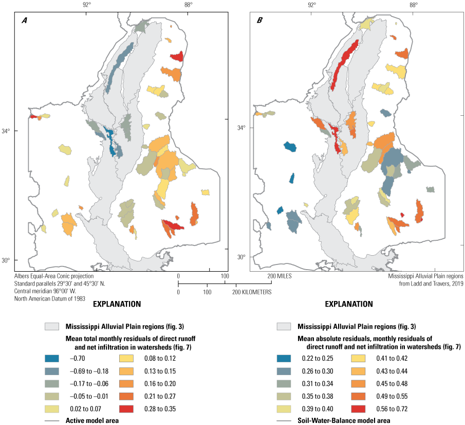
Residuals for watershed-based observations (annual runoff, annual base flow, monthly runoff, and monthly base flow) in the Soil-Water-Balance model area. A, mean total residual, and B, mean absolute residual.
Another way to view the model calibration fit to the observed values is to compare the three major components of the water budget (ET, net infiltration, and runoff) over an annual cycle for a set of watersheds. Figure 13 shows actual ET, net infiltration, and runoff components derived from observation datasets compared to SWB output values. Many of the watersheds shown (Bayou Macon, Big Sunflower River, Bayou Bartholomew, and Big Black River) have almost equal simulated and observed actual ET values for most of the months. Most of the watersheds shown have very low observed surface-water flows (combined base flow and runoff) in the summer. The SWB model results mimic this pattern well for most of these; however, the simulated net infiltration and runoff values for the Bayou Macon watershed are much higher than observed year round. December, January, and February actual ET values as simulated by SWB are generally larger than the observed values.
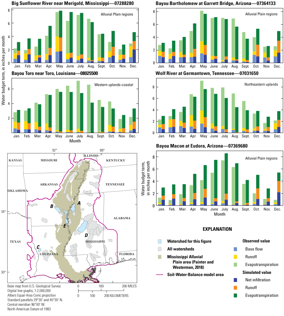
Simulated and observed monthly water budget terms (base flow, actual evapotranspiration, runoff, and net infiltration) for watersheds in the Mississippi embayment region.
Spatial Estimates of Water Budget Terms
To understand how the SWB model distributes the various water budget terms across the study area, it is useful to recall that the spatial variability of the average annual gross precipitation (fig. 4) ranges from less than 50 inches per year in the northwest and western part of the model domain to greater than 70 inches per year along the gulf coast. The average annual gross precipitation for the regions in the Mississippi Alluvial Plain (fig. 3) ranges from 53.5 inches in the Cache region to 63.5 inches in the Atchafalaya region.
Figure 14 illustrates the model-wide simulations of the annual mean input terms for the water budget of the Mississippi embayment region (gross precipitation and irrigation) and the output terms (actual ET, runoff, and net infiltration). The mean annual simulated values for the model domain as a whole and the generalized regions are given in table 7. On an annual basis, the actual ET across the regions of the alluvial plain (39.6 to 45.6 inches) accounts for between 62 and 72 percent of the total precipitation plus additions from irrigation. The combined net infiltration and runoff (5.7–12.5 inches, and 10.3–19.7 inches, respectively) accounts for the remaining 29–39 percent of the total precipitation plus irrigation inputs. Where precipitation is lower in the northwest part of the model area (fig. 14A), in the Cache, St. Francis, and Grand Prairie regions (fig. 3), the applied irrigation input evens out the actual ET in that area to be comparable to parts of the study area with less precipitation. The simulated runoff and net infiltration are higher in the agricultural alluvial plain area than in the surrounding uplands (fig. 14B). This could be explained by the shallow rooting depth of crops in the alluvial plain area relative to the forested uplands because trees have a deeper rooting zone available for plant uptake and ET.
Table 7.
Mean annual simulated water budget terms for the Mississippi embayment region model area and for the generalized regions of the Mississippi Alluvial Plain.| Area (fig. 3) | Mean annual simulated water budget term, in inches | ||||
|---|---|---|---|---|---|
| Gross precipitation | Actual evapotranspiration | Net infiltration | Runoff | Irrigation | |
| Entire model domain | 58.9 | 42.0 | 7.6 | 11.0 | 1.5 |
| Atchafalaya | 63.5 | 45.6 | 6.7 | 11.9 | 0.2 |
| Boeuf | 58.3 | 40.9 | 8.2 | 13.2 | 3.4 |
| Cache | 53.5 | 39.6 | 12.5 | 11.9 | 10.4 |
| Delta | 57.5 | 39.8 | 10.7 | 12.7 | 4.9 |
| Deltaic and Chenier Plains | 64.5 | 41.3 | 5.7 | 19.7 | 0 |
| Grand Prairie | 54.3 | 40 | 9.6 | 12.3 | 7.0 |
| St. Francis | 52.7 | 37.7 | 12.1 | 11 | 7.7 |
| Uplands outside alluvial plain | 59.5 | 42.6 | 6.9 | 10.3 | 0.11 |
Irrigation across the model varies considerably by year, depending on the amount of rainfall during the summer, and by crop type. As illustrated in figure 11, the amount of irrigation applied to rice is more than double the amount applied to corn, soybeans, and cotton overall. The mean annual amount of simulated irrigation applied for the entire model area (fig. 14A) ranges from about 5 inches to greater than 20 inches.

Gridded datasets showing annual Soil-Water-Balance simulated mean A, inputs (gross precipitation and irrigation) and B, outputs (actual evapotranspiration, runoff, and net infiltration) for 2000–20.
The total amount of inputs (gross precipitation plus irrigation) and outputs (actual ET, runoff, and net infiltration) in the water budget across the Mississippi Alluvial Plain area also vary considerably from year to year (fig. 15)—during 2000–20, the range in precipitation for most of the regions was between 38 inches to about 70 inches. Cropland irrigation adds an additional 4.9 to 10.4 inches to the input terms for these areas. In years with low overall precipitation such as 2009 and 2012, actual ET accounts for almost 75 percent of the output because plant uptake uses most of the available moisture during dry years, leaving little extra for runoff and infiltration.
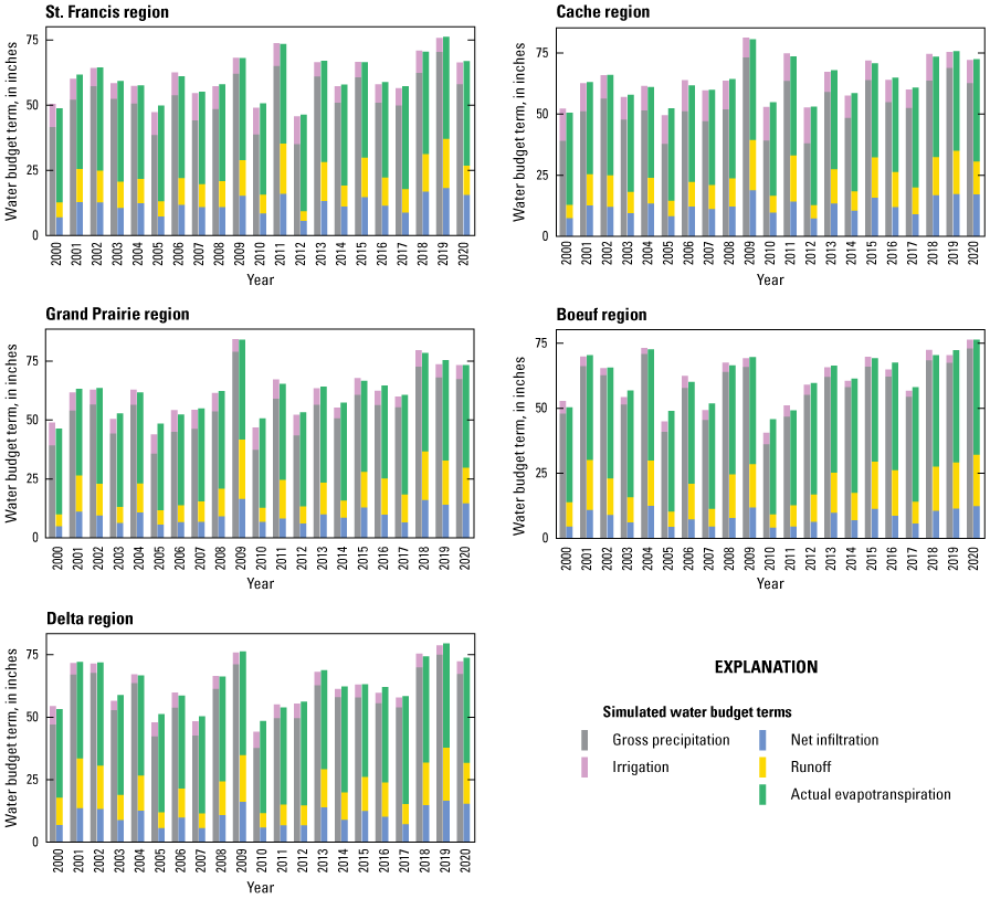
Annual Soil-Water-Balance simulated water budget estimates in the Mississippi Alluvial Plain regions, 2000–20.
There was an apparent increase in precipitation in the Mississippi Alluvial Plain during the study period (2000–20): in all the regions, the average gross precipitation during 2000–12 was about 50 inches; average gross precipitation increased to about 60 inches during 2013–20 (fig. 15). The increase in precipitation over this period is most pronounced in the summer months and holds for all the regions (fig 16A). The effect of this observed increase during the summer was a simulated decrease in the amount of water needed for irrigation (fig. 16B). The Cache region, which is heavily dominated by rice production, has the highest irrigation water demand; this keeps the total actual ET much more constant than in the other regions, which have a greater mix of crops with more modest irrigation demands.
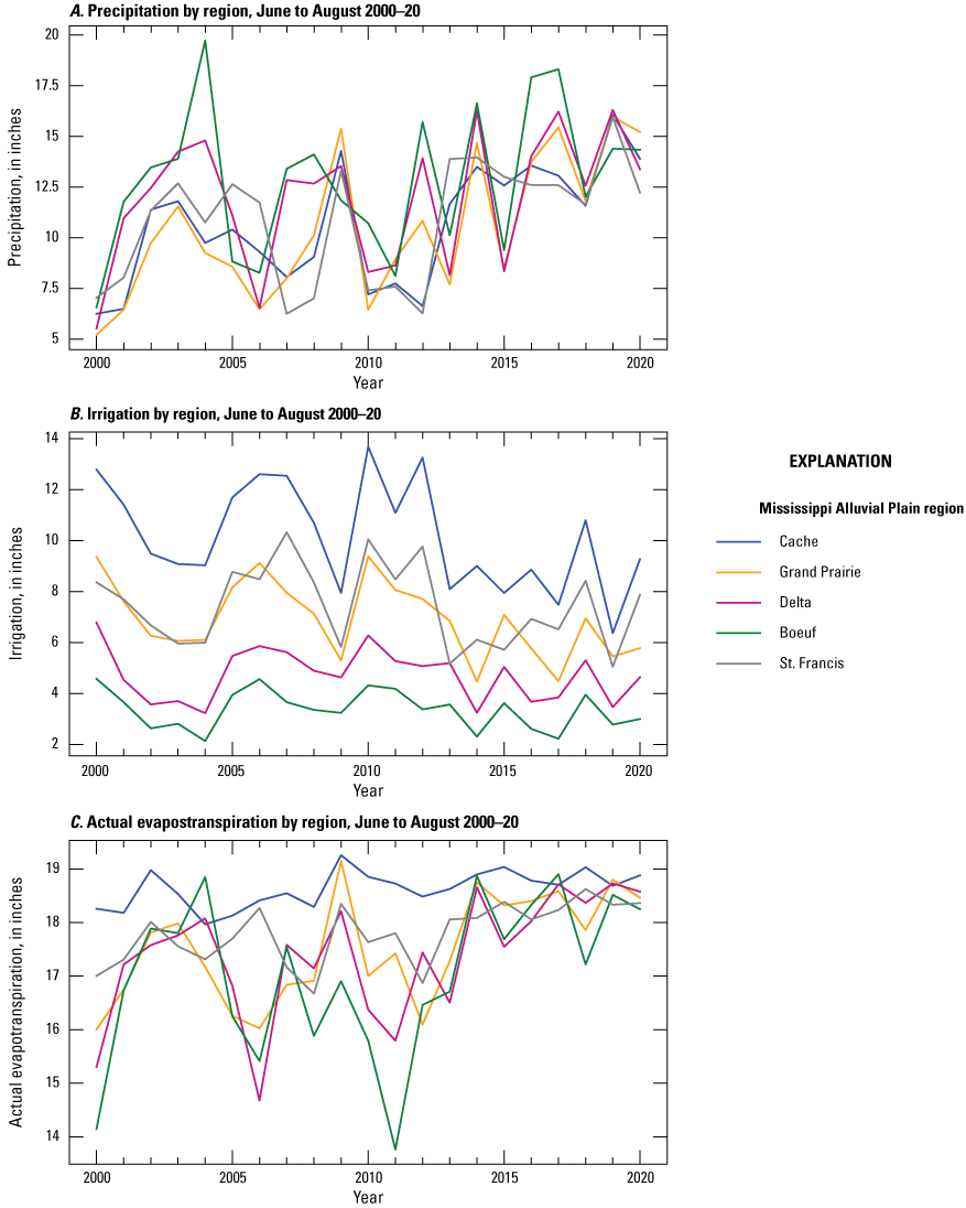
Average summer (June–August) A, precipitation, B, irrigation, and C, actual evapotranspiration in the Mississippi Alluvial Plain regions, 2000–20.
Seasonal Patterns in Water Budgets
The SWB model for the Mississippi embayment region calculated daily water balance terms for the study period (2000–20), but the results are most useful aggregated into monthly, annual, and average values. The overall variability of the actual ET, net infiltration, runoff, and irrigation are heavily dependent on the variability in the input precipitation, which varies spatially across the region as well as year-to-year. To illustrate the seasonal spatial patterns in the water budget terms, we used the 10-digit hydrologic units (U.S. Geological Survey, 2021) that cover the Mississippi Alluvial Plain area as analysis zones for the 1-kilometer output datasets from the SWB model (fig. 17).
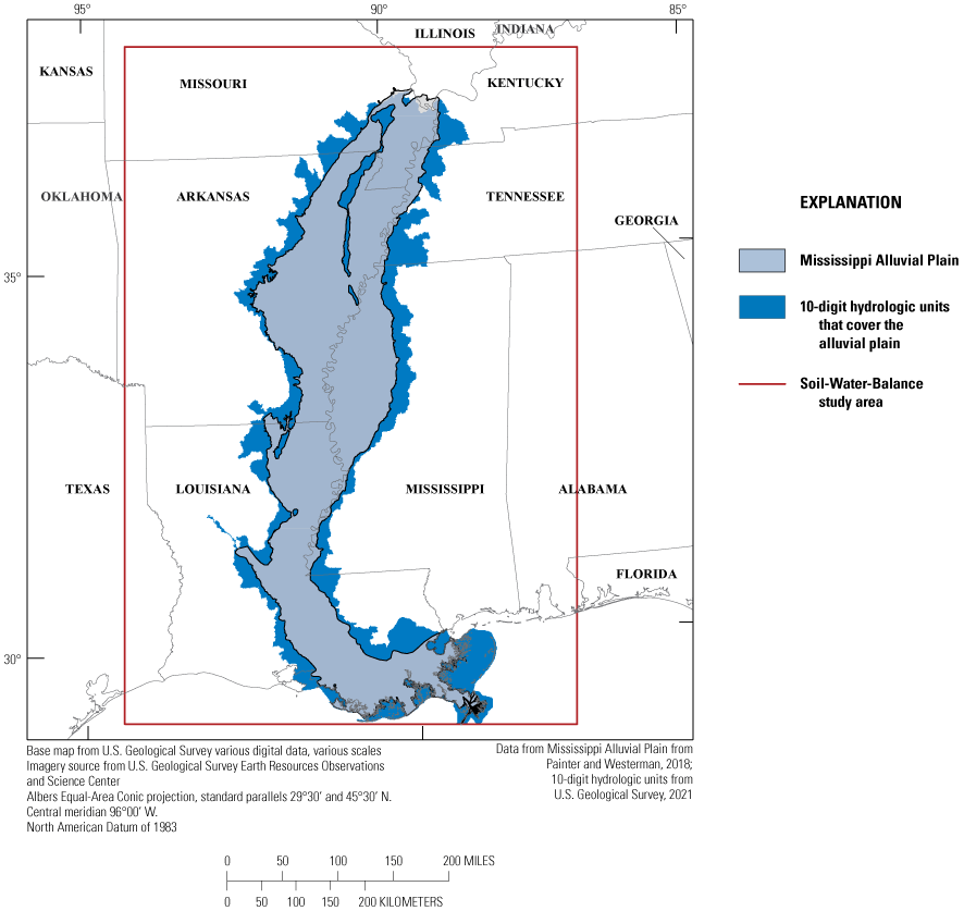
Extent of 10-digit hydrologic unit analysis zones for the Mississippi embayment region Soil-Water-Balance model.
Precipitation, Actual Evapotranspiration, and Irrigation
There is considerable monthly variability in precipitation on an annual cycle across the Mississippi Alluvial Plain area (fig. 18A). In January through May, the area receiving the highest amount of monthly precipitation (about 5–6 inches per month) progresses northward. From June through October, the northern part of the Mississippi Alluvial Plain area experiences relatively little precipitation (typically less than 4 inches per month), whereas the southern areas (which are close to the gulf coast) have the highest monthly precipitation of the year in June through August (7–10 inches per month). October is relatively dry across the model area, and then precipitation increases again across the model in November and December.
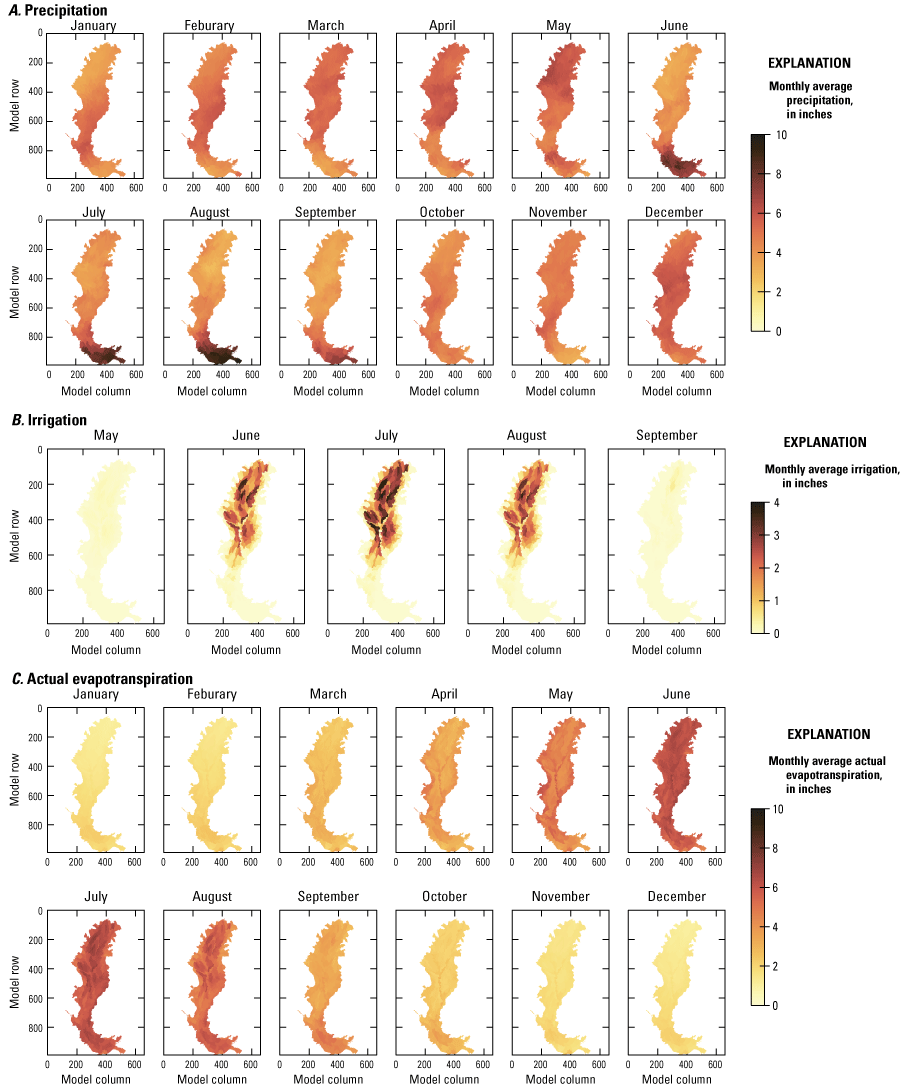
Gridded datasets showing monthly average A, precipitation, B, irrigation, and C, actual evapotranspiration for the 10-digit hydrologic units covering the Mississippi Alluvial Plain.
The actual ET is directly related to the precipitation and temperature, as would be expected, but also to the amount of irrigation applied to crops (fig. 18B) during the growing season. Because the Mississippi Alluvial Plain part of the study area is heavily dominated by cropland (fig. 6), the monthly patterns of simulated actual ET (fig. 18C) reflect this. The colder months (January through March, and October through December) are times of less active plant growth (crops or forest), so actual ET is low. In April and May, forested areas green up and start to pump moisture into the atmosphere, and actual ET rates rise in these areas to greater than 4 inches per month; cropland is not fully vegetated at this point. In June, July, and August irrigation on cropland provides much available moisture for plant growth (fig. 18B), and the actual ET rates are high (greater than 6 inches per month) in most crop areas. Actual ET rates slow down considerably in September as crops mature and irrigation is needed less.
Net Infiltration and Runoff
As noted above, precipitation progresses northward across the alluvial plain from January to May, tapers off greatly in the summer, and progresses northward again in September through December; runoff and net infiltration have similar progression (fig. 19), and maximum values in the alluvial plain occur in the winter months. The small amount of runoff (fig. 19A) and net infiltration (fig. 19B) simulated in the summer months is more a result of excess water from irrigation applications than natural excess precipitation.
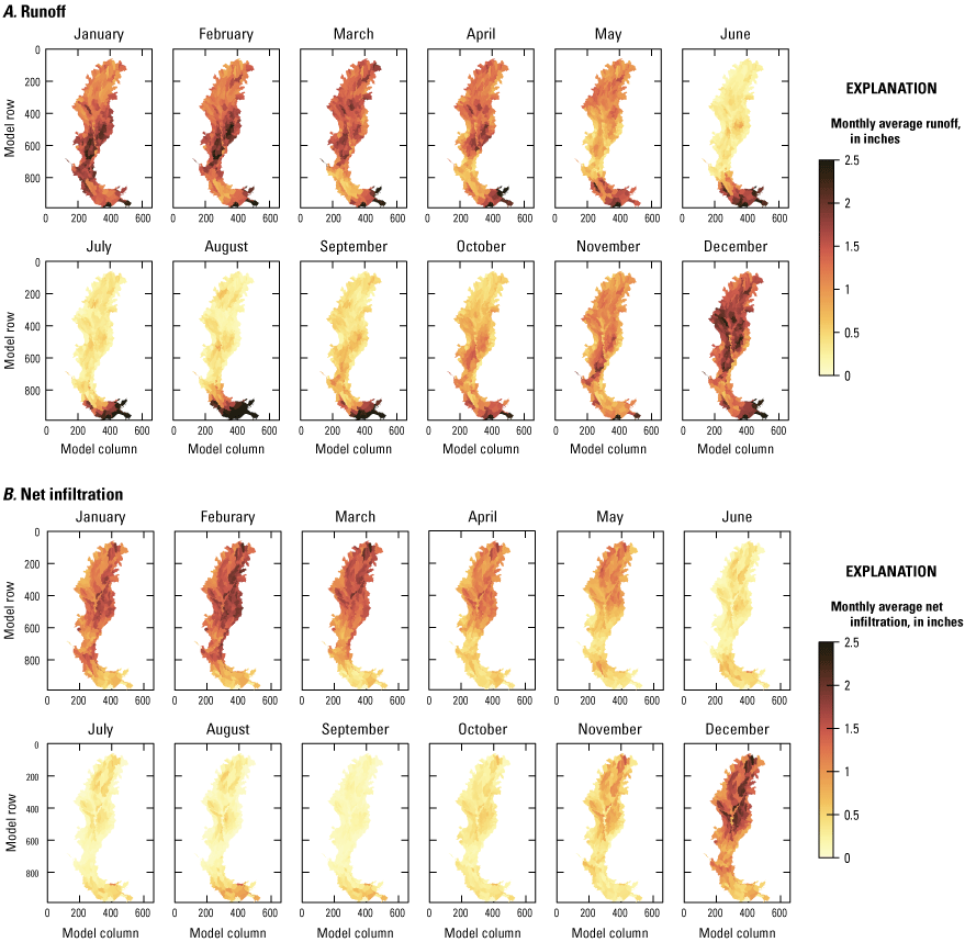
Gridded datasets showing monthly average runoff and net infiltration in the 10-digit hydrologic units covering the Mississippi Alluvial Plain.
Monthly water budget graphs for several of the watersheds used in the calibration exhibit a typical cycle of soil moisture throughout the year in the alluvial plain. The monthly average water balance terms for each of the regions in the alluvial plain area (fig. 20) reveal that the runoff and net infiltration components are very seasonal and are much higher in the fall and winter than in the summer. Without applied irrigation, the net infiltration and runoff in the summer would approach zero. Because precipitation during the summer is much lower in the north (St. Francis, Cache, and Grand Prairie regions), most of the irrigation needed to sustain crops is applied in these regions.
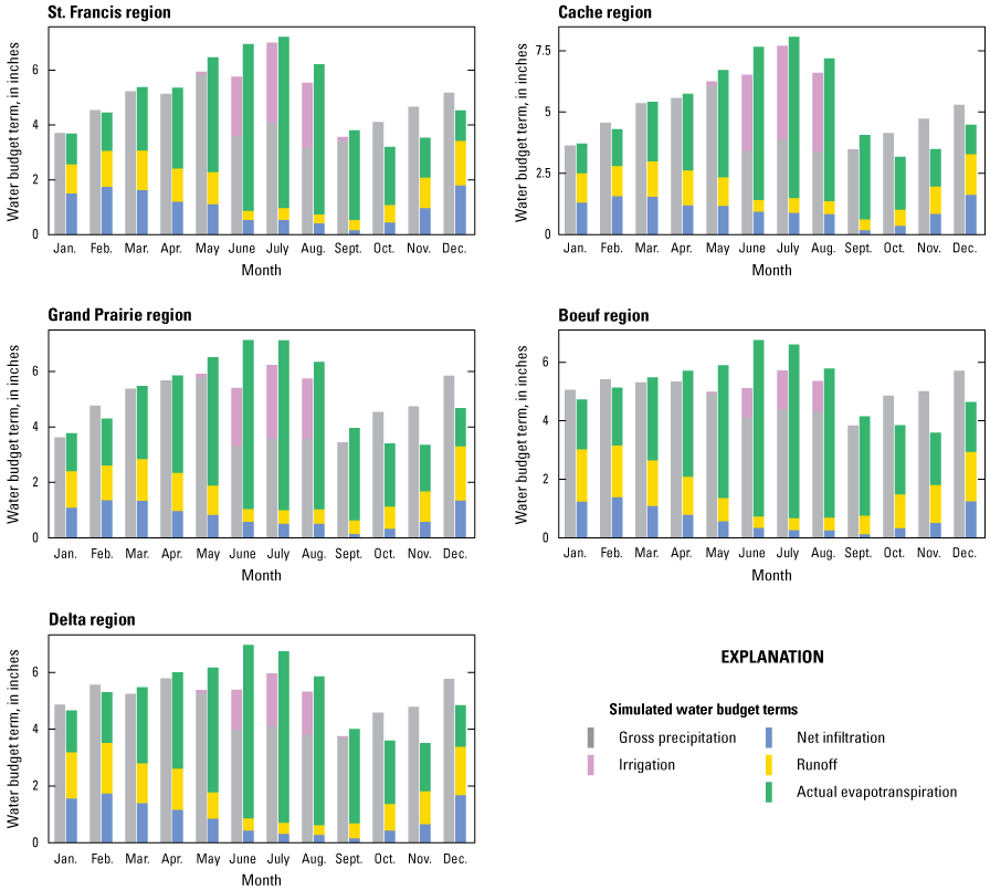
Average monthly simulated water balance terms for the major regions of the Mississippi Alluvial Plain aquifer, 2000–20.
Model Limitations and Uncertainty
Every model is an imperfect representation of reality. An understanding of the model limitations (structural model errors) and model sensitivity and uncertainty will help the reader evaluate the application of these results to various science and management questions. The use of PEST as a model calibration tool enables the modeler to perform tests of the uncertainty inherent in the parameters used in the model and which types of parameters affect the calibration more than others. Structural model error and other factors also contribute to the overall uncertainty in the recharge estimates, but because they are not model parameters, they cannot be addressed in a PEST uncertainty analysis and are not considered explicitly here.
Model Limitations
Some of the limitations of the SWB model of the Mississippi embayment region area are inherent in the data used as inputs to the model, limitations in the runoff and baseflow observations in the alluvial plain part of the study area, and some of the limitations involve assumptions inherent in the way the water balance terms are calculated.
Net infiltration below the rooting zone is not equivalent to recharge that reaches the water table; the SWB model does not simulate processes that happen within the unsaturated zone between the bottom of the rooting zone and the water table. In the Mississippi Alluvial Plain area, there is a widespread silt- and clay-rich zone between the land surface and the water table in the upper alluvial plain aquifer, which substantially impedes net infiltration from the rooting zone in reaching the water table as recharge. As discussed later in the report, much of the water leaving the rooting zone as net infiltration eventually ends up discharging to rivers and streams in the study area and does not necessarily reach the water table.
Additionally, some activities in the Mississippi Alluvial Plain area that impact water movement below the land surface are not well represented in the SWB model area, including large aquaculture operations, which fill up artificial ponds continually to raise fish, and the use of rice paddies in the fall for duck habitat, whereby they are filled up with standing water for about 1 month in October and November. Any water infiltrating below the land surface because of either of these activities is not captured by the SWB model.
Uncertainty
There are many sources of uncertainty in the SWB model for the study area. These include uncertainty in the input datasets (climate data, soil data, and land-use data), uncertainty in the observations used for calculations, and uncertainty in the parameters that were adjusted during calibration. The uncertainty in the input data cannot be described or accounted for in a quantitative way. Uncertainty in the observations was partially accounted for in the weights used in the calibration. The uncertainty in the SWB model results caused by uncertainty in the calibrated parameter values was calculated using a Monte Carlo approach and is discussed in the “Parameter Sensitivity and Influence” section. Using PEST++ and the IES tools used for parameter estimation, an ensemble of 350 separate model runs was produced, each with a unique set of parameter values pulled from a range of parameter values centered around the calibrated value for each parameter. The total ϕ (the measure of model fit to the observations) for each run was compared to a range of acceptable ϕ values, and runs that had poor model fit were discarded from further analysis, resulting in a total of 290 separate models. A series of python scripts were used to calculate the standard deviation of the suite of models, for each of the model outputs for every pixel. A standard deviation grid was calculated for the mean annual values and mean monthly values for actual ET, irrigation, net infiltration, and runoff.
Figure 21 illustrates the standard deviations in the mean annual values for the four primary model outputs across the entire model domain. Although spatial trends were not particularly evident in the annual net infiltration and runoff standard deviation, the actual ET annual standard deviation is lower in the alluvial plain area than in much of the rest of the study area. Overall, the actual ET annual standard deviation is generally lower across the study area than the net infiltration and the runoff. The standard deviation of the irrigation estimates is highest in the northern part of the alluvial plain area.
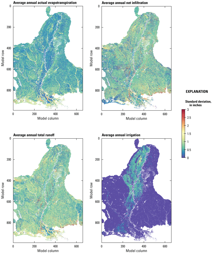
Average annual uncertainty (standard deviation) grids for actual evapotranspiration, net infiltration, total runoff, and irrigation in the Soil-Water-Balance model area.
The standard deviation values can be converted to a 95-percent confidence interval on the annual and monthly water budget terms for specific areas and seasons of interest. The 95-percent confidence interval is two times the standard deviation above and below the mean value, or four times the standard deviation. In this report, the percent uncertainty is defined as the 95-percent confidence interval divided by the simulated value for a given area. Applying these calculations to the 58 watersheds used in the model calibration (fig. 7) shows that the percent uncertainty is low for the actual ET simulations (less than 5 percent). The percent uncertainty for the irrigation, net infiltration, and runoff simulations is highly variable across the study area (fig. 22), but the means average around 20 percent for all watersheds. Scaling up to the regions of the Mississippi Alluvial Plain, table 8 lists the uncertainty for each region’s annual confidence intervals and uncertainty for the four water budget components calculated by SWB for this study. The Deltaic and Chenier Plains and Atchafalaya regions, having fewer observations and a different climate profile than the areas to the north, have the greatest uncertainty in most of the budget components for the regions. On a monthly basis, the uncertainty in water budget components across the whole study area (fig. 23A) is focused on the actual ET and irrigation in the summer months, when those are the largest water budget components. The runoff and net infiltration uncertainty contribute the most to the late fall and winter overall model uncertainty. Focusing on the alluvial plain regions and just the summer months (June, July, and August), the irrigation is the most uncertain part of the whole water budget (fig. 23B, table 9).
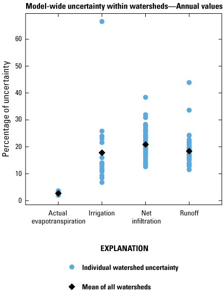
Distribution of the calculated uncertainty in the actual evapotranspiration, irrigation, net infiltration, and runoff estimates for 58 watersheds in the study area, and the mean uncertainty for each category, expressed as uncertainty percentages.
Table 8.
Mean annual simulated water budget terms for each generalized region, and 95-percent confidence limits and uncertainty as a percentage of the simulated value.[Data are summarized from Westenbroek and Nielsen (2023). 95-percent confidence limit ranges were calculated as four times the standard deviation (plus or minus two standard deviations). NA, not applicable; ET, evapotranspiration]
| Mississippi Alluvial Plain generalized region (fig. 3) | Water budget term | Mean modeled value, in inches | 95-percent confidence interval | Uncertainty (95-percent confidence interval) as a percentage of the mean value |
|---|---|---|---|---|
| Atchafalaya | Irrigation | 0.2 | 0.03 | 15.0 |
| Boeuf | Irrigation | 3.4 | 0.39 | 11.5 |
| Delta | Irrigation | 4.9 | 0.58 | 11.8 |
| Deltaic and Chenier Plains | Irrigation | 0.0 | 0.00 | NA |
| Grand Prairie | Irrigation | 7.0 | 0.59 | 8.4 |
| St. Francis | Irrigation | 7.7 | 0.89 | 11.6 |
| Cache | Irrigation | 10.4 | 0.82 | 7.9 |
| Atchafalaya | Actual ET | 45.6 | 1.44 | 3.2 |
| Boeuf | Actual ET | 40.9 | 1.15 | 2.8 |
| Delta | Actual ET | 39.8 | 0.82 | 2.1 |
| Deltaic and Chenier Plains | Actual ET | 41.3 | 1.85 | 4.5 |
| Grand Prairie | Actual ET | 40.0 | 1.11 | 2.8 |
| St. Francis | Actual ET | 37.7 | 0.93 | 2.5 |
| Cache | Actual ET | 39.6 | 0.97 | 2.4 |
| Atchafalaya | Net infiltration | 6.7 | 1.76 | 26.3 |
| Boeuf | Net infiltration | 8.2 | 1.61 | 19.6 |
| Delta | Net infiltration | 10.7 | 1.62 | 15.1 |
| Deltaic and Chenier Plains | Net infiltration | 5.7 | 1.85 | 32.5 |
| Grand Prairie | Net infiltration | 9.6 | 1.62 | 16.9 |
| St. Francis | Net infiltration | 12.1 | 1.61 | 13.3 |
| Cache | Net infiltration | 12.5 | 1.70 | 13.6 |
| Atchafalaya | Runoff | 11.9 | 1.91 | 16.1 |
| Boeuf | Runoff | 13.2 | 1.74 | 13.2 |
| Delta | Runoff | 12.7 | 1.60 | 12.6 |
| Deltaic and Chenier Plains | Runoff | 19.7 | 2.22 | 11.3 |
| Grand Prairie | Runoff | 12.3 | 1.74 | 14.1 |
| St. Francis | Runoff | 11.0 | 1.61 | 14.6 |
| Cache | Runoff | 11.9 | 1.75 | 14.7 |
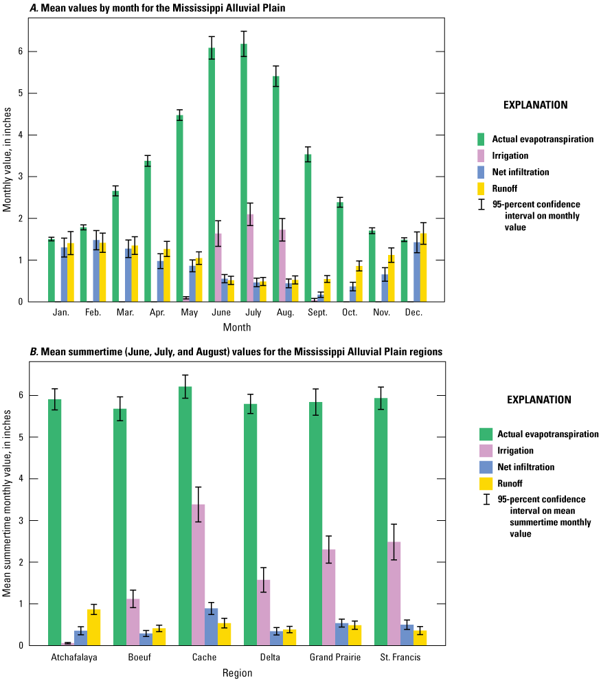
Uncertainty (95-percent confidence intervals) on simulated water budget terms in the Mississippi Alluvial Plain regions. A, mean monthly values, and B, mean summertime (June, July, and August) monthly values.
Table 9.
Mean monthly simulated water budget terms, 95-percent confidence limits, and uncertainty as a percentage of the simulated value for the Mississippi Alluvial Plain regions.[95-percent confidence limit range calculated as four times the standard deviation (plus or minus two standard deviations); MMV, mean modeled value; in., inch; %, percent; CL, confidence limit; NA, not applicable]
| Mississippi Alluvial Plain region (fig. 3) | Month | Irrigation | Actual evapotranspiration | Net infiltration | Runoff | ||||||||
|---|---|---|---|---|---|---|---|---|---|---|---|---|---|
| MMV (in.) | 95% CL range | Uncertainty (CL range) as a % of the MMV | MMV (in.) | 95% CL range | Uncertainty (CL range) as a % of the MMV | MMV (in.) | 95% CL range | Uncertainty (CL range) as a % of the MMV | MMV (in.) | 95% CL range | Uncertainty (CL range) as a % of the MMV | ||
| Boeuf | Jan. | 0 | 0 | NA | 1.7 | 0.1 | 6 | 1.25 | 0.514 | 41.2 | 1.78 | 0.592 | 33.3 |
| Boeuf | Feb. | 0 | 0 | NA | 2 | 0.14 | 7.1 | 1.4 | 0.498 | 35.7 | 1.77 | 0.501 | 28.4 |
| Boeuf | Mar. | 0 | 0 | NA | 2.8 | 0.28 | 10 | 1.09 | 0.431 | 39.4 | 1.55 | 0.447 | 28.8 |
| Boeuf | Apr. | 0 | 0 | NA | 3.6 | 0.3 | 8.4 | 0.79 | 0.34 | 43.2 | 1.3 | 0.361 | 27.8 |
| Boeuf | May | 0.1 | 0.04 | 71.1 | 4.5 | 0.3 | 6.7 | 0.57 | 0.212 | 37 | 0.79 | 0.244 | 30.9 |
| Boeuf | June | 1 | 0.45 | 45.1 | 6 | 0.6 | 9.9 | 0.34 | 0.149 | 43.5 | 0.39 | 0.159 | 40.5 |
| Boeuf | July | 1.3 | 0.41 | 30.8 | 5.9 | 0.64 | 10.8 | 0.27 | 0.138 | 52.1 | 0.41 | 0.146 | 35.6 |
| Boeuf | Aug. | 1 | 0.41 | 39 | 5.1 | 0.48 | 9.4 | 0.26 | 0.152 | 58.5 | 0.43 | 0.16 | 37 |
| Boeuf | Sept. | 0 | 0.06 | 228.2 | 3.4 | 0.34 | 10 | 0.13 | 0.1 | 77.4 | 0.63 | 0.142 | 22.3 |
| Boeuf | Oct. | 0 | 0 | NA | 2.4 | 0.27 | 11.4 | 0.34 | 0.218 | 64.6 | 1.15 | 0.262 | 22.8 |
| Boeuf | Nov. | 0 | 0 | NA | 1.8 | 0.16 | 9.1 | 0.52 | 0.316 | 61.1 | 1.29 | 0.368 | 28.4 |
| Boeuf | Dec. | 0 | 0 | NA | 1.7 | 0.1 | 5.9 | 1.25 | 0.512 | 41.1 | 1.7 | 0.543 | 32 |
| Delta | Jan. | 0 | 0 | NA | 1.5 | 0.08 | 5.1 | 1.56 | 0.485 | 31.1 | 1.63 | 0.518 | 31.8 |
| Delta | Feb. | 0 | 0 | NA | 1.8 | 0.1 | 5.8 | 1.74 | 0.481 | 27.7 | 1.79 | 0.469 | 26.2 |
| Delta | Mar. | 0 | 0 | NA | 2.7 | 0.21 | 7.7 | 1.4 | 0.414 | 29.6 | 1.4 | 0.404 | 28.8 |
| Delta | Apr. | 0 | 0 | NA | 3.4 | 0.23 | 6.9 | 1.16 | 0.38 | 32.7 | 1.45 | 0.376 | 25.9 |
| Delta | May | 0.1 | 0.06 | 61.7 | 4.4 | 0.21 | 4.8 | 0.85 | 0.243 | 28.5 | 0.93 | 0.243 | 26.2 |
| Delta | June | 1.4 | 0.64 | 45.8 | 6.1 | 0.47 | 7.6 | 0.43 | 0.182 | 42.1 | 0.43 | 0.158 | 37.2 |
| Delta | July | 1.8 | 0.57 | 31.5 | 6 | 0.5 | 8.3 | 0.32 | 0.18 | 56 | 0.39 | 0.156 | 40 |
| Delta | Aug. | 1.5 | 0.55 | 36.6 | 5.2 | 0.41 | 7.9 | 0.28 | 0.167 | 60.2 | 0.34 | 0.145 | 43 |
| Delta | Sept. | 0.1 | 0.1 | 200.2 | 3.3 | 0.3 | 9.1 | 0.16 | 0.122 | 76 | 0.53 | 0.126 | 23.8 |
| Delta | Oct. | 0 | 0 | NA | 2.2 | 0.2 | 8.8 | 0.43 | 0.216 | 49.8 | 0.93 | 0.207 | 22.2 |
| Delta | Nov. | 0 | 0 | NA | 1.7 | 0.12 | 7.4 | 0.66 | 0.308 | 47 | 1.16 | 0.28 | 24.1 |
| Delta | Dec. | 0 | 0 | NA | 1.5 | 0.08 | 5.1 | 1.68 | 0.515 | 30.7 | 1.71 | 0.503 | 29.4 |
| Grand Prairie | Jan. | 0 | 0 | NA | 1.4 | 0.07 | 5.1 | 1.09 | 0.407 | 37.2 | 1.32 | 0.599 | 45.5 |
| Grand Prairie | Feb. | 0 | 0 | NA | 1.7 | 0.09 | 5.5 | 1.36 | 0.458 | 33.7 | 1.26 | 0.484 | 38.5 |
| Grand Prairie | Mar. | 0 | 0 | NA | 2.6 | 0.19 | 7.3 | 1.34 | 0.464 | 34.7 | 1.51 | 0.485 | 32.1 |
| Grand Prairie | Apr. | 0 | 0 | NA | 3.5 | 0.23 | 6.6 | 0.97 | 0.367 | 37.8 | 1.37 | 0.39 | 28.4 |
| Grand Prairie | May | 0.1 | 0.07 | 54.8 | 4.6 | 0.21 | 4.5 | 0.83 | 0.282 | 34 | 1.06 | 0.306 | 28.9 |
| Grand Prairie | June | 2.1 | 0.7 | 33.4 | 6.1 | 0.6 | 9.8 | 0.58 | 0.159 | 27.5 | 0.47 | 0.176 | 37.8 |
| Grand Prairie | July | 2.7 | 0.62 | 23.4 | 6.1 | 0.74 | 12.1 | 0.52 | 0.192 | 37.3 | 0.49 | 0.204 | 41.5 |
| Grand Prairie | Aug. | 2.2 | 0.65 | 29.7 | 5.3 | 0.56 | 10.5 | 0.52 | 0.214 | 41.3 | 0.51 | 0.222 | 43.6 |
| Grand Prairie | Sept. | 0 | 0.01 | 230.1 | 3.3 | 0.42 | 12.6 | 0.14 | 0.101 | 70.8 | 0.49 | 0.157 | 31.9 |
| Grand Prairie | Oct. | 0 | 0 | NA | 2.3 | 0.22 | 9.5 | 0.33 | 0.185 | 55.3 | 0.8 | 0.225 | 28.2 |
| Grand Prairie | Nov. | 0 | 0 | NA | 1.7 | 0.11 | 6.7 | 0.59 | 0.333 | 56.9 | 1.1 | 0.398 | 36.3 |
| Grand Prairie | Dec. | 0 | 0 | NA | 1.4 | 0.07 | 4.7 | 1.35 | 0.519 | 38.4 | 1.95 | 0.579 | 29.6 |
| St. Francis | Jan. | 0 | 0 | NA | 1.1 | 0.05 | 4.8 | 1.51 | 0.407 | 27 | 1.06 | 0.483 | 45.6 |
| St. Francis | Feb. | 0 | 0 | NA | 1.4 | 0.08 | 5.4 | 1.75 | 0.421 | 24.1 | 1.31 | 0.414 | 31.5 |
| St. Francis | Mar. | 0 | 0 | NA | 2.3 | 0.15 | 6.6 | 1.63 | 0.421 | 25.8 | 1.44 | 0.415 | 28.9 |
| St. Francis | Apr. | 0 | 0 | NA | 3 | 0.22 | 7.4 | 1.21 | 0.337 | 27.9 | 1.21 | 0.325 | 27 |
| St. Francis | May | 0.1 | 0.07 | 65.4 | 4.2 | 0.21 | 4.9 | 1.11 | 0.311 | 28 | 1.16 | 0.301 | 25.9 |
| St. Francis | June | 2.2 | 0.99 | 45.7 | 6.1 | 0.51 | 8.4 | 0.54 | 0.218 | 40.6 | 0.33 | 0.178 | 53.6 |
| St. Francis | July | 2.9 | 0.8 | 27.4 | 6.3 | 0.59 | 9.5 | 0.54 | 0.258 | 47.8 | 0.43 | 0.228 | 53.2 |
| St. Francis | Aug. | 2.4 | 0.79 | 33.1 | 5.5 | 0.5 | 9.1 | 0.42 | 0.207 | 49.1 | 0.32 | 0.18 | 56.9 |
| St. Francis | Sept. | 0.2 | 0.24 | 162.4 | 3.3 | 0.38 | 11.6 | 0.16 | 0.143 | 87.6 | 0.38 | 0.152 | 40.4 |
| St. Francis | Oct. | 0 | 0 | NA | 2.1 | 0.17 | 7.9 | 0.45 | 0.229 | 51.4 | 0.64 | 0.228 | 35.8 |
| St. Francis | Nov. | 0 | 0 | NA | 1.5 | 0.08 | 5.8 | 0.98 | 0.363 | 37.2 | 1.11 | 0.359 | 32.5 |
| St. Francis | Dec. | 0 | 0 | NA | 1.1 | 0.05 | 4.7 | 1.79 | 0.482 | 26.9 | 1.63 | 0.494 | 30.4 |
| Cache | Jan. | 0 | 0 | NA | 1.2 | 0.06 | 4.9 | 1.31 | 0.381 | 29 | 1.19 | 0.521 | 43.7 |
| Cache | Feb. | 0 | 0 | NA | 1.5 | 0.08 | 5.4 | 1.57 | 0.424 | 27 | 1.22 | 0.436 | 35.7 |
| Cache | Mar. | 0 | 0 | NA | 2.4 | 0.17 | 7 | 1.55 | 0.444 | 28.7 | 1.44 | 0.457 | 31.7 |
| Cache | Apr. | 0 | 0 | NA | 3.1 | 0.22 | 7.1 | 1.2 | 0.388 | 32.3 | 1.42 | 0.399 | 28.2 |
| Cache | May | 0.2 | 0.09 | 48.1 | 4.4 | 0.2 | 4.5 | 1.17 | 0.34 | 29 | 1.16 | 0.355 | 30.6 |
| Cache | June | 3.1 | 0.89 | 28.7 | 6.2 | 0.52 | 8.2 | 0.94 | 0.224 | 23.9 | 0.48 | 0.215 | 45 |
| Cache | July | 3.8 | 0.8 | 20.9 | 6.6 | 0.62 | 9.5 | 0.9 | 0.318 | 35.4 | 0.59 | 0.251 | 42.3 |
| Cache | Aug. | 3.2 | 0.82 | 25.5 | 5.8 | 0.52 | 9 | 0.83 | 0.322 | 38.5 | 0.54 | 0.227 | 42.1 |
| Cache | Sept. | 0 | 0.04 | 185.6 | 3.4 | 0.41 | 11.9 | 0.19 | 0.131 | 69.1 | 0.44 | 0.174 | 39.4 |
| Cache | Oct. | 0 | 0 | NA | 2.2 | 0.2 | 9.1 | 0.36 | 0.179 | 49 | 0.65 | 0.22 | 33.8 |
| Cache | Nov. | 0 | 0 | NA | 1.5 | 0.1 | 6.4 | 0.85 | 0.367 | 43 | 1.11 | 0.387 | 34.8 |
| Cache | Dec. | 0 | 0 | NA | 1.2 | 0.06 | 4.8 | 1.63 | 0.486 | 29.8 | 1.65 | 0.512 | 31 |
Parameter Sensitivity and Influence
An important measure of the sensitivity of a model to variations in model input parameters (when the true value of the parameter is not known) is a parameter sensitivity analysis. Sensitivity of the model to the parameter values can be determined by PEST when a Jacobian matrix is calculated during a PEST–GLM run that implements the GLM algorithm for least-squares parameter estimation. The PEST output from a PEST–GLM run enables an analysis of the total sensitivity of the model observations, for all the parameter types together, and for just the recharge observations by themselves. Parameter identifiability (Doherty and Hunt, 2009; Anderson and others, 2015) is a type of sensitivity analysis that analyzes the amount of information contained by the observations about each parameter. The calculation of this statistic uses singular-value decomposition on the matrix expressing the sensitivity of every observation to every parameter. The result is unaffected by parameter correlation, which makes it a better statistic than weighted sensitivities (Doherty and Hunt, 2009).
At the end of the calibration process for the Mississippi embayment region SWB model, a PEST–GLM run was done (White and others, 2020) to help understand model sensitivity, particularly parameter identifiability. Most of the adjustable model inputs (lookup tables) set as parameters did not receive enough information from the observations to be influential in the calibration. In other words, they did not express enough sensitivity to substantially affect the model calibration. Of the 536 parameters that were adjusted during the calibration, the observations provided to the calibration were most informative to a relatively small but diverse set of parameters (see the top 35 in fig. 24). Put another way, these parameters were the most sensitive to the information in the observations and were therefore the parameters to which the model is most sensitive. Some of the crop plant growth and irrigation-application parameters were in the group with the greatest identifiability (Kcb midseason values for corn, soy, and rice, and the maximum allowable depletion factors for soy and the “crop1” group, which includes corn). The maximum allowable depletion factor is a variable that determines how dry the soil for a particular crop is allowed to get before irrigation is applied in the model. Other parameters with high identifiability included rooting zone depths for the “crop2” group (which includes soybeans and wheat) and curve numbers for a diverse set of soil and land-use types (fig. 24). Of all the parameter groups, the soil evaporation factors and maximum potential recharge values were relatively lower on the identifiability scale, and few are among the top 35 in the model.
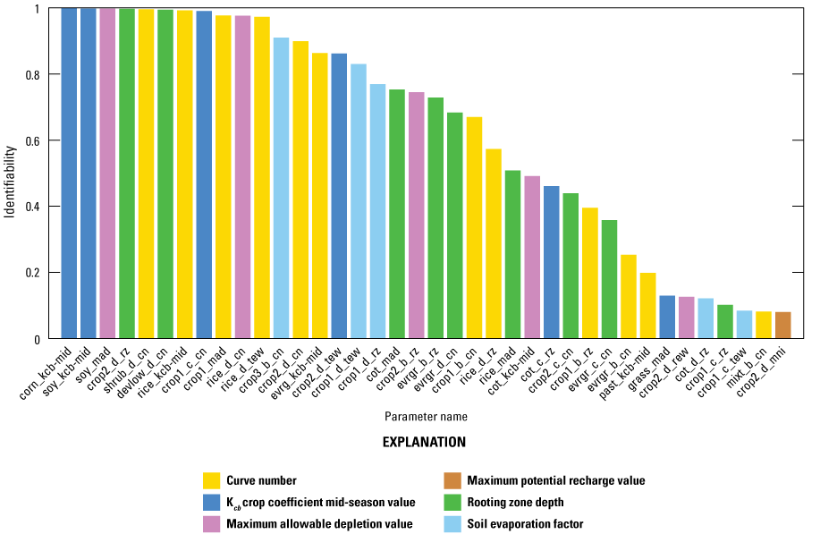
Parameter identifiability for the 35 most-sensitive parameters in the Mississippi Alluvial Plain Soil-Water-Balance model.
Discussion
The modeling of water budget components of the Mississippi embayment region study area using the SWB model has provided an opportunity for new insight into how the hydrologic system behaves and how water moves in the system. This is particularly true of the processes that are involved in recharge to the groundwater of the unconfined alluvial plain aquifer that underlies the Mississippi Alluvial Plain. Comparing the performance of the model to observed values also provides some insight into the strengths and limitations of the SWB model itself. Findings from this study can be used in potential future work to improve our understanding of the system even further.
Unique Characteristics of the Mississippi Alluvial Plain
Understanding the movement of water within the Mississippi Alluvial Plain is extremely challenging. Irrigation return flows change the shape of observed hydrographs and increase base flow during irrigation operations. Perched water tables intercept flow from the root zone and create isolated pockets of groundwater storage that are disconnected from the regional system. Backwater during flood season modifies the shape of the hydrograph further. The numerous duck and catfish ponds create surface-water features that potentially could supply focused recharge to the underlying aquifer.
The sediments making up the alluvial plain were laid down over thousands of years of work and re-work by the Mississippi River and other Mississippi Alluvial Plain rivers, resulting in layers of clay, sand, and silt, oxbow lakes, and possible perched water tables (O’Reilly and others, 2020). Infiltrated water must pass through the overlying unsaturated zone, which consists of a heterogeneous mixture of silt, clay, and sand, before it becomes recharge when it reaches the water table. Silt and clay predominate at the surface and to a depth greater than 100 feet in many areas, particularly in the southern part of the alluvial aquifer (Arthur, 1994). The surficial sediments generally coarsen to the north, although pockets of sand are found at the surface throughout the alluvial plain. The heterogeneous structure of the surficial sediments was investigated by Minsley and others (2021), using large-scale airborne geophysical surveys of the region. Shallow aquifer connectivity and geologic structures mapped by this effort have identified previously unmapped paleochannels, areas of high and low surface connectivity, as well as fault structures. Water passing through the root zone in the Mississippi Alluvial Plain either passes through this mélange of sediments to become recharge to the underlying aquifer, or, if the rate of water passing the rooting zone is too great to move through the more impermeable sediments, the water is either diverted to shallow surface-water bodies such as the local river and stream network (Dunne and Leopold, 1978)—or it could be diverted horizontally to a zone with a greater surface connection to the underlying aquifer.
Perkins and others (2011, “Summary” section) describe observations of this phenomenon in the study area. In describing the transport mechanisms within and below the root zone in a fallow soybean field, they found
“Lateral flow of water at shallow depths was extensive and spatially non-uniform, reaching up to 10m from the [tracer infiltration] pond within 2 months. Within 1 month, the wetting front reached a textural boundary at 4–5m between the fine-textured soil and sandy alluvium, now a potential capillary barrier which, prior to extensive irrigation withdrawals, was below the water table. Within 10 weeks, tracer was detectable at the water table which is presently about 12m below land surface. Results indicate that 43% of percolation may be through preferential flow paths and that any water breaking through the capillary barrier (as potential recharge) likely does so in fingers which are difficult to detect with coring methods.”
Evapotranspiration Estimates
The calibration of the SWB model to the monthly actual ET data from Reitz and others (2017) was generally successful, as measured by the small amount of error in the ET simulated values compared to the other water budget terms (fig. 10). However, if we look at how that error is distributed over the months of the year, the SWB model as parameterized underpredicted actual ET relative to the observations for July, August, and September, and overpredicted the actual ET for November, December, January, and February. The land-use types with the largest actual ET summer discrepancy included corn, evergreen forest, and wetland forest (fig. 25). Crop actual ET observations were not used in the fall and winter, but the model overpredicted actual ET in all the forest types used in the observation dataset (deciduous, evergreen, and forested wetlands). This may indicate that in the summer, more water is retained within the rooting zone of these plants than SWB expects and does not drain out of the rooting zone, so that SWB calculations indicate soil moisture being drier than it actually is (and less water available for ET). In the winter, the SWB calibration may have some terms that cause the nongrowing season bare soil to lose more water to the atmosphere than it would in reality.
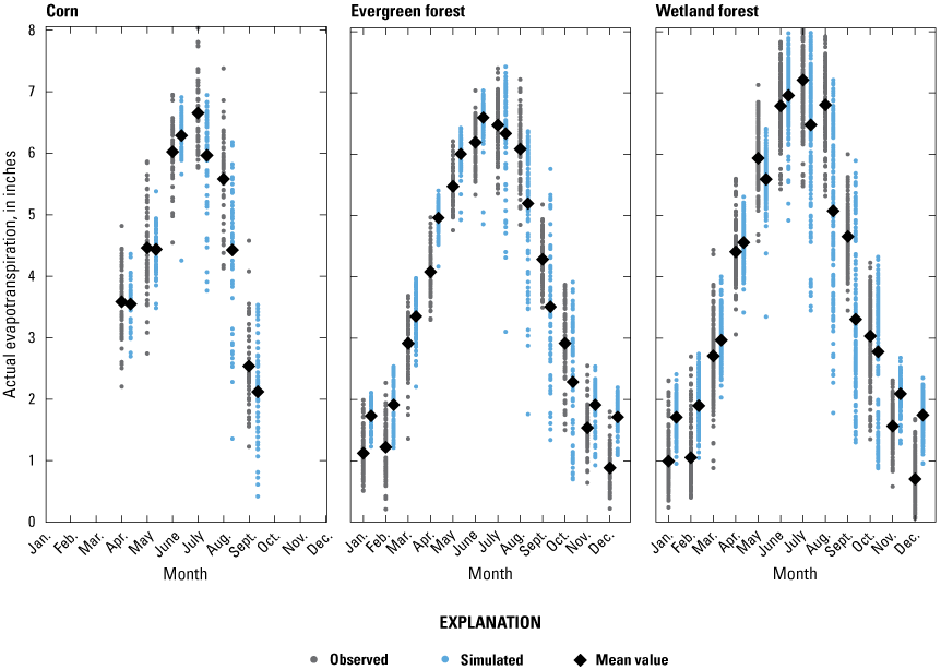
Monthly observed and simulated actual evapotranspiration values for corn, evergreen forest, and wetland forest.
Another comparison to ground-truth data that we used was comparing the daily actual ET simulations to eddy-covariance flux tower data in the study area (Reba, 2021; Runkle and others, 2017). Very little of these data existed in the study area at the time the calibration was done, so the data were not used during the calibration, but some spot checks were done to ensure that the simulation was reproducing the annual cycle as recorded by these towers (fig. 26).
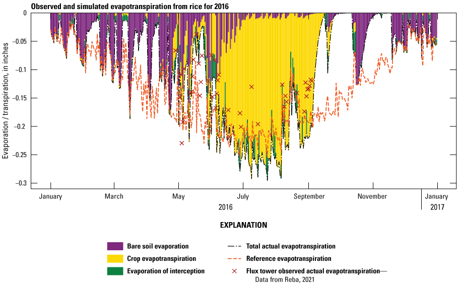
Daily potential and actual evapotranspiration simulated values and observations from an eddy-covariance flux tower in Humnoke, Arkansas.
Irrigation Estimates
As discussed previously in the “Model Fit to Observations” section and shown in figure 11, the ability of the SWB model to estimate irrigation for the Mississippi Alluvial Plain is acceptable for a growing season overall. In the Mississippi Delta area, the model generally reproduces the total inches of applied irrigation for rice, corn, soybeans, and cotton, but the monthly total amounts vary widely from the field-specific monitoring data provided by the MDEQ. One contributing factor for this could include the mismatch in the grid size of the SWB model (1 kilometer) compared to individual fields represented in that dataset. In addition, the SWB model does not include parameters that would represent all the factors that an individual farmer uses in making decisions on when and how much to irrigate a given crop. Given the sensitivity of the model to some of the ET and irrigation parameters that were used in the model, and the fact that additional variables in the SWB lookup tables for irrigation were not used as parameters in the calibration, additional work on irrigation calibration could improve the model performance overall. Generally, more field data on irrigation, better point data on ET, and better ET calibration would help in being able to more accurately model irrigation demands in this setting.
The irrigation efficiency setting in SWB is set by default to be 1.0 (100 percent efficiency, or no excess runoff generated from the applied water; all applied irrigation water goes to growing the plants and is converted to excess actual ET), but it is recognized that not all irrigation applied in the Mississippi Alluvial Plain area is 100-percent efficient. For example, irrigation is applied to rice fields to keep them in standing water, and the amount applied is not based specifically on how much water the plant needs for growth. The monthly county irrigation estimates used in the model calibration (AIWUM model, version 1.0) are not sufficiently detailed to evaluate whether the SWB model irrigation efficiency setting was appropriate. The MDEQ data, which were used to verify the SWB irrigation amounts, helped to properly set the irrigation efficiency settings. Initially, with all crops set to 100-percent efficiency, the SWB-estimated rice irrigation rates were about 50 percent of what they should be. After decreasing the rice efficiency to 0.5, the overall irrigation rates for each of these crops fell to within a close match of the MDEQ data (fig. 11).
Recharge Versus Net Infiltration
As stated earlier, one of the most important things to keep in mind when using the SWB water budget results for the Mississippi Alluvial Plain is that the amount of water leaving the root zone as net infiltration is rarely the same as the amount of water that joins the water table as recharge. In other parts of the country, it is easy to conflate net infiltration and recharge because they are similar in magnitude. In the Mississippi Alluvial Plain, much of the water that SWB calculates to be leaving the root zone never makes it to the local water table as recharge.
This Soil-Water-Balance study of the Mississippi Embayment Region is part of an integrated analysis of the groundwater hydrology in the Mississippi Alluvial Plain. Two other concurrent studies integrate with the net infiltration results to provide some important insights into groundwater recharge in the alluvial plain aquifer. A large remote-sensing study using aerial electromagnetic techniques (Minsley and others, 2021) provided a new, detailed interpretation of the near-surface stratigraphy above the alluvial plain aquifer. One product of that study provided datasets on the hydraulic connectivity between the surface and underlying aquifer (James and Minsley, 2021), which shows the relative amount of connection between water movement and availability at the land surface with the underlying alluvial aquifer. The aerial electromagnetic surface connectivity zones used values ranging from −3 (for low connectivity) to 3 (for high connectivity). The second integrative effort was a series of regional MODFLOW 6 (Langevin and others, 2017, 202236) groundwater models for several of the generalized regions in the alluvial plain. The Delta MODFLOW 6 model (Leaf and others, 2023) used the SWB net infiltration simulations and the surface connectivity data in calibrating the spatial distribution of total recharge to the underlying aquifer.
Comparison of Model-Calibrated Recharge and Soil-Water-Balance Net Infiltration
Recall that previous investigations of recharge to the alluvial plain aquifer suggested about 2–5 inches of annual recharge, whereas the annual net infiltration rates produced by the SWB model range from 5.7 to 12.5 inches per year. To learn more about the difference between recharge to the groundwater system and the net infiltration simulated by SWB in the Mississippi Alluvial Plain, SWB net infiltration was compared to the model-calibrated recharge in the Mississippi Delta region of the Mississippi Alluvial Plain (Leaf and others, 2023). The monthly SWB net infiltration simulations were given as input to the Delta MODFLOW 6 model calibration, and the amount reaching the water table as recharge was calibrated by history matching of well hydrographs and streamflow under the observed pumping stresses in the region. The Delta MODFLOW 6 model domain is shown in figure 27.
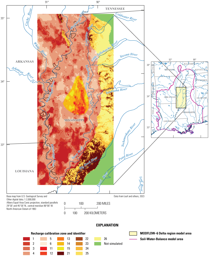
Recharge calibration zones in the Delta region MODFLOW 6 model area.
To condition the MODFLOW 6 model calibration, a grid of zones representing more- and less-transmissive sediments was provided, such that each zone was allowed to pass a unique percentage of the SWB net infiltration through as recharge. The geophysical investigations provided the primary source (specifically, the surface connectivity) for the recharge calibration zones (James and Minsley, 2021). In addition to the connectivity zones, additional geologic terrane zones were used in the final MODFLOW 6 recharge calibration zones (fig. 27).
The resulting calibrated recharge to the alluvial aquifer in the MODFLOW 6 model for 2 water years (a water year is a 12-month period from October 1 to the following September 30 and is designated by the year in which it ends), 2017 and 2018, is compared to the SWB net infiltration (fig. 28). The total amount of recharge averaged over the Delta region was 2.09 and 4.11 inches, respectively, for these 2 years in the calibrated model, which is in agreement with previous estimates. The SWB net infiltration for these years is 6.54 and 9.45 inches, respectively. The previous estimates of recharge, unlike the current studies, had no spatial heterogeneity information. Compared to the SWB net infiltration, the calibrated recharge (using the connectivity zones to condition the spatial distribution) is much more heterogeneous. The difference between the two sets of information reveals that in some areas the calibrated recharge is actually many inches greater than the net infiltration in that location. What can this reveal about how recharge actually behaves in this system?
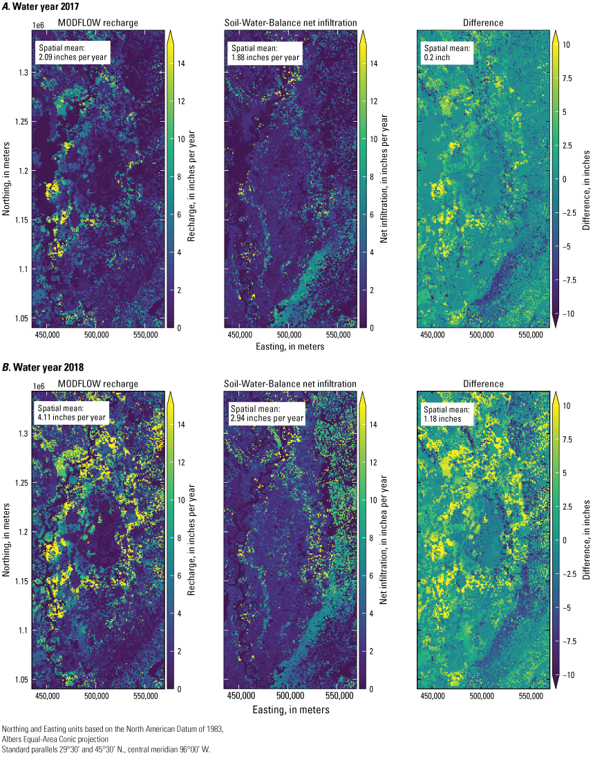
Comparisons of calibrated recharge to net infiltration simulations for the Delta region MODFLOW 6 model area, water years 2017 and 2018.
From these observations, we suggest that the spatial differences in the calibrated recharge and the net infiltration may be the result of focused recharge zones through the surficial sediments overlying the alluvial aquifer, and some perching and lateral movement of groundwater may be happening within the unsaturated zone. The excess simulated net infiltration that does not become actual recharge likely discharges back to the surface-water system downstream from the watershed in which the infiltration occurred.
Potential Future Work
Incorporating new datasets into the calibration approach could further constrain the simulated water budget components. Providing additional constraints to these water budget components could, in turn, constrain the net infiltration estimate.
Any future work could consider including one or more of the following improvements to the methods or observations:
-
• Chemical base-flow separation: use chloride or specific conductivity data to adjust the runoff-base flow proportions in the alluvial plain area
-
• Curve-number-aligner: add this simple curve-number estimator (Hawkins and others, 2009) to the PEST process to constrain runoff curve numbers to values that increase numerically relative to soil type
-
• Flux tower actual ET: add estimates of ET from flux tower datasets to the observations; this allows for greater confidence that crop growth timing is correct
-
• Real-time water-use gages: provide a carefully curated set of real-time water-use gage data to the calibration process
-
• Stepwise calibration: perform model calibration of ET first and then the other variables.
-
• Growing degree-days: define Kcb curves in terms of growing degree days rather than day of year; this will allow key inflection points in the Kcb curves to respond to changing climate over time.
-
• High-resolution daily weather: use high-resolution daily weather drivers for past and future conditions to drive SWB in a consistent manner
-
• Determine if an algorithm for estimating infiltration of ponded water from aquaculture and duck ponds (in rice fields) can be developed.
Summary and Conclusions
We constructed a Soil-Water-Balance (SWB) model for the Mississippi Embayment Region for 2000–20 as part of an integrated assessment of groundwater availability for the Mississippi Alluvial Plain aquifer and surrounding areas. This study built upon previous SWB modeling efforts in the area around the Mississippi Alluvial Plain to better understand the spatial patterns and uncertainty in calculations of net infiltration, evapotranspiration (ET), and runoff. Herein, we aimed to provide simulations of net infiltration to serve as an initial estimate of potential recharge for several groundwater flow models in the study area, which used parameter estimation calibration methods to refine the spatial distribution of recharge reaching the water table given new vertical surface connectivity data obtained from airborne electromagnetic geophysical studies in the Mississippi Alluvial Plain region. The SWB model provided calculations of water available for recharge (net infiltration) as part of a complex series of calculations partitioning daily incoming precipitation into its component pathways (primarily actual evapotranspiration, runoff, and net infiltration).
The SWB model of the Mississippi embayment region was calibrated using more types of observations than the earlier SWB model, which enabled the calibration to have a better balance between each of the primary outputs (actual ET, runoff, and net infiltration). In addition, this modeling effort incorporated an uncertainty evaluation using null-space Monte Carlo analysis and several hundred alternate model realizations to derive a confidence interval around the final estimates of net infiltration.
SWB calculates net infiltration by dividing inputs to the hydrologic system being modeled (precipitation and snowmelt) into fractions of direct runoff, plant interception (and subsequent evaporation), soil infiltration, ET by plants, bare soil evaporation, soil moisture storage, rejected recharge, and infiltration of excess soil moisture beyond the rooting zone (net infiltration). For this study, direct runoff and rejected recharge are added together into a combined “runoff” term. The data inputs required for running this SWB model consist of (a) grids describing the study domain (land use, hydrologic soil groups, and soil available water capacity); (b) grids of daily climate data; (c) lookup table values for the water balance calculations that include runoff curve numbers, maximum potential infiltration rates, maximum rooting depths for the vegetation types, and information on how interception is handled; and (d) lookup table values for the implementation of the Food and Agriculture Organization of the United Nations Irrigation and Drainage Paper 56 method ET calculations, including plant growth crop coefficient values, growing season and irrigation season lengths, bare soil evaporation settings, and other irrigation settings.
The U.S. Department of Agriculture’s National Agricultural Statistical Service Cropland Data Layer (CDL) for 2008–20 composed the primary land-use data used in the model. Because CDL data were not available from 2000 to 2007, CDL data for 2010–17 were applied to 2000–2007. Hydrologic soil groups and the available water capacity input grids were from the U.S. Department of Agriculture Natural Resources Conservation Service (gridded national soil survey geographic database). The hydrologic soil groups are used in SWB alongside the land-use categories to classify the landscape into combinations of land use/vegetation and soil texture that should, in theory, transmit water similarly through the rooting zone and unsaturated zone to the water table under the same climatic conditions. We used PRISM datasets for the required daily climate inputs. The SWB model for the Mississippi embayment region was constructed using a 1-kilometer grid spacing consisting of 661 rows, and 989 columns.
We calibrated the SWB model for the Mississippi embayment region using the Parameter Estimation Iterative Ensemble Smoother (PEST++, version 5) to adjust 546 parameters controlling model output. To reduce the predictive uncertainty in the model, observations compared to model output from four water budget terms were used in the calibration: actual ET, runoff, net infiltration, and irrigation. We used more than 4,900 monthly ET observations, 1,780 annual runoff and potential recharge observations, 5,983 monthly runoff and potential recharge observations, and more than 3,000 monthly county-based irrigation estimates as observations. The model parameters included values for the SWB lookup tables including curve numbers, maximum rooting depths, maximum soil infiltration rates, plant growth factors, bare soil evaporation factors, and irrigation management parameters.
The best-fit model calibration yielded a model with an overall coefficient of determination (r2) of 0.72 and a standard error of 0.004. The model simulated the actual ET values somewhat better than the net infiltration and runoff. The actual ET, runoff, and net infiltration simulations each have a coefficient of determination (r2) of 0.89, 0.91, and 0.90, respectively, compared to the observed values. The actual ET and runoff values have a small amount of skew in the residuals—in both cases the model overpredicts somewhat when the values are low and underpredicts when the values are higher than average. In an analysis of watersheds across the study area, the observations of net infiltration and runoff were more accurately simulated in watersheds outside of the alluvial plain. Although the model’s prediction of monthly irrigation rates did not perform as well as the other terms, the simulated values for total annual irrigation rates compare favorably with annual reported field values from the Mississippi Department of Environmental Quality for corn, soybeans, and rice. Overall, this model of water balance terms has an overall better fit and less skewed simulated values compared to the observations than an earlier SWB model of the Mississippi embayment region.
There is considerable spatial variability in all the water balance terms in the Mississippi embayment region SWB model, primarily because of the spatial variability in the input precipitation, which ranges from over 65 inches per year near the gulf coast to about 50 inches per year in the northwestern and western part of the model domain. Cropland irrigation adds an additional 4.9 to 10.4 inches of water to the land surface where there are irrigated crops in the alluvial plain area. Actual ET accounts for most of the water leaving the land surface, ranging from 62 to 72 percent of the incoming precipitation. Runoff accounts for about 20 percent of the precipitation over most of the model area, except in the far southern coastal areas where it accounts for 30 percent of the precipitation. Net infiltration (not to be confused with actual recharge), averages 7.6 inches per year across the whole model domain but is higher in the alluvial plain area (5.7–12.5 inches per year), and accounts for 11 to 17 percent of the precipitation. Simulated irrigation water demand for the generalized regions of the alluvial plain ranges from 4.9 to 10.3 inches per year (over the whole area, not just crop areas). Irrigation varies considerably by year, depending on the amount of rainfall during the summer and by crop type. Rice irrigation rates (about 20–25 inches per year) were three to four times higher than corn, cotton, and soybeans (5–10 inches per year).
Monthly variability in the precipitation across the Mississippi Alluvial Plain area also drives the seasonal water budget. Following the variability in monthly precipitation over the year and temperature-driven increases in actual ET in the summer months, the runoff and net infiltration components also are highly seasonal and are much higher in the fall and winter than in the summer. Without applied irrigation across the alluvial plain area, the net infiltration and runoff in the summer would approach zero in that area.
The use of PEST as a calibration tool allowed for quantitative analysis of the uncertainty in the model results that is driven by uncertainty in the calibration parameters. Other factors also contribute to the overall model uncertainty, but because they are either nonvarying components of the model (such as the available water capacity grid) or do not lend themselves to variability testing (such as the climate data or land use data), they cannot be changed to evaluate their contribution to the total uncertainty. We used a Monte Carlo approach and the PEST++ Iterative Ensemble Smoother tools used for parameter estimation to run an ensemble of 350 alternate model runs, using 290 of these runs that met criteria for acceptable model error (ϕ) to develop standard deviation grids of the monthly and annual values for actual ET, irrigation, net infiltration, and runoff. The standard deviation grids were applied to 58 watersheds across the study area, and 95-percent confidence intervals were calculated. The 95-percent confidence intervals were then expressed as a percent uncertainty for each of the water budget terms. The uncertainty in actual ET is the lowest, at 5 percent. The uncertainty for the irrigation, net infiltration, and runoff simulations is highly variable across the study area but averages around 20 percent. On a monthly basis, the uncertainty is focused on the actual ET and irrigation in the summer months (when they are the largest water budget component), and the net infiltration and runoff uncertainty contribute the most to the late fall and winter overall uncertainty in the model.
The modeling of water budget components of the Mississippi embayment region study area using the SWB model has provided an opportunity for new insight into how the hydrologic system behaves and how water moves in the system. Previous geologic and hydrologic investigations in the alluvial plain and the alluvial aquifer have shown that the unsaturated zone above the water table in the alluvial aquifer is a complex series of layers of clay, sand and silt, oxbow lakes, and possible perched water tables. Recent geophysical investigations elucidating the hydraulic connectivity of the land surface with the deeper saturated sediments have been combined with groundwater flow modeling and the SWB net infiltration estimates to develop a better understanding of the spatial heterogeneity in deep percolation (recharge) to the alluvial aquifer. The calibrated recharge in a groundwater flow model in the Mississippi Delta region was overall several inches less than the SWB net infiltration, but it was much more focused on areas with higher surface connectivity and was substantially higher than the SWB net infiltration in several areas. Other field-level studies of infiltration in the unsaturated zone revealed horizontal flow of water beneath the rooting zone. These results suggest that some of the excess net infiltration becomes focused groundwater recharge and some of it likely returns to surface water downgradient.
Findings from this study can be used in potential future work to improve our understanding of the system even further. Some topics that could be further investigated include possible focused recharge zones through the surficial sediments overlying the alluvial aquifer, incorporating flux-tower evapotranspiration measurements in model calibration, using chemical base-flow separation to evaluate surface runoff and groundwater recharge patterns, incorporating higher-resolution water use data into model calibration, and determining if a method to evaluate infiltration of ponded water from aquaculture and duck ponds (in rice fields) can be developed.
Acknowledgments
We would like to thank the U.S. Geological Survey Water Resources Assessment Program who provided funding for this work. Also, thank you to David A. Ladd, U.S. Geological Survey, for preparing many of the input gridded data files used in the Soil-Water-Balance model for this study.
References Cited
Ackerman, D.J., 1989, Hydrology of the Mississippi River Valley alluvial aquiver, south-central United States—A preliminary assessment of the regional flow system: U.S. Geological Survey Water-Resources Investigations Report 88–4028, 74 p., accessed July 26, 2021, at https://doi.org/10.3133/wri884028.
Ackerman, D.J., 1996, Hydrology of the Mississippi River Valley alluvial aquifer, south-central United States: U.S. Geological Survey Professional Paper 1416–D, 56 p., accessed July 26, 2021, at https://doi.org/10.3133/pp1416D.
Allen, R.G., Pereira, L.S., Raes, D., and Smith, M., 1998, Crop evapotranspiration—Guidelines for computing crop water requirements: Rome, Food and Agriculture Organization of the United Nations, Irrigation and Drainage Paper 56, 174 p. [Also available at http://www.fao.org/3/X0490E/x0490e00.htm#Contents.]
Anderson, M.P., Woessner, W.W., and Hunt, R.J., 2015, Applied groundwater modeling—Simulation of flow and advective transport (2d ed.): Elsevier, 564 p. [Also available at https://doi.org/10.1016/C2009-0-21563-7.]
Arthur, J.K., 1994, Thickness of the upper and lower confining units of the Mississippi River alluvial aquifer in northwestern Mississippi: U.S. Geological Survey Water-Resources Investigations Report 94–4172, 1 plate, accessed December 19, 2022, at https://doi.org/10.3133/wri944172.
Arthur, J.K., and Taylor, R.E., 1998, Ground-water flow analysis of the Mississippi embayment aquifer system, south-central United States: U.S. Geological Survey Professional Paper 1416–I, 148 p., accessed July 26, 2021, at https://doi.org/10.3133/pp1416I.
Arthur, J.K., 2001, Hydrogeology, model description, and flow analysis of the Mississippi River alluvial aquifer in northwestern Mississippi: U.S. Geological Survey Water-Resources Investigations Report 2001–4035, 47 p., accessed July 26, 2021, at https://doi.org/10.3133/wri014035.
Barlow, P.M., Cunningham, W.L., Zhai, T., and Gray, M., 2015, U.S. Geological Survey Groundwater Toolbox, a graphical and mapping interface for analysis of hydrologic data (version 1.0)—User guide for estimation of base flow, runoff, and groundwater recharge from streamflow data: U.S. Geological Survey Techniques and Methods, book 3, chap. B10, 27 p., accessed October 2017 at https://doi.org/10.3133/tm3B10.
Boswell, E.H., Cushing, E.M., Hosman, R.L., and Jeffery, H.G., 1968, Quaternary aquifers in the Mississippi embayment, chap. E. of Water resources of the Mississippi embayment: U.S. Geological Survey Professional Paper 448–E, 15 p., 2 plates, accessed February 28, 2020, at https://doi.org/10.3133/pp448E.
Brahana, J.V., and Broshears, R.E., 2001, Hydrogeology and ground-water flow in the Memphis and Fort Pillow aquifers in the Memphis area, Tennessee: U.S. Geological Survey Water-Resources Investigations Report 89–4131, 56 p., accessed July 27, 2021, at https://doi.org/10.3133/wri894131.
Brahana, J.V., and Mesko, T.O., 1988, Hydrogeology and preliminary assessment of regional flow in the upper Cretaceous and adjacent aquifers in the northern Mississippi embayment: U.S. Geological Survey Water-Resources Investigations Report 87–4000, accessed July 26, 2021, at https://doi.org/10.3133/wri874000.
Broom, M.E., and Reed, J.E., 1973, Hydrology of the Bayou Bartholomew alluvial aquifer-stream system, Arkansas: U.S. Geological Survey Open-File Report 73–34, 91 p., accessed July 26, 2021, at https://doi.org/10.3133/ofr7334.
Clark, B.R., and Hart, R.M., 2009, The Mississippi Embayment Regional Aquifer Study (MERAS)—Documentation of a groundwater-flow model constructed to assess water availability in the Mississippi embayment: U.S. Geological Survey Scientific Investigation Report 2009–5172, 61 p., accessed July 26, 2021, at https://doi.org/10.3133/sir20095172.
Clark, B.R., Hart, R.M., and Gurdak, J.J., 2011, Groundwater availability of the Mississippi embayment: U.S. Geological Survey Professional Paper 1785, 62 p., accessed July 26, 2021, at https://doi.org/10.3133/pp1785.
Clark, B.R., Westerman, D.A., and Fugitt, D.T., 2013, Enhancements to the Mississippi Embayment Regional Aquifer Study (MERAS) groundwater-flow model and simulations of sustainable water-level scenarios: U.S. Geological Survey Scientific Investigations Report 2013–5161, 29 p., accessed July 26, 2021, at https://doi.org/10.3133/sir20135161.
Cronshey, R., McCuen, R., Miller, N., Rawls, W., Robbins, S., and Woodward, D., 1986, Urban hydrology for small watersheds: U.S. Department of Agriculture, Soil Conservation Service, Engineering Division, Technical Release 55, accessed November 28, 2017, at http://www.nrcs.usda.gov/Internet/FSE_DOCUMENTS/16/stelprdb1044171.pdf.
Cushing, E.M., Boswell, E.H., Speer, P.R., and Hosman, R.L., 1970, Availability of water in the Mississippi embayment, chap. A of Water resources of the Mississippi embayment: U.S. Geological Survey Professional Paper 448–A, 23 p., 7 plates, accessed July 26, 2021, at https://doi.org/10.3133/pp448A.
Doherty, J., 2004, PEST—Model-independent parameter estimation user manual (5th ed.): Brisbane, Australia, Watermark Numerical Computing, 336 p. [Also available at https://www.nrc.gov/docs/ML0923/ML092360221.pdf.]
Doherty, J.E., and Hunt, R.J., 2009, Two statistics for evaluating parameter identifiability and error reduction: Journal of Hydrology, v. 366, no. 1–4, p. 119–127. [Also available at https://doi.org/10.1016/j.jhydrol.2008.12.018.]
Doherty, J.E., and Hunt, R.J., 2010, Approaches to highly parameterized inversion—A guide to using PEST for groundwater-model calibration: U.S. Geological Survey Scientific Investigations Report 2010–5169, 59 p. [Also available at https://doi.org/10.3133/sir20105169.]
Falgout, J.T., Gordon, J., Williams, B., and Davis, M.J., 2022, Advanced Research Computing (ARC): U.S. Geological Survey web page, accessed February 2022 at https://doi.org/10.5066/P9PSW367.
Fienen, M.N., Haserodt, M.J., Leaf, A.T., and Westenbroek, S.M., 2022, Simulation of regional groundwater flow and groundwater/lake interactions in the Central Sands, Wisconsin: Scientific Investigations Report 2022–5046, 128 p., accessed April, 2023 at https://doi.org/10.3133/sir20225046.
Gratzer, M.C., Davidson, G.R., O’Reilly, A.M., and Rigby, J.R., 2020, Groundwater recharge from an oxbow lake-wetland system in the Mississippi Alluvial Plain: Hydrological Processes, v. 34, no. 6, p. 1359–1370, accessed July 29, 2021, at https://doi.org/10.1002/hyp.13680.
Halford, K.J., and Mayer, G.C., 2000, Problems associated with estimating ground water discharge and recharge from stream-discharge records: Groundwater, v. 38, no. 3, p. 331–342. [Also available at https://doi.org/10.1111/j.1745-6584.2000.tb00218.x.]
Healy, R.W., 2010, Estimating groundwater recharge: Cambridge University Press, 245 p. [Also available at https://doi.org/10.1017/CBO9780511780745.]
James, S.R., and Minsley, B.J., 2021, Combined results and derivative products of hydrogeologic structure and properties from airborne electromagnetic surveys in the Mississippi Alluvial Plain: U.S. Geological Survey data release, accessed May 2021 at https://doi.org/10.5066/P9382RCI.
Jette, M., and Grondona, M., 2003, SLURM—Simple Linux Utility for Resource Management, in ClusterWorld Conference and Expo, San Jose, Calif., June 23–26, 2003, Proceedings: San Jose, Calif., Lawrence Livermore National Laboratory, 31 p., accessed December 1, 2022, at https://slurm.schedmd.com/slurm_design.pdf.
Killian, C.D., Asquith, W.H., Barlow, J.R.B., Bent, G.C., Kress, W.H., Barlow, P.M., and Schmitz, D.W., 2019, Characterizing groundwater and surface-water interaction using hydrograph-separation techniques and groundwater-level data throughout the Mississippi Delta, USA: Hydrogeology Journal, v. 27, no. 6, p. 2167–2179. [Also available at https://doi.org/10.1007/s10040-019-01981-6.]
Kresse, T.M., and Clark, B.R., 2008, Occurrence, distribution, sources, and trends of elevated chloride concentrations in the Mississippi River Valley alluvial aquifer in southeastern Arkansas: U.S. Geological Survey Scientific Investigations Report 2008–5193, 34 p., accessed July 26, 2021, at https://pubs.er.usgs.gov/publication/sir20085193.
Ladd, D.E., and Travers, L.R., 2019, Generalized regions of the Mississippi Alluvial Plain: U.S. Geological Survey data release, accessed April 2020 at https://doi.org/10.5066/P915ZZQM.
Langevin, C.D., Hughes, J.D., Banta, E.R., Provost, A.M., Niswonger, R.G., and Panday, S., 2017, MODFLOW 6 Modular Hydrologic Model: U.S. Geological Survey Software, available online at https://doi.org/10.5066/F76Q1VQV.
Langevin, C.D., Hughes, J.D., Provost, A.M., Russcher, M.J., and Niswonger, R.G., Panday, S., Merrick, D., Morway, E.D., Reno, M.J., Bonelli, W.P., and Banta, E.R., 2022, MODFLOW 6 Modular Hydrologic Model version 6.4.1: U.S. Geological Survey Software Release, 9 December 2022, available online at https://doi.org/10.5066/P9FL1JCC.
Leaf, A.T., Duncan, L.L., Haugh, C.J., Hunt, R.J., and Rigby, J.R., 2023, Simulating groundwater flow in the Mississippi Alluvial Plain with a focus on the Mississippi Delta: U.S. Geological Survey Scientific Investigations Report 2023–5100, 143 p., https://doi.org/10.3133/sir20235100.
Lovelace, J.K., Nielsen, M.G., Read, A.L., Murphy, C.J., and Maupin, M.A., 2020, Estimated groundwater withdrawals from principal aquifers in the United States, 2015 (ver. 1.2, October 16, 2020): U.S. Geological Survey Circular 1464, 70 p., accessed October 20, 2020, at https://doi.org/10.3133/cir1464.
Mahon, G.L., and Ludwig, A.H., 1990, Simulation of ground-water flow in the Mississippi River Valley alluvial aquifer in eastern Arkansas: U.S. Geological Survey Water-Resources Investigations Report 89–4145, accessed July 26, 2021, at https://doi.org/10.3133/wri894145.
Mahon, G.L., and Poynter, D.T., 1993, Development, calibration, and testing of ground-water flow models for the Mississippi River Valley alluvial aquifer in eastern Arkansas using one-square-mile cells: U.S. Geological Survey Water-Resources Investigations Report 92–4106, 33 p. [Also available at https://doi.org/10.3133/wri924106.]
McKee, P.W., and Clark, B.R., 2003, Development and calibration of a ground-water flow model for the Sparta Aquifer of southeastern Arkansas and north-central Louisiana and simulated response to withdrawals, 1998–2027: U.S. Geological Survey Water-Resources Investigations Report 2003–4132, 71 p., accessed July 26, 2021, at https://doi.org/10.3133/wri034132.
Minsley, B.J., Rigby, J.R., James, S.R., Burton, B.L., Knierim, K.J., Pace, M.D.M., Bedrosian, P.A., and Kress, W.H., 2021, Airborne geophysical surveys of the lower Mississippi Valley demonstrate system-scale mapping of subsurface architecture: Communications Earth & Environment, v. 2, no. 1, 131 p., accessed June 30, 2021, at https://www.nature.com/articles/s43247-021-00200-z.
Mississippi Department of Environmental Quality, 2022, Delta Voluntary Metering Program: Mississippi Department of Environmental Quality web page, accessed August 11, 2022, at https://www.mdeq.ms.gov/water/water-availability-and-use/delta-voluntary-metering-program/.
Nielsen, M.G., and Westenbroek, S.M., 2019, Groundwater recharge estimates for Maine using a Soil-Water-Balance model—25-year average, range, and uncertainty, 1991 to 2015: U.S. Geological Survey Scientific Investigations Report 2019–5125, 56 p., accessed January 2020 at https://doi.org/10.3133/sir20195125.
O’Reilly, A.M., Holt, R.M., Davidson, G.R., Patton, A.C., and Rigby, J.R., 2020, A dynamic water balance/nonlinear reservoir model of a perched phreatic aquifer–river system with hydrogeologic threshold effects: Water Resources Research, v. 56, no. 6, 27 p., accessed September 2022 at https://doi.org/10.1029/2019WR025382.
Painter, J.A., and Westerman, D.A., 2018, Mississippi Alluvial Plain Extent, November 2017: U.S. Geological Survey data release, accessed July 2019 at https://doi.org/10.5066/F70R9NMJ.
Perkins, K.S., Nimmo, J.R., Rose, C.E., and Coupe, R.H., 2011, Field tracer investigation of unsaturated zone flow paths and mechanisms in agricultural soils of northwestern Mississippi, USA: Journal of Hydrology, v. 396, no. 1–2, 11 p., accessed August 2019 at https://doi.org/10.1016/j.jhydrol.2010.09.009.
PRISM Climate Group and Oregon State University, 2022, PRISM climate data: Northwest Alliance for Computation Science & Engineering website, accessed November 22, 2022, at https://prism.oregonstate.edu/.
Reba, M.L., 2021, Dataset: AmeriFlux BASE US-HRC Humnoke Farm Rice Field – Field C: AmeriFlux Monitoring Project, accessed May 2023 at https://doi.org/10.17190/AMF/1543375.
Reed, T.B., 2003, Recalibration of a ground-water flow model of the Mississippi River Valley alluvial aquifer of northeastern Arkansas, 1918–1998, with simulations of water levels caused by projected ground-water withdrawals through 2049: U.S. Geological Survey Water-Resources Investigations Report 03–4109, 58 p., accessed July 26, 2021, at https://doi.org/10.3133/wri034109.
Reitz, M., and Kress, W.H., 2019, The use of national datasets to produce an average annual water budget for the Mississippi Alluvial Plain, 2000–13: U.S. Geological Survey Fact Sheet 2019–3001, 4 p., accessed August 24, 2021, at https://doi.org/10.3133/fs20193001.
Reitz, M., Sanford, W.E., Senay, G.B., and Cazenas, J., 2017, Annual estimates of recharge, quick-flow runoff, and evapotranspiration for the contiguous U.S. using empirical regression equations: Journal of the American Water Resources Association, v. 53, no. 4, p. 961–983. [Also available at https://doi.org/10.1111/1752-1688.12546.]
Rigby, J.R., and Kress, W., 2019, @ Mississippi Alluvial Plain (MAP) regional water-availability study: U.S. Geological Survey data release, accessed July 2023 at https://www.sciencebase.gov/catalog/item/58a5d9c5e4b057081a24f3fd.
Runkle, B.R.K., Rigby, J.R., Reba, M.L., Anapalli, S.S., Bhattacharjee, J., Krauss, K.W., Liang, L., Locke, M.A., Novick, K.A., Sui, R., Suvočarev, K., and White, P.M., 2017, Delta-flux—An eddy covariance network for a climate-smart lower Mississippi Basin: ael, v. 2, no. 1, https://doi.org/10.2134/ael2017.01.0003.
Schilling, O.S., Cook, P.G., and Brunner, P., 2019, Beyond classical observations in hydrogeology—The advantages of including exchange flux, temperature, tracer concentration, residence time, and soil moisture observations in groundwater model calibration: Reviews of Geophysics, v. 57, no. 1, p. 146–182. [Also available at https://doi.org/10.1029/2018RG000619.]
Soil Survey Staff, 2019, Gridded National Soil Survey Geographic (gNATSGO) database for the conterminous United States: U.S. Department of Agriculture, Natural Resources Conservation Service web page, accessed December 1, 2019, at https://nrcs.app.box.com/v/soils.
Stanton, G.P., and Clark, B.R., 2003, Recalibration of a ground-water flow model of the Mississippi River Valley alluvial aquifer in southeastern Arkansas, 1918, with simulations of hydraulic heads caused by projected ground-water withdrawals through 2049: U.S. Geological Survey Water-Resources Investigations Report 2003–0432, 48 p., accessed October 19, 2022, at https://doi.org/10.3133/wri034232.
Sumner, D.M., and Wasson, B.E., 1990, Geohydrology and simulated effects of large ground-water withdrawals on the Mississippi River alluvial aquifer in northwestern Mississippi: U.S. Geological Survey Water-Supply Paper 2292, 60 p., accessed February 28, 2020, at https://doi.org/10.3133/wsp2292.
U.S. Department of Agriculture [USDA], 2007, Hydrologic soil groups, chap. 7 of Hydrology, pt. 630 of National engineering handbook: U.S. Department of Agriculture, p. 7-1–7-5. [Also available at https://directives.sc.egov.usda.gov/OpenNonWebContent.aspx?content=17757.wba.]
U.S. Department of Agriculture [USDA] National Agricultural Statistics Service, 2020, CropScape—Cropland Data Layer [2008–2020]: U.S. Department of Agriculture database, accessed June 15, 2020, at https://nassgeodata.gmu.edu/CropScape/.
U.S. Geological Survey, 2015, Mississippi River Valley alluvial aquifer, version 2.0, updated Feb, 2015: Ground Water Atlas of the United States HA–730–F, accessed online January 2019 at https://water.usgs.gov/lookup/getspatial?mississippi_river_valley_alluvial_aquifer.
U.S. Geological Survey, 2020, USGS water data for the nation: U.S. Geological Survey National Water Information System database, accessed April 10, 2020, at https://doi.org/10.5066/F7P55KJN.
U.S. Geological Survey, 2021, USGS Watershed Boundary Dataset (WBD) for 2-digit Hydrologic Unit–08 [published 20210310]: U.S. Geological Survey digital data, accessed March 9, 2021, at https://prd-tnm.s3.amazonaws.com/StagedProducts/Hydrography/WBD/HU2/GDB/WBD_08_HU2_GDB.zip.
Wacaster, S.R., 2020, Using tritium and general geochemistry to constrain estimates of recharge to the Mississippi River Valley alluvial aquifer: The University of Mississippi ProQuest Dissertations Publishing, M.S. thesis, 92 p., accessed October 19, 2022, at https://www.proquest.com/docview/2452988076/abstract/F44473CBB2174C6CPQ/1.
Westenbroek, S.M., Engott, J.A., Kelson, V.A., and Hunt, R.J., 2018, SWB version 2.0—A Soil-Water-Balance code for estimating net infiltration and other water-budget components: U.S. Geological Survey Techniques and Methods, book 6, chap. A59, 118 p., accessed January 1, 2019, at https://doi.org/10.3133/tm6A59.
Westenbroek, S.M., Kelson, V.A., Dripps, W.R., Hunt, R.J., and Bradbury, K.R., 2010, SWB—A modified Thornthwaite-Mather Soil-Water-Balance code for estimating groundwater recharge: U.S. Geological Survey Techniques and Methods, book 6, chap. A31, 60 p., accessed January 1, 2015, at https://doi.org/10.3133/tm6A31.
Westenbroek, S.M. and Nielsen, M.G., 2023, Model archive and output files for net infiltration, runoff, and irrigation water use for the Mississippi Embayment Regional Aquifer System, 2000 to 2020, simulated with the Soil-Water-Balance model: U.S. Geological Survey data release, https://doi.org/10.5066/P97KK17G.
Westenbroek, S.M., Nielsen, M.G., and Ladd, D.E., 2021, Initial estimates of net infiltration and irrigation from a Soil-Water-Balance model of the Mississippi Embayment Regional Aquifer Study area: U.S. Geological Survey Open-File Report 2021–1008, 29 p., accessed June 1, 2021, at https://doi.org/10.3133/ofr20211008.
White, J.T., 2018, A model-independent iterative ensemble smoother for efficient history-matching and uncertainty quantification in very high dimensions: Environmental Modelling & Software, v. 109, p. 191–201. [Also available at https://doi.org/10.1016/j.envsoft.2018.06.009.]
White, J.T., Fienen, M.N., and Doherty, J.E., 2016, A python framework for environmental model uncertainty analysis: Environmental Modelling & Software, v. 85, p. 217–228. [Also available at https://doi.org/10.1016/j.envsoft.2016.08.017.]
White, J.T., Hunt, R.J., Fienen, M.N., and Doherty, J.E., 2020, Approaches to highly parameterized inversion—PEST++ version 5, a software suite for parameter estimation, uncertainty analysis, management optimization and sensitivity analysis: U.S. Geological Survey Techniques and Methods, book 7, chap. C26, 52 p., accessed January 1, 2021, at https://doi.org/10.3133/tm7C26.
Wilson, J.L., 2021a, Aquaculture and Irrigation Water-Use Model (AIWUM) version 1.0—An agricultural water-use model developed for the Mississippi Alluvial Plain, 1999–2017: U.S. Geological Survey Scientific Investigations Report 2021–5011, 36 p., accessed May 2021 at https://doi.org/10.3133/sir20215011.
Wilson, J.L., 2021b, Aquaculture and Irrigation Water-Use Model (AIWUM) version 1.0 estimates and related datasets for the Mississippi Alluvial Plain, 1999–2017 (ver. 2.0, April 2021): U.S. Geological Survey data release, accessed May 2021 at https://doi.org/10.5066/P9JMO9G4.
Worland, S.C., Steinschneider, S., Asquith, W., Knight, R., and Wieczorek, M., 2019, Prediction and inference of flow duration curves using multioutput neural networks: Water Resources Research, v. 55, no. 8, p. 6850–6868. [Also available at https://doi.org/10.1029/2018WR024463.]
Xie, Y., and Lark, T.J., 2021, Mapping annual irrigation from Landsat imagery and environmental variables across the conterminous United States: Remote Sensing of Environment, v. 260, 17 p., accessed September 3, 2021, at https://doi.org/10.1016/j.rse.2021.112445.
Conversion Factors
Datum
Vertical coordinate information is referenced to the North American Vertical Datum of 1988 (NAVD 88).
Horizontal coordinate information is referenced to the North American Datum of 1983 (NAD 83).
Supplemental Information
The model grid size and model coordinate system are given in meters (m) in this report. The water budget terms are in inches per year (in/yr) or inches per month (in/mo).
Available water capacity is given in inches per foot of soil thickness (in/ft).
Abbreviations
AIWUM
Aquaculture and Irrigation Water-Use Model
CDL
Cropland Data Layer
ET
evapotranspiration
FAO56
Food and Agriculture Organization of the United Nations Irrigation and Drainage Paper 56
GLM
Gauss-Levenberg-Marquardt
gNATSGO
U.S. Department of Agriculture gridded National Soil Survey Geographic Database
HSG
hydrologic soil group
IES
Iterative Ensemble Smoother
Kcb
crop coefficient
MDEQ
Mississippi Department of Environmental Quality
MODFLOW 6
USGS modular three-dimensional finite-difference hydrologic simulation modeling package
PEST
Parameter ESTimation
SSEbop
operational Simplified Surface Energy Balance
SWB
Soil-Water-Balance
USDA
U.S. Department of Agriculture
USGS
U.S. Geological Survey
For more information about this publication, contact:
Director, USGS Upper Midwest Water Science Center
1 Gifford Pinchot Drive
Madison, WI 53726
For additional information, visit: https://www.usgs.gov/centers/upper-midwest-water-science-center
Publishing support provided by the Rolla Publishing Service Center
Disclaimers
Any use of trade, firm, or product names is for descriptive purposes only and does not imply endorsement by the U.S. Government.
Although this information product, for the most part, is in the public domain, it also may contain copyrighted materials as noted in the text. Permission to reproduce copyrighted items must be secured from the copyright owner.
Suggested Citation
Nielsen, M.G., and Westenbroek, S.M., 2023, Updated estimates of water budget components for the Mississippi embayment region using a Soil-Water-Balance model, 2000–2020: U.S. Geological Survey Scientific Investigations Report 2023–5080, 58 p., https://doi.org/10.3133/sir20235080
ISSN: 2328-0328 (online)
Study Area
| Publication type | Report |
|---|---|
| Publication Subtype | USGS Numbered Series |
| Title | Updated estimates of water budget components for the Mississippi Embayment Region using a soil-water-balance model, 2000–2020 |
| Series title | Scientific Investigations Report |
| Series number | 2023-5080 |
| DOI | 10.3133/sir20235080 |
| Publication Date | December 22, 2023 |
| Year Published | 2023 |
| Language | English |
| Publisher | U.S. Geological Survey |
| Publisher location | Reston, VA |
| Contributing office(s) | Upper Midwest Water Science Center |
| Description | Report: vii, 58 p.; Data Release; Dataset |
| Country | United States |
| Other Geospatial | Mississippi Embayment Region |
| Online Only (Y/N) | Y |
| Additional Online Files (Y/N) | N |