

Approaches for Assessing Flows, Concentrations, and Loads of Highway and Urban Runoff and Receiving-Stream Stormwater in Southern New England With the Stochastic Empirical Loading and Dilution Model (SELDM)
Links
- Document: Report (8.64 MB pdf) , HTML , XML
- Data Releases:
- USGS data release - Model archive for analysis of flows, concentrations, and loads of highway and urban runoff and receiving-stream stormwater in southern New England with the Stochastic Empirical Loading and Dilution Model (SELDM)
- USGS data release - Model archive for analysis of long-term annual yields of highway and urban runoff in selected areas of California with the Stochastic Empirical Loading Dilution Model (SELDM)
- USGS data release - Model archive for analysis of the effects of impervious cover on receiving-water quality with the Stochastic Empirical Loading Dilution Model (SELDM)
- USGS data release - Basin characteristics and point locations of road crossings in Connecticut, Massachusetts, and Rhode Island for highway-runoff mitigation analyses using the Stochastic Empirical Loading and Dilution Model
- NGMDB Index Page: National Geologic Map Database Index Page (html)
- Software Releases:
- USGS software release - Best management practices statistical estimator (BMPSE) version 1.2.0
- USGS software release - Stochastic Empirical Loading and Dilution Model (SELDM) software archive
- Download citation as: RIS | Dublin Core
Acknowledgments
The authors thank the many people who assisted with this report and the associated digital media. Susan C. Jones of the Federal Highway Administration helped design the study. Adam Fox and Daniel Imig of the Connecticut Department of Transportation, Henry Barbaro and Hung Pham of the Massachusetts Department of Transportation, Mark Nimiroski and Allison Hamel of the Rhode Island Department of Transportation, and Susan C. Jones of the Federal Highway Administration provided oversight and input that improved the content and presentation of information in this report.
Abstract
The Stochastic Empirical Loading and Dilution Model (SELDM) was designed to help quantify the risk of adverse effects of runoff on receiving waters, the potential need for mitigation measures, and the potential effectiveness of such management measures for reducing these risks. SELDM is calibrated using representative hydrological and water-quality input statistics. This report by the U.S. Geological Survey, in cooperation with the Federal Highway Administration and the Connecticut, Massachusetts, and Rhode Island Departments of Transportation, documents approaches for assessing flows, concentrations, and loads of highway- and urban-runoff and receiving-stream stormwater in southern New England with SELDM. In this report, the term “urban runoff” is used to identify stormwater flows from developed areas with impervious fractions ranging from 10 to 100 percent without regard to the U.S. Census Bureau designation for any given location. There are more than 48,000 delineated road-stream crossings in southern New England, but because there are relatively few precipitation, streamflow, and water-quality monitoring sites in this area, methods were needed to simulate conditions at unmonitored sites. This report documents simulation methods, methods for interpreting stochastic model results, sensitivity analyses to identify the most critical variables of concern, and examples demonstrating how simulation results can be used to inform scientific decision-making processes. Results of 7,511 SELDM simulations were used to do the sensitivity analyses and provide information decisionmakers can use to address runoff-quality issues in southern New England and other areas of the Nation.
The sensitivity analyses indicate the relatively strong effect of input variables on variations in output results. These analyses indicate that highway and urban runoff quality and upstream water-quality statistics that vary considerably from site to site have the greatest effect on simulated results. Further data are needed to improve available water-quality statistics, and because the number of monitored sites will never approach the number of sites of interest for water-quality management, research is needed to identify methods to select statistics for unmonitored sites and quantify the uncertainties in the selection process. Hydrologically, prestorm streamflows with and without zero flows are the most sensitive and therefore the most important hydrologic variables to quantify. Results of analyses also are sensitive to statistics used for simulating structural best management practices.
Although the focus of the report is on data, statistics, simulation methods, and methods to interpret stochastic simulations, the examples in this report provide results that can be used to inform scientific decision-making processes. The results of 441 simulations that provide regional and site-specific highway and urban runoff yields across southern New England can be used for total maximum daily load analyses. The example stormwater load analysis done for 16 tributaries of the Narragansett Bay demonstrates that highway nitrogen loads are a small fraction of stormwater loads (about 3.6 percent), and a much smaller fraction of all nitrogen loads to the bay, primarily because highways have a small footprint on the land. Examples evaluating the potential effectiveness of end-of-pipe treatment indicate that offsite treatment is warranted in developed areas, and land conservation may be an effective mitigation strategy. The results of these analyses are consistent with conclusions from other simulation and monitoring studies.
Introduction
Decisionmakers need information about flows, concentrations, and loads of highway and urban runoff and receiving-stream stormwater to assess potential effects of runoff and the potential to mitigate such risks (National Research Council, 2009b; Granato, 2013; Granato and Jones, 2014; Lantin and others, 2019). The Federal Highway Administration (FHWA) and State transportation agencies are responsible for determining and minimizing the effects of highway runoff on water quality while planning, designing, building, operating, and maintaining the Nation's highway infrastructure (McGowen and others 2009; Granato and Jones, 2014; U.S. Environmental Protection Agency, 2018). The Connecticut, Massachusetts, and Rhode Island Departments of Transportation (CTDOT, MADOT, and RIDOT, respectively) are striving to minimize adverse effects of runoff under their National Pollutant Discharge Elimination System (NPDES) Municipal Separate Storm Sewer Systems (MS4) permits. Transportation agencies also need information about the quantity and quality of runoff and discharges from their stormwater control measure best management practices (BMPs) to address their responsibilities to establish total maximum daily loads (TMDLs) for impaired waters (Taylor and others, 2014; Granato and Jones, 2017b; Stonewall and others, 2018; Lantin and others, 2019).
The State highway systems are thin ribbons of land within the surrounding developed and undeveloped areas. Therefore, transportation agencies also need information about the quality and quantity of runoff and BMP discharges from developed areas to assess the risk for water-quality exceedances at highway-stream crossings and to assess the magnitude of runoff loads from State roadways in comparison to developed-area runoff loads in impaired receiving waters. In the national highway-runoff monitoring study by the FHWA (Driscoll and others, 1990), highway runoff-quality monitoring sites were categorized as being “rural” or “urban” based on an annual average daily traffic value of 30,000 vehicles per day (VPD); this threshold is known as the Strecker number. The quality and volume of runoff from other developed land-cover parcels, however, may be a function of imperviousness and land use on and around the parcel of interest. Nationally, however, identification of an area, bridge, or road type as urban, urbanized, or rural is based on the designations from the U.S. Census Bureau (U.S. Census Bureau, 1994; American Association of State Highway and Transportation Officials, 2001; National Association of Clean Water Agencies, 2018; Federal Highway Administration, 2020; 23 U.S.C 101). Regulation of stormwater from an area as part of a MS4 also is based on the U.S. Census Bureau designations of urban or urbanized areas (National Association of Clean Water Agencies, 2018; 40 CFR 122.2. 40). Although the U.S. Census Bureau designations are primarily based on the total population within the boundaries of political divisions, a population density of 1,000 per square mile also is defined within these specifications (U.S. Census Bureau, 1994). Using imperviousness and population density data from 6,255 stream basins in the United States, Granato (2010, appendix 6) developed a regression equation indicating that a density of 1,000 persons per square mile is equivalent to an impervious coverage of about 9.3 percent, which is approximately equal to thresholds of adverse effects of development on receiving water ecology (Jeznach and Granato, 2020). In this report, however, the term “urban runoff” is used to identify stormwater flows from developed areas with impervious fractions ranging from 10 to 100 percent without regard to the U.S. Census Bureau designation for any given location.
Stormwater management by State Departments of Transportation (DOTs) is complicated because the DOTs operate extensive linear systems with limited rights of way that cross thousands of receiving waters across each State (Taylor and others, 2014; U.S. Environmental Protection Agency, 2018; Lantin and others, 2019). Although the word “highway” may connote an image of a limited access freeway or expressway, a highway is defined as any publicly maintained road, street, or parkway (23 U.S.C. 101). In this report, the term “highway” will be used to include all roadways owned by State DOTs (table 1). A roadway is defined by the American Association of State Highway and Transportation Officials (AASHTO; AASHTO, 2001) as the travel lanes and shoulders designed for vehicular use, and divided highways defined as having two or more roadways. The 2014 highway census indicates that CTDOT, MADOT, and RIDOT operate about 3,715; 2,997; and 1,105 miles of roadway across each State, respectively (table 2; Federal Highway Administration, 2022a, b). On average, the State DOT road networks in southern New England (defined herein as the area encompassing Connecticut, Massachusetts, and Rhode Island) are composed of about 21 percent limited-access highways (freeways, expressways, and interstates), 57 percent other arterial highways, and 22 percent lower capacity roads. Because the non-State road networks are large, the CTDOT, MADOT, and RIDOT operate only about 17.2, 8.1, and 18.3 percent of the total road network within each State, respectively (table 2).
Table 1.
Federal Highway Administration definitions of road classes and the associated categories of The National Map and StreamStats from the U.S. Geological Survey.[Road classes are listed in order of increasing functional class. Official road-class definitions are not quantitative. For more extensive definitions, see Federal Highway Administration (FHWA, 2021) or American Association of State Highway and Transportation Officials (2001). StreamStats (U.S. Geological Survey, 2022) road category numbers were assigned by categories (Spaetzel and others, 2020). The National Map Functional Road Classification categories are from U.S. Geological Survey (2019) and described in Spaetzel and others (2020)]
Table 2.
Road length, ownership, and geometry statistics for Connecticut, Massachusetts, and Rhode Island.[See table 1 for the definition of road class. Road length and ownership statistics are from the Federal Highway Administration (FHWA; 2022a, b). The FHWA road lanes are calculated by dividing the statewide lane-mile values (FHWA, 2022b, table HM60) by the centerline lengths (FHWA, 2022a, table HM50). The percentage of total road length is the percent of road miles of each road class category. The FHWA (2022b) calculates lane miles for local and rural minor collector roads by assuming these road classes have two lanes. The FHWA (2020) road lanes are calculated using the number of lanes on the bridge in the National Bridge Inventory; separate parallel bridges on divided highways were paired to derive the lane count. The FHWA (2020) lane estimates are based on 3,690, 4,367, and 664 crossing locations in Connecticut, Massachusetts, and Rhode Island, respectively. The FHWA (2020) lane-width estimates are based on 3,244, 4,065, and 627 bridges in Connecticut, Massachusetts, and Rhode Island, respectively. mi, mile; DOT, department of transportation; ft/lane, foot per lane; NA, not applicable]
| FHWA road class | Percentage of total road length | Road length owned (mi) | DOT-owned percentage | Number of lanes | Bridge width (ft/lane) | |||||
|---|---|---|---|---|---|---|---|---|---|---|
| National average | State | State DOT | Other | Average, FHWA (2022a, b) | Average, FHWA (2020) | Median, FHWA (2020) | Average | Median | ||
| Local | 69.09 | 68.67 | 19.98 | 14,795.33 | 0.13 | 2.0 | 2.0 | 2.0 | 13.6 | 13.3 |
| Collector, minor | 6.73 | 3.41 | 32.39 | 703.18 | 4.40 | 2.0 | 2.0 | 2.0 | 13.7 | 13.8 |
| Collector, major | 12.90 | 12.40 | 1,103.81 | 1,570.91 | 41.27 | 2.0 | 2.1 | 2.0 | 15.8 | 14.9 |
| Arterial, minor | 5.91 | 8.76 | 1,154.38 | 735.61 | 61.08 | 2.2 | 2.5 | 2.0 | 16.4 | 16.0 |
| Arterial, principal | 3.76 | 3.87 | 779.18 | 54.81 | 93.43 | 2.6 | 3.0 | 2.0 | 17.1 | 16.4 |
| Arterial, freeways and expressways | 0.45 | 1.28 | 279.12 | 0.00 | 100.00 | 4.1 | 4.2 | 4.0 | 19.9 | 19.0 |
| Arterial, interstate | 1.16 | 1.61 | 346.34 | 0.00 | 100.00 | 5.4 | 5.1 | 5.0 | 20.2 | 19.0 |
| Total | 100.00 | 100.00 | 3,715.20 | 17,859.84 | NA | NA | NA | NA | NA | NA |
| Local | 69.09 | 67.73 | 54.45 | 24,881.55 | 0.22 | 2.0 | 2.1 | 2.0 | 13.5 | 13.0 |
| Collector, minor | 6.73 | 1.67 | 4.46 | 611.97 | 0.72 | 2.0 | 2.0 | 2.0 | 13.3 | 13.0 |
| Collector, major | 12.90 | 10.70 | 185.45 | 3,752.12 | 4.71 | 2.0 | 2.1 | 2.0 |
15.0 | 14.8 |
| Arterial, minor | 5.91 | 11.81 | 834.18 | 3,513.10 | 19.19 | 2.1 | 2.4 | 2.0 | 16.9 | 16.1 |
| Arterial, principal | 3.76 | 5.64 | 1,026.35 | 1,049.66 | 49.44 | 2.5 | 3.0 | 2.0 | 18.2 | 17.5 |
| Arterial, freeways and expressways | 0.45 | 0.91 | 324.29 | 9.84 | 97.06 | 4.2 | 4.8 | 4.0 | 19.2 | 19.0 |
| Arterial, interstate | 1.16 | 1.54 | 567.37 | 0.46 | 99.92 | 5.6 | 5.8 | 6.0 | 18.0 | 17.3 |
| Total | 100.00 | 100.00 | 2,996.55 | 33,818.70 | NA | NA | NA | NA | NA | NA |
| Local | 69.09 | 68.20 | 23.27 | 4,085.50 | 0.57 | 2.0 | 2.0 | 2.0 | 13.4 | 13.5 |
| Collector, minor | 6.73 | 3.10 | 44.52 | 142.36 | 23.82 | 2.0 | 2.2 | 2.0 | 13.4 | 13.0 |
| Collector, major | 12.90 | 11.86 | 226.26 | 488.02 | 31.68 | 2.0 | 2.0 | 2.0 | 15.9 | 14.9 |
| Arterial, minor | 5.91 | 6.84 | 252.69 | 159.70 | 61.28 | 2.1 | 2.4 | 2.0 | 17.3 | 17.1 |
| Arterial, principal | 3.76 | 7.31 | 404.44 | 35.93 | 91.84 | 2.5 | 3.0 | 3.0 | 16.6 | 15.0 |
| Arterial, freeways and expressways | 0.45 | 1.53 | 83.49 | 8.63 | 90.63 | 4.0 | 4.1 | 4.0 | 19.1 | 18.5 |
| Arterial, interstate | 1.16 | 1.16 | 70.01 | 0.00 | 100.00 | 5.4 | 5.8 | 6.0 | 20.0 | 19.0 |
| Total | 100.00 | 100.00 | 1,104.68 | 4,920.14 | NA | NA | NA | NA | NA | NA |
As indicated by the number of road-stream crossings in each State, these DOTs maintain hundreds to thousands of stormwater outfalls and stormwater control measure BMPs. Runoff collected on roadways and structures crossing the stream (bridges or culverts) may be diverted through stormwater conveyances from each roadway approach to the stream and from the structures themselves. Therefore, each road-stream crossing may have multiple outfalls and multiple BMPs. The potential number of BMPs in each State are of concern in part because BMPs are costly to build and maintain with life-cycle costs that can exceed $70,000 per pound per year for some constituents of concern (Taylor and others, 2014). The National Bridge Inventory (NBI; Federal Highway Administration, 1996, 2020) indicates that CTDOT, MADOT, and RIDOT maintain 1,197; 981; and 217 bridges and large culverts crossing waterways, respectively. Spaetzel and others (2020) indicate that there are 21,907; 24,242; and 2,750 roads crossing streams with drainage areas greater than or equal to 0.025 square miles in Connecticut, Massachusetts, and Rhode Island, respectively. Given the percentage of road miles owned by the State departments of transportation (table 2), these numbers may represent about 4,600; 2,200; and 610 DOT-owned stream crossings in Connecticut, Massachusetts, and Rhode Island, respectively. There may be many more stormwater outfalls from roadways that run parallel to the State’s waterways (Susan C. Jones, Federal Highway Administration, written commun., April 29, 2017). The road-crossing statistics derived from Spaetzel and others (2020) indicate that there are many more roads crossing streams (about 17,000; 22,000; and 2,100 in Connecticut, Massachusetts, and Rhode Island, respectively) owned by municipalities and other organizations subject to MS4 permits in southern New England than crossings owned by State departments of transportation. Therefore, State DOTs, and other organizations subject to MS4 permits, need information and data about the quantity and quality of roadway and developed-area runoff to assess the potential effect of runoff on receiving waters and the need for management measures to mitigate the potential for these effects.
The Stochastic Empirical Loading and Dilution Model (SELDM) was developed by the U.S. Geological Survey (USGS) in cooperation with the Federal Highway Administration for simulating stormwater event mean concentrations (EMCs) to indicate the risk for stormwater flows, concentrations, and loads to be above user-selected water-quality goals and to evaluate the potential effectiveness of mitigation measures to reduce such risks (Granato, 2013, 2014; Granato and Jones, 2014, 2017a, 2019; Granato and others, 2021). Although SELDM is nominally a roadway-runoff model, it is a lumped parameter model that can be used to simulate runoff from various land covers (Granato, 2013; Stonewall and others, 2018; Lantin and others, 2019; Jeznach and Granato, 2020; Granato and Friesz, 2021a). SELDM simulates prestorm streamflows, precipitation, runoff coefficients, hydrograph timing variables, runoff and upstream water quality, and BMP performance values stochastically by using literature and public database-derived statistics from hundreds to thousands of sites (Granato 2013; Granato and Jones, 2014; Stonewall and others, 2019; Weaver and others, 2019; Jeznach and Granato, 2020; Granato and Friesz, 2021a). Unlike deterministic models, which are either uncalibrated or calibrated by adjusting model parameters so that model outputs match a limited set of measured values, SELDM is calibrated using representative input statistics (Granato 2013; Jeznach and Granato, 2020). Although the SELDM database application contains selected regional and local input statistics, recent studies indicate that refined statistics from local data can be used to better represent local conditions (Risley and Granato, 2014; Granato and Jones, 2017a, b; Smith and others, 2018; Stonewall and others, 2019; Weaver and others, 2019).
Purpose and Scope
The purpose of this report is to document approaches for assessing flows, concentrations, and loads of highway and urban runoff and receiving-stream stormwater in southern New England with SELDM. Specifically, this report documents application of statistics for highway and upstream basin properties, hydrologic variables, and stormwater quality that can be used to represent conditions in this area. The report describes methods for interpreting simulation results; documents results of sensitivity analyses designed to guide the selection of input-variables for runoff-quality simulations; and provides example simulations used to illustrate use of simulation results for decision making.
In this report, southern New England is defined as the areas within Connecticut, Massachusetts, and Rhode Island that drain to the ocean or to large rivers that flow into these areas. For example, tributaries to the Connecticut River within these States are included but the main stem and tributaries completely outside these three States are not. For the purpose of calculating basin properties within these States, the southern New England area also includes headwater areas in New Hampshire, New York, and Vermont draining to streams and rivers predominantly located within southern New England. Data from precipitation, streamflow, and water-quality monitoring stations in New Hampshire, New York, and Vermont also were used to supplement data collected within southern New England to improve statistical estimates.
This report is designed to provide information that can be used for robust decision making by highway practitioners, regulators, and decisionmakers. The data, information, and statistics described in this report are intended to facilitate stochastic analysis of the potential effects of stormwater runoff on receiving waters at unmonitored sites (or sites with limited monitoring data). SELDM can be used to simulate long-term conditions at monitoring sites with data, but because there are more than 48,000 delineated road-stream crossings in southern New England stream-basins (Spaetzel and others, 2020), the probability that data will be available at a site of interest is very low. Because most stormwater-quality datasets have less than one year of data from individual monitoring sites (Granato and others, 2022), much of the data available at monitored sites is not sufficient to characterize long-term stormwater-quality conditions. The methods and statistics described in this report and the supporting model-archive data release (Granato and others, 2022) were designed for use with SELDM but may be used with other methods or models. The study described in this report was done by the USGS in cooperation with the Federal Highway Administration, and the Connecticut, Massachusetts, and Rhode Island Departments of Transportation.
Simulation Methods
SELDM uses basin characteristics and statistics for storm-event hydrology, stormwater quality, and stormwater treatment to simulate a population of stormflows, concentrations, and loads from runoff-producing events. SELDM uses a stochastic mass-balance approach in which the flows, concentrations, and loads from the upstream basin and a site of interest are used to calculate the combined downstream flows, concentrations, and loads (fig. 1). SELDM simulates the hydrology and stormwater quality from a site of interest (a highway or other developed area) and from the basin upstream from the point of interest. The statistics used to simulate the hydrology and water quality upstream from, at, and downstream from the site of interest determine the simulated risks for adverse effects of runoff on receiving waters. The statistics used to simulate stormwater treatment measures determine the potential for stormwater treatment measures to reduce those risks. This section of the report describes robust methods needed to inform the professional judgements necessary to select representative values.
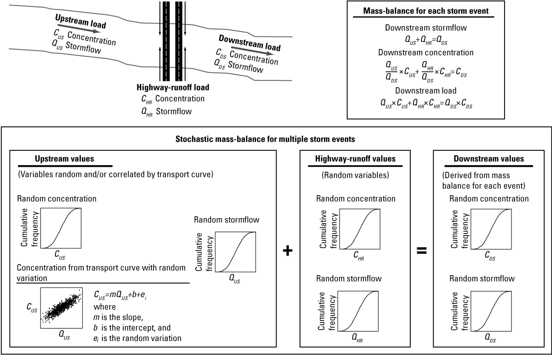
Schematic diagram showing the stochastic mass-balance approach for estimating stormflows, concentrations, and loads of water-quality constituents upstream of a highway-runoff outfall, from the highway, and downstream from the outfall (modified from Granato, 2013).
In this study, regression equations were used to provide planning-level estimates of selected variables from related variables or to simulate water-quality values by using a transport curve or dependent relation (Granato, 2013). These equations were developed to inform professional judgment in the selection of input variables used with SELDM rather than as quantitative stand-alone estimates. The basic form of the regression equation is:
whereYi
is the response variable for a given input;
Intercept
is the intercept of the regression equation;
Slope
is the slope of the regression equation;
Xi
is the predictor variable input to the equation; and
ei
is the random variation around the line.
In SELDM, the relations between imperviousness and runoff-coefficient statistics are developed in arithmetic space without logarithmic transformations (Granato, 2010, 2013). If the equation describing the relation of a certain value of imperviousness to a runoff coefficient is developed by using the common logarithms of the X and Y data, then the retransformed Y variable may be calculated as the following:
or,In SELDM studies, relations to estimate basin properties, streamflow statistics, concentrations from water-quality transport curves, concentrations from dependent relations, and concentration from other explanatory variables commonly are developed by using the logarithms of data (Granato, 2013; Stonewall and others, 2019; Weaver and others, 2019). If the equation estimating those properties is developed by using the common logarithms of the X data and the untransformed Y data, then the Y variable may be calculated as the following:
If a regression equation is being used to simulate individual values by using the frequency factor method, then the random-variation term ei is set equal to a measure of variability, either the standard deviation or median absolute deviation (MAD), of the regression residuals and multiplied by the standard normal variate (Kn). Kn values greater than zero result in scatter above the regression equation line, and Kn values less than zero result in scatter below the line. Adding the product of Kn and either the standard deviation or MAD value to represent ei results in a population of simulated values with characteristics that are similar to the original dataset.
Basin Characteristics
SELDM uses the location (latitude and longitude) of the site of interest, five physical basin characteristics, and the upstream hydrograph recession-ratio statistics to simulate the hydrologic characteristics of the site of interest and the upstream basin (Granato, 2012, 2013; Granato and Jones, 2014). The five physical basin characteristics for both the site of interest and the upstream basin are (1) the drainage area, (2) the total impervious area (TIA), (3) main-channel drainage length, (4) main-channel drainage slope, and (5) the basin development factor (BDF). However, only the area and the imperviousness of the site of interest need to be specified quantitatively to do a runoff-load or runoff-yield analysis for the site of interest because the timing of runoff is not used to calculate loads (Granato, 2013; Granato and Jones, 2017b; Stonewall and others, 2018; Granato and Friesz, 2021a).
The drainage area and imperviousness of the site of interest and the upstream basin were used to simulate the volume and timing of stormflows in this study. The drainage area of the site of interest is used to calculate the precipitation volume for that area. The drainage area of the upstream basin is used to calculate the precipitation and prestorm streamflow volumes for that area. The impervious fraction of the site of interest and the upstream basin are used to estimate the runoff coefficient statistics, which are used to transform precipitation volumes into runoff volumes from each area.
The main-channel length and main-channel slope were used to simulate the timing of stormflows in this study. The main-channel drainage length (also known as basin length) is the length of the main channel measured from the point of interest to the basin divide. The main-channel drainage slope (also known as the mean basin slope or 10-85 slope) is the average slope of the main channel upstream from the point of interest. It is calculated by determining the locations and elevations of points at 10 and 85 percent along the main channel from the point of interest to the basin divide and then by dividing the difference in elevations by the channel length between these points. The main-channel length and slope of the drainage network of the site of interest are used to simulate the timing of runoff from the site (Granato, 2012, 2013; Stonewall and others, 2019), whereas the main-channel length and slope of the stream basin above the point of interest are used to simulate the timing of runoff from the upstream basin. For the mixing analysis, timing of stormflows that occur from the site of interest with and without BMP treatment are used to calculate the concurrent volumes (Granato, 2013).
SELDM also has a basin development factor (BDF) variable that can be used with main-channel length and slope to calculate the timing of runoff from the site of interest and the upstream basin (Granato, 2012, 2013). The timing of runoff is calculated by using the basin lagtime, which is the time between the centroids of the precipitation hyetograph and the runoff hydrograph. The BDF approach was developed as a standard method to analyze urban floods but was adapted for use in SELDM. The BDF is specified as an integer between 0 and 12 with higher numbers indicating increasing use of engineered drainage pathways. The BDF is specified by using a complex algorithm that cannot be readily automated (Granato, 2010, 2012, 2013). Because the BDF is difficult to automate, the basin impervious fraction can be used in lieu of the BDF to estimate the basin lagtime. In SELDM, the user can specify a BDF value equal to −1 to use the impervious fraction to estimate basin lagtime for the site of interest and the upstream basin. This impervious-fraction option was selected because imperviousness can be easily obtained from StreamStats, geographic information system (GIS) analyses, or manual delineation. Because the impervious fraction can be used in lieu of the basin development factor to estimate the timing of runoff (Granato 2012, 2013), only the first four basin characteristics need to be determined to do the mass-balance mixing-analyses. This approach was used in all the simulations done for this study.
In SELDM, the site location (latitude and longitude) is used to select regional precipitation, prestorm-streamflow, and upstream-water-quality statistics. The site location also can be used to select precipitation and prestorm-streamflow statistics from nearby monitoring sites. The latitude and longitude coordinates entered can be precise (down to fractions of a second) in order to document the exact location of a particular site of interest and delineate the associated upstream basin, but this precision is not necessary for planning-level regional or statewide analyses. For these analyses, the precision of the coordinates entered can be about one degree of latitude and longitude as long as the selected point falls within the intended region or State. For general or basin-wide analyses, the precision of the selected coordinates can be as coarse as the density of the regional data monitoring networks. For example, the density of National Oceanic and Atmospheric Administration (NOAA) rain-gages included in the SELDM database for southern New England is about 784 square miles per station, so the maximum precision would need to be about 0.23 degrees of latitude and 0.27 degrees of longitude to properly select the nearest rain gage (if they were evenly spaced on a grid). To select the USGS streamgage from within the National SELDM database that is closest to a selected site of interest in southern New England, a precision of about 0.11 degrees of latitude and 0.13 degrees of longitude is needed. This is because the streamgage density in southern New England is about 179 square miles per station. Granato (2017) calculated streamflow statistics for 381 USGS streamgages in southern New England, which resulted in a density of about 45.5 square miles per station and a theoretical maximum precision of about 0.055 degrees of latitude and 0.065 degrees of longitude.
In this study, representative statistics were needed to do the sensitivity analyses necessary for identifying the effect of different SELDM input variable selections on the results of water-quality simulations. Upstream and highway- (or developed-area-) site characteristics can be determined for a specific site by using the USGS StreamStats application (U.S. Geological Survey, 2022), the GIS datasets developed by Spaetzel and others (2020), and other available GIS datasets. There are, however, almost infinite combinations of these basin characteristics that could be used to simulate the quantity and quality of stormflows in southern New England. The GIS datasets developed by Spaetzel and others (2020) were used in this study to quantify upstream-basin characteristics. Various publicly available transportation datasets were used to estimate highway site characteristics.
Upstream Basin Characteristics
The dataset of upstream basin characteristics was developed by delineating stream basins upstream from the intersections between roads and streams in southern New England and analyzing selected basin properties by using GIS software. Spaetzel and others (2020) generated this dataset of basin properties above road-stream crossings by using the intersections of roads as defined by the USGS National Transportation Dataset and streams as defined by the USGS StreamStats modified National Hydrography Dataset. Although all the detected road crossings were within southern New England, the delineated basins include basin properties and roadway characteristics from areas of New York, Vermont, and New Hampshire that are within the delineated basins. The selected basin characteristics are drainage area (in square miles), 10-85 slope (in feet of elevation change per mile), longest flow path (in miles), number of road crossings by road class, impervious cover (in percent), length of roads by road class (in miles), and length of streams (in miles; Spaetzel and others, 2020). The 10-85 slope and longest flow path in this dataset correspond to the slope and main-channel length in SELDM. The number of road crossings, length of roads by type, and impervious cover were determined to assess variations in the magnitude of development in southern New England stream basins. The length of streams was determined so that it could be used with drainage area to estimate the stream density (in miles per square mile). The stream density commonly is used to develop streamflow estimates (Bent and others, 2014), and it can be used to estimate the length of overland flow from drainage divides to tributary stream channels within the upstream basin (Horton 1945; Carlston 1963; Jeznach and Granato, 2020).
The geographic analysis by Spaetzel and others (2020) resulted in 53,131 basin delineations in southern New England with drainage areas ranging from 0.000032 to 1,938.8 square miles. Because delineation of very small basins and determining their characteristics is highly uncertain, the 48,466 basins delineated upstream from paved roads with a minimum drainage area of 0.025 square miles (16 acres) and a main-channel length, main-channel slope, and a drainage density greater than zero were selected for further analysis (fig. 2). Only 5,545 (about 11 percent) of these basins were delineated upstream from arterial roads (The National Map Functional Road Classification definitions in table 1); these basins will be described herein as the arterial-upstream basins. About 22 percent of these 48,466 basins contain one or more upstream arterial road crossings.
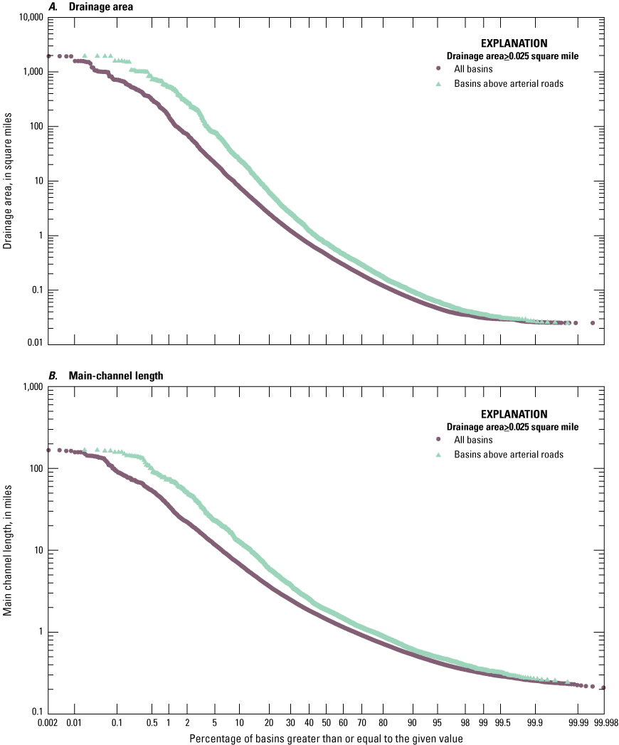
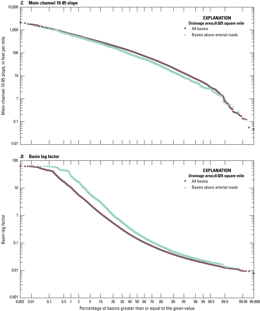
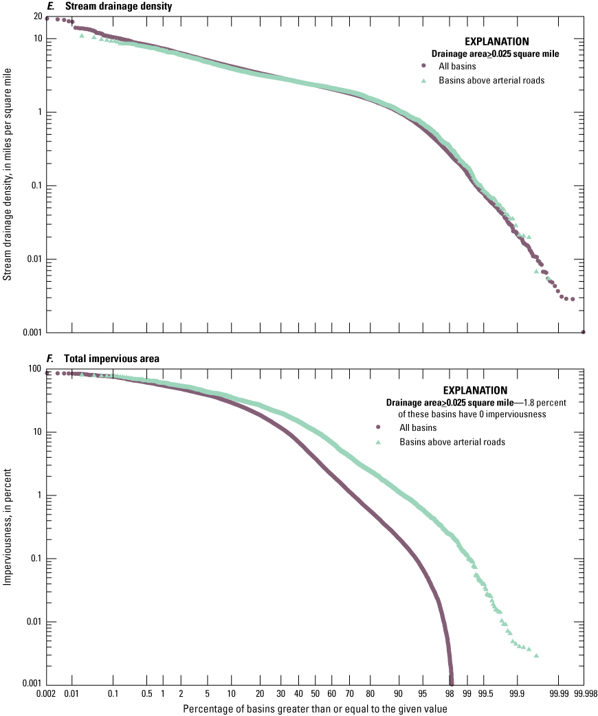
Probability plots showing the distribution of various properties of 48,466 drainage basins above roadways and 5,545 basins delineated above arterial roadways, computed by Spaetzel and others (2020). A, Drainage area. B, Main-channel length. C, Main-channel (10-85) slope. D, Basin-lag factor (main-channel length divided by the square root of the slope). E, Stream-drainage density. F, Total impervious area.
The road-crossing basin count may seem large for southern New England, but most delineated basins are nested within larger basins. For example, the Blackstone River Basin above Interstate 95 in Providence, Rhode Island is 475 mi2, has an imperviousness of about 12 percent, and has 2,340 upstream road crossings; the Charles River Basin above Interstate 93 in Boston, Massachusetts is 313 mi2, has an imperviousness of about 23 percent, and has 1,365 upstream road crossings; and the Park River Basin above Interstate 91 in Hartford, Connecticut is 77.2 mi2, has an imperviousness of about 27 percent, and has 539 upstream road crossings. These delineated basins, by definition, do not represent the confluence of tributary streams, but the drainage-area pattern is similar to Giusti’s law, which indicates that the number of upstream basins of any size is about 0.3 times the ratio of the basin area to the selected subbasin area (Giusti and Schneider, 1965). For example, this relation would indicate that a 250-square-mile basin would be expected to have 30, 300, and 3,000 tributary stream subbasins with drainages areas of 2.5, 0.25, and 0.025 mi2, respectively.
The characteristics of southern New England stream basins are shown in figure 2 and table 3. The values of basin characteristics for all the basins and the arterial-upstream basins vary by almost three (for basin length) to almost five (for drainage area) orders of magnitude. The coefficient of variation (COV) for drainage areas, which is the standard deviation divided by the average, also indicates the large variability of the basin properties. For example, the COV of the drainage areas is 6.65 for all basins and 5.04 for arterial-upstream basins. Although the values are wide ranging, most basins have small drainage areas. For example, the median, average, and geometric mean drainage areas for all basins are 0.455, 7.65, and 0.6 square miles, respectively. The median, average, and geometric mean drainage areas for arterial-upstream basins are almost twice the size with values of 0.721, 22.0, and 1.11 square miles, respectively.
Table 3.
Descriptive statistics for basin characteristics of 48,466 stream basins delineated upstream from all road-stream crossings and a subset of 5,545 stream basins delineated upstream from arterial road-stream crossings in southern New England.[See table 1 for the definition of arterial roadways. Data from Spaetzel and others (2020). Selected basins were delineated above paved roads with a minimum drainage area of 0.025 square mile (16 acres) and a main-channel length, main-channel slope, and a drainage density greater than zero. COV, coefficient of variation, unitless; DRNAREA, basin drainage area, in square miles; CSL10_85, main-channel slope between the points 10 and 85 percent from the road-stream crossing to the basin divide, in feet of elevation change per mile; Strm_density, stream density, the length of all streams in the basin in miles divided by the drainage area in square miles; LFPLENGTH, the main-channel length, in miles; LC16IMP, the total impervious area (TIA) divided by the basin area, in percent; BLF, basin-lag factor, which is the main-channel length (LFPLENGTH), in miles divided by the square root of the main-channel slope (CSL10_85), in feet per mile; —, not quantifiable because 860 basins have LC16IMP values equal to 0]
Information about relations between basin properties is needed to guide the choice of a limited but representative set of values for simulating the potential effect of runoff on receiving waters. To this end, an analysis of correlations between basin properties was done by calculating the nonparametric rank correlation coefficient (Spearman’s rho) and the product-moment correlation coefficient (Pearson's R) for the logarithms of data (table 4). Spearman’s rho is calculated by ranking the data and calculating the correlation coefficients between the rank values rather than the data values (Haan, 1977; Helsel and Hirsch, 2002). Spearman’s rho indicates the strength of the relation regardless of the linearity of the relation between variables. Correlations among the drainage area, the main-channel (10-85) slope, the main-channel length, and the basin-lag factor (BLF) are moderate (correlation coefficients with an absolute value greater than or equal to 0.5 and less than 0.75) to strong (correlation coefficients with an absolute value greater than or equal to 0.85, table 4). Drainage density and imperviousness of the basins may be considered to be random variables with respect to the other basin properties because they have weak correlations (correlation coefficients with an absolute value less than 0.5) with all the other basin variables.
Table 4.
Correlation coefficients for basin characteristics of 48,466 stream basins delineated upstream from road crossings in southern New England.[Data from Spaetzel and others (2020). Because of the sample sizes, all correlation coefficients are statistically significant at the 95-percent confidence limit (Haan, 1977). Selected basins were delineated above paved roads with a minimum drainage area of 0.025 square mile (16 acres) and a main-channel length, main-channel slope, and a drainage density greater than zero. Correlations for the logarithms of total impervious area were calculated by using the 47,606 nonzero values. Correlation coefficients that are greater than 0.5 are defined as moderately strong to strong. DRNAREA, basin drainage area, in square miles; CSL10_85, main-channel slope in feet per mile; Strm_density, the length of all streams in the basin in miles divided by the drainage area in square miles; LFPLENGTH, the main-channel length in miles; LC16IMP, the total impervious area (TIA), in percent of the basin area; BLF, the basin-lag factor, which is the main-channel length (LFPLENGTH) in miles divided by the square root of the main-channel slope (CSL10_85), in feet per mile; Spearman’s rho, rank correlation coefficient; Pearson's R, Pearson product-moment correlation coefficient]
Correlations for the basin-lag factor (BLF), which is the main-channel length divided by the square root of the main-channel slope, also were calculated (table 4) because the BLF is the controlling variable used to calculate the basin lagtime that determines the timing of runoff from the upstream basin (Granato, 2012, 2013). Although correlations of the BLF to length and slope are strong because the BLF is a function of length and slope, the correlation between the BLF and drainage area indicates the potential for using drainage area as the master variable for other basin properties. The correlations between drainage area and BLF in this study are very similar to the correlations calculated by Granato (2012) using National datasets with hundreds of sites. Although the correlations between drainage area and main-channel slope are only moderately strong (correlation coefficients with an absolute value greater than or equal to 0.5 and less than 0.75), correlations between drainage area and length are strong. This indicates that potential relations between drainage area and main-channel slope are less influential than the relation between drainage area and length for simulating basin lagtimes in southern New England. Granato (2012) also determined that drainage area was almost as strong a predictor for basin lagtime than the BLF and imperviousness, which further indicates that drainage area is the master variable for simulating the timing of stormflow from the upstream basin.
Regression relations were developed to select representative values of main-channel length and slope from drainage area (fig. 3, table 5). Because the potential effects of high-leverage outliers in datasets ranging over several orders of magnitude on regression relations can be large, the Kendall-Theil robust line method (Granato, 2006) was used to develop these equations. Because use of the Kendall-Theil robust line method on the full 48,466 basin dataset would require the calculation of about 1.2 billion slopes in arithmetic and 1.2 billion slopes in logarithmic space, the full dataset is too big to process in the KTRLine software (Granato, 2006). Therefore, a subsample of 6,923 basins was used to develop the regression equations. The subsample was created by sorting the dataset by basin size, and the data from every seventh basin out of the 48,466 were selected. The basins were selected if the remainder, or modulus, of the index number divided by 7 equals zero. Experiments conducted by shifting the index number and repeating the regression analysis indicated that the regression equations in table 5 are representative of the whole dataset.
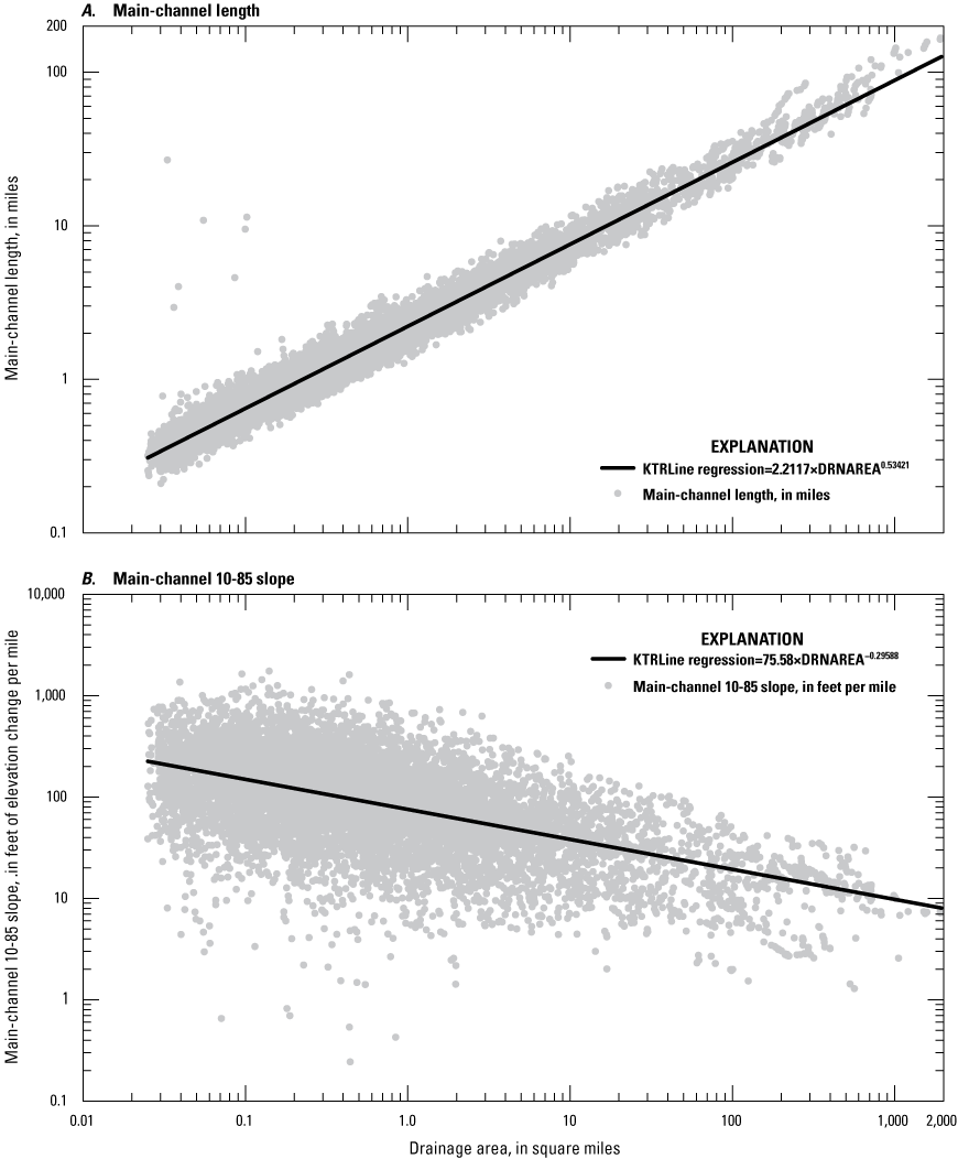
Scatterplots showing relations between drainage area and the main-channel length and slope for 48,466 basins above roadways delineated by Spaetzel and others (2020) and regression lines calculated by using a subsample of 6,923 of these basins from the full dataset. A, Main-channel length. B, Main-channel 10-85 slope.
Table 5.
Regression equation statistics developed by using the Kendall-Theil robust line method for estimating the logarithms of main-channel length and slope from the logarithms of drainage areas of selected stream basins delineated upstream from road crossings in southern New England.[Data from Spaetzel and others (2020). Because the KTRLine program is limited to datasets less than 15,000 points the 48,466 road-crossing dataset was sampled by sorting the data by basin size and using every seventh data point (index number modulus of 7), which resulted in a sample size of 6,923 basins; representativeness was confirmed by repeated subsampling starting on a different index number. KTRLine, Kendall-Theil Robust Line (Granato, 2006); RMSE, root mean square error, unitless; MAD, median absolute deviation, unitless; BCF, Bias Correction Factor, unitless; ASEE, average standard error of the estimate, in percent; CSL10_85, main-channel slope, in feet of elevation change per mile; LFPLENGTH, main-channel length, in miles]
The total impervious area (TIA) is an important variable for simulating runoff because it is used to calculate runoff coefficients and basin lagtimes in SELDM (Granato, 2010, 2012, 2013; Granato and Jones, 2014; Jeznach and Granato, 2020). The TIA of the delineated basins ranges from 0 to 85.8 percent with a median of about 3.84 percent among all basins and 10.43 percent among the arterial-upstream basins (fig. 2, LC16IMP in table 3). About 45 percent of all delineated basins and 66 percent of arterial-upstream basins exceed the TIA threshold of 5 percent that is commonly used to indicate the lower limit of substantial stream ecologic degradation (Jeznach and Granato, 2020). About 18 percent of all delineated basins and 30 percent of arterial upstream basins exceed the TIA threshold of 20 percent that is commonly used to indicate complete degradation of natural stream ecology. Because correlations between TIA (LC16IMP) and other basin variables are very weak (table 4), this variable must be considered as a random variable with respect to the other basin properties.
The stream density, which is the length of all streams in the basin divided by the drainage area, has a smaller range than the other basin characteristics in this study, and the differences between stream density for all the basins and the arterial-upstream basins are relatively minor. One-half of the reciprocal of the stream density can be used to estimate the length of overland flow from drainage divides to tributary stream channels; this estimate is known as the Horton half-distance (Horton 1945; Carlston 1963; Jeznach and Granato, 2020). The average stream density in the study area is 2.52 miles per square mile, and the reciprocal of this value is about 0.4 mile. Therefore, the Horton half-distance for overland flow in southern New England would be about 0.2 mile, or 1,056 feet.
Highway Site Characteristics
SELDM is nominally a highway-runoff model, but it can be used to simulate runoff for any site of interest by using the characteristics of the site of interest and representative water quality. Because SELDM is a lumped-parameter model, the basin characteristic values chosen for the highway, urban, or other developed areas that are simulated as the site of interest can be literal or interpretive (Granato, 2013; Stonewall and others, 2019; Jeznach and Granato, 2020). A literal site would be simulated by using the particular characteristics of an individual drainage pathway. For example, a literal site may be a section of roadway draining to a stream or a developed area with a trunkline drainage system. The basin characteristics for a literal site may be derived from actual drainage plans or estimated by using online tools like StreamStats and Google Earth. Interpretive sites may have multiple drainage pathways. Interpretive sites are used to simulate the net effect of multiple outfalls on the receiving water quality downstream from a point of interest (Granato, 2013; Granato and Jones, 2017a; Stonewall and others, 2019; Jeznach and Granato, 2020). For example, an interpretive site may represent a bridge (or two highway bridges in parallel) with many individual scupper drains, a bridge with two approach sections that discharge to a stream through multiple outfall locations, a road paralleling a stream with multiple outfall locations, or an agglomeration of developed areas that drain to a point of interest along a stream. An interpretive site may be simulated by selecting representative basin properties that produce the volume and timing of runoff characteristic of the entire simulated drainage area. Because decisionmakers commonly need information about the net effect of multiple stormwater outfalls on the receiving water quality at a given location, interpretive sites commonly are used to simulate stormwater quality (Granato and Jones, 2017a; Smith and others, 2018; Stonewall and others, 2019; Weaver and others, 2019; Jeznach and Granato, 2020).
If simulations are done to develop annual total maximum daily load (TMDL) yields, then the timing of runoff during individual events is not of concern and the site may be simulated by using an area of 1 acre and a representative TIA value; the remaining basin properties may be specified by using generic values (Granato and Jones, 2017b, Stonewall and others, 2018; Granato and Friesz, 2021a). For TMDLs, the yields can be applied to the areas of different road classes and to the developed impervious or land-use areas to estimate loads from simulated yields (Granato and Jones, 2017b, Stonewall and others, 2018; Lantin and others, 2019; Granato and Friesz, 2021a).
In this study, available information about roadway geometry and drainage-system characteristics were used to simulate runoff from hypothetical, but representative sites. Runoff from roadways was simulated by using the paved area rather than the area of the entire right-of-way because roadway-runoff quality data collected in southern New England were collected from paved areas (Smith, 2002; Smith and Granato, 2010; Smith and others, 2018; Granato, 2019a), and the grassy swales and strips of the shoulders and medians alter the flows, concentrations, and loads from pavements in ways that are unique to each site (Granato, 2014; Taylor and others, 2014; Granato and others, 2021). Roadway geometry and drainage characteristics were estimated by using the AASHTO (2001) policy on geometric design of highways and streets and Federal Highway Administration Hydraulic Engineering circulars (Young and others, 1992; Federal Highway Administration, 1993, 2013). The State DOTs in southern New England follow these standards with minor modifications (Massachusetts Highway Department, 2004, 2006; Rhode Island Department of Transportation, 2008; Connecticut Department of Transportation, 2020).
The road data incorporated into StreamStats provides information about the lengths of various road classes above any given point on a stream, but information about road widths is needed to estimate the drainage areas of roads within a delineated basin. The AASHTO (2001) guidelines indicate that roadway widths are commonly specified by road class, rated speed limits, and traffic volume. Individual travel-lane widths commonly range from 9 to 12 feet. Safety is the prime consideration for travel-lane widths, but there are many design considerations such as access for pedestrians or bicyclists and parking that may come into play. Although 12-foot lane widths have become a design standard, 9-foot lanes are considered acceptable for low speed, low volume rural and residential roads. Lane widths less than 12 feet may be legacy widths or the result of right-of-way constraints in urban areas. The width of each roadway also includes the width of paved shoulders. A minimum shoulder width is 1 foot for drainage, 2 feet to help protect the integrity of the pavement edge, and up to a full 12-foot shoulder to permit emergency parking along multilane limited-access roadways. A minimum width of 4 feet is the design standard for the shoulder where vertical barriers or guard rails are present. The minimum parking-lane width for residential areas commonly is 8 feet. Parking lanes may be 10 feet wide on connecting roads and full access arterial roadways. Bicycle-lane design standards are a minimum of 4 feet wide in open areas and 6 feet in commercial areas. The desired width is 8 feet to accommodate multiple bicyclists within the lane. In southern New England where rights-of-way are constrained, bicycle lanes commonly are created by reducing motor vehicle lane widths rather than widening the paved roadway area.
The area of paved roads is needed to calculate the road-runoff flows and loads. Typical road widths may be estimated based on the AASHTO (2001) guidelines and information about the number of lanes from the road census (Federal Highway Administration, 2022a, b) and NBI (Federal Highway Administration, 2020) for southern New England listed in table 1. On average, local roads and minor collectors have 2 travel lanes. Major collectors have an average of 2.1 travel lanes, which indicates that about 94 percent of these roads have 2 travel lanes and 6 percent have 4 or more lanes. On average, minor arterial roads have 2.2 to 2.5 travel lanes indicating that about 75 to 90 percent of these roads are 2-lane roads. On average, principal arterial roads have 2.6 to 3 travel lanes indicating that about 50 to 70 percent of these roads are 2-lane roads. Road widths of principal arterials are similar to minor arterials, but there is a greater proportion of principal arterial roadways with multiple lanes in each direction. The divided limited-access highways including freeways and expressways and interstates were combined in table 1 to calculate the number of lanes in both directions. The average number of lanes for freeways and expressways are about 4.2 lanes, indicating that about 90 percent of these road types have 2 travel lanes in each direction within southern New England. Using these estimates of width and the number of lanes for each road type, the estimated pavement area may range from about 2.4 acres per mile for a 2-lane local road without roadside parking to 7.8 acres per mile for each roadway of an 8-lane limited-access arterial roadway (table 6).
Table 6.
Pavement areas per mile of roadway by road class, estimated from statistics for the number of lanes by road class and roadway design guidelines for roads in southern New England.[Road classes are defined in table 1. The number of lanes by road class are defined in table 2. Road widths are estimated from the American Association of State Highway and Transportation Officials (2001) design guidelines. Values for limited-access arterials in parentheses are the values for both roadways]
Because the cost of building and maintaining drainage systems to manage runoff are large, direct drainage to the local land surface is used where possible for infiltration. Highway drainage-design guidelines specify use of grass strips and swales rather than storm sewer systems wherever practical (American Association of State Highway and Transportation Officials, 2001). Consequently, only a small part of the road network may drain directly to receiving waters. Available information (Granato and others, 2022) on the impervious areas draining to roadway stormwater-conveyances in Massachusetts and Rhode Island indicates that the distributions of designed drainage networks in these States are similar to each other (fig. 4A). The values shown for Massachusetts are the percent distribution of impervious roadway area sizes contributing to the structural stormwater best management practices, and the values shown for Rhode Island are the percent distribution of impervious roadway area sizes contributing to stormwater conveyances, which may include areas draining to a single stormwater inlet. These roadway drainage areas range from about 0.01 to 32 acres, with a median of 0.63 acres for Massachusetts and 0.57 acres for Rhode Island (fig. 4A). These distributions are similar, which may be the result of the similarities in hydrology within southern New England and use of hydrologic design guidelines based on National standards.
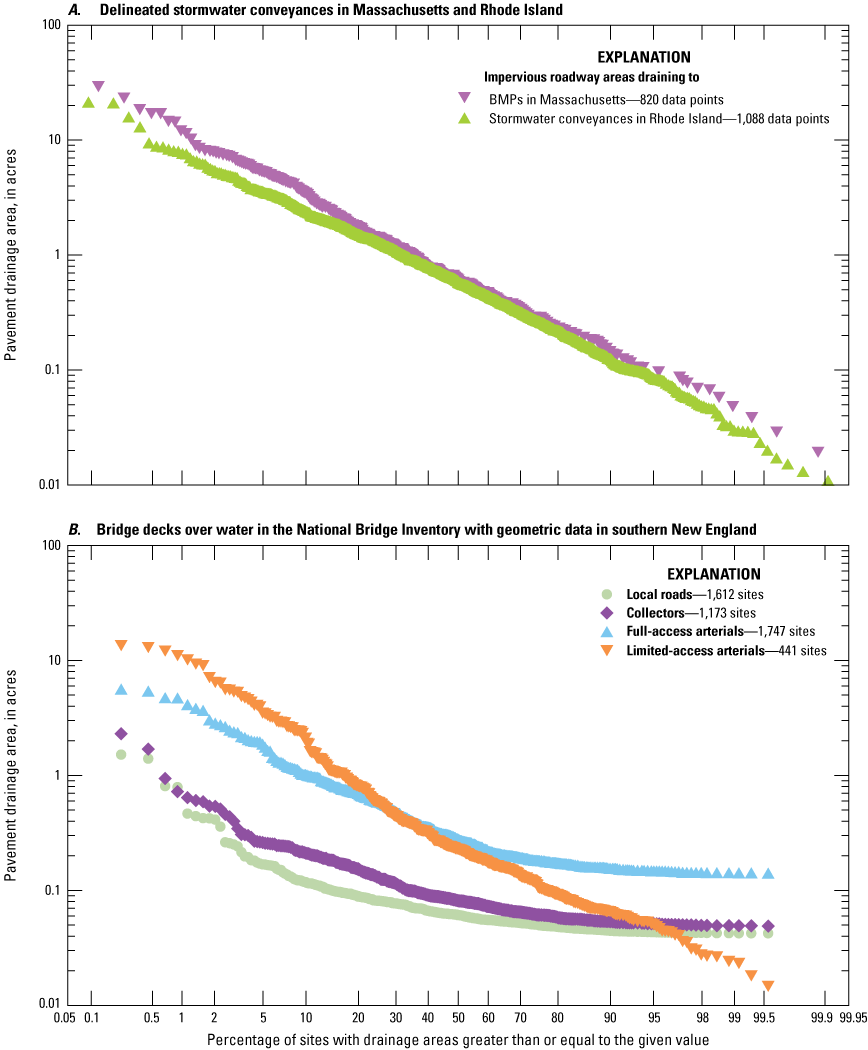
Probability plots showing the distribution of pavement drainage areas of highway sites. A, Delineated stormwater conveyances in Massachusetts and Rhode Island. B, Bridge-decks over water in the National Bridge Inventory with geometric data in southern New England. Road classes are defined in table 1. BMP, best management practice.
The NBI (Federal Highway Administration, 2020) also provides information that can be used to estimate roadway-runoff source areas; the NBI can be considered as a random sample of road characteristics across each State. Precipitation that falls on bridges may be directly discharged by using bridge scuppers or routed to stormwater treatment facilities adjacent to the receiving water body (Federal Highway Administration, 1993). Figure 4B shows the distribution of areas of 4,973 roadway bridge decks over water in southern New England that have the bridge deck width and structure length values in the NBI, which are needed to calculate the bridge-deck areas, and the functional class, which is needed to identify different road types (there are another 514 roadway bridge decks over water that do not have all of these values in the NBI). These bridge-deck areas range from 0.007 to 13.98 acres with a median of 0.045 acres. Median bridge-deck areas for local roads, collectors, full-access arterials, and limited-access arterials are 0.0275, 0.0386, 0.0686, and 0.236 acres, respectively. The minimum areas may be smaller than would be expected given the average road widths and areas shown in table 6, but the NBI includes bridges and large culverts, which both may have spans as short as 20 feet.
In SELDM, the length of the drainage flow path is used with its slope to simulate the timing of runoff from the highway or urban site to the point of interest. The site of interest may have two lengths; the physical length for calculating drainage-basin area, and the main-channel drainage length used for calculating the hydrologic basin lagtime for the site. The main-channel drainage length for the site of interest is estimated as the characteristic drainage length that controls the timing of runoff from the drainage divide to the stormwater outfall. For example, when simulating runoff from a bridge with direct-discharge scuppers, the physical length of the bridge may be used to calculate area, and the average distance from the crown of the road to the nearest scupper, which is the average length of the flow path of precipitation on the bridge, may be the hydraulic length. Similarly, on a long stretch of highway with multiple drainages of varying lengths to a parallel stream, the length of that road segment may be used to calculate area, and the average distance from the crown of the road through the drainage system to the nearest outfall may be the hydraulic length. If a highway site stretches across the entire hydrologic stream basin and there is one outfall where it crosses the stream, then the divide-to-divide distance would be used to calculate the roadway area, and the hydraulic length would be the longer distance from the stream to one of the divides. The physical length of highway conveyances can be estimated from the information in table 6 and figure 4. For example, given a median area of about 0.6 acre, the length of a local road without parking can be estimated as about 1,320 feet, and the length of a two-lane full-access arterial road can be estimated as about 930 feet. The length of a divided 4-lane limited access highway may be estimated as about 660 feet if one of the roadways of the highway drains to the conveyance, and 330 feet if both roadways of the divided highway drain to the same conveyance. Similarly to finding physical lengths of parking lot conveyances, the area of a parking lot may be calculated from a physical length, and the hydraulic length may be the route that the main drainage pipe follows from one edge of the parking lot to collect water from the pavement and discharge it to the receiving water body.
Highway drainage slopes can be estimated by using information from roadway design guidelines and hydraulic design circulars (table 7). Highway and drainage design guidelines commonly specify slopes by using percentages or dimensionless ratios, but SELDM uses the watershed slope convention of (vertical) feet of elevation change per (horizontal) mile. Pavement cross slopes may represent the first segment of the flow path from the drainage divide to the drainage-system outfall. Because SELDM uses a representative slope calculated from the elevations of points at 15 and 85 percent up the main channel from the outlet, the pavement cross slopes may not be critical except in the case of a bridge deck for calculating the timing of runoff from the crown of the road to the nearest scupper. The minimum and maximum of longitudinal drainage slopes and road grades may be used to estimate drainage slopes for drainage pathways that follow the highway to the waterway; these slopes commonly represent the longest distance of the flow path. The selected slope may depend on the components of the drainage system. The minimum storm-drain slopes, which are designed to maintain the self-cleaning flow velocity of 3 feet per second, represent minimum slopes for closed drainage systems (table 7). The maximum unlined channel slope specification of 2 percent, which is equivalent to about 106 feet per mile (ft/mi), represents the open channel velocity at which unwanted erosion of roadside swales may begin. The estimated range of roadway drainage slopes in table 7 is about 4 to 900 ft/mi; this is well within the range of 0.046 to 2,186 ft/mi for main-channel slopes of stream basins above of road crossings in southern New England (table 3). When road drainage slopes are being calculated, any vertical drops (such as from the road surface to the catch basin outflow or from a bridge deck scupper or an overhanging drainage outlet to the stream) should not be included in the slope. This is because vertical drops are almost instantaneous and so do not contribute to the basin lagtime of the highway (or urban) runoff drainage pathway.
Table 7.
Highway-drainage slopes estimated from roadway-design guidelines and Federal Highway Administration hydraulic-design circulars.[Design guidelines are AASHTO green, the American Association of State Highway and Transportation Officials (2001) green book; HEC-22, Hydraulic Engineering Circular No. 22 (Federal Highway Administration, 1993); and HEC-21, Hydraulic Engineering Circular No. 21 (Federal Highway Administration, 2013). Longitudinal grades are the slopes in the direction of the roadway. Cross slopes are perpendicular to the direction of the roadway. The self-cleaning velocity is the velocity of water in a pipe that is sufficient to mobilize sediment within a pipe to prevent buildup and clogging]
The drainage characteristics, which include drainage area, length, slope, and imperviousness, for other developed land covers also can be estimated from StreamStats, highway design information, and other sources. SELDM can be used to simulate runoff from a particular site or the upstream drainage areas can be aggregated into a site by lumping the areas and using representative hydraulic characteristics (Stonewall and others, 2019; Jeznach and Granato, 2020). If specific sites are to be simulated, then actual basin characteristics may be derived by using local GIS data (Granato and Friesz, 2021a). The drainage area for simulating runoff from developed areas may be estimated by using the imperviousness, the percent developed area, or land-cover areas (Stonewall and others, 2018, 2019, Jeznach and Granato, 2020; Granato and Friesz, 2021a). Studies of the components of impervious surfaces in developed areas consistently indicate that, on average, off-street parking, roofs, roads, and other anthropogenic surfaces comprise about 35, 32, 25, and 8 percent of the TIA in these areas, respectively (Tilley and Slonecker, 2006; Roy and Shuster, 2009; Wang, 2013). If, as indicated in table 2, the State DOTs own about 15 percent of the road network (about 17.2, 8.1, and 18.3 percent of roadways in Connecticut, Massachusetts, and Rhode Island, respectively), then DOT owned roads would represent about 3.8 percent of the total impervious area in urban areas. However, the percentage of imperviousness composed of local roadways and State-owned roadways may be much higher outside developed areas than in developed areas with a high proportion of off-street parking, roofs, and other anthropogenic surfaces. Granato and Friesz (2021a) determined that the imperviousness of developed areas increase with increasing percentages of developed area because of urban intensification. In southern New England, the areas of State roadways can be estimated from StreamStats (Spaetzel and others, 2020) and subtracted from the total impervious area to produce a more robust estimate of DOT and non-DOT runoff areas. The drainage length may be measured if a literal site is being simulated but must be estimated for interpretive sites. Jeznach and Granato (2020) used the Horton half distance calculated from stream density as the drainage-length to simulate the timing of urban runoff because it is the average distance from the local drainage divide to the nearest stream segment. Roadway and drainage-system slopes in table 7 also may be used to simulate urban runoff because many of the same drainage design constraints influence urban drainage design. As with highway sites, a basin development factor equal to –1 can be specified to use the basin lagtime equation that is based on the imperviousness of the site.
The annual average daily traffic (AADT) volume, which is a count of the number of vehicles using the roadway per day, is commonly viewed as a basin characteristic of roadway sites that is indicative of runoff quality. AADT data is primarily collected to measure and plan roadway capacity needs, but it has been used, with mixed success, as an explanatory variable for estimating highway-runoff quality (Driscoll and others, 1990; Granato and Cazenas, 2009; Smith, and Granato, 2010; Wagner and others, 2011; Granato and Friesz, 2021a). In the National highway-runoff monitoring study by the FHWA (Driscoll and others, 1990) water-quality monitoring sites were categorized as being “rural” if they had an AADT value of less than 30,000 vehicles per day (VPD), and were categorized as “urban,” if they had an AADT greater than or equal to 30,000 VPD based on statistical differences in runoff quality.
State DOTs run small numbers of continuous traffic monitoring stations and supplement these stations spatially by using many more short-period counting locations, which are used to estimate AADT values (Krile and others, 2015). Studies show that the uncertainty in AADT estimates from short-term monitoring stations commonly is on the order of ±20 percent and as high as ±50 percent for low AADT roads (less than 1,000 vehicles per day) and that estimates are highly uncertain for all traffic volumes with measurement durations of less than a full day (Krile and others, 2015).
The NBI (Federal Highway Administration, 2020) was used as a sample of roadway locations in southern New England to assess the AADT population characteristics of roadways near stream crossings. Figure 5 shows the distribution of AADT of the population of all bridges and State-maintained bridges over water in southern New England. The State-maintained bridge population has higher AADTs (median of 11,700 VPD) than the AADTs (median of 3,995 VPD) for the population of all bridges in this area because State-maintained bridges carry higher capacity motorways. About 9.2 percent of all bridge crossings and 20.3 percent of State-maintained bridge crossings in southern New England have AADT values over 30,000 vehicles per day, which is the traditional rural to urban water-quality threshold known as the Strecker number (Driscoll and others, 1990). In comparison, the population of Highway-Runoff Database monitoring sites (Granato and Cazenas, 2009; Granato, 2019a; Granato and Friesz, 2021b) in southern New England has a median of 61,534 VPD, with 69 percent of sites having AADT values greater than 30,000 VPD (fig. 5).
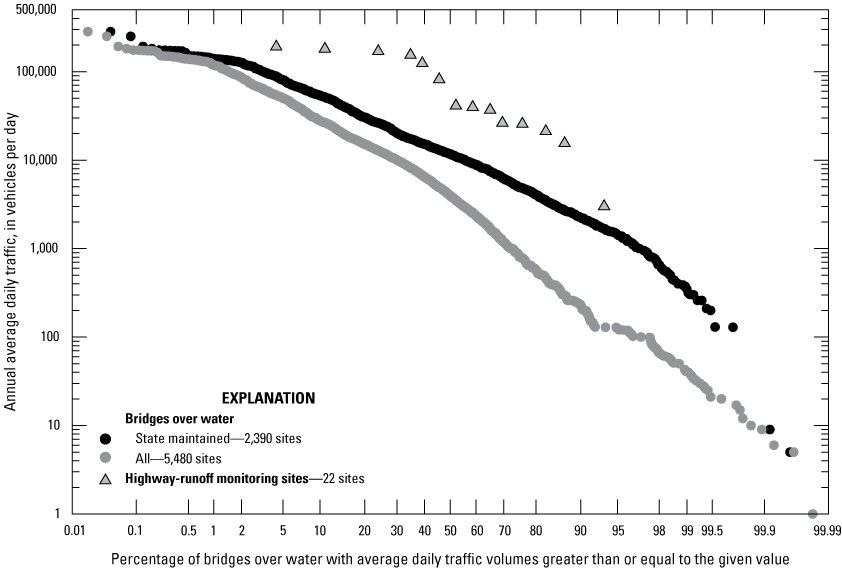
Probability plot showing the distribution of annual average daily traffic volumes, in vehicles per day, for all bridges over water and State-maintained bridges over water from the National Bridge Inventory Database (Federal Highway Administration, 2020) and highway-runoff monitoring sites from the Highway Runoff Database (Granato and Friesz, 2021b) for locations in southern New England.
The population of all southern New England bridges in the NBI (Federal Highway Administration, 2020) was used to examine AADT by road class (fig. 6). While the road-class labels in the NBI are slightly different than in table 1 and the roadways on the bridges are identified as rural or urban, the descriptors in table 1 broadly apply to the categories in figure 6. The NBI definitions of rural or urban are based on the census designation for the location of the bridge, rather than being based on the traffic volume or the traditional 30,000 VPD runoff-quality threshold (Federal Highway Administration, 2020). The AADT values are shown as VPD per lane in figure 6 to normalize the values for comparison across roads with different numbers of lanes. Even when normalized for lane count, AADT values increase from category to category and from rural to urban within categories. For example, among rural road classes, the median per-lane traffic volume for interstate arterials is about 68 times the median traffic volume for local-roads (fig. 6A). In comparison, the median per-lane traffic volume for interstate arterials is about 24 times the median traffic volume for local-roads among urban road classes (fig. 6B). Comparison of the urban to rural traffic volumes for similar road classes indicates that the urban road medians are about 1.4 times and 4.7 times the rural road medians for principal arterials and local roads, respectively. Traffic volumes per lane for urban local-roads are comparable to rural collectors; volumes for urban collectors are comparable to rural minor arterials; volumes for urban minor arterials are comparable to rural principal arterials, and volumes for urban principal arterials are comparable to rural interstate highways (fig. 6). Therefore, given the overlapping traffic volumes between urban roads and rural roads, uncertainty in individual AADT values, differences in traffic patterns (more starting and stopping on urban roads), background air quality between urban and rural areas, and other factors, road class and traffic volume may have limited use as a predictor variable for the quality of roadway runoff at the watershed scale (Granato and Friesz, 2021a, b).
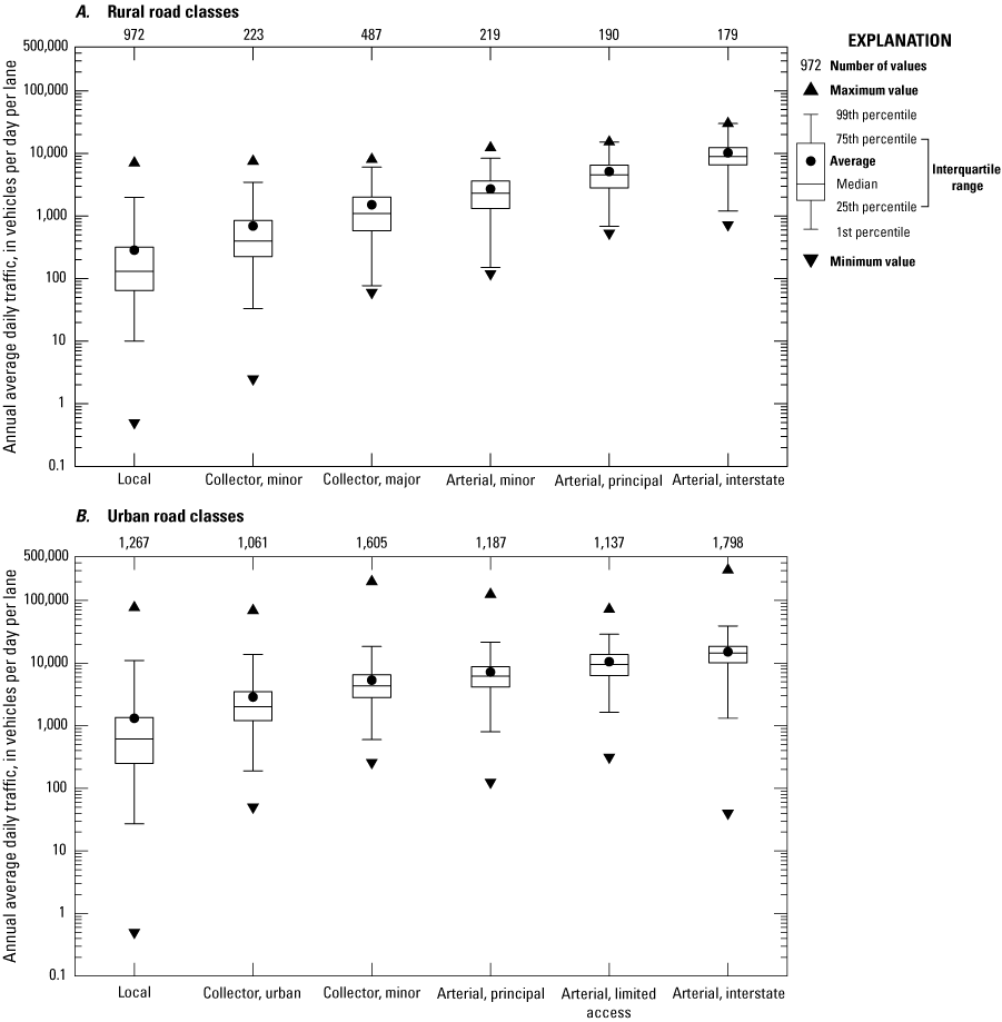
Box plots showing annual average daily traffic volumes, in vehicles per day per lane, by road class. A, Rural road classes. B, Urban road classes. Data are for all bridges in southern New England from the National Bridge Inventory database (Federal Highway Administration, 2020). Road categories are defined in table 1.
Storm Event Hydrology
SELDM simulates the volume of stormflows from runoff-generating events by using statistics for prestorm streamflows, precipitation, and runoff coefficients (Granato 2013). Individual prestorm streamflows, precipitation event characteristics, and runoff-coefficient values are simulated by using the log-Pearson Type III distribution, the two-parameter exponential distribution, and the Pearson Type III distribution, respectively. In SELDM the storm-event hydrology can be specified using regional statistics (described as a level 1 analysis), statistics from a site or sites selected from SELDM as being hydrologically similar to conditions at a site of interest (described as a level 2 analysis), or from data collected at the site of interest and entered in SELDM as user-defined values (described as a level 3 analysis). In this study, statistics from additional sites in southern New England were developed to refine statistics available within SELDM.
Regional simulations were done by using prestorm streamflow and precipitation statistics for three U.S. Environmental Protection Agency (EPA) Level III ecoregions that include parts of Massachusetts, Connecticut, or Rhode Island (the Northeastern Highlands, Northeastern Coastal Zone, and Atlantic Coastal Pine Barrens ecoregions; fig. 7, table 8). Regional statistics provide initial planning-level estimates that can be applied over a large area or a site of interest without detailed knowledge about conditions at the site. Regional analyses are useful for developing planning-level estimates, but regional values may not capture local variations in precipitation characteristics. This is most evident in larger ecoregions like the Northeastern Highlands which stretches from New Jersey to Maine and is more than twice the size of the two other ecoregions partly located in southern New England (table 8). Although the ecoregion median is theoretically the best estimate for any randomly selected location in an ecoregion, knowledge about local conditions can be applied to improve such estimates.
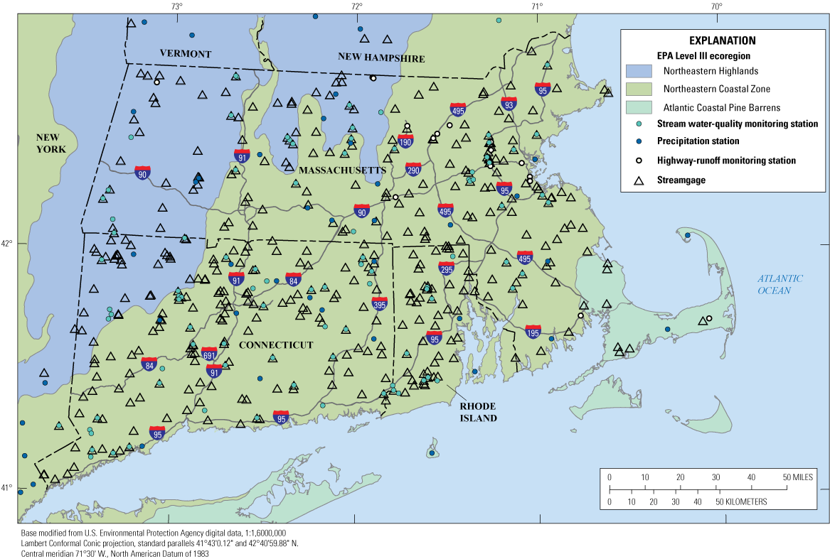
Map showing U.S. Environmental Protection Agency (EPA, 2013) Level III ecoregions and the distribution of stream water-quality monitoring stations, precipitation stations, highway-runoff monitoring stations, and streamgages in and adjacent to southern New England.
Table 8.
U.S. Environmental Protection Agency Level III ecoregions that lie partly within Connecticut, Massachusetts, or Rhode Island.[U.S. Environmental Protection Agency Level III ecoregion numbers, names, and definitions are defined by the U.S. Environmental Protection Agency (2013). The Stochastic Empirical Loading and Dilution Model (SELDM) area is the discretized area of each ecoregion in SELDM (Granato, 2013) calculated by using the number of grid cells and the average area of a 0.25-degree grid cell in the ecoregion; calculated areas are for the entire ecoregion. mi2, square mile]
Precipitation Statistics
SELDM uses precipitation statistics to stochastically simulate a large series of runoff-generating events. Storm-event precipitation statistics define the characteristics of each simulated storm event and the number of events in the simulation (Granato, 2013, Risley and Granato, 2014, Stonewall and others, 2019, Weaver and others, 2019). SELDM also uses precipitation statistics to aggregate events into annual-load accounting years, which can be used to assess long-term annual loads or yields that can be used for TMDL analyses (Granato, 2013; Granato, and Jones, 2017b; Smith and others, 2018; Stonewall and others, 2018; Lantin and others, 2019; Granato and Friesz, 2021a). SELDM uses the EPA definition of a runoff-generating event, which is based on hourly precipitation values, a minimum precipitation volume of 0.1 inch (in.), and a minimum inter-event period of 6 hours between events (Driscoll, Palhegyi and others, 1989; Granato, 2010, 2013). To simulate the events, SELDM uses the event volume (in inches), duration (in hours), and the time between event midpoints (in hours). SELDM uses the event duration and the time between event midpoints to group random collections of events into the annual-load accounting years; subsequent events are assigned to a year when the accumulated hours equal 365 or 366 days. The number of runoff-generating events per year specified from the selected precipitation statistics is used to calculate the minimum number of events to be simulated in each run (Granato, 2013).
Regional simulations were done by using precipitation statistics for three EPA Level III ecoregions that include parts of Massachusetts, Connecticut, or Rhode Island, and statistics for southern New England (table 9, fig. 7). The ecoregion statistics are the median of statistics for all NOAA hourly precipitation data stations in the ecoregions, which cover areas inside and outside the southern New England States. The statistics for southern New England were calculated as the median of values from precipitation data stations within and adjacent to Connecticut, Massachusetts, and Rhode Island (table 10, fig. 7). Precipitation stations outside but adjacent to southern New England were selected to better characterize conditions within this region even though the additional area of the bounding box reduced the station density in comparison to ecoregion 59 (the Northeastern Coastal Zone), which covers most of southern New England (table 9).
Table 9.
Synoptic-precipitation statistics for the southern New England area and selected U.S. Environmental Protection Agency Level III ecoregions that lie in whole or in part within Connecticut, Massachusetts, or Rhode Island.[U.S. Environmental Protection Agency Level III ecoregions are defined in U.S. Environmental Protection Agency (2013) and listed in table 8. Southern New England is defined as the area within Connecticut, Massachusetts, and Rhode Island. Synoptic-precipitation statistics were calculated by using the definition of a runoff-generating event with a minimum interevent time of 6 hours and a minimum precipitation volume of 0.1 inch of liquid precipitation. The statistics are the medians of statistics for each specified region from the National Oceanic and Atmospheric Administration (NOAA) hourly precipitation data stations with at least 25 years of data from 1965 to 2006 (Granato, 2010). The area of the southern New England region used to calculate the average area per station is the area of Stochastic Empirical Loading and Dilution Model (SELDM) grid squares in a latitude-longitude box (−74 to −70 longitude, 40.75 to 43.25 latitude) that contains precipitation-data stations within, and adjacent to, Connecticut, Massachusetts, and Rhode Island (table 10), which is about 35,294 square miles. In comparison, the combined area of the three States is 17,322 square miles. Delta is the time between storm midpoints. mi2, square mile; in/yr, inch per year; in., inch; hr, hour; —, not applicable]
Table 10.
Synoptic-precipitation statistics from National Oceanic and Atmospheric Administration hourly precipitation-data stations that are in and adjacent to southern New England States.[Synoptic-precipitation statistics were calculated by using the definition of a runoff-generating event with a minimum interevent time of 6 hours and a minimum precipitation volume of 0.1 inch of liquid precipitation; the statistics are the medians of statistics from selected National Oceanic and Atmospheric Administration (NOAA) hourly precipitation-data stations with at least 25 years of data from 1965 to 2006 (Granato, 2010) that are located within or near southern New England. Hourly precipitation-data stations were selected to represent the hydrology of Connecticut (CT), Massachusetts (MA), and Rhode Island (RI) in addition to stations in New Hampshire (NH) and Vermont (VT). Level III ecoregion index numbers are defined by the U.S. Environmental Protection Agency (2013) and listed in table 8. The NOAA ID is the NOAA National Weather Service hourly-precipitation station identification number. The sensitivity-analysis column indicates whether a station was used in the precipitation sensitivity-analysis simulations. Delta is the time between storm-event midpoints. in/yr, inch per year; in., inch; hr, hour; Y, yes; N, no]
In this study, precipitation statistics for individual NOAA precipitation data stations also were used to do TMDL simulations (a level 2 analysis) to provide information about variations in long-term average yields and to do sensitivity analyses on the effect of variations in precipitation statistics on flows, concentrations, and loads of runoff-constituents of concern within the region. Statistics for the 45 precipitation stations within and adjacent to southern New England are shown in table 10 and are compared to the southern New England median (shown as a red line in figure 8) and the ecoregion medians (shown as black diamonds in figure 8). The median statistics for the Northeastern Highlands (ecoregion 58) are offset from the estimated median of selected southern New England stations in this ecoregion because only a small part of the Northeastern Highlands ecoregion lies within the Southern New England States. The median statistics for the Northeastern Coastal Zone (ecoregion 59) are similar to the estimated median of selected southern New England sites because most stations within the Northeastern Coastal Zone ecoregion are located within or near Connecticut, Massachusetts, or Rhode Island. The median statistics for the Atlantic Coastal Pine Barrens (ecoregion 84) also are similar to the estimated median of selected precipitation stations in this ecoregion within southern New England, even though most of the precipitation monitoring stations in the Atlantic Coastal Pine Barrens ecoregion are located in New Jersey and New York. Among the 45 stations within and adjacent to southern New England, the event volumes, durations, and time between midpoints in table 10 vary from the minimum to maximum values by a factor of about 1.41, 1.77, and 1.48 respectively. Among the 45 precipitation stations in southern New England, the event volume is not strongly correlated to the duration or time between midpoints (with Spearman’s rank correlation coefficient values of −0.24 and 0.37). The duration and delta statistics are moderately correlated (with a Spearman’s rank correlation coefficient value of −0.714) because half the storm-event durations before and after each time between midpoint are a component of that value.
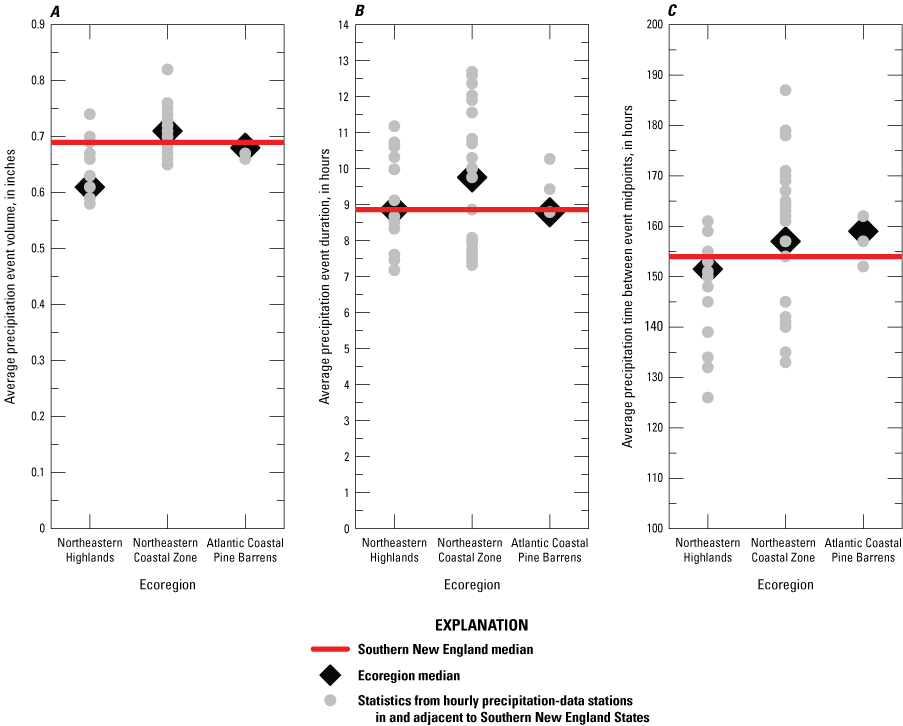
Graph showing the precipitation event statistics for hourly precipitation-data stations in and adjacent to southern New England, the median of sites representing statistics for southern New England, and the medians of statistics for all hourly precipitation data stations within the Northeastern Highlands, Northeastern Coastal Zone, and Atlantic Coastal Pine Barrens U.S. Environmental Agency Level III ecoregions used for annual-yield analyses conducted in Connecticut, Massachusetts, and Rhode Island with the Stochastic Empirical Loading and Dilution Model. A, Average event volume. B, Average event duration. C, Average time between event midpoints.
Prestorm Streamflow Statistics
SELDM uses streamflow statistics to stochastically simulate a large series of prestorm streamflow volumes from the basin upstream from the point of interest (Granato, 2013; Risley and Granato, 2014; Stonewall and others, 2019; Weaver and others, 2019). SELDM uses the frequency factor method to generate a population of nonzero streamflows from the average, standard deviation, and skew of the logarithms of nonzero flows; and conditional probability methods to simulate the fraction of zero flows (Granato, 2013). Prestorm streamflow, which may include base flow (generally defined as groundwater discharge) and stormflow from a previous storm, is one component of the total stormflow from the upstream basin. The prestorm streamflow is simulated as the instantaneous flow at the beginning of a storm, which is added to the current storm runoff for the duration of the runoff or BMP discharge from the site of interest. This is used to simulate the total flow available for dilution in the current storm. The prestorm streamflow is simulated by using the average, standard deviation, and skew of the logarithms of streamflow data. Some proportion of prestorm streamflows may equal 0 if the stream is intermittent or ephemeral. Granato (2010) provides a detailed discussion of the methods and data used for estimating prestorm streamflows for use with SELDM. Estimates of prestorm streamflow in receiving waters are important for assessing risks of adverse effects of runoff on water quality because prestorm streamflow can be a substantial proportion of total stormflow.
Streamflow statistics for three EPA Level III ecoregions that include areas within and outside of Massachusetts, Connecticut, or Rhode Island, (the Northeastern Highlands, Northeastern Coastal Zone, and Atlantic Coastal Pine Barrens ecoregions; tables 8, 11) were considered for use in streamflow simulations. The selected ecoregion statistics were the median of statistics for all USGS streamgages included in the SELDM database within each ecoregion. As table 11 indicates, there is much more variation within each ecoregion than there is between the regional medians in this area of the country.
Table 11.
Streamflow statistics for the southern New England area and selected U.S. Environmental Protection Agency Level III ecoregions that lie in whole or in part within Connecticut, Massachusetts, or Rhode Island.[Statistics are for the retransformed common logarithms of nonzero flows and the proportion of zero flows; the statistics are the medians and ranges of statistics for each specified region or dataset. Southern New England is defined as the area within Connecticut, Massachusetts, and Rhode Island. The U.S. Environmental Protection Agency Level III ecoregions are defined in U.S. Environmental Protection Agency (2013) and listed in table 8; the area used to calculate the streamgage density for the ecoregions is the area of the Stochastic Empirical Loading and Dilution Model (SELDM) grid squares in the ecoregions in table 8. The SELDM regional dataset contains all the streamgages in the southern New England States within the SELDM database (Granato, 2013); the area used to compute streamgage density for this dataset is the combined area of the three States (17,322 square miles). The 1901–2015 regional dataset (Granato and others, 2017) includes all streamgages with 1 or more years of record during 1901–2015 in the area of the three southern New England States (Granato and others, 2017). The Index regional dataset includes streamgages commonly used to represent streamflows in southern New England (Granato and others, 2022); the area used to calculate the Index streamgage statistics is from a latitude-longitude box (40.75 to 43.25 latitude, −74 to −70 longitude) that contains the streamgages in and adjacent to Connecticut, Massachusetts, and Rhode Island (35,294 square miles). Streamgage densities are rounded to 3 significant figures. mi2, square mile; ft3/s/mi2, cubic foot per second per square mile; —, not applicable]
Because these three ecoregions also include large areas outside of southern New England, statistics from three other streamflow datasets also were evaluated as alternatives for simulating prestorm streamflows (table 11). The first “SELDM” dataset includes all streamgages within Connecticut, Massachusetts, or Rhode Island that were originally included in the SELDM database (Granato, 2013); this dataset includes 106 streamgages with at least 24 complete years of record during the period 1960–2003 with drainage areas ranging from 10.6 to 497 square miles. The second, the “1901–2015” dataset, includes all 385 streamgages in Massachusetts, Connecticut, or Rhode Island with 1 or more complete years of record during water years 1901–2015 with drainage areas ranging from 0.35 to 9,660 square miles (Granato, 2017; Granato and others, 2017). The third, the “Index” dataset, includes streamgages that are within or adjacent to southern New England and are commonly selected as index streamgages for characterizing minimally altered streamflows over a common period in this area (Granato and others, 2022). This index dataset includes 73 streamgages with drainage areas ranging from 0.49 to 404 square miles. The period of record for these streamgages was water years 1961 through 2017 (57 years of record); 32 of these streamgages had complete periods of record and 41 streamgages had records that were extended to cover the full period by using the maintenance of variance type 1 (MOVE.1) technique (Granato, 2009; Granato and others, 2022).
Although the drainage-area distributions and periods of record are different, statistics for the three datasets are similar (fig. 9). Some of the similarity in flow statistics is a result of the fact that these datasets share many streamgages. The SELDM dataset shares 92 stream gages with the 1901–2015 dataset and 31 streamgages with the Index dataset; the Index dataset shares 59 streamgages with the 1901–2015 dataset. The 1901–2015 dataset has the greatest variability in statistics because it is composed of many streamgages with short-term records that may not represent long-term conditions. The Index dataset is slightly more variable than the SELDM dataset because it covers a wider geographic area and has a much wider range in drainage areas. The drainage areas for all three streamgage datasets (fig. 9) are larger than many of the drainage-basin areas above road crossings in southern New England (fig. 2). The minimum drainage area among the streamgages in the three streamflow datasets is 0.35 square miles; about 45 percent of basins above roadways have drainage areas less than this value (fig. 2). Only 8.5 percent of basins above roadways have drainage areas greater than 10 square miles (fig. 2); in comparison, 100 percent of SELDM dataset gages, 67 percent of the1901–2015 dataset gages, and 64 percent of Index gages have drainage areas greater than 10 square miles (fig. 8).
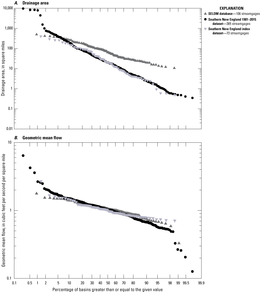
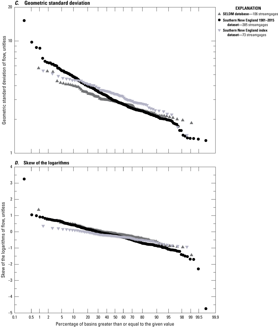
Scatterplot showing the distribution of streamflow statistics to the percentage of basins greater than or equal to various values for streamflow from streamgages in the Stochastic Empirical Loading and Dilution Model (SELDM) database (Granato, 2013), southern New England 1901–2015 dataset (Granato and others, 2017), and southern New England Index streamgage dataset (Granato and others, 2022). A, Drainage area. B, Geometric mean flow. C, Geometric standard deviation. D, Skew of the logarithms.
Information about relations between the average, standard deviation, and skew of nonzero streamflows is needed to guide the choice of a limited but representative set of values for simulating the potential effect of runoff on receiving waters. To this end, the nonparametric rank correlation coefficient (Spearman’s rho) was calculated among these statistics for each of the three streamflow datasets (table 12). Correlations between drainage area and the geometric mean streamflow in cubic feet per second are very strong (greater than or equal to 0.97) because drainage area is the controlling variable. However, the residual correlation between drainage area and the normalized geometric mean streamflow in cubic feet per second per square mile is weak (less than or equal to 0.34). This indicates that the selected values of the normalized geometric mean streamflow may be applied across drainage areas. Any other correlations to drainage area are only moderate to weak indicating that the geometric standard deviation and skew of the logarithms also may be applied across drainage areas. The correlations between the normalized geometric mean streamflow and geometric standard deviation are moderately strong (−0.74 to −0.82), indicating that these statistics covary. Similarly, the correlations between the geometric standard deviation and the skew of the logarithms of streamflow are moderately strong (−0.66 to −0.73), indicating that these statistics also covary. The standard deviation is calculated by using the mean and the skew is calculated by using the mean and the standard deviation, so these correlations can be used to assess the potential strength of a regression relation but should not be used for statistical inference.
Table 12.
Spearman’s rank-correlation coefficients for streamflow statistics for the common logarithms of nonzero flows from streamgages representative of conditions in southern New England.[Datasets (listed in table 11) were selected to be representative of streamflows in southern New England. Southern New England is defined as the area in the States of Connecticut, Massachusetts, and Rhode Island. Because of the sample sizes, all correlation coefficients are statistically significant at the 95-percent confidence limit (Haan, 1977). The Stochastic Empirical Loading and Dilution Model (SELDM) dataset includes all the streamgages in southern New England within the SELDM database (Granato, 2013). The southern New England 1901–2015 dataset includes all streamgages with 1 or more years of record during 1901–2015 (Granato and others, 2017). The southern New England index dataset (Index) includes streamgages commonly used to calculate streamflow statistics for studies in the region (Granato and others, 2022). Correlation coefficients that are greater than 0.5 are defined as moderately strong to strong. mi2, square mile; ft3/s, cubic foot per second; N, number of streamgages in each dataset]
Based on these correlations (table 12), regression relations were developed to select representative statistics for the geometric standard deviation and skew of the logarithms of streamflow values by using each of the three datasets (table 13). Because the potential effects of high-leverage outliers in datasets ranging over several orders-of-magnitude on regression relations can be large, the Kendall-Theil robust line method (Granato, 2006) was used to develop these equations. The objective was to produce the best estimate of the geometric standard deviation and skew of the logarithms of streamflow values given a selected value for the geometric mean of streamflows. Because the direct correlation between the geometric mean and the skew was weak, a fourth equation, which was calculated by algebraic combination of the regression equations of the mean to the standard deviation and the standard deviation to the skew, was developed and tested for each dataset. Despite the weak correlation, the direct regression equation between the geometric mean and skew was slightly more predictive than the algebraic combination. The equations in table 13 indicate that if the geometric mean flow was increased from 0.5 to 2 cubic feet per square mile over a series of simulations, then the associated geometric standard deviation would decrease from about 5.5 to about 1.8, and the associated skew would increase from about −0.7 to 0.3. At the median of geometric mean flows of about 1.03, the associated geometric standard deviation and the associated skew would be about 3.1 and −0.2, respectively.
Table 13.
Regression equation statistics developed by using the Kendall-Theil robust line method for estimating the mean, standard deviation, and skew of the common logarithms of streamflow data and the fraction of zero streamflows in southern New England.[The regression equations were developed by using the logarithms of data (Granato and others, 2022). Statistics are the mean, standard deviation, and skew of the logarithms of nonzero flows and the fraction of zero flows. Normalized streamflows are divided by area with units of cubic feet per second per square mile. Datasets: Index, southern New England 73 index streamgages (Granato and others, 2022); SELDM, 106 Stochastic Empirical Loading and Dilution Model database streamgages (Granato, 2013); 1901–2015, 385 Southern New England 1901–2015 streamgages (Granato and others, 2017). The algebraic estimate of skew from mean of the logarithms of normalized streamflow is derived by combining equations I and II in this table. The fraction of zero flows is estimated by using the mean of the logarithms of nonzero streamflow, in cubic feet per second. KTRLine, Kendall-Theil robust line (Granato, 2006); RMSE, root mean square error, unitless; MAD, median absolute deviation, unitless; BCF, Bias Correction Factor, unitless; ASEE, average standard error of the estimate, in percent; —, not applicable]
SELDM uses the specified fraction of zero flows to simulate the effect of runoff on ephemeral or intermittent streams by using conditional-probability methods. When the prestorm streamflow value is zero, the runoff or BMP discharge volumes are likely to be a larger fraction of downstream flows than for similar runoff events with nonzero prestorm streamflows. The upstream flow also will depend on the upstream area and lagtime, which are deterministic variables in SELDM, and the upstream runoff coefficients and recession ratios, which are stochastic variables in SELDM. An ephemeral stream has no baseflow; it flows only in response to runoff. Therefore, in theory, the maximum fraction of zero prestorm streamflow for an ephemeral stream is 1. Because the EPA definition of a runoff-generating event has an interevent dry time of 6 hours, multiple runoff events could take place within one day. Given an average number of runoff-generating events per year equal to 52 (table 9), the fraction of days with zero flows is at a minimum 0.8576 for an ephemeral stream. Perennial and intermittent streams both are defined as having flows that are sustained by groundwater discharge between runoff events. Distinctions between these categories, however, are operationally defined and such definitions are not consistent from State to State in southern New England. If the Massachusetts definition of streamflows less than 0.01 cubic feet per second at the 99-percent flow duration (Massachusetts Department of Environmental Protection, 2002) is used, then the risk, expressed as a probability fraction, of zero flows for intermittent streams would range from about 0.8576 to 0.01 (the 99-percent flow duration), and the risk of zero flows for perennial streams would range from about 0.01 to 0. Based on precipitation statistics (table 10), SELDM simulations for southern New England commonly result in about 30 years of runoff-generating events; algebraically, 1 zero-flow day during a 30-year period would have a risk of zero flows equal to about 0.0001. Stochastically, in theory, a risk value less than 0.0001 would not produce any prestorm flow values equal to zero; conversely, because SELDM is a Monte Carlo model, it can produce one or more prestorm flows that are equal to zero if the proportion of prestorm flows is specified as any number greater than zero.
Although the fraction of zero flow is commonly thought to be a function of drainage area, it also depends on physiography, geography, and water use. Streamflow statistics in the datasets selected to represent conditions in southern New England indicate that zero flows occur across a wide range of drainage areas (table 14). Spearman’s rank correlation coefficients between drainage area and the fraction of zero flows are −0.32 for the SELDM dataset, −0.46 for the 1901–2015 dataset, and −0.58 for the index dataset, which indicates that drainage area may be important but it is not the only variable of interest. Comparison of the means, standard deviations, and skews of streamflow for streamgages with zero flows to streamgages without zero flows indicates that these statistics are different between these groups. The geometric means are lower, the variability (standard deviations) is higher, and the skews are more negative for streamgages with zero flows than for streamgages without zero flows (table 11). These difference in streamflow statistics may be attributed to the effects of physiography, geography, and water use.
Table 14.
Percent of streamgages with one or more zero flows by drainage-area category from datasets selected to be representative of conditions in southern New England.[The Stochastic Empirical Loading and Dilution Model (SELDM) regional dataset includes all the streamgages in the southern New England States within SELDM (Granato, 2013). The 1901–2015 dataset includes all streamgages with one or more years of record during the 1901–2015 period in southern New England (Granato and others, 2017). The Index dataset includes streamgages commonly used to calculate streamflow statistics for studies in the southern New England region (Granato and others, 2022). mi2, square mile; N, number of streamgages in each dataset; —, not applicable]
Regression equations were developed to estimate the fraction of zero flows from the average of the logarithms of flow (table 13; eq. 5) to guide the choice of simulation values at ungaged sites. The average of the logarithms of flow (in cubic feet per second) was used as the predictor variable rather than the normalized average (in cubic feet per second per square mile) to capture the variation in drainage area and normalized mean flow of the sites with one or more zero flows in each dataset. The regression equation developed by using the SELDM dataset (table 13) should not be used for small basins (less than about 10 square miles) because there are only six streamgages in this dataset with one or more zero flows and the smallest drainage area among these streamgages is 10.6 square miles. Given the geometric mean streamflow of 0.87 cubic feet per second square mile for the SELDM dataset of southern New England streamgages (table 11), the fraction of zero flows calculated by using this equation is greater than or equal to 1 (100 percent of flows) if the drainage area is less than or equal to about 1.31 square miles. In comparison, using the geometric means of 0.796 and 0.809 cubic feet per second per square mile for the zero-flow streamgages in the 1901–2015 and Index datasets (table 11) and solving the associated regression equations in table 13 for a ratio of 1 results in drainage-area estimates of about 0.010 and 0.039 square miles for each dataset, respectively. These areas are much less then the drainage areas of 0.35 square miles for the 1901–2015 dataset streamgages and 0.49 square miles for the Index dataset streamgages with one or more zero flows (table 11). Given the geometric mean flows (table 11) and zero-fraction equations (table 13) for streamgages with one or more zero flows, the estimates of the fraction of zero flows for a 1-square-mile basin would be about 0.023 and 0.006 for the 1901–2015 and Index streamgage datasets, respectively. Similarly, the estimates for the fraction of zero flows in a 10-square-mile basin would be about 0.0034 and 0.00014 for the 1901–2015 and Index streamgage datasets, respectively. Given the large standard error of the estimates of the equations for the fraction of zero flows in table 13, these estimates of the fraction of zero flows among the streamgage datasets may be substantially different but are not significantly different at the 95-percent confidence limit.
Although SELDM will simulate nonzero prestorm streamflows below the commonly used USGS minimum reported streamflow measurement of 0.01 cubic foot per second (ft3/s; Rantz, 1982; Granato, 2010, 2013), the USGS streamflow records used to calculate the fraction of zero flows and other statistics are censored at this flow rate. SELDM uses the frequency factor method to generate a population of nonzero streamflows; that method also can be used to estimate the probability of nonzero flows below the reporting limit given the statistics for nonzero flows. If a value of 0.01 ft3/s is substituted into the frequency factor equation and it is rearranged to solve for the lognormal (if the skew is near 0) or log Pearson Type III (if the skew is substantially different from 0) frequency factor, then the resulting equation for the zero-streamflow reporting limit of 0.01 ft3/s (Rantz, 1982) is the following:
whereK
is the lognormal or log Pearson Type III frequency factor, which is a function of the skew value;
log(0.01)
is the logarithm of the minimum streamflow reporting limit, in cubic feet per second (Rantz, 1982);
log(DA)
is the logarithm of drainage area, in square miles;
log(Q)
is the average of the logarithms of streamflow, in cubic feet per second per square mile; and
log(SD)
is the standard deviation of the logarithms of streamflow.
The frequency-factor value (K) calculated by using equation 4 can be converted to a probability value by using probability tables or algebraic transfer functions (Haan, 1977; Natural Resources Conservation Service, 1998; Granato, 2010, 2013). Using the average and standard deviation of the logarithms of normalized streamflow among streamgages with one or more zero flows for the 1901–2015 dataset in table 11 results in K values of −1.339, −2.824, and −4.31 for drainage areas equal to 0.1, 1.0, and 10 square miles, respectively. Using probabilities for these K values associated with a skew of −0.775 (table 11) results in zero-flow-fraction estimates of about 0.0997, 0.0111, and 0.0009 for drainage areas of 0.1, 1.0, and 10 square miles, respectively. The equivalent estimates made using the Index dataset statistics in table 11 are 0.0914, 0.0067, and 0.0003 for drainage areas of 0.1, 1.0, and 10 square miles, respectively. Alternatively, the FrequencyFactors2021 program (Granato and others, 2022) can be used to generate a table of exceedance values from the statistics of the logarithms of streamflow; these values can be used to estimate the risks for flows less than 0.01 cubic feet per second. Calculations show that using the medians of the average, standard deviation, and skew of all streamgages in the 1901–2015 dataset and Index dataset results in the fraction of zero flows of less than 0.0001 for basins greater than one square mile. The different dataset estimates are substantially different from each other and are different from the regression-based estimates. Also, substantial percentages of streamgages with drainage areas less than 30 square miles have zero-flow fractions greater than the 0.0001 (30 year) threshold (table 14). Therefore, an average of estimates calculated by using different methods and different datasets may inform professional judgement for estimating the percentage of zero flows at an ungaged site or a site with a very short record.
Runoff Coefficient Statistics
SELDM simulates runoff from precipitation by using stochastic runoff coefficients, which are the ratio of the volume of runoff in watershed inches to the volume of basin-average precipitation (in inches) during each storm event (Granato, 2013). SELDM simulates runoff coefficients from the site of interest and the upstream basin by using the Pearson type III distribution, which is defined by the input average, standard deviation, and skew of the runoff coefficients. The effects of antecedent conditions on upstream runoff coefficients are simulated by using the rank correlation to prestorm streamflow. Wetter antecedent conditions, which tend to increase runoff coefficients, commonly are associated with higher prestorm streamflows (Granato, 2010, 2013). The user-entered rank correlation coefficients between prestorm flows and upstream runoff coefficients commonly are about 0.75 for high quality datasets (Granato, 2010, 2013). The effect of antecedent conditions on runoff coefficients for the site of interest are simulated indirectly by using correlations between runoff coefficients for the upstream basin and the site of interest. These correlations, which are calculated within SELDM, are at a maximum if the imperviousness of the upstream basin and the site of interest are equal and are reduced as the impervious fractions diverge (Granato, 2010, 2013).
In SELDM, runoff coefficient statistics can be calculated as a function of the total impervious area of the site of interest and the upstream basin by using regression equations (table 15) or by entering user-defined values. The regression equations developed to calculate the average, standard deviation, and skew of the runoff coefficients for highway sites were developed with rainfall-runoff data from 58 highway basins across the country, and the regression equations for the upstream basins (or nonhighway sites of interest) were developed with data from 167 basins across the country with various nonhighway land uses (Granato, 2010, 2013). The average, standard deviation, and skew of the runoff coefficients calculated by using regression equations for completely impervious highway areas (TIA equal to 1.0) are 0.785, 0.1917, and −1.19, respectively (table 15). The average, standard deviation, and skew of the runoff coefficients of completely impervious nonhighway areas calculated by using regression equations are 0.769, 0.114, and −0.51, respectively. The average runoff coefficient for the completely impervious highway sites is higher than the average for the completely impervious nonhighway sites; this may be caused by random sampling of different sites or the difference may be caused by highway-engineering design practices to rapidly drain runoff from the roadway and efficiently convey runoff from the road to stormwater discharge locations to maintain safe driving conditions (Brown and others, 2009). Both of these average runoff coefficient values are lower than the commonly used values, which can be as high as 0.96 for completely impervious areas (Granato, 2010, 2013). Field studies show that evaporation and infiltration from paved surfaces commonly reduce the average runoff from such areas by 20 to 30 percent (Ragab and others, 2003; Mansell and Rollet, 2006; Ramier and others, 2006; Wiles and Sharp, 2008; Wanielista and others, 2010; Redfern and others, 2016; Timm and others, 2018; Salt and Kjeldsen, 2019; Rammal and Berthier, 2020). Therefore, the default average values used by SELDM (0.785 or 0.769) are more representative of measured runoff results than higher average runoff coefficient values commonly used in the literature (Granato, 2010, 2013). Although the stochastic runoff-generation algorithms in SELDM produce many events with simulated runoff coefficients at or near a value of 1 for highly impervious sites, a substantial number of events with lower simulated runoff coefficients will show the precipitation losses evident in high-quality runoff monitoring datasets (Granato, 2013).
Table 15.
Regression equation statistics developed by using the Kendall-Theil robust line method for estimating the average, standard deviation, and skew of runoff coefficients from the total impervious fraction.[Regression equations were developed for use in the Stochastic Empirical Loading and Dilution Model (SELDM) and other applications by using rainfall and runoff data from 58 highway and 167 nonhighway sites (Granato and Cazenas, 2009; Granato, 2010, 2013). The highway equations were developed by using sites with impervious fractions from 0.27 to 1.00; the nonhighway equations were developed by using sites with impervious fractions from 0.0001 to 0.994. Granato (2013) combined the KTRLine intercept of −0.02495 with the bias correction factor (BCF) of 0.05487 to calculate the intercept of 0.03 so that the regression would not produce runoff coefficients that are less than or equal to zero when the impervious ratio is less than or equal to a fraction of 0.032 (3.2 percent). The intercept of the equations for the standard deviation and skew of highway-site runoff coefficients also were adjusted by using the bias correction factor. KTRLine, Kendall-Theil robust line (Granato, 2006), RMSE, root mean square error, unitless; MAD, median absolute deviation, unitless; MaxX, the maximum value of the predictor variable (in this case imperviousness) applicable to the regression-equation segment; N, number of sites]
Hydrograph Recession-Ratio Statistics
The timing of runoff from the upstream basin is defined by using the basin lagtime and the hydrograph recession ratio, which is the ratio of the duration of the falling limb to the rising limb (or time to peak) of the hydrograph (Granato, 2010, 2012, 2013). In SELDM, a triangular hydrograph is used to simulate the timing of runoff stochastically. The duration of the runoff-generating precipitation event is simulated as a random variable. The basin lagtime, which is the time between the centroid of precipitation to the centroid of runoff, is simulated as a constant value based on the main-channel length, slope, and imperviousness of the upstream basin. The hydrograph recession ratio is used to calculate the time to peak, the recession time, and therefore the duration of the highway and upstream hydrographs. The rational-method hydrograph recession ratio for highly impervious basins, which is equal to 1, is used in SELDM to simulate runoff for the highway site. The hydrograph recession ratio for the upstream basin, however, is simulated as a stochastic variable by using a triangular distribution. The triangular distribution of ratios is parametrized by using the minimum, most probable value, and maximum of ratios (Granato, 2012, 2013). The upstream hydrograph is used with the highway-runoff and BMP-discharge durations to calculate the proportion of the total upstream stormflow that is used in the mass balance and dilution calculations (Granato, 2013).
Granato (2012) calculated hydrograph recession-ratio statistics by using least-squares optimization techniques with measured runoff hydrographs from multiple storms from 41 streamgages across the United States. This dataset included 30 stream basins in Massachusetts, 1 stream basin in Connecticut, and 1 in Rhode Island. In the current study, methods developed by Granato (2012) were used to calculate hydrograph recession-ratio statistics from 20 or more runoff events for an additional 13 basins in Connecticut and 6 basins in Rhode Island (Granato and others, 2022). These analyses were done to build a 51-streamgage dataset to simulate runoff events in southern New England. These recession ratios are presented with selected basin properties in table 16. The minimums of recession ratios in the combined dataset ranged from 1.00 to 2.05 with a median of 1.10 and an average of 1.20. The most probable values of recession ratios in the combined dataset ranged from 1.00 to 2.87 with a median of 1.50 and an average of 1.67. The maximums of recession ratios in the combined dataset ranged from 2.49 to 9.67 with a median of 4.42 and an average of 4.80. In comparison, the default values for the minimum, most probable value, and maximum recession ratios within SELDM are 1.00, 1.85, and 4.40, respectively (table 17). In comparison, the median recession ratios for non-New England gages calculated by Granato (2012) were 1.0 for the minimum, 1.16 for the most probable value, and 4.05 for the maximum of the triangular distribution. Similarly, Weaver and others (2019) analyzed hydrographs from multiple storms from 30 sites in North Carolina and calculated median recession ratio values of 1.0 for the minimum, 1.07 for the most probable value, and 4.72 for the maximum of the triangular distribution. Stonewall and others (2019) analyzed hydrographs from multiple storms from 13 sites in Oregon and calculated median recession ratio values of 1.0 for the minimum, 2.22 for the most probable value, and 4.37 for the maximum of the triangular distribution. The similarities in these statistics from hydrographs in the different areas of the country indicate that, like physiography, common hydrologic processes result in similar outcomes.
Table 16.
Best-fit triangular-hydrograph recession ratios estimated from 20 or more storm-event hydrographs at each listed U.S. Geological Survey streamgage in southern New England.[Basin properties were obtained from source reports (Granato, 2012) or calculated by using the U.S. Geological Survey StreamStats application. Min, minimum; MPV, most probable value; Max, maximum; Avg, the average of the three recession-ratio statistics; DRNAREA, drainage area in square miles; LENGTH, main-channel length in miles; CSL10_85, main-channel slope in feet per mile; BLF, basin-lag factor, which is the basin length (LENGTH) in miles divided by the square root of the channel slope (CSL10_85) in feet per mile; NLCD, National Land Cover Database; Impervious %, total impervious area in percent; MA, Massachusetts; RI, Rhode Island; CT, Connecticut; Y, yes; N, no]
| Streamgage number | Name | Hydrograph-recession ratios | Basin properties (and basin-lag equation variables) | Sensitivity analysis | |||||||||
|---|---|---|---|---|---|---|---|---|---|---|---|---|---|
| Min | MPV | Max | Avg | DRNAREA | LENGTH | CSL10_85 | BLF | NLCD Impervious % | Stream density | Reference | |||
| 01118300 | Pendleton Hill Brook near Clark Falls, CT | 1.35 | 1.35 | 6.05 | 2.92 | 4.02 | 3.92 | 76.5 | 0.45 | 0.41 | 1.58 | Current study | Y |
| 01115280 | Cork Brook at Rockland Scituate Rd near Clayville, RI | 1.18 | 1.18 | 6.89 | 3.08 | 1.79 | 3.28 | 80.62 | 0.37 | 2.12 | 1.2 | Current study | N |
| 01117468 | Beaver River near Usquepaug, RI | 1.08 | 1.08 | 4.36 | 2.17 | 8.87 | 8.82 | 33.36 | 1.53 | 1.28 | 1.6 | Current study | N |
| 01115187 | Ponaganset River at South Foster, RI | 1.35 | 1.35 | 3.91 | 2.2 | 14.4 | 8.09 | 46.73 | 1.18 | 1.07 | 2.59 | Current study | N |
| 01111300 | Nipmuc River near Harrisville, RI | 1 | 1 | 5.17 | 2.39 | 16 | 7.87 | 34.45 | 1.34 | 1.08 | 2.51 | Current study | N |
| 01117800 | Wood River near Arcadia, RI | 1.91 | 1.91 | 6.04 | 3.29 | 35.2 | 12.13 | 29.86 | 2.22 | 0.68 | 1.37 | Current study | N |
| 01115190 | Dolly Cole Brook at Old Danielson Park at S Foster, RI | 2.05 | 2.05 | 6.28 | 3.46 | 4.9 | 4.74 | 78.05 | 0.54 | 1.21 | 2.06 | Current study | Y |
| 01203510 | Pootatuck River at Sandy Hook, CT | 1.1 | 1.1 | 7.29 | 3.16 | 24.91 | 11.2 | 45.46 | 1.66 | 6.38 | 2.74 | Current study | N |
| 01188000 | Bunnell Brook near Burlington, CT | 1 | 1 | 2.92 | 1.64 | 4.1 | 4.23 | 52.18 | 0.58 | 2.37 | 2.66 | Current study | Y |
| 01195100 | Indian River near Clinton, CT | 1.19 | 1.19 | 4.28 | 2.22 | 5.68 | 6.84 | 68.87 | 0.82 | 2.43 | 3.95 | Current study | Y |
| 01208950 | Sasco Brook near Southport, CT | 1.15 | 1.15 | 3.58 | 1.96 | 7.38 | 6.02 | 54.26 | 0.82 | 5.94 | 3.44 | Current study | Y |
| 01184100 | Stony Brook near West Suffield, CT | 1.23 | 1.23 | 2.49 | 1.65 | 10.4 | 7.02 | 11.76 | 2.05 | 2.62 | 3.19 | Current study | N |
| 01208990 | Saugatuck River near Redding, CT | 1.08 | 1.08 | 5.73 | 2.63 | 21 | 12.06 | 29.51 | 2.22 | 1.37 | 2.77 | Current study | N |
| 01203805 | Weekeepeemee River at Hotchkissville, CT | 1 | 1 | 3.75 | 1.92 | 27.05 | 11.55 | 70.95 | 1.37 | 0.82 | 2.48 | Current study | N |
| 01123000 | Little River near Hanover, CT | 1 | 1 | 4.36 | 2.12 | 30 | 17.03 | 20.76 | 3.74 | 0.51 | 3.53 | Current study | N |
| 01187300 | Hubbard River near West Hartland, CT | 1.38 | 1.38 | 5.93 | 2.9 | 19.9 | 10.49 | 74.22 | 1.22 | 0.18 | 1.9 | Current study | N |
| 01187800 | Nepaug River near Nepaug, CT | 1 | 1 | 3.14 | 1.71 | 23.5 | 11.38 | 34.69 | 1.93 | 1.01 | 2.49 | Current study | N |
| 01194000 | Eightmile River at North Plain, CT | 1.22 | 1.22 | 3.46 | 1.97 | 20.1 | 10.33 | 48.99 | 1.48 | 0.65 | 2.66 | Current study | N |
| 01208873 | Rooster River at Fairfield, CT | 1.08 | 1.08 | 2.76 | 1.64 | 10.71 | 9.82 | 51.28 | 1.37 | 36.82 | 1.9 | Current study | N |
| 01111300 | Nipmuc River near Harrisville, RI | 1 | 2.53 | 5.73 | 3.09 | 16 | 7.79 | 30.4 | 1.41 | 1.08 | 2.51 | Granato (2012) | N |
| 01187300 | Hubbard River near West Hartland, CT | 1.67 | 1.67 | 9.13 | 4.16 | 19.9 | 10.4 | 67.5 | 1.26 | 0.18 | 1.9 | Granato (2012) | N |
| 01094400 | North Nashua River at Fitchburg, MA | 1 | 2.23 | 5 | 2.74 | 63.4 | 17.8 | 40.7 | 2.78 | 5.98 | 1.74 | Granato (2012) | N |
| 01094500 | North Nashua River near Leominster, MA | 1 | 2.83 | 4.27 | 2.7 | 110 | 25.6 | 32.6 | 4.49 | 10.6 | 1.82 | Granato (2012) | N |
| 01095220 | Stillwater River near Sterling, MA | 1.66 | 2.01 | 4.05 | 2.57 | 30.4 | 11.5 | 39.3 | 1.83 | 1.52 | 1.67 | Granato (2012) | N |
| 01096000 | Squannacook River near West Groton, MA | 1.03 | 1.95 | 2.66 | 1.88 | 64.4 | 18.3 | 41.7 | 2.83 | 2.13 | 2.01 | Granato (2012) | N |
| 01097000 | Assabet River at Maynard, MA | 1 | 1.83 | 5.04 | 2.62 | 116 | 28.1 | 4.69 | 13 | 11.1 | 2.5 | Granato (2012) | Y |
| 01097300 | Nashoba Brook near Acton, MA | 1.16 | 1.16 | 3.18 | 1.83 | 12.9 | 5.83 | 8.62 | 1.99 | 7.85 | 2.75 | Granato (2012) | Y |
| 01100600 | Shawsheen River near Wilmington, MA | 1.08 | 1.34 | 3.08 | 1.83 | 36.5 | 16.2 | 8.61 | 5.52 | 25.3 | 1.68 | Granato (2012) | N |
| 01102500 | Aberjona River at Winchester, MA | 1 | 1 | 5.11 | 2.37 | 24.1 | 10.3 | 9.64 | 3.32 | 40.6 | 1.81 | Granato (2012) | N |
| 01103280 | Charles River at Medway, MA | 1.16 | 2.34 | 9.67 | 4.39 | 65.7 | 21.4 | 7.83 | 7.65 | 14.2 | 2.33 | Granato (2012) | N |
| 01105500 | East Branch Neponset River at Canton, MA | 1.25 | 2.2 | 6.23 | 3.23 | 27.2 | 8.32 | 23.4 | 1.72 | 20 | 2.36 | Granato (2012) | Y |
| 01105600 | Old Swamp River near South Weymouth, MA | 1 | 1 | 3.39 | 1.8 | 4.47 | 4.76 | 10.3 | 1.49 | 25.5 | 2 | Granato (2012) | N |
| 01105730 | Indian Head River at Hanover, MA | 1.77 | 1.85 | 4.62 | 2.75 | 30.2 | 13.3 | 9.92 | 4.24 | 14.8 | 2.29 | Granato (2012) | N |
| 01108000 | Taunton River near Bridgewater, MA | 1 | 1.58 | 5.44 | 2.67 | 258 | 33.5 | 3.63 | 17.6 | 9.71 | 2.09 | Granato (2012) | N |
| 01109000 | Wading River near Norton, MA | 1.02 | 2.22 | 3.99 | 2.41 | 43.3 | 19.6 | 7.55 | 7.12 | 9.22 | 2.12 | Granato (2012) | N |
| 01109060 | Threemile River at North Dighton, MA | 1 | 1.22 | 5.56 | 2.59 | 84.3 | 32.5 | 5.91 | 13.3 | 10.8 | 2.37 | Granato (2012) | N |
| 01109070 | Segreganset River near Dighton, MA | 1.41 | 1.46 | 4.75 | 2.54 | 10.6 | 7.36 | 8.67 | 2.5 | 3.94 | 2.41 | Granato (2012) | N |
| 01111200 | West River below West Hill Dam, near Uxbridge, MA | 1 | 2.68 | 4.47 | 2.72 | 27.8 | 13.3 | 13.7 | 3.61 | 2.55 | 2.68 | Granato (2012) | N |
| 01162500 | Priest Brook near Winchendon, MA | 1.2 | 2.51 | 4.56 | 2.76 | 19.2 | 15.2 | 19 | 3.49 | 0.52 | 1.82 | Granato (2012) | N |
| 01163200 | Otter River at Otter River, MA | 1.48 | 2.25 | 3.48 | 2.4 | 34.1 | 12.3 | 16.5 | 3.02 | 9.14 | 1.86 | Granato (2012) | N |
| 01169000 | North River at Shattuckville, MA | 1.18 | 2.87 | 3.24 | 2.43 | 89.9 | 22.6 | 49 | 3.23 | 0.56 | 2.05 | Granato (2012) | N |
| 01169900 | South River near Conway, MA | 1 | 1.38 | 3.81 | 2.06 | 24.1 | 14.6 | 58.1 | 1.91 | 0.89 | 2.05 | Granato (2012) | Y |
| 01170100 | Green River near Colrain, MA | 1 | 2.07 | 4.09 | 2.39 | 41.3 | 19.1 | 59.4 | 2.48 | 0.24 | 2.38 | Granato (2012) | Y |
| 01171500 | Mill River at Northampton, MA | 1.37 | 1.5 | 3.9 | 2.26 | 54 | 18 | 76.1 | 2.06 | 1.94 | 1.97 | Granato (2012) | N |
| 01173500 | Ware River at Gibbs Crossing, MA | 1 | 1 | 4.42 | 2.14 | 197 | 43.7 | 25.1 | 8.72 | 1.22 | 2.04 | Granato (2012) | N |
| 01174565 | West Branch Swift River near Shutesbury, MA | 1 | 2.64 | 6.22 | 3.29 | 12.6 | 7.83 | 61 | 1 | 0.24 | 1.89 | Granato (2012) | N |
| 01174600 | Cadwell Creek near Pelham, MA | 1.21 | 2.02 | 4.02 | 2.42 | 0.6 | 1.91 | 129 | 0.17 | 0.43 | 1.93 | Granato (2012) | N |
| 01174900 | Cadwell Creek near Belchertown, MA | 1 | 2.77 | 4.56 | 2.78 | 2.89 | 3.95 | 135 | 0.34 | 0.17 | 1.99 | Granato (2012) | N |
| 01175670 | Sevenmile River near Spencer, MA | 1.59 | 1.67 | 8.6 | 3.95 | 8.69 | 7.95 | 39.4 | 1.27 | 0.71 | 2.84 | Granato (2012) | Y |
| 01181000 | West Branch Westfield River at Huntington, MA | 1.22 | 2.13 | 6.11 | 3.15 | 93.7 | 23.3 | 44.2 | 3.5 | 0.43 | 1.6 | Granato (2012) | N |
| 01331500 | Hoosic River at Adams, MA | 1.24 | 2.1 | 4.12 | 2.49 | 46.7 | 14.4 | 10.3 | 4.49 | 1.52 | 1.74 | Granato (2012) | N |
Table 17.
Summary statistics for the best-fit triangular-hydrograph recession ratios estimated from 20 or more storm-event hydrographs at each listed U.S. Geological Survey streamgage in southern New England.[Basin properties were obtained from source reports or calculated by using StreamStats. Min, minimum; MPV, most probable value; Max, maximum; Avg, the average of the three recession-ratio statistics; DRNAREA, drainage area in square miles; LENGTH, main-channel length in miles; CSL10_85, main-channel slope in feet per mile; BLF, basin-lag factor, which is the basin length (LENGTH) in miles divided by the square root of the channel slope (CSL10_85) in feet per mile; NLCD, National Land Cover Database; Impervious %, total impervious area in percent; SELDM, Stochastic Empirical Loading and Dilution Model; —, not applicable]
Spearman’s rank correlation analyses were done in an attempt to provide guidance on the selection of hydrograph recession-ratio statistics by using basin properties. The rank correlations among recession-ratio statistics were about 0.193 between the minimum and the most probable value, about 0.189 between the minimum and maximum, and about 0.228 between the most probable value and the maximum. Correlations between the three triangular-distribution statistics and the drainage area, main-channel length, main-channel slope, basin-lag factor, and imperviousness were of mixed sign and had absolute values ranging from 0.00027 and 0.292. These low correlations indicate that basin properties cannot be used to quantitatively select recession-ratio statistics. These results are similar to the results of correlation analyses done by Granato (2012), which also included 15 other variables that included land cover, wetlands, impoundments, and other hydrologic variables. Therefore, the hydrograph recession-ratio statistics are random variables with respect to each other and to basin properties, and the median values are robust estimates for unmonitored sites.
Stormwater Quality
Statistics were calculated for 21 water-quality properties and constituents of concern (table 18) in southern New England, and these statistics were used to simulate the water quality and loads from long-term populations of runoff events. The water-quality constituents simulated in this study were selected to represent constituents of concern for impaired waters in southern New England (EPA, 2021). The categories include water-quality properties (turbidity), sediment and solids, nutrients, minor and trace inorganic chemicals (metals), organic chemicals (polycyclic aromatic hydrocarbons [PAHs]), biological constituents (bacteria), and major ionic constituents (chloride). Although low dissolved oxygen concentrations and excess aquatic vegetation are of concern for many waterbodies (EPA, 2021), these problems commonly are associated with elevated nutrient concentrations in receiving waters. Statistics for 12 to 19 highway sites in Massachusetts (depending on the constituent of interest) were calculated by using the highway-runoff database and were used to characterize highway runoff for constituents that have been measured in Massachusetts datasets (Granato 2019a; Granato and Friesz, 2021b). Statistics for constituents without sufficient data from the Massachusetts sites for characterization were calculated by using the highway-runoff database by using data from sites outside the region. Data from 4 to 241 urban-runoff sites were used to simulate developed-area runoff quality (table 18). Data from 82 stream water-quality monitoring sites were used to calculate upstream stormflow statistics. The number of stream sites with available data ranged from 0 to 69 sites so it was necessary to develop dependent relations for some constituents with insufficient sites (table 18).
Table 18.
Runoff-quality constituents analyzed in this study with counts of the number of highway-runoff sites, urban-runoff sites, and the best management practice treatment analysis method.[Pcode is the water-quality parameter code denoted by the letter p and the five-digit identification number from the U.S. Geological Survey (2021) National Water Information System (NWIS). The Pcode pXXX05 is defined in the Highway Runoff Database (Granato, 2019a) as the sum of polycyclic aromatic hydrocarbons measured or estimated in stormwater samples. HN is the number of highway sites in the Highway-Runoff Database (Granato and Friesz, 2021b); UN is the number of urban sites in the Best Management Practices Statistical Estimator (Granato, 2021a); and SQ (stream quality) is the number of instream water-quality monitoring sites with 10 or more paired values of concentration and instantaneous flows collected by the U.S. Geological Survey using currently accepted protocols that were used to calculate constituent-concentration statistics (U.S. Geological Survey, 2021). BMP is the best management practice treatment estimate indicated by M, estimated from measured data by Granato and others (2021, table 1.1); or S, water-quality-treatment estimate from a similar constituent. e, estimated from a similar constituent; eu, estimated from urban runoff data; PAHs, polycyclic aromatic hydrocarbons; EPA, Environmental Protection Agency]
Available data for simulating runoff and receiving water quality are limited in comparison to the number of sites where estimates of water quality may be needed (table 18). There are about 57,000 miles of non-State maintained roadway, about 7,800 miles of State-maintained roadway, and more than 48,000 road-stream crossings in the stream basins of southern New England (tables 2, 3). Robust methods are needed to use available data from monitored sites to estimate potential effects of runoff at unmonitored sites because the uncertainties in the selection process are not well defined. Because data are limited in comparison to the number of potential sites of interest and because the current study did not include a field-monitoring effort to generate site-specific data, available data are used to represent water quality at hypothetical sites of interest in the study area. Local data were used when possible, but representative National data were used in other instances. Water-quality statistics were selected to simulate populations of constituent concentrations that could be expected to be found at sites in southern New England.
Although the nominally dissolved (filtered) fraction of many constituents is of regulatory concern, the whole-water (unfiltered) concentrations were simulated because sediment concentrations and the distribution between the filtered and unfiltered fractions can change as runoff travels from developed and agricultural surfaces through conveyances and stormwater treatment facilities (Granato, 2013; Granato and others, 2021). Sediment concentrations and the distribution between the filtered and unfiltered fractions also commonly change rapidly in the receiving waters below the discharge point. Filtered concentrations, which are theoretically lower than unfiltered concentrations, have greater uncertainty than unfiltered concentrations because of potential contamination and filtering artifacts that may occur in the sample handling process (Breault and Granato, 2000). For these, and other reasons, filtered-concentration data are less abundant in highway and urban runoff datasets than the whole-water concentration data (Pitt and others, 2015; Granato, 2019a, 2021a). Chloride is the exception in this study (table 18) because chloride concentrations of concern are large, sample-processing methods have minimal effects on chloride, and the standard analysis methods are for the filtered fraction.
SELDM provides three methods for simulating stormflow quality (fig. 1; Granato, 2013). Runoff from the site of interest and upstream water quality can be simulated by using the frequency factor method, which uses the average, standard deviation, and skew of data (or more commonly the logarithms of data) to generate a population of random concentration values. Runoff and upstream water-quality concentrations also can be simulated as dependent variables. The dependent-variable method uses a linear relation between two water-quality constituents with random variation above and below the line. Using this method, the analyst can simulate concentrations of one constituent as a function of another. Dependent methods commonly are used if there is abundant data for one constituent and relatively little data for another related constituent. Upstream water-quality concentrations also can be simulated by using a transport curve, which is a regression relation between streamflow and concentration (fig. 1). The variations in simulated dependent or transport-curve concentrations are simulated by using the variability of residuals above and below the line. In SELDM, the dependent relations and transport curves may have one, two, or three segments to simulate changes in the linear relation over the range of available data.
All concentrations were simulated by using statistics for the logarithms of data. The logarithms of concentration and stormflow commonly are analyzed and simulated by using the logarithms of the data because these variables vary by orders of magnitude and are bounded by zero (Driscoll and others, 1979; Athayde and others, 1983; Di Toro, 1984; Van Buren and others, 1997; Novotny, 2004; Granato and Cazenas, 2009; National Research Council, 2009b; Smith and Granato, 2010; Granato, 2013; Smith and others, 2018; Stonewall and others, 2019; Weaver and others, 2019; Jeznach and Granato, 2020; Granato and Friesz, 2021a). The logarithms of concentration were used to develop the random statistics and dependent-relation statistics. The logarithms of flow and concentration were used to develop the transport-curve statistics.
Highway Runoff
Highway-runoff quality statistics for commonly measured properties and constituents (tables 18, 19) were calculated by using version 1.1.0b of the Highway-Runoff Database (HRDB; Granato and Cazenas, 2009; Granato, 2019a; Granato and Friesz, 2021b). All highway-runoff concentrations were simulated as random variables by using the frequency-factor method with the average, standard deviation, and skew of the transformed (logarithmic) values (Granato, 2013). Dependent relations were not used to simulate highway-runoff quality, but two bacterial constituents (p31625 and p50569) were simulated by using statistics for other equivalent bacterial constituents, and one bacterial constituent (p31673) was simulated by using statistics for urban-runoff data (tables 18, 19).
Table 19.
Statistics for the common logarithms of data used to simulate highway-runoff quality in southern New England with the Stochastic Empirical Loading and Dilution Model (SELDM).[Pcode is a water-quality parameter code denoted by the letter p and the five-digit identification number from the U.S. Geological Survey (2021) National Water Information System (NWIS) or the Highway-Runoff Database (Granato and Friesz, 2021b). Parameter codes and names are defined in table 18. Percentage not skewed means the percentage of sites with a skew value that is not significantly different from 0 at the 95-percent confidence limit (Interagency Advisory Committee on Water Data, 1982). BMPSE urban-runoff data are from the Best Management Practice Statistical Estimator (Granato, 2021a); data are from studies sponsored by the department of transportation for State(s) indicated (CA, California; NV, Nevada; OR, Oregon; SC, South Carolina; WA, Washington). The average estimate—low and average estimate—high are the 15th and 85th percentile of the average logarithmic concentrations from sites with data. The Pcode pXXX05 is defined in the Highway Runoff Database (Granato, 2019a) as the sum of polyaromatic hydrocarbons measured or estimated in stormwater samples. AADT, average Annual daily traffic, in vehicles per day]
Rank correlation (rho) analysis using Spearman’s rho was used to evaluate the correlation between the average and standard deviation of the logarithms of concentrations to determine whether the values used for simulation could be selected independently. Rank correlation values for highway-runoff constituents ranged from −0.8 to 0.393 with a median correlation of −0.18 (table 19), but none of these values were statistically different from 0 at the 95-percent confidence limit (Haan, 1977). Therefore, the average and standard deviation of the logarithms of concentrations could be selected independently to simulate highway runoff quality.
Concentrations of highway runoff for all constituents were simulated by using a skew value of 0. This value was selected because the percentage of datasets with skew values that were not significantly different from 0 at the 95-percent confidence limit (Haan, 1977) was large. For highway runoff, the percentage of constituent datasets with calculated skews that were not significantly different from 0 ranged from 75 to 100 percent with an average of 93.8 percent (table 19). Skew values of 0 were used because most constituents could be characterized as lognormal and because use of a skew equal to 0 would reduce the risks for generating improbable extreme outliers in the simulated urban-runoff concentration populations (Risley and Granato, 2014).
Rank correlation analysis using Spearman’s rho also was used to examine relations between the geometric mean concentrations of constituents and the AADT reported for each highway monitoring site. These rank correlation values ranged from −0.8 to 0.93 with a median correlation of 0.445 (table 19). Only 9 of 20 highway-runoff constituents had rank correlation values that were statistically different from 0 at the 95-percent confidence limit (Haan, 1977). Regression equations between the logarithms of AADT and geometric mean concentration were developed for these 9 constituents, which included total nitrogen, total phosphorus (p00665), trace elements (except mercury), and total PAHs (table 20). Although some of the rank correlations are strong, there is considerable uncertainty in geometric-mean predictions for a given AADT value. Based on the root mean square error in logarithmic space (Helsel and Hirsch, 2002), the 95-percent prediction interval ranges by a factor of 1.4 for total nickel (p01067) and as high as a factor of about 6.86 for total phosphorus (p00665).
Table 20.
Regression equation statistics developed by using the Kendall-Theil robust line method for estimating the average of the common logarithms of highway-runoff constituents from the common logarithms of average daily traffic volumes.[Regression equations developed for constituents with statistically significant Spearman's rank correlation coefficients greater than 0.5 in table 19. Concentrations are from data collected at Massachusetts highway monitoring stations with average daily traffic (AADT) values ranging from 3,000 to190,993 vehicles per day. Pcode is a water-quality parameter code denoted by the letter p and the 5-digit identification number from the U.S. Geological Survey (2021) National Water Information System (NWIS) or the Highway-Runoff Database (Granato and Friesz, 2021b); parameter codes and names are defined in table 18. The Pcode pXXX05 is defined in the Highway Runoff Database (Granato, 2019a) as the sum of polycyclic aromatic hydrocarbons measured or estimated in stormwater samples. MAD, median absolute deviation; RMSE, root mean square error; ASEE, average standard error of the estimate, in percent]
Although regression equations are provided, the results will not be used for simulations in this study because there are many complications for application of specific AADT estimates. AADT may not be the primary causal variable. Increased AADT is associated with increases in the imperviousness of land covers within a mile radius of highway-runoff monitoring sites (Smith and Granato, 2010; Granato and Friesz, 2021a, b). Smith and Granato (2010) determined that surrounding-area imperviousness may have a greater effect on runoff quality than AADT. Similarly, Wagner and others (2011) found only weak relations between concentrations and AADT but found that bridge deck runoff concentrations were higher in urban areas than in rural areas. Prediction uncertainties in regression results are calculated assuming that the value of the predictor variable (in this case AADT) is known (Helsel and Hirsch, 2002). Uncertainty in point AADT estimates from short-term monitoring stations commonly is on the order of plus or minus 20 percent and as high as plus or minus 50 percent for roads with less than 1,000 vehicles per day (Krile and others, 2015). Uncertainties in AADT may be much greater in basin-wide areas than at single road-stream crossings because traffic counts can change dramatically from route to route and as a road crosses each intersection. Because the application of the AADT-based estimates of the geometric mean concentrations may be highly uncertain, the median of geometric mean concentrations is the robust choice for simulating runoff quality at unmonitored sites (Stonewall and others, 2019; Weaver and others, 2019; Jeznach and Granato, 2020; Granato and Friesz, 2021a). Two other estimates, labeled the low- and high-concentration values in table 19, represent the 15th and 85th percentile of at-site geometric mean concentrations. These low- and high-geometric-mean concentration estimates may be used in rural low-traffic or urban high-traffic areas, respectively.
Urban Runoff
National urban-runoff quality statistics for commonly measured properties and constituents (table 21) were calculated by using version 1.2.0 of the Best Management Practices Statistical Estimator (BMPSE), which includes urban runoff data from the December 2019 version of the International BMP database (Granato, 2021a). Although this report is using the term “urban runoff” to describe the stormwater quality from developed areas and many of the stormwater monitoring sites in the BMPSE are fully impervious, these sites may exist outside U.S. Census Bureau (1994) defined urban areas. These urban-runoff statistics were calculated by using data from available monitoring sites, which included commercial, industrial, mixed use, parking, residential, roadway, and open-space land-cover areas. All urban-runoff concentrations were simulated as random variables by using the frequency-factor method with the average, standard deviation, and skew of the transformed (logarithmic) values (Granato, 2013). Dependent relations were not used to simulate urban-runoff quality, but two bacteria constituents (p31625 and p50569) were simulated by using statistics for other equivalent bacterial constituents (tables 18, 21).
Table 21.
Statistics for the common logarithms of national urban-runoff quality data used to simulate developed-area runoff quality in southern New England with the Stochastic Empirical Loading and Dilution Model (SELDM).[Statistics were calculated by using the Best Management Practices (BMPs) Statistical Estimator version 1.2.0 (Granato, 2021a). Data are from the 2019 version of the International BMP database. Pcode, water-quality parameter code denoted by the letter p and the 5-digit identification number from the U.S. Geological Survey (2021) National Water Information System (NWIS) or the Highway-Runoff Database (Granato and Friesz, 2021b); parameter codes and names are defined in table 18; percentage not skewed, percentage of sites with a skew value that is not significantly different from 0 at the 95-percent confidence interval (Interagency Advisory Committee on Water Data, 1982); —, insufficient data to calculate statistic]
Rank correlation analysis using Spearman’s rho was used to evaluate the cross-correlation between the average and standard deviation of the logarithms of concentrations to determine whether the values used for simulation could be selected independently. Rank correlation (rho) values for urban-runoff constituents ranged from −0.4 to 0.66 with a median correlation of −0.040 (table 21). The only seemingly strong correlation (0.66) was for Mercury (p71900), but because of the small number of sites (8) for this constituent (table 18), this correlation value is not statistically different from 0 at the 95-percent confidence limit (Haan, 1977). Therefore, the medians of the average and standard deviation of the logarithms of concentration were used to simulate urban-runoff concentrations with a skew of 0 (table 21). Because urban-runoff simulations are not the focus of this study, alternate runoff statistics were not used for these simulations.
Concentrations of urban runoff for all constituents were simulated by using a skew value of 0. This value was selected because the percentage of datasets with skew values that were not significantly different from 0 at the 95-percent confidence limit (Haan, 1977) was large. For urban runoff, the percentage of datasets with calculated skews that were not significantly different from 0 ranged from 50 to 100 percent with an average of 88 percent (table 21). Skew values of 0 were used because most constituents could be characterized as lognormal and because use of a skew equal to 0 would reduce the risks for generating improbable extreme outliers in the simulated urban-runoff concentration populations (Risley and Granato, 2014).
Risk-Based Analyses
The risk assessment process is the foundation of the regulatory framework for numeric and narrative water-quality criteria (U.S. Environmental Protection Agency, 1991, 1998, 2002; National Research Council, 2009a; National Academies of Sciences, Engineering, and Medicine, 2013). Numeric criteria are based on a concentration, frequency of occurrence, and exposure duration from which an aquatic ecosystem can recover. Based on ecological research (Niemi and others, 1990; U.S. Environmental Protection Agency, 1991, 1998), the U.S. Environmental Protection Agency (EPA) has specified three years as the acceptable risk-based frequency of occurrence for water-quality excursions. In southern New England, where the simulated long-term average number of runoff-generating events per year can range from about 55 to 59, the risk of one event in three years calculated by the Cunnane plotting position formula is about 0.559 to 0.595 percent. In many of the comparisons, however, an approximate value of 0.5 percent is used to approximate a 3-year risk. Narrative water-quality criteria commonly are statements of an objective for one or more intended uses for the waterbody; although they do not assign a numeric value, these criteria are employed with causal presumptions that trigger targeted load reductions in the watershed. In such cases, risk assessments can be used to examine the potential load reductions from different areas and the necessary margin of safety to meet various objectives.
Available stormwater data can provide information about the distribution of event mean concentrations (EMCs) to estimate the potential for exceeding a specified concentration standard or an assigned load limit, but statistics calculated from available data must be extrapolated to estimate long-term exceedance probabilities. Version 1.1.0 of the HRDB contains 106,441 concentration values with data for 414 different water-quality constituents (Granato, 2019a). However, large datasets for individual water-quality constituents are not common. For example, the HRDB has suspended solids (table 18, p00530) data for only 216 sites across the country and total phosphorus (table 18, p00665) data for only 201 sites across the country, even though these constituents are among the most commonly measured constituents. For suspended solids, the most commonly measured constituent in the HRDB, the number of EMCs per site range from 1 to 127, with a median of 16 EMCs and an average of 18 EMCs. For total phosphorus, also a commonly measured constituent, the number of EMCs per site range from 1 to 53, with a median of 15 EMCs and an average of 16 EMCs. Similarly, among instream water-quality monitoring sites with sufficient total phosphorus data to estimate transport curves (table 22), the number of samples per site ranged from 10 to 712, with a median of 24 and an average of 79. The long-term average number of events per year in southern New England ranges from about 41 to 67 events by site (table 10). Nationwide, only 10 sites in the HRDB have more than 40 suspended-sediment EMCs, and only 5 sites have more than 40 total phosphorus EMCs. Only 30 of the 69 instream sampling sites had more than 40 total-phosphorus concentration values. Using available statistics, SELDM simulates a population of long-term values based on available data.
Table 22.
Stream water-quality monitoring stations on minimally developed, developed, and wastewater-affected receiving streams that were used to develop individual and categorical transport-curve statistics for simulating upstream water quality in southern New England with the Stochastic Empirical Loading and Dilution Model (SELDM).[Streamgage names can be found in the National Water Information System (NWIS, U.S. Geological Survey, 2021). National Land Cover Database (NLCD) characteristics (Homer and others, 2015) and road-crossing density (Spaetzel and others, 2020) computed in USGS StreamStats application (Ries and others, 2017; U.S. Geological Survey, 2022). NLCD land covers do not sum to 100 percent because other land covers may be present and the impervious area, which is identified independently from other areas, is a subset of developed areas or may be present in other land-cover areas. Wastewater treatment plants (WWTPs) were identified by using the U.S. Environmental Protection Agency (2019) Facility Registry Service. Minimally developed stream basins have imperviousness less than or equal to 5 percent without any WWTPs, developed basins have imperviousness greater than 5 percent without any WWTPs, and wastewater-affected basins have one or more WWTPs in the basin above the water-quality monitoring location, irrespective of imperviousness. Road crossing density is not an available basin characteristic for Vermont (VT) and New Hampshire (NH). USGS, U.S. Geological Survey; mi2, square mile; MA, Massachusetts; CT, Connecticut; RI, Rhode Island; —, data not available]
Neither the available data nor simulated results match the commonly used regulatory exposure durations (U.S. Environmental Protection Agency, 1991, 1998). This is because of the high variability of flows, concentrations, and loads within storm events and because EMCs commonly represent differing time periods. Few datasets contain within-storm subsamples and runoff sampling events have large variations in duration. For example, version 1.1.0 of the HRDB contains 3,161 sampled events with a known duration; these highway-runoff durations range from 0.17 to 459 hours with an average of about 14.3 and a median of about 9.18 hours (Granato, 2019a). Long-term precipitation datasets indicate that average event durations range from 7.18 to 12.69 hours at stations within and adjacent to southern New England (table 10). Therefore, stormwater data do not fit within commonly used 8-, 24-, or 96-hour regulatory exposure durations. EPA guidance, however, indicates that these exposure durations are approximations and can be modified to address different conditions (U.S. Environmental Protection Agency, 1991, 1998).
Many water-quality constituents of potential concern do not have numeric water-quality criteria, but risk-assessment techniques are still relevant to decision making. Risk-assessment techniques can be used to assess changes in risks for various flow, concentration, and load levels upstream from an area of interest, from an area of interest, and downstream from discharge locations. Risk-based analyses also can be used to assess the potential for mitigation measures to reduce risks for adverse effects on receiving waters.
Figure 10 is an example of the risk-based information that SELDM can provide. This figure shows results of simulations for a 1-acre (fig. 10A) and a 10-acre (fig. 10B) highway site draining to a 1-square-mile basin (table 5). In these example simulations, hydrologic statistics representing southern New England (tables 9, 11) were used. The highway water-quality was simulated by using median statistics (table 19) and the upstream water quality was simulated by using the median transport curve for minimally developed basins (table 23). If a numeric criterion exists, then SELDM can be used to assess exceedance risk. Figure 10 indicates that, if a water-quality criterion of 0.1 mg/L is used, then the simulated upstream stormflow quality has a very low risk (less than about 0.04 percent) of exceeding this criterion, but if a criterion value of 0.025 mg/L is used, then the minimally developed upstream-stormflow quality will exceed this concentration in about 38.9 percent of runoff events. Simulation results indicate that the downstream stormflow quality will exceed 0.1 mg/L in less than about 0.04 percent of events with a 1-acre highway-runoff contributing area (fig. 10A) and in about 5.23 percent of events with a 10-acre highway-runoff contributing area (fig. 10B). Simulation results for the 10-acre highway site (fig. 10B) also indicate that the risk of exceeding the 0.1 mg/L criterion is reduced to 0.096 percent of events if the median-performance BMP is used. SELDM could be used iteratively to find the largest highway-runoff contributing area that would result in an acceptable exceedance risk without BMP treatment (for example, Weaver and others, 2021). Similarly, SELDM can be used to estimate the changing risks as the highway-runoff drainage area increases to estimate an area-change threshold that would exceed acceptable risk, or the precision of stormwater-quality measurements.
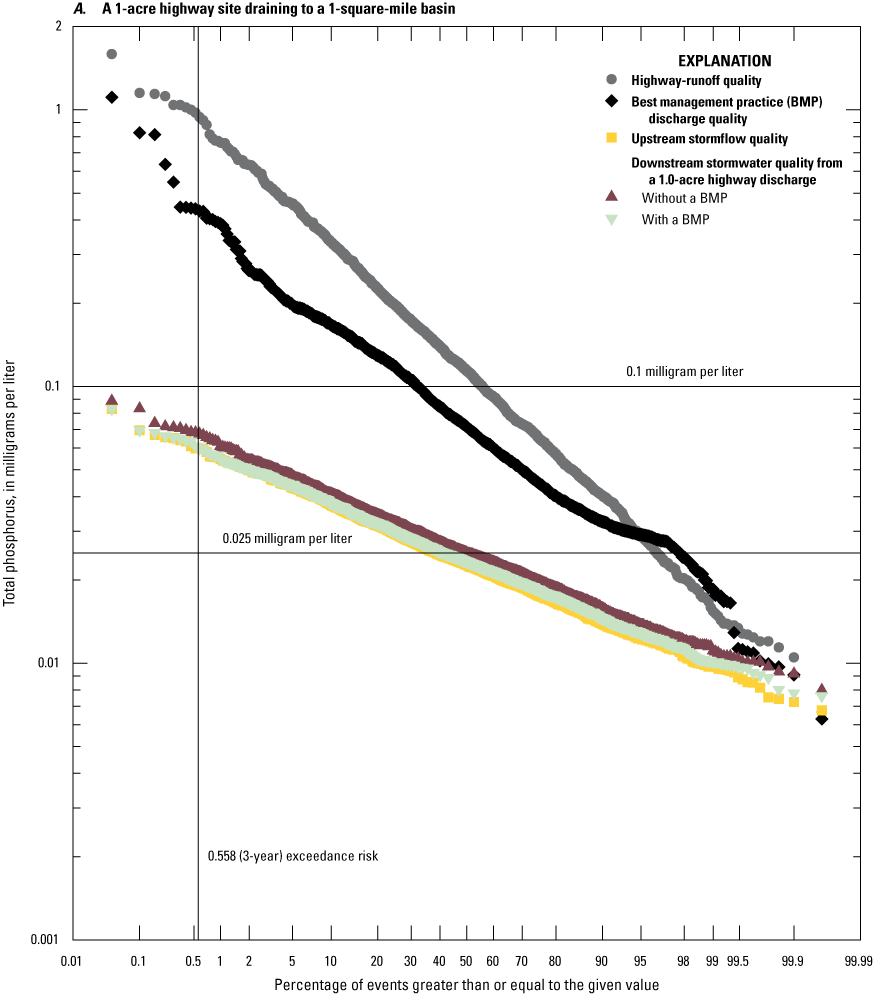
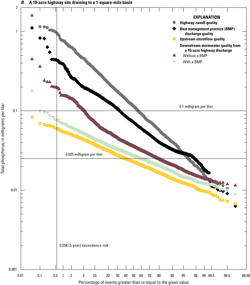
Scatterplots showing the populations of simulated event mean phosphorus concentrations for highway-runoff quality, stormwater best management practice discharge quality, and receiving stream stormflow upstream and downstream from a discharge point. A, A 1-acre highway site draining to a 1-square-mile basin. B, A 10-acre highway site draining to a 1-square-mile basin. The vertical line shows a commonly used 3-year exceedance risk, which is equal to about 0.558 percent in these simulations, and the horizontal lines show two example water-quality criteria (0.025 and 0.1 milligram per liter [mg/L]) for total phosphorus used for discussion. See table 18 for parameter code.
Table 23.
Water-quality transport-curve statistics developed by using the Kendall-Theil robust line method for estimating the common logarithms of constituent concentrations from the common logarithms of area-normalized streamflow. Regression statistics represent the median of statistics for minimally developed, developed, and wastewater-affected receiving streams in southern New England.[Method used is defined in Granato (2006). Pcodes and names from the National Water Information System (U.S. Geological Survey, 2021). Water-quality transport curves were developed from the common logarithms of streamflows, in cubic feet per second per square mile, as the explanatory variable (X) and the common logarithms of concentrations as the dependent variable (Y). Equations were developed by using data from 82 U.S. Geological Survey streamgages in New England (table 22, Granato and others, 2022). Minimally developed (MD) receiving waters are defined as stream basins without wastewater treatment plants that have impervious percentages less than or equal to 5 percent; developed (D) receiving waters are defined as stream basins without wastewater treatment plants that have impervious percentages greater than 5 percent; wastewater-affected (WA) receiving streams are defined as having one or more wastewater treatment plants in the basin upstream from the water-quality monitoring location, irrespective of imperviousness. MAD, median absolute deviation; MaxX, maximum measured flow; M, the final equation represents the median of regression statistics from multiple stations with the MaxX of the first segment adjusted to ensure the segments intersect properly; S, the final equation was selected from one station because there was only one station with data for that constituent or equations from alternate stations were not physiochemically sound; —, not applicable]
Risk-based analyses using SELDM also can be used to evaluate numeric water-quality criteria. Jeznach and Granato (2020) concluded that numeric criteria developed for low-flow waste-water regulation may not represent stormflow quality even in minimally developed basins. For example, simulation results shown in figure 10 indicate that upstream stormflow quality simulated by using the median transport curve from minimally developed basins does not exceed a 0.1 mg/L criterion but does exceed the 0.025 mg/L criterion in about 38.9 percent of events. This risk analysis indicates that the lower criterion may be too stringent for application to stormwater quality because the 0.025 mg/L concentration is regularly exceeded. To fully explore different criteria, however, it would be necessary to do a random-seed analysis to evaluate random variation with the median transport curve and to simulate transport curves from multiple minimally developed basins to evaluate potential variations from basin to basin.
SELDM-derived estimates also can be used to quantitatively examine water-quality exceedance risks in the absence of a numeric criteria. With or without a fixed criterion, SELDM can be used to examine the changes in concentrations that may occur between the upstream and downstream concentrations or between upstream concentrations simulated by using different statistics to determine if such changes are large enough to be detectable with monitoring data. For example, Jeznach and Granato (2020) used SELDM to compare water-quality changes with increasing imperviousness and found patterns in the changes that mirrored the results of ecological studies. If a 3-year exceedance probability (a risk of about 0.558 percent in these simulations) is protective for aquatic ecosystems (Niemi and others, 1990; U.S. Environmental Protection Agency, 1991, 1998), then comparison of changes in flows, concentrations, or loads can be used to assess risk. In the simulation for the 1-acre highway site shown in figure 10A, the simulated downstream concentration of phosphorus at the site without a BMP was only about 0.008 mg/L greater than the upstream concentration at the 3-year exceedance probability. If the median-performance BMP was used, then the simulated downstream phosphorus concentration at the site was only 0.0004 mg/L greater than the upstream concentration at the 3-year exceedance probability. These differences are within laboratory measurement uncertainties and much smaller than stormwater-concentration measurement uncertainties (Harmel and others, 2006). In the simulation for the 10-acre highway site shown in figure 10B, however, the simulated downstream phosphorus concentration without a BMP was 0.136 mg/L greater than the upstream concentration at the 3-year exceedance probability and the simulated downstream concentration with a BMP was only 0.017 mg/L greater than the upstream concentration at the same probability. These results indicate that the 10-acre highways site may have a potential effect on the concentrations of phosphorus in the receiving stream in this 1-square-mile basin but use of a BMP reduces the difference between upstream and downstream concentrations at the three-year risk probability to within the uncertainty of measured stormwater concentrations. Because DOTs are limited in their ability to construct and maintain the long-term performance of BMPs (Taylor and others, 2014), risk-based analyses can be used to prioritize sites where BMPs can provide a quantifiable change in downstream water quality.
Upstream Transport Curves
Water-quality transport curves, which are regression relations between streamflow and instream concentrations (fig. 1), were developed to simulate upstream stormflow quality for constituents of concern in southern New England (table 18). Transport curves are used in SELDM because many constituents vary with streamflow because of wash off and dilution processes in receiving waters. There is wash off when constituents are mobilized from the land surface or stream bed and banks during storms, whereas there is dilution when constituents are present in the base flow at higher concentrations than in stormwater, such that concentrations decrease during stormflow events. Suspended sediment and sediment-related constituents are mobilized by wash off processes, so it is expected that as discharge increases, erosion and wash off will increase the concentration of sediment constituents in the stream.
Transport curves were developed for one water-quality property (turbidity), sediment and solids, unfiltered nutrients, unfiltered minor and trace inorganics (metals), biological constituents, and one major ion (chloride). SELDM uses the selected regression model and error term to generate stochastic estimates of water-quality concentrations for the constituent of interest (Granato, 2013). Estimating instream concentrations by using area-normalized streamflow is common in water-quality assessments and constituent load estimations (Glysson, 1987; Vogel and others, 2005; Granato, 2006; Granato and others, 2009; Weaver and others, 2019). Constituents that are primarily produced by groundwater discharge and dry-weather point sources, such as municipal wastewater treatment plants (WWTPs), commonly are diluted as streamflows increase. The presence of WWTP discharges in the basin upstream from monitoring locations is therefore a key consideration when selecting representative water-quality transport curves to represent water quality at a site of interest.
Water-quality transport curves were developed using the nonparametric Kendall-Theil robust line method as implemented in the software program KTRLine version 1.0 (Granato, 2006). KTRLine facilitates data transformation and specification of multisegment regression models using both graphical and statistical analysis to determine the simplest model that provides a good fit to data and consistency with dilution and wash off theory. Transport curves developed in this study are composed of one or two segments and each segment is defined by an intercept, slope, median absolute deviation (MAD), and maximum measured flow. The MAD is the median of the absolute values of the difference between each paired data point and the associated regression-prediction value (Helsel and Hirsch, 2002; Granato, 2006; Granato and others, 2009). The maximum measured flow of the first segment in a two-segment transport curve indicates the flow value at which the regression-equation transitions to the next segment. To determine the median statistics for mixed groups of one and two-segment models, statistics for one-segment models were repeated for the statistics of a second segment. A median transport curve with two segments was retained only if the median statistics of the two segments were different.
Data from 82 stream water-quality monitoring stations within and adjacent to southern New England (fig. 7, table 22) were obtained from the USGS National Water Information System website (NWIS; U.S. Geological Survey, 2021). These stations were selected because they have 10 or more paired instantaneous streamflow (p00061) and concentration values for one or more of the constituents of concern (table 18). Concentrations of metals were limited to samples collected after 1994 because a USGS study determined that trace-element data were subject to contamination; the contamination risk was addressed with new sampling and processing protocols implemented in October 1994 (U.S. Geological Survey, 1992, 1993). An iterative site-selection process was used to maximize the spatial coverage of selected stations, minimize drainage areas, and ensure a range of basin characteristics were represented. Sites were selected from NWIS using the R dataRetrieval package (DeCicco and Hirsch, 2022) by querying for stations in Connecticut, Massachusetts, Rhode Island, New Hampshire, and Vermont with a minimum of 10 samples that included results for one or more of the constituents of interest and a paired instantaneous flow measurement in the water-quality record or from the streamgage record. Datasets with 75 percent or more samples collected at flow rates greater than or equal to 1 cubic foot per second per square mile were retained. This generalized threshold was based on the geometric mean of prestorm streamflows from streamgages in the southern New England with no zero flows (table 11). This streamflow threshold was used to ensure that some of the samples used to construct the transport curves would represent stormflow conditions.
Candidate sites were reviewed in GIS software to exclude stations located immediately downstream from limited-access highways or within 0.25 miles of a reservoir or pond outlet. Stations located immediately downstream from limited-access highways were excluded from the analysis because the objective was to characterize background water quality above roadway stormwater outfalls. Stations located downstream from impoundments were excluded from the analysis because particle settling, biological action, and flow mixing in impoundments were expected to change or obscure relations between streamflow and constituent concentrations. Examination of transport curves developed from selected stations indicates that downstream proximity to wetlands may have similar effects, but transport curves for these stations were retained because riparian wetlands are a common feature in stream basins of southern New England. Stations that met the data and geographic requirements were used to determine a drainage-area threshold that allowed for sufficient data to be retained while minimizing the effect of large drainage areas. Larger basins are more likely to include impoundments that alter the flow regime and affect water quality (Meade and Parker, 1985; Smith and others, 1993). For nutrient and sediment samples, 50 square miles was selected as the maximum drainage area; however, because of the scarcity of trace-metal data, a drainage-area threshold was not enforced for those constituents.
Among the 82 stations for which transport curves were developed, 36 are located in Connecticut, 28 are located in Massachusetts, and 10 are located in Rhode Island (table 22). Four stations in both Vermont and New Hampshire were also included. The minimum drainage area is 0.19 mi2 and the maximum is 430.63 mi2; however, stations greater than 50 mi2 were only used to develop transport curves for concentrations of metals. Stream stations were stratified by imperviousness and the presence of WWTPs to facilitate selection of representative upstream water quality at unmonitored sites. Minimally developed stream basins were defined as basins without WWTPs and TIA values less than or equal to 5 percent above the monitoring location; 45 monitoring sites met these criteria (table 22). Developed basins are defined as basins without WWTPs and TIA values greater than 5 percent above the monitoring location; 24 monitoring sites met these criteria (table 22). Wastewater-affected receiving waters were defined as having one or more WWTPs in the basin above the monitoring location, regardless of TIA; 13 monitoring sites met these criteria (table 22). Wastewater-affected sites were not stratified by imperviousness because the WWTPs are located in larger basins and commonly serve substantial pockets of developed areas that may contribute runoff even within largely undeveloped stream basins. Land-cover percentages were compiled from the 2011 National Land Cover Database, and the number of road-stream crossings were computed in the USGS StreamStats application for those States with available data (Spaetzel and others, 2020; https://StreamStats.usgs.gov/ss/).
Data for available constituents at individual stations were used to develop 347 water-quality transport curves, which are available in the model-archive data release for this project (Granato and others, 2022). Individual transport curves may be selected for a runoff site of interest by selecting the monitoring station with a drainage area, number of WWTPs, road-crossing density, land-cover characteristics, and imperviousness (table 22) that best match the stream basin above the site of interest. Transport curves for an individual site, however, may be affected by the number of measurements, the range of sampled flows, known sources or sinks (for example a large lake or wetland), and unknown sources or sinks for a given constituent in the upstream basin. Therefore, categorical transport-curve statistics representing the median of transport curves from multiple sites were estimated from individual site statistics (table 23). These median transport-curve statistics developed for the three stream-basin categories in southern New England offer more refined estimates for local conditions over regional regression models developed by Granato and others (2009) and in many instances may equal or exceed the predictive capability of an individually selected transport curve for an unmonitored site (Granato and others, 2022).
Within SELDM, an additional water-quality transport-curve segment was added for flows above the largest value in the water-quality dataset at the individual monitoring station to reduce the risk of simulating unrealistic instream concentrations, which may take place if positive- or negative-slope segments of the transport curve are extended far beyond available data. This step is necessary because SELDM is designed to simulate runoff events that may take place over a long period of time, the number of simulated events can greatly exceed the number of stream samples available for developing the transport curve, and simulated stormflows over long periods may exceed the range of flows at which water-quality samples were collected. To develop the additional transport-curve segment, the maximum flow value (MaxX, table 23) of the final calculated segment was increased by 10 percent and the value of the regression line segment at that point was calculated. The additional transport-curve segment has an intercept equal to this adjusted intersection point, a slope of zero to avoid extrapolation, and the MAD value of the previous segment to preserve the variability of concentration in that regression-derived segment.
Upstream Dependent Relations
Dependent water-quality relations, which are equations used to estimate concentrations of one constituent from another more readily available constituent (Granato, 2013), were developed to simulate upstream stormflow quality for constituents of concern in southern New England (table 18). Dependent relations (table 24) were developed by using regression analysis to estimate total suspended solids (p00530) from concurrently measured suspended sediment concentrations (p80154) and estimate analytically determined total nitrogen (p62855) from concurrently measured total nitrogen (p00600) because relatively few stations had sufficient data for estimating transport curves for total suspended solids or analytically determined total nitrogen (table 23). Dependent relations to simulate total-metal concentrations and total PAH concentrations from suspended sediment concentrations were developed by using alternate methods because insufficient total-metal and PAH concentration data were available for developing transport curves or direct regression relations. Dependent relations for total-metal concentrations were limited to minimally developed sites because the distribution between the dissolved and particulate metal constituent phases is affected by changes in pH, salinity, volatile solids, nutrients, and organic chemicals associated with urban runoff and wastewater plant effluent (Pelletier, 1996; Benoit and Rozan, 1999; Breault and Granato, 2000; Tomczak and others, 2019; Miranda and others, 2021). Upstream stormwater-quality statistics in developed basins can be estimated by simulating minimally developed upstream water-quality with developed-area runoff quality with SELDM and using the resulting downstream water-quality values to calculate developed water-quality statistics (Granato and Jones, 2017a; Stonewall and others, 2019; Jeznach and Granato, 2020).
Table 24.
Regression equation statistics developed by using the Kendall-Theil robust line method for estimating the common logarithms of dependent concentrations from the common logarithms of predictor concentrations.[All regression relations developed by using available data from U.S. Geological Survey streamflow-quality values for a given constituent (table 22). The parameter codes for streambed-sediment fractions for metals are defined in the National Water Information System (U.S. Geological Survey, 2021) and are listed in table 18. Stage 1 is extraction of absorbed, exchanged and carbonate bound metals; Stage 2 is stage 1 and extraction of metals bound to hydrous iron and manganese oxides (Method 30-5 stage sequential extractions). MAD, median absolute deviation; MaxX, maximum measured concentration; NonWWTP, streamflow-quality monitoring stations without upstream wastewater-treatment plants; WWTP, streamflow-quality monitoring stations with upstream wastewater-treatment plants; TIA, total impervious area, TIA<6 percent is from sediment-quality measurements documented by Harris (1997), Chalmers (2002), and Coles and others (2019) from selected sites with small to moderate drainage areas (less than 100 square miles) and low development (estimated imperviousness less than 6 percent); KTRLine, regression relations determined by using the Kendall-Theil robust line method (Granato, 2006); PAH, polycyclic aromatic hydrocarbon; SedC, sediment or soil concentrations, in micrograms per milligram, used to estimate sediment-associated receiving-water concentrations; mm, millimeter; —, not applicable; %, percent]
| Water-quality data category | Type of relation | Number of pairs | Segment 1 | |||
|---|---|---|---|---|---|---|
| Intercept | Slope | MAD | MaxX | |||
| All data | KTRLine | 40 | 0.13945 | 0.66207 | 0.20179 | 1.9085 |
| NonWWTP | KTRLine | 21 | 0.08805 | 0.50000 | 0.18399 | 1.7482 |
| WWTP | KTRLine | 19 | 0.17569 | 0.79210 | 0.14613 | 1.9085 |
| All data | KTRLine | 1432 | −0.01261 | 0.99603 | 0.02112 | 0.66276 |
| All data | KTRLine | 1432 | 0.00805 | 0.97298 | 0.02054 | 0.63649 |
| Streambed sediment smaller than 2 mm, total digestion (p04049; Coles and others, 2019) | SedC | 13 | −3.8938 | 1.0000 | 0.17150 | — |
| Streambed sediment smaller than 0.0625 mm, total digestion (p34825; Horowitz and Stephens, 2008) | SedC | 15 | −3.0270 | 1.0000 | 0.25193 | — |
| Streambed sediment, smaller than 2 mm, stage 2 recoverable (p53686; Coles and others, 2019) | SedC | 14 | −4.4686 | 1.0000 | 0.30381 | — |
| Streambed sediment, smaller than 2 mm, stage 1 recoverable (p01028; Coles and others, 2019) | SedC | 15 | −3.4035 | 1.0000 | 0.22145 | — |
| Streambed sediment smaller than 2 mm, total digestion (p04052; Coles and others, 2019) | SedC | 14 | −1.7366 | 1.0000 | 0.31950 | — |
| Streambed sediment smaller than 0.0625 mm, total digestion (p34840; Horowitz and Stephens, 2008) | SedC | 15 | −1.1602 | 1.0000 | 0.21255 | — |
| Streambed sediment, smaller than 2 mm, stage 2 recoverable (p53689; Coles and others, 2019) | SedC | 14 | −2.9708 | 1.0000 | 0.48193 | — |
| Streambed sediment, smaller than 2 mm, stage 1 recoverable (p01029; Coles and others, 2019) | SedC | 14 | −2.9684 | 1.0000 | 0.48019 | — |
| Streambed sediment smaller than 2 mm, total digestion (p04054; Coles and others, 2019) | SedC | 14 | −2.4117 | 1.0000 | 0.37764 | — |
| Streambed sediment smaller than 0.0625 mm, total digestion (p34850; Horowitz and Stephens, 2008) | SedC | 15 | −1.3544 | 1.0000 | 0.30824 | — |
| Streambed sediment, smaller than 2 mm, stage 2 recoverable (p53691; Coles and others, 2019) | SedC | 14 | −2.6740 | 1.0000 | 0.23776 | — |
| Streambed sediment, smaller than 2 mm, stage 1 recoverable (p01043; Coles and others, 2019) | SedC | 14 | −2.8297 | 1.0000 | 0.83926 | — |
| Streambed sediment smaller than 2 mm, total digestion (p04130; Coles and others, 2019) | SedC | 14 | −1.7470 | 1.0000 | 0.15080 | — |
| Streambed sediment smaller than 0.0625 mm, total digestion (p34890; Horowitz and Stephens, 2008) | SedC | 15 | −1.1094 | 1.0000 | 0.28541 | — |
| Streambed sediment, smaller than 2 mm, stage 2 recoverable (p53707; Coles and others, 2019) | SedC | 14 | −2.9709 | 1.0000 | 0.25861 | — |
| Streambed sediment, smaller than 2 mm, stage 1 recoverable (p01052; Coles and others, 2019) | SedC | 15 | −2.4314 | 1.0000 | 0.48871 | — |
| Streambed sediment smaller than 2 mm, total digestion (p04132; Coles and others, 2019) | SedC | 14 | −2.1504 | 1.0000 | 0.30958 | — |
| Streambed sediment smaller than 0.0625 mm, total digestion (p34925; Horowitz and Stephens, 2008) | SedC | 15 | −1.5018 | 1.0000 | 0.17898 | — |
| Streambed sediment, smaller than 2 mm, stage 2 recoverable (p53705; Coles and others, 2019) | SedC | 14 | −2.9720 | 1.0000 | 0.26135 | — |
| Streambed sediment, smaller than 2 mm, stage 1 recoverable (p01068; Coles and others, 2019) | SedC | 14 | −3.2816 | 1.0000 | 0.64887 | — |
| Streambed sediment smaller than 2 mm, total digestion (p04131; Coles and others, 2019) | SedC | 14 | −1.4394 | 1.0000 | 0.18526 | — |
| Streambed sediment smaller than 0.0625 mm, total digestion (p35020; Horowitz and Stephens, 2008) | SedC | 15 | −0.69867 | 1.0000 | 0.22469 | — |
| Streambed sediment, smaller than 2 mm, stage 2 recoverable (p53723; Coles and others, 2019) | SedC | 14 | −2.1926 | 1.0000 | 0.22176 | — |
| Streambed sediment, smaller than 2 mm, stage 1 recoverable (p01093; Coles and others, 2019) | SedC | 14 | −2.2344 | 1.0000 | 0.56463 | — |
| Streambed sediment smaller than 2 mm, total digestion (p04133; Coles and others, 2019) | SedC | 14 | −4.7598 | 1.0000 | 0.38823 | — |
| Streambed sediment smaller than 0.0625 mm, total digestion (p34910; Horowitz and Stephens, 2008) | SedC | 15 | −3.7780 | 1.0000 | 0.33741 | — |
| Background soil (Bradley and others, 1994) | SedC | 18 | −2.2028 | 1.0000 | 0.3253 | — |
| Soil near pavement (Bradley and others, 1994) | SedC | 42 | −1.8956 | 1.0000 | 0.452775 | — |
| Streambed sediment (TIA < 6%; Harris, 1997; Chalmers, 2002; and Coles and others, 2019) | SedC | 14 | −3.2374 | 1.0000 | 0.96119 | — |
| Background soil times 1.04 (Bradley and others, 1994, Chen and others, 2015) | SedC | 18 | −2.1858 | 1.0000 | 0.32530 | — |
| Soil near pavement times 1.04 (Bradley and others, 1994; Chen and others, 2015) | SedC | 42 | −1.8786 | 1.0000 | 0.45278 | — |
| Streambed sediment (TIA<6%) times 1.04 (Harris, 1997; Chalmers, 2002; Chen and others, 2015; Coles and others, 2019) | SedC | 14 | −3.2204 | 1.0000 | 0.96119 | — |
Dependent water-quality relations for total metal concentrations were developed by using a five-step process developed by Granato and Jones (2017a). First, a water-quality transport curve is developed to represent suspended sediment concentrations as a function of streamflow in basins of interest. Second, dependent relations to estimate sediment-associated metal concentrations from sediment chemistry and suspended sediment concentrations were developed. Third, distribution coefficients (Kd), which are the ratio of dissolved metal to particulate metal concentrations (Pelletier, 1996; Breault and Granato, 2000; Granato and Jones, 2017a; Tomczak and others, 2019) were calculated. Because Kd is a function of suspended sediment concentration (Pelletier, 1996; Benoit and Rozan, 1999; Tomczak and others, 2019; Miranda and others, 2021), a stochastic population of Kd values was generated by using suspended sediment concentrations. Fourth, a population of whole-water concentrations (the sum of particulate and dissolved fractions) was calculated by using the particulate metal concentrations, simulated sediment concentrations, and a normally distributed random number. Fifth, dependent relations between particulate-metal concentrations and whole-water metal concentrations and between suspended sediment and whole-water metal concentrations were developed.
First the suspended-sediment transport curves were developed by using concurrent streamflow and concentration data (table 23); second the concentration of particle-associated metals was estimated by using streambed-chemistry data from USGS study sites (Harris, 1997; Chalmers, 2002; Horowitz and Stephens, 2008; Coles and others, 2019) with drainage areas less than 100 square miles and estimated imperviousness values less than 6 percent (table 24). The dependent relation is expressed in terms of the equation of a line (eq. 1). The intercept is the mean of the logarithms of the concentration of the metal on the sediment particles in micrograms of metal per milligram of sediment. The slope of the logarithmic relation is 1 because it is the mass of the metal on the sediment particles per unit mass of sediment. The median absolute deviation used to represent variation of the relation in the stochastic analysis is estimated by using the standard deviation of the concentration of the metal on the sediment particles among minimally developed bed-sediment sampling sites (Harris, 1997; Chalmers, 2002; Horowitz and Stephens, 2008; Coles and others, 2019). Sediment-metal concentrations identified by Coles and others (2019) as either stage 1 or stage 2 extraction refer to sequential extraction methods that are intended to quantify the bioavailable fractions of a constituent on streambed sediment by extracting the absorbed, exchanged, and carbonate bound metals (stage 1) and extracting metals bound to hydrous iron oxides and manganese oxides (stage 2; Breault and Granato, 2000). Total digestion methods involve decomposing the material with strong acid and heat to measure the sediment-bound concentration and the sediment-grain matrix concentration (Breault and Granato, 2000; Smith and others, 2013). Different sediment-chemistry datasets produce substantially different metal-concentration estimates. For example, given a suspended sediment concentration of 10 milligrams per liter, the particulate-associated copper concentration based on the linear equations (table 24) would range from 0.0148 (based on the Coles and others, 2019 stage 1 dataset) to 0.442 micrograms per liter (based on the Horowitz and Stephens, 2008 total-digestion dataset). Given stochastic variability, simulated values within a 95-percent confidence interval could be between 0.00062 and 0.356 micrograms per liter for the equation based on the Coles and others (2019) stage 1 dataset and between 0.138 and 1.42 for the equation based on the Horowitz and Stephens (2008) total-digestion dataset. After review of the available information, the Coles and others (2019) stage 2 dataset was selected because the grain-size range and the analytical method were judged to be most representative of concentrations measured for whole-water metal samples (Breault and Granato, 2000; Smith and others, 2013). Stage 2 data were not available for mercury so the most comparable data from Coles and others (2019) were used (table 24). A SELDM analysis using each dependent-metal relation was used to simulate a 29-year population of suspended sediment and the associated dependent sediment-associated metal concentrations for each constituent (Granato and others, 2022).
In the third step for developing dependent water-quality relations for total metal concentrations, regression relations developed by Tomczak and others (2019) were used to estimate Kd statistics from suspended-sediment concentrations for each metal (table 25). These equations provided values of the average and standard deviation of the logarithms of Kd values for each simulated suspended-sediment concentration value. Each Kd value was calculated by using the average and standard deviation of the logarithms associated with a given suspended sediment concentration; with the value equal to the local average by using the equation:
whereLog(Kdi)
is the logarithm of an individual Kd estimate (in liters per kilogram) for the ith simulated event;
LogAvgKd(f(SSCi))
is the average of the logarithms of Kd values as a function (f) of the given value of suspended sediment concentration (SSCi) for the ith event as defined in table 25;
LogSDKd(f(SSCi))
is the standard deviation of the logarithms of Kd values for the ith event as a function (f) of the given value of suspended sediment concentration as defined in table 25; and
Knormi
is a value of a standard-normal variate for the ith event used to calculate an individual estimate.
Table 25.
Dependent water-quality relations calculated by using metal-sediment distribution coefficients and regression relations between results of simulations for suspended sediment and particulate metals developed by using the Kendall-Theil robust line method.[Calculated statistics are for the common logarithms of distribution coefficient and concentration data and are for the logarithms of distribution coefficient and concentration values from Tomczak and others (2019). Kd, the distribution coefficient, in liters per kilogram, that is the concentration ratio between the particulate phase and the dissolved phase; CT, concentration of the total particulate and dissolved phases in the water column, in micrograms per liter; CP, concentration associated with particulates in the water column; SSC, suspended-sediment concentration. Dependent regression relations to calculate CT from CP and CT from SSC determined by using the Kendall-Theil Robust Line software (Granato, 2006, Granato and Jones 2017a); MAD, median absolute deviation]
| Particulate metal | Kd equations from SSC (Tomczak and others, 2019) | Total concentration (CT) from particulate concentration (CP) | Total concentration (CT) from suspended-sediment concentration (SSC) | |||||||
|---|---|---|---|---|---|---|---|---|---|---|
| Average Kd | Standard deviation of Kd | |||||||||
| Intercept | Slope | Intercept | Slope | Intercept | Slope | MAD | Intercept | Slope | MAD | |
| Cadmium | 5.9299 | −0.83 | 0.4378 | 0.02 | 0.19376 | 0.96424 | 0.15980 | −4.0885 | 0.93897 | 0.24832 |
| Chromium | 5.6335 | −0.53 | 0.3160 | 0.02 | 0.14095 | 0.92655 | 0.11432 | −2.4798 | 0.80608 | 0.34553 |
| Copper | 5.1399 | −0.43 | 0.4362 | −0.02 | 0.11837 | 0.75449 | 0.19577 | −1.8019 | 0.65575 | 0.24101 |
| Lead | 5.9289 | −0.45 | 0.3674 | −0.03 | 0.00606 | 0.91709 | 0.07397 | −2.6583 | 0.85751 | 0.18857 |
| Nickel | 4.5944 | −0.06 | −0.4318 | 0.74 | −0.2046 | 0.57888 | 0.17579 | −1.7497 | 0.40090 | 0.22893 |
| Zinc | 5.6628 | −0.51 | 0.6848 | −0.12 | 0.18566 | 0.88364 | 0.18453 | −1.6708 | 0.80294 | 0.22250 |
| Mercury | 5.6884 | −0.58 | 0.4281 | −0.01 | −0.06412 | 0.94007 | 0.07219 | −4.4449 | 0.85690 | 0.27310 |
In the fourth step for developing dependent water-quality relations for total metal concentrations, individual simulated suspended sediment concentrations, particulate metal concentrations, and associated Kd values were used to calculate individual whole water (or total) metal concentrations for each simulated event by using the equation:
whereCTotali
is the total or whole water concentration, in micrograms per liter for the ith event; and
Cparticulatei
is the particulate metal concentration, in micrograms per liter for the ith event.
In the fifth step for developing dependent water-quality relations for whole-water metal concentrations, the populations of simulated suspended sediment and particulate metal concentrations were used with the calculated whole-water concentrations to develop dependent relations between the simulated and calculated values by using the Kendall-Theil Robust Line software (Granato, 2006). These relations, which are shown in table 25, were developed manually because SELDM does not have an algorithm to simulate upstream concentrations by using equation 7. Because the relation between suspended sediment and particulate metals and the relation between suspended sediment and Kd both include substantial random variations, equation 7 is far less deterministic than the form of the equation may suggest. Therefore, using a regression-based dependent relation with random variation to simulate whole-water metals from particulate-metal or suspended-sediment concentrations is a more robust way to develop planning-level estimates than a deterministic application of equation 7. Comparison of metal concentrations calculated by using stochastic distribution coefficients, simulated by using particulate metal concentrations, and simulated by using regression relations to suspended sediment concentrations indicate that these three simulation methods produce comparable results to a stochastic application of equation 7 (fig. 11). The particulate-metal simulations and whole-water metal regression files are available in the model-archive data release for this study (Granato and others, 2022). The particulate-metal simulations are in the analyses with the prefix “QWSedC” and an example of the use of these equations is in the “MetalexampleUS1sqmiTIA0_Hwy1Ac” file within the “14000-USQW” project archive file in the model-archive data release (Granato and others, 2022). The suspended-sediment-based equations (table 25) were selected for use with SELDM to simplify subsequent simulations.
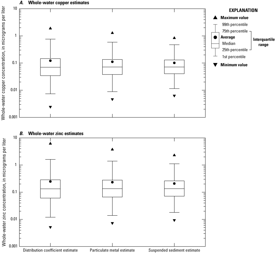
Boxplots showing the distribution of total whole-water metal concentrations in minimally developed basins simulated by using stochastic distribution coefficients, regression relations to simulated particulate-metal concentrations, and regression relations to simulated suspended-sediment concentrations. A, Whole-water copper estimates. B, Whole-water zinc estimates.
There also was insufficient data to estimate total PAHs in minimally developed basins, so particulate associated concentrations from bed sediment and soil were estimated and these estimates were adjusted to represent whole-water total PAH statistics as a function of simulated suspended-sediment concentrations. Table 24 includes dependent relations to estimate total PAH concentrations from streambed sediment and soil data. Only relations from PAHs from minimally developed streambed sampling sites (less than 6 percent TIA) are included in this report because PAHs in streambed sediments in developed southern New England streams may be more related to historical industrial discharge than current nonpoint source contamination from stormwater (table 24). Breault and others (2013) found that relations between total PAH concentrations in sediment cores from impoundments in Massachusetts were not substantially or statistically correlated to imperviousness or an index of commercial, industrial, and transportation land uses in 1971 and 2005, but total-sediment PAH concentrations were substantially and statistically correlated to the number of upstream factories that existed in the 1830s. Chalmers and others (2007) found correlations to the index of commercial, industrial, and transportation land uses, but also found that bed-sediment concentrations in highly urban areas decreased with sediment age except in newly developed areas. Therefore, background (minimally developed) sediment concentrations will be used with highway and urban runoff concentrations to assess receiving water quality. A dependent relation using total PAH concentrations from soil samples near pavement also is included in table 24 because it can be used to assess stormflow PAH concentrations that may be associated with stormwater-runoff particulates in developed areas.
The sediment-associated PAH equations were adjusted to represent whole-water concentrations by using a simple ratio because the partitioning chemistry is complex and is different for individual PAH constituents. Although PAHs are commonly associated with suspended sediment rather than from the dissolved fraction in the water column, many PAH’s are soluble; for example, the solubility of individual PAHs in water ranges from 0.26 µg/L for Benzo(ghi)perylene to 34,400 µg/L for Naphthalene (May and others, 1978; Smith and others, 1988). Also, the total PAH values may exceed the sediment-associated concentrations during storm events because experiments show that sediment-associated PAHs can repartition to the dissolved phase when bed sediments are resuspended in the water column (Belles and others, 2016). Chen and others (2015) measured the PAHs dissolved in the water column, incorporated into suspended particulate matter, and incorporated into bed sediment and calculated the concentrations of total PAHs in these matrices for 37 sampling sites; based on these results, the average and median ratios of the total (dissolved plus suspended sediment-bound fractions) to the sediment-bound fraction were 1.05 and 1.03, respectively. A simple adjustment calculating the whole-water PAH concentration as 1.04 times the suspended-particulate PAH concentration was selected because the comprehensive stormwater-quality data, such as PAH concentrations and concentrations of dissolved and sediment-associated organic matter, needed to precisely calculate the ratio of total to dissolved concentrations are not available for streams in southern New England. This adjustment is represented by adding 0.017 to the intercept in the logarithmic particulate-sediment equations for background soil, soil near pavement, and streambed sediment from minimally developed basins shown in table 24. As with the total-metal concentrations, developed-area total PAH concentration statistics can be estimated by superimposing urban-runoff loads on the minimally developed PAH concentrations.
Upstream Point-Source Contributions
Point-source discharges, such as wastewater treatment plants (WWTPs), add to the base-load of many constituents in basins where they are present. Methods are needed to assess potential effects of stormwater runoff from a point of interest on the quality of receiving waters in wastewater-affected basins. Water-quality transport curves were developed by using flow and water-quality data from 13 wastewater-affected water-quality monitoring sites with drainage areas ranging from 14.5 to 431 square miles and impervious percentages ranging from 0.916 to 13.9 percent (table 22). Each wastewater-affected transport curve represents a unique combination of basin characteristics, total upstream wastewater discharges, and the distance from the upstream outfall to the water-quality monitoring site that is the source of data (table 23). However, the wastewater-affected transport curves are not as transferable as transport curves for undeveloped or developed basins without WWTPs, because the point source concentrations are continuously diluted below the outfall in dry and wet weather. Therefore, an alternative method for simulating wastewater contributions to constituent concentrations at any point of potential interest was needed.
Discharge quality and volume data from 30 to 143 WWTP facilities each located in Connecticut, Massachusetts, and Rhode Island were obtained from the EPA Enforcement and Compliance History website (EPA, 2022) and were used to calculate statistics for discharge loads and WWTP design flows (table 26). The average and standard deviation of the logarithms of monthly average concentrations and flows were calculated. To calculate loads, measured concentrations were converted from milligrams per liter to micrograms per liter so the nutrient and metal data would be consistent and measured flows were converted from millions of gallons per day to liters per second to develop instantaneous loads with consistent units. Multiplying the concentrations times flows results in loads with units of micrograms per second. For each constituent of interest, only stations with a minimum of 10 monthly average concentrations were used.
Table 26.
Logarithmic regression relations between wastewater treatment plant-design flow and the average and standard deviation of monthly average constituent discharge loads for facilities in Connecticut, Massachusetts, and Rhode Island.[Method described in Granato and others (2022). Data used to develop the regression relations are from the U.S. Environmental Protection Agency (2022). Parameter codes and descriptions from the National Water Information System (U.S. Geological Survey, 2021) are listed in table 18. Regression equations were developed by using the common logarithms of treatment plant-design flow, in millions of gallons per day, as the explanatory variable and average monthly load, in micrograms per second, as the dependent variable. Equation parameters are presented in logarithmic (base 10) form. NWIS, National Water Information System; MAD, Median absolute deviation; rho, spearman’s rank correlation coefficient; %, percent]
Spearman’s rank correlation (rho) values and their 95-percent confidence intervals were calculated for the average and standard deviation of the logarithms of each constituent load and the associated WWTP design flows. The design flows were used to predict the average and standard deviation of actual monthly flows because the design flows are readily available in permits and do not vary without a change in WWTP design (U.S. Environmental Protection Agency, 2022). The rank correlations between design flows and the average of load values were semistrong (0.75 to 0.85) to strong (greater than 0.85) and statistically significant, as evidenced by 95-percent confidence intervals that did not cross 0 (Granato, 2014; Granato and others, 2021). Therefore, the Kendall-Theil Robust line method was used to develop nonparametric regression equations between the common logarithms of design flows in millions of gallons per day and the common logarithms of loads in micrograms per second (table 26). The correlation coefficient statistics and average of the standard deviations of monthly average loads also are documented in (table 26), but regression equations were not developed for the standard deviations of monthly average loads because the correlation coefficients were weak (less than 0.5) and, for all except nitrogen and zinc, statistically insignificant as evidenced by 95-percent confidence intervals that did cross zero (table 26). Granato and others (2022) provide the data used for analysis and a more detailed description of the process used to develop the statistics in table 26.
Developing planning-level estimates of concentrations in the stream upstream from the runoff outfall is a six-step process. The first step is to simulate a population of stormflows and concentrations from a minimally developed or developed basin without a point-source discharge. The example shown in figure 12A was done by using a transport curve and water-quality simulation for an undeveloped 10-square-mile basin developed by Jeznach and Granato (2020) and documented by Granato and Jeznach (2020). The transport curve and simulated data show random variations with stormflows less than about 1 cubic foot per second per square mile and increasing concentration with increasing discharge above that threshold. The second step is to determine the total design flows for WWTPs above the point of interest. In the example shown in figure 12B, a value of 0.5 million gallons per day was used with the total phosphorus equation in table 26 to calculate a logarithmic average of 3.611 and select a logarithmic standard deviation of 0.33. The third step is to apply these statistics to develop a dilution curve for total phosphorus concentrations in milligrams per liter (fig. 12B). The intercept, in logarithmic space, is the average minus 3 (dividing by 1,000 to convert from micrograms to milligrams) and the slope is −1 times the logarithm of flow. The values from the simulation are in cubic feet per second per square miles so the flow must be multiplied by the upstream drainage area at the point of interest (in this example 10 square miles) and multiplied by the conversion factor from cubic feet to liters per second (28.3168). This is equivalent to adding 2.452 in log space (fig. 12B). The fourth step is to create a random concentration value from the point source discharge for each simulated event (fig. 12B). To do this, the standard deviation of monthly flows is multiplied by a population of normally distributed random numbers (Knorm) and added to (or subtracted from) the dilution curve to develop a population of event values outside of SELDM. To develop planning-level estimates, a random set of Knorm values can be generated by using data analysis tools in Microsoft Excel, commonly used statistical software, or commonly available programming language tools. The fifth step is to add the stormwater concentration to the point-source concentration to develop the population of wastewater-affected concentrations shown in figure 12C. The sixth, and final, step is to develop a water-quality transport curve for the combined concentrations. If the point of interest was on a smaller or bigger basin than this 10-square-mile basin or if the area-normalized streamflows were lower or higher, then the point source concentrations from the wastewater load in the receiving stream would be proportionally larger or smaller (fig. 12B), and the random-concentration sums and the wastewater-adjusted transport curve shown on figure 12C would be different. Although the dilution is proportional to drainage area, the combination of the storm and point source loads are not proportional because they are added together.
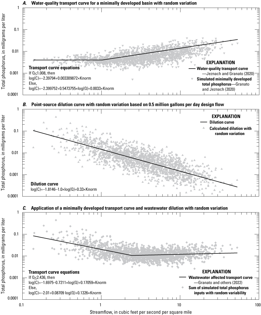
Scatterplots showing example applications of wastewater-treatment statistics used to develop a water-quality transport curve adjusted to represent the effects of point-source discharges. The steps include using A, a water-quality transport curve with random variation to simulate background water quality for a minimally developed basin (Granato and Jeznach, 2020); B, a point-source dilution curve with random variation based on 0.5 million gallons per day design flow; and C, application of total phosphorus concentrations to develop an adjusted transport curve. C is concentration, Q is flow, and Knorm is a normally distributed random variate.
This method is designed to produce planning-level estimates to assess the risk of water-quality exceedances above and below the point of interest with and without point source contributions, but these estimates are recognized to have considerable uncertainties. The estimates are based on available data, which are the averages and standard deviations of monthly wastewater concentrations and flows. Ideally, estimates calculated by using hourly or daily data would be more accurate, but a properly designed and maintained WWTP should have fairly consistent outflows even with highly variable inflows. As the distance between the WWTP and the simulated point of interest grows, some settling and biological transformation of point-source contributions may be expected; therefore, reductions based solely on dilution may be less than what would occur in a receiving stream. However, Jeznach and Granato (2020) estimated that travel times during stormflow events in small to moderate sized basins (less than 50 square miles) would minimize attenuation in comparison to conditions during dry-weather low flows. Stormflow velocities also would reduce attenuation caused by instream settling of point source waste loads. The planning-level estimates shown in figure 12 are not compared to simulated values using the wastewater-affected transport curves shown in table 23 because there are many potentially confounding variables that cannot be quantified by using available data from specific monitoring sites, and the median of transport curves do not explicitly define water quality at a specific sampling site. However, the calculated slopes of wastewater-affected transport curves for most nutrients and minor and trace inorganic constituents are close to zero, zero, or negative (table 23), which is consistent with the mixed effects of dilution of point source loads and the increase in runoff loads that would be expected as stormflows increase (Granato and others, 2009).
Stormwater Treatment
SELDM simulates the potential effect of stormwater control measures by using statistics approximating the net effects of structural and nonstructural BMPs. In this report, structural BMPs, also known as stormwater control measures, are defined as the components of the drainage pathway between the source of runoff and a stormwater discharge location that affect the timing, volume, or quality of runoff. SELDM can be used to explicitly simulate the effects of structural BMPs on the timing, volume, and quality of runoff by using professional judgment or by fitting the trapezoidal distribution to available data (Granato, 2013, 2014). The trapezoidal-distribution statistics and rank correlation coefficients used by SELDM provide a stochastic transfer function to approximate the duration, quantity, and quality of BMP effluents given a population of inflow values. SELDM uses hydrograph extension statistics to simulate the duration of runoff from structural BMPs; it uses statistics for the ratios of outflow to inflow volumes to simulate runoff-volume reductions; and it uses statistics for ratios of outflow to inflow stormwater concentrations to simulate runoff-concentration reductions stochastically for each simulated runoff event.
Granato and others (2021) calculated BMP treatment statistics by using data from the 2019 version of the International Stormflow Best Management Practices Database (Wright Water Engineers, Inc. and Geosyntec Consultants, 2019). Sufficient data were available for Granato and others (2021) to estimate statistics for 8 to 12 BMP categories by using data from 44 to more than 265 monitoring sites, nationwide. The medians of the best-fit statistics were used to construct generalized cumulative distribution functions for the three treatment variables. In cases where data are not available for a category of interest, or a stream basin with multiple BMPs is being simulated, then these generalized parameter values, which are the medians of categorical medians, may guide professional judgement in these cases (Granato, 2013, 2014; Granato and others, 2021). These combined BMP statistics are identified as the median (or generic) BMP in this report. Granato (2021b) incorporated these statistics into version 1.1 of SELDM, and Granato and others (2022) used these statistics for all simulations in the current study.
Hydrograph Extension
Hydrograph extension is the practice of slowing the discharge of runoff flows and releasing these flows to the receiving water body over an extended period of time (Granato, 2013, 2014; Granato and others, 2021). SELDM simulates the potential effects of structural BMPs on the timing of runoff as a stochastic variable by generating a population of BMP hydrograph extension durations (in hours) and adding these durations to the runoff duration from the site of interest. SELDM preserves the structure of hydrograph extension monitoring data in simulation results by using the trapezoidal distribution and the rank correlation with the highway stormflow volume (Granato, 2013, 2014). Although SELDM does not alter the water-quality treatment statistics with the hydrograph extension variable, extending the duration of the highway-runoff hydrograph can make a substantial difference in the amount of dilution in a receiving stream, especially in the rising limb of the upstream storm-event hydrograph (Granato, 2013; Granato and Jones, 2014, 2019; Risley and Granato, 2014; Stonewall and others, 2019; Weaver and others, 2019; Jeznach and Granato, 2020). If the simulated BMP discharge concentration is higher than the concurrent upstream stormflow concentration, then hydrograph extension will decrease concurrent downstream concentrations by dilution. If, however, the simulated BMP discharge is lower than the upstream stormflow concentration, then hydrograph extension will increase the concurrent downstream concentrations because a greater proportion of the upstream load will be used to calculate the downstream concentration. Granato and others (2021) calculated hydrograph extension statistics for 12 BMP categories and for a generic BMP representing the median of categorical hydrograph extension statistics.
Runoff Volume Reduction
Runoff volume reduction is the practice of retaining, detaining, or routing runoff flows to increase the amount of infiltration, evapotranspiration, or diversion between the pavement and the outfall (Granato, 2013, 2014; Granato and others, 2021). SELDM simulates the net effect of these processes on the volume of runoff by generating a stochastic population of the ratios of outflow to inflow volumes by using the trapezoidal distribution and applying these ratios to the stochastic population of inflow volumes from the site of interest. SELDM preserves the structure of BMP flow-monitoring data in simulation results by using the rank correlation between inflow volumes and the treatment ratios. These correlations, which are generally positive, result in lower ratios (good flow reduction by the BMP) for low inflow volumes and higher ratios (poor flow reduction by the BMP) for high inflow volumes. In many BMP datasets, outflow volumes exceed inflow volumes, presumably because of carryover from previous events or exfiltration of groundwater from BMPs in contact with groundwater. For example, the median values for the percentage of events with outflows that exceed inflows is about 28 percent for detention ponds and 31 percent for retention ponds; these structures have extended outflow durations that can exceed the time between runoff events (Granato and others, 2021). The median values for the percentage of events with outflows that exceed inflows is 56 percent for wetland basins and 32 percent for wetland channels (Granato and others, 2021). Wetland basins and channels and wet ponds commonly are in contact with groundwater, which will contribute to outflow volumes; this may explain why outflows exceed inflows in these types of BMPs.
Water-Quality Treatment
Water-quality treatment is the practice of using physical, chemical, and biological processes in an attempt to trap and hold sediment and chemical constituents in runoff (Granato, 2013, 2014; Granato and others, 2021). Although water-quality treatment is commonly described in terms of concentration reductions, the BMP discharge concentrations can exceed inflow concentrations, especially when inflow concentrations are low. Outflow concentrations may exceed inflow concentrations if there is carryover in BMP storage from one runoff event to the next; if flow through the BMP mobilizes previously retained constituents during some events; or if physical, chemical, or biological processes mobilize constituents between events (Granato and others, 2021). SELDM simulates the net effect of water-quality treatment variables as a stochastic variable by generating a population of ratios of outflow to inflow concentrations by using the trapezoidal distribution and applying these ratios to the stochastic population of inflow volumes from the site of interest. SELDM preserves the structure of BMP water-quality monitoring data in simulation results by using the rank correlation between inflow concentrations and the treatment ratios. These correlations, which are generally negative result in high ratios (poor treatment) for low inflow concentrations and lower ratios (good treatment) for high inflow concentrations. SELDM also simulates the minimum irreducible concentration, which is the lowest outflow concentration a given BMP may achieve by replacing simulated outflow concentrations that are less than the minimum irreducible concentration with the selected value. Because the minimum irreducible concentration is commonly a small fraction of the geometric mean inflow concentration (Granato and others, 2021), this lower bound commonly has only a small effect on annual discharge loads or the number of water-quality exceedances downstream from the outfall.
Granato (2021a) added the BMP treatment statistics that were developed by Granato and others (2021) to SELDM version 1.1. However, the December 2019 version of the International BMP database used by Granato and others (2021) did not include sufficient data for all the constituents of concern in southern New England (table 18). Therefore, estimates of treatments statistics for the remaining constituents of concern were developed and added to SELDM by using treatment statistics for available and analogous constituents. The BMP database has treatment statistics for mercury in nanograms per liter (p50286) but the New England datasets were in micrograms per liter (p71900). Therefore, existing mercury treatment ratios and correlations were applied, and the minimum irreducible concentration was adjusted for the change in units. The BMP database has treatment statistics for total coliforms using parameter code p31507, whereas the New England water-quality dataset use an analogous code (p50569) representing a potential difference in laboratory method. Because uncertainties in BMP performance statistics are larger than differences in laboratory methods (Granato and others, 2021), total-coliform treatment statistics for p50569 were incorporated from statistics for p31507 (Total coliform, completed test, water, most probable number per 100 milliliters). Constituents of interest in New England include fecal coliforms measured by using parameter codes p31616 (0.45-micron filtration) and p31625 (0.7-micron filtration). However, the analysis by Granato and others (2021) includes only treatment statistics for fecal coliforms from samples collected by 0.45-micron filtration with parameter code p31616. Laboratory experiments indicate that wide-spectrum recoveries for both filtration methods are similar, but differences for small-diameter bacterial colonies are about 20 percent higher for the 0.45-micron filters (MilliporeSigma, 2020). This difference, however, is within expectations for the total uncertainties expected for stormwater sampling efforts (Harmel and others, 2006) and well within uncertainties in BMP performance statistics (Granato and others, 2021). Therefore, treatment statistics for p31625 were incorporated into SELDM by using statistics for p31616 that were developed by Granato and others (2021). Treatment statistics for enterococci (p31649) and fecal streptococci (p31673) were estimated by using the medians of treatment statistics for the data for bacterial constituents (p31507, p31616, and p50468) already in SELDM (Granato, 2021a, b; Granato and others, 2021; Granato and others, 2022).
Simulation Results
In this study, 7,511 simulations were done to examine flows, concentrations, and loads of stormwater in southern New England (table 27). Within SELDM and in SELDM output directories, the results of a simulation are known as an analysis, and related analyses are saved in project directories. In SELDM, each project may be an actual highway construction or improvement project, a scientific investigation, or just a series of related analyses (Granato, 2013). Projects are used to organize analyses into groups that share input statistics and information. The SELDM project identification number is an alphanumeric code used as the folder name for all project analyses in the SELDM output folder. Each project folder of this study is contained in a zip file in the model-archive data release associated with this report (Granato and others, 2022). An analysis represents all the information and statistics to do a single SELDM simulation, and the analysis name is used to construct the folder name for each analysis that was run. SELDM output files document all the inputs and all the results in a tab-delimited text format (Granato, 2013; Granato and others, 2022).
Table 27.
Summary of Stochastic Empirical Loading and Dilution Model (SELDM) analysis projects used to assess the effect of variations in input values on simulation results and demonstrate results of analyses in southern New England.[All simulation results are documented within project directories by Granato and others (2022). The Stochastic Empirical Loading and Dilution Model (SELDM) project identification (ID) number is an alphanumeric code used to identify an analysis project in the model archive (Granato and others, 2022); the project number is used as the folder name for all project analyses in the SELDM output folder. The number of analyses run are the product of the number of highway site and upstream basin configurations and the variations in the hydrologic variables being used for simulations. Water-quality constituent categories are defined in table 18. ID, identification; SNE, southern New England; SA, sensitivity analysis; TIA, total impervious area; Rv, volumetric runoff coefficient; BMP, best management practice; N, no; Y, yes]
| Project ID number | Project short title | Project title | Sensitivity analysis category | Number of analyses |
|---|---|---|---|---|
| 01000-Seed | 01 SNE seed analysis | Southern New England random-seed analysis. | Random-seed selection, selection of highway water-quality statistics, and selection of upstream water-quality statistics | 1,000 |
| 02000-SA-Rain | 02 Sensitivity analysis precipitation | Precipitation-sensitivity analysis using median statistics for 3 ecoregions, southern New England gages, and 17 precipitation gages; using median statistics for other variables. | Selection of hydrologic statistics | 1,008 |
| 03000-SA-Stream | 03 Sensitivity analysis streamflow | Streamflow-sensitivity analysis (with no zero flows) using median statistics for 3 southern New England datasets and 17 individual values; using median statistics for other variables. | Selection of hydrologic statistics | 528 |
| 04000-SA-StreamZed | 04 Sensitivity analysis zero streamflow | Streamflow-sensitivity analysis for zero flows using median statistics for 3 southern New England datasets and 17 individual values; using median statistics for other variables. | Selection of hydrologic statistics | 576 |
| 05000-SA-USTIA | 05 Sensitivity analysis upstream TIA | Sensitivity analysis on upstream imperviousness from 0 to 90 percent, using median statistics for other variables; using median statistics for other variables. | Selection of basin properties with 3 different random seeds | 396 |
| 06000-SA-USLarge | 06 Sensitivity analysis large upstream basins | Sensitivity analysis on large upstream basins (40, 80, and 100 square miles; 0, 5, 10, and 20 percent TIA); using median statistics for other variables. | Selection of basin properties | 36 |
| 07000-SA-HwyLS | 07 Sensitivity analysis highway length and slope | Sensitivity analysis on highway-site properties with short and long lengths; steep and shallow slopes; using median statistics for other variables. | Selection of basin properties | 432 |
| 08000-SA-HwyRv | 08 Sensitivity analysis highway Rv Equations | Sensitivity analysis on highway-site runoff-coefficient equations looking at the highway and nonhighway runoff statistics; using median statistics for other variables. | Selection of hydrologic statistics | 192 |
| 09000-SA-USRvCor | 09 Sensitivity analysis upstream Rv correlation | Sensitivity-analysis rank correlation of the upstream runoff coefficient statistics to prestorm-flow plotting position; using median statistics for other variables. | Selection of hydrologic statistics | 1,584 |
| 10000-SA-Ratio | 10 Sensitivity- analysis recession ratios | Sensitivity-analysis recession-ratio statistics; using median statistics for other variables. | Selection of hydrologic statistics | 672 |
| 11000-HwyYields | 11 Highway- runoff yield analyses | Simulations to develop highway-runoff yields (loads per acre) by using highway-runoff-quality statistics with regional and local precipitation statistics. | Selection of highway-runoff quality and precipitation statistics | 147 |
| 12000-UrbanYields | 12 Urban- runoff yield analyses | Simulations to develop urban-runoff yields (loads per acre) by using urban runoff-quality statistics with regional and local precipitation statistics. | Selection of urban-runoff quality statistics in comparison to highway-runoff quality statistics and precipitation statistics | 294 |
| 13000-BMPs | 13 Structural BMP performance | Simulations to examine the long-term average stormwater-control measure performance using statistics from Granato and others (2021). | Selection of BMP treatment statistics | 576 |
| 14000-USQW | 14 Upstream water-quality analyses | Simulations to examine various methods to simulate upstream water quality including dependent relations and transport curves formulated by using literature-based, regional, or site-specific statistics. | Selection of upstream water-quality statistics (38 minimally developed total phosphorus transport-curve analyses, 24 developed total phosphorus transport-curve analyses, and 8 metal analyses) | 70 |
Table 27.
Summary of Stochastic Empirical Loading and Dilution Model (SELDM) analysis projects used to assess the effect of variations in input values on simulation results and demonstrate results of analyses in southern New England—Continued[All simulation results are documented within project directories by Granato and others (2022). The Stochastic Empirical Loading and Dilution Model (SELDM) project identification (ID) number is an alphanumeric code used to identify an analysis project in the model archive (Granato and others, 2022); the project number is used as the folder name for all project analyses in the SELDM output folder. The number of analyses run are the product of the number of highway site and upstream basin configurations and the variations in the hydrologic variables being used for simulations. Water-quality constituent categories are defined in table 18. ID, identification; SNE, southern New England; SA, sensitivity analysis; TIA, total impervious area; Rv, volumetric runoff coefficient; BMP, best management practice; N, no; Y, yes]
| Number of water-quality constituents | Water-quality constituent category (table 18) | |||||||||
|---|---|---|---|---|---|---|---|---|---|---|
| Highway | Urban | Upstream | Downstream | Properties | Sediments | Nutrients | Metals | Organics | Biologicals | Majors |
| 4 | 0 | 4 | 4 | N | Y | Y | N | N | Y | N |
| 3 | 0 | 3 | 3 | N | Y | Y | N | N | N | N |
| 3 | 0 | 3 | 3 | N | Y | Y | N | N | N | N |
| 3 | 0 | 3 | 3 | N | Y | Y | N | N | N | N |
| 3 | 0 | 3 | 3 | N | Y | Y | N | N | N | N |
| 3 | 0 | 3 | 3 | N | Y | Y | N | N | N | N |
| 3 | 0 | 3 | 3 | N | Y | Y | N | N | N | N |
| 3 | 0 | 3 | 3 | N | Y | Y | N | N | N | N |
| 3 | 0 | 3 | 3 | N | Y | Y | N | N | N | N |
| 3 | 0 | 3 | 3 | N | Y | Y | N | N | N | N |
| 21 | 0 | 0 | 0 | Y | Y | Y | Y | Y | Y | Y |
| 0 | 21 | 0 | 0 | Y | Y | Y | Y | Y | Y | Y |
| 21 | 0 | 5 | 10 | Y | Y | Y | Y | Y | Y | Y |
| 9 | 0 | 9 | 16 | N | Y | Y | Y | N | N | N |
The number of analyses run in each project (table 27) is the product of the number of highway site and upstream basin configurations and the variations in the hydrologic variables being used for simulations. Each of the SELDM analysis projects that were run was focused on variation in one or more related variables. Hydrologic and water-quality variables that were not the focus of the analyses in a given project commonly were set to southern New England or ecoregion median statistics. The first project (01000-Seed) is a random-seed analysis, the next nine projects (02000-SA-Rain through 10000-SA-Ratio) are sensitivity analyses that focus on hydrologic-variable and basin-property inputs. The next two projects (11000-HwyYields and 12000-UrbanYields) were done to produce yield values by using precipitation statistics for southern New England and the Northeastern Highlands (58), Northeastern Coastal Zone (59), and Atlantic Coastal Pine Barrens (84) ecoregions (table 9) along with 45 individual precipitation stations in and adjacent to southern New England (table 10). Project 13000-BMPs was done to compare the effectiveness of different BMP categories by using performance statistics calculated by Granato and others (2021). Project 14000-USQW was done to evaluate different methods for simulating upstream water quality including dependent relations and transport curves. The information and statistics in all these projects, which are available in the model-archive data release associated with this report (Granato and others, 2022) can be used by stormwater practitioners, decisionmakers, or scientists to do additional simulations that meet future information needs. Because 7,511 simulations produce thousands of folders and tens of thousands of output files containing hundreds of thousands of individual storm event values, representative examples were selected to illustrate the concepts discussed in this report.
For most analyses, three representative highway-site configurations were used for simulating highway or urban runoff. These sites were 0.25, 1, and 10 acres of pavement to represent typical contributing drainage areas (fig. 4). Associated lengths and slopes were selected to represent typical drainage conditions (tables 6, 7). The lengths and slopes of the highway sites were varied in project 07000-SA-HwyLS (table 27) to characterize short (bridge width), medium, and long drainage lengths with standard (10 ft/mi), medium (100 ft/mi), and steep (300 ft/mi) drainage slopes to examine the sensitivity of results to variations in these basin properties. Three impervious values (25, 50, and 100 percent) for the highway-sites were used in project 12000-UrbanYields (table 27) to examine the effect of changes in flow on urban water-quality yields.
For most analyses, 16 representative upstream basin configurations (fig. 3) were used for simulating the effects of runoff on downstream stormwater. These sites had areas of 0.1, 1, 10, and 20 square miles with associated lengths and slopes calculated by using the regression equations in table 5. In most analyses, imperviousness of 0, 5, 10, and 20 percent were used with each basin size to represent the majority of stream basins in southern New England (fig. 2). In project 05000-SA-USTIA (table 27), imperviousness of 0, 5, 10, 20, 30, 60, and 90 percent were used to compare results across a wide range of impervious values. In project 06000-SA-USLarge (table 27), upstream basin areas of 40, 80, and 100 square miles were used to provide results for runoff in much larger basins than those used in the other projects.
Interpreting Simulation Results
SELDM was developed to be a tool that can be used to transform disparate and complex scientific data into meaningful information about the risk for adverse effects of runoff on receiving waters, the potential need for mitigation measures, and the potential effectiveness of such measures for reducing these risks (Granato, 2013). SELDM uses Monte Carlo methods because it is the combination of different distributions of precipitation, prestorm streamflows, runoff coefficients, and water-quality concentrations that determines the potential risk of water-quality excursions. Deterministic methods are not able to characterize the interaction of different distributions for hydrologic parameters and BMP-performance measures. Unlike deterministic hydrologic models, SELDM is not calibrated by changing values of input variables to match a historical record of values; SELDM is calibrated by using representative site characteristics and statistics for each hydrologic variable. SELDM produces a collection of random events rather than a time series. Each storm that is generated in SELDM is identified by sequence number and annual-load accounting year. The model generates each storm randomly; there is no serial correlation, and the order of storms does not reflect seasonal patterns. The annual-load accounting years are random collections of events grouped such that the sequential time between event midpoints exceeds 365 or 366 days. Annual-load accounting years are used to generate populations of yearly runoff flows and constituent loads for TMDL analyses and lake basin analyses (Granato, 2013).
Dilution Factor Analysis
Dilution-factor analysis is useful for assessing potential effects of runoff on receiving waters. The dilution-factor analysis technique was developed by researchers using statistical mass-balance models to quantify potential effects of urban runoff on receiving waters (Warn and Brew, 1980; Di Toro, 1984; Driscoll, Shelley and others 1989, 1990). They defined the “dilution factor” as the ratio of the discharge into a stream at a point of interest divided by the concurrent stormflow immediately below this point, which is composed of the sum of the stormwater discharge and the concurrent upstream stormflow. Figure 13 shows the exceedance probabilities for a set of simulated dilution-factor populations for nine combinations of 100-percent impervious pavement areas and 100-percent pervious upstream basin areas. These results were extracted from simulation project 05000-SA-USTIA (table 27, Granato and others, 2022) by using the InterpretSELDM postprocessor (Granato, 2019b). A dilution factor of 1 indicates that the downstream flow is 100 percent urban- or highway-runoff discharge from the site of interest during the period of discharge, and a dilution factor near 0 indicates that the runoff discharge from the site of interest is a negligible portion of the concurrent downstream flow. As such, a higher dilution factor indicates that there is less dilution in the receiving stream. Using the term “dilution factor” for a variable that increases with decreasing dilution is at first counterintuitive, but the reciprocal of the dilution factor would not represent the fraction of downstream flow composed of runoff from the site of interest.
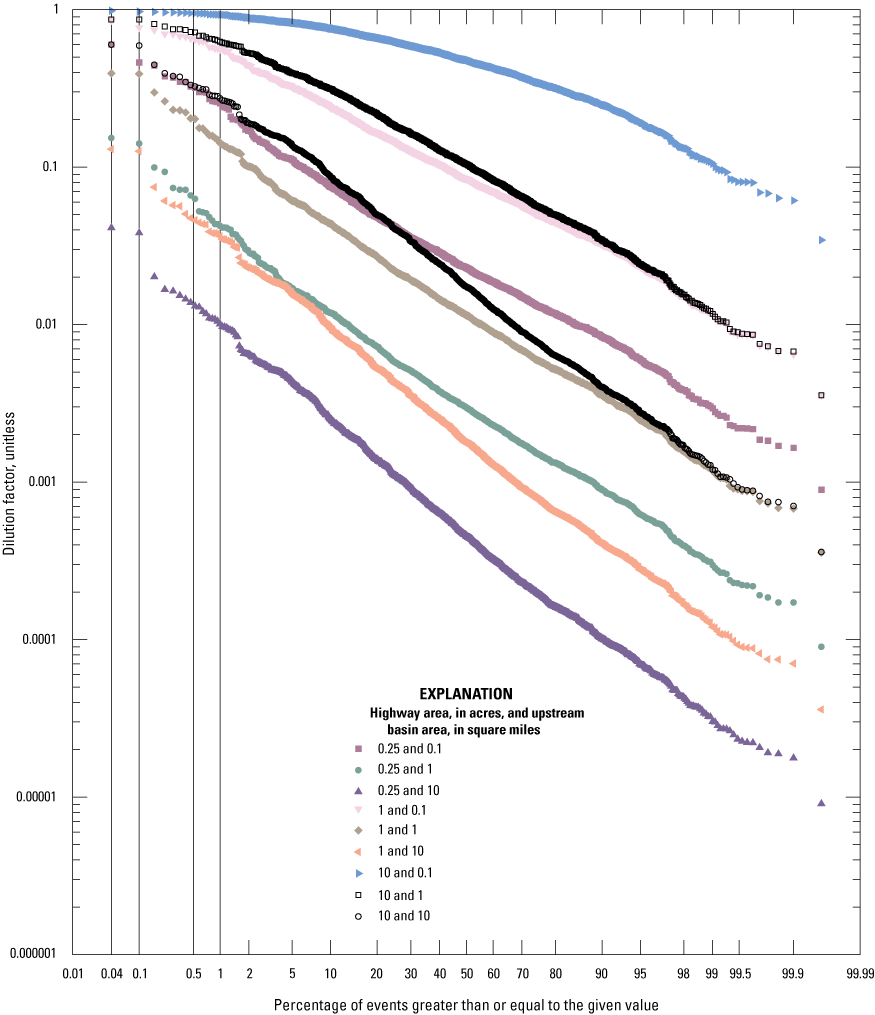
Scatterplot of simulated populations of dilution factors, the ratio of highway runoff to downstream flow, for nine combinations of pavement and upstream areas for basins with upstream-impervious fractions equal to zero. The vertical lines show selected exceedance percentiles used in this report to examine the effects of variations in hydrologic variables on receiving-water quality.
Recognizing that runoff from developed areas was a complex mixture of many different water-quality constituents, each with different potential effects on stream biota, Driscoll and others (1990) used several simplifying assumptions to develop a nomograph method that used dilution factors and the ratio of watershed area to impervious area to develop screening-level analyses of the potential effect of highway runoff on receiving waters. Zgheib and others (2011) used a similar approach to derive a dilution factor calculated as the ratio of maximum urban runoff concentration to the regulatory limit for each constituent, which is effectively the reciprocal of the Driscoll dilution factors. The dilution factors calculated by Zgheib and others (2011) ranged by several orders of magnitude among the different stormwater constituents, demonstrating the complexity of constituent-based risk assessments. Granato (2013) included dilution-factor analysis in SELDM to facilitate risk-based decision making without the need for analysis of multiple water-quality constituents. Therefore, SELDM can be used to simulate runoff quality or to use the dilution factor as a surrogate to assess potential adverse effects of runoff in the stream and the potential for mitigating those risks by reducing the volume of runoff and increasing the duration of runoff to the stream.
A dilution-factor analysis can provide a quick initial assessment of the risks for water-quality excursions with and without BMP treatment (Granato, 2013). Examination of the population of simulated dilution factors for each of several highway-stream crossings can be used to identify the streams with the highest risk for adverse effects of runoff on receiving waters. If a highway runs parallel to a stream and has many different stormwater outfall points, then information about the cumulative upstream drainage and pavement areas at each outfall can be used to do a dilution-factor analysis for each point. The dilution-factor population for each outfall can be used to identify the point along the stream with the highest risk for adverse effects of runoff on receiving waters. In both cases, this information can be used to allocate resources for a detailed analysis of flows, concentrations, and loads at the most critical sites.
A dilution factor analysis has several advantages over an analysis of only a few water-quality constituents. Highway and urban runoff contains a host of different water-quality constituents that can vary by orders of magnitude in concentration (Athayde and others 1983; Novotny, 2004; National Research Council, 2009b; Smith and Granato, 2010; Zgheib and others, 2011, 2012; Masoner and others, 2019). Water-quality measurements include uncertainties in flow measurements, the effects of subsampling events, potential effects of sample handling in the field and laboratory, analytical measurements in the laboratory, and uncertainties in the application of water-quality statistics to unmonitored sites (Harmel and others, 2006). Dilution-factor analyses are largely based on site properties, precipitation, and streamflow data. These data are more readily available and reliably transferable than water-quality data. Results of water-quality-based assessments of adverse effects of runoff may be ambiguous because stormwater from undeveloped areas may naturally exceed numeric water-quality criteria if the selected criteria were developed for regulation of wastewater discharges to receiving waters during periods of low streamflow (Rossman, 1990; Jeznach and Granato, 2020). Also, simulated or measured concentrations from one or more constituents may indicate small risks for adverse effects of runoff in receiving waters, while concentrations of other constituents may indicate large risks for adverse effects in the same storm event. Therefore, results of dilution-factor analyses, which indicate the proportion of runoff from a site of interest in downstream flow, may be more robust than results of water-quality analyses, especially in the absence of site-specific water-quality data.
The dilution factors also can be used to inform risk-based analyses. As previously demonstrated with selected concentrations (fig. 10), dilution factors can be used to examine the magnitude of potential changes in risks for a given dilution-factor value or values for a given risk. For example, if adverse effects of runoff were expected in events where runoff from the site of interest equaled or exceeded 10 percent of the downstream flow (a dilution factor of 0.1), then simulation results would indicate that, for an upstream imperviousness of 0, the exceedance probability would increase from less than 0.04 percent to 99.1 percent as the drainage-area ratio increased from 0.025 to 100 acres of pavement per square mile of upstream basin (fig. 13). From a risk perspective, figure 13 indicates that given a 0.5 percent exceedance risk, the dilution factors for the simulated basins would range from about 0.013 (for a 0.25-acre site on a 10-square-mile basin) to about 0.949 (for a 10-acre site on a 0.1-square-mile basin). Four exceedance-risk values, 0.04, 0.1, 0.5, and 1 percent, are highlighted on figure 13 because these values will be used in this report to examine the potential effects of variations in hydrologic variables on receiving-water quality.
Yield Analyses
State DOTs and other MS4 permittees need information about potential yields (loads per unit area) of constituents of concern in stormwater runoff and BMP discharges. The National Cooperative Highway Research Program study on TMDLs concluded that SELDM is a useful method for estimating yields and loads of urban and highway runoff and BMP discharges (Lantin and others, 2019). Similarly, Granato and Jones (2017b), Smith and others (2018), Stonewall and others (2018), and Granato and Friesz (2021a) demonstrated the use of SELDM to simulate long-term average annual yields in runoff and BMP discharges from roadways and other land covers to provide information needed for decision making. The long-term average annual yields commonly are used in constituent loading analyses because this average represents the sum of all constituent loads divided by the number of years in the simulation (Granato and Jones, 2017b, Smith and others, 2018, Stonewall and others, 2018, Lantin and others, 2019; Granato and Friesz, 2021a). Because SELDM also produces a set of individual annual yields, it provides information that can be used to assess risks of exceedance and the standard error of the simulated average, which is information that can be used to help assess the margin of safety needed for TMDL analyses.
SELDM simulates individual event loads and loads for annual load accounting years for constituents, reported in units of mass per unit volume (for example, milligrams per liter; Granato, 2013). For pH, which is the negative common logarithm of the concentration of the hydronium ion, SELDM calculates loads of the hydronium ion from simulated pH values. For other constituents that are not measured with units of mass per unit volume, including turbidity, specific conductance, and measures of bacterial concentrations, SELDM calculates flow-weighted loading values that are the product of water-quality measurement statistics and flow but are not actual mass values. These flow-weighted values, however, can be used to estimate downstream constituent concentration values and the potential effectiveness of BMPs to reduce flows and flow-weighted constituent loading values (Granato, 2013).
Granato and others (2022) document results of SELDM simulations for highway and developed-area runoff for TMDL analyses by using precipitation statistics representing southern New England, the Northeastern Highlands, Northeastern Coastal Zone, and Atlantic Coastal Pine Barrens EPA ecoregions (table 9), and data from 45 individual hourly precipitation data stations within and adjacent to southern New England (table 10, fig. 7). The simulated highway yields are in the project 11000-HwyYields files, and the developed-area yields are in the 12000-UrbanYields files, documented by Granato and others (2022). The 147 highway-runoff simulations include 3 sets of water-quality statistics representing the median (50th percentile), low (15th percentile), and high (85th percentile) highway-runoff quality statistics (table 19). The highway-runoff simulations used the highway-runoff coefficient statistics for 100-percent impervious pavement areas (table 15). The 294 urban (developed-area) simulations used the National urban-runoff quality statistics (table 21) with runoff-coefficient statistics for nonhighway sites (table 15). The urban runoff quality statistics were calculated from data in the 2019 version of the international BMP database by using the Best Management Practices Statistical Estimator (Granato, 2021a). The yields reported by Granato and others (2022) were calculated by using the medians of runoff-quality statistics for all BMP inflow sites in the 2019 version of the international BMP database with seven or more EMCs. These urban simulations used runoff-coefficient statistics for 100-percent impervious pavement areas and urban areas that are 25- and 50-percent impervious. The highway- and developed-area-runoff simulations were done by using BMP statistics for the generic (median) BMP that were developed and documented by Granato and others (2021). The potential yield reductions simulated by using treatment statistics for the median BMP and 12 other BMP categories developed by Granato and others (2021) are indicated by results of the BMP sensitivity analyses (project 13000-BMPs, table 27) documented by Granato and others (2022).
Application of simulated runoff yields to specific regulatory-TMDL areas in southern New England is beyond the scope of this report, but an example was done to illustrate a simplified method to estimate highway and nonhighway constituent loads from simulated constituent yields. Analysis of simulation results indicates that there may be substantial variations in individual annual yield values (fig. 14). Annual highway total nitrogen yields in figure 14 represent the sums of individual event values simulated by using the median precipitation statistics for southern New England (table 9), the highway runoff coefficient statistics for a 100-percent impervious site (table 15), and the median of highway runoff-quality statistics for total nitrogen (p00600, table 19). The sum of constituent loads from all events resulted in a long-term average highway-runoff yield of 9.55 pounds of total nitrogen per acre per year (fig. 14). Annual urban-runoff yields of total nitrogen were simulated by using the median precipitation statistics for southern New England (table 9), the nonhighway runoff coefficient statistics for a 100-percent impervious site (table 15), and the median urban runoff-quality statistics for total nitrogen (p00600, table 21). The long-term average urban pavement yield was about 11.9 pounds of total nitrogen per acre per year (fig. 14). The flow reduction and water-quality treatment by the generic (median) BMP resulted in long-term average highway-discharge yields of about 5.23 pounds of total nitrogen per acre per year and urban discharge yields of about 6.50 pounds of total nitrogen per acre per year (fig. 14).
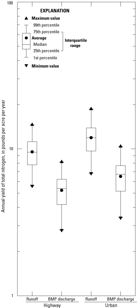
Boxplot showing the population of 29 annual total-nitrogen yields in pounds per acre per year, from 1,640 individual runoff-generating events, for 100 percent highway and impervious areas simulated by using precipitation statistics for southern New England, highway and urban runoff-coefficient statistics, highway and urban runoff-quality statistics, and treatment by the generic (median) structural best management practice (BMP).
Once long-term average constituent yields for different land covers are calculated, information about different land-cover areas obtained from a GIS or from StreamStats can be used to estimate total constituent loads from each land-cover area in a stream basin of interest (Granato and Jones, 2017b; Stonewall and others, 2018; Granato and Friesz, 2021a). In this example, information from the USGS StreamStats web-based application, which provides basin properties, imperviousness, road lengths by category, and road crossings by category in southern New England (U.S. Geological Survey, 2022) was used to illustrate methods to estimate constituent loads from simulated yields. Using SELDM results with StreamStats can provide initial planning-level load estimates, but detailed GIS data including types of land development, road geometry, and the highway and urban storm-sewer network would be needed to provide more precise constituent loading estimates from SELDM yield estimates. Detailed information about the proportions of directly connected impervious area and directly connected impervious area treated by stormwater BMPs would be needed to further improve constituent loading estimates. However, this detailed drainage-pathway information was not available throughout the Narraganset Bay basin to inform the example stormwater load analysis performed in this study (Narragansett Bay Estuary Program, 2017, 2019).
The example constituent load analysis for total nitrogen was done by using 16 basins that are tributaries to Narragansett Bay (table 28). These basins include tributary areas in Massachusetts and Rhode Island. Table 28 includes three basin properties taken directly from StreamStats (DRNAREA, the drainage area to the point of interest on the stream in square miles; LC11IMP, average percentage of impervious area from the National Land Cover Database; and LC11DEV, the percentage of developed land from selected classes in the National Land Cover Database) and five calculated variables. The “Major road TIA” values were calculated by adding the category 1 (interstates and limited access highways including ramps) and category 2 (secondary highways, arterials, or major connecting roads) road lengths from StreamStats (Spaetzel and others, 2020), multiplying these values by a representative road width of 52 feet (table 6), and converting these area values to acres. The “Other TIA” values were calculated by calculating the total impervious area (LC11IMP) in acres and subtracting the “Major road TIA” areas. The highway constituent loads were calculated by multiplying the “Major road TIA” areas times the long-term average highway-runoff constituent yield (9.55 pounds per acre per year; fig. 14). The urban constituent loads were calculated by multiplying the “Other TIA” areas times the long-term average urban-runoff constituent yield (11.9 pounds per acre per year; fig. 14). The total constituent loads from highway and nonhighway impervious areas shown in table 28 probably are larger than actual loading values because not all impervious areas drain directly to waterways and some areas are treated by BMPs.
Table 28.
StreamStats drainage-basin properties and estimated long-term average total-nitrogen loads from highways and developed areas for selected streams and rivers draining to Narragansett Bay, Rhode Island.[Basin data are from U.S. Geological Survey (2022). Road class information and data are from Spaetzel and others (2020). Land-cover data are from the National Land Cover Database (NLCD, U.S. Geological Survey, 2014). All simulation results are documented in project directories by Granato and others (2022). For maps of the basin, please see Narragansett Bay Estuary Program (2017, 2019). Major road TIA values were calculated by adding the category 1 (interstates and limited access highways including ramps) and category 2 (secondary highways, arterials, or major connecting roads) road lengths from StreamStats (Spaetzel and others, 2020), multiplying these values by a representative road width of 52 feet (table 6), and converting these area values to acres. DRNAREA, area that drains to the point of interest on the stream, in square miles (mi2); LC11IMP, average percentage of impervious area determined from NLCD 2011 impervious data; LC11DEV, percentage of developed land from the NLCD 2011 classes 21–24; TIA, the total impervious area as a percent of the drainage area; lb/yr, pound per year; —, not applicable]
Results of this planning-level analysis indicate that highways are a small part of the total annual constituent loads. The percent highway constituent load values in table 28 were calculated by dividing the highway loads by the sum of highway (major road) and urban (nonhighway) impervious-area loads and multiplying by 100 percent. The results indicate that the highway constituent loads range from 0 to 11.8 percent of the urban impervious-area constituent loads in the delineated basins, and the highway loads represent about 3.63 percent of the total tributary-basin impervious constituent loads (table 28). If the stormwater contributions from the pervious developed areas (LC11DEV) were included, which are about 2.6 times the total impervious area (LC11IMP; table 28), then the highway contribution would be a much smaller percentage of the total stormwater load than was calculated. In addition, the stormwater loads shown in table 28 do not include the wastewater contributions. WWTP constituent loads are estimated to be about 5,570,000 pounds of nitrogen per year (Narragansett Bay Estuary Program, 2017, 2019). Because the population of residents using onsite wastewater systems is 60 percent of the size of the population served by WWTPs, groundwater may additionally deliver about 3,000,000 pounds of nitrogen per year from onsite wastewater systems to the bay (Narragansett Bay Estuary Program, 2017, 2019). This onsite wastewater load is about twice the tributary total annual load from stormwater runoff used to calculate the percentage of the highway contribution. Therefore, highway-runoff loads are a much smaller percentage of the total annual nitrogen loads to the bay. These results indicate that the total highway-network contribution is well within the uncertainty of the total annual load estimates from other sources.
If BMP-discharge nitrogen yields are used for a loading analysis instead of the direct-discharge yields (fig. 14) with the entire impervious areas, then the calculated highway discharge nitrogen load would be about 31,000 pounds per year and the calculated nonhighway impervious discharge loads would be about 821,000 pounds per year. In this scenario, the highway would be about 3.64 percent of the total impervious constituent load. Large portions of runoff from highways may be characterized by using the BMP constituent loads because highway drainage design guidelines specify use of grass strips and swales rather than storm sewer systems wherever practical (American Association of State Highway and Transportation Officials, 2001) and grass strips and swales are effective BMPs for total nitrogen (Granato and others, 2021). Conversely, because the historical pattern of development in the Narragansett Bay watershed has been progressing from stream-side urban areas to suburban development in upland areas and most historically developed areas are not treated by using water-quality BMPs (Narragansett Bay Estuary Program, 2017, 2019), much of the nonhighway impervious stormwater loads from such areas may not be treated by using stormwater BMPs. Therefore, the nonhighway constituent loads may be closer to the estimated direct-discharge loads in table 28 than the BMP discharge loads. Although application of stormwater yields from this study may have considerable uncertainty for any particular stormwater outfall, the study does provide robust estimates within TMDL uncertainties to support basin-scale runoff-load analyses in southern New England. Given that highway runoff loads commonly are a very small portion of total watershed loads, the National Cooperative Highway Research Program report on approaches for determining and complying with TMDL requirements indicates that DOTs should participate in TMDL development before waste load allocations are formulated (Lantin and others, 2019).
Limitations of the Analysis
The analyses described in this report were designed to produce statistical estimates of stormwater flows, concentrations, and loads from highway and urban land-cover areas with and without BMP treatment and constituent loads from stream basins upstream from stormwater outfalls. SELDM is not calibrated by fitting input values to a historical record; SELDM is calibrated by selecting statistics for hydrologic, runoff-quality, and BMP-treatment variables from robust and representative datasets (Granato, 2013, 2014; Risley and Granato, 2014; Granato and Jones, 2014, 2017a, b, 2019; Stonewall and others, 2019; Weaver and others, 2019). Conclusions derived from simulations and the representativeness of results for any particular location depend on the input statistics used. While there are uncertainties in statistics for individual sites, available statistics are sufficient to evaluate the relation between input statistics and simulation results discussed in this report. Knowledge of potential uncertainties, however, is important for understanding decision risks of using SELDM outputs.
The uncertainty of selected input statistics for a given purpose depends on many factors, and uncertainties in input values are proportional to uncertainties in simulation results. Many uncertainties may affect results from any model. These include uncertainties in individual measurements (Harmel and others 2006; Jordan and Cassidy, 2011), population statistics calculated from individual measurements (Haan, 1977; Interagency Advisory Committee on Water Data, 1982; Jordan and Cassidy, 2011; Leutnant and others, 2018), use of statistics from monitored sites to unmonitored sites (Farmer and Levin, 2018; Granato and others, 2021), and use of statistics from monitored time periods to unmonitored time periods (Park and others, 2009; Granato, 2010). Cumulative uncertainties commonly are calculated as the square root of the sum of square errors, so the largest uncertainties, by and large, dominate the total uncertainties.
Uncertainties in measured concentrations and loads can be more than 100 percent of the reported values. Harmel and others (2006) studied the cumulative uncertainty in measured streamflow and water-quality data for small watersheds and found that, under typical conditions, uncertainties in event loads ranged from ±8 to ±110 percent, but worse-case uncertainties could be as high as about ±420 percent. Using a two-year total phosphorus dataset composed of 3 samples per hour in a 1.93 square-mile basin, Jordan and Cassidy (2011) determined that uncertainties in annual total phosphorus loads were highly dependent on sampling frequency. They found that monthly sampling (12 samples per year each year) could lead to uncertainties of about −50 to 180 percent in annual total phosphorus loads, and that samples collected every 6 hours (1,460 samples per year) were needed to reduce risks to within about ±10 percent. To balance information needs with logistics, they suggest using a standard 24-bottle autosampler configured to take a sample every 7 hours over each week (1,248 samples each year) to achieve uncertainties of about −20 to 30 percent in annual total phosphorus loads. In comparison, 65 of the 82 water-quality monitoring sites queried for the current study (table 22) had 10 or more total phosphorus concentrations. For total phosphorus, the maximum number of samples per site was 712 with a median of 24 samples per site. Many of the sites in table 22 have been monitored over multiyear periods so the sampling frequency is much lower than suggested by Jordan and Cassidy (2011).
If it is assumed that data are fairly precise and representative of conditions of interest, then uncertainties in environmental statistics are a function of sample size (Haan, 1977; Interagency Advisory Committee on Water Data, 1982; Driscoll and others, 1979; Burton and Pitt, 2002; California Department of Transportation, 2009; Granato, 2014; Leutnant and others, 2018). This principle is applicable to the number of samples at a site used to calculate site-specific statistics and the number of sites used to calculate categorical statistics. Driscoll and others (1979) recommend the collection of 20–40 EMC samples to characterize runoff for any given site on the basis of the variability of commonly measured runoff constituents. Similarly, Burton and Pitt (2002) indicate that, at a minimum, 25–50 EMC samples may be needed to characterize runoff for any given site. The California Department of Transportation (2009) provides examples in their BMP monitoring handbook that indicate that 50–113 paired EMC samples may be needed to detect differences in mean inflow and outflow concentrations. Leutnant and others (2018) determined that 40 EMC samples would need to be collected to characterize total suspended solids concentrations using a lognormal distribution.
In this study, the number of water-quality monitoring sites and the number of samples per site varied greatly for the highway, urban, upstream, and BMP data. The number of samples used to develop the 197 water-quality transport curves (summarized in table 23) ranged from 10, the selected minimum, to a maximum of 712, with a median value of 29 samples per sampling site. The number of sites per constituent ranged from 6 to 40 for constituents with data. For other constituents, including unfiltered trace elements and total PAH, none of the sites had 10 or more samples that met the data-quality criteria (table 18, Granato and others, 2022). There were insufficient data to develop transport curves for minimally developed, developed, and wastewater-affected sites for some constituents (table 23). For the urban runoff statistics, which were calculated by using a National dataset, individual sites with as few as 7 events were included and the number of sites per constituent ranged from 4 to 241 for constituents with some data. Similarly, because of limitations in available data, Granato and others (2021) had to use a National dataset (Granato, 2021a) with as few as 7 events per site and as few as 1 site per category to estimate BMP performance statistics for some less-commonly measured water-quality constituents. Comparison of uncertainty from constituent to constituent is not linear because the constituents with more sites also tend to have more EMCs per site and the uncertainty also depends on the variability in measured values (Haan, 1977; Interagency Advisory Committee on Water Data, 1982). Uncertainties in water-quality data and statistics are smallest in all these categories for the most commonly measured constituents such as nutrients and suspended sediments and solids (table 18).
Uncertainties in the use of statistics from monitored sites to simulate conditions at unmonitored sites may be considerable. The geographic analysis of basin properties in southern New England indicates that there are more than 48,000 road-stream crossings in this area (Spaetzel and others, 2020). In comparison, for sites within or adjacent to southern New England, there are sufficient published data from 45 precipitation monitoring sites (table 10), 385 streamflow monitoring sites (table 11), less than 20 highway-runoff quality monitoring sites (table 18), and less than 69 stream water-quality monitoring sites. Statistics for some highway runoff constituents were calculated by using data collected outside the region because sufficient data were not available within southern New England (table 19). Similarly, urban runoff-quality statistics (Granato, 2021a; table 21) and BMP performance statistics (Granato and others, 2021) were calculated by using National datasets because sufficient data were not available within southern New England. Without sufficient local data for comparison, it is difficult to precisely quantify uncertainties caused by using these National stormwater datasets.
The purpose of this study was to examine relations between variables for generic but representative sites rather than an attempt to predict historical or future water quality at a particular location. For this type of analysis, individual uncertainties must be recognized but are not as critical to the interpretation of results from stochastic models such as SELDM as they would be for deterministic or process-based models that use history matching for calibration. In this study, some of the uncertainty in statistics for individual sites and the transfer of statistics from monitored sites for simulations at unmonitored sites is mitigated by use of the median statistics from multiple sites to represent the general characteristics of highway runoff, urban runoff, BMP treatment, and upstream water quality. The median of site statistics represents the central tendency of all site statistics, without the potential influence of extreme outliers that could be caused by monitoring bias or uncharacteristic conditions at a few sites. If the objective of a study is to assess the risk of adverse effects of runoff at a particular stormwater outfall, then operational definitions for selected statistics are needed. In the absence of such definitions, site-specific data may be needed to reach a consensus decision. However, the time and resources needed to obtain sufficient data to substantially reduce uncertainties may preclude most site-specific data collection efforts. Even if monitoring studies were conducted widely, changes in the roadway or the upstream land area would affect water quality at the site of interest, so the monitoring data collected may not represent future conditions at that site (Granato, 2013).
Results of Sensitivity Analyses
A model sensitivity analysis is a systematic study to evaluate the effect of perturbations in input values on simulated results (National Research Council, 2007). SELDM was developed by using Monte Carlo methods to assess potential effects of runoff on receiving waters because available data are limited and the interactions between hydrologic, water-quality, and BMP treatment variables defy analytical solutions (Granato, 2013). The sensitivity analyses were done to help identify which variables have the greatest effect on simulated results. This knowledge can be used to focus efforts for refined data collection and analysis. Sensitivity analyses were done to examine the effects of random-seed selection (project 01000-Seed) and the selection of basin properties (projects 05000-SA-USTIA, 06000-SA-USLarge, and 07000-SA-HwyLS), hydrologic statistics (projects 02000-SA-Rain, 03000-SA-Stream, 04000-SA-StreamZed, 08000-SA-HwyRv, 09000-SA-USRvCor, and 10000-SA-Ratio), highway water-quality statistics (project 01000-Seed and 11000-HwyYields), upstream water-quality statistics (project 01000-Seed and 14000-USQW), and BMP treatment statistics (project 13000-BMPs) on simulated output values (table 27). Although the results of the sensitivity analysis will be demonstrated by using selected representative examples, results from all 7,511 simulations are available in the model-archive data release assembled by Granato and others (2022). The sensitivity simulation data were extracted from the SELDM output files by using the InterpretSELDM post processor, which is designed to use linear interpolation to calculate output values that fall between simulated risk percentiles (Granato, 2019b). In InterpretSELDM, the linear interpolation is done by using the common logarithms of concentrations and flow values and the normal variate associated with the risk percentiles.
The focus of the master random-seed (Granato, 2013) and hydrologic sensitivity analyses (table 27) was primarily on dilution factors rather than water quality, so only a few constituents were simulated, but the yield, structural BMP performance, and upstream water-quality sensitivity analyses had a water-quality focus. With the exception of the seed analysis, each set of sensitivity analyses were simulated by using three water-quality constituents selected to represent constituents commonly included in TMDL analyses (table 27). These constituents are total nitrogen (p00600), total phosphorus (p00665), and suspended sediment (p80154) as defined in table 18. Median highway runoff statistics and upstream transport-curve statistics for minimally developed areas were used. The master random-seed analysis also was conducted by simulating Escherichia coli bacteria (p50468) as defined in table 18. Downstream concentrations were simulated by using the highway and upstream constituent pairs without BMP treatment. The highway-runoff yield, urban-runoff yield, and structural BMP performance analyses (table 27) were simulated by using all 21 water-quality constituents (table 18). The upstream water-quality analyses (table 27) were simulated by using 9 water-quality constituents.
The focus of the hydrologic sensitivity analyses (table 27) was primarily on dilution factors because the dilution factors are a function of precipitation, basin properties, runoff coefficients, and prestorm streamflow. Because the dilution factor is the ratio of highway or runoff to downstream flows, the dilution factors can be used to indicate the potential effects of runoff on receiving waters. The magnitude of changes in dilution factors from changes in each selected hydrologic variable indicates the sensitivity of the downstream effects to that variable. Variables with high sensitivity require more careful selection than variables with low sensitivity.
The sensitivities were examined graphically and statistically. The six different hydrologic sensitivity projects included 36 to 1,584 individual analyses (table 27). The sensitivity analyses using master random-seed number equal to 8,556 resulted in 1,659 individual events each with a specific exceedance probability. Sensitivities were examined visually by looking at graphs of selected exceedance probability-percentiles for individual values. The 0.5 percent exceedance risk was selected to illustrate results for many of the analyses because it approximates the risk of one event per 3-years that is used for evaluating the effects of water-quality on aquatic life (Niemi and others, 1990; U.S. Environmental Protection Agency, 1991, 1998; Jeznach and Granato, 2020). Sensitivities were examined statistically by using the coefficient of variation (COV), which is the ratio of the standard deviation to the average dilution factor. The COV was calculated for selected exceedance probability percentiles for all the analyses using each combination of highway site and its upstream basin.
Because SELDM was designed to help quantify the risk of adverse effects of runoff on receiving waters, the potential need for mitigation measures, and the potential effectiveness of such management measures for reducing these risks, results of the analyses are focused on statistics for selected exceedance risks. The same exceedance risk for one variable or even for seemingly paired variables may come from different individual storm events because the stochastic rather than deterministic approach can reshuffle the values of related variables (Granato, 2013). For example, the BMP treatment is a random variable for each event rather than a constant ratio for all events. Therefore, a high BMP inflow concentration for one event may be paired with a large concentration reduction, and a low BMP inflow concentration for a different event may be paired with a small concentration reduction. As discussed by Granato (2013), this could result in a very low outflow concentration for the event with the high inflow concentration and a higher outflow concentration for the event with the lower inflow concentration. If this occurs in a simulation, then the relative exceedance risk of outflow concentrations may be the opposite of the relative exceedance risk of inflow concentrations.
Master Random Seeds
SELDM uses a random-seed management algorithm to ensure that each runoff-quality analysis will be reproducible; details about the Monte Carlo methods used are documented in appendix 1 of the manual (Granato, 2013). Each analysis uses a master random-seed identification number to select one of the 11,111 random-seed pairs in the seed table of the database application, and that seed pair is used to set the (pseudo) random-number generator. This master random seed is used to set the random seeds for each simulated hydrologic and water-quality variable simulated. Changing the seed values shuffles the simulated population of times between event midpoints, which will vary the number of events and annual-load accounting years from simulation to simulation (Granato, 2013). Changing the seed values also shuffles the random combinations of stormflow variables, concentrations, and treatment efficiencies among the storm events. As a result, this shuffles the simulated storm and annual constituent loads. When given precipitation statistics representative of conditions in southern New England, SELDM will commonly generate about 1,400 to 1,900 events representing a timespan of about 27 to 30 years. This record is long enough to approach numerical convergence to the values of input statistics without greatly exceeding commonly available precipitation and streamflow record lengths. However, Monte Carlo methods can produce events that greatly exceed the sample probability in the simulated record. Although a 100-, 500-, or 1,000-year precipitation event would not be expected during a typical 30-year simulation period, such events can take place randomly, and the presence of such events can greatly inflate constituent loads, especially if large events are randomly paired with large runoff coefficients and high concentrations.
Two similar SELDM studies, designed to produce long-term annual constituent loads, did multiple-seed sensitivity analyses. Granato and Jones (2017b) did a 7-seed sensitivity analysis focused on the median of highway runoff constituent loads produced. Granato and Friesz (2021a) did a 111-seed sensitivity analysis focused on the runoff volume because this was the value used to calculate the yields for all the constituents of concern. These two studies, however, were designed to produce long-term annual loads rather than to produce individual event-based values.
In the current study, a sensitivity analysis with 500 unique, master random seeds was done to reduce the potential for extreme output values and explore the potential variability in event and annual-load accounting year values from simulation to simulation. The results of this analysis are documented in the 01000-Seed project files (table 27; Granato and others, 2022). In these simulations, all the input basin properties, hydrologic statistics, and water-quality statistics were held constant while the master random seed was varied randomly. Hydrologic statistics representing median values for southern New England were used (tables 9, 11, 15, 16). The same 500 random seeds were used in two sets of simulations to characterize the effect of variables on output statistics. In the first (10 acre) set of 500 simulations, a highway area of 10 acres and an upstream area of 10 square miles was selected for analysis with corresponding basin characteristics. An upstream imperviousness of 10 percent also was selected for these simulations. In the second (1 acre) set of 500 simulations, the same seeds were used but with a highway area of 1 acre, and an upstream basin area of 1 square mile with corresponding basin characteristics and an upstream imperviousness of 0 percent. This second (1 acre) set of 500 random-seed simulations was used to compare stochastic variability with input transport-curve variability. In the second (1 acre) set, four water-quality constituents (table 18) including total nitrogen (p00600), total phosphorus (p00665), suspended sediment (p80154), and Escherichia coli (p50468) were simulated by using median highway-runoff quality statistics (table 19), and water-quality transport curves for minimally developed basins (table 23) were used. Downstream concentrations in the second (1 acre) set were simulated by using the highway and upstream constituent pairs without BMP treatment. The first (10 acre) set of 500 simulations is used to examine stochastic variability in the following discussion within this master random-seed analysis section.
The population of long-term average annual yield values have substantial variability but, in comparison to long-term maximum annual yields, are relatively robust to changes in the random-seed values. Figure 15 shows yields simulated by using total phosphorus concentrations from median highway-runoff statistics (table 19) and the median BMP performance statistics in all 500 master random-seed simulations as an example (Granato and others, 2021). The long-term average annual highway-runoff yield values range from 1.02 to 1.29 pounds per acre per year, which is a multiplier (ratio of the maximum to the minimum) of about 1.26. Similarly, the long-term average-annual BMP discharge yields range from 0.441 to 0.537 pounds per acre per year, which is a multiplier of 1.22. Differences from the average long-term average highway runoff and BMP discharges among the 500 different master random-seed simulations are on the order of 9 to 14 percent. In comparison, the maximum-annual highway-runoff and BMP discharge yields range from 1.36 to 3.55 pounds per acre per year and 0.574 to 1.23 pounds per acre per year, respectively. These are multipliers of 2.61 and 2.14, respectively. The lower variation in long-term averages is to be expected because variations in individual simulated hydrologic, water quality, and BMP values will tend to even out over the entire simulation period when combined into annual and long-term average values. The maximum long-term annual yield values show more variability than the average annual yields, but it is the long-term averages that are used for TMDL calculations because the average is the sum of all loads from the entire simulation period divided by the number of simulated years (Granato and Jones, 2017b; Stonewall and others, 2018; Lantin and others, 2019; Granato and Friesz, 2021a). The modest variability in long-term average values in this random-seed sensitivity analysis indicates that variations in selected statistics for hydrologic, water-quality, and BMP-treatment variables may exceed master random-seed variability when annual or long-term values are considered. However, there is enough variability among these 500 random-seed simulations to warrant selection of a seed value that will represent the most likely outcomes.
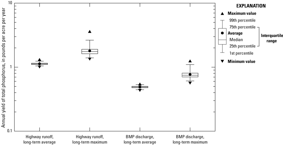
Boxplots showing the distribution of long-term average and maximum annual yields of total phosphorus in pounds per acre per year from highway runoff and structural stormwater best management practice (BMP) discharge for 500 different master random-seed simulations.
Stochastic random-seed variability for individual events simulated in SELDM can be substantial. For example, figure 16 is a boxplot showing variation in individual-event dilution factors from selected exceedance percentages. Among results of the 500 (10 acre) individual seed analyses, the maximum dilution factors for each simulation (with an exceedance risk of about 0.04 percent) range from about 0.352 to 0.945; the median of these maximum dilution-factor values was 0.612. Thus, with all the same input variables and different random seeds there was a multiplier of 2.68 between maximum (about 0.04 percent exceedance risk) dilution factors from simulation to simulation. In comparison, the median dilution factors (with a 50 percent exceedance risk) among the 500 simulations range from 0.0138 to 0.0156 with a median value of about 0.0147 (fig. 16). This range in dilution factors at the 50 percent exceedance risk represents a multiplier of only 1.13. However, because the effects of extreme events commonly are the focus of ecological-health assessments (Niemi and others, 1990), selection of a seed value that will represent the most likely outcomes is warranted.
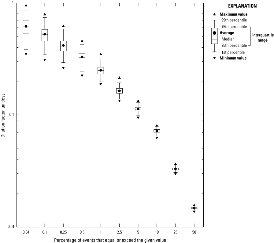
Boxplots showing the variation in individual-event dilution factors from selected exceedance percentages from 500 master random-seed simulations. These simulations were done by using a 10-acre 100-percent-impervious highway site with a 10-square-mile 10-percent-impervious upstream basin.
Variability in individual event concentrations also were examined. As an example, figure 17 shows total phosphorus concentrations for selected exceedance probabilities. These concentrations were simulated by using the 500 different master random-seed values with the median highway-runoff statistics (table 19) and the total phosphorus transport curve for minimally developed basins (table 23). The maximum highway-runoff concentrations (at a 0.04-percent exceedance probability) ranged from about 1.1 to 4.39 mg/L (a multiplier of 3.99) and median highway-runoff concentrations that ranged from 0.106 to 0.124 (a multiplier of 1.17, fig. 17A). The maximum upstream-stormflow concentrations (at a 0.04-percent exceedance probability) ranged from 0.0615 to 0.134 (a multiplier of 2.17, fig. 17B); the median (50-percent exceedance probability) upstream total phosphorus concentrations ranged from 0.0209 to 0.0226 (a multiplier of 1.08). The variation in transport curve concentrations among master random-seed simulations is less than the variation in highway runoff concentrations because the upstream concentrations are tempered by the combination of the random flow used in the transport curve and the random variation in concentrations above and below the transport curve line (fig. 1). To generate an extreme upstream concentration with the total-phosphorus transport curve for minimally developed basins requires generation of a high stormflow and a large variation above the transport curve within the same event. Because the consequences of inflated concentration estimates can be high (U.S. Environmental Protection Agency, 2002; Taylor and others, 2014; Lantin and others, 2019), selection of a master random-seed value that does not produce anomalously high or low concentrations is warranted.
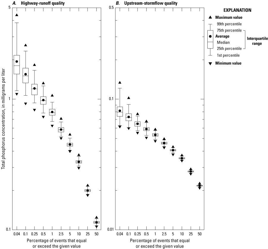
Boxplots showing individual-event concentrations of total phosphorus concentrations (p00665) from selected exceedance percentages from 500 master random-seed simulations for A, highway-runoff quality and B, upstream-stormflow quality. These simulations were done by using a 10-acre, 100-percent-impervious highway site with a 10 square-mile, 10-percent-impervious upstream basin.
The variations and extreme values simulated in the master random-seed analyses are consistent with statistical sampling theory (Haan, 1977) because 820,256 individual events within 14,391 annual-load accounting years were simulated in the 500 simulations. The extreme values, however, may not represent conditions in an average simulation of about 1,640 events within 29 annual-load accounting years. To select a representative master random seed for use in the sensitivity analyses and scenario analysis projects (table 27), a 5-step process was used to winnow the collection of 500 master random seeds. In the first step, the maximum annual precipitation, highway runoff, and BMP discharge volumes from all 500 analyses were sorted, and master random seeds that produced values outside the 5th and 95th percentiles were discarded from further analysis. Because some of the extreme high and low values of maximum annual precipitation, highway runoff, and BMP discharge volumes were simulated by using the same master random seed, only 110 master random seeds were discarded in this step. In the second step, the maximum individual-event concentrations of total nitrogen (p00600), total phosphorus (p00665), suspended sediment (p80154), and Escherichia coli (p50468) were sorted and examined. Master random seeds from simulations that produced values that exceeded the top 1 percent of concentration values were discarded with the equivalent number of the lowest maximum-concentration values; 130 master random seeds were discarded in this step. In the third step, the master random seeds that produced the top and bottom 33 percent of maximum individual-event dilution factors were discarded; 172 master random seeds were discarded in this step. In the fourth step, the master random seeds that produced the top and bottom 40 percent of maximum individual-annual yields of the 4 water-quality constituents were discarded; 70 master random seeds were discarded in this step. The median values of the different population statistics did not vary substantially through the winnowing process because a minimum value was discarded for each maximum value that was discarded. The fifth and final step was to rank the remaining 18 seeds by precipitation, runoff, BMP discharge, dilution factors, concentrations, and yields to select the random master seed that produced results that best approximated the medians of each value. The master random-seed value of 8,556 had an average ranking of 0.487, which was closest to the theoretical median of 0.5; this master random seed was used for all the subsequent analyses that did not include a random-seed test.
Precipitation Statistics
SELDM uses statistics for three variables; precipitation volume, event duration, and time between event midpoints; to simulate a population of runoff-generating events (Granato, 2010, 2013). The precipitation sensitivity analysis included 1,008 individual simulations done by using the primary master random seed (number 8,556). Precipitation statistics for southern New England (which is the median of 45 precipitation stations in and around southern New England) and median statistics for the three ecoregions that include areas in Connecticut, Massachusetts, or Rhode Island were used (table 9). Additionally, precipitation statistics for 17 additional individual hourly precipitation data stations that represent the maximum and minimum of the precipitation volume, event duration, and time between event midpoints and representative values across the distributions of these three statistics were selected for this sensitivity analysis (table 10). The results of these analyses are documented in the 02000-SA-Rain project files (table 27, Granato and others, 2022). Simulations using precipitation statistics for the three ecoregions, southern New England, and all 45 individual hourly precipitation data stations were done for the highway- and urban-runoff yield analyses (table 27).
Each of the 21 sets of precipitation statistics were simulated with 48 combinations of 3 highway-site and 16 upstream-basin configurations. Three 100-percent impervious highway-site configurations with areas of 0.25, 1.0, and 10 acres were used for these simulations. The representative lengths (table 6) were 300, 1,056, and 1,056 feet, respectively, and the representative slopes were all 10 feet per mile (table 7). The 16 simulated upstream basins had drainage areas of 0.1, 1, 10, or 20 square miles with proportional lengths and slopes (table 5) and impervious values equal to 0, 5, 10, or 20 percent.
To examine the sensitivity of the simulated dilution factors to the selected precipitation statistics, variations in dilution factors were compared to variations in precipitation statistics. Figure 18 shows an example of the variations in dilutions factors for selected exceedance percentiles over the full range of simulated precipitation volume. Because the exceedance probabilities indicate the percentage of precipitation events with dilution factors that are greater than or equal to the selected value in each simulation, the dilution factors increase with descending exceedance percentiles (fig. 13). The rank correlations between the average precipitation volume and the average event duration and average time between event midpoints are weak (with Spearman’s rho values of about −0.24 and 0.37 respectively). It was these weak correlations that guided the decision to test the sensitivity with actual precipitation station statistics rather than by varying each variable systematically. However, the rank correlation between the average event duration and average time between event midpoints is moderately strong (with a Spearman’s rho value of about 0.71) because the variables are related in time. For the same master random-seed value, a shorter average time between event midpoints generally results in generation of more events in one simulation than for simulations with a longer average time between event midpoints. If there are more events, then the potential for simulating more extreme events is increased. Extreme events have smaller exceedance-risk percentiles; therefore, there is greater variability in the increasing dilution factors with smaller exceedance-risk percentiles (fig. 18).
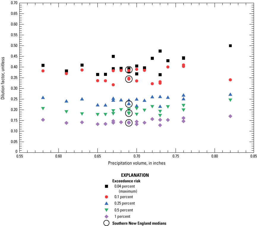
Scatterplot of dilution factors for selected exceedance percentiles as a function of precipitation volumes with a 1-acre highway site and 1-square-mile, 0-percent impervious upstream basin. Results are from 21 simulations with precipitation statistics that represent regional medians and the range of individual precipitation-gage statistics.
As indicated in figure 18, the dilution factors do not increase monotonically with increasing average event precipitation volume. This is, in part, because the same precipitation volume falls on the highway site and upstream basin during a precipitation event and increasing the precipitation produces additional runoff from both areas. For the selected combination of a 1-acre fully paved highway site and a 1-square-mile, zero-percent impervious upstream basin, the dilution factors with a 1-percent exceedance risk ranged from about 0.128 to 0.17 (12.8 to 17 percent of downstream flow) over an average precipitation volume range of 0.58 to 0.82 inches of rain. The dilution factors with the maximum percent exceedance risk of 0.04 ranged from about 0.364 to 0.5 over the same precipitation volume range.
The sensitivity of dilution factors to variations in precipitation for all 1,008 simulations is shown in figure 19. The 0.5 percent exceedance risk was selected for this example because it approximates the one event in three-year risk among the precipitation simulations with different numbers of events, and this percentage was not as variable from simulation to simulation as the more extreme (lower) exceedance percentiles (fig. 18). As expected, the average dilution factors generally increase with increasing drainage-area ratios (fig. 19A). The smallest average dilution factors result from a 0.25-acre highway site draining to a 20-square-mile upstream basin (a drainage-area ratio of 0.0125). The largest average dilution factors result from a 10-acre highway site draining to a 0.1-square-mile basin (a drainage-area ratio of 100). Variations in average dilution factors at the same drainage-area ratios are caused by the timing of runoff from different highway and upstream basins of different sizes and imperviousness.
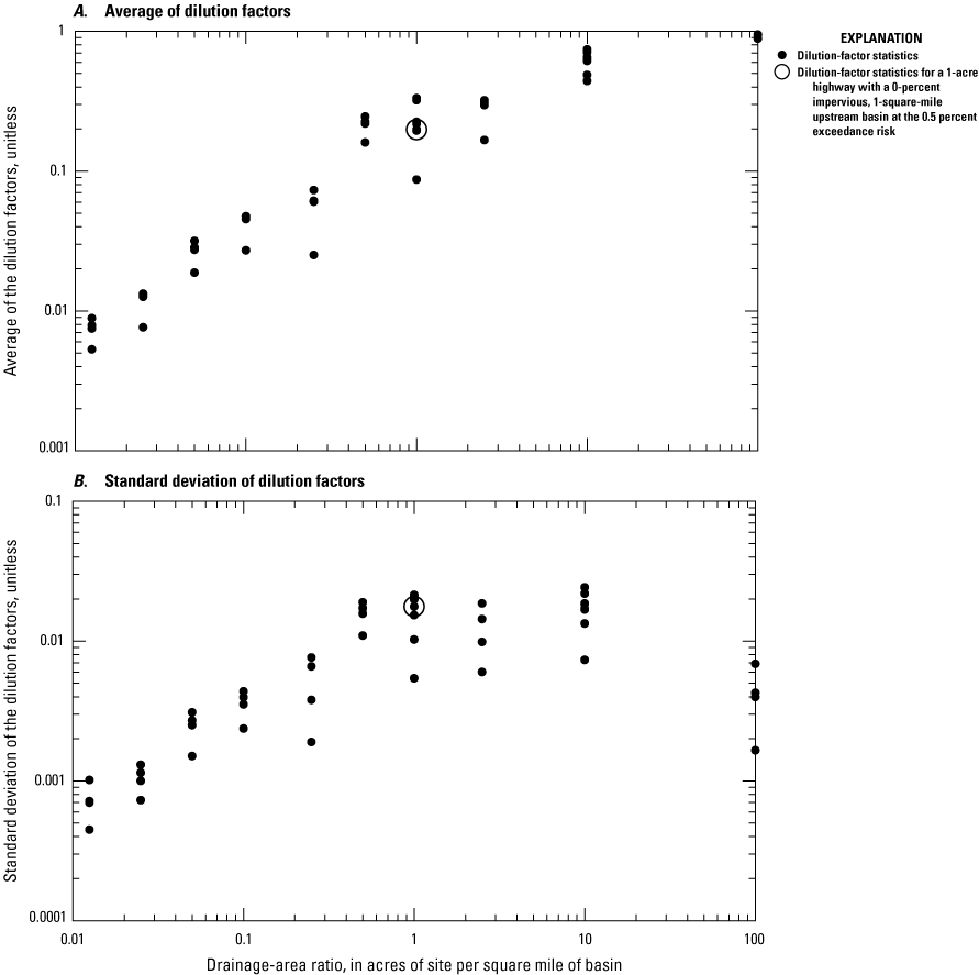
Scatterplots of the dilution-factor statistics at the 0.5 percent exceedance risk for the precipitation-statistics sensitivity analyses as a function of the drainage-area ratios. A, Average of dilution factors. B, Standard deviation of dilution factors. Statistics were calculated for the 21 precipitation-statistics simulations done for each of the 48 combinations of highway-site and upstream-basin areas and upstream-basin imperviousness.
The standard deviation values shown in figure 19B represent the variability of dilution factors over the full range of precipitation statistics at precipitation monitoring stations within and adjacent to southern New England. Figure 19B indicates that the variations in precipitation statistics do not have a strong effect on dilution factors because the standard deviations are low in comparison to the average values. At low drainage-area ratios, the variability is small in part because the highway sites are so small in relation to the upstream basin. At the maximum drainage-area ratio simulated (100 acres per square mile), the variability in dilution factors is very low (less than about 0.007) because the highway runoff is such a large portion of downstream flows at the 0.5 percent exceedance risk (fig. 19A). Even the maximum standard deviation of dilution factors for this percentile in these simulations (about 0.024 for drainage-area ratio or 10 acres per square mile) represents a coefficient of variation (COV), the standard deviation divided by the average, of only about 0.033. Among all precipitation sensitivity simulations, the COVs range from 0.00175 to 0.114 with an average COV of 0.0639. In comparison, the average of COV values for EMCs measured at highway-runoff monitoring sites in Massachusetts with 10 or more EMCs was about 1.18 for total nitrogen (p00600), 0.859 for total phosphorus (p00665), and 1.28 for suspended sediment (p80154).
Prestorm Streamflow Statistics for Sites Without Zero Flows
SELDM uses prestorm streamflow statistics to simulate the flow in the receiving stream at the site of interest when the event begins (Granato, 2013). SELDM uses four statistics to simulate prestorm streamflows; these include the average, standard deviation, and skew of the logarithms of mean daily flows and the proportion of zero flows. In the environment, the components of prestorm streamflow may include base flow (generally defined as groundwater discharge) and stormflow from a previous storm. In the environment and in SELDM analyses, some proportion of prestorm streamflows may be less than the mean daily minimum reporting limit of 0.01 cubic feet per second (Rantz, 1982) even if the stream is not considered intermittent or ephemeral (Rossman, 1990; Granato, 2010). This series of analyses was done to evaluate the effect of variations in average, standard deviation, and skew of the logarithms of mean daily flows representing perennial streams with no zero flows on simulation results. Values representing the median of the nonzero flow statistics from the SELDM database streamgages (the “SELDM” dataset), the Southern New England 1901–2015 streamgages (the “1901–2015” dataset), and the selected southern New England index streamgages (the “Index” dataset) were used (table 11). The statistics for all the individual stations are documented by Granato and others (2022). Geometric mean values representing the minimum, maximum, and median of the Index streamgages and values representing the 10, 25, 40, 60, 75, and 90th percentile geometric mean values were used for these simulations. These geometric mean values ranged from about 0.709 to 2.7 cubic feet per second per square mile. Because the area-normalized average of the logarithms had moderately strong negative rank correlations with the standard deviation and skew (table 12), the standard deviations and skew values associated with these geometric means were calculated by using the equations in table 13 and used in these simulations. This prestorm streamflow sensitivity analysis included 528 individual simulations done by using the primary master random seed (number 8,556). The results of these analyses are documented in the 03000-SA-Stream project files (table 27, Granato and others, 2022).
Each set of prestorm streamflow statistics were simulated with 48 combinations of highway site and upstream basin configurations. Three 100-percent impervious highway-site configurations with 0.25, 1.0, and 10 acres were used for these simulations. The representative highway site lengths (table 6) were 300, 1,056, and 1,056 feet, respectively, and the representative slopes were all 10 feet per mile (table 7). The 16 simulated upstream basins had drainage areas of 0.1, 1, 10, and 20 square miles with proportional lengths and slopes (table 5) and impervious values equal to 0, 5, 10, and 20 percent.
To examine the sensitivity of dilution factors to the selected streamflow statistics, variations in dilution factors were compared to variations in the simulated geometric mean streamflows. Figure 20 shows an example of the variations in dilution factors for selected exceedance percentiles over the full range of simulated geometric mean streamflows. The large gap in geometric mean streamflows is caused because the maximum of geometric means is a high outlier among the available streamgage statistics (Granato and others, 2022). Because the exceedance probabilities indicate the percentage of events with dilution factors that are greater than or equal to the selected value, the dilution factors increase with descending percentiles (fig. 13); this explains the greater variability in the increasing dilution factors with smaller exceedance-risk percentiles (fig. 20). Within these simulations, there are substantial decreases in the dilution factors with increasing geometric mean streamflow over the range of simulated streamflow statistics. The maximum dilution factor for each exceedance percentile is about 2.27 to 3.49 times the minimum value across the simulated range of geometric mean streamflows (fig. 20).
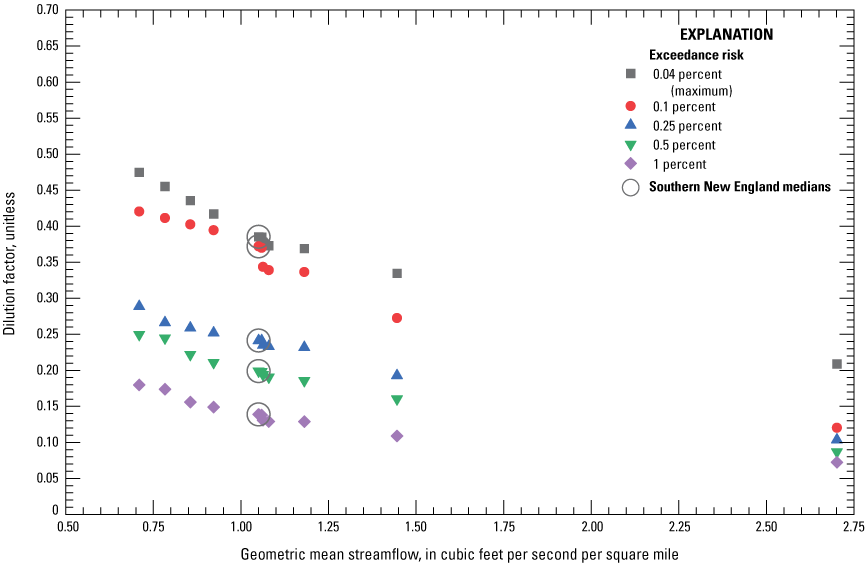
Scatterplot of dilution factors for selected exceedance percentiles as a function of geometric mean streamflow with a 1-acre highway site and 1-square-mile, 0-percent-impervious upstream basin. Results are from 11 simulations with streamflow statistics that represent regional medians and the range of individual streamgage statistics.
The sensitivity of dilution factors to variations in simulated streamflow statistics for all 528 simulations is shown in figure 21. Each point represents statistics for the 11 streamflow-statistics simulations for 1 of the 48 combinations of highway- and upstream-area and upstream imperviousness. The average dilution factors generally increase with increasing drainage-area ratios (fig. 21A). The smallest average dilution factors result from a 0.25-acre highway site draining to a 20-square-mile upstream basin (a drainage-area ratio of 0.0125). The largest average dilution factors result from a 10-acre highway site draining to a 0.1-square-mile basin (a drainage-area ratio of 100). Variations in average dilution factors at the same drainage-area ratios are caused by the simulated streamflow statistics and the timing of runoff from different highway and upstream basins with the same drainage-area ratio but with different combinations of drainage-area and imperviousness values.
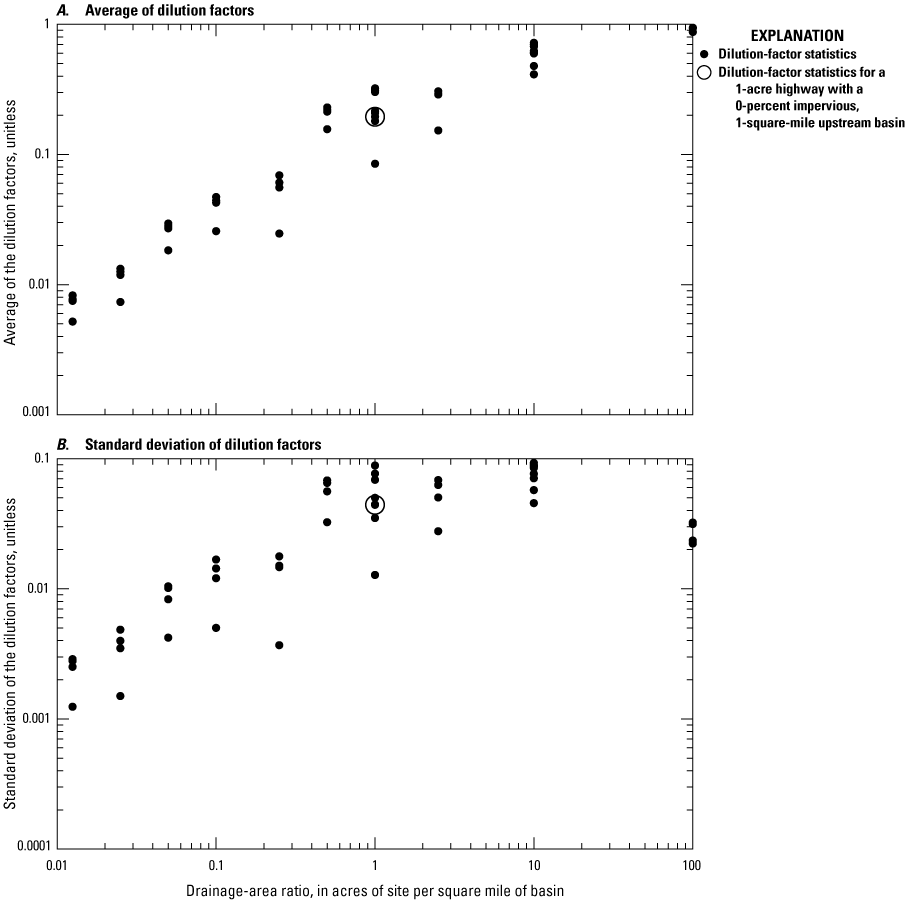
Scatterplots of the dilution-factor statistics at the 0.5 percent exceedance risk for the prestorm streamflow-statistics sensitivity analyses as a function of the drainage-area ratios. A, Average of dilution factors. B, Standard deviation of the dilution factors. Statistics are calculated for the 11 streamflow-statistics simulations done for each of the 48 combinations of highway-site and upstream-basin areas and upstream-basin imperviousness.
The standard deviation values for the 0.5 percent exceedance risk shown in figure 21B represent the variability of dilution factors over the full range of the simulated streamflow statistics. This graph indicates that the variations in streamflow statistics have a much stronger effect on dilution factors than the simulated variations in precipitation. On average, the standard deviations in the streamflow simulations were about four times the variation in precipitation simulations. At low drainage-area ratios (less than 0.5 acre per square mile), the variability is smaller than in the midrange of drainage-area ratios (about 1 acre per square mile) in part because the highway sites are so small in relation to the upstream basin. At the maximum simulated drainage-area ratio, the variability is lower than at the midrange because the highway runoff is such a large portion of downstream flows (fig. 21A). The maximum standard deviation of dilution factors for the 0.5 percent exceedance risk in these simulations (about 0.0925) represents a COV of about 0.153. Among these streamflow-statistics sensitivity simulations, the COVs range from 0.0238 to 0.375 with an average COV of 0.22. The COVs of dilution factors associated with variations in streamflow statistics are, on average, more than three times the COVs associated with variations in precipitation statistics.
This sensitivity analysis indicates that, for estimating the potential effects of runoff on receiving waters, the upstream prestorm streamflow statistics are among the most influential variables. Because the potential effects of runoff are heavily dependent on prestorm streamflow volumes, methods are needed to estimate flow statistics at any site of interest on a stream. The simplest method to refine a regional estimate of a surface-water statistic is to use the selected-station average or selected-station median from the SELDM dataset (Granato, 2013), the 1901–2015 dataset (Granato and others, 2017), or the Index dataset (Granato and others, 2022), which are available in the southern New England SELDM application (Granato and others, 2022). This approach is based on the drainage-area ratio method; more refined estimates may be developed by using the regression on basin characteristics method by using StreamStats to obtain basin properties (for Connecticut and Massachusetts) or daily mean flow percentiles (for Rhode Island).
StreamStats can be used to estimate site-specific statistics for any point within each State in southern New England, but the available statistics and available tools are different from State to State. In Connecticut, StreamStats can be used with the Connecticut Streamflow and Sustainable Water Use Estimator (Granato and Levin, 2018a) to produce a long-term flow record that can be used to calculate the streamflow statistics used by SELDM. Water-use data of some areas of Connecticut are available in StreamStats, which can be used to adjust estimates of streamflow statistics for water withdrawals and wastewater discharges. In Massachusetts, StreamStats can be used with the Massachusetts Sustainable-Yield Estimator (Granato and Levin, 2018b) to produce a long-term flow record that can be used to calculate the streamflow statistics to be used by SELDM, and this record can be adjusted for upstream water use. In Rhode Island, StreamStats can provide selected streamflow percentiles for delineated basins (Bent and others, 2014). If a regression equation is developed between the normal frequency factor associated with each percentile and the predicted streamflow value provided by StreamStats, then the intercept of the line will be the average and the slope will be the standard deviation of the logarithms of the StreamStats estimated daily flows for Rhode Island. The skew of the logarithms can be estimated by using Pearson’s second skew which is equal to three times the difference between the mean and the median divided by the standard deviation. If the logarithms of flow plot concave down, then the skew is negative; if they plot concave up, then the skew is positive. Once calculated, the site-specific streamflow statistics can be entered in SELDM by using the user-defined option.
Prestorm Streamflow Statistics for Sites With Zero Flows
SELDM uses prestorm streamflow statistics to simulate the flow in the receiving stream at the site of interest when the event begins; in some cases, the streamflow record may contain zero flows (Granato, 2013). In this series of sensitivity analyses (project 04000-SA-StreamZed, table 27), the effect of different zero-flow fractions was simulated. Three sets of regional median statistics for streamgages with one or more zero flows were used. These included statistics from the SELDM database of southern New England streamgages, the Southern New England 1901–2015 streamgages, and the selected southern New England index streamgages (table 11). The fractions of zero flows that were simulated were 0.00277, 0.00647, and 0.00043 for these three datasets, respectively. A set of nine additional zero-flow fractions (0.00001, 0.0001, 0.00027, 0.001, 0.0014, 0.0027, 0.01, 0.1, and 0.25) were simulated by using the medians of the average, standard deviation, and skew of the logarithms of nonzero streamflows taken from the southern New England index streamgages with one or more zero flows (table 11). The zero-flow fraction 0.00001 was simulated to examine the effect of the nonzero flow statistics for streamgages with one or more zero flows without producing a zero flow in the simulated record. The fractions 0.0001, 0.00027, 0.001, 0.0014, and 0.0027 represent one dry day in about 27, 10, 3, 2, and 1 year on average, respectively. The zero-flow fractions greater than 0.0027 represent more than one dry day per year on average. The maximum zero-flow fraction tested in this sensitivity analysis was 0.25 because this is much larger than the fraction of zero flows in the SELDM database of southern New England streamgages and the Index dataset of southern New England stations and is approximately equal to the maximum zero-flow fraction of the 1901–2015 dataset streamgages in southern New England (table 14). In theory, once the percentage of dry (zero flow) days exceeds the exceedance risk percentage, the dilution factor for a given highway-runoff volume is controlled by the runoff contribution of the upstream basin rather than a stormwater volume that is the sum of prestorm streamflow and runoff.
Ephemeral streams, which flow only in response to runoff are a special case. Precipitation statistics indicate that there are about 41 to 67 runoff-generating events per year in southern New England (table 10), which would produce zero flow ratios of 0.82 to 0.89 for an ephemeral stream. The nonzero flow days are caused when runoff events supply flow to the ephemeral stream, but the EPA definition of a runoff-generating event is based on hourly precipitation with a 6-hour interevent period so there may be multiple events within a single day. To simulate this situation with SELDM, the prestorm zero-flow fraction could be between 0.82 and 1 for an ephemeral stream site, and the nonzero flow statistics would be a result of runoff with little if any baseflow contributions. Although the USGS monitored areas as small as 0.35 square miles, the USGS did not have recording streamgages on ephemeral streams in southern New England during the 1901–2015 period (Granato and others, 2017). In comparison, about 44 percent of road-stream crossings and about 34 percent of arterial road-stream crossings have drainage areas less than 0.35 square miles (fig. 2). Although this sensitivity analysis is focused on perennial streams with few zero flows and intermittent streams with a moderate fraction of zero flows (definitions of the division between these two stream categories vary), the results are instructive for simulating runoff at ephemeral stream crossings.
SELDM uses the conditional-probability Monte-Carlo method to simulate the occurrence of zero flows (Granato, 2013). Therefore, the input risk for zero flows may not equal the number of generated zero-flow values in any given simulation. Analysis of the binomial distribution (Haan, 1977) indicates that with 1,659 trials (generated storm events), the probability that no zero-streamflow events would be generated would be about 85, 64, 19, 9.8, and 1.1 percent if the risk fractions for zero flows are 0.0001, 0.00027, 0.001, 0.0014, and 0.0027, respectively. With the selected master random seed (number 8,556), no zero-flow values were generated for simulated risk fractions less than 0.001 (0.1 percent, Granato and others, 2022).
To do the zero-flow sensitivity analysis, each set of streamflow statistics were simulated with 48 combinations of highway site and upstream basin configurations, resulting in a total of 576 zero-flow simulations done by using the primary master random seed (number 8,556). Three 100-percent impervious highway-site configurations with areas of 0.25, 1.0, and 10 acres, respectively, were used for these simulations. The representative lengths (table 6) were 300, 1,056, and 1,056 feet, respectively, and the representative slopes were all 10 feet per mile (table 7). The 16 simulated upstream basins had drainage areas of 0.1, 1, 10, and 20 square miles, respectively, with proportional lengths and slopes (table 5). Upstream impervious values equal to 0, 5, 10, and 20 percent were used for these simulations. The results of these analyses are documented in the 04000-SA-StreamZed project files (table 27, Granato and others, 2022).
To examine the sensitivity of dilution factors to the selected streamflow statistics, variations in dilution factors were compared to variations in the simulated fraction of zero flows. Figure 22 shows an example of the variations in dilutions factors for selected exceedance percentiles over the full range of simulated zero-flow fractions. Because no zero flows were generated for zero-flow risk fractions less than 0.001, all the dilution factors in figure 22 are invariant to the fraction of zero flows below this threshold. Above this risk threshold, the dilution factors are invariant to the fraction of zero flows as long as the exceedance percentile of interest is greater than the simulated zero-flow fraction. The dilution factors for all percentiles have substantial changes above the specified zero-flow fraction of 0.01.
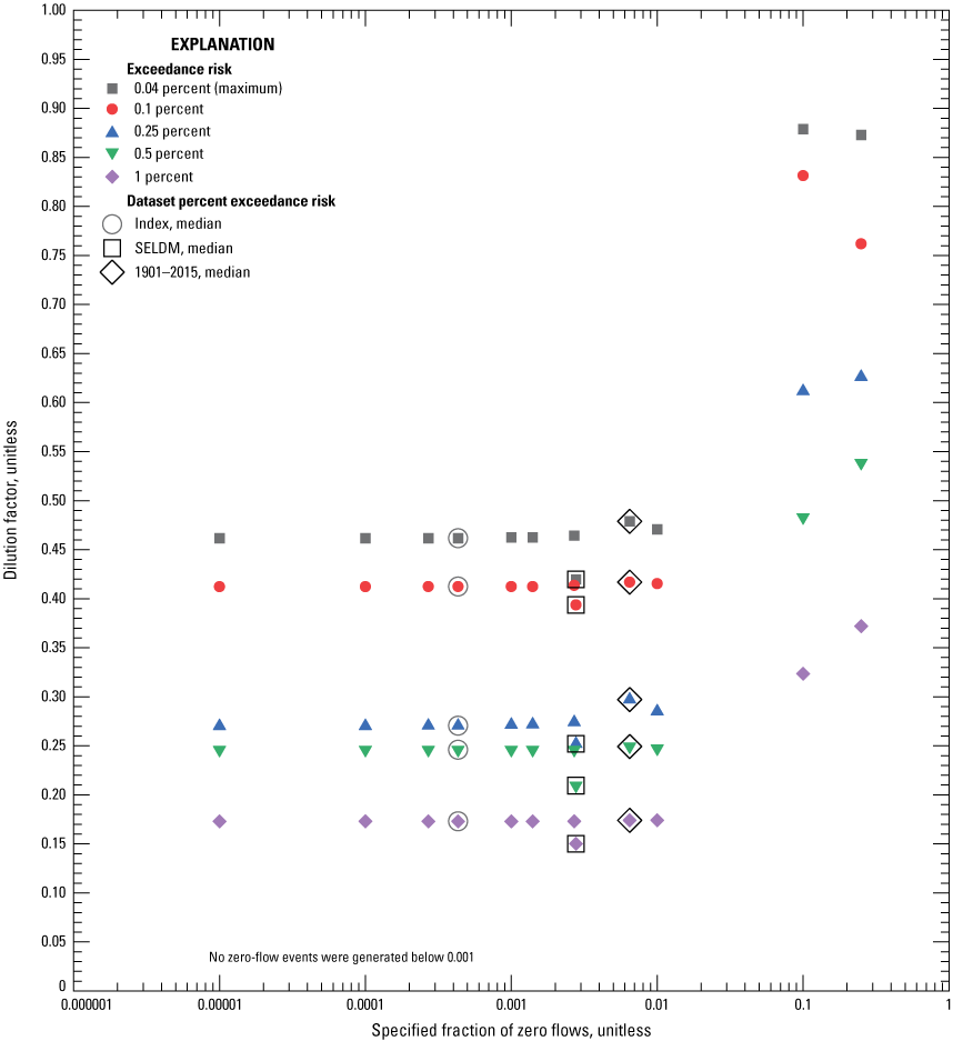
Scatterplot of dilution factors for selected exceedance percentiles as a function of the fractions of zero flow with a 1-acre highway site and 1-square-mile, 0-percent-impervious upstream basin. Results are from 12 simulations with zero-flow statistics that represent regional medians and zero-flow fractions from 0.00001 to 0.25.
Below a specified zero-flow fraction of 0.01, the most substantial variations in simulated dilution factors are caused by variations in the statistics for the logarithms of nonzero flows that were used in simulations (fig. 22). The symbols showing simulation results developed by using the statistics for streamgages with one or more zero flows (table 11) indicate that the average, standard deviation, and skew of nonzero flows have a greater effect than the fraction of zero flows as long as the simulated fraction of zero flows is smaller than the associated exceedance risk of concern. For example, the SELDM dataset geometric mean is larger than the geometric mean of the Index and 1901–2015 datasets, and the geometric standard deviation is smaller in the SELDM dataset than the values for the other two datasets (table 11). Therefore, the nonzero flows simulated using the SELDM-database statistics are higher and less variable than simulations using statistics from the other two datasets, and the dilution factors are correspondingly lower than for the other datasets (fig. 22). The seeming anomalies in the change in dilution factors for the 0.04 percent and 0.1 percent exceedance risk as the fraction of zero flows increase from 0.1 to 0.25 (fig. 22) are caused by the shuffling of storm-event values that can take place if prestorm streamflows are 0.
The sensitivity of dilution factors to variations in simulated streamflow statistics for all 576 simulations is shown in figure 23. Each point represents statistics for the 12 simulations of one of the 48 combinations of highway- and upstream-area and upstream imperviousness.
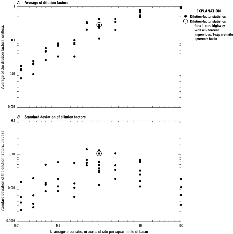
Scatterplots of the dilution-factor statistics at the 0.5 percent exceedance risk for zero-flow sensitivity analyses as a function of the drainage-area ratios. A, Average of dilution factors. B, Standard deviation of dilution factors. The averages and standard deviations are shown as a function of drainage-area ratios in acres per square mile. Statistics are calculated for 12 zero-flow scenarios done for each of the 48 combinations of highway-site and upstream-basin areas and upstream-basin imperviousness.
As expected, the average dilution factors generally increase with increasing drainage-area ratios (fig. 23A). The smallest average dilution factors result from a 0.25-acre highway site draining to a 20-square-mile upstream basin (a drainage-area ratio of 0.0125). The largest average dilution factors result from a 10-acre highway site draining to a 0.1-square-mile basin (a drainage-area ratio of 100). Variations in average dilution factors at the same drainage-area ratios are caused by the simulated streamflow statistics and the timing of runoff from different highway and upstream basins of different sizes and imperviousness. The average dilution factors are also higher for the zero-flow simulations (fig. 23A) than for the associated nonzero flow simulations (fig. 21A). The averages of dilution factors for the zero-flow simulations are about 1.02 to 2.07 times the nonzero-flow averages (for drainage-area ratios of 100 and 0.0125, respectively). On average, the ratio of zero flow to nonzero-flow dilution-factor averages is 1.39 for the simulations tested. This, in part, is a result of differences in statistics for the logarithms of nonzero flows between the streamgages with and without zero flows (table 11). The average dilution factors in these simulations also are larger than the averages without zero because 4 of the 12 simulations have zero-flow ratios greater than the 0.5 percent risk results; in these scenarios at the 0.5 percent risk, the prestorm streamflow is zero and the upstream flows are smaller.
Although dilution factors are invariant to zero-flow ratios less than the exceedance risk of concern (fig. 22), the four simulations that have zero-flow ratios greater than the 0.5 percent risk result in the inflated standard deviations shown in figure 23B. The ratios of standard deviation values in figure 23 range from 0.098 to 6.04 times the standard deviation values in figure 21 and are on average about 1.54 times the standard deviation values in figure 21. The variations in these zero-flow simulations also are, on average, about 6 times the variations in precipitation simulations. The maximum standard deviation of dilution factors for this percentile in the zero-flow simulations (about 0.141) represents a COV of about 0.410. Among these streamflow-statistics sensitivity simulations, the COVs range from 0.0033 to 0.886 with an average COV of 0.238. As with the simulation results for sites without zero flows, the COVs of dilution factors associated with variations in streamflow statistics are, on average, more than three times the COVs associated with variations in precipitation statistics.
This sensitivity analysis indicates that, for estimating the potential effects of runoff on receiving waters in SELDM, the basin’s status as a stream with zero flows and the nonzero flow statistics is more important than an exact zero-flow fraction specification, especially if the fraction of zero flows is small. Bent and Steeves (2006) indicate that, in areas of Massachusetts, the presence of zero flow depends on drainage area, the percentage of sand and gravel deposits, the percentage of forest, and the location of the basin. This information with the methods described in the sections of the current report on simulation methods and the prestorm streamflow sensitivity analysis for sites without zero flows provides methods to estimate statistics for sites suspected of having zero flows. In Massachusetts and in parts of Connecticut with compiled water-use data, the sustainable water-use tools developed by Granato and Levin (2018a, b) can be used with water-use information and basin properties provided by StreamStats to estimate the unaltered streamflows and streamflows altered by water use.
Correlation of Upstream Runoff Coefficients to Prestorm Streamflow
SELDM uses the rank correlation between prestorm streamflow and the average upstream runoff coefficient to represent potential effects of antecedent wetness on simulated runoff coefficients for individual events (Granato, 2010, 2013). The rank correlation between upstream basin runoff coefficients and prestorm streamflow is specified in the SELDM interface with the runoff-coefficient statistics. In theory, increasing antecedent wetness will tend to increase the runoff coefficients in comparison to similar events falling on dry basins because previous storm events will have saturated the basin to promote infiltration-excess overland flow and saturation-excess overland flow, but there are many confounding processes. During the SELDM development process, Granato (2010, 2013) examined correlation between various measures of antecedent wetness and runoff coefficients and determined that prestorm streamflow was best suited to simulate effects of antecedent wetness on runoff coefficients. Granato (2010) found large variations in correlation coefficients (from −0.25 to 0.9) among different datasets but found that 22 of 43 studies, including many with the largest datasets and therefore the most robust correlations, clustered between a rank correlation of 0.6 and 0.9. A default value of 0.75 was selected for use in SELDM because it is in the middle of this range. Use of the rank correlation between prestorm streamflow volume and upstream runoff coefficients does not change the statistics of the prestorm streamflows or runoff coefficients; this variable affects the pairing of values. Paring high prestorm streamflows with high runoff coefficients and pairing low prestorm streamflows with low runoff coefficients would tend to increase the total upstream stormflow volume of high-flow events and decrease the volume of low-flow events.
The effect of rank correlation on simulation results was tested by using rank correlation values of 0.0, 0.5, 0.6, 0.65, 0.7, 0.72, 0.73, 0.75, 0.77, 0.8, and 0.9. These 11 values were selected to cover the range of potential values with a focus on values representing the most robust datasets (Granato, 2010). Each rank correlation value was simulated with 48 combinations of highway site and upstream basin configurations. Three 100-percent impervious highway-site configurations with 0.25, 1.0, and 10 acres were used for these simulations. The representative lengths (table 6) were 300, 1,056, and 1,056 feet, respectively, and the representative slopes were all 10 feet per mile (table 7). The 16 simulated upstream basins had drainage areas of 0.1, 1, 10, and 20 square miles, respectively, with proportional lengths and slopes (table 5), and each drainage-area category was combined with impervious values equal to 0, 5, 10, and 20 percent. Therefore, this rank correlation sensitivity analysis included 528 individual simulations for each master random seed tested. Variations in the rank correlations result in a stochastic shuffling of the prestorm streamflow, upstream runoff coefficients, and highway runoff coefficients as the correlation is changed. Therefore, the selected master random-seed number 8,556 was used and additional simulations with master random-seed values equal to 8,619 and 9,077 also were used to better characterize potential effects of the correlations between prestorm flow and upstream runoff coefficients. The master random-seed values of 8,619 and 9,077 were selected because they produced relatively low and high dilution-factor values in the random-seed analysis simulations (project 01000-Seed, table 27). Therefore the 528 individual simulations were repeated with 3 master random-seed values resulting in 1,584 simulations. The results of these analyses are documented in the 09000-SA-USRvCor project files (table 27, Granato and others, 2022).
These simulations demonstrated that systematic changes in the dilution factor with changes in prestorm rank correlation were indistinguishable from the effects of the stochastic shuffle that took place because of the change in simulated rank correlations. Figure 24 shows that the dilution factor for the 0.5 percentile exceedance risk varies substantially from value to value, and the changes with increasing rank correlation values are not monotonic and are not consistent for different random-seed values. The lack of a systematic response is consistent with the large random variability in paired values that occurs when rank correlation values are less than 0.9 (Granato, 2013). Any systematic relation between rank correlation values and dilution factors also may be obscured by the effects of stochastic variations in the component variables, which include prestorm streamflow, precipitation event characteristics, upstream runoff coefficients, highway runoff coefficients, and hydrograph recession ratios. Although the variations were not systematic with respect to the correlation coefficient, they were substantial; varying by a factor of about 2 from value to value and master seed to master seed. These variations in dilution factors with respect to the correlation coefficients are similar to the magnitude of variations simulated by using a single correlation coefficient value (0.75) with 500 master random seeds (fig. 16), which indicates that the effects of random variability from master seed to master seed are on the same order of magnitude as variability caused by selection of the rank correlation coefficient between prestorm streamflow and upstream runoff coefficients. By happenstance, the default SELDM correlation coefficient value of 0.75, which was selected based on a range of correlation coefficients from robust datasets, produces fairly consistent dilution factors for these three random-seed values at the 0.5 percentile exceedance risk.
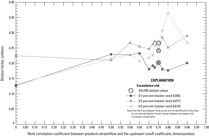
Line graph showing dilution factors for the 0.5 exceedance percentiles as a function of the rank correlation coefficient between prestorm streamflow and upstream runoff coefficients for a 1-acre highway site and 1-square-mile, 0-percent impervious upstream basin. Results are from 11 simulations that were repeated by using 3 master random-seed values. SELDM, Stochastic Empirical Loading and Dilution Model.
The sensitivity of dilution factors to variations in simulated prestorm-streamflow correlation coefficient statistics for all 528 simulations using the master random-seed number of 8,556 is shown in figure 25. Each point represents statistics for the 11 simulations for one of the 48 combinations of highway- and upstream-area and upstream imperviousness. The average dilution factors generally increase with increasing drainage-area ratios (fig. 25A). Variations in average dilution factors at the same drainage-area ratios are caused by the simulated streamflow statistics and the timing of runoff from different highway and upstream basins with the same ratio but different drainage-area and imperviousness values.
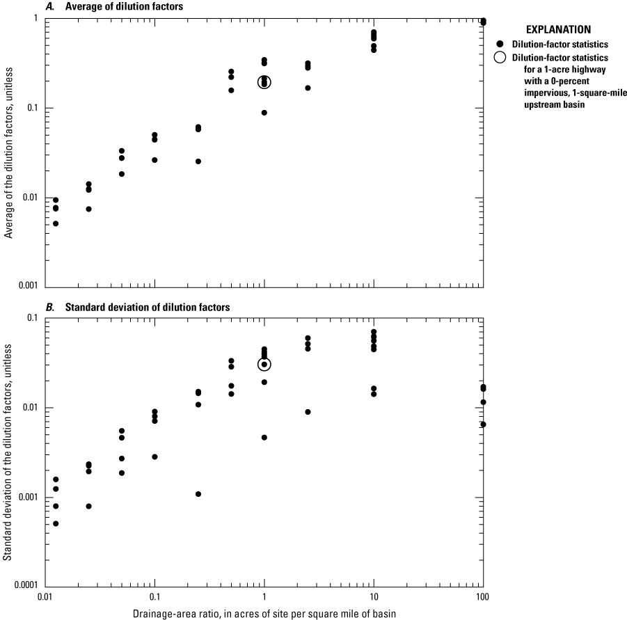
Scatterplots of the dilution-factor statistics at the 0.5 percent exceedance risk for runoff-coefficient correlation sensitivity analyses as a function of the drainage-area ratios. A, Average of dilution factors. B, Standard deviation of dilution factors. Statistics are calculated for the 11 simulations done for each of the 48 combinations of highway-site and upstream-basin areas and upstream-basin imperviousness by using the master random-seed number of 8,556.
The standard deviation values shown on figure 25B represent the variability of dilution factors over the full range of prestorm-flow correlation coefficients. At low drainage-area ratios, the variability is smaller than in the mid-range (about 1 to 10 acres per square mile) in part because the highway sites are so small in relation to the upstream basin (fig. 25B). At the maximum simulated drainage-area ratio, the variability is lower than at the midrange because the highway runoff is such a large portion of downstream flows at the 0.5 percent exceedance risk (fig. 25A). The maximum standard deviation of dilution factors for the 0.5 exceedance risk percentile in these simulations (about 0.0704 when the drainage-area ratio is 10) represents a COV of about 0.115. Among these prestorm-flow correlation sensitivity simulations, the COVs range from 0.00734 to 0.251 with an average COV of 0.121. The COVs of dilution factors associated with variations in prestorm-flow correlation are, on average, almost twice as high as the COVs associated with variations in precipitation statistics and about half as high as the COVs associated with variations in prestorm-flow volume statistics (with or without zero flows).
Although variations in dilution factors that are associated with the selected correlation coefficient between prestorm streamflows and runoff coefficients can be substantial, developing a precise site-specific estimate of this correlation coefficient may be difficult (Granato, 2010). Estimating the correlation coefficient between prestorm streamflow and the runoff coefficients for a stream basin requires data from a dense network of precipitation gages within or around the basin and a continuous-record streamgage for monitoring streamflow. The regional densities of about one NOAA hourly precipitation station per 400 to 900 square miles (table 9, fig. 7) is much too sparse to estimate the correlation coefficient, both the precipitation and streamflow need to be measured at a high frequency (every 15 minutes or less). An interpretive baseflow separation analysis must be done for each event to determine the runoff-contributed flow, which can be used to find a storm-specific runoff coefficient from the precipitation and streamflow records. Precisely quantifying a correlation coefficient may be difficult because each variable can have substantial measurement and interpretive uncertainties (Granato, 2010, appendix 1). Furthermore, there are many potentially confounding processes such as snowmelt or water-use fluctuations that may alter the correlation between the prestorm flow and the runoff coefficient at a given site. Even with a perfect dataset, an analysis of more than 50 events would be necessary to constrain the 95-percent confidence interval of the default SELDM prestorm-streamflow correlation coefficient (0.75) to within the likely range of correlation coefficient values from 0.6 to 0.9 (Haan, 1977). Analysis of about 400 events would be necessary to constrain the 95-percent confidence interval of the correlation coefficient value to within a range from 0.7 to 0.8 (Haan, 1977).
If dilution factors are used to evaluate potential effects of runoff on receiving waters, then this correlation analysis indicates that a specified prestorm-correlation coefficient would be needed to standardize the dilution-factor response to other hydrologic variables. Because the default SELDM correlation value provides fairly consistent dilution-factor values from seed to seed (figs. 16, 24), a correlation coefficient of 0.75 may be useful for establishing a relation between any given input variable and the output dilution factors without over specifying the relation between prestorm streamflow and the upstream runoff coefficient (Granato, 2013). Given the lack of a systematic relation between the correlation coefficient and the dilution factors, efforts to refine the default estimate for a given site may have limited value among all the uncertainties of simulating stormflow quality at unmonitored sites.
Recession Ratio Statistics
SELDM uses recession ratio statistics to simulate the timing of the upstream stormflow hydrograph limbs and therefore the duration of concurrent flows from the highway site or structural BMP outfall (Granato, 2012, 2013; Stonewall and others, 2019; Weaver and others, 2019). The recession ratio is the ratio of the length of the falling to rising limb of the hydrograph, which is simulated as a stochastic variable because this variable varies from event to event. SELDM uses the minimum, most probable value, and maximum ratio to simulate recession ratios by using a triangular distribution (Granato, 2013). The recession-ratio sensitivity analysis included 672 individual simulations done by using the primary master random seed (number 8,556). A total of 14 sets of recession ratio statistics including the SELDM default values, the mean and median of New England sites, and values from 11 individual streamgages were used in a sensitivity analysis to evaluate the effect of variations of selected recession ratios on simulation results (tables 16, 17). The SELDM default values and the mean and median of New England sites were selected from table 17 to represent central tendencies in recession-ratio statistics, and the 11 individual streamgages were selected from table 16 to represent the distribution of minimum, most probable values, and maximum recession ratios that are representative of hydrographs in southern New England. The results of these simulations are documented in the project 10000-SA-Ratio project files (table 27) of the model-archive data release associated with this report (Granato and others, 2022).
Each set of recession-ratio statistics were simulated with 48 combinations of highway site and upstream basin configurations. Three 100-percent impervious highway-site configurations with 0.25, 1.0, and 10 acres were used for these simulations. The representative lengths (table 6) were 300, 1,056, and 1,056 feet, respectively, and the representative slopes were all 10 feet per mile (table 7). The 16 simulated upstream basins had drainage areas of 0.1, 1, 10, and 20 square miles with proportional lengths and slopes (table 5), each drainage area was combined with upstream impervious values equal to 0, 5, 10, and 20 percent.
To examine the sensitivity of dilution factors to the selected recession-ratio statistics, variations in dilution factors were compared to variations in the average recession-ratios for different combinations of highway site and upstream basin. Figure 26 shows an example of the variations in dilutions factors for selected exceedance percentiles over the full range of average recession ratios. Because the exceedance probabilities indicate the percentage of events with dilution factors that are greater than or equal to the selected value, the dilution factors increase with descending exceedance probability percentiles (fig. 13). The results of the simulations shown in figure 26 indicate that the dilution factors are not highly sensitive to the choice of recession-ratio statistics. Although the average recession-ratio value increases by a factor of 2, the ratio of the maximum to minimum dilution factor ranges from about 1.04 to 1.08 over the different risk levels (fig. 26). Figure 26 indicates that the default SELDM statistics (table 17), which were developed by using many streamgages from southern New England, are representative of conditions in this area.
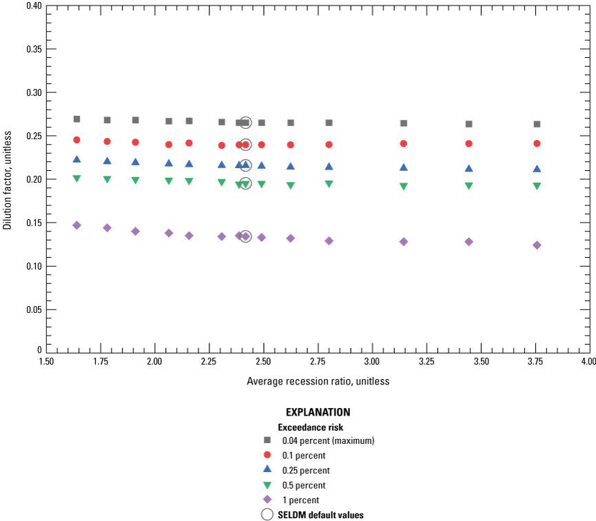
Scatterplot of dilution factors for selected exceedance percentiles as a function of recession-ratio statistics for a 1-acre highway site and 1-square-mile, 0-percent-impervious upstream basin. Results are from 14 simulations including the average and median of southern New England statistics, and the range of individual streamgage statistics. SELDM, Stochastic Empirical Loading and Dilution Model.
The sensitivity of dilution factors to variations in recession-ratio statistics for all 672 simulations is shown in figure 27. Each point represents the statistics for 14 simulations of 1 of the 48 combinations of highway- and upstream-area and upstream imperviousness. As with the other sensitivity analyses, the average dilution factors generally increase with increasing drainage-area ratios (fig. 27A). The smallest average dilution factors result from a 0.25-acre highway site draining to a 20-square-mile upstream basin (a drainage-area ratio of 0.0125). The largest average dilution factors result from a 10-acre highway site draining to a 0.1-square-mile basin (a drainage-area ratio of 100). Variations in average dilution factors at the same drainage-area ratios are caused by variations in the basin lagtime, which is caused by variations in the combinations of the length, slope, and imperviousness of the highway site and upstream basin. The largest variations are found for individual drainage-area ratios that result from different combinations of highway and upstream area.
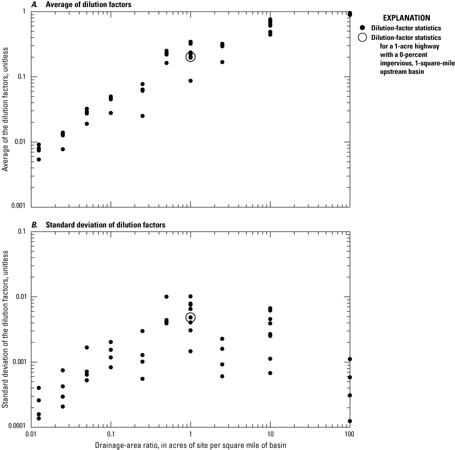
Scatterplots of the dilution-factor statistics at the 0.5 percent exceedance risk for recession-ratio sensitivity analyses as a function of the drainage-area ratios. A, Average of dilution factors. B, Standard deviation of dilution factors. Statistics are calculated for the 14 recession-ratio simulations done for each of the 48 combinations of highway-site and upstream-basin areas and upstream-basin imperviousness.
The standard deviation values shown on figure 27B represent the variability of dilution factors over the full range of recession-ratio statistics in simulations done using the median precipitation and streamflow statistics for southern New England. This graph indicates that the variations in recession-ratio statistics have minimal effects on dilution factors because the standard deviations in figure 27B are low in comparison to the average values shown in figure 27A. At low drainage-area ratios, the variability is smaller than for midrange drainage-area ratios (about 1 acre per square mile) in part because the highway sites are so small in relation to the upstream basin. At the maximum simulated drainage-area ratio (100 acres per square mile), the variability is lower than at the midrange because the highway runoff is such a large portion of downstream flows at the 0.5 percent exceedance risk (fig. 27A). The maximum standard deviation of dilution factors for this risk exceedance percentile in these simulations (about 0.01) represents a COV of about 0.031. Among these recession-ratio sensitivity simulations, the COVs range from 0.000131 to 0.0056 with an average COV of 0.021. Variations caused by recession-ratio selections are much smaller than variations caused by selection of precipitation and streamflow statistics. On average, the COVs for the corresponding precipitation, streamflow, and zero-flow simulations are about 3.12, 10.7 and 11.6 times the COVs in the recession-ratio simulations, respectively.
Given the large effort needed to develop and select recession-ratio statistics and the small effect that variations in these statistics have on simulation results, use of the SELDM default recession-ratio statistics is warranted for planning-level analyses in southern New England and other areas of the country. Developing site specific recession-ratio statistics requires one or more years of continuous-record data at a site of interest or a hydrologically similar site and a substantial effort to process and analyze the data (Granato, 2012, 2013). Strong causative relations between readily identifiable basin characteristics and recession-ratio statistics are not apparent within available datasets (Granato, 2012; Stonewall and others, 2019; Weaver and others, 2019). The SELDM default recession-ratio statistics are similar to site-specific and regional values in southern New England (tables 16, 17) and therefore produce simulation results that are representative of conditions in this area (fig. 26).
Upstream Basin Size
In the upstream-basin size sensitivity analysis, the effect of upstream basin size is examined by using selected simulations from the upstream-imperviousness simulations (project 05000-SA-USTIA, table 27) and the large upstream-area simulations (project 06000-SA-USLarge, table 27) documented by Granato and others (2022). The purpose of this sensitivity analysis is to help identify drainage-area ratio thresholds where the potential for adverse effects of runoff is remote that could be used to support, or reject, a “finding of no significant impact” (40 CFR §1508.13) without a detailed modeling study. Within SELDM, the highway-site area is the contributing area from the site of interest, which may be a highway or another developed area (Stonewall and others, 2018; Jeznach and Granato, 2020; Granato and Friesz, 2021a), and the upstream-basin area is the area of the stream basin contributing stormflow to the point of interest, but not including the area of the site of interest (Granato, 2013; Stonewall and others, 2019; Jeznach and Granato, 2020). In this report, the effects of relative basin size are examined in terms of a drainage-area ratio in acres of pavement of the site of interest per square mile of upstream stream basin. This drainage-area ratio decreases as the upstream area increases or the highway area decreases.
The effects of upstream basin size were simulated by using 84 combinations of highway site and upstream basin configurations. The simulations were done with 3 highway-site configurations, 16 upstream-basin configurations from project 05000-SA-USTIA (table 27), and 12 upstream-basin configurations from project 06000-SA-USLarge (table 27). The three 100-percent impervious highway-site configurations had areas of 0.25, 1.0, and 10 acres, respectively, with the proportional lengths (table 6) and slopes (table 7). The 16 upstream-basin configurations from project 05000-SA-USTIA used in this analysis had areas of 0.1,1, 10, and 20 square miles with upstream impervious areas of 0, 5, 10 and 20 percent. The 12 upstream-basin configurations from project 06000-SA-USLarge had areas of 40, 80, and 100 square miles with upstream impervious areas of 0, 5, 10 and 20 percent. The upstream lengths and slopes were proportional to drainage area (table 5). Median precipitation (table 9) and prestorm-flow statistics (table 11) for southern New England were used with median highway-runoff concentration statistics (table 19) and the transport curves for minimally developed basins (table 23). The simulations were done by using the primary master random seed (number 8,556). The results of these analyses are documented in the project files of the model-archive data release associated with this report (Granato and others, 2022).
The sensitivity of dilution factors to variations in upstream-basin size for all 84 simulations is shown in figure 28. The large basin-area ratios were the focus of the 06000-SA-USLarge simulations. These large basins have drainage-area ratios ranging from 0.0025 acres per square mile (the 0.25-acre highway and 100-square-mile basin) to 0.25 acres per square mile (the 10-acre highway and 40-square-mile basin). The selected 05000-SA-USTIA simulations have drainage-area ratios ranging from 0.0125 acres per square mile (the 0.25-acre highway and 20-square-mile basin) to 100 acres per square mile (the 10-acre highway and 0.1-square-mile basin). Each point in figure 28 represents the simulation results for one of the 84 combinations of highway area and upstream area and upstream imperviousness. As expected, the dilution factors generally increase with increasing drainage-area ratios (fig. 28). Variations in the dilution factors at the same drainage-area ratios are caused by the timing of runoff from different highway and upstream basins with the same area ratio but with different drainage-area and imperviousness values. Differences in upstream impervious values also change the correlations between highway and upstream runoff coefficients, which causes some stochastic shuffling of event values, especially at low upstream impervious values.
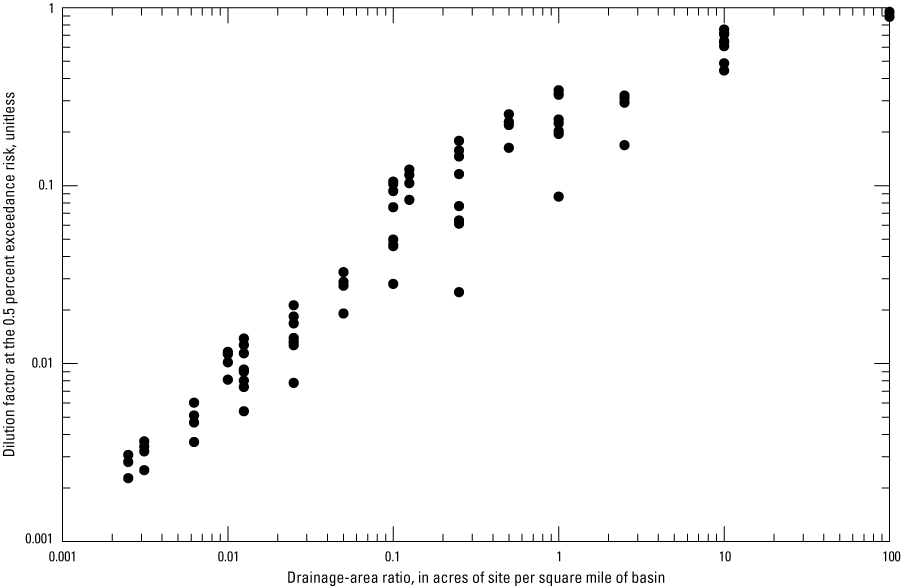
Scatterplot of the simulated dilution factors at the 0.5 percent exceedance risk for 84 combinations of highway site area, basin site area, and upstream percent imperviousness over the range of simulated drainage-area ratios. Dilution factors represent highway site areas of 0.25, 1, and 10 acres, and upstream basin-size areas of 0.1, 1.0, 10, 20, 40, and 80 square miles. Simulated upstream impervious areas were 0, 5, 10, and 20 percent. Median statistics were used for precipitation, streamflow without zero flows, and water quality.
The sensitivity of downstream concentrations to a wide range of basin sizes also is used to estimate an upstream basin area threshold for which an urban or highway discharge would have little effect. The potential sensitivity of downstream concentrations to drainage-area ratios is shown as the ratio of downstream to upstream concentrations in figure 29. Concentrations of total phosphorus (p00665) and suspended sediment concentration (p80154) at the 0.1 and 0.5 percent exceedance risks were selected to represent constituents of concern. The sensitivity of the ratio of downstream to upstream phosphorus and suspended sediment concentrations are graphed in relation to drainage-area ratios in figure 29A–D. An increased downstream to upstream constituent concentration ratio indicates that an increased proportion of the constituent from runoff was discharged to the receiving stream (fig. 29). The median highway runoff concentration statistics (table 19) and the median transport curves for minimally developed basins (table 23) were used for these simulations. Although the upstream impervious fractions ranged from 0 to 20 percent in these simulations, the transport curves for minimally developed basins were used in all these simulations to isolate the effects of the hydrologic changes in water-quality caused by variations in highway- and upstream-basin properties. Using minimally developed basin concentrations accentuates the potential adverse effects of runoff because the denominators of the concentration ratios are smaller than denominators would be for high upstream concentrations in developed areas. The water-quality ratios simulated by using minimally developed basin concentrations show a general increase with drainage-area ratio, as would be expected with decreasing upstream areas, but the relation is neither linear nor consistent for a given drainage-area ratio (fig. 29).
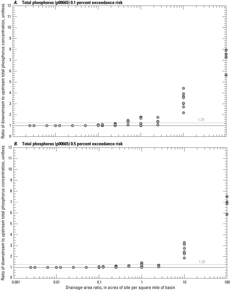
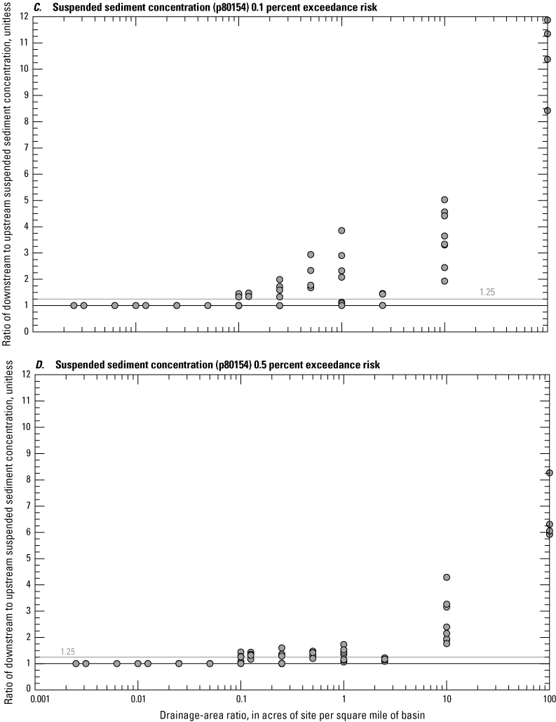
Scatterplots showing the ratio of simulated downstream to upstream concentrations for 84 combinations of drainage-area ratios. A, Total phosphorus at the 0.1 percent exceedance risk; B, total phosphorus at the 0.5 percent exceedance risk; C, suspended sediment concentration at the 0.1 percent exceedance risk; and D, suspended sediment concentration at the 0.5 percent exceedance risk. Simulations were run with combinations of highway site areas of 0.25, 1, and 10 acres and upstream basin-size areas of 0.1, 1.0, 10, 20, 40, and 80 square miles. Simulated upstream impervious areas were 0, 5, 10, and 20 percent. Median statistics were used for precipitation, streamflow without zero flows, and water quality. The horizontal line at a ratio of 1.25 downstream to upstream concentration represents the uncertainty in a stormwater-quality concentration measurement (Harmel and others, 2006). Constituents are defined in table 18.
Although there are 84 combinations of highway and upstream basin properties in figure 29, the graph seems to have fewer individual points than this because there are many tied water-quality ratios, especially for water-quality ratios near or at a value of 1. A value of 1 indicates no change in constituent concentrations from upstream to downstream of the discharge point at the site of interest. Although a value of 1 should be algebraically impossible if the constituent concentration in the runoff is different from the upstream concentration, it indicates that the change between the upstream and downstream concentration is smaller than the precision of reported values. Water-quality values commonly are reported to three significant digits, so three significant digits is the default output for water-quality values from SELDM. If the difference between the upstream concentration and the downstream concentration is a value with fewer than three-significant digits, this would result in a water-quality ratio equal to 1. Although concentrations and flows commonly are reported to three significant digits, measurement uncertainties in storm loads are on the order of 8 to 110 percent of the actual value for total phosphorus and 7 to 53 percent of the actual value for suspended solids (Harmel and others, 2006). In comparison, the random-seed analysis results (Project 01000-Seed, table 27), simulated by using the same transport curve but individual event values, indicate that large variations may occur because of stochastic variability (fig. 16) which is consistent with uncertainties reported by Harmel and others (2006) for measured storm loads. In these random-seed analysis results, the ratio of the maximum to minimum upstream total phosphorus (p00665) concentrations is about 1.33, and the ratio of the 99th to 1st percentile is about 1.25 at the 0.5 percent exceedance risk.
Simulation results indicate different drainage-area ratios that would have no effect on the downstream concentration for different water-quality constituents and risk levels (fig. 29). For total phosphorus (p00665) at the 0.5 percent exceedance risk (fig. 29B), only 27 percent of simulations result in downstream to upstream concentration ratios that equal or exceed 1.1 (a 10-percent increase in concentration from upstream to downstream) and only about 18 percent exceed downstream to upstream concentration ratios that equal or exceed 1.25 (a 25-percent increase from upstream to downstream). These concentration increases correspond to the uncertainty in stormwater concentration measurements described by Harmel and others (2006). Simulation results indicate that for total phosphorus at the 0.5 percent exceedance risk, the downstream to upstream concentration ratio does not exceed 1.1 for drainage-area ratios less than 0.25, and the downstream to upstream concentration ratio does not exceed 1.25 for drainage-area ratios less than 1 (fig. 29B). However, it should be noted that when the upstream area is greater than 0.1 square mile, only simulations with 10 or more acres of highway exceed these phosphorus concentration ratios. For suspended sediment (p80154) at the 0.5 percent exceedance risk (fig. 29D), only about 43 percent of simulations result in downstream to upstream concentration ratios that equal or exceed 1.1, and only about 35 percent exceed downstream to upstream concentration ratios that equal or exceed 1.25. Simulation results indicate that, for suspended sediment at the 0.5 percent exceedance risk, the downstream to upstream concentration ratio does not exceed 1.1 or 1.25 for drainage-area ratios less than 0.10 (fig. 29D). When the upstream area is greater than 1 square mile, only simulations with 10 or more acres of highway exceed a downstream to upstream suspended sediment concentration ratio of 1.1.
Simulation results at the 0.1 percent exceedance risk for phosphorus and suspended sediment concentrations are similar in pattern to 0.5 percent exceedance results, but as expected with higher runoff concentrations, a higher proportion of simulated values are greater than the specified concentration ratios (fig. 29A, C). For total phosphorus at the 0.1 percent exceedance risk level, only 32 percent of simulations result in downstream to upstream concentration ratios that equal or exceed 1.1 and only about 25 percent of simulations exceed downstream to upstream concentration ratios that equal or exceed 1.25. All three highway-site configurations (0.25, 1, and 10 acres) produced one or more simulations with a downstream to upstream concentration ratio that equals or exceeds 1.1. However, for total phosphorus at the 0.1 percent exceedance risk, none of the sites with 100-square-mile upstream areas produced a downstream to upstream total phosphorus concentration ratio that equals or exceeds 1.1, and only the 10-acre site produced a concentration ratio that equals or exceeds 1.1 when the simulated upstream area exceeds 1 square mile. For suspended sediment at the 0.1 percent exceedance risk level, only about 42 percent of simulations result in downstream to upstream suspended sediment concentration ratios that equal or exceed 1.1, and only about 40 percent of simulations exceed downstream to upstream concentration ratios that equal or exceed 1.25. All three highway-site configurations produced one or more simulations with a downstream to upstream suspended sediment concentration ratio that equals or exceeds 1.1. The 10-acre highway site produces one or more downstream to upstream suspended sediment concentration ratios that equals or exceeds 1.1 for all upstream basin sizes. The 1-acre highway site produced one downstream suspended sediment ratio that equals or exceeds 1.1 for a simulated upstream area of 1 square mile, and all three highway sites produced one or more upstream to downstream suspended sediment concentration ratios that equal or exceed 1.1 when the simulated upstream area is equal to 0.1 square mile.
The results shown in figure 29 are not universal; the ratios will be different if different statistics for highway runoff quality or upstream water quality are simulated. If the simulated highway-runoff concentrations are higher than the simulations in figure 29, then the ratio of downstream to upstream concentrations will also tend to be higher than those shown in figure 29. If the simulated upstream stormflow concentrations are higher than the simulations in figure 29, then the ratio of downstream to upstream concentrations will tend to be lower than those shown in figure 29. If upstream concentrations are higher than the highway concentrations (for example, in highly developed MS4 areas), then highway runoff will dilute the downstream concentrations, potentially resulting in ratios less than one. The changes in the ratios shown in figure 29 may be substantial if water quality at a site of interest is different from the median statistics that were used in these simulations (tables 19, 23). For example, results of the upstream water-quality analyses (Project 14000-USQW, table 27) indicate that among all the individual transport curves for the minimally developed basins (table 22, Granato and others, 2022), the maximum upstream and downstream total phosphorus concentrations for the 0.5 percent exceedance risk both are about 157 times the respective minimum upstream and downstream concentrations. The maximum upstream and downstream total phosphorus concentrations generated with individual transport curves for the 0.5 percent exceedance risk are about 25 times the values simulated by using the median transport curve in table 23. In the individual transport curve simulations for the 1-acre highway site and the 0-percent impervious 1-square-mile upstream site (Project 14000-USQW, table 27), if the simulated upstream total phosphorus concentration is greater than about 0.075 mg/L at the 0.5 percent exceedance risk, then the ratio of downstream to upstream concentrations will be less than or equal to 1.1.
The upstream basin-size analysis provides a large range of dilution factors (fig. 28) and ratios of downstream to upstream concentrations (fig. 29) that can be used to examine water-quality ratios as a function of dilution factors (fig. 30). In this example (fig. 30), only concentration ratios at the 0.5 percent exceedance risk are shown to focus on concentration ratios that may be applicable to water-quality criteria (Niemi and others, 1990; U.S. Environmental Protection Agency, 1991, 1998). The relations between dilution factors and the ratio of downstream to upstream constituent concentrations cannot be quantified by a simple and universal relation. When the dilution factor is below a critical threshold, all the concentration ratio values are approximately equal to 1. Above this threshold, the fact that the 0.5 percent exceedance-risk event can be different for the dilution factor, upstream concentration, and downstream concentration (Granato, 2013) results in nonmonotonic variations in the concentration ratios for similar dilution factors. For total phosphorus (fig. 30A), none of the downstream to upstream concentration ratios exceed 1.1 for dilution factors less than about 0.15, and all the concentration ratios exceed 1.1 for dilution factors greater than about 0.25. Between these ratios, about 40 percent of the simulated values exceed 1.1. For total phosphorus (fig. 30A), none of the downstream to upstream concentration ratios exceed 1.25 for dilution factors less than about 0.324, and all the ratios exceed 1.25 for dilution factors greater than about 0.324. For suspended sediment (fig. 30B), none of the concentration ratios exceed 1.1 for dilution factors less than about 0.075, and all the concentration ratios exceed 1.1 for dilution factors greater than about 0.31. Between these dilution factors, about 80 percent of the simulated concentration ratios values exceed 1.1. None of the suspended sediment concentration ratios exceed 1.25 for dilution factors less than about 0.075 and all the concentration ratios exceed 1.25 for dilution factors greater than about 0.32. Between these ratios, about 54 percent of the simulated values exceed 1.25. Therefore, even with a predetermined risk level and allowable change in water quality from upstream to downstream, there is no universal risk criterion for different water-quality constituents. Because instream water-quality data are limited for most constituents (tables 18, 23), stochastic variability (fig. 17) and site-to-site variability in water-quality are large, and relations between dilution factors and exceedances are not monotonic, an operational definition would be required to establish a decision rule for water-quality risk assessment.
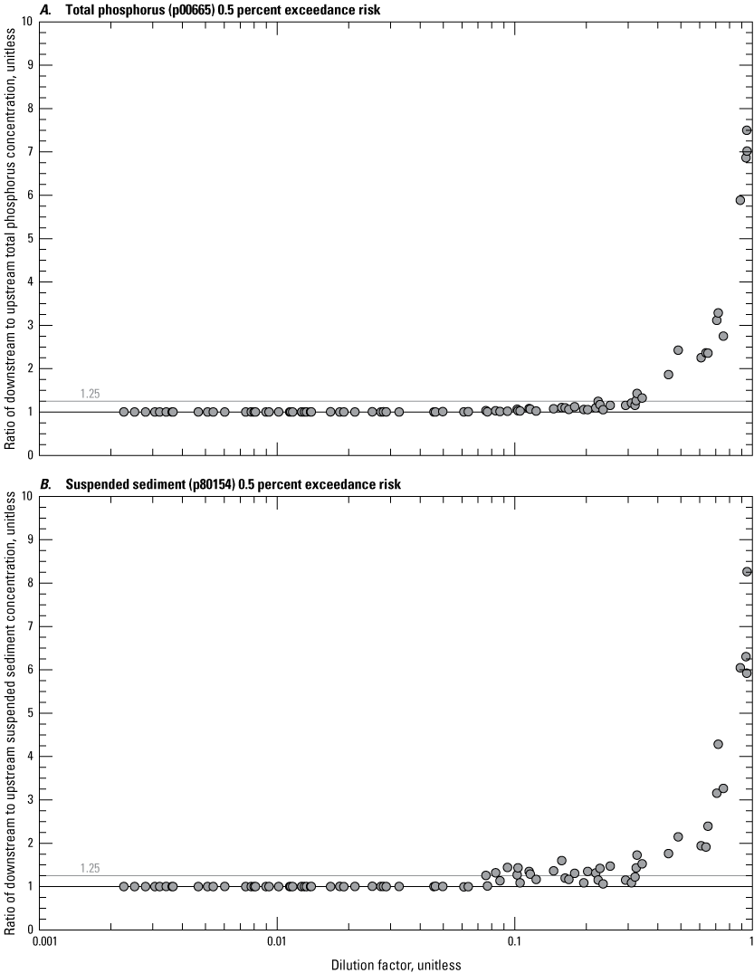
Scatterplots showing the ratio of downstream to upstream concentrations as a function of the dilution factor. A, Total phosphorus at the 0.5 percent exceedance risk. B, Suspended sediment at the 0.5 percent exceedance risk.
The results shown in figure 30 are for highway runoff without BMP treatment. BMPs that reduce flow will tend to decrease highway and downstream flows, which should reduce the dilution factor because the highway runoff flows are being reduced and the upstream flows remain the same. BMPs that reduce flow also will tend to decrease downstream concentrations at sites with upstream concentrations that are less than the runoff concentrations; this would decrease the concentration ratios. However, at sites with upstream concentrations that are greater than runoff concentrations, the BMP flow reductions will increase downstream concentrations. BMPs that reduce runoff with high constituent concentrations will decrease the combined downstream concentration and the downstream to upstream concentration ratio in comparison to a simulation without a BMP. Potential effects of different BMP categories were simulated in the structural BMP performance simulations described later in this report (Project 13000-BMPs, table 27).
Upstream Basin Imperviousness
SELDM uses the drainage area, imperviousness, and drainage length and slope to simulate the volume and timing of stormflow from the stream basin upstream of the site of interest (Granato, 2013). In SELDM, the upstream impervious fraction is used to specify the average, standard deviation, and skew of the runoff coefficients. Imperviousness can be used to specify the basin lagtime. The upstream impervious fraction is used with the impervious fraction of the highway site to establish a rank correlation between the runoff coefficients of the upstream basin and the runoff coefficients of the highway site. Simulating the runoff coefficients without correlation does not account for the proximity of the highway site to the upstream basins and therefore the similarity in antecedent conditions for both areas. However, simulating the runoff coefficients with perfect correlation does not represent potential differences in the runoff-generating processes for the highway site and the upstream basin, especially if the land cover and drainage characteristics of these areas are different. In SELDM, correlation between the upstream and highway-site runoff coefficients is established as a function of the similarity of impervious fractions and the degree of imperviousness of both areas (Granato, 2013). Because the runoff coefficients are simulated by using rank correlation, changing the impervious fractions results in stochastic shuffling of hydrologic values from event to event.
In this sensitivity analysis, 11 upstream impervious percentages equal to 0, 1, 2.5, 5, 7.5, 10, 20, 30, 45, 60, and 90 percent were simulated. Three 100-percent impervious highway-site configurations with 0.25, 1.0, and 10 acres were used for these simulations. The representative highway lengths (table 6) were 300, 1,056, and 1,056 feet, respectively, and the representative slopes were all 10 feet per mile (table 7). Upstream-basin configurations having drainage areas of 0.1, 1, 10, and 20 square miles with proportional lengths and slopes (table 5) were simulated with each of the 11 impervious values. Because a change in imperviousness and therefore a change in the correlation between upstream and highway runoff coefficients will cause random shuffling in paired runoff coefficients, the selected master random-seed value of 8,556 was used, and additional simulations with master random-seed values equal to 8,619 and 9,077 also were used to better characterize the effect of imperviousness on dilution factors. The combinations of highway and upstream basin properties resulted in 132 simulations for each random seed tested. The results of the 132 analyses for each master random seed tested are documented in the 05000-SA-USTIA project files (table 27, Granato and others, 2022).
These simulations demonstrated that the stochastic shuffle that took place because of the change in correlation values between the highway and upstream basin runoff coefficients may be larger than the systematic changes in stormflows caused by small incremental changes in the upstream imperviousness, especially at low impervious values (fig. 31). Given a 100 percent impervious highway site, the correlations between highway and upstream runoff coefficients were 0.375, 0.38, 0.387, 0.4, 0.413, 0.426, 0.478, 0.534, 0.621, 0.714, and 0.916 for upstream basin imperviousness percentages equal to 0, 1, 2.5, 5, 7.5, 10, 20, 30, 45, 60, and 90 percent, respectively (Granato, 2013). There is a substantial amount of random variation between variables at correlation coefficient values less than about 0.9 (Haan, 1977; Granato, 2013). The stochastic shuffling is more pronounced when impervious percentages are low because the correlation coefficient is lower, and the regression relations between imperviousness and the average, standard deviation, and skew of runoff coefficients have low slopes when impervious fractions are low (table 15). Figure 31 shows that for upstream impervious percentages less than or equal to 20 percent, the simulated dilution factor for the 0.5 percentile exceedance risk varies substantially among the different seed values and from impervious value to impervious value. Although the relations between imperviousness and runoff-coefficient statistics (table 13) would indicate a monotonically decreasing trend in dilution factors with increasing upstream imperviousness, this pattern is not apparent below an upstream impervious percentage of about 10 percent (fig. 31). Although the trend in dilution factors with increasing imperviousness at low impervious percentages is not as monotonic as might be expected, detailed analyses of the SELDM outputs prove that component variables for individual events and for the simulated populations are simulated correctly.
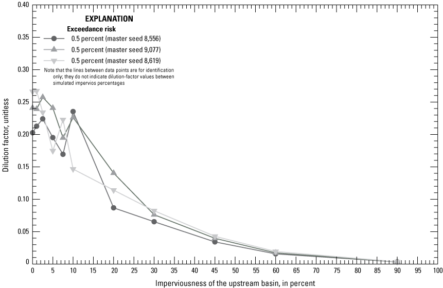
Line graph showing dilution factors for the 0.5 exceedance percentiles as a function of the upstream impervious percentage for a 1-acre highway site and 1-square-mile upstream basin. Results are from 11 impervious-percentage simulations that were repeated by using three random master random-seed values.
The sensitivity of dilution factors to variations in drainage-area ratios for all 132 simulations with the selected master random-seed number 8,556 is shown in figure 32. Each point represents the 11 upstream simulations per imperviousness value which was repeated with 12 combinations of highway and upstream area. The average dilution factors generally increase with increasing drainage-area ratios (fig. 32A). As with other variables, the smallest average dilution factors result from a 0.25-acre highway site draining to a 20-square-mile upstream basin (a drainage-area ratio of 0.0125). The largest average dilution factors result from a 10-acre highway site draining to a 0.1-square-mile basin (a drainage-area ratio of 100). Variations in average dilution factors at the same drainage-area ratios are caused by the simulated streamflow statistics and the timing of runoff from different highway and upstream basins with the same ratio but of different drainage-area and imperviousness values.
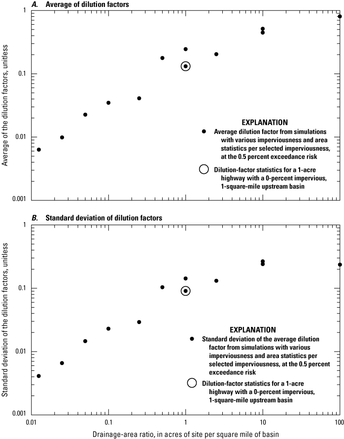
Scatterplots of the dilution-factor statistics at the 0.5 percent exceedance risk for upstream-imperviousness sensitivity analyses as a function of the drainage-area ratios. A, Average of dilution factors. B, Standard deviation of dilution factors. The averages and standard deviations are shown as a function of drainage-area ratios in acres per square mile. Statistics are calculated for the 11 impervious area simulations done for each of the 12 combinations of highway-site and upstream-basin areas by using the master random-seed value of 8,556.
The standard deviation values shown on figure 32B represent the variability of dilution factors over the full range of upstream impervious-percentages in simulations done by using the master random-seed value of 8,556 with median precipitation and streamflow statistics for southern New England. Figure 32B shows the variability of dilution factors in relation to drainage-area ratios for 11 impervious percentages in simulations. The large standard deviations indicate that the variations in upstream impervious percentages have large effects on dilution factors because the standard deviations are large in comparison to the average values shown in figure 32A. In these simulations, the standard deviation values increase with increasing drainage-area ratios until the drainage-area ratio is about 10, and they decrease slightly above this value. The maximum standard deviation of dilution factors of about 0.266 for the 0.5 risk exceedance percentile in these simulations occurs at a drainage-area ratio of 10 and represents a COV of about 0.518. Among these recession-ratio sensitivity simulations, the COVs range from 0.293 to 0.715 with an average COV of 0.599. Variations caused by upstream impervious selections are much larger than variations caused by selection of other hydrologic variables. On average, the COVs for the upstream impervious simulations are about 9.37, 2.72, 2.52, 4.96 and 129.2 times the corresponding COVs for precipitation, streamflow, zero-flow, recession-ratio, and runoff-coefficient correlation simulations, respectively.
This sensitivity analysis indicates that, for estimating the potential effects of runoff on receiving waters, the upstream impervious percentage is among the most influential hydrologic variables. The upstream impervious percentage, however, is a physical property of the upstream basin at sites of interest that can be easily ascertained by using StreamStats or other tools. Although there can be substantial differences in impervious-percentage estimates for a given drainage basin (Granato, 2010, appendix 1), uncertainties in the runoff-coefficient statistics for any given site with a nominal impervious percentage can be substantial (as evidenced by the median absolute deviations for the equations in table 15). Also, if SELDM is being used to estimate the potential for adverse effects of runoff on receiving waters over a long time period, then upstream impervious percentages are likely to increase with additional upstream development over time. The upstream impervious percentage is important, but the uncertainties in estimating this variable are less than uncertainties involved in estimating other hydrologic and water-quality variables at unmonitored sites.
Highway Runoff-Coefficient Equation
SELDM uses the average, standard deviation, and skew of runoff coefficients to generate runoff volumes from precipitation volumes for each simulated runoff event (Granato, 2013). Although the SELDM user can specify their own statistics, SELDM uses regression relations developed with data from 58 highway sites and 167 nonhighway sites to estimate runoff-coefficient statistics from the highway site and the upstream basin (table 15). Although imperviousness is commonly described as a percentage, SELDM uses the impervious fraction rather than the impervious percentage because values in the range 0–1 are less ambiguous than values in the range 0–100; therefore, there is less risk for a data-entry error. The highway runoff-coefficient equations were developed by using data from sites with drainage areas ranging from 0.05 to 106 acres and impervious percentages ranging from 27 to 100 percent (fractions from 0.27 to 1.00). The nonhighway runoff-coefficient equations were developed by using data from sites with drainage areas ranging from 0.005 to 93.47 square miles and impervious percentages ranging from 0.01 to 99.4 percent (fractions from 0.0001 to 0.994).
This runoff-coefficient equation sensitivity analysis was designed to quantify potential effects of selecting either the highway runoff-coefficient equations or the nonhighway runoff-coefficient equations for simulating runoff from the site of interest (highway or urban site). This analysis was done to examine the differences in flows and loads that can be attributed to the runoff-coefficient statistics selected for analysis because SELDM is a lumped parameter model that can be used to simulate the quality and quantity of runoff from highways or other land covers. This sensitivity analysis included 192 individual simulations done by using the primary master random-seed variable (number 8,556). Each set of runoff-coefficient equations was simulated by using 96 combinations of highway site and upstream basin configurations. Three 100-percent impervious highway-site configurations with 0.25, 1.0, and 10 acres with representative lengths (table 6) and slopes (table 7) were used for these simulations. Three of the same highway-site configurations with impervious values equal to 50 percent also were simulated (resulting in two highway-site impervious values being simulated for this sensitivity analysis). The 16 simulated upstream basins had drainage areas of 0.1, 1, 10, and 20 square miles with proportional lengths and slopes (table 5) and impervious values equal to 0, 5, 10, and 20 percent. The results of the 192 analyses done by using the primary master random seed (number 8,556) are documented in the 08000-SA-HwyRv project files (table 27, Granato and others, 2022).
The differences in stormwater flows, concentrations, and loads caused by changes in runoff-coefficient statistics do not have a purely analytic solution because the differences in the average, standard deviation, and skew of runoff coefficients vary with imperviousness, and the imperviousness of the highway site and upstream basin also affects the correlation between the highway and upstream runoff coefficients. The average and standard deviation calculated by using the highway regression relations (table 15) are higher than the nonhighway equations over the range of available data (Granato, 2010, 2013). The highway equation produces higher averages over the range of available highway-runoff data than the nonhighway equation. The highway and nonhighway equations for the average runoff coefficient come close to converging at about 19 and 100 percent imperviousness and the difference is most pronounced at an imperviousness value of 0.55 where the two nonhighway regression segments meet (table 15). The average, standard deviation, and skew of the runoff coefficients calculated by using the highway regression equations for completely impervious areas (TIA fraction equal to 1.0) are 0.785, 0.1917, and −1.19, respectively (table 15). The average, standard deviation, and skew of the runoff coefficients calculated by using the nonhighway regression equations for completely impervious areas are 0.769, 0.114, and −0.51, respectively. For sites with impervious percentages equal to 50 percent (TIA fraction equal to 0.5), the average, standard deviation, and skew of the runoff coefficients calculated by using the highway regression equations are 0.4075, 0.21035, and 0.47, respectively. The average, standard deviation, and skew of the runoff coefficients calculated by using the nonhighway regression equations for a site with an imperviousness of 50 percent (TIA fraction equal to 0.5) are 0.2415, 0.1065, and 0.8015, respectively. The highway and nonhighway equations are equal at an impervious fraction of about 0.1868 (18.68 percent), but the highway equation should not be used for impervious values less than the minimum impervious value for monitored highway sites used to develop the equations, which was 27 percent impervious.
As indicated by the runoff-coefficient statistics, generated dilution-factor values for the 100 percent impervious sites are similar for the highway and nonhighway equations (on average within a 5.1 percent difference), but the dilution-factor values calculated by using the highway runoff-coefficient statistics are on average about 1.6 times the values calculated by using the nonhighway statistics for the 50-percent impervious sites. Figure 33 shows the dilution factors simulated by using the highway runoff-coefficient statistics in comparison to dilution factors calculated by using the nonhighway runoff-coefficient statistics for sites with 50 or 100 percent impervious highway area at the 0.5 percent exceedance risk. Each point on figure 33 represents the paired dilution factors for the highway and nonhighway values with one of the 96 combinations of highway site and upstream-basin configurations. The results for the 100- and 50-percent impervious highway sites are grouped separately to demonstrate the difference in results. For the site of interest with an impervious area of 100 percent, the ratios of highway to nonhighway dilution factors range from about 1.31 to about 0.936 with an average of about 1.04. For the site of interest with an impervious area of 50 percent, the ratios of highway to nonhighway dilution factors range from about 1.05 to about 2.3 with an average of about 1.5. The runoff-coefficient statistics selected also are critical for estimating long-term annual yields for runoff quality constituents. On average, the ratios of highway to nonhighway yields are about 1.02 for total nitrogen (p00600), total phosphorus (p00665), and suspended sediment (p80154) for sites of interest that are 100 percent impervious. For sites that are 50 percent impervious, however, the average ratios of highway to nonhighway yields are about 1.73, 1.75, and 1.71 for total nitrogen (p00600), total phosphorus (p00665), and suspended sediment (p80154), respectively. Both the highway and nonhighway site simulations were done using median highway-runoff statistics (table 19) so these differences are caused by variations in stormflows rather than differences in highway and nonhighway concentrations.
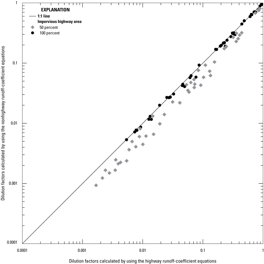
Scatterplot comparing dilution factors at the 0.5 percent exceedance risk calculated by using the highway and nonhighway regression relations between the imperviousness of the site of interest and the average, standard deviation, and skew of runoff coefficients for 2 highway site impervious percentages and 48 combinations of highway site and upstream basin configurations.
The results of these simulations indicate that the effect of the runoff-coefficient equation selection depends on the imperviousness of the simulated site. Because most of the highway sites used to develop the highway runoff-coefficient equations had high impervious percentages and because 26 of the 27 New England highway-runoff monitoring sites with concentration data in the HRDB (Granato, 2019a; Granato and Friesz, 2021b) are fully impervious, highway sites were simulated as being 100 percent impervious throughout this report. Simulations evaluating the potential effect of runoff on receiving waters may count vegetated shoulders or median areas as part of the stormwater treatment train (Granato and Friesz, 2021a; Granato and others 2021). The urban-runoff quality sites, however, represent a wide range of impervious percentages (Granato, 2021a) and, therefore, it may be better to simulate developed areas (nonhighway sites) with various impervious fractions. The calculation of higher runoff coefficients from highway equations than those calculated from nonhighway equations (table 15) may be an artifact of the availability of data or may represent the effects of highway-engineering design practices to rapidly drain runoff from the roadway and efficiently convey runoff from the road to stormwater discharge locations to maintain safe driving conditions in comparison to nonhighway drainage pathways (Brown and others, 2009). Therefore, the selection of drainage area, imperviousness, and the runoff-coefficient equations used to simulate runoff from the site of interest should depend on the configuration of the site and the water-quality statistic used. If pervious areas are stormwater conveyances or treatment areas (such as along a highway), then they may be simulated as part of a treatment train for the completely impervious area. If, however, pervious areas are part of the primary runoff-generating source areas, then they may be simulated as part of a partially impervious area. If the pervious areas are simply conveyances, then the highway runoff coefficient equations may be more applicable, and if the pervious areas are source areas, then the nonhighway runoff coefficient equations may be more applicable.
Highway Length and Slope
SELDM is a lumped parameter model that uses drainage area, imperviousness, and drainage length and slope to simulate the volume and timing of runoff from the site of interest (highway site) and the upstream basin (Granato, 2013). In SELDM, the area of the site of interest (developed area or roadway) and the simulated runoff-coefficient population control the runoff volumes (Granato, 2013). The drainage length and slope and imperviousness of the site of interest control the simulated basin lagtime, which affects the volumes of concurrent upstream stormflow (Granato, 2012, 2013). In this sensitivity analysis, 27 fully impervious highway sites (representing three highway drainage areas combined with three drainage length categories, these all respectively combined with three drainage slope categories) were used with 16 upstream-basin configurations for a total of 432 simulations. The roadway configurations were based on the number of lanes (table 2), the road widths (table 6), and the drainage slopes (table 7) by road class, and the percent distribution of drainage areas for bridges and delineated highway-site drainage areas (fig. 4). The 16 simulated upstream basins had drainage areas of 0.1, 1, 10, and 20 square miles with proportional lengths and slopes (table 5) and impervious values equal to 0, 5, 10, and 20 percent. The results of these 432 analyses done by using the primary master random-seed number 8,556 are documented in the 07000-SA-HwyLS project files (table 27, Granato and others, 2022).
In this series of analyses, the highway-site characteristics were varied to determine the sensitivity of results to a range of highway-site drainage lengths and slopes. The site combination characteristics included three highway drainage areas, 0.25, 1.0, and 10 acres, that were used in simulations with short, medium, and long drainage lengths and shallow, medium, and steep drainage slopes to simulate the timing of runoff from typical highway sites. Drainage lengths were based on bridge, roadway, and upstream basin characteristics (tables 2, 6). Drainage slopes were based on pavement cross slopes, longitudinal roadway slopes, and commonly used drainage slopes (table 7).
The simulated highway drainage lengths were selected to be representative of possible values. The short lengths, which are meant to simulate the distance from the centerline crown of the road to the scuppers of a bridge, were 14, 26, and 38 feet for the 0.25-, 1.0-, and 10-acre sites, respectively. These lengths are based on half the width of a 2-, 4-, and 6-lane bridge. The remaining lengths were selected to represent roadways that are approaching the waterway from two directions. The medium length of 300 ft for the 0.25-acre site was based on a 2-lane road width (table 6). The medium length of the 1.0- and 10-acre sites, 1,056 feet, was based on the regional average length of overland flow from stream-basin drainage divides to tributary stream channels known as the Horton half-distance (Horton, 1945; Carlston, 1963; Jeznach and Granato, 2020). The long drainage lengths of the 0.25-, 1-, and 10-acre sites were 500, 2,000, and 4,000 feet, respectively. These lengths were based on the widths of a 4-, 4-, and 6-lane roadway, respectively (table 6).
The same drainage slopes were used for all three drainage areas. A shallow slope of 10 feet elevation change per mile was selected because it is a commonly used value related to the self-cleaning velocity of flow in a storm-sewer pipe (Jeznach and Granato, 2020). The medium slope of 100 feet per mile was selected because it is within the range of commonly used pavement cross slopes, longitudinal drainage slopes, and storm drain slopes (table 7). The steep drainage slope of 300 feet per mile was selected because it is within the range of various commonly used drainage slopes and the maximum longitudinal road grades for different road types crossing different types of terrains (table 7).
To examine the sensitivity of dilution factors to the selected highway-site configurations, variations in dilution factors are compared to variations in the basin-lag factor, which is the drainage length divided by the square root of the drainage slope (Granato, 2012, 2013). Figure 34 shows an example of the variations in dilutions factors for selected exceedance percentiles over the full range of simulated basin-lag factors. Because the exceedance probabilities indicate the percentage of events with dilution factors that are greater than or equal to the selected value, the dilution factors increase with descending percentiles (fig. 13). Within these simulations, there are only minor decreases in the dilution factors with increasing basin-lag factors per exceedance risk level. The dilution factor is not highly responsive to basin-lag factor; the maximum dilution factor for each exceedance percentile was only about 1.14 to 1.21 times the respective minimum dilution factor value even though the maximum basin-lag factor was about 422 times minimum basin-lag factor in these simulations (fig. 34). In comparison, the maximum dilution factor for the precipitation sensitivity analyses at each exceedance percentile was about 1.26 to 1.41 times the minimum value (fig. 18), and the maximum dilution factor for the streamflow sensitivity analyses at each exceedance percentile was about 2.27 to 3.49 times the minimum value over the ranges of possible values (fig. 20).
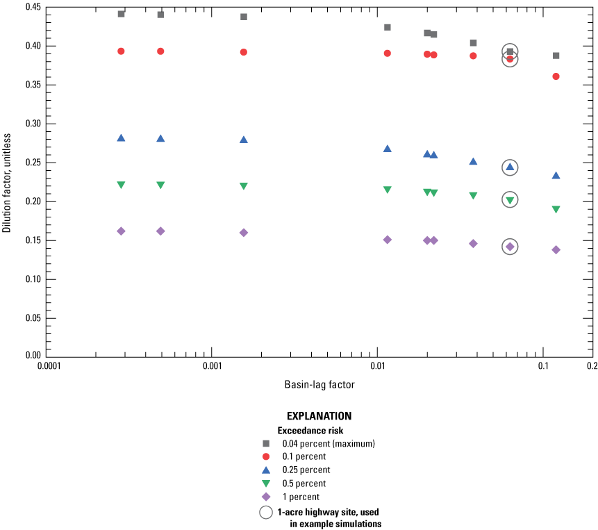
Scatterplot of dilution factors for selected exceedance percentiles as a function of basin-lag-factor values for a 1-acre highway site and 1-square-mile, 0-percent-impervious upstream basin. Results are from 9 simulations including highway drainage lengths ranging from 14 to 4,000 feet and drainage slopes ranging from 10 to 300 feet per mile. The combination of length and slope is expressed as the basin lag factor, which is the length in miles divided by the square root of slope in feet per mile.
The sensitivity of dilution factors to variations in the drainage-area ratio for all 432 simulations is shown in figure 35. Each point represents simulated statistics for the 9 highway area, length, and slope combinations for one of the 48 combinations of highway area, upstream area, and upstream imperviousness. As with other analyses, the average dilution factors generally increase with increasing drainage-area ratios (fig. 35A). Variations in average dilution factors at the same drainage-area ratios are caused by variations in the simulated streamflow statistics and the timing of runoff from highway and upstream basins with different drainage-area and imperviousness values.
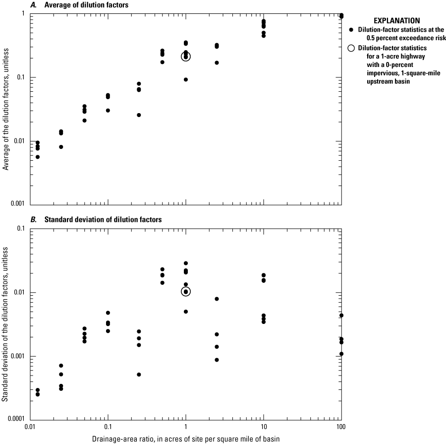
Scatterplots of the dilution-factor statistics at the 0.5 percent exceedance risk for basin-lag factor sensitivity analyses as a function of the drainage-area ratios. A, Average of dilution factors. B, Standard deviation of dilution factors. Statistics are calculated for the 9 basin-lag factor simulations done for each of the 48 combinations of highway-site and upstream-basin areas and upstream-basin imperviousness.
The standard deviation values shown on figure 35B represent the variability of dilution factors over the full range of basin-lag factors in simulations done using the median precipitation and streamflow statistics for southern New England. These standard deviation values are about equal to the precipitation values and about 25 percent of similar prestorm streamflows even though the basin-lag factors had a much larger multiplier (fig. 35) than precipitation (fig. 21) or streamflow (fig. 19). The maximum standard deviation of dilution factors for the 0.5 percent risk exceedance in these simulations, about 0.344, represents a COV of about 0.0834. Among these basin-lag factor sensitivity simulations, the COVs range from 0.00115 to 0.0109 with an average COV of 0.0427. The COVs of dilution factors associated with variations in streamflow statistics are, on average, more than five times the COVs associated with variations in basin-lag factors.
The low variability in dilution factors for widely varying highway-site configurations indicates that dilution factors are not sensitive to the length and slope of sites of interest, and these do not need to be specified exactly. This lack of sensitivity is good because real highway and urban drainage systems can be complex, as-built plans for existing drainage systems may not be readily available, and detailed drainage plans may not have been drafted at the planning stage for new or upgraded facilities. The lack of sensitivity also indicates that example simulations may be, within the uncertainty of all statistics used to simulate highway or urban runoff, representative of a wide range of similar sites. For example, if a roadway follows a stream, then variations in the roadway drainage pathways from outfall to outfall may not be substantial enough to warrant separate simulations.
Highway Runoff-Quality Statistics
SELDM uses highway and urban runoff statistics to simulate concentrations and loads of runoff from the site of interest (Granato, 2013). In this study, runoff quality was simulated as a random variable by using the frequency-factor method with the average, standard deviation, and skew of the logarithms of highway and urban runoff concentrations. In this highway-runoff quality sensitivity analysis, the 15th percentile, median (50th percentile), and 85th percentile geometric mean concentrations of representative highway runoff datasets (table 19) were used to assess the magnitude of potential variability in water-quality statistics from site to site. The 15th and 85th percentile geometric mean values were selected rather than the maximum and minimum because uncertainties in the representativeness of statistics can be large especially when sample sizes are small. These concentrations are identified as the low and high geometric means in table 19, respectively. The same (median) standard deviation was used for the three geometric-mean simulations for each constituent because relations between the average and standard deviation of the logarithms of concentrations were weak and for many constituents, not significantly different from 0 (table 19). Runoff concentrations were simulated lognormally (with a logarithmic skew of 0) because the percentage of datasets with skew values that were not significantly different from 0 at the 95-percent confidence interval was large (table 19). Also, the skew value is commonly more uncertain than the other statistics and using a skew value of zero reduces the risk of generating extreme and potentially unrealistic concentrations in a long-period simulation (Risley and Granato, 2014; Smith and others, 2018).
These highway-runoff constituent-yield sensitivity analyses included 147 simulations done by using the primary master random-seed value (number 8,556). In this series of analyses, a 1-acre 100-percent impervious highway site configuration was used to perform the sensitivity analysis and to provide highway runoff yields for potential use in TMDL analyses (for example, Granato and Jones, 2017b; Granato and Friesz, 2021a). A 10-square-mile, 0-percent impervious upstream basin was used to run the simulations, but downstream water-quality analyses were not included. These analyses were done by using 49 sets of precipitation statistics. The precipitation statistics included values for the Northeastern Highlands, Northeastern Coastal Zone, and Atlantic Coastal Pine Barrens EPA Level III ecoregions and the median of the southern New England area (table 9). Precipitation statistics for 45 individual precipitation stations in and around southern New England also were used in these simulations (table 10). The results of these 147 analyses are documented in the 11000-HwyYields project files (table 27, Granato and others, 2022).
In this series of analyses, the highway runoff constituent concentration statistics were varied to determine the sensitivity of results to a range of geometric-mean highway-runoff concentrations. Statistics for 21 constituents of potential concern (table 18) including turbidity, sediment and solids, nutrients, minor and trace inorganics, organic, biological, and major ionic constituents were used in each of the 147 simulations. The highway runoff concentration statistics are shown in table 19. The ratios of the 85th to 15th percentile geometric-mean concentrations range from 1.24 to 17.7. The medians of these ratios for the suspended sediment, nutrients, metals, organics, and bacteria categories are 17.3, 2.38, 3.27, 5.31, and 3.53, respectively. Figure 36 shows the variations in long-term average runoff yields for total nitrogen, total phosphorus, and suspended sediment. This figure shows the analogous variations in long-term average Escherichia coli concentrations rather than yields because calculating a yield for bacteria is not meaningful. The constituent-yield populations from the master random-seed simulations shown in figure 36A–D, done by using the median concentrations and median precipitation statistics, are included in the figure to show the potential random variability of yield results. The variability in simulated populations for the 15th, 50th, and 85th percentile geometric mean concentrations is the result of using the southern New England and ecoregion precipitation statistics (table 9) and precipitation statistics from the 45 individual precipitation monitoring stations in and near southern New England (table 10). The location (median and average) of each boxplot within each graph shows the differences caused by selection of the geometric mean concentration statistics used in simulations. The random-seed and median boxplots have similar locations in figures 36A–D because the median concentration statistics were used for all the random-seed and median constituent simulations; slight differences occur because of the influence of random variations in the precipitation and runoff coefficient variables on the simulated values. Simulation results indicate that for all these water-quality constituents, differences caused by selecting the geometric mean concentrations are much larger than random variability or differences in simulated precipitation values (fig. 36). The populations of total nitrogen yields simulated by using the 15th and 85th percentile of geometric mean concentrations are approximately evenly spaced above and below the population simulated by using the median of geometric-mean concentrations. For total phosphorus and suspended sediment, the populations simulated by using 15th and 50th (median) percentile of geometric means are more closely aligned than the population simulated by using the 85th percentile of geometric mean values, which is much larger than the 15th and 50th geometric-mean concentrations yields. For Escherichia coli, however, the populations simulated by using 50th and 85th percentiles of geometric means are more closely aligned than the population simulated by using the 15th percentile of geometric mean concentrations, which is much smaller than the other geometric mean concentrations.
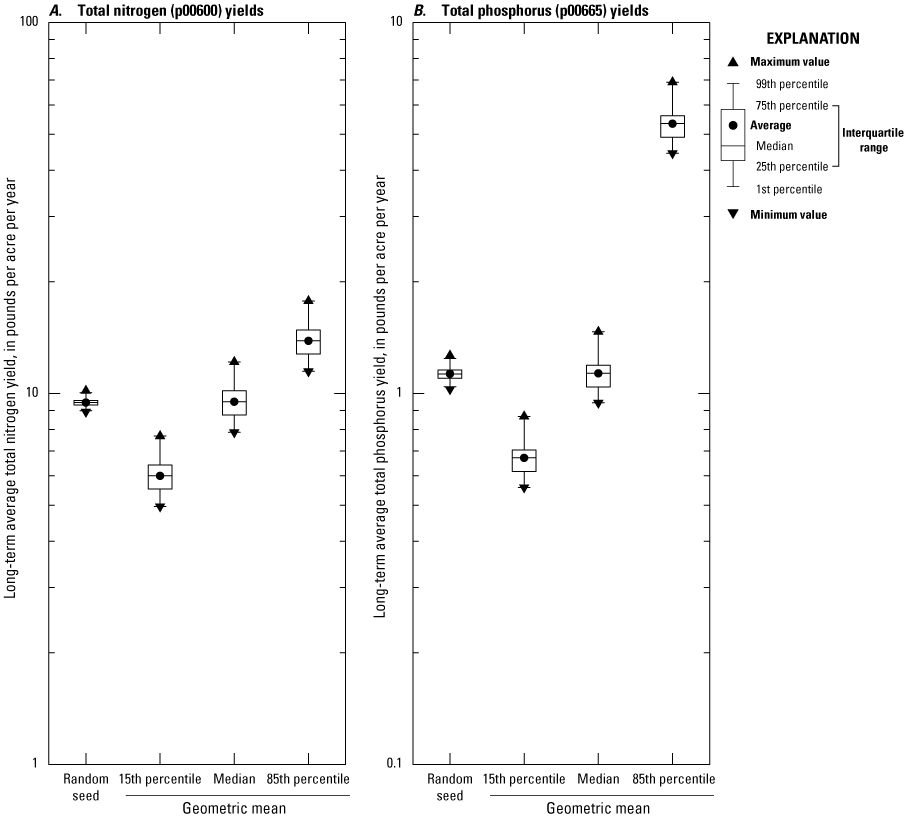
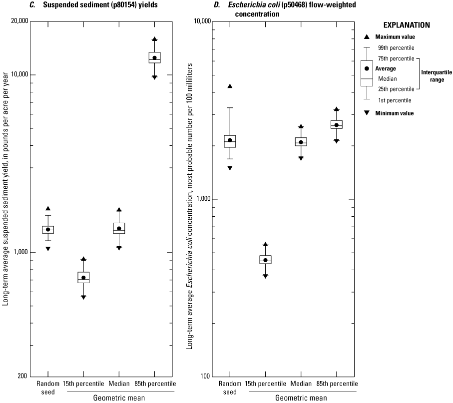
Boxplots showing simulated populations of long-term average annual constituent yields of A, total nitrogen yields (p00600); B, total phosphorus yields (p00665); C, suspended sediment (p80154); and D, long-term average annual flow-weighted concentrations of Escherichia coli (p50468). These values were simulated by using the 15th, 50th, and 85th percentile geometric mean concentrations and precipitation statistics for southern New England and ecoregions and individual precipitation monitoring stations in and around southern New England. Constituents are defined in table 18.
Results of this analysis indicate that selecting representative highway-runoff statistics has a greater influence on simulated runoff-quality results than random variability from master seed to master seed, and the selected precipitation statistics (fig. 36). It is important to note that the available highway-runoff monitoring sites used in these simulations have higher AADT values than other sites including bridges over water and the State maintained bridges over water in southern New England (fig. 5); the available data may be biased high if AADT is a reliable predictor for a given constituent (table 20). The National Cooperative Highway Research Program report on approaches for determining and complying with TMDL requirements indicates that collection and characterization of monitoring data from TMDL areas in each State is the most effective way to determine the most accurate pollutant loads from roadways (Lantin and others, 2019). Therefore, these results indicate that more data are needed to better characterize highway and urban runoff statistics in southern New England. The at-site geometric mean statistics were selected for this sensitivity analysis based on available data, including 4 to 19 highway sites (table 18); in comparison, table 3 indicates that there are about 48,466 stream basins above road crossings and 5,545 stream basins above arterial-road crossings in southern New England. If available sites are representative of a single population, statistical theory indicates that at least 7 sites would be needed for the available data to capture the true median within the range of the available dataset, and about 35 sites would be needed to capture the true 15th and 85th percentile geometric means within the range of the available dataset if a 95-percent confidence interval is used for selection (Ialongo, 2019; Granato and others, 2021). Although the data were focused on sites in southern New England, data from other States (and, for Fecal streptococci urban runoff data) were used for constituents without sufficient data in southern New England (table 19); this adds more uncertainty in the runoff-quality statistics used for southern New England. Sampling more events at each site would better refine statistics for available monitoring sites. Sampling more sites would better define the characteristics of highway (and urban) runoff in southern New England (table 19) and would help to better define relations between potential explanatory variables and runoff-quality statistics in the region (table 20). Although there are large differences in statistics from monitoring site to monitoring site, selecting a particular set of statistics may be difficult, especially for TMDL analyses for stream basins with many different roadway contributing areas (Granato and Jones, 2017b, 2019; Lantin and others, 2019; Granato and Friesz, 2021a). Even if the relations to AADT in table 20 are used to calculate a geometric mean for a site of interest, the uncertainty of the estimate would still be large. For example, at 40,000 vehicles per day, the retransformed geometric mean concentration of total phosphorus in runoff would be 0.113 mg/L in arithmetic space, but the 95-percent confidence interval would extend from 0.0474 to 0.269 mg/L; in comparison, the retransformed low and high geometric mean values from table 19 would be 0.0673 mg/L and 0.536 mg/L. Because of the uncertainties in statistics from available data, the median estimate may be the most robust selection for any given unmonitored site unless a detailed analysis is done for each contributing area.
This sensitivity analysis focused on highway runoff quality, but similar issues affect urban runoff quality estimates. The results of 294 urban-runoff quality analyses are documented in the 12000-UrbanYields project files (table 27, Granato and others, 2022); these analyses include simulations done using precipitation statistics for the southern New England area, the three ecoregions (table 9), and from the 45 individual precipitation monitoring stations (table 10). Runoff was simulated by using the highway and nonhighway runoff-coefficient statistics for sites of interest with impervious percentages of 25, 50, and 100 percent. A detailed urban-runoff concentration sensitivity analyses was not done because of limitations in available data. There were many more urban sites used to calculate the urban-runoff statistics (table 18), but for many constituents, there were no urban runoff sites in southern New England (Granato, 2021a).
Because of the large differences in simulated statistics over the range of available data for southern New England and the differences in results for different constituents, an operational definition would be needed to develop a simple decision-support system for assessing potential effects of runoff in southern New England. In North Carolina, the Department of Transportation worked with the State Department of Environmental Quality and the USGS to develop an operational definition to assess risk by using suspended-sediment concentrations as a sentinel water-quality indicator (Weaver and others, 2019, 2021). Median highway-runoff statistics from 15 sites within North Carolina were selected for use in SELDM to develop the decision rule for the North Carolina Department of Transportation decision-support system.
Upstream Stormflow-Quality Statistics
SELDM uses instream water-quality statistics to simulate concentrations and loads of stormwater in the receiving stream upstream from the site of interest (Granato, 2013). SELDM can simulate upstream water quality as a random variable, a dependent variable, or as a flow-dependent variable. Random variables are simulated by using the frequency-factor method, dependent variables are simulated by using a regression relation to another water-quality variable with random variation, and flow-dependent variables are simulated by using water-quality transport curves with random variation. In this study, upstream stormflow quality was simulated by using transport curves (table 23) and dependent relations (tables 24, 25).
In this upstream stormflow-quality sensitivity analysis, the median total phosphorus (p00665) transport curve (table 23) and 38 individual total phosphorus transport curves from minimally developed sites (Granato and others, 2022) were used. The median transport curve was used with 500 different random-seed values to assess the magnitude of stochastic variation from simulation to simulation. The results of the 500 random-seed analyses are documented in the 01000-Seed project files (table 27, Granato and others, 2022). The individual transport curves simulated by using the primary master random-seed number (8,556) were used to assess the potential magnitude of variation in the selection of representative upstream stormflow-quality statistics. The results of the 38 individual transport curves for minimally developed basins (table 22) discussed in this section are documented in the 14000-USQW project files (table 27, Granato and others, 2022). The simulations from both sets of analyses were done by using the 1-acre highway site and the 1-square-mile upstream basin to isolate how selection of a random seed and the transport curve equation can affect downstream constituent concentrations.
In this series of analyses, comparison of the stochastic variations with the median transport curve and variations caused by use of different transport curves indicates that water-quality selection uncertainty is much higher than stochastic variability from simulation to simulation. Figure 37 shows the population of simulated upstream total phosphorus concentrations for the 500 random seed and the 38 individual transport curve simulations at different concentration-exceedance risks. The ratios of the maximum to minimum of simulated concentrations range from 1.23 to 2.35 for the random-seed analyses and from 63.2 to 279 for the individual transport curve analyses. Similarly, the interquartile ranges, which correspond to the box height in figure 37, range from 1.05 to 1.19 for the random-seed analyses and from 5.86 to 9.21 for the individual transport curve analyses. Two example water-quality criterion concentrations, 0.025 and 0.1 mg/L are shown on the graph to indicate how the selection of a transport curve and the selection of a target exceedance-risk could affect upstream water-quality assessment. All the random-seed median transport-curve simulations shown in figure 37 exceed the 0.025 mg/L water-quality criterion value. However, if a water-quality criterion of 0.1 mg/L is selected, only 1 percent of the random-seed simulations at the 0.1 exceedance risk percentile and only about 15 percent of the random-seed simulations at the 0.04 exceedance risk percentile produced a total phosphorus (p00665) concentration larger than this criterion concentration (fig. 37). Among the individual transport curve simulations, all exceed the 0.025 mg/L criterion concentrations at the 0.4 and 0.1 exceedance risk percentiles, 97.2 percent of simulations exceed this criterion at the 0.25 and 0.5 percent exceedance risk percentiles, and 92 percent of simulations exceed this criterion concentration at the 1.0 exceedance risk percentile (fig. 37). If a water-quality criterion of 0.1 mg/L is selected, then about 70, 50, 50, 47, and 44 percent of simulations exceed this criterion concentration at the 0.04, 0.1, 0.25, 0.5, and 1.0 exceedance risk percentiles, respectively (fig. 37). Therefore, results of this sensitivity analysis indicate that selecting representative upstream stormflow-quality statistics has a greater influence on simulated runoff-quality results and the potential for water-quality excursions than random variability from master seed to master seed. The results of these simulations also indicate that there are wide variations in water-quality statistics from site to site and that decisions about the risk for excursions and therefore decisions about the need for treatment are sensitive to the selection of representative water-quality statistics. These findings are consistent with the results of the sensitivity-analysis done by using the highway runoff-quality statistics in the section “Highway Runoff-Quality Statistics.”
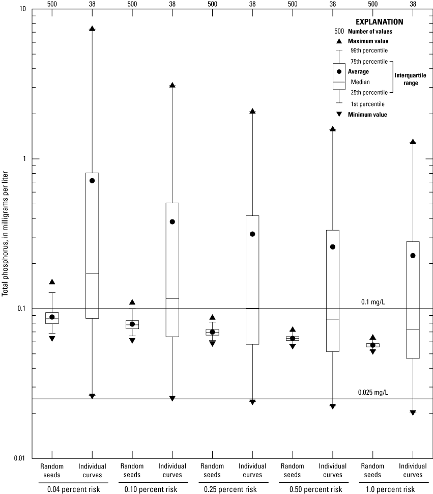
Boxplots showing populations of simulated event mean total phosphorus (p00665) concentrations in receiving-stream stormflow upstream from a site of interest generated by using a median transport curve and 500 different master random seeds or 38 individual transport curves with the selected master random-seed number 8,556. Simulations are for a 1 square-mile completely pervious upstream basin. The horizontal lines are two example water-quality criteria (0.025 and 0.1 milligram per liter [mg/L]) for total phosphorus that are shown for discussion. Constituents are defined in table 18.
The method used to develop representative regional transport curves may have unanticipated effects on the simulation results. For example, the high-concentration estimates of total phosphorus from the transport curve developed by using the medians of transport-curve coefficients for minimally developed basins, which are shown as the random-seed simulation results, are in the lower quartile of estimates for individual transport curves (fig. 37). An alternate method to develop a median transport curve is to pool data regionally and generate a transport curve by using all available data as was done by Granato and others (2009) for each ecoregion. In that approach, however, systematic differences between datasets result in much greater variation in the regression residuals and therefore the simulation results for a given value of stormflow than would be calculated for transport curves developed by using individual stations. For example, the MAD values for the transport curves for the Northeastern Highlands, Northeastern Coastal Zone, and Atlantic Coastal Pine Barrens ecoregions (Granato and others, 2009) are about three times the MAD values for the individual-station transport curves for minimally developed basins developed by Granato and others (2022). The ecoregion transport curves incorporated into SELDM (Granato, 2013) provide information for initial planning-level estimates, but as indicated by figure 37, regional equations come with substantial uncertainty for any given location.
An alternate to regional transport curves or using the median of transport curve coefficients would be to pool data from a selected subset of hydrologically similar stream basins with similar levels of development and develop a representative transport curve from the pooled data. This approach would be suitable for assessing conditions at a particular site of interest without a water-quality dataset. This approach could demand considerable effort, however, because a detailed analysis of different combinations would need to be done and the highly interpretive nature of such an effort may be subject to challenge.
The difference between use of the median transport curve or an individual-station transport curve for a given constituent has two conflicting effects for developing a simple decision method for estimating the potential risks of runoff on receiving waters and the potential for reducing such risks. If the median transport curve underestimates the population of concentrations, then a decision method based on the number of simulated water-quality excursions may lead to underestimation of the risk for upstream and downstream water-quality excursions. This may result in BMP decisions that do not adequately reduce water-quality excursion risks at some sites. Alternately, if the decision method is based on the change in concentrations from upstream to downstream and the highway or urban runoff concentrations are higher than the upstream concentrations, then the decision method based on the median transport curve may lead to an overestimation of the risk for adverse effects of runoff on receiving-water quality. Overestimating risks may result in application of advanced BMPs where they are not needed to protect downstream water quality. The results of the study by Taylor and others (2014) indicate that the lifecycle cost of designing, building, and maintaining BMPs at thousands to tens of thousands of road-stream crossings in southern New England (table 2, table 3, Federal Highway Administration, 2020; Spaetzel and others, 2020) may not be sustainable with limited stormwater-mitigation funds available to DOTs and MS4s. Therefore, an operational definition for selecting representative transport curves for estimating upstream concentrations would be needed to develop a decision-support system to help optimize runoff-treatment decisions. This is especially true given the large variability in results simulated by using the individual transport curves for minimally developed basins (fig. 37). If results for transport curves for developed and wastewater-affected basins also were included in this analysis, then the variability in results would be even larger. In North Carolina, the DOT worked with the USGS and the State Department of Environmental Quality to develop an operational definition to standardize the water-quality risk analysis by using an individual transport curve that produced concentrations deemed representative of a typical road-stream crossing in the State (Weaver and others, 2019, 2021). The simple decision support system developed in North Carolina does not preclude additional analyses at sites where more detailed information is needed.
BMP Treatment Statistics
SELDM uses statistics for volume reduction, hydrograph extension, and water-quality treatment to simulate the effects of structural stormwater runoff BMPs on flows, concentrations, and loads of runoff from the site of interest and their effects on flows, concentrations, and loads in stormwater downstream from the discharge outfall (Granato, 2013, 2014; Granato and others, 2021). SELDM uses the trapezoidal distribution to simulate these processes stochastically. It also simulates the minimum irreducible concentration by substitution deterministically, but this variable does not affect the high concentrations in BMP discharge that are most likely to adversely affect water quality (Granato and others, 2021). In this sensitivity analysis, BMP treatment statistics for 11 BMP categories and the median-treatment BMP for a total of 12 BMPs were simulated to assess the sensitivity of results to the choice of BMP (table 29). The median-treatment BMP is defined by Granato and others (2021) as the median of treatment statistics for different BMP categories with sufficient data to calculate performance statistics. The median BMP ratios in table 29 are simulated from these statistics; they are not the medians of the simulated long-term ratios for different BMP categories in this table.
Table 29.
Long-term average best management practice performance for runoff stormflows and constituent loads calculated by using individual storm statistics for 29 annual-load accounting years for southern New England.[The long-term average ratios in this table should not be confused with percent removals; they are the long-term average of individual storm events, each of which may depart substantially from the long-term values (Granato, 2014; Granato and others, 2021). The categories for structural best management practices (BMPs) are defined in the International BMP Database (Granato, 2014, Leisenring and others, 2020, Granato and others, 2021). The median BMP is defined by Granato and others (2021) as the median of treatment statistics for different BMP categories with sufficient data to calculate performance statistics; this is not the median of long-term ratios for different BMP categories in this table. Porous pavement statistics are for pavement systems designed for parking areas or low-speed travel ways designed for infiltration; this category does not include data from permeable friction course sites commonly used for highways, which have a porous asphalt pavement placed on top of a regular impermeable roadway. The performance rank is the average rank of the ranks of stormflow and water-quality performance ratios; 1 is the best and 12 is the worst performance. The adjusted cost rank is the rank of the sum of the costs per unit constituent load reduction by category in table S.2 of the National Cooperative Highway Research Program report on the long-term performance and life-cycle costs of stormwater best management practices (Taylor and others, 2014); 1 is the lowest cost and 12 is the highest cost per unit constituent load reduction; tied ranks apply to categories that were combined by Taylor and others (2014). Water-quality constituents are fully defined in table 18. SS, suspended sediment (p80154); TN, total nitrogen, water, unfiltered (p00600); TP, phosphorus, water, unfiltered (p00665); TCu, copper, water, unfiltered (p01042); TPb, lead, water, unfiltered (p01051); TZn, zinc, water, unfiltered (p01092); PAH, sum of 16 polycyclic aromatic hydrocarbons (PAHs) not censored; Bio, biological constituents (bacteria); —, not available]
Individual treatment statistics were not varied independently and systematically in these analyses because the three treatment variables, volume reduction, hydrograph extension, and water-quality treatment, have interdependent effects on the outflow loads. There are large variations in treatment statistics within and between BMP categories when individual monitoring sites are considered, so performance results for different BMP categories commonly overlap each other. Leisenring and others (2013) analyzed the effects of structural BMP design parameters on achievable reductions in effluent concentrations by using data from 530 monitoring sites in the International BMP Database and found that BMP design variables had weak correlation to performance. Therefore, results of these analyses are described in categorical terms, but the performance of an individual BMP constructed at a site of interest may cross categorical boundaries.
This BMP performance sensitivity analysis included 576 individual simulations done by using the primary master random-seed value (8,556). Each of the 12 BMPs were simulated by using 48 combinations of highway site and upstream-basin configurations. Three 100-percent impervious highway-site configurations with 0.25, 1.0, and 10 acres were used for these simulations. The representative lengths (table 6) were 300, 1,056, and 1,056 feet, respectively, and the representative slopes were all 10 feet of elevation change per mile (table 7). The 16 simulated upstream basins had drainage areas of 0.1, 1, 10, and 20 square miles with proportional lengths and slopes (table 5) and impervious values equal to 0, 5, 10, and 20 percent. The results of these analyses are documented in the 13000-BMPs project files (table 27, Granato and others, 2022).
Results of this BMP sensitivity analysis, shown in table 29, indicate the BMP performance as the ratio of outflow to inflow values and relative performance as ranks. Among the BMP categories in this table, the maximum stormflow ratio is about 5.75 times the minimum ratio. The long-term average stormflow ratio for manufactured devices is equal to 1 because these BMPs commonly are closed systems that are not designed for flow reductions (Granato and others, 2021). The wetland BMPs have long-term average stormflow ratios greater than 1 because wetlands commonly are groundwater discharge sites. Water-quality load ratios are the result of the combination of flow and concentration reduction ratios. The maximum constituent load ratio, on average across the constituents, is 7.93 times the minimum. The wetland BMPs may have nutrient ratios larger than 1 because of groundwater discharges to and biological processes in the wetland systems. Manufactured devices have bacteria ratios (table 29, “Bio” column) greater than 1 because the nutrients and carbon they hold between events and the sheltered conditions they have may make them incubators for bacteria (Granato and others, 2021).
The ratios in table 29 may be converted to percent removals by subtracting the ratio from 1 and multiplying by 100, but the average ratio was not and should not be applied to individual events or a short series of events (Granato, 2013, 2014; Granato and others, 2021). The long-term values in table 29 are not used for every storm event because individual event values vary substantially from the long-term average, and outflows can exceed inflows for some events (Granato, 2013, 2014; Granato and others, 2021). Also, in SELDM, the structure of BMP monitoring data is preserved by simulated rank correlation to inflow values (Granato, 2013, 2014; Granato and others, 2021). Overall, as indicated by monitoring data from many studies, grass strips and bioretention have the best performance (lowest ranks), and manufactured devices and wetland channels have the worst performance (highest rank). Estimates of the long-term life-cycle costs of stormwater best management practices by Taylor and others (2014) were used with the SELDM simulation results to assess the adjusted cost rank of different BMP categories. The results shown in table 29 indicate that grass strips and dry basins are the most economically efficient BMPs (lowest rank), and wet basins are the least (highest rank) economically efficient BMPs.
The sensitivity of dilution factors to variations in BMP statistics for all 576 simulations is shown in figure 38. BMPs affect the downstream dilution factors by flow reduction and hydrograph extension. A net flow reduction lowers the proportion of runoff in concurrent downstream flow, which reduces the dilution factor. Hydrograph extension increases the duration of discharge and therefore the volume of upstream flow, which reduces the dilution factor. Each point in figure 38 represents statistics for the 12 BMP simulations (table 29) for each of the 48 combinations of highway area, upstream area, and upstream imperviousness. As with the other sensitivity analyses, the average dilution factors generally increase with increasing drainage-area ratios (fig. 38A). The smallest average dilution factors result from a 0.25-acre highway site draining to a 20-square-mile upstream basin (a drainage-area ratio of 0.0125). The largest average dilution factors result from a 10-acre highway site draining to a 0.1-square-mile basin (a drainage-area ratio of 100). Variations in average dilution factors at the same drainage-area ratios are caused by differences in the basin lagtime, which are caused by variations in the combinations of the length, slope, imperviousness, and area of the highway site and upstream basin. The largest variations occur for individual drainage-area ratios that result from different combinations of highway and upstream area.
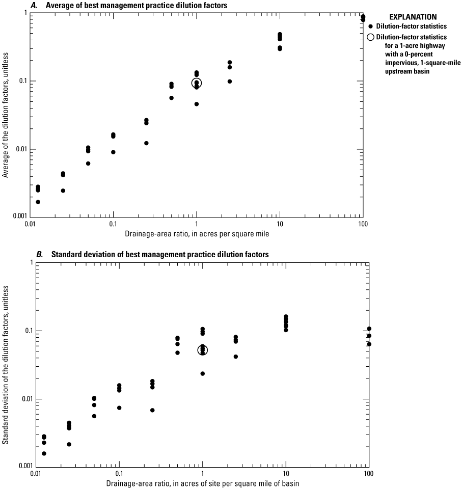
Scatterplots of the dilution-factor statistics at the 0.5 percent exceedance risk for best management practice (BMP) sensitivity analyses. A, Average of BMP dilution factors. B, Standard deviation of BMP dilution factors. The averages and standard deviations are shown as a function of drainage-area ratios in acres per square mile. Statistics are calculated for the 11 BMP categories and median BMP simulations done for each of the 48 combinations of highway-site and upstream-basin areas and upstream-basin imperviousness.
The standard deviation values shown on figure 38B represent the variability of dilution factors among the 11 BMP categories and the median BMP in simulations. These simulations were done using the median precipitation and streamflow statistics for southern New England. This graph indicates that the variations in BMP statistics have substantial effects on dilution factors because the standard deviations are substantial in comparison to the average values shown in figure 38A. At low drainage-area ratios, the variability is smaller than the variability of the midrange drainage-area ratios (about 1–10 acres per square mile) in part because the highway sites of the low ratios are so small in relation to the upstream basin. The variability of the maximum simulated drainage-area ratio also has a lower variability than for the midrange drainage-area ratios because at the maximum ratio the BMP discharge is such a large portion of downstream flows at the 0.5 percent exceedance risk (fig. 38A). The maximum standard deviation of dilution factors for the 0.5 percent risk percentile in these simulations of about 0.162 represents a COV of about 0.37. Among these BMP sensitivity simulations, the COVs range from 0.072 to 1.08 with an average COV of 0.641. Variations caused by BMP selections are, on average, about 10 times the variations caused by selection of precipitation statistics, about 3 times the variations caused by selection of streamflow statistics, and 3 to 31 times the variations caused by selection of other hydrologic variables. The average dilution factors used in the BMP analysis are smaller than the associated highway-runoff dilution factors, which tends to inflate the COV, but the variability caused by BMP selection is larger than variability caused by selection of other variables.
Although the large variability in results indicates that BMP selection is an important factor in simulated results, this BMP sensitivity analysis and the comparison to BMP cost data are generalized. Selection of a BMP for a particular site depends on many factors and constraints, some of which may be particular to a linear transportation system with limited rights of way (Massachusetts Highway Department, 2004, 2006; Rhode Island Department of Transportation, 2008; McGowen and others, 2009; Leisenring and others, 2013; Taylor and others, 2014; Lantin and others, 2019; Connecticut Department of Transportation, 2020). Because correlations between BMP performance within categories are dependent on inflow quality rather than design variables, more data are needed regionally and nationally to better quantify performance (Leisenring and others, 2013; Taylor and others, 2014). Complex deterministic simulation models commonly are used as an alternative to stochastic modeling, but the assumptions of such models break down under examination. For example, Stoke’s Law used to calculate particle settling velocities used by many such models does not accurately predict settling velocities of sediment size ranges typical of highway urban runoff and grain size distributions (Gibbs and others, 1971; Granato, 2013). Real grain size distributions, sediment density, and water temperature vary by orders of magnitude, which result in settling velocities that vary by orders of magnitude from site to site and event to event (Granato, 2013). Other constituents including nutrients and trace elements can undergo settling with sediment, chemical changes, and biological uptake and release. Therefore, these constituents are much more difficult to simulate deterministically without long-term, site-specific data for calibration. Such data are not commonly available in southern New England or across the country (Leisenring and others, 2013; Taylor and others, 2014; Wright Water Engineers, Inc. and Geosyntec Consultants, 2019). Stochastic simulation based on actual data may allow for more uncertainty in data and results than the generalization of process-based model results at unmonitored sites.
For the purpose of TMDL analyses, a median (generic) BMP may be used to represent the effects of many different BMPs in a stream basin of concern (Granato and Jones, 2017b; Lantin and others, 2019; Granato and Friesz, 2021a). Although a generic BMP may not be the optimal choice for any particular outfall, the median performance will account for variations in performance of various BMPs across a watershed. Even in basins with only one outfall, all the uncertainties and large at-site variations in flows, concentrations, loads, and BMP performance at unmonitored sites reduce the efficacy of detailed selection of a BMP with SELDM. These problems confound quantitative application of complex deterministic models for determining the effects of BMP treatment on receiving-water quality. Weaver and others (2021) used statistics for a generic low-performance BMP and a generic high-performance BMP to provide a decision tool to identify highway crossings where BMP modification would not substantially improve downstream water quality or where a basic (low performance) or advanced (high performance) BMP was needed. Such an approach may be useful for decision making in southern New England.
Example Runoff-Quality Simulations
SELDM was designed to transform complex scientific data into meaningful information about the risk of adverse effects of runoff on receiving waters, the potential need for mitigation measures, and the potential effectiveness of such management measures for reducing these risks (Granato, 2013). Estimates of the frequency and magnitude of potential adverse effects on receiving-water quality are used in planning efforts to assess potential needs for various mitigation strategies, such as the implementation of structural onsite BMPs as part of a design solution where water-quality problems have been identified. The following example simulations were done to help stormwater practitioners and decisionmakers assess the efficacy of onsite treatment as compared to alternative management strategies. These simulations were done by using the primary master random-seed value (8,556) with the representative 1-acre highway site and the 1-square-mile, 0-percent-impervious upstream basin. Median hydrologic statistics representing southern New England (tables 9, 11) were used. The highway water-quality (table 19) and BMP treatment also were simulated by using median statistics. In these simulations, individual transport curves for the 38 minimally developed basins and 24 developed basins without upstream wastewater treatment plants listed in table 22 were used. Although the water-quality transport curves used in this analysis come from basins with different locations and varying land-cover characteristics, all other hydrologic variables were held constant in these simulations so that all differences in outcomes could be ascribed to differences in the transport curves used. The total phosphorus transport curves and results of the 62 simulations discussed in this section are documented in the 14000-USQW project files (table 27, Granato and others, 2022). Total phosphorus (p00665) was the constituent simulated in these examples because this nutrient is a constituent of concern, numeric water-quality criteria exist for this constituent for streams entering lakes or reservoirs, and this constituent is the most widely measured constituent of interest in southern New England (table 18).
In this series of analyses, the potential efficacy of onsite BMPs will be discussed in terms of the reductions in downstream concentrations and the reductions in risks for water-quality exceedances that may take place if onsite BMPs are used. Figure 39 is an example probability plot of simulated highway runoff, BMP discharge, and instream total phosphorus concentrations. The instream concentrations include upstream concentrations simulated by using transport curves derived from data from two USGS water-quality monitoring stations and the downstream concentrations that were simulated with runoff from a highway site with and without BMP treatment. The median BMP used in these simulations includes volume reduction, hydrograph extension, and water-quality treatment (Granato and others, 2021). Simulations using water-quality transport curves from monitoring stations 01073562 and 01098360 were selected for illustration in figure 39 because the simulated upstream 0.5-percent risk concentrations at these stations (0.031 and 0.362 mg/L, respectively) differ from each other by about an order of magnitude, and the forest cover percentages (69.7 and 10.2 percent, respectively) also differ substantially. As this graph indicates, the upstream water-quality has a substantial effect on the downstream water quality and the ability of onsite BMP treatment to modify downstream concentrations. When the upstream concentrations are high, such as in the 01098360 scenario, the BMP does not have a substantial effect on downstream water quality. However, when the upstream concentrations are low, such as in the 01073562 scenario, the same BMP treatment may have a substantial effect on downstream water quality.
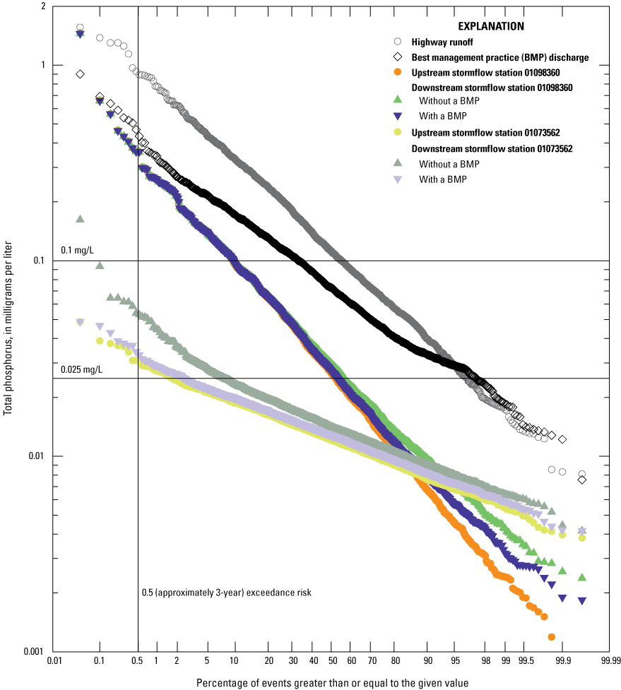
Scatterplot of populations of simulated event mean concentrations of total phosphorus for highway runoff, stormwater best management practice discharges, and receiving-stream stormflow upstream and downstream from a discharge point. Upstream stormflow concentrations were simulated by using water-quality transport curves developed by using data from U.S. Geological Survey (USGS) water-quality monitoring stations 01098360 and 01073562. Simulations are for a 1-acre highway site draining to a 1-square-mile basin. The horizontal lines are two example water-quality criteria (0.025 and 0.1 milligram per liter [mg/L]) for total phosphorus. The approximate one-event-in-3-year risk level (0.5 percent exceedance risk), which is considered protective for aquatic life (Niemi and others, 1990; U.S. Environmental Protection Agency, 1991, 1998), is shown as a vertical line on the graph. Constituents are defined in table 18.
As discussed in the section of this report on “Risk-Based Analyses,” numeric water-quality criteria commonly are based on a specified concentration, frequency of occurrence, and exposure duration (Niemi and others, 1990; U.S. Environmental Protection Agency, 1991, 1998). Figure 39 shows two commonly used receiving water criteria-concentrations for total phosphorus, which are equal to 0.025 and 0.1 mg/L, as horizontal lines on the graph (Jeznach, and Granato, 2020). The approximate one-event-in-3-year risk level (0.5 percent exceedance risk), which is considered protective for aquatic life (Niemi and others, 1990; U.S. Environmental Protection Agency, 1991, 1998), is shown as a vertical line on the graph. All the points above the lines exceed the concentration threshold, but only the points to the right of the 0.5 percent exceedance risk are water-quality excursions at this risk level.
The two examples in figure 39 are illustrative of the general results of the 62 stormwater-quality simulations (Granato and others, 2022). The total phosphorus EMC in the minimally developed basin (01073562) upstream from the highway discharge point would exceed the 0.025 mg/L criterion concentration in about 1.72 percent of runoff events but would not exceed the 0.1 mg/L criterion concentration within the simulated events. However, the total phosphorus EMC in the developed basin (01098360) upstream from the highway discharge point would exceed the 0.025 and 0.1 mg/L criterion concentrations in about 52.41 and 9.44 percent of runoff events, respectively. Therefore, neither basin would meet the 0.025 mg/L criterion concentration at the 0.5 percent risk level during runoff events. The results in figure 39 indicate that highway runoff and BMP treatment contributions have a much greater effect on downstream concentrations if upstream concentrations are low. These results are similar to urban runoff results described by Jeznach and Granato (2020) using completely different input statistics that are, however, also representative of the hydrology of southern New England.
Figure 40 shows the ratio of downstream flow concentrations that result from untreated highway runoff and treated BMP discharges as a function of the upstream concentration at the 0.5 percent risk level for the 62 water-quality monitoring stations. Figure 39 shows the complete populations of concentrations simulated by using water-quality transport curves for two monitoring stations; a similar graph containing simulated results for all 62 water-quality monitoring stations would contain a point cloud that would be difficult to interpret meaningfully. Alternatively, a large series of individual graphs for the 62 monitoring stations would be difficult to compare. Therefore, figure 40 is presented as a slice of the EMC populations that would appear along the vertical 0.5 percent risk exceedance line in figure 39. The paired concentrations and ratios of water-quality monitoring stations 01073562 and 01098360 in figure 40 are emphasized to help demonstrate how the values in figure 40 are extracted from populations of simulation results such as those shown in figure 39. Ratios greater than 1.00 indicate that the downstream concentration without BMP treatment is greater than the downstream concentration with BMP treatment for a given upstream concentration. Ratios that approximate 1.0 indicate that differences in downstream concentrations with and without BMP treatment are approximately equal within three significant digits. Figure 40 shows that as upstream concentrations increase, the efficacy of BMP treatment on downstream water quality decreases, even though the simulated volume and concentration of total phosphorus in the highway runoff and BMP discharge are the same in all these simulations. At the 0.5 percent exceedance risk level, all the ratios are less than 1.25 if the upstream total phosphorus concentrations are greater than 0.045 milligram per liter; all the ratios are less than 1.1 if upstream concentrations are greater than 0.076 milligram per liter; and all the ratios are less than 1.05 if upstream concentrations are greater than 0.114 milligram per liter. Therefore, given an exceedance risk of 0.5 percent and these three concentration-ratio thresholds, use of BMPs to treat runoff has a diminishing effect on downstream stormflow quality as upstream total phosphorus concentrations increase.
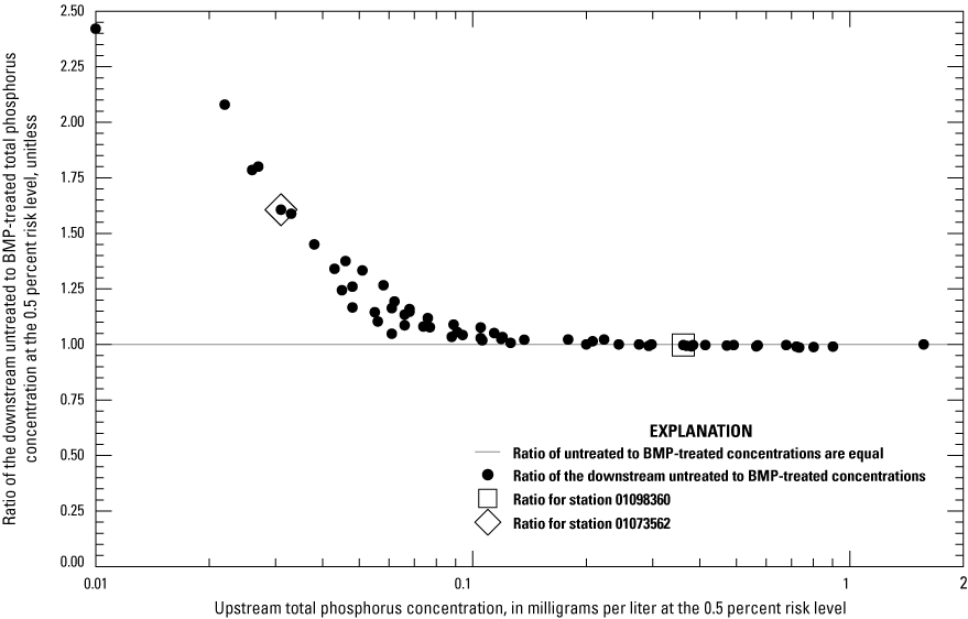
Scatterplot showing the ratio of downstream total phosphorus (p00665) concentration without best management practice (BMP) treatment to the downstream total phosphorus concentration with treatment as a function of the upstream total phosphorus concentration at the 0.5 percent risk level. Upstream concentrations were simulated by using water-quality transport curves for total phosphorus developed by using data from 62 water-quality monitoring stations. Simulations are for a 1-acre highway site draining to a 0-percent impervious, 1-square-mile stream basin. Constituents are defined in table 18.
The risk for exceeding the 0.025 milligram per liter and 0.1 milligram per liter total phosphorus concentration criteria in the receiving stream downstream from the runoff discharge point with and without BMP treatment are shown as a function of the risk for exceeding the criterion concentrations upstream from the discharge point in figure 41. In this figure, the 0.5 percent exceedance risk levels are shown on the horizontal and vertical axes, both of which are graphed on a probability scale. In figure 41, simulated risk levels that meet each criterion concentration upstream from the highway discharge point appear to the left of the vertical line and simulated risk levels that meet each criterion concentration downstream from the highway discharge point appear below the horizontal line. The simulation results for stations 01073562 and 01098360 with and without BMP treatment are shown to facilitate comparison of this upstream risk to downstream risk graph (fig. 41) to the runoff concentration probability plot (fig. 39). At the 0.5 percent risk level, the upstream and downstream concentrations for station 01073562 are all above the 0.025 mg/L criterion concentration and below the 0.1 mg/L criterion concentration (fig. 39). Therefore, the symbols for station 01073562 are above and to the right of the 0.5 percent risk lines in figure 41A and below and to the left of the 0.5 percent risk lines in figure 41B. The risk of exceedance for the downstream water quality with or without BMP treatment is greater than the upstream water-quality risk for station 01073562 (fig. 39) so the symbols for these results in figure 41 are above the diagonal 1:1 ratio line. The upstream and downstream concentrations for station 01098360 are well above the 0.025 mg/L and 0.1 mg/L criterion concentrations at the 0.5 percent risk level (fig. 39). Therefore, the symbols for station 01098360 are all above and to the right of the 0.5 percent risk lines in figure 41. The risk of exceedance for the downstream water quality with or without BMP treatment is about equal to the upstream water quality for station 01098360 (fig. 39) so the symbols for these results in figure 41 plot close to each other and the diagonal 1:1 ratio line.
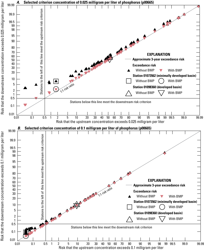
Scatterplots showing the simulated risk for exceeding the selected total phosphorus criterion concentrations upstream and downstream from a discharge point. A, Selected criterion concentration of 0.025 milligram per liter of total phosphorus (p00665); and B, Selected criterion concentration of 0.1 milligram per liter of total phosphorus (p00665). Upstream concentrations were simulated by using water-quality transport curves developed by using data from 62 water-quality monitoring stations. Simulations are for a one-acre highway site draining to a 1-square-mile basin with and without treatment by the median structural best management practice (BMP). Paired scenarios with and without BMP treatment have the same upstream exceedance risk. The horizontal and vertical lines show an approximate 3-year exceedance risk, which is equal to about 0.5 percent. Constituents are defined in table 18.
Comparison of simulation results done by using transport curves for all 62 water-quality monitoring stations indicates that only 3 streams do not exceed the 0.025 mg/L criterion concentration, and 31 do not exceed the 0.1 mg/L criterion concentration at the 0.5 percent risk level during storm events upstream from the simulated stormwater outfall of concern (fig. 41). None of the upstream risks that were above each 0.5-percent risk criterion in these examples are associated with downstream risk values below the 0.5-percent risk criterion for the specified concentration, indicating that, for this constituent (total phosphorus) in these simulations, BMP treatment of runoff discharging to the stream will not convert instream concentrations from upstream exceedances to downstream non-exceedances. For the three basins plotted in the lower left quadrant of figure 41A, where the upstream stormflow quality meets the criterion concentration of 0.025 mg/L, downstream concentrations exceed the 0.5 percent risk but BMP treatment of runoff from the site of interest reduces the downstream risk of exceedance below the 0.5 percent risk. For these three basins, the BMP treatment of runoff mitigates exceedance risk for the 0.025 mg/L total phosphorus concentration criterion. If the 0.1 mg/L total phosphorus criterion concentration is applied instead of the 0.025 mg/L criterion (fig. 41B), then many more streams would meet the criterion downstream from the runoff discharge point at the 0.5 percent risk level, but BMP treatment of runoff would not reduce any instream concentrations from noncompliance to compliance downstream from the discharge point.
For both total phosphorus criterion concentrations in figure 41, increases in upstream exceedance percentiles, which are associated with larger upstream concentrations, result in smaller downstream risk reductions from BMP treatment. This is shown in figure 41 by the decreasing vertical distance between the paired risk with and without BMPs with increasing upstream risk. In 16 basins, the upstream exceedance risks are greater than the downstream exceedance risk and the points fall below the diagonal 1:1 line. This occurs for one basin in which the upstream concentrations are greater than the highway runoff and BMP discharge concentrations and for another 15 basins in which the upstream concentrations are greater than the highway runoff concentrations. Although BMPs may reduce flows, concentrations, and loads of runoff from the site of interest (fig. 39), installation of BMPs will have little if any effect on downstream water quality if upstream quality is poor (figs. 40, 41). Therefore, results of the example simulations shown in figures 39, 40, and 41 indicate that BMPs can help protect instream water quality in streams where upstream stormwater quality is good.
Decision rules are needed to evaluate conditions at unmonitored sites by using available data because there are about 48,000 road stream crossings in southern New England (table 3) and there are only 62 water-quality monitoring sites that are on small to moderately sized stream basins (less than 50 square miles), without WWTP discharges, and that have 10 or more paired values of concentration and streamflow (tables 22, 23). Nonparametric rank correlation coefficient (Spearman’s rho) analyses were done by using basin properties (table 22) and simulation results to examine the potential for developing water-quality decision rules from land-cover characteristics (table 29). The moderate, but statistically significant, positive correlations between agriculture and upstream exceedance percentages (table 30) indicate potential effects of agricultural practices on instream water quality. Stonewall and others (2018) evaluated stormwater yields and loads from various land covers in the Willamette basin in Oregon and concluded that small improvements in agricultural practices could substantially reduce total phosphorus loads in basins where a large percentage of the area is agricultural land. The correlation analysis indicates that wetlands had small to moderate and statistically insignificant correlations to the water-quality variables (table 30). This may be because wetlands can be both a source and sink for nutrients. The moderate, but statistically significant, negative correlations between the percentage of forest cover and the total phosphorus concentrations and exceedance percentages for stormwater (table 30) indicate that upstream water quality improves with increasing forest cover. Rank correlations between upstream total phosphorus concentrations and between risk percentile exceedances with the percent developed and percent impervious land covers are weak and statistically insignificant (table 30). Imperviousness commonly is used as a surrogate for water quality in receiving streams, because highway and urban runoff can convey phosphorus to receiving streams (Granato and Jones, 2019; Jeznach and Granato, 2020). However, a number of factors may combine to limit the developed- and impervious-area correlations. For example, suburban development is associated with a high proportion of actively managed landscaped areas, but the presence of higher density residential and commercial development (urban intensification) reduces the prevalence of the actively managed landscaped areas that can act as a source of nutrients to runoff. Also, forest and agricultural land covers, which have opposite correlations with phosphorus concentrations, both tend to decrease with increasing development. The results of this correlation analysis indicate that more research may be needed to develop runoff-quality decision rules for unmonitored sites in southern New England.
Table 30.
Correlation between simulated upstream stormflow statistics and land-cover percentages for 62 water-quality monitoring stations with total phosphorus concentration data in southern New England.[Land-cover characteristics (Homer and others, 2015) were computed in the U.S. Geological Survey StreamStats application (Ries and others, 2017; U.S. Geological Survey, 2022). Simulation results are available from Granato and others (2022). NLCD, National Land Cover Database; mg/L, milligram per liter]
Formulation of a stormwater treatment decision rule for unmonitored sites by using relations between land cover and total phosphorus is not simple because the correlations between total phosphorus and land-cover percentages are not strong (table 30). Total phosphorus was the subject of many of the analyses in this report because it is a constituent of concern in many TMDL analyses and because receiving-water data for other highway and urban runoff constituents are lacking (tables 18, 23). Correlations between developed area or imperviousness and concentrations of other runoff constituents such as chloride, trace elements, and PAHs may be stronger than the correlations for total phosphorus shown in table 30. This is because developed-area stormwater sources for such constituents may be greater than for runoff from undeveloped and agricultural land covers. Therefore, other runoff-quality constituents may be of interest for developing decision rules for prioritizing runoff-quality treatment efforts, but more monitoring data are needed to formulate a decision rule based on stormwater constituent concentrations.
Although relations between land-cover percentages and total phosphorus concentrations are not strong, the findings demonstrated in figures 39, 40, and 41 are expected to be similar for other constituents of interest. If the upstream water quality is poor, then improvements in runoff quality by onsite BMP treatment will have a smaller effect on downstream water quality than if upstream water quality is good. For example, Granato and Jones (2017a) simulated total copper concentrations in the Charles River by using upstream water-quality statistics representing minimally developed and fully developed basins. They demonstrated that onsite BMP treatment substantially reduced downstream concentrations in the minimally developed scenarios, which had low upstream copper concentrations, but not in the developed-basin scenarios, which had much higher upstream copper concentrations. Stonewall and others (2019) showed similar results for sediment, phosphorus, and copper concentrations for developed and minimally developed basins. Stonewall and others (2019) showed that the relative effectiveness of onsite runoff treatment for modifying downstream quality depended on the upstream water quality.
Simulation results shown in figure 41 may indicate the limitations in the selected water-quality criterion concentrations for evaluating the quality of instream stormwater runoff. Among the 38 minimally developed basins (with TIA values less than or equal to 5 percent), only about 8 percent would not exceed the 0.025 mg/L total phosphorus criterion concentration, and only 55 percent would not exceed the 0.1 mg/L total phosphorus criterion concentration at the 0.5 percent risk level. Among the 7 developed basins with TIA values greater than 5 and less than or equal to 10 percent, all would exceed the 0.025 mg/L total phosphorus criterion concentration, and only 3 basins would not exceed the 0.1 mg/L total phosphorus criterion concentration at the 0.5 percent risk level (Granato and others, 2022). Jeznach and Granato (2020) reached similar conclusions by simulating developed and undeveloped conditions in southern New England by using urban runoff quality. They concluded that a total phosphorus criterion concentration of about 0.45 mg/L for instream stormflows may be ecologically protective based on the results of numerous studies indicating that 5 percent TIA is a lower threshold for the adverse effects of runoff on the aquatic ecology (Jeznach and Granato, 2020). The simulation results shown in figure 40, however, show that the effectiveness of structural BMPs for changing downstream water quality is not a function of the criteria concentration selected.
The simulation results described in this report and the cited literature indicate that alternatives to onsite BMP stormwater treatment are needed if the objective is to improve receiving-water quality. In a long-term study, Walsh and others (2022) determined that implementation of BMPs was most successful for preserving or protecting aquatic ecosystems in less developed basins and that it was more difficult to install BMPs in densely developed established watershed areas than in minimally developed or developing watershed areas. BMP performance sensitivity-analyses in this report (table 28) indicate that long-term average annual BMP performance of the manufactured devices commonly used in highly developed areas are among the least effective treatment systems. Similarly, available research indicates that structural BMPs feasible for use in highly developed areas commonly are less effective and more costly to construct and maintain than BMPs in less developed areas (National Academies of Sciences, Engineering, and Medicine, 2012, 2014, 2015, 2017, 2019; Taylor and others, 2014). The Massachusetts guidelines for offsite mitigation for redevelopment projects propose that offsite mitigation efforts focus on locations in the same hydrologic unit code (HUC) 10 stream basins (on average 227 square miles) or HUC 12 stream basins (on average 40 square miles) containing the redevelopment project (Center for Watershed Protection, 2018). Such flexibility, if applied to highway improvement projects, may be used to implement roadway runoff BMPs at alternate sites in less constricted areas with good upstream water quality or may be used by other organizations to implement developed-area-runoff BMPs at feasible sites (National Academies of Sciences, Engineering, and Medicine, 2017; U.S. Environmental Protection Agency, 2018).
The results of this study and the literature indicate that land-preservation efforts may be the most effective offsite mitigation strategy to maintain instream quality upstream from developed areas. This is because onsite BMPs have the greatest effect for preserving good water quality (fig. 40) and because increases in instream concentrations are negatively correlated to the percentage of upstream forest (table 30). Stonewall and others (2018) determined that, for total phosphorus, developed-area runoff yields (loads per unit area) from impervious surfaces were about 60 to 80 times the forest yields; those developed-area runoff yields (from the combined pervious and impervious surfaces simulated by using urban-runoff data) were about 20 times the forest yields; and that agricultural runoff yields were about 10 times the forest yields. In that study, impervious and developed yields after BMP treatment were still about 30 to 40 times and 11 times the forest yields, respectively (Stonewall and others, 2018). Similarly, Jeznach and Granato (2020) used urban-runoff quality simulations to conclude that efforts to preserve undeveloped stream basins may be more effective than efforts to remediate conditions in highly developed basins. In that study, widespread implementation of onsite structural BMPs in developed areas could reduce runoff total phosphorus loads but would not substantially improve instream water-quality (Jeznach and Granato, 2020). The National Research Council (2009b) discussed the limitations of end-of-pipe solutions in developed watersheds. Connecticut, Massachusetts, and Rhode Island have existing land-conservation efforts that would benefit from resources targeted toward offsite mitigation strategies described by the U.S. Environmental Protection Agency (2016, 2018; Parrish, 2018) and the National Academies of Sciences, Engineering, and Medicine (2017). Land conservation also has many other benefits including flood management, preservation of terrestrial and aquatic ecosystems and vernal pools, climate-change mitigation, and various societal and economic benefits (Mass Audubon, 2022; Commonwealth of Massachusetts, 2023).
Summary
The purpose of this report is to document approaches for assessing flows, concentrations, and loads of highway- and urban-runoff and receiving-stream stormwater in southern New England and demonstrate how results may be used by stormwater practitioners to help inform resource-management decisions. This effort was done to help inform scientific decision-making processes used by the Federal Highway Administration, State Departments of Transportation (DOTs), and their regulatory partners. To this end, data and statistics for basin properties, precipitation, streamflow, and water quality were collected and calculated. Using this information, a total of 7,511 simulations were done using the Stochastic Empirical Loading and Dilution Model (SELDM) to examine flows, concentrations, and loads of stormwater in southern New England and adjacent areas. Results of these simulations were used to demonstrate methods for interpreting stochastic simulation results, identify the most important variables of interest, and demonstrate how simulation results can be used to inform scientific decision-making processes.
In this report, southern New England is defined as the areas within Connecticut, Massachusetts, and Rhode Island that drain to the ocean or to large rivers that flow into these areas. For example, tributaries to the Connecticut River within these States are included but the main stem and tributaries completely outside these three States are not. For the purpose of calculating basin properties within these States, the southern New England area also includes headwater areas in New Hampshire, New York, and Vermont draining to streams and rivers predominantly located within southern New England. Data from precipitation, streamflow, and water-quality monitoring stations in New Hampshire, New York, and Vermont also were used to supplement data collected within southern New England to improve statistical estimates.
The data, information, and statistics described in this report are intended to facilitate stochastic analysis of the potential effects of stormwater runoff on receiving waters at unmonitored sites (or sites with limited monitoring data). SELDM can be used to simulate long-term conditions at monitoring sites with data, but there are more than 48,000 delineated road-stream crossings in southern New England. Therefore, the probability that data will be available at a site of interest is very low. Because most water-quality monitoring sites have less than 1 year of data, much of the data available at monitored sites is not sufficient to characterize long-term stormwater-quality conditions. SELDM can be used to simulate these long-term values by using statistics calculated from the available data. The methods, data, and statistics described in this report and the supporting data releases were designed for use with SELDM but may be used with other methods or models.
Information about basin characteristics, storm-event hydrology, stormwater quality, and stormwater treatment were compiled to document data and statistics needed to facilitate planning-level and detailed simulations in southern New England. Stream basins above 48,466 road crossings in this area were delineated, characterized, and included in StreamStats. Main-channel length is highly correlated to drainage area and to main-channel slope, but other characteristics such as stream density and imperviousness are not correlated to other basin characteristic variables. Regression equations using drainage area as the explanatory variable were developed to calculate associated main-channel length and slope values for planning-level purposes. These three variables, and many other variables, can be obtained from StreamStats to simulate conditions for any given location in southern New England. Basin characteristics for highway sites were developed from highway design guidelines, data on 5,480 bridges over water in southern New England taken from the National Bridge inventory, and information about 2,436 stormwater conveyances supplied by State Departments of Transportation. Precipitation and streamflow statistics were compiled from 45 precipitation and 385 streamgages in and around southern New England to calculate statistics for three U.S. Environmental Protection Agency Level III ecoregions that intersect southern New England, for the southern New England area, and for areas within southern New England. Hydrograph recession ratio statistics were calculated from 51 streamgages in this area. Statistics from 4 to 19 highway-runoff sites, 4 to 196 urban-runoff sites, and 6 to 69 stream sites were used to develop individual and regional water-quality estimates. Even when using National datasets, statistics for some water-quality constituents of interest had to be estimated by using alternative methods. Statistics to estimate potential effects of wastewater treatment plant (WWTP) discharges on stormflow quality at any location downstream from such facilities were calculated by using data in discharge permits from 30 to 143 municipal wastewater treatment plants. Methods used to simulate stormwater treatment by structural best management practices (BMPs) were described in this report. Detailed, cited BMP treatment statistics used in this study were derived from data collected at hundreds of sites. Therefore, detailed statistics for flow reduction, hydrograph extension, and water-quality treatment are cited to a recently completed study and were included in the model-archive data release rather than duplicated within this report.
Many of the simulation results were evaluated in terms of dilution factors. Dilution factors are the ratio of the discharge into a stream at a point of interest divided by the concurrent stormflow immediately below this point, which is composed of the discharge plus the concurrent upstream stormflow. A dilution factor of one indicates that the downstream stormflow is 100 percent urban- or highway-runoff discharge from the site of interest during the period of discharge, and a dilution factor near zero indicates that the runoff discharge from the site of interest is a negligible portion of the concurrent downstream flow. Dilution-factor analyses are useful because there are many different water-quality constituents in highway and urban runoff, each of which may have different ecological effects and regulatory criteria. Furthermore, application of water-quality statistics from monitored to unmonitored sites is more uncertain than application of hydrologic statistics from monitored to unmonitored sites. Although dilution-factor analyses provide good screening-level information, reliance on dilution factors alone may not capture all the information needed to assess risks for adverse effects of runoff on receiving waters or the potential effectiveness of mitigation measures to reduce those risks.
An example planning-level stormwater-loading analysis was done by using highway- and urban-runoff constituent yields calculated by using SELDM with basin properties, road lengths, and land-cover percentages from StreamStats. In this report, the term urban runoff is used to identify stormwater flows from developed land-cover areas with impervious fractions ranging from 10 to 100 percent without regard to the U.S. Census designation for any given location. Yields of total nitrogen from highways and other impervious areas with and without BMP treatment were simulated by using SELDM. To calculate runoff loads from different areas, the highway and urban yields were multiplied by the areas of major roads and other impervious areas, respectively. Loads were calculated for 16 tributaries that drain from areas in Massachusetts and Rhode Island to the Narragansett Bay. Using this method, it was estimated that highway runoff may be about 3.6 percent of the impervious stormwater loads to the basin. If estimated WWTP and onsite wastewater loads to the bay are included in the loading estimate, then the contribution of highway runoff would be less than 0.6 percent of the total annual load. Even the 3.6 percent loading value is much less than uncertainties in stormflow loading estimates to the bay.
Sensitivity analyses were done to identify the variables that have the greatest effects on simulated values. Analysts using SELDM can focus efforts to collect or identify data and calculate statistics for the most sensitive variables. Sensitivity analyses were done by varying each variable of interest in turn while holding other variables constant at representative values for southern New England in SELDM simulations. Example graphs of the simulated dilution factors or concentrations with respect to the variable of interest indicated the sensitivity of results to that variable. Variations caused by the perturbation of each variable over different highway and upstream basin configurations were evaluated by examining the average, standard deviation, and coefficient of variation of all the simulations for each combination of basin properties. The drainage-area ratios, in acres of pavement per square mile of upstream basin, were used to show the populations of average and standard deviations for many of the sensitivity analysis outcomes. However, differences in results for different simulations with same drainage-area ratios indicate that proportionality in drainage areas alone will not precisely define simulation outcomes. For example, hydrologic differences between a 1-acre highway site with a 1-square-mile upstream basin and a 10-acre highway site with a 10-square-mile upstream basin, have the same ratio but lead to different results. Therefore, the drainage-area ratio alone is not sufficient to precisely estimate the proportion of runoff from the site of interest in downstream flows. This result is similar to analyses done by the USGS in cooperation with the North Carolina DOT to develop a decision support system that translates information from StreamStats into screening-level treatment decisions without the need for detailed simulations at every site.
Results of the sensitivity analyses on the hydrologic statistics provided information needed to focus attention and resources on the variables that will provide the needed information. If results are not strongly sensitive to a variable, then the statistics for that variable may be specified with less certainty than variables that cause large changes in output values. In this report, comparisons among sensitivity analysis variables were made by using the average of the coefficients of variation (COV) of dilution factors for each set of simulations. The COVs were calculated by dividing the standard deviation of dilution factors by the average of dilution factors for each combination of highway site and upstream basin. Within southern New England, simulation results were only moderately sensitive to precipitation statistics, which had an average COV of 0.064. This is because the same events are applied to the highway and upstream basin and because precipitation statistics do not vary dramatically in this area. In comparison, selection of BMP statistics, streamflow statistics with zero flows, streamflow statistics without zero flows, and the correlation of upstream runoff coefficients to prestorm streamflow had much larger effects on simulation results with COV values equal to about 0.64, 0.24, 0.22, and 0.12, respectively. Alternatively, selection of the basin-lag factor (length and slope) of the highway drainage system and the upstream hydrograph recession ratio were much less sensitive than precipitation with COV values of about 0.043 and 0.021. Although the highway, urban, BMP, and upstream water-quality results could not be compared to other variables by dilution factor analyses alone, the large variations in simulation results were much greater than those caused by random variations among simulations. Simulation results are sensitive to upstream area and imperviousness, but these variables can be reliably obtained from available data for a given site of interest by using StreamStats or geographic information systems.
The sensitivity analyses for streamflow with and without zero flows indicate that results of simulations are highly sensitive to the statistics selected for upstream prestorm flows. The results seem to indicate that the presence of zero flows has a large effect on dilution factors, but these effects are primarily caused by the nonzero flow statistics; basins with zero flows also have lower and more variable nonzero flow volumes than basins without zero flows. This indicates that regulation of water withdrawals may have substantial effects on downstream stormwater quality. Compared to other variables needed to assess stormwater quality, the data, statistics, analytical tools, and decision support systems for estimating streamflow are plentiful. Southern New England has a dense USGS streamgage network and many streamgages with long periods of record. However, compared to the drainage-area distribution of road stream crossings, which have a median drainage area of 0.455 square miles, available streamgage data are by and large from much larger perennial-stream basins. For example, the minimum drainage areas in the SELDM, 1901–2015, and Index streamgage datasets are 10.6, 0.35 and 0.49 square miles and the median drainage areas are 64.0, 20.2, and 20.1 square miles, respectively.
The sensitivity analyses indicate that simulation results are very sensitive to the water-quality statistics used to characterize runoff and upstream water quality. The number of highway and instream monitoring sites is limited in comparison to the 48,000 road-stream crossings in this area, which limits the ability to quantitatively identify archetypal statistics for different types of unmonitored sites. The number of samples per site for many constituents is limited, which limits the ability to quantitatively identify at-site statistics. The example runoff-quality simulations also indicate that instream effectiveness of runoff treatment also is dependent on the statistics used for simulation. These results indicate that more water-quality data are needed to better characterize highway- and urban-runoff quality data and the quality of receiving waters in southern New England. Unfortunately, the time and resources needed to collect and document high-quality stormwater datasets limit the availability of data in southern New England and across the country. The water-quality sensitivity analysis results also indicate that research is needed to guide selection of water-quality statistics for unmonitored sites and to quantify uncertainties introduced in this selection process.
The BMP sensitivity analysis included comparison of long-term average annual load reductions for selected constituents including sediment, nutrients, trace elements, and bacteria. The results presented as long-term average ratios of outflow to inflow loads should not be confused with a deterministic percent-reduction paradigm. The long-term average constituent loads result from compilation of individual event constituent loads that were simulated by using ratios and correlations between outflow and inflow values. These ratios and correlation coefficient statistics were calculated from data in the international BMP database. In this report, the combined long-term hydrologic and water-quality performances of different BMP categories were ranked and cost estimates from a National Cooperative Highway Research Program study were used to develop an adjusted cost rank for the BMP categories with available cost estimates.
Results of the sensitivity analyses indicate development of a decision support system to simplify the process for assessing potential effects of highway or urban runoff and potential mitigation strategies would depend on operational definitions for the input values used and the decision criteria. In North Carolina, the State DOT worked with the USGS and the State Department of Environmental Quality to create a simple system that translates information from StreamStats into screening-level treatment decisions without the need for detailed simulations at every site. The simple decision support system developed in North Carolina does not preclude additional analyses at sites where more detailed information is needed. The information and results of simulations documented in this report provide the foundation for development of a decision support system within southern New England. Adoption of such a system, however, would require collaboration among decision makers to specify operational definitions and decision rules.
A series of example runoff-quality simulations were done to demonstrate how SELDM can be used to inform water-resource management decisions. Water-quality transport curves, which are relations between stormflow and constituent concentrations, were developed by using total phosphorus data from 38 minimally developed basins and 24 developed basins without upstream wastewater treatment plants. Minimally developed basins and developed basins were operationally defined as having total impervious percentages less than or equal to 5 percent and greater than 5 percent, respectively. Results of these 62 simulations indicate that end-of-pipe structural BMP treatment is ineffective for altering downstream water quality unless upstream concentrations are low. The largest and most statistically significant correlation between selected concentrations and basin properties was percent forest cover. Therefore, the example simulation results indicate that in developed areas offsite stormwater mitigation strategies located within or immediately downstream from the least developed areas of stream basins may have the greatest effects on stormwater quality. Furthermore, alternative strategies such as land conservation, may have the greatest potential to maintain instream water quality. The results of the example analyses are similar to results from other simulation studies, ecological analyses, and long-term field studies in the literature.
References Cited
Athayde, D.N., Shelley, P.E., Driscoll, E.D., Gaboury, D., and Boyd, G.B., 1983, Results of the nationwide urban runoff program—Volume I, final report: Washington, D.C., U.S. Environmental Protection Agency, WH–554, 198 p. [Also available at https://www3.epa.gov/npdes/pubs/sw_nurp_vol_1_finalreport.pdf.]
Belles, A., Mamindy-Pajany, Y., and Alary, C., 2016, Simulation of aromatic polycyclic hydrocarbons remobilization from a river sediment using laboratory experiments supported by passive sampling techniques: Environmental Science and Pollution Research, v. 23, p. 2426–2436, accessed March 15, 2023, at https://doi.org/10.1007/s11356-015-5462-y.
Benoit, G., and Rozan, T.F., 1999, The influence of size distribution on the particle concentration effect and trace metal partitioning in rivers: Geochimica et Cosmochimica Acta, v. 63, no. 1, p. 113–127. [Also available at https://doi.org/10.1016/S0016-7037(98)00276-2.]
Bent, G.C., and Steeves, P.A., 2006, A revised logistic regression equation and an automated procedure for mapping the probability of a stream flowing perennially in Massachusetts: U.S. Geological Survey Scientific Investigations Report 2006–5031, 107 p. [Also available at https://doi.org/10.3133/sir20065031.]
Bent, G.C., Steeves, P.A., and Waite, A.M., 2014, Equations for estimating selected streamflow statistics in Rhode Island: U.S. Geological Survey Scientific Investigations Report 2014–5010, 65 p. [Also available at https://doi.org/10.3133/sir20145010.]
Bradley, L.J.N., Magee, B.H., and Allen, S.L., 1994, Background levels of polycyclic aromatic hydrocarbons (PAH) and selected metals in New England urban soils: Journal of Soil Contamination, v. 3, no. 4, p. 349–361. [Also available at https://doi.org/10.1080/15320389409383475.]
Breault, R.F., and Granato, G.E., 2000, A synopsis of technical issues for monitoring trace elements in highway and urban runoff: U.S. Geological Survey Open-File Report 00–422, 67 p. [Also available at https://doi.org/10.3133/ofr2000422.]
Breault, R.F., Sorenson, J.R., and Weiskel, P.K., 2013, Estimated sediment thickness, quality, and toxicity to benthic organisms in selected impoundments in Massachusetts: U.S. Geological Survey Scientific Investigations Report 2012–5191, 42 p. [Also available at https://doi.org/10.3133/sir20125191.]
Brown, S.A., Schall, J.D., Morris, J.L., Doherty, C.L., Stein, S.M., and Warner, J.C., 2009, Urban drainage design manual (3d ed.): Federal Highway Administration Hydraulic Engineering Circular No. 22, FHWA–NHI–10–009, [variously paged; 478 p.]., accessed April 1, 2022, https://www.fhwa.dot.gov/engineering/hydraulics/pubs/10009/10009.pdf.
California Department of Transportation, 2009, BMP pilot study guidance manual: California Department of Transportation report CTSW–RT–06–171.02.1, 368 p. [Also available at https://citeseerx.ist.psu.edu/viewdoc/download?doi=10.1.1.377.9833&rep=rep1&type=pdf.]
Carlston, C.W., 1963, Drainage density and streamflow: U.S. Geological Survey Professional Paper 422–C, 8 p. [Also available at https://doi.org/10.3133/pp422C.]
Center for Watershed Protection, 2018, Guidance for developing an off-site stormwater compliance program for redevelopment projects in Massachusetts: Pioneer Valley Planning Commission, [variously paged; 64 p.], accessed April 2, 2022, at https://www3.epa.gov/region1/npdes/stormwater/ma/ma-off-site-mitigation-guidance-manual.pdf.
Chalmers, A.T., 2002, Trace elements and organic compounds in streambed sediment and fish tissue of coastal New England streams, 1998–99: U.S. Geological Survey Water-Resources Investigations Report 02–4179, 30 p. [Also available at https://doi.org/10.3133/wri024179.]
Chalmers, A.T., Van Metre, P.C., and Callender, E., 2007, The chemical response of particle-associated contaminants in aquatic sediments to urbanization in New England, U.S.A.: Journal of Contaminant Hydrology, v. 91, nos. 1–2, p. 4–25. [Also available at https://doi.org/10.1016/j.jconhyd.2006.08.007.]
Chen, Y., Jia, R., and Yang, S., 2015, Distribution and source of polycyclic aromatic hydrocarbons (PAHs) in water dissolved phase, suspended particulate matter and sediment from Weihe River in northwest China: International Journal of Environmental Research and Public Health, v. 12, no. 11, p. 14148–14163., accessed March 10, 2023, at https://doi.org/10.3390/ijerph121114148.
Coles, J.F., Riva-Murray, K., Van Metre, P.C., Button, D.T., Bell, A.H., Qi, S.L., Journey, C.A., and Sheibley, R.W., 2019, Design and methods of the U.S. Geological Survey Northeast Stream Quality Assessment (NESQA), 2016: U.S. Geological Survey Open-File Report 2018–1183, 46 p. [Also available at https://doi.org/10.3133/ofr20181183.]
Commonwealth of Massachusetts, 2023, Conservation tools for towns and land trusts: Commonwealth of Massachusetts web page, accessed March 11, 2023, at https://www.mass.gov/conservation-tools-for-towns-and-land-trusts.
Connecticut Department of Transportation, 2020, Highway design manual 2003 edition (including revisions to June 2020): Hartford, Conn., Connecticut Department of Transportation, 603 p., accessed July 23, 2021, at https://portal.ct.gov/DOT/Office-of-Engineering/Division-of-Highway-Design.
DeCicco L.A. and Hirsch, R.M., 2022, Introduction to the dataRetrieval package: U.S. Geological Survey software release, accessed March 2, 2022, at https://cran.r-project.org/web/packages/dataRetrieval/vignettes/dataRetrieval.html.
Di Toro, D.M., 1984, Probability model of stream quality due to runoff: Journal of Environmental Engineering, v. 110, no. 3, p. 607–628. [Also available at https://doi.org/10.1061/(ASCE)0733-9372(1984)110:3(607).]
Driscoll, E.D., Di Toro, D.M., and Thomann, R.V., 1979, A statistical method for assessment of urban stormwater: U.S. Environmental Protection Agency report EPA 440/3–79–023, [variously paged; 436 p.]. [Also available at https://nepis.epa.gov/Exe/ZyPDF.cgi/2000KZDZ.PDF?Dockey=2000KZDZ.pdf.]
Driscoll, E.D., Palhegyi, G.E., Strecker, E.W., and Shelley, P.E., 1989, Analysis of storm event characteristics for selected rainfall gages throughout the United States: U.S. Environmental Protection Agency report OCLC 30534890, 43 p. [Also available at https://nepis.epa.gov/Exe/ZyPURL.cgi?Dockey=P100F7F7.txt.]
Driscoll, E.D., Shelley, P.E., Gaboury, D.R., and Salhotra, A., 1989, A probabilistic methodology for analyzing water quality effects of urban runoff on rivers and streams: U.S. Environmental Protection Agency report EPA 841–R89–101, [variously paged; 148 p.]. [Also available at https://nepis.epa.gov/Exe/ZyPURL.cgi?Dockey=20004REH.txt.]
Driscoll, E.D., Shelley, P.E., and Strecker, E.W., 1990, Pollutant loadings and impacts from highway stormwater runoff, volume III—Analytical investigation and research report: Washington, D.C., Federal Highway Administration Final Report, FHWA-RD-88-008, 160 p., accessed March 11, 2023, at https://www.usgs.gov/centers/new-england-water-science-center/science/fhwa-1990-driscoll-model-pollutant-loadings-and.
Farmer, W.H., and Levin, S.B., 2018, Characterizing uncertainty in daily streamflow estimates at ungauged locations for the Massachusetts sustainable yield estimator: Journal of the American Water Resources Association, v. 54, no. 1, p. 198–210, accessed February 14, 2018, at https://doi.org/10.1111/1752-1688.12603.
Federal Highway Administration [FHWA], 1993, Design of bridge deck drainage—Hydraulic engineering circular No. 21: Federal Highway Administration Publication, FHWA–SA–92–010, 138 p., accessed February 14, 2023, at https://www.fhwa.dot.gov/engineering/hydraulics/pubs/hec/hec21.pdf.
Federal Highway Administration [FHWA], 1996, Recording and coding guide for the structure inventory and appraisal of the nation's bridges: Federal Highway Administration report FHWA–PD–96–001, [variously paged; 124 p.]. [Also available at https://www.fhwa.dot.gov/bridge/mtguide.pdf.]
Federal Highway Administration [FHWA], 2013, Urban drainage design manual—Hydraulic engineering circular no. 22 (rev. August 2013): Federal Highway Administration, Publication No. FHWA–NHI–10–009, [variously paged; 478 p.]. [Also available at https://www.fhwa.dot.gov/engineering/hydraulics/pubs/10009/10009.pdf.]
Federal Highway Administration [FHWA], 2020, National Bridge Inventory (NBI): Federal Highway Administration, Office of Bridges and Structures, web page, accessed October 27, 2020, at https://www.fhwa.dot.gov/bridge/nbi.cfm.
Federal Highway Administration [FHWA], 2021, Highway functional classification concepts, criteria, and procedures—2013 edition: Federal Highway Administration web page, accessed February 2, 2021, at https://www.fhwa.dot.gov/planning/processes/statewide/related/highway_functional_classifications/.
Federal Highway Administration [FHWA], 2022a, State tables–Length by functional system and ownership (table HM–50), chap. 4.4.1.3 of Highway statistics 2020: Federal Highway Administration Office of Policy and Governmental Affairs, 5 p., accessed March 2, 2023, at https://www.fhwa.dot.gov/policyinformation/statistics/2020/.
Federal Highway Administration [FHWA], 2022b, State tables– Estimated lane-miles by functional system (table HM–60), chap. 4.4.1.4 of Highway statistics 2020: Federal Highway Administration Office of Policy and Governmental Affairs, 1 p., accessed March 2, 2023, at https://www.fhwa.dot.gov/policyinformation/statistics/2020/.
Gibbs, R.J., Matthews, M.D., and Link, D.A., 1971, The relationship between sphere size and settling velocity: Journal of Sedimentary Petrology, v. 41, no. 1, p. 7–18. [Also available at https://doi.org/10.1306/74D721D0-2B21-11D7-8648000102C1865D.]
Giusti, E.V., and Schneider, W.J., 1965, The distribution of branches in river networks: U.S. Geological Survey Professional Paper 422–G, 10 p. [Also available at https://doi.org/10.3133/pp422G.]
Glysson, G.D., 1987, Sediment-transport curves: U.S. Geological Survey Open-File Report 87–218, 47 p. [Also available at https://doi.org/10.3133/ofr87218.]
Granato, G.E., 2006, Kendall-Theil Robust Line (KTRLine—version 1.0)—A Visual Basic program for calculating and graphing robust nonparametric estimates of linear-regression coefficients between two continuous variables: U.S. Geological Survey Techniques and Methods, book 4, chap. A7, 31 p., 1 CD–ROM. [Also available at https://doi.org/10.3133/tm4A7.]
Granato, G.E., 2009, Computer programs for obtaining and analyzing daily mean streamflow data from the U.S. Geological Survey National Water Information System web site: U.S. Geological Survey Open-File Report 2008–1362, 123 p., 5 app., 1 CD–ROM. [Also available at https://doi.org/10.3133/ofr20081362.]
Granato, G.E., 2010, Methods for development of planning-level estimates of stormflow at unmonitored sites in the conterminous United States: Federal Highway Administration report FHWA–HEP–09–005, 90 p., 1 CD–ROM. [Also available at https://rosap.ntl.bts.gov/view/dot/64838.]
Granato, G.E., 2012, Estimating basin lagtime and hydrograph-timing indexes used to characterize stormflows for runoff-quality analysis: U.S. Geological Survey Scientific Investigations Report 2012–5110, 47 p. [Also available at https://doi.org/10.3133/sir20125110.]
Granato, G.E., 2013, Stochastic empirical loading and dilution model (SELDM) version 1.0.0: U.S. Geological Survey Techniques and Methods, book 4, chap. C3, 112 p., 1 CD–ROM. [Also available at https://doi.org/10.3133/tm4C3.]
Granato, G.E., 2014, Statistics for stochastic modeling of volume reduction, hydrograph extension, and water-quality treatment by structural stormwater runoff best management practices (BMPs): U.S. Geological Survey Scientific Investigations Report 2014–5037, 37 p. [Also available at https://doi.org/10.3133/sir20145037.]
Granato, G.E., 2017, Streamflow statistics calculated from daily mean streamflow data collected during water years 1901–2015 for selected U.S. Geological Survey streamgages: U.S. Geological Survey data release, accessed October 2017 at https://doi.org/10.5066/F71V5CFT.
Granato, G.E., 2019a, Highway-runoff database (HRDB) version 1.1.0: U.S. Geological Survey data release, https://doi.org/10.5066/P94VL32J.
Granato, G.E., 2019b, InterpretSELDM version 1.0—The Stochastic Empirical Loading and Dilution Model (SELDM) output interpreter: U.S. Geological Survey software release, https://doi.org/10.5066/P9395YHY.
Granato, G.E., 2021a, Best management practices statistical estimator (BMPSE) version 1.2.0: U.S. Geological Survey software release, https://doi.org/10.5066/P9XBPIOB.
Granato, G.E., 2021b, Stochastic Empirical Loading and Dilution Model (SELDM) software archive: U.S. Geological Survey software release, https://doi.org/10.5066/P9PYG7T5.
Granato, G.E., and Cazenas, P.A., 2009, Highway-runoff database (HRDB version 1.0)—A data warehouse and preprocessor for the stochastic empirical loading and dilution model: Federal Highway Administration report FHWA–HEP–09–004, 57 p. [Also available at https://pubs.usgs.gov/sir/2009/5269/disc_content_100a_web/FHWA-HEP-09-004.pdf.]
Granato, G.E., and Friesz, P.J., 2021a, Approaches for assessing long-term annual yields of highway and urban runoff in selected areas of California with the Stochastic Empirical Loading and Dilution Model (SELDM): U.S. Geological Survey Scientific Investigations Report 2021–5043, 37 p. [Also available at https://doi.org/10.3133/sir20215043.]
Granato, G.E. and Friesz, P.J., 2021b, Model archive for analysis of long-term annual yields of highway and urban runoff in selected areas of California with the Stochastic Empirical Loading Dilution Model (SELDM): U.S. Geological Survey data release, https://doi.org/10.5066/P9B02EUZ.
Granato, G.E., and Jeznach, L.C., 2020, Model archive for analysis of the effects of impervious cover on receiving-water quality with the Stochastic Empirical Loading Dilution Model (SELDM): U.S. Geological Survey data release, https://doi.org/10.5066/P9K0Y7XR.
Granato, G.E., and Jones, S.C., 2014, Stochastic empirical loading and dilution model for analysis of flows, concentrations, and loads of highway runoff constituents: Transportation Research Record: Journal of the Transportation Research Board, v. 2436, no. 1, p. 139–147. [Also available at https://doi.org/10.3141/2436-14.]
Granato, G.E., and Jones, S.C., 2017a, Estimating risks for water-quality exceedances of total-copper from highway and urban runoff under predevelopment and current conditions with the Stochastic Empirical Loading and Dilution Model (SELDM), in Dunn, C.N., and Van Weele, B., eds., World Environmental and Water Resources Congress 2017—Watershed management, irrigation and drainage, and water resources planning and management, Sacramento, Calif., May 21–25, 2017, [Proceedings]: Reston, Va., American Society of Civil Engineers, p. 313–327. [Also available at https://doi.org/10.1061/9780784480601.028.]
Granato, G.E., and Jones, S.C., 2017b, Estimating total maximum daily loads with the Stochastic Empirical Loading and Dilution Model: Transportation Research Record: Journal of the Transportation Research Board, v. 2638, no. 1, p. 104–112. [Also available at https://doi.org/10.3141/2638-12.]
Granato, G.E., and Jones, S.C., 2019, Simulating runoff quality with the highway runoff database and the stochastic empirical loading and dilution model: Transportation Research Record: Journal of the Transportation Research Board, v. 2673, no. 1, p. 136–142. [Also available at https://doi.org/10.1177/0361198118822821.]
Granato, G.E., and Levin, S.B., 2018a, User guide for the Connecticut Streamflow and Sustainable Water Use Estimator (CT SSWUE—Version 1.0) computer program: U.S. Geological Survey Open-File Report 2018–1163, 7 p. [Also available at https://doi.org/10.3133/ofr20181163.]
Granato, G.E., and Levin, S.B., 2018b, User guide for the Massachusetts Sustainable-Yield Estimator (MA SYE—version 2.0) computer program: U.S. Geological Survey Open-File Report 2018–1169, 7 p. [Also available at https://doi.org/10.3133/ofr20181169.]
Granato, G.E., Carlson, C.S., and Sniderman, B.S., 2009, Methods for development of planning-level estimates of water quality at unmonitored sites in the conterminous United States: Washington, D.C., Federal Highway Administration report FHWA–HEP–09–003, 53 p. [Also available at https://rosap.ntl.bts.gov/view/dot/60530.]
Granato, G.E., Ries, K.G., III, and Steeves, P.A., 2017, Compilation of streamflow statistics calculated from daily mean streamflow data collected during water years 1901–2015 for selected U.S. Geological Survey streamgages: U.S. Geological Survey Open-File Report 2017–1108, 17 p. [Also available at https://doi.org/10.3133/ofr20171108.]
Granato, G.E., Spaetzel, A.B., and Jeznach, L.C., 2022, Model archive for analysis of flows, concentrations, and loads of highway and urban runoff and receiving-stream stormwater in southern New England with the Stochastic Empirical Loading and Dilution Model (SELDM): U.S. Geological Survey data release, https://doi.org/10.5066/P9CZNIH5.
Granato, G.E., Spaetzel, A.B., and Medalie, L., 2021, Statistical methods for simulating structural stormwater runoff best management practices (BMPs) with the Stochastic Empirical Loading and Dilution Model (SELDM): U.S. Geological Survey Scientific Investigations Report 2020–5136, 41 p. [Also available at https://doi.org/10.3133/sir20205136.]
Harmel, R.D., Cooper, R.J., Slade, R.M., Haney, R.L., and Arnold, J.G., 2006, Cumulative uncertainty in measured streamflow and water quality data for small watersheds: Transactions of the ASABE, v. 49, no. 3, p. 689–701. [Also available at https://www.ars.usda.gov/ARSUserFiles/30980000/graphics/cumWQuncertain.pdf.]
Harris, S.L., 1997, Inorganic and organic constituents and grain-size distribution in streambed sediment and ancillary data for the Connecticut, Housatonic, and Thames River Basins study unit, 1992–94: U.S. Geological Survey Open-File Report 96–397, 39 p. [Also available at https://doi.org/10.3133/ofr96397.]
Helsel, D.R., and Hirsch, R.M., 2002, Statistical methods in water resources—Hydrologic analysis and interpretation: U.S. Geological Survey Techniques of Water-Resources Investigations, book 4, chap. A3, 510 p. [Also available at https://doi.org/10.3133/twri04A3. Superseded in 2020 by USGS Techniques and Methods, book 4, chap. A3, available at https://doi.org/10.3133/tm4A3.]
Homer, C.G., Dewitz, J.A., Yang, L., Jin, S., Danielson, P., Xian, G., Coulston, J., Herold, N.D., Wickham, J.D., and Megown, K., 2015, Completion of the 2011 National Land Cover Database for the conterminous United States—Representing a decade of land cover change information: Photogrammetric Engineering & Remote Sensing, v. 81, no. 5, p. 345–354. [Also available at https://www.ingentaconnect.com/content/asprs/pers/2015/00000081/00000005/art00002#.]
Horton, R.E., 1945, Erosional development of streams and their drainage basins; hydrophysical approach to quantitative morphology: Geological Society of America Bulletin, v. 56, no. 3, p. 275–370. [Also available at https://doi.org/10.1130/0016-7606(1945)56[275:EDOSAT]2.0.CO;2.]
Horowitz, A.J., and Stephens, V.C., 2008, The effects of land use on fluvial sediment chemistry for the conterminous U.S.—Results from the first cycle of the NAWQA program— Trace and major elements, phosphorus, carbon, and sulfur: Science of the Total Environment, v. 400, nos. 1–3, p. 290–314. [Also available at https://doi.org/10.1016/j.scitotenv.2008.04.027.]
Ialongo, C., 2019, Confidence interval for quantiles and percentiles: Biochemia Medica, v. 29, no. 1, article 010101, 13 p. [Also available at https://doi.org/10.11613/BM.2019.010101.]
Interagency Advisory Committee on Water Data, 1982, Guidelines for determining flood flow frequency: Reston, Va., U.S. Geological Survey, Bulletin 17B of the Hydrology Subcommittee, Office of Water Data Coordination, [variously paged; 194 p.]. [Also available at https://water.usgs.gov/osw/bulletin17b/dl_flow.pdf.]
Jeznach, L.C., and Granato, G.E., 2020, Comparison of SELDM simulated total-phosphorus concentrations with ecological impervious-area criteria: Journal of Environmental Engineering, v. 146, no. 8, 10 p. [Also available at https://doi.org/10.1061/(ASCE)EE.1943-7870.0001763.]
Jordan, P., and Cassidy, R., 2011, Technical note—Assessing a 24/7 solution for monitoring water quality loads in small river catchments: Hydrology and Earth System Sciences, v. 15, no. 10, p. 3093–3100. [Also available at https://doi.org/10.5194/hess-15-3093-2011.]
Krile, R., Todt, F., and Schroeder, J., 2015, Assessing roadway traffic count duration and frequency impacts on annual average daily traffic estimation—Assessing AADT accuracy issues related to short-term count durations: Federal Highway Administration report FHWA–PL–16–008, [variously paged; 45 p.], accessed March 4, 2021, at https://www.fhwa.dot.gov/policyinformation/travel_monitoring/pubs/aadt/aadt_task_3_final_report_nov_2015.pdf.
Lantin, A., Larsen, L., Vyas, A., Barrett, M., Leisenring, M., Koryto, K., and Pechacek, L., 2019, Approaches for determining and complying with TMDL requirements related to roadway stormwater runoff: National Academies Press, National Cooperative Highway Research Program Research Report 918, 133 p. [Also available at https://doi.org/10.17226/25473.]
Leisenring, M., Hobson, P., Clary, J., and Krall, J., 2013, International stormwater best management practices (BMP) database advanced analysis—Influence of design parameters on achievable effluent concentrations: International Stormwater BMP Database, 74 p., accessed March 10, 2023, at https://static1.squarespace.com/static/5f8dbde10268ab224c895ad7/t/5fbd3bfc313e84192f19812f/1606237209852/2013_BMPDB_AdvancedAnalysis_Final.pdf.
Leisenring, M., Hobson, P., Pankani, D., Nguyen, L., Clary, J., Rogers, H., Jones, J., and Strecker, E., 2020, Use of the State department of transportation portal to the International Stormwater Best Management Practices Database: National Cooperative Highway Research Program Project 25–25, Task 120 final report, 102 p., accessed March 10, 2023, at https://onlinepubs.trb.org/onlinepubs/nchrp/docs/NCHRP25-25-120Report.pdf.
Leutnant, D., Muschalla, D., and Uhl, M., 2018, Statistical distribution of TSS event loads from small urban environments: Water, v. 10, no. 6, article 769, 11 p. [Also available at https://doi.org/10.3390/w10060769.]
Mansell, M., and Rollet, F., 2006, Water balance and the behaviour of different paving surfaces: Water and Environment Journal, v. 20, no. 1, p. 7–10. [Also available at https://doi.org/10.1111/j.1747-6593.2005.00015.x.]
Masoner, J.R., Kolpin, D.W., Cozzarelli, I.M., Barber, L.B., Burden, D.S., Foreman, W.T., Forshay, K.J., Furlong, E.T., Groves, J.F., Hladik, M.L., Hopton, M.E., Jaeschke, J.B., Keefe, S.H., Krabbenhoft, D.P., Lowrance, R., Romanok, K.M., Rus, D.L., Selbig, W.R., Williams, B.H., and Bradley, P.M., 2019, Urban stormwater—An overlooked pathway of extensive mixed contaminants to surface and groundwaters in the United States: Environmental Science & Technology, v. 53, no. 17, p. 10070–10081, accessed April 12, 2021, at https://doi.org/10.1021/acs.est.9b02867.
Mass Audubon, 2022, The value of nature: Mass Audubon web page, accessed April 2, 2022, at https://www.massaudubon.org/our-conservation-work/policy-advocacy/shaping-climate-resilient-communities/our-projects/the-value-of-nature.
Massachusetts Department of Environmental Protection, 2002, Wetlands protection, 310 CMR 10,00: Massachusetts Department of Environmental Protection regulation, 245 p., accessed July 23, 2014, at https://www.mass.gov/doc/310-cmr-10-wetlands-protection/.
Massachusetts Highway Department, 2004, The stormwater handbook for highways and bridges: Massachusetts Department of Transportation and Massachusetts Department of Environmental Protection, 160 p., accessed March 12, 2023, at https://www.mass.gov/doc/storm-water-handbook-for-highways-and-bridges/download.
Massachusetts Highway Department, 2006, Project development and design guide: Massachusetts Department of Transportation, [variously paged; 1,069 p.], accessed March 12, 2023, at https://www.mass.gov/doc/2006-project-development-and-design-guide/download.
May, W.E., Wasik, S.P., and Freeman, D.H., 1978, Determination of the solubility behavior of some polycyclic aromatic hydrocarbons in water: Analytical Chemistry, v. 50, no. 7, p. 997–1000, accessed March 11, 2023, at https://doi.org/10.1021/ac50029a042.
McGowen, S., Smith, B., Taylor, S., Brindle, F., Cazenas, P.A., Davis, V.W., Hemmerlein, M., Herbert, R., Lauffer, M.S., Lewis, J., and Ripka, T., 2009, Best practices in addressing NPDES and other water quality issues in highway system management: National Cooperative Highway Research Program, Scan Team Report 08–03, [variously paged; 192 p.], accessed March 11, 2023, at https://onlinepubs.trb.org/onlinepubs/nchrp/docs/NCHRP20-68A_08-03.pdf.
Meade, R.H., and Parker, R.S., 1985, Sediment in rivers of the United States, in National water summary 1984—Hydrologic events, selected water-quality trends, and ground-water resources: U.S. Geological Survey Water Supply Paper 2275, p. 49–60. [Also available at https://doi.org/10.3133/wsp2275.]
MilliporeSigma, 2020, Effect of membrane filter pore size on microbial recovery and colony morphology (ver. 1.0): MilliporeSigma Technical Bulletin MS_TN6309EN, 5 p., accessed March 11, 2023, at https://www.sigmaaldrich.com/deepweb/assets/sigmaaldrich/marketing/global/documents/510/554/membrane-filter-pore-size-tn6309en-ms.pdf.
Miranda, L.S., Wijesiri, B., Ayoko, G.A., Egodawatta, P., and Goonetilleke, A., 2021, Water-sediment interactions and mobility of heavy metals in aquatic environments: Water Research, v. 202, article 117386, 9 p., accessed March 11, 2023, at https://doi.org/10.1016/j.watres.2021.117386.
Narragansett Bay Estuary Program, 2017, State of Narragansett Bay and its watershed technical report: Providence, R.I., Narragansett Bay Estuary Program, 500 p. [Also available at https://www.nbep.org/state-of-the-bay#technical-reports.]
Narragansett Bay Estuary Program, [2019], State of Narragansett Bay and its watershed technical report—Errata: Narragansett Bay Estuary Program, 12 p. [Also available at https://www.nbep.org/state-of-the-bay#technical-reports.]
National Academies of Sciences, Engineering, and Medicine, 2012, Guidelines for evaluating and selecting modifications to existing roadway drainage infrastructure to improve water quality in ultra-urban areas: National Cooperative Highway Research Program Report 728, 167 p. [Also available at https://doi.org/10.17226/22031.]
National Academies of Sciences, Engineering, and Medicine, 2013, Environmental decisions in the face of uncertainty: Washington, D.C., National Academies Press, 260 p. [Also available at https://doi.org/10.17226/12568.]
National Academies of Sciences, Engineering, and Medicine, 2014, Measuring and removing dissolved metals from stormwater in highly urbanized areas: Washington, D.C., National Cooperative Highway Research Program Report 767, [variously paged; 172 p.]. [Also available at https://doi.org/10.17226/22389.]
National Academies of Sciences, Engineering, and Medicine, 2015, Volume reduction of highway runoff in urban areas—Guidance manual: Washington, D.C., National Cooperative Highway Research Program Report 802, 132 p., 3 app., accessed March 11, 2023, at https://doi.org/10.17226/22170.
National Academies of Sciences, Engineering, and Medicine, 2017, A watershed approach to mitigating stormwater impacts: National Cooperative Highway Research Program Report 840, 116 p. [Also available at https://doi.org/10.17226/24753.]
National Academies of Sciences, Engineering, and Medicine, 2019, Stormwater infiltration in the highway environment—Guidance manual: Washington, D.C., National Cooperative Highway Research Program, Research Report 922, 210 p. [Also available at https://doi.org/10.17226/25705.]
National Association of Clean Water Agencies, 2018, MS4 stormwater permitting guide: National Association of Clean Water Agencies white paper, 88 p., accessed March 11, 2023, at https://www.nacwa.org/docs/default-source/news-publications/white-papers/2018-03-07permittingguide.pdf?sfvrsn=29e1f761_4.
National Research Council, 2007, Models in environmental regulatory decision making: Washington, D.C., National Academies Press, 268 p. [Also available at https://doi.org/10.17226/11972.]
National Research Council, 2009a, Science and decisions—Advancing risk assessment: Washington, D.C., National Academies Press, 403 p. [Also available at https://doi.org/10.17226/12209.]
National Research Council, 2009b, Urban stormwater management in the United States: Washington, D.C., National Academies Press, 610 p. [Also available at https://doi.org/10.17226/12465.]
Niemi, G.J., DeVore, P., Detenbeck, N., Taylor, D., Lima, A., Pastor, J., Yount, J.D., and Naiman, R.J., 1990, Overview of case studies on recovery of aquatic systems from disturbance: Environmental Management, v. 14, no. 5, p. 571–587, accessed March 17, 2023, at https://doi.org/10.1007/BF02394710.
Novotny, V., 2004, Simplified databased total maximum daily loads, or the world is log-normal: Journal of Environmental Engineering, v. 130, no. 6, p. 674–683. [Also available at https://doi.org/10.1061/(ASCE)0733-9372(2004)130:6(674).]
Park, M.-H., Swamikannu, X., and Stenstrom, M.K., 2009, Accuracy and precision of the volume-concentration method for urban stormwater modeling: Water Research, v. 43, no. 11, p. 2773–2786, accessed March 17, 2023, at https://doi.org/10.1016/j.watres.2009.03.045.
Parrish, J., 2018, Off-site stormwater crediting—Lessons from wetland mitigation: U.S. Environmental Protection Agency, Region 9 report, 32 p., accessed April 1, 2022, at https://www.epa.gov/sites/default/files/2018-10/documents/off-site_stormwater_crediting_lessons_from_wetland_mitigation-2018-04.pdf.
Pelletier, G., 1996, Applying metals criteria to water quality-based discharge limits—Empirical models of the dissolved fraction of cadmium, copper, lead, and zinc: Washington State Department of Ecology publication no. 96–339, 24 p., 1 app. [Also available at https://apps.ecology.wa.gov/publications/documents/96339.pdf.]
Pitt, R., Maestre, A., and Morquecho, R., 2015, National Stormwater Quality Database (ver. 4.02, March 17, 2015): International Stormwater BMP (Best Management Practices), National Stormwater Quality Database, accessed October 16, 2020, at https://www.bmpdatabase.org/nsqd.html.
Ragab, R., Rosier, P., Dixon, A., Bromley, J., and Cooper, J.D., 2003, Experimental study of water fluxes in a residential area—2. Road infiltration, runoff and evaporation: Hydrological Processes, v. 17, no. 12, p. 2423–2437. [Also available at https://doi.org/10.1002/hyp.1251.]
Ramier, D., Berthier, E., Dangla, P., and Andrieu, H., 2006, Study of the water budget of streets—Experimentation and modelling: Water Science & Technology, v. 54, nos. 6–7, p. 41–48. [Also available at https://doi.org/10.2166/wst.2006.587.]
Rammal, M., and Berthier, E., 2020, Runoff losses on urban surfaces during frequent rainfall events—A review of observations and modeling attempts: Water (Basel), v. 12, no. 10, article 2777, 36 p., accessed March 17, 2023, at https://doi.org/10.3390/w12102777.
Rantz, S.E., ed., 1982, Measurement and computation of streamflow: U.S. Geological Survey Water-Supply Paper 2175, v. 1, 284 p., v. 2, 346 p. [Also available at https://doi.org/10.3133/wsp2175.]
Redfern, T.W., Macdonald, N., Kjeldsen, T.R., Miller, J.D., and Reynard, N., 2016, Current understanding of hydrological processes on common urban surfaces: Progress in Physical Geography, v. 40, no. 5, p. 699–713, accessed March 17, 2023, at https://doi.org/10.1177/0309133316652819.
Rhode Island Department of Transportation, 2008, Highway design manual: Providence R.I., Rhode Island Department of Transportation, [variously paged; 104 p.], accessed July 23, 2021, at http://www.dot.ri.gov/business/highwaydesignmanual.php.
Ries, K.G., III, Newson, J.K., Smith, M.J., Guthrie, J.D., Steeves, P.A., Haluska, T.L., Kolb, K.R., Thompson, R.F., Santoro, R.D., and Vraga, H.W., 2017, StreamStats (ver. 4): U.S. Geological Survey Fact Sheet 2017–3046, 4 p. [Also available at https://doi.org/10.3133/fs20173046. Supersedes USGS Fact Sheet 2008–3067.]
Risley, J.C., and Granato, G.E., 2014, Assessing potential effects of highway runoff on receiving-water quality at selected sites in Oregon with the Stochastic Empirical Loading and Dilution Model (SELDM): U.S. Geological Survey Scientific Investigations Report 2014–5099, 74 p. [Also available at https://doi.org/10.3133/sir20145099].
Roy, A.H., and Shuster, W.D., 2009, Assessing impervious surface connectivity and applications for watershed management: Journal of the American Water Resources Association, v. 45, no. 1, p. 198–209. [Also available at https://doi.org/10.1111/j.1752-1688.2008.00271.x.]
Salt, C., and Kjeldsen, T.R., 2019, Infiltration capacity of cracked pavements: Water Management, v. 172, no. 6, p. 291–300, accessed March 17, 2023, at https://doi.org/10.1680/jwama.18.00001.
Smith, D.B., Cannon, W.F., Woodruff, L.G., Solano, F., Kilburn, J.E., and Fey, D.L., 2013, Geochemical and mineralogical data for soils of the conterminous United States: U.S. Geological Survey Data Series 801, 19 p., accessed September 25, 2021, at https://doi.org/10.3133/ds801.
Smith, J.A., Witkowski, P.J., and Fusillo, T.V., 1988, Manmade organic compounds in the surface waters of the United States—A review of current understanding: U.S. Geological Survey Circular 1007, 92 p. [Also available at https://doi.org/10.3133/cir1007.]
Smith, K.P., 2002, Effectiveness of three best management practices for highway-runoff quality along the Southeast Expressway, Boston, Massachusetts: Water-Resources Investigations Report 02–4059, 62 p., 1 app., 1 CD-ROM. [Also available at https://doi.org/10.3133/wri024059.]
Smith, K.P., and Granato, G.E., 2010, Quality of stormwater runoff discharged from Massachusetts highways, 2005–07: U.S. Geological Survey Scientific Investigations Report 2009–5269, 198 p., 1 CD-ROM. [Also available at https://doi.org/10.3133/sir20095269.]
Smith, K.P., Sorenson, J.R., and Granato, G.E., 2018, Characterization of stormwater runoff from bridge decks in eastern Massachusetts, 2014–16: U.S. Geological Survey Scientific Investigations Report 2018–5033, 73 p. [Also available at https://doi.org/10.3133/sir20185033.]
Smith, R.A., Alexander, R.B., and Lanfear, K.J., 1993, Stream water quality in the conterminous United States—Status and trends of selected indicators during the 1980’s, in Paulson, R.W., Chase E.B., Williams, J.S., and Moody, D.W., comps., National water summary 1990–91—Hydrologic events and stream water quality: U.S. Geological Survey Water-Supply Paper 2400, p. 111–140. [Also available at https://doi.org/10.3133/wsp2400.]
Spaetzel, A.B., Steeves, P.A., and Granato, G.E., 2020, Basin characteristics and point locations of road crossings in Connecticut, Massachusetts, and Rhode Island for highway-runoff mitigation analyses using the Stochastic Empirical Loading and Dilution Model: U.S. Geological Survey data release, https://doi.org/10.5066/P9VK1MCG.
Stonewall, A.J., Granato, G.E., and Haluska, T.L., 2018, Assessing roadway contributions to stormwater flows, concentrations, and loads by using the StreamStats application: Transportation Research Record, Journal of the Transportation Research Board, v. 2672, no. 39, p. 79–87. [Also available at https://doi.org/10.1177/0361198118758679.]
Stonewall, A.J., Granato, G.E., and Glover-Cutter, K.M., 2019, Assessing potential effects of highway and urban runoff on receiving streams in total maximum daily load watersheds in Oregon using the Stochastic Empirical Loading and Dilution Model: U.S. Geological Survey Scientific Investigations Report 2019–5053, 116 p. [Also available at https://doi.org/10.3133/sir20195053.]
Taylor, S., Barrett, M., Leisenring, M., Sahu, S., Pankani, D., Poresky, A., Questad, A., Strecker, E., Weinstein, N., and Venner, M., 2014, Long-term performance and life-cycle costs of stormwater best management practices: National Cooperative Highway Research Program Report 792, 148 p. [Also available at https://doi.org/10.17226/22275.]
Tilley, J.S., and Slonecker, E.T., 2006, Quantifying the components of impervious surfaces: U.S. Geological Survey Open-File Report 2007–1008, 33 p., accessed June 23, 2020, at https://doi.org/10.3133/ofr20071008.
Timm, A., Kluge, B., and Wessolek, G., 2018, Hydrological balance of paved surfaces in moist mid-latitude climate—A review: Landscape and Urban Planning, v. 175, p. 80–91, accessed March 17, 2023, at https://doi.org/10.1016/j.landurbplan.2018.03.014.
Tomczak, W., Boyer, P., Krimissa, M., and Radakovitch, O., 2019, Kd distributions in freshwater systems as a function of material type, mass-volume ratio, dissolved organic carbon and pH: Applied Geochemistry, v. 105, p. 68–77, accessed March 17, 2023, at https://doi.org/10.1016/j.apgeochem.2019.04.003.
U.S. Census Bureau, 1994, Geographic areas reference manual: U.S. Department of Commerce web page, accessed March 17, 2023, at https://web.archive.org/web/20220805142334/https://www.census.gov/programs-surveys/geography/guidance/geographic-areas-reference-manual.html.
U.S. Environmental Protection Agency [EPA], 1991, Technical support document for water quality-based toxics control: U.S. Environmental Protection Agency report EPA–505/2–90/001, [variously paged; 315 p.]. [Also available at https://www3.epa.gov/npdes/pubs/owm0264.pdf.]
U.S. Environmental Protection Agency [EPA], 1998, Guidelines for ecological risk assessment: U.S. Environmental Protection Agency report EPA/630/R–95/002F, [variously paged; 188 p.]. [Also available at https://www.epa.gov/sites/default/files/2014-11/documents/eco_risk_assessment1998.pdf.]
U.S. Environmental Protection Agency [EPA], 2002, The twenty needs report—How research can improve the TMDL program: U.S. Environmental Protection Agency report EPA–841–B–02–002, 43 p. [Also available at https://nepis.epa.gov/Exe/ZyPURL.cgi?Dockey=20004KVG.txt.]
U.S. Environmental Protection Agency [EPA], 2013, Level III ecoregions of the continental United States: Corvallis, Oregon, U.S. Environmental Protection Agency, National Health and Environmental Effects Research Laboratory, 1 sheet, scale 1:7,500,000, accessed September 9, 2021, at https://www.epa.gov/eco-research/level-iii-and-iv-ecoregions-continental-united-states.
U.S. Environmental Protection Agency [EPA], 2016, General permits for stormwater discharges from small municipal separate storm sewer systems in Massachusetts [modified November 2018]: U.S. Environmental Protection Agency, Massachusetts Small MS4 General Permit, 60 p., accessed April 2, 2022, at https://www3.epa.gov/region1/npdes/stormwater/ma/2016fpd/final-2016-ma-sms4-gp.pdf.
U.S. Environmental Protection Agency [EPA], 2018, Transportation stormwater permit compendium: U.S. Environmental Protection Agency report EPA–833–R–18–001, 80 p., accessed October 28, 2020, at https://www.epa.gov/sites/default/files/2018-11/documents/dot_ms4_compendium_10.16.18.pdf.
U.S. Environmental Protection Agency [EPA], 2019, Environmental Protection Agency (EPA) Facility Registry Service (FRS) wastewater treatment plants: U.S. Environmental Protection Agency database, accessed May 17, 2021, at https://hub.arcgis.com/datasets/geoplatform:environmental-protection-agency-epa-facility-registry-service-frs-wastewater-treatment-plants/explore?loca tion=6.268363%2C-1.272850%2C2.08.
U.S. Environmental Protection Agency [EPA], 2021, Region 1 impaired waters and 303(d) lists by State: U.S. Environmental Protection Agency webpage, accessed August 27, 2021, at https://www.epa.gov/tmdl/region-1-impaired-waters-and-303d-lists-state.
U.S. Environmental Protection Agency [EPA], 2022, ECHO—Enforcement and compliance history online: U.S. Environmental Protection Agency database, accessed March 11, 2022, at https://echo.epa.gov/trends/loading-tool/get-data/custom-search.
U.S. Geological Survey, 1992, Programs and plans—Quality of existing dissolved trace-element data: U.S. Geological Survey Office of Water Quality Technical Memorandum 92.05, 4 p., accessed June 21, 2021, at https://water.usgs.gov/admin/memo/QW/qw92.05.html.
U.S. Geological Survey, 1993, Trace-element contamination, findings of study on the cleaning of sampler caps, nozzles, bottles, and bags for trace-element work at the part-per-billion level: U.S. Geological Survey Office of Water Quality Technical Memorandum 93.06, 2 p., accessed June 21, 2021, at https://water.usgs.gov/admin/memo/QW/qw93.06.html.
U.S. Geological Survey, 2014, National Land Cover Database (NLCD) 2011 land cover conterminous United States: U.S. Geological Survey data release, accessed May 27, 2021, at https://doi.org/10.5066/P97S2IID.
U.S. Geological Survey, 2019, The National Map—New data delivery homepage, advanced viewer, lidar visualization: U.S. Geological Survey Fact Sheet 2019–3032, 2 p., accessed May 27, 2021, at https://doi.org/10.3133/fs20193032.
U.S. Geological Survey, 2021, USGS water data for the Nation: U.S. Geological Survey National Water Information System database, accessed September 1, 2021, at https://doi.org/10.5066/F7P55KJN.
U.S. Geological Survey, 2022, StreamStats—Streamflow statistics and spatial analysis tools for water-resources applications: U.S. Geological Survey database, accessed February 7, 2022, at https://streamstats.usgs.gov/.
Van Buren, M.A., Watt, W.E., and Marsalek, J., 1997, Application of the log-normal and normal distributions to stormwater quality parameters: Water Research, v. 31, no. 1, p. 95–104. [Also available at https://doi.org/10.1016/S0043-1354(96)00246-1.]
Vogel, R.M., Rudolph, B.E., and Hooper, R.P., 2005, Probabilistic behavior of water-quality loads: Journal of Environmental Engineering, v. 131, no. 7, p. 1081–1089. [Also available at https://doi.org/10.1061/(ASCE)0733-9372(2005)131:7(1081).]
Wagner, C.R., Fitzgerald, S.A., Sherrell, R.D., Harned, D.A., Staub, E.L., Pointer, B.H., and Wehmeyer, L.L., 2011, Characterization of stormwater runoff from bridges in North Carolina and the effects of bridge deck runoff on receiving streams: U.S. Geological Survey Scientific Investigations Report 2011–5180, 95 p., 8 app. [Also available at https://doi.org/10.3133/sir20115180.]
Walsh, C.J., Burns, M.J., Fletcher, T.D., Bos, D.G., Poelsma, P., Kunapo, J., and Imberger, M., 2022, Linking stormwater control performance to stream ecosystem outcomes—Incorporating a performance metric into effective imperviousness: PLOS Water, v. 1, no. 2, article e0000004, 22 p., accessed March 10, 2023, at https://doi.org/10.1371/journal.pwat.0000004.
Wang, Y.R., 2013, A method to estimate effective impervious surface and its application in pollutant loading computation—UEP 231 introduction to GIS final paper: Medford, Mass., Tufts University, 17 p., accessed December 4, 2020, at https://wikis.uit.tufts.edu/confluence/download/attachments/57780329/Final_Paper.pdf?api=v2.
Wanielista, M.P., Hardin, M., Runnebaum, N., and Cohen, R., 2010, Recharge and runoff from urban impervious surfaces, in 2010 Annual Florida Stormwater Association Conference, Fort Myers, Fla., June 2010 [Proceedings]: Florida Stormwater Association, accessed January 1, 2012, at http://www.stormwater.ucf.edu/research/FSAJune2010meeting.pdf.
Warn, A.E., and Brew, J.S., 1980, Mass balance: Water Research, v. 14, no. 10, p. 1427–1434. [Also available at https://doi.org/10.1016/0043-1354(80)90007-X.]
Weaver, J.C., Granato, G.E., and Fitzgerald, S.A., 2019, Assessing water quality from highway runoff at selected sites in North Carolina with the Stochastic Empirical Loading and Dilution Model (SELDM) (ver. 1.1, July 2, 2019): U.S. Geological Survey Scientific Investigations Report 2019–5031, 99 p., accessed May 20, 2019, at https://doi.org/10.3133/sir20195031.
Weaver, J.C., Stillwell, C.C., Granato, G.E., McDaniel, A.H., Lipscomb, B.S., and Mullins, R.M., 2021, Application of the North Carolina Stochastic Empirical Loading and Dilution Model (SELDM) to assess potential impacts of highway runoff: U.S. Geological Survey data release, accessed February 29, 2022, at https://doi.org/10.5066/P9LCXHLN.
Wiles, T.J., and Sharp, J.M., Jr., 2008, The secondary permeability of impervious cover: Environmental & Engineering Geoscience, v. 14, no. 4, p. 251–265. [Also available at https://doi.org/10.2113/gseegeosci.14.4.251.]
Wright Water Engineers, Inc., and Geosyntec Consultants, 2019, International stormwater BMP database: Water Research Foundation database, accessed December 31, 2020, at https://bmpdatabase.org/.
Young, G.K., Walker, S.E., and Chang, F., 1992, Design of bridge deck drainage: Federal Highway Administration Hydraulic Engineering Circular 21 (HEC 21), FHWA–SA–92–010, [variously paged; 138 p.]. [Also available at https://www.fhwa.dot.gov/engineering/hydraulics/library_arc.cfm?pub_number=21&id=46.]
Zgheib, S., Moilleron, R., and Chebbo, G., 2012, Priority pollutants in urban stormwater—Part 1—Case of separate storm sewers: Water Research, v. 46, no. 20, p. 6683–6692. [Also available at https://doi.org/10.1016/j.watres.2011.12.012.]
Zgheib, S., Moilleron, R., Saad, M., and Chebbo, G., 2011, Partition of pollution between dissolved and particulate phases—What about emerging substances in urban stormwater catchments?: Water Research, v. 45, no. 2, p. 913–925. [Also available at https://doi.org/10.1016/j.watres.2010.09.032.]
Conversion Factors
U.S. customary units to International System of Units
Temperature in degrees Celsius (°C) may be converted to degrees Fahrenheit (°F) as follows: °F = (1.8 × °C) + 32.
Supplemental Information
Bacterial concentrations are given in colonies per 100 milliliters or the most probable number per 100 milliliters.
Concentrations of chemical constituents in water are given in milligrams per liter (mg/L), micrograms per liter (µg/L), or nanograms per liter (ng/L).
Specific conductance is given in microsiemens per centimeter at 25 degrees Celsius (µS/cm at 25 °C).
Abbreviations
AASHTO
American Association of State Highway and Transportation Officials
AADT
annual average daily traffic
BDF
basin development factor
BLF
basin-lag factor
BMP
best management practice
BMPSE
Best Management Practices Statistical Estimator
COV
coefficient of variation
CTDOT
Connecticut Department of Transportation
DOT
department of transportation
EMC
event mean concentrations
EPA
U.S. Environmental Protection Agency
FHWA
Federal Highway Administration
GIS
geographic information system
HRDB
Highway-Runoff Database
Knorm
normally distributed random numbers
KTRLine
Kendall-Theil Robust Line
MAD
median absolute deviation
MADOT
Massachusetts Department of Transportation
MS4
Municipal Separate Storm Sewer System
NBI
National Bridge Inventory
NLCD
National Land Cover Database
NOAA
National Oceanic and Atmospheric Administration
NWIS
National Water Information System
PAHs
polycyclic aromatic hydrocarbons
RIDOT
Rhode Island Department of Transportation
SELDM
Stochastic Empirical Loading and Dilution Model
TIA
total impervious area
TMDL
total maximum daily load
USGS
U.S. Geological Survey
VPD
vehicles per day
WWTP
wastewater treatment plant
For more information, contact
Director, New England Water Science Center
U.S. Geological Survey
10 Bearfoot Road
Northborough, MA 01532
dc_nweng@usgs.gov
or visit our website at
https://www.usgs.gov/centers/new-england-water-science-center
Disclaimers
Any use of trade, firm, or product names is for descriptive purposes only and does not imply endorsement by the U.S. Government.
Although this information product, for the most part, is in the public domain, it also may contain copyrighted materials as noted in the text. Permission to reproduce copyrighted items must be secured from the copyright owner.
Suggested Citation
Granato, G.E., Spaetzel, A.B., and Jeznach, L.C., 2023, Approaches for assessing flows, concentrations, and loads of highway and urban runoff and receiving-stream stormwater in southern New England with the Stochastic Empirical Loading and Dilution Model (SELDM): U.S. Geological Survey Scientific Investigations Report 2023–5087, 152 p., https://doi.org/10.3133/sir20235087.
ISSN: 2328-0328 (online)
Study Area
| Publication type | Report |
|---|---|
| Publication Subtype | USGS Numbered Series |
| Title | Approaches for assessing flows, concentrations, and loads of highway and urban runoff and receiving-stream stormwater in southern New England with the Stochastic Empirical Loading and Dilution Model (SELDM) |
| Series title | Scientific Investigations Report |
| Series number | 2023-5087 |
| DOI | 10.3133/sir20235087 |
| Publication Date | September 12, 2023 |
| Year Published | 2023 |
| Language | English |
| Publisher | U.S. Geological Survey |
| Publisher location | Reston, VA |
| Contributing office(s) | New England Water Science Center |
| Description | Report: xii, 152 p.; Software Release; 4 Data Releases |
| Country | United States |
| State | Connecticut, Massachusetts, New Hampshire, Rhode Island, Vermont |
| Online Only (Y/N) | Y |
| Additional Online Files (Y/N) | N |