

Developing Fluvial Fish Species Distribution Models Across the Conterminous United States—A Scientific Framework to Support Management and Conservation
Links
- Document: Report (26.1 MB pdf) , HTML , XML
- Data Releases:
- USGS data release - Aquatic Gap Analysis Project (Aquatic GAP) Aquatic Species Distribution Modeling on the National Hydrography Dataset Plus Version 2.1
- USGS data release - Fluvial Fish Native Distributions for the Conterminous United States using the NHDPlusV2.1 and Boosted Regression Tree (BRT) Models (ver. 2.0, December 2024)
- Download citation as: RIS | Dublin Core
Acknowledgments
We acknowledge the U.S. Geological Survey (USGS) Aquatic Gap Analysis Project for funding most of this effort (agreement numbers G17AC00185 and G21AC00013). We also acknowledge support from the Michigan Department of Natural Resources and from the U.S. Department of Agriculture National Institute of Food and Agriculture through Michigan State University AgBioResearch.
Fish data compiled specifically for this effort came from the Connecticut Department of Energy and Environmental Protection; Delaware Department of Natural Resources and Environmental Control; Florida Fish and Wildlife Conservation Commission; Idaho Department of Fish and Game; Illinois Department of Natural Resources; Indiana Department of Environmental Management; Iowa Department of Natural Resources; Kentucky Department of Fish and Wildlife Resources; Maine Department of Inland Fisheries and Wildlife; Maryland Department of Natural Resources; Massachusetts Department of Fisheries and Wildlife; Michigan Department of Natural Resources; Montana Department of Fish, Wildlife and Parks; Multistate Aquatic Resources Information System; New Hampshire Fish and Game; New Jersey Division of Fish and Wildlife; North Carolina Inland Fisheries Division; Oklahoma Conservation Commission; South Dakota Game, Fish and Parks; Tennessee Wildlife Resources Agency; Texas Parks and Wildlife; USGS BioData; USGS Lower Mississippi-Gulf Water Science Center; Virginia Department of Game and Inland Fisheries; and Washington State Department of Ecology. Additional data and approaches for managing data for this effort were supported by the U.S. Fish and Wildlife Service with funding for the 2015 National Assessment of Stream Fish Habitats. A list of fish data providers who supported that effort can be found in Crawford and others, 2016 (table 2 therein; “Stream fish data providers for 2015 national assessment of stream fish habitats”).
Others who have made important contributions to this project include Yin Phan Tsang (University of Hawaii), John Young (USGS Eastern Ecological Science Center), Elizabeth Sellers (data manager, USGS Science Analytics and Synthesis Program), and Wes Daniel and Matthew Neilson (USGS Nonindigenous Aquatic Species Program). Additionally, a team of individuals helped establish the need for national-scale efforts to model aquatic species distributions including Andrea Ostroff, Emmanuel Frimpong, William A. Gould, Robert Hughes, Andrew Loftus, and James E. McKenna. We also wish to thank Kyle Herreman for assistance in managing data used for this effort.
Abstract
This report explains the steps and specific methods used to predict fluvial fish occurrences in their native ranges for the conterminous United States. In this study, boosted regression tree models predict distributions of 271 ecologically important fluvial fish species using relations between fish presence/absence and 22 natural and anthropogenic landscape variables. Models developed for the freshwater portions of the ranges for species represented 28 families. Cyprinidae was the family with the most species (87 of 271) modeled for this study, followed by Percidae (34) and Ictaluridae (17). Model predictive performance was evaluated using four metrics: area under the receiver operating characteristic curve, sensitivity, specificity, and True Skill Statistic, which are all from tenfold cross-validation results. The relative importance of the predictor variables in the boosted regression tree models was calculated and ranked for each species. The three strongest natural predictors of fish distributions were network catchment area, the mean annual air temperature of the local catchment, and the maximum elevation of the local catchment, while the three strongest anthropogenic predictors were downstream main stem dam density, distance to downstream main stem dam, and the percentage of pasture/hay land use area within network catchment boundaries. Study results showed 61 fish species were sensitive to climate variables, and 40 fish species were sensitive to anthropogenic stressors. The models developed in this study can be used to derive critical information regarding habitat protection priorities, anthropogenic threats, and potential effects of climate change on habitat suitability, aiding in efforts to conserve fluvial fishes now and into the future.
Introduction
An overarching mission of the U.S. Geological Survey (USGS) Aquatic Gap Analysis Project (GAP) is to support national and regional assessments of the conservation status of vertebrate species and plant communities by providing information on the most common and abundant aquatic species found in the United States, while also advancing knowledge on distributions and habitat suitability of rarer, poorly characterized aquatic species. To meet these needs, Aquatic GAP uses spatial analyses and species distribution models (SDMs) to assess aquatic biodiversity and habitats to identify gaps in species protection or threats to habitats. Products of these analyses contribute to conservation planning and prioritization efforts throughout the United States. However, data characterizing habitat suitability and key landscape factors limiting species distributions are lacking for many fluvial fishes in the United States. Development of fluvial fish SDMs provides an opportunity to fill these knowledge gaps.
SDMs are widely used as a management tool to analyze freshwater species distributions and quantify habitat suitability (Bouska and others, 2015). Regression-based approaches are commonly used in SDM development (Guisan and Zimmermann, 2000). Through a logit link function, species presence/absence data are used as the response variable, whereas landscape data can be used as predictor variables for habitat characteristics. This is based on the established understanding that landscape factors of stream catchments can affect fishes through effects on habitats (Allan, 2004). However, regression-based models have several limitations, such as sensitivity to multicollinearity, influence of outliers, and difficulties representing interactions among predictor variables (Elith and others, 2008). Nonparametric machine learning models can overcome limitations inherent in regression-based models (Elith and others, 2008). Machine learning models can improve model performance automatically by experience; this occurs through building a model based on part of the sample data (training set) and using the remaining data points (testing set) to tune the model. This process is done iteratively to improve model predictions and maximize the proportion of model deviation that is explained (Hastie and others, 2009). Among machine learning approaches, boosted regression trees (BRT) have been recognized as a powerful and robust method for SDM development (Elith and others, 2008).
An important aspect of SDM development is the evaluation of candidate model performance and final selection of the model with the best predictive ability. Reporting this predictive ability assures users of the validity of SDMs and their corresponding use in conservation planning and biodiversity assessments. Many evaluation metrics can be derived from a confusion matrix (Liu and others, 2011), which is a simple table that records numbers of correctly and incorrectly predicted presences and absences. Sensitivity and specificity, two metrics commonly derived from a confusion matrix, indicate the proportions of correctly predicted presences and correctly predicted absences.
Most evaluation metrics are calculated by identifying a threshold value associated with probabilities of SDM predictions. For example, 0.5 is often used as a threshold value for sampling data with similar numbers of presences and absences (Liu and others, 2011). However, the number of presences is often much smaller than the number of absences in an aquatic species survey, and 0.5 may not be suitable in these situations. Besides threshold-dependent evaluation metrics, threshold-independent metrics (for example, area under the receiver operating characteristic curve [AUC]) are frequently used in model evaluation (Liu and others, 2011). Due to inherent differences among evaluation metrics and associated strengths and weaknesses in measuring accuracy, no single metric provides a comprehensive measure of model predictive ability. Therefore, combining multiple evaluation metrics is crucial to appropriately assess model performance.
In addition to predicted habitat suitability, another important outcome of SDM development is the ability to characterize potential species responses to environmental factors that may be important drivers of species distributions. In the context of SDMs, this information can be derived from predictor variable contributions and evaluation of partial dependence plots. In SDMs, the contribution of each predictor variable to response variable prediction (species presence or absence) provides information on the major natural and anthropogenic factors influencing species distributions. Predictor variable contributions often vary among species; thus, SDMs can reveal critical patterns of predictor variable relative importance across multiple species. For instance, including both climate and anthropogenic predictor contributions in each model can help identify climate-sensitive species and species sensitive to anthropogenic stressors. Partial dependence plots investigate the influence of each individual predictor independently by holding all other predictors to their mean values, and they can be used to visualize complex, nonlinear species responses to predictors. Collectively, this information can assist managers in prioritizing conservation policies and management of habitats such as forest cover, dam density, and water withdrawals, based on the relative importance and fish responses to these landscape variables.
This report describes the development of SDMs for 271 fluvial fish species across the conterminous United States. Descriptions of SDM development include the following: (1) an overview for developing SDMs for the Aquatic GAP, (2) results from five diagnostic metrics evaluating overall model performance, (3) important model predictor variables that provide insights into the natural and anthropogenic factors limiting fluvial fish species distributions, (4) species presence/absence predictions for all stream reaches within their native ranges, and (5) habitat suitability assessment that offers valuable information for natural resources management.
Materials and Methods
This section includes detailed descriptions of response variables, predictor variables, statistical models, and model evaluation metrics. The following section titled “Spatial Framework and Landscape Predictors” describes the variables that were used to predict distributions of species.
Spatial Framework and Landscape Predictors
The 1:100,000 scale National Hydrography Dataset Plus Version 2.1, or NHDPlusV2.1, was used as the spatial framework for this project (McKay and others, 2012). This dataset includes ~2.3 million stream reaches in the conterminous United States. In this framework local catchments are defined as the land area draining directly to a given stream reach, while network catchments are defined as the entire upstream drainage area above a stream reach including a stream reach’s own local catchment. Similarly, local buffers include riparian land area within the local catchment that is 90 meters (m) on either side of stream reach, while network buffers include the 180-m riparian land area in the entire upstream network, including a stream reach’s own local buffer. Nine natural and 13 anthropogenic landscape factors were attributed to the spatial framework and used as predictor variables in species distribution modeling (table 1). These predictor variables have also been used in earlier Aquatic GAP fluvial fish distribution model development (Cooper and others, 2019; Yu and others, 2020) and were summarized within five spatial units, including the stream reach, catchments, or buffers (fig. 1).
Table 1.
Predictor variables used in species distribution model development.[km2, square kilometer; EPA, U.S. Environmental Protection Agency; USGS, U.S. Geological Survey; %, percent; km, kilometer; mm, millimeter; OCS, Oregon Climate Service; °C, degrees Celsius; m/m, meter per meter; cm, centimeter; MRLC, Multi-Resolution Land Cover Characteristics Consortium; m, meter; NA, not applicable; no./km, number per square kilometer; PCS, permit compliance system; ICIS, Integrated Compliance Information System; SEMS, Superfund Enterprise Management System; NPDES, National Pollutant Discharge Elimination System; TRIS, toxic release inventory system; kg/km2; kilogram per square kilometer; SPARROW, SPAtially Referenced Regression On Watershed attributes; HUC8, 8-digit hydrologic unit code; HUC12, 12-digit hydrologic unit code; TIGER, Topologically Integrated Geographic Encoding and Referencing]
| Variable and description (units) | Source | Dataset | Scale or resolution |
|---|---|---|---|
| N_areasqkm: network catchment area (km2) | Ross and others, 2022 | National Hydrography Dataset Plus version 2 | 1:100,000 |
| N_bfi: network catchment base-flow index (% of base flow contribution to total flow) | Ross and others, 2022 | Base-Flow Index Grid for the Conterminous United States (2003) | 1 km |
| N_precip: network catchment mean annual precipitation (mm) | Ross and others, 2022 | OCS PRISM 1990–2010 | 4 km |
| L_temp: local catchment mean annual air temperature (°C) | Ross and others, 2022 | OCS PRISM 1990–2010 | 4 km |
| L_fl_slope: stream reach gradient (m/m) | Ross and others, 2022 | National Hydrography Dataset Plus version 2 | 1:100,000 |
| L_maxelev: local catchment maximum elevation (cm) | Ross and others, 2022 | National Hydrography Dataset Plus version 2 | 30 m |
| NB_nlcd11_41_43: network buffer forest land cover (%) | Ross and others, 2022 | 2011 National Land Cover Database | 30 m |
| N_nlcd11_11c: network catchment water land cover (%) | Ross and others, 2022 | 2011 National Land Cover Database | 30 m |
| N_nlcd11_90_95: network catchment woody and emergent herbaceous wetland land cover (%) | Ross and others, 2022 | 2011 National Land Cover Database | 30 m |
| N_nlcd11_21_24: network catchment urban land use; developed open, low, medium, and high intensity (%) | Ross and others, 2022 | 2011 National Land Cover Database | 30 m |
| N_nlcd81: network catchment cultivated crops (%) | Ross and others, 2022 | 2011 National Land Cover Database | 30 m |
| N_nlcd82: network catchment pasture/hay (%) | Ross and others, 2022 | 2011 National Land Cover Database | 30 m |
| N_pop11den: network catchment human population density (no./km2) | Ross and others, 2022 | U.S. Census 2010 | 1:100,000 |
| N_allepa_den: network catchment density of EPA point-source pollution sites (PCS, ICIS, SEMS, NPDES, and TRIS sites) (no./km2) | Ross and others, 2022 | EPA Facility Registry Service | NA |
| N_allmine_den: network catchment mineral, coal, and uranium mine density (no./km2) | Ross and others 2022 | Locations of mines and mining activity in the United States | NA |
| N_total_p_yield: network catchment total phosphorus yield (kg/km2) | Ross and others, 2022 | SPARROW | HUC8 |
| N_totww_mgalc: network catchment total water withdrawal (million gallons/year) | Ross and others, 2022 | EnviroAtlas | HUC12 |
| UDOR: degree of regulation: estimated annual discharge stored in upstream reservoirs (%) | Cooper and Infante (2022) | Dam fragmentation | 1:100,000 |
| UNDR: upstream network dam density (no./100 km) | Cooper and Infante (2022) | Dam fragmentation | 1:100,000 |
| DMD: downstream main stem dam density (no./100 km) | Cooper and Infante (2022) | Dam fragmentation | 1:100,000 |
| DM2D_fishtail: distance to downstream main stem dam if present; otherwise distance to network outlet if no downstream dam is present (km) | Cooper and Infante (2022) | Dam fragmentation | 1:100,000 |
| N_rx_stlen_dens: stream network road crossing density (no./km) | Ross and others, 2022 | 2006 TIGER Roads SE | 1:100,000 |
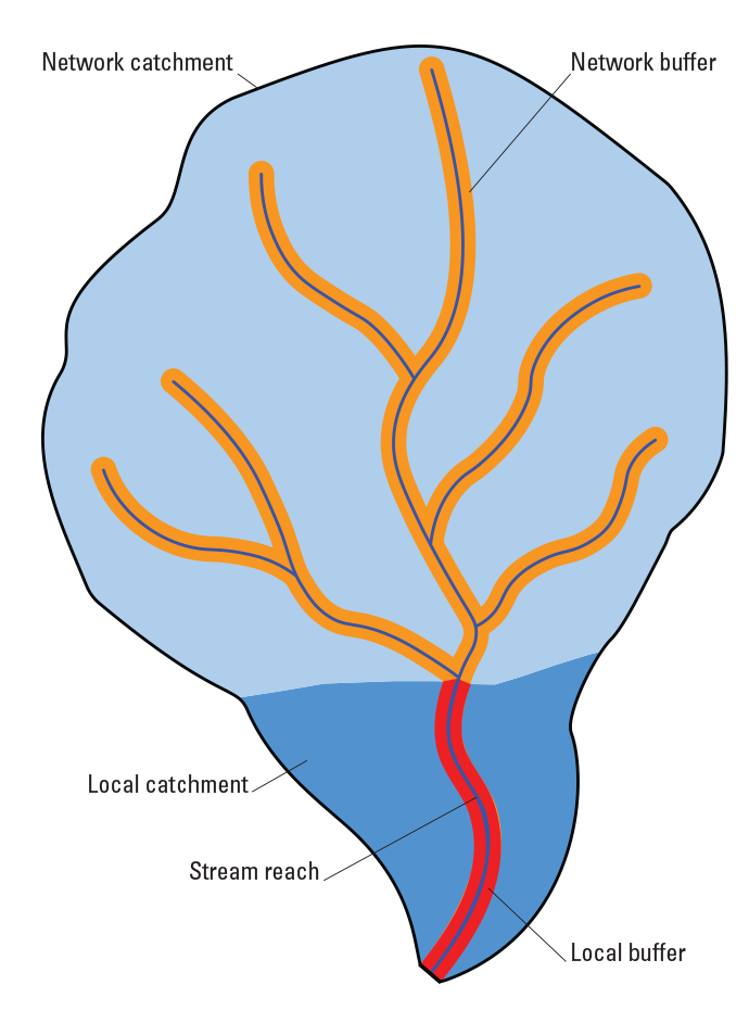
Simplified diagram representing the five spatial units used to summarize landscape variables.
Nine natural landscape variables were used as predictors in modeling. These included five at the network catchment scale, including catchment area, mean annual precipitation, percentage of overall wetland (combining forested and emergent wetlands) and open-water land-cover types, and base-flow index (percentage contribution of base flow to overall streamflow). The remaining four natural landscape predictor variables included mean annual air temperature and maximum elevation in local catchments, amount of forest land cover within network buffers, and stream reach slope (gradient). The 13 anthropogenic variables used as model predictors included the following: total urban land use (combining open, low, medium, and high urban), row crop land use, pasture land use, human population density, total water withdrawal, total phosphorous yield, mine density, and point source pollution site density in network catchments. Dam influences were represented by downstream main stem dam density, downstream main stem availability, upstream network dam density, and upstream degree of regulation (percentage of predicted annual streamflow volume stored in all upstream reservoirs) (Cooper and others, 2017), while road influences were represented by upstream road-crossing density in network catchments for stream reaches.
Fish Community Data
The fish data used for presence/absence species distribution modeling were derived from an existing fish database developed for a national fish habitat assessment in support of the National Fish Habitat Partnership (NFHP; http://assessment.fishhabitat.org/) and additional fish data collected in support of this project. Goals for collecting additional fish data were threefold. First, because NFHP fish data span the period 1990–2013, more recent data from 2014 to 2019 were needed to evaluate current conditions. Second, few western States were represented with fish data in the NFHP fish database, thus collection of fish data from data-poor regions was given a high priority to fill in spatial gaps in data availability. Third, whereas NFHP analyses required data that characterized the abundances of all species comprising assemblages, methods for creating SDMs used in this study required presence/absence data. Presence/absence data enabled use of datasets that included targeted samples of specific species or that reported species presence/absence compared to relative abundances. In total, 51 State, academic, and nonprofit sources were contacted, with a total of 14 institutions providing new fish data that could be used for this effort in addition to many datasets previously provided for NFHP. The models also included data from a Federal source (USGS BioData, https://apps.usgs.gov/biodata/; March 15. 2019), an existing consortium of State agency fish databases called Multistate Aquatic Resources Information System (USGS, 2013), and publicly available online State databases. All samples were georeferenced to stream reaches in the National Hydrography Dataset Plus Version 2.1, and the Latin species, genus, and family names used here were validated against and referenced by Integrated Taxonomic Information System taxonomic serial numbers for all records (Integrated Taxonomic Information System, 2019).
A tiered site-selection process based on sample species richness and year sampled was used to create the final fish dataset used in presence/absence modeling. This process ensured that a single, most recent, and species-rich sample was selected for stream reaches that had multiple sampling events. First, samples were assigned to one of six periods (1990–94, 1995–1999, 2000–4, 2005–9, 2010–14, and 2015–19). For each stream reach, the sample with the highest species richness within the most recent period was selected. When the most recent period for a given reach had multiple samples with the same species richness, the sample with the most recent sampling date was selected. This process resulted in the final selection of 35,918 fish samples spanning 1990–2019 for the conterminous United States (fig. 2).
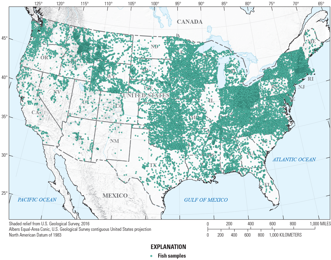
Locations of the 35,918 fish samples for the conterminous United States spanning 1990–2019.
Fish Species Native Ranges
Fish species native range maps were used to constrain model input (fish presence/absence data) and output (projected model presence/absence). The USGS Nonindigenous Aquatic Species Program assisted in acquisition of USGS eight-digit hydrologic unit code (HUC8) -level range maps of 149 species, delineating their range status as native or introduced (Daniel and Neilson, 2020) (fig. 3; table 2). In these cases, use of these range maps ensured that SDMs were built with presence/absence data occurring within a species’ native range, excluding presence locations from introduced portions of the range. Species’ introduced ranges could represent novel environmental conditions, and therefore, affect model development and potentially limit utility of results intended to support native species conservation. Additionally, range maps were used to limit model projections to stream reaches located within a given species’ native range, ensuring that predicted presence/absence locations were not projected to areas where species are not known to be native.
Table 2.
List of fluvial fish species analyzed.[ITIS TSN, Integrated Taxonomic Information System taxonomic serial number; SGCN, species of greatest conservation need identification; NAS, native range developed by U.S. Geological Survey Nonindigenous Aquatic Species Program; Y, yes for at least one State; N, no for every State; MSU, coarse range developed by Michigan State University]
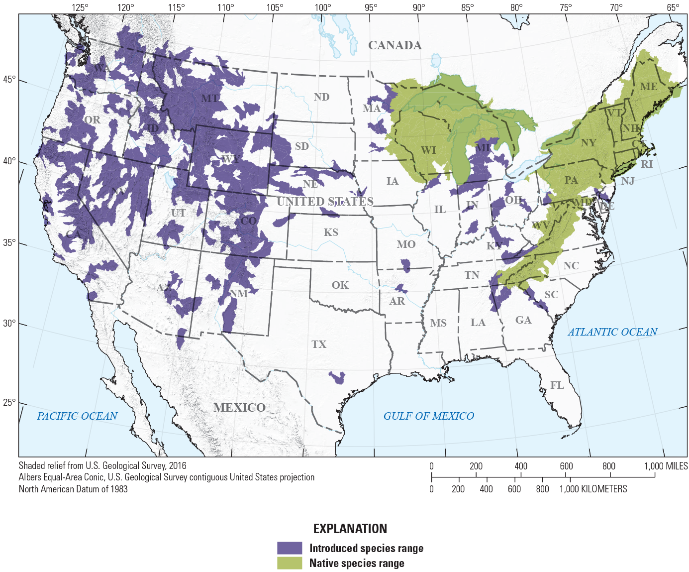
Example U.S. Geological Survey Nonindigenous Aquatic Species range map depicting native compared to introduced eight-digit hydrologic unit code (HUC8) origin status for Salvelinus fontinalis (Mitchill, 1814) (brook trout).
For an additional 122 species lacking detailed native and introduced range maps, HUC8 range maps were developed using all known occurrences (noted as Michigan State University, or MSU, in table 2). These range maps were derived from four data sources: point occurrences from the Aquatic GAP fish database (previously described), point occurrences from the IchthyMaps dataset (Frimpong and others, 2015), point occurrences from Global Biodiversity Information Facility (2020), and HUC8 level range maps developed by NatureServe (NatureServe, 2020) (fig. 4). For Global Biodiversity Information Facility, or GBIF, data, the following data filters were applied to ensure accuracy of both species identification and observation locations: (1) observations were limited to the United States only, (2) observation coordinate uncertainty was less than or equal to 1,000 meters, and (3) observations were made by collectors from Federal, State, or academic institutions (observations based on citizen science were excluded). While these range maps do not include native compared to introduced range status, they do provide geographic boundaries from which to constrain model input/output data and are based on a large set of known occurrences and ranges.
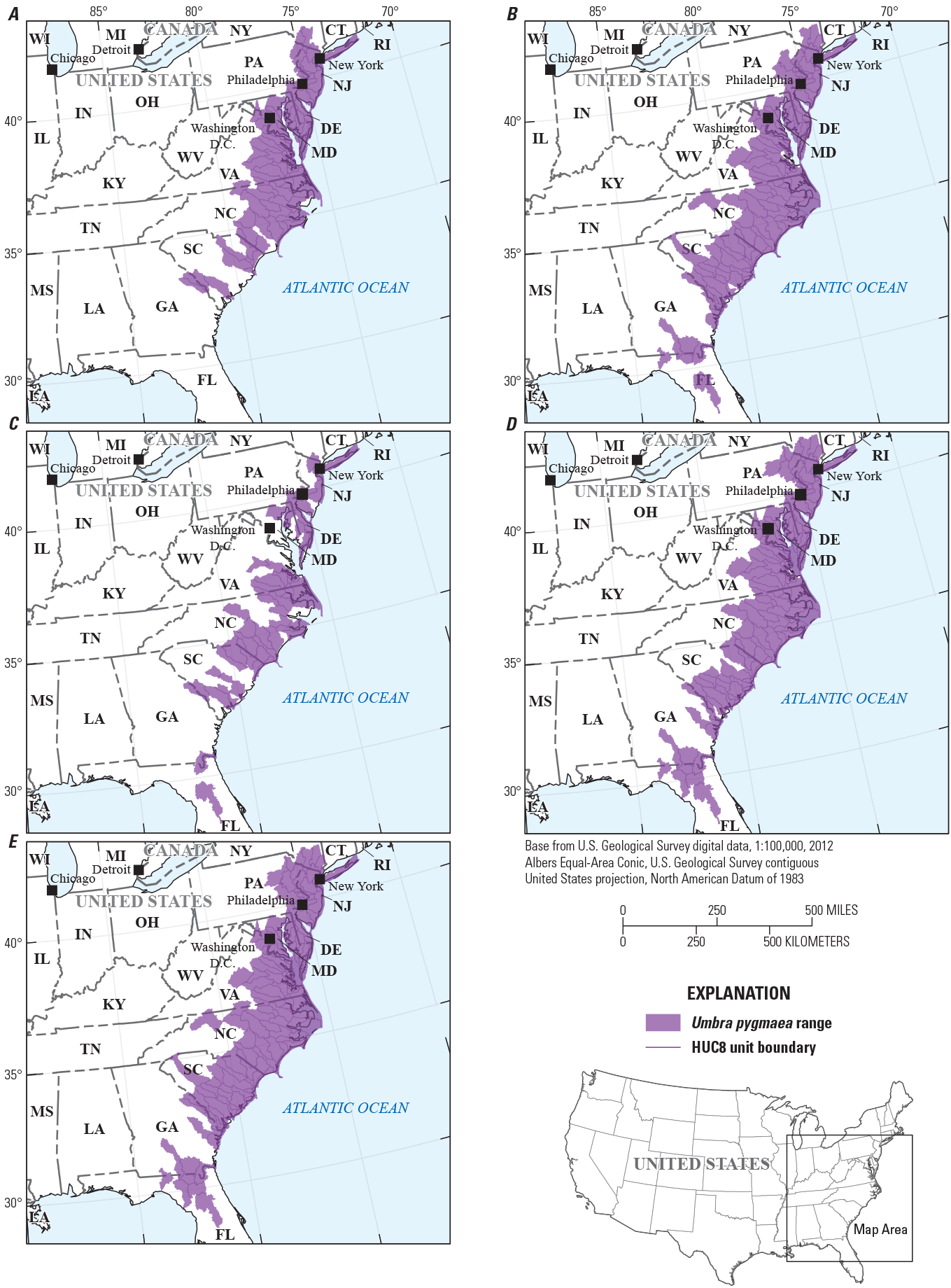
Example range map development for Umbra pygmaea (DeKay, 1842) (eastern mudminnow) using all known occurrences from A, the Aquatic Gap Analysis Project fish database, B, IchthyMaps, C, Global Biodiversity Information Facility, and D, NatureServe to produce E, a final range map used to constrain model input/output for this species.
Species Distribution Modeling with Boosted Regression Trees
Previous analyses by the USGS Aquatic GAP tested multiple species distribution modeling techniques for fluvial fishes, including logistic regression, BRT, classification and regression trees, and MaxEnt (A. Ostroff, U.S. Geological Survey, written commun., 2013). Based on results of these analyses and feedback from Aquatic GAP steering committee members, the BRT approach was selected for Aquatic GAP species distribution modeling efforts. BRT differs significantly from regression-based approaches by adaptively combining simple tree models using a boosting technique to improve predictive ability (Elith and others, 2008). Boosting is a sequentially stagewise procedure to link simple trees by emphasizing observations underrepresented in simpler models. Like other machine learning models, regularization is required for BRT to avoid overfitting in the training dataset. Three regularization parameters are commonly used in BRT: learning rate, tree complexity, and bag fraction. Learning rate is used to shrink the contribution of each individual tree in BRT. Tree complexity, ranging from 1 to 5, determines the number of nodes in each tree in the model. If the tree complexity equals 1, interaction effects are not analyzed in the BRT model. If the tree complexity equals 2, BRT models are fit with up to two-way interactions and so on (Elith and others, 2008). Finally, bag fraction is defined as the proportion of training data that are selected in each iteration, which introduces randomness into boosting. A preliminary study evaluated different value combinations of learning rate, tree complexity, and bag fraction (Cooper and others, 2019). Based on results of Cooper and others (2019), an initial learning rate of 0.05 for species with many occurrences (greater than 100) and a learning rate of 0.01 for species with few occurrences (less than or equal to 100) was used in this study. A tree complexity of 5 and bag fraction of 0.75 were used in each model. To ensure a minimum of 1,000 trees in the final model, the learning rate was divided by 2 in each iteration with the maximum number of trees capped at 10,000 to avoid overfitting. All the models were developed using the dismo package (Species Distribution Modeling Version 1.3-3R; Hijmans and others, 2020).
BRT models were evaluated using a tenfold cross-validation procedure in which the entire dataset was split into 10 nonoverlapping subsets and the BRT model was run 10 times. Each time, one of the 10 subsets was used as a test set while the remaining formed a training set for model fitting. The predicted values of all 10 test sets were then used to calculate diagnostic metrics for evaluating the BRT models.
Model Evaluation
Five diagnostic metrics were used to evaluate model performance in this study, including four fundamental measures often used in SDM evaluation: proportion of deviance explained (Elith and others, 2008), sensitivity, specificity, AUC, and True Skill Statistic (TSS) (Allouche and others, 2006). AUC is a threshold-independent metric that avoids the subjective selection of presence/absence cutoff values to develop a confusion matrix for model evaluation. AUC values range between 0 and 1, with larger values indicating better predictive ability. An AUC of 0.5 means that the prediction capability of the model is no better than random, and values greater than 0.7 are considered adequate for modeling species distributions (Swets, 1988). TSS is equal to the sum of sensitivity and specificity minus 1 (Fielding and Bell, 1997). In this study, predicted presences and absences for each fish species were separated by a threshold value that equals the observed prevalence of each sample species, where prevalence represents the proportion of sites in which the species was recorded present.
Predictor Relative Importance
The relative importance (or percent contribution) of each predictor variable was calculated for each species as follows:
wherestands for the relative importance of the ith predictor variable,
M
is the number of trees, and
is the squared improvement of each predictor weighted by the number of times it was chosen as the splitting variable in tree m (Hastie and others, 2009).
Results
We modeled the distributions of 271 species out of a set of 298 total fluvial fish species (table 2). For 27 species, lack of occurrences resulted in either the inability to attempt model development due to low number of occurrences (less than 10) or an inability of the BRT approach to create a stable model due to lack of model convergence (see table 1.1 in app. 1). For modeled species, the range in number of presences, number of absences, and prevalence was large (figs. 5 and 6). In total, 263 species were considered to have low to moderate prevalence (less than 0.5), while 10 species had high prevalence (greater than 0.5). Species prevalence ranged from 0.0021 (Acipenser fulvescens, lake sturgeon) to 0.6335 (Lepomis gibbosus, pumpkinseed), with a mean of all the prevalence values plus or minus (±) standard error of 0.1566 ± 0.0082. The proportion of deviance explained by the BRT model also varied considerably across fish species (table 3; fig. 7), ranging from 0.0562 (Moxostoma congestum, gray redhorse) to 0.7198 (Micropterus cataractae, shoal bass) with a mean of 0.3442 ± 0.0065. The model predictive performance evaluation metrics calculated from tenfold cross validation varied across models (table 3; fig. 7). In total, 270 of 271 models were considered acceptable based on AUC values (greater than or equal to 0.7).
Table 3.
Proportion of boosted regression tree model deviance and performance statistics for fluvial fish species distribution models.[ITIS TSN, Integrated Taxonomic Information System taxonomic serial number; dev exp, deviance explained; AUC, area under the receiver operating characteristic curve; TSS, True Skill Statistic]
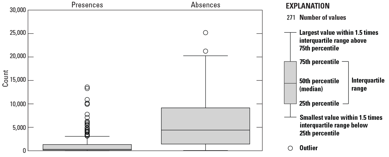
Boxplots of presences and absences for the 271 fish species modeled. The left boxplot represents the distribution of presences of the 271 fish species, and the right boxplot represents the distribution of absences of the 271 fish species.
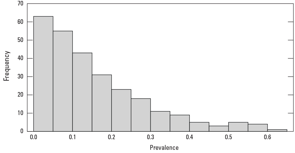
Histogram of prevalence for the 271 fish species modeled.
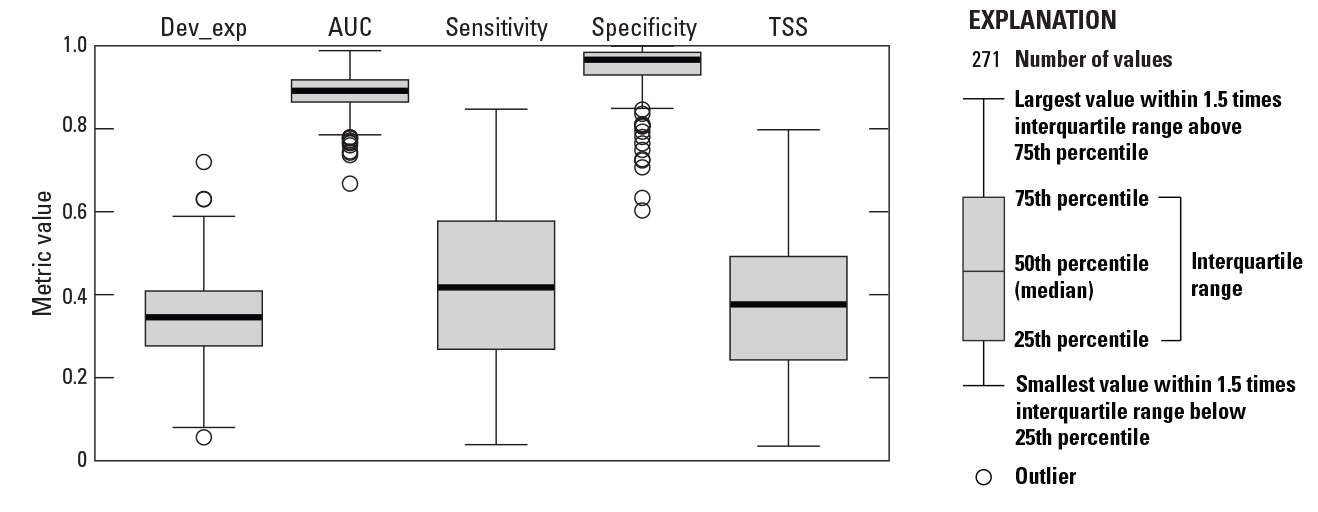
Boxplots of proportion of model deviance explained. Dev_exp, deviance explained; AUC, area under the receiver operating curve; TSS, True Skill Statistic.
The contributions of the predictor variables varied across species; however, network catchment area was consistently the most influential predictor, and overall, natural variables tended to have the greatest influence across species (fig. 8). The top three natural predictors, listed here with their variable names in order of mean relative importance, were network catchment area (N_areasqkm, 14.88 percent), local catchment mean annual air temperature (L_temp, 9.12 percent), and local catchment maximum elevation (L_maxelev, 6.70 percent). The top three anthropogenic predictors based on mean relative importance were downstream main stem dam density (DMD, 5.59 percent), distance to downstream main stem dam (DM2D_fishtail, 4.85 percent), and network catchment pasture and hay (N_nlcd82, 4.03 percent). There were seven predictors whose mean relative importance was less than 3 percent. These included upstream network dam density, network catchment mine density, degree of regulation, network catchment point source pollution density, network catchment human population density, network catchment urban land use, and stream network road crossing density. While average relative importance for these variables was low, influence of these variables was occasionally very high (greater than 20 percent) for certain species. These predictors could be reassessed for future modeling efforts, potentially dropping these predictors for some species or regions. Among climate-based predictors, mean annual air temperature played an important role in BRT models (relative importance greater than 10 percent) for 87 of 271 species modeled, while precipitation was less important with 37 of 271 species modeled meeting this cutoff. The influences of these climate variables pointed to 61 climate-sensitive fish species (having a sum relative importance of mean annual air temperature and precipitation greater than 20 percent) (table 4). Further, 40 fish species were responsive to anthropogenic stressors (having a sum relative importance of all anthropogenic variables greater than 50 percent) (table 5). The summaries in this section are based on 2 climate predictor variables and 13 anthropogenic predictor variables used to develop SDMs for each species.
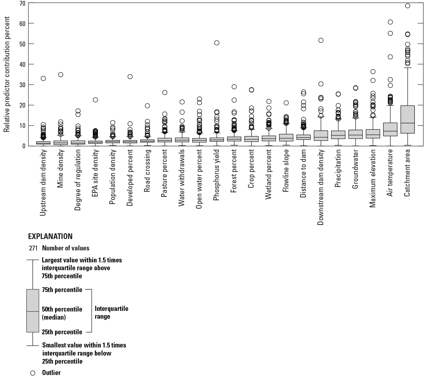
Boxplots of relative importance of the predictor variables for fluvial fish species presence, absence, and prevalence. See table 1 for predictor variable explanations. EPA, Environmental Protection Agency.
Table 4.
Fluvial fish species considered sensitive to climate influences in the conterminous United States.[L_temp represents the relative importance of mean annual air temperature in percent, and N_precip represents the relative importance of mean annual precipitation in percent. Species with the sum of temperature and precipitation (sum) with variable importance greater than 20 percent are considered sensitive. ITIS TSN, Integrated Taxonomic Information System taxonomic serial number]
Table 5.
Fluvial fish species in the conterminous United States considered responsive to anthropogenic stressors.[Species for which the sum of the anthropogenic variable importance (sum of relative importance) values is greater than 50 percent are considered sensitive. ITIS TSN, Integrated Taxonomic Information System taxonomic serial number]
To provide examples of SDM output, three fish species with differing prevalence characteristics were selected as example species (table 6; figs. 9–11). The AUC plots of these species showed that the AUC scores were related to the number of presences (fig. 12). Partial dependence plots of predictor variables for these species showed the relative importance of the top 12 predictor variables (fig. 13). The predictor variables showed different levels of importance to species’ distributions. For instance, network catchment area was the most important predictor variable for Semotilus atromaculatus (Mitchill, 1818) (creek chub), the sixth most important for Cottus beldingii (Eigenmann and Eigenmann, 1891) (Paiute sculpin), and not in the top 12 for Enneacanthus chaetodon (Baird, 1955) (blackbanded sunfish).
Table 6.
Presences, absences, and prevalence for three fluvial fish species selected to provide examples of species distribution model output.[ITIS, Integrated Taxonomic Information System]
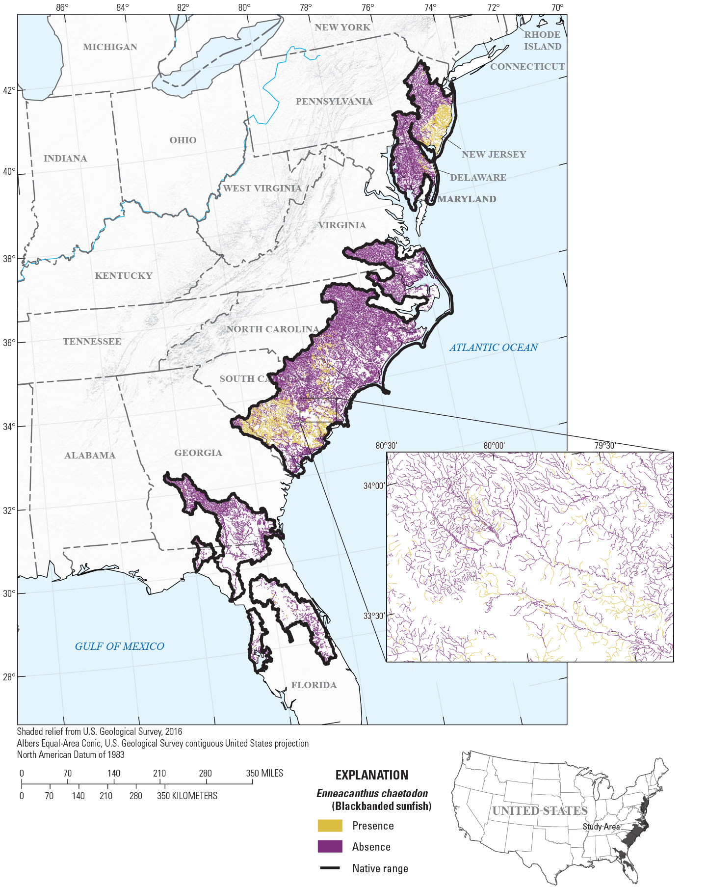
Map of species distribution model predictions for Enneacanthus chaetodon (Baird, 1855) (blackbanded sunfish).
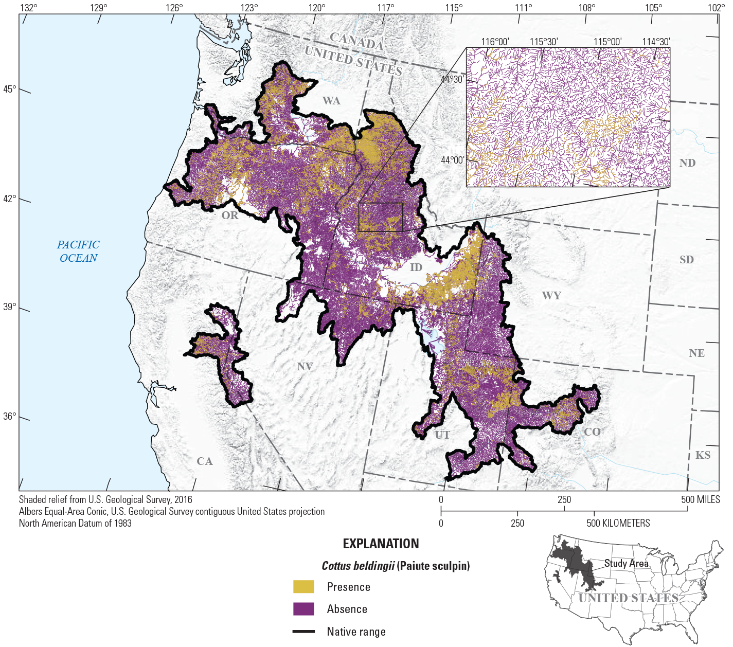
Map of species distribution model predictions for Cottus beldingii (Eigenmann and Eigenmann, 1891) (Paiute sculpin).
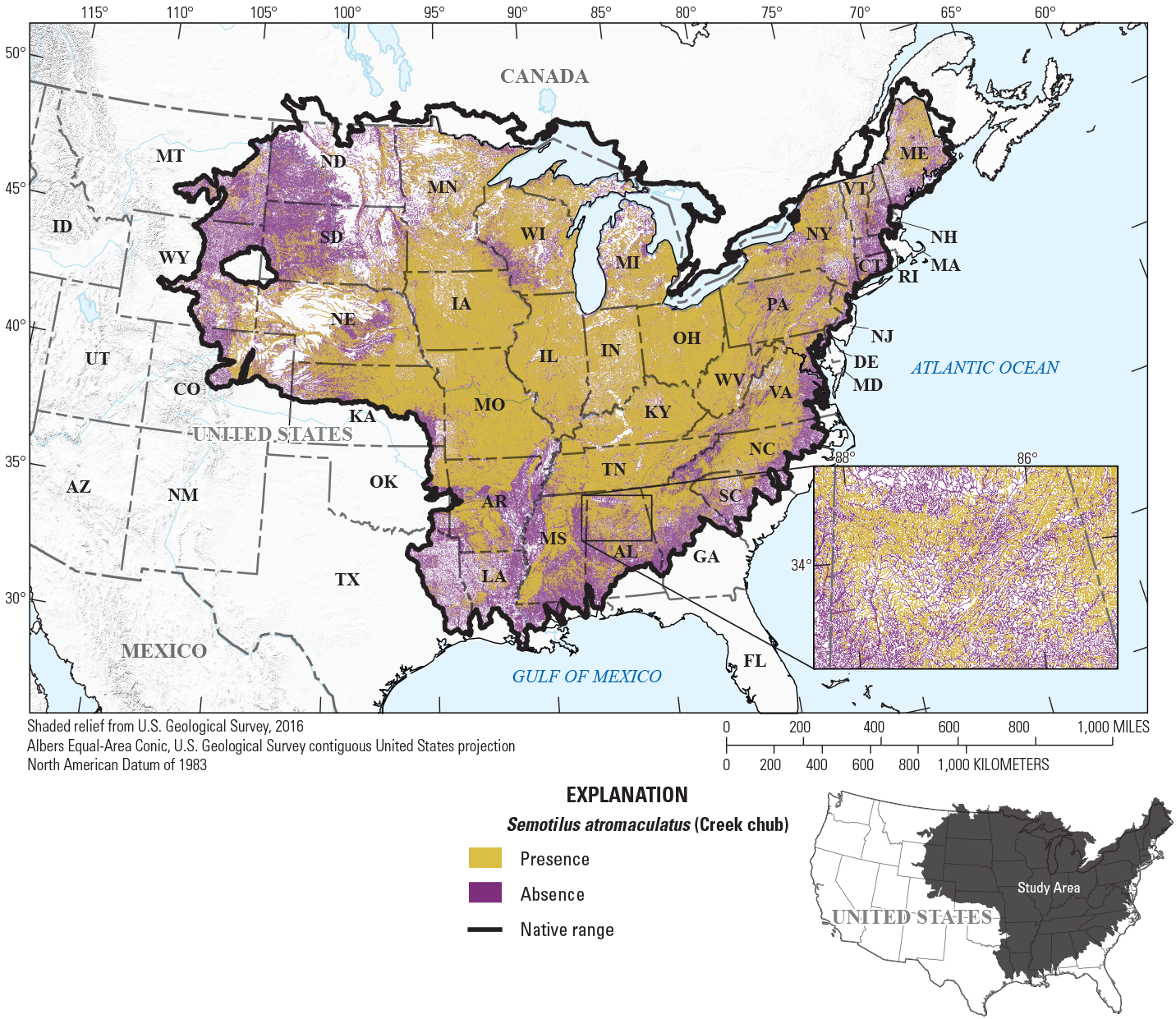
Map of species distribution model predictions for Semotilus atromaculatus (Mitchill, 1818) (creek chub).
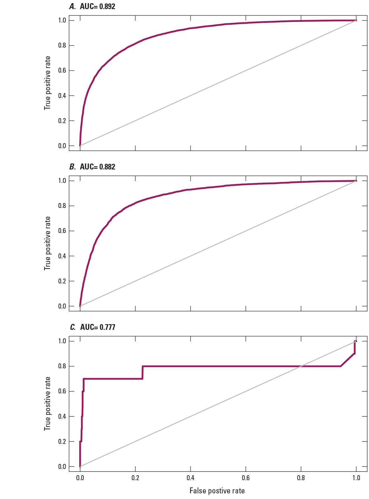
Area under the receiver operating characteristic curve (AUC) plots for three example fish species: A, Semotilus atromaculatus (Mitchill, 1818); B, Cottus beldingii (Eigenmann and Eigenmann, 1891); and C, Enneacanthus chaetodon (Baird, 1855).
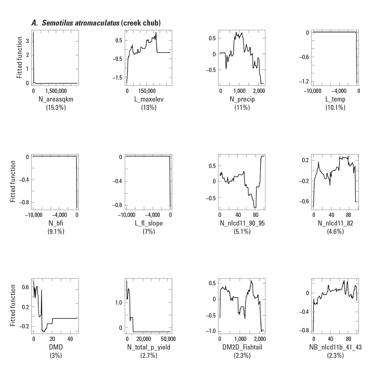
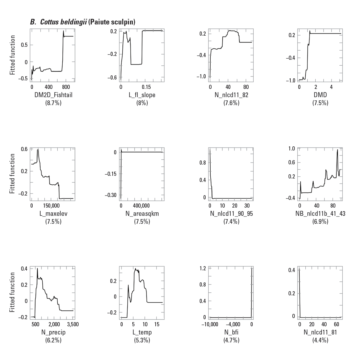
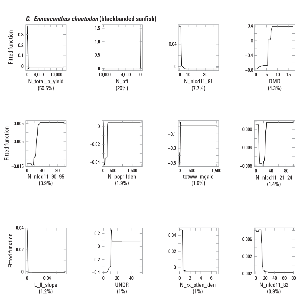
Partial dependence plots for three example fish species: A, Semotilus atromaculatus (Mitchill, 1818) (creek chub); B, Cottus beldingii (Eigenmann and Eigenmann, 1891) (Paiute sculpin); and C, Enneacanthus chaetodon (Baird, 1855) (blackbanded sunfish). The rug tiles in each figure represent the distribution of predictor variable values. <panel>a,b,c</panel>
Discussion
The models in this study represent 271 (~34 percent) of approximately 800 known freshwater fish species in the United States (Warren and Burr, 1994), and to our knowledge, this study represents the largest effort of its type for freshwater fishes based on geographic and taxonomic scope in the conterminous United States. In addition, the unprecedented spatial scale of this modeling effort provides the ability to identify locations that support many species and locations that support individual species of conservation or recreational importance, including Species of Greatest Conservation Need or priority game fish.
With this scope in mind, the SDMs generated provide a critical framework to develop additional products that may be beneficial to management and conservation of fluvial fishes in the United States. In Cooper and others (2019), species characterized as common within nine large ecoregions in the conterminous United States were evaluated using range extent, abundance, and habitat usage, and their distributions were modeled within ecoregions. The amount of protected land area in catchments required to consider them protected (protection target levels) was established for all streams in the conterminous United States by using information on protected areas from the USGS Protected Areas Database of the United States (USGS, 2020) and the known responses of fish communities to two prominent landscape stressors (urban and agricultural land uses). An assessment of protection target levels in conjunction with predicted species distributions indicated that protected areas are severely lacking among fish habitats for most common species in the United States (Cooper and others, 2019). Based on these methods, predicted presences from SDMs developed in this study can be coupled with protected areas from the Protected Areas Database of the United States dataset to identify the percentage and location of habitats that meet protection target levels. This type of analysis can identify spatial gaps in species protection for both rare and common species and harkens to the foundational analyses that spurred the inception of the USGS Gap Analysis Project.
Future expansion of this modeling could provide additional insights and products in support of aquatic conservation initiatives. For instance, further evaluation of species responses based on model results can be used to gain understanding of the natural and anthropogenic factors limiting species distributions. Model results for more climate-sensitive fish species can be used to understand potential effects on habitat suitability from climate change, and they can also help map habitats potentially gained or lost with projected changes in climate for individual species. Further, this information could be coupled with known locations of dams to explore the role of fragmentation in constraining range expansions and population dynamics under climate change. For a subset of species in this study, both native and introduced ranges were available. This information could be used to test or project native range models into introduced portions of a species’ range, providing an analytical framework for understanding potential invasiveness and ability of species to inhabit environments with novel conditions outside of a species’ known native range.
Evaluating Habitat Condition
Data representing stream fragmentation by dams (Cooper and others, 2017) can be used to analyze species-level fragmentation, quantifying the amount of connected habitat for any given location. Such information can be used as the basis for analyzing fish passage mitigation opportunities and identifying potential project locations that maximize habitat reconnections for multiple species, including migratory or imperiled species. Projected species presence/absence can result in much-needed information for conservation because these projections provide results for numerous unsampled stream reaches through a given species’ range. This information could inform field sampling efforts, with potential to identify previously unknown populations.
Identifying Sensitive Species
Climate change may dramatically affect fluvial fish distribution by altering air temperature and precipitation. The SDMs used in this study can be used to assess the effects of a changing climate by incorporating climate variables as predictor variables. The framework of building up SDMs, selecting model evaluation metrics, and ranking predictor relative importance will help classify and identify climate-sensitive species and sensitive stream reaches, information that can benefit natural resource managers.
Next Steps in Modeling
Extending modeling efforts to additional freshwater fish species could provide SDMs for species that have limited distributions or are underrepresented in the current Aquatic GAP fish database. Modeling of these species would likely require testing and application of novel analytical techniques (for example, weighted BRT, Maxent, random forest, deep-learning techniques, and community-based modeling approaches) to account for cases of limited presence/absence data. Further, adding measures of model uncertainty would improve model output by providing users with predictive uncertainty values that could be applied and analyzed for all predicted habitats for a given species. Yu and others (2020) used a novel approach that uses species abundances in model weighting to develop presence/absence SDMs. Results for 55 fluvial fish species native to the northeast United States indicated that this weighting approach outperforms a traditional, unweighted modeling approach for rarer fish species that have smaller range extents, lower abundance, and less diverse habitat usage (Yu and others, 2020). As a result, this new approach has the potential to improve SDMs for species of high conservation importance, with utility not only in aquatic studies but terrestrial realms as well. While updating the fish dataset used in SDM analysis was a focus during this project, acquiring new information on distributions of other types of aquatic organisms, including freshwater mussels, would set the stage for developing SDMs for other aquatic taxa.
Summary
This study offers insights into stream habitat suitability for 271 fluvial fish species (including Species of Greatest Conservation Need and game species) in the conterminous United States. Our results showed that network catchment area, mean annual air temperature of the local catchment, and maximum elevation of the local catchment were the three strongest natural predictors of fish distributions. Additionally, downstream main stem dam density, distance to downstream main stem dam, and the percentage of pasture/hay land use area within network catchment boundaries were the three strongest anthropogenic predictors of distributions. Additionally, by considering species-specific responses to individual environmental variables, we found that 40 fish species were sensitive to anthropogenic stressors, and 61 species were sensitive to climate variables. Such insights into the overall important predictors of fish distributions as well as important predictors for specific species can help natural resource managers better understand current habitat conditions and potential variations in the future. These and additional modeling efforts and potential applications using results from species distribution models, such as those described here, could contribute to efforts to conduct a national assessment in support of the Aquatic Gap Analysis Project, including integrating the effects of conservation actions into a landscape-scale context.
Data Access
Each of the datasets produced for this analysis are available to the public. The data are organized under a parent item with four child items. The parent item describes the modeling effort and includes a species list (species_model_list.csv), which provides a complete list of the species that have been modeled to date with the common name and the Integrated Taxonomic Information System taxonomic serial number allowing the user to know which species have been modeled. In addition, the species list includes the model’s digital object identifier, the modeled habitat type, and geographic extent of that model. The citations for the data products include the following:
References Cited
Allan, J.D., 2004, Landscapes and riverscapes—The influence of land use on stream ecosystems: Annual Review of Ecology Evolution and Systematics, v. 35, p. 257–284, accessed December 1, 2019, at https://doi.org/10.1146/annurev.ecolsys.35.120202.110122.
Allouche, O., Tsoar, A., Kadmon, R., 2006, Assessing the accuracy of species distribution models—Prevalence, kappa and the true skill statistic (TSS): Journal of Applied Ecology, v. 43, no. 6, p. 1223–1232, accessed December 1, 2019, at https://doi.org/10.1111/j.1365-2664.2006.01214.x.
Bouska, K.L., Whitledge, G.W., and Lant, C., 2015, Development and evaluation of species distribution models for fourteen native central U.S. fish species: Hydrobiologia, v. 747, p. 159–176, accessed December 1, 2019, at https://doi.org/10.1007/s10750-014-2134-8.
Cooper, A.R., and Infante, D.M., 2022, Dam metrics representing stream fragmentation and flow alteration for the conterminous United States linked to the NHDPLUSV2.1: U.S. Geological Survey data release, accessed May 20, 2022, at https://doi.org/10.5066/P94JQOFU.
Cooper, A.R., Infante, D.M., Daniel, W.M., Wehrly, K.E., Wang, L., and Brenden, T.O., 2017, Assessment of dam effects on streams and fish assemblages of the conterminous USA: Science of the Total Environment, v. 586, p. 879–889, accessed December 1, 2019, at https://doi.org/10.1016/j.scitotenv.2017.02.067.
Cooper, A.R., Tsang, Y.P., Infante, D.M., Daniel, W.M., McKerrow, A.J., and Wieferich, D.J., 2019, Protected areas lacking for many common fluvial fishes of the conterminous USA: Diversity and Distributions, v. 25, no. 8, p. 1289–1303, accessed December 1, 2019, at https://doi.org/10.1111/ddi.12937.
Cooper, A.R., Yu, H., Infante, D.M., and Ross, J.A., 2022, Coarse range maps for fish species in the conterminous United States using HUC8s: U.S. Geological Survey data release, https://doi.org/10.5066/P9V390V2.
Crawford, S., Whelan, G., Infante, D.M., Blackhart, K., Daniel, W.M., Fuller, P.L., Birdsong, T., Wieferich, D.J., McClees-Funinan, R., Stedman, S.M., Herreman, K., and Ruhl, P., 2016, Through a fish's eye—The status of fish habitats in the United States 2015: National Fish Habitat Partnership website, accessed October 29, 2021, at http://assessment.fishhabitat.org.
Daniel, W.M., and Neilson, M.E., 2020, Native ranges of freshwater fishes of North America (ver. 1.0, May 2020): U.S. Geological Survey data release, accessed June 1, 2020, at https://doi.org/10.5066/P9C4N10N.
Elith, J., Leathwick, J.R., and Hastie, T., 2008, A working guide to boosted regression trees: Journal of Animal Ecology, v. 77, no. 4, p. 802–813, accessed December 1, 2019, at https://doi.org/10.1111/j.1365-2656.2008.01390.x.
Fielding, A.H., and Bell, J.F., 1997, A review of methods for the assessment of prediction errors in conservation presence/absence models: Environmental Conservation, v. 24, no. 1, p. 38–49, accessed December 1, 2019, at https://doi.org/10.1017/S0376892997000088.
Frimpong, E.A., Huang, J., and Liang, Y., 2015, Historical stream fish distribution database for the conterminous United States (1950–1990)—IchthyMaps: U.S. Geological Survey data release, accessed December 1, 2019, at http://doi.org/10.5066/F7M32ST8.
Global Biodiversity Information Facility, 2020, Global Biodiversity Information Facility Species Occurrence Downloads: Global Biodiversity Information Facility website, accessed July 18, 2020, at https://www.gbif.org/occurrence.
Guisan, A., and Zimmermann, N.E., 2000, Predictive habitat distribution models in ecology: Ecological Modelling, v. 135, nos. 2–3, p. 147–186, accessed December 1, 2019, at https://doi.org/10.1016/S0304-3800(00)00354-9.
Hastie, T., Tibshirani, R., and Friedman, J., 2009, The elements of statistical learning (2d ed.): New York, Springer, 745 p., accessed December 1, 2019, at https://doi.org/10.1007/978-0-387-84858-7.
Hijmans, R.J., Phillips, S., Leathwick, J., and Elith, J., 2020, dismo—Species distribution modeling, version 1.3-3: The Comprehensive R Archive Network website, accessed November 17, 2020, at http://cran.r-project.org/web/packages/dismo/index.html.
Integrated Taxonomic Information System, 2019, Integrated Taxonomic Information System online database, accessed November 20, 2019, at www.itis.gov. [Also available at https://doi.org/10.5066/F7KH0KBK.]
Liu, C., White, M., and Newell, G., 2011, Measuring and comparing the accuracy of species distribution models with presence-absence data: Ecography, v. 34, no. 2, p. 232–243. [Also available at https://doi.org/10.1111/j.1600-0587.2010.06354.x.]
McKay, L., Bondelid, T., Dewald, T., Johnston, J., Moore, R., and Rea, A., 2012, NHDPlus version 2—User guide: U.S. Environmental Protection Agency, Horizon Systems NHDPlus website, 182 p., accessed December 1, 2019, at https://www.nhdplus.com/NHDPlus/NHDPlusV2_data.php.
NatureServe, 2020, NatureServe Explorer [web application]: Arlington, Va., NatureServe, accessed July 13, 2020, at https://explorer.natureserve.org/.
Ross, J.A., Infante, D.M., and Herreman, K., 2022, Anthropogenic disturbances and natural variables in the conterminous United States linked to catchments and buffers of the National Hydrography Dataset Plus version 2.1: U.S. Geological Survey data release, https://doi.org/10.5066/P9PM4HD0.
Swets, J.A., 1988, Measuring the accuracy of diagnostic systems: Science, v. 240, no. 4857, p. 1285–1293. [Also available at https://doi.org/10.1126/science.3287615.]
U.S. Geological Survey [USGS], 2013, Multistate Aquatic Resources Information System (MARIS): U.S. Geological Survey data release, accessed January 15, 2014, at https://doi.org/10.5066/F7BZ641R.
U.S. Geological Survey [USGS], 2020, Protected areas database of the United States (PAD-US) 2.1: U.S. Geological Survey data release, accessed September 15, 2020, at https://doi.org/10.5066/P92QM3NT.
Warren, M.L., Jr., and Burr, B.M., 1994, Status of freshwater fishes of the United States—Overview of an imperiled fauna: Fisheries, v. 19, no. 1, p. 6–18. [Also available at https://doi.org/10.1577/1548-8446(1994)019<0006:SOFFOT>2.0.CO;2.]
Wieferich, D.J., McKerrow, A., Cooper, A.R., Yu, H., Ross, J., and Infante, D.M., 2022, Aquatic Gap Analysis Project (Aquatic GAP) aquatic species distribution modeling on the National Hydrography Dataset Plus version 2.1: U.S. Geological Survey data release, accessed December 1, 2019, at https://doi.org/10.5066/P94XM9XV.
Yu, H., Cooper, A.R., and Infante, D.M., 2020, Improving species distribution model predictive accuracy using species abundance—Application with boosted regression trees: Ecological Modelling, v. 432, article 109202, 11 p. [Also available at https://doi.org/10.1016/j.ecolmodel.2020.109202.]
Yu, H., Cooper, A.R., Infante, D.M., and Ross, J., 2022, Fluvial fish native distributions for the conterminous United States using the NHDPlusV2.1 and boosted regression tree models: U.S. Geological Survey data release, https://doi.org/10.5066/P9YX3EX6.
Yu, H., Ross, J., Cooper, A.R., and Infante, D.M., 2022, Presence absence database of fish in the conterminous United States: U.S. Geological Survey data release, https://doi.org/10.5066/P9FZ6J6R.
Appendix 1. Fluvial Fish for Which Insufficient Occurrence Data Were Available to Support Species Distribution Modeling
Table 1.1.
Fluvial fish for which insufficient occurrence data were available to support species distribution modeling.[ITIS TSN, Integrated Taxonomic Information System taxonomic serial number]
Conversion Factors
International System of Units to U.S. customary units
Temperature in degrees Celsius (°C) may be converted to degrees Fahrenheit (°F) as follows:
°F = (1.8 × °C) + 32.
Datum
Vertical coordinate information is referenced to the North American Vertical Datum of 1988 (NAVD 88).
Horizontal coordinate information is referenced to the North American Datum of 1983 (NAD 83).
Abbreviations
AUC
area under the receiver operating characteristic curve
BRT
boosted regression trees
GAP
Gap Analysis Project
GBIF
Global Biodiversity Information Facility
HUC
hydrologic unit code
NFHP
National Fish Habitat Partnership
NLCD
National Land Cover Database
SDM
species distribution model
TSS
True Skill Statistic
USGS
U.S. Geological Survey
Publishing support provided by the Science Publishing Network,
Denver and Reston Publishing Service Centers
For more information concerning the research in this report, contact the
Center Director, USGS Science Analytics and Synthesis Program
P.O. Box 25046, Mail Stop 302
Denver, CO 80225
Or visit the Science Analytics and Synthesis Program website at
https://www.usgs.gov/programs/science-analytics-and-synthesis-sas
Disclaimers
Any use of trade, firm, or product names is for descriptive purposes only and does not imply endorsement by the U.S. Government.
Although this information product, for the most part, is in the public domain, it also may contain copyrighted materials as noted in the text. Permission to reproduce copyrighted items must be secured from the copyright owner.
Suggested Citation
Yu, H., Cooper, A.R., Ross, J., McKerrow, A., Wieferich, D.J., and Infante, D.M., 2023, Developing fluvial fish species distribution models across the conterminous United States—A framework for management and conservation: U.S. Geological Survey Scientific Investigations Report 2023–5088, 41 p., https://doi.org/10.3133/sir20235088.
ISSN: 2328-0328 (online)
Study Area
| Publication type | Report |
|---|---|
| Publication Subtype | USGS Numbered Series |
| Title | Developing fluvial fish species distribution models across the conterminous United States—A framework for management and conservation |
| Series title | Scientific Investigations Report |
| Series number | 2023-5088 |
| DOI | 10.3133/sir20235088 |
| Publication Date | November 13, 2023 |
| Year Published | 2023 |
| Language | English |
| Publisher | U.S. Geological Survey |
| Publisher location | Reston VA |
| Contributing office(s) | Science Analytics and Synthesis |
| Description | Report: vii, 41 p.; Data Release |
| Country | United States |
| Other Geospatial | Conterminous United States |
| Online Only (Y/N) | Y |