

Groundwater Quality in Abandoned Underground Coal Mine Aquifers Across West Virginia
Links
- Document: Report (11.9 MB pdf) , HTML , XML
- Data Release: USGS Data Release - Site and Groundwater-Quality Sample Data for Abandoned Underground Coal Mine Aquifers in West Virginia, 1973–2016
- NGMDB Index Page: National Geologic Map Database Index Page (html)
- Download citation as: RIS | Dublin Core
Acknowledgments
The authors would like to acknowledge Brian Carr of the West Virginia Department of Health and Human Resources and Dawn Newell of the West Virginia Department of Environmental Protection for helping to complete this project. The authors would also like to acknowledge Joseph Donovan of West Virginia University (Department of Geology and Geography), Tim Denicola of Civil & Environmental Consultants, Inc., Rachelle Thorne of Preston County Parks and Recreation, and Nick Schaer of Office of Surface Mining Reclamation and Enforcement for their guidance and data. Douglas Chambers and Dominick Antolino of the U.S. Geological Survey are thanked for their thoughtful reviews that have improved this report.
Abstract
Abandoned underground coal mine aquifers cover a large part of West Virginia and could supply substantial quantities of water for agricultural, industrial, residential, and public use. Several Federal, State, and academic institutions have studied the availability and quality of water stored in abandoned underground coal mine aquifers for a variety of applications, such as economic development, geothermal energy, aquaculture, and wastewater disposal. However, the spatial and stratigraphic controls on water quality produced from abandoned underground coal mine aquifers are still poorly constrained on a state-wide basis. In response to these knowledge gaps, the U.S. Geological Survey initiated a study, in cooperation with the West Virginia Department of Environmental Protection, to understand the applicability of using existing secondary source data for understanding water quality in abandoned underground coal mine aquifers across the State.
Results from the calculation of net alkalinity indicated that Upper Pennsylvanian coal beds primarily produce net acidic waters and Lower Pennsylvanian coal beds primarily produce net alkaline waters. Multivariate statistical analysis of elemental data supports the conclusion that abandoned underground coal mine aquifers in the northern part of the State generally produce poor water quality and abandoned underground coal mine aquifers in southern West Virginia primarily produce good water quality. These results substantiate the potential benefits of leveraging abandoned underground coal mine aquifers as a multifaceted resource in West Virginia and can be used as a reconnaissance tool for water managers to characterize abandoned underground coal mine aquifers on a local scale.
Introduction
Underground coal mines cover a large part of West Virginia (fig. 1). However, once mining ceases, they commonly flood if positioned below local streams, forming abandoned underground coal mine aquifers. Abandoned underground coal mine aquifers are plentiful water sources for public, agricultural, and industrial use (Hobba, 1987; Kozar and others, 2012), often requiring minimal treatment (for example, chlorination), and have been shown to provide water that is sufficient in quality and quantity for private households (Ferrell, 1992; Kozar and others, 2020).
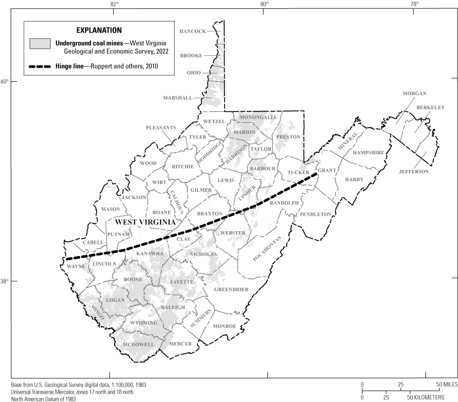
Map showing the spatial distribution of underground coal mines in West Virginia.
The hydraulic properties (porosity and permeability) of abandoned underground coal mine aquifers are conducive to high yields of groundwater in areas with sufficient recharge. Strata overlying inactive coal mines can collapse and partially fill the void space left after mining. The high porosity in abandoned underground coal mine aquifers is partially transferred through overlying strata in the form of vertical subsidence fractures and expansion of bedding plane partings (Stoner, 1983; Booth, 1986). The complexity of abandoned underground coal mine aquifers increases when individual underground mines collectively form a basin-scale aquifer system that is hydrologically connected through horizontal barrier leakage (McCoy, 2006).
Water from abandoned underground coal mine aquifers that is pumped to the surface from wells or discharged from mine outfalls, frequently exhibits water quality ranging from suitable for public supply to not suitable for public supply because of high acidity, high sulfate concentrations, and other constituents. Determining the quality of water coming from abandoned underground coal mine aquifers is critical because it gives water managers information that can be crucial to counteract the potential adverse effects poor water quality (for example, highly acidic water) imposes on receiving waterbodies (Rose and Cravotta, 1998).
Acidity, a key determinant of water quality, represents the base-neutralizing capacity of a volume of water and is a parameter commonly used to assess acid-sulfate waters emanating from coal mines (also known as acid mine drainage; Hedin and others, 1994). Acidity is caused by the oxidation of sulfide minerals (for example, pyrite) which releases ferrous iron, sulfate, and hydrogen into solution. Concentrations of aluminum and manganese increase in the solution when aluminosilicate minerals dissolve under acidic conditions. Acidity increases when ferrous iron oxidizes to ferric iron. Additional acidity is added during precipitation of ferric iron, aluminum, and manganese, which generates hydrogen ions during hydrolysis reactions (Rose and Cravotta, 1998). As these reactions produce increasingly acidic conditions, acid-sulfate waters may precipitate several insoluble oxyhydroxide and hydroxysulfate minerals if a combination of certain solute concentrations, redox conditions, and pH are present (Bigham and Nordstrom, 2000). Coal beds and adjacent stratigraphic intervals commonly have a higher sulfide mineral content (for example, pyrite) relative to non-coal lithologies and acidity production is exacerbated by the mining process whereby sulfide minerals are more readily oxidized. Acid-sulfate waters may persist in abandoned underground coal mine aquifers, where acid-neutralizing capacity from carbonate minerals in the overburden is not sufficient to neutralize the acidity generated from sulfide oxidation. Where the acid-neutralizing capacity is sufficient to neutralize acidity, the mine water may evolve to be alkaline but still have high sulfate concentrations (Rose and Cravotta, 1998; Perry, 2001).
The quality of water in abandoned underground coal mine aquifers is known to vary throughout West Virginia and to change over time at specific sites. Donovan and others (2004) determined that the spatial variability of water quality from abandoned underground coal mine aquifers in the Pittsburgh coal bed was likely controlled by the age of mine discharge, depth of the mine, degree of flooding, geochemistry, and mine reclamation strategy. Water quality improved at some sites over several decades and deeper fully flooded mines tended to have the greatest improvement in water quality. This improvement was likely caused by the lower oxidation rate of pyrite under anoxic, fully flooded conditions, but even some coal mines that are not fully flooded have shown improvements in water quality over time (Lambert and others, 2004; Perry and Rauch, 2006). Sulfide oxidation initializes acidity production and sulfur content of coal beds is a control on the fate of water quality in abandoned underground coal mine aquifers (Rose and Cravotta, 1998).
Cecil and others (1985) determined that the sulfur content of coal in West Virginia varies from north to south with changes in Pennsylvanian strata (fig.2); the northern part of the State exhibits higher percentages of sulfur in coal beds than the southern part of the State. This spatial and stratigraphic variability of sulfur concentrations across West Virginia has been attributed to temporally dynamic paleoclimates. Contrasting climatic regimes throughout the Middle Pennsylvanian age (Kanawha and Allegheny Formations; fig. 2) produced distinct depositional environments and diagenetic processes that ultimately governed syngenetic sulfur content in coal-bearing intervals (Cecil and others, 1985).
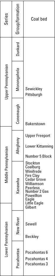
Diagram showing the stratigraphic position of referenced Pennsylvanian-age coal beds in West Virginia. Geologic names, coal bed names, and stratigraphic position of coal beds from McColloch and others (2012).
The U.S. Geological Survey, the West Virginia Department of Environmental Protection, the West Virginia Geologic and Economic Survey (WVGES), and multiple academic institutions have studied the quantity and quality of water in abandoned underground coal mine aquifers for several decades. These studies have been driven by many objectives, including suitability for public supply, possible economic development, environmental protection, and feasibility of underground injection (Hobba, 1987; Ferrell, 1992; West Virginia Department of Environmental Protection, 2009; McColloch and others, 2012). A recent data compilation (McAdoo and Kozar, 2017b) identified existing water-quality data for 770 samples at 294 abandoned underground coal mine aquifer sites across the State (fig. 3), and these data were used for the statistical analyses summarized by this report.
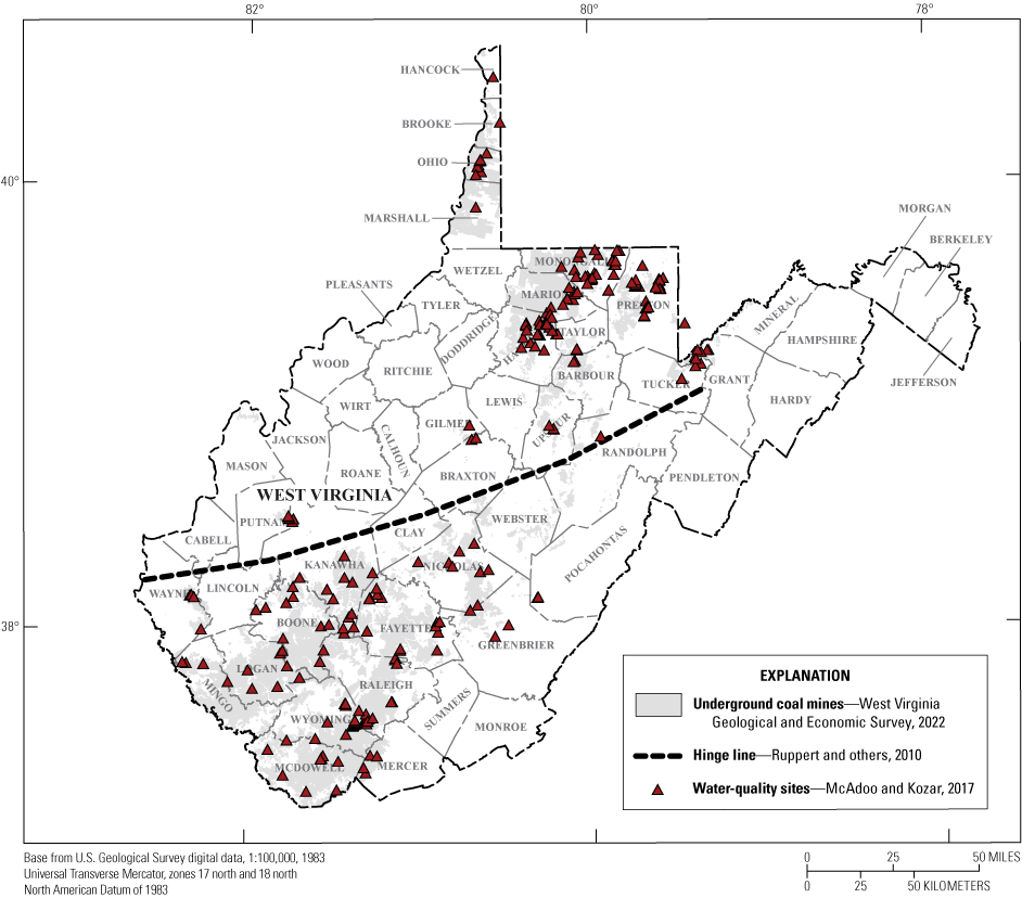
Map showing the sites in West Virginia where this study’s water-quality data were collected.
Geologic Setting
Geologic names in this report are consistent with prior work done by WVGES (McColloch and others, 2012). The southern West Virginia coal field (located in the central Appalachian coal region) is differentiated from the northern West Virginia coalfield (located in the northern Appalachian coal region) by depositional, stratigraphic, and lithologic controls (Ruppert and others, 2010). These two coalfields have distinct lithologies because of their differing paleoenvironmental settings and are separated by the hinge line defined by Arkle (1974), which differentiates the high sulfur northern coalfield (in the northern Appalachian coal region) from the low sulfur southern coalfield (in the central Appalachian coal region; Ruppert and others, 2010).
The boundary between the northern and southern West Virginia coalfields generally corresponds to the geologic contact between the older Kanawha and Allegheny Formations and the younger Conemaugh Formation (Ruppert and others, 2010). The depositional environments for the two coal regions were different. As a result, the lithologic composition of the older rocks comprising the southern West Virginia coalfield displays a higher proportion of sandstone and thin carbonate units than the lithologic composition of the northern West Virginia coalfield, which displays a higher proportion of shale, siltstone, and mudstone.
Methods of Analysis
The methods used for this analysis were chosen based on the type of data and limitations of the data available for the project. The dataset used for this analysis (McAdoo and Kozar, 2017b) is fully explained and qualified by McAdoo and Kozar (2017a) and limitations are discussed in the “Data Limitations” section of this report. Summary statistics were computed to better understand how the water quality in abandoned underground coal mine aquifers compares to drinking water standards. Nonparametric methods as described by Helsel (2012) were used to preserve information from samples with multiple censoring levels. Net alkalinity was used as a measure of water quality because the analytes needed for its calculation are often collected for research and regulatory requirements at coal mine discharges. The data were grouped using hierarchical agglomerative cluster analysis (HACA), and statistically significant clusters were mapped to understand the hydrogeological processes controlling the spatial distribution of water quality in abandoned underground coal mine aquifers across the State.
Data Limitations
The data used for this analysis are from several studies that utilized varied field collection and laboratory methods. As such, many samples from these studies have a specific number of analytes chosen for the purpose of each study, and representative sampling distributions are lacking when data are scrutinized at smaller scales. Although these data can be used for many purposes, multi-sourced data restrict the level of interpretation that can be applied. Multi-source data are also hard to validate, which then makes the qualification of the data necessary, casting uncertainty upon any resulting analysis.
Samples were not evenly distributed across all coal beds and within coal beds in this study—some coal beds had over 100 samples, whereas others had only 1 sample. Also, data interpretation and dataset utility are confounded by many sites having multiple samples. For this study, which is a regional analysis, all samples were considered to be independent observations to maximize the number of samples that could be used for univariate and multivariate statistics. Repeated samples from the same site or same mine can potentially skew the summary statistics, particularly if there is little to no variability among the samples or where only a few sites are used to represent entire coal beds. The use of repeated samples may indicate that some locations have water quality that varies over time or within the same mine complex. Using consistent field sampling and laboratory analysis methods and compiling addition site metadata would strengthen the dataset and subsequent analysis.
Determination of Net Alkalinity
Alkalinity and acidity balance is often used to determine treatment strategies for acidic coal mine discharges. For this study, calculated net alkalinity was used to understand the suitability of the water in abandoned underground coal mine aquifers for different uses because (1) data required for calculating net alkalinity are routinely collected for regulatory and research purposes, and (2) net alkalinity accounts for possible metal hydrolysis reactions that may precipitate undesirable minerals that adversely affect water quality (Rose and Cravotta, 1998). The acidity of a solution is represented by the release of hydrogen by oxidation, hydrolysis, and precipitation reactions that may result in the subsequent consumption of alkalinity. Acidity in acid mine drainage comes from elevated hydrogen ion, dissolved iron, aluminum, and manganese concentrations (Rose and Cravotta, 1998).
Net alkalinity or net acidity (in cases where the net alkalinity is negative), is reported in milligrams per liter (mg/L) as calcium carbonate and may be calculated by subtracting acidity (calculated by eq. 1; Kirby and Cravotta, 2005a) from field alkalinity (measured in the field by titration). Kirby and Cravotta (2005a) state that the preferred method of measuring net alkalinity is by standard hot acidity titration (American Public Health Association, 1995) but also show that net alkalinity may be calculated by equation 2 (Kirby and Cravotta, 2005a) when standard hot acidity titration results are unavailable. The relation between calculated net acidity and measured acidity has been confirmed by several authors (Rose and Cravotta, 1998; Kirby and Cravotta, 2005b). For this investigation, the calculated values were used to maximize the number of data points available for calculating net alkalinity.
whereAcidityCalculated
is the acidity in milligrams per liter as calcium carbonate;
pH
is the negative logarithm of the hydrogen concentration;
CFe
is the dissolved iron concentration in milligrams per liter;
CMn
is the dissolved manganese concentration in milligrams per liter; and
CAl
is the dissolved aluminum concentration in milligrams per liter.
AcidityCalculated
is the acidity determined by equation 1;
Measured Acidity
is the acidity reported using the standard method of hot acidity titration.
To calculate acidity, Hedin and others (1994) proposed an equation like equation 1; however, they included the common redox states of iron—ferrous (Fe2+) and ferric (Fe3+). Kirby and Cravotta (2005b) determined that the effects of excluding ferric iron when calculating acidity were minimal for water with a pH range of 2.5 to 8.3 (most waters). For this report, the contribution of iron was assumed to be in the ferrous redox state because the available dataset did not distinguish between redox states and the pH was predominantly greater than (>)3. A more precise calculation of acidity can be determined by full speciation using geochemical modeling software (Kirby and Cravotta, 2005b), but this dataset had sparse data for which calculation of acidity from full speciation could be performed; therefore, acidity was calculated by equation 1.
Statistical Analyses
Univariate and multivariate statistical methods were used to evaluate constituents affecting abandoned underground coal mine aquifer water quality, the types of water in abandoned underground coal mine aquifers, and how abandoned underground coal mine aquifer water quality varies throughout the State. Statistical analyses were completed, and graphics were created, using the R statistical computing environment (ver. 3.5.3) (R Core Team, 2021). Nonparametric techniques were used to compute descriptive and multivariate statistics from water-quality data; data that were sometimes censored at multiple levels. Censored values are water-quality results that are reported at less than a specified laboratory value and for which an exact value was not determined.
Prior to descriptive and multivariate statistical analyses, censored data were coded as u-scores with the codeU function in the U.S. Geological Survey smwrQW package (Lorenz, 2018). The u-score is the sum of the algebraic sign of the differences between each value. Using u-scores allows for the computation of multivariate relations without censoring at the highest reporting limit and retains information at multiple reporting limits. In cases where a column of data has only one censoring level, the u-scores are the same as ordinal methods of ranking for one reporting limit (Helsel, 2012).
Summary Statistics for Censored Data
The nonparametric models—Kaplan-Meier (KM) and robust regression on order statistics (ROS)— were used to estimate the summary statistics for censored data following the methods described by Ryberg (2006) and Helsel (2012). When more than 80 percent of a constituent was censored, the maximum concentration was reported. The minimum concentration was reported as less than the lowest reporting level. When a sample had 50 to 80 percent of its values censored, the robust ROS model was used. The robust ROS model was used for this range of censoring because of its ability to make accurate estimates and handle multiple censoring levels with a small number of observations (less than [<]50 observations). When the data were censored at >50 percent, the KM model was used to estimate the summary statistics. The KM estimate was used to account for multiple censoring levels, because it does not depend on the assumption of a distributional shape with data that are censored at >50 percent. When no values were censored, nonparametric methods were not necessary and summary statistics were computed using standard methods of statistical analysis.
Truncated boxplots are used throughout this report to display statistical distributions of data (fig. 4). Values below the 10th and above the 90th percentiles are not shown in figures throughout this report, but minimum and maximum values are reported along with summary statistics in table 1. The interquartile range is represented by the box in the boxplot with the whiskers extending to the 10th and 90th percentiles. Samples may have many reporting levels that were used in the calculation of the summary and multivariate statistics, and the dotted lines on boxplots represent the highest censoring level. Where the robust ROS method is used to estimate the statistical distribution, a red line represents imputed values above the highest censoring level.
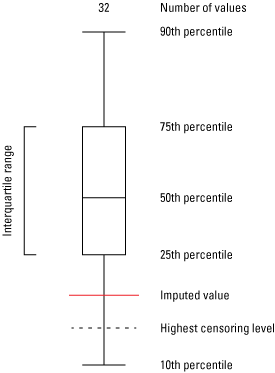
Explanation of a truncated box plot used to display summary statistics.
Hierarchical Agglomerative Cluster Analysis
Hierarchical agglomerative cluster analysis (HACA) is an effective multivariate statistical technique for analyzing water chemistry data and has been implemented by previous studies (for example, Güler and others, 2002; Ryberg, 2006). It is used to group data based on chemical concentrations and field measurements. Samples with results for pH, specific conductance (SC), alkalinity, calcium, magnesium, sodium, potassium, iron, aluminum, manganese, chloride, and sulfate were included in the HACA. Samples lacking results for these constituents were omitted from HACA, resulting in the use of only 102 (13.2 percent) of the original 770 samples. Total dissolved solids and acidity were not included in the HACA to reduce possible redundancies; major ions and field measurements were used to calculate these constituents.
As previously described, the dataset used in this study had variables with multiple censoring levels, necessitating the use of u-scores, which enabled direct implementation of multivariate techniques like correlation, principal component analysis, and cluster analysis. When the data were converted to u-scores for HACA, variables with higher percentages of censoring could be used without the need to substitute censored values, which reduced the possibility of introducing extraneous signals in the data (Helsel, 2012). Similarity was computed using Euclidean distance, and clusters were merged using Ward’s method as described by Güler and others (2002). The agglomerative coefficient produces a numerical value between 0 and 1 and was used to assess the clustering structure (Kaufman and Rousseeuw, 1990). The similarity profile test was used to identify significant clusters (Clarke and others, 2008; Somerfield and Clarke, 2013). Identifying significant clusters is necessary to reduce misinterpretation of the HACA, but ultimately the number of clusters chosen for further investigation was based on ability to interpret the cluster results.
Groundwater Quality in Abandoned Underground Coal Mine Aquifers
Studies of groundwater quality in abandoned underground coal mine aquifers in West Virginia commonly focus on individual coal beds, specific regions of the State, or a limited set of mines. The statewide analysis in this report is unique because of the scope and use of nonparametric statistical techniques to summarize and group spatially extensive data. This analysis focused on analytes commonly measured for regulatory purposes or remediation efforts due to the availability and abundance of their data for statistical analyses. The results of this report’s analysis of key analytes will be presented in relation to drinking water standards and net alkalinity, and determination of water-quality types will aid in highlighting the spatial distribution of water quality throughout the State.
Water Quality in Relation to Drinking Water Standards
Assessing the quality of water within underground mines in relation to drinking water standards is important because many private households and public utilities in the southern part of the State use abandoned underground coal mine aquifers as the primary source of water (Kozar and others, 2020). Constituents that exist in groundwater because of natural processes or are introduced by human activities may pose a risk to health where concentrations of those constituents exceed U.S. Environmental Protection Agency (EPA) maximum contaminant levels (MCLs; also known as primary drinking water standards). The MCLs that regulate public supplies can also be used as guidance for private households (U.S. Environmental Protection Agency, 2018). Other EPA water-quality guidelines include secondary maximum contaminant levels (SMCLs) and health advisories (HAs). SMCLs are given for select constituents that have no known health risks when in drinking water but may still produce bad taste, odor, or staining. The HAs can be listed for constituents that have no MCL or in addition to an MCL (U.S. Environmental Protection Agency, 2019). It is important to note that samples in this analysis were collected and analyzed using many different methods, at different times of the year, and under varying conditions. Chemistry at these sites may vary over time or on a seasonal basis, and these results may not fully characterize the water quality or risk to human health. Additional analyses can be completed at individual sites under consideration as potential water supply sources to understand the full range of analyte concentrations.
The number of samples and minimum, maximum, and median concentrations are provided for several analytes in the dataset (table 1). These analytes were compared to MCLs, HAs, and SMCLs and are displayed as the number and percentage of samples exceeding those standards. Several analytes in table 1 do not have drinking water standards or were not detected at levels exceeding drinking water standards, so they are not explicitly discussed relative to drinking water standards. The only field parameter in the dataset that had a drinking water standard is pH (table 1), and it is represented by a SMCL range of 6.5–8.5 pH units. Five hundred and fifty-six samples had field pH values in the dataset, and 356 of those samples had values that were outside of the SMCL range, comprising 64 percent of the total. Laboratory pH was reported in 270 samples, of which only 30 samples (11 percent) were outside of the SMCL range. Relatively high values, exceeding the 500 mg/L SMCL, were reported for total dissolved solids concentrations in 278 samples (77 percent of the samples)
Table 1.
Site characteristics, parameters measured in the field, laboratory analyses, major ions, nutrients, and trace constituents for samples reported by McAdoo and Kozar (2017b).[MCL, maximum contaminant level; HA, health advisory; SMCL, secondary maximum contaminant levels; —, not available; °C, degree Celsius; µS/cm, microsiemen per centimeter; mg/L, milligram per liter; <, less than; ANC, acid neutralizing capacity; CaCO3, calcium carbonate; SiO2, silicon dioxide; N, nitrogen; P, phosphorus; µg/L, microgram per liter]
Measurements of major ions, nutrients, and trace constituents were included in this study’s dataset. Five major ion analytes exceeded drinking water standards, and sulfate is the analyte that most frequently exceeds its drinking water standard. Elevated sulfate concentrations are common in mine discharges and can contribute to the non-carbonate hardness and anionic balance in a sample. Water types are characterized by major ions, and sulfate makes up the largest percentage of anion mass (fig. 5). Sulfate exceeded the 250 mg/L SMCL in 457 (69 percent) of 656 samples (table 1), and 652 samples (99 percent) were above the laboratory reporting limit for sulfate, which indicates that high concentrations of sulfate are prevalent throughout the study area.
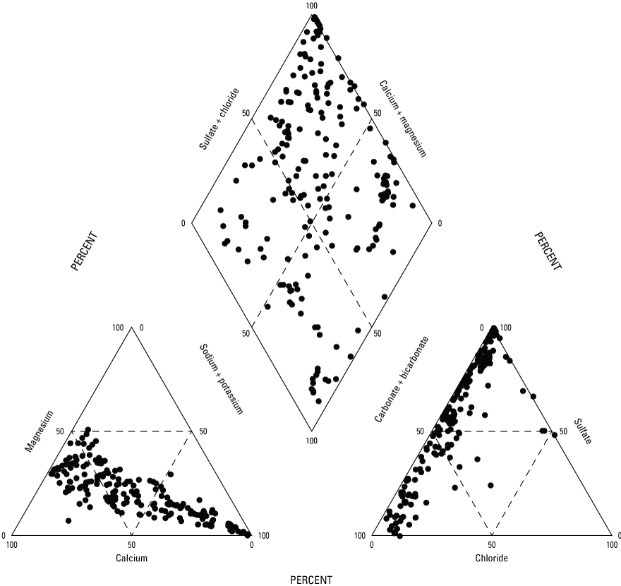
Piper plot depicting major ions, which characterize water types.
Commonly monitored and identified trace constituents in mine discharges include iron, aluminum, and manganese. Out of the 43 dissolved and total trace constituents in table 1, these three analytes have the most reported values in the dataset. The dissolved (that is, filtered) component of the trace constituents was more commonly analyzed than the total (that is, unfiltered) component, but there was usually less than a 10-percent difference between dissolved and total (table 1). This report focuses on the dissolved component, but understanding which component is reported is important because that information may have an effect on the results. Iron had 619 dissolved samples with 490 (79 percent) above the 300 micrograms per liter (μg/L) SMCL, aluminum had 547 dissolved samples with 349 (63 percent) above the lower SMCL (50 μg/L), and manganese had 368 dissolved samples with 333 (90 percent) above the 50 μg/L SMCL (table 1). Manganese also has a HA (300 μg/L), and 284 manganese samples (77 percent of the total) exceeded this HA. Other constituents related to the geochemistry of acid mine drainage also exceeded drinking water standards; 24 percent of arsenic samples exceeded the MCL of 10 μg/L.
Net Alkalinity in Abandoned Underground Coal Mine Aquifers
In addition to drinking water standards, water discharging from mines is often characterized by net alkalinity or net acidity. Net alkalinity (eq. 2) is the measurement primarily used to determine the requirements for the site-specific treatment of acid mine drainage but may also be used to evaluate general measures of water quality and water’s suitability for a particular application. Calculation of net alkalinity (determined by using eqs. 1 and 2), instead of measured acidity, affords a better spatial representation because the constituents required for computation of net alkalinity are more likely to be available than complete water chemistry data needed to calculate acidity from aqueous speciation and mineral equilibria (Kirby and Cravotta, 2005b).
Before acidity was calculated to determine net alkalinity, differences in filtered and unfiltered iron and aluminum and manganese values were evaluated to assess the effect of filtration on the measured analyte concentrations. Several authors have shown the differences between filtered and unfiltered sample values, as well as the differences between laboratory pH and field pH values (Gammons and others, 2000; Kirby and Cravotta, 2005b). These differences in reported values may be because of changes in equilibrium caused by oxidizing conditions and may or may not represent in situ aquifer conditions. Many samples in this dataset had filtered and unfiltered results, as well as field and laboratory pH measurements, which permitted examination of any potential effects filtering may impose on elemental concentrations and pH (figs. 6 and 7). Iron and aluminum clearly show deviation from the 1:1 line and substantial increases (>100 percent) in the concentrations of iron and aluminum observed in some unfiltered samples. The processes controlling iron and aluminum concentrations in mine water have been explained by several investigations (Rose and Cravotta, 1998; Bigham and Nordstrom, 2000; Kirby and Cravotta, 2005a). Those investigations found that differences in filtered and unfiltered samples are commonly the result of metal oxidation and hydrolysis reactions, which may precipitate iron and aluminum hydroxide or hydroxysulfate minerals. In unfiltered samples, these precipitates are redissolved by nitric acid, a preservative used for samples in this study, and the resulting measured concentration represents the total of the dissolved and mineral component. In addition to inorganic precipitation of iron-bearing mineral species, additional contributions from iron-precipitating bacteria may exacerbate aquifer degradation (Smith and Tuovinen, 1985). Filtering the sample before preservation removes these mineral particulates and reduces microbially mediated transformations, resulting in concentrations that represent only the dissolved fraction of the sample that can pass through a filter. For this study, only filtered values of iron and aluminum were used for the calculation of acidity (eq. 1) to reduce the possibility of overestimating acidity caused by the difference in filtered and unfiltered samples.
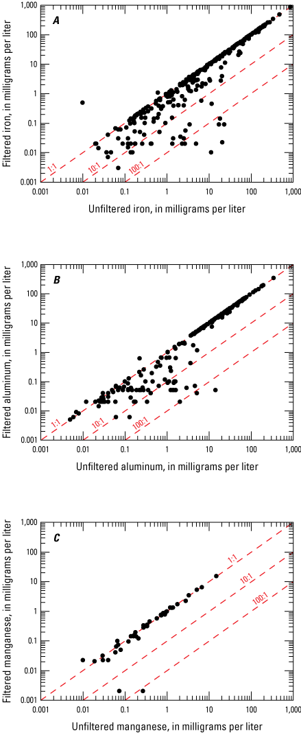
Scatterplots showing the comparison of filtered and unfiltered A, iron; B, aluminum; and C, manganese at abandoned underground coal mine aquifer sites in West Virginia.
When possible, filtered manganese samples were used for the calculation of acidity, but unfiltered samples were used when filtered samples were not available. Unlike iron and aluminum, a strong relation was observed between filtered and unfiltered manganese concentrations (fig. 6), indicating that the dissolved fraction generally contained the majority of the manganese. Because of this linear relation observed in figure 6, manganese concentrations in filtered and unfiltered samples were assumed to not differ greatly. The use of filtered and unfiltered manganese values increased the number of values that could be used to calculate acidity by 179.
Although unfiltered manganese concentrations were also used in this study to increase the number of data points, manganese can precipitate under certain geochemical conditions, and this may not be suitable for every study. Kinetics of manganese oxidation are strongly affected by pH and the abiotic oxidation of manganese is very slow at pH<8, which includes most of the samples in this study. Hydrolysis of iron and manganese in aqueous solutions is a sequential process; most of the iron must be removed before manganese (Hedin and others, 1994), making manganese precipitation less likely in these samples.
Field-measured pH data and laboratory-measured pH data had bimodal distribution groups of near neutral (around 7) and acidic (below 4) when compared (fig. 7). The near neutral group had higher values for laboratory-measured pH, and the acidic group had slightly higher values for field-measured pH. Similar observations were made by Kirby and Cravotta (2005b), who attributed this difference of values to the disequilibria of field pH measured in mine water exposed to atmospheric conditions at the time of sample collection. pH becomes stable over time with equilibrium among gaseous, aqueous, and mineral components of the sample, which is likely the reason for discrepancies in pH from field values measured at the time of sample collection and laboratory values measured after equilibration. For this study, field pH was used to calculate acidity when possible, and laboratory pH was only used when field pH was missing. Equilibrium reactions that affect pH may include metal hydrolysis reactions that precipitate minerals and decrease pH or dissolution of carbonates that may increase pH and alkalinity, but these reactions are accounted for when calculating acidity and net alkalinity using equations 1 and 2.
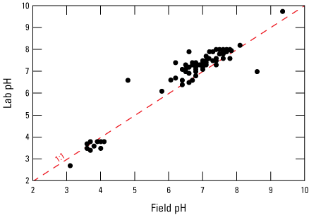
Scatterplot showing the comparison of laboratory pH and field pH measured at abandoned underground coal mine aquifer sites.
Net acidity and laboratory-measured acidity were compared in 150 samples (fig. 8). A linear relation demonstrating good agreement among values >10 mg/L as calcium carbonate was observed between these two measures of acidity in this study, which is consistent with other studies (Rose and Cravotta, 1998; Kirby and Cravotta, 2005b) and validates the use of net acidity values calculated by way of equation 2. Sites with negative net acidity were not included in the comparison because acidity reported by the laboratory was censored at values of 5 mg/L as calcium carbonate, allowing no negative values to be available. At low values of net acidity (<10 mg/L as calcium carbonate), acidity reported by the laboratory is consistently higher than the net acidity calculated by equations 1 and 2. This is consistent with the findings of Kirby and Cravotta (2005b), but their samples were net alkaline, and the divergence from linearity may have been because of calcite precipitation. Calcite precipitation is unlikely to happen with samples in this study because they are net acidic and unlikely to precipitate calcite at low pH. Ultimately, the number of values at this range of acidity are sparse, so the divergence from linearity cannot be definitely determined from these data.
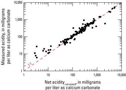
Scatterplot showing the comparison of acidity reported by the laboratory (measured acidity) and net acidity calculated by equations 1 and 2 (Net aciditycalculated).
Sufficient data were available to compute the net alkalinity of 387 samples from 180 sites, which represented 134 individual underground mines (table 2). Twenty-three coal beds are represented by at least 1 sample. Data were collected at these sites from April 5, 1978, to September 7, 2016; however, 89 percent of samples were collected after January 1, 2000 (McAdoo and Kozar, 2017b). The coal beds in table 2 are in stratigraphic order (McColloch and others, 2012); the table demonstrates that the younger coal beds of northern West Virginia have most of the available data used to calculate acidity.
Table 2.
Statistical summary of net alkalinity for 23 coalbeds in West Virginia.[Coal region is from Ruppert and others (2010). Coal beds are in stratigraphic order according to McColloch and others (2012). mg/L, milligrams per liter; CaCO3, calcium carbonate; —, not available]
The northern region of West Virginia contains mostly younger coal beds, including the Sewickley, Pittsburgh, Bakerstown, Upper Freeport, Lower Kittanning (also mined to a lesser degree in the southern region), and Number 5 Block (fig. 2), and the southern region contains mostly older coal beds spanning the Stockton to Pocahontas 3 (table 2). The coal beds in the northern part of West Virginia show a wide distribution of net alkalinity: the Pittsburgh coal bed has the lowest alkalinity values (−5,292 mg/L as calcium carbonate), and the Upper Freeport bed has the highest alkalinity value (1,761 mg/L as calcium carbonate). Most samples from the northern part of the State had negative net alkalinity (fig. 9), which is indicative of high metal concentrations, low pH, and low alkalinity. Net alkalinity values calculated for the southern part of West Virginia (n equal to [=] 133) had a tighter distribution of values (fig. 9); the lowest value came from the Pocahontas 3 coal bed (−181 mg/L as calcium carbonate), and the highest value came from the Eagle coal bed (620 mg/L as calcium carbonate).
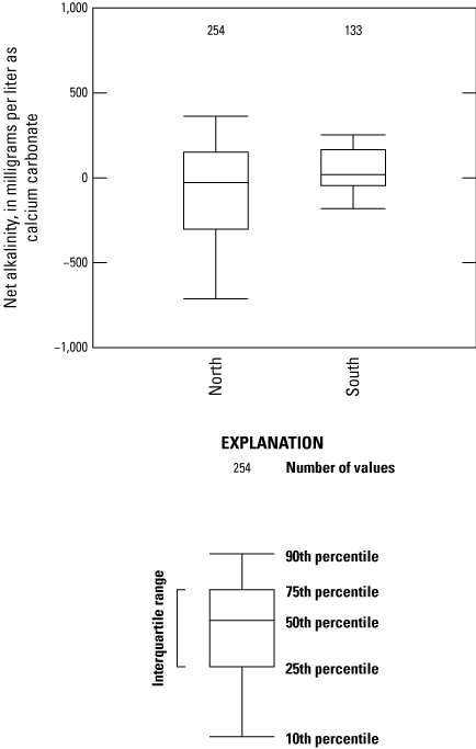
Boxplots showing net alkalinity from coal beds in the northern and southern parts of West Virginia. Net-alkalinity outliers above the 90th percentile and below the 10th percentile were used in the calculation of the box plots but are not shown in this figure.
Sulfur content in coal has been directly linked to the subsequent water quality of mine discharges; poor water quality is directly related to high sulfur content in coalbeds (Rose and Cravotta, 1998). Moving up the stratigraphic column (from older to younger formations), water quality clearly changes from being primarily positive (net alkaline) to being primarily negative (net acidic). This change occurs in the Middle Pennsylvanian age as sulfur content increases between the Number 2 Gas and Coalburg coal beds (fig. 10). Cecil and others (1985) concluded that the sulfur content of older coal beds in the southern part of the State is lower than the sulfur content of the younger coal beds in northern West Virginia. They also proposed that this difference in sulfur content is the result of a shift in climate from an ever-wet marine tropical setting in the Early Pennsylvanian age to a subtropical fluvial depositional setting in the Middle and Late Pennsylvanian age. This change in climate fundamentally altered peat bog morphology (for example, domed or planar), leading to contrasting geochemical conditions that increased the sulfur content of coal deposits in the Middle Pennsylvanian age at the contact of the Kanawha and Allegheny Formations. This stratigraphic and spatial hinge line in the Middle Pennsylvanian coal beds was observed by Cecil and others (1985) and coincides with the transition of net alkaline to net acidic water quality between the Number 2 Gas and Coalburg coal beds (fig. 10). Further evidence that climate has affected sulfur content is corroborated by the general overlap of coal beds with high sulfur content and the subsequent deposition of marine sediments (Williams and Keith, 1963); all this evidence suggests that a sustained temporal shift in paleoenvironmental conditions took place from the early to late Pennsylvanian age.
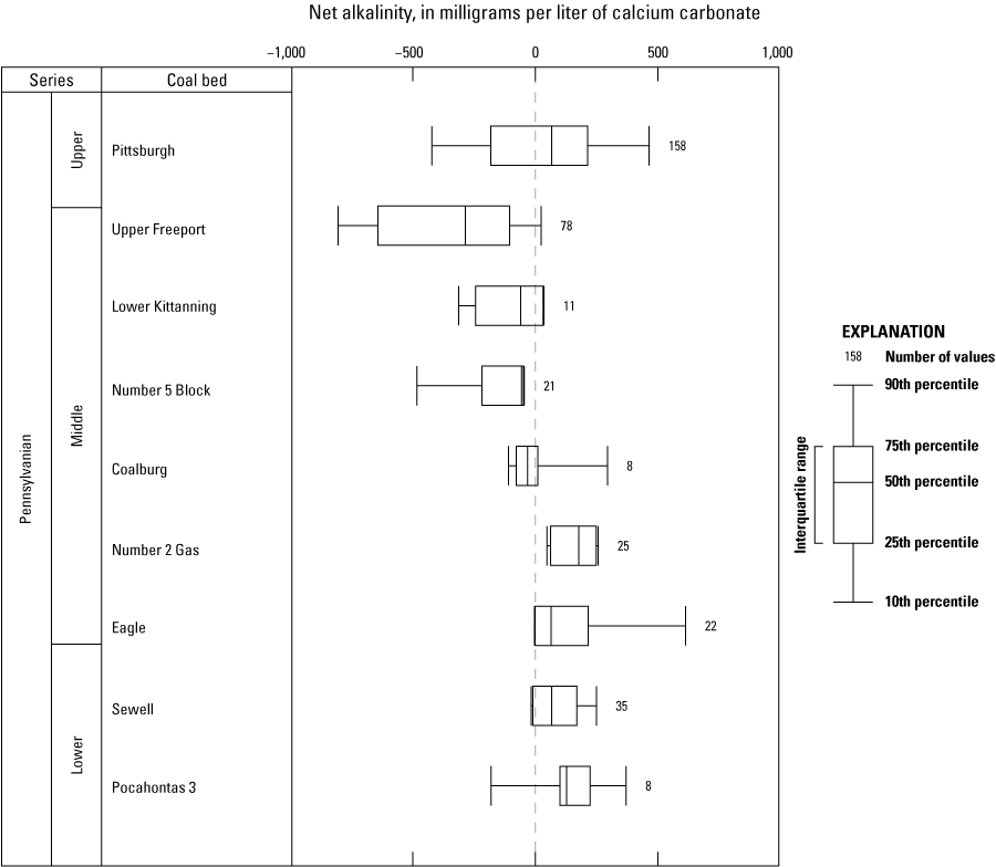
Boxplots showing the net alkalinity of individual coal beds in West Virginia ordered by stratigraphic position.
Sites Grouped by Water-Quality Characteristics
The primary output from HACA is a dendrogram depicting the clustering structure of the input data (fig. 11). Individual samples are represented by vertical lines at the bottom of the figure, and the merging of similar clusters is represented by horizontal lines connecting clusters. Clusters that merge near the bottom of the dendrogram have similar water chemistry. Clusters that do not merge until the top of the dendrogram represent groups of samples that have contrasting water chemistries. Specific analytes and parameters used for the HACA in this study included pH, SC, alkalinity, aluminum, calcium, iron, magnesium, manganese, potassium, sodium, chloride, and sulfate which resulted in a HACA with 102 samples. These samples were collected at 81 different sites which represented 71 individual mines and 16 different coal beds.
The major cluster groups in this study’s HACA were represented by capital letters (A, B, and C), and cluster subgroups were represented by numbers (1 through 6; fig. 11). The agglomerative coefficient—a value between 0 and 1 used to assess the HACA (Kaufman and Rousseeuw, 1990)—was 0.935, a number that provides confidence in the HACA structure. The similarity profile test identified 11 significant clusters (p<0.001), 6 of which were used for further analysis. Most of the samples in the HACA are from the Pittsburgh coal bed (42), whereas several coal beds only had 1 sample in the HACA (table 3). The Pittsburgh, Sewell, and Upper Freeport coal beds have the highest number of samples in the HACA and show variability among major cluster groups. Variability among coal bed clusters could be a product of greater sample density within a cluster or other factors in samples, such as mine age, depth of the coal mine, degree of flooding, and subsequent mine recovery. The specific reason why clusters are classified differently within a specific coal bed is not apparent with these data. Group A has 36 samples that are generally net alkaline but has a nearly neutral pH; these samples also have lower SC relative to groups B and C (fig. 12). Group B has 38 samples that range from net alkaline to net acidic (pH ranging from <5 to >7). Group B has the highest values for SC. Group C’s 28 samples had the lowest values for net alkalinity and pH.
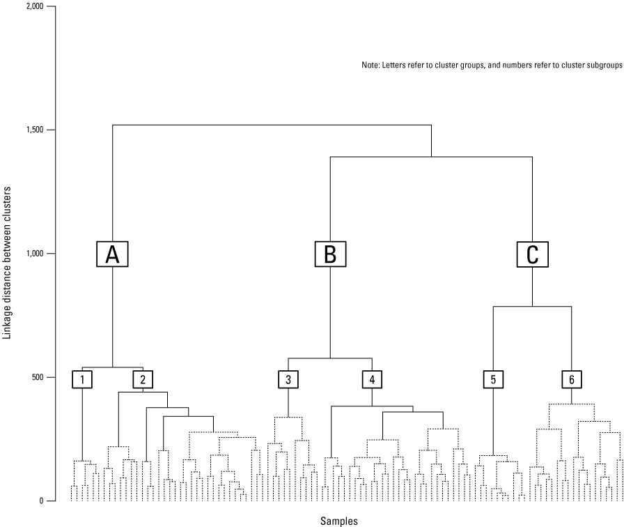
Dendrogram showing the output from a hierarchical agglomerative cluster analysis of water-quality data. Solid lines represent significant (p<0.001) clusters determined by the similarity profile test. Letters represent major cluster groups, and numbers represent subgroups of major cluster groups.
Table 3.
Summary table describing the number of samples in each cluster from 16 West Virginia coal beds.[Coal beds are given in stratigraphic order as in McColloch and others (2012). —, not available]
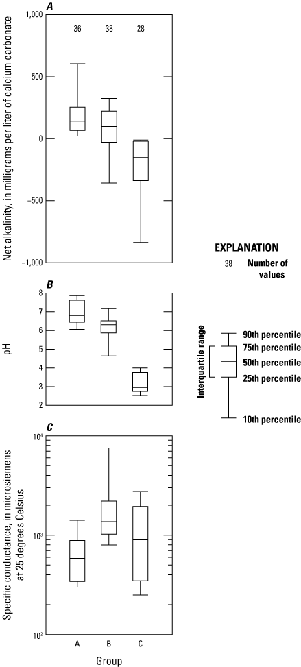
Boxplots showing summaries of A, net alkalinity; B, pH; and C, specific conductance in major cluster groups determined by a hierarchical agglomerative cluster analysis. Outliers above the 90th percentile and below the 10th percentile were included in the calculation of these boxplots, but they have been removed to clarify the centroids.
Distinct differences in major ion chemistry were observed between HACA cluster groups (fig. 13). Cluster group A’s samples have the widest distribution of water types ranging from samples with higher proportions of sodium and bicarbonate to samples with higher proportions of calcium and sulfate. Most samples in cluster group B showed higher proportions of calcium and sulfate but five samples in this cluster showed higher proportions of sodium. Samples from cluster group C had the smallest distribution of water types; all samples had higher proportions of calcium and sulfate.
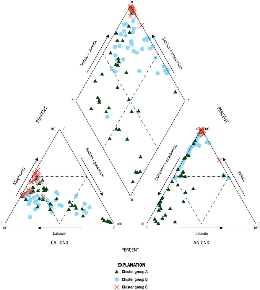
Trilinear diagrams showing the ions (which determine water type) of the major cluster groups determined by the hierarchical agglomerative cluster analysis.
Cluster subgroups are within larger cluster groups (A, B, and C) and represented by numbers 1 through 6 (fig. 11; table 3). Subgroup 1 has the lowest number of samples (6), and subgroup 2 has the highest number of samples (30; fig. 14). These two subgroups have the lowest values for acidity, aluminum, iron, and manganese, which is expected because cluster group A has relatively high net alkalinity and pH (fig. 12). Cluster subgroups 3 through 6 all had high acidity relative to subgroups 1 and 2. However, the metals associated with acidity in these subgroups varied. Cluster subgroup 6 had the highest median values for aluminum and manganese, whereas cluster subgroup 3 had the highest median values for iron (fig.14).
Table 4.
Description of major cluster groups and cluster subgroups based on central tendencies from hierarchical agglomerative cluster analysis (HACA).[SC, specific conductance; Ca, calcium; Mg, magnesium; Na, sodium; Cl, chlorine; SO4, sulfate; Fe, iron; Al, aluminum; Mn, manganese]
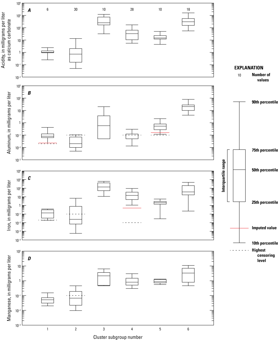
Boxplots showing summaries of A, acidity; B, aluminum; C, iron; and D, manganese values in cluster subgroups determined by hierarchical agglomerative cluster analysis (HACA).
Cluster group B had the highest values for SC (fig. 12), which is explained by the high values for major ion chemistry (fig. 15). Subgroups 3 and 4 have the highest values of the chemical constituents that contribute to SC, values such as calcium, magnesium, sodium, chloride, and sulfate. Higher concentrations of calcium and magnesium indicate higher rates of carbonate dissolution which buffers acidity by adding alkalinity. Sodium and chloride may be higher in the samples of subgroups 3 and 4 because they may be representative of chemistry located deeper in the subsurface or because of cation exchange of calcium and magnesium with sodium.
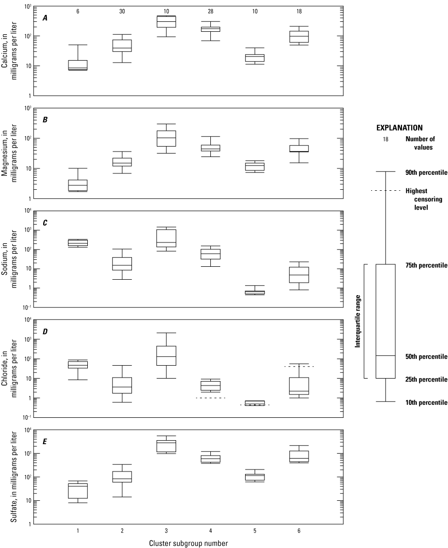
Boxplots showing summaries of A, calcium; B, magnesium; C, sodium; D, chloride; and E, sulfate values in cluster subgroups determined by hierarchical agglomerative cluster analysis (HACA).
The spatial distribution of cluster groups across West Virginia shows a distinct difference between the northern and southern coal fields in the State (fig. 16). The southern part of the State has more samples from cluster group A than from B and C. The northern part of the State has more samples from cluster groups B and C than A. Abandoned underground coal mine aquifers in the southern part of the State have more samples that are characterized by relatively high alkalinity (net alkaline throughout) and low concentrations of aluminum, iron, and manganese (table 4). In contrast, the northern part of the State is characterized by low to negative net alkalinity, higher SC, and higher concentrations of aluminum, iron, and manganese.
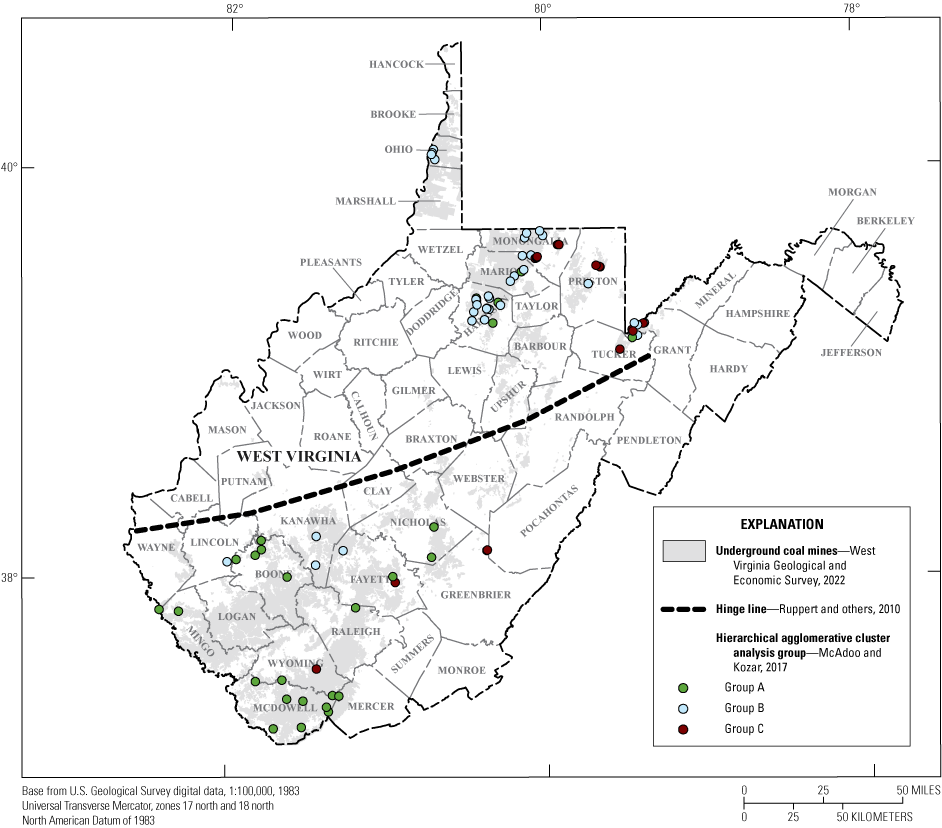
Map showing the spatial distribution of cluster groups.
Discussion and Limitations
This report describes the statistical analysis of water-quality data from abandoned underground coal mine aquifers in West Virginia over a statewide scale. Post-mining water quality can vary considerably within the same geologic section because of many factors, such as the presence of carbonates, the length of time since mine closure, mining strategy, and reclamation practices (Rose and Cravotta, 1998). These factors, although important, were not considered within the scope of this regional assessment. Although this assessment was made with available data, additional investigations with consistent data and more site information can be made on site-specific and coal-seam specific scales to assess the validity of the current study when applied to smaller scales.
The data used for this report are from several studies that implemented different field collection and laboratory methods. As such, many samples had a small number of analytes that were chosen for the purpose of the individual study where the data originated. Although data from multiple studies can be used for many purposes, multi-sourced data restrict the level of interpretation that can be derived from them. Multi-sourced data are also harder to validate and require data qualification that can cast skepticism upon the results of any analysis. Additionally, the objectives of these original studies may skew the water-quality data positively for studies related to water supply or economic development or negatively for studies related to regulatory purposes, potentially resulting in a bimodal distribution of the best and worst conditions. Compilation of additional site information and metadata may be useful for future analyses designed to determine the effects of mine construction and reclamation on water quality. Additional efforts using consistent field sampling methods and laboratory analyses may provide better confidence in future investigations.
Summary
This study was completed to understand the utility of existing water-quality data from West Virginia’s abandoned underground coal mine aquifers using secondary source data that were previously compiled, standardized, and published (McAdoo and Kozar, 2017b). Upon initial examination of the dataset, it was apparent that not all analytes relevant to this study were measured for every site and multiple censoring levels were used for samples over many years. These factors reduced the usefulness of the dataset by restricting the number of samples that could be used for statistical tests and calculation of net alkalinity. Because of the lack of standard censoring levels and prevalence of non-normal data distributions, nonparametric statistical techniques were used to maximize the number of samples that could be used for this analysis.
Several samples had field parameters or analytes with values that were not considered acceptable by U.S. Environmental Protection Agency drinking water standards. Sixty-four percent of the samples with field pH had values outside of the recommended secondary maximum contaminant level (SMCL), whereas 11 percent of the samples measured for laboratory pH were outside of the recommended SMCL. Sulfate exceeded the 250 milligrams per liter SMCL in 69 percent of samples, which indicated that high concentrations of sulfate are prevalent throughout the study area. Iron exceeded the 300 micrograms per liter (μg/L) SMCL in 79 percent of samples, aluminum exceeded the lower 50 μg/L SMCL in 63 percent of samples, manganese exceeded the 50 μg/L SMCL in 90 percent of samples, and arsenic exceeded the 10 μg/L maximum contaminant level in 24 percent of samples. Manganese also had 77 percent of its samples exceed its health advisory of 300 micrograms per liter. Some abandoned underground coal mine aquifers may produce water that is of high quality, which was observed in samples from southern West Virginia, but some may produce water that exhibits high concentrations of metals, sulfate, and low pH. Overall, special consideration and monitoring may be necessary when using an abandoned underground coal mine aquifer for a drinking water source because water quality may change over time and by location (sometimes at short distances). Samples in the dataset used for this report had filtered and unfiltered analytes, as well as pH measured under field and laboratory conditions. Filtered and unfiltered concentrations of iron and aluminum were different from each other in many samples, and sometimes exhibited a 100-percent increase of unfiltered concentrations. Manganese did not increase in unfiltered concentrations and generally followed a linear relation between filtered and unfiltered samples. The dynamics observed in filtered and unfiltered samples from this dataset highlight the need for standard sampling methods and show that different sampling techniques can affect data interpretation. For any future investigations concerning abandoned underground coal mine aquifers that involve sampling, a clear understanding of the objectives of the investigations should be realized, and proper sampling techniques should be used to maximize the usefulness of the data.
The results from the hierarchical agglomerative cluster analysis and the calculation of net alkalinity support the conclusion that poorer water quality was more commonly associated with younger coal beds primarily in the northern part of the State and better water quality was associated with older coal beds primarily in the southern part of the State. This disparity in net alkalinity between the north and south is likely because of the differences of sulfur content in the coal beds between these regions. Net acidic, high-sulfur coal is predominantly associated with younger coal beds north of the hinge line and relatively lower sulfur coal is primarily limited to the older coal beds in the south. Pronounced changes in depositional environments caused by paleoclimatic shifts across the stratigraphic interval (in other words, Pennsylvanian time period) enabled broad generalizations of abandoned underground coal mine aquifer water quality across the State, but local effects such as mine age, depth of coal mine, degree of flooding, and subsequent mine recovery may alter water quality in ways that deviate from the regional interpretation. This statistical analysis can be used as a reconnaissance tool for water managers focusing on additional protection efforts and demonstrates that abandoned underground coal mine aquifers in West Virginia may be suitable for a variety of uses. Use of a specific mine may be determined after a rigorous and focused evaluation of the site-specific hydraulics and water chemistry.
References Cited
American Public Health Association, 1995, Acidity, pt. 2310 of Standard methods for the examination of water and wastewater (19th ed.): Washington, D.C., American Public Health Association Press, accessed March 10, 2021, at https://www.standardmethods.org/doi/abs/10.2105/SMWW.2882.022.
Arkle, T., Jr., 1974, Stratigraphy of the Pennsylvanian and Permian systems of the central Appalachians, in Briggs, G., ed., Carboniferous of the southeastern United States: Geological Society of America Special Paper 148, p. 5–29, accessed June 15, 2023, at https://doi.org/10.1130/SPE148-p5.
Bigham, J.M., and Nordstrom, D.K., 2000, Iron and aluminum hydroxysulfates from acid sulfate waters: Reviews in Mineralogy and Geochemistry, v. 40, no. 1, p. 351–403, accessed March 10, 2021, at https://doi.org/10.2138/rmg.2000.40.7.
Booth, C.J., 1986, Strata-movement concepts and the hydrogeological impact of underground coal mining: Ground Water, v. 24, no. 4, p. 507–515, accessed October 2, 2017, at https://doi.org/10.1111/j.1745-6584.1986.tb01030.x.
Cecil, C.B., Stanton, R.W., Neuzil, S.G., Dulong, F.T., Ruppert, L.F., and Pierce, B.S., 1985, Paleoclimate controls on late paleozoic sedimentation and peat formation in the central appalachian basin (U.S.A.): International Journal of Coal Geology, v. 5, no. 1–2, p. 195–230, accessed February 7, 2019, at https://doi.org/10.1016/0166-5162(85)90014-X.
Clarke, K.R., Somerfield, P.J., and Gorley, R.N., 2008, Testing of null hypotheses in exploratory community analyses—Similarity profiles and biota-environment linkage: Journal of Experimental Marine Biology and Ecology, v. 366, no. 1-2, p. 56–69, accessed June 1, 2021, at https://doi.org/10.1016/j.jembe.2008.07.009.
Donovan, J.J., Duffy, B., Leavitt, B.R., Stiles, J., Vandivort, T., and Werner, E., 2004, WV173 Monongahela Basin mine pool project: West Virginia Water Research Institute, National Mine Land Reclamation Center, West Virginia University, 133 p., accessed October 9, 2017, at http://www.hrc.nrcce.wvu.edu/final/2004report/FinalReport.pdf.
Ferrell, G.M., 1992, Hydrologic characteristics of abandoned coal mines used as sources of public water supply in McDowell County, West Virginia: U.S. Geological Survey Water-Resources Investigations Report 92–4073, 37 p., accessed October 2, 2017, at https://doi.org/10.3133/wri924073.
Gammons, C.H., Mulholland, T.P., and Frandsen, A.K., 2000, A comparison of filtered vs. unfiltered metal concentrations in treatment wetlands: Mine Water and the Environment, v. 19, no. 2, p. 111–123, accessed March 8, 2021, at https://doi.org/10.1007/BF02687259.
Güler, C., Thyne, G.D., McCray, J.E., and Turner, K.A., 2002, Evaluation of graphical and multivariate statistical methods for classification of water chemistry data: Hydrogeology Journal, v. 10, no. 4, p. 455–474, accessed March 10, 2021, at https://doi.org/10.1007/s10040-002-0196-6.
Hedin, R.S., Nairn, R.W., and Kleinmann, R.L.P., 1994, Passive treatment of coal mine drainage: Washington, D.C., U.S. Bureau of Mines Information Circular 9389, 35 p., accessed March 10, 2021, at https://www.hedinenv.com/pdf/ptcmd.pdf.
Hobba, W.A., Jr., 1987, Underground coal mines as sources of water for public supply in northern Upshur County, West Virginia: U.S. Geological Survey Water-Resources Investigations Report 84–4115, 38 p., accessed October 2, 2017, at https://doi.org/10.3133/wri844115.
Kirby, C.S., and Cravotta, C.A., III, 2005a, Net alkalinity and net acidity 1—Theoretical considerations: Applied Geochemistry, v. 20, no. 10, p. 1920–1940, accessed February 2, 2020, at https://doi.org/10.1016/j.apgeochem.2005.07.002.
Kirby, C.S., and Cravotta, C.A., III, 2005b, Net alkalinity and net acidity 2—Practical considerations: Applied Geochemistry, v. 20, no. 10, p. 1941–1964, accessed February 2, 2020, at https://doi.org/10.1016/j.apgeochem.2005.07.003.
Kozar, M.D., McCoy, K.J., Britton, J.Q., and Blake, B.M., Jr., 2012, Hydrology, groundwater flow, and groundwater quality of an abandoned underground coal-mine aquifer, Elkhorn area, West Virginia: West Virginia Geological and Economic Survey Bulletin B–46, 103 p., accessed October 2, 2017, at http://downloads.wvgs.wvnet.edu/pubcat/docs/Bulletin_46_Hydrogeology,%20Groundwater%20Abandoned%20Coal%20Mine%20Aquifer,%20Elkhorn,%20WV_(2012).pdf.
Kozar, M.D., McAdoo, M.A., and Haase, K.B., 2020, Groundwater quality and geochemistry of West Virginia’s southern coal fields: U.S. Geological Survey Scientific Investigations Report 2019−5059, 78 p., accessed June 1, 2021, at https://doi.org/10.3133/sir20195059.
Lambert, D.C., McDonough, K.M., and Dzombak, D.A., 2004, Long-term changes in quality of discharge water from abandoned underground coal mines in Uniontown Syncline, Fayette County, PA, USA: Water Research, v. 38, no. 2, p. 277–288, accessed October 2, 2017, at https://doi.org/10.1016/j.watres.2003.09.017.
Lorenz, D.L., 2018, smwrQW—Tools for censored data analysis (ver. 0.7.14): R Package Documentation web page, accessed June 15, 2023, at https://rdrr.io/github/USGS-R/smwrQW/.
McAdoo, M.A., and Kozar, M.D., 2017a, Groundwater-quality data associated with abandoned underground coal mine aquifers in West Virginia, 1973–2016: Compilation of existing data from multiple sources: U.S. Geological Survey Data Series 1069, 7 p., accessed January 30, 2020, at https://doi.org/10.3133/ds1069.
McAdoo, M.A., and Kozar, M.D., 2017b, Site and groundwater-quality sample data for abandoned underground coal mine aquifers in West Virginia, 1973–2016: U.S. Geological Survey data release, accessed January 30, 2020, at https://doi.org/10.5066/F7TM78C5.
McColloch, J.S., Binns, R.D., Jr., Blake, B.M., Jr., Clifford, M.T., and Gooding, S.E., 2012, West Virginia mine pool atlas: Charleston W. Va., West Virginia Department of Environmental Protection, 172 p., accessed October 2, 2017, at http://www.dep.wv.gov/WWE/wateruse/Pages/MinePoolAtlas.aspx.
McCoy, K.J., 2006, Horizontal hydraulic conductivity estimates for intact coal barriers between closed underground mines: Environmental & Engineering Geoscience, v. 12, no. 3, p. 273–282, accessed October 2, 2017, at https://doi.org/10.2113/gseegeosci.12.3.273.
Perry, E.F., 2001, Modelling rock–water interactions in flooded underground coal mines, Northern Appalachian Basin: Geochemistry Exploration Environment Analysis, v. 1, no. 1, p. 61–70, accessed October 2, 2017, at https://doi.org/10.1144/geochem.1.1.61.
Perry, E.F., and Rauch, H.W., 2006, Water quality evolution in flooded and unflooded coal-mine pools in 7th International Conference on Acid Rock Drainage, St. Louis, Mo., March 26–30, 2006: Lexington Kentucky, American Society of Mining and Reclamation, p. 1564–1581, accessed June 4, 2021, at https://www.asrs.us/Publications/Conference-Proceedings/2006/1565-Perry.pdf.
R Core Team, 2021, R—A language and environment for statistical computing: Vienna, Austria, R Foundation for Statistical Computing software release, accessed May 1, 2021, at https://www.R-project.org/.
Rose, A.W., and Cravotta, C.A., III, 1998, Geochemistry of coal-mine drainage, chap. 1 of Brady, K.B.C., Smith, M.W., and Schueck, J., eds., Coal mine drainage prediction and pollution prevention in Pennsylvania: Harrisburg, Pa., Pennsylvania Department of Environmental Protection, 22 p., accessed February 2, 2020, at https://files.dep.state.pa.us/Mining/BureauOfMiningPrograms/BMPPortalFiles/Coal_Mine_Drainage_Prediction_and_Pollution_Prevention_in_Pennsylvania.pdf.
Ruppert, L.F., Trippi, M.H., and Slucher, E.R., 2010, Correlation chart of Pennsylvanian rocks in Alabama, Tennessee, Kentucky, Virginia, West Virginia, Ohio, Maryland, and Pennsylvania showing approximate position of coal beds, coal zones, and key stratigraphic units: U.S. Geological Survey Scientific Investigations Report 2010–5152, 9 p., 3 plates, available only online at https://pubs.usgs.gov/sir/2010/5152/.
Ryberg, K.R., 2006, Cluster analysis of water-quality data for Lake Sakakawea, Audubon Lake, and McClusky Canal, central North Dakota, 1990–2003: U.S. Geological Survey Scientific Investigations Report 2006–5202, 38 p., accessed December 15, 2020, at https://pubs.usgs.gov/sir/2006/5202/pdf/sir20065202.pdf.
Smith, S.A., and Tuovinen, O.H., 1985, Environmental analysis of iron-precipitating bacteria in ground water and wells: Ground Water Monitoring and Remediation, v. 5, no. 4, p. 45–52, accessed February 14, 2022, at https://doi.org/10.1111/j.1745-6592.1985.tb00937.x.
Somerfield, P.J., and Clarke, K.R., 2013, Inverse analysis in non-parametric multivariate analyses—Distinguishing groups of associated species which covary coherently across samples: Journal of Experimental Marine Biology and Ecology, v. 449, p. 261–273, accessed June 1, 2021, at https://doi.org/10.1016/j.jembe.2013.10.002.
Stoner, J.D., 1983, Probable hydrologic effects of subsurface mining: Ground Water Monitoring and Remediation, v. 3, no. 1, p. 128–137, accessed October 2, 2017, at https://doi.org/10.1111/j.1745-6592.1983.tb00874.x.
U.S. Environmental Protection Agency, 2018, 2018 Edition of the drinking water standards and health advisories tables: U.S. Environmental Protection Agency EPA 822-S-12-001, accessed March 3, 2021, at https://www.epa.gov/system/files/documents/2022-01/dwtable2018.pdf.
U.S. Environmental Protection Agency, 2019, Secondary drinking water standards—Guidance for nuisance chemicals: Environmental Protection Agency website, accessed March 3, 2021, at https://www.epa.gov/sdwa/secondary-drinking-water-standards-guidance-nuisance-chemicals.
West Virginia Department of Environmental Protection, 2009, Senate Concurrent Resolution-15—An evaluation of the underground injection of coal slurry in West Virginia [Phase I—Environmental Investigation]: Charleston W. Va., West Virginia Department of Environmental Protection, 80 p., accessed October 2, 2017, at http://www.dep.wv.gov/dmr/studies%20and%20investigations/Documents/Slurry%20UIC%20Investigation.pdf.
Williams, E.G., and Keith, M.L., 1963, Relationship between sulfur in coals and the occurrence of marine roof beds: Economic Geology, v. 58, no. 5, p. 720–729, accessed February 14, 2022, at https://doi.org/10.2113/gsecongeo.58.5.720.
Conversion Factors
Datum
Vertical coordinate information is referenced to the North American Vertical Datum of 1988 (NAVD 88).
Horizontal coordinate information is referenced to the North American Datum of 1983 (NAD 83).
Supplemental Information
Specific conductance is given in microsiemens per centimeter at 25 degrees Celsius (µS/cm at 25 °C).
Concentrations of chemical constituents in water are given in either milligrams per liter (mg/L) or micrograms per liter (µg/L).
Abbreviations
EPA
U.S. Environmental Protection Agency
HA
health advisory
HACA
hierarchical agglomerative cluster analysis
KM
Kaplan-Meier
MCL
maximum contaminant level
mg/L
milligram per liter
ROS
robust regression on order statistics
SC
specific conductance
SMCL
secondary maximum contaminant level
μg/L
microgram per liter
WVGES
West Virginia Geologic and Economic Survey
For additional information, contact:
Director, Virginia and West Virginia Water Science Center
U.S. Geological Survey
1730 East Parham Road
Richmond, VA 23228
Or visit our website at:
https://www.usgs.gov/centers/virginia-and-west-virginia-water-science-center
Publishing support provided by the Baltimore Publishing Service Center
Disclaimers
Any use of trade, firm, or product names is for descriptive purposes only and does not imply endorsement by the U.S. Government.
Although this information product, for the most part, is in the public domain, it also may contain copyrighted materials as noted in the text. Permission to reproduce copyrighted items must be secured from the copyright owner.
Suggested Citation
McAdoo, M.A., Connock, G.T., and Kozar, M.D., 2023, Groundwater quality in abandoned underground coal mine aquifers across West Virginia: U.S. Geological Survey Scientific Investigations Report 2023–5091, 31 p., https://doi.org/10.3133/sir20235091.
ISSN: 2328-0328 (online)
Study Area
| Publication type | Report |
|---|---|
| Publication Subtype | USGS Numbered Series |
| Title | Groundwater quality in abandoned underground coal mine aquifers across West Virginia |
| Series title | Scientific Investigations Report |
| Series number | 2023-5091 |
| DOI | 10.3133/sir20235091 |
| Publication Date | September 15, 2023 |
| Year Published | 2023 |
| Language | English |
| Publisher | U.S. Geological Survey |
| Publisher location | Reston, VA |
| Contributing office(s) | Virginia and West Virginia Water Science Center |
| Description | Report: vii, 28 p.; Data Release |
| Country | United States |
| State | West Virginia |
| Online Only (Y/N) | Y |
| Additional Online Files (Y/N) | N |