

Surrogate Regression Models Estimating Nitrate Concentrations at Six Springs in Gooding County, South-Central Idaho, 2018–22
Links
- Document: Report (3.8 MB pdf) , HTML , XML
- Data Release: USGS data release - Surrogate regression model data for estimating nitrate concentrations at six springs in Gooding County, south-central Idaho
- NGMDB Index Page: National Geologic Map Database Index Page (html)
- Download citation as: RIS | Dublin Core
Acknowledgments
Special thanks to U.S. Geological Survey employees Rhonda Fosness, Sean Patton, and Michael Allen for continuous water-quality site installation, operation, and data processing. Also, thanks to Idaho Power and Idaho Fish and Game for access to property and facilities at Niagara, Banbury, and Hatchery Springs.
Abstract
Populations of endangered Banbury Springs limpet (Idaholanx fresti) and threatened Bliss Rapids snail (Taylorconcha serpenticola) are declining in springs north of the Snake River along the southern Gooding County boundary, in south-central Idaho. One hypothesis for the decline is that increased macrophyte growth, associated with elevated nitrate concentrations in the springs, is decreasing aquatic habitat for the limpet and snail populations. In support of U.S. Fish and Wildlife Service efforts to understand the population declines, the U.S. Geological Survey developed surrogate regression models to estimate nitrate concentrations at six springs influenced by upgradient agriculture, which results in an increase and decrease each year of streamflow, specific conductance, and nitrate concentrations. The surrogate regression models use continuous specific conductance data and streamflow data (available at two springs from existing U.S. Geological Survey streamgages).
The spring surrogate regression models showed that specific conductance can be an effective surrogate for nitrate in springs affected by agriculture and that the model results improved when streamflow data were included. Four of the six springs had surrogate regression models (using specific conductance and day of the year as explanatory variables) that performed well based on model summary statistics, and these models improved further with the inclusion of streamflow as an explanatory variable. The surrogate regression models at four springs had coefficient of determination (R2) values ranging from 0.79 to 0.94. The root mean squared error of the four models ranged from 0.07 to 0.11 milligrams per liter. Two of the six springs were not well modeled, with adjusted R2 values of 0.15 and 0.80. The surrogate regression models for these two springs also did not meet the required assumption of linearity between explanatory and response variables for linear regression. The surrogate regression models show that specific conductance can be an effective surrogate for nitrate in springs affected by agriculture and that models are improved where streamflow data are included. These surrogates improve understanding of nitrate concentration variability in the springs.
Introduction
Several springs along the north side of the Snake River along the southern Gooding County boundary, in south-central Idaho, have populations of the endangered Banbury Springs limpet (Idaholanx fresti) (hereinafter, BSL) and the threatened Bliss Rapids snail (Taylorconcha serpenticola) (hereinafter, BRS) (fig. 1). BSL populations have declined substantially during the last decade, whereas populations of the threatened BRS have disappeared from at least two historically occupied locations (U.S. Fish and Wildlife Service, 2018a, 2018b). The BSL exist only in the cold-water habitats present in four of these springs, whereas the BRS occurs in many of these springs from Crystal Springs down to the Malad River and within parts of the Snake River that receive discharge from springs and are influenced by spring flow (U.S. Fish and Wildlife Service, 2018a, 2018b). A better understanding of what affects these species’ aquatic habitats could contribute to their recovery.
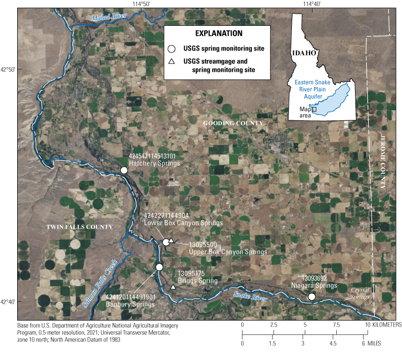
U.S. Geological Survey spring monitoring and streamgage sites using short names listed in table 1, south-central Idaho. Data from U.S. Geological Survey (2021).
Macrophyte growth is reducing habitat for the BSL and the BRS and may be related to elevated nutrient concentrations in spring water (U.S. Fish and Wildlife Service, 2017). The study springs are sourced by groundwater discharge from the Eastern Snake River Plain (ESRP) aquifer. Elevated nutrient concentrations in spring water are attributable to upgradient agricultural input (Skinner and Rupert, 2012). Previous efforts to monitor the springs’ water quality have been limited to periodic and opportunistic discrete sampling. The U.S. Fish and Wildlife Service (USFWS) and Idaho Power Company deployed water-temperature logging sensors as part of the BSL and BRS monitoring. Flooding occurred during February 9–12, 2017, in the area around the BSL- and BRS-populated springs. During February 10–12, 2017, the temperature loggers recorded an instantaneous decrease in water temperature of about 4 degrees Celsius (°C), which then slowly recovered to the original temperature (U.S. Fish and Wildlife Service, 2017). Subsequent BSL population surveys in Banbury Springs documented a substantial decline and the lowest density of BSL since monitoring began in 2008. The extent and duration of water-quality events like this vary by spring and throughout the year, making it difficult to identify when they may affect the snails and their habitats. More information collected throughout the year may support a better understanding of how nutrient concentrations and other water-quality parameters vary which may in turn affect the species and their habitats. Continuous water-quality monitoring would enable the USFWS to identify these events and their duration.
Continuous water-quality monitoring of some parameters such as water temperature and specific conductance is less expensive compared to continuous nitrate-concentration monitoring and discrete-sample collection and analysis. Less expensive water-quality parameters often are used as surrogates for other parameters using regression models (Helsel and others, 2020). However, the statistical relation between the parameters also should include a physical basis. In this case, specific conductance and nitrate concentrations in spring water are both related to upgradient agricultural input affecting the ESRP aquifer (Skinner and Rupert, 2012). This allows specific conductance to be evaluated as a surrogate for nitrate concentration. Continuous water-quality monitoring and surrogate regression models may provide a suitable method to evaluate the impact of water quality on the endangered BSL and threatened BRS.
Purpose and Scope
This report documents surrogate regression-model development at six springs in southern Gooding County, south-central Idaho, using linear regression models. The six springs in upstream-to-downstream order are: (1) Niagara Springs at Diversion Number 2 near Buhl (U.S. Geological Survey [USGS] site 13093692), (2) Briggs Springs near Buhl (USGS site 13095175), (3) Banbury Springs near Buhl (USGS site 424120114491901), (4) Box Canyon Springs near Wendell (USGS site 13095500), (5) Box Canyon Springs below aqueduct diversion near Wendell (USGS site 4242271144904), and (6) Hatchery Springs near Hagerman (USGS site 424547114513101) (fig. 1; U.S. Geological Survey, 2021). The springs are referred to with abbreviated site names throughout the report, as defined in table 1. The statistical regression models relate specific conductance to nitrate concentrations from 2018 to 2022 in spring water to determine if specific conductance can be used as a surrogate for nitrate concentration changes, providing the USFWS with less expensive method to determine nitrate concentrations compared to measuring nitrate concentrations directly.
Table 1.
Spring surrogate regression sites and their abbreviated site names, south-central Idaho.[See figure 1 for locations of sites. Data source: U.S. Geological Survey (2021)]
Specific conductance, streamflow, and nitrate concentrations fluctuate throughout the year in the springs, typically increasing from summer to late autumn and then decreasing until the following summer. The day of the year is evaluated as an explanatory variable in the surrogate regression models to account for the fluctuation of specific conductance and nitrate concentrations throughout the year. Two springs, Briggs Spring and Upper Box Canyon Spring, have existing USGS streamgages near the continuous water-quality measurement location, and hence streamflow also is evaluated as an explanatory variable in the surrogate regression models. Specific-conductance measurements at the six springs started during May 2018–November 2019, depending on the spring, and continued through December 2022. The discrete water-quality data used to build the surrogate regression models were measured monthly. Two springs, Briggs Spring and Niagara Springs, also have continuous specific-conductance, streamflow, and nitrate concentration data (monitored at 15- or 20-minute intervals) that were used to build the surrogate models for at least part of the period (Skinner, 2023).
Description of Study Area
The six springs are in canyons along the north side of the Snake River in southern Gooding County. The spring-monitoring locations are upstream from the endangered BSL and threatened BRS populations where possible. The springs’ water source is discharge from the ESRP aquifer. Groundwater in the ESRP aquifer moves from the northeast to the southwest (Rupert, 1997), discharging to the springs. The ESRP aquifer is a regional basalt aquifer that is composed primarily of a series of vesicular and fractured olivine basalt flows (Quaternary age) of the Snake River Group (Whitehead, 1992). These basalt flows average from 20 to 25 feet (ft) thick with a regional basalt aquifer estimated maximum thickness of about 6,300 ft (Twining and Bartholomay, 2011; Rupert and others, 2014). The top of the basalt generally is less than 100 ft below land surface. The layered basalt flows in the ESRP aquifer yield exceptionally large volumes of water to wells and springs.
Regional groundwater in the ESRP aquifer originates as good-quality, mountain-front recharge along the north margin of the ESRP or as recharge through undeveloped rangeland (Skinner and Rupert, 2012). Most of the land near the Snake River and overlying the downgradient parts of the ESRP aquifer is agricultural. Recharge through these agricultural lands acquires large amounts of nutrients from fertilizers and cattle manure, ultimately mixing with the regional groundwater before discharging to springs (Skinner and Rupert, 2012).
Methods
Continuous specific conductance data were measured at six springs along the north and northeastern side of the Snake River in southern Gooding County and paired with discrete nitrate-concentration samples to create surrogate regression models. The continuous data collection started during May 2018–November 2019, depending on the spring, and continued through December 2022 (table 2). The discrete nitrate-concentration samples were collected monthly at all six springs and two springs, Briggs Spring and Niagara Springs, also had continuous nitrate data measured starting in March 2019 and June 2021, respectively. Briggs and Upper Box Canyon Springs also have existing USGS streamgages, so streamflow also was evaluated in surrogate regression models at these springs. All continuous and discrete water-quality data are available in the USGS National Water Information System database (U.S. Geological Survey, 2021) and data used in the surrogate regression models also are available in the associated data release (Skinner, 2023).
Table 2.
Nitrate concentration surrogate regression models and explanatory variables and ranges at six springs, south-central Idaho.[See figure 1 for locations of sites. Data from Skinner (2023). day, day of the year; Nitrate, nitrate plus (+) nitrite as nitrogen concentrations in milligrams per liter (mg/L); mm-dd-yyyy, month, day, year (date range); n, number of observations; n/a, not applicable; Q, streamflow in cubic feet per second (ft3/s); SC, specific conductance in µS/cm (microsiemens per centimeter) at 25 degrees Celsius; USGS, U.S. Geological Survey; <, less than]
Continuous Water-Quality Monitoring
The six spring sites were instrumented to measure specific conductance at 15-minute intervals and two of the springs, Briggs and Niagara Springs, also had continuous nitrate sensors installed measuring nitrate concentrations every 20 minutes. Briggs and Upper Box Canyon Springs had the continuous water-quality sensors installed next to existing streamgages. Sondes at these two springs also continuously measured water temperature, dissolved oxygen, and pH at 15-minute intervals. The other four springs without streamgages had measurements of water depth concurrently with water temperature. Continuous sensor deployment, calibration, maintenance, and data reporting followed the methods described in Pellerin and others (2013) and Wagner and others (2006). These guidelines and procedures include site selection, routine sensor calibration, data corrections for drift and fouling, and evaluating data representation (that is, cross-section data corrections). Springs have very low sediment content, a major source of potential water-quality sensor fouling; hence, minimal fouling occurred. The continuous nitrate sensors measure nitrate plus nitrite and, therefore, are reported as nitrate plus nitrite as nitrogen concentrations (Pellerin and others, 2013). However, nitrite typically is not detected in spring water at these six sites so the nitrate plus nitrite as nitrogen concentrations represent nitrate concentrations, and hereinafter are referred to as just nitrate.
Discrete Water-Quality Data Collection
Water-quality sampling occurred monthly at the six spring sites and followed the protocols in the USGS National Field Manual for the Collection of Water-Quality Data (U.S. Geological Survey, [variously dated]). All discrete water-quality samples were analyzed by the USGS National Water Quality Laboratory (Denver, Colorado). Water-quality samples were collected as grab samples at the continuous measurement locations to optimize comparability. During each spring visit, field parameters were measured (water temperature, specific conductance, dissolved oxygen, and pH) and a nutrient sample was collected. The nutrient sample included analyses for ammonia (NH3 + NH4+) as nitrogen, nitrate plus nitrite as nitrogen, nitrite as nitrogen, and orthophosphate as phosphorus. Nitrate plus nitrite as nitrogen concentrations were used in the surrogate regression models and as verification data for the continuous nitrate concentration measurements. Nitrite concentrations are less than laboratory detection levels of 0.0010 milligrams per liter (mg/L) in 237 of the 273 (87 percent) samples from all six springs. The nitrate samples have an average nitrite concentration of 0.0024 mg/L and a maximum nitrite concentration of 0.0061 mg/L in the 36 samples with a nitrite detection. Considering the low nitrite concentrations (most are less than the detection limit), the nitrate plus nitrite concentrations effectively represent just nitrate concentration.
Quality Assurance and Quality Control
Quality assurance (QA) and quality control (QC) sequential replicate nutrient samples were collected to identify, quantify, and document variability in the nitrate concentration data resulting from collecting, processing, handling, and analyzing samples (Mueller and others, 2015). The QA/QC samples were collected following protocols described in the USGS National Field Manual for the Collection of Water-Quality Data (U.S. Geological Survey, [variously dated]). Five sequential replicate samples were collected at each of the six springs for a total of 30 nitrate concentration replicate samples. The relative percent difference (RPD) of the nitrate concentration replicates ranged from 0.01 to 4.43 percent, with a mean 1.11 percent RPD.
Continuous water-quality measurement followed the methods described in Pellerin and others (2013) and Wagner and others (2006), which prescribe criteria for water-quality meter calibration and data corrections. Continuous water-quality data corrections only are done when the cause(s) of data error(s) can be validated or explained as a data collection or monitor error such as fouling, calibration drift, and other errors explained by field personnel, field notes, comparison with other water-quality parameters at the spring, or information from nearby sites. For example, sondes at a couple of spring sites were slow to adjust to ambient water conditions after being pulled from the spring for calibration and maintenance; this recovery period was deleted. Data corrections are needed when a data error exceeds certain criteria. For continuously measured specific conductance, errors greater than the criteria of plus or minus (±) 5 microsiemens per centimeter or ± 3 percent of the measured value, whichever is greater, must be corrected (Wagner and others, 2006). However, the criteria can be reduced based on study needs, and because of the small range of continuously measured water-quality parameters at the six springs, data corrections were applied at a smaller criterion such as specific conductance errors being corrected at 2 percent of the measured value or less.
Nitrate concentrations from monthly grab samples and laboratory analysis as well as from continuous field measurements were included in the same surrogate regression models for Briggs Spring and Niagara Springs. Both measurement methods of nitrate concentration produce the same type of results (nitrate + nitrite as nitrogen), allowing laboratory nitrate concentrations to be used as bias corrections, such as biological fouling to the continuously measured nitrate concentrations as noted by Pellerin and others (2013). In the presence of both nitrate-measurement methods, the corrected continuous nitrate concentrations were used in the surrogate regression-model development. The two methods of nitrate concentration measurement were compared for the 52 coincident measurements at both springs, with an average difference of 0.01 mg/L, a minimum difference of 0.00 mg/L, and a maximum difference of 0.21 mg/L (fig. 2).
![Comparison of nitrate plus nitrite as nitrogen concentrations from grab sample and
laboratory analysis with continuous field measurements at Briggs Spring (U.S. Geological
Survey [USGS] site 13095175) and Niagara Springs (USGS site13093692) showing a near
one-to-one relation, south-central Idaho.](https://pubs.usgs.gov/sir/2023/5095/images/sir20235095_fig02.png)
Comparison of nitrate plus nitrite as nitrogen concentrations from grab sample and laboratory analysis with continuous field measurements at Briggs Spring (U.S. Geological Survey [USGS] site 13095175) and Niagara Springs (USGS site13093692), south-central Idaho. Data source: U.S. Geological Survey (2021).
Another correction typically applied to continuous water-quality measurements is a cross-section correction based on the variability of a water-quality parameter horizontally and vertically across the spring (Pellerin and others, 2013). Because the specific-conductance and nitrate-concentration measurements and nitrate samples are all collected from the same point location, cross-sectional variability does not affect data quality as related to the surrogate regression models. However, the incorporation of streamflow in two surrogate regression models (Briggs and Upper Box Canyon Springs) requires cross-sectional variability to be assessed and corrected if needed because streamflow is measured using the full cross-sectional area of a stream and not at a single location like the water-quality parameters. Five separate cross-sectional profiles of specific conductance were measured at Briggs Spring, and RPDs between these profiles and the corresponding point measurements ranged from 0.22 to 3.83 percent, with anveragee RPD of 1.36. These low RPD values reflect a good relation between specific-conductance point measurements and cross-sectional streamflow. Upper Box Canyon Springs cannot have cross sections measured because of extreme safety concerns; however, the water quality and streamgage location is just downstream from a waterfall, which likely causes good mixing resulting in a uniform distribution of water quality.
Regression Model Development
The surrogate regression models were developed using the Surrogate Analysis and Index Developer tool (SAID) (Domanski and others, 2015). The SAID tool relates surrogate explanatory variables to a response variable using ordinary least squares linear regression models. SAID provides several overall model summary statistics and observational diagnostic statistics using multiple plots, tabular data views, and output reports. To use ordinary least squares linear regression to develop surrogate models, the explanatory variables need to be matched with the response variables by time. SAID performs the time matching between the variables, allowing for a user-specified maximum time offset. A 5-minute maximum matching time difference was allowed to match the explanatory and response variables.
Ordinary least squares linear regression models require several assumptions, depending on the purpose of the regression (Helsel and others, 2020). Linear regression assumptions for the surrogate regression models are as follows:
-
• Response variable is linearly related to the surrogate variables,
-
• Surrogate variables are representative of the response variable,
-
• Variance of the residuals need to be constant (homoscedastic),
-
• Residuals are independent of the surrogate variables, and
-
• Residuals are normally distributed.
All surrogate model variables at the six springs have a periodic increase and decrease of specific conductance, streamflow, and nitrate concentrations throughout the year. The large fluctuations of these variables each year are related to upgradient agriculture (Skinner and Rupert, 2012). This is exemplified well at Briggs Spring because it has the longest measurement duration. Specific conductance and nitrate concentrations are highest from October to early November and lowest from April to July depending on the spring. Streamflow at Briggs and Upper Box Canyon Springs also peaks from October to early November and is lowest from April to June of each year (fig. 3). To account for the periodic nature of the variables, the day of the year was evaluated as an explanatory variable, using both the periodic functions sine and cosine of the day of the year.
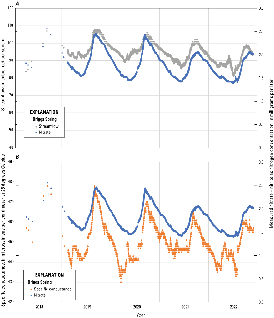
Graphs showing (A) streamflow and measured nitrate plus (+) nitrite as nitrogen concentrations and (B) specific conductance and measured nitrate + nitrite as nitrogen concentrations, at Briggs Spring (U.S. Geological Survey site 13095175), south-central Idaho, 2018–22. Data source: U.S. Geological Survey (2021).
The surrogate regression models were evaluated based on overall model-fit statistics, the coefficient of determination (R2 and adjusted R2 if more than one explanatory variable was used) and the F-statistic compared to constant model and corresponding probability value (p-value). The explanatory variables’ individual p-values also were evaluated to confirm the significance of each explanatory variable within the surrogate regression model and the Prediction Error Sum of Squares (PRESS) statistic was used to compare alternate regression models at the same spring using different explanatory variables (Helsel and others, 2020). The surrogate regression model with the lowest PRESS statistic produces the least error when using the surrogate regression model to make predictions.
Observational diagnostic statistics provided by SAID were used to identify outliers and individual data values with a high influence on the surrogate regression model. Observation diagnostics include residual plots, leverage, and the influence statistics: Cook’s D and DFFITS (difference in fit) (Helsel and others, 2020). Removal of outliers identified by residual, leverage, and influence statistics alone may overestimate the certainty of the surrogate regression models (Helsel and others, 2020, Stone and Klager, 2022); therefore, it is important to consider whether each outlier represents an error or a rare but real event.
Nitrate Surrogate Regression Model Results
Specific conductance and day of the year were evaluated as explanatory variables in surrogate regression models to estimate nitrate concentrations at six springs. The surrogate regression models relate specific conductance to nitrate concentrations from 2018 to 2022 in spring water to determine if specific conductance can be used as a surrogate for nitrate concentration. To determine if streamflow data could improve the surrogate model results, streamflow from existing streamgages located at two of the springs also was evaluated in those surrogate models.
Observational diagnostic statistics (residuals, leverage, and the influence statistics—Cook’s D and DFFITS) were used to identify data with excessive influence on surrogate model fit. These outliers were evaluated to determine if the influence is data variability or an error. Review of the springs’ surrogate regression models identified data with elevated residuals, leverage, and influence in the surrogate regression models using only laboratory-analyzed nitrate concentrations. These models were used at Banbury, Upper Box Canyon, Lower Box Canyon, and Hatchery Springs. The surrogate models at these sites identified the December 7, 2021 data points as having a large residual, leverage, and influence on the corresponding surrogate models. This outlier was related to laboratory-measured nitrate concentrations and specific-conductance concentrations measured with one specific field sonde. The December 2, 2021 combination-nitrate concentration and specific-conductance data did not match surrounding temporal measurements, indicating that the data were unduly influenced by nitrate sampling and laboratory error and field-specific conductance measurements with a single specific sonde. The Banbury Spring nitrate concentration on March 11, 2021 was substantially lower than all other nitrate values and seemed to be a sample-labelling error or laboratory mix-up with Hatchery Springs, which had identical sample results. The two springs using mean monthly nitrate concentrations from the continuous sensors did not have any observations removed from the surrogate regression models.
Overall Model Summary Results
Specific conductance, day of the year, and streamflow, where available, were able to model nitrate concentrations in various combinations for four of the six springs. The two springs with streamgages (Briggs and Upper Box Canyon Springs) included streamflow as an additional explanatory variable. The surrogate regression models and their explanatory variables and ranges are listed in table 2, and the model statistic results are listed in table 3. The springs farthest to the east have the most upgradient agricultural input, and springs to the west have the least upgradient agricultural input. This relation is indicated by decreasing specific conductance and nitrate concentrations from the eastern to western springs (table 2). The adjusted R2 (R2 if only one explanatory variable) surrogate regression summary statistics for the models range from 0.15 to 0.94. Surrogate regression models performed well at four of the six springs considering all of the diagnostic statistical results.
Table 3.
Nitrate concentration surrogate regression model results at six springs, south-central Idaho.[See figure 1 for locations of sites. Data from Skinner (2023). Models in bold represent the best surrogate regression model at that spring. Root mean squared error is in units of milligrams per liter nitrate concentration. day, day of the year; n/a, not applicable; Nitrate, nitrate plus (+) nitrite as nitrogen concentrations in milligrams per liter; Q, streamflow in cubic feet per second; p-value, probability value; R2, coefficient of determination; SC, specific conductance in µS/cm (microsiemens per centimeter) at 25 degrees Celsius; USGS, U.S. Geological Survey; <, less than]
The two springs with streamflow available as an explanatory variable in the surrogate regression models (Briggs and Upper Box Canyon Springs) resulted in the best surrogate regression models with adjusted R2 surrogate regression summary statistic values of 0.94 and 0.89, and low PRESS values of 0.51 and 0.48 respectively. The root mean squared error or standard error of the regression (table 3) provides the average model error in units of the response variable (nitrate concentration) and ranges from 0.05 to 0.23 mg/L for all the surrogate regression models. The surrogate regression models for the six springs all have a probability plot correlation coefficient greater than or equal to 0.84 indicating normality of residuals, which is one of the required assumptions necessary for linear regression. Along with the probability plot correlation coefficients, the probability plots themselves were visually evaluated to confirm normality or residuals. All of the surrogate regression models except for one of the Banbury Springs surrogate regression models have p-values of less than 0.01 for the overall surrogate regression model F-tests, indicating that the regression relations are statistically significant and not due to chance.
Observational Diagnostic Model Results
Individual observation diagnostic statistics support the assumptions required for linear regression models. The observational diagnostic statistics were evaluated for all of the surrogate regression models and are available in the related data release (Skinner, 2023). Some of the surrogate regression model assumptions were partially or completely invalid and required changes to the models. These linear regression assumption issues are discussed and exemplified in the paragraphs that follow.
Plots of the explanatory variables and measured nitrate concentrations help us evaluate if the required linear relation exists between them. Upper and Lower Box Canyon Springs are good examples in that the linear relation between specific conductance and nitrate concentrations change through time. Both Upper and Lower Box Canyon Springs have a flat or nonlinear relation between specific conductance and nitrate concentrations between specific conductance values of 403 to 410 microsiemens per centimeter (µS/cm) at 25 °C. From 410 µS/cm to the maximum specific conductance value of 431 µS/cm at 25 °C, as specific conductance values increase, nitrate concentration also increases signifying the required linear relation (fig. 4).
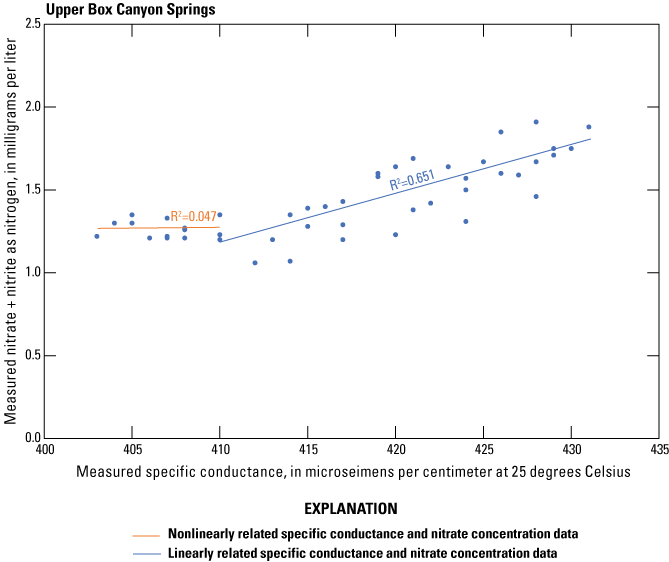
Relation of specific conductance to nitrate concentration at Upper Box Canyon Springs (U.S. Geological Survey site 13095500), south-central Idaho. Flat horizontal line indicates data with a nonlinear relation and upward slanting line indicates data with a linear relation. R2, coefficient of determination. Data from Skinner (2023).
Plots of surrogate regression model residuals with time are used to evaluate serial correlation and determine if the model varies with time. Serial correlation is identified when nearby samples (nearby in time for this study) are similar and correlated with each other. This is identified in plots of surrogate regression model residuals with time whereby points tend to follow each other and form a pattern. The Briggs Springs residual compared to time plot from the surrogate regression model (using the continuously measured explanatory variables) shows the presence of serial correlation and that nearby points in time have similar residuals (fig. 5A). However, the surrogate regression model using the monthly mean explanatory variables shows that the serial correlation has been minimized or removed (fig. 5B).
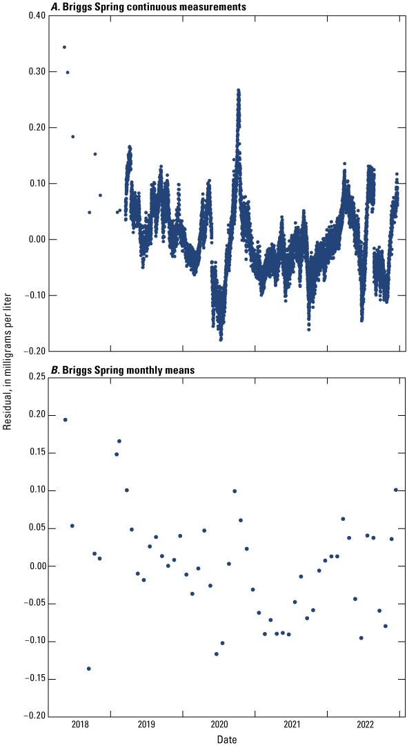
Surrogate regression model residuals using explanatory variables with (A) continuous measurements and (B) monthly means at Briggs Spring (U.S. Geological Survey site 13095175), south-central Idaho, 2018–22. Data from Skinner (2023).
The Banbury Springs residual compared to time plot (fig. 6) indicates a possible residual trend over time or a step change, starting in autumn 2021, that shows more negative residuals. A surrogate regression model with trending residuals invalidates an assumption for linear regression models and weakens the model’s ability to predict values.
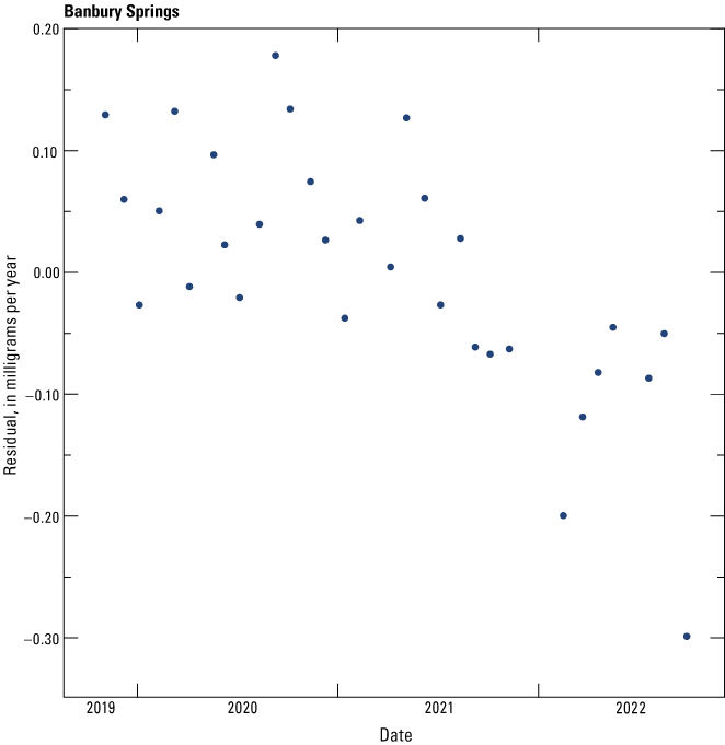
Surrogate regression model residuals at Banbury Springs (U.S. Geological Survey site 424120114491901), south-central Idaho, 2019–22. Data from Skinner (2023).
Plots of predicted nitrate concentrations and their residuals (difference between the observed and predicted nitrate concentrations) in the surrogate regression model were used to identify the presence of heteroscedasticity and curvature (Helsel and others, 2020). All of the surrogate regression models show fairly uniform variance or homoscedasticity, as exemplified by Lower Box Canyon Springs in figure 7.
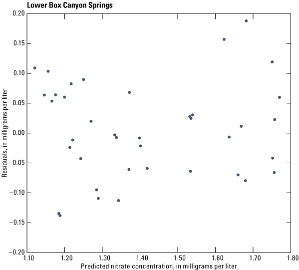
Surrogate regression modeled nitrate concentration and residuals at Lower Box Canyon Springs (U.S. Geological Survey site 4242271144904), south-central Idaho. Data from Skinner (2023).
Individual Surrogate Regression Model Results
Banbury Springs
The Banbury Springs surrogate regression models have a poor linear relation between specific conductance and nitrate concentration, resulting in a surrogate regression model not following a required assumption for linear regression. The surrogate regression model with only the day of the year explanatory variables produces reasonable results; however, a plot of residuals over time indicates that a decreasing nitrate concentration trend may be starting in 2021 that will weaken the surrogate regression model if the trend continues and is not accounted for with additional explanatory variables.
Upper Box Canyon Springs
The Upper Box Canyon Springs surrogate regression model has a linear relation between specific conductance and nitrate concentrations for specific conductance values starting at 410 µS/cm. At specific conductance values less than 410 µS/cm, nitrate concentrations and specific conductance do not have a linear relation. If the specific conductance values less than 410 µS/cm are excluded from the surrogate regression models, then the resulting models meet required assumptions and produce acceptable results. Upper Box Canyon Springs has two surrogate regression models that are considered the best models, both of which use specific conductance and streamflow as explanatory variables and one of which also includes day of the year. Both of these models exclude specific conductance values less than 410 µS/cm. The surrogate regression model using only specific conductance and streamflow has very similar overall model diagnostics but a better individual variable p-value for specific conductance than the surrogate regression model including day of the year. The surrogate regression model including day of the year has slightly better overall model diagnostics (especially a lower PRESS value) than the surrogate regression model without day of the year. However, the individual variable p-value for specific conductance is 0.08 (table 3), just less than the 95-percent confidence interval.
Lower Box Canyon Springs
Like Upper Box Canyon Springs, the surrogate regression model for Lower Box Canyon Springs has a poor linear relation between specific conductance and nitrate concentrations for specific conductance values less than 410 µS/cm. The surrogate regression model for Lower Box Canyon Springs using only the explanatory variable specific conductance and excluding values less than 410 µS/cm produces the best surrogate regression model using specific conductance as an explanatory variable for this spring. This is the only model at this spring with a specific conductance p-value less than 0.05. This surrogate regression model also has a good PRESS value of 0.59 which is higher than the other surrogate regression models (table 3). The best overall surrogate regression model has explanatory variables day of the year and specific conductance excluding values less than 410 µS/cm. This model has the best adjusted R2 values of 0.86 and PRESS value of 0.47; however, the p-value for specific conductance is 0.20, indicating only 80-percent confidence in specific conductance for the model (table 3).
Briggs Spring
Evaluations of surrogate regression models at Briggs Spring included streamflow from an existing USGS streamgage. All the explanatory variables were reduced to monthly means to minimize serial correlation. Each combination of explanatory variables produced good surrogate regression models based on the statistical evaluations. The adjusted R2, root mean squared error, and PRESS statistic all indicate that the surrogate regression model (including all of the explanatory variables) produces the smallest predicted error, making this the best model for Briggs Spring. However, this model is only slightly better than the other surrogate regression models at this spring.
Niagara Spring
Like Briggs Spring, Niagara Spring had the explanatory variables reduced to monthly means to minimize serial correlation. The surrogate regression models using the specific conductance and both specific conductance and day of the year as explanatory variables resulted in good surrogate regression models based on statistical evaluations. The surrogate regression model including both specific conductance and day of the year is a slightly better model than the model solely using specific conductance, based on the R2 and adjusted R2 values and PRESS statistic.
Hatchery Spring
Hatchery Spring does not have a linear relation between specific conductance and nitrate concentrations, which invalidates a main assumption for linear regression modeling. The lack of a linear relation between specific conductance and nitrate concentrations also is reflected in the poor R2 and adjusted R2 values for the surrogate regression models.
Discussion
The habitats of endangered BSL and threatened BRS in springs north of the Snake River are hypothesized to be declining because of increased macrophyte growth associated with elevated nitrate concentrations. Monitoring nitrate concentrations by discrete sampling often can miss sudden changes or peaks in concentrations and continuous monitoring of nitrate is not always possible. However, surrogate regression models using continuously monitored specific conductance may allow monitoring of continuous nitrate concentration in these springs.
The springs provide an optimum environment for continuous monitoring of specific conductance because they have little sediment content, which typically causes fouling for deployed water-quality sensors. The springs also have annual increases and decreases of streamflow, specific conductance, and nitrate concentration attributable to upgradient agriculture influence (fig. 3). This variation in explanatory variable values is needed for regression modeling and allows for the development of surrogate models in the springs with the most agriculture influence. The spring (Hatchery Springs) with fairly constant nutrient concentrations (0.81–1.10 mg/L) attributable to little upgradient agriculture input had the poorest surrogate regression model results partly because specific conductance also showed little variation (318–341 µS/cm at 25 ° C; table 2). The explanatory variable data were collected over 3–4.5 years depending on the spring (table 2).
The lack of linearity between the explanatory variables and nitrate concentrations prevents a surrogate regression model. The lack of a linear relation between specific conductance and nitrate concentrations also prevents surrogate regression model development at Banbury Springs even with variation amongst other variable values. Upper and Lower Box Canyon Springs both have a nonlinear relation between specific conductance and nitrate concentrations at specific conductance values less than 410 µS/cm at 25 °C; however, the relation is linear at values greater than this so the surrogate regression models at these two springs are limited to specific conductance values greater than or equal to 410 µS/cm at 25 °C. Continuous nitrate concentration data were available at Briggs and Niagara Springs; however, these data led to serial correlation, which was minimized by using the monthly mean of all variables for the surrogate regression models at these two springs.
Niagara, Briggs, and Upper and Lower Box Canyon Springs all have surrogate regression models using specific conductance and day of the year as explanatory variables that performed well based on model summary statistics. The inclusion of streamflow as an explanatory variable, which is only available at Briggs and Upper Box Canyon Springs, improved the surrogate regression models. Upper and Lower Box Canyon Springs also have well-performing surrogate regression models using only specific conductance and streamflow (at Upper Box Canyon Springs). Observational diagnostic results for the surrogate regression models were evaluated to identify outliers, to verify that the linear regression assumptions were met, and to determine how the models performed over time. Observation residual plots over time indicate that the surrogate models performed uniformly over time, except for Banbury Springs, indicating a decreasing trend starting in autumn 2021 (fig. 6). Future sampling of nitrate in the springs may support continued validation of the surrogate regression models.
Summary
The U.S. Geological Survey (USGS) developed surrogate regression models to estimate nitrate concentrations in springs near the Snake River in southern Gooding County, south-central Idaho. The surrogate regression equations may assist in U.S. Fish and Wildlife Service efforts to understand declines in endangered Banbury Springs limpet (Idaholanx fresti) and threatened Bliss Rapids snail (Taylorconcha serpenticola) populations. The Banbury Springs limpet and Bliss Rapids snail habitats may be shrinking because of increased macrophyte growth likely related to elevated nitrate concentrations. The USGS developed surrogate regression models using specific conductance as a surrogate for nitrate concentration to estimate nitrate concentrations.
Surrogate regression models were developed at six springs: (1) Niagara Springs at Diversion Number 2 near Buhl (USGS site 13093692), (2) Briggs Springs near Buhl (USGS 13095175), (3) Banbury Springs near Buhl (USGS 424120114491901), (4) Box Canyon Springs near Wendell (USGS 13095500), (5) Box Canyon Springs below aqueduct diversion near Wendell (USGS 4242271144904), and (6) Hatchery Springs near Hagerman (USGS 424547114513101). Surrogate regression models were developed at all six springs using various combinations of explanatory variables including specific conductance, day of the year, and streamflow (available at Briggs and Upper Box Canyon Springs, USGS sites 13095175 and 13095500, respectively) to estimate nitrate concentrations.
Surrogate regression models were developed at four of the six springs (Niagara, Briggs, and Upper and Lower Box Canyon Springs) that performed well based on model summary statistics. The surrogate regression models used specific conductance, day of the year, and streamflow (available only at Briggs and Upper Box Canyon Springs) as explanatory variables. Upper and Lower Box Canyon Springs also had surrogate regression models that performed well without day of the year as an explanatory variable. The surrogate regression models at these four springs had adjusted coefficient of determination (R2) values (R2 values if only one explanatory variable) of 0.82–0.89, with the model for Hatchery Springs having an R2 value of 0.48. The two surrogate regression models that included streamflow as an additional explanatory variable (Briggs and Upper Box Canyon Springs) had R2 values of 0.79–0.94. The root mean squared error, which provides the average model error, ranged from 0.07 to 0.11 milligrams per liter. One surrogate regression model at Banbury Springs performed well based on summary statistics; however, the model only includes day of the year as an explanatory variable and the residual compared to time plot indicates a possible trend starting in 2021 that weakens the surrogate regression model. No surrogate regression models produced good results at Hatchery Springs because of nonlinearity between the explanatory variables and nitrate concentrations.
The surrogate regression models were able to model nitrate concentrations in springs with upgradient agricultural input. We improved surrogate regression model performance at two springs by including streamflow with specific conductance and day of the year.
References Cited
Domanski, M.M., Straub, T.D., and Landers, M.N., 2015, Surrogate Analysis and Index Developer (SAID) tool (ver. 1.0, September 2015): U.S. Geological Survey Open-File Report 2015–1177, 38 p. [Also available at https://doi.org/10.3133/ofr20151177.]
Helsel, D.R., Hirsch, R.M., Ryberg, K.R., Archfield, S.A., and Gilroy, E.J., 2020, Statistical methods in water resources: U.S. Geological Survey Techniques and Methods, book 4, chap. A3, 458 p. [Supersedes USGS Techniques of Water-Resources Investigations, book 4, chap. A3, version 1.1.] [Also available at https://doi.org/10.3133/tm4A3.]
Mueller, D.K., Schertz, T.L., Martin, J.D., and Sandstrom, M.W., 2015, Design, analysis, and interpretation of field quality-control data for water-sampling projects: U.S. Geological Survey Techniques and Methods, book 4, chap. C4, 54 p. [Also available at https://doi.org/10.3133/tm4C4.]
Pellerin, B.A., Bergamaschi, B.A., Downing, B.D., Saraceno, J.F., Garrett, J.A., and Olsen, L.D., 2013, Optical techniques for the determination of nitrate in environmental waters—Guidelines for instrument selection, operation, deployment, maintenance, quality assurance, and data reporting: U.S. Geological Survey Techniques and Methods 1–D5, 37 p. [Also available at https://doi.org/10.3133/tm1D5.]
Rupert, M.G., 1997, Nitrate (NO2 + NO3 – N) in ground water of the upper Snake River Basin, Idaho and western Wyoming, 1991–95: U.S. Geological Survey Water-Resources Investigations Report 97–4174, 47 p. [Also available at https://doi.org/10.3133/wri974174.]
Rupert, M.G., Hunt, C.D., Jr., Skinner, K.D., Frans, L.M., and Mahler, B.J., 2014, The quality of our Nation’s waters—Groundwater quality in the Columbia Plateau and Snake River Plain basin-fill and basaltic-rock aquifers and the Hawaiian volcanic-rock aquifers, Washington, Idaho, and Hawaii, 1993–2005: U.S. Geological Survey Circular 1359, 88 p., [Also available at https://doi.org/10.3133/cir1359.]
Skinner, K.D., 2023, Surrogate regression model data for estimating nitrate concentrations at six springs in Gooding County, south-central, Idaho: U.S. Geological Survey data release, https://doi.org/10.5066/ P9BXIBF9.
Skinner, K.D., and Rupert, M.G., 2012, Numerical model simulations of nitrate concentrations in groundwater using various nitrogen input scenarios, mid-Snake region, south-central Idaho: U.S. Geological Survey Scientific Investigations Report 2012–5237, 30 p. [Also available at https://doi.org/10.3133/sir20125237.]
Stone, M.L., and Klager, B.J., 2022, Documentation of models describing relations between continuous real-time and discrete water-quality constituents in the Little Arkansas River, south-central Kansas, 1998–2019: U.S. Geological Survey Open-File Report 2022–1010, 34 p., [Also available at https://doi.org/10.3133/ofr20221010.]
Twining, B.V., and Bartholomay, R.C., 2011, Geophysical logs and water-quality data collected for boreholes Kimama-1A and -1B, and a Kimama water supply well near Kimama, southern Idaho: U.S. Geological Survey Data Series 622 (DOE/ID 22215), 18 p., plus app. [Also available at https://pubs.usgs.gov/ds/622/.]
U.S. Fish and Wildlife Service, 2018a, Banbury Springs limpet (Lanx n sp.)(undescribed), 5-year review—Summary and evaluation: U.S. Fish and Wildlife Service, Idaho Fish and Wildlife Office, 40 p. [Also available at https://www.fws.gov/node/65346.]
U.S. Fish and Wildlife Service, 2018b, Bliss Rapids snail (Taylorconcha serpenticola), 5-year review—Summary and evaluation. U.S. Fish and Wildlife Service, Idaho Fish and Wildlife Office, 43 p. [Also available at https://www.fws.gov/node/65342.]
U.S. Geological Survey, 2021, USGS water data for the Nation: U.S. Geological Survey National Water Information System database. [Also available at https://doi.org/10.5066/F7P55KJN.]
U.S. Geological Survey, [variously dated], National field manual for the collection of water- quality data: U.S. Geological Survey Techniques of Water-Resources Investigations, book 9, chaps. A1–A10. [Also available at https://pubs.water.usgs.gov/twri9A.]
Wagner, R.J., Boulger, R.W., Jr., Oblinger, C.J., and Smith, B.A., 2006, Guidelines and standard procedures for continuous water-quality monitors—Station operation, record computation, and data reporting: U.S. Geological Survey Techniques and Methods 1–D3, 51 p. + 8 attachments. [Also available at https://pubs.water.usgs.gov/tm1d3.]
Whitehead, R.L., 1992, Geohydrologic framework of the Snake River Plain regional aquifer system, Idaho and eastern Oregon: U.S. Geological Survey Professional Paper 1408–B, 32 p., 6 pls. [Also available at https://doi.org/10.3133/pp1408B.]
Conversion Factors
Supplemental Information
Specific conductance is given in microsiemens per centimeter at 25 degrees Celsius (µS/cm at 25 °C).
Concentrations of chemical constituents in water are given in milligrams per liter (mg/L).
Abbreviations
BRS
Bliss Rapids snail (Taylorconcha serpenticola)
BSL
Banbury Springs limpet (Idaholanx fresti)
ESRP
Eastern Snake River Plain
p-value
probability value
PRESS
Prediction Error Sum of Squares
QA
quality assurance
QC
quality control
R2
coefficient of determination
RPD
relative percent difference
SAID
Surrogate Analysis and Index Developer tool
USFWS
U.S. Fish and Wildlife Service
USGS
U.S. Geological Survey
For more information about the research in this report, contact
Director, Idaho Water Science Center
U.S. Geological Survey
230 Collins Road
Boise, Idaho 83702-4520
https://www.usgs.gov/centers/idaho-water-science-center
Manuscript approved on July 21, 2023
Publishing support provided by the U.S. Geological Survey
Science Publishing Network, Tacoma Publishing Service Center
Disclaimers
Any use of trade, firm, or product names is for descriptive purposes only and does not imply endorsement by the U.S. Government.
Although this information product, for the most part, is in the public domain, it also may contain copyrighted materials as noted in the text. Permission to reproduce copyrighted items must be secured from the copyright owner.
Suggested Citation
Skinner, K.D., 2023, Surrogate regression models estimating nitrate concentrations at six springs in Gooding County, south-central Idaho, 2018–22: U.S. Geological Survey Scientific Investigations Report 2023–5095, 22 p., https://doi.org/10.3133/sir20235095.
ISSN: 2328-0328 (online)
Study Area
| Publication type | Report |
|---|---|
| Publication Subtype | USGS Numbered Series |
| Title | Surrogate regression models estimating nitrate concentrations at six springs in Gooding County, south-central Idaho, 2018–22 |
| Series title | Scientific Investigations Report |
| Series number | 2023-5095 |
| DOI | 10.3133/sir20235095 |
| Publication Date | August 31, 2023 |
| Year Published | 2023 |
| Language | English |
| Publisher | U.S. Geological Survey |
| Publisher location | Reston, VA |
| Contributing office(s) | Idaho Water Science Center |
| Description | Report: vii, 22 p.; Data Release |
| Country | United States |
| State | Idaho |
| County | Gooding County |
| Online Only (Y/N) | Y |