

Groundwater Flow Model Investigation of the Vulnerability of Water Resources at Chaco Culture National Historical Park Related to Unconventional Oil and Gas Development
Links
- Document: Report (3.51 MB pdf) , HTML , XML
- Data Release: USGS data release - MODFLOW-2005 and MODPATH models in support of groundwater flow model investigation of water resources at Chaco Culture National Historical Park: U.S. Geological Survey data release
- NGMDB Index Page: National Geologic Map Database Index Page (html)
- Download citation as: RIS | Dublin Core
Acknowledgments
This work was funded through the U.S. Geological Survey (USGS)-National Park Service Water Quality Program. The work was made possible with help from the Navajo Nation and assistance from USGS technicians. This work was also significantly improved by the suggestions of reviewers.
Abstract
Chaco Culture National Historical Park (CCNHP), located in northwestern New Mexico, protects the greatest concentration of Chacoan historical sites in the American Southwest. Geologically, CCNHP is located within the San Juan structural basin, which consists in part of complex Cretaceous stratigraphy and hosts a variety of energy resources. As part of a larger study to investigate the vulnerability of water resources at CCNHP related to oil and natural gas extraction activities, a MODFLOW groundwater model of the Mancos Shale and Gallup Sandstone units was created by the U.S. Geological Survey, as a part of a cooperative study with the National Park Service, to assess advective groundwater flow paths and traveltimes. The model determined that groundwater flow directions currently trend from south-southeast to north-northwest within the vicinity of CCNHP, groundwater traveltime through the Gallup Sandstone ranges from thousands to tens of thousands of years, and traveltime through the Mancos Shale may range from millions to tens of millions of years. The capture zone of the main CCNHP well (referred to as the “Chaco well”) extends to the south-southeast and ranges in width from approximately 1 to 12 miles, depending on pumping rate. Eighteen inactive hydrocarbon related wells are located within the capture zone and within 10 kilometers of the Chaco well. Given model estimates of traveltimes of groundwater in the Gallup Sandstone aquifer, advective groundwater transport to the Chaco well would take approximately 430 years from the nearest inactive hydrocarbon related wells. Differencing of historical and modern-day potentiometric surfaces of the Gallup Sandstone indicate a drop in groundwater levels between 34 and 96 feet within the CCNHP boundaries. Hydraulic fracturing, simulated as increased hydraulic conductivity zones, decreased groundwater traveltimes (from millions to thousands of years) and acted as permeable pathways from the Mancos Shale to the Gallup Sandstone.
Introduction
Chaco Culture National Historical Park (CCNHP) is in the Four Corners region of the United States in northwestern New Mexico (fig. 1) and preserves a major center of Ancestral Puebloan culture dating between 850 and 1250 A.D. CCNHP covers an area of approximately 53 square miles, and within CCNHP, the National Park Service (NPS) protects over 4,000 sites, which is the greatest concentration of Chacoan historical sites in the American Southwest (NPS, 2015). Today, CCNHP is a United Nations Educational, Scientific, and Cultural Organization (UNESCO) World Heritage Site as well as an important ceremonial site for the Navajo and Pueblo peoples. The park attracts approximately 60,000 visitors per year, many of whom stay overnight in the park campgrounds. Geologically, the park is located within the San Juan structural basin, a Late Cretaceous-Paleogene age structural depression on the eastern edge of the Colorado Plateau that hosts a variety of energy resources, including oil and natural gas, uranium, and coal (Stone and others, 1983). Major aquifers in the region include generally confined sandstones of Paleogene, Cretaceous, and Jurassic age (Stone and others, 1983). The NPS constructed a 3,100-foot (ft)-deep well (referred to hereafter as the “Chaco well”) into the Cretaceous Gallup Sandstone aquifer (fig. 2) in 1972 to provide the park with its first reliable drinking water source, following unsuccessful attempts to develop usable near-surface water sources (Colleen Filippone, National Park Service, oral commun., 2018). In the subsurface beneath CCNHP, the 100- to 200-ft-thick Gallup Sandstone is stratigraphically located between thick confining sequences of lower-permeability Mancos Shale. The Mancos Shale and Gallup Sandstone have been subject to both conventional and unconventional oil and gas development, including hydraulic fracturing (HF) (Engler and others, 2015). This study by the U.S. Geological Survey (USGS), in cooperation with NPS, was initiated largely in response to growing public concern about how current and future oil and gas development may negatively influence the drinking water source at CCNHP. The study is complemented by a geochemical analysis of groundwater age, groundwater flow directions, and potential mixing between aquifers (Linhoff and others, 2023).
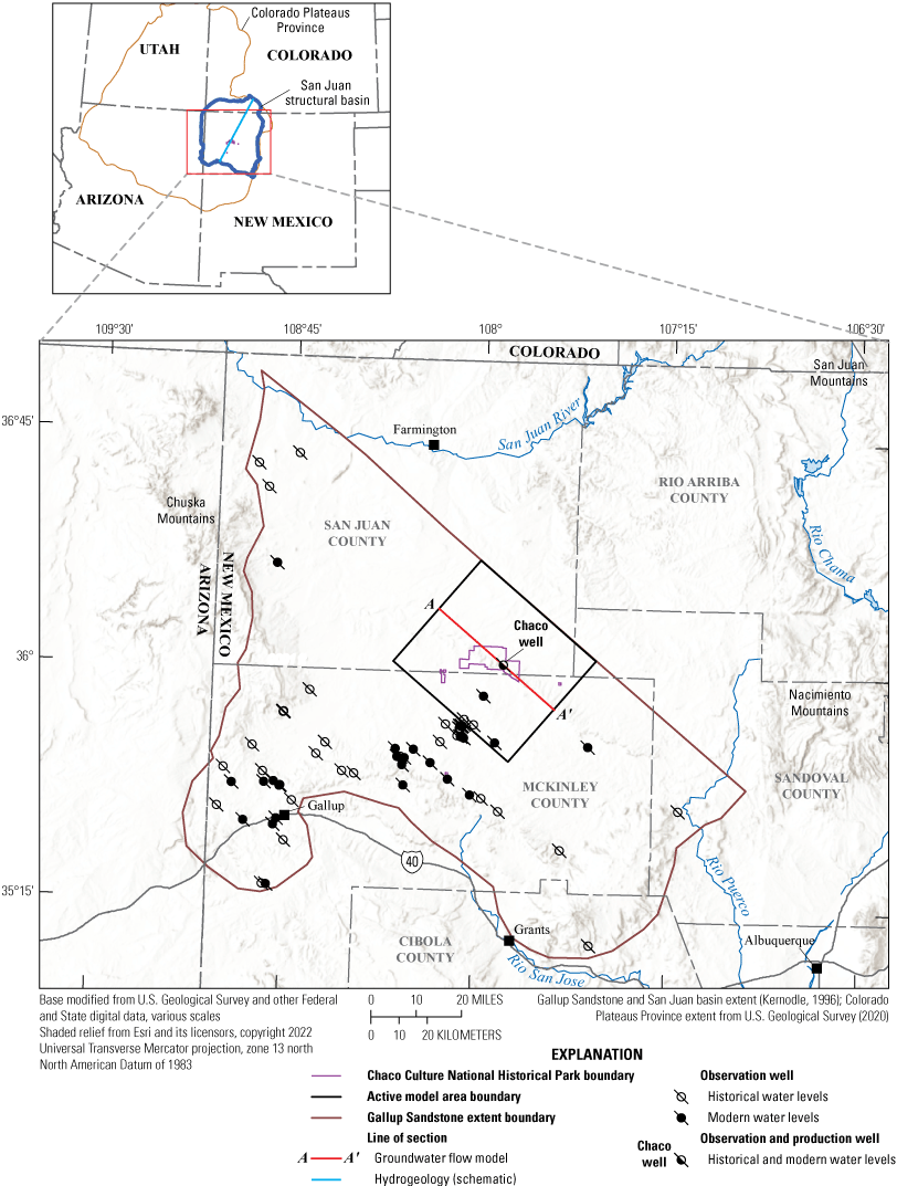
Study area, plan view of the active groundwater flow model area, and groundwater level observation points used in model calibration and potentiometric surface development. The Gallup Sandstone extent map unit represents the surface and subsurface extent of the unit.
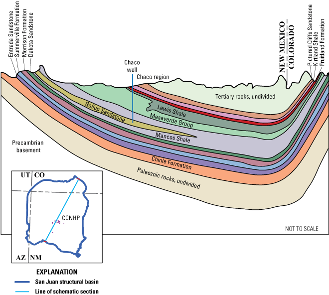
Schematic geologic cross section of the San Juan structural basin (modified from Stone and others, 1983). CCNHP, Chaco Culture National Historical Park.
This study involved (1) the development of a MODFLOW numerical groundwater model to assess groundwater flow directions and traveltimes through the Gallup Sandstone and Mancos Shale surrounding the CCNHP and (2) the creation of potentiometric surfaces in the Gallup Sandstone to assess groundwater drawdown within the water bearing unit in the vicinity of CCNHP. Model results are presented to delineate the area contributing flow to the Chaco well from the source area (otherwise known as the capture zone), assess groundwater travel-times of captured water, and develop simple scenarios simulating potential future oil and gas development. These tools and analyses are needed to inform the NPS about the susceptibility of the drinking water supply at CCNHP to potential contamination of HF fluids and depletion of water through water extraction. This work may serve as a template for studies examining drinking water resources that are susceptible to contamination in oil and gas producing areas.
Purpose and Scope
This report documents the investigation of the vulnerability of water resources at CCNHP related to unconventional oil and gas development. Specifically, the report documents the following:
-
1. creation of updated potentiometric surfaces of the Gallup Sandstone to inform the groundwater model and to assess the change in hydraulic head (head) between historical and modern timeframes;
-
2. development of a numerical model to assess groundwater flow directions in the region; and
-
3. application of the model and simulations, including
-
a. delineation of the area contributing flow to the Chaco well from the source area (the capture zone);
-
b. estimation of advective groundwater flow traveltimes of water captured by the Chaco well; and
-
c. simulation of potential influence of HF by altering hydraulic conditions in the Mancos Shale to evaluate the effect on particle pathways, traveltimes, and potential influence on the Chaco well.
-
Hydrogeologic Framework
The San Juan structural Basin has been studied for over a century, and major hydrogeologic framework summaries of the San Juan structural basin include Stone and others (1983), Kernodle (1996), and Craigg (2001). The San Juan structural basin is an asymmetric, structural depression located primarily in the east-central portion of the Colorado Plateaus Province (fig. 1), and the regional aquifer is the part of the structural basin that contains rocks of Triassic through Paleogene age (Craigg, 2001). The Chaco well is screened within the Cretaceous Gallup Sandstone, which is stratigraphically located between two tongues of lower-permeability Mancos Shale, both Cretaceous in age (fig. 2). San Juan structural Basin Cretaceous stratigraphy is complex, consisting of sedimentary deposits from the Western Interior Seaway that formed between about 100 and 65 million years ago (Stone and others, 1983). Other Cretaceous units overlying the Mancos Shale include parts of the Mesaverde Group, including the Cliff House Sandstone of Mesaverde Group (hereafter “Cliff House Sandstone”), the Menefee Formation of Mesaverde Group (hereafter “Menefee Formation”), and the Point Lookout Sandstone of Mesaverde Group (hereafter “Point Lookout Sandstone”) (fig. 2). The Mancos Shale is underlain by Jurassic sedimentary deposits, and it intertongues with the Dakota Sandstone.
The Gallup Sandstone is generally a fine- to medium-grained lithic arkose that ranges in thickness from 93 to 700 ft, pinching out to the northeast (fig. 1). The northeastern extent of the Gallup Sandstone coincides with the northeastern groundwater-model boundary. The Mancos Shale consists of gray to black shale and claystone, with discontinuous calcareous siltstone and sandstone. The main body of the Mancos Shale in the northern part of the basin reaches a maximum thickness of about 2,300 ft (Stone and others, 1983). In the vicinity of CCNHP, the Gallup Sandstone and Mancos Shale both generally dip to the northeast and range in thickness from 100 to 200 ft and from 600 to 1,300 ft, respectively. Recharge to the Gallup Sandstone generally occurs where the unit crops out to the south of CCNHP, although it has been noted that leakage may occur locally between adjacent Cretaceous units (Stone and others, 1983). Mixing between the Gallup Sandstone aquifer and surrounding units was confirmed by Linhoff and others (2023). Wells in the region are commonly under pressure, meaning there are artesian and free flowing wells. At least three artesian wells screened in the Gallup Sandstone south of CCNHP within the modeled domain are currently free flowing at the surface (Linhoff and others, 2023).
Oil and Gas Development in the San Juan Structural Basin
Oil and gas were originally discovered in the San Juan structural Basin around 1910 (Parker and others, 1977). By the early 2000s, most existing Mancos Shale and Gallup Sandstone oil and gas development was approaching depletion, producing marginally economic amounts of oil through conventional drilling (Engler and others, 2015). However, recent technological advances, including HF, and the success of other shale plays in the United States brought about renewed interest in the Mancos/Gallup play in the San Juan structural Basin. Horizontal well development in the Mancos Shale started in 2010 and quickly gained traction (Engler and others, 2015; U.S. Energy Information Administration, 2015). This increase in HF has targeted both the Gallup Sandstone, which provides the park’s only water supply, and the Mancos Shale that confines the Gallup Sandstone. Horizontal drilling may extend at depth for more than a mile (Kelley and others, 2014), and although drilling has primarily occurred outside of CCNHP boundaries, the distance between the park’s water supply and HF activity is unknown.
During the HF process, water mixed with sand and chemical additives is injected into low-permeability petroleum reservoirs under high pressure to fracture the rock. These fractures increase permeability by orders of magnitude and mobilize fluid such as natural gas, allowing for easier extraction. The sand contained in the fluid aids in holding the fractures open. The fracturing fluid generally flows back to the surface, where it is either reinjected into the subsurface or is stored in ponds on the surface and is later treated, although some of the fracturing fluid is unrecoverable and remains in the formation (Clark, and others, 2013; Gallegos and Varela, 2015). Self-reported chemical disclosures of fracturing fluid can be found within the FracFocus database (https://fracfocus.org/). Water used in hydraulic fracturing for vertical wells drilled in the San Juan structural Basin averages between 105,000 and 207,000 gallons per well, and horizontal wells average approximately 1 million gallons per well (Kelley and others, 2014).
Potential water quality impairment from HF operations can stem from stray gas migration in aquifers of gas phase hydrocarbon via leaking well casings and surface spills of extracted fluids that can contaminate shallow aquifers (Vengosh and others, 2014). Additionally, overextraction of water resources used for HF can lead to groundwater depletion, water shortages, and changes in the direction of groundwater flow (Gregory and others, 2011; Clark and others, 2013). Although surface spills and leaking well casings are typically cited as the most likely contamination source, subsurface flow of HF fluids from reinjection or nonrecoverable HF fluids have the potential to negatively affect groundwater quality. Previous modeling efforts to assess the risks of HF fluid migration in other study areas have ranged in complexity and have indicated several key processes relating to driving forces and pathways of flow (Birdsell and others, 2015). Realistic and comprehensive assessment of HF fluid migration could include processes such as topographically driven flow, overpressure in shale reservoirs, buoyancy of HF fluids, and increased pressure in shale from HF fluid injection (Myers, 2012; Gassiat and others, 2013; Kissinger and others, 2013). Permeable pathways, such as faults, fractures, or abandoned wells, can act as conduits for HF fluid to cross geologic formations, even when the separation between shale gas reservoirs and groundwater aquifers is large (U.S. Department of Energy, 2009; Birdsell and others, 2015). Additionally, HF fluid migration is a multiphase flow problem, so multiphase flow effects may also need to be accounted for, such as capillary imbibition and reduced relative permeability, which can inhibit upward migration of fluid and reduce the ability of one fluid to migrate in the presence of another fluid phase (Byrnes, 2011; Engelder, 2012).
Given the 3,100-ft depth of the screened interval of the Chaco well at CCNHP and the large thickness of the overlying confining stratigraphic units, contamination of the CCNHP water source is more likely to be caused by HF fluid migration than through surface spills. Groundwater flow directions in the Gallup Sandstone have not been assessed recently (Frenzel and Lyford, 1982; Kernodle, 1996), meaning that current (2023) advective groundwater flow pathways and groundwater traveltimes to the CCNHP well are uncertain. Thus, little is known about the proximity of source water in the Chaco well to HF operations. Additionally, with limited recharge to the Gallup Sandstone aquifer, the Chaco well may be at risk of groundwater shortages in the aquifer from extraction of water resources from oil and gas development and general water use in the region (Vengosh and others, 2014).
Climate and Water Use in the Region
The climate near CCNHP is semiarid, with a total precipitation normal of approximately 11 inches per year between 1991 and 2020. Precipitation is typically greatest during the late summer and early fall between July and September, when average monthly totals are greater than 1.25 inches. Mean maximum temperatures range from approximately 40 degrees Fahrenheit (°F) in the winter months to 88 °F in midsummer months. Mean minimum temperatures range from approximately 19 °F in the winter to 58 °F in the midsummer (NOAA, 2023).
The San Juan structural basin lies partly within several New Mexico counties, including Rio Arriba, Sandoval, Cibola, McKinley, and San Juan Counties (fig. 1). The population of these counties combined is approximately 411,000 people as of the year 2020 (U.S. Census Bureau, 2020). The population density is quite low, ranging from approximately 6 to 40 people per square mile. The closest population centers include the Farmington, N. Mex., area and the Gallup, N. Mex., area, which include over 60,000 and 20,000 people, respectively, as of the year 2020.
Water used for mining in all five counties of the San Juan structural Basin totaled approximately 1,200 acre-feet (acre-ft) (3.91 × 10⁸ gallons) in 2015, and approximately 10 percent of that usage was reported as oil and gas related, with a vast majority coming from groundwater. Total water use of Cibola, Rio Arriba, and Sandoval Counties was 7,872, 132,493, and 62,836 acre-ft, respectively. CCNHP lies near the boundary of San Juan and McKinley Counties. San Juan County relies almost primarily on surface water from the Lower Colorado River Basin for general water use. Groundwater use for domestic, livestock, mining (including water used in oil and gas production) and public water supply use totaled approximately 1,800 acre-ft in 2015 (Magnuson and others, 2019). Groundwater use makes up less than 1 percent of the total water use (374,567 acre-ft) in the county, the remainder coming from surface water sources. Water use in McKinley County totaled 10,243 acre-ft in 2015, and more than 98 percent of the water used was groundwater. Irrigated agriculture in the county was sourced from surface water. Public water supply use totaled approximately 3,600 acre-ft, all from groundwater. Domestic self-supplied water use totaled approximately 3,200 acre-ft, and livestock use totaled approximately 100 acre-ft. Power generation water use totaled 2,834 acre-ft, all from groundwater.
Previous Modeling Efforts
Several modeling efforts in the San Juan structural Basin have been conducted with various focuses and scale, many of which are summarized in Stewart (2018). That report also documents a numerical modeling study that used particle tracking to identify the timing of groundwater recovery and potential pathways for groundwater transport of metals that may be leached from stored coal combustion byproducts.
Efforts that included numerical modeling of the Gallup Sandstone aquifer are summarized here. Frenzel and Lyford (1982) created a finite-difference steady-state model of the San Juan structural Basin and modeled several major aquifers, including the Gallup Sandstone aquifer. Model-derived steady-state potentiometric heads for the Gallup Sandstone aquifer indicated groundwater flows south-southeast to northwest below the CCNHP, with a general upward vertical flow gradient throughout the modeled area. However, specifically below the CCNHP, the model predicted a downward hydraulic gradient between the Gallup Sandstone aquifer and underlying Jurassic Entrada Sandstone of the San Rafael Group, implying a downward gradient through intervening Cretaceous and Jurassic layers, and an upward gradient between the Gallup Sandstone aquifer and overlying Cretaceous layers, including the Cliff House Sandstone, Menefee Formation, and Point Lookout Sandstone. Kernodle (1996) computed steady-state heads for the Gallup Sandstone aquifer that indicate a general groundwater flow direction from the southeast to the northwest. Kernodle (1996) also indicated that there are distinct head differences between the Gallup Sandstone aquifer and Dakota Sandstone aquifer and between the Gallup Sandstone aquifer and Point Lookout Sandstone aquifer in the San Juan structural Basin that suggest a very large isolating thickness of the upper and lower Mancos Shale. These studies did not, however, explicitly assess groundwater flow paths to the Chaco well or investigate specific HF scenarios and their potential influence on the Chaco well.
Methods
Water-Level Measurements
Water-level measurements for the construction of the updated potentiometric surface were collected following standard USGS field procedures (tables 1 and 2; Cunningham and Schalk, 2011). Measurements were made by various means, including steel tape, electronic tape, and pressure transducers when wells were under enough hydrostatic pressure for their potentiometric surfaces to be above the land surface. Data used to create the new potentiometric surface are stored in the USGS National Water Information System (U.S. Geological Survey, 2022) and include geographic coordinates (longitude, latitude, and land surface elevation) and depth-to-groundwater measurements relative to land surface for each of the monitoring sites. Depth-to-groundwater measurements were converted to groundwater elevation by subtracting depth-to-groundwater measurements from land surface elevation. Adjusted and reported elevations in tables 1 and 2 are given relative to the North American Vertical Datum of 1988 (NAVD 88). The accuracy of groundwater levels used in this report is related to the methods used to measure land surface elevation and depth to groundwater at each monitoring site. Groundwater levels typically have an accuracy ranging from plus or minus (±) 0.01 to ±1 ft (U.S. Geological Survey, 2022). Some datum discrepancies (for example, usage of the National Geodetic Vertical Datum of 1929 instead of NAVD 88) during analysis of data have led to errors in water level data as great as −3.7 ft in 65 percent of the historical groundwater level measurements and 69 percent of the modern groundwater level measurements. However, these errors are small relative to other sources of error.
Table 1.
Observation sites and groundwater elevation for the modern potentiometric surface.[Dates shown as month/day/year. Latitude and longitude shown in decimal degrees, referenced to the North American Datum of 1983. ID, identification; ft, foot; NAVD 88, North American Vertical Datum of 1988; NGVD 29, National Geodetic Vertical Datum of 1929; NA, data not applicable]
Table 2.
Observation sites and groundwater elevation for the historical potentiometric surface.[Dates shown as month/day/year. Latitude and longitude shown in decimal degrees, referenced to the North American Datum of 1983. ID, identification; ft, foot; NAVD 88, North American Vertical Datum of 1988; NGVD 29, National Geodetic Vertical Datum of 1929; NA, data not applicable]
Potentiometric-Surface Construction (Kriging)
The potentiometric surfaces of the Gallup Sandstone were developed using a kriging spatial interpolation algorithm (Ritchie and Pepin, 2020). This methodology uses a dataset that includes geographic coordinates and groundwater elevations from wells located within the study area, identified as the surface and subsurface extent of the Gallup Sandstone (fig. 1; Kernodle, 1996). These data are used to develop a semivariogram model of the correlation versus distance relation, which in turn is used by the kriging algorithm to estimate groundwater elevations throughout the study area. The kriging workflow was developed in the R programming language (R Core Team, 2019). This workflow used the “ObsNetwork” package, a spatial optimization algorithm (Fisher, 2013). ObsNetwork uses a geostatistical technique known as universal kriging to interpolate the groundwater elevation at unmeasured sites within the study area. The general implementation of this workflow involves (1) spatial trend modeling, (2) semivariogram development, and (3) kriged surface development and assessment.
Spatial trend modeling addresses the kriging assumption that the mean value of the data being estimated does not change when shifted in space. Groundwater elevations typically have spatial trends that violate this assumption. To correct for this, a trend model is subtracted from the groundwater elevations, and the semivariogram and kriged surface are developed for the residuals. The trend is added back to the kriged surface to acquire the final kriged groundwater-elevation estimates.
For the semivariogram development, empirical and theoretical semivariograms were developed for the new surface. Semivariance for all pairs of monitoring sites are calculated as one-half the variance of the difference between the residual groundwater elevations at the sites. The empirical variogram is computed by grouping the semivariance values into bins based on the distance (lag) between monitoring site pairs and averaging the semivariance values within each bin. Kriging relies on a continuous theoretical semivariogram that is fit to the empirical variogram. This fitting process requires the consideration of semivariogram shape, which is strongly influenced by three components called the nugget, sill, and range. The nugget is the semivariance value at a lag of zero, which typically is related to noise in the data and is user specified by visual inspection. The sill is the semivariance value at which the mean semivariance stops changing with increasing distance. The range is the distance at which the sill is reached and indicates the distance over which data are correlated. Circular, exponential, gaussian, linear, and spherical models were all considered in fitting the theoretical semivariogram.
For the kriged surface development and assessment, universal kriging was used to interpolate groundwater elevation and quantify uncertainty associated with the interpolated values. Interpolation was performed at a uniform grid size measuring 500 by 500 ft. The grid resolution was chosen to be smaller than the minimum distance between sites and the groundwater model grid size.
Leave-one-out cross validation was used to test the performance of the theoretical semivariogram model (Fisher, 2013). This method removes each measurement point from the dataset one by one and estimates the groundwater elevation at the removed site by using the theoretical semivariogram model developed for the entire dataset to krige with the remaining data. The estimation error from this method is calculated as the difference between the observed and estimated groundwater elevation at the omitted site.
Kriging is advantageous because it produces measurements of uncertainty associated with the estimates of water-level elevation. Uncertainty is presented as standard error, or the square root of the estimated variance (Fisher, 2013). Standard error is essentially a scaled version of the distance to the nearest measurement point, meaning standard error is zero at the water level observation points, given a nugget of zero, and increases with distance.
Potentiometric surfaces were kriged for both modern data (data range between 2016 and 2020, table 1) and for historical data (data range between 1954 and 1989, table 2). These new potentiometric surfaces were used to derive drawdown maps and calibrate the groundwater model. Drawdown was calculated as the difference between the two kriged potentiometric surfaces.
Groundwater Numerical Model
The following sections describe the model and its capabilities in detail. However, many of the complex fluid flow processes described in the “Introduction” section, as well as a detailed accounting of both natural and human-made permeable pathways and potential for stray gas migration along leaking well casings, are outside of the scope and intended complexity of this project.
Description of Numerical Groundwater Flow Model
The numerical groundwater flow model (“model”) (Shephard and others, 2023) was constructed using MODFLOW-2005 version 1.12.0 (Harbaugh, 2005), a well-documented and commonly used three-dimensional finite-difference groundwater flow model developed by the USGS that simulates steady and nonsteady flow in irregularly shaped flow systems. The MODFLOW code was executed in part in Groundwater Vistas (GWV) version 6 (Rumbaugh and Rumbaugh, 2011), a graphical user interface that can run source code for several different groundwater models and particle tracking simulators. GWV also has built-in visualization functions as well as calibration and sensitivity analysis functions. The model was also run directly from the MODFLOW-2005 program executable for various runs and simulations. MODPATH version 7.2.001 (Pollock, 2016), a USGS particle tracking model for MODFLOW also executed in GWV and directly from the program executable, was used to assess relative groundwater flow paths and traveltimes within the constructed MODFLOW model.
Spatial and Temporal Discretization
The active model area is a rectangle measuring approximately 25 x 31 miles (mi), approximately centered around CCNHP (fig. 1). These model dimensions were chosen to ensure that pumping operations inside or outside of the proposed model domain produce minimal changes in the potentiometric surface at the model boundaries. The grid cells are 1,500 by 1,500 ft, and the model grid consists of 119 rows and 104 columns. Cell size was determined on the basis of layer thicknesses (described in the “Model Layer Description” methods section). Given the relatively small thicknesses of the Gallup Sandstone in the model domain, the Mancos Shale model layers were split into multiple layers of smaller cells to avoid the creation of relatively thin cells in the Gallup Sandstone in MODFLOW. The grid is rotated approximately 50.3 degrees counterclockwise from grid north to align with the general direction of groundwater flow and the geographic extent of the Gallup Sandstone (Kernodle, 1996).
The model simulates steady-state conditions relative to the modern potentiometric surface in the Gallup Sandstone (see the “Water-Level Measurements” methods section). Under steady-state conditions, the potentiometric surface does not change with time. The results presented in this study comparing the historical and modern potentiometric surfaces in the Gallup Sandstone indicate that the hydrologic system is not in steady state. However, construction of a model with time-varying inflows and outflows was beyond the scope of this study. A model of this type could change in response to well injection and extraction of water resources over time. Incorporation of time-varying flows into further versions of the model may be useful to understand the temporal dynamics of influences on the Chaco well.
Model Layer Descriptions
The model domain features one Gallup Sandstone layer and two main Mancos Shale units. The model specifically only simulates the deep groundwater system of these units below CCNHP and does not simulate flow in shallower aquifers or groundwater flow of the entire San Juan structural Basin or greater region. The upper and lower Mancos Shale units within the model domain each range from 600 to 1,300 ft in thickness, whereas the Gallup Sandstone ranges from 100 to 200 ft in thickness. Large differences in thickness between adjacent layers could cause potential issues when running MODFLOW. To account for this, the Mancos Shale units are split into multiple layers so that no layer is drastically thicker than the Gallup Sandstone layer. The upper and lower Mancos Shale model units consist of 5 layers each, which together with the Gallup Sandstone layer, compose a total of 11 model layers. The upper Mancos Shale bottom geometry was assumed to be the same as the Gallup Sandstone top geometry. The top geometry for the upper Mancos Shale unit was derived from available structural data (Kernodle and others, 1989) on the top elevation of the Point Lookout Sandstone, the stratigraphic unit that overlies the upper Mancos Shale in the model domain. Using well log data, a relative thickness of the Point Lookout Sandstone in the model domain was estimated. This thickness was subtracted from structural top data of the Point Lookout Sandstone to construct the elevation and geometry of the top of the Upper Mancos Shale. The Gallup Sandstone layer was constructed using available data on the elevation of the structural top of the unit from Kernodle and others (1989). These data were digitized using a geographic information system (GIS) and then brought into the model to produce the top geometry.
The thickness of the Gallup Sandstone was based on available well log data. This thickness was subtracted from the structural top of the Gallup Sandstone to produce the bottom geometry for the layer. The lower Mancos Shale unit top geometry was assumed to be the same as the bottom of the Gallup Sandstone. The bottom geometry for the lower Mancos Shale unit was estimated from the available structural data from Kernodle and others (1989) describing the top of the Dakota Sandstone, the stratigraphic unit located below the lower Mancos Shale.
Hydrologic Boundaries
The northeast boundary was simulated as a no-flow boundary because updated potentiometric surfaces of the Gallup Sandstone and additional references to previously published surfaces (Frenzel and Lyford, 1982; Kernodle, 1996) show that this boundary is roughly parallel to groundwater flow. Additionally, this boundary is the northeasternmost extent of the Gallup Sandstone where it pinches out, also justifying it as a no-flow boundary. The northwest boundary was simulated as a constant head boundary in the Gallup Sandstone layer, set to the head of the modern potentiometric surface. The southeast and southwest boundaries were simulated as flux-in boundaries in the Gallup Sandstone layer. Fluxes into the model were initially estimated from the hydraulic gradient, cell thickness, and initial hydraulic conductivity of the layer and were later calibrated (described in the “Calibration and Sensitivity Analysis” section). The model top and bottom were simulated as no flow boundaries because, as noted in previous work, flow into and out of the top and bottom of the Mancos Shale was assumed to be insignificant. There is generally no recharge to the Gallup Sandstone in this region from precipitation or surface water, indicated by the old age of the water (Linhoff and others, 2023) and the isolating thickness of the Mancos Shale (Stone and others, 1983).
Calibration and Sensitivity Analysis
Groundwater model calibration was conducted by matching simulated and observed heads. Calibration targets were created by extracting values from a GIS raster of the modern potentiometric surface derived from data collected for this study. These values were extracted at evenly spaced intervals throughout the model. A spacing of 20,000 ft was used for extraction points, which produced 69 evenly spaced points in the domain at a relatively high density for the size of the model area. For the calibration process, the hydraulic heads extracted at these points were used as the observed values, which were compared to the model simulated values at these points in the Gallup Sandstone (model layer 6).
Calibration and uncertainty analysis were carried out manually in GMV and automatically using the model-independent Parameter ESTimation (PEST) and uncertainty analysis program (Doherty, 2018a, b). PEST is a commonly used program for automatic environmental model calibration and uncertainty analysis. The program implements traditional parameter estimation approaches on the basis of a few parameters by running a model as many times as needed while adjusting parameters to reach a best fit between the simulated and observed data by minimizing weighted least squares errors. Parameter ranges for PEST input were set on the basis of the same literature values used in the manual calibration process (table 3). Adjustments to parameter values during calibration were based on the ability of model simulated heads, which were extracted from the model using the Head-Observation package (Hill and others, 2000), to reproduce the heads extracted from the modern potentiometric surface. Head observation weights within PEST were applied to give equal importance to each head observation. Model files, including those used for PEST calibration, can be found in the model archive associated with this report (Shephard and others, 2023).
Table 3.
Hydraulic properties of Mancos Shale and Gallup Sandstone from previous works.[Small hydraulic conductivity values are shown in E notation. ft/d, foot per day; %, percent; --, data not available]
| Unit | Hydraulic conductivity (ft/d) | Porosity (%) | Source | |
|---|---|---|---|---|
| Horizontal | Vertical | |||
| Mancos Shale | 1.0 E-4 | 1.0 E-4 | -- | Kernodle, 1996 |
| Mancos Shale | 8.64 E-4–8.64 E-3 | 8.64 E-8 | -- | Frenzel and Lyford, 1982 |
| Mancos Shale | -- | -- | 3.5–4.25 | U.S. Energy Information Administration, 2015 |
| Gallup Sandstone | 1 | 2.0 E-3 | -- | Kernodle, 1996 |
| Gallup Sandstone | 0.1–0.14 | 1.4 E-5 | -- | Frenzel and Lyford, 1982 |
| Gallup Sandstone | -- | -- | 3–8 | Stone and others, 1983 |
| Gallup Sandstone | -- | -- | 3.9–27.2 | Reneau and Harris, 1957 |
Parameter inputs for the model and parameter calibration ranges were determined through values reported in previous works. A summary of available data is provided in tables 3 and 4. Primarily, the parameters altered during the calibration process were the vertical and horizontal hydraulic conductivity and the flux rates into the model, simulated as wells in MODFLOW. Specific yield and storativity were not calibrated because the model was run as steady state. Porosity was estimated from literature values for use in MODPATH, but it was not calibrated. However, this report does provide groundwater traveltime analysis for a range of porosity values. Parameters in the 10 Mancos Shale layers and single Gallup Sandstone layer were calibrated independently. The upper and lower Mancos Shale were treated as separate homogeneous and anisotropic zones, although they were calibrated at the same time with the same parameters. The flux-in boundary along the southwest and southeast parts of the model was divided evenly into three sections along the southwest and southeast boundaries, for a total of six reaches that simulated the boundary condition of groundwater flux into the model.
Table 4.
Model hydrologic input range and initial value to be used in modeling.[Small hydraulic conductivity values are shown in E notation. ft/d, foot per day; %, percent],
Sensitivity Analysis
A model sensitivity analysis of various model input parameters was conducted to identify the parameters that have the greatest influence on model performance. The sensitivity analysis presented in this report was conducted following model calibration; however, an initial sensitivity analysis was also conducted (not reported) to determine which model parameters should be calibrated. The sensitivity analysis was conducted using the auto-sensitivity function in GWV. Parameter values were varied by ±50 percent of the calibrated model parameter in 10 increments, resulting in 11 model runs that vary a single parameter 10 percent between each run, including the initial calibrated parameters. This process is repeated for each parameter of interest. For each of these model runs, the absolute residual mean (RM) between the observed and simulated data is calculated and plotted against the incremental parameter values. These RM plots are used to assess the sensitivity of each model parameter from a magnitude and rate of change perspective. The model parameters used in the sensitivity analysis were the horizontal and vertical conductivities of the Mancos Shale and Gallup Sandstone layers, and the flux-in boundary for the Gallup Sandstone model layer. For vertical and horizontal hydraulic conductivities, the parameters for all 10 Mancos Shale model layers were changed at the same time to assess Mancos Shale parameter sensitivity, and the Gallup Sandstone hydraulic conductivity was changed independently of the Mancos Shale, during different sensitivity runs. The sensitivity of the flux-in boundaries of each reach of the Gallup Sandstone was tested separately, resulting in six separate sensitivity analyses for the flux-in boundary. Additionally, the constant head boundary sensitivity was tested.
Model Application and Simulations
The calibrated model was used to simulate the groundwater flow paths of water that reach the Chaco well, and how proximity of potential HF operations to the Chaco well capture zone may influence the Chaco well. Modeling simulations primarily made use of forward and reverse particle tracking using MODPATH. The model and the scenarios only consider advective groundwater transport effects of potential conductivity changes caused by HF. Four simulations carried out following model calibration are described here.
Simulation 1. Capture-Zone Assessment
Capture zones for the Chaco well were assessed for the calibrated model using forward particle tracking. Particles were released in each cell along the southwest and southeast boundary of the model in all 11 layers of the model, given that the groundwater flux into the model occurs along these boundaries in the Gallup Sandstone layer. Particles were considered to be captured by the Chaco well if the end point of the particle shared the same cell as the Chaco well. The captured particle travel paths were then used to assess the extent of the capture zone. Two Chaco well pumping rates were tested: 1,200 cubic feet per day (ft3/d), the reported maximum pumping rate (Martin, 2005) and the rate used during model calibration, and 10,000 ft3/d to represent a hypothetical increase in future pumping rates that likely exceed the future increase in water usage. The capture zones for the two separate pumping rates became the basis for the remaining model scenario analysis.
Simulation 2. Travel-Time Analysis
Minimum and maximum particle traveltimes from the model boundary to the Chaco well were assessed by altering the porosity of the Gallup Sandstone and Mancos Shale layers to the maximum and minimum literature values (table 3). Traveltimes were estimated through forward tracking of particles released along the flux-in boundary of the Gallup Sandstone layer and at the model domain boundary of the Mancos Shale layers of the model until their capture by the Chaco well at a pumping rate of 1,200 ft3/d. The model runs used the calibrated hydraulic conductivity and flux boundaries and only altered the porosity. The porosity values that were used for model scenario runs are described as the low and high porosity values in table 4.
Simulation 3. Potential Influence of Hydrologic Fracturing-Maximum Depth and Hydraulic Conductivity
Limited literature exists on how to assess the direction, length, and cross-sectional area of HF fracture zones, and specific locations or zones for potential future HF operations are currently unknown. For this scenario, large changes to the Mancos Shale layers were made to simulate the maximum distance and depth that altering the hydraulic conductivity through HF could potentially influence the Chaco well. For model simulations to represent potential HF operations, the horizontal and vertical hydraulic conductivity of each Mancos Shale layer was systematically varied individually by several orders of magnitude. Specifically, for each scenario model run, horizontal and vertical conductivities for each Mancos Shale layer were altered individually, the model was executed, and then the particles were tracked in reverse to record groundwater flow paths from model cells in layer 6 (Gallup Sandstone) surrounding the Chaco well to the boundaries of the model. This was done by incrementally altering the horizontal and vertical conductivities in each layer separately by an order of magnitude from 10E−3 to 10E+3. The location of the particles through time and space were logged during the tracking simulation. If the particle passed through the altered Mancos Shale layer, this was seen as an indication that fracturing in that particular layer and location could lead to advective groundwater flow from that layer to the Chaco well. This analysis was repeated for the 1,200 and 10,000 ft3/d pumping rates, resulting in a total of 180 model runs. The placement of the particles for reverse tracking was based on the previously determined capture zones.
Simulation 4. Potential Influence of Hydrologic Fracturing-Zones Forward Tracking, Two Pumping Rates, Two Hydraulic Conductivities
In simulation 3, hydraulic conductivity values were changed for entire layers representing Mancos Shale. In simulation 4, more localized changes to the Mancos Shale hydraulic conductivity were simulated. Potential future placement of HF wells is unknown, but this scenario provides a representative hypothetical example. Hydraulic conductivities in parameter zones within and adjacent to the capture zones determined in simulation 1 were increased to simulate hypothetical HF wells. These circular hypothetical HF zones were assigned a 10,000-ft radius to represent possible horizontally drilled distances and the zone of influence of an individual fracturing well (Meng, 2015). The zones were chosen specifically to be either within the two previously defined capture zones (Chaco well pumping rates of 1,200 and 10,000 ft3/d) or outside of the two capture zones. The model was run with Chaco well pumping rates of 1,200 and 10,000 ft3/d. For either scenario, the horizontal and vertical hydraulic conductivities were altered in the zones in layer 4 to 1 foot per day (ft/d) and 100 ft/d, respectively, resulting in a total of four separate model runs. These two values were used, given the uncertainty of the magnitude of hydraulic conductivity change caused by HF. Forward tracking was implemented by releasing particles in each of the cells occupying the zones and tracking their flow paths. A representative schematic of the 11 model layers and altered hydraulic conductivity values is shown in figure 3.
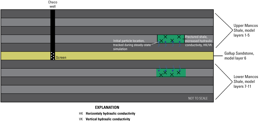
Conceptual depiction of hydraulic conductivity changes in hydraulic fracturing simulations within model layers.
Results
In the following sections, results from the potentiometric surface kriging, model calibration, model sensitivity analysis, and simulation particle tracking are described. Also addressed are uncertainty and potential error in the results.
Potentiometric-Surface Results
After testing different linear and polynomial models of potentiometric-surface trend, a first-order linear trend model (R2 = 0.50, median residual = 15.07) was removed from the modern potentiometric surface groundwater elevation data to allow for the kriging workflow to operate under the assumption of stationarity. The trend formula used is expressed below:
wherez(S)
is median groundwater elevation at point S, in feet above NAVD 88;
β0
is deterministic unknown trend coefficient, in feet above NAVD 88;
βi
are deterministic unknown trend coefficients, in dimensionless units (i = 1 through 2);
x(S)
is easterly coordinate at point S, in feet; and
y(S)
is northerly coordinate at point S, in feet.
The theoretical semivariogram for the modern data was modeled as spherical, with no nugget, a sill of 53,009 ft, and a range of 43,566 ft. The bin width used to compute the empirical semivariogram was set to 5,000 ft because it yielded the most readily identifiable semivariogram curvature, and the spatial distance to which monitoring site pairs were included in the semivariance estimates was set at 38,500 ft, or approximately half the maximum distance between data locations. The R-squared fit between the theoretical and the empirical variogram was 0.4.
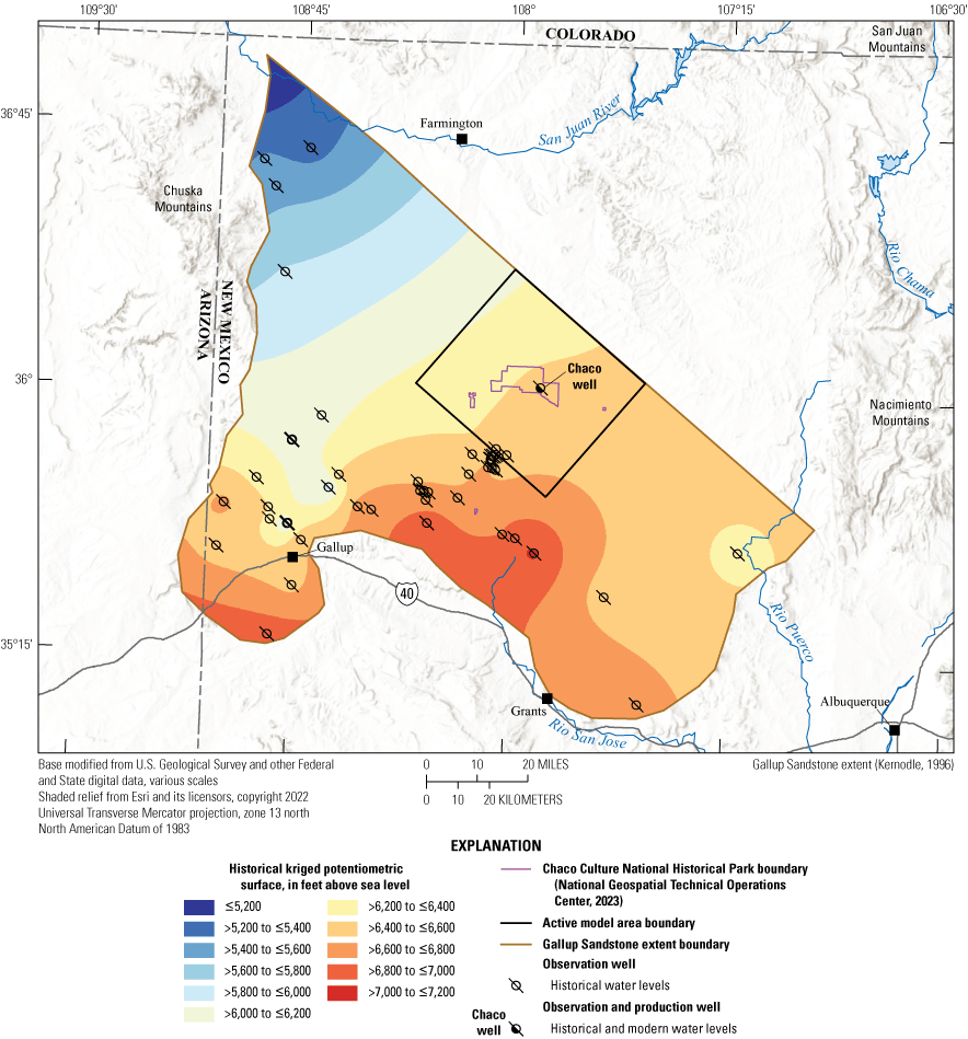
The modern (2016–20) interpolated potentiometric surface indicates that the groundwater elevation was highest in the southeast, sloping toward the San Juan River in the northwest (fig. 4). The surface shown in figure 4 was created with a grid cell size of 500 by 500 ft. For the entire interpolated surface, which is composed primarily of the area outside of the model domain, the mean estimation error for the leave-one-out cross validation was 28.8 ft, which is less than 10 percent of total head drop across the model domain. However, the minimum error was –203.1 ft and the maximum error was 383.9 ft, and ideally both would be close to zero. This range in error is comparably large relative to that within the model domain, with the minimum error being 56.6 ft and the maximum error being 68.9 ft, showing little spatial heterogeneity of error across the model domain. The correlation between observed and predicted groundwater elevations from leave-one-out cross validation was high (R2= 0.85), and the correlation between predicted and residual was low (R2 = −0.22), indicating that the estimation error is independent of the magnitude of the estimated groundwater elevation from cross validation and that stationarity may be assumed for the residual groundwater elevations used for kriging (Fisher, 2013).
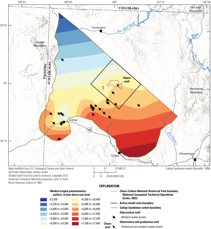
Modern (2016–20) kriged potentiometric surface and groundwater level observation points. Wells are screened in the Gallup Sandstone.
The same potentiometric surface interpolation was conducted for the historical surface (fig. 5), where the newest data from 1954 to 1989 for each site were used to assess the potentiometric surface before oil and gas development (U.S. Geological Survey, 2022). The two surfaces were differenced to assess the change in potentiometric surface after the onset, initiation, and (or) presence of oil and gas development. The linear trend model for the historical surface had an R2 of 0.73 and a median residual of −8.1; the same first-order trend equation was applied to the historical surface (eq. 1).
Historical (1954–89) kriged potentiometric surface and groundwater level observation points. Wells are screened in the Gallup Sandstone.
The variogram for the historical kriged surface used an exponential model, a range of 17,315 ft, a sill of 49,449 ft, and no nugget. The spatial distance to which monitoring site pairs were included in the semivariance estimates was set at 51,933 ft, or approximately half the maximum distance between data locations. The R2 fit between the theoretical and the empirical variogram was 0.29. A uniform grid cell size for the historical surface was also 500 by 500 ft. The leave-one-out cross validation mean error was 7.7 ft, and the correlation between observed and predicted values was 0.90, with a correlation of predicted and residual of −0.09, which validates the underlying assumptions of the kriging model.
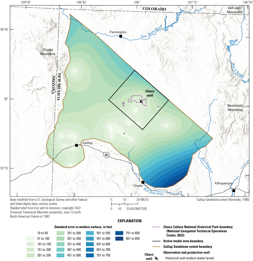
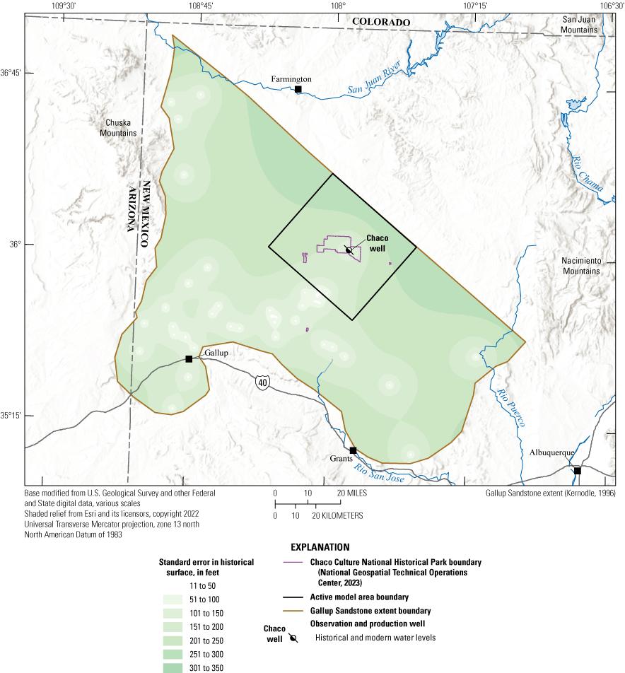
Standard error was highest near the outer areas of the Gallup Sandstone extent for both the modern and historical kriged surfaces where observed data were sparse (figs. 6 and 7). For the modern surface, standard error was particularly great in the northwestern (greater than [>] 450 ft) and southeastern (>800 ft) corners where data points were scant (fig. 6). Observation data in the historical surface had better spatial distribution, although standard error reached >300 ft along the northeastern extent of the Gallup Sandstone (fig. 7). The kriged surfaces, as well as the drawdown maps, have great uncertainty in regions where data are sparse. The error leads to potential physical interpretation errors in areas where recharge occurs along the southern portion of the Gallup Sandstone where it crops out at the surface. Potentiometric surfaces need to be considered in context with the standard error data and maps. However, standard error was generally less within the model domain, ranging between 10 and 463.5 ft in the modern surface and 11.3 and 300.5 ft in the historical surface. Values are highest in the northeastern part of the active model area where there is increased uncertainty because of sparse data. This area is generally downgradient from the Chaco well and near the edge of the Gallup Sandstone extent. Standard error was least near the southwestern part of the active model area where observation point density was greatest. Near the Chaco well itself, standard error approached zero. Additional error and variation in the kriged surfaces could be due to short term pumping effects and seasonal effects, as data were collected at various times of the year.
Modern kriged potentiometric surface standard error.
Historical kriged potentiometric surface standard error.
The drawdown surface is calculated as the modern surface minus the historical surface. Drawdown values ranged from –250 to 9 ft across the model domain, with a mean value of −90 ft (standard deviation 60 ft), indicating a general drop in the potentiometric surface elevation between the historical and modern potentiometric surfaces across the study area (fig. 8). Drawdown was not calculated for this report beyond the active model area because of large interpolation error, especially in the southeastern portion of the Gallup Sandstone in the modern potentiometric surface (fig. 6). Standard error of either surface should be taken into consideration when interpreting changes in the potentiometric surface. Direct water-level observations of the Chaco well indicate that head decreased by 70.5 ft between March 1989 and August 2017 (U.S. Geological Survey, 2022). The increase in potentiometric surface elevation in the southeastern portion of the active model area could be due to interpolation error.
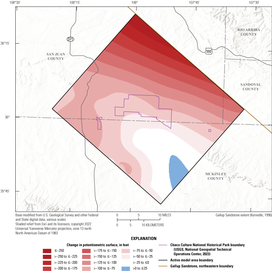
Change in the potentiometric surface from historical (1954–89) to modern (2016–20) conditions. Negative and positive values indicate decreasing and increasing elevation, respectively, from the historical to modern potentiometric surface.
The decreases in potentiometric surface elevation were generally greater in the northern and northeastern parts of the active model area, whereas the increases in elevation occurred near the southern and southeastern parts of the active model area. Head change values within the CCNHP boundaries ranged between –34 and –96 ft (mean –65 ft, standard deviation 12 ft). The greatest groundwater elevation decline values tended to be in the northeastern part of the primary CCNHP area and in the western detached part of the CCNHP. Groundwater elevation decline could be an artifact of interpolation error, although physical explanations could include reduction in recharge from areas outside of the active model area, water extraction for public and domestic water supply, or water used in power production, given that these are the most common uses of groundwater in the counties near CCNHP (Magnuson and others, 2019). Other causes could be related to nearby hydrocarbon extraction sites, mines, or pumping directly at CCNHP, although these activities are documented to draw relatively less water than those activities previously stated.
Carbon isotope and noble gas dating indicate groundwater in the Gallup Sandstone at CCNHP is exceptionally old, likely >52,000 years before present, which indicates limited recharge within the active model area (Linhoff and others, 2023). Although drawdown is likely due to multiple factors, the cause was not specifically investigated as part of this study.
Model Calibration and Sensitivity Analysis Results
The following sections describe the model calibration results, as well as a sensitivity analysis that followed model calibration. An initial sensitivity analysis (not reported) was conducted to inform which parameters should be calibrated.
Model Calibration
Horizontal and vertical hydraulic conductivity values in the Mancos Shale and Gallup Sandstone and groundwater flux into the model were calibrated using modern head observations (table 5). The calibrated parameters are determined as being best fit by PEST, assuming the constant head boundary is equal to the head of the modern potentiometric surface in those model cells. Calibration ranges used as input for PEST were determined from well logs and literature sources (tables 2–4). Calibrated PEST hydraulic conductivity values in the Mancos Shale (horizontal hydraulic conductivity [HK] approximately [~] 0.0001 ft/d, vertical hydraulic conductivity [VK] ~0.0001 ft/d) were almost identical to parameters reported in Kernodle (1996) (HK = 0.0001 ft/d, VK = 0.0001 ft/d). HK was slightly lower than reported by Frenzel and Lyford (1982) (HK = 0.000864–0.00864 ft/d), but vertical hydraulic conductivity in this study was higher (Frenzel and Lyford [1982] reported VK = 0.0000000864 ft/d). Horizontal hydraulic conductivity in the Gallup Sandstone in this study (HK ~0.41 ft/d) was in-between the values of Kernodle (1996) (HK = 1 ft/d) and Frenzel and Lyford (1982) (HK = 0.1–0.14 ft/d), and vertical hydraulic conductivity was identical to that of Kernodle (1996) (VK = 0.002 ft/d).
Table 5.
Calibrated groundwater model parameter dataset.[Unit refers to the geologic unit represented by the model layer. Reach refers to the model flux-in reach, which was divided into six equal length parts along the southwest and southeast model boundaries. ft/d, foot per day; ft3/d, cubic foot per day; NA, not applicable]
The model was calibrated to the updated modern surface hydraulic heads (described in the “Calibration and Sensitivity Analysis” section), where calibration targets were extracted from an overlain grid at 20,000 ft intervals from the kriged modern potentiometric surface. Total model mass balance errors were very small (0.01 percent), and the model successfully converged with head change and residual convergence criteria of 0.001 ft and 1 ft3/d, respectively, using the Preconditioned Conjugate-Gradient solver. The mean residual (simulated minus observed) of the model was 2 ft, and the absolute residual mean was 33 ft, which is less than 5 percent of the total head drop across the active model area (~730 ft). The standard deviation of residuals was 42 ft. The minimum residual was −82 ft, and the maximum residual was 106 ft. Previously published models in the vicinity of this study area reported residuals of as much as 150 ft between model-derived potentiometric surface and observed head as “good fit,” given the total range of heads in the study area (Frenzel and Lyford, 1982), although some residuals were not reported (Kernodle, 1996). The R2 between the simulated and observed head values was 0.93, indicating good agreement between simulated and observed values (fig. 9). However, comparison of the linear fit of the simulated against observed values, as well as the plot of the residuals versus observed values, indicate a slight tendency to overpredict at lower observed head values and a slight tendency to underpredict at higher observed head values (kriged head versus residuals R2 = 0.14, slope = −0.10) (figs. 9 and 10).
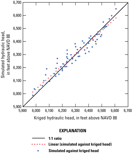
Kriged (observed) hydraulic head versus model simulated head and calibration target data comparison. NAVD 88, North American Vertical Datum of 1988.
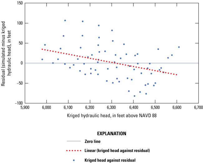
Kriged (observed) hydraulic head versus residuals (model simulated hydraulic head minus kriged hydraulic head). NAVD 88, North American Vertical Datum of 1988.
Though RMs are generally low, there is some spatial heterogeneity among residual values (fig. 11). Residuals are generally most positive (>50 ft) along the northeast boundary of the active model area, near the extent of the Gallup Sandstone, and most negative just south of CCNHP (less than −50 ft). Large residuals could be due to kriging interpolation error. Residuals generally are closest to zero (−10 to 10 ft) along the northwest boundary, which is a constant head boundary, and scattered elsewhere between areas of higher residuals. Numerical groundwater models are simplified representations of natural systems, and these spatial biases are likely an artifact of the actual spatial heterogeneity of the vertical and hydraulic conductivity. The model treats the Mancos Shale and Gallup Sandstone layers as spatially homogeneous for the purpose of simplicity and because of the lack of data or other evidence to populate the model heterogeneously.
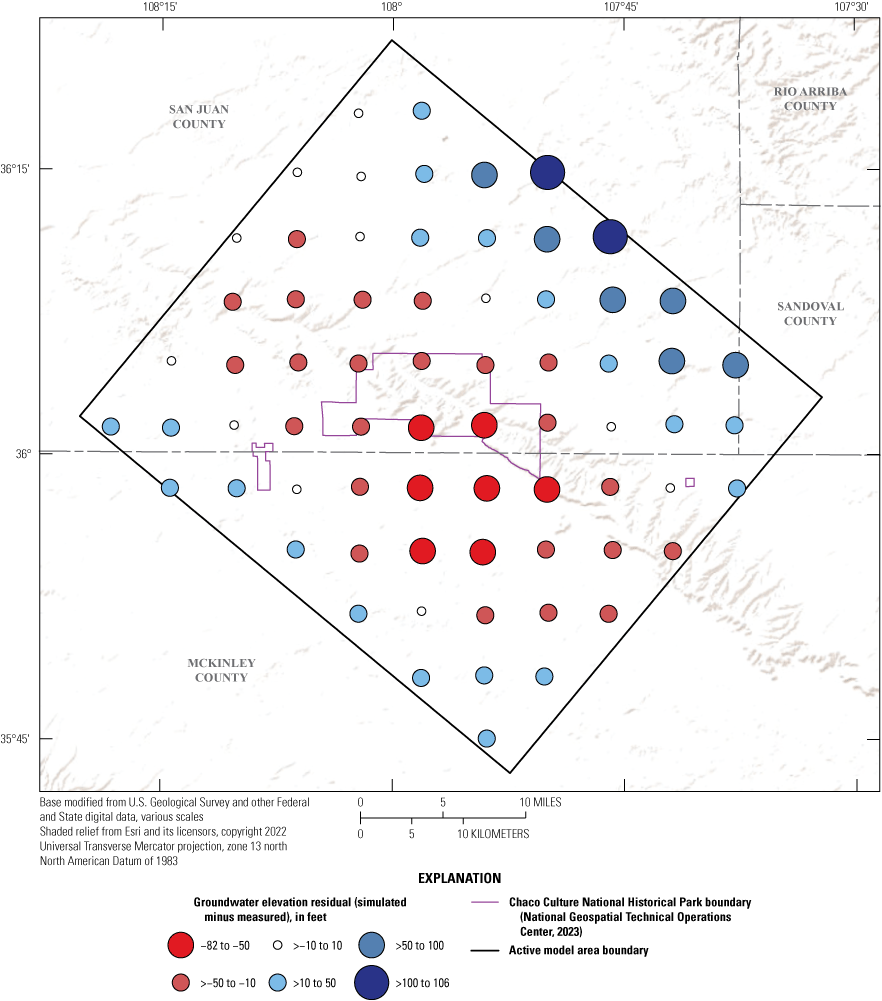
Spatial distribution of groundwater elevation residuals (simulated hydraulic head minus observed hydraulic head) for the calibrated groundwater flow model.
Several additional factors contribute to model uncertainty, including model error associated with the groundwater-level measurements and the standard error of the modern kriged surface (fig. 6). Parameter ranges for calibration were based largely on previously reported values (table 3), which were determined either physically or through parameters previously calibrated for earlier models, which also have uncertainty and various limitations. MODPATH, which was used to generate simulated groundwater flow paths, potentially yields simplified flow paths or uncertain traveltimes because it considers only advective groundwater flow and ignores preferential flow features and dispersive flow features of water-bearing formations (Baca, 1999). Additionally, subsurface features such as faults and anthropogenic preferential pathways such as abandoned well casings were not represented. Pumping wells other than the Chaco well were not included because of a lack of data but were assumed individually to have negligible influence because of their smaller pumping volumes. As noted earlier, there may be up to 10,000 acre-ft of groundwater used in McKinley County per year. The model simulations in this report are simplistic representations of how HF operation may influence subsurface processes and advective groundwater flow paths and thus may neglect other complex HF influences, as described in the “Introduction” section (Birdsell and others, 2015).
Sensitivity Analysis
Sensitivity analysis results are plotted as a percentage of parameter change from the calibrated parameter value versus the RM between simulated and observed heads (fig. 12A–C). The parameters included in the sensitivity analysis were horizontal and vertical hydraulic conductivities of the Mancos Shale and Gallup Sandstone model layers and the fluxes into the Gallup Sandstone. The sensitivity of particle traveltimes to porosity is discussed in the “Traveltimes” section of this report.
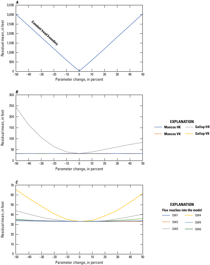
Sensitivity analysis (residual mean versus change in calibrated parameter value) for A, constant head boundary, B, horizontal hydraulic conductivity (HK) and vertical hydraulic conductivity (VK), C, model flux-in. Flux-in boundary definitions: QW1, Gallup Sandstone/1; QW2, Gallup Sandstone/2; QW3, Gallup Sandstone/3; QW4, Gallup Sandstone/4; QW5, Gallup Sandstone/5; QW6, Gallup Sandstone/6.
For hydraulic conductivity, only the HK RM in the Gallup Sandstone had high sensitivity (fig. 12B). The Gallup HK RM ranges from approximately 33 to 243 ft. The VK in the Gallup Sandstone as well as the HK and VK of the Mancos Shale are generally insensitive. Flux-in for reaches 3 and 4 were the most sensitive of the six flux-in parameters (fig. 12C). The reach 3 RM ranges from approximately 33 to 44 ft, and reach 4 ranges from 33 to 65 ft. The constant head boundary was found to be the most sensitive parameter in the entire sensitivity analysis, with the RM ranging from 33 to 3,033 ft (fig. 12A).
The Mancos Shale VK and HK have lower sensitivity, and as a result, altering the hydraulic conductivity through HF may have a lesser impact on model performance than initially anticipated. Reaches 3 and 4 are located along the steepest head gradient of the model, so the greater rate of change in RM for these reaches makes sense, because they contribute greater amounts of flux into the model than other reaches. The constant head boundary is the most sensitive parameter but also has the most quantitatively uncertain results through kriged standard error.
Simulation Results
General Flow Directions and Gradients
Flow directions in the model are largely a function of head gradient derived from the modern kriged potentiometric surface, which may be subject to interpolation error. The flow directions and behavior in the model are also in part a function of the specified model boundaries. Water generally enters the model through the flux-in boundary along the southwest and southeast boundaries, flows parallel along the northeast boundary, and exits the model along the northwest boundary. Previously published potentiometric head contours (Frenzel and Lyford, 1982; Kernodle, 1996) are in relative agreement with this study in terms of gradient direction but are not digitized and are difficult to quantitatively compare with new results (Stewart, 2018). However, the hydraulic gradients in this study in the vicinity of the CCNHP (minimum and maximum values range ~730 ft) tend to be steeper (greater range) compared to previous contour maps of head (Kernodle, 1996), potentially from increased or continued groundwater extraction from the Gallup Sandstone aquifer, coupled with limited aquifer recharge.
For most of the active model area, flow vectors in cross section view indicate that groundwater tends to flow horizontally between model cells, with limited mixing between the Mancos Shale and Gallup Sandstone layers. However, model results indicate slight vertical mixing of water between the Mancos Shale and the Gallup Sandstone, primarily near the Chaco well where pumping is occurring (fig. 13A, B). Hydraulic head is lowered substantially in the model cells near the Chaco well, especially those cells extending vertically to the top and bottom of the active model area. This change in hydraulic gradient causes groundwater to flow from the Mancos Shale layers to the Gallup Sandstone layer, and the gradient increases when the pumping rate is increased from the reported 1,200 ft3/d to the theoretical 10,000 ft3/d. The model framework did not account for all pumping wells in the area and does not have the available data to account for potential abandoned or compromised wells that could act as permeable pathways between the Mancos Shale and Gallup Sandstone or other surrounding units (Birdsell and others, 2015). These gradients and pathways presumably exist elsewhere in the model domain, which could promote additional vertical mixing between the Gallup Sandstone and Mancos Shale layers.
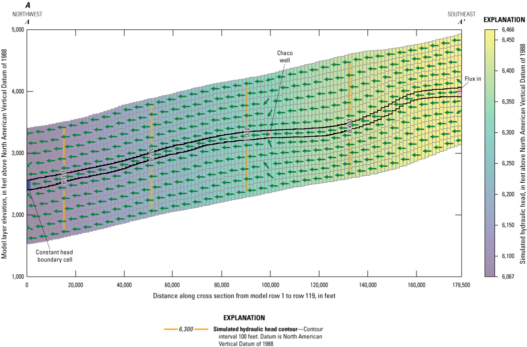
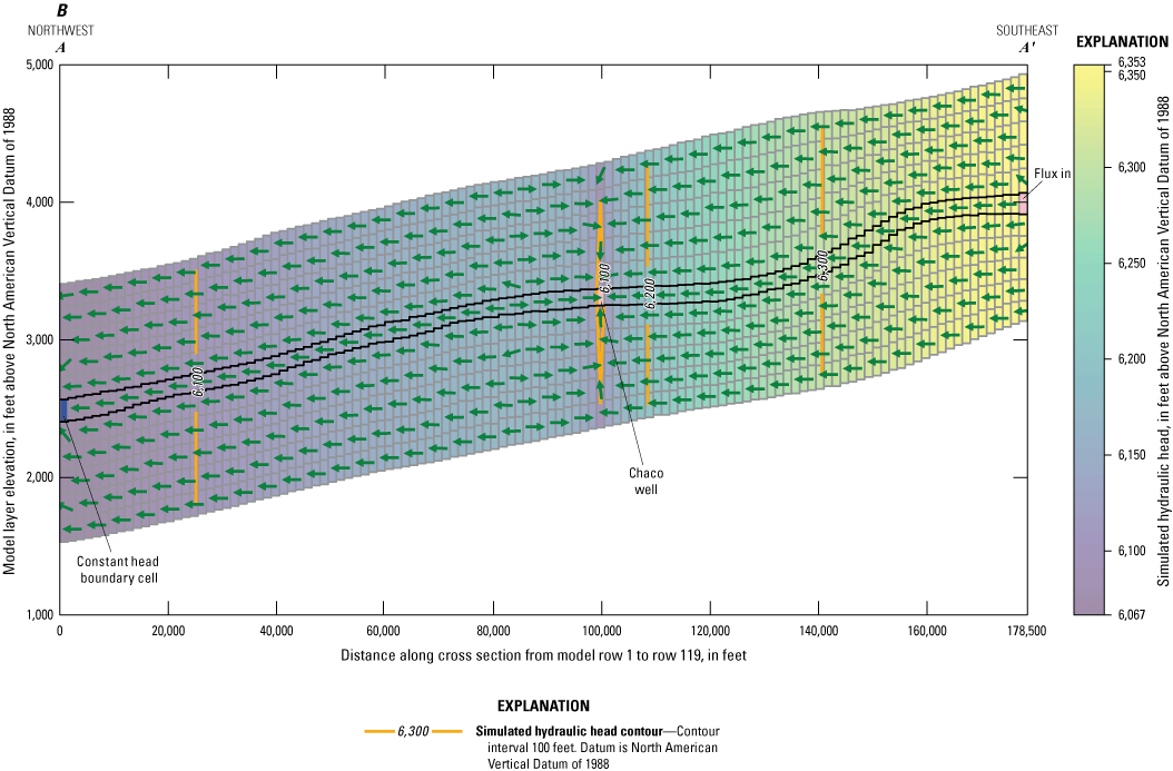
Cross-sectional view (A–A′, fig. 1) of groundwater flow model through model column 55 containing Chaco well (row 67) pumping rates of A, 1,200 cubic feet per day, and B, 10,000 cubic feet per day. Arrows are not scaled to the magnitude of flux and only indicate the direction of simulated flow.
Capture Zones
Capture zones were assessed by forward tracking particles placed along the flux-in boundary of the model domain until their capture by the Chaco well. Capture zones for the hypothetical Chaco well pumping rate of 10,000 ft3/d are shown in figure 14A, B in two-dimensional space and are depicted in three-dimensional space by the color of the pathways. These are representative figures of particles released in model layers 5 and 7 (Mancos Shale), representing average depths approximately 125 ft above and 175 ft below the Gallup Sandstone, respectively. The capture zone for either pumping rate tends to originate at the southeast flux-in boundary and take an arched northwest-trending path through the model until the particles are captured. Increasing the pumping rate substantially increases the capture zone width. The average width of the capture zone is approximately 1 mi for the 1,200 ft3/d pumping rate (not shown) and approximately 12 mi for the 10,000 ft3/d pumping rate.
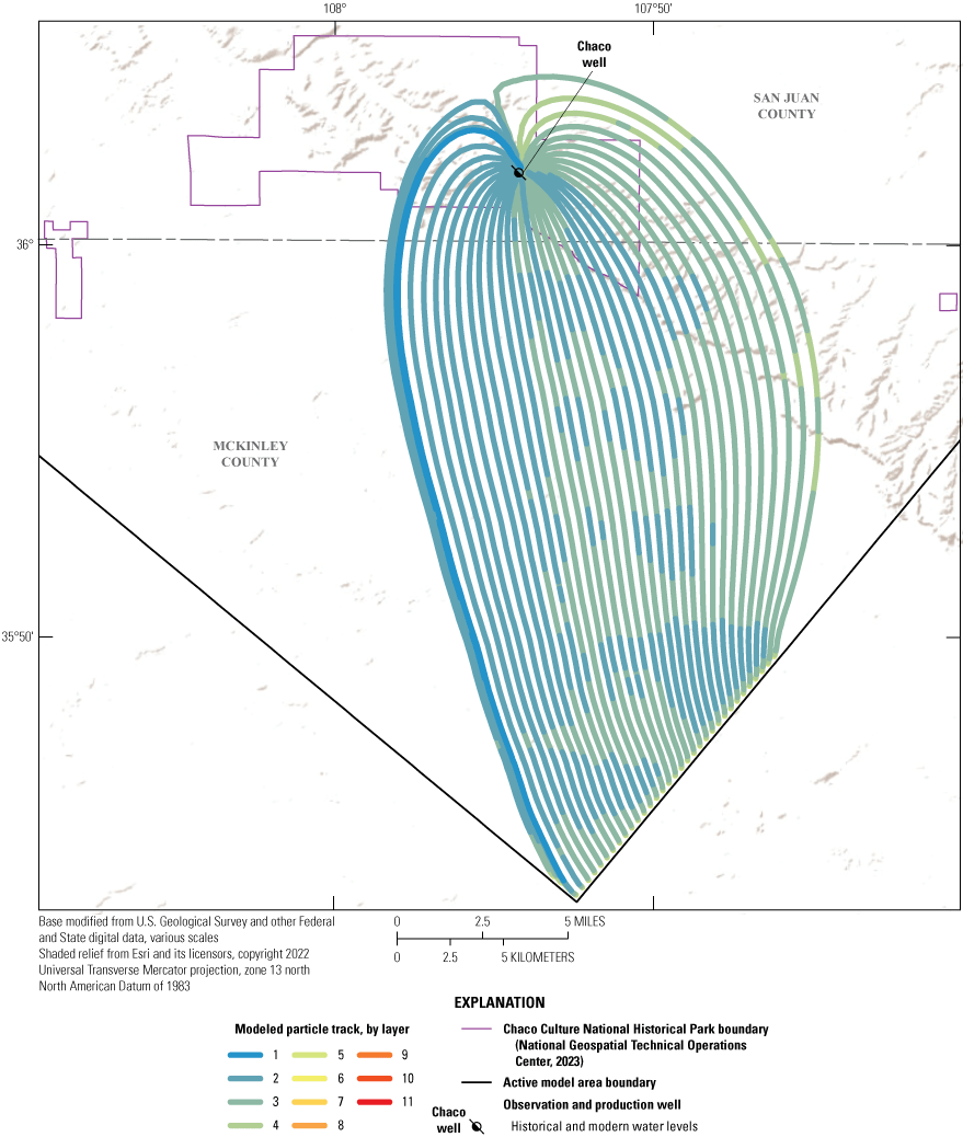
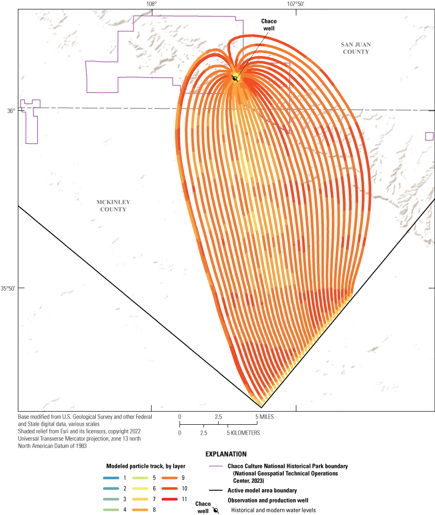
Chaco well groundwater capture zone, determined by particle tracking paths of well-captured particles for a pumping rate of 10,000 cubic feet per day for particles released in A, model layer 5, and B, model layer 7.
A total of 2,442 particles were released in all 11 model layers in each cell along the southwest and southeast flux-in boundaries. Of these particles, 41 and 387 were captured by the well at pumping rates of 1,200 and 10,000 ft3/d, respectively. The remaining particles did not pass through or terminate in the cell containing the Chaco well. Particle traveltimes ranged between approximately 28,500 and 34.2 million years for captured particles at a pumping rate of 1,200 ft3/d and between approximately 24,300 and 76.4 million years at a pumping rate of 10,000 ft3/d. The longer traveltimes for the larger pumping rate are due to the resulting larger capture zone that is created. Carbon isotope dating of water from three Gallup Sandstone wells within the modeled domain indicated an age range from ~43,000 to >52,000 years before present, the latter being greater than the method can resolve (Linhoff and others, 2023). Although these sampled waters travel from an unknown recharge area, and the active model area only occupies a portion of the basin, the order of magnitude of ages and traveltimes suggest a level of consistency and accuracy between both methods. These traveltimes are theoretical and dependent on running the model in steady-state simulation until all particles reach their endpoint at the calibrated parameter set and initially determined assumed porosity values (table 6). Traveltimes are calculated for a range of porosity values suggested in the literature (examined in the “Traveltimes” section).
Particles released in layer 5 primarily remained in the upper Mancos Shale layers (layers 2–4) stratigraphically above the Gallup Sandstone and did not reach the Gallup Sandstone until they were within 1,500 ft of the Chaco well. Similarly, the particles released in layer 7 remained in the lower Mancos Shale layers (layers 7–10) stratigraphically below the Gallup Sandstone and did not reach the Gallup Sandstone until they were within 1,500 ft of the Chaco well. These particle tracking pathways indicate that mixing between the Gallup Sandstone and Mancos Shale likely occurs primarily near pumping wells or near very permeable pathways such as compromised well casings or fractured rock.
Traveltimes
Two additional model runs were conducted that used the calibrated model parameters and Chaco well pumping rate of 1,200 ft3/d with the minimum and maximum porosity values for the Mancos Shale and Gallup Sandstone from the literature (table 4; Martin, 2005) to assess potential minimum and maximum groundwater traveltimes. Similar to the process for capture zones, a total of 2,442 particles were released in all 11 model layers in each cell along the southwest and southeast flux-in boundaries and forward tracked in steady-state simulation. Traveltimes are generally slower with higher porosity, given that flow paths are less tortuous, and fluid velocity through a porous media is mathematically expressed as Darcy flux divided by the porosity. For minimum porosity values, traveltimes ranged from approximately 5,700 years to 30 million years. For maximum porosity values, traveltimes ranged between approximately 52,000 years and 36.3 million years. The minimum traveltimes reflect particles that originated in and primarily flowed through the Gallup Sandstone, whereas maximum values reflect particles that originated in and primarily flowed through the Mancos Shale.
These simulated values represent traveltimes from the boundary of the active model area, not total traveltimes from the time water enters the subsurface. Water typically enters the Gallup Sandstone from surface outcrops far to the south and southeast of the Chaco well and the active model area (Stone and others, 1983), meaning traveltimes to the Chaco well are longer than those determined by the model. However, computed model traveltimes for minimum porosity values and the assumed additional travel from outside of the active model area are consistent with computed carbon isotope ages of samples collected in the Gallup Sandstone within the modeled domain (43,000 to >52,000 years before present; Linhoff and others, 2023).
Hydraulic Fracturing Scenarios
Several scenarios representing different HF operations were investigated (table 6). Hydraulic conductivities of each Mancos Shale layer were altered individually by several orders of magnitude to simulate the maximum distance and depth that potential HF-induced changes in hydraulic conductivity could potentially influence the Chaco well. In table 6, each row represents a model layer (Mancos Shale = layers 1–5, 7–11; Gallup Sandstone = layer 6), and each column represents the hydraulic conductivity assigned to simulate potential HF operation. For each scenario model run, Mancos Shale layer hydraulic conductivity (horizontal and vertical) was altered separately by layer (one layer per model run), the model was executed, and then particles were tracked in reverse to record their path in space and time from model cells surrounding the Chaco well. If a particle passed through the altered Mancos Shale layer, this was an indication that HF operation in that particular layer could potentially influence the Chaco well. This simulation was conducted for Chaco well pumping rates of 1,200 and 10,000 ft3/d.
For the 1,200 ft3/d pumping rate, increased HK and VK in the Mancos Shale began to influence the Chaco well when hydraulic conductivity reached 1 ft/d, which is five orders of magnitude above the hydraulic conductivity determined through model calibration (HK and VK ~0.0001 ft/d). Hydraulic conductivity has been determined to change by three to five orders of magnitude from HF in laboratory settings (Gehne and Benson, 2019). Model results indicate that if HF alters hydraulic conductivity by less than five orders of magnitude, there will be no influence on the Chaco well. For a hydraulic conductivity of 1 ft/d, only the first Mancos Shale layers above and below the Gallup Sandstone (layers 5 and 7) influenced flow to the Chaco well, and for hydraulic conductivities above 10 ft/d, three layers above and below the Gallup Sandstone influenced flow to the Chaco well (layers 3–5 and 7–9). For hydraulic conductivities of 100 ft/d or more, four layers above and below the Gallup Sandstone influenced flow to the Chaco well (layers 2–5 and 7–10). However, the top and bottom layers of the model (layers 1 and 11) did not pass any particles that were captured by the Chaco well for any hydraulic conductivity values (as much as 1,000 ft/d) at the 1,200-ft3/d pumping rate.
For the 10,000-ft3/d pumping rate, flow to the Chaco well began to be influenced by high HK and VK in the Mancos Shale layers at a hydraulic conductivity of 0.1 ft/d, and more layers above and below the Gallup Sandstone began to influence flow to the Chaco well. At hydraulic conductivities of 1 ft/d or more, all of the layers above and below the Gallup Sandstone influenced water flowing to the Chaco well.
Table 6.
Indicated particle travel or nontravel through individual model layers for selected hydraulic conductivities and Chaco well pumping rates.[ft, foot; ft/d, foot per day; ft3/d, cubic foot per day; x, particle passes through layer; --, particle does not pass through layer; /, Gallup Sandstone layer unaltered]
Changing the horizontal and vertical hydraulic conductivities of the entire layer may have a different effect on the behavior of subsurface flow than changing them in smaller, isolated areas. Changing the hydraulic conductivity of the Mancos Shale over an entire model layer to values above the Gallup Sandstone hydraulic conductivity may promote flow through the Mancos Shale layers, rather than promoting the movement of water from the Mancos Shale to the Gallup Sandstone. This behavior may not be indicative to how HF may influence flow pathways and traveltimes. Altering the hydraulic conductivity in small areas in the Mancos Shale layers, similar to how an HF well may alter hydraulic conductivity, effectively creates preferential pathways for groundwater flow between the Mancos Shale and the Gallup Sandstone.
For example, figure 15A, B shows the pathlines and starting locations in layer 4 for the particles captured by the Chaco well that originated from smaller areas (having a radius of about 10,000 ft) of altered hydraulic conductivity to emulate HF fracture zones. These particles passed vertically through the Mancos Shale, reached the Gallup Sandstone, and continued to pass through the Gallup Sandstone before reaching the Chaco well. Altering the hydraulic conductivity allowed groundwater to reach the Gallup Sandstone earlier than it otherwise would have and ultimately decreased the traveltimes to the Chaco well. This behavior occurred at modeled hydraulic conductivities of 1 and 100 ft/d, which suggests that a substantial change in hydraulic conductivity in a small area of the Mancos Shale may provide preferential pathways for groundwater travel to the Gallup Sandstone. These scenarios were run for both Chaco well pumping scenarios (1,200 and 10,000 ft3/d). Particles placed in smaller altered zones within the original capture zone (with original calibrated model parameters based on known, present-day, or observed conditions) in horizontal space (fig. 15A, B) were also captured by the Chaco well. Particles placed outside of the original capture zone (in horizontal space) were still not captured by the well, indicating that changes in hydraulic conductivity have limited influence on advective flow pathways outside of the HF zone.
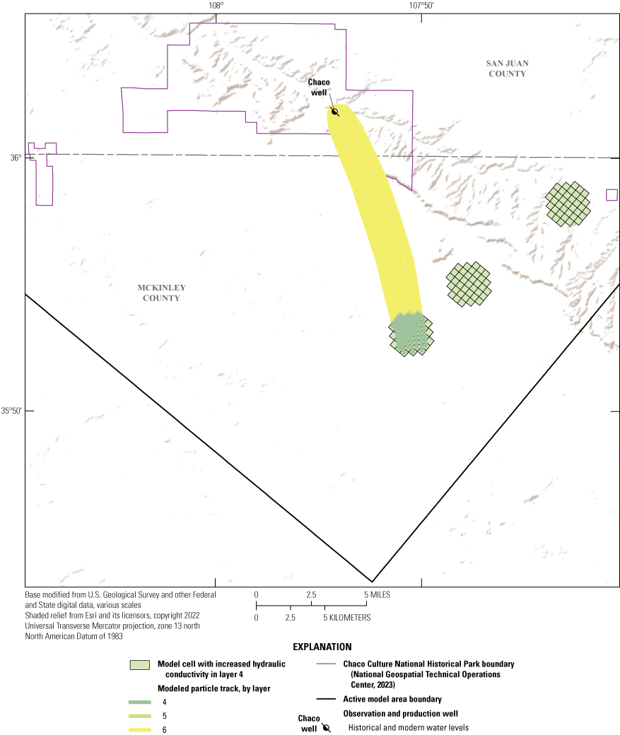
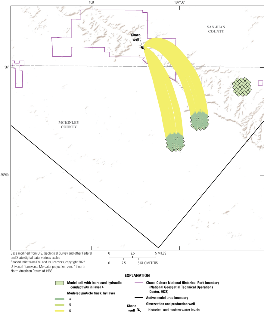
Particle pathways for particles released in select zones in model layer 4 at a hydraulic conductivity of 1 foot per day and a pumping rate of A, 1,200 cubic feet per day, and B, 10,000 cubic feet per day.
These emulated HF zones decreased groundwater traveltimes from the Mancos Shale to the Gallup Sandstone by providing increased hydraulic conductivity and preferential pathways between the layers. Mean traveltimes for particles captured by the Chaco well that originated in altered HF zones were approximately 14,300 years for Chaco well pumping rates of 10,000 ft3/d compared to 18.5 million years for unaltered zones. The decrease in traveltime was primarily due to the HF zones changing the travel paths of the particles directly into the Gallup Sandstone.
Discussion of Potential Chaco Well Contamination
Potential water quality impairment from HF operations can result from stray gas phase hydrocarbon migration in aquifers via leaking well casings and surface spills of extracted fluids that can contaminate shallow aquifers (Vengosh and others, 2014). Given the low hydraulic conductivities and confining thickness of the Mancos Shale, as well as the depth of the Chaco well, it is unlikely that contamination of the Gallup Sandstone aquifer could occur from surface spills. However, vertical mixing between aquifers is possible through improper casing or plugging of hydrocarbon wells in the region. Stone and others (1983) noted that leakage may occur locally between adjacent Cretaceous units, generally at low rates through shale beds and greater rates in localized areas associated with faults and fractures. This vertical mixing could introduce hydrocarbon related compounds and could be increased by hydrocarbon extraction activities.
The groundwater model indicates mixing between the Mancos Shale and Gallup Sandstone aquifers. A companion study to this report found several lines of evidence for vertical mixing between the Gallup Sandstone aquifer and surrounding aquifers, as well as groundwater chemistry influenced by hydrocarbons (Linhoff and others, 2023). First, noble gas analysis suggested mixing with hydrocarbon influenced groundwater. Second, hydrocarbon associated volatile organic compounds including benzene, toluene, ethylbenzene, and xylene were found at low levels in the Gallup Sandstone aquifer—including in the Chaco well. Lastly, mixing between aquifers was identified through major ion and isotopic geochemical analysis (Linhoff and others, 2023). Further investigation could help determine whether interaquifer mixing and the presence of volatile organic compounds is naturally occurring or related to oil and gas activity.
Several inactive oil and gas related wells were identified within the Chaco well capture zone in the Gallup Sandstone, Entrada Sandstone, Dakota Sandstone, and Morrison Formation (fig. 16; Linhoff and others, 2023). Seven and 22 inactive hydrocarbon wells were identified within 5 and 10 kilometers of the Chaco well, respectively (fig. 16; Linhoff and others, 2023). Eighteen inactive hydrocarbon related wells are located within the capture zone and within 10 kilometers of the Chaco well. Given the initial porosity values from table 4 in the Gallup Sandstone aquifer, simulated advective groundwater transport to the Chaco well is estimated to be approximately 430 years from the nearest inactive hydrocarbon related wells. If some of these inactive hydrocarbon related wells were improperly cased or plugged, they could potentially act as conduits for vertical groundwater movement through relatively impermeable units such as the Mancos Shale (Kernodle, 1996).
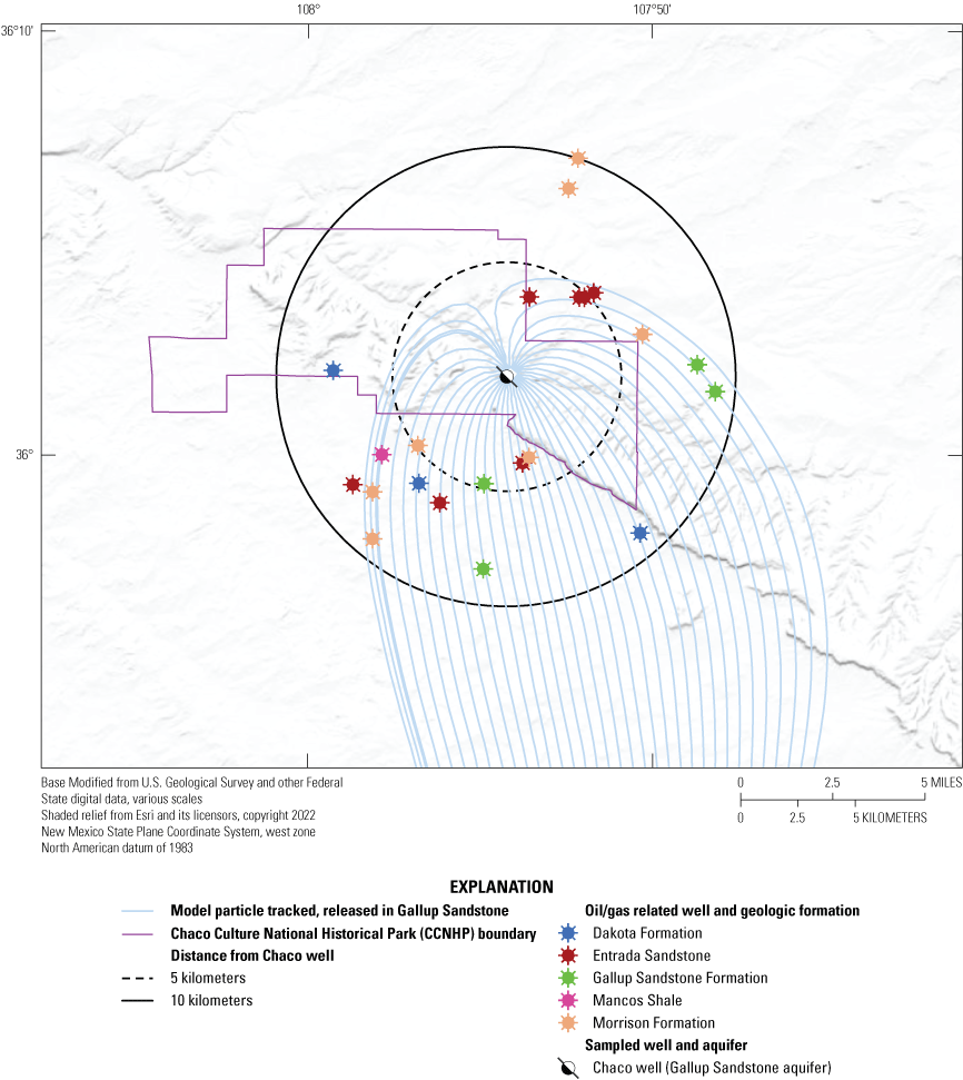
Inactive and plugged oil and gas wells within 5 and 10 kilometers of the Chaco well, with modeled particle pathways for particles released in the Gallup Sandstone aquifer unit. The Chaco well pumping rate is 10,000 cubic feet per day in this simulation. Figure adapted, and oil and gas related well data sourced, from Linhoff and others (2023).
Combined modeling and geochemical results imply that contaminants from hydrocarbon extraction activities in the San Juan structural Basin could travel between aquifers and could affect water quality in the Gallup Sandstone aquifer. Although further investigation, including examination of well completion and integrity, would be necessary to determine if contamination is actually facilitated, inactive oil and gas related wells found within the Chaco well capture zone could be sources of contamination for the Chaco well via vertical mixing of hydrocarbon bearing waters and Gallup Sandstone aquifer waters. Potential contamination at Chaco well may depend on three factors:
-
• Groundwater traveltimes through these geologic units are slow, so the distance a contaminant needs to travel to reach the Chaco well may influence the potential for drinking water contamination.
-
• The proximity of oil and gas related wells to the Chaco well (both horizontally and with respect to the unit they are completed in) may facilitate vertical mixing and decrease groundwater traveltimes.
-
• In the Chaco well groundwater capture zone, contaminants that originate upgradient of the Chaco well may have greater potential for drinking water contamination than those that originate downgradient of the Chaco well.
Limitations and Further Model Development
Although numerical groundwater modeling is a useful tool, there are limitations to the analysis documented herein. Additional groundwater level observations would reduce the standard error of the interpolated potentiometric surfaces. This error leads to potential errors in physical interpretation in areas where recharge occurs along the southern portion of the Gallup Sandstone where it crops out at the surface. Potentiometric surfaces need to be considered within the context of the standard error data and maps. Model performance could also be improved if the model was provided with more data on the spatial heterogeneity of hydrologic characteristics of the subsurface. Such data could include additional boreholes to refine basin lithology, nested piezometers to refine vertical groundwater gradients, and a greater density of groundwater-level measurements with closer temporal proximity.
The focus of the model scenarios was to observe particle pathways and capture zones of groundwater to the Chaco well and to visually present specific areas where HF operations could increase advective transport toward the Chaco well. This model could serve as a starting point to build a more comprehensive model that includes a detailed accounting of existing oil and gas wells, including depth, integrity, and any injections, to assess whether steady-state flow paths intersect any of these oil and gas features and to assess the potential traveltimes from these features to the Chaco well. Comprehensive assessment of HF fluid migration could include processes such as topographically driven flow, overpressure in shale reservoirs, buoyancy of HF fluids, and the increased pressure in shale from HF fluid injection. Additionally, a comprehensive model could include a detailed accounting of permeable pathways such as faults, fractures, or abandoned wells and the inclusion of more complicated multiphase flow effects, such as capillary imbibition and reduced relative permeability. Ultimately, transport mechanisms beyond advective transport, to which this report is limited, should be considered for a comprehensive study. In this study, only flow through the deep portions of the Gallup Sandstone and Mancos Shale was modeled. Although vertical hydraulic gradients between aquifers have been explored in previous studies, the substantial changes in potentiometric surface observed in this study could indicate changes in either horizontal or vertical flow paths and mixing between other aquifers. New models (potentially built by adapting the model produced for this study), could simulate additional aquifers in the San Juan structural basin using the same approach, or existing San Juan models could be adapted to new boundary conditions with the intent of assessing the amount of mixing occurring between subsurface layers. Additionally, new comprehensive San Juan structural basin models could be run for a transient time period if an accounting of various flux estimates could be determined. Finally, a detailed accounting of pumping rates and recharge in the Gallup Sandstone could be conducted to assess the cause of the declining head.
Summary and Conclusions
Through drawdown analysis and MODFLOW groundwater modeling, this study sought to determine the potential risk of hydraulic fracturing (HF) to the main drinking water well at Chaco Culture National Historical Park (CCNHP), located in northwestern New Mexico. The Gallup Sandstone of the San Juan structural Basin is a confined aquifer that supplies drinking water to CCNHP and is stratigraphically located between thick, low-permeability layers of Mancos Shale. The San Juan structural Basin, including the Mancos Shale, has been the subject of renewed interest in oil and gas development within the past decade. “Unconventional” reservoirs can cost-effectively produce gas, primarily through special recovery processes and technology. Unconventional methods of extraction including HF are being implemented in the Mancos Shale. Although the main CCNHP well is screened at a depth of 3,100 feet (ft) and is unlikely to be influenced by surface spills associated with extracted HF fluids, increased hydraulic conductivity caused by HF, migration of unextracted HF fluids and leaking well casings, and overextraction of water resources have the potential to negatively influence water quality and water availability for CCNHP.
New potentiometric surfaces kriged from observed historical and modern water-level measurements in the Gallup Sandstone indicate that potentiometric head has decreased by approximately 34–96 ft within the CCNHP prior to the unconventional oil and gas development in 2019. Direct water-level observations of the Chaco well indicate that head decreased by 70.5 ft between March 1989 and August 2017. The cause of this drawdown was not investigated, although this finding indicates depletion of water resources for CCNHP. In general, the modeling indicates that groundwater in the Gallup Sandstone travels from south-southeast to north-northwest within the active model area and through CCNHP.
In some groundwater systems, the loss in aquifer storage from pumping is balanced by increased recharge and (or) decreased discharge to surface water or evapotranspiration. However, because of the depth and isolating thickness of the Mancos Shale, there is likely limited recharge to the Gallup Sandstone besides where surface outcrops are near the unit boundary. Traveltimes through the Gallup Sandstone range from thousands to tens of thousands of years through the active model area depending on the pumping rate and chosen subsurface porosity values. Groundwater traveltimes through the Mancos Shale are very long, on the order of tens of millions of years. Hence, because of the age and the very slow groundwater traveltimes, modern groundwater recharge should not be expected to replace groundwater drawdown observed in the study area. Capture zone maps created by the model in this study may help indicate when compromised well casings and HF activity are within the advective groundwater flow paths to the CCNHP main well and may lead to negative water quality influence on the CCNHP drinking water supply. Eighteen inactive hydrocarbon related wells are located within the capture zone and within 10 kilometers of the Chaco well. Given model estimates of traveltimes of groundwater in the Gallup Sandstone aquifer, advective groundwater transport to the Chaco well would take approximately 430 years from the nearest inactive hydrocarbon related wells.
Model simulations indicated that increased hydraulic conductivity from fracturing activity could decrease groundwater traveltimes (from millions to thousands of years) between the Mancos Shale and the Chaco well by creating preferential flow pathways between the Mancos Shale and the Gallup Sandstone. Comprehensive modeling scenarios that capture the complexities of HF fluid migration could aid the assessment, and improve our understanding, of the absolute vulnerability of the Chaco well to HF activity.
References Cited
Baca, E., 1999, On the misuse of the simplest transport model: Ground Water, v. 37, no. 4, p. 483, accessed March 23, 2023, at https://doi.org/10.1111/j.1745-6584.1999.tb01128.x.
Birdsell, D.T., Rajaram, H., Dempsey, D., and Viswanathan, H.S., 2015, Hydraulic fracturing fluid migration in the subsurface—A review and expanded modeling results: Water Resources Research, v. 51, no. 9, p. 7159–7188, accessed March 23, 2023, at https://doi.org/10.1002/2015WR017810.
Byrnes, A.P., 2011, Role of induced and natural imbibition in frac fluid transport and fate in gas shales in Technical Workshops for Hydraulic Fracturing Study, Arlington, Virginia, March 28–29, 2011, [Proceedings]: U.S. Environmental Protection Agency, 28 p., accessed March 23, 2023, at https://www.epa.gov/sites/default/files/documents/roleofinducedandnaturalimbibitioninfracfluid.pdf.
Craigg, S.D., 2001, Geologic framework of the San Juan structural basin of New Mexico, Colorado, Arizona, and Utah, with emphasis on Triassic through Tertiary rocks: U.S. Geological Survey Professional Paper 1420, 70 p., accessed September 21, 2023, at https://doi.org/10.3133/pp1420.
Cunningham, W.L., and Schalk, C.W., comps., 2011, Groundwater technical procedures of the U.S. Geological Survey: U.S. Geological Survey Techniques and Methods, book 1, chap. A1, 151 p. [Also available at https://pubs.usgs.gov/tm/1a1/.]
Engelder, T., 2012, Capillary tension and imbibition sequester frack fluid in Marcellus gas shale: Proceedings of the National Academy of Sciences of the United States of America, v. 109, no. 52, article E3625, 1 p., accessed March 23, 2023, at https://doi.org/10.1073/pnas.1216133110.
Fisher, J.C., 2013, Optimization of water-level monitoring networks in the eastern Snake River Plain aquifer using a kriging-based genetic algorithm method: U.S. Geological Survey Scientific Investigations Report 2013–5120, DOE/ID–22224, 74 p., accessed October 23, 2018, at https://doi.org/10.3133/sir20135120.
Frenzel, P.F., and Lyford, F.P., 1982, Estimates of vertical hydraulic conductivity and regional ground-water flow rates in rocks of Jurassic and Cretaceous age, San Juan Basin, New Mexico and Colorado: U.S. Geological Survey Water-Resources Investigations Report 82–4015, 67 p., accessed March 23, 2023, at https://doi.org/10.3133/wri824015.
Gassiat, C., Gleeson, T., Lefebvre, R., and McKenzie, J., 2013, Hydraulic fracturing in faulted sedimentary basins—Numerical simulation of potential contamination of shallow aquifers over long time scales: Water Resources Research, v. 49, no. 12, p. 8310–8327, accessed March 23, 2023, at https://doi.org/10.1002/2013WR014287.
Gehne, S., and Benson, P.M., 2019, Permeability enhancement through hydraulic fracturing—Laboratory measurements combining a 3D printed jacket and pore fluid over-pressure: Scientific Reports, v. 9, no. 1, article 12573, accessed March 23, 2023, at https://doi.org/10.1038/s41598-019-49093-1.
Hill, M.C., Banta, E.R., Harbaugh, A.W., and Anderman, E.R., 2000, MODFLOW-2000, the U.S. Geological Survey modular ground-water model—User guide to the Observation, Sensitivity, and Parameter-Estimation Processes and three post-processing programs: U.S. Geological Survey Open-File Report 00–184, 210 p.
Kelley, S., Engler, T., Cather, M., Pokorny, C., Yang, C., Mamer, E., Hoffman, G., Wilch, J., Johnson, P., and Zeigler, K., 2014, Hydrologic assessment of oil and gas resource development of the Mancos Shale in the San Juan Basin, New Mexico: New Mexico Bureau of Geology and Mineral Resources Open-File Report 566, 65 p.
Kernodle, J.M., 1996, Hydrogeology and steady-state simulation of ground-water flow in the San Juan Basin, New Mexico, Colorado, Arizona, and Utah: U.S. Geological Survey Water-Resources Investigation Report 95–4187, 117 p., accessed March 23, 2023, at https://pubs.er.usgs.gov/publication/wri954187.
Linhoff, S.B., Beisner, K.R., Hunt, A.G., and Shephard, Z.M., 2023, Water quality at Chaco Culture National Historical Park and the potential effects of hydrocarbon extraction: Journal of Hydrology: Regional Studies, v. 47, article 101430, 20 p., https://doi.org/10.1016/j.ejrh.2023.101430.
Meng, Q., 2015, Spatial analysis of environment and population at risk of natural gas fracking in the State of Pennsylvania, USA: Science of The Total Environment, v. 515–516, p. 198–206, accessed March 23, 2023, at https://doi.org/10.1016/j.scitotenv.2015.02.030.
Myers, T., 2012, Potential contaminant pathways from hydraulically fractured shale to aquifers: Ground Water, v. 50, no. 6, p. 872–882, accessed March 23, 2023, at https://doi.org/10.1111/j.1745-6584.2012.00933.x.
National Oceanic and Atmospheric Administration, [NOAA], 2023, NowData-NOAA online weather data: National Oceanic and Atmospheric Administration database accessed March 23, 2023, at https://www.nws.noaa.gov/climate.php/ xmaxis.php%3fwfo=abq.
National Park Service [NPS], 2015, Foundation document Chaco Culture National Historical Park—New Mexico: National Park Service, 40 p., accessed March 23, 2023, at https://www.nps.gov/chcu/getinvolved/upload/CHCU_FD_PRINT.pdf.
Parker, J.M., Riggs, E.A., and Fisher, W.L., 1977, Oil and gas potential of the San Juan Basin, in Fassett, J.E., James, H.L., and Hodgson, H.E., eds., New Mexico Geological Survey Twenty-Eighth Field Conference, September 14–17, 1977, Guidebook: Socorro, N. Mex., New Mexico Geological Society, p. 227–241.
Pollock, D.W., 2016, User guide for MODPATH version 7—A particle-tracking model for MODFLOW: U.S. Geological Survey Open-File Report 2016–1086, 35 p., accessed September 21, 2023, at https://doi.org/10.3133/ofr20161086.
R Core Team, 2019, R—A language and environment for statistical computing: Vienna, Austria, R Foundation for Statistical Computing, accessed August 13, 2019, at https://www.R-project.org/.
Ritchie, A.B., and Pepin, J.D., 2020, Optimization assessment of a groundwater-level observation network in the Middle Rio Grande Basin, New Mexico (ver. 2, December 2020): U.S. Geological Survey Scientific Investigations Report 2020–5007, 113 p., accessed March 23, 2023, at https://doi.org/10.3133/sir20205007.
Shephard, Z.M., Ritchie, A.B., Linhoff, B.S., and Lunzer, J., 2023, MODFLOW-2005 and MODPATH models in support of groundwater flow model investigation of water resources at Chaco Culture National Historical Park: U.S. Geological Survey data release, https://doi.org/10.5066/P98LTTER.
Stewart, A.M., 2018, Hydrologic assessment and numerical simulation of groundwater flow, San Juan Mine, San Juan County, New Mexico, 2010–13: U.S. Geological Survey Scientific Investigations Report 2017–5155, 94 p., accessed March 23, 2023, at https://doi.org/10.3133/sir20175155.
U.S. Census Bureau, 2020, QuickFacts—New Mexico: U.S. Census Bureau, accessed March 23, 2023, at https://www.census.gov/quickfacts/fact/table/US/PST045222
U.S. Energy Information Administration, 2015, Annual energy outlook 2015: Washington, D.C., Office of Integrated and International Energy Analysis, 154 p., accessed March 23, 2023, at https://www.nrc.gov/docs/ML1617/ML16172A121.pdf.
U.S. Geological Survey, 2022, National Water Information System: U.S. Geological Survey database, accessed March 23, 2023, at https://nm.water.usgs.gov/infodata.
Conversion Factors
U.S. customary units to International System of Units
Temperature in degrees Fahrenheit (°F) may be converted to degrees Celsius (°C) as follows:
°C = (°F – 32) / 1.8.
Datum
Vertical coordinate information is referenced to the North American Vertical Datum of 1988 (NAVD 88) and the National Geodetic Vertical Datum of 1929 (NGVD 29).
Horizontal coordinate information is referenced to the American Datum of 1983 (NAD 83).
Elevation, as used in this report, refers to distance above the vertical datum.
Abbreviations
CCNHP
Chaco Culture National Historical Park
GIS
geographic information system
GWV
Groundwater Vistas
HF
hydraulic fracturing
HK
horizontal hydraulic conductivity
NPS
National Park Service
RM
residual mean
UNESCO
United Nations Educational, Scientific and Cultural Organization
USGS
U.S. Geological Survey
VK
vertical hydraulic conductivity
For more information about this publication, contact
Director, New Mexico Water Science Center
U.S. Geological Survey
6700 Edith Blvd. NE
Albuquerque, NM 87113
For additional information, visit
https://www.usgs.gov/centers/nm-water
Publishing support provided by
Lafayette Publishing Service Center
Disclaimers
Any use of trade, firm, or product names is for descriptive purposes only and does not imply endorsement by the U.S. Government.
Although this information product, for the most part, is in the public domain, it also may contain copyrighted materials as noted in the text. Permission to reproduce copyrighted items must be secured from the copyright owner.
Suggested Citation
Shephard, Z.M., Ritchie, A., Linhoff, B.S., and Lunzer, J.J., 2023, Groundwater flow model investigation of the vulnerability of water resources at Chaco Culture National Historical Park related to unconventional oil and gas development: U.S. Geological Survey Scientific Investigations Report 2023–5097, 39 p., https://doi.org/10.3133/sir20235097.
ISSN: 2328-0328 (online)
Study Area
| Publication type | Report |
|---|---|
| Publication Subtype | USGS Numbered Series |
| Title | Groundwater flow model investigation of the vulnerability of water resources at Chaco Culture National Historical Park related to unconventional oil and gas development |
| Series title | Scientific Investigations Report |
| Series number | 2023-5097 |
| DOI | 10.3133/sir20235097 |
| Publication Date | December 02, 2023 |
| Year Published | 2023 |
| Language | English |
| Publisher | U.S. Geological Survey |
| Publisher location | Reston, VA |
| Contributing office(s) | New Mexico Water Science Center |
| Description | Report: viii, 39 p.; Data Release |
| Country | United States |
| State | Arizona, New Mexico |
| Other Geospatial | Chaco Culture National Historical Park |
| Online Only (Y/N) | Y |