

Groundwater Discharge by Evapotranspiration from the Amargosa Wild and Scenic River and Contributing Areas, Inyo and San Bernardino Counties, California
Links
- Document: Report (10 MB pdf) , HTML , XML
- Data Releases:
- USGS Data Release - Geospatial data for the report Groundwater Discharge by Evapotranspiration from the Amargosa Wild and Scenic River and Contributing Areas, Inyo and San Bernardino Counties, California
- USGS Data Release - Supplemental data for the report groundwater discharge by evapotranspiration from the Amargosa Wild and Scenic River and contributing areas, Inyo and San Bernardino Counties, California
- NGMDB Index Page: National Geologic Map Database Index Page (html)
- Download citation as: RIS | Dublin Core
Acknowledgments
The authors would like to thank Susan Sorrells, who allowed the U.S. Geological Survey to install evapotranspiration-monitoring sites on her property. We also would like to thank Naomi Fraga, with the California Botanic Garden, who helped with plant identification.
Abstract
The Amargosa Wild and Scenic River, located in the southwestern Mojave Desert in Inyo and San Bernardino Counties, California, is a Federally protected waterway that supports the biodiversity of the region. Water in the river primarily comes from interbasin groundwater flow that originates as precipitation in the Spring Mountains. The precipitation enters the regional groundwater system and flows westerly beneath Pahrump, Chicago, and California Valleys before discharging into the Amargosa Wild and Scenic River system. In Pahrump Valley, groundwater discharge occurs as evapotranspiration (ET), spring discharge, and groundwater pumping, and in Chicago and California Valleys, groundwater discharge occurs as ET and spring discharge. Remaining groundwater flows into the Amargosa Wild and Scenic River and its main tributary, the China Ranch Wash, or is discharged from regional springs downgradient from Chicago and California Valleys. The Amargosa Wild and Scenic River and the China Ranch Wash sustain areas of deep-rooted vegetation (phreatophytes) that consume regional groundwater. Discharge from regional springs in the area only flows on the land surface for short distances before seeping back into the ground where the water generally is consumed by evaporation from moist soil or by transpiration of plants. Intermittent Amargosa River flow out of the study area is the only other form of discharge. In arid regions such as the Mojave Desert, groundwater discharge by evapotranspiration (ETg) often is the only significant form of discharge in a regional water budget, and therefore, an estimate of annual ETg is a good approximation of the total annual groundwater discharge. In this study area, however, total annual discharge is annual ETg plus the annual surface-water discharge of the Amargosa River that exits the study area. Therefore, the annual ETg from Chicago and California Valleys and along the Amargosa Wild and Scenic River and the China Ranch Wash, plus the discharge of the Amargosa River, is a good approximation of the total annual groundwater discharge required to sustain the riparian habitats and surface-water flow in the Amargosa Wild and Scenic River.
The Amargosa Conservancy and Inyo County, Calif., are interested in quantifying the total annual groundwater discharge required to sustain the riparian habitats and surface-water flow in the Amargosa Wild and Scenic River and entered into a cooperative agreement with the U.S. Geological Survey to estimate ETg from the Amargosa Wild and Scenic River study area. The study area consists of open-water bodies, areas with perennially moist soil, and areas with phreatophytes, all of which are discharging regional groundwater in Chicago and California Valleys, along the Amargosa Wild and Scenic River, and in the China Ranch Wash.
Annual ETg for the Amargosa Wild and Scenic River study area is estimated to be 10,139,000 cubic meters. The estimate was determined by delineating boundaries of open water, perennially moist soil, and phreatophytes, multiplying the areas by appropriate site-scale ETg to derive annual ETg for each ET unit, and then adding the annual ETg for all ET units in the GDAs and study area. Boundaries of discharge areas were visually delineated using high-resolution aerial imagery and refined by field verification. Open water and moist soil ETg were estimated in previous investigations, and phreatophyte ETg was estimated from a quadratic relation between site-scale ETg and a vegetation index of the study area. The quadratic relation was derived from four points. Two points were based on the site-scale ETg estimated for this study and two points corresponded to theoretical minimum and maximum points. Site-scale ETg was measured at two ET-monitoring sites using the eddy-covariance method. At one site, located in sparse shrubs, ETg was 0.121 meters per year, and at the other site, located in dense wetland vegetation, ETg was 1.056 meters per year. A scaled normalized difference vegetation index (NDVI) that encompasses the study area was created from 0.6-meter resolution multispectral (4-band) aerial imagery from 2020 and was used as an indicator of plant density or cover.
Introduction
The Amargosa River is in the Mojave Desert and the southwestern part of the Great Basin section of the Basin and Range physiographic province (fig. 1). The river is about 300 kilometers (km) in length, and it is the longest river in the Death Valley region. The river flows from Oasis Valley, Nevada, at an altitude of about 1,100 meters (m), to Death Valley, California, at an altitude of about minus 85 m. The Amargosa River is hydrologically and biologically important to the region because it is the terminal discharge area of the regional groundwater flow system, represents a groundwater-dependent ecosystem that sustains riparian vegetation and rare desert habitats, and provides a pathway for species distribution (Zaimes, 2007; Stevens and Meretsky, 2008; Parker and others, 2021; Schultz and others, 2021; and Stevens and others, 2021). The Amargosa River flows through parts of the Mojave Desert that are designated as Areas of Critical Environmental Concern by the Bureau of Land Management (BLM); these are Federally protected areas to preserve natural, cultural, or historical resources (Bureau of Land Management, 2020a).
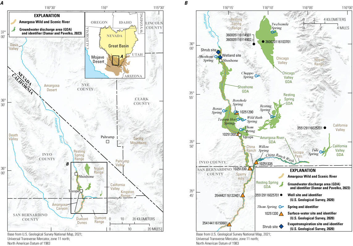
A, Regional view; and B, study-area view of the Amargosa Wild and Scenic River (AWSR) study area, Inyo and San Bernardino Counties, California. Abbreviation: GDA, groundwater discharge area.
Much of the biodiversity in the region is in groundwater dependent ecosystems along the Amargosa River and tributary streams and springs, including endemic, threatened, and endangered species. The flora and fauna of a groundwater dependent ecosystem is supported by an area of shallow groundwater discharge, referred to in this study as a groundwater discharge area (GDA). For this study, GDAs are areas of relatively shallow groundwater that are naturally discharging, and they include rivers, wetlands, springs, and areas of deep-rooted vegetation (phreatophytes), all of which are found along the Amargosa River and its tributaries. The difference between a GDA and a groundwater dependent ecosystem is that a GDA only includes the area where shallow groundwater discharges, whereas the groundwater dependent ecosystem is much larger and includes the GDA and the ranges of animals that visit the GDA for water, forage, or prey. Along the Amargosa River and its tributaries, Least Bell's vireo (Vireo bellii pusillus), southwestern willow flycatcher (Empidonax traillii extimus), endemic Amargosa vole (Microtus californicus), and endemic Amargosa niterwort (Nitrophila mohavensis) are listed by the U.S. Fish and Wildlife Service (FWS) as endangered (U.S. Fish and Wildlife Service, 2023a, 2023b, 2023c, 2023d); yellow-billed cuckoo (Coccyzus americanus) is listed by the FWS as threatened (U.S. Fish and Wildlife Service, 2023e); Swainson's hawk (Buteo swainsoni) is listed by the California Fish and Game Commission as threatened (California Department of Fish and Wildlife, 2023); and endemic Amargosa pupfish (Cyprinodon nevadensis) and endemic Amargosa speckled dace (Rhinichthys osculus nevadensis) are designated by the BLM as sensitive species (Bureau of Land Management, 2020b). Additionally, the Amargosa River and tributary streams have provided water to indigenous people, explorers, pioneers, and miners for centuries, which has resulted in cultural and historical resources along the river (Bureau of Land Management, 2020b).
The importance of the Amargosa River to the biodiversity and the cultural and historical resources of the region prompted the United States Congress to incorporate a segment of the Amargosa River into the National Wild and Scenic River System (fig. 1; Public Law 111-11, 111th Congress, March 30, 2009, and Public Law 116-9, 116th Congress, March 12, 2019). Rivers are designated as Wild and Scenic because they possess “outstandingly remarkable scenic, recreational, geologic, fish and wildlife, historic, cultural or other similar values,” and designated rivers “shall be preserved in free-flowing condition, and that they and their immediate environments shall be protected for the benefit and enjoyment of present and future generations” (Wild and Scenic Rivers Act, Public Law 90-542; 16 U.S.C. 1271 et seq, October 2, 1968).
The Amargosa Wild and Scenic River (AWSR) is a 54.4-km segment of river that is managed by the BLM (fig. 1). The AWSR begins near the town of Shoshone, Calif., where the flow is intermittent, then it flows south, past the town of Tecopa, Calif. Near Tecopa, the AWSR flow becomes perennial and flows south through the Amargosa Canyon in the Sperry Hills. Flow in the China Ranch Wash is ephemeral in California Valley and becomes perennial near Willow Spring. Below Amargosa Canyon, the China Ranch Wash joins the AWSR and, near the Dumont Dunes area, flow in the AWSR becomes intermittent near the end of the designated Wild and Scenic segment of the Amargosa River. The source of nearly all surface-water flow in the AWSR is discharge from interbasin groundwater flow and nearly all surface-water flow in the AWSR is discharged by evapotranspiration (ET), with the remainder discharging from the study area as intermittent surface-water flow.
The AWSR is in the southwestern part of the Death Valley regional groundwater flow system (DVRFS), which is about 41,000 square kilometers (km2) and comprised of 30 groundwater basins that are connected, to various extents, by interbasin groundwater flow through underlying carbonate- and volcanic-rock aquifers, as defined by Harrill and others (1988). As part of a regional groundwater flow system, the AWSR is hydraulically linked to nearby groundwater basins and can be affected by hydrologic changes in those basins. Nearly all water in the AWSR originates as Spring Mountains (fig. 1) precipitation that infiltrates carbonate bedrock and recharges the regional aquifer system (Malmberg, 1967; Winograd and Thordarson, 1975; Belcher and others, 2017, 20195; Halford and Jackson, 2020). Groundwater that is not discharged or withdrawn in Pahrump Valley flows westerly into Chicago Valley, California Valley, and the Amargosa River system, three of the lowest-altitude areas in the DVRFS. In Pahrump Valley, regional groundwater is the main water supply for a growing population, and in Amargosa Desert, regional groundwater is the main water supply for agricultural activities, and both areas are next to and at higher altitudes than the AWSR. There are concerns that continued groundwater withdrawals in Pahrump Valley and Amargosa Desert could result in groundwater drawdowns along the AWSR, or in Chicago or California Valleys (Nelson and Jackson, 2020); areas that contribute interbasin groundwater flow to the AWSR. Groundwater drawdowns could lead to less flow in the Amargosa River and a reduction or loss of available groundwater discharge, which would have a negative effect on protected desert habitats, groundwater dependent ecosystems, and GDAs in the AWSR study area.
To address limited information about the annual amount of groundwater required to sustain the riparian habitats and surface-water flow in the AWSR, the U.S. Geological Survey (USGS), in cooperation with The Amargosa Conservancy and Inyo County, Calif., estimated annual groundwater discharge by evapotranspiration (ETg) from the AWSR and Chicago and California Valleys. The purpose of this study was to estimate annual ETg for the AWSR study area by incorporating site-scale ET measurements made in the study area and a vegetation index from near the time of the ET-data collection; previous ETg estimates were based on measurements made in other locations. Evapotranspiration is the combined processes of evaporation and transpiration of near-surface water, and it accounts for most groundwater discharge in the Basin and Range Province (Maxey and Eakin, 1949; Harrill and others, 1983; Nichols, 2000). In a water budget, ETg is the part of ET derived only from groundwater and it is calculated by subtracting other water balance components, such as precipitation and soil moisture, from total ET. Moreover, nearly all perennial flow in the AWSR is sourced from interbasin groundwater, and all that groundwater, except intermittent AWSR flow out of the study area, is discharged by ETg. Therefore, an estimate of ETg from the study area plus the intermittent AWSR flow out of the study area is a good approximation of the flux of interbasin groundwater flow that is required to sustain the riparian habitats and surface-water flow in the AWSR. For the AWSR study area, ETg was estimated using techniques similar to other studies in the Basin and Range Province, including Laczniak and others (1999, 2001, 2008), Nichols (2000), Reiner and others (2002), Maurer and others (2006), Groeneveld and others (2007), Moreo and others (2007, 2020), DeMeo and others (2008), Allander and others (2009), Devitt and others (2011), Garcia and others (2014), Berger and others (2016), Huntington and others (2016), and Albano and others (2021).
Purpose and Scope
The purpose of this report is to summarize the methods and results used to estimate annual ETg for the AWSR study area (fig. 1). The 28,229,000 square meter (m2) AWSR study area is comprised of five GDAs along the AWSR and China Ranch Wash, and in Chicago and California Valleys. This study uses site-scale ETg measured at two ET-monitoring sites in the AWSR study area—a sparse shrub site and a dense wetland site. Data were collected at these sites from March 2017 to May 2019, and ETg was calculated for January 2018–19. Total ET was measured using the eddy-covariance method and measurements were adjusted using an energy-balance closure method. Precipitation was subtracted from total adjusted ET to calculate site-scale ETg. Groundwater discharge areas in the study area were visually delineated using high-resolution aerial imagery, subdivided into open-water, moist-soil, and vegetated ET units, and refined by field verification. An ET unit is an area with a uniform ET rate, such as the open-water and moist-soil ET units, or an area with a variable but predictable ET rate, such as the vegetated ET unit. The open-water and moist-soil ET units were assigned site-scale ETg based on Laczniak and others (2001) and Jackson and others (2018). The vegetated ET units were assigned site-scale ETg that varied according to a quadratic equation developed for this study that relates site-scale ETg to a normalized difference vegetation index (NDVI) derived from aerial imagery acquired July 2, 2020. Annual ETg for the AWSR study area was calculated by adding the annual ETg for all the ET units in the study area.
This report presents an estimate of annual ETg for the AWSR study area and provides baseline groundwater-discharge data to support a mandated comprehensive management plan for the AWSR (Wild and Scenic Rivers Act, October 2, 1968). A supporting geospatial dataset of the ET-unit and GDA boundaries and a supporting dataset of flux and ET data are presented in associated USGS data releases (Damar and Pavelko, 2023, and Pavelko, 2023). The annual ETg estimate helps constrain past estimates because this study measured ET at sites within the study-area boundaries and used multispectral data that were collected within 2 years of the ET-data collection. Previous ETg studies measured ET at locations outside of the study area and used multispectral data that were collected before ET was measured (Laczniak and others, 2001) or used ET that was empirically derived and 30-year composite multispectral data (Huntington and others, 2016). The ET-unit and GDA boundaries can be compared with future delineations to help determine any changes to the ET units or GDAs. Data collected during the 1-year period of analysis for the Shrub ET-monitoring site (USGS site 355846116160401) and Wetland ET-monitoring site (USGS site 355918116161801) are stored in the USGS National Water Information System (NWIS) and are publicly accessible at the NWIS web portal (U.S. Geological Survey, 2020) using their NWIS site numbers. Data collected for this study and stored in NWIS include air temperature, relative humidity, wind speed, wind direction, net radiation, atmospheric water-vapor density, soil temperature, volumetric soil-moisture content, soil-heat flux, sensible-heat flux, latent-heat flux, and total ET.
Previous Studies
There have been two reconnaissance-level ETg studies of the AWSR study area (Laczniak and others, 2001, and Huntington and others, 2016) and two studies that estimated moist-soil ET in Death Valley (DeMeo and others, 2003, and Jackson and others, 2018). Laczniak and others (2001) delineated and subdivided groundwater discharge areas in the study area and used site-scale ETg measured from 1994 to 1997 in Ash Meadows, Nevada (Laczniak and others, 1999), about 60-km north of the AWSR study area, and values from a 1992 vegetation index to estimate an annual ETg of 11,015,000 cubic meters (m3). Laczniak and others (2001) subdivided discharge areas based on plant communities and their similarities in multispectral imagery. Huntington and others (2016) used the discharge areas delineated by Laczniak and others (2001) and used empirically derived site-scale ETg across the discharge areas (Beamer and others, 2013) and a multiple-year composite (1984–2015) of remotely sensed multispectral data to estimate an annual ETg of 9,923,000 m3.
Study Area
The AWSR study area comprises five GDAs, the Amargosa River GDA in Inyo and San Bernardino Counties, Calif., and the Shoshone, Chicago Valley, Resting Spring, and California Valley GDAs in Inyo County, Calif. (fig. 1). The Amargosa River GDA also includes the tributary China Ranch Wash. The China Ranch Wash and Chicago and California Valleys are included in the study area because they contribute regional groundwater to the AWSR. In the study area, regional groundwater derived from interbasin flow is the primary source of recharge, ETg is the primary source of discharge, intermittent AWSR flow out of the study area is the secondary source of discharge, and all other water-budget components are considered negligible (Malmberg, 1967; Harrill, 1986; Harrill and Prudic, 1998; Belcher and others, 2019; Halford and Jackson, 2020). Interbasin groundwater flow primarily comes from the east, in Pahrump Valley, where precipitation on the Spring Mountains infiltrates a carbonate mountain block and recharges the regional groundwater flow system. From Pahrump Valley, groundwater flows beneath the Nopah Range and recharges the Chicago Valley, Resting Spring, and California Valley GDAs before flowing toward the Shoshone and Amargosa River GDAs. In the AWSR study area, annual precipitation estimates range from about 500,000 to 1,100,000 m3 (Hevesi and others, 2003; Belcher and others, 2017; Halford and Jackson, 2020) whereas recharge by interbasin groundwater estimates range from about 11,200,000 to 19,900,000 m3, with about 600,000 m3 coming from the Amargosa Desert to the north and the remainder coming from Pahrump Valley to the east (fig. 1; Harrill and others, 1988; Belcher and others, 2019).
Flow in the AWSR is perennial in most of the study area where there are gaining and losing sections. However, flow is ephemeral into the study area and intermittent out of the study area with flow occurring in these areas primarily during and after rainfall (Belcher and others, 2019). Based on geochemical analyses of spring discharges and insufficient precipitation to sustain the spring discharges, Belcher and others (2019) determined most springs in the study area discharge regional groundwater. Study-area springs with discharge greater than about 0.3 liter per second (L/s) and water temperatures greater than about 30-degrees Celsius (°C) include Shoshone Spring in the Shoshone GDA and Borehole, Borax, and Willow Springs, Tecopa Hot Springs, and the unnamed seeps and springs in Amargosa Canyon in the Amargosa River GDA (The Source Group, Inc., 2011). Thom Spring, in the Amargosa River GDA has discharge greater than about 0.3 L/s (The Source Group, Inc., 2011). Spring and seep discharge in the study area does not substantially contribute to regional recharge or discharge because nearly all spring and seep water that discharges to the surface subsequently is discharged as ETg (Belcher and others, 2019), with the remainder discharging from the study area as intermittent surface-water flow in the Amargosa River. Borehole Spring, Borax Spring, and Thom Spring are geographic features that are not named in the Geographic Names Information System (Yost and Carswell, 2009) but have been identified and named in The Source Group, Inc. (2011) and Belcher and others (2019).
The study area has typical Mojave Desert climate, with long hot summers, where most precipitation is from widespread, long-duration storms during cooler months and from shorter-duration, thunderstorms during warmer months (Hereford and others, 2004). In Shoshone, from 1981 to 2010, the mean annual minimum temperature was about 13 °C and the mean annual maximum temperature was about 28 °C (Western Regional Climate Center, 2020). In Shoshone, the mean annual precipitation from 1981 through 2010 was 123 millimeters (mm), with about 60 percent of precipitation falling in December through March, and the mean-annual air temperature was about 21 °C (Western Regional Climate Center, 2020). In Tecopa, the mean annual precipitation from 2007 through 2020 was 85 mm, and annual precipitation in 2018 was 74 mm (Community Environmental Monitoring Program, 2022), or about 87 percent of the 2007–20 Tecopa average.
Vegetation in the study area predominantly is phreatophytes interspersed with xerophytes, which is typical of areas in the Mojave Desert with shallow regional groundwater (Nichols, 2000). Discharge from phreatophytes often is the largest component of regional discharge in the Basin and Range Province (Harrill and Prudic, 1998; Nichols, 2000). Phreatophytes require a constant water source and have relatively deep root systems, as much as about 20 m below land surface, and can obtain water from deeper regional aquifers, shallow local systems, and soil moisture derived from precipitation (Meinzer, 1923; Robinson, 1958). Xerophytes are plants that generally have relatively shallow root systems that obtain water stored as soil moisture. Phreatophytes and xerophytes grow together in areas where the depth to water is shallow, but in areas where the depth to water is deeper than about 20 m below land surface, only xerophytes grow. Xerophytes that grow among phreatophytes consume shallow regional groundwater and contribute to regional ETg. Phreatophytes in the study area grow in riparian and wetland areas, woodlands, shrublands, and grasslands. Riparian areas occur along perennial water ways and springs and can be a mixture of wetland vegetation, trees, shrubs, and grasses. Common wetland plants in the study area include American bulrush (Schoenoplectus americanus), common reeds (Phragmites australis), rushes (Juncus sp.), cat tails (Typha sp.), and wiregrass (Juncus tenuis). Common trees in woodland areas in the study area include western honey mesquite (Prosopis glandulosa var. torreyana), desert willow (Chilopsis linearis), tamarisk (Tamarix ramosissima), and date palm (Phoenix dactylifera). Other trees in the study area include screwbean mesquite (Prosopis pubescens), athel tamarisk (Tamarix aphylla), Mexican fan palm (Washingtonia robusta), California fan palm (Washingtonia filifera), and Fremont’s cottonwood (Populus fremontii). A mesquite bosque is a dense, near-monoculture of mesquite trees, typically growing along floodplains or arroyos; in the study area, bosques primarily consist of western honey mesquite. In the study area, common shrubs include greasewood (Sarcobatus vermiculatus), bush seepweed (Suaeda nigra), and quailbush (Atriplex lentiformis), and common grasses include saltgrass (Distichlis spicata) and alkali sacaton (Sporobolus airoides). Some of the most common xerophytes in the study area are creosote bush (Larrea tridentata), white bursage (Ambrosia dumosa), blackbrush (Coleogyne ramosissima), and brittlebush (Encelia farinosa).
For this study, a GDA is defined as an area that has relatively shallow groundwater that naturally discharges from a groundwater system, and GDAs are subdivided into open-water, moist-soil, and vegetated ET units. Open-water ET units consist of ponds and reservoirs. Moist-soil ET units consist primarily of unvegetated areas with soil that is perennially moist from regional groundwater, sometimes salty or with salt encrustations, sparse phreatophytes, or both. Vegetated ET units primarily consist of phreatophytes, which most commonly grow along the banks and floodplains of the AWSR and China Ranch Wash, near regional springs and seeps, and in riparian and wetland areas, woodlands, shrublands, and grasslands.
The Chicago Valley GDA is in central Chicago Valley, which is bounded on the north and west by the Resting Spring Range and on the south and east by the Nopah Range (fig. 1). Interbasin groundwater flow from Pahrump Valley is the primary source of water for the Chicago Valley GDA (Belcher and others, 2019). The Chicago Valley GDA includes one periodically pumped well (Belcher and others, 2019), but the pumping contributes negligibly to regional groundwater discharge. Groundwater that does not discharge in the GDA either flows west, under the Resting Spring Range and toward the AWSR, or flows south and toward the Resting Spring GDA (Belcher and others, 2019; Halford and Jackson, 202041). There is no surface-water outflow from the Chicago Valley GDA and there are no open-water or moist-soil ET units. Vegetated ET units in the Chicago Valley GDA primarily consist of western honey mesquite bosques separated by dry sandy soils, sparse desert shrubs, and other xerophytes. In Chicago Valley, the sizes of bosques generally are less than 3,000 m2, but there are longer, linear bosques as much as about 100,000 m2 that grow in dry arroyos.
The Resting Spring GDA is in southern Chicago Valley, along the southeastern and southern end of the Resting Spring Range, and it is associated with Resting Spring (fig. 1). Interbasin groundwater flow from Pahrump Valley and California Valley are the primary source of water for the Resting Spring GDA (Belcher and others, 2019). Groundwater that does not discharge in the GDA flows toward the AWSR to the west. All Resting Spring discharge is consumed primarily by phreatophytes and secondarily by Resting Springs Ranch; there is no surface-water outflow, and there are no open-water or moist-soil ET units in the Resting Spring GDA. Water use at the ranch is considered negligible. The GDA primarily consists of dense western honey mesquite bosques growing in dry washes, and the ranch includes turf grass, mixed palm trees, and Fremont’s cottonwood. Bosques generally are less than about 40,000 m2 and separated by areas with dry soils and sparse xerophytes, although there is one bosque that is about 500,000 m2. Resting Spring is developed and sustains the ranch; discharge from Resting Spring was about 9.5 L/s on January 23, 2011 (The Source Group, Inc., 2011).
The California Valley GDA is in the west-central part of California Valley, which is bounded on the northeast by an indistinct border with foothills of the Nopah and Kingston Ranges, on the southeast by the Kingston Range, on the south by the Dumont Hills, and on the west by the Nopah Range (fig. 1). Interbasin groundwater flow from Pahrump Valley is the primary source of water for the California Valley GDA (Belcher and others, 2019). Regional groundwater that does not discharge from the GDA flows south and discharges into the China Ranch Wash, a tributary of the AWSR (Belcher and others, 2019). There is no surface-water outflow and there are no open-water or moist-soil ET units in the California Valley GDA. Vegetation in the California Valley GDA primarily consists of western honey mesquite bosques separated by sandy soil, sometimes with sparse saltgrass. The California Valley GDA includes Tule Spring, which no longer discharges water (The Source Group, Inc., 2011).
The Shoshone GDA is along the uppermost section of the AWSR, from about 2 km north of Shoshone to about 7 km south of Shoshone, and both ET-monitoring sites used for this study were located there (fig. 1). Interbasin groundwater flow from Pahrump and Chicago Valleys is the primary source of water for the Shoshone GDA (Belcher and others, 2019). Flow in the AWSR is perennial in much of the GDA but flow becomes intermittent near the southern boundary. Groundwater that does not discharge in the GDA flows south through a shallow groundwater system and supplies water to the Amargosa River GDA near Tecopa (Belcher and others, 2019). The Shoshone GDA has open-water, moist-soil, and vegetated ET units. The only open-water ET unit is a pond in Shoshone that is about 2,400 m2. Moist-soil ET units generally are found in the southern part of the GDA along the AWSR floodplain and typically are salt-encrusted and have sparse saltgrass; soil-grain sizes are variable, including coarser sediments transported during occasional flooding. Vegetated ET units occur along the AWSR and floodplain and include a variety of phreatophytes, including sparse to dense saltgrass and shrubs, wetland and riparian vegetation, and mesquite bosques. The Shoshone GDA also includes Shoshone Spring, which discharges about 14–16 L/s (The Source Group, Inc., 2011; Belcher and others, 2019) and is the sole municipal water supply for Shoshone. Shoshone Spring discharge is used for drinking water for Shoshone residents, irrigation water for residences, a municipal pool, the pond, a wetlands park near Shoshone Spring, and a grassy park (about 30,000 m2) with large (some taller than about 30 m) phreatophyte trees, including athel tamarisk and Mexican fan palm. All Shoshone Spring discharge, except the amount consumed by humans, is either consumed by ET or flows into the AWSR.
The Amargosa River GDA is along the AWSR, from the Tecopa Hot Springs area to the southern Sperry Hills, and along the China Ranch Wash, from about 2 km east of Tecopa Pass to its confluence with the AWSR below China Ranch (fig. 1). Interbasin groundwater flow from Pahrump and California Valleys is the primary source of water for the Amargosa River GDA (Belcher and others, 2019). Evapotranspiration consumes nearly all water in the GDA, with no substantial subsurface discharge and only intermittent surface-water discharge (Belcher and others, 2019). The Amargosa River GDA includes domestic pumping in the Tecopa area and at China Ranch (Belcher and others, 2019), but the pumping contributes negligibly to regional groundwater discharge. The Amargosa River GDA has open-water, moist-soil, and vegetated ET units. Open-water ET units are found as small ponds and reservoirs in the Tecopa Hot Springs area and near Willow Spring. Moist-soil ET units are found in the playa area west of the Tecopa Hot Springs area and generally consist of clay to fine-grained sediments that sometimes are salty or salt-encrusted, similar to playa sediments described for Death Valley (DeMeo and others, 2003; Jackson and others, 2018). Vegetated ET units include a variety of phreatophytes, including sparse to dense grasses and shrubs, wetland and riparian vegetation, and western honey mesquite, screwbean mesquite, desert willow, and tamarisk woodlands. The Amargosa River GDA includes China Ranch, which grows about 100,000 m2 of various date palms, and Willow Spring, which supplies water to a reservoir (about 5,250 m2) for China Ranch. From Tecopa to the confluence with the China Ranch Wash, the AWSR has gaining and losing sections (Belcher and others, 2019). The China Ranch Wash, which is tributary to the AWSR, is intermittent below Willow Spring. Other seeps and springs in the GDA include Borehole Spring, Borax Spring, Thom Spring, Wild Bath Spring, seeps and springs in the Amargosa Canyon and China Ranch Wash, and hot seeps and springs in the Tecopa Hot Springs area (fig. 1). Wild Bath Spring is a geographic feature that is not named in the Geographic Names Information System (Yost and Carswell, 2009) but has been identified and named in The Source Group, Inc. (2011) and Belcher and others (2019).
Four USGS streamgages in the Amargosa River GDA continuously monitor discharge from the Amargosa River, China Ranch Wash, and Borehole Spring (fig. 1), and another streamgage is on the Amargosa River about 6 km downstream from the study area boundary. Data from the streamgages are stored in NWIS and are publicly accessible at the NWIS web portal (U.S. Geological Survey, 2020) by using their NWIS site numbers. The Amargosa River at Tecopa, Calif. (USGS streamgage 10251300), has been measured periodically since 1962, nearly continuously since 1983, and continuously since 2000; the average annual discharge for water years 2000–19 is 70 L/s. The Amargosa River above China Ranch Wash, near Tecopa, Calif. (USGS streamgage 10251330), has been measured continuously since 2007 and the average annual discharge for water years 2007–19 is 84 L/s. Willow Spring, which discharges perennial flow into the China Ranch Wash, is monitored by Willow Creek at China Ranch, Calif. (USGS streamgage 10251335), and has been monitored continuously since 2014, and the average annual discharge for water years 2014–19 is 4 L/s. Borehole Spring channel, near Tecopa Hot Springs, Calif. (USGS streamgage 10251290), which discharges perennial flow to the AWSR near Tecopa Hot Springs, has been monitored continuously since 2014, and the average annual discharge for water years 2014–19 is 7 L/s. The Amargosa River at Dumont Dunes, near Death Valley, Calif. (USGS streamgage 10251375), which is outside of the study area, was periodically measured from 1998 to 2001, continuously measured from 1999 to 2001, and the average annual discharge for water years 2000–01 is 42 L/s.
The Shoshone and Amargosa River GDAs, which are along the perennial Amargosa River and China Ranch Wash, differ from the Chicago Valley, Resting Spring, and California Valley GDAs, which do not have perennial surface water. In the Shoshone and Amargosa River GDAs, there is open water, moist soil, and phreatophytes that generally grow along the AWSR and China Ranch Wash in long and narrow patches that have a high diversity of species and a wide range of vegetation density. In contrast, the Chicago Valley, Resting Spring, and California Valley GDAs, contain no open water or moist soil, and phreatophytes generally consist of pockets of dense woodlands, typically western honey mesquite bosques, separated by dry soils and xerophytes and sometimes with very sparse desert grasses or shrubs. The different vegetation characteristics likely are a result of the shallow groundwater that is available to the phreatophytes along the AWSR as opposed to the deeper groundwater in the other GDAs that is accessible only to phreatophytes with deeper root systems. Groundwater levels measured in Chicago Valley (USGS site 360020116103701; USGS site 360005116114902; and USGS site 360005116114901) and California Valley (USGS site 355129116025701; fig. 1B) generally are more than 6 m to the water table and springs generally have gone dry in these valleys (Belcher and others, 2019). In this setting, mesquite trees, with their deep root systems, can reach the water table, whereas phreatophytic shrubs and grasses cannot.
Evapotranspiration
Evapotranspiration is the transfer of liquid water from the Earth’s surface to the atmosphere as vapor, and because that transfer requires energy, ET is a direct link between a water budget and an energy budget (Brutsaert, 1982; Healy and others, 2007). Evapotranspiration is a combination of hydrologic processes—evaporation, sublimation, and transpiration. Evaporation uses energy, the latent heat of vaporization, to convert open or near-surface water into water vapor, sublimation uses energy to convert ice into water vapor, and transpiration uses energy for the evaporation of water through the stomata of plants. For this study, sublimation is considered negligible because ice rarely is present in the study area.
A water budget is an accounting of the water entering (recharging) and leaving (discharging) a hydrologic system. Water recharging a system typically comes from precipitation and from surface water and groundwater that flow into the system. Water discharging from a system typically flows out as surface water or groundwater, is withdrawn by wells, or is consumed by ET. Water consumed by ET can be derived from precipitation, surface water, or groundwater. An energy budget is similar to a water budget in that it is an accounting of the energy entering and exiting a system. The primary source of energy at the Earth’s surface is heat from the sun, and that energy is used in hydrologic processes, such as evaporation, and biologic processes, such as transpiration. Evapotranspiration is the connecting link of water and energy budgets because it is a water-discharging component of a water budget and an energy-consuming component of an energy budget.
Evapotranspiration is controlled by the availability of water and energy at the evaporating surface (Shuttleworth, 1993), and for this study, ET was measured with the eddy-covariance method (Foken and others, 2012a). Evapotranspiration occurs as water vapor at or near the Earth’s surface and is carried by eddies up into the atmosphere. Eddies are turbulent air currents created by wind, surface roughness, and convective heat flow in the atmosphere (Swinbank, 1951; Brutsaert, 1982; Kaimal and Finnigan, 1994). Large and small eddies exist in the same vicinity and, collectively, they are continually transferring water vapor away from and toward the Earth’s surface in a process referred to as turbulent-energy exchange. As wind-driven eddies pass across the land, they interact with the land surface and plants below. Hot dry surfaces with no vegetation, will heat up and dry out eddies, whereas cooler surfaces with dense vegetation will cool down and humidify eddies. Water availability at the evaporating surface is dependent on short- and long-term hydrologic conditions. Energy availability is dependent primarily on sunlight or solar radiation. The eddy-covariance method derives ET by calculating the covariance between the vertical component of wind speed and the water-vapor content of eddies, both of which are measured with fast-response sensors. The fast-response sensors used in this study recorded data at 10 hertz (Hz), to capture the rapid fluctuations that occur during turbulent-energy exchange. Covariance, here, is the mean value of the product of the 10-Hz deviations of vertical wind speed and water-vapor content from their respective 30-minute means. Water that is consumed by ET is water that has been discharged from the system and no longer is available to other components of the water budget, including sustaining flow in a river.
In the water budget of typical DVRFS groundwater basins, interbasin groundwater flow often is a primary recharge component, followed by precipitation; ETg is the primary discharge component, and surface-water flow, spring discharge, and pumping groundwater from the system often are minor components (Halford and Jackson, 2020). In these DVRFS basins, spring discharge is not considered to be a large discharge component because the water that is discharged by the springs is consumed by ET and not by spring or stream flow out of the basin. The presence of a river, such as the AWSR, is not typical in DVRFS groundwater basins, but it is similar to spring flow, in that the AWSR does not flow into the basin, water in the river nearly is completely consumed by ET, and only intermittent surface water flows out of the area. Groundwater discharge by ET occurs in areas where regional groundwater is at or near land surface, such as springs, wetlands, open-water bodies, areas with soils that are moist for much or all the year, and areas with phreatophytes. In areas where phreatophytes grow, the rate of ET primarily is controlled by the amount of plant cover, or density, which refers to the percentage of ground that plants cover in a given area. Recharge by surface-water inflow and discharge from springs typically evaporates or infiltrates soils or shallow aquifers where water is stored until it is consumed by ET. Water consumed by ET can be from precipitation, open water, moist soil, or groundwater. Discharge by pumping groundwater from the system typically withdraws groundwater from aquifers and can be a small or large part of a water budget depending on the magnitude of water use.
Energy Budget
The site-scale surface-energy budget for this study includes available energy—net radiation (Rn) and soil-heat flux at land surface (G)—and turbulent fluxes—sensible-heat flux (H) and latent-heat flux (λE). Energy budget components are evaluated to assess and constrain the turbulent-flux measurements that are used to calculate site-scale ET (Bowen, 1926; Penman, 1956; Montieth, 1973; Brutsaert, 1982). Heat flux, as used here, is a term that describes the amount of heat energy transferred to or from the land surface. Available energy is the energy that drives land-surface processes and turbulent fluxes are the energy that is exchanged or consumed by land-surface processes. Based on the law of conservation of energy, available energy equals turbulent fluxes plus any energy that may be in storage (Brutsaert, 1982; Stull, 1988). For this study, energy in storage was considered negligible and therefore,
whereRn
is net radiation, in watts per square meter (W/m2),
G
is soil-heat flux at land surface, in W/m2,
H
is sensible-heat flux, in W/m2, and
λE
is latent-heat flux, in W/m2.
During the daytime, when the sun is unobstructed by clouds, available energy primarily comes from incoming solar radiation (heat energy). Where water is limited, such as in the AWSR study area, most of the heat energy first is transferred into latent energy, which drives ET, and then, as water becomes even more limited due to ET, the incoming heat energy is transferred to sensible heat, which warms the air. Net radiation, which is the heat flux of atmospheric air, is the sum of incoming long- and short-wave solar radiation and reflected long-wave radiation from the Earth’s surface. Net radiation, which is directly measured in this study, is positive during daytime when heating the Earth’s surface (fig. 2). Net radiation is the primary driver of ET, because it heats the Earth’s surface and causes it to be warmer than the overlying air and the underlying soil. Soil-heat flux at land surface is the heat energy transferred by conduction between near-surface soils and near-surface air and is negative when heat energy is transferred into near-surface soils. Sensible-heat flux is the heat energy transferred by convection between the Earth’s surface and near-surface air. When Rn is positive and warming the Earth’s surface, H is negative, as heat energy in the near-surface air is transferred upward and into cooler atmospheric air. Latent-heat flux is the energy required to drive a liquid-to-vapor phase change and when there is available energy and water, λE is positive and ET can occur. Thus, excess daytime available energy heats soils and drives turbulent fluxes and ET. After the sun sets, available energy sharply decreases, the energy-budget becomes unstable, turbulent fluxes fluctuate around zero, and ET essentially stops (fig. 2; Stull, 1988).
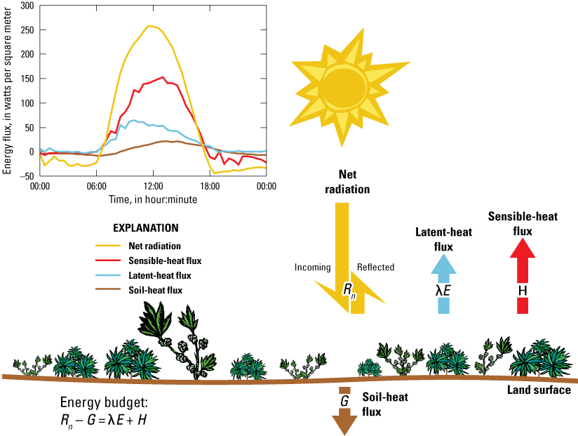
Generalized daily energy-budget trends in an arid environment.
Soil-heat flux at land surface is calculated from measurements of soil-heat flux at depth (Gd), soil temperatures (Tp and Tc), and volumetric soil-water content (θv):
whereGd
is soil-heat flux measured at depth, in W/m2,
Tp
is the preceding soil temperature, in °C,
Tc
is the current soil temperature, in °C,
Cs
is the heat capacity of soil, in joules per °C (J/°C),
D
is the depth of the soil-heat-flux plate, in m, and
t
is the time between temperature measurements, in seconds.
ρb
is the dry bulk density of soil, estimated to be 1,270 kilograms per cubic meter (kg/m3; Moreo and others, 2020),
Cd
is the heat capacity of dry soil, 840 joules per kilogram per °C (J/kg/°C),
θm
is the gravimetric soil-water content, in fraction of total mass, and
Cw
is the heat capacity of water, 4,186 J/kg/°C.
ρw
is the density of water, 1,000 kg/m3,
ρb
is the dry bulk density of soil, estimated to be 1,270 kg/m3 (Moreo and others, 2020), and
θv
is the measured volumetric soil-water content, in fraction of total volume.
Sensible-heat flux is averaged for 30-minute periods with the eddy-covariance method using 10-Hz measurements of vertical wind speed and air temperature as:
whereis the density of air, in kg/m3,
is the specific heat of air at constant pressure, in J/kg/°C,
is the deviation from the mean vertical component of wind speed during the 30-minute averaging period, in meters per second (m/s),
is the deviation from the mean air temperature during the 30-minute averaging period, in °C, and
is the covariance of and during the 30-minute averaging period.
Latent-heat flux, where λ is the latent heat of vaporization of water, in J/kg, and E is the evaporation rate, in meters per 30-minute period, has units of W/m2 and is calculated with the eddy-covariance method using 10-Hz measurements of vertical wind speed and water-vapor density as:
whereλ
is the latent heat of vaporization of water, in J/kg,
is the deviation from the mean vertical component of wind speed during the 30-minute averaging period, in m/s,
is the deviation from the mean water vapor density during the 30-minute averaging period, in kg/m3, and
is the covariance of and during the 30-minute averaging period.
Evapotranspiration, in m/s, is then calculated as:
whereλE
is latent-heat flux, in W/m2, as derived from equation 6,
λ
is the latent heat of vaporization of water, in J/kg, and
is the mean water vapor density during the 30-minute averaging period, in kg/m3.
λE
is latent-heat flux, in W/m2, as derived from equation 6, and
T
is the air temperature, in °C.
Based on the law of conservation of energy, available energy is, on average, equal to turbulent fluxes and the surface-energy budget is in balance, but field measurements often result in an imbalance between available energy and turbulent fluxes (Twine and others, 2000; Wilson and others, 2002; Foken, 2008) and, therefore, a potential miscalculation of ET. The energy-balance ratio (EBR) for a given period is
whereΣλE
is the sum of all latent-heat flux measurements, in W/m2, for the given period,
ΣH
is the sum of all sensible-heat flux measurements, in W/m2, for the given period,
ΣRn
is the sum of all net radiation measurements, in W/m2, for the given period, and
ΣG
is the sum of all soil-heat flux measurements, in W/m2, for the given period.
Turbulent-Flux Source Area and Site Footprint
The turbulent-flux source area is the theoretically infinite area that influences the measured turbulent fluxes at an eddy-covariance ET-monitoring site, and a site footprint, for this study, is a finite, circular area surrounding a site that is used to analyze measured turbulent fluxes. The turbulent-flux source area includes all vegetation and other surfaces surrounding a site that affect the moisture and heat (energy) content of eddies before they reach site sensors (fig. 3). A site footprint is smaller in size than the turbulent-flux source area and primarily contains targeted vegetation, or cover, while being large enough to account for most of the measured turbulent fluxes. Site-scale ET data are upscaled to the footprint area and then related to corresponding values on a vegetation index, which allows site-scale ETg to be associated with a larger area in the scaled NDVI, rather than the 0.6×0.6-m pixel area that corresponds to a site location. At a site, the size of a footprint is sensitive to the height of the fast-response sensors above the average canopy height, the surface roughness of the source area, and atmospheric stability, such that sensors with low heights relative to the average canopy height, a rough source area, and an unstable atmosphere reduce the size of the site footprint (Schuepp and others, 1990). For this study, the footprint area is evaluated using cumulative normalized flux (CNF) data for different circular zones surrounding each ET-monitoring site (Schuepp and others, 1990; Rannik and others, 2012; Garcia and others, 2014).
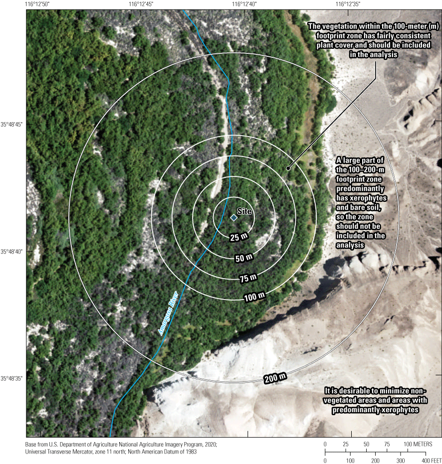
A theoretical evapotranspiration-monitoring site and the 0–25, 25–50, 50–75, 75–100, and 100–200-meter footprint zones.
A CNF value for a given distance from a site is a measure of the relative flux contributions from the upwind area to the total measured fluxes (Schuepp and others, 1990; Kormann and Meixner, 2001). For example, for a 50-m radius around a site, a CNF value of 0.83 means that 83 percent of the total measured fluxes were affected only by the surfaces within 50 m of the site and the remaining 17 percent of the measured fluxes were affected by the surfaces beyond 50 m from the site. If, at the same site, the CNF value for 100 m is 0.94, then 94 percent of the total measured fluxes were affected only by the surfaces within 100 m, 6 percent of the fluxes were affected by the surfaces beyond 100 m, and, therefore, 11 percent of the fluxes (94 minus 83 percent) were affected by surfaces from 50 to 100 m. When the selected footprint area maximizes fluxes and minimizes surfaces that do not have targeted vegetation, the annual daytime mean CNF values represent the percentage of the total fluxes.
Site-Scale Methods and Results
Site-scale ETg was estimated from measurements of precipitation, air temperature, and λE at the Shrub and Wetland ET-monitoring sites in the AWSR study area. Total ET was calculated from λE, and then total ET was adjusted for the EBR, which required measurements of Rn, G, and H. Net radiation was directly measured, G was estimated from measurements of other soil parameters (eq. 2), H and λE were measured using the eddy-covariance method (eqs. 5 and 6), and total ET was calculated from air temperature and λE measurements (eq. 9). Site-scale ETg was the average of the measured total ET and the EBR-adjusted total ET, minus precipitation. Finally, the footprint size was selected for each site based on annual daytime mean CNF values for various footprint sizes and the vegetation corresponding to those footprint sizes.
The locations of the ET-monitoring sites were selected because they were in areas conducive to eddy-covariance measurements and because the two sites had different plant covers. Sites conducive to eddy-covariance measurements generally have a large area of relatively flat ground, where predominantly phreatophytes grow, with near-homogeneous plant cover, surface roughness, canopy height, and soil-moisture conditions. These site attributes help ensure that the turbulent fluxes measured at the site primarily are affected by the targeted area (Rosenberry and others, 2007). Having two sites with different plant covers, such as sparse shrubs and dense wetlands, helps to broaden the ranges of site-scale ETg and scaled NDVI values used to develop the quadratic relation for estimating annual ETg.
The Shrub ET-monitoring site was located in moderately sparse phreatophytes on the floodplain of an intermittent section of the Amargosa River between the current (2018) riparian corridor and the riparian corridor of a relict section of the river (table 1; figs. 1, 4, and 5). The riparian corridors near the Shrub site were oriented about north-south, the floodplain between the two riparian corridors was about 150 m wide, and the north-south extent of sparse shrubs was about 220 m wide. The area surrounding the site primarily consisted of dry soil and moderately sparse phreatophytic shrubs and grasses with an uneven distribution (fig. 5A) and an average canopy height of about 0.76 m. Vegetation surrounding the site primarily consisted of bush seepweed, saltgrass, white bursage, greasewood, creosote bush, and blackbrush. The near-surface soil at the Shrub site was very light gray in color and clay to fine-grained sand in texture.
Table 1.
Location and sensor information for the Shrub and Wetland evapotranspiration-monitoring sites, Shoshone, Inyo County, California (U.S. Geological Survey, 2020).[Location of evapotranspiration-monitoring sites are shown on figure 1B. Fast-response sensors are a sonic anemometer used to measure vertical wind speed and air temperature and a krypton hygrometer used to measure water-vapor fluctuations. NA, not applicable because there was no quantum sensor at the Wetland site. Abbreviations: USGS, U.S. Geological Survey; USGS site no., unique numeric site identifier for the National Water Information System; NAD 83, North American Datum of 1983; NGVD 29, National Geodetic Vertical Datum of 1929]
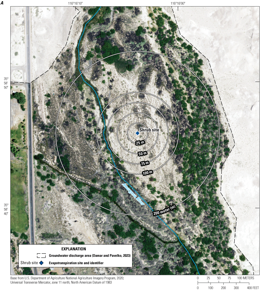
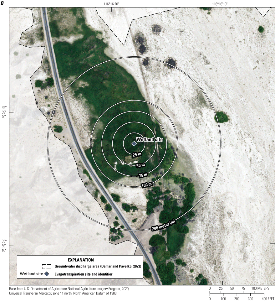
The 0–25, 25–50, 50–75, 75–100, and 100–200-meter (m) footprint zones for the A, Shrub; and B, Wetland evapotranspiration-monitoring sites, Shoshone, Inyo County, California.
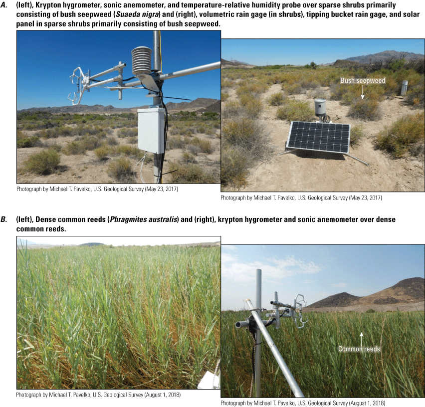
Vegetation and instruments at the A, Shrub and B, Wetland evapotranspiration-monitoring sites, Shoshone, Inyo County, California.
The Wetland ET-monitoring site was located in about 53,000 m2 of wetlands about 350 m west of an intermittent section of the Amargosa River (table 1; figs. 1, 4, and 5). The area surrounding the site primarily consisted of dense wetland vegetation with a uniform distribution (fig. 5B) and an average canopy height of about 3 m. Vegetation surrounding the site primarily consisted of common reeds with minor amounts of cattail; phreatophytes growing along the margins of the wetland primarily consisted of saltgrass, common reeds, bush seepweed, yerba mansa (Anemopsis californica), western honey mesquite, desert willow, and tamarisk. The near-surface soil at the Wetland site was brown to dark gray in color, silty clay in grain size, contained living and dead roots, and generally was well-shaded by vegetation.
Measurements
Air temperature, relative humidity, precipitation, Rn, photosynthetically active radiation (PAR), G, H, λE, and total ET were either directly measured or were calculated from direct measurements of other parameters. Data were collected at the Shrub site from March 8, 2017, to May 1, 2019, and data were collected at the Wetland site from April 20, 2017, to May 7, 2019 (U.S. Geological Survey, 2020). Sites were visited about monthly to inspect sensors and equipment, document site conditions, and download data. All sensors and equipment used at the sites (table 1) were calibrated, maintained, and positioned according to manufacturer recommendations. At both sites, data were collected for more than 1 year and were recorded and stored to a data logger every 30 minutes. Air temperature and relative humidity were directly measured at both sites with a temperature and relative humidity probe (Campbell Scientific, Inc., 2015b).
Precipitation was measured during each site visit with volumetric rain gages at both sites and with a recording tipping-bucket rain gage at the Shrub site. Volumetric rain gages, which do not record data, are more accurate than tipping-bucket rain gages because tipping-bucket rain gages can under-measure during light rains, when precipitation can evaporate before a bucket is tipped, and during intense rains, when precipitation falls too fast to register (Humphrey and others, 1997). Tipping-bucket rain gages accurately record the timing and duration of rainfall, but their volumetric totals must be corrected to the volumetric totals. Because the sites were 1 km apart, it was assumed that the timing of rainfall at the Wetlands site was similar to the measured rainfall at the Shrub site. The volumetric rain gages were standard 20.3-centimeter (cm) diameter gages (National Weather Service, 2020) measured with a 0.254-mm resolution ruler and installed such that the gage intakes were about 0.84 m above ground. A small volume of mineral oil, which floats on water, was added to the precipitation reservoirs of the volumetric gages to help prevent evaporative losses between site visits (Sevruk, 1973). The tipping-bucket rain gage (Campbell Scientific, Inc., 2010d), installed at the Shrub site, was at a height of 1.04 m above ground and recorded with a 0.254-mm resolution. During the study, snowfall was not observed at either site.
Net radiation was directly measured at both sites and PAR was directly measured only at the Shrub site. Net radiation was measured with net radiometers, where the downward-facing field of view was a circular area with a radius of 10 times the sensor height (Campbell Scientific, Inc., 2010c). At each site, the net radiometer was installed at a height and location to measure an area representative of the targeted vegetation with the downward-facing sensor and positioned to have an unobstructed upward-facing view of the sky. At the Shrub site, the height of the net radiometer captured shrubs and bare soil within a ground radius of about 28.8 m, and at the Wetland site, the height of the radiometer captured primarily dense common reeds within a ground radius of about 37.3 m. Photosynthetically active radiation, a measure of incoming photons with wavelengths that plants use during photosynthesis, was measured with a quantum sensor (Campbell Scientific, Inc., 2015a) that was positioned to have an unobstructed upward-facing view of the sky.
Soil-heat flux at land surface was calculated for both sites from below-ground measurements of G, soil temperature, and soil-moisture content (eq. 2). Soil-heat flux at depth was measured 8 centimeters (cm) below land surface with two soil-heat-flux plates (Campbell Scientific, Inc., 2016), soil temperature was measured at 2 and 6 cm below land surface with thermistors (Campbell Scientific, Inc., 2018), and soil-moisture content at 2.5 cm below land surface was measured with a water-content reflectometer (Campbell Scientific, Inc., 2011b). At each site, soil sensors were installed in representative locations of vegetation such that the land surface above the sensors received a corresponding amount of shade and direct sunlight. At the Shrub site, the soil sensors were installed next to shrubs such that the patch of soil above the sensors received a representative amount of shade and direct sunlight throughout the course of a typical day. At the Wetland site, the soil sensors were beneath about a 14-cm thick layer of dying, dead, and decaying common reeds such that the patch of soil above the sensors rarely received direct sunlight.
Sensible-heat flux and λE were calculated using the eddy-covariance method using measurements from two fast-response sensors at each site—a three-dimensional sonic anemometer used to measure vertical wind speeds and air temperatures, and a krypton hygrometer used to measure water-vapor fluctuations (Campbell Scientific, Inc., 2010a, 2010b). Sensible-heat flux was calculated from measurements of vertical wind speed and air temperature (eq. 5), and λE was calculated from measurements of vertical wind speed and water-vapor fluctuations (eq. 6). At each site, the fast-response sensors were installed at heights to capture fluxes from the targeted vegetation and oriented toward an azimuth of 208 degrees from north to best capture prevailing winds. From 2007 to 2016, wind at Tecopa generally was bidirectional, primarily coming from between the south-southeast and south (157.5–180 degrees from north) with a secondary component coming from between the northwest and north-northwest (315–337.5 degrees from north; Community Environmental Monitoring Program, 2022). At the Shrub site, the fast-response sensors were 2.14 m above land surface and measured fluxes primarily affected by sparse shrubs and dry soil. At the Wetland site, the fast-response sensors were 3.64 m above land surface and measured fluxes primarily influenced by common reeds.
Data Processing
For each ET-monitoring site, site-scale ETg was estimated and annual daytime mean CNF values were calculated. A 1-year period of analysis was selected for each site where each period of analysis was selected to minimize missing and suspect data. Site-scale data were processed with a data-logger program and the software packages LoggerNet (Campbell Scientific, Inc., 2011a) and EdiRe (Clement, 1999), and then the data were examined and post-processed in a spreadsheet to calculate site-scale ETg and the EBR. A data logger (Campbell Scientific, Inc., 2011c) and program were used at each site to store data and to perform initial data processing, including calculating raw turbulent-flux values using site-specific data. Site-specific data used in each data-logger program were the atmospheric pressure of the site, the orientation (azimuth) of the sonic anemometer, and the calibration constants for the hygrometer, radiometer, quantum sensor, and heat-flux plates. LoggerNet was used to convert logger output files into formats that could be read into EdiRe and a spreadsheet. EdiRe, a software package for micrometeorological applications, was used to process and correct 10-Hz data and aggregate them into 30-minute averages or covariances, and to calculate available energy, turbulent fluxes, and mean CNF values. The processed 30-minute data were examined for missing and suspect values and post-processed in a spreadsheet to calculate available energy and turbulent flux values, the annual EBR, site-scale ETg, EBR-adjusted turbulent flux values, EBR-adjusted site-scale ETg, and annual daytime mean CNF values.
The 10-Hz data from the fast-response sensors were corrected and processed into 30-minute H and λE values using EdiRe (Clement, 1999). Data spikes were filtered according to a method described by Højstrup (1993) and corrected to compensate for any signal lag between the anemometer and hygrometer. Raw covariances were mathematically two-dimensionally rotated to force the mean vertical and crosswind velocities to zero, which compensates for errors associated with small misalignments of the sonic anemometer (Kaimal and Finnigan, 1994). Frequency response corrections were applied to the data to compensate for the inability of the sensors to measure the flux contributions from larger (greater than 1 km) and smaller (less than 10 cm) eddies (Moore, 1986). Corrections were applied to vertical wind speeds to compensate for variations in air density that result from fluctuating temperatures and humidity (Webb and others, 1980). Latent-heat flux values were corrected to compensate for the attenuation of the hygrometer signal caused by oxygen in the krypton laser signal path (Tanner and Greene, 1989; Campbell Scientific, Inc., 1998). Sensible-heat flux values were corrected to compensate for air density and sound-path deflection, which affect the sonic-derived temperatures used to calculate H (Schotanus and others, 1983).
Data then were examined and post-processed to perform additional corrections, address missing or suspect data, determine daytime and nighttime, and to calculate site-scale ETg. Precipitation for the Shrub site, which had a volumetric and tipping-bucket rain gage, was calculated by adjusting the tipping bucket rain gage values so that they equaled the more accurate volumetric rain gage values (World Meteorological Organization, 2008). The volumetric-corrected tipping-bucket data then were wind-speed corrected for periods when wind speeds exceeded 5 m/s because precipitation can be undermeasured if there is wind turbulence at the rain gage (World Meteorological Organization, 2008). For the Wetland site, which only had a volumetric rain gage, precipitation was calculated by first determining the linear relation between the volumetric measurements from both sites measured on the same day and then deriving the corrected amount by applying the linear relation to the measured volumes. The volumetric measurements were corrected based on the assumption that wind speeds were similar at the two sites, which were about 1 km apart. Net radiation values were corrected for periods when wind speeds exceeded 5 m/s to compensate for convective cooling caused by wind blowing across the sensors (Brotzge and Duchon, 2000; Campbell Scientific, Inc., 2010c). For periods when EdiRe-calculated H and λE data were missing or suspect, H and λE values calculated by the data logger program were frequency-corrected and used (Moore, 1986; Massman, 2000).
Data were examined for missing or suspect values, which were censored and replaced with estimated values. Net radiation, PAR, G, H, and λE values were flagged as suspect if they did not conform to expected daily or seasonal trends or if the values exceeded suggested guidelines. Suggested data-range guidelines were that Rn values should not be less than −200 W/m2 or greater than 900 W/m2, PAR values should not be less than zero or greater than 2,200 micromoles per second per square meter (µmol/s/m2), G values should not be less than −50 W/m2 or greater than 50 W/m2, and H and λE values should not be less than −150 W/m2 or greater than 700 W/m2 (Law and others, 2005). If a value exceeded suggested guidelines but conformed to expected trends, then the value was not flagged as suspect. If a value exceeded suggested guidelines or did not conform to expected trends, then it was censored and replaced with an estimated value. Suspect Rn, G, and H data were censored and replaced with linearly interpolated values. Suspect λE values that were collected during the daytime were censored and replaced with linearly interpolated values and suspect λE values that were collected at nighttime were censored and replaced with zero. If a consecutive series of suspect λE values occurred during the transition from nighttime to daytime, or daytime to nighttime, then the nighttime values were edited to zero and the daytime values were linearly interpolated from, or to, zero, respectively. Missing or suspect λE values at nighttime were edited to zero rather than being replaced with linearly interpolated values because there generally is very little or no available energy at nighttime and measured turbulent-flux values tend to fluctuate around zero.
For this study, daytime and nighttime were defined using Rn and PAR data. It was daytime if Rn was greater than −5 W/m2 and PAR was greater than 200 µmol/s/m2. If the Rn and PAR definitions disagreed (for example, if Rn was more than −5 W/m2 but PAR was less than 200 µmol/s/m2, or if the Rn and PAR values both did not fit expected daily temporal trends (for example, if Rn was less than −5 W/m2 and PAR was less than 200 μmol/s/m2 as a result of cloudy skies during the late morning or afternoon), then daytime and nighttime were delineated based on the daily trends preceding and following the suspect data.
For the Shrub site, the 1-year period of analysis, from January 4, 2018, to January 3, 2019, included 17,520 thirty-minute values. There were no missing data but there were 4 Rn values; 5,911 G values; 13 H values; and 141 λE values that were flagged as suspect (Law and others, 2005); no PAR data were suspect. There were 1,042 Rn values that were wind-speed corrected because the corresponding wind speeds exceeded 5 m/s. Suspect Rn and H values did not fit expected daily trends, so they were censored and replaced with linearly interpolated values. All suspect G values fit expected daily and seasonal trends and therefore, no G values were censored. Of the 141 suspect λE values, 90 values were censored and replaced with linearly interpolated values and 51 were replaced with zero; all values that were replaced with zero occurred at nighttime, or within 1 hour of nighttime, as defined by Rn and PAR data. When defining daytime and nighttime, there were 1,005 disagreements between the Rn and PAR data and there were 36 values when Rn and PAR data did not fit expected trends.
For the Wetland site, the 1-year period of analysis, from January 1 to December 31, 2018, included 17,520 thirty-minute values. There were no missing H values but there were 193 missing λE values and 2 missing Rn values; 7 G values, 397 H values, and 877 λE values were considered suspect (Law and others, 2005). There were 146 Rn values that were wind-speed corrected because the corresponding wind speeds exceeded 5 m/s. The suspect Rn and G values were censored and replaced with linearly interpolated values. Of the 397 suspect H values, 330 values fit expected daily and seasonal trends and were not censored, and 67 values were censored and replaced with linearly interpolated values. Of the 1,070 missing (193) and suspect (877) λE values, 756 values fit expected daily trends and were not censored, 179 values were censored and edited to zero, and 135 values were censored and replaced with linearly interpolated values. All 179 λE values that were censored and edited to zero were associated with rain and 165 of them occurred at nighttime or within 1 hour of nighttime. When defining daytime and nighttime, there were 505 disagreements between Rn data at the Wetland site and PAR data at the Shrub site and there were 17 values when Rn and PAR data did not fit expected daily trends.
Site-scale ETg, which equals total ET minus precipitation, was calculated from the 30-minute available-energy, turbulent-flux, and precipitation data for each site. Total ET was calculated as the average of measured total ET and EBR-adjusted total ET (Moreo and Swancar, 2013). Measured total ET was calculated from measured 30-minute air-temperature and λE (eq. 9). An annual EBR was calculated from measured 30-minute available-energy and turbulent-flux data (eq. 10). Measured turbulent fluxes (H and λE) then were adjusted, while maintaining the Bowen ratio, to achieve energy balance or an annual EBR of one (Twine and others, 2000; Foken and others, 2012b; Garcia and others, 2014). The Bowen ratio is H divided by λE (Bowen, 1926; Sverdrup, 1943). The EBR-adjusted total ET was calculated from air temperature and EBR-adjusted λE (eq. 9). Evapotranspiration from soil moisture was not a consideration when calculating ETg because the soil-moisture content at the beginnings and endings of the periods of analyses were similar (Allander and others, 2009; Garcia and others, 2014). Uncertainty in site-scale ETg was calculated as one-half of the percentage of difference between measured and EBR-adjusted ETg values (Moreo and Swancar, 2013).
The final step in site-scale data processing was calculating annual daytime mean CNF values for selected footprint sizes (Schuepp and others, 1990; Kormann and Meixner, 2001) and determining the footprint sizes that were used in the analyses. For this study, 30-minute CNF values were calculated using EdiRe software (Clement, 1999) for six zones centered on each site corresponding to radii of 25, 50, 75, 100, 200, and 300 m. Annual daytime mean CNF values represent an entire year of analysis but do not include nighttime data, when the surface-energy budget generally is unstable and site-scale ET fluctuates around zero.
Site-Scale Groundwater Discharge by Evapotranspiration
At the Shrub site, site-scale ETg for the 1-year period of analysis was 0.121±0.005 m, or 3.9 percent (table 2). Site-scale ETg was calculated by subtracting precipitation (0.068 m) from total ET (0.189 m). Precipitation is based on a wind-speed correction to the tipping-bucket rain gage total (0.048 m), which was corrected for the volumetric rain gage total (0.063 m). Total ET is the average of measured total ET (0.197 m; fig. 6) and EBR-adjusted total ET (0.182 m). The EBR for the Shrub site was 1.085. Based on the annual daytime mean CNF values and the surrounding plant cover, a 75-m radius footprint was selected for the Shrub site, which accounted for about 82 percent of the measured turbulent fluxes, and therefore, 82 percent of the measured ET (table 3). The footprint size was limited to a 75-m radius because the area from 75 to 200 m from the site had uneven plant cover and the area beyond 200 m from the site included a highway and vegetation that predominantly was xerophytes (fig. 4A).
Table 2.
Precipitation, evapotranspiration, and energy-balance data for the Shrub and Wetland evapotranspiration-monitoring sites, Shoshone, Inyo County, California (U.S. Geological Survey, 2020; Pavelko, 2023).[Location of evapotranspiration-monitoring sites are shown in figure 1B. Analysis period: mm/dd/yyyy, month/day/year. Abbreviations: ET, evapotranspiration; m/yr, meters per year; EBR, energy-balance ratio; ETg, groundwater discharge by ET]
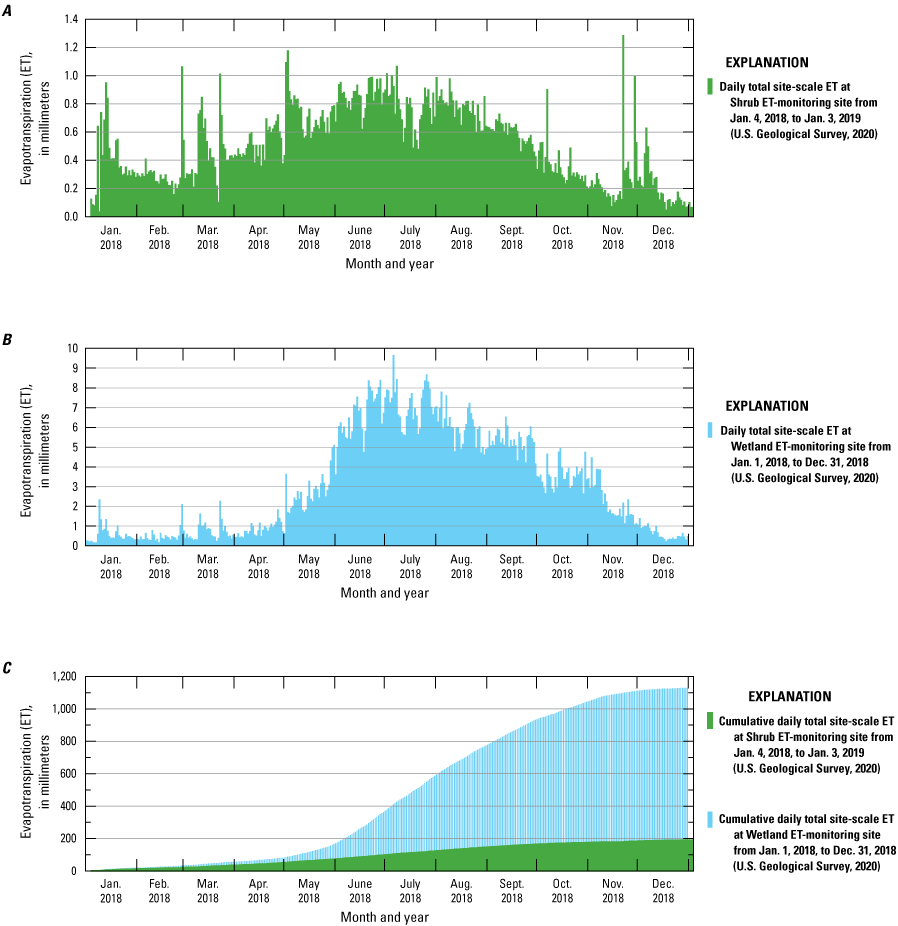
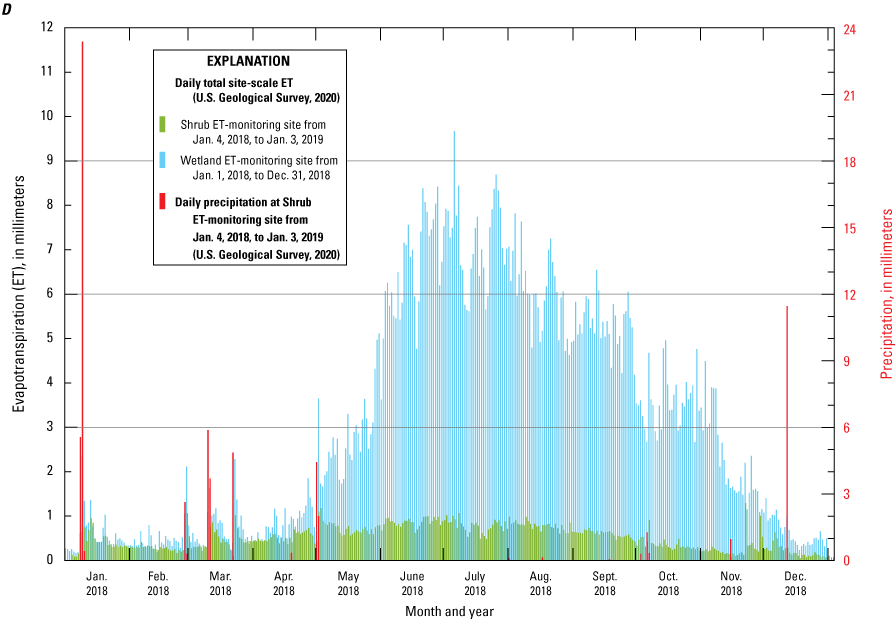
2018 daily total evapotranspiration and precipitation for the A, Shrub evapotranspiration-monitoring site; B, Wetland evapotranspiration-monitoring site; C, Shrub and Wetland evapotranspiration-monitoring sites; and D, 2018 cumulative daily total evapotranspiration for the Shrub and Wetland evapotranspiration-monitoring sites, Shoshone, Inyo County, California.
Table 3.
Cumulative normalized flux data and mean scaled normalized difference vegetation index values for the Shrub and Wetland sites, Shoshone, Inyo County, California.[Location of evapotranspiration-monitoring sites are shown on figure 1B. Value: Annual daytime mean cumulative normalized flux (CNF) values and mean daytime CNF values, scaled to 0–75 meters (m), were calculated from values in Pavelko (2023) and then rounded to the nearest 0.01. Mean scaled normalized difference vegetation index (NDVI) values were calculated from values in Damar and Pavelko (2023) and then rounded to the nearest integer. Footprint-weighted mean scaled NDVI values were calculated from mean scaled NDVI values and annual daytime mean values, using equation 11. The period of analysis for the Shrub site is from January 4, 2018, to January 3, 2019, and the period of analysis for the Wetland site is from January 1 to December 31, 2018. Abbreviations: m, meters; NA, not applicable because roads, xerophytes, and variable phreatophyte cover were not representative of targeted vegetation; NC, not calculated]
Cumulative normalized flux data were calculated using the EdiRe software package (Clement, 1999).
At the Wetland site, site-scale ETg for the 1-year period of analysis was 1.056±0.076 m, or 7.2 percent (table 2). Site-scale ETg was calculated by subtracting precipitation (0.073 m) from total ET (1.129 m). Total ET is the average of measured total ET (1.053 m; fig. 6) and EBR-adjusted total ET (1.205 m). The EBR for the Wetland site was 0.873. Precipitation is based on wind-speed corrected volumetric measurements of 0.068 m. Based on the annual daytime mean CNF values and the surrounding plant cover, a 75-m radius footprint was selected for the Wetland site, which accounted for about 85 percent of the measured turbulent fluxes, and therefore, 85 percent of the measured ET (table 3). The footprint size of the Wetland site was limited to a 75-m radius because much of the area from 75 to 100 m from the site included sparse grasses and a large part of the area beyond 100 m from the site included a highway and vegetation that predominantly was xerophytes (fig. 4B).
Study-Area Scale Methods
Annual ETg for the AWSR study area was calculated by multiplying the area of each ET unit by the appropriate site-scale ETg to derive annual ETg for each ET unit and then adding the annual ETg for all ET units in the GDAs and study area. Groundwater discharge areas were delineated and then subdivided into open-water, moist-soil, and vegetated ET units. Open-water and moist-soil ET units were assigned site-scale ETg estimated from previous studies (Laczniak and others, 2001; Jackson and others, 2018). Vegetated ET units were assigned a range of site-scale ETg on a pixel-by-pixel basis derived from a quadratic equation relating site-scale ETg to a scaled NDVI that encompasses the AWSR study area.
The primary goal of delineating GDA boundaries was to include as many areas of open water, moist soil, and phreatophytes as possible while minimizing areas of xerophytes or dry bare soil, and the primary goal of delineating ET-unit boundaries was to quantify the areas of the ET units. Initially, boundaries were visually delineated using various imagery sources, including 2014 National Agriculture Imagery Program (NAIP) aerial imagery (U.S. Department of Agriculture, 2012) and Esri World Imagery (Esri and others, 2022). The GDA and ET-unit boundaries were continually refined throughout the study period based on imagery and field verification. The imagery-based delineations were checked by visiting about 160 locations in and around the study area, generally where GDA or ET-unit boundaries were not clear on imagery.
Many studies throughout the Basin and Range Province have documented a strong relation between ET and vegetation indexes (Ustin, 1992; Laczniak and others, 1999, 2001, 2006; Nichols, 2000; Nagler and others, 2001, 2005; Reiner and others 2002; DeMeo and others, 2003; Smith and others, 2007; Glenn and others, 2008; Allander and others, 2009; Garcia and others, 2014; Berger and others, 2016; Moreo and others, 2020). A vegetation index is a mathematical combination, typically a dimensionless ratio, of the reflectance of solar radiation in two or more bands of the electromagnetic spectrum that has been shown to indicate various properties of green vegetation, including chlorophyll content, photosynthetic activity, green biomass, abundance, and percentage of cover (Goetz and others, 1983; Jensen, 2000). Relating site-scale ETg estimates to a vegetation index that encompasses the study area allows site-scale ETg to be spatially distributed on a pixel-by-pixel basis across the vegetated ET units using the values of the vegetation index as a scalar (Beamer and others, 2013).
Processing the Scaled Vegetation Index
A scaled NDVI (Rouse and others, 1974) that encompasses the AWSR study area was calculated from the red and near-infrared bands of 0.6-m resolution 4-band NAIP aerial imagery collected in 2020 (Damar and Pavelko, 2023). The NAIP imagery is collected every other year in most States, including California, and the imagery is well-suited for use in ET studies. In addition to visible spectrum bands of red, green, and blue, NAIP imagery includes a near-infrared spectral band, which is necessary to calculate common vegetation indexes. The NAIP imagery typically is collected during periods when vegetation is considered near the peak of seasonal growth, and the flight paths allow large areas to be collected on a single day (U.S. Department of Agriculture, 2017). A vegetation index derived from imagery collected in a single day, as opposed to over several weeks or months, minimizes variations in sun angle, atmospheric conditions, and ground conditions so that values across the scene are comparable. The scaled NDVI used in this study was derived from imagery collected almost entirely on July 2, 2020, with less than one-half of 1 percent of the study area, at the southern end of the Amargosa River GDA, collected on May 23, 2020. Ideally, the collection date also is at least 30 days after any rainfall in the study area and is contemporaneous with the ET measurements. Antecedent rainfall can cause an unseasonable growth spurt in vegetation that could misrepresent the vigor (health) of the plants for the time of year. Contemporaneous data collection ensures that the imagery is representative of measurement conditions. The 2020 NAIP imagery used in this study was collected with no antecedent rain for at least 30 days, but it was not collected contemporaneously with the ET measurements. Although NAIP imagery also was collected in 2018, the imagery covering the study area was collected over multiple days in late August of that year, when vegetation is not in peak vigor. It was assumed that undisturbed vegetation, such as in the AWSR study area, varied minimally during the 2 years after ET-data collection and, therefore the imagery collected in July 2020 is the better representation of peak growing season conditions in 2018.
The NDVI was selected as the vegetation index for this study because the radiometric correction applied to the NAIP imagery does not include conversion to percentage of reflectance, which is required for more complex vegetation indexes. The NDVI is a normalized ratio of reflectance in the near-infrared band to reflectance in the red band. These two bands can be used as indicators of the presence of vegetation because plant leaves reflect near-infrared energy and chlorophyll absorbs red energy (U.S. Department of Agriculture, 2017). Raw NDVI values range from −1 to 1, with values from 0 to 1 being positively correlated to amount of green biomass (Jensen, 2000). For this study, negative NDVI values were set to zero and all other NDVI values were scaled by 10,000 (Damar and Pavelko, 2023). These scaled values were used in the calculations of this study and are referred to as scaled NDVI values.
A footprint-weighted mean scaled NDVI value for each ET-monitoring site was calculated using site-scale CNF data and scaled NDVI values that corresponded to the selected footprint sizes (table 3). The size of a footprint was selected based on the annual daytime mean CNF values for six areas surrounding the site and the vegetation and other surfaces in those areas, where the largest footprint was selected that contained predominantly the targeted vegetation. Footprint-weighted mean scaled NDVI values were used to develop the quadratic equation because they represent the site footprint, whereas the scaled NDVI value for the site location only corresponds to a 0.6×0.6 m pixel. After the footprint size of a site was determined, it was assumed that all measured fluxes come from within the footprint area. A footprint-weighted mean scaled NDVI value then was determined by calculating the mean scaled NDVI value for each footprint zone around the site (0–25, 25–50, 50–75, 75–100, and 100–200 m; table 3; figs. 7A and 7B), weighting each mean scaled NDVI value for each zone with the corresponding annual daytime mean CNF value, and then adding the weighted means of each zone. The Shrub and the Wetland ET sites have a 75-m radius footprint, each comprised of three footprint zones, 0–25, 25–50, and 50–75 m, therefore the footprint-weighted mean scaled NDVI value is calculated as:
whereNDVI0–25, NDVI25–50, and NDVI50–75
are mean scaled NDVI values for the 0–25, 25–50, and 50–75 m footprint zones, respectively, and
CNF0–25, C0–50, and CNF0–75
are annual daytime mean CNF values for the 0–25, 0–50, and 0–75 m footprint zones, respectively.
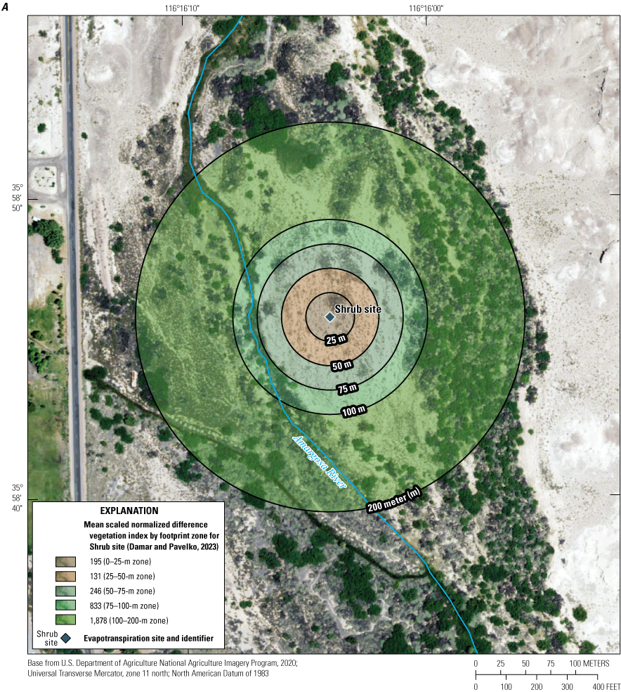
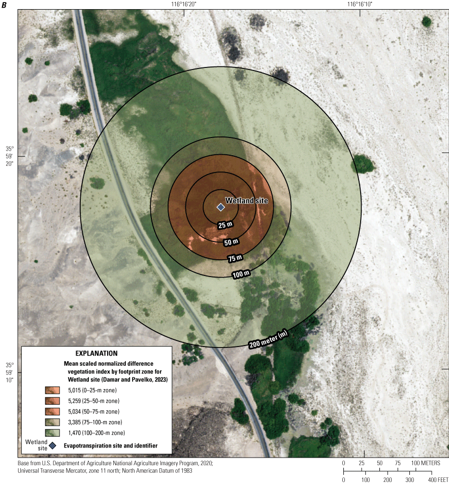
The 0–25, 25–50, 50–75, 75–100, and 100–200-meter (m) footprint zones and corresponding footprint-weighted mean scaled normalized difference vegetation index values for the A, Shrub site; and B, Wetland site, Shoshone, Inyo County, California.
Assigning Rates and Uncertainty
Open-water and moist-soil ET units were assigned site-scale ETg derived from previous studies and vegetated ET units were assigned site-scale ETg estimated for this study. For open water in the Great Basin, site-scale ETg ranges from about 1.49 meters per year (m/yr) at Walker Lake to about 2.62 m/yr at Ash Meadows (Laczniak and others, 1999; Berger and others, 2001; Westenburg and others, 2006; Allander and others, 2009; Moreo and Swancar, 2013; Earp and Moreo, 2021). For this study, open-water ET units were assigned a site-scale ETg of 2.53 m/yr, which is the open-water rate estimated for the Tecopa/California Valley area by Laczniak and others (2001). For moist soil in the Great Basin, estimated site-scale ETg ranges from about 0 m/yr for salt-encrusted playas of Death Valley (Jackson and others, 2018) to about 0.792 m/yr for moist bare soil in Ash Meadows (Laczniak and others, 1999). Moist-soil ET units were assigned a site-scale ETg of 0.322 m/yr, which is the average of the site-scale ETg for the moist bare soil ET unit in the Shoshone and Tecopa/California Valley areas (0.643 m/yr) from Laczniak and others (2001) and the site-scale ETg for the salt-encrusted playas of Death Valley (0.00000002 m/yr) of Jackson and others (2018).
Vegetated ET units were assigned site-scale ETg defined by a quadratic relation between site-scale ETg, as the dependent variable, and scaled NDVI values, as the independent variable, similar to Allander and others (2009) and Beamer and others (2013). The quadratic relation (fig. 8) was developed using four points. The first two points are derived from the site-scale ETg measurements (table 2) and corresponding footprint-weighted mean scaled NDVI values (table 3). The second two points are theoretical, one point representing a theoretical minimum site-scale ETg of zero and a scaled NDVI value of zero and a second point representing a maximum site-scale ETg of 1.222 m/yr and the maximum scaled NDVI value of 10,000. The estimated maximum site-scale ETg for the AWSR study area was assumed to be 1.222 m/yr because that was the highest site-scale ETg estimated for the DVRFS and corresponded to dense wetland vegetation in the Shoshone area (Laczniak and others, 2001). The relation was developed following the assumptions that an increase in scaled NDVI values must result in an increase in site-scale ETg, that scaled NDVI values equal to zero were assigned an ETg of zero, and that the relation would not extend beyond the maximum scaled NDVI value of 10,000 or the estimated maximum site-scale ETg of 1.222 m/yr.
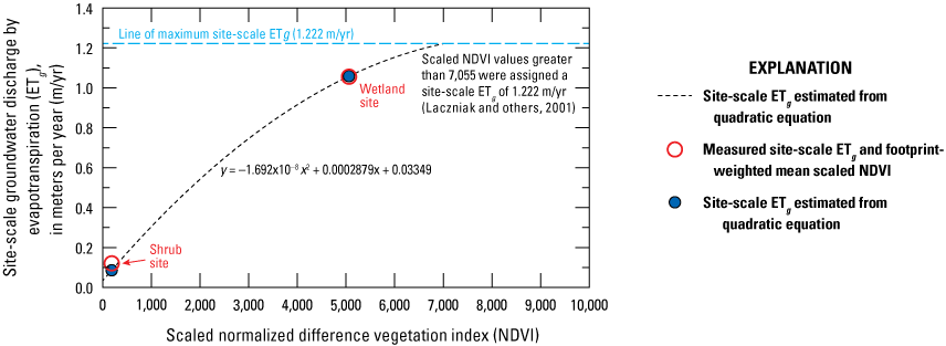
Quadratic relation between scaled normalized difference vegetation index values and annual groundwater discharge by evapotranspiration for the Amargosa Wild and Scenic River study area, Inyo and San Bernardino Counties, California.
The range of annual ETg for the study area was computed using the lowest and highest estimated site-scale ETg. The lowest estimated annual ETg for the study area was computed using an open-water site-scale ETg of 1.494 m/yr (Allander and others, 2009) and a moist-soil site-scale ETg of 0.00000002 m/yr (Jackson and others, 2018). The lowest estimated annual ETg for vegetated areas was computed from a quadratic relation that, for each site, used only the smaller of measured and EBR-adjusted values (table 2) instead of their average. The highest estimated annual ETg for the study area was computed using an open-water site-scale ETg of 2.62 m/yr (Laczniak and others, 1999) and a moist-soil site-scale ETg of 0.792 m/yr (Laczniak and others, 1999). The highest estimated annual ETg for vegetated areas was computed from a quadratic relation that, for each site, used only the larger of measured and EBR-adjusted values (table 2) instead of their average.
Annual Groundwater Discharge by Evapotranspiration for the Amargosa Wild and Scenic River Study Area
Annual ETg for the AWSR study area was about 10,139,000 m3 in 2018 and ranged from 7,059,000 to 14,321,000 m3 (table 4). Annual ETg was estimated by delineating the open-water, moist-soil, and vegetated ET units in each GDA, assigning site-scale ETg to each ET unit, multiplying the site-scale ETg by the ET-unit areas to derive annual ETg for each ET unit, and then adding all annual ET-unit values. Evapotranspiration-unit and GDA boundaries were iteratively delineated using aerial imagery and field verification.
Table 4.
Annual groundwater discharge by evapotranspiration from the Amargosa Wild and Scenic River study area, by groundwater discharge area and evapotranspiration unit, Inyo and San Bernardino Counties, California (Damar and Pavelko, 2023).[Groundwater discharge areas are shown in figure 1B. Area values are rounded to the nearest 1,000 so individual components may not add up to totals in this table. Abbreviations: ET, evapotranspiration; m2, square meters; ETg, groundwater discharge by evapotranspiration; m3, cubic meters]
The AWSR study area was 28,229,000 m2 and consisted of vegetated ET units (20,522,000 m2 or about 73 percent of the study area), moist-soil ET units (7,652,000 m2 or about 27 percent of the study area), and open-water ET units (55,000 m2 or about 0.2 percent of the study area; table 4). The outer boundaries of GDAs generally were moist-soil and vegetated ET units. Where outer boundaries were moist-soil ET units, boundaries were distinct and easily identified. Where outer boundaries were vegetated ET units, phreatophytes were decreasing in abundance and xerophytes were increasing in abundance, relative to the center of the GDA, and the boundary areas often were slightly elevated above the central part of the GDA. In the Shoshone and Amargosa River GDAs, the vegetated ET units had a wide range of phreatophyte types and cover. In the Chicago Valley, Resting Spring, and California Valley GDAs, the vegetated ET units generally consisted of pockets of dense woodlands separated by dry soils and xerophytes.
The site-scale ETg data at each site have a corresponding footprint-weighted mean scaled NDVI value (table 3). Figure 7 shows that although neither site footprint had an entirely homogeneous vegetation distribution, the scaled NDVI values within the selected footprint zones did not substantially vary, indicating that each site was adequately located and that the footprint-weighted mean scaled NDVI value for each site was reasonably representative of the site.
Site-scale ETg assigned to open-water (2.530 m/yr) and moist-soil (0.322 m/yr) ET units were derived from previous investigations and site-scale ETg assigned to vegetated ET units were derived from a quadratic relation between site-scale ETg in the AWSR study area and a 2020 scaled NDVI that encompasses the study area (fig. 8). The quadratic relation was developed using four points, two points derived from the site-scale ETg measurements and corresponding footprint-weighted mean scaled NDVI values (tables 2 and 3), and two theoretical points, one point corresponding to zero ETg and a scaled NDVI value of zero and one point corresponding to the estimated maximum site-scale ETg (1.222 m/yr) and the maximum scaled NDVI value of 10,000. The quadratic relation used to estimate site-scale ETg for vegetated ET units was
where Scaled NDVI values in vegetated ET units ranged from 24 to 8,667, which results in estimated site-scale ETg in the study area ranging from 0.040 to 1.258 m/yr. According to the quadratic relation, scaled NDVI values greater than 7,055 result in site-scale ETg greater than 1.222 m/yr. However, because 1.222 m/yr is considered the maximum site-scale ETg, all scaled NDVI values greater than 7,055 were assigned a site-scale ETg of 1.222 m/yr. The quadratic ETg-NDVI relation developed for this study does not necessarily apply to areas outside of the AWSR study area because the ETg and scaled NDVI values used to develop the relation were collected from the same study area. Moreover, this relation does not necessarily apply to other periods of time because the ETg and scaled NDVI data were collected within 2 years of each other, a relatively short period compared to other studies (Laczniak and others, 1999, 2001, Reiner and others, 2002, Berger and others, 2016).For vegetated ET units, site-scale ETg derived from the quadratic equation varied across the AWSR study area (figs. 9–13). The highest site-scale ETg was along the AWSR and China Ranch Wash, in the Tecopa Hot Springs area, and in the lowland areas of the Chicago Valley (fig. 9B), Resting Spring (fig. 11B), and California Valley GDAs (fig. 13B).
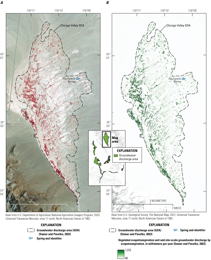
A, Color infrared imagery, where brighter shades of red indicate more plant cover because the near-infrared spectral band is displayed as shades of red, the red band as shades of green, and the green band as shades of blue; and B, annual groundwater discharge by evapotranspiration for the Chicago Valley groundwater discharge area, Inyo County, California.
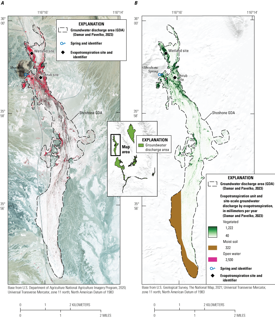
A, Color infrared imagery, where brighter shades of red indicate more plant cover because the near-infrared spectral band is displayed as shades of red, the red band as shades of green, and the green band as shades of blue; and B, annual groundwater discharge by evapotranspiration for the Shoshone groundwater discharge area, Inyo County, California.
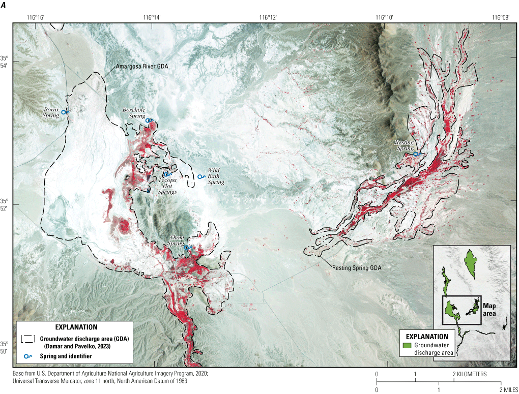
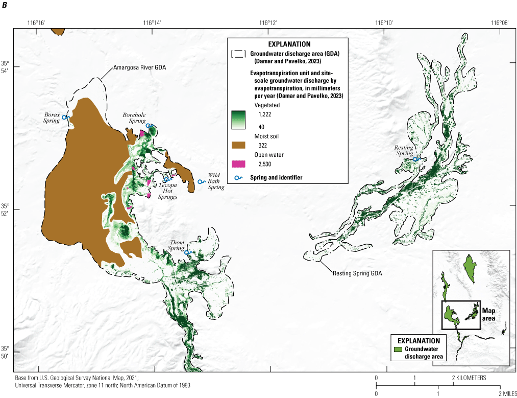
A, Color infrared imagery, where brighter shades of red indicate more plant cover because the near-infrared spectral band is displayed as shades of red, the red band as shades of green, and the green band as shades of blue; and B, annual groundwater discharge by evapotranspiration for the Resting Spring groundwater discharge area and the northern part of the Amargosa River groundwater discharge area, Inyo County, California.
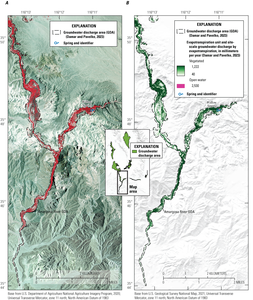
A, Color infrared imagery, where brighter shades of red indicate more plant cover because the near-infrared spectral band is displayed as shades of red, the red band as shades of green, and the green band as shades of blue; and B, annual groundwater discharge by evapotranspiration for the southern part of the Amargosa River groundwater discharge area, Inyo and San Bernardino Counties, California.
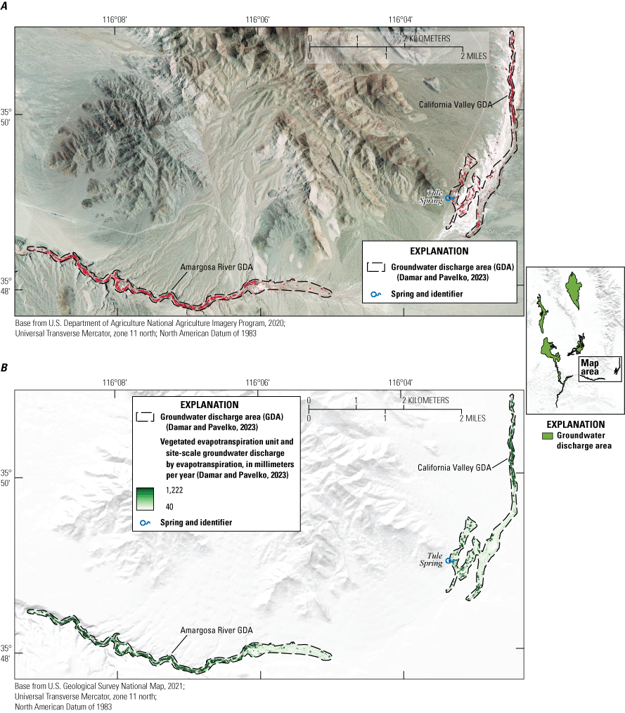
A, Color infrared imagery, where brighter shades of red indicate more plant cover because the near-infrared spectral band is displayed as shades of red, the red band as shades of green, and the green band as shades of blue; and B, annual groundwater discharge by evapotranspiration for the California Valley groundwater discharge area and the eastern part of the Amargosa River groundwater discharge area, Inyo County, California.
The estimated annual ETg for the AWSR study area presented in this report (10,139,000 m3) is within the range of previous estimates based on conceptual or numerical models or field measurements (tables 4, 5, and 6). Results of conceptual model water budgets provide estimates from about 7,400,000 to 23,440,000 m3 of annual interbasin groundwater flow from Pahrump Valley into the study area (Malmberg, 1967; Harrill, 1986) and from about 0 to 10,360,000 m3 of annual interbasin groundwater flow out of the study area (Belcher and others, 2019). Accordingly, annually there is up to 23,440,000 m3 of groundwater available for ETg. Estimated predevelopment annual ETg in the AWSR study area, computed from numerical models, is about 10,665,000 m3 (Halford and Jackson, 2020). The AWSR study area is about 28,229,000 m2, which is about 21 percent larger than the Laczniak and others (2001) estimate (22,310,000 m2). The annual ETg estimate for this study (10,139,000 m3) is about an 8-percent decrease compared to the Laczniak and others (2001) estimate (11,015,000 m3) and is about a 2-percent increase compared to the Huntington and others (2016) estimate (9,923,000 m3).
The Shoshone GDA in this study is in the same vicinity as the “Shoshone area” described in Laczniak and others (2001), but the Shoshone GDA for this study (4,320,000 m2) is about a 30-percent decrease compared to the Laczniak and others (2001) estimate (5,617,000 m2). The annual ETg estimate for the Shoshone GDA for this study (1,142,000 m3) is about a 27-percent decrease compared to the Huntington and others (2016) estimate (1,699,000 m3) and about a 52-percent decrease compared to the Laczniak and others (2001) estimate (2,590,000 m3).
The Chicago Valley GDA in this study is in the same vicinity as the “Chicago Valley” area described in Laczniak and others (2001), but the Chicago Valley GDA for this study (8,198,000 m2) is more than three times larger. The annual ETg estimate for the Chicago Valley GDA for this study (2,078,000 m3) is almost three times larger than the Huntington and others (2016) estimate (730,000 m3) and almost four times larger than the Laczniak and others (2001) estimate (530,000 m3).
The combined Resting Spring, Amargosa River, and California Valley GDAs in this study are in the same vicinity as the “Tecopa/California Valley area” described in Laczniak and others (2001), but the area of the combined GDAs for this study (15,711,00 m2) is about a 10-percent increase compared to the Laczniak and others (2001) estimate (14,217,000 m2). The annual ETg estimate for the combined Resting Spring, Amargosa River, and California Valley GDAs for this study (6,919,000 m3) is about an 8-percent decrease compared to the Huntington and others (2016) estimate (7,495,000 m3) and about a 12-percent decrease compared to the Laczniak and others (2001) estimate (7,894,000 m3).
Table 5.
A comparison of annual groundwater discharge by evapotranspiration from the Amargosa Wild and Scenic River study area, by groundwater discharge area and evapotranspiration unit, Inyo and San Bernardino Counties, California.[All values have been rounded to the nearest 1,000 so individual components may not add up to totals in this table. Abbreviations: ET, evapotranspiration; m2, square meters; ETg, groundwater discharge by evapotranspiration; m3, cubic meters; +, plus]
Table 6.
A comparison of annual groundwater discharge by evapotranspiration from the Amargosa Wild and Scenic River study area, by groundwater discharge area, Inyo and San Bernardino Counties, California.[All values have been rounded to the nearest 1,000 so individual components may not add up to totals in this table. Abbreviations: m2, square meters; ETg, groundwater discharge by evapotranspiration; m3, cubic meters; +, plus]
| Groundwater discharge area |
This study (Damar and Pavelko, 2023) | Laczniak and others (2001) | Huntington and others (2016)1 | |||
|---|---|---|---|---|---|---|
| Area (m2) |
Annual ETg (m3) |
Area (m2) |
Annual ETg (m3) |
Area (m2) |
Annual ETg (m3) |
|
| Chicago Valley | 8,198,000 | 2,078,000 | 2,477,000 | 530,000 | 2,477,000 | 730,000 |
| Shoshone | 4,320,000 | 1,142,000 | 5,617,000 | 2,590,000 | 5,617,000 | 1,699,000 |
| Resting Spring + California Valley + Amargosa River |
15,711,000 | 6,919,000 | 14,217,000 | 7,894,000 | 14,217,000 | 7,495,000 |
| Study-area total | 28,229,000 | 10,139,000 | 22,310,000 | 11,015,000 | 22,310,000 | 9,923,000 |
Limitations
The accuracy of the annual ETg estimate for the AWSR study area is limited by hydrologic assumptions, the accuracy of ET-unit and GDA boundaries, and the accuracy of the site-scale ETg assigned to ET units. It was assumed that plant cover, site-scale ETg, and scaled NDVI values are positively correlated, as discussed in section “Study-Area Scale Methods,” and that scaled NDVI values can accurately predict plant cover, which are well-established assumptions for ET studies in the Basin and Range Province that do not substantially affect the accuracy of results (Ustin, 1992; Laczniak and others, 1999, 2001, 2006; Nichols, 2000; Nagler and others, 2001, 2005; Reiner and others 2002; DeMeo and others, 2003; Smith and others, 2007; Glenn and others, 2008; Allander and others, 2009; Garcia and others, 2014; Berger and others, 2016; Moreo and others, 2020). Related to this assumption, it also was assumed that within vegetated ET-units, plant cover, as determined by scaled NDVI values, is the determining factor of ETg, not whether plants are phreatophytes or xerophytes. This assumption does not substantially affect the accuracy of results because in areas where phreatophytes grow, groundwater is shallow and accessible to xerophytes, which allows them to behave as facultative phreatophytes that will consume groundwater when it is available (Robinson, 1958). Furthermore, the assumption of xerophytes behaving as facultative phreatophytes in GDAs is supported by the higher diversity and plant cover of xerophytes growing along the AWSR compared to xerophytes growing at the outer GDA boundaries. Finally, it was assumed that, except for spring-fed, intermittent AWSR discharge from the study area, all spring discharge in the AWSR study area is evaporated or transpired in the study area, which is a well-established assumption for ET studies in the Basin and Range Province that does not substantially affect the accuracy of results (Laczniak and others, 1999; Nichols, 2000; Moreo and others, 2007; Garcia and others, 2014). The assumption that all spring discharge in the AWSR study area is consumed by ET also is supported by the lack of perennial surface-water discharge out of the study area, as measured at AR32 - AMARGOSA RIVER SEEPAGE RUN (USGS streamgage 354144116150601; U.S. Geological Survey, 2020) and AR19 - AMARGOSA RIVER SEEPAGE RUN (USGS streamgage 354442116132401; U.S. Geological Survey, 2020), and by studies that have estimated small amounts to no groundwater discharge from the study area (Belcher and others, 2019; Halford and Jackson, 2020).
The accuracy of ET-unit and GDA boundaries delineated for this study were not considered a substantial source of error in the AWSR annual ETg estimate. When delineating ET-unit boundaries, it is possible that relatively small (about 100 m2 or less), isolated, areas of open water, moist soil, xerophytes, or no vegetation were not identified and, similarly, when delineating GDA boundaries, it is possible that relatively small, isolated, areas of phreatophytes were not included. The errors associated with delineating boundaries may have resulted in assigning incorrect site-scale ETg to small, isolated areas but it was assumed that those errors, relative to the annual ETg estimate, were negligible. Outer vegetated GDA boundaries were important because a scaled NDVI does not distinguish between phreatophytes and xerophytes, which generally are both green and reflect similar multispectral bands, but they often are indefinite in the field and imagery because they typically were in a gradational transition zone of decreasing phreatophytes and increasing xerophytes. Including xerophytes, or not including phreatophytes, in vegetated ET units resulted in inaccurate annual ETg estimates, but these errors also were considered negligible compared to the annual ETg estimate.
The accuracy of the AWSR annual ETg estimate is limited by the site-scale ETg assigned to the open-water and moist-soil ET units, which only are in the Shoshone and Amargosa River GDAs. Because open-water ET units comprised only about 0.2 percent of the study area, the assigned ETg did not have a very large effect on the study-area estimate. To determine the effects of assigning different site-scale open-water ETg, open-water ETg was reduced by 50 percent to 1.265 m/yr and doubled to 5.060 m/yr. For the combined open-water ET units in the Shoshone and Amargosa River GDAs, when open-water ETg was 2.530 m/yr, annual open-water ETg was 139,000 m3 and annual ETg for the study area was 10,139,000 m3. When open-water ETg was reduced by 50 percent, then annual ETg for the study area was 10,069,000 m3, a reduction of less than 1 percent, and when open-water ETg was doubled, then annual ETg for the study area was 10,277,000 m3, which is an increase of about 1 percent. Moist-soil ET units comprised about 27 percent of the study area; therefore, the ETg assigned to moist-soil ET units had a larger effect on the annual estimate than the ETg assigned to open-water ET units. Variability in the characteristics of moist soil found in the Shoshone and Amargosa River GDAs, as described in the “Study Area” section, likely resulted in some areas being assigned inaccurate ETg. To determine the effects of assigning different moist-soil ETg, moist-soil ETg was reduced by 50 percent, to 0.161 m/yr, and doubled, to 0.644 m/yr. For the combined moist-soil ET units in the Shoshone and Amargosa River GDAs, when moist-soil ETg was 0.322 m/yr, annual moist-soil ETg was 2,464,000 m3 and annual ETg for the study area was 10,139,000 m3. When moist-soil ETg was reduced by 50 percent, then annual ETg for the study area was 8,837,000 m3, which is a reduction of about 13 percent, and when moist-soil ETg was doubled, then annual ETg for the study area was 12,603,000 m3, which is an increase of about 20 percent.
The accuracy of site-scale ETg for vegetated ET units was limited by (1) the accuracy of the site-scale data, which were used to estimate site-scale ETg and calculate the footprint-weighted mean scaled NDVI values of the sites and (2) the quadratic relation, which was based on the assumption that site-scale ETg from vegetation adequately can be scaled (predicted) across the study area using a single year of data for two sites and a single scaled NDVI. The accuracy of the site-scale data from this study were considered of good quality because the EBRs of the Shrub site (1.085) and the Wetland site (0.873) were greater than the mean EBR of about 0.8 (Twine and others, 2000; Wilson and others, 2002; Foken, 2008) and were within, or greater than, the range of EBRs from recent Basin and Range Province studies (Moreo and others, 2007, 2017, 2020; Allander and others, 2009; Garcia and others, 2014; Berger and others, 2016). Additionally, ETg measured at the Shrub site (0.121 m/yr) was similar to ETg measured in Oasis Valley for areas of sparse shrubs, and ETg measured at the Wetland site (1.056 m/yr) was similar to ETg measured in Ash Meadows and Oasis Valley for areas of dense wetland vegetation, dense meadow vegetation, and dense grassland vegetation (Reiner and others, 2002). The eddy covariance method possibly underestimates latent-energy fluxes due to instrument biases of sonic anemometers not sampling very small or very large eddies and not accounting for regional advection (Wilson and others, 2002), but these errors generally are compensated for when correcting for the EBR.
There are several limitations associated with estimating site-scale ETg for vegetated ET units using the quadratic relation developed for this study. Past studies have applied uniform site-scale ET to multiple types of vegetated ET units (Laczniak and others, 1999, 2001, 2006; Nichols, 2000; Reiner and others 2002; DeMeo and others, 2003; Smith and others, 2007), but more recent studies have used linear (Garcia and others, 2014; Berger and others, 2016; Moreo and others, 2020) and quadratic (Allander and others, 2009; Beamer and others, 2013; Huntington and others, 2016) relations to estimate vegetated site-scale ET based on a vegetation index. Past studies also primarily have used total ET to develop linear or quadratic relations, and some have relied on precipitation models to estimate study-area precipitation, which is then removed from total ET to derive ETg. In this study, ETg was used to develop the quadratic relation instead of total ET because (1) a single annual ETg value was more representative of the long-term average than a single total annual ET value and (2) the study-area scaled NDVI was considered representative of a date when ETg was equal to total ET. In the AWSR study area, total ET varies from year to year primarily because of fluctuations in annual precipitation, which do not affect site-scale ETg. Annual ETg for native, undisturbed phreatophytic vegetation, such as in the AWSR study area, was assumed to vary minimally from year to year, compared to annual total ET, and therefore the annual ETg estimate for the AWSR study area is considered representative of regional long-term rates (Berger and others, 2016). Additionally, past studies generally have used precipitation models to estimate study-area precipitation and then subtract the estimated precipitation from estimated total ET. For this study, annual precipitation was subtracted from measured total ET at the shrub and wetlands sites; therefore, eliminating some uncertainty associated with estimating precipitation across a large area. Moreover, when there has been no rain during a desert summer for at least 30 days, it was assumed that total ET is equal to ETg because previous precipitation and soil moisture have been completely consumed and only regional groundwater is available for ET. Therefore, a single-date scaled NDVI from a date with no antecedent rain for more than 30 days, such as the scaled NDVI used in this study, is considered representative of a date when total ET equaled ETg and eliminates the need for precipitation models. Evapotranspiration estimates based on single-date vegetation indexes have worked well in arid, vegetated areas with shallow groundwater (Groeneveld and others, 2007), such as the GDAs in the study area. It is uncertain if ETg increases during years with below-average precipitation rates, such as 2018, as a result of phreatophytes consuming regional groundwater rather than water from precipitation. However, based on the use of the single-date scaled NDVI method, the uncertainty associated with precipitation-related ETg fluctuations was considered negligible for this study.
The quadratic relation developed for this study is based on four points (fig. 8), but only two were derived from measured data, which results in a relation with a low statistical strength that increases the uncertainty of the annual ETg estimate. Both points represent only 1 year of site-scale data from a single location. Having ET-monitoring sites that collect data for multiple years and having more than two ET-monitoring sites located across the study area and in various phreatophyte plant covers could strengthen the relation and decrease the uncertainty of estimated ETg.
Summary
Annual site-scale groundwater discharge by evapotranspiration (ETg) was measured using the eddy-covariance method at a site in sparse shrubs and at a site in dense wetland vegetation. At the Shrub site, site-scale ETg was 0.121 meters per year (m/yr) ±0.005 m/yr, or 3.9 percent of the total, and at the Wetland site, site-scale ETg was 1.056 m/yr ±0.076 m/yr, or 7.2 percent of the total. Annual ETg for the 28,229,000 square meters (m2) Amargosa Wild and Scenic River (AWSR) study area was 10,139,000 cubic meters (m3) in 2018 and may have ranged from 7,059,000 to 14,321,000 m3. Annual ETg for the 8,198,000 m2 Chicago Valley groundwater discharge area (GDA) was 2,078,000 m3; annual ETg for the 2,535,000 m2 Resting Spring GDA was 1,139,000 m3; annual ETg for the 712,000 m2 California Valley GDA was 214,000 m3; annual ETg for the 4,320,000 m2 Shoshone GDA was 1,142,000 m3; and annual ETg for the 12,464,000 m2 Amargosa River GDA was 5,566,000 m3. The AWSR study area is about 21 percent larger than the previous estimate of about 22,310,000 m2 and the annual ETg estimate for this study is about 2–8 percent different than previous estimates.
References Cited
Albano, C.M., Minor, B.A., Morton, C.G., and Huntington, J.L., 2021, Baseline assessment of groundwater dependent vegetation in relation to climate and groundwater levels in select hydrographic basins of Nevada–Pueblo, Continental Lake, Mud Meadow, Dixie, Railroad-North, Steptoe, Goshute, and Independence Valleys: Desert Research Institute Publication 41283, 135 p., 2 appendixes.
Allander, K.K., Smith, J.L., and Johnson, M.J., 2009, Evapotranspiration from the lower Walker River Basin, west-central Nevada, water years 2005–07: U.S. Geological Survey Scientific Investigations Report 2009–5079, 62 p., accessed April 20, 2018, at https://doi.org/10.3133/sir20095079.
Beamer, J.P., Huntington, J.L., Morton, C.G., and Pohll, G.M., 2013, Estimating annual groundwater evapotranspiration from phreatophytes in the Great Basin using Landsat and flux tower measurements: Journal of the American Water Resources Association, v. 49, no. 3, p. 518–533, accessed August 10, 2020, at https://doi.org/10.1111/jawr.12058.
Belcher, W.R., Sweetkind, D.S., Faunt, C.C., Pavelko, M.T., and Hill, M.C., 2017, An update of the Death Valley regional groundwater flow system transient model, Nevada and California: U.S. Geological Survey Scientific Investigations Report 2016–5150, 74 p., 1 pl., accessed November 2, 2018, at https://doi.org/10.3133/sir20165150.
Belcher, W.R., Sweetkind, D.S., Hopkins, C.B., and Poff, M.E., 2019, Hydrogeology of Lower Amargosa Valley and groundwater discharge to the Amargosa Wild and Scenic River, Inyo and San Bernardino Counties, California, and adjacent areas in Nye and Clark Counties, Nevada: U.S. Geological Survey Scientific Investigations Report 2018–5151, 131 p., 1 pl., accessed February 11, 2020, at https://doi.org/10.3133/sir20185151.
Berger, D.L., Johnson, M.J., Tumbusch, M.L., and Mackay, J., 2001, Estimates of evapotranspiration from the Ruby Lake National Wildlife Refuge Area, Ruby Valley, northeastern Nevada, May 1999–October 2000: U.S. Geological Water-Resources Investigations Report 2001–4234, 38 p., accessed March 2, 2022, at https://pubs.usgs.gov/wri/wri014234/.
Berger, D.L., Mayers, C.J., Garcia, C.A., Buto, S.G., and Huntington, J.M., 2016, Budgets and chemical characterization of groundwater for the Diamond Valley flow system, central Nevada, 2011–12: U.S. Geological Survey Scientific Investigations Report 2016–5055, 83 p., accessed December 26, 2017, at https://doi.org/10.3133/sir20165055.
Bowen, I.S., 1926, The ratio of heat losses by conduction and by evaporation from any water surface: Physical Review, v. 27, no. 6, p. 779–787, accessed May 5, 2020, at https://doi.org/10.1103/PhysRev.27.779.
Brotzge, J.A., and Duchon, C.E., 2000, A field comparison among a domeless net radiometer, two four-component net radiometers, and a domed net radiometer: Journal of Atmospheric and Oceanic Technology, v. 17, no. 12, p. 1569–1582, accessed April 23, 2020, at https://www.researchgate.net/publication/232422065.
Brutsaert, W.H., 1982, Evaporation into the atmosphere: Boston, Mass., D. Reidel Publishing, 302 p. [Available at https://doi.org/10.1007/978-94-017-1497-6.]
Bureau of Land Management, 2020a, Areas of critical environmental concern: Bureau of Land Management web page, accessed March 26, 2020, at https://www.blm.gov/programs/planning-and-nepa/planning-101/special-planning-designations/acec.
Bureau of Land Management, 2020b, Amargosa Wild and Scenic River: Bureau of Land Management web page, accessed March 26, 2020, at https://www.blm.gov/programs/national-conservation-lands/california/amargosa-wsr.
California Department of Fish and Wildlife, 2023, Swainson's Hawks in California: California Department of Fish and Wildlife web page, accessed March 26, 2020, at https://wildlife.ca.gov/Conservation/Birds/Swainsons-Hawk.
Campbell Scientific, Inc., 1998, Instruction manual eddy covariance system CA27 and KH20, revision 7/98: Campbell Scientific, Inc., variously paged, 5 appendixes, accessed July 2, 2020, at https://s.campbellsci.com/documents/us/manuals/eddy.pdf.
Campbell Scientific, Inc., 2010a, Instruction manual KH20 krypton hygrometer, revision 2/10: Campbell Scientific, Inc., 10 p., 1 appendix, accessed December 23, 2010, at https://s.campbellsci.com/documents/us/manuals/kh20.pdf.
Campbell Scientific, Inc., 2010b, Instruction manual CSAT3 three-dimensional anemometer, revision 6/10: Campbell Scientific, Inc., 44 p., 4 appendixes, accessed September 28, 2011, at https://s.campbellsci.com/documents/us/manuals/csat3.pdf.
Campbell Scientific, Inc., 2010c, Instruction manual NR-LITE2 net radiometer, revision 9/10: Campbell Scientific, Inc., 16 p., accessed June 23, 2012, at https://s.campbellsci.com/documents/us/manuals/nr-lite2.pdf.
Campbell Scientific, Inc., 2010d, Instruction manual TB4 and TB4MM rain gage, revision 10/10: Campbell Scientific, Inc., 15 p., accessed March 22, 2016, at https://s.campbellsci.com/documents/us/manuals/tb4.pdf.
Campbell Scientific, Inc., 2011a, Instruction manual LoggerNet Version 4.1, revision 1/11: Campbell Scientific, Inc., 15 p., accessed September 29, 2011, at https://s.campbellsci.com/documents/us/manuals/loggernet.pdf.
Campbell Scientific, Inc., 2011b, Instruction manual CS616 and CS625 water content reflectometers, revision 6/11: Campbell Scientific, Inc., 42 p., accessed February 10, 2015, at https://s.campbellsci.com/documents/us/manuals/cs616.pdf.
Campbell Scientific, Inc., 2011c, Operator’s manual CR3000 Micrologger, revision 7/11: Campbell Scientific, Inc., 526 p., accessed February 19, 2013, at https://s.campbellsci.com/documents/us/manuals/cr3000.pdf.
Campbell Scientific, Inc., 2015a, Instruction manual LI190SB quantum sensor, revision 2/15: Campbell Scientific, Inc., 16 p., 5 appendixes, accessed May 28, 2019, at https://s.campbellsci.com/documents/us/manuals/li190sb.pdf.
Campbell Scientific, Inc., 2015b, Instruction manual HC2S3 temperature and relative humidity probe, revision 7/15: Campbell Scientific, Inc., 16 p., 5 appendixes, accessed March 10, 2017, at https://s.campbellsci.com/documents/us/manuals/hc2s3.pdf.
Campbell Scientific, Inc., 2016, Instruction manual model HFP01 soil heat flux plate, revision 10/16: Campbell Scientific, Inc., 6 p., 2 appendixes, accessed September 8, 2011, at https://s.campbellsci.com/documents/us/manuals/hfp01.pdf.
Campbell Scientific, Inc., 2018, Product manual TCAV averaging thermocouple probe, revision 7/18: Campbell Scientific, Inc., 3 p., accessed January 29, 2019, at https://s.campbellsci.com/documents/us/manuals/tcav.pdf.
Clement, R., 1999, EdiRe data software: University of Edinburgh, version 1.5.0.32, accessed December 12, 2018, at https://www.geos.ed.ac.uk/homes/jbm/micromet/EdiRe/.
Community Environmental Monitoring Program, 2022, Station summary— Tecopa/Shoshone California: Community Environmental Monitoring Program website, accessed May 26, 2022, at https://cemp.dri.edu/cgi-bin/cemp_stations.pl?stn=teco.
Damar, N.A., and Pavelko, M.T., 2023, Geospatial data for the report groundwater discharge by evapotranspiration from the Amargosa Wild and Scenic River and contributing areas, Inyo and San Bernardino Counties, California: U.S. Geological Survey data release, https://doi.org/10.5066/P9KH3Q2D.
DeMeo, G.A., Laczniak, R.J., Boyd, R.A., Smith, J.L., and Nylund, W.E., 2003, Estimated ground-water discharge by evapotranspiration from Death Valley, California, 1997–2001: U.S. Geological Survey Water-Resources Investigations Report 2003–4254, 27 p., 1 pl., accessed May 31, 2005, at https://doi.org/10.3133/wri034254.
DeMeo, G.A., Smith, J.L., Damar, N.A., and Darnell, J., 2008, Quantifying ground-water and surface-water discharge from evapotranspiration processes in 12 hydrographic areas of the Colorado Regional Ground-Water Flow System, Nevada, Utah, and Arizona: U.S. Geological Survey Scientific Investigations Report 2008–5116, 22 p., accessed August 5, 2020, at https://doi.org/10.3133/sir20085116.
Devitt, D.A., Fenstermaker, L.F., Young, M.H., Conrad, B., Baghzouz, M., and Bird, B.M., 2011, Evapotranspiration of mixed shrub communities in phreatophytic zones of the Great Basin region of Nevada (USA): Ecohydrology, v. 4, no. 6, p. 807–822, accessed February, 23, 2021, at https://doi.org/10.1002/eco.169.
Earp, K.J., and Moreo, M.T., 2021, Evaporation from Lake Mead and Lake Mohave, Nevada and Arizona, 2010–2019: U.S. Geological Survey Open-File Report 2021–1022, 36 p., accessed May 24, 2021, at https://doi.org/10.3133/ofr20211022.
Esri, Maxar, Earstar Geographics, U.S. Department of Agriculture Forest Service Administration, U.S. Geological Survey, Aerogrid, IGN, IGP, and the GIS User Community, 2022, World imagery map: Esri website, available at https://www.arcgis.com/home/item.html?id=10df2279f9684e4a9f6a7f08febac2a9.
Foken, T., 2008, Micrometeorology: Springer-Verlag Berlin Heidelberg, 306 p. [Available at https://doi.org/10.1007/978-3-642-25440-6.]
Foken, T., Aubinet, M., and Leuning, R., 2012a, The eddy-covariance method, in Aubinet, M., Vesala, T., and Papale, D., eds., Eddy covariance—A practical guide to measurement and data analysis: Springer, 438 p., accessed May 18, 2020, at https://doi.org/10.1007/978-94-007-2351-1_1.
Foken, T., Leuning, R., Oncley, S.R., Mauder, M., and Aubinet, M., 2012b, Corrections and data quality control, chap. 4 in Aubinet, M., Vesala, T., and Papale, D., eds., Eddy covariance—A practical guide to measurement and data analysis: Springer, 438 p., accessed May 18, 2020, at https://doi.org/10.1007/978-94-007-2351-1_4.
Garcia, C.A., Huntington, J.M., Buto, S.G., Moreo, M.T., Smith, J.L., and Andraski, B.J., 2014, Groundwater discharge by evapotranspiration, Dixie Valley, west-central Nevada, March 2009–September 2011 (ver. 1.1, April 2015): U.S. Geological Survey Professional Paper 1805, 90 p., accessed April 25, 2018, at http://doi.org/10.3133/pp1805.
Glenn, E.P., Huete, A.R., Nagler, P.L., and Nelson, S.G., 2008, Relationship between remotely-sensed vegetation indices, canopy attributes and plant physiological processes—What vegetation indices can and cannot tell us about the landscape: Sensors (Basel), v. 8, no. 4, p. 2136–2160, accessed March 3, 2022, at https://doi.org/10.3390/s8042136.
Goetz, A.F.H., Rock, B.N., and Rowan, L.C., 1983, Remote sensing for exploration—An overview: Economic Geology, v. 78, no. 4, p. 573–590, accessed May 27, 2020, at https://doi.org/10.2113/gsecongeo.78.4.573.
Groeneveld, D.P., Baugh, W.M., Sanderson, J.S., and Cooper, D.J., 2007, Annual groundwater evapotranspiration mapped from single satellite scenes: Journal of Hydrology, v. 344, nos. 1–2, p. 146–156, accessed June 8, 2020, at https://doi.org/10.1016/j.jhydrol.2007.07.002.
Halford, K.J., and Jackson, T.R., 2020, Groundwater characterization and effects of pumping in the Death Valley regional groundwater flow system, Nevada and California, with special reference to Devils Hole: U.S. Geological Survey Professional Paper 1863, 178 p., accessed March 6, 2020, at https://doi.org/10.3133/pp1863.
Harrill, J.R., 1986, Ground-water storage depletion in Pahrump Valley, Nevada–California, 1962–75: U.S. Geological Survey Water Supply Paper 2279, 53 p., accessed July 9, 2020, at https://doi.org/10.3133/wsp2279.
Harrill, J.R., Gates, J.S., and Thomas, J.M., 1988, Major ground-water flow systems in the Great Basin region of Nevada, Utah, and adjacent states: U.S. Geological Survey Hydrologic Atlas 694–C, 2 sheets, scale 1:1,000,000, accessed December 9, 2019, at https://doi.org/10.3133/ha694C.
Harrill, J.R., and Prudic, D.E., 1998, Aquifer systems in the Great Basin region of Nevada, Utah, and adjacent states—Summary report: U.S. Geological Survey Professional Paper 1409–A, 66 p., accessed April 24, 2020, at https://doi.org/10.3133/pp1409A.
Harrill, J.R., Welch, A.H., Prudic, D.E., Thomas, J.M., Carman, R.L., Plume, R.W., Gates, J.S., and Mason, J.L., 1983, Aquifer systems in the Great Basin region of Nevada, Utah, and adjacent states—A study plan: U.S. Geological Survey Open-File Report 82–445, 49 p., 1 pl., accessed December 6, 2019, at https://doi.org/10.3133/ofr82445.
Healy, R.W., Winter, T.C., LaBaugh, J.W., and Franke, O.L., 2007, Water budgets—Foundations for effective water-resources and environmental management: U.S. Geological Survey Circular 1308, 90 p., accessed December 6, 2019, at https://doi.org/10.3133/cir1308.
Hereford, R., Webb, R.H., and Longpre, C.I., 2004, Precipitation history of the Mojave Desert region, 1893–2001: U.S. Geological Survey Fact Sheet 117–03, 4 p., accessed November 12, 2021, at https://doi.org/10.3133/fs11703.
Hevesi, J.A., Flint, A.L., and Flint, L.E., 2003, Simulation of net infiltration and potential recharge using a distributed‑parameter watershed model of the Death Valley region, Nevada and California: U.S. Geological Survey Water-Resources Investigations Report 2003–4090, 171 p., accessed May 31, 2005, at https://doi.org/10.3133/wri034090.
Højstrup, J., 1993, A statistical data screening procedure: Measurement Science and Technology, v. 4, no. 2, p. 153–157, accessed March 3, 2020, at https://doi.org/10.1088/0957-0233/4/2/003.
Humphrey, M.D., Istok, J.D., Lee, J.Y., Hevesi, J.A., and Flint, A.L., 1997, A new method for automated dynamic calibration of tipping-bucket rain gauges: Journal of Atmospheric and Oceanic Technology, v. 14, no. 6, p. 1513–1519, accessed May 18, 2020, at https://doi.org/10.1175/1520-0426(1997)014<1513:ANMFAD>2.0.CO;2.
Jackson, T.R., Halford, K.J., Gardner, P.M., and Garcia, A., 2018, Evaluating micrometeorological estimates of groundwater discharge from Great Basin desert playas: Groundwater, v. 56, no. 6, p. 909–920, accessed May 24, 2018, at https://doi.org/10.1111/gwat.12647.
Kaimal, J.C., and Finnigan, J.J., 1994, Atmospheric boundary layer flows, their structure and measurement: New York, Oxford University Press, 289 p. [Available at https://doi.org/10.1093/oso/9780195062397.001.0001.]
Kormann, R., and Meixner, F.X., 2001, An analytical footprint model for non-neutral stratification: Boundary-Layer Meteorology, v. 99, no. 2, p. 207–224, accessed October 25, 2012, at https://doi.org/10.1023/A:1018991015119.
Laczniak, R.J., DeMeo, G.A., Reiner, S.R., Smith, J.L., and Nylund, W.E., 1999, Estimates of ground-water discharge as determined from measurements of evapotranspiration, Ash Meadows area, Nye County, Nevada: U.S. Geological Survey Water-Resources Investigations Report 99–4079, 70 p., accessed December 26, 2017, at https://doi.org/10.3133/wri994079.
Laczniak, R.J., Flint, A.L., Moreo, M.T., Knochenmus, L.A., Lundmark, K.W., Pohll, G., Carroll, R.W.H., LaRue Smith, J., Welborn, T.L., Heilweil, V.M., Pavelko, M.T., Hershey, R.L., Thomas, J.M., Earman, S., and Lyles, B.F., 2008, Ground-water budgets, in Welch, A.H., Bright, D.J., and Knochenmus, L.A., eds., Water resources of the Basin and Range carbonate-rock aquifer system, White Pine County, Nevada, and adjacent areas in Nevada and Utah: U.S. Geological Survey Scientific Investigations Report 2007–5261, p. 43–82, accessed March 2, 2020, at https://doi.org/10.3133/sir20075261.
Laczniak, R.J., Smith J.L., and DeMeo, G.A., 2006, Annual ground-water discharge by evapotranspiration from areas of spring-fed riparian vegetation along the eastern margin of Death Valley, 2002–02: U.S. Geological Survey Scientific Investigations Report 2006–5145, 46 p., accessed November 22, 2006, at https://doi.org/10.3133/sir20065145.
Laczniak, R.J., Smith, J.L., Elliott, P.E., DeMeo, G.A., Chatigny, M.A., and Roemer, G.J., 2001, Ground-water discharge determined from estimates of evapotranspiration, Death Valley regional flow system, Nevada and California: U.S. Geological Survey Water-Resources Investigations Report 2001–4195, 51 p., accessed September 26, 2012, at https://doi.org/10.3133/wri014195.
Malmberg, G.T., 1967, Hydrology of the valley-fill and carbonate-rock reservoirs, Pahrump Valley, Nevada–California: U.S. Geological Survey Water Supply Paper 1832, 47 p., 5 pls., accessed January 23, 2020, at https://doi.org/10.3133/wsp1832.
Massman, W.J., 2000, A simple method for estimating frequency response corrections for eddy covariance systems: Agricultural and Forest Meteorology, v. 104, no. 3, p. 185–198, accessed April 23, 2010, at https://doi.org/10.1016/S0168-1923(00)00164-7.
Mauder, M., Foken, T., and Cuxart, J., 2020, Surface-energy-balance closure over land—A review: Boundary-Layer Meteorology, v. 177, p. 395–426, accessed December 10, 2021, at https://doi.org/10.1007/s10546-020-00529-6.
Maurer, D.K., Berger, D.L., Tumbusch, M.L., and Johnson, M.J., 2006, Rates of evapotranspiration, recharge from precipitation beneath selected areas of native vegetation, and streamflow gain and loss in Carson Valley, Douglas County, Nevada, and Alpine County, California: U.S. Geological Survey Scientific Investigations Report 2005–5288, 70 p., accessed June 2, 2020, at https://doi.org/10.3133/sir20055288.
Maxey, G.B., and Eakin, T.E., 1949, Ground water in White River Valley, White Pine, Nye, and Lincoln Counties, Nevada: Nevada State Engineer, Water Resources Bulletin 8, 59 p., accessed February 23, 2021, at http://images.water.nv.gov/images/publications/water%20resources%20bulletins/Bulletin8.pdf.
Meinzer, O.E., 1923, Outline of ground-water hydrology with definitions: U.S. Geological Survey Water Supply Paper 494, 71 p., accessed August 21, 2007, at https://doi.org/10.3133/wsp494.
Moore, C.J., 1986, Frequency response corrections for eddy correlation systems: Boundary-Layer Meteorology, v. 37, nos. 1–2, p. 17–35, accessed February 27, 2008, at https://doi.org/10.1007/BF00122754.
Moreo, M.T., Andraski, B.J., and Garcia, C.A., 2017, Groundwater discharge by evapotranspiration, flow of water in unsaturated soil, and stable isotope water sourcing in areas of sparse vegetation, Amargosa Desert, Nye County, Nevada: U.S. Geological Survey Scientific Investigations Report 2017–5079, 55 p., accessed July 16, 2018, at https://doi.org/10.3133/sir20175079.
Moreo, M.T., Buto, S.G., Smith, D.W., and Nelson, N.C., 2020, Estimates of groundwater discharge by evapotranspiration, Stump Spring and Hiko Springs, Clark County, southern Nevada, 2016–18: U.S. Geological Survey Scientific Investigations Report 2020–5075, 39 p., 1 appendix, accessed August 3, 2020, at https://doi.org/10.3133/sir20205075.
Moreo, M.T., Laczniak, R.J., and Stannard, D.I., 2007, Evapotranspiration rate estimates of vegetation typical of ground-water discharge areas in the Basin and Range carbonate-rock aquifer system, Nevada and Utah, September 2005–August 2006: U.S. Geological Survey Scientific Investigations Report 2007–5078, 36 p., accessed April 20, 2018, at https://doi.org/10.3133/sir20075078.
Moreo, M.T., and Swancar, A., 2013, Evaporation from Lake Mead, Nevada and Arizona, March 2010 through February 2012: U.S. Geological Survey Scientific Investigations Report 2013–5229, 40 p., accessed May 5, 2020, at https://doi.org/10.3133/sir20135229.
Nagler, P.L., Glenn, E.P., and Huete, A.R., 2001, Assessment of spectral vegetation indices for riparian vegetation in the Colorado River delta, Mexico: Journal of Arid Environments, v. 49, no. 1, p. 91–110, accessed November 24, 2001, at https://doi.org/10.1006/jare.2001.0844.
Nagler, P.L., Scott, R.L., Westenburg, C., Cleverly, J.R., Glenn, E.P., and Huete, A.R., 2005, Evapotranspiration on western U.S. rivers estimated using the Enhanced Vegetation Index from MODIS and data from eddy covariance and Bowen ratio flux towers: Remote Sensing of Environment, v. 97, no. 3, p. 337–351, accessed November 23, 2001, at https://doi.org/10.1016/j.rse.2005.05.011.
National Weather Service, 2020, 8-inch rain gage: Web page, accessed February 21, 2020, at https://www.weather.gov/iwx/coop_8inch.
Nelson, N.C., and Jackson, T.R., 2020, Simulated effects of pumping in the Death Valley regional groundwater flow system, Nevada and California—Selected management scenarios projected to 2120: U.S. Geological Survey Scientific Investigations Report 2020–5103, 30 p., accessed February 9, 2021, at https://doi.org/10.3133/sir20205103.
Nichols, W.D., 2000, Regional ground-water evapotranspiration and ground-water budgets, Great Basin, Nevada: U.S. Geological Survey Professional Paper 1628, 101 p., 4 pls., accessed August 6, 2020, at https://doi.org/10.3133/pp1628.
Parker, S.S., Zdon, A., Christian, W.T., Cohen, B.S., Palacios Mejia, M., Fraga, N.S., Curd, E.E., Edalati, K., and Renshaw, M.A., 2021, Conservation of Mojave Desert springs and associated biota—Status, threats, and policy opportunities: Biodiversity and Conservation, v. 30, no. 2, p. 311–327, accessed July 7, 2021, at https://doi.org/10.1007/s10531-020-02090-7.
Pavelko, M.T., 2023, Supplemental data for the report groundwater discharge by evapotranspiration from the Amargosa Wild and Scenic River and contributing areas, Inyo and San Bernardino Counties, California: U.S. Geological Survey data release, https://doi.org/10.5066/P9LKMX8K.
Penman, H.L., 1956, Estimating evaporation: Eos, Transactions American Geophysical Union, v. 37, no. 1, p. 43–50. [Available at https://doi.org/10.1029/TR037i001p00043.]
Rannik, Ü., Sogachev, A., Foken, T., Göckede, M., Kljun, N., Leclerc, M., and Vesala, T., 2012, Footprint analysis, chap. 8 in Aubinet, M., Vesala, T., and Papale, D., eds., Eddy covariance—A practical field guide to measurement and data analysis: Heidelberg London New York, Springer Dordrecht 438 p., accessed May 18, 2020, at https://doi.org/10.1007/978-94-007-2351-1_8.
Reiner, S.R., Laczniak, R.J., DeMeo, G.A., Smith, J.L., Elliott, P.E., Nylund, W.E., and Fridrich, C.J., 2002, Ground-water discharge determined from measurements of evapotranspiration, other available hydrologic components, and shallow water-level changes, Oasis Valley, Nye County, Nevada: U.S. Geological Survey Water-Resources Investigations Report 2001–4239, 65 p., accessed October 10, 2012, at https://doi.org/10.3133/wri014239.
Robinson, T.W., 1958, Phreatophytes: U.S. Geological Survey Water Supply Paper 1423, 84 p., accessed August 16, 2016, at https://doi.org/10.3133/wsp1423.
Rosenberry, D.O., Winter, T.C., Buso, D.C., and Likens, G.E., 2007, Comparison of 15 evaporation methods applied to a small mountain lake in the northeastern USA: Journal of Hydrology, v. 340, p. 149–166, accessed February 13, 2012, at https://doi.org/10.1016/j.jhydrol.2007.03.018.
Rouse, Jr., J.W., Haas, R.H., Schell, J.A., and Deering, D.W., 1974, Monitoring vegetation systems in the Great Plains with ERTS: Texas A&M University Remote Sensing Center, 9 p., accessed March 1, 2022, at https://ntrs.nasa.gov/api/citations/19740022614/downloads/19740022614.pdf.
Schotanus, P., Nieuwstadt, F.T.M., and de Bruin, H.A.R., 1983, Temperature measurement with a sonic anemometer and its application to heat and moisture fluxes: Boundary-Layer Meteorology, v. 26, no. 1, p. 81–93, accessed March 3, 2020, at https://doi.org/10.1007/BF00164332.
Schuepp, P.H., LeClerc, M.Y., MacPherson, J.I., and Desjardins, R.L., 1990, Footprint prediction of scalar fluxes from analytical solutions of the diffusion equation: Boundary-Layer Meteorology, v. 50, p. 355–373, accessed March 20, 2006, at https://doi.org/10.1007/BF00120530.
Schultz, R.C., Udawatta, R.P., Isenhart, T.M., Simpkins, W.W., and Schultz, P.L. 2021, Riparian and upland buffer practices, in Garrett, H.E., Jose, S., and Gold, M.A., eds., North American Agroforestry (3d ed.): John Wiley & Sons, p. 205–279, accessed November 24, 2021, at https://doi.org/10.1002/9780891183785.ch8.
Shuttleworth, J.W., 1993, Evaporation, in Maidment, D.R., ed., Handbook of hydrology: McGraw-Hill, Inc., p. 4.1–4.53. [Available at https://doi.org/10.1061/9780784401385.]
Smith, J.L., Laczniak, R.J., Moreo, M.T., and Welborn, T.L., 2007, Mapping evapotranspiration units in the Basin and Range carbonate-rock aquifer system, White Pine County, Nevada and adjacent areas in Nevada and Utah: U.S. Geological Survey Scientific Investigations Report 2007–5087, 21 p., accessed September 12, 2018, at https://doi.org/10.3133/sir20075087.
Stevens, L.E., and Meretsky, V.J., 2008, Aridland springs in North America—Ecology and Conservation: The University of Arizona Press, 432 p. [Available at https://uapress.arizona.edu/book/aridland-springs-in-north-america.]
Stevens, L.E., Schenk, E.R., and Springer, A.E., 2021, Springs ecosystem classification: Ecological Applications, v. 31, no. 1, article no. e2218, 28 p., accessed November 29, 2021, at https://doi.org/10.1002/eap.2218.
Stull, R.B., eds., 1988, An introduction to boundary layer meteorology: Kluwer Academic Publishers, 670 p. [Available at https://doi.org/10.1007/978-94-009-3027-8.]
Sverdrup, H.U., 1943, On the ratio between heat conduction from the sea surface and heat used for evaporation: Annals of the New York Academy of Sciences, v. 44, no. 1, p. 81–88. [Available at https://doi.org/10.1111/j.1749-6632.1943.tb31294.x.]
Swinbank, W.C., 1951, The measurement of vertical transfer of heat and water vapor by eddies in the lower atmosphere: Journal of the Atmospheric Sciences, v. 8, no. 3, p. 135–145, accessed May 2, 2006, at https://doi.org/10.1175/1520-0469(1951)008<0135:TMOVTO>2.0.CO;2.
Twine, T.E., Kustas, W.P., Norman, J.M., Cook, D.R., Houser, P.R., Meyers, T.P., Prueger, J.H., Starks, P.J., and Wesely, M.L., 2000, Correcting eddy-covariance flux underestimates over a grassland: Agricultural and Forest Meteorology, v. 103, no. 3, p. 279–300, accessed April 10, 2017, at https://doi.org/10.1016/S0168-1923(00)00123-4.
U.S. Department of Agriculture, 2012, National Agriculture Imagery Program (NAIP) Information Sheet: U.S. Department of Agriculture, accessed March 3, 2020, at https://www.fsa.usda.gov/Internet/FSA_File/naip_2012_final.pdf.
U.S. Department of Agriculture, 2017, Four Band Digital Imagery Information Sheet: U.S. Department of Agriculture, accessed June 21, 2021, at https://www.fsa.usda.gov/Assets/USDA-FSA-Public/usdafiles/APFO/support-documents/pdfs/fourband_infosheet_2017-1.pdf.
U.S. Fish and Wildlife Service, 2023a, Least Bell’s vireo: U.S. Fish and Wildlife Service web page, accessed September 1, 2023, at https://www.fws.gov/story/least-bells-vireo.
U.S. Fish and Wildlife Service, 2023b, Southwestern willow flycatcher (Empidonax traillii extimus): U.S. Fish and Wildlife Service Environmental Conservation Online System, accessed September 1, 2023, at https://ecos.fws.gov/ecp/species/6749.
U.S. Fish and Wildlife Service, 2023c, Amargosa vole: U.S. Fish and Wildlife Service web page, accessed September 1, 2023, at https://www.fws.gov/species/amargosa-vole-microtus-californicus-scirpensis.
U.S. Fish and Wildlife Service, 2023d, Amargosa niterwort (Nitrophila mohavensis): U.S. Fish and Wildlife Service Environmental Conservation Online System, accessed September 1, 2023, at https://ecos.fws.gov/ecp/species/4072.
U.S. Fish and Wildlife Service, 2023e, Yellow-billed cuckoo (Coccyzus americanus): U.S. Fish and Wildlife Service Environmental Conservation Online System, accessed September 1, 2023, at https://ecos.fws.gov/ecp/species/3911.
U.S. Geological Survey, 2020, USGS water data for the Nation: U.S. Geological Survey database, accessed April 20, 2020, at https://doi.org/10.5066/F7P55KJN.
Ustin, S.L., 1992, Thematic mapper vegetation cover model, chap. F of Wilson, D.H., Reginato, R.J., and Hollett, K.J., eds., Evapotranspiration measurements of native vegetation, Owens Valley, California, June 1986: U.S. Geological Survey Water-Resources Investigations Report 91–4159, p. 61–70, accessed October 6, 2021, at https://doi.org/10.3133/wri914159.
Webb, E.K., Pearman, G.I., and Leuning, R., 1980, Correction of flux measurements for density effects due to heat and water vapour transfer: Quarterly Journal of the Royal Meteorological Society, v. 106, no. 447, p. 85–100, accessed March 19, 2020, at https://doi.org/10.1002/qj.49710644707.
Westenburg, C.L., DeMeo, G.A., and Tanko, D.J., 2006, Evaporation from Lake Mead, Arizona and Nevada, 1997–99: U.S. Geological Survey Scientific Investigations Report 2006–5252, 24 p., accessed February 27, 2007, at https://doi.org/10.3133/sir20065252.
Western Regional Climate Center, 2020, Shoshone, California (048200): Western Regional Climate Center web page, accessed April 14, 2020, at https://wrcc.dri.edu/cgi-bin/cliMAIN.pl?ca8200.
Wilson, K., Goldstein, A., Falge, E., Aubinet, M., Baldocchi, D., Berbigier, P., Bernhofer, C., Ceulemans, R., Dolman, H., Field, C., Grelle, A., Ibrom, A., Law, B.E., Kowalski, A., Meyers, T., Moncrieff, J., Monson, R., Oechel, W., Tenhunen, J., Valentini, R., and Verma, S., 2002, Energy balance closure at FLUXNET sites: Agricultural and Forest Meteorology, v. 113, nos. 1–4, p. 223–243, accessed May 2, 2006, at https://doi.org/10.1016/S0168-1923(02)00109-0.
Winograd, I.J., and Thordarson, W., 1975, Hydrogeologic and hydrochemical framework, south-central Great Basin, Nevada–California, with special reference to the Nevada Test Site: U.S. Geological Survey Professional Paper 712–C, 125 p., 3 pls. [Available at https://doi.org/10.3133/pp712C.]
World Meteorological Organization, 2008, Guide to meteorological instruments and methods of observation (7th ed.): Geneva, Switzerland, World Meteorological Organization, no. 8, accessed May 27, 2022, at https://www.weather.gov/media/epz/mesonet/CWOP-WMO8.pdf.
Yost, L., and Carswell, W.J., Jr., 2009, The national map—Geographic names: U.S. Geological Survey Fact Sheet 2009–3016, 2 p, accessed September 1, 2023, at https://doi.org/10.3133/fs20093016.
Zaimes, G., 2007, Understanding Arizona’s riparian areas: Arizona, The University of Arizona, Cooperative Extension, College of Agriculture and Life Sciences, 109 p., accessed July 29, 2020, at https://extension.arizona.edu/sites/extension.arizona.edu/files/pubs/az1432.pdf.
Conversion Factors
International System of Units to U.S. customary units
Temperature in degrees Celsius (°C) may be converted to degrees Fahrenheit (°F) as follows:
°F = (1.8 × °C) + 32.
Datum
Vertical coordinate information is referenced to the National Geodetic Vertical Datum of 1929 (NGVD 29).
Horizontal coordinate information is referenced to the North American Datum of 1983 (NAD 83).
Altitude, as used in this report, refers to the distance above or below the vertical datum.
Abbreviations
λE
latent-heat flux
AWSR
Amargosa Wild and Scenic River
BLM
Bureau of Land Management
CNF
cumulative normalized flux
DVRFS
Death Valley regional groundwater flow system
EBR
energy-balance ratio
ET
evapotranspiration
ETg
groundwater discharge by evapotranspiration
G
soil-heat flux at land surface
GDA
groundwater discharge area
H
sensible-heat flux
NAIP
National Agriculture Imagery Program
NDVI
normalized difference vegetation index
NWIS
National Water Information System
PAR
photosynthetically active radiation
Rn
net radiation
USGS
U.S. Geological Survey
For more information concerning the research in this report, contact the
Nevada Water Science Center
U.S. Geological Survey
2730 N. Deer Run Road
Carson City, Nevada 89701
https://www.usgs.gov/centers/nv-water
Publishing support provided by the U.S. Geological Survey
Science Publishing Network, Sacramento Publishing Service Center
Disclaimers
Any use of trade, firm, or product names is for descriptive purposes only and does not imply endorsement by the U.S. Government.
Although this information product, for the most part, is in the public domain, it also may contain copyrighted materials as noted in the text. Permission to reproduce copyrighted items must be secured from the copyright owner.
Suggested Citation
Pavelko, M.T., and Damar, N.A., 2023, Groundwater discharge by evapotranspiration from the Amargosa Wild and Scenic River and contributing areas, Inyo and San Bernardino Counties, California: U.S. Geological Survey Scientific Investigations Report 2023–5106, 44 p., https://doi.org/10.3133/sir20235106.
ISSN: 2328-0328 (online)
Study Area
| Publication type | Report |
|---|---|
| Publication Subtype | USGS Numbered Series |
| Title | Groundwater discharge by evapotranspiration from the Amargosa Wild and Scenic River and contributing areas, Inyo and San Bernardino Counties, California |
| Series title | Scientific Investigations Report |
| Series number | 2023-5106 |
| DOI | 10.3133/sir20235106 |
| Publication Date | December 29, 2023 |
| Year Published | 2023 |
| Language | English |
| Publisher | U.S. Geological Survey |
| Publisher location | Reston, VA |
| Contributing office(s) | Nevada Water Science Center |
| Description | Report: viii, 44 p.; 2 Data Releases |
| Country | United States |
| State | California |
| County | Inyo County, San Bernardino County |
| Online Only (Y/N) | Y |