

Groundwater Hydrology, Groundwater and Surface-Water Interactions, Aquifer Testing, and Groundwater-Flow Simulations for the Fountain Creek Alluvial Aquifer, near Colorado Springs, Colorado, 2018–20
Links
- Document: Report (6.49 MB pdf) , HTML , XML
- Data Releases:
- USGS data release - Water-level and well-discharge data related to aquifer testing in Fountain Creek alluvial aquifer, El Paso County, Colorado, 2019
- USGS data release - Statistical and groundwater-flow models of the Fountain Creek alluvial aquifer near Colorado Springs, Colorado
- Database: USGS Water Data for the Nation U.S. Geological Survey National Water Information System database
- NGMDB Index Page: National Geologic Map Database Index Page (html)
- Download citation as: RIS | Dublin Core
Abstract
From 2018 through 2020, the U.S. Geological Survey, in cooperation with the Air Force Civil Engineering Center, conducted an integrated study of the Fountain Creek alluvial aquifer located near Colorado Springs, Colorado. The objective of the study was to characterize hydrologic conditions for the alluvial aquifer pertinent to the potential for transport of solutes. Specific goals of this report were to characterize the groundwater hydrology of the area, to quantify groundwater and surface-water interactions, to estimate hydraulic properties of the aquifer using aquifer testing, and to complete numerical simulations of groundwater flow.
Synoptic groundwater-level elevation measurements completed throughout this study, and as part of other U.S. Geological Survey programs between 1994 and 2020, indicate groundwater-level elevations fluctuate on annual and interannual timeframes. Groundwater-level fluctuations likely were caused by temporally variable groundwater recharge and discharge components in the area, with many wells showing maximum groundwater-level elevations during the winter months (November through March). From an interannual perspective, groundwater-level fluctuations appear to have reached maximum values during 2000 to 2003, decreased during 2003 to 2006, and remained relatively constant since that time, with the exception of several wells which have displayed rising groundwater-level elevations since 2018. Spatial evaluation of groundwater-level elevations indicates groundwater flow is generally from northeast to southwest within the vicinity of several alluvial paleochannels occurring along the northeastern margin of the aquifer. Within the center of the aquifer along Fountain Creek, groundwater flow is generally from north to south, approximately paralleling surface-water flow. To quantitatively understand the potential effect of groundwater recharge and groundwater pumping on fluctuations in groundwater-level elevation, a statistical transfer-function-noise model was applied. Results of the statistical model indicate throughout most of the aquifer, fluctuations were primarily the result of recharge seasonality. In the main stem of the aquifer where groundwater pumping wells were more concentrated, however, groundwater-level elevation fluctuations were also attributable to groundwater pumping through time.
Three-dimensional evaluation of the aquifer geometry near Fountain Creek was combined with synoptic streamflow measurement and accounting of stream gains and losses to evaluate groundwater and surface-water interactions in the study area. Streamflow gain or loss calculations indicate Fountain Creek both gains from and loses flow to the alluvial aquifer, and gaining or losing reaches of the stream may be partially controlled by the depth to bedrock near the stream. Reaches with streamflow gains tend to coincide with areas where the estimated depth to bedrock is decreasing, meaning the alluvial aquifer is likely thinning in these areas and groundwater-flow paths may be converging and discharging groundwater to the stream. Losing reaches tended to coincide with locally greater depth to bedrock where the alluvial aquifer is likely thicker and has greater storage potential for surface water lost from Fountain Creek.
Results of aquifer testing indicate hydraulic conductivity, estimated from slug tests and single-well pumping tests, ranged from 0.32 to 1,410 feet per day (ft/d) and 4.13 to 664 ft/d, respectively. These results are similar to the range of values from previous aquifer tests in the study area. Hydraulic conductivities from aquifer testing for this study were generally greater than the estimates of previous slug tests and had a mean value less than the estimates from previous pumping tests. Spatial evaluation of aquifer testing results indicates hydraulic conductivity tends to be greater in the main stem of the alluvial aquifer and lower in paleochannels upgradient from the main stem of the aquifer. The spatial variation in hydraulic conductivity may be attributed to the geomorphologic processes that formed the alluvial aquifer. Compacted sediment in the paleochannels has not been potentially transported sufficient distance to cause grain-size sorting, resulting in a poorly sorted deposit and lower hydraulic conductivities. In the central portion of the alluvial aquifer, near Fountain Creek, the sediments have been transported farther from their source areas and are likely better sorted, removing finer grained sediments that would cause lower hydraulic conductivity.
A numerical groundwater-flow model was calibrated for the Fountain Creek alluvial aquifer for 2000–19 to simulate water-budget components, groundwater-flow directions, and groundwater-flow paths. The model simulated precipitation recharge, groundwater and surface-water interactions, evapotranspiration, high-volume groundwater pumping by pumping wells, and external inflows and outflows occurring along the boundaries of the alluvial aquifer. Model calibration was completed using manual and automated approaches, the latter of which assisted in quantifying model results sensitivity to input parameters. The calibrated model corresponds well with groundwater-level elevation observations, with a mean residual (observed minus simulated groundwater-level elevation) equal to −0.60 feet. Simulated groundwater base flow to streams was typically within 10 percent of base flow estimated by independent methods. Groundwater and surface-water interactions represented the largest water-budget components of the aquifer, with the second largest groundwater discharge component coming from pumping wells. Groundwater and surface-water interactions represent both the largest gain and loss terms in the water budget, because these interactions differ spatially, meaning in some areas of the model domain groundwater is being recharged by streams, whereas in other areas, groundwater is discharged to streams. Estimates of advective groundwater-flow paths indicate pumping wells may capture groundwater recharged from losing streams and groundwater that flows into the main stem of the alluvial aquifer from paleochannels.
Introduction
Groundwater resources are valuable along the Front Range urban corridor in Colorado because of the area’s semiarid climate and increasing population. The Front Range urban corridor was responsible for approximately 96 percent of Colorado’s population growth between 2010 and 2015 (Colorado State Demography Office, 2017). In this area, groundwater is primarily used for municipal, industrial, and domestic purposes (Topper and others, 2003). Aquifers along the Front Range urban corridor range in composition from the consolidated bedrock aquifers of the Denver Basin to alluvial aquifers occupying past and present-day stream channels (Topper and others, 2003). Because of the ranges in groundwater use, both groundwater quality and quantity are of interest to water managers. Several groundwater quality and quantity studies have been completed by the U.S. Geological Survey (USGS) along the Front Range urban corridor, ranging from studies focused on regional-scale processes (Paschke, 2011; Bauch and others, 2014) to local evaluations of specific aquifers (Wellman and Rupert, 2016).
The unconfined alluvial aquifer in the Fountain Creek valley near Colorado Springs, Colorado (fig. 1), has been a valuable water supply for the communities of Stratmoor Hills, Security, Widefield, and Fountain since the 1960s (Jenkins, 1964; Lewis, 1995). As such, water quantity and quality in the Fountain Creek alluvial aquifer, previously described as the Widefield aquifer (Edelmann and Cain, 1985; Cain and Edelmann, 1986), is of interest to nearby communities. Groundwater hydrology and water quality of the Fountain Creek alluvial aquifer have been investigated by several previous USGS studies (Edelmann and Cain, 1985; Cain and Edelmann, 1986; Lewis, 1995), and water quality, groundwater-level elevations, and streamflow in the area are currently (as of 2023) monitored by the USGS in cooperation with local water resource managers (Colarullo and Miller, 2019).
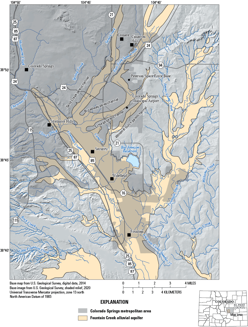
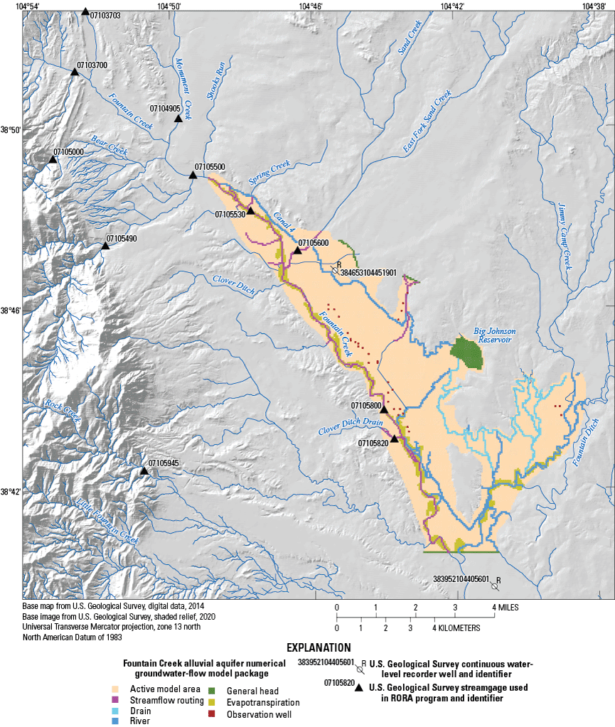
Study location and Fountain Creek alluvial aquifer (Topper and others, 2003) near Colorado Springs, Colorado, 2018–20.
Beginning in 2015, per- and polyfluoroalkyl substances (PFAS) were detected in the Fountain Creek alluvial aquifer and in public-supply wells (referred to in this report as “pumping wells”) southeast of Colorado Springs after the U.S. Environmental Protection Agency (EPA) required large public water systems across the United States to monitor for PFAS as part of the Unregulated Contaminant Monitoring Rule (Hu and others, 2016). Per- and polyfluoroalkyl substances are a group of human-made, fluorine-containing chemicals used since the 1950s to manufacture consumer products resistant to stains, grease, and water (National Ground Water Association, 2017). Aqueous film-forming foam, which is commonly used for extinguishing high-temperature fuel fires, also is formulated using PFAS (Hu and others, 2016). Per- and polyfluoroalkyl substances do not degrade easily in the environment (Trautmann and others, 2015), making them mobile in water and easily transported from source areas to downgradient groundwater and surface-water bodies. Concentrations of PFAS have exceeded the EPA lifetime health advisory limit at some locations in the Fountain Creek alluvial aquifer (Hu and others, 2016; McDonough and others, 2021), and many of the affected pumping wells have ceased pumping (U.S. Army Corps of Engineers, 2018a; U.S. Army Corps of Engineers, 2018b; U.S. Army Corps of Engineers, 2018c). Drinking water formerly sourced from groundwater is presently brought into the affected communities from Colorado Springs Utilities or by the Southern Delivery System pipeline from Pueblo Reservoir (not shown on any maps; U.S. Army Corps of Engineers, 2018a; U.S. Army Corps of Engineers, 2018b; U.S. Army Corps of Engineers, 2018c). Aqueous film-forming foam use at Peterson Space Force Base or the colocated Colorado Springs Airport east of Colorado Springs (fig. 1), or both, are potential PFAS sources in the Fountain Creek alluvial aquifer, and in 2016, the Air Force Civil Engineering Center began investigating potential PFAS source areas at Peterson Space Force Base in collaboration with the U.S. Army Corps of Engineers, EPA, and the Colorado Department of Public Health and Environment. From 2018 through 2020, the USGS, in cooperation with the Air Force Civil Engineering Center, conducted an integrated study of the Fountain Creek alluvial aquifer located near Colorado Springs, Colo. As part of this investigation, groundwater, streamflow, and water-quality data were collected (Newman and others, 2021). The study objective was to characterize hydrologic conditions of the Fountain Creek alluvial aquifer, southeast of Colorado Springs, to support investigation activities at Peterson Space Force Base and the surrounding area by providing a quantitative foundational understanding of the processes controlling groundwater recharge and movement in the Fountain Creek alluvial aquifer.
Study Area
The Fountain Creek alluvial aquifer, which includes the area previously designated as the Widefield aquifer (Edelmann and Cain, 1985), is composed of unconsolidated and permeable Quaternary-age sand and gravel alluvium deposited along the main valley of Fountain Creek. The alluvial aquifer is located in an urban area of Colorado Springs and surrounding communities in a semiarid climate with a mean annual precipitation of approximately 18.48 inches per year based on gridded datasets (PRISM Climate Group, 2020). The alluvium is generally coarse grained and lacks substantial intervening clay confining layers (AECOM, 2017), with a mean hydraulic conductivity (K) of about 830 feet per day (ft/d; Edelmann and Cain, 1985). The Fountain Creek alluvial aquifer is underlain by the relatively impermeable bedrock of the Late Cretaceous Pierre Shale, which prevents the downward movement of groundwater and promotes horizontal flow in the permeable alluvial deposits (Edelmann and Cain, 1985). The top of the Pierre Shale beneath the Fountain Creek alluvial aquifer is a Quaternary erosional surface exhibiting paleochannels and ridges (Radell and others, 1994; Lewis, 1995; AECOM, 2017). Four named tributary paleochannels drain from the Peterson Space Force Base to the main stem of the Fountain Creek alluvial aquifer (fig. 1): Sand Creek, Broadway, Schlage, and Windmill Gulch (AECOM, 2017). The Sand Creek, upper Broadway, and Windmill Gulch paleochannels coincide with existing stream channels, whereas the lower Broadway and Schlage paleochannels do not (AECOM, 2017). Groundwater flow in the center of the aquifer generally follows the top of the impermeable bedrock surface, and variably saturated groundwater conditions occur in several tributary alluvium paleochannels (Lewis, 1995; AECOM, 2017). The alluvium thickness ranges from 0 to about 100 feet, and the saturated thickness ranges from 0 to about 45 feet (Radell and others, 1994). Saturated thickness within each paleochannel is generally greatest along their central axis (AECOM, 2017). In the main valley of Fountain Creek, saturated thickness in the alluvial aquifer is greatest along a northwest to southeast trending axis between the tributaries of Sand Creek and Windmill Gulch (Lewis, 1995). Alluvial, colluvial, and eolian deposits located on ridges, outside of the alluvial aquifer extent on the top of bedrock surface were often unsaturated (Lewis, 1995; AECOM, 2017).
Study area streamflow varies seasonally because of snowmelt, contributions from groundwater base flow, and discharges from wastewater treatment plants (WWTP). Peak streamflow in Fountain Creek generally occurs May through July (USGS, 2021) coincident with snowmelt runoff from the adjacent mountains. Low streamflow periods in Fountain Creek were characterized by inputs from WWTP (Mau and others, 2007) and by groundwater discharge. In addition to Fountain Creek, Canal 4 is an artificial surface water body in the study area. Canal 4 runs along the northeastern extent of the alluvial aquifer and indicated by previous studies to be a source of groundwater recharge (fig. 1; Newman and others, 2021).
Previous investigations indicated variable spatial representations of the saturated extent of the Fountain Creek alluvial aquifer. For instance, in early investigations by Edelmann and Cain (1985) and Cain and Edelmann (1986), the saturated extent was indicated to closely follow the modern stream channel, with minor saturation in paleochannels. Topper and others (2003) mapped alluvial aquifers on a regional scale and in the vicinity of the study area indicated saturated conditions could be expected farther up the paleochannels than the original extents by Edelmann and Cain (1985) and Cain and Edelmann (1986). More recent investigations specific to the area near Peterson Space Force Base (AECOM, 2017) further delineated saturated conditions in both the paleochannels and in the main stem. The estimate of saturated extent from AECOM (2017), however, does not include paleochannels on the western side of the aquifer extending toward the mountain front mapped by Topper and others (2003). In this investigation, the datasets of Topper and others (2003) and AECOM (2017) were combined to create a new estimate of the extent of the alluvial aquifer, which is illustrated in figure 1 and included in Russell and Newman (2024).
Groundwater and surface-water interaction is a principal aspect of the water budget for the Fountain Creek alluvial aquifer because of the potential hydrologic connection to Fountain Creek. Previous water budgets for the Fountain Creek alluvial aquifer indicated the primary source of inflow to the aquifer is recharge from Fountain Creek streamflow losses that occur mainly in the reach between the tributaries of Spring Creek and Sand Creek (fig. 1; Edelmann and Cain, 1985). Other sources of recharge included infiltration from precipitation, irrigation return flows, and irrigation canal seepage; underflow from tributary alluvium and upgradient parts of the Fountain Creek alluvial aquifer; and infiltration from septic systems and sewage lagoons (Edelmann and Cain, 1985). Edelmann and Cain (1985) focused on the occurrence and distribution of nitrogen in groundwater, because at that time, a large percentage of the surface-water flow in Fountain Creek was derived from the Colorado Springs WWTP, and wastewater contained elevated nitrogen concentrations (Edelmann and Cain, 1985). Groundwater and surface-water interaction, as well as the distribution of nitrate in the Fountain Creek alluvial aquifer, were the focuses of the Lewis (1995) groundwater-quality study in the Fountain Creek valley.
Groundwater discharge components from the Fountain Creek alluvial aquifer used in this study include evapotranspiration (ET), discharge to Fountain Creek, discharge from groundwater wells, and groundwater flow to downgradient parts of the aquifer. Discharge to ET is facilitated by a shallow groundwater table and dense stands of cottonwood trees in the Fountain Creek valley. Groundwater and surface-water interaction is hypothesized to be controlled by depth to the groundwater table and the top of bedrock, which results in areas of groundwater recharge and discharge along Fountain Creek. Between the tributaries of Spring and Sand Creeks, Fountain Creek was previously considered a losing stream that recharged the aquifer based on water-budget calculations (Edelmann and Cain, 1985). Downstream from Sand Creek, groundwater generally discharged to the stream, and Fountain Creek was considered a gaining stream (Edelmann and Cain, 1985). Groundwater discharge from wells occurs primarily in the main valley of the Fountain Creek alluvial aquifer. Pumping wells provided water to the communities of Security, Widefield, and Fountain, and domestic, stock, and commercial wells also pump groundwater from the Fountain Creek alluvial aquifer (U.S. Army Corps of Engineers, 2018a; U.S. Army Corps of Engineers, 2018b; U.S. Army Corps of Engineers, 2018c).
Previous Studies
Several previous studies and ongoing data collection by the USGS in the Fountain Creek valley contributed to understanding the groundwater and surface-water conditions in the study area. Groundwater hydrology and water quality were investigated by Edelmann and Cain (1985), Cain and Edelmann (1986), and Lewis (1995) to support an understanding of water budgets and groundwater-flow directions. In the 1980s, the USGS developed and has since maintained a computer program estimating streamflow gains and losses in Fountain Creek, known as the transit-loss model (Kuhn, 1988, 1991; Kuhn and others, 1998, 2007; Kuhn and Arnold, 2006; Colarullo and Miller, 2019). The transit-loss model is used by the Colorado Division of Water Resources and local water providers for daily native water accounting, transmountain diversions, transit losses, and water allocations along Fountain Creek and Monument Creek (not shown on any maps). Results from the transit-loss model provide a detailed accounting of stream gains and losses, which can be used to quantify gaining and losing reaches of Fountain Creek.
In 1998, the USGS, in cooperation with Colorado Springs City Engineering, began a study of the Fountain Creek and Monument Creek Basins to characterize the effects of wastewater-treatment effluent and storm runoff on water quality and suspended-sediment conditions (Mau and others, 2007). Water-quality samples were collected at 11 main-stem sites between 1981 and 2001 and at 14 tributary sites in 2003. Suspended-sediment samples were collected daily at 7 main-stem sites from 1998 through 2001, daily at 6 main-stem sites from 2003 through 2006, and intermittently at 13 tributary sites from 2003 through 2006 (Mau and others, 2007). Water-quality samples were analyzed for nutrients, fecal coliform, and trace elements, and the results were evaluated in terms of base flow, normal flow, and stormflow. Stormflow samples exhibited concentrations of fecal coliform that frequently exceeded water-quality standards 1998–2006 on main-stem and tributary sites, and suspended sediment, nitrogen, phosphorous, and trace-element load substantially increased during stormflow, indicating these constituents were transported to surface water primarily by storm runoff (Mau and others, 2007).
As part of the study discussed in this report, an extensive water-quality dataset was collected from groundwater wells and surface waters September 2018 through May 2019 to evaluate sources of recharge to the aquifer as well as sources of solutes. This dataset included major and trace elements, rare earth elements, pharmaceutical and wastewater indicator compounds, and groundwater age tracers. The water-quality dataset was published in the National Water Information System (NWIS) database (USGS, 2021) and interpretations were reported in Newman and others (2021). In general, Newman and others (2021) found surface waters were sources of aquifer recharge based on the presence of pharmaceutical and wastewater indicator compounds in groundwater wells in close proximity to both Fountain Creek and Canal 4 (fig. 1). Spatial distribution of groundwater age estimates also indicates Fountain Creek and Canal 4 were sources of recharge, because groundwater near these surface water bodies was generally younger than groundwater in the center of the aquifer. Groundwater ages estimated in Newman and others (2021) ranged from several months to approximately 21 years old. The findings of Newman and others (2021) assist in conceptualizing the hydrologic conditions discussed in this report.
Purpose and Scope
The purpose of this report is to characterize the groundwater flow and movement in the Fountain Creek alluvial aquifer 2018 through 2020 during decreased groundwater withdrawals from pumping wells. Additionally, this report provides hydrologic conditions for the alluvial aquifer pertinent to the potential for transport of solutes. An integrated approach was used to evaluate groundwater hydrologic processes, assess groundwater and surface-water interactions, estimate hydraulic aquifer properties using aquifer testing, and complete numerical groundwater-flow simulations. Groundwater-flow directions were determined from continuous and periodically measured groundwater-level elevations, and groundwater and surface-water interactions were evaluated using synoptic streamflow measurements. Groundwater-flow processes were evaluated quantitatively using statistical water-level modeling approaches and a numerical groundwater-flow model; the latter is used to simulate recharge and discharge from the alluvial aquifer, interactions with surface water, and groundwater-flow paths. Input and model files facilitating quantitative analyses using statistical approaches and the numerical groundwater-flow model were compiled into a USGS data release (Kisfalusi and Newman, 2022) and a model archive associated with this report (Russell and Newman, 2024). This data release and model archive may be used to reproduce this report results or be updated for future conditions. Synoptic water-quality data were collected and interpreted to indicate physical and chemical processes occurring in the aquifer, and water-quality sampling analyses and results are reported in Newman and others (2021) and available in the NWIS database (USGS, 2021).
Study Methods
An integrated approach was used in this report to evaluate groundwater hydrologic processes, assess groundwater and surface-water interactions, estimate hydraulic properties of the aquifer using aquifer testing, and complete numerical simulations of groundwater flow. The methods used in the integrated approach are described in detail in this section.
Groundwater Hydrology
An understanding of the groundwater-flow directions in the Fountain Creek alluvial aquifer was determined from groundwater-level elevation measurements. As part of the study, groundwater levels were measured at 31 locations (fig. 2; table 1), many were measured in previous USGS studies (for example, Radell and others, 1994; Lewis, 1995). Discrete depth-to-groundwater measurements were collected at each location and then converted to groundwater-level elevations in feet (ft) above the North American Vertical Datum of 1988 (NAVD 88) using the depth below land surface of the groundwater level and the land-surface elevation of the location in NAVD 88. Groundwater levels were measured using either an electric or a steel tape according to standard methods described in Cunningham and Schalk (2011).
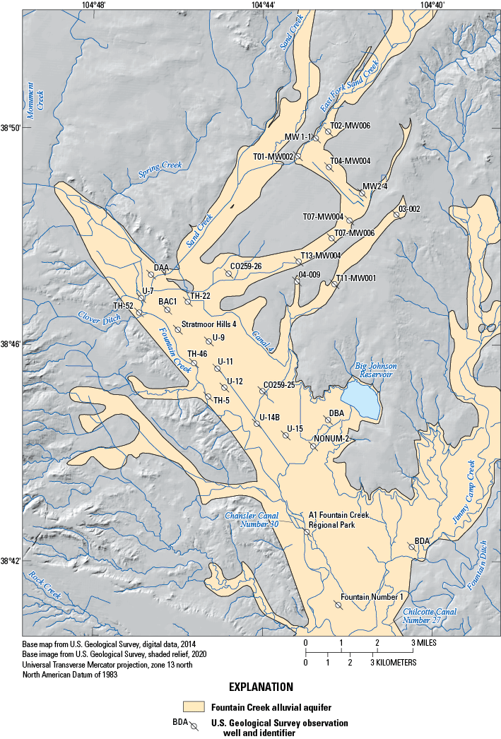
Groundwater-level observation well locations from the National Water Information System database (U.S. Geological Survey, 2021) within the Fountain Creek alluvial aquifer extent near Colorado Springs, Colorado, 2018–20.
Table 1.
Groundwater-level observation well location site numbers and site common names in the Fountain Creek alluvial aquifer study area.[U.S. Geological Survey (USGS) site numbers and site common names for the observation locations are linked to the National Water Information System database (U.S. Geological Survey, 2021)]
Three locations were additionally equipped with pressure transducers to collect continuous groundwater-level data. Pressure transducers were installed at wells MW1-1, T11-MW001, and TH-22 (fig. 2). Pressure transducers were set to record groundwater levels at one-hour intervals. During each site visit, the continuous data were downloaded and discrete depth to groundwater was measured to allow drift correction of continuous data recorded by the pressure transducer according to methods described in Cunningham and Schalk (2011). Both discrete and continuous groundwater-level elevation data were used to assess the distribution and movement of groundwater within the study area.
Statistical groundwater-level modeling of groundwater-level elevations was completed to determine the primary physical processes controlling groundwater flow. Specifically, a transfer-function-noise (TFN) approach was useful for indicating the effect of external hydrologic stressors (for example, recharge, groundwater pumping, and streamflow) on groundwater-level elevation fluctuations in individual wells (Bakker and Schaars, 2019). The TFN approach uses statistical signal analysis algorithms to decompose the observed fluctuation in groundwater-level elevations into response functions, which represent different hydraulic stressors. For example, the effect of a groundwater pumping well on groundwater-level elevation fluctuations in an observation well may be evaluated using a Hantush function (Bakker and Schaars, 2019). Using the TFN approach, the proportion of the total observed variation in groundwater-level elevation fluctuations may be attributed to different hydrologic stressors.
Groundwater-level modeling was conducted with the TFN approach for the Fountain Creek alluvial aquifer using the Pastas package (Collenteur and others, 2019) implemented in the Python programming language. The Pastas package was used because of the number of response functions included and the ability to programmatically conduct TFN modeling. Input requirements were time series of groundwater-level observations, estimated recharge, and pumping discharge. The groundwater-level model was completed using discrete data from groundwater-level elevation observation locations. Groundwater-level data that predated the study data for this report were also included in the analysis. Two groundwater-level models were completed: one in which only recharge was considered and one in which only groundwater pumping was considered. These two groundwater-level models allow for the two primary hypothesized stressors in the study area to be evaluated individually. The groundwater-level model considering only recharge was constructed by estimating a daily time series of precipitation and ET for the study area using the Climate Engine online tool (Huntington and others, 2017). A time series of point recharge at each observation well was calculated as precipitation minus ET. The groundwater-level model using only groundwater pumping was constructed by aggregating pumping rates for nearby observation wells on a daily basis. Groundwater-level model code, inputs, and outputs are provided in a USGS data release and a model archive associated with this study (Russell and Newman, 2024).
Groundwater and Surface-Water Interactions
Evaluation of the interaction between groundwater and Fountain Creek was included in this study because previous studies indicated the exchange of groundwater and surface water were major terms in the local water budget (Edelmann and Cain, 1985; Cain and Edelmann, 1986). When groundwater-level elevations near the streambed are higher than the stream-surface elevation, groundwater may flow into the stream, known as a gaining stream. Conversely, if the groundwater-level elevation is lower than the stream-surface elevation, then water may flow from the stream into the groundwater, known as a losing stream. Gaining streams are groundwater discharge locations, whereas losing streams are groundwater recharge locations (Winter and others, 1998).
To assess streamflow gain or loss in the study area, synoptic streamflow measurements were made in March 2019 at sites corresponding to the Fountain Creek transit-loss model where established USGS streamgages do not exist (fig. 3 of this report; Kuhn and Arnold, 2006). Streamflow was measured using an acoustic Doppler velocimeter according to methods described in Rehmel (2007) and Turnipseed and Sauer (2010). To supplement discrete streamflow data, the daily mean streamflow from three continuous USGS streamgages (Fountain Creek at Colorado Springs, CO, 07105500; Fountain Creek below Janitell Road below Colorado Springs, CO, 07105530; and Fountain Creek at Security, CO, 07105800) was extracted from the National Water Information System (NWIS) database (USGS, 2021) on the date of the synoptic streamflow measurements. Data supplemented from the NWIS database provided a more spatially detailed understanding of groundwater and surface-water interactions.
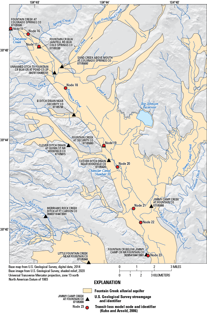
U.S. Geological Survey streamgages from the National Water Information System database (U.S. Geological Survey, 2021) and transit-loss model nodes within the Fountain Creek alluvial aquifer extent near Colorado Springs, Colorado, 2019.
Using streamflow measured from the transit-loss model at upstream and downstream locations, net streamflow gain or loss from each reach was calculated according to equation 1 (modified from Simonds and Sinclair, 2002)
whereΔQ
is the net streamflow gain or loss, in cubic feet per second (ft3/s);
Qd
is the streamflow at the downstream end of the reach, in ft3/s;
Qu
is the streamflow at the upstream end of the reach, in ft3/s;
T
is the sum of tributary inflows within the reach, in ft3/s; and
D
is the sum of diversions within the reach, in ft3/s.
Values of ΔQ less than zero indicate the stream reach is losing (a source of groundwater recharge), and values of ΔQ greater than zero indicate the stream reach is gaining (a point of groundwater discharge).
The net streamflow gain or loss along each reach is subject to errors in streamflow measurement, which are accumulated by different sources of error in each measurement (Rosenberry and LaBaugh, 2008). Total error for each reach gain loss was calculated according to the error propagation formula (Harmel and others, 2006):
whereE
is the total error, in ft3/s;
EN
is the error of the Nth measurement, in ft3/s; and
N
is the number of measurements.
Error in individual measurements was quantified using the interpolated variance estimator described by Cohn and others (2013) and recorded by the acoustic Doppler velocimeter. Individual measurement and net errors were calculated in the unit of the streamflow analysis, in ft3/s, by multiplying the quantitative error (5 percent) by the measured streamflow, yielding an estimate in ft3/s of the absolute error of the measurement.
A number of potential diversions and inflows to Fountain Creek in the study area, primarily from irrigation ditches divert surface water from Fountain Creek, and WWTP discharge treated effluent into Fountain Creek (Kuhn and others, 2007; Mau and others, 2007). Streamflow, at each diversion and inflow, was not measured as part of this study, but values for each were extracted from the transit-loss model and the NWIS database for the date of the synoptic measurements (March 3, 2019). These values were used for computing streamflow gain or loss assuming an error in each diversion and inflow value of 10 percent, which is the likely amount of error, assuming the diversion and inflow values had qualitative indicators of poor given by the field data collector (Turnipseed and Sauer, 2010).
Aquifer Testing
Hydraulic properties of an aquifer govern the flow of groundwater through the aquifer from the recharge area to the discharge area. Hydraulic properties such as K, specific storage (Ss), and specific yield (Sy) may be estimated from reference materials for a given aquifer type (Freeze and Cherry, 1979), computed with inverse methods from spatially distributed groundwater-level observations (Shapoori and others, 2015), or directly estimated through aquifer testing (Kruseman and de Ridder, 1990; Butler, 1997). Aquifer testing consists of stressing the hydrologic system, typically by either adding or removing water from a well and observing the time-dependent system recovery to the pretest conditions. Data from the test may then be compared to various analytical solutions selected based on the hydrogeologic conceptualization of the aquifer and used to calculate hydraulic properties.
Single-well aquifer tests were conducted in 11 observation wells during July 2019 (fig. 4; table 2). Three wells were located in the Broadway paleochannel, two wells were located in the Windmill Gulch paleochannel, and six wells were located within the main stem of the Fountain Creek alluvial aquifer. Six wells were tested with traditional slug tests, and five wells had a combination of traditional slug tests along with single-well pumping tests (table 2). Each traditional slug test consisted of a falling-head (slug-in) and a rising-head (slug-out) test. In these tests, different initial displacements were used to evaluate the presence of complicating factors such as unidirectional flow or low-K well skins (materials within the well bore that inhibit connection between the well and the aquifer; Butler, 1997). Each solid slug was dropped below the groundwater table for the falling-head test, and when the groundwater level reached the equilibrated initial groundwater level, the slug was pulled above the groundwater table for the rising-head test (Butler, 1997; Cunningham and Schalk, 2011). Single-well pumping and recovery tests were conducted using a Grundfos Redi-Flo 2 pump. Pumping was initiated once static groundwater levels were confirmed by pressure transducer measurements. When groundwater-level displacement was deemed substantial based on the length of pumping period and observed groundwater-level change rate, pumping was discontinued, and recovery was observed until approximate static conditions (within 0.06 ft of initial groundwater level) were reached.
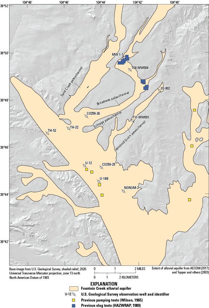
Aquifer testing observation well locations from 2019 from the National Water Information System database (U.S. Geological Survey, 2021). Aquifer testing observation well locations described in Wilson (1965) were not assigned coordinates, and exact coordinates of aquifer test wells were not known. Assigned coordinates were georeferenced to quarter-quarter-quarter sections on the Public Land Survey System.
Table 2.
Observation well completion and aquifer testing information.[Well locations are shown in figure 4. U.S. Geological Survey (USGS) site numbers and site common names for the observation wells are linked to the National Water Information System database (U.S. Geological Survey, 2021). ft, feet; bls, below land surface]
For each test type, a vented pressure transducer was placed near the bottom of the well (below the solid slug or the pump) to measure groundwater-level displacement (Cunningham and Schalk, 2011). Pressure transducers were placed as far as possible away from the groundwater-level perturbation to minimize signal noise during data collection. Groundwater levels were measured at a frequency of 0.5 seconds with observations made before, during, and after an aquifer test to differentiate drawdown and recovery from groundwater-level changes caused by environmental factors. Well completion diagrams for those observation wells included in aquifer testing are included as part of a USGS data release (Kisfalusi and Newman, 2022).
The aquifer testing goal was to quantify hydraulic properties in the Fountain Creek alluvial aquifer and to evaluate spatial variability in the hydraulic properties. The primary hydraulic property estimated using the aquifer-test results was K, although in some instances estimation of storage properties (for example, Ss and Sy) may also be possible. Aquifer-testing data were analyzed using the software AQTESOLV version 4.5 (Duffield, 2007). Analysis of slug-test data used the methods of Bouwer and Rice (1976), Springer and Gelhar (1991), and model of Hyder and others (1994). The Bouwer and Rice (1976) method is best suited for application to unconfined aquifers and has various assumptions relating to aquifer penetration, well screen position, and well flow behavior (Butler, 1997). The Springer and Gelhar (1991) method was used to account for inertial effects in the wells and the oscillatory responses seen in the study area. The Springer and Gelhar (1991) solution also incorporates frictional well loss in small-diameter wells (Butler, 1997). The Hyder and others (1994) model was useful when the presence of a variable behavior between rising-head and falling-head tests was observed, potentially because of interferences between the aquifer material and the well bore (Butler, 1997), commonly known as “well-skin effects,” which were evident during one test. The single-well pumping tests were analyzed using the Cooper and Jacob (1946) method to evaluate both the pumping and recovery data. Halford and others (2006) indicate the Cooper and Jacob (1946) method was the analytical solution most applicable to single-well pumping tests for unconfined conditions, regardless of partial penetration or other potentially complicating factors.
Groundwater-Flow Simulations
Given the complex nature of the Fountain Creek alluvial aquifer and multiple potential hydrologic stressors in the system (for example, groundwater pumping and groundwater and surface-water interactions) it was necessary to apply a groundwater-flow model to simulate and predict groundwater movement. In this setting, a groundwater-flow model may be used to evaluate conceptual groundwater recharge models and discharge sources, quantify changing groundwater budgets under transient conditions, and quantitatively predict groundwater-flow paths. A numerical groundwater-flow model was constructed for the Fountain Creek alluvial aquifer using the finite-difference code MODFLOW with the Newton formulation solver (MODFLOW-NWT; Niswonger and others, 2011). The model was spatially discretized into individual cells whose size and properties were specified through user input, with user-specified time steps for temporal discretization of the MODFLOW model. Discretization of the groundwater-flow model and application of boundary conditions are described in detail in the following paragraphs and illustrated in figure 5. The numerical groundwater-flow model and all associated input files are included as a USGS data release associated with this report (Russell and Newman, 2024).
Model discretization and boundary conditions for the Fountain Creek alluvial aquifer numerical groundwater-flow model, near Colorado Springs, Colorado, 2000–19. Model files are provided as a U.S. Geological Survey data release associated with this report (Russell and Newman, 2024); RORA as described by Rutledge (2000).
The numerical model of the Fountain Creek alluvial aquifer has 1 layer of 291 rows and 254 columns of 200-ft by 200-ft size cells, with a total of 17,610 active cells (fig. 5). A one-layer model was used because the alluvium overlies Upper Cretaceous Pierre Shale with low permeability, which serves as a vertical no-flow boundary for the groundwater-flow system. The model grid was projected and aligned relative to the Colorado State Plane Coordinate System (North American Datum of 1983, units: feet, zone: Colorado Central Zone).
The active model grid extent was based on the extent of the Quaternary alluvium deposits that compose the Fountain Creek alluvial aquifer. The active extent of the model grid did not include the paleochannels present to the northeast of the primary aquifer. The paleochannels were excluded because of transient unsaturated conditions and thin saturated thickness, as indicated by groundwater-level monitoring, though these paleochannels may be dominant sources of chemical constituents to the aquifer (Newman and others, 2021). To evaluate groundwater flow from the paleochannels, the General-Head Boundary (GHB) package (Harbaugh and others, 2000) was used to represent flow originating in the Broadway and Windmill Gulch paleochannels.
The model simulates time periods as model stress periods, and during each model stress period, hydrologic stressors were specified and held constant for the stress period duration. The Fountain Creek alluvial aquifer model contains 241 stress periods. Of these 241 stress periods, the initial stress period represents a steady state period, and the other 240 stress periods were transient, simulating each month from 2000 to 2019. For the initial stress period of the numerical model, hydrologic stressors and groundwater-flow rates were assumed to be constant, and the stress period represents mean annual data throughout the transient stress periods. The outputs from the steady-state model stress period were used as inputs for the subsequent transient stress period.
The Fountain Creek alluvial aquifer system numerical groundwater-flow model is composed of multiple hydrologic boundaries representing areas of inflow or outflow. These hydrologic boundaries were simulated through MODFLOW packages (fig. 5). The hydrologic boundaries simulated in this numerical model were separated into two different types: head-dependent and specified-flux boundaries. Head-dependent boundaries allow flow into or out of the model based on differences between user-specified groundwater levels. Specified-flux boundaries allow flow into or out of the model based on user-specified flux rates. Recharge and well withdrawals were simulated in the model using specified-flux boundaries, and evapotranspiration, streams, reservoirs, and lateral groundwater flow were simulated using head-dependent boundaries.
Recharge for the numerical model was simulated using the Recharge (RCH) package (Harbaugh and others, 2000) and precipitation data from the Parameter-elevation Regressions on Independent Slopes Model (PRISM) dataset from Oregon State University (PRISM Climate Group, 2020). The PRISM data were modified using the ArcGIS Resample tool (Esri, 2021), which interpolated the precipitation data to fit the model grid cell size. Distributed recharge is caused by infiltration of precipitation (rain and snow) into the aquifer system. The amount of water infiltrating the land surface is affected by several factors, such as precipitation rates, evapotranspiration rates, unsaturated-zone permeability and moisture capacity, and land surface slope; therefore, only a fraction of the amount of precipitation from the PRISM dataset recharges the aquifer. This fraction is applied to the recharge arrays as a multiplier for each simulated stress period.
To determine the recharge amount applied to the aquifer, the RORA program (Rutledge, 2000) was applied to USGS streamgage streamflow data from the NWIS database (USGS, 2021) throughout and nearby the active model area. RORA is a program that estimates recharge for the drainage basin of a specified streamgage using a recession-curve displacement method. This method uses the upward displacement of the streamflow-recession curve during groundwater recharge periods, such as storms, to determine the rate of groundwater recharge to an idealized, homogenous aquifer (Rutledge, 2000). Estimation of recharge using the RORA program differs from the point estimates of recharge used as inputs to the TFN model because RORA estimates spatially integrated recharge rates for a drainage basin above a streamgage, whereas point estimates of recharge at wells used in the TFN model are not spatially integrated but vary through time. The RORA program was used for 11 USGS streamgages from 2000 to 2019 (fig. 5). The recharge estimates output by RORA ranged from 2.14 to 3.47 inches per year (in/yr). These outputs were then weighted based on the basin size and period of record of the streamflow data, with the mean weighted estimate of recharge being 2.53 in/yr, or about 13.72 percent of the mean annual precipitation (18.48 in/yr) from the PRISM dataset. The recharge multipliers within the recharge package were constrained so recharge for the numerical model would not deviate too far from the mean weighted estimate of recharge, with a final mean annual recharge rate of 2.68 in/yr used for the numerical model transient stress periods.
Evapotranspiration is the process by which water is directly transferred into the atmosphere through evaporation and through plant transpiration; evapotranspiration represents a water-budget outflow from the alluvial aquifer. The Evapotranspiration (EVT) package (Harbaugh and others, 2000) was used to simulate this process in the numerical model. Evapotranspiration within the model was limited to cells with cottonwood trees identified based on satellite imagery from Google Earth (Russell and Newman, 2024) and found mostly along the main reach of Fountain Creek (fig. 5). A simulated root-zone depth of 0.40 ft was used, and the simulated ET rate varied each month based on seasonal ET rates from remotely sensed imagery showing cottonwood trees in the lower Colorado River Basin by Jetton (2008).
Given the evidence of groundwater and surface-water interactions in the aquifer as indicated by previous studies (Edelmann and Cain, 1985; Cain and Edelmann, 1986; Lewis, 1995), it is hypothesized streamflow losses may be a substantial groundwater recharge source. A detailed water-quality analysis of groundwater and surface water, carried out in conjunction with this study, indicated wells near Fountain Creek displayed water-quality signatures consistent with streamflow recharge (Newman and others, 2021). To evaluate exchanges between groundwater and surface water, streams within the active model area were simulated using the Streamflow-Routing (SFR) (Niswonger and Prudic, 2005), the Drain (DRN) and the River (RIV) (Harbaugh and others, 2000) packages. Concrete-lined streams within the active model area, as shown on satellite imagery from Google Earth (Russell and Newman, 2024), were not simulated, as the concrete acts as an impermeable boundary between the stream and the underlying aquifer. An example of a concrete-lined stream not simulated as interacting with the aquifer is Windmill Gulch between Canal 4 and Fountain Creek (fig. 1). The main reach of Fountain Creek and its tributaries were simulated using the SFR package. The SFR package uses Darcy’s Law, streambed conductance, groundwater-table elevation, and stream stage to determine flow between the stream and the surrounding aquifer. Specified inflows within the SFR package allow for base flows from tributaries outside the model active area to be incorporated into the model, allowing for more accurate simulated streamflows. SFR calculates the simulated base flows along specified segments and routes the base flows downstream until they were outside of the active model area or captured by a different hydrologic boundary.
All SFR stream segments had a thickness of 1.0 ft and a Manning’s roughness coefficient of 0.025, based on common assumptions for the SFR package (Niswonger and Prudic, 2005). Streambed conductivity for each stream segment ranged from 0.01 to 50.0 ft/d. This wide range of conductivity is because of the Pierre Shale outcropping in some parts of the stream, whereas the rest of the streambed is predominantly fine to coarse sand. Simulated stream widths ranged from 20.0 to 95.0 ft and were estimated using satellite imagery from Google Earth (Russell and Newman, 2024). Streambed elevations were modified using USGS 5-meter digital elevation model values to allow for accurate simulated base flows (USGS, 2020). Monthly base flow inflows from outside the active model area included Fountain Creek, Shooks Run, Spring Creek, Sand Creek, B Ditch Drain, and Clover Ditch and were input using the SFR package. Data gaps in the monthly base flow data were filled with the mean base flow for the corresponding month and location. The main reach of Fountain Creek has several points of artificial inflows and diversions (Kuhn and Arnold, 2006). However, these points were not simulated in the numerical model, because they were determined to be minor components of the water budget.
The SFR package routes flow downstream to connected stream reaches. Because of this functionality, streams can only be simulated within the package if the upstream reaches were higher than or equal in elevation to the downstream reaches. This elevation requirement can cause an issue with artificial canals, such as Canal 4. Therefore, the canals and other streams not included in the SFR package were simulated using the DRN and RIV packages (fig. 5). The difference between the two packages is the RIV package allows for flow into and out of the groundwater systems to a simulated surface-water feature, whereas the DRN package only allows for outflow from the groundwater system to the simulated surface-water feature. Flow between the aquifer and surface-water features in the RIV package is dependent on stage of the surface-water feature, hydraulic conductivity of the feature-aquifer interconnection, and the head at the node in the cell underlying the surface-water feature. Flow in the DRN package is dependent on the feature’s conductance, elevation, and head in the cell. Flow from the aquifer into the drain feature will only be simulated if the head in the drain cell is above the drain elevation. Because the DRN package only allows for flow out of the aquifer and into surface-water features, the RIV package was predominantly used for streams and canals. However, in areas where the numerical model experienced hydraulic heads above land surface, the DRN package was implemented.
All the RIV and DRN package cells were channelized, meaning the cell elevations were set below land surface to simulate a stream channel. For the RIV package, the cell elevations were set to 4 ft below land surface, and the DRN package cell elevations were typically set to 1.0 ft above the bottom of the model (representing the interface between the alluvial aquifer and the Pierre Shale). The DRN cells have the potential to remove water from the alluvial aquifer based on the gradient between the aquifer and DRN in each cell location. However, because the aquifer is typically thin in the vicinity of most DRN cells (AECOM, 2017), the DRN package is limited in its ability to cause unrealistic water budget outflows from the model. The ability for the RIV and DRN packages to transmit water is governed by hydraulic conductivity values. The hydraulic conductivity values for the RIV package varied based on location and ranged from 107 to 17,500 feet per day (ft/d). The hydraulic conductivity values for the DRN package also varied based on location and ranged from 2,978 to 44,800 ft/d. For the RIV package, a stage elevation of 1.0 ft above the streambed was set for all simulated streams.
Lateral inflows into the model from external water sources (Big Johnson Reservoir and the Broadway and Windmill Gulch paleochannels) were simulated using the GHB package (Harbaugh and others, 2000). Flow between the GHB and aquifer is the product of hydraulic conductivity of the boundary and the difference between the head in the aquifer and head in the GHB. Big Johnson Reservoir, an approximately 300-acre artificial lake and one of the major surface-water features in the active model area (fig. 5), was simulated using a GHB head of 5,800 ft and a hydraulic conductivity of 15.0 ft/d. Water-quality data indicated leakage from Big Johnson Reservoir may recharge the aquifer (Newman and others, 2021). Although water levels in Big Johnson Reservoir declined beginning in 2016 when draining the reservoir began for repairs (Steiner, 2017), noble gas data in groundwater from wells downgradient from the reservoir indicated recent equilibrium with the atmosphere, whereas other nearby groundwater wells did not (Newman and others, 2021). Recent atmospheric equilibrium indicates the reservoir is a source of recharge to the aquifer.
Lateral inflow and outflow were other substantial components of the modeled water budget, because the paleochannels were not directly simulated in the active model area and because the alluvial aquifer continues to the south, outside of the active model domain. Groundwater flow from paleochannels to the part of the aquifer simulated in the numerical model was simulated using several GHBs (fig. 5), and a GHB was used to represent the southern end of the model domain. Based on a previous water budget for the aquifer, Edelmann and Cain (1985) found groundwater flow likely exits the study area to the south. Head elevations for the GHBs were set using data from nearby USGS groundwater-level observation wells 384653104451901 and 383952104405601. The monthly means of observed groundwater levels, recorded in feet below land surface for 384653104451901 were used for the GHB heads in the Broadway and Windmill Gulch paleochannels, and the monthly means of observed groundwater levels for 383952104405601 were used for the GHB heads at the southern boundary. Hydraulic conductivity of 15.0 ft/d was used, and model inputs were compiled into the GHB package (Russell and Newman, 2024).
A primary hydrologic stressor in the Fountain Creek alluvial aquifer is groundwater pumping for municipal use. Several water-supply districts in the area operated pumping wells, prior to the PFAS compounds discovery (U.S. Army Corps of Engineers, 2018a; U.S. Army Corps of Engineers, 2018b; U.S. Army Corps of Engineers, 2018c; McDonough and others, 2021). The distribution of 38 known pumping wells in the study area is illustrated in figure 6A, along with reported groundwater pumpage through time (fig. 6B). Groundwater pumping data are included in the data release associated with this study (Russell and Newman, 2024). Most pumping wells were located in the central part of the alluvial aquifer, near Fountain Creek. Total groundwater pumpage, for 2000 to 2018 (fig. 6B) varied, but trends in specific water-supply districts are apparent, with groundwater pumpage from the Security district decreasing beginning in 2013, coinciding with an increase in pumping from the Widefield district. The effect of groundwater pumping on specific wells was assessed via the TFN groundwater-level model (as discussed in the “Groundwater Hydrology” section of this report), and the variation in groundwater pumping was used to inform the transient calibration of the groundwater-flow model, as described in the next paragraph. Groundwater pumping wells were simulated in the model using the Well (WEL) package (Harbaugh and others, 2000). The mean value of all well pumping during the transient stress period was used in the steady-state stress period.
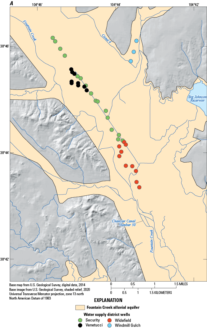
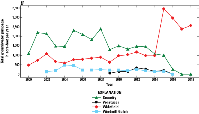
A, distribution of pumping wells in the Fountain Creek alluvial aquifer near Colorado Springs, Colorado, and B, reported groundwater pumpage, 2000–18, for distinct groundwater-supply districts near Colorado Springs, Colorado, 2000–18 (Russell and Newman, 2024).
Following initial parameterization, the numerical model was calibrated to achieve better agreement between groundwater-level observations and base flows. This model calibration process includes manual and automated calibration steps. Manual calibration was done by changing input parameter values until a user specified and subjective reasonable fit for groundwater-level elevations was achieved, after which automated calibration using computer programs was used to complete the calibration process based on quantitative criteria. The computer programs used in the automated calibration step continuously change user-specified parameters to minimize the differences between simulated and observed groundwater-level elevations and base flows. These user-specified parameters were set within a predetermined range that conceptually match the properties of the Fountain Creek alluvial aquifer. To complete this parameter estimation, the program PEST++ iterative ensemble smoother (PEST++IES) was used, which applies an iterative ensemble smoother algorithm to minimize a user-defined objective function that describes discrepancies between the model simulations and observations (White and others, 2020).
The automated calibration process for the alluvial aquifer used groups of input parameters and groups of observations. Input parameters were split into 8 groups of 477 total parameters, and observations were split into 5 groups of 2,100 total observations. Of the 477 parameters, there were 241 parameters for recharge, 93 parameters for horizontal hydraulic conductivity (Kh), 93 parameters for the vertical to horizontal hydraulic conductivity ratio (Kv/h), 21 parameters for SFR streambed conductance, 14 parameters for ET, 4 parameters for SFR stream widths, 4 parameters for RIV riverbed conductance, 3 parameters for GHB conductance, and 1 parameter each for Ss, Sy, SFR stream thickness, and DRN conductance. The recharge parameters were multipliers applied to each recharge array for every stress period within the numerical model, and the range of the recharge multipliers were limited to only allow realistic rates of recharge to the simulated groundwater system. The 93 parameters for Kh were evenly spaced points throughout the active model domain using a pilot points approach (Doherty, 2003), and the range of Kh was based on aquifer testing data collected as part of this study. The 93 parameters for Kv/h were fixed, meaning they were not changed during the automated calibration process. Most ET parameters were multipliers (13 of 14) used similarly to recharge array multipliers. Twelve of the multipliers represented monthly ET rates, and the other multiplier represented the ET rate for the steady-state stress period of the numerical model. The last evapotranspiration parameter adjusted the root-zone depth in the EVT package. All boundary conductance parameters were limited to realistic boundary conductance values calculated using K values and area of model cells.
Of the 2,100 total observations used in the automated calibration process, 1,136 groundwater-level elevation were observations from 42 wells and 964 were base flow observations from 4 USGS streamgages (Fountain Creek below Janitell Road below Colorado Springs, CO, 07105530; Sand Creek above Mouth at Colorado Springs, CO, 07105600; Fountain Creek at Security, CO, 07105800; and Clover Ditch Drain near Widefield, CO, 07105820; fig. 5). All groundwater-level elevation data were retrieved from the USGS NWIS database (USGS, 2021). The 964 base flow observations were obtained from the USGS NWIS database and processed using the USGS Groundwater Toolbox (Barlow and others, 2017). Base flow was estimated for the two streamgages located along Fountain Creek (07105530 and 07105800; fig. 5) throughout the entire transient stress period of the numerical model, 2000–19. Base flow was estimated for the streamgage along Sand Creek (07105600) seasonally for the months April–September between 2003 and 2014 and transitioned to estimates for each month throughout the year between 2014 and 2019. Base flow was estimated monthly for the streamgage along Clover Ditch Drain (07105820) beginning in November 2017 and extending through 2019. Any periods of missing base flow estimates were filled with the mean monthly base flow for the site using the available data (USGS, 2021). Most of the streamflow measurements made at these streamgages, during the transient period of the numerical model, were rated as fair by the hydrographer conducting the measurement, meaning streamflow measurements were within 8 percent of true streamflow (Turnipseed and Sauer, 2010).
These observations were categorized into five groups, one group for the groundwater-level elevation observations and a separate group for each of the four streamgages. The contribution of the observation groups to the objective function were adjusted to maintain a balance between the observation groups during the calibration process. The base flow observations accounted for 81 percent of the observation group contribution to the objective function, meaning the model was most sensitive to changes in base flow.
The ability of the model to emulate observed groundwater-level elevations was assessed quantitatively using the root-mean-squared-error (RMSE) and the normalized RMSE (nRMSE) calculated according to
wheren
is the number of observations,
oi
is the observed groundwater-level elevation at the ith well,
si
is the simulated groundwater-level elevation at the ith well,
omax
is the maximum observed groundwater-level elevation within the model domain, and
omin
is the minimum observed groundwater-level elevation within the model domain.
The RMSE and nRMSE were useful model calibration indicators, because they quantitatively indicate the ability of the model to simulate the hydrologic system. The calibration goal is to reduce both the RMSE and nRMSE. An nRMSE less than or equal to 10 percent is generally considered to represent a well-calibrated model (Anderson and others, 2015). All results of model calibration and simulations are described in the “Groundwater-Flow Simulations” section of this report.
The approximate groundwater-flow paths of water sourced in pumping wells was assessed using the calibrated model and the particle tracking software MODPATH version 7 (Pollock, 2016). MODPATH is a software package that computes the approximate trajectory of hypothetical particles within the aquifer based on advective transport. Particle tracking may be useful for understanding source zones of groundwater discharged from pumping wells (Moeck and others, 2020). In the context of the Fountain Creek alluvial aquifer, the groundwater to pumping wells source is pertinent because of the occurrence of PFAS compounds in drinking water in the area (Hu and others, 2016; McDonough and others, 2021). MODPATH simulations were created using the steady-state numerical model, as is common for particle-tracking applications in complex aquifers (Moeck and others, 2020). Particle tracking was conducted in reverse mode, meaning a hypothetical particle was placed in each model cell containing a pumping well. The model then was run in reverse to calculate the trajectory of each particle from the pumping wells to the origin of the particle. This analysis essentially outlines the areas of the aquifer contributing groundwater to pumping wells. The Python scripts used for MODPATH model creation and processing are included in the USGS data release associated with this report (Russell and Newman, 2024).
Groundwater Hydrology
Groundwater-level elevations in the Fountain Creek alluvial aquifer vary seasonally and on interannual timescales. Example hydrographs showing seasonal and long-term groundwater-level elevation fluctuations are illustrated in figure 7A, B. Groundwater-level elevation data for all observation wells included in this study are available from the USGS NWIS database (USGS, 2021), using the USGS site identifiers listed in table 1. Seasonal fluctuations tend to cause maximum groundwater-level elevations in the winter months in many wells, such as in well CO259-25 (fig. 7A). Maximum groundwater-level elevations in the winter months were likely caused by reduced groundwater pumping and groundwater ET in winter months. Groundwater-level elevations also show longer-term variation possibly linked to climate or pumping. As seen in figure 7, groundwater-level elevations in both CO259-25 and U-9 appear to reach maximum values in 2000 to 2003, decrease from 2003 to 2006 (with the exception of one measurement in CO259-25 in 2005), and have remained relatively constant since 2006. Groundwater pumping in the aquifer (fig. 6) has been variable 2000 to 2015 and decreased starting in 2016. Moderate groundwater-level elevation increases beginning in 2016 observed in CO259-25 (fig. 7A) may be caused by pumping decreases. The groundwater pumping effect on specific groundwater-elevation observation wells was evaluated further using groundwater-level modeling.
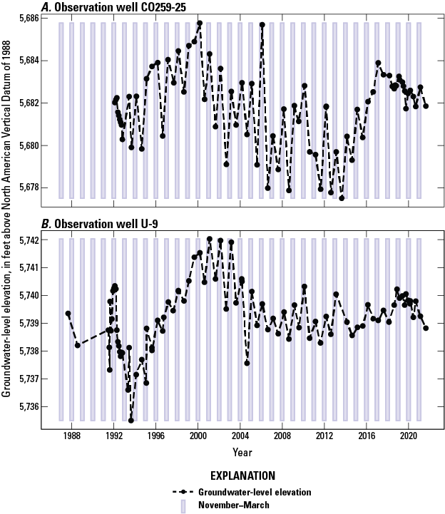
Groundwater-level elevations in the Fountain Creek alluvial aquifer near Colorado Springs from the National Water Information System database (U.S. Geological Survey, 2021), Colorado, 1988–2020, A, observation well CO259-25; and B, observation well U-9.
The elevation of the groundwater table throughout the Fountain Creek alluvial aquifer and groundwater-flow directions were estimated using the median groundwater-level elevation observations for 2018 to 2020. Median groundwater-level elevations in each observation well were calculated and then interpolated using a kriging approach to produce contours of equal groundwater-level elevation, illustrated in figure 8. Approximate groundwater-flow directions are shown in figure 8 and are oriented perpendicular to lines of equal groundwater-level elevation. The groundwater-table elevation contours distribution indicates groundwater generally flows from north to south within the alluvial aquifer main stem, consistent with the surface-water flow direction of Fountain Creek. Within the tributary alluvium, groundwater flow is generally to the southwest, toward the main stem of the alluvial aquifer. Groundwater-table elevation contours are limited to the groundwater-level elevation observation extent locations within the aquifer, which is why contours do not extend across the entire alluvial aquifer main stem.
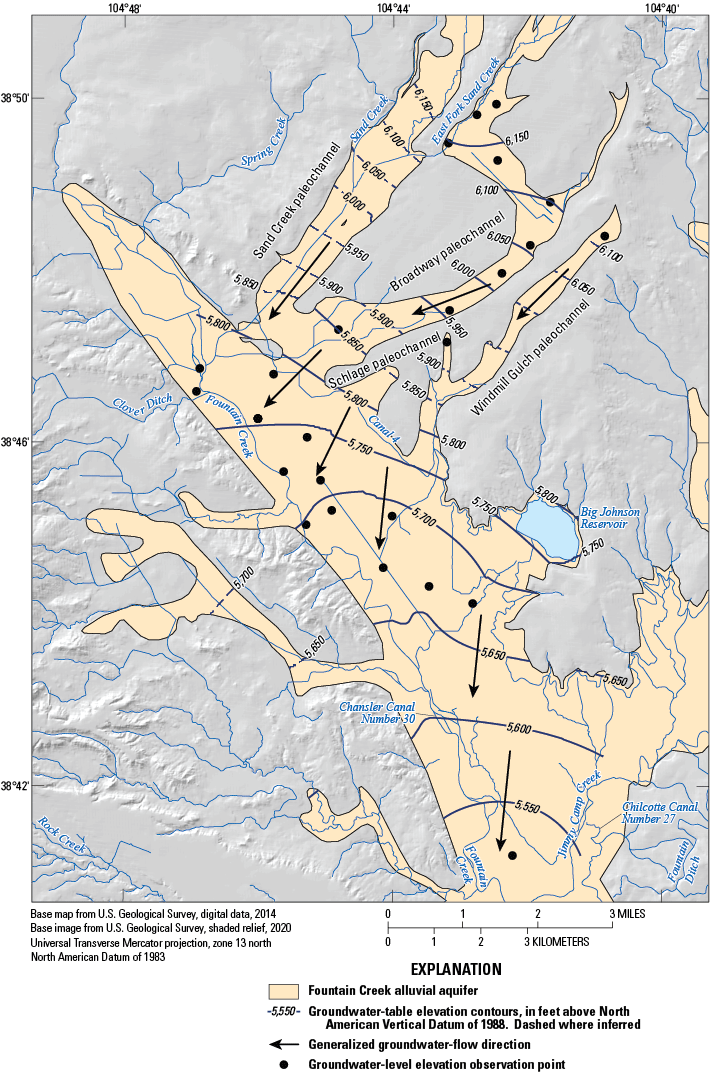
Estimated groundwater-table elevation contours and groundwater-flow directions in the Fountain Creek alluvial aquifer near Colorado Springs, Colorado, 2018–20 (U.S. Geological Survey, 2021).
Groundwater-level modeling results indicate the degree to which individual groundwater wells were affected by recharge and groundwater pumping and spatial associations between wells affected by similar processes. The spatial distribution of groundwater-level model results is displayed in figure 9. Not all the groundwater-level elevation observation wells included in this study (table 1) were included in the groundwater-level model results, because a minimum of five groundwater-level elevation observations through time were needed for the model to converge; thus, wells with less than five groundwater-level elevation observations were excluded from the model. Percentages of observed groundwater-level elevation fluctuations explained by recharge and pumping ranged from 0 to 55 percent, meaning a minimum of 45 percent of observed groundwater-level elevation fluctuations were unexplained by groundwater-level modeling. The unexplained observed groundwater-level elevation fluctuations could be attributed to streamflow, which may be implemented in groundwater-level models (Bakker and Schaars, 2019). Streamflow was not included in groundwater-level modeling for the Fountain Creek alluvial aquifer, however, because there was not an appropriate daily streamflow dataset for all wells.
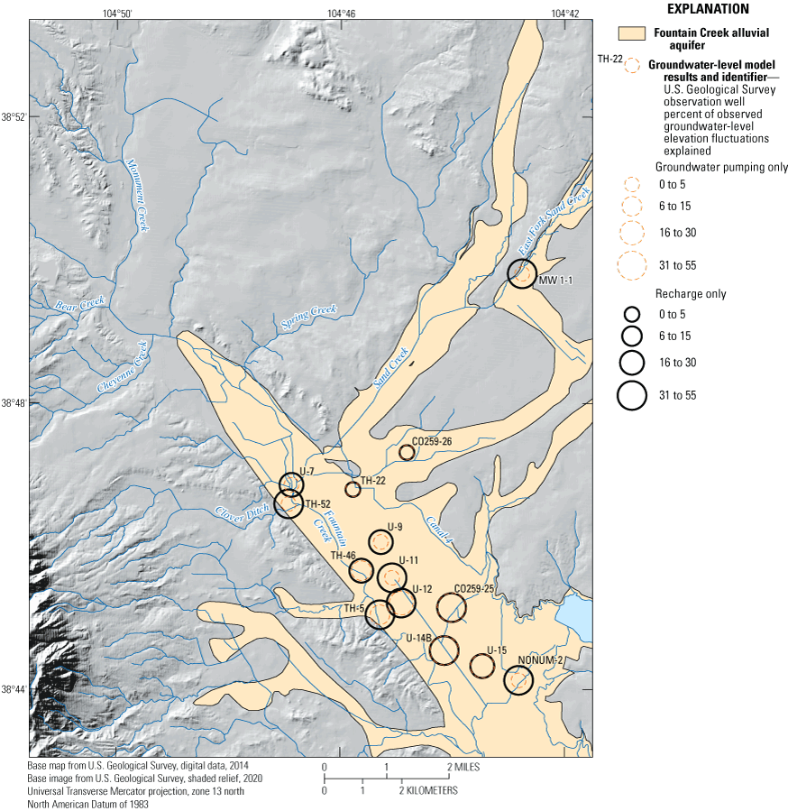
Groundwater-level model results indicating proportion of observed groundwater-level elevation fluctuations explainable by recharge and groundwater pumping for the Fountain Creek alluvial aquifer near Colorado Springs, Colorado. Model results are provided as a USGS data release associated with this report (Russell and Newman, 2024).
Figure 9 indicates observed groundwater-level elevation fluctuations in most observation wells were more explained by recharge than pumping. For example, the symbols are larger for recharge-only groundwater-level models than pumping-only groundwater-level models for sites MW 1-1, U-7, U-9, U-11, U-12, TH-5, TH-46, TH-52, and NONUM-2. However, recharge and pumping explain a nearly equal proportion of observed groundwater-level fluctuation in some wells (CO259-25, CO259-26, TH-22, U-14B, and U-15), and these wells were spatially associated with one another in the central part of the alluvial aquifer, with the exception of CO259-26 which is at the base of the Broadway paleochannel. The greater percentage of observed groundwater-level elevation fluctuations explained by pumping in these wells indicates this area of the aquifer may be more susceptible to pumping drawdowns, a key conceptual understanding, which aids in the numerical groundwater-flow model formulation. Increased susceptibility to pumping drawdowns in the main stem also may indicate the aquifer is thinner in that location, as aquifer thinning would result in less storage. Example transient groundwater-level modeling results and observations for groundwater well CO259-25 are illustrated in figure 10. All other groundwater-level model results are illustrated in Russell and Newman (2024). Transient results of the recharge-only groundwater-level model appear to accurately represent much of the seasonal observed groundwater-level fluctuations from 1997 to 2000. Between 1992 and 1996 and after 2000, the recharge-only groundwater-level model is unable to replicate the observed minimum groundwater-level elevations, whereas the pumping-only water-level model closely predicts several of the minimums, indicating the importance of groundwater pumping on this area of the alluvial aquifer. Future studies in the area could use the groundwater-level modeling approach to try to predict the effects of reinitiated groundwater pumping, as described by Bakker and Schaars (2019), which may offer computational and logistical benefits in contrast to numerical groundwater-flow modeling. Additionally, groundwater-level modeling results could guide future data collection efforts by indicating which wells were affected by different processes, which could help to define how and where data collection may need to be focused.
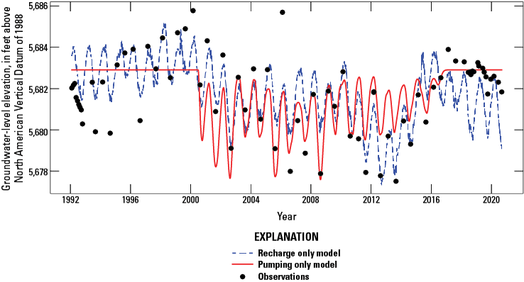
Transient groundwater-level modeling results and groundwater-level elevation observations for U.S. Geological Survey observation well CO259-25, in the Fountain Creek alluvial aquifer near Colorado Springs, Colorado, 1992–2020. Model results are provided as a USGS data release associated with this report (Russell and Newman, 2024). [NAVD 88, North American Vertical Datum of 1988]
Groundwater and Surface-Water Interactions
March 2019 synoptic streamflow measurements were combined with the Fountain Creek transit-loss model data (Kuhn and Arnold, 2006) and the NWIS database (USGS, 2021) to estimate streamflow gain or loss along Fountain Creek. The streamflow gain or loss calculation results and the estimated depth to bedrock along Fountain Creek are illustrated in figure 11. Estimated depth to bedrock was calculated using geographic information systems (GIS) in ArcMap version 10.7 (Esri, 2021) according to the following steps. First, the bedrock surface elevation was interpolated using data from Radell and others (1994) and AECOM (2017). Second, point objects were created at a 328 ft interval along Fountain Creek through the study area. Third, the interpolated bedrock surface elevation at each point along Fountain Creek was extracted. Fourth, the depth to bedrock was calculated by subtracting the elevation of the top of bedrock from the USGS 5-meter digital elevation model (USGS, 2020) of the land surface elevation. The GIS dataset created is included in the USGS data release associated with this investigation (Russell and Newman, 2024).

Streamflow gain or loss calculation results and estimated depth to bedrock in the Fountain Creek alluvial aquifer near Colorado Springs, Colorado, March 7, 2019, from the National Water Information System database (U.S. Geological Survey, 2021) and transit-loss model (Colarullo and Miller, 2019). Accumulated error in each streamflow gain or loss calculation is shown by the error bars on each point calculated according to equation 2.
Streamflow gain or loss calculations indicate Fountain Creek both gains and loses flow to the alluvial aquifer, and gaining or losing reaches of the stream may be partially controlled by the depth to bedrock near the stream (fig. 11). Specifically, streamflow gain or loss calculations indicate streamflow gains at approximately 2.5, 10.9, and 16.7 stream miles downstream from the northern study area extent. These locations tend to coincide with areas where the estimated depth to bedrock is decreasing. The alluvial aquifer is likely thinning in these areas, and groundwater-flow paths may be converging, potentially resulting in groundwater discharge to Fountain Creek. Streamflow gain or loss calculations also indicate losing conditions at approximately 1.0, 6.0, and 12.7 stream miles downstream from the northern study area extent. These locations tend to coincide with locally greater depths to bedrock where the alluvial aquifer is likely thicker and has greater storage potential for surface water lost from Fountain Creek. Accumulated errors in streamflow gain or loss calculations were generally not substantial enough to cause uncertainty in the direction of groundwater and surface-water interaction (fig. 11). Accumulated errors were only substantial enough to cause uncertainty as to gaining or losing conditions for the station at 17.5 stream miles downstream from the northern study area extent (fig. 11; node 22 of the transit loss model of Kuhn and Arnold, 2006).
Streamflow gain or loss calculation results made using synoptic streamflow data are consistent with water-quality results and analysis summarized in Newman and others (2021). Water-quality data indicate Fountain Creek and Canal 4 likely lose flow to groundwater, based on the occurrence of rare earth elements, pharmaceuticals, and wastewater indicator compounds in both surface waters and groundwater wells. The streamflow gain or loss spatial distribution also agrees between both analyses. The losing reach between 0 and 1.0 stream miles downstream from the northern study area extent corresponds to groundwater wells U-7 and TH-52 (fig. 2) near Fountain Creek that displayed water quality indicative of streamflow losses (Newman and others, 2021).
One consideration is streamflow gain or loss calculations were completed on a single day in March 2019, and thus may not represent long-term conditions in the study area. Because synoptic streamflow measurements were made during spring (March) and before snowmelt runoff or increased ET, it is likely that these measurements represent base flow conditions in Fountain Creek, which may be more representative of the groundwater and surface-water interactions in the absence of storm runoff. In other reaches in Fountain Creek, Arnold and others (2016) noted streamflow gain or loss varied temporally, and similar conditions may be expected in the Fountain Creek reach in this study. These results do provide independent evidence to assess the results of numerical groundwater-flow modeling of exchanges between groundwater and surface water, described in the “Groundwater-Flow Simulations” section of this report.
Aquifer Testing
Aquifer testing was completed in July 2019 and incorporated both slug tests and pumping tests. Data from aquifer testing were analyzed using the computer program AQTESOLV (Duffield, 2007). The raw testing data, drawdown and recovery hydrographs, pumping rates (between 2 and 5.5 gallons per minute for 7 to 20 minutes), and AQTESOLV results are included in a USGS data release (Kisfalusi and Newman, 2022). The near instantaneous recovery during testing across the aquifer led to using the Springer and Gelhar (1991) method as the analytical solution for the majority of the tests, but some wells were analyzed using the Bouwer and Rice (1976) method for comparison. The underdamped response from high K was visible in the oscillatory nature of the analysis in many of the wells (Springer and Gelhar, 1991). The Hyder and others (1994) analytical method was used to analyze the first slug test at T11-MW001 (table 3), because a well-skin effect was evident from pumping analysis. Aquifer testing results completed as part of this study were compared to previous aquifer testing compiled by Wilson (1965) and HAZWRAP (1989).
Table 3.
Summary of aquifer testing data and results from 11 observation wells in the Fountain Creek alluvial aquifer study area.[Aquifer testing results are provided in a USGS data release associated with this report (Kisfalusi and Newman, 2022). USGS, U.S. Geological Survey; K, hydraulic conductivity; ft/d, foot per day; falling head slug, falling-head slug test; rising head slug, rising-head slug test. —, no final solution calculated because of data limitations]
| USGS site identifier | Site common name | Test date | Test type | Analytical method | Solution result K (ft/d) | Analysis notes |
|---|---|---|---|---|---|---|
| 384408104424701 | NONUM-2 | 7/10/2019 | Falling head slug | Springer and Gelhar (1991) | 18.21 | |
| Rising head slug | Springer and Gelhar (1991) | 14.61 | ||||
| Falling head slug | Springer and Gelhar (1991) | 14.89 | ||||
| Rising head slug | Springer and Gelhar (1991) | 16.36 | ||||
| Falling head slug | Springer and Gelhar (1991) | 15.03 | ||||
| Rising head slug | Springer and Gelhar (1991) | 17.00 | ||||
| 384433104440701 | U-14B | 7/10/2019 | Recovery | Cooper and Jacob (1946) | 20.43 | |
| Falling head slug | Springer and Gelhar (1991) | 56.67 | ||||
| Rising head slug | Springer and Gelhar (1991) | 38.54 | ||||
| Falling head slug | Springer and Gelhar (1991) | 31.71 | ||||
| Rising head slug | Springer and Gelhar (1991) | 32.63 | ||||
| Falling head slug | Springer and Gelhar (1991) | 27.72 | ||||
| Rising head slug | Springer and Gelhar (1991) | 30.43 | ||||
| 384509104435901 | CO259-25 | 7/10/2019 | Falling head slug | Springer and Gelhar (1991) | 385.00 | |
| Rising head slug | Springer and Gelhar (1991) | 269.20 | ||||
| Falling head slug | Springer and Gelhar (1991) | 215.40 | ||||
| Rising head slug | Springer and Gelhar (1991) | 205.30 | ||||
| Falling head slug | Springer and Gelhar (1991) | 79.30 | ||||
| Rising head slug | Springer and Gelhar (1991) | 222.40 | ||||
| Falling head slug | Springer and Gelhar (1991) | 119.20 | ||||
| Rising head slug | Springer and Gelhar (1991) | 154.40 | ||||
| 384513104445302 | U-12 | 7/10/2019 | Recovery | Cooper and Jacob (1946) | 144.78 | |
| Falling head slug | Springer and Gelhar (1991) | 245.80 | ||||
| Rising head slug | Springer and Gelhar (1991) | 329.30 | ||||
| Falling head slug | Springer and Gelhar (1991) | 289.20 | ||||
| Rising head slug | Springer and Gelhar (1991) | 325.40 | ||||
| Falling head slug | Springer and Gelhar (1991) | 394.20 | ||||
| Rising head slug | Springer and Gelhar (1991) | 379.10 | ||||
| 384636104465401 | TH-52 | 7/10/2019 | Recovery | Cooper and Jacob (1946) | 664.95 | |
| Falling head slug | Springer and Gelhar (1991) | 91.57 | ||||
| Rising head slug | Springer and Gelhar (1991) | 90.38 | ||||
| Falling head slug | Springer and Gelhar (1991) | 226.40 | ||||
| Rising head slug | Springer and Gelhar (1991) | 106.40 | ||||
| 384648104454501 | TH-22 | 7/8/2019 | Falling head slug | Springer and Gelhar (1991) | 111.50 | |
| Rising head slug | Springer and Gelhar (1991) | 65.57 | ||||
| Falling head slug | Springer and Gelhar (1991) | 313.60 | Noisy data | |||
| Rising head slug | Springer and Gelhar (1991) | 1,408.10 | Noisy data | |||
| 384707104421901 | T11-MW001 | 7/9/2019 | Falling head slug | Springer and Gelhar (1991) | 118.90 | Skin effects evident |
| Falling head slug | Hyder and others (1994) | 65.58 | Skin effects evident | |||
| Falling head slug | Bouwer and Rice (1976) | 47.65 | ||||
| Rising head slug | Bouwer and Rice (1976) | 6.03 | ||||
| Falling head slug | — | — | Skin effects evident | |||
| Rising head slug | Bouwer and Rice (1976) | 5.79 | ||||
| 384719104444701 | CO259-26 | 7/8/2019 | Falling head slug | — | — | Slug broke, noisy data |
| Rising head slug | — | — | Slug broke, noisy data | |||
| Falling head slug | Springer and Gelhar (1991) | 125.60 | ||||
| Rising head slug | Springer and Gelhar (1991) | 35.83 | ||||
| 384824104405101 | 03-002 | 7/9/2019 | Recovery | Cooper and Jacob (1946) | 10.80 | Pumped dry |
| Recovery | Cooper and Jacob (1946) | 4.13 | Pumped dry | |||
| Falling head slug | Springer and Gelhar (1991) | 2.75 | ||||
| Falling head slug | Bouwer and Rice (1976) | 0.39 | ||||
| Falling head slug | Bouwer and Rice (1976) | 6.43 | Early data only | |||
| Rising head slug | Springer and Gelhar (1991) | 0.64 | ||||
| Rising head slug | Bouwer and Rice (1976) | 0.32 | ||||
| Rising head slug | Bouwer and Rice (1976) | 3.90 | Early data only | |||
| 384917104422701 | T04-MW004 | 7/9/2019 | Falling head slug | Springer and Gelhar (1991) | 1.05 | |
| Falling head slug | Bouwer and Rice (1976) | 0.82 | ||||
| Rising head slug | Springer and Gelhar (1991) | 0.89 | ||||
| Rising head slug | Bouwer and Rice (1976) | 0.78 | ||||
| Falling head slug | Springer and Gelhar (1991) | 1.00 | ||||
| Rising head slug | Springer and Gelhar (1991) | 0.92 | ||||
| Falling head slug | Bouwer and Rice (1976) | 0.38 | Manual test | |||
| Rising head slug | Springer and Gelhar (1991) | 0.91 | Manual test | |||
| Rising head slug | Bouwer and Rice (1976) | 0.79 | Manual test | |||
| 384949104424501 | MW 1-1 | 7/9/2019 | Recovery | Cooper and Jacob (1946) | 122.90 | |
| Falling head slug | Springer and Gelhar (1991) | 350.10 | ||||
| Rising head slug | Springer and Gelhar (1991) | 338.40 | ||||
| Falling head slug | Springer and Gelhar (1991) | 157.20 | ||||
| Rising head slug | — | — | No appreciable water level displacement |
Calculated K values are summarized for each well in table 3, and a summary of K values calculated in this study and compared to values from previous studies is illustrated in figure 12. Calculated K values derived from slug tests and pumping tests in this study generally cover the same range, though slug tests have slightly lesser minimum and slightly greater maximum calculated K values. Calculated K values from slug and pumping tests conducted as part of this study ranged from 0.32 to 1,410 ft/d and 4.13 to 664 ft/d, respectively. Previous slug tests summarized by HAZWRAP (1989) have substantially lower K values, ranging from 0.07 to 140 ft/d (fig. 12). Slug testing completed by HAZWRAP (1989) was spatially limited to the area at the northeastern extent of the Broadway paleochannel (fig. 4). When compared to aquifer testing results from the current study in the same Broadway paleochannel area (MW 1-1 and T04-MW004), the ranges are similar to the range observed in the HAZWRAP (1989) tests (minimum and maximum K values from MW 1-1 and T04-MW004 are 122 to 350 ft/d and 0.38 to 1.05 ft/d, respectively; table 3). Previous pumping tests summarized by Wilson (1965) span a wider range than any other calculated K values, ranging from 32.3 to 1,650 ft/d (fig. 12).
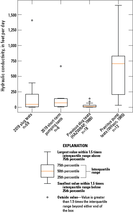
Calculated hydraulic conductivity values from slug tests and pumping tests completed in 2019 and in previous investigations of the Fountain Creek alluvial aquifer near Colorado Springs, Colorado. Aquifer testing results are provided in a USGS data release associated with this report (Kisfalusi and Newman, 2022).
Ranges in the calculated K values from this study and previous studies (Wilson, 1965; HAZWRAP, 1989) may be attributed to both testing method design and spatial location within the Fountain Creek alluvial aquifer. Aquifer testing completed in 2019 included both slug tests and pumping tests. Slug tests were designed to be rapidly conducted and generally do not stress a substantial volume of the aquifer material (Butler, 1997), thus producing localized K estimates. Pumping tests need more infrastructure and longer timeframes but may produce K estimates more representative of the bulk aquifer (Kruseman and de Ridder, 1990), as opposed to local conditions. Given these test-design considerations, slug-testing results from this study and from HAZWRAP (1989) likely represent localized K values in the tested wells immediate vicinity. These localized results were useful for evaluating spatial variability that could lead to local variations in groundwater recharge or discharge. Results of pumping tests from this study and Wilson (1965) likely represent the bulk behavior of the aquifer, because these tests were more spatially distributed throughout the aquifer instead of focused in paleochannels. These aquifer testing results were useful for guiding numerical groundwater-flow model development.
Mean aquifer testing results spatial evaluation from each observation well provided in figure 13 indicates K values tend to be greater in the main stem of the alluvial aquifer and are lower in paleochannels. The spatial variation in K values may be attributed to the geomorphologic processes that formed the alluvial aquifer. Compacted sediment in the paleochannels likely has not been transported sufficient distance to result in grain-size sorting, and the alluvium in these areas is likely poorly sorted, leading to lower K values because of smaller particles filling in pore spaces between large grains. In the main stem of the alluvial aquifer, near Fountain Creek, the sediments have been transported farther from their source areas and are consequently better sorted. More uniform grain-size distributions likely result in greater K values.
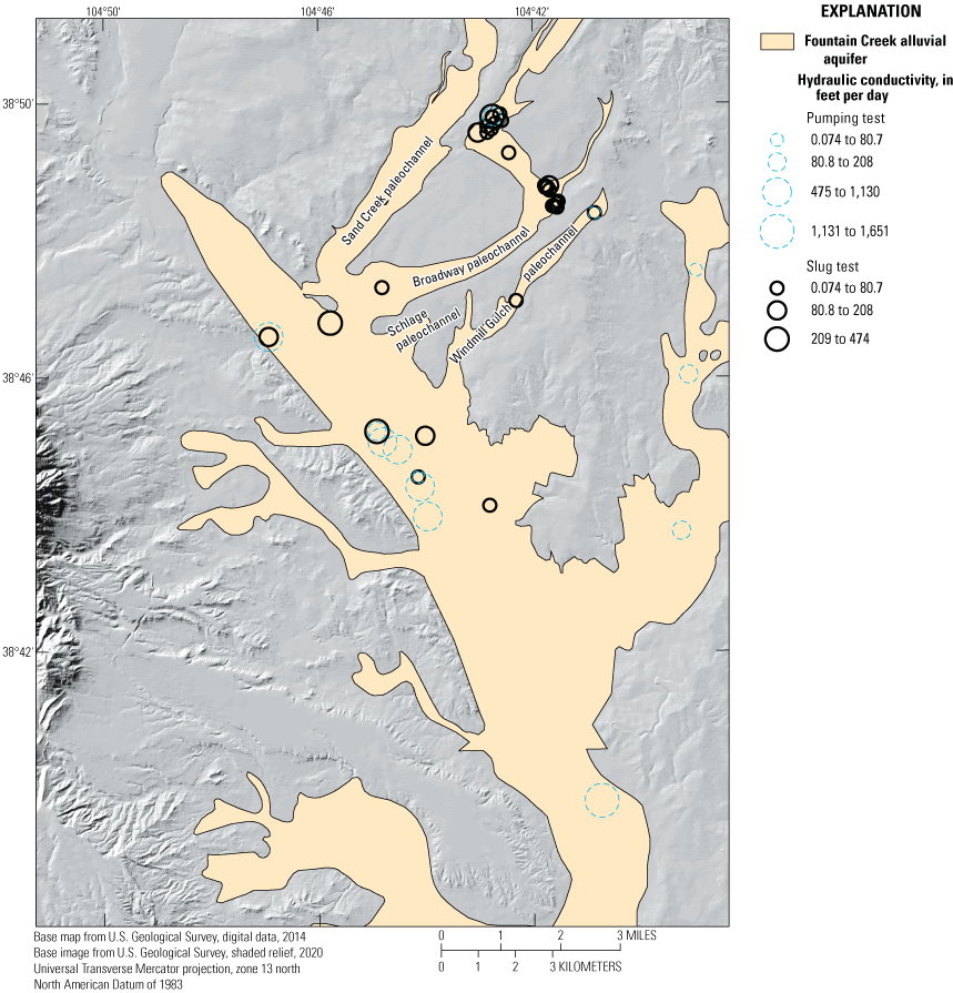
Calculated hydraulic conductivity values from aquifer testing completed in 2019 in observation wells in the Fountain Creek alluvial aquifer, Colorado Springs, Colorado, and from Wilson (1965) and HAZWRAP (1989). Aquifer testing results are provided in a USGS data release associated with this report (Kisfalusi and Newman, 2022).
Estimated K values were incorporated into the numerical groundwater-flow model. Specifically, the statistical K variability (fig. 12) and the spatial K distribution (fig. 13) each help to constrain the range of K included in the model. Aquifer testing results were incorporated into a pilot points analysis (Doherty, 2003), as described in the next section, “Groundwater-Flow Simulations.”
Groundwater-Flow Simulations
The numerical groundwater-flow model for the Fountain Creek alluvial aquifer was constructed using the finite-difference groundwater modeling code MODFLOW-NWT (Niswonger and others, 2011). The model was both manually and automatically calibrated, the latter using PEST++IES (White and others, 2020). The calibration processes goal was to maximize the fit between observed and simulated streamflow and groundwater-level elevations. The calibrated model was used to quantify components of the alluvial aquifer groundwater budget, including groundwater and surface-water interactions, groundwater withdrawal by wells, and groundwater recharge. The calibrated model was also used to simulate advective transport of nonreactive particles within the aquifer using the particle tracking software MODPATH (Pollock, 2016). Following manual and automated calibration, the mean difference between the observed and simulated groundwater-level elevation observations was −0.60 ft, indicating on average the model-simulated groundwater-level elevations were within one foot of observed values. A plot of simulated compared to observed groundwater-level elevations (fig. 14) indicates the model was able to simulate the full observed range of groundwater-level elevations with reasonable accuracy. Spatial evaluation of calibration residuals indicates larger residuals were mostly distributed within the main stem of the active model area and were typically located near lower residuals (fig. 15), indicating the model did not have any areas of substantial bias. Most of the main stem of the active model area is developed and urbanized and has a complex network of surface-water features. Each of these factors can introduce complexity to the numerical model and may explain why the simulated groundwater-level elevations show variable agreement in the main stem of the model domain.
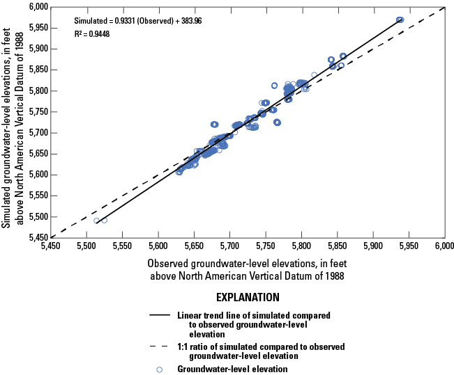
Simulated compared to observed groundwater-level elevations for the Fountain Creek alluvial aquifer near Colorado Springs, Colorado, 2000–19. Model results are provided as a USGS data release associated with this report (Russell and Newman, 2024). [NAVD 88, North American Vertical Datum of 1988]
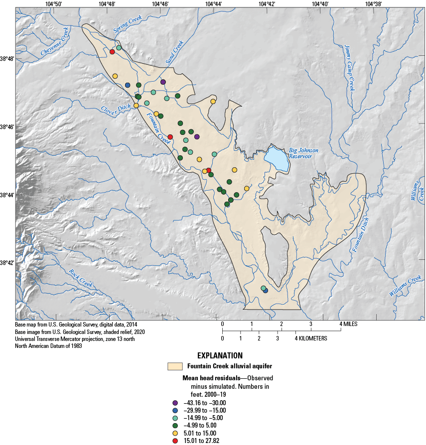
Mean head residuals between simulated and observed groundwater-level elevations for the Fountain Creek alluvial aquifer near Colorado Springs, Colorado, 2000–19. Model results are provided as a USGS data release associated with this report (Russell and Newman, 2024).
The residuals RMSE from the numerical model was found to be 14.28 ft, and 75 percent of the residuals were within 6.44 ft of the observed groundwater levels. The calibrated model nRMSE was 2.12 percent (using the RMSE of 14.28 ft and the range of observed groundwater-level elevations of 673 ft). Anderson and others (2015) suggest a maximum nRMSE of 10 percent. The nRMSE of 2.12 percent of the calibrated Fountain Creek alluvial aquifer model indicates the model is expected to reasonably reproduce the behavior of the system.
The simulated base flow at the four USGS streamgage locations used for calibration (Fountain Creek below Janitell Road below Colorado Springs, CO, 07105530; Sand Creek above Mouth at Colorado Springs, CO, 07105600; Fountain Creek at Security, CO, 07105800; and Clover Ditch Drain near Widefield, CO, 07105820) was similar to the observed base-flow values and trends recorded by the streamgages. The mean simulated base flow for streamgages along Fountain Creek was lower than the mean observed base flow by 17.39 ft3/s (07105530; fig. 16A) and 11.02 ft3/s (07105800; fig. 16B). The mean simulated base flow for 07105600 was 0.66 ft3/s higher than the mean observed base flow (fig. 16C), and the mean simulated base flow for 07105820 were 0.04 ft3/s lower than the mean observed base flow (fig. 16D). The RMSE was 11.52 ft3/s for 07105530, or within 14 percent of the range of observed base flows; the RMSE was 0.30 ft3/s for 07105600, or within 20 percent of the range of observed base flows; the RMSE was 10.42 ft3/s for 0715800, or within 10 percent of observed base flows; and the RMSE was 0.02 ft3/s for 07105820, or within 1 percent of observed base flows. Although the simulated base-flow values for the Fountain Creek streamgages were close to the observed values, some of the discrepancy may be because of additions and withdrawals along Fountain Creek (Kuhn and Arnold, 2006), which were not all directly simulated in the groundwater-flow model. The discrepancy between simulated and observed base flow for Sand Creek (07105600) could be attributed to most of the streamflow measurements made during the transient stress period being rated poor, meaning 95 percent of the streamflow measurements made were outside of 8 percent of the true streamflow value (Turnipseed and Sauer, 2010). Overall, the results of the calibration to base flow at streamgages indicate the model is reasonably reproducing exchanges between groundwater and surface water within the study area.
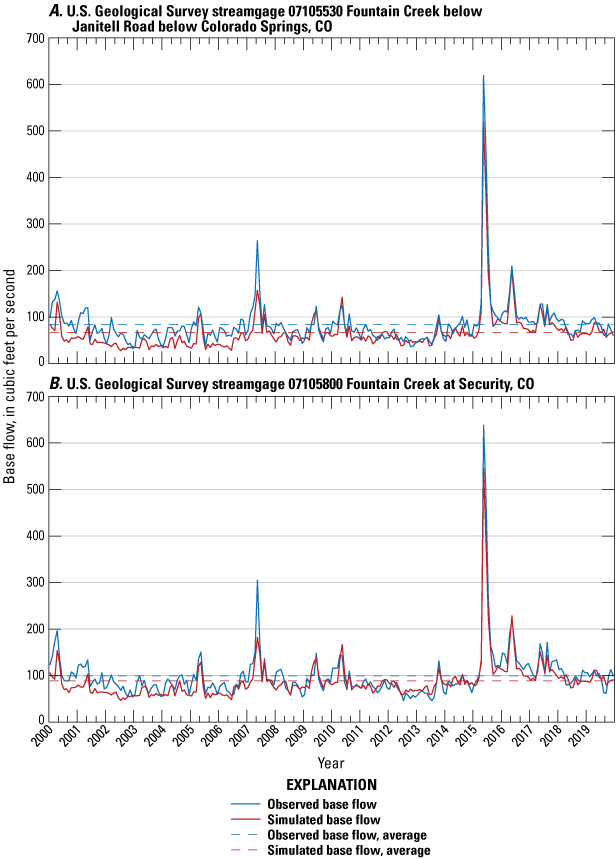
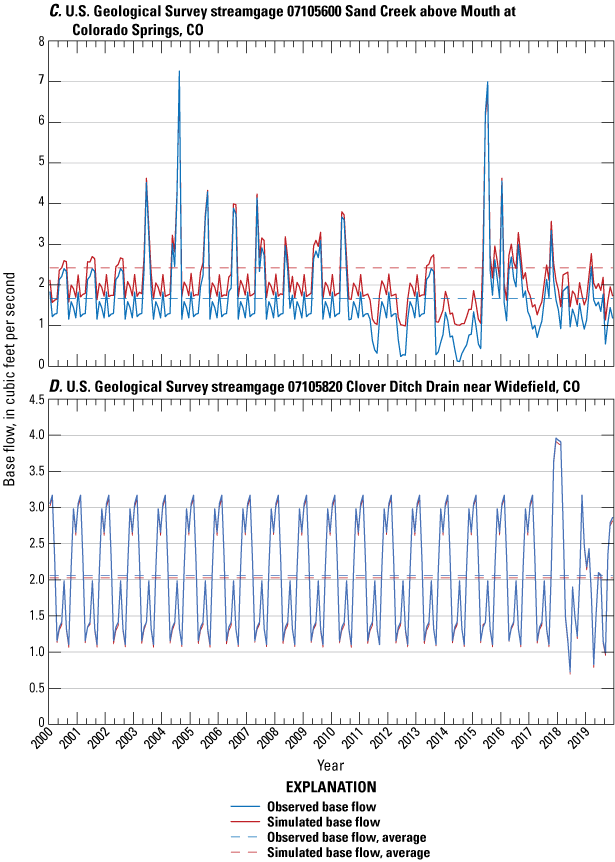
Simulated and observed base flow at USGS streamgages, 2000–19 from the National Water Information System database (U.S. Geological Survey, 2021), A, Fountain Creek below Janitell Road below Colorado Springs, CO, 07105530; B, Fountain Creek at Security, CO, 07105800; C, Sand Creek above Mouth at Colorado Springs, CO, 07105600; and D, Clover Ditch Drain near Widefield, CO, 07105820. Model results are provided as a USGS data release associated with this report (Russell and Newman, 2024).
An analysis using PEST++IES (White and others, 2020) was completed to determine how sensitive the observation groups were to the automated calibration parameters. The more sensitive the observation groups were to a parameter, the more likely changes in the parameter will affect model behavior. The sensitivity analysis was completed on the combined base flows and the groundwater-level elevation observations. The sensitivity analysis showed simulated base flow was more sensitive to the automated calibration parameters than the groundwater-level elevations, and base flow and groundwater-level elevations were most sensitive to horizontal K and GHB conductance values (fig. 17). The areas where the numerical model is most sensitive to changes in horizontal hydraulic conductivity are toward the northwestern portion of the active model area near Sand Creek.
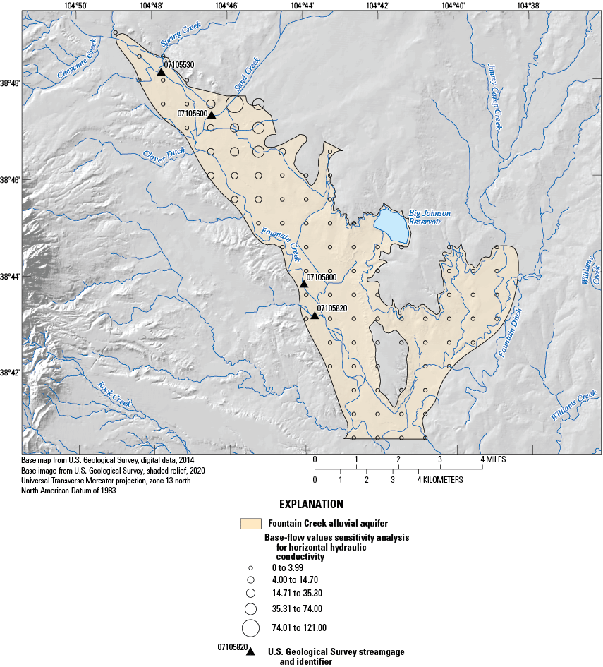
Results of base flow sensitivity analysis for horizontal hydraulic conductivity in the Fountain Creek alluvial aquifer groundwater-flow model, 2000–19. Model results are provided as a USGS data release associated with this report (Russell and Newman, 2024).
The calibrated water budget for the Fountain Creek alluvial aquifer during the transient stress period, 2000–19, shows the simulated inflows and outflows for the aquifer (table 4). There were instances of a single water budget category being composed of multiple MODFLOW packages, such as the net streambed seepage portion being made up of the SFR, RIV, and DRN packages. The largest inflow into the aquifer came from seepage from all streams in the active model area (about 85 percent of the mean annual inflow) and accounted for a mean annual inflow of 64,079 acre-feet per year (acre-ft/yr). Lateral inflow and seepage from Big Johnson Reservoir accounted for a mean annual inflow of 7,645 acre-ft/yr, or 10.15 percent of the mean annual inflows, and distributed recharge accounted for a mean annual inflow of 3,619 acre-ft/yr, or 4.81 percent of the mean annual inflows. Seepage from the aquifer to the streams was also the largest outflow from the aquifer and accounted for a mean annual outflow of 72,811 acre-ft/yr, or 96.68 percent of the mean annual outflows from the aquifer. Well withdrawals made up the second largest outflow from the aquifer and accounted for 2,237 acre-ft/yr, or 2.97 percent of the mean annual outflows from the aquifer, and lateral outflow, seepage to Big Johnson Reservoir, and ET accounted for 267 acre-ft/yr of outflow, or less than 1 percent of the mean annual outflow from the aquifer.
Table 4.
Water budget for the Fountain Creek alluvial aquifer from the transient numerical groundwater-flow model, 2000–19. Model results are provided as a USGS data release associated with this report (Russell and Newman, 2024).[All units in acre-feet per year. Net water-budget totals calculated as the difference of outflow and inflow. NA, not applicable]
The yearly net flows from each model package (fig. 18A) provide a detailed summary of water-budget components. The RIV package (primarily representing Canal 4) is the largest inflow and is followed by the GHB and RCH packages; the SFR package (primarily representing Fountain Creek) is the largest outflow and is followed by the DRN and WEL packages. The yearly inflow and outflow simulated by each package in the numerical model does not change substantially through time, but the most noticeable change in trends is the lack of well pumping in 2019 following the discovery of PFAS compounds in drinking water between 2013 and 2015 (Hu and others, 2016). The mean monthly net flows from each model package show the seasonal trends within each package (fig. 18B). On average, August had the most inflow into the aquifer, with the inflow split evenly between the RCH, GHB, and RIV packages. A seasonal trend is evident where mean monthly inflows from the GHB package (representing Big Johnson Reservoir and the Broadway and Windmill Gulch paleochannels) compensate for lower RCH inflow rates during the winter months from November through March. The monthly net flows also illustrate most of the well pumping occurs during the summer months from April through October.
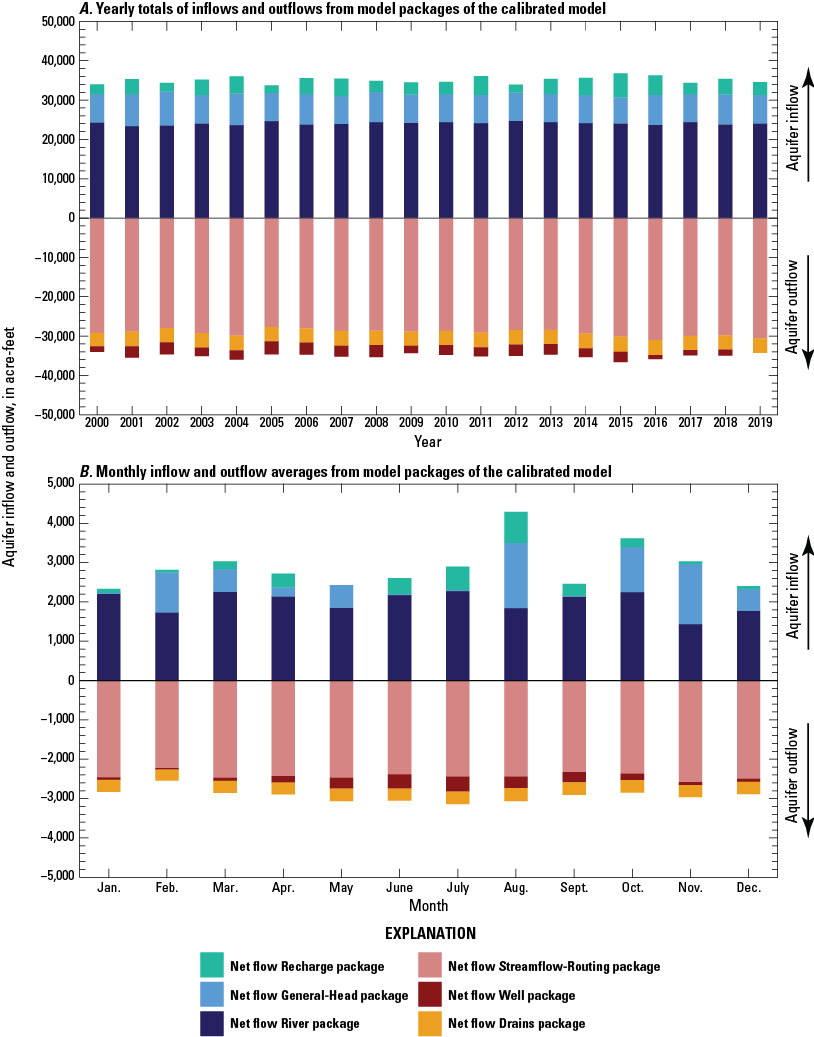
Water-budget components of the Fountain Creek alluvial aquifer groundwater-flow model, 2000–19, including A, yearly net water-budget components and B, mean monthly net water-budget components. Model results are provided as a USGS data release associated with this report (Russell and Newman, 2024).
The simulated groundwater-level elevations from the final model period (December 2019) ranged from about 5,496 to 5,938 ft, with highest groundwater-table elevations along the north to northeastern edge of the active model area and decreasing in the southern direction (fig. 19). Simulated groundwater-table contours did not change substantially through time, thus the final model period illustrated in figure 19 is representative of other time periods in the model. The simulated groundwater table is similar to the observed groundwater table illustrated in figure 8. The simulated flow direction was typically toward Fountain Creek or its accompanying tributaries. The simulated saturated thickness of the Fountain Creek alluvial aquifer for the last simulated transient stress period ranged from 0 to about 79 ft (fig. 20), with a mean saturated thickness of 19.44 ft. The areas with the highest saturated thickness were along the base of the Sand Creek and Broadway paleochannels and the eastern and southern edges of the active model area. These saturated areas were also areas with high numerical model thickness, which includes the unsaturated zone. Mean saturated thickness was approximately 49.55 ft.
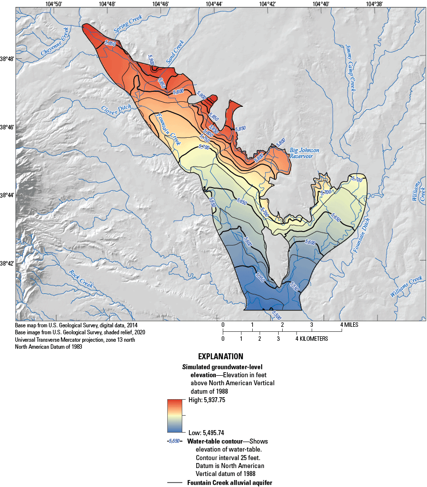
Simulated groundwater-level elevations in the Fountain Creek alluvial aquifer near Colorado Springs, Colorado, 2000–19. Model results are provided as a USGS data release associated with this report (Russell and Newman, 2024).
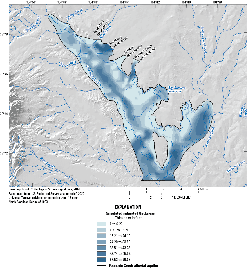
Saturated thickness of the simulated Fountain Creek alluvial aquifer near Colorado Springs, Colorado, 2000–19. Model results are provided as a USGS data release associated with this report (Russell and Newman, 2024).
Advective particle tracking simulations for groundwater-flow paths captured by wells indicate flow paths generally originate in the northeast portion of the aquifer, along the boundary of the aquifer with Canal 4 and within the tributary alluvium paleochannels (fig. 21). Numerous groundwater-flow paths originate in the Windmill Gulch paleochannel, both from the GHB simulated at the northern extent of the paleochannel in the numerical groundwater-flow model and in the SFR reach that originates from the paleochannel. Several groundwater-flow paths also originate in other locations, listed from north to south: from the intersection of Canal 4 with Sand Creek; within the Schlage paleochannel; near Big Johnson Reservoir; and near the edge of the active model domain near Jimmy Camp Creek. Notably, no groundwater-flow paths terminating in pumping wells originate from the GHB at the head of the Sand Creek paleochannel. Groundwater-flow paths were distorted in several areas of the aquifer, both in the main stem where flow paths appear to bend to the south (consistent with the general groundwater-flow direction; fig. 8) and in the area immediately downgradient from the Big Johnson Reservoir, where flow paths originating from Canal 4 appear to bend to the southwest. Flow paths distortions were likely because of recharge from surface-water features in these model areas, or may be because of spatially variable aquifer thickness or K.
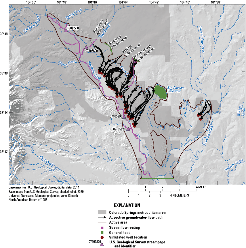
Advective groundwater-flow paths contributing to simulated well locations near Colorado Springs, Colorado, 2000–19, using the calibrated steady-state groundwater-flow model and MODPATH software (Pollock, 2016). Model results are provided as a USGS data release associated with this report (Russell and Newman, 2024).
Particle tracking results provide information related to the potential for solute transport within the alluvial aquifer, such as the transport of PFAS. Groundwater-flow paths originating from Canal 4 indicate surface water recharges groundwater from Canal 4 losses, based on water-quality data (Newman and others, 2021), and may be captured by pumping wells. Water-quality data indicated solutes derived from Canal 4, such as pharmaceuticals and wastewater-indicator compounds, were present in groundwater downgradient from the canal (Newman and others, 2021). These compounds possibly can be captured by pumping wells and be present in the produced water. These results indicate leakage from Canal 4 could be a direct source of solutes to pumping wells. Because several wells also capture groundwater-flow paths that originate at the GHB in the Windmill Gulch paleochannel, these wells possibly also capture groundwater from the upper area of the paleochannel not directly simulated in the model because of the thin saturated thickness. If solutes were transported conservatively, without degradation or retardation, then possibly this subset of pumping wells could also capture solutes from upgradient within the Windmill Gulch paleochannel. An additional consideration is the advective groundwater-flow path simulations completed by MODPATH do not incorporate many complex processes that control the transport of PFAS compounds in groundwater such as sorption and degradation (Weber and others, 2017). The advective particle tracking results should be interpreted as first estimates of the potential source areas of solutes (including PFAS) to pumping wells.
Model Limitations
Limitations to the numerical groundwater-flow model for the Fountain Creek alluvial aquifer include the nature of the spatial and temporal variability of the model discretization, the necessary simplifications used in representing hydrologic boundaries, and the necessary simplifications of the approach used to evaluate groundwater capture by pumping wells. Each of these limitations is discussed in detail in the following paragraphs.
The process of numerical groundwater-flow model creation results in the discretization both spatially and temporally of the physical system into a framework that allows for model calculations to converge. This means hydraulic parameters of the aquifer must be smoothed in a manner fitting the spatial discretization of the system; the result is generally a simplified distribution of K with respect to reality. Temporally variable input parameters, such as precipitation recharge and groundwater pumping, were also smoothed and averaged in a manner allowing these parameters to be used by the model, but this is a simplification of real-world behavior. Spatial and temporal discretization of the model was done to minimize these effects on the ultimate model outputs, but these simplifications mean the model is not a perfect analog for the hydrologic system.
Hydrologic boundaries, such as surface water boundaries, may be implemented in the model in different ways, and the way they were incorporated controls the ability of boundaries to interact with the remainder of the model domain. Several different MODFLOW packages were used to represent surface water: GHB, SFR, RIV, and DRN. The GHB boundary represented the Big Johnson Reservoir, which is reasonable for representation of lakes and reservoirs that were sources of groundwater recharge (Anderson and others, 2015). The SFR package was used for streams expected to have the most direct connection to groundwater, such as along the main stem of Fountain Creek, because this package allows for two-directional flow between groundwater and surface water. The SFR package, however, can create convergence issues in some portions of the model. The RIV and DRN packages were used to represent areas where groundwater and surface-water interactions were hypothesized to compose a smaller water-budget component of the model when compared to areas simulated with the SFR package, which can represent bidirectional flow into and out of the aquifer. This is a necessary simplification to achieve model convergence, and means groundwater and surface-water exchange was unidirectional in areas of the model simulated with the DRN package. This simplification is not expected to cause inaccurate representations of boundaries in the model, based on spatial analysis of water-quality data presented in Newman and others (2021).
The way advective groundwater-flow paths were simulated also included necessary simplifications. One simplification was the steady-state simulation was used to simulate flow paths, which is a common approach in evaluating sources of water to pumping wells (Moeck and others, 2020). Using transient models in particle tracking may result in complications because of starting time and location of particles, the rate of change of heads in the transient model, and the complexity of the model framework (Rayne and others, 2014). For the Fountain Creek alluvial aquifer, results of the steady-state simulated groundwater-level elevations closely resemble the long-term median groundwater-level elevations (fig. 8), indicating the steady-state model is a reasonable representation of the long-term groundwater system and groundwater-flow paths from the steady-state model were likely reasonable representations of actual flow paths under most conditions. Some seasonal variations in flow paths are likely because of seasonal changes in groundwater-level elevations, but these are expected to cause only minor variation in the groundwater-flow paths as illustrated in figure 21. Another simplification of the advective particle tracking model is only the calibrated model was used in simulating flow paths, as opposed to integrating a full uncertainty analysis of flow path density from multiple uncalibrated models (for example, Moeck and others, 2020). In their analysis of particle tracking, Moeck and others (2020) illustrated uncertainty in hydraulic properties of the aquifer results in uncertainty as to flow paths and the delineation of groundwater source areas to wells. The Fountain Creek alluvial aquifer model incorporated an inverse model analysis using PEST++IES to understand uncertainty in the K of the aquifer, but not every uncalibrated model realization from the uncertainty analysis was carried forward for particle tracking. Qualitatively, sensitivity analysis (fig. 17) indicates base flows and groundwater-level elevation simulations were most sensitive near the Sand Creek paleochannel, but sensitivity is low elsewhere in the model domain. Groundwater-flow paths were therefore unlikely to change substantially in the majority of the model domain as a result of uncertainty in the hydraulic property values.
Because the MODPATH simulations use the steady-state model, they cannot be used to estimate time of travel within the transient groundwater system. Use of the steady-state model was needed because of numerical constraints and issues arising from transient simulations, as described in the previous paragraph. Although time of travel between recharge sources and wells cannot be computed with the current model, these results can be used in conjunction with groundwater age dating described in Newman and others (2021). The combination of these methods generally indicates solutes occurring in wells have likely been recharged within the last 10 years, and these solutes could be derived from the locations of the particle sources on figure 21.
Summary
From 2018 through 2020, the U.S. Geological Survey, in cooperation with the Air Force Civil Engineering Center, conducted an integrated study of the Fountain Creek alluvial aquifer located near Colorado Springs, Colorado. The study objective was to characterize hydrologic conditions for the alluvial aquifer pertinent to the determination of potential for transport of solutes. Specific goals of the report were to characterize the groundwater hydrology of the area, to quantify groundwater and surface-water interactions, to estimate hydraulic properties of the aquifer using aquifer testing, and to complete numerical simulations of groundwater flow. The results presented in this report build on a water-quality dataset collected as part of this study.
Synoptic groundwater-level elevation measurements, completed throughout this study and as part of other U.S. Geological Survey programs beginning in 1994, indicate groundwater-level elevations fluctuate on annual and interannual timeframes. Groundwater-level fluctuations likely were caused by the effect of precipitation, groundwater pumping, and interaction with surface water in the area, with many wells showing maximum groundwater-level elevations during the winter months (November through March). From an interannual perspective, groundwater-level fluctuations appear to have reached maximum values from 2000 to 2003, decreased from 2003 to 2006, and remained relatively constant since 2006 with some exceptions where groundwater-level elevations have slightly increased since 2018. Spatial evaluation of groundwater-level elevations indicates groundwater flow is generally from northeast to southwest within the vicinity of the paleochannels occurring along the northeastern margin of the aquifer. Within the main stem of the aquifer, along Fountain Creek, groundwater flow is generally from north to south, approximately paralleling surface-water flow. To quantitatively understand the potential effect of groundwater recharge and groundwater pumping on groundwater-level elevation fluctuations, a statistical transfer-function-noise model was applied. Results of the statistical transfer-function-noise model indicated throughout most of the aquifer, fluctuations were primarily the result of recharge seasonality. In the central portion of the aquifer, where groundwater pumping wells were more concentrated, however, groundwater-level elevation fluctuations were more attributable to groundwater pumping through time.
Three-dimensional evaluation of the aquifer geometry near Fountain Creek, as represented by the estimated depth to bedrock within the alluvial aquifer, was combined with synoptic streamflow measurement and accounting of stream gains and losses to evaluate groundwater and surface-water interactions in the study area. Streamflow gain or loss calculations indicate Fountain Creek both gains flow from and loses flow to the alluvial aquifer, and gaining or losing reaches of the stream may be partially controlled by the depth to bedrock near the stream. Reaches with streamflow gain tend to coincide with areas where the estimated depth to bedrock is decreasing, meaning the alluvial aquifer is likely thinning in these areas, and groundwater-flow paths may be converging and discharging groundwater to the streambed. Losing reaches tended to coincide with locally greater depth to bedrock where the alluvial aquifer is likely thicker and has greater storage potential for surface water lost from Fountain Creek.
Results of aquifer testing indicate hydraulic conductivity estimated from slug tests and single-well pumping tests ranged from 0.32 to 1,410 feet per day and 4.13 to 664 feet per day, respectively. These results correspond well to previous aquifer tests including slug tests and pumping tests. Hydraulic conductivities from aquifer testing in this study were generally greater than the estimates of previous slug tests and had a mean value less than the estimates of previous pumping tests, but all results cover a similar range in hydraulic conductivity values. Spatial evaluation of aquifer testing results indicates hydraulic conductivity tends to be greater in the main stem of the alluvial aquifer and is lower in paleochannels. The spatial variation in hydraulic conductivity values may be attributed to the geomorphologic processes that formed the alluvial aquifer. Compacted sediment in the paleochannels likely was not transported a sufficient distance to cause grain-size sorting, which led to lower hydraulic conductivity values. In the central portion of the alluvial aquifer near Fountain Creek, the sediments were transported farther from their source areas and consequently better sorted.
A numerical groundwater-flow model was calibrated for the Fountain Creek alluvial aquifer for 2000–19 to simulate water-budget components, groundwater-flow directions, and groundwater-flow paths. The model simulated precipitation recharge, groundwater and surface-water interactions, evapotranspiration, groundwater pumping by pumping wells, and external inflows and outflows occurring along the alluvial aquifer boundaries. Manual and automated model calibration was completed. Automated model calibration assisted in quantifying sensitivity results to input parameters. The calibrated model corresponded well with groundwater-level elevation observations, with a mean residual equal to −0.60 feet (observed minus simulated groundwater-level elevation). Simulated groundwater base flow to streams was typically within 10 percent of estimated base flow. Groundwater and surface-water interactions represented the largest aquifer water-budget components, with the second-largest groundwater discharge component coming from pumping wells. Groundwater and surface-water interactions can represent both the largest gain and loss terms in the budget, because these interactions differ spatially, meaning in some areas of the model domain groundwater is recharged by streams, whereas in other areas groundwater is discharged to streams. Estimates of advective groundwater-flow paths indicate pumping wells may capture groundwater recharged from losing streams, including Canal 4, Sand Creek, and others, and groundwater flows into the main stem of the alluvial aquifer from paleochannels.
Acknowledgments
This study was aided by U.S. Geological Survey colleagues who assisted with water-quality data collection, aquifer testing, streamflow measurement, and groundwater-flow model construction, including Nancy Bauch, Evan Gohring, Michael Holmberg, Colin Penn, and Emily Baker.
References Cited
Arnold, L.R., Ortiz, R.F., Brown, C.R., and Watts, K.R., 2016, Groundwater and surface-water interaction, water quality, and processes affecting loads of dissolved solids, selenium, and uranium in Fountain Creek, near, Colorado, 2012–2014: U.S. Geological Survey Scientific Investigations Report 2016–5134, 78 p., accessed January 21, 2020, at https://doi.org/10.3133/sir20165134.
Bakker, M., and Schaars, F., 2019, Solving groundwater flow problems with time series analysis—You may not even need another model: Groundwater, v. 57, no. 6, p. 826–833, accessed February 19, 2020, at https://doi.org/10.1111/gwat.12927.
Barlow, P.M., Cunningham, W.L., Zhai, T., and Gray, M., 2017, U.S. Geological Survey Groundwater toolbox version 1.3.1, a graphical and mapping interface for analysis of hydrologic data: U.S. Geological Survey software release, accessed April 21, 2019, at https://doi.org/10.5066/F7R78C9G.
Bauch, N.J., Musgrove, ML., Mahler, B.J., and Paschke, S.S., 2014, The quality of our Nation’s waters—Water quality in the Denver Basin aquifer system, Colorado, 2003–05: U.S. Geological Survey Circular 1357, 100 p., accessed September 12, 2019, at https://doi.org/10.3133/cir1357.
Bouwer, H., and Rice, R.C., 1976, A slug test for determining hydraulic conductivity of unconfined aquifers with completely or partially penetrating wells: Water Resources Research, v. 12, no. 3, p. 423–428, accessed March 28, 2020, https://doi.org/10.1029/WR012i003p00423.
Butler, J.J., 1997, The design, performance, and analysis of slug tests: Boca Raton, Fla., Lewis Publishers, 262 p. [Also available at https://doi.org/10.1201/9781482229370.]
Cain, D., and Edelmann, P., 1986, A reconnaissance water-quality appraisal of the Fountain Creek alluvial aquifer between Colorado Springs and Pueblo, Colorado, including trace elements and organic constituents: U.S. Geological Survey Water-Resources Investigations Report 86–4085, 45 p, accessed January 12, 2020, at https://doi.org/10.3133/wri864085.
Cohn, T.A., Kiang, J.E., and Mason, R.R., Jr., 2013, Estimating discharge measurement uncertainty using the interpolated variance estimator: Journal of Hydraulic Engineering (New York, N.Y), v. 139, no. 5, p. 502–510, accessed June 12, 2019, at https://doi.org/10.1061/(ASCE)HY.1943-7900.0000695.
Colarullo, S.J., and Miller, L.D., 2019, Upgrades to a Fortran program for estimating stream transit losses of reusable water, El Paso and Pueblo Counties, Colorado: U.S. Geological Survey Scientific Investigations Report 2018–5163, 21 p., accessed April 1, 2020, at https://doi.org/10.3133/sir20185163.
Collenteur, R.A., Bakker, M., Caljé, R., Klop, S.A., and Schaars, F., 2019, Pastas—Open source software for the analysis of groundwater time series: Groundwater, v. 57, no. 6, p. 877–885, accessed June 1, 2020, at https://doi.org/10.1111/gwat.12925.
Colorado State Demography Office, 2017, A closer look at the economics & demographics of Colorado—Colorado’s 2016 population & economic overview: Colorado Department of Local Affairs State Demography Office website, accessed December 1, 2021, at https://coloradodemography.github.io/crosstabs/2016-overview/.
Cooper, H.H., and Jacob, C.E., 1946, A generalized graphical method for evaluating formation constants and summarizing well-field history: Transactions, American Geophysical Union, v. 27, no. 4, p. 526–534. [Also available at https://doi.org/10.1029/TR027i004p00526.]
Cunningham, W.L., and Schalk, C.W., comps., 2011, Groundwater technical procedures of the U.S. Geological Survey: U.S. Geological Survey Techniques and Methods, book 1, chap. A1, 151 p., accessed September 4, 2019, at https://pubs.usgs.gov/tm/1a1/.
Doherty, J., 2003, Ground water model calibration using pilot points and regularization: Groundwater, v. 41, no. 2, p. 170–177, accessed January 4, 2019, at https://doi.org/10.1111/j.1745-6584.2003.tb02580.x.
Edelmann, P., and Cain, D., 1985, Sources of water and nitrogen to the Widefield aquifer, southwestern El Paso County, Colorado: U.S. Geological Survey Water-Resources Investigations Report 85–4162, 81 p., accessed February 4, 2019, at https://doi.org/10.3133/wri854162.
Esri, 2021, ArcGIS Desktop—Release 10.8: Redlands, Calif., Esri, accessed March 21, 2021, at https://www.esri.com/en-us/arcgis/about-arcgis/overview.
Halford, K.J., Weight, W.D., and Schreiber, R.P., 2006, Interpretation of transmissivity estimates from single-well pumping aquifer tests: Groundwater, v. 44, no. 3, p. 467–471, accessed May 8, 2020, at https://doi.org/10.1111/j.1745-6584.2005.00151.x.
Harbaugh, A.W., Banta, E.R., Hill, M.C., and McDonald, M.G., 2000, MODFLOW-2000, the U.S. Geological Survey modular ground-water model—User guide to modularization concepts and the ground-water flow process: U.S. Geological Survey Open-File Report 00–92, 121 p. [Also available at https://doi.org/10.3133/ofr200092.]
Harmel, R.D., Cooper, R.J., Slade, R.M., Haney, R.L., and Arnold, J.G., 2006, Cumulative uncertainty in measured streamflow and water quality data for small watersheds: Transactions of the ASABE, v. 49, no. 3, p. 689–701. [Also available at https://doi.org/10.13031/2013.20488.]
Hu, X.C., Andrews, D.Q., Lindstrom, A.B., Bruton, T.A., Schaider, L.A., Grandjean, P., Lohmann, R., Carignan, C.C., Blum, A., Balan, S.A., Higgins, C.P., and Sunderland, E.M., 2016, Detection of poly- and perfluoroalkyl substances (PFASs) in U.S. drinking water linked to industrial sites, military fire training areas, and wastewater treatment plants: Environmental Science & Technology Letters, v. 3, no. 10, p. 344–350, accessed August 21, 2019, at https://doi.org/10.1021/acs.estlett.6b00260.
Huntington, J.L., Hegewisch, K.C., Daudert, B., Morton, C.G., Abatzoglou, J.T., McEvoy, D.J., and Erickson, T., 2017, Climate engine—Cloud computing and visualization of climate and remote sensing data for advanced natural resource monitoring and process understanding: Bulletin of the American Meteorological Society, v. 98, no. 11, p. 2397–2410, accessed June 20, 2019, at https://doi.org/10.1175/BAMS-D-15-00324.1.
Hyder, Z., Butler, J.J., Jr., McElwee, C.D., and Liu, W., 1994, Slug tests in partially penetrating wells: Water Resources Research, v. 30, no. 11, p. 2945–2957, accessed May 5, 2020, at https://doi.org/10.1029/94WR01670.
Jetton, A.J., 2008, Estimation of evapotranspiration of cottonwood trees in the Cibola National Wildlife Refuge, Cibola, Arizona: Fairborn, Ohio, Wright State University, M.S. thesis, 164 p., accessed August 5, 2020, at https://corescholar.libraries.wright.edu/etd_all/825/.
Kisfalusi, Z.D., and Newman, C.P., 2022, Water-level and well-discharge data related to aquifer testing in Fountain Creek alluvial aquifer, El Paso County, Colorado, 2019: U.S. Geological Survey data release, https://doi.org/10.5066/P9GHPDS1.
Kuhn, G., 1988, Methods to determine transit losses for return flows of transmountain water in Fountain Creek between Colorado Springs and the Arkansas River, Colorado: U.S. Geological Survey Water-Resources Investigations Report 87–4119, 183 p. [Also available at https://doi.org/10.3133/wri874119.]
Kuhn, G., 1991, Calibration, verification, and use of a steady-state stream water-quality model for Monument and Fountain Creeks, east-central Colorado: U.S. Geological Survey Water-Resources Investigations Report 91–4055, 149 p. [Also available at https://doi.org/10.3133/wri914055.]
Kuhn, G., and Arnold, L.R., 2006, Application of a stream-aquifer model to Monument Creek for development of a method to estimate transit losses for reusable water, El Paso County, Colorado: U.S. Geological Survey Scientific Investigations Report 2006–5184, 111 p. [Also available at https://doi.org/10.3133/sir20065184.]
Kuhn, G., Krammes, G.S., and Beal, V.J., 2007, Description and user manual for a web-based interface to a transit-loss accounting program for Monument and Fountain Creeks, El Paso and Pueblo Counties, Colorado: U.S. Geological Survey Scientific Investigations Report 2007–5028, 36 p, accessed June 7, 2019, at https://doi.org/10.3133/sir20075028.
Kuhn, G., Samuels, E.L., Bemis, W.D., and Steger, R.D., 1998, Descriptions of the program changes (1989–97) and a user manual for a transit-loss accounting program applied to Fountain Creek between Colorado Springs and the Arkansas River, Colorado: U.S. Geological Survey Open-File Report 97–637, 39 p. [Also available at https://doi.org/10.3133/ofr97637.]
Lewis, M.E., 1995, Quality of water in the alluvial aquifer and tributary alluvium of the Fountain Creek valley, southwestern El Paso County, Colorado, 1991–92: U.S. Geological Survey Water-Resources Investigations Report 94–4118, 39 p. [Also available at https://doi.org/10.3133/wri944118.]
Mau, D.P., Stogner, R.W., Sr., and Edelmann, P., 2007, Characterization of stormflows and wastewater treatment-plant effluent discharges on water quality, suspended sediment, and stream morphology for Fountain and Monument Creek watersheds, Colorado, 1981–2006: U.S. Geological Survey Scientific Investigations Report 2007–5104, 76 p., accessed July 7, 2020, at https://doi.org/10.3133/sir20075104.
McDonough, C.A., Choyke, S., Barton, K.E., Mass, S., Starling, A.P., Adgate, J.L., and Higgins, C.P., 2021, Unsaturated PFOS and other PFASs in human serum and drinking water from an AFFF-impacted community: Environmental Science & Technology, v. 55, no. 12, p. 8139–8148, accessed January 4, 2022, at https://doi.org/10.1021/acs.est.1c00522.
Moeck, C., Molson, J., and Schirmer, M., 2020, Pathline density distributions in a null‐space Monte Carlo approach to assess groundwater pathways: Groundwater, v. 58, no. 2, p. 189–207, accessed December 5, 2020, at https://doi.org/10.1111/gwat.12900.
Newman, C.P., Paschke, S.S., and Keith, G., 2021, Natural and anthropogenic geochemical tracers to investigate residence times and groundwater–surface-water interactions in an urban alluvial aquifer: Water, v. 13, no. 6, article 871, 30 p., accessed March 2, 2021, at https://doi.org/10.3390/w13060871.
Niswonger, R.G., Panday, S., and Ibaraki, M., 2011, MODFLOW-NWT, A Newton formulation for MODFLOW-2005: U.S. Geological Survey Techniques and Methods, book 6, chap. A37, 44 p, accessed April 9, 2019, at https://pubs.usgs.gov/tm/tm6a37/.
Niswonger, R.G., and Prudic, D.E., 2005, Documentation of the Streamflow-Routing (SFR2) Package to include unsaturated flow beneath streams—A modification to SFR1: U.S. Geological Survey Techniques and Methods, book 6, chap. A13, 50 p., accessed April 9, 2019, at https://doi.org/10.3133/tm6A13.
Paschke, S.S., ed., 2011, Groundwater availability of the Denver Basin aquifer system, Colorado: U.S. Geological Survey Professional Paper 1770, 274 p., accessed January 5, 2019, at https://doi.org/10.3133/pp1770.
Pollock, D.W., 2016, User guide for MODPATH Version 7—A particle-tracking model for MODFLOW: U.S. Geological Survey Open-File Report 2016–1086, 35 p., accessed April 9, 2019, at https://doi.org/10.3133/ofr20161086.
PRISM Climate Group, 2020, PRISM climate data: Oregon State University, PRISM Climate Group website, accessed September 9, 2020, at https://prism.oregonstate.edu.
Radell, M.J., Lewis, M.E., and Watts, K.R., 1994, Hydrogeologic characteristics of the alluvial aquifer and adjacent deposits of the Fountain Creek valley, El Paso County, Colorado: U.S. Geological Survey Water-Resources Investigations Report 94–4129, 4 map sheets. [Also available at https://doi.org/10.3133/wri944129.]
Rayne, T.W., Bradbury, K.R., and Zheng, C., 2014, Correct delineation of capture zones using particle tracking under transient conditions: Groundwater, v. 52, no. 3, p. 332–334, accessed March 5, 2019, at https://doi.org/10.1111/gwat.12141.
Rehmel, M., 2007, Application of acoustic Doppler velocimeters for streamflow measurements: Journal of Hydraulic Engineering, v. 133, no. 12, p. 1433–1438, accessed June 2, 2020, at https://doi.org/10.1061/(ASCE)0733-9429(2007)133:12(1433).
Rosenberry, D.O., and LaBaugh, J.W., eds., 2008, Field techniques for estimating water fluxes between surface water and ground water: U.S. Geological Survey Techniques and Methods, book 4, chap. D2, 128 p., accessed August 9, 2019, at https://doi.org/10.3133/tm4D2.
Russell, C.A., and Newman, C.P., 2024, Statistical and groundwater-flow models of the Fountain Creek alluvial aquifer near Colorado Springs, Colorado: U.S. Geological Survey data release, https://doi.org/10.5066/P9L6TRZW.
Rutledge, A.T., 2000, Considerations for use of the RORA program to estimate ground-water recharge from streamflow records: U.S. Geological Survey Open-File Report 00–156, 44 p., accessed September 3, 2019, at https://doi.org/10.3133/ofr00156.
Shapoori, V., Peterson, T.J., Western, A.W., and Costelloe, J.F., 2015, Estimating aquifer properties using groundwater hydrograph modelling: Hydrological Processes, v. 29, no. 26, p. 5424–5437, accessed June 8, 2020, at https://doi.org/10.1002/hyp.10583.
Simonds, F.W., and Sinclair, K.A., 2002, Surface water-ground water interactions along the lower Dungeness River and vertical hydraulic conductivity of streambed sediments, Clallam County, Washington, September 1999–July 2001: U.S. Geological Survey Water-Resources Investigations Report 02–4161, 69 p., accessed May 20, 2019, at https://doi.org/10.3133/wri024161.
Steiner, M., 2017, Big Johnson Reservoir drained for repairs: The Gazette, February 21, 2017 [updated March 17, 2019], accessed June 28, 2019, at https://gazette.com/news/big-johnson-reservoir-drained-for-repairs/article_90365e7f-51bb-5546-b721-4728f0fcd60b.html.
Trautmann, A.M., Schell, H., Schmidt, K.R., Mangold, K.M., and Tiehm, A., 2015, Electrochemical degradation of perfluoroalkyl and polyfluoroalkyl substances (PFASs) in groundwater: Water Science and Technology, v. 71, no. 10, p. 1569–1575, accessed February 9, 2019, at https://doi.org/10.2166/wst.2015.143.
Turnipseed, D.P., and Sauer, V.B., 2010, Discharge measurements at gaging stations: U.S. Geological Survey Techniques and Methods, book 3, chap. A8, 87 p., accessed June 2, 2019, at https://doi.org/10.3133/tm3A8.
U.S. Geological Survey [USGS], 2020, National elevation dataset: U.S. Geological Survey database, accessed February 2021 at https://apps.nationalmap.gov/downloader/.
U.S. Geological Survey [USGS], 2021, USGS water data for the Nation: U.S. Geological Survey National Water Information System database, accessed April 6, 2021, at https://doi.org/10.5066/F7P55KJN.
Weber, A.K., Barber, L.B., LeBlanc, D.R., Sunderland, E.M., and Vecitis, C.D., 2017, Geochemical and hydrologic factors controlling subsurface transport of poly- and perfluoroalkyl substances, Cape Cod, Massachusetts: Environmental Science & Technology, v. 51, p. 4269–4279, accessed September 21, 2020, at https://doi.org/10.1021/acs.est.6b05573.
Wellman, T.P., and Rupert, M.G., 2016, Groundwater quality, age, and susceptibility and vulnerability to nitrate contamination with linkages to land use and groundwater flow, Upper Black Squirrel Creek Basin, Colorado, 2013: U.S. Geological Survey Scientific Investigations Report 2016–5020, 77 p., accessed June 12, 2019, at https://doi.org/10.3133/sir20165020.
White, J.T., Hunt, R.J., Fienen, M.N., and Doherty, J.E., 2020, Approaches to highly parameterized inversion—PEST++ Version 5, a software suite for parameter estimation, uncertainty analysis, management optimization and sensitivity analysis: U.S. Geological Survey Techniques and Methods, book 7, chap. C26, 52 p., accessed on May 19, 2021, at https://doi.org/10.3133/tm7C26.
Winter, T.C., Harvey, J.W., Franke, O.L., and Alley, W.M., 1998, Ground water and surface water—A single resource: U.S. Geological Survey Circular 1139, 79 p., accessed May 20, 2019, at https://pubs.usgs.gov/circ/circ1139/#pdf.
Conversion Factors
U.S. customary units to International System of Units
Datum
Vertical coordinate information is referenced to the North American Vertical Datum of 1988 (NAVD 88).
Horizontal coordinate information is referenced to the Colorado State Plane coordinate system (North American Datum of 1983 [NAD 83], units: feet, zone: Colorado Central Zone).
Elevation, as used in this report, refers to distance above the vertical datum.
Abbreviations
bls
below land surface
EPA
U.S. Environmental Protection Agency
ET
evapotranspiration
GIS
geographic information systems
K
hydraulic conductivity
Kh
horizontal hydraulic conductivity
Kv/h
vertical to horizontal hydraulic conductivity ratio
NWIS
National Water Information System
PFAS
per- and polyfluoroalkyl substances
PRISM
Parameter-elevation Regressions on Independent Slopes Model
RMSE
root-mean-squared-error
Ss
specific storage
Sy
specific yield
TFN
transfer-function-noise
USGS
U.S. Geological Survey
WWTP
wastewater treatment plant
Publishing support provided by the Science Publishing Network,
Denver Publishing Service Center
For more information concerning the research in this report, contact the
Director, USGS Colorado Water Science Center
Box 25046, Mail Stop 415
Denver, CO 80225
(303) 236-4882
Or visit the Colorado Water Science Center website at
Disclaimers
Any use of trade, firm, or product names is for descriptive purposes only and does not imply endorsement by the U.S. Government.
Although this information product, for the most part, is in the public domain, it also may contain copyrighted materials as noted in the text. Permission to reproduce copyrighted items must be secured from the copyright owner.
Suggested Citation
Newman, C.P., Russell, C.A., Kisfalusi, Z.D., and Paschke, S.S., 2024, Groundwater hydrology, groundwater and surface-water interactions, aquifer testing, and groundwater-flow simulations for the Fountain Creek alluvial aquifer, near Colorado Springs, Colorado, 2018–20: U.S. Geological Survey Scientific Investigations Report 2023–5119, 45 p., https://doi.org/10.3133/sir20235119.
ISSN: 2328-0328 (online)
Study Area
| Publication type | Report |
|---|---|
| Publication Subtype | USGS Numbered Series |
| Title | Groundwater hydrology, groundwater and surface-water interactions, aquifer testing, and groundwater-flow simulations for the Fountain Creek alluvial aquifer, near Colorado Springs, Colorado, 2018–20 |
| Series title | Scientific Investigations Report |
| Series number | 2023-5119 |
| DOI | 10.3133/sir20235119 |
| Publication Date | April 03, 2024 |
| Year Published | 2024 |
| Language | English |
| Publisher | U.S. Geological Survey |
| Publisher location | Reston VA |
| Contributing office(s) | Colorado Water Science Center |
| Description | Report: vi, 45 p.; 2 Data Releases; Database |
| Country | United States |
| State | Colorado |
| City | Colorado Springs |
| Other Geospatial | Fountain Creek alluvial aquifer |
| Online Only (Y/N) | Y |