

Hydrogeology, Karst, and Groundwater Availability of Monroe County, West Virginia
Links
- Document: Report (36.5 MB pdf) , HTML , XML
- Appendixes:
- Appendix 1 (15.6 KB csv) - Well Depth, Casing, Yield, Water Level, and Specific Capacity Data From County Health Department Well Completion Reports
- Appendix 2 (17.3 KB csv) - Base-flow Data for 83 Sites Measured in September 2019 in Monroe County, West Virginia
- Appendix 3 (111 KB zip) - Results of Monthly Hydrograph Analyses for Four Major Watersheds in Monroe County and for the Greenbrier River at Alderson, West Virginia
- Appendix 4 (14.9 KB zip) - Results of Annual Hydrograph Analyses for Four Major Watersheds in Monroe County and for the Greenbrier River at Alderson, West Virginia
- Companion Files:
- Plate of Figure 4 (19.7 MB) - Hydrogeologic Map of Monroe County, West Virginia
- Plate of Figure 5 (10.7 MB) - Geologic Map of Monroe County, West Virginia
- Plate of Figure 25 (1.98 MB) - Potentiometric-Surface Map of Monroe County, West Virginia
- Data Releases:
- USGS data release - Density raster of caves in Monroe County, West Virginia
- USGS data release - Lidar-derived closed depression vector data and density raster in karst areas of Monroe County, West Virginia
- USGS data release - Lidar-derived imagery and digital elevation model of Monroe County, West Virginia at 3-meter resolution
- USGS data release - Fluorescein and Rhodamine WT concentration and recovery data for select samples collected in Monroe County, West Virginia, in August and September 2019
- USGS data release - Interpolated groundwater levels and altitudes for Monroe County, West Virginia, 2017–2019
- NGMDB Index Page: National Geologic Map Database Index Page (html)
- Download citation as: RIS | Dublin Core
Acknowledgments
The U.S. Geological Survey (USGS) would like to acknowledge Brian A. Carr, of the West Virginia Department of Health & Human Resources, Patrick V. Campbell (retired), of the West Virginia Department of Environmental Protection, and past and present members of the Monroe County Commission—especially Donald J. Evans the Monroe County Clerk and Clyde Gum, County Commissioner of Monroe County—for their assistance in providing support to bring this study to fruition. Harold “Rocky” Parsons and Howard “Howdy” Henritz are also acknowledged for assisting with field reconnaissance of study sites and sampling of the sites for the dye-tracer tests discussed in this report, while providing communication with local landowners to access property for data collection activities for this investigation. Rocky and Howdy devoted countless hours of their time voluntarily supporting the USGS in this study, and the USGS thanks them for their assistance. Finally, the USGS would like to acknowledge the residents of Monroe County who allowed access to their wells, for water-level measurements, and land, for dye-tracer tests, geological mapping, and base-flow stream surveys. This study would not have been possible without the assistance of the aforementioned individuals. This study was executed by the U.S. Geological Survey in cooperation with the West Virginia Department of Environmental Protection and with the Monroe County Commission with grant support from the West Virginia Department of Health & Human Resources.
Abstract
Monroe County is in southeastern West Virginia, encompassing an area of 474 square miles. The area consists of karst and siliciclastic aquifers of Ordovician, Silurian, Devonian, and Mississippian age and is in parts of two physiographic provinces: the Valley and Ridge Province to the east of Peters Mountain, and the Appalachian Plateau Province to the west of Peters Mountain. This study was developed in response to inquiries from the Monroe County Commission requesting assessment of the water resources of the county to better understand the quantity of the county’s groundwater resources, for both current [2023] and future demand, and to provide information to support protection and management of the county’s valuable groundwater resources.
Various products were developed for this study that provide knowledge with respect to water availability and contamination susceptibility of the karst aquifers within the county. U.S. Geological Survey (USGS) geologists conducted extensive geologic mapping in support of the project, producing (1) a countywide bedrock geologic map, (2) a countywide hydrogeologic map, and (3) a light detection and ranging (lidar)-derived countywide digital elevation model and associated sinkhole map. A significant part of this work was to map in detail the Greenbrier Group at the formation level, which prior to this study had only partially been completed. The report also includes (4) a description of the lithologic units identified as part of the geologic mapping process.
U.S. Geological Survey hydrologists completed several additional products for the hydrology part of the effort, including development of (1) a countywide potentiometric surface (water-table) map, (2) a countywide base-flow stream assessment, (3) countywide water-budget estimates, (4) well log surveys for 15 wells to better understand subsurface controls on groundwater flow within the study area, (5) two groundwater tracer tests to better refine the groundwater divide from the northern and southern parts of the karst aquifer in Monroe County; and finally, based on all available data collected for the study including the potentiometric surface map, geologic map, current [2023] and legacy fluorometric groundwater tracer tests, and base-flow stream assessments, (6) groundwater-basin delineations were reassessed for principal groundwater basins within the Greenbrier aquifer.
In Monroe County, four principal hydrogeologic settings produce large yields of water for residential, agricultural, and other uses. The most relied upon water-bearing zone with respect to current [2023] public water supply is from springs along Peters Mountain. These springs are derived from intervals of fractured sandstone and resultant alluvial deposits. Groundwater flows downslope through these permeable alluvial deposits and discharges at the contact with less permeable strata, such as the Reedsville Shale. The second most relied upon water-bearing zone in Monroe County is within the karstic Greenbrier Group aquifer, in which the basal Hillsdale Limestone overlies the less permeable Maccrady Shale. This geologic contact between the Hillsdale Limestone and Maccrady Shale is not only targeted as a source of water for agricultural supply but also is targeted as a source of water for residential supply. The third most relied upon water-bearing zone is composed of shallow perched aquifers within the Greenbrier Group. The discontinuous nature of these perched aquifers makes mapping their extent impossible, but they are related to permeable geologic strata, such as karstified limestones with solutionally enhanced permeability that overlies less permeable shale or chert bedrock. During geologic mapping of the county, several of these perched aquifers were documented in the Pickaway, Union, and Alderson Limestones. A fourth zone consists of springs from Ordovician carbonates at the base of Peters Mountain, which are influenced by sinking streams as well as upwelling along faults. In terms of water quantity, the most sustainable springs are those having deeper-sourced flows.
Public supplies are a principal source of water used for residential and commercial supply in the region, accounting for 0.49 million gallons per day (Mgal/d) of fresh-water withdrawals (0.14 Mgal/d of groundwater and 0.35 Mgal/d of surface water) for residential and commercial use and serving 6,645 individuals (49.2 percent of the population). An estimated 6,861 people, (50.8 percent of the population) primarily rely on private wells or other unregulated sources, such as springs, and withdraw 0.55 Mgal/d of groundwater for their residential use. Public water supply in the region is primarily (71.4 percent) derived from springs and augmented by stream withdrawals (backup sources mainly during low-flow periods), with the remaining portion (28.6 percent) derived from groundwater withdrawals from wells. For rural residents, however, 100 percent of their withdrawals are derived from groundwater (wells or springs).
Introduction
Monroe County, in southeastern West Virginia, is predominantly dependent on groundwater resources as a source of water for public and residential supply. The groundwater resources of the county are comprised of karstic carbonate, fractured sandstone, and shale bedrock aquifers, with lesser aquifers within surficial sediments on hillslopes and in floodplains. Water availability from the two principal bedrock aquifer types varies dramatically, as the karst aquifers may produce prolific quantities of water, whereas water from the fractured siliciclastic bedrock aquifers is not as abundant. Responsible management of available groundwater resources is dependent on a thorough understanding of the structural and lithologic controls on groundwater flow and groundwater recharge. Future economic development—commercial, industrial, agricultural, suburban, and rural residential—is dependent on quantification of available groundwater resources. Enhanced understanding of groundwater flow processes, rates, and direction will aid local water managers to better utilize and protect available groundwater resources. This information can also be used to assess potential effects of unintentional contaminant releases to the karstic aquifers of Monroe County, which are especially susceptible to contamination (Bishop, 2010).
Purpose and Scope
This study was developed at the request of the Monroe County Commission to help them better understand the quantity of the county’s groundwater resources for both current [2023] and future demand and to provide information to support decisions related to protection and management of the county’s groundwater resources. The project involved scientists with specialties in both hydrology and geology. A multidisciplinary approach was necessary because understanding the hydrology of the county was dependent on a thorough understanding of the county’s geology. Prior to this study, the various geologic formations within the Greenbrier Group had not been fully mapped, thus interpretation of hydrologic and geologic data collected as part of the water-resources assessment step of the study was contingent on mapping these formations.
Specific objectives of the Monroe County hydrogeologic assessment were to (1) develop a countywide hydrogeologic framework for the carbonate and siliciclastic aquifers, (2) determine directions of groundwater flow by creating a regional potentiometric surface map of groundwater levels, (3) develop groundwater budgets for the county’s carbonate and siliciclastic aquifers, (4) document rates and directions of groundwater flow to better delineate groundwater divides, (5) characterize fracture and bedding controls on groundwater flow processes, and (6) develop a better conceptual understanding of the groundwater flow system by collecting, compiling, and interpreting borehole geophysical log data. Specific products produced for the Monroe County hydrogeologic assessment were (1) a countywide geologic map at the formation level for the Greenbrier Group and for other geologic units within the county, (2) a detailed digital elevation model (DEM) processed from available light detection and ranging (lidar) imagery, (3) countywide sinkhole and fracture trace maps developed using the new DEM, (4) a countywide potentiometric surface map developed from water levels measured for the study, and (5) a countywide map showing base-flow measurements and basin yields for respective tributary streams within the county.
Description of Study Area
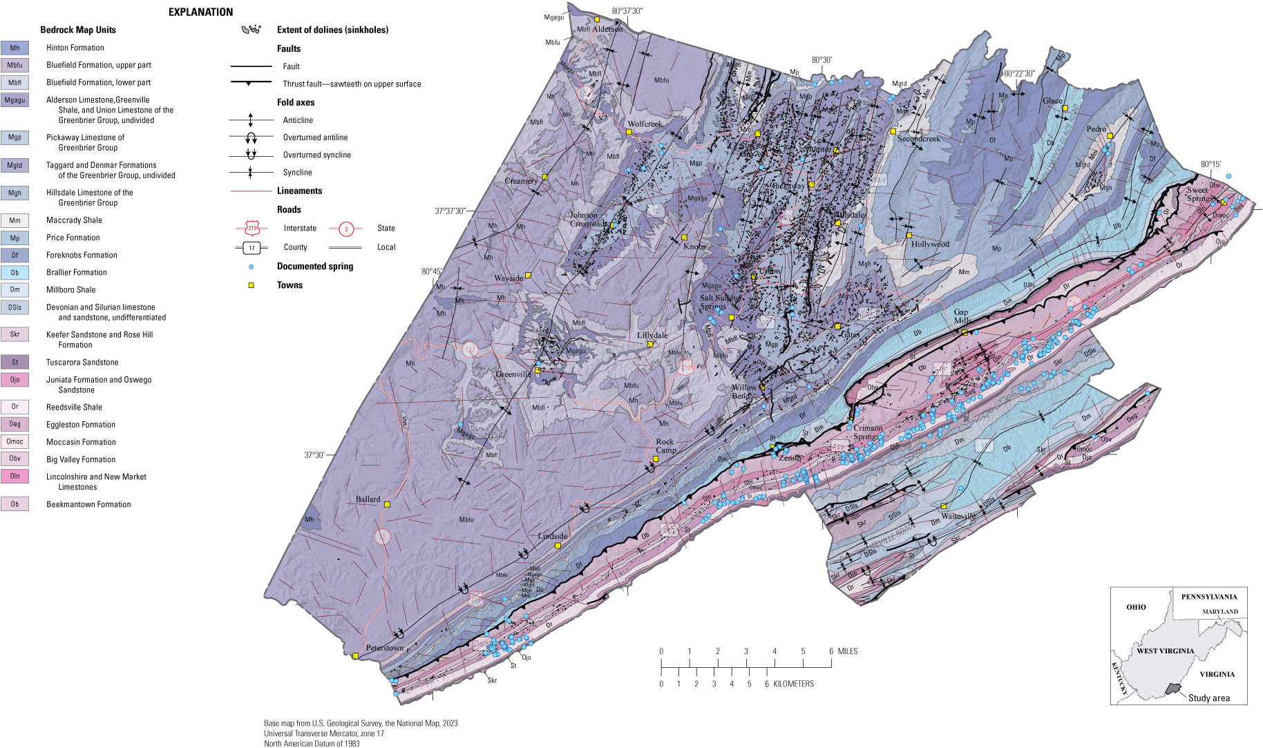
Monroe County is a 474 square mile (mi2) area (fig. 1) underlain by carbonate and siliciclastic bedrock aquifers of Ordovician, Silurian, Devonian, and Mississippian age. It is in parts of two physiographic provinces, the Valley and Ridge Province in the eastern part of the county and the Appalachian Plateau Province in the western part of the county (Fenneman and Johnson, 1946).
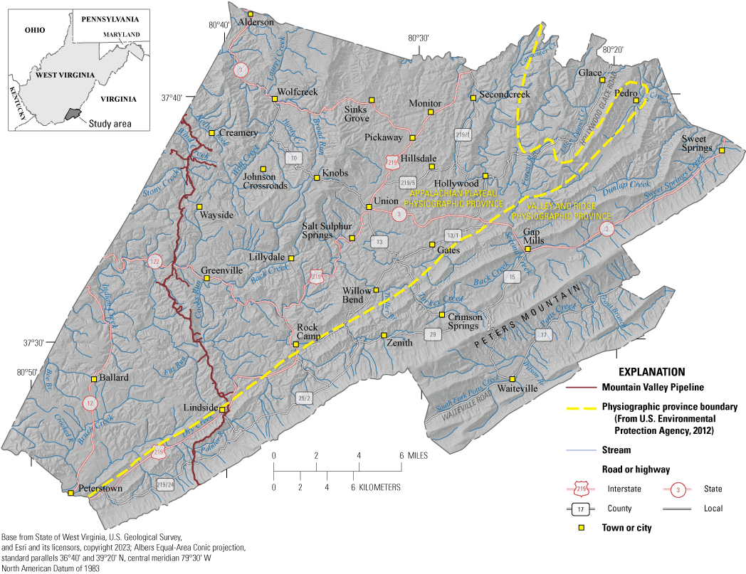
Map showing the location of the study area, Monroe County, West Virginia.
The average annual precipitation from 1991 to 2020 for the study area was 38.8 inches per year (in/yr), with annual average maximum precipitation in the spring (11.41 inches [in.]) and annual average minimum precipitation in the winter (7.8 in.). Average summer temperature was 70.9 degrees Fahrenheit (°F) and average winter temperature was 34.4 °F (table 1; National Oceanic and Atmospheric Administration, 2021).
Table 1.
Station annual and seasonal normals of temperature and precipitation for the Town of Union, West Virginia, from 1991 to 2020.[Data are for the National Weather Service station (UNION 3 SSE, WV) from National Oceanic and Atmospheric Administration, 2021. °F, degrees Fahrenheit; in., inch]
Public supplies are a principal source of water for residential and commercial use in the region, accounting for 0.49 million gallons per day (Mgal/d) of fresh-water withdrawals (0.14 Mgal/d of groundwater and 0.35 Mgal/d of surface water) made by 6,645 individuals. An estimated 6,681 people rely on private wells or other unregulated sources, such as springs, primarily for not only residential use but also, to a much lesser extent, for commercial use, and withdraw an additional 0.55 Mgal/d of groundwater for their residential and commercial supplies (tables 2 and 3; U.S. Geological Survey, 2021). Therefore, rural residential water systems, primarily from individual wells, supply 50.8 percent of all water used for residential use in the study area. Public supplies provide 49.2 percent of water used for residential supplies. Most water used for public supply in the region (71.4 percent) is derived primarily from springs, augmented by stream withdrawals (backup sources mainly during low-flow periods), and the remaining portion (28.6 percent) is derived from groundwater withdrawals. For rural residents, however, 100 percent of their withdrawals are derived from groundwater (wells or springs).
Table 2.
Water-use data for Monroe County, West Virginia, for 2015.[Data are from U.S. Geological Survey, 2021. Mgal/d, million gallons per day; gallons/person/day, gallons per person per day]
Table 3.
Site-specific water-use data for the three public water systems in Monroe County, West Virginia, for 2020.[Data retrieved for 2020 by the West Virginia Department of Environmental Protection's large quantity user database (Laura Cooper, written commun., 2020). Gap Mills public service district (PSD), Red Sulphur PSD, and Town of Union are public water systems; Sweet Springs Valley Water Company is privately owned; all are spring water sources; withdrawal amounts measured in gallons]
Hydrogeologic Setting
Monroe County has karst within carbonate bedrock of the Mississippian Greenbrier Group (Hillsdale Limestone, Denmar Formation, Pickaway Limestone, Union Limestone, and Alderson Limestone) and the Ordovician Beekmantown Formation, New Market Limestone, Lincolnshire Limestone, Big Valley Formation, and Eggleston Formation. These karstified carbonate aquifers are prone to sinkhole and cave formation (Cox and Doctor, 2021b, c) and contain many large springs that are commonly used as a source of water for public supply within the county (Baker, 2005; Bausher, 2018). These karst aquifers are especially susceptible to contamination from activities occurring at the land surface because of the enhanced permeability of limestone and dolomite bedrock due to solution enlargement of bedding planes, joints, faults, and other bedrock fractures. Other non-carbonate siliciclastic aquifers also occur within Monroe County, mostly in the southern, western, and northwestern parts of the county. The aquifers within Monroe County formed from complex geologic and hydrologic processes, which will be discussed in greater detail later in the hydrogeology section of the report.
Sturms (2008) provided a description of the structural geology of the study area. The ridge of Peters Mountain is primarily held up by exposures of the Tuscarora Sandstone within a thick sequence of westward-dipping strata. Two major phases of deformation happened during the Alleghenian orogeny (mountain building event), in which bedrock was thrust over underlying Proterozoic basement rocks, forming the major faults and folds within the study area. The orogeny formed the Allegheny structural front, separating the highly folded and faulted Paleozoic sedimentary strata in the Valley and Ridge Province to the east from the relatively flat-lying, gently-dipping, and less-deformed sedimentary strata of the Appalachian Plateau to the west (fig.1).
Sturms (2008) also concluded that large thrust faults control geologic structure in the Valley and Ridge section, while smaller amplitude folds are typical of the Appalachian Plateau section, and the amount of folding and faulting decreases farther to the west. Two important features are present at the Allegheny structural front, the St. Clair thrust fault and the adjacent Glen Lyn syncline to the west, accompanied by a large number of smaller magnitude thrust faults, anticlines, and synclines.
A large proportion of the geology of Monroe County consists of karstic limestone, which has a high density of springs. Spring data for this study were derived from several sources, including spring location information provided by a West Virginia University master thesis written by Geoff Richards (2006), the USGS National Water Information System database (U.S. Geological Survey, 2019), the Indian Creek Watershed Association (Judy Azulay, unpub. data, 2018), West Virginia Speleological Survey (George Dasher, unpub. data, 2018), the West Virginia Department of Environmental Protection (Nick Schaer, unpub. data, 2018), and West Virginia University (Dorothy Vesper, unpub. data, June 2020). The aggregated locations of the known springs in Monroe County indicate a large concentration of springs along Peters Mountain, an area that provides water to public water systems in the county.
Land Use
Land use in the study area is predominately forested, with 326.5 mi2 (69.0 percent) deciduous forest, 11.1 mi2 (2.3 percent) is evergreen forest, and 4.4 mi2 (0.9 percent) is mixed forest (fig. 2 and table 4). The second largest portion of the county consists of agricultural land of which 94.8 mi2 (20 percent) is pasture hay and an additional 2.27 mi2 (0.5 percent) is cultivated crops. Only 28.8 mi2 (6.1 percent) is developed low, medium, or high intensity or developed open land space. The remaining 5.5 mi2 portion of the county (1.1 percent) comprises of a combination of open water, barren land, shrub, herbaceous grassland, and wetlands (Multi-Resolution Land Characteristics Consortium, 2019).
Table 4.
Land-use data for Monroe County, West Virginia, for 2011.[Data are from Multi-Resolution Land Characteristics Consortium, 2019. mi2, square mile]
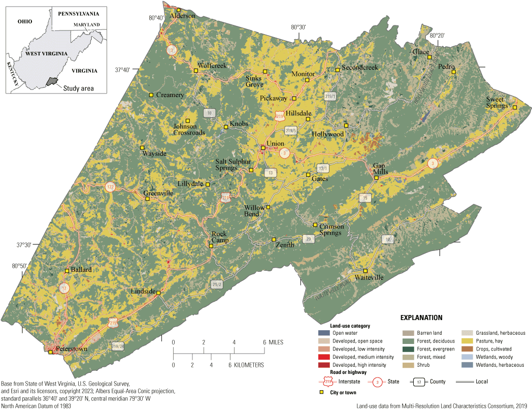
Map showing land use in Monroe County, West Virginia.
Previous Investigations
Numerous previous groundwater investigations for Monroe County, W. Va., and the surrounding region, were primarily focused on hydrogeology—especially in karst areas of the Greenbrier Group. A groundwater protection plan for source-water supplies for the Red Sulphur, Town of Union, Gap Mills, Trout Lodge, and Sweet Springs Valley Water Company water systems (Baker, 2005) stated that bedrock strata of Peters Mountain dip steeply to the southeast, as does the St. Clair fault zone at its northwestern base. Generally, two types of springs are on Peters Mountain (1) larger springs that emanate from the cavernous, more massive carbonate rocks, and (2) smaller springs that emanate from the fractured calcareous shales and limestones. Springs with the largest flows are near the base of Peters Mountain and along the trace of the St. Clair fault zone. These springs tend to be in the Beekmantown Formation. The largest of these springs have flows in the hundreds to thousands of gallons per minute. Recharge to the contributing area of these springs occurs at sinkholes and swales in the Beekmantown Formation and in overlying limestones units (New Market and Lincolnshire Limestones). Included in the recharge to these large springs is the flow from numerous smaller springs higher up on the mountain. The large springs have large recharge areas that extend to the ridge of Peters Mountain and horizontally along the base of the mountain.
Baker (2005) stated that springs emerging on Peters Mountain from shale and limestone bedrock of the Moccasin and Eggleston Formations and the Reedsville Shale typically have flows less than 100 gallons per minute (gal/min). Sandstone bedrock caps the ridges above these springs and provides recharge to some of the downdip aquifers. Colluvial deposits form local aquifers along Peters Mountain.
Baker (2005) cited estimates of groundwater recharge to the springs of approximately 20 in/yr, and flow ranging from 27 to 1,570 gal/min. Most of the water supplied by the Red Sulphur Public Service District (PSD), the Town of Union, the Gap Mills PSD, and the Sweet Springs Valley Water Company is derived from spring discharge. The Red Sulphur PSD also occasionally withdraws water from an intake on Rich Creek near Peterstown as a supplemental source of water. The public water systems also have backup wells completed in the Greenbrier aquifer that can be tapped as an alternate source of water when needed, but the quality of water from the Greenbrier aquifers wells is inferior to that derived from the principal springs that provide most of the public-supplied water in the county.
In a detailed study of the Scott Hollow groundwater basin, Bishop (2010) stated that due to activities on the surface, especially agricultural activity, the Scott Hollow groundwater basin is susceptible to contamination. Fertilizers and manure can easily be funneled into the aquifer during periods of moderate to heavy precipitation. A series of qualitative dye-tracer tests were completed by Bishop (2010) to help redefine the Scott Hollow drainage basin and establish hydrologic connections between the surface and subsurface, in conjunction with a water-quality analysis. Bishop (2010) stated that the dye-trace results indicated that geologic structure and stratigraphy exert a strong influence on groundwater flow processes. Three dyes were injected near the entrance of Scott Hollow Cave and then detected down gradient in two sections of the cave. Additional dye-tracer tests conducted on the eastern part of the cave indicated that groundwater flows toward the south, wraps around the plunge of the Sinks Grove anticline, and then reverses course, flowing toward the north and discharging along the Greenbrier River.
Groundwater samples were analyzed for nitrates, sulfates, chloride, and total coliform bacteria and then compared to season, local total precipitation, and percentage wooded land use in each subbasin to determine the influence of land use on groundwater quality (Bishop, 2010). Nitrate values ranged from 0 to 47.7 mg/L, sulfate values from 1.4 mg/L to 193.5 mg/L, and chloride values ranged from 0.97 mg/L to 177 mg/L. Nitrate concentrations not only exhibit a seasonal trend but also correlate to precipitation rates. Concentrations of total coliform bacteria in samples collected for Bishop’s (2010) study ranged from 0 to 576 colonies per 100 milliliters. Bishop (2010) also concluded that the total coliform bacteria concentrations were correlated with rainfall; however, no correlation was found between water-quality constituents in wooded areas when compared to non-wooded areas within the basin.
Based on data from Jones (1997), Bishop (2010) concluded that the subsurface groundwater basin drains approximately 18.61 mi2 near Sinks Grove. However, the drainage area for the Scott Hollow surface watershed is only 8.7 mi2, indicating inter-basin transfer via the subsurface. Jones (1997) concluded that groundwater in Scott Hollow Cave travels for about 3.3 mi before emerging from Gloria’s Spring along the Greenbrier River.
Bishop (2010) also states that karst features including sinkholes, caves, springs, sinking streams, and vertical shafts are common in the Scott Hollow groundwater basin. Virtually no surface streams are in the basin. Most precipitation and other surface water infiltrates directly into the underlying aquifer. Numerous cave passages are within the Scott Hollow groundwater basin and form along the contact between the Hillsdale Limestone and the Maccrady Shale. Groundwater flows mostly through solutional conduits and discharges at base level streams, small seeps, and larger springs (Jones, 1973).
Based on previous dye traces completed in this area (Jones, 1997; Tuggle, 2018; Nick Schaer, West Virginia Department of Environmental Protection, written commun., 2018), many of the underground flow paths do not follow stratigraphic or topographic lineament orientations and thus are not affected by surface topography. Average subsurface flow rates, determined from dye tracing (Jones, 1997), are estimated to be 0.36 miles per day (mi/d).
Scott Hollow Cave is characterized as an extensive dendritic subsurface flow system first documented in 1984 (Dore, 1995). The cave formed along the contact between the Hillsdale Limestone and the Maccrady Shale. The Scott Hollow Cave has more than 50 km of surveyed cave passages formed along structural features including bedding planes, cleavage planes, joints, and faults (Davis, 1999; Lane and others, 2018). Numerous subsurface tributaries flow downdip until discharging into the Mystic River.
Several dye traces were completed by Bishop (2010) in the Scott Hollow groundwater basin. Fluorescein dye injected into Marcus Wiley Cave was detected in the Mystic River within Scott Hollow Cave, traveling 1.7 mi in less than a week. Rhodamine WT was injected into Boyd Spring Sink and traveled 2.5 mi, also emerging in the Mystic River in less than a week. The Mystic River discharges to Gloria’s Spring, adjacent to the Greenbrier River.
Bishop (2010) used results of dye-trace tests to determine surface and subsurface flow connections for the Scott Hollow groundwater basin and to delineate the point of origin for all cave streams in the basin. Tracer test results conclude that geologic structure and lithology govern the direction of groundwater flow in the basin.
Building on Ogden’s (1976) previous hypothesis of the Maccrady-Hillsdale aquifer and the Taggard aquifer, Heller (1980) studied the Greenbrier Group karst of neighboring central Greenbrier County and hypothesized the presence of three major aquifers that include (1) an aquifer at the base of the Greenbrier Group at the contact between the Hillsdale Limestone and underlying Maccrady Shale, (2) an aquifer in the Taggard Formation, and (3) an unconfined aquifer in the Pickaway and Union Limestones. Groundwater flow was found to occur predominantly parallel to regional bedrock strike. Several miles south of the area is a major structural shift that marks the boundary between the central and southern Appalachian Mountain regions. In the study area, most wells have been drilled in two aquifers, the deeper Maccrady-Hillsdale and the upper Pickaway-Union, as well as, to a lesser extent, the Taggard aquifers. Of wells inventoried, 50 were completed in the Maccrady-Hillsdale aquifer, 22 were completed in the Pickaway-Union aquifer, 12 were completed in the Taggard aquifer, and 3 were withdrawing water from the Alderson Limestone. Based on these sparse data, Heller (1980) determined that median well yield of the Maccrady-Hillsdale aquifer was 16 gal/min, for the Taggard aquifer was 10 gal/min, and for the Pickaway-Union aquifer was 30 gal/min. The Pickaway-Union aquifer was stated to be the most productive aquifer within the study area with a median well yield of 30 gal/min. Heller (1980) concluded that the deeper aquifer in the Maccrady-Hillsdale is diffuse flow dominated, but very large and extensive cave passages are known to occur within that stratigraphic interval.
Heller (1980) concluded that wells with a high yield-to-depth ratio are associated with increasing proximity to topographic lineaments and with greater dip of strata (greater than [>] 30°); however, limited data did not afford an intensive analysis of structural controls on well yields with respect to lineaments and other structural data. Heller (1980) alluded that wells drilled in bedrock of steeper dip have higher median well yields, but the premise is limited by a small dataset.
Hirko (2012) studied the origin and paleohydrology of Haynes Cave, Monroe County, W. Va. The paleoclimate and sediment assessment documented sediments of an approximate age of 990,000 years and an incision rate of 0.14 meters per thousand years (m/ka). The cave was originally formed by phreatic processes, by dissolution of limestone at or below the water table. Haynes Cave is a relict phreatic cave that formed in the geologic past, as part of phreatic-groundwater flow and karst-dissolution processes that sits high in the geologic sequence above Dickson (Big) Spring and has been further developed by later vadose zone flow processes.
Hirko (2012) also provided a comprehensive assessment of overall structural trends in Monroe County. Hirko (2012) states that in southeastern West Virginia, a change in fold orientation marks a boundary between the central and southern Appalachians. Folds in the southern Appalachian trend approximately N. 60° E., whereas folds in the central Appalachian trend approximately N. 10°–30° E. The transition between the central and southern Appalachians is located where the Roanoke Recess, bounded by the Covington lineament to the north, converges with the St. Clair thrust fault and Glen Lyn syncline. This same feature, in Monroe County, marks the proximal extent of the Appalachian structural front (Dean and others, 1988).
Hirko (2012) further states that, in the central Appalachians, multiple thrust sheets overlap, resulting in longitudinal and vertical displacement at the surface, with axial traces of anticlines and synclines trending N. 10°–30° E. The southern Appalachians are characterized by vertically offset, imbricate thrust sheets, trending N. 60° E.
Hirko (2012) found that linear features in central Monroe County correlate with sinkhole collapses, trending N. 10°–20° E., N. 30°–40° E., and N. 50°–80° E., parallel to major fractures in the limestone bedrock of the region (Lessing, 1979; 1981). Bedding with a low plunge angle dips approximately 15° or less with increasing dip along fold limbs, fold axes, and thrust fault margins (Ogden, 1976). Average strike of Greenbrier Group rocks in Monroe County is approximately 0° N.–N. 25° E. (Ogden, 1976). Plunge directions of major folds, with two folds being overturned, is to the south-southwest. Folds parallel to the St. Clair thrust fault to the southeast trend N. 55° E. (Ogden, 1976).
Ogden (1976) studied the hydrogeology of central Monroe County, W. Va., karst and hypothesized three main confined aquifers within the Greenbrier Group (1) a Maccrady-Hillsdale aquifer, (2) a Patton-Taggard aquifer (upper Denmar-Taggard aquifer in this report), and (3) a Union-Greenville aquifer; there is also a minor aquifer of local importance only in the Sinks Grove Limestone (lower part of the Denmar Formation in this report). This differs slightly from Heller’s (1980) description where an aquifer in the Pickaway and Union Limestones, not the Union Limestone and Greenville Shale, is referenced. The nomenclature used by Ogden (1976) and Heller (1980) is inconsistent with the nomenclature used within this report (see “Lithologic Units” section), which was updated based on more recent geologic mapping conducted for this investigation. The nomenclature of this report groups the Patton and Sinks Grove Limestones together as the Denmar Formation, as defined by Wells (1950). Additionally, in this report, the Taggard and Denmar Formations are mapped as one unit on the geologic and hydrogeologic maps.
Ogden (1976) developed potentiometric surface maps for each aquifer where sufficient data allowed, but data were limited for the stratigraphic units and bedrock geology corresponding to the water level measurements used to develop the maps. The report contains an important description of the stratigraphy for the Greenbrier Group, but these descriptions have been updated with this study’s more recent geologic mapping.
Ogden (1976) mapped numerous significant anticlines and synclines for Monroe County and discussed joint orientations. Only a few minor faults were mapped in the Greenbrier Group according to Ogden (1976); however, more recent mapping has revealed large faults north of Willow Bend in the central part of the county. Topographic lineaments were mapped for central Monroe County, including the Monitor lineament. Ogden (1976) theorized that the Monitor lineament is related to increased fracturing, not faulting, and stated there is no apparent water-bearing capacity for the lineament.
Sinkholes are described by geologic formation, with sinkhole development lowest in the Alderson Limestone, intermediate in the Hillsdale Limestone and Taggard Formation, and higher in the Patton and Sinks Grove Formations, Pickaway Limestone, and Union Limestone (Ogden, 1976). Cavern lengths are longest in the Union Limestone and Patton and Sinks Grove Formations, and lowest in the Hillsdale Limestone, Taggard Formation, Pickaway Limestone, and Alderson Limestone. No photo-lineaments correlate with any of the geologic formations. Only sinkhole density and cavern length were statistically correlated among the variables assessed. McPeak Spring is at the Union Limestone-Greenville Shale contact. Two small streams sink near the Pickaway-Union contact and flow to McPeak Spring. The Greenville Shale acts as a retarding unit along the head of Indian Creek.
Several types of caves are in Monroe County; the caves near Swopes Knob form as water flows across the surface in streams over the impure Alderson Limestone and sink into the Union Limestone, with the Greenville Shale acting as a cap rock. Vertical or near vertical pits or sinkholes form in a similar manner at the top of the Denmar Formation with the Taggard Formation acting in a similar manner as the Greenville Shale (Ogden, 1976). The highly impure nature of the Alderson Limestone results in the lowest amount of cavern development of the carbonate units within Monroe County. Ogden (1976) determined that limestone cave development is common and often extensive in the upper part of the Hillsdale Limestone and Sinks Grove (lower part of the Denmar Formation in this report). Caves in this setting are often canyon-like, form downdip, and open into large rooms with siphons. Many of the caves are dry in the upper part but contain streams in their lower sections, of which Ellison’s and Rehobeth Church’s caves are examples. Caves in the Denmar Formation and Union Limestone typically are large in diameter and volume and form along bedding with a large width-to-height ratio. An example of this type of cave is Crowder Cave. Caves and springs are common above the informal upper red shale of the Taggard Formation. Many of the caves in Monroe County form along the strike of bedrock, and the majority form in the Denmar Formation and Union Limestone, which are the most calcite dominant carbonate units in the Greenbrier Group. These formations often are adjacent to shale confining units. Ogden (1976) stated that although caves tend to form along strike, that trend is not statistically significant and joints are also a controlling factor, especially those oriented N. 58° W. and N. 27° W. Stratigraphic dip averages about 15° but may be near vertical or overturned in areas. The gradient of the Hillsdale-Maccrady aquifer potentiometric surface is high at 85 feet per mile and recharge occurs along Little Mountain. The Greenbrier Group carbonate aquifer is recharged in the northeastern section of the county and is funneled to the southwest towards Burnside Branch by a plunging syncline. Karst denudation rates were estimated to range from 19.0±7.2 to 20.1±5.1 millimeters per 1,000 years.
Ogden (1976) also analyzed well data for Monroe County and found that wells are typically deep and target the Hillsdale-Maccrady contact, or at shallower depths within the Denmar-Taggard and Pickaway-Union aquifers. Water quality varied greatly each season within the Denmar-Taggard and Pickaway-Union aquifers, but little, if any, seasonal variability was in the deeper Hillsdale-Maccrady aquifer. Wells in the Taggard Formation indicated elevated chloride and nitrate concentrations, while wells in the Hillsdale-Maccrady aquifer had higher concentrations of sulfate.
Richards (2006) evaluated the aqueous geochemistry of 221 springs along Peters Mountain in Monroe County, W. Va. Of the 221 springs, 76 were assessed for pH, temperature, and specific conductance. Twenty-two springs were assessed for major water-quality constituents. The springs were subdivided into three groups based on geochemical, lithologic, and geologic properties:
-
Group 1.—Springs discharging from Silurian and Devonian clastic rocks below Peters Mountain containing concentrations of pH and dissolved solids similar to rainwater, with minimal dissolution of calcite. Some of these springs may be ephemeral.
-
Group 2.—Springs discharging from the Ordovician Reedsville Shale or from soluble limestones interbedded with clastic units believed to form perched aquifers. Waters from these springs are of two distinct chemical signatures. Springs emerging from the clastic rocks of the upper part of the Reedsville have lower alkalinities (buffering capacity) and total dissolved solids concentrations, similar to Group 1 springs. The second type are springs emerging at the base of the Reedsville Shale. Water from these springs contain higher alkalinities derived mostly from calcite dissolution but are still undersaturated with respect to calcite, having alkalinity no more than 2 milliequivalents per Liter.
-
Group 3.—Springs discharging lower in the valley from the Ordovician dolomites at the western base of Peters Mountain. Sinking streams flowing off Peters Mountain provide recharge to these conduit-dominated aquifers. The St. Clair thrust fault forms a structural boundary limiting groundwater flow to the west. Group 3 springs also possess two chemical signatures. Springs dominated by flow entirely through Ordovician limestones represent the first chemical signature, with molar ratios of calcium and magnesium (Ca:Mg) ranging from 12 to 20. Springs emerging from dolomitic rocks represent the second chemical signature, with molar ratios of Ca:Mg nearly equal to one.
Sturms (2008) completed geologic mapping and kinematic modeling of the St. Clair thrust fault, Monroe County, W. Va. The report provides a detailed discussion of the lithologic composition of the primary geologic formations and groups in the study area, which includes a large part of Monroe County, W. Va. The work by Sturms (2008) contains a significant amount of modeling to approximate and better understand how faults and associated shear stress are formed and how folds form as part of fault propagation.
The St. Clair thrust fault trends in a southwest to northeast direction through the map area terminating just east of the West Virginia–Virginia border, in Allegheny County, Virginia (Sturms, 2008). The hanging wall within the study area consists of the Lower to Middle section of the Ordovician Beekmantown Formation through the Devonian Millboro Shale. The footwall of the St. Clair thrust fault is composed of Devonian rocks through the Upper Mississippian Mauch Chunk Group. The St. Clair thrust fault terminates within the core of the Wills Mountain anticline.
Sturms (2008) found that the St. Clair thrust fault formed as the result of two separate processes (1) trishear deformation (triangular zone of outward and upward deformation) and (2) fault-bend folding. The overturned footwall of the syncline formed by trishear deformation. The hanging wall was formed by fault-bend folding. Sturms (2008) used modeling to recreate the sequential cross-sections for three cross-sections and determined the amount of displacement needed for each cross-section. The first cross-section was modeled with a displacement of approximately 7,550 ft. The second cross-section was modeled with a displacement of 24,600 ft, and the third cross-section indicated a modeled displacement of 21,980 ft.
The second and third cross-sections indicate a decrease in displacement of 2,630 ft (10.66 percent) to the northeast. Using the trishear modeling program Fault/Fold by Allmendinger (1998), Sturms (2008) estimated the strain within the trishear triangle zone. Through kinematic modeling, Sturms (2008) determined that the St. Clair thrust fault exhibited a small propagation-to-slip ratio during the initial trishear deformation phase prior to initiation of fault-bend folding.
In a West Virginia University study, Bausher (2018) provided a qualitative and quantitative analysis of carbonate water in the Peters Mountain region of Monroe County, W. Va. Geochemical interpretation of water-quality data for 15 springs provided the basis for the study. Seven of these springs were high on Peters Mountain and situated primarily within the Reedsville Shale, while seven other springs emanated predominantly from limestones of the Beekmantown Formation or the New Market Limestone in the carbonate valley at the base of Peters Mountain. The 15th spring was a thermal spring emanating from the New Market Limestone in the northern part of the Ordovician karst valley near Sweet Springs, W. Va. Geochemical data collected from the springs included common cations and anions, the indicator bacteria total coliform and Escherichia coli, and organic carbon. Mineral saturation indices, partial pressure of carbon dioxide, and ionic strength were computed for each spring sample to assess geochemical composition and then compared to assess geochemical controls on the chemistry of the spring waters.
Based on the geochemical analysis performed by Bausher (2018), the springs were identified to be of three major types (1) carbonate springs in the valley at lower elevation in the Helderberg Group-Oriskany Sandstone section, and the Beekmantown Formation and New Market Limestone; (2) clastic springs that emerge from interbedded siliciclastic and carbonate units in the Reedsville Shale and Juniata Formation on the mountain flanks; and (3) a thermal spring that emerges from the Eggleston Formation and likely associated with the St. Clair thrust fault. Clastic and carbonate springs were classified as calcium-magnesium-bicarbonate type waters with neutral pH and alkalinities, and the thermal spring was classified as a calcium-magnesium-sulfate-carbonate water with low pH and high specific conductance and alkalinity and was associated with deep flow along the St. Clair thrust fault.
The West Virginia Speleological Survey published a report (Dasher, 2019) providing a comprehensive discussion of the caves, springs, and sinks of Monroe County for 16 primary karst areas and includes general location maps for the larger caves, springs, and sinks, detailed cave maps, location and elevation data, and photographs of the larger caves, springs, and sinks. Dasher (2019) also provides a section on the bats found in caves of Monroe County, fossils commonly found in Monroe County, and includes a discussion of the karst and geologic setting of Monroe County. A summary of Dasher (2019) is beyond the scope of this report because of the details contained in the report (474 pages). Dasher (2019) provides the most comprehensive assessments of caves, springs, and karst areas and basins within Monroe County, W. Va. available to date.
Methods of Data Collection and Analysis
The methods of data collection and analysis described in this report consisted of numerous field data collection efforts and data analytical methods as part of a multidisciplinary study of the geology and hydrology of Monroe County. Principal field data collected by USGS geologists centered upon geologic mapping of the bedrock formations cropping out in Monroe County, but also included mapping karst features, such as caves, springs, and sinkholes. Hydrologic data collected for the project by USGS hydrologists and hydrologic technicians included synoptic groundwater-level and base-flow stream surveys, borehole geophysical surveys, fluorometric groundwater tracer tests, monitoring streamflow at four gaging stations and groundwater levels at continuous recording groundwater-monitoring well.
Groundwater-level data, used for preparation of the water-table map, were collected according to standard USGS policies and procedures (Cunningham and Schalk, 2011) using a combination of graduated steel or electrical tapes, or where measurement of water levels using steel or electrical tapes was not possible, by use of acoustic water-level meters. The primary purpose of the areal groundwater-level synoptic survey was to prepare a potentiometric surface map of Monroe County. Notably, even though 268 groundwater-level measurements, 121 spring locations, and 2,049 control points of stream-elevation data were used to develop the potentiometric surface map of the county, mapping the discontinuous perched aquifers within the Greenbrier Group or other geologic formations within the county was impossible because of disconnected and sparse distribution of confining or semi-confining units within the geologic formations comprising the Greenbrier Group. As a result, the potentiometric surface map represents combined heads in open boreholes and should be considered a composite headwater-table map.
Three major data layers were used to produce the potentiometric surface map. These data layers consisted of (1) 268 synoptic groundwater-level measurements made in October 2017 and August and September 2019 under similar groundwater conditions; (2) 121 spring locations compiled from various sources including a West Virginia University master thesis written by Geoff Richards (2006), the USGS National Water Information System database (U.S. Geological Survey, 2019), the Indian Creek Watershed Association (Judy Azulay, unpub. data, 2018), West Virginia Speleological Survey (George Dasher, unpub. data, 2018), the West Virginia Department of Environmental Protection (Nick Schaer, unpub. data, 2018), and West Virginia University (Dorothy Vesper, unpub. data, June 2020); and (3) 2,049 stream elevation control points derived from the USGS National Hydrographic Dataset (U.S. Geological Survey, 2018). Elevation data for the potentiometric surface map were obtained from the 3-meter (m) lidar dataset compiled for the project (Cox and Doctor, 2021c). The water-level contour lines derived from the potentiometric surface map and the associated water-level data are published in an accompanying USGS Data Release (Schipke and Kozar, 2023).
Streamflow data were collected according to established USGS policies and procedures (Turnipseed and Sauer, 2010). A total of 162 streamflow or spring-discharge measurements were made for the study including (1) 83 base-flow stream- and spring-measurements made as part of the base-flow synoptic survey, and (2) 79 streamflow measurements made at 4 USGS gaging stations. Twenty measurements each were made at the Indian Creek near Red Sulphur Springs, W. Va., (USGS site 03177480); Rich Creek near Peterstown, W. Va., (USGS site 03176400); and Second Creek near Second Creek, W. Va., (USGS site 03183000), gaging stations. The last 19 measurements were made at the Wolf Creek near Alderson, W. Va., gaging station (USGS site 03183567). These measurements were made to further refine and develop rating curves for the four continuous-record streamgages to provide quantitative data for assessment of groundwater recharge and overall water-balance assessments for Monroe County. Continuous records of streamflow data were also processed, stored, and analyzed using AQUARIUS streamflow data and analysis software (Aquatic Informatics, 2023). These streamflow data are available through the USGS National Water Information System database (U.S. Geological Survey, 2019).
Continuous streamflow data were analyzed using PART, a hydrograph analysis program, to compute groundwater recharge rates. This program is a tool documented within the USGS Groundwater Toolbox (Barlow and others, 2014), available from Barlow and others (2017). Groundwater recharge was also computed using the Soil-Water-Balance (SWB) model (Westenbroek and others, 2010) as part of a groundwater resources appraisal of the regional Pennsylvanian and Mississippian aquifer system (McCoy and others, 2015). The SWB model, which is based on available soil and precipitation data, produces accurate regional estimates of groundwater recharge but is limited in estimating groundwater recharge at a local scale. Because of this limitation, PART hydrographic analysis was used to verify estimates of the SWB model and to assess groundwater recharge at the local and county scale for Monroe County.
Water-tracing tests using fluorescent dyes are an established technique to determine connections between input points of water (stream sinks, caves) and springs or seeps where the water returns to the surface. These tests typically work well in karst aquifers with conduit flow and fast travel times. The techniques for water-tracing studies are described by Alexander and Quinlan (1996), Aley (2019), Kass (1998), and Jones (2019). Monitoring for the tracers is usually qualitative using passive detectors of activated carbon (dye traps or “bugs”) or quantitative by measuring the fluorescence of dye in water samples collected over time. Monitoring for dye recovery from the two tracer tests conducted for this study was quantitative using filter fluorometers at the sampling sites and collecting grab samples that were later analyzed in the lab. The passive detectors were changed at one- to two-week intervals as a back-up means of verifying the presence of the dyes, thus preventing ambiguous results from the water samples. Two tracer tests were conducted from streams sinking into the Greenbrier Limestone south of the Town of Union, W. Va.; details on the tracer tests are provided in the “Dye-Tracer Tests” section of this report. Fluorescein sodium (CI 54350) and Rhodamine WT (CI Acid Red 388) were injected in different streams under low-flow conditions on July 10, 2019 (fig. 3A, B).
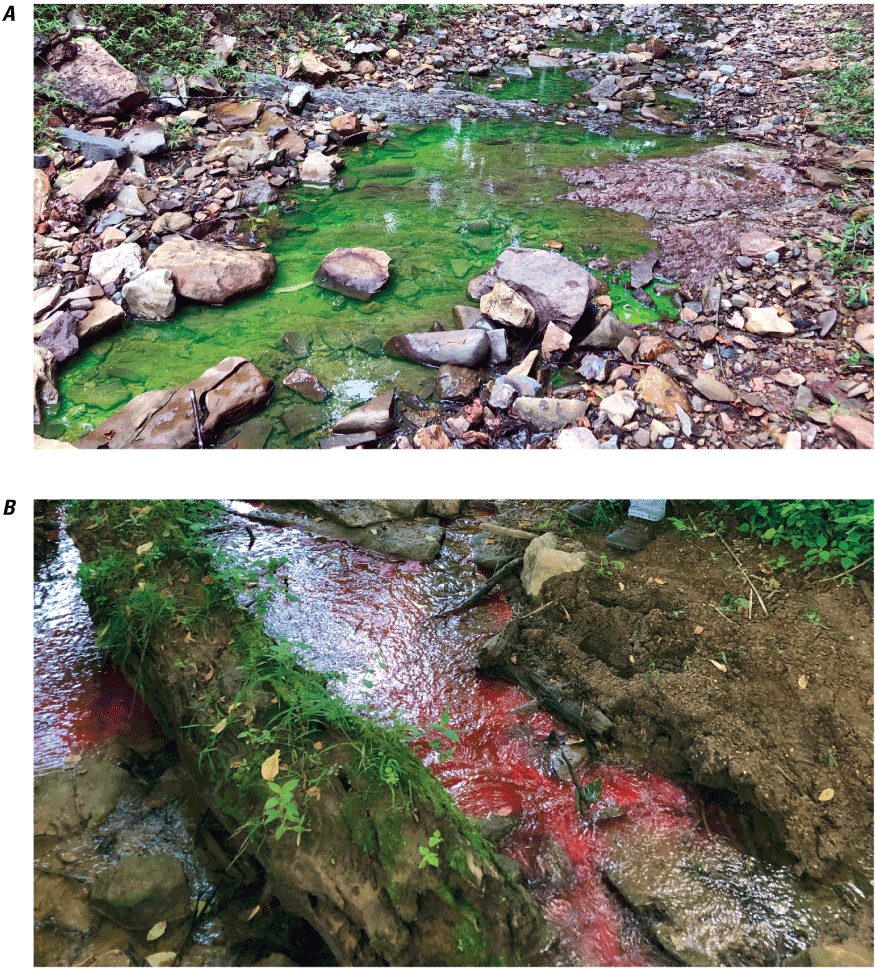
Photographs of A, Fluorescein sodium and B, Rhodamine WT dye injections for a groundwater tracer test initiated in Monroe County, West Virginia, on July 10, 2019. Photographs by Daniel Doctor, U.S. Geological Survey.
Twenty-one locations in the Indian Creek watershed and Dickson Spring on Second Creek were monitored by collecting water samples once per day for the first two weeks and with passive detectors and an automated sampler on Dickson Spring for two months after dye injection. Water samples and carbon-dye traps were placed at each monitoring site and analyzed two weeks prior to the start of the tests to determine fluorescence background.
Water samples were analyzed at the time of collection using a Turner Design AquaFluor field fluorometer on a 15-minute interval at the head of Indian Creek and Dickson Spring. An ISCO automatic water sampler was started at Dickson Spring on August 7, 2019. It then collected water samples at eight-hour intervals for one month; after which time the samples were analyzed in the lab using a Shimadzu RF-5000U scanning spectrofluorophotometer fitted with a high-sensitivity sample holder. The results from the water samples were converted from the relative fluorescence output from the fluorometer to dye concentration in micrograms per liter. An approximation of the percentage of the injected dye mass recovered in the water samples over the sampling period was calculated based on the average discharge during the sampling period.
Borehole geophysical data were collected using two different manufacturer’s equipment to characterize fracture controls on groundwater flow, assess borehole lithology, and quantify water producing zones in the boreholes. A Century Geophysical System VI data acquisition and processing unit was interfaced with a Century Geophysical draw works winch and cable to power six different borehole geophysical tools, including (1) a 3-arm caliper, (2) electromagnetic (EM) induction tool, (3) an EM flowmeter, (4) an acoustic televiewer, (5) a multiparameter (resistivity, spontaneous potential, and natural gamma) tool, and (6) a full wave sonic porosity tool. Data collected by the various tools were transmitted via the Century Geophysical draw works 4-wire cable and were processed on site using Century Geophysical Log VI software version 3.60L (Century Geophysical, 2017). An additional logging tool, a (7) Mount Sopris 6 optical televiewer was used with a Mount Sopris Matrix data acquisition system (Mount Sopris, 2017) and the Century Geophysical draw works system to collect digital borehole imagery for fracture analysis. Calibration of the geophysical tools was done in accordance with manufacturer’s specifications. The 3-arm caliper and EM-induction tools were calibrated at every site prior to initiation of logging. All geophysical tools were evaluated prior to collecting data to ensure they were operating within acceptable manufacturer’s specifications. EM flow and other tools were calibrated as needed during the logging phase of the study. All borehole logs collected for this study were analyzed using WellCAD version 5.1, which is a product of ALT Corporation in Redange, Luxembourg.
Geologic mapping was conducted in conjunction with this study using traditional methods. At each bedrock outcrop locality, the lithologic character of the rock was noted, and measurements of bedding attitude and fracture orientations were made, where discernible, using a Brunton geologic transit compass. Data were recorded on digital mobile devices in the field and compiled within geographic information system software in the office. A singular, 3-m resolution DEM was produced of the county, as well as an enhanced image of the terrain at 3-m resolution to provide base-map imagery for facilitating geologic mapping and geomorphologic interpretations. These products are available as USGS data releases (Cox and Doctor, 2021a, b, c); details on the methods used for their production are provided in the associated metadata.
Hydrogeology
The hydrogeology of Monroe County is extremely complex, affected by structural, geologic, lithologic, and physiographic controls. A primary control is physiography. Monroe County is situated in two physiographic regions (Fenneman,1938), the Appalachian Plateau Province, which consists of flat to gently dipping siliciclastic and carbonate bedrock predominantly of Devonian to Mississippian age, and a much more complex Valley and Ridge Province, characterized by long linear ridges and intervening valleys formed by compressional stress as a result of previous orogenic (mountain building) processes during the Alleghenian orogeny. These prior orogenic processes resulted in significant thrust faulting of older Ordovician, Silurian, and Devonian rocks over the younger Devonian and Mississippian rocks to the northwest.
In addition to physiographic controls, bedrock within the study area in both physiographic provinces is highly heterogenous and comprises potentially karst-forming limestones and dolomites, and non-carbonate siliciclastic units composed of predominantly shales and sandstones. These differences in lithology, especially with respect to limestone and dolomite outcrops, are responsible for karst topography in both physiographic provinces, although the karst in the Appalachian Plateau Province is of much greater areal extent and contains more karst features than the karst topography within the Valley and Ridge part of the study area.
Another important lithologic control on hydrogeology within the study area is the contact between the Hillsdale Limestone, which is the basal formation within the Greenbrier Group, and the underlying Maccrady Shale. This geologic contact has been documented to be base level control of groundwater occurrence and cave development within the Greenbrier Group (Balfour, 2018). The Maccrady-Hillsdale contact is host to many caves and is frequently targeted by drillers as a source of water for large-capacity agricultural and smaller-capacity residential water wells within the study area. Within the Greenbrier Group, localized, and often discontinuous, layers of lower permeability shale, calcareous shale, and chert bedrock may result in localized perched aquifers within the geologic formations of the Greenbrier Group. The occurrence of these perched aquifers is difficult to map because the geologic strata responsible for the perched aquifers are intercalated (alternating layers of differing sediments) and laterally discontinuous, making mapping these thin confining or semi-confining units with any degree of certainty impossible.
Other structural controls on the hydrogeology of the study area determined during the course of this study include bedding planes, faults, joints, cleavage planes, and folds. Because the bedrock within the study area lacks sufficient intergranular porosity for storage and movement of water, most of the water within these fractured-rock or karstic aquifers resides and moves along fractures within the bedrock. Bedding planes are a primary control on discharge and movement of groundwater within the study area, especially where sufficiently fractured rock, such as fractured sandstones or solutionally enlarged fractures within limestone or dolomite layers, are situated on top of less permeable, less fractured strata. Faults can also provide for both storage and movement of groundwater, especially where such faults have been solutionally enlarged by movement of water in carbonate limestone and dolomite strata. Joints, which may occur as fractures within the bedrock and cleavage planes, can sometimes serve as open avenues for groundwater storage and movement, if not filled with calcite or silica cement. Finally, folds consisting of anticlinal uparching and, more importantly, synclines can provide for fracturing of bedrock within the structures or can compartmentalize groundwater flow within the synclines, resulting in preferential flow paths, especially within the more karstic parts of the aquifers within the study area. These factors combine to form the various hydrogeologic units within the study area.
Geology
Geologic processes exert a significant and highly complex control on the hydrogeology of Monroe County. Geologic factors influencing the hydrogeology of Monroe County include (1) lithologic controls of numerous geologic formations ranging in age from Ordovician to Mississippian with mixed lithologies consisting of carbonate, karst forming limestone units and siliciclastic non-carbonate sandstone, shale, and siltstone units; (2) physiographic controls with associated steep linear ridges and regional thrust faults in the Valley and Ridge Province and more flat lying but highly dissected and eroded bedrock within the Appalachian Plateau Province; and (3) numerous structural controls resulting from thrust and normal faults, bedding planes, joints, and bedrock cleavage. All these factors combine to form the numerous complex hydrogeologic units found in the study area. A countywide hydrogeologic map was developed for the study and shows the alluvial deposits and colluvial deposits resulting from weathering and transport of weathered overburden strata, creating numerous surficial alluvial deposits (fig. 4). In addition, the bedrock geologic formations and groups were mapped in Monroe County showing the complex geology of the various formations and groups within Monroe County, W. Va. (fig. 5). The alluvial deposits along Peters Mountain are a prolific source of water for public supplies in Monroe County.
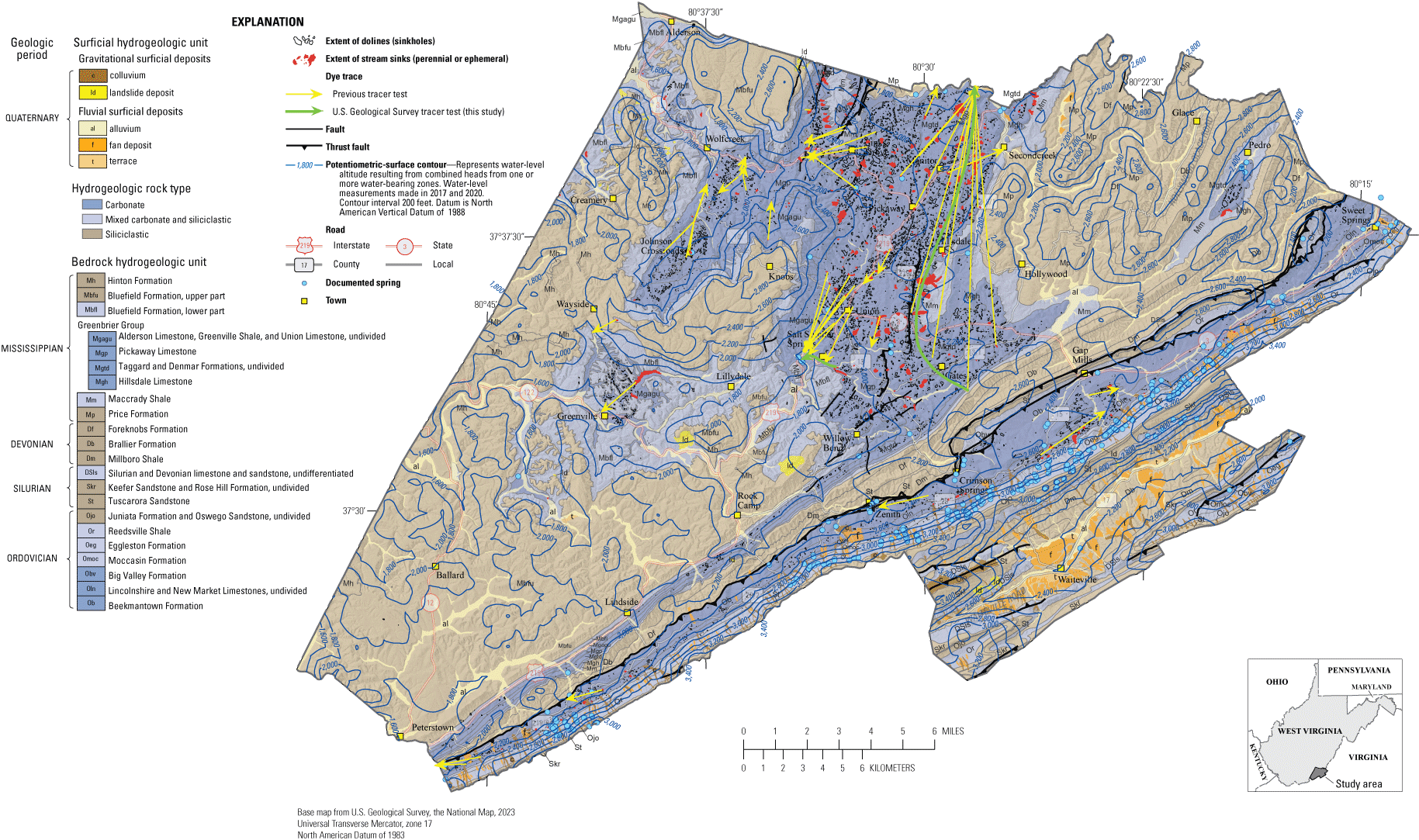
Countywide hydrogeologic map showing extent of colluvial, alluvial, terrace, landslide, and fan deposits in Monroe County, West Virginia.
Countywide geologic map showing extent of geologic formations and groups, faults, and fold axes of anticlines and synclines in Monroe County, West Virginia.
Lithologic Units
As part of this project, the USGS mapped the county in greater detail than the original map by Reger and Price (1926); two maps are provided in this report (fig. 4 surficial geologic map; fig. 5 bedrock geologic map). The rocks exposed in Monroe County are Paleozoic sedimentary rocks ranging from Ordovician to Mississippian in age. The descriptions of rock units are listed below in stratigraphic order from oldest to youngest.
Beekmantown Formation (Ob)
The Beekmantown Formation is composed of interbedded dolomite and dolomitic limestone. This unit is generally massive and provides good exposure in outcrop. The dolomite tends to weather to a beige-gray color and often exhibits elephant-skin type weathering patterns on exposed surfaces where fractures are weathered to form linear troughs on the rock surfaces. Chert is abundant in the middle part of the unit and may form along bedding plane partings or form in irregular, spongy masses that weather out and become scattered on the surface as part of the regolith overlying the rock. In Giles County, the equivalent units have been mapped as Mascot Dolomite and Kingsport Dolomite, undivided (Schultz and others, 1986). Further to the south, this unit is mapped as part of the Knox Group (Miller and Meissner, 1977). The Beekmantown is at least 1,312 feet (ft; 400 m) thick; however, the complete thickness of the formation is not exposed in Monroe County because of truncation of the unit along the St. Clair thrust fault. The Beekmantown Formation is a karst-forming unit containing caves and abundant sinkholes.
Lincolnshire and New Market Limestones, Undivided (Oln)
The New Market Limestone is primarily a fine-grained, microcrystalline, high-purity dove-gray limestone throughout most of its thickness. Previous work by Kay (1956) identified the same interval of rocks as the Lurich formation; however, this name was not formalized, and recent mapping for this study indicates the equivalency to the New Market. This limestone unit is generally massive and forms good outcrop (fig. 6).
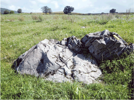
Photograph of an outcrop of the New Market Formation in Monroe County, West Virginia. Note the rillenkarren solutional features visible on the far-left vertical surface of the outcrop. Photograph by Daniel Doctor, U.S. Geological Survey.
Thin lags of conglomerate composed of carbonate clasts are sporadically found within the layers of finer-grained limestone (fig. 7). Good exposures of the New Market Limestone can be seen along Limestone Hill Road between Gap Mills and Zenith where the unit is approximately 243 ft (74 m) thick. The base of the formation has distinctive pinkish-orange beds that contain lithic fragments and conglomeratic clasts of chert. At the contact with the underlying Beekmantown Formation, the clasts in the conglomerate are mostly angular, can be as much as 10 centimeters across, and are composed of angular clasts of chert, dolostone, and some lithic fragments. This lower conglomeratic interval is as much as 115 ft (35 m) thick and may be equivalent to the Tumbez Formation (Cooper, 1945); however, the lower conglomeratic interval is discontinuous in Monroe County and, thus, is included in the New Market Limestone. The New Market is a significant karst-forming unit, containing the largest caves in the Ordovician limestone units and abundant sinkholes.
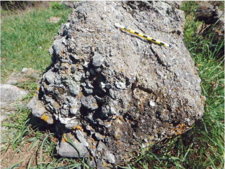
Photograph showing angular clasts of chert and limestone in a bedded conglomerate at the base of the New Market Limestone in Monroe County, West Virginia. Note the angular clasts of chert and limestone in a bedded outcrop of the conglomerate at the base. Photograph by Daniel Doctor, U.S. Geological Survey.
The Lincolnshire Limestone lies immediately above the New Market and is a very dark gray to black limestone containing abundant black chert, is generally thin-bedded, and contains wispy argillaceous layers. The Lincolnshire Limestone is very thin and discontinuous in Monroe County. Good outcrops of the Lincolnshire exist in the Paint Bank and Gap Mills 7.5-minute quadrangles near Gap Mills where it has been measured to be approximately 33 ft (10 m) thick. Due to its discontinuous outcrop in Monroe County, the Lincolnshire has been mapped along with the New Market Limestone as a single unit.
Big Valley Formation (Obv)
The Big Valley Formation is used in place of the previously defined Benbolt, McGlone, and McGraw Limestones that are either not recognized or too thin to be mapped as formations in Monroe County. The type section of the Big Valley Formation is in Big Valley, Virginia (Bick, 1962) and is dominated by limestones that may be thin- or thick-bedded, containing wispy layers of siliceous sediment or dolomitic mottling. The Big Valley also contains dark-gray, fine-grained, cobbly limestone, and dark-gray argillaceous limestone. The Big Valley Formation is approximately 184 ft (56 m) thick as measured near Zenith along a section parallel to Limestone Hill Road.
Moccasin Formation (Omoc)
The Moccasin Formation is a heterolithic unit composed of interbedded argillaceous limestone and calcareous shale. Shale in the Moccasin Formation is commonly pinkish-grey, as well as tan and greenish-beige in color (fig. 8). Mud cracks are commonly observed in the pinkish shale. Limestone beds in the formation are generally less than 1 ft (30 centimeter [cm]) thick. The top of the Moccasin Formation is marked by the thin 6.5 ft (less than [<] 2 m) thick Walker Mountain Sandstone Member (Butts and Edmundson, 1943; Haynes and Goggin, 1993). The total thickness of the Moccasin Formation is estimated to be 73 ft (24 m) based on sections measured along Limestone Hill Road near Zenith. Karst features are not commonly observed in the Moccasin Formation, although solutional voids have been observed along fractures and bedding partings.
Photograph showing mud cracks in pinkish-grey calcareous shale of the Moccasin Formation in Monroe County, West Virginia. Photograph by Daniel Doctor, U.S. Geological Survey.
Eggleston Formation (Oeg)
The Eggleston Formation consists of interbedded thin limestone and brownish-gray calcareous shale. Limestone beds in the Eggleston may be as much as 1.5 ft (45 cm) thick. Two prominent ridge-forming zones in the lower part of the Eggleston can be followed throughout most of the length of southeast Monroe County along the base of Peters Mountain. These ridge-forming zones are held up by competent beds of fossiliferous limestone. The Eggleston Formation is approximately 486 ft (148 m) thick as determined in the Paint Bank 7.5-minute quadrangle along a farm road extending off Mountain View Lane. Determination of an accurate thickness for the formation is hindered by lack of outcrop and frequent internal deformation of the strata.
Reedsville Shale (Or)
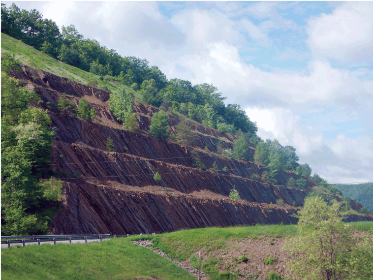
The Reedsville Shale consists of interbedded grayish-brown siltstone and fossiliferous shale, with more abundant shale in the lower third of the formation. The lower third of the Reedsville Shale weathers to a distinctive yellowish orange color and may be equivalent to a similar facies of the Martinsburg Formation that is recognized elsewhere in West Virginia. This lower part of the unit is less competent than the upper part, contains sparse brachiopod and graptolite fossils, and does not form good outcrop. Excellent exposure of the contact between the lower and upper part of the Reedsville can be observed in road cuts along Route 311, between Sweet Springs and the crest of Peters Mountain heading southeast toward Paint Bank. The upper part of the Reedsville Shale is a mixture of interbedded siltstone and calcareous shale with some zones of the shale being very fossiliferous. The upper part of the Reedsville Shale is generally chocolate brown to brownish-gray in color. The brachiopod Orthorhynchula linneyi is abundant within a conspicuous zone in the upper part. Total thickness of the Reedsville is estimated to be approximately 705 ft (215 m); however, in most areas in Monroe County the map pattern shows a much greater thickness because of the repetition of strata resulting from local tight folding.
Juniata Formation and Oswego Sandstone, Undivided (Ojo)
The Oswego Sandstone is a thin, heterolithic unit and varies from arkosic sandstone to fine-grained mudstone. The Oswego Sandstone is best exposed along Route 311 near the state line between Virginia and West Virginia. At that locality, the Oswego is approximately 33 ft (10 m) thick. The Juniata Formation is a series of interbedded sandstone and mudstone that has a characteristic brownish-red color. The Juniata is best exposed along Route 3 at Gap Mills. At this locality, the beds are overturned and approximately 295 ft (90 m) thick. These units have been described in the study area in greater detail by Diecchio (1985).
Tuscarora Sandstone (St)
The Tuscarora Sandstone is a hard, well-cemented, very light gray to white quartz sandstone that forms conspicuous ridges throughout its extent in Monroe County. The Tuscarora Sandstone holds up the ridges along Peters Mountain and Gap Mountain. A thickness of 39 ft (12 m) is well exposed along Route 3 at Gap Mills where the beds are overturned along the southeast limb of the Glen Lyn syncline and probably thinned to some extent. In the far southeast part of Monroe County, the Tuscarora is composed of two distinct zones of quartz sandstone, each 20 ft (6 m) thick, separated by approximately 33 ft (10 m) of light-tan shale. This package of rock is well exposed along Route 311 between Paint Bank and the state fish hatchery and has a total thickness of approximately 73 ft (22 m).
Keefer Sandstone and Rose Hill Formation, Undivided (Skr)
The character and thickness of the Rose Hill Formation and Keefer Sandstone across Monroe County vary and, therefore, these two formations have been lumped into a single map unit at the county scale. The Rose Hill Formation is predominantly composed of maroon-to-red hematitic sandstone, maroon-to-red mudstone, and thin intervals of fossiliferous shale. The Rose Hill Formation is approximately 220 ft (67 m) thick. Above the Rose Hill Formation lies the Keefer Sandstone, which, in the lower part, is a friable rusty yellow weathering quartz sandstone approximately 20 ft (6 m) thick, followed by an interval of approximately 20 ft (6 m) of shale, and overlain by a hard well-cemented quartz sandstone at least 30 ft (10 m) thick that forms prominent ridges in the topography. The upper part of the Keefer Sandstone weathers to a red color and often contains iron oxides and manganese oxides along fractures; it is brecciated in places, such as along Route 3 near Gap Mills.
Devonian and Silurian Limestone and Sandstone, Undifferentiated (DSls)
This map unit represents a heterolithic package of limestones and sandstones with intervals of shale that is approximately from 230 to 295 ft (70–90 m) thick. The lowermost part of this unit contains limestones of the Tonoloway Limestone and Helderberg Group. Incomplete sections of the Tonoloway and Helderberg Group limestones have been observed in the southeastern part of Monroe County near Paint Bank. Overlying the Helderberg Group is the Oriskany Sandstone, which is a friable and rusty weathered quartz sandstone that forms low topographic ridges but does not generally provide good outcrop. The Oriskany Sandstone is vuggy and is often iron cemented with occasional manganese oxide cement. The contact zone between the Oriskany Sandstone and the underlying limestones has historically been a target for iron and manganese mining. Although the limestones and sandstones described here are locally recognized in Monroe County, these units are believed to thin out to the southwest and become amalgamated into the Rocky Gap Sandstone as described by Dorobek and Read (1986).
Millboro Shale (Dm)
The Millboro Shale is a dark-gray to black, fissile, platy-weathering shale that is interspersed with siltstone. This shale often contains iron sulfide minerals and weathers to a dusky yellow color. The Millboro Shale is approximately 738 ft (225 m) thick, although true thickness is difficult to determine because of poor outcrop and internal deformation.
Brallier Formation (Db)
The Brallier Formation is a sequence of intercalated siltstone, sandstone, and shale. The rocks of this formation are generally dark gray in color (fig. 9). Beds of fine-grained graywacke can be as much as 3.3 ft (1 m) thick and form local ridges in the topography. The lower part of the Brallier generally has thinner beds than the upper part of the unit. The rocks tend to weather a pinkish orange and tan color. The Brallier Formation in Monroe County is approximately 2,640 ft (800 m) thick; however, the true thickness is difficult to estimate since most outcrop belts contain intraformational folding. The Brallier Formation is mostly exposed in the eastern part of the county and outcrops can be seen in the southeast side of the valley along Moncove Lake Road and along Hollywood-Glace Road in the core of the Glace anticline. A belt of outcrop of the Brallier Formation also occurs in the footwall of the St. Clair thrust fault that extends from the northeast to the far southwest of the county below Peters Mountain. A third zone of outcrop occurs in the southeastern extension of Monroe County in the vicinity of the town of Waiteville.
Photograph of an outcrop of the Brallier Formation along Tuckahoe Road near the dam on Dry Creek in southern Greenbrier County, West Virginia. Photograph by Daniel Doctor, U.S. Geological Survey.
Foreknobs Formation (Df)
The Foreknobs Formation is a series of intercalated siltstones, sandstones, and shales that are generally fossiliferous. The thickness of the Foreknobs Formation is approximately 1,205 ft (365 m) as measured along the southeast limb of the Pedro syncline in the Glace 7.5-minute quadrangle. The lower half of the Foreknobs Formation is similar in character to the Brallier Formation except for the greater abundance of sandstone and greater abundance of fossils, especially brachiopods and crinoids. The base of the Foreknobs Formation is marked by distinctive quartz-rich sandstone and conglomerate; this basal sandstone can be as much as 33 ft (10 m) thick and traced throughout Monroe County. This unit may be equivalent to the Briery Gap Sandstone of Dennison (1970) and forms an excellent marker bed for mapping purposes as it is readily visible in lidar-derived topographic terrain imagery. The upper half of the Foreknobs Formation is finer-grained than the lower half and consists primarily of thin bedded siltstone and shale that is brownish-gray to tan and reddish-gray in color. The uppermost beds of the Foreknobs Formation are not well-exposed in the county; however, red mudstone, shale and residual red soils are common at this stratigraphic position. The top of the Foreknobs Formation is an erosional surface marked by a series of quartz pebble conglomerate beds within the overlying Price Formation.
Price Formation (Mp)
The Price Formation is a siliciclastic unit composed of sandstone, siltstone, and shale that is approximately 1,337 ft (405 m) thick as measured along the southeast limb of the Pedro syncline in the Glace 7.5-minute quadrangle. The rocks of the Price Formation vary in color from very light gray to very dark gray, with intervals of reddish and tan sandstones and shales. The Price Formation is fossiliferous in places and is marked by the presence of spheroidal siderite nodules at the basal surfaces of certain sandstone and siltstone beds in the middle part of the unit. The base of the Price Formation is marked by a conspicuous quartz pebble conglomerate with clasts ranging in size from millimeters to several centimeters in diameter (fig. 10). This basal conglomerate may be equivalent to the Cloyd conglomerate of Butts (1940) and Carter and Kammer (1990).
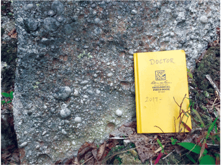
Photograph of a conglomerate at the base of the Price Formation in Monroe County, West Virginia. Photograph by Daniel Doctor, U.S. Geological Survey.
Much like the uppermost Foreknobs Formation, the lower part of the Price Formation is characterized by dark gray to reddish-brown marine and terrestrial strata that grades upward into terrestrial mudstones and sandstones. The mudstones in the upper part tend to be red and tan in color and the sandstones tend to be light gray. The top of the Price Formation is marked by a massive cross-bedded sandstone that is as much as 33 ft (10 m) thick (fig. 11).
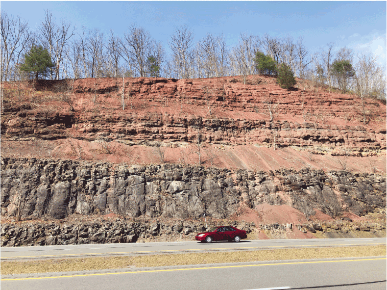
Photograph of massive sandstone at the top of the Price Formation overlain by red shales and mudstones of the Maccrady Shale in a roadcut along Interstate 64 just south of the Greenbrier River at Caldwell, West Virginia. Photograph by Daniel Doctor, U.S. Geological Survey.
Maccrady Shale (Mm)
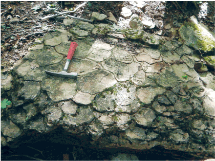
The Maccrady Shale is a distinctive red mudstone and shale with thin horizons of reduced iron content that exhibit a pale green color; root casts indicate paleosols are common at these greenish horizons (fig. 12A). The Maccrady Shale has calcareous beds throughout and contains vugs of calcite and gypsum (fig. 12B). Good exposures of the Maccrady Shale were observed along County Road 11 (Hillsdale Road) between Pickaway and Hillsdale. In southern Greenbrier County off of Route 219, the top of the Maccrady Shale is marked by a very thin, fine-grained calcareous unit that may be equivalent to the Little Valley Limestone; however, this same interval has not been observed in Monroe County because of the lack of exposure. The total thickness of the Maccrady Shale is approximately 363 ft (110 m).
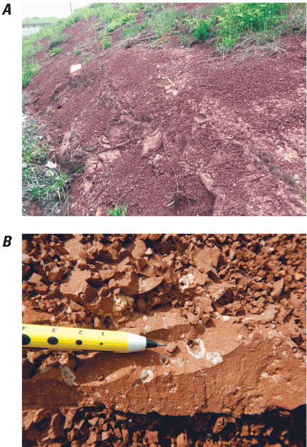
Photographs of A, red mudstone and B, red mudstone with calcite vugs in the Maccrady Shale along County Road 11 (Hillsdale Road), Monroe County, West Virginia. Photographs by Daniel Doctor, U.S. Geological Survey.
Hillsdale Limestone of the Greenbrier Group (Mgh)
The Hillsdale Limestone is primarily a cherty, argillaceous carbonate unit with a total thickness of approximately 330 ft (100 m). The lowermost part of the Hillsdale Limestone contains abundant black chert that often forms curled nodules. The upper two thirds of the formation do not appear to resist weathering in most of Monroe County and, instead, are found as light tan to orangish-yellow, clay-rich regolith with abundant chert nodules that are generally light in color, ranging from white to tan. Therefore, the topographic expression of the Hillsdale Limestone does not often exhibit distinct karst features even though this limestone contains some of the largest cave passages within the Greenbrier Group. A common marker fossil within the Hillsdale Limestone is the coral Lithostrotionella (which, when silicified, is the West Virginia state gem), although this fossil has not been observed by the authors in Monroe County.
Taggard and Denmar Formations of the Greenbrier Group, Undivided (Mgtd)
The Denmar Formation (Wells, 1950) is a unit composed of interbedded, light gray, oolitic limestones and thinner yellowish-tan shales. The lower part of the Denmar Formation is characterized by being predominantly massive limestone with abundant black chert nodules; the lower part was previously referred to as the Sinks Grove Limestone by Reger and Price (1926), but this unit was not formalized. The upper part of the Denmar Formation is composed of thick-bedded, fossiliferous, oolitic limestone and beige-to-tan calcareous shale; the upper part was previously referred to as the Patton Limestone by Reger and Price (1926), but the unit was not formalized. The upper part of the Denmar has at least three shale horizons that can be as much as 4 to 5 ft (1.2 to 1.5 m) thick and are generally light tan in color. Reger and Price (1926) described an interval of a “gray and highly calcareous but somewhat lenticular deposit, varying in thickness from 10 to 20 ft, when present, and separating the Patton Limestone from the Sinks Grove Limestone” (p. 483). Reger named this the Patton Shale, but noted, “It is named from association with the Patton Limestone but was not observed at the type locality of the latter” (Reger and Price, 1926, p. 483). Wells (1950) later redefined the Sinks Grove and Patton Limestones as the Denmar Formation, under protest by Reger (1950). During geologic mapping for this project, the authors could not distinguish a singular, mappable Patton shale, thus no discernible contact to define the Sinks Grove Limestone separate from the Patton Limestone was found. In fact, the authors of this study observed multiple discontinuous shales within this interval of strata, as did Reger and Price (1926, p. 482). We have, therefore, held to mapping the unit defined as Denmar Formation by Wells (1950).
The shale horizons within the Denmar are laterally discontinuous. One of them is well exposed in the back of Haynes Cave, as well as on the surface along the farm road leading to the cave entrance. This shale was mistaken for the shale in the Taggard Formation by Hirko (2012); instead, surface mapping demonstrates that this shale is within the lower part of the Denmar Formation. Between the shales are limestones that tend to be oolitic and highly fossiliferous. Good exposures of the Denmar Formation can be seen along Charles Booth Road in the eastern part of Monroe County, and along Hillsdale Road. The Denmar Formation is approximately 429 ft (130 m) thick in Monroe County.
The Taggard Formation is primarily composed of red calcareous shale and oolitic limestone, with calcareous sandstone at its base (fig. 13A). This formation had previously been described by Reger and Price (1926) as having an upper and lower shale separated by a limestone; however, detailed work in Monroe County has revealed those divisions to only be expressed locally. The thickness of this unit varies greatly and can be anywhere from 6.6 to 33 ft (2 to 10 m) thick where observed. A complete section of the Taggard Formation is exposed in a roadcut along County Route 43/1 on the west side of the Greenbrier River between Fort Spring and Frazier. Here the entire formation is approximately 30 ft (10 m) thick.
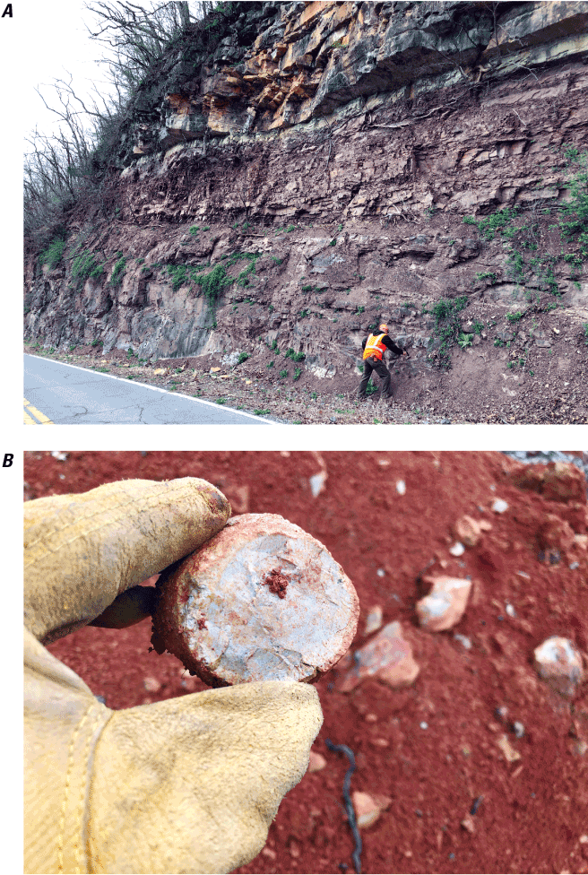
Photographs showing A, the complete exposure of the Taggard Formation and B, rusty red regolith with light-colored chert nodules on the Taggard Formation at an outcrop along County Route 43/1 between Fort Spring and Frazier in Greenbrier County, West Virginia. Scientist standing at the base of the unit, which is marked by blocky-weathering calcareous sandstone. The top of the formation is marked by a greenish shale, which is overlain by blocky overhanging ledges of the Pickaway Limestone. Photographs by Daniel Doctor, U.S. Geological Survey.
The unit is discontinuous, but where recognized the shale usually has a distinctive red color, but the shale can also be tan, or pale pinkish-green in color. Locally the Taggard Formation is expressed as a rusty red weathered shale regolith having abundant spheroidal chert nodules that are generally light in color from white to light tan, much like the upper part of the Hillsdale Limestone (fig. 13B).
At its type locality along Taggard Branch, the Taggard Formation has an interval of very light gray to white oolitic limestone that is approximately 5 ft (1.5 m) thick and is sandwiched between red and tan shales above and below. Exposure at the type locality is poor, but a complete section is visible along Route 3 approximately 3.2 mi (2 km) to the north. The base of the Taggard Formation is marked by a quartz-rich, reddish-brown calcareous sandstone that is traceable through much of the county and is at least 5 ft (1.5 m) thick but may be thicker in places (fig. 14).
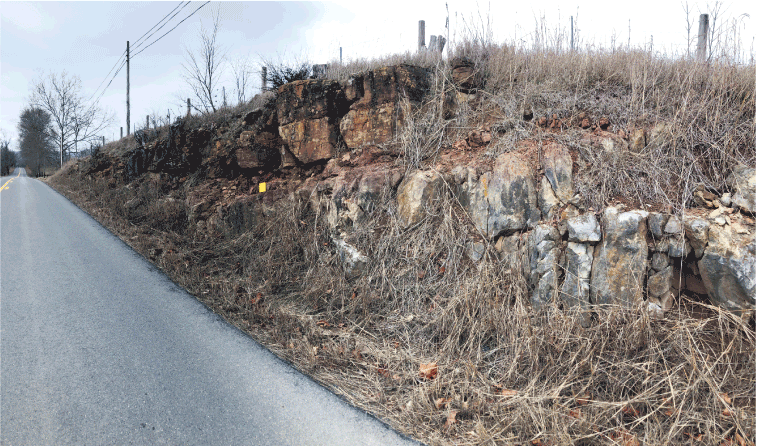
Photograph of a new reference section for the Taggard Formation along Route 13 on Willow Bend Road in Monroe County, West Virginia. Yellow notebook is resting on red shale layers with greenish blebs indicative of a paleosol. Photograph by Daniel Doctor, U.S. Geological Survey.
Pickaway Limestone of the Greenbrier Group (Mgp)
The Pickaway Limestone is a sequence of massive- to thin-bedded limestones and thin shales approximately 445 ft (135 m) thick. A variety of textures occurs within the Pickaway Limestone; however, the most distinctive texture is of vertical wavy fractures that are oriented vertically with respect to bedding and are often filled with secondary calcite and siliceous minerals (fig. 15).
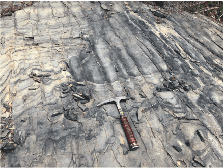
Photograph showing vertical fracturing within the Pickaway Limestone exposed along Wayside Road in Monroe County, West Virginia. This pavement type outcrop shows the exposed surface subparallel to bedding planes and cut by the parallel vertical fractures within the limestone. Photograph by Daniel Doctor, U.S. Geological Survey.
These vertical fractures appear to have formed in response to compressive forces and represent anastomosing cleavage in the rock. The zones of spaced, disjunctive cleavages are most often seen in the finer grained and laminated limestone beds that tend to cap cycles of fining-upward sequences. Four of these fining-upward sequences have been observed in the Fraser Quarry near the Greenbrier and Monroe County line where thin discontinuous shales separate each of the cycles. The shales are typically light beige or tan or pale green in color. The base of each of these cycles is characterized by coarse-grained, often fossiliferous limestones and packstones. The lower parts of these cycles tend to yield good outcrop in the formation and can easily be confused with fossiliferous grainstones of the overlying Union Limestone. The Pickaway exhibits abundant karst features at the land surface and contains caves. Solution channels are commonly visible in outcrops of the Pickaway Limestone, indicating that the formation is likely a water-bearing zone where saturated (fig. 16).
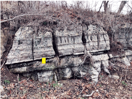
Photograph showing solution channels along vertical fractures in the Pickaway Limestone along Route 3 in Monroe County, West Virginia. Photograph by Daniel Doctor, U.S. Geological Survey.
Alderson Limestone, Greenville Shale and Union Limestone of the Greenbrier Group, undivided (Mgagu)
The Union Limestone is a medium-gray, massive, fossiliferous limestone throughout much of its thickness. The Union Limestone generally forms good outcrops expressed as whalebacks in the land surface (fig. 17).
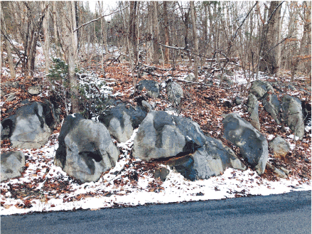
Photograph showing typical rounded whaleback outcrops near the base of the Union Limestone along Knobs Road, Monroe County, West Virginia. Photographs by Daniel Doctor, U.S. Geological Survey.
Solutional karst features and sinkholes are common within it, as well as large cave passages. The Union Limestone is approximately 347 ft (105 m) thick in Monroe County as measured along Knobs Road heading north and west out of the Town of Union. The top of the Union Limestone occasionally contains high-energy crossbeds with rounded eolian quartz grains that were reworked into the marine environment (fig. 18). Horn corals (fig. 19A) and crinoid stem fragments (fig. 19B) are commonly found within the Union Limestone; excellent exposures containing these fossils can be seen at the West Virginia University farm property north of Willow Bend.
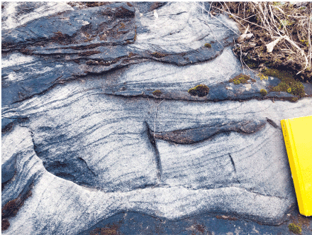
Photograph showing rounded grains and crossbeds near the top of the Union Limestone in Monroe County, West Virginia. Photograph by Daniel Doctor, U.S. Geological Survey.
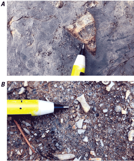
Photographs showing A, horn coral at Farming Smiles Farm and B, crinoid stem fragments in the Union Limestone in Monroe County, West Virginia. Photograph by Daniel Doctor, U.S. Geological Survey.
The Greenville Shale is a distinctive black shale that is from approximately 15 to 20 ft (4.5 to 6 m) at its maximum thickness and is discontinuous in Monroe County. The Greenville Shale was apparently misidentified at its type section near Greenville; the exposure at that locality has been determined through new mapping to be the Lillydale Shale Member of the Bluefield Formation. The Greenville Shale is lumped within the map unit Mgagu because it is too thin to map separately.
The Alderson Limestone is a medium gray, argillaceous, generally thin-bedded limestone that weathers to a yellowish-beige color limestone and generally does not provide good outcrop. Thickness of the Alderson Limestone is approximately 396 ft (120 m) as measured along Knobs Road (fig. 20). In central and western Monroe County, the Alderson Limestone may contain coarser-grained intervals that are cross-bedded and more massive (fig. 21).
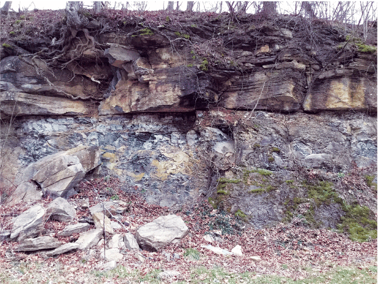
Photograph showing Alderson Limestone atop the Greenville Shale at Salt Sulphur Springs, Monroe County, West Virginia. Photograph by Daniel Doctor, U.S. Geological Survey.
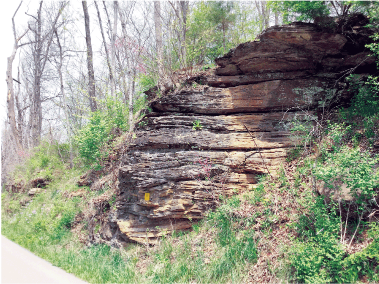
Photograph showing cross-bedded sandy-limestone near the base of the Alderson Limestone in Monroe County, West Virginia. Photograph by Daniel Doctor, U.S. Geological Survey.
The Alderson limestone does not contain significant caves; however, solutional features are observed along bedding plane partings and fractures. At least one interval of shale exists within the formation, but this shale unit has not been mapped with consistency through the county because of poor outcrop; however, good exposure can be seen along Knobs Road near the crest of the Knobs.
Bluefield Formation, Lower Part (Mbfl)
The Bluefield Formation is a heterogeneous unit composed of both siliciclastic and carbonate rocks. In this report, it has been subdivided informally into a lower and upper unit because the lower part contains the most carbonate. The lower part of the Bluefield Formation includes shale and siltstone of the Lillydale Shale Member at its base, the Glenray Limestone Member atop the Lillydale Shale Member, and extends upward through the top of the Reynolds Limestone Member. The thickness of the lower part of the Bluefield Formation is variable, thickening east to west from approximately 363 ft (110 m) along Knobs Road to 726 ft (220 m) on Wolf Creek Mountain.
The Lillydale Shale Member is a thick package of very dark gray to greenish-gray shale interspersed with zones of more resistant siltstones, calcareous and micaceous shale, and thin limestone beds. In places, the Lillydale Shale Member is a dark reddish-brown color and, in those intervals, contains a greater proportion of siltstone. The Lillydale Shale Member is utilized as a resource for shale fill and road spoil with numerous small quarries found scattered throughout the county. Good exposures can be found along Knobs Road. Nodules of iron carbonate (siderite) have been observed within the Lillydale Shale Member. Thickness varies from 80 to 130 ft (24 to 40 m).
The Glenray Limestone Member of the Bluefield Formation has about 20 ft (6 m) of coarse-grained, fossiliferous, dark-gray limestone that forms a conspicuous marker bed throughout the county (fig. 22).
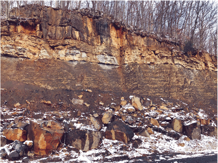
Photograph of the Glenray Limestone Member atop the Lillydale Shale Member along Knobs Road, Monroe County, West Virginia. Photograph by Daniel Doctor, U.S. Geological Survey.
The Reynolds Limestone Member of the Bluefield Formation is a sequence of interbedded calcareous shale and more massive fossiliferous limestone beds. Much of the Reynolds Limestone Member is argillaceous and does not yield good outcrop; however, it is expressed as a topographic bench throughout most of the county and can be discerned using the elevation models derived from lidar (fig. 23) The Reynolds Limestone Member has solutional channels formed along vertical fractures in the thicker limestone beds that may contribute to weakening of steeper slopes, making them prone to slump failure, and potentially a water-bearing unit where saturated.
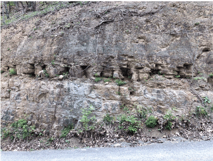
Photograph showing solutional channels along vertical fractures in the Reynolds Limestone Member at its type locality near the intersection of Raines Road and Johnson Crossroads in Monroe County, West Virginia. Photograph by Daniel Doctor, U.S. Geological Survey.
Between the Glenray Limestone Member and Reynolds Limestone Member is a sequence of generally brown to maroon-red siltstone, shale, and sporadic beds of thicker sandstone. The thickness of the lower Bluefield Formation is approximately 800 ft (244 m) in Monroe County.
Bluefield Formation, Upper Part (Mbfu)
The upper part of the Bluefield Formation is primarily fine-grained siltstone and shale grading upward into more massive sandstone beds. The upper part of the Bluefield thickens east to west from approximately 479 ft (145 m) along Knobs Road to 1,320 ft (400 m) on Wolf Creek Mountain. The first stratum overlying the shaly Reynolds Limestone Member is a fairly thick interval of red and greenish-grey shale, with minor interbedded siltstone and sandstone. Above this interval are two marker zones of sandstone that form benches in the topography.
The lowest sandstone above the red or tan shale is only from 3 to 4 ft (0.9 to 1.2 m) thick, with a maximum thickness of around 6 ft (1.8 m). It is very well sorted, with grain size that is upper very fine (0.095 to 0.125 millimeter [mm]), subrounded to rounded grains, with zones of Fe-oxide weathered out, and low angle cross-bedding that weather out to give the rock a ropy texture.
Above this thin sandstone is a sequence of olive-grey shale and siltstone, at least 30 ft thick. This is capped by a thicker sandstone (as much as 20 ft [6 m]), with similar character as the thinner one below it. Both are very fine, well-sorted sandstones, low angle crossbeds, with iron staining and concretions. The upper one of these sandstone packages may be equivalent to the Droop Sandstone Member of Reger and Price (1926); the lower sandstone package is as yet unnamed. Above this is some beige and red shale, until the sequence is capped by the coarser sandstone of the Stony Gap Sandstone Member of the Hinton Formation.
Stony Gap Sandstone Member of the Hinton Formation (Mh)
The highest stratigraphic unit exposed in Monroe County is the Hinton Formation, and what is exposed of this formation in the county is limited to exposures of the Stony Gap Sandstone Member, which is the lowest member of the formation (fig. 24). The Stony Gap Sandstone Member is a hard, light gray, very coarse to conglomeratic quartz sandstone. It varies in thickness but has been observed to be as much as 20 ft (6 m) thick. The Stony Gap is coarser and less well-sorted than the sandstones below it, possesses high-angle crossbedding, and weathers light gray. It forms distinct topographic mesas and ridges because it is more resistant to weathering.
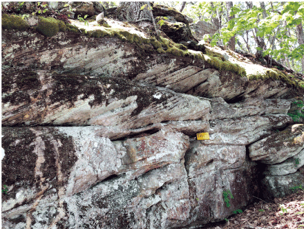
Photograph of an outcrop of the Stony Gap Sandstone Member of the Hinton Formation in Monroe County, West Virginia. Total height of exposure is at least 20 feet. Photograph by Daniel Doctor, U.S. Geological Survey.
Hydrogeologic Units
In Monroe County, the three principal hydrogeologic units and associated aquifer types are (1) carbonate rock units, (2) siliciclastic rock units, and (3) alluvial sediments. Each aquifer type has differing hydrogeologic characteristics based on lithology, solubility and permeability, or depositional history, and are discussed individually as follows. Jones (White, 2018a) states that insoluble beds within the Greenbrier Group may perch underground streams well above the apparent base level, and the underlying Maccrady Shale acts as an aquitard with several large caves developed along the contact of the shale and overlying Hillsdale Limestone. Jones further states that much of the study area can be considered contact karst with the clastic rocks providing recharge to the soluble limestones with underlying shales forcing the return of conduit water to the surface. Jones (White, 2018a) surmises that available data for water wells suggest that many wells are actually producing from shaley units with the limestones acting as confining units. Water-level and well-log data collected for this study indicate that perching of groundwater above low permeability beds occurs in certain areas of the county, but the density of available well data and, more importantly, associated well logs were insufficient to identify specific lithologies that control perching of groundwater within the study area.
Carbonate Rock Units
Two packages of carbonate strata of different age provide the principal bedrock aquifers within Monroe County. The first is a package of Ordovician carbonate rocks within an elongated valley at the northwest base of Peters Mountain situated structurally in the hanging wall of the St. Clair thrust fault and a second smaller exposure in the far southeast of Monroe County in the valley to the northwest of Potts Mountain (fig. 4). The units in this package and their abbreviations on the geologic map are the Beekmantown Formation (Ob), the Lincolnshire and New Market Limestones (Oln), the Big Valley Formation (Obv), the Moccasin Formation (Omoc), and the Eggleston Formation (Oeg). The overlying Reedsville Shale (Or) can be calcareous in certain zones and, thus, is mentioned here as some small springs on the northwest flank of Peters Mountain appear to have their source within the Reedsville Shale.
The second package of carbonates include the units of the Greenbrier Group. The Greenbrier Group limestones are collectively more than 1,000 ft (300 m) thick and provide productive bedrock aquifers for Monroe County. Carbonate units within the Greenbrier Group include the Hillsdale (Mgh), Denmar (Mgtd), Pickaway (Mgp), and Union and Alderson Limestones (Mgagu). Each of these units provides large water-bearing zones where solutionally enlarged fractures and bedding planes occur. The degree of solutional karst development is locally controlled by geologic structure and the prevailing hydraulic gradient. Local development of subsurface karst features is extremely difficult to predict given that karst aquifer development took place over hundreds of thousands or perhaps millions of years, so hydraulic gradients of the past do not necessarily reflect those of the present. Numerous caves in the county, their position, and their passage development provide insight into the regional karst aquifer and are summarized by White (2018a) and Dasher (2019). For example, caves often occur at the contact between the Hillsdale Limestone, which sits at the base of the Greenbrier Group, and the underlying Maccrady Shale; the contact between the formations is often targeted by well drillers seeking high yields of water for agricultural wells (fig. 5).
In addition to the principal carbonate aquifers within the belt of Ordovician carbonates in the southeast of the county and the Greenbrier Group, two thin zones of limestone within the Bluefield Formation are important carbonate aquifers. The Reynolds Limestone Member is a significant water-bearing zone and marks the top of the lower part of the Bluefield Formation. A dye-tracer test (Jones, 1997) documented water sinks at Green’s Cave that resurges at Indian Draft Cave about 0.6 miles south of Wayside and flows through the Reynolds and Glenray Limestone Members and emerges within the Alderson Limestone. The Glenray Limestone Member in the lower part of the Bluefield Formation is also another significant water-bearing zone that is between overlying and underlying low permeability shale layers.
Siliciclastic Rock Units
Three distinct packages of siliciclastic rocks are within Monroe County. The first is a package of younger Mississippian rocks in the western part of the county comprised of rocks within the lower and upper parts of the Bluefield Formation (Mbfu and Mbfl) and the Hinton Formation (Mh; fig. 4). The second is a package of older Ordovician, Silurian, and Devonian siliciclastic rocks in the eastern part of the county, east of the St. Clair thrust fault, which places older Ordovician, Silurian, and Devonian rocks over younger Mississippian rocks. This second package of siliciclastic rocks comprises Ordovician rocks of the Moccasin Formation (Omoc), Eggleston Formation (Oeg), Reedsville Formation (Or), Juniata Formation and Oswego Sandstone (Ojo), Silurian rocks of the Tuscarora Sandstone (St), Keefer Sandstone and Rose Hill Formation (Skr), Wills Creek Formation (DSls), Tonoloway Limestone (DSls), Oriskany Sandstone (DSls), and Huntersville Chert (DSls), and Devonian strata of the Millboro Shale (Dm), and lower part of the Brallier Formation (Db). The third is a package of Devonian and Mississippian rocks comprised of the upper part of the Brallier Formation (Db), Foreknobs Formation (Df), and the Price Formation (Mp; fig. 4).
These three siliciclastic rock packages are composed of various percentages of sandstone, shale, siltstone, and thin limestone. Data collected for this study was not sufficient to identify particular units within these three packages that contribute substantially to groundwater flow. However, secondary permeability resulting from bedding plane contacts, fractures associated with fold axes, joints, faults, and other secondary permeability features within the units provide most of the groundwater storage because these units are well cemented and primary porosity within the strata comprising the packages is negligible.
Ogden (1976) and Heller (1980) surmised that some wells that appear to be completed in limestone units may actually be producing water from shaley units within the Greenbrier Group or the underlying Maccrady Shale. Short circuiting of natural groundwater flow may occur where wells are drilled because open boreholes allow water from overlying aquifers to comingle with water in deeper aquifers, sometimes manifesting as flow into the ceiling of cave passages. Given that shale units are often highly fractured, it is entirely possible for shale layers to act as significantly productive aquifers. Even though a few wells were logged for this project, the lack of complex well logs, which include flow logs, stratigraphic logs, and mapping of specific bedding planes and fractures that produce water, makes mapping perched zones and their lithologic composition impossible at anything other than a local scale in the few places where well logs were collected for this study.
Alluvial Aquifers
Deposits of surficial sediments (fig. 4) are situated throughout Monroe County as the result of streams reworking detritus from weathered bedrock, slump deposits, landslides, and other erosional processes that have aggregated at the base of steeper slopes. Alluvial deposits along streams and alluvial fan deposits may be important aquifers in certain areas. For example, part of the water supply for the Red Sulphur PSD comes from a small spring box buried in colluvium high up on the slope of Peters Mountain at an elevation of 2,340 ft, which is fed by perforated infiltration lines buried within the colluvium (Baker, 2005). However, flow rates from this secondary, smaller source have not been reported, so the relative significance in terms of water quantity has not been assessed. The surficial colluvial deposits at this site cover fractured bedrock of the Reedsville Shale, and flow from the bedrock may serve to supply part of the spring flow at this and other small spring sites along the northwestern slope of Peters Mountain (see “Springs” section). In the lower valleys, alluvial terrace deposits in floodplains may also serve as shallow water sources. Such floodplain deposits are thickest in the floodplain of Potts Creek in the far southeast extension of the county near Waiteville along parts of the floodplain of Indian Creek, upstream from the confluence between Hans Creek and Indian Creek, and at the downstream end of Wolf Creek near the county boundary. No known wells tap these deposits.
Structural Geology
The geologic structure of Monroe County includes the transition from folding and thrust faulting of the Valley and Ridge Province in the southeastern part of the county to primarily upright folds of the Appalachian Plateau in the northwest. Two distinctive structural trends transition between the southern and central Appalachians in the study area. A southern Appalachian trend of folds and thrust faults strike N. 60° E. in the southern and southeastern part of the county, whereas a N. 30° E. strike occurs in the northern part of the county (figs. 4 and 5). The southern to central Appalachian transition is demonstrated on the geologic map of Monroe County (fig. 5) where faults and folds of the Valley and Ridge province bend more northerly in the northeastern most part of the county.
The structural features in Monroe County result from tectonic processes from past orogenic events, principally the Alleghenian orogeny that occurred from the Late Mississippian to Permian (Hatcher and others, 1989). Thrust faulting and folding formed synclines and anticlines that trend parallel to the thrust faults, and brittle fractures formed multiple joint orientations and cleavage because of the Alleghenian orogeny. The major geologic structure in Monroe County is the St. Clair thrust fault, a thrust fault zone that mostly trends N. 60° E. but bends more northerly near the northeast terminus of the county. From the hanging wall in the southeast to the footwall to the northwest, Ordovician carbonate and clastic rocks are overthrust onto Devonian and Mississippian rocks. The St. Clair thrust fault is a zone of imbricated thrusts within a zone as much as 0.75 mi wide. The northern end of the St. Clair thrust zone begins to terminate in the vicinity of Sweet Springs where deformation is accommodated by a series of folds and minor faults that extend into Allegheny County, Virginia. The complex structural deformation has allowed deep-circulating groundwaters that exhibit water temperatures elevated above ambient shallow groundwater as well as anomalous geochemistry to rise to the surface at Sweet Springs and Sweet Chalybeate Springs (Bausher, 2018; Vesper and others, 2022). At Zenith, the St. Clair thrust fault places Beekmantown Formation atop Tuscarora Sandstone and several large springs are associated with the fault (Vesper and others, 2022).
Several cross faults were recognized mainly in the footwall that probably resulted late during the orogenic events. These cross faults are mapped by an offset of stratigraphic units and structures. Some of the lineament features noted in the county may be faults. Among the most prominent is the Willow Bend fault, which offsets the Pickaway and Union limestones and is exposed in the road cut along Willow Bend Road at Willow Bend.
Broad asymmetric northeast trending folds of low plunge are dominant in the study area. Some of the more prominent folds from west to east are the Creamery syncline, Abbs Mountain anticline, Sinks Grove anticline, Hillsdale anticline, Dorr syncline, Highland anticline, Hollywood syncline, Harts Run anticline, Kates Mountain syncline, Glace anticline, Glen Lyn syncline, Pedro syncline, North Fork syncline, Forks Mountain anticline, Waiteville syncline, Back Valley Anticline, and Ray Syncline (fig. 5).
Bedding planes, joints, and cleavage within bedrock units may provide secondary porosity and permeability for storage and flow of groundwater. Fracturing of rock is associated with folds, especially those of high amplitude, and these fractures may be reservoirs for groundwater storage or result in increased permeability of the rock in proximity to the folds. White (2018a) stated that rocks within the Greenbrier Group are well-jointed. Many cave passages follow joint traces with guiding joints clearly visible in cave walls or ceilings, but other cave passages within low dip limestone units may develop along bedding planes (the most continuous fracture type) rather than vertical joints. North of Willow Bend in the Pickaway Limestone and the Denmar Formation, fracturing along folds controls cave passage development.
Hydrology
The hydrology of Monroe County is a result of the numerous structural, lithologic, physiographic, and topographic controls that have combined to form the groundwater and surface-water flow system in Monroe County. The groundwater hydrology of Monroe County was analyzed by examining (1) available well completion reports completed by well drillers as part of the State’s well-permitting process, (2) a countywide synoptic water-level survey resulting in a countywide potentiometric-surface map, (3) countywide synoptic-stream base-flow surveys to assess groundwater recharge, (4) borehole geophysical surveys to determine geologic controls on groundwater flow processes within the county, and (5) fluorometric dye-tracer tests to quantify groundwater flow rates and directions of flow.
Hydrogeologic Characteristics and Well Construction
Well completion reports completed by local well drillers as part of the water-well permitting process were retrieved from the Monroe County Health Department for 278 wells completed from 2008 to 2018 (app. 1). These well completion reports contain data on (1) the depth the well was drilled, (2) the length of casing placed in the well, (3) the yield of the well in gal/min, (4) the lithologic composition of the rock in which the well was completed, and (5) drawdown tests (for a subset of wells) that can be used to compute the specific capacity of the well (the discharge of the well divided by the drawdown resulting from pumping the well, in gallons per minute per foot [gal/min/ft]). Data for the 278 wells were parsed into two subsets, the first consisting of a subset of 220 wells completed in carbonate bedrock (predominantly limestone) and a second subset of 58 wells completed in non-carbonate siliciclastic bedrock (predominantly sandstone and shale).
Well Depths and Casing Length
Median, maximum, and minimum well depths for the 58 siliciclastic wells were 203, 700, and 60 ft, respectively, and median, maximum, and minimum well depths for the 220 carbonate wells was 340, 880, and 20 ft, respectively. The deeper median well depths for the carbonate wells is a result of well drillers often drilling for the geologic contact between the Hillsdale Limestone of the Greenbrier Group and the underlying Maccrady Shale for agricultural wells, which require a larger well yield than is necessary for a common residential homeowner well.
Wells drilled in the study area are typically completed as open holes, and screened intervals are rarely needed. Median, maximum, and minimum casing lengths for the 58 siliciclastic wells was 40, 108, and 20 ft, respectively, and median, maximum, and minimum casing lengths for the 220 carbonate wells was 40, 241, and 4 ft, respectively. The similarity in median casing lengths likely reflects a similar depth of weathered rock and regolith in the siliciclastic and carbonate bedrock within the county.
Well Yield and Transmissivity
Well yield, expressed in gal/min, and specific capacity, expressed in gal/min/ft of drawdown, are two common measures of a well’s ability to transmit water from an aquifer. Median, maximum, and minimum well yield for the 58 siliciclastic wells was 8.0, 80.0, and 1.5 gal/min, respectively, and median, maximum, and minimum well yield for the 220 carbonate wells was 10.0, 100.0, and 0.5 gal/min respectively. Median well yields of 8 to 10 gal/min are sufficient for a residential supply but are marginal for agriculture or public supply.
Transmissivity is a measure of an aquifer’s ability to transmit water and is expressed in cubic feet per foot of cross-sectional area of the aquifer per day (ft2/day). Transmissivity was computed based on borehole geophysical flow-meter data collected at 10 of the wells, 6 completed in siliciclastic rocks and 4 completed in carbonate rocks. The method used to analyze the well log data and compute transmissivity was the USGS Flow-Log Analysis of Single Holes (FLASH) software (Day-Lewis and others, 2011). FLASH uses fracture data identified in the boreholes using either an optical televiewer or acoustic televiewer and measurements of borehole flow made with an EM flowmeter to analyze data collected to analytically determine transmissivity. Results of the analysis indicate that most of the transmissivity in the wells analyzed is derived predominantly from shallow fractures in the upper 20 to 100 feet of the borehole, even though there can be multiple fractures within the borehole (table 5). Fracture data from the acoustic and optical televiewer logs are summarized in tables 6 and 7 and show most fractures within a borehole are not significant water-bearing fractures, and most water-bearing fractures are at shallower depths within the boreholes.
Table 5.
Fracture transmissivity for borehole geophysical surveys in Monroe County, West Virginia.[Data are from U.S. Geological Survey, 2019. Discrete fracture transmissivity analysis was performed on 10 boreholes using the FLASH software (Day-Lewis and others, 2011). USGS, U.S. Geological Survey; ID, identification number; ft, foot; gal/min, gallon per minute; ft2/d, foot squared per day; %, percent]
Table 6.
Site and well construction data for wells logged in Monroe County, West Virginia, in 2017 and 2018.[Data are from U.S. Geological Survey, 2019. USGS, U.S. Geological Survey; ID, identification number; ft, foot; in, inch; nd, no data; >, greater than]
Table 7.
Borehole geophysical information for wells logged in Monroe County, West Virginia, for 2017 and 2018.[Data are from U.S. Geological Survey, 2019. Dates shown as month–day–year. LSD, land-surface datum; ft, foot; USGS, U.S. Geological Survey; ID, identification number; —, not applicable; OV, optical video; OT, optical televiewer; CT, three arm caliper; ZE, gamma, long/short normal resistivity, spontaneous potential, single-point resistance, fluid resistivity, and temperature; MI, electromagnetic induction log; AT, acoustic televiewer; AS, acoustic porosity; FE, electromagnetic flowmeter; µS/cm, microsiemens per centimeter at 25 degrees Celsius; ft bls, foot below land surface]
Water Levels and Potentiometric Surfaces
A survey of synoptic water levels across Monroe County took place from October 23 to October 31, 2017. A total of 205 water levels were collected by USGS staff from 197 residential and agricultural wells and 8 springs. An additional 63 water levels were measured by USGS staff from August 18 to September 19, 2020, at 62 residential and agricultural wells and 1 spring. Flow conditions during the August to September 2020 sampling period at the Greenbrier River (Alderson, W. Va.) bordering the study area were similar to conditions measured during October 2017. Although wide coverage of the county was the primary goal of the survey, there was a focus on measuring water levels in karstic regions where surface water in streams is less prevalent and significant groundwater recharge to the underlying karst aquifer is a dominant process, with groundwater discharging to large karst springs and focused recharge occurring through sinkholes and losing stream reaches. Additional criteria for well selection included proximity to potential structural controls on the flow system (for example, Monitor lineament, geologic contacts, and so forth), well coverage in all the major watersheds, and availability of residential and agricultural wells.
Water levels were collected by one of four methods according to standard USGS procedures (Cunningham and Schalk, 2011). The first was by use of an electrical tape that has a sensor that buzzes and a light that illuminates when the sensor reaches the water table. Electrical tapes only were used where the depth to groundwater was shallow, typically less than 200 feet. A steel tape, or a narrow line coaxial electrical tape, was used to collect water levels in groundwater wells that contained wiring, drop pipe, drop-pipe centralizers, and (or) pumps. Steel tape measurements are less susceptible to becoming entangled in the wiring or wrapping around the drop pipe than is the larger probe found on most electrical tapes. For deep water levels, typically in excess of 400 to 500 feet, a sonic water-level instrument was used to ping a sonic signal off the water table. The timing of the return of the echo is then translated within the sonic sensor to display the depth to water. The accuracy of steel and electrical tapes is typically less than ±0.05 feet for the range of water levels measured for this study. The accuracy of water levels measured with either the narrow coaxial-type electrical tape or the sonic water-level meter was typically less than ±0.50 feet for the range of water levels measured for this study. Water-level accuracy was assessed by collecting water levels at a subset of wells using all four devices—the common larger diameter electrical tape and probe, the narrow diameter coaxial electrical tape, the sonic water-level meter—and then comparing them to steel tape measurements, which were the most accurate of the four methods used during the study. The overall error of the measurements was well within the tolerance typically required for developing potentiometric surface maps, such as the one presented in this report.
Additional information collected during the synoptic water-level survey included GPS determined latitude and longitude, overall depth of the well, and length of the well casing if documented on the well cap or if reported by the landowner. Information on casing lengths was limited, but 217 of the 259 (84 percent) wells measured had documented well depths.
A countywide potentiometric surface (water-table) map (fig. 25) was constructed from the synoptic survey water-level measurements made in October 2017 and August and September 2019, and from spring locations and stream elevations from the USGS National Hydrography data (U.S. Geological Survey, 2018). Elevation values were interpolated using a natural neighbor algorithm within the ArcGIS Spatial Analyst toolset (Esri, 2022). The potentiometric surface map prepared for this study was based on composite head water-level measurements within open boreholes. As a result, the map provides a fairly accurate assessment of the water table within the county but does not have the capacity to assess perched aquifers which can occur locally at specific isolated areas within the county. Regardless, the map may be used to identify directions of groundwater flow and, in conjunction with results of groundwater tracer tests, can be used to better assess and document the extent of local karst basins. The potentiometric-surface contours were also used to redefine and more accurately delineate the groundwater basins within the Greenbrier aquifer (fig. 26).
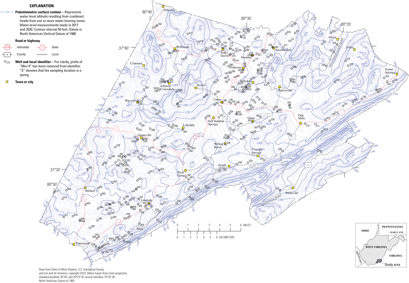
Potentiometric-surface map (50-foot contour interval potentiometric surface map) for Monroe County, West Virginia.
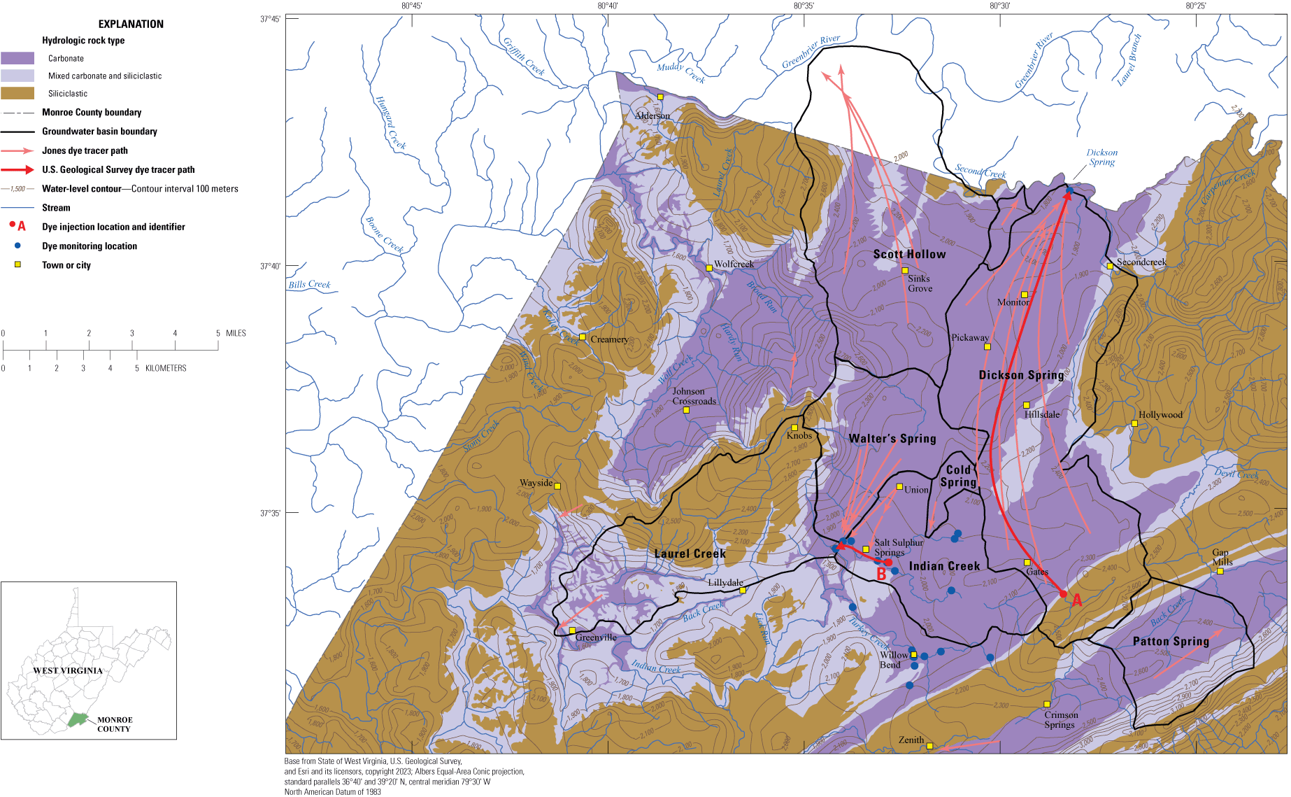
Map showing locations of dye injection and monitoring points for two recently completed tracer tests, dye vectors from previously completed tracer tests (Jones, 1997), previously identified basins modified based on tracer tests, and the countywide water-table map developed for the study.
Limitations of the Potentiometric Surface Map
The approach to create the potentiometric surface map has one major assumption. This assumption is that the entire Monroe County aquifer system can be modeled as an unconfined aquifer, such that surface-water features are visible representations of that aquifer. This is a particularly significant assumption for the Greenbrier aquifer, where the presence of separate aquifers above and below the Taggard Formation had been postulated (Ogden, 1976). The major problems, both historically and in this work, with delineating separate aquifers is twofold. First, there is a lack of detailed stratigraphy for the separate Greenbrier units, with very few detailed geologic logs or borehole geophysical well logs for wells completed in Monroe County. Second, it is unclear which unit any given well is drilled into in the Greenbrier because of either missing information on well depth or an open borehole well where multiple units contribute water to a given well. These two issues do not preclude the use of well data in reconstructing a potentiometric-surface (water-table) map of the Greenbrier karst of the Appalachian Plateau nor of the Ordovician karst of the Valley and Ridge; it does, however, open the possibility that any anomalous points of water-level elevation might be due to this major assumption being broken.
The potentiometric-surface map (fig. 25) therefore represents a combined heads map representing water levels from multiple water-bearing zones of varying potentiometric head within the aquifer. The potentiometric-surface map essentially represents a subdued replica of topography. However, the Greenbrier aquifer is much more complex because there is a drainage divide between the northern Greenbrier Valley and Indian Creek. An additional confounding factor is that there is a possibility that some mapped springs and shallow wells are representative of shallow perched or phreatic subsurface streams or springs representing discharge from epikarst (Williams, 2008). Epikarst is defined as the near-surface karstification that has the tendency to produce perched aquifers above major water-bearing formations. For example, Mnr–0183 and Mnr–0184 are less than 400 feet apart with over 100-foot difference in hydraulic head. The former well, Mnr–0183, has no documented well depth, and, if significantly different in depth, could explain why the water levels are so different.
Well completion reports (app. 1) obtained from the Monroe County Health Department in Town of Union, W. Va., indicate that many wells are drilled as uncased or partially cased wells, often penetrating multiple water-bearing fractures, bedding planes, or subsurface water-filled cave or solution conduits. Upon completion of these type of wells, the water level will eventually equilibrate. The combined head often represents the overall head in the aquifer associated with the predominant water-bearing zone. As such, the potentiometric-surface map can be used to infer directions of groundwater flow, to map subsurface groundwater divides, and to assess the depth to groundwater within specific areas of the county. The issue related to multiple water-bearing zones is common in the fractured-rock aquifers typical in West Virginia but can be more problematic for karst aquifers, such as that within the Greenbrier. For this study, mapping of individual water-bearing zones or perched aquifers associated with specific geologic units within the Greenbrier Group was not possible, even given the large number of wells measured for this investigation.
Monitoring of Groundwater Levels and Streamflow
Groundwater-level conditions were monitored at 15-minute intervals using a submersible pressure transducer instrumented in an unused 6-inch, 129-foot-deep water well (fig. 27) at the West Virginia University agricultural research farm, south of the Town of Union, W. Va. Groundwater-level data were collected during the course of the study from December 12, 2017, through December 31, 2020. Groundwater-level data collection continues to be collected at well Mnr–0162, and all data are available on the internet interface to the USGS NWIS database (U.S. Geological Survey, 2019).
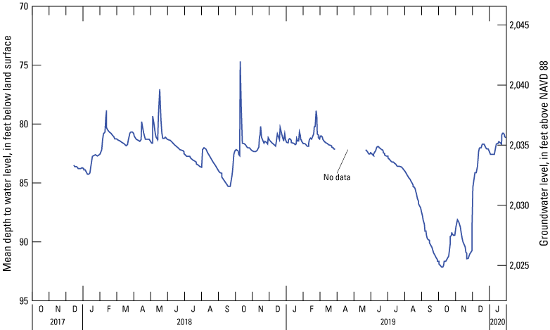
Hydrograph of groundwater levels for U.S. Geological Survey station name Mnr–0162 at the West Virginia University agricultural research farm south of Town of Union near Willow Bend, West Virginia, for the period December 12, 2017, through January 31, 2020.
Streamflow data for the Indian Creek at Red Sulphur Springs, W. Va., gaging station (USGS site 03177480) were collected for the period of study from December 1, 2017, through January 31, 2020 (fig. 28). Neither the groundwater-level data for the Monroe County monitoring well (Mnr-0162) nor the streamflow data for the Indian Creek at Red Sulphur Springs, W.Va., gaging station provide context as to what would be considered normal, above normal, or below normal flow conditions. To provide the needed context to assess flow conditions for the sites established for the study, streamflow records for the Greenbrier River at Alderson (USGS site 03183500) were analyzed (fig. 29). Data for both stream-gaging stations and the monitoring well are available through the USGS National Water Information System database (U.S. Geological Survey, 2019).
The period of record for the Greenbrier River at Alderson gaging station dates back to 1895 and runs through the present, so comparing streamflow conditions at the Indian Creek at Red Sulphur Springs gaging station (USGS site 03177480) and groundwater levels for the Monroe County monitoring well (Mnr-0162) for the period of the study to the long-term record for the Greenbrier River at Alderson, which is immediately east of the study area, provides a good context to what is considered normal, below normal, or above normal. The 10th, 25th, 50th, 75th, and 90th percentiles of flow for the Greenbrier River at Alderson, W. Va., are 145; 315; 956; 2,340; and 4,830 cubic feet per second (ft3/s), respectively. The 25th to 75th percentiles of flow represent normal flow conditions, values less than the 25th percentile of flow represent below normal flow conditions, and values exceeding the 75th percentile represent above normal streamflow conditions (fig. 29). Initial groundwater measurements, made when the study began in 2017, were at a time when streamflow and concurrent groundwater base flow for the study area were below normal. Just a few weeks later, however, precipitation began, and streamflow conditions rose into the normal and above normal range for most of the study through June 2019. Then, for the period from July to early November 2019, streamflow conditions dropped to below normal, and the area was amid a moderate drought. Precipitation returned in late November and streamflow conditions returned to a more normal range.
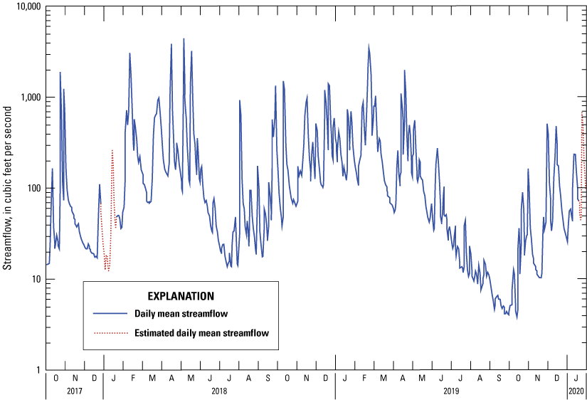
Hydrograph of streamflow at U.S. Geological Survey streamgaging station 03177480 on Indian Creek at Red Sulphur Springs, West Virginia for the period October 1, 2017, through January 31, 2020.
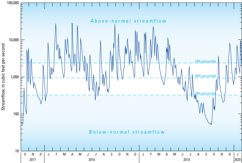
Hydrograph of mean daily streamflow for the Greenbrier River at Alderson, West Virginia for the period of October 1, 2017, through January 31, 2020, with 25th, 50th, and 75th flow-duration values showing above and below normal periods of streamflow.
Given the context provided by the long-term data for the Greenbrier River at Alderson, W.Va., gaging station (fig. 29), daily groundwater-level data (fig. 27) indicate that groundwater levels were near normal at the start of the study in December 2017. Abnormally high precipitation early in the study created higher water-level conditions for most of 2018 and into 2019, then dropped to below normal levels and into a mild drought condition in summer and fall 2019, before returning to above normal groundwater-level conditions in December 2019, maintaining those levels through the summer 2020. Groundwater levels returned to more normal conditions in fall 2020. These data are valuable for contextualizing the data collected for this study with respect to normal, below normal, or above normal flow conditions, especially for assessment of the base-flow and stream data to be discussed later in the report. Another observation from examination of the hydrograph (fig. 27) is that groundwater levels can have a pronounced short-term response to precipitation events, as is evidenced by the large value peaks on several days, but groundwater levels quickly recede to base-flow levels.
Dye-Tracer Tests
Two fluorometric dye-tracer tests were started on July 10, 2019. Water levels were under base-flow conditions, indicative of a time interval when streamflow was predominantly comprised of groundwater discharge and remained so for the duration of the monitoring period for both tracer tests. Data for the two tracer tests are presented in tables 8 and 9 and are also available as a USGS data release (Jones and others, 2023). One pound of fluorescein sodium (powder) was injected in Taggart Branch that was sinking in its bed near the contact between the Maccrady Shale and Hillsdale Limestone (dye injection location A on fig. 26). Flow upstream from the losing reach was 0.031 ft3/s. This selected injection site is consistent with the injection site used by Jones (1997). Nineteen locations in the Indian Creek watershed were monitored for two months after the start of the test, but no fluorescein was detected in the Indian Creek watershed (fig. 26; table 8).
Table 8.
Fluorescein concentration data (Jones and others, 2023) for select samples collected in Monroe County, West Virginia, in August and September 2019.[Dates shown as month/day/year; time given in military time. μg/L, microgram per liter; μg, microgram]
Water samples from Dickson Spring were collected three times per day using an ISCO automatic sampler and documented the first measurable dye recovery on August 9th, 2019 (29 days from dye injection; fig. 30). The highest measured dye concentration was on August 14 (35 days from the start of the test; fig. 30). Sampling was stopped on September 3 (55 days from dye injection) although dye was still in the spring at low concentrations. Discharge was measured at 6.87 ft3/s at Dickson Spring on August 26, and this was used as an average flow to estimate percentage recovery of the mass of injected dye. The percentage dye recovery at the end of the monitoring period was 8.72 percent of the injected mass. This dye-tracer test was conducted under very low-flow conditions that, in addition to the distance from the sink point to the resurgence 9.4 miles to the north in straight-line distance, contributed to a long travel time. The average velocity for the tracer was 1,710 feet per day assuming a straight-line distance of 9.4 miles from sink to spring and the first arrival of the tracer at 29 days from the start of the test. The apparently low recovery of the tracer is probably a function of dye moving into stagnant storage zones with falling water levels, the long travel time, and distance from the sink to the spring. Fluorescein was not detected at any of the other monitoring locations. Based on potentiometric-surface contours and geologic contacts, the geologic contact between the Hillsdale Limestone and underlying Maccrady Shale was theorized to be the most probable flow path for the tracer test.
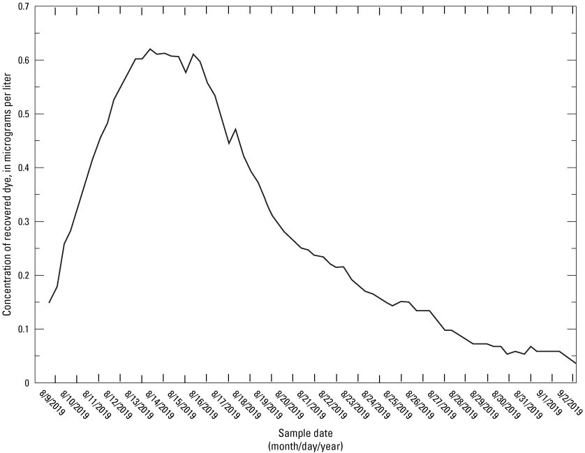
Line graph showing fluorescein dye recovery of injected mass of dye at Dickson Spring, Monroe County, West Virginia, for the period of peak dye recovery for the fluorescein dye tracer test conducted in the summer 2019.
One liter of Rhodamine WT (liquid, 20 percent solution) was injected in a sinking reach of Burnside Branch upstream from the Burnside Branch entrance to Steels Cave south of Town of Union (dye monitoring location B on fig. 26). Streamflow in Burnside Branch was 0.378 ft3/s at the start of the test. The water from Steels Cave resurges in a pond created by a dam at the head of Indian Creek. The Rhodamine tracer was first detected in the pond at the head of Indian Creek one day after dye injection and then downstream in Indian Creek at Salt Sulphur Springs two days after dye injection (fig. 31; table 9). The dye recovery in downstream Indian Creek is assumed to be entirely from the outlet at the head of the creek. No dye was detected in any of the other springs discharging into Indian Creek between the head spring and Salt Sulphur Springs. The springs at the old Salt Sulphur Springs spa have little flow and appear to be highly mineralized water from a deeper aquifer system. Assuming a straight-line distance of 0.36 miles from the sink to the resurgence, the average velocity for the tracer was 1,900 feet per day.
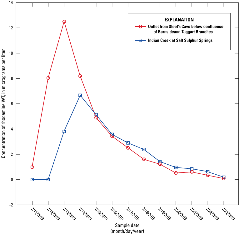
Line graph showing Rhodamine WT dye recovery at pond below the confluence of Burnside and Taggart Branches and Steel’s Cave near Salt Sulphur Springs and in Indian Creek at Salt Sulphur Springs, Monroe County, West Virginia, for the Rhodamine WT dye-tracer test conducted in the summer 2019.
Grab samples of water from Indian Creek at the head pond and at Salt Sulphur Springs were collected once per day for two weeks after dye injection. Collected water samples were analyzed for Rhodamine WT and plots of the dye concentrations are presented in figure 31. About 71 percent of the injected mass of the dye was recovered, as calculated based on an average streamflow of 0.84 ft3/s for Indian Creek during the recovery period.
Table 9.
Rhoadmine WT fluorometer concentration data (Jones and others, 2023) for tracer test conducted in Monroe County, West Virginia, July 2019.[Dates shown as month/day/year. µg/L, micrograms per liter; µg, microgram]
Karst Basin Delineation
Based on previous dye-tracer tests, groundwater basins were estimated within Monroe County (Jones, 1997). This study revised those estimates (fig. 26) based on two additional dye-tracer tests and the countywide potentiometric-surface map developed for the study (fig. 25). The countywide potentiometric-surface map was especially useful for revising the previously identified karst basins, as it provided additional constraints on the groundwater divides among the respective groundwater basins.
The karst basins assessed are shown in figure 26 and match both the tracer tests conducted (for this and previous studies) and the groundwater divides as identified on the countywide potentiometric-surface map. These identified groundwater basins and the countywide water-table map provide valuable data that may be used to assess potential directions of groundwater flow in the event of an unanticipated contamination event and for managing water availability and use in the basins.
Borehole Geophysics
Seven different borehole geophysical tools, including (1) a 3-arm caliper, (2) EM induction tool, (3) an EM flowmeter, (4) an acoustic televiewer, (5) an optical televiewer, (6) a multiparameter (resistivity, spontaneous potential, and natural gamma) e-logging tool, and (7) a full wave sonic porosity tool, were available for investigating subsurface geologic structural and lithologic controls on groundwater flow processes. Borehole geophysical investigations of 15 wells (fig. 32) were conducted during this study, with multiple borehole geophysical tools being used on the logged wells. Data collected for the borehole geophysical surveys are summarized in table 7 with accompanying lithologic interpretations. Original logs are available at the USGS GeoLog Locator (https://webapps.usgs.gov/GeoLogLocator/#!/).
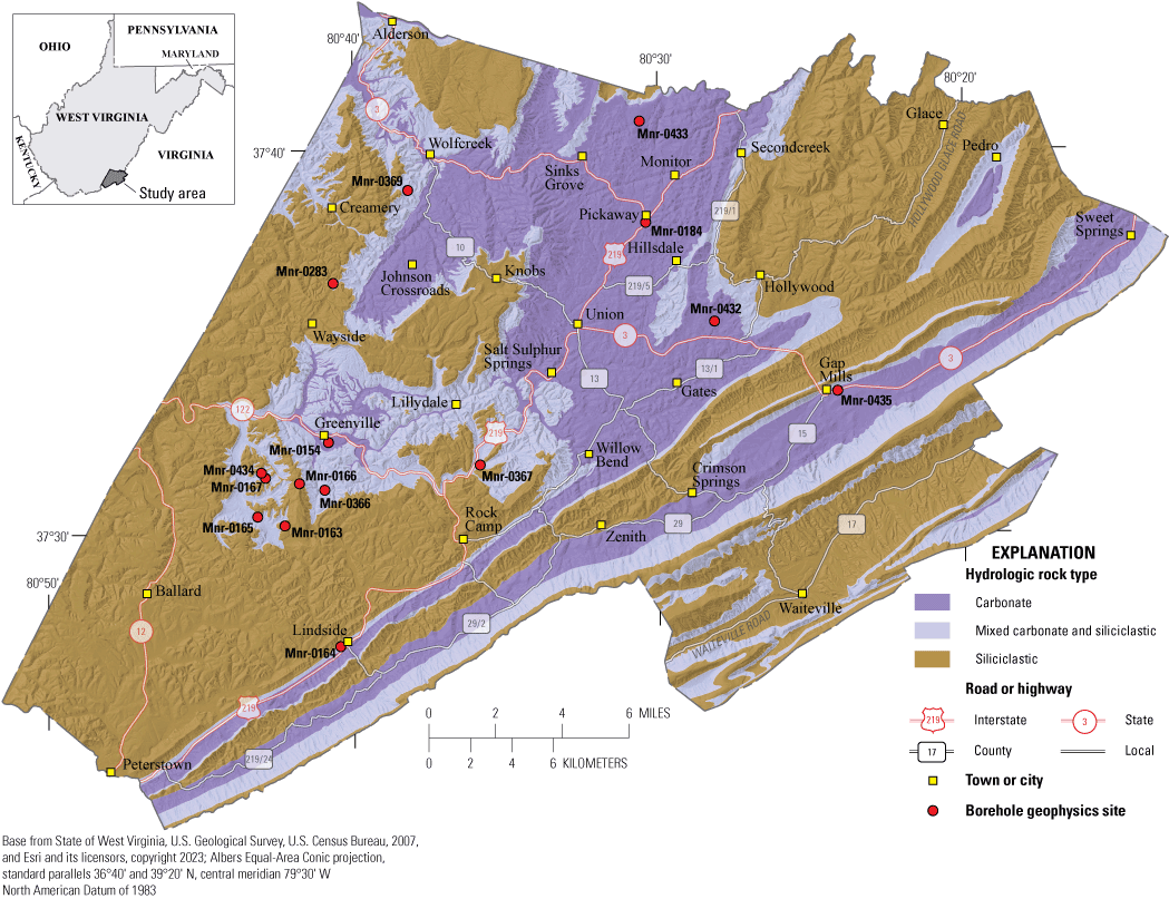
Map showing the location of 15 wells logged for borehole geophysical data in Monroe County, West Virginia.
The bedrock in Monroe County comprises sedimentary sequences of sandstone, shale, and limestone as well as various intermediate composite strata representing gradations from these dominant rock types, including argillaceous or shaly sandstone, argillaceous or shaly limestone, calcareous shale, and siltstone. Other than shale, none of the rock of the various lithologies contain any appreciable primary porosity. Although the shale can have moderately high porosity, the effective porosity of the shale is limited because of the small pore size between the silt and clay grains, which are so small as to preclude yielding significant water to wells. Because primary porosity and permeability of bedrock in the study area is limited, most of the water within an aquifer is stored and moves through open secondary porosity features, such as bedding plane partings, faults, joints, and cleavage. Many of these secondary fractures are cemented with calcite or silica cement, and only a few of the mapped fractures are actually water bearing. Mapping the extent of these fractures within the aquifer is necessary to understand groundwater flow processes dominant within the aquifer.
Relation of Lithology to Groundwater Flow
Borehole geophysical surveys documented 492 fractures within 4,646 feet of borehole in 14 of 15 wells logged for the study (one log did not map borehole fractures), resulting in a distribution of approximately 1 fracture per each 9.4 feet of borehole. The number of water-bearing fractures (tables 6 and 7), however, was much lower with only 28 of the 492 fractures, or 5.7 percent of all mapped fractures determined to be water bearing. This very low overall distribution of water-bearing fractures emphasizes the importance of understanding controls on fracture occurrence and distribution within the aquifer.
For water-bearing fractures, 7 were mapped in limestone units, 3 were mapped in argillaceous sandstone units, 3 were mapped in shale units, 3 were mapped in sandstone units, 1 was mapped in a siltstone unit, 6 were mapped in a sandy or silty shale unit, and 5 were mapped in argillaceous limestone units. Thus 12 of 28 (42.9 percent) water-bearing fractures were associated with limestone or argillaceous limestone units, 6 of 28 (21.4 percent) were associated with sandstone or argillaceous sandstone units, and 10 of 28 (35.7 percent) were associated with shale, sandy or silty shale, or siltstone units. The high proportion of water-bearing fractures associated with shale dominant units was unexpected as most of the water-bearing fractures were anticipated to be derived from limestone dominant units. This is likely because of the distribution of wells logged, as most wells logged (10 of 15) were in the Bluefield Formation (5 in the upper and 5 in the lower Bluefield Formations), which is dominated by sequences of sandstone and shale and only contains a few thin limestone units. However, shale units are easily fractured by tectonic stress and by stress relief and other compressive and tensional stress and, as such, are not necessarily aquitards but can yield sufficient water for residential supply, making them productive aquifers.
If we assess the fracture distribution for the karst limestone forming units, four of which are in the Mississippian Greenbrier Group, the (1) Hillsdale Limestone, (2) Taggard and Denmar Formations, (3) Pickaway Limestone, and (4) Alderson Limestone-Greenville Shale- Union Limestone, and with one in the (1) the Ordovician Beekmantown Formation, 201 total fractures were mapped, with 12 of 201 (6 percent) being identified as water-bearing fractures. This is similar to the distribution of water-bearing fractures in the more sandstone and shale dominated Bluefield Formation with 16 water-bearing fractures (5.5 percent) out of a total of 291 mapped fractures. For the karst water-bearing fractures, 5 were in argillaceous limestone units, 4 were in limestone units, and 3 were in argillaceous sandstone units. Thus, 9 of the 12 water-bearing fractures in karst limestone lithologies were in calcareous, potentially karst-forming, units.
Relation of Geologic Structure to Groundwater Flow
Mapping of the strike and dip of fractures can provide insight into potential structural controls on groundwater flow. Relatively flat lying to slightly dipping fractures (0 to 25° dip) are more commonly associated with bedding plane partings, while higher angle fractures are commonly associated with joints or faults. Figure 33A and B shows the poles to planes stereographic projection of the dip and azimuth of fractures mapped using borehole geophysical methods in Monroe County, W. Va., and figure 34 is rose diagrams showing the azimuth of the mapped fractures. Data collected for the borehole geophysical surveys are summarized in table 7 with accompanying lithologic interpretations. Original logs are available at the USGS GeoLog Locator (https://webapps.usgs.gov/GeoLogLocator/#!/).
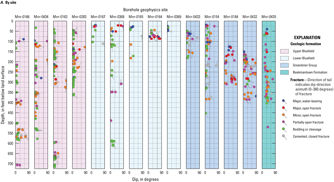
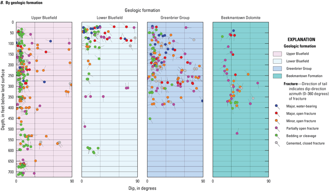
Tadpole plots showing A, the dip (0 to 90°) and dip direction azimuth of fractures mapped in 15 wells logged in Monroe County, West Virginia, and B, fracture data for the same 15 wells showing dip (0 to 90°) and dip direction azimuth of the fractures mapped aggregated by geologic formation.
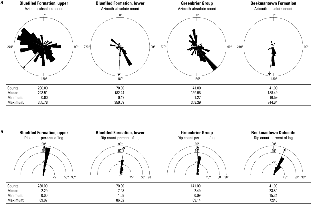
Rose diagrams showing A, the primary azimuth of mapped fractures in 14 wells logged in Monroe County, West Virginia, and B, the dip direction azimuths for the various fractures mapped in Monroe County aggregated by geologic formation.
Although the orientation (dip and dip azimuth) of fractures varies locally because of folds (anticlines and synclines) and variation in bedrock dip across the county, assessment of the fracture data can provide significant insight into the nature of fractures within the bedrock of various geologic formations within the study area. Figure 33A and B shows the fractures mapped in 15 wells logged in various geologic formations and areas within Monroe County. Most of the water-bearing fractures (identified as blue dots on fig. 33A and B) are primarily shallow features, less than 375 feet below land surface with the majority less than 200 feet in depth. The dip of the fractures varies greatly, with fractures less than 15 degrees being associated primarily with bedding planes. Higher angle fractures are likely a result of joints within the bedrock except for the fractures mapped in well Mnr–0435. Mnr–0435 is completed in the Beekmantown Formation along the St. Clair thrust fault and the fractures mapped in this well likely reflect the general dip of the thrust fault in the Ordovician limestone belt in the eastern part of the county.
Fracture data gathered from the borehole analysis and grouped by geologic formation revealed similarity in patterns of fractures (fig. 33A and B). These fracture data not only indicate the predominance of bedding plane partings on fracture distribution within the lower and upper parts of the Bluefield Formation (dip less than 20°) but also document that the Greenbrier Group has a high concentration of high angle fractures (60° to 90°) and that the dip of the St. Clair thrust fault influences the data for the well logged in the Beekmantown Formation. Rose diagrams show the dip azimuth direction (fig. 34A) and overall count and dip magnitude (fig. 34B) for the fracture data aggregated by geologic formation. There is a strong dip azimuth orthogonal to bedrock strike (fig. 34A) to the northwest and southeast for fractures mapped in the Greenbrier Group and the upper and lower parts of the Bluefield Formation, which is expected. Fracture azimuth data for the well logged along the St. Clair thrust fault in the Beekmantown Formation, however, indicate a dip direction predominantly to the south. The number of fractures and magnitude of the dip (fig. 34B) show similar trends to that of the tadpole plots, with mean dip typically less than 8° for the lower and upper parts of the Bluefield Formation and the Greenbrier Group, and corresponding higher distribution of steeper mean dip (23.8°) for the fractures within the Beekmantown Formation.
Base-Flow Stream Surveys
In September 2019, a synoptic streamflow survey of select large headwater streams was conducted in Monroe County, W. Va. (app. 2). Streamflow was measured at a total of 70 streamflow sites and 13 springs (fig. 35). Streamflow was divided by the respective surface-water basin area to determine streamflow yield per unit area of the surface watershed (app. 2) and reported as cubic feet per second per square mile ([ft3/s]/mi2) of drainage area. The synoptic streamflow survey was conducted during a drought period and could not be postponed until a later date given the timeframe of the study. As a result, 19 of the 83 sites identified for measurement of streamflow or spring discharge were dry (no flow).
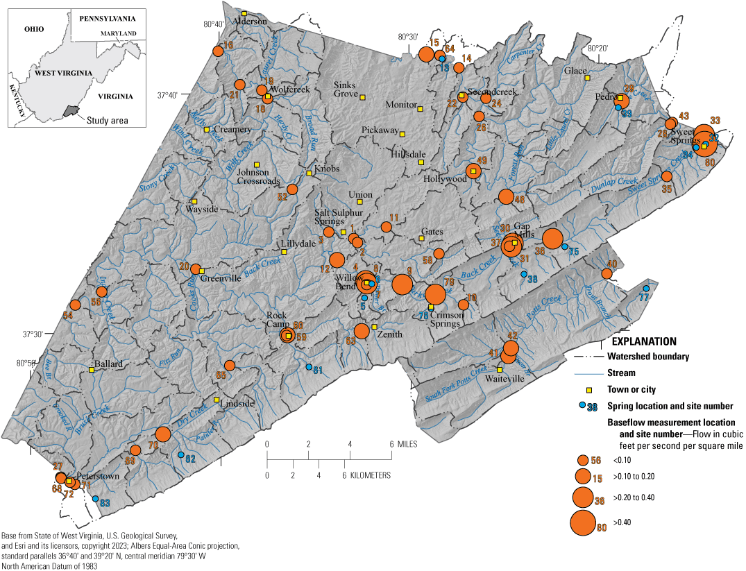
Map showing distribution of 70 streamflow and 13 spring locations at which streamflow or spring discharge was measured in Monroe County, West Virginia in September 2019. Some watersheds extend beyond county boundaries. Data plotted on this map are from appendix 2 and are also available from the U.S. Geological Survey National Water Information System database (U.S. Geological Survey, 2019).
Relation Between Groundwater and Surface Water
Because the synoptic streamflow and spring survey was conducted in the midst of a moderate seasonal drought, all streamflow and spring discharge was derived from groundwater base-flow contribution to the springs or tributary streams. Measured streamflow, for those sites with measurable flow, was highly variable and ranged from 0.001 to 11.7 ft3/s (app. 2). Measured unit streamflow yield for those sites with measurable flow was also highly variable, ranging from a minimum of 0.0001 (ft3/s)/mi2 to a maximum of 4.21 (ft3/s)/mi2. For the watersheds containing more than 50 percent karst bedrock in their recharge areas, median streamflow yield was 0.028 (ft3/s)/mi2, and for watersheds containing less than 50 percent karst bedrock, median streamflow yield also was 0.028 (ft3/s)/mi2. Therefore, type of bedrock does not seem to be the controlling factor affecting variability in unit streamflow yield. Higher base-flow yields appear distributed in the streams at the base of Peters Mountain emerging from the Ordovician age limestone units (figs. 5 and 35) and lower base-flow yields appear for streams emerging from areas dominated by the Upper and Lower Bluefield Formations. A base-flow synoptic-survey conducted during more normal or high streamflows and groundwater level conditions would result in higher (ft3/s)/mi2 streamflow yields. Regardless, the uniform 0.028 (ft3/s)/mi2 median streamflow yield provides a lower statistic for assessing water availability for similar drought conditions.
Disappearing streams in Monroe County also complicate the understanding of streamflow distribution. Near Greenville, Hans Creek completely sinks into the Alderson Limestone and emerges approximately 600 meters downstream. Also, in the Greenville area, Laurel Creek completely sinks twice and reemerges in Indian Creek. Such disappearing streams are not common in Monroe County, so overall streamflow yield can be estimated effectively. Since the watersheds and basins for the groundwater basin map (fig. 26) and the base-flow measurement map (fig. 35) do not coincide, interbasin transfer of groundwater is occurring within the karst, as would be expected; therefore, the groundwater basin map is more reliable for assessing groundwater flow than the base-flow delineated surface-water subwatersheds.
Water-Bearing Zones
Well completion reports, borehole geophysics, and geologic mapping provided data for assessment of potential water-bearing zones in Monroe County. Three principal and several secondary water-bearing zones are within the bedrock aquifers of Monroe County. The most relied upon water-bearing zone with respect to current [2023] public water supply is from springs along Peters Mountain. These springs are derived from intervals of fractured sandstone and resultant alluvial deposits. Groundwater flows downslope through these permeable alluvial deposits and discharges at the contact with less permeable strata, such as the Reedsville Shale.
The second most relied upon water-bearing zone in Monroe County is within the karstic Greenbrier Group aquifer, in which the basal Hillsdale Limestone overlies the less permeable Maccrady Shale. This geologic contact between the Hillsdale Limestone and the Maccrady Shale is not only targeted as a source of water for agricultural supply (Dewey Broyles, U.S. Department of Agriculture Natural Resources Conservation Service, oral commun., 2019) but also is targeted as a source of water for residential supply.
The third most relied upon water-bearing zone is shallow perched aquifers within the Greenbrier Group. The discontinuous nature of these perched aquifers makes mapping their extent impossible, but they are related to permeable geologic strata, such as karstic solutionally enhanced permeable limestones, which overlie less permeable shale or chert bedrock. Several of these perched aquifers were documented during geologic mapping of the county and were present in the Pickaway, Union, and Alderson Limestones.
The fourth water-bearing zone is contained within the karstic Ordovician carbonates in the valley at the northwestern base of Peters Mountain. This karst aquifer is fed by flow originating at higher elevations on Peters Mountain within fractured sandstone aquifers with intervening layers of permeable limestone and less permeable shale bedrock. A smaller zone is also present in the far eastern part of Monroe County east of Peters Mountain.
The fifth water-bearing zone is thin limestones of the Reynolds Limestone Member at the base of the upper part of the Bluefield Formation. The Reynolds Limestone Member of the Bluefield Formation is a significant water-bearing zone and marks the top of the lower part of the Bluefield Formation. The Glenray Limestone Member in the lower part of the Bluefield Formation is another significant water-bearing zone which is between overlying and underlying low permeability shale layers.
Revised Conceptual Model of Groundwater Flow
Groundwater flow within Monroe County is extremely complex, owing to the complexity of the geologic and physiographic controls on groundwater flow processes. Five principal aquifers have been identified within the county, and there are potentially multiple water-bearing zones controlled by specific geologic formations and related confining units within those five principal aquifers. The following are the five principal aquifers:
-
(1) alluvial aquifers formed from paleo talus, alluvial fan, and colluvial deposits from the Oswego and Tuscarora Sandstones along Peters Mountain,
-
(2) karst aquifers within the various limestone formations of the Greenbrier Group, including
-
(a) a deeper base level aquifer at the contact between the Maccrady Shale and the Hillsdale Limestone, and
-
(b) upper perched aquifers within the Pickaway, Union, and Alderson Limestones above the Taggard Formation, which at times acts as a confining or semi confining unit between deeper older and shallower younger geologic formations within the Greenbrier Group,
-
-
(3) karst aquifers of Ordovician age limestones in the valley at the base of Peters Mountain,
-
(4) siliciclastic fractured bedrock aquifers of Mississippian age in the western part of Monroe County, and
-
(5) siliciclastic fractured-rock aquifers of Ordovician, Silurian, and Devonian ages in the northeastern and eastern parts of Monroe County.
A detailed discussion of the conceptual understanding of each of the principal aquifer systems follows and is based on data collected for this study and previous investigations.
Peters Mountain Alluvial Aquifers
Alluvial aquifers below the crest of Peters Mountain are derived from prior colluvial deposits, typically large angular blocks of sandstone, alluvial fan, and other deposits from the resistant Oswego and Tuscarora Sandstones, and, to a lesser extent, the Keefer Sandstone that lies above the Moccasin and Eggleston Formations and Reedsville Shale, which acts as confining units below these deposits. These alluvial deposits are not everywhere along Peters Mountain but are mapped on the county surficial geologic map prepared for this study (fig. 4). The bedrock in this hard resistant sandstone dips to the east-southeast and is partially confined by Devonian shale to the east. Recharge from precipitation falling on Peters Mountain primarily discharges as springs in the alluvial aquifers on the west side of Peters Mountain. These springs are a principal source of water for public supply in Monroe County, with the Red Sulphur PSD, the Town of Union, and the Gap Mills PSD all deriving water for public supply from these prolific alluvial aquifers (Richards, 2006; U.S. Geological Survey, 2019; George Dasher, West Virginia Speleological Survey, written commun., 2018; Nick Schaer, West Virginia Department of Environmental Protection, written commun., 2018). Data for springs (fig. 5) clearly show the alluvial deposits correlate with the presence of many of the alluvial features along Peters Mountain.
Greenbrier Aquifers
The principal aquifer within the Greenbrier Group is controlled by the geologic contact between the base of the Greenbrier Group, at the geologic contact between the Hillsdale Limestone and the underlying Maccrady Shale. This same geologic contact is also a major control on cave development within the Greenbrier aquifer, as large cave systems, such as Scott Hollow Cave, Destitute Cave, and Hurricane Ridge Cave, form at this interval. This geologic contact is also targeted by local well drillers especially for agricultural wells which require a sufficient yield to meet needs for cattle and dairy operations. Well completion reports for Monroe County commonly reference this geologic contact as the final depth of these often deep agricultural wells, which can be more than 800 feet.
In addition to this deep aquifer, evidence from water-level data collected for this study also support the presence of shallow perched aquifers in intervals of limestone in the Denmar Formation and above the Taggard Formation within the Pickaway Limestone. Ogden’s doctoral dissertation (1976) pointed to the presence of perched aquifers within what he called the Patton-Taggard aquifer and the Union-Greenville aquifer. While the geologic maps used for Ogden’s dissertation and the one produced for this study differ significantly, both allude to a perched aquifer above the Taggard Formation. Ogden also points towards a perched aquifer, in what he termed the Union-Greenville aquifer, which is mapped as the Union Limestone, Greenville Shale and Alderson Limestone in this report. Groundwater-level data collected for this study indicate a possible perched aquifer in the Pickaway Limestone. Regardless, neither data available for the Ogden study nor collected for this study conclusively identify the specific extent of perched aquifers or the confining or semi-confining units controlling the perched aquifers. The primary reason for this is that wells are only drilled to sufficient depth to provide the required well yield, and often penetrate multiple geologic formations or aquifers. The possibility of comingling water from shallow perched aquifers with deeper confined aquifers is a common process, as wells are often completed as open boreholes across multiple aquifers, which makes identification of the existence and extent of perched aquifers difficult. As a result, the potentiometric-surface map (fig. 25) prepared for this study is based on composite heads across multiple geologic formations and potentially multiple aquifers.
Ordovician Age Karst Valley Aquifers
In the long linear valley that lies at the base of Peters Mountain and extends from Peterstown in the south to Sweet Springs in the north, numerous large springs emanate from the Ordovician Beekmantown Formation and the New Market and Lincolnshire Limestones. These limestones are likely fed by water from two sources, (1) recharge from precipitation falling directly on these karst aquifers, and (2) recharge from sinking streams originating from the Peters Mountain alluvial aquifers which is then captured by sinkholes predominantly within the New Market and Lincolnshire Limestones and Big Valley Formation, and, to a lesser extent, in the Moccasin Formation. Most of the groundwater then discharges as springs and base-flow near the center of the valley in the Ordovician Beekmantown Formation and the New Market and Lincolnshire Limestones.
Mississippian Age Siliciclastic Fractured-Rock Aquifers
In the western part of Monroe County, the aquifers are predominantly siliciclastic fractured-rock aquifers of Mississippian age, not only within the Bluefield Formation but also within the Hinton Formation. While the Bluefield Formation is predominantly sandstone, siltstone, and shale, thin limestone or calcareous shale strata are also within the formation. The Bluefield Formation has been mapped stratigraphically as an upper part and a lower part, with the Reynolds Limestone Member forming the base of the upper part of the Bluefield Formation. The Reynolds Limestone Member has been identified as karst forming with a few small sinkholes mapped along its outcrop. This unit has also been associated with small-scale landslides in underlying strata triggered by groundwater discharge from solution conduits within the Reynolds that causes underlying soils and rock strata to become saturated with water, locally elevating pore pressures in overlying sediments, thus providing conditions that can cause localized landslides. By and large however, the Bluefield and Hinton Formations form siliciclastic fractured-rock aquifers that are controlled by stress-relief processes (Wyrick and Borchers, 1981). Stress-relief fractures form in valley settings because of the isostatic rebound of overburden strata, which has been eroded resulting in upward arching of bedrock in valley bottoms and near vertical stress-relief fractures in hillsides. This associated stress-relief fracturing results in typically increased permeability in valley settings.
Ordovician, Silurian, Devonian, and Mississippian Age Siliciclastic Fractured-Rock Aquifers
Another predominantly siliciclastic fractured-rock aquifer is in the eastern and north-central parts of Monroe County and comprises predominantly siliciclastic rocks of Ordovician, Silurian, Devonian, and Mississippian age. The eastern part of this aquifer is east of Peters Mountain and consists predominantly of sandstones and shales of the Ordovician age Reedsville Shale, Oswego Sandstone, and Juniata Formation, Silurian Tuscarora Sandstone, Rose Hill Formation, and Keefer Sandstone, the Devonian Millboro Shale, Brallier Formation, and undifferentiated sandstone and thin limestones. Ordovician limestones of the Big Valley, Moccasin, and Eggleston Formations also crop out in this area; however, this aquifer has relatively less karst development because few sinkholes were mapped in this part of Monroe County.
The north-central part of the non-karstic aquifer consists predominantly of shale and sandstone of the Devonian Millboro Shale, Brallier Formation, and Foreknobs Formation, and the Mississippian Price Formation, and Maccrady Shale. Both the north-central and eastern Ordovician, Silurian, and Devonian aquifers are therefore similar to the Mississippian siliciclastic rock aquifers and are dominated by stress-relief fractures along hillsides and in valley bottoms.
Karst Features
Solutional karst features are developed in all the carbonate rock units in Monroe County, with the most abundant formed within the limestone rocks of the Greenbrier Group. Much of the central part of Monroe County is characterized by a mature doline plain developed on the limestones of the Greenbrier Group. This landscape contains numerous karst features including dolines (sinkholes), sinking streams, blind valleys, dry valleys, large springs, caves, and a general absence of surface streams. Two recently published books that describe the karst of Monroe County and the Greenbrier Group units in greater detail are those by White (2018a) and by Dasher (2019).
Sinkholes
Sinkholes are typically classified as solution dolines, collapse sinkholes, and vertical shafts; although, there may be a combination of these features. All three types (and hybrids) of sinkholes are found in Monroe County, but most are probably surface-solution dolines or cover-collapse sinkholes and are not the direct result of the collapse of an underlying cave passage.
Sinkhole data in this report were published as a USGS data release (Cox and Doctor, 2021b), and locations are shown on figures 4 and 5. Closed depressions were identified using a semi-automated workflow in ArcGIS. Lidar-derived elevation data acquired in late December 2016 from the USGS 3D Elevation Program were used to create a 3-meter resolution working digital elevation model (DEM), from which closed depressions were identified. Tools from the HydroCutter v1.2 toolbox (Wall and others, 2015) were used to define streams within the lidar data according to a user-defined accumulation threshold and to cut paths through the DEM where streams intersected roads. This permitted streams to flow across artificial barriers which further filtered out artificial depressions created at these intersections. The output result was a burned DEM which was used in the Sinker_v2 tool (Wall and others, 2015). This tool allowed an area and depth threshold to be set for identifying closed depressions. Running the tool resulted in the creation of sinkhole polygons with a minimum area of 9 square meters (m2; 97 square ft [ft2]) and a minimum depth of 0.2 m (0.7 ft).
Polygons of closed depressions in carbonate units with areas greater than 100 square meters and a minimum depth of 0.2 m (0.7 ft) were created using a contour-tree identification approach to capture nested depressions, such that individual depressions were defined along the highest localized closed-contour interval of 0.5 m (1.6 ft) that did not enclose any other separate depressions. These closed depressions were created using the Contour Tree Tools Public toolbox (Wu and others, 2015).
Depressions in the automated inventory were systematically checked within a grid of 1.5 km2 (0.9 mi) tiles using aerial imagery, lidar-derived imagery, and 3D viewing of the lidar imagery. Distinguishing features, such as modification by human activities or hydrological significance (stream sink, ephemerally ponded, and so forth), were noted wherever relevant to a particular depression. Relative confidence in depression identification was determined by whether the depression was visible in the lidar imagery, aerial imagery, or both.
Center points of the sinkhole polygons were created using the Feature-to-Point tool in ArcGIS Pro (Esri, 2022). The center points for the closed depressions were used as input for the Point-Density tool. The parameters were set to use a cell size of 150 m (492 ft) and a circular neighborhood with a radius of 1,000 m (3,280 ft) for the density calculations. The output resulted in a raster map displaying the number of closed depression points per square kilometer.
The raster was symbolized by classification with six intervals. Classes are represented by colors ranging from deep green to bright red, with lower densities shown in green and higher densities in red. Areas with as much as six closed depressions per square kilometer were not symbolized by any color to emphasize areas with significant closed depression densities. The highest density class contains values from >48 closed depressions per square kilometer.
The density raster (fig. 36) shows that the greatest clustering of sinkholes occurs in the northcentral part of Monroe County. An area around and just northeast of Town of Union has the highest density with as many as 81 sinkholes per square kilometer. This area contains the Denmar Formation, Pickaway Limestone, and Union Limestone geologic units. These three units contain the most sinkholes in the county, with the Pickaway Limestone hosting the greatest number with a total of 2,132 closed depressions. The community of Sinks Grove is named for the large dolines in this region, where the dolines are mainly formed within the Denmar Formation and Pickaway Limestone.
Cave and karst features are also developed within a band of Ordovician carbonates that crop out in the eastern part of the county and parallel the western flank of Peters Mountain. An area near Gap Mills has from 73 to 78 sinkholes per square kilometer. This hotspot of sinkholes is primarily in the New Market and Lincolnshire Limestones (undivided) unit, which is ranked as the unit having the fourth largest number of closed depressions in the county.
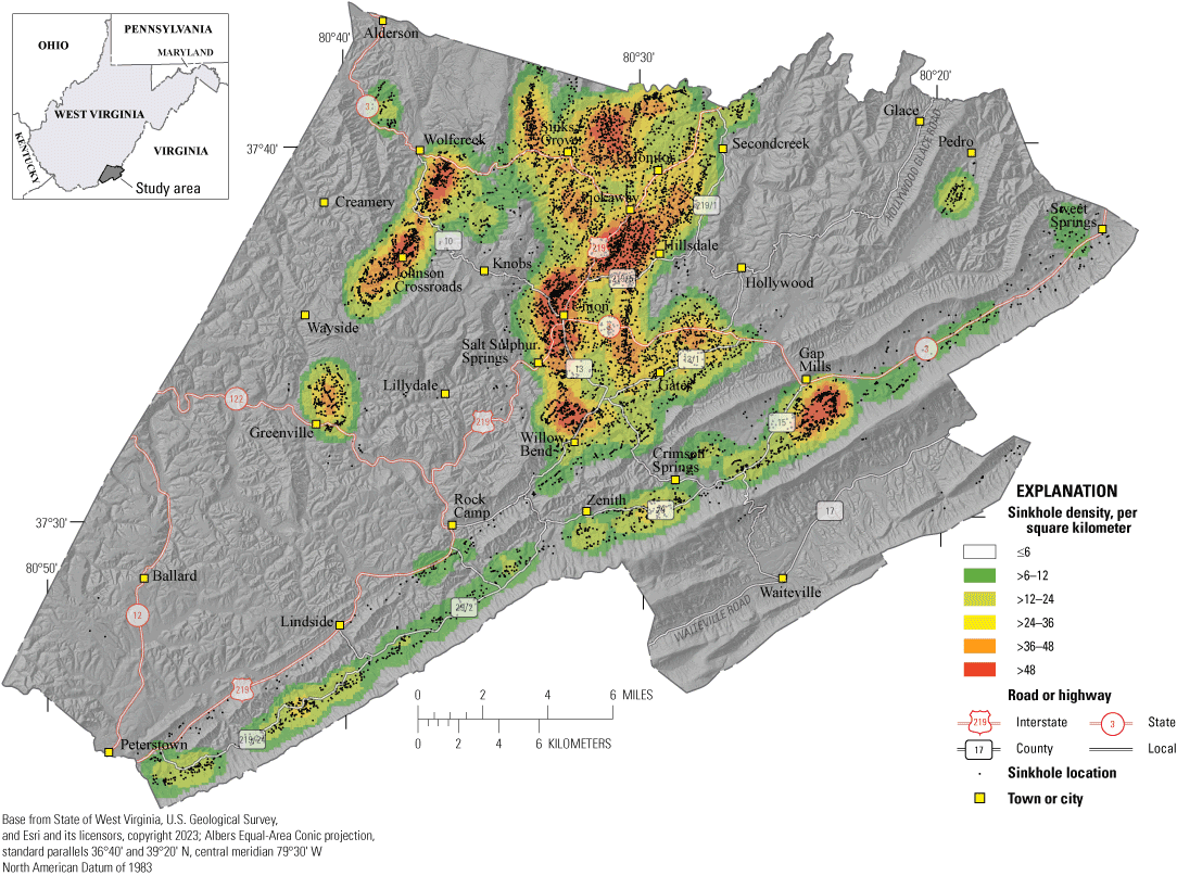
Map showing sinkhole distribution and density in Monroe County, West Virginia.
Caves
Caves are solution conduits and often are hydrologically connected to surface karst features. Sinking streams, such as Laurel Creek that flows into a cave at a blind valley near Greenville, represent the direct diversion of surface water to the subsurface (White, 2018b). Dolines also drain surface runoff downward to the underlying karst aquifers. Much of the water movement through these karst aquifers is through the 500 caves reported from Monroe County in Dasher (2019). Many of these caves are small (less than 100 feet long) but Dasher (2019) classifies 40 of the Monroe County caves as significant with important speleological characteristics including length, fauna, history, and hydrology. The longest cave is Scott Hollow Cave near Sinks Grove with 29.5 miles of surveyed passage and is described in detail by Lane and others (2018). Cave development is greatest at the contact between carbonate rocks and siliciclastic rocks. Such contact caves include Scott Hollow Cave, Hurricane Ridge Cave, and others (Balfour, 2018; Dasher, 2019). Additional descriptions of Monroe County Caves are presented in works by Davies (1958), Hempel (1975), and Dasher (2019).
A mapped estimate of cave density was produced as part of this report (fig. 37), and the digital raster was published as a data release (Cox and Doctor, 2021a). The location data of cave entrances from Dasher (2019) was used to create the cave density raster. The Point Density tool in ArcGIS Pro was used to create this raster. The parameters were set to use a cell size of 150 and a circular neighborhood with a radius of 750 for the density calculations. The output resulted in a raster displaying the number of cave entrance points per square kilometer. The raster was symbolized similarly to the sinkhole density raster. Areas with one or zero caves per square kilometer were not symbolized by any color to emphasize areas with significant cave densities. The highest density class contains values from 6 to 10 cave entrances per square kilometer.
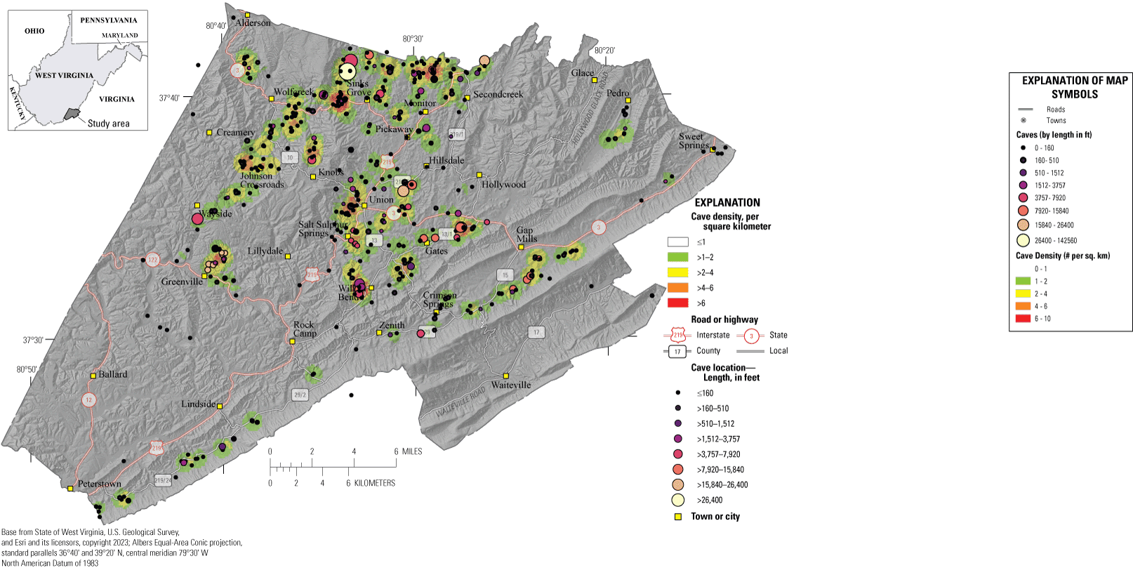
Map showing cave distribution and density in Monroe County, West Virginia.
The density raster shows that the northcentral part of the county contains the greatest clustering of cave entrances. Scott Hollow has the highest density with as many as 10 cave entrances per square kilometer. As many as 8 cave entrances per square kilometer were located near Patton and southwest of Willow Bend near Turkey Creek. Areas near Town of Union, Greenville, and Gates also contain a clustering of as many as 7 cave entrances per square kilometer. The areas with the highest density of cave entrances contain the Denmar Formation, Pickaway Limestone, and Union Limestone geologic units. The unit with the most cave entrances in the county is the Pickaway Limestone, hosting a total of 101 caves. Few to no known caves are in the southeast and southwest parts of the county.
Springs
Streams for the study area are shown on figure 35. Several of the subsurface cave or conduit streams rise as springs (fig. 5) that flow across surface exposures of carbonate rock as perennial or ephemeral surface streams, which may receive discharge from additional springs. Second Creek rises as a spring fed by water flowing through Patton Cave on the Ordovician limestones near Gap Mills. Second Creek then flows to the west crossing some clastic units and then the limestones of the Greenbrier Group before joining the Greenbrier River south of Fort Spring. Several large springs are tributary to Second Creek, including Dickson Spring which drains about 26 mi2. Scott Hollow Cave drains the area around Sinks Grove with the water flowing north to resurge from several submerged springs in the channel of the Greenbrier River between Fort Spring and Alderson. Indian Creek emerges as a spring just south of Town of Union and flows south and west to the New River. The Laurel Creek watershed at Greenville is another karst drainage basin that flows to Indian Creek. Several springs flow into Rich Creek from Ordovician carbonates near Peterstown and are also part of the New River drainage basin. The karst drainage basins for most of the major springs in Monroe County have been determined through water-tracing studies reported by Jones (1997), Jones (2018), and Dasher (2019). Tracer tests and potentiometric-surface contouring conducted for this report have further refined the karst catchment boundaries.
Known springs were documented as part of this study and are shown on figures 4 and 5. It must be noted, however, that the springs shown on figures 4 and 5 do not reflect the total population of springs within Monroe County. Only those springs that were documented during routine field investigations as part of this study or that had been previously published in other hydrologic and geologic reports or resident in accessible databases are presented on figures 4 and 5. The distribution of springs with respect to the geologic formations from which they emanate are shown in figure 38.
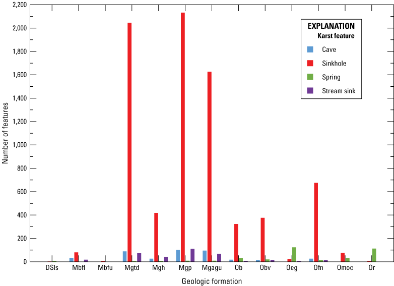
Bar graph of the distribution of caves, sinkholes, springs, and stream sinks by geologic formation in Monroe County, West Virginia. DSls, Silurian and Devonian limestones and sandstones, undifferentiated; Mbfl, Bluefield Formation, lower; Mbfu, Bluefield Formation, upper; Mgtd, Taggard and Denmar Formations, undivided; Mgh, Hillsdale Limestone; Mgp, Pickaway Limestone; Mgagu, Union Limestone, Greenville Shale, and Alderson Limestone of the Greenbrier Group, undivided; Ob, Beekmantown Formation; Obv, Big Valley Formation; Oeg, Eggleston Formation; Oln, New Market and Lincolnshire Limestones; Omoc, Moccasin Formation; Or, Reedsville Shale.
From the available data, the greatest number of springs emanates from the Eggleston Formation with a total of 123 documented springs, followed closely by the Reedsville Shale with 113 documented springs. Most of these springs occur on the steep slopes of Peters Mountain, which serves as the source area for the major public water supplies in Monroe County. Together, the Eggleston Formation and Reedsville Shale account for 65 percent of known springs in Monroe County and far outnumber any other geologic units within the county with respect to the number of springs; however, many of these springs rise through surficial deposits that cover these bedrock units, thus it is unknown whether the water storage occurs within the localized surficial aquifers or within bedrock aquifers. Of the 123 springs in the Eggleston Formation, 59 of them are within surficial deposits recognized through mapping from lidar-derived imagery. Of the 113 springs in the Reedsville Shale, 38 of them are within mapped surficial deposits covering the bedrock. Other geologic units with a significant number of springs include the Moccasin Formation (30 documented springs), the Beekmantown Formation (29 documented springs), the Big Valley Formation (20 documented springs), and the Lincolnshire and New Market Limestones (12 documented springs), all of which contain limestone to varying degrees.
Groundwater Availability
Water budgets for Monroe County were extracted from regional- and national-scale models (Wolock, 2003; Sanford and Selnick, 2013; Senay and others, 2013; McCoy and others, 2015; Reitz and others, 2017a, b). The components of the water budget, evapotranspiration, groundwater recharge, and runoff were determined for (1) Monroe County, (2) seven hydrostratigraphic units, and (3) four historically gaged watersheds in the county. Analysis of streamflow data for the four principal stream basins were analyzed by hydrograph separation methods using the USGS hydrograph separation program PART, which is part of a larger groundwater analysis software suite, the USGS Groundwater Toolbox (Barlow and others, 2014). The comparison of water-budget components with data in gaged basins allowed for an assessment of the representativeness of the regional and national models for local conditions.
Soil-Water-Balance
McCoy and others (2015) estimated hydrologic budgets for the aquifers of the Appalachian Plateau Province. These aquifers cover most of Monroe County. The folded Valley and Ridge formations along the southeastern edge of the county were not included in their analysis and are accounted for with alternate approaches. Their results were developed using the Soil-Water-Balance (SWB) model (Westenbroek and others, 2010) in combination with regionally available spatial datasets. The SWB model estimates spatial and temporal variability in groundwater recharge using a modified version of the Thornthwaite-Mather Soil-Water-Balance approach with climatological, soil, and landscape properties as input. The SWB model is a cascading procedure that partitions precipitation input into various reservoirs based on physical and empirical parameter values. The end-product is a gridded (0.6- by 0.6-mi wide grid cells) model domain with spatially varying estimates of recharge, evapotranspiration, and surface runoff.
Average estimates of water-budget components were computed from all grid cells that overlapped the county. Water-budget estimates are summarized in table 10. A central observation, from this analysis, is the dominant role of evapotranspiration in the water budget. Almost 70 percent of all precipitation that falls in the county is returned to the atmosphere through evapotranspiration. In contrast, recharge makes up approximately 16 percent of the county’s water budget (fig. 39). Recharge appears to be heavily influenced by surface topography and mimics the distribution of precipitation over the county implying topographically driven recharge (fig. 39). Smaller scale variations in recharge across the county are likely due to the heterogeneity in land cover and soil properties, geologic controls, as well as the complex topography, particularly in the eastern section of the county.
Table 10.
Water-budget estimates by the Soil-Water-Balance model and Reitz and others (2017b) for Monroe County, West Virginia.[All water-budget estimate components listed are in inches per year followed by percentage of total precipitation. %, percent]
| Method | Precipitation | Evapotranspiration | Recharge | Runoff |
|---|---|---|---|---|
| Soil-Water-Balance model (SWB)1 | 41.86 | 29.12 (69.6%) | 6.57 (15.7%) | 6.17 (14.7%) |
| Reitz2 | 40.25 | 27.16 (67.5%) | 6.49 (12.1%) | 6.60 (16.4%) |
SWB data are from McCoy and others, 2015.
Data are from Reitz and others, 2017b.
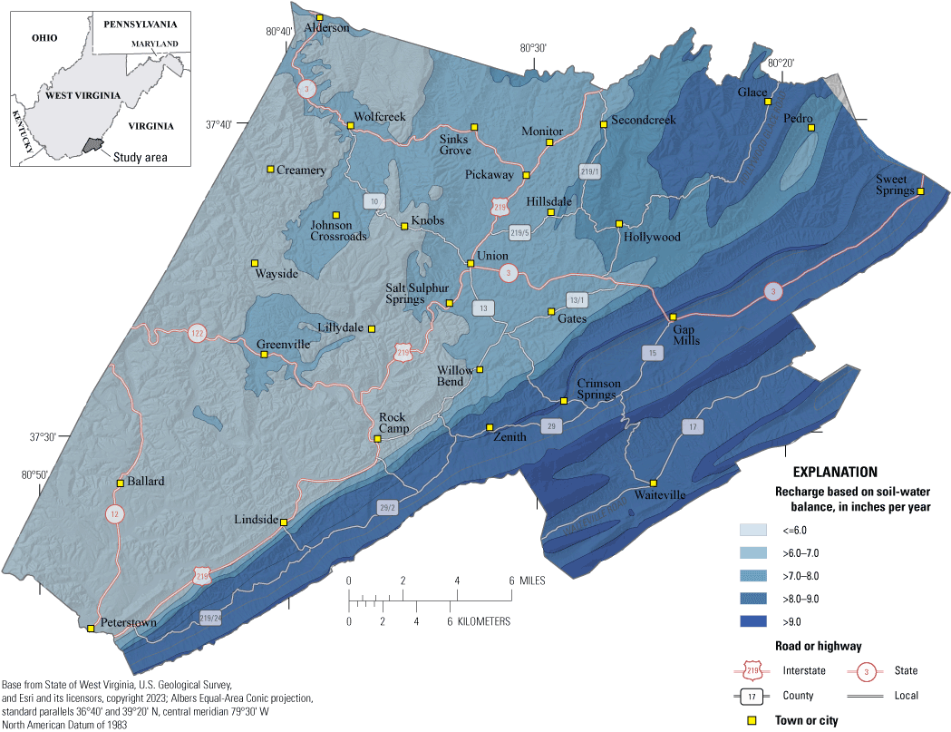
Map showing distribution of estimated Soil-Water-Balance groundwater recharge in Monroe County, West Virginia.
Regional Water-Budget Estimates
Reitz and others (2017a, b) used regression equations to compute annual rates of quick-flow runoff and evapotranspiration for the contiguous United States on an 800-m spatial scale. Recharge was computed by assessing the water budget for those terms related to precipitation. Precipitation was derived from the PRISM Climate Group at Oregon State University (PRISM Climate Group, 2012) with corrections based on groundwater-derived irrigation. An empirical regression for evapotranspiration was estimated as a function of land cover, precipitation, and air temperature. Similar to the evapotranspiration (ET) method, quick-flow runoff was computed as a function of soil properties and surficial geology cover. Lastly, recharge was computed as the remaining precipitation that is not taken up by ET or quick flow. The approach by Reitz and others (2017b) maintains a closed water budget through the recharge calculation. Figure 40 shows a map of the regional estimates of groundwater recharge, and table 10 shows a comparison between the SWB and Reitz and others (2017b) regional estimates. Evapotranspiration estimates for Monroe County were summarized using various methods (table 11).
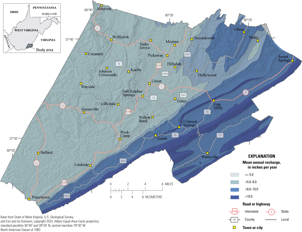
Map showing regional estimates of groundwater recharge for Monroe County, West Virginia.
Table 11.
Evapotranspiration averages for Monroe County, West Virginia.[SWB, Soil-Water-Balance model; SSEBop, operational Simplified Surface Energy Balance model]
| Analysis method | Years of record | Evapotranspiration estimate, in inches per year |
|---|---|---|
| SWB1 | 1980–2011 | 29.12 |
| Reitz2 | 2000–13 | 27.16 |
| Sanford3 | 1971–2000 | 25.24 |
| Senay4 | 2000–11 | 15.61 |
| SSEBop5 | 2000–15 | 31.93 |
SWB data are from McCoy and others, 2015.
Data are from Reitz and others, 2017b.
Data are from Sanford and Selnick, 2013.
Data are from Senay and others, 2007.
Data are from Reitz and others, 2017a.
Similar to the SWB results, mean results for the regression water-budget estimates were extracted for Monroe County (table 10). The regression estimates from Reitz and others (2017a, b) confirm the general trends seen in the water-budget results obtained using the SWB model. Evapotranspiration makes up most of the water budget, while recharge and runoff share similar average rates across the county. Along with the major difference between estimating water-budget components through empirical equations versus deterministic modeling approaches, there are two other controlling factors that account for discrepancies between the SWB and regression-model estimates.
The first controlling factor responsible for discrepancies between SWB and regression-model estimates is that the periods of record between these two water-budget studies are not the same. While the SWB results are averaged from 1980 to 2011, the regression results of Reitz and others (2017a, b) range from 2000 to 2013. To address the differences in time periods, the overlapping period was extracted and analyzed for both the SWB and regression models. Evapotranspiration from the regression method tended to be lower and respond less dramatically to increases in precipitation during wetter years. One possible explanation for this is that the regression equation used to estimate evapotranspiration incorporates time-insensitive variables, such as land-cover distribution, leading to more time-insensitive annual estimates. While these variables do change with time, Reitz and others (2017b) used constant values. In contrast, the SWB’s cascading flow procedure operates on a daily timestep allowing for more dynamic year-to-year estimates. Between both methods, runoff and recharge estimates tracked much closer together than for estimates of evapotranspiration.
The second controlling factor responsible for discrepancies between the SWB and regression-model estimates could be related to differences between the spatial coverage of the two models. The SWB model did not cover all of Monroe County and leaves out parts of the Valley and Ridge (<20 percent of the total area of these provinces). While posing a problem for perfect comparison between methods, most of the county and the majority of each of the regional aquifer systems did intersect with the SWB model results.
National Water-Budget Estimates
While few studies evaluate the entire water budget at regional scales overlapping Monroe County, other relevant studies have estimated individual water-budget components. A few of the most applicable studies have been selected to either provide an extra point of reference or to cover a period of record not included in one, or both, of the previous approaches. Results of the national-level analysis of groundwater recharge (fig. 41) produce estimates of recharge that are not very useful for assessing groundwater budgets at a county scale. A comparison of the SWB (McCoy and others, 2015), regional (Reitz and others, 2017a, b), and national estimates (Sanford and Selnick, 2013) are shown in tables 10 and 11.
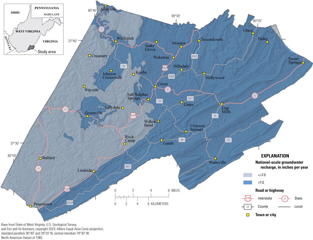
National scale estimates of groundwater recharge for Monroe County, West Virginia.
Estimates of evapotranspiration across the contiguous United States generally fall into two categories, (1) modeling approaches that incorporate meteorological data, and (2) modeling approaches that utilize remotely sensed data (Senay and others, 2013). The SWB and regression models discussed above incorporate meteorological data. Sanford and Selnick (2013) also used regression equations, like Reitz and others (2017a, b), to estimate evapotranspiration for the period 1971–2000; their results are included and averaged across this period (table 11). In contrast, the Simplified Surface Energy Balance (Senay and others, 2013) for operational applications (SSEBop) is an energy-balance approach that leverages remotely sensed thermal data. In contrast to typical energy-balance approaches that solve the full energy balance to compute latent heat flux, or the energy consumed by evapotranspiration, SSEBop simplifies the procedure such that evapotranspiration can be estimated from land surface temperature, Global Data Assimilation Systems model output reference evapotranspiration, and air temperature (Senay and others, 2007, 2011, 2013). The evapotranspiration estimates from Senay and others (2013) for the contiguous United States were extracted for Monroe County (table 11). Reitz and others (2017a) used a combined water-balance and remote-sensing approach that incorporated data from the SSEBop model with more localized water-balance constraints. According to Reitz and others (2017a), a water-balance approach tends to illustrate the highest correlation with ground-based data; however, this approach cannot utilize the temporal variability that remote-sensing data products allow. The combined approach improved in correlation with ground-based data (Reitz and others, 2017a).
Estimated ET rates differ among the five models (table 11). The hydrologic-modeling approaches (both the statistical regression approach of Sanford and Selnick [2013] and Reitz and others [2017b] and the Soil-Water-Balance approach of McCoy and others [2015]) were more similar than the remote-sensing approach of Senay and others (2013) and the combined approach of Reitz and others (2017a). Average ET from the remote-sensing approach yielded a particularly low value of 15.61 in/yr. This result follows the trend seen in McCoy and others (2015), where the authors found that SWB estimates in higher elevation areas with higher available-water content tended to be higher than the SSEBop model. Unusually low estimates of ET by SSEBop can be a function of topographically rugged areas, where the SSEBop model cannot account for dramatic temperature changes over a small areal extent (Senay and others, 2013). In contrast, the combined approach from Reitz and others (2017a) yielded the highest ET estimate of 31.93 in/yr which is more than 2 in/yr greater than the SWB result of 29.12 in/yr. Reitz and others (2017a) validated their model as well as the regression estimates of Reitz and others (2017b) and found that the regression estimates were most strongly correlated with ground-based data, especially results of hydrograph separation of streamflow. Therefore, those values may be the most useful for this study.
Summary of Water-Budget Estimates
Overall, annual water-budget estimates of groundwater recharge, ET, and surface runoff for the SWB and regional-regression methods assessed for this study are illustrated in figures 42 and 43. Summary of the annual estimates based on the two methods show close agreement. Even though there is similarity in the SWB and regional annual water-budget estimates at a countywide scale and based on annual estimates, estimates vary for specific monthly and annual periods, specific geologic formations, and specific watersheds within the county. The estimates become less reliable at a local scale because specific structural geologic and lithologic controls dominate, resulting in greater variability in estimates at a local scale or monthly time scale. The SWB and regional-regression methods provide estimates of groundwater recharge and other water-budget components for an annual time scale but also are less accurate when dealing with shorter time periods, such as monthly estimates; however, seasonal estimates are often sufficient for most analyses, as there are substantial differences and seasonal variability in precipitation, surface runoff, evapotranspiration, and groundwater recharge.
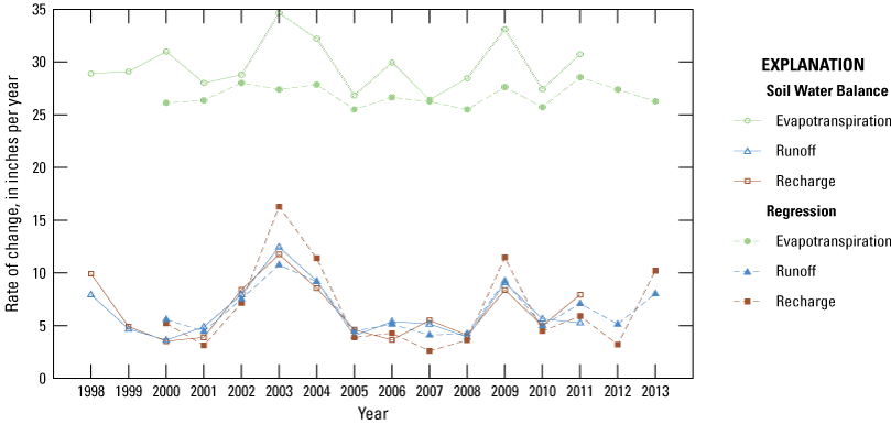
Illustration showing water-budget estimates of evapotranspiration, groundwater recharge, and surface runoff for Monroe County, West Virginia, based on the Soil-Water-Balance and regional estimation methods for the period 1998 through 2013.
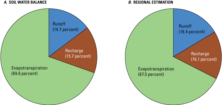
Pie charts showing similarity of water-budget estimates of evapotranspiration, groundwater recharge, and surface runoff for Monroe County based on the Soil-Water-Balance for the period 1998-2013 and regional estimation methods for the period 2000–13.
Water-Budget Estimates for Geologic Units
Monroe County contains two major physiographic provinces, the Appalachian Plateau and the Valley and Ridge. The Appalachian Plateau covers most of the county, while the Valley and Ridge province covers the southeastern part of the county (fig. 1). The Appalachian Plateau can be split into the following three major aquifers based on lithology:
-
(1) the western section is Mississippian siliciclastic units of the Mauch Chunk Group that include the Bluefield and Hinton Formations, which are comprised of shale and sandstone with thin limestone beds;
-
(2) northeast of these units are the Mississippian-units of the Greenbrier Group, which are characterized as having well-developed karst with sinkholes covering much of the landscape in the middle of the county;
-
(3) the north-northeast section of the county is siliciclastic Price Formation with Maccrady Shale underlying the Greenbrier Group and cropping out. The Maccrady Shale is a red shale, and the Price Formation consists of massive, but dirty, sandstone that represents the eastern boundary of the Greenbrier karst aquifers (White, 2018a).
The more heavily folded rocks of the Valley and Ridge province are harder to group into well-defined aquifer systems. We have chosen to classify them primarily based on geologic age and general rock type (for example, carbonate versus siliciclastic). The four units of this group contain Ordovician siliciclastic, Ordovician carbonates, Silurian siliciclastic, and Devonian siliciclastic rocks. These units crop out in multiple discontinuous areas in Monroe County but have been left grouped together because of complex folding in this physiographic province.
Recharge in the Appalachian Plateau province is generally less than that of the Valley and Ridge province (figs. 39 and 40). A trend of increasing recharge from northwest to southeast is seen in all three models with the most dramatic increase occurring from the Greenbrier to the Price-Maccrady aquifer system (table 12). A definite pattern emerges with respect to recharge and elevation related to orographic lifting, with areas along Peters Mountain having higher estimated precipitation and recharge than lower lying areas. For instance, the regression models of Reitz and others (2017b) estimate a 7.6 in/yr recharge into the Price Formation and Maccrady Shale compared to a 4.0 in/yr recharge for the Greenbrier Group to the west. Generally, precipitation is greater in the elevated eastern section of the county, where resistant siliciclastic rocks have not weathered down into the low-lying valleys of the central karst region. Increased precipitation combined with a relatively consistent evapotranspiration rate between the two aquifer systems leads to greater recharge in the Price Formation and Maccrady Shale (table 12). For example, evapotranspiration estimates from the Reitz and others (2017b) regression models ranged from 25.7 to 27.6 in/yr across all seven aquifer systems (table 13), a difference of 1.9 in/yr; while recharge estimates varied from 4.03 to 11.45 in/yr, a difference of 7.42 in/yr (table 12).
Table 12.
Estimates of groundwater recharge for hydrostratigraphic units within Monroe County, West Virginia, from 1951 to 2013.[Estimates given in inches per year. SWB, Soil-Water-Balance model]
SWB data are from McCoy and others, 2015.
Data are from Reitz and others, 2017b.
Data are from Wolock, 2003.
Table 13.
Estimates of evapotranspiration for hydrostratigraphic units within Monroe County, West Virginia, from 1980 to 2013.[Estimates given in inches per year. SWB, Soil-Water-Balance model]
SWB data are from McCoy and others, 2015.
Data are from Reitz and others, 2017b.
In the Valley and Ridge, there is slightly more homogeneity between the aquifer systems, with patterns emerging based on valleys and ridgelines. For all three recharge models, the Ordovician carbonate and Devonian siliciclastic rock recharge rates are less than the Ordovician and Silurian siliciclastic rock. The Ordovician carbonate and Devonian siliciclastic rock recharge rates tend to represent the valleys while the Ordovician and Silurian siliciclastic rock recharge rates represent ridgelines, which, upon initial consideration, implies a pattern of topographically driven recharge in these aquifer systems. Discharge along the flanks of the ridgelines likely contributes to point-source recharge of the Ordovician carbonates that is not explicitly represented in any of these national models. Evidence of this phenomenon can be seen in springs lining the edge of the Ordovician carbonates, adjacent to the mountain slopes, and is characterized by streams which disappear into the underlying Ordovician carbonate rocks (figs. 4 and 5).
Hydrograph Analysis
In addition to differences in water budgets between aquifers, differences in water budgets between major watersheds have also been explored. The four major watersheds as defined by data from USGS streamgages in Monroe County are (1) Rich Creek near Peterstown in the southern end of the county; (2) Indian Creek at Red Sulphur Springs in the center of the county; (3) Second Creek near Second Creek in the northeast part of the county; and (4) Wolf Creek near Alderson in the northwest part of the county (fig. 44).
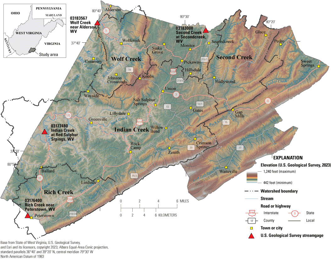
Map showing the location of four major watersheds in Monroe County, West Virginia, that were analyzed using hydrograph analysis methods to verify water-budget estimates.
Major Streams
The basin boundaries for the four major stream watersheds in Monroe County are shown in figure 44. Recharge components were estimated for all four of these watersheds (table 14) and are shown graphically on figure 45. All four watersheds fall within the SWB model extent. Progressively more variation in recharge estimates among watersheds is seen comparing the Wolock (2003) estimates (6.84–7.88 in/yr) to the SWB model estimates (5.86–7.70 in/yr) to the Reitz and others (2017b) regression results (4.51–8.27 in/yr). Except for Second Creek, the regression results estimate the lowest recharge rates for the watersheds whereas the Wolock results estimate the highest recharge rates. This is likely because of the Reitz and others (2017b) model having the higher cell resolution (0.5-mi square grid cells) compared to the other two models (0.6 mi). Second Creek has some of the most rugged topography, explaining the high recharge rates estimated by all three of the models. Although Rich Creek and Wolf Creek both show similar recharge estimates, they drain dramatically different groundwater systems; Wolf Creek is underlain primarily by the heavily karstified Greenbrier Group while Rich Creek is composed primarily of siliciclastic rocks of the Bluefield and Hinton Formations.
Table 14.
Summary of groundwater recharge from water-budget analysis for the major watersheds and Dickson Spring in Monroe County, West Virginia.[Groundwater recharge given in inches per year. USGS, U.S. Geological Survey; ID, identification number; SWB, Soil-Water-Balance model; WV, West Virginia; —, not applicable]
SWB data are from McCoy and others, 2015.
Data are from Reitz and others, 2017b.
Data are from Wolock, 2003.
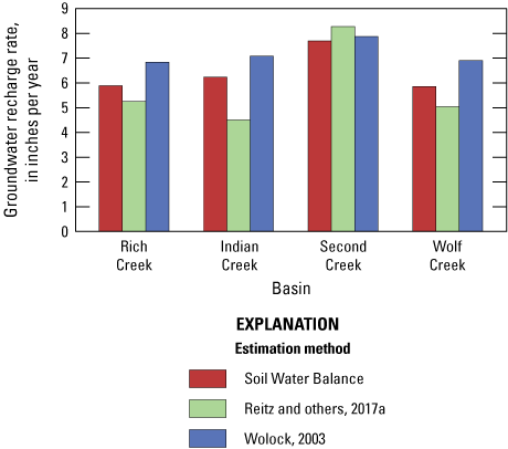
Groundwater recharge estimates for the four major watersheds in Monroe County, West Virginia.
Historical streamflow data were also used to quantify base-flow values (table 15) using hydrograph separation techniques (Barlow and others, 2014). Base flow can serve as a proxy for annual recharge if losses of groundwater from the watershed (for example, riparian evapotranspiration) are assumed to be negligible (Nelms and others, 2015). A longer discussion of these techniques is available in Nelms and others (2015). Ideally, a long period of record would better ensure that groundwater recharge is approximately equal to base flow; however, for the Monroe County watersheds, Second Creek was the only watershed with a period of record greater than 20 years. No historical streamflow data exists for Wolf Creek, so, to augment the lack of historical data, approximately a year and a half of continuous streamflow data were collected for this study at Wolf Creek, Second Creek, and Indian Creek. These historical data along with streamflow data measured for this study were analyzed using PART and HYSEP (Barlow and others, 2014) to estimate groundwater recharge and develop water budgets for the four primary basins within Monroe County (table 15).
Table 15.
Base-flow separation estimates of groundwater recharge based on historic streamflow data for the major watersheds and the Greenbriar River streamgage in Monroe County, West Virginia.[PART and HYSEP are streamflow separation estimate programs. Base-flow separation estimates given in inches per year; USGS, U.S. Geological Survey; ID, identification number; WV, West Virginia]
Base-flow separation techniques consistently yield lower values of groundwater recharge than the three recharge estimation models if base flow is assumed equal to groundwater recharge (tables 14 and 15). The pattern observed in base-flow separation data shows Indian Creek having the lowest recharge and Second Creek having the highest, tracks more closely with the Reitz and others (2017b) regression results than with the SWB and Wolock (2003; McCoy and others, 2015) results (fig. 45). The magnitudes of the regression results line up closely for Rich Creek and Indian Creek, while base-flow separation (table 15) yields lower values for Second Creek (5.65 to 6.73 in/yr) compared to results from the regression and SWB (table 14) methods (7.70 to 8.27 in/yr). One potential explanation for this result involves the karst systems that underlie sections of the Second Creek watershed. The Ordovician carbonate system comprises a large part of the southern end of the watershed and continues into Indian Creek to the west. Possible loss and rerouting of the recharge by conduit flow pathways in the karst could be responsible for recharge values not appearing as base flow. Additional rerouting by the karst system could be occurring farther to the north at the contact between the Price Formation and Maccrady Shale and the Greenbrier Group. Water could be lost into the karst as it passes over the contact from those siliciclastic rocks into the more permeable carbonate rocks.
Base-flow indices were also computed for the four major watersheds in Monroe County (table 16). Base-flow indices represent the ratio of base flow to total streamflow and reflect the degree of karstification of a basin. Watersheds with higher base-flow percentages have a higher proportion of base-flow discharge and, conversely, less surface runoff. Based on the base-flow index percentages, Second Creek and Rich Creek have the highest base-flow percentages, followed closely by Indian Creek, which is indicative of the high proportion of karst topography in these watersheds. Wolf Creek has a fairly low base-flow percentage, which is indicative of the siliciclastic non-karstic rocks that predominantly comprise a large proportion of the Wolf Creek watershed. It should be noted that the base-flow index for Wolf Creek was computed based on streamflow data collected for only one year, which does not reflect long-term average conditions for the watershed.
Table 16.
Base-flow indices for the major watersheds based on historic streamflow data in Monroe County, West Virginia, from 1942 to 2020.[PART and HYSEP are streamflow hydrograph separation estimate programs. Streamflow as base-flow discharge given in percent. USGS, U.S. Geological Survey; ID, identification number; WV, West Virginia]
Dickson Spring
Dickson Spring is the largest spring of the Greenbrier Group in Monroe County (Ogden, 1976) and, as such, warrants specific discussion based on its overall discharge of groundwater from the geologic formations within the karstic Greenbrier aquifer. Ogden (1976) reported an approximate average spring flow of 30 ft3/s with a range of measured values from 6.6 to 107 ft3/s taken from September 1974 to October 1975. By extracting only low-flow values from the Dickson Spring hydrograph in Ogden (1976), an average base-flow value of 9.39 ft3/s was computed for the spring flow. Jones (1997) mapped out a spring-shed for Dickson Spring using dye-tracer test results. The spring-shed was digitized and georeferenced to compute recharge rates similar to the approach used for surface water basins. A discrepancy emerges between the area (24.68 mi2) of the spring-shed reported by Ogden (1976) and Jones (1997) when compared to the digitized version (31.33 mi2). This difference in area might be an error in the original area calculation, an error introduced by digitizing, or as is most likely, a combination of both and is probably attributed to interbasin transfer where surface-stream watersheds and groundwater basins do not coincide.
Spring-shed recharge and base-flow estimates for the various methods were computed for Dickson Spring (table 17). Base-flow results from Ogden (1976) fall within those of the three models, coming closest to the Reitz (2017a, b) regression estimate (9.39 ft3/s versus 8.90 ft3/s). This agreement in base flow follows the pattern seen in the comparison between the surface-water hydrograph separation values and estimated recharge rates. Assuming recharge rates would be approximately similar, a lower area closer to the one reported by Jones (1997) would draw the SWB (McCoy and others, 2015) and Wolock (2003) estimates closer to the base-flow estimate of Ogden (1976) and the regression estimates farther from it. However, based on the uncertainty in the digitized spring-shed and discrepancies between models, these results should not be overinterpreted. An updated spring-shed determination probably requires reexamining boundaries delineated from prior dye-tracing work.
Table 17.
Base-flow and recharge estimates for Dickson Spring, Monroe County, West Virginia.[SWB, Soil-Water-Balance model; in/yr, inch per year; —, not applicable; ft3/s, cubic feet per second]
| Measurement | SWB1 | Reitz2 | Wolock3 | Ogden hydrograph4 |
|---|---|---|---|---|
| Recharge rate (in/yr) | 6.33 | 3.86 | 7.59 | — |
| Base flow (ft3/s) | 14.62 | 8.90 | 17.52 | 9.39 |
SWB data are from McCoy and others, 2015.
Data are from Reitz and others, 2017b.
Data are from Wolock, 2003.
Data are from Ogden, 1976.
Comparison of Methods
The primary purpose for analyzing streamflow data was to verify the accuracy of the estimates provided by the SWB, regional hydrograph analysis, and national water-budget estimates. Recharge estimates were compared to those based on measured streamflow for the study area to assess the validity of the modeled estimates (table 18). Results from the hydrograph separation analyses are shown at a monthly time interval in appendix 3 and on a yearly basis in appendix 4. Collection of streamflow data began in December 2017 at four gaging stations, Second Creek Near Second Creek, Wolf Creek near Alderson, Rich Creek at Peterstown, and Indian Creek at Red Sulphur Springs, West Virginia. The entire period was characteristic of unusual streamflow conditions (fig. 28 and fig. 29). Streamflow was highly skewed for the period measured in this study, bracketed by drought periods at the beginning and end of the study, in December 2017 through February 2018 and from September through October 2019 (fig. 28 and fig. 29), then with significantly above normal streamflow in the middle period of the study from February through May 2018 and to a lesser extent in March and April 2019 (fig. 28).
The median annual streamflow for the Greenbrier River at Alderson, W. Va., was 1,944 ft3/s, and streamflow at the Greenbrier River at Alderson in 2019 was almost the same at 1,960 ft3/s. Data for Second Creek near Second Creek, Wolf Creek near Alderson, and Indian Creek at Red Sulphur Springs, W. Va., for 2019 would therefore be expected to represent average annual flow conditions for those streams. Even though the median annual streamflow values for 2019 for the Greenbrier River were indicative of long-term average conditions, extreme variability, and short periods of data values for this study—for example, Indian Creek at Red Sulphur Springs (3 years of record available for analysis) and Wolf Creek near Alderson (only 1 year of streamflow data available for analysis)—make comparison with SWB, regional, and national water-budget estimates difficult. Overall estimates from the SWB, regional, and national estimates of groundwater recharge and other water-budget components are in the range of what was measured for the study area (table 18).
Table 18.
Recharge estimates for major watersheds based on soil-water-balance, regional, and national estimates and based on available streamflow data collected in Monroe County, West Virginia.[Recharge estimates given in inches per year. USGS, U.S. Geological Survey; ID, identification number, SWB, Soil-Water-Balance model; WV, West Virginia; n/a, not available]
Summary
Monroe County is in southeastern West Virginia, encompassing an area of 474 square miles, and contains karst and siliciclastic aquifers of Ordovician, Silurian, Devonian, and Mississippian age. The county encompasses parts of two physiographic provinces, the Valley and Ridge province to the east of Peters Mountain, and the Appalachian Plateau province to the west of Peters Mountain (Fenneman and Johnson, 1946). This study was developed in response to inquiries from the Monroe County Commission requesting assessment of the water resources of the county to provide information for protection and management of the county’s valuable groundwater resources and to assess water availability for both current [2023] and future demand.
Various products were developed for this study that help to address concerns over the county’s water availability and contamination susceptibility of the karst aquifers. U.S. Geological Survey (USGS) geologists conducted extensive geologic mapping to produce (1) a countywide bedrock geologic map, (2) countywide surficial geologic map, and (3) a light detection and ranging-derived countywide digital elevation model and associated sinkhole map. A significant part of this work was to map the Greenbrier Group at the formation level, which, prior to this study, had only partially been completed. The report also includes a description of the lithologic units identified as part of the geologic mapping process.
U.S. Geological Survey hydrologists developed (1) a countywide potentiometric-surface (water-table) map of the county, (2) a countywide base-flow stream assessment, (3) countywide water-budget estimates, (4) well log surveys for 15 wells to better understand subsurface controls on groundwater flow within the study area, and (5) two groundwater tracer tests to better refine the groundwater divide between the northern and southern parts of the karst Greenbrier aquifer in Monroe County. Finally, groundwater-basin delineations were reassessed for principal groundwater basins within the county using potentiometric-surface and geologic maps, current [2023] and legacy fluorometric groundwater-tracer tests, and base-flow stream assessments. The earlier delineations were similar to delineations made for this study, but the areal extent of the groundwater basins was slightly larger and more precise for the groundwater basins delineated for this study.
In Monroe County, four principal hydrogeologic settings produce large yields of water for residential, agricultural, and other uses. The first and presently most important water-bearing zone with respect to current [2023] public water supply is from springs along Peters Mountain. These springs are derived from intervals of fractured sandstone and resultant alluvial deposits. Groundwater flows downslope through these permeable alluvial deposits and discharges at the contact with less permeable strata, such as the Reedsville Shale. The second most relied upon water-bearing zone in Monroe County is within the karstic Greenbrier Group aquifer, in which the basal Hillsdale Limestone overlies the less permeable Maccrady Shale. This geologic contact between the Hillsdale Limestone and Maccrady Shale is not only targeted as a source of water for agricultural supply (Dewey Broyles, U.S. Department of Agriculture Natural Resources Conservation Service, oral commun., 2019) but also is targeted as a source of water for residential supply. The third most relied upon water-bearing zone is shallow perched aquifers within the Greenbrier Group. The discontinuous nature of these perched aquifers makes mapping their extent impossible, but they are related to permeable geologic strata, such as karstic solutionally enhanced permeable limestones, which overlie less permeable shale or chert bedrock. During geologic mapping of the county, several of these perched aquifers were documented in the Pickaway, Union, and Alderson Limestones. A fourth zone is springs from Ordovician carbonates at the base of Peters Mountain, which are influenced by sinking streams as well as upwelling along faults. In terms of water quantity, the springs having deeper sourced flows may be the most sustainable.
Public supplies are a principal source of water used for residential and commercial supply in the region, accounting for 0.49 million gallons per day (Mgal/d) of fresh-water withdrawals (0.14 Mgal/d of groundwater and 0.35 Mgal/d of surface water) for residential and commercial use and serving 6,645 individuals (49.2 percent of the population). An estimated 6,861 people (50.8 percent of the population) rely on private wells or other unregulated sources, such as springs, primarily for not only residential use but also, to a much lesser extent, for commercial use, and withdraw an additional 0.55 Mgal/d of groundwater for their residential and commercial supplies. Most of the water used for public supply in the region (71.4 percent) is derived primarily from springs emanating along the flanks of Peters Mountain and augmented by stream withdrawals (backup sources mainly during low-flow periods), and the remaining portion (28.6 percent) is derived from groundwater withdrawals from wells. For rural residential homeowners, however, 100 percent of their withdrawals are derived from groundwater (wells or springs).
Five principal aquifers have been identified within the county that contain multiple water-bearing zones controlled by specific geologic formations and related confining units. The five principal aquifers are:
-
(1) alluvial aquifers formed from paleo talus, alluvial fan, and colluvial deposits from the Oswego and Tuscarora Sandstones along Peters Mountain;
-
(2) karst aquifers within the various limestone formations of the Greenbrier Group, including
-
(a) a deeper base level aquifer at the contact between the Maccrady Shale and the Hillsdale Limestone, and
-
(b) upper perched aquifers within the Pickaway, Union, and Alderson Limestones above the Taggard Formation, which at times acts as a confining or semi confining unit between deeper/older and shallower/younger geologic formations within the Group;
-
-
(3) Ordovician age karst aquifers and springs in the valley at the base of Peters Mountain;
-
(4) siliciclastic fractured-rock aquifers of Mississippian age in the western part of Monroe County; and
-
(5) siliciclastic fractured-rock aquifers of Ordovician, Silurian, and Devonian age in the northeastern and eastern parts of Monroe County.
The hydrogeology of Monroe County is extremely complex, affected by structural, geologic, lithologic, and physiographic controls. Monroe County is situated in two physiographic regions (Fenneman, 1938), the Appalachian Plateau province, which consists of flat to gently dipping siliciclastic and carbonate bedrock, predominantly of Devonian to Mississippian age; and a much more complex Valley and Ridge province, characterized by long linear ridges and intervening valleys formed by compressional stress because of previous orogenic (mountain building) processes. These prior orogenic processes resulted in significant thrust faulting, thrusting older Ordovician, Silurian, and Devonian rocks over the younger Devonian and Mississippian rocks.
In addition to physiographic controls, bedrock within the study area in both physiographic provinces is highly heterogenous and comprises potentially karst-forming limestones and dolomites and non-carbonate siliciclastic units composed of predominantly shales and sandstones. These differences in lithology, especially with respect to limestone and dolomite outcrops, are responsible for karst topography in both physiographic provinces, although the karst in the Appalachian Plateau province is of much greater areal extent and contains more karst features than the karst topography within the Valley and Ridge. Another important lithologic control on the county’s hydrogeology is the contact between the Hillsdale Limestone, which is the basal formation within the Greenbrier Group, and the underlying Maccrady Shale. This geologic contact has been documented to be the base level control of groundwater occurrence and cave development within the Greenbrier Group (Balfour, 2018), is host to many caves, and is frequently targeted by drillers as a source of water for large capacity agricultural and smaller capacity residential water wells. Within the Greenbrier Group, localized, and often discontinuous, layers of lower permeability shale, calcareous shale, and chert bedrock may result in localized perched aquifers within the geologic formations. The occurrence of these perched aquifers is difficult to map because the geologic strata responsible for the perched aquifers are lenticular, laterally discontinuous, and, therefore, not possible to map to any degree of certainty.
Most of the water within the fractured-rock or karstic aquifers of Monroe County reside and move along fractures within the bedrock because the bedrock lacks sufficient intergranular porosity for storage and movement of water. Other structural controls on the hydrogeology of the study area include faults, joints, bedding planes, cleavage planes, and folds. Faults may also provide for both storage and movement of groundwater, especially where such faults have been solutionally enlarged by movement of water in carbonate limestone and dolomite strata. Joints, which may occur as fractures within the bedrock and cleavage planes, can also serve as open avenues for groundwater storage and movement, although these features can often be filled with calcite or silica cement. Bedding planes are a primary control on discharge and movement of groundwater especially where sufficiently fractured rock, such as fractured sandstones or solutionally enlarged fractures within limestone or dolomite layers, are situated on top of less permeable less fractured strata. Finally, folds consisting of anticlines and synclines may provide for fracturing of bedrock within the structures or may compartmentalize groundwater flow within the synclines, resulting in preferential flow paths, especially within the more karstic parts of the aquifers.
A survey of synoptic water levels across Monroe County took place from October 23 to 31, 2017. A total of 205 water levels were collected from 197 residential and agricultural wells and 8 springs. An additional 63 water levels were measured (under similar flow conditions) from August 20 to September 19, 2020, from 62 residential and agricultural wells and 1 spring. A countywide potentiometric-surface map (fig. 25) was constructed from the synoptic water-level survey measurements as well as spring locations and stream elevations from the USGS National Hydrography data (U.S. Geological Survey, 2018). This potentiometric-surface map was used, along with previously conducted fluorometric groundwater-tracer tests and two similar tracer tests, to better refine the groundwater divide between the southern and northern parts of the karst aquifer in Monroe County to more fully map groundwater basins that were previously mapped (Jones, 1997).
Water budgets for Monroe County were extracted from regional and national scale models (Wolock, 2003; Sanford and Selnick, 2013; Senay and others, 2013; McCoy and others 2015; Reitz and others, 2017a, b). The components of the water budget, evapotranspiration, groundwater recharge, and runoff were determined for (1) Monroe County, (2) seven hydrostratigraphic units, and (3) four historically gaged watersheds in the county. Analysis of streamflow data for the four major watersheds were analyzed by hydrograph separation methods. The comparison of water-budget components with data in gaged basins allowed for an assessment of the representativeness of the regional and national models for local conditions.
A central observation from this analysis is the dominant role of evapotranspiration in the water budget. Of the 41.86 inches per year (in/yr) of precipitation that falls on Monroe County, 29.12 in/yr (69.6 percent) is lost to evapotranspiration, another 6.17 in/yr (14.7 percent) is surface runoff to streams, and the remaining 6.57 in/yr (15.7 percent) results in recharge to groundwater aquifers. Recharge appears to be heavily influenced by surface topography and mimics the distribution of precipitation over the county implying topographically driven recharge, with higher percentage of precipitation (and associate recharge) due to orographic lifting in areas near Peters Mountain. Smaller scale variations in recharge across the county are likely due to the heterogeneity in land cover and soil properties, geologic controls, as well as the complex topography, particularly in the eastern section of the county.
The data and findings of this report provide meaningful information for assessing current [2023] and future availability of groundwater resources within Monroe County, West Virginia. Given anticipated economic development within the county, the information will provide water-resource managers with a better understanding of the county’s available water resources while also providing an added understanding of groundwater flow processes. This understanding, combined with the mapping of karst groundwater basin divides and mapping of the groundwater table, will provide emergency services with a much more accurate assessment of rates and directions of groundwater flow. Such information is critical in the event of an unanticipated contaminant discharge on the sensitive karst landscape of the county.
References Cited
Aley, T., 2019, Groundwater tracing handbook: Protem, Mo., Ozark Underground Laboratory, 41 p., accessed January 2017 at https://www.ozarkundergroundlab.com/assets/oul_groundwater_tracing_handbook-2019-revised.pdf.
Allmendinger, R.W., 1998, Inverse and forward numerical modeling of trishear fault-propagation folds: Tectonics, v. 17, no. 4, p. 640–656, accessed January 2017 at https://doi.org/10.1029/98TC01907.
Aquatic Informatics, 2023, AQUARIUS—Streamflow data analysis and processing software: Aquatic Informatics, Vancouver, British Columbia, Canada, accessed October 2023 at https://aquaticinformatics.com/products/aquarius-environmental-water-data-management/.
Balfour, W.M., 2018, The contact caves of central Greenbrier County, chap. 11 of White, W.B., ed., Caves and karst of the Greenbrier Valley in West Virginia, in LaMoreaux, J.W., ed., Cave and Karst Systems of the World: Cham, Switzerland, Springer, p. 207–230. [Also available at https://doi.org/10.1007/978-3-319-65801-8_11.]
Barlow, P.M., Cunningham, W.L., Zhai, T., and Gray, M., 2014, U.S. Geological Survey groundwater toolbox—A graphical and mapping interface for analysis of hydrologic data (version 1.0)—User guide for estimation of base flow, runoff, and groundwater recharge from streamflow data: U.S. Geological Survey Techniques and Methods, book 3, chap. B10, 27 p. accessed December 9, 2021, at https://pubs.usgs.gov/tm/03/b10/.
Barlow, P.M., Cunningham, W.L., Zhai, T., and Gray, M., 2017, U.S. Geological Survey Groundwater Toolbox version 1.3.1, a graphical and mapping interface for analysis of hydrologic data: U.S. Geological Survey software release, May 26, 2017, accessed December 2021 at http://doi.org/10.5066/F7R78C9G.
Bausher, E.A., 2018, Qualitative and quantitative analysis of carbonate waters in the Peters Mountain Region of Monroe County, West Virginia: Morgantown, W. Va., West Virginia University, master’s thesis, 123 p. [Also available at https://researchrepository.wvu.edu/etd/3741/.]
Bishop, M.R., 2010, A detailed hydrologic study of the Scott Hollow groundwater basin, Greenbrier and Monroe Counties, West Virginia: Akron, Ohio, University of Akron, master’s thesis, 135 p., 10 app., 1 pl., accessed December 7, 2016, at http://rave.ohiolink.edu/etdc/view?acc_num=akron1279892824.
Butts, C., and Edmundson, R.S., 1943, Geology of the southwestern end of Walker Mountain, Virginia: Geological Society of America Bulletin, v. 54, no. 11, p. 1669–1691, accessed January 2017 at https://doi.org/10.1130/GSAB-54-1669.
Carter, J.L., and Kammer, T.W., 1990, Late Devonian and early Carboniferous brachiopods (Brachiopoda, Articulata) from the Price Formation of West Virginia and adjacent areas of Pennsylvania and Maryland: Annals of the Carnegie Museum, v. 59, no. 2, p. 77–103, accessed January 2017 at https://doi.org/10.5962/p.240767.
Century Geophysical, 2017, Log—Log acquisition software for processing data collected from Century Geophysical downhole borehole geophysics tools: Tulsa, Oklahoma, Century Geophysical LLC, accessed March 2017 at https://www.century-geo.com/software-log.
Cox, C.L., and Doctor, D.H., 2021a, Density raster of caves in Monroe County, West Virginia: U.S. Geological Survey data release, https://doi.org/10.5066/P9TKR3XJ.
Cox, C.L., and Doctor, D.H., 2021b, Lidar-derived closed depression vector data and density raster in karst areas of Monroe County, West Virginia: U.S. Geological Survey data release, https://doi.org/10.5066/P9O85K6T.
Cox, C.L., and Doctor, D.H., 2021c, Lidar-derived imagery and digital elevation model of Monroe County, West Virginia at 3-meter resolution: U.S. Geological Survey data release, https://doi.org/10.5066/P92JLWRM.
Cunningham, W.L., and Schalk, C.W., comps., 2011, Groundwater technical procedures of the U.S. Geological Survey: U.S. Geological Survey Techniques and Methods 1–A1, 151 p., accessed March 2017 at https://pubs.usgs.gov/tm/1a1/.
Day-Lewis, F.D., Johnson, C.D., Paillet, F.L., and Halford, K.J., 2011, A computer program for flow-log analysis of single holes (FLASH): Ground Water, v. 49, no. 6, p. 926–931, accessed March 2017 at https://doi.org/10.1111/j.1745-6584.2011.00798.x.
Dean, S.L., Kulander, B.R., and Skinner, J.M., 1988, Structural chronology of the Alleghenian orogeny in southeastern West Virginia: Geological Society of America Bulletin, v. 100, no. 2, p. 299–310, accessed January 2017 at https://doi.org/10.1130/0016-7606(1988)100<0299:SCOTAO>2.3.CO;2.
Dennison, J.M., 1970, Stratigraphic divisions of Upper Devonian Greenland Gap Group (“Chemung Formation”) along Allegheny Front in West Virginia, Maryland, and Highland County—Duke University Press: Southeastern Geology, v. 12, no. 1, p. 53–82. [Also available at http://libres.uncg.edu/ir/asu/f/SoutheasternGeology_Vol012_No01_1970_M.pdf.]
Dorobek, S.L., and Read, J.F., 1986, Sedimentology and basin evolution of the Siluro-Devonian Helderberg Group, central Appalachians: Journal of Sedimentary Research, v. 56, no. 5, p. 601–613, accessed January 2017 at https://doi.org/10.1306/212F89E5-2B24-11D7-8648000102C1865D.
Esri, 2022, GIS mapping software—Location intelligence & spatial analytics: Redlands, California, Esri, accessed July 2022 at https://www.esri.com/en-us/arcgis/products/arcgis-pro/overview.
Fenneman, N.M., and Johnson, D.W., 1946, Physiographic divisions of the conterminous United States: U.S. Geological Physiography Committee special map, 1 sheet, scale 1:7,000,000. [Also available at https://catalog.data.gov/dataset/physiographic-divisions-of-the-conterminous-u-s.]
Hatcher, R.D., Jr., Thomas, W.A., Geiser, P.A., Snoke, A.W., Mosher, S., and Wiltschcko, D.V., 1989, Alleghenian orogen, chap. 5 of Hatcher, R.D., Jr., Thomas, W.A., and Viele, G.W., eds., The Appalachian-Ouachita orogen in the United States: Boulder, Colo., Geological Society of America; Geology of North America, v. F-2, p. 233–318.
Haynes, J.T., and Goggin, K.E., 1993, Field guide to the Ordovician Walker Mountain Sandstone Member—Proposed type section and other exposures: Virginia Minerals, v. 39, no. 4, p. 25–39. [Also available at https://energy.virginia.gov/commercedocs/VAMIN_VOL39_NO04.pdf.]
Heller, S.A., 1980, A hydrogeologic study of the Greenbrier limestone karst of central Greenbrier County, West Virginia: Morgantown, W. Va., West Virginia University, master’s thesis, 167 p., 2 pls. [Also available at https://researchrepository.wvu.edu/etd/9020/.]
Jones, W.K., 2018, Hydrology of the Greenbrier karst, chap. 3 of White, W.B., ed., Caves and karst of the Greenbrier Valley in West Virginia, in LaMoreaux, J.W., ed., Cave and Karst Systems of the World: Cham, Switzerland, Springer, p. 21–43. [Also available at https://doi.org/10.1007/978-3-319-65801-8.]
Jones, W.K., 2019, Water tracing in karst aquifers, chap. 134 of White, W.B., Culver, D.C., and Pipan, T., eds., Encyclopedia of caves (3d ed.): Elsevier, p. 1144–1155. [Also available at https://doi.org/10.1016/B978-0-12-814124-3.00134-5.]
Jones, W.K., Kozar, M.D., Doctor, D.H., and Wander, N.J., 2023, Fluorescein and Rhodamine WT concentration and recovery data for select samples collected in Monroe County, West Virginia, in August and September 2019: U.S. Geological Survey data release, https://doi.org/10.5066/P9KF9FD2.
Kay, M., 1956, Ordovician limestones in the western anticlines of the Appalachians in West Virginia and Virginia northeast of the New River: Geological Society of America Bulletin, v. 67, no. 1, p. 55–106. [Also available at https://doi.org/10.1130/0016-7606(1956)67[55:OLITWA]2.0.CO;2.]
Lane, S.B., Bishop, M.R., Dore, M.J., and Sasowsky, I.D., 2018, Scott Hollow Cave, chap. 16 of White, W.B., ed., Caves and karst of the Greenbrier Valley in West Virginia, in LaMoreaux, J.W., ed., Cave and Karst Systems of the World: Cham, Switzerland, Springer, p. 339–357. [Also available at https://link.springer.com/chapter/10.1007/978-3-319-65801-8_16.]
McCoy, K.J., Yager, R.M., Nelms, D.L., and Ladd, D.E., Monti, J., Jr., and Kozar, M.D., 2015, Hydrologic budget and conditions of Permian, Pennsylvanian, and Mississippian aquifers in the Appalachian Plateaus Physiographic Province (ver 1.1, October 2015): U.S. Geological Survey Scientific Investigations Report 2015–5106, 77 p., accessed July 24, 2018, at https://doi.org/10.3133/sir20155106.
Miller, R.L., and Meissner, C.R., Jr., 1977, Geologic map of the Big A Mountain quadrangle, Buchanan and Russell Counties, Virgina: US Geological Survey Geologic Quadrangle Map GQ–1350, 1 sheet. [Also available at https://doi.org/10.3133/gq1350; Supersedes USGS Open-File Report 73–186.]
Mount Sopris, 2017, Matrix Data Acquision System — Log acquisition software for processing data collected from Mount Sopris downhole borehole geophysics tool: Denver, Colorado, Mount Sopris Instruments, March 2017, available at https://mountsopris.com/matrix-data-acquisition-system/.
Multi-Resolution Land Characteristics Consortium, 2019, National land cover database 2011: U.S. Geological Survey data release, accessed January 27, 2020, at https://catalog.data.gov/dataset/nlcd-2011-database.
National Oceanic and Atmospheric Administration, 2021, U.S. climate normals quick access—Station normals for West Virginia NWS Union 3 SSE weather station, 1991–2020: National Centers for Environmental Information, accessed August 25, 2021, at https://www.ncei.noaa.gov/access/us-climate-normals/#dataset=normals-annualseasonal&timeframe=30&location=WV&station=USC00469011.
Nelms, D.L., Messinger, T., and McCoy, K.J., 2015, Annual and average estimates of water-budget components based on hydrograph separation and PRISM precipitation for gaged basins in the Appalachian Plateaus Region, 1900–2011: U.S. Geological Survey Data Series 944, 10 p., 3 app., accessed July 24, 2018, at https://doi.org/10.3133/ds944.
Ogden, A.E., 1976, The hydrogeology of the central Monroe County karst, West Virginia: Morgantown, West Virginia, West Virginia University, Ph.D. dissertation, 235 p., 6 app., 6 pls. [Also available at https://researchrepository.wvu.edu/etd/9527/.]
PRISM Climate Group, 2012, Prism climate data: Oregon State University, Northwest Alliance for Computational Science & Engineering database accessed November 1, 2012, at http://prism.oregonstate.edu.
Reger, D.B., 1950, Lower Middle Mississippian of southeastern West Virginia—Discussion: American Association of Petroleum Geologists Bulletin, v. 34, no. 9, p. 1910–1912, accessed June 2023 at https://doi.org/10.1306/3D934055-16B1-11D7-8645000102C1865D.
Reger, D.B., and Price, P.H., 1926, Mercer, Monroe, and Summers Counties: Wheeling, W. Va., West Virginia Geological Survey County Geologic Report CGR-15, 963 p., 34 pls., 6 sheets, 1:62,500 scale. [Also available at https://archive.org/details/mercermonroesumm00west/mode/2up.]
Reitz, M., Sanford, W.E., Senay, G.B., and Cazenas, J., 2017a, Annual estimates of recharge, quick-flow runoff, and ET for the contiguous US using empirical regression equations, 2000–2013: U.S. Geological Survey data release, accessed July 24, 2018, at https://doi.org/10.5066/F7PN93P0.
Reitz, M., Sanford, W.E., Senay, G.B., and Cazenas, J., 2017b, Annual estimates of recharge, quick-flow runoff, and evapotranspiration for the contiguous U.S. using empirical regression equations: Journal of the American Water Resources Association, v. 53, no. 4, p. 961–983, accessed June 2019 at https://doi.org/10.1111/1752-1688.12546.
Richards, B.G., 2006, Aqueous geochemistry of springs along Peters Mountain in Monroe County, West Virginia: Morgantown, West Virginia, West Virginia University, master’s thesis, 64 p., 2 app., 1 pl. [Also available at http://www.hrc.nrcce.wvu.edu/outgoing/Richards_Brian_thesis.pdf.]
Sanford, W.E., and Selnick, D.L., 2013, Estimation of evapotranspiration across the conterminous Unites States using a regression with climate and land cover data: Journal of the American Water Resources Association, v. 49, no. 1, p. 217–230, accessed July 24, 2018, at https://doi.org/10.1111/jawr.12010.
Schipke, K.A., and Kozar, M.D., 2023, Interpolated groundwater levels and altitudes for Monroe County, West Virginia, 2017–2019: U.S. Geological Survey data release, https://doi.org/10.5066/P9TFAN5X.
Schultz, A.P., Stanley, C.B., Gathright, T.M., Rader, E.K., Bartholomew, M.J., Lewis, S.E., and Evans, N.H., 1986, Geologic map of Giles County: Charlotteville, Va., Virginia Division of Mineral Resources Publication 69, 1 sheet, scale 1:50,000. [Also available at https://ngmdb.usgs.gov/Prodesc/proddesc_39822.htm.]
Senay, G.B., Bohms, S., Singh, R.K., Gowda, P.H., Velpuri, N.M., Alemu, H., and Verdin, J.P., 2013, Operational evapotranspiration mapping using remote sensing and weather datasets—A new parameterization for the SSEB approach: Journal of the American Water Resources Association, v. 49, no. 3, p. 577–591, accessed July 24, 2018, at https://doi.org/10.1111/jawr.12057.
Senay, G.B., Budde, M., Verdin, J.P., and Melesse, A.M., 2007, A coupled remote sensing and simplified surface energy balance approach to estimate actual evapotranspiration from irrigated field: Sensors (Basel), v. 7, no. 6, p. 979–1000, accessed July 24, 2018, at https://doi.org/10.3390/s7060979.
Senay, G.B., Leake, S., Nagler, P.L., Artan, G., Dickinson, J., Cordova, J.T., and Glenn, E.P., 2011, Estimating basin scale evapotransiration (ET) by water balance and remote sensing methods: Hydrological Processes, v. 25, no. 26, p. 4037–4049, accessed July 24, 2018, at https://doi.org/10.1002/hyp.8379.
Sturms, J.M., 2008, Surficial mapping and kinematic modeling of the St. Clair thrust fault, Monroe County, West Virginia: Morgantown, W. Va., West Virginia University, master’s thesis, 84 p. [Also available at http://pages.geo.wvu.edu/~jtoro/download/Sturms_Thesis08.pdf.]
Turnipseed, D.P., and Sauer, V.B., 2010, Discharge measurements at gaging stations: U.S. Geological Survey Techniques and Methods, book 3, chap. A8, 87 p. [Also available at https://pubs.usgs.gov/tm/tm3-a8/.]
U.S. Geological Survey, 2018, USGS national hydrography dataset plus high resolution national release 1 FileGDB: U.S. Geological Survey, accessed March 2018 at https://doi.org/10.5066/P9WFOBQI.
U.S. Geological Survey, 2019, USGS water data for West Virginia: U.S. Geological Survey National Water Information System database, accessed January 2019 at https://doi.org/10.5066/F7P55KJN.
U.S. Geological Survey, 2021, USGS water use data for West Virginia: U.S. Geological Survey National Water Information System database, accessed August 25, 2021, at https://doi.org/10.5066/F7P55KJN.
Vesper, D.J., Bausher, E.A., and Downey, A., 2022, Comparison of microbial indicators and seasonal temperatures as means for evaluating the vulnerability of water resources from karst and siliciclastic springs: Hydrogeology Journal, v. 30, p. 1219–1232, accessed August 31, 2022, at https://doi.org/10.1007/s10040-022-02496-3.
Wall, J., Doctor, D.H., and Terziotti, S., 2015, A semi-automated tool for reducing the creation of false closed depressions from a filled LIDAR-derived digital elevation model, in Doctor, D.H., Land. L., Stephenson, J.B., eds., Proceedings of the 14th Multidisciplinary Conference on Sinkholes and the Engineering and Environmental Impacts of Karst National Cave and Karst Research Institute Symposium 5, October 5–9, 2015, Rochester, Minnesota: National Cave and Karst Research Institute, p. 255–262, accessed January 2017 at https://doi.org/10.5038/9780991000951.1057.
Westenbroek, S.M., Kelson, V.A., Dripps, W.R., Hunt, R.J., and Bradbury, K.R., 2010, SWB—A modified Thornthwaite-Mather Soil-Water-Balance code for estimating groundwater recharge: U.S. Geological Survey Techniques and Methods, book 6, chap. A31, 60 p., accessed September 1, 2021, at https://pubs.usgs.gov/tm/tm6-a31/.
White, W.B., ed., 2018a, Caves and karst of the Greenbrier Valley in West Virginia in LaMoreaux, J.W., ed., Cave and Karst Systems of the World: Cham, Switzerland, Springer, 411 p., accessed January 2017 at https://doi.org/10.1007/978-3-319-65801-8.
White, W.B., 2018b, The Laurel Creek basin and Greenville Saltpeter cave, chap. 17 of White, W.B., ed., Caves and karst of the Greenbrier Valley in West Virginia in LaMoreaux, J.W., ed., Cave and Karst Systems of the World: Cham, Switzerland, Springer, p. 359–370, accessed January 2017 at https://doi.org/10.1007/978-3-319-65801-8_17.
Williams, P.W., 2008, The role of the epikarst in karst and cave hydrogeology—A review—Bologna, Italy: International Journal of Speleology, v. 37, no. 1, p. 1–10, accessed January 2017 at https://doi.org/10.5038/1827-806X.37.1.1.
Wolock, D.M., 2003, Estimated mean annual natural ground-water recharge in the conterminous United States: U.S. Geological Survey Open-File Report 2003–2311, accessed May 12, 2023, at https://doi.org/10.3133/ofr03311.
Wu, Q., Liu, H., Wang, S., Yu, B., Beck, R., and Hinkel, K., 2015, A localized contour tree method for deriving geometric and topological properties of complex surface depressions based on high-resolution topographical data: International Journal of Geographical Information Science, v. 29, no. 12, p. 2041–2060, accessed March 2017 at https://doi.org/10.1080/13658816.2015.1038719.
Wyrick, G.G., and Borchers, J.W., 1981, Hydrologic effects of stress-relief fracturing in an Appalachian Valley: U.S. Geological Survey Water-Supply Paper 2177, 51 p., accessed January 2017 at https://doi.org/10.3133/wsp2177.
Appendix 1. Well Depth, Casing, Yield, Water Level, and Specific Capacity Data From County Health Department Well Completion Reports
Appendix 2. Base-flow Data for 83 Sites Measured in September 2019 in Monroe County, West Virginia
References Cited
U.S. Geological Survey, 2019, USGS water data for West Virginia: U.S. Geological Survey National Water Information System database, accessed January 2019, at https://doi.org/10.5066/F7P55KJN.
Appendix 3. Results of Monthly Hydrograph Analyses for Four Major Watersheds in Monroe County and for the Greenbrier River at Alderson, West Virginia
References Cited
U.S. Geological Survey, 2019, USGS water data for West Virginia: U.S. Geological Survey National Water Information System database, accessed January 2019, at https://doi.org/10.5066/F7P55KJN.
Appendix 4. Results of Annual Hydrograph Analyses for Four Major Watersheds in Monroe County and for the Greenbrier River at Alderson, West Virginia
References Cited
U.S. Geological Survey, 2019, USGS water data for West Virginia: U.S. Geological Survey National Water Information System database, accessed January 2019, at https://doi.org/10.5066/F7P55KJN.
Conversion Factors
U.S. customary units to International System of Units
International System of Units to U.S. customary units
Temperature in degrees Celsius (°C) may be converted to degrees Fahrenheit (°F) as follows:
°F=(1.8×°C)+32.
Temperature in degrees Fahrenheit (°F) may be converted to degrees Celsius (°C) as follows:
°C=(°F–32)/1.8.
Datums
Vertical coordinate information is referenced to the North American Vertical Datum of 1988 (NAVD 88).
Horizontal coordinate information is referenced to the North American Datum of 1983 (NAD 83).
Elevation, as used in this report, refers to distance above the vertical datum.
Supplemental Information
Specific conductance is given in microsiemens per centimeter at 25 degrees Celsius (µS/cm at 25 °C).
Concentrations of chemical constituents in water are given in either milligrams per liter (mg/L), micrograms per liter (µg/L), milligrams per kilogram (mg/kg), or nanograms per liter (ng/L).
Concentrations of dissolved hydrocarbons within this report are given in milligrams per kilogram (mg/kg), which for freshwater is equivalent to milligrams per liter (mg/L).
For more information about this report, contact:
Director, Virginia and West Virginia Water Science Center
U.S. Geological Survey
1730 East Parham Road
Richmond, Virginia 23228
or visit our website at
https://www.usgs.gov/centers/va-wv-water
Publishing support provided by the Baltimore Publishing Service Center
Disclaimers
Any use of trade, firm, or product names is for descriptive purposes only and does not imply endorsement by the U.S. Government.
Although this information product, for the most part, is in the public domain, it also may contain copyrighted materials as noted in the text. Permission to reproduce copyrighted items must be secured from the copyright owner.
Suggested Citation
Kozar, M.D., Doctor, D.H., Jones, W.K., Chien, N., Cox, C.E., Orndorff, R.C., Weary, D.J., Weaver, M.R., McAdoo, M.A., and Parker, M., 2023, Hydrogeology, karst, and groundwater availability of Monroe County, West Virginia: U.S. Geological Survey Scientific Investigations Report 2023–5121, 82 p., https://doi.org/10.3133/sir20235121.
ISSN: 2328-0328 (online)
ISSN: 2328-031X (print)
Study Area
| Publication type | Report |
|---|---|
| Publication Subtype | USGS Numbered Series |
| Title | Hydrogeology, karst, and groundwater availability of Monroe County, West Virginia |
| Series title | Scientific Investigations Report |
| Series number | 2023-5121 |
| ISBN | 978-1-4113-4541-6 |
| DOI | 10.3133/sir20235121 |
| Publication Date | December 14, 2023 |
| Year Published | 2023 |
| Language | English |
| Publisher | U.S. Geological Survey |
| Publisher location | Reston, VA |
| Contributing office(s) | Virginia and West Virginia Water Science Center |
| Description | Report: xii, 81 p.; 4 Appendixes, 5 Data Releases |
| Country | United States |
| State | West Virginia |
| County | Monroe County |
| Online Only (Y/N) | N |
| Additional Online Files (Y/N) | Y |