

Characterizing Future Streamflows in Massachusetts Using Stochastic Modeling—A Pilot Study
Links
- Document: Report (1.67 MB pdf) , HTML , XML
- Data Release: USGS data release - Data for a pilot study characterizing future climate and hydrology in Massachusetts
- NGMDB Index Page: National Geologic Map Database Index Page (html)
- Download citation as: RIS | Dublin Core
Abstract
Communities throughout Massachusetts face the potential effects of climate change, ranging from more extreme rainfall to more pronounced and frequent droughts. Understanding the effects of climate change on hydrology is important to State and community officials to evaluate the potential effects on infrastructure and water systems. To better understand the effects of climate change on hydrology, the U.S. Geological Survey, in partnership with Cornell University and Tufts University, conducted a study in cooperation with the Massachusetts Executive Office of Energy and Environmental Affairs to develop tools for projecting 21st-century climate and hydrologic characteristics in Massachusetts.
A stochastic weather generator was developed to project future climatic characteristics for Massachusetts. The stochastic weather generator estimates daily precipitation, minimum temperature, and maximum temperature for 17 warming scenarios (from 0 to 8 degrees Celsius, in 0.5-degree increments). To project future hydrologic characteristics, the stochastic weather generator output data were input to the Precipitation-Watershed Modeling System deterministic watershed model for the Squannacook River watershed, which is the watershed selected as the pilot study location for investigating future hydrologic characteristics. Hydrologic data output from the deterministic watershed model were then input to a stochastic watershed model developed for this study to correct model errors (model errors are often observed in the output from deterministic models at the high- and low-flow extremes). The output from the stochastic watershed model was then used to characterize hydrology for the 17 warming scenarios. For the Squannacook River watershed, the results project more extreme flood and low streamflows under the warming scenarios.
Output from the tools allows the characterization of future streamflows for the years 2030, 2050, 2070, and 2090, which expands our understanding of 21st-century climatic and hydrologic risk in Massachusetts. These tools could improve Federal, State, and community officials’ ability to mitigate the effects of climate change over the next several decades.
Introduction
Hydrologic-trend studies in New England have documented changes in several components of the water cycle, including streamflows, during the last several decades. Winter and spring streamflows, which consist of snowmelt runoff and rain, are occurring earlier in the northern and mountainous sections of the northeastern United States (Dudley and Hodgkins, 2002; Hodgkins and others, 2003; Hodgkins and Dudley, 2006; Dudley and others, 2017). Annual peak flows have increased in the northeastern United States during the last 50 to 100 years (Hodgkins and Dudley, 2005; Collins, 2009; Hodgkins and others, 2019), and summer-stormflow magnitudes have increased in many rivers (Hodgkins and Dudley, 2011).
In addition, projections for climate change in the northeastern United States include warmer temperatures and increases in precipitation. Annual precipitation in the northeastern United States is projected to increase by about 5 to 8 percent by the middle of the 21st century and by about 7 to 14 percent by the end of the 21st century (Hayhoe and others, 2007a). Annual mean air temperature in the northeastern United States is projected to increase by about 2.1 to 2.9 degrees Celsius (°C) by the middle of the 21st century and by about 2.9 to 5.2 °C by the end of the 21st century (Hayhoe and others, 2007a).
In response, some State and Federal agencies responsible for the management of the water resources, civil infrastructure, and human resources that depend on hydrologic systems have been proactively preparing for the effects of climate-related changes to the Nation’s hydrology. To expand on the information available for decision making on watershed and infrastructure management, the U.S. Geological Survey (USGS), in cooperation with the Massachusetts Executive Office of Energy and Environmental Affairs, and in partnership with Cornell University and Tufts University, developed tools for projecting 21st-century climate and hydrologic risk in Massachusetts. These tools included the development of a stochastic watershed model (SWM; Shabestanipour and others, 2023) based on output from a deterministic watershed model. A stochastic model predicts statistical outcomes by accounting for variance in historical data, whereas a deterministic model computes simulations for a given set of inputs. The deterministic watershed model uses input from a stochastic weather generator (SWG; Steinschneider and Najibi, 2022) that estimates climate variables representing various future scenarios of climatic warming in Massachusetts.
Output from these tools should expand on the understanding of 21st-century climatic and hydrologic changes in Massachusetts. This understanding could improve Federal, State, and community officials’ ability to mitigate the effects of climate change over the next several decades.
Previous Studies
Scientists have estimated that the northeastern United States will experience the largest increases in temperatures in the contiguous United States. These temperature increases are predicted to occur by 2035, as much as two decades before global average temperatures should achieve similar increases (Reidmiller and others, 2018). Thus, the prediction of hydrologic vulnerability caused by future climate variation has increasingly become a major focus of research in the northeastern United States.
Although many climatologic and hydrologic studies have been done to date, two previous studies are foundational to this investigation. The first study is the development of the SWG for Massachusetts. The SWG was developed at Cornell University (Steinschneider and others, 2019; Steinschneider and Najibi, 2022) and was designed to generate synthetic weather data while allowing perturbations related to climate change. The second study foundational to our investigation is the development of the SWM (Shabestanipour and others, 2023). The SWM was designed to address systematic biases of extreme events often exhibited by deterministic watershed models.
Purpose and Scope
The purpose of this study is to develop tools for projecting 21st-century hydrologic characteristics in Massachusetts that give more-accurate estimates of future streamflows at the high- and low-flow extremes. This report presents the data, methods, and results of a cooperative study of the Squannacook River watershed (fig. 1) of Massachusetts to build a SWM that uses output from a calibrated deterministic model. The calibrated deterministic model simulates future hydrology on the basis of projected climate estimates from a SWG. Multiple future scenarios of rising temperatures are simulated with the models, and the percent change in streamflow characteristics are provided. All data used for this study are available in an associated USGS data release (Olson and others, 2024).
The Squannacook River Watershed Study Area
For this study, a watershed was needed that met several criteria related to data availability and physical setting. First, the watershed needed a streamgage with a long-term continuous streamflow record. A long-term record allows for a means to calibrate a deterministic model and provides enough data for the SWM to correct for bias. Second, the watershed needed to be mostly free of substantial hydrologic manipulations, such as regulation and flood control. Although this criterion was not strictly adhered to, the intent was to avoid complexities in developing the pilot application. Third, the watershed needed to have basin characteristics typical of watersheds in Massachusetts. The intent of this third criterion was to select a watershed that would streamline the transfer of the methods developed in this study to other watersheds in Massachusetts. To meet the third criterion, the selection of watersheds was limited to those with hydrology and climate that were not substantially affected by urban, coastal, or orographic effects. The last criterion, the location of a streamgage in the watershed, where streamflow was determined, needed to have a corresponding computational node in the National Hydrologic Model (NHM; Viger and Bock, 2014). Meeting this last criterion allowed the extraction and use of a local watershed model from the NHM without significant model adjustment or recalibration.
From the 28 Massachusetts watersheds determined to be potential study areas, the Squannacook River watershed (fig. 1) was selected. The streamgage within the watershed (Squannacook River Near West Groton, Massachusetts [USGS streamgage 01096000; USGS, 2023]) has 74 years of continuous streamflow record from October 1949 to date (2023). The basin and climatic characteristics of the Squannacook River watershed (table 1) are typical of Massachusetts, and the streamgage location has a corresponding location in the NHM where streamflow was calibrated and computed. Some anthropogenic effects exist in the form of groundwater withdrawals, occasional regulation at low streamflows, and streamflow diversion from 2.2 square miles (mi2) of drainage by the Fitchburg Reservoir (USGS, 2023), but these effects were considered insignificant relative to anthropogenic effects of many watersheds with streamgages in Massachusetts.
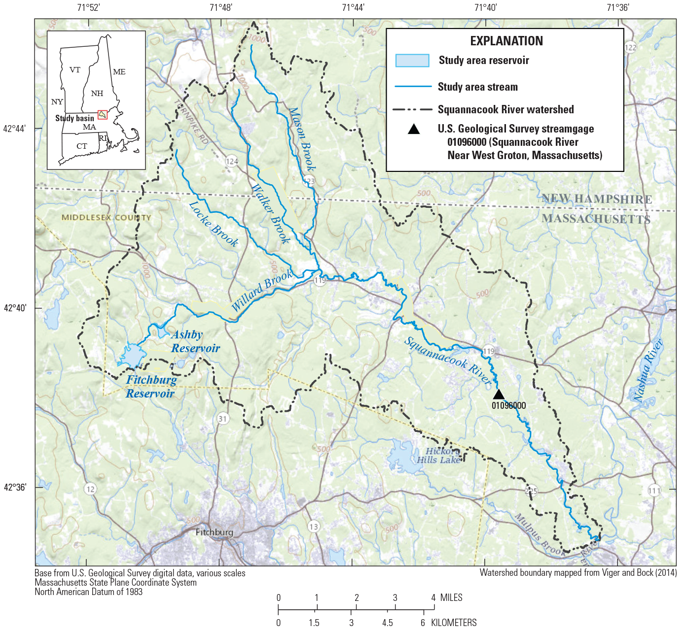
Map showing the Squannacook River watershed, New Hampshire and Massachusetts, and the U.S. Geological Survey streamgage 01096000 (Squannacook River Near West Groton, Massachusetts).
Table 1.
Selected characteristics of the Squannacook River watershed upstream from the U.S. Geological Survey streamgage 01096000 (Squannacook River Near West Groton, Massachusetts).[Station location is shown on figure 1]
Data are from U.S. Geological Survey (2023).
Data are from Geospatial Attributes of Gages for Evaluating Streamflow, version II, database (Falcone, 2011).
Data are from National Oceanic and Atmospheric Administration (2021b).
The Squannacook River watershed is in north-central Massachusetts (fig. 1) and crosses the State border into New Hampshire. The watershed is primarily forested and contains more than 7,000 acres of State- and town-owned forest lands. Areas of development are along transportation corridors and in the center of Townsend, Mass. The Squannacook River originates from the confluence of four brooks draining the western end of the watershed: Mason Brook, Walker Brook, Locke Brook, and Willard Brook. The brooks drain hilly, forested lands with elevations as high as 1,500 feet (ft). The elevation at the confluence of the brooks is about 300 ft. Downstream from the confluence, the Squannacook River flows southeasterly along a winding, 11-mile path to the location of the USGS streamgage (01096000; fig. 1). The drainage area and elevation of the streamgage are 65.9 mi2 (Falcone, 2011) and 250 ft (USGS, undated a), respectively. Past the streamgage, the river continues another winding 6 miles where it flows into the Nashua River. At the mouth of the Squannacook River, the drainage area and elevation are 72.5 mi2 (USGS, undated b) and 200 ft (USGS, undated a), respectively.
In the headwaters of the Squannacook River watershed, at the upstream end of Willard Brook, are two reservoirs: Fitchburg Reservoir and Ashby Reservoir. These reservoirs are owned and operated by the City of Fitchburg (fig. 1). Fitchburg Reservoir is on the Squannacook River watershed boundary and was constructed in 1915 as an emergency water supply for the City of Fitchburg. The reservoir covers about 155 acres and has a north spillway and gated outlet that drains to Willard Brook and the Squannacook River watershed; the reservoir has a south spillway and gated outlet that drains to a neighboring watershed and other reservoirs supplying water to Fitchburg. The south spillway, as reconstructed in 1963, is 0.56 ft higher than the north spillway and rarely overflows. The gate valve on the north outlet leading to Willard Brook has malfunctioned and is stuck in a partially open position. The south reservoir outlet has two gate valves that are partially functional and are used to divert additional water as needed for water supply to Fitchburg. The streamflows are not metered, and no formal records are maintained for the reservoir (City of Fitchburg, 2013b).
Ashby Reservoir is entirely within the Squannacook River watershed and is downstream from Fitchburg Reservoir. It covers about 39 acres and was constructed in 1917 as a compensatory water supply for mill owners downstream. The reservoir now serves as a site for recreation and is not used to regulate streamflow. No formal operating or streamflow records are kept for the dam at the outlet of Ashby Reservoir (City of Fitchburg, 2013a).
The climate in the Squannacook River watershed is temperate (mild summers and cold winters). The mean annual air temperature during 1981–2010 was about 7.8 °C and mean monthly air temperatures ranged from about −5.6 °C in January to 20.6 °C in July (National Oceanic and Atmospheric Administration, 2021a). For the same period, the mean annual precipitation was 48 inches (in.), and the mean annual potential evapotranspiration for the area was 23 in. (National Oceanic and Atmospheric Administration, 2021a, b25).
Study Methodology
Climatologic and hydrologic stochastic modeling techniques were used to characterize current and future streamflows in the Squannacook River watershed in Massachusetts. These techniques included the SWG, a stochastic generator of climatological data. The climate data for several climate change scenarios computed by the SWG were then input to the Precipitation-Runoff Modeling System (PRMS; Leavesley and others, 1983; Markstrom and others, 2015), the deterministic model used in this study. Last, the SWM, a stochastic watershed modeling technique, was used to correct the biases inherent with a deterministic model.
The Stochastic Weather Generator
The SWG was developed for Massachusetts to estimate the future climatologic data (daily precipitation and air temperature) needed to run the deterministic model. The SWG was developed at Cornell University (Steinschneider and others, 2019; Steinschneider and Najibi, 2022) and was designed to generate synthetic weather data while allowing perturbations related to climate change. The SWG synthesizes weather data using a resampling algorithm on observed weather records within selected weather regimes (the weather regimes selected reflect recurring large-scale, persistent atmospheric-flow patterns). The SWG can synthesize future scenarios of weather data by (1) perturbing the frequency of weather regimes, (2) adjusting air temperature by simple addition, and (3) adjusting precipitation using a Clausius-Clapeyron scaling method (Held and Soden, 2006) that relates the effects of warming temperatures on precipitation because of increases in the moisture holding capacity of the atmosphere.
The observed weather records used as the basis for the SWG was the Livneh and others (2015) climate dataset, referred to in this report as the “Livneh dataset”, gridded to 1/16-degree resolution. The period of record used from the Livneh dataset was 1950 to 2013. This study used 17 warming scenarios, covering 0 °C to 8 °C, in 0.5-degree increments. For each scenario, the SWG generated an ensemble of 100 members. Each ensemble member contained a 64-year record of daily precipitation, minimum air temperature, and maximum air temperature gridded at the same resolution as the Livneh dataset covering Massachusetts. These data were input to the PRMS deterministic model.
The Deterministic Model
The deterministic watershed model used for this investigation was the USGS PRMS version 5.1.0 (Leavesley and others, 1983; Markstrom and others, 2015). The PRMS is a distributed-parameter, physically based watershed-modeling system. Responses to climate and land-cover changes are simulated in terms of water and energy balances, streamflow regimes, flood peaks and volumes, soil-water relations, and groundwater recharge. In PRMS, the components of streamflow include contributions from surface runoff, subsurface (soils) interflow, and groundwater. The watershed’s water budget consists of storage in snowpack; soil moisture; groundwater; inputs from precipitation and snowmelt; losses to evapotranspiration; recharge to the deeper aquifer system; and outflows to streams from surface, subsurface, and shallow-groundwater reservoirs.
The PRMS is a modular modeling system, whereby modules that represent watershed-process algorithms, selected from a library of subroutine modules, are combined into a customized model. The customized PRMS can then simulate components of a particular hydrologic system, including water, energy processes, and stream temperature. The PRMS operates on a fixed daily time step and is driven by daily inputs of total precipitation and maximum and minimum temperatures. The data release for the deterministic model (Olson and others, 2024) includes a list of modules used in this configuration. Supplemental information regarding PRMS modules and source code specific to the PRMS configuration presented in this report is available in the PRMS users’ manual (Markstrom and others, 2015) and the USGS PRMS developers’ website (https://www.usgs.gov/software/precipitation-runoff-modeling-system-prms).
The PRMS model for the Squannacook River watershed was extracted from the NHM (Regan and others, 2018). The NHM is a model platform that uses the PRMS hydrologic simulation code and was developed as a comprehensive, consistent hydrologic model for the contiguous United States. The NHM uses parameters derived from characteristics of topography, land cover, soils, geology, and hydrography; these characteristics are obtained using traditional geographic information system (GIS) methods. Some parameters are set to long-established default values, whereas others are determined through calibration. The Daymet climate dataset (Thornton and others, 2016) was used to configure and calibrate the NHM (Hay and LaFontaine, 2020).
In a PRMS model, and thus in the NHM, a modeled region is divided into polygon-shaped subwatersheds called hydrologic response units (HRUs). The daily water balance is simulated in each HRU on the basis of precipitation and temperature input data. The HRUs in the NHM have a wide range of sizes and have boundaries that coincide with land use or catchments that drain to confluences. The mean area of HRUs in the NHM is 29 mi2. The total runoff simulated by the model is aggregated from the HRUs draining to and routed through stream segments that represent the stream-channel network. Each stream segment represents a channel reach bounded by an HRU or, in most cases, bounded on each side of the channel by an HRU. Each channel, except for the most upstream segment, is fed by a segment upstream from it and by the bounding HRUs. The accumulated discharge in the segment is routed to the next downstream segment by a Muskingum routing scheme (Markstrom and others, 2015).
The PRMS model extracted from the NHM for the Squannacook River watershed upstream from the mouth of the river consisted of three HRU catchments and two stream segments. Only one HRU and one stream segment were upstream from the location of interest for this study, streamgage 01096000 (fig. 2). Two HRUs and one stream segment were downstream from the streamgage location to the mouth of the river. The upstream HRU and the stream segment corresponding to the streamgage location was used for additional model calibration, and the streamflow computed at this location was used to develop the SWM.
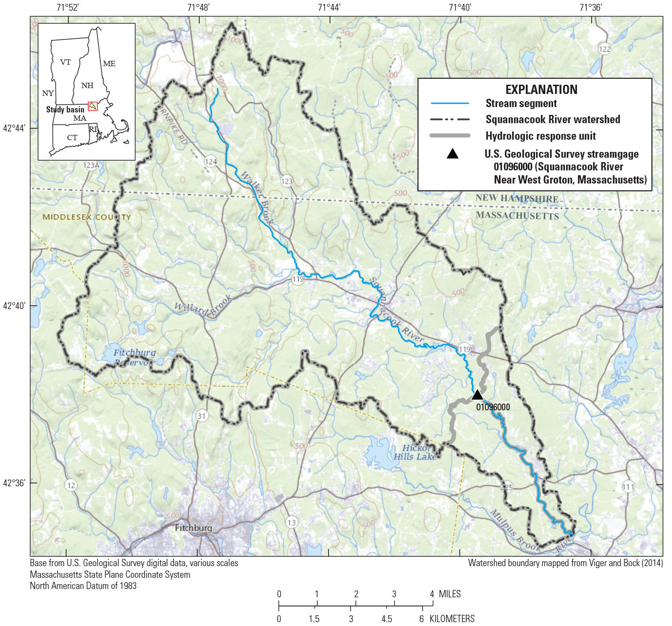
Map showing the hydrologic response units and stream segments of the Squannacook River watershed Precipitation-Runoff Modeling System model extracted from the National Hydrologic Model, New Hampshire and Massachusetts.
Calibration of the Squannacook River Watershed PRMS Model
The PRMS model uses physically based algorithms to simulate various hydrologic processes (Markstrom and others, 2015). Within the model, parameters are assigned to HRUs and stream segments. These parameters are used in the algorithms’ computations to determine the hydrologic response of each HRU and stream segment. The PRMS simulates the hydrologic cycle by using the spatial variation in measurable physical characteristics (including land cover, topography, soil, and geology) that can be quantified within a GIS. A GIS method developed for the NHM derived the initial values for the parameters in the model (Regan and others, 2018).
The NHM was calibrated using Daymet climate data and available USGS streamflow records (USGS, 2023). However, some parameters were adjusted to align with the design of this study and to improve model performance. Model performance was evaluated on the basis of the Daymet climate data and available streamflow records for streamgage 01096000.
The first parameters adjusted were the monthly adjustment factors to the minimum temperature, the maximum temperature, the precipitation, and the precipitation determined to be snow. In the NHM, these parameters varied from month to month and were likely influenced by seasonality. Because the focus of this study is on climate change and warming scenarios that may change the seasonality of hydrology, these monthly adjustment factors were made constant throughout the year. The monthly adjustments to temperature (tmax_cbh_adj and tmin_cbh_adj) were changed from monthly values that ranged from 1.5 ° to 3.0 °Fahrenheit (F; 0.8 to 1.7 °C) to a constant 1.0 °F (0.6 °C). The monthly precipitation adjustment factors (rain_cbh_adj) were changed from monthly values that ranged from 0.5 to 1.17 (a unitless multiplication factor) to a constant 0.85. The monthly adjustment factors of the precipitation determined to be snow (snow_cbh_adj) were changed from monthly values that ranged from 0.82 to 1.53 to a constant 1.15. These updated, constant monthly adjustment factors were determined based upon the mean, range, and mode of the NHM monthly adjustment factors and improvement of model goodness-of-fit statistics described in “Evaluation of the Squannacook River Watershed PRMS Model Performance” section.
Although several additional parameters were tested, only two parameters significantly improved model performance and were adjusted. The monthly air-temperature coefficients used in the potential evapotranspiration computation for an HRU (jh_coef; per degrees Fahrenheit) were increased by 20 percent. The coefficient in the equation to compute groundwater discharge (gwflow_coef; in fractions per day) was decreased by 10 percent.
In an attempt to improve estimation of low streamflows by the PRMS model, the maximum available water-holding capacity of soils (soil_moist_max; in inches) was adjusted. Adjustments did improve accuracy of low streamflows but at the expense of overall model performance; thus, this parameter was not adjusted from the NHM values.
Because the NHM model that the Squannacook River PRMS model was extracted from is calibrated with the Daymet climate data, and the SWG was based on the Livneh climate data, the Daymet and Livneh datasets for the Squannacook River watershed were compared. The comparison showed that the temperature data were similar. The mean annual maximum temperature for both datasets was 57.7 °F. The mean annual minimum temperature was 35.8 °F and 35.0 °F for the Daymet and Livneh datasets, respectively. However, the daily precipitation was markedly different. The Livneh dataset has more days with precipitation, but lower precipitation amounts on average. For the period from 1980 to 2013, for example, the Daymet and Livneh datasets included 4,578 and 7,042 days of precipitation, respectively. For the same period, the Daymet and Livneh datasets had mean annual precipitation values of 49.3 and 47.7 in., respectively.
Evaluation of the Squannacook River Watershed PRMS Model Performance
To evaluate model performance, the Daymet climate data—used in the NHM calibration—was input to the PRMS model. The model output was compared with daily streamflow data from streamgage 01096000 (USGS, 2023). Although the volume of water diverted from the Squannacook River watershed at the Fitchburg Reservoir is unknown, it is considered to have an insignificant effect on the streamflow records because the reservoir is in the headwaters of the watershed and its primary outlet drains into the Squannacook River watershed. The Fitchburg Reservoir has a drainage area of 2.2 mi2 or only about 3.4 percent of the gaged drainage area. Hence for this study, the observed streamflows at the streamgage were considered unaffected by storage, regulation, and diversion.
The concurrent Daymet and streamflow record data used to evaluate model performance extended from January 1, 1981, to December 31, 2013. The 33-year period provides time-series data of sufficient length to yield mean values and variability representative enough to ensure that inferential statistics would be meaningful. Additional evaluation of model performance was done using the Livneh dataset and concurrent streamflow records from January 1, 1981, to December 31, 2013.
The model’s performance was evaluated by matching general water-balance information and by goodness-of-fit statistics for simulated streamflow compared with USGS measured streamflow. The goodness-of-fit statistics included the Nash-Sutcliffe Efficiency (NSE) statistic (Nash and Sutcliffe, 1970). Following Moriasi and others (2007), an NSE of 0.5 or greater is considered a satisfactory or good fit between the simulated and measured hydrographs, and an NSE of 0.4 to 0.5 is considered marginally satisfactory. Values of NSE less than 0.4 are considered unsatisfactory. Additional goodness-of-fit statistics included the normalized root-mean-square error (NRMSE; normalized on the difference between the maximum and minimum values in the record), and the percent bias (PBIAS). A comparison of streamflow-quantiles was also used for evaluating model performance.
The PRMS-simulated long-term water balance (greater than 30 years) for the watershed upstream from the streamgage had values for annual precipitation, evapotranspiration, and runoff within the expected ranges. The mean annual precipitation input to the model from the Daymet dataset was 49.0 in.; the expected value for the Squannacook River watershed is about 48 in. The mean annual evapotranspiration computed by the model for the watershed was 20.9 in.; the expected value is about 23 in. The mean annual runoff simulated by PRMS was 22.5 in., slightly larger than the concurrently measured 21.3 in.
In addition to the general water balance, the calibrated model simulations of streamflow were compared with the USGS measured streamflows using the NSE statistic, the PBIAS, the NRMSE expressed as a percent, and the log residual of the simulated streamflow minus the measured streamflow. The mean and the standard deviation of the log residual reduce the weight (effect) of low- and- high-streamflow errors and thus provide a better picture of the typical residual error of a time series in which the daily and monthly residual errors are averaged. These statistics of the calibrated model runs were computed using the period of 1981–2013.
Using the Daymet climate data, which calibrated the original HNM model, the Squannacook River PRMS model showed good simulation of the mean streamflow (fig. 3; table 2). The error for the mean-annual simulated daily streamflows was −6.61 percent, which indicates that the annual water balance, on average, was well simulated. The NSE, log residual, the PBIAS, and the NRMSE together characterize the overall error and bias in the simulated hydrograph compared with the measured hydrograph. The NSE statistic is a measure of how well a simulated time series (streamflow hydrograph) fits the measured time series during the period of record relative to the mean, accounting for timing and quantity. A value of 1 for the NSE indicates that the simulated and measured time series are identical, and a value of 0 indicates that the simulated time series provides as much predictive information as the mean of the measured time series alone. An NSE statistic of 0.5 or higher indicates a satisfactory or “good” calibration; 0.4 to less than 0.5, a marginal or “fair” calibration; and less than 0.4, a relatively “poor” calibration (Moriasi and others, 2007). The NSE for the model was 0.647 and 0.524 using the Daymet and Livneh climate datasets, respectively. For this study, the mean log residual of 0.0062 indicates a satisfactory calibration; an NRMSE of less than 10 percent is considered satisfactory; and a PBIAS greater than 20 percent is considered to represent a fair or poor simulation (Moriasi and others, 2007).
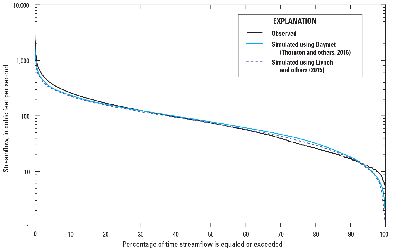
Graph showing observed streamflow-duration and Precipitation-Runoff Modeling System simulated streamflow-duration curves with Daymet (Thornton and others, 2016) and Livneh and others (2015) climate data input for the U.S. Geological Survey streamgage 01096000 (Squannacook River Near West Groton, Massachusetts).
Table 2.
Statistics calculated for streamflows measured at the U.S. Geological Survey streamgage 01096000 (Squannacook River Near West Groton, Massachusetts) and Precipitation-Runoff Modeling System simulated streamflows using Daymet and Livneh and others (2015) climate input data.[Location of streamgage is shown in figure 1. Data are from Olson and others (2024). Daymet climate dataset from Thornton and others (2016). PRMS, Precipitation-Runoff Modeling System; ft3/s, cubic foot per second; —, not applicable; NRMSE, normalized root-mean-square error; percentile is the percentage of streamflows in the record that exceed the listed streamflow value]
| Statistic1 | Measured streamflow at calibration streamgage 01096000 (Squannacook River Near West Groton, Massachusetts) | PRMS simulated streamflow with selected climate input data | |
|---|---|---|---|
| Daymet climate data | Livneh and others (2015) climate data | ||
| Mean of streamflow (ft3/s) | 121 | 113 | 107 |
| Standard deviation of streamflow (ft3/s) | 168 | 126 | 119 |
| Percent error of the mean | — | −6.61 | −11.6 |
| Percent error of the standard deviation | — | −25.0 | −29.2 |
| Percent bias | — | −6.88 | −11.3 |
| NRMSE,2 in percent | — | 2.75 | 3.19 |
| Nash-Sutcliffe Efficiency coefficient | — | 0.647 | 0.524 |
| Mean of the log residuals | — | 0.0062 | 0.019 |
| Standard deviation of the log residuals | — | 0.245 | 0.265 |
| 99th-percentile streamflow (ft3/s) | 7.98 | 5.32 | 3.89 |
| 90th-percentile streamflow (ft3/s) | 17.0 | 18.3 | 17.7 |
| 80th-percentile streamflow (ft3/s) | 26.3 | 32.3 | 29.9 |
| 20th-percentile streamflow (ft3/s) | 172 | 163 | 157 |
| 10th-percentile streamflow (ft3/s) | 263 | 238 | 230 |
| 1st-percentile streamflow (ft3/s) | 744 | 619 | 558 |
Whereas the goodness-of-fit statistics listed in table 2 show that the simulation has a good calibration on the basis of the NSE, PBIAS, NRMSE, and mean log-residual, the error of the standard deviation of the log residuals and the relatively large percent error (compared to the mean statistics) of the standard deviations (more than 10 percent) indicates that the simulation is not representing the range of flows as well as it is representing the mean and timing of the streamflow. The large percent error of the standard deviation is the result of the large relative errors at the high and low ends of the streamflow distribution (fig. 3; table 2). The larger errors on the high and low ends of the discharge range are relatively common with deterministic rainfall-runoff models (Farmer and Vogel, 2016) and is the reason this study uses stochastic watershed modeling.
As stated in “The Stochastic Weather Generator” section, the SWG was used to generate climate input data for warming scenarios that could potentially occur in future climates. Whereas the PRMS model was calibrated using the Daymet climate data, the Livneh climate dataset was used to develop the SWG because of its record length (1950–2013). The evaluation of the PRMS model using the Livneh climate dataset was deemed satisfactory with the goodness-of-fit statistics shown in table 2.
Applying Stochastic Weather Generator Data to the PRMS
The SWG generated 100 ensemble members, each member containing 64 years of daily precipitation, minimum temperature, and maximum temperature for 17 warming scenarios of 0 °C to 8 °C, in 0.5-degree increments, covering Massachusetts (Olson and others, 2024). The data from the SWG were gridded to 1/16-degree resolution. These gridded data were spatially area weighted to the Squannacook River watershed and input to the PRMS deterministic model. The output of these 1,700 PRMS model runs were then input to the SWM as described in the “Stochastic Watershed Model” section to correct for model biases.
Stochastic Watershed Model
Because of the performance inadequacies involved with simulating the extreme high- and low-flow events commonly exhibited by deterministic models, simulated daily mean streamflows often have lower variance than the observed record the model was based upon. Relying on the output of deterministic models can lead to a systematic bias of extreme events. To address these performance issues (low variance and bias), a SWM was developed at Tufts University (Shabestanipour and others, 2023). The SWM applies model residuals to the simulated streamflow output producing a stochastic output of streamflow ensembles to better represent observed extreme streamflows.
The SWM is an autoregressive model of the logarithm of the ratios of observed and simulated streamflows combined with a bootstrap residual resampling approach to generate streamflow ensembles. Details of the SWM and its validation and verification are in Shabestanipour and others (2023). For validation purposes, the SWM was used to generate 10,000 realizations of daily streamflow records. Shabestanipour and others (2023) compared the percent error of the mode of the 10,000 low-flow and flood-flow statistics of the SWM output with the percent error of the PRMS results. The SWM output showed improvements over the deterministic PRMS model output (table 3).
Table 3.
Statistics calculated for observed streamflows (1980–2017) at U.S. Geological Survey streamgage 01096000 (Squannacook River Near West Groton, Massachusetts), and percent errors of statistics from output from the Precipitation-Runoff Modeling System and the stochastic watershed model.[Modified from Shabestanipour and others (2023, table 1). ft3/s, cubic foot per second; PRMS, Precipitation-Runoff Modeling System; SWM, stochastic watershed model]
The SWG and SWM were developed concurrently using different meteorological datasets with different periods of record, as described in “Evaluation of the Squannacook River Watershed PRMS Model Performance” section. The SWG was developed using the longer Livneh dataset (1950–2013), whereas the SWM was developed using residuals from the PRMS model with the Daymet dataset (1980–2017) used as input. The change in meteorological product altered the performance of the PRMS model and the characteristics of the residuals. Because the SWM operates by replicating the characteristics of the residuals, the change of meteorological product was conveyed to the operation of the SWM (by means of the altered characteristics of the residuals), thereby degrading the performance of the SWM. Though the SWM could be altered to account for the different residual structure, or the PRMS model recalibrated with the Livneh climate dataset, both options were deemed beyond the scope of this pilot project, except for a small change to the bootstrapping approach. To account for any emergent biases introduced by the different meteorological dataset, changes to flood- and low-flow statistics resulting from this investigation are reported in terms of percent changes from the baseline 0 °C warming scenario.
The SWM was applied to PRMS output for each of the 17 temperature change scenarios: 0 °C to 8 °C, in 0.5-degree increments. Using output from the SWG, PRMS simulated 100 ensembles of 64 years of daily streamflow estimates for each of the 17 temperature scenarios. The SWM was used to generate 10,000 realizations from each ensemble, for a total of 1 million realizations for each temperature scenario. Because of the degraded performance of the SWM discussed above, the SWM procedure was altered slightly from Shabestanipour and others (2023) by using separate, simple bootstrapping for simulated streamflows above and below 10 cubic feet per second for the autoregressive model. The residuals used in the bootstrapping technique were resampled from the run of PRMS that used Livneh dataset inputs. For each realization, the annual maximum flood flow at the 2-, 5-, 10-, 25-, 50-, 100-, and 500-year recurrence intervals; and the 7-day low flows at the 2- and 10-year recurrence intervals were determined. Also, the percent changes from the 0 °C warming scenario was computed for each realization.
Characterizing Future Streamflows for the Squannacook River Using Stochastic Modeling Methods
Future Streamflows of the Squannacook River From ModelingThe intent of the study is to characterize changes in future streamflows that could reflect future climate scenarios. The streamflow characteristics analyzed are the annual daily maximum discharges at the 2-, 5-, 10-, 25-, 50-, 100-, and 500-year recurrence intervals; and the 7-day low flows at the 2- and 10-year recurrence intervals. These streamflow characteristics are determined for modeled warming scenarios.
Baseline Streamflow Characteristics
The output from the SWM of 0 °C temperature change scenario was used to compute the baseline streamflow characteristics. Each temperature scenario covered the 64-year modeled period and had 1 million realizations from the SWM. For each realization, the 2-, 5-, 10-, 25-, 50-, 100-, and 500-year recurrence intervals of the annual maximum daily discharge; and the 7-day low flow at the 2- and 10-year recurrence intervals were determined. The streamflow statistics were determined on a calendar year basis and were computed using a log-Pearson type 3 distribution. The median of each flow statistic from the realizations is considered the final SWM result.
For verification of the baseline streamflow characteristics (0 °C temperature scenario) from SWM, the streamflow characteristics were compared to streamflow characteristics computed from the observed record (1950–2013) of streamgage 01096000 using table 4. Table 4 also provides streamflow statistics from the 64 years of PRMS deterministic model output with the Livneh dataset (1950–2013) as input. Although the SWM did not have extreme streamflow results that were more comparable to the observed streamflow than the PRMS results, the goal of the study was limited to determining the percent change in streamflow characteristics for future warming scenarios to account for biases in results.
Table 4.
Streamflow characteristics calculated for the baseline period (1950–2013) at selected recurrence intervals computed from observed record and modeled streamflow record at U.S. Geological Survey streamgage 01096000 (Squannacook River Near West Groton, Massachusetts).[Data are from Olson and others (2024). ft3/s, cubic foot per second; PRMS, Precipitation-Runoff Modeling System; SWM, stochastic watershed model]
Streamflow Characteristics for Warming Scenarios
Streamflow statistics for the 2-, 5-, 10-, 25-, 50-, 100-, and 500-year recurrence intervals of the annual maximum daily discharge and the 7-day low flow at the 2- and 10-year recurrence intervals were determined from the output of the SWM for the warming scenarios in the same manner as done for the baseline conditions. Then, for a given temperature scenario, the median and the 5th and 95th percentile of the percent change in streamflow statistics from the baseline conditions were determined (tables 5 and 6) for the flood-flow and low-flow characteristics, respectively.
Table 5.
Percent change in the annual maximum daily streamflow at selected recurrence intervals calculated from the stochastic watershed model output ensembles for selected warming scenarios at U.S. Geological Survey streamgage 01096000 (Squannacook River Near West Groton, Massachusetts).[Data are from Olson and others (2024). °C, degree Celsius]
Table 6.
Percent change in the annual 7-day low streamflow at selected recurrence intervals calculated from the stochastic watershed model output for selected warming scenarios at U.S. Geological Survey streamgage 01096000 (Squannacook River Near West Groton, Massachusetts).[Data are from Olson and others (2024). °C, degree Celsius]
Table 5 indicates that floods of all recurrence intervals increase with warming. For example, the 500-year flood has an 82.9 percent increase for the 8 °C warming scenario compared to the 0 °C warming scenario. Figure 4 also illustrates that the increase caused by warming is greater with each recurrence interval. That is, for a fixed warming scenario, the streamflows at the greater recurrence intervals are expected to increase more than the lower recurrence intervals. Figure 5 illustrates a similar dynamic for low flows. Under warming conditions, low streamflows are expected to decrease. In addition, for a fixed warming scenario, the 7-day low streamflow at a 10-year recurrence interval is expected to decrease more than the 7-day low streamflow at a 2-year recurrence interval. That is, for the 8 °C warming scenario, the median 7-day low streamflow at a 10-year recurrence interval is projected to decrease by 36.0 percent compared with the 0 °C warming scenario, whereas the median 7-day low streamflow at a 2-year recurrence interval decreases by 21.3 percent for the same warming scenario (8 °C; fig. 5).
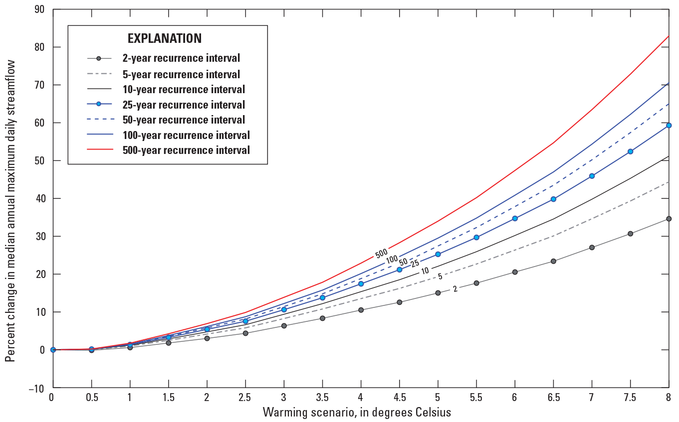
Graph showing percent change in median annual maximum daily streamflow at selected recurrence intervals for the warming scenarios at U.S. Geological Survey streamgage 01096000 (Squannacook River Near West Groton, Massachusetts).
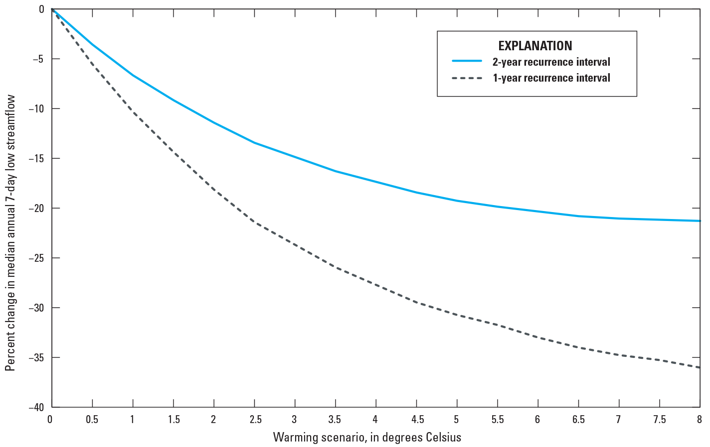
Graph showing percent change in median 7-day low streamflow at selected recurrence intervals for the warming scenarios at U.S. Geological Survey streamgage 01096000 (Squannacook River Near West Groton, Massachusetts).
Future Streamflow Characteristics
To evaluate the streamflow characteristics that may occur in response to climate change in the future—for instance, the decades of 2030, 2050, 2070, and 2090—the warming scenario applicable to these target decades is needed. Estimating the localized warming scenario for future projections requires data from downscaled Global Circulation Models (GCMs); such data were obtained from the Multivariate Adaptive Constructed Analogs (MACA) archive (Abatzoglou and Brown, 2012; Abatzoglou and Brown, undated). The MACA archive contains downscaled output from 20 GCMs of the Coupled Model Inter-Comparison Project Phase 5 for the contiguous United States and for future Representative Concentration Pathways (RCPs) with a historical baseline of 1950–2005. For this investigation, the RCP8.5 emissions scenario was used. RCP8.5 is an emissions trajectory that assumes a future, in 2100, in which no actions are taken to reduce emissions, equivalent to radiative forcing of more than 8.5 watts per square meter (IPCC Core Writing Team and others, 2014, p. 127).
From the MACA-downscaled GCM projection data, the 30-year average annual temperature changes around each of the target decades was determined for the Nashua River watershed area (the Squannacook River watershed is within the Nashua River watershed). From these ensembles of data, the medians of the ensembles were determined and are shown in table 7.
Table 7.
The median of ensembles of temperature change in the Nashua River watershed determined from 20 global climate models, in degrees Celsius, for the decades of 2030, 2050, 2070, and 2090.[Data are from Steinschneider and Najibi (2022)]
Using table 7, one can determine which warming scenario to use for a target decade. For example, to determine the percent change of the annual daily-maximum streamflow at the 50-year recurrence interval for the 2070s, table 7 could be used to find the temperature change for 2070 of 4.64 °C. The user would then select the closest warming scenario to 4.64 °C, 4.5 °C, to find in table 5 that the 50-year recurrence interval streamflow estimate would increase by about 23 percent above the baseline conditions (0 °C scenario) on the Squannacook River.
Limitations
This study investigates the effect that potential climate change may have on the severity and frequency of flooding and low streamflows, predicted through hydrologic modeling. Episodic events such as floods, which are affected by hourly and finer time-scale precipitation events, are not addressed by the climate input data or models’ output at these time scales. Following the discussion of the deterministic model calibration, simulated daily time series are likely subject to greater uncertainty when the calibration statistics are unsatisfactory. Other limitations of the techniques applied in this investigation are listed below:
-
• Water withdrawals and returns are not simulated;
-
• The effect of frozen ground on runoff is not explicitly simulated; and
-
• The hydrologic effects associated with land-use and land-cover change, which are not simulated, may be important in determining future streamflow trends and could be an important driver of hydrologic change.
Database of Project Results
A data release was created for this project (Olson and others, 2024). This data release contains the output of the SWG for the Nashua River watershed, the PRMS model and the model’s input and output, and the streamflow characteristics computed from the realizations generated from the SWM.
The plan for the next phase of this project is to analyze watersheds throughout Massachusetts using the methods described in this report. An online interactive interface may be developed that could provide access to the hydrologic data from this investigation for the Squannacook River and additional river watersheds.
Summary
Communities throughout Massachusetts face the potential consequences of climate change, ranging from more extreme rainfall to more pronounced and frequent droughts. Understanding the potential changes in hydrology resulting from climate change is important to State and community officials to evaluate the potential threats to infrastructure and water systems. To better understand the effects of climate change on hydrology, the U.S. Geological Survey, in cooperation with the Massachusetts Executive Office of Energy and Environmental Affairs, and in partnership with Cornell University and Tufts University, developed tools for projecting 21st-century climate and hydrologic characteristics in Massachusetts.
To project future climatic characteristics, a stochastic weather generator (SWG) was developed for Massachusetts. The SWG estimates daily precipitation and minimum and maximum temperature for 17 warming scenarios: from 0 to 8 degrees Celsius, in 0.5-degree increments. The SWG output data were used to characterize future climate. To project future hydrologic characteristics, the SWG data are input to a deterministic watershed model for a selected watershed, the Squannacook River watershed. Hydrologic data output from the deterministic model were then input to a stochastic watershed model developed for this study to correct model errors (model errors are often observed in output from deterministic models at the high- and low-flow extremes). The output from the stochastic watershed model was then used to characterize hydrology for the 17 warming scenarios, which allowed assessment of the changes in extreme streamflows that may be observed in the years 2030, 2050, 2070, and 2090. Under the warming scenarios, the results project more extreme flood and low streamflows. In addition, for a fixed warming scenario, the degree of magnification increased with each greater recurrence interval. For example, the percent increase in the 500-year flood was greater than the 2-year flood.
This investigation was done for the Squannacook River watershed as a pilot project. The plan for the next phase of the project is to apply the tools developed across all Massachusetts watersheds; the results of which could be incorporated into an online tool to easily access and visualize changes to hydrology in a warming climate.
Selected References
Abatzoglou, J.T. and Brown, T.J., [undated], Multivariate adaptive constructed analogs (MACA) datasets: University of California at Merced database, accessed September 15, 2023, at https://climate.northwestknowledge.net/MACA/.
Abatzoglou, J.T. and Brown, T.J., 2012, A comparison of statistical downscaling methods suited for wildfire applications: International Journal of Climatology, v. 32, no. 5, p. 772–780, accessed December 22, 2022, at https://doi.org/10.1002/joc.2312.
Collins, M.J., 2009, Evidence for changing flood risk in New England since the late 20th century: Journal of the American Water Resources Association, v. 45., no. 2, p. 279–290, accessed December 22, 2022, at https://doi.org/10.1111/j.1752-1688.2008.00277.x.
Dudley, R.W., and Hodgkins, G.A., 2002, Trends in streamflow, river ice, and snowpack for coastal river basins in Maine during the 20th century: U.S. Geological Survey Water-Resources Investigations Report 02–4245, 26 p., accessed October 1, 2018, at https://doi.org/10.3133/wri20024245.
Dudley, R.W., Hodgkins, G.A., McHale, M.R., Kolian, M.J., and Renard, B., 2017, Trends in snowmelt-related streamflow timing in the conterminous United States: Journal of Hydrology, v. 547, p. 208–221, accessed October 1, 2018, at https://doi.org/10.1016/j.jhydrol.2017.01.051.
Falcone, J.A., 2011, GAGES–II—Geospatial attributes of gages for evaluating streamflow: U.S. Geological Survey dataset, accessed October 13, 2021, at https://doi.org/10.3133/70046617.
Farmer, W.H., and Vogel, R.M., 2016, On the deterministic and stochastic use of hydrologic models: Water Resources Research, v. 52, no. 7, p. 5619–5633, accessed October 8, 2021, at https://doi.org/10.1002/2016WR019129.
Hay, L.E., and LaFontaine, J.H., 2020, Application of the National Hydrologic Model infrastructure with the Precipitation-Runoff Modeling System (NHM-PRMS), 1980–2016, Daymet version 3 calibration: U.S. Geological Survey data release, accessed July 3, 2023, at https://doi.org/10.5066/P9PGZE0S.
Hayhoe, K., Wake, C., Anderson, B., Liang, X.-Z., Maurer, E., Zhu, J., Bradbury, J., DeGaetano, A., Stoner, A.M., and Wuebbles, D., 2007a, Regional climate change projections for the Northeast USA: Mitigation and Adaptation Strategies for Global Change, v. 13, nos. 5–6, p. 425–436. [Also available at https://doi.org/10.1007/s11027-007-9133-2.]
Held, I.M., and Soden, B.J., 2006, Robust responses of the hydrological cycle to global warming: Journal of Climate, v. 19, no. 21, p. 5686–5699, accessed October 14, 2021, at https://doi.org/10.1175/JCLI3990.1.
Hodgkins, G.A., and Dudley, R.W., 2005, Changes in the magnitude of annual and monthly streamflows in New England, 1902–2002: U.S. Geological Survey Scientific Investigations Report 2005–5135, 37 p., accessed October 1, 2018, at https://doi.org/10.3133/sir20055135.
Hodgkins, G.A., and Dudley, R.W., 2006, Changes in late-winter snowpack depth, water equivalent, and density in Maine, 1926–2004: Hydrological Processes, v. 20, no. 4, p. 741–751, accessed October 1, 2018, https://doi.org/10.1002/hyp.6111.
Hodgkins, G.A., and Dudley, R.W., 2011, Historical summer base flow and stormflow trends for New England rivers: Water Resources Research, v. 47, no. 7, 16 p., accessed October 1, 2018, at https://doi.org/10.1029/2010WR009109.
Hodgkins, G.A., Dudley, R.W., Archfield, S.A., and Renard, B., 2019, Effects of climate, regulation, and urbanization on historical flood trends in the United States: Journal of Hydrology, v. 573, p. 697–709, accessed October 1, 2018, at https://doi.org/10.1016/j.jhydrol.2019.03.102.
Hodgkins, G.A., Dudley, R.W., and Huntington, T.G., 2003, Changes in the timing of high river flows in New England over the 20th century: Journal of Hydrology, v. 278, nos. 1–4, p. 244–252, accessed October 1, 2018, at https://doi.org/10.1016/S0022-1694(03)00155-0.
IPCC Core Writing Team, Pachauri, P.K., and Meyer, L., eds., 2014, Climate change 2014—Synthesis report: Geneva, Switzerland, Intergovernmental Panel of Climate Change, 151 p, accessed February 12, 2024, at https://www.ipcc.ch/report/ar5/syr/.
Leavesley, G.H., Lichty, R.W., Troutman, B.M., and Saindon, L.G., 1983, Precipitation-runoff modeling system—User’s manual: U.S. Geological Survey Water-Resources Investigations Report 83–4238, 206 p., accessed October 1, 2018, at https://doi.org/10.3133/wri834238.
Livneh, B., Bohn, T.J., Pierce, D.S., Munoz-Ariola, F., Nijssen, B., Vose, R., Cayan, D., and Brekke, L.D., 2015, A spatially comprehensive, hydrometeorological data set for Mexico, the U.S., and southern Canada 1950–2013: National Oceanic and Atmospheric Administration National Centers for Environmental Information dataset, accessed October 14, 2021, at https://www.ncei.noaa.gov/access/metadata/landing-page/bin/iso?id=gov.noaa.nodc:Livneh-Model.
Markstrom, S.L., Regan, R.S., Hay, L.E., Viger, R.J., Webb, R.M.T., Payn, R.A., and LaFontaine, J.H., 2015, PRMS–IV, the precipitation-runoff modeling system, version 4: U.S. Geological Survey Techniques and Methods, book 6, chap. B7, 158 p., accessed October 1, 2018, at https://doi.org/10.3133/tm6B7.
Moriasi, D.N., Arnold, J.G., Van Liew, M.W., Bingner, R.L., Harmel, R.D., and Veith, T.L., 2007, Model evaluation guidelines for systematic quantification of accuracy in watershed simulations: Transactions of the ASABE, v. 50, no. 3, p. 885–900, accessed October 1, 2018, at https://doi.org/10.13031/2013.23153.
Nash, J.E., and Sutcliffe, J.V., 1970, River flow forecasting through conceptual models part I—A discussion of principles: Journal of Hydrology, v. 10, no. 3, p. 282–290, accessed October 1, 2018, at https://doi.org/10.1016/0022-1694(70)90255-6.
National Oceanic and Atmospheric Administration [NOAA], 2021a, 1981–2010 normals: National Oceanic and Atmospheric Administration database, accessed September 15, 2023, at https://www.ncei.noaa.gov/access/us-climate-normals/.
National Oceanic and Atmospheric Administration [NOAA], 2021b, Potential evapotranspiration for selected locations: Northeast Regional Climate Center web page, accessed October 13, 2021, at http://www.nrcc.cornell.edu/wxstation/pet/pet.html.
Olson, S.A., Steinschneider, S., Shabestanipour, G., and Lamontangne, J., 2024, Data for a pilot study characterizing future climate and hydrology in Massachusetts: U.S. Geological Survey data release, https://doi.org/10.5066/P9JHB2X2.
Regan, R.S., Markstrom, S.L., Hay, L.E., Viger, R.J., Norton, P.A., Driscoll, J.M., and LaFontaine, J.H., 2018, Description of the National Hydrologic Model for use with the Precipitation-Runoff Modeling System (PRMS): U.S. Geological Survey Techniques and Methods, book 6, chap. B9, 38 p., accessed October 1, 2018, at https://doi.org/10.3133/tm6B9.
Reidmiller, D.R., Avery, C.W., Easterling, D.R., Kunkel, K.E., Lewis, K.L.M., Maycock, T.K., and Stewart, B.C., eds., 2018, Impacts, risks, and adaptation in the United States, v. II of Fourth national climate assessment: U.S. Global Change Research Program report, 1,515 p., accessed October 8, 2021, at https://doi.org/10.7930/NCA4.2018.
Shabestanipour, G., Brodeur, Z., Farmer, W.H., Steinschneider, S., Vogel, R.M., and Lamontagne, J.R., 2023, Stochastic watershed model ensembles for long-range planning—Verification and validation: Water Resources Research, v. 59, no. 2, 20 p., accessed April 28, 2023, at https://doi.org/10.1029/2022WR032201.
Steinschneider, S., Ray, P., Rahat, S.H., and Kucharski, J., 2019, A weather‐regime-based stochastic weather generator for climate vulnerability assessments of water systems in the Western United States: Water Resources Research, v. 55, no. 8, p. 6923–6945, accessed September 21, 2021, at https://doi.org/10.1029/2018WR024446.
Steinschneider, S., and Najibi, N., 2022, A weather-regime based stochastic weather generator for climate scenario development across Massachusetts—Technical documentation: Ithaca, N.Y., Cornell University, [Department of] Biological and Environmental Engineering report, 47 p., accessed February 16, 2023, at https://eea-nescaum-dataservices-assets-prd.s3.amazonaws.com/cms/GUIDELINES/FinalTechnicalDocumentation_WGEN_20220405.pdf.
Thornton, P.E., Thornton, M.M., Mayer, B.W., Wei, Y., Devarakonda, R., Vose, R.S., and Cook, R.B., 2016, Daymet—Daily surface weather data on a 1-km grid for North America (ver. 3): Oak Ridge National Laboratory Distributed Active Archive Center (ORNL DAAC) for Biogeochemical Dynamics digital data, accessed October 15, 2021, at https://doi.org/10.3334/ORNLDAAC/1328.
U.S. Geological Survey [USGS], [undated a], The National map viewer: U.S. Geological Survey database, accessed September 15, 2023, at https://apps.nationalmap.gov/viewer/.
U.S. Geological Survey [USGS], [undated b], StreamStats (ver. 4.17.0, 2023): U.S. Geological Survey database, accessed September 15, 2023, at https://streamstats.usgs.gov/ss/.
U.S. Geological Survey [USGS], 2023, USGS water data for the Nation: U.S. Geological Survey National Water Information System database, accessed July 3, 2023, at https://doi.org/10.5066/F7P55KJN.
U.S. Geological Survey [USGS], 2024, NHDPlus HR: U.S. Geological Survey dataset, accessed February 13, 2024, at https://www.usgs.gov/national-hydrography/access-national-hydrography-products.
Viger, R.J., and Bock, A., 2014, GIS features of the Geospatial Fabric for National Hydrologic Modeling (ver. 1.0): U.S. Geological Survey dataset, accessed June 15, 2023, at https://doi.org/10.5066/f7542kmd.
Conversion Factors
U.S. customary units to International System of Units
Temperature in degrees Celsius (°C) may be converted to degrees Fahrenheit (°F) as follows:
°F = (1.8 × °C) + 32.
Temperature in degrees Fahrenheit (°F) may be converted to degrees Celsius (°C) as follows:
°C = (°F – 32) / 1.8.
Datums
Vertical coordinate information is referenced to the North American Vertical Datum of 1988 (NAVD 88).
Horizontal coordinate information is referenced to the North American Datum of 1983 (NAD 83).
Abbreviations
GCM
global circulation model
GIS
geographic information system
HRU
hydrologic response unit
MACA
Multivariate Adaptive Constructed Analogs
NHM
National Hydrologic Model
NRMSE
normalized root-mean-square error
NSE
Nash-Sutcliff Efficiency
PBIAS
percent bias
PRMS
Precipitation-Runoff Modeling System
RCP
Representative Concentration Pathways
SWG
stochastic weather generator
SWM
stochastic watershed model
USGS
U.S. Geological Survey
For more information, contact:
Director, New England Water Science Center
U.S. Geological Survey
10 Bearfoot Road
Northborough, MA 01532
dc_nweng@usgs.gov
or visit our website at
Disclaimers
Any use of trade, firm, or product names is for descriptive purposes only and does not imply endorsement by the U.S. Government.
Although this information product, for the most part, is in the public domain, it also may contain copyrighted materials as noted in the text. Permission to reproduce copyrighted items must be secured from the copyright owner.
Suggested Citation
Olson, S.A., Shabestanipour, G., Lamontagne, J., and Steinschneider, S., 2024, Characterizing future streamflows in Massachusetts using stochastic modeling—A pilot study: U.S. Geological Survey Scientific Investigations Report 2023–5134, 19 p., https://doi.org/10.3133/sir20235134.
ISSN: 2328-0328 (online)
Study Area
| Publication type | Report |
|---|---|
| Publication Subtype | USGS Numbered Series |
| Title | Characterizing future streamflows in Massachusetts using stochastic modeling—A pilot study |
| Series title | Scientific Investigations Report |
| Series number | 2023-5134 |
| DOI | 10.3133/sir20235134 |
| Publication Date | March 19, 2024 |
| Year Published | 2024 |
| Language | English |
| Publisher | U.S. Geological Survey |
| Publisher location | Reston, VA |
| Contributing office(s) | New England Water Science Center |
| Description | Report: v, 19 p.; Data Release |
| Country | United States |
| State | Massachusetts |
| Online Only (Y/N) | Y |
| Additional Online Files (Y/N) | N |