

Water-Quality Indicators of Surface-Water-Influenced Groundwater Supplies in the Ohio River Alluvial Aquifer of West Virginia
Links
- Document: Report (2.88 MB pdf) , HTML , XML
- Data Release: USGS data release - PHREEQC files for geochemical simulations in the Ohio River Alluvial Aquifer of West Virginia
- Download citation as: RIS | Dublin Core
Acknowledgments
The authors thank public water-system managers in West Virginia for imparting their knowledge and assisting during sampling. We also acknowledge the cooperation, assistance, and knowledge provided by Brian Carr of the West Virginia Department of Health and Human Resources. Lisa Senior and Carly Maas of the U.S. Geological Survey are thanked for their thoughtful reviews that have improved this report.
Abstract
The U.S. Geological Survey, in cooperation with the West Virginia Department of Health and Human Resources, studied surface-water-influenced groundwater supplies in the Ohio River alluvial aquifer of West Virginia for the purpose of understanding the influence of surface water on groundwater chemistry. Public groundwater supplies obtained from these aquifers receive substantial recharge from surface-water sources and are highly susceptible to degradation from water-soluble contaminants. Water samples were collected from 4 sites in the Ohio River and 23 groundwater wells in the alluvial aquifer from June 2019 to January 2020. Surface-water influence was assessed through characterization of groundwater quality, determination of recharge sources, estimation of groundwater age, and estimation of the fraction of Ohio River water entering groundwater pumped by wells in the alluvial aquifers.
Hydrogeochemical processes controlling solute concentrations in the Ohio River alluvial aquifer were evaluated with multivariate statistical analysis and identified to be primarily controlled by redox processes, input from sources of salinity, and carbonate dissolution. Meteoric recharge from the Ohio River and precipitation on the alluvium are the main sources of water entering the aquifer. The age of groundwater in the system was determined to be primarily from a modern source. Groundwater samples from every well included in this study had detections for at least one geochemical indicator of surface-water influence, and every well was determined to be susceptible and vulnerable to contamination from surface sources.
Results from binary mixing models and inverse geochemical models showed that sulfate, silica, and bicarbonate concentrations predict the fraction of Ohio River water entering alluvial wells for preliminary determination of surface-water influence when compared to fractions predicted using a numerical groundwater-flow model. In the absence of extensive analytes and geochemical or groundwater modeling capabilities, preliminary assessment of the fraction of Ohio River water entering groundwater wells in the Ohio River alluvium can be estimated for most sites using a linear relation between the equivalent ratio of bicarbonate to sulfate and the fraction of water computed by the average of the three geochemical models presented in this report. This approximation of the fraction of Ohio River water, coupled with information on the hydrogeological framework and geochemical indicators of surface-water influence, may be sufficient for preliminary assessment of surface-water influence in the absence of more detailed site information or reaction-transport models.
Introduction
Alluvial aquifers along the Ohio River in West Virginia (fig. 1) represent a substantial groundwater resource for public, domestic, agricultural, and industrial use (Kozar and Brown, 1995; Bader and others, 1997). Despite a small areal extent limited to the Ohio River Valley floodplains, these alluvial aquifers have been estimated to contain more than 50-billion gallons of groundwater (Bader and others, 1997). This exceptional storage capacity derives from favorable aquifer properties related to the heterogenous lithology of the alluvium produced by shifting depositional regimes over time. In general, glacial outwash deposits of medium- to coarse-grained sediments ranging from sand to gravel are overlain by finer-grained fluvial deposits ranging from clay to gravel (Deutsch and others, 1966; Simard, 1989), creating a highly productive, predominantly unconfined, aquifer of variable thickness (Carlston and Graeff 1956; Bader and others, 1997). Compared to the sedimentary bedrock aquifers, the unconsolidated alluvial aquifers produce the greatest yields in West Virginia (Puente, 1985) because of the high transmissivities and specific capacities inherent to the alluvium (Kozar and Mathes, 2001).
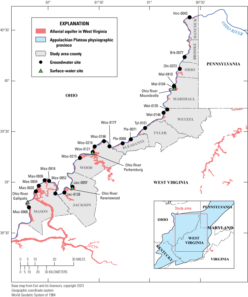
Map showing the study area and sampling locations in the Ohio River alluvial aquifer, West Virginia, June 2019–January 2020. U.S. Geological Survey (USGS) site official names and shortened names are in table 1.
Precipitation is the primary natural recharge mechanism to the Ohio River alluvial aquifer (Jeffords, 1945; Bader and others, 1997). However, induced infiltration (recharge from the pumping of wells or flooding) from the Ohio River has become an increasingly important process that can greatly exceed recharge via precipitation (Kozar and McCoy, 2004). The proximity of wells penetrating the alluvium to the Ohio River, combined with highly transmissive aquifers (Kozar and Paybins, 2016), facilitates reversal of natural hydraulic gradients from the river to the aquifer during high river stage and because of frequent pumping in dense wellfields (fig. 2; Jeffords, 1945; Kozar and McCoy, 2004). Whereas high river stage is transient, pumping water from wells is persistent (Maharjan and Donovan, 2017). Consequently, it has been shown that as much as 75 percent of water pumped from the alluvium is attributed to induced infiltration of Ohio River surface water (Kozar and McCoy, 2004), which is further supported by age-dating, water-temperature, and water-chemistry studies (Jeffords, 1945; McCoy and Kozar, 2007; Kozar and Paybins, 2016; Maharjan and Donovan, 2017). Thus, a combination of anthropogenic factors (for example, groundwater pumping), compounded by certain aquifer properties (for example, high transmissivity), has predisposed the Ohio River alluvial aquifer to qualify as a public surface-water-influenced groundwater supply (SWIG) in West Virginia.
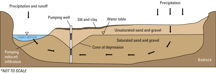
Representational block diagram of groundwater flow to a pumping well in the Ohio River alluvial aquifer of West Virginia. Modified from Maharjan and Donovan (2017). The inverted triangle denotes the water table.
Surface-Water-Influenced Groundwater Supply (SWIG)
A SWIG, as defined by West Virginia Code §22-30-3 (West Virginia Legislature, 2014), is “a source of water supply for a public water system which is directly drawn from an underground well, underground river or stream, underground reservoir or underground mine, and the quantity and quality of the water in that underground supply source is heavily influenced, directly or indirectly, by the quantity and quality of surface water in the immediate area.” However, this report assumes a previously published, modification of a SWIG to include “a groundwater supply that is heavily influenced by water recharging the well from adjacent rivers, streams, ponds, lakes, irrigation water, or even precipitation that pools at the surface” (Kozar and Paybins, 2016, p. 2). This definition permits the inclusion of additional sources of contamination from shallow surface processes (for example, crop irrigation) that may affect sources prone to rapid infiltration.
Determination of the intrinsic susceptibility and vulnerability is critical when assessing if an aquifer may be a SWIG (Kozar and Paybins, 2016). Intrinsic susceptibility includes factors like hydrogeologic properties that influence fluid transport in the unsaturated zone of an aquifer (Focazio and others, 2002). Vulnerability of an aquifer includes extrinsic factors like proximal contaminant sources and the ease of contaminant transport into and through an aquifer, which may be exacerbated by well construction design, active physical and chemical subsurface processes, and the intrinsic susceptibility of the aquifer (Eberts and others, 2013).
As SWIGs, portions of the Ohio River alluvial aquifer are defined by high intrinsic susceptibility and high vulnerability to nonmicrobial contaminants (for example, volatile organic compounds, nitrate). High transmissivities in the alluvium (4,800 feet squared per day; Kozar and Mathes, 2001) allow rapid infiltration of overland flow, either from precipitation or flooding, and induced infiltration directly from the Ohio River because of pumping (Kozar and Paybins, 2016). Progressive urbanization, industrialization, and agricultural development along the Ohio River has created multiple sources of contamination and removed surficial clays that retard infiltration (Ferrel, 1987). This removal simultaneously increases the intrinsic susceptibility and vulnerability of the alluvial aquifers that are a major groundwater resource in West Virginia, underlining the need to refine current [2019] delineations of SWIGs in the Ohio River alluvium.
In 2019, the U.S. Geological Survey (USGS) began a study in cooperation with the West Virginia Department of Health and Human Resources for the purpose of understanding the influence of surface water on groundwater chemistry in the alluvial aquifers bordering the Ohio River in West Virginia. The study was limited to the alluvial aquifers along the Ohio River in the Appalachian Plateau physiographic province of West Virginia (fig. 1) and does not include alluvial deposits of the Kanawha River or other minor tributaries. This study focused on surface-water influence in the Ohio River alluvial aquifer but not groundwater under direct influence (GWUDI) of surface water as defined by the National Primary Drinking Water Regulation (40 CFR 59570 part 141). As of 2023, no alluvial aquifers in West Virginia are classified as GWUDI, despite high intrinsic susceptibilities, because of a lack of detected pathogens (for example, virus or bacteria) and microscopic particulates in raw process water (Kozar and Paybins, 2016).
Purpose and Scope
This report describes and interprets water-quality data studied by the U.S. Geological Survey in cooperation with the West Virginia Department of Health and Human Resources to help understand the influence of surface water on groundwater chemistry in the alluvial aquifers bordering the Ohio River in West Virginia. This assessment is based on the chemical composition of surface-water samples collected from 4 sites on the Ohio River and groundwater samples collected from 23 wells in alluvial aquifers from June 2019 to January 2020. Chemical analyses of samples included major ions, dissolved organic carbon (DOC), selected man-made organic compounds, dissolved gases, tritium, and carbon-13 isotopes. Specific objectives of this study are 1) characterization of groundwater quality in relation to health-based standards and geochemical processes, 2) determination of recharge sources, 3) estimation of groundwater age, and 4) estimation of the fraction of Ohio River water entering groundwater that supplies wells in the Ohio River alluvial aquifer in the state of West Virginia. Results of multivariate analyses of water-quality samples are discussed to provide insight into geochemical processes controlling groundwater. Binary mixing models and inverse geochemical models were used to estimate the fraction of surface water in groundwater pumped by wells in the alluvial aquifer and compared to fractions estimated from previously published numerical groundwater-flow models. An improved understanding of SWIGs along the Ohio River will aid preventative efforts seeking to protect the alluvial aquifers from potential degradation associated with surface activities.
Study Area and Previous Investigations
The Ohio River alluvial aquifer in West Virginia is in the Appalachian Plateau physiographic province along the West Virginia-Ohio border (fig. 1) with alluvial sediments confined to river terraces and floodplains within the Ohio River Valley (Puente, 1985). It represents one of two major aquifer types and one of five hydrogeologic terrains (lithologies that share similar hydrogeologic properties) in the State. For context, consolidated sedimentary bedrock aquifers represent the other major aquifer type (Schwietering, 1981; Puente, 1985).
The predominantly mountainous terrain and geographic setting have a pronounced effect on climate, which is classified as temperate continental with four well-defined seasons that are locally influenced by topography (Friel and others, 1987; Battelle Memorial Institute, 2003). Average maximum and minimum temperatures from 1900 to 2016 ranged from 40 degrees Fahrenheit (°F) to 65°F, respectively. Mean precipitation, which is affected by orographic lift as atmospheric currents track eastward (Friel and others, 1987), over the same time period was 42.4 inches (Kutta and Hubbart, 2019).
The Ohio River Valley is highly developed and consists of residential, industrial, and agricultural land use. The estimated population of the 10 counties included in this study (fig.1) was 286,954 in 2022, approximately 16 percent of the State’s total population (U.S. Census Bureau, 2023). Development, particularly agriculture, decreases away from the river because of rugged terrain that typifies the Appalachian Plateau physiographic province. Residential land use is a result of the Ohio River facilitating transport across the mountainous topography during settlement, which has spawned a diverse industrial presence including electric-power generation, chemical and metal manufacturing, and petroleum refinement that supports municipal growth alongside agriculture activity (Ferrel, 1987; Bader and others, 1997; Battelle Memorial Institute, 2003). Agricultural land use, which is concentrated in the Ohio River Valley, has declined by 58 percent since 1950 (Kutta and Hubbart, 2019).
Geology
The Ohio River alluvium is confined to the floodplains within the Ohio River Valley, which extends approximately (~) 280 miles along a gentle gradient between the borders of West Virginia and Ohio. Headwaters and river morphology observed today are remnants of successive Pleistocene glaciations that altered drainage dynamics and depositional sequences that formed the alluvial aquifers (Carlston, 1962). The basal alluvium, as much as 125-feet (ft) thick, comprises glaciofluvial deposits of medium- to coarse-grained gravel and sands associated with the Wisconsin glaciation. As much as 83 percent of these sediments are derived from eroded Pennsylvanian and Permian substratum consisting of cyclothem deposits of shale, limestone, coal, underclay, and sandstone (Cross and Schemel, 1956). The remaining igneous and metamorphic pebbles are classified as exogenous to local stratigraphy and consistent with the glacial outwash origin of the lower alluvial aquifers (Carlston, 1962). Alluvial fill of reworked late Pleistocene material overlies the glaciofluvial sediments and generally ranges from 20 to 30 ft in thickness, thinning downstream and toward valley walls. Deposition of the heterogenous fill, ranging from clay to gravel and defined by lenticular interbeds of variable grain size (Cross and Schemel, 1956) has formed terraces along the Ohio River (Simard, 1989) that are overlain by Holocene floodplain deposits of silts and clays (Carlston, 1962). On average, the surface sediments are ~10 ft thick and may act as a confining unit locally that produces semi-confined aquifer conditions in the alluvium (Cross and Schemel, 1956).
Hydrogeology
The high proportion of coarse-grained glacial outwash in the Ohio River alluvial aquifer provides the foundation for an excellent groundwater resource in West Virginia. Hydrologic properties of the alluvium are ideal in the context of a groundwater resource but are subject to the intrinsic spatial and stratigraphic geological heterogeneities that affect aquifer characteristics and the extent of induced infiltration from the Ohio River. Available storage-coefficient and specific-yield data (median of 0.20) support conceptual evidence that the alluvial aquifers with a median saturated thickness of 50 ft are unconfined, albeit highly variable site to site. Median depth to water is 43 ft below land surface, far deeper than the potentially confining surficial clays. Specific capacity ranges from 4 to 381 gallons per minute per foot of drawdown (median of 31.8 gallons per minute per foot) and a median transmissivity of 4,800 feet squared per day is reported, consistent with the highly productive nature of the alluvium (Bader and others, 1997; Kozar and Mathes, 2001).
The alluvium may recharge through the following processes: (1) precipitation, (2) induced infiltration because of flooding or proximity to pumping centers, (3) inflow through underlying fractured-bedrock systems, and (4) inflow through gravel deltas from tributary streams (Bader and others, 1997). The focus of this report is on the first two processes; although, the other recharge mechanisms may be important on a local scale (Mathes and others, 1997). Initial studies discounted precipitation as a major source of direct recharge to the Ohio River alluvial aquifer because of the perceived impermeability of the surficial clay or silt layer (Carlston and Graeff, 1956); however, the clay or silt layer is not spatially homogenous or omnipresent, and water-quality data suggest percolation through this layer to the coarse-grained sediments below does happen, meaning precipitation is one of the most important sources of recharge to the alluvium (Jeffords, 1945; Bader and others, 1997). The spatial extent and magnitude of precipitation as recharge is variable though, dependent on the composition of alluvial deposits. For example, the predominance of coarser sediments, such as gravel and sand, led to a fourfold increase in recharge estimations (ranging from 3 inches per year to 12 inches per year) relative to sediments mainly composed of silt and clay (Kozar and McCoy, 2004).
Induced infiltration represents another principal source of recharge, either because of flooding of the Ohio River or in response to substantial groundwater withdrawals via pumping. Hydraulic gradients are nearly always from the alluvial aquifers to the Ohio River under normal baseflow conditions (Kazmann and others, 1943). Hydraulic gradients reverse in response to river stage (Jeffords, 1945) and nearby pumping activity (Kozar and McCoy, 2004; Maharjan and Donovan, 2017), producing induced infiltration of water from the Ohio River to the adjacent alluvium. Locally, induced infiltration may be impeded by the spatially variable nature of benthic river sediments (Mathes and others, 1997), but impediment is challenging to quantify. Induced infiltration associated with transient events, such as floods, implies a minimal effect on the hydrologic budget of the alluvium; however, persistent reversals in hydraulic gradients, associated with cones of depression created by extensive pumping, may impart a large effect. Frequent use of radial collector wells (also known as “Ranney wells”) that extend beneath the riverbed at pumping centers only exacerbate induced infiltration from the Ohio River. Simulations of groundwater flow in select areas of the Ohio River alluvial aquifer in West Virginia demonstrated the spatial variability of induced infiltration, which accounted for 4 to 75 percent of water pumped at various sites. Well-field density and surficial-sediment compositions were identified as potential factors controlling the magnitude of induced infiltration, with large cones of depression tied to closely spaced wells and higher percentages of fine-grained sediments in the alluvium (Kozar and McCoy, 2004).
Water Quality
The Ohio River Valley represents a major transportation corridor and population center in West Virginia where extensive industrial and agricultural activity has adversely affected groundwater quality in the intrinsically susceptible alluvial aquifers. Notwithstanding, water quality is generally acceptable in the Ohio River alluvial aquifer, which accounts for over 50 percent of public groundwater supplies in the State (Ferrel, 1987). Water is hard (median hardness of 220 milligrams per liter [mg/L]) and prone to elevated iron and manganese concentrations that exceed secondary maximum-contaminant levels (SMCLs). Both characteristics have been attributed to alluvium mineralogy (Carlston and Graeff, 1956; Ferrel, 1987; Bader and others, 1997). Geological features of the alluvial aquifer also indirectly affect water quality by facilitating contaminant transport associated with surface activities.
Rapid transport of surficial water into the alluvium, either from precipitation, runoff, or induced infiltration from the Ohio River, is evident by water-quality data. Contamination from agricultural and industrial activity is apparent in the form of elevated nitrogen (nitrate plus nitrite) and volatile organic compound (VOC) concentrations, respectively. Nitrogen (N) levels in the alluvial aquifers are greater than those observed in any other aquifer system across West Virginia. Of the 35 alluvial aquifer wells included in the West Virginia ambient groundwater-quality monitoring network (Chambers and others, 2012), 1 sample (11 mg/L as N) exceeded the U.S. Environmental Protection Agency (EPA) National Primary Drinking Water Regulation (40 CFR 59570 part 141) maximum-contaminant level (MCL) of 10 mg/L as N for nitrate plus nitrite, and 5 samples exhibited levels above background concentrations (5 mg/L as N). Further degradation of water quality from the pronounced industrial presence along the Ohio River is underlined by the presence of VOCs in most (60 percent) of the samples from alluvial aquifer wells (Chambers and others, 2012). For context, no other aquifer included in the ambient monitoring network had detections of VOCs in most samples. Despite the clear susceptibility of the alluvium to surface contamination, alluvial sediments do act as effective microbial biofilters that inhibit bacterial infestation (Jeffords, 1945; Chambers and others, 2012). Samples from only 1 of the 42 wells analyzed in the Ohio River alluvial aquifer had a positive detection of fecal coliform. Still, the widespread presence of surficial contaminant species, such as nitrate and VOCs, in the Ohio River alluvium signifies the susceptibility and vulnerability of this critical groundwater resource to degradative surface activities in the area.
SWIG Recognition in the Ohio River Alluvial Aquifer
The Ohio River alluvial aquifer is defined by a high intrinsic susceptibility and high vulnerability because of a combination of hydrogeologic and anthropogenic factors previously outlined in this report. Early recognition of potential induced infiltration from the Ohio River (Jeffords, 1945) has been substantiated by extensive study. Most work has centered on indirectly qualifying and quantifying how groundwater demand, fulfilled primarily by pumping centers, has altered the natural hydraulic gradients in the alluvium. Consequently, the likelihood for the Ohio River alluvial aquifer to be classified as a SWIG has dramatically increased over time.
Multiple data types indicate that surface water from the Ohio River interacts with the alluvial aquifers. Chlorofluorocarbon age dating techniques (McCoy and Kozar, 2007) and thermal covariation between water in the Ohio River and groundwater in alluvial wells (Jeffords, 1945) indicates that the groundwater in the alluvium is almost exclusively young (less than [<]60 years). Additional analysis of temperature data demonstrated a disruption of thermal stratification in alluvial aquifers proximal to high-frequency pumping centers caused by induced infiltration from the Ohio River (Maharjan and Donovan, 2017). Water-quality data from the Ohio River alluvial aquifer are congruent with water-quality in the Ohio River, with elevated nitrate and VOC concentrations attributed to surface activities (for example agriculture and industry) (Kozar and Paybins, 2016). Comparison between proximal (<1,000 ft from Ohio River) and distal (greater than [>] 1,000 ft from Ohio River) alluvial well water chemistry to Ohio River water revealed consistencies between river and groundwater in proximal wells, such as low total dissolved solids (TDS), electric conductivity (EC), alkalinity, and enriched delta carbon-13 (δ13C) values of dissolved inorganic carbon (DIC), indicative of induced infiltration. Conversely, distal wells exhibited higher TDS, EC, alkalinity, and relatively depleted δ13C values of DIC and were not affected by exfiltration from the Ohio River (Maharjan and Donovan, 2017). Simulations of groundwater flow in select well fields along the Ohio River not only corroborate the induced infiltration based on field data but also highlight the complexities of SWIG classification arising from the inherent heterogeneities of the alluvium (Kozar and McCoy, 2004).
Spatial and stratigraphic variability in the Ohio River alluvium precludes blanket classification as a SWIG across the entire aquifer system. The magnitude of induced infiltration is highly variable across space, contributing to 4 to 75 percent of water pumped based on numerical groundwater flow modeling of multiple well fields (Kozar and McCoy, 2004). In addition to aquifer properties (for example storage capacity, transmissivity, confinement), the proximity to pumping centers, pumping rates, cone of depression morphology, groundwater levels relative to river stage elevation, and duration of hydraulic gradient reversal collectively determine the potential for induced infiltration, and, by extension, SWIG conditions (Donovan, 2019). Thus, an updated and refined classification of possible SWIGs within the Ohio River alluvial aquifer in West Virginia is paramount to safeguard this critical groundwater resource against current [2019] and future surface contamination.
Methods of Study
Water-quality samples were collected by the USGS from 4 surface-water sites and 23 groundwater wells (fig.1; table 1) in the study area from June 2019 to January 2020. The surface-water sites were chosen with the intention of evenly distributing surface-water samples in the Ohio River across the study area. Groundwater wells were chosen for sampling with the intention of having a representative distribution of sites based on distance to the Ohio River. Distance to the Ohio River was estimated using aerial photography in a geographic information system program. Well depth below land surface values in table 1 were not surveyed and should be considered estimates.
Table 1.
Site information for 4 surface-water sites and 23 groundwater wells in West Virginia where samples were collected for the study from June 2019 to January 2020. Well-depth data from the U.S. Geological Survey National Water Information System (U.S. Geological Survey, 2023).[The column labeled distance represents the distance estimated from the sampling location to the Ohio River. U.S. Geological Survey site numbers have not been shared for groundwater sites because they are based on sensitive information. USGS, U.S. Geological Survey; ft, feet; BLS, below land surface; OR, Ohio River; SW, surface water; —, not applicable; @, at; WV, West Virginia; GW, groundwater]
Analytical results are documented in McAdoo, Grindle, and Grindle (2022) and the USGS National Water Information System (U.S. Geological Survey, 2023). Some data either are not available or have limited availability because of restrictions dictated by West Virginia State Law §22-26-4 and USGS policy concerning the release of sensitive water related information.
Sampling Methods
To prevent environmental contamination, samples were collected and processed inside a mobile field laboratory or a portable processing chamber assembled near the sampling location. Surface-water samples were collected by scientists on a boat at multiple stations across the Ohio River using a 1-liter Nalgene narrow mouth bottle and weighted bottle sampler. Samples were width-integrated from eight vertical stations across the river, and the vertical samples collected were poured into an 8-liter polyethylene churn splitter for sample processing. A multi-parameter water-quality sonde (YSI EXO 2, Yellow Springs, Ohio) was used to measure water temperature, pH, specific conductance, dissolved oxygen, and turbidity according to procedures described in the USGS National Field Manual (U.S. Geological Survey, variously dated).
Groundwater samples were collected at public water system wells in the Ohio River alluvium. Raw-water taps, as identified by the operator at the public water system, were tested with commercially available chlorine test strips to ensure the sample point was located before the system’s disinfection processes. Often located at 3/8-inch hose bibs, raw-water taps came in many configurations including lab faucets, threaded and unthreaded plumbing connections made of various metals, PVC pipes, and other plastic connections. Standard sample tubing was connected to raw-water taps using a combination of nylon connectors, stainless-steel fittings, and hose clamps to ensure an airtight connection. Sample tubing was connected to a flow-through chamber with a YSI multiparameter water-quality sonde, which was calibrated daily and measured temperature, pH, specific conductance, dissolved oxygen, and turbidity. All samples were collected at active high-production wells and did not require purging based on well volume. Field parameters were monitored for a minimum of 25 minutes and readings were recorded every 5 minutes to meet stability criteria according to the National Field Manual (U.S. Geological Survey, variously dated) and to collect enough data to calculate median values for each parameter. After field parameters were recorded, samples were collected in recommended sample containers and preserved according to lab instructions.
All samples (surface water and groundwater) were analyzed for field measurements of water quality (pH, water temperature, specific conductance, dissolved oxygen concentration, and turbidity), alkalinity, major ions, trace elements, nutrients, DOC, and per- and polyfluoroalkyl substances (PFAS; table 2). Subsets of samples at proximal wells were analyzed for microbiological indicators of fecal contamination (table 3), VOCs (table 4), semi-volatile organic compounds (SVOCs; table 5), and pesticides (table 6) to assess potential aquifer degradation from surface-water influence. Field measurements and samples for inorganic analytes, VOCs, SVOCs, DOC, and pesticides were processed using standard USGS protocols described by the USGS National Field Manual for the Collection of Water Quality Data (U.S. Geological Survey, variously dated). These protocols specified that samples collected for determination of dissolved concentrations (major ions, trace elements, nutrients, DOC) were filtered in the field through a 0.45-micron filter and, for some analyses (cations, trace elements), preserved with nitric acid.
Samples collected for determination of major inorganic element, trace element, nutrient, VOC, SVOC, and pesticide concentrations were chilled on ice and shipped overnight to the USGS National Water Quality Laboratory in Lakewood, Colorado, for analysis. Samples collected for determination of microbiological indicators of fecal contamination were chilled on ice and shipped overnight to the USGS Ohio Microbiology Laboratory in Columbus, Ohio. Samples for determination of PFAS concentrations were analyzed by RTI Laboratories in Livonia, Michigan, according to PFAS analysis compliant with U.S. Department of Defense Quality Systems Manual (U.S. Department of Defense, 2019).
Table 2.
List of general water-quality characteristics, major ions, trace elements, nutrients, and per- and polyfluoroalkyl substances and associated laboratory reporting levels for analyses of 4 surface-water samples and 23 groundwater samples collected from the Ohio River and the Ohio River alluvial aquifer from June 2019 to January 2020.[Dissolved concentrations were determined for all analytes except per- and polyfluoroalkyl (PFAS). mg/L, milligrams per liter; —, not applicable; °C, degrees Celsius; μS/cm, microsiemens per centimeter; NTU, nephelometric turbidity units; CaCO3, calcium carbonate; μg/L, micrograms per liter; N, nitrogen; P, phosphorus; ng/L, nanogram per liter; FTS, fluorotelomer sulfonate]
Table 3.
Microbiological indicators of fecal contamination and associated laboratory reporting levels for analyses of 18 groundwater samples collected from wells in the Ohio River alluvial aquifer from June 2019 to January 2020.[MPN, most probable number; DSTM, defined substrate test method; cfu, colony-forming unit; —, not applicable]
Table 4.
Volatile organic compounds and associated laboratory reporting levels for analyses of 19 groundwater samples collected from wells in the Ohio River alluvial aquifer from June 2019 to January 2020.[µg/L, micrograms per liter]
Table 5.
Semi-volatile organic compounds and associated laboratory reporting levels for analyses of 13 groundwater samples collected from wells in the Ohio River alluvial aquifer from June 2019 to January 2020.[µg/L, micrograms per liter]
Table 6.
Pesticides, herbicides, and associated laboratory reporting levels for analyses of 19 groundwater samples collected from wells in the Ohio River alluvial aquifer from June 2019 to January 2020.[ng/L, nanogram per liter]
Quality Control and Quality Assurance
Quality-assurance samples were collected to provide confidence in analytical results, identify potential sample contamination issues, and describe the magnitude of combined sample and analytical variability. Blank samples were used to determine the extent to which sampling or analytical methods may contaminate samples, which may bias analytical results. Replicate samples are used to determine the variability inherent in collection and analysis of environmental samples. Together, blank and replicate samples were used to characterize the accuracy and precision of water-quality data.
Where sufficient data were available, the ionic charge-balance error (CBE) was calculated to evaluate the electroneutrality of the water sample, identify transcription errors during field activities, and identify laboratory analytical errors. The CBE can be used to assess the accuracy and completeness of field and laboratory results for constituents contributing to sample ionic charge, which typically include the major ions (Freeze and Cherry, 1979). The CBE is calculated by the following formula:
wherez
is the absolute value of the ionic valence,
mc
is the molality of the cation species, and
ma
is the molality of the anion species.
The CBE has a positive value when the sum of cations exceeds the sum of anions but a negative value when the sum of anions is greater than the sum of cations. Calculated CBEs are rarely zero and values as much as 10 percent are typically considered acceptable; however, CBEs may exceed this threshold for waters with low-ionic strength (specific conductance <100 µS/cm) or in acidic waters (Fritz, 1994). Analysis of quality-assurance data showed that no sites had a CBE greater than 10 percent for this study and concentrations of replicate sample pairs differed by small amounts, typically less than 15 percent of the relative percent difference (RPD). Constituents with higher RPD were usually constituents at low concentration at or below the method detection limit. Analytical or sampling variability was considered minimal as a result.
A combination of equipment blanks and field blanks was used to identify and quantify potential sources of contamination. An equipment blank consists of a volume of water of known quality that is processed through the sampling equipment in a laboratory environment. A field blank consists of a volume of water processed through the sampling equipment under the same field conditions in which the samples were processed. Equipment blanks were run through two sets of sampling equipment prior to environmental sampling. One equipment blank had detections above the laboratory reporting level for cobalt, copper, and zinc. That set of sampling equipment was discarded and not used for environmental samples.
Variability for a replicate sample pair was quantified by calculating the RPD of the samples. The RPD was calculated using the following formula:
whereStatistical Analysis
Both univariate and multivariate statistical methods were used to ascertain significant constituent variations and distributions impacting water quality and water-quality dispersal throughout the study area. Statistical analyses were computed, and graphics created, using the R statistical computing environment, version 3.5.3 (R Core Team, 2022). Nonparametric techniques were used for computing descriptive and multivariate statistics from water-quality data that were censored at multiple levels. Censored values are water-quality results that are reported as less than a laboratory reporting level.
Prior to multivariate and summary statistical analyses, censored data were recoded to u-scores with the codeU function in the USGS smwrQW package (Lorenz, 2018). The u-score is the sum of the sign of the differences between each value and all other values and is equivalent to the rank but scaled so the median is equal to zero. Using u-scores allows for the computation of multivariate relations without requiring censoring at the highest reporting limit and retains information at multiple reporting limits. When a column of data has only one censoring level, the u-scores are the same as ordinal methods of ranking for one reporting limit (Helsel, 2012).
Summary Statistics for Censored Data
The nonparametric Kaplan-Meier (KM) and robust regression on order statistics models were used for estimation of summary statistics for censored data following the methods described by Ryberg (2006) and Helsel (2012). When a sample had from 50 to 80 percent censored values, the robust regression on order statistics model was used. The robust regression on order statistics model was used for this range of censoring because of its ability to make accurate estimates and handle multiple censoring levels with fewer than 50 observations. When less than 50 percent of the data were censored, the KM model was used to estimate the summary statistics. The KM estimate was used to account for multiple censoring levels because it does not depend on the assumption of a distributional shape with data that are censored at rates greater than 50 percent. When no values were censored, nonparametric estimates were not necessary and summary statistics were computed using standard methods.
Multivariate Statistics for Censored Water-Quality Data
Principal components analysis (PCA) and hierarchical agglomerative cluster analysis (HACA) were used to delineate groundwater hydrochemical-facies throughout the study area. Hydrochemical-facies is a term used to specify the chemical composition and hydrochemical processes in a portion of the aquifer (Back, 1966). Principal components analysis was used to identify relations among the major chemical and hydrological processes that could explain dissolved element concentrations in the water-quality dataset. Principal components analysis was computed with the principal function in the R psych package (Revelle, 2023), which first computes correlation coefficients (Spearman’s rho) for the raw u-scores (ranks) and then performs a PCA on the resulting Spearman rank correlation matrix. Varimax rotation was applied to redistribute the explained variance across principal components and simplify the structure of the PCA model, which maximizes the differences in components and aids in the interpretation of results (Kachigan 1986). Water-quality variables that had missing values or were censored in more than 40 percent of the values were excluded from the PCA. Specific analytes and parameters used in the PCA for this study included dissolved oxygen, DOC, calcium, magnesium, potassium, sodium, chloride, nitrate, bicarbonate, sulfate, silica, iron, and manganese. The variable loadings from the varimax-rotated PCA were used to determine the master variables for each rotated component. Resulting loadings from the PCA and statistically significant correlations (p<0.01) from the correlation matrix were retained and used for further interpretation of the dataset.
Hierarchical agglomerative cluster analysis has been shown to be an effective multivariate statistical technique for the analysis of water chemistry data and has been used by previous studies (Güler and others, 2002; Ryberg, 2006) to group data based on chemical concentrations and field measurements. Specific analytes and parameters used in the HACA for this study included delta hydrogen-2 (δ2H), delta oxygen-18 (δ18O), delta carbon-13 (δ13C), pH, specific conductance, dissolved oxygen, DOC, calcium, magnesium, potassium, sodium, chloride, fluoride, bicarbonate, silica, sulfate, iron, and manganese. Similarity was computed using Euclidian distance, and clusters were merged using Ward’s method as described by Güler and others (2002). The agglomerative coefficient produces a numerical value between 0 and 1 and was used to assess the clustering structure (Kaufman and Rousseeuw, 1990). The similarity profile (SIMPROF) test was used to identify significant clusters (p<0.01; Clarke and others, 2008). Using the SIMPROF test to identify significant clusters was necessary to reduce misinterpretation of the HACA, but ultimately, the number of clusters chosen for further study was based on the study objectives, data, and results.
Geochemical Modeling and Interpretation
The surface-water influence on groundwater quality was evaluated through four methods of geochemical modeling and interpretation. Stable isotopes and groundwater age analysis was used to determine recharge sources and assess the aquifer’s susceptibility to contamination from surface-water sources. Binary mixing models and geochemical inverse models were used to delineate the proportion of Ohio River water entering SWIG wells in the alluvial aquifer.
Stable Isotopes
Stable isotopes of water (δ2H and δ18O) were evaluated to determine variation in recharge sources throughout the study area by comparing measured isotopic concentrations at sampling sites to the isotopic composition reported in precipitation. Samples were compared to the local meteoric water line (LMWL) published by Smith and others (2021; δ2H=7.58 x δ18O+9.16), which was used to represent precipitation in the Ohio River Valley. The line-conditioned excess (LC-excess; Landwehr and Coplen, 2006) was computed for groundwater samples to indicate additional evaporative fractionation relative to the LMWL. Samples with negative LC-excess values indicated the likelihood of post-precipitation evaporation, whereas positive LC-excess values indicated an input from distinct recharge sources, including higher elevations or stronger seasonal influence, with stable isotope compositions different from the assumed areal modern precipitation.
Groundwater Age Analysis
For this study, environmental tracer concentrations of dissolved gases (nitrogen and the noble gases) were used to determine recharge conditions and compute concentrations of tritiogenic helium-3 (3Hetrit) and radiogenic helium-4 (4Herad). Computed 3Hetrit and measured concentrations of tritium (3H), sulfur hexafluoride (SF6), and corrected carbon-14 (14C) were used for estimating groundwater age. Delta carbon-13 (δ13C) was used for geochemical correction of 14C in DIC. Field parameters (water temperature, pH, and alkalinity), dissolved oxygen, and the inorganic and trace element chemistry were used to parameterize 14C correction models, assess redox conditions, and develop conceptual models that guide interpretation of tracer concentrations.
Dissolved Gases
Nitrogen and noble gases naturally exist in the atmosphere. The heavy noble gases of neon (Ne), argon (Ar), krypton (Kr), and xenon (X) and (or) Ar and nitrogen gas (N2) dissolved in water were interpreted through the closed-system equilibration model or the unfractionated air model (Aeschbach-Hertig and others, 2000; Aeschbach-Hertig and Solomon, 2013) for determining noble gas recharge temperature (NGT; a proxy for altitude and timing of recharge), excess air (Ae) or entrapped air (EA), and the fractionation factor (F) of the gases during recharge. The fractionation factor cannot be estimated for samples that only have Ar and N2 analysis available. N2 in excess of atmospheric solubility is primarily derived from denitrification. Presence of suboxic to anoxic conditions suggest possible denitrification. Excess N2 was included as an additional dissolved gas model parameter at select sites with suboxic or anoxic redox conditions.
Helium isotopes, helium-3 (3He) and helium-4 (4He) were used to determine the helium isotopic ratio of the sample to that of the atmosphere (R/Ra) and the amount of helium derived from radiogenic sources (4Herad) and the decay of tritium (3Hetrit; Solomon 2000; Solomon and Cook 2000). Calculations of 4Herad and 3Hetrit assumed a terrigenic 3He/4He ratio of 2.8×10⁻⁸, a value within the measured range of helium production from uranium (U)- and thorium (Th)-series decay that represents helium of mantle or crustal origin (Andrews, 1985). Following previous work (Aeschbach-Hertig and others, 2000; Manning and Solomon, 2003; Aeschbach-Hertig and Solomon, 2013) the computed recharge parameters (EA, F) were evaluated with the Dissolved Gas Modeling and Environmental Tracer Analysis Computer Program (DGMETA, Jurgens and others 2020) by minimization of the error-weighted misfits (χ2) between measured and modeled noble gas concentrations.
Tritium
Tritium is naturally produced as a cosmogenic isotope (half-life of 12.32 years; Lucas and Unterweger, 2000) and is also produced in nuclear fission. High concentrations of 3H were released to the atmosphere during above-ground nuclear testing from 1953 to the early 1960s. Recharge during this period has an elevated bomb-pulse 3H signal. Water containing greater than 0.5 tritium units (TU) was interpreted here as having at least some fraction of recharge after 1953, whereas concentrations less than 0.5 TU were considered tritium-dead in accordance with the analytical uncertainty. Atmospheric 3H concentration curve used for lumped parameter models was based on interpolation of nation-wide precipitation measurements (Michel, 1989).
Sulfur Hexafluoride
Sulfur hexafluoride is primarily sourced from industrial applications and used to evaluate the age of younger (less than 60 years [yr]) groundwater or identify a component of young water in a mixed signal. Atmospheric concentrations of SF6 have increased since 1970 (Busenberg and Plummer, 2000) and have a long atmospheric lifetime (~3,200 yr; Land and Huff, 2010) making it a useful age tracer for young groundwater. Sulfur hexafluoride concentrations are subject to potential anthropogenic and natural contamination. For example, SF6 is produced naturally in fluorite deposits and volcanic or hydrothermal terrains (Busenberg and Plummer, 2000). Sulfur hexafluoride concentrations were corrected for EA using the computed value from noble gas modeling as described previously and have not been corrected for the potential unsaturated zone time-lag (Cook and Solomon, 1995). Inputs for lumped parameter modeling are from the USGS Reston Groundwater Dating Laboratory (https://water.usgs.gov/lab/software/air_curve/). Throughout the study area, SF6 inputs were assumed to be constant.
Carbon Isotopes
Carbon-14 is naturally produced as a cosmogenic isotope and is also produced in nuclear fission (Kalin, 2000). With a 5,568.3 yr half-life, 14C of DIC was used to evaluate the age of pre-1950s groundwater and identify the presence of old groundwater in mixtures of differing recharge sources. Groundwater conditions are conducive to DIC geochemical and isotopic exchange, making 14C more difficult to interpret, and available groundwater age tracers for dating of thousands of years-old waters remain meager.
The graphical method of Han and others (2012) was used to estimate the isotopic composition of the various carbon exchange reservoirs and indicated the Revised Fontes and Garnier (RFG; Han and Plummer, 2013) analytical correction model is appropriate for most samples in accounting for DIC from soil zone gas and saturated aquifer carbonates. Carbon-14 and δ13C values for the soil zone gas and the aquifer carbonates were estimated from the plot and further refined by checking corrected final 14C values against other tracers. Sites appropriately captured by the RFG model were corrected using the open-system model, which accounts for continued gas exchange between the atmosphere and groundwater. Model parameterization and 14C correction methods are discussed in the carbon isotope analysis section of this report.
Binary Mixing Models
Mixing of Ohio River water with distal groundwater wells in the alluvium was evaluated to assess relative percentages of these end members contributing water to intermediate groundwater wells proximal to the Ohio River. The Ohio River end member was assumed to be represented by the average of all four surface-water samples. The distal-well end member consisted of the average of 4 wells located greater than 1,000 ft from the Ohio River (Mas-0852, Jac-0128, Jac-0057, Woo-0196). Although Mas-0920 and Ple-0071 are also greater than 1,000 ft from the Ohio River (table 1), they were not included in the calculation for the distal-well end member because an inverse model was needed for Mas-0920 to compare to groundwater model results reported by Kozar and McCoy (2004) and Ple-0071 was identified as possibly being influenced by an unknown surface-water source (explained in the Water-Quality Indicators of Surface-Water Influence on Groundwater Wells section).
The following two chemical constituents were used for mixing models: 1) the silica concentration of the sample, and 2) the ratio of the equivalents of bicarbonate as a percentage of anions to the equivalents of sulfate as a percentage of anions. Generally, binary mixing models use conservative chemical constituents to compute fractions of contribution from different sources. Although bicarbonate, sulfate, and silica may not be conservative at every site, fractions of the Ohio River water end member computed with binary mixing models using these constituents yielded results that significantly correlated with inverse models and groundwater models (explained in subsequent sections). Binary mixing models were calculated with the following formula:
where Solving for xGeochemical Inverse Models
Where possible, geochemical inverse models (also known as mole-balance models) were calculated to estimate fractions of end member chemistries supplying wells located less than 1,000 ft from the Ohio River. Geochemical inverse models were computed using PHREEQC (Parkhurst and Appelo, 2013) to account for non-conservative analytes and mixing. PHREEQC input and output files are available as a USGS data release (McAdoo, 2024). Geochemical inverse models use sets of chemical reactions that quantitatively compensate for changes in chemical and isotopic compositions of water along a flow path and may include contributions from different sources (Parkhurst, 1997). The thermodynamic data file used for speciation and inverse model calculations was WATEQ4F (Ball and Nordstrom, 1991). Chemical constituents used for inverse models included dissolved oxygen, pH, temperature, calcium, magnesium, sodium, alkalinity (as CaCO3), chloride, silica (as SiO2), sulfate, and iron. Reactive mineral and gas phases used as sinks (precipitation) or sources (dissolution) for mole balances included calcite, dolomite, amorphous silica, halite, organic matter (CH2O), carbon dioxide, hydrogen sulfide, goethite, amorphous ferrihydrite, pyrite, and sodium exchange with calcium and magnesium. Chemical constituents of two end members (referred to as initial solutions in the PHREEQC input file) were mixed and allowed to react with the specified list of mineral phases and uncertainty of 10 percent to produce a final solution. Inverse models may produce multiple non-unique solutions and for this study the simplest model with the minimum number of mineral phases was retained for each inverse model.
The first initial solution consisted of the average of chemical constituents for all four surface-water sites and represented the Ohio River end member. The second initial solution consisted of the average of chemical constituents for 4 wells greater than 1,000 ft from the Ohio River (Mas-0852, Jac-0128, Jac-0057, Woo-0196) and represents the distal-well end member. Although Mas-0920 and Ple-0071 are also greater than 1,000 ft from the Ohio River (table 1), they were not included in the calculation for the distal well end member because 1) an inverse model was needed for Mas-0920 to compare to groundwater-flow simulations of the amount of river water that infiltrates the aquifer and is captured by pumping wells (Kozar and McCoy, 2004), and 2) Ple-0071 was identified as possibly being influenced by an unknown surface-water source (explained in further detail in subsequent sections). The initial solutions for every inverse model were represented by the Ohio River end member and the distal-well end member as described, but the final solution for each inverse model was represented by the analytical results measured at each well located less than 1,000 ft from the Ohio River and Mas-0920 (1,475 ft from the river).
Groundwater Quality of the Ohio River Alluvial Aquifer
Groundwater quality in the Ohio River alluvial aquifer was assessed using analytical results for samples collected from 23 wells from June 2019 to January 2020. These water-quality data were described by summary statistics and compared to drinking water standards. Multivariate statistics were used to provide insight into factors affecting the groundwater quality.
Statistical Summary of Field Parameters and Analytical Results
The sites sampled for this study represent raw-water supplies. Many of these sites have additional treatment after the point sampled, so the statistical summary of results presented here characterizes source water that may not be representative of supplied drinking water. Nevertheless, these data were compared to human-health benchmarks established by EPA (Environmental Protection Agency, 2018) to describe source-water quality relative to drinking-water standards. The EPA’s regulatory primary standards are established to protect human health, are mandatory for public supplies, and define the maximum-contaminant levels (MCL) or highest allowable concentrations in drinking water. Other non-regulatory EPA drinking-water guidelines used to assess this dataset include health advisories (HA) and secondary maximum-contaminant levels (SMCL). Health advisories, which are non-enforceable, provide technical information to state agencies and other public health officials on potential health effects for selected constituents that have no MCL or, in addition to the MCL. Secondary maximum-contaminant levels are listed for selected constituents that pose no known health risk but may have adverse aesthetic effects, such as staining or undesirable taste or odor.
Field Parameters and Total Dissolved Solids
Parameters used for general water-quality characterization included field measurements of pH, specific conductance, temperature, turbidity, and alkalinity (table 7). The only field measurement to have an established secondary drinking-water standard is pH. The SMCL range for pH is from 6.5 to 8.5 units. Water with pH less than 6.5 may be corrosive and could leach metals like copper or lead from plumbing. Water with a measured pH less than, greater than, or equal to 7 is acidic, basic, or neutral, respectively. The pH of groundwater measured in samples from all 23 wells ranged from 6 to 7.4, with a median of 7. Three of 23 samples (13 percent) were outside of the SMCL range, and all 3 had pH lower than 6.5.
Total dissolved solids is used as a measure of salinity, with freshwater typically having TDS concentrations less than 1,000 mg/L. Concentrations of TDS of groundwater samples from the 23 wells ranged from 195 mg/L to 727 mg/L. Only one groundwater sample had TDS concentrations that exceeded the SMCL of 500 mg/L in drinking water.
Table 7.
Descriptive statistics of chemical properties measured in the field and total dissolved solids and dissolved major ion concentrations measured in the laboratory for groundwater samples collected from 23 wells in the Ohio River alluvial aquifer, West Virginia, June 2019–January 2020.[Human-health benchmarks from U.S. Environmental Protection Agency (2018). MCL, maximum-contaminant level; HA, health advisory; SMCL, secondary maximum-contaminant level; mg/L, milligrams per liter; —, not applicable because there is no set standard for this constituent; n.d., no data; μS/cm, microsiemens per centimeter at 25 degrees Celsius; SU, standard units; NTRU, nephelometric turbidity unit; CaCO3, calcium carbonate; SiO2, silica]
Major Ions, Nutrients, and Trace Elements
Sources of major ions in the Ohio River alluvium may include precipitation, dissolution of minerals, and constituents introduced through various anthropogenic activities, such as deicing salts and septic systems. The only major ion with an MCL is fluoride, at 4 mg/L, and no samples had fluoride concentrations that exceeded this threshold. The SMCLs have been established for two major ions, 250 mg/L SMCL for sulfate and 250 mg/L SMCL for chloride, but no sample had concentrations of these constituents that exceeded the respective standards. Although chloride concentrations did not exceed a drinking-water standard, chloride concentrations higher than 10 are likely to be above natural background levels (Davis and others, 2005). The health-based drinking-water advisory of 20 mg/L sodium established by EPA for individuals on a sodium-restricted diet was exceeded in 12 of 23 (52 percent) samples. The EPA taste-based drinking-water advisory of 30–60 mg/L sodium was exceeded in samples from 4 wells, with those concentrations ranging from 30.1 to 54.1 mg/L.
Nitrate was detected above the reporting level at all 23 sites, ranging from 0.153 to 7.18 mg/L as N, but was not measured above the MCL of 10 mg/L as N in samples from any well in the study area (table 8). Nitrite was detected above the reporting level at 10 of 23 wells (43 percent) but was not measured in samples from any well above the MCL of 1 mg/L as N. Ammonia has a HA level and taste-based drinking-water advisory of 30 mg/L, but no samples had ammonia concentrations that exceeded this threshold. Nitrate and nitrite are common nutrients that can exceed drinking-water standards in agricultural areas of West Virginia, but the occurrence of nitrate and other nutrients at concentrations approaching drinking-water standards is uncommon for non-agricultural areas of the state (Chambers and others, 2012). Nitrate is not only derived from agricultural fertilizers, both from synthetic and animal sources, but also can be derived from wastewater treatment plant effluent or septic systems.
Table 8.
Descriptive statistics of nutrients and trace elements measured in the laboratory for samples collected from groundwater wells in the Ohio River alluvial aquifer, West Virginia, June 2019–January 2020.[Human-health benchmarks from U.S. Environmental Protection Agency (2018). MCL, maximum-contaminant level; HA, Health Advisory; SMCL, secondary maximum-contaminant level; mg/L, milligrams per liter; N, nitrogen; <, less than; —, not applicable; P, phosphorus; μg/L, micrograms per liter]
Concentrations of 23 trace elements, 20 of which have established drinking-water standards (MCLs, SMCL, or HAs), were analyzed at all 23 groundwater sites (table 8). Eighteen of these analytes were detected above the reporting level, with 14 analytes detected at more than 70 percent of sites, but no trace element was measured in concentrations above any established MCL. Manganese exceeded its criteria (SMCL and HA) more frequently than any other trace element. Iron was the second most frequent trace element to exceed its criteria. The SMCL of 50 micrograms per liter for manganese was exceeded in samples from 11 of 23 wells (48 percent) and the HA threshold of 300 mg/L was exceeded in 5 of 23 samples (22 percent). The SMCL of 300 mg/L for iron was exceeded in samples from 4 of 23 wells (17 percent).
Microbiological Indicators
Although fecal-indicator bacteria rarely cause illness, their presence in groundwater indicates the possible presence of pathogens associated with fecal contamination from sewage, agricultural activities, or surface-derived sources. Total coliforms are bacteria in animal intestines, in soils, and on vegetation. Escherichia coli, a coliform bacteria, is a natural inhabitant of the gastrointestinal tract of warm-blooded animals and is direct evidence of fecal contamination in source water. Enterococci bacteria are commonly present in the feces of warm-blooded animals. Enterococci are more persistent in water than coliforms and provide a different assessment of the transport of fecal contamination in groundwater than coliforms because of their unique shape and survival rate. Somatic coliphage and F-specific coliphage are viral indicators that infect and replicate in Escherichia coli bacteria. No sample had detections over the reporting level for any of the 5 fecal indicators analyzed at 18 sites in the aquifer (table 3).
Dissolved Organic Carbon and Anthropogenic Organic Compounds
Dissolved organic carbon was analyzed in groundwater samples from all 23 wells in the study area. Often the most common electron donor available in groundwater systems, DOC is used by microorganisms that catalyze redox processes. In alluvial aquifers, DOC concentrations have been shown to be higher near rivers, which leads to increased reduction and mobilization of manganese in shallow groundwater systems influenced by surface water (McMahon and others, 2019). Dissolved organic carbon was detected above the reporting level at all 23 sites and the median value for DOC in the aquifer was 0.81 mg/L (table 9).
Volatile organic compounds include solvents, fuel additives, and chemicals used in industrial processes that are typically characterized by exhibiting low vapor pressure. For this study, a suite of 81 VOCs was analyzed in groundwater samples from a subset of 19 wells. Only 9 of the 82 VOCs were detected in these samples; however, no VOCs were detected above any established health-based thresholds (table 9). Chloroform (also known as trichloromethane) was the most frequently detected VOC, with low concentrations in 52 percent of samples. Three other VOCs that were frequently detected in the aquifer at low concentrations included 1,1,1-trichloroethane, tetrachloroethene (also known as tetrachloroethylene or PCE), and trichloroethene (also known as trichloroethylene or TCE), all of which were in 37 percent of the samples.
A suite of 55 SVOCs was analyzed in groundwater samples from a subset of 13 wells in the study area. Infrequently contaminating groundwater in West Virginia, SVOCs are anthropogenic organic compounds characterized by low vapor pressure (Chambers and others, 2012). No SVOCs were detected above the reporting level in any sample collected for this study.
A suite of 82 pesticides and herbicides was evaluated in groundwater samples from 19 wells (table 9). Only 6 of these 82 analytes were detected. The detected compounds were metolachlor sulfonic acid, 2-Hydroxy-4-isopropylamino-6-ethylamino-s-triazine, dechlorometolachlor, tebuthiuron, metolachlor, and atrazine. Of those, only atrazine has an established MCL, but no sample had atrazine concentrations above that MCL. Metolachlor sulfonic acid was detected most frequently of the 82 analytes, being detected in groundwater from 7 of 23 (37 percent) sampled wells. Metolachlor sulfonic acid, a commonly used herbicide, is a metabolite of metolachlor (Aga and others, 1996), which was also detected in groundwater samples from two wells.
PFAS results were evaluated in terms of concentrations that were reported above the laboratory reporting level, and 10 different PFAS were detected in the Ohio River alluvial aquifer (table 9). Other PFAS were detected below laboratory reporting levels in numerous samples and these concentrations are reported as estimated values in McAdoo, Grindle, and Grindle (2022) but are not discussed in this report. McAdoo, Connock, and Messinger (2022) generated a statewide assessment of PFAS, providing detailed information about the occurrence and distribution of PFAS in West Virginia’s source water and the Ohio River alluvial aquifer.
Table 9.
Descriptive statistics of dissolved organic matter and organic compounds detected in samples from the Ohio River alluvial aquifer, West Virginia, June 2019–January 2020. Human-health benchmarks from U.S. Environmental Protection Agency (2018).[There were no secondary maximum-contaminant levels for analytes in this table. MCL, maximum-contaminant level; HA, Health Advisory; μg/L, micrograms per liter; ng/L, nanograms per liter; PFAS, per- and polyfluoroalkyl substances; VOC, volatile organic compound; —, not applicable; <, less than]
Geochemistry of the Ohio River Alluvial Aquifer
The generalized conceptual model of flow in the Ohio River alluvial aquifer (fig. 2) assumes that recharge to the aquifer is primarily from meteoric sources. Specifically, precipitation falling on the alluvium percolates through the unsaturated zone into saturated sands and gravels, and water infiltrates from the Ohio River in areas of high pumping or during periods of high river stage (Jeffords, 1945; Mathes and others, 1997; Maharjan and Donovan, 2017).
Assessment of major ion chemistry with trilinear diagrams (fig. 3) supports this assumption of two major recharge sources because surface water and groundwater distant from the river have different chemical compositions; samples collected from surface-water sources appear to have a sulfate plus chloride dominated anion abundance, whereas the percentage of anions for wells located greater than 1,000 feet from the river has more carbonate plus bicarbonate. Differentiation of these two groups, with most intermediate wells located between these analyte abundances on trilinear diagrams, suggests that the conceptual model of two end members for recharge sources is representative of the system.
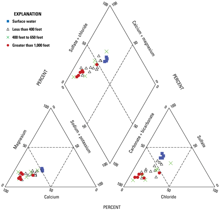
Trilinear diagrams showing the calcium, magnesium, sodium, potassium, sulfate, carbonate, bicarbonate, and chloride ion composition in 23 groundwater wells and 4 surface-water samples collected in the Ohio River and adjacent Ohio River alluvial aquifer, West Virginia, June 2019–January 2020.
Hydrogeochemical processes controlling solute concentrations in the Ohio River alluvial aquifer were evaluated with multivariate statistical analysis of the available chemical data for the 23 wells sampled using PCA and graphical analysis. The results of the PCA (table 10) show 3 major hydrogeochemical processes—redox, salinity, and carbonate dissolution—predominantly control the geochemical system, with 73 percent of the variance explained by the first 3 components of the PCA. Twelve variables were represented in the PCA by loadings, which correlate individual variables to specific principal components. Positive loadings indicate that as the value of one constituent increases, the value of the correlated constituent also increases; whereas, negative loadings indicate that as the value of one constituent increases, the value of the correlated constituent decreases.
Table 10.
Distribution of eigenvector loadings and significant Spearman’s correlation coefficients for the principal component analysis model.[Communality ranges from 0 to 1 and represents the proportion of the variables variance resulting from the principal components (PC). %, percent; —, not applicable; p, probability value of statistical significance]
Reduction and Oxidation Processes
The first principal component (PC1, table 10) is representative of ions generally controlled by redox processes, explains 26 percent of the variance, and has significant (p<0.01) positive loadings for manganese, iron, and DOC. Negative loadings on PC1 include dissolved oxygen, nitrate, and distance. Significant (p<0.01) negative loading of distance (distance of a well from the Ohio River) on PC1 indicates that wells located closer to the Ohio River have higher concentrations of manganese, iron, and DOC, but lower concentrations of dissolved oxygen and nitrate. Likewise, wells located further from the Ohio River would be expected to have higher concentrations of dissolved oxygen and nitrate, although manganese, iron, and DOC would be expected to be lower. Also, significant (p<0.05) negative loading of silica on PC1 indicates that silicates may dissolve more readily in wells farther from the river. As noted in the section on “Dissolved Organic Carbon and Anthropogenic Compounds,” DOC is a common electron donor available in groundwater systems and is used by microorganisms that catalyze redox processes. In alluvial aquifers, DOC concentrations have been shown to be higher near rivers, which leads to increased reduction and mobilization of manganese in shallow groundwater systems influenced by surface water (McMahon and others, 2019).
Sources of Salinity
The second principal component (PC2, table 10) has significant (p< 0.01) positive loadings for sodium, chloride, and potassium, which are constituents commonly associated with sources of salinity and may be related to land-use or waste-disposal practices. Sources of salinity and associated constituents (sodium, chloride, potassium, bromide) have been identified using chloride to bromide ratios by several authors (Davis and others, 2005; Katz and others, 2011). Chloride to bromide mass ratios calculated with the data collected for this study ranged from 144 to 1,731 (fig. 4). Chloride to bromide mass ratios with values in this range and measured chloride concentrations from approximately 20 to 120 mg/L in samples from the 23 wells (table 2) are typical of animal waste or sewage (300–1,000 mg/L) and halite dissolution (1,000–10,000 mg/L from natural and anthropogenic salt sources), which are the probable sodium, potassium, chloride, and bromide sources to groundwater in this area (Davis and others, 2005; Mullaney and others, 2009; Katz and others, 2011).
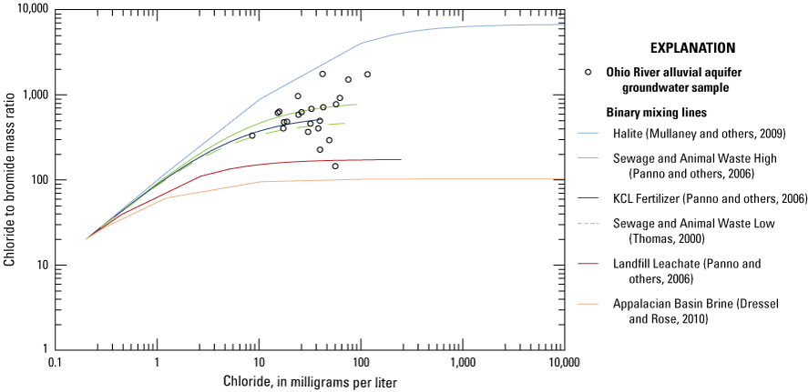
Scatterplot of chloride to bromide mass ratio versus chloride concentration in the 23 wells sampled in the Ohio River alluvial aquifer, West Virginia, June 2019–January 2020, in relation to the binary mixing lines of previous studies. Data are from Thomas (2000), Panno and others (2006), Dresel and Rose (2010), and Mullaney and others (2009).
Magnesium commonly has positive correlation with calcium and significant loading on the principal component that explains carbonate dissolution when magnesium is derived from calcium-carbonate solid-phase sources, but it has a significant (p<0.01) positive loading on PC2 and significant correlation with the constituents responsible for salinity. This positive loading indicates that the main source of magnesium may be from wastewater. Another possible explanation for this significant loading is that additional sodium added to the aquifer through different salinity sources may promote cation exchange of sodium with calcium or magnesium, thus magnesium concentrations may increase more through cation exchange processes rather than dissolution of magnesium-rich carbonates, such as dolomite. Calcium plus magnesium to bicarbonate molar ratios are >1 (fig. 5), indicating that there may be an abundance of magnesium or calcium that cannot be explained by carbonate dissolution alone. Sodium and chloride molar ratios plot close to 1 (fig. 5) indicating that cation exchange may not be an important process controlling magnesium concentrations and the origin of magnesium could be from several different wastewater sources.
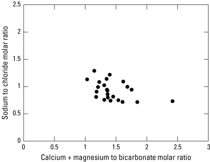
Scatterplot comparing the sodium to chloride mass ratio to the calcium plus magnesium to bicarbonate molar ratio calculated from the water-quality data for 23 wells sampled in the Ohio River alluvial aquifer, West Virginia, June 2019–January 2020.
Carbonate Dissolution
The third principal component (PC3, table 10) has significant (p<0.01) positive loadings for bicarbonate and calcium, which is indicative of carbonate dissolution. Significant (p<0.01) positive loading for the distance of a well from the Ohio River indicates that calcium and bicarbonate concentrations increase through carbonate dissolution in distal wells. This increase may be indicative of recharge from precipitation in distal wells that is more chemically aggressive than river water and capable of higher rates of carbonate mineral dissolution. The molar ratio of calcium to magnesium shows a much higher mass of calcium (fig. 6), which implies that calcite is the main carbonate mineral involved in carbonate mineral dissolution processes throughout the aquifer. The molar ratio of calcium to bicarbonate confirms this observation, that these two constituents follow a linear one-to-one relationship (fig. 7), and supports the previous assumption that magnesium may be supplied to the aquifer by originating from sources other than calcium, such as weathering magnesium-bearing minerals or through wastewater rather than carbonate dissolution.
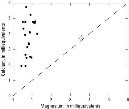
Scatterplot comparing the molar ratio of calcium and magnesium calculated from the water-quality data for 23 wells sampled in the Ohio River alluvial aquifer, West Virginia, June 2019–January 2020.
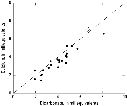
Scatterplot comparison of the equivalent mass of calcium and bicarbonate calculated from the water-quality data for 23 wells sampled in the Ohio River alluvial aquifer, West Virginia, June 2019–January 2020.
Water-Quality Indicators of Surface-Water Influence on Groundwater Wells
Constituents related to surface water and near surface or surface sources were used as indicators to evaluate their potential influence on groundwater. A combination of isotope analysis, age-tracer analysis, binary mixing models, and geochemical inverse models were used to determine recharge sources, estimate groundwater age, and assess the influence of the Ohio River on the adjacent alluvial aquifer.
Nitrate, Pesticides, Volatile Organic Compounds, 3H, and Dissolved Organic Carbon
Kozar and Paybins (2016) identified bacteria, nitrate, pesticides, volatile organic compounds, and chlorofluorocarbons as indicators of potential surface-water influence on, and vulnerability to contamination from surface or near-surface sources in, groundwater. Chlorofluorocarbons were not collected for this study but 3H was used in its place to indicate infiltration of modern water and assess aquifer vulnerability to surface contamination. Additionally, DOC may indicate strong connections among groundwater and near-surface sources or surface water (Shen and others, 2015). The presence of nitrate and DOC measured in concentrations above reporting levels in all 23 groundwater samples and detections of one or more man-made organic compounds in 22 groundwater samples (tables 8, 9, and 11; McAdoo, Grindle, and Grindle (2022) indicates that the alluvial aquifer is potentially contaminated or recharged by surface or near-surface water. Although no groundwater samples had detections for any of the five microbial constituents analyzed for this study, Kozar and Paybins (2016) stated that detections of bacteria in groundwater from alluvial aquifers in West Virginia may be infrequent because of alluvial sediments acting as a large sand filter that naturally retards the movement of bacteria. However, concentrations of nitrate and DOC and detections of 3H and man-made organic compounds are consistent with potential surface-water or surface-sources’ influence on groundwater. Samples from 19 wells had nitrate concentrations >1 mg/L as N, samples from 9 wells had DOC concentrations >1 mg/L, samples from 18 wells had detectable 3H, samples from 17 wells had detections for VOCs, and samples from 11 wells had detections for pesticides (table 11). Every well sampled for this study in the Ohio River alluvial aquifer had detections for at least one of these indicators of surface-water influence.
Table 11.
Water-quality indicators of surface-water influence on, or vulnerability to surface contamination of, groundwater wells as defined by Kozar and Paybins (2016). Wells listed in order of distance from the Ohio River.[U.S. Geological Survey (USGS) site identification official names and shortened names are found in table 1. ID, identification; Micro, the number of times a microbiological constituent was detected in a sample; mg/L, milligrams per liter; N, nitrogen; DOC, dissolved organic carbon concentration; 3He, helium-3; TU, tritium units; VOC, the number of times a volatile organic compound analyte was detected in a sample; Pest, the number of times a pesticide analyte was detected in a sample; ND, not detected; —, not available because no measurements were taken]
Stable Isotope Analysis
Stable isotopes of water (δ2H and δ18O) were evaluated to determine variation in recharge sources throughout the study area by comparing measured isotopic concentrations at sampling sites (wells and river locations) to the isotopic composition reported in precipitation. Values of δ18O ranged from −8.33 to −5.63 parts per thousand (permil) and values of δ2H ranged from −54.5 to −40.0 permil (table 12). The LMWL published by Smith and others (2021; δ2H=7.58 x δ18O+9.16) was used to represent precipitation in the Ohio River Valley. This line deviates from the global meteoric water line (δ2H=8 x δ18O+10; Craig, 1961) and indicates enrichment of isotopes in precipitation at the local scale (fig. 8). Stable isotope data collected for this study generally follow the LMWL, indicating that recharge to the alluvial aquifer is from a meteoric source of precipitation, with the exception of one site (Mas-0918). River water samples were collected in November 2019 and the stable isotopic composition of these samples (fig. 8) may partly reflect seasonal conditions, with lighter values in cooler months.
Values for line-conditioned (LC) excess are all generally below the one standard deviation measurement uncertainty (S=1.13) except for Ohio River at Moundsville (site name shortened to OR Moundsville in this report) with a LC-excess of −1.51, and Mas-0918 with a LC excess of −6.48. Negative values of LC-excess indicate evaporative enrichment after precipitation. The reason for elevated LC-excess at OR Moundsville is unknown, but the magnitude of the departure from the LMWL is relatively small in comparison to Mas-0918. This site is within 1,000 feet of wetlands and ponds that may experience evaporation, which subsequently enriches the isotopic concentrations in groundwater recharge in that area.
Table 12.
Results for isotopes and age tracers collected at 4 surface-water sites from the Ohio River and 23 groundwater wells sampled in the Ohio River alluvial aquifer, West Virginia, June 2019–January 2020. Wells listed in order of distance from the Ohio River.[U.S. Geological Survey (USGS) site identification official names and shortened names are found in table 1. ID, identification; δ2H, delta hydrogen-2; ‰, permil; δ18O, delta oxygen-18; LC-excess, line-conditioned excess; TU, tritium units; δ13C, delta carbon-13; 14C, carbon-14; pmC, precent modern carbon; OR, Ohio River; —, not available because no measurements were taken]
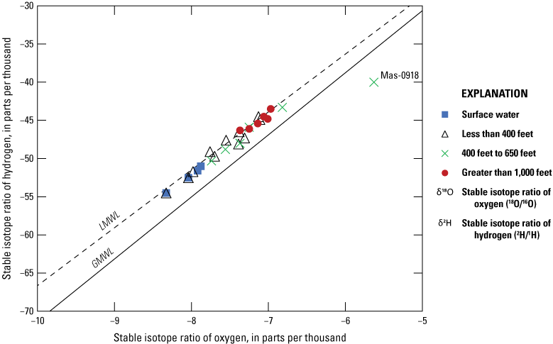
Scatterplot showing stable hydrogen (δ2H) and oxygen (δ18O) isotope ratios in water for 23 wells sampled in the Ohio River alluvial aquifer, West Virginia, June 2019–January 2020. The local meteoric water line (LMWL) is from Smith and others (2021). The global meteoric water line (GMWL) is from Craig (1961).
Carbon Isotope Analysis
Surface-water samples had δ13C values between −11.4 and −10.81 permil. Groundwater samples generally had values of δ13C that were less than −13.57 permil except for Mas-0918, which had a δ13C value of −11.91 permil. Mas-0918 was identified as having an LC-excess indicative of an evaporative source, likely from wetlands in the immediate area, and a bicarbonate/sulfate signature that deviated from other intermediate well samples. This high δ13C value may further indicate that the groundwater entering Mas-0918 may be heavily influenced by the proximal wetlands source.
Groundwater samples generally plot to the left of the zero-age line for the open system RFG analytical model (fig. 9; Han and Plummer, 2013). The model was parameterized with values for δ13C soil gas and solid carbonates of −25 permil and 2 permil, respectively, which are consistent with typical soil-zone gases and marine carbonate isotopic compositions (Clark and Fritz, 1997). The position of some samples on the figure (close to the zero-age line) indicates that the dominant controls of DIC in the study area are carbonate dissolution and open system exchange with soil CO2, but several samples do not follow the zero-age line, which may indicate that other processes affect carbon isotope chemistry. The more fractionated δ13C signal of these samples is possibly driven by organic carbon oxidation by microbial processes indicated by samples with low dissolved oxygen or high concentrations of iron or manganese. Without appropriate correction for microbial processes and carbon sources, 14C has limited utility for quantification of groundwater age in samples in which controls on DIC are not accounted for.
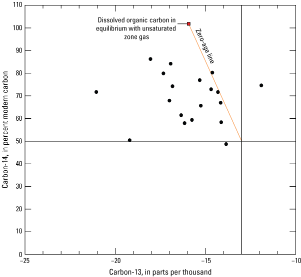
Scatterplot of open system revised Fonts and Garnier model for 14C correction of dissolved inorganic carbon for 23 wells sampled in the Ohio River alluvial aquifer, West Virginia, June 2019–January 2020.
Where possible, the final adjusted 14C (table 12) for these samples was computed, resulting in a range from 100 to 133 percent modern carbon (pmC). The corrected 14C values are generally consistent with other tracers and indicate that recent recharge along local flow paths is captured at these sites. Carbon-14 has limited utility for quantitative age dating of modern samples because of (1) elevated atmospheric 14C (for example, >100 pmC) from above-ground nuclear testing since late 1950s and (2) high sensitivity of modern interpreted ages to the geochemical correction. High pmC values of 14C and the presence of 3H at every site indicates no, or very little, pre-1950s water in any sample collected for this study.
Groundwater Age Tracer Analysis
Measured concentrations of noble gasses were generally within 20 percent of atmospheric solubility equilibrium with Ne, Ar, Kr, and Xe exhibiting average deviations from solubility equilibrium of 20.9, 14.1, 9.2, and 6.1 percent, respectively (table 13). Dissolved noble gas data were well-fit by solubility models with statistically significant model solutions (χ2 values less than critical value of 3.84; one-sided, one degree of freedom, 95 percent confidence). One sample (Ohi-0372) was determined to have re-equilibrated with the atmosphere because of sample container malfunction and was not used for further dissolved gas analysis. Noble gas solubility models provided a good estimate of the groundwater recharge temperature (referred to as noble gas recharge temperature; NGT) and the amount of EA for each sample. Noble gas temperatures generally group around the mean annual air temperature modeled for the study area (PRISM Climate Group, 2022). Modeled NGTs ranged from 11.0 to 13.7 °C with two outlier values of 15.1 °C and 16.9 °C at Woo-0121and Mas-0936, respectively.
The He isotopic ratio (R/Ra) indicates a possible contribution from a premodern groundwater source, with a high proportion of terrigenic helium (4Heterr) observed in every sample except for Mas-0918. Four samples with R/Ra values between 0.81 and 0.73 were identified as having some 4Heterr, but 12 samples with R/Ra values less than 0.70 were identified as having high 4Heterr. The only sample in the dataset to have a R/Ra value close to 1 (indicating solubility equilibrium with the atmosphere) was Mas-0918, which was identified by stable isotope analysis as possibly being influenced by a wetland or pond source rather than representing the groundwater conditions in the rest of the aquifer. All samples in the dataset contain tritium (table 12) and are likely modern, which limits the ability to estimate the 4Heterr isotopic ratio. Therefore, 3Hetrit could not be reliably estimated for most samples in the dataset, which reduced the number of available tracers for age determination. The source of high 4Heterr in almost every sample collected for the study is not currently [2019] known but other investigators have also identified high 4Heterr accumulation rates in other glacially deposited shallow alluvial aquifers (Solomon and others, 1996).
Table 13.
Dissolved noble gas solubility modeling results determined using model described by Aeschbach-Hertig and others (2000) for 18 groundwater wells in the Ohio River alluvial aquifer, West Virginia, June 2019–January 2020. Wells listed in order of distance from the Ohio River. Dissolved gas data from the U.S. Geological Survey National Water Information System (U.S. Geological Survey, 2023).[Δ, deviation of sample from solubility equilibrium with the atmosphere; χ2, Chi-squared; elev., elevation; m, meter; NGT, noble gas temperature; °C, degrees Celsius; Ae, entrapped air; ccSTP/g, cubic centimeters per gram at standard temperature and pressure (25 ̊C, 1 atm); F, fractionation factor; R, ratio of helium-3 to helium-4 in the sample; Ra, ratio of helium-3 to helium-4 in atmosphere; —, not available]
Measured SF6 concentrations were corrected for excess air and found to exceed expected concentrations from atmospheric inputs. The contamination source of excess SF6 observed in the aquifer is not known but high concentrations of SF6 preclude its use for groundwater age analysis. With area-wide contamination of SF6, 14C concentrations that indicated predominantly modern recharge, and high 4Heterr observed in most samples that limited the use of 3Hetrit, 3H was the only modern tracer left to estimate groundwater age. At six sites, 3H was measured above background levels (approx. 10 TU), which may be indicative of an additional non-atmospheric local source of 3H. Bomb-pulse elevated atmospheric sources of 3H can be distinguished from local 3H sources based on 14C, which increased in the atmosphere over the same period in response to above-ground nuclear testing. At five of the six samples with elevated 3H concentrations (table 12), it was possible to correct 14C using the RFG model. At all five sites, elevated 3H concentrations did not correspond to elevated 14C concentrations, indicating a local source of 3H may be present.
Assessment of non-atmospheric sources of 3H yielded possible contribution from a nuclear power plant on the Ohio River, upstream of every site in the study area. This facility regularly releases 3H into the Ohio River at concentrations that are higher than atmospheric background levels (Paciello and others, 2019). Helium-3 was not sampled in the Ohio River for this study but 35 3H samples were collected in the Ohio River at a surface-water site near Newell, West Virginia (USGS 03109670) between April 17, 2002, and August 2, 2010 (U.S. Geological Survey, 2023; https://waterdata.usgs.gov/nwis/inventory?agency_code=USGS&site_no=03109670). This surface-water site is adjacent to Hnc-0043, and samples collected there had an average value for 3H of 19 TU. This 3H value supports the possibility of elevated 3H in the Ohio River but without the ability to corroborate age dates across multiple tracers and the possibility of a non-atmospheric source of 3H affecting concentrations in the aquifer, obtaining accurate estimates of groundwater age in the aquifer is not probable with these data. What can be determined from the age analysis for this study is that all water captured by wells in the Ohio River alluvial aquifer is likely from a relatively modern source.
Statistical Relations Between Ohio River Water and Groundwater Chemistry
The two major sources of recharge to the Ohio River alluvial aquifer in West Virginia are local precipitation and infiltration from the Ohio River (Jeffords, 1945). Hierarchical agglomerative cluster analysis (HACA) was used to confirm and further characterize these sources. The primary output from HACA is a dendrogram depicting the clustering structure of the input data (fig. 10). Individual samples are represented by vertical lines at the bottom of the figure, and the merging of similar clusters are represented by horizontal lines connecting clusters. Clusters that merge toward the bottom of the dendrogram have similar water chemistry. Clusters that do not merge until the top of the dendrogram represent groups of samples that have less similar water chemistries. Specific analytes and parameters used in the HACA for this study included δ2H, δ18O, δ 13C, pH, specific conductance, dissolved oxygen, DOC, calcium, magnesium, potassium, sodium, chloride, fluoride, bicarbonate, silica, sulfate, iron, and manganese. This resulted in a HACA with 4 surface-water sites and 23 groundwater wells (table 1) that included field parameters, major ions, trace metals, and isotopes important in end-member characterization. Constituent values were converted to u-scores, and the distance matrix was computed as described in the “Methods of Study” section.
The HACA resulted in 3 clusters represented by capital letters (A, B, C). The agglomerative coefficient, a numerical value used to assess the structure of the clustering, ranges from 0 to 1, with values closer to 1 representing better cluster structure (Kaufman and Rousseeuw, 1990). The agglomerative coefficient produced was 0.77, which provides confidence in the HACA structure. The SIMPROF test was applied to the cluster analysis and identified 11 significant clusters (p<0.01), of which 3 clusters (A, B, C) were used for further analysis.
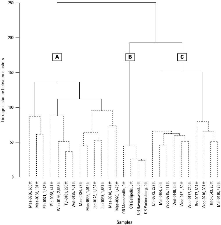
Dendrogram output from hierarchical agglomerative cluster analysis of water-quality data. Solid lines represent significant (p<0.001) clusters determined by the similarity profile test. Letters represent major clusters. Significant clusters are identified by solid lines, whereas nonsignificant clusters, according to the similarity profile test, are identified by dashed lines. Sites identified with distance from the Ohio River given in feet (ft).
Cluster B includes all four surface-water samples and represents the surface-water end member of the system. Clusters C and B merge before coming together with cluster A at the final merge point in the HACA. This merge point indicates that sites in cluster C are more closely associated with surface-water sites in cluster B than other groundwater sites in cluster A. Cluster C includes 10 wells that have an average distance of 217 ft from the river and are representative of sites that may be highly influenced by Ohio River water chemistry. Cluster A includes 13 wells that have an average distance of 906 ft from the river. This cluster includes wells greater than 1,000 ft from the river and wells that may have some influence from the Ohio River water chemistry but are probably more influenced by water from the recharge area of the aquifer, as depicted in the conceptual model (fig. 2). Results indicate that two hydrochemical facies are contributing water to the SWIG wells in the alluvium but the Ohio River is the most likely source contributing an increasing proportion of water to wells as distance to the river decreases.
Mixing models to estimate Ohio River Water Influence on Groundwater Chemistry
Jeffords (1945) states that analyses of major anions are adequate for use in determining the source of water recharging any well field in the Ohio River alluvium and that the greatest difference in Ohio River water and groundwater not influenced by the Ohio River is in the respective concentrations of sulfate and bicarbonate. Data collected for this study show a similar result, with anions that represent noncarbonate hardness (sulfate and chloride) comprising a higher proportion of total hardness in surface-water samples and anions that represent carbonate hardness (carbonate and bicarbonate) comprising a higher percentage of total hardness in groundwater samples greater than 1,000 ft from the river (fig. 3). Likewise, comparison of the equivalents of bicarbonate as a percentage of anions with the equivalents of sulfate as a percentage of anions (fig. 11) shows differentiation of three groups. The first group consists of surface-water samples collected in the Ohio River and is characterized by sulfate comprising over 35 percent of anion equivalents. The second group is comprised of samples greater than 1,000 ft from the Ohio River and is characterized by bicarbonate comprising over 70 percent of anion equivalents. The third group consists of samples with mixtures of Ohio River water and groundwater because they plot between the distal wells and surface water sites. Samples from three wells do not follow this general association between bicarbonate and sulfate, with the sample from Mas-0918 (444 ft from river) containing a relatively high percentage of bicarbonate compared to other wells at intermediate distances (400–650 ft) from the Ohio River, the sample from Ple-0071(1,473 ft from river) containing a low percentage of bicarbonate relative to other wells located greater than 1,000 ft from the Ohio River, and the sample Mas-0936 (650 ft from river) containing relatively more sulfate but less bicarbonate than samples from other wells at intermediate distances (400–650 ft) from the Ohio River, plotting in an area that is not indicative of surface water from the Ohio River or groundwater from more distal wells (fig. 11). These three sites may be indicative of the heterogenous nature of the Ohio River alluvial aquifer or may be supplied by an unknown source with an unidentified bicarbonate/sulfate signature.
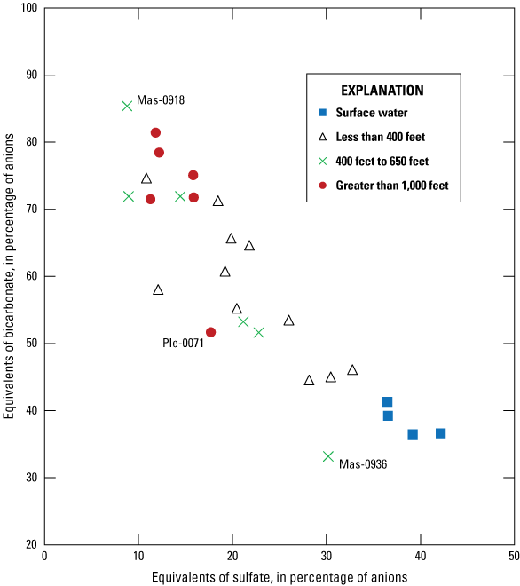
Scatterplot of the equivalent mass of bicarbonate and sulfate as a percentage of total anions calculated from the water-quality data for 23 wells sampled in the Ohio River alluvial aquifer, West Virginia, June 2019–January 2020.
Groundwater-flow simulations in the Ohio River alluvium by Kozar and McCoy (2004) estimated fractions of Ohio River water contribution to the groundwater system at Parkersburg, Lubeck, Glendale, and Point Pleasant, to be 0.75, 0.39, 0.72, and 0.04, respectively (table 14). The sites Parkersburg, Lubeck, Glendale, and Point Pleasant specified in Kozar and McCoy (2004) were represented in this study by Woo-0121, Woo-0215, Mal-0410, and Mas-0920, respectively. Binary-mixing models were computed with analytical data collected from this study and used as a first-order approximation for fractions of the two major recharge sources. Several analytes were considered for binary mixing, including δ2H, δ18O, and chloride, but the binary mixing model that had the most significant correlation (r=0.97, p<0.03) with groundwater modeling results was the ratio of bicarbonate equivalents as a percentage of anions to sulfate equivalents as a percentage of anions, which was shown to have a linear relation in figure 11. Silica (SiO2) concentrations were found to have significant negative correlation (r=−0.91, p<0.08) with groundwater modeling results, showed similar behavior as bicarbonate (lower concentrations in Ohio River samples and higher concentrations in distal wells), and were also considered for binary mixing models (table 14). The Ohio River end member (table 14) was represented by the average of results of the four surface-water samples (table 1). The alluvial well end member was represented by the average of results for four wells greater than 1,000 ft from the Ohio River (Mas-0852, Jac-0128, Jac-0057, Woo-0196), with results from two wells excluded for the following reasons: Mas-0920 (1,475 ft from river) results were excluded because an estimate of the end member fractions for this site was needed to compare to the value reported in the groundwater-flow model, and Ple-0071 (1,473 ft from river) as this site was identified as possibly having a contribution from an unknown recharge source with a different bicarbonate/sulfate signature (fig. 11).
Table 14.
Chemical compositions of end members representing Ohio River water and groundwater in alluvial aquifer at the greatest distance from river and of sample results from wells at various distances from the Ohio River, and estimated fraction of Ohio River water contribution to surface-water influenced wells in the Ohio River alluvial aquifer of West Virginia, June 2019–January 2020.[OR, Ohio River; SW, surface water; GW, groundwater; —, not available; Distance, distance from the Ohio River; ft, feet; mg/L, milligrams per liter; GM, Groundwater model from Kozar and McCoy (2004); BMM, Binary Mixing Model; IM, Inverse Model; equivalent percent, equivalents as a percentage of anions]
The estimated fractions of Ohio River water contribution to the groundwater system from the groundwater-flow model (Kozar and McCoy, 2004) were used to validate the results of the silica and equivalent-ratio binary mixing models. Fractions of river water in the aquifer computed using the silica binary-mixing model were significantly correlated with those determined from the groundwater-model for 4 sites (Woo-0121, Woo-0215, Mal-0410, and Mas-0920; r=0.91, p less than 0.09), with three sites showing 6 percent difference or less. The percentage of Ohio River water calculated by the silica binary mixing model for Woo-121 was 29 percent less than the percentage of Ohio River water calculated in the groundwater model results for Ohio River @ Mile 183.0 (site name shortened to OR Parkersburg in this report), which suggests that the silica binary-mixing model may not be accurate at all sites or that Woo-121 may not be representative of the Parkersburg area as simulated by the groundwater model. The percentage of Ohio River water calculated with the equivalent ratio (bicarbonate equivalent as percentage of anion equivalents to sulfate equivalent as percentage of anions equivalents) binary mixing model was significantly correlated with the percentage of Ohio River water estimated by the groundwater model at the four sites (r=0.97, p less than 0.03). Of the 4 sites, the percentage of Ohio River water for Woo-0121 was most different between these 2 models, with the equivalent ratio model results being 15 percent greater than the percentage of Ohio River water calculated in the groundwater model results for OR Parkersburg. The disparity among models in calculated results of the same site indicates that non-conservative mixing may be important at some sites where geochemical processes are not accounted for in binary mixing models.
Inverse geochemical models that met the specified uncertainty (10 percent or less) were computed for Mas-0920 and 13 of the groundwater sites located less than 1,000 ft from the river (table 14). The percentage of Ohio River water computed by inverse models was significantly correlated with the percentage of Ohio River water estimated by the groundwater model (r=0.98, p<0.02). The percentage of Ohio River water for Woo-0121, Woo-0215, and Mal-0410 calculated with the inverse model was within 8 percent of the results reported from the groundwater model. The percentage of Ohio River water for Mas-0920 was 16 percent greater than the results in the groundwater model for Point Pleasant, which indicates that the inverse model may be more accurate for sites less than 1,000 ft from the river. The average of all three geochemical models (silica binary mixing model, equivalent ratio binary mixing model, inverse model) yields the most significant correlation (r=0.99, p<0.006) with the results from the groundwater model. By using the average of all three models, all 4 sites had average results that are within 7 percent of the groundwater model results (table 14, fig. 12).
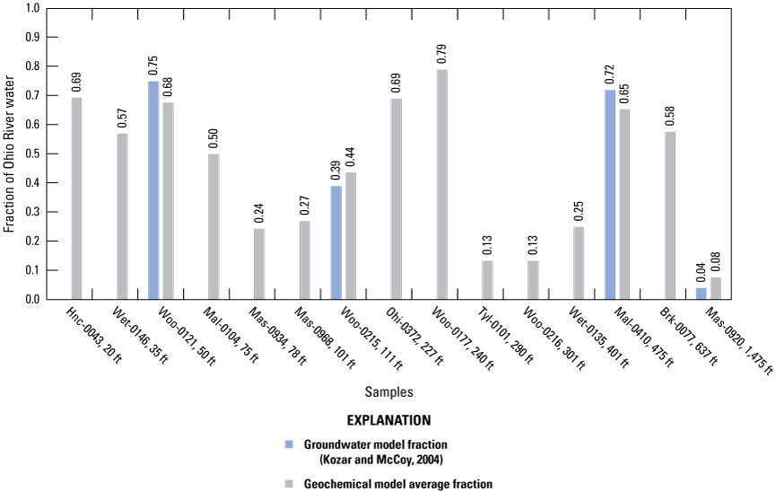
Bar chart showing the fraction of Ohio River water in alluvial wells in West Virginia from groundwater modeling by Kozar and McCoy (2004) and the average of three different geochemical models presented in this study. Site names followed by feet (ft) from the river.
Discussion and Limitations
The broad overview and analysis presented in this report may not be appropriate for all groundwater sites in the Ohio River alluvium and site-specific information may be needed when making detailed assessments of surface-water influence on alluvial wells. Reactive transport modeling, including kinetic parameters for mineral precipitation/dissolution, may be created as more site-specific hydrological, geological, mineralogical, and geochemical data and information become available. Focused studies with well-developed reaction transport models may give a better understanding of the influence from the Ohio River on alluvial wells and can be used to confirm relevance of simple linear relationships, but without this information, the linear relation between analytes and fraction of Ohio River water presented here may be adequate for preliminary assessments of surface-water influence in the Ohio River alluvial aquifer.
The Ohio River Alluvial Aquifer is Susceptible to Contamination from Surface Water
Meteoric recharge from the Ohio River and precipitation on the alluvium and subsequent recharge through the vadose zone are the main sources of water entering the aquifer, but isotope ratios and concentrations of major ions indicate other surface-water sources may affect groundwater chemistry at individual sites (Mas-0918, Ple-0071, Mas-0936) on a local scale (fig. 8, 11). Generally, groundwater from wells located over 1,000 ft from the river, which represented the chemistry of the precipitation dominated portion of the aquifer, had a chemical signature that was different than Ohio River water (fig. 8, 10, 11), with a higher percentage of bicarbonate relative to sulfate observed in wells located closer to the Ohio River. These results are consistent with Maharjan and Donovan (2017), who observed low total dissolved solids specific conductance, alkalinity, and enriched δ 13C values of dissolved inorganic carbon, indicative of induced infiltration in proximal (less than 1,000 ft from Ohio River) groundwater wells. Also consistent with Maharjan and Donovan (2017) was the observation that distal (more than 1,000 ft from Ohio River) alluvial well water chemistry exhibited higher total dissolved solids, specific conductance, alkalinity, and relatively depleted δ13C values and was not affected by exfiltration from the Ohio River.
Every well sampled for this study (distal and proximal) is intrinsically susceptible and potentially vulnerable to surface contamination. Kozar and Paybins (2016) identify bacteria, nitrate, pesticides, VOCs, and chlorofluorocarbons as indicators of surface-water influence in groundwater wells. No microbial fecal indicators were found in any groundwater sample from wells throughout the study area, indicating these sites are not likely GWUDI, but all sites sampled for this study had detections for at least one water-quality indicator of surface-water influence (table 11). These observations suggest that one tracer or parameter is not sufficient to assess surface-water-influence in the Ohio River alluvium, but when multiple constituents are included in the analysis, it is apparent that every site in the Ohio River alluvial aquifer is influenced by surface water to some extent and vulnerable to surface contamination.
Ohio River Water Influences Groundwater Chemistry in the Alluvial Aquifer
Jeffords (1945) stated that the approximate amount of river water recharging groundwater wells in the Ohio River alluvium can be determined by obtaining the percentage of bicarbonate and sulfate and comparing these with similar data on water from the Ohio River and from wells that obtain little or no recharge from the river. Likewise, results from binary mixing models and inverse models created for this study suggest that sulfate, silica, or bicarbonate concentrations adequately predict the fraction of Ohio River water entering alluvial wells for preliminary investigations of surface-water influence. These three constituents are commonly measured in water-quality analyses for regulatory purposes and are more readily available for preliminary assessment of surface-water influence than many other analytes, such as isotopes. Binary mixing models do not consider time variability of end-member signatures or the reactive nature of sulfate, bicarbonate, and silica. Nevertheless, results from binary mixing models showed significant correlation with the inverse models computed for this study and groundwater models published by Kozar and McCoy (2004). Using the average of the fraction of Ohio River water computed from the three geochemically based models (silica binary mixing model, equivalent ratio binary mixing model, and inverses models) yielded the highest correlation with fractions estimated using the groundwater-flow model (table 14).
In the absence of extensive analytes and geochemical or groundwater-flow modeling capabilities, preliminary assessment of the fraction of Ohio River water entering groundwater wells in the Ohio River alluvium may be estimated for most sites (including sites not specified in this study) using the linear relation between the equivalent ratio of bicarbonate to sulfate and the fraction of water computed by the average of the three geochemical models (fig. 13A, table 14). Additionally, the linear relationship of sulfate concentration with the proportion of Ohio River water computed from the average of three geochemical models (fig. 13B) or the linear relationship of silica concentration with the proportion of Ohio River water computed from the average of three geochemical models (fig. 13C) may be used to provide a preliminary assessment of the potential influence from surface water entering wells in the Ohio River alluvium, although this approach might not be sufficient for samples with high concentrations of sulfate or silica without equivalent-weight normalization. For samples with high concentrations, the equivalent ratio of bicarbonate to sulfate may yield better results for outlier sites because it normalizes the concentrations by the molecular weight and anion percentage. Although first-order calculations of the fraction of Ohio River water presented in this study may be sufficient for a broad understanding of the Ohio River alluvial aquifer or a preliminary assessment of an individual groundwater site, focused reaction-transport models or other types of biological or geochemical data could enhance understanding in localized areas.
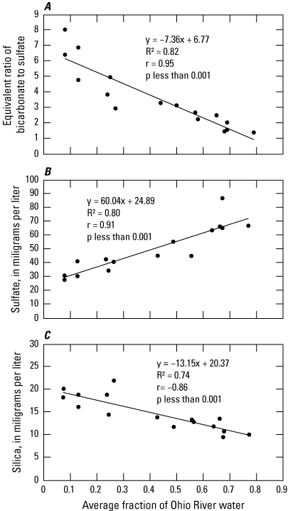
Graphs showing the linear relations between select parameters and the average fraction of Ohio River water entering studied groundwater wells in the Ohio River alluvial aquifer, West Virginia, computer by three geochemical models: A, equivalent ration of bicarbonate to sulfate, B, sulfate concentration, and, C, silica (as SiO2) concentration.
This study indicates that the chemistry of groundwater wells in the Ohio River alluvium is influenced by recharge from the Ohio River but distance from the Ohio River was not always a good indication of the amount a SWIG site will be influenced by Ohio River water chemistry. The data and related analyses indicate that Ohio River water chemistry has more influence at some sites over 400 ft from the Ohio River (for example Mal-0410) than at some sites located less than 100 ft from the Ohio River (for example Mas-0934) and that distance from the Ohio River was not significantly correlated with the computed average fraction of Ohio River water, although models indicated the smallest fraction of river water at the well most distant from the river Mas-0920 (table 14). This general finding of inconsistent relations between distance from the river and estimated fraction of river water in groundwater indicates that influence from the Ohio River on alluvial well water chemistry may be affected by local-scale heterogeneity in alluvial sediments (permeability and mineralogy), well construction, or transient pumping by the local public water system in addition to river proximity. Pumping can induce infiltration from the river, and the analysis presented in this study could be further refined if pumping were included as a factor.
Summary
Public groundwater supplies obtained from the alluvial aquifers bordering the Ohio River in West Virginia receive substantial recharge from surface-water sources and are highly susceptible to degradation from water-soluble contaminants. Surface-water-influenced groundwater systems include any underground public-water supply that is heavily influenced by the quality of surface water in the immediate area of a well. Even though alluvial aquifers have a relatively small footprint in comparison to other aquifers in West Virginia, these sand and gravel aquifers are the primary water supply for numerous large communities along the Ohio River. Protection of public-water supplies requires an understanding of aquifer interactions with the Ohio River and tributary streams that contribute to the chemistry of groundwater from pumping wells.
Surface-water-influence on groundwater-well chemistry in the Ohio River alluvial aquifer of West Virginia was studied in cooperation with the West Virginia Department of Health and Human Resources, Bureau for Public Health. Water-quality samples were collected from 4 surface-water sites and 23 groundwater wells in the study area from June 2019 to January 2020. Comparison of results to human-health benchmarks established by U.S. Environmental Protection Agency indicated that no sites had concentrations that exceeded maximum-contaminant levels for any analyte. Manganese has a secondary maximum-contaminant level for aesthetic criterion of 50 micrograms per liter, which was exceeded in 48 percent of samples. Concentrations for manganese also exceeded the health advisory of 300 micrograms per liter, in 17 percent of samples. Sodium concentration exceeded the 20 milligrams per liter health advisory for people on a sodium-restricted diet in 52 percent of samples and iron exceeded its secondary maximum-contaminant level for aesthetic criterion of 300 micrograms per liter in 17 percent of samples.
Hydrogeochemical processes controlling solute concentrations in the Ohio River alluvial aquifer were identified to be redox processes, input from sources of salinity, and carbonate dissolution. Wells located closer to the Ohio River had higher concentrations of manganese, iron, and dissolved organic carbon but lower concentrations of dissolved oxygen and nitrate. Likewise, wells located farther from the Ohio River generally had higher concentrations of dissolved oxygen and nitrate, whereas manganese, iron, and dissolved organic carbon concentrations were lower. Sources of salinity and associated constituents (sodium, chloride, potassium, bromide) were identified using chloride/bromide ratios. Chloride to bromide mass ratios calculated with the data collected for this study ranged from 325 to 3,944 and chloride concentrations ranged from 20 to 120 milligrams per liter. These ranges are typical values for sources of salinity from halite dissolution and animal waste or sewage. Calcium and bicarbonate concentrations generally increased with the distance of a well from the Ohio River, which indicated that carbonate dissolution was an important hydrochemical process in distal wells.
Every well sampled for this study (distal and proximal to the Ohio River) had detections for at least one water-quality indicator of surface-water influence, including recent recharge. No microbial fecal indicators were found in any groundwater well throughout the study area, indicating these sites are not likely groundwater-under-direct-influence of surface water but one tracer or parameter is not sufficient to assess surface-water-influence in the Ohio River alluvium. When multiple constituents were included in the analysis, the data show that every site in the Ohio River alluvial aquifer is influenced by surface water to some extent and vulnerable to surface contamination.
Analysis of groundwater age tracers overall indicate relatively recent water, but some tracer data were not useable or indicated conflicting interpretations. Measured sulfur hexafluoride concentrations were corrected for excess air and found to exceed expected concentrations from atmospheric inputs at most sites. The He isotopic ratio indicated contribution from a premodern groundwater source, with a high proportion of terrigenic helium (4Heterr) observed in every sample, but tritium concentrations and corrected carbon-14 values indicated that water in the Ohio River alluvium was derived exclusively from a modern source. Tritiogenic helium (3Hetrit) could not be reliably estimated for most samples in the dataset, because of the high proportion of 4Heterr, which reduced the number of available tracers for age determination. Additionally, tritium was measured above expected atmospheric background levels at six sites, which indicated the possibility of an additional non-atmospheric local source of tritium. Obtaining accurate estimates of groundwater age in the aquifer was not possible without the ability to confirm groundwater age across multiple tracers, but the age analysis for this study indicated that all water captured by wells in the Ohio River alluvial aquifer was likely from a relatively modern source (post-1950s).
Stable isotope ratios of water indicated that meteoric recharge from the Ohio River and precipitation on the alluvium are the main sources of water entering the aquifer. Groundwater wells located over 1,000 ft from the river generally had a different chemical signature than Ohio River water, with a higher percentage of bicarbonate relative to sulfate. Silica concentrations were also observed to be higher in distal wells relative to proximal wells. Because of the disparity in analyte concentrations observed in distal wells and samples collected in the Ohio River, end-member analysis considered bicarbonate, sulfate, and silica.
Results from binary mixing models and inverse models computed for this study suggest that sulfate, silica, and bicarbonate concentrations adequately predict the fraction of Ohio River water entering alluvial wells for preliminary assessments of surface-water influence. These three constituents are more commonly available for preliminary assessment of surface-water influence than other analytes such as isotopes. The fraction of Ohio River water entering groundwater wells in the Ohio River alluvium computed with binary mixing models showed significant correlation with those estimated using the inverse geochemical models for this study and using previously published groundwater-flow models of the study area. The average of the fraction of Ohio River water computed from three geochemical models yielded the highest correlation with fractions determined from groundwater-flow models compared to correlation with any single geochemical model and the groundwater-flow model.
In the absence of extensive analytes and geochemical or groundwater modeling capabilities, preliminary assessment of the fraction of Ohio River water entering groundwater supplies to wells in the Ohio River alluvium may be estimated for most sites (including sites not specified in this study) using the linear relation between the equivalent ratio of bicarbonate to sulfate and the fraction of water computed by the average of the three geochemical models presented in this report. Additionally, the linear relation of silica concentration with the proportion of Ohio River water, or the linear relationship of sulfate concentration with the proportion of Ohio River water, may also supply sufficient results to make a preliminary assessment of the potential influence from surface water entering wells in the Ohio River alluvium. This approximation of the fraction of Ohio River water, coupled with information on the hydrogeological framework and geochemical indicators of surface-water influence, may be adequate for preliminary assessment of surface-water influence until more detailed site information or reaction-transport models can be developed.
References Cited
Aeschbach-Hertig, W., Peeters, F., Beyerle, U., and Kipfer, R., 2000, Palaeotemperature reconstruction from noble gases in ground water taking into account equilibration with entrapped air: Nature, v. 405, p. 1040–1044, accessed February 20, 2023, at https://doi.org/10.1038/35016542.
Aeschbach-Hertig, W., and Solomon, D.K., 2013, Noble gas thermometry in groundwater hydrology in Burnard P., ed., The noble gases as geochemical tracers—Advances in isotope geochemistry: Springer, p. 81–122, accessed February 10, 2022, at https://doi.org/10.1007/978-3-642-28836-4_5.
Aga, D.S., Thurman, E.M., Yockel, M.E., Zimmerman, L.R., and Williams, T.D., 1996, Identification of a new sulfonic acid metabolite of metolachlor in soil: Environmental Science & Technology, v. 30, no. 2, p. 592–597, accessed January 26, 2023, at https://doi.org/10.1021/es9503600.
Andrews, J.N., 1985, The isotopic composition of radiogenic helium and its use to study groundwater movement in confined aquifers: Chemical Geology, v. 49, n. 1–3, p. 339-351, accessed August 2, 2022, at https://doi.org/10.1016/0009-2541(85)90166-4.
Back, W., 1966, Hydrochemical facies and ground-water flow patterns in Northern part of Atlantic Coastal Plain: U.S. Geological Survey Professional Paper 498-A, 50 p., accessed November 11, 2023, at https://pubs.usgs.gov/publication/pp498A.
Bader, J.S., Mathes, M.V., and Schults, R.A., 1997, Ground-water hydrology of the area bordering the Ohio River between Chester and Waverly, West Virginia: U.S. Geological Survey Open File Report 95–710, 61 p., accessed August 18, 2022, at https://doi.org/10.3133/ofr95710.
Ball, J.W., and Nordstrom, D.K., 1991, User's manual for WATEQ4F, with revised thermodynamic data base and test cases for calculating speciation of major, trace, and redox elements in natural waters: U.S. Geological Survey Open-File Report 91–183, 189 p., accessed May 5, 2023, at https://doi.org/10.3133/ofr91183.
Busenberg, E., and Plummer, L.N., 2000, Dating young groundwater with sulfur hexafluoride—Natural and anthropogenic sources of sulfur hexafluoride: Water Resources Research, v. 36, no. 10, p. 3011–3030, accessed August 12, 2022, at https://doi.org/10.1029/2000WR900151.
Battelle Memorial Institute, 2003, Preliminary assessment of deep saline reservoirs and coal seams: U.S. Department of Energy, National Energy Technology Laboratory, Interim Topical Report—The Ohio River Valley CO2 storage project DE-AC26-98FT40418, prepared by Battelle Memorial Institute, Columbus, Ohio, 74 p., accessed August 31, 2022, at https://doi.org/10.2172/821467.
Carlston, C.W., 1962, Character and history of the upper Ohio River Valley: Geological Survey Bulletin 1141–I, 10 p., accessed August 18, 2022, at https://pubs.usgs.gov/publication/b1141I.
Chambers, D.B., Kozar, M.D., White, J.S., and Paybins, K.S., 2012, Groundwater quality in West Virginia, 1993–2008: U.S. Geological Survey Scientific Investigations Report 2012–5186, p. 47, accessed October 13, 2021, at https://doi.org/10.3133/sir20125186.
Clarke, K.R., Somerfield, P.J., and Gorley, R.N., 2008, Testing of null hypotheses in exploratory community analyses—Similarity profiles and biota-environment linkage: Journal of Experimental Marine Biology and Ecology, v. 366, no. 1–2, p. 56–69, accessed June 1, 2021, at https://doi.org/10.1016/j.jembe.2008.07.009.
Cook, P. G., and Solomon, D. K., 1995, Transport of atmospheric trace gases to the water table— Implications for groundwater dating with chlorofluorocarbons and krypton 85: Water Resources Research, v. 31, n. 2, p. 263– 270, accessed January 5, 2022, at https://doi.org/10.1029/94WR02232.
Craig, H., 1961, Isotopic variations in meteoric waters: Science, v. 133, no. 3465, p. 1702–1703. [Also available at https://doi.org/10.1126/science.133.3465.1702.]
Davis, S.N., Whittemore, D.O., and Fabryka-Martin, J., 2005, Uses of chloride/bromide ratios in studies of potable water: Groundwater, v. 36, no. 2, p. 338–350, accessed October 13, 2021, at https://doi.org/10.1111/j.1745-6584.1998.tb01099.x.
Eberts, S.M., Thomas, M.A., and Jagucki, M.L., 2013, Factors affecting public-supply-well vulnerability to contamination—Understanding observed water quality and anticipating future water quality: U.S. Geological Survey Circular 1385, 120 p., accessed August 31, 2022, at https://doi.org/10.3133/cir1385.
Ferrel, G.M., 1987, West Virginia ground-water quality: U.S. Geological Survey Open File Report 87–0761, 9 p., accessed October 13, 2021, at https://pubs.usgs.gov/of/1987/0761/report.pdf.
Focazio, M.J., Reilly, T.E., Rupert, M.G., and Helsel, D.R., 2002, Assessing ground-water vulnerability to contamination—Providing scientifically defensible information for decision makers: U.S. Geological Survey Circular 1224, 33 p., accessed August 31, 2022, at https://doi.org/10.3133/cir1224.
Friel, E.A., Ehlke, T.A., Hobba, W.A., Jr., Ward, S.M., and Schultz, R.A., 1987, Hydrology of area 8, eastern coal province, West Virginia and Ohio: U.S. Geological Survey Water Resource Investigations Open File Report 84–463, 78 p., accessed August 31, 2022, at https://doi.org/10.3133/ofr84463.
Fritz, S.J., 1994, A survey of charge-balance errors on published analyses of potable ground and surface waters: Groundwater, v. 32, no. 4, p. 539-546, accessed October 27, 2022, at https://doi.org/10.1111/j.1745-6584.1994.tb00888.x.
Güler, C., Thyne, G.D., McCray, J.E., and Turner, A.K., 2002, Evaluation of graphical and multivariate statistical methods for classification of water chemistry data: Hydrogeology Journal, v. 10, p. 455–474, accessed March 10, 2021, at https://doi.org/10.1007/s10040-002-0196-6.
Han, L.-F., and Plummer, L.N., 2013, Revision of Fontes & Garnier’s model for the initial 14C content of dissolved inorganic carbon used in groundwater dating: Chemical Geology, v. 351, p. 105–114, accessed October 20, 2022, at https://doi.org/10.1016/j.chemgeo.2013.05.011.
Han, L.-F., Plummer, L.N., and Aggarwal, P., 2012, A graphical method to evaluate predominant geochemical processes occurring in groundwater systems for radiocarbon dating: Chemical Geology, v. 318–319, p. 88–112, accessed January 15, 2023, at https://doi.org/10.1016/j.chemgeo.2012.05.004.
Helsel, D.R., 2012, Statistics for censored environmental data using Minitab and R (2d ed.): Hoboken, N. J., John Wiley & Sons, 343 p. [Also available at https://doi.org/ 10.1002/9781118162729].
Jeffords, R.M., 1945, Recharge to water-bearing formations along the Ohio River Valley: American Water Works Association, v. 37, no. 2, p. 144–154, accessed August 31, 2022, at https://www.jstor.org/stable/23347258.
Jurgens, B.C., Böhlke, J.K., Haase, K., Busenberg, E., Hunt, A.G., and Hansen, J.A., 2020, DGMETA (version 1)—Dissolved gas modeling and environmental tracer analysis computer program: U.S. Geological Survey Techniques and Methods 4–F5, 50 p., accessed July 7, 2021, at https://doi.org/10.3133/tm4F5.
Kalin, R.M., 2000, Radiocarbon dating of groundwater systems, chap. 4 of Cook, P.G., and Herczeg A.L., eds., Environmental tracers in subsurface hydrology: Boston, Kluwer Academic Publishers, p. 111–144, accessed June 6, 2023, at https://link.springer.com/chapter/10.1007/978-1-4615-4557-6_4.
Katz, B.G., Eberts, S.M., and Kauffman, L.J., 2011, Using Cl/Br ratios and other indicators to assess potential impacts on groundwater quality from septic systems—A review and examples from principal aquifers in the United States: Journal of Hydrology, v. 397, nos. 3–4, p. 151–166, accessed August 31, 2022, at https://doi.org/10.1016/j.jhydrol.2010.11.017.
Kozar, M.D., and Brown, D.P., 1995, Location and site characteristics of the ambient ground-water-quality-monitoring network in West Virginia: U.S. Geological Survey Open File Report 95–130, 48 p., accessed August 31, 2022, at https://doi.org/10.3133/ofr95130.
Kozar, M.D., and Mathes, M.V., 2001, Aquifer-characteristics data for West Virginia: U.S. Geological Survey Water-Resources Investigations Report 2001–4036, 74 p., accessed August 31, 2022, at https://doi.org/10.3133/wri014036.
Kozar, M.D., and McCoy, K.J., 2004, Geohydrology and simulation of ground-water flow in Ohio River alluvial aquifers near Point Pleasant, Lubeck, Parkersburg, Vienna, Moundsville, and Glendale, West Virginia: U.S. Geological Survey Scientific Investigations Report 2004–5088, 39 p., accessed August 31, 2022, at https://doi.org/10.3133/sir20045088.
Kozar, M.D., and Paybins, K.S., 2016, Assessment of hydrogeologic terrains, well-construction characteristics, groundwater hydraulics, and water-quality and microbial data for determination of surface-water-influenced groundwater supplies in West Virginia: U.S. Geological Survey Scientific Investigations Report 2016–5048, 54 p., accessed August 31, 2022, at https://doi.org/10.3133/sir20165048.
Kutta, E., and Hubbart, J.A., 2019, Observed climatic changes in West Virginia and opportunities for agriculture: Regional Environmental Change, v. 19, no. 4, p. 1087–1099, accessed August 31, 2022, at https://doi.org/10.1007/s10113-018-1455-y.
Land, L., and Huff, G.F., 2010, Multi-tracer investigation of groundwater residence time in a karstic aquifer: Bitter Lakes National Wildlife Refuge, New Mexico, USA: Hydrogeology Journal, v. 18, n. 2, p. 455–472, accessed January 27, 2023, at https://link.springer.com/article/10.1007/s10040-009-0522-3.
Landwehr, J.M., and Coplen, T.B., 2006, Line-conditioned excess—A new method for characterizing stable hydrogen and oxygen isotope ratios in hydrologic systems, in Isotopes in environmental studies—Aquatic Forum 2004, Monaco, October 25–29, 2004, Conference and symposium papers: International Atomic Energy Agency, p. 132–135, accessed January 27, 2023, at https://www-pub.iaea.org/MTCD/publications/PDF/CSP_26_web.pdf.
Lorenz, D.L., 2018, USGS-R/smwrQW—Tools for censored data analysis, Version 0.7.14, accessed February 7, 2021, at https://rdrr.io/github/USGS-R/smwrQW/.
Lucas, L.L., and Unterweger, M.P., 2000, Comprehensive review and critical evaluation of the half-life of Tritium: Journal of Research of the National Institute of Standards and Technology, v. 105, p. 541–549, accessed January 16, 2023, at https://nvlpubs.nist.gov/nistpubs/jres/105/4/j54luc2.pdf.
Manning, A.H., and Solomon, D.K., 2003, Using noble gases to investigate mountain-front recharge: Journal of Hydrology, v. 275, nos. 3–4, p. 194–207, accessed June 7, 2022, at https://doi.org/10.1016/S0022-1694(03)00043-X.
Mathes, M.V., Schultz, R.A., and Bader, J.S., 1997, Ground-water hydrology of the area bordering the Ohio River between Kenova and Waverly, West Virginia: U.S. Geological Survey Open File Report 95–711, 46 p., accessed August 18, 2022, at https://pubs.usgs.gov/publication/ofr95711.
McAdoo, M.A., Connock, G.T., and Messinger, T., 2022, Occurrence of per- and polyfluoroalkyl substances and inorganic analytes in groundwater and surface water used as sources for public water supply in West Virginia: U.S. Geological Survey Scientific Investigations Report 2022–5067, 37 p., accessed January 26, 2023, at https://doi.org/10.3133/sir20225067.
McAdoo, M.A., Grindle, K.F., and Grindle, C.B., 2022, Data collected to assess the occurrence and distribution of per- and polyfluoroalkyl substances in West Virginia’s public source-water supplies, 2019–2021: U.S. Geological Survey data release, accessed February 17, 2022, at https://doi.org/10.5066/P9NE6TVL.
McAdoo, M.A., 2024, PHREEQC files for geochemical simulations in the Ohio River Alluvial Aquifer of West Virginia: U.S. Geological Survey data release, https://doi.org/10.5066/P13TPVMI.
McCoy, J.K., and Kozar, M.D., 2007, Relation of chlorofluorocarbon ground-water age dates to water quality in aquifers of West Virginia: U.S. Geological Survey Scientific Investigations Report 2006–5221, 37 p., accessed August 18, 2022, at https://pubs.usgs.gov/publication/sir20065221.
McMahon, P.B., Belitz, K., Reddy, J.E., and Johnson, T.D., 2019, Elevated manganese concentrations in United States groundwater, role of land surface-soil-aquifer connections: Environmental Science & Technology, v. 53, no. 1, p. 29–38, accessed January 26, 2023, at https://doi.org/10.1021/acs.est.8b04055.
Michel, R.L., 1989, Tritium deposition in the continental United States, 1953–1983: U.S. Geological Survey Water-Resources Investigation Report 89–4072, 46 p., accessed January 15, 2023, at https://doi.org/10.3133/wri894072.
Mullaney, J.R., Lorenz, D.L., and Arntson, A.D., 2009, Chloride in groundwater and surface water in areas underlain by the glacial aquifer system, northern United States: U.S. Geological Survey Scientific Investigations Report 2009–5086, 43 p., accessed February 20, 2023, at https://doi.org/10.3133/sir20095086.
Paciello, L.R., Casto, C.F., Winters, R.R., and Crosby, E.H. III, 2019, Annual radioactive effluent release report and annual radiological environmental operating report: Energy Harbor Nuclear Corp., Beaver Valley Power Station Units No. 1 and 2 Technical Report RTL A9.690E, 194 p., accessed July 14, 2022, at https://www.nrc.gov/docs/ML2012/ML20125A183.pdf.
Panno, S.V., Hackley, K.C., Hwang, H.H., Greenberg, S.E., Krapac, I.G., Landsberger, S., and O’Kelly, D.J., 2006, Characterization and identification of Na-Cl sources in ground water: Ground Water, v. 44, no. 2, p. 176–187, accessed June 4, 2023, at https://doi.org/10.1111/j.1745-6584.2005.00127.x.
Parkhurst, D.L., 1997, Geochemical mole-balance modeling with uncertain data: Water Resources Research, v. 33, no. 8, p. 1957–1970, accessed January 5, 2023, at https://doi.org/10.1029/97WR01125.
Parkhurst, D.L., Appelo, C.A.J., 2013, Description of input and examples for PHREEQC version 3—A computer program for speciation, batch-reaction, one-dimensional transport, and inverse geochemical calculations: U.S. Geological Survey Techniques and Methods 6–A43, book 6, chap. 43, 497 p., accessed May 5, 2023, at https://doi.org/10.3133/tm6A43.
PRISM Climate Group, 2022, 30-year normal mean temperature—Annual [period: 1991–2020], in 30-year normals: Oregon State University dataset, accessed January 20, 2022, at https://prism.oregonstate.edu.
Puente, C., 1985, West Virginia ground-water resources, in National water summary 1984—Hydrologic events, selected water-quality trends, and ground-water resources: U.S. Geological Survey Water-Supply Paper 2275, p. 439–446, accessed August 31, 2022, at https://doi.org/10.3133/wsp2275.
R Core Team, 2022, R: A language and environment for statistical computing: Vienna, Austria, R Foundation for Statistical Computing, accessed January 1, 2022, at https://www.R-project.org/.
Revelle, W., 2023, Package ‘psych’: Procedures for psychological, psychometric, and personality research: Evanston, Ill., Northwestern University, 445 p., accessed November 11, 2023, at https://cran.r-project.org/web/packages/psych/psych.pdf.
Ryberg, K.R., 2006, Cluster analysis of water-quality data for Lake Sakakawea, Audubon Lake, and McClusky Canal, Central North Dakota, 1990–2003: US Geological Survey Scientific Investigations Report 2006–5202, 38 p., accessed December 15, 2020, at https://doi.org/10.3133/sir20065202.
Shen, Y., Chapelle, F.H., Strom, E.W., and Benner, R., 2015, Origins and bioavailability of dissolved organic matter in groundwater: Biogeochemistry, v. 122, p. 61–78, accessed July 6, 2023, at https://doi.org/10.1007/s10533-014-0029-4.
Solomon, D.K., Hunt, A., and Poreda, R.J., 1996, Source of radiogenic helium 4 in shallow aquifers—Implications for dating young groundwater: Water Resources Research, v. 32, no. 6, p. 1805–1813, accessed January 4, 2023, at https://doi.org/10.1029/96WR00600.
Solomon, D.K., and Cook, P.G., 2000, 3H and 3He, in Cook, P.G. and Herczeg, A.L., eds., Environmental Tracers in Subsurface Hydrology: Boston, Kluwer Academic Publishers, p. 397–424, accessed February 16, 2023, at https://doi.org/10.1007/978-1-4615-4557-6_13.
Solomon, D.K., 2000, 4He in groundwater, in Cook, P.G. and Herczeg, A.L., eds., Environmental Tracers in Subsurface Hydrology: Boston, Kluwer Academic Publishers, p. 425–439, accessed February 1, 2023, at https://doi.org/10.1007/978-1-4615-4557-6_14.
Smith, D.F., Saelens, E., Leslie, D.L., and Carey, A.E., 2021, Local meteoric water lines describe extratropical precipitation: Hydrological Processes, v. 35, no. 2, article e14059, 15 p., accessed January 12, 2023, at https://doi.org/10.1002/hyp.14059.
Thomas, M., 2000, The effect of residential development on ground-water quality near Detroit, Michigan: Journal of the American Water Resources Association, v. 36, no. 5, p. 1023–1038, accessed June 8, 2023, at https://doi.org/10.1111/j.1752-1688.2000.tb05707.x.
U.S. Census Bureau, 2023, Annual estimates of the resident population for counties—April 1, 2020 to July 1, 2022 (CO-EST2022-POP) [West Virginia] in County population totals and components of change—2020–2022: U.S. Census Bureau, Population Division, CO-EST2022-POP-54, accessed June 28, 2023, at https://www.census.gov/data/tables/time-series/demo/popest/2020s-counties-total.html#v2022.
U.S. Department of Defense, 2019, Department of Defense (DoD) Department of Energy (DOE) consolidated quality systems manual (QSM) for environmental laboratories (version 5.3): U.S. Department of Defense Environmental Data Quality Workgroup and U.S. Department of Energy Consolidated Audit Program, Data Quality Workgroup, p. 213–225, accessed February 23, 2022, at https://www.denix.osd.mil/edqw/denix-files/sites/43/2019/05/QSM-Version-5.3-FINAL.pdf.
U.S. Environmental Protection Agency, 2018, 2018 Edition of the drinking water standards and health advisories tables: U.S. Environmental Protection Agency, EPA 822-F-18-001, 20 p., accessed March 8, 2022, at https://semspub.epa.gov/work/HQ/100002014.pdf.
U.S. Geological Survey, [variously dated], National field manual for the collection of water-quality data, section A of Handbooks for water-resources investigations: U.S. Geological Survey Techniques of Water-Resources Investigations, book 9, chaps. 10 chap. (A1–A10), accessed June 19, 2021, at https://pubs.water.usgs.gov/twri9A.
U.S. Geological Survey, 2023, USGS water data for the Nation: U.S. Geological Survey National Water Information System database, accessed January 16, 2023, at https://doi.org/10.5066/F7P55KJN.
West Virginia Legislature, 2014, West Virginia Code §22-30-3—Definitions, in Chapter 22—Environmental Resources, Article 30—The aboveground storage tank act: West Virginia Code, accessed August 2023 at https://code.wvlegislature.gov/22-30-3/.
Conversion Factors
Datums
Vertical coordinate information is referenced to the North American Vertical Datum of 1988 (NAVD 88).
Horizontal coordinate information is referenced to the North American Datum of 1983 (NAD 83).
Supplemental Information
Specific conductance is given in microsiemens per centimeter at 25 degrees Celsius (μS/cm at 25 °C).
Concentrations of chemical constituents in water are given in either milligrams per liter (mg/L) or micrograms per liter (μg/L).
Activities for radioactive constituents in water are given in picocuries per liter (pCi/L).
Results for measurements of stable isotopes of an element (with symbol E) in water, solids, and dissolved constituents commonly are expressed as the relative difference in the ratio of the number of the less abundant isotope (iE) to the number of the more abundant isotope of a sample with respect to a measurement standard.
Abbreviations
~
approximately
14C
carbon-14
δ13C
delta carbon-13
3Hetrit
tritiogenic helium-3
4Herad
radiogenic helium-4
3H
tritium
Ar
argon
CBE
charge-balance error
DIC
dissolved inorganic carbon
DOC
dissolved organic carbon
EA
entrapped air
EPA
U.S. Environmental Protection Agency
GWUDI
groundwater under direct influence
HA
health advisory
HACA
hierarchical agglomerative cluster analysis
KM
Kaplan-Meier
Kr
krypton
LC
line-conditioned
MCL
maximum-contaminant level
N
nitrogen
N2
nitrogen gas
Ne
neon
NGT
noble gas recharge temperature
permil
parts per thousand
PFAS
per- and polyfluoroalkyl substances
PCA
principal components analysis
R/Ra
the helium isotopic ratio of the sample to that of the atmosphere
RPD
relative percentage difference
SMCL
secondary maximum-contaminant level
SVOC
semi-volatile organic compound
SIMPROF
similarity profile
SF6
sulfur hexafluoride
SWIG
surface-water-influenced groundwater supply
TDS
total dissolved solids
TU
tritium units
USGS
U.S. Geological Survey
VOC
volatile organic compounds
X
xenon
For more information about this report, contact:
Director, Virginia and West Virginia Water Science Center
U.S. Geological Survey
1730 East Parham Road
Richmond, Virginia 23228
or visit our website at
https://www.usgs.gov/centers/virginia-and-west-virginia-water-science-center
Publishing support provided by the Baltimore Publishing Service Center.
Disclaimers
Any use of trade, firm, or product names is for descriptive purposes only and does not imply endorsement by the U.S. Government.
Although this information product, for the most part, is in the public domain, it also may contain copyrighted materials as noted in the text. Permission to reproduce copyrighted items must be secured from the copyright owner.
Suggested Citation
McAdoo, M.A., and Connock, G.T., 2024, Water-quality indicators of surface-water-influenced groundwater supplies in the Ohio River alluvial aquifer of West Virginia: U.S. Geological Survey Scientific Investigations Report 2023–5139, 42 p., https://doi.org/10.3133/sir20235139.
ISSN: 2328-0328 (online)
Study Area
| Publication type | Report |
|---|---|
| Publication Subtype | USGS Numbered Series |
| Title | Water-quality indicators of surface-water-influenced groundwater supplies in the Ohio River alluvial aquifer of West Virginia |
| Series title | Scientific Investigations Report |
| Series number | 2023-5139 |
| DOI | 10.3133/sir20235139 |
| Publication Date | January 24, 2024 |
| Year Published | 2024 |
| Language | English |
| Publisher | U.S. Geological Survey |
| Publisher location | Reston, VA |
| Contributing office(s) | Virginia and West Virginia Water Science Center |
| Description | Report: x, 42 p.; Data Release |
| Country | United States |
| State | West Virginia |
| County | Brooke County, Hancock County, Jackson County, Marshall County, Mason County, Ohio County, Pleasants County, Tyler County, Wetzel County, Wood County |
| Online Only (Y/N) | Y |
| Additional Online Files (Y/N) | N |