

Evaluation of the Characteristics, Discharge, and Water Quality of Selected Springs at Fort Irwin National Training Center, San Bernardino County, California
Links
- Document: Report (25.9 MB pdf) , HTML , XML
- Data Releases:
- USGS Data Release - Electrical resistivity tomography data at Fort Irwin National Training Center, San Bernardino County, California, 2015 and 2017
- USGS Data Release - Temperature and discharge data of selected springs at Fort Irwin National Training Center, San Bernardino County, California
- NGMDB Index Page: National Geologic Map Database Index Page (html)
- Download citation as: RIS | Dublin Core
Acknowledgments
This study was funded by the U.S. Army’s Fort Irwin National Training Center. The authors thank the following personnel at the National Training Center: Justine Dishart, Muhammed Bari, Chris Woodruff, Clarence Everly, Gerald Espinosa, and Liana Aker for access assistance and the personnel at Range Operations for providing downrange access and for helping to ensure field personnel safety. The authors also thank the following U.S. Geological Survey personnel for their assistance in the field and office: Andrew Morita, Sandra Bond, and Ryan Mesmer.
Abstract
Eight springs and seeps at Fort Irwin National Training Center were described and categorized by their general characteristics, discharge, geophysical properties, and water quality between 2015 and 2017. The data collected establish a modern (2017) baseline of hydrologic conditions at the springs. Two types of springs were identified: (1) precipitation-fed upland springs (Cave, Desert King, Devouge, No Name, and Panther Springs) and (2) groundwater discharge-fed basin springs (Garlic, Bitter, and Jack Springs). Comparison of electrical resistivity tomography data collected at groundwater basin springs from 2015 to 2017 indicated that spring discharge and connection to the underlying groundwater system is highly focused, although the springs themselves appear diffuse and are spread out over a large area.
Spring discharge was consistently less than reported by Thompson (1929), except at Garlic Spring where discharges and vegetation have increased in recent years. Multiple discrete flume and seepage meter measurements taken between October 2015 and April 2016 indicated that discharge changed predictably on diurnal and seasonal timescales in response to evapotranspiration. These preliminary results and the lush vegetation noted at some of the springs, particularly at Bitter, Garlic, and Jack Springs, indicated plant evapotranspiration accounts for a substantial part of the discharge from these springs.
The quality of water ranges from fresh in precipitation-fed upland springs (Cave, Desert King, Devouge, and Panther Springs) to slightly saline (Garlic and Jack Springs) and moderately saline (Bitter Spring) in groundwater-fed discharge springs. Nitrate concentrations from water at most of the springs were less than 3 milligrams per liter, except for samples from Devouge and Desert King Springs and one sample from Jack Spring. An analysis of delta nitrogen-15 in nitrate (δ15N-NO3) and delta oxygen-18 in nitrate (δ18O-NO3) indicates high nitrate concentrations in excess of the U.S. Environmental Protection Agency maximum contaminant level at Jack Spring and Desert King Spring resulting from the dissolution of nitrate-bearing caliche deposits; nitrate concentrations at Devouge Spring are a result of algal growth within the spring, and the source of nitrate concentrations in Garlic Spring are consistent with a treated wastewater origin from Langford Valley-Irwin subbasin upgradient. The source of water in upland springs, indicated by values of delta oxygen-18 (δ18O) and delta deuterium (δD) are consistent with recharge from winter precipitation. In groundwater basin springs, values of δ18O and δD are consistent with groundwater sampled from nearby wells. Summer monsoonal precipitation appears to contribute little water to spring flow. Most springs contain low levels of tritium and appear to be primarily older (pre-1950s) groundwater. Groundwater basin springs with detectable tritium may result from occasional streamflow in nearby washes. These springs could be susceptible to decreases in flow during extended dry periods when the localized recharge may be reduced due to the loss of focused recharge through nearby washes.
Groundwater samples from Garlic and Bitter Springs contained arsenic concentrations above the U.S. Environmental Protection Agency maximum contaminant level. Groundwater samples from all springs, except Cave, Desert King, and Devouge Springs, exceeded the State of California maximum contaminant level for fluoride. Garlic Spring was the only sampled spring that contained vanadium concentrations that exceeded the State of California notification level. Only a single water sample from Jack Spring contained uranium at a concentration that exceeded the U.S. Environmental Protection Agency maximum contaminant level.
Many other constituents of concern were analyzed, including those from anthropogenic sources that may be a result of military activities. Most of these constituents were not detected above their respective reporting levels in spring water; only 15 were detected in spring waters. Diesel and gasoline degradants, many of which also occur naturally, were the most commonly detected compounds. Several other organic compounds, primarily solvents or their degradants, were detected in groundwater basin springs. These constituents, in order of decreasing detection frequency, were carbon disulfide; perchlorate; mercury; acetone; methylnaphthalene; toluene; methyl ethyl ketone; cyanide; and styrene; 4-iso-propyl-toluene; isopropylbenzene; methyl salicylate; and phenol. Except for Garlic Spring, which is affected by discharges of treated wastewater, the quality of water from most springs appears to be relatively unaffected by activities at the Fort Irwin National Training Center.
Introduction
The U.S. Army Fort Irwin National Training Center (NTC), approximately 35 miles (mi) north-northeast of Barstow, California, covers approximately 1,177 square miles (mi2; fig. 1). The NTC contains 10 groundwater basins: Bicycle Valley, Langford Valley, Superior Valley, Goldstone Valley, Cronise Valley, Red Pass Valley, Avawatz Valley (locally called Drinkwater), Leach Valley, Coyote Lake Valley, and Riggs Valley (California Department of Water Resources, 2016). Langford Valley groundwater basin is subdivided into the Irwin and Langford Well Lake subbasins (California Department of Water Resources, 2016). Langford Valley-Langford Well Lake subbasin is herein referred to as “Langford subbasin” and Langford Valley-Irwin subbasin is referred to as “Irwin subbasin” in this report. Most of these groundwater basins are currently (2022) undeveloped for groundwater supply; only two groundwater basins (Langford Valley and Bicycle Valley) are developed.
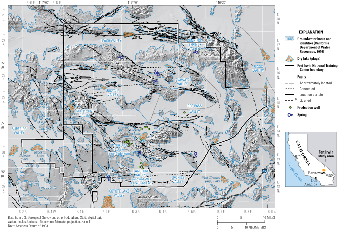
Location of the study area, production wells, springs, and groundwater basins within the Fort Irwin National Training Center, California.
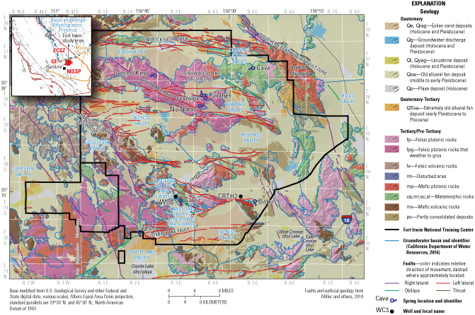
Generalized geology and faults and well and spring locations within Fort Irwin National Training Center, California. Inset map shows general locations of the Eastern California shear zone (ECSZ; Dokka and Travis, 1990a, 1990b), Mojave Strike Slip Province (MSSP; Miller and Yount, 2002), and the Garlock Fault Zone (GF; Miller and others, 2014). Well and spring information is available in table 1.
Table 1.
Summary of monitoring sites, instrumentation, and measurements at selected springs and wells sampled during 2015–17, Fort Irwin National Training Center, California (U.S. Geological Survey, 2017).[Site locations are shown on figure 2. Geographic Names Information System can be found at https://www.usgs.gov/tools/geographic-names-information-system-gnis. Abbreviations: USGS, U.S. Geological Survey; GNIS, Geographic Names Information System; drpt, drive point; tdb, HOBO TidbiT Temperature Logger; ho, HOBO U20 Water Level Data Logger; t, temperature; h, hydraulic head; sc, specific conductance; —, not available; dvr, TD-Diver transducer; BS, Bitter Spring Upper; Up, upper; GS-1 Trod (mid), Garlic Spring Trod Middle; GS-2 Trod (East-up), Garlic Spring Trod East upper; Trod, temperature rod; mw, monitoring well]
Historically, the NTC has relied on groundwater pumped from the developed groundwater basins (Bicycle Valley groundwater basin and the Irwin and Langford subbasins) to supply the water needs for base operations. Groundwater development at the NTC began in 1941 in Irwin subbasin (Densmore and Londquist, 1997). As a result of groundwater pumping, water levels have declined as much as 40 feet (ft) in Irwin and Langford subbasins (Densmore and Londquist, 1997; Voronin and others, 2013) and 100 ft in Bicycle Valley groundwater basin (Densmore and others, 2018). Water levels have stabilized or recovered throughout much of the Irwin subbasin because of reduced pumping (due to water-quality issues in the basin and water imported from Bicycle Valley groundwater basin and Langford subbasin since the 1990s) and artificial recharge by infiltration from ponds with treated wastewater from Irwin subbasin, Bicycle Valley groundwater basin, and Langford subbasin (Voronin and others, 2013); however, water levels have continued to decline in Bicycle Valley groundwater basin and Langford subbasin where pumping continues.
The U.S. Geological Survey (USGS) has been studying water-resources issues at Fort Irwin since the early 1990s. One issue of concern is the effect of groundwater development, resulting from training expansion and infrastructure at the NTC, on discharge at natural springs and seeps, which are important water sources for wildlife. In 2010, the USGS collaborated with the U.S. Army to characterize groundwater resources, focusing primarily on undeveloped basins within the NTC. As part of the work to characterize water resources, this study included evaluating discharge and water quality at eight springs and associated seeps at the NTC during 2015–17.
To evaluate the characteristics of springs and seeps within the NTC, the USGS did geophysical surveys and collected hydrological data (discharge and temperature measurements) and water-quality samples to provide a baseline of current (2015–17) hydrologic conditions at selected springs with diffuse discharge. The locations of the springs are presented on figure 2, and more information about the sites are shown in table 1. Two of the springs (Garlic and Jack Springs) are spread throughout a larger area and have at least three main discharge areas or seeps (discussed in the “Description of Study Areas” section). The baseline samples provide a snapshot of groundwater quality and can be compared with samples collected in the future to identify any changes in quality. These data were used to (1) estimate current discharge, (2) document water quality, and (3) determine if anthropogenic compounds (resulting from military activities) are present in samples collected at the springs. These collected data can be used to evaluate potential anthropogenic contamination of these wildlife water sources and allow the NTC staff to track changes in discharge and water quality over time.
Purpose and Scope
This report presents a description and evaluation of the spring water resources at the NTC. These springs are ecologically important for wildlife at the NTC, and there is concern that groundwater development and military activities in nearby basins could affect these springs. The U.S. Geological Survey began a study in 2015, in cooperation with the U.S. Army Fort Irwin National Training Center, to better understand the characteristics and water quality of the springs and how the water quality could change in response to military activities nearby. The scope of the report includes measurements of the physical and chemical characteristics of the springs, including geophysical, discharge, and water-quality data. These data were used herein to provide a baseline characterization of current (2015–17) hydrologic conditions and water quality of eight springs and associated seeps at the NTC and to evaluate any hydraulic connection of these springs to the nearby groundwater basins where data were available. For the purpose of this report, it was presumed that groundwater basin springs are hydraulically connected to nearby groundwater basins, whereas upland springs may or may not be connected to groundwater basins. Because of access restrictions to springs in bombing and live-fire areas, additional springs beyond the eight selected at the NTC could not be evaluated.
Previous Investigations
The USGS has been studying water-resources issues at Fort Irwin since the early 1990s. One issue of concern is the effect of groundwater development, resulting from training expansion and infrastructure at the NTC, on discharge at natural springs and seeps, which are important water sources for wildlife. Limited historical data are available for most of the NTC springs. Mendenhall (1909, p. 7) documented desert watering places in southeastern California and southwestern Nevada based on personal information collected by several sources to provide “knowledge of watering places in this region, and it was hoped that even the incomplete information assembled was useful for those traveling through this area.” Thompson (1929) provided a geographic, geologic, and hydrologic reconnaissance of the Mojave Desert for water resources. Thompson (1929, p. xi) noted that “The vast extent and scarcity of inhabitants and watering places made any comprehensive and thorough survey of its water resources a formidable undertaking.” As such, not all springs described in this report were visited by Mendenhall (1909) or Thompson (1929). Bowen (1943) produced an internal open-file war document that provided an assessment of the springs at the NTC. This document included springs not previously visited by Mendenhall (1909) and Thompson (1929). These historical reports provided insight into the condition (location and quality) of some of the springs at the time they were visited.
The names for the NTC springs used in this report are the names provided by Fort Irwin personnel and, where possible, have been cross-referenced with previous studies and, where possible, with the Geographic Names Information System (fig. 2; table 2). Garlic, Bitter, and Cave Springs were described by Mendenhall (1909) and Thompson (1929). Desert King Spring was described in Bowen (1943) and briefly mentioned but not visited by Thompson (1929). Thompson (1929) described visiting a spring called “Drinkwater Spring” in the general vicinity of the present-day (2016) Devouge Spring. Based on Thompson’s description of the Spring’s location relative to a playa in Avawatz Valley groundwater basin, “Drinkwater Spring” could be what is now referred to as “Devouge Spring.” Bowen (1943) also reported visiting Drinkwater Spring, where he located a cabin and perhaps a well but did not locate the actual spring. However, follow-up communication with Fort Irwin personnel suggest that Drinkwater Spring is west of Devouge Spring and was reportedly dry (Liana Ayers, U.S. Army, oral commun., 2017). Panther and Jack Springs, evaluated as part of this study, were not described in any of the historical reports (Mendenhall, 1909; Thompson, 1929; Bowen, 1943). Based on the description of the man-made features observed in 2015, No Name Spring is believed to be the same as “Taylor Spring” described by Bowen (1943). No Name Spring was not described by either Mendenhall (1909) or Thompson (1929); “Taylor Spring” described by Thompson (1929) was not located at the NTC, so it cannot be the same spring.
Accessing Groundwater Data
The groundwater-level data presented in this report can be accessed through the USGS National Water Information System (NWIS) at (https://waterdata.usgs.gov/ca/nwis/gw/; U.S. Geological Survey, 2017) and can be accessed by interactive map with National Water Information System (NWIS) Mapper (U.S. Geological Survey, 2018). The NWISWeb serves as an interface to a database of site information, including current and historical groundwater, surface-water, and water-quality data collected from locations throughout the United States and elsewhere. Data can be retrieved by state, category, and geographic area and can be selectively refined by specific location or parameter field. NWISWeb can output groundwater-level and water-quality graphs, site maps, and data tables (in Hypertext Markup Language [HTML] and American Standard Code for Information Exchange [ASCII] formats).
Characterization Methods: Geophysical, Hydrological, and Water Quality
Several methods were used to characterize the springs described in this report (see the “Description of Study Areas” section). The methods evaluated included (1) surface geophysical surveys to define the subsurface hydrogeologic conditions around the springs; (2) hydrological data collection, including direct discrete measurements of discharge and temperature; (3) water-quality sampling from drive points (small-diameter wells) and open holes (Garlic and Jack Springs) through time and at depth; and (4) use of high-resolution satellite imagery to delineate the areal extent of each spring and its vegetation type for inferring annual discharge. Initial canvassing of each spring, described in the “Description of Study Areas” section, was done to determine what methods, if any, were appropriate for spring characterization. During canvassing, it was determined that one or more of methods 1–3 were suitable for Garlic, Bitter, Jack, and Devouge Springs. For method 4, preliminary assessments of available high-resolution aerial photographs provided by NTC personnel for multiple years (1998–2015) indicated that plant type could not be mapped to the species level, and only rough annual discharge estimates could be calculated based on the spring areas and the list of known plant types in the area from vegetation surveys.
Multispectral imagery is useful for determining vegetation distributions and identifying areas of increased surface moisture in desert environments (DeMeo and others, 2003; Laczniak and others, 2006). Freely available multispectral satellite imagery (Landsat) also was considered for use in delineating vegetation and water extent in the springs area, but the pixel resolution was too coarse (30-meter [m] pixels) to remotely determine and map individual plant types for even the largest spring (Bitter Spring with an area of 412,800 square feet [ft2]). The use of higher-resolution multispectral or aerial imagery collection methods coupled with detailed field mapping and in situ atmospheric monitoring instrumentation could allow more successful remote monitoring of vegetation types and spring outflow.
Geophysical Methods
Geophysical methods are commonly used for imaging subsurface stratigraphy and structure and for characterizing and monitoring geological and hydrological features (Telford and others, 1990). Electrical resistivity is a material property that describes how easily a geologic material conducts an electric current. The main hydrogeologic factors that affect the resistivity of shallow sediments and rocks include the amount of interconnected pore water (porosity and saturation), the water quality (pore-water conductivity primarily dependent on total dissolved solids [TDS] concentration), lithologic texture, and the amount of clay and other conductive minerals (Telford and others, 1990). The substantial differences in resistivity of various sediment and rock types make it possible to differentiate among the geologic materials present (Daniels and Alberty, 1966; Keller and Frischknecht, 1966; Loke, 2004); for instance, resistivities of alluvium generally ranged from 10 to 800 ohm-meters (ohm-m), whereas clay-rich sediments often range from 1 to 100 ohm-m (Daniels and Alberty, 1966; Keller and Frischknecht, 1966; Loke, 2004). Variations in resistivity provide the basis for imaging the hydrogeologic conditions around each spring. In time-lapse studies, assuming no movement of solid subsurface materials, changes in resistivity through time can be attributed to relative changes in water quality or saturation. Reynolds (1997), Sharma (1997), and Butler (2005) provide more detailed descriptions of the resistivity method and resistivity values for common geologic materials.
Data Collection
Electrical resistivity tomography (ERT) using direct-current (DC) electrical measurements is a common approach for imaging subsurface geology, soil, and hydrologic structures (Telford and others, 1990; Loke, 2004). Resistivity measurements are taken by injecting a known current into the subsurface using two current electrodes along a survey line and measuring the resulting voltage difference between two potential electrodes along a linear profile. Based on Ohm’s law (R=V/I), the resistance (R) is calculated by taking the ratio of the measured voltage (V) and the transmitted current (I). The apparent resistivity (ρa) of the material, expressed in ohm-m, can then be determined by multiplying each resistance value by the corresponding geometric factor (k), which is based on the electrode geometry and spacing:
ERT surveys were done at selected springs in October 2015 and April 2017 to image the subsurface structure around these springs and to assess changes in subsurface resistivity that could be attributed to changes in water saturation or water quality. Global Positioning System (GPS) positions for the start and end of each ERT profile were recorded by the 2015 crew. The 2017 crew used an Arrow 100 GPS (EOS Positioning Systems, Terrebonne, Quebec, Canada) with submeter horizontal accuracy to locate the 2015 profile locations and reoccupy the same locations. During both years, ERT data were acquired using an Advanced Geosciences, Inc., SuperSting R8 resistivity/induced polarization meter (Advanced Geosciences, Inc., Austin, Texas) with a maximum of 56 electrodes. Each stainless-steel electrode is approximately 18 inches (in.) long and 0.5 in. in diameter. For each profile, the electrodes were hammered into the ground and regularly spaced along a line. A dilute saltwater solution was poured on each of the electrodes to reduce contact resistance; overall, the observed contact resistance values were relatively low, typically ranging from 0.01 to 2 kilo-ohms. Each electrode position was recorded using the Arrow 100 GPS to obtain lateral and topographic position. Many different combinations of current and potential electrode pairs were used to take measurements along each profile. Information about lateral resistivity variability in the subsurface is gained as the measuring electrodes are translated across the profile, whereas information about greater depths is obtained by increasing the spacing between the electrode pairs. A dipole-dipole array was used for both surveys for its measurement efficiency and good lateral resolution (Binley and Kemna, 2005). The 8-channel resistivity meter uses a command file to acquire measurements from predetermined current and potential electrode configurations. The resistivity meter is powered by two 12-volt batteries and is capable of injecting as much as 2,000 milliamperes (mA) of current into the ground. Data acquisition parameters are summarized in table 2; additional details about the ERT data collection are described by Thayer and others (2018).
Table 2.
Summary of two-dimensional direct-current resistivity line acquisition parameters, Fort Irwin National Training Center, California, 2015 and 2017 (Thayer and others, 2018).Data Processing and Inversion
The apparent resistivity measurements derived from the ERT measurements represent an equivalent homogeneous, isotropic half space. To solve for the resistivity structure in a more realistic heterogeneous subsurface, an iterative inversion algorithm is used to develop a best-fit layered-earth model of resistivity that minimizes the misfit with all measured ρa, according to regularization constraints and an estimate of data noise. This inversion process is used to produce two-dimensional (2D) cross-sections of the subsurface resistivity structure underlying each ERT profile.
Each ERT profile was inverted using the robust finite-element inversion method in the Advanced Geosciences, Inc. EarthImager 2D software version 2.4.0 build 617 (Advanced Geosciences, Inc., 2009). The robust inversion method is based on the assumption of an exponential distribution of data errors and minimizes an L1-norm parameter that is a combination of the model data misfit and stabilizing function. The method typically performs well on datasets containing low-quality data and resolves resistivity boundaries well (Advanced Geosciences, Inc., 2009). Topographic information obtained from GPS was incorporated into the inversion to accurately account for electrode geometry over the irregular terrain.
After preliminary inversion, the lowest-quality data were removed using a percentage data misfit threshold. This threshold was chosen by evaluating a histogram of data misfit and removing data associated with the upper tail of the distribution. The inversion was then run another time with the remaining data, and this process was repeated iteratively to achieve a balance between low root-mean-square error and realistic model structure. Depth of investigation (DOI) was calculated individually for each model by comparing model response to changing homogenous starting models varying across 4 orders of magnitude (Oldenburg and Li, 1999), and a mask was applied to all final model images based on this calculated DOI. The inversion parameters are summarized in table 3; additional details about data processing and inversion are described by Thayer and others (2018).
Table 3.
Summary of inversion parameters used in processing electrical resistivity tomography data in EarthImager 2D (Thayer and others, 2018).[Min., minimum; mV, millivolt; ohm-m, ohm-meter; Max., maximum; %, percent; RMS, root-mean square]
Hydrological Methods
Hydrological methods used in this study included discrete discharge measurements to evaluate surface flow from the springs and temperature measurements to trace groundwater movement beneath the springs. In addition to discrete discharge measurements, one to three sites were selected in the discharge area of selected springs for installation of drive points (small-diameter [2-in.] wells with a 2–3-ft perforated interval) to allow for the collection of temperature and water-quality samples (described later in the “Water Quality” section; table 1). These drive points were driven into the ground with a fence-post hammer until the bottom of the drive-point coupling was at land surface. Temperature measurements were collected at several depths using HOBO TidbiT temperature loggers (Tidbit; Onset Computer Corporation, 2017), and discrete water levels were measured using TD-Diver pressure transducers (VanEssen Instruments, Tucker, Georgia) or HOBO U20 Water Level Data Loggers (Onset Computer, Bourne, Massachusetts) to determine the direction, magnitude, and variability of the vertical hydraulic gradient in each drive point’s open interval. Additionally, subsurface temperature profiling rods called “Trods” (Naranjo and Turcotte, 2015) were installed to collect temperature data at four to six discrete depths along a 0.75-in. diameter, 3 ft (1-meter [m]) long, sealed, polyvinyl chloride pipe. The temperature sensors were secured inside a waterproof enclosure to prevent moisture damage to electronics. A heavy-duty submersible communication cable was used to download the temperature data. Each Trod was installed in streambed sediment for measuring temperature in the streambed and surface water; however, data collection from the Trods was discontinued because of several issues, including animals chewing through cables, equipment breakage during installation, and cables destroyed or lost during flash flooding.
Discrete Measurements (Discharge and Vertical Hydraulic-Head Gradient)
Discrete discharge and vertical hydraulic-head gradient measurements were taken using (1) a Parshall flume to measure surface-water level and discharge, (2) seepage meters to measure flux directly across the sediment-water interface at the bottom of the surface-water body, and (3) a manometer to measure the vertical hydraulic-head gradient by providing a comparison between the stage of a surface-water body and the hydraulic head beneath the surface-water body at the depth to which the perforated interval at the end of the probe was driven (Winter and others, 1988). Three springs (Garlic, Bitter, and Jack Springs) had the necessary characteristics to take point measurements of observed surface flow and discharge from the groundwater system using one or more of the methods introduced and described in detail in the “Description of Study Areas” section.
The standard portable Parshall flume is useful for measuring discharge when the depths are shallow and the velocities are low (Turnipseed and Sauer, 2010). A modified Parshall flume, consisting of a converging (upstream) section and a throat, was used to measure discharge during free-flow conditions. The floor of the upstream section is level longitudinally and transversely when in place, and the floor of the throat section slopes downward. For this study, a 3-in. Parshall flume was used to measure discharge at discrete locations where flow could be channeled through the flume at Garlic and Bitter Springs and one location at Jack Spring. The measurement point varied depending on where the surface flow was at the time of the measurement. The flume was placed in the center of flow and small levees were built to ensure that all flow passed through the flume. A standard Parshall flume that is properly constructed has an accuracy of 2–3 percent in free-flow conditions (see ASTM D 1941-91, 2007). The discharges observed during this study were on the lower limit of what the standard 3-in. flume was designed to measure; thus, in extremely low-flow conditions, the uncertainty of the results likely increases. These measurements provided a “snapshot” in time of the observed surface-water flow at one point along a reach and also provide insight into the relative rate and diurnal and seasonal variability of flow along the reach during this study but were not necessarily representative of total discharge from the spring. Kilpatrick and Schneider (1983) provide additional detail on the design principles of commonly used Parshall flumes and their discharge ratings.
The seepage meter allows direct measurement of seepage flux across the sediment-water interface (Zamora, 2008). The seepage meter consists of a bottomless cylinder formed from an inverted drum or bucket connected to a collection bag by a length of tubing. Initially developed by Lee (1977), the seepage meter design consisted of the cut-off end of a 55-gallon storage drum. Because of the small areal extent and low flow at springs within the NTC, a low-profile seepage meter (Rosenberry and LaBaugh, 2008; Rosenberry and others, 2020) was used in this study. The seepage meter was 25 in. in diameter and 3.5 in. in height, with an area of 255 square inches (in2) or 1.8 square feet ft2. The seepage meter was pushed into the bed of a stream, and a collection bag with a known volume of water was attached. The collection bag was then removed after a period of elapsed time, and the rate of vertical groundwater flux through the area enclosed by the seepage meter was calculated from the increase or decrease in the initial volume of water, the length of time elapsed, and the area of the seepage meter to obtain the flux rate in units of length per time. The seepage meter provided measurements of the general rate of seepage discharge, the temporal variability in seepage from multiple measurements, and provided a direct measurement of groundwater flux rates for comparison with flux rates estimated from simulations of temperature data. An increase in the initial volume of water indicated a positive vertical flux rate (movement of groundwater to surface water), and a decrease in initial volume indicated a negative vertical flux rate (movement of surface water to groundwater).
The manometer, also referred to as a “mini-piezometer,” provided a comparison between the stage of a surface-water body and the hydraulic head beneath the surface-water body at the depth to which the screen at the end of the probe was driven (Winter and others, 1988). The difference in head divided by the distance between the screen and the sediment-water interface was a measurement of the vertical hydraulic gradient. The device does not give a direct quantification of seepage flux, but when used in combination with a seepage meter, which does measure water flux, the two devices can yield information about the hydraulic conductivity of the sediments (Zamora, 2008). The manometer measurements provided a quick characterization of the direction and magnitude of the vertical hydraulic gradient. This method can be used as a reconnaissance tool in wetlands and in areas where wells do not exist, are sparsely distributed, or are impractical to install and maintain.
Temperature Measurements
Heat as a tracer is a simple yet powerful tool for detecting and quantifying water movement across a surface water-groundwater interface (Lapham, 1989; Constantz and others, 1994; Ronan and others, 1998; Constantz, 1998, 2008; Stonestrom and Constantz, 2003; Stewart and others, 2007; Essaid and others, 2008). Three springs (Garlic, Bitter, and Jack Springs), described in the “Description of Study Areas” section, were instrumented with temperature loggers and pressure transducers in drive points or individual temperature profiling probes for the purpose of using heat as tracer to estimate groundwater discharge at springs. As a result of damage from wildlife, equipment fouling, or loss due to flash flooding at some of the sites, the hydraulic-gradient data were inadequate, and estimates of groundwater discharge for the springs were not made. Instead, the collected temperature profiles were used as a qualitative tool to discern relative groundwater discharge by analyzing the degree of “damping” of the collected temperature profiles with depth. An oscillating, solar-driven, surface-temperature signal is expected to attenuate at shallow depths because of upward advection of the relatively constant groundwater temperature signal (Silliman and Booth, 1993). Thus, for high groundwater discharges, it was expected that the saturated sediment temperatures would have little to no diurnal variation, whereas for slight groundwater discharges, it was expected that the saturated sediment temperatures would have small diurnal variations that attenuate with depth.
Sites were selected and drive points were installed based on field observations of groundwater springs with visible ponding at land surface. Each drive point was instrumented with three Tidbit temperature loggers spaced at 0.5-ft intervals below the bottom of the drive-point coupling (0.5, 1, and 1.5 ft below land surface [bls]). An additional Tidbit temperature logger at each site continuously recorded air temperature. The Tidbits were calibrated by the manufacturer, Onset Computer, and spot-checked before deployment, but the temperature data were considered uncalibrated. The temperature data were used to provide information on “relative” groundwater discharge at drive-point locations. Although Trods also were installed, they were discontinued (previously described) and only the data from Tidbits were used. Continuous temperature values were recorded at 15-minute intervals beginning in November 2015 and ending in February 2017; however, the period of record was not continuous (data gaps exist) for any of the sites. Garlic and Bitter Springs were instrumented once, whereas Jack Spring was instrumented at two seeps, referred to as “Jack Spring East” and “Jack Spring West.”
Water Quality
Water-quality samples were collected to provide a snapshot of water-quality conditions at accessible springs at the NTC, to augment existing water-quality data from the springs, and for retrospective comparison as well as to serve as the baseline for tracking changes in the future. Sampling procedures followed protocols described in the USGS National Field Manual (U.S. Geological Survey, variously dated). Water samples were collected with a peristaltic pump and flexible tubing lowered to the bottom of pooled water, emplaced in the shallow streams (no more than a few centimeters deep), or lowered to the bottom of the drive point at instrumented springs (table 1). A short stainless-steel tube was affixed to the inlet end of the flexible tubing as ballast to hold the intake in place just above the bottom of the pool or drive point while water was being pumped into collection bottles.
At each sampling, field parameters were measured first, and then water samples were collected for laboratory determinations of major and minor ions, TDS, alkalinity, trace elements, nutrients and associated isotopes, stable isotopes in water, radioactive isotopes, and a selected set of other constituents (organics, perchlorate, mercury, cyanide, and others). These constituent groups serve to organize the water-quality methods description. The water-quality data are stored in the USGS National Water Information System (U.S. Geological Survey, 2017) and can be accessed at https://waterdata.usgs.gov/ca/nwis/nwis.
Water samples were collected and analyzed in the field for specific conductance, pH, alkalinity, and dissolved oxygen. Alkalinity was determined by the incremental titration method (U.S. Geological Survey, variously dated).
Samples for major and minor ions, nutrients, trace elements, alkalinity, and TDS analyses required filling one 250-milliliter (mL) polyethylene bottle with raw groundwater and one 500-mL and one 250-mL polyethylene bottle with filtered groundwater (Wilde and others, 2004). Nutrient samples, including those for determining nitrate, nitrate plus nitrite, ammonia, ammonium, phosphorus, and orthophosphate were filtered into a 125-mL brown polyethylene bottle and kept chilled until analysis. Samples for trace elements and laboratory-determined alkalinity were filtered using a 0.45-micrometer (μm) capsule filter and preserved with 7.5 normal nitric acid to a pH below 2.0. Major ions, nutrients, selected trace elements, alkalinity, and TDS were analyzed at the USGS National Water-Quality Laboratory (NWQL) or by laboratories contracted by the NWQL, using methods by Fishman and Friedman (1989), Fishman (1993), and Garbarino and others (2002, 200642). Laboratory reporting levels for selected constituents are listed in appendix 1.
The stable isotopes of oxygen (O) and hydrogen (H) in water were determined to provide insight on hydrologic processes. Samples were collected in 60-mL clear glass bottles and filled with unfiltered water and capped; caps were secured using electrical tape to prevent leakage and evaporation. Stable isotopes were analyzed by the USGS Stable Isotope Laboratory using methods described by Epstein and Mayeda (1953), Coplen and others (1991), and Coplen (1994). Oxygen-18 (18O) and deuterium (D or 2H) abundances are reported as ratios with the more abundant isotopes oxygen-16 (16O) and hydrogen-1 (1H), relative to those ratios in the Vienna Standard Mean Ocean Water–Standard Light Antarctic Precipitation scale (Coplen and others, 1999). The ratios are reported in delta (δ) notation as delta oxygen-18 (δ18O) and delta deuterium (δD), in units of parts per thousand (per mil) differences relative to the isotopic ratios in the standards.
Samples for nitrogen (N) isotopes were collected in 125-mL amber polyethylene bottles filled with unfiltered water, closed using caps with a conical insert, and were measured by mass spectrometry at the USGS Reston Stable Isotope Laboratory in Reston, Virginia, using methods described by Coplen, and others, (2012). Water samples from selected springs were analyzed for the delta nitrogen-15 (δ15N) in nitrate (δ15N-NO3) and delta oxygen-18 (δ18O) in nitrate (δ18O-NO3). Delta nitrogen-15 is reported as the ratio of nitrogen-15 (15N) to nitrogen-14 (14N) in a water sample, relative to atmospheric nitrogen gas.
Samples were analyzed for radioactive isotopes of hydrogen (tritium [3H]), carbon-14 (14C), and radon-222. Tritium samples were collected by filling 1-liter (L) polyethylene bottles with unfiltered water, closed using caps with a conical insert, and secured using electrical tape. Carbon-14 samples were collected by filling a 1-L glass bottle with filtered water and were analyzed by accelerator mass spectrometry (Beukens, 1992). For the collection of radon-222, a 10-mL sample was taken through the tubing attached to the peristaltic pump using a glass syringe affixed with a stainless-steel needle and then injected into a 25-mL vial partially filled with scintillation mixture (mineral oil) and shaken. The vial was then placed in a cardboard tube to shield it from light during shipping. Tritium was analyzed by the USGS Stable Isotope and Tritium Laboratory in Menlo Park, California, using methods described by Thatcher and others (1977); Carbon-14 was analyzed by Woods Hole Oceanographic Institution, National Ocean Sciences Accelerator Mass Spectrometry Facility in Massachusetts, using methods described by Vogel and others (1987), Donahue and others (1990), Gagnon and Jones (1993), and Schneider and others (1994). Radon samples were analyzed by the USGS Saint Petersburg, Florida, using methods described in Prichard and Gesell (1977), Prichard and others (1980), Clesceri and others (1989), McCurdy and others (2008), and Smith and others (2008).
The remaining other constituents include volatile organic compounds (VOCs), petroleum hydrocarbons, semi-volatile organic compounds (SVOCs, including munitions), polycyclic aromatic hydrocarbons (PAHs), perchlorate, and mercury. The other constituents include many of the “constituents of concern” in groundwater at the NTC; specifically, the other constituents are those commonly from anthropogenic sources that may be a result of military training activities. The organic compounds analyzed in water samples collected for this study included diesel and gasoline degradates, munitions, and industrial compounds including selected VOCs, SVOCs, and PAHs. The compounds analyzed are listed in appendix 2.
VOC samples were collected in three 40-mL sample vials that were purged with three vial volumes of unfiltered groundwater before bottom filling to eliminate atmospheric contamination. A one-to-one solution of hydrochloric acid to water was added as a preservative to the VOC samples. Total petroleum hydrocarbons (TPH, including gasoline range organics, diesel-range organics and motor-oil-range organics) were collected in three 40-mL sample vials for gasoline-range organics and a 1-L amber glass bottle was filled with unfiltered water and preserved with hydrochloric acid for diesel and motor oil-range organics. Samples for SVOCs and PAHs were collected by filling two 1-L amber-glass bottles to the shoulder with unfiltered groundwater. Samples for perchlorate analysis were collected in a sterile 125-mL polystyrene bottle and then filtered in two or three 20-mL aliquots of groundwater through a 0.20-μm pore-size syringe-tip disk filter into a sterilized 125-mL bottle. VOC, TPH, SVOCs, and PAH samples were analyzed at the USGS National Water-Quality Laboratory (NWQL) or by laboratories contracted by the NWQL.
The quality-assurance procedures used and quality-control (QC) samples collected for this study followed the protocols used by the USGS National Water Quality Assessment Project (Koterba and others, 1995) and are described in the National Field Manual (U.S. Geological Survey, variously dated). Quality-control samples were collected at eight of the springs in the study. Four types of QC samples were collected and evaluated in this study: (1) field blank samples collected to assess positive bias as a result of contamination during sample handling or analysis, (2) concurrent replicate samples collected to assess overall sampling precision (variability), (3) matrix-spike samples collected to assess positive or negative bias caused by the environmental matrices, and (4) surrogate compounds added to samples analyzed for organic constituents to assess precision and potential bias of laboratory analytical methods.
Except for gasoline and diesel-range compounds, blanks did not contain detectable concentrations of any constituent, indicating that contamination from sample-collection procedures was not biased in the data for these samples. Gasoline- and diesel-range organics were detected in blanks, indicating potential contamination, which likely resulted in higher reported values of these detected constituents in spring-water samples.
Replicate samples generally were within the limits of acceptable analytical reproducibility (that is, differences among replicate concentrations were expressed as relative percent difference [RPD; calculated as the concentration difference divided by the mean concentration of the pair, ×100] and the RPD was less than maximum acceptable RPD, which was constituent specific). Only a few VOCs were detected in paired-replicate samples; replicate sample RPDs agreed for styrene within 0.009 microgram per liter (µg/L), for methyl ethyl ketone within 1.0 µg/L, and for acetone within 0.9 µg/L. The median values of matrix-spike recoveries were within the acceptable range (70–130 percent) for all the VOCs. Therefore, detected VOC concentrations in samples were not modified on the basis of the matrix-spike recovery results.
Of the environmental samples, 12 were spiked with surrogate 1,2-dichlorobenzene-d4, 1,2-dichloroethane-d4, 1-bromo-3-chloropropane-d6, 1-bromo-4-fluorobenzene, 2-fluorobiphenyl, caffeine-d9, decafluorobiphenyl, fluoranthene-d10, nitrobenzene-d5, p-terphenyl-d14, squalene, and toluene-d8. Most surrogate recoveries were within the acceptable range of 70–130 percent. The VOCs with surrogate recoveries outside the acceptable range included 2-fluorobiphenyl (unacceptable recoveries ranged from 38 to 69 percent in 5 of 12 samples); decafluorobiphenyl (36 percent in 1 of 1 sample); nitrobenzene-d5 (38–67 percent in 4 of 12 samples); p-terphenylterphenyl-d14 (56–68 percent in 2 of 12 samples); and squalene, a diesel-range organic (48–58 percent and 238 percent in 6 of 9 samples). With the exception of squalene, none of these surrogate compounds were detected in environmental samples from the springs. The range in squalene recoveries indicate imprecision in analytical methods for most of the diesel-range organics and consequently more uncertainty about the reported values.
Description of Study Areas
The NTC is in the Mojave Desert region of southern California (fig. 2) and lies in a geologically complex and heavily faulted area at the intersection of the eastern end of the Garlock Fault Zone (Miller and others, 2014), the Eastern California Shear Zone (Dokka and Travis, 1990a, b) and the Mojave Strike Slip Province (Miller and Yount, 2002) and is within the Basin and Range physiographic province (Planert and Williams, 1995). The mountain altitudes range from more than 4,000 ft above the North American Vertical Datum of 1988 (NAVD 88) in the northern and western parts of the NTC to about 1,300 ft above NAVD 88 in the southeastern part around Cronise Valley groundwater basin, and to less than 900 ft above NAVD 88 in the eastern part around Riggs Valley groundwater basin (fig. 1). The NTC is dissected by northwest-southeast trending right-lateral, east-west trending left-lateral, oblique, and thrust faults (fig. 2). The NTC is bounded by the Garlock Fault Zone (Petersen and Wesnousky, 1994) on the north, the Southern Death Valley Fault Zone on the northeast, the Coyote Lake Fault on the south, and the Goldstone Lake Fault Zone on the west (fig. 2; Jennings, 1994).
The geology across the NTC is highly variable with a wide variety of rock types and faults (figs. 1, 2). Mountains in the region consist primarily of pre-Tertiary (Mesozoic and older) crystalline rocks with local accumulations of Tertiary (Miocene to Pliocene) volcanic and sedimentary rocks (Miller and others, 2014; fig. 2). Broad valleys containing Quaternary and Tertiary basin-fill deposits lie among these mountains (Miller and others, 2014; fig. 2). The western part of the NTC lies along the eastern and southern edges of the Tertiary (Miocene) age Eagle Crags Volcanic Complex that includes thick accumulations of lava flows, pyroclastic rocks (fallout tephra deposits and ignimbrite), and volcaniclastic and tuffaceous sandstone and conglomerate (Sabin, 1994). Toward the eastern part of the NTC, the basin-fill deposits become progressively finer grained. Basin-fill deposits in the eastern part of the NTC consist of fine-to coarse-grained alluvium and partly consolidated deposits, including thick sections of clays and lacustrine deposits observed in borehole lithological and geophysical logs (Kjos and others, 2014; Miller and others, 2014). The NTC area includes numerous faults that are part of the Eastern California Shear Zone, a north-trending structural zone across the Mojave Desert block that formed about 10 million years ago (Schermer and others, 1996) and the Mojave Strike Slip Province. Although many of the faults do not cut Holocene deposits, some faults had Holocene activity (Miller and others, 2014).
The hydrogeology of the basins at the NTC is typical of many basins in the Mojave Desert. Basins are underlain by a pre-Tertiary age basement complex of plutonic and metamorphic rocks (Densmore and others, 2017). Volcanic rocks, predominantly in western basins, have highly variable permeability; some volcanic rocks are welded and impermeable, whereas others are highly fractured and may yield water. The basin fill consists of semi-consolidated to unconsolidated Tertiary and Quaternary deposits derived from the surrounding mountains. The Quaternary deposits generally are more permeable than the older Tertiary deposits and typically have higher yield. The numerous faults crossing the NTC control the lateral extent and movement of groundwater, where some faults act as barriers and others as conduits (Plummer and others, 2004). The aquifer systems and associated geochemical frameworks have not been defined for most of the NTC basins, except for Bicycle Valley groundwater basin and the Irwin and Langford subbasins, which are discussed in detail, in Densmore and Londquist (1997), Voronin and others (2013), and Densmore and others (2018). Additional information on the other undeveloped groundwater basins at the NTC, including hydrogeologic, hydrologic testing, and water-level and water-quality data from boreholes in these basins can be found in Kjos and others (2014) and Nawikas and others (2019).
Average annual precipitation is about 4 in. and primarily falls in the highland area in the western part of the NTC and on the higher mountains during winter rains and short summer thunderstorms (Densmore and others, 2017). Natural recharge takes place at the base of the mountain fronts and along seasonal washes that drain from the highlands in the west to the low areas and playas in the east. These washes can experience flash floods where isolated thunderstorms happen during the monsoonal summer season.
Study Areas: Physiographic, Geologic, and Hydrogeologic Setting
A spring is a place where water issues from the ground and flows (Bryan, 1919), and a seep is a type of spring where the water issues not from a well-defined opening, but through the pores of the ground over a considerable area. Bryan (1919) classified springs into two main groups: (1) deep-seated water springs related to volcanic or tectonic disturbances, including fissure and fault-controlled springs and (2) shallow water springs, including springs in porous rock, porous rock overlying impervious rock, and porous rock between impervious rock, or in impervious rock.
There were 8 of 10 active springs and associated seeps within the NTC boundary that were studied (fig. 2; table 1) and are described in subsequent report sections (presented in order from north to south). Two springs were not evaluated because they were inaccessible because of their location within a bombing and live-fire area. The eight springs and associated seeps were canvassed in October 2015. The springs studied generally are shallow water springs (Bryan, 1919) that include some combination of porous rock, impervious rock, and fissure and fault-controlled features but not of deep-seated nature. For this study, these springs were divided into two groups: (1) the upland springs (akin to Mendenhall’s “mountain springs”; Mendenhall, 1909) and (2) groundwater basin springs.
Upland Springs
The upland springs include springs with fissure-controlled features (Cave, Desert King, Panther, and No Name Springs). Devouge spring also likely includes porous fractured rock overlying an impervious rock.
Cave Spring
Cave spring is an upland spring located at the northern boundary of the NTC in the Avawatz Mountains, about 25 mi northeast of Irwin subbasin (fig. 2). The spring is near the intersection of the Garlock and Southern Death Valley Fault Zones in a narrow northward-draining canyon about 2 mi north of the main drainage divide of the Avawatz Mountains (figs. 2, 3, 4). Cave Spring was described by Mendenhall (1909) and used by travelers between Barstow (fig. 1) and Death Valley, California (not shown). Cave spring is on the east sidewall of the wash in fractured metamorphic rocks (fig. 4). Mendenhall (1909) reported that two springs, each about 5 ft across and 5 ft deep, existed in the early 1900s. Thompson (1929) described two caves or short tunnels about 40 ft apart that were dug 10 ft into the wall of the canyon. However, when these caves were visited in 2015, only the northern cave contained water. Land-surface altitude of Cave Spring is about 3,605 ft above NAVD 88.
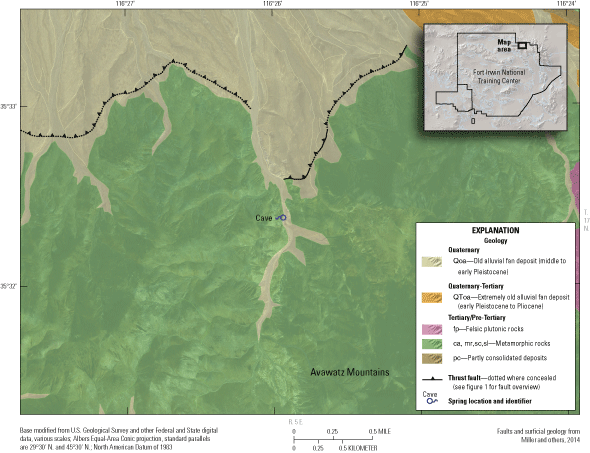
Generalized geology and faults near Cave Spring, Fort Irwin National Training Center, California.
Vegetation at Cave Spring (U.S. Department of Agriculture, 2020), Fort Irwin National Training Center, California.
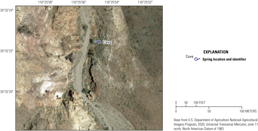
Cave Spring is fed by water seeping from fractured metamorphic rocks into a pond inside the northern cave that covered an area of at least 5 ft across. Water also is present in a second shallow pond outside the cave wall; this pond is about 5 ft south of the northern cave entrance and adjacent to the east sidewall of the canyon, where it flowed a short distance and infiltrated into the thin wash deposits within the canyon (fig. 5). The pond in the wash presumably is fed by seepage through fractures along the cave wall. The main area of vegetation, primarily grasses, cattails, and a small tree, was around this second pond, which covers an area of about 5 ft and where the ground was moist.
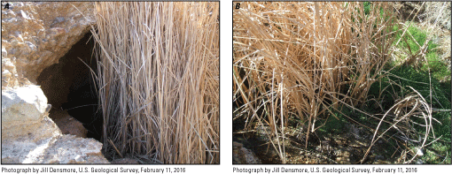
Cave Spring, February 11, 2016, Fort Irwin National Training Center, California. A, spring sampling location; B, vegetation from mouth of cave toward wash. Photographs by Jill Densmore, U.S. Geological Survey, February 11, 2016.
Vegetation
Vegetation surveys were completed by NTC personnel at Cave Spring during 2013–15 (J. Uzzardo, Redhorse Corporation, written commun., 2013; T. Pereira, Redhorse Corporation, written commun., 2014; H. Erickson, Redhorse Corporation, written commun., 2015). The main species identified along the surveyed transects were cattle saltbush (Atriplex polycarpa), compact brome (Bromus madritensis), Goodding's black willow (Salix gooddingii), mustard family (Brassicaceae [Family]), and cattail (Typha latifolia). Other species identified a short distance away from the wetted spring area included creosote bush (Larrea tridentata), Fremont’s cottonwood (Populus fremontii), brittlebush (Encelia farinosa), bristly fiddleneck (Amsinckia tessellata), and burrobush (Ambrosia salsola).
Desert King Spring
Desert King Spring is on the north side of the Granite Mountains and along the southern edge of Leach Valley (fig. 2), about 20 mi north of Irwin subbasin. This spring is along an unnamed shear zone and may be part of the Garlock and Southern Death Valley Fault Zones. Desert King Spring lies in a north-northeasterly canyon, about 2 mi north of the main drainage divide of the Granite Mountains (fig. 2). The spring/seep is on the east side of the wash in fractured plutonic rocks. Land-surface altitude of the spring is about 2,900 ft above NAVD 88.
In 1917, Thompson (1929) described Desert King Spring as a well east of the wash, about 900 ft south of and 50 ft above an old cabin and stamp mill. Thompson observed a small pond of water near the well that was dug 15 ft into granite and had a depth to water of about 1 ft below land surface ft bls. Bowen (1943) reported locating a 5 by 5 ft, 12.5-ft-deep well with a depth to water of about 2 ft bls, excavated in granite on the west side of a pronounced north/south-trending shear zone about 50-ft wide and with a nearly vertical dip. Bowen (1943) measured discharge at the outlet of a 1-in. diameter pipe from the well at about 0.17 gallons per minute (gal/min). Based on Bowen’s (1943) suggestions, a well reportedly was dug along the south side of the wash and west side of the shear zone to further develop this spring. In 2015, neither a pond nor wells were observed. The present (2016) location of Desert King Spring (figs. 6, 7) is about 400 ft south of the site reported by Thompson (1929). This “present-day” spring is a small 1 by 1 ft wetted area, where water was present on the surface and supported grasses and melons, near an old bathtub (fig. 8). White deposits, presumably nitrate-bearing caliche, were observed upgradient from this location and appear to lie along or near the shear zone.
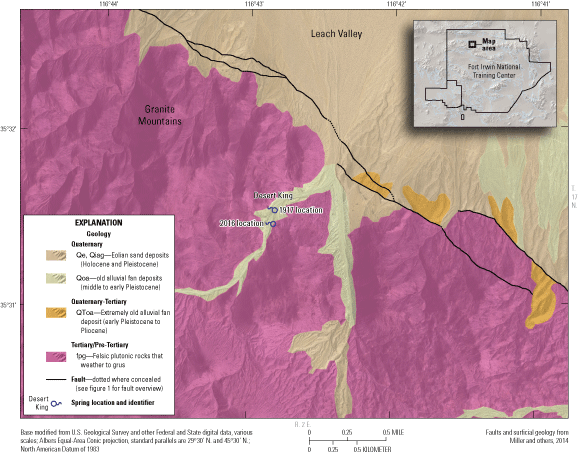
Generalized geology and faults near Desert King Spring study area, Fort Irwin National Training Center, California. (1917 location of spring is from Thompson [1929]).
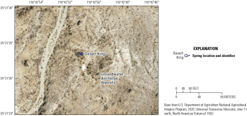
Aerial image of Desert King Spring (U.S. Department of Agriculture, 2020), Fort Irwin National Training Center, California.
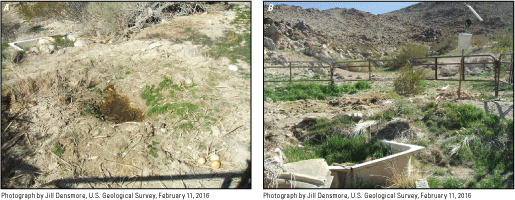
Desert King Spring, Fort Irwin National Training Center, California; A, sampling location, looking toward wash; B, overview looking southeast. Photographs by Jill Densmore, U.S. Geological Survey, February 11, 2016.
Vegetation
Vegetation surveys were completed by NTC personnel at Desert King Spring during 2013–15 (J. Uzzardo, Redhorse Corporation, written commun., 2013; T. Pereira, Redhorse Corporation, written commun., 2014; H. Erickson, Redhorse Corporation, written commun., 2015). The main species identified along the surveyed transects were Devil’s lettuce (Amsinckia tessellata), fourwing saltbush (Atriplex canescens), compact brome (Bromus madritensis), coyote melon (Cucurbita palmata), western tansymustard (Descurainia pinnata), saltgrass (Distichlis spicata), brittlebush (Encelia farinosa), creosote bush or chaparral (Larrea tridentata), desert tobacco (Nicotiana obtusifolia), notch-leaf scorpion-weed (Phacelia crenulata), and annual rabbitsfoot grass (Polypogon monspeliensis).
Devouge Spring
Devouge Spring is an upland spring in the southern part of Avawatz Valley groundwater basin. The spring is a small seep on an alluvial fan. The Drinkwater Lake Fault (Schermer and others, 1996) and Granite Mountains (fig. 9) are south of the spring. The Granite Mountains are comprised of felsic plutonic rocks (Miller and others, 2014) that generally are non-water bearing except where jointed or fractured (Densmore and Londquist, 1997). The spring is east of an outcrop of plutonic rocks that extends north from the main part of the Granite Mountains and indicates shallow bedrock is in this area (fig. 9). Land-surface altitude of the spring is about 3,720 ft above NAVD 88.
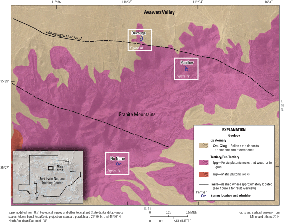
Generalized geology and faults near Devouge, Panther, and No Name Spring study areas, Fort Irwin National Training Center, California.
Devouge Spring covers a wetted area about 6 ft long (oriented downslope from the mountain front) and 5 ft wide (fig. 10); this is a main area of vegetation, primarily cattails, shrubs, and grasses, where the ground is moist (fig. 11). An open pit that appears to be a hand-dug well is about 150 ft in distance upslope from the seep (fig. 10). The open pit is approximately 5 ft square and about 14 ft deep, and it appeared to be dry. An old metal water tank is about 200 ft downslope from the wetted area (fig. 10). Old piping lies between the wetted area and tank, indicating that water (presumably from the open pit) may have been piped and stored in the tank and the flow from the spring was likely greater than flow observed in 2015. Because of the location of the wetted area relative to the old piping, it appears that Devouge Spring may actually be seepage from a break in the buried piping resulting in a “man-made” wetted area.
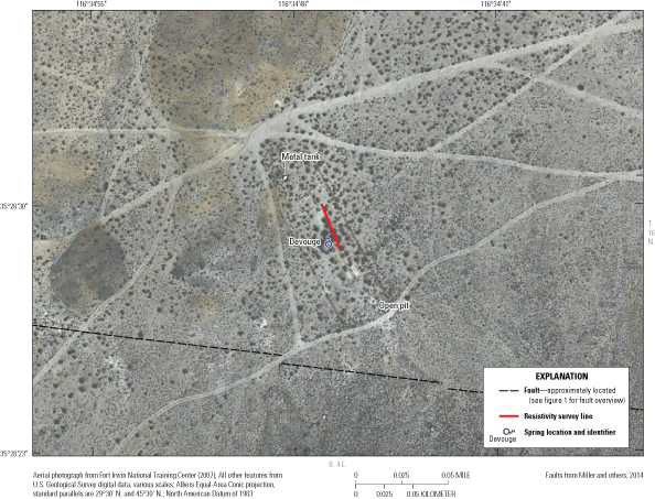
Monitoring site and resistivity survey line at Devouge Spring study area, Fort Irwin National Training Center, California.
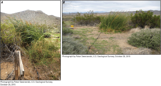
Devouge Spring on October 28, 2015, Fort Irwin National Training Center, California. A, sampling location, looking south toward Granite Mountains; and B, looking north. Photographs by Peter Swarzenski, U.S. Geological Survey, October 28, 2015.
Thompson (1929) described visiting a spring called “Drinkwater Spring” in the general vicinity of the present day (2016) Devouge Spring. When Thompson visited in 1917, there was a cabin with a well dug in granite about 250 ft east of the cabin. Thompson (1929) reported the depth of the well was about 8 ft and the depth to water was 3 ft in 1917. In Thompson’s 1929 report, this well was mistaken for the spring, which was observed to be several hundred feet farther southeast, on the southeastern side of the granite ridge. Although not sampled by Thompson (1929), Drinkwater Spring reportedly had “good” quality water. Based on the location description relative to a playa in Avawatz Valley groundwater basin, Devouge Spring, visited in 2015, could be Thompson’s Drinkwater Spring. Bowen (1943) also reported visiting Drinkwater Spring, where he located the cabin and perhaps the former well, but not any spring. Follow-up communications with NTC personnel (Liana Ayers, U.S. Army, written commun., 2017) indicated that Drinkwater Spring is west of Devouge Spring and was reportedly dry.
Vegetation
Vegetation surveys were completed by NTC personnel at Devouge Spring during 2013–15 (J. Uzzardo, Redhorse Corporation, written commun., 2013; T. Pereira, Redhorse Corporation, written commun., 2014; H. Erickson, Redhorse Corporation, written commun., 2015). The main species identified along the surveyed transects were white bursage (Ambrosia dumosa), bristly fiddleneck (Amsinckia tessellata), brome (Bromus spp.), saltgrass (Distichlis spicata), creosote bush or chaparral (Larrea tridentata), water jacket (Lycium andersonii), and cattail (Typha latifolia).
Location of Hydrological and Electrical Resistivity Tomography Surveys
Hydrological and ERT surveys were completed at Devouge Spring (see “Characterization Methods: Geophysical, Hydrological, and Water Quality” section for method description). Hydrological data were collected at a drivepoint installed in the seep at Devouge Spring (fig. 10; table 1). The drivepoint site is in the small, wetted area at the downslope (or northern) end of the vegetation to assess the variability in groundwater flux. An ERT survey was completed in 2015 across the wetted area to provide a subsurface resistivity profile of the spring (resistivity survey line shown on fig. 10). Changes in ERT through time could not be evaluated because a repeat survey could not be done in 2017 because of site access issues; thus, the 2015 survey is not described in the “Evaluation of Springs” section of this report.
Panther Spring
Panther Spring is in the Granite Mountains, south of Avawatz Valley groundwater basin (fig. 2). The spring lies in a narrow wash on the north side of the Granite Mountains. Land-surface altitude of the spring is 3,825 ft above NAVD 88. Panther Spring is between a series of fault splays of the Drinkwater Lake Fault (figs. 9, 12). The spring is in thin wash deposits among felsic plutonic rocks, indicating shallow bedrock in this area (fig. 9). The active channel of the wash is lined with a thin veneer of younger alluvium composed of decomposed granite (unconsolidated sand and gravels derived from the plutonic rocks).
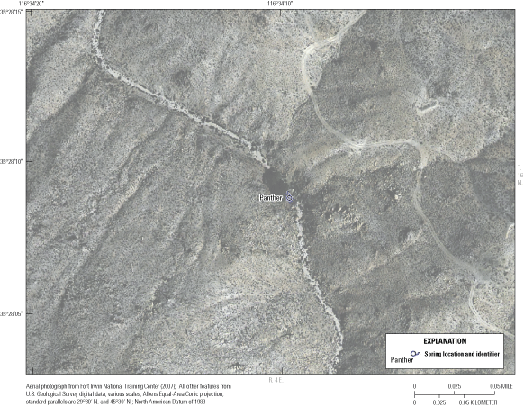
Panther Spring study area, Fort Irwin National Training Center, California.
Panther Spring appears as a series of intermittent shallow pools in an ephemeral wash that flows only after precipitation (fig. 12). The shallow pools can hold water for several months after precipitation but reportedly dry up because of lack of substantial, sustained groundwater discharge from the fractured plutonic rocks or wash deposits coupled with high evaporation rates (Liana Ayers, U.S. Army, oral commun., 2017). A man-made trough built to capture water was dry when visited in 2016. The main area of wetland vegetation covers about 6,465 ft2 and consists of a few trees dominating the west side of the wash (fig. 13).
Panther Spring, Fort Irwin National Training Center, California; A, sampling location, looking east; and B, looking south. Photographs by Jill Densmore, U.S. Geological Survey, February 10, 2016.
Vegetation
Vegetation surveys were completed by NTC personnel at Panther Spring during 2013–15 (J. Uzzardo, Redhorse Corporation, written commun., 2013; T. Pereira, Redhorse Corporation, written commun., 2014; H. Erickson, Redhorse Corporation, written commun., 2015). The main species identified along the surveyed transects were Devil’s lettuce (Amsinckia tessellata), saltgrass (Distichlis spicata), Fremont cottonwood (Populus fremontii), annual beard-grass (Polypogon monspeliensis), desert almond (Prunus fasciculata), and Goodding's black willow (Salix gooddingii).
No Name Spring
No Name Spring is in the Granite Mountains, near the southwest side of the Avawatz Valley groundwater basin (fig. 2). The spring lies in a narrow wash on the eastern end of the Granite Mountains. Land-surface altitude of the spring is 4,520 ft above NAVD 88. No Name Spring is between splays of the Drinkwater Lake Fault (fig. 9). The spring is about 1.5 mi southwest of Devouge and Panther Springs. The spring is in thin wash deposits overlying felsic plutonic rocks, indicating shallow bedrock in this area. Scattered patches of younger alluvium line the active channel of the wash. These wash deposits are composed of coarse-grained decomposed granite.
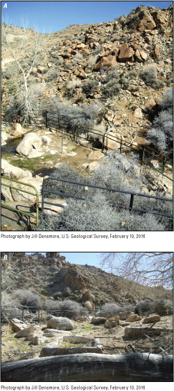
No Name Spring appears as an area of vegetation, primarily grasses and shrubs, covering about 2,200 ft2 (figs. 14, 15). A small 1-in. diameter buried pipe was observed at the downstream end of the vegetated area but was not followed to its termination. An old metal water tank is about 200 ft downstream from the vegetated area (fig. 14), indicating that the spring may have previously had more discharge for capture than was observed in the current study (2016). Bowen (1943) reported visiting a spring called “Taylor Spring.” Based on the description of the man-made features, it is believed that No Name Spring may be the same as Taylor Spring described by Bowen (1943). In 1943, discharge of the spring was measured at the outlet of the 1-in. diameter pipe at a rate of 0.5 gal/min. During 2016, discharge from No Name Spring was merely a slow drip from the 1-in.-diameter pipe and was insufficient for determining either a flow rate or collecting water-quality samples.
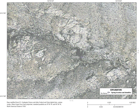
No Name Spring study area, Fort Irwin National Training Center, California.
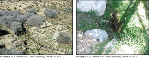
No Name Spring, Fort Irwin National Training Center, California. A, spring location overview looking north; and B, 1-in. diameter pipe.
Vegetation
Vegetation surveys were completed at No Name Spring during 2012, 2013, and 2014. In 2012, NTC personnel identified the following 11 species: fringed amaranth (Amaranthus fimbriatus), blackbrush (Coleogyne ramosissima), Nevada Mormon tea (Ephedra nevadensis), Coopers’s goldenbush (Ericameria cooperi), Eastern Mojave buckwheat (Eriogonum fasciculatum), Panamint Mountain buckwheat (Eriogonum panamintense), threadleaf snake weed (Gutierrezia microcephala), desert almond (Prunus fasciculata), antelope bitterbrush Purshia tridentata), bladdersage (Salazaria mexicana), and Mojave aster (Xylorhiza tortifolia; A. Fowler, U.S. Army, written commun., 2012). The main species identified by NTC personnel during the 2013 vegetation survey was water jacket (Lychum andersonii). During 2014, the main species identified along the surveyed transects were compact brome (Bromus madritensis), saltgrass (Distichlis spicata), and wild almond (Prunus fasciculata; J. Uzzardo, Redhorse Corporation, written commun., 2013; T. Pereira, Redhorse Corporation, written commun., 2014; H. Erickson, Redhorse Corporation, written commun., 2015). The number of species identified during 2013 and 2014 was much smaller than the 11 species identified in 2012. The decrease in the number of inventoried vegetation species was from donkey disturbances (Liana Ayers, U.S. Army, oral commun., 2017).
Groundwater Basin Springs
The groundwater basin springs include springs with fault-controlled features and impervious rock. Garlic, Bitter, and Jack Springs are all groundwater basin springs. These springs are near the southern boundary of the NTC.
Garlic Spring
The spring lies at the base of the low hills that separate the Langford Valley groundwater basin from the Bicycle Valley and Cronise Valley groundwater basins to the east (fig. 2). Garlic Spring is between Irwin subbasin and Langford subbasin (fig. 2). Land-surface altitude of the spring is 2,312 ft above NAVD 88. Garlic Spring is on the northeast side of a dry wash that flows only during extreme precipitation through a narrow gap between low hills that connects Irwin and Langford subbasins (fig. 16). The hills are crossed by several faults and are composed of felsic and mafic plutonic, schistose, and carbonate rocks (Miller and others, 2014) that generally are non-water bearing except where jointed or fractured (Densmore and Londquist, 1997). Garlic Spring appears in a relatively narrow part of the wash and forms as a series of seepages along the trend of the Garlic Spring Fault (fig. 16) that discharge southwest toward the wash. The NTC wastewater-treatment facility (not shown) and disposal ponds also are about 1-mile northeast near this wash (fig. 16).
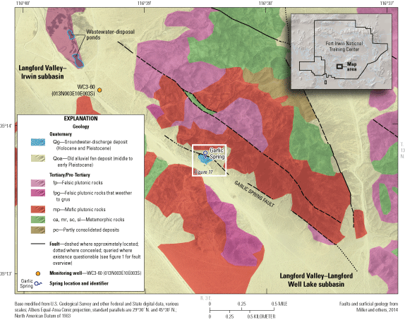
Generalized geology, faults, and monitoring well WC3-60 near the Garlic Spring study area, Fort Irwin National Training Center, California.
The spring appears as an area of wetland seeps for a distance of about 450 ft. There are three main areas of vegetation: (1) where groundwater discharges to the surface, (2) flows downgradient from the surface discharge, and (3) and infiltrates into the main channel of the dry wash (figs. 17, 18). The western area supports large trees, shrubs, and grasses; the middle area supports cattails and small shrubs and trees; the eastern area supports cattails, grasses, and an occasional small tree (fig. 18). The extent of vegetation shown in areal photographs of Garlic Spring in 2007 (fig. 17) is greater than vegetated extent near Garlic Spring indicated by areal photographs taken in 1995 (U.S Geological Survey National Aerial Photography Program, September 30, 1995, accessed November 15, 2016, at https://earthexplorer.usgs.gov/; not shown on fig. 17). Two seepage points along the eastern side of the spring are reported to have been developed by shallow excavation (Bowen, 1943). During 2015, removal of invasive species vegetation by NTC personnel uncovered one of these excavations, an approximate 5- by 5-ft square pit that is about 14 ft deep on the eastern most end of the seepages. Water-quality samples collected from this pit in 1993 are representative of Garlic Spring; the location of the excavation where water samples were collected in 1993 is about 320 ft southeast of the general location shown on figure 17 and near the temperature profile site GS-2 Trod (East-Up).
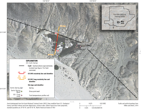
Locations of monitoring sites and resistivity surveys at Garlic Spring study area, Fort Irwin National Training Center, California.
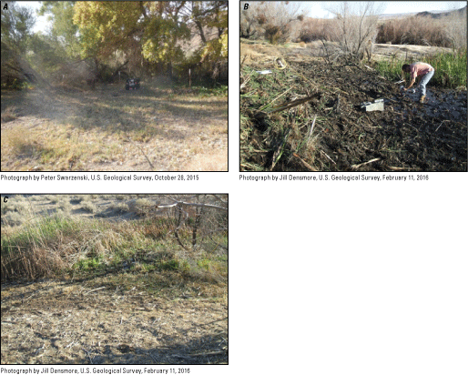
Garlic Spring, Fort Irwin National Training Center (NTC), California. A, western sampling location; B, middle sampling location (after cattail removal efforts by NTC personnel); and C, eastern sampling location.
Vegetation
Vegetation surveys were completed by NTC personnel at Garlic Spring during 2013–15 (J. Uzzardo, Redhorse Corporation, written commun., 2013; T. Pereira, Redhorse Corporation, written commun., 2014; H. Erickson, Redhorse Corporation, written commun., 2015). The main species identified along the surveyed transects were yerba mansa (Anemopsis californica), cattle saltbush (Atriplex polycarpa), mule fat (Baccharis salicifolia), sweetbush (Bebbia juncea), saltgrass (Distichlis spicata), salt heliotrope (Heliotropium curassavicum), burrobush (Hymenoclea salsola), Mexican rush (Juncus balticus ssp. mexicanus), prickly lettuce (Lactuca serriola), California phacelia (Phacelia californica), annual beard-grass (Polypogon monspeliensis), screwbean mesquite (Prosopis pubescens), narrowleaf willow (Salix exigua), salt cedar (Tamarix ramosissima), and cattail (Typha latifolia). Larger trees, primarily cottonwood, grow along the western end of the spring, whereas salt cedar, honey mesquite, saltgrasses and bushes, and cattails grow in the middle section and eastern end of the spring.
Location of Hydrological and Resistivity Surveys
Hydrological data were collected at selected sites at Garlic Spring (fig. 17; table 1). The sites were along the fault trend and at the lower end of the vegetation to assess the variability in groundwater flow. Two ERT surveys were completed on the westernmost end of the spring in 2015 and 2017 to provide a subsurface resistivity profile of the spring.
Bitter Spring
Bitter Spring, the largest spring by area at Fort Irwin, is in Cronise Valley (fig. 2). Bitter Spring is about 1 mi southeast of the Langford Lake Main Supply Route (fig. 19). Land-surface altitude of Bitter Spring ranges from about 1,360 ft above NAVD 88 at the northern extent of vegetation to about 1,330 ft above NAVD 88 at the southern extent. The spring lies in the Bicycle Lake Fault Zone (fig. 19).
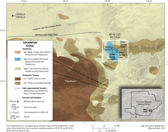
Generalized geology, faults, and location of monitoring wells CRTH2 #1 and CRTH2 #2 (U.S. Geological Survey, 2017), near Bitter Spring study area, Fort Irwin National Training Center, California.
Bitter Spring is in a sandy wash cutting through hills consisting of Tertiary, partly consolidated deposits and northeast of a black volcanic hill composed of basalt, which is a mafic volcanic rock (also known as “The Whale”; fig. 19). The wash generally drains from the northern part of Cronise Valley groundwater basin to the southeastern part where the West and East Cronise Lake (dry) playas are located (fig. 1). This wash flows during extreme precipitation. The partly consolidated deposits that form the hills (fig. 19) are composed of coarse-grained deposits, such as conglomerate and sandstone underlain by tight clays. The coarse-grained deposits dip northeasterly, with the underlying clays forming a barrier to southward groundwater flow (Bowen, 1943). Several faults, splays of the Bicycle Lake Fault Zone, cross this area and may have offset or tilted the tight clay so that the altitude of the top of the clay is higher south of the faults than it is north of the faults. Bowen (1943) mapped the deposits in the east wall of the wash as dipping approximately 60–65 degrees to the northeast. Bitter Spring formed by groundwater draining from Cronise Valley groundwater basin being forced to the surface by the fault, through the overlying coarser-grained deposits and above the saturated tight clay that is part of the aquifer system.
Bitter Spring supports an extensive area of vegetation, primarily small trees, shrubs, and grasses, within the wash for about 1,500 ft (figs. 20, 21). This area of vegetation indicates that groundwater is shallow in this part of the wash. Along the southeastern end of the vegetation are several wildlife watering holes that are the surface expression of the water table. Reportedly, several trenches were dug before the 1940s along the southeastern part of the spring to better develop this area (Bowen, 1943); however, no obvious evidence of these trenches was observed during this study. The trenches may have been eroded during flash flooding, which commonly happens in the wash during precipitation. In 2016, the wash and much of the vegetation at Bitter Spring was concentrated along the southeastern part of the wash. Comparison of historical imagery showed that the area of vegetation changes because of flash floods, several of which happened during this study. Several small ponds of water and surface flow are present in two main incised channels that were about 5 ft below the land surface where the vegetation is well established. It is possible that these ponds may be the remnants of the trenches described by Bowen (1943). A well was canvassed by USGS in 1965 but was not located in 2016.
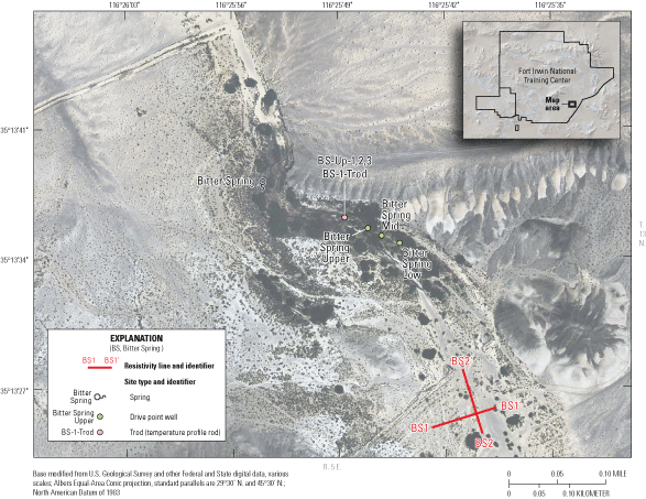
Locations of monitoring sites and resistivity surveys at Bitter Spring study area, Fort Irwin National Training Center, California. Abbreviations: BS1, Bitter Spring 1; BS2, Bitter Spring 2; Trod, Temperature profile rod.
Bitter Spring Fort Irwin National Training Center, California. A, overview of upstream end of wash, looking southwest; B, overview of downstream end of wash, looking southwest; C, overview of dense vegetation; D, view of mixed vegetation; and E, wildlife watering hole in wash, looking west.
A borehole log from nearby multiple-well monitoring site CRTH2 (site name 013N005E08B001–2S; Kjos and others, 2014; U.S. Geological Survey, 2017; Nawikas and others, 2019), located about 2.5 mi northwest of Bitter Spring (fig. 19), indicated sandy, gravelly alluvial deposits overlie a 660-ft-thick clay deposit from 200 to about 860 ft bls (Kjos and others, 2014) and was consistent with the lithology observed in the hills east of the spring. The top of the clay deposit at monitoring site CRTH2 is at an altitude of 1,230 ft above NAVD 88, which is about 100 ft below the altitude of about 1,330 ft where the clay layer is observed along the northern wall of the wash at Bitter Spring.
Vegetation
Vegetation surveys were completed by NTC personnel at Bitter Spring during 2013–15 and numerous plants species were identified (J. Uzzardo, Redhorse Corporation, written commun., 2013; T. Pereira, Redhorse Corporation, written commun., 2014; H. Erickson, Redhorse Corporation, written commun., 2015). The main species identified along the surveyed transects were saltgrass (Distichlis spicata), common reed (Phragmites australis), mesquite mistletoe (Phoradendron californicum), honey mesquite (Prosopis glandulosa), Arabian schismus (Schismus aabicus) and compact brome (Bromus madritensis), salt heliotrope (Heliotropium curassavicum), salt cedar (Tamarix ramosissima), and cattail (Typha latifolia).
Location of Hydrological and Resistivity Surveys
Hydrological data were collected at selected sites at Bitter Spring (fig. 20; table 1). The sites were along the lower end of the vegetation to assess the variability in groundwater flow. During October 2015, three sites were installed and instrumented with temperature probes and water-level loggers (table 1), but the instruments were washed away during a flash flood in July 2016. Two replacement temperature probes were installed in November 2016. Data collection from one of these sites was discontinued after the cable was ripped off and one probe was buried during a flash flood in July 2017. The other probe was moved to the uppermost location of the active wash, and three drive points were installed and instrumented with water-level loggers. The shallowest drive point and logger were washed away during a flash flood in 2019. Two ERT surveys (Bitter Spring 1 and 2 [BS1 and BS2, respectively]) were completed on the southeast end of the spring to provide subsurface resistivity profiles of the spring (fig. 20). The location of the resistivity survey lines was chosen because of ease of access. This was the closest location that could be reached by vehicle because of fencing surrounding this spring.
Jack Spring
Jack Spring is near the northwest end of the Coyote Lake Valley groundwater basin (fig. 2). The spring is about 0.3 mi east of Fort Irwin Road that connects the NTC to Barstow (figs. 1, 22). Land-surface altitude of Jack Spring ranges from about 2,390 ft above NAVD 88 along the western extent to about 2,400 ft above NAVD 88 along the eastern extent. The spring lies within a zone of small faults along the Coyote Lake Fault and between sandy washes that cut through low hills consisting of plutonic and metamorphic (schistose) rocks (Miller and others, 2014) that are offset by faulting (fig. 22). These washes flow during extreme precipitation.
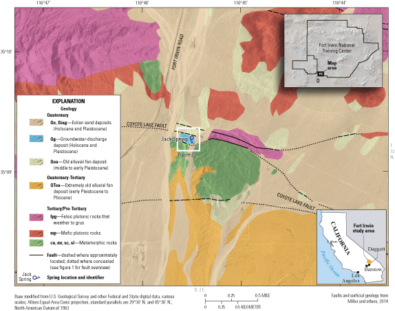
Generalized geology, faults, and location of Jack Spring study area, Fort Irwin National Training Center, California.
The washes that bound Jack Spring drain surface flows from the low hills that separate Irwin subbasin, to the north, from Coyote Lake Valley to the south, where Coyote Lake (dry) playa is located (fig. 2). The plutonic and metamorphic (schistose) rocks weather into coarse-grained alluvial deposits. Several faults cross this area and are likely splays of the Coyote Lake Fault (figs. 22, 23). Jack Spring appears as three separate seeps defined as east, middle, and west by areas of vegetation that are within about 500 ft (fig. 24). In this report, the east, middle, and west seeps are referred to as “Jack Spring East,” “Jack Spring,” and “Jack Spring West,” respectively. Jack Spring East supports large trees, cattails, grasses, and small shrubs; Jack Spring supports grasses and small shrubs; and Jack Spring West is a mounded region that primarily supports grasses and some cattails (fig. 24). These three areas of extensive vegetation indicate that shallow groundwater is in this area where shallow bedrock forces and joints and fractures in the rocks provide conduits for groundwater to flow to the surface.
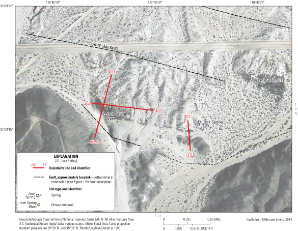
Locations of monitoring sites and resistivity surveys at Jack Spring study area, Fort Irwin Training Center, California. Abbreviations: JS1, Jack Spring; JS2, Jack Spring 2; JS2C, Jack Spring 2 Cross.
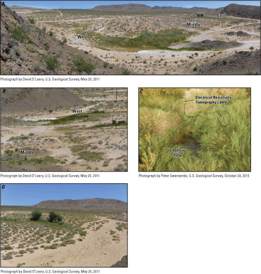
Jack Spring, Fort Irwin National Training Center, California. A, overview of the three seeps at Jack Spring, looking toward the northeast; B, overview of the middle and west seeps at Jack Spring, looking northeast; C, vegetation and an electrical resistivity tomography cable at Jack Spring; and D, vegetation around Jack Spring East, looking north.
Vegetation
Vegetation surveys were completed by NTC personnel at Jack Spring during 2013–15 and numerous plants species were identified (J. Uzzardo, Redhorse Corporation, written commun., 2013; T. Pereira, Redhorse Corporation, written commun., 2014; H. Erickson, Redhorse Corporation, written commun., 2015). The main species identified along the surveyed transects were white bursage (Ambrosia dumosa), shrubby alkaliaster (Arida carnosa), cattle saltbush (Atriplex polycarpa), sweetbush (Bebbia juncea), saltgrass (Distichlis spicata), California jointfir (Ephedra californica), alkali goldenbush (Isocoma acradenia), toad rush (Juncus bufonius), Mexican rush (Juncus mexicanus), Fremont’s cottonwood (Populus fremontii), annual rabbitsfoot grass (Polypogon monspeliensis) and cattail (Typha latifolia). Grasses and cattails predominantly grow in the west and middle seeps of Jack Spring, whereas the larger trees and bushes, primarily cottonwoods and cattails, grow along Jack Spring East (fig. 24).
Location of Hydrological and Resistivity Surveys
Hydrological data were collected at three sites at Jack Spring (fig. 23; table 1). The three sites were in each separate area of seepage to assess the variability in groundwater flow and are identified as Jack Spring West, Jack Spring, and Jack Spring East. Jack Spring (fig. 23) has a shallow open hole, presumably hand dug (fig. 24C). Jack Spring West and Jack Spring East are drive points installed in the west and east seeps, respectively (fig. 24), and are described in detail in the “Characterization Methods: Geophysical, Hydrological, and Water Quality” section. Hydrological data were collected at Jack Spring West and Jack Spring East, which were instrumented with temperature and water-level loggers (table 1). Three ERT surveys were completed to provide a subsurface resistivity profile of the seeps: two on the western seep (one subparallel and one perpendicular to the fault trends, identified as Jack Spring 2 [JS2] and Jack Spring 2 Cross [JS2C]); and one on the middle seep perpendicular to the fault trends (Jack Spring 1 [JS1]; fig. 23).
Evaluation of Springs
Geophysical, hydrological, and water-quality data were collected during 2015–17 to characterize the springs. These data provide a baseline of current groundwater conditions at springs and seeps with diffuse discharge at the NTC. These findings are presented in the next section.
Geophysics (Electrical Resistivity Tomography)
In this study, ERT surveys were completed at Garlic, Bitter, and Jack Springs (figs. 17, 20, 23) in 2015 and 2017 to image the subsurface structure of these springs and review the potential changes in subsurface water saturation or water quality. The data from these surveys are available online (Thayer and others, 2018).
Apparent Resistivity Analysis
Comparison of ERT data between fall 2015 and spring 2017 surveys allowed for investigating the change in subsurface resistivity at Garlic, Bitter, and Jack Springs during this 2-year interval. Trends were assessed in the raw ρa data by comparing measurements at identical electrode combinations collected in 2015 and repeated in 2017. If the electrodes were in the same location during the 2015 and 2017 surveys (which was not possible in all cases, as discussed later), this comparison provided a first-order assessment of how the physical properties changed. For example, for each measurement in 2017, the measured parcel of the subsurface was compared with the corresponding measurement from 2015 to determine if it became drier (more resistive) or wetter (less resistive) during the 2-year interval.
Variations in the change in apparent resistivity (Δρa) between 2015 and 2017 with electrode spacing factor for each spring were compared. As the electrode spacing factor increases, the distance between electrodes is increased. The electrode spacing factor roughly correlates with depth of investigation and was calculated for each measurement configuration of four electrodes, according to the following equation for a dipole-dipole array (Loke, 2004).For current electrodes pair C1, C2 and potential electrodes pair P1, P2:
When comparing Δρa and electrode spacing factor, two patterns were evident (fig. 25). In the first pattern, Δρa was unrelated with the electrode spacing factor, indicating that the apparent resistivity differences between datasets were not depth dependent and may be more likely to result from measurement sensitivity and different electrode placements between surveys than changes in subsurface properties. In the other pattern, Δρa was highest at low electrode spacing factor (measurements closer to the surface), supporting a depth-dependent change in subsurface resistivity between survey dates. Based on this analysis, the measurements at Garlic Spring (GS) were not likely sensitive to changes in physical properties near the surface; the measurements at Bitter Spring (BS) were likely sensitive to changes in physical properties near the surface. It is suspected that resistivity survey line position differences between the 2015 and 2017 resistivity surveys at Jack Spring 1 do not permit one-to-one measurement comparisons, so the Δρa at Jack Spring 1 was not used. The Jack Spring 2 (JS2) resistivity profile at Jack Spring West was not likely sensitive to shallow, near-surface changes, although more variability in ρa was associated with a higher electrode spacing factor and therefore deeper measurements.
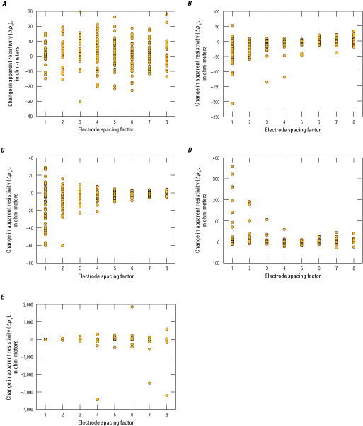
Comparison of change in apparent resistivity (Δρa) and electrode spacing factor between 2015 and 2017 electrical resistivity tomography surveys at A, Garlic Spring (GS); B, Bitter Spring 1 (BS1); C, Bitter Spring 2 (BS2); D, Jack Spring 1 (JS1); and E, Jack Spring 2 (JS2), Fort Irwin National Training Center, California (Thayer and others, 2018).
These analyses indicate that between 2015 and 2017, the following conclusions regarding physical properties at the three surveyed springs could be made: (1) there was little change at Garlic Spring in physical properties, (2) there was a change at Bitter Spring toward higher conductivity near the surface (wetter), (3) there was little change in near-surface physical properties at Jack Spring West (JS2), and (4) the analysis at Jack Spring was unclear due to uncertainty in resistivity survey line position (see the “Electrical Resistivity Tomography Model Analysis” section). Overall, these ERT data indicated relatively constant saturation and water quality at Garlic and Jack Springs. Although discharge at Bitter Spring also was relatively constant based on the historical presence of vegetation, the ERT data were representative of changes in saturation in a losing reach of the wash, downstream from the main source of spring discharge, with 2017 being wetter than 2015. Although precipitation data were not available for Bitter Spring, the changes seen at Bitter Spring were consistent with recharge from surface flow in the wash and a wet period between ERT surveys when rainfall was measured during November 2015–March 2017 (total of 9.57 in. and 6.43 in. in Goldstone Valley and Irwin subbasins, respectively; David Housman, U.S. Army, written commun., 2019).
Electrical Resistivity Tomography Model Analysis
Figures 26–32 show results of the 2015 and 2017 ERT surveys at Garlic, Bitter, and Jack Springs. The resistivity scale, in ohm-meters, shows more resistive (less conductive) material as red and less resistive (more conductive) material as blue. All models were masked at the estimated DOI.
Garlic Spring
At Garlic Spring, the 2015 and 2017 ERT model comparisons (2017 resistivity–2015 resistivity; figs. 26A, 26B) showed larger inverted resistivity differences than the apparent resistivity analysis indicated, although both model and apparent resistivity comparisons indicated a lack of clear depth dependent change. The 2015 and 2017 models generally resolve the same geometry of the resistivity structure, and differences primarily are attributed to higher relative contrasts in the 2017 models, possibly resulting from model non-uniqueness in independent inversions in a complex, faulted geologic setting. However, discharge measurements of Garlic Spring taken in December 2015 and March 2016 (Mesmer and others, 2024) indicate that spring discharge may be higher in spring than in fall, which could support the interpretation that the more conductive areas in the 2017 ERT model results may indicate higher water content.
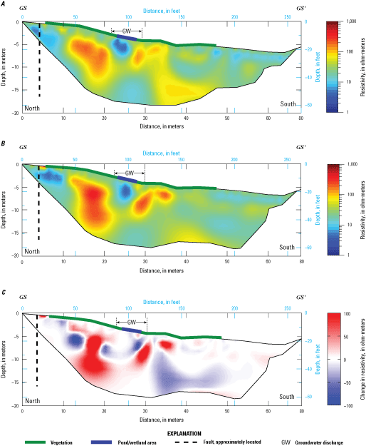
Electrical resistivity tomography surveys at Garlic Spring (GS) in A, 2015 (GS 2015); B, 2017 (GS 2017); and C, differences in resistivity between 2015 and 2017 surveys, Fort Irwin National Training Center, California (location of surveys shown on fig. 17; Thayer and others, 2018).
The ERT models showed two shallow conductive bodies (1–8 ohm-m; indicated by the darker blue areas) near Garlic Spring (figs. 26A, 26B). One conductive body lies just beneath the surface at the location of a shallow pond and wetland area (at about 82 ft), and one lies beneath the surface at the uphill end of the vegetated area (at about 5 m; figs. 26A, 26B). Both conductive bodies were bordered by highly resistive bodies (200–1000 ohm-m) representing low-permeability bedrock (figs. 26A, 26B). In 2017, an additional long profile was collected to include the mapped fault in the resistivity profile (fig. 27A). The long resistivity profile confirmed that the uphill conductive region coincides with the location of the Garlic Spring Fault. Together, the position of the conductive bodies relative to the Garlic Spring Fault, the pond and wetland, and the vegetated area strongly indicated these bodies are higher-porosity saturated zones or fault splays and serve as conduits for groundwater feeding this spring, whereas the highly resistive bodies bordering the fault splays are blocks of lower porosity, lower water-content bedrock.
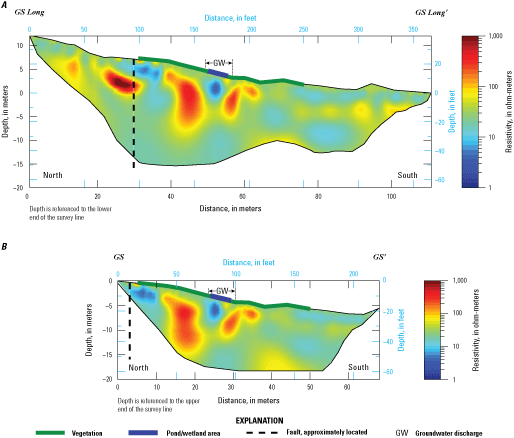
Electrical resistivity tomography surveys at Garlic Spring (GS) A, 2017 long resistivity line (GS long 2017); and B, 2017 original survey line (GS 2017), Fort Irwin National Training Center, California (location of surveys shown on fig. 17; Thayer and others, 2018).
Bitter Spring
At the two resistivity profiles downstream from Bitter Spring (figs. 28A, 28B, 29A, 29B), the ERT model comparison showed clear resistivity changes in the upper 0–9 ft in the wash. Model subtractions of 2015 and 2017 data at Bitter Spring 1 and 2 resistivity profiles (figs. 28C, 29C) showed a negative change in resistivity (more conductive, indicating wetter) in much of the upper 6–9 ft, with smaller areas showing a positive change in resistivity (more resistive, indicating drier). In both resistivity profiles, the larger, negative changes were measured in the most resistive regions of the resistivity profile, which correlate to sandy areas on the surface in the wash. These results were supported by the apparent resistivity patterns—apparent resistivity data became generally more conductive (less resistive) between 2015 and 2017 and Δρa was most strongly negative at small electrode spacing (figs. 25B, 25C), indicating the largest changes near the surface. These data indicate that much of the upper 0–9 ft of sandy material along the wash was wetter or more saline during the 2017 survey.
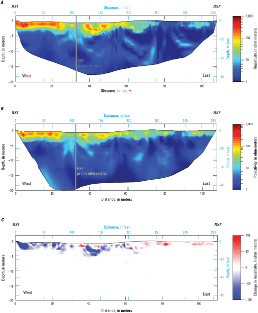
Electrical resistivity tomography surveys at Bitter Spring 1 (BS1) in A, 2015 (BS1 2015); B, 2017 (BS1 2017); and C, differences in resistivity between 2015 and 2017 surveys, Fort Irwin National Training Center, California (location of surveys shown on fig. 20; Thayer and others, 2018).
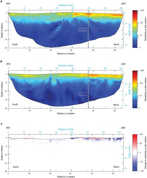
Electrical resistivity tomography surveys of Bitter Spring 2 (BS2) in A, 2015 (BS2 2015); B, 2017 (BS2 2017); and C, differences in resistivity between 2015 and 2017 surveys Fort Irwin National Training Center, California (location of surveys shown on fig. 20; Thayer and others, 2018).
The subsurface beneath the Bitter Spring resistivity lines was a relatively simple 2-layer structure, with a moderately resistive layer (20–1,000 ohm-m), at approximately 9–15 ft depth, likely representing wash deposits sitting on top of a generally homogeneous, highly conductive region (1–8 ohm-m), presumably associated with the clay layer observed in the northern wall of the wash at Bitter Spring (see “Bitter Spring” subsection in the “Description of Study Areas” section). As previously stated, Bitter Spring was formed by groundwater draining from the Cronise Valley groundwater basin being forced to the surface by the Bicycle Lake Fault Zone and above the tight clay. The high conductivity of the deeper subsurface here could be attributed to elevated groundwater or soil salinity at depth, which is consistent with the relatively high TDS concentrations (greater than 3,000 milligrams per liter [mg/L]) measured in Bitter Spring (see the “Water Quality” section). The low resistivity values seen in the ERT models generally are inconsistent with dry, non-saline sand below 9 ft. Additional subsurface data such as borehole lithology would be helpful in determining the nature of the conductive unit at depth.
Jack Spring
Electrical resistivity tomography data were collected along three profiles at Jack Spring. The ERT surveys were numbered based on the order in which they were completed; Jack Spring 1 (JS1) was done at Jack Spring and Jack Spring 2 (JS2) and Jack Spring 2 Cross (JS2C) was done at the west seep (Jack Spring West). An ERT survey was not done at Jack Spring East.
Jack Spring 1 (JS1)
At Jack Spring 1 (JS1), ERT data strongly indicated that the electrode profiles were offset by about 16 ft between the 2015 and 2017 surveys (fig. 30). In the 2015 ERT model (fig. 30A), there was a conductive (low resistivity) vertical body at a lateral position about 125 ft that connected the conductive surface to a conductive body below 16 ft. In the 2017 model (fig. 30B), this conductive body appeared but was offset about 16 ft to the south, as was a conductive body at a lateral position of 39–52 ft. Although this is a tectonically active region, only a few small (less than magnitude 3) earthquakes were reported within a 15-mile radius during this study (U.S. Geological Survey, 2022). The magnitudes of these earthquakes were believed to not be strong enough to shift the faults and subsurface bodies 16 ft. It was more likely that the resistivity lines were offset by 16 ft. This kind of resistivity line positioning error could be caused by GPS accuracy differences between surveys or erroneous coordinates. The potential for lateral offset between profiles precluded subtracting models or direct comparisons between 2015 and 2017. Apparent resistivity patterns also were non-conclusive for the same reason.
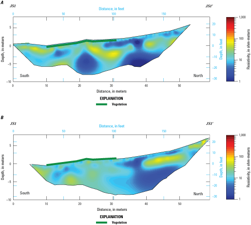
Electrical resistivity tomography surveys of Jack Spring 1 (JS1) in A, 2015 (JS1 2015); and B, 2017 (JS1 2017), Fort Irwin National Training Center, California (location of surveys shown on fig. 23; Thayer and others, 2018).
A 16-ft offset was applied to the plots for the 2015 and 2017 models so notable features matched (fig. 30). Qualitative comparison of the two models showed relatively little change in resistivity. Both models indicate a complex structure: the southern half of the model generally was a moderately resistive body (12–80 ohm-m) with a conductive body sitting from 8- to 16-ft depth at a lateral position of roughly 26–52 ft, whereas the northern half of the model showed a three-layer structure, consisting of (from shallowest to deepest) a conductive surface (1–12 ohm-m), a moderately resistive slope-parallel layer from 9- to 16-ft depth, and a conductive subsurface beneath (1–5 ohm-m). A vertical body of conductive material connects the subsurface to the surface at a lateral position about 125 ft. We hypothesize that this vertical body represents a higher porosity saturated zone, likely a fault splay, that serves as a conduit to transfer groundwater to the surface. Although there was no obvious flowing groundwater discharge along this profile immediately downhill from this feature, the presence of vegetation, primarily grasses, indicate focused spring discharge. The highly conductive body at lateral position 66–88 ft in the 2015 model was suspect because of data-quality issues.
Jack Spring 2 (JS2)
At Jack Spring 2 (JS2), 2015 ERT data were collected on a profile that followed an elevation contour across a sandy, partially vegetated mound that forms the main geomorphic feature of the spring. Groundwater discharge was visible in puddles 7–26 ft along the southern edge of the mound and south of this profile. ERT models for the 2015 and 2017 surveys (figs. 31A, 31B) showed a three-layer structure: from shallowest to deepest, a conductive (9–30 ohm-m) layer in the upper 10–13 ft, a resistive (80–800 ohm-m) layer between 13- and 33-ft depth, and a conductive layer beneath that, with the exception of a conductive (1–3 ohm-m) body at lateral position 125–164 ft. Model subtraction (fig. 31C) showed that the most pronounced differences in resistivity appeared below 9 ft between 2015 and 2017. Similar to the differences seen between ERT surveys at Garlic Springs, the 2015 and 2017 surveys showed similar resistivity geometry and could be related to inversion differences in this more complex setting. Apparent resistivity and inversion results indicated that the shallow conditions above 9 ft near the Jack Spring West seep did not notably change between surveys.
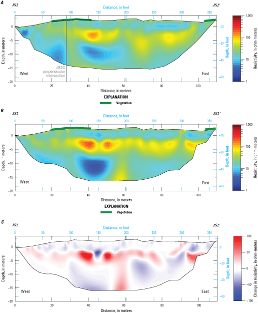
Electrical resistivity tomography surveys of Jack Spring 2 (JS2) in A, 2015 (JS2 2015); B, 2017 (JS2 2017); and C, differences in resistivity between 2015 and 2017 surveys, Fort Irwin National Training Center, California (location of surveys shown on fig. 23; Thayer and others, 2018).
The Jack Spring West seep is along a splay of the Coyote Lake Fault that runs approximately east–west through a shallow wash (fig. 23). The Jack Spring 2 resistivity profile (JS2) is parallel to the fault. To aid in understanding the three-dimensional hydrologic structure of Jack Spring West seep and how it relates to the Coyote Lake Fault, a supplemental cross profile (JS2C 2017), perpendicular to the existing resistivity profile, was created (fig. 32) to bisect the fault. The ERT model of this cross-resistivity profile (JS2C 2017) showed that the north and south sides of the Coyote Lake Fault have similar resistivity (20–90 ohm-m), whereas the surface on the hill above the spring is conductive (1–5 ohm-m), likely due to copious natural salts occurring on the hill surface. Notably, there was a conductive vertical region that coincided with the surface location of the fault and the groundwater discharge zone (fig. 32). The ERT data indicate that the fault acts as a conduit for groundwater to reach the surface. The fault geometry is unknown at depth but is hypothesized to be high-angle based on regional geology (Miller and others, 2014).
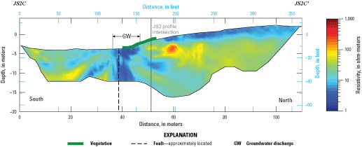
Electrical resistivity tomography survey of Jack Spring 2 Cross in 2017 (JS2C 2017), Fort Irwin National Training Center, California (location of surveys shown on fig, 23; Thayer and others, 2018).
Hydrology (Discrete Discharge, Seepage, Hydraulic Gradient, and Temperature)
Hydrological data were collected during 2015–17 to help characterize discharge at the springs at the NTC (table 1; Mesmer and others, 2024). Discrete discharge measurements and temperature data were used to assess surface flows from the springs and groundwater movement at discrete points beneath the springs. Temperature data collected at three springs (Garlic, Bitter, and Jack Springs) were used to evaluate groundwater conditions diurnally and seasonally. Discrete discharge and temperature measurements showed diurnal and seasonal variability that was consistent with the interpretation that the hydrologies of Garlic, Bitter, and Jack Springs are dominated by evapotranspiration from plants.
Discrete Measurements (Discharge and Vertical Hydraulic Gradient)
Discrete measurements from a flume, seepage meters, and a manometer provided insight into variability of flow along the reach, general rate of seepage, and vertical hydraulic gradient, respectively, at point locations at Garlic Spring East Low, Bitter Spring (Upper, Middle, Low), and Jack Spring West (table 1; Mesmer and others, 2024). These locations were chosen in areas where discharge data could be obtained but might not necessarily represent flow from the spring. Temporal variability in discharge and seepage was evaluated by taking multiple flume and seepage meter measurements, if possible. Likewise, spatial variability was evaluated by taking manometer measurements at two different locations during the same day at Bitter Spring. Generally, spring discharges (Mesmer and others, 2024) changed through time and season with surface flow, varying diurnally (for example, during the afternoon when evaporation is highest, evapotranspiration is highest) and seasonally (during the late spring when temperature and plant growth increase in contrast to during winter when temperature decreases and plants are dormant). Manometer measurements indicated upward vertical hydraulic gradients at one location at both locations at Bitter Spring.
Temperature Measurements
Subsurface temperature profiles were continuously collected at each of the instrumented spring sites from November 2015 through May 2016 (table 1; Mesmer and others, 2024). The lack of hydraulic gradient data and field estimates of vertical and lateral hydraulic conductivity at each of the instrumented sites did not allow for estimation of groundwater discharge rates using common temperature modeling techniques (Stonestrom and Constantz, 2003; Constantz, 2008); therefore, collected temperature profiles were used in a qualitative manner to infer “relative” groundwater conditions. Temperatures measured in saturated subsurface sediment at the spring sites were expected to attenuate with depth compared to the solar-driven diurnal temperature fluctuations of saturated sediment at land surface. That is, as a spring discharges to the surface, advection preserves the relatively static temperature signal of groundwater, resulting in an attenuation (damping) of temperature profiles that can be used to qualitatively infer the relative magnitude of groundwater discharge. A small diurnal variation in temperature that decreases with depth would indicate a low groundwater discharge, whereas no diurnal variation with depth would indicate a high groundwater discharge.
For each of the four instrumented sites (that is, drive points instrumented with temperature loggers), three 1-week periods were selected to depict a window of the groundwater conditions (figs. 33AD) during December 2015, February 2016, and April 2016. These periods were selected to represent the winter, early spring, and late spring seasons, respectively, and revealed that shallow preferential flow likely dominated the period of temperature collection at each of these sites. Although qualitative temperature analysis of each site was done for the period of record, only the three periods shown in each of the respective parts of figure 33 are used to depict examples of saturated conditions and variably saturated conditions during a longer time frame.
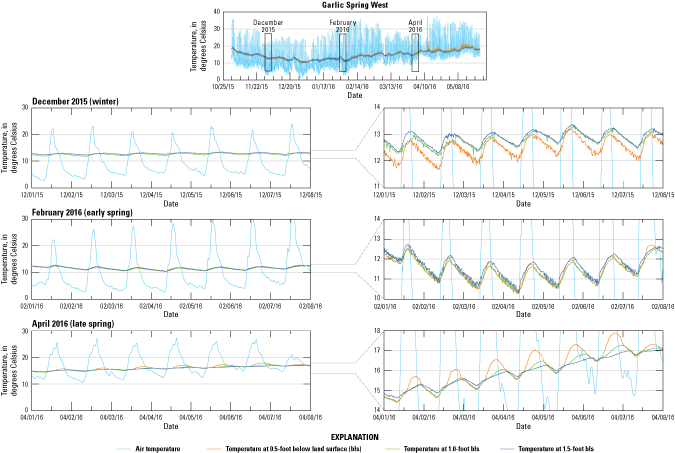
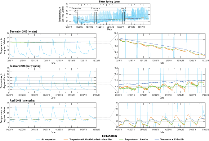
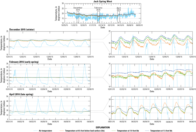
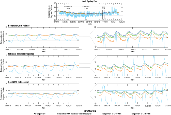
Temperature profiles for subsurface sediment at A, Garlic Spring West; B, Bitter Spring Upper; C, Jack Spring West; and D, Jack Spring East, Fort Irwin National Training Center, California, 201516 (Mesmer and others, 2024). Abbreviation: mm/dd/yy, month/day/year.
Garlic Spring
Qualitative analysis of the temperature profiles at each of the instrumented sites indicated that variably saturated conditions likely existed throughout the period of temperature profile collection rather than just during continuously saturated conditions. In this study, variably saturated conditions were defined as periods of high soil moisture but not full saturation of spring sediments at the collected depths. Overall, the temperature profiles showed that the diurnal signal dominated the temperature with depth (figs. 33A–D). The phase shift in the signal varied depending on the time of year. The temperatures in December and February showed a similar phase shift with depth, whereas temperatures in April showed a greater separation between the temperatures in the shallow logger and the temperatures in the deeper loggers when the air temperature and plant growth increased. The data indicate shallow preferential flow (that is, rapid movement of groundwater between the sensors) rather than advective upwelling zones (as evidenced by the lack of a distinct phase shift with depth in the temperature record and no damping with depth of the temperature signal; Briggs and others, 2014). We assumed that the upwelling zone of the spring sites is upgradient from or adjacent to the drive points at Garlic, Bitter, and Jack Springs and that groundwater flowed along shallow preferential flow paths and discharged in visible areas of developed vegetation (figs. 18, 21, 24). During winter 2015, for example, diffuse discharge was observed east of Garlic Spring West (fig. 17) after vegetation was cleared by the NTC personnel. The purpose of the vegetation removal was an attempt at removing invasive species. The vegetation removal revealed saturated conditions, with surface discharge happening downslope of the cleared area. A seepage meter measurement was collected at Garlic Spring (Mesmer and others, 2024) in the cleared area where water upwelled. The discharge from these clear areas was substantial but spread out over a large, diffuse area; however, by April 2016, the vegetation had grown back, and water upwelling could no longer be seen.
Water Quality
The water quality of springs at the NTC is controlled by the quality of precipitation that recharges the groundwater that feeds these springs. Water-quality samples were collected from eight springs to provide a “snapshot” of baseline groundwater quality in 2016, to augment existing historical water-quality data, and for comparison of the baseline sample with future samples, allowing tracking of changes. The water-quality conditions measured during this study are compared in this report section with water-quality data collected during 1917–2016 from springs and wells (Thompson, 1929; U.S. Geological Survey, 2017).
Major-ion Composition
The major-ion composition of the spring samples collected during 2016 was evaluated using trilinear and water-quality diagrams. Both types of diagrams provide a graphical representation of the relative contribution of major cations and anions to the total ionic content of the water (Piper, 1944; Stiff, 1951). In the trilinear diagrams (fig. 34), a percentage scale shows the cation concentrations on the upper right and lower left sides of the diamond and the anion concentrations on the upper left and lower right sides. The position of a sample on the diagram shows the major-ion composition of the water and allows comparisons to be made between different samples. Similar shaped Stiff diagrams indicate water with similar ionic composition; the overall width of the diagrams differs according to the TDS concentration. Stiff diagrams are presented on a map to facilitate comparison among sites (fig. 35).
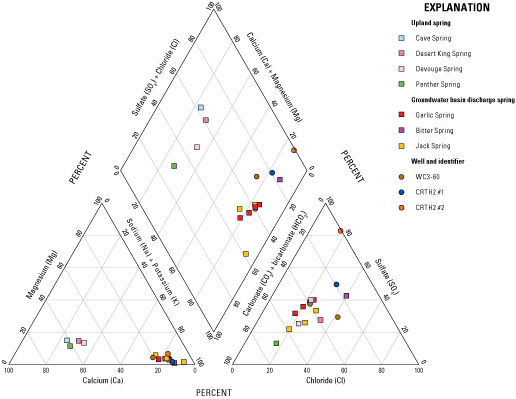
Major-ion composition of groundwater from selected springs and wells at Fort Irwin National Training Center, California. (Location of springs and wells shown on fig. 2; U.S. Geological Survey, 2017).
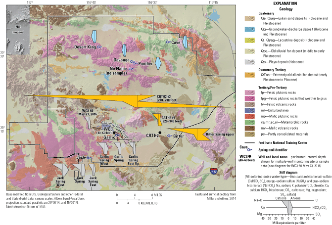
Areal distribution of water-quality diagrams of groundwater from selected springs and wells, 2014–16, Fort Irwin National Training Center, California (U.S. Geological Survey, 2017).
At the upland springs, in the northern part of the NTC, the water type of groundwater samples from Cave, Desert King, Devouge, and Panther Springs was a calcium/bicarbonate-sulfate type (figs. 34, 35), with dissolved solids ranging from 446 to 556 mg/L (U.S. Geological Survey, 2017). In contrast, at groundwater basin springs, Garlic and Jack Springs generally had sodium/bicarbonate-type waters with secondary anions of sulfate or chloride, depending on spring site location. Bitter Spring had a sodium/sulfate-type water with a secondary anion of chloride (figs. 34, 35). Total dissolved solids concentrations in Garlic and Jack Springs ranged from 584 to 1,130 mg/L (U.S. Geological Survey, 2017). The highest TDS concentration of any sampled spring, 3,340 mg/L, was in water from Bitter Spring (U.S. Geological Survey, 2017). Garlic, Jack, and Bitter Springs are in the southern part of the NTC (fig. 35) and are fed by groundwater with high TDS from nearby unconsolidated aquifers, whereas Cave, Desert King, Devouge, and Panther Springs are fed primarily by groundwater with low TDS, likely derived from local precipitation through the fractured rock in the mountains.
Thompson (1929) suggested that groundwater at Garlic Spring originates from the Bicycle Valley groundwater basin to the north; however, a comparison with water quality reported by Densmore and others (2018; fig. 11) for wells in the southern part of the Bicycle Valley groundwater basin showed that water quality in the southern part of the Bicycle Valley groundwater basin had higher sodium (greater than 200 mg/L) and lower calcium concentrations (less than 10 mg/L) than samples from Garlic Spring (sodium less than 200 mg/L and calcium greater than 24 mg/L). The water quality of the southern Bicycle Valley groundwater basin samples indicate that some part of recharge to the Bicycle Valley groundwater basin likely infiltrates from the Bicycle Lake playa. Based on ionic composition of the water-quality samples and the separation of the Irwin subbasin and Bicycle Valley groundwater basin by bedrock hills composed of plutonic, metamorphic, and volcanic rocks, it is unlikely that groundwater from the Bicycle Valley groundwater basin reaches Garlic Spring and more likely that groundwater feeding Garlic Spring originates as groundwater flow from the Irwin subbasin, flowing along the Garlic Spring Fault (fig. 16). Ionic composition of waters in samples from Garlic Spring and the nearest shallow well, WC3-60, in Irwin subbasin generally was similar, but well WC3-60 had greater chloride content (fig. 34). Since the 1980s, treated wastewater has been disposed in ponds near well WC3-60 where it infiltrates into the groundwater system, resulting in rising water levels in Irwin subbasin, particularly in the southeastern part of Irwin subbasin (Densmore and Londquist, 1997; Voronin and others, 2013). The water-level elevation measured on May 26, 2016, in shallow well WC3-60 (USGS station 351416116392203; perforated interval 40–60 ft bls), was 2,322.16 ft above NAVD 88 (U.S. Geological Survey, 2017), whereas the water level measured on December 8, 2016, in the drive point, Garlic Spring West (USGS station 351347116383001; fig. 17), was at land surface (2,302 ft above NAVD 88). The groundwater elevations in wells in Bicycle Valley, about 3-miles away, were about 2,220 ft above NAVD 88 (U.S. Geological Survey, 2017), which was lower than Garlic Spring. Additionally, aerial imagery of Garlic Spring for 1995 and 2014 (U.S Geological Survey National Aerial Photography Program, September 30, 1995; U.S. Department of Agriculture National Agriculture Imagery Program, July 2, 2014; accessed November 15, 2016, at https://earthexplorer.usgs.gov/) show that vegetation at Garlic Spring expanded during this period. Increases in vegetation and increased discharge from the spring are consistent with water level rises of 10 ft in well WC3-60 (U.S. Geological Survey, 2017) associated with treated wastewater discharge in the Langford Valley-Irwin subbasin 1 mile upgradient (Voronin and others, 2013). Additional evidence is discussed in the “Tritium and Carbon-14” section.
Water at Jack Spring discharges from low hills that separate Irwin subbasin from Coyote Lake Valley groundwater basin to the south (fig. 2). Waters sampled from Jack Springs generally were a sodium/bicarbonate type (figs. 34, 35). Total dissolved solids concentrations in Jack Spring samples ranged from 584 mg/L at Jack Spring East to 1,130 mg/L at Jack Spring (U.S. Geological Survey, 2017). The lower TDS concentrations in water from Jack Spring East samples in comparison with Jack Spring and Jack Spring West samples indicate groundwater and locally recharged precipitation mix in a wash adjacent to Jack Spring East that drains surface runoff from the hills south to Coyote Lake Valley groundwater basin. Further evidence of the mixing is discussed in the “Tritium and Carbon-14” section. There were not any nearby wells with water-level data available to assess groundwater-flow direction near Jack Spring East.
Water at Bitter Spring likely originates as groundwater discharge from Cronise Valley groundwater basin. Water at Bitter Spring was a sodium/sulfate type with secondary anion of chloride (figs. 34, 35) and had the highest TDS (3,340 mg/L) measured (of the springs sampled at the NTC; U.S. Geological Survey, 2017). The ionic composition of water at Bitter Spring was similar to the composition of water from upgradient wells CRTH2 #1 and CRTH2 #2 (figs. 34, 35) within Cronise Valley. Further evidence that groundwater from Cronise Valley groundwater basin is the source feeding Bitter Spring is discussed in the “Total Dissolved Solids and Chloride Concentrations” section.
Total Dissolved Solids and Chloride Concentrations
Total dissolved solids and chloride concentrations were used to further describe the areal variation in the water quality of spring discharge. Total dissolved solids commonly are used as a qualitative measure of groundwater salinity, as defined by Robinove and others (1958). In this report, groundwater salinity is defined by five ranges of TDS concentration: (1) less than 1,000 mg/L, fresh water; (2) 1,000–3,000 mg/L, slightly saline water; (3) greater than 3,000–10,000 mg/L, moderately saline water; (4) greater than 10,000–35,000 mg/L, highly saline water; and (5) greater than 35,000 mg/L, briny water. Salinity of sampled spring water ranged from fresh in upland springs (Cave, Desert King, Devouge, and Panther Springs) to slightly saline in groundwater basin springs (Jack and Garlic Springs) and moderately saline in Bitter Spring (U.S. Geological Survey, 2017).
The TDS concentrations in water samples from upland springs ranged from 446 mg/L at Devouge Spring to 556 mg/L at Desert King Spring, whereas concentrations in samples from groundwater basin springs ranged from 584 mg/L at Jack Spring East to 3,340 mg/L at Bitter Spring. The chloride concentrations in water samples from upland springs ranged from 42.5 mg/L at Panther Spring to 85.6 mg/L at Desert King Spring, whereas concentrations in samples from groundwater basin springs ranged from 69.4 mg/L at Garlic Spring to 685 mg/L at Bitter Spring (U.S. Geological Survey, 2017).
The highest TDS and chloride concentrations were measured in a sample collected from Bitter Spring. The concentrations in 2016 greatly exceeded concentrations in a sample collected from Bitter Spring in 1918 (Thompson, 1929, p. 545). The sample collected on February 26, 1918, had a TDS concentration of 1,628 mg/L (3,340 mg/L in sample collected on April 19, 2016) and a chloride concentration of 246 mg/L (385 mg/L in sample collected on April 19, 2016; U.S. Geological Survey, 2017). The moderately saline (TDS=3,340 mg/L) water discharging at Bitter Spring likely originates from buried lacustrine deposits in the Cronise Valley groundwater basin. These deposits are present in nearby multiple-well monitoring site CRTH2 (fig. 2), where the shallow well CRTH2 #2 is perforated from 270 to 290 ft bls in a 660-ft-thick clay deposit and in the Tertiary, partly consolidated clay deposits at the base of the hills bordering the wash where Bitter Spring appears (Kjos and others, 2014). Groundwater quality likely indicates remobilization of buried salts from these lacustrine deposits. The lower salinity water (TDS=3,340 mg/L) from Bitter Spring in comparison to the highly saline groundwater (TDS=13,400 mg/L in 2014) from shallow well CRTH2 #2 and slightly saline groundwater (TDS=829 mg/L in 2014) from deep well CRTH2 #1 (perforated from 920 to 940 ft bls) indicates that water discharging from Bitter Spring is a mixture of deep and shallow groundwater and a small percentage of surface water from occasional storms. The increase in TDS and chloride concentrations at Bitter Spring since 1918, indicate that in 1918, a greater proportion of shallow groundwater was mixing with deep groundwater discharging from the aquifer. Increased evaporation at the spring is another possible explanation for the increasing TDS and chloride concentrations. Further evidence of the mixture of source waters is provided in the “Stable Isotopes of Oxygen and Hydrogen” and “Tritium and Carbon-14” sections.
The lowest TDS and chloride concentrations measured in this study were in water samples from upland springs (Panther, Devouge, and Cave Springs) that are fed primarily by precipitation recharge infiltrating through the fractured rock in the mountains and not by groundwater discharge from nearby groundwater basins that interacts with unconsolidated, coarse-grained deposits interbedded with clays and salts. Although the TDS concentration in the 2016 water sample from Desert King Spring also was relatively low (556 mg/L, U.S. Geological Survey, 2017), the chloride concentration (85.6 mg/L) was slightly higher than the concentrations at the other upland springs (range=42.5–61 mg/L).
Nitrate Concentrations, Redox Status, and Nitrogen and Oxygen Isotopes of Nitrate
Nitrate plus nitrite as nitrogen (NO3+NO2 as N) concentrations were measured for most water samples collected from springs during this study. However, nitrite typically is not detected in the water samples, less than laboratory reporting levels of 0.001 mg/L or concentrations are low relative to the total concentration of nitrate plus nitrite as N (less than 5 percent; U.S. Geological Survey, 2017), so the nitrate plus nitrite as N concentrations represent nitrate concentrations and hereinafter are referred to as just “nitrate.” Nitrate concentrations in water samples collected during 2016 varied from less than the reporting level of 0.040 mg/L at Jack, Garlic, and Bitter Springs to 17.3 mg/L at Desert King Spring. Nitrate concentration in a water sample from Desert King Spring in October 1917 was reported at 8.4 mg/L (Thompson, 1929; U.S. Geological Survey, 2017110). Nitrate concentrations commonly differed at springs with multiple sample collection sites (that is, different seeps at an individual spring). For example, nitrate concentrations in samples from Jack Spring East were 9.1 and 9.6 mg/L, whereas concentrations from Jack Spring and Jack Spring West were 0.4 mg/L and less than the reporting level of 0.040 mg/L, respectively (U.S. Geological Survey, 2017).
Nitrate derived naturally from precipitation, soils, and geologic sources generally occurs in groundwater at concentrations ranging from less than 1 to 3 mg/L (Mueller and Helsel, 1996; Dwivedi and others, 2007; Dubrovsky and others, 2010; Izbicki and others, 2015). Devouge, Desert King, and Jack Spring East had at least one sample with nitrate concentrations greater than 3 mg/L; the Desert King Spring sample (17.3 mg/L) exceeded the U.S. Environmental Protection Agency (EPA) maximum contaminant level (MCL; U.S. Environmental Protection Agency, 2023) of 10 mg/L for nitrate as N. Most springs at the NTC are remote, and nitrate concentrations greater than 3 mg/L could result from animal activity, most notably wild donkeys (Equus asinus), which are not native to the Mojave Desert. At the time of this study (2016), most springs were fenced for protection from animals, including Desert King and Devouge Springs, which had nitrate concentrations as high as 17.3 and 8.6 mg/L, respectively (U.S. Geological Survey, 2017). Garlic and Bitter Springs were accessible through breaks in the fence. Jack Spring East and Jack Spring West were not fenced. Evidence of wild donkeys was present at Garlic, Bitter, and Jack Springs.
Orthophosphate as phosphorous (henceforth, orthophosphate) concentrations, when elevated, are commonly associated with animal waste but were low in 2016 and ranged from 0.01 mg/L at Jack, Garlic, and Devouge Springs to 0.14 mg/L at Panther Spring, with all samples having detectable concentrations of orthophosphate (U.S. Geological Survey, 2017). The highest orthophosphate concentration (0.14 mg/L) was in water from Panther Spring. The spring is fenced to keep donkeys out, although evidence of donkeys was present upslope of the fenced area. Nitrate concentrations were not detectable in Panther Spring.
Nitrogen in animal waste can be oxidized to ammonium and then to nitrate in the presence of dissolved oxygen and bacteria. In water, the nitrate can be reduced to nitrogen gas (dissolved but removed from the system when in contact with the atmosphere) in the absence of dissolved oxygen. For the purposes of this study, the reporting limit for dissolved oxygen was 0.2 mg/L. Except for Jack Spring, most sampled springs at the NTC contained measurable dissolved oxygen. Dissolved oxygen concentrations among other sampled springs were as low as 0.8 mg/L in Bitter Spring, but concentrations varied widely, as seen in Panther Spring where dissolved oxygen concentrations ranged from 0.4 to 7.7 mg/L in the 2016 samples. Springs are complex environments that may be oxygenated near the surface and reduced (that is, lacking dissolved oxygen) at depth, with redox conditions changing throughout the day in response to spring discharge, productivity from biogeochemical reactions within the spring, and possibly other factors. Consequently, collecting representative samples from springs and seeps with small diffuse discharges can be difficult, and individual samples may not completely characterize the complex geochemical and redox environment at small springs and seeps.
McMahon and Chapelle (2007) used iron and manganese concentrations to evaluate redox conditions within groundwater in the absence of dissolved oxygen data. In their study, iron concentrations greater than 100 µg/L and manganese concentrations greater than 50 µg/L were evidence of reducing conditions (dissolved oxygen absent) within groundwater. Although other redox processes may occur in aquifer systems, constituents diagnostic of other redox processes are not routinely measured (McMahon and others, 2009). Therefore, in this study, iron and manganese concentrations were used to determine if spring water containing dissolved oxygen may have been exposed to reducing conditions elsewhere within the spring. Spring water that has dissolved-oxygen concentrations greater than 1 mg/L but iron concentrations greater than 100 µg/L or manganese concentrations greater than 50 µg/L in one or more samples were classified as “suboxic” or as “variably oxic” if not all samples were consistent with iron and manganese reducing conditions within the spring (McMahon and Chapelle, 2007; Jurgens and others, 2009).
During this study, iron concentrations ranged from less than the laboratory reporting level (LRL) of 4.0 µg/L in Desert King Spring and Cave Spring to 1,350 µg/L in Bitter Spring; iron concentrations greater than 100 µg/L indicated reduced conditions in one or more samples from Jack Spring West, Bitter Spring, and Panther Spring. Manganese concentrations ranged from less than the LRL of 0.04 µg/L in Cave Spring to 1,240 µg/L in Panther Spring; concentrations greater than 50 µg/L indicated reduced conditions in one or more samples from Jack Spring East, Jack Spring West, Garlic Spring East, Garlic Spring West, Bitter Spring, and Panther Spring. Suboxic or variably oxic conditions were present in samples from Jack Spring East, Jack Spring West, Bitter Spring, Garlic Spring East, Garlic Spring West, and Panther Springs. Dissolved-oxygen concentrations less than 0.2 mg/L and reduced conditions relative to iron and manganese were present in water in Jack Spring. Oxic conditions were consistently present in samples from Garlic, Devouge, Desert King, and Cave Springs.
In addition to chemical constituents, water samples from selected springs also were analyzed for the delta nitrogen-15 (δ15N) in nitrate (δ15N-NO3) and the delta oxygen-18 (δ18O) in nitrate (δ18O-NO3). Although nitrogen is biogeochemically reactive and the nitrogen cycle is complex, isotopes of nitrogen and oxygen can provide insight into potential sources of nitrate and biochemical processes that may have altered nitrate chemistry and isotopic composition in the hydrologic system. Nitrate concentrations above the natural range (0–3 mg/L) and δ15N-NO3 compositions greater than about 6 parts per thousand (per mil) indicated that in some springs samples, human waste could be a potential source of nitrate (Hinkle and others, 2008), and δ15N-NO3 compositions greater than 10 per mil indicate than animal waste could be a potential source of nitrate (Kendall, 1998).
A geochemical framework model incorporating changes in nitrogen concentration and isotope composition (fig. 36A) was used to evaluate potential sources of nitrate concentrations above the natural range in some of the springs. δ15N-NO3 data were used to evaluate the environmental history of nitrogen with respect to microbially mediated denitrification and subsequent removal of nitrate. δ18O-NO3 data were used to determine whether the source of nitrate was from precipitation or if nitrate was from the microbially mediated conversion of nitrogen to ammonia in animal waste (ammonification) or from the fixation from the atmosphere by algae or vegetation (such as cattails) within a spring. The primary limitation on collection and analysis of nitrogen and oxygen isotopes of nitrate was that the sample had to have at least 0.06 mg/L of nitrate as N (Coplen and others, 2012). None of the samples had enough ammonia to analyze for the δ15N composition of ammonium (δ15N-NH4).
δ15N-NO3 values in spring water ranged from 5.8 to 20.2 per mil (Devouge and Jack Springs, respectively; U.S. Geological Survey, 2017; fig. 36). Higher δ15N-NO3 values were associated with reduced, suboxic, or variably oxic redox conditions, whereas lower values were associated with oxic conditions. Nitrate concentrations generally decreased with increasing δ15N-NO3 values (fig. 36A). The δ15N-NO3 composition of animal waste, presumably as ammonia or organic nitrogen, ranges from 0 to 35 per mil, with most values between 10 and 20 per mil (fig. 36A; Kendall, 1998). Data were not available for the δ15N-NO3 composition of donkey waste at the NTC. Groundwater samples affected by wastewater in Irwin subbasin had δ15N-NO3 values ranging from 10 to 20 per mil (Densmore and Böhlke, 2000). The range of nitrate directly measured in samples of human waste is narrow; the δ15N-NO3 value for wastewater from human sources was about 7 per mil (Hinkle and others, 2008) and generally is representative of sewage. Higher values in the Irwin subbasin likely reflect a combination of denitrification and microbially mediated changes in nitrogen isotope composition of nitrate during treatment and infiltration from ponds.
δ15N-NO3 values commonly increase during nitrification as a result of transformation of ammonia from animal waste. δ15N-NO3 values in water from Jack Spring, Jack Spring East, and Garlic Spring East, all of which had evidence of donkey activity, were within the published ranges for animal waste (Kendall, 1998). However, because of its wide range in composition, δ15N-NO3 generally is not definitively diagnostic of nitrogen sources when used alone. Additionally, water from Jack Spring, Jack Spring East, and Garlic Spring was reduced or suboxic and may have been partly denitrified, lowering nitrate concentrations and increasing δ15N-NO3 values.
Decreases in NO3 as N concentrations with increases in δ15N-NO3 values in suboxic/variably oxic or reduced spring water are consistent with denitrification. Assuming a reductive fractionation factor of α=−29.4 derived from laboratory data (Mariotti and others, 1981), denitrification trend lines were calculated that show decreases in nitrate concentrations expected as δ15N-NO3 values increased as a result of possible denitrification for selected springs (fig. 36A).
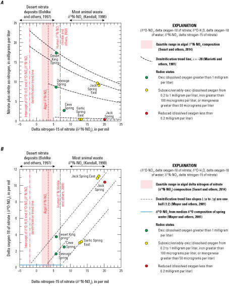
A, nitrate plus nitrite as nitrogen concentrations as a function of delta nitrogen-15 of nitrate (δ15N-NO3); and B, delta oxygen-18 of nitrate (δ18O-NO3) values as a function of δ15N-NO3 values in water from selected springs, Fort Irwin National Training Center, California, April–May 2016 (U.S. Geological Survey, 2017).
δ18O-NO3 data were used to provide additional evidence of denitrification at selected springs, evaluate the initial δ15N-NO3 composition, and evaluate the potential source of nitrate in spring water. δ18O-NO3 values in spring water ranged from 1.65 to 11.16 per mil (for Devouge and Jack Springs, respectively; U.S. Geological Survey, 2017). The two sites with the highest values of δ18O-NO3 (10.42–11.16 per mil at Jack Spring and Jack Spring East) had suboxic and reduced water; Devouge, Cave, Desert King Springs, and Garlic Spring East had lower values (1.65–3.74 per mil) and had oxic and suboxic water (fig. 36B). Denitrification happens along a trend having a slope (Δx to Δy) of 0.5 (1:2). The three lines shown on figure 36B represent potential denitrification through selected wells.
The δ18O composition of water (δ18O-H2O) in the springs ranged from −11.7 to −9.4 per mil (Garlic and Jack Springs, respectively), with a median value of −10.9 per mil. Given that during nitrification one-third of the oxygen in nitrate is contributed from dissolved oxygen within the water and two-thirds of the oxygen is contributed from hydrolysis of the water molecule (Mayer and others, 2001) and given a δ18O composition of atmospheric oxygen of 23 per mil (Mayer and others, 2001), the initial δ18O-NO3 composition set during nitrification of ammonia from animal waste would be 0.3 per mil (blue line on fig. 36B). Projecting measured δ15N-NO3 values in Jack Spring along a denitrification trend line to the calculated initial δ18O-NO3 composition (intercept of δ18O-NO3 composition set during nitrification and denitrification trend line; fig. 36B), an initial δ15N-NO3 composition of −1 per mil would be expected in Jack Spring. A value of −1 per mil is outside the literature reported range for δ15N-NO3 in most animal waste (Kendall, 1998), and the data are not consistent with an animal waste origin for nitrate; the value is consistent with nitrate from desert nitrate deposits (Böhlke and others, 1997) observed at the site. In contrast, δ15N-NO3 and δ18O-NO3 data from Garlic Spring differ from data at Jack Spring (fig. 36B). Projecting measured δ15N-NO3 values from Garlic Spring along a denitrification trend line to the calculated initial δ18O-NO3 composition (fig. 36B), the initial δ15N-NO3 composition in Garlic Spring would have been about 7 per mil. A value of 7 per mil is outside the literature reported range for δ15N-NO3 in most animal waste (Kendall, 1998) but is consistent with a human origin for nitrate (Hinkle and others, 2008) and may be associated with treated wastewater discharges in the Irwin groundwater subbasin about 0.5 miles upstream (fig. 16). Increases in flow at Garlic Spring, expansion of areal extent of vegetated area, and changes in major-ion data through time also are consistent with treated wastewater from the Irwin subbasin that may have reached Garlic Spring.
Water from Desert King, Cave, and Devouge Springs is oxic and nitrate in spring water likely has not been extensively denitrified in the same manner as water from Jack or Garlic Springs (fig. 36). Measured δ15N-NO3 values from Cave and Devouge Springs are within the range of compositions expected for nitrate fixed from algae (fig. 36B) and closely approximate the median composition from algal sources (3.4 per mil δ15N-NO3) estimated by Swart and others (2014). However, the δ15N- NO3 compositions of algae are poorly described in the literature and likely differ among species, and an algal nitrate source was not definitive for Cave and Devouge Springs because of the overlap with the range of desert nitrate deposits. Although nitrate concentrations are higher and δ15N-NO3 and δ18O-NO3 compositions differ from those in Cave and Devouge Springs, algal sources also are possible for nitrate in Desert King Spring (fig. 36). Desert King Spring is fenced to protect it from donkeys and exclude animal waste sources.
The geochemical framework model used to estimate nitrate sources and processes affecting nitrate concentrations within sampled springs is not definitive. The ranges in δ15N-NO3 isotope compositions are often broad and, in many cases, especially for nitrate from algal sources, poorly defined. Although isotope composition of atmospheric oxygen is known, possible fractionation of oxygen as it dissolves in water and reacts within the spring system were not considered in the calculations presented. However, the data indicate that sources of nitrate other than animal waste are possible in reduced water from Jack and Garlic Springs, and Desert King Spring, the spring having the highest nitrate concentrations. Interpretation of isotope data, especially δ18O-NO3 data (fig. 36B), indicate that additional management efforts intended to exclude donkeys from these springs may not yield the desired water-quality results.
Source and Age
The ratios of the stable isotopes of oxygen and hydrogen are used as tracers of the movement of the water and to understand the source and hydrologic history of water (Mazor, 1991). Likewise, the radioactive isotopes of hydrogen (tritium) and carbon (carbon-14) are used for determining the age (time since recharge or isolation from the atmosphere) of groundwater, locating sources of recharge, and identifying geologic controls on the movement of groundwater (Mazor, 1991). In this study, δ18O, δD, 3H, and 14C were analyzed in water samples from seven springs to help determine the source, movement, and apparent age, or time since recharge, of water at these springs (U.S. Geological Survey, 2017). As stated in the “Description of Study Areas” section, the springs are divided into upland springs (“mountain springs”), which include fissure-controlled features (Cave, Desert King, Panther, and No Name Springs) or likely porous fractured rock overlying an impervious rock (Devouge Spring) and groundwater basin springs, which also include fault-controlled features and impervious rock (Garlic, Bitter, and Jack Spring).
Stable Isotopes of Oxygen and Hydrogen
More negative values of δ18O and δD represent enrichment in the lighter isotopes 16O and 1H (or a depletion in the heavier isotopes 18O and D), and less negative values represent enrichment in the heavier isotope of 18O and D.
There was no further change in isotopic composition at low temperatures of most groundwater systems at Fort Irwin after recharged water had migrated below the depth of evaporation. If groundwater flows to a depth where geothermal heat has raised water temperatures sufficiently, isotopic exchange between the oxygen isotopes in water and the large reservoir of oxygen in rocks is possible, complicating the interpretation of 18O isotopes in samples. However, this process does not appear to affect the isotopic composition of the spring samples (Smith and others, 2002). Therefore, any subsequent differences in the isotopic composition of groundwater along a flow path between the points of recharge and discharge generally reflect mixing within the aquifer system or concentration by evaporation. As a consequence, the δ18O and δD composition of groundwater relative to the global meteoric water line (Craig, 1961) and the isotopic composition of other potential source waters can be an indicator of the source of groundwater to the sampled springs.
The δ18O and δD composition of 28 groundwater samples from 7 springs at the NTC ranged from −9.37 to −11.88 per mil and from −79.3 to −95.5 per mil, respectively (fig. 37A). The isotopic data of spring samples plotted to the right of the global meteoric water line (Craig, 1961) and indicated possible partial evaporation during precipitation (before recharge), possible evaporation at or below land surface before recharge or at the spring discharge location, or a “local” meteoric water line that is sub-parallel to and differs slightly from the global meteoric water line. The isotopic compositions of groundwater from sampled wells in the Irwin subbasin (Densmore and Londquist, 1997), representing groundwater samples with an evaporated signature, were plotted for comparison (fig. 37A). A volume-weighted sample of averaged desert winter precipitation (Izbicki, 2004), representing modern-day (2004) precipitation in the western Mojave Desert, plotted near the global meteoric water line (fig. 37A). A volume-weighted sample of local precipitation at Daggett, California (fig. 1; Friedman and others, 1992), plotted to the right of the global meteoric water line and to the upper right of the spring samples (fig. 37A). The Daggett sample, representing the isotopic composition of precipitation collected during summer 1985 through winter 1987, was notably different from the weighted average composition for winter precipitation in the Mojave Desert. A sample of local precipitation at Goldstone weather station (fig. 1), plotted to the right of the spring samples and evaporated groundwater (fig. 37A). The variation in isotopic compositions in the precipitation samples illustrate the seasonal variability of the isotopic composition of precipitation. More recent precipitation samples were not available for comparison.
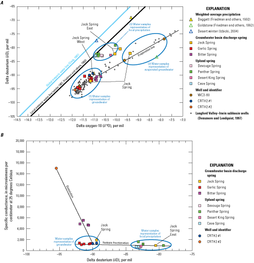
A, relation between stable isotopes of oxygen and hydrogen in water for samples from seven springs and selected wells in Cronise Valley groundwater basin and Langford Valley-Irwin subbasin, along with volume-weighted average samples of precipitation from nearby sites; and B, relation between specific conductance and delta deuterium (δD) in water for samples from seven springs and selected wells, Fort Irwin National Training Center, California (U.S. Geological Survey, 2017).
The water samples from the springs plotted into three main groups (circled and numbered on fig. 37A): (1) water samples with lighter isotopic composition (more negative), representative of groundwater inflow from nearby groundwater basins; (2) water samples with heavier isotopic composition (more positive), representative of evaporated groundwater that plots along an evaporation trend line; and (3) water samples that represent young spring discharge that was recharged from local precipitation (fig. 37A). Water samples from Garlic and Bitter Springs and Jack Spring West plotted among group 1, which was consistent with a groundwater source in nearby unconsolidated deposits. Water samples from most wells in Irwin subbasin are isotopically light and plotted among group 1. Water samples from wells affected by artificial recharge from wastewater and irrigation-return flow (Densmore and Londquist, 1997) that have undergone evaporation were isotopically heavier and plotted in group 2. A water sample from Jack Spring, also groundwater sourced, plotted along an evaporation line representing group 2 from the middle site and group 3 from the east site. The water samples from Jack Spring East were a mixture of evaporated basin groundwater (evaporation line) and local precipitation (local meteoric water line). Water samples from Cave, Desert King, Devouge, and Panther Springs plotted among group 3, which was consistent with a local precipitation source. Overall, the δ18O and δD data show the isotopic compositions in upland springs were consistent with recharge from winter precipitation, and compositions in groundwater basin springs were consistent with groundwater sampled from nearby wells. Summer precipitation from monsoonal storms often flowed away quickly overland and seemed to contribute little water to discharge at the springs.
Water samples from Bitter Spring were isotopically light, plotted with groundwater samples, and were isotopically similar to water from deep well CRTH2 #2 at multiple-well monitoring site CRTH2 (fig. 37). The relation between specific conductance (as a surrogate for TDS) and δD has been used to determine if dissolution of soluble minerals or concentration by partial evaporation is the predominant cause of increased salinity in groundwater (Densmore and Londquist, 1997). If evaporation is the only process concentrating salinity, δD should increase more rapidly than with increasing specific conductance. If dissolution of evaporites is the only process increasing salinity, δD will not change as salinity increases along a mixing trend. If dissolution of evaporites is the dominant process increasing salinity, δD increases less rapidly than it does with evaporation and δD and specific conductance would not be strongly correlated. Comparison of specific conductance and δD indicated that water from Bitter Spring had higher specific conductance relative to δD than water from the deep well CRTH2 #1 and lower specific conductance relative to δD than water from shallow well CRTH2 #2 (fig. 37B). This difference is consistent with a mixture of water from shallow well CRTH2 #2 and deeper well CRTH2 #1. However, the mixture of shallow and deep groundwater discharging at Bitter Spring alone does not explain the complex story of the sources feeding discharge at Bitter Spring. Further evidence is provided in the “Tritium and Carbon-14” section.
Tritium and Carbon-14
The radioactive isotopes of hydrogen (tritium) and carbon (carbon-14 or 14C) were used to determine the age (time since recharge) of groundwater, locate sources of recharge, and identify geologic controls on the movement of groundwater that discharges at sampled springs. Tritium and 14C can be used to help determine the age and movement of groundwater discharging to these springs (that is, older and younger springs), which can provide insight into sustainability of the springs. Older groundwater at springs typically is related to regional groundwater flow systems; whereas younger groundwater at springs typically is locally recharged groundwater and can be more sensitive to long-term dry conditions. In general, all spring discharges measured during 2015–16 were less than spring discharges reported by Thompson (1929).
Tritium is a naturally occurring radioactive isotope of hydrogen with a half-life of 12.3 years (Lucas and Unterweger, 2000). The concentration of tritium typically is reported in tritium units (TU). About 760 pounds of tritium was released into the atmosphere between 1952 and 1962 because of the atmospheric testing of nuclear weapons, with atmospheric concentrations of tritium reaching a maximum of more than 1,000 TU in 1963–64 (Michel, 1976). As a result, tritium concentrations in precipitation and groundwater recharge increased during 1963–64. Tritium concentrations are not affected by chemical reactions other than radioactive decay because tritium is part of the water molecule. The process of radioactive decay means tritium can be used to trace the movement and relative age of water to about 70 years before present (pre-1952).
Tritium concentrations in modern-day (2012) precipitation in the part of the Mojave Desert that includes the NTC are about 5 TU (Eastoe and others, 2012). In this report, groundwater samples with 3H concentrations less than the detection limit of 0.20 TU were interpreted as water recharged before 1952, and groundwater samples with greater concentrations (measurable 3H) were interpreted as waters recharged after 1952, or recent recharge. Eastoe and others (2012) predict the threshold of ambiguity for using tritium alone as a tool for mapping aquifer recharge will occur between 2025 and 2030.
Carbon-14 is a naturally occurring radioactive isotope of carbon that has a half-life of about 5,730 years (Mook, 1980). Carbon-14 data are expressed as percent modern carbon (pmC) by comparing 14C activities to the specific activity of National Bureau of Standards oxalic acid: 13.56 disintegrations per minute per gram of carbon in the year 1950 equals 100 pmC (Kalin, 2000). Carbon-14 above natural levels was produced, as was tritium, by the atmospheric testing of nuclear weapons (Mook, 1980), and as a result, 14C activities may exceed 100 pmC in areas where groundwater contains tritium. Carbon-14 activities are used to determine the age of a groundwater sample on timescales ranging from recent to more than 20,000 years before present. Carbon-14 is not part of the water molecule; therefore, 14C activities in groundwater may be affected by chemical reactions that remove or add carbon to solution or by mixing of younger groundwater that has high 14C activity with older groundwater that has low 14C activity. Izbicki and Michel (2004) reported an initial 14C activity of 85 pmC for groundwaters in the Mojave Desert region before atmospheric testing of nuclear weapons.
Carbon-14 ages presented in this report did not account for changes in 14C activities resulting from chemical reactions that remove or add carbon to solution or mixing and, therefore, were considered uncorrected (or apparent) ages. These ages were interpolated and not individually calculated. In general, uncorrected 14C ages were older than the actual age of the associated water due to mixing with radiocarbon “dead” dissolved inorganic carbon. Izbicki and others (1995) estimated that uncorrected 14C ages were as much as 30-percent older than the actual ages of groundwater in the regional aquifer in the Mojave River groundwater basin near Victorville, California (not shown), which is about 60-mi southwest of the study area. In this report, groundwater samples from wells or springs with 14C activities less than 85 pmC were interpreted as being recharged before 1952, whereas samples with 14C activities greater than 85 pmC were interpreted as being recharged after 1952 (Izbicki and Michel, 2004).
Tritium concentrations in 10 water samples from 6 springs (and associated spring sites) ranged from less than 0.20 (Cave, Devouge, and Panther Springs; Garlic Spring and Garlic Spring East; Jack Spring) to 0.44 TU (Jack Spring East; fig. 38; U.S. Geological Survey, 2017). Tritium concentrations less than 0.20 TU indicated that water discharging at these spring sites (Cave, Devouge, and Panther Springs and the east sites at Garlic Spring) was recharged before 1952, and greater concentrations (Garlic Spring West, Bitter Spring, Jack Spring East, and Jack Spring West) indicated that water discharging at these spring sites was (or had some part) recharged since the early 1950s. Measurable 3H (0.2 TU or greater) in water from Garlic Spring West and increased discharge at Garlic Spring (based on aerial imagery and major-ion data previously described) indicated that discharges of treated wastewater from the Irwin subbasin along the Garlic Spring Fault may have reached Garlic Spring West. Measurable 3H (0.2 TU or greater) in water from Bitter Spring and Jack Spring East and West indicated younger groundwater (likely originating as surface-water runoff from intermittent storms in nearby washes) could be mixed with primarily older groundwater flowing and ultimately discharging to these springs (based on 14C data discussed later in the text). During an extended dry period, there may not be surface-water runoff, and the discharge from Bitter and Jack Springs could decrease.
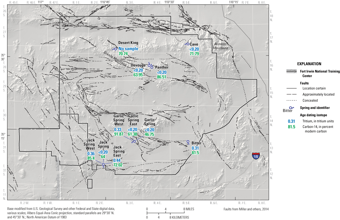
Locations of tritium concentrations and carbon-14 activities in samples from selected springs, 2016–17, at Fort Irwin National Training Center, California (U.S. Geological Survey, 2017). Abbreviation: >, greater than
Uncorrected 14C data indicated the waters of these springs had apparent ages of about 700–6,300 years old and were much younger in comparison to apparent ages of about 12,000–40,000 years for groundwater sampled in nearby groundwater basins (Densmore and Londquist, 1997; Voronin and others, 2013; Densmore and others, 2018). Measured 14C activities in water samples from sampling points at the seven springs studied ranged from 46.75 pmC at Garlic Spring to 91.87 pmC at Garlic Spring West drive point (fig. 38; table 1; U.S. Geological Survey, 2017). The highest 14C activity (91.87 pmC) was measured in water from Garlic Spring West, at the western end of the series of seeps along the Garlic Spring Fault (fig. 17) and nearest to well WC3-60 at the southeastern-most end of the ponds where treated wastewater infiltrates in Irwin subbasin (fig. 16). The uncorrected 14C data indicated that groundwater at Garlic Spring West and well WC3-60 was about 700 years old. Conversely, the lowest 14C activity (46.75 pmC) was measured in water from Garlic Spring, at the eastern end of the seeps, where the uncorrected 14C data indicated that groundwater in this site was about 6,276 years old. Carbon-14 activities in water samples from all other springs were between these outliers.
Measured 14C activities in water samples from upland springs (Cave, Desert King, Devouge, and Panther Springs) ranged from 63.95 and 86.51 pmC (fig. 38). The 14C data (unadjusted from reactions with aquifer material) indicated that water at these springs were from about 3,700 to 1,200 years old. Water from Cave, Devouge, and Panther Springs did not contain measurable 3H (3H data were not available for Desert King Spring). Water from Panther Spring had a 14C activity of greater than 85 pmC, indicating it may contain recent water, even though there was no measurable tritium present in the sample. Thus, water from Panther Spring was interpreted to be a mixture of water from the fractured bedrock at the spring and local precipitation, with each source containing different 3H and 14C concentrations.
Water from Garlic Spring, with the highest and lowest 14C activities (91.87 and 46.75 pmC) of any sampled spring sites, had corresponding tritium concentrations of 0.33 and less than 0.20 TU in the western- and the eastern-most samples, respectively (fig. 38). These 14C activities (unadjusted for reactions with aquifer material) indicated that water from these two Garlic Spring sites was about 6,300 and 700 years old (46.75 and 91.87 pmC, respectively). The 14C activity (91.87 pmC) measured at Garlic Spring West, at an activity greater than 85 pmC, combined with measurable tritium (0.33 TU), indicated that water at the western edge of Garlic Spring contained a higher fraction of young water than the other seeps; however, a 14C activity (61.38 pmC) of less than 85 pmC measured at Garlic Spring East, combined with no measurable tritium, indicated that groundwater at the eastern edge of Garlic Spring was older. Water from Garlic Spring West was a mixture of water from wastewater-infiltration ponds in Irwin subbasin (based on 14C activities in water from well WC3-60 at the southeastern-most end of the ponds) and old groundwater, with each containing different 3H concentrations and 14C activities. These 14C data provide further support that Garlic Spring Fault acts, in part, as a conduit for groundwater flow. The fact that splays of the Garlic Spring Fault are bordered by blocks of nonporous bedrock, with splay geometries controlled by the architecture of the fault, supports the interpretation of the observed differences in 3H concentrations and 14C activities.
Water from Bitter Spring had a 14C activity of 81.5 pmC and a 3H concentration of 0.31 TU (fig. 38). The 14C activity (unadjusted for reactions with aquifer material) indicated that water at this spring was less than 1,700 years old. Based on stable isotope data and TDS concentrations (previously described), water from Bitter Spring was a mixture of shallow and deep groundwater. Water from this spring also had measurable tritium (0.31 TU) and a relatively large 14C activity (81.5 pmC), indicating some percentage of recent recharge. Shallow and deep groundwater sampled from monitoring wells at multiple-well monitoring site CRTH2 did not contain measurable tritium (less than 0.2 TU) and had very low 14C (7.87 and 9.87 pmC), indicating old water. As previously described in the “Stable Isotopes of Oxygen and Hydrogen” section, a mixture of shallow and deep groundwater discharges at Bitter Spring. Thus, water at Bitter Spring may have contained some recent, focused recharge of surface-water runoff from intermittent storms based on the tritium and 14C data.
Water from the three seeps at Jack Spring had 14C activities ranging from 64 to 85.4 pmC and tritium concentrations ranging from less than 0.20 to 0.44 TU (fig. 38). These 14C activities (unadjusted for reactions with aquifer material) indicated that waters from these seeps were about 3,700–1,400 years old; based on 14C activities and tritium concentrations, the youngest water was at the west and east seeps, which lie along dry washes draining the nearby granitic hills (figs. 22, 23). Like Garlic Spring, water from the west and east seeps was a mixture of water from the fractured bedrock moving along the Coyote Lake Fault and recent, focused recharge by surface-water runoff from intermittent storms. These data supported the interpretation that Coyote Lake Fault also acts as a conduit for groundwater flow. Water from Jack Spring was representative of water discharging primarily from the fractured bedrock that had the least mixing with recent recharge.
Overall, most springs contained little detectable tritium (0.2 TU or greater) and appeared to be primarily older groundwater. The relatively high 14C activities and the variability in measurable 3H indicated that some of these springs have received some percentage of their water from recent recharge with measurable 3H sufficient to be detected in the groundwater samples collected for this study. Tritium was detected at concentrations greater than the study reporting level (0.2 TU or greater) in groundwater basin springs, which could be a result of occasional surface-water runoff from infrequent storms in nearby washes near the springs (Bitter and Jack Spring East and West) or from recharged wastewater (Garlic Spring). These groundwater basin springs may be susceptible to decreases in discharge during extended dry periods due to the loss of focused recharge through nearby washes near the springs. These data also indicated that some recharge since 1952 was present in shallower parts of the groundwater system, along faults, and where groundwater mixes with storm water runoff along washes, specifically at Bitter Spring, Garlic Spring West, and Jack Spring East and West. Recharge of local precipitation through the fractured bedrock in upland springs at Cave, Desert King, and Devouge Springs happened within the last several thousand years. Recharge of local precipitation in the fractured bedrock in the mountains at Panther Spring happened more recently (less than 1,000 years ago), but before 1952, where ages based on 14C data indicate water is younger but lacks measurable 3H.
The sampled springs may be sensitive to future groundwater development and pumping of nearby existing production wells (fig. 1). The groundwater basin springs are especially sensitive to water-level declines in nearby groundwater basins from which they are fed. The upland springs also may be sensitive to pumping if they are hydraulically connected to nearby groundwater basins. Data were not collected to assess hydraulic connections between springs at the NTC and nearby groundwater basins as part of this study because there were few wells in the nearby groundwater basins; the exception was hydraulic data from wells in Irwin subbasin near Garlic Spring and in Cronise Valley groundwater basin near Bitter Spring.
Constituents of Concern
Constituents of concern are any physical, chemical, biological, or radiological substance in any environmental media that could be dangerous to human or ecological health. Some water-quality constituents are of concern to water managers because of the likelihood they may exceed water-quality criteria such as human-health-based benchmarks (California State Water Resources Control Board, 2022). Constituents of concern can have natural and anthropogenic sources and include inorganic trace elements and other, mostly organic, constituents from anthropogenic sources. Constituents of concern are summarized in this section and those that were detected are listed by spring site in table 4.
Table 4.
Summary of anthropogenic constituents of concern detected during 2015–17 in selected springs, Fort Irwin National Training Center, California (U.S. Geological Survey, 2017).[—Left][The five-digit number in parentheses below the constituent name is the U.S. Geological Survey (USGS) parameter code used to uniquely identify a specific constituent or property. For the complete list of constituents analyzed, see appendix 2. Benchmark standard: Maximum contaminant level benchmarks are listed as MCL-US when the MCL-US and MCL-CA are identical, and as MCL-CA when the MCL-CA is lower than the MCL-US or no MCL-US exists. Abbreviations: MCL-US, U.S. Environmental Protection Agency (2023) maximum contaminant level; MCL-CA; California State Water Resources Control Board (2022) maximum contaminant level. Other abbreviations: mm/dd/yy, month/day/year; hhmm, hour minute; μg/L, microgram per liter; mg/L, milligram per liter; <, less than; —, not analyzed; E, estimated value; M, presence verified but not quantified]
Trace elements and the major ion, fluoride, are of concern in groundwater in the Mojave Desert. High concentrations of arsenic and fluoride are present in many of the groundwater basins of the NTC (Densmore and Londquist, 1997; Voronin and others, 2013). These constituents tend to be in higher concentrations in fine-grained deposits and generally are associated with basin-fill deposits of alluvial-lacustrine origin, particularly in semi-arid areas or volcanic deposits (Welch and others, 1988; García and Borgnino, 2015). Arsenic, fluoride, vanadium, and uranium were detected at concentrations exceeding benchmark standards, such as MCLs (U.S. Geological Survey, 2017; California State Water Resources Control Board, 2022; U.S. Environmental Protection Agency, 2023108) in water from some of the springs sampled for this study. These trace elements usually are geogenic (naturally occurring) contaminants.
The concentrations of arsenic, fluoride, vanadium, and uranium were greater in the arid to semi-arid regions, where processes such as pH and redox (oxidation-reduction) act to varying degrees to mobilize these elements (Welch and others, 1988). Arsenic concentrations in water samples from the springs ranged from 1.0 µg/L at Cave Spring to 138 µg/L at Bitter Spring, and fluoride concentrations ranged from 0.67 mg/L at Desert King to 13 mg/L at Jack Spring (U.S. Geological Survey, 2017). Water samples from Garlic and Bitter Springs contained arsenic concentrations that exceeded the EPA MCL of 10 µg/L (U.S. Environmental Protection Agency, 2023). Water samples from all springs, except Cave, Desert King, and Devouge Springs, exceeded the State of California MCL of 2 mg/L for fluoride (California State Water Resources Control Board, 2022). Vanadium concentrations in water from the springs ranged from 0.76 µg/L at Cave Spring to 83.7 µg/L at Garlic Spring. Uranium concentrations ranged from 1.69 µg/L at Panther Spring to 78.9 µg/L at Jack Spring. Only water samples from Garlic Spring contained vanadium concentrations that exceeded the State of California notification level of 50 µg/L (California State Water Resources Control Board, 2022). Only a water sample from Jack Spring contained uranium concentrations that exceeded the U.S. Environmental Protection Agency MCL of 30 µg/L (U.S. Environmental Protection Agency, 2023).
Many other constituents of concern in groundwater at the NTC were analyzed, including those from anthropogenic sources that may be a result of military training activity. There were 181 constituents of concern analyzed in water samples collected for this study, including diesel and gasoline degradants, munitions, and industrial compounds (including selected volatile organic compounds). The constituents analyzed are listed in appendix 2. Of the 181 constituents of concern analyzed, only 15 were detected in any springs (table 4); diesel and gasoline degradants (fuel-related organics) were the most commonly detected compounds. Although usually indicative of diesel or gasoline contamination, these organic compounds are not necessarily specific to anthropogenic sources. Jack Spring had an oily sheen, which was tested by NTC personnel and determined to be naturally occurring, organic material (Justine Dishart, U.S. Army, oral commun., 2018). Panther Spring is not directly accessible by motor vehicle, so the typically fuel-related constituents detected in samples from that site (toluene, gasoline- and diesel-range organics) were more likely from natural sources and contamination from motor vehicles is unlikely to be the source. For most other springs, sources of any of these organic compounds could be fuel-related.
The constituents detected are summarized in table 4. Discussed in order of decreasing detection frequency, they were carbon disulfide (seven samples at five springs); perchlorate (six samples at five springs); mercury (five samples at five springs); acetone (four samples at four springs); 2-methylnaphthalene and toluene, (three samples at three springs); methyl ethyl ketone, cyanide, and styrene (two samples at two springs); and 4-iso-propyl-toluene, isopropylbenzene, methyl salicylate, and phenol (one sample at one spring). 2-methylnaphthalene, methyl ethyl ketone, styrene, 4-iso-propyl-toluene, isopropylbenzene, and methyl salicylate are not naturally occurring; except for methyl ethyl ketone detected at Jack Spring West and toluene at Panther Spring, most of the detections were low at or near the detection level. Jack Spring West is located off base and is accessible by motor vehicle. Panther Spring is located in a wash in a remote canyon in the live-fire area that is not accessible by motor vehicle, although there is a dirt road on the hillside east of the spring; contamination could be related to this dirt road or live-fire activities in this area.
The most constituents detected (carbon disulfide, perchlorate, mercury, acetone, methylnaphthalene, methyl ethyl ketone, cyanide, styrene, 4-iso-propyl-toluene, methyl salicylate, and phenol) were in water samples from the three sites at Garlic Spring. The presence of these contaminants was likely related to groundwater flow along Garlic Spring Fault from Irwin subbasin, as previously described (fig. 16). Perchlorate was detected in water samples from Devouge and Cave Springs. Perchlorate, although used in munitions, is naturally occurring in desert areas at the concentration ranges detected (Fram and Belitz, 2011). Cyanide concentrations, detected in water samples from Panther and Garlic Springs, exceeded the California MCL of 0.20 mg/L (California State Water Resources Control Board, 2022). All other constituents detected were at concentrations less than benchmark standards.
Summary and Conclusions
The U.S. Geological Survey has been studying water-resources issues at the U.S. Army Fort Irwin National Training Center (NTC), including the effect of groundwater development resulting from training expansion and infrastructure at the NTC (on natural springs and associated seeps). This study included evaluating discharge and water quality at eight springs and associated seeps at the NTC during 2015–17. These springs are important water sources for wildlife at the NTC. To evaluate the characteristics of springs and seeps within the NTC, geophysical surveys were completed and hydrological (discharge, vertical hydraulic gradient, and temperature measurements) and water-quality data were collected during 2015–17 to provide a baseline of groundwater conditions at selected springs.
Of the 10 springs located within the NTC, 8 springs (Cave, Desert, Devouge, Panther, No Name, Garlic, Bitter, and Jack Springs) were studied. The two springs not studied were inaccessible because of their location within a bombing and live-fire area. Studied springs were divided into two groups: upland springs, which include fissure-controlled features (Cave, Desert King, Panther, and No Name Springs) or likely porous fractured rock overlying an impervious rock (Devouge Spring) and groundwater basin springs, which also include fault-controlled features and impervious rock (Garlic, Bitter, and Jack Springs).
Geophysical surveys were done using electrical resistivity tomography (ERT), a geophysical method for imaging subsurface geology, soil, and hydrologic structures using electrical resistivity measurements taken at the land surface. ERT data were collected at groundwater basin springs (Garlic, Bitter, and Jack Springs) in 2015 and 2017 and used to produce two-dimensional (2D) cross-section profiles of the subsurface to assess changes in subsurface hydrogeologic conditions near the springs. These data indicated that, in most cases, the spring connection to the underlying groundwater system was focused along faults or fractures, although the springs themselves appeared very diffuse at the surface based on the areal extent of vegetation and seepage.
Comparison of the 2015 and 2017 ERT models for Garlic Spring showed little hydrologic change. Two conductive bodies were detected beneath Garlic Spring. These bodies appear to be relatively high porosity saturated zones or fault splays that serve as conduits for groundwater feeding discharge at this spring.
Comparison of the 2015 and 2017 ERT models for Bitter Spring showed hydrologic change in the upper 0–9 feet (ft). The comparison showed a negative change in resistivity (or more conductive, indicating wetter or more saline) in much of the upper 6–9 ft, with smaller areas showing a positive change in resistivity (or more resistive, indicating drier). The negative changes were measured in the most resistive regions of the resistivity profile, which are sandy areas on the surface in the wash. Beneath the wash deposits was a highly conductive layer, possibly the same clay layer that was observed in the northern wall of the wash at Bitter Spring, groundwater of elevated salinity, or a combination of both. The models did not indicate the presence of dry, non-saline sand below 9 ft and indicated that much of the upper 0–9 ft of sandy material became wetter between 2015 and 2017, most likely due to precipitation infiltration in the wash.
The 2015 and 2017 ERT model data for Jack Spring showed a vertical body of conductive material connecting the subsurface to the surface, possibly representing a saturated zone. This vertical body was most likely a fault splay that serves as a conduit to transfer groundwater to the surface. Although there was no obvious groundwater discharge present along this profile, the presence of vegetation, primarily grasses, indicated persistent and focused spring discharge. ERT models of Jack Spring West showed a three-layer structure with alternating conductive and resistive layers. A supplemental ERT profile in 2017 perpendicular to the existing resistivity profile showed that the north and south sides of the Coyote Lake Fault at Jack Spring West had a similar resistivity, whereas the surface on the hill of Jack Spring West was conductive due to naturally occurring salts. A conductive vertical region coincided with the surface location of the fault and groundwater discharge zone, indicating that the fault acts as a conduit for groundwater to reach the surface. Lack of shallow changes between the 2015 and 2017 ERT models indicated near-surface hydrologic conditions at Jack Spring West were relatively constant.
Discrete measurements from a flume, seepage meters, and manometers provided insight into variability of surface flow from the springs, general rate of seepage, and vertical hydraulic gradient, respectively, at point locations at groundwater basin springs (Jack, Bitter, and Garlic Springs). Temporal variability in discharge and seepage was evaluated by collecting multiple flume and seepage meter measurements, if possible. Generally, spring discharges changed predictably over time and season, with surface flow varying diurnally (for example, during the afternoon when evapotranspiration is highest) and seasonally (that is, during the late spring when temperature and plant growth increases in contrast to winter when temperatures decrease and plants are dormant). Manometer measurements indicated upward vertical hydraulic gradients at one location at Garlic Spring and both locations at Bitter Spring.
Temperature data were collected at three springs (Garlic, Bitter, and Jack Springs) for the purpose of using heat as a tracer to evaluate groundwater conditions at the springs. Subsurface temperature profiles were continuously collected at each of the instrumented spring sites from November 2015 through May 2016. Qualitative analysis of the temperature profiles at each of the four instrumented sites indicated that variably saturated conditions (periods of high soil moisture but not full saturation of spring sediments at the collected depths) likely existed throughout the period of temperature profile collection, rather than saturated conditions. These preliminary results and the lush vegetation noted at some of the springs, particularly at Bitter, Garlic, and Jack Springs, indicated plants transpire most of the discharge at these groundwater basin springs.
The water quality of springs at the NTC is controlled by the quality of precipitation that recharges and groundwater that feed these springs. At the upland springs in the northern part of the NTC, the water type of samples from Cave, Desert King, Devouge, and Panther Springs was a calcium/bicarbonate-sulfate type, and total dissolved solids (TDS) ranged from 446 to 556 milligrams per liter (mg/L). In contrast, at groundwater basin springs, Garlic and Jack Springs generally had sodium/bicarbonate type waters with secondary anions of sulfate or chloride, depending on spring site location. Bitter Spring had a sodium/sulfate-type water with a secondary anion of chloride and had the highest measured TDS (3,340 mg/L) of the springs sampled at the NTC. Total dissolved solids concentrations in samples from Garlic and Jack Springs ranged from 584 to 1,130 mg/L. The major-ion data indicated that Cave, Desert King, Devouge, and Panther Springs (upland springs) are fed primarily by groundwater with low TDS derived from infiltration of precipitation through fractured rock in the local mountains and do not interact with the regional groundwater from nearby groundwater basins. Major-ion data also indicated that Garlic, Jack, and Bitter Springs, located in the southern part of the NTC, are fed by groundwater with high TDS from nearby unconsolidated aquifers.
Total dissolved solids (a qualitative measure of salinity) and chloride concentrations were used to further describe the areal variation in the water quality of spring discharge. Salinity of sampled spring water ranged from fresh (TDS<1,000 mg/L) in upland springs (Cave, Desert King, Devouge, and Panther Springs) to slightly saline (TDS=1,000–3,000 mg/L) in groundwater basin springs (Jack and Garlic Springs) and moderately saline (TDS>3,000 mg/L) in Bitter Spring. Total dissolved solids concentrations in water samples from upland springs ranged from 446 mg/L at Devouge Spring to 556 mg/L at Cave Spring, whereas concentrations in water samples from groundwater basin springs ranged from 584 mg/L at Jack Spring East to 3,340 mg/L at Bitter Spring. The chloride concentrations in water samples from upland springs ranged from 42.5 mg/L at Panther Spring to 85.6 mg/L at Desert King Spring, whereas concentrations in samples from groundwater basin springs ranged from 69.4 mg/L at Garlic Spring to 685 mg/L at Bitter Spring.
Nitrate as nitrogen (nitrate) concentrations in spring water samples collected during 2016 ranged from less than the reporting level of 0.040 mg/L (Jack, Garlic, and Bitter Springs) to 17.3 mg/L at Desert King Spring. Nitrate concentrations commonly differed at springs with multiple sample collection sites (that is, different seeps at an individual spring). Devouge, Desert King, and Jack Spring East had at least one sample with nitrate concentrations above the natural range in groundwater (0–3 mg/L); the Desert King Spring sample (17.3 mg/L) exceeded the U.S. Environmental Protection Agency (EPA) maximum contaminant level (MCL) of 10 mg/L for nitrate as nitrogen. Water samples from selected springs were analyzed for the stable isotopes of nitrogen and oxygen, nitrogen-15 in nitrate (δ15N-NO3) and oxygen-18 in nitrate (δ18O-NO3) to provide insight into potential sources of nitrate. δ15N-NO3 and δ 18O-NO3 data indicated nitrate at concentrations near the EPA MCL (10 mg/L) in samples from Jack Spring East (9.1 and 9.6 mg/L) and at a concentration greater than the EPA MCL in a sample from Desert King Spring (17.3 mg/L), which likely originated from naturally occurring nitrate accumulated within soils and nitrate-bearing caliche deposits, respectively. δ15N-NO3 and δ18O-NO3 data indicated nitrate in the samples from Devouge and Cave Springs (8.6 and 2.7 mg/L, respectively) could be a result of algal growth within the spring. Increases in flow and expansion of extent of vegetated area observed in aerial imagery at Garlic Spring and changes in major-ion data over time indicate that discharges of treated wastewater from the Irwin subbasin may have reached the westernmost site at Garlic Spring (Garlic Spring West). The δ 15N-NO3 and δ 18O-NO3 data were consistent with this interpretation. Most springs are fenced to limit animal (donkey) access to discharge areas. Animal (donkey) waste does not appear to be an important source of nitrate to springs, including at springs where donkeys have access to the spring and animal waste was observed.
Sampled springs were analyzed for delta oxygen-18 (δ18O) and delta deuterium (δD) in water, tritium(3H), and carbon-14 (14C) to help determine the source, age, or time since recharge of water from the springs. The δ18O and δD values for 28 water samples from 7 springs at the NTC ranged from −9.37 to −11.88 parts per thousand (per mil) and from −79.3 to −95.5 per mil, respectively. Overall, the δ18O and δD data indicated the isotopic compositions in upland springs were consistent with recharge from winter precipitation, and compositions in groundwater basin springs were consistent with groundwater sampled from nearby wells. Summer monsoonal precipitation generally flowed away quickly and seemed to contribute little water to spring flow.
Tritium concentrations in 10 water samples from 6 springs ranged from less than 0.20 tritium units (TU; Cave, Devouge, and Panther Springs; Garlic Spring and Garlic Spring East; Jack Spring) to 0.44 TU (Jack Spring East). Tritium concentrations less than 0.20 TU (Cave, Devouge, and Panther Springs, and the east sites at Garlic Spring) indicated that all or part of the water discharging at these spring sites was recharged since the early 1950s. Most springs contained little detectable tritium (0.2 TU or greater) and primarily contained older groundwater. The variability in measurable 3H indicated that some of these springs have received a percentage of water from recent recharge with measurable 3H sufficient to be detected in the groundwater samples collected for this study. Tritium was detected at concentrations greater than the study reporting level (0.2 TU or greater) in groundwater basin springs, which could have resulted from occasional surface-water runoff from infrequent storms in washes near the springs (Bitter and Jack Spring East and West and Garlic Spring West) or from recharge from treated wastewater in the case of Garlic Spring. These springs may be susceptible to decreases in flow during extended dry periods when the localized recharge may be reduced due to the loss of focused recharge through washes near the springs.
Measured carbon-14 (14C) activities in samples from these springs ranged from 46.8 percent modern carbon (pmC) at Garlic Spring to 91.9 pmC at Garlic Spring West; 14C activities (and thus, apparent ages) in water samples from all other springs were within this range. The 14C data (unadjusted from reactions with aquifer material) indicated that water at the upland springs (Cave, Desert King, Devouge, and Panther) was about 3,700–1,200 years old, whereas the 14C data indicated that water at the Garlic Spring was about 6,300–700 years old, water at Bitter Spring was about 1,700 years old, and water at Jack Spring was about 3,700–1,400 years old. Uncorrected 14C data indicated the water at these springs had apparent ages of about 700–6,300 years old, which is much younger in comparison to apparent ages of about 12,000–40,000 years in groundwater in nearby basins. The springs may be sensitive to future groundwater development and nearby pumping of existing production wells. The groundwater basin springs are especially sensitive to water-level declines in nearby basins from which they are fed. The upland springs also may be sensitive to pumping if they are hydraulically connected to nearby groundwater. Data were not collected to assess hydraulic connections between springs at the NTC and nearby groundwater basins as part of this study because there are no wells in the nearby basins; the exception was hydraulic data from wells in Irwin subbasin near Garlic Spring and in Cronise Valley groundwater basin near Bitter Spring.
Some water-quality constituents are of concern to water managers because of the likelihood they may exceed water-quality criteria such as human-health-based benchmarks. Inorganic constituent, the major ion, fluoride, and the trace element arsenic are of particular concern because they commonly are present in groundwater in the Mojave Desert (including Bicycle Valley and Langford Valley groundwater basins) at concentrations greater than benchmark standards (such as MCLs or other standards). High concentrations of arsenic and fluoride are present in many of the desert basins at Fort Irwin where they tend to be concentrated in fine-grained deposits and generally are associated with basin-fill deposits of alluvial-lacustrine origin, particularly in semi-arid areas and volcanic deposits. Arsenic, fluoride, vanadium, and uranium were detected at concentrations exceeding benchmark standards in water from some of the springs. Water samples from Garlic and Bitter Springs contained arsenic concentrations that exceeded the EPA MCL of 10 micrograms per liter (µg/L). Water samples from all sampled springs, except Cave, Desert King, and Devouge Springs, exceeded the State of California MCL of 2.0 milligrams per liter (mg/L) for fluoride. Garlic Spring was the only sampled spring that contained vanadium concentrations that exceeded the State of California notification level of 50 µg/L. Only a water sample from Jack Spring contained uranium at a concentration that exceeded the EPA MCL of 30 µg/L.
Many other constituents of concern were analyzed, including those from anthropogenic sources that could be a result of military activities. Most of these constituents were not detected above their respective reporting levels in spring water. Of these constituents, 15 were detected in one or more springs, and diesel and gasoline degradants (fuel-related organics) were the most commonly detected constituents. Although usually indicative of diesel or gasoline contamination, these organic compounds are not necessarily specific to anthropogenic sources. Other constituents of concern detected in spring water included the following (in order of decreasing detection frequency): carbon disulfide; perchlorate; mercury; acetone; methylnaphthalene; toluene; methyl ethyl ketone; cyanide; styrene; 4-iso-propyl-toluene; isopropylbenzene; methyl salicylate; and phenol. The spring where the most constituents were detected (carbon disulfide, perchlorate, mercury, acetone, methylnaphthalene, methyl ethyl ketone, cyanide, styrene, 4-iso-propyl-toluene, methyl salicylate, and phenol) were at Garlic Spring, where their presence in water samples from the three sites was likely related to groundwater flow along Garlic Spring Fault from Irwin subbasin. Perchlorate was detected in water samples from Devouge and Cave Springs. Perchlorate, although used in munitions, is naturally present in desert areas at the concentration ranges detected. Cyanide was detected in water samples from Panther and Garlic Springs at concentrations that exceeded the California MCL of 0.20 mg/L. Except for Garlic Spring, which is affected by discharges of treated wastewater, the quality of water from most springs seems to be relatively unaffected by activities at the Fort Irwin National Training Center.
References Cited
ASTM D 1941-91, 2007, Standard test method for open channel flow measurement of water with Parshall flume 3-inch Parshall flume discharge table reproduced in Bureau of Reclamation, Water Measurement Manual (3d ed.): Bureau of Reclamation, accessed September 22, 2022, at https://www.openchannelflow.com/assets/uploads/documents/3-inch-parshall-flume-discharge-table.pdf.
Beukens, R.P., 1992, Radiocarbon accelerator mass spectrometry—Background, precision, and accuracy, in Taylor, R.E., Long, A., and Kra, R.S., eds., Radiocarbon after four decades—An interdisciplinary perspective: New York, N.Y., Springer-Verlag, p. 230–239. [Available at https://doi.org/10.1007/978-1-4757-4249-7_16.]
Binley, A., and Kemna, A., 2005, DC resistivity and induced polarization methods, chap. 5 in Rubin Y., and Hubbard S.S., eds., Hydrogeophysics, Water science and technology library: Dordrecht, Netherlands, Springer, v. 50, p. 129–156, accessed September 22, 2022, at https://doi.org/10.1007/1-4020-3102-5_5.
Böhlke, J.K., Ericksen, G.E., and Revesz, K., 1997, Stable isotope evidence for an atmospheric origin of desert nitrate deposits in northern Chile and southern California, U.S.A.: Chemical Geology, v. 136, nos. 1–2, p. 135–152, accessed September 22, 2022, at https://doi.org/10.1016/S0009-2541(96)00124-6.
Briggs, M.A., Lautz, L.K., Buckley, S.F., and Lane, J.W., 2014, Practical limitations on the use of diurnal temperature signals to quantify groundwater upwelling: Journal of Hydrology, v. 519, part B, p. 1739–1751. [Available at https://doi.org/10.1016/j.jhydrol.2014.09.030.]
Bryan, K., 1919, Classification of springs: The Journal of Geology, v. 27, no. 7, p. 522–561. [Available at https://doi.org/10.1086/622677.]
Burton, C.A., and Wright, M.T., 2018, Status and understanding of groundwater quality in the Monterey-Salinas Shallow Aquifer study unit, 2012–13—California GAMA Priority Basin Project (ver. 1.1, September 2018): U.S. Geological Survey Scientific Investigations Report 2018–5057, 116 p. [Available at https://doi.org/10.3133/sir20185057.]
Butler, D.K., ed., 2005, Near-surface geophysics—Investigations in geophysics 13: Tulsa, Okla., Society of Exploration Geophysicists, 758 p. [Available at https://doi.org/10.1190/1.9781560801719.]
California Department of Water Resources, 2016, California’s groundwater—Working toward sustainability: California Department of Water Resources Bulletin 118 Interim Update 2016, 45 p., accessed September 21, 2019, at https://cawaterlibrary.net/document/bulletin-118-californias-groundwater-interim-update-2016/.
California State Water Resources Control Board, 2022, Contaminants in drinking water: California Water Boards website, accessed August 19, 2022, at https://www.waterboards.ca.gov/drinking_water/certlic/drinkingwater/Chemicalcontaminants.html.
Constantz, J., 1998, Interaction between stream temperature, streamflow, and ground-water exchanges in alpine streams: Water Resources Research, v. 34, no. 7, p. 1609–1615, accessed September 22, 2022, at https://doi.org/10.1029/98WR00998.
Constantz, J., 2008, Heat as a tracer to determine streambed water exchanges: Water Resources Research, v. 44, no. 4. [Available at https://doi.org/10.1029/2008WR006996.]
Constantz, J., Thomas, C.L., and Zellweger, G., 1994, Influence of diurnal variations in stream temperature on streamflow loss and groundwater recharge: Water Resources Research, v. 30, no. 12, p. 3253–3264, accessed September 22, 2022, at https://doi.org/10.1029/94WR01968.
Coplen, T.B., 1994, Reporting of stable hydrogen, carbon, and oxygen isotopic abundances: Pure and Applied Chemistry, v. 66, no. 2, p. 273–276. [Available at https://doi.org/10.1351/pac199466020273.]
Coplen, T.B., Qi, H., Révész, K., Casciotti, K., and Hannon, J.E., 2012, Determination of the δ15N and δ18O of nitrate in water—RSIL lab code 2900, chap. 17 of Stable isotope-ratio methods, sec. C of Révész, K., and Coplen, T.B., eds., Methods of the Reston Stable Isotope Laboratory (slightly revised from version 1.0 released in 2007): U.S. Geological Survey Techniques and Methods book 10, chap. C17, 35 p. [Available at https://doi.org/10.3133/tm10C17.]
Coplen, T.B., Wildman, J.D., and Chen, J., 1991, Improvements in the gaseous hydrogen-water equilibration technique for hydrogen isotope-ratio analysis: Analytical Chemistry, v. 63, no. 9, p. 910–912. [Available at https://doi.org/10.1021/ac00009a014.]
Craig, H., 1961, Isotopic variations in meteoric waters: Science, v. 133, no. 3465, p. 1702–1703. [Available at https://doi.org/10.1126/science.133.3465.1702.]
DeMeo, G.A., Laczniak, R.J., Boyd, R.A., Smith, J.L., and Nylund, W.E., 2003, Estimated ground-water discharge by evapotranspiration from Death Valley, California, 1997–2001: U.S. Geological Survey Water-Resources Investigations Report 2003–4254, accessed September 22, 2022, at https://doi.org/10.3133/wri034254.
Densmore, J.N., and Londquist, C.J., 1997, Ground-water hydrology and water quality of the Irwin Basin at Fort Irwin National Training Center, California: U.S. Geological Survey Water-Resources Investigations Report 97–4092, 159 p., accessed September 22, 2022, at https://doi.org/10.3133/wri974092.
Densmore, J.N., and Böhlke, J.K., 2000, Use of nitrogen isotopes to determine nitrate contamination in two desert basins in California: Santiago, Chile, International Association of Hydrological Sciences (IAHS) Interdisciplinary Perspective on Drinking Water Risk Assessment and Management Proceedings, September 1998, p. 63–73.
Densmore, J.N., Dishart, J.E., Miller, D.M., Buesch, D.C., Ball, L.B., Bedrosian, P.A., Woolfenden, L.W., Cromwell, G., Burgess, M., Nawikas, J.M., O’Leary, D.R., Kjos, A.R., Sneed, M., and Brandt, J., 2017, Water-resources and land-surface deformation evaluation studies at Fort Irwin National Training Center, Mojave Desert, California, in Reynolds, R.E., ed., ECSZ Does It—Revisiting the Eastern California Shear Zone, California State University Desert Studies Center 2017 Desert Symposium Field Guide and Proceedings April 2017, accessed September 22, 2022, at http://www.desertsymposium.org/DS_2017_ECSZ_does_it.pdf.
Densmore, J.N., Woolfenden, L.R., Rewis, D.L., Martin, P.M., Sneed, M., Ellett, K.M., Solt, M., and Miller, D.M., 2018, Geohydrology, geochemistry, and numerical simulation of groundwater flow and land subsidence in the Bicycle Basin: U.S. Geological Survey Scientific Investigations Report 2018–5067, 176 p.
Dokka, R.K., and Travis, C.J., 1990a, Role of the eastern California shear zone in accommodating Pacific–North American plate motion: Geophysical Research Letters, v. 17, no. 9, p. 1323–1326. [Available at https://doi.org/10.1029/GL017i009p01323.]
Dokka, R.K., and Travis, C.J., 1990b, Late Cenozoic strike-slip faulting in the Mojave Desert, California: Tectonics, v. 9, no. 2, p. 311–340. [Available at https://doi.org/10.1029/TC009i002p00311.]
Donahue, D.J., Linick, T.W., and Jull, A.J.T., 1990, Isotope-ratio and background corrections for accelerator mass spectrometry radiocarbon measurements: Radiocarbon, v. 32, no. 2, p. 135–142. [Available at https://doi.org/10.1017/S0033822200040121.]
Dubrovsky, N.M., Burow, K.R., Clark, G.M., Gronberg, J.M., Hamilton, P.A., Hitt, K.J., Mueller, D.K., Munn, M.D., Nolan, B.T., Puckett, L.J., Rupert, M.G., Short, T.M., Spahr, N.E., Sprague, L.A., and Wilber, W.G., 2010, The quality of our Nation’s waters—Nutrients in the Nation’s streams and groundwater, 1992–2004: U.S. Geological Survey Circular 1350, 174 p. [Available at https://doi.org/10.3133/cir1350.]
Dwivedi, U.N., Mishra, S., Singh, P., and Tripathi, R.D., 2007, Nitrate pollution and its remediation, in Singh, S.N., and Tripathi, R.D., eds., Environmental bioremediation technologies: Heidelberg, Berlin, Springer, accessed September 22, 2022, at https://doi.org/10.1007/978-3-540-34793-4_16.
Eastoe, C.J., Watts, C.J., Ploughe, M., and Wright, W.E., 2012, Future use of tritium in mapping pre-bomb groundwater volumes: Groundwater, v. 50, no. 1, p. 87–93, accessed September 22, 2022, at https://doi.org/10.1111/j.1745-6584.2011.00806.x.
Epstein, S., and Mayeda, T.K., 1953, Variation of O18 content of waters from natural sources: Geochimica et Cosmochimica Acta, v. 4, no. 5, p. 213–224. [Available at https://doi.org/10.1016/0016-7037(53)90051-9.]
Essaid, H.I., Zamora, C.M., McCarthy, K.A., Vogel, J.R., and Wilson, J.T., 2008, Using heat to characterize streambed water flux variability in four stream reaches: Journal of Environmental Quality, v. 37, no. 3, p. 1010–1023. [Available at https://doi.org/10.2134/jeq2006.0448.]
Fishman, M.J., 1993, Methods of analysis by the U.S. Geological Survey National Water Quality Laboratory-Determination of inorganic and organic constituents in water and fluvial sediments: U.S. Geological Survey Open-File Report 93–125, 217 p. [Available at https://doi.org/10.3133/ofr93125.]
Fishman, M.J., and Friedman, L.C., 1989, Methods for determination of inorganic substances in water and fluvial sediments: U.S. Geological Survey Techniques of Water-Resources Investigations 05-A1, 545 p. [Available at https://doi.org/10.3133/twri05A1.]
Fram, M.S., and Belitz, K., 2011, Probability of detecting perchlorate under natural conditions in deep groundwater in California and the southwestern United States: Environmental Science and Technology, v. 45, no. 4, p. 1271–1277, accessed September 22, 2022, at https://doi.org/10.1021/es103103p.
Friedman, I., Smith, G.I., Gleason, J.D., Warden, A., and Harris, J.M., 1992, Stable isotope composition of waters in southeastern California 1. Modern precipitation: Journal of Geophysical Research, v. 97, no. D5, p. 5795–5812. [Available at https://doi.org/10.1029/92JD00184.]
Gagnon, A.R., and Jones, G.A., 1993, AMS-graphite target production methods at the Woods Hole Oceanographic Institution during 1986–1991: Radiocarbon, v. 35, no. 2, p. 301–310. [Available at https://doi.org/10.1017/S0033822200064985.]
Garbarino, J.R., Bednar, A.J., and Burkhardt, M.R., 2002, Methods of analysis by the U.S. Geological Survey National Water Quality Laboratory-Arsenic speciation in natural-water samples using laboratory and field methods: U.S. Geological Survey Water-Resources Investigations Report 2002–4144, 40 p. [Available at https://doi.org/10.3133/wri024144.]
Garbarino, J.R., Kanagy, L.K., and Cree, M.E., 2006, Determination of elements in natural-water, biota, sediment, and soil samples using collision/reaction cell inductively coupled plasma-mass spectrometry: U.S. Geological Survey Techniques and Methods book 5, chap. B1, 87 p., accessed September 22, 2022, at https://doi.org/10.3133/tm5B1.
García, M.G., and Borgnino, L., 2015, Fluoride in the context of the environment, chap. 1 in Preedy, V.R., ed., Fluorine–Chemistry, analysis, function and effects: Washington D.C., Royal Society of Chemistry, p. 3–21, accessed September 22, 2022, at https://doi.org/10.1039/9781782628507-00003.
Hinkle, S.R., Böhlke, J.K., and Fisher, L.H., 2008, Mass balance and isotope effects during nitrogen transport through septic tank systems with packed-bed (sand) filters: Science of the Total Environment, v. 407, no. 1, p. 324–332. [Available at https://doi.org/10.1016/j.scitotenv.2008.08.036.]
Izbicki, J.A., 2004, Source and movement of ground water in the western part of the Mojave Desert, Southern California, USA: U.S. Geological Survey Water-Resources Investigations Report 2003–4313, 36 p. [Available at https://doi.org/10.3133/wri034313.]
Izbicki, J.A., 2014, Fate of nutrients in shallow groundwater receiving treated septage, Malibu, California: Groundwater, v. 52, no. S1, p. 218–233, accessed September 22, 2022, at https://doi.org/10.1111/gwat.12194.
Izbicki, J.A., and Michel, R.L., 2004, Movement and age of ground water in the western part of the Mojave Desert, Southern California, USA: U.S. Geological Survey Water-Resources Investigations Report 2003–4314, 35 p. [Available at https://doi.org/10.3133/wri034314.]
Izbicki, J.A., Martin, P.M., and Michel, R.L., 1995, Source, movement and age of groundwater in the upper part of the Mojave River Basin, California, USA, in Adar, E.M., and Leibundget, Christian, eds., Application of tracers in arid zone hydrology: Wallingford, United Kingdom, International Association of Hydrological Sciences, v. 232, p. 43–56.
Izbicki, J.A., Flint, A.L., O’Leary, D.R., Nishikawa, T., Martin, P., Johnson, R.D., and Clark, D.A., 2015, Storage and mobilization of natural and septic nitrate in thick unsaturated zones, California: Journal of Hydrology, v. 524, p. 147–165. [Available at https://doi.org/10.1016/j.jhydrol.2015.02.005.]
Jurgens, B.C., McMahon, P.B., Chapelle, F.H., and Eberts, S.M., 2009, An Excel workbook for identifying redox processes in ground water: U.S. Geological Survey Open-File Report 2009–1004, 8 p. [Available at https://doi.org/10.3133/ofr20091004.]
Kalin, R.M., 2000, Radiocarbon dating of groundwater systems, in Cook, P., and Herczeg, A.L., eds., Environmental tracers in subsurface hydrology: Boston, Mass., Kluwer Academic Publishers, p. 111–144. [Available at https://doi.org/10.1007/978-1-4615-4557-6_4.]
Kendall, C., 1998, Tracing nitrogen sources and cycling in catchments, in Kendall, C., and McDonnell, J.J., eds., Isotope tracers in catchment hydrology: Amsterdam, Elsevier, p. 519–576. [Available at https://doi.org/10.1016/B978-0-444-81546-0.50023-9.]
Kilpatrick, F.A., and Schneider, V.R., 1983, Use of flumes in measuring discharge: U.S. Geological Survey Techniques of Water-Resources Investigations, book 3, chap. A14, 46 p. accessed September 22, 2022, at https://pubs.usgs.gov/twri/twri3-a14/.
Kjos, A.R., Densmore, J.N., Nawikas, J.M., and Brown, A.A., 2014, Construction, water-level, and water-quality data for multiple-well monitoring sites and test wells, Fort Irwin National Training Center, San Bernardino County, California, 2009–12: U.S. Geological Survey Data Series 788, 139 p., accessed September 22, 2022, at https://doi.org/10.3133/ds788.
Koterba, M.T., Wilde, F.D., and Lapham, W.W., 1995, Ground-water data-collection protocols and procedures for the National Water-Quality Assessment Program—Collection and documentation of water-quality samples and related data: U.S. Geological Survey Open-File Report 95–399, 114 p. [Available at https://doi.org/10.3133/ofr95399.]
Laczniak, R.J., Smith, J.L., and DeMeo, G.A., 2006, Annual ground-water discharge by evapotranspiration from areas of spring-fed riparian vegetation along the eastern margin of Death Valley, 2000–02: U.S. Geological Survey Scientific Investigations Report 2006–5145, 46 p. [Available at https://doi.org/10.3133/sir20065145.]
Lee, D.R., 1977, A device for measuring seepage flux in lakes and estuaries: Association for the Sciences of Limnology and Oceanography, v. 22, no. 1, p. 140–147, accessed September 22, 2022, at https://doi.org/10.4319/lo.1977.22.1.0140.
Loke, M.H., 2004, Tutorial—2-D and 3-D electrical imaging surveys: Penang, Malaysia, Geotomo Software, 173 p., accessed March 20, 2014, at http://www.geotomosoft.com/downloads.php.
Lucas, L.L., and Unterweger, M.P., 2000, Comprehensive review and critical evaluation of the half-life of tritium: Journal of Research of the National Institute of Standards and Technology, v. 105, no. 4, p. 541–549, accessed October 5, 2021, at https://doi.org/10.6028/jres.105.043.
Mariotti, A., Germon, J.C., Hubert, P., Kaiser, P., Letolle, R., Tardieux, A., and Tardieux, P., 1981, Experimental determination of nitrogen kinetic isotope fractionation—Some principles—Illustration for the denitrification and nitrification processes: Plant and Soil, v. 62, p. 413–430, accessed January 20, 2017, at https://doi.org/10.1007/BF02374138.
Mayer, B., Bollwerk, S.M., Mansfeldt, T., Hutter, B., and Veizer, J., 2001, The oxygen isotopic composition of nitrate generated by nitrification in acid forest floors: Geochimica et Cosmochimica Acta, v. 65, no. 16, p. 2743–2756. [Available at https://doi.org/10.1016/S0016-7037(01)00612-3.]
McMahon, P.B., and Chapelle, F.H., 2007, Redox processes and water quality of selected principal aquifer systems: Groundwater, v. 46, no. 2, p. 259–271, accessed September 22, 2022, at https://doi.org/10.1111/j.1745-6584.2007.00385.x.
McMahon, P.B., Cowdery, T.K., Chapelle, F.H., and Jurgens, B.C., 2009, Redox conditions in selected principal aquifers of the United States: U.S. Geological Survey Fact Sheet 2009–3041, 6 p. [Available at https://doi.org/10.3133/fs20093041.]
Mendenhall, W.C., 1909, Some desert watering places in southeastern California and southwestern Nevada: U.S. Geological Survey Water-Supply Paper 224, 98 p. [Available at https://doi.org/10.3133/wsp224.]
Mesmer, R.D., Dick, M.C., and Densmore, J.N., 2024, Temperature and discharge data of selected springs at Fort Irwin National Training Center, San Bernardino County, California: U.S. Geological Survey data release, available at https://doi.org/10.5066/P901E9C2.
Michel, R.L., 1976, Tritium inventories of the world oceans and their implications: Nature, v. 263, p. 103–106. [Available at https://doi.org/10.1038/263103a0.]
Miller, D.M., and Yount, J.C., 2002, Late Cenozoic tectonic evolution of the north-central Mojave Desert inferred from fault history and physiographic evolution of the Fort Irwin area, California: Boulder, Colo., Geological Society of America, v. 195, p. 173–197. [Available at https://doi.org/10.1130/0-8137-1195-9.173.]
Miller, D.M., Menges, C.M., and Lidke, D.J., 2014, Generalized surficial geologic map of the Fort Irwin area, San Bernardino County, California, chap. B of Buesch, D.C., ed., Geology and geophysics applied to groundwater hydrology at Fort Irwin, California: U.S. Geological Survey Open-File Report 2013–1024, 11 p., scale 1:100,000, accessed September 22, 2022, at https://doi.org/10.3133/ofr20131024B.
Mueller, D.K., and Helsel, D.R., 1996, Nutrients in the Nation’s waters—Too much of a good thing?: U.S. Geological Survey Circular 1136, 24 p. [Available at https://doi.org/10.3133/cir1136.]
Naranjo, R.C., and Turcotte, R., 2015, A new temperature profiling probe for investigating groundwater-surface water interaction: Water Resources Research, v. 51, no. 9, p. 7790–7797. [Available at https://doi.org/10.1002/2015WR017574.]
Nawikas, J.M., Densmore, J.N., O’Leary, D.R., Buesch, D.C., and Izbicki, J.A., 2019, Summary of hydrologic testing, wellbore-flow data, and expanded water-level and water-quality data, 2011–15, Fort Irwin National Training Center, San Bernardino County, California: U.S. Geological Survey Scientific Investigations Report 2019–5091, 161 p., accessed September 22, 2022, at https://doi.org/10.3133/sir20195091.
Oldenburg, D.W., and Li, Y., 1999, Estimating depth of investigation in DC resistivity and IP surveys: Geophysics, v. 64, no. 2, p. 403–416. [Available at https://doi.org/10.1190/1.1444545.]
Onset Computer Corporation, 2017, HOBO TidbiT v2 Water Temperature Data Logger: Onset Computer Corporation, accessed April 6, 2007, at https://www.onsetcomp.com/products/data-loggers/utbi-001.
Piper, A.M., 1944, A graphic procedure in the geochemical interpretation of water analyses: Eos, Transactions American Geophysical Union, v. 25, no. 6, p. 914–928, accessed September 22, 2022, at https://doi.org/10.1029/TR025i006p00914.
Planert, M., and Williams, J.S., 1995, Ground water atlas of the United States—Segment 1, California, Nevada: U.S. Geological Survey Hydrologic Atlas HA 730–B, accessed September 22, 2022, at https://doi.org/10.3133/ha730B.
Plummer, L.N., Bexfield, L.M., Anderholm, S.K., Sanford, W.E., and Busenberg, E., 2004, Hydrochemical tracers in the middle Rio Grande Basin, USA—1. Conceptualization of groundwater flow: Hydrogeology Journal, v. 12, p. 359–388. [Available at https://doi.org/10.1007/s10040-004-0324-6.]
Ronan, A.D., Prudic, D.E., Thodal, C.E., and Constantz, J., 1998, Field study and simulation of diurnal temperature effects on infiltration and variably saturated flow beneath an ephemeral stream: Water Resources Research, v. 34, no. 9, p. 2137–2153, accessed September 22, 2022, at https://doi.org/10.1029/98WR01572.
Rosenberry, D.O., and LaBaugh, J.W., 2008, Field techniques for estimating water fluxes between surface water and ground water: U.S. Geological Survey Techniques and Methods, book 4, chap. D2, 128 p., accessed September 22, 2022, at https://doi.org/10.3133/tm4D2.
Rosenberry, D.O., Duque, C., and Lee, D.R., 2020, History and evolution of seepage meters for quantifying flow between groundwater and surface water—Part 1—Freshwater settings: Earth-Science Reviews, v. 204. [Available at https://doi.org/10.1016/j.earscirev.2020.103167.]
Sabin, A.E., 1994, Geology of the Eagle Crags volcanic field, northern Mojave Desert, China Lake Naval Air Weapons Station, California: Golden, Colorado School of Mines, Ph.D. dissertation, 209 p., accessed September 22, 2022, at https://repository.mines.edu/handle/11124/170512.
Schermer, E.R., Luyendyk, B.P., and Cisowski, S., 1996, Late Cenozoic structure and tectonics of the northern Mojave Desert: Tectonics, v. 15, no. 5, p. 905–932. [Available at https://doi.org/10.1029/96TC00131.]
Schneider, R.J., Jones, G.A., McNichol, A.P., von Reden, K.F., Elder, K.L., Huang, K., and Kessel, E.D., 1994, Methods for data screening, flagging, and error analysis at the National Ocean Sciences AMS Facility: Nuclear Instruments and Methods in Physics Research, Section B—Beam Interactions with Materials and Atoms, v. 92, nos. 1–4, p. 172–175, accessed September 22, 2022, at https://doi.org/10.1016/0168-583X(94)96000-3.
Sharma, P.V., 1997, Environmental and engineering geophysics: Cambridge, United Kingdom, Cambridge University Press, 475 p. [Available at https://doi.org/10.1017/CBO9781139171168.]
Silliman, S.E., and Booth, D.F., 1993, Analysis of time-series measurements of sediment temperature for identification of gaining vs. losing portions of Juday Creek, Indiana: Journal of Hydrology, v. 146, p. 131–148. [Available at https://doi.org/10.1016/0022-1694(93)90273-C.]
Smith, C.G., Cable, J.E., Martin, J.B., and Roy, M., 2008, Evaluating the source and seasonality of submarine groundwater discharge using a radon-222 pore water transport model: Earth and Planetary Science Letters, v. 273, nos. 3–4, p.312–322. [Available at https://doi.org/10.1016/j.epsl.2008.06.043.]
Smith, G.I., Friedman, I., Veronda, G., and Johnson, C.A., 2002, Stable isotope compositions of waters in the Great Basin, United States 3. Comparison of groundwaters with modern precipitation: Journal of Geophysical Research, v. 107, no. D19, p. ACL 16-1 to ACL 16-15. [Available at https://doi.org/10.1029/2001JD000567.]
Stiff, H.A., Jr., 1951, The interpretation of chemical water analysis by means of patterns: Journal of Petroleum Transactions, v. 192, no. 10, p. 376–379. [Available at https://doi.org/10.2118/951376-G.]
Stonestrom, D.A., and Constantz, J., eds., 2003, Heat as a tool for studying the movement of ground water near streams: U.S. Geological Survey Circular, 96 p. [Available at https://doi.org/10.3133/cir1260.]
Swart, P.K., Evans, S., Capo, T., and Altabet, M.A., 2014, The fractionation of nitrogen and oxygen isotopes in macroalgae during the assimilation of nitrate: Biogeosciences, v. 11, p. 6147–6157, accessed September 22, 2022, at https://doi.org/10.5194/bg-11-6147-2014.
Telford, W.M., Geldart, L.P., and Sheriff, R.E., 1990, Applied Geophysics (2d ed.): Cambridge, Cambridge University Press, 770 p. [Available at https://doi.org/10.1017/CBO9781139167932.]
Thayer, D.C., Ball, L.B., Densmore, J.N., Swarzenski, P.W., and Johnson, C., 2018, Electrical resistivity tomography data at Fort Irwin National Training Center, San Bernardino County, California, 2015 and 2017: U.S. Geological Survey data release, accessed September 22, 2022, at https://doi.org/10.5066/F77W6BF0.
Turnipseed, D.P., and Sauer, V.B., 2010, Discharge measurements at gaging stations: U.S. Geological Survey Techniques and Methods, book 3, chap. A8, 87 p., accessed September 22, 2022, at https://doi.org/10.3133/tm3A8.
U.S. Department of Agriculture, 2020, National Agriculture Imagery Program San Bernardino county mosaic: U.S. Department of Agriculture website, accessed January 21, 2021, at https://nrcs.app.box.com/v/naip.
U.S. Environmental Protection Agency, 2023, National Primary Drinking Water Regulations: U.S. Environmental Protection Agency, accessed May 31, 2023, at https://www.epa.gov/ground-water-and-drinking-water/national-primary-drinking-water-regulations.
U.S. Geological Survey, variously dated, National field manual for the collection of water-quality data (ver. 7): U.S. Geological Survey Techniques and Method, book 9, chaps. A1–A9, accessed April 5, 2013, at https://water.usgs.gov/owq/FieldManual/.
U.S. Geological Survey, 2017, USGS groundwater data for California, in USGS water data for the Nation: U.S. Geological Survey National Water Information System database, accessed December 20, 2017, at https://doi.org/10.5066/F7P55KJN.
U.S. Geological Survey, 2018, National Water Information System—Mapper, in USGS water data for the Nation: U.S. Geological Survey National Water Information System database, accessed March 7, 2018, at https://doi.org/10.5066/F7P55KJN.
U.S. Geological Survey, 2022, ShakeMap: U.S. Geological Survey website, accessed July 1, 2022, at https://earthquake.usgs.gov/data/shakemap/.
Vogel, J.S., Nelson, D.E., and Southon, J.R., 1987, 14C Background levels in an accelerator mass spectrometry system: Radiocarbon, v. 29, no. 3, p. 323–333. [Available at https://doi.org/10.1017/S0033822200043733.]
Voronin, L., Densmore, J., Brush, C.F., Carlson, C.S., and Miller, D.M., 2013, Geohydrology, geochemistry, and groundwater simulation (1992–2011) and analysis of potential water-supply management options, 2010–60, of the Langford Basin, California: U.S. Geological Survey Scientific Investigations Report 2013–5101, 86 p., accessed September 22, 2022, at https://doi.org/10.3133/sir20135101.
Welch, A.H., Lico, M.S., and Hughes, J.L., 1988, Arsenic in ground water of the western United States: Groundwater, v. 26, no. 3, p. 333–347. [Available at https://doi.org/10.1111/j.1745-6584.1988.tb00397.x.]
Wilde, F.D., Radtke, D.B., Gibs, J., and Iwatsubo, R.T., 2004, Preparations for water sampling: U.S. Geological Survey Techniques of Water-Resources Investigations, book 9, chap. A1, accessed July 15, 2010, at https://pubs.water.usgs.gov/twri9A5/.
Winter, T.C., LaBaugh, J.W., and Rosenberry, D.O., 1988, The design and use of a hydraulic potentiomanometer for direct measurement of differences in hydraulic head between groundwater and surface water: Limnology and Oceanography, v. 33, no. 5, p. 1209–1214. [Available at https://doi.org/10.4319/lo.1988.33.5.1209.]
Zamora, C., 2008, Estimating water fluxes across the sediment-water interface in the lower Merced River, California: U.S. Geological Survey Scientific Investigations Report 2007–5216, 47 p. [Available at https://doi.org/10.3133/sir20075216.]
Appendix 1
Table 1.1.
List of selected constituents (major ions and trace elements; U.S. Geological Survey, 2017), benchmark standards (Norman and others, 2018; California State Water Resources Control Board, 2022; California State Water Resources Control Board, 2023; U.S. Environmental Protection Agency, 2023), and reporting limits for samples from springs, 2015–17, Fort Irwin National Training Center, California.[Maximum contaminant level benchmark are listed as MCL-US when the MCL-US and MCL-CA are identical, and as MCL-CA when the MCL-CA is lower than the MCL-US or no MCL-US exists. Abbreviations: USGS, U.S. Geological Survey; —, not applicable; SMCL-CA; California secondary maximum contaminant level; MCL-CA; California maximum contaminant level; MCL-US, U.S. Environmental Protection Agency maximum contaminant level; AL-US, EPA action level; HBSL, U.S. Geological Survey Health Based Screening Levels; HAL-US, U.S. Environmental Protection Agency health advisory level; NL-CA, California notification level; ssLC, sample-specific critical level]
Reporting limit defined by Burton and Wright (2018).
Reporting limits vary by sample (McCurdy and others, 2008).
References Cited
Burton, C.A., and Wright, M.T., 2018, Status and understanding of groundwater quality in the Monterey–Salinas Shallow Aquifer study unit, 2012–13—California GAMA Priority Basin Project (ver. 1.1, September 2018): U.S. Geological Survey Scientific Investigations Report 2018–5057, 116 p. [Available at https://doi.org/10.3133/sir20185057.]
California State Water Resources Control Board, 2022, Contaminants in drinking water: California State Water Resources Control Board website, accessed August 19, 2022, at https://www.waterboards.ca.gov/drinking_water/certlic/drinkingwater/Chemicalcontaminants.html.
California State Water Resources Control Board, 2023, Drinking water notification levels: California State Water Resources Control Board website, accessed September 26, 2023, at https://www.waterboards.ca.gov/drinking_water/certlic/drinkingwater/NotificationLevels.html.
McCurdy, D.E., Garbarino, J.R., and Mullin, A.H., 2008, Interpreting and reporting radiological water-quality data: U.S. Geological Survey Techniques and Methods, book 5, chap. B6, 33 p. [Available at https://pubs.usgs.gov/tm/05b06/.]
Norman, J.E., Toccalino, P.L., Morman, S.A., 2018, Health-based screening levels for evaluating water-quality data (2d ed.): U.S. Geological Survey web page, accessed August 19, 2022, at https://doi.org/10.5066/F71C1TWP.
U.S. Environmental Protection Agency, 2023, National primary drinking water regulations: U.S. Environmental Protection Agency website, accessed May 31, 2023, at https://www.epa.gov/ground-water-and-drinking-water/national-primary-drinking-water-regulations.
U.S. Geological Survey, 2017, USGS groundwater data for California, in USGS water data for the Nation: U.S. Geological Survey National Water Information System web interface, accessed December 20, 2017, at https://doi.org/10.5066/F7P55KJN.
Appendix 2
Table 2.1.
List of anthropogenic (organic and explosive) constituents (U.S. Geological Survey, 2017) and benchmark standards (California State Water Resources Control Board, 2022; U.S. Environmental Protection Agency, 2023) sampled for in 2015–17 from springs at Fort Irwin National Training Center, California.[MCL-CA, California maximum contaminant level; —, not applicable; MCL-US, U.S. Environmental Protection Agency maximum contaminant level]
References Cited
California State Water Resources Control Board, 2022, Contaminants in drinking water: California Water Resources Control Board website, accessed August 19, 2022, at https://www.waterboards.ca.gov/drinking_water/certlic/drinkingwater/Chemicalcontaminants.html.
U.S. Environmental Protection Agency, 2023, National primary drinking water regulations: U.S. Environmental Protection Agency website, accessed May 31, 2023, at https://www.epa.gov/ground-water-and-drinking-water/national-primary-drinking-water-regulations.
U.S. Geological Survey, 2017, USGS groundwater data for California, in USGS water data for the Nation: U.S. Geological Survey National Water Information System web interface, accessed December 20, 2017, at https://doi.org/10.5066/F7P55KJN.
Conversion Factors
U.S. customary units to International System of Units
International System of Units to U.S. customary units
Temperature in degrees Celsius (°C) may be converted to degrees Fahrenheit (°F) as follows:
°F = (1.8 × °C) + 32.
Temperature in degrees Fahrenheit (°F) may be converted to degrees Celsius (°C) as follows:
°C = (°F − 32) / 1.8.
Datum
Vertical coordinate information is referenced to the North American Vertical Datum of 1988 (NAVD 88).
Horizontal coordinate information is referenced to the North American Datum of 1983 (NAD 83).
Altitude, as used in this report, refers to distance above the vertical datum.
Depth measurements in wells are given in feet below land surface (ft bls).
Supplemental Information
Specific conductance is given in microsiemens per centimeter at 25 degrees Celsius (µS/cm at 25 °C).
Concentrations of chemical constituents in water are given in either milligrams per liter (mg/L) or micrograms per liter (µg/L).
Activities for radioactive constituents in water are given in picocuries per liter (pCi/L).
Results for measurements of stable isotopes of an element (with symbol E) in water, solids, and dissolved constituents commonly are expressed as the relative difference in the ratio of the number of the less abundant isotope (iE) to the number of the more abundant isotope of a sample with respect to a measurement standard.
Electrical resistivities are given in ohm-meters (ohm-m).
Contact resistance is given in kilo-ohms (kohm).
Electrical currents are given in milliamperes (mA).
Water-quality sample volumes are given in milliliters (mL).
Filter sizes are given in micrometers (μm).
Concentrations of tritium are given in tritium units (TU).
Carbon-14 activities are given in units of percent modern carbon (pmC).
Delta (δ) notation ratios are given in units of parts per thousand (per mil).
Abbreviations
ρa
apparent resistivity
Δρa
change in apparent resistivity
14C
carbon-14
δD
deuterium to hydrogen ratio relative to the standard concentration in seawater
δ18O
oxygen-18 to oxygen-16 ratio relative to the standard concentration in seawater
δ15N
nitrogen-15 to nitrogen-14 ratio relative to atmospheric nitrogen
δ15N-NH4
delta nitrogen-15 in ammonium
δ15N-NO3
delta nitrogen-15 in nitrate
δ18O-NO3
delta oxygen-18 in nitrate
BS1
Bitter Spring 1
BS2
Bitter Spring 2
D
deuterium
DC
direct-current
DOI
depth of investigation
EPA
U.S. Environmental Protection Agency
ERT
electrical resistivity tomography
GPS
Global Positioning System
H
hydrogen
1H
protium (hydrogen-1)
2H
deuterium (hydrogen-2)
3H
tritium
JS1
Jack Spring 1
JS2
Jack Spring 2
N
nitrogen
14N
nitrogen-14
15N
nitrogen-15
MCL
maximum contaminant level
NO2
nitrite
NO3
nitrate
NTC
U.S. Army Fort Irwin National Training Center
NWIS
National Water Information System
O
oxygen
16O
oxygen-16
18O
oxygen-18
PAH
polycyclic aromatic hydrocarbon
QC
quality control
RMS
root-mean-square
RPD
relative percent difference
SVOC
semi-volatile organic compound
TDS
total dissolved solids
USGS
U.S. Geological Survey
VOC
volatile organic compound
For more information concerning the research in this report, contact the
Director, California Water Science Center
U.S. Geological Survey
6000 J Street, Placer Hall
Sacramento, California 95819
https://www.usgs.gov/centers/ca-water/
Publishing support provided by the U.S. Geological Survey
Science Publishing Network, Sacramento Publishing Service Center
Disclaimers
Any use of trade, firm, or product names is for descriptive purposes only and does not imply endorsement by the U.S. Government.
Although this information product, for the most part, is in the public domain, it also may contain copyrighted materials as noted in the text. Permission to reproduce copyrighted items must be secured from the copyright owner.
Suggested Citation
Densmore, J.N., Thayer, D.C., Dick, M.C., Swarzenski, P.W., Ball, L.B., Rosecrans, C.Z., and Johnson, C., 2024, Evaluation of the characteristics, discharge, and water quality of selected springs at Fort Irwin National Training Center, San Bernardino County, California: U.S. Geological Survey Scientific Investigations Report 2023–5142, 87 p., https://doi.org/10.3133/sir20235142.
ISSN: 2328-0328 (online)
Study Area
| Publication type | Report |
|---|---|
| Publication Subtype | USGS Numbered Series |
| Title | Evaluation of the characteristics, discharge, and water quality of selected springs at Fort Irwin National Training Center, San Bernardino County, California |
| Series title | Scientific Investigations Report |
| Series number | 2023-5142 |
| DOI | 10.3133/sir20235142 |
| Publication Date | March 29, 2024 |
| Year Published | 2024 |
| Language | English |
| Publisher | U.S. Geological Survey |
| Publisher location | Reston, VA |
| Contributing office(s) | California Water Science Center, Crustal Geophysics and Geochemistry Science Center, Pacific Coastal and Marine Science Center |
| Description | Report: xii, 87 p.; 2 Data Releases |
| Country | United States |
| State | California |
| Other Geospatial | Fort Irwin National Training Center |
| Online Only (Y/N) | Y |