Assessment and characterization of ephemeral stream channel stability and mechanisms affecting erosion in Grand Valley, western Colorado, 2018–21

Joel William Homan

doi:10.3133/sir20235145

Assessment and Characterization of Ephemeral Stream Channel Stability and Mechanisms Affecting Erosion in Grand Valley, Western Colorado, 2018–21

Scientific Investigations Report 2023-5145

Prepared in cooperation with the Bureau of Land Management

By: Joel William Homan

https://doi.org/10.3133/sir20235145

Links

Document: Report (4.14 MB pdf) , HTML , XML
Data Release: USGS data release— Ephemeral Stream Channel Stability Data from the Grand Valley, Western Colorado, 2018-21
Download citation as: RIS | Dublin Core

Abstract

The Grand Valley in western Colorado is in the semiarid Southwest United States. The north side of the Grand Valley has many ungaged ephemeral streams, which are of particular interest because (1) the underlying bedrock geology, Late Cretaceous Mancos Shale, is a sedimentary rock deposit identified as a major salinity contributor to the Colorado River and (2) despite infrequent streamflows of short duration, monsoon-derived floods in these ephemeral streams can carry substantial amounts of sediment downstream, affecting upstream and downstream banks and channel cross sections. The study area is of interest, because salinity, or the total dissolved solids concentration, in the Colorado River causes an estimated $300 million to $400 million per year in economic damages in the United States, and it is estimated 62 percent of the Upper Colorado River Basin’s total dissolved solid loads originate from geologic sources. In an effort to minimize salt contributions to the Colorado River from public lands administered by the Bureau of Land Management, a comprehensive salinity control approach is typically used to reduce nonpoint sources of salinity through land management techniques and practices.

In 2018, the U.S. Geological Survey, in cooperation with the Bureau of Land Management, began an assessment of ephemeral streams located on the north side of the Grand Valley, western Colorado, to characterize stream channel stability and identify mechanisms affecting erosion. The U.S. Geological Survey developed a method for automatically extracting channel cross-section geometry from existing remotely sensed terrain models. Based on estimated flood stage and surrogate streamflows, hydraulic characteristics were calculated. Furthermore, the channel geometries and hydraulic characteristics were used to estimate channel stability using a statistical model.

Cross-section stabilities were determined from a stream channel stability assessment for a subset of 1,406 visited (field observed) locations out of 13,415 cross sections, which were delineated from remotely sensed terrain models. The application of Manning’s resistance equation in combination with multiple logistic regression models demonstrated channel stability can be estimated with a 0.845 goodness of fit for a validation dataset when using a combination of drainage area, width-to-depth ratio, sinuosity, and shear stress as the explanatory variables. Stream channel stability was extrapolated for 13,415 unvisited (not field observed) cross sections using the multiple logistic regression model and defined explanatory variables. Mapping of the ephemeral streams and their associated stabilities may be used by the Bureau of Land Management to prioritize areas for remediation or changes in management strategies to reduce sediment and salinity loading to the Colorado River.

The study found channel stability within the ephemeral streams to be spatially variable, longitudinally discontinuous, and dictated by changes in channel bed slope. The stable ephemeral streams were relatively wide and shallow and often had smaller drainage areas with less potential for producing shear stresses capable of overcoming channel adhesion. A change in channel bed slope can provide the means necessary to generate shear stresses appropriate to initiate erosion and a subsequent stability transition to incising channels. Channel widening happens when either or both banks of an incising channel reach a critical height for mass wasting, or when channel curvature causes higher sidewall stress. Regardless, widening channels can promote increases in sinuosity and subsequently reduce steep channel bed slopes. Consequently, stable and widening channels can have comparable bed slopes, making channel bed slope a poor explanatory variable to predict channel stability overall, despite its function to initiate channel instability.

The results were based on a surrogate 0.10 annual exceedance probability (AEP; return period equal to the 10-year flood) interval streamflow, although it was recognized fluctuations in streamflow would also affect channel stability. Past and current changes within the study area affect streamflow; therefore, mechanisms affecting erosion include land use disturbances, soil compaction, loss of vegetation cover, drought, less frequent and more extreme precipitation, and fires—which all intensify the potential runoff and erosion within the study area.

Introduction

There are two types of nonperennial streams, which are categorized by their flow: intermittent streams flow seasonally and ephemeral streams flow only briefly after rain or snowmelt. Nonperennial streams are present across all continents, ecoregions, and climate types (Messager and others, 2021). Although nonperennial streams constitute more than half the global stream network length (Messager and others, 2021), they make up approximately 59 percent of all streams in the United States (excluding Alaska) and more than 81 percent of streams in the arid and semiarid Southwest (Arizona, New Mexico, Nevada, Utah, Colorado, and California; Levick and others, 2008). Hydrological and ecological research has predominantly focused on perennial waters, in part because streamgage networks tend to be located on larger rivers (Zimmer and others, 2020). However, nonperennial streams have garnered increasing consideration in recent years (Leigh and others, 2016; Allen and others, 2020; Shanafield and others, 2020, 2021). This attention will likely continue, because of the predicted increase of nonperennial streams in systems that experience dry conditions due to climate change and land use alterations. (Palmer and others, 2008; Larned and others, 2010; Jaeger and others, 2014; Datry and others, 2018; Ward and Walsh, 2020). Using U.S. Geological Survey (USGS) streamgage data (USGS, 2021), Zipper and others (2021) showed this trend is already in effect in the arid and semiarid Southwest United States, where the degree of intermittency in most streams has been increasing during the past 30 years. Additionally, the Zipper and others (2021) study highlighted the critical need for adequate nonperennial stream assessments as streamgages are typically installed on perennial streams to support human-oriented water needs, including allocation of water resources, flood hazard mitigation, and riverine navigation (Ruhi and others, 2018).

The Grand Valley in western Colorado is in the semiarid Southwest United States. The north side of the Grand Valley has many ungaged ephemeral streams, which are of particular interest because (1) the underlying bedrock geology, Mancos Shale, is a sedimentary rock formation deposited in a shallow marine environment during the Late Cretaceous and has been identified as a major contributor of dissolved mineral salts to the Colorado River (Whittig and others, 1982; Weltz and others, 2014) and (2) despite infrequent flows of short duration, monsoon-derived floods in ephemeral streams can transport substantial amounts of sediment downstream (Hassan, 1990). These points of interest are significant because salinity, or total dissolved solids concentration, in the Colorado River causes an estimated $300 million to $400 million per year in economic damages in the United States (Bureau of Reclamation, 2017). Dissolved solids in water occur naturally because of weathering and dissolution of minerals in soils and rocks; however, various human activities can increase total dissolved solid loading greater than natural levels (Anning and others, 2007). Geology, land cover, land use practices, and climate are factors known to affect total dissolved solids loading to streams (Kenney and others, 2009). To address these challenges, the Colorado River Basin Salinity Control Forum was established in 1973 (Colorado River Basin Salinity Control Forum, 2014) to enhance and protect the Colorado River water quality for use in the United States and Mexico, in accordance with the 1972 Clean Water Act and the Colorado River Basin Salinity Control Act of 1974 (Ward, 1999; Bureau of Reclamation, 2017).

Within the Colorado River Basin, the Bureau of Land Management (BLM) administers approximately 53 million acres of public lands, and approximately 7.2 million of those acres contain saline soils (BLM, 1987; Boyd and Green, 2018). Within these lands, nonpoint salt sources include surface runoff, eroded soils, stream sediment, and groundwater discharge to streams. The greatest salt concentrations were from land with marine shales and mudstones such as the Mancos Shale (Bentley and others, 1978). Within the Colorado River Basin, highly saline soils generally occur in rangeland areas that receive low annual precipitation (less than 20 centimeters [cm]). Although salt concentration can be very high in runoff water from these lands, the runoff frequency and volume is very low due to the ephemeral nature of the stream system. Regardless, runoff from highly to moderately saline soils in the Upper Colorado River Basin contributes approximately half of the annual salt load from BLM-administered public lands (Bentley and others, 1978; BLM, 1987, 2004), and it is estimated 62 percent of Upper Colorado River Basin total dissolved-solid loads originate from geologic sources (Miller and others, 2017).

In an effort to minimize salt contributions to the Colorado River from public lands administered by the BLM, a comprehensive three-pronged salinity control approach is used, which incorporates (1) controlling point sources of salinity, such as streamflow from abandoned wells and mines; (2) controlling nonpoint sources of salinity, such as reducing sediment transport from past activities through land management programs and watershed restoration activities; and (3) preventing nonpoint sources of salinity from ongoing, authorized activities through land use planning, permit stipulations, best management practices, and related conservation actions (Boyd and Green, 2018). Ephemeral streams are one salt transport mechanism in arid rangelands, where salt may be transported either in solution or attached to eroded soil particles and sediments. Salt loading in these environments is closely associated with sediment loading (Jackson and others, 1985; Schumm and Gregory, 1986; BLM, 1987; Gellis and others, 1991; Bureau of Reclamation, 2001). Any practices that reduce erosion or store sediments outside the active channel in highly saline arid landscapes, especially in headwater areas, may affect the retention of salt from these associated sediments.

In 2018, the USGS, in cooperation with BLM, began an ephemeral streams assessment located on the north side of the Grand Valley in western Colorado (fig. 1) to characterize stream channel stability and identify mechanisms affecting erosion. The ephemeral streams within the study area lacked sediment and hydrological data, so rather than implementing a sediment transport model or hydraulically driven analysis to assess their stability, channel geometries and surrogate streamflows were used. Channel cross-section geometries were acquired from existing remotely sensed terrain models, and calculated hydraulic characteristics were based on surrogate StreamStats streamflows (Kircher and others, 1985; Capesius and Stephens, 2009; Kohn and others, 2017; USGS, 2019b). Instead of relying on available software, such as HEC-RAS (Hydrologic Engineering Center, 2021), to manually extract channel cross sections and generate associated channel geometries and hydraulic characteristics for more than 10,000 stream channel locations, an automated process was developed by the USGS. All data associated with this report, including channel cross sections, geometry characteristics and hydraulics are available in a USGS data release (Homan, 2024). Using a statistical model, the channel geometries and hydraulic characteristics were used as predictor variables to estimate the channel stability probability for the ephemeral streams. The channel stability probability in this arid rangeland was estimated and mapped, and areas with low channel stability probability may be used by the BLM to evaluate and prioritize areas to target for remediation or changes in management strategies to reduce sediment and salinity loading to the Colorado River.

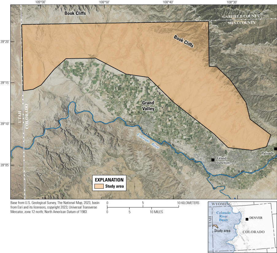
Study area is in the western part of Colorado, in the Colorado River Basin, near the
Utah border. — Figure 1.
Study area, in Grand Valley, western Colorado.

Purpose and Scope

The purpose of this report is to provide information regarding the ephemeral stream channel stability on the north side of the Grand Valley, western Colorado, which is underlain by Mancos Shale, a major contributor of dissolved mineral salts to the Colorado River. To understand the connection between channel stability and geometry, geomorphic erosion processes and characteristics are outlined. The methods used to develop a technique to predict and map ephemeral stream channel stability are presented. Additionally, this report identifies mechanisms and processes affecting erosion and identifies areas in the Grand Valley of greatest instability probability. Using a combination of existing remotely sensed terrain models, surrogate streamflows, the Manning’s resistance equation, and multiple logistic regression models, ephemeral stream channel stabilities are estimated and mapped.

Description of the Study Area

The study area is within the Upper Colorado River Basin and is specifically bound to the north by the Book Cliff escarpment and the Mesa–Garfield County line. The study area extends from the eastern edge of the Grand Valley, near Palisade, Colorado, to the Colorado–Utah State line to the west (fig. 1). The section of Book Cliffs within the study area forms a sinuous southwest-facing escarpment and is continuously bordered to the south by the Grand Valley lowland. The terrain transitions from the lowlands to the highlands, including the cliff fronts and stops atop the ridgeline.

The region is arid, with an average rainfall between 10 and 25 cm, which results in few perennial streams, sparse flora and fauna, and large barren areas of well-exposed strata (Fisher and others, 1960). The terrain is intricately dissected by ephemeral streams draining into the Colorado River. The underlying geology is characterized predominantly as Late Cretaceous Mancos Shale, which is a massive marine deposit composed of shale with interbedded sandstone (Hettinger and Kirschbaum, 2002; Tuttle, 2009; Tuttle and others, 2014). The Mancos Shale is a known nonpoint source for a substantial portion of the salinity loads in the Colorado River (Tuttle and others, 2014). The overlying soils are poorly developed with salt-desert shrub-type vegetation (consisting of Sarcobatus vermiculatus [black greasewood], Atriplex corrugata [mat saltbrush], Artemisia tridentata [big sagebrush], and Ericameria nauseosus [rubber rabbitbrush]) that is native and drought tolerant in the arid environment of western Colorado (Lusby and others, 1963; Küchler, 1964; Lusby and others, 1971; Branson and others, 1976). Extensive biological soil crusts can develop on stable soils from all substrates regardless of slope angle, but especially on shallow, fine-textured, and calcareous soils (Belnap and others, 2001).

The entire study area, which is approximately 50 kilometers (km) long and 10 km wide (500 square kilometers [km²]), is managed by BLM for motorized and nonmotorized use. Historically, this area was primarily used for seasonal livestock grazing for herds migrating between winter and summer ranges, beginning in the 1880s (Lusby, 1979). Early grazing rates by sheep and cattle were heavy, although they later diminished and after 1988 only cattle were allowed to graze on the allotment (Fick and others, 2020).

Geomorphic Erosion Processes and Characteristics

Streams, whether perennial or ephemeral, are dynamic, open systems—dynamic because they are constantly changing, and open because they can be affected or changed by a variety of external forces and factors (Trent and Brown, 1984). Stream morphology describes the stream channel shape and how they change through time. The stream channel morphology is a function of several processes and environmental conditions, including the composition and erodibility of the streambed and streambanks (for example, bedrock, sand, clay), where erosion comes from the force of the flow. Additional factors such as sediment size, composition and availability, vegetation type and amount, and human interaction also affect the stream morphology (Trent and Brown, 1984). Proper interpretation of stream instabilities requires an understanding of stream morphology and the physical processes involved. The environmental conditions and factors affecting the geometric stability and characteristics of ephemeral streams are discussed in the “Geomorphic Erosion Processes, Relations, and Responses” section of this report.

Geomorphic Erosion Processes, Relations, and Responses

The stream system channel geometry (for example, its depth, width, and plan-view form [sinuosity or other channel forms]) is a function of the erosion processes (channel hydraulics and external constraints) applied to the system, which include streamflow, sediment discharge, valley slope, and controls imposed by the region (Trent and Brown, 1984). The valley slope and geologic constraints are generally assumed to be constant; however, the streamflow and sediment discharge will vary with every flow occurrence. Because the channel hydraulic geometry is a function of these dynamic elements, a stream system will attempt to adjust its geometry in response to changing conditions to maintain or create a dynamic equilibrium condition with respect to water, sediment load, and channel morphology (Trent and Brown, 1984).

Results of numerous studies show geomorphic proportionalities that describe functional relations between the water and sediment load of a channel and the resulting channel size, shape, and sinuosity (Lane, 1954; Leopold and others, 1964; Schumm, 1977; Simons and Sentürk, 1977). These geomorphic studies revealed channel width, depth, and plan view are constantly adjusting, and channel stability is an evolutionary process not constant through time (Schumm and others, 1984). Evolutionary phases of channel stability range from total disequilibrium to a new state of quasi equilibrium. A quasi-equilibrium phase implies the system is not static through time but during a period of years the average condition is of stability (Watson and others, 2002). If the observational period of a channel is limited, a method of assessing channel evolution is to assume distance downstream is equivalent to the passage of time. This is the process of location-for-time substitution, and the “technique assumes that by observing channel form as one moves downstream along a channel, the effect of physical processes at one location through time can be observed” (Schumm and others, 1984; Watson and others, 2002).

Stream channels not in equilibrium conditions experience sediment distribution with channel erosion or deposition occurring up and down the length of the stream. Three geomorphic responses or processes result from changes in dominant streamflow and sediment conditions: channel widening (bank erosion), channel deepening, and a change in plan-view form (Trent and Brown, 1984). All three responses will, however, cause some level of streambank erosion.

Channel widening is evidenced through an increase in channel width, with or without an increase in channel depth. Bank failures in fluvial systems caused by channel widening generally occur in one of three ways: (1) hydraulic forces remove erodible bed or bank material, (2) channel geometry instabilities result in mass wasting, or (3) a combination of channel geometry and hydraulic forces cause bank collapse (Fischenich and others, 1989). Hydraulic-caused bank collapse occurs when flowing water exerts a tractive force (the force needed to overcome the resistance caused by friction) exceeding the critical shear stress for a particular streambank material. Geometry-caused bank collapse unrelated to hydraulic forces is usually a result of bank moisture, where moisture can affect the ability of a bank material to withstand stresses. The most common bank collapses are due to a combination of channel hydraulics and geometry. The most widely known and generally accepted cause of bank erosion is shear stress on streambanks caused by fast-moving water during peak streamflow (Leopold and others, 1964).

Channel incision (in other words, bed erosion, degradation, or lowering) occurs because of four main processes: (1) decreases in sediment supply (sediment transport capacity of the bed material exceeds the sediment supply delivered to the channel), (2) increases in channel bed slope (channel straightening), (3) increases in streamflow, and (4) increases in velocity (as a result of increased streamflow and not associated with an increase in channel bed slope) (Simon and Darby, 1997; Bledsoe, 1999). Under such conditions, channel bed and bank stabilities are affected, and stream morphology is ultimately altered. Bed channel erosion is generally initially dominant more than channel widening, but as the bank heights of an incising channel increase due to degradation, banks may reach a critical height for mass wasting, and widening may prevail (Harvey and Watson, 1986; Watson and others, 2002).

Plan-view form includes changes in channel shape and position as viewed from above. Changes in plan-view form are most often demonstrated through the downstream migration of meandering bends and changes in the sinuosity of meander bends. Generally, these changes result from alterations of channel bed slope. Channel bed slope reduction often results in a reduction of sediment discharge and bed channel aggradation (Lane, 1954). Consequently, a reduction in channel bed slope can lead to a tendency toward increased bank erosion and increased channel sinuosity.

Geomorphic Characteristics for Ephemeral Streams

The spatial and temporal relations of fluvial processes for dryland ephemeral streams and those in humid regions were confirmed to differ greatly (Graf and Lecce, 1988; Reid and Laronne, 1995; Tooth, 2000; Bull and Kirkby, 2002; Reid and Frostick, 2011). In arid regions, the annual exceedance probability for bankfull streamflow ranges from about 1 to 32 years; in contrast, temperate zone streams have an annual exceedance probability of approximately 1.5 years (Graf and Lecce, 1988; Bull and Kirkby, 2002). The highly variable annual exceedance probability in arid regions stems from infrequent and spatially sporadic precipitation large enough to produce infiltration excess and generate runoff. These isolated storms typically cover only a part of a basin and downstream flow losses by high rates of infiltration into dry, unconsolidated alluvial beds result in ephemeral streams exhibiting large downstream decreases in unit streamflow (Babcock and Cushing, 1942; Cornish, 1961; Keppel and Renard, 1962; Lane and others, 1971; Walters and others, 1988; Hughes and Sami, 1992; Constantz and others, 1994; Goodrich and others, 1997; Tooth, 2000; Bull and Kirkby, 2002). In a positive feedback cycle, the downstream decrease in streamflow results in a reduction of the sediment transport capacity and an increase in aggradation, causing an increase in the extent and thickness of alluvium, and associated increases in infiltration capacity and streamflow losses (Graf and Lecce, 1988, Merritt and Wohl, 2003; Reid and Frostick, 2011).

Short-lived and infrequent streamflow in arid-region ephemeral streams results in progressive episodes of channel incision and filling (Schumm, 1977; Patton and Schumm, 1981) accompanied by channel widening (Hooke, 1967; Bull and Kirkby, 2002; Powell and others, 2005). Despite relatively long periods of no streamflow and stable streamflow characteristics in ephemeral streams, channel characteristics commonly exhibit spatial variability and longitudinal discontinuity in arid regions. Changes in lithology and valley characteristics generally dictate the longitudinal alterations within ephemeral streams (Leopold and others, 1964; Graf and Lecce, 1988; Bull and Kirkby, 2002).

Methods for Ephemeral Stream Channel Assessment

This section provides details on the techniques and procedures used to acquire the needed information and how it is used to predict areas with the greatest probability of instability. Specifically, this section covers the stream channel delineation within the study area using existing remotely sensed data and the extraction of cross sections along those channels. Ground truthing of the extracted remotely sensed cross sections, techniques for obtaining channel geometry characteristics from the cross sections, and using them in a hydraulic analysis are discussed. Lastly, the process for estimating channel stability using the channel geometry and hydraulic analysis parameters, referred to as explanatory or predictor variables, is outlined. All data associated with this report, including cross-section profiles, survey data, Manning roughness coefficients, channel geometry characteristics and hydraulics, and channel stabilities are available in a USGS data release (Homan, 2024).

Stream Channel Delineation, Cross-Section Profiles, and Surveys

Along the north side of the Grand Valley, stream channels were delineated from a 1-meter (m) bare-earth digital elevation model (DEM) derived from light detection and ranging (lidar) elevation data acquired from the 3D Elevation Program (3DEP) managed by the USGS National Geospatial Program (USGS, 2019a). The 1-m DEM has a 1-m by 1-m cell size with a 19.6-cm vertical accuracy at the 95-percent confidence level, which is equivalent to the 10-cm root mean square error in the z-dimension and referenced to the North American Datum of 1983 (NAD 83). Concentered streamflow accumulation was used to delineate stream channels using the 3DEP downloaded 1-m DEM and ArcGIS (a geographic information system) software version 10.8.1 (Esri, 2020).

To assess stream channel geometry characteristics, channel cross-section profiles along the extracted stream reaches were obtained. The original concept was to physically survey cross sections at a minimum of 40 locations per stream reach. Instead, the high-resolution 1-m DEM was used to extract cross-section profile elevations, which provided almost 10 times as many cross sections as originally planned for this study while simultaneously reducing the amount of required fieldwork. The cross-section profiles were extracted from the stream channels using a combination of R code and RStudio statistical software version 4.2.2 (RStudio Team, 2022), and ArcGIS. Each cross-section profile is perpendicular to the stream channel and longitudinally spaced at a 25-m interval distance, starting at the upstream end. The cross sections are each 100 m long and have elevation information every 1 m.

To confirm the stream channels had not been altered since the lidar acquisition, three streams, each consisting of 40 cross sections, were surveyed using a setup comprised of real-time kinematic (RTK) and Global Navigation Satellite System (GNSS) methods. The surveyed elevation data were collected with a Trimble R8 GNSS base unit receiver and R8 GNSS rover receiver with TSC3 data collector following the techniques and methods in Rydlund and Densmore (2012) and Trimble (2003). The horizontal coordinate data are referenced to Universal Transverse Mercator zone 12 north projection, NAD 83, and the vertical coordinate information is referenced to the North American Vertical Datum of 1988 (NAVD 88). The RTK–GNSS position precision, as rated by the manufacturer, is 1 cm horizontally and 2 cm vertically (Trimble, 2003).

Cross-Section Hydraulic Analysis

Cross-section data to construct relations between streamflow, channel geometry, and various hydraulic characteristics are useful for reconstructing the conditions associated with a particular channel and streamflow. The Manning’s resistance equation was used to reconstruct the hydraulic conditions (average velocity, streamflow area, hydraulic radius) for each cross section associated with a predefined streamflow rate. The Manning’s resistance equation is an empirical equation applying to uniform streamflow in open channels and is a function of the channel streamflow area, average velocity, channel bed slope, and a roughness coefficient expressed in equation 1 (Chow, 1959):

Q = V A = (\frac{1}{n}) A R^{\frac{2}{3}} \sqrt{S} [M e t r i c]

,

(1)

where

Q: is the streamflow, in m³/s;
V: is the average velocity of streamflow, in m/s;
A: is the streamflow area, in m²;
n: is Manning roughness coefficient;
R: is the hydraulic radius, in m;
S: is the dimensionless energy slope approximated by the channel bed slope; and
1: is the conversion factor, 1 for International System of Units and 1.49 for U.S. customary units.

The Manning’s resistance equation is balanced using the Manning roughness coefficient (n), which represents the roughness or friction applied to the streamflow from the channel bed and banks. For this study, the channel cross-section Manning roughness coefficients were estimated following the methods described in Cowan (1956). The channel bed material, surface irregularities, variations in shape and size of the channel, obstructions, vegetation, and meandering of the channel were determined during field observation at a subset of cross sections in the study area. Cross sections were visited (field observed) on an alternating pattern of 100-m and 300-m spacing (4th and 12th cross sections, respectively). Roughness coefficients for unvisited (not field observed) cross sections from the original 25-m interval were set as the average value from the closest upstream and downstream field-based estimations. Verification of roughness coefficients was done based on the reference coefficients of Phillips and Ingersoll (1998). The roughness coefficients were used within the Manning’s resistance equation for the cross-section hydraulic analysis.

Because the streams within the study area are ephemeral, the surrogate streamflows used in the Manning’s resistance equation were not measured but obtained from USGS StreamStats streamflow data for the 0.10 annual exceedance probability (Q₁₀) peak streamflow (Homan, 2024). These data were acquired for each stream channel and at each cross section using StreamStats version 5.04 Batch Processing Tool, which uses regression equations to extrapolate peak-streamflow statistics (USGS, 2019b). As stated in the “Geomorphic Characteristics for Ephemeral Streams” section of this report, the annual exceedance probability for bankfull streamflow in arid regions can range from about 1 to 32 years. A Q₁₀ was selected as the hydrologic condition of interest because it simulated a stream stage that filled most cross sections without inundating the floodplain. In addition to streamflow estimates, upstream drainage areas were delineated for each cross section using the StreamStats Batch Processing Tool.

Along with a Manning’s n value and streamflow, the Manning’s resistance equation requires the water surface slope. Under the assumption of uniform streamflow conditions, the channel bed slope approximates the energy grade line and the water surface slopes. The channel bed slope at a given cross section was determined by measuring the change in DEM thalweg (lowest elevation within the channel) elevation between the upstream and downstream cross sections and dividing the vertical difference by the horizontal distance between thalweg locations.

There are no computational difficulties in solving the Manning’s resistance equation when the channel bed slope or channel streamflow are unknown. However, when the streamflow cross-section area is the unknown, the solution generally cannot be found explicitly. The known DEM-extracted stream cross-section profiles are for 100-m-long cross-section lines, not cross sections specifically for the streamflow areas inundated by a specified 0.10 annual exceedance probability streamflow (Q₁₀).

To find the streamflow area within the channel cross-section profile, a six-step computationally iterative process was used: (1) use a cross-section profile and an arbitrarily low depth of water, for example 1 cm (y_i), to calculate the inundated streamflow area (A), the cross-sectional area for a streamflow measured normal to the direction of flow; (2) calculate the wetted perimeter (Wp), the length of the wetted surface measured normal to the direction of flow, of the streamflow area; (3) use the streamflow area (A) and wetted perimeter (Wp) to calculate the hydraulic radius (R), the ratio of the area to wetted perimeter (A/Wp); (4) use the Manning’s resistance equation (eq. 1) to calculate the streamflow for the prescribed depth of water; (5) compare the calculated streamflow (Q_c) to the surrogate 0.10 annual exceedance probability streamflow (Q₁₀); and (6) if Q_c < Q₁₀, then incrementally adjust the depth of water by a small amount, for example 0.01 cm (y_i + 0.01 cm), and repeat steps one through five until the calculated streamflow rate is within 0.10 cm of the 0.10 annual exceedance probability streamflow (Q₁₀).

RStudio software was used to perform the calculations (RStudio Team, 2022). Upon the convergence of the streamflows (Q_c ~ Q₁₀), cross-sectional streamflow areas (A₁₀), average velocities (V₁₀, Q₁₀ /A₁₀), wetted perimeters (Wp₁₀), and hydraulic radiuses (R₁₀) for the 0.10 annual exceedance probability streamflow (Q₁₀) are known and can be used as predictor variables to predict ephemeral channel stability within the north side of the Grand Valley, described in the “Stream Channel Stability” section of this report. Additionally, knowing the Manning’s resistance equation parameters allows supplementary channel geometry and hydraulic characteristics associated with a surrogate 0.10 annual exceedance probability flood to be calculated.

Channel geometry refers to the three spatial dimensions of width, depth, and plan view for a stream. The channel width for a specified streamflow is the horizontal distance between streambanks at the water surface elevation and is known as the top width (B). The average channel depth (D) for a specified streamflow is the cross-sectional streamflow area divided by the top width, whereas the maximum depth of water (Y) is the water surface elevation subtracted by the cross-section minimum elevation (thalweg). The channel cross-section plan view is numerically expressed by the stream channel sinuosity. Sinuosity is the stream length ratio (distance traveled if you floated downstream) divided by valley length (as a crow flies distance; the most direct route). The greater the sinuosity, the more tortuous (strongly meandering) the stream path (Schumm and others, 1984). For this study, sinuosity is calculated using stream and valley lengths between 20 upstream and downstream cross sections representing an approximate distance of 1 km of channel length. For example, the sinuosity for the 100th downstream cross section would be calculated using stream and valley lengths measured between cross sections 80 and 120. Sinuosity for the first and last 20 cross sections were, however, calculated with limited information. Like the Manning’s resistance equation parameters, the calculated channel geometries (width, depth, and plan view) were based on the 0.10 annual exceedance probability streamflow (Q₁₀) and were used to predict ephemeral channel stability, described in the “Stream Channel Stability” section of this report.

To predict ephemeral channel stability, the cross-section hydraulic analysis also included a channel hydraulic characteristics evaluation, which can help assess the ability of a stream to erode material from the channel bed and banks or to aggrade (deposit) material. An analysis of physical samples of suspended sediment and bedload would be instructive, but in most arid or semiarid regions ephemeral channels, such data are not available (Graf, 1983). Instead, stream characterization related to channel stability can be done using a tractive and resisting forces comparison through a potential energy and stresses evaluation (Graf, 1983). For this study, the evaluated channel hydraulic characteristics included total stream power, unit (specific) stream power, shear stress, Froude number, and width-to-depth ratio.

Total stream power is related to sediment transport and computed from channel dimensions and streamflow information (Bagnold, 1966, 1977; Graf, 1984). Because total stream power is a function of channel dimensions and streamflow, it is more valuable in a process analysis than are the individual channel dimensions when considered separately. Total stream power (Ω) is the power exerted by flowing water over a unit length of channel (Bagnold, 1966, 1977) and is defined as unit stream power times the channel width in equation 2:

Ω = ωB = ρ g R S V B

,

(2)

where

Ω: is total stream power, in newtons per second [N/s], or watts per meter [W/m];
ω: is unit (specific) stream power, in watts per square meter [W/m²];
ρ: is density of the fluid, in kilograms per cubic meter [kg/m³];
g: is acceleration due to gravity, in meters per second squared [m/s²];
R: is the hydraulic radius, in m;
S: is the dimensionless energy slope approximated by the channel bed slope;
V: is the average velocity of streamflow, in m/s; and
B: is top width, in meters.

Equation 2 assumes a steady uniform streamflow, and ρg = 9,807 newtons per cubic meter (N/m³; Carson, 1971). Stream power along its length is directly related to potential sediment transport (Graf, 1984), is an indication of the potential for deposition and (or) erosion, and is a channel stability indicator. Bizzi and Lerner (2015) showed total stream power for values around 2,000 W/m to provide a transition zone between unstable (erosion) and stable (deposition) channels.

Instead of potential energy per unit stream length, (specific) stream power (ω) is stream power per unit top width (Bagnold, 1977). Normalizing the stream power by the stream width allows for a better comparison of streams of various widths. By transformation, specific stream power may be as expressed in equation 3 (Petit and others, 2005):

ω = τ V

,

(3)

where

V: is the average velocity of streamflow, in meters per second; and
τ: is the total shear stress averaged for the width of the stream, in newtons per square meter.

Like total stream power, specific stream power between 30 and 40 W/m² was shown to provide a transition zone between unstable (erosion) and stable (deposition) channels (Bizzi and Lerner, 2015). Additionally, the lower the system energy, the more stable the system will be, so decreases in specific and total stream power lead to stream channel stabilization and deposition dominance.

Shear stress as shown in equation 3 is based on the conservation of momentum principle, another erosion potential predictor, and is the force of water trying to drag the channel bed surface downstream with it (Meyer-Peter and Müller, 1948; Fernandez Luque and Beek, 1976; Petit and others, 2005). Critical shear stress is when the drag force of flowing water against a channel particle is greater than the gravitational force holding it in place, the particle begins to move. Channel stability is closely related to bed material movement; the greater the quantity of bed material in motion, the lower the channel stability, even if on average the sediment motion is balanced by input material from upstream (Jia, 1990). When shear stress is equal to or less than critical shear stress, the channel will likely be stable. Where shear stress is greater than critical shear stress, channel degradation will likely result, and the channel will be unstable (Wohl, 2000).

An alternative way of evaluating the distribution of available energy within a channel is the Froude number as shown in equation 4 (Froude, 1861):

Fr = \frac{V}{\sqrt{g d}}

,

(4)

where

Fr: is the Froude number (dimensionless);
V: is the average velocity of streamflow, in meters per second;
g: is acceleration due to gravity, in meters per second squared [m/s²]; and
d: is the average depth of water, in meters.

The Froude number provides a way to assess the streamflow energy state based on the relation between streamflow velocity and depth (inertial and gravitation forces). Small Froude numbers relate to low-energy states indicative of deep, slow streamflow. Increasing Froude numbers represent shallower, faster streamflow and a sharp increase in potential sediment transport rates (Simon and Darby, 1997). Channels will tend to have the lowest bed material movement and highest stability for the minimum streamflow energy state, and therefore, a smaller Froude number (Jia, 1990).

Hydraulic geometry relations have also been useful in describing width, depth, cross-sectional area, and velocity as power functions of streamflow (Osterkamp and others, 1983; Rosgen, 1998). Geomorphic dimensions (for example, bankfull width, depth) were combined into dimensional ratios (for example, width-to-depth ratio) as surrogates for the channel sediment characteristics and shear stress distributions (Osterkamp and others, 1983). High width-to-depth ratios (shallow and wide channels) place stress within the near bank region, and as the width-to-depth ratio value increases (as the channel grows wider and shallower), the hydraulic stress at the banks also increases. Bank erosion may be accelerated because of increased hydraulic stress (Osterkamp and others, 1983; Kleinhans and Berg, 2011). Because the width-to-depth ratio is a proxy for shear stress distributions, channels with the minimum values tend to have the highest stability.

The evaluated channel hydraulic characteristics, including total stream power, unit (specific) stream power, shear stress, Froude number, and width-to-depth ratio were calculated for each cross section and are available in Homan (2024). The calculated parameters are used as predictor variables within the multiple logistic regression models described in the report, “Stability Extrapolation” section of this report.

Stream Channel Stability

The hydraulic analysis results provide mathematical solutions for channel cross-section streamflow areas and associated parameters for defined streamflows and accompanying potential energies and stresses but do not empirically specify the channel beds or banks stability. During the field work to collect roughness coefficient information, five digital images were collected at each field-visited cross section. The images included snapshots of the channel bed, left and right stream banks, and the channel profiles looking upstream and downstream from the cross-section observation locations. A post-field work review of the images was completed, and channel stability classifications were assigned to each cross section. The review identified indicators of channel disturbances (where present) including channel head cuts and bank erosion presence, such as soil falling off the side slopes (sloughing), scouring, mass wasting, and undercutting. If neither channel bed nor banks presented active erosion evidence, the cross sections were classified as “stable.” If evidence of erosion was identified on either channel bed or banks, the cross sections were classified as “active.” To break down the channel stability assessment one step further, bed or bank erosion indicators were noted in actively eroding channels. Actively eroding cross sections with only bed erosion signs were classified as incising channels; cross sections with only indications of bank erosion were classified as widening channels. The digital images used in the interpretation and stability classifications for the channel beds and banks are available in Homan (2024). The stability classifications are used as field-based channel stability observations and split into calibration and validation datasets used in the “Stability Extrapolation” section of this report.

Stability Extrapolation

Stream channel stability was classified using field-based images at a subset of cross sections. A logistic regression model was used to predict whether nonvisited cross sections are stable or actively eroding. Logistic regression models use parameter classifications to determine the probability of binary outcomes, in this case active or stable stream channel cross sections (Berkson, 1944, 1951). The statistical model uses a logistic sigmoid (S-shaped) function (fig. 2), to fit observations. Unlike linear regressions, which model continuous dependent variables, logistic regression models are limited to either 0 or 1 on the y-axis.

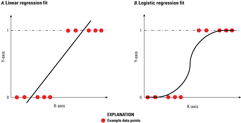
Graph of the linear regression is a straight line, whereas the graph of the logistic
regression is a curved line that resembles the letter S. — Figure 2.
Example comparison of A, linear regression fit, and B, logistic regression sigmoid.

Multiple logistic regression analysis applies when there is a single binary outcome and more than one independent explanatory variable, such as if a channel is stable or actively eroding given its streamflow, slope, and specific power (Cox and Lewis, 1966; Theil, 1969). The outcome in logistic regression analysis is coded as 0 or 1, where 1 indicates that the outcome of interest is present (for example, active erosion), and 0 indicates the outcome of interest is absent (for example, stable or no erosion). If p is the probability that the outcome is 1, the multiple logistic regression model can be written as follows in equation 5 (Helsel and others, 2020):

\hat{p} = \frac{exp (b_{0} + b_{1} X_{1} + b_{2} X_{2} + \dots + b_{p} X_{p})}{1 + exp (b_{0} + b_{1} X_{1} + b_{2} X_{2} + \dots + b_{p} X_{p})}

,

(5)

where

$\hat{p}$: is the expected probability the outcome is present;
exp: is an abbreviation for exponential;
X₁ through X_p: are the distinct independent variables; and
b₁ through b_p: are the regression coefficients.

The multiple logistic regression model can also be written as shown in equation 6, in which the outcome is the expected log of odds or the odds of probability that the outcome is present (Helsel and others, 2020):

\log (\frac{\hat{p}}{(1 - \hat{p})}) = b_{0} + b_{1} X_{1} + b_{2} X_{2} + \dots + b_{p} X_{p}

.

(6)

Multiple logistic regression models were developed to predict whether nonobserved cross sections are stable or experiencing erosion (binary outcome), using associated channel geometry (width, depth, and plan view [sinuosity]) and hydraulic characteristic (total stream power, unit [specific] stream power, shear stress, Froude number, and width-to-depth ratio) as independent explanatory variables. Stream channel stability is also a function of the underlying geology and soils, vegetation cover, presence of grazing, and human effects (such as proximity to roads and the overall density of the nearby road network) (Schumm and others, 1984). These additional explanatory variables were also taken into consideration when developing the multiple logistic regression models.

The entire study area, underlain by geology consisting almost exclusively of Mancos Shale has soils predominantly poorly developed (Whittig and others, 1982), vegetation cover composed solely of salt-desert shrubs (Hop and others, 2016), and has been entirely subjected to grazing (Lusby, 1979; Fick and others, 2020). These variables are homogeneous throughout the study area and, as such, lack predictive effect for estimating stream channel stability. By contrast, human disturbances within the study area are diverse and considered to be a channel stability factor. Specifically, the study area has an extensive network of unpaved roads and trails (BLM, 2020).

The proximity of stream channel cross sections to their nearest unpaved road or trail was determined using ArcGIS software (Esri, 2020), as well as the road densities (cumulative unpaved road and trail distance in kilometers per square kilometer [km/km²]) surrounding each cross section, both are available in Homan (2024). Along with the channel geometry and hydraulic characteristics, the road proximity and road densities were used as independent explanatory variables within the multiple logistic regression models.

Models predict channel stability as a function of the explanatory variables used, with not all variables providing the same predictive powers. Model optimization is achieved when a model provides the best predictive powers with the fewest explanatory variables. There are various methods to select, adjust, or change the explanatory variables used in the multiple logistic regression models. RStudio has a variety of statistical methods for selecting variables and optimizing models (RStudio Team, 2022). An R script was coded to create stepwise-based multiple logistic regression models, where the predictive variables are selected by an automatic algorithm involving three approaches, explicitly: forward selection, backward elimination, and (or) both directions (Efroymson, 1960; Hocking, 1976; Draper and Smith, 1981). Additional R code created bootstrap-based multiple logistic regression models, which repeatedly sample a dataset with random replacement of different predictive variable combinations to create various simulated samples sets (Efron and Tibshirani, 1993; Efron, 2003). Akaike information criterion (AIC) (Stoica and Selen, 2004; Taddy, 2019), which is a mathematical method for evaluating how well a model fits the data from which it was generated, was used to evaluate the stepwise- and bootstrapped-based multiple logistic regression models. The R script also included code to create multiple logistic regression models based on least absolute shrinkage and selection operator (LASSO), which uses a variable selection technique through examining p-values of coefficients and automatically discarding those variables whose coefficients are not significant (Santosa and Symes, 1986; Tibshirani, 1996). Multiple logistic regression models were also created using dominance analysis, which determines predictor importance not based on model selection but rather by uncovering the individual contributions of the predictors and comparing the incremental R-squared (McFadden’s pseudo r²) contribution across all subset models (Budescu, 1993; Azen and Budescu, 2006). The McFadden’s pseudo r² interpretation between 0.2 and 0.4 is considered to represent excellent contribution or model fit (McFadden, 1974; Laitila, 1993; Veall and Zimmermann, 1996). Regardless of the machine learning method coded within the R script, the goal was to determine which combination of explanatory variables best predicts the channel stability binary outcome.

To construct the models and assess the binary stream channel stability outputs accuracy, the models were originally developed exclusively for the cross sections subset with field-based channel stability observations. The visited cross sections subset was split into a calibration and a validation dataset. The calibration dataset contains 70 percent of the field-based channel stability observations; the remaining 30 percent of the field-based channel stability observations were reserved for the validation dataset. Using the calibration dataset, different combinations of explanatory variables were tested to optimize the multiple logistic regression models. Four different machine learning methods were used to assist in the explanatory variable selections: stepwise regression (forward, backward, and both directions), bootstrapping, LASSO, and dominance analysis. The multiple logistic regression model outputs are not only a product of the explanatory variables used but also based on the selection or split of the sample population into the calibration and validation datasets. As a result, each multiple logistic regression model was calibrated and validated using 1,000 randomly split datasets observing the 70 percent calibration and 30 percent verification rules.

The model outputs were probabilities of the validation cross sections having active erosion or being stable, and the outputs ranged from 0 to 1. The modeled probabilities could not be directly compared to the stability assessments within the validation datasets, so probabilities greater than 50 percent were defined as an active binary value, whereas probabilities less than 50 percent were defined as stable. Validation of the model’s predictive abilities were based on goodness-of-fit r-squared (r²), AIC, and McFadden’s pseudo r² values. Larger r² values represent smaller differences between the observed data and the fitted values, and a better-fit model (Healy, 1984); lower AIC values indicate a better-fit model (Kenny, 2020); and McFadden’s pseudo r² values 0.2 or greater indicate good-to-excellent model fit (Lane and others, 2009).

Using the top performing multiple logistic regression model, stream channel stability was extrapolated for the remaining unvisited cross sections. The modeled erosion probabilities for all cross sections were subsequently mapped in ArcGIS to identify locations of instability.

To evaluate the statistical significance between the active and stable channel cross sections, the most effective stream channel stability predictors were evaluated using a one-way analysis of variance (ANOVA) test (Cuevas and others, 2004). Using RStudio (RStudio Team, 2022), an R script was coded to create ANOVA statistical models used to test for significant differences between the means of more than two independent groups and is regarded as a multiple group extension of the t-test. However, if applied to two groups, ANOVA will return a result similar to the t-test (Hazra and Gogtay, 2016). The null hypothesis for (any) ANOVA is all population means are exactly equal (Cuevas and others, 2004). For this study, the null hypothesis is the active and stable cross sections have the same stability predictor sample mean value. An ANOVA compares the sample data and derives a p-value, or probability value, which is a number describing how likely it is the data would have occurred with the null hypothesis (Hazra and Gogtay, 2016). If the p-values are greater than 0.05, then the null hypothesis cannot be rejected, and the sample means are considered statistically equivalent. Whereas, p-values less than 0.05 indicate the null hypotheses is rejected, and the sample means of the stability predictors for the active and stable cross sections are statistically different. Additionally, an R script was coded to create ANOVA tests within the active cross sections to compare incising and widening channels.

To assess the channel characteristics among the stability classifications, the geomorphic and hydraulic parameters were normalized using minimum-maximum (Min-Max) feature scaling. Min-Max normalization is a technique to adjust values on different scales into the range (0,1) (Henderi and others, 2021). The formula for a Min-Max normalization is provided in equation 7:

\overset{´}{x} = \frac{x - m i n (x)}{m a x (x) - m i n (x)}

,

(7)

where

x: is an original value; and
$\overset{´}{x}$: is the normalized value.

Ephemeral Stream Channel Assessment

To predict ephemeral channel stability within the north side of the Grand Valley, 48 streams channels were delineated along the thalweg, using a 1-m DEM (fig. 3). The streams originate in the headwaters of the Book Cliffs (fig. 3), are generally aligned northeast to southwest, and terminate on the Grand Valley floor. Stream channel summary statistics, including stream channel length, change in elevation, average channel bed slope, and sinuosity values for the 48 stream channels are available in Homan (2024).

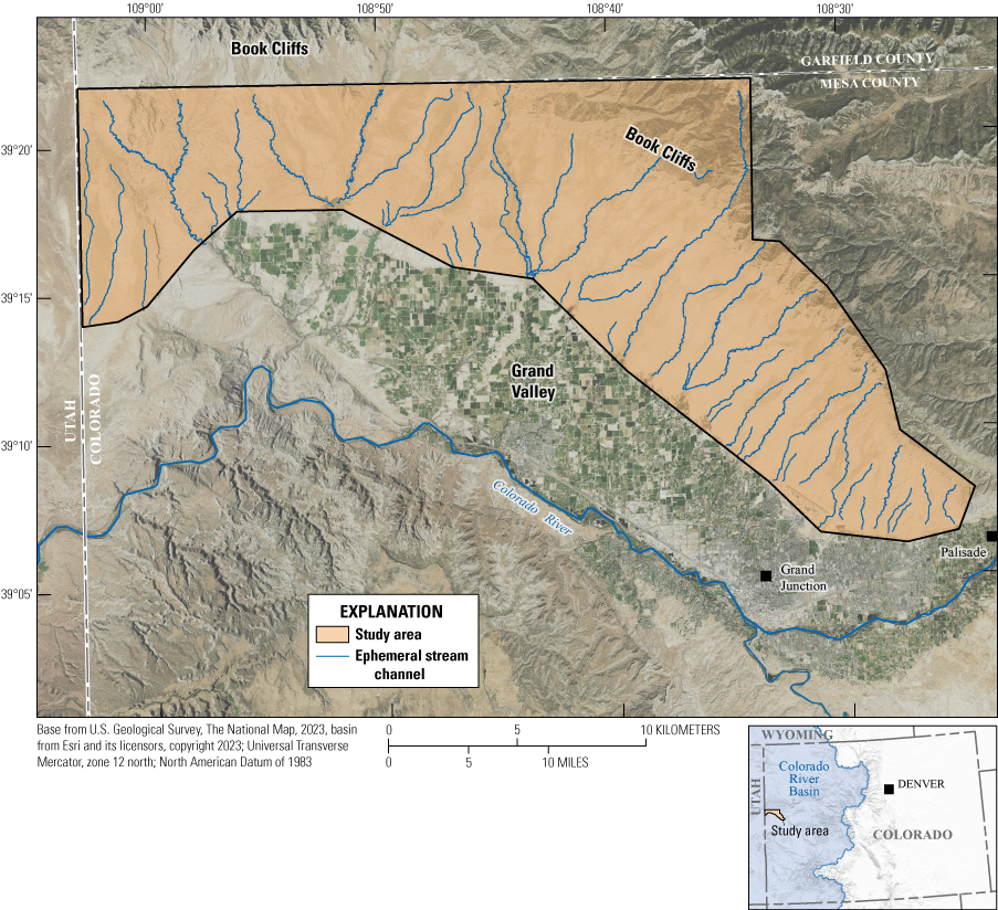
Map of 48 ephemeral stream channels in the Grand Valley, western Colorado, extracted
from a 1-meter digital elevation model. — Figure 3.
Network of 48 ephemeral stream channels extracted from a 1-meter digital elevation model in Grand Valley, western Colorado (U.S. Geological Survey [USGS], 2019a).

Cross-Section Profiles

The network of 48 ephemeral stream channels of the study area provides the information on channel geometry and hydraulics, resistance-equation relations, and stream channel stability. The subsequent step, obtaining channel characteristic information longitudinally within the stream channels, was completed at point locations. From the network of 48 ephemeral stream channels and using 25-m longitudinal spacing starting at the upstream end of each channel, 18,486 sample locations were defined. At each of the sample locations, 100-m perpendicular cross-section profiles were extracted from the same 1-m DEM used to delineate the channels. As a result of all 48 channels being ephemeral and having no water in their channels, complete cross-section profiles of channel and overbanks were obtained. Each channel length is unique, so the number of cross sections per reach is variable. A table with cross sections per stream channel is available in Homan (2024).

To verify the accuracy of the DEM-extracted cross-section profiles and confirm the stream channels had not been altered since the lidar acquisition, 124 cross sections were ground truthed by field surveys using RTK-GNSS methods. The surveyed cross sections were measured along three streams, each consisting of roughly 40 cross sections. The surveyed cross-section data are available in Homan (2024). The ground-truthing comparison indicated a consistent offset between the DEM-extracted, cross-section profiles and the surveyed data. The offset consists of a 1.55-m horizontal shift and a 0.83-m vertical shift. Despite the small axes offset, the boundary shape of the DEM-extracted cross-section profiles matched the surveyed profiles, which is important for the channel cross-section hydraulic analysis. Consequently, the axes offset was not applied to the profile data, and the extracted cross-section profiles were deemed accurate and validated.

Estimated Ephemeral Channel Streamflows

The extracted cross-section profiles provided the channel geometry information needed to reconstruct the conditions associated with streamflow data having a 0.10 annual exceedance probability (Q₁₀). All obtained Q₁₀ values from StreamStats (USGS, 2019b) and upstream drainage areas for the 18,486 cross sections are available in Homan (2024), as are some summary streamflow and drainage area statistics per stream. Because the streamflow values are based on a regression equation, each stream has Q₁₀ streamflows that increase consecutively downstream with each subsequent cross section, with the farthest downstream cross section having the largest streamflow. Validation of the batch processing used to acquire Q₁₀ and drainage area data was completed using manually obtained StreamStats (USGS, 2019b) data for selected cross sections that represented a range of streams, drainage areas, reach lengths, and streamflows.

Hydraulic Analysis Using the Manning’s Resistance Equation

To use the Manning’s resistance equation to construct relations between the extracted cross-section profile geometries and estimated Q₁₀ streamflow data, channel surface slopes and a roughness coefficient were needed for each cross section. For this study, streamflow conditions were assumed to be uniform, so water surface slopes are the same as channel bed slopes, which were determined by measuring the change in elevation between the upstream and downstream cross sections and dividing the vertical difference by the horizontal distance. The channel bed slopes for the 18,486 cross sections are available in Homan (2024), as are some summary channel bed slope statistics per stream.

The last parameter needed to apply the Manning’s resistance equation is the Manning roughness coefficient. These coefficients were obtained from field-based observations at a subset of visited cross sections in the study area. The subset of visited cross sections with field-based roughness coefficient estimations totaled 1,406. Roughness coefficients for the remainder of the unvisited intermediate cross sections with the original 25-m interval were filled in with averaged values from the closest upstream and downstream field-based estimations. The 1,406 field-based roughness coefficients are available in Homan (2024), as well as the estimated roughness coefficients for all remaining 17,080 cross sections.

With the addition of the channel bed slopes and roughness coefficients, the Manning’s resistance equation was used to construct relations between the extracted cross-section profiles and the estimated Q₁₀ streamflow data. Following the procedures outlined in the “Cross-Section Hydraulic Analysis” section of this report, streamflow area, average velocity, wetted perimeter, and hydraulic radius associated with Q₁₀ streamflows were computed for all 18,486 cross sections. During the iterative calculation process involving microincreases in water surface elevations to systematically enlarge the calculated streamflow area, and thus streamflow rates until the calculated streamflow values (Q_c) converged with the estimated Q₁₀ streamflow values. Depending on the profile of the cross sections, the streamflow areas of the Q_c streamflows took on different flood capacity magnitudes. For cross sections with a greater topographic relief, Q₁₀ streamflows fit securely within the bounds of the 100-m wide profile, but for cross sections with less topographic relief, Q₁₀ streamflows sometimes exceeded the profile flood capacity. Of the 18,486 cross sections with iterative calculations, 5,071 profiles had calculated water surface elevations surpass the profile flood capacities before the Q_c streamflows reached flows equivalent to the Q₁₀ values. The cross-section profiles inundated by the Q₁₀ streamflows were removed from the analysis, leaving 13,415 cross sections with hydraulic analysis results. The calculated cross-section streamflow areas, average velocities, wetted perimeters, and hydraulic radiuses for Q₁₀ streamflows are available in Homan (2024).

Explanatory Variables Used Within the Multiple Logistic Regression Models

Using multiple logistic regression models to predict whether nonobserved ephemeral stream cross sections are stable or experiencing erosion, explanatory variables were required. Derived from the surrogate 0.10 annual exceedance probability streamflow and for each of the 13,415 cross sections, 18 explanatory variables were acquired (table 1) and are available in Homan (2024). Following is a summary of each variable: Q₁₀ streamflow and drainage area explanatory variables were acquired from StreamStats. Channel bed slope and sinuosity explanatory variables were calculated from the 1-m DEM. The Manning roughness explanatory variable was based on field observations. The hydraulic analysis using the Manning’s resistance equation provided channel and hydraulic explanatory variables, including cross-section streamflow area, average velocity, channel top width, maximum depth of water, wetted perimeter, and hydraulic radius. Total stream power, specific stream power, shear stress, Froude number, and width-to-depth ratio are the calculated potential energy and stress explanatory variables. Proximity to road and surrounding road density explanatory variables were determined using ArcGIS software (Esri, 2020). Each explanatory variable was used to construct multiple logistic regression models and predict ephemeral stream channel stability.

Table 1.

Explanatory variables used within the multiple logistic regression models.

Table 1. Explanatory variables used within the multiple logistic regression models.
Streamflow (Q₁₀)	Average velocity (V)	Specific stream power (ω)
Drainage area	Channel top width (B)	Shear stress (τ)
Channel bed slope (S)	Maximum depth of water (Y)	Froude number (Fr)
Sinuosity	Wetted perimeter (Wp)	Width-to-depth ratio (W/D)
Manning roughness coefficient (n)	Hydraulic radius (R)	Road proximity
Streamflow area (A)	Total stream power (Ω)	Road density

Stream Channel Stability Assessment

The stream channel cross-section explanatory variables previously outlined were calculated and obtained for predicting stream channel stability within multiple logistic regression models. To calibrate the models and assess the outputs of stream channel stability, a ground-truthing component was needed. At the subset of 1,406 cross sections where field-based roughness coefficients were estimated, 9,494 photograph images were taken. From the photograph images, channel cross sections were classified as either stable or active with regards to the absence or presence of erosional indicators. The channel cross-section stability assessments and photograph images are available in Homan (2024). Of the 1,406 cross sections with stability assessments, 570 appeared stable with no signs of active erosion, but 836 had visual signs of active bed or bank erosion. Of the 836 cross sections with signs of erosion, 512 had indications of active bed and bank erosion, 166 cross sections exhibited only signs of channel bed erosion or incision, and 158 showed only minor indications of channel bank erosion or widening.

Based on the stream channel stability assessments, cross-section stabilities were known for the subset of 1,406 visited cross sections but were needed at all 13,415 cross sections with explanatory variables. Multiple logistic regression models were used to extrapolate stream channel stability to the unvisited cross sections. Working with the 18 explanatory variables (table 1) and 4 machine learning methods (stepwise, bootstrapping, LASSO, and dominance analysis) to assist the explanatory variable selections, 28 explanatory variable combinations were designated. Using the 1,000 randomly split calibration and validation datasets (described in the “Stability Extrapolation” section of this report) and 28 explanatory variable combinations, 28,000 multiple logistic regression models were created and subsequently used to predict channel stability at the validation dataset cross sections.

The summary results for the top three performing models (labeled glm_20, glm_21, and glm_lasso, where glm stands for generalized linear model) with the highest r² values, lowest AIC values, and largest pseudo r² values are presented in table 2. Because the models were run for 1,000 different dataset splits, the minimum, average, and maximum values are based on the 1,000 iterations. The top three models consistently incorporated three of the same explanatory variables: drainage area, width-to-depth ratio, and sinuosity.

Table 2.

Minimum, average, and maximum goodness-of-fit r-squared; Akaike information criterion; and McFadden’s pseudo r² for the top three generalized linear models for the 1,000 validation datasets (Homan, 2024).

^{[r², r-squared; AIC, Akaike information criterion; pseudo r², McFadden’s pseudo r²; glm, generalized linear models; min, minimum; max, maximum]}

Table 2. Minimum, average, and maximum goodness-of-fit r-squared; Akaike information criterion; and McFadden’s pseudo r2 for the top three generalized linear models for the 1,000 validation datasets (Homan, 2024).
	r²	AIC	Pseudo r²	glm
Min	0.299	1,070	0.13	glm_20
Average	0.845	1,121	0.16	Drainage area + Sinuosity + Shear stress + Width-to-depth ratio
Max	0.974	1,169	0.20
Min	0.303	1,079	0.12	glm_21
Average	0.834	1,133	0.15	Drainage area + Sinuosity + Average water velocity + Width-to-depth ratio
Max	0.983	1,176	0.20
Min	0.187	1,074	0.13	glm_lasso
Average	0.844	1,125	0.17	Drainage area + Sinuosity + Average water velocity + Width-to-depth ratio +
Max	0.979	1,173	0.20	Maximum water depth + Hydraulic radius + Shear stress

The best average performing model (glm_20) had the highest average r² and lowest average AIC and used the three previously mentioned explanatory variables in addition to shear stress (table 2). However, the model with the overall maximum r² was model glm_21, which used the three explanatory variables in conjunction with average velocity instead of shear stress. Shear stress, also called friction velocity, is a better predictor of erosion potential than velocity, because it uses the actual force of the water on the boundary of the channel (Chen and Cotton, 1986), so glm_20 is the top performing multiple logistic regression model. The glm_lasso model also performed well, having the second highest average r² and second lowest AIC, and used the three previously mentioned explanatory variables (table 2). The downside to the glm_lasso model was it used four additional predictor variables, including shear stress, average velocity, maximum depth of water, and hydraulic radius. As a result of using seven explanatory variables, the glm_lasso model had the highest average pseudo-r² value, because the McFadden variable is additive based on predictor contribution of each variable (Lane and others, 2009). Because the original goal was to develop a model that provides the best predictive powers with the fewest explanatory variables, the glm_lasso model was not considered better than model glm_20.

For the stream channel stability validation dataset, which consisted of 422 cross sections dispersed throughout the study area, the glm_20 model correctly estimated channel stability with an 0.845 goodness of fit when using a combination of drainage area, width-to-depth ratio, sinuosity, and shear stress as the explanatory variables (table 2). Using this top-performing multiple logistic regression model (glm_20), stream channel stability was extrapolated for the remaining unvisited cross sections, and the results are available in Homan (2024). Figure 4 shows the modeled erosion probabilities (0 to 100 percent) mapped at all 13,415 cross sections along the 48 ephemeral streams within the north side of the Grand Valley. The erosion probabilities are modeled confidence levels that the cross sections have erosion, without indication of the severity or magnitude of erosion.

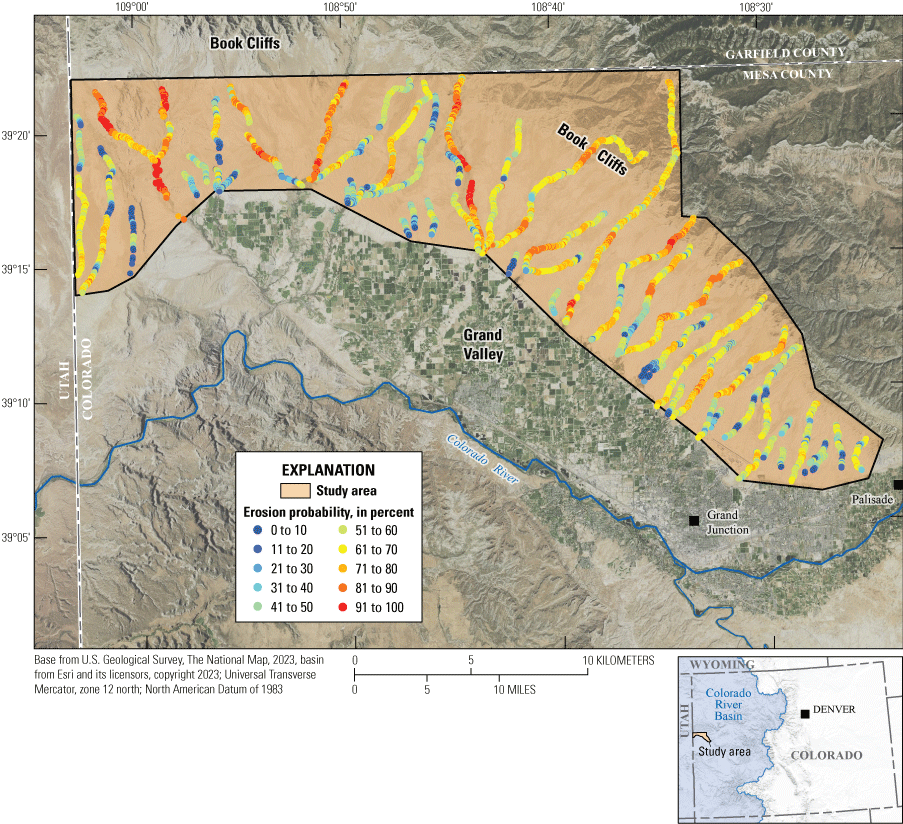
Most of the cross sections have high erosion probabilities, indicating they are active. — Figure 4.
Multiple logistic regression erosion probabilities for the 13,415 cross sections along 48 ephemeral streams in Grand Valley, western Colorado (Homan, 2024).

Based on the cross sections criteria with erosion probabilities greater than 50 percent are active and cross sections with erosion probabilities less than 50 percent are stable, 10,080 cross sections, or roughly 75 percent, are modeled as active (fig. 5). On review of the erosion probabilities within the 48 ephemeral stream channels, no visual or statistical pattern was identified as to where erosion is more likely to occur within the channel reaches. For the channel terminuses, 32 of the 48 channels had stable cross sections, whereas 28 of the 48 channels had stable headwater cross sections. Figure 5 shows the location of active or stable cross sections but does not indicate the severity of erosion or magnitude of sediment potential. To assess potential sediment contribution, a scaling component could be added.

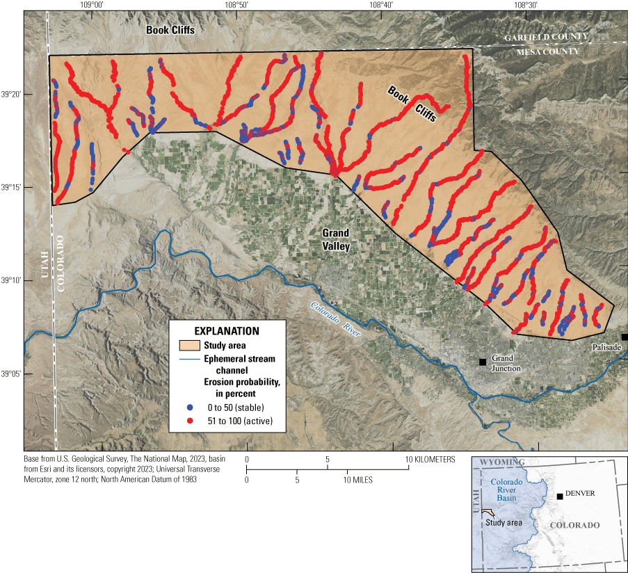
Active or stable cross sections. — Figure 5.
Multiple logistic regression erosion probabilities for the 13,415 stable or active cross sections along 48 ephemeral streams in Grand Valley, western Colorado (Homan, 2024).

Based on the evaluation of erosion probabilities within the validation dataset and corresponding images, active erosion in smaller cross sections (for example, 1 m wide and a few centimeters deep) have less potential sediment transport compared to larger cross sections (for example, 10 m wide and 2 m deep) (fig. 6). The concept of a larger area having more sediment potential is not new, but it is especially true for ephemeral streams, which are not sediment supply limited like perennial channels (Reid and Laronne, 1995). Therefore, larger cross-sectional surface areas have a greater amount of potential sediment for transport. To account for potential sediment within active cross sections, the erosion probabilities were weighted (multiplied) by the cross-sectional streamflow areas. The resultant high-resolution map (fig. 7) of weighted erosion probabilities can help to prioritize specific areas for more intensive study. The weighted erosion probabilities consider the multiple logistic regression modeled confidence levels as well as the amount of potentially available sediment. Unlike figure 5, which shows three-fourths of the study area as having active erosion, figure 7 shows fewer stream channels with the greatest levels of potential sediment and therefore salinity loading to the Colorado River.

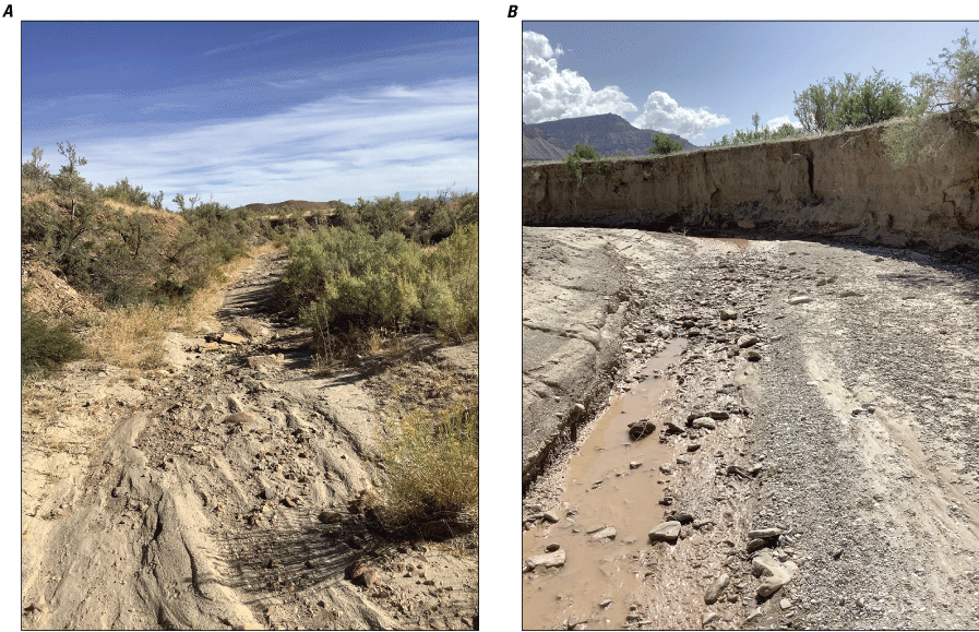
The first photo shows a shallow, narrow streambed; the second shows a wider streambed
with higher sides. — Figure 6.
Ephemeral stream cross sections in Grand Valley, western Colorado. A, smaller cross section with less sediment potential than B, larger cross section with greater sediment potential [Photographs by Joel Homan, 2020] (Homan, 2024).

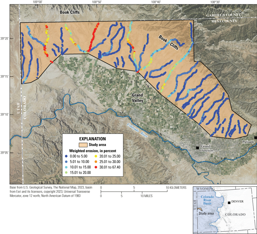
Most of the cross sections indicate lower weighted erosion probabilities. — Figure 7.
Weighted erosion probabilities for 13,415 cross sections of 48 ephemeral stream channels in Grand Valley, western Colorado (Homan, 2024).

Stability Predictor Variables

Of the 18 explanatory variables modeled and tested, drainage area, sinuosity, shear stress, and width-to-depth ratio were determined to be the most effective stream channel stability predictors. The following is a review of the significant predictor variables based on the 1,406 cross sections with field-based channel stability observations, which consisted of stable and active classifications and subclassifications of incising and widening within the active cross sections.

Figure 8 shows ANOVA boxplots to compare the means between active and stable cross sections for drainage area, sinuosity, shear stress, and width-to-depth ratio. Each of the four stream channel stability predictors had ANOVA p-values less than 0.05, indicating statistically significant differences between the active and stable cross sections. Stable cross sections have smaller drainage areas, are straighter (less sinuous), have less potential energy (shear stress), and have larger width-to-depth ratios.

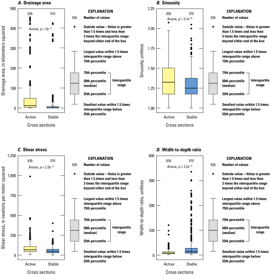
Stable cross sections have smaller drainage areas, are straighter (less sinuous),
have less potential energy (shear stress), and have larger width-to-depth ratios. — Figure 8.
Comparison of the means of active and stable cross sections using the ANOVA method for A, drainage area, B, sinuosity, C, shear stress, and D, width-to-depth ratio. If p-values (p) are less than 0.05, there is statistically significant difference between the group means (Homan, 2024).

Figure 9 shows ANOVA boxplots to compare the means of the active cross sections subclassifications (incising and widening) for drainage area, sinuosity, shear stress, and width-to-depth ratio. The active cross sections have drainage areas and sinuosities statistically different based on p-values less than 0.05, whereas the shear stresses and width-to-depth ratios are not significantly different based on p-values greater than 0.05.

Widening cross sections have significantly larger drainage areas and are more sinuous
than incising cross sections, whereas the shear stresses and width-to-depth ratios
are not significantly different based p-values greater than 0.05. — Figure 9.
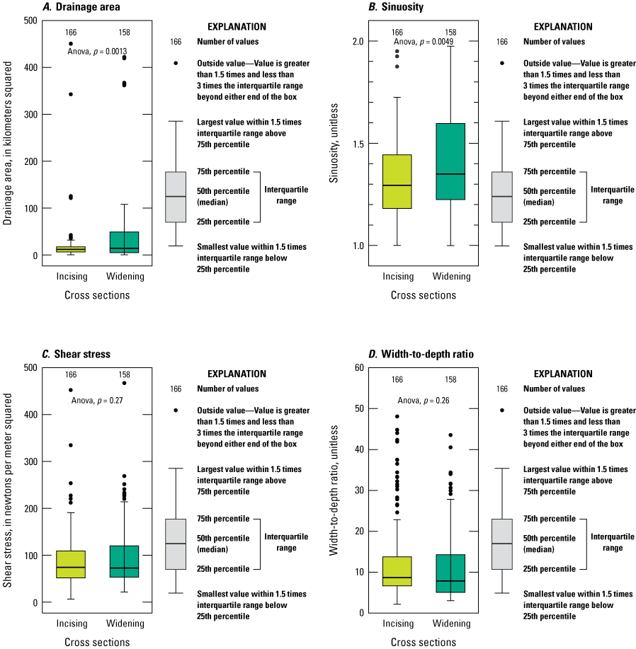
Comparison of the means of incising and widening active cross sections using the ANOVA method for A, drainage area, B, sinuosity, C, shear stress, and D, width-to-depth ratio. If p-values (p) are less than 0.05, there is statistically significant difference between the group means (Homan, 2024).

Channel stability trends and thresholds are compared in figures 8 and 9. The median drainage area for stable cross sections is 5.8 km², which is less than half the size of drainage areas for active cross sections. Within the active channel reaches, incising channels have smaller drainage areas. As drainage area increases, bank heights of the incising channels appear to reach a critical height for mass wasting resulting in the largest drainage areas with a stability classification of widening (fig. 9A). To assess if there is a drainage area threshold that activates stable channels to become unstable (incising or widening), majority rule was used to isolate a transitional zone between the stability classifications. For example, more than half the stable channels have drainage areas smaller than those of active channels. Of the 570 stable cross sections, a majority (51 percent) had drainage areas smaller than 5.8 km², whereas the majority of the 836 active (observed erosion) cross sections had drainage areas greater than 13.2 km². In contrast, 77 percent of stable cross sections had drainage areas smaller than 13.2 km², and 67 percent of active cross sections had drainage areas larger than 5.7 km² (fig. 8A). Based on the majority rule, most channels transition from stable to active for drainage areas between about 6 and 13 km². The drainage areas within the study area range from 1 to 450 km² (fig. 8A; Homan, 2024).

A similar trend is presented with increases in sinuosity (fig. 8B). Channels with lower sinuosities are predominantly stable, and increases in sinuousness lead to a greater likelihood of channel instability. Straighter (lower sinuosity) cross sections with evidence of active erosion are dominated by incision, whereas more sinuous cross sections exhibit greater widening (fig. 9B). Of the 570 stable cross sections, the majority (51 percent) had sinuosity at or less than 1.25, whereas the majority of the 836 active cross sections had sinuosities greater than 1.32. In contrast, 56 percent of stable cross sections had sinuosities smaller than 1.32, and 65 percent of active cross sections had sinuosities greater than 1.25. Overall, sinuosities range from 1 to 2.07 (fig. 8B; Homan, 2024), and increasing sinuousness is shown to relate to channel instability, with a stability transition range between 1.25 and 1.32.

Cross sections with larger shear stress had greater channel instability (fig. 8C), even if shear stress is not statistically different between the incising and widening channels (fig. 9C). Of the 570 stable cross sections, a majority (51 percent) had shear stress at or less than 47 N/m², whereas the majority of the 836 active cross sections had shear stress greater than 68 N/m² (fig. 8C). In contrast, 72 percent of stable cross sections have shear stress less than 68 N/m², and 73 percent of active cross sections had shear stress greater than 47 N/m². Overall, shear stress ranges from 1.7 to 990 N/m² (fig. 8C; Homan, 2024), and increases in shear stress are shown to relate to channel instability, with a stability transition range between 48 and 68 N/m².

Width-to-depth (W/D) ratios display an opposite trend from the three previously discussed explanatory variables because larger values relate to increases in stability (fig. 8D). Like shear stress, W/D ratios were not statistically distinguishable between incising and widening channels (fig. 9D). Of the 570 stable cross sections, a majority (51 percent) had W/D ratios equal to or greater than 13, whereas the majority of the 836 active cross sections had W/D ratios less than 9. In contrast, 79 percent of stable cross sections had W/D ratios larger than 9, and 75 percent of active cross sections had W/D ratios less than 13. Overall, the W/D ratio ranged from 1.5 to 335 for the active and stable cross sections (fig. 8D; Homan, 2024), and decreases in W/D ratio are shown to relate to channel instability, with a stability transition range between 13 and 9.

In summary, predominantly stable cross sections had a drainage area of less than 6 km², sinuosity less than 1.25, shear stress smaller than 47 N/m², and a W/D ratio greater than 13. Cross sections with active erosion generally had a drainage area of greater than 13 km², sinuosity more than 1.32, shear stress larger than 68 N/m², and a W/D ratio smaller than 9. Stream sections between these ranges are considered stability transition zones. These zones are based on the majority rule and contribute to our understanding of when stable channels become unstable, which is helpful for predicting channel stability, but the identification of such zones does not necessarily outline which mechanisms are affecting erosion.

Channel Stability Characteristics

The evaluation of the most effective predictor variables highlighted a consistent progression of stream channel cross sections progressing from stable, to incising, to, ultimately, widening. To assess the channel stability characteristics of the 1,406 cross sections with field-based stability classifications, the geomorphic and hydraulic parameters were normalized using the Min-Max technique (eq. 7), and the key explanatory variables are provided in table 3. The normalization goal is to make every data parameter have the same weight, so each feature is equally important. The geomorphic and hydraulic parameters were derived from the Q₁₀ streamflow acquired from StreamStats, and the normalized results show stable channels to be relatively wide and shallow with consequently larger W/D ratios and smaller streamflow cross-sectional areas (table 3). Their drainage areas are also reduced, which equates to less Q₁₀ streamflow, because StreamStats streamflows are based on drainage area regressions (USGS, 2019b). Given less Q₁₀ streamflow, stable channels also have lower velocities, as well as smaller shear stresses (table 3).

Table 3.

Minimum-maximum normalization values (unitless) for explanatory variables affecting channel instability.

Table 3. Minimum-maximum normalization values (unitless) for explanatory variables affecting channel instability.
	Stable	Incising	Widening
Drainage area	0.05	0.05	0.12
Sinuosity	0.26	0.30	0.37
Shear stress	0.06	0.09	0.09
Width to depth	0.09	0.03	0.03
Channel bed slope	0.10	0.11	0.09
Streamflow area	0.13	0.15	0.23
Hydraulic radius	0.25	0.34	0.44
Water depth	0.18	0.25	0.33
Top width	0.19	0.18	0.20
Water velocity	0.25	0.29	0.29

When comparing stable and incising channels, all explanatory variables in table 3 are different, except for drainage area and, therefore, Q₁₀ streamflow. In the previous sections, active and stable channels have statistically different mean drainage areas (fig. 8A), but analysis included all active channels compared to all stable channels. Figure 10 shows direct comparisons of drainage areas for stable, incising, and widening channels, where p-values (p) less than or equal to 0.05 (the significance level) illustrates statistically significant difference between the group means. The drainage areas for stable and incising channels are not significantly different, whereas widening channels have significantly different drainage areas. Compared to stable channels, table 3 shows incised stream channels are deeper, are faster flowing (higher velocities), and have greater shear stresses without an increase in drainage areas and therefore Q₁₀ streamflow. As mentioned earlier, a channel incising stream response can be a byproduct of decreases in sediment supply, increases in channel bed slope, increases in streamflow, and (or) increases in velocity not associated with an increase in channel bed slope. Without an increase in streamflow (Q), a stable channel cross section (A) is not expected to manifest sudden increases in velocity (V) not associated with an increase in channel bed slope based on equation 1 (Q = VA). Additionally, sediment supplies are not likely limited, because the Mancos Shale is highly erodible (Whittig and others, 1982). The initiation of downcutting likely results from an increase in channel bed slope. Examination of table 3 shows incising channels have the maximum channel bed slopes among the three stability classifications. Overall, incising channels present steeper channel bed slopes, which are considered the affecting force in inducing higher velocities and greater shear stresses. In turn, higher velocities and greater shear stresses cause the channels to become deeper, narrower, and to have reduced W/D ratios (table 3).

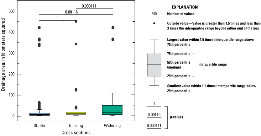
Comparison of mean drainage areas. — Figure 10.
Comparison of the mean drainage areas of stable, incising, and widening cross sections of reaches in ephemeral streams in Grand Valley, western Colorado. If p-values (p) are less than 0.05, there is a statistically significant difference between the group means (Homan, 2024).

During the evolutionary progression (either temporally or spatially) of channel stability, channel incision processes dominate initial channel adjustments more than channel widening. However, channel widening begins either because bank heights of incising channels reach a critical height for mass wasting, or because channel curvatures cause higher sidewall stresses. Table 3 and figure 9 show channel widening results in amplified sinuosities and corresponding decreases in channel bed slopes.

Figure 11 shows the locations of stable, incising, widening, and incising and widening channels. Visually, there is no consistent channel evolutionary pattern. The heterogeneous occurrence of channel stability is likely a result of the 48 stream channels having sizable ranges in lengths (1 to 29 km), drainage areas (1 to 450 km²), and elevation changes (20 to 680 m) (Homan, 2024). A short, steep channel responds differently than a long, gradual channel, and channels extending into the Book Cliff escarpments respond differently than those residing primarily in the valley floor. Regardless, the observed dataset encompasses the entire study area, and the normalized results present a summary of all scenarios. The lack of consistent evolutionary pattern was not unexpected. As mentioned in the “Geomorphic Characteristics for Ephemeral Streams” section of this report, other studies demonstrated ephemeral channels commonly exhibit spatial variability and longitudinal discontinuity in arid regions (Leopold and others, 1964; Graf and Lecce, 1988; Bull and Kirkby, 2002).

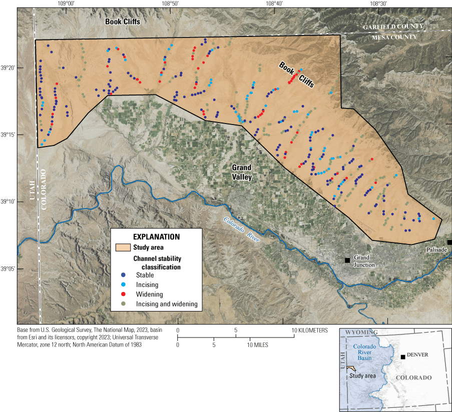
Visually there is no consistent channel evolutionary pattern. — Figure 11.
Map showing channels with stable, incising, incising and widening, and widening cross sections in the Grand Valley, western Colorado (Homan, 2024).

Mechanisms Affecting Erosion

Hydraulically stable channels are those with channel bed slopes resisting forces affecting Earth’s materials downstream. Shear stress, the force applied by flowing liquid to its boundary, is described as the force of water trying to drag the channel surface downstream with it (Meyer-Peter and Müller, 1948; Fernandez Luque and Beek, 1976; Petit and others, 2005). Based on the channel stability evolution within the study area and assessment of explanatory variables, the mechanism affecting changes in channel stability was fluctuations in channel bed slope and shear stress. Channel bed slope and shear stress are also in the theoretical equation for bed shear stress (DuBoys, 1879), where increases in channel bed slope results in increased bed shear stress. Variations in channel bed slope in ephemeral streams often relate to responses in short-lived, infrequent streamflow resulting in progressive episodes of channel incision and filling and from changes in the sinuosity of meander bends (Schumm, 1977; Patton and Schumm, 1981).

Initially, smaller drainage areas within the study area begin with stable channels (fig. 8A). Increased channel slopes result in shear stresses large enough to start erosion (table 3) with bed channel erosion (incision) first dominating more than channel widening. Incision and subsequent increases in water depths create a feedback system amplifying shear stress. For straight channels, shear stress is the same across the width of the channel bottom (Chen and Cotton, 1986); however, if the channel curves, shear stress will be higher on the outside of the bend as compared to the inside of the bend (the sharper the bend, the greater the effect). Either because bank heights of incising channels reach a critical height for mass wasting, or because channel curvatures cause higher sidewall stresses, channel widening begins. Additional channel widening leads to increases in sinuosity, and resultant decreases in channel bed slope (table 3). As a result, stable and widening channels can have lower channel bed slopes, making channel bed slope a poor explanatory variable despite its ability to drive channel erosion.

Relations between bed shear stress and streamflow have also shown cross-sectional average bed shear stress to increase with streamflow (Sambrook Smith and others, 2010). The current investigation was based on a specified 0.10 annual exceedance probability streamflow (Q₁₀), and it recognized fluctuations in streamflow would also affect channel stability. Following is a discussion about past and current changes within the study area that affect streamflow and therefore affect the mechanisms affecting erosion.

Historical and current grazing (Lusby, 1979; Fick and others, 2020) and an extensive network of unpaved roads and trails (BLM, 2020) are land use disturbances within the study area that potentially altered flow characteristic and increased stream channel instability. These two forms of land degradation cause soil compaction and loss of native plants (Al-Dousari and others, 2019), which decrease precipitation infiltration and increase runoff (Greene and others, 1994). The unprecedented surface disturbances levels also destroyed biological crusts and increased soil erosion rates, making this region less tolerant to drought (Schwinning and others, 2008). To compound the situation further, the Upper Colorado River Basin is in an ongoing 22-year megadrought (Gangopadhyay and others, 2022), which further reduces vegetation cover on slopes and makes hillslope soils more prone to erosion during heavy precipitation (McAuliffe and others, 2006). As global and Colorado River Basin temperatures rise, extreme temperature and precipitation are also becoming more frequent and (or) intense (Intergovernmental Panel on Climate Change, 2012, 2021). Research shows a decline in monsoon frequency in the Colorado River Basin, but it also shows an increase in more extreme monsoon storms (Pascale and others, 2017; McCoy and others, 2022). Intensifying erosion further during this study, vegetation surrounding the upper headwaters of the study area caught fire and at the time became the largest wildfire in Colorado State history (Encyclopedia Staff, 2023). Wildland fires on western United States rangelands also exposes landscapes to amplified runoff and erosion during the short and long term and increase the risk of damage to soil (Pierson and others, 2011). Land use disturbances, soil compaction, vegetation cover loss, drought, less frequent and more extreme precipitation, and fires have all intensified the potential runoff and erosion within the study area.

Summary

The Grand Valley in western Colorado is in the semiarid Southwest United States. The north side of the Grand Valley has many ungaged ephemeral streams, which are of particular interest because (1) the underlying bedrock geology, Mancos Shale, is a sedimentary rock deposit identified as a major contributor of dissolved mineral salts to the Colorado River and (2) despite infrequent streamflow of short duration, monsoon-derived floods in these ephemeral streams can carry substantial amounts of sediment downstream. These points of interest are important because salinity, or the total dissolved solids concentration, in the Colorado River causes an estimated $300 million to $400 million per year in economic damages in the United States, and it is estimated 62 percent of the total dissolved solid loads in the Upper Colorado River Basin originate from geologic sources. Salt loading in these environments is closely associated with sediment loading. Any practices to reduce erosion and store sediment in highly saline arid landscapes, especially in headwater areas, could have the effect of retaining salt in the trapped sediment. In an effort to minimize salt contributions to the Colorado River from public lands administered by the Bureau of Land Management, a comprehensive salinity control approach is typically used to reduce nonpoint sources of salinity through land management techniques and practices.

In 2018, the U.S. Geological Survey, in cooperation with the Bureau of Land Management, began an assessment of ephemeral streams located in the north side of the Grand Valley, western Colorado, to characterize stream channel stability and identify mechanisms affecting erosion. In doing so, the U.S. Geological Survey developed a method for automatically extracting channel geometries from existing remotely sensed terrain models and based on estimated flood stage streamflows, hydraulic characteristics were calculated. Furthermore, channel geometries and hydraulic characteristics were used in a statistical model to estimate channel stability for the ephemeral streams at individual cross sections.

Based on a stream channel stability assessment, cross-section stabilities were available for a subset of 1,406 visited locations but still needed for the 13,415 cross sections delineated from remotely sensed terrain models. Manning’s resistance equation application in combination with multiple logistic regression models demonstrated channel stability can be estimated with a 0.845 goodness of fit for a validation dataset when using an explanatory variable combination of drainage area, width-to-depth ratio, sinuosity, and shear stress. Using the multiple logistic regression model and defined explanatory variables, stream channel stability was extrapolated for the remaining unvisited cross sections. Mapping the ephemeral streams and their stabilities in this arid rangeland underlain by saline-rich Mancos Shale may be used to prioritize areas for remediation or changes in management strategies to reduce sediment and salinity loading to the Colorado River.

The study results demonstrated channel stability within the ephemeral streams to be spatially variable, longitudinally discontinuous, and dictated by channel bed slope changes. Stable ephemeral streams were relatively wide, shallow, and direct channels with smaller drainage areas and little potential for producing shear stresses able to overcome channel adhesion. A channel bed slope change can provide the means necessary to generate shear stresses appropriate to initiate erosion and a subsequent stability transition to an incising channel. Channel widening happens when either incising channel bank heights reach a mass wasting critical height, or when channel curvatures cause higher sidewall stresses. Regardless, widening channels increase sinuosities and subsequently cause shallower channel bed slopes. Consequently, stable and widening channels can have comparable channel bed slopes, making channel bed slope a poor explanatory variable for predicting channel stability, despite its capability to initiate channel instability.

The results were based on a specified 0.10 annual exceedance probability streamflow, and showed fluctuations in streamflow would also affect channel stability. Past and current changes within the study area that affect streamflow and therefore mechanisms affecting erosion include land use disturbances, soil compaction, vegetation cover loss, drought, less frequent more extreme precipitation, and fires, all of which intensify the potential runoff and erosion within the study area.

References Cited

Al-Dousari, A.M., Alsaleh, A., Ahmed, M., Misak, R., Al-Dousari, N., Al-Shatti, F., Elrawi, M., and William, T., 2019, Off-road vehicle tracks and grazing points in relation to soil compaction and land degradation: Earth Systems and Environment 3, p. 471–482, accessed October 2021 at https://doi.org/10.1007/s41748-019-00115-y.

Allen, D.C., Datry, T., Boersma, K.S., Bogan, M.T., Boulton, A.J., Bruno, D., Busch, M.H., Costigan, K.H., Dodds, W.K., Fritz, K.M., Godsey, S.E., Jones, J.B., Kaletova, T., Kampf, S.K., Mims, M.C., Neeson, T.M., Olden, J.D., Pastor, A.V., Poff, N.LR., Ruddell, B.L., Ruhi, A., Singer, G., Vezza, P., Ward, A.S., and Zimmer, M., 2020, River ecosystem conceptual models and non‐perennial rivers—A critical review: WIREs Water, v. 7, no. 5, accessed October 2021 at https://doi.org/10.1002/wat2.1473.

Anning, D.W., Bauch, N.J., Gerner, S.J., Flynn, M.E., Hamlin, S.N., Moore, S.J., Schaefer, D.H., Anderholm, S.K., and Spangler, L.E., 2007, Dissolved solids in basin-fill aquifers and streams in the southwestern United States (ver. 1.1, March 2010): U.S. Geological Survey Scientific Investigations Report 2006–5315, 168 p. [Also available at https://doi.org/10.3133/sir20065315.]

Azen, R., and Budescu, D.V., 2006, Comparing predictors in multivariate regression models—An extension of dominance analysis: Journal of Educational and Behavioral Statistics, v. 31, no. 2, p. 157–180, accessed October 2021 at https://doi.org/10.3102/10769986031002157.

Babcock, H.M., and Cushing, E.M., 1942, Recharge to ground‐water from floods in a typical desert wash, Pinal County, Arizona: Eos, Transactions, American Geophysical Union, v. 23, no. 1, p. 49–56. [Also available at https://doi.org/10.1029/TR023i001p00049.]

Bagnold, R.A., 1966, An approach to the sediment transport problem from general physics: U.S. Geological Survey Professional Paper 422-I, 137 p. [Also available at https://doi.org/10.3133/pp422I.]

Bagnold, R.A., 1977, Bed load transport by natural rivers: Water Resources Research, v.13, no. 2, p. 303–312. [Also available at https://doi.org/10.1029/WR013i002p00303.]

Belnap, J., Büdel, B., and Lange, O.L., 2001, Biological soil crusts—Characteristics and distribution, chap. 1 of Belnap, J., and Lange, O.L., eds., Biological soil crusts—Structure, function, and management, v. 150 of Baldwin, I.T., Caldwell, M.M., Heldmaier, G., Lange, O.L., Mooney, H.A., Schulze, E.–D., Sommer, U., eds., Ecological Studies: Heidelberg, Springer-Verlag, p. 3–30. [Also available at https://doi.org/10.1007/978-3-642-56475-8_1.]

Bentley, R.G., Jr., Eggleston, K.O., Price, D., Frandsen, E.R., Dickerman, A.R., Thompson, J.H., and Heath, A.P., 1978, The effects of surface disturbance (primarily livestock use) on the salinity of public lands in the upper Colorado River Basin—1977 status report: Bureau of Land Management, 274 p.

Berkson, J., 1944, Application of the logistic function to bio-assay: Journal of the American Statistical Association, v. 39, no. 227, p. 357–365.

Berkson, J., 1951, Relative precision of minimum chi-square and maximum likelihood estimates of regression coefficients, in Neyman, J., ed., Proceedings of the Second Berkeley Symposium on Mathematical Statistics and Probability, Berkeley, Calif., July 31–August 12, 1950: Berkeley, Calif., University of California Press, v. 2, p. 471–479.

Bizzi, S., and Lerner, D.N., 2015, The use of stream power as an indicator of channel sensitivity to erosion and deposition processes: River Research and Applications, v. 31, no. 1, p. 16–27, accessed October 2021 at https://doi.org/10.1002/rra.2717.

Bledsoe, B.P., 1999, Specific stream power as an indicator of channel pattern, stability, and response to urbanization: Fort Collins, Colorado, Colorado State University, Ph.D. dissertation, p. 1–24.

Boyd, R., and Green, C., 2018, A framework for improving the effectiveness of the Colorado River Basin Salinity Control Program, 2018–2023: Denver, Colo., Bureau of Land Management, National Operations Center, p. 1–20, accessed October 2021 at https://www.blm.gov/documents/national-office/blm-library/report/framework-improving-effectiveness-colorado-river-basin.

Branson, F.A., Miller, R.F., and McQueen, I.S., 1976, Moisture relationships in twelve northern desert shrub communities near Grand Junction, Colorado: Ecology, v. 57, no. 6, p. 1104–1124, accessed October 2021 at https://doi.org/10.2307/1935039.

Budescu, D.V., 1993, Dominance analysis—A new approach to the problem of relative importance of predictors in multiple regression: Psychological Bulletin, v. 114, no. 3, p. 542–551, accessed October 2021 at https://doi.org/10.1037/0033-2909.114.3.542.

Bull, L.J., and Kirkby, M.J., 2002, Dryland rivers—Hydrology and geomorphology of semi-arid channels: Chichester, United Kingdom, Wiley, 398 p.

Bureau of Land Management [BLM], 1987, Salinity control on BLM-administered public lands in the Colorado River Basin—A report to Congress, BLM/YA/PT-87/019+7000, July 1987: Bureau of Land Management, 43 p.

Bureau of Land Management [BLM], 2004, Salinity control on Bureau of Land Management (BLM)-administered public lands in the Colorado River Basin—A report to Congress, December 2004: Bureau of Land Management, 41p.

Bureau of Land Management [BLM], 2020, BLM national ground transportation linear feature public display polylines: Bureau of Land Management, accessed October 2021 at https://www.arcgis.com/home/item.html?id=f94999eb674d4085be0c86729fe4a151.

Bureau of Reclamation, 2001, Quality of water, Colorado River Basin, Upper Colorado Region, Bureau of Reclamation Progress Report No. 20.

Bureau of Reclamation, 2017, Quality of water, Colorado River Basin: Bureau of Reclamation, Progress Report No. 25, p. 76, accessed October 2021 at https://www.usbr.gov/uc/progact/salinity/pdfs/ProgressReports/PR25final.pdf.

Capesius, J.P., and Stephens, V.C., 2009, Regional regression equations for estimation of natural streamflow statistics in Colorado: U.S. Geological Survey Scientific Investigations Report 2009–5136, 46 p., accessed October 2021 at https://pubs.usgs.gov/sir/2009/5136/.

Carson, M.A., 1971, The mechanics of erosion—Monographs in spatial and environmental systems analysis: London, Pion Press, 174 p.

Chen, Y.H., and Cotton, G.K., 1986, Design of roadside channels with flexible linings: Federal Highway Administration, Hydraulic Engineering Circular No. 15, Report No. FHWA-IP-86-5.

Chow, V.T., 1959, Open‐channel hydraulics: New York, McGraw‐Hill, 680 p.

Colorado River Basin Salinity Control Forum, 2014, 2014 Review—Water quality standards for salinity, Colorado River System: Colorado River Basin Salinity Control Forum, 100 p., accessed October 2021 at https://coloradoriversalinity.org/docs/2014%20Final%20REVIEW%20-%20complete.pdf.

Constantz, J., Thomas, C.L., and Zellweger, G., 1994, Influence of diurnal variations in stream temperature on streamflow loss and groundwater recharge: Water Resources Research, v. 30, no. 12, p. 3253–3264, accessed October 20, 2021, at https://doi.org/10.1029/94WR01968.

Cornish, J.H., 1961, Flow losses in dry sandy channels: Journal of Geophysical Research, v. 66, no. 6, p. 1845–1853, accessed October 2021 at https://doi.org/10.1029/JZ066i006p01845.

Cowan, W.L., 1956, Estimating hydraulic roughness coefficients: Agricultural Engineering, v. 37, no. 7, p. 473–475.

Cox, D.R., and Lewis, P.A.W., 1966, The statistical analysis of series of events: London, Methuen, 285 p.

Cuevas, A., Febrero, M., and Fraiman, R., 2004, An anova test for functional data: Computational Statistics & Data Analysis, v. 47, no. 1, p. 111–122. [Also available at https://doi.org/10.1016/j.csda.2003.10.021.]

Datry, T., Boulton, A.J., Bonada, N., Fritz, K., Leigh, C., Sauquet, E., Tockner, K., Hugueny, B., and Dahm, C.N., 2018, Flow intermittence and ecosystem services in rivers of the Anthropocene: Journal of Applied Ecology, v. 55, no. 1, p. 353–364. [Also available at https://doi.org/10.1111/1365-2664.12941.]

Draper, N., and Smith, H., 1981, Applied regression analysis (2d ed.): New York, Wiley, 709 p.

DuBoys, M.P., 1879, Etudes du regime et l’action exercée par les eaux sur un lit a fond de graviers indefinement affouilable: Annals des Ponts et Chaussées, v. 18 of 5, p. 141–195.

Efron, B., 2003, Second thoughts on the bootstrap: Statistical Science, v. 18, no. 2, p. 135–140, accessed October 2021 at https://doi.org/10.1214/ss/1063994968.

Efron, B., and Tibshirani, R.J., 1993, An introduction to the bootstrap, v. 57 of Cox, D.R., Hinkley, D.V., Reid, N., Rubin, D.B., and Silverman, B.W., eds., Monographs on statistics and applied probability: New York, Chapman & Hall/CRC, 456 p.

Efroymson, M.A., 1960, Multiple regression analysis, in Ralston, A., and Wilf, H.S., eds., Mathematical methods for digital computers: New York, Wiley, p. 191–203.

Encyclopedia Staff, 2023, Pine Gulch Fire, Colorado Encyclopedia, last modified July 18, 2023, accessed July 2023 at https://coloradoencyclopedia.org/article/pine-gulch-fire.

Esri, 2020, ArcGIS: Redlands, Calif., Esri version 10.8.1.

Fernandez Luque, R., and Beek, R., van, 1976, Erosion and transport of bed-load sediment: Journal of Hydraulic Research, v. 14, no. 2, p. 127–144, accessed October 2021 at https://doi.org/10.1080/00221687609499677.

Fick, S.E., Belnap, J., and Duniway, M.C., 2020, Grazing-induced changes to biological soil crust cover mediate hillslope erosion in long-term exclosure experiment: Rangeland Ecology & Management, v. 73, no. 1, p. 61–72, accessed October 2021 at https://doi.org/10.1016/j.rama.2019.08.007.

Fischenich, J.C., Woessmer, W., and Potts, D.F., 1989, Channel erosion analysis and control, Symposium proceedings Headwaters Hydrology, American Water Resources Association.

Fisher, D.J., Erdmann, C.E., and Reeside, J.B., Jr., 1960, Cretaceous and Tertiary formations of the Book Cliffs, Carbon, Emery, and Grand counties, Utah, and Garfield and Mesa Counties, Colorado: U.S. Geological Survey Professional Paper 332, 80 p., accessed June 13, 2022, at https://doi.org/10.3133/pp332.

Froude, W., 1861, On the rolling of ships: Transactions of the Institution of Naval Architects, v. 3, p. 45–62.

Gangopadhyay, S., Woodhouse, C.A., McCabe, G.J., Routson, C.C., and Meko, D.M., 2022, Tree rings reveal unmatched 2nd century drought in the Colorado River Basin: Geophysical Research Letters, v. 49, no. 11, p. 1–10, accessed October 2021 at https://doi.org/10.1029/2022GL098781.

Gellis, A., Hereford, R., Schumm, S.A., and Hayes, B.R., 1991, Channel evolution and hydrologic variations in the Colorado River basin—Factors influencing sediment and salt loads: Journal of Hydrology, v. 124, nos. 3–4, p. 317–344. [Also available at https://doi.org/10.1016/0022-1694(91)90022-A.]

Goodrich, D.C., Lane, L.J., Shillito, R.M., Miller, S.N., Syed, K.H., and Woolhiser, D.A., 1997, Linearity of basin response as a function of scale in a semiarid watershed: Water Resources Research, v. 33, no. 12, p. 2951–2965. [Also available at https://doi.org/10.1029/97WR01422.]

Graf, W.H., 1984, Hydraulics of sediment transport: Highlands Ranch, Colo., Water Resources Publications, p. 1–501.

Graf, W.L., 1983, Downstream changes in stream power in the Henry Mountains, Utah: Annals of the Association of American Geographers, v. 73, no. 3, p. 373–387. [Also available at https://doi.org/10.1111/j.1467-8306.1983.tb01423.x.]

Graf, W.L., and Lecce, S.A., 1988, Fluvial processes in dryland rivers: New York, Springer-Verlag, p. 1–346.

Greene, R.S.B., Kinnell, P.I.A., and Wood, J.T., 1994, Role of plant cover and stock trampling on runoff and soil-erosion from semi-arid wooded rangelands: Soil Research, v. 32, no. 5, p. 953–973. [Also available at https://doi.org/10.1071/SR9940953.]

Harvey, M.D., and Watson, C.C., 1986, Fluvial processes and morphological thresholds in incised channels restoration: Journal of the American Water Resources Association, v. 22, no. 3, p. 359–368. [Also available at https://doi.org/10.1111/j.1752-1688.1986.tb01890.x.]

Hassan, M.A., 1990, Observations of desert flood bores: Earth Surface Processes and Landforms, v. 15, no. 5, p. 481–485. [Also available at https://doi.org/10.1002/esp.3290150512.]

Hazra, A., and Gogtay, N., 2016, Biostatistics series module 3—Comparing groups—Numerical variables: Indian Journal of Dermatology, v. 61, no. 3, p. 251–260. [Also available at https://doi.org/10.4103/0019-5154.182416.]

Healy, M.J.R., 1984, The use of R² as a measure of goodness of fit: Journal of the Royal Statistical Society. Series A (General), v. 147, no. 4, p. 608–609, accessed October 2021 at https://doi.org/10.2307/2981848.

Helsel, D.R., Hirsch, R.M., Ryberg, K.R., Archfield, S.A., and Gilroy, E.J., 2020, Statistical methods in water resources: U.S. Geological Survey Techniques and Methods, book 4, chap. A3, 458 p., accessed October 2021 at https://doi.org/10.3133/tm4a3. [Supersedes USGS Techniques of Water-Resources Investigations, book 4, chap. A3, version 1.1.]

Henderi, H., Wahyuningsih, T., and Rahwanto, E., 2021, Comparison of Min-Max normalization and Z-score normalization in the K-nearest neighbor (kNN) algorithm to test the accuracy of types of breast cancer: International Journal of Informatics and Information Systems, v. 4, no. 1, p. 13–20. [Also available at https://doi.org/10.47738/ijiis.v4i1.73.]

Hettinger, R., and Kirschbaum, M., 2002, Stratigraphy of the Upper Cretaceous Mancos Shale (upper part) and Mesaverde Group in the southern part of the Uinta and Piceance basins, Utah and Colorado: U.S. Geological Survey Digital Data Series, DDS 69–B, accessed October 2021 at https://pubs.usgs.gov/dds/dds-069/dds-069-b/REPORTS/Chapter_12.pdf.

Hocking, R.R., 1976, A Biometrics invited paper—The analysis and selection of variables in linear regression: Biometrics, v. 32, no. 1, p. 1–49. [Also available at https://doi.org/10.2307/2529336.]

Homan, J.W., 2024, Ephemeral stream channel stability data from the Grand Valley, western Colorado, 2018–21: U.S. Geological Survey data release, https://doi.org/10.5066/P1DX9QXB.

Hooke, R.LB., 1967, Processes on arid-region alluvial fans: The Journal of Geology, v. 75, no. 4, p. 438–460. [Also available at https://doi.org/10.1086/627271.]

Hop, K., Strassman, A., Nordman, C., Pyne, M., White, R., Jakusz, J., Hoy, E., and Dieck, J., 2016, National Park Service Vegetation Mapping Inventory Program—Natchez Trace Parkway vegetation mapping project: National Park Service Natural Resource Report NPS/GULN/NRR—2016/1255, accessed October 2021 at https://www.nps.gov/im/vmi-natr.htm.

Hughes, D.A., and Sami, K., 1992, Transmission losses to alluvium and associated moisture dynamics in a semiarid ephemeral channel system in southern Africa: Hydrological Processes, v. 6, no. 1, p. 45–53. [Also available at https://doi.org/10.1002/hyp.3360060105.]

Hydrologic Engineering Center, 2021, HEC-RAS user’s manual, U.S. Army Corps of Engineers, accessed April 2021 at https://www.hec.usace.army.mil/confluence/rasdocs/rasum/latest.

Intergovernmental Panel on Climate Change, 2012, Summary for policymakers, in Field, C.B., Barros, V., Stocker, T.F., Qin, D., Dokken, D.J., Ebi, K.L., Mastrandrea, M.D., Mach, K.J., Plattner, G.-K., Allen, S.K., Tignor, M., and Midgley, P.M., eds., Managing the risks of extreme events and disasters to advance climate change adaptation—Special Report of the Intergovernmental Panel on Climate Change: Cambridge, United Kingdom, and New York, Cambridge University Press, p. 1–19, accessed October 2021 at https://doi.org/10.1017/CBO9781139177245.

Intergovernmental Panel on Climate Change, 2021, Summary for policymakers, in Masson-Delmotte, V., Zhai, P., Pirani, A., Connors, S.L., Péan, C., Berger, S., Caud, N., Chen, Y., Goldfarb, L., Gomis, M.I., Huang, M., Leitzell, K., Lonnoy, E., Matthews, J.B.R., Maycock, T.K., Waterfield, T., Yelekçi, O., Yu, R., and Zhou, B., eds., Climate change 2021—The physical science basis, working group I contribution to the sixth assessment report of the Intergovernmental Panel on Climate Change, p. 3–32: Cambridge, United Kingdom, Cambridge University Press.

Jackson, W.L., Janes, E.B, and Van Haveren, B.P., 1985, Managing headwater areas for control of sediment and salt production from western rangelands, in Moore, M.L., ed., Perspectives on nonpoint source pollution—Proceedings of a National Conference, Kansas City, Mo., May 19–22, 1985: U.S. Environmental Protection Agency, EPA 440/5-85-001, p. 347–351.

Jaeger, K.L., Olden, J.D., and Pelland, N.A., 2014, Climate change poised to threaten hydrologic connectivity and endemic fishes in dryland streams: Proceedings of the National Academy of Sciences, v. 111, no. 38, p. 13894–13899, accessed October 2021 at https://doi.org/10.1073/pnas.1320890111.

Jia, Y., 1990, Minimum Froude number and the equilibrium of alluvial sand rivers: Earth Surface Processes and Landforms, v. 15, no. 3, p. 199–209. [Also available at https://doi.org/10.1002/esp.3290150303.]

Kenny, D.A., 2020, Measuring model fit, accessed October 2021 at https://davidakenny.net/cm/fit.htm.

Kenney, T.A., Gerner, S.J., Buto, S.G., and Spangler, L.E., 2009, Spatially referenced statistical assessment of dissolved-solids load sources and transport in streams of the Upper Colorado River Basin: U.S. Geological Survey Scientific Investigations Report 2009–5007, 50 p., accessed October 2021 at https://doi.org/10.3133/sir20095007.

Keppel, R.V., and Renard, K.G., 1962, Transmission losses in ephemeral stream beds: Journal of the Hydraulics Division, v. 88, no. 3, p. 59–68. [Also available at https://doi.org/10.1061/JYCEAJ.0000734.]

Kircher, J.E., Choquette, A.F., and Richter, B.D., 1985, Estimation of natural streamflow characteristics in western Colorado: U.S. Geological Survey Water-Resources Investigations Report 85–4086, 28 p. [Also available at https://doi.org/10.3133/wri854086.]

Kleinhans, M.G., and Berg, J.H., van den, 2011, River channel and bar patterns explained and predicted by an empirical and a physics‐based method: Earth Surface Processes and Landforms, v. 36, no. 6, p. 721–738, accessed October 2021 at https://doi.org/10.1002/esp.2090.

Kohn, M.S., Stevens, M.R., Mommandi, A., and Khan, A.R., 2017, Peak discharge, flood frequency, and peak stage of floods on Big Cottonwood Creek at U.S. Highway 50 near Coaldale, Colorado, and Fountain Creek below U.S. Highway 24 in Colorado Springs, Colorado, 2016: U.S. Geological Survey Scientific Investigations Report 2017–5107, 58 p., accessed October 2021 at https://doi.org/10.3133/sir20175107.

Küchler, A.W., 1964, Manual to accompany the map, Potential natural vegetation of the conterminous United States: New York, American Geographical Society, Special publication no. 36, p. 39.

Laitila, T., 1993, A pseudo-R² measure for limited and qualitative dependent variable models: Journal of Econometrics, v. 56, no. 3, p. 341–355, accessed October 2021 at https://doi.org/10.1016/0304-4076(93)90125-O.

Lane, E.W., 1954, The importance of fluvial morphology in hydraulic engineering: Bureau of Reclamation, Engineering Laboratories, and Commissioner’s Office Hydraulic laboratory report no. 372, 19 p.

Lane, J.Q., Raimondi, P.T., and Kudela, R.M., 2009, Development of a logistic regression model for the prediction of toxigenic Pseudo-nitzschia blooms in Monterey Bay, California: Marine Ecology Progress Series, v. 383, p. 37–51, accessed October 2021 at https://doi.org/10.3354/meps07999.

Lane, L.J., Diskin, M.H., and Renard, K.G., 1971, Input-output relationships for an ephemeral stream channel system: Journal of Hydrology, v. 13, p. 22–40. [Also available at https://doi.org/10.1016/0022-1694(71)90198-3.]

Larned, S.T., Datry, T., Arscott, D.B., and Tockner, K., 2010, Emerging concepts in temporary‐river ecology: Freshwater Biology, v. 55, no. 4, p. 717–738, accessed October 2021 at https://doi.org/10.1111/j.1365-2427.2009.02322.x.

Leigh, C., Boulton, A.J., Courtwright, J.L., Fritz, K., May, C.L., Walker, R.H., and Datry, T., 2016, Ecological research and management of intermittent rivers—An historical review and future directions: Freshwater Biology, v. 61, no. 8, p. 1181–1199, accessed October 2021 at https://doi.org/10.1111/fwb.12646.

Leopold, L.B., Wolman, M.G., and Miller, J.P., 1964, Fluvial processes in geomorphology: New York, NY, Dover Publications, 544 p.

Levick, L., Fonseca, J., Goodrich, D., Hernandez, M., Semmens, D., Stromberg, J., Leidy, R., Scianni, M., Guertin, D.P., Tluczek, M., and Kepner, W., 2008, The ecological and hydrological significance of ephemeral and intermittent streams in the arid and semi-arid American Southwest: U.S. Environmental Protection Agency and USDA/ARS Southwest Watershed Research Center, EPA/600/R-08/134, ARS/233046, 116 p.

Lusby, G.C., 1979, Effects of grazing on runoff and sediment yield from desert rangeland at Badger Wash in western Colorado, 1953–73: U.S. Geological Survey Water-Supply Paper 1532–I, 134 p.

Lusby, G.C., Reid, V.H., and Knipe, O.D.,1971, Effects of grazing on the hydrology and biology of the Badger Wash Basin in western Colorado, 1953–66: U.S. Geological Survey Water-Supply Paper 1532–D, 90 p.

Lusby, G.C., Turner, G.T., Thompson, J.R., and Reid, V.H., 1963, Hydrologic and biotic characteristics of grazed and ungrazed watersheds of the Badger Wash Basin in western Colorado, 1953–58: U.S. Geological Survey Water‐Supply Paper 1532–B, 73 p.

McAuliffe, J.R., Scuderi, L.A., and McFadden, L.D., 2006, Tree-ring record of hillslope erosion and valley floor dynamics—Landscape responses to climate variation during the last 400 yr in the Colorado Plateau, northeastern Arizona: Global and Planetary Change, v. 50, nos. 3–4, p. 184–201, accessed October 2021 at https://doi.org/10.1016/j.gloplacha.2005.12.003.

McCoy, A.L., Jacobs, K.L., Vano, J.A., Wilson, J.K., Martin, S., Pendergrass, A.G., and Cifelli, R., 2022, The press and pulse of climate change—Extreme events in the Colorado River Basin: Journal of the American Water Resources Association [JAWRA], v. 58, no. 6, p. 1076–1097, accessed October 2021 at https://doi.org/10.1111/1752-1688.13021.

McFadden, D., 1974, The measurement of urban travel demand: Journal of Public Economics, v. 3, no. 4, p. 303–328. [Also available at https://doi.org/10.1016/0047-2727(74)90003-6.]

Merritt, D.M., and Wohl, E.E., 2003, Downstream hydraulic geometry and channel adjustment during a flood along an ephemeral, arid-region drainage: Geomorphology, v. 52, nos. 3–4, p. 165–180. [Also available at https://doi.org/10.1016/S0169-555X(02)00241-6.]

Messager, M.L., Lehner, B., Cockburn, C., Lamouroux, N., Pella, H., Snelder, T., Tockner, K., Trautmann, T., Watt, C., and Datry, T., 2021, Global prevalence of non-perennial rivers and streams: Nature, v. 594, p. 391–397, accessed October 2021 at https://doi.org/10.1038/s41586-021-03565-5.

Meyer-Peter, E., and Müller, R., 1948, Formulas for bed-load transport: International Association for Hydraulic Structures Research 2nd meeting, Stockholm, appendix 2.

Miller, M.P., Buto, S.G., Lambert, P.M., and Rumsey, C.A., 2017, Enhanced and updated spatially referenced statistical assessment of dissolved-solids load sources and transport in streams of the Upper Colorado River Basin: U.S. Geological Survey Scientific Investigations Report 2017–5009, 23 p., accessed October 2021 at https://doi.org/10.3133/sir20175009.

Osterkamp, W.R., Lane, L.J., and Foster, G.R., 1983, An analytical treatment of channel-morphology relations: U.S. Geological Survey Professional Paper 1288, 21 p.

Palmer, M.A., Reidy Liermann, C.A., Nilsson, C., Flörke, M., Alcamo, J., Lake, P.S., and Bond, N., 2008, Climate change and the world’s river basins—Anticipating management options: Frontiers in Ecology and the Environment, v. 6, no. 2, p. 81–89, accessed October 2021 at https://doi.org/10.1890/060148.

Pascale, S., Boos, W.R., Bordoni, S., Delworth, T.L., Kapnick, S.B., Murakami, H., Vecchi, G.A., and Zhang, W., 2017, Weakening of the North American monsoon with global warming: Nature Climate Change, v. 7, p. 806–812, accessed October 2021 at https://doi.org/10.1038/nclimate3412.

Patton, P.C., and Schumm, S.A., 1981, Ephemeral-stream processes—Implications for studies of Quaternary valley fills: Quaternary Research, v. 15, no. 1, p. 24–43. [Also available at https://doi.org/10.1016/0033-5894(81)90112-5.]

Petit, F., Gob, F., Houbrechts, G., and Assani, A.A., 2005, Critical specific stream power in gravel-bed rivers: Geomorphology, v. 69, nos. 1–4, p. 92–101. [Also available at https://doi.org/10.1016/j.geomorph.2004.12.004.]

Phillips, J.V., and Ingersoll, T.L., 1998, Verification of roughness coefficients for selected natural and constructed stream channels in Arizona: U.S. Geological Survey Professional Paper 1584, 77 p.

Pierson, F.B., Williams, C.J., Hardegree, S.P., Weltz, M.A., Stone, J.J., and Clark, P.E., 2011, Fire, plant invasions, and erosion events on western rangelands: Rangeland Ecology & Management, v. 64, no. 5, p. 439–449, accessed October 2021 at https://doi.org/10.2111/REM-D-09-00147.1.

Powell, D.M., Brazier, R., Wainwright, J., Parsons, A., and Kaduk, J., 2005, Streambed scour and fill in low‐order dryland channels: Water Resources Research, v. 41, no. 5, 13 p. [Also available at https://doi.org/10.1029/2004WR003662.]

Reid, I., and Frostick, L.E., 2011, Channel form, flows and sediments of endogenous ephemeral rivers in deserts, chap. 13 of Thomas, D.S.G., ed., Arid zone geomorphology—Process, form and change in drylands (3d ed.): Chichester, United Kingdom, Wiley, p. 301–332. [Also available at https://doi.org/10.1002/9780470710777.ch13.]

Reid, I., and Laronne, J.B., 1995, Bed load sediment transport in an ephemeral stream and a comparison with seasonal and perennial counterparts: Water Resources Research, v. 31, no. 3, p. 773–781. [Also available at https://doi.org/10.1029/94WR02233.]

Rosgen, D., 1998, The reference reach—A blueprint for natural channel design, in Hayes, D.F., Engineering approaches to ecosystem restoration—Conference proceedings, 1998 Wetlands Engineering & River Restoration Conference, Denver, Colo., March 22–27, 1998: Reston, Va., American Society of Civil Engineers, p. 1009–1016, accessed October 2021 at https://doi.org/10.1061/40382(1998)166.

RStudio Team, 2022, RStudio—Integrated development environment for R: Boston, Mass., RStudio, PBC, accessed October 2021 at http://www.rstudio.com.

Ruhi, A., Messager, M.L., and Olden, J.D., 2018, Tracking the pulse of the Earth’s fresh waters: Nature Sustainability, v. 1, p. 198–203, accessed October 2021 at https://doi.org/10.1038/s41893-018-0047-7.

Rydlund, P.H., Jr., and Densmore, B.K., 2012, Methods of practice and guidelines for using survey-grade global navigation satellite systems (GNSS) to establish vertical datum in the United States Geological Survey: U.S. Geological Survey Techniques and Methods, book 11, chap. D1, 102 p. [Also available at https://doi.org/10.3133/tm11D1.]

Sambrook Smith, G.H., Best, J.L., Ashworth, P.J., Lane, S.N., Parker, N.O., Lunt, I.A., Thomas, R.E., and Simpson, C.J., 2010, Can we distinguish flood frequency and magnitude in the sedimentological record of rivers?: Geology, v. 38, no. 7, p. 579–582, accessed October 2021 at https://doi.org/10.1130/G30861.1.

Santosa, F., and Symes, W.W., 1986, Linear inversion of band-limited reflection seismograms: SIAM Journal on Scientific and Statistical Computing, v. 7, no. 4, p. 1307–1330, accessed October 2021 at https://doi.org/10.1137/0907087.

Schumm, S.A., 1977, The fluvial system: New York, Wiley, 338 p.

Schumm, S.A., and Gregory, D.I., 1986, Diffuse-source salinity—Mancos Shale terrain: Bureau of Land Management, prepared by Water Engineering and Technology, Fort Collins, Colo., under contract no. CO-910-PH5-591, Technical Note 337, Report BLM-YA-PT-86-008-4341, 169 p.

Schumm, S.A., Harvey, M.D., and Watson, C.C., 1984, Incised channels—Morphology, dynamics, and control: Lone Tree, Colo., Water Resources Publications, 200 p.

Schwinning, S., Belnap, J., Bowling, D.R., and Ehleringer, J.R., 2008, Sensitivity of the Colorado Plateau to change—Climate, ecosystems, and society: Ecology and Society, v. 13, no. 2, p. 1–20, accessed October 2021 at https://www.jstor.org/stable/26268003.

Shanafield, M., Bourke, S.A., Zimmer, M.A., and Costigan, K.H., 2021, An overview of the hydrology of non‐perennial rivers and streams: WIREs Water, v. 8, no. 2, accessed October 2021 at https://doi.org/10.1002/wat2.1504.

Shanafield, M., Godsey, S., Datry, T., Hale, R., Zipper, S.C., Costigan, K., Krabbenhoft, C.A., Dodds, W.K., Zimmer, M., Allen, D.C., Bogan, M., Kaiser, K.E., Burrows, R.M., Hammond, J.C., Busch, M., Kampf, S., Mims, M.C., Burgin, A., and Olden, J.D., 2020, Science gets up to speed on dry rivers: Eos, v. 101, p 1–8, accessed October 2021 at https://doi.org/10.1029/2020EO139902.

Simon, A., and Darby, S.E., 1997, Process-form interactions in unstable sand-bed river channels—A numerical modeling approach: Geomorphology, v. 21, no. 2, p. 85–106. [Also available at https://doi.org/10.1016/S0169-555X(97)00043-3.]

Simons, D.B., and Sentürk, F., 1977, Sediment transport technology—Water and sediment dynamics: Lone Tree, Colo., Water Resources Publications, 871 p.

Stoica, P., and Selen, Y., 2004, Model-order selection—A review of information criterion rules: IEEE Signal Processing Magazine, v. 21, no. 4, p. 36–47, accessed October 2021 at https://doi.org/10.1109/MSP.2004.1311138.

Taddy, M., 2019, Business data science—Combining machine learning and economics to optimize, automate, and accelerate business decisions: New York, McGraw Hill, 384 p.

Theil, H., 1969, A multinomial extension of the linear logit model: International Economic Review, v. 10, no. 3, p. 251–259. [Also available at https://doi.org/10.2307/2525642.]

Tibshirani, R., 1996, Regression shrinkage and selection via the lasso: Journal of the Royal Statistical Society, Series B (Methodological), v. 58, no. 1, p. 267–288, accessed October 2021 at https://www.jstor.org/stable/2346178.

Tooth, S., 2000, Process, form and change in dryland rivers—A review of recent research: Earth-Science Reviews, v. 51, no. 1–4, p. 67–107. [Also available at https://doi.org/10.1016/S0012-8252(00)00014-3.]

Trent, R.E., and Brown, S.A., 1984, An overview of factors affecting river stability: Transportation Research Record 950, no. 2, p. 156–163.

Trimble, 2003, Trimble R7/R8 GPS receiver user guide, revision A: Trimble Navigation Limited, Engineering and Construction Division, 216 p.

Tuttle, M.L.W., 2009, Salt and selenium in the upper Colorado River—Processes of supply and transport from the Cretaceous Mancos Shale [abs.]: Geological Society of America Abstracts with Programs, v. 41, no. 7, p. 682, session no. 264, accessed October 2021 at https://gsa.confex.com/gsa/2009AM/webprogram/Paper163048.html.

Tuttle, M.L.W., Fahy, J.W., Elliott, J.G., Grauch, R.I., and Stillings, L.L., 2014, Contaminants from Cretaceous black shale—I. Natural weathering processes controlling contaminant cycling in Mancos Shale, southwestern United States, with emphasis on salinity and selenium: Applied Geochemistry, v. 46, p. 57–71. [Also available at https://doi.org/10.1016/j.apgeochem.2013.12.010.]

U.S. Geological Survey [USGS], 2019a, 3D Elevation Program 1-meter resolution digital elevation model [published 20200606]: U.S. Geological Survey website accessed October 17, 2019, at https://www.usgs.gov/the-national-map-data-delivery.

U.S. Geological Survey [USGS], 2019b, StreamStats program for Colorado: U.S. Geological Survey website accessed June 4, 2019, at https://water.usgs.gov/osw/streamstats/colorado.html.

U.S. Geological Survey [USGS], 2021, USGS water data for the Nation: U.S. Geological Survey National Water Information System database, accessed June 4, 2019, at https://doi.org/10.5066/F7P55KJN.

Veall, M.R., and Zimmermann, K.F., 1996, Pseudo-R² measures for some common limited dependent variable models: Journal of Economic Surveys, v. 10, no. 3, p. 241–259, accessed October 2021 at https://doi.org/10.1111/j.1467-6419.1996.tb00013.x.

Walters, C.J., Collie, J.S., and Webb, T., 1988, Experimental designs for estimating transient responses to management disturbances: Canadian Journal of Fisheries and Aquatic Sciences, v. 45, no. 3, p. 530–538. [Also available at https://doi.org/10.1139/f88-062.]

Ward, A.S., and Walsh, R., 2020, New Clean Water Act rule leaves U.S. waters vulnerable: Eos 101, accessed October 2021 at https://doi.org/10.1029/2020EO140022.

Ward, E.R., 1999, The Politics of place—Domestic and diplomatic priorities of the Colorado River Salinity Control Act (1974): Journal of Political Ecology, v. 6, no. 1, p. 31–56.

Watson, C.C., Biedenharn, D.S., and Bledsoe, B.P., 2002, Use of incised channel evolution models in understanding rehabilitation alternatives: Journal of the American Water Resources Association, v. 38, no. 1, p. 151–160. [Also available at https://doi.org/10.1111/j.1752-1688.2002.tb01542.x.]

Weltz, M.A., Nouwakpo, S.K., Rossi, C., Jolley, L.W., and Frasier, G., 2014, Salinity mobilization and transport from rangelands—Assessment, recommendations, and knowledge gaps: U.S. Department of Agriculture, General Technical Report 1, 61 p.

Whittig, L.D., Deyo, A.E., and Tanji, K.K., 1982, Evaporite mineral species in Mancos Shale and salt efflorescence, Upper Colorado River Basin: Soil Science Society of America Journal, v. 46, no. 3, p. 645–651, accessed October 2021 at https://doi.org/10.2136/sssaj1982.03615995004600030039x.

Wohl, E., 2000, Mountain Rivers, v. 14 of Water Resources Monograph: Washington, D.C., American Geophysical Union, 320 p. [Also available at https://doi.org/10.1029/WM014.]

Zimmer, M.A., Kaiser, K.E., Blaszczak, J.R., Zipper, S.C., Hammond, J.C., Fritz, K.M., Costigan, K.H., Hosen, J., Godsey, S.E., Allen, G.H., Kampf, S., Burrows, R.M., Krabbenhoft, C.A., Dodds, W., Hale, R., Olden, J.D., Shanafield, M., DelVecchia, A.G., Ward, A.S., Mims, M.C., Datry, T., Bogan, M.T., Boersma, K.S., Busch, M.H., Jones, C.N., Burgin, A.J., and Allen, D.C., 2020, Zero or not? Causes and consequences of zero‐flow stream gage readings: WIREs Water, v. 7, no. 3, p. e1436, accessed October 2021 at https://doi.org/10.1002/wat2.1436.

Zipper, S.C., Hammond, J.C., Shanafield, M., Zimmer, M., Datry, T., Jones, C.N., Kaiser, K.E., Godsey, S.E., Burrows, R.M., Blaszczak, J.R., Busch, M.H., Price, A.N., Boersma, K.S., Ward, A.S., Costigan, K., Allen, G.H., Krabbenhoft, C.A., Dodds, W.K., Mims, M.C., Olden, J.D., Kampf, S.K., Burgin, A.J., and Allen, D.C., 2021, Pervasive changes in stream intermittency across the United States: Environmental Research Letters, v. 16, no. 8, 17 p., accessed October 2021 at https://doi.org/10.1088/1748-9326/ac14ec.

Conversion Factors

International System of Units to U.S. customary units


Multiply	By	To obtain
Length
centimeter (cm)	0.3937	inch (in.)
meter (m)	3.281	foot (ft)
kilometer (km)	0.6214	mile (mi)
Area
square meter (m²)	0.0002471	acre
square kilometer (km²)	247.1	acre
Volume
cubic meter (m³)	35.31	cubic foot (ft³)
Flow rate
cubic meter per second (m³/s)	35.31	cubic foot per second (ft³/s)
meter per second (m/s)	3.281	foot per second (ft/s)
Mass
kilogram (kg)	2.205	pound avoirdupois (lb)
Density
kilogram per cubic meter (kg/m³)	0.06242	pound per cubic foot (lb/ft³)
Energy
joule (J)	0.0000002	kilowatthour (kWh)
Acceleration
gravity (g)	32.17405	foot per squared second (ft/s²)
Power
total stream power (Ω)	0.224809	pound-force per second (lbf/s)
unit (specific) stream power (ω)	0.317	BTU/hour square foot (BTU/h∙ft²)
Pressure
total shear stress averaged for stream width (τ)	0.000145037	pound per square inch (psi)

Datums

Vertical coordinate information is referenced to the North American Vertical Datum of 1988 (NAVD 88).

Horizontal coordinate information is referenced to the North American Datum of 1983 (NAD 83).

Elevation, as used in this report, refers to distance above the vertical datum.

Supplemental Information

Streamflow is given in cubic meter per second.

Acceleration due to gravity is in meter per second squared.

One newton (symbol: N) is the force needed to accelerate one kilogram of mass at the rate of one meter per second squared.

A watt (symbol: W) is a unit of power that is equal to 1 joule per second.

Abbreviations

3DEP: 3D Elevation Program
AIC: Akaike information criterion
DEM: digital elevation model
GNSS: Global Navigation Satellite System
km: kilometer
km²: square kilometer
LASSO: least absolute shrinkage and selection operator
lidar: light detection and ranging
m: meter
Min-Max: minimum-maximum
NAD 83: North American Datum of 1983
NAVD 88: North American Vertical Datum of 1988
Q: streamflow
Q_c: calculated streamflow
Q₁₀: 0.10 annual exceedance probability streamflow
USGS: U.S. Geological Survey
W/D: width-to-depth

Publishing support provided by the Science Publishing Network,

Denver Publishing Service Center

For more information concerning the research in this report, contact the

Director, USGS Colorado Water Science Center

Box 25046, Mail Stop 415

Denver, CO 80225

(303) 236-4882

Or visit the Colorado Water Science Center website at

https://www.usgs.gov/centers/co-water

Disclaimers

Any use of trade, firm, or product names is for descriptive purposes only and does not imply endorsement by the U.S. Government.

Although this information product, for the most part, is in the public domain, it also may contain copyrighted materials as noted in the text. Permission to reproduce copyrighted items must be secured from the copyright owner.

Suggested Citation

Homan, J.W., 2024, Assessment and characterization of ephemeral stream channel stability and mechanisms affecting erosion in Grand Valley, western Colorado, 2018–21: U.S. Geological Survey Scientific Investigations Report 2023–5145, 33 p., https://doi.org/10.3133/sir20235145.

ISSN: 2328-0328 (online)

Study Area

Additional publication details
Publication type	Report
Publication Subtype	USGS Numbered Series
Title	Assessment and characterization of ephemeral stream channel stability and mechanisms affecting erosion in Grand Valley, western Colorado, 2018–21
Series title	Scientific Investigations Report
Series number	2023-5145
DOI	10.3133/sir20235145
Year Published	2024
Language	English
Publisher	U.S. Geological Survey
Publisher location	Reston, VA
Contributing office(s)	Colorado Water Science Center
Description	Report: v, 33 p.; Data Release
Country	United States
State	Colorado
Other Geospatial	Grand Valley
Online Only (Y/N)	Y
Google Analytic Metrics	Metrics page

Assessment and Characterization of Ephemeral Stream Channel Stability and Mechanisms Affecting Erosion in Grand Valley, Western Colorado, 2018–21

Table of Contents

Links

Abstract

Introduction

Purpose and Scope

Description of the Study Area

Geomorphic Erosion Processes and Characteristics

Geomorphic Erosion Processes, Relations, and Responses

Geomorphic Characteristics for Ephemeral Streams

Methods for Ephemeral Stream Channel Assessment

Stream Channel Delineation, Cross-Section Profiles, and Surveys

Cross-Section Hydraulic Analysis

(1)

(2)

(3)

(4)

Stream Channel Stability

Stability Extrapolation

(5)

(6)

(7)

Ephemeral Stream Channel Assessment

Cross-Section Profiles

Estimated Ephemeral Channel Streamflows

Hydraulic Analysis Using the Manning’s Resistance Equation

Explanatory Variables Used Within the Multiple Logistic Regression Models

Table 1.

Stream Channel Stability Assessment

Table 2.

Stability Predictor Variables

Channel Stability Characteristics

Table 3.

Mechanisms Affecting Erosion

Summary

References Cited

Conversion Factors

Datums

Supplemental Information

Abbreviations

Disclaimers

Suggested Citation

Study Area