

Streamflow, Base Flow, and Precipitation Trends and Simulated Effects of Rush Springs Aquifer Groundwater Withdrawals on Base Flows Upgradient From Fort Cobb Reservoir, Western Oklahoma
Links
- Document: Report (6.76 MB pdf) , HTML , XML
- Data Release: USGS Data Release - MODFLOW-NWT model used to evaluate groundwater withdrawal scenarios for the Rush Springs aquifer upgradient from the Fort Cobb Reservoir, western Oklahoma, 1979–2015, including streamflow, base flow, and precipitation statistics
- NGMDB Index Page: National Geologic Map Database Index Page (html)
- Download citation as: RIS | Dublin Core
Acknowledgments
The project documented in this report was done by the U.S. Geological Survey in cooperation with the Bureau of Reclamation (Reclamation). Appreciation is extended to Collins Balcombe (Reclamation) and Anna Hoag (Reclamation) for initiating and supporting the project.
Abstract
To better understand the relation between groundwater use in the Rush Springs aquifer and inflows to the Fort Cobb Reservoir, the U.S. Geological Survey, in cooperation with the Bureau of Reclamation, used a previously published numerical groundwater-flow model and historical streamflow records to evaluate four scenarios to investigate how changing groundwater withdrawals could affect base flows in streams that flow into Fort Cobb Reservoir. These scenarios consisted of observing simulated base-flow response by (1) scaling the 20-year equal-proportionate-share groundwater-withdrawal rate by various percentages over a 50-year period; (2) scaling the historical groundwater-withdrawal rates by various percentages across the entire Rush Springs aquifer; (3) scaling the historical groundwater-withdrawal rates within various subareas (zones) of the Fort Cobb Reservoir surface watershed; and (4) simulating a base-flow-depletion scenario. Cobb, Lake, and Willow Creeks are the major streams upgradient from the Fort Cobb Reservoir (listed from highest to lowest mean annual base flow). The results of scenarios 1 and 2 indicated that Willow Creek is the most susceptible to drying, but Cobb Creek was the most likely to have reduced base flow. Scenarios 3 and 4 indicated that groundwater withdrawals affect Cobb Creek base flows over a broader watershed area compared to Lake and Willow Creeks. In scenario 4, Cobb Creek base-flow depletion was higher across a larger area than Lake Creek and Willow Creek. Groundwater withdrawals in the Cobb Creek watershed tended to affect total inflows into Fort Cobb Reservoir more than other areas in the extent of the Rush Springs aquifer.
Introduction
The Rush Springs aquifer is a bedrock aquifer in western Oklahoma (fig. 1) and is an important resource for municipal and irrigation water supply (Oklahoma Water Resources Board, 2012; Ellis, 2018b; Neel and others, 2018). Stakeholders, including the Bureau of Reclamation (Reclamation), are concerned with the ability of the Rush Springs aquifer to sustain increasing groundwater demand without decreasing base flows to streams that supply surface water to the Fort Cobb Reservoir. The Fort Cobb Reservoir is centrally located within the areal extent of the Rush Springs aquifer and the Cobb Creek surface-water watershed (hereinafter referred to as “Cobb Creek watershed”). Groundwater use within the study area is generally higher within the areal extent of the Cobb Creek watershed compared to other areas overlying the Rush Springs aquifer (Ellis, 2018b). The Cobb Creek watershed was defined for this analysis by the most applicable 10-digit hydrologic unit code (1113030205) (U.S. Geological Survey, 2017a). Cobb Creek, Lake Creek, and Willow Creek (fig. 1) contribute most of the surface-water inflow to the Fort Cobb Reservoir, which is used for flood control, public water supply, and recreational use. Groundwater use could potentially diminish base flows (the component of streamflow derived from groundwater; Heath, 1983; Barlow and Leake, 2012) and reduce the water supply to the Fort Cobb Reservoir.
The 1973 Oklahoma Water Law (82 OK Stat § 82-1020.5 [Oklahoma State Legislature, 2023b]) requires that the Oklahoma Water Resources Board (OWRB) conduct hydrologic investigations of the State’s groundwater basins to support a determination of the maximum annual yield (MAY) for each groundwater basin. The MAY is the maximum volume of fresh groundwater (less than 5,000 parts per million total dissolved solids [82 OK Stat § 82-1020.1 (Oklahoma State Legislature, 2023a)]) that can be withdrawn to “preserve” the groundwater basin that contains the Rush Springs aquifer for 20 years (OWRB, 2023; 82 OK Stat § 82-1020.5 [Oklahoma State Legislature, 2023b]). A bedrock aquifer (such as the Rush Springs aquifer) is considered preserved if at least 50 percent of the aquifer retains a saturated thickness of 15 feet (ft) after 20 years of groundwater withdrawals equally apportioned over the aquifer (Oklahoma Secretary of State, 2023). Once established, the MAY defines the annual volume of water allocated to that groundwater permit applicant based on the amount of land owned or leased by the permit applicant.
To help inform the decision-making process for establishment of the MAY for an aquifer, the OWRB considers information such as stakeholder input, political and legal considerations, and the results of hydrologic investigations which often include groundwater-flow models used to simulate groundwater-use scenarios for the aquifer. Ellis (2018b) completed a hydrologic investigation of the Rush Springs aquifer which used a calibrated groundwater-flow model (1979–2015) to 20-, 40-, and 50-year MAYs obtained by simulating equal groundwater withdrawals for each cell in the aquifer for the groundwater-flow model and incrementally modifying groundwater withdrawals until saturated thickness was less than 15 ft for 50 percent of the aquifer. The 20-, 40-, and 50-year MAYs refer to the simulated MAYs for 2035, 2055, and 2065, respectively. Currently (2023), the OWRB has not designated a MAY for the Rush Springs aquifer, but the permitting system allows a default equal-proportionate-share (EPS) rate of 2 acre-feet (acre-ft) per acre per year in aquifers without a specific MAY designation by the OWRB until a MAY has been determined (OWRB, 2023). An EPS rate is the maximum allowed annual groundwater-withdrawal rate for an aquifer per acre of land owned or leased by the permit holder (Oklahoma Secretary of State, 2023). The EPS rate that the OWRB establishes can differ from the EPS rate that Ellis (2018b) estimated from simulating the Rush Springs aquifer, as the hydrologic investigation is only one source of information that the OWRB considers when determining a MAY.
Historically, the OWRB often managed groundwater and surface-water resources separately according to the Oklahoma Water Law, which does not recognize the connection between groundwater and surface water (Walker and Bradford, 2009) except for sole source aquifers (82 OK Stat § 82-1020.9 [Oklahoma State Legislature, 2023c]; 82 OK Stat § 1020.9A [Oklahoma State Legislature, 2023d]). A sole source aquifer (designated by the U.S. Environmental Protection Agency [EPA]) “supplies at least 50 percent of drinking water for its service area [and] there are no other reasonably available alternative drinking water sources for the service area should the aquifer become contaminated” (EPA, 2023a). The Rush Springs aquifer is not considered a sole source aquifer (EPA, 2023b), and there is no legal requirement for consideration of the effects of groundwater use on surface water when determining a MAY (82 OK Stat § 82-1020.5 [Oklahoma State Legislature, 2023b]). Therefore, as of 2023, there was no legal requirement in Oklahoma to minimize the potential reduction in streamflow that could be induced by additional groundwater use from the Rush Springs aquifer. To better understand the relation between groundwater use from the Rush Springs aquifer and inflows to the Fort Cobb Reservoir, the U.S. Geological Survey, in cooperation with the Bureau of Reclamation (Reclamation), used a numerical groundwater-flow model (Ellis, 2018a) and historical streamflow records to investigate how changing groundwater withdrawals could affect base flows in streams which flow into Fort Cobb Reservoir.
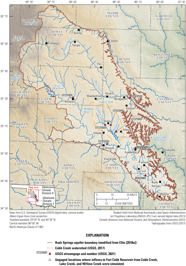
U.S. Geological Survey streamgage locations, ungaged locations where inflows to the Fort Cobb Reservoir were simulated, selected Oklahoma climate divisions (National Oceanic and Atmospheric Administration, 2022), and the extent of the Rush Springs aquifer as delineated by Ellis (2018b).
Purpose and Scope
This report describes the simulated effects of changes in groundwater withdrawals from the Rush Springs aquifer on base flows in streams upgradient from the Fort Cobb Reservoir (Cobb Creek, Lake Creek, and Willow Creek) by using a modified, previously published numerical groundwater-flow model (hereinafter referred to as the “Ellis (2018a) groundwater-flow model”) to simulate several scaled-groundwater-withdrawal scenarios. The scaled-groundwater-withdrawal scenarios consist of (1) a scaled-EPS-groundwater-withdrawal scenario; (2) a scaled-historical-groundwater-withdrawal scenario using the Ellis (2018a) historical groundwater withdrawals; (3) a zonal-scaled-historical-groundwater-withdrawal scenario, where Ellis (2018a) historical groundwater withdrawals were scaled within eight subareas (zones) that compose the Cobb Creek watershed; and (4) a simulated base-flow-depletion scenario within the Cobb Creek watershed. Long-term trends in streamflow, base flow, and precipitation for the watersheds that drain into Fort Cobb Reservoir were evaluated as part of the assessment of the simulated effects of changes in groundwater withdrawals on base flows.
Description of Study Area
This section is modified from Ellis (2018b), Ellis and others (2020), and Labriola and others (2022). The Rush Springs aquifer underlies about 4,970 square miles in Blaine, Caddo, Canadian, Comanche, Custer, Dewey, Ellis, Grady, Kiowa, Major, Roger Mills, Stephens, Washita, and Woodward Counties (fig. 1). The Rush Springs aquifer provides an important groundwater resource for municipal and irrigation uses; irrigation use consists of about 89 percent of total annual groundwater use, and municipal use was second highest at 9 percent (1979–2015; Ellis, 2018b). Groundwater seepage from the Rush Springs aquifer sustains base flows in streams in the study area, including the streams that are the primary sources of total inflows into Fort Cobb Reservoir (Cobb Creek, Lake Creek, and Willow Creek; fig. 1). Cobb Creek supplies most of the streamflow and base-flow inflows to the Fort Cobb Reservoir, followed by Lake Creek and then Willow Creek (fig. 2). The physiography of the study area is characterized by gently rolling hills dissected by deep drainage channels and surface-water features. Gypsum beds in the western part of the study area create erosion-resistant caprocks that form steep-sided ledges in areas near alluvial valleys (Becker and Runkle, 1998).
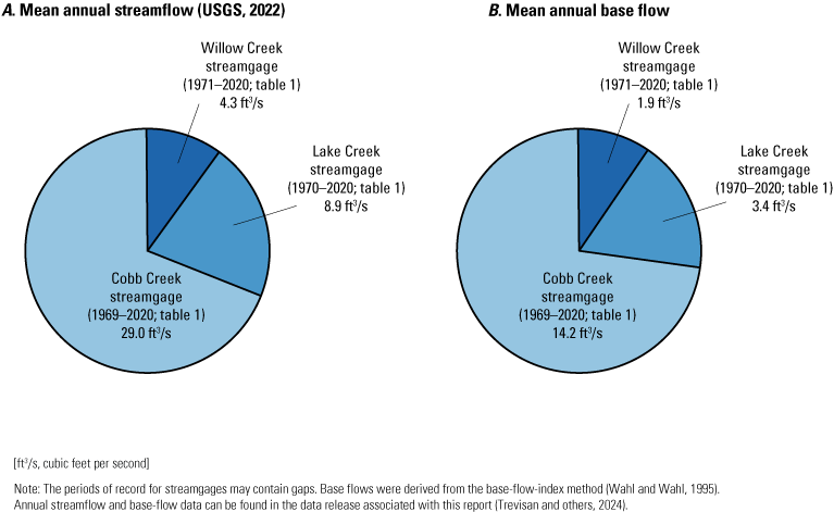
A, Mean annual streamflow and B, mean annual base flow for inflows to the Fort Cobb Reservoir from U.S. Geological Survey (USGS) streamgages (USGS, 2021; Trevisan and others, 2024) 07325800 Cobb Creek near Eakly, Okla. (Cobb Creek streamgage), 07325850 Lake Creek near Eakly, Okla. (Lake Creek streamgage), and 07325860 Willow Creek near Albert, Okla. (Willow Creek streamgage).
Streamflow, Base-Flow, and Precipitation Trends and Groundwater Withdrawals
Streamflow records from the U.S. Geological Survey (USGS) streamgages listed in table 1 were analyzed for trends over their respective periods of record. Trend analyses were performed on time series of annual peak streamflow, annual mean streamflow (hereinafter referred to as “annual streamflow”), annual mean base flow (hereinafter referred to as “annual base flow”), and annual base-flow index (hereinafter referred to as “annual BFI”) as a percentage of streamflow that is estimated as base flow for the following eight streamgages listed in downstream order: USGS streamgage 07228500 Canadian River at Bridgeport, Okla. (hereinafter referred to as the “Bridgeport streamgage”), USGS streamgage 07325000 Washita River near Clinton, Okla. (hereinafter referred to as the “Clinton streamgage”), USGS streamgage 07325500 Washita River at Carnegie, Okla. (hereinafter referred to as the “Carnegie streamgage”), USGS streamgage 07325800 Cobb Creek near Eakly, Okla. (hereinafter referred to as the “Cobb Creek streamgage”), USGS streamgage 07325850 Lake Creek near Eakly, Okla. (hereinafter referred to as the “Lake Creek streamgage”), USGS streamgage 07325860 Willow Creek near Albert, Okla. (hereinafter referred to as the “Willow Creek streamgage”), USGS streamgage 07326500 Washita River at Anadarko, Okla. (hereinafter referred to as the “Anadarko streamgage”), and USGS streamgage 07327447 Little Washita River near Cement, Okla. (hereinafter referred to as the “Cement streamgage”). These streamgages recorded data within the simulated period (1979–2015) from Ellis (2018b) (table 1). Trend analyses for time-series for annual streamflow, annual base flow, and annual BFI were analyzed on a calendar year basis (January 1 through December 31), whereas peak streamflow time-series (reported by water year) were analyzed on a water year basis; a water year is the 12-month period from October 1 through September 30 and is designated by the calendar year in which it ends.
Trends were analyzed by evaluating the Kendall’s tau-b rank correlation coefficient (hereinafter referred to as “Kendall’s tau”; Kendall, 1938, 1945, 1975; Helsel and others, 2020) and the Theil-Sen slope estimator, (Theil, 1950; Sen, 1968; Helsel and others, 2020). Patterns in streamflow were illustrated by using locally weighted scatterplot smoothing curves (Cleveland, 1979) with a smoothing factor of 0.75; patterns of wet and dry periods for precipitation were illustrated by using locally weighted scatterplot smoothing curves with a smoothing factor of 0.15. Annual peak streamflow data were obtained from the USGS National Water Information System (NWIS) database (USGS, 2021), and annual streamflow, annual base flow, and annual BFI were calculated from the USGS Groundwater Toolbox (Barlow and others, 2015). The USGS Groundwater Toolbox uses daily mean streamflow data from USGS streamgages obtained from NWIS (USGS, 2021). Although the periods of record for the Lake Creek and Willow Creek streamgages begin in January 1970 and January 1971, respectively, and were ongoing as of December 2020, there were data gaps for each streamgage from about 1978 to 2004. Trends for these streamgages were analyzed, but statistical inferences about apparent trends could not be made because of the 1978–2004 data gap and because climatic conditions were different between their first periods of record when data first were collected at these streamgages in either 1970 or 1971 through 1977 and their second periods of record from 2005 through 2020. Other selected streamgages (table 1) contained mostly continuous records with some relatively small data gaps of approximately 5 years or less (Trevisan and others, 2024).
Table 1.
Description of selected streamgages, in downstream order, used for annual statistical analysis for the Fort Cobb Reservoir study area, western Oklahoma.[mi2, square mile; Okla., Oklahoma; Data from U.S. Geological Survey (2022)]
| U.S. Geological Survey streamgage number and name (fig. 1) | Streamgage by short name | Drainage area, in mi2 |
Latitude, in decimal degrees | Longitude, in decimal degrees | Period analyzed for trends (may contain data gaps) |
|
|---|---|---|---|---|---|---|
| Begin | End | |||||
| 07228500 Canadian River at Bridgeport, Okla. | Bridgeport streamgage | 24,698 | 35.544 | −98.318 | January 1945 | December 2020 |
| 07325000 Washita River near Clinton, Okla. | Clinton streamgage | 1,961 | 35.531 | −98.967 | January 1936 | December 2020 |
| 07325500 Washita River at Carnegie, Okla. | Carnegie streamgage | 3,116 | 35.117 | −98.564 | January 1938 | September 2006 |
| 07325800 Cobb Creek near Eakly, Okla. | Cobb Creek streamgage | 132 | 35.291 | −98.594 | January 1969 | December 2020 |
| 07325850 Lake Creek near Eakly, Okla. | Lake Creek streamgage | 52.5 | 35.291 | −98.529 | January 1970 | December 2020 |
| 07325860 Willow Creek near Albert, Okla. | Willow Creek streamgage | 28.2 | 35.233 | −98.466 | January 1971 | December 2020 |
| 07326500 Washita River at Anadarko, Okla. | Anadarko streamgage | 3,640 | 35.084 | −98.243 | January 1903 | December 2020 |
| 07327447 Little Washita River near Cement, Okla. | Cement streamgage | 62.3 | 34.838 | −98.124 | January 1993 | December 2020 |
Base-flow separation was done by using the BFI method (Wahl and Wahl, 1995) provided in the USGS Groundwater Toolbox (Barlow and others, 2015). The BFI method uses a user-specified number of days (n-day) window where the minimum daily mean streamflow is selected for each n-day bin. From the minimum n-day value, values referred to as “turning points” are established by selecting the minimum n-day value for which 0.9 times the n-day base flow is less than the n-day base flow of adjacent n-day bins. Base flow is then linearly interpolated between each turning point at daily intervals. Base flow is set equal to streamflow when base flow exceeds streamflow for each day along the linear interpolation (Barlow and others, 2015). Annual base flows and annual BFIs were determined by using a 5-day bin consistent with the Ellis (2018a) BFI-method analysis done using streamflow data collected at the streamgages listed in table 1. The annual BFI output is provided in the companion USGS data release for this report (Trevisan and others, 2024).
Statistical trends in annual peak streamflow, annual streamflow, annual base flow, annual BFI, annual no-flow days, annual low-flow days (defined in this report as the number of days under the 10th percentile of the daily mean streamflow for the period analyzed for trends; table 1), and annual precipitation were analyzed by using Kendall’s tau and the Theil-Sen slope estimator. Seasonal and monthly trends in streamflow and base flow were also analyzed using these statistics. For each streamgage, only years, seasons, or months with complete records were used for the analysis.
The Theil–Sen slope estimator is a nonparametric linear regression method used to fit a straight line to paired data such as streamflow values and time. Streamflow data collected over time contains outliers (large peak values in responses to stormwater runoff). Compared to ordinary least squares linear regression, the Theil–Sen estimator is less sensitive to outliers, which makes it a preferred method for evaluating trends in streamflow data.
The Kendall’s tau is another robust nonparametric statistic used to determine the statistical significance the ordinal data pairs such as association between streamflow values and time. Used together, the Kendall’s tau and Theil-Sen slope estimator provide complimentary lines of evidence for determining upward and downward trends in streamflow over time (Helsel and others, 2020). The statistical significance of the trend associated with Kendall’s tau can be estimated using a hypothesis test (Kendall, 1975). The hypothesis test used in this analysis was a two-sided test using a null hypothesis that no trend exists in the dataset (that is, Kendall’s tau is zero). For this assessment, a probability value (p-value) of 0.05 was considered the threshold for statistical significance for the presence of a trend (Helsel and others, 2020).
Kendall’s tau and Theil-Sen slope were calculated by using the kendalltau and theilslopes algorithms, respectively, from the SciPy package (version 1.7.1; Virtanen and others, 2020) for the Python programming language (Python; Rossum, 1995; Python Software Foundation, 2021). Streamflow, base-flow, and precipitation statistics were calculated by using the Python distribution package; the streamflow and precipitation data are included in the data release associated with this report (Trevisan and others, 2024).
Streamflow and Base-Flow Trends
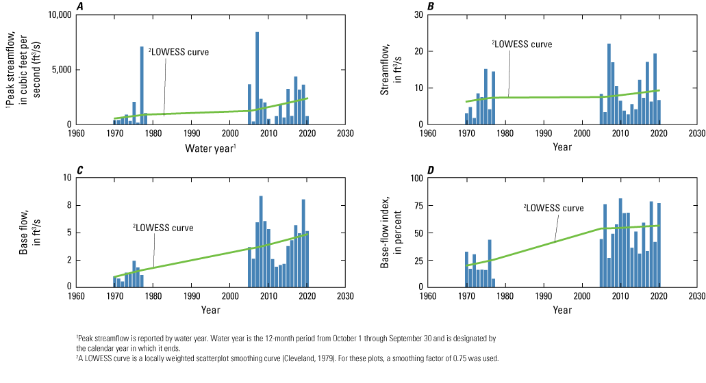
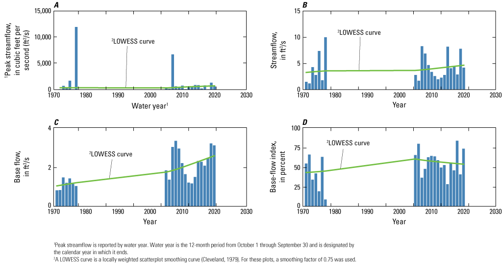
Annual streamflows and base flows at the Cobb Creek streamgage increased during the late 1960s to the mid-1990s and then decreased through 2020 (fig. 3B, C). However, the annual BFI steadily increased over the period of record (1969–2020), meaning base flow became an increasingly larger component of streamflow over time (fig. 3D). At the Lake Creek streamgage, annual peak streamflow, annual streamflow, annual base flow, and annual BFI generally increased over the period of record (1970 to 2020), although as previously mentioned, there was a long data gap from 1978 to 2004 (fig. 4). It is possible, but not known, that streamflows and base flows at this streamgage followed patterns similar to those for the Cobb Creek streamgage. Streamflow patterns for the Willow Creek streamgage were similar to those for the Lake Creek streamgage (fig. 5); the Willow Creek streamgage record also contains a data gap from 1978 to 2004. Annual BFI for the Willow Creek streamgage slightly decreased from about 2005 to 2020 (fig. 5D).
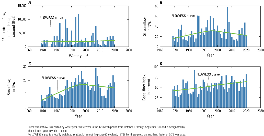
A, Annual peak streamflow, B, annual streamflow, C, annual base flow, and D, annual base-flow index for the U.S. Geological Survey streamgage 07325800 Cobb Creek near Eakly, Okla.
A, Annual peak streamflow, B, annual streamflow, C, annual base flow, and D, annual base-flow index for the U.S. Geological Survey streamgage 07325850 Lake Creek near Eakly, Okla.
A, Annual peak streamflow, B, annual streamflow, C, annual base flow, and D, annual base-flow index for the U.S. Geological Survey streamgage 07325860 Willow Creek near Albert, Okla.
Typically, the patterns in annual streamflows and annual peak streamflows tended to be downward or not apparent (no upward or downward pattern); few statistically significant upward or downward trends were detected (table 2). Most of the statistically significant trends in base flow and BFI were upward. The Theil-Sen slope was highest for the Carnegie streamgage with an upward Theil-Sen slope for base flow of 2.12 cubic feet per second per year ([ft3/s]/yr). The trends for base flow and BFI for the Cobb Creek, Lake Creek, and Willow Creek streamgages were slightly upward, and nearly all of these trends were statistically significant, indicating that base flow is becoming a larger component of streamflow at these streamgages, although the changes over time are relatively small. The BFI trend for the Willow Creek streamgage was not statistically significant (p-value of 0.64). Changes in streamflow over time for the Carnegie streamgage were statistically significant, indicating that streamflow was increasing each year. At the Anadarko, Cobb Creek, Lake Creek, and Willow Creek streamgages, the streamflows also appeared to increase each year. As indicated by the Theil-Sen slope, these changes were generally small, except the Theil-Sen slope of 1.65 (ft3/s)/yr for the Anadarko streamgage, and none of the changes were statistically significant.
Table 2.
Kendall’s tau and Theil-Sen slope statistics for annual base flow, base-flow index, streamflow, and peak streamflow for the period of record for eight selected U.S. Geological Survey streamgages used for statistical analysis for the Fort Cobb Reservoir study area, western Oklahoma (Trevisan and others, 2024).[p-value, probability value; (ft3/s)/yr, cubic foot per second per year; <, less than]
| Streamgage by short name (table 1) |
Base flow | Base-flow index | Streamflow | Peak streamflow | Period analyzed for trends (may contain data gaps) | ||||||||
|---|---|---|---|---|---|---|---|---|---|---|---|---|---|
| Kendall’s tau | p-value | Theil-Sen slope, in (ft3/s)/yr | Kendall’s tau | p-value | Theil-Sen slope, in percent per year | Kendall’s tau | p-value | Theil-Sen slope, in (ft3/s)/yr | Kendall’s tau | p-value | Theil-Sen slope, in (ft3/s)/yr | ||
| Anadarko streamgage | 0.16 | 0.07 | 1.46 | 0.22 | <0.05 | 0.15 | 0.10 | 0.24 | 1.65 | −0.02 | 0.80 | −4.82 | Jan. 1903– Dec. 2020 |
| Bridgeport streamgage | 0.44 | <0.05 | 1.78 | 0.61 | <0.05 | 0.72 | −0.12 | 0.16 | −2.04 | −0.29 | <0.05 | −281.39 | Jan. 1945– Dec. 2020 |
| Carnegie streamgage | 0.36 | <0.05 | 2.12 | 0.44 | <0.05 | 0.44 | 0.16 | 0.05 | 2.62 | −0.17 | <0.05 | −47.03 | Jan. 1938–Sept. 2006 |
| Cement streamgage | −0.32 | <0.05 | −0.34 | −0.40 | <0.05 | −0.97 | −0.21 | 0.11 | −0.44 | 0 | 1 | −0.28 | Jan. 1993– Dec. 2020 |
| Clinton streamgage | 0.19 | <0.05 | 0.32 | 0.52 | <0.05 | 0.61 | −0.08 | 0.29 | −0.33 | −0.45 | <0.05 | −68.57 | Jan. 1936–Dec. 2020 |
| Cobb Creek streamgage1 | 0.32 | <0.05 | 0.20 | 0.32 | <0.05 | 0.46 | 0.10 | 0.28 | 0.13 | 0 | 1 | 0.14 | Jan. 1969–Dec. 2020 |
| Lake Creek streamgage1 | 0.51 | <0.05 | 0.08 | 0.39 | <0.05 | 0.72 | 0.16 | 0.26 | 0.06 | 0.23 | 0.11 | 26.11 | Jan. 1970–Dec. 2020 |
| Willow Creek streamgage1 | 0.47 | <0.05 | 0.03 | 0.08 | 0.64 | 0.17 | 0.19 | 0.20 | 0.03 | 0.09 | 0.55 | 3.14 | Jan. 1971–Dec. 2020 |
Annual no-flow days and low-flow days were analyzed for trends for the periods of record for each of the eight streamgages (table 3). Typically, the number of no-flow days trended downward for each streamgage, and the Theil-Sen slope show no trend in no-flow days for any of the streamgages (fig. 6A–C). Theil-Sen slopes of zero result from the way Theil-Sen slopes are calculated (the median of the pairwise slopes), where a sufficient number of zero counts would result in a zero slope (that is, the median of the pairwise slopes is zero, which is guaranteed if more than 50 percent of the slopes are zero). Therefore, the Theil-Sen slope estimator is likely less useful than Kendall’s tau for identifying trends in the presence of zeros because Kendall’s tau can account for the upward or downward trends in this instance (Kendall, 1975). Low-flow days generally trended downward for each streamgage, with statistically significant Theil-Sen slopes of –0.70,–1.80, and –1.06 (ft3/s)/yr for the Cobb, Lake, and Willow Creek streamgages, respectively (table 3). Trends for no-flow days were similar to those for low-flow days. Generally, trends for no-flow days and low-flow days were moderate (about 1 to 2 days per year) or minimal (less than 0.5 day per year).
Table 3.
Kendall’s tau and Theil-Sen slope statistics for annual no-flow days and low-flow days for the period of record for eight selected U.S. Geological Survey streamgages used for statistical analysis for the Fort Cobb Reservoir study area, western Oklahoma (Trevisan and others, 2024).[p-value, probability value; <, less than; 0.00, indicates value is exactly zero]
| Streamgage by short name (table 1) | Number of no-flow days | Number of low-flow days | ||||
|---|---|---|---|---|---|---|
| Kendall’s tau | p-value | Theil-Sen slope, in number of days per year | Kendall’s tau | p-value | Theil-Sen slope, in number of days per year | |
| Anadarko streamgage | −0.14 | 0.17 | 0.001 | −0.14 | 0.13 | 0.001 |
| Bridgeport streamgage | −0.21 | <0.05 | 0.001 | −0.23 | <0.05 | −0.38 |
| Carnegie streamgage | −0.04 | 0.70 | 0.001 | −0.38 | <0.05 | −0.31 |
| Cement streamgage | 0.20 | 0.20 | 0.001 | 0.22 | 0.12 | 0.001 |
| Clinton streamgage | −0.21 | <0.05 | 0.001 | −0.30 | <0.05 | 0.001 |
| Cobb Creek streamgage | −0.26 | <0.05 | 0.001 | −0.43 | <0.05 | −0.70 |
| Lake Creek streamgage | −0.62 | <0.05 | 0.001 | −0.61 | <0.05 | −1.80 |
| Willow Creek streamgage | −0.55 | <0.05 | 0.001 | −0.53 | <0.05 | −1.06 |
For Theil-Sen slopes, counts for each year can be zero no-flow or low-flow days; given enough years with zero no-flow or low-flow days, using the median pairwise slopes would result in a zero slope. Kendall’s tau is not affected by zeros in the same manner because only the counts of concordant and discordant points are used; if one or more years have non-zero counts, then Kendall’s tau will be non-zero unless equal numbers of concordant and discordant points were present. Due to these limitations, the Theil-Sen slope estimator is likely less useful than Kendall’s tau to identify trends in this context.
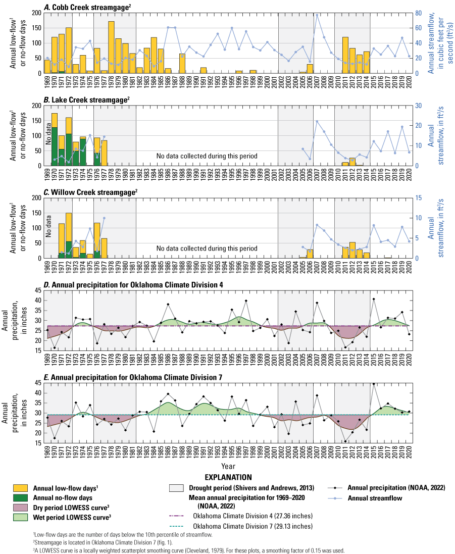
Annual low-flow or no-flow days and annual streamflow for U.S. Geological Survey streamgages A, 07325800 Cobb Creek near Eakly, Okla. (Cobb Creek streamgage), B, 07325850 Lake Creek near Eakly, Okla. (Lake Creek streamgage), and C, 07325860 Willow Creek near Albert, Okla. (Willow Creek streamgage) (U.S. Geological Survey, 2021) and annual precipitation for D, Oklahoma Climate Division 4, and E, Oklahoma Climate Division 7 (National Oceanic and Atmospheric Administration [NOAA], 2022).
Monthly and seasonal trends in streamflow and base flow were analyzed by using the Kendall’s tau and Theil-Sen slope estimator. Seasons were categorized as follows: spring consisted of March, April, and May; summer consisted of June, July, and August; fall consisted of September, October, and November; and winter consisted of December, January, and February. Trends were mostly upward for streamflow and base flow except for the Cement streamgage (figs. 7–8). Base flows at the Cobb Creek, Lake Creek, and Willow Creek streamgages were all increasing monthly and seasonally, and the base-flow trends were statistically significant. The only exception for these sites was during March for the Willow creek streamgage, where the base-flow pattern was generally upward but the trend was not statistically significant. At most of the streamgages, streamflow was generally increasing over time but at a rate that was less than that for base flows. Many of monthly and seasonal Theil-Sen slopes for base flow were statistically significant. For streamflow, the statistical significance of the monthly and seasonal Theil-Sen slopes varied considerably for the different streamgages, ranging from 1 to 6 months and from 2 to 4 seasons with statistically significant Theil-Sen slopes. The Theil-Sen slopes that were not statistically significant were mostly smaller in magnitude than those that were statistically significant. The Cement streamgage was the only streamgage with consistent downward trends in monthly and seasonal base flows and streamflows. This could be potentially because the early 1990s (which marked the beginning of the period of record for the Cement streamgage) was generally wetter than most of following period (Ellis, 2018b). The other seven streamgages recorded data for at least 20 years prior to the beginning of the period of record for the Cement streamgage (table 1). Seasonal and monthly trends (figs. 7–8) were similar to the trends in annual base flow and streamflow for each of the streamgages (table 2).
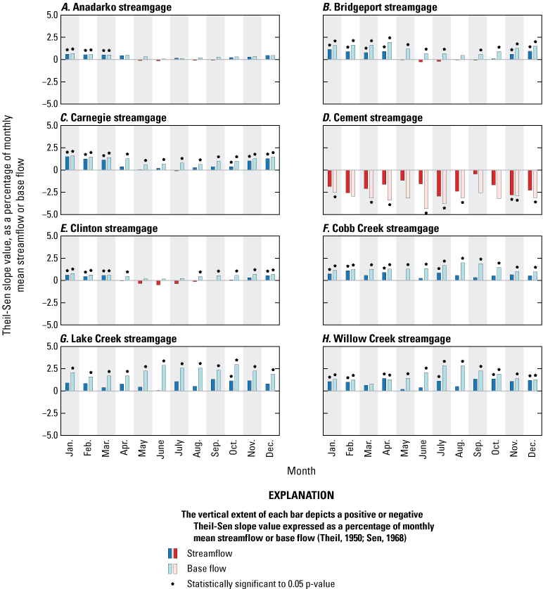
Theil-Sen slope or monthly streamflow and base flow normalized to monthly mean streamflow and base flow for U.S. Geological Survey streamgages A, 07326500 Washita River at Anadarko, Okla. (Anadarko streamgage); B, 07228500 Canadian River at Bridgeport, Okla. (Bridgeport streamgage); C, 07325500 Washita River at Carnegie, Okla. (Carnegie streamgage); D, 07327447 Little Washita River near Cement, Okla. (Cement streamgage); E, 07325000 Washita River near Clinton, Okla. (Clinton streamgage); F, 07325800 Cobb Creek near Eakly, Okla. (Cobb Creek streamgage); G, 07325850 Lake Creek near Eakly, Okla. (Lake Creek streamgage); and H, 07325860 Willow Creek near Albert, Okla. (Willow Creek streamgage) (U.S. Geological Survey, 2021).
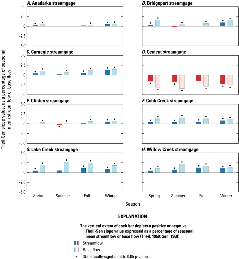
Theil-Sen slope for seasonal streamflow and base flow normalized to seasonal mean streamflow and base flow for U.S. Geological Survey streamgages A, 07326500 Washita River at Anadarko, Okla. (Anadarko streamgage); B, 07228500 Canadian River at Bridgeport, Okla. (Bridgeport streamgage); C, 07325500 Washita River at Carnegie, Okla. (Carnegie streamgage); D, 07327447 Little Washita River near Cement, Okla. (Cement streamgage); E, 07325000 Washita River near Clinton, Okla. (Clinton streamgage); F, 07325800 Cobb Creek near Eakly, Okla. (Cobb Creek streamgage); G, 07325850 Lake Creek near Eakly, Okla. (Lake Creek streamgage); and H, 07325860 Willow Creek near Albert, Okla. (Willow Creek streamgage) (U.S. Geological Survey, 2021).
Precipitation Trends and Groundwater Withdrawals
Annual precipitation data from Oklahoma Climate Divisions 4 and 7 (table 4; fig. 1; National Oceanic and Atmospheric Administration [NOAA], 2022) were analyzed for trends for the period of record (1895–2020) and the approximate periods of record of the Cobb Creek, Lake Creek, and Willow Creek streamgages (1969–2020).
Mean annual precipitation ranged from 26.28 to 27.36 inches for Oklahoma Climate Division 4 for the two periods analyzed (table 4; fig. 6D). Mean annual precipitation ranged from 27.88 to 29.13 inches for Oklahoma Climate Division 7 for the two periods analyzed (table 4; fig. 6E). These values were close to the mean annual precipitation estimated by Neel and others (2018) of 28.2 inches for the Rush Springs aquifer from 1905 to 2015. Long-term (1895–2020 and 1969–2020) precipitation appeared relatively stable, with only a minimal increase in precipitation of about 0.03 to 0.05 inch per year, and the results of trends tests were not statistically significant. Periods of the 1910s, 1930s, mid-1940s to mid-1950s, early 1960s to early 1970s, and 2010 to 2014 were the driest on record (Shivers and Andrews, 2013; Oklahoma Climatological Survey, 2023a, b). Wetter periods were more frequent and dry periods were less prolonged in the years since 1980 compared to the years prior to 1980 (Oklahoma Climatological Survey, 2023a, b).
Neel and others (2018, fig. 16 on p. 23) reported groundwater withdrawals in the study area for 1967 through 2015. The reported groundwater withdrawals in the study area ranged from about 60,000 acre-ft in 1967 to about 130,000 acre-ft in 2014. Between 1967 and 2004, groundwater withdrawals varied considerably with no apparent upward changes over time. From 2005 through 2015, reported groundwater withdrawals generally increased each year from about 50,000 acre-ft in 2005 to about 110,000 acre-ft in 2015 (Neel and others, 2018). As mentioned in the “Streamflow and Base-Flow Trends” section of this report, base flows at streamgages in the study area generally trended upward for their individual periods of record, which ranged from 1903 through 2020 for the Anadarko streamgage to 1993 through 2020 for the Cement streamgage (table 2). Although these results could indicate that groundwater withdrawals during 2005–15 did not strongly affect base flows in streams within the areal extent of the Rush Springs aquifer, climatological factors could also affect the quantity of base flows and the demand for groundwater withdrawals. More years were identified as wetter than normal than as drier than normal during the study period (1979–2015) (Oklahoma Climatological Survey, 2023a, b; fig. 6D–E). A groundwater-flow model, rather than analytical methods, is useful for isolating factors that influence groundwater flow. The purpose of the following groundwater-flow model scenarios was to assess the responsiveness of streams in the Cobb Creek watershed to changing groundwater withdrawals independent of climatological factors.
Table 4.
Kendall’s tau and Theil-Sen slope statistics for historical precipitation for Oklahoma Climate Divisions 4 and 7.[Precipitation data and climate divisions are from the National Oceanic and Atmospheric Administration (2022); p-value, probability value]
Simulated Effects of Rush Springs Aquifer Groundwater Withdrawals on Base Flows
Ellis (2018a) developed a groundwater-flow model for the Rush Springs aquifer in western Oklahoma (fig. 1) by using MODFLOW-2005 (Harbaugh, 2005) with the Newton formulation solver (MODFLOW-NWT, version 1.0.8; Niswonger and others, 2011). A detailed description of the groundwater-flow model is provided in Ellis (2018b). The groundwater-flow model domain is the full extent of the Rush Springs aquifer (fig. 1). The model consists of 1,362 rows and 1,083 columns with 500-ft by 500-ft uniform grid spacing. It includes three layers:
-
• A top layer (layer 1) representing the Cloud Chief Formation of the Foss Group (an interbedded reddish-brown to orange-brown shale of Permian age [Carr and Bergman, 1976; Fay and Hart, 1978]),
-
• A middle layer (layer 2) representing alluvium and terrace deposits (sand, silt, and clay deposits [Tanaka and Davis, 1963]) plus the upper 30 ft of the Whitehorse Group of Permian age, and
-
• A bottom layer (layer 3) representing the rest of the Whitehorse Group (orange-brown, fine-grained sandstone and siltstone with some dolomite, gypsum, and reddish-brown to orange-brown cross-bedded sandstone [Tanaka and Davis, 1963; Fay and Hart, 1978]) (fig. 9).
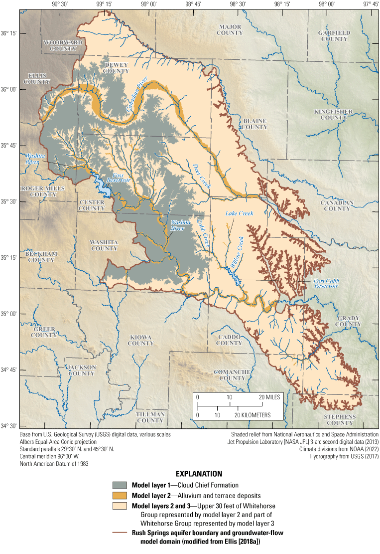
The three model layers within the extent of the Rush Springs aquifer groundwater-flow model domain, Fort Cobb Reservoir study area, western Oklahoma.
Simulation of Groundwater Flow
The MODFLOW groundwater-flow model consists of several packages that simulate various inflows and outflows across the boundaries of the Rush Springs aquifer (fig. 10). Recharge and saturated-zone evapotranspiration were simulated by using the Recharge (RCH) and Evapotranspiration (EVT) packages (Harbaugh, 2005; Niswonger and others, 2011). The evapotranspiration and recharge rates used for the EVT and RCH packages, respectively, were derived from a Thornthwaite-Mather (Thornthwaite and Mather, 1957) Soil-Water-Balance simulation (Westenbroek and others, 2010) published by Ellis (2018a, b). The RCH package adds water to the aquifer at a user-specified rate for the uppermost active cell for the Ellis (2018a) groundwater-flow model. The EVT package was only applied to model cells representing alluvium and terrace deposits. The EVT package removes water from the aquifer at a rate specified in the EVT package when groundwater altitudes exceed the user-specified evapotranspiration (ET) surface. When groundwater altitudes decrease to less than the ET surface, the EVT package rate is linearly interpolated to zero from the ET surface to the ET surface less a user-specified extinction depth (eq. 6–12B in Harbaugh, 2005), which commonly represents the maximum depth below land surface to which plant roots can penetrate into the subsurface (Shah and others, 2007); the extinction depths for the Ellis (2018a) groundwater-flow model were the plant-root depths that were calibrated for the Soil-Water-Balance simulation (Ellis, 2018b).
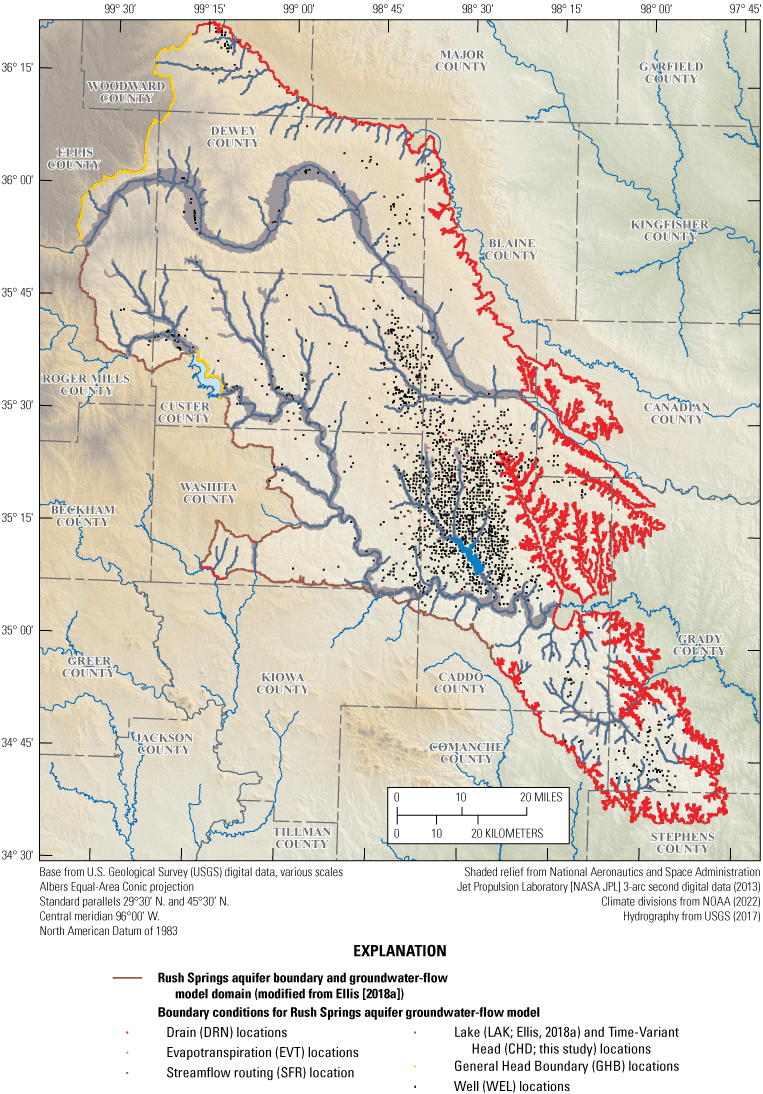
Boundary conditions applied to the Rush Springs aquifer groundwater-flow model by Ellis (2018a), Fort Cobb Reservoir study area, western Oklahoma.
Springs were represented in the groundwater-flow model by using the Drain (DRN) package (Harbaugh, 2005). The DRN package functions by simulating the removal of groundwater exceeding a user-specified altitude at a rate proportional to the product of a user-specified conductance and the difference between the simulated groundwater altitude and the user-specified groundwater altitude when simulated groundwater altitudes exceed the user-specified groundwater altitude (eq. 6–10 in Harbaugh, 2005). For a groundwater-flow model, conductance is the product of hydraulic conductivity and the saturated cross-sectional area orthogonal to flow divided by the distance of flow between cells (that is, the distance between cell centroids for a finite-difference simulation). Land surface altitude of the springs were obtained from the NWIS (Ellis, 2018b).
Lateral groundwater flow and flow into and from Foss Reservoir (fig. 1) were simulated by using the General Head Boundary (GHB) package (Harbaugh, 2005). The GHB package is used to calculate flux across the boundary by using the difference in simulated groundwater altitudes between adjacent cells and the groundwater altitude in the GHB package cell. Flux is controlled by adjusting a user-specified conductance value. The user-specified groundwater altitude was determined from water levels obtained from NWIS (U.S. Geological Survey, 2017b).
Streams were simulated by using the Streamflow Routing (SFR) package (Niswonger and Prudic, 2005). The SFR package simulates base flow between the aquifer and stream cells and routes base flow downstream along contiguous stream reaches (a cell used for the SFR package) and segments (a collection of SFR reaches). Groundwater flow from the aquifer to the stream is calculated by Darcy’s Law (Heath, 1983) where stream stage is estimated by using Manning’s equation (Manning, 1891), which can be used to calculate stream stage from streamflow and stream-channel properties.
The Fort Cobb Reservoir (fig. 1) was represented by using the Lake (LAK) package (Merritt and Konikow, 2000; Niswonger and Prudic, 2005). The LAK package is used to incorporate inflows from the SFR package in order to simulate releases into a downstream segment of the SFR package. Additionally, flow between the lake and the aquifer are determined from the difference between lake-stage altitudes and groundwater altitudes. Lake-stage altitudes and releases used for the LAK package were obtained from Reclamation (2017a, b). For the scenarios in this report, only the scaled-EPS-groundwater-withdrawal scenario used the LAK package. The modifications to the groundwater-flow models for the other scenarios are discussed in the following section.
Modifications to the Groundwater-Flow Model
Some MODFLOW-NWT solver settings were modified to increase the likelihood of convergence. The maximum number of outer iterations for the Newton solver was modified from 1,000 to 1,500. This allows the solver to conduct more iterations for finding a solution before considering a model run failed (Niswonger and others, 2011). The coefficient used to reduce the weight applied to the change in simulated head for the non-linear solutions was also modified from 0.90 to 0.85, slightly increasing the weight applied to the step size (thus increasing the permitted step size) for heads between each nonlinear iteration (Niswonger and others, 2011). These changes are within the ranges of suggested values for the solver settings (Winston, 2022). The head- and flux- tolerance criteria were not modified. These changes to the solver settings caused only minor effects on the solution.
To improve the stability of the Rush Springs aquifer groundwater-flow model for the current (2023) study, the LAK package (Merritt and Konikow, 2000) was replaced with a Time-Variant Head (CHD) package (Harbaugh, 2005) to simulate the interactions between the Rush Springs aquifer and Fort Cobb Reservoir except for the scaled-EPS-groundwater-withdrawal scenario. The CHD package is a specified-head-boundary-condition package—the user specifies groundwater altitudes for the beginning and end of each stress period for each cell specified in the CHD package. The CHD package was used to interpolate differences in groundwater altitudes throughout the stress period to estimate groundwater flow between model cells representing the Rush Springs aquifer and model cells representing Fort Cobb Reservoir. For each stress period, the beginning CHD package groundwater altitudes were set to the LAK package stage from the previous stress period, and the ending CHD package groundwater altitudes were set to the LAK package stage from the current stress period. The starting and ending CHD package groundwater altitudes for the steady-state stress period were assigned the steady-state LAK package stage from the calibrated groundwater-flow model (Ellis, 2018a). Additionally, some cell thicknesses assigned to the CHD package were small, and some cells lacked thickness.
Altitudes were not used in the LAK package for cells in layer 2 (Ellis, 2018b), and cells in layer 2 that were part of the LAK package were considered inactive. The altitude for the bottom of layer 2 was adjusted (decreased) to allow sufficient cell thickness (minimum thickness of 1 ft) for MODFLOW-NWT when activating the cells in the LAK package for use with the CHD package (Ellis, 2018b).
The base flows and groundwater altitudes for the groundwater-flow simulation using the CHD package were similar to those from the groundwater-flow simulation using the LAK package (table 5). For most streamgages and for the net aquifer seepage for the SFR package, the root mean square error was less than 0.10 cubic foot per second (ft3/s). Changes in groundwater altitudes were small, with a root mean square error of 0.02 ft for all simulated groundwater altitudes from both groundwater-flow simulations.
Some simulated groundwater-withdrawal rates were not scaled during the scaled-groundwater-withdrawal scenarios (see the sections “Scenario 2” and “Scenario 3” for more details) to improve solver stability. The wells with unscaled groundwater-withdrawal rates were typically downgradient from Cobb, Lake, and Willow Creeks or many miles away from Cobb, Lake, and Willow Creeks (fig. 11). These wells were assumed to minimally affect base flows in Cobb, Lake, and Willow Creeks.
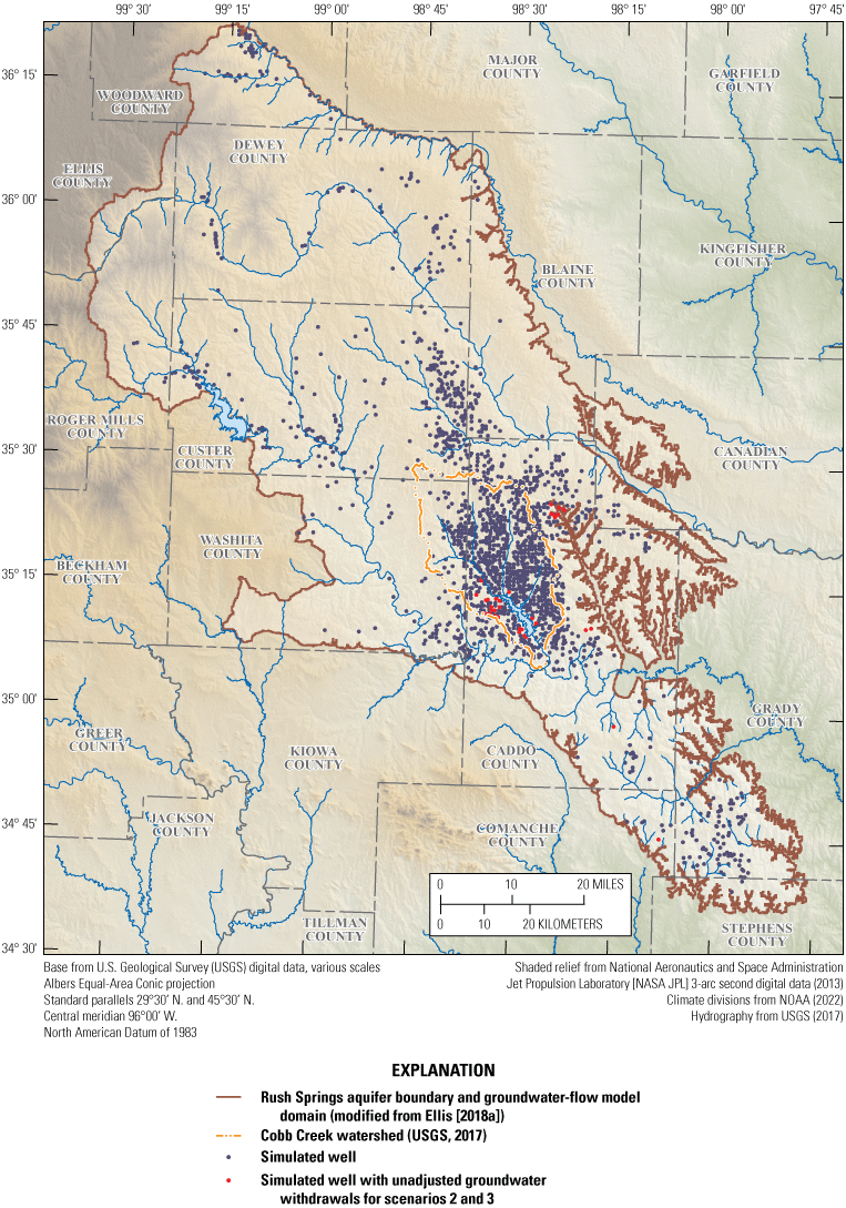
Location of groundwater withdrawal wells implemented in Ellis (2018a) and the location of wells that were not scaled for scenarios 2 and 3, Fort Cobb Reservoir study area, western Oklahoma.
Table 5.
Root mean square errors for net seepage from the aquifer to the stream, simulated base flows, and simulated groundwater altitudes calculated from the Ellis (2018a) groundwater-flow simulated outputs using the Lake package (LAK; Ellis, 2018a) and the simulated outputs using the Time-Variant Head package (CHD) for all stress periods, Fort Cobb Reservoir study area, western Oklahoma.[RMSE, root mean square error; SFR, Streamflow Routing package; <, less than; USGS, U.S. Geological Survey; ft3/s, cubic foot per second; ft, foot]
Groundwater-Flow Model Scenarios
Four groundwater-flow model scenarios were developed to assess streams’ base-flow response caused by modifying groundwater withdrawals near the Fort Cobb Reservoir by using the Ellis (2018a) groundwater-flow model. These base-flow response scenarios involved (1) scaling the 20-year EPS groundwater-withdrawal rate (Ellis, 2018a) for several 50-year groundwater-flow simulations; (2) scaling historical groundwater withdrawals (Ellis, 2018a); (3) scaling historical groundwater withdrawals throughout various zones that compose the Cobb Creek watershed; and (4) adding groundwater withdrawals for a single, hypothetical pumping well individually for each cell within the Cobb Creek watershed to observe the effects on base flow (Barlow and Leake, 2012). The first scenario addressed the length of time base flows can be sustained by using scaled EPS rates. Groundwater-flow models using EPS rates (groundwater withdrawals equally apportioned over an aquifer) are a common tool for informing regulatory decisions regarding Oklahoma aquifers (OWRB, 2023). The second scenario addressed the temporal changes to base flows when historical groundwater withdrawals are changed, and the third scenario addressed the spatial distribution of base-flow response when historical groundwater withdrawals are changed. Quantifying and predicting groundwater withdrawals at a regional scale can be difficult. Using historical groundwater withdrawals provided a simple means of representing these variables in the groundwater-flow model without needing to predict groundwater withdrawals. Historical groundwater withdrawals were not scaled for the fourth scenario. Instead, a hypothetical well was used to add additional groundwater withdrawals simulated individually for each cell. Other processes in the groundwater-flow model were isolated such that groundwater withdrawals were the only user-modified groundwater-flow boundary rate. However, altering groundwater withdrawals can change the simulated groundwater altitudes and change the simulated groundwater-flow rates for aquifer boundaries (such as in the DRN and EVT packages) affected by simulated groundwater altitudes (Barlow and Leake, 2012; Nadler and others, 2018). The fourth scenario addressed the spatial response of groundwater withdrawals with respect to base flow while isolating climatic conditions and isolating changes to groundwater withdrawals to a single model cell (unlike scenario 2 or 3, which used historical climatic conditions and groundwater withdrawals over multiple cells).
Total inflows into Fort Cobb Reservoir were used to characterize base-flow response to groundwater withdrawals. For this study, total inflow to the Fort Cobb Reservoir consisted only of the base-flow component of streamflow and was the sum of base-flow inflows from Cobb, Lake, and Willow Creeks. For the scenarios described in this report, any reference to Cobb Creek also included is two main tributaries (fig. 1); inflows from these two tributaries were included in the simulated inflow from Cobb Creek to the Fort Cobb Reservoir. Inflows from tributaries for Lake and Willow Creeks were not simulated (fig. 10).
Scenario 1: Scaled-EPS-Groundwater-Withdrawal Scenario
Ellis (2018a) developed a 20-year EPS groundwater-withdrawal scenario by using the Rush Springs aquifer groundwater-flow model. For the 20-year EPS groundwater-withdrawal scenario, existing simulated wells were replaced with a simulated well for each active cell representing the Rush Springs aquifer within the groundwater-flow model. The use of a simulated well for each active cell facilitated the hypothetical application of groundwater withdrawals on an equal basis over the spatial extent of the aquifer. The simulated wells then withdrew water at a uniform rate that was incrementally scaled until half of the model cells retained a saturated thickness at least 15 ft after 20 years. The 20-year-EPS-groundwater-withdrawal rate (hereinafter referred to as “baseline EPS rate”) from this scenario was used as the basis for assessing the effects on base flows in Cobb, Lake, and Willow Creeks by scaling that rate by selected percentages. For consistency with the previously published groundwater-flow model (Ellis, 2018a), the LAK package (not the CHD package) was used to simulate Fort Cobb Reservoir for the scaled-EPS-groundwater-withdrawal scenario documented in this report. Ellis (2018a, b) used constant long-term (1979–2015) mean stresses for package inputs (except for groundwater withdrawals), which were then used for the scaled-EPS-groundwater-withdrawal scenario.
The scaled-EPS-groundwater-withdrawal scenario consisted of six simulations scaling the baseline EPS rate by 25, 40, 50, 75, 100, and 120 percent for a period of 50 years to see the effects of these EPS rates over a longer time period than the 20-year period simulated in Ellis (2018a). For the 50-year simulations, streams (1) never ceased flowing under the 25-percent scaling scenario (fig. 12A); (2) ceased flowing after about 26 years under the 40-percent scaling scenario (fig. 12B); (3) ceased flowing after about 12 years using the 50-percent scaling scenario (fig. 12C); (4) ceased flowing after about 4 years using the 75-percent scaling scenario (fig. 12D); (5) ceased flowing after about 2 years using the baseline EPS rate (fig. 12E); and (6) ceased flowing after about 1 year using the 120-percent scaling scenario (fig. 12F).
As the EPS-rate scaling factor increased, base flows generally declined more sharply until approaching no flow (fig. 12). Cobb Creek began each simulation with the largest amount of base flow and sustained the largest losses in base flows when increasing the EPS-rate scaling factor. Lake Creek base flows often decreased in the same manner as Cobb Creek base flows, but by a smaller amount. Willow Creek base flows remained close to zero for most of the scaled-EPS-rate simulations, although base flows remained low (about 1 ft3/s) even after 50 years when using an EPS-rate scaling factor of 25 percent (fig. 12A). As the EPS-rate scaling factor increased, however, base flows for Lake and Willow Creeks declined more rapidly than base flows for Cobb Creek, likely because base flows for Cobb Creek are generally greater than the base flows in Lake and Willow Creeks and therefore can withstand greater groundwater withdrawals. The simulated EPS rates in this report represent a high volume of groundwater withdrawals that tend to quickly (often in less than 10 years) cause dry streams. To maintain stream base flow, the EPS rate would likely need to be much less than the EPS rate determined by using MAY targets (50 percent of the aquifer with less than 15 ft saturated thickness over 20 years of continuous EPS withdrawals).
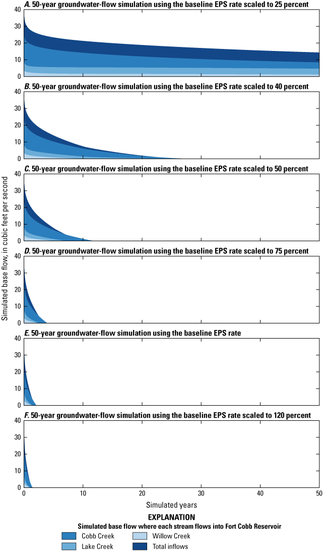
Simulated base flows for ungaged locations where Cobb Creek, Lake Creek, and Willow Creek flow into Fort Cobb Reservoir for 50-year groundwater-flow simulations using the baseline equal-proportionate-share (EPS) rate scaled to A, 25 percent; B, 40 percent; C, 50 percent; D, 75 percent; and E, the 20-year-EPS-groundwater-withdrawal rate (baseline EPS rate); and F, 120 percent. Total inflows into Fort Cobb Reservoir are the sum of simulated base flows for ungaged locations where Cobb Creek, Lake Creek, and Willow Creek flow into Fort Cobb Reservoir.
Scenario 2: Scaled-Historical-Groundwater-Withdrawal Scenario
To investigate the effects of groundwater withdrawals on base flows in Cobb, Lake, and Willow Creeks, a scenario was developed to modify historical groundwater withdrawals implemented in the Ellis (2018a) groundwater-flow model. The scaled-historical-groundwater-withdrawal scenario consisted of 10 simulations scaling the Ellis (2018a) historical groundwater-withdrawal rates by 50, 60, 70, 80, 90, 100, 125, 150, 175, and 200 percent. The scenario with 100-percent scaled historical-groundwater-withdrawal rates (hereinafter referred to as the “historical baseline rate”) was identical to the Ellis (2018a) groundwater-flow model except that the CHD package was used to simulate Fort Cobb Reservoir instead of the LAK package. The outputs from the historical-baseline-rate simulation were used for comparison with the results from the Ellis (2018a) groundwater-flow model (table 5). Ellis (2018b) estimated 500 gallons per minute (gal/min) as the maximum groundwater-withdrawal rate that the Rush Springs aquifer could sustain over longer periods of continuous pumping (such as monthly or annually). Therefore, scaled-groundwater-withdrawal rates were not permitted to exceed 500 gal/min. Historical groundwater withdrawals for the steady-state stress period were not scaled for each simulation to ensure identical starting conditions for each simulation.
Base flows were more sensitive to increases in groundwater withdrawals than to decreases in groundwater withdrawals; that is, the absolute magnitude of the change in base flow was greater for simulated increases in groundwater withdrawals than for simulated decreases in groundwater withdrawals (fig. 13A–C). Changes in base flows were generally highest for Cobb Creek (fig. 13A), intermediary for Lake Creek (fig. 13B), and lowest for Willow Creek (fig. 13C). Changes in base flow for Lake Creek were similar to those for Cobb Creek during some years. Base flows for Lake and Willow Creeks resulted in small streamflows approximating no-flow conditions for a few years, which would mean a lack of water available for diversions from each stream. For the simulation with the highest groundwater withdrawals, total inflows into Fort Cobb Reservoir declined about 16 ft3/s during some years (fig. 13D) with corresponding decreases in base flow of as much as 70 percent. Lake and Willow Creeks combined contributed about the same quantity of base flow as Cobb Creek.
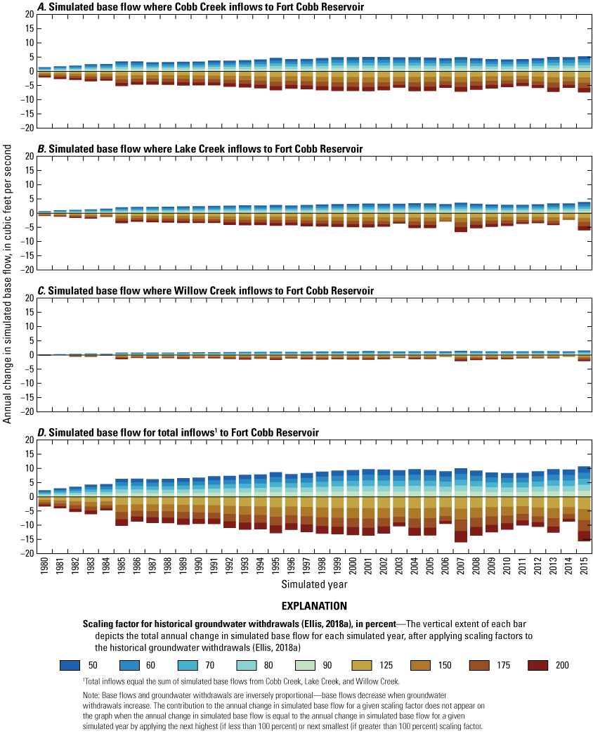
Annual change in simulated base flows for ungaged locations where A, Cobb Creek, B, Lake Creek, and C, Willow Creek inflow to the Fort Cobb Reservoir and for D, total inflows into Fort Cobb Reservoir, western Oklahoma, 1980–2015.
The largest percentage changes in base flow were simulated for streams with the smallest overall flow (fig. 14A–C). Percentage change was calculated by using
whereQx
is the simulated annual base flow for the scenario using scaled historical groundwater withdrawals (scale factor of x percent historical groundwater withdrawals); and
Q100
is the simulated annual base flow for the scenario using historical groundwater withdrawals (scale factor of 100 percent historical groundwater withdrawals).
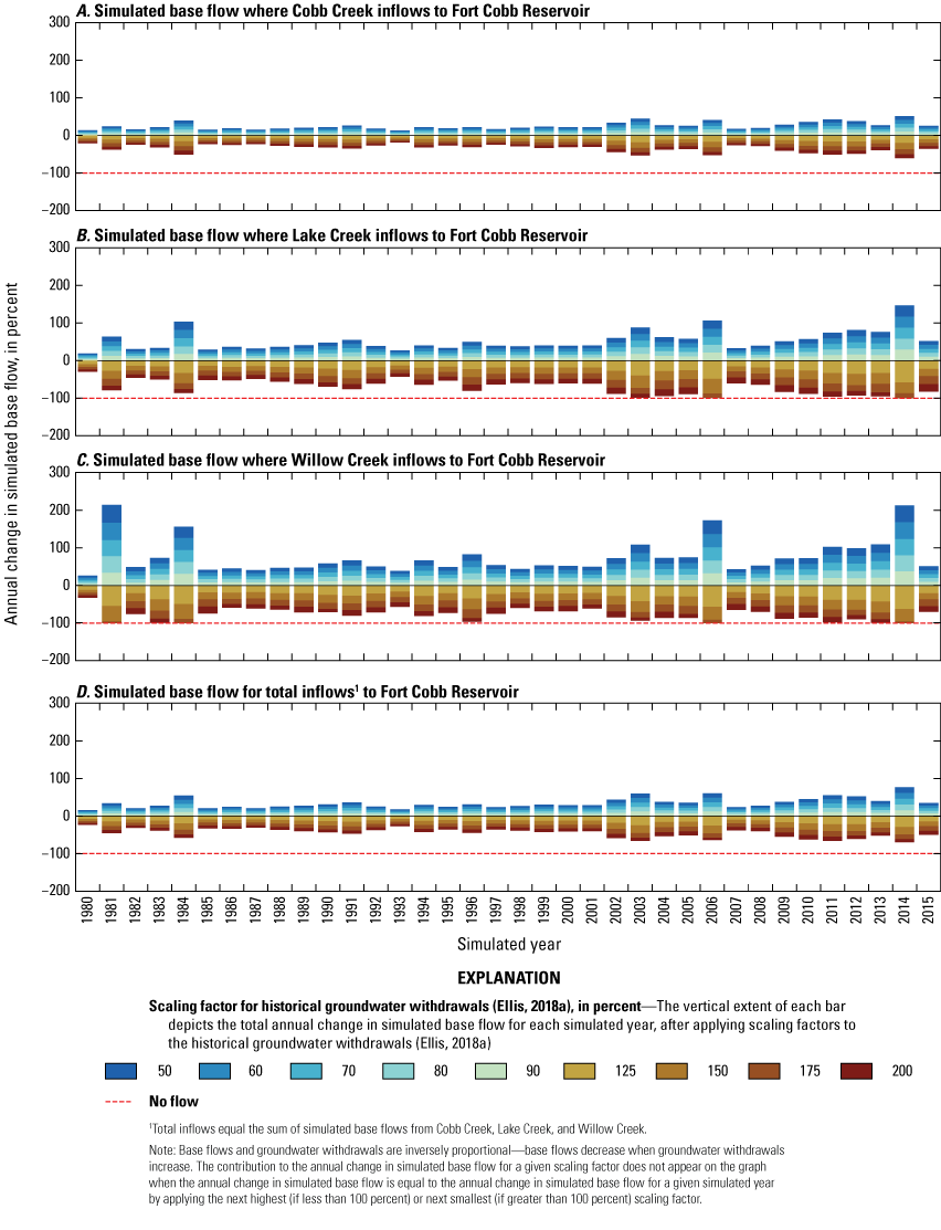
Annual percentage change in simulated base flows for ungaged locations where A, Cobb Creek, B, Lake Creek, and C, Willow Creek inflow to the Fort Cobb Reservoir and for D, total inflows into Fort Cobb Reservoir, western Oklahoma, 1980–2015.
For observed long-term (1979–2015) base-flow changes, the slope of the relation between the percentage change in groundwater withdrawals and the percentage change in mean annual base flows was negative (fig. 15). A more negative slope in the curves depicted in figure 15 indicates that mean annual base flows declined by a greater percentage for a given percentage change in groundwater withdrawals. Slopes were generally more negative for increasing groundwater withdrawals (positive percentage change in groundwater withdrawals) than for decreasing groundwater withdrawals (negative percentage change in groundwater withdrawals). Base flows were thus more affected by simulated increases in groundwater withdrawals than they were to simulated decreases in groundwater withdrawals. Percentage changes in mean annual base flow (fig. 15) followed similar patterns to those of annual base flow (fig. 14); the percentage changes in Willow Creek base flows were highest, followed by Lake Creek base flows, then total inflows into Fort Cobb Reservoir, and lastly Cobb Creek base flows. Simulating an increase in groundwater withdrawals generally reduced base flows more in Cobb Creek than in Lake Creek or Willow Creek. Additional groundwater withdrawals near Cobb Creek would likely reduce inflows to the Fort Cobb Reservoir more appreciably compared to the reductions in inflows caused by additional groundwater withdrawals near Lake and Willow Creeks.
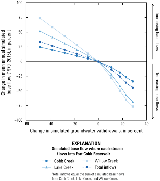
Percentage change in groundwater withdrawals and percentage change in mean annual simulated base flows at the ungaged locations (fig. 1) where inflows from Cobb Creek, Lake Creek, and Willow Creek were simulated and the sum of the total inflow of simulated base flows, Fort Cobb Reservoir study area, western Oklahoma.
Scenario 3: Zonal-Scaled-Historical-Groundwater-Withdrawal Scenario
A scenario was developed to assess the effects of increased historical groundwater withdrawals within eight zones that compose the Cobb Creek watershed. Groundwater withdrawals outside the Cobb Creek watershed were assumed to negligibly affect base flows in streams within the watershed (fig. 1). Zones were created by using a k-means spatial clustering algorithm for the location of historical groundwater withdrawals (as represented as the model cell centroid; QGIS, 2022). The k-means spatial clustering algorithm facilitates the creation of a user-specified number of groups or zones of points such that the distance between each point in a group and the mean location for points assigned to the same group is smallest relative to the distance to the mean locations of points assigned to other groups (QGIS, 2022). Use of the k-means spatial clustering algorithm method made it possible to maintain relatively similar total groundwater withdrawals for each zone (fig. 16B).
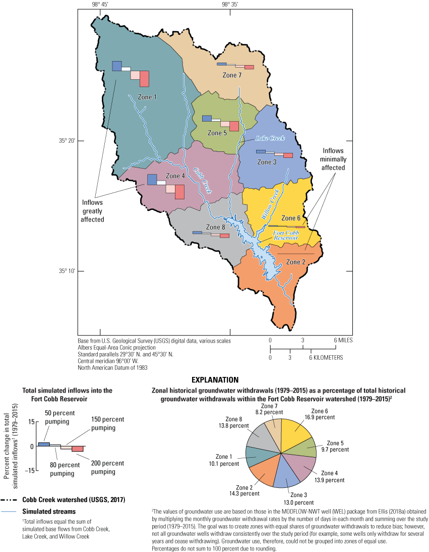
Percentage changes in total simulated inflows into Fort Cobb Reservoir for eight zones that compose the Cobb Creek watershed for simulated pumping rates scaled to 50, 80, 150, and 200 percent of historical groundwater withdrawals during 1979–2015 (Ellis, 2018a).
The total historical groundwater withdrawals during 1979–2015 were divided among the eight zones of the Cobb Creek watershed (fig. 16). For simulating future scenarios, groundwater-withdrawal rates were scaled to 50, 80, 100, 150, and 200 percent of the historical groundwater-withdrawal rates (Ellis, 2018a) for each zone. Because Ellis (2018b) estimated that 500 gal/min was the maximum groundwater-withdrawal rate that the Rush Springs aquifer could sustain over longer periods of continuous pumping (such as monthly or annually), groundwater-withdrawal rates were set to 500 gal/min if they exceeded this value when scaled. Groundwater withdrawals for the steady-state stress period were not changed from the Ellis (2018a) groundwater-flow model to maintain identical starting conditions for each groundwater-flow simulation. Because of long simulation run times (9 hours or more), the scenario used PEST++ version 4 parameter estimations software. PEST++ version 4 was modified from PEST++ version 3 (Welter and others, 2015) and is available from the USGS Github repository at https://github.com/usgs/pestpp/releases/tag/4.3.17. PEST++ version 4 includes a utility program that can be used to evaluate sets of parameter values in parallel (PESTPP-SWP). The PESTPP-SWP utility program was used to run the 40 groundwater-flow simulations in parallel using a high-performance computing environment (Condor Team, 2012). The simulations using unscaled historical groundwater withdrawals from each of the eight zones of the Cobb Creek watershed were used for error checking and simplifying after processing because outputs were referenced to these simulations.
To observe how each zone affects total inflows to the Fort Cobb Reservoir, total inflows from each scaled-historical-baseline rate simulation were subtracted from total inflows from the historical-baseline-rate simulation and divided by total inflows from the historical-baseline-rate simulation represented as a percentage of total inflows (fig. 16). Larger percentage changes in the contribution to total inflows from a given zone indicate that increasing groundwater withdrawals in that zone resulted in a larger increase of total inflows compared to other zones. Percentage changes in total inflows for zones farther upgradient in the watershed were generally greater than for zones farther downgradient (fig. 16). Percentage changes in total inflows for zones farther upgradient in the watershed were generally greater than for zones farther downgradient (fig. 16), possibly because with sufficient pumping, groundwater withdrawals could act as a barrier to groundwater flow, restricting downgradient water flow (Heath, 1983). Simulated stream seepage in the Cobb Creek watershed was frequently farther upgradient in the watershed than closer to the Fort Cobb Reservoir (Ellis, 2018b). Greater stream seepage provides more groundwater available for capture, which is likely the reason why base flows responded more to changes in groundwater withdrawals in the upgradient parts of the watershed compared to the parts of the watershed closer to the Fort Cobb Reservoir.
To further investigate how changes in groundwater withdrawals within each zone affect total inflows, linear regression equations were used to compare mean annual groundwater withdrawals to mean annual changes in total inflows for individual wells grouped by zone (fig. 17). The slopes of the linear regression equations represent the sensitivity of base flows to changing groundwater withdrawals for each zone. Zones where the regression-equation slopes were more negative (for example, zones 1, 4, and 5, where the slopes ranged from −0.41 to −0.70) indicate that reductions in groundwater withdrawals in these zones tend to have a larger effect on total inflows compared to other zones where the slopes of the regression equations were less negative (for example, zones 2, 3, 6, 7, and 8, where the slopes ranged from −0.0025 to −0.24).
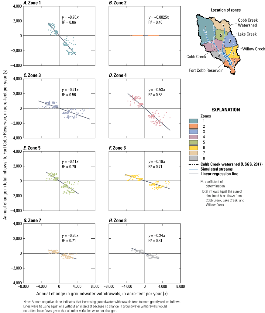
The relation between annual change in groundwater withdrawals (x) and annual change in total inflows (y) for each of the eight zones within the Cobb Creek watershed used in scenario 3 with the modified numerical groundwater-flow model from Ellis (2018a), simulated for 1979–2015.
Total inflows to the Fort Cobb Reservoir were most responsive to changes in groundwater withdrawals near Cobb Creek, followed by changes in groundwater withdrawals near Lake Creek and then Willow Creek (fig. 16A). Groundwater withdrawals in zones 1 and 4 affected base flows more than withdrawals in the other zones (table 6; figs. 16–17). This is likely because zone 1 covers much of Cobb Creek farther upgradient in the watershed (where base flows were higher [Ellis, 2018b]) and zone 4 covers the area between Cobb and Lake Creeks which constitute the majority of total inflows to the Fort Cobb Reservoir (about 90 percent of total inflows, where mean annual base flow was 17.6 ft3/s and mean annual total inflows were 37.9 ft3/s; fig. 2). Base flows were next most affected by groundwater withdrawals in zone 5 (figs. 16–17). Base flows in zone 5 were not as responsive to changes in groundwater withdrawals as those in zone 4 likely because zone 5 covered an area between Cobb and Lake Creeks but was closer to Lake Creek, whereas zone 4 covered an area that overlapped both Cobb and Lake Creeks where more base flow was available for capture. Base flows in zones 3, 7, and 8 were about equally responsive to changing groundwater withdrawals (table 6; figs. 16–17), likely because these zones included areas upgradient from the start of the simulated streams for zone 7 (Lake Creek) and zone 3 (Willow Creek) or areas mostly downgradient of the inflows to the Fort Cobb Reservoir (zone 8 for Cobb and Lake Creeks). Base flows were minimally affected by groundwater withdrawals in zones 6 and 2 (figs. 16–17). Zone 6 was mostly near Willow Creek, and Willow Creek generally contributes a small percentage of inflows to the Fort Cobb Reservoir (fig. 2), which is likely why this zone was not very responsive. Zone 2 was a control zone used to verify that groundwater use downgradient of the streams would not influence base flows, indicated by the nearly flat slope of the regression equations for this zone (fig. 17).
Table 6.
Simulated changes in total inflows to the Fort Cobb Reservoir during 1979–2015 when historical groundwater withdrawals for each of the eight subareas (zones) of the Cobb Creek watershed were scaled from 50 to 200 percent of the measured historical groundwater withdrawals.[Values correspond to the bar charts for each zone on figure 16. >, greater than; <, less than]
| Scaling factor for historical groundwater withdrawals, in percent | Zone number (fig. 16) | |||||||
|---|---|---|---|---|---|---|---|---|
| 1 | 2 | 3 | 4 | 5 | 6 | 7 | 8 | |
| Change in total inflows to the Fort Cobb Reservoir (1979–2015), in percent | ||||||||
| 50 | 7.37 | >0 to <0.01 | 2.25 | 7.76 | 4.39 | 0.67 | 1.72 | 2.20 |
| 80 | 2.94 | >0 to <0.01 | 0.89 | 3.08 | 1.75 | 0.26 | 0.69 | 0.88 |
| 150 | −6.42 | >−0.01 to <0 | −1.93 | −6.08 | −3.94 | −0.57 | −1.58 | −1.78 |
| 200 | −11.84 | >−0.01 to <0 | −3.55 | −10.82 | −7.35 | −1.07 | −2.97 | −3.23 |
The relations between reducing groundwater withdrawals and increasing groundwater withdrawals in the simulations were similar for the zonal-scaled-historical-groundwater-withdrawal scenario and the scaled-historical-groundwater-withdrawal scenario (table 6; figs. 15–16). When increases in groundwater withdrawals were simulated, total inflows tended to decrease by a greater amount than the equivalent increase in total inflows caused by a reduction in groundwater withdrawals (fig. 16). When fitting a linear regression equation to annual change in groundwater withdrawals and annual change in total inflows to the Fort Cobb Reservoir, the relation between increasing and decreasing groundwater withdrawals was not as strong (less negative slope) for zones farther downgradient within the Cobb Creek watershed and zones farther away from Cobb Creek (fig. 17). Years with the greatest absolute change in total inflows to the Fort Cobb Reservoir were those when the simulated groundwater withdrawals were increased (fig. 17). The simulation with the 50-percent scaling factor for historical groundwater withdrawals produced greater absolute changes in total inflows to the Fort Cobb Reservoir than the simulation using the 150-percent scaling factor for historical groundwater withdrawals (which would imply equal changes in groundwater withdrawals between both simulations). Because groundwater withdrawals were capped at 500 gal/min and because using the WEL package results in gradually decreasing groundwater-withdrawal rates when hydraulic head altitudes were also decreasing under a certain threshold for solver stability (Niswonger and others, 2011), the groundwater-withdrawal rates for the 50- and 150-percent scaling factors may not simulate equivalent changes in historical groundwater withdrawals. Smaller simulated increases in annual groundwater withdrawals (about 1,000 acre-ft per year) still resulted in declines in total inflows to the Fort Cobb Reservoir greater than any increase in base flows from reducing groundwater withdrawals (fig. 17), which likely indicates that increasing groundwater withdrawals affects total inflows to the Fort Cobb Reservoir more than reducing groundwater withdrawals.
Linear regression equations were computed to show the general responsiveness of base flows in each zone of the Cobb Creek watershed to simulated changes in groundwater withdrawals; the sum of the base flows from each zone equals the total inflows to the Fort Cobb Reservoir (table 6; fig. 17). Regression equations with larger negative slopes correspond to zones where the base flows were more affected by groundwater withdrawals compared to zones with less negatively sloped regression equations. Overall, Cobb Creek (zones 1, 4, and 8) base flows were most responsive to zonal changes in groundwater withdrawals, followed by those of Lake Creek (zones 4, 5, 7, and 8) and Willow Creek (zones 3 and 6). In general, groundwater withdrawals nearest Cobb Creek more greatly affected total inflows to the Fort Cobb Reservoir compared to groundwater withdrawals nearest Lake and Willow Creeks.
Scenario 4: Simulated Base-Flow Depletion Scenario
A base-flow-depletion scenario (Barlow and Leake, 2012) for the Rush Springs aquifer using the Ellis (2018a) groundwater-flow model was constructed by simulating additional pumping of a hypothetical well in each model cell within the Cobb Creek watershed (fig. 1). The base-flow-depletion scenario totaled 36,638 cells and thus the same number of simulations. The goal of this scenario was to assess the spatial sensitivity of groundwater withdrawals on base flows while holding parameters other than groundwater withdrawals (such as climate parameters) constant. In doing so, the effects of groundwater withdrawals can be isolated. Inflows from Cobb, Lake, and Willow Creeks to the Fort Cobb Reservoir (from the SFR package) were used as the basis for calculating base-flow depletion. A base-flow-depletion fraction equation was developed by following the steps of the “Constructing Capture Maps” section of Leake and others (2010):
wheredf
is the base-flow-depletion fraction;
Qkij
is the base flow at given outflow location with the addition of the hypothetical groundwater withdrawal at a cell in layer k, row i, and column j;
Qbase
is the base flow at a given outflow location without any additional hypothetical groundwater withdrawals; and
qwell
is the groundwater-withdrawal rate for the hypothetical well at a cell in layer k, row i, and column j.
The base-flow-depletion fraction is calculated for each cell by using the amount of groundwater withdrawn from the hypothetical well in that cell and the corresponding change in base flow at a specified point (which represents net base flow for all stream segments upstream from that point). The results of the simulations can be used to compute capture maps—a matrix with the dimensions of the groundwater-flow model grid containing a base-flow-depletion fraction for each cell for which a hypothetical well was simulated (Leake and others, 2010; Barlow and Leake, 2012). For this report, base-flow depletion was represented as a percentage, where each cell indicated how much base flow would decrease as a percentage of how much groundwater was withdrawn. If groundwater withdrawals from the hypothetical well resulted in 100 percent base-flow depletion, then all groundwater withdrawn from the hypothetical well was captured from base flow. A base-flow depletion of 0 percent indicated that groundwater withdrawn from the hypothetical well captured no base flow. Groundwater withdrawals can capture groundwater from a variety of sources, including groundwater that would have otherwise been lost to evapotranspiration, groundwater in storage, and groundwater that would have otherwise contributed to base flow (Barlow and Leake, 2012); however, this study focused on the capture associated with base flow (that is, groundwater withdrawals resulting in base-flow depletion). Several capture maps were constructed for total inflows to the Fort Cobb Reservoir (fig. 18) and for each inflow to the Fort Cobb Reservoir from Cobb, Lake, and Willow Creeks (figs. 19–20). Because the simulations for this scenario used the SFR package (which routes base flow downstream), the simulated base flows from each of the three major streams that drain into the Fort Cobb Reservoir represent the net base flow for the entire Fort Cobb Reservoir watershed as explained in the “Introduction” section of this report.
The base-flow depletion scenario was created by using the steady-state simulation from the Ellis (2018a) groundwater-flow model with the CHD package for simulating Fort Cobb Reservoir and the historical groundwater withdrawals used in that simulation. Timing of base-flow depletion cannot be determined from a steady-state simulation because a steady-state simulation lacks a time component. Therefore, base-flow depletion calculations derived from the steady-state simulation represent conditions after an equilibrium is established between the additional groundwater withdrawals, the groundwater system, and the groundwater discharges that form the base flows in streams.
PESTPP-SWP was used to run the simulations associated with the base-flow depletion scenario in parallel using a high-performance computing environment to complete the 36,638 simulations that were needed to construct the capture map. The groundwater-withdrawal rate used for the analysis was approximately 20 gal/min (3,876.45 cubic feet per day), which was the mean historical groundwater-withdrawal rate for the steady-state simulation of the Ellis (2018a) groundwater-flow model. This rate was considered a moderate, realistic groundwater-withdrawal rate that is less likely to create issues with nonlinearity ascribed to higher groundwater-withdrawal rates when calculating the base-flow-depletion fraction (Barlow and Leake, 2012). The groundwater-withdrawal rate was applied to layer 3 for each simulation. Layer 3 represented most of the Whitehorse Group (the main unit of the Rush Springs aquifer), and layer 2 represented the upper 30 ft of the Whitehorse Group and the alluvium and terrace deposits (where present) to facilitate the simulation of lateral groundwater flow between the alluvium and terrace deposits and the Rush Springs aquifer (fig. 3; Ellis, 2018b). Wells were not simulated in layer 2 (for groundwater-flow model cells representing the Whitehorse Group) to reduce the effect of structural noise associated with the base of layer 2, because the base of layer 2 was set to an arbitrary altitude for groundwater-flow model cells representing Whitehorse Group where the aquifer system is not overlain by the alluvium and terrace deposits.
Barlow and Leake (2012, p. 65) describe conditions where nonlinearity related to groundwater flow with respect to base flow may occur as
“(1) drawdown that causes substantial changes in aquifer saturated thickness and corresponding changes in transmissivity, (2) drawing aquifer water levels below the base of a streambed so that the stream is no longer in direct hydraulic connection with the aquifer, (3) drawing water levels down below the evapotranspiration extinction depth so that evapotranspiration ceases, and (4) drying up a spring or reach of a stream.”
Nonlinearity was likely minimal for the approximately 20-gal/min groundwater-withdrawal rate because it was unlikely that (1) such a low groundwater-withdrawal rate would cause large changes in saturated thickness, (2) water levels would be drawn below the streambed or below the evapotranspiration extinction depth, and (3) the groundwater-withdrawal rate would be sufficient to dry the stream.
The capture maps created from the base-flow-depletion scenario were used to assess the response of base flows caused by hypothetical groundwater withdrawals (in addition to historical groundwater withdrawals for the steady-state simulation). For figure 18, the sum of base flows for Cobb, Lake, and Willow Creeks (total inflows) was used to calculate base-flow depletion. Thus, the base-flow-depletion percentages shown in figure 18 represent the responsiveness of total inflows to additional groundwater withdrawals. Figure 19A represents the base-flow depletion capture map for Cobb Creek when only Cobb Creek base flows were used to determine base-flow depletion. Figures 19B, C represent the same concept as figure 19A, except figures 19B, C use Lake Creek base flows and Willow Creek base flows, respectively, when calculating base-flow depletion. Thus, the maps in figure 19 show the responsiveness of base flows to additional groundwater withdrawals for each stream individually.
Cobb Creek base flows were more responsive to groundwater withdrawals over a broader area compared to the responsiveness of base flows in Lake and Willow Creeks to groundwater withdrawals (figs. 18, 19A–C). This is likely because the inclusion of the two main tributaries to Cobb Creek in the simulation provided more sources for base-flow capture over a broader area compared to the areas of base-flow capture for Lake and Willow Creeks. Proximity to other streams may be a contributing factor to base-flow-depletion response for a specific stream. For example, when groundwater withdrawals from wells are nearer to Lake Creek, base-flow-depletion quickly declines for Cobb and Willow Creeks (fig. 19). Although wells nearer to Lake Creek likely capture most of the base flow from Lake Creek or intercept groundwater that would otherwise flow into Lake Creek, the potential for additional base-flow capture remains high when considering ungaged locations where inflows to the Fort Cobb Reservoir from Cobb, Lake, and Willow Creeks were simulated because a given well might withdraw groundwater from the watersheds of multiple streams (figs. 18–19).

Percentages of base-flow depletions obtained from steady-state, base-flow-depletion simulations representing long-term equilibrium for the Cobb Creek watershed and using total inflows to the Fort Cobb Reservoir, western Oklahoma.
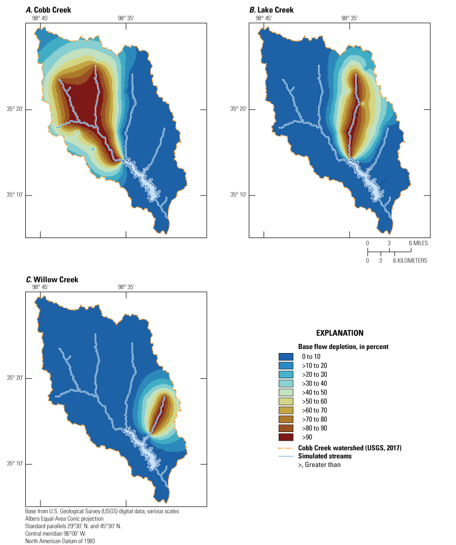
Base-flow depletion capture maps using steady-state, base-flow depletion simulations (representing long-term equilibrium) for A, Cobb Creek, B, Lake Creek, and C, Willow Creek individually using the total inflows to the Fort Cobb Reservoir as an observation.
To assess how base-flow depletion varied among streams, various offset distances were constructed and the cell centroids within those offset distances were used to calculate base-flow depletion summary statistics. Offset distances were arbitrary distances created to help summarize the base-flow depletion statistics as a function of distance away from the stream. A groundwater-flow model cell was considered to be within the offset distance if its centroid was within the offset distance from the stream. The data shown on each capture map in figure 20 were used to calculate mean base-flow depletion and mean base-flow depletion scaled by mean annual base flow as a fraction of mean annual inflow (hereinafter referred to as “scaled mean base-flow depletion”) for each stream (fig. 21). The data shown on the capture maps for each individual stream were used to remove the influence of base-flow depletion for the other streams.
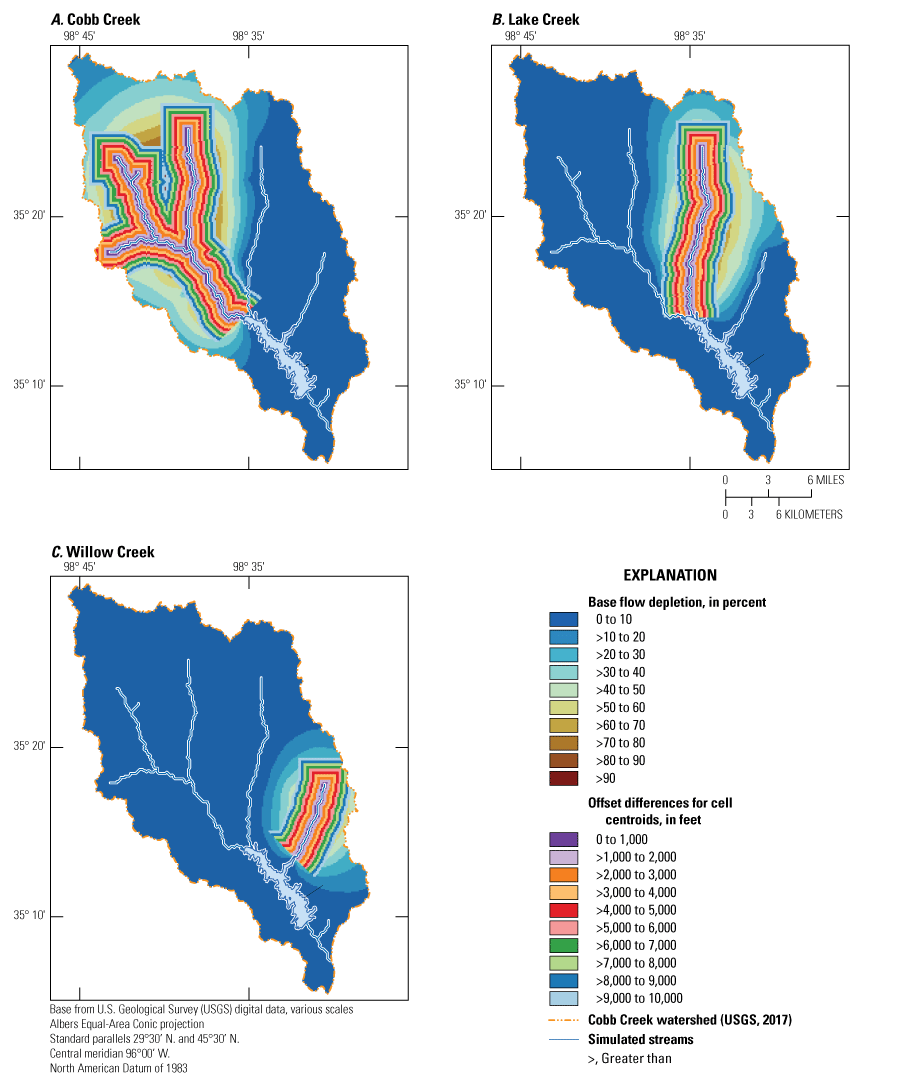
Offset distances for cell centroids for the steady-state, base-flow depletion simulations (representing long-term equilibrium) overlain on the capture maps that were used to calculate statistics for A, Cobb Creek, B, Lake Creek, and C, Willow Creek.
Groundwater wells can only capture a finite amount of water from streams. To contextualize base-flow depletion for each stream, scaled mean base-flow depletion was used to normalize the potential effects of base-flow depletion and to better represent how each stream contributes to total inflows to the Fort Cobb Reservoir. Scaling mean base-flow depletion contextualizes how each stream would contribute to total inflows. Because a small groundwater-withdrawal rate was used for each base-flow depletion simulation, only small quantities of base flow would be captured. If higher groundwater-withdrawal rates were used, streams with less base flow could become dry and no longer yield water to the aquifer, therefore producing a smaller base-flow depletion value than when simulating a smaller groundwater-withdrawal rate. Thus, scaling mean base-flow depletion for Cobb, Lake, and Willow Creeks to their proportion of total inflows contextualizes how base-flow depletion for each stream would affect total inflows. Mean base-flow depletion decreases to about 60 percent for Cobb Creek and to less than 50 percent for Lake and Willow Creeks when an offset distance ranging from more than 9,000 to 10,000 ft is applied (fig. 21). Mean base-flow depletion moderately declined from about 90 percent near the streams for offset distances of less than 1,000 ft to about 35 to 50 percent at the offset distance ranging from more 9,000 to 10,000 ft. Scaled mean base-flow depletion for Cobb Creek was the highest by about a factor of three, followed by Lake Creek (scaled mean base-flow depletion of about one-third of Cobb Creek), then Willow Creek (scaled mean base-flow depletion of about one-tenth of Cobb Creek). Groundwater withdrawals near Cobb Creek likely affect total inflows to the Fort Cobb Reservoir much more than those near Lake and Willow Creeks.
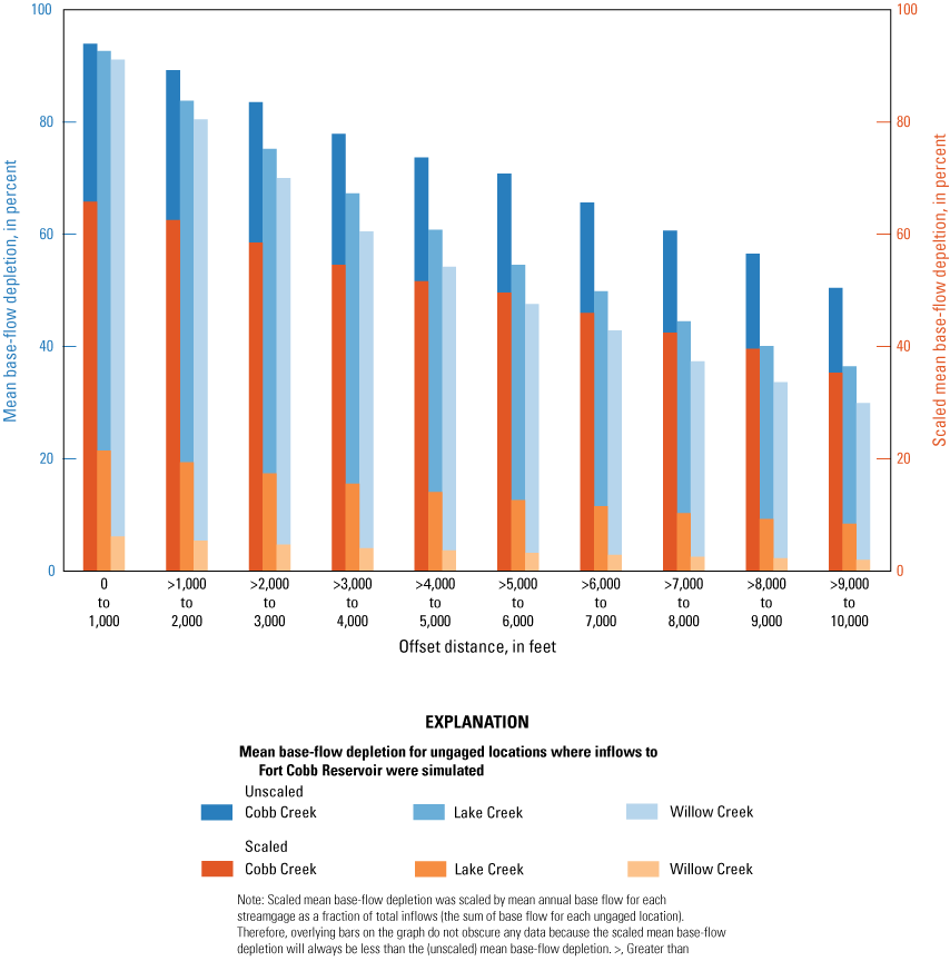
Mean base-flow depletion and scaled mean base-flow depletion at various offset distances for Cobb, Lake, and Willow Creeks in the Cobb Creek watershed, western Oklahoma.
Overall, high base-flow depletion (more than 80 percent) covers a broader watershed area for Cobb Creek compared to base-flow depletion for Lake and Willow Creeks. When considering the contributions of each stream to total inflows for Fort Cobb Reservoir, additional groundwater withdrawals near Cobb Creek are more likely to reduce total inflows to the Fort Cobb Reservoir compared to additional withdrawals in areas near Lake and Willow Creeks (fig. 19). However, base-flow depletion was consistently high (more than 80 percent) for all three major streams (Cobb, Lake, and Willow Creeks) for offset distance ranging from 0 to about 2,000 ft (fig. 21). For areas downgradient from Cobb, Lake, and Willow Creeks and in the northwest corner of the Cobb Creek watershed, changes in groundwater withdrawals resulted in minimal changes to base flow (base-flow depletions were typically less than 10 percent); therefore, total inflows to the Fort Cobb Reservoir were minimally reduced compared to other areas within the Cobb Creek watershed (figs. 18–19). Results from the groundwater-flow model demonstrated that additional groundwater withdrawals closer to the Fort Cobb Reservoir were not as likely to reduce inflows to the reservoir by as much as additional groundwater withdrawals further upgradient in the Cobb Creek watershed.
Model Assumptions and Limitations
Limitations are associated with the groundwater-flow model scenarios for the Rush Springs aquifer because the groundwater-flow model approximates the complex, real-world groundwater-flow regime of the Rush Springs aquifer. Many of the limitations for the calibrated groundwater-flow model apply to the scenarios in this report. Limitations of the groundwater-flow model used for the scenarios and the limitations for the scenarios themselves are summarized herein. Refer to Ellis (2018b) for a more detailed discussion of the limitations of the groundwater-flow model.
MODFLOW-NWT simulates groundwater flow by using Darcy’s Law which assumes that groundwater is of uniform density and incompressible and that groundwater flow is laminar and occurs through porous media (Heath, 1983). Although groundwater flow in Rush Springs aquifer is governed by Darcy’s Law, groundwater flow could deviate from some of the inherent assumptions of Darcy’s Law in some locations; for example, groundwater flow may not be laminar for fractured rocks contained in the Rush Springs aquifer. Groundwater withdrawals are not metered in Oklahoma, and the groundwater withdrawals for the calibrated Rush Springs groundwater-flow model were from reported groundwater use (Ellis, 2018b). OWRB does not require permitting for domestic groundwater use, so any domestic groundwater use was unknown and not included in the calibrated Rush Springs groundwater-flow model (Ellis, 2018b). Domestic groundwater withdrawals were assumed to be a relatively minor component of total groundwater withdrawals (Ellis, 2018b).
The uncertainty associated with construction of the bases of aquifers in the study area and the spatial discretization required to represent those bases in a model can inhibit matching groundwater-flow model outputs to observations (Doherty, 2015). The Rush Springs aquifer groundwater-flow model consists of 500-ft by 500-ft cell spacing. Properties and boundary conditions for each cell are assumed to be uniform. Ellis (2018b) implemented streams and lakes into the calibrated Rush Springs groundwater-flow model that were best represented at a regional to subregional scale. Although the streams implemented in the groundwater-flow simulation likely contained most of the base flow from the Rush Springs aquifer, the quantity of base flow in smaller ordered streams that were not included in the modeling scenarios is an unknown and thus a source of some uncertainty. The LAK package was replaced with the CHD package for the Fort Cobb Reservoir for the groundwater-flow models in this study. As a result of the change to the CHD package, changes in reservoir storage and changes in stage cannot be observed and were outside the scope of this report.
Uncertainty also arises from the limited availability and quality of groundwater altitude and base-flow data used to calibrate the groundwater-flow model. Relatively few parameter and observation data were available, and the available data were not distributed uniformly temporally or spatially. Calibration targets and observations were sparse throughout certain locations of the groundwater-flow model that were typically outside of the Cobb Creek watershed (the focus of this report; Ellis, 2018b). All groundwater-flow model inputs and observations have uncertainty associated with them. The base-flow separation inputs and observations, Soil-Water-Balance climate inputs, hydraulic properties, groundwater withdrawals, groundwater altitude observations, and stream properties were all estimated and therefore subject to measurement and human error. Ellis (2018b) modified many of those parameters during calibration to better match calibration targets (observations). Many of these parameters affect base flow and can affect the results of the simulations done for this study; however, automated calibration should reduce the effect of this uncertainty because parameters in the model should be closer to their “true” values (Doherty, 2015).
Ellis (2018b) completed a sensitivity analysis for the calibrated Rush Springs groundwater-flow model by incrementing individual parameters by 1 percent and recording the response. Ellis (2018b) identified that recharge, hydraulic conductivity, and evapotranspiration were most sensitive with respect to base flows. Recharge, hydraulic conductivity, and the rates specified for the EVT package were not modified for the scenarios in this study. These values could be different from their “true” values. In such instances, base-flow responses may differ from the “true” response. Ellis (2018b) also completed an identifiability analysis for parameters modified during calibration. Doherty and Hunt (2009) provide a detailed discussion of identifiability analyses in groundwater models. Parameters affect observations to a lesser extent when the parameter identifiability is lower compared to parameters with higher identifiability. The hydraulic-conductivity parameters and the evapotranspiration extinction-depth parameter were considered less identifiable (Doherty and Hunt, 2009) compared to the other parameters used in the model, so the hydraulic-conductivity parameters and the evapotranspiration extinction-depth parameter were relatively uncertain. Hydraulic conductivity and extinction depth contribute the most to capture map bias (Nadler and others, 2018). Thus, uncertainties associated with simulated base flows may be higher than if those parameters were more certain. However, Nadler and others (2018) calculated higher capture map bias for low hydraulic conductivities. The Rush Springs aquifer model contained moderate hydraulic conductivities; about 75 percent of the Rush Springs aquifer was simulated with hydraulic conductivities greater than 3 ft per day (Ellis, 2018b).
Because the intent of the EPS scenario is to dry aquifer cells (which can no longer yield water) and not all cells become dry at the same time, the mean EPS rate (total volume pumped divided by the area of the aquifer and the number of years of the simulation) likely differs from the rate specified in the WEL package. This implies that the EPS rate is not applied uniformly over the entire aquifer. Therefore, mean EPS rates for the simulations in scenario 1 (the scaled-EPS-groundwater-withdrawal scenario) might not be equivalent to multiplying the baseline EPS rate by the specified percentage used to scale groundwater withdrawals for the simulations in scenario 1. Additionally, the mean EPS rate for scenario 1 will be different if calculated over the first 20 simulated years or over the entire simulated 50-year period as a result of the progressive reduction in groundwater availability.
For the zonal-scaled-historical-groundwater-withdrawal scenario (scenario 2), zones were created to contain approximately equal groundwater withdrawals to attempt to reduce bias. This was difficult to achieve because dissimilar groundwater withdrawals had to be discretized spatially and temporally. That is, not all groundwater withdrawals persist through time and are therefore difficult to group spatially while maintaining equal groundwater-withdrawal rates for all zones. Some zones contained more groundwater withdrawals than other zones, so some bias was still present because the relation between groundwater withdrawals and base flows is not always linear (Barlow and Leake, 2012).
The base-flow-depletion scenario (scenario 4) was completed by using mean climatic conditions. It is possible that other climatic conditions (such as droughts or flooding) would produce different base-flow-depletion fractions (particularly if no-flow conditions prevailed in the streams during drought conditions or if there was no flow in certain reaches that subsequently began flowing during flooding conditions). The base-flow-depletion scenario was done by using a steady-state simulation. When a well first begins withdrawing water, there is a time delay until the water levels in the aquifer reach equilibrium with the groundwater being withdrawn (Heath, 1983; Barlow and Leake, 2012). The timing of the changes to base flows and other groundwater-flow components cannot be determined by using the simulation because the steady-state simulation assumes no time component. Because the Rush Springs simulation was designed for a subregional to regional scale, base-flow depletion may not be appropriate when assessing the effects on base flows by groundwater withdrawals from individual wells. Depletion fraction calculations rely on the principle of superposition and, thus, assume that groundwater flow is linear within a groundwater system (Barlow and Leake, 2012). Somewhat nonlinear groundwater systems can still be approximated by using superposition (Reilly and others, 1987). Groundwater flow from the base-flow-depletion scenario was assumed to be linear or only somewhat nonlinear because a small groundwater-withdrawal rate was used (about 20 gal/min). Nonlinearity (for a base-flow depletion simulation) is, in large part, a result of changes in transmissivity caused by a declining water table (Barlow and Leake, 2012; Nadler and others, 2018); a small groundwater-withdrawal rate would not likely produce a large decline in the water table.
Summary
To better understand the relation between groundwater use in the Rush Springs aquifer and inflows to the Fort Cobb Reservoir, the U.S. Geological Survey, in cooperation with the Bureau of Reclamation (Reclamation), used a previously published numerical groundwater-flow model and historical streamflow records to investigate how changing groundwater withdrawals could affect base flows in streams which flow into Fort Cobb Reservoir by evaluating four scenarios. These scenarios consisted of observing simulated base-flow response by (1) scaling the 20-year equal-proportionate-share (EPS) groundwater-withdrawal rate by various percentages over a 50-year period; (2) scaling the historical groundwater-withdrawal rates by various percentages across the entire Rush Springs aquifer; (3) scaling the historical groundwater-withdrawal rates within various subareas (zones) of the Fort Cobb Reservoir surface watershed; and (4) simulating a base-flow-depletion scenario.
Cobb, Lake, and Willow Creeks are the major streams upgradient from Fort Cobb Reservoir (listed by highest to lowest mean annual base flow). Results from scenario 1 indicate that changes to the simulated EPS groundwater-withdrawal rates impart minor changes in base flow because base flows tend to decline rapidly for these simulations; streams mostly dried in less than a decade. Because of the extreme simulated groundwater-withdrawal rates for an EPS groundwater-withdrawal scenario, groundwater levels tend to decrease to altitudes below the altitude of the streambed rapidly, thus causing base flows to decline rapidly. For all simulations except for the one where the EPS rate was scaled to 25 percent of its baseline, groundwater withdrawals induced no-flow conditions for Willow and Lake Creeks in less than 20 years. The simulation using the EPS rate scaled to 25 percent of its baseline was the only simulation where Cobb, Lake, and Willow Creeks did not stop flowing within the 50-year timeframe.
Results from scenario 2 indicate that base flows tended to decrease by a greater amount for increasing groundwater withdrawals compared to the increase in base flows when groundwater withdrawals were reduced by an equivalent amount. Willow Creek base flow was lowest compared to the base flows for Lake and Cobb Creeks, and, if base flow for all streams were reduced by an equal amount, percentage change in base flow for Willow Creek would be the highest; a large negative percentage change would indicate that a stream was more susceptible to undergoing sustained periods of no flow. Simulating an increase in groundwater withdrawals generally reduced base flows more in Cobb Creek than in Lake Creek or Willow Creek. Additional groundwater withdrawals near Cobb Creek would likely reduce inflows to the Fort Cobb Reservoir more appreciably compared to the reductions in inflows caused by additional groundwater withdrawals near Lake and Willow Creeks.
Results from scenario 3 indicate that total inflows to the Fort Cobb Reservoir were most responsive to changes in groundwater withdrawals from subareas (zones) near Cobb Creek. Zones upgradient in the watershed generally affected base flows more than zones farther downgradient, likely because base flows were often greater farther upgradient in the watershed than those closer to the Fort Cobb Reservoir. Overall, changes in groundwater withdrawals in zones near Willow Creek tended to affect base flows the least compared to groundwater withdrawals nearest Lake and Cobb Creeks when groundwater withdrawals were scaled in those zones.
Results from scenario 4 indicate that base-flow depletion is most spatially extensive around Cobb Creek (and its two main tributaries for which changes in base flow were also simulated), followed by Lake Creek, and lastly Willow Creek. Mean base-flow depletion at various offset distances for Cobb Creek was highest, followed by the depletion for Lake Creek and then for Willow Creek. The Cobb Creek tributaries likely contribute to groundwater -withdrawals affecting Cobb Creek base flow over a larger area compared to Lake Creek and Willow Creek base flow.
Overall, changes to groundwater withdrawals in areas around Cobb Creek tended to affect base flows more than changes to groundwater withdrawals in areas around Lake and Willow Creeks. This is likely because Cobb Creek drains a larger watershed area over the Rush Springs aquifer compared to Lake and Willow Creeks, and base flows are greater in Cobb Creek and constitute most inflows to the Fort Cobb Reservoir. Managing groundwater withdrawals in the Cobb Creek area could preserve total inflows to the Fort Cobb Reservoir more than in other areas throughout the Cobb Creek watershed. Groundwater withdrawals towards the southern and northwestern areas of the Cobb Creek watershed tend to least affect total inflows to the Fort Cobb Reservoir. The groundwater-flow model demonstrated that additional groundwater withdrawals in the southern and northwestern areas of the Cobb Creek watershed may not reduce total inflows to the Fort Cobb Reservoir as much as withdrawals from other areas of the Cobb Creek watershed.
References Cited
Barlow, P.M., Cunningham, W.L., Zhai, T., and Gray, M., 2015, U.S. Geological Survey Groundwater Toolbox, a graphical and mapping interface for analysis of hydrologic data (version 1.0)—User guide for estimation of base flow, runoff, and groundwater recharge from streamflow data: U.S. Geological Survey Techniques and Methods, book 3, chap. B10, 27 p., accessed July 19, 2016, at https://doi.org/10.3133/tm3B10.
Barlow, P.M., and Leake, S.A., 2012, Streamflow depletion by wells—Understanding and managing the effects of groundwater pumping on streamflow: U.S. Geological Survey Circular 1376, 84 p., accessed February 23, 2023, at https://doi.org/10.3133/cir1376.
Becker, M.F., and Runkle, D.L., 1998, Hydrogeology, water quality, and geochemistry of the Rush Springs aquifer, western Oklahoma: U.S. Geological Survey Water-Resources Investigations Report 98–4081, 37 p., accessed October 5, 2023, at https://doi.org/10.3133/wri984081.
Bureau of Reclamation [Reclamation], 2017a, Reservoir release, storage, evaporation, and precipitation data for Fort Cobb Reservoir, Oklahoma: Bureau of Reclamation web page, accessed March 15, 2017, at https://www.usbr.gov/gp-bin/custom.pl?SWE221A&cobb.
Bureau of Reclamation [Reclamation], 2017b, Reservoir release, storage, evaporation, and precipitation data for Foss Reservoir, Oklahoma: Bureau of Reclamation web page, accessed March 15, 2017, at https://www.usbr.gov/gp-bin/custom.pl?SWE221A&foss.
Carr, J.E., and Bergman, D.L., 1976, Reconnaissance of the water resources of the Clinton quadrangle, west-central Oklahoma: Oklahoma Geological Survey Hydrologic Atlas 5, 4 sheets, scale 1:250,000, accessed October 5, 2023, at http://ogs.ou.edu/docs/hydrologicatlases/HA5P4.pdf.
Cleveland, W.S., 1979, Robust locally weighted regression and smoothing scatterplots: Journal of the American Statistical Association, v. 74, no. 368, p. 829–836, accessed May 22, 2023, at https://doi.org/10.1080/01621459.1979.10481038.
Condor Team, 2012, High-Throughput Computing (HTC) and its requirements—Condor manual (ver. 7.7.5): Madison, Wis., University of Wisconsin, accessed October 18, 2023, at https://pages.cs.wisc.edu/~danb/ref-v7.7.5/1_1High_Throughput_Computin.html.
Doherty, J., and Hunt, R.J., 2009, Two statistics for evaluating parameter identifiability and error reduction: Journal of Hydrology, v. 366, no. 1–4, p. 119–127, accessed October 5, 2023, at https://doi.org/10.1016/j.jhydrol.2008.12.018.
Doherty, J.E., 2015, Calibration and uncertainty analysis for complex environmental models: Brisbane, Australia, Watermark Numerical Computing, accessed October 11, 2023, at https://pesthomepage.org/pest-book.
Ellis, J.H., 2018a, MODFLOW model used in simulation of groundwater flow and analysis of projected water use for the Rush Springs aquifer, western Oklahoma: U.S. Geological Survey data release, accessed April 4, 2021, at https://doi.org/10.5066/F7Q52NXK.
Ellis, J.H., 2018b, Simulation of groundwater flow and analysis of projected water use for the Rush Springs aquifer, western Oklahoma: U.S. Geological Survey Scientific Investigations Report 2018–5136, 156 p., accessed October 5, 2023, at https://doi.org/10.3133/sir20185136.
Ellis, J.H., Ryter, D.W., Fuhrig, L.T., Spears, K.W., Mashburn, S.L., and Rogers, I.M.J., 2020, Hydrogeology, numerical simulation of groundwater flow, and effects of future water use and drought for reach 1 of the Washita River alluvial aquifer, Roger Mills and Custer Counties, western Oklahoma, 1980–2015: U.S. Geological Survey Scientific Investigations Report 2020–5118, 81 p., accessed October 5, 2023, at https://doi.org/10.3133/sir20205118.
Fay, R.O., and Hart, D.L., Jr., 1978, Geology and mineral resources (exclusive of petroleum) of Custer County, Oklahoma: Oklahoma Geological Survey Bulletin 114, 88 p., accessed October 5, 2023, at http://ogs.ou.edu/docs/bulletins/B114.pdf.
Harbaugh, A.W., 2005, MODFLOW-2005—The U.S. Geological Survey modular ground-water model—The ground-water flow process: U.S. Geological Survey Techniques and Methods, book 6, chap. A16, [variously paged], accessed October 5, 2023, at https://doi.org/10.3133/tm6A16.
Heath, R.C., 1983, Basic ground-water hydrology: U.S. Geological Survey Water-Supply Paper 2220, 86 p., accessed October 5, 2023, at https://doi.org/10.3133/wsp2220.
Helsel, D.R., Hirsch, R.M., Ryberg, K.R., Archfield, S.A., and Gilroy, E.J., 2020, Statistical methods in water resources: U.S. Geological Survey Techniques and Methods, book 4, chap. A3, 458 p., accessed October 5, 2023, at https://doi.org/10.3133/tm4A3. [Supersedes USGS Techniques of Water-Resources Investigations, book 4, chap. A3, version 1.1.]
Kendall, M.G., 1938, A new measure of rank correlation: Biometrika, v. 30, no. 1–2, p. 81–93, accessed March 3, 2022, at https://doi.org/10.1093/biomet/30.1-2.81.
Kendall, M.G., 1945, The treatment of ties in ranking problems: Biometrika, v. 33, no. 3, p. 239–251, accessed March 3, 2022, at https://doi.org/10.1093/biomet/33.3.239.
Labriola, L.G., Russell, C.A., and Ellis, J.H., 2022, Potential effects of out-of-basin groundwater transfers on spring discharge, base flow, and groundwater storage pertaining to the Rush Springs aquifer in and near the Caddo Nation of Oklahoma Tribal jurisdictional area, western Oklahoma: U.S. Geological Survey Scientific Investigations Report 2022–5044, 32 p., accessed October 5, 2023, at https://doi.org/10.3133/sir20225044.
Leake, S.A., Reeves, H.W., and Dickinson, J.E., 2010, A new capture fraction method to map how pumpage affects surface water flow: Groundwater, v. 48, no. 5, p. 690–700, accessed October 5, 2023, at https://doi.org/10.1111/j.1745-6584.2010.00701.x.
Manning, R., 1891, On the flow of water in open channels and pipes: Transactions of the Institution of Civil Engineers of Ireland, v. 20, p. 161–207, accessed October 5, 2023, at https://doi.org/10.48495/r207ts96k.
Merritt, M.L., and Konikow, L.F., 2000, Documentation of a computer program to simulate lake-aquifer interaction using the MODFLOW ground-water flow model and the MOC3D solute-transport model: U.S. Geological Survey Water-Resources Investigations Report 00–4167, 146 p., accessed October 5, 2023, at https://doi.org/10.3133/wri004167.
Nadler, C., Allander, K., Pohll, G., Morway, E., Naranjo, R., and Huntington, J., 2018, Evaluation of bias associated with capture maps derived from nonlinear groundwater flow models: Groundwater, v. 56, no. 3, p. 458–469, accessed March 31, 2022, at https://doi.org/10.1111/gwat.12597.
National Aeronautics and Space Administration Jet Propulsion Laboratory [NASA JPL], 2013, NASA Shuttle Radar Topography Mission Global 3 arc second: National Aeronautics and Space Administration Jet Propulsion Laboratory dataset, accessed February 2, 2022, at https://doi.org/10.5067/MEaSUREs/SRTM/SRTMGL3.003.
National Oceanic and Atmospheric Administration [NOAA], 2022, Climate at a glance—Divisional time series (July 2022): National Oceanic and Atmospheric Administration database, accessed July 15, 2022, at https://www.ncei.noaa.gov/cag/.
Neel, C.R., Wagner, D.L., Correll, J.S., Sanford, J.E., Hernandez, R.J., Spears, K.W., and Waltman, P.B., 2018, Hydrologic investigation report of the Rush Springs aquifer in west-central Oklahoma: Oklahoma Water Resources Board, 61 p., accessed October 4, 2023, at https://www.owrb.ok.gov/reports/studies/RushSprings2015.pdf.
Niswonger, R.G., Panday, S., and Ibaraki, M., 2011, MODFLOW-NWT—A Newton formulation for MODFLOW-2005: U.S. Geological Survey Techniques and Methods, book 6, chap. A37, 44 p., accessed October 5, 2023, at https://doi.org/10.3133/tm6A37.
Niswonger, R.G., and Prudic, D.E., 2005, Documentation of the Streamflow-Routing (SFR2) package to include unsaturated flow beneath streams—A modification to SFR1: U.S. Geological Survey Techniques and Methods, book 6, chap. A13, 50 p., accessed October 5, 2023, at https://doi.org/10.3133/tm6A13.
Oklahoma Climatological Survey, 2023a, Precipitation history—Annual, west central (CD4): Oklahoma Climatological Survey web page, accessed July 19, 2023, at https://climate.ok.gov/index.php/climate/climate_trends/precipitation_history_annual_statewide/CD04/prcp/Annual.
Oklahoma Climatological Survey, 2023b, Precipitation history—Annual, southwest (CD7): Oklahoma Climatological Survey web page, accessed July 19, 2022, at https://climate.ok.gov/index.php/climate/climate_trends/precipitation_history_annual_statewide/CD07/prcp/Annual.
Oklahoma Secretary of State, 2023, General provisions, chap. 20, subchap. 1, sec. 2 of Appropriation and use of stream water: Oklahoma Secretary of State, Oklahoma administrative code, title 785, accessed May 16, 2023, at https://rules.ok.gov/code.
Oklahoma State Legislature, 2023a, Definitions, chap. 1020, sec. 1 of Waters and water rights: Oklahoma State Legislature, Oklahoma Statutes, title 82, accessed April 3, 2023, at https://oksenate.gov/sites/default/files/2019-12/os82.pdf.
Oklahoma State Legislature, 2023b, Determination of maximum annual yield, chap. 1020, sec. 5 of Waters and water rights: Oklahoma State Legislature, Oklahoma Statutes, title 82, accessed April 3, 2023, at https://oksenate.gov/sites/default/files/2019-12/os82.pdf.
Oklahoma State Legislature, 2023c, Approval of application, chap. 1020, sec. 9 of Waters and water rights: Oklahoma State Legislature, Oklahoma Statutes, title 82, accessed April 3, 2023, at https://oksenate.gov/sites/default/files/2019-12/os82.pdf.
Oklahoma State Legislature, 2023d, Sensitive sole source groundwater basins or subbasins—Moratorium on issuance of certain temporary permits, chap. 1020, sec. 9A of Waters and water rights: Oklahoma State Legislature, Oklahoma Statutes, title 82, accessed April 3, 2023, at https://oksenate.gov/sites/default/files/2019-12/os82.pdf.
Oklahoma Water Resources Board [OWRB], 2012, Oklahoma Comprehensive Water Plan—West Central Watershed Planning Region Report (ver. 1.1): Oklahoma Water Resources Board, 168 p., accessed October 5, 2023, at https://oklahoma.gov/content/dam/ok/en/owrb/documents/water-planning/ocwp/OCWP_WestCentral_Region_Report.pdf.
Oklahoma Water Resources Board [OWRB], 2023, Maximum annual yield: Oklahoma Water Resources Board Fact Sheet, 2 p., accessed April 3, 2023, at https://rest.owrb.ok.gov/about/about_pdf/Fact-MAY.pdf.
Python Software Foundation, 2021, Python language reference (ver. 3.9.7, August 30, 2021): Python Software Foundation software release, accessed October 5, 2023, at https://www.python.org.
QGIS, 2022, QGIS—A free and open source geographic information system: QGIS Association website, accessed October 5, 2023, at http://www.qgis.org.
Reilly, T.E., Franke, O.L., and Bennett, G.D., 1987, The principle of superposition and its application in ground-water hydraulics: U.S. Geological Survey Techniques of Water-Resources Investigations, book 3, chap. B6, 28 p., accessed October 5, 2023, at https://doi.org/10.3133/twri03B6. [Supersedes USGS Open-File Report 84–459.]
Rossum, G. van, 1995, Python tutorial: Amsterdam, Centrum voor Wiskunde en Informatica, Technical Report CS–R9526, 65 p., accessed October 5, 2023, at https://ir.cwi.nl/pub/5007/05007D.pdf.
Sen, P.K., 1968, Estimates of the regression coefficient based on Kendall’s tau: Journal of the American Statistical Association, v. 63, no. 324, p. 1379–1389, accessed October 5, 2023, at https://doi.org/10.1080/01621459.1968.10480934.
Shah, N., Nachabe, M., and Ross, M., 2007, Extinction depth and evapotranspiration from ground water under selected land covers: Groundwater, v. 45, no. 3, p. 329–338, accessed October 19, 2023, at https://doi.org/10.1111/j.1745-6584.2007.00302.x.
Shivers, M.J., and Andrews, W.J., 2013, Hydrologic drought of water year 2011 compared to four major drought periods of the 20th century in Oklahoma: U.S. Geological Survey Scientific Investigations Report 2013–5018, 52 p., accessed October 5, 2023, at https://doi.org/10.3133/sir20135018.
Tanaka, H.H., and Davis, L.V., 1963, Ground-water resources of the Rush Springs sandstone in the Caddo County area, Oklahoma: Oklahoma Geological Survey Circular 61, 63 p., accessed October 5, 2023, at http://ogs.ou.edu/docs/circulars/C61.pdf.
Theil, H., 1950, A rank-invariant method of linear and polynomial regression analysis—Parts I, II, and III: Proceedings of the Royal Netherlands Academy of Sciences, v. 53, p. 386–392, 521–525, and 1397–1412, accessed October 5, 2023, at https://link.springer.com/chapter/10.1007/978-94-011-2546-8_20.
Thornthwaite, C.W., and Mather, J.R., 1957, Instructions and tables for computing potential evapotranspiration and the water balance: Centerton, N.J., Drexel Institute of Technology Laboratory of Climatology, Publications in Climatology, v. 10, no. 3, p. 185–311, accessed October 5, 2023, at https://www.wrc.udel.edu/wp-content/publications/ThornthwaiteandMather1957Instructions_Tables_ComputingPotentialEvapotranspiration_Water%20Balance.pdf.
Trevisan, A.R., Labriola, L.G., and Ellis, J.H., 2024, MODFLOW-NWT model used to evaluate groundwater withdrawal scenarios for the Rush Springs aquifer upgradient from the Fort Cobb Reservoir, western Oklahoma, 1979–2015, including streamflow, base flow, and precipitation statistics: U.S. Geological Survey data release, https://doi.org/10.5066/P9K413D1.
U.S. Environmental Protection Agency [EPA], 2023a, Sole source aquifers for drinking water–What is a sole source aquifer (SSA)?: U.S. Environmental Protection Agency web page, accessed April 3, 2023, at https://www.epa.gov/sole-source-aquifers-drinking-water/overview-drinking-water-sole-source-aquifer-program#What_Is_SSA.
U.S. Environmental Protection Agency [EPA], 2023b, Sole source aquifers for drinking water–Interactive map of SSAs [sole source aquifers]: U.S. Environmental Protection Agency web page, accessed April 3, 2023, at https://epa.maps.arcgis.com/apps/webappviewer/index.html?id=9ebb047ba3ec41ada1877155fe31356b.
U.S. Geological Survey [USGS], 2017a, National Hydrography Dataset: U.S. Geological Survey database, accessed September 14, 2017, at https://nhd.usgs.gov/data.html.
U.S. Geological Survey [USGS], 2017b, U.S. Geological Survey water data for Oklahoma: U.S. Geological Survey National Water Information System database, accessed March 14, 2017, at http://waterdata.usgs.gov/ok/nwis/.
U.S. Geological Survey [USGS], 2021, U.S. Geological Survey water data for Oklahoma: U.S. Geological Survey National Water Information System database, accessed June 17, 2021, at https://waterdata.usgs.gov/ok/nwis/.
U.S. Geological Survey [USGS], 2022, U.S. Geological Survey water data for Oklahoma: U.S. Geological Survey National Water Information System database, accessed May 4, 2022, at https://waterdata.usgs.gov/ok/nwis/.
Virtanen, P., Gommers, R., Oliphant, T.E., Haberland, M., Reddy, T., Cournapeau, D., Burovski, E., Peterson, P., Weckesser, W., Bright, J., van der Walt, S.J., Brett, M., Wilson, J., Millman, K.J., Mayorov, N., Nelson, A.R.J., Jones, E., Kern, R., Larson, E., Carey, C.J., Polat, I., Feng, Y., Moore, E.W., VanderPlas, J., Laxalde, D., Perktold, J., Cimrman, R., Henriksen, I., Quintero, E.A., Harris, C.R., Archibald, A.M., Ribeiro, A.H., Pedregosa, F., van Mulbregt, P., and others, 2020, SciPy 1.0—Fundamental algorithms for scientific computing in Python: Nature Methods, v. 17, no. 3, p. 261–272, accessed October 5, 2023, at https://doi.org/10.1038/s41592-019-0686-2.
Wahl, K.L., and Wahl, T.L., 1995, Determining the flow of Comal Springs at New Braunfels, Texas, in Texas Water ‘95—A Component Conference of the First International Conference on Water Resources Engineering, San Antonio, Texas, August 16–17, 1995, [Proceedings]: American Society of Civil Engineers, p. 77–86, accessed October 19, 2023, at https://www.usbr.gov/tsc/techreferences/hydraulics_lab/pubs/PAP/PAP-0708.pdf.
Walker, L.M., and Bradford, R.E., 2009, The basics of Oklahoma water law—What every practitioner should know: The Oklahoma Bar Journal, v. 80, no. 23, p. 1748–1751, accessed October 5, 2023, at https://www.okbar.org/wp-content/uploads/2018/06/OBJ2009Sept05-sm.pdf.
Welter, D.E., White, J.T., Hunt, R.J., and Doherty, J.E., 2015, Approaches in highly parameterized inversion—PEST++ version 3, a parameter ESTimation and uncertainty analysis software suite optimized for large environmental models: U.S. Geological Survey Techniques and Methods, book 7, chap. C12, 54 p., accessed October 18, 2023, at https://doi.org/10.3133/tm7C12.
Westenbroek, S.M., Kelson, V.A., Dripps, W.R., Hunt, R.J., and Bradbury, K.R., 2010, SWB—A modified Thornthwaite-Mather Soil-Water-Balance code for estimating groundwater recharge: U.S. Geological Survey Techniques and Methods, book 6, chap. A31, 59 p., accessed October 5, 2023, at https://doi.org/10.3133/tm6A31.
Winston, R.B., 2022, Online guide to MODFLOW-NWT: U.S. Geological Survey web page, accessed May 22, 2023, at https://water.usgs.gov/ogw/modflow-nwt/MODFLOW-NWT-Guide/index.html.
Conversion Factors
U.S. customary units to International System of Units
Temperature in degrees Fahrenheit (°F) may be converted to degrees Celsius (°C) as follows: °C = (°F – 32) / 1.8.
Datum
Vertical coordinate information is referenced to the North American Vertical Datum of 1988 (NAVD 88) with the exception of the lake-stage altitudes of Foss and Fort Cobb Reservoirs which are referenced to the National Geodetic Vertical Datum of 1929 (NGVD 29).
Horizontal coordinate information is referenced to the North American Datum of 1983 (NAD 83).
Altitude, as used in this report, refers to distance above the vertical datum.
Abbreviations
BFI
base-flow index
CHD
Time-variant head package for MODFLOW-NWT
DRN
Drain package for MODFLOW-NWT
EPA
U.S. Environmental Protection Agency
EPS
equal proportionate share
ET
evapotranspiration
EVT
Evapotranspiration package for MODFLOW-NWT
GHB
General Head Boundary package for MODFLOW-NWT
LAK
Lake package for MODFLOW-NWT
MAY
maximum annual yield
MAXITEROUT
Maximum number of outer iterations for the Newton solver
n-day
number of days
NOAA
National Oceanic and Atmospheric Administration
NWIS
National Water Information System (USGS database)
OWRB
Oklahoma Water Resources Board
PEST++
parameter estimation software version 4
PESTPP-SWP
PEST++ parameter sweep utility
p-value
probability value
RCH
Recharge package for MODFLOW-NWT
Reclamation
Bureau of Reclamation
SFR
Streamflow Routing package for MODFLOW-NWT
SWB
Soil-Water-Balance simulation
USGS
U.S. Geological Survey
For more information about this publication, contact
Director, Oklahoma-Texas Water Science Center
U.S. Geological Survey
1505 Ferguson Lane
Austin, TX 78754-4501
For additional information, visit
https://www.usgs.gov/centers/ot-water
Publishing support provided by
Lafayette Publishing Service Center
Disclaimers
Any use of trade, firm, or product names is for descriptive purposes only and does not imply endorsement by the U.S. Government.
Although this information product, for the most part, is in the public domain, it also may contain copyrighted materials as noted in the text. Permission to reproduce copyrighted items must be secured from the copyright owner.
Suggested Citation
Trevisan, A.R., Labriola, L.G., and Ellis, J.H., 2024, Streamflow, base flow, and precipitation trends and simulated effects of Rush Springs aquifer groundwater withdrawals on base flows upgradient from Fort Cobb Reservoir, western Oklahoma: U.S. Geological Survey Scientific Investigations Report 2024–5002, 42 p., https://doi.org/10.3133/sir20245002.
ISSN: 2328-0328 (online)
Study Area
| Publication type | Report |
|---|---|
| Publication Subtype | USGS Numbered Series |
| Title | Streamflow, base flow, and precipitation trends and simulated effects of Rush Springs aquifer groundwater withdrawals on base flows upgradient from Fort Cobb Reservoir, western Oklahoma |
| Series title | Scientific Investigations Report |
| Series number | 2024-5002 |
| DOI | 10.3133/sir20245002 |
| Publication Date | March 04, 2024 |
| Year Published | 2024 |
| Language | English |
| Publisher | U.S. Geological Survey |
| Publisher location | Reston, VA |
| Contributing office(s) | Oklahoma-Texas Water Science Center |
| Description | Report: x, 42 p.; Data Release |
| Country | United States |
| State | Oklahoma |
| Other Geospatial | Fort Cobb Reservoir |
| Online Only (Y/N) | Y |