

Development and Calibration of HEC–RAS Hydraulic, Temperature, and Nutrient Models for the Mohawk River, New York
Links
- Document: Report (20.5 MB pdf) , HTML , XML
- Data Release: USGS data release - HEC–RAS hydraulic, temperature, and nutrient models for the Mohawk River between Rome and Cohoes, New York
- NGMDB Index Page: National Geologic Map Database Index Page (html)
- Download citation as: RIS | Dublin Core
Acknowledgments
The authors would like to express their appreciation to Alexander Smith, Karen Stainbrook, Kenneth Kosinski, Katherine Czajkowski, Robert Capowski, Andrea Conine, Edward Schneider, Michaela Schnore, Eric Weigert, Alon Dominitz, and Kelli Higgins-Roche of the New York State Department of Environmental Conservation, and Derek Thorsland, Robert Streeter, and Michael Bocchi from the regional offices of the New York State Department of Environmental Conservation. The authors would like to express their appreciation to Howard Goebel and Thomas McDonald (New York Power Authority, Canal Corporation), and Kenneth Avery (Bergmann Associates) for their contributions towards finding and sharing some of the source hydraulic model information used in the study. The authors would also like to thank our U.S. Geological Survey colleagues Robert Breault and Gary Wall who provided coordination support with the New York State Department of Environmental Conservation, Elizabeth Nystrom for providing technical review of the resulting model and report, David (Samuel) Wallace for providing technical review of the resulting report, Daniel Edwards (retired), Kaitlyn Colella, Richard Kropp (retired), Jeffrey Fischer (retired), Jon Janowicz, Heather Heckathorn, and Lukasz Niemoczynski for support in building report figures.
Abstract
In support of a preliminary analysis performed by New York State Department of Environmental Conservation that found elevated nutrient levels along selected reaches of the Mohawk River, a one-dimensional, unsteady hydraulic and water-quality model (Hydrologic Engineering Center River Analysis System Nutrient Simulation Module 1 [HEC–RAS NSM I]) was developed by the U.S. Geological Survey for the 127-mile reach of the Mohawk River between Rome and Cohoes, New York. The model was designed to accurately simulate within-channel flow conditions for this highly regulated, control-structure dense river reach. The model was calibrated for the period of May through September 2016 using available streamflow, temperature, and water-quality data. Nitrogen, phosphorus, dissolved oxygen, and water column algae were balanced within the model; however, the nutrient model calibration was focused on phosphorus.
The HEC–RAS hydraulic model simulated streamflow adequately at the calibration locations with observed and simulated daily flows demonstrating coefficient of determination (r2) values ranging from 0.91 to 0.97, mean absolute error ranging from 15–20 percent, and bias ranging from −7 to 16 percent. The water temperature model within HEC–RAS NSM I demonstrated remarkable ability to simulate water temperature: typical water temperature errors were less than 1.0 degree Celsius (°C). Simulated water temperature results closely tracked observed continuous water temperature data at three locations on the Mohawk River, with mean absolute error for the 2016 study period ranging from 0.87 to 0.90 °C, and a root mean square error of 1.00 to 1.07 °C.
Performance criteria for the water-quality (nutrient) model were applied differently than the water temperature model because of the temporally coarse discrete samples collected for the project. The average difference between final simulated concentrations and observed concentrations of organic phosphorus for all sample locations was within 0.01 milligrams per liter (mg/L) and within 0.09 mg/L for orthophosphate using all locations except Rome, which was within 0.25 mg/L.
The calibrated model was used to implement nine phosphorus reduction scenarios by applying reductions to wastewater treatment plant effluent concentrations within the model. Monthly mean differences were computed for five comparison locations. Scenario results were generally linear and predictable; scenarios implementing the highest reductions showed correspondingly larger differences in Mohawk River concentrations downstream from the wastewater treatment plants associated with those reductions. The largest monthly mean differences were realized from reduction scenario nine and ranged from −0.018 to −0.076 mg/L for organic phosphorus and from 0.001 to −0.138 mg/L for orthophosphate.
Introduction
The Mohawk River is the largest tributary to the Hudson River and flows about 140 miles from its headwaters upstream from the Delta Reservoir between the Tug Hill Plateau and the Adirondack Mountains. The watershed drains about 3,480 square miles (U.S. Geological Survey, 2022a), including a large inflow from the Catskill Mountains region through the Schoharie Creek. The waters of the Mohawk River are used for recreation, agriculture, industry, and water supply and are needed to support aquatic life (New York State Department of Environmental Conservation, 2016). The New York State Department of Environmental Conservation (NYSDEC) uses a watershed-based approach to outline and implement plans to protect and improve water-quality conditions for a waterbody. NYSDEC has been building an action agenda for several years (New York State Department of Environmental Conservation, 2021) to protect and restore the Mohawk River and contributing watersheds. One of the drainage basin goals of NYSDEC has been to develop a better understanding of in-channel water-quality conditions in impounded reaches of the Mohawk River. Understanding the influence of point and non-point-source pollution on the Mohawk River is an important first step in improving the water-quality conditions.
To develop a better understanding of the state of the Mohawk River, NYDEC has collected data and published biological assessments and water-quality and bacteria monitoring reports about the river and several of its tributaries over the last 15 to 20 years (New York State Department of Environmental Conservation, 2022a). The general results of sampling and analysis of Mohawk River and tributary waters indicated some reaches showed elevated nutrient concentrations and other reaches were potentially not meeting the criteria for designated use as drinking water. The U.S. Geological Survey (USGS) and the NYSDEC worked cooperatively on a project to develop and calibrate a one-dimensional hydraulic and water-quality model of the main stem of the Mohawk River to simulate in-channel river conditions.
The assimilative capacity of the Mohawk River is complex and is affected by many interactions, including several impoundments. The development of a nutrient water-quality model first requires the development of a hydraulic model of the reach to provide the necessary hydraulics and flow data to the water-quality model for nutrient computations. After the calibration of the hydraulic model, the nutrient water-quality model could be calibrated using water-quality sample data, streamflow data, discharge and withdrawal data, land-use classifications, and meteorological data. Computer modeling techniques could then be used to simulate changes in water-quality conditions in the Mohawk River. The resulting model can be used to better understand the impacts of nutrient concentrations entering the Mohawk River.
The U.S. Army Corps of Engineers Hydraulic Engineering Center River Analysis System (HEC–RAS) was used for hydraulic modeling of the river and complex hydraulic structures (U.S. Army Corps of Engineers, 2016, version 5.0.3). The HEC–RAS model was also dynamically linked to a nutrient simulation module (NSM) within the software package that was calibrated for water temperature and nutrient parameters. This model was developed for the 127-mile reach of the Mohawk River from Rome to Cohoes, New York and was designed to simulate within-channel streamflow and water-quality conditions for the period of May to September 2016. Because the study area lacked a long-term dataset for water quality, the simulation period was selected to correspond to a comprehensive sampling project that collected nutrient samples throughout this reach in 2016 (U.S. Geological Survey, 2019).
Purpose and Scope
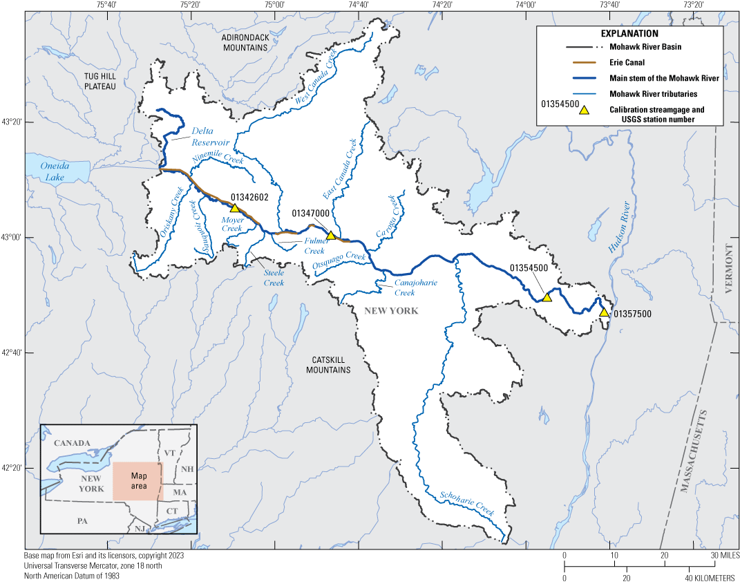
The NYSDEC and the USGS entered into a joint collaborative agreement to develop a hydraulic and nutrient model of the Mohawk River to better inform planning and protection of the waters of the Mohawk River. The purpose of this report is to document the development and calibration of a HEC–RAS hydraulic and nutrient model for a 127-mile reach of the Mohawk River from Rome to Cohoes, N.Y. (fig 1). The model was developed to support NYSDEC and their development of guidelines that will help to improve the water quality along the Mohawk River during base and lower flow conditions.
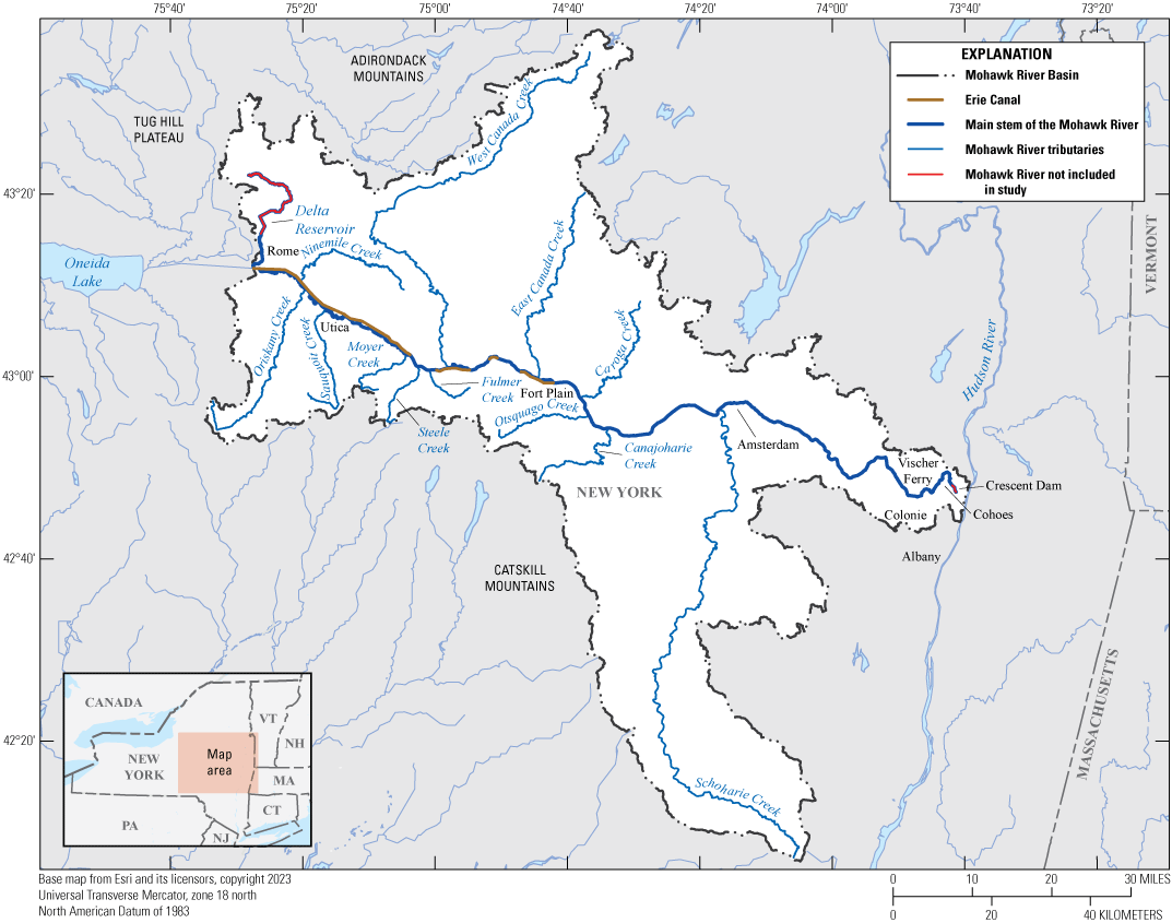
Map of Mohawk River Basin, modeled main-stem Mohawk River, and major tributaries.
Previous Studies
The NYSDEC Vision Approach to implement the Clean Water Act (section 303[d]) program and the “Clean Water Planning” report (New York State Department of Environmental Conservation, 2015) documents the State’s approach to implementing guidelines set forth by the U.S. Environmental Protection Agency (EPA). In 2016, NYSDEC prepared the “Mohawk River Basin Research Initiative” that described a partnership with the “Mighty Waters” cabinet level working group and a steering committee (New York State Department of Environmental Conservation, 2016). The action agenda established five primary goals of which goal 1 focused on fish, wildlife, and habitats and goal 2 focused on water quality. NYSDEC has been monitoring the water quality of the Mohawk River since the early 1970s as part of their ambient water-quality network, but to help provide a better understanding of nutrient levels and the overall water-quality health of the river, two rounds of more intense sampling were performed. The NYSDEC started this latest round of sampling along tributaries and the main-stem Mohawk River in the early 2000s. Also, sampling and assessments of a few tributaries as well as along the main stem were done to evaluate the water-quality conditions in the watershed. The assessments generally showed reaches with slightly impaired to poor water-quality conditions. Some locations indicated elevated nutrient concentrations and higher than acceptable bacteria concentrations (New York State Department of Environmental Conservation, 2022a).
Elevated levels of nutrients in the waters of the Mohawk River can lead to eutrophication and potentially toxic blue-green algal blooms. In a proactive approach to the problem, NYSDEC, in cooperation with the USGS, collected a wide variety of water-quality samples from April to October 2016 at many locations along the Mohawk River (fig 2). These data were collected as the first step in assessing the condition of the river by determining concentrations of nutrients and other constituents to provide necessary data for the development and calibration of a nutrient water-quality model for the Mohawk River. The Clean Water Act of 1972 (33 U.S.C. 1251 et seq.; US Environmental Protection Agency, 2022) mandated that a plan should be put in place that limits the Total Maximum Daily Loads (TMDLs) for impaired surface-water bodies. A TMDL refers to a calculation of the maximum amount of a pollutant that a water body can receive daily and still meet water-quality standards. TMDLs are implemented on a state-by-state basis. The EPA has placed the responsibility of developing TMDLs and ambient water-quality standards for the waters of New York on the NYSDEC. The NYSDEC Division of Water, Bureau of Water Resource Management, oversees the development of strategies to restore and protect the waters of New York State. This bureau’s responsibilities include developing water-quality based effluent limits, participating in watershed management groups, and creating water-quality restoration strategies such as TMDLs.
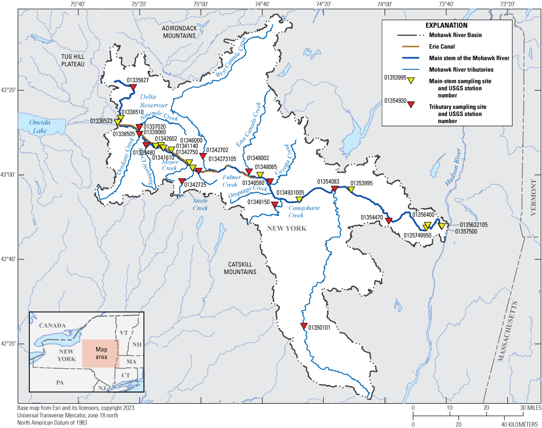
Map of water-quality sample collection locations in the Mohawk River Basin during the April to October 2016 data collection effort. USGS, U.S. Geological Survey.
Study Area
The Mohawk River Basin is entirely within New York State. The Mohawk River originates in the valley between the western Adirondacks and the Tug Hill Plateau in upstate New York and flows about 140 miles to the east where it joins the Hudson River near Albany, N.Y. (fig 1). This study focused on a 127-mile reach of the Mohawk from Rome to Cohoes, N.Y. At the upstream end of the study reach is the USGS streamgage Mohawk River below Delta Dam near Rome, N.Y. (station no. 01336000). The downstream limits of the study reach extend to the pool just downstream from USGS streamgage Mohawk River at Cohoes, N.Y. (station no. 01357500), draining 3,450 square miles of the basin. The Mohawk River is not a natural and unaltered channel for carrying waters from its headwaters down to the confluence with the Hudson near Cohoes, N.Y. The water surface for the range of streamflow in a large reach of the Mohawk River from Delta Dam to the fixed concrete dam at Lock 7 near Vischers Ferry, N.Y., is controlled differently in the spring and summer as compared to fall and winter using positionable dams. The spring-summer period is locally described as the navigation season, whereas the fall-winter period is the non-navigation season. The Mohawk River has been used as a transportation corridor for as far back as local knowledge can recall. Construction began on the positionable dams around 1905 as part of the creation of the Erie Canal (Erie Canalway, 2023). Each dam has a series of steel gates that are lowered or raised vertically to alter the pool elevation (water surface of the river) behind each dam. Each positionable dam also has an associated lock structure to allow safe passage of boats and barges around the dams (Erie Canalway, 2023). Effectively, the Erie Canal constantly transitions between being part of the main river channel and being part of the short lock access channels that funnel boat and barge traffic through each lock to get around the positionable dams. These positionable dam structures had to be included in the model to properly simulate recorded water surfaces. The modeled reach also includes inputs from 10 tributaries with continuous-record streamgages and an additional 35 ungaged tributaries throughout the reach. This study does not include any modeling of the actual tributary reaches; it only accepts a net input at the confluence location. Point-source nutrients from existing wastewater treatment plants (WWTP) were included, and non-point-source nutrient inputs were estimated at the tributary confluence for tributaries included in the model framework.
Methods and Approach
The development of a computer model to simulate water-quality conditions along the Mohawk River was determined to be the best approach for providing NYSDEC with a tool to help manage the water-quality conditions along the river. Complex hydraulics, diverse hydrology, and lack of continuous water-quality monitoring along the main stem and tributaries influenced the software choices and methods available for this study. The computer modeling software selected needed to be capable of handling complex hydraulics associated with many multi-gate control structures and other gate structures, fixed concrete dams, inflows from the canal system, and inflows from many gaged and ungaged tributaries in the reach. The lack of continuous water-quality data and sparse discrete sampling data dictated the need to estimate many data parameters. HEC–RAS is a one- or two-dimensional hydraulic routing model that is capable of modeling steady-state and unsteady-state flow while handling complex hydraulics and gate structures with multiple gates in addition to fixed structures and other inflows (U.S. Army Corps of Engineers, 2016, version 5.0.3). Embedded within HEC–RAS is Nutrient Simulation Module (NSM) I (Zhang and Johnson, 2016), version one of a module for performing water-quality analysis to simulate nutrient conditions along the Mohawk River. HEC–RAS NSM I is referred to interchangeably with RAS NSM in this report. The module uses the QUICKEST-ULTIMATE explicit numerical scheme (Leonard, 1991) to solve a one-dimensional advection-dispersion equation. Utilizing this included feature eliminates the need to link HEC–RAS hydraulics with other water-quality modeling software. The goal of developing a water-quality analysis package within HEC–RAS eventually resulted in the creation of dynamic linked libraries added to HEC–RAS in the form of the NSM (Zhang and Johnson, 2016). The selection of HEC–RAS and the internally linked NSM for the development of the hydraulic and water-quality modeling met the requirements of handling complex hydraulics, simplified water-quality modeling, and open-source public domain access to the final report and model.
Development of Hydraulic Model
The hydraulic and associated temperature and nutrient models were all developed and calibrated within HEC–RAS version 5.0.3. The model used available data from several existing sources, including the New York State (NYS) Canal Corporation’s operational flood model developed in Danish Hydrologic Institute MIKE 11 modeling software and several published Federal Emergency Management Agency (FEMA) flood insurance study models for individual reaches within the Mohawk River, and did not include any field work for new data collection. Data from these existing models were evaluated and merged to build a main-stem model reach from the best available data. Table 1 identifies the sections of the completed model by HEC–RAS river station that came from each source. HEC–RAS river stations begin at zero at the downstream end of the reach, and the highest numbers represent the furthest upstream areas of the reach. Figure 3 shows each section of the modeled reach color coded to match the corresponding native model source. Manual review and adjustments of cross-section and structure data were needed to produce a model geometry that was consistent with hydraulic conditions along the reach and to generate stable simulations. The completed model was set to a standard horizontal datum projection of Universal Transverse Mercator (UTM) zone 18 North in units of feet and a standard vertical datum of North American Vertical Datum of 1988 (NAVD 88). All source models were native to NAVD 88, except for the operational flood model (New York State Canal Corporation, 2012), which used a local datum known as Barge Canal Datum (BCD). BCD was converted to NAVD 88 using conversion factors within the FEMA hydraulic report for the flood study by Baker Group from Utica to Schenectady, N.Y. (Federal Emergency Management Agency, 2009). A summary of adjustments made to geometry and structure data is presented in the following sections.
Table 1.
Location within the model referenced by cross-section, in feet upstream from downstream model boundary, and model geometry data source and software format.[ft, foot; FEMA, Federal Emergency Management Agency; HEC–RAS, Hydrologic Engineering Center–River Analysis System; NYS, New York State; DHI, Danish Hydraulic Institute; N/A, not applicable]
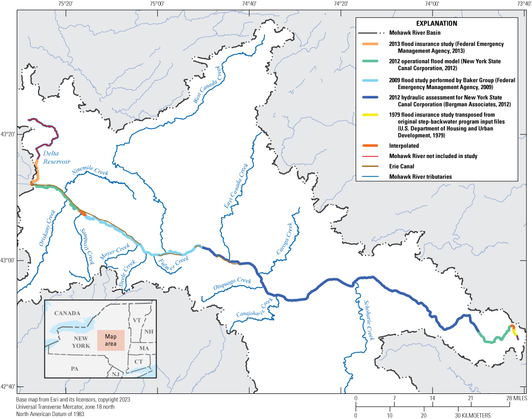
Map of modeled study reach on the Mohawk River and corresponding color-coded model sources.
Model Geometry Data
In HEC–RAS, geometry data for a one-dimensional or 1D model can consist of cross sections, bridges and culverts, inline structures (such as weirs and dams), and lateral structures along the channel. Additionally, features such as ineffective flow areas, blocked obstructions, and storage areas can be added. For this study, cross-section data sourced from existing models were modified to optimize model performance for in-channel streamflows. Some model data obtained from previously published studies included expansive overbank flow areas extending several thousand feet outside of the main river channel (fig. 4). Vast extension of the overbank was necessary in the source models to compute flood flows that would rise beyond the natural banks of the channel and inundate these areas. To compute in-channel streamflows for this study, the large extensions of the overbank area were unnecessary and were generally truncated to simplify model geometry and accelerate model simulation time.
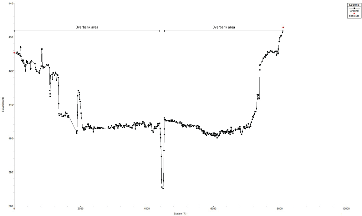
Hydraulic Engineering Center’s River Analysis System (HEC–RAS) screenshot showing expansive overbank flow areas from the New York State Canal Corporation MIKE 11 model.
From Rome through Frankfort, N.Y., the Erie Canal runs alongside the natural channel of the Mohawk River. Some interactions between the natural channel and the canal constitute navigational locks for watercraft and were assumed to account for only occasional additions or withdrawals of flow through this part of the reach due to change in storage. As such, most sections of the canal were not included within this part of the model.
One section of the canal was retained to connect the natural channel of the Mohawk River from the southern side of Rome, N.Y., to the spillway and into the natural channel downstream from the State Route 49 Bridge. This is an area of complex connections because Wheelers Creek, the Mohawk River, and the Erie Canal converge within several river miles along the canal. Naming convention for the streams within this area varies depending upon map source, and sometimes a source names the same stream reach in different ways. The FEMA flood insurance study for the city of Rome names this section of the Erie Canal both “Erie Canal” and “Mohawk River Reach 1” (Federal Emergency Management Agency, 2013). This study also names the natural channel adjacent to the section of the canal as “Wheelers Creek.” Regardless of the naming convention, the natural channel adjacent to the canal in this area was not retained because of insufficient cross sections to characterize it. The Mohawk River downstream from Rome connects to a section of the Erie Canal that leads east and then splits between a connection to Wheelers Creek and the canal after about 0.75 miles. Farther downstream, about 3.25 miles along this canal reach, there is a second connection to the natural channel via a large spillway. Instead of attempting to maintain both connections between the canal and the natural channel, given the coarse nature of the model data between these two points (in the natural channel), only the second connection was maintained.
Three locations were identified where spillway or gate flows between the canal and natural channel exist and would likely present significant effects on streamflow. Unlike the lockages mentioned previously these structures between the Erie Canal and the Mohawk River would likely contribute large flow volumes during runoff events from change in canal storage. These structures were included within the model flow file and are discussed in further detail in the “Streamflow Data” section of the report.
To facilitate a stable unsteady-state hydraulic model, interpolated cross sections were inserted throughout the reach at approximately 250-foot intervals, as they were permitted by existing cross sections and structures. Areas where modeled reaches from different sources were merged occasionally required additional cross sections to fill in small gaps. Generally, these areas between reaches were unable to be appropriately filled by RAS-generated interpolated cross sections because of dramatic changes in cross-sectional shape. In these circumstances, adjacent cross sections were copied upstream or downstream with an incremental adjustment to cross-section elevations to fill these gaps. In total, the model reach was populated with approximately 2,900 cross sections.
Most of the cross sections, used from their native models, had areas designated as “blocked ineffective flow areas” or “blocked obstructions” in parts of the overbank. Sometimes overbank areas that appeared to potentially require the addition of ineffective flow areas had “blocked features” added instead. Blocked features allow more resolution within a cross section than “normal” ineffective flow areas, which are delineated by a single offset and elevation on each bank versus the multiple offsets and elevations of blocked features. HEC–RAS does not provide a routine for perpetuating these blocked cross section features through into interpolated cross sections. Normal ineffective flow areas can be carried through into interpolated cross sections, but most of the cross sections could not be easily converted from blocked to normal ineffective flow areas. The only means to carry blocked cross sections through into interpolated cross sections was to hand-enter them in each interpolated cross section which would have been time-consuming with largely negligible results because the modeled period was primarily within-channel flow regimes. To quantify the possible differences, a sensitivity test was performed where all blocked ineffective flow areas were removed, and normal ineffective flow areas were approximated and entered for all cross sections. Using normal ineffective flow areas provided the ability for the cross-section interpolation routine to perpetuate these areas throughout all interpolated cross sections. One month of the model simulation was run to compute flow volume differences and changes in simulated river stage. The largest differences were noted at the gage at Utica, where computed volumes changed less than 0.1 percent, and mean error in stage changed from −0.09 ft to 0.11 feet when comparing observed versus simulated values for each iteration. These differences were considered negligible for the purposes of the model.
Structures and Gates
Structures within the study reach include bridges of several sizes, fixed low-head dams, and many dams with movable gates—all these structures pose challenges for hydraulic modelers. Within the study reach, 38 bridges and 17 fixed or gated inline structures were implemented. Attention given to creation of these structures within the model geometry varied depending on the model data source with four general levels of work required. The first level included sections of the model from FEMA flood insurance studies that were provided to the USGS in HEC–RAS format. The second level included sections of the model from FEMA flood insurance studies in MIKE 11 format. The third level were sections of the model from the NYS Canal Corporation operational flood model in MIKE 11 format. The fourth level involved transposition of data from analog FEMA flood insurance studies from microfiche. These structures were implemented within the completed model using several methods described in the following sections.
Bridges
Sections of the model constructed from FEMA flood insurance models in HEC–RAS format typically included detailed bridges and did not require the structure geometry to be modified. These sections were generally reviewed for anomalies and any significant errors before implementation. Cross-section data from FEMA flood insurance studies in MIKE 11 format were able to be imported into HEC–RAS with a utility in the RAS environment (U.S. Army Corps of Engineers, 2016). The utility, however, could not ingest structure data. Instead, bridge dimensions were manually obtained from the native MIKE 11 model and the detailed documentation from the flood insurance study and were accurately recreated in HEC–RAS (Federal Emergency Management Agency, 2009).
In the reaches where NYS Canal Corporation’s MIKE 11 model was used, bridge structure geometry required significant attention. This was partly due to the MIKE 11 model “simplifying” bridge structures to presumably allow for an overall faster operational runtime for flood forecasting ahead of a hydrologic event. This simplification generally included eliminating piers and bridge decks and applying extremely coarse internal bridge cross sections: items which would have a negligible effect on a high-flow flood model. However, the water-quality model for the project study reach was focused on low to medium in-channel flows, thus the coarse resolution of these structures was not acceptable. Furthermore, field surveys of these structures were not within the scope of this project. However, most structures that were not within the source models were able to be reconstructed within the geometry in the following manner: bridge low chord elevations were obtained from watercraft navigational information published by the New York State Canal Corporation (New York State Canal Corporation, 2020), piers and abutments were reviewed, and approximate measurements were obtained using georeferenced aerial imagery within a geographic information system.
No bridge structures were within the small subsection of the model that was transposed from the FEMA flood insurance studies on microfiche. A small subset, 8 out of 48 noted bridge structures in the study reach was not included in the hydraulic model. Mostly, these bridges were not included because their geometries were not readily available, such as the walking bridge in the city of Amsterdam, N.Y., or because their introduction into the model was assumed to have a negligible impact on in-channel flows because of structure span width and height, such as the New York State (NYS) Thruway bridges near the city of Utica, N.Y. One bridge was removed because it created model instabilities by being immediately adjacent to an inline structure (Mohawk Street Bridge in Herkimer, N.Y.). Table 2 lists bridges within the study reach, their corresponding model cross section, and if and how the bridge was reconstructed within the HEC–RAS model. Figure 5 shows a modeled bridge within the HEC–RAS environment.
Table 2.
Summary of bridge structures with name, location (referenced by model cross-section number in feet, upstream from downstream model boundary), native model format, and implementation method within the Mohawk River hydraulic model.[ft, foot; HEC–RAS, Hydrologic Engineering Center River Analysis System; DHI, Danish Hydrologic Institute; N.Y., New York; N/A, not applicable; I–90, Interstate 90; I–790, Interstate 790; NAVD 88, North American Vertical Datum of 1988; I–890, Interstate 890; I–87, Interstate 87]
| Bridge name | Model cross-section number (ft) | Original model format | Bridge geometry adjustment or modification |
|---|---|---|---|
| Rome-Westernville | 679,641.6 | HEC–RAS | None; reviewed for completeness |
| Rome-Wright Settlement | 669,026.9 | HEC–RAS | None; reviewed for completeness |
| Rome-Chestnut Street | 663,951.6 | HEC–RAS | None; reviewed for completeness |
| Rome-Floyd Avenue | 66,0651.1 | HEC–RAS | None; reviewed for completeness |
| Rome-Garden Street | 656,809.2 | HEC–RAS | None; reviewed for completeness |
| Rome-Dominick Street | 652,680.2 | HEC–RAS | None; reviewed for completeness |
| Rome-Railroad Street | 652,349.2 | HEC–RAS | None; reviewed for completeness |
| Rome-Mill Street1 | 648,729.9 | DHI-MIKE 11 | Geometry converted manually from native model. |
| N.Y. Route 365/49 | 643,306.1 | N/A | Not implemented within model |
| Erie Canal Railroad Bridge | 640,226.7 | DHI-MIKE 11 | Geometry converted manually from native model. |
| Oriskany Road/River Street | 601,479 | DHI-MIKE 11 | Geometry converted manually from native model. |
| N.Y. Route 291 | 585,563.3 | DHI-MIKE 11 | Geometry converted manually from native model. |
| I–90 | 578,440.5 | N/A | Not implemented within model |
| Mohawk Street | 576,532.5 | DHI-MIKE 11 | Geometry converted manually from native model. |
| Utica-Barnes Avenue | 561,331.3 | DHI-MIKE 11 | Geometry converted manually from native model. |
| I–790 | 558,610.3 | N/A | Not implemented within model |
| Railroad Bridge adjacent to I–790 | 558,250.3 | DHI-MIKE 11 | Geometry converted manually. from native model. |
| Genesee Street | 549,546.3 | DHI-MIKE 11 | Geometry converted manually from native model. |
| Leland Avenue | 547,562.3 | DHI-MIKE 11 | Geometry converted manually from native model. |
| Dyke Road | 528,908.5 | DHI-MIKE 11 | Geometry converted manually from native model. |
| Railroad Bridge downstream from Dyke Road | 526,750.8 | DHI-MIKE 11 | Geometry converted manually from native model. |
| Railroad Street | 491,247.4 | DHI-MIKE 11 | Geometry converted manually from native model. |
| Central Avenue | 478,323 | DHI-MIKE 11 | Geometry converted manually from native model. |
| Herkimer-Mohawk Street | 468,252.5 | N/A | Not implemented within model |
| I–90/Thruway | 464,576.3 | N/A | Not implemented within model |
| South Washington Street | 463,899.5 | N/A | Not implemented within model |
| Hansen Island Bridge | 426,503.5 | N/A | Not implemented within model |
| Route 167 | 425,169.9 | DHI-MIKE 11 | Geometry converted manually from native model. |
| Little Falls-Canal Place | 424,669.5 | DHI-MIKE 11 | Geometry converted manually from native model. |
| Little Falls-Walking Bridge | 423,351 | DHI-MIKE 11 | Geometry converted manually from native model. |
| State Route 169 | 420,496.6 | N/A | Not implemented within model |
| St. Johnsville-Bridge Street | 369,981.6 | HEC–RAS | None; reviewed for completeness |
| Fort Plain-River Street | 340,006.2 | HEC–RAS | None; reviewed for completeness |
| Canajoharie-Church Street | 322,577.8 | HEC–RAS | None; reviewed for completeness |
| Fultonville-Main Street | 258,994.2 | HEC–RAS | None; reviewed for completeness |
| Tribes Hill-Main Street | 232,505 | N/A | Bridge is a component of superstructure for inline structure; see associated inline structure within table 3. |
| Amsterdam-Walking Bridge | 203,934.4 | N/A | Not implemented within model |
| Amsterdam-Route 30 | 203,278.1 | HEC–RAS | None; reviewed for completeness |
| Pattersonville Railroad Bridge | 152,065.3 | HEC–RAS | None; reviewed for completeness |
| Rotterdam Junction-Bridge Street | 144,428.3 | N/A | Bridge is a component of superstructure for inline structure; see associated inline structure within table 3. |
| CSX Railroad Bridge | 134,341.6 | Added to model | Bridge not within native model; reconstructed using invert elevations.1 Converted to NAVD 88 and approximate dimensions. |
| I–890 | 127,113.9 | Added to model | Bridge not within native model; reconstructed using invert elevations.1 Converted to NAVD 88 and approximate dimensions. |
| Western Gateway/Route 5 | 105,410.6 | HEC–RAS | None; reviewed for completeness |
| Conrail, Delaware, and Hudson Railroad bridges | 102,085.3 | HEC–RAS | None; reviewed for completeness |
| Freeman’s Bridge | 97,526.60 | HEC–RAS | None; reviewed for completeness |
| Delaware and Hudson Railroad Bridge | 95,893.55 | HEC–RAS | None; reviewed for completeness |
| Niskayuna-Balltown Road | 82,463.14 | Added to model | Bridge not within native model; reconstructed using invert elevations.1 Converted to NAVD 88 and approximate dimensions. |
| I–87/Northway | 23,521.73 | Added to model | Bridge not within native model; reconstructed using invert elevations.1 Converted to NAVD 88 and approximate dimensions. |
| New Loudon Road/Highway 9 | 9,780.87 | DHI-MIKE 11 | Geometry converted manually from native model. |
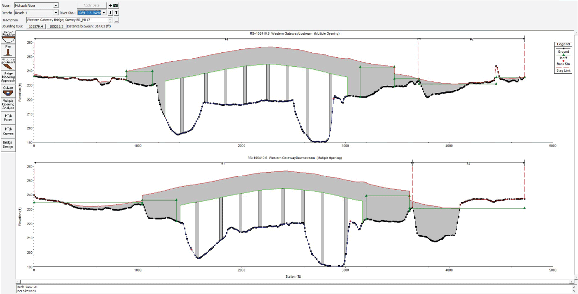
Hydraulic Engineering Center River Analysis System (HEC–RAS) screenshot of a modeled bridge structure; the bridge is the Western Gateway/Route 5 Bridge carrying New York Route 5 over the Mohawk River in Rotterdam, New York.
Inline Structures
Inline structures consisted of fixed examples, such as the low-head weir modeled at the Mohawk River/Erie Canal confluence south of Rome, N.Y., and structures with many movable gates, such as the dams farther downstream in Amsterdam and Schenectady, N.Y. (table 3). Sections of the model constructed from FEMA flood insurance models in HEC–RAS format typically included detailed inline structures and did not require any modification to the structure geometry. They were generally reviewed for anomalies and any significant errors in gate dimensions and structure elevations before implementation. Like the source data for bridge structures, source data for inline structures from FEMA flood insurance studies modeled in MIKE 11 required reconstruction in RAS using detailed information retrieved from the native MIKE 11 models and model documentation. These were able to be reliably reproduced within the HEC–RAS environment.
Few examples of inline structures were in the sections of the model sourced from the NYS Canal Corporation. Two low-head weirs at river stations 650075 and 632966.1 connected the respective upstream and downstream ends of the 3.25-mile section of the Erie Canal to areas in the model farther downstream. These low-head weirs were constructed from best available data within the Canal Corporation MIKE 11 model and cross-referenced with vertical and horizontal positional data obtained within the geographic information system. Crescent Dam, towards the furthest downstream end of the Mohawk River study reach, was reconstructed in HEC–RAS using geometry transposed from the 1979 flood insurance study for the town of Colonie, N.Y. (U.S. Department of Housing and Urban Development, 1979). The resolution provided by the flood insurance study for the upstream cross section is somewhat coarse, along with the definition of the dam itself. Information on the single gate modeled within Crescent Dam is considered approximate.
Gates
Gates, where applicable, were modeled using the best available data within each section of the model. Sometimes gate design specifics, not directly available within the models, were obtained from the NYS Canal Corporation through NYSDEC (Michaela Schnore, written commun., 2019). Table 3 lists inline structures included in the model and gate types used in that structure, as applicable. Many of the inline structures along the Mohawk River have operable upper and lower gates that control the water elevations in the river during the marine navigation season (fig. 6). Examples of these inline structures include Lock E–15 Dam at Fort Plain, Lock E–11 Dam at Amsterdam, and Lock E–8 Dam at Schenectady. HEC–RAS allows a user to create and model as much as 40 gate “groups” with as much as 25 individual gates each. The gates within each group need to be a fixed type and dimension. Additionally, when developing a flow file for the gates within an unsteady flow simulation, each gate group is operated together, meaning individual gates within a group cannot deviate from the instructions provided to the model for the group. Modeling gates within the structure geometry required careful review of the gate operation data provided to the USGS from the NYS Canal Corporation through NYSDEC (Michaela Schnore, written commun., 2019) to determine the best approach to correctly apply gate operation during an unsteady flow simulation. Typically, the lower gates along the control structures remained raised through the late autumn into early spring to keep pool elevations low during the river ice season. During the mid-spring, these gates are dropped into position to facilitate the higher pool elevations necessary for marine navigation and remain in place through autumn. The upper gates in inline structures were controlled individually according to data provided by NYS Canal Corporation through NYSDEC (Michaela Schnore, written commun., 2019), and their positions varied depending on river flow. The most convenient way to apply gate operations within HEC–RAS was to model the upper gates individually, each as its own “group” to facilitate their flow-dependent operation, and the lower gates as an aggregate group because of their typically simpler operation. Gate position data typically indicated the “percent opened” for each gate, and a time stamp indicated when changes were made to the gate’s position at each structure. These records were transformed into a time series based on gate dimensions and the noted percentage of the gate that was open, along with timing information. Gates were assumed to remain in their last noted position until a change was recorded within the data for that gate.
Table 3.
Summary of inline structures with location (referenced by model cross-section number in feet, upstream from downstream model boundary), native format, and implementation method within the Mohawk River hydraulic model.[ft, feet; DEM, digital elevation model; DHI, Danish Hydraulic Institute; HEC–RAS, Hydrologic Engineering Center River Analysis System]
Several other gate types needed to be included in the model. The broad-crested weir in the city of Utica, N.Y., used radial arm Tainter gates that assisted the city in controlling the harbor elevation along the Mohawk River. Farther downstream in the Village of Herkimer, a smaller set of lower and upper movable gates are used in combination with crest gates. At Vischer Ferry Dam, flashboards are used to control and adjust the upstream pool elevation. Flashboards are long sections of wood that fit into engineered slots within a dam or other hydraulic control structure to raise the effective height of the dam. They are typically designed to break away during high-flow runoff events. The NYS Canal Corporation had very little data about flashboard insertion, removal, or adjustments at Vischer Ferry Dam. In addition, dimensions and number of flashboards used at the dam were not available. Ten “flashboards” were modeled as overflow gates, and HEC–RAS simulated the effects these flashboards would create on upstream pool elevations. During calibration of the model, an iterative process was used to arrive at the number of flashboards and timing of flashboard removal and replacement.
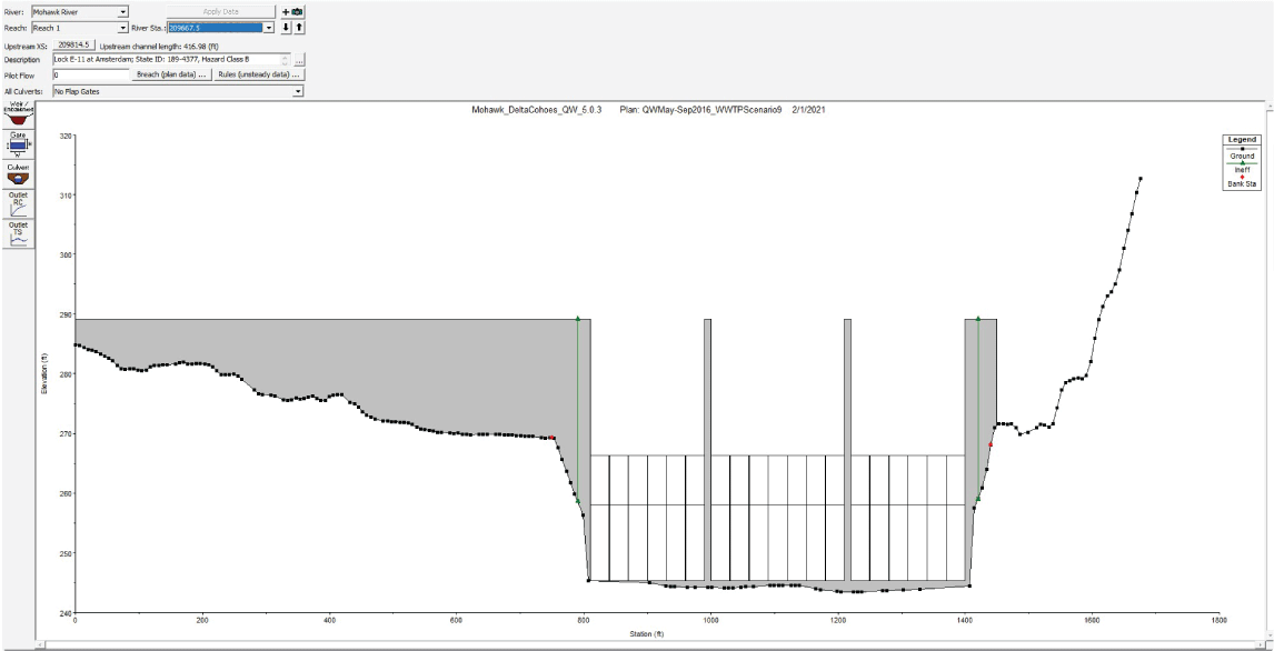
Hydraulic Engineering Center River Analysis System (HEC–RAS) screenshot showing a modeled inline structure with multiple gates; the structure is the dam at Lock E–11 at Amsterdam, New York.
Energy-Loss Factors
Hydraulic models require the use of factors that represent energy losses from frictional resistance between flow and the channel throughout the study reach. Energy-loss factors are typically quantified by Manning’s roughness coefficient (n value). The roughness coefficient incorporates major factors such as channel-surface roughness, channel irregularity and shape variation, obstructions, and vegetation as well as other factors such as depth of flow, meandering, and bedload (Coon, 1994). Determining Manning’s n values for energy loss (friction) is typically done by assessing channel bed and bank sediments and vegetation as well as channel morphology in the field. As mentioned previously, no new cross sectional or other field data were collected as part of this study. Existing Manning’s n values associated with the furnished models for this study were compared to other published n values for moderate sized streams and rivers in the central New York State region to ensure that they generally aligned with known channel conditions. Channel conditions in the study reach were assumed to be consistent with the channel conditions of streams such as the Sacandaga River, Onondaga Creek, Tioughnioga River, and Esopus Creek that had a range of n values between 0.026–0.050 during a channel roughness study done in 1994 by the USGS (Coon, 1994). In most cases, preexisting n values from furnished models were retained. However, a few sections of the model required preexisting n values to be altered to reflect changes implemented when building the aggregate model for the study reach. Notably, one section of the model that was changed was the 3.25-mile section of the Erie Canal that was used to connect the natural channel of the Mohawk River from the southern side of Rome, N.Y., to the spillway into the natural channel near the East Rome guard gate along the Erie Canal. The n values for this section were lowered to reflect the lower roughness coefficients that would be within the channelized reach of the canal. Additionally, during model calibration, the initial selection of n values was sometimes adjusted to obtain close agreement between simulated and recorded stage values within specific sections of the study reach during the calibration process. This adjustment/calibration procedure is discussed in more detail in the “Calibration and Validation of Flows” section of this report. Based upon the preceding information, finalized n values were determined and applied throughout the modelled study reach as shown in table 4.
Table 4.
Summary of the final Manning’s roughness coefficients used for the modeled study reach of the Mohawk River by location (referenced by model cross-section number in feet, upstream from downstream model boundary).[ft, feet]
Streamflow Data
Within the HEC–RAS environment, several boundary conditions, such as streamflow and stage hydrographs, hydraulic control structure opening time series, and storage area definitions were added to an unsteady flow file that was then used to apply a simulation to the model geometry for the study period of May through September 2016. The modeled study reach begins on the Mohawk River downstream from Delta Dam, and the upstream model boundary condition was populated using the streamflow hydrograph from USGS station no. 01336000, Mohawk River below Delta Dam near Rome, N.Y (U.S. Geological Survey, 2022b). Within the section of the Mohawk River Basin that supports the modeled study reach, the USGS operates streamgages on 10 tributaries near their confluence with the Mohawk River (table 5, fig. 7). HEC–RAS provides two options for entering lateral inflows within the unsteady flow data editor. The “lateral inflow hydrograph,” the first option, which was used to enter the gaged streamflow hydrographs previously mentioned, permits a user to add flow at a specific cross section along the river reach, with the change in flow not showing up until the next cross section downstream from the inflow hydrograph (U.S. Army Corps of Engineers, 2016). The second option is the “uniform lateral inflow.” This option permits a user to insert a hydrograph and, instead of having the flows be added to the model at a specific location, the program will uniformly distribute the flow change between two user-defined cross sections (U.S. Army Corps of Engineers, 2016).
Hydrographs adjusted from their native 15-minute time step to a 1-hour time step for these 10 streamgages were added to the unsteady flow file as lateral inflow hydrographs, entering the model at the cross section nearest their confluence location with the main-stem of the Mohawk River. Time steps were adjusted by retaining their hourly readings and removing their intermediate 15-, 30-, and 45-minute readings. In most cases, the streamgages were close to the confluence with the Mohawk River main stem. This proximity facilitated using the published streamflow hydrographs from the streamgages directly within the model. Streamgages on the Schoharie Creek, Canajoharie Creek, Fulmer Creek, and the Moyer Creek all had drainage area differences between the gaged location and the tributary’s confluence location with the Mohawk River up to 13.6 percent (Schoharie Creek) and were handled separately. For Fulmer and Moyer Creeks, the differences in streamflows had negligible impacts on the overall model because of these creeks’ small drainage areas (21.7 mi2 and 18.2 mi2, respectively). Schoharie and Canajoharie Creeks had larger drainage areas (886 mi2 and 59.7 mi2, respectively), and lateral inflows were adjusted 4.6 and 13.6 percent, respectively, to account for the drainage area increase between the gaged location and the confluence.
Table 5.
Summary of U.S. Geological Survey streamgages near tributary confluences with the Mohawk River within the study reach, their drainage areas, and whether drainage-area adjustment was performed.[USGS, U.S. Geological Survey; DA, drainage area; mi2, square mile; NY, New York]
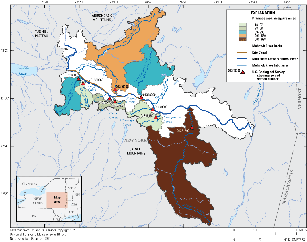
Map showing locations of U.S. Geological Survey streamgages on tributaries and their corresponding basins within the Mohawk River Basin that were used in the modeled study reach.
Despite extensive coverage of the Mohawk River sub-basins by the USGS streamgage network, only approximately 60 percent of the overall basin drainage area was gaged. To account for this disparity in gaged drainage area, additional flow hydrographs were necessary. The interaction between the HEC–RAS hydraulic module and the nutrient simulation module (NSM) is such that time series for water-quality parameters within the NSM are connected to each model boundary condition. Because the overall goal of this model was to provide the ability to investigate and evaluate point-source nutrient contributions to the Mohawk River main stem, adding the ungaged drainage area within the basin using a series of specific lateral inflow hydrographs was distinctly more advantageous than adding a distributed uniform inflow hydrograph. In addition, any future streamgage additions, USGS or otherwise, could easily be inserted within a model framework built around these specific lateral inflow boundary-condition locations. The additional lateral inflow hydrographs would need to be estimated and entered at locations of prominent ungaged tributaries throughout the study reach. A matrix was created to evaluate the ungaged parts of the study basin and to choose the appropriate tributary inflow to be added to the model.
The USGS Streamstats product for New York State (U.S. Geological Survey, 2022a) was reviewed and used to select 35 tributaries that flow to the main stem of the Mohawk River within the study reach. These 35 tributaries represent many streams throughout the study reach, and individual drainage basins were generally larger than 5 square miles. However, some tributaries that were being included in follow-up sampling studies by NYSDEC, smaller than 5 square miles, were also included, such as Nail Creek within the city of Utica, N.Y. The 35 tributaries covered about 20 percent of the modeled Mohawk River drainage area. Locations for tributary confluences were selected based on locations displayed in the USGS Streamstats mapper. Notably, in one instance, the drainage areas for two streams (Ferguson and Wood Creeks) were combined into one aggregate drainage area, as they enter the Mohawk at approximately the same location within the model (thus, effectively 34 tributary hydrographs were added as lateral inflow hydrographs). Table 6 lists the ungaged tributaries included within the model and figure 8 shows their locations.
Table 6.
List of ungaged Mohawk River tributaries added into the hydraulic model as lateral flow hydrographs, drainage areas, and their source.[mi2, square mile; USGS, U.S. Geological Survey; no., number]
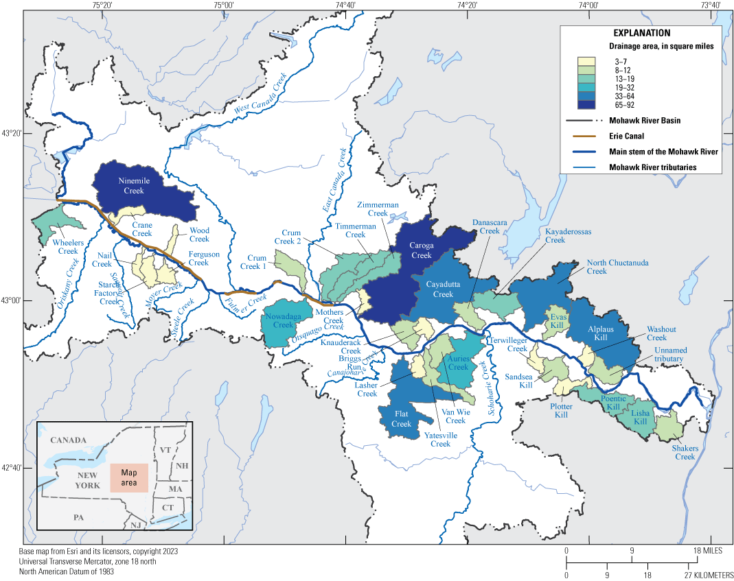
Map of ungaged tributaries added into the hydraulic model and their corresponding basins within the Mohawk River Basin that were used in the modeled study reach.
To create synthetic hydrographs for the additional tributaries that could be added to the HEC–RAS unsteady flow file, flow was adjusted to the drainage area for each tributary using two gaged streams based on the drainage areas provided from USGS Streamstats for New York State (U.S. Geological Survey, 2022a). The two gaged streams that were chosen to be the “index” streams for drainage area adjustments were the streams with streamgages at Sauquoit Creek at Whitesboro, N.Y., and Canajoharie Creek near Canajoharie, N.Y. The decision to use these two gaged streams versus others (Schoharie, East Canada, or West Canada Creeks) was based on their drainage areas of 59.8 square miles (Sauquoit Creek) and 59.7 square miles (Canajoharie Creek) being more similar to the ungaged tributaries. Also, East Canada and West Canada Creeks are heavily regulated, and their unique hydrographs would not be suitable for computing drainage area adjusted hydrographs. Synthetic hydrographs in the western and eastern parts of the basin were generated using Sauquoit Creek and Canajoharie Creek, respectively. A simple proportion was assigned to each hourly unit-value flow in the published streamflow hydrograph based on the ungaged-gaged drainage area ratio (eq. 1.) to create the synthetic hydrograph for each added tributary using the equation below:
whereQe
is the estimated streamflow in cubic feet per second, at time step n, at the ungaged tributary,
Qi
is the published streamflow in cubic feet per second, at time step n, at the gaged index tributary,
DAe
is the drainage area in square miles of the ungaged tributary, and
DAi
is the drainage area in square miles of the gaged index tributary.
During the construction and initial simulations of the model, using only aggregate tributary inflows from Rome through Frankfort, N.Y., did not adequately reproduce the hydrograph at the USGS streamgage on the Mohawk River near Utica, N.Y. Low to medium flows were well represented; however, the model simulation had large missing flow volumes during runoff events. Depending upon the magnitude of the runoff event, the difference could be several hundred cubic feet per second (ft3/s), or during periods of base flow, it could be zero. We assumed that the missing volume was from a combination of flows entering the natural channel of the Mohawk from several spillways and gates between the Erie Canal and the Mohawk River as well as many contributing smaller tributaries and inflows that were not directly included within the model upstream from the Utica streamgage. The lack of these small tributaries and inflows is also reflected in the total drainage area of the tributary inflows that were added directly to the model. The aggregate drainage area for specific lateral flow inputs from individual tributary hydrographs composes about 85 percent of the drainage area of the Mohawk River at the Cohoes streamgage. A method was devised to account for the extra drainage area and flow by creating a hydrograph for what was called the “intervening drainage area and canal storage estimation” by subtracting the aggregate tributary discharges between the upstream end of the model and the Utica streamgage from the published streamflows at the Utica streamgage. The flow within this net flow hydrograph was then apportioned by three additional lateral flow hydrographs within the HEC–RAS unsteady flow file representing exchange between the Erie Canal and the natural channel of the Mohawk River. The locations of these inflows correspond to three spillways (fig. 9). Two spillways are near the canal confluences of Ninemile Creek and Crane Creek. The third spillway is adjacent to a set of gates downstream from the city of Utica. During model calibration, the best apportionment of the associated flow from the spillways was with 12.5 percent being allocated to each spillway for Ninemile and Crane creeks and the remaining 75 percent being allocated to the spillway and gate structure near Utica. These percentages were determined by running the hydraulic simulation and visually comparing size and timing of simulated runoff events versus published flows at the Mohawk River near the Utica streamgage for the study period.
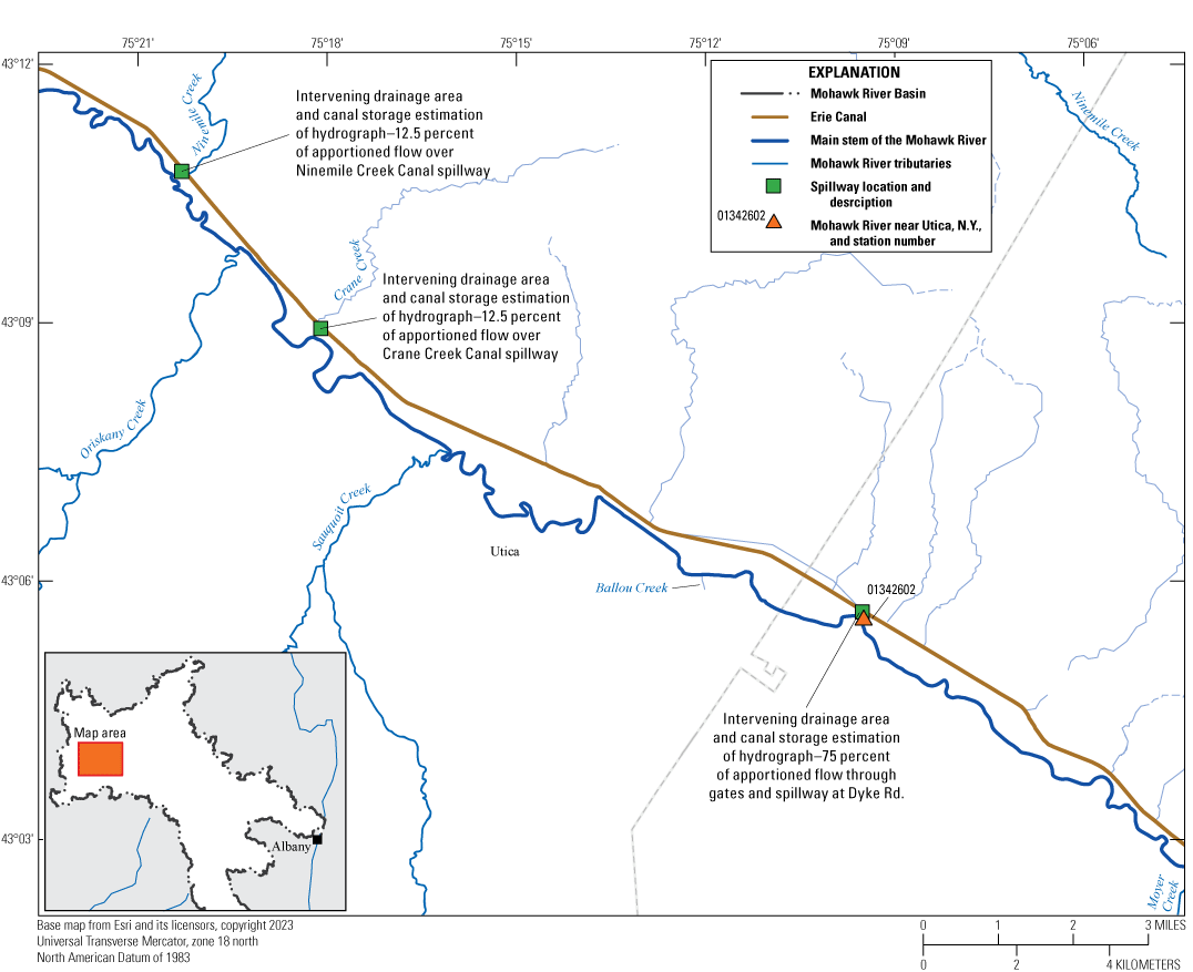
Map showing locations of spillways and gates between the Erie Canal and the Mohawk River included within the Hydraulic Engineering Center River Analysis System (HEC–RAS) model as lateral flow hydrographs and the location of the U.S. Geological Survey streamgage on the Mohawk River near Utica, New York (station number 01342602). N.Y., New York; Rd., road.
Municipal Withdrawals and Discharges
Municipal point-source discharges from 14 wastewater treatment plants (WWTPs) were included within the HEC–RAS unsteady flow file as lateral inflow hydrographs on a daily time step. Average daily wastewater effluent flows were obtained from discharge monitoring reports (DMR) from May through September 2016 (U.S. Environmental Protection Agency, 2019) and were converted from millions of gallons per day to cubic feet per second. One WWTP (Niskayuna) had 12-hour averages for effluent flow and was entered as such within the model. Except where specific discharge location information was available, the lateral inflow hydrographs for the WWTPs were placed within model cross sections nearest the physical location of the associated WWTP. For this model, three WWTPs had discharge locations that were noted by the NYS Department of Environmental Conservation to not be collocated with the plant’s physical location. The three plants were Rome WWTP, Rotterdam Sewage Treatment Plant (STP), and Herkimer County WWTP. Table 7 shows the facility names and associated cross section where WWTP discharges are within the HEC–RAS model. Figure 10 shows locations of WWTPs that are point-source dischargers.
Table 7.
Wastewater treatment facilities, their State Pollutant Discharge Elimination System permit number, and the cross-section location of their associated lateral flow boundary condition within the hydraulic model.[SPDES, State Pollutant Discharge Elimination System; WPCP, water pollution control plant; WWTP, wastewater treatment plant; SD, sanitary district; no., number; STP, sewage treatment plant]
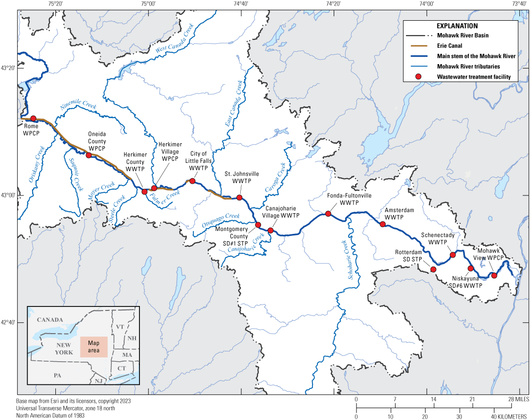
Map showing locations of wastewater treatment plants, water pollution control plants, and sewage treatment plants that discharge directly into the main-stem Mohawk River. SD, sanitary district; STP, sewage treatment plants; WPCP, water pollution control plants; WWTP, wastewater treatment plants; #, number.
Municipal withdrawals were not included within the model; however, annual withdrawal data were reviewed from the New York State water withdrawal database (State of New York Open Data, 2022). Data were reviewed for calendar year 2016 primarily for large municipal surface water withdrawals that would warrant application within the hydraulic model. A review of the withdrawal records found that of the municipalities along the Mohawk River, many have water supplies originating from sources upstream of the Mohawk River and are not withdrawing from the river directly. Of the water withdrawals within the database that are indicated as “surface water” and are withdrawing water directly from the Mohawk River, all had average daily withdrawal values of less than 5 million gallons per day. Withdrawals of this magnitude were determined to have an overall negligible impact on model simulated flows. We assumed that these withdrawals’ volume would be a negligible reduction to simulated flows and would be less than the flow of the smallest contributing tributaries that were excluded from the model.
Starting Water-Surface Elevation and Model Initial Conditions
Running an unsteady model simulation within HEC–RAS requires setting the initial conditions for the stream reach, including starting water-surface elevations within each cross-section. To obtain an appropriate starting water-surface elevation for each cross section within the hydraulic model, a steady-state simulation was performed. Flows for the steady-state flow regime were entered into the steady flow file within HEC–RAS; the furthest upstream flow below Delta Dam was set as the published flow (from the gaging station) on May 1, 2016, at 0000-hours. Flow change locations were added within the steady flow file at each cross section with a tributary inflow using the corresponding tributary flows from the same date and time. The flows from the tributaries were added to the overall flow along the main stem of the Mohawk River throughout the study reach. WWTP discharges were not added within the steady flow file as separate flow change locations. Instead, for purposes of simplicity, each WWTP discharge was added into the aggregate flow at the next flow change location downstream from where the discharge location was on the main-stem Mohawk River. Gate settings for the inline structures were implemented within the steady flow file for the same May 1, 2016, 0000-hour time step. The results from the steady-state simulation were linked to the unsteady flow editor and corresponding unsteady flow file to set the initial conditions for stage and flow for the unsteady flow simulation.
Downstream Boundary Conditions
The downstream boundary condition for the unsteady flow file was set as “normal depth” within HEC–RAS. Using normal depth as the downstream boundary condition for the model relies upon the assumption that the channel downstream from the study reach is flowing under similar conditions as the downstream end of the hydraulic model. A slope of the channel is then entered within the normal depth field in HEC–RAS. To apply the normal depth downstream boundary condition for the study reach, 10 cross sections downstream from Crescent Dam were reviewed, and the thalweg of each cross section was extracted and entered as part of a longitudinal profile. The average slope of this profile was computed to be 0.0026 and was input within the normal depth field. Importantly, even if the normal depth entered within the downstream boundary of the model does not fully represent the true slope or normal depth of the reach downstream, generally only the few cross sections closest to the downstream model boundary will be affected. Cross sections further upstream become increasingly unaffected by inaccuracies within the downstream boundary the further upstream they are.
Model Simulation
The HEC–RAS hydraulic model was run with an unsteady hydrodynamic flow regime using HEC–RAS version 5.0.3. The simulation was started on May 1, 2016, at 0000-hours and run until October 1, 2016, at 0000-hours. The computation interval was set to 30 seconds with output every hour. The computation interval was adjusted several times during model calibration; however, the 30-second interval proved to be the best combination of stability and simulation speed. When the model was initially constructed, the unsteady flow file and associated boundary conditions and hydrographs were populated using the native 15-minute time step of the published flow data. Further into the development of the model, we found that the number of rows within the unsteady flow file that HEC–RAS permits for boundary-condition hydrograph time steps did not allow the entire 5-month period of May–September 2016 to be added. To account for this, the model was broken into monthly sections understanding that a model “restart” file would be used to run the monthly sections of the hydraulic model individually while maintaining continuity between periods. This process worked well for the hydraulic part of the HEC–RAS model. However, during subsequent development of the nutrient model within NSM, the restart process possessed a “bug” within the NSM that would not generate a usable restart file for the nutrient model. Reducing the resolution of the input hydrographs for the unsteady flow file to an hourly time step provided a workaround to this bug. This workaround permitted the entire period of May–September 2016 to fit within the confines of what HEC–RAS allows for number of rows within a boundary-condition hydrograph. The model was summarily able to run in its entirety without having to use restart files. All data and model files that support this study are available from the associated data release published concurrently with this report (Niemoczynski and others, 2024).
Calibration and Validation of Flows
The simulated streamflow along the Mohawk River was evaluated against observed published data from four USGS streamgages along the main-stem Mohawk River to check that the hydraulic model was simulating flow conditions correctly. The data from USGS streamgages along the Mohawk River near Utica, N.Y. (station no. 01342602), -near Little Falls (station no. 01347000), -at Freemans Bridge near Schenectady (station no. 01354500), and –at Cohoes (station no. 01357500) were used as they represented the upstream, central, downstream, and downstream terminus of the study reach, respectively (fig. 11). Simulated flows for the period of May 8, 2016, through September 30, 2016, were evaluated on a daily time step using the statistical parameters of r2, Nash-Sutcliffe efficiency coefficient, mean absolute error (MAE), and percent bias. The initial week of the model simulation was not included within evaluation parameters, because model start-up errors would disproportionately affect model evaluation. Tables 8 through 11 and figures 12 A–D and 13 A–D demonstrate the statistical evaluation results. The results are displayed by metrics for the entire period, and then individually for each complete month of the evaluation period at each streamgage location. Of note, the r2 for the daily flows in the month of September is not the best representation of the model’s performance for the middle and downstream areas of the study reach. An extremely limited range of flows, combined with modest timing errors from coarse and incomplete gate timing at control structures, resulted in this parameter being very low. Reviewing monthly volume errors as discussed later in the “Calibration and Validation of Flows” section provides a more accurate assessment of the model’s performance during the month of September and is consistent with the other parts of the study period.
Map showing flow calibration locations along the main stem of the Mohawk River. USGS, U.S. Geological Survey.
Table 8.
Hydraulic Engineering Center River Analysis System (HEC–RAS) hydraulic model validation matrices for daily streamflow, including the range of simulated and observed daily streamflow, coefficient of determination (r2), Nash-Sutcliffe efficiency coefficient, mean absolute percent error, and percent bias for the period of May 8, 2016, through September 30, 2016, and individual months of June, July, August, and September 2016 at the U.S. Geological Survey streamgage Mohawk River near Utica, New York (station number 01342602).[Observed streamflow values are from U.S. Geological Survey (2022b). ft3/s, cubic foot per second; r2, coefficient of determination; NSE, Nash-Sutcliffe efficiency coefficient; MAPE, mean absolute percent error; %, percent]
Table 9.
Hydraulic Engineering Center River Analysis System (HEC–RAS) hydraulic model validation matrices for daily streamflow, including the range of simulated and observed daily streamflow, coefficient of determination (r2), Nash-Sutcliffe efficiency coefficient, mean absolute percent error, and percent bias for the period of May 8, 2016, through September 30, 2016, and individual months of June, July, August, and September 2016 at the U.S. Geological Survey streamgage Mohawk River near Little Falls, New York (station number 01347000).[Observed streamflow values are from U.S. Geological Survey (2022b). ft3/s, cubic foot per second; r2, coefficient of determination; NSE, Nash-Sutcliffe efficiency coefficient; MAPE, mean absolute percent error; %, percent]
Table 10.
Hydraulic Engineering Center’s River Analysis System (HEC–RAS) hydraulic model validation matrices for daily streamflow, including the range of simulated and observed daily streamflow, coefficient of determination (r2), Nash-Sutcliffe efficiency coefficient, mean absolute percent error, and percent bias for the period of May 8, 2016, through September 30, 2016, and individual months of June, July, August, and September 2016 at the U.S. Geological Survey streamgage Mohawk River at Freemans Bridge near Schenectady, New York (station number 01354500).[Observed streamflow values are from U.S. Geological Survey (2022b). ft3/s, cubic foot per second; r2, coefficient of determination; NSE, Nash-Sutcliffe efficiency coefficient; MAPE, mean absolute percent error; %, percent]
Table 11.
Hydraulic Engineering Center’s River Analysis System (HEC–RAS) hydraulic model validation matrices for daily streamflow including the range of simulated and observed daily streamflow, coefficient of determination (r2), Nash-Sutcliffe efficiency coefficient, mean absolute percent error, and percent bias for the period of May 8, 2016, through September 30, 2016, and individual months of June, July, August, and September 2016 at the U.S. Geological Survey streamgage Mohawk River at Cohoes, New York (station number 01357500).[Observed streamflow values are from U.S. Geological Survey (2022b). ft3/s, cubic foot per second; r2, coefficient of determination; NSE, Nash-Sutcliffe efficiency coefficient; MAPE, mean absolute percent error; %, percent]
Scatter plots showing observed and simulated daily flows for the model evaluation period for the four different streamgages are shown in figure 12. Additionally, figure 13A through 13D compare observed and simulated streamflow time series for each streamgage for the evaluation period. Including these visual references helps demonstrate the model’s performance and suitability for application within the NSM. Simulated streamflow results demonstrated a reasonable fit to observed values at low to medium flows; however, high-flow events showed larger differences, particularly in the upstream areas of the reach above Little Falls and Utica, N.Y. A positive bias in flows is visible in the upstream calibration sites that seems to fade as the models move into the downstream parts of the basin. This difference was assumed to result from unquantified interactions with the sections of the Erie Canal at the three noted spillways between the canal and the Mohawk River. In addition, variability from small unmodeled ephemeral tributaries during runoff events likely contributed to these high-flow event disparities. Generally, streamflow predictions in the upstream reach tended to be biased higher than in the lower reach, in contrast to observed streamflows.
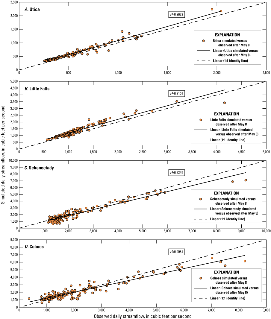
Graphs showing correlations between observed daily streamflow (U.S. Geological Survey, 2022b) and simulated daily streamflow in cubic feet per second for the model evaluation period of May 8 through September 30, 2016, for U.S. Geological Survey streamgages on the A, Mohawk River near Utica; B, -near Little Falls; C, -at Freeman's Bridge near Schenectady; and D, -at Cohoes, New York. r2, coefficient of determination.
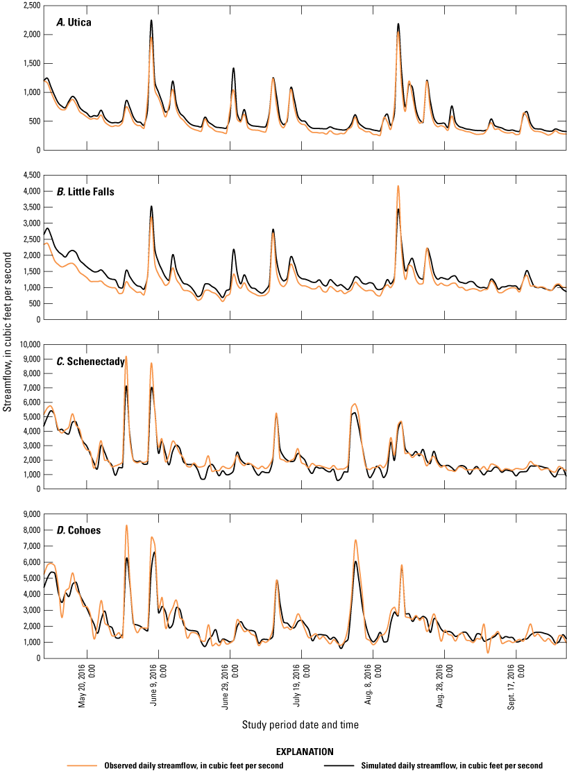
Hydrographs of observed daily streamflow (U.S. Geological Survey, 2022b) versus simulated daily streamflow in cubic feet per second for U.S. Geological Survey streamgages on the A, Mohawk River near Utica; B, -near Little Falls; C, -at Freeman's Bridge near Schenectady; and D, -at Cohoes, New York, for May 8 through Sep 30. Apr., April; Aug., August; Sept., September; Oct., October.
Errors in hourly aggregate volumes between observed and simulated streamflows at the four streamgages were computed in addition to the metrics for daily streamflow (table 12). Errors in volumes range from 11.2 to 14.7 percent at Utica, 6.7 to 21.4 percent at Little Falls, −10.2 to −3.7 percent at Schenectady, and −4.4 to 7.4 percent at the Cohoes streamgage. Volumes were typically biased higher in the upstream parts of the reach represented by the Utica and Little Falls streamgages, and then fell more in line with observed values in the lower end of the study reach demonstrating an overall volume bias for the period of June through September at the Cohoes streamgage of −1.5 percent. During model calibration, any attempt to alter the pattern of estimated tributary inflows to account for some of the volume bias in the upstream reach resulted in an equivalent shift in computed volumes in the downstream reach. Therefore, any attempt to lower the positive/higher bias in the upstream reach led to lower streamflows in the downstream reach, where the bias was already negative/lower. The final model calibration balanced the volume errors of all areas of the hydraulic model best.
Table 12.
Error in simulated versus observed hourly aggregate flow volumes for the period of May 8, 2016, through September 30, 2016, and individual months of June, July, August, and September 2016 at the U.S. Geological Survey streamgages on the Mohawk River near Utica, -near Little Falls, -at Freeman's Bridge near Schenectady, and -at Cohoes, New York.[%, percent]
Hourly river elevation, or stage, was analyzed at the four index streamgages in addition to daily streamflow and volume. Root mean square error (RMSE), mean error, and MAE were computed for the period of May 8 through September 30, 2016, and individually for the months of June, July, August, and September 2016. The model simulation of stage at the streamgages at Utica and Little Falls showed close agreement with observed stage at these stations, generally within a few tenths of a foot. The model simulation for the Schenectady streamgage demonstrated higher variation between observed and simulated values owing to the explanation provided later in this section.
Stage values in most parts of the hydraulic model are substantially affected by hydraulic control structures with gates. Although the best attempt to obtain accurate operational data on these control structures was made, some errors likely resulted from the coarse format of the operational data on the gates that was provided, in addition to periods that were missing within the data records. Furthermore, in the downstream parts of the reach at the Vischer Ferry Dam, flashboards are used to control the upstream pool elevation. Flashboards are typically long wooden boards that will temporarily increase pool elevation when inserted into receptacles at the crest of a control structure. During a flooding event, the flashboards may break away, resulting in a control structure with a dynamic, changing crest height. Recordkeeping of flashboard placement at Vischer Ferry Dam was generally unavailable for the study period, and an iterative process within the model was performed to assume flashboard placement and removal as noted previously in the above section on modeled gates. The pool above Vischer Ferry extends upstream and affects stage values at the Schenectady streamgage. Thus, comparisons of observed stage with simulated stage at the Schenectady streamgage were negatively affected by deficiencies in the data describing timing and positioning of flashboard gates and movable gates. Table 13 demonstrates model performance for simulated stage relative to observed stage at the streamgages near Utica, near Little Falls, and at Freemans Bridge near Schenectady, N.Y. The streamgage at Cohoes was not able to be included in these comparisons of stage data because the model’s downstream boundary did not extend substantially beyond the gaged pool at the Cohoes streamgage because of poor or unavailable cross-section data.
Table 13.
Errors in hourly simulated versus observed stage values for the period of June 2016–September 2016 and individual months of June, July, August, and September 2016 at the U.S. Geological Survey streamgages on the Mohawk River near Utica, -near Little Falls, and -at Freeman's Bridge near Schenectady, New York.[RMSE, root mean square error; ft, feet]
Hydraulic Model Sensitivity Analysis
A sensitivity analysis was done to test the model’s reaction to iterative changes in streamflow from the estimated tributaries and changes in Manning’s n values throughout the study reach. Estimated flow hydrographs for the ungaged drainage area accounted for a significant part of the flow inputs into the model. Therefore, visualizing how sensitive the model was to alterations in the estimated flows was important. Similarly, roughness coefficients, in the form of Manning’s n values, affect computed stage, timing, and, subsequently, flow throughout the study reach, and understanding potential sensitivity to these energy-loss factors was critical. RAS provides the ability, within the unsteady flow file, to apply coefficients to the tabular input data for the estimated tributary inflows. Using this functionality, factors of 0.8 through 1.2 (at an increment of 0.1) were applied to estimated flow data throughout the model, and simulations were run. Change in total and monthly volumes were computed and can be viewed in table 14. Because of the balance being maintained between upstream and downstream parts of the reach, any improvements realized in one area of the reach (upstream for example) typically resulted in negative effects on model performance at the opposing end of the reach. Changes were incremental, and no large shifts were noticed when different factors were applied to estimated flows. Additional improvements might be realized with enhanced, individualized refinements to the estimated tributary flow inputs by using supplemental time-series data collected at additional streamgages on larger ungaged tributaries. However, such potential refinements were beyond the scope of this study.
Similar results were documented when Manning’s n values were adjusted within the model. Factors of 0.8 through 1.2 (at an increment of 0.1) were applied to the tabular roughness coefficient values throughout the model. Model-wide adjustments might typically improve one area of model performance, while degrading another area. Shifts in computed aggregate volumes and daily streamflow values were less than 1 percent and were considered negligible for the study period for all iterations of the sensitivity analysis. RMSE, mean error, and MAE were computed for the sensitivity analysis simulations and compared to the calibrated model simulation. Hourly stage changes were typically incremental and minor, demonstrating that the model was not sensitive to modification of roughness coefficients. Table 15 demonstrates the largest changes in stage that were realized by adjusting the roughness coefficients. The streamgage at Schenectady notably showed negligible differences in stage with the adjusted roughness coefficients, owing to the high error induced by the data deficiencies for the previously mentioned downstream control structures.
Table 14.
Summary of adjustments to estimated tributary inflows and the corresponding effects on simulated flow volumes for the period of May 8, 2016, through September 30, 2016, and individual months of June, July, August, and September 2016 at the U.S. Geological Survey streamgages on the Mohawk River near Utica, -near Little Falls, -at Freeman's Bridge near Schenectady, and -at Cohoes, New York.[%, percent]
Summary of adjustments to model roughness coefficients and corresponding effects on hourly simulated stage values for the period of May 8, 2016, through September 30, 2016, and the individual months of June, July, August, and September 2016 at the U.S. Geological Survey streamgages on the Mohawk River near Utica, -near Little Falls, and -at Freeman's Bridge near Schenectady, New York.
Table 15.
Summary of adjustments to model roughness coefficients and corresponding effects on hourly simulated stage values for the period of May 8, 2016, through September 30, 2016, and the individual months of June, July, August, and September 2016 at the U.S. Geological Survey streamgages on the Mohawk River near Utica, -near Little Falls, and -at Freeman's Bridge near Schenectady, New York.[RMSE, root mean square error; ft, foot]
Development of Water-Quality Model
Water-quality analysis using HEC–RAS NSM simulates the fate and transport of water temperature, dissolved nitrogen, dissolved phosphorus, algae, carbonaceous biochemical oxygen demand (CBOD), DO, and other constituents. One prerequisite required before a user can run the water-quality analysis is the need for a working and calibrated HEC–RAS flow model. NSM organizes constituents, sources, and sinks into three major groups: temperature modeling, nutrient modeling, and other constituents. Once the HEC–RAS flow model was developed and calibrated, the calibration of NSM could begin. In this report, the term water-quality model refers to the combined water temperature module and nutrient module linked under the HEC–RAS NSM definition. The individual water temperature or nutrient modules will simply be referred to as models throughout this report when discussed separately to reduce confusion between definitions of a module compared to the more commonly used model reference. The first step is to calibrate the water temperature model within HEC–RAS NSM. Once a calibrated HEC–RAS flow model and a calibrated water temperature model are complete, the nutrient module within NSM can be calibrated.
The initial steps to developing the water-quality model included determining necessary input datasets, water-quality cell sizes, and boundary-condition requirements. When the water-quality model in HEC–RAS is initially opened, the cell sizes are automatically set to match the area between cross sections. After several adjustments were made to balance stability and model time step, the resulting minimum cell sizes for this model were set to 1,000 ft. The required data, boundary conditions, and parameterization for the water temperature and nutrient models are described in the following sections by model type.
Development of Water Temperature Model
The water temperature model is part of the nutrient simulation model built into HEC–RAS. It uses the framework developed for the hydraulics model and initially establishes water-quality cells between existing cross sections used in the hydraulic model. The water-quality computational node is then located directly between the bounding cross sections. This initial configuration can be changed to account for irregular cross-section spacing and, hence, cell sizes by combining multiple cells into single larger cells. This type of combining is typically done to correct model instability resulting from irregular cell sizes. More discussion about cell sizes is included in the description of the calibration of the water temperature and nutrients models.
The water temperature model requires a time-series boundary condition to be entered at all locations where streamflow enters the modeled system. The hydraulic model includes inflows from all 10 tributaries to the main stem of the Mohawk River with active USGS continuous-record streamflow streamgages in the reach from near Rome to Cohoes, N.Y. The model also includes estimated inflows from 34 additional tributaries that discharge directly to the main stem of the Mohawk River but are not continuously gaged by the USGS. The combined inflows from the gaged and estimated ungaged tributaries as well as the 3 ungaged intervening area inflows total 47 inputs to the modeled main-stem reach. Although the streamflow in the basin is well gaged, continuously recorded water temperature data are not available for most locations in the modeled reach. The model requirement to enter boundary conditions for all inflow locations presented the need to estimate water temperature data for most of the tributary inflow locations. Time series of water temperature data were estimated on an hourly time step for gaged tributaries and on a daily time step for ungaged tributaries and lateral inputs for intervening areas. More information about how water temperature data were estimated are in a subsequent section of this report titled “Estimating Water Temperature Data.”
Calibrating the water temperature model also required the input of a full meteorological dataset. Each meteorological dataset entered must include data for atmospheric pressure, air temperature, humidity, solar radiation, wind speed, and cloudiness. Like other boundary-condition requirements, meteorological data need to be entered as a time series but with the requirement that at least one new reading must be made every 3 hours to simulate diurnal water temperature variations. The meteorological data used in this model were downloaded from the NYS Mesonet meteorological network (New York State Mesonet, 2019). Additional information on the meteorological data used within the model is in the “Meteorological Data” section of this report.
Methods and Data used to Estimate Boundary Conditions in the Water Temperature Simulation
The Mohawk River has 10 gaged tributaries that discharge directly into the main stem downstream from Delta Reservoir to Cohoes, N.Y. Only one of these gaged tributaries, Canajoharie Creek at Canajoharie, N.Y., has approved water temperature data available for May through September of 2016 (U.S. Geological Survey, 2019). The lack of available water temperature data made it necessary to develop methods to estimate water temperature from available air temperature. Although many reports have been written discussing the relationship between air and water temperature, this project required an added level of estimation and adaption of existing methods to estimate hourly water temperature readings from daily air temperature records.
Water temperature is a critical variable in most water-quality modeling and management operations and needs to be estimated in many instances when recorded data are not available. Professors Gang Chen and Xing Fang of Auburn University in Alabama successfully demonstrated the utility of adapting methods originally developed to estimate hourly air temperature could be used to estimate water temperature (Chen and Fang, 2015). The diurnal variation of water temperature is a combination of a periodic sine wave function and an exponential decay function (Reicosky and others, 1989). Cornelis Teunis de Wit initially presented a wave form (WF) model in 1978 (de Wit, 1978) that was later also used by Reicosky (Reicosky and others, 1989) to estimate hourly air temperature from daily maximum and minimum air temperatures. Chen and Fang (2015) noted that Reicosky assumed maximum daily air temperature occurs at 1400 hours and minimum air temperature is at sunrise, but these assumptions need to be lagged to transfer the relationship to water temperature. They investigated this relationship at eight stations in Alabama and determined the average time for maximum water temperature occurred at about 1619 hours which was statistically the same as indicating the time of daily water temperature occurred between 1600 and 1700 hours in 122 stream-temperature logger sites in the Great Lakes Basin (Chen and Fang, 2015). Similarly, their study determined minimum water temperature occurred around 0803 hours each day which was about 2 hours after the statistical sunrise at about 0542 hours.
Applying the methods of Reicosky and others (1989) and Chen and Fang (2015), a two-step process, using daily air temperature records from the NYS Mesonet stations, was developed for this study to estimate daily maximum and minimum water temperature readings at each gaged tributary. These daily estimates would then be later used by applying the WF model to estimate hourly water temperatures using the estimated daily maximum and minimum water temperatures for the gaged tributaries.
Three NYS Mesonet stations (Cold Brook, Johnstown, and Sprakers) listed in table 16 were selected for this study to estimate daily water temperatures based on their proximity to the tributaries being estimated and completeness of available temperature records. The water temperature record from Canajoharie Creek at Canajoharie, N.Y., was used to develop regression equations that relate streamflow and air temperature to water temperature because it was the only available water temperature record within the study area (U.S. Geological Survey, 2019). An iterative trial and error process was applied to determine the best multi-parameter regression equation to predict daily maximum and minimum water temperatures for the gaged tributaries using the recorded water temperature data at Canajoharie Creek and the Johnstown Mesonet air temperature record. The resulting equations used the logarithm (log) of discharge from the tributary and the daily maximum, or minimum, air temperature from the Johnstown Mesonet station; each lagged by 1 day. The multiple R, r2, and standard errors for the resulting maximum and minimum equations are 0.84, 0.71, and 1.70 and 0.85, 0.73, and 1.49, respectively. These two equations were applied to the gaged tributaries, excluding the period of available water temperature data at Canajoharie Creek, to estimate the daily maximum and minimum water temperatures needed as inputs to the previously described WF model. To illustrate the fit of the regression equations, a graphical comparison of the recorded and estimated daily maximum water temperatures for Canajoharie Creek is shown in figure 14.
Table 16.
New York State Mesonet meteorological stations used, latitude and longitude in decimal degrees, and available period-of-record for the study period.[NYS, New York State; DD, decimal degrees; °, degree]
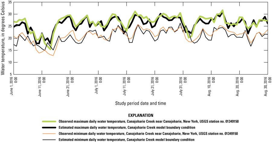
Recorded (U.S. Geological Survey, 2019) and estimated daily maximum and minimum water temperature at Canajoharie Creek near Canajoharie, New York, from regression equations that used daily discharge and air temperature from the Johnstown Mesonet station for June 1 to August 31, 2016. USGS, U.S. Geological Survey; no., number; Aug., August.
The WF model uses a lag between the time of maximum air and water temperature and a lag between sunrise and the time of minimum water temperature. The Chen and Fang (2015) application of the model used two forms of the model equation each day to reproduce the daily diurnal pattern of the recorded water temperature record shown below as equations 1 and 2.
whereRISE
is the time of sunrise in hours for each day,
Tw(H)
is the water temperature at the time H, in hours,
H’
is H + 8 if H<(Rise+2), or H’ = H−16 if H>1600 hours,
Twave
is the daily mean water temperature defined as: Twave = (Twmax+Twmin)/2, and
AMP
is the daily water temperature amplitude defined as: AMP= (Twmax−Twmin)/2.
The WF model, as described by Chen and Fang (2015), was used to generate hourly water temperature estimates for Canajoharie Creek using the daily maximum and minimum temperatures from the streamgage record to calibrate and check model performance. A graphical analysis of the estimated hourly water temperatures produced by the WF model showed the results were representative of the recorded data at the Canajoharie Creek streamgage. One notable anomaly in the estimated temperature record was a jump or sharp change around midnight when the range in daily temperature was changing from day to day. This is a result of the use of the daily maximum and minimum temperatures for each day. When the daily range changes, a jump or sharp change is not uncommon as the model formula switches to the maximum and minimum for the next day. To compensate for this, Chen and Fang (2015) added additional conditions to the WF model that substituted the average of the maximum or minimum temperature from the current and previous day for the daily average computation if the maximum increased by more than 2 °Celsius or the minimum dropped by more than 3 °Celsius. This complex adjustment was applied in our study too, but the resulting hourly estimates still showed some rapid changes or jumps in the estimated time series. Whether these rapid changes in water temperature would create any instability in the water temperature model is unclear, but we determined that an attempt should be made to smooth the transitions without adversely impacting the model accuracy. The WF model equations were examined for ways to smooth the transition between days while not producing notable reductions in the overall accuracy of the estimated data. Complex attempts using the previous day’s mean and the current day maximum and new forms of the WF equations were explored. After several trial-and-error attempts were made to improve the estimated hourly time series, a slight modification to the original equations was used. The WF model equations were modified to subdivide the day into four sections. The 0000-to-0800-hour time block was divided into two equal blocks, and local time offsets were adjusted to calibrate results of Canajoharie Creek recorded water temperatures. The remaining time blocks, sunrise plus 120 minutes (2-hours) to 1600 hours and 1600 hours to 2400 hours, were maintained unchanged, but a few of the time offsets in the original equations were adjusted to calibrate the resulting estimates to the local recorded water temperature at Canajoharie Creek. The resulting modification to the WF model application is listed in equations 3, 4, and 5.
whereRISE
is the time of sunrise in hours for each day, assumed to be 0600 for this study,
Tw(H)
is the water temperature at the time H, in hours,
H’
is H + 8 if H <(Rise−2), or H’=H+9 if (RISE−2) < H < (RISE+2), and H’ = H–8 if 1600h < H < 2400h, and
Twave
is the daily mean water temperature defined as: Twave = (Twmax+Twmin)/2.
The modified WF model equations (eqs. 3–5) were used to estimate water temperatures at hourly time series for nine tributary inputs to the main-stem model, without the added smoothing algorithm developed by Chen and Fang (2015). The smoothing algorithm was not applied because it did not completely remove the jumps in estimated data and did not improve the statistical relationship between the recorded and estimated data at Canajoharie Creek. The recorded water temperature data for Canajoharie Creek was used directly when available.
The computed hourly water temperature estimates from the newly modified equations and the original WF model equations were compared to the recorded hourly data from Canajoharie Creek for validation. The original equations by Chen and Fang (2015), with the smoothing algorithm added, produced an r2=0.71 and a standard error of 1.8 °Celsius when compared to the approved recorded record from Canajoharie Creek. The newly modified equations did not provide a major level of improvement to fit with a r2=0.73 and a standard error of 1.75 °Celsius when compared to the approved record from Canajoharie Creek, but in some areas, the graphical comparison seemed to fit slightly better. Figure 15 A–B shows two examples from the study period that compare recorded water temperature at Canajoharie Creek to estimated hourly water temperatures, computed from daily maximum and minimum water temperatures.
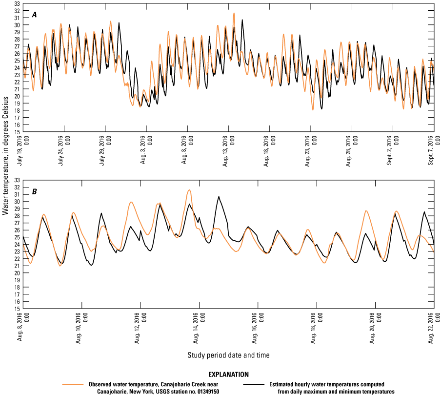
Recorded hourly water temperature at U.S. Geological Survey streamgage Canajoharie Creek at Canajoharie, New York (U.S. Geological Survey, 2019), and hourly water temperatures estimated from daily maximum and minimum water temperature using modified wave form model from A, July 19 to September 7, 2016, and B, August 8 to August 22, 2016. USGS, U.S. Geological Survey; no., number; Aug., August; Sept., September.
The water temperature boundary conditions for the remaining ungaged tributary inputs to the main-stem Mohawk River model were estimated at a daily time step. This was accomplished by estimating daily water temperature from the log of daily discharge estimates and NYS Mesonet daily air temperatures. Table 17 lists the Mesonet stations used to estimate hourly and daily water temperature boundary conditions for each of the gaged and ungaged tributaries, respectively.
Table 17.
New York State Mesonet station, tributary, water temperature boundary-condition time step, and data source used.[NYS, New York State; no., number; N.Y., New York]
Meteorological Data
The HEC–RAS water temperature model requires the input of one full meteorological dataset. As indicated earlier in this report, several meteorological stations from the NYS Mesonet system were selected for use in this project (table 16) (Brotzge and others, 2020). The required parameters, atmospheric pressure, air temperature, humidity, short wave radiation, and wind speed were available and entered as hourly reading time series.
The required cloudiness input was not available from the Mesonet stations selected for this study. The only available source for cloudiness data for the study period were from the National Oceanic and Atmospheric Administration meteorological station at the Albany International Airport in Albany, N.Y. (National Oceanic and Atmospheric Administration, 2019). Therefore, we decided to simply use the Albany cloudiness data as a surrogate for each of the three pre-selected Mesonet stations. Despite the Albany location not being centralized to the model study area, no other citable cloudiness data for the study period were available. Cloudiness data are entered within the temperature model on a scale from 0.0 to 1.0—1.0 indicating overcast conditions and 0.0 indicating completely clear skies. The cloudiness data available from the Albany station were broken down into 9 categories, from 00 to 08— 00 indicating clear conditions and 08 indicating overcast conditions on an hourly time scale with associated cloud elevation observations. We performed a simple proportional adjustment to transpose the 9-point resolution Albany station data to the 10-point resolution scale of the model (0.0 to 1.0). After this, the hourly cloudiness data were entered into the cloudiness time series for each weather station used within the temperature model in NSM.
Once the necessary meteorological data are populated, each water-quality cell needs to be associated with one of the meteorological stations. The meteorological stations were assigned to a range of cross sections primarily based on their physical proximity to each section of modeled reach. Figure 16 shows the locations of the Mesonet stations and associated model reach for each station.
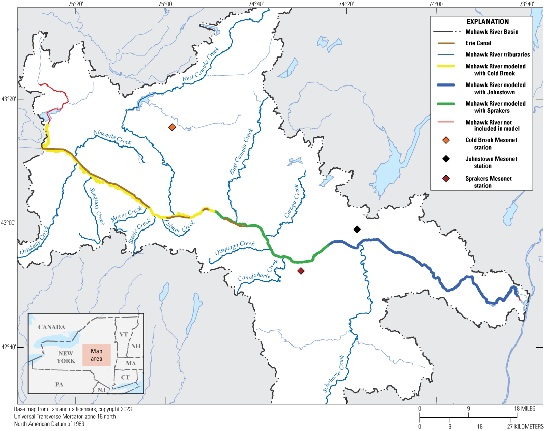
Map of the Mohawk River Basin with selected New York State Mesonet stations and the associated section of the of main-stem model reach for each Mesonet station.
Calibration of Water Temperature Model
The Mohawk River hydraulic and water-quality model was calibrated from May 1 to Sept 30, 2016, but the first 2 weeks of May were reserved as the model start-up and equalization period. This period will not be formally referenced in terms of performance or calibration. The model calibration period was selected because of the binary way in which the streamflow in the Mohawk River is regulated. The streamflow in the Mohawk River is controlled differently in spring and summer as compared to fall and winter. The spring-summer period (navigation season) and fall-winter period (non-navigation season) are controlled using gated control structures, locally referred to as moving dams, which impound water for increased depth and reduced low-flow velocity during navigation season. The operation of the gated control structures can substantially change the flow patterns in the Mohawk River during low to moderately high-flow conditions at many locations along the river.
The model was considered calibrated when simulated daily water temperatures adequately represented recorded water temperature data in the Mohawk River. The Hudson River Environmental Conditions Observing System (HRECOS) provides the only available continuous-record water temperature data for the main-stem Mohawk River from Rome to Cohoes, N.Y. (Hudson River Environmental Conditions Observing System (HRECOS), 2019). These data were available at three recording stations within the study reach: Mohawk River at Ilion, Mohawk River at Lock 8, and Mohawk River at Rexford Bridge. These data were primarily used to validate the model’s continuous simulation of water temperature along the Mohawk River. Discrete water temperature readings taken by the USGS or NYSDEC and retrieved from the USGS National Water Information System (U.S Geological Survey, 2019) at several additional locations along the Mohawk River were also used to verify the simulated water temperature data throughout the reach.
The model simulated hourly water temperatures were analyzed and compared to recorded hourly data from the HRECOS stations, but summary statistics were only reported on a daily, monthly, and seasonal basis. The recorded temperature at the Ilion, Lock 8, and Rexford Bridge HRECOS stations ranged from about 12 to 28 °Celsius for the period of May 15 to September 30, 2016. The overall pattern of the recorded to simulated water temperatures for the three stations was generally a good fit. The hourly temperatures were used to compute the MAE and the RMSE statistics for the entire modeled period: the MAE for the Ilion and Lock 8 stations were 0.90 and 0.89 °Celsius, respectively, and the MAE for Rexford Bridge was 0.87 °Celsius. The RMSE for Ilion and Rexford Bridge were 1.06 and 1.07, respectively, and the RMSE for Lock 8 was 1.00 °Celsius. May and June had the largest range in water temperature, as expected. The low for the June to September period happened around mid-June, but temperatures slowly climbed through the end of June and into July (fig. 17). The simulated water temperatures followed this pattern well, generally remaining within 1 degree Celsius of the recorded values. The simulated water temperature was generally below the recorded water temperature for the July and August periods when analyzed graphically. The pattern remained consistent across the range of recorded temperatures, including a nearly 5-degree swing in recorded temperature from late June through late July. Additional comparisons were done to simulated temperatures and discrete water temperature readings taken during water-quality sample collection in June through September. This comparison showed the simulated water temperatures generally balanced the recorded water temperatures to within 1 to 2 °Celsius and, at some locations, was even closer to the water temperature recorded during sample collection in July.
Daily average water temperatures were computed for the recorded and simulated temperature data at the Ilion and Lock 8 stations to examine the statistics fit between the two datasets. As expected, the daily water temperature statistics matched closely with the earlier analysis of the hourly data. The MAE for the daily average water temperatures at the Ilion and the Lock 8 stations rounded to about 0.84 °Celsius, and the RMSE for the Ilion and Lock 8 stations was 0.99 and 0.95 °Celsius, respectively. One possible reason for the slight bias in simulated temperatures was because of the location of the temperature sensor. The recorded data are point measurements of water temperature near one bank of the river and may not be representative of the average cross-sectional temperature during certain times of the year. Data to relate the recorded temperatures to the mean temperature in the cross section were not available but, because the overall fit between the recorded and simulated temperatures was generally within 1-degree Celsius, the slight negative bias during July and August was considered acceptable. June through July and August through September water temperatures are shown in 2-month plots for each station in figure 18. These plots are presented at a slightly finer scale to help illustrate how the model output does a good job of simulating the recorded variability on daily and monthly time steps. The mean absolute percent error was computed in °Celsius as another check on the overall accuracy of the simulated water temperatures. The mean absolute percent error of the simulated water temperature at the Ilion, Lock 8, and Rexford Bridge stations was 4.0, 3.8, and 4.1 percent in °Celsius, respectively, which is well within the range defined by the project as being an acceptable error for this simulation.
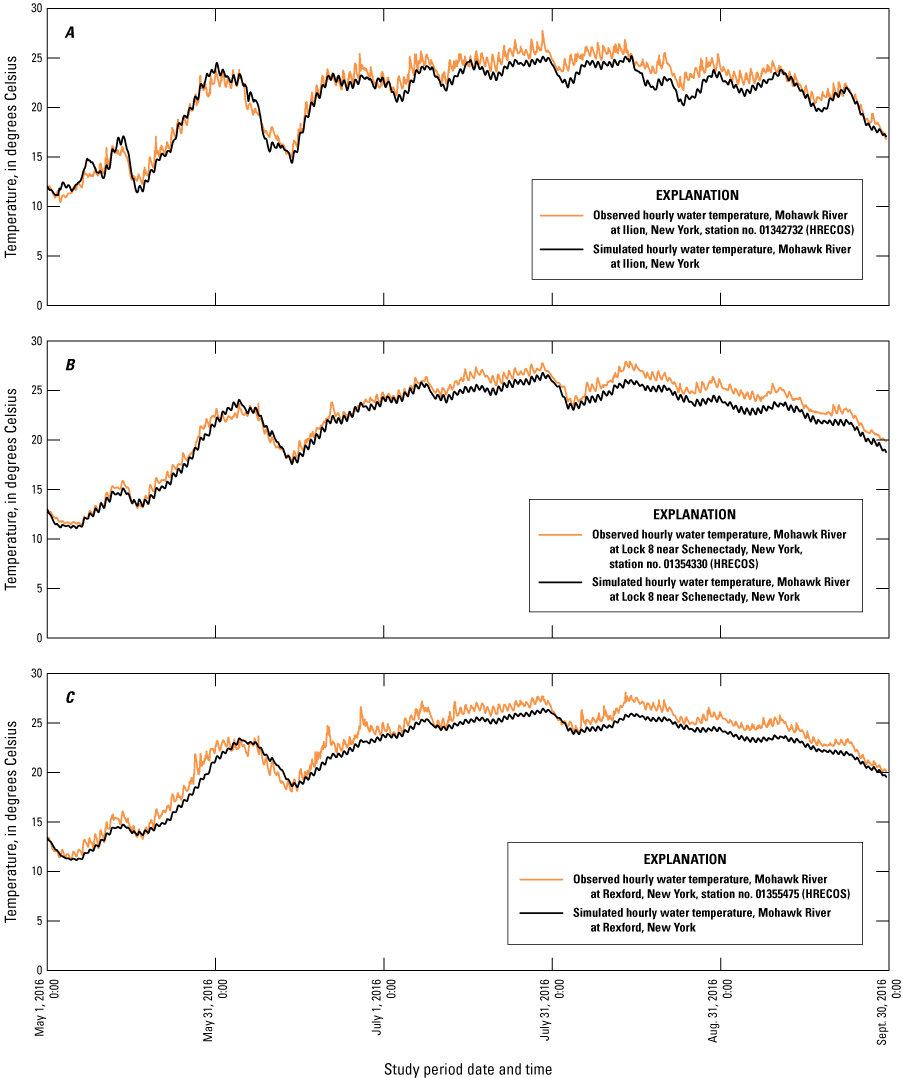
Graphs showing the hourly comparisons of recorded (U.S. Geological Survey, 2019) to simulated water temperature at the Hudson River Environmental Conditions Observing Systems stations at A, Ilion; B, Lock 8; and C, Rexford Bridge for May through September 2016. no., number; HRECOS, Hudson River Environmental Conditions Observing System; Aug., August; Sept., September.
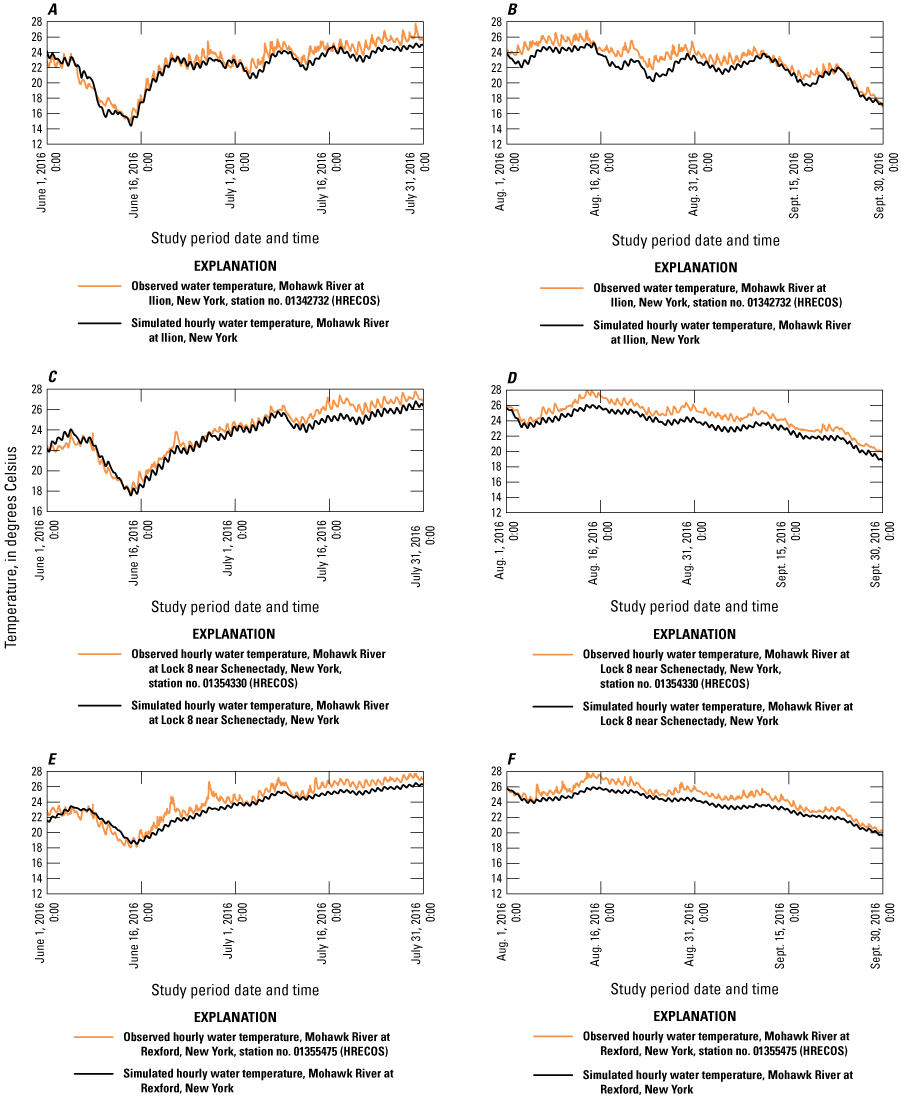
Graphs showing the hourly comparisons of recorded (U.S. Geological Survey, 2019) to simulated water temperature at the Hudson River Environmental Conditions Observing Systems stations at A–B, Ilion; C–D, Lock 8; and E–F, Rexford Bridge for 2-month periods from June through September 2016. no., number; HRECOS, Hudson River Environmental Conditions Observing System; Aug., August; Sept., September.
Methods and Data used to Estimate Boundary Conditions for the Nutrient Simulation Model
In addition to the calibrated hydraulic and water temperature outputs, the nutrient simulations in the NSM I, dynamically linked in HEC–RAS, require input of the boundary conditions for the following parameters, known as state variables: DO, algae, carbonaceous biological oxygen demand (CBOD), organic nitrogen, ammonium, nitrate, nitrite, organic phosphorus, and inorganic phosphorus (table 18).
Table 18.
Hydrologic Engineering Center’s River Analysis System (HEC–RAS) Nutrient Simulation Module (NSM) Version 1 list of state variables.[mg, milligram; A, algae; L, liter; g, gram; m2, square meter; BOD, biochemical oxygen demand; HEC–RAS, Hydrologic Engineering Center River Analysis System; N, nitrogen; P, phosphorus; O, oxygen]
A time series of these concentrations was not available from either USGS or NYSDEC sources. Discrete sample data were collected at a select number of tributaries and used to estimate time-series concentrations as described in the following sections. A time series of nutrient data were estimated for gaged tributaries using an hourly time step, whereas nutrient data boundary conditions at ungaged tributaries were estimated on a daily time step.
Availability of Discrete Sample Data
The hydraulic and water-quality model for the main-stem Mohawk River includes inputs from all USGS gaged tributaries from Rome to Cohoes, N.Y., and ungaged tributaries with a drainage area generally greater than 5 square miles (fig.19). Samples collected from April to October of 2016 at the gaged tributaries, along with any additional samples collected at or near these locations from about 2000 through 2018, were considered for use in computing nutrient input boundary conditions. Unfortunately, few samples collected beyond 2016 were available for the computation of boundary conditions. In 2019, the NYSDEC made efforts to collect some additional water-quality samples during higher flow, or runoff conditions, at a few selected sites to provide some added data to better understand how some nutrient concentrations changed during runoff events. The total number of samples, including 2019 samples, at most sites was still less than the recommended minimum needed to use a traditional load estimator tool like LOADEST (Runkel and others, 2004) or Weighted Regressions on Time, Discharge, and Season (WRTDS) (Hirsch and others, 2010), so custom methods were needed to estimate the necessary time series of constituent concentrations to populate the model boundary conditions. The time series of boundary conditions for the required nutrient concentrations were estimated by applying regression techniques to periods when streamflow was in the lower to medium range with minimum runoff conditions; streamflow and water temperature were used as explanatory variables. Constant event mean concentrations (EMCs), based on land-use categories, were used when flows were higher and overland runoff was expected. The approach of using literature values for EMCs for required nutrient boundary conditions was considered acceptable to estimate concentrations during higher flow events because the primary focus of this model was to target instream lower-flow conditions. Details related to the development of regression equations and equations to weight EMCs based on land-use categories are in the following sections of the report.
Estimating Nutrient Boundary Conditions for Tributaries with Discrete Sample Data
Limited availability of approved and published nutrient sample concentrations required a somewhat nontraditional approach to estimating time-series data for the model’s nutrient boundary conditions. Although a few methods were investigated, we ultimately decided that a multi-parameter regression model would be developed to estimate nutrients in the low to moderate range of streamflow, which typically had minimal contributions from overland runoff. Using the available nutrient sample concentrations, log transformed USGS streamflow, and estimated water temperature data for the gaged tributaries produced equations that were used to estimate boundary conditions for lower to medium flows. A list of regression coefficients from these models are in table 1.1. A total of eight gaged tributaries had approved and published nutrient samples available for estimating the low to medium flow concentrations of necessary boundary-condition parameters at an hourly time step. The remaining inputs were estimated at a daily time step because the available data lacked enough resolution.
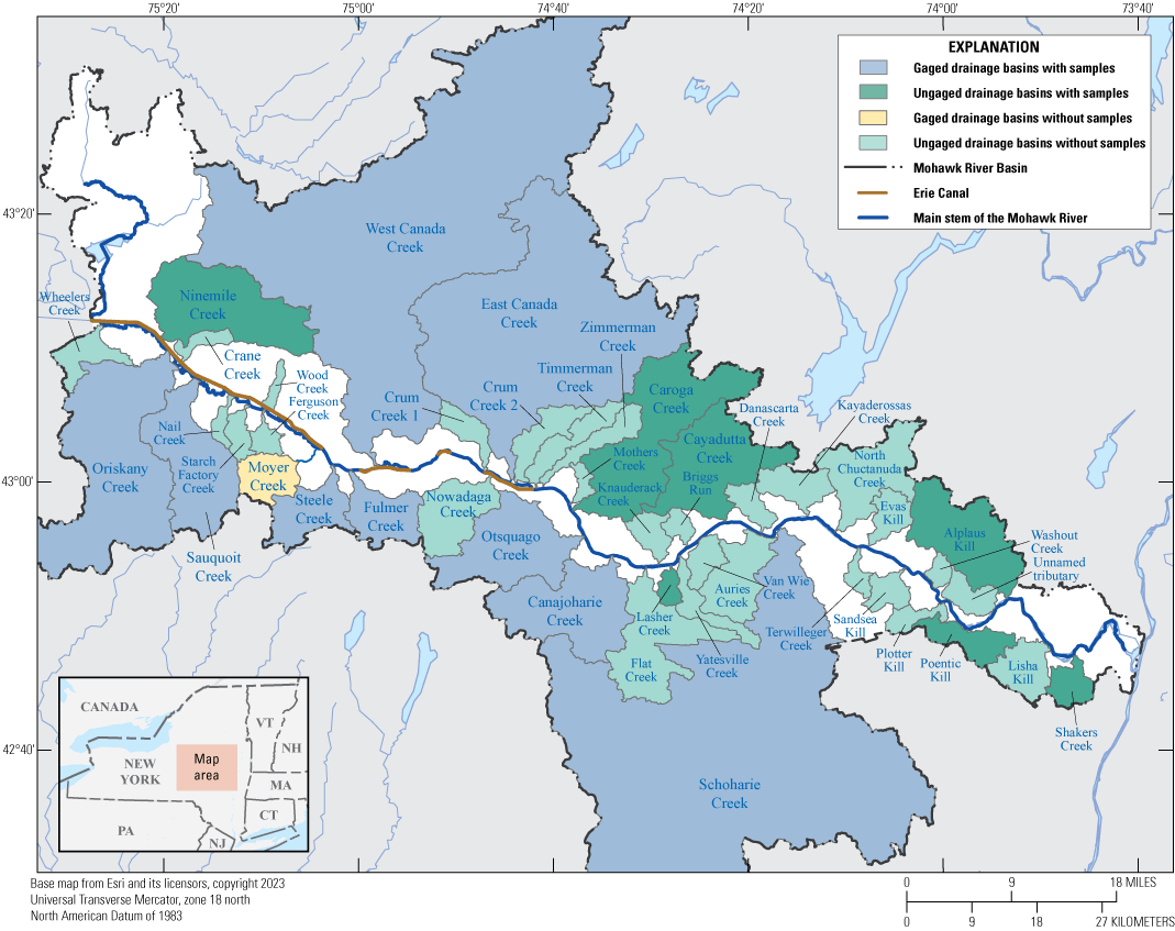
Map of study area showing tributary drainage basins color-coded by gaging and sample status (gaged with samples, gaged without samples, ungaged with samples, ungaged without samples).
Canajoharie Creek near Canajoharie, N.Y., was one of the few gaged tributaries with more than 25 nutrient samples available for most parameters. The Canajoharie Creek streamgage was part of the USGS National Water-Quality Assessment (NAQWA) project during the 1990s and into early 2000s, which, in part, is why more samples were available. The NAQWA project was established by Congress in the early 1990s to address, among other things, how, when, and why our Nation’s waters have changed and if they are continuing to change into the future (U.S. Geological Survey, 2022c). Many water-quality samples were collected, and research projects and reports were completed as part of that major project (U.S. Geological Survey, 2022d). In 2016, samples were also taken at the Canajoharie Creek streamgage as part of the Northeast Stream Quality Assessment done by NAQWA to investigate the quality and health of wadable streams in the northeastern United States. Consequently, many samples were available at the Canajoharie Creek streamgage, but not all samples were useful for estimating boundary conditions for the specific parameters used in the model. Generally, more than 157 samples were available for most boundary-condition parameters at the Canajoharie Creek streamgage using a selection window from 2006 to 2016. Evaluation of the available data and the development of multi-parameter equations with nutrient concentrations, streamflow, and water temperature identified a relationship between the explanatory and response variables resulting in r2 values ranging from 0.50 to about 0.86 (table 19).
Table 19.
Results from linear regressions performed on Canajoharie Creek discrete samples.[Data from U.S. Geological Survey (2019). mg/L, milligram per liter; µg/L, microgram per liter; r2, coefficient of determination]
Five-digit code used to identify the measured constituent in the National Water Information System (NWIS; U.S. Geological Survey, 2019).
Of the remaining 7 gaged tributaries, West Canada Creek had the next largest dataset, 25 samples being available for most parameters. The number of approved samples available to develop equations to estimate boundary conditions for the remaining 6 gaged tributaries generally ranged from 6 to about 24 samples. Tables 20 and 21 list the gaged sites, drainage areas, numbers of samples, and median concentrations for the nutrient samples used to estimate gaged tributary input boundary conditions.
Table 20.
Streamgage sites, drainage area, number of samples, and median concentrations for the nutrient samples used to estimate input boundary conditions for the gaged tributaries.[Data from U.S. Geological Survey (2019). DA, drainage area; USGS, U.S. Geological Survey; mg/L, milligram per liter; µg/L, microgram per liter]
Five-digit code used to identify the measured constituent in the National Water Information System (U.S. Geological Survey, 2019).
Table 21.
Non-gaged sites, drainage area, number of samples, and median concentrations for the nutrient samples used to estimate input boundary conditions for the gaged tributaries.[mi2, square mile; mg/L, milligram per liter; μg/lb, microgram per pound; --, not sampled; no., number; N.Y., New York; N, number of samples; <, less than; NSMI, nutrient simulation module 1]
Sites labeled with North or South regression were either not sampled or have a number of samples where N<6.
Because the small number of samples and concentrations did not cover the full range of conditions during the 2016 modeled period, evaluation statistics, such as the predicted residual error sum of squares (PRESS) statistic for determining regression equation predictive ability, were not applied. Fit and predictive ability for the regression equations were mostly evaluated graphically by analyzing the residual plots of observed versus predicted concentrations. Figure 20 A–E shows the relationship between discrete sample concentrations and daily average concentrations for simulated hourly nutrient boundary conditions for the day discrete samples were collected. Figure 21 A–E shows the observed and estimated concentrations for nitrogen and phosphorus species parameters at the Canajoharie Creek streamgage. The review of available samples and the analysis of observed versus predicted concentrations showed the data and resulting predictive equations would likely not adequately cover the full range of observed conditions during the 2016 model period, so the use of these equations was generally limited to less than bankfull streamflow conditions or streamflows less than the statistical 1.25-year recurrence interval (80-percent annual chance probability). Additional methods described further in this section were used to produce input boundary conditions appropriate for the range of flow conditions simulated for 2016.
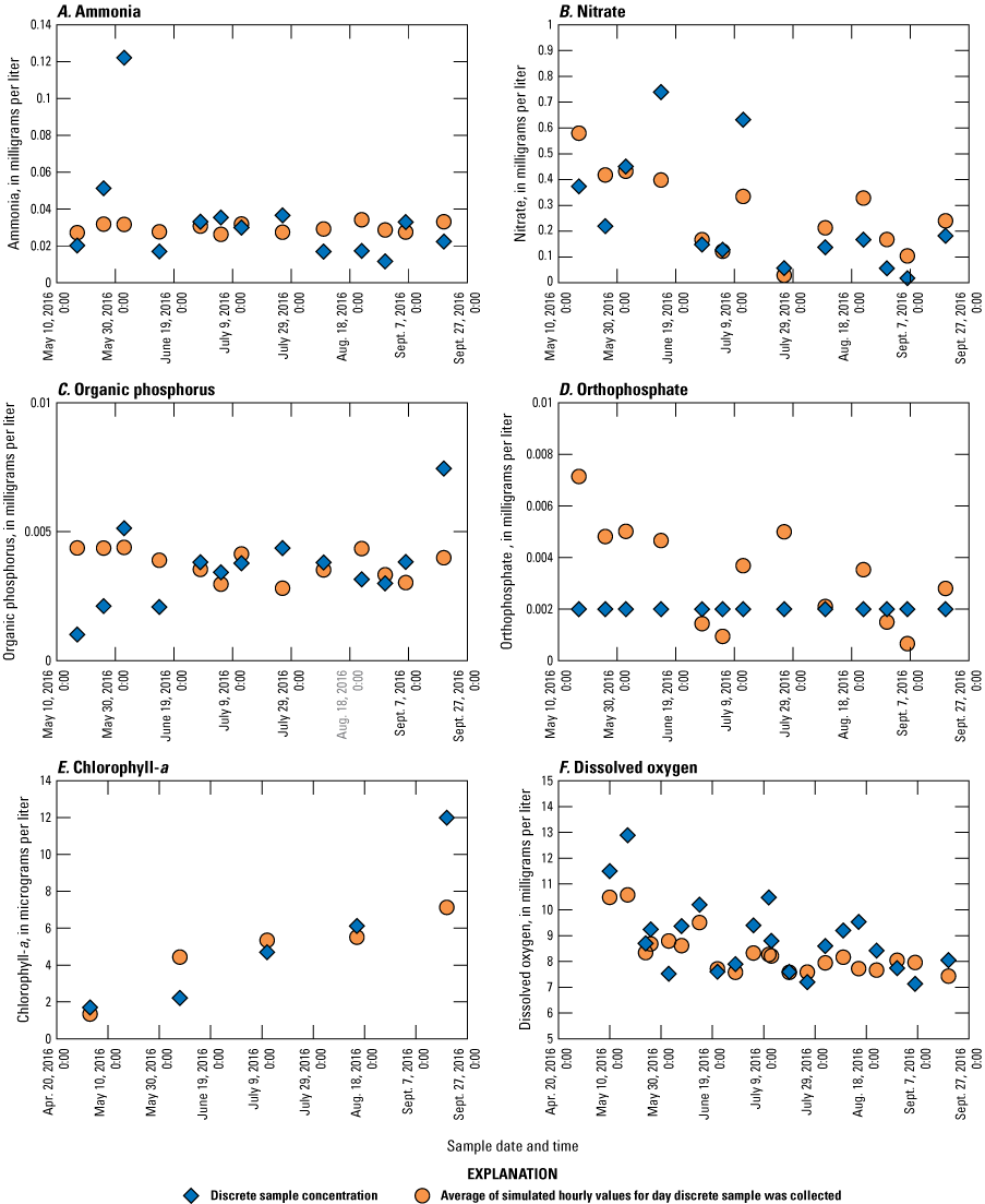
Plots showing relations between discrete sample concentrations (U.S. Geological Survey, 2019) and average daily simulated concentrations for A, ammonia; B, nitrate; C, organic phosphorus; D, orthophosphate; and E, chlorophyll-a at the Canajoharie Creek streamgage. Aug., August; Sept., September.
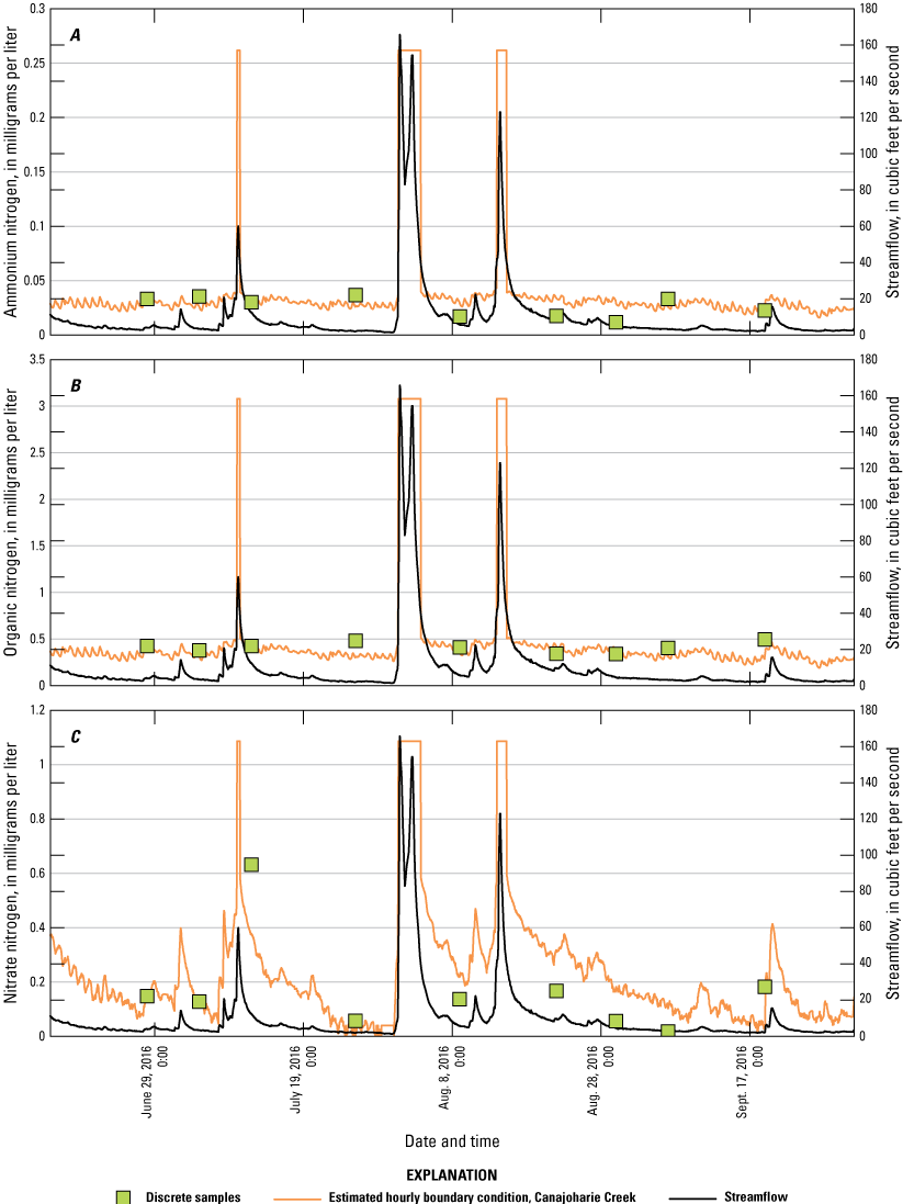
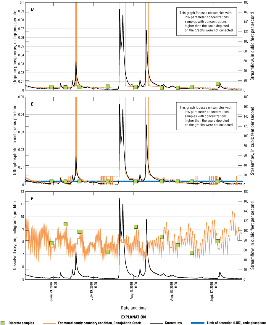
Hydrographs showing relations between observed (U.S. Geological Survey, 2019) and estimated concentrations of A, ammonium nitrogen; B, organic nitrogen; C, nitrate nitrogen; D, organic phosphorus; E, orthophosphate; and F, dissolved oxygen at varying flow conditions during the model period at the Canajoharie Creek streamgage. Aug., August; Sept., September; Oct., October.
Estimating Nutrient Boundary Conditions for Tributaries with no Discrete Sample Data During the Model Simulation Period
A boundary condition time series needed to be estimated for the ungaged tributaries that were not sampled during the 2016 model simulation period. This presented a difficult challenge because typically discrete nutrient samples need to be used to estimate base-flow concentrations or potentially even a simple mean concentration. Without a robust set of current or historic discrete samples to use, a novel approach was needed to estimate the needed boundary conditions. To overcome this discrete sample limitation, existing samples from select neighboring streams in the study area were grouped and used to estimate parameter concentrations. Land use, drainage area, availability of data, where the tributary enters the main stem, and flow conditions were used to identify and group the streams that would be included in the regional analysis. This method grossly simplifies the regionalization methods often used by the USGS, or other science agencies, to inform areas without local data. Collecting additional data and developing regional equations for ungaged and unsampled tributaries included in the model was beyond the scope of this project, so a simple pooling of the samples by geographic area was applied and regression equations were developed for two regions for each parameter. The equations were developed using discrete water-quality nutrient samples from nearby streams for the tributaries in the model with no samples during the model simulation period or for tributaries with historically sparse samples entering the main-stem Mohawk River from the north and from the south. Table 22 identifies which tributary drainage basins were used to generate the regional equations. These simplified regional equations were used to estimate nutrient input boundary concentrations at low to medium flow conditions at a daily time step. Although the uncertainty of these estimates is unclear, the sum of the contributing drainage areas for all the ungaged tributaries is less than 25 percent of the total drainage area at the downstream end of the reach. The unsampled tributaries and streamgages used with the north and south regression equations are shown in figure 22.
Table 22.
Gaged streams used to generate regional models for estimating nutrient boundary conditions.[NA, not applicable]
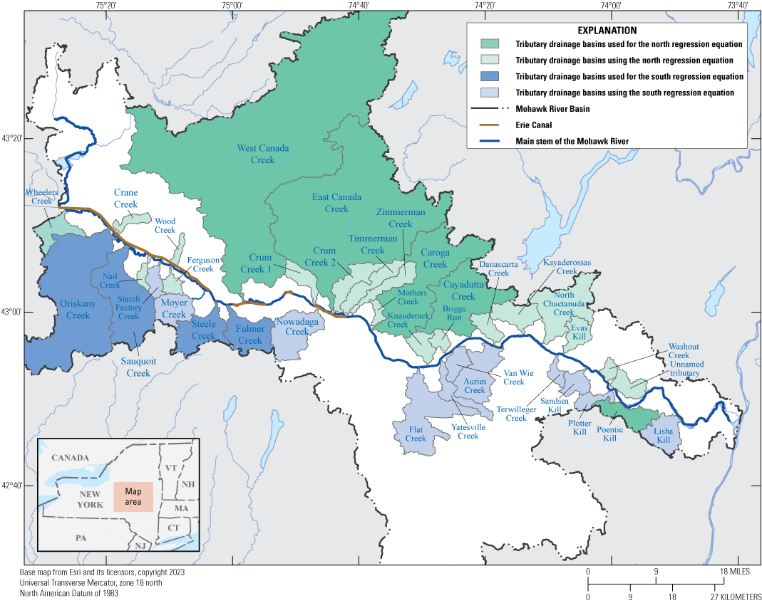
Map showing color-coded basins where north/south regression equations were applied to estimate boundary conditions based on regional equations.
As flow conditions changed and the potential for runoff to transport nutrients from the landscape increased, EMCs were clearly needed to estimate the concentrations of nutrients from the catchment landscape during higher runoff events. The modeled 2016 water year (defined by the USGS as the 12-month period October 1 through September 30) was not a year with historic flooding or even a year where peak streamflows equaled or exceeded the 2-year recurrence interval (50-percent annual exceedance probability) at the Little Falls or Cohoes streamgages. The moderate flow conditions in 2016 and a primary focus on evaluating the impacts of WWTP discharges on lower in-channel flows from WWTP made utilizing land-use weighted EMCs to estimate larger runoff event concentrations not measured during routine time-lapse scheduled sampling more reasonable. The next section describes how EMCs were used to help fill in gaps in sample data to compute a time series of concentrations for the gaged tributary input boundary conditions.
Applying Event Mean Concentrations to Estimate Runoff Concentrations for Unsampled Range of Flow
The use of EMCs is an important part of many projects that need to estimate nutrient or pollutant concentrations associated with stormwater runoff. For this project, EMCs were used to estimate concentrations for a small range of higher-flow runoff events required as model input boundary-condition parameters. At tributaries with continuous-record, tributaries with USGS streamgages and tributaries with discrete nutrient water-quality samples taken from them, the time series of required nutrient boundary conditions were estimated by combining the results of regression models built from approved data and land-use weighted EMCs. At most gaged tributaries, storm sampling was not done, so few if any high-flow or runoff event samples are available to help estimate nutrient concentrations. To fill in this gap of missing storm event concentrations, EMCs from the literature were applied to nutrient boundary conditions based on land-use type and weighted by percentage of total drainage area. Findings from the National Stormwater Quality Database research project provided usable EMCs for the following land-use types: commercial, freeways, industrial, institutional, open space, and residential (computed from data in the National Stormwater Quality Database; Pitt and others, 2004). Crops and agriculture, forest, and institutional EMCs were derived from the Upper Neuse River Basin, North Carolina, study (Line and others, 2002). This final set of EMCs for the required nutrient parameters are listed in table 23.
The computation of a weighted EMC required deriving land-use percentages for each of the categories listed above for all 44 gaged and ungaged tributary input locations. Once the necessary basin characteristics were derived, a weighted EMC could be computed using the percentage of each land-use category. A conditional logic statement was then used to determine if the streamflow was above a given threshold at which time the hourly or daily concentration was estimated using the weighted EMC as a surrogate for when concentrations from runoff events were dominating input in the tributaries. The threshold was always set below the mean annual flow, utilizing the 1.25-year recurrence interval (80-percent annual exceedance probability) as a general guide. Because of the lack of storm samples and, in many instances, gaged data, many estimates needed to be made. A graphical analysis was done to adjust the initial thresholds to become active when the streamflow increased beyond its typical range for the period consistent with when increased runoff would contribute to changes in nutrient concentrations. The drainage basins and land-use for the sampled and unsampled tributaries are shown in figures 23 and 24.
Because EMCs do not exist for chlorophyll-a and DO concentrations, scaling these EMCs for higher flows could only be estimated by utilizing the regression equations generated by existing data from each tributary or grouping tributaries regionally and using the grouped data with temperature and streamflow as variables to scale those values. Plotting the generated boundary-condition datasets against discrete sample concentrations at the Canajoharie streamgage (figure 21A–F) shows a reasonable agreement given the flow and temperature conditions. The primary goal of this exercise was to ensure the regression-simulated boundary conditions were not unacceptably biased in either direction.
For chlorophyll-a, an additional verification step was taken to tabulate the mean and median chlorophyll-a sample concentrations at all streams with available samples, and the grouped-regional streams, and check these values against the regressed chlorophyll-a boundary condition datasets to ensure the regressions did not generate a chlorophyll-a boundary condition that was biased high or low. A final step was taken to convert chlorophyll-a in micrograms per liter to the NSM I-required milligrams per liter.
Table 23.
List of event mean concentrations for nutrient parameters used in the Nutrient Simulation Module for the Mohawk River.[EMC, event mean concentration; mg/L, milligram per liter, N.C., North Carolina; TSS, total suspended solids]
Adapted from Line and others (2002).
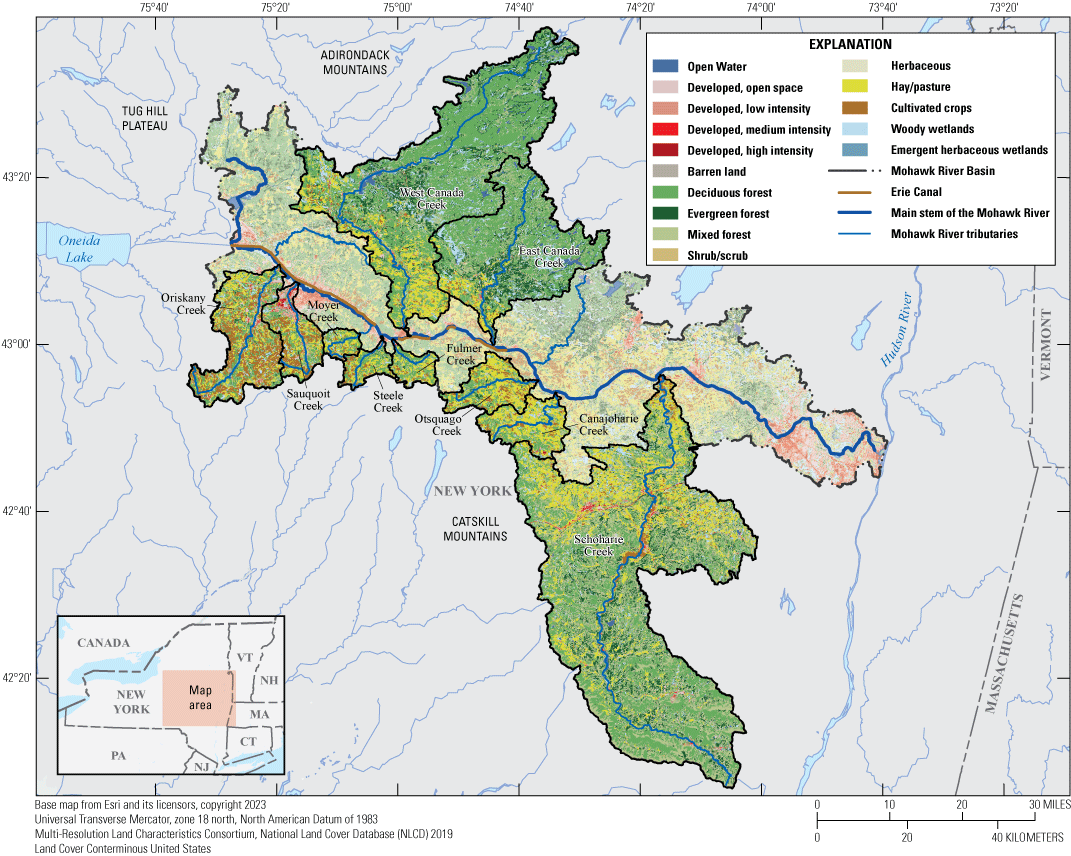
Map of study area, drainage basins, and land-use categories for gaged tributaries.
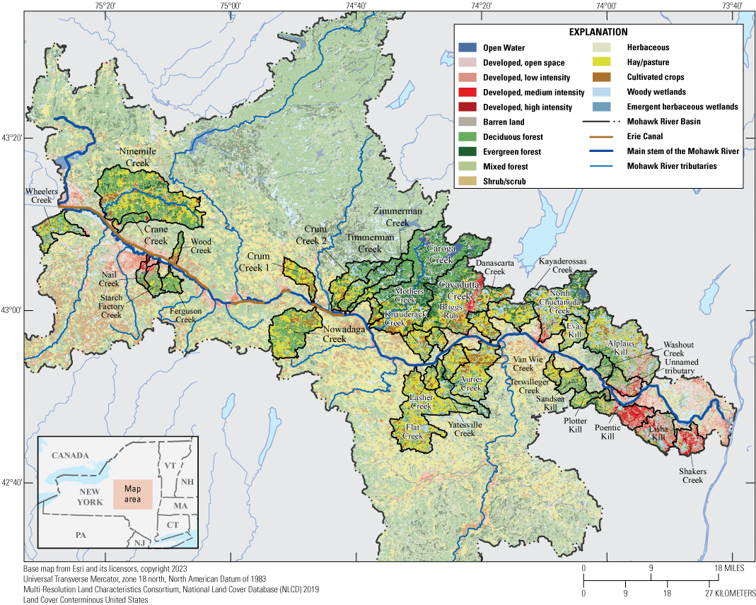
Map of study area, drainage basins, and land-use categories for ungaged tributaries.
Methods to Check Combined Regression Analysis and Event Mean Concentration Estimates with the Regional Loading Model
Model outputs from the USGS SPAtially Referenced Regressions On Watershed attributes (SPARROW) (Schwarz and others, 2006) were used to check the quality of the custom methods used to estimate nutrient boundary conditions. SPARROW is a watershed model that estimates nutrient flux and loading utilizing geospatial watershed information and data from a network of long-term monitoring locations throughout the United States. The SPARROW modeling in the northeast involved developing individual models for the region to represent streamflow and total loads of nitrogen and phosphorus (Ator, 2019a). One of the main objectives behind the development of SPARROW was to provide a statistical basis for nutrient load estimates at locations that are not monitored. The most current and available model outputs, which are from the 2012 SPARROW model, for annual total phosphorus and total nitrogen loads were retrieved from the USGS SPARROW Mapper for each tributary in the Mohawk Basin (Ator, 2019b). The annual loads for total phosphorus and total nitrogen calculated by SPARROW were scaled to only represent water year 2016 by applying the relationship between the 2016 approved annual mean streamflow for the tributary streamgage and the SPARROW average annual streamflow at the same streamgage for the period of record as a percentage. The resulting load was scaled further by applying a 50-percent multiplier to reduce the annual load and bring it closer to the modeled season from May through September. These SPARROW data were adjusted for tributaries and the main stem to provide a generalized independent estimate of the nutrient loads as an additional way to verify that the model results were reasonable. These scaled data provided a way to double check the estimated nutrient concentration curve boundary condition and the computed loads for the modeling period. The comparison between the SPARROW data and the estimated boundary conditions also helped justify minor adjustments on the threshold for EMC usage. If any of the simulated loads were largely different from the scaled SPARROW estimates and the simulated streamflow and sample regression equations seemed reasonable, the associated streamflow used to switch to EMC nutrient concentration estimates were adjusted slightly to narrow the gap between SPARROW and modeled results.
Estimating Point-Source Concentrations from Wastewater Treatment Plants
The principal goal of wastewater treatment is to remove waste material from the water before the effluent is released back into the environment. Different levels of treatment are available based on the construction of the treatment plant and the permitting level set by EPA. However, all WWTPs use primary treatment that removes roughly 60 percent of suspended solids, usually by settling, and aerates the effluent (U.S. Geological Survey, 2018). Secondary treatment, also known as activated sludge treatment, involves the breakdown of biosolids and dissolved nutrients using biological oxidation by beneficial bacteria. Secondary treatment can remove an additional 30 percent of suspended solids and starts the removal of nitrogen and phosphorus (U.S. Geological Survey, 2018). During the modeled period of May to September 2016, all the WWTPs in the study reach used only secondary treatment methods except Rome, which uses both primary treatment and secondary treatment for nitrogen reduction. None of the wastewater treatment facilities in the study reach, represented in figure 10, use secondary treatment for phosphorus. To assist with model calibration, the NYDEC provided the level of treatment, also called the treatment train, for all WWTPs in the Mohawk Basin (table 24).
Table 24.
Wastewater treatment plant facility name, State Pollutant Discharge Elimination System permit number, nutrient treatment level, and receiving water body.[SPDES, State Pollutant Discharge Elimination System; S, secondary; WPCP, water pollution control plant; WWTP, wastewater treatment plant; SD, sanitary district; no., number; STP, sewage treatment plant]
Treatment level is associated with nitrogen removal. At the time the report was written, wastewater treatment plants in the Mohawk Basin were permitted and regulated for nitrogen as the only nutrient; however, other parameters were reported on discharge monitoring reports and used in model development.
As part of the Clean Water Act (33 U.S.C. 1251 et seq.), WWTPs are permitted by the EPA National Pollutant Discharge Elimination System (NPDES) and are required to submit monthly Discharge Monitoring Reports (DMRs) to the designated NPDES permitting authority (EPA), which has the ability to adapt the NPDES permitting program to address the specific needs of their locality. In New York, the EPA-approved State Pollutant Discharge Elimination System is broader in scope because it regulates point discharges to groundwater in addition to surface water (New York State Department of Environmental Conservation, 2022b). DMRs for permitted facilities in the State of New York are submitted through EPA’s electronic reporting system called NetDMR and can be accessed electronically by State and local officials. Data from the NYSDEC compiled DMRs were used for the WWTP included in our study area for the timeframe of the model simulation (Niemoczynski and others, 2024). WWTPs that discharge directly to the main stem of the Mohawk and large WWTPs that discharge near a tributary near the confluence with the Mohawk were included as boundary conditions to the model. Nutrient loads from treatment plants on tributaries that are a significant distance from their confluence with the main-stem Mohawk River were assumed to be represented in the discrete water-quality samples that were used in developing the nutrient time series for the tributaries and were not added to the framework as additional inputs. Ammonium, organic nitrogen, nitrate, organic phosphorus, inorganic phosphorus, and ultimate CBOD are required model parameters in HEC–RAS NSM I. Because WWTPs in the Mohawk Basin have varying reporting requirements based on individual permits in place, some plants do not test for and report all nutrient concentrations. In these cases, additional analysis of basinwide data and standard values from previous studies were examined in cooperation with NYSDEC to determine appropriate standard values for estimating the missing data. To calculate the concentrations of nutrient species, ratios from “Section 7” of the Chesapeake Bay Phase 5.3 Community Watershed Model entitled “Point Sources, Combined Sewer Overflows, Water Withdraws, and on-site Waste Disposal Systems” (U.S. Environmental Protection Agency, 2010) were used to inform ratios of nutrient speciation when creating the monthly time series for each WWTP.
Estimating Nitrogen Species Concentrations
The monthly DMRs were compiled and organized to summarize all available WWTP water-quality effluent parameters for the months of May through September before estimates with missing parameters were computed. For WWTPs where total Kjeldahl nitrogen (TKN) and ammonia (NH3) were reported, a ratio from the Chesapeake Bay Model corresponding to the WWTP treatment train (table 25) was used to back calculate ammonium, organic nitrogen, and nitrate.
Table 25.
Nitrogen nutrient species default relationships for point-source data modified from table 7–6 of “Section 7” of the Chesapeake Bay Phase 5.3 Community Watershed Model (U.S. Environmental Protection Agency, 2010) titled “Point Sources, Combined Sewer Overflows, Water Withdraws, and on-site Waste Disposal Systems Report.”[NH3, ammonia; OrgN, organic nitrogen; NO3−, nitrate]
Three of the twelve WWTPs included in the model did not report nitrogen species up to 2022 when this report was written. The three plants in Montgomery County, the Village of Saint Johnsville, and the Village of Herkimer are small WWTP plants with small effluent flow contributions. The monthly average flow for these plants ranged from 0.5 to 0.9 ft3/s with an aggregate average monthly total of 2 ft3/s. This value is approximately 2.1 percent of the total average monthly effluent input (92 ft3/s) into the Mohawk River from all 12 WWTPs plants in this model (Niemoczynski and others, 2024).
For WWTPs where nitrogen was not reported in the DMRs, a standard value from a large-scale study about WWTP efficiency in China was used (Qiu and others, 2010). This study summarizes nutrient concentrations in influent and average removal rates based on several types of treatment. Using the average removal rates from this report, it was determined, in discussion with NYDEC (Michaela Schnore, written commun., September 12, 2019), that a value of 21 mg/L of total nitrogen would be applied to the WWTPs at Montgomery, St. Johnsville, and Herkimer. From this standard value, the appropriate Chesapeake Bay Model ratio (table 25) was applied to calculate the model input parameters of ammonia, organic nitrogen, and nitrate. Nitrite is a boundary condition for HEC–RAS NSM I; however, the proportion of nitrite in wastewater is such a small part of the nitrogen speciation that the Chesapeake Bay Model (table 25) informed a boundary-condition concentration of 0 mg/L that was applied to the Mohawk River Model.
Estimating Organic and Inorganic Phosphorus Concentrations
At the time of modeling, DMR phosphorus data from Mohawk Basin facilities was sparse, and some unusually low phosphorus values were reported. To determine appropriate standard phosphorus values for WWTPs in the Mohawk Basin, NYDEC and USGS compiled all available total phosphorus concentrations reported in DMRs from May 2016 through August 24, 2020. During subsequent model development discussions with NYSDEC, it was decided to select average concentrations for WWTP effluent of 3 mg/L for total phosphorus when primary treatment has been used, 1.5 mg/L when secondary treatment has been used, and 0.5 mg/L when more rigorous tertiary treatments like disinfection, nitrification and denitrification for nitrogen removal, and microbial uptake or chemical precipitation for phosphorus removal, has been used. The selection of these average concentrations was based, in part, on concentrations used in the Chesapeake Bay Model (Chesapeake Bay Program, 2010) and data in the EPA Municipal Nutrient Removal Technologies Technical report (US Environmental Protection Agency, 2008). Total phosphorus concentrations reported by WWTPs on the main stem of the Mohawk were generally lower than the 3 mg/L from the Chesapeake Bay Model. However, because the reporting WWTPs were not permitted and regulated for this nutrient, the methods used to collect and analyze the samples were not well understood. Whether reported concentrations of phosphorus at these WWTPs were attained from the same EPA-certified laboratories that the nitrogen species were analyzed at was unclear. To better estimate the concentrations of phosphorus in WWTP effluent to the Mohawk River, an average concentration was calculated for each of the main-stem facilities included in the model using data from the individual DMRs. If the average value of total phosphorus reported by the facility was below 1.5 mg/L, then that value needed further verification by NYDEC because of the known treatment trains being used and was not used in the analysis. This verification process could not be completed during model development because it would have required additional sampling, analysis, and quality assurance, which was outside the scope of this project. To generate reasonable phosphorus concentrations, the average concentration for each facility was averaged together to calculate a single value to estimate the total phosphorus concentration at all main-stem facilities. This final total phosphorus value, computed and used for all facilities, was 2.38 mg/L. The next step was estimating the orthophosphate and organic phosphorus species from the computed standard value of total phosphorus. The ratios used in the Chesapeake Bay Model corresponded to the WWTP treatment trains and were also used to estimate the orthophosphate and organic phosphorus species and are listed in table 26.
Table 26.
Phosphorus nutrient species default relationships for point-source data modified from table 7–6 of “Section 7. Point Sources, combined sewer overflows, water withdraws, and on-site waste disposal systems” of the “Chesapeake Bay Phase 5.3 Community Watershed Report” (U.S. Environmental Protection Agency, 2010).[U.S. Environmental Protection Agency, 2010. TP, total phosphorus; PO4, orthophosphate; TOP, total organic phosphorus]
Estimating Carbonaceous Biological Oxygen Demand Concentrations for Wastewater Treatment Plants and Tributaries
The availability of carbonaceous biological oxygen demand (CBOD) data for point-source WWTPs contributions and non-point-source tributary contributions was split. WWTP permits are designed and regulated using 5-day CBOD, also called CBOD5; therefore, ultimate CBOD, or CBODu, which is performed via a laboratory analysis of CBOD over 20 days, had to be informed from CBOD5. Because of the consistent availability of CBOD5 at WWTPs, two literature methods described below were used to scale CBOD5 to CBODu, which was then used to directly populate the boundary conditions for each WWTP. To accomplish this, two simple estimation methods were used. One method, discussed in “Surface Water Quality Modeling” (Chapra, 1997), is based on the premise that the typical relationship of CBODu to CBOD5 is 1.6 for primary and secondary wastewater. The second method, identified by Martin P. Wanielista and Yousef A. Yousef in “Stormwater Management” (Wanielista, 1993), suggests a simple scaling of CBOD5 using a divisor of 0.68, assuming the decay constant, or the rate that oxygen is consumed, is 0.1 day-1 (base 10) or d-1). Each method results in very similar values, so the average of both methods was used for the boundary condition.
Little CBOD information was available for estimating values for tributaries to the Mohawk. Most of the sample results available were below the reporting detection limit (RDL) of 2 mg/L. CBODu can be estimated, but because the estimations typically require the availability of a valid set of sample concentrations greater than the lower reporting detection limit, the reliability of the resulting CBODu values was unclear. A literature search was done to find reasonable values for CBODu at any of the tributaries included in the model, but good references were not found. A second data search was done using the USGS National Water Information System (U.S. Geological Survey, 2019) and expanding the search area to entire State of New York and all available CBOD data, making historical CBOD5 and CBOD20 data along Irondequoit Creek in western New York available (U.S. Geological Survey, 2019). CBOD20 is the analytical test that is typically run as a surrogate for ultimate CBOD. Data for all samples collected along different reaches of Irondequoit Creek were pooled and filtered to exclude two high-end outliers from a sample on June 19, 1981, and July 2, 1981. The resulting sample set includes 52 concurrent results of CBOD5 and CBOD20, which was to represent CBODu, in this study, from which to build a relationship. Simple linear regression was selected to estimate a relationship between CBOD5 and CBOD20, using multiple combinations of the available data resulting in an average r2=0.549 (table 27). The next step in calculating ultimate CBOD at sites with little to no historical CBOD5 and CBOD20 data was to apply a substitution method for the non-detect values and scale those values to CBODu.
At sites with few CBOD5 data and where most of the values were less than the reporting limit (<0.2 mg/L), a standard substitution method for handling non-detects was applied. Because data below the reporting limit of detection (RLD), 2 mg/L, was not uniformly distributed, the formula RLD/square root (2) was used to derive a constant value of 1.4 mg/L for CBOD5 data that were previously censored (Helsel, 2005). Using the model developed from the Irondequoit Creek samples (figure 25) and the standardized value of 1.4 mg/L, CBOD5 was transformed to a concentration of 4.23 mg/L and used as a surrogate for CBODu boundary-condition values. This value was applied to the tributary boundary conditions as a constant.
Table 27.
Results from the regression modeling of historical carbonaceous biological oxygen demand data in New York.[Data from U.S. Geological Survey, 2019. CBOD5, 5-day carbonaceous biological oxygen demand; CBOD20, surrogate analytic test for ultimate carbonaceous biological oxygen demand; RLD/SQRT 2, reporting limit of detection/square root (2); r2, coefficient of determination; y, dependent variable; =, equal; x, independent variable; +, plus; <, less than; mg/L, milligram per liter; NA, not applicable]
Two tributaries, Nail Creek and Ballou Creek, had CBOD5 samples from 2016 that were much higher than the reporting level of 0.2 mg/L; therefore, an alternative approach was required. Nail Creek was included as a lateral inflow hydrograph and boundary condition within the model. However, because of its very small drainage area (0.09 square miles) and piped urban runoff, Ballou Creek was not included directly as a lateral inflow hydrograph and boundary condition. Two different approaches were used to reflect CBOD values on these tributaries. Six CBOD samples were collected in Nail Creek during the summer of 2016 ranging from <2 mg/L to 104 mg/L with a median value of 9.5 and an average of 24.5 mg/L. The extreme variability within a small group of samples makes justifying using a simple average of the sample concentrations difficult. Removing the single highest and lowest outliers seems to still skew the average because the next highest sample was 19.8 mg/L, still nearly double the concentration at all other tributaries. Because Nail Creek had a range of CBOD values, including some non-detects, not heavily biasing this input on the high end was important. Ultimately, the highest and lowest outliers were removed, all values above 15 mg/L (two high outliers) were removed, and the resulting average was converted to an ultimate CBOD value of 10 mg/L that was used in the model.
The Erie Canal spillway near Utica was not directly sampled but required a CBOD boundary-condition dataset. Because this input is downstream from Ballou Creek (figure 9), all CBOD data from that site, along with the Mohawk River main-stem data from Utica, were filtered to determine the scale at which the Erie Canal likely contributes CBOD to the Mohawk River. The variability and somewhat inconsistency of sample concentrations collected on Ballou Creek made concentration selection difficult. Some non-detect results for CBOD5 seemed inconsistent with samples from other tributaries with a similar history of high demand under similar conditions. Using an average of the CBOD5 samples with measurable results suggests an ultimate CBOD of approximately 9 mg/L for Ballou Creek before weighting with other samples. Taking the uncertainty, low sample count, and history of higher results into consideration, a high CBODu of 15 mg/L was selected and used in the model for this one boundary condition.
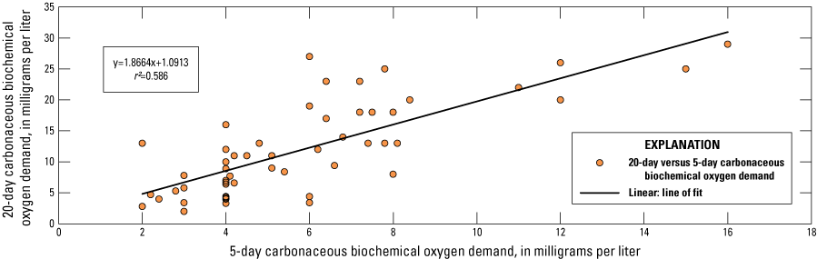
Graphs showing simple linear regression to estimate the relation between the 5-day (CBOD5) and the 20-day (CBODu) carbonaceous biochemical oxygen demand (CBOD) concentrations from Irondequoit Creek in western New York. r2, coefficient of determination.
Model Simulation of Nutrient Concentrations
As indicated earlier in this report, the nutrient simulations in the HEC–RAS NSM I module require boundary conditions to be input for the following parameters: water temperature, DO, algae, CBOD, organic nitrogen, ammonium, nitrate, nitrite, organic phosphorus, and inorganic phosphorus. Although these boundary conditions were required to run the simulations, the target for model calibration, discussed later in this report, was phosphorus. The water-quality data file is used to specify all the user-entered data for the nutrient and temperature model, including water-quality cell sizes and related options, nutrient boundary conditions, model initial conditions, dispersion coefficients, meteorology datasets, model nutrient parameters, and observed data points (discrete and continuous). Model simulation options for water-quality provide mechanisms to control aspects of the water-quality analysis and simulation. Many of these items have been described succinctly in the “Development of Water Temperature Model” report section and will be discussed in more detail within the “Nutrient Model Parameters” report section.
Initial Model Conditions
Like setting initial flow conditions for the unsteady flow hydraulic simulation, the nutrient model required a breakdown of preexisting water temperatures and nutrient concentrations in the study reach for model start up. Initial conditions for water temperature and nutrients are entered into specific cross sections (river stations), and the nutrient model interpolates across all water-quality cells using the parameterized cross sections. Ten locations were selected for loading initial model conditions primarily based on data availability. Three of these locations correspond to HRECOS stations with recorded water temperature and DO, and the seven other locations correspond to discrete sample locations along the main stem of the Mohawk River.
Initial water temperatures were populated, in part, using values obtained from the temperature traces on May 1, 2016, at the three HRECOS monitoring stations at Mohawk River at Ilion, Mohawk River at Lock 8, and Mohawk River at Rexford Bridge, N.Y., for their respective cross sections. At the remaining 7 locations, the closest available HRECOS water temperature was used to define the initial water temperature. The internal model routine interpolates, if necessary, between these river stations to populate all water-quality cells at the beginning of a run.
Initial values for nutrient concentrations were determined differently. Discrete water-quality samples from the preceding month and around the model startup period in May, 2016 were used. A generalized assumption that samples taken earlier and later than the actual startup time of the model on May 1, 2016, were representative of conditions in the Mohawk at the startup time was necessary. Because no other sample data were available for this period, this assumption was considered the most appropriate approach. Discrete samples used to estimate the initial nutrient values for May 1, 2016, range in date from April 11 through May 9, 2016, corresponding to the dates when the samples were collected. Importantly, once the model simulation begins, any imbalance caused by potential bias from the initial values is typically not a concern because, after several days of simulation, the results are representative of the actual simulation parameters and data. Simulation results for the first 2 weeks of May were considered part of the model “start-up” period and were not considered during calibration and validation for these reasons.
Water-Quality Cell Size and Dispersion Coefficients
Water-quality cell faces coincide with hydraulic model cross sections within RAS NSM I, although depending on the cell size, several cross sections may be contained within each water-quality cell. Selecting an appropriate water-quality cell size is critical within the nutrient model because misapplication of cell size will result in model instability, producing poor internal solutions or potentially not completing the simulation. Unlike the hydraulic simulation where the user selects the model time step, the water-quality model’s time step is dynamic throughout a model run and is directly related to water-quality cell size. In RAS NSM I, the cross-section face properties of the Courant and Peclet numbers can reduce or force a short duration computation time step if water-quality cell sizes are small (Zhang and Johnson, 2016). Thus, this capability will lead to possible instability or increased simulation times if water-quality cells are too small or small cells are interspersed with large cells, which is common around hydraulic structures because of typical close-proximity model cross-section spacing. For this study, the modeled minimum water-quality cell size was set to 1,000 feet, resulting in water-quality cell sizes ranging from 1,000 to 3,332 feet; no fixed cell faces were used. For reference, cross-section spacing for the hydraulic model ranges from approximately 28 to 2,332 feet with a median of approximately 240 feet.
Another aspect of setting up a water-quality data file within the NSM includes assigning dispersion coefficients for the modeled reach. Dispersion coefficients can be set to “fixed” and assigned by the user or can be set to “computed,” which calculates dispersion coefficients on-the-fly based on hydraulic variables across each water-quality cell face. This avoids possible instability when cross sections with a smaller water-quality cell face area and smaller dispersion coefficient are preceded by cells with large cell face areas and large dispersion coefficients (U.S. Army Corps of Engineers, 2016). Additional information on the equation RAS NSM I uses to compute this coefficient is in “Chapter 19: Water Quality Modeling” of the RAS NSM user manual (U.S. Army Corps of Engineers, 2016). For this study, “computed” was selected based in part on the assumption that selecting this option would help deal with the instability of pools behind hydraulic control structures. Limits placed on the computed dispersion coefficients were not set.
Nutrient Model Parameters
The nutrient model was calibrated in several stages. As discussed in previous sections of this report, parameters in the hydraulic model were adjusted to maximize their relationship to observed values taken from recording stations for streamflow and water-surface elevation. After the hydraulic model was calibrated, the temperature model was adjusted to fit observed values. Following these two steps, the next calibration phase involved adjusting parameters within the NSM to obtain an acceptable fit to observed continuous and discrete water-quality samples.
The HEC-RAS NSM I is a simplified aquatic eutrophication simulation that uses minimum state variables and streamlined processes (Zhang and Johnson, 2016). The schematic describing the parameterization and major processes involved in the water column of the NSM nutrient model is shown in figure 26. The state variables used to represent the nitrogen cycle are organic nitrogen, ammonium nitrogen, nitrite nitrogen, and nitrate nitrogen. The NSM models the phosphorus cycle using organic phosphorus and orthophosphate. The remaining state variables consist of algae, CBOD, and DO. The rate constants and several other parameters shown in figure 26 control the pathways between these variables. Table 28 details the final rate constants and parameter selection for the calibrated nutrient model for the Mohawk River. All constants and parameter values were maintained within the boundaries of literature values, and within the default range determined in the NSM. However, although rate constants and parameters for benthic algae could be altered, benthic algae as a state variable was not available within the version of NSM in HEC–RAS 5.0.3. Errata in Zhang and Johnson (2016) states that benthic algae is available as a separate state variable in NSM I, or it is only available in later versions of NSM I after HEC–RAS 5.0.3.
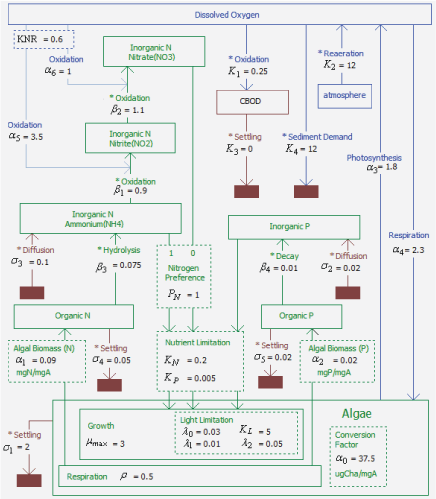
Schematic showing parameterization and processing steps for the nutrient simulation module version 1 (NSM I) taken from the Hydraulic Engineering Center River Analysis System (HEC–RAS) (U.S. Army Corps of Engineers, 2016).
Table 28.
Final nutrient modeling parameters used for the calibrated nutrient simulation module version 1 model for the study reach and suggested default range for parameter values.[NSM, nutrient simulation module; µg, microgram; mg, milligram; N/A, not applicable, m2, square meter; L, liter; >, greater than; m, meter; NH4, dissolved ammonium nitrogen; NO2, dissolved nitrite nitrogen; CBOD, carbonaceous biochemical oxygen demand; NO3, dissolved nitrate nitrogen]
Model Simulation
Initially, the nutrient model was intended to be run on the native 15-minute streamflow time step of the gaged inflows of the Mohawk River. However, HEC–RAS 5.0.3 only allows 10,000 ordinates to be entered within the lateral flow hydrograph window. This limitation required flow files to be broken down into the 5 individual months of the study from May–September 2016 with the intention to use model “restart” files generated at the end of each month’s simulation to begin the subsequent month’s simulation (U.S Army Corps of Engineers, 2016). An error was found in the program’s ability to successfully write the water-quality restart file at the end of a simulation. This necessitated changing all input data (hydraulic, temperature, and nutrient) to an hourly time step to fit the entire study period into one simulation.
Within the water-quality simulation, common simulation options were selected as follows. The “preserve conservation” option was selected for the resolution of hydrodynamic continuity error. This option is considered the most stable and resolves small continuity errors in water volume that result because of the hydraulic model and the water-quality model solving for continuity in different ways (U.S Army Corps of Engineers, 2016). The option for the ULTIMATE Limiter was left on, which filters oscillations and errors caused by advection issues within the water-quality simulation (U.S Army Corps of Engineers, 2016). As mentioned previously, the water-quality simulation time step varies and is related to water-quality cell size. The user can select a maximum allowable time step to ensure the computational time step does not extend beyond what is preferred. For the simulation in this study, the maximum allowable time step was set to 1 hour to match the intended output option of 1-hour even time intervals.
Calibration of Nutrient Model
One of the primary differences between calibrating the hydraulic and temperature models versus the nutrient model was how the models were evaluated for performance during calibration. The hydraulic model simulation flow and water-surface elevation values were compared against observed flow recorded at 4 continuous-record streamgages and against water-surface elevation values at 3 continuous-record streamgages along the Mohawk River. Similarly, simulated water temperature was able to be compared against water temperature from three continuous-record temperature stations along the Mohawk River. The nutrient model simulation data were compared to continuous-record dissolved oxygen (DO) data at the same stations where water temperature was collected along the Mohawk River and a series of discrete samples made at several sampling locations throughout the study reach. Figure 27 highlights the locations where discrete sampling was done and continuous-record water-quality data were collected. The discrete samples were analyzed for a variety of parameters, including the nitrogen and phosphorus species needed for calibrating a model simulation. The station names, number of available samples, and range of concentrations for total phosphorus are among the data presented in table 29 as examples of the quantity and measured range of phosphorus concentrations available for calibration validation.
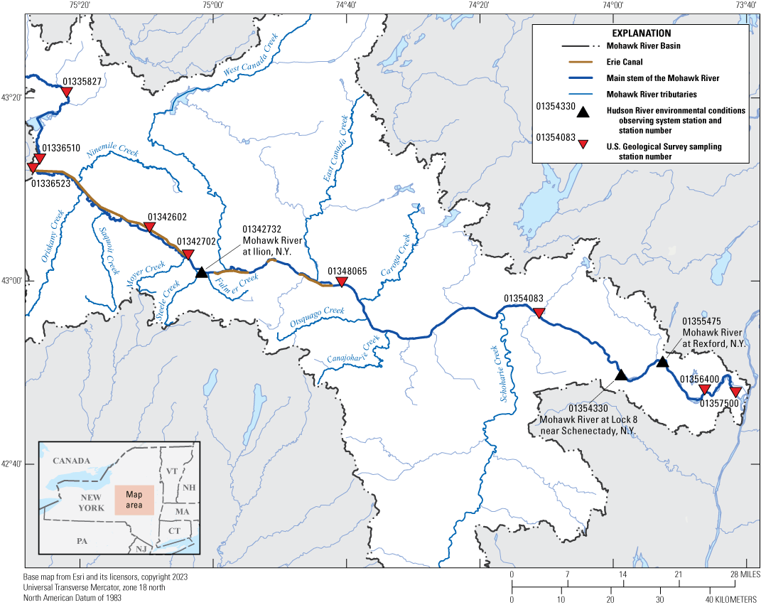
Map showing Hudson River Environmental Conditions Observing System (HRECOS) stations where continuous-record water-quality data (HRECOS, 2019) were collected and sites along the main-stem Mohawk River where discrete sample data were collected to be used to calibrate the nutrient model. N.Y., New York.
Table 29.
Summary of discrete sampling locations, number of available samples, dates of collection, and range of total phosphorus concentrations measured for the main stem of the Mohawk River, New York.[Data from U.S. Geological Survey (2022b). Dates shown as month/day/year. mg/L, milligram per liter; N.Y., New York; <, less than]
The RAS NSM model calibration was evaluated by comparing its simulated water-quality concentrations to observed data for DO at the HRECOS streamgages and discrete samples at other selected cross sections along the Mohawk River. The final values for the model rate constants and parameter variables are shown in table 23. These values were gradually adjusted from the model default values in an iterative process while attempting to balance oxygen concentration and competing nutrient concentrations at the cross sections with available data, with this process conceivably extending for an extensive period. Each model run generally took about 12 to 15 hours to complete and, after more than 60 tuning calibration runs and many others for early calibration adjustments, a balance to the available data was reached.
As discussed earlier, the only continuously recorded parameter available for model calibration during the study period that is closely related to the nutrification process other than water temperature was DO. Model simulated concentrations of DO were compared to the discrete sample data and the continuously recorded data. The averaged difference in concentration between the discrete samples and model simulated concentrations of DO at the six main-stem sampled locations (Rome, Utica, Frankfort, St. Johnsville, Amsterdam, and Latham) provided reasonable results. The average difference of all DO sample concentrations at all locations and times compared to the simulated concentrations for the same locations and times was −0.025 mg/L. The average difference per cross section between discrete sample concentrations and simulated concentrations for the time the samples were collected ranged from −1.04 mg/L at Amsterdam to 0.898 mg/L at St. Johnsville. The absolute value of the difference was about 0.53 mg/L. Although this seems like a reasonable difference, it should be restated that the samples are collected monthly and a few outliers within the discrete sample dataset might explain why the model and samples do not align. For example, at Frankfort, the May and August sample data agree well with the continuous simulated data, but the June and July discrete sample concentrations are 1 to about 1.5 mg/L lower than the simulated concentrations. The simulated results could not be reduced for this period by adjusting global variables without affecting other parts of the simulation period and other water-quality parameters. We assumed a lack of input data needed to define the physical processes in this reach for these periods was causing the model to not simulate enough reduction in DO. Comparisons between observed and simulated DO at the St. Johnsville sampling location showed similar results. Conversely, at the Amsterdam location, the relationship changes; May, July, and August sample data demonstrate a reasonable fit to the simulated data. However, in June, the discrete sample concentration value at Amsterdam is more than 3 mg/L higher than the concurrent simulated concentration value of 11.8 mg/L. This may be related to a local condition caused by aeration from gate operations at the lock just upstream from the sampling location, which the model would not be expected to reproduce, or it may also be influenced by being downstream from Schoharie and North Chuctanunda Creek. Farther downstream at Latham, the relation between discrete and simulated concentrations of DO tracks more closely for all sampled months. The Latham sampling location is downstream from movable gate structures used to control pool elevation along the Mohawk River upstream from Crescent Dam, which may help explain a more consistent relation between the monthly DO sample concentrations and the simulated DO concentrations. The simulated DO concentrations were also compared to hourly DO concentration readings from the HRECOS continuous water-quality monitors at the three HRECOS locations along the Mohawk River.
The continuous hourly HRECOS DO data were useful for understanding how DO conditions within the river are changing between the coarse discrete monthly samples. The comparison between HRECOS DO data and the data collected from discrete monthly samples provide more information about how the model responds to changing conditions in the river system and provides some insight about the inherent limitations created by a coarse calibration dataset and how well variability of the discrete samples is simulated. The comparison shows a generally good agreement between the model simulation of changes and the recorded HRECOS data. The recorded data are more varied or somewhat “noisy” during the modeled period, whereas the model changes are more gradual, potentially attributed in part to modeling changes to the entire cross section compared to HRECOS sensor location. The graphical comparison of the data from Mohawk River at Ilion shows the simulated data generally balancing the variability of the recorded data in May and then a constant difference of about 1 mg/L. Downstream at Mohawk River at Lock 8 the simulated data are slightly low from May into June and gradually transition to a fair balance and then slightly higher concentrations through the end of the modeling period. One noted deviation is the simulation not reproducing a large increasing spike in DO in late June and a notable drop in DO during late July and early August before recovering to a more normal pattern. It was assumed there were undocumented conditions affecting local conditions recorded by the HRECOS sondes, but without associated data to inform the model simulation it is understandable the simulated data did not match these events. A series of three sub-reach comparisons of the recorded DO readings from the HRECOS streamgages to simulated DO concentrations and discrete sample concentrations from the next closest sampling location are shown in figure 28 to help illustrate the variability described above.
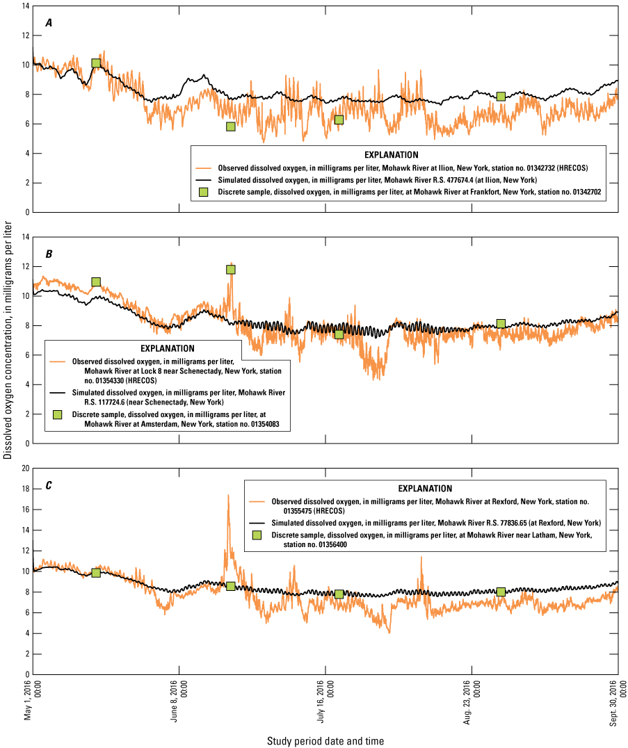
Plots of simulated and observed dissolved oxygen concentrations and dissolved oxygen concentrations from discrete samples (U.S. Geological Survey, 2019) taken at a nearby location downstream. A, concentrations for Ilion and discrete samples at Frankfort; B, concentrations for Lock 8 and discrete samples at Amsterdam; and C, concentrations for Rexford and discrete samples at Latham. no., number; HRECOS, Hudson River Environmental Conditions Observing System; R.S., river station; Aug., August; Sept., September.
The goal of the DO calibration was to facilitate the primary objective of optimizing the simulation of phosphorus concentrations because DO can be correlated with nutrient concentrations in the river reach. As indicated earlier, a dense set of nitrogen and phosphorus sample concentrations was not available as calibration checks for simulated concentrations. The calibration of phosphorus (and the nitrogen species) was checked against once monthly samples at six locations along the main stem of the Mohawk River. The averaged difference of simulated to observed concentration by location for all samples during the modeling period ranged from about −0.174 to 0.150 mg/L for organic phosphorus. The averaged difference was smallest at the Rome, Frankfort, St. Johnsville, and Amsterdam locations with differences from −0.012 to 0.068 mg/L. The Latham location showed the highest differences with an average difference of 0.150 mg/L. When evaluated, the simulated orthophosphate concentrations showed similar results as the concentrations of orthophosphate at the observed locations overall, but the locations with the largest differences in orthophosphate were not consistent with the locations that showed the largest differences in organic phosphorus. The differences in simulated to observed orthophosphate concentrations ranged from −0.245 mg/L to 0.151 mg/L. The average difference for all samples at the Frankfort, St. Johnsville, and Amsterdam locations showed good overall consistency through this reach with computed differences of 0.141, 0.151, and 0.128 mg/L, respectively. The Rome location showed the largest average difference for all samples at −0.245 mg/L, and the tightest fit for all samples was at the Latham location with an overall difference of 0.060 mg/L.
Comparison between simulated and observed monthly sample concentrations showed a reasonable fit—most locations had differences of about 0.15 mg/L or less, although a few exceeded that limit. However, the overall complexity of the system is better understood by looking at a graphic showing the simulated daily concentrations of organic phosphorus and orthophosphate throughout the modeled period. The variability in concentrations is driven by multiple factors. Hydrologic events, point-source discharges, non-point-source pollution, and regulation actions affect flow and water-surface elevations and influence the spikes, dips, and short-term patterns. Figure 29 shows the variability of simulated organic phosphorus and orthophosphate concentrations during the modeling period. At times, concentrations of organic phosphorus can spike over 0.3 mg/L at Utica and Little Falls and about 0.5 mg/L at Amsterdam. Concentrations of orthophosphate at Utica were generally below 0.3 mg/L, but spikes over 0.4 mg/L were simulated in three months of the simulation period. Further downstream at Little Falls and Amsterdam, the spikes were not as pronounced, and simulated concentrations were generally below 0.2 mg/L. As noted earlier, once monthly calibration data and a review of simulated variability in phosphorus concentrations seem to highlight the need for higher fidelity calibration data to further verify and potentially improve model performance. However, simulating exact observed concentrations is not necessarily the most important outcome. The general purpose of these models is to provide information about how conditions in the river might change by altering treatment methods in use for the study period for point-source pollutants. Reviewing the differences between simulated and observed concentrations over the model study period provides an opportunity to see if selected point-source reduction scenarios cause change if they are implemented. Utilizing the average change approach, the calibrated model was used to test several point-source pollution reduction scenarios by comparing the simulated water-quality conditions (phosphorus concentration) to conditions that would prevail if the nutrient concentrations of selected point-source dischargers were reduced or altered because of improved treatment methods. This approach allows scientists and State officials to simulate the potential improvements in water-quality conditions along the Mohawk River before prioritizing specific point-source improvements in pollution reduction technology.
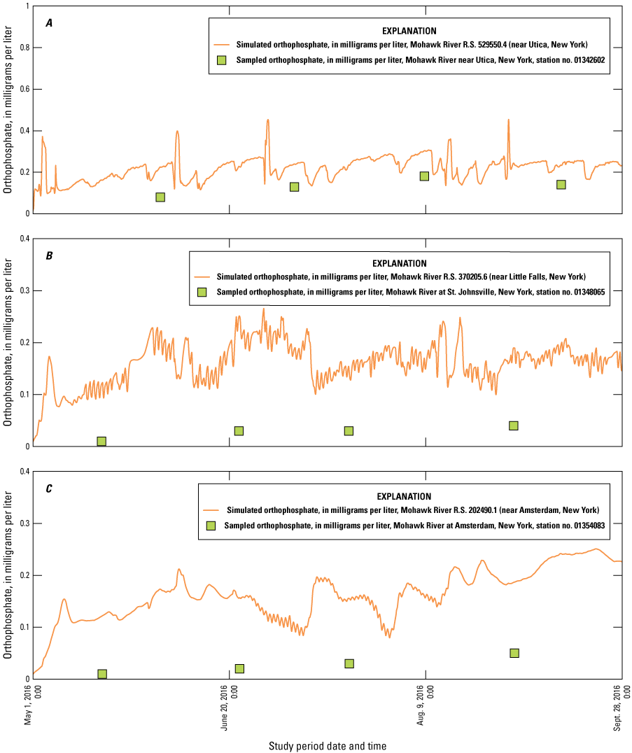
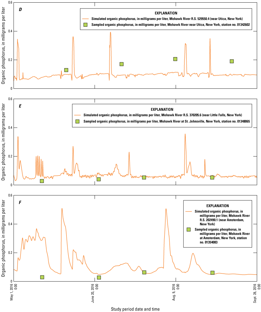
Plots of simulated orthophosphate and organic phosphorus concentrations and observed concentrations from monthly discrete samples (U.S. Geological Survey, 2019) collected at the nearest location downstream for: A, orthophosphate at Utica; B, orthophosphate at Little Falls; C, orthophosphate at Amsterdam; D, organic phosphorus at Utica; E, organic phosphorus at Little Falls; and F, organic phosphorus at Amsterdam, New York. R.S., river station; no., number; Aug., August; Sept., September.
Wastewater Treatment Plant Phosphorus Scenario Results
The Mohawk River is a complex and dynamic river system. Understanding the connection between potential changes in water-quality conditions and upgrades to one or more selected WWTPs (point-source discharges) is not simple. The calibrated hydraulic, water temperature, and nutrient model package was used to evaluate the potential improvements in water-quality conditions along the Mohawk River if selected point-source nutrient reduction scenarios were implemented. The USGS and the NYSDEC worked together to identify nine different point-source nutrient reduction scenarios that ranged from those assumed to be more practical and cost effective to implement to those requiring more extensive technology improvements and higher funding investments. The framework for this model included 14 WWTP facilities, as indicated earlier, most of which only use primary treatment trains for nitrogen and phosphorus. The nutrient reduction scenarios selected by the NYDEC were based primarily on designated facility size and proximity to the mouth of the Mohawk River near Cohoes, N.Y. Table 30 and accompanying figure 30 highlight the changes used within the nutrient model for each WWTP facility and each scenario. After scenario criteria within the nutrient model were implemented, the USGS and NYDEC selected five locations along the Mohawk River to compare scenario simulation results with the calibrated model results. The locations were selected based on alignment with municipal water withdrawals and features within the river, such as proximity to confluences with tributaries. These locations are shown in figure 30, along with changes in phosphorus concentrations at each location generated from the calibrated model. Tables 31 and 32 highlight monthly mean organic phosphorus and orthophosphate reductions from scenarios.
Table 30.
Wastewater treatment facilities, approximate facility size designation, relative distance from Cohoes, New York, and total phosphorus contributions implemented for each wastewater treatment plant scenario.[0.50 milligrams per liter (mg/L)=79-percent reduction in total phosphorus output, shown in green; 1 mg/L=68-percent reduction in total phosphorus output, shown in yellow; 2.38 mg/L=no reduction in total phosphorus output, shown in red. N.Y., New York; mg/L, milligram per liter; =, equal; %, percent; WPCP, water pollution control plant; WWTP, wastewater treatment plant; SD, sanitary district; no., number; STP, sewage treatment plant]
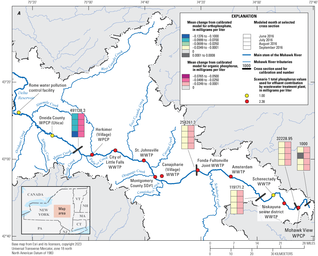
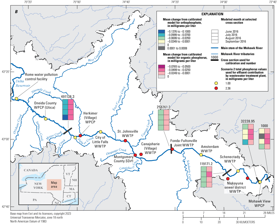
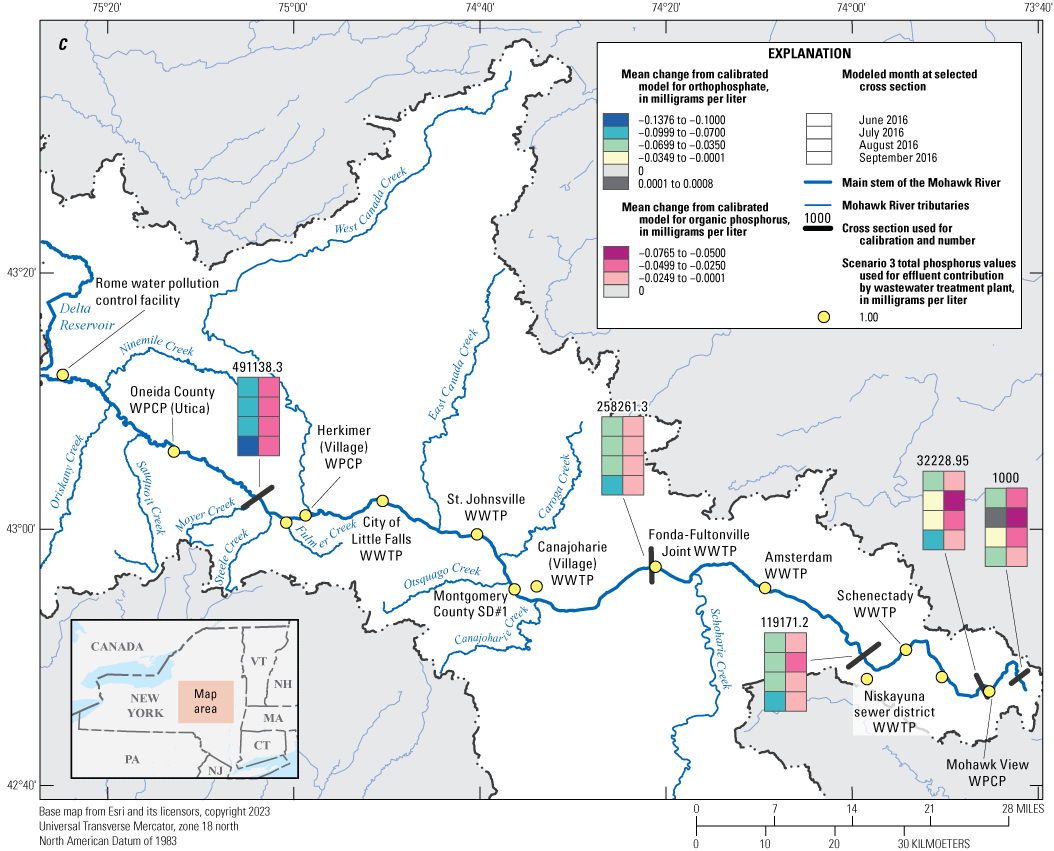
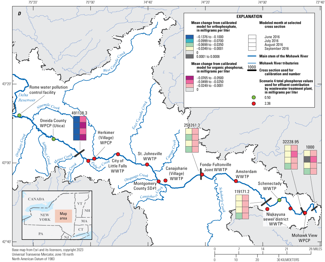
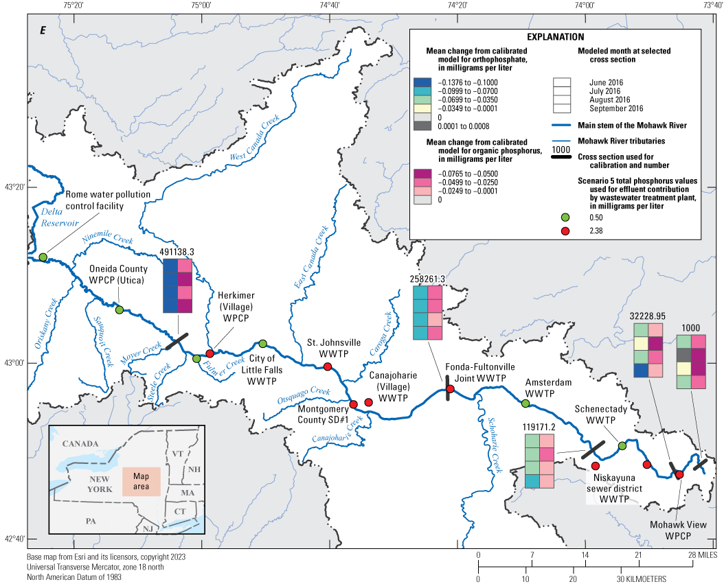
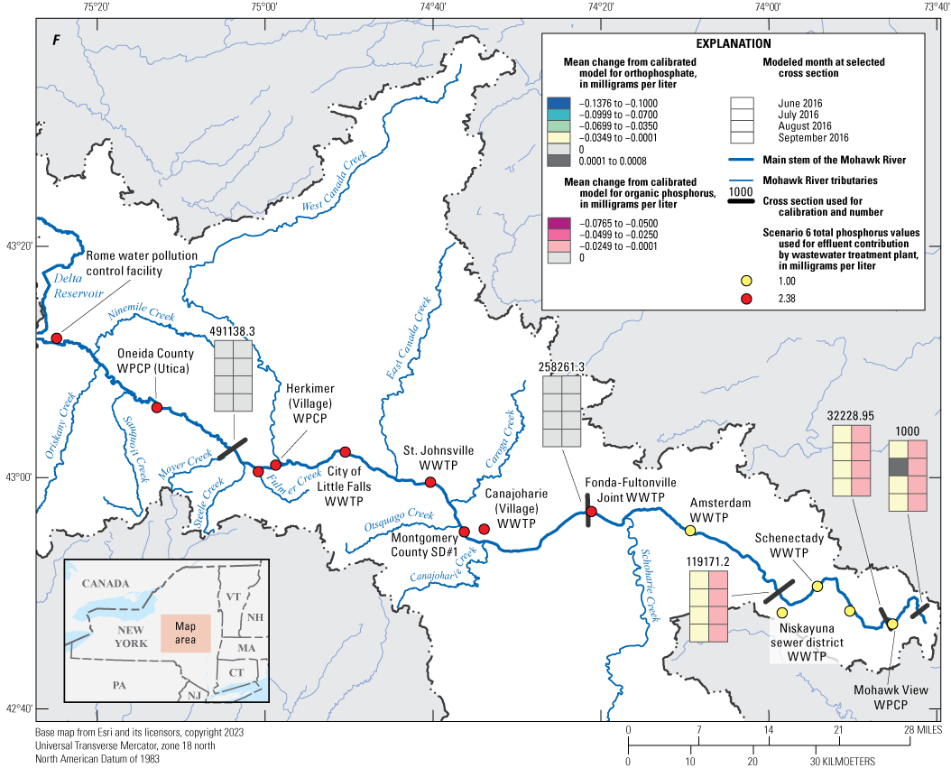
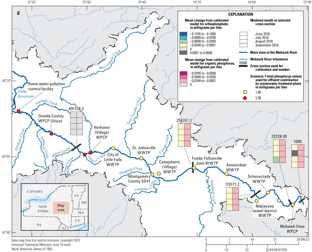

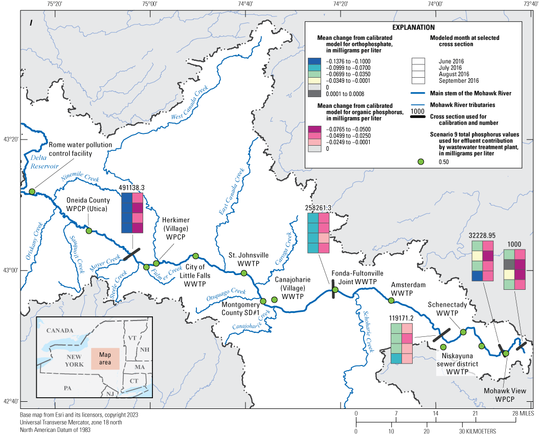
Map displaying total phosphorus values for wastewater treatment plants in nine simulated phosphorus reduction scenarios and corresponding changes in organic phosphorus and orthophosphate concentrations from the calibrated models for each scenario along the Mohawk River with model cross section noted. WPCP, water pollution control plant; WWTP, wastewater treatment plant; SD#1, sanitary district number 1.
Scenarios 1 and 4 simulated phosphorus reductions at the three large phosphorus contributing facilities in the study reach, whereas scenarios 2 and 5 simulate reductions at both the large and medium facilities. Notably, model simulation results at comparison stations showing no change from the calibrated model have no adjustments to WWTP concentrations upstream from these comparison stations. Moving farther downstream, differences between scenario simulation results and calibrated simulation results realized from scenarios 1 and 4 from the large Rome and Utica facilities have largely attenuated at comparison station 119,171.2. These differences immediately increased downstream from the large Schenectady facility, reflecting this facility’s overall high phosphorus contributions to the system. When the medium and large facilities were included in the reductions, as in scenarios 2 and 5, the differences between calibrated and scenario-based phosphorus concentrations within the system were more spatially consistent.
Scenarios 6 and 8 simulated conditions if facilities at locations nearest to Cohoes implemented phosphorus reductions, whereas scenario 7 demonstrates reductions at plants in the middle and downstream parts of the reach. Changes in simulated phosphorus concentrations were not realized until comparison station 119,171.2 for scenarios 6 and 8 and show a predictable reduction response for both adjustments to the WWTP concentrations. Scenario 7, which increases the spatial scope of reductions to the middle basin WWTPs, only reduced Mohawk River phosphorus concentrations marginally beyond what was achieved by scenarios 6 and 8. This is likely because most of the plants in this area were small (excluding Little Falls-medium) and had small effluent flow contributions.
Lastly, scenarios 3 and 9 implemented reductions across all facilities and had correspondingly larger reductions in simulated phosphorus levels that were spatially consistent with the calibrated model. Scenario 3 implemented a reduction from the total phosphorus value of 2.38 mg/L to 1.00 mg/L and scenario 9 implemented a reduction from 2.38 mg/L to 0.50 mg/L for all contributing WWTPs.
Table 31.
Monthly mean change in simulated organic phosphorus concentrations between the calibrated nutrient model and nine nutrient reduction scenarios at five selected locations along the Mohawk River, New York.[ft, foot; mg/L, milligram per liter]
Table 32.
Monthly mean change in simulated orthophosphate concentrations between the calibrated nutrient model and nine nutrient reduction scenarios at five selected locations along the Mohawk River.[ft, feet; mg/L, milligram per liter]
Summary
The Mohawk River is the largest tributary to the Hudson River and flows about 140 miles from its headwaters in the Adirondack Mountains to its mouth near Cohoes, New York. The watershed of the Mohawk River drains about 3,460 square miles, including a large inflow from Schoharie Creek, which flows north from the Catskill Mountains. The waters of the Mohawk River are used for recreation, agriculture, industry, water supply, and aquatic life. The New York State (NYS) Department of Environmental Conservation uses a watershed-based approach to outline and implement plans to protect and improve water-quality conditions and has been building an action agenda to protect and restore the Mohawk River and contributing watersheds. To better understand the influence of point and non-point-source pollution on the in-channel water-quality conditions of the Mohawk River, a nutrient water-quality model was developed. The nutrient water-quality model was dynamically linked to a hydraulic and water temperature model to provide the necessary information about flow, velocity, and temperature to properly simulate the nutrient growth and decay processes. The U.S. Army Corps of Engineers Hydraulic Engineering Center River Analysis System (HEC–RAS) was used to model the river and its complex hydraulic structures, and the HEC–RAS Nutrient Simulation Module version I was used to generate water temperature and nutrient simulations. These models are dynamically linked within HEC–RAS, which optimized the efficiency of data transfer between each model. The models were developed for the main channel reach from Rome to Cohoes, N.Y. The model includes inputs from 10 gaged and 35 ungaged tributaries and 12 wastewater treatment plants (WWTPs) discharging directly into the Mohawk River. The simulation period was from May 1 to September 30, 2016, but the first week of May was reserved as the model start up and equalization period. This period was not formally referenced in terms of performance or calibration.
The geometry of the HEC–RAS hydraulic model was constructed from several preexisting models completed within HEC–RAS or Danish Hydrologic Institute MIKE 11 modeling software that were sourced from Federal Emergency Management Agency flood studies and the NYS Canal Corporation operational flood model. Existing model was evaluated, edited to optimize for in-channel flows necessary for the water temperature and nutrient models, and merged to construct a main-stem model reach for the Mohawk River. Model geometry data consisted of approximately 2,900 preexisting or model-interpolated cross sections at approximately 250-foot (ft) intervals. Additionally, 38 bridges and 17 fixed or gated inline structures, including dams and weirs, were implemented within the study reach. Hydraulic structure data were taken from source models, where available, or reconstructed within the model using the best available data. Data on gate positions and operations were provided by NYS Canal corporation. For some features, such as the flashboards for Vischer Ferry Dam, logical assumptions for these “gates” were necessary, and an iterative process was used to determine placement and the timing of removal and replacement. Energy-loss factors quantified by Manning’s roughness coefficients from the source hydraulic models were reviewed and applied to the completed main-stem model. These energy-loss factor values were compared against published values from similar streams in New York State and determined to be suitable and representative of actual channel conditions.
Streamflow inputs into the HEC–RAS hydraulic model included observed hourly data from 10 U.S. Geological Survey (USGS) streamgages and estimated hydrographs from 35 ungaged tributaries entering the Mohawk River within the study reach. Hydrographs for two gaged tributaries, Canajoharie and Schoharie Creeks, were adjusted to compensate for additional drainage area between the streamgages’ locations and their confluence with the Mohawk River. Hydrographs for ungaged tributaries were synthesized using reference streamgage hydrographs from 1 of the 10 gaged tributaries and proportionally adjusted based on drainage area differences. Three additional hydrographs were included within the hydraulic model to represent additional flow exchange between certain sections of the Erie Canal and the Mohawk River, where overflow spillways between the river and the canal were adjacent to tributary confluences with the canal. Flows from 12 WWTPs distributed throughout the reach discharging directly into the Mohawk River were also added to the model. The flow numbers were generally on a daily time step and were taken from daily mean effluent flows noted on discharge monitoring reports.
The final model simulation was run under an unsteady/hydrodynamic flow regime using HEC–RAS version 5.0.3 with the computation interval set to 30 seconds and output generated hourly. Simulated streamflow data from the model were evaluated against observed, published streamflow data from four USGS streamgages along the Mohawk River main stem: the Mohawk River near Utica (station number (no.) 01342602), -near Little Falls (station no. 01347000), -at Freemans Bridge near Schenectady (station no. 01354500), and -at Cohoes (station no. 01357500). All flow data were evaluated on a daily time step. Statistical parameters of coefficient of determination (r2), mean absolute error (MAE), and percent bias were used to evaluate the flows. Agreement between simulated and observed flows for the study period was considered good, and r2 values fell between 0.91 and 0.97 for the four comparison stations. MAE ranged from 15.5 to 20.2 percent and generally increased moving downstream. This was attributed to small aggregate timing and flow differences accumulating in the downstream part of the reach. Percent bias for the study period ranged from −7.2 to 16.4 percent, and the least bias was at the Cohoes streamgage location. Total flow volumes for the study period were also evaluated and closely tracked, and the percent bias noted for the four comparison stations. Total simulated flow volumes at Cohoes were within 2 percent of the observed streamgage volumes. Stream stage, or elevation, was also evaluated between simulated values and observed values at Mohawk River near Utica, -near Little Falls, and -at Freemans Bridge near Schenectady. Cohoes was unable to be used for this evaluation method because the pool for the Cohoes gaging station was just beyond the downstream limits of the model. The root mean square error (RMSE) between simulated and observed stage values for the study period was 0.18 and 0.21 ft for the streamgages at Utica and Little Falls, respectively. The RMSE of 0.96 ft at Schenectady for the study period reflected the general uncertainty in flashboard assumptions made at the Vischer Ferry dam. The mean error (for the study period) for stage values at the three comparison locations was −0.04 ft, 0.11 ft, and 0.00 ft for the streamgages at Utica, Little Falls, and Schenectady, respectively. Sensitivity analyses done on the hydraulic model for roughness coefficients and estimated tributary inflows indicated that the hydraulic model responded linearly and as expected when the values for either of these parameters were adjusted. The model did not prove to be overly sensitive to adjustment of estimated tributary inflows or roughness coefficients.
The water temperature model simulated hourly water temperatures, but the results were evaluated at a daily, monthly, and seasonal time step. Continuous water temperature data recorded by the Hudson River Environmental Conditions Observing System (HRECOS) along the Mohawk River were used to evaluate the calibration of the water temperature model. These data were not included as inputs or boundary conditions and were only used to evaluate the performance of simulated temperatures compared to observed temperatures. The recorded temperature at the Ilion, Lock 8, and Rexford Bridge HRECOS stations ranged from about 12 to 28 °Celsius (°C). The MAE in daily water temperature averaged to about 0.90 °Celsius for the Ilion and Lock 8 streamgages, and the RMSEs were 1.06 and 1.00 °Celsius, respectively. The MAE for Rexford bridge was 0.87 °Celsius with a RMSE of 1.07 °Celsius. The simulated water temperature data were considered a good fit to the observed, and generally remained within 1 °Celsius of the recorded values. Graphically, the simulated water temperature data showed a slight trend by remaining below the recorded readings from the July and August periods. Additional comparisons were made between simulated water temperature readings and the discrete water temperature readings taken during water-quality sample collection in June through September. This comparison showed the simulated water temperatures generally matched the recorded water temperatures to within 1 to 2 °Celsius.
The nutrient simulation model received flow and temperature inputs directly from the other models, but separate nutrient boundary conditions and state variable settings were used to control the chemical and biological processes. The model uses a simplified aquatic eutrophication simulation with a state variable to represent the nitrogen and phosphorus cycles. The nitrogen cycle species included in the model are organic nitrogen, ammonium nitrogen, nitrite nitrogen, and nitrate nitrogen. The phosphorus cycle is simulated using organic phosphorus and orthophosphate. The remaining state variables consist of algae, carbonaceous biochemical oxygen demand, and dissolved oxygen (DO). Several rate constants and other parameters are used to control the simulation. The targeted nutrient parameter for this study was phosphorus, although other parameters were considered in the process. Continuous data or high-density discrete nutrient samples were not available for this calibration. The hydraulic and water temperature model simulations had the benefit of being able to be compared to continuously observed data to evaluate the calibration. Nutrient data from along the main stem of the Mohawk River and some selected tributaries were generally limited to once monthly samples taken during the simulation period. Continuous data for DO were available at three HRECOS locations in the simulation reach and were used to help evaluate the performance of the nutrient simulation. Because of the lack of large, discrete nutrient datasets and the close connection between DO and nutrient concentrations in rivers and streams, DO data from the HRECOS locations were determined to be a reasonable proxy to help evaluate nutrient simulation results.
The simulated concentrations of DO were compared to discrete samples and the continuously recorded data. The averaged difference in concentration between the discrete sample concentrations and the simulated concentrations of DO at the six main-stem sampled locations (Rome, Utica, Frankfort, St. Johnsville, Amsterdam, and Latham) was −0.025 milligrams per liter (mg/L). The average difference per cross section between the discrete sample concentration and those simulated during the same time step ranged from −1.04 mg/L at Amsterdam to 0.898 mg/L at St. Johnsville. The comparison between continuously observed HRECOS DO data and the simulation DO data generally showed a good agreement. The observed data showed more variability during the study period, whereas the simulated data, for the same period, displayed more gradual changes, potentially attributable, in part, to differences between simulating average conditions in the cross section compared to HRECOS sensor location point data. Although DO can be correlated with concentrations of nutrients in the river, the primary objective of the nutrient model was to simulate phosphorus concentrations. The nutrient model simulated concentrations of orthophosphate and organic phosphorus. The averaged differences between simulated and observed concentrations by location for all samples of orthophosphate ranged from −0.245 mg/L to 0.06 mg/L. The average difference for concentrations of orthophosphate at the Frankfort, St. Johnsville, and Amsterdam locations showed good overall consistency, all near 0.15 mg/L. The averaged differences of simulated to observed concentrations of organic phosphorus by location for all samples ranged from about −0.174 to 0.150 mg/L. The average differences of organic phosphorus were smallest at the Rome, Frankfort, St. Johnsville, and Amsterdam locations—differences ranged from −0.012 to 0.068 mg/L. Although measuring the exact differences between the sample concentrations and the simulation concentrations is important, the exact differences may be less meaningful than when the model is used to simulate point-source pollution reduction scenarios. Scenario testing provides an opportunity to simulate potential improvements to water-quality conditions to help prioritize wastewater treatment upgrades.
The USGS and the New York State Department of Environmental Conservation identified nine different point-source nutrient reduction scenarios to implement with a calibrated HEC–RAS Nutrient Simulation Module model. The nutrient reduction scenarios were implemented across 12 WWTP facilities, and scenarios were based primarily on designated facility size and proximity to the mouth of the Mohawk River near Cohoes, N.Y. WWTP input phosphorus concentrations from the calibrated model were reduced to 1.00 mg/L or 0.50 mg/L, reflecting potential technology improvements at WWTPs. Scenario simulation results were compared to calibrated simulation results at five selected locations along the Mohawk River. Results were generally linear and predictable, and scenarios that implemented the highest reductions showed correspondingly larger differences in concentrations downstream from the WWTPs associated with those reductions. The highest monthly mean differences were from scenario 9, which reduced total phosphorus concentrations in WWTP effluent to 0.50 mg/L for all contributing plants within the model; resulting changes in simulated concentrations ranged from −0.018 to −0.076 mg/L for organic phosphorus and from 0.001 to −0.138 mg/L for orthophosphate, month and comparison station dependent.
References Cited
Ator, S.W., 2019a, Spatially referenced models of streamflow and nitrogen, phosphorus, and suspended-sediment loads in streams of the northeastern United States: U.S. Geological Survey Scientific Investigations Report 2019–5118, 57 p., accessed May 6, 2022, at https://doi.org/10.3133/sir20195118.
Ator, S.W., 2019b, SPARROW model inputs and simulated streamflow, nutrient and suspended-sediment loads in streams of the Northeastern United States, 2012 Base Year: U.S. Geological Survey data release, accessed May 6, 2022, at https://doi.org/10.5066/P9NKNVQO.
Brotzge, J.A., Wang, J., Thorncroft, C.D., Joseph, E., Bain, N., Bassill, N., Farruggio, N., Freedman, J.M., Hemker, K., Jr., Johnston, D., Kane, E., McKim, S., Miller, S.D., Minder, J.R., Naple, P., Perez, S., Schwab, J.J., Schwab, M.J., and Sicker, J., 2020, A technical overview of the New York State Mesonet standard network: Journal of Atmospheric and Oceanic Technology, v. 37, no. 10, p. 1827–1845. [Also available at https://journals.ametsoc.org/view/journals/atot/37/10/jtech-d-19-0220.1.xml.]
Bergmann Associates, 2012, Hydraulic assessment report—Mohawk River portion of the Erie Canal between lock E–7 and Montgomery/Herkimer County Line, Schenectady and Montgomery Counties, NY: hydraulic model and accompanying report. Limited access to unpublished data available by contacting New York State Canal Corporation, Albany, New York.
Chen, G., and Fang, X., 2015, Accuracy of hourly water temperature in rivers calculated from air temperatures: Water, v. 7, no. 3, p. 1068–1087. [Also available at https://www.researchgate.net/publication/276839773_Accuracy_of_Hourly_Water_Temperatures_in_Rivers_Calculated_from_Air_Temperatures.]
Chesapeake Bay Program, 2010, Chesapeake assessment scenario tool—The 2010 Chesapeake Bay TMDL for nitrogen, phosphorus and sediment allocations for the Bay: Chesapeake Bay Program Office web page, accessed September 12, 2019, at https://cast.chesapeakebay.net/Home/TMDLTracking#tributaryRptsSection.
Danish Hydraulic Institute (DHI), 2017, MIKE-11—River and channel modelling—Short introduction – Tutorial: accessed January 24, 2024, at https://manuals.mikepoweredbydhi.help/2017/Water_Resources/MIKE_11_Short_Introduction-Tutorial.pdf#:~:text=MIKE%2011%2C%20developed%20by%20DHI%2C%20is %20a%20software,estuaries%2C%20rivers%2C%20irrigation%20channels%20and%20other%20water%20bodies.
de Wit, C.T., 1978, Simulation of assimilation, respiration, and transpiration of crops: Wageningen, The Netherlands, Pudoc, 148 p. [Also available at https://edepot.wur.nl/167486.]
Erie Canalway, 2023, New York’s canal system is famous for its engineering: Erie Canalway National Heritage Corridor, accessed Oct 3, 2023, at https://eriecanalway.org/explore/locks.
Federal Emergency Management Agency, 2013, Flood insurance study—Oneida County, New York, (All jurisdictions): Washington, D.C., Flood Insurance Study Number 39169CV000A, 91 p. [Also available at https://map1.msc.fema.gov/data/36/S/PDF/36065CV002A.pdf?LOC=f5fd163dec0399e8f1c8be3e6256d567.]
Hirsch, R.M., Moyer, D.L., Archfield, S.A., 2010, Weighted regression on time, discharge, and season (WRTDS), with an application to Chesapeake Bay River inputs: Journal of the American Water Resources Association: v. 46, no. 5, p. 857–880. [Also available at https://onlinelibrary.wiley.com/doi/epdf/10.1111/j.1752-1688.2010.00482.x.]
Hudson River Environmental Conditions Observing System (HRECOS), 2019, 2016 historic data: Hudson River Environmental Conditions Observing System web page, accessed June 21, 2019, at https://hrecos.org/track-conditions/#historic.
Leonard, B.P., 1991, The ULTIMATE conservative difference scheme applied to unsteady one–dimensional advection: Computer Methods in Applied Mechanics and Engineering, v. 88, no. 1, p. 17–74, accessed March 7, 2023, at https://doi.org/10.1016/0045-7825(91)90232-U.
Line, D.E., White, N.M., Osmond, D.L., Jennings, G.D., and Mojonnier, C.B., 2002, Pollutant export from various land uses in the Upper Neuse River Basin: Water Environment Research, v. 74, no. 1, p. 100–108. [Also available at https://www.jstor.org/stable/pdf/25045577.pdf.]
National Oceanic and Atmospheric Administration, 2019, Local climatological data station details [Albany International Airport, NY US, WBAN:14735]: National Centers for Environmental Information database, accessed June 21, 2019, at https://www.ncdc.noaa.gov/cdo-web/datasets/LCD/stations/WBAN:14735/detail.
New York State Canal Corporation, 2012, Flood Warning Operations System, Cross-sectional geometry from hydraulic model of Mohawk River: New York State Power Authority- Canal Corporation hydraulic model. Limited access to unpublished data available by contacting New York State Canal Corporation, Albany, New York.
New York State Canal Corporation, 2020, Bridge heights: New York State Canal Corporation web page, accessed March 4, 2020, at https://www.canals.ny.gov/boating/bridgeheights.html.
New York State Department of Environmental Conservation, 2015, Vision approach—To implement the Clean Water Act 303(d) program and clean water planning: New York State Department of Environmental Conservation, accessed May 7, 2022, at https://www.dec.ny.gov/docs/water_pdf/dowvision.pdf.
New York State Department of Environmental Conservation, 2016, Mohawk River Basin research initiative 2014–2016: New York State Department of Environmental Conservation, accessed October 18, 2023, at https://www.dec.ny.gov/docs/water_pdf/mohawkresearch.pdf.
New York State Department of Environmental Conservation, 2021, Mohawk River Basin action agenda—Conserving, preserving, and restoring the Mohawk River watershed: New York State Department of Environmental Conservation, accessed October 18, 2023, at https://www.dec.ny.gov/docs/water_pdf/mohawkrbaa2021.pdf.
New York State Department of Environmental Conservation, 2022a, Mohawk River watershed—Published water quality monitoring and assessment reports: New York State Department of Environmental Conservation, accessed May 7, 2022, at https://www.dec.ny.gov/lands/48041.html.
New York State Department of Environmental Conservation, 2022b, State pollutant discharge elimination system permit program: New York State Department of Environmental Conservation, accessed May 7, 2022, at https://www.dec.ny.gov/permits/6054.html.
New York State Mesonet, 2019, Request data: New York State Mesonet web page, accessed April 4, 2019, at http://www.nysmesonet.org/weather/requestdata.
New York State Mesonet, 2023, Station metadata: New York State Mesonet web page, accessed October 18, 2023, at http://www.nysmesonet.org/about/sites#network=nysm.
New York State Geographic Information Systems, [undated], 2 Meter digital elevation model: New York State Geographic Information Systems, accessed June 4, 2018, at https://gis.ny.gov/nys-dem.
Niemoczynski, M.J., Suro, T.P,., Boetsma, A.C., 2024, HEC-RAS hydraulic, temperature, and nutrient models for the Mohawk River between Rome and Cohoes, New York: U.S. Geological Survey data release, https://doi.org/10.5066/P9FRAYLT.
Pitt, R., Maestre, A., Morquecho, R., Brown, T., Schueler, T., Cappiella, K., Sturm, P., and Swann, C., 2004, Findings from the national stormwater quality database: University of Alabama, Department of Civil and Environmental Engineering and Center for Watershed Protection, 10 p. [Also available at https://chesapeakestormwater.net/wp-content/uploads/2022/07/3328-3.pdf.]
Qiu, Y., Shi, H-C., He, Miao, 2010, Nitrogen and phosphorous removal in municipal wastewater treatment plants in China—A review: International Journal of Chemical Engineering, 10 p. [Also available at https://www.hindawi.com/journals/ijce/2010/914159/.]
Reicosky, D.C., Winkelman, L.J., Baker, J.M., and Baker, D.G., 1989, Accuracy of hourly air temperatures calculated from daily minima and maxima: Agricultural and Forest Meteorology, v. 46, no. 3, p. 193–209, accessed December 17, 2019, at https://doi.org/10.1016/0168-1923(89)90064-6.
Runkel, R.L., Crawford, C.G., and Cohn, T.A., 2004, Load estimator (LOADEST)—A FORTRAN program for estimating constituent loads in streams and rivers: U.S. Geological Survey Techniques and Methods, book 4, chap. A5, 69 p. [Also available at https://doi.org/10.3133/tm4A5.]
Schwarz, G.E., Hoos, A.B., Alexander, R.B., and Smith, R.A., 2006, The SPARROW surface water-quality model—Theory, applications and user documentation: U.S. Geological Survey Techniques and Methods, book 6, chap. B3, 248 p., accessed May 6, 2022, at https://doi.org/10.3133/tm6B3.
State of New York Open Data, 2022, Water withdrawals by facility—Beginning 2009: State of New York Open Data, accessed December 29, 2022, at https://data.ny.gov/Energy-Environment/Water-Withdrawals-by-Facility-Beginning-2009/94ue-tysy/data.
U.S. Army Corps of Engineers, 2016, HEC–RAS River analysis system—User’s manual, version 5.0: Davis, Calif., U.S. Army Corps of Engineers Institute for Water Resources, Hydrologic Engineering Center, [variously paged]. [Also available at https://www.hec.usace.army.mil/software/hec-ras/documentation/HEC-RAS%205.0%20Users%20Manual.pdf.]
U.S. Department of Housing and Urban Development, 1979, Flood Insurance Study—Town of Colonie, New York, Albany County: Washington, D.C., U.S. Department of Housing and Urban Development, Federal Insurance Administration, 41 p., 23 pls. [Also available at https://catalog.hathitrust.org/Record/102199748.]
U.S. Environmental Protection Agency, 2008, Municipal nutrient removal technologies reference document: EPA 832-R-08-006, U.S. Environmental Protection Agency Office of Wastewater Management, Municipal Support Division, Technical Report v1.0, accessed April 10, 2019, at https://www.epa.gov/sites/default/files/2019-08/documents/municipal_nutrient_removal_technologies_vol_i.pdf.
U.S. Environmental Protection Agency, 2010, Chesapeake Bay phase 5.3 community watershed model: Annapolis Md., EPA 903S10002–CBP/TRS-303-10, U.S. Environmental Protection Agency, Chesapeake Bay Program Office, accessed April 10, 2019, at https://ches.communitymodeling.org/models/CBPhase5/documentation.php#p5modeldoc.
U.S. Environmental Protection Agency, 2019, ICIS-NPDES permit limit and discharge monitoring report dataset for New York jurisdiction, 2016: U.S. Environmental Protection Agency web page, accessed March 12, 2019, at https://echo.epa.gov/tools/data-downloads/icis-npdes-dmr-and-limit-data-set
U.S. Environmental Protection Agency, 2022, Summary of the Clean Water Act: U.S. Environmental Protection Agency web page, accessed January 4, 2022, at https://www.epa.gov/laws-regulations/summary-clean-water-act.
U.S. Geological Survey, 2018, Wastewater treatment water use: U.S. Geological Survey web page, accessed April 10, 2019, at https://www.usgs.gov/special-topics/water-science-school/science/wastewater-treatment-water-use.
U.S. Geological Survey, 2019, USGS water data for the nation: U.S. Geological Survey National Water Information System database, accessed April 10, 2019, at http://dx.doi.org/10.5066/F7P55KJN. [Water-quality data can be directly accessed at https://waterdata.usgs.gov/ny/nwis/qw.]
U.S. Geological Survey, 2022a, StreamStats: U.S. Geological Survey web page, accessed October 20, 2022, at https://streamstats.usgs.gov/ss/.
U.S. Geological Survey, 2022b, USGS water data for the nation: U.S. Geological Survey National Water Information System database, accessed January 4, 2022, at http://dx.doi.org/10.5066/F7P55KJN.
U.S. Geological Survey, 2022c, National Water Quality Assessment—Overview: U.S. Geological Survey web page, accessed January 4, 2022, at https://www.usgs.gov/mission-areas/water-resources/science/national-water-quality-assessment-nawqa#overview.
U.S. Geological Survey, 2022d, National water quality assessment (NAWQA): U.S. Geological Survey web page, accessed January 4, 2022, at https://www.usgs.gov/mission-areas/water-resources/science/national-water-quality-assessment-nawqa#publications.
Zhang, Z., and Johnson, B.E., 2016, Aquatic nutrient simulation modules (NSMs) developed for hydrologic and hydraulic models: Vicksburg, Miss., U.S. Army Corps of Engineers Engineer Research and Development Center, Environmental Laboratory, [variously paged]. [Also available at https://erdc-library.erdc.dren.mil/jspui/bitstream/11681/10112/1/ERDC-EL-TR-16-1.pdf.]
Appendix 1
Table 1.
Tributary name, time-step for estimated water temperatures in the tributary, source of tributary flow data, and list of coefficients generated from regression models run on nutrient sample concentrations, log transformed U.S. Geological Survey streamflow, and estimated water temperature for the gaged tributaries.[If an input is not listed in this table, a regional equation and methodology were applied. mg/L, milligram per liter; μg/lb, microgram per pound]
Conversion Factors
U.S. customary units to International System of Units
International System of Units to U.S. customary units
Temperature in degrees Celsius (°C) may be converted to degrees Fahrenheit (°F) as follows:
°F = (1.8 × °C) + 32.
Temperature in degrees Fahrenheit (°F) may be converted to degrees Celsius (°C) as follows:
°C = (°F – 32) / 1.8.
Datum
Vertical coordinate information is referenced to the North American Vertical Datum of 1988 (NAVD 88).
Horizontal coordinate information is referenced to the North American Datum of 1983 (NAD 83).
Supplemental Information
Concentrations of chemical constituents in water are given in either milligrams per liter (mg/L) or micrograms per liter (µg/L).
Abbreviations
BCD
Barge Canal Datum
CBOD
carbonaceous biochemical oxygen demand
DEM
digital elevation model
DMR
discharge monitoring reports
DO
dissolved oxygen
EMC
event mean concentration
EPA
U.S. Environmental Protection Agency
FEMA
Federal Emergency Management Agency
HEC–RAS
Hydrologic Engineering Center River Analysis System
HRECOS
Hudson River Environmental Conditions Observing System
MAE
mean absolute error
NPDES
National Pollutant Discharge Elimination System
NSM
Nutrient Simulation Module
NYSDEC
New York State Department of Environmental Conservation
NYS
New York State
ppm
parts per million
PRESS
predicted residual error sum of squares
RLD
reporting limit of detection
RMSE
root mean square error
SD
sanitary district
SPARROW
SPAtially Referenced Regressions On Watershed attributes
SPDES
State Pollutant Discharge Elimination System
STP
sewage treatment plant
TKN
total Kjeldahl nitrogen
TMDL
Total Maximum Daily Load
USGS
U.S. Geological Survey
UTM
Universal Transverse Mercator
WF
wave form
WPCP
water pollution control plant
WRTDS
Weighted Regressions on Time, Discharge, and Season
WWTP
wastewater treatment plant
For more information about this report, contact:
Director, New Jersey Water Science Center
U.S. Geological Survey
3450 Princeton Pike
Lawrenceville, NJ 08648, suite 110
https://www.usgs.gov/centers/new-jersey-water-science-center
Publishing support provided by the Baltimore Publishing Service Center
Disclaimers
Any use of trade, firm, or product names is for descriptive purposes only and does not imply endorsement by the U.S. Government.
Although this information product, for the most part, is in the public domain, it also may contain copyrighted materials as noted in the text. Permission to reproduce copyrighted items must be secured from the copyright owner.
Suggested Citation
Suro, T.P., Niemoczynski, M.J., and Boetsma, A., 2024, Development and calibration of HEC–RAS hydraulic, temperature, and nutrient models for the Mohawk River, New York: U.S. Geological Survey Scientific Investigations Report 2024–5005, 90 p., https://doi.org/10.3133/sir20245005
ISSN: 2328-0328 (online)
Study Area
| Publication type | Report |
|---|---|
| Publication Subtype | USGS Numbered Series |
| Title | Development and calibration of HEC–RAS hydraulic, temperature, and nutrient models for the Mohawk River, New York |
| Series title | Scientific Investigations Report |
| Series number | 2024-5005 |
| DOI | 10.3133/sir20245005 |
| Publication Date | February 26, 2024 |
| Year Published | 2024 |
| Language | English |
| Publisher | U.S. Geological Survey |
| Publisher location | Reston, VA |
| Contributing office(s) | New Jersey Water Science Center |
| Description | Report: xii, 90 p.; Data Release |
| Country | United States |
| State | New York |
| Other Geospatial | Mohawk River |
| Online Only (Y/N) | Y |
| Additional Online Files (Y/N) | N |