

A Comparison of Contemporary and Historical Hydrology and Water Quality in the Foothills and Coastal Plain of the Arctic National Wildlife Refuge, Arctic Slope, Northern Alaska
Links
- Document: Report (12.1 MB pdf) , HTML , XML
- Companion File: Correction note (1 KB txt)
- Data Releases:
- USGS data release - Macroinvertebrates from streams and springs in the 1002 region of the Arctic National Wildlife Refuge, Alaska, 2021
- USGS data release - Rasters of observed aufeis deposits within rivers of the 1002 Area based on historical Landsat imagery, 1985-2022
- NGMDB Index Page: National Geologic Map Database Index Page (html)
- Download citation as: RIS | Dublin Core
Acknowledgments
Kenneth Hill, National Park Service, and Meg Perdue, Fish and Wildlife Service, provided helpful comments that improved this report. We thank Janet Curran, U.S. Geological Survey, for help with comparing historical and contemporary flood-frequency analyses and Maddy Rea, U.S. Geological Survey, for generating basin drainage areas and compiling precipitation data for computing annual exceedance probability for each of the rivers.
Abstract
The Arctic National Wildlife Refuge is a unique landscape in northern Alaska with limited water resources, substantial biodiversity of rare and threatened species, as well as oil and gas resources. The region has unique hydrology related to perennial springs, and the formation of large aufeis fields—sheets of ice that grow in the river channels where water reaches the surface in the winter and freezes. This work aims to update our understanding of water resources and water quality in the springs, streams, rivers, and lakes of this region, returning to sites sampled by the U.S. Geological Survey in the 1970s. We resampled eight streams, four springs, and six lakes for hydrological metrics, water quality, and macroinvertebrates, and recalculated flood-frequency metrics for rivers using updated data and modern techniques. Aufeis field melt rates were also assessed for the past several decades. Although the available data preclude trend determinations in most cases, our analysis and comparison to the historical sampling indicates an increase in dissolved ions for streams and springs, faster and earlier aufeis melt, and similar macroinvertebrate populations.
Introduction
The foothills and coastal plain of the Arctic National Wildlife Refuge (ANWR), known as the 1002 Area, is composed of rolling terrain that is important habitat for wildlife, and a potential location of oil and gas development. The region is unique in that, although it is underlain by permafrost, it is lake-poor and generally drier than the well-studied western Alaska coastal plain. This region also has unique hydrology related to groundwater springs and the formation of aufeis fields in river channels during the winter months. The region is bounded by the ANWR wilderness and Brooks Range foothills to the south, the Beaufort Sea to the north, the Canning River to the west, and the Aichilik River to the east (fig. 1). Kaktovik is the only community in the region.
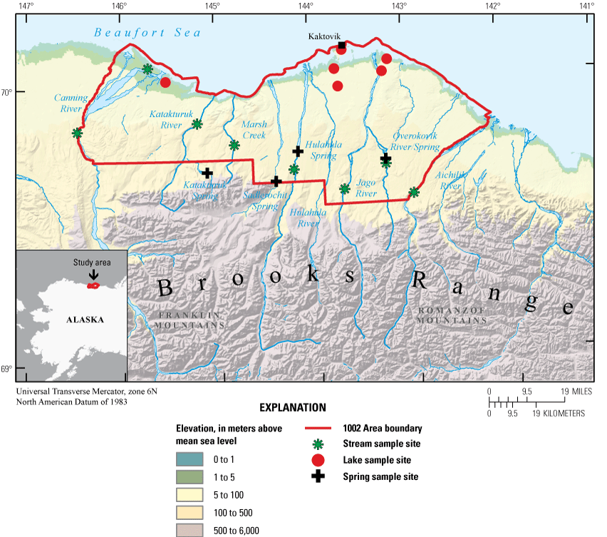
Study area indicating sampling locations, Arctic Slope, northern Alaska (baselayer from Porter and others, 2023).
The potential for oil and gas development in the area prompted the U.S. Geological Survey (USGS) to do reconnaissance water-quality and water-quantity work on a large part of the Eastern North Slope, including the 1002 Area in 1975 (Childers and others, 1977). Fieldwork was conducted in April 1975 to identify and sample winter water resources related to springs, overwinter flow in major rivers, and liquid water in lakes. Water quality was determined in 18 springs and 12 lakes. Fieldwork was conducted in August to determine flood characteristics of 14 selected streams, sample water quality at 26 stream and 12 lake locations, and revisit springs identified during the winter. This work serves as baseline information for the 1002 Area.
In addition to its potential value as an oil and gas source, the foothills and coastal plain of ANWR provide critical and unique habitat. ANWR is a critical region for polar bear denning, and part of the summer calving grounds of the Porcupine Caribou Herd (Lieland, 2006). The rivers contain Arctic cisco (Coregonus autumnalis), Arctic grayling (Thymallus arcticus), and Dolly Varden (Salvelinus malma), fish species that are used for subsistence harvest by the residents of Kaktovik and others (Carey and others, 2021). The limited availability of water in this region, especially compared to the western Arctic coastal plain, motivates the careful management of water resources.
Our contemporary resampling of 1002 Area water sources was undertaken to reassess the findings from the initial Childers sampling, while accounting for drastic changes in Arctic climatology, hydrology, and ecosystems related to climate change. The Arctic is warming faster than other regions of the globe (Pachauri and others, 2014; Rantanen and others, 2022) in a process known as Arctic amplification (Serreze and Barry, 2011). Warmer temperatures are altering rain and snowfall magnitude and timing (Stuefer and others, 2017), snowpack size and distribution (Stuefer and others, 2013) and melt (Musselman and others, 2017; Arp and others, 2020). Arctic environments are often underlain by permafrost, meaning that infiltration potential is limited, resulting in flashy snowmelt and rainfall hydrographs (McNamara and others, 1997; Bowling and others, 2003;). Thawing of the cryosphere is altering regional hydrology (Smith and others, 2005; Liljedahl and others, 2016; Koch, Sjöberg, and others, 2022); the depth of infiltration; and thus the river hydrographs (McClelland and others, 2006; Blaskey and others, 2023), as more water moves through longer, deeper flow paths to reach rivers (Walvoord and Striegl, 2007; Walvoord and others, 2012; Liu and others, 2022). Deeper flow paths impact water quality, altering inflowing water temperature (Sjöberg and others, 2021), the overall solute load (Toohey and others, 2016), nutrient availability (MacLean and others, 1999; Frey and McClelland, 2009; Reyes and Lougheed, 2015; Koch, Jorgenson, and others, 2018), and carbon concentration and quality (Striegl and others, 2005; Tank and others, 2016; O'Donnell and others, 2017; O’Donnell and others, 2020; Koch, Bogard, and others, 2022). These interacting changes may substantially impact ecosystems (Becker and others, 2015; Vonk and others, 2015; O’Donnell and others, 2020) and wildlife (Van Hemert and others, 2015). These impacts are observable on broad-scale changes in vegetation (Chapin and others, 2005; Sturm and others, 2001; Tape and others, 2006; Jorgenson and others, 2013), and ongoing ground subsidence (Hjort and others, 2018; Obu and others, 2019) Given the rapid pace of warming over the last several decades, a resampling of the 1002 Area’s waters was warranted to assess current conditions and changes since the historical sampling.
As of 2023, the 1002 Area remains remote and undeveloped, no comprehensive work of similar scope has been done since the historical work by Childers, and only a single streamgage is currently maintained (Hulahula River, USGS station 15980000) within the area (U.S. Geological Survey, 2022a). The lack of data from the 1002 Area coupled with the changes to hydrologic regimes noted throughout the Arctic and Alaska (Hinzman and others, 2005; Jorgenson and others, 2006) prompted this effort to revisit selected sites from the historical study (Childers and others, 1977) and collect similar data. In April 2021, four spring sites were visited for water-quality and water-quantity sampling, followed by return visits to those springs plus eight stream sites and six lake sites in August 2021 (fig. 1). Additionally, aufeis fields, which form downstream of springs or areas where continuous winter streamflow is forced out of its channel by ice formation (Alekseyev, 2015; Ensom and others, 2020), were mapped using satellite imagery available over the four intervening decades between the historical and contemporary sampling efforts. Although contemporary water quality (U.S. Geological Survey, 2022a), macroinvertebrate (Koch and others, 2023), and aufeis data (Baughman, 2023) allow comparisons with historical samples and some inference regarding ongoing environmental change, a robust analysis is challenged by the limited temporal sampling.
Methods
Water Quality and Macroinvertebrates
Samples were collected in streams, springs, rivers, and lakes for trace metals, major ions and nutrients. Sites were accessed by helicopter and hiking when necessary to reach locations within the ANWR wilderness. Suspended sediments were collected in springs and streams. All samples were collected following USGS protocols (Wilde and others, 1998). Samples from each site were composited into a clean, acid-rinsed polytetrafluoroethylene or polypropylene container and either processed on-site or transported back to base where they were processed within 4 hours. Nutrient sample was preserved with 1 milliliter (mL) of sulfuric acid. The metals sample was preserved with 2 mL of nitric acid and the organic carbon sample was preserved with 1 mL of sulfuric acid. All samples were kept chilled following processing. All samples were analyzed at the USGS National Water Quality Laboratory in Lakewood, Colorado. Filtered subsamples were analyzed for metals, major ions, nutrients, organic carbon and alkalinity. Unfiltered subsamples were analyzed for nutrients (including ammonia, organic nitrogen, phosphorus), turbidity, pH, and specific conductance (SpC).
Streams were sampled in August to capture conditions similar to those sampled during the historical study. August was chosen in the historical study to avoid snowmelt signal in the rivers and sample summertime base flow. River-flow conditions were noted as “fairly low and the stream water was clear” by Childers and others (1977, p. 36) and discharge was either directly measured or estimated. The only site noted in the baseline study as having turbidity was the Katakturuk River, owing to a rainstorm in the headwaters on the day preceding the sampling. In the historical sampling, springs were sampled in April (tables 1 and 2) for the entire suite of parameters noted in the baseline study, and most of the 12 lakes were sampled through ice in November. Only two lakes were sampled during the summer (August) in the historical sampling and only one of those lakes is in the 1002 Area, the lake on Barter Island near Kaktovik. This lake was sampled again along with five others during the contemporary sampling in August 2021. Data collection included water-quality samples and lake depth at the sampling location. Parentheses in location names (table 1) indicate where names in the National Water Information System (NWIS; U.S. Geological Survey, 2022a) deviate from original site names in Childers and others (1977). Data for two lakes sampled by Childers and others (1977; Barter Island [Navarakpuk] lake and Unnamed lake [9.6 mi SE of] near Kaktovik.) were not found in NWIS.
Table 1.
Sample site location latitude and longitude, Arctic Slope, northern Alaska.[Abbreviations: mi, miles; SE, southeast; nr; near; R, river; N, north; W, west]
Table 2.
Dissolved chemical constituents and physical parameters for springs, Arctic Slope, northern Alaska, 1975 (Childers and others, 1977) and 2021 (U.S. Geological Survey, 2022a).[All constituents reported in milligrams per liter unless otherwise noted. Latitude and longitude data for each sampling location are shown in table 1. Abbreviations: M[M]/DD/YY, sample date as month-day-year; ft3/s, cubic foot per second; μg/L, micrograms per liter; CaCO3, calcium carbonate; µS/cm, microsiemens per centimeter; °C, degrees Celsius; <, indicates that the value is below the detection limit; –, no data given]
Water-quality trends are difficult to analyze robustly given that so few samples exist and the impact that seasonal hydrology may play in controlling solute concentrations. Lakes are particularly difficult to compare, given large differences that may exist related to intra- and inter-annual trends in high latitude and snowmelt dominated systems (Gibson and others, 2002; Koch, Fondell, and others, 2018). For streams and lakes, we compared historical and contemporary values collected from the same time of the year (August). Spring samples are compared in April, when inputs of snowmelt and (or) shallow runoff are least likely because of the frozen surface and subsurface conditions. Comparisons between historical and contemporary data were made by first looking for similarities in physical conditions such as discharge and turbidity. For sites where flow conditions were similar between the historical and contemporary sampling, chemical concentrations were compared to assess broad trends across chemical parameters and sites.
For the contemporary sampling, macroinvertebrates were collected in stream, springs, and rivers following standard methods (Cuffney and others, 1993; Merritt and Cummins, 1996). Invertebrates were collected using an hour-long deployment of a Surber net as a drift sampler. The net was placed in an area of moderate flow with the bottom of the net frame against the streambed and the top of the net frame above the water surface to collect surface film. After collection of the drift sample, the invertebrates were sampled at eight locations within the channel by agitating the bottom materials within the frame attached to the Surber net for 1 minute at each location. Macroinvertebrates were analyzed at the National Aquatic Monitoring Center at Utah State University. Macroinvertebrates between historical and contemporary datasets were compared at broad levels by comparing the number of taxa present and by calculating Shannon’s and Simpson’s diversity indices (Ludwig and Reynolds, 1988). The historical sampling followed similar protocols, except in some cases kick samples were not collected.
Discharge
Point discharge measurements were made in streams, springs, and rivers by standard USGS methods (Rantz, 1982). All streams, springs, and river channels small enough to be waded were measured using a pygmy or Price AA mechanical meter on a top-setting wading rod with a tag-line to measure distances along the width of the stream; total discharge was computed using mid-section methods. The original Childers campaign used the same methods and equipment. At rivers suitable for acoustic Doppler current profiler (ADCP) measurements and too deep or swift to wade (Canning, Aichilik, and Hulahula) flow measurements were made using a TRDI StreamPro (TeleDyne Analytical Instruments, City of Industry, California) ADCP from an inflatable kayak following USGS methods (Mueller and others, 2009).
In streams and rivers, discharge measurements were made where all flow was contained in a single channel. For spring discharge measurements, we attempted to find a location where a single channel contained all the flow or made discharge measurements or estimates in multiple channels if only a few main channels were present; depending on the season, this was not a straightforward task at most springs besides Sadlerochit Spring.
Stream Hydrology
The historical study made bankfull discharge estimates and maximum evident flood estimates at 14 stream sites through flood surveys, including bankfull stage determinations (Leopold and Skibitzke, 1967) and slope-conveyance methods (Benson and Dalrymple, 1967). For the contemporary effort, field surveys of channel parameters and flood computations were not repeated under the assumption that the large errors associated with these methods would prevent meaningful comparison of the results. Childers and others (1977) also presented computations of the Q2 and Q50 floods from regional (Alaska) multiple regression analysis based on three basin characteristics: drainage area, mean annual precipitation, and main channel slope (Childers, 1970). Q2 and Q50 refer to floods having a 2-percent and 50-percent annual exceedance probability (AEP), respectively. Regional multiple regression analyses for Alaska have progressed since the Childers (1970) equations, mainly because of the greater number of streamflow measurements and climatic data available, which allow us to report updated flood-frequency estimates for streams. Additionally, an 11-year streamflow record on the Hulahula River is now available for flood-frequency analysis to be directly compared with the flood estimates generated from modern regional regressions (Curran and others, 2016) using drainage area and mean annual precipitation in the basin from the PRISM climate dataset 1971–2000 (Gibson, 2009).
Aufeis
The historical sampling used Landsat 1 imagery to identify the location of icings (Childers and others, 1977). For the contemporary aufeis analysis (Baughman, 2023), Landsat scenes from 1985 to 2021 were compiled and analyzed for aerial extent of aufeis within all major creeks and rivers within the 1002 Area. Aufeis extent was opportunistically estimated for all clear-sky scenes collected between the peak of aufeis formation in late March (Julian date 115) through summer melt and into early October (Julian date 280) when aufeis has completely melted or formation resumes. Aufeis deposits were divided into two populations based on two periods, 1985–2003 and 2004–2021. This split achieved nearly equal temporal duration for both periods, each of which is characterized by an overall increase in mean annual air temperature and summer warmth index (Raynolds and others, 2014).
Aufeis extent was constrained to the floodplains where such features are common. The floodplain was interpreted as the part of the landscape on either side of prominent flowlines bounded by the first prominent sloping features derived from a digital elevation model. This floodplain area of interest (AOI) was manually digitized in a geographic information system (GIS) environment using a combination of imagery and interferometric synthetic aperture radar digital elevation models (Baughman, 2023). The AOI was coarsely digitized at the 1:30,000 scale and masked to exclude areas within 30 meters (m) of prominent bluff features (slope greater than [>] 8 degrees) capable of producing and retaining large snowdrifts.
We classified aufeis features using the Normalized Difference Snow Index (NDSI), which is an index whose value that ranges from −1.0 and +1.0 with the magnitude of positive values corresponding to the likelihood of a surface being snow or ice (Brombierstäudl and others, 2021). The NDSI has been successfully used for aufeis classification across various landscapes (Brombierstäudl and others, 2021). The index value is derived from the green and shortwave infrared parts of the electromagnetic spectrum (eq. 1).
whereGreen
is the common name of the Landsat band used to detect surface reflectance wavelengths ranging from 0.52 to 0.60 micrometers (μm); and
SWIR1
is the common name of the Landsat band used to detect surface reflectance wavelengths ranging from 1.55 to 1.75 μm.
This index responds to snow and ice owing to these materials being highly reflective in visible wavelengths (for example, green) and poorly reflective in the shortwave infrared wavelengths (Dozier, 1989; Riggs and others, 1994). The index is ideal because, beginning with the launch of Landsat 4 in 1982, all subsequent Landsat platforms have sensed reflected radiation in nearly identical bands spanning these wavelengths (table 2).
For our study, an NDSI raster was derived for each scene. Using a GIS, pixels within the floodplain AOI were clipped from the NDSI raster and reclassified to binary rasters where a pixel value of “1” represents aufeis and a pixel value of “0” represents all other land surfaces. Dozier (1989) determined that NDSI values greater than 0.4 are universally consistent with snow-covered surfaces. For our study location, we determined that a threshold of 0.3 was ideal for classifying surfaces covered in aufeis across the spring and summer season. The lower threshold is necessary for identifying late-season aufeis that we determined to be less reflective in late summer. Using zonal statistics from the AOIs, the area of aufeis present on a sample date equals the number of pixels classified as aufeis multiplied by a unit area (0.0009 square kilometers [km2]). We compared our estimates of aufeis area derived from 30-m Landsat scenes with independent estimates based on panchromatic, high-resolution commercial satellite platforms with sub-meter spatial resolution for dates where concurrent observations were available for prominent, persistent aufeis fields. For three dates, Landsat-based estimates were within 4 percent across the range of Landsat sensors.
Trends in seasonal aufeis loss patterns were analyzed at four persistent icing locations across the 1002 Area (Baughman, 2023). Persistent aufeis fields were individually analyzed for trends in the seasonal extent and pattern of decay. For this analysis, all available scenes (May–September) were included regardless of aufeis presence. The area of aufeis present within the field on available sample dates was averaged and plotted by day of year (DOY). We compared the average area of aufeis present on a given DOY for two time periods: 1985–2003 and 2004–2021. Sigmoidal decay models were solved for each period based on the available data using a model that describes the magnitude of the response of a system as a function of exposure to a stimulus or stressor over time (Di Veroli and others, 2015):
whereAx
is the area of aufeis present on a given day;
Ai
is the known initial area of aufeis before the thaw season;
Af
is the final simulated aufeis area on 30 September, which is the assumed end of the thaw season;
Dx
is the day of the year;
D1/2
is the simulated date of 50-percent loss of the initial aufeis area; and
n
is a coefficient that determines the rate of thaw.
The model was solved using the Solver tool in Microsoft Excel (Microsoft Corporation, 2022), which requires initial values for all model parameters. All models were constrained with an initial area value (Ai) equal to the full extent of the perennial field on D115, a date we chose that universally precedes the perceivable thaw season in this study area. Primer values of 10 and 160 were entered for n and D1/2, respectively. Within the Solver tool, we set an objective to minimize the residual sum of squares. After initial solving, curves were manually adjusted to achieve best reasonable fits as needed. Small negative Af values were required in some cases to achieve the best fit.
A second analysis quantified changes in the occurrence of aufeis across the 1002 Area from June 10 to September 30, thereby mostly avoiding inclusion of river ice in counts. These data are presented for all years of data and divided into two populations by year. Counting the occurrence of aufeis at a given location within the timeframe of our study identifies locations where aufeis has historically occurred and suggests the regularity of aufeis development. The Landsat dataset does not permit estimating annual aufeis extent for a given location, but we can infer the fidelity of aufeis for a location based on the frequency of detections within the available Landsat scenes. We classified aufeis fidelity into four occurrence classes—Persistent, Regular, Ephemeral, and Uncommon. Persistent aufeis is that which occurs in the same location every year, persists late into summer, and may fail to completely melt during summer. These locations are characterized with counts >1.5 standard deviations (sigma [σ]) above the mean number of detections for the entire 1002 Area. Regular aufeis fields are those areas around the more persistent fields but that either consistently melt away during the thaw season or are irregularly persistent. We classify regular aufeis occurrence based on count values 0.5–1.5 σ greater than the mean. Ephemeral aufeis represents the distal margins of the major aufeis fields that quickly melt in late spring and early summer. We classify ephemeral aufeis as locations with occurrence counts 0.5 σ greater than or less than the mean. We classify uncommon aufeis as irregular and limited occurrences of aufeis with count values <0.05 σ less than the mean. These locations represent unique and rare occurrences of aufeis.
Comparing Hydrology and Water Quality Between the Historical and Contemporary Periods
River and Spring Hydrology and Water Quality
Springs were visited using a helicopter and walking in April (fig. 2) and August (fig. 3) 2021. These images show that springs on the Okerokovik, Hulahula, and Katakturuk Rivers occur within or adjacent to braided streambeds and have multiple channels that are most easily identified as distinct from other streamflow in the winter when surface flows in the adjacent streams cease. Sadlerochit Spring is the most distinctly separated from its associated river system as it issues from three hillside orifices rather than emerging from alluvium. At all the springs during winter, open water was the obvious sign of their location, whereas during summer, the lush green growth of instream and bank vegetation was the distinguishing factor. Additionally, water quality parameters were helpful in identifying the springs as separate systems from nearby surface-water-fed rivers or streams.
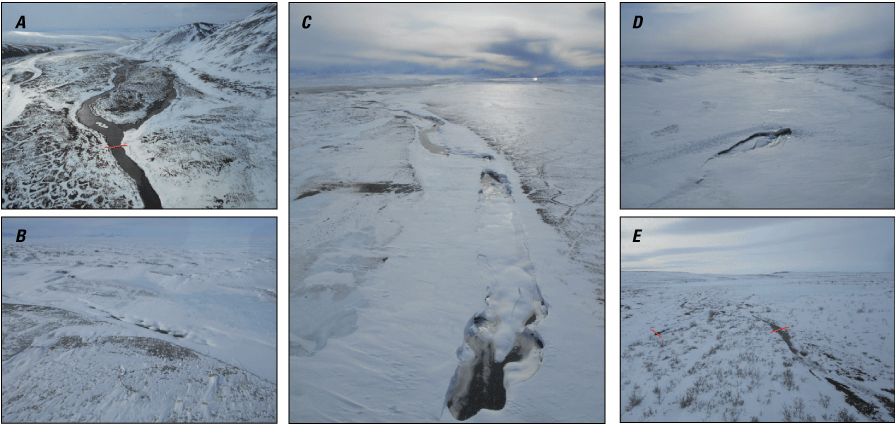
Four sampled spring sites, Arctic Slope, northern Alaska, April 2021. A, Sadlerochit Spring with sampling and discharge measurement section indicated with a line. B, Hulahula Spring seen as open water in main river channel. C, Hulahula Spring seen as open lead. Note building in upper left of photograph near where spring was found isolated from main channel during August 2021 sampling. D, Okerokovik Spring open lead. E, Katakturuk Spring with multiple channels; the two lines indicate where discharge measurements were made to obtain total flow. Photographs by Charles Couvillion and Heather Best, U.S. Geological Survey, April 21–22, 2021.
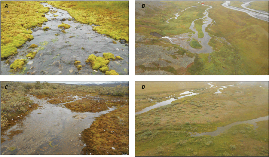
Four sampled springs, Arctic Slope, northern Alaska, August 2021. A, Algae and mosses in Hulahula River Spring, making it distinct from the clean cobbles seen in the active river channel. B, Sadlerochit Spring with sampling and measurement location shown with a line. Active river channel is seen in upper right of photograph. C, Katakturuk Spring with lush algae and moss growth. D, Multiple channels of the Okerokovik Spring. Photographs by Charles Couvillion and Heather Best, U.S. Geological Survey, August 15 and 17, 2021.
The Hulahula River Spring had only one obvious open-water channel during our April visit, in the main river channel on the west side of the broad braided alluvial channel. During our August visit, the spring sampling location was on the opposite (east) side of the channel, just downstream from a fish camp. This observation suggests that many spring upwellings are present in the area and that winter flow is mainly consolidated in the river channel, whereas, in summer, upwellings may occur throughout the alluvial channel. Spring discharges therefore may not be directly comparable between seasons. Streamgage data just upstream from the spring locations at the USGS Hulahula River (U.S. Geological Survey, 2022a; site ID 15980000) indicate the cessation of flow in early winter (November), suggesting that all winter flow originates from springs and not the river.
Okerokovik Spring appeared as a single lead in April but in August had several distributed channels (fig. 3D). The total flow was estimated based on measurement of a single channel and estimation from the air of additional flow in the remaining channels. Katakturuk Spring had multiple channels in winter (fig. 2E) Flow was measured in the main channel on the right side of the photograph and estimated in the smaller channel on the left side of the photograph. This procedure was repeated for the summer visit with sampling and a flow measurement on the main channel and additional flow estimated in a few minor channels.
In August 2021, river levels were low with clear water in streams, with two exceptions: Marsh Creek and Hulahula River. Marsh Creek was not affected by rain, but the water was turbid and iron-colored; a flight to the headwaters indicated that this orange color originated at red oxidized rock layers that are present in the upper basin. The Hulahula River discharge was elevated because of rainfall when it was visited in August 2021.
Consistent changes in water quality (table 2) were noted across streams and springs between the historical and contemporary measurements. Measured discharge averaged across streams showed a 1.3-fold mean increase. River solute concentrations and discharge are often inversely proportional (Godsey and others, 2009); thus, we might expect the discharge increase to result in decreased stream specific conductance. However, we measured general increases in mean stream specific conductance (1.9-fold ±0.3) and pH (1.1-fold ±0.0). Mean stream water temperatures also increased in most streams (1.6-fold ±0.7; fig. 4).
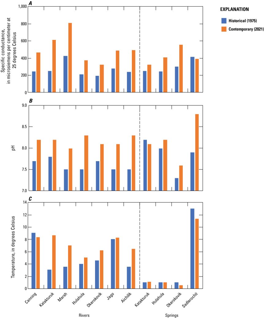
Graphs showing measurements of water-quality change in rivers and springs between historical (1975; Childers and others, 1977) and contemporary (2021; U.S. Geological Survey, 2022a) sampling, Arctic Slope, northern Alaska.
Springs showed more stable discharge, but trends in chemistry similar to those of the streams (table 3). Discharge was consistent between historical and contemporary periods for three of the springs, whereas discharge increased 1.9-fold at Sadlerochit Spring. This change makes it difficult to analyze trends in chemistry for Sadlerochit Spring. Focusing on the three of four springs with temporally stable discharge, specific conductance increased substantially (fig. 4), with a mean increase between the historical and current period of a factor of 1.6 (±0.3), which is mostly attributable to an increase in sulfate (increase factor of 4.3 ±0.9) and non-carbonate hardness (increase factor of 2.6 ±0.9).
Table 3.
Dissolved chemical constituents and physical parameters for streams, Arctic Slope, northern Alaska, 1975 (Childers and others, 1977) and 2021 (U.S. Geological Survey, 2022a).[All constituents reported in milligrams per liter unless otherwise noted. Latitude and longitude data for each sampling location are shown in table 1. Abbreviations: M[M]/DD/YY, sample date as month-day-year; ft3/s, cubic foot per second; μg/L, micrograms per liter; CaCO3, calcium carbonate; µS/cm, microsiemens per centimeter; °C, degrees Celsius; <, indicates that the value is below the detection limit; –, no data given]
Lake Water Quality
A comparison of historical and contemporary lake samples (table 4) suggests that the lakes had generally similar chemistry between the historical and contemporary measurements. One exception is Navarakpuk Lake, which had substantially higher sodium, chloride, and specific conductance in 1975 compared to 1972, potentially indicating a marine incursion prior to the 1975 sampling. It is unclear how often such incursions occur. Substantial changes in SpC or major ions were not measured in the other lakes, and small changes in lake chemistry should not be taken as evidence of significant change. Arctic lake chemistry can vary greatly over the season and interannually as a result of snowmelt and ecosystem activity, depending on morphology and position in the drainage network (Gibson and others, 2002, 2008; Koch, Fondell, and others, 2018).
Table 4.
Dissolved chemical constituents and physical parameters for lakes, Arctic Slope, northern Alaska, 1972–2021 (Childers and others, 1977; U.S. Geological Survey, 2022a).[All constituents reported in milligrams per liter unless otherwise noted. Latitude and longitude data for each sampling location are shown in table 1. Abbreviations: M[M]/DD/YY, sample date as month-day-year; ft3/s, cubic foot per second; μg/L, micrograms per liter; CaCO3, calcium carbonate; µS/cm, microsiemens per centimeter; °C, degrees Celsius; mi SE, miles southeast; <, indicates that the value is below the detection limit; –, no data given]
Water depth plus ice thickness from table 4 (Childers and others, 1977).
Macroinvertebrates
Arctic rivers have less macroinvertebrate diversity compared to lower latitudes because of less ecosystem productivity from low light levels, cold temperatures, short growing seasons, snow and ice cover, and less nutrients entering the ecosystem (Lento and others, 2022). We noted low taxa richness in both the historical and contemporary (Koch and others, 2023) collection of macroinvertebrates consistent with the expectation of lower richness in Arctic streams relative to lower-latitude streams (fig. 5). The historical sampling only collected drift measurements in summer, and no obvious change in richness occurred between the present and historical summer drift sampling. In the present sampling, seasonal differences were measured in macroinvertebrate richness collected in the stream drift. Drift richness increasing between the spring and summer sampling periods likely reflected higher nutrient inflows from terrestrial sources and more terrestrial insects falling into the surface flow, along with more autochthonous production through the growing season. No differences were detected in spring between the present and historical samples for the benthic assemblage or between spring and summer in the present sampling. A comparison of Shannon’s Diversity index and Simpson’s Index between spring and summer with the present data indicated no differences between seasons using drift nets or benthic sampling. We measured a difference in summer between the historical and contemporary drift data for Shannon’s Diversity Index. No differences were found between historical and present drift data with Simpson’s Diversity Index. Shannon’s Diversity Index emphasizes rare species, whereas Simpson’s Index emphasizes common species. The difference in Shannon’s Diversity Index suggests that rare taxa are driving the difference between the historical and present samples, with more rare taxa collected in the present. Overall, the common taxa are present in both time periods, as indicated by similarity between the time periods for Simpson’s Diversity Index. In the benthic data, we see a similar pattern of no differences between spring and summer in the present sampling, but a difference between Shannon’s Diversity Index for the present compared to historical data in the spring. Like the drift data, we suspect that rare taxa present in the present sampling are driving the differences between present and historical sample periods and that the common taxa are consistent between periods. The consistency of common taxa in the spring between time periods is also suggested by the similarity with Simpson’s Diversity Index. Although there seems to be increased diversity in spring between the present and historical sampling, differences in sampling methods preclude direct comparison of these two periods. The kicknetting used during the contemporaneous sampling is a more thorough technique and likely to have collected more rare taxa than the rock collection used in the historical sampling.
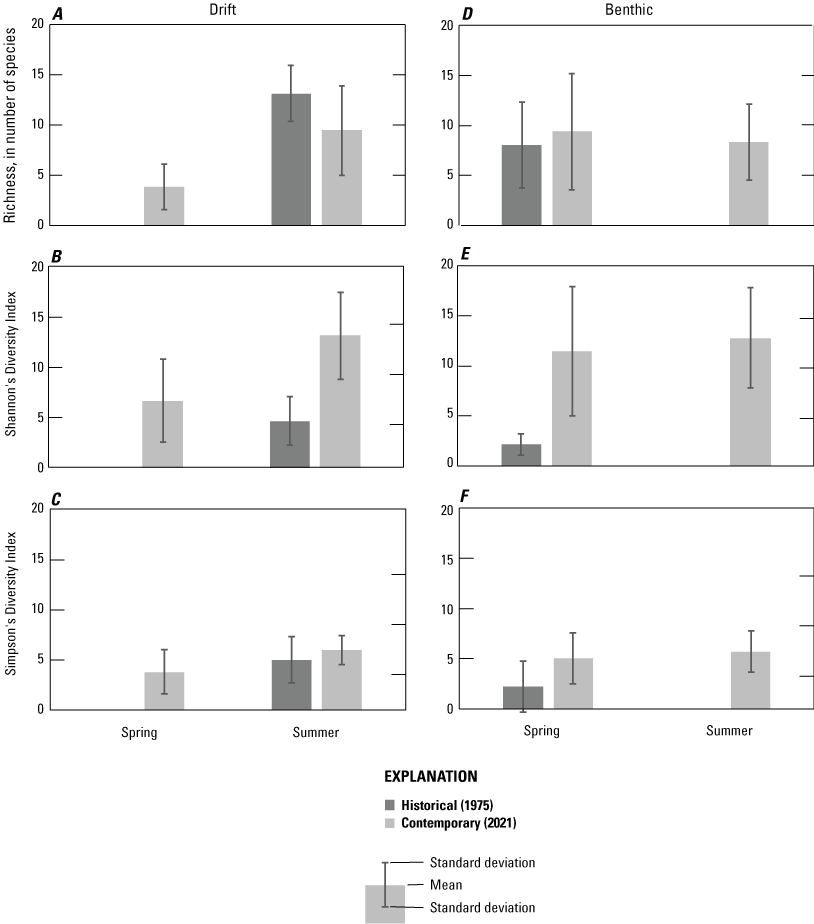
Macroinvertebrate richness and diversity for the historical (Childers and others, 1977) and contemporary (Koch and others, 2023) samplings, Arctic Slope, northern Alaska. Bars represent mean values across all sites and whiskers indicate one standard deviation from the mean.
Stream Hydrology
Statewide regression equations for Alaska (Curran and others, 2016; Curran, 2022) were used to calculate values for 50-percent AEP and 2-percent AEP flow returns for each of the revisited stream sites (table 5). Higher flows are predicted by the modern statewide regressions, resulting in values at some streams closer to the computations for bankfull flow and maximum evident flood made by the historical study. For ease of comparison, bankfull flows are typically associated with 1.5-year return rates (67-percent AEP; Edwards and others, 2019) and thus should be closely comparable to the 50-percent AEP predicted flows. However, the historical study computations of bankfull flows and maximum evident floods are subject to more uncertainty than the same computations performed on sub-Arctic rivers as the determination of flood flows from bankfull markers in Arctic basins can be problematic because of the complex interactions of ice dynamics during break-up events coupled with ice rich banks either resisting or increasing susceptibility to erosion seasonally (McNamara and Kane, 2009). The possibility that maximum evident flood markers were deposited when ice occupied some of the channel could result in the overestimation of the associated flows. For Marsh Creek, as noted by Childers and others (1977), flood markers are potentially not deposited during high flow events because of snow-lined banks during the peak snowmelt flows, thus resulting in under-computation of the maximum evident flood flow.
Table 5.
Bankfull channel, maximum evident flood, and streamflow estimates from statewide regression analyses for selected eastern Arctic Slope streams, northern Alaska, 1970–2016.[All measurements are in cubic feet per second. AEP, annual exceedance probability]
| Stream site | Field survey computed streamflows from Childers and others (1977) | Statewide regression streamflow estimates from Childers (1970) | Statewide regression streamflow estimates from Curran and others (2016) | |||
|---|---|---|---|---|---|---|
| Bankfull channel | Maximum evident flood | 50-percent AEP |
2-percent AEP |
50-percent AEP |
2-percent AEP |
|
| Aichilik River | 33,000 | 27,000 | 1,900 | 6,300 | 3,740 | 9,680 |
| Okerokovik River | 10,000 | 23,000 | 650 | 2,600 | 949 | 2,990 |
| Jago River | 14,000 | 14,000 | 1,000 | 3,600 | 2,650 | 6,990 |
| Hulahula River | 23,000 | 10,000 | 1,800 | 6,300 | 4,740 | 11,900 |
| Marsh Creek | 14,000 | 500 | 750 | 3,100 | 200 | 749 |
| Katakturuk River | 17,000 | 10,000 | 660 | 2,800 | 1,270 | 3,850 |
| Canning River | 31,000 | 53,000 | 4,400 | 13,500 | 10,000 | 23,400 |
Changes in streamflow estimates between Childers (1970), Curran and others (2016), and Curran (2022) can be attributed to additional and better data used in the more recent computations. These computations are based on basin characteristics and improvements in the available data including longer datasets for streamflow, precipitation, and air temperature. The current regression equations (Curran and others, 2016; Curran, 2022) use basin drainage area and mean annual precipitation, whereas the historical regression methods (Childers, 1970) used basin drainage area, mean channel slope, and mean annual precipitation.
Aufeis
The Landsat archive offered a long-term and accurate way to obtain moderate resolution estimates of aufeis area at the landscape scale (Baughman, 2023). We specifically used Landsat analysis ready data (ARD) scenes that overlap with the 1002 Area. Landsat ARD scenes are consistently processed to the highest scientific standards and level of processing required for direct use in monitoring and assessing landscape change. Scenes relevant to this study were downloaded from the Landsat Collection 2 U.S. ARD Surface Reflectance product (Dwyer and others, 2018) hosted by EarthExplorer (U.S. Geological Survey, 2022b). The 1002 Area comprises two ARD tiles, identified by their horizontal and vertical position within the Alaska ARD tile grid region. Tile h016v001 captures the western third of the 1002 Area, and h017v001 captures the eastern two-thirds. Our scene-selection criteria ultimately produced 470 scenes collectively acquired from 1985 to 2021 during May–September. Two scenes from late April (Landsat 5) were also incorporated to improve continuity of early-season scene coverage for 1986 and 2005. Landsat 8 and the Operational Land Imaging (OLI) sensor produced 117 scenes, Landsat 7 and the Enhanced Thematic Mapper Plus (ETM+) produced 273 scenes, and the Thematic Mapper Sensor (TM) found on Landsat 5 and Landsat 4 produced 80 scenes. Scenes were roughly split between the two ARD tiles, with h016v001 receiving slightly more coverage (about 10 scenes) mostly from Landsat 7 (table 6).
Table 6.
Number of analysis ready data (ARD) scenes acquired by each Landsat system (Baughman, 2023).The analysis of seasonal trends within persistent fields uses a subset of scenes (n=461) including spring (April–May) scenes as well as scenes where no aufeis is detectable. For trend analysis, it was essential to document the absence as well as the presence of aufeis. Data gaps exist for years 1989–1991, 1993, and 1996–98 owing to a combination of scene availability and historical Landsat scene acquisition scheduling.
In the absence of ground-truth data, we validated our estimates of aufeis area derived from 30-m Landsat scenes by comparing them to independent estimates based on panchromatic, high-resolution commercial satellite platforms with sub-meter spatial resolution on dates where concurrent observations were available for prominent, persistent aufeis fields (table 7). For three dates, moderate resolution estimates were within 4 percent across the range of Landsat sensors (for example, TM, ETM+ and OLI). Correct discrimination of aufeis deposits (and other snow and ice features) from all other land and water surfaces is very accurate. Accuracy assessments, completed for the same three dates and aufeis fields and using the high-resolution satellite imagery for comparison, consistently achieved overall classification accuracies greater than 90 percent (table 7). Classification accuracy is based on 500 random equally stratified sample points distributed about the persistent field. Kappa coefficients are also consistently high with an average value of 0.91 ±0.02 (table 8).
Table 7.
Comparison of moderate and high resolution aufeis area determinations, Arctic Slope, northern Alaska, 2008–17 (Baughman, 2023).[Dates given in M/DD/YY, month-day-year format. Commercial satellite scenes were acquired through Maxar’s Global Enhanced GEOINT Delivery (G-EGD; Dwyer and other, 2018). Identifiers used are as follows: on 6/11/08, Sadlerochit Sp Legacy Identifier, 1010010008465800; on 6/14/12, Okerokovik Legacy Identifier, 10300100188DFF00; and on 6/11/17, Hulahula Legacy Identifier, 104001002EAACF00. Abbreviations: m, meters; km2, square kilometers; %, percent; Pan, panchromatic (in other words, black and white imagery); L8 OLI, Landsat 8 satellite with Operational Land Imaging sensor; L7 ETM+, Landsat 7 satellite with Enhanced Thematic Mapper Plus sensor; L5 TM, Landsat 5 satellite with Thematic Mapper sensor]
Quickbird 2 (Maxar Technologies Inc., 2023a).
Worldview 2 (Maxar Technologies Inc., 2023b).
Worldview 3 (Maxar Technologies Inc., 2023c).
Table 8.
Classification accuracy using Landsat data (Baughman, 2023).[Aufeis absent: Aufeis absent, test location classified as having no ice cover Aufeis present: Aufeis present, test location classified as being ice covered Abbreviations PA, producer’s accuracy; Omi., omission; UA, user’s accuracy; Com., commission; Kappa, overall agreement between classification and reference (true) values, can range from 0 (no agreement) to 1 (perfect agreement); OA, overall accuracy; %, percent; –, no data given]
Quickbird 2 (Maxar Technologies Inc., 2023a).
Worldview 2 (Maxar Technologies Inc., 2023b).
Worldview 3 (Maxar Technologies Inc., 2023c).
All four persistent aufeis fields analyzed for seasonal trends suggest, on average, that aufeis fields are melting faster and earlier within the thaw season than during the historic period (fig. 6). Model fit for both time periods across all four aufeis fields is very good. Average coefficient of determination (r2) is 0.96 ±0.02 (table 9). Observations show that the average area of aufeis within a persistent field for the 2004–2021 period decayed from the maximal extent sooner in the summer compared to the 1985–2003 time period. The difference in melt rate between the historic and contemporary period is indicated by the comparative “deflation” of the decay curve. One metric indicative of this trend is D½, the average day of the year with one-half of the initial aufeis area remaining. Compared to 1986–2003, the D½ value for the Tamayariak River moves back in time by 15 days, shifting from June 19 to June 4 for the 2004–2021 time period. D½ values for the Sadlerochit Spring, Hulahula River, and Okerokovik River also occur 13 days earlier, 10 days earlier, and 6 days earlier, respectively. The D½ shifts from June 14 (1986–2003) to June 1 (2004–2021) for Sadlerochit Spring, from June 15 to June 5 for the Hulahula River, and from June 15 to June 9 for the Okerokovik River.
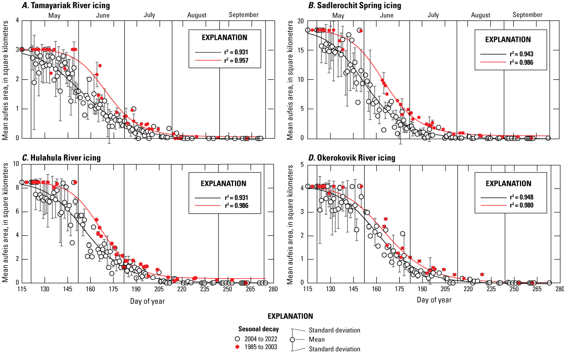
Aufeis seasonal decay from four aufeis fields, where curves represent the best fits for two time periods, 1985–2003 and 2004–21, Arctic Slope, northern Alaska (Baughman, 2023). Points indicate means when multiple images were available for a given day of year within the two time periods. Error bars indicate one standard deviation from the mean. Points with no error bars represent values with only one historical observation. Multiple acquisitions for a given day of year are more likely in the recent period because of improved consistency in Landsat observations.
Table 9.
Model parameters for mean seasonal aufeis decay, where parameters are defined in equation 1, eastern Arctic Slope, northern Alaska (Baughman, 2023).[Abbreviations: Ai, the known initial area of aufeis before the thaw season; Af, the final simulated aufeis area on 30 September, which is the assumed end of the thaw season; D1/2, the simulated day of the year with 50-percent loss of the initial aufeis area; D0, the day of the year at which the aufeis has completed melted; n, a coefficient that determines the rate of thaw; ssr, the residual sum of squares, r2, the coefficient of determination; –, no data given]
Persistent aufeis fields are also more likely to disappear completely today as compared to periods in the past. The modeled decay functions for mean daily area during 1985–2003 suggests the fields associated with Sadlerochit Spring and Tamayariak, Hulahula, and Okerokovik Rivers persisted, on average, into the following freezing season (October 1) as indicated by positive AF values and the absence of D0 values (table 9). During 2004–2021, decay models suggest, on average, that aufeis within Tamayariak River, Sadlerochit Spring, and Okerokovik River fields thaw completely. The D0 values reported for these fields, the modeled day of year that aufeis is completely thawed, correspond to August 20, September 2, and August 23, respectively.
The average rate of aufeis loss in 2004–2021 is reduced compared to 1986–2002. The average 1986–2002 value for n for all four fields is 16.5 ±1.8. This value drops to 11.5 ±0.1 for the 2004–2021 time period (table 9). A reduced n value corresponds to a reduced slope of the decay curve and, therefore, a reduced rate of loss.
Distribution of aufeis fields varies between river systems, and prominent changes in the extent and type of aufeis distribution occurred across the 1002 Area when comparing the early (1986–2002) and later (2004–2021) time periods. The occurrence plots show more nuance with increases in aufeis fields on the lower Canning River and decreases at all other sites. The causes of these changes remain to be determined.
Summary
This study presents updated data and a comparison with historical data on the water quality and hydrology of springs, rivers, lakes, and aufeis in the foothills and coastal plain of the Arctic National Wildlife Refuge, on the Arctic Slope of northern Alaska. Updated basin boundaries and flood-frequency curves provide greater certainty in river discharge and flooding trends. Water quality from the springs and streams, coupled with aufeis trends, provides evidence of changing Arctic hydrology and increased thaw of near-surface soils. We measured earlier melting of aufeis fields in the more recent timeframe (2004–2021). Earlier river ice-off times (Magnuson and others, 2000; Blaskey and others, 2023) and warmer summer air temperatures have been documented throughout the Arctic (Serreze and Barry, 2011; Rantanen and others, 2022) and are expected to reduce aufeis field size (Yoshikawa and others, 2007; Pavelsky and Zarnetske, 2017). Stream water temperatures increased in most systems, which could indicate greater runoff through shallow subsurface flow paths that tend to be relatively warm (Sjöberg and others, 2021). Water chemistry from springs and streams indicated consistent increases in dissolved ion loads (for example, specific conductance and hardness) between the historical and contemporary samplings. Increasing specific conductance is a common trend in headwater streams in permafrost regions, indicative of deepening flow paths allowing runoff to contact deeper, mineral soils (Toohey and others, 2016; Koch, Sjöberg, and others, 2022). The increase in pH is also consistent with an increase in thawed depth and greater movement of water through mineral soils, rather than the shallow organic soils that can contribute organic acids. Although our analysis is constrained by only having two points in time for water-quality data, consistent changes across streams and in some cases streams and springs provides confidence in the findings. More regular repetition of the sampling could aid in the determination of the magnitudes and significance of these trends.
References Cited
Baughman, C.A., 2023, Rasters of observed aufeis deposits within rivers of the 1002 Area based on historical Landsat imagery, 1985–2022: U.S. Geological Survey data release, accessed January 1, 2024, at https://doi.org/10.5066/F7KK98VP.
Brombierstäudl, D., Schmidt, S., and Nüsser, M., 2021, Distribution and relevance of aufeis (icing) in the Upper Indus Basin: Science of the Total Environment, v. 780, p. 146604, accessed December 19, 2023, at https://doi.org/10.1016/j.scitotenv.2021.146604.
Curran, J.H., 2022, Flood frequency data for a streamgage in the Hulahula River Basin, Alaska, 2011–2021: U.S. Geological Survey data release, accessed December 19, 2023, at https://doi.org/10.5066/P9YGWNDR.
Curran, J.H., Barth, N.A., Veilleux, A.G., and Ourso, R.T., 2016, Estimating flood magnitude and frequency at gaged and ungaged sites on streams in Alaska and conterminous basins in Canada, based on data through water year 2012: U.S. Geological Survey Scientific Investigations Report 2016–5024, 47 p, accessed December 19, 2023, at https://doi.org/10.3133/sir20165024.
Gibson, W., 2009, Mean precipitation for Alaska 1971–2000 (Geospatial Dataset-2170508): Anchorage, Alaska, National Park Service, Alaska Regional Office, accessed December 19, 2023, at https://irma.nps.gov/DataStore/Reference/Profile/2170508.
Hinzman, L.D., Bettez, N.D., Bolton, W.R., Chapin, F.S., Dyurgerov, M.B., Fastie, C.L., Griffith, B., Hollister, R.D., Hope, A., Huntington, H.P., Jensen, A.M., Gensuo, J.J., Jorgenson, T., Kane, D.L., Klein, D.R., Kofinas, G., Lynch, A.H., Lloyd, A.H., McGuire, A.D., Nelson, F.E., Oechel, W.C., Osterkamp, T.E., Racine, C.H., Romanovsky, V.E., Stone, R.S., Stow, D.A., Sturm, M., Tweedie, C.E., Vourlitis, G.L., Walker, M.D., Walker, D.A., Webber, P.J., Welker, J.M., Winker, K.S., and Yoshikawa, K., 2005, Evidence and implications of recent climate change in Northern Alaska and other Arctic regions: Climatic Change, v. 72, no. 3, p. 251–298.
Jorgenson, M.T., Harden, J., Kenvskiy, M., O’Donnell, J., Wickland, K., Ewing, S., Manies, K., Zhuang, Q., Shur, Y., Striegl, R., and Koch, J., 2013, Reorganization of vegetation, hydrology and soil carbon after permafrost degradation across heterogeneous boreal landscapes: Environmental Research Letters, v. 8, no. 3, p. 035017.
Koch, J.C., Bogard, M.J., Butman, D.E., Finlay, K., Ebel, B., James, J., Johnston, S.E., Jorgenson, M.T., Pastick, N.J., and Spencer, R.G., 2022a, Heterogeneous patterns of aged organic carbon export driven by hydrologic flow paths, soil texture, fire, and thaw in discontinuous permafrost headwaters: Global Biogeochemical Cycles, v. 36, no. 4, p. e2021GB007242.
Koch, J.C., Couvillion, C., Best, H., and Carey, M.P., 2023, Macroinvertebrates from streams and springs in the 1002 region of the Arctic National Wildlife Refuge, Alaska, 2021: U.S. Geological Survey data release, accessed December 19, 2023, at https://doi.org/10.5066/F7X34VHM.
Lento, J., Laske, S.M., Lavoie, I., Bogan, D., Brua, R.B., Campeau, S., Chin, K., Culp, J.M., Levenstein, B., Power, M., Saulnier-Talbot, É., Shaftel, R., Swanson, H., Whitman, M., and Zimmerman, C.E., 2022, Diversity of diatoms, benthic macroinvertebrates, and fish varies in response to different environmental correlates in Arctic rivers across North America: Freshwater Biology, v. 67, no. 1, p. 95–115.
Liljedahl, A.K., Boike, J., Daanen, R.P., Fedorov, A.N., Frost, G.V., Grosse, G., Hinzman, L.D., Iijma, Y., Jorgenson, J.C., Matveyeva, N., Necsoiu, M., Raynolds, M.K., Romanovsky, V.E., Schulla, J., Tape, K.D., Walker, D.A., Wilson, C.J., Yabuki, H., and Zona, D., 2016, Pan-Arctic ice-wedge degradation in warming permafrost and its influence on tundra hydrology: Nature Geoscience, v. 9, no. 4, p. 312–318.
Magnuson, J.J., Robertson, D.M., Benson, B.J., Wynne, R.H., Livingstone, D.M., Arai, T., Assel, R.A., Barry, R.G., Card, V., Kuusisto, E., Granin, N.G., Prowse, T.D., Stewart, K.M., and Vuglinski, V.S., 2000, Historical trends in lake and river ice cover in the Northern Hemisphere: Science, v. 289, no. 5485, p. 1743–1746.
Maxar Technologies Inc., 2023a, QuickBird: Maxar Technologies Inc., accessed December 19, 2023, at https://resources.maxar.com/data-sheets/quickbird.
Maxar Technologies Inc., 2023b, Worldview-2: Maxar Technologies Inc., accessed December 19, 2023, at https://resources.maxar.com/data-sheets/worldview-2.
Maxar Technologies Inc., 2023c, Worldview-3: Maxar Technologies Inc., accessed December 19, 2023, at https://resources.maxar.com/data-sheets/worldview-3.
Microsoft Corporation, 2022, Microsoft Excel, available at https://office.microsoft.com/excel.
Obu, J., Westermann, S., Bartsch, A., Berdnikov, N., Christiansen, H.H., Dashtseren, A., Delaloye, R., Elberling, B., Etzelmüller, B., Kholodov, A., Khomutov, A., Kääb, A., Leibman, M.O., Lewkowicz, A.G., Panda, S.K., Romanovsky, V., Way, R.G., Westergaard-Nielsen, A., Wu, T., Yamkhin, J., and Zou, D., 2019, Northern hemisphere permafrost map based on TTOP modelling for 2000–2016 at 1 km2 scale: Earth-Science Reviews, v. 193, p. 299–316.
Pachauri, R.K., Allen, M.R., Barros, V.R., Broome, J., Cramer, W., Christ, R., Church, J.A., Clarke, L., Dahe, Q., and Dasgupta, P., 2014, Climatic change—Synthesis report, contribution of working groups I, II and III to the fifth assessment report of the Intergovernmental Panel on Climate Change: Geneva, Switzerland, Intergovernmental Panel on Climate Change, 151 p.
Porter, C., Howat, I., Noh, M-J., Husby, E., Khuvis, S., Danish, E., Tomko, K., Gardiner, J., Negrete, A., Yadav, B., Klassen, J., Kelleher, C., Cloutier, M., Bakker, J., Enos, J., Arnold, G., Bauer, G., and Morin, P., 2023, ArcticDEM, version 4.1: Harvard Dataverse, V1, accessed February 3, 2019, at https://doi.org/10.7910/DVN/3VDC4W.
Raynolds, M.K., Walker, D.A., Ambrosius, K.J., Brown, J., Everett, K.R., Kanevskiy, M., Kofinas, G.P., Romanovsky, V.E., Shur, Y., and Webber, P.J., 2014, Cumulative geoecological effects of 62 years of infrastructure and climate change in ice‐rich permafrost landscapes, Prudhoe Bay Oilfield, Alaska: Global Change Biology, v. 20, no. 4, p. 1211–1224.
Riggs, G.A., Hall, D.K., and Salomonson, V.V., 1994, A snow index for the Landsat thematic mapper and moderate resolution imaging spectroradiometer: Paper presented at proceedings of IGARSS'94—1994 IEEE International Geoscience and Remote Sensing Symposium, Pasadena, California, IEEE, v. 4, p. 1942–1944.
U.S. Geological Survey, 2022b, Earth explorer—Water data for the Nation: U.S. Geological Survey database, accessed June 20, 2022, at https://earthexplorer.usgs.gov/.
U.S. Geological Survey, 2022a, Water data for the Nation: U.S. Geological Survey National Water Information System database, accessed June 10, 2022, at https://doi.org/10.5066/F7P55KJN.
Vonk, J.E., Tank, S.E., Bowden, W.B., Laurion, I., Vincent, W.F., Alekseychik, P., Amyot, M., Billet, M., Canario, J., Cory, R.M., Deshpande, B.N., Helbig, M., Jammet, M., Karlsson, J., Larouche, J., MacMillan, G., Rautio, M., Walter Anthony, K.M., and Wickland, K.P., 2015, Reviews and syntheses—Effects of permafrost thaw on Arctic aquatic ecosystems: Biogeosciences, v. 12, no. 23, p. 7129–7167.
Conversion Factors
U.S. customary units to International System of Units
International System of Units to U.S. customary units
Temperature in degrees Celsius (°C) may be converted to degrees Fahrenheit (°F) as follows:
°F = (1.8 × °C) + 32.
Supplemental Information
Specific conductance is given in microsiemens per centimeter at 25 degrees Celsius (µS/cm at 25 °C).
Concentrations of chemical constituents in water are given in either milligrams per liter (mg/L) or micrograms per liter (µg/L).
For more information concerning the research in this report, contact the
U.S. Geological Survey
4210 University Drive
Anchorage, Alaska 99508
https://www.usgs.gov/centers/asc/
Manuscript approved on January 24, 2024
Publishing support provided by the U.S. Geological Survey
Science Publishing Network, Tacoma Publishing Service Center
Edited by John Osias and Vanessa Ball
Layout and design by Luis Menoyo
Disclaimers
Any use of trade, firm, or product names is for descriptive purposes only and does not imply endorsement by the U.S. Government.
Although this information product, for the most part, is in the public domain, it also may contain copyrighted materials as noted in the text. Permission to reproduce copyrighted items must be secured from the copyright owner.
Suggested Citation
Koch, J.C., Best, H., Baughman, C., Couvillion, C., Carey, M.P., and Conaway, J., 2024, A comparison of contemporary and historical hydrology and water quality in the foothills and coastal plain of the Arctic National Wildlife Refuge, Arctic Slope, northern Alaska: U.S. Geological Survey Scientific Investigations Report 2024–5008, 24 p., https://doi.org/10.3133/sir20245008.
ISSN: 2328-0328 (online)
Study Area
| Publication type | Report |
|---|---|
| Publication Subtype | USGS Numbered Series |
| Title | A comparison of contemporary and historical hydrology and water quality in the foothills and coastal plain of the Arctic National Wildlife Refuge, Arctic Slope, northern Alaska |
| Series title | Scientific Investigations Report |
| Series number | 2024-5008 |
| DOI | 10.3133/sir20245008 |
| Publication Date | March 28, 2024 |
| Year Published | 2024 |
| Language | English |
| Publisher | U.S. Geological Survey |
| Publisher location | Reston, VA |
| Contributing office(s) | Alaska Science Center Water |
| Description | Report: viii, 24 p.; 2 Data Releases; Correction Note |
| Country | United States |
| State | Alaska |
| Other Geospatial | Arctic National Wildlife Refuge |
| Online Only (Y/N) | Y |
| Additional Online Files (Y/N) | Y |