

Status of Water Quality in Groundwater Resources Used for Drinking-Water Supply in the Southeastern San Joaquin Valley, 2013–15: California GAMA Priority Basin Project
Links
- Document: Report (16 MB pdf) , HTML , XML
- Data Release: USGS Data Release - Data sets for: Status of water quality in groundwater resources used for drinking water supply in the southeast San Joaquin Valley, 2013–2015—California GAMA Priority Basin Project
- NGMDB Index Page: National Geologic Map Database Index Page (html)
- Download citation as: RIS | Dublin Core
Acknowledgments
We thank the site owners for their generosity in allowing the U.S. Geological Survey (USGS) to collect samples from their wells. We thank Carmen Burton, Angi Paul, and Rebecca Frus of the USGS for providing thoughtful reviews of this report. For consistent presentation of results from the California Groundwater Ambient Monitoring and Assessment Program Priority Basin Project (GAMA-PBP), parts of this report were written following a template originally developed by Landon and others (2010). Most of the funding for this work was provided by the California State Water Resources Control Boards’ Groundwater Ambient Monitoring and Assessment (GAMA) Program. Additional funding was provided by USGS Cooperative Matching Funds, the USGS National Water-Quality Assessment Project, and the USGS California Water Science Center.
Abstract
The California Groundwater Ambient Monitoring and Assessment Program Priority Basin Project (GAMA-PBP) investigated water quality of groundwater resources used for drinking-water supplies in the Madera-Chowchilla, Kings, Kaweah, Tule, and Tulare Lake groundwater subbasins of the southeastern San Joaquin Valley during 2013–15. The study focused primarily on groundwater resources used for domestic-supply wells in the southeastern San Joaquin Valley (SESJV-D), which correspond mostly to shallower parts of aquifer systems, compared to the groundwater resources used for public-supply wells in the southeastern San Joaquin Valley (SESJV-P). The investigation had three components: (1) characterization of the status of water quality in the SESJV-D, (2) comparison between water quality in the SESJV-D and SESJV-P, and (3) identification of natural and anthropogenic factors that potentially could affect water quality in these resources.
The characterization of water quality in the SESJV-D was based on data collected from 198 domestic wells sampled during 2013–15 by the U.S. Geological Survey (USGS); characterization of water quality in the SESJV-P was based on data collected from 124 wells sampled by the USGS during 2005–18 and an additional 1,577 wells with publicly available data reported to the California State Water Resources Control Board Division of Drinking Water (SWRCB-DDW). Measured concentrations were compared to regulatory and non-regulatory drinking-water quality benchmarks. A grid-based method was used to estimate the areal proportions of each study area and the whole southeastern San Joaquin Valley with high (greater than benchmark concentration), moderate (greater than half of the benchmark for inorganic and one-tenth of the benchmark for organic), and low concentrations relative to those benchmarks.
Natural and anthropogenic factors that could affect groundwater quality for the SESJV-D were identified in the context of the hydrogeologic setting of the southeastern San Joaquin Valley. The considered factors represented hydrologic conditions and position in the groundwater flow system (well depth, lateral position, presence of hydric soils, percentage of coarse-grained sediment, and aridity index), land-use characteristics (percentages of agricultural, urban, and natural land use, percentage of orchard or vineyard land use, and densities of septic tanks and underground storage tanks near the wells), and geochemical conditions (groundwater age class, oxidation-reduction class, pH, and dissolved oxygen and bicarbonate concentrations). Factors are compared between SESJV-D and SESJV-P at the scale of the five study areas.
One or more inorganic constituents with U.S. Environmental Protection Agency (EPA) or California maximum contaminant levels (MCLs) were detected at high concentrations in 47 percent of the SESJV-D and in 32 percent of the SESJV-P. The inorganic constituents most commonly present at high concentrations in the SESJV-D were nitrate, uranium, and arsenic. Within the SESJV-D, the proportion of the study area with high concentrations of inorganic constituents ranged from 19 percent in Madera-Chowchilla to 60 percent in Kings and Tulare Lake. One or more inorganic constituents with California State Water Resources Control Board Division of Drinking Water secondary maximum contaminant levels (SMCL-CAs) were detected at high concentrations in 14 percent of the SESJV-D and in 19 percent of the SESJV-P. The constituents most commonly present at high concentrations were manganese, iron, and total dissolved solids (TDS). Although the proportion of SESJV-D and SESJV-P with high concentrations of TDS greater than the upper SMCL were similar at 4 percent, the proportion of the SESJV-D with moderate concentrations (between the recommended and upper SMCL-CA), 30 percent, was greater than the proportion of the SESJV-P with moderate concentrations, 12 percent.
One or more organic constituents with MCLs were present at high concentrations in 19 percent of the SESJV-D and in 12 percent of the SESJV-P. All the constituents detected at high concentrations in the SESJV-D were fumigants, primarily 1,2,3-trichloropropane (1,2,3-TCP) and 1,2-dibromo-3-chloropropane (DBCP). Fumigants also were the constituents most commonly detected at high concentrations in the SESJV-P, although high concentrations of solvents also were detected. The SESJV-D dataset included analysis of many organic constituents without MCL benchmarks and with detection levels far below drinking water benchmark concentrations; detections at these low concentrations can be used as tracers of anthropogenic influence on groundwater. Pesticides and degradates of pesticides were detected in 60 percent of the SESJV-D; the most frequently detected pesticides were the herbicides simazine, didealkylatrazine (CAAT, a degradate of simazine and atrazine), diuron, and bromacil.
Introduction
Groundwater provides about 40–60 percent of the water used for domestic and public drinking-water supply in California (Dieter and others, 2018; California Department of Water Resources, 2023a). The California Groundwater Ambient Monitoring and Assessment Program Priority Basin Project (GAMA-PBP) is a cooperative project between the California State Water Resources Control Board (SWRCB) and the U.S. Geological Survey (USGS). The objectives of the GAMA-PBP are to (1) characterize water quality in groundwater resources used for drinking-water supplies, (2) help better understand and identify risks to groundwater resources, and (3) increase the availability and usability of information about groundwater quality to the public and entities engaged in groundwater resources management (California State Water Resources Control Board, 2023a; U.S. Geological Survey, 2023a).
The first phase of the GAMA-PBP (2004–12) characterized water quality in groundwater resources used by public drinking-water supply wells (Belitz and others, 2003; California State Water Resources Control Board, 2003). California has more than 15,000 community and non-community public-supply wells with water-quality data (California State Water Resources Control Board, 2023b), and these wells provided drinking water to more than 15 million people in 2010 (Johnson and others, 2022). The GAMA-PBP public-supply aquifer assessment included 35 study units that covered 90 percent of the area with public-supply wells statewide (Belitz and others, 2015; U.S. Geological Survey, 2023a).
In 2012, the GAMA-PBP began the second phase of the project, which focused on (1) characterization of groundwater resources used by domestic wells and (2) comparison between the groundwater resources used by public- and domestic-supply wells (U.S. Geological Survey, 2023a; Shelton and Tejeda, 2024). Approximately two million California residents rely on private, self-supplied domestic wells or small water systems serving fewer than 25 people for their drinking water (Johnson and others, 2019). Private, self-supplied domestic wells and small water systems are collectively referred to as “domestic-supply wells” in this report. The 2012 California Human Right to Water Act established that all residents are entitled to safe, reliable, affordable drinking water (California State Water Resources Control Board, 2023c). Analysis of water-quality data for public-supply systems reported to the California State Water Resources Control Board Division of Drinking Water (SWRCB-DDW) for regulatory compliance purposes, and the limited available water-quality data for domestic wells indicated that smaller public-supply systems and domestic wells had a greater frequency of detections of constituents at concentrations that exceeded U.S. Environmental Protection Agency (EPA) or SWRCB-DDW maximum contaminant levels (MCL-US and MCL-CA, respectively) than did larger public-supply systems (California State Water Resources Control Board, 2013; Bangia and others, 2020). Smaller systems may not have the resources or flexibility to treat or blend water, drill new wells, or obtain alternative supplies. Because of this inverse relation between system size and frequency of detections with concentrations above MCLs, the SWRCB identified a critical information gap: the lack of data about the quality of groundwater used by systems serving fewer than 25 people and by private domestic wells serving individual households (California State Water Resources Control Board, 2013; 2022a). The GAMA-PBP will be characterizing groundwater resources used by domestic wells in approximately 20 areas of California during 2012–24 (U.S. Geological Survey, 2023a), including areas accounting for approximately 75 percent of the households using domestic wells statewide (Johnson and Belitz, 2015; Shelton and Tejeda, 2024).
The southeastern San Joaquin Valley was identified as among the highest priority areas for characterization of groundwater quality in the GAMA-PBP public-supply aquifer and domestic-supply aquifer assessments. The southeastern San Joaquin Valley composes the southern two-thirds of the Central Valley (fig. 1) and consists of five study areas that correspond to California Department of Water Resources groundwater basins (California Department of Water Resources, 2003): Madera-Chowchilla (two groundwater basins combined into one study area for this study), Kings, Kaweah, Tule, and Tulare Lake groundwater basins (fig. 1). Prioritization of groundwater basins for the public-supply assessment was based primarily on the number of public-supply wells in each groundwater basin and secondarily on municipal population served, volume of agricultural pumping, abundance of registered pesticide applications, and number of underground storage tank clean-up sites (Belitz and others, 2003). Prioritization for the domestic-supply assessment was based on the estimated number and density of households using domestic wells (Johnson and Belitz, 2015).

Hydrogeologic provinces of California and the location of southeastern San Joaquin Valley study areas, California Groundwater Ambient Monitoring and Assessment Program Priority Basin Project.
Many other evaluations of groundwater resources and groundwater quality have identified the groundwater water basins of the southeastern San Joaquin Valley as among the highest priority areas in California for assessment, ongoing monitoring, and application of management actions to ensure availability of drinking-water supplies. For example, the area is classified as high priority under the 2014 California Sustainable Groundwater Management Act because of several factors, including a large population relying on groundwater, a high density of production wells and irrigated lands, and the existence of documented adverse effects on the groundwater system, such as overdraft, subsidence, and water-quality degradation (California Department of Water Resources, 2020).
The GAMA-PBP was designed to include three types of groundwater resource studies: (1) characterization of water quality in groundwater resources used by public or domestic drinking-water supply wells during a defined period, (2) identification of natural and anthropogenic factors that could affect groundwater quality, and (3) monitoring and prediction of changes in groundwater quality through time (Belitz and others, 2003; Kent and Landon, 2016). The GAMA-PBP study framework was modeled after the USGS National Water-Quality Assessment (NAWQA) Project (Hirsch and others, 1988). The sample collection protocols used in this study were designed to obtain representative samples of ambient groundwater in the aquifer; therefore, the GAMA-PBP study results apply to the quality of the groundwater tapped by domestic- or public-supply wells but not to the quality of drinking water served by domestic- or public-supply wells. The quality of ambient groundwater in the aquifer can differ from the quality of drinking water because water chemistry can change as a result of contact with plumbing systems or the atmosphere, storage in pressure or holding tanks, application of water treatment, such as softening or disinfection, or blending with water from other sources.
Well depth was not considered in the selection of wells for this study; however, to the extent that domestic- and public-supply wells in the study areas have different depth characteristics, the assessment results for domestic- and public-supply wells may apply to different depth zones in the aquifer system. The characterization of these groundwater resources includes using the depths of the screened or open intervals of the wells sampled for the study to define the depth zones of the groundwater resources used by domestic- and public-supply wells. In the southeastern San Joaquin Valley, wells used for domestic-supply generally are shallower than wells used for public-supply (Burow and others, 2008; Pauloo, 2018; Voss and others, 2019; California Department of Water Resources, 2023b).
Purpose and Scope
The purposes of this report are to (1) provide a brief description of the hydrogeologic setting of the southeastern San Joaquin Valley, (2) assess the status of water quality in groundwater resources used for domestic drinking-water supply during 2013–15, (3) identify natural and anthropogenic factors that could be affecting groundwater quality, and (4) compare the quality of groundwater resources used for domestic drinking-water supply and the characteristics of domestic-supply wells to the quality of groundwater resources used for public drinking-water supply and the characteristics of public-supply wells. Temporal trends in groundwater quality were not examined in this report. This report follows a format similar to previous GAMA-PBP reports on the quality of resources used by domestic wells (Bennett, 2017, 2022; Burton and Wright, 2018; Levy and Fram, 2021; Harkness, 2023).
The status assessment is designed to provide a statistically representative characterization of groundwater resources used for drinking-water supply at the study-area scale for the period of the assessment. A stratified, random, grid-based design was used to select wells for sampling and aggregate data for calculating aquifer-scale proportions for different water-quality constituents (Belitz and others, 2003, 2010, 2015). Aquifer-scale proportion is defined as the areal proportion of the groundwater resource in a study area having groundwater of defined quality (Belitz and others, 2010). Groundwater quality is defined in terms of relative concentrations, which is the ratio of the measured concentration to the concentration of a benchmark level. The selected benchmarks are Federal and State regulatory and non-regulatory benchmarks used for drinking water. Relative concentrations were assigned to categories of high, moderate, and low and aquifer-scale proportions were computed for the categories.
The assessment of the status of groundwater resources used for domestic supply is based on water-quality data for 198 domestic wells sampled in the southeastern San Joaquin Valley during 2013–15 (Arnold and others, 2016, 2018; Bennett and others, 2017; Shelton and Fram, 2017). Data from 124 public-supply wells sampled by the USGS during 2005–18 (Burton and Belitz, 2008; Shelton and others, 2009; Jurgens and others, 2018) and an additional 1,577 public-supply wells with data in the SWRCB-DDW regulatory compliance database (California State Water Resources Control Board, 2023b) were used to represent the groundwater resources used by public-supply wells. Status assessment results are presented for the southeastern San Joaquin Valley and for five study areas that correspond to the groundwater basins in the southeastern San Joaquin Valley: (1) Madera-Chowchilla, (2) Kings, (3) Kaweah, (4) Tule, and (5) Tulare Lake. Aquifer-scale proportions for selected constituents and classes of constituents in the domestic groundwater resources are compared to those in the public groundwater resources. For convenience of terminology, this report uses the abbreviations, SESJV-D or SESJV-P, to refer to the groundwater resources used for domestic-supply wells or public-supply wells, respectively, in the southeastern San Joaquin Valley. The SESJV-D and SESJV-P both comprise the same five southeastern San Joaquin Valley study areas; however, they could correspond to different parts of the groundwater resources in each of those five study areas because domestic-supply and public-supply wells could have different spatial distributions across the study area and could tap groundwater from different depth zones within the aquifer system.
The identification of natural and anthropogenic processes that could affect water quality primarily relies on examining the relations between groundwater quality and potential explanatory factors. Data for the following potential explanatory factors were evaluated: hydrogeology and position in the flow system (average percent of coarse-grained sediments in the depth zone of the well, well depth, and lateral position in the basin), land-use characteristics (percentages of urban, agricultural, and natural land use, percentage of orchard and vineyard land use, and densities of septic tanks and leaking or formerly leaking underground storage tanks), and geochemical conditions (redox class, presence of hydric soils, dissolved oxygen, bicarbonate concentration, pH, and groundwater-age class). Additionally, relations among individual constituent concentrations were examined. Comparisons between the characteristics of resources used for domestic drinking water (SESJV-D) and those used for public drinking-water supply (SESJV-P) were made at the scale of the five study areas.
Hydrogeologic Setting
The hydrogeologic setting of the Central Valley has been described in detail by Page (1986), Williamson and others (1989), Gronberg and others (1998), Faunt (2009), and references therein. Features relevant to the GAMA-PBP studies in the southeastern San Joaquin Valley were summarized by Burton and others (2012), Shelton and others (2013), and Fram (2017a). Only a brief summary is provided in this report. Normalized lateral position is used to denote relative position in the Central Valley (McPherson and Faunt, 2023). Figure 2 shows lateral position for the part of the Central Valley that includes the southeastern San Joaquin Valley. The southeastern part of the San Joaquin Valley comprises the southern two-thirds of the Central Valley (fig. 1). Lateral position can be used to describe relative location in the generalized regional groundwater flow system and in the major geomorphic features of the San Joaquin Valley. The valley trough is defined as lateral position of 0, and the eastern and western margins of the valley are defined as lateral position of 1,000 (fig. 2; McPherson and Faunt, 2023). The generalized regional groundwater flow direction in the southern San Joaquin Valley is from the margins of the valley toward the valley trough (fig. 2; Faunt, 2009). The major rivers flowing from the Sierra Nevada into the southern San Joaquin Valley have produced alluvial fan deposits that are mapped from the point where the rivers exit the Sierra Nevada to the valley trough (fig. 2; Weissmann and others, 2005). Lateral positions of 0–200 generally are considered at the “distal” end of these alluvial fans and of generalized regional groundwater flow system, lateral positions of 600–1,000 are described as “proximal,” and lateral positions of 200–600 are described as “intermediate.” The groundwater basins that comprise the southeastern San Joaquin Valley are bounded on the east by the western slope of the Sierra Nevada and on the west by the valley trough (fig. 2).

Normalized lateral position and locations of major hydrologic features, southeastern San Joaquin Valley.
The major surface-water features of the southeastern San Joaquin Valley are rivers draining the Sierra Nevada and an extensive infrastructure built to route surface water primarily for agricultural irrigation (fig. 2). All the major rivers entering the southeastern San Joaquin Valley have dams and reservoirs, and there are thousands of kilometers of canals, sloughs, pipelines, aqueducts, and ditches that are used to route surface water from rivers and reservoirs (Faunt, 2009 and references therein). The Chowchilla, Fresno, and San Joaquin Rivers are part of the San Joaquin watershed (USGS Watershed Boundary Dataset 4-digit Hydrologic Unit Code 1804; Jones and others, 2022; not shown). The San Joaquin River flows north, eventually emptying into the Sacramento-San Joaquin Delta (not shown). The Kings, Kaweah, Tule, and White Rivers are part of the Tulare-Buena Vista Lakes watershed (HUC-4 watershed 1803; not shown), which is a hydrologically closed basin. During predevelopment conditions, the Tulare Lake Bed was a vast wetland with shallow ephemeral lakes. The Tulare Lake Bed generally has been dry for the last century largely because of diversion of river flows (Faunt, 2009). The climate in the region is characterized by hot, dry summers and cool, moist winters, with average annual rainfall ranging from about 18 centimeters (cm) in the southwest to about 28 cm in the northeast (Gronberg and others, 1998).
In addition to the extensive surface-water infrastructure, there are more than 15,000 irrigation wells in the groundwater basins of the southeastern San Joaquin Valley with well-completion reports filed with the California Department of Water Resources since 1977 (California Department of Water Resources, 2023c). The average hydrologic budget estimated for the region during 1962–2003 indicated 55 percent of water used for irrigation was derived from groundwater (Faunt, 2009).
Land use in the southeastern San Joaquin Valley primarily is agricultural (fig. 3). The dominant crops are orchards and vineyards on the eastern side, cotton in the southwest, and a variety of other field crops (Gronberg and others, 1998). The largest urban area is Fresno, which had a population of about 540,000 people in 2020 (U.S. Census Bureau, 2023). The population of the four counties (Madera, Fresno, Tulare, and Kings), including the southeastern San Joaquin Valley, has grown by more than 250 percent between 1970 and 2020 (U.S. Census Bureau, 1971, 2023), resulting in growth of urban land use in areas formally used for agriculture. Natural lands are mainly grasslands and wetlands. Most residents of urban areas are served by public water systems that use groundwater; there are about 2,155 public-supply wells in the 5 study areas of the southeastern San Joaquin Valley, 1,701 of which had water-quality data available for samples collected during the period selected for this study (California State Water Resources Control Board, 2023b; fig. 4). Approximately 190,000 people in the five study areas are served by private domestic wells (Johnson and others, 2022; fig. 5).

Land-use characteristics of the southeastern San Joaquin Valley.
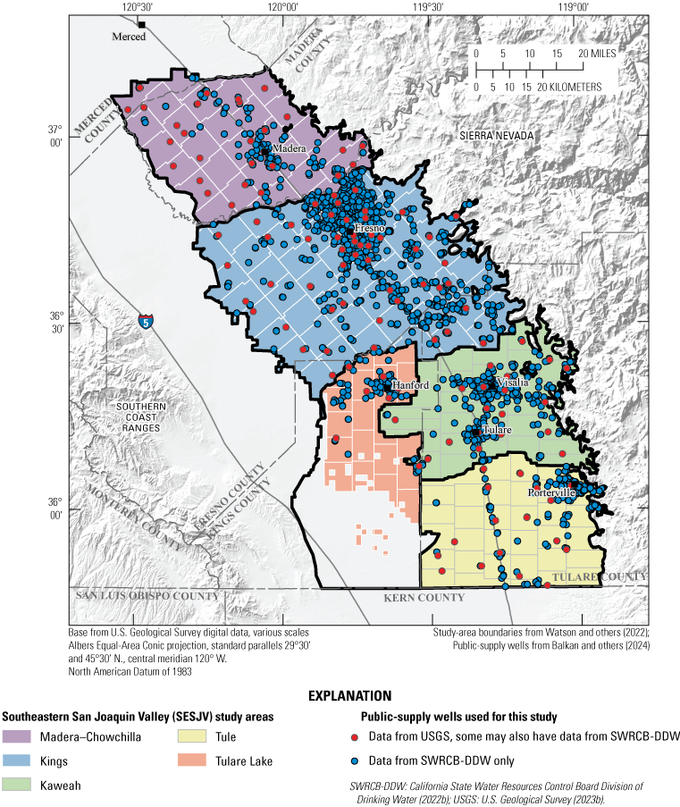
Locations of public-supply wells with water-quality data in the southeastern San Joaquin Valley during 2005–18. The wells are used to characterize the groundwater resources used for public-supply in the southeastern San Joaquin Valley (SESJV-P).

Estimated number of people served by private domestic-supply wells in 2010.
The San Joaquin Valley is a structural trough filled with thousands of feet (ft) of marine and continental sediment deposits. The continental deposits at the top of the pile consist of Pliocene, Pleistocene, and Holocene alluvial fan and fluvial deposits with some interbedded lacustrine deposits. These deposits are divided into geomorphic provinces (fig. 6; Faunt, 2009) that may not correspond exactly to chronostratigraphic periods; the dissected uplands sediment includes Pliocene and Pleistocene deposits and the other geomorphic provinces are largely comprised of Holocene deposits but may also include Pleistocene deposits. In the southeastern San Joaquin Valley, the saturated thickness of fresh groundwater in these continental deposits is generally 1,000–3,000 ft thick and is underlain by brackish and saline connate water in the marine sediments below the continental deposits (Williamson and others, 1989; Planert and Williams, 1995).
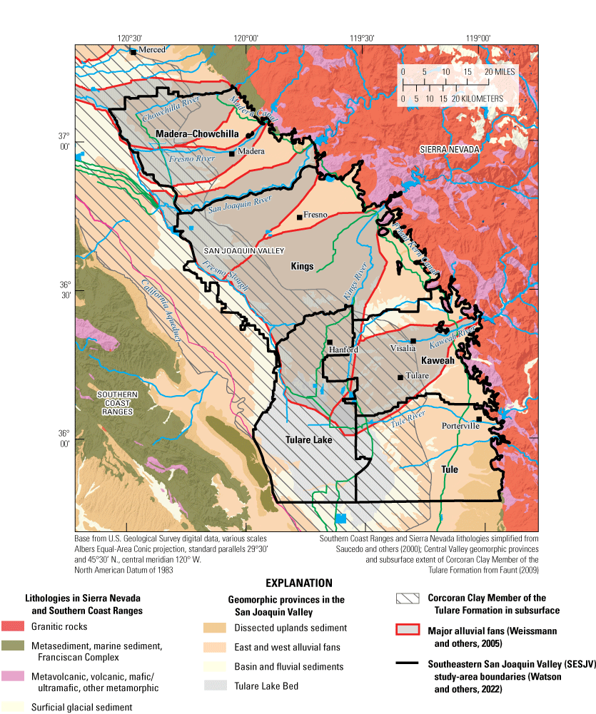
Generalized surface lithologies and geologic and geomorphic features in the southeastern San Joaquin Valley.
The freshwater-bearing part of the aquifer system in the San Joaquin Valley generally is described as a continuous, heterogenous aquifer system because the characteristics and spatial extents of specific stratigraphic units are generally poorly known (Williamson and others, 1989; Faunt, 2009). The Corcoran Clay Member of the Tulare Formation (hereinafter referred to as the “Corcoran Clay”), a laterally extensive lacustrine clay deposited during the Pleistocene, is one of the few specific stratigraphic units that is mapped across large areas of the San Joaquin Valley. The Corcoran Clay divides the freshwater groundwater system of the western part of the San Joaquin Valley (figs. 6, 7) into an upper unconfined to semi-confined system and a lower confined system (Williamson and others, 1989; Belitz and Heimes, 1990; Burow and others, 2004; Faunt, 2009). Extensive perforation of the Corcoran Clay by wellbores has increased the exchange of groundwater between these upper and lower zones (Bertoldi and others, 1991; Dubrovsky and others, 1991; Gailey, 2018).
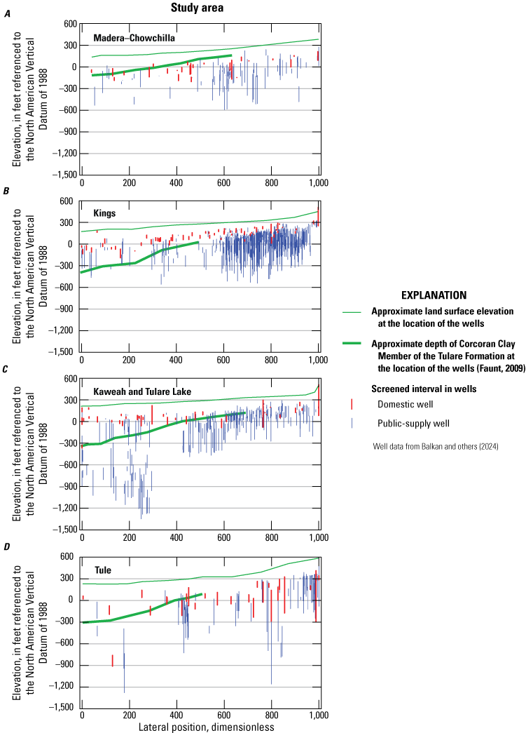
Screened intervals of domestic-supply and public-supply wells in four areas of the southeastern San Joaquin Valley. A, Madera-Chowchilla study area; B, Kings study area; C, Kaweah and Tulare Lake study areas; and D, Tule study area.
The chemical composition and hydrogeologic properties of the sediments comprising the freshwater aquifer system vary depending on the sediment provenance and depositional environment (Gronberg and others, 1998; Weissmann and others, 2005; Faunt, 2009 and references therein). In the southeastern San Joaquin Valley, the main water-bearing units are the alluvial fans deposited by streams that transport sediment from the Sierra Nevada (fig. 6). The alluvial fan deposits are composed of interlayered lenses of gravel, sand, silt, and clay. These alluvial fan deposits generally become finer with distance from the Sierra Nevada, grading into the basin deposits in the center of the San Joaquin Valley that are dominated by silts and clays. The San Joaquin, Kings, and Kaweah Rivers are large rivers that primarily drain the high elevation glaciated areas of the Sierra Nevada that have granitic bedrock; therefore, the alluvial fans are largely composed of material derived from granitic rocks (Weissmann and others, 2005). The Fresno and Chowchilla Rivers are smaller and primarily drain lower elevation watersheds where bedrock consists of a mixture of Mesozoic and Paleozoic metasedimentary and metavolcanic rocks, mafic intrusive rocks, and granitic rocks (Jennings, 1977; Saucedo and others, 2000; Weissmann and others, 2005).
Along the western side of the southeastern San Joaquin Valley, the sediments derived from the Sierra Nevada may interfinger with sediments derived from the Coast Ranges (Laudon and Belitz, 1989; Belitz and Heimes, 1990). The Coast Ranges alluvium is generally finer grained than alluvium derived from granitic rocks of the Sierra Nevada. The Coast Ranges alluvium is deposited by ephemeral and a few small perennial streams that drain areas with bedrock composited largely of marine sedimentary rocks (Gronberg and others, 1998). The western side of the southeastern San Joaquin Valley groundwater basins consists of basin deposits, and at the southern end, deposits of the Tulare Lake Bed that are generally finer grained and less permeable than the alluvial fan and fluvial deposits in the central and eastern parts of the basins (Faunt and others, 2010; fig. 6).
Groundwater flow and recharge in the San Joaquin Valley is complex and has been greatly altered by pumping for irrigation and public supply (Faunt, 2009). The conceptual model of groundwater flow in the southeastern San Joaquin Valley is based on previous studies in the San Joaquin Valley (for example, Davis and others, 1959; Burow and others, 2004, 2007, 2008; Phillips and others, 2007; Faunt, 2009). Regional lateral flow of groundwater on the eastern side of the San Joaquin Valley and within the study region is toward the southwest along the dip of the water-bearing units, and generally groundwater flows toward the axis of the San Joaquin Valley (fig. 2).
Irrigation return flows are the primary source of groundwater recharge, and groundwater pumping is the primary source of discharge from the southeastern San Joaquin Valley groundwater system during post-development conditions (Faunt, 2009). Groundwater on a lateral flow path may be extracted by pumping wells and reapplied at the surface as irrigation multiple times before reaching the San Joaquin Valley trough (Phillips and others, 2007). This recharge and discharge pattern results in a substantial increase of the downward vertical flow component compared to the downward vertical flow component during natural conditions (Burow and others, 2004; Phillips and others, 2007; Faunt, 2009). These enhanced vertical flow components accelerate vertical movement of water from recharge areas to the perforated intervals of withdrawal wells. Vertical movement may be accelerated in agricultural and urban land-use areas. Water recharged after development of the modern hydrologic system with enhanced vertical flow has reached the depth zone tapped by many drinking-water supply wells. Wells that straddle this depth zone pump a mixture of modern (recharged since about 1950) and premodern (recharged from pre-1950 to tens of thousands of years ago) water (Jurgens and others, 2016).
Groundwater pumping for agricultural and municipal use in excess of recharge has resulted in an overall decrease in groundwater levels in the southeastern San Joaquin Valley (Faunt, 2009). In the early 1900s, the center of the San Joaquin Valley was a groundwater discharge zone with artesian conditions (Mendenhall, 1908; Mendenhall and others, 1916; fig. 2). During 2000–20, groundwater levels in the southeastern San Joaquin Valley range from near surface to greater than about 250 ft below land surface (bls; Faunt, 2009; Levy and others, 2021; California Department of Water Resources, 2023c). The lowering of water levels, especially during drought periods, has resulted in shallower wells going dry and the need to deepen wells or drill new ones (California Department of Water Resources, 2003; California Department of Water Resources, 2014; Pauloo and others, 2020).
The five study areas of the southeastern San Joaquin Valley cover approximately 12,000 square kilometers (km2; table 1) in parts of Merced, Madera, Fresno, Kings, and Tulare Counties (fig. 4). The boundaries of the five study areas correspond to the boundaries of the Madera-Chowchilla, Kings, Kaweah, Tule, and Tulare Lake groundwater subbasins of the San Joaquin Valley groundwater basin during 2013–15 (California Department of Water Resources, 2003), and they also correspond to the study area boundaries used for the GAMA-PBP public-supply aquifer assessment studies during 2005–08 in the same region (Burton and others, 2012; Shelton and others, 2013). Some of the basin boundaries were modified as part of the implementation of the Sustainable Groundwater Management Act (California Department of Water Resources, 2018), but the study-area boundaries in this report were not changed to reflect these basin boundary adjustments. The boundaries of the California Department of Water Resources-defined groundwater subbasins do not correspond to watershed boundaries nor to alluvial fan boundaries.
Table 1.
Study areas and domestic and public-supply wells used for assessment of groundwater quality in the southeastern San Joaquin Valley, 2013–15, California Groundwater Ambient Monitoring and Assessment Program Priority Basin Project.[Well information is tabulated in Balkan and others (2024). Abbreviations: km2, square kilometers; USGS, U.S. Geological Survey; SWRCB-DDW, California State Water Resources Control Board Division of Drinking Water]
The study-area boundaries correspond to the boundaries of the eponymous groundwater basins (California Department of Water Resources, 2003). Study-area boundaries and grid cells are available in Watson and others (2022).
Domestic and public-supply wells in the southeastern San Joaquin Valley that are used in this study have depths ranging from less than 50 ft to greater than 1,600 ft bls, and well depths vary systematically by well type, study area, and lateral position (fig. 7). The selection of wells used in this study is described in the “Methods” section. Other than the Corcoran Clay present in the subsurface in the western part of the southeastern San Joaquin Valley, there are no readily identifiable regional stratigraphic marker horizons (Faunt, 2009); thus, the only stratigraphic categorization assigned to wells was location of the screened interval of the well relative to the Corcoran Clay. All wells used in this study are inferred to be screened in late-Pliocene, Pleistocene, and Holocene continental deposits. In general, domestic wells are shallower than public-supply wells, although the shallowest public-supply wells have depths similar to nearby domestic wells (fig. 7).
Methods
This section describes the methods used to (1) define groundwater quality using established benchmarks, (2) select wells for sampling, (3) compile water-quality data for this study and select constituents for discussion, (4) calculate aquifer-scale proportions, (5) compile data for potential explanatory factors, and (6) use statistical tests to quantify associations between water-quality constituents and potential explanatory factors and compare the water-quality and explanatory factor characteristics between domestic-supply and public-supply aquifers in the five study areas. Methods used to collect and analyze groundwater samples and associated quality-assurance protocols are reported by Shelton and Fram (2017) and Bennett and others (2017).
Groundwater Quality Defined as Relative Concentrations
Groundwater quality was defined by comparing measured concentrations in groundwater samples to the concentrations of regulatory and non-regulatory benchmarks applied to drinking water. The “relative concentration” is defined as the ratio of the concentration of a constituent measured in a groundwater sample to the concentration of a regulatory or non-regulatory benchmark used to evaluate drinking-water quality for that constituent. This framework of defining groundwater quality in terms of relative concentrations has been used in all GAMA-PBP assessments of public-supply and domestic-supply aquifers (Belitz and others, 2003, 2015; U.S. Geological Survey, 2023a) and is similar to the approach used in other studies to provide context for the concentrations of constituents in groundwater (for example, Toccalino and others, 2004; Belitz and others, 2022). The EPA and the SWRCB-DDW establish regulatory and non-regulatory benchmarks to define the quality of drinking water served to consumers by public water systems. The USGS developed benchmarks for some constituents without EPA benchmarks to increase the number of constituents for which the relative concentration approach can be used (Toccalino and others, 2004).
Concentrations are defined as “high,” ”moderate,” and “low” relative to the benchmarks. Concentrations of any constituent greater than the benchmark are defined as high. Concentrations of inorganic constituents greater than half of the benchmark and concentrations of organic constituents greater than one-tenth of the benchmark are defined as moderate. Concentrations less than moderate are defined as low. Nondetections may either be included in the low category or considered a separate category. Although more complex classifications could be devised based on the properties and sources of individual constituents, use of a single relative concentration value to separate moderate and low concentrations for each of the two primary groups of constituents provided consistent objective criteria for distinguishing constituents present at moderate, rather than low, concentrations (Fram and Belitz, 2012; Belitz and others, 2015).
The classification of a measured concentration as high, moderate, or low depends on the value of the benchmark selected. For constituents with multiple benchmarks, the comparison benchmark was selected in the following order of priority:
(1) Regulatory, health-based levels established by the SWRCB-DDW and the EPA: SWRCB-DDW and EPA maximum contaminant levels (MCL-CA and MCL-US, respectively), EPA action levels (AL-US), and SWRCB-DDW treatment technique levels (TT-CA; U.S. Environmental Protection Agency, 2018; California State Water Resources Control Board Division of Drinking Water, 2022a48). An MCL benchmark is called MCL-US if the MCL-US and MCL-CA are the same value and MCL-CA if the MCL-CA is lower than the MCL-US or the MCL-US does not exist.
(2) Aesthetic-based levels established by SWRCB-DDW: secondary maximum contaminant levels (SMCL-CA; California State Water Resources Control Board Division of Drinking Water, 2022b). The salinity indicators chloride, sulfate, and total dissolved solids (TDS) have recommended and upper SMCL-CA levels, and the values for the upper levels were used as water-quality benchmarks in this report.
(3) Non-regulatory, health-based levels established by the EPA and SWRCB-DDW: EPA human health benchmarks for pesticides (HHBPs), EPA lifetime health advisory levels (HAL-US), and SWRCB-DDW notification and response levels (RL-CA and NL-CA; U.S. Environmental Protection Agency, 2018; U.S. Environmental Protection Agency, 2021; California State Water Resources Control Board Division of Drinking Water, 2022c). The HHBP benchmarks may have both cancer and non-cancer levels; non-cancer levels were used. For constituents with both RL-CA and HAL-US benchmarks, the benchmark with the lower concentration was used as the comparison benchmark. For constituents with RL-CA, the boundary between moderate and low concentrations is defined as the SWRCB-DDW notification level (NL-CA) rather than either one-half or one-tenth the HAL-US or RL-CA benchmark used to define the boundary between high and moderate concentrations.
(4) Non-regulatory, health-based levels established by the USGS: USGS health-based screening levels (HBSLs; Norman and others, 2018). HBSLs were only used for constituents lacking EPA and SWRCB-DDW benchmarks. The HBSL benchmarks may have both cancer and non-cancer levels; non-cancer levels were used. HBSL based on toxicity data from EPA Provisional Peer-Reviewed Toxicity Values (Norman and others, 2018) were not used.
The comparison benchmarks for all constituents detected in samples collected from domestic wells are listed in tables 2, 3, and 4. Additional information about the types of benchmarks used and the listings of the benchmark values for all constituents analyzed are provided by Shelton and Fram (2017). The only exception to the hierarchy described here is manganese. Manganese has an SMCL-CA of 50 micrograms per liter (µg/L) but also is compared to the HAL-US of 300 µg/L.
Table 2.
Primary benchmark type, value, and unit, constituent type, and primary source or typical use for constituents present at moderate or high relative concentrations in domestic wells or for organic constituents detected at any concentration in more than 10 percent of the groundwater resources used for domestic supply in any of the five study areas sampled for the southeastern San Joaquin Valley groundwater quality assessment study, 2013–15, California Groundwater Ambient Monitoring and Assessment Program Priority Basin Project.[A measured concentration greater than the benchmark concentration is defined as a high relative concentration. For most constituents, a measured concentration greater than or equal to half (inorganic constituents) or one-tenth (organic constituents) the benchmark concentration but less than the benchmark concentration is defined as a moderate relative concentration. Exceptions are described in the footnotes. Benchmark type: MCL-US, U.S. Environmental Protection Agency (EPA) maximum contaminant level; MCL-CA, California State Water Resources Control Board Division of Drinking Water maximum contaminant level; SWRCB-DDW, California State Water Resources Control Board Division of Drinking Water; SMCL-CA, California State Water Resources Control Board Division of Drinking Water secondary maximum contaminant level; HAL-US, EPA lifetime health advisory level; RL-CA, California State Water Resources Control Board Division of Drinking Water response level SWRCB-DDW response level; HBSL-NC, U.S. Geological Survey (USGS) non-cancer health-based screening level; HHBP-NC, EPA non-cancer human-health benchmark for pesticides; TT-CA, SWRCB-DDW treatment technique level. Benchmark units: mg/L, milligrams per liter; µg/L, micrograms per liter; pCi/L, picocuries per liter]
Typical uses and sources from Bennett and others (2017), Shelton and Fram (2017), and Bexfield and others (2021, 2022).
Maximum contaminant level benchmarks are listed as MCL-US when the MCL-US and MCL-CA are identical and as MCL-CA when the MCL-CA is lower than the MCL-US or no MCL-US exists. Sources of benchmarks: California State Water Resources Control Board Division of Drinking Water (2022a, 2022b, 2022c), U.S. Environmental Protection Agency (2018, 2021), Norman and others (2018).
The MCL-US for gross beta particle activity is no longer an official regulatory level, but 50 pCi/L is still used by the EPA and the SWRCB-DDW as a "trigger level" to determine if further testing for specific gross-beta particle emitters is necessary (California State Water Resources Control Board, 2017a).
Manganese is categorized as both a constituent with an SMCL-CA benchmark and as a constituent with a non-regulatory health-based benchmark. When manganese is considered an SMCL-CA constituent, the boundary between high and moderate concentrations is the SMCL-CA, and the boundary between moderate and low concentrations is half the SMCL-CA. When manganese is considered a trace element with a heath-based benchmark, the boundary between high and moderate concentrations is the HAL-US, and the boundary between moderate and low concentrations is the SMCL-CA.
The low-to-moderate concentration boundary for boron is the SWRCB-DDW notification level (NL-CA) of 1,000 µg/L and not half of the primary benchmark.
The low-to-moderate concentration boundary for vanadium is the SWRCB-DDW notification level (NL-CA) of 50 µg/L and not half of the primary benchmark.
The MCL-US benchmark for trihalomethanes is for the sum of trichloromethane, bromodichloromethane, dibromochloromethane, and tribromomethane.
The low-to-moderate concentration boundary for 1,4-dioxane is the SWRCB-DDW notification level (NL-CA) of 1 µg/L and not one-tenth of the primary benchmark.
CAAT is a degradant of both simazine and atrazine (Scribner and others, 2000).
Determination of violations of the benchmarks for microbial constituents requires repeat sampling (California State Water Resources Control Board, 2019), which was not done for this study. The TT-CA for Enterococci is part of the California Ground Water Rule, which incorporates the text of the Federal Ground Water Rule (§64430 in California State Water Resources Control Board Division of Drinking Water, 2022a).
Table 3.
Primary benchmark type value and units, constituent type, and primary source or typical use for inorganic constituents detected in samples from domestic wells only at low relative concentrations or having no comparison benchmark, southeastern San Joaquin Valley groundwater quality assessment study, 2013–15, California Groundwater Ambient Monitoring and Assessment Program Priority Basin Project.[A measured concentration greater than the benchmark concentration is defined as a high relative concentration. For most constituents, a measured concentration greater than or equal to half (inorganic constituents) or one-tenth (organic constituents) the benchmark concentration but less than the benchmark concentration is defined as a moderate relative concentration. Exceptions are described in the footnotes. Benchmark type: MCL-CA, California State Water Resources Control Board Division of Drinking Water maximum contaminant level; SWRCB-DDW, California State Water Resources Control Board Division of Drinking Water; MCL-US, U.S. Environmental Protection Agency (EPA) maximum contaminant level; AL-US, EPA action level; SMCL-CA, California State Water Resources Control Board Division of Drinking Water secondary maximum contaminant level; HAL-US, EPA lifetime health advisory level; HBSL-NC, U.S. Geological Survey (USGS) non-cancer health-based screening level. Benchmark units: µg/L, micrograms per liter; mg/L, milligrams per liter; CaCO3, calcium carbonate; SiO2, silicon dioxide]
Typical uses and sources from Bennett and others (2017), Shelton and Fram (2017), and Bexfield and others (2021, 2022).
Maximum contaminant level benchmarks are listed as MCL-US when the MCL-US and MCL-CA are identical and as MCL-CA when the MCL-CA is lower than the MCL-US or no MCL-US exists. Sources of benchmarks: California State Water Resources Control Board Division of Drinking Water (2022a, 2022b, 2022c), U.S. Environmental Protection Agency (2018, 2021), Norman and others (2018).
Chromium(VI) was not analyzed in samples collected in the Madera-Chowchilla and Kings study areas. Chromium(VI) had an MCL-CA benchmark of 10 µg/L between July 2014 and September 2017 (California State Water Resources Control Board, 2022b), but the MCL-CA did not exist at the time this report was being prepared; therefore, the HBSL-NC benchmark of 20 µg/L was used instead.
Lithium has an HBSL benchmark that was not used in this study because it is based on toxicity data from EPA Provisional Peer Reviewed Toxicity Value, which are considered less reliable than the data used for other HBSL benchmarks (Belitz and others, 2022).
Table 4.
Primary benchmark type value and units, constituent type, and primary source or typical use for organic constituents detected in samples from domestic wells having no comparison benchmark or detected at only low concentrations within less than 10 percent of the groundwater resources used for domestic supply in all the five study areas sampled for the southeastern San Joaquin Valley groundwater quality assessment study, 2013–15, California Groundwater Ambient Monitoring and Assessment Program Priority Basin Project.[A measured concentration greater than the benchmark concentration is defined as a high relative concentration. For most constituents, a measured concentration greater than or equal to half (inorganic constituents) or one-tenth (organic constituents) the benchmark concentration but less than the benchmark concentration is defined as a moderate relative concentration. Exceptions are described in the footnotes. Benchmark type: MCL-CA, California State Water Resources Control Board Division of Drinking Water maximum contaminant level; SWRCB-DDW, California State Water Resources Control Board Division of Drinking Water; MCL-US, U.S. Environmental Protection Agency (EPA) maximum contaminant level; HHBP-NC, EPA non-cancer human-health benchmark for pesticides. Benchmark units: µg/L, micrograms per liter; mg/L, milligrams per liter]
Typical uses and sources from Bennett and others (2017), Shelton and Fram (2017), and Bexfield and others (2021, 202221).
Maximum contaminant level benchmarks are listed as MCL-US when the MCL-US and MCL-CA are identical and as MCL-CA when the MCL-CA is lower than the MCL-US or no MCL-US exists. Sources of benchmarks: California State Water Resources Control Board Division of Drinking Water (2022a, 2022b, 2022c), U.S. Environmental Protection Agency (2018, 2021), Norman and others (2018).
Carbendazim, metolachlor, methyl parathion, and pendimethalin were reported as detected in either Bennett and others (2017) or Shelton and Fram (2017) but are reported as not detected in this report because all detections had concentrations less than the highest method detection level used during 2013–14.
Triazine herbicides include simazine and atrazine. Some degradation products may be produced by degradation of more than one parent triazine herbicide (Scribner and others, 2000).
Well Selection
Groundwater-quality, well construction, and location data for 198 domestic wells and 124 wells representative of public-supply wells were obtained from sites sampled by the USGS for the GAMA-PBP or for the NAWQA project (table 1). Of the 124 wells representative of public-supply wells, 104 wells had public-supply well identification numbers listed in the SWRCB-DDW regulatory compliance database (Balkan and others, 2024), and 20 wells were irrigation or domestic wells with depths similar to nearby public-supply wells (Burton and Belitz, 2008; Shelton and others, 2009; Balkan and others, 2024). Data for an additional 1,577 public-supply wells were obtained from sites sampled by water agencies for regulatory compliance purposes (California State Water Resources Control Board, 2023a; California State Water Resources Control Board Division of Drinking Water, 2022d). Some of the public-supply wells sampled by the USGS also had data collected by water agencies for regulatory compliance. The 198 domestic wells were used to represent the SESJV-D, the groundwater resources used by domestic wells in the southeastern San Joaquin Valley; the 1,701 public-supply wells are used to represent the SESJV-P, the groundwater resources used by public-supply wells in the southeastern San Joaquin Valley.
Domestic Wells
The GAMA-PBP sampled 153 domestic wells in the southeastern San Joaquin Valley during 2013–15 (Bennett and others, 2017; Shelton and Fram, 2017). The wells were selected using a grid-based design to ensure that the selected wells were distributed across the entire area. Each study area was divided into equal-area grid cells (Scott, 1990), and the grid cells were used to select wells for sampling and to aggregate data in areas with greater density of sampled wells.
The grids were designed to encompass areas where domestic wells were used for drinking-water supply. Grids were constructed to cover the entire Madera-Chowchilla, Kings, Kaweah, and Tule study areas because domestic wells were distributed across nearly the entire study area (Johnson and Belitz, 2015). Few domestic wells were located in the southern part of the Tulare Lake study area, and to avoid having grid cells without wells available for sampling, the gridded area was defined as a subset of the study area. This subset was defined as the aggregate of all 1-square mile (mi2) public land survey sections estimated to contain a non-zero number of domestic wells by Johnson and Belitz (2015). Figure 5 shows the estimated locations of people using domestic wells in 2010 (Johnson and others, 2019). Some parts of the Tulare Lake study area that were included in the gridded area, based on estimated locations of domestic wells by Johnson and Belitz (2015), were estimated to have no domestic wells in 2010. The Madera-Chowchilla and Kings study areas were divided into 80-km2 grid cells, and the Kaweah, Tule, and Tulare Lake study areas were divided into 60-km2 grid cells (fig. 8). Grid cells may be composed of non-contiguous pieces, and the number of cells in each study area ranged from 49 to 18 (table 1).

Locations of grid cells and domestic-supply wells sampled in the southeastern San Joaquin Valley, 2013–15. The wells are used to characterize the groundwater resources used for domestic-supply in the southeastern San Joaquin Valley. Well identification numbers are shown on figure 1.1.
Wells were selected from lists of domestic wells compiled from three sources: (1) wells used by small water systems registered with County health departments or with the SWRCB-DDW, (2) domestic wells previously sampled by the USGS or the SWRCB GAMA program, and (3) domestic wells with well-completion reports filed with the California Department of Water Resources.
Water systems serving fewer than 25 people and having fewer than 15 service connections are classified as “State small systems” (California State Water Resources Control Board, 2021), and these systems were not included in the earlier GAMA-PBP assessments of groundwater resources used by public-supply wells. State small systems generally consist of one well serving several households, and the wells generally have depths similar to the depths of domestic wells serving individual households in the same area. The absence of water-quality data for State small water systems was identified as a critical information gap by the SWRCB (California State Water Resources Control Board, 2013). Wells belonging to public systems serving fewer than about 300 people also were considered as potential targets if the wells had depths similar to nearby domestic wells. Domestic wells previously sampled in 2006 by the SWRCB for a study of water quality in domestic wells in Tulare County (California State Water Resources Control Board, 2016) and domestic wells with previous water-quality or water-level data in the USGS National Water Information System (NWIS; U.S. Geological Survey, 2023b) were included as potential targets because we assumed that previously sampled wells would likely meet the criteria for sampling in this study. Domestic wells with well-completion reports in the California Department of Water Resources library of scanned images of well-completion reports (Online System for Well Completion Reports [OSWCR]; California Department of Water Resources, 2023b) provided several potential target wells. The OSWCR system locates wells at the centroid of the 1-mi2 township-range-sections; for this study, many of the wells were assigned point locations using well addresses or other location information from the well-completion report (Stork and others, 2019).
Sites with potential wells on the target list were visited by USGS field personnel, beginning with the well nearest to a randomly selected location in the grid cell to ensure random selection of wells. Door-to-door canvassing continued until permission was obtained to sample a well meeting the criteria for the study or until all potential target wells on the list for that cell were exhausted. The criteria were as follows: (1) water is used for domestic drinking-water supply, (2) a well-completion report or other documentation of well depth is available, (3) samples could be collected upstream from treatment systems or tanks, and (4) the well has the capacity to pump for long enough to properly purge the well and collect the sample (Bennett and others, 2017; Shelton and Fram, 2017175).
The 5 study areas contained a total of 157 cells, and wells in 140 of the cells were sampled (fig. 8; appendix 1). For several cells that did not have available wells, a well less than 1 mile outside of the cell was selected to represent the cell (Bennett and others, 2017; Shelton and Fram, 2017). However, for consistency with Belitz and others (2015), these wells were reassigned to the cell in which they were located for this report. The 153 wells sampled for this study included 139 private domestic wells, 5 State small system or small public-supply system wells, 3 irrigation wells, and 6 monitoring wells (Stork and Fram, 2021; Balkan and others, 2024).
Irrigation and monitoring wells were sampled only when permission could not be obtained for domestic wells and when the well depths were similar to the depths of domestic wells within the township-range sections closest to the well. Depths of wells in nearby sections were obtained from Stork and others (2019). Two irrigation wells originally sampled as grid wells representing the domestic-well aquifer in the Tule study area (TLE01 and TLE08; Bennett and others, 2017) were not counted as grid wells in this report. Well TLE08 is more than 1,000 ft deeper than nearby domestic wells, and well TLE01 is in a grid cell without domestic wells, indicating that the resource was not used for domestic drinking-water supply. In addition, TLE01 and TLE08 were sampled as grid wells, TULE-11 and TULE-12, respectively, for the GAMA-PBP public-supply aquifer assessment (Burton and Belitz, 2008; Burton and others, 2012). Two of the State small system wells sampled as grid wells for the domestic-well study also were sampled as grid wells in the GAMA-PBP public-supply aquifer assessment study (TLE02 and TLE16 are the same as TULE-15 and TULE-13, respectively). However, nearby public-supply and domestic wells had similar depths; therefore, these wells were retained as grid wells for public-supply and domestic-supply aquifer assessments.
Wells were named with an alphanumeric GAMA identification code that consisted of a prefix identifying the type of GAMA-PBP study, the study unit, the study area the well was originally sampled, and a numeric suffix (appendix 1). For logistical purposes, the five study areas in this report were sampled as part of two study units in successive years, S3_MACK in 2013–14 and S4_TUSK in 2014–15. Because the study unit names are not relevant to this report, the study unit prefixes are omitted when sites are labeled on figures or discussed in this report.
Wells in the Madera-Chowchilla and Kings study areas were sampled between August 2013 and April 2014, and wells in the Kaweah, Tule, and Tulare Lake study areas were sampled between November 2014 and August 2015. The 2014–15 study also included sampling of 20 wells in the Sierra Nevada foothills east of the Kaweah and Tule study areas, referred to as the “Highlands study area” in Bennett and others (2017). Only the three sites with mapped locations within the boundary of the Kaweah study area are included in this report.
The details of methods used to collect and analyze the samples are described in Shelton and Fram (2017) and Bennett and others (2017). Field sample collection methods followed the USGS National Field Manual (U.S. Geological Survey, variously dated), with minor modifications to protocols. The primary modification was that samples were collected close to the well, using sampling lines that were approximately 0.5 meter (m) in length, and sampling chambers were not used. The USGS National Field Manual describes sampling lines approximately 10–20 m in length that are routed from the well into a sampling chamber inside a mobile laboratory. The purpose of the sampling chamber is ostensibly to protect the sample from contamination from the atmosphere during sampling, particularly for trace element and volatile organic carbon (VOC) samples. For VOCs, Fram and others (2012) determined that sampling with short lines and no sampling chambers resulted in less contamination of field blanks with VOCs than sampling with long lines and sampling chambers. Field blanks collected by the GAMA-PBP had substantially lower detection frequencies of contamination with VOCs than field blanks collected contemporaneously by other USGS projects that required use of long sampling lines and sampling chambers (Fram and others, 2012). Detection frequencies of trace elements in field blanks collected by the GAMA-PBP are consistently low and indicative of contact with metal fittings in the sampling equipment being the primary source of contamination, not airborne particles (Olsen and others, 2010; Bennett, 2020).
To increase the spatial density of data, 45 additional domestic wells sampled by the USGS NAWQA project between April 2013 and August 2015 were included in the dataset for this report, increasing the number of cells with at least 1 well to 142 cells. This inclusion increased the number of wells per cell for 32 cells that already had wells sampled for the GAMA-PBP (fig. 8; appendix 1, tables 1.1–1.5). These additional wells are part of the NAWQA networks representing the regional San Joaquin Valley aquifer system (SANJSUS1; Burow and others, 1998a; Arnold and others, 2018), orchard, vineyard, and row crop land use in the San Joaquin Valley (SANJLUSCR1A, SANJLUSOR1A; Burow and others, 1998b; Arnold and others, 2016), and a regional flow path across the Kings groundwater subbasin (CVALFPS1, CVALFPS2; appendix 1). The well selection process and methods of groundwater sample collection and analysis used by NAWQA were similar to those used by GAMA-PBP. Wells were named with an alphanumeric code that consisted of the network name and a sequence number. Because the network names are not relevant to this report, the NAWQA sites were assigned short names for this report: the prefix “NQ” and a sequence number. The full and short site names are listed in appendix tables 1.1–1.5 (appendix 1) and in Balkan and others (2024).
Public-Supply Wells
Two sources of data for public-supply wells were used for this study: (1) data from wells sampled by the USGS for the GAMA-PBP or NAWQA projects and (2) data from wells sampled for regulatory compliance by water agencies and submitted to the SWRCB-DDW. The GAMA-PBP sampled 119 public-supply wells for assessment studies in these areas during 2005–08 (Burton and others, 2012; Shelton and others, 2013) and resampled approximately 20 percent of the wells during 2008–17 (Jurgens and others, 2018). Another five public-supply wells were sampled as part of the NAWQA CVALFPS2 network in 2014 (appendix 1). The SWRCB-DDW database contained data for 69,283 samples from 1,681 public-supply wells sampled during October 2005–October 2018 (California State Water Resources Control Board, 2023b; California State Water Resources Control Board Division of Drinking Water, 2022d). Wells with data in both databases were matched using the SWRCB-DDW public supply code (PSCODE). All wells were assigned to cells based on latitude and longitude. There were 1,701 public-supply wells with water-quality data distributed across 135 cells with 1–112 wells per cell (median is 7 wells per cell; Balkan and others, 2024). Well-construction information for public-supply wells were compiled by Levy and Borkovich (2022).
Water-Quality Data
Samples collected by the USGS were analyzed for approximately 375 constituents, including field water-quality parameters, major ions, trace elements, nutrients, VOCs, pesticides, a set of isotopic and groundwater age dating tracers, and other constituents of particular interest in the State of California (Bennett and others, 2017; Shelton and Fram, 2017). The results for organic constituents are based on 183 domestic wells rather than the 198 domestic wells used for the results on inorganic constituents because some of the wells sampled for the NAWQA studies were not analyzed for organic constituents.
Samples collected at public-supply wells by water agencies for regulatory compliance data reported to the SWRCB-DDW were analyzed for fewer constituents. Regulatory compliance sampling primarily is focused on constituents for which concentrations are regulated in public drinking-water supplies; analyses of unregulated constituents and geochemical and age-dating tracers are not systematically included.
All published and quality-assured water-quality data collected by the USGS are available online from multiple sources: the USGS GAMA-PBP website (Jurgens and others, 2018), the SWRCB GAMA Groundwater Information System (California State Water Resources Control Board, 2023b), the USGS NWIS web interface (U.S. Geological Survey, 2023b), and published reports (Arnold and others, 2016, 2018; Bennett and others, 2017; Shelton and Fram, 2017). The authoritative source of USGS data is NWIS (U.S. Geological Survey, 2023b); published reports represent a snapshot of data in NWIS at the time of publication. All data compiled from the SWRCB-DDW are available online from SWRCB GAMA Groundwater Information System (California State Water Resources Control Board, 2023b) and directly from SWRCB-DDW (California State Water Resources Control Board Division of Drinking Water, 2022d).
U.S. Geological Survey data for organic constituents were censored to meet GAMA-PBP data-quality objectives. Detections that were reported to NWIS that have concentrations less than the method detection level were re-coded as nondetections (Fram and Stork, 2019; Fram, 2020; Bexfield and others, 2021, 2022). Because sampled collection dates spanned 3 years, detection levels for some constituents changed, and the highest detection level used during the period was used to censor all the data. Note that NWIS reports nondetections as less than the reporting level, and the reporting level is commonly twice the detection level (Foreman and others, 2021). For example, for 1,2,3-trichloropropane (1,2,3-TCP), the reporting level at the time the domestic well samples were analyzed was 0.006 µg/L, and the method detection level was 0.003 µg/L. For this study, the USGS data were censored such that detections with concentrations less than 0.003 microgram per liter (µg/L) were recoded as nondetections. Before 2014, some USGS samples were analyzed for 1,2,3-TCP with a method that had a reporting level of 0.18 µg/L; nondetections in samples analyzed by this method were removed from the dataset.
Many wells have been sampled more than once, and because evaluation of trends in water quality was not part of this study, one sample was selected to represent each well. For the 198 wells representing the domestic-supply aquifer, each well was sampled once between July 2013 and August 2015, and that sample was used to represent the well. For the 1,701 wells representing the public-supply aquifer, a “pseudosample” was constructed for each well (Levy and Fram, 2021); for each constituent, the analysis from the date closest to June 26, 2014 (the midpoint of the GAMA-PBP domestic well sampling period), was selected to represent the well. Sample collection was during October 2005 through October 2018. The earliest date of October 2005 was selected to include the data collected for Burton and others (2012). The pseudosample may consist of data from samples collected on different dates because samples may only be analyzed for a subset of constituents at each sampling date. About 60 percent of the data in the pseudosamples for public-supply wells were from samples collected within the same 2-year time interval as the domestic well sampling, and 85 percent of the data were collected within an 8-year window (2010–18) centered on the midpoint date of the GAMA-PBP domestic well sampling. Most of the data derived from samples outside of this 8-year window were from public-supply wells that did not have more recent data for all constituents in the SWRCB-DDW database and were sampled by the USGS during 2008–10.
Data collected by the USGS and data compiled from SWRCB-DDW are reported with different reporting levels, which affects the comparisons that can be made between water quality in the domestic-supply aquifer (based on only USGS data) and the public-supply aquifer (based on a combination of USGS and SWRCB-DDW data). For all inorganic constituents, reporting levels used by USGS laboratories are lower than the reporting levels in the SWRCB-DDW database (Burton and others, 2012). However, for all inorganic constituents except perchlorate, the USGS and SWRCB-DDW data selected for public-supply well pseudosamples had reporting levels with concentrations lower than the boundary between moderate and low concentrations for the constituent. Nondetections that were reported relative to raised reporting levels with concentrations greater than the boundary were removed from the data compilation before selection of data for the pseudosamples. Because the data analysis in this study does not distinguish between low concentrations and nondetections for inorganic constituents, the difference between USGS and SWRCB-DDW reporting levels did not affect use of inorganic constituent data, except for perchlorate data.
The differences in reporting levels for perchlorate limited comparisons. The SWRCB-DDW reporting level for perchlorate generally was 4 µg/L, which is sufficient to identify high concentrations above the MCL-CA of 6 µg/L but not to distinguish between moderate and low concentrations. The USGS reporting level was 0.1 µg/L for the domestic-well samples and either 0.1 or 0.5 µg/L for the public-supply well samples. Aquifer-scale proportions of high, moderate, and low concentrations and detection frequencies are compared among the domestic-supply aquifer study areas, but the only comparisons made between the domestic-supply and public-supply aquifer study areas are for the proportion of high concentrations. Review of the SWRCB-DDW data for perchlorate identified potential errors in reporting nondetections where some nondetections appeared to have been reported as detections at the reporting level of 4 µg/L. This type of data-reporting error was suspected because the dataset includes several instances where multiple wells belonging to a single water agency sampled during the same week all had results of detection at a concentration of 4 µg/L, and previous and subsequent samples from the same wells all had results of nondetection reported with a concentration of 0 µg/L. This type of reporting error would cause overestimation of the prevalence of moderate concentrations of perchlorate. Limiting the use of the SWRCB-DDW perchlorate data to only identify high concentrations eliminated the need to further investigate this potential data-reporting issue.
Uranium can be measured using either mass units (µg/L) or in radioactivity units (picocuries per liter, pCi/L). The uranium data collected by USGS and used in this report were measured in mass units. The SWRCB-DDW dataset includes both types of uranium data; uranium in units of pCi/L was converted to mass units using the conversion factor 0.67 picocuries per liter per microgram (pCi/µg).
The SWRCB-DDW reporting levels for most organic constituents were several orders of magnitude higher than the USGS detections levels, and the SWRCB-DDW reporting levels for many organic constituents have concentrations greater than the boundary between low and moderate concentrations. Thus, aquifer-scale proportions of high, moderate, and low concentrations and detection frequencies are compared among the domestic-supply aquifer study areas, but the only comparisons made between the domestic-supply and public-supply aquifer study areas were for the proportion of high concentrations. Review of the SWRCB-DDW data for organic constituents identified potential errors in reporting nondetections, where some nondetections appeared to have been reported as detections at the reporting level. This type of data-reporting error was suspected because the dataset includes many instances where a single sample was reported as having detections of multiple organic constituents, with all detections having concentrations equal to the reporting level. In addition, previous and subsequent samples from the same well had results of nondetection reported with a concentration of 0 µg/L for all of the constituents. Because the SWRCB-DDW reporting levels for many organic constituents are in the range of moderate concentrations, this type of reporting error would cause over-estimation of the prevalence of moderate concentrations of organic constituents. Limiting the use of the SWRCB-DDW dataset to only identifying high concentrations eliminated the need to further investigate this potential data-reporting issue.
The following criteria were used to select constituents for discussion in this report. Of the approximately 375 constituents analyzed, approximately half had a comparison benchmark and were therefore included in the assessment of water quality. Assessment results are presented for the 34 constituents that were detected at moderate or high concentrations in at least 1 domestic well or for organic constituents detected at a frequency of greater than 10 percent in domestic wells in any of the 5 study areas (table 2). Constituents detected only at low concentrations in samples from domestic wells and detected constituents lacking benchmarks are listed in tables 3 and 4. Constituents analyzed but not detected are listed in Bennett and others (2017) and Shelton and Fram (2017). A few pesticides and pesticide degradate constituents reported as detected in one or two wells in Bennett and others (2017) or Shelton and Fram (2017) are not reported as detected in this study because the concentrations were below the highest detection level used during 2013–15. A subset of the constituents listed in table 2 were selected for identification of natural and human factors that may affect concentrations of the constituents in samples from domestic wells. This subset included most constituents present at high concentrations in greater than approximately 5 percent of the domestic-supply aquifer.
The regulatory benchmarks for microbial indicator constituents specify evaluation of results from repeat sampling, which was not done for this study. Results are presented for microbial indicator constituents detected in at least one domestic well in the one-time sampling done by GAMA-PBP (table 2). The field parameter specific conductance (SC) was detected at values above the SMCL-CA benchmark, but results are not presented. All the domestic wells had data for SC and TDS. All samples with concentrations of TDS above the upper SMCL-CA benchmark for TDS (high) also had values of SC above the upper SMCL-CA benchmark for SC; all samples with concentrations of TDS between the recommended and upper SMCL-CA benchmark for TDS (moderate) also had values of SC between the recommended and upper SMCL-CA benchmark for SC (Bennett and others, 2017; Shelton and Fram, 2017). A few public-supply wells had SC data but lacked TDS data; these wells were assigned to the categories of high, moderate, or low TDS based on the SC values. Values of pH outside of the SMCL-CA range of 6.5–8.5 standard units were detected, but the framework of high, moderate, and low values relative to a benchmark was not applicable to a benchmark that is defined as a range of values. In this report, pH is used as a potential explanatory factor rather than as a water-quality constituent.
Calculation of Aquifer-Scale Proportions
This report uses aquifer-scale proportions to characterize the water quality in the groundwater resources used by domestic and public-supply wells in each of the five study areas and in the entire southeastern San Joaquin Valley. Aquifer-scale proportion is defined as the areal proportion of a study area that has a specified groundwater quality (Belitz and others, 2010). In other words, aquifer-scale proportion is the percentage of the area of a study area that has a specified groundwater quality; aquifer-scale proportion does not refer to a percentage of the volume of the groundwater resource in the study area. In this report, the specified groundwater-quality conditions are categories of concentrations of individual constituents or classes of constituents: high, moderate, or low concentrations relative to an established benchmark. Aquifer-scale proportions are calculated separately for domestic and public-supply wells in each study area to facilitate comparison of water quality in the groundwater resources used by the two types of wells. The proportions are areal proportions, not volumetric proportions, because the depths of the wells are not considered in the calculations. In the southeastern San Joaquin Valley, public-supply wells generally are deeper than domestic wells (fig. 7); therefore, the aquifer-scale proportion calculated from the public-supply wells generally characterizes the water quality in a deeper part of the aquifer system within a study area than the aquifer-scale proportion calculated from the domestic wells in the same study area.
The calculations of aquifer-scale proportions are based on the equal-area grids drawn for each of the five study areas (fig. 8). In a grid-based approach, one well would be sampled per grid cell, and the aquifer-scale proportion of the specified water quality would be the same as the detection frequency of the specified water quality in the grid wells. However, as explained in the “Well Selection” section, the inclusion of the wells sampled by NAWQA and the reassignment of wells sampled by GAMA-PBP to the cells in which they are located resulted in up to four domestic wells in some cells, and the combination of the wells sampled by the USGS and the wells with data from SWRCB-DDW resulted in multiple public-supply wells in most cells (fig. 4). These additional wells increased the likelihood that the range of water-quality conditions present in the groundwater resource were represented in the dataset, particularly conditions present in only small proportions of the resource (Belitz and others, 2010).
The calculations of aquifer-scale proportions for study areas having multiple wells per grid cell are done with cell declustering (Isaaks and Srivastava, 1989), also called spatial weighting (Belitz and others, 2010), to ensure that the calculated proportion remains a spatially unbiased areal proportion. An aquifer-scale proportion of high concentrations calculated using spatial weighting is not the same as the percentage of wells with high concentrations (Belitz and others, 2010; appendix B in Fram and Belitz, 2012).
Spatially weighted aquifer-scale proportions are calculated by computing the proportion of wells with the specified water quality in each cell and then averaging those proportions in all the cells in the study area (eq. 1; Isaaks and Srivastava, 1989; Belitz and others, 2010). In this report, aquifer-scale proportions were calculated for the proportions of each study area with high, moderate, and low concentrations of individual constituents or constituent classes. To simplify the explanation, equation 1 is written in terms of the proportion with high concentrations of a constituent, and the same equation was used to calculate proportions with moderate and low concentrations by substituting the counts of the numbers of wells in each cell that had high concentrations with the numbers of wells in each cell that had moderate or low concentrations.
whereis the proportion of study area that had high concentrations of the constituent,
is the number of wells in cell c that had high concentrations of the constituent,
is the number of wells in cell c that had data for the constituent, and
is the number of cells in the study area that had at least one well with data for the constituent.
Equation 1 also was used to calculate spatially weighted detection frequencies for organic constituents by substituting the counts of the numbers of wells in each cell with detection of the constituent at any concentration for the counts of the numbers of wells in each cell with high concentrations (Wchigh). The spatially weighted detection frequencies for organic constituents calculated in this report for the five study units are not the same as the detection frequencies reported in Burton and others (2012), Shelton and others (2013), Fram (2017b), and Fram and Shelton (2018). The detection frequencies in the earlier reports were grid-based detection frequencies calculated from the one-well-per-cell sampling by GAMA-PBP. The spatially weighted detection frequencies used all wells sampled by the USGS.
Aquifer-scale proportions in the entire southeastern San Joaquin Valley were calculated as an area-weighted combination of the results in the five study areas (eq. 2). An area-weighted combination was required because the cell sizes were not the same in all the study areas (table 1). If equation 1 were applied to the entire southeastern San Joaquin Valley directly, the resulting aquifer-scale proportions would be biased toward the study areas with the smaller cell sizes (appendix B in Fram and Belitz, 2012).
whereis the proportion of the southeastern San Joaquin Valley that had high concentrations of the constituent,
is the number of cells in the study area that had at least one well with data for the constituent,
is the area of a cell in the study area (table 1).
is the proportion of study area that had high concentrations of the constituent.
Calculations of aquifer-scale proportions were made for individual constituents and for classes of constituents. Each constituent class was represented by the constituent with the maximum relative concentration. For example, a well having a high relative concentration for arsenic, moderate relative concentration for fluoride, and low relative concentrations for molybdenum, boron, selenium, and other trace elements would be counted as having a high relative concentration for the class of trace elements with health-based benchmarks because it had a high relative concentration for arsenic. Many public-supply wells were analyzed for only a subset of the constituents; for example, 1,664 public-supply wells had data for nitrate, whereas only 95 had data for gross beta particle activity. These differences in data availability between constituents could have affected the results when constituents were aggregated into classes; therefore, only wells with data for key constituents were used to calculate aquifer-scale proportions of constituent classes (Fram and Belitz, 2014). For example, aquifer-scale proportions for the class of inorganic constituents with MCL benchmarks were calculated using only wells that had data for both nitrate and arsenic.
The aquifer-scale proportions of high, moderate, and low concentrations depend on the selection of comparison benchmarks. For example, the aquifer-scale proportions of high, moderate, and low concentrations of fumigants in public-supply aquifers for the five study areas calculated for this report were not directly comparable to those presented in Burton and others (2012) and Shelton and others (2013). In those earlier reports, the HAL-US benchmark of 40 µg/L for 1,2,3-TCP was used, whereas in this report, the MCL-CA of 0.005 µg/L that was established in 2014 was used (California State Water Resources Control Board, 2017a). Because of the change in the benchmark, the proportions of high and moderate concentrations for 1,2,3-TCP, the class of fumigants, and the class of organic constituents in the public-supply well aquifer are much greater in this report even though the datasets used in this report and the previous reports are similar.
Potential Explanatory Factors
Characteristics of the SESJV-D and the five study areas within it are described using explanatory factor data compiled for the 198 domestic wells. Data were compiled for three types of potential explanatory factors: (1) hydrogeology and position in the flow system, (2) land-use characteristics, and (3) geochemical conditions and groundwater age. Characteristics of the SESJV-P and the five study areas within it are described using explanatory factors compiled for the 1,701 public-supply wells, although data were not available for all factors for all wells (Balkan and others, 2024). The methods used to compile the data for most of the potential explanatory factors are described in detail in previous reports in this series (Burton and others, 2012; Shelton and others, 2013; Fram, 2017a; Levy and Fram, 2021; Bennett, 2017, 2022; Harkness, 2023) and in the data release that accompanies this report (Balkan and others, 2024). Brief summaries are provided in this report; longer descriptions are only provided for factors that are not described in detail elsewhere.
Well-construction data for the domestic wells primarily were obtained from well-completion reports filed with the California Department of Water Resources (Stork and others, 2019; California Department of Water Resources, 2023b). In some cases, well-construction data were obtained from ancillary records of site owners or from the USGS NWIS (U.S. Geological Survey, 2023b). As expected from the location of the wells in the Central Valley, lithologic descriptions on well completion reports indicated nearly all wells penetrated sediments consisting of some combination of clays, silts, sands, gravels, and cobbles. A few wells near the boundary between the Central Valley and the Sierra Nevada penetrate granitic or metamorphic rocks below the surficial sediment cover (Balkan and others, 2024). Well-construction data for public-supply wells were obtained from the compilation of Levy and Borkovich (2022). Well-completion reports and well-construction data can contain up to three measures of well depth for each well. For this report, “well depth” is defined as depth to the bottom of the lowermost screened or open interval, if available, or as depth of the finished well if screen interval depth data are not available, or as depth of the drilled hole if screened interval and finished well depth data are not available.
Position relative to the Corcoran Clay (above, below, or outside) was estimated by comparing the well depth information to the depth of the top and bottom of the Corcoran Clay layer from Faunt (2009) at the location of the well. Wells that were not in the region with the Corcoran Clay in the subsurface (figs. 6, 7) were classified as “Outside.” Wells screened entirely above or within and above the Corcoran Clay were classified as “above.” Wells screened entirely below or within and below the Corcoran Clay were classified as “below.” Two SESJV-D wells were screened both above and below the Corcoran Clay (TLE10, TLE11) and were classified as “above” because most of the screened interval was above the Corcoran Clay. Two SESJV-D wells with well depth information but no information for top of screen (M09 and KAW10) were classified as “below” because even if the top of screen was at the land surface, most of the screened interval would be below the Corcoran Clay.
To represent areas of coarse-grained sediments, which may be more vulnerable to contamination originating from the land surface, sediment texture was determined for domestic well locations (Balkan and others, 2024). Using well-completion reports and geophysical logs, Faunt and others (2010) developed the distribution of sediment texture at 1-mi2 resolution for the Central Valley Hydrologic Model (CVHM; Faunt, 2009). The texture variable used in this report was defined as the average percentage of coarse-grained sediment present in the upper part of aquifer system that generally corresponds to the depth zone of domestic wells (see fig. 6 in Faunt and others, 2010). Areas with greater percentages of coarse-grained sediment generally have higher hydraulic conductivity and transmissivity, which could affect geochemical conditions and transport of constituents.
The normalized lateral position was calculated as the ratio of the distance from the well to the valley trough and the total distance from the valley trough to the valley margin on the east or west side of the valley (McPherson and Faunt, 2023). The valley trough was assigned a value of 0, and the valley margin was assigned a value of 1,000 (fig. 2). All sites in this study are in the valley trough or on the eastern side of the valley.
Elevation was determined at each well site in the southeastern San Joaquin Valley from the USGS National Elevation Dataset (U.S. Geological Survey, 2006). Land-surface elevations are reported in feet relative to the North American Vertical Datum of 1988 (NAVD 88).
The aridity index at each well site is defined as the ratio of average annual precipitation (PRISM Climate Group, 2022) to average annual potential evapotranspiration (California Irrigation Management Information System, 2005; Flint and Flint, 2007). High values of aridity index correspond to wetter conditions. All SESJV-D sites had aridity indices in the range of arid (0.05–0.20) or semiarid (0.20–0.50; United Nations Environment Programme, 1997).
Land-use characteristics (percentages of agricultural, natural, and urban land used, percentage of orchard vineyard land use, and average densities of underground storage tanks and septic tanks) were calculated for the areas within 500-m buffers around each well location. Percentages of urban, agricultural, and natural land use were computed from the 2011 National Land Cover Dataset (Jin and others, 2013). The 16 land-cover classes in the dataset were condensed into 3 classes. The percentage of orchard and vineyard land use was computed from the 1992 National Land Cover Dataset (Nakagaki and Wolock, 2005; Nakagaki and others, 2007146) because orchard and vineyard land use was not distinguished as a separate category from other crops in the 2011 National Land Cover Dataset. Previous studies have identified orchard and vineyard land use as an important explanatory factor for understanding the distribution of fumigants and other constituents in groundwater in the southeastern San Joaquin Valley (Burow and others, 1998a, 1998b, 1999, 2007, 2008; Burton and others, 2012; Shelton and others, 2013). Because of changes in land use between 1992 and 2011, the percentage of orchard and vineyard land use in 1992 may not be representative of the percentage in 2011.
The density of underground storage tanks was computed using spatial interpolation based on data from the State Water Resources Control Board database of environmental cleanup sites (California State Water Resources Control Board, 2007). The mean density of septic tanks was computed based on the 1990 Census of Population and Housing (U.S. Census Bureau, 1992).
Groundwater ages were classified as “modern,” “mixed,” or “premodern” using tritium and carbon-14 activities. A classification system based only on tritium activities (Lindsey and others, 2019) was used as a starting point for assigning groundwater-age classifications. Modern groundwater is water that recharged after approximately 1950; premodern groundwater is water that recharged before 1950, including water that recharged hundreds to thousands of years ago. Mixed groundwater contains modern and premodern groundwater. Threshold values of 0.3 tritium units (TU) for the boundary between premodern and mixed and 2.0 TU for the boundary between mixed and modern in 2014 were determined using the method in Lindsey and others (2019) and data for tritium in precipitation at the latitude and longitude of the southeastern San Joaquin Valley from Michel and others (2018) and Jurgens (2018). Measured tritium activities were decay-corrected to the value the sample would have had in June 2014 and then assigned to modern, mixed, and premodern categories using the threshold values. Of the 320 samples from domestic and public-supply wells with tritium data, 224 had carbon-14 data. The initial tritium-based classification was modified using carbon-14; samples that were modern in the tritium-based classification but had uncorrected carbon-14 activities of less than 85-percent modern carbon (pmC) were reclassified as mixed, and samples that were premodern in the tritium-based classification but had uncorrected carbon-14 activities greater than 85 pmC were reclassified as mixed. The threshold of 85 pmC for uncorrected carbon-14 was selected for consistency with Faulkner and Jurgens (2022) and Faulkner and others (2023). Only 10 samples were reclassified using carbon-14 (less than 5 percent of samples), thus the potential for misclassification of the samples that did not have carbon-14 data was considered small.
Groundwater oxidation-reduction (redox) conditions were classified as “oxic,” “mixed,” or “anoxic” using a modified version of the system presented by McMahon and Chapelle (2008) and Jurgens and others (2009). Most samples with dissolved oxygen concentrations greater than 0.5 milligrams per liter (mg/L) were classified as “oxic.” Samples with dissolved oxygen concentrations greater than 0.5 mg/L that had manganese concentrations greater than 50 µg/L or iron concentrations greater than 100 µg/L were classified as “mixed.” All samples with dissolved oxygen concentrations less than 0.5 mg/L were classified as anoxic. For most statistical tests, the mixed and anoxic categories were combined. Mixed redox samples may indicate groundwater mixing in wells whose screens span oxic and anoxic zones in the aquifer. Most mixed samples had dissolved oxygen concentrations less than 2.0 mg/L. Redox classification was only done for wells sampled by USGS because data for dissolved oxygen concentrations are not available in the SWRCB-DDW dataset.
Statistical and Graphical Methods
Nonparametric statistical methods were used to (1) quantify associations among potential explanatory factors and water-quality constituents for the 198 wells representing the domestic-supply aquifer and (2) compare hydrogeologic characteristics of the domestic-supply aquifers to the hydrogeologic characteristics of the public-supply aquifers. Hydrogeologic characteristics of the domestic-supply and public-supply aquifers in the five study areas were evaluated to identify differences that could explain observed differences in groundwater quality between domestic-supply and public-supply aquifers in the five study areas. Nonparametric statistics are rank-based and robust to the effects of non-normality and outliers, which are commonly observed in groundwater-quality data (Helsel and others, 2020). A level of significance (α) of 0.05 was used to evaluate probability values (p-values) for statistical hypothesis tests, where p-values less than α resulted in rejection of the null hypothesis.
Three types of statistical analyses were used because water-quality constituents and explanatory factors included continuous and categorical variables. Continuous variables can have any value within a given interval: for example, well depth is a continuous variable because it theoretically can have any value between the depth of the shallowest well and the depth of the deepest well. Categorical variables are factor variables that have a finite number of possible discrete values: for example, position of the screened interval in the well relative to the Corcoran Clay is a categorical variable because wells are assigned one of only three values (above the Corcoran Clay, below the Corcoran Clay, or outside of the area where the Corcoran Clay is present in the subsurface; Balkan and others, 2024). Concentrations of water-quality constituents were treated as continuous variables. The dataset for each constituent was censored to a single detection level, and zeros were substituted for the non-detections in test calculations. Substitution is acceptable in rank-based statistical tests when the dataset has a single detection level (Helsel and others, 2020). Presence or absence of microbial indicator constituents and detection or non-detection of organic constituents were treated as categorical variables. Among the potential explanatory variables, well depth and depth to top of screened interval, lateral position, percentage of coarse sediment, land-use percentages, septic tank density, UST density, pH, and dissolved oxygen concentration were treated as continuous variables. Position relative to the Corcoran Clay, groundwater-age class, redox class, and presence of hydric soils were treated as categorical variables.
Monotonic correlations between continuous variables were tested using Spearman’s rank-correlation test. Rank-order correlation coefficients (ρ or rho) and p-values were calculated for each pair of variables. For pairs with p-values less than 0.05, the null hypothesis of “not correlated” was rejected, and the rho value was used to indicate the strength of the correlation. Rho can range from −1.0 to 1.0, with positive values indicating direct correlation and negative values indicating inverse correlation. Spearman’s tests were done using the “Spearman Rank Order” test in SigmaPlot, version 14.5 (Systat Software, Inc., 2022).
Differences in values for continuous variables among groups defined by categorical variables were tested using the Kruskal-Wallis test. If the skewness and spread of the data in the groups being compared are similar, then the null hypothesis for the Kruskall-Wallis test is that the median values of the continuous variable do not differ among the groups. If the skewness and spread of the data for the groups being compared are not similar, then the Kruskall-Wallis test may detect a difference between groups that have the same median value but substantially different distributions (Helsel and others, 2020). Hydrologic data commonly are skewed. For this report, we assumed that the skewness and spread of data in groups were similar enough that the Kruskall-Wallis test was primarily testing for the significance of differences between medians. This assumption was not tested; however, visual inspection of box plots indicated that Kruskall-Wallis tests finding significant differences between groups generally displayed medians of one group being outside the inter-quartile range of the other group, indicating that the test is identifying differences in medians. For categorical variables with three or more groups, if the Kruskall-Wallis test had a p-value of less than 0.05, indicating a significant difference, the post-hoc Dunn’s test with Bonferonni correction to p-values was used to test which of the pairwise combinations of the groups had significantly different median values for the continuous variable. The Bonferonni correction was used rather than the Benjamini-Hochberg correction (Helsel and others, 2020) to reduce the probability of Type I errors (rejection of the null hypothesis when the medians are not truly different). Kruskall-Wallis tests were done using the “ANOVA on Ranks” test in SigmaPlot, version 14.5 (Systat Software, Inc., 2022). If there are only two groups, the Kruskal-Wallis test is the same as the rank-sum test (Helsel and others, 2020). Mann-Whitney rank-sum tests were done using the “Rank Sum” test in SigmaPlot, version 14.5 (Systat Software, Inc., 2022).
Relations among categorical variables were evaluated using the chi-square test for contingency tables. The chi-square test for independence tabulates data as a matrix of counts with categories of one variable assigned to rows and categories of another variable assigned to columns. The chi-square test then compares the observed counts to the expected counts if the two variables are independent. The resultant test statistic is compared to the quantiles of the chi-square distribution. For tests indicating a significant difference, the combinations of categories contributing most the difference were identified as those with the largest absolute value of the residual between the observed and expected matrix components of the test statistic. Chi-square tests were done using the “chisq.test” function in R (R Core Team, 2021).
For tests of relations between water quality and potential explanatory factors for the domestic-supply aquifer, data from all 198 domestic wells in the 142 cells were used. The dataset was not reduced to one well per cell (Landon and others, 2010) because all the wells were domestic wells or other types of wells representative of the domestic-supply aquifer. In addition, the extra 56 wells were distributed across 43 cells (appendix 1, tables 1.1–1.5; fig. 8), which minimized spatial bias in their distribution.
Potential explanatory factors were compared between the domestic-supply and public-supply aquifers at the scale of the five study areas. Aquifer-scale proportions of high, moderate, and low concentrations of water-quality constituents were areal proportions, and spatial weighting (eq. 1) was used to minimize spatial bias caused by uneven spatial distribution of wells. Similarly, spatial weighting was used to summarize hydrologic, land-use, and geochemical characteristics at the scale of the five study areas.
The statistical significance of differences in aquifer-scale proportions of high concentrations within the SESJV-D results was evaluated using confidence intervals for the SESJV-D results. A 90-percent confidence interval was calculated for the aquifer-scale proportion of high concentrations for constituents and constituent classes in the five domestic-supply aquifer study areas. The rank-sum test generally rejects the null hypothesis of no significant difference if the median value of each group is outside the interquartile range of the other group; overlap is allowed between the interquartile ranges of the two groups. By analogy, we define the aquifer-scale proportions of two SESJV-D study areas as significantly different if the proportion in each study area is outside the 90-percent confidence interval around the proportion in the other study area, but we allow the 90-percent confidence intervals to have overlap. For example, if the aquifer-scale proportion of high concentrations of trace elements with MCLs was 6.8 percent with a confidence interval of 3.2–12 percent in one study area and 18 percent with a confidence interval of 9.4–30 percent in the other study area, the results were considered significantly different even though the confidence intervals had some overlap.
The confidence intervals were estimated using the Jeffreys interval for the binomial distribution (Brown and others, 2001; Belitz and others, 2010). For the simple case of a study area with one well per cell, the Jeffreys confidence interval for the proportion of the study area having high concentrations is calculated using equation 3:
whereL
is the lower bound of the Jeffreys confidence interval,
k
is the number of cells represented by a well with a high concentration,
β
is the beta distribution function,
α
is the probability (for a 90-percent confidence interval, α is 0.1),
n
is the number of cells, and
U
is the upper bound of the Jeffreys confidence interval.
For datasets containing more than one well per cell, the variable n in equation 3 is replaced by an adjusted-n that lies between a minimum value equal to the number of cells and a maximum value equal to the total number of wells (Belitz and others, 2010). In this report, we substituted the total number of wells for adjusted-n and estimated k as the total number of wells multiplied by aquifer-scale proportion of high concentrations. The effect of substituting the total number of wells for adjusted-n is to decrease the width of the estimated confidence interval. However, test calculations indicated that the maximum potential error in the width of the confidence interval was no more than a few percent for the domestic well study areas and therefore unlikely to affect the inferences of significant differences. Jeffreys intervals were calculated using the “beta.inv” function in Microsoft Excel (version Office 365).
Confidence intervals were not estimated for the aquifer-scale proportions for the public-supply aquifer study areas. Test calculations indicated that the maximum potential error in the width of the confidence interval introduced by using the total number of wells instead of adjusted-n was unacceptably large. The maximum difference between the number of cells and number of wells in a study area was 76 wells in 44 cells for the Kings domestic-supply aquifer but was 920 wells in 47 cells for the Kings public-supply aquifer. For comparisons between aquifer-scale proportions in the domestic-supply and public-supply aquifers, the proportions were considered significantly different if the proportion for the public-supply aquifer was outside of the 90-percent confidence interval around the proportion for the domestic-supply aquifer.
All graphs were plotted using the SigmaPlot 14.5 graphing software package (Systat Software, Inc., 2022). Graphical presentations used in this report include Piper plots (Piper, 1944), X-Y scatter and line plots, box plots, bar charts, and pie diagrams.
Hydrogeologic, Land-Use, and Geochemical Characteristics
The hydrogeologic, land-use, and geochemical characteristics of the groundwater resources used by domestic-supply wells (hereinafter referred to as “SESJV-D”) and those used by public-supply wells (hereinafter referred to as “SESJV-P”) are described using data compiled for the wells. Compiled data are presented in Balkan and others (2024), and a subset of the data are discussed here. Characteristics of the SESJV-P were described previously by Burton and others (2012) and Shelton and others (2013) based on wells sampled by the USGS; the description here includes characteristics for all wells used to represent the SESJV-P. General characteristics, such as hydrogeologic factors, well depth, groundwater-age classification, land-use classification, and geochemical conditions, were examined to identify aquifer-system characteristics that could explain the differences in water quality to between the SESJV-D and SESJV-P.
Hydrogeology and Position in the Flow System
Figure 7 shows well-depth data for individual domestic-supply and public-supply wells, and figure 9 shows the same data summarized by study area using spatial weighting. Each study area, Madera-Chowchilla, Kings, Kaweah, Tule, and Tulare Lake, has the same areal footprint in the SESJV-P (fig. 4) as it does in the SESJV-D (fig. 8). The box plots in figure 9 are constructed from the median depths of wells in each cell in each study area; thus, the median value in a box is the spatially weighted median well depth for a study area. The spatially weighted median depth may be different from the median depth of all wells in the study area if the wells are not distributed evenly across the study area and there is a relation between location and depth. The spatially weighted median depth is analogous to spatial weighting for the calculation of aquifer scale proportions for water quality (eq. 1).

Well-depth characteristics of domestic-supply and public-supply wells used for assessment of groundwater quality in the five study areas of the southeastern San Joaquin Valley, California: A, depth to top of screened interval in well; and B, well depth.
Spatially weighted median depth to top of screened interval ranged from 143 to 257 ft bls in the five SESJV-D study areas and from 194 to 405 ft bls in the five SESJV-P study areas (fig. 9A). In three of the study areas, Madera-Chowchilla, Kings, and Tulare Lake, the median depth to top of screened interval in the SESJV-P was significantly greater than the median depth to top of screened interval in the SESJV-D (fig. 9A). Spatially weighted median well depth ranged from 172 to 366 ft bls in the five SESJV-D study areas and from 301 to 605 ft bls in the five SESJV-P study areas (fig. 9B). In all five study areas, the median well depth in the SESJV-P was significantly greater than the median well depth in the SESJV-D (fig. 9B). Although public-supply wells have median depths greater than domestic-supply wells, the depth zones in the aquifer system used by domestic-supply and public-supply wells overlap (figs. 7, 9; Voss and others, 2019).
The Corcoran Clay was present in the subsurface of the western part of the southeastern San Joaquin Valley, and there was a strong north to south variation in the depths of wells relative to the Clay (fig. 7). In the Madera-Chowchilla study area, the Corcoran Clay was closest to the land surface, and most domestic-supply and public-supply wells were screened below the Corcoran Clay. In the Kings study area, domestic-supply wells were all above the Corcoran Clay, and public-supply wells shifted from mostly below to mostly above the Corcoran Clay as the Corcoran Clay became deeper toward the San Joaquin Valley trough (lateral position of zero; fig. 2). The dense cluster of public-supply wells near Fresno, in the Kings study area, was east of the Corcoran Clay. In the Kaweah and Tulare Lake study areas, at a lateral position of 0–300, nearly all domestic wells were above the Corcoran Clay, and public-supply wells were either above or below the Corcoran Clay. The Tule study area had the least difference between the depth characteristics of domestic-supply and public-supply wells.
Land-Use Characteristics
The land-use attributes of the wells are used to describe the land-use characteristics of the SESJV-D and SESJV-P. The SESJV-D and SESJV-P do not necessarily have the same land-use characteristics as the southeastern San Joaquin Valley (fig. 3) because of the differences in locations of domestic and public-supply wells (compare fig. 4 to fig. 5). Spatially weighted average land use within 500 m of SESJV-D wells is 60–80 percent agricultural and 10–20 percent urban in all five study areas (fig. 10). Wells in the Madera-Chowchilla study area are surrounded by a significantly greater percentage of natural land use than wells in the Kings and Tulare Lake study areas (Kruskall-Wallis p<0.001, Dunn’s pairwise p=0.001 and p=0.032, respectively); no other differences were statistically significant at a threshold of alpha=0.05 (not shown).
Land use near SESJV-P wells was more urban and less agricultural than land use near SESJV-D wells in all five study areas, which was expected because public-supply water systems are preferentially located in more densely populated areas. Spatially weighted average land use within 500 m of SESJV-P wells was 20–40 percent urban in all five study areas (fig. 10). Average land use within 500 m of SESJV-P wells was even more urban (35–65 percent) because of the high density of public-supply wells in the larger urban areas, like Fresno (fig. 4).
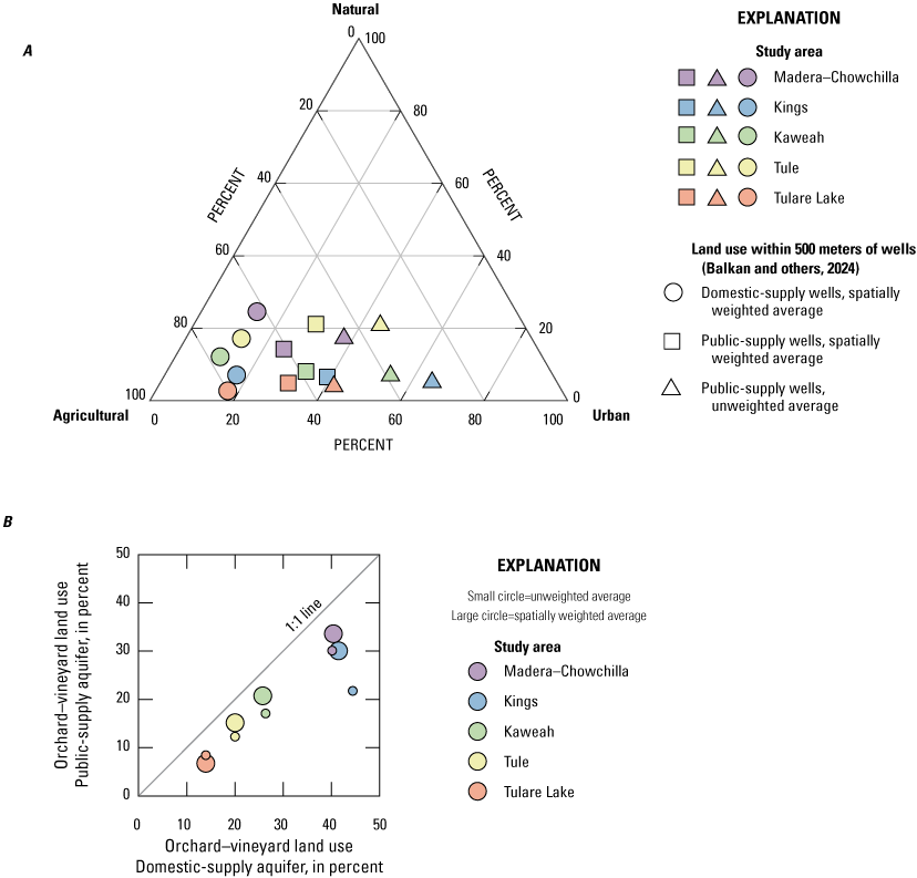
A, Average percentages of urban, agricultural, and natural land use; and B, percentages of orchard and vineyard land use within the 500-meter buffers around domestic-supply and public-supply wells used for assessment of groundwater quality in the five study areas of the southeastern San Joaquin Valley.
Within agricultural land use, orchard and vineyard land use was considered as a separate category because previous studies identified it as an important explanatory factor, such as for the spatial distribution of detections of fumigants in groundwater (Burow and others, 1999; 2019). The spatially weighted average percentage of orchard and vineyard land use in the five study areas ranged from 12 percent in Tulare Lake to 40 percent in Madera-Chowchilla and Kings for SESJV-D (fig. 10) and was greater around SESJV-D wells than around SESJV-P wells in all five study areas. Average percentage of orchard and vineyard land use was the same as spatially weighted average percentage of orchard vineyard land use for the SESJV-D study areas (fig. 10B) because of the even spatial distribution of the extra wells (see the “Methods” section). For SESJV-P study areas, the average percentage of orchard and vineyard land use was less than spatially weighted average percentage of orchard and vineyard land use, especially for the Kings study area (fig. 10B), because of the concentration of public-supply wells in urban areas.
Groundwater Age and Geochemical Conditions
The age of groundwater used for drinking-water supply in the southeastern San Joaquin Valley varied substantially by location and well depth. The depth of penetration of modern groundwater into the aquifer system ranged from about 150 to 300 ft bls in the southeastern San Joaquin Valley (Faulkner and others, 2023). The depth of penetration below land surface of modern groundwater generally was greatest in the Tule study area (fig. 11) because the depth of the water table below land surface generally increased from north to south in the eastern San Joaquin Valley (Faunt, 2009; Levy and others, 2021). Within each of the four cross sections on figure 11, wells with modern groundwater generally were shallower than wells with premodern groundwater. The Corcoran Clay was not a barrier to penetration of modern groundwater because there were wells with modern groundwater both above and below the unit, especially at intermediate values of lateral positions (350–600) where the unit was closest to the land surface (fig. 11). At the distal end (lateral position<200), there were shallow wells above the Corcoran Clay with premodern groundwater, likely indicating that the San Joaquin trough historically was the discharge zone at the end of the regional groundwater flow system (Mendenhall and others, 1916; Davis and others, 1959; Burow and others, 2004, 2007, 2008; Phillips and others, 2007; Faunt, 2009).
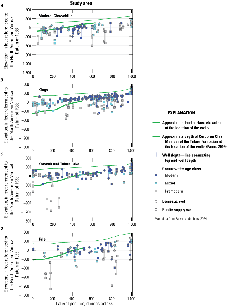
Groundwater-age classification and depths of screened intervals in domestic-supply and public-supply wells in the southeastern San Joaquin Valley: A, Madera-Chowchilla study area; B, Kings study area; C, Kaweah and Tulare Lake study areas; and D, Tule study area.
Figure 12 shows the spatially weighted proportion of wells in each SESJV-D and SESJV-P study area with modern, mixed, and premodern groundwater. Except for the SESJV-P Tulare Lake study area, all the study areas had approximately 25–35 percent mixed groundwater and differ in their proportions of modern and premodern groundwater. Many of the wells with mixed groundwater had longer screened intervals (fig. 11) and may have intersected the upper and lower parts of the stratified groundwater age structure (Jurgens and others, 2016). For the Madera-Chowchilla, Kings, Tule, and Tulare Lake study areas, the spatially weighted proportion of wells in the SESJV-D with modern groundwater was 20–60 percent greater than the proportion in the SESJV-P (fig. 12), which we expected because the SESJV-D wells were generally shallower than the SESJV-P wells (figs. 7, 9).

Spatially weighted proportions of modern, mixed, and premodern groundwater in groundwater resources used for domestic-supply and public-supply in the southeastern San Joaquin Valley.
The geochemical characteristics of groundwater affect the mobilization and persistence of constituents in groundwater. Many constituents are sensitive to groundwater oxidation-reduction (redox) conditions and may become soluble or insoluble or degrade during different conditions. The major ion composition of groundwater, such as bicarbonate concentrations and pH values, may affect the sorbtion and desorbtion of constituents from mineral surfaces.
Groundwater conditions were dominantly oxic in the SESJV-D and SESJV-P in the Madera-Chowchilla, Kings, Kaweah, and Tule study areas, and anoxic conditions were common in the SESJV-D and SESJV-P in the Tulare Lake study area (fig. 13). In the Kings, Kaweah, Tule, and Tulare Lake study areas, most wells located at lateral positions between 0 and 200 had anoxic or mixed redox conditions (fig. 13). This area corresponded to the distal parts of the alluvial fans and to the basinal and lakebed deposits where anoxic conditions were known to be common (Landon and others, 2011; Burow and others, 2013; Rosecrans and others, 2017). A few wells in the central and proximal areas of the fans (lateral positions greater than 200) had mixed or anoxic redox conditions; most of these wells were deeper and tapped mixed-age or premodern-age groundwater (compare fig. 11 to fig. 13). Most wells with anoxic or mixed redox were in areas with hydric soils (Natural Resources Conservation Service, 2021; fig. 14). Hydric soils are soils that are seasonally wet enough to develop anoxic conditions. Redox sensitive constituents, such as manganese, could be influenced by the presence of hydric soils (McMahon and others, 2019).

Oxidation-reduction classification and depths of screened intervals in domestic-supply and public-supply wells in the southeastern San Joaquin Valley: A, Madera-Chowchilla study area; B, Kings study area; C, Kaweah and Tulare Lake study areas; and D, Tule study area.
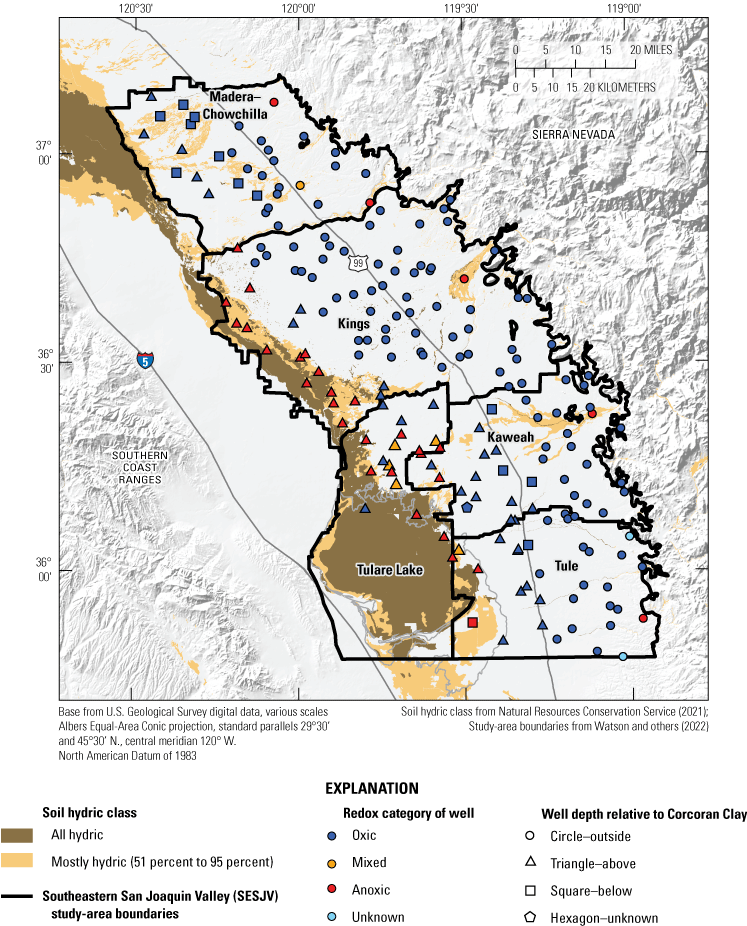
Spatial distribution of hydric soils and depth of the well screen relative to the depth of the Corcoran Clay Member of the Tulare Formation and groundwater oxidation-reduction classification for domestic-supply wells, southeastern San Joaquin Valley, 2013–15, California Groundwater Ambient Monitoring and Assessment Program Priority Basin Project.
The pH conditions of groundwater were evaluated using field measurements at the time of sampling, and pH values in the domestic wells ranged from 6.1 to 9.6 (Bennett and others, 2017; Shelton and Fram, 2017). The spatial pattern of pH was not as marked as the pattern in redox. In the SESJV-D, pH values greater than 8 generally were in wells toward the distal side of the fans in the Madera-Chowchilla and Kings study areas but were more widespread in the Kaweah, Tule, and Tulare Lake study areas (fig. 15). In the SESJV-D, pH was positively correlated with depth to top of screen and well depth (Spearman test, p<0.001, rho 0.44 and 0.38, respectively), which was consistent with higher pH values observed in deeper public-supply wells in the cross sections. Values of pH were related to groundwater age and redox conditions; pH values were greater in premodern compared to modern or mixed (Kruskall-Wallis, p<0.001) and in oxic compared to anoxic or mixed (Wilcoxon, p<0.001).
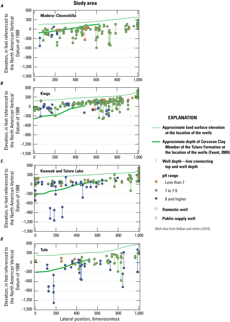
Depths of screened intervals and pH values in domestic and public-supply wells in the southeastern San Joaquin Valley: A, Madera-Chowchilla study area; B, Kings study area; C, Kaweah and Tulare Lake study areas; and D, Tule study area.
Status of Groundwater Quality
The status assessment for groundwater quality identified constituents and constituent classes present at moderate and high relative concentrations in the domestic-supply aquifer and compared aquifer-scale proportion results among the five study areas and between the domestic-supply (SESJV-D) and public-supply (SESJV-P) resources. The section “Statistical and Graphical Methods” describes how confidence intervals were used to define the significance of differences between aquifer-scale proportions of high concentrations among SESJV-D study areas and between SESJV-D and SESJV-P study areas. Brief discussions of potential explanatory factors that may explain observed spatial patterns in groundwater-quality conditions are then presented for a subset of constituents. Similar discussions of potential explanatory factors that may affect concentrations of selected constituents in public-supply wells were presented in Burton and others (2012) and Shelton and others (2013).
Inorganic Constituents
Inorganic constituents generally are naturally present in groundwater as result of water-rock interactions and other natural processes, and their concentrations may be influenced by human activities and natural factors (Hem, 1985; Appelo and Postma, 2005). All inorganic constituents (nutrients, major ions, trace elements, perchlorate, and radioactive constituents) analyzed in samples collected from domestic wells for this study were detected in at least one sample (Bennett and others, 2017; Shelton and Fram, 2017).
There were 18 inorganic constituents detected at moderate or high concentrations relative to their selected comparison benchmarks (table 2; fig. 16). The nutrients nitrate and nitrite, the trace elements arsenic, barium, fluoride, and uranium, radioactive constituents adjusted gross alpha and adjusted gross beta particle activities, and perchlorate were detected at moderate or high concentrations relative to regulatory health-based benchmarks (MCL-CA or MCL-US); total dissolved solids, chloride, sulfate, manganese, and iron were detected at moderate or high concentrations relative to secondary maximum contaminant level benchmarks (SMCL-CA); and the trace elements boron, molybdenum, manganese, vanadium, and strontium were detected at moderate or high concentrations relative to non-regulatory health-based benchmarks (HAL-US or RL-CA). Another 25 inorganic constituents were detected, but the constituents were either only at low concentrations relative to their selected comparison benchmarks or did not have comparison benchmarks (table 3; fig. 16).

Maximum relative concentrations of constituents detected in domestic-supply wells sampled in the southeastern San Joaquin Valley, 2013–15, California Groundwater Ambient Monitoring and Assessment Program Priority Basin Project.
As a class, inorganic constituents with MCL benchmarks were present at high concentrations in 47 percent of SESJV-D and at moderate concentrations in 28 percent of SESJV-D (table 5; fig. 17). The proportion of each study area with high concentrations ranged from about 19 percent in Madera-Chowchilla to about 60 percent in Kings and Tulare Lake. Expanding the class to include inorganic constituents with MCL or non-regulatory health-based benchmarks increased the proportion of SESJV-D with high concentrations by about 2 percent (table 5).

Aquifer-scale proportion for high (yellow), moderate (green), and low (blue) concentrations of the classes of inorganic and organic constituents with maximum contaminant level benchmarks in the domestic-supply (-D) and public-supply (-P) aquifers of A, the Madera-Chowchilla study area; B, Kings study area; C, Kaweah study area; D, Tule study area; E, Tulare Lake study area; and F, southeastern San Joaquin Valley (SESJV) as a whole, 2013–15, California Groundwater Ambient Monitoring and Assessment Program Priority Basin Project.
Table 5.
Aquifer-scale proportions for constituent classes in the domestic-supply and public-supply aquifers, Southeastern San Joaquin Valley, 2013–14, California Groundwater Ambient Monitoring and Assessment Program Priority Basin Project.[Aquifer-scale proportion is the areal proportion of the study area with high or moderate concentrations calculated using a cell-declustering method; well percentage is the percentage of wells with high concentrations. Areal proportion of high concentrations and percentage of wells with high concentrations may differ if wells are clustered. The proportion of high concentrations in the groundwater resources used for public-supply wells in the southeastern San Joaquin Valley (SESJV-P) is considered different than the proportion on the groundwater resources used for domestic-supply wells in the southeastern San Joaquin Valley (SESJV-D) if it is outside of the confidence interval for the SESJV-D proportion. Relative-concentration categories: high, at least one constituent in the class has a concentration above the benchmark; moderate, at least one constituent in the class has a concentration above one-half (inorganic constituents) or one-tenth (organic constituents) benchmark, and none have a concentration above the benchmark. Tables 2–4 have lists of constituents in each class and concentrations of the benchmarks. Abbreviations: SMCL, secondary maximum contaminant level; MCL, maximum contaminant level]
Study area boundaries and grid cells are available in Watson and others (2022).
Aquifer-scale proportions for the SESJV-D were calculated using equations 1 and 2 from data for 198 wells representative of domestic-supply wells and sampled by the U.S. Geological Survey (USGS) during 2013–15 (table 1.1; U.S. Geological Survey, 2023b; Balkan and others, 2024).
The confidence interval is the Jeffrey's interval for the binomial distribution calculated for a 90-percent confidence (equation 3; Brown and others, 2001; Belitz and others, 2010). Confidence intervals were only calculated for the SESJV-D because of the high degree of clustering of wells in the SESJV-P. The proportion of the SESJV-P with high concentrations is considered different than the proportion of the SESJV-D with high concentrations if the SESJV-P value is outside the confidence interval for the SESJV-D.
Aquifer-scale proportions for the SESJV-P were calculated using equations 1 and 2 from data for 1,701 wells representative of public-supply wells and either sampled by the USGS (U.S. Geological Survey, 2023b; Balkan and others, 2024) or having publicly available regulatory compliance data in the California State Water Resources Control Board Division of Drinking Water (SWRCB-DDW) database (California State Water Resources Control Board, 2023b; California State Water Resources Control Board Division of Drinking Water, 2022d).
Aquifer-scale proportions and well percentages for concentration categories of any inorganic constituent with SMCLs were calculated using only wells having data for both total dissolved solids (TDS) and manganese. Hence, the number of wells used to calculate aquifer-scale proportions and well percentages for the subclasses of salinity indicators with SMCLs and trace elements with SMCLs can be larger than the number of wells used for the calculations for the combined class of inorganic constituents with SMCLs.
Aquifer-scale proportions and well percentages for concentration categories of any inorganic constituent with MCLs were calculated using only wells having data for both nitrate and arsenic. Hence, the number of wells used to calculate aquifer-scale proportions and well percentages for the subclasses of nutrients with MCLs and trace elements with MCLs can be larger than the number of wells used for the calculations for the combined class of inorganic constituents with MCLs. The aquifer-scale proportions of moderate relative concentrations for any inorganic constituent with an MCL may be larger than reported because the most common reporting limit for perchlorate in the SWRCB-DDW database of regulatory compliance data for public-supply wells is greater than one-half of the MCL. For this table, perchlorate data collected by the USGS were recensored to the SWRCB-DDW reporting level. Aquifer-scale proportion results calculated from uncensored USGS perchlorate data are reported in table 6.
The inorganic constituents with non-regulatory, health-based benchmarks that were present at high or moderate concentrations, and therefore contributed to these results, are listed in table 2 (boron, molybdenum, strontium, vanadium, and manganese).
The aquifer-scale proportions of moderate concentrations for organic constituent classes may be larger than reported because the reporting limits for some organic constituents in the SWRCB-DDW database of regulatory compliance data for public-supply wells are greater than one-tenth of the MCL. For this table, data collected by the USGS were recensored to the reporting limits used in the SWRCB-DDW database. The constituents affected by censoring to the SWRCB-DDW reporting limits were the following: Fumigants: 1,2,3-trichloropropane and 1,2-dibromoethane; Solvents: tetrachloromethane and 1,2-dichloroethane; Other volatile organic carbon compounds: methyl tert-butyl ether and benzene; Pesticides: atrazine, simazine, and bentazon. Table 6 presents aquifer-scale proportions of moderate concentrations of organic constituents in the SESJV-D calculated using USGS censoring levels rather than SWRCB-DDW censoring levels.
Inorganic constituents with MCL benchmarks were present at high concentrations in a greater proportion of the SESJV-D than the SESJV-P (table 5; proportion of high concentrations in the SESJV-P was below the lower end of confidence interval around the proportion of high concentrations in the SESJV-D). Among the five study areas, the Kings study area had the largest difference between SESJV-D and SESJV-P (table 4; fig. 17). The proportion of the Kings study area with high concentrations of any inorganic constituent with an MCL was 61 percent for SESJV-D but only 29 percent for SESJV-P (table 4; fig. 17).
The areal proportion with high concentrations and the percentage of wells with high concentrations of any inorganic constituent with an MCL were similar in each of the five SESJV-D study areas (table 5). In contrast, for all five SESJV-P study areas, the areal proportions with high concentrations were greater than the percentages of wells with high concentrations. In this study, the domestic wells were more evenly distributed (fig. 8) than the public-supply wells (fig. 4). The difference between the spatially weighted proportion and detection frequency of high concentrations of inorganic constituents in the public-supply wells demonstrates that the areas with the greatest density of wells generally had lower concentrations of inorganic constituents with MCLs compared to areas with lower density of wells. This was expected from the observation that for public-supply wells, wells belonging to smaller systems were more likely to have concentrations of constituents greater than MCL benchmarks (California State Water Resources Control Board, 2013; Bangia and others, 2020). Public-supply wells in areas with low density of public-supply wells were more likely to belong to public water systems serving smaller numbers of people and those systems are more likely to have wells that have shallow depths similar to nearby domestic-supply wells (fig. 7; Shelton and others, 2013; Bangia and others, 2020).
This report is focused on evaluation of the groundwater resources used by the wells, not on the wells or the population served by the wells; therefore, results are presented as spatially weighted, but the well percentages are provided for reference. Belitz and others (2015) computed results for prevalence of high concentrations in three ways and compared them to each other: aquifer-scale proportions (areal proportions), percentages of wells, and proportion of population served at the scale of study areas.
As a class, inorganic constituents with SMCL benchmarks were present at high concentrations in 14 percent of SESJV-D and at moderate concentrations in 26 percent (table 5). The proportion of each study area with high concentrations ranged from 3.6 percent in Tule to 58 percent in Tulare Lake. The proportion of the SESJV-P with high concentrations (19 percent) was greater than the proportion of the SESJV-D with high concentrations (14 percent; table 4; fig. 17).
Nutrients
Nutrients have natural and anthropogenic sources in groundwater (Dubrovsky and others, 2010). Natural sources include atmospheric deposition, animal waste, and dissolution of organic material in soils. Anthropogenic sources include fertilizer application, livestock and human waste, sewage and septic effluents, and combustion of fossil fuels (emits nitrogen oxides to the atmosphere). Three nitrogenous nutrients have benchmarks: nitrate and nitrite have MCL-US benchmarks (table 2), and ammonia has a HAL-US benchmark (table 3). Orthophosphate also is a nutrient that was analyzed in samples collected for this study; however, orthophosphate does not have a drinking-water benchmark (table 3) and is not included in the status assessment. The most common forms of dissolved nitrogen in groundwater are nitrate, nitrite, ammonia or ammonium, and dissolved nitrogen gas. The form of nitrogen that dominates depends on redox conditions (McMahon and Chapelle, 2008). Nitrate is the most oxidized form of nitrogen and is the most common form in oxic groundwater systems. Although evapotranspiration from shallow groundwater can increase concentrations of nutrients in groundwater, concentrations of nitrate that are greater than about 2 mg/L (relative concentration of 0.2) generally result from anthropogenic inputs (Nolan and others, 2002; Dubrovsky and others, 2010).
Nutrients were present at high concentrations in 27 percent of the SESJV-D and at moderate concentrations in 25 percent of the SESJV-D (table 5). Nitrate was the only nutrient present at high concentrations (greater than the MCL-US of 10 mg/L) and also accounted for most of the moderate concentrations of nutrients (fig. 18A). The proportion of SESJV-D with high concentrations of nitrate ranged from 8.9 percent in Tulare Lake to 40 percent in Kaweah, and the proportions of high concentrations were greater in the Kings and Kaweah study areas than in the Madera-Chowchilla and Tulare Lake study areas (tables 6–10; fig. 19). Nitrite was present at moderate concentrations (greater than 0.5 mg/L and less than or equal to 1 mg/L) in the Kaweah and Tulare Lake study areas (tables 6–10; fig. 18A). None of the samples with moderate concentrations of nitrite had moderate or high concentrations of nitrate (Bennett and others, 2017).
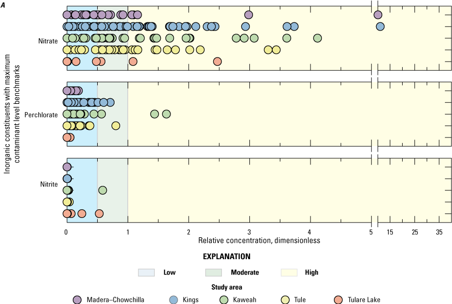
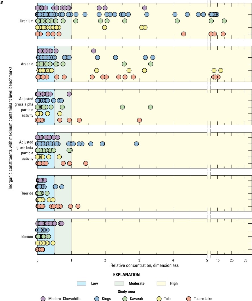

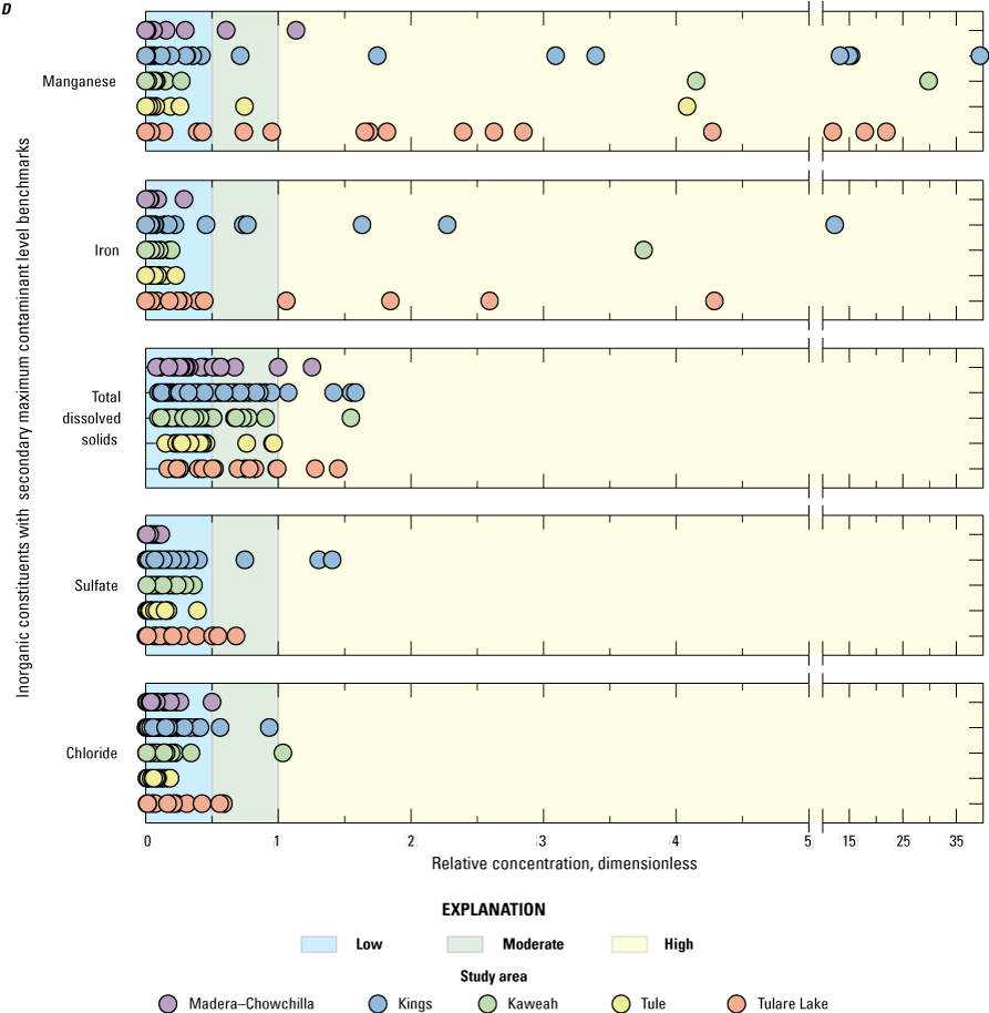
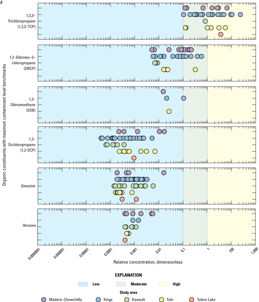
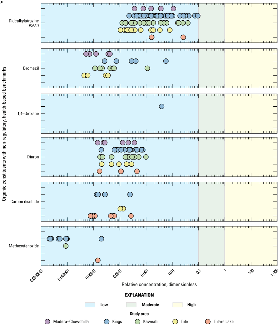

Relative concentrations of selected constituents in groundwater samples collected from domestic-supply wells, southeastern San Joaquin Valley, 2013–15, California Groundwater Ambient Monitoring and Assessment Program Priority Basin Project. A, inorganic constituents (nutrients and perchlorate) with maximum contaminant level benchmarks; B, inorganic constituents (trace elements and radioactivity) with maximum contaminant level benchmarks; C, inorganic constituents with non-regulatory, health-based benchmarks; D, inorganic constituents with secondary maximum contaminant level benchmarks; E, organic constituents (fumigants and herbicides) with maximum contaminant levels; F, organic constituents with non-regulatory, health-based benchmarks; and G, organic constituents (volatile organic compounds) with maximum contaminant levels. Benchmarks are listed in table 2.
Table 6.
Aquifer-scale proportions for inorganic constituents in groundwater resources used for domestic-supply (SESJV-P) and public-supply (SESJV-P), Madera-Chowchilla study area, southeastern San Joaquin Valley, 2013–15, California Groundwater Ambient Monitoring and Assessment Program Priority Basin Project.[—Left][Aquifer-scale proportion is the areal proportion of the study area with high or moderate concentrations calculated using a cell-declustering method; well percentage is the percentage of wells with high concentrations. Areal proportion of high concentrations and percentage of wells with high concentrations may differ if wells are clustered. The proportion of high concentrations in the SESJV-P is considered different than the proportion on the SESJV-D if it is outside of the confidence interval for the SESJV-D proportion. An "x" indicates that proportions were not calculated because fewer than one-half of the grid cells in a study area had at least one well with data for the constituent. Relative-concentration categories: high, at least one constituent in the class has a concentration above the benchmark; moderate, at least one constituent in the class has a concentration above one-half (inorganic constituents) or one-tenth (organic constituents) the benchmark, and none have a concentration above the benchmark. Tables 2–4 have lists of constituents in each class and concentrations of the benchmarks. Abbreviations: SESJV-D, groundwater resources used by domestic wells in the five study areas of the southeastern San Joaquin Valley; SESJV-P, groundwater resources used by public-supply wells in the five study areas of the southeastern San Joaquin Valley; SMCL, secondary maximum contaminant level; MCL, maximum containment level]
Study area boundaries and grid cells are available in Watson and others (2022).
Aquifer-scale proportions and well percentages for the SESJV-D Madera-Chowchilla study area were calculated from data for 34 wells representative of domestic wells and sampled by the USGS during 2013–15 (table 1.1; U.S. Geological Survey, 2023b; Balkan and others, 2024).
The confidence interval is the Jeffrey's interval for the binomial distribution calculated for a 90-percent confidence (Brown and others, 2001; Belitz and others, 2010). Confidence intervals were only calculated for the SESJV-D because of the high degree of clustering of wells in the SESJV-P. The proportion of the SESJV-P with high concentrations is considered different than the proportion of the SESJV-D with high concentrations if the SESJV-P value is outside the confidence interval for the SESJV-D.
Aquifer-scale proportions and well percentages for the SESJV-P Madera-Chowchilla study area were calculated from data for 179 wells representative of public-supply wells and either sampled by the USGS (U.S. Geological Survey, 2023b; Balkan and others, 2024) or having publicly available regulatory compliance data (California State Water Resources Control Board, 2023b; Balkan and others, 2024).
Two sets of results are presented for manganese because concentrations were compared to the SMCL benchmark and to the non-regulatory, health-based benchmark (table 2).
Table 7.
Aquifer-scale proportions for inorganic constituents in groundwater resources used for domestic-supply (SESJV-D) and public-supply (SESJV-P), Kings study area, southeastern San Joaquin Valley, 2013–15, California Groundwater Ambient Monitoring and Assessment Program Priority Basin Project.[—Left][Aquifer-scale proportion is the areal proportion of the study area with high or moderate concentrations calculated using a cell-declustering method; well percentage is the percentage of wells with high concentrations. Areal proportion of high concentrations and percentage of wells with high concentrations may differ if wells are clustered. The proportion of high concentrations in the SESJV-P is considered different than the proportion on the SESJV-D if it is outside of the confidence interval for the SESJV-D proportion. An "x" indicates that proportions were not calculated because fewer than one-half of the grid cells in a study area had at least one well with data for the constituent. Relative-concentration categories: high, at least one constituent in the class has a concentration above the benchmark; moderate, at least one constituent in the class has a concentration above one-half (inorganic constituents) or one-tenth (organic constituents) the benchmark, and none have a concentration above the benchmark. Tables 2–4 have lists of constituents in each class and concentrations of the benchmarks. Abbreviations: SMCL, secondary maximum contaminant level; MCL, maximum containment level]
Study area boundaries and grid cells are available in Watson and others (2022).
Aquifer-scale proportions and well percentages for the SESJV-D Kings study area were calculated from data for 76 wells representative of domestic wells and sampled by the USGS during 2013–15 (table 1.2; U.S. Geological Survey, 2023b; Balkan and others, 2024).
The confidence interval is the Jeffrey's interval for the binomial distribution calculated for a 90-percent confidence (Brown and others, 2001; Belitz and others, 2010). Confidence intervals were only calculated for the SESJV-D because of the high degree of clustering of wells in the SESJV-P. The proportion of the SESJV-P with high concentrations is considered different than the proportion of the SESJV-D with high concentrations if the SESJV-P value is outside the confidence interval for the SESJV-D.
Aquifer-scale proportions and well percentages for the SESJV-P Kings study area were calculated from data for 920 wells representative of public-supply wells and either sampled by the USGS (U.S. Geological Survey, 2023b; Balkan and others, 2024) or having publicly available regulatory compliance data (California State Water Resources Control Board, 2023b; Balkan and others, 2024).
Two sets of results are presented for manganese because concentrations were compared to the SMCL benchmark and to the non-regulatory, health-based benchmark (table 2).
Table 8.
Aquifer-scale proportions for inorganic constituents in groundwater resources used for domestic-supply (SESJV-D) and public-supply (SESJV-P), Kaweah study area, southeastern San Joaquin Valley, 2013–15, California Groundwater Ambient Monitoring and Assessment Program Priority Basin Project.[—Left][Aquifer-scale proportion is the areal proportion of the study area with high or moderate concentrations calculated using a cell-declustering method; well percentage is the percentage of wells with high concentrations. Areal proportion of high concentrations and percentage of wells with high concentrations may differ if wells are clustered. The proportion of high concentrations in the SESJV-P is considered different than the proportion on the SESJV-D if it is outside of the confidence interval for the SESJV-D proportion. An "x" indicates that proportions were not calculated because fewer than one-half of the grid cells in a study area had at least one well with data for the constituent. Relative-concentration categories: high, at least one constituent in the class has a concentration above the benchmark; moderate, at least one constituent in the class has a concentration above one-half (inorganic constituents) or one-tenth (organic constituents) the benchmark, and none have a concentration above the benchmark. Tables 2–4 have lists of constituents in each class and concentrations of the benchmarks. Abbreviations: SMCL, secondary maximum contaminant level; MCL, maximum containment level]
Study area boundaries and grid cells are available in Watson and others (2022).
Aquifer-scale proportions and well percentages for the SESJV-D Kaweah study area were calculated from data for 36 wells representative of domestic wells and sampled by the USGS during 2013–15 (table 1.3; U.S. Geological Survey, 2023b; Balkan and others, 2024).
The confidence interval is the Jeffrey's interval for the binomial distribution calculated for a 90-percent confidence (Brown and others, 2001; Belitz and others, 2010). Confidence intervals were only calculated for the SESJV-D because of the high degree of clustering of wells in the SESJV-P. The proportion of the SESJV-P with high concentrations is considered different than the proportion of the SESJV-D with high concentrations if the SESJV-P value is outside the confidence interval for the SESJV-D.
Aquifer-scale proportions and well percentages for the SESJV-P Kaweah study area were calculated from data for 309 wells representative of public-supply wells and either sampled by the USGS (U.S. Geological Survey, 2023b; Balkan and others, 2024) or having publicly available regulatory compliance data (California State Water Resources Control Board, 2023b; Balkan and others, 2024).
Two sets of results are presented for manganese because concentrations were compared to the SMCL benchmark and to the non-regulatory, health-based benchmark (table 2).
Table 9.
Aquifer-scale proportions for inorganic constituents in groundwater resources used for domestic-supply (SESJV-D) and public-supply (SESJV-P), Tule study area, southeastern San Joaquin Valley, 2013–15, California Groundwater Ambient Monitoring and Assessment Program Priority Basin Project.[—Left][Aquifer-scale proportion is the areal proportion of the study area with high or moderate concentrations calculated using a cell-declustering method; well percentage is the percentage of wells with high concentrations. Areal proportion of high concentrations and percentage of wells with high concentrations may differ if wells are clustered. The proportion of high concentrations in the SESJV-P is considered different than the proportion on the SESJV-D if it is outside of the confidence interval for the SESJV-D proportion. An "x" indicates that proportions were not calculated because fewer than one-half of the grid cells in a study area had at least one well with data for the constituent. Relative-concentration categories: high, at least one constituent in the class has a concentration above the benchmark; moderate, at least one constituent in the class has a concentration above one-half (inorganic constituents) or one-tenth (organic constituents) the benchmark, and none have a concentration above the benchmark. Tables 2–4 have lists of constituents in each class and concentrations of the benchmarks. Abbreviations: SMCL, secondary maximum contaminant level; MCL, maximum containment level]
Study area boundaries and grid cells are available in Watson and others (2022).
Aquifer-scale proportions and well percentages for the SESJV-D Tule study area were calculated from data for 34 wells representative of domestic wells and sampled by the USGS during 2013–15 (table 1.4; U.S. Geological Survey, 2023b; Balkan and others, 2024).
The confidence interval is the Jeffrey's interval for the binomial distribution calculated for a 90-percent confidence (Brown and others, 2001; Belitz and others, 2010). Confidence intervals were only calculated for the SESJV-D because of the high degree of clustering of wells in the SESJV-P. The proportion of the SESJV-P with high concentrations is considered different than the proportion of the SESJV-D with high concentrations if the SESJV-P value is outside the confidence interval for the SESJV-D.
Aquifer-scale proportions and well percentages for the SESJV-P Tule study area were calculated from data for 195 wells representative of public-supply wells and either sampled by the USGS (California State Water Resources Control Board, 2023b; U.S. Geological Survey, 2023b; Balkan and others, 2024) or having publicly available regulatory compliance data (Balkan and others, 2024).
Two sets of results are presented for manganese because concentrations were compared to the SMCL benchmark and to the non-regulatory, health-based benchmark (table 2).
Table 10.
Aquifer-scale proportions for inorganic constituents in groundwater resources used for domestic-supply (SESJV-D) and public-supply (SESJV-P), Tulare Lake study area, southeastern San Joaquin Valley, 2013–15, California Groundwater Ambient Monitoring and Assessment Program Priority Basin Project.[—Left][Aquifer-scale proportion is the areal proportion of the study area with high or moderate concentrations calculated using a cell-declustering method; well percentage is the percentage of wells with high concentrations. Areal proportion of high concentrations and percentage of wells with high concentrations may differ if wells are clustered. The proportion of high concentrations in the SESJV-P is considered different than the proportion on the SESJV-D if it is outside of the confidence interval for the SESJV-D proportion. An "x" indicates that proportions were not calculated because fewer than one-half of the grid cells in a study area had at least one well with data for the constituent. Relative-concentration categories: high, at least one constituent in the class has a concentration above the benchmark; moderate, at least one constituent in the class has a concentration above one-half (inorganic constituents) or one-tenth (organic constituents) the benchmark, and none have a concentration above the benchmark. Tables 2–4 have lists of constituents in each class and concentrations of the benchmarks. Abbreviations: SMCL, secondary maximum contaminant level; MCL, maximum containment level]
Study area boundaries and grid cells are available in Watson and others (2022).
Aquifer-scale proportions and well percentages for the SESJV-D Tulare Lake study area were calculated from data for 18 wells representative of domestic wells and sampled by the USGS during 2013–15 (table 1.5; U.S. Geological Survey, 2023b; Balkan and others, 2024).
The confidence interval is the Jeffrey's interval for the binomial distribution calculated for a 90-percent confidence (Brown and others, 2001; Belitz and others, 2010). Confidence intervals were only calculated for the SESJV-D because of the high degree of clustering of wells in the SESJV-P. The proportion of the SESJV-P with high concentrations is considered different than the proportion of the SESJV-D with high concentrations if the SESJV-P value is outside the confidence interval for the SESJV-D.
Aquifer-scale proportions and well percentages for the SESJV-P Tulare Lake study area were calculated from data for 98 wells representative of public-supply wells and either sampled by the USGS (U.S. Geological Survey, 2023b; Balkan and others, 2024) or having publicly available regulatory compliance data (California State Water Resources Control Board, 2023b; Balkan and others, 2024).
Two sets of results are presented for manganese because concentrations were compared to the SMCL benchmark and to the non-regulatory, health-based benchmark (table 2).
Table 11.
Aquifer-scale proportions for inorganic constituents in groundwater resources used for domestic-supply (SESJV-D) and public-supply (SESJV-P), southeastern San Joaquin Valley, 2013–15, California Groundwater Ambient Monitoring and Assessment Program Priority Basin Project.[—Left][Aquifer-scale proportion is the areal proportion of the study area with high or moderate concentrations calculated using a cell-declustering method; well percentage is the percentage of wells with high concentrations. Areal proportion of high concentrations and percentage of wells with high concentrations may differ if wells are clustered. The proportion of high concentrations in the SESJV-P is considered different than the proportion on the SESJV-D if it is outside of the confidence interval for the SESJV-D proportion. An "x" indicates that proportions were not calculated because fewer than one-half of the grid cells in a study area had at least one well with data for the constituent. Relative-concentration categories: high, at least one constituent in the class has a concentration above the benchmark; moderate, at least one constituent in the class has a concentration above one-half (inorganic constituents) or one-tenth (organic constituents) the benchmark, and none have a concentration above the benchmark. Tables 2–4 have lists of constituents in each class and concentrations of the benchmarks. Abbreviations: SMCL, secondary maximum contaminant level; MCL, maximum containment level]
Study area boundaries and grid cells are available in Watson and others (2022).
Aquifer-scale proportions and well percentages for the SESJV-D were calculated from data for 198 wells representative of domestic wells and sampled by the USGS during 2013–15 (tables 1.1–1.5; U.S. Geological Survey, 2023b; Balkan and others, 2024).
The confidence interval is the Jeffrey's interval for the binomial distribution calculated for a 90-percent confidence (Brown and others, 2001; Belitz and others, 2010). Confidence intervals were only calculated for the SESJV-D because of the high degree of clustering of wells in the SESJV-P. The proportion of the SESJV-P with high concentrations is considered different than the proportion of the SESJV-D with high concentrations if the SESJV-P value is outside the confidence interval for the SESJV-D.
Aquifer-scale proportions and well percentages for the SESJV-P were calculated from data for 1,701 wells representative of public-supply wells and either sampled by the USGS (California State Water Resources Control Board, 2023b; U.S. Geological Survey, 2023b; Balkan and others, 2024) or having publicly available regulatory compliance data (Balkan and others, 2024).
Two sets of results are presented for manganese because concentrations were compared to the SMCL benchmark and to the non-regulatory, health-based benchmark (table 2).

Aquifer-scale proportion for high (yellow), moderate (green), and low (blue) concentrations of nitrate in groundwater resources used for domestic-supply (-D) and public-supply (-P) aquifers of A, the Madera-Chowchilla study area, B, Kings study area, C, Kaweah study area, D, Tule study area, E, Tulare Lake study area, and F, southeastern San Joaquin Valley (SESJV) as a whole, 2013–15, California Groundwater Ambient Monitoring and Assessment Program Priority Basin Project.
Nitrate also was the only nutrient present at high concentrations in the public-supply aquifer (table 11). The proportion of the SESJV-P with high concentrations of nitrate (10 percent) was significantly lower than the proportion in the SESJV-D (27 percent; table 11). The proportion with high concentrations of nitrate was significantly greater in the domestic-supply aquifer than in the public-supply aquifer in the Kings, Kaweah, Tule, and Tulare Lake study areas (tables 6–10; fig. 19).
The spatial distribution of elevated nitrate concentrations in San Joaquin Valley groundwater primarily is explained by sources of nitrate from fertilizer inputs in agricultural areas and by redox processes that cause degradation of nitrate in anoxic groundwater (Burow and others, 2008; Landon and others, 2011; Nolan and others, 2014; Ransom and others, 2017). The application of nitrogenous fertilizers increased substantially beginning in the 1950s, and nitrogenous fertilizers have been applied to agricultural lands across the southeastern San Joaquin Valley (Burow and others, 2013). In SESJV-D, nitrate was not significantly correlated with percentage of agricultural land use (Spearman test, p=0.201, rho=0.09). This apparently counter-intuitive result indicates that nitrate behaved as a widespread non-point source contaminant in the southeastern San Joaquin Valley and that factors in addition to land use affect nitrate concentrations in groundwater. Nearly all the domestic-supply wells were in areas with agricultural land use (figs. 10, 20): the median percentage of agricultural land use with 500-m of the wells was 88 percent with interquartile range of 70 percent to 93 percent agricultural land use (Balkan and others, 2024). The amount of nitrogenous fertilizer applied to agricultural land varies with crop type and cultivation practices, therefore although presence of agricultural land use generally indicates use of nitrogenous fertilizers at the land surface, the percentage of agricultural land use does not necessary correlate with the magnitude of use of nitrogenous fertilizers near the well. Detailed spatial analysis of nitrogenous fertilizer use in the southeastern San Joaquin Valley was outside of the scope of this report. In the absence of such an analysis, the variable used in this report as a proxy for nitrogenous fertilizer sources at the land surface, percentage of agricultural land use, is an imprecise estimate, hence lack of statistically significant correlation between nitrate concentrations in groundwater and percentage of agricultural land use in areas dominated by agricultural land use was not unexpected.
High and moderate nitrate concentrations were detected throughout the central and eastern parts of the southeastern San Joaquin Valley on the proximal and intermediate areas of the alluvial fans and in interfan areas (fig. 20). Nitrate concentrations were lowest along the western edge of the southeastern San Joaquin Valley (fig. 20), on the distal parts of the alluvial fans at the ends of regional flow paths near the center of the basin where anoxic groundwater conditions are most prevalent (fig. 14). This spatial distribution of elevated nitrate concentrations in domestic wells was consistent with Ransom and others (2017) prediction of the widespread distribution of elevated nitrate concentrations at the depth zone used by domestic wells in the southeastern San Joaquin Valley. The spatial distribution of high concentrations of nitrate in the SESJV-D was similar to the spatial distribution of high and moderate concentrations of nitrate in the SESJV-P (compare SESJV-D data shown on fig. 20 to SESJV-P data shown on fig. 17G in Burton and others, 2012 and fig. 14 in Shelton and others, 2013).
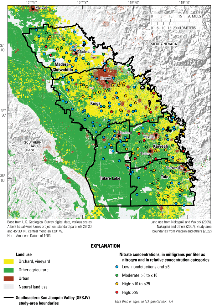
Concentrations of nitrate in domestic-supply wells, southeastern San Joaquin Valley, 2013–15, California Groundwater Ambient Monitoring and Assessment Program Priority Basin Project.
The spatial distribution of elevated nitrate concentrations largely matched distributions of redox conditions that affect nitrate stability and ages of groundwater accessed by the wells. Nitrate concentrations in oxic groundwater were greater than nitrate concentrations in anoxic or mixed-redox groundwater (Wilcoxon, p<0.001). Nitrate concentrations also were greatest in modern groundwater and least in premodern groundwater (Kruskall-Wallis, p<0.001). Both oxic conditions and presence of at least some modern groundwater were needed for elevated nitrate concentrations; modern or mixed groundwater with anoxic or mixed redox conditions and premodern groundwater with oxic redox conditions had lower nitrate concentrations than modern or mixed groundwater with oxic redox conditions (fig. 21). Anoxic conditions were most prevalent in wells in the basin deposits along the western edge of the southeastern San Joaquin Valley (figs. 13, 14) where nitrate concentrations were low (fig. 20). Anoxic conditions dominated the Tulare Lake study area; therefore, elevated nitrate concentrations were absent even though the Tulare Lake study area had shallow wells that tapped modern-age or mixed-age groundwater (fig. 11) in areas with sources of agricultural nitrate. Nitrate isotope data indicated that denitrification reduced nitrate concentrations in anoxic groundwater from wells in the San Joaquin Valley basin deposits and Tulare Lakebed area (Landon and others, 2010; Fram, 2017a).
The Madera-Chowchilla study area was dominated by oxic conditions that typically favor the preservation of nitrate (figs. 13, 14). However, the Madera-Chowchilla study area had lower prevalence of high nitrate concentrations than the Kings and Kaweah study areas (fig. 19), even though it had a greater prevalence of oxic conditions (figs. 13, 14). The lower prevalence of high nitrate concentrations in the Madera-Chowchilla study could be due to the age of the groundwater and land use. Agricultural nitrate is primarily associated with modern groundwater (Burow and others, 2013), and the Madera-Chowchilla study area had a substantially greater proportion of wells with premodern or mixed-age groundwater than the Kings and Kaweah study areas (fig. 12). The Madera-Chowchilla study area also had the greatest proportion of natural land use (fig. 10), with a corresponding lower proportion of agricultural land use.

Relations among nitrate concentrations, groundwater ages (modern, mixed, and premodern), and groundwater oxidation-reduction conditions (oxic or anoxic/mixed) in domestic-supply wells of the southeastern San Joaquin Valley, 2013–15, California Groundwater Ambient Monitoring and Assessment Program Priority Basin Project.
Greater prevalence of high nitrate concentrations in SESJV-D compared to SESJV-P was consistent with the observed differences in hydrologic and geochemical characteristics. In all study areas, except Madera-Chowchilla, the domestic wells were in areas with higher percentages of agricultural land use than the public-supply wells (fig. 10), and greater nitrate loading at the land surface generally is associated with agricultural land use. Domestic wells were significantly shallower than public-supply wells in all five study areas (fig. 9) and thus were more likely to access groundwater closer to the land surface where nitrogen fertilizers were applied. In all five study areas, a higher proportion of domestic wells tapped modern groundwater that was more likely to contain nitrate, and in all study areas except Kaweah, a lower proportion of domestic wells tapped premodern groundwater that was unlikely to contain elevated nitrate (fig. 12).
Trace Elements
The constituent class of trace elements included a variety of metallic and non-metallic constituents that typically are present in groundwater at concentrations less than 1 mg/L. At least one trace element with an MCL was detected at high RCs in 30 percent and at moderate RCs in 18 percent of SESJV-D (table 5). The aquifer scale proportion of the SESJV-D high RCs for any trace element with an MCL ranged from 10 percent in Madera-Chowchilla to 60 percent in Tulare Lake (table 5). Arsenic and uranium were present at high and moderate concentrations in all five study areas (tables 6–10; fig. 18B) and are discussed in more detail later in the text. Fluoride was present at high concentrations in less than 1 percent of SESJV-D, and barium was only detected at moderate concentrations (table 11; fig. 18B).
Five trace elements with non-regulatory health-based benchmarks—boron, molybdenum, vanadium, strontium, and manganese—were present at high or moderate concentrations (table 11; fig. 18C). Manganese has a HAL-US benchmark of 300 µg/L and an SMCL-CA benchmark of 50 µg/L, and both benchmarks are used in this report. Manganese was present at concentrations above the HAL-US in 4.9 percent of SESJV-D and is discussed in the “Constituents with Secondary Maximum Contaminant Level Benchmarks” section. Molybdenum was present at high concentrations in 3.4 percent of SESJV-D and is discussed in more detail in the next paragraph. Boron, vanadium, and strontium were only detected at moderate concentrations (table 11; fig. 18C).
The prevalence of high concentrations of boron, molybdenum, vanadium, and strontium in SESJV-D could not be compared to the prevalence of high concentrations in SESJV-P because the available data were insufficient for these four constituents in the public-supply well dataset used for this study. The SWRCB-DDW dataset did not include a lot of data for these constituents because they do not have regulatory benchmarks. GAMA-PBP sampling of public-supply wells in the Madera-Chowchilla study area (Shelton and others, 2009) included analysis of trace element in all wells, but sampling in the Kings, Kaweah, Tule, and Tulare Lake study areas (Burton and Belitz, 2008) only included analysis of trace elements at a subset of wells. For this study, aquifer-scale proportions were only calculated for constituents and study areas for which at least half of the grid cells had data for the constituent (tables 6–11).
Boron was detected at concentrations greater than the NL-CA of 1,000 µg/L in four wells at the western edge of the Tulare Lake and Kings study areas (not shown; Bennett and others, 2017), which was similar to locations of public-supply wells with boron concentrations exceeding the NL-CA (fig. 17C in Burton and others, 2012). Concentrations greater than the NL-CA were defined as moderate in this report (table 2) but were defined as high in all reports for the GAMA-PBP statewide assessments of water quality in groundwater resources used for public drinking-water supply, including the ones covering areas of the southeastern San Joaquin Valley (Burton and others, 2012; Shelton and others, 2013; Belitz and others, 2015; Fram, 2017a). The public-supply assessment for the Westside study area in the western San Joaquin Valley adjacent to the Tulare Lake and Kings study areas indicated that 45 percent of the public-supply aquifer had boron concentrations greater than the NL-CA and that elevated boron concentrations generally were associated with groundwater recharge derived from Coast Ranges watersheds that contained boron derived from marine shales or from geothermal sources (Fram, 2017a). Elevated boron concentrations at the western edge of the southeastern San Joaquin Valley may indicate mixing of groundwater recharge derived from the Coast Ranges to the west and Sierra Nevada to the east in the center of the San Joaquin Valley.
Vanadium was detected at concentrations greater than the NL-CA of 50 µg/L in four wells in the interfan region between the Kings and Kaweah River fans (not shown; Bennett and others, 2017; Shelton and Fram, 2017). Concentrations greater than the NL-CA are defined as moderate in this report (table 2) but were defined as high in Burton and others (2012), Shelton and others (2013), Belitz and others (2015), and Fram (2017a). Wright and Belitz (2010) documented that in a statewide dataset, vanadium concentrations were positively correlated with pH values and that higher concentrations of vanadium were associated with locations likely to have aquifer sediments derived from mafic materials and oxic groundwater conditions. However, the relation between vanadium and pH for SESJV-D samples was not statistically significant (Spearman test p=0.182, rho= −0.10) and Burton and others (2012) and Shelton and others (2013) determined that the relation between vanadium and pH was not significant for SESJV-P samples. This lack of significant relation between vanadium and pH could indicate that local variability in sediment composition is an important factor in determining vanadium concentrations in groundwater in the southeastern San Joaquin Valley.
Arsenic
An estimated 8 percent of groundwater resources used for drinking water in the United States have high concentrations of arsenic (Focazio and others, 2000; Welch and others, 2000), and high concentrations of arsenic in groundwater used for drinking water are a worldwide concern (Smedley and Kinniburgh, 2002; Welch and others, 2006). The EPA lowered the MCL-US for arsenic from 50 to 10 μg/L in 2001 (U.S. Environmental Protection Agency, 2001). Natural sources of arsenic in groundwater include dissolution of arsenic-bearing minerals, desorption of arsenic from mineral surfaces, and mixing with hydrothermal fluids (Smedley and Kinniburgh, 2002; Welch and Stollenwerk, 2003). Potential anthropogenic sources of arsenic can include copper ore smelting, coal combustion, arsenical pesticides, and wood preservatives (Welch and Stollenwerk, 2003). In addition, mining for copper, gold, and other metals can increase the rate of dissolution of natural arsenic-bearing minerals (Smedley and Kinniburgh, 2002).
Arsenic was present at high concentrations (above the MCL-US of 10 µg/L) in 11 percent and at moderate concentrations in 5.4 percent of SESJV-D (table 11). The aquifer-scale proportions of high concentrations of arsenic for the five SESJV-D study areas fell into three groups that meet the criteria for significant difference (see discussion of equation 3 in the “Statistical and Graphical Methods” subsection of the “Methods” section). The proportions of the Madera-Chowchilla, Kings, and Kaweah study areas with high concentrations of arsenic were 3.7, 6.8, and 4.8 percent, respectively, but these proportions were not significantly different from each other because of the overlap of the values with the 90-percent confidence intervals (all three had similar confidence intervals of approximately 1.2–13 percent; tables 6–10). The proportion of the Tule study area with high concentrations of arsenic was significantly greater than the proportion in the Madera-Chowchilla, Kings, or Kaweah study areas because the proportion in Tule (18 percent) was greater than the upper confidence limit for the others (13 percent), and the proportions in the others, 3.7–6.8 percent, were lower than the lower confidence limit for Tule (9.2 percent). The proportion of the Tulare Lake study area with high concentrations of arsenic (49 percent, with confidence interval of 31–67 percent) was significantly greater than the proportion in the Tule study area (18 percent, with confidence interval of 9.2–30 percent; tables 6–10; fig. 22). Most of the wells with high or moderate concentrations of arsenic were along the western edge of the southeastern San Joaquin Valley in the basin and lakebed deposits and in the distal parts of the Kings River fan (fig. 23).

Aquifer-scale proportions for high (yellow), moderate (green), and low (blue) concentrations of arsenic in the domestic-supply (-D) and public-supply (-P) aquifers of A, the Madera-Chowchilla study area; B, Kings study area, C, Kaweah study area; D, Tule study area; E, Tulare Lake study area; and F, southeastern San Joaquin Valley (SESJV) as a whole, 2013–15, California Groundwater Ambient Monitoring and Assessment Program Priority Basin Project.

Concentrations of arsenic in domestic-supply wells, southeastern San Joaquin Valley, 2013–15, California Groundwater Ambient Monitoring and Assessment Program Priority Basin Project.
The aquifer-scale proportions of high concentrations of arsenic and the spatial distributions of wells with high arsenic concentrations in the SESJV-D and SESJV-P were compared to help infer the processes controlling the presence of high arsenic concentrations in groundwater. The proportion of SESJV-P with high concentrations of arsenic, 16 percent, was greater than the proportion of the SESJV-D with high concentrations (11 percent; table 11; fig. 22). The proportions with high concentrations were greater in the SESJV-P in all five study areas, although the difference was only significant in the Kings study area (tables 6–10). The locations of wells with high concentrations of arsenic in the Kings, Kaweah, Tule, and Tulare Lake study areas were similar (compare SESJV-D data shown on fig. 23 to SESJV-P data shown on fig. 17A in Burton and others, 2012), but locations in the Madera-Chowchilla study area were different (compare SESJV-D data shown on fig. 23 to SESJV-P data shown on fig. 17 in Shelton and others, 2013). The greater proportion of high arsenic concentrations in the SESJV-P and the difference in spatial distribution of wells with high arsenic concentrations can be explained by redox and sorption processes controlling arsenic solubility, the differences in well depth and groundwater age between the SESJV-P and SESJV-D wells, and the spatial variations in the compositions of sediments in the southeastern San Joaquin Valley.
Redox and sorption processes were dominant controls on arsenic solubility in groundwater in the southeastern San Joaquin Valley. Arsenic mobilization under iron- and manganese-reducing conditions has been attributed to reductive dissolution of iron and manganese oxyhydroxides, a process by which arsenic that is sorbed or co-precipitated with iron and manganese oxyhydroxides is released (Smedley and Kinniburgh, 2002; Belitz and others, 2003; Welch and others, 2006). Reducing conditions may also increase arsenic mobilization by reducing arsenate that is sorbed on mineral surfaces to arsenite, which is less strongly sorbed (Zobrist and others, 2000).
Sorption of arsenic decreases as pH increases; at pH values greater than about 7.8, the primary arsenic species is hydrogen arsenate, which is relatively soluble (Smedley and Kinniburgh, 2002). The highest median arsenic concentrations were measured in groundwater that had pH values greater than 7.7 and had either mixed or anoxic redox conditions (fig. 24). The maximum arsenic concentration in groundwater with pH less than 7.7 and oxic conditions was 5.5 µg/L. Groundwater with high pH and anoxic conditions was most prevalent near the Tulare Lake Bed (figs. 13, 14, 15). Welch and others (1997) and Welch and Lico (1998) inferred that high arsenic concentrations in Carson Desert (not shown) groundwater were caused by interaction between lacustrine and riverine sediments and groundwater with high pH and low dissolved oxygen concentrations.

Relations among arsenic concentrations, pH, and classified groundwater oxidation-reduction conditions in domestic-supply wells of southeastern San Joaquin Valley, 2013–15, California Groundwater Ambient Monitoring and Assessment Program Priority Basin Project.
Fujii and Swain (1995) determined that evaporative concentration contributed to increased arsenic concentrations in shallow groundwater in the Tulare Lake Bed region; however, the groundwater in domestic wells was not extensively evaporated (see discussion in the “Total Dissolved Solids” section), indicating evaporation was not an important mechanism for increasing concentration of constituents in domestic wells.
Contribution of arsenic from legacy use of arsenical pesticides cannot be ruled out; however, relations between arsenic concentrations and indicators of contamination from agricultural sources indicate legacy use of arsenical pesticides are not the primary source of arsenic. Arsenic concentrations were inversely correlated with concentrations of fumigants (Spearman test, DBCP, p=0.002, rho= −0.23; 1,2,3-TCP p=0.013, rho= −0.18) and pesticides (Spearman test, atrazine+simazine, p<0.001, rho= −0.37, total pesticides and degradates p<0.001, rho= −0.29).
The geochemical conditions favorable to arsenic solubility commonly are associated with hydrologic conditions that may enhance accumulation of arsenic in groundwater. Long contact times between groundwater and aquifer materials increase the reaction time with aquifer materials; therefore, elevated arsenic concentrations are often associated with older groundwater ages, decreased rates of flushing and recharge, and increased distance along groundwater flow paths (Smedley and Kinniburgh, 2002; Anning and others, 2012).The greater prevalence of high arsenic concentrations in the SESJV-P compared to the prevalence of high arsenic concentrations in the SESJV-D in the Madera-Chowchilla, Kings, Tule, and Tulare Lake study areas (fig. 22) is consistent with the greater prevalence of premodern groundwater in the SESJV-P compared to the SESJV-D for those study areas (fig. 12).
Molybdenum
Molybdenum is a metallic trace element used in high-strength steel alloys, dry lubricants, and other industrial products. High concentrations of molybdenum are present in organic-rich sediments and sedimentary rocks deposited in sulfide-reducing environments (Crusius and others, 1996). However, most molybdenum ore deposits are associated with porphyry granite or quartz monzonite plutons, and the primary ore mineral is molybdenite (MoS2; Misra, 2000). Molybdenum has a non-regulatory, health-based benchmark (table 2) but is listed on EPA Contaminant Candidate Lists 3, 4, and 5 (U.S. Environmental Protection Agency, 2023). Under the Safe Drinking Water Act, the EPA (1) lists constituents that are not subject to any proposed regulations at the time the list is compiled but are known or anticipated to be present in public water systems at concentrations that might be of concern, (2) collects information about their presence and potential health effects, and (3) determines whether or not to start a process to evaluate setting an MCL for a constituent (U.S. Environmental Protection Agency, 2023).
Molybdenum was present at high concentrations (greater than the HAL-US of 40 µg/L) in 3.4 percent and at moderate concentrations in 2.0 percent of the SESJV-D (table 11). The proportions of the five study areas with high concentrations of molybdenum fell into three categories: the proportions in Madera-Chowchilla, Kaweah, and Kings study areas ranged from 0 to 2.4 percent and were not statistically significantly different from each other; the proportion was 7.1 percent in the Tule study area and 13 percent in the Tulare Lake study area (tables 6–10). The prevalence of high concentrations of molybdenum in the SESJV-D could not be compared to the prevalence in the SESJV-P because there were insufficient data for molybdenum concentrations in most of the SESJV-P (tables 6–11).
Molybdenum concentrations in groundwater primarily are controlled by groundwater redox conditions, pH, and availability of molybdenum from aquifer materials (Evans and Barabash, 2010; Harkness and others, 2017; Smedley and Kinniburgh, 2017). Molybdenum concentrations had a strong positive correlation with arsenic concentrations (Spearman test, p<0.001, rho=0.58). Similar to arsenic, two primary mechanisms for enhanced solubility of molybdenum in groundwater are (1) reductive dissolution of oxides or sulfides and (2) inhibition of sorption of molybdenum to mineral surfaces at higher pH (Evans and Barabash, 2010; Harkness and others, 2017; Smedley and Kinniburgh, 2017180).
Most of the domestic wells with moderate or high concentrations of molybdenum were near the margin of the Tulare Lake Bed (fig. 25) where anoxic conditions and higher pH conditions are more prevalent (figs. 13, 14, 15). Shallow groundwater from monitoring wells in the Tulare Lake Bed had molybdenum concentrations as high as 15,000 µg/L (Fujii and Swain, 1995). The greater prevalence of elevated molybdenum concentrations in groundwater near the Tulare Lake Bed compared to other areas of the southeastern San Joaquin Valley that have geochemical conditions favorable for molybdenum solubility (higher pH, older groundwater, reduced conditions) is likely related to the distribution of sediments that contain higher concentrations of molybdenum. Sediments near the Tulare Lake Bed include a higher proportion of sediments derived from marine sedimentary sequences in the Coast Ranges (Fujii and Swain, 1995). Sediments eroded from the Coast Ranges interfinger with sediments eroded from the Sierra Nevada along the trough of the San Joaquin Valley (Belitz and Heimes, 1990), and sediments derived from organic-rich shales in the Coast Ranges are a source of boron, molybdenum, selenium, TDS, and other inorganic constituents to groundwater in the western San Joaquin Valley (Deverel and Millard, 1988; Dubrovsky and others, 1991; Fujii and Swain, 1995; Fram, 2017a).

Concentrations of molybdenum in domestic-supply wells, southeastern San Joaquin Valley, 2013–15, California Groundwater Ambient Monitoring and Assessment Program Priority Basin Project.
Uranium
Radioactive decay of uranium and thorium and their radioactive progeny are the main sources of natural radioactivity in groundwater (Hem, 1985). Ingestion of uranium may cause adverse health effects due to the radioactivity of uranium, but the primary health effect leading to establishment of the MCL-US of 30 µg/L is noncancer kidney toxicity (U.S. Environmental Protection Agency, 2000).
Uranium was present at high concentrations in 20 percent and at moderate concentrations in 13 percent of the SESJV-D (table 11). The proportions of the five study areas with high concentrations of uranium fell into three categories: (1) the proportions in Madera-Chowchilla and Tule were 6.5 and 7.1 percent, respectively, and were not statistically significantly different from each other; (2) the proportions in Kaweah and Tulare Lake were 19 and 22 percent, respectively, and were not statistically different form each other; and (3) the proportion in Kings was 39 percent (tables 6–10; fig. 26). High concentrations of uranium were detected primarily in wells on the San Joaquin, Kings, and Kaweah River fans in the intermediate and distal areas of the fans (fig. 27).

Aquifer-scale proportions for high (yellow), moderate (green), and low (blue) concentrations of uranium in the domestic-supply (-D) and public-supply (-P) aquifers of A, the Madera-Chowchilla study area; B, Kings study area; C, Kaweah study area; D, Tule study area; E, Tulare Lake study area; and F, southeastern San Joaquin Valley (SESJV) as a whole, 2013–15, California Groundwater Ambient Monitoring and Assessment Program Priority Basin Project.
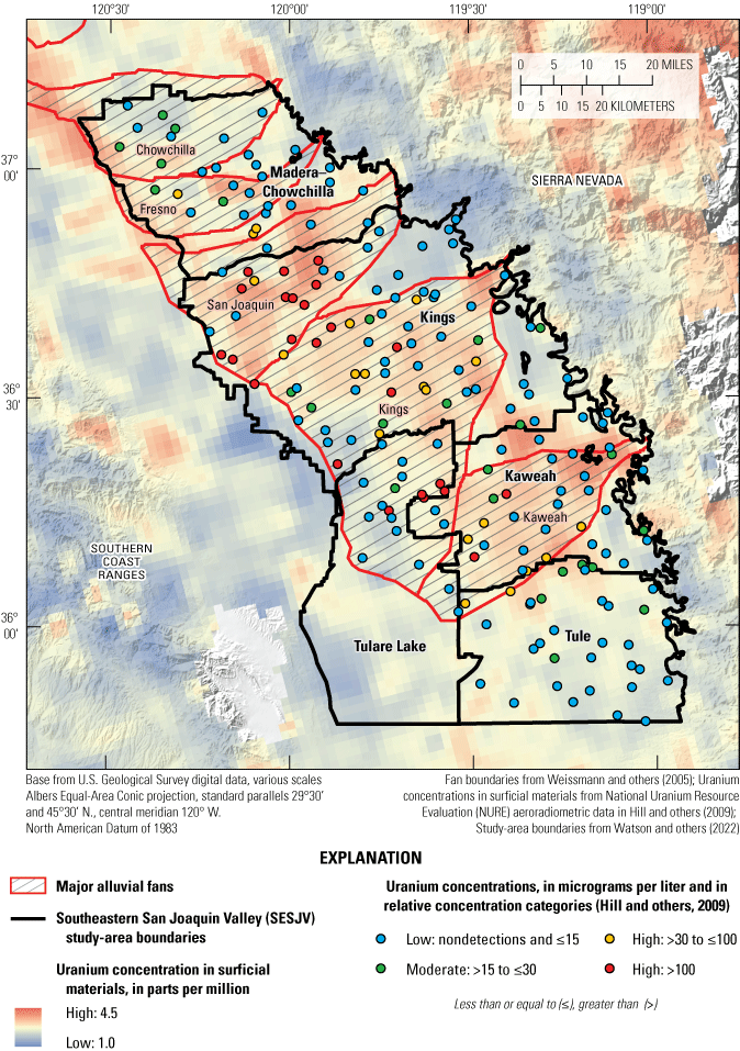
Concentrations of uranium in domestic-supply wells, southeastern San Joaquin Valley, 2013–15, California Groundwater Ambient Monitoring and Assessment Program Priority Basin Project.
The aquifer-scale proportions of high concentrations of uranium and the spatial distributions of wells with high uranium concentrations in the SESJV-D and SESJV-P were compared to help infer the processes controlling the occurrence of high uranium concentrations in groundwater. The proportion of the SESJV-D with high concentrations of uranium, 20 percent, was higher than the proportion in the SESJV-P, 10 percent (table 11; fig. 26). The largest differences were observed in the Kings and Kaweah study areas (tables 6–10; fig. 26). In the Kings and Kaweah study areas, the area dominated by high concentrations of uranium in SESJV-D had a mixture of high, moderate, and low concentrations in SESJV-P (compare SESJV-D data shown on fig. 27 to SESJV-P data shown on fig. 17F in Burton and others, 2012 and fig. 21 in Shelton and others, 2013).
The spatial distribution of high concentrations of uranium in groundwater in the study area can be related, in part, to the spatial distribution of high concentrations of uranium in surficial rocks and sediment (Rosen and others, 2019). The highest concentrations of uranium in surficial rocks and sediment were related to the source of the sediment in the Sierra Nevada that was deposited in the alluvial fans and valleys. Alluvial fans deposited by the San Joaquin, Kings, and Kaweah Rivers drain large, glaciated watersheds in the Sierra Nevada that are dominated by granitic rocks (Weissmann and others, 2005). Granitic rocks of the Sierra Nevada contain uranium-bearing accessory minerals (Wollenberg and Smith, 1968; Ague and Brimhall, 1988; Thomas and others, 1993). Estimated uranium concentrations in surficial sediments (Hill and others, 2009) were higher in the San Joaquin, Kings, and Kaweah River fans than in the Chowchilla and Fresno River fans or the interfan areas (fig. 27; Rosen and others, 2019). Leaching experiments indicated that a substantial part of the uranium on southeastern San Joaquin Valley sediments was sorbed to mineral surfaces and not readily soluble in natural conditions (Jurgens and others, 2008).
Differences in the prevalence of high uranium concentrations between SESJV-D and SESJV-P and in the spatial distribution of elevated uranium concentrations in the SESJV-D were expected based on the conceptual models of Jurgens and others (2010), Burow and others (2017), and Rosen and others (2019). In SESJV-D, uranium concentrations were positively correlated with bicarbonate (fig. 28), TDS, and nitrate concentrations (Spearman p<0.001, rho=0.62, 0.58, and 0.46, respectively). Uranium concentrations also were greater in modern- and mixed-age groundwater compared to premodern-age groundwater (Kruskall-Wallis, p<0.001, Dunn’s p<0.001, and p=0.007, respectively; fig. 28). Uranium also was inversely correlated with depth to top of screened interval in the SESJV-D (Spearman, p=0.007, rho=0.22) and SESJV-P (Burton and others, 2012; Shelton and others, 2013). Jurgens and others (2010) and Burow and others (2017) documented that higher concentrations of uranium were associated with modern, oxic groundwater sourced from agricultural irrigation return flow, and higher concentrations of uranium were associated with higher concentrations of other constituents linked to agricultural irrigation, including bicarbonate, TDS, and nitrate.

Relations among uranium concentrations in domestic-supply wells and bicarbonate concentrations, groundwater age classes, and groundwater oxidation-reduction (redox) classes, southeastern San Joaquin Valley, 2013–15, California Groundwater Ambient Monitoring and Assessment Program Priority Basin Project.
Laboratory experiments (Jurgens and others, 2008) and geochemical modeling (Jurgens and others, 2010) indicated that the correlation between uranium and bicarbonate was due to formation of soluble uranium-bicarbonate complexes from uranium that had been sorbed on iron-oxyhydroxide coatings, sediment grains, clay mineral edges, or to organic matter in aquifer sediments. The correlation between uranium and nitrate did not indicate oxidation of reduced uranium minerals by agricultural nitrate as proposed by Nolan and Weber (2015); rather, uranium and nitrate were correlated because both have elevated concentrations in groundwater containing recharge from agricultural irrigation return flow (Rosen and others, 2019). The irrigation-return flows contain nitrate from application of fertilizers and uranium mobilized from aquifer sediments by the elevated bicarbonate produced by plant productivity under irrigated conditions. The greater proportions of high concentrations of nitrate and uranium in the SESJV-D compared to the proportions in the SESJV-P (figs. 19, 26) indicate that recharge from irrigation-return flows has reached the depth zone used by domestic-supply wells in many areas of the southeastern San Joaquin Valley. Trends of increasing nitrate and uranium concentrations in public-supply wells indicate that this front of groundwater containing elevated nitrate and uranium concentrations is gradually reaching the greater depth zones used by public supply wells (Jurgens and others, 2010, 2020).
Some of the highest uranium concentrations are in anoxic or mixed-redox groundwater at the distal ends of the alluvial fans (figs. 27, 28; Rosen and others, 2019). At a given bicarbonate concentration, these anoxic and mixed redox wells have higher uranium concentrations than oxic wells (fig. 28), indicating that there is an additional source of uranium contributing to anoxic and mixed wells that does not contribute to oxic wells. Rosen and others (2019) observed that these wells with anoxic or mixed redox groundwater and higher uranium concentrations (fig. 28) are located near the boundary of the old discharge zone of the groundwater system (see fig. 10 in Rosen and others, 2019). This old discharge zone had artesian conditions in the early 1900s before extensive pumping began (Mendenhall, 1908; Mendenhall and others, 1916). This boundary between recharge and discharge zones also was a redox boundary, and uranium may have accumulated in the sediment at the boundary by processes similar to formation of uranium roll-front mineral deposits (Rosen and others, 2019). Uranium roll-front deposits form when oxic groundwater with dissolved uranium crosses from oxic to anoxic zones along a groundwater flow path in the aquifer, and there is sufficient uranium to precipitate as uraninite or other reduced uranium minerals (Harshman, 1975; Abzalov, 2012). If the redox conditions in the groundwater at the boundary later change, then the uranium minerals may dissolve. Rosen and others (2019) observed that the domestic wells with anoxic or mixed redox conditions and high uranium concentrations all have modern or mixed age groundwater and geochemistry consistent with being mixtures of younger oxic water and older anoxic water. Rosen and others (2019) concluded that the anomalously high uranium concentrations in these wells may be the result of dissolution of uraninite at the old redox boundary in the aquifer system by modern recharge that is undersaturated with uraninite because it is oxic and has high bicarbonate concentrations. The spatial pattern of recharge in the San Joaquin Valley has changed from a natural system where recharge primarily entered the groundwater system at the sides of the San Joaquin Valley near the mountains and along the major rivers and flowed toward discharge zones in the San Joaquin Valley trough area, to a modern system where agricultural irrigation return flow enhances recharge across the entire San Joaquin Valley and the combination of groundwater pumping and recharge of applied irrigation water results in much greater rate of downward movement of modern water into the aquifer system (Williamson and others, 1989; Burow and others, 2004; Phillips and others, 2007; Faunt, 2009; Jurgens and others, 2016). Haugen and others (2021) examined trends in arsenic concentrations in public-supply wells in the San Joaquin Valley and concluded that decreasing trends in arsenic concentrations in wells from the San Joaquin Valley trough area may be caused by decreased solubility of arsenic as modern, oxic groundwater moves into the capture zones of wells that previously accessed only older groundwater.
Radioactive Constituents
Most of the radioactivity in groundwater comes from the decay of naturally occurring uranium and thorium in the rocks or sediments that compose the aquifers (Hem, 1985; Appelo and Postma, 2005). Radioactive decay of uranium and thorium isotopes produces a long series of radioactive daughter products, including isotopes of radium, uranium, and radon. These elements have different chemical properties, and their solubility in groundwater varies with geochemical conditions, water chemistry, and aquifer mineralogy (Hem, 1985). In this study, we assessed data for adjusted gross alpha and adjusted gross beta particle activities, which is consistent with how the benchmarks for gross alpha and adjusted gross beta are defined.
Adjusted gross alpha particle activity is the measured gross alpha particle activity minus the alpha activity accounted for by the concentration of uranium in the sample. Uranium concentrations were converted to activities using a conversion factor of 0.67 pCi/µg. Adjusted gross beta particle activity is the measured gross beta particle activity minus the beta activity attributed to potassium-40. Potassium concentrations were converted to activities using a conversion factor of 0.82 pCi/mg (Welch and others, 1995). The measured values of gross alpha and beta depend on the initial composition of the water sample and on the time intervals between sample collection, sample preparation, and analysis. The differences among measured values at various combinations of time intervals can be used to estimate the relative abundance of isotopes contributing to the alpha or beta emissions. Measured values change with time because of radioactive decay and ingrowth during hold time as a water sample or after preparation of the solid residue for analysis.
Samples collected by the USGS were commonly analyzed after hold times of 72 hours and 30 days between collection and analysis, and the analytical method excludes isotopes that were gases at the time samples were prepared for analysis. Data from samples analyzed after the 30-day-hold time were used in this study because the longer hold time was more comparable to the hold times used in regulatory compliance sampling of public-supply wells. The primary contributors to adjusted gross beta in most groundwater samples were radium-228 and its progeny actinium-228 and the beta-emitting progeny of uranium-238, protactinium-234, and thorium-234 (Welch and others, 1995). The primary contributors to adjusted gross alpha are alpha-emitting isotopes on the decay series for radium-224, radium-226, radium-228, lead-210, and polonium-210 (Arndt, 2010).
Radioactive constituents with MCL benchmarks were present at high concentrations in 7.7 percent and at moderate concentrations in 8.1 percent of the SESJV-D (table 5). The proportions of the five study areas with high concentrations of radioactive constituents with MCL benchmarks fell into three categories: (1) the proportions in Madera-Chowchilla and Tule were 0 percent; (2) the proportion in Kaweah was 4.8 percent; and (3) the proportions in Kings and Tulare Lake were 16 and 17 percent, respectively (table 5). High concentrations of adjusted gross beta particle activities were more prevalent in SESJV-D than high concentrations of adjusted gross alpha particle activities (table 11; fig. 18B).
The SESJV-P dataset contained insufficient data to calculate aquifer-scale proportions for adjusted gross beta particle activities. Adjusted gross beta is regulated, but analysis is not required unless a system is classified as potentially vulnerable to having elevated gross beta activities (California State Water Resources Control Board, 2017b). In addition, sampling requirements are lower for systems with previously measured gross beta particle activities less than the 50-pCi/L trigger level (California State Water Resources Control Board, 2017b).
Most SESJV-D wells with moderate or high concentrations of adjusted gross beta particle activities were on the intermediate and distal parts of the San Joaquin and Kings River fans and had high concentrations of uranium (compare fig. 27 to fig. 29). Adjusted gross beta particle activities were positively correlated with uranium concentrations (Spearman test, p<0.001, rho=0.80; fig. 30). Beta particle activity from ingrowth of thorium-234 and protactinium-234 from decay of uranium-238 during the 30-day-hold time before sample analysis was estimated using the half-lives for thorium-234 and protactinium-234 and the concentration of uranium (Welch and others, 1995). The estimated activity from decay of thorium-234 and protactinium-234 formed by uranium present in samples accounts for nearly all the adjusted gross beta particle activity in 23 of the 24 wells with high or moderate adjusted gross beta particle activities. Beta activity from decay of radium-228 (and its progeny actinium-228) may be an important contributor to adjusted gross beta activity in samples for which the decay series of uranium-238 during sample holding time does not account for the measured adjusted gross beta activities (Welch and others, 1995).
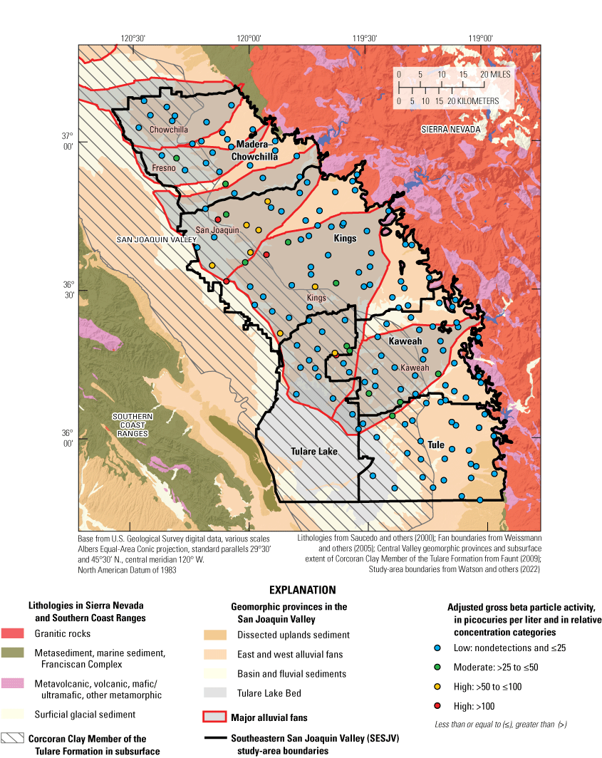
Adjusted gross beta particle activities in domestic wells, southeastern San Joaquin Valley, 2013–15, California Groundwater Ambient Monitoring and Assessment Program Priority Basin Project.
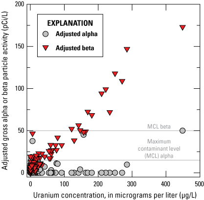
Relations between uranium concentrations and gross alpha and gross beta particle activities in domestic wells, southeastern San Joaquin Valley, 2013–15, California Groundwater Ambient Monitoring and Assessment Program Priority Basin Project.
Most of the unadjusted gross alpha particle activity in SESJV-D groundwater samples was accounted for by uranium. For the 170 SESJV-D samples with data for gross alpha particle activity and uranium concentration, calculated uranium activity equaled a median of 93 percent (interquartile range of 56 to 117 percent) of the unadjusted gross alpha particle activity (Arnold and others, 2016, 20186; Bennett and others, 2017; Shelton and Fram, 2017). A total of 41 percent of samples had unadjusted gross alpha particle activities greater than 7.5 pCi/L, but only 7 percent of samples had adjusted gross alpha particle activities greater than 7.5 pCi/L, corresponding to moderate or high relative concentrations. The uncertainty in gross alpha particle activity measurements can be large (Arndt, 2010); therefore, adjusted gross alpha particle activities, particularly in samples with large unadjusted gross alpha particle activities, may have large uncertainties.
Adjusted gross alpha activities were not correlated with uranium concentrations (Spearman test, p=0.158, rho= −0.10; fig. 30). The lack of correlation with uranium may indicate that the adjusted gross alpha particle activity is primarily from of alpha-emitting isotopes on the decay chains of radioactive isotopes other than uranium present in the groundwater at the time of sample collection. Inference of isotopes contributing to the adjusted gross alpha activity was not attempted because of the uncertainty in gross alpha particle activity measurements (Arndt, 2010) and because samples for direct analysis of radium isotopes, lead-210, and polonium-210 were not collected for this study.
Constituents with Secondary Maximum Contaminant Level Benchmarks
The class of constituents with SMCL benchmarks includes salinity indicators (chloride, sulfate, and TDS) and the trace elements iron and manganese. These constituents can affect the aesthetic properties of water, such as taste, color, and odor, or create technical problems, such as scaling and staining. Secondary maximum contaminant level benchmarks are based on these aesthetic and technical concerns and are not health-based benchmarks (California State Water Resources Control Board Division of Drinking Water, 2022b).
Constituents with SMCL benchmarks were present at high concentrations in 14 percent and at moderate concentrations in 26 percent of the SESJV-D (table 5). Salinity indicators (chloride, sulfate, or TDS) were present at a high concentration in 4.3 percent, and iron or manganese were present at a high concentration in 12 percent of the SESJV-D. The constituents most commonly responsible for the high concentrations were TDS and manganese, which were present at high and moderate concentrations in all five study areas (tables 6–10; fig. 18D). The proportion of SESJV-P with high concentrations of salinity indicators (4.0 percent) was not different from the proportion in the SESJV-D (4.3 percent, confidence interval 2.4–7.2 percent), although the proportion with moderate concentrations was lower in the SESJV-P (12 percent) compared to SESJV-D (30 percent; table 5). The proportion of the SESJV-P with high concentrations of trace elements with SMCLs (17 percent), was higher than the proportion in the SESJV-D (12 percent; table 5). The only trace elements with SMCLs present at moderate or high concentrations were manganese and iron (tables 2–4).
Manganese and Iron
Natural sources of manganese and iron to groundwater include weathering and dissolution of minerals in soils, sediments, and rocks. Manganese- and iron-oxyhydroxide minerals commonly coat sediment grains, and manganese commonly substitutes for iron in silicate and oxide minerals in the iron-bearing silicate, sulfide, or oxide minerals present in most rocks and sediments. The solubilities of manganese and iron are strongly dependent on redox conditions; more reduced species are generally more soluble (Hem, 1985).
Manganese was present at concentrations above the HAL-US in 4.9 percent and at concentrations between the SMCL-CA and HAL-US in 7.2 percent of the SESJV-D (table 11; fig. 31). Wells with concentrations above the SMCL-CA were present in all five study areas, and concentrations above the HAL-US were present in Kings, Kaweah, and Tulare Lake study areas (tables 6–10; figs. 18, 32). All wells with high concentrations of iron also had concentrations of manganese above the SMCL-CA (Bennett and others, 2017; Shelton and Fram, 2017), and manganese and iron were positively correlated (Spearman’t test, p<0.001, rho=0.67). Most wells with concentrations of manganese above benchmarks were along the western edge of the SESJV-D, primarily in the Kings and Tulare Lake study areas (fig. 32). The locations of domestic wells with high concentrations of manganese were expected based on the locations of groundwater with anoxic or mixed redox conditions in the hydrologic system of the SESJV-D. Anoxic and mixed redox conditions were most prevalent along the western edge of the SESJV-D (fig. 14), and most wells with high manganese concentrations were along the western edge of the SESJV-D (fig. 32). The locations of domestic wells with manganese concentrations greater than the SMCL-CA and HAL-US benchmarks were consistent with the maps of Rosecrans and others (2017, 2018) which showed that the highest probabilities of occurrence of elevated manganese concentrations were in the San Joaquin Valley trough with sparse scattered zones of slightly elevated probability near the eastern margin of the valley.

Aquifer-scale proportions for high (yellow), moderate (green), and low (blue) concentrations of manganese in the domestic-supply (-D) and public-supply (-P) aquifers of A, the Madera-Chowchilla study area; B, Kings study area; C, Kaweah study area; D, Tule study area; E, Tulare Lake study area; and F, southeastern San Joaquin Valley (SESJV) as a whole, 2013–15, California Groundwater Ambient Monitoring and Assessment Program Priority Basin Project.
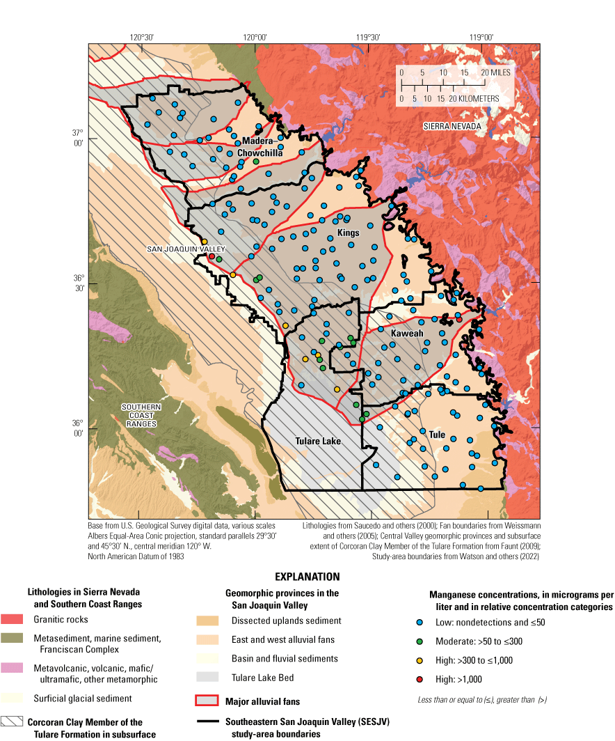
Concentrations of manganese in domestic-supply wells, southeastern San Joaquin Valley, 2013–15, California Groundwater Ambient Monitoring and Assessment Program Priority Basin Project.
Manganese was present at concentrations above the HAL-US in 2.6 percent and at concentrations between the SMCL-CA and HAL-US in 8.7 percent of the SESJV-P (table 11; fig. 31). As in SESJV-D, wells in SESJV-P with concentrations of manganese above benchmarks were primarily detected along the western edge of the southeastern San Joaquin Valley, in the Kings and Tulare Lake study areas, although a few were along the eastern edge close to the boundary between the Central Valley and the Sierra Nevada in the Tule, Kaweah, and Kings study areas (compare SESJV-D data shown on fig. 32 to SESJV-P data shown on fig. 17H in Burton and others, 2012). The SESJV-P wells with high concentrations of manganese along the eastern side of the southeastern San Joaquin Valley are represented entirely by SWRCB-DDW data in the dataset used for this report. The wells do not have dissolved oxygen concentration data to corroborate anoxic conditions and most do not have depth information. Elevated manganese concentrations in some samples in the SWRCB-DDW dataset may be due to sample collection protocols. All USGS data are for filtered samples, whereas SWRCB-DDW data may be for filtered or unfiltered samples. Agreement between USGS and SWRCB-DDW data for samples collected at the same well near the same time was poorest for constituents like manganese that may be associated with particulates in groundwater samples (appendix B in Fram and Shelton, 2015).
Manganese concentrations were significantly greater in premodern groundwater compared to modern groundwater in the SESJV-P (Burton and others, 2012) but were not significantly different in the SESJV-D (Kruskall-Wallis p=0.006, Dunn’s p=0.070). Manganese concentrations in the SESJV-D also did not have a significant correlation with well depth (Spearman, p=0.588, rho=0.04). Wells above the Corcoran Clay in the Kings and Tulare Lake study areas had anoxic conditions because of their location in the basin and Tulare Lake Bed deposits, but these wells are shallow and can have modern, mixed, or premodern groundwater (fig. 11). McMahon and others (2019) observed that elevated manganese concentrations were associated with shallow, anoxic water tables and soils enriched in organic carbon. Public-supply wells in the same area also were anoxic because of the sediments but were deep and had premodern or mixed-age groundwater (Burton and others, 2012).
Total Dissolved Solids
Groundwater salinity may be affected by many natural and anthropogenic factors (Hem, 1985; Appelo and Postma, 2005). The list of potential factors that may be relevant in the southeastern San Joaquin Valley includes, but is not limited to, the following: sources and quality of stream water recharging and contributing salts to the shallow groundwater; sources of depositional sediments in alluvial fans; use of water for irrigation and recharge of drainage water; evaporation and evapotranspiration; mixing with hydrothermal fluids; mixing with connate fluids from marine or lacustrine sediments; contributions from fertilizers; discharges from treatment plants, septic systems, and agricultural operations; geochemical processes, such as ion exchange, mineral dissolution and precipitation; and biological reactions that affect redox sensitive elements (Hem, 1985; Appelo and Postma, 2005). Furthermore, use of water for irrigation in the San Joaquin Valley has caused changes to groundwater chemistry that contribute to increased TDS concentrations in groundwater (Hansen and others, 2018).
Total dissolved solids is an indicator of salinity that was present at high concentrations (above the upper SMCL-CA of 1,000 mg/L) in 4.3 percent and at moderate concentrations (between the recommended SMCL-CA of 500 mg/L and the upper SMCL-CA) in 30 percent of SESJV-D (table 11). The proportions of the five study areas with high concentrations fell into two groups: (1) Madera-Chowchilla, Kaweah, and Tule study areas had high concentrations in 1.9, 1.8, and 0 percent of the study area, respectively, and (2) Kings and Tulare Lake had high concentrations of TDS in 8.0 and 8.9 percent of the study area, respectively (tables 6–10; fig. 33). High concentrations of TDS were detected in the distal parts of the alluvial fans near the center of the basin, and moderate concentrations were distributed across much of the SESJV-D area (fig. 34). Moderate concentrations were detected in all study areas (figs. 18, 33). The spatial distribution of TDS concentrations in the SESJV-D was similar to the spatial distribution predicted for the San Joaquin Valley using a larger dataset (Luhdorff and Scalmanini Consulting Engineers, 2016). Chloride and sulfate were present at high concentrations in 0.3 and 1.6 percent of the SESJV-D, respectively (table 11), and all wells with high concentrations of chloride or sulfate also had high concentrations of TDS (Bennett and others, 2017; Shelton and Fram, 2017).

Aquifer-scale proportions for high (yellow), moderate (green), and low (blue) concentrations of total dissolved solids in the domestic-supply (-D) and public-supply (-P) aquifers of A, the Madera-Chowchilla study area; B, Kings study area; C, Kaweah study area; D, Tule study area; E, Tulare Lake study area; and F, southeastern San Joaquin Valley (SESJV) as a whole, 2013–15, California Groundwater Ambient Monitoring and Assessment Program Priority Basin Project.

Concentrations of total dissolved solids in domestic wells, southeastern San Joaquin Valley, 2013–15, California Groundwater Ambient Monitoring and Assessment Program Priority Basin Project.
The proportions of the Madera-Chowchilla, Kings, Kaweah, and Tule study areas that had high concentrations of TDS were similar in the SESJV-D and SESJV-P; the proportion of the Tulare Lake study area with high concentrations of TDS was greater in the SESJV-D than the SESJV-P (table 11; fig. 33). However, the SESJV-D had a substantially greater proportion with moderate concentrations of TDS (30 percent) compared to the SESJV-P (12 percent; table 11), and the proportion with moderate concentrations was greater in the SESJV-D than SESJV-P for all five study areas (tables 6–10; fig. 33). Differences in the spatial distribution of wells with high or moderate concentrations of TDS between the SESJV-D and the SESJV-P were greatest in the Tulare Lake study area and the central part of the Kings study area (compare SESJV-D data on fig. 34 to SESJV-P data on fig. 17J in Burton and others, 2012).
The diversity of major ion compositions of groundwater and the lack of a consistent relation between major ion composition and TDS concentration (fig. 35) indicated that multiple sources and processes affect TDS concentrations in SESJV-D (Mendenhall and others, 1916; Page, 1973; Planert and Williams, 1995; Larry Walker and Associates, 2010; Fram, 2017a; Hansen and others, 2018; Pauloo and others, 2021; Central Valley Salinity Alternatives for Long-term Sustainability, 2023). Because of this diversity of sources and processes, simple statistical tests for associations between water quality and potential explanatory factors were not effective for identifying factors controlling TDS concentrations (Fram, 2017a), and a more in-depth evaluation of the sources of salinity was beyond the scope of this report.

Total dissolved solids concentrations for groundwater samples from domestic-supply wells in the southeastern San Joaquin Valley, 2013–15, California Groundwater Ambient Monitoring and Assessment Program Priority Basin Project.
Selected processes and sources that may affect salinity in the SESJV-D are briefly described in this section. Hansen and others (2018) determined that the increases in TDS in the southeastern San Joaquin Valley during the past century can largely be explained by enhanced dissolution of minerals promoted by the increased bicarbonate generated by irrigated agriculture. Uranium and TDS were positively correlated in the SESJV-D (Spearman p<0.001, rho=0.58). As discussed in the “Uranium” section, uranium also was more prevalent at concentrations above benchmarks in the SESJV-D than in the SESJV-P, especially in the Kings study area. The positive statistical correlation between TDS and uranium supports previous findings that TDS and uranium are affected by agriculture.
Pauloo and others (2021) modeled salt accumulation in the Tulare Basin (including the Kings, Kaweah, Tule, and Tulare Lake study areas) that resulted from basin closure. Salts from imported surface water, pumped groundwater, and concentration from evapotranspiration and water-rock interaction result in increasing salinity (first in the shallow aquifer and later in deeper aquifers). Fram (2017a) used isotopic and major ion data to track sources of salinity in the western San Joaquin Valley. These sources of salts may affect groundwater in the SESJV-D along the western margin of the southeastern San Joaquin Valley.
Similar to the findings of Visser and others (2018) for public-supply groundwater in the eastern San Joaquin Valley and Fram (2017a) for the western San Joaquin Valley, extensive amounts of evaporative concentration were not observed in groundwater in the SESJV-D. The SESJV-D samples have stable isotopic compositions close to the local meteoric water line (LMWL) defined by Visser and others (2018; fig. 36). In contrast, the shallow groundwater from monitoring wells in the Tulare Lake Bed includes samples with stable isotope compositions plotting on evaporation lines extending from the LMWL, and the relation between TDS concentrations and stable isotope composition indicated evaporative concentration was an important mechanism contributing to high TDS concentrations in shallow groundwater (Fujii and Swain, 1995). The absence of evaporation trend lines in the stable isotope diagram for the SESJV-D (fig. 36) indicates that the extensively evaporated water in the shallow groundwater system identified by Fujii and Swain (1995) in the Tulare Lake Bed region apparently had not penetrated in large amounts to the depth zones used by domestic- or public-supply wells at the time of sampling in this study.

Oxygen and hydrogen stable isotopic composition of water and total dissolved solids concentrations in groundwater samples collected from domestic-supply wells in the southeastern San Joaquin Valley, 2013–15, California Groundwater Ambient Monitoring and Assessment Program Priority Basin Project.
The range in stable isotopic compositions in the SESJV-D indicated sources of recharge ranging from local precipitation at relatively low elevations in the San Joaquin Valley and nearby foothills (heavier delta oxygen-18 values greater than about −9 per mil) to large rivers predominantly fed by high-elevation precipitation (fig. 36). The spatial pattern of stable isotopic composition lighter delta oxygen-18 values less than about −12 per mil) was similar to the spatial pattern observed in public-supply wells by Visser and others (2018; compare fig. 37 to fig. 4 in Visser and others, 2018). Wells in the interfan areas along the eastern side of the southeastern San Joaquin Valley commonly had stable isotope compositions greater than −10 per mil, indicating a source from low-elevation precipitation. Wells in the fans of the Chowchilla and Fresno Rivers also had stable isotope compositions in the range from −11 to greater than −8 per mil, consistent with watersheds predominantly in the lower-elevation foothills of the Sierra Nevada. The Kings and Kaweah River fans and parts of San Joaquin River fan generally have stable isotope compositions from −11 to less than −13 per mil that indicate high-elevation sources of water from the headwaters of the rivers.

Oxygen stable isotopic composition of water in groundwater samples collected from domestic wells in the southeastern San Joaquin Valley, 2013–15, California Groundwater Ambient Monitoring and Assessment Program Priority Basin Project.
The main difference between the spatial pattern on figure 37 and the pattern observed for public-supply wells by Visser and others (2018) was that the region dominated by high elevation recharge in the Kings River fan is larger in the SESJV-D. In the Kings and Tulare Lake study areas, where the Kings River fan is located, the SESJV-D has a greater proportion of modern groundwater than the SESJV-D (fig. 12). The larger region dominated by recharge from high-elevation sources in the SESJV-D compared to the SESJV-P indicates that imported surface water routed to the area for irrigation is recharging the aquifer system and is reaching the depths of domestic-supply wells, but not yet the depths of public-supply wells.
Perchlorate
Perchlorate is an inorganic anion with natural and anthropogenic sources that is formed naturally in the atmosphere and is present in precipitation (Dasgupta and others, 2005; Parker and others, 2008; Rajagopalan and others, 2009). Perchlorate can accumulate in salts that precipitate in soils and unsaturated zones of aquifer systems in arid areas (Walvoord and others, 2003; Rao and others, 2007; Jackson and others, 2010). The probability of detecting perchlorate in groundwater during natural conditions increases as conditions become more arid (Fram and Belitz, 2011). Perchlorate salts are a primary ingredient in solid rocket fuels and are used in explosives, safety flares, and fireworks; thus, manufacture, use, or disposal of those products are potential sources of perchlorate contamination to groundwater (Interstate Technology and Regulatory Council, 2005; U.S. Environmental Protection Agency, 2014; California State Water Resources Control Board, 2022b). Perchlorate also is present as a minor salt in the Chilean nitrate fertilizer that was used extensively in California before industrial sources of nitrate fertilizer were plentiful (Dasgupta and others, 2006; Böhlke and others, 2009).
Perchlorate was detected at high concentrations (above the MCL-CA of 6 µg/L) in 0.9 percent and at moderate concentrations in 3.3 percent of the SESJV-D (table 11). The prevalence of high concentrations in SESJV-P was the same (0.9 percent; table 11). The computed prevalence of moderate concentrations in the SESJV-P (0.9 percent; table 11) was a minimum estimate because the reporting limit used for most perchlorate data in the SWRCB-DDW database is 4 µg/L (California State Water Resources Control Board Division of Drinking Water, 2022d; California State Water Resources Control Board, 2023b).
Logistic regression models of Fram and Belitz (2011) were used to estimate if the perchlorate detected in the SESJV-D was primarily natural or anthropogenic in origin. This estimation was only done for the SESJV-D because all perchlorate data had reporting levels of 0.1 µg/L. The proportion of the SESJV-D with detection of perchlorate at concentrations greater than the detection limit of 0.1 µg/L was 70 percent (66 percent at low concentrations, 3.3 percent at moderate, and 0.9 percent at high; table 12).
Table 12.
Aquifer-scale proportions for organic constituents, organic constituent classes, and perchlorate in the domestic-supply aquifer (SESJV-D) of the southeastern San Joaquin Valley, 2013–15, California Groundwater Ambient Monitoring and Assessment Program Priority Basin Project.[—Left][Aquifer-scale proportion is the areal proportion of the study area with high, moderate, or low concentrations calculated using a cell-declustering method. Calculations are based on data from 183 wells sampled by the California Groundwater Ambient Monitoring and Assessment Program Priority Basin Project (GAMA-PBP) during 2013–15 (table 1.1–1.5; U.S. Geological Survey, 2023b; Balkan and others, 2024). Concentration categories: high, constituent has a concentration above the benchmark; moderate, constituent has a concentration above the one-tenth the benchmark but less than or equal to the benchmark; low, constituent has a concentration greater than or equal to the method detection level and less than or equal to one-tenth the benchmark. Tables 2 and 4 list the concentrations of the benchmarks; detection levels in Shelton and Fram (2017), Bennett and others (2017), and Fram (2020). Abbreviations: MCL, maximum contaminant level benchmark; NR, non-regulatory health-based benchmark]
Detection frequencies of perchlorate were compared to predicted probabilities of perchlorate detection in groundwater for the aridity conditions in the southeastern San Joaquin Valley. Because perchlorate degrades under redox conditions similar to conditions for degradation of nitrate (Coates and Achenbach, 2004), the SESJV-D dataset was trimmed to remove 26 samples for which the nondetection of perchlorate could either have been due to absence of perchlorate input to the sample or to degradation of perchlorate that had been present in the sample. These 26 samples were anoxic or mixed redox samples that had nondetections of perchlorate and had nitrate concentrations less than 0.5 mg/L. Of the 15 Tulare Lake samples, 8 were removed, leaving an insufficient number of samples with which to evaluate perchlorate detections in the Tulare Lake study area by this method. Detection frequencies of perchlorate in the remaining 126 samples relative to threshold levels of 0.1, 0.5, and 1.0 µg/L were compared to predicted probabilities of detecting perchlorate in groundwater at concentrations above those thresholds under natural conditions at the study-area scale (fig. 38; Fram and Belitz, 2011). Error bars for the measured detection frequencies were estimated as the 90-percent Jeffreys confidence interval (equation 3; Brown and others, 2001; Belitz and others, 2010); ranges for the predicted probabilities of detection were estimated as the predicted probability values for a range in aridity index of plus or minus two standard deviations from the mean aridity index for the samples.
The observed detection frequencies of perchlorate relative to threshold levels of 0.1, 0.5, and 1.0 µg/L were all greater than the predicted probabilities of detection for the Madera-Chowchilla, Kings, Kaweah, and Tule study areas. All measured detection frequencies were greater than predicted probabilities of detection (fig. 38), indicating presence of some anthropogenic sources of perchlorate. The differences between predicted and observed detection frequencies were greatest for the higher concentrations (greater than 0.5 and 1.0 µg/L) and in the Kings, Kaweah, and Tule study areas. Perchlorate concentration was positively correlated with nitrate concentration (Spearman, p<0.001, rho=0.81), and 94 percent of samples with perchlorate greater than 0.5 µg/L also had nitrate greater than 5 mg/L, indicating the contribution of anthropogenic sources of nitrate. Nitrate concentrations in groundwater greater than 2 mg/L generally indicate contributions from anthropogenic sources of nitrate (Dubrovsky and others, 2010). We used a more conservative threshold of 5 mg/L (Burow and others, 2013) to increase the certainty that the elevated nitrate concentrations were indicative of anthropogenic sources of nitrate. Because both nitrate and perchlorate have agricultural sources, if elevated concentrations of both nitrate and perchlorate are detected, and agricultural sources of nitrate contribute to the nitrate load in the groundwater, it is likely that anthropogenic sources contributed to the perchlorate load in the groundwater. The relation between nitrate and perchlorate concentrations indicates that most perchlorate detections with concentrations greater than 0.5 µg/L are consistent with contribution from anthropogenic sources of perchlorate.

Relation between predicted probability of detecting perchlorate in groundwater during natural conditions and observed detection frequencies of perchlorate relative to three concentration thresholds (0.1, 0.5, and 1.0 micrograms per liter [µg/L]).
The predicted probabilities of detection relative to a threshold of 0.1 µg/L under natural conditions were 60–70 percent (fig. 38), indicating that most of the perchlorate detections at concentrations between 0.1 and 0.5 µg/L likely were due to natural sources. Only 25 percent of samples with perchlorate concentrations less than 0.5 µg/L also had nitrate greater than 5 mg/L. The two agricultural sources are nitrate fertilizers that contain perchlorate and perchlorate from the unsaturated zone swept by increased recharge from irrigation (Walvoord and others, 2003; Dasgupta and others, 2006; Rao and others, 2007; Böhlke and others, 2009; Jackson and others, 2010; Fram and Belitz, 2011); differentiating between the two agricultural sources is beyond the scope of this report.
Organic Constituents
Organic constituents measured in this study included volatile organic compounds (VOCs) and pesticides and their degradation products (tables 2, 4). Nearly all the organic constituents analyzed for this study are produced by human activities; thus, their presence in groundwater indicates anthropogenic influence on groundwater quality (Gilliom and others, 2006; Zogorski and others, 2006). VOCs are present in a wide array of human-made products, including paints, solvents, fuels, refrigerants, and fumigants and are produced as a by-product of disinfection. A few of the VOCs analyzed in this study also can be present naturally in groundwater near hydrocarbon deposits or in anoxic groundwater. Pesticides include herbicides, fumigants, insecticides, and fungicides that are used to control unwanted vegetation, insects, fungi, and other pests. Fumigants can be classified as VOCs because of their volatile nature but also are classified as pesticides because they are used to control pests.
A total of 317 organic constituents (90 VOCs, including fumigants, and 227 pesticides and pesticide degradate compounds) were analyzed (Bennett and others, 2017; Shelton and Fram, 2017), and 52 organic constituents were detected at any concentration in 1 or more of the 183 domestic wells used in this study (tables 2, 4). Of these 52 detected organic constituents, 19 did not have comparison benchmarks, 17 had non-regulatory health-based benchmarks (HAL-US, RL-CA, HBSL-NC, or HHBP-NC), and 16 had regulatory benchmarks (MCL-CA or MCL-US). Many of the organic constituents lacking comparison benchmarks were degradation products of pesticides with benchmarks that were detected in samples from the SESJV-D.
One or more organic constituent with MCL benchmarks were detected at high concentrations in 19 percent of the SESJV-D, at moderate concentrations in 3.6 percent, and at low concentrations in 36 percent of the SESJV-D (table 12). For organic constituents, low concentrations were defined as greater than or equal to the applied detection level and less than or equal to one-tenth of the comparison benchmark. Results for moderate concentrations in table 6 for the SESJV-D are not the same as the results in table 5; the results in table 5 were calculated with the SESJV-D data censored to the reporting levels used in the SWRCB-DDW database to facilitate comparison between SESJV-P and SESJV-D (see the “Water-Quality Data” subsection in the “Methods” section). Organic constituents with MCL benchmarks were not present at concentrations above the USGS analytical detection levels in 41 percent of the SESJV-D. The proportion of each study area with high concentrations of organic constituents with MCLs ranged from 3.6 percent for Kaweah to 30 percent for Madera-Chowchilla (table 6; fig. 17). All the organic constituents with MCLs that were detected at high concentrations were classified as fumigants (figs. 18E–18G).
The proportion of SESJV-P with high concentrations of organic constituents (12 percent) was significantly less than the proportion of SESJV-D with high concentrations of organic constituents (19 percent, confidence interval 15–24 percent; table 5; fig. 17). The difference in the prevalence of high concentrations of organic constituents between SESJV-P and SESJV-D is primarily due to the greater prevalence of high concentrations of fumigants (19 percent, confidence interval 15–24 percent) in the SESJV-D compared to the SESJV-P (15 percent; table 5). The SESJV-P also had high concentrations of solvents, but the proportion of the SESJV-P with high concentrations of solvents (0.5 percent) was within the confidence interval of the proportion of high concentrations of solvents (0.0–0.7 percent) observed in the SESJV-D (table 5).
Fumigants
Soil fumigants can be used to kill or manage pests in urban and agricultural settings and are of particular interest in California because of their widespread historical use in certain agricultural settings, including in the San Joaquin Valley. Nine VOCs used as fumigant pesticides or included in fumigant mixtures were analyzed (Bennett and others, 2017; Shelton and Fram, 2017), and four were detected: 1,2-dibromo-3-chloropropane (DBCP), 1,2-dibromoethane (EDB), 1,2-dichloropropane (1,2-DCP), and 1,2,3-trichloropropane (1,2,3-TCP; table 2; fig. 18E). Use of the soil fumigants DBCP, EDB, and 1,2-DCP was banned in California beginning in the late 1970s and early 1980s. The fumigant DBCP was used from 1955 to 1977 primarily to control nematodes on vineyard crops but also on some orchard and vegetable crops (Peoples and others, 1980; Domagalski and Dubrovsky, 1992; Kloos, 1996; Burow and others, 1999). The fumigant EDB was used from about 1948 to 1983, and it was also used as a gasoline additive beginning in the 1920s (Kloos, 1996). Fumigant mixtures of 1,2-DCP and 1,3-dichloropropene isomers were used from 1942 to 1984 (Deeley and others, 1991; Loague and others, 1998). The VOC 1,2,3-TCP is used as a solvent but also was present in fumigant mixtures containing 1,2-DCP (Oki and Giambelluca, 1987; Zebarth and others, 1998; California State Water Resources Control Board, 2017a).
Fumigants were present at high concentrations in 19 percent, at moderate concentrations in 2.0 percent, and at low concentrations in 9.0 percent of the SESJV-D. Fumigants were not detected at concentrations greater than analytical detection limits in 70 percent of the SESJV-D (table 12). High concentrations of fumigants were detected in all five study areas, ranging from 3.6 percent in Kaweah study area to 30 percent in Madera-Chowchilla study area.
Most of the detections at high concentrations throughout all study areas were for 1,2,3-TCP (fig. 18E). The health-based benchmarks for the fumigants have different magnitudes. The MCL-CA for 1,2,3-TCP is 40 times less than the MCL-US for DBCP and one thousand times less than the MCL-US for 1,2-DCP (table 2). The median detected concentration of 1,2,3-TCP was significantly greater than the median detected concentration of 1,2-DCP (Wilcoxon test, p=0.023) but not significantly different from the median detected concentrations of DBCP or EDB (Wilcoxon test, p=0.203 and p=0.096, respectively). However, because the benchmark for 1,2,3-TCP is less than the benchmarks for the other fumigants, detections of 1,2,3-TCP were more likely to have concentrations greater than the benchmark than were detections of the other fumigants.
The compound 1,2,3-TCP was detected at high concentrations in 15 percent of the SESJV-D (table 12). Because the detection level of 0.003 µg/L (half of the laboratory reporting level of 0.006 µg/L) was close to the MCL-CA, the presence of 1,2,3-TCP at moderate and low RCs could not be determined. There were high concentrations detected in all five study areas (fig. 39), with the proportion of high concentrations falling into two groups: (1) 3.6 and 6.7 percent, respectively, in the Kaweah and Tulare Lake study areas and (2) 19, 18, and 21 percent, respectively, in the Madera-Chowchilla, Kings, and Tule study areas (table 12; Burow and others, 2019) detected 1,2,3-TCP at concentrations above the MCL-CA in about 8 percent of domestic wells statewide and in 18 percent of domestic wells in the San Joaquin Valley. The fumigant DBCP was detected in the Madera-Chowchilla, Kings, Kaweah, and Tule study areas (fig. 40), corresponding to 16 percent of the SESJV-D. DBCP, and was present at high and moderate concentrations in 4.8 and 7.0 percent of the area, respectively (table 12). The proportion of high concentrations ranged from 0 percent in Tulare Lake and Kaweah to 12 percent in Madera-Chowchilla (table 12). Burow and others (2019) observed that samples with detections of 1,2,3-TCP commonly had detections of other fumigant compounds. All samples from SESJV-D domestic wells that had a detection of 1,2,3-TCP also had detections of at least one other fumigant (Bennett and others, 2017; Shelton and Fram, 2017; Fram and Shelton, 2018), and concentrations of 1,2,3-TCP were positively correlated with concentrations of DBCP (Spearman test, p<0.001, rho 0.47) and 1,2-DCP concentrations (Spearman test, p<0.001, rho 0.68).

Concentrations of 1,2,3-trichloropropane in groundwater samples collected from domestic-supply wells in southeastern San Joaquin Valley, 2013–15, California Groundwater Ambient Monitoring and Assessment Program Priority Basin Project.
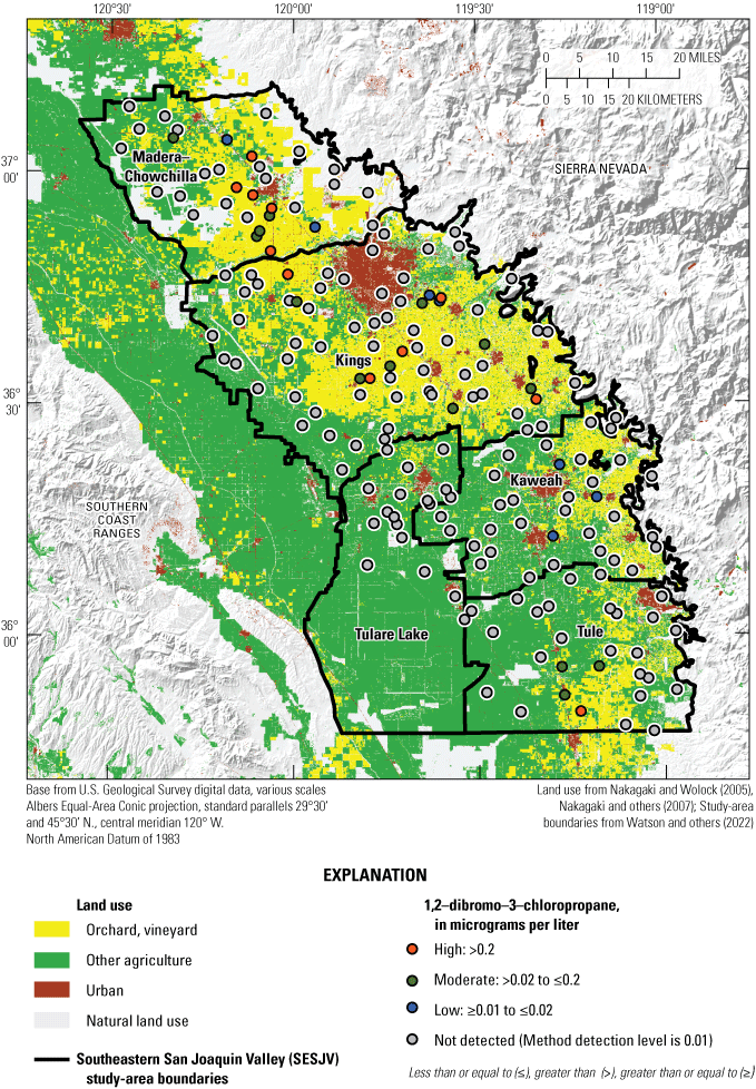
Concentrations of 1,2-dibromo-3-chloropropane in groundwater samples collected from domestic-supply wells in southeastern San Joaquin Valley, 2013–15, California Groundwater Ambient Monitoring and Assessment Program Priority Basin Project.
Together, two explanatory factors, percentage of orchard and vineyard land use and groundwater age, described the occurrence pattern of DBCP and 1,2,3-TCP in SESJV-D wells. Because DBCP and fumigants containing 1,2,3-TCP were both used on orchard and vineyard crops, it was not surprising that wells with detections of 1,2,3-TCP and DBCP were primarily in areas of orchard and vineyard land use (figs. 39, 40). The detection frequency of DBCP or 123-TCP in SESJV-D samples was greater in modern (34 percent) and mixed (16 percent) groundwater compared to the detection frequency in premodern groundwater (4 percent; not shown). Although DBCP and 1,2,3-TCP are human-made compounds and therefore generally not present in groundwater that does not contain a component of modern recharge, the presence of modern recharge alone is not sufficient to predict presence of DBCP or 1,2,3-TCP in a well. When the dataset was stratified by land use, the relation between groundwater age and detection frequency became stronger. The detection frequency of DBCP or 123-TCP in SESJV-D samples from wells surrounded by greater than 35-percent orchard or vineyard land use and having modern groundwater was 53 percent compared to a detection frequency of 8.5 percent in wells having modern groundwater but surrounded by less than 35-percent orchard or vineyard land use (fig. 41).

Relations among detection of 1,2,3-trichloropropane (1,2,3-TCP) or 1,2-dibromo-3-chloropropane (DBCP), groundwater age (modern, mixed, and premodern), and land use (less than or greater than 35-percent orchard or vineyard crops) in groundwater samples collected from domestic-supply wells in the southeastern San Joaquin Valley, 2013–15, California Groundwater Ambient Monitoring and Assessment Program Priority Basin Project.
Burow and others (2008) reported that DBCP was detected in 50 percent of domestic wells beneath vineyards or almond orchards in the eastern San Joaquin Valley during 2001–02. Concentrations were above the MCL in 32 percent of the wells, and although concentrations near the water table decreased through time, concentrations at the depth of domestic wells increased between the 1990s and 2000s as DBCP moved deeper in the groundwater system (Burow and others, 2007, 2008). Because of the long half-lives of DBCP and 1,2,3-TCP, both compounds are expected to persist in groundwater for a long time (Burow and others, 2019). Concentrations of DBCP and 1,2,3-TCP were not correlated to well depths in the SESJV-D (Spearman test, p=0.915, rho= −0.01 and Spearman test p=0.787, rho= 0.02, respectively). Studies of public-supply wells in the southeastern San Joaquin Valley reported either weak, inverse correlations between DBCP or 1,2,3-TCP and well depth or no significant correlations (Kloos, 1996; Burton and others, 2012; Shelton and others, 2013). This lack of significant relation to depth may be due to limitations of using the Spearman’s test for correlations on a dataset with many nondetections (Helsel and others, 2020), the uneven distribution of fumigant applications at the land surface, or the complex relations between well depth and location in the southeastern San Joaquin Valley (fig. 7) that were not considered in a simple test of correlation between well depth and fumigant concentration.
Herbicides and Herbicide Degradates
A total of 125 herbicides or select herbicide degradates were analyzed (Bennett and others, 2017; Shelton and Fram, 2017175), and 29 of these constituents were detected in at least 1 of the 180 domestic-supply wells for which pesticide data were available. Of the 12 herbicides detected, 3 had MCL benchmarks and 8 had non-regulatory health-based benchmarks. Of the 17 herbicide degradates detected, 2 had non-regulatory benchmarks and the rest did not have benchmarks (tables 2, 4). Most the degradates detected were degradation products of herbicides.
Herbicides were not detected at concentrations greater than MCLs, and the only herbicide detected at moderate concentrations (greater than one-tenth of the MCL) was simazine, which was detected in one well in the Madera-Chowchilla study area (fig. 18E). Most detections of herbicides and herbicide degradates with benchmarks were detected at concentrations less than one-one hundredth of the benchmark concentrations (fig. 18E, F), which is similar to what was observed in a national study of the same herbicides using the same methods (Bexfield and others, 2021).
Comparison between SESJV-D and SESJV-P required censoring data collected by the USGS to the same reporting level as used for data in the SWRCB-DDW regulatory compliance database (California State Water Resources Control Board Division of Drinking Water, 2022d; California State Water Resources Control Board, 2023b). The one SESJV-D well with a moderate concentration of simazine (M23 in the Madera-Chowchilla study area) had a concentration of 0.64 µg/L, which is less than the SWRCB-DDW reporting level of 1 µg/L; therefore, this sample was considered a nondetection for the comparison of SESJV-D and SESJV-P. All three pesticides with MCLs detected in SESJV-D were herbicides (atrazine, simazine, and bentazon; tables 2, 4). Bentazon was only detected in one sample (Bennett and others, 2017). Simazine, atrazine, or both were detected in all five study areas (figs. 18, 42). The proportions of SESJV-D and SESJV-P with moderate or high concentrations of pesticides with MCLs was zero (table 5). Detection frequencies relative to the SWRCB-DDW reporting levels also were zero in the SESJV-P and SESJV-D.
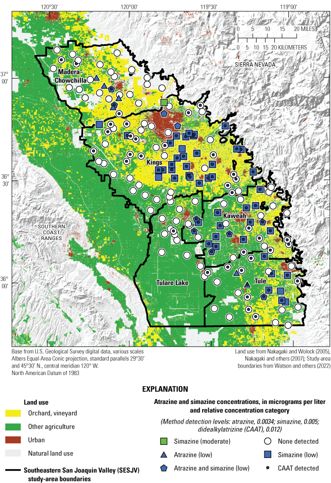
Concentrations of atrazine and simazine in groundwater samples collected from domestic-supply wells in the southeastern San Joaquin Valley, 2013–15, California Groundwater Ambient Monitoring and Assessment Program Priority Basin Project.
Herbicides with MCLs were detected at low concentrations in 30 percent and at moderate concentrations in 0.8 percent of the SESJV-D (table 12). The detection frequency ranged from 13 percent in Tulare Lake to 46 percent in Kings (table 12). Herbicides have been widely used in the San Joaquin Valley for roadside weed control and on agricultural crops (California Department of Pesticide Regulation, 2023). The patterns of herbicide detections in this study were similar to the results shown for sampling of domestic wells in 2012 in parts of the Kings, Kaweah, and Tule study areas by the California Department of Pesticide Regulation (CDPR; Troiano and others, 2013). The CDPR regulates applications of pesticides and regularly monitors domestic wells to determine if regulated pesticides or their degradation products are reaching drinking-water supply wells (Troiano and others, 2001). Low concentrations of simazine, degradation products of simazine, diuron, and bromacil were the most commonly detected herbicide constituents in domestic wells in SESJV-D (table 12; Troiano and others, 2013).
Simazine was the most frequently detected herbicide with an MCL; it was detected at low concentrations in 27 percent and at moderate concentrations in 0.8 percent of the SESJV-D (table 12). Didealkylatrazine (CAAT) is a degradate of both simazine and atrazine (Scribner and others, 2000) and has a non-regulatory health-based benchmark (table 2). CAAT was detected at low concentrations in 37 percent and at moderate concentrations in 5.8 percent of the SESJV-D (table 12). Of samples with detections of atrazine or simazine, 80 percent also had detections of CAAT; of samples with detections of CAAT, 60 percent also had detections of atrazine or simazine (Bennett and others, 2017; Shelton and Fram, 2017).
Detections of simazine and CAAT were related to groundwater age. This finding was expected because the first products containing simazine and atrazine were registered in 1958 (U.S. Environmental Protection Agency, 2019, 2020); therefore, simazine and CAAT can only be present in groundwater that contains water recharged after 1958. For this study, modern groundwater is defined as water recharged after 1952; premodern groundwater as recharged before 1952, including water that may have recharged hundreds or thousands of years ago; and mixed as groundwater containing both modern and premodern recharge. As expected, given that simazine and CAAT should only be present in groundwater containing a component of modern recharge, the detection frequencies of simazine and CAAT are significantly greater in modern groundwater than in mixed groundwater and significantly greater in mixed groundwater than in premodern groundwater (fig. 43). As described in the “Methods” section of this report, detection frequencies are defined as significantly different if the Jeffrey’s 90-percent confidence intervals do not overlap (fig. 43).

Relations among detection of simazine and 2-chloro-4,6-diamino-s-triazine (CAAT) and groundwater ages (modern, mixed, and premodern) in groundwater samples collected from domestic-supply wells in the southeastern San Joaquin Valley, 2013–15, California Groundwater Ambient Monitoring and Assessment Program Priority Basin Project.
Burow and others (2008) observed that simazine concentrations in San Joaquin Valley groundwater generally increased from the 1970s to the 2000s. Troiano and others (2013) observed that concentrations of simazine, diuron, bromacil, and their degradates in San Joaquin Valley groundwater decreased between 2001 and 2012. Troiano and others (2013) concluded that the decrease in herbicide concentrations in groundwater likely represents the effects of regulation of these herbicides and the time required for recharge to reach the depths of the wells. Regulation of herbicide applications began around 1990, and groundwater age modeling indicates that it takes 3–33 years for recharge at the land surface to reach the depths of the wells (Spurlock and others, 2000; Troiano and others, 2013).
Simazine and CAAT concentrations in the SESJV-D were negatively correlated with well depth (Spearman test, p<0.001, rho= −0.33 and −0.31, respectively). Although the relations between simazine and CAAT and well depth were statistically significant, the low absolute values of the rho values indicate that substantial amounts of the variations in concentrations are not explained by the relation with well depth. A non-monotonic change in simazine input with time due to regulation (Troiano and others, 2013), uneven application of simazine across the landscape and with time, and degradation of simazine and CAAT during different aquifer conditions with time (Burow and others, 2008) likely contribute to the amount of variabilities in concentrations of simazine and CAAT that are not explained by relations with well depth.
Volatile Organic Compounds Other than Fumigants
A total of 81 VOCs that were not fumigants were analyzed (Bennett and others, 2017; Shelton and Fram, 2017175), and 13 of these VOCs were detected in at least 1 of the 198 SESJV-D domestic-supply wells. Of the 13 VOCs detected, 9 had MCL benchmarks, 3 had non-regulatory health-based benchmarks, and 1 did not have a benchmark (tables 2, 4). Non-fumigant VOCs with MCLs were not detected at high concentrations in the SESJV-D, and most detections had concentrations less than one-tenth of benchmark concentrations (fig. 18G). Detected VOCs included disinfection byproducts, solvents, gasoline oxygenates, refrigerants, and naturally occurring VOCs.
Well owners are commonly advised to use hypochlorite solutions (bleach) to disinfect well water used for drinking water and other household uses in domestic, municipal, and community systems (Centers for Disease Control and Prevention and U.S. Department of Housing and Urban Development, 2006). However, hypochlorite reacts with organic matter to produce trihalomethanes and other chlorinated and brominated disinfection byproducts. The trihalomethane trichloromethane was detected at low concentrations in 10 percent of the SESJV-D (table 12). Another trihalomethane, bromodichloromethane, was detected in some samples in which trichloromethane was detected (Bennett and others, 2017; Shelton and Fram, 2017). Trichloromethane is the most frequently detected VOC nationwide (Zogorski and others, 2006; Bexfield and others, 2022).
Solvents with MCL benchmarks were detected at moderate concentrations in 1.1 percent and at low concentrations in 4.7 percent of the SESJV-D (table 12). The most frequently detected solvent was tetrachloroethene (PCE), which also was the most frequently detected solvent in groundwater nationally (Zogorski and others, 2006; Bexfield and others, 2022). Tetrachloroethene also was the only solvent with an MCL detected at moderate concentrations in the SESJV-D. Tetrachloroethene typically is used for dry-cleaning of fabrics and degreasing metal parts and is an ingredient in a wide range of products, including paint removers, polishes, printing inks, lubricants, and adhesives (Zogorski and others, 2006).
The gasoline oxygenate methyl tert-butyl ether (MTBE) was detected at low concentrations in 11 percent of the SESJV-D (table 12). Methyl tert-butyl ether was used as a gasoline oxygenate from 1979 until it was banned in California at the start of 2004, with peak usage in the late 1990s (California State Water Resources Control Board, 2017c). None of the wells with detections of MTBE had detections of hydrocarbons associated with gasoline, and MTBE concentrations were not significantly related to underground storage tank density (Spearman test, p=0.089, rho=0.13). These relations indicate that leaks from fuel tanks were not the primary source of MTBE in SESJV-D wells.
However, concentrations of MTBE detected in SESJV-D wells were in a range that would be consistent with an atmospheric source for the MTBE. The median MTBE concentration in the atmosphere in Fresno during 1996–2000 of about 1.5 parts per billion by volume (ppbV; California Air Resources Board, 2023) would be in equilibrium with precipitation containing a concentration of approximately 0.33 µg/L at 20 degrees Celsius (Baehr and others, 1999). Concentrations of MTBE detected in SESJV-D samples ranged from 0.009 to 0.17 ug/L, with a median detected concentration of 0.017 µg/L (Bennett and others, 2017; Shelton and Fram, 2017).
Even shorter-screened wells like many of the SESJV-D wells generally capture groundwater that consists of a mixture of groundwater ages. For this report, groundwater age was summarized by classification as modern, mixed, or premodern groundwater; 14 of the SESJV-D wells with MTBE detections were modern, and 4 were mixed. The MTBE concentrations detected in the groundwater samples could be produced from a mixture consisting of 3–51 percent water recharged during the time MTBE was used (1979–2004; California State Water Resources Control Board, 2017c), and 97–49 percent water recharged before or after that time. Faulkner and Jurgens (2022) presented results of lumped parameter models for groundwater age that proved more resolution of groundwater ages than the simple classification used in this report. However, that level of analysis is beyond the scope of this report.
Carbon disulfide was detected at low concentrations in 8.7 percent of the SESJV-D, and detection frequencies ranged from 0 percent in the Madera and Kaweah study areas to 42 percent in Tulare Lake study area (table 12). Of the wells with carbon disulfide detections, 82 percent had anoxic or mixed redox conditions, and 72 percent did not have other VOCs detected in the samples (Bennett and others, 2017; Shelton and Fram, 2017). These detection results were consistent with natural sources of carbon disulfide (U.S. Department of Health and Human Services, Agency for Toxic Substances and Disease Registry, 1996; Fram and others, 2012; Bexfield and others, 2022).
Microbial Indicator Constituents
Total coliform bacteria, Escherichia coli (E. coli), and Enterococci are microbial indicator constituents that are commonly used as indicators of potential contamination of water supplies from human or animal waste (California State Water Resources Control Board, 2019). Coliform bacteria are ubiquitous in soils and surface water but also are present in the digestive tracts of warm-blooded animals, including humans. E.coli and Enterococci are more specific to fecal-waste sources compared to total coliform. Total coliform bacteria, E.coli, and Enterococci have MCL-CA or TT-CA benchmarks (California State Water Resources Control Board Division of Drinking Water, 2022a). The benchmarks are based on results from repeated sampling of wells, and the sampling for this study did not include repeat sampling.
Total coliform bacteria were analyzed in 145 wells representing 133 cells, and the spatially weighted detection frequency in the SESJV-D was 19 percent (table 13). Fecal coliform bacteria (E.coli) was analyzed but not detected. The spatially weighted detection frequency of Enterococci was 4.0 percent. Detections of Enterococci and total coliform bacteria were significantly associated (contingency table test p=0.025) because 60 percent of samples with Enterococci detections also had total coliform bacteria detections. The detection frequency of total coliform bacteria ranged from 4.2 percent in the Madera-Chowchilla study area to 36 percent in the Kaweah study area (table 13; fig. 44). The frequency of detection of total coliform bacteria in this study was similar to a previous study of domestic wells in Tulare County: total coliform bacteria were detected in 33 percent of the 115 wells in the Kaweah and Tule study areas (California State Water Resources Control Board, 2016, 2023b). In the previous study (California State Water Resources Control Board, 2016), fecal coliform bacteria were detected in 7.8 percent of wells in the Kaweah and Tule study areas, but fecal coliform bacteria were not detected in this study. The reason for the observed differences is unknown.
Table 13.
Aquifer-scale proportions for microbial indicator constituents in the domestic-supply aquifer (SESJV-D) of the southeastern San Joaquin Valley, 2013–15, California Groundwater Ambient Monitoring and Assessment Program Priority Basin Project.[Aquifer-scale proportion is the areal proportion of the study area with a detection of the microbial indicator constituent calculated using a cell-declustering method. Calculations are based on data from 145 wells sampled by the California Groundwater Ambient Monitoring and Assessment Program Priority Basin Project (GAMA-PBP) during 2013–15 (tables 1.1–1.5; Bennett and others, 2017; Shelton and Fram, 2017; Balkan and others, 2024)]
Study area boundaries and grid cells are available in Watson and others (2022).

Detections of total coliform bacteria in groundwater samples collected from domestic wells in the southeastern San Joaquin Valley, 2013–15, California Groundwater Ambient Monitoring and Assessment Program Priority Basin Project.
Detections of total coliform bacteria were not significantly associated with septic tank density near the well (Wilcoxon test, p=0.913). The lack of association between the likely source of bacteria from human fecal material and the absence of detections of E.coli indicate that occurrence of total coliform bacteria may be related to natural sources in soils rather than indicating contamination by fecal matter.
Analyses of deoxyribonucleic acid (DNA) from microbial colonies cultured from groundwater from wells sampled for this study support the hypothesis that the dominant source of total coliform bacteria detections is naturally occurring bacteria in soils. Sampling in the Madera-Chowchilla and Kings study areas also included collection of microbial samples for DNA analysis to try to identify bacterial species (Burton and Lawrence, 2021). Most bacterial genera identified in the samples are naturally present in soil or groundwater, and the genera that include possible human pathogens are also natural inhabitants of soils, plants, and groundwater. However, even if the source is not fecal, the presence of total coliform bacteria in groundwater samples indicates communication between near surface soils and the well (Burton and Lawrence, 2021).
Summary
The California Groundwater Ambient Monitoring and Assessment Program Priority Basin Project (GAMA-PBP) investigated water quality in groundwater resources used by domestic and public drinking-water supply wells in the southeastern San Joaquin Valley. The GAMA-PBP is a cooperative project between the California State Water Resources Control Board (SWRCB) and the U.S. Geological Survey (USGS). This report provides a general description of the hydrogeologic setting of the southeastern San Joaquin Valley, an assessment and comparison of the status of water quality in the resources used by domestic wells (SESJV-D) and public-supply wells (SESJV-P) in the southeastern San Joaquin Valley during 2013–15, and a general evaluation of potential explanatory factors that may affect groundwater quality and explain differences among study areas and between SESJV-D and SESJV-P. Results are presented for five study areas that correspond to the California Department of Water Resources groundwater basins in the SESJV: (1) Madera-Chowchilla, (2) Kings, (3) Kaweah, (4) Tule, and (5) Tulare Lake.
The SESJV-D was characterized using data collected by the USGS from 198 domestic wells during 2013–15. To ensure representation of the entire area of the used resource, wells were selected using a stratified random design based on a net of 157-, 60-, or 80-square kilometer grid cells covering the southeastern San Joaquin Valley; 1 to 4 wells were sampled in 142 of the cells. Water-quality data collected included inorganic (major ions, trace elements, nutrients, radioactive constituents, and trace inorganic compounds) and organic (volatile organic compounds, pesticides, and pesticide degradates) constituents, microbial indicator constituents, and selected age-dating and isotopic tracer constituents. Data also were compiled for each well for potential explanatory factors representing hydrology (well depth, lateral position, position relative to the Corcoran Clay Member of the Tulare Formation, sediment texture, presence of hydric soils, and aridity index), land use (percentages of urban, agricultural, and natural land use, percentage of orchard or vineyard land use, and densities of septic tanks and underground storage tanks), and geochemical conditions (groundwater-age class, oxidation-reduction class, pH, and dissolved oxygen and bicarbonate concentrations).
The SESJV-P was characterized using data collected by the USGS from 124 public-supply wells during 2005–18 and data compiled for an additional 1,577 public-supply wells with publicly available data from regulatory compliance sampling for the California State Water Resources Control Board Division of Drinking Water (SWRCB-DDW). Wells were assigned to the grid cells used for domestic wells; 135 cells contained 1–112 wells. Data for all water-quality constituents and for all potential explanatory factors were not available at all SESJV-P wells.
Water-quality conditions were characterized by comparing measured concentrations to the concentrations of Federal and State benchmarks used for drinking water. U.S. Environmental Protection Agency (EPA) and SWRCB-DDW maximum contamination levels (MCLs), SWRCB-DDW secondary maximum contaminant levels (SMCLs), and non-regulatory health-based benchmarks established by the EPA, SWRCB-DDW, and USGS were used. Measured concentrations greater than benchmarks were defined as high, concentrations between the benchmark and half (inorganic constituents) or one-tenth (organic constituents) of the benchmark concentration were defined as moderate in nearly all cases, and concentrations below moderate and nondetections were defined as low. Aquifer-scale proportions were used to summarize water quality for individual constituents and classes of constituents for the five study areas and the entire southeastern San Joaquin Valley. Aquifer-scale proportion was defined as the proportion of the study area having water quality in a specified category and was calculated using spatial weighting in the grid cells for each study area. Spatial weighting also was used to summarize the potential explanatory factors at the scale of the study areas.
One or more inorganic constituent with an EPA or SWRCB-DDW MCL was detected at high concentrations in 47 percent of the SESJV-D compared to 32 percent of the SESJV-P. Within SESJV-D, the proportion of the study area with high concentrations of inorganic constituents ranged from 19 percent in the Madera-Chowchilla study area to 60 percent in the Kings and Tulare Lake study areas. The inorganic constituents with MCLs most commonly present at high concentrations in SESJV-D were nitrate, uranium, and arsenic; other constituents with MCLs present at high concentrations included adjusted gross beta and alpha particle activities, perchlorate, and fluoride. Including inorganic constituents with non-regulatory health-based benchmarks increased the proportion of the SESJV-D with high concentrations of inorganic constituents with health-based benchmarks to 49 percent; molybdenum and manganese were present at concentrations greater than their EPA lifetime health advisory levels.
The proportions of the SESJV-D with concentrations of nitrate exceeding the MCL were 12, 33, 40, 29, and 8.9 percent in the Madera-Chowchilla, Kings, Kaweah, Tule, and Tulare Lake study areas, respectively, and the proportions with high concentrations were greater in the SESJV-D than the SESJV-P for all study areas. High nitrate concentrations in the SESJV-D were associated with greater agricultural land use with shallower wells that were more likely to tap modern groundwater, and with oxic conditions. Nitrate concentrations were lower in the western side of the SESJV-D where anoxic conditions that promote nitrate degradation were more common.
The proportions of SESJV-D with concentrations of uranium exceeding the MCL were 6.5, 36, 19, 7.1, and 22 percent in the Madera-Chowchilla, Kings, Kaweah, Tule, and Tulare Lake study areas, respectively, and the proportions with high concentrations were greater in the SESJV-D than the SESJV-P for all study areas. High uranium concentrations in the SESJV-D were associated with greater agricultural land use, shallower wells that were more likely to tap modern-age groundwater, and locations on the San Joaquin, Kings, and Kaweah River alluvial fans. Downward movement of recharge in the aquifer system would result in future migration of the high nitrate and uranium concentrations present in domestic wells at the time of this study (2013–15) to the depth zones used by public-supply wells.
The proportions of the SESJV-D with concentrations of arsenic exceeding the MCL were 3.7, 6.8, 4.8, 18, and 49 percent in the Madera-Chowchilla, Kings, Kaweah, Tule, and Tulare Lake study areas, respectively, and the proportions with high concentrations were smaller in the SESJV-D than the SESJV-P for all study areas. High arsenic concentrations in the SESJV-D were associated with anoxic or mixed redox conditions and pH values greater than 7.7; these conditions were most prevalent in the basinal deposits, especially near the Tulare Lake Bed. Age of groundwater and depth of well were not important factors controlling arsenic concentrations in basinal deposits because high arsenic concentrations were detected in groundwater from wells screened above and below the Corcoran Clay Member of the Tulare Formation and in groundwater of all ages.
One or more inorganic constituents with SWRCB-DDW SMCLs were detected at high concentrations in 14 percent of the SESJV-D compared to 19 percent of the SESJV-P. The constituents most commonly present at high concentrations were manganese, iron, and total dissolved solids (TDS). The proportion of the SESJV-D with high concentrations of manganese (exceeding the SMCL) were 3.7, 13, 5.4, 3.6, and 58 percent in the Madera-Chowchilla, Kings, Kaweah, Tule, and Tulare Lake study areas, respectively, and the proportions with high concentrations were greater in the SESJV-D than the SESJV-P for the Tulare Lake study area. Most wells with high manganese concentrations were in the San Joaquin Valley trough where anoxic conditions are most common.
The SESJV-D and SESJV-P had the same proportions (4 percent) of high concentrations of TDS (greater than the upper SMCL), but SESJV-D had a higher (30 percent) proportion of moderate concentrations (between the recommended and upper SMCL) compared to SESJV-P (12 percent), with the greatest observed differences in the Kings River fan of the Kings study area and in the Tulare Lake study areas. Stable isotope data used to map sources of recharge to SESJV-D compared to a previously published study of the SESJV-P indicated a larger area of the Kings River fan dominated by surface-water recharge, indicating that the greater proportion of TDS over the recommended SMCL may be caused by recharge of irrigation water.
At least one organic constituent with an MCL was present at high concentrations in 19 percent of the SESJV-D compared to 12 percent of the SESJV-P. All organic constituents detected at high concentrations in the SESJV-D were fumigants, primarily1,2,3-trichloropropane (1,2,3-TCP) and 1,2-dibromo-3-chloropropane (DBCP). Fumigants also were the constituents most commonly detected at high concentration in the SESJV-P, although high concentrations of solvents also were detected. Organic constituents with MCLs detected at moderate concentrations in the SESJV-D included the fumigants 1,2-dibromoethane (ethylene dibromide, EDB) and 1,2-dichloropropane, the solvent tetrachloroethene, and the herbicide simazine. High concentrations of 1,2,3-TCP and DBCP were detected in areas with orchard or vineyard land use and in modern groundwater, which is consistent with the usage pattern of these fumigants.
References Cited
Abzalov, M.Z., 2012, Sandstone-hosted uranium deposits amenable for exploitation by in situ leaching technologies: Transactions of the Institution of Mining and Metallurgy—Section B, Applied Earth Science, v. 121, no. 2, p. 55–64. [Available at https://doi.org/10.1179/1743275812Y.0000000021.]
Ague, J.J., and Brimhall, G.H., 1988, Regional variations in bulk chemistry, mineralogy, and the compositions of mafic and accessory minerals in the batholiths of California: Geological Society of America Bulletin, v. 100, no. 6, p. 891–911. [Available at https://doi.org/10.1130/0016-7606(1988)100<0891:RVIBCM>2.3.CO;2.]
Anning, D.W., Paul, A.P., McKinney, T.S., Huntington, J.M., Bexfield, L.M., and Thiros, S.A., 2012, Predicted nitrate and arsenic concentrations in basin-fill aquifers of the Southwestern United States: U.S. Geological Survey Scientific Investigations Report 2012–5065, 78 p., accessed July 6, 2023, at https://doi.org/10.3133/sir20125065.
Arndt, M.F., 2010, Evaluation of gross alpha and uranium measurements for MCL compliance: Denver, Colo., The Water Research Foundation, 299 p., accessed July 6, 2023, at https://www.waterrf.org/research/projects/evaluation-gross-alpha-and-uranium-measurements-mcl-compliance.
Arnold, T.L., Bexfield, L.M., Musgrove, M., Stackelberg, P.E., Lindsey, B.D., Kingsbury, J.A., Kulongoski, J.T., and Belitz, K., 2018, Groundwater-quality and select quality-control data from the National Water-Quality Assessment Project, January through December 2015, and previously unpublished data from 2013 to 2014: U.S. Geological Survey Data Series 1087, 67 p., accessed July 6, 2023, at https://doi.org/10.3133/ds1087.
Arnold, T.L., DeSimone, L.A., Bexfield, L.M., Lindsey, B.D., Barlow, J.R., Kulongoski, J.T., Musgrove, M., Kingsbury, J.A., and Belitz, K., 2016, Groundwater quality data from the National Water-Quality Assessment Project, May 2012 through December 2013 (ver. 1.1, November 2016): U.S. Geological Survey Data Series 997, 56 p., accessed July 6, 2023, at https://doi.org/10.3133/ds997.
Baehr, A.L., Stackelberg, P.E., and Baker, R.J., 1999, Evaluation of the atmosphere as a source of volatile organic compounds in shallow groundwater: Water Resources Research, v. 35, no. 1, p. 127–136, accessed February 18, 2023, at https://doi.org/10.1029/1998WR900030.
Balkan, M., Burow, K.R., Shelton, J.L., and Fram, M.S., 2024, Data sets for: Status of water quality in groundwater resources used for drinking water supply in the southeast San Joaquin Valley, 2013–2015—California GAMA Priority Basin Project: U.S. Geological Survey data release, accessed January 22, 2024, at https://doi.org/10.5066/P9DCTLXV.
Bangia, K., August, L., Slocombe, A., Faust, J., 2020, Assessment of contaminants in California drinking water by region and system size: American Water Works Association Water Science, v. 2, no. 5, article e1194, accessed July 6, 2023, at https://doi.org/10.1002/aws2.1194.
Belitz, K.R., and Heimes, F.J., 1990, Character and evolution of the ground-water flow system in the central part of the western San Joaquin Valley, California: U.S. Geological Survey Water-Supply Paper 2348, 28 p., accessed July 6, 2023, at https://doi.org/10.3133/wsp2348.
Belitz, K.R., Dubrovsky, N.M., Burow, K., Jurgens, B., and Johnson, T., 2003, Framework for a ground-water quality monitoring and assessment program for California: U.S. Geological Survey Water Resources Investigations Report 03–4166, 78 p., accessed July 6, 2023, at https://pubs.usgs.gov/wri/wri034166/.
Belitz, K.R., Fram, M.S., and Johnson, T.D., 2015, Metrics for assessing the quality of groundwater used for public supply, CA, USA—Equivalent-population and area: Environmental Science & Technology, v. 49, no. 14, p. 8330–8338, accessed July 6, 2023, at https://doi.org/10.1021/acs.est.5b00265.
Belitz, K.R., Fram, M.S., Lindsey, B.D., Stackelberg, P.E., Bexfield, L.M., Johnson, T.D., Jurgens, B.C., Kingsbury, J.A., McMahon, P.B., and Dubrovsky, N.M., 2022, Quality of groundwater used for public supply in the continental United States—A comprehensive assessment: Environmental Science & Technology Water, v. 2, no. 12, p. 2645–2656, accessed July 6, 2023, at https://doi.org/10.1021/acsestwater.2c00390.
Belitz, K.R., Jurgens, B., Landon, M.K., Fram, M.S., and Johnson, T., 2010, Estimation of aquifer scale proportion using equal area grids—Assessment of regional scale groundwater quality: Water Resources Research, v. 46, no. 11, 14 p., accessed July 6, 2023, at https://doi.org/10.1029/2010WR009321.
Bennett, G.L.V, 2017, Status and understanding of groundwater quality in the north San Francisco Bay shallow aquifer study unit, 2012—California GAMA Priority Basin Project: U.S. Geological Survey Scientific Investigations Report 2017–5051, 74 p., accessed July 6, 2023, at https://doi.org/10.3133/sir20175051.
Bennett, G.L.V, 2020, Updated study reporting levels (SRLs) for trace-element data collected for the California Groundwater Ambient Monitoring and Assessment (GAMA) Program Priority Basin Project, October 2009–October 2018: U.S. Geological Survey Scientific Investigations Report 2020–5034, 24 p., accessed July 6, 2023, at https://doi.org/10.3133/sir20205034.
Bennett, G.L.V, 2022, Status and understanding of groundwater quality in the Sacramento Metropolitan Domestic-Supply Aquifer study unit, 2017—California GAMA Priority Basin Project: U.S. Geological Survey Scientific Investigations Report 2022–5021, 52 p., accessed July 6, 2023, at https://doi.org/10.3133/sir20225021.
Bennett, G.L.V, Fram, M.S., and Johnson, T.D., 2017, Groundwater-quality data in the Tulare shallow aquifer study unit, 2014–2015: Results from the California GAMA Priority Basin Project: U.S. Geological Survey data release, accessed July 6, 2023, at https://doi.org/10.5066/F7BP00W8.
Bertoldi, G.L., Johnston, R.H., and Evenson, K.D., 1991, Ground water in the Central Valley, California—A summary report: U.S. Geological Survey Professional Paper 1401–A, accessed July 6, 2023, at https://pubs.usgs.gov/pp/1401a/report.pdf.
Bexfield, L.M., Belitz, K., Fram, M.S., and Lindsey, B.D., 2022, Volatile organic compounds in groundwater used for public supply across the United States: Occurrence, explanatory factors, and human-health context: Science of the Total Environment, v. 827, article 154313, accessed July 6, 2023, at https://doi.org/10.1016/j.scitotenv.2022.154313.
Bexfield, L.M., Belitz, K., Lindsey, B.D., Toccalino, P., and Nowell, L.H., 2021, Pesticides and pesticide degradates in groundwater used for public supply across the United States: Occurrence and human-health context: Environmental Science & Technology, v. 55, no. 1, p. 362–372, accessed July 6, 2023, at https://doi.org/10.1021/acs.est.0c05793.
Böhlke, J.K., Hatzinger, P.B., Sturchio, N.C., Gu, B. Abbene, I., and Mroczkowski, S.J., 2009, Atacama perchlorate as an agricultural contaminant in groundwater—Isotopic and chronologic evidence from Long Island, New York: Environmental Science & Technology, v. 43, no. 15, p. 5619–5625, accessed January 11, 2021, at https://doi.org/10.1021/es9006433.
Brown, L.D., Cai, T.T., and DasGupta, A., 2001, Interval estimation for a binomial proportion: Statistical Science, v. 16, no. 2, p. 101–133, accessed July 6, 2023, at https://projecteuclid.org/download/pdf_1/euclid.ss/1009213286.
Burow, K.R., Belitz, K., Dubrovsky, N.M., and Jurgens, B.C., 2017, Large decadal-scale changes in uranium and bicarbonate in groundwater of the irrigated western U.S.: Science of the Total Environment, v. 586, p. 87–95, accessed July 6, 2023, at https://doi.org/10.1016/j.scitotenv.2017.01.220.
Burow, K.R., Dubrovsky, N.M., and Shelton, J.L., 2007, Temporal trends in concentrations of DBCP and nitrate in groundwater in the eastern San Joaquin Valley, California, USA: Hydrogeology Journal, v. 15, p. 991–1007, accessed July 6, 2023, at https://doi.org/10.1007/s10040-006-0148-7.
Burow, K.R., Floyd, W.D., and Landon, M.K., 2019, Factors affecting 1,2,3-trichloropropane contamination in groundwater in California: Science of the Total Environment, v. 672, p. 324–334, accessed July 6, 2023, at https://doi.org/10.1016/j.scitotenv.2019.03.420.
Burow, K.R., Jurgens, B.C., Belitz, K., and Dubrovsky, N.M., 2013, Assessment of regional change in nitrate concentrations in groundwater in the Central Valley, California, USA, 1950s–2000s: Environmental Earth Sciences, v. 69, p. 2609–2621, accessed July 6, 2023, at https://doi.org/10.1007/s12665-012-2082-4.
Burow, K.R., Panshin, S.Y., Dubrovsky, N.M., Vanbrocklin, D., and Fogg, G.E., 1999, Evaluation of processes affecting 1,2-dibromo-3-chloropropane (DBCP) concentrations in ground water in the eastern San Joaquin Valley, California—Analysis of chemical data and ground-water flow and transport simulations: U.S. Geological Survey Water-Resources Investigations Report 99–4059, 57 p., accessed July 6, 2023, at https://doi.org/10.3133/wri994059.
Burow, K.R., Shelton, J.L., and Dubrovsky, N.M., 1998b, Occurrence of nitrate and pesticides in ground water beneath three agricultural land-use settings in the eastern San Joaquin Valley, California, 1993–1995: U.S. Geological Survey Water-Resources Investigations Report 97–4284, 51 p., accessed July 6, 2023, at https://pubs.usgs.gov/wri/1997/4284/report.pdf.
Burow, K.R., Shelton, J.L., and Dubrovsky, N.M., 2008, Regional nitrate and pesticide trends in ground water in the eastern San Joaquin Valley, California: Journal of Environmental Quality, v. 37, no. S5, p. S-249–S-263, accessed July 6, 2023, at https://doi.org/10.2134/jeq2007.0061.
Burow, K.R., Shelton, J.L., Hevesi, J.A., and Weissmann, G.S., 2004, Hydrogeologic characterization of the Modesto area, San Joaquin Valley, California: U.S. Geological Survey Scientific Investigations Report 2004–5232, 54 p., accessed July 6, 2023, at https://pubs.usgs.gov/sir/2004/5232/.
Burow, K.R., Stork, S.V., and Dubrovsky, N.M., 1998a, Nitrate and pesticides in ground water in the eastern San Joaquin Valley, California—Occurrence and trends: U.S. Geological Survey Water-Resources Investigations Report 98–4040, 33 p., accessed July 6, 2023, at https://pubs.usgs.gov/wri/1998/4040a/report.pdf.
Burton, C.A., and Belitz, K., 2008, Ground-water quality data in the southeast San Joaquin Valley, 2005–2006—Results from the California GAMA Program: U.S. Geological Survey Data Series 351, 103 p., accessed July 6, 2023, at https://pubs.usgs.gov/ds/351/.
Burton, C.A., and Lawrence, C.J., 2021, Identification of bacteria in groundwater used for domestic supply in the southeast San Joaquin Valley, California, 2014: U.S. Geological Survey Scientific Investigations Report 2021–5030, 20 p., accessed July 6, 2023, at https://doi.org/10.3133/sir20215030.
Burton, C.A., and Wright, M.T., 2018, Status and understanding of groundwater quality in the Monterey-Salinas shallow aquifer study unit, 2012–13: California GAMA Priority Basin Project: U.S. Geological Survey Scientific Investigations Report 2018–5057, 116 p., accessed July 6, 2023, at https://doi.org/10.3133/sir20185057.
California Air Resources Board, 2023, Annual toxics summary, Fresno 1st Street, Methyl tertiary-Butyl ether, accessed February 18, 2023, at https://www.arb.ca.gov/adam/toxics/sitepages/mtbefsno.html.
California Department of Pesticide Regulation, 2023, Pesticide use reporting, accessed February 12, 2023, at https://www.cdpr.ca.gov/docs/pur/purmain.htm.
California Department of Water Resources, 2003, California's groundwater (Bulletin 118): California Department of Water Resources Bulletin 118, 246 p., accessed February 9, 2023, at https://water.ca.gov/programs/groundwater-management/bulletin-118.
California Department of Water Resources, 2014, Public update for drought response—Groundwater basins with potential water shortages and gaps in groundwater monitoring: California Department of Water Resources Report to the Governor’s Drought Task Force, 45 p., accessed February 10, 2023, at https://cawaterlibrary.net/document/public-update-for-drought-response-groundwater-basins-with-potential-water-shortages-gaps-in-groundwater-monitorin g-monitoring-of-land-subsidence-and-agricultural-land-fallowing/.
California Department of Water Resources, 2018, Basin boundary modifications: California Department of Water Resources website, accessed February 12, 2023, at https://water.ca.gov/Programs/Groundwater-Management/Basin-Boundary-Modifications and https://sgma.water.ca.gov/webgis/?appid=SGMADataViewer#boundaries.
California Department of Water Resources, 2020, Sustainable Groundwater Management Act 2019 Basin Prioritization—Process and results: California Department of Water Resources, 43 p. and appendices, accessed February 9, 2023, at https://data.cnra.ca.gov/dataset/13ebd2d3-4e62-4fee-9342-d7c3ef3e0079/resource/ffafd27b-5e7e-4db3-b846-e7b3cb5c614c/download/sgma_bp_process_document. pdf.
California Department of Water Resources, 2023a, Groundwater: California Department of Water Resources website, accessed February 9, 2023, at https://water.ca.gov/Water-Basics/Groundwater.
California Department of Water Resources, 2023b, Online System for Well Completion Reports (OSWCR) well completion reports dataset: California Natural Resources Agency website, accessed February 9, 2023, at https://data.cnra.ca.gov/dataset/well-completion-reports.
California Department of Water Resources, 2023c, California’s Groundwater Live: California Department of Water Resources webpage, accessed February 10, 2023, at https://sgma.water.ca.gov/CalGWLive/.
California Irrigation Management Information System, 2005, California Irrigation Management Information System reference evapotranspiration zones: California Irrigation Management Information System website, accessed November 18, 2020, at http://wwwcimis.water.ca.gov/App_Themes/images/etozonemap.jpg.
California State Water Resources Control Board Division of Drinking Water, 2022a, Domestic water quality and monitoring regulations: California Code of Regulations—Title 22, Division 4, Chapter 15, Article 4, §64431, Chapter 15, Article 5.5 §64444, Chapter 15, Article 3 §64421–64427, Chapter 15, Article 3.5, §64430, and Chapter 15.5, Article 2, §64533, accessed December 30, 2022, at http://ccr.oal.ca.gov/.
California State Water Resources Control Board Division of Drinking Water, 2022b, Domestic water quality and monitoring regulations—Secondary maximum contaminant levels: California Code of Regulations—Title 22, Division 4, Chapter 15, Article 16, §64449, accessed July 6, 2023, at http://ccr.oal.ca.gov/.
California State Water Resources Control Board Division of Drinking Water, 2022c, Drinking water notification and response levels—An overview: California State Water Resources Control Board, Division of Drinking Water website, accessed July 6, 2023, at https://www.waterboards.ca.gov/drinking_water/certlic/drinkingwater/documents/notificationlevels/notification_response_level_overview_2022_11_01.pdf.
California State Water Resources Control Board Division of Drinking Water, 2022d, EDT library and water quality analyses data and download page: California State Water Resources Control Board website, accessed February 12, 2023, at https://www.waterboards.ca.gov/drinking_water/certlic/drinkingwater/EDTlibrary.html.
California State Water Resources Control Board, 2003, A comprehensive groundwater quality monitoring program for California: Assembly Bill 599, Report to the Governor and Legislature, March 2003, 100 p., accessed February 9, 2023, at https://www.waterboards.ca.gov/publications_forms/publications/legislative/docs/2003/ab599.pdf.
California State Water Resources Control Board, 2007, GeoTracker: California State Water Resources Control Board website, accessed November 2007 at https://geotracker.waterboards.ca.gov/.
California State Water Resources Control Board, 2013, Communities that rely on a contaminated groundwater source for drinking water: California State Water Resources Control Board Report to the Legislature, accessed February 9, 2023, at https://www.waterboards.ca.gov/gama/ab2222/docs/ab2222.pdf.
California State Water Resources Control Board, 2016, Groundwater Ambient Monitoring and Assessment (GAMA) domestic well project groundwater quality data report Tulare County focus area, 76 p., accessed February 12, 2023, at https://www.waterboards.ca.gov/water_issues/programs/gama/docs/tularesummaryreport.pdf.
California State Water Resources Control Board, 2017b, Groundwater information sheet—Radionuclides: California State Water Resources Control Board website, 13 p., accessed February 13, 2023, at https://www.waterboards.ca.gov/gama/docs/coc_radionuclides.pdf.
California State Water Resources Control Board, 2017a. Groundwater information sheet—1,2,3-Trichloropropane (TCP): California State Water Resources Control Board website, 8 p., accessed July 6, 2023, at https://www.waterboards.ca.gov/gama/docs/coc_tcp123.pdf.
California State Water Resources Control Board, 2017c, Groundwater information sheet—Methyl tertiary-butyl ether (MTBE): California State Water Resources Control Board website, 8 p., accessed February 18, 2023, at https://www.waterboards.ca.gov/gama/docs/coc_mtbe.pdf.
California State Water Resources Control Board, 2019, Groundwater information sheet—Bacteria indicators: California State Water Resources Control Board, Division of Water Quality, GAMA Program, 7 p., accessed October 5, 2021, at https://www.waterboards.ca.gov/gama/docs/coc_bacteria_indicators.pdf.
California State Water Resources Control Board, 2021, Decision tree for classification of water systems: California State Water Resources Control Board, Division of Drinking Water, 4 p., accessed November 18, 2023, at https://www.waterboards.ca.gov/drinking_water/certlic/drinkingwater/docs/class_dec_tree.pdf.
California State Water Resources Control Board, 2022a, 2022 Drinking water needs assessment: California State Water Resources Control Board website, 241 p., accessed February 13, 2023, at https://www.waterboards.ca.gov/drinking_water/certlic/drinkingwater/documents/needs/2022needsassessment.pdf.
California State Water Resources Control Board, 2022b, Chromium-6 drinking water MCL: California State Water Resources Control Board website, accessed February 13, 2023, at https://www.waterboards.ca.gov/drinking_water/certlic/drinkingwater/Chromium6.html.
California State Water Resources Control Board, 2023a, Groundwater Ambient Monitoring and Assessment Program (GAMA): California State Water Resources Control Board website, accessed February 9, 2023, at https://www.waterboards.ca.gov/water_issues/programs/gama/.
California State Water Resources Control Board, 2023b, Groundwater Ambient Monitoring and Assessment Program (GAMA) Groundwater Information System: California State Water Resources Control Board website, accessed February 9, 2023, at https://gamagroundwater.waterboards.ca.gov/gama/gamamap/public/.
California State Water Resources Control Board, 2023c, Human right to water portal: California State Water Resources Control Board website, accessed February 9, 2023, at https://www.waterboards.ca.gov/water_issues/programs/hr2w/.
Centers for Disease Control and Prevention and U.S. Department of Housing and Urban Development, 2006, Rural water supplies and water-quality issues, chap. 8 of Healthy housing reference manual: U.S. Department of Health and Human Services website, accessed February 12, 2023, at https://www.cdc.gov/nceh/publications/books/housing/cha08.htm.
Central Valley Salinity Alternatives for Long-term Sustainability, 2023, Salt control program overview, accessed February 18, 2023, at https://www.cvsalinity.org/salt-program/.
Coates, J.D., and Achenbach, L.A., 2004, Microbial perchlorate reduction—Rocket-fueled metabolism: Nature Reviews Microbiology, v. 2, p. 569–580, accessed July 6, 2023, at https://doi.org/10.1038/nrmicro926.
Crusius, J., Calvert, S., Pedersen, T., and Sage, D., 1996, Rhenium and molybdenum enrichments in sediments as indicators of oxic, suboxic and sulfidic concentrations of deposition: Earth and Planetary Science Letters, v. 145, nos. 1–4, p. 65–78, accessed July 6, 2023, at https://doi.org/10.1016/S0012-821X(96)00204-X.
Dasgupta, P.K., Dyke, J.V., Kirk, A.B., and Jackson, W.A., 2006, Perchlorate in the United States—Analysis of relative source contributions to the food chain: Environmental Science & Technology, v. 40, no. 21, p. 6608–6614, accessed July 6, 2023, at https://doi.org/10.1021/es061321z.
Dasgupta, P.K., Martinelango, P.K., Jackson, W.A., Anderson, T.A., Tian, K., Tock, R.W., and Rajogopalan, S., 2005, The origin of naturally occurring perchlorate—The role of the atmospheric processes: Environmental Science & Technology, v. 39, no. 6, p. 1569–1575, accessed February 8, 2021, at https://doi.org/10.1021/es048612x.
Davis, G.H., Green, J.H., Olmsted, F.H., and Brown, D.W., 1959, Groundwater conditions and storage capacity in the San Joaquin Valley, California: U.S. Geological Survey Water-Supply Paper 1469, 277 p., accessed July 6, 2023, at https://doi.org/10.3133/wsp1469.
Deeley, G.M., Reinhard, M., and Stearns, S.M., 1991, Transformation and sorption of 1,2-dibromo-3-chloropropane in subsurface samples collected at Fresno, California: Journal of Environmental Quality, v. 20, no. 3, p. 547–556, accessed July 6, 2023, at https://doi.org/10.2134/jeq1991.00472425002000030008x.
Deverel, S.J., and Millard, S.P., 1988, Distribution and mobility of selenium and other trace elements in shallow groundwater of the western San Joaquin Valley, California: Environmental Science & Technology, v. 22, no. 6, p. 697–702. [Available at https://doi.org/10.1021/es00171a013.]
Dieter, C.A., Maupin, M.A., Caldwell, R.R., Harris, M.A., Ivahnenko, T.I., Lovelace, J.K., Barber, N.L., and Linsey, K.S., 2018, Estimated use of water in the United States in 2015: U.S. Geological Survey Circular 1441, 65 p. [Available at https://doi.org/10.3133/cir1441.]
Domagalski, J.L., and Dubrovsky, N.M., 1992, Pesticide residues in ground water of the San Joaquin Valley, California: Journal of Hydrology, v. 130, nos. 1–4, p. 299–338, accessed July 6, 2023, at https://doi.org/10.1016/0022-1694(92)90115-C.
Dubrovsky, N.M., Burow, K.R., Clark, G.M., Gronberg, J.M., Hamilton, P.A., Hitt, K.J., Mueller, D.K., Munn, M.D., Nolan, B.T., Puckett, L.J., Rupert, M.G., Short, T.M., Spahr, N.E., Sprague, L.A., and Wilber, W.G., 2010, The quality of our Nation’s waters—Nutrients in the Nation’s streams and groundwater, 1992–2004: U.S. Geological Survey Circular 1350, 174 p., accessed July 6, 2023, at https://pubs.usgs.gov/circ/1350.
Dubrovsky, N.M., Neil, J.M., Welker, M.C., and Evenson, K.D., 1991, Geochemical relations and distribution of selected trace elements in ground water of the northern part of the western San Joaquin Valley, California: U.S. Geological Survey Water-Supply Paper 2380, 51 p., accessed July 6, 2023, at https://doi.org/10.3133/wsp2380.
Evans, L.J., and Barabash, S.J., 2010, Molybdenum, silver, thallium, and vanadium, in Hooda, P.S. (ed.), Trace elements in soils: Chichester, United Kingdom, John Wiley, p. 515–550, accessed July 6, 2023, at https://doi.org/10.1002/9781444319477.
Faulkner, K.E., and Jurgens, B.C., 2022, Data for assessing the penetration depth post-1950s water in the Central Valley aquifer system, California (July 2022): U.S. Geological Survey data release, accessed July 6, 2023, at https://doi.org/10.5066/P9CL07RX.
Faulkner, K.E., Jurgens, B.C., Voss, S.A., Dupuy, D.I., and Levy, Z.F., 2023, Modeling the dynamic penetration depth of post-1950s water in unconfined aquifers using environmental tracers—Central Valley, California: Journal of Hydrology, v. 616, article 128818, accessed July 6, 2023, at https://doi.org/10.1016/j.jhydrol.2022.128818.
Faunt, C.C., ed., 2009, Groundwater availability of the Central Valley aquifer, California: U.S. Geological Survey Professional Paper 1766, 225 p., accessed July 6, 2023, at https://pubs.usgs.gov/pp/1766.
Faunt, C.C., Belitz, K., and Hanson, R.T., 2010, Development of a three-dimensional model of sedimentary texture in valley-fill deposits of Central Valley, California, USA: Hydrogeology Journal, v. 18, p. 625–649, accessed July 6, 2023, at https://doi.org/10.1007/s10040-009-0539-7.
Flint, L.E., and Flint, A.L., 2007, Regional analysis of groundwater recharge, in Stonestrom, D.A., Constantz, J., Ferré, T.P.A., and Leake, S.A., eds., Ground-water recharge in the arid and semiarid southwestern United States: U.S. Geological Survey Professional Paper 1703–B, p. 29–60, accessed January 11, 2021, at https://doi.org/10.3133/pp1703.
Focazio, M.J., Welch, A.H., Watkins, S.A., Helsel, D.R., and Horn, M.A., 2000, A retrospective analysis on the occurrence of arsenic in ground-water resources of the United States and limitations in drinking-water-supply characterizations: U.S. Geological Survey Water-Resources Investigations Report 99–4279, 21 p., accessed July 6, 2023, at https://pubs.usgs.gov/wri/wri994279/.
Foreman, W.T., Williams, T.L., Furlong, E.T., Hemmerle, D.M., Stetson, S.J., Jha, V.K., Noriega, M.C., Decess, J.A., Reed-Parker, C., and Sandstrom, M.W., 2021, Comparison of detection limits estimated using single- and multi-concentration spike-based and blank-based procedures: Talanta, v. 228, article 122139, accessed July 6, 2023, at https://doi.org/10.1016/j.talanta.2021.122139.
Fram, M.S., 2017a, Groundwater quality in the western San Joaquin Valley study unit, 2010—California GAMA Priority Basin Project: U.S. Geological Survey Scientific Investigations Report 2017–5032, 130 p., accessed July 6, 2023, at https://doi.org/10.3133/sir20175032.
Fram, M.S., 2017b, Groundwater quality in the shallow aquifers of the Tulare, Kaweah, and Tule Groundwater Basins and adjacent highlands areas, Southern San Joaquin Valley, California: U.S. Geological Survey Fact Sheet 2017–3001, 4 p., accessed July 6, 2023, at https://doi.org/10.3133/fs20173001.
Fram, M.S., 2020, Pesticide constituent data from the California Groundwater Ambient Monitoring and Assessment Program Priority Basin Project (GAMA-PBP), August 2013–May 2018, schedule 2437 constituents: U.S. Geological Survey data release, accessed July 6, 2023, at https://doi.org/10.5066/P9IYH6ZY.
Fram, M.S., and Belitz, K., 2011, Probability of detecting perchlorate under natural conditions in deep groundwater in California and the southwestern United States: Environmental Science & Technology, v. 45, no. 4, p. 1271–1277, accessed February 8, 2021, at https://doi.org/10.1021/es103103p.
Fram, M.S., and Belitz, K., 2012, Status and understanding of groundwater quality in the Tahoe-Martis, Central Sierra, and Southern Sierra study units, 2006–2007—California GAMA Priority Basin Project: U.S. Geological Survey Scientific Investigations Report 2011–5216, 164 p., accessed July 6, 2023, at https://doi.org/10.3133/sir20115216.
Fram, M.S., and Belitz, K., 2014, Status and understanding of groundwater quality in the Sierra Nevada Regional study unit, 2008—California GAMA Priority Basin Project: U.S. Geological Survey Scientific Investigations Report 2014–5174, 118 p., accessed July 6, 2023, at https://doi.org/10.3133/sir20145174.
Fram, M.S., and Shelton, J.L., 2015, Status and understanding of groundwater quality in the Cascade Range and Modoc Plateau study unit, 2010—California GAMA Priority Basin Project: U.S. Geological Survey Scientific Investigations Report 2014–5238, 131 p., accessed July 6, 2023, at https://doi.org/10.3133/sir20145238.
Fram, M.S., and Shelton, J.L., 2018, Groundwater quality in the shallow aquifers of the Madera-Chowchilla and Kings subbasins, San Joaquin Valley, California: U.S. Geological Survey Open-File Report 2017–1162, 4 p., accessed July 6, 2023, at https://doi.org/10.3133/ofr20171162.
Fram, M.S., and Stork, S.V., 2019, Determination of study reporting limits for pesticide constituent data for the California Groundwater Ambient Monitoring and Assessment Program Priority Basin Project, 2004–2018—Part 1—National Water Quality schedules 2003, 2032, or 2033, and 2060: U.S. Geological Survey Scientific Investigations Report 2019–5107, 129 p., accessed July 6, 2023, at https://doi.org/10.3133/sir20195107.
Fram, M.S., Olsen, L.D., and Belitz, K., 2012, Evaluation of volatile organic compound (VOC) blank data and application of study reporting levels to groundwater data collected for the California GAMA Priority Basin Project, May 2004 through September 2010: U.S. Geological Survey Scientific Investigations Report 2012–5139, 94 p., accessed July 6, 2023, at https://doi.org/10.3133/sir20125139.
Fujii, R., and Swain, W.C., 1995, Areal distribution of selected trace elements, salinity, and major ions in shallow ground water, Tulare Basin, southern San Joaquin Valley, California: U.S. Geological Survey Water-Resources Investigations Report 95–4048, 67 p., accessed July 6, 2023, at https://doi.org/10.3133/wri954048.
Gailey, R.M., 2018, Using geographic distribution of well-screen depths and hydrogeologic conditions to identify areas of concern for contaminant migration through inactive supply wells: Hydrogeology Journal, v. 26, p. 2071–2088, accessed July 6, 2023, at https://doi.org/10.1007/s10040-018-1734-1.
Gilliom, R.J., Barbash, J.E., Crawford, C.G., Hamilton, P.A., Martin, J.D., Nakagaki, N., Nowell, L.H., Scott, J.C., Stackelberg, P.E., Thelin, G.P., and Wolock, D.M., 2006, Pesticides in the Nation’s streams and ground water, 1992–2001: U.S. Geological Survey Circular 1291, 184 p., accessed November 18, 2020, at https://doi.org/10.3133/cir1291.
Gronberg, J.A., Dubrovsky, N.M., Kratzer, C.R., Domagalski, J.L., Brown, L.R., and Burow, K.R., 1998, Environmental setting of the San Joaquin-Tulare basins, California: U.S. Geological Survey Water-Resources Investigations Report 97–4205, 45 p., accessed July 6, 2023, at https://doi.org/10.3133/wri974205.
Hansen, J.A., Jurgens, B.C., and Fram, M.S., 2018, Quantifying anthropogenic contributions to century-scale groundwater salinity changes, San Joaquin Valley, California, USA: Science of the Total Environment, v. 642, p. 125–136, accessed July 6, 2023, at https://doi.org/10.1016/j.scitotenv.2018.05.333.
Harkness, J.S., 2023, Status and understanding of groundwater quality in the Redding–Red Bluff shallow aquifer study unit, 2019—California GAMA Priority Basin Project: U.S. Geological Survey Scientific Investigations Report 2022–5127, 76 p., accessed July 6, 2023, at https://doi.org/10.3133/sir20225127.
Harkness, J.S., Darrah, T.H., Moore, M.T., Whyte, C.J., Mathewson, P.D., Cook, T., and Vengosh, A., 2017, Naturally occurring versus anthropogenic sources of elevated molybdenum in groundwater—Evidence for geogenic contamination from southeast Wisconsin, United States: Environmental Science & Technology, v. 51, no. 21, p. 12190–12199, accessed July 6, 2023, at https://doi.org/10.1021/acs.est.7b03716.
Harshman, E.N., 1975, Distribution of elements in some roll-type uranium deposits, in Form of uranium ore deposits—Proceedings Series, May 6, 1974: Athens, Greece, International Atomic Energy Agency, p. 169–183, accessed July 6, 2023, at http://refhub.elsevier.com/S0022-1694(19)30729-2/h0100.
Haugen, E.A., Jurgens, B.C., Arroyo-Lopez, J.A., and Bennett, G.L., 2021, Groundwater development leads to decreasing arsenic concentrations in the San Joaquin Valley, California: Science of the Total Environment, v. 771, article 145223, accessed July 6, 2023, at https://doi.org/10.1016/j.scitotenv.2021.145223.
Helsel, D.R., Hirsch, R.M., Ryberg, K.R., Archfield, S.A., and Gilroy, E.J., 2020, Statistical methods in water resources: U.S. Geological Survey Techniques and Methods, book 4, chap. A3, 458 p., accessed July 6, 2023, at https://doi.org/10.3133/tm4A3.
Hem, J.D., 1985, Study and interpretation of the chemical characteristics of natural water (3d ed.): U.S. Geological Survey Water-Supply Paper 2254, 263 p., accessed November 18, 2020, at https://doi.org/10.3133/wsp2254.
Hill, P.L., Kucks, R.P., and Ravat, D., 2009, Aeromagnetic and aeroradiometric data for the conterminous United States and Alaska from the National Uranium Resources Evaluation (NURE) Program of the U.S. Department of Energy: U.S. Geological Survey Open-File Report 2009–1129, accessed July 6, 2023, at https://pubs.usgs.gov/of/2009/1129/.
Hirsch, R.M., Alley, W.M., and Wilber, W.G., 1988, Concepts for a National Water-Quality Assessment Program: U.S. Geological Survey Circular 1021, 42 p., accessed July 6, 2023, at https://doi.org/10.3133/cir1021.
Interstate Technology and Regulatory Council, 2005, Perchlorate—Overview of issues, status, and remedial options, PERCHLORATE-1: Washington, D.C., Interstate Technology and Regulatory Council, Perchlorate Team, accessed August 1, 2021, at http://itrcweb.org/Guidance/GetDocument?documentID=60.
Jackson, W.A., Böhlke, J.K., Gu, B., Hatzinger, P.B., and Sturchio, N.C., 2010, Isotopic composition and origin of indigenous natural perchlorate and co-occurring nitrate in the southwestern United States, Environmental Science & Technology, v. 44, no. 13, p. 4869–4876, accessed July 6, 2023, at https://doi.org/10.1021/es903802j.
Jennings, C.W., 1977, Geologic map of California: California Department of Conservation, Division of Mines and Geology, Geologic Data Map No. 2, scale 1:750,000, accessed April 11, 2024, at https://www.conservation.ca.gov/cgs/pages/program-rglm/2010_geologicmap.aspx.
Jin, S., Yang, L., Danielson, P., Homer, C., Fry, J., and Xian, G., 2013, A comprehensive change detection method for updating the National Land Cover Database to circa 2011: Remote Sensing of Environment, v. 132, p. 159–175, accessed November 18, 2020, at https://doi.org/10.1016/j.rse.2013.01.012.
Johnson, T.D., and Belitz, K., 2015, Identifying the location and population served by domestic wells in California: Journal of Hydrology—Regional Studies, v. 3, p. 31–86. [Available at https://doi.org/10.1016/j.ejrh.2014.09.002.]
Johnson, T.D., Belitz, K., and Lombard, M.A., 2019, Estimating domestic well locations and populations served in the contiguous U.S. for years 2000 and 2010: Science of The Total Environment, v. 687, p. 1261–1273, accessed July 6, 2023, at https://doi.org/10.1016/j.scitotenv.2019.06.036.
Johnson, T.D., Belitz, K., Kauffman, L.J., Watson, E., and Wilson, J.T., 2022, Populations using public-supply groundwater in the conterminous U.S. 2010; Identifying the wells, hydrogeologic regions, and hydrogeologic mapping units: Science of The Total Environment, v. 806, part 2, article 150618, accessed July 6, 2023, at https://doi.org/10.1016/j.scitotenv.2021.150618.
Jones, K.A., Niknami, L.S., Buto, S.G., and Decker, D., 2022, Federal standards and procedures for the national Watershed Boundary Dataset (WBD; 5th ed.): U.S. Geological Survey Techniques and Methods, book 11, chap. A3, 54 p., accessed July 6, 2023, at https://doi.org/10.3133/tm11a3.
Jurgens, B.C., 2018, Data for Tritium deposition in precipitation in the United States, 1953–2023 (ver. 2.0, May 2023): U.S. Geological Survey data release, accessed July 6, 2023, at https://doi.org/10.5066/P92CEFXN.
Jurgens, B.C., Böhlke, J.K., Kauffman, L.J., Belitz, K., and Esser, B.K., 2016, A partial exponential lumped parameter model to evaluate groundwater age distributions and nitrate trends in long-screened wells: Journal of Hydrology, v. 543, part A, p. 109–126, accessed July 6, 2023, at https://doi.org/10.1016/j.jhydrol.2016.05.011.
Jurgens, B.C., Burow, K.R., Dalgish, B.A., and Shelton, J.L., 2008, Hydrogeology, water chemistry, and factors affecting the transport of contaminants in the zone of contribution of a public-supply well in Modesto, eastern San Joaquin Valley, California: U.S. Geological Survey Scientific Investigations Report 2008–5156, 78 p., accessed July 6, 2023, at https://doi.org/10.3133/sir20085156.
Jurgens, B.C., Fram, M.S., Belitz, K., Burow, K.R., and Landon, M.K., 2010, Effects of groundwater development on uranium—Central Valley, California, USA: Groundwater, v. 48, no. 6, p. 913–928, accessed July 6, 2023, at https://doi.org/10.1111/j.1745-6584.2009.00635.x.
Jurgens, B.C., Fram, M.S., Rutledge, J., and Bennett, G.L.,V, 2020, Identifying areas of degrading and improving groundwater-quality conditions in the State of California, USA, 1974–2014: Environmental Monitoring and Assessment, v. 192, article 250, accessed July 6, 2023, at https://doi.org/10.1007/s10661-020-8180-y.
Jurgens, B.C., Jasper, M., Nguyen, D.H., and Bennett, G.L., 2018, USGS California Groundwater Ambient Monitoring and Assessment Program Priority Basin Project (GAMA-PBP) groundwater-quality results—Assessment and trends: U.S. Geological Survey website, accessed July 6, 2023, at https://doi.org/10.5066/P91WJ2G1.
Jurgens, B.C., McMahon, P.B., Chapelle, F.H., and Eberts, S.M., 2009, An Excel workbook for identifying redox processes in ground water: U.S. Geological Survey Open-File Report 2009–1004, 8 p., accessed November 18, 2020, at https://doi.org/10.3133/ofr20091004.
Kent, R.H., and Landon, M.K., 2016, Triennial changes in groundwater quality in aquifers used for public supply in California—Utility as indicators of temporal trends: Environmental Monitoring and Assessment, v. 188, article 610, accessed July 6, 2023, at https://doi.org/10.1007/s10661-016-5618-3.
Kloos, H., 1996, 1,2 dibromo-3-chloropropane (DBCP) and ethylene dibromide (EDB) in well water in the Fresno/Clovis metropolitan area, California: Archives of Environmental Health, v. 51, no. 4, p. 291–299, accessed July 6, 2023, at https://doi.org/10.1080/00039896.1996.9936028.
Landon, M.K., Belitz, K., Jurgens, B.C., Kulongoski, J.T., and Johnson, T.D., 2010, Status and understanding of groundwater quality in the central-eastside San Joaquin Basin, 2006—California GAMA Priority Basin Project: U.S. Geological Survey Scientific Investigations Report 2009–5266, 97 p., accessed July 6, 2023, at https://doi.org/10.3133/sir20095266.
Landon, M.K., Green, C.T., Belitz, K., Singleton, M.J., and Esser, B.K., 2011, Relations of hydrogeologic factors, groundwater reduction-oxidation conditions, and temporal and spatial distributions of nitrate, central-eastside San Joaquin Valley, California USA: Hydrogeology Journal, v. 19, p. 1203–1224, accessed July 6, 2023, at https://doi.org/10.1007/s10040-011-0750-1.
Larry Walker and Associates, 2010, Salt and nitrate sources pilot implementation study report, accessed February 18, 2023, at https://cvsalinity-my.sharepoint.com/:b:/g/personal/cv-salts_cvsalinity_org/ESfSyAEgzcZAtdqJ4Sdxyd8BOE52MoChFV6USKLO36jK9A?e=0edEE8.
Laudon, J., and Belitz, K., 1989, Texture and depositional history of near-surface alluvial deposits in the central part of the western San Joaquin Valley, California: U.S. Geological Survey Open-File Report 89–235, 19 p., accessed July 6, 2023, at https://doi.org/10.3133/ofr89235.
Levy, Z.F., and Borkovich, J.G., 2022, Compilation of public-supply well construction depths in California: U.S. Geological Survey data release, accessed July 6, 2023, at https://doi.org/10.5066/P90OHVIC.
Levy, Z.F., and Fram, M.S., 2021, Status and understanding of groundwater quality in the northern Sierra Nevada foothills domestic-supply aquifer study units, 2015–17—California GAMA Priority Basin Project: U.S. Geological Survey Scientific Investigations Report 2021–5019, 120 p., accessed July 6, 2023, at https://doi.org/10.3133/sir20215019.
Levy, Z.F., Jurgens, B.C., Burow, K.R., Voss, S.A., Faulkner, K.E., Arroyo-Lopez, J.A., and Fram, M.S., 2021, Critical aquifer overdraft accelerates degradation of groundwater quality in California’s Central Valley during drought: Geophysical Research Letters, v. 48, no. 17, article e2021GL094398, accessed July 6, 2023, at https://doi.org/10.1029/2021GL094398.
Lindsey, B.D., Jurgens, B.C., and Belitz, K., 2019, Tritium as an indicator of modern, mixed, and premodern groundwater age: U.S. Geological Survey Scientific Investigations Report 2019–5090, 18 p., accessed July 6, 2023, at https://doi.org/10.3133/sir20195090.
Loague, K., D’Artagnan, L., Nguyen, A., Davis, S.N., and Abrams, R.H., 1998, A case study simulation of DBCP groundwater contamination in Fresno County, California, 1. Leaching through the unsaturated subsurface: Journal of Contaminant Hydrology, v. 29, no. 2, p. 109–136, accessed July 6, 2023, at https://doi.org/10.1016/S0169-7722(97)00027-2.
Luhdorff and Scalmanini Consulting Engineers, 2016, Region 5—Updated groundwater quality analysis and high resolution mapping for Central Valley salt and nutrient management plan, accessed February 18, 2023, at https://cvsalinity-my.sharepoint.com/:b:/g/personal/cv-salts_cvsalinity_org/EcqPE3DPtP1OhW664GYoiLgBxhRd4i2rpuOB2djnGOmNWg?e=r0zaeo.
McMahon, P.B., and Chapelle, F.H., 2008, Redox processes and water quality of selected principal aquifer systems: Groundwater, v. 46, no. 2, p. 259–271, accessed November 8, 2019, at https://doi.org/10.1111/j.1745-6584.2007.00385.x.
McMahon, P.B., Belitz, K., Reddy, J.E., and Johnson, T.D., 2019, Elevated manganese concentrations in United States groundwater, role of land surface–soil–aquifer connections: Environmental Science & Technology, v. 53, no. 1, p. 29–38, accessed July 6, 2023, at https://doi.org/10.1021/acs.est.8b04055.
McPherson, K.R., and Faunt, C.C., 2023, Relative distance of California’s Central Valley from trough to valley edge and supporting data: U.S. Geological Survey data release, accessed July 6, 2023, at https://doi.org/10.5066/P9KEZJQS.
Mendenhall, W.C., 1908, Preliminary report on the ground waters of San Joaquin Valley, California: U.S. Geological Survey Water-Supply Paper 222, 52 p., accessed July 6, 2023, at https://doi.org/10.3133/wsp222.
Mendenhall, W.C., Dole, R.B., and Stabler, H., 1916, Ground water in San Joaquin Valley, California: U.S. Geological Survey Water-Supply Paper 398, 310 p., accessed July 6, 2023, at https://doi.org/10.3133/wsp398.
Michel, R.L., Jurgens, B.C., and Young, M.B., 2018, Tritium deposition in precipitation in the United States, 1953–2012: U.S. Geological Survey Scientific Investigations Report 2018–5086, 11 p., accessed July 6, 2023, at https://doi.org/10.3133/sir20185086.
Misra, K.C., 2000, Understanding mineral deposits: Dordrecht, The Netherlands, Kluwer Academic Publishers, 847 p., accessed July 6, 2023, at https://doi.org/10.1007/978-94-011-3925-0.
Nakagaki, N., and Wolock, D.M., 2005, Estimation of agricultural pesticide use in drainage basins using land cover maps and county pesticide data: U.S. Geological Survey Open-File Report 2005–1188, 46 p., accessed July 6, 2023, at https://pubs.usgs.gov/of/2005/1188.
Nakagaki, N., Price, C.V., Falcone, J.A., Hitt, K.J., and Ruddy, B.C., 2007, Enhanced national land cover data 1992 (NLCDe 92): U.S. Geological Survey raster digital data, accessed February 10, 2023, at http://water.usgs.gov/lookup/getspatial?nlcde92.
Natural Resources Conservation Service, 2021, Soil Survey Geographic Database (SSURGO)—Soil hydric class: U.S. Department of Agriculture website, accessed July 6, 2023, at https://www.nrcs.usda.gov/resources/data-and-reports/soil-survey-geographic-database-ssurgo.
Nolan, B.T., Gronberg, J.M., Faunt, C.C., Eberts, S.M., and Belitz, K., 2014, Modeling nitrate at domestic and pubic-supply well depths in the Central Valley, California: Environmental Science & Technology, v. 48, no. 10, p. 5643–5651, accessed July 6, 2023, at https://doi.org/10.1021/es405452q.
Nolan, B.T., Hitt, K.J., and Ruddy, B.C., 2002, Probability of nitrate contamination of recently recharged groundwaters in the conterminous United States: Environmental Science & Technology, v. 36, no. 10, p. 2138–2145, accessed July 6, 2023, at https://doi.org/10.1021/es0113854.
Nolan, J., and Weber, K.A., 2015, Natural uranium contamination in major U.S. aquifers linked to nitrate: Environmental Science & Technology Letters, v. 2, no. 8, p. 215–220, accessed July 6, 2023, at https://doi.org/10.1021/acs.estlett.5b00174.
Norman, J.E., Toccalino, P.L., and Morman, S.A., 2018, Health-based screening levels for evaluating water-quality data (2d ed.): U.S. Geological Survey website, accessed February 12, 2023, at https://doi.org/10.5066/F71C1TWP.
Oki, D.S., and Giambelluca, T.W., 1987, DBCP, EDB, and TCP contamination of ground water in Hawaii: Groundwater, v. 25, no. 6, p. 693–702, accessed July 6, 2023, at https://doi.org/10.1111/j.1745-6584.1987.tb02210.x.
Olsen, L.D., Fram, M.S., and Belitz, K., 2010, Review of trace-element field-blank data collected for the California Groundwater Ambient Monitoring and Assessment (GAMA) Program, May 2004–January 2008: U.S. Geological Survey Scientific Investigations Report 2009–5220, 47 p., accessed July 6, 2023, at https://doi.org/10.3133/sir20095220.
Page, R.W., 1973, Base of fresh ground water (approximately 3,000 micromhos) in the San Joaquin Valley, California: U.S. Geological Survey Hydrologic Investigations Atlas HA–489, accessed July 6, 2023, at https://doi.org/10.3133/ha489.
Page, R.W., 1986, Geology of the fresh ground-water basin of the Central Valley, California, with texture maps and sections: U.S. Geological Survey Professional Paper 1401–C, 54 p. accessed July 6, 2023, at https://doi.org/10.3133/pp1401C.
Parker, D.R., Seyfferth, A.L., and Reese, B.K., 2008, Perchlorate in groundwater—A synoptic survey of “pristine” sites in the coterminous United States: Environmental Science & Technology, v. 42, no. 5, p. 1465–1471, accessed July 6, 2023, at https://doi.org/10.1021/es7021957.
Pauloo, R.A., Escriva-Bou, A., Dahlke, H., Fencl, A., Guillon, H., and Fogg, G.E., 2020, Domestic well vulnerability to drought duration and unsustainable groundwater management in California’s Central Valley: Environmental Research Letters, v. 15, article 044010, accessed July 6, 2023, at https://doi.org/10.1088/1748-9326/ab6f10.
Pauloo, R.A., Fogg, G.E., Guo, Z., and Harter, T., 2021, Anthropogenic basin closure and groundwater salinization (ABCSAL): Journal of Hydrology, v. 593, article 125787, accessed July 6, 2023, at https://doi.org/10.1016/j.jhydrol.2020.125787.
Pauloo, R., 2018, An exploratory data analysis of California’s well completion reports: accessed July 6, 2023, at https://richpauloo.github.io/oswcr_1.html.
Peoples, S.A., Maddy, K.T., Cusick, W., Jackson, T., Cooper, C., and Frederickson, A.S., 1980, A study of samples of well water collected from selected areas in California to determine the presence of DBCP and certain other pesticide residues: Bulletin of Environmental Contamination and Toxicology, v. 24, p. 611–618, accessed July 6, 2023, at https://doi.org/10.1007/BF01608163.
Phillips, S.P., Green, C.T., Burow, K.R., Shelton, J.L., and Rewis, D.L., 2007, Simulation of multiscale ground-water flow in part of the northeastern San Joaquin Valley, California: U.S. Geological Survey Scientific Investigations Report 2007–5009, 43 p., accessed July 6, 2023, at https://pubs.usgs.gov/sir/2007/5009/.
Piper, A.M., 1944, A graphic procedure in the geochemical interpretation of water analyses: Eos, Transactions American Geophysical Union, v. 25, no. 6, p. 914–928. [Available at https://doi.org/10.1029/TR025i006p00914.]
Planert, M., and Williams, J.S., 1995, Ground water atlas of the United States—Segment 1, California, Nevada: U.S. Geological Survey Hydrologic Atlas HA-730-B, accessed July 6, 2023, at https://doi.org/10.3133/ha730B.
PRISM Climate Group, 2022, United States average annual precipitation, 1991–2020: Oregon State University, PRISM Climate Group website, accessed September 20, 2023, at https://prism.oregonstate.edu/normals/.
R Core Team, 2021, R—A language and environment for statistical computing, version 4.1.1 (2012-08-10): R Foundation for Statistical Computing, Vienna, Austria, software release accessed September 15, 2021, at https://www.R-project.org/.
Rajagopalan, S., Anderson, T., Cox, S., Harvey, G., Cheng, Q., and Jackson, W.A., 2009, Perchlorate in wet deposition across North America: Environmental Science & Technology, v. 43, no. 3, p. 616–622, accessed January 9, 2021, at https://doi.org/10.1021/es801737u.
Ransom, K.M., Nolan, B.T., Traum, J.A., Faunt, C.C., Bell, A.M., Gronberg, J.M., Wheeler, D.C., Rosecrans, C.Z., Jurgens, B., Schwarz, G.E., Belitz, K., Eberts, S.M., Kourakos, G., and Harter, T., 2017, A hybrid machine learning model to predict and visualize nitrate concentration throughout the Central Valley aquifer, California, USA: Science of the Total Environment, v. 601–602, p. 1160–1172, accessed July 6, 2023, at https://doi.org/10.1016/j.scitotenv.2017.05.192.
Rao, B., Anderson, T.A., Orris, G.J., Rainwater, K.A., Rajagopalan, S., Sandvig, R.M., Scanlon, B.R., Stonestrom, D.A., Walvoord, M.A., and Jackson, W.A., 2007, Widespread natural perchlorate in unsaturated zones of the southwest United States: Environmental Science & Technology, v. 41, no. 13, p. 4522–4528, accessed January 9, 2021, at https://doi.org/10.1021/es062853i.
Rosecrans, C.Z., Nolan, B.T., and Gronberg, J.M., 2017, Prediction and visualization of redox conditions in the groundwater of the Central Valley, California: Journal of Hydrology, v. 546, p. 341–356, accessed July 6, 2023, at https://doi.org/10.1016/j.jhydrol.2017.01.014.
Rosecrans, C.Z., Nolan, B.T., and Gronberg, J.M., 2018, Maps showing predicted probabilities for selected dissolved oxygen and dissolved manganese threshold events in depth zones used by the domestic and public drinking water supply wells, Central Valley, California: U.S. Geological Survey Scientific Investigations Map 3397, 2 sheets, various scales, accessed July 6, 2023, at https://doi.org/10.3133/sim3397.
Rosen, M.R., Burow, K.R., and Fram, M.S., 2019, Anthropogenic and geologic causes of anomalously high uranium concentrations in groundwater used for drinking water supply in the southeastern San Joaquin Valley, CA: Journal of Hydrology, v. 577, article 124009, p. 1–15, accessed July 6, 2023, at https://doi.org/10.1016/j.jhydrol.2019.124009.
Saucedo, G.J., Bedford, D.R., Raines, G.L., Miller, R.J., and Wentworth, C.M., 2000, GIS data for the geologic map of California (version 2.0): Sacramento, Calif., California Department of Conservation, Division of Mines and Geology, accessed April 11, 2024, at https://maps.conservation.ca.gov/cgs/gmc/App/.
Scott, J.C., 1990, Computerized stratified random site-selection approaches for design of a ground-water-quality sampling network: U.S. Geological Survey Water-Resources Investigations Report 90–4101, 109 p., accessed July 6, 2023, at https://doi.org/10.3133/wri904101.
Scribner, E.A., Thurman, E.M., and Zimmerman, L.R., 2000, Analysis of selected herbicide metabolites in surface and ground water of the United States: Science of the Total Environment, v. 248, nos. 2–3, p. 157–167, accessed July 6, 2023, at https://doi.org/10.1016/S0048-9697(99)00539-2.
Shelton, J.L., and Fram, M.S., 2017, Groundwater-quality data for the Madera/Chowchilla-Kings shallow aquifer study unit, 2013–14—Results from the California GAMA Program: U.S. Geological Survey Data Series 1019, 115 p., accessed July 6, 2023, at https://doi.org/10.3133/ds1019.
Shelton, J.L., and Tejeda, E., 2024, California Groundwater Ambient Monitoring and Assessment (GAMA) Program Priority Basin Project—Domestic-supply assessment: U.S. Geological Survey Fact Sheet 2024–3002, 2 p., accessed March 19, 2024, at https://doi.org/10.3133/fs20243002.
Shelton, J.L., Fram, M.S., and Belitz, K., 2009, Groundwater-quality data in the Madera-Chowchilla study unit, 2008—Results from the California GAMA Program: U.S. Geological Survey Data Series 455, 80 p., accessed July 6, 2023, at https://pubs.usgs.gov/ds/455/.
Shelton, J.L., Fram, M.S., Belitz, K., and Jurgens, B.C., 2013, Status and understanding of groundwater quality in the Madera-Chowchilla study unit, 2008—GAMA Priority Basin Project: U.S. Geological Survey Scientific Investigations Report 2012–5094, 86 p., accessed July 6, 2023, at https://pubs.usgs.gov/sir/2012/5094.
Smedley, P.L., and Kinniburgh, D.G., 2002, A review of the source, behaviour and distribution of arsenic in natural waters: Applied Geochemistry, v. 17, no. 5, p. 517–568, accessed July 6, 2023, at https://doi.org/10.1016/S0883-2927(02)00018-5.
Smedley, P.L., and Kinniburgh, D.G., 2017, Molybdenum in natural waters—A review of occurrence, distributions and controls: Applied Geochemistry, v. 84, p. 387–432, accessed April 23, 2023, at https://doi.org/10.1016/j.apgeochem.2017.05.008.
Spurlock, F., Burow, K., and Dubrovsky, N., 2000, Chlorofluorocarbon dating of herbicide-containing well waters in Fresno and Tulare counties, California: Journal of Environmental Quality, v. 29, no. 2, p. 474–483, accessed July 6, 2023, at https://doi.org/10.2134/jeq2000.00472425002900020016x.
Stork, S.V., and Fram, M.S., 2021, Water use information for sites sampled by the California Groundwater Ambient Monitoring and Assessment Program Priority Basin Project (GAMA-PBP), 2004–2021 (ver. 2.0, September 2022): U.S. Geological Survey data release, accessed July 6, 2023, at https://doi.org/10.5066/P9EHLFZM.
Stork, S.V., McGregor, A.M., Balkan, M., Arroyo-Lopez, J., Borkovich, J.G., Lor, V., Peng, S., Jasper, M., Haugen, E.A., Soldavini, A.L., Estrada, C.L., McVey, C.J., Grechkosey, D.P., Koepke, J.E., Oldham, N.A., Vroman, R.C., Handley, R.A.Q., and Bennett, G.L., 2019, Attributed California water supply well completion report data for selected areas, derived from CA WCR OSCWR Data (ver. 2.0, January 2023): U.S. Geological Survey data release, accessed July 6, 2023, at https://doi.org/10.5066/P9R1V41Q.
Systat Software, Inc., 2022, SigmaPlot for graphing and data visualization (version 14.5, July 2022), accessed July 18, 2022, at https://systatsoftware.com/sigmaplot/.
Thomas, J.M., Welch, A.H., Lico, M.S., Hughes, J.L., and Whitney, R., 1993, Radionuclides in groundwater of the Carson River basin, western Nevada and eastern California, U.S.A.: Applied Geochemistry, v. 8, no. 5, p. 447–471. [Available at https://doi.org/10.1016/0883-2927(93)90075-R.]
Toccalino, P.L., Norman, J.E., Phillips, R.H., Kauffman, L.J., Stackelberg, P.E., Nowell, L.H., Krietzman, S.J., and Post, G.B., 2004, Application of health-based screening levels to ground-water quality data in a state-scale pilot effort: U.S. Geological Survey Scientific Investigations Report 2004–5174, 64 p., accessed July 6, 2023, at https://doi.org/10.3133/sir20045174.
Troiano, J., Weaver, D., Marade, J., Spurlock, F., Pepple, M., Nordmark, C., and Bartkowiak, D., 2001, Summary of well water sampling in California to detect pesticide residues resulting from nonpoint-source applications: Journal of Environmental Quality, v. 30, no. 2, p. 448–459, accessed July 6, 2023, at https://doi.org/10.2134/jeq2001.302448x.
Troiano, J., Garretson, C., Dasilva, A., Marade, J., and Barry, T., 2013, Pesticide and nitrate trends in domestic wells where pesticide use is regulated in Fresno and Tulare Counties, California: Journal of Environmental Quality, v. 42, no. 6, p. 1711–1723, accessed July 6, 2023, at https://doi.org/10.2134/jeq2013.06.0219.
U.S. Census Bureau, 1971, 1970 Census—Population, advance report—Final population counts—California PC(V1)-6: U.S. Census Bureau reports PC(V1), chap. 6, 19 p., accessed February 10, 2023, at https://www.census.gov/library/publications/1971/dec/pc-v1.html.
U.S. Census Bureau, 1992, Census of population and housing, 1990—Summary tape file 3A (ICPSR9782): Inter-university Consortium for Political and Social Research, accessed November 2020 at https://doi.org/10.3886/ICPSR09782.v1.
U.S. Census Bureau, 2023, QuickFacts: U.S. Census Bureau website: U.S. Census Bureau, accessed February 10, 2023, at https://www.census.gov/quickfacts/fact/table/US/PST045222.
U.S. Department of Health and Human Services, Agency for Toxic Substances and Disease Registry, 1996, Toxicological profile for carbon disulfide: U.S. Department of Health and Human Services, accessed February 12, 2023, at https://www.atsdr.cdc.gov/toxprofiles/tp82.pdf.
U.S. Environmental Protection Agency, 2000, National primary drinking water regulations—Radionuclides—Final rule: U.S. Environmental Protection Agency, accessed February 18, 2023, at https://www.federalregister.gov/documents/2000/12/07/00-30421/national-primary-drinking-water-regulations-radionuclides-final-rule.
U.S. Environmental Protection Agency, 2001, Technical fact sheet—Final rule for arsenic in drinking water: U.S. Environmental Protection Agency, EPA 815-F-00-016, accessed May 24, 2023, at https://nepis.epa.gov/Exe/ZyPdf.cgi?Dockey=20001XXE.txt.
U.S. Environmental Protection Agency, 2014, Technical fact sheet—Perchlorate: U.S. Environmental Protection Agency, accessed July 6, 2023, at https://nepis.epa.gov/Exe/ZyPURL.cgi?Dockey=P100SMY9.txt.
U.S. Environmental Protection Agency, 2018, 2018 edition of the drinking water standards and health advisories tables: Washington, D.C., U.S. Environmental Protection Agency, EPA 822-F-18-001, 20 p. [Available at https://www.epa.gov/system/files/documents/2022-01/dwtable2018.pdf.]
U.S. Environmental Protection Agency, 2019, Simazine—Proposed interim registration review decision, case number 0070: U.S. Environmental Protection Agency, Docket number EPA-HQ-OPP-2013-0251, accessed February 2020 at https://www.epa.gov/sites/production/files/2019-12/documents/simazine_pid_signed.pdf.
U.S. Environmental Protection Agency, 2020, Atrazine—Interim registration review decision, case number 0062: U.S. Environmental Protection Agency, Docket number EPA-HQ-OPP-2013-0266-1605, accessed May 25, 2023, at https://www.regulations.gov/document/EPA-HQ-OPP-2013-0266-1605.
U.S. Environmental Protection Agency, 2021, 2021 Human health benchmarks for pesticides: U.S. Environmental Protection Agency website, accessed February 12, 2023, at https://www.epa.gov/sdwa/2021-human-health-benchmarks-pesticides.
U.S. Environmental Protection Agency, 2023, Drinking water contaminant candidate list (CCL) and regulatory determination: U.S. Environmental Protection Agency website, accessed February 12, 2023, at https://www.epa.gov/ccl.
U.S. Geological Survey, 2006, The national map: U.S. Geological Survey database, assessed November 2007 at https://www.usgs.gov/programs/national-geospatial-program/national-map.
U.S. Geological Survey, 2023a, Groundwater Ambient Monitoring and Assessment Program Priority Basin Project: U.S. Geological Survey website, accessed February 9, 2023, at https://webapps.usgs.gov/gama/.
U.S. Geological Survey, 2023b, USGS water data for the Nation: U.S. Geological Survey National Water Information System, accessed February 12, 2023, at https://doi.org/10.5066/F7P55KJN.
U.S. Geological Survey, [variously dated], National field manual for the collection of water-quality data: U.S. Geological Survey Techniques of Water-Resources Investigations, book 9, chaps. A1–A9, variously paginated. [Available at https://doi.org/10.3133/twri09.]
Visser, A., Moran, J.E., Singleton, M.J., and Esser, B.K., 2018, Importance of river water recharge to the San Joaquin Valley groundwater system: Hydrological Processes, v. 32, no. 9, p. 1202–1213, accessed July 6, 2023, at https://doi.org/10.1002/hyp.11468.
Voss, S.A., Jurgens, B.C., Fram, M.S., and Bennett, G.L.V., 2019, Delineation of spatial extent, depth, thickness, and potential volume of aquifers used for domestic and public water-supply in the Central Valley, California: U.S. Geological Survey Scientific Investigations Report 2019–5076, 34 p., accessed July 6, 2023, at https://doi.org/10.3133/sir20195076.
Walvoord, M.A., Phillips, F.M., Stonestrom, D.A., Evans, R.D., Hartsough, P.C., Newman, B.D., and Striegl, R.G., 2003, A reservoir of nitrate beneath desert soils: Science, v. 302, no. 5647, p. 1021–1024. [Available at https://doi.org/10.1126/science.1086435.]
Watson, E., Johnson, T.D., and Dupuy, D.I., 2022, California Groundwater Ambient Monitoring and Assessment (GAMA) Program Domestic-supply (shallow) aquifer assessment study unit boundaries and grid cells for assessment of groundwater resources (ver. 2.0, January 2023): U.S. Geological Survey data release, accessed July 6, 2023, at https://doi.org/10.5066/P931PZRC.
Weissmann, G.S., Bennett, G., and Lansdale, A.L., 2005, Factors controlling sequence development on Quaternary fluvial fans, San Joaquin Basin, California, USA, in Harvey, A., Mather, A., and Stokes, M., eds., Alluvial fans—Geomorphology, sedimentology, dynamics: London, Geological Society of London Special Publications 251, p. 169–186. [Available at https://doi.org/10.1144/GSL.SP.2005.251.01.12.]
Welch, A.H., and Lico, M.S., 1998, Factors controlling As and U in shallow ground water, southern Carson Desert, Nevada: Applied Geochemistry, v. 13, no. 4, p. 521–539, accessed July 6, 2023, at https://doi.org/10.1016/S0883-2927(97)00083-8.
Welch, A.H., and Stollenwerk, K.G., eds., 2003, Arsenic in ground water—Geochemistry and occurrence: Boston, Kluwer Academic Publishers, 475 p. [Available at https://doi.org/10.1007/b101867.]
Welch, A.H., Lawrence, S.J., Lico, M.S., Thomas, J.M., and Schaefer, D.H., 1997, Ground-water quality assessment of the Carson River basin, Nevada and California—Results of investigations, 1987–91: U.S. Geological Survey Water-Supply Paper 2356–A, 93 p., accessed July 6, 2023, at https://doi.org/10.3133/wsp2356A.
Welch, A.H., Szabo, Z., Parkhurst, D.L., Van Metre, P.C., and Mullin, A.H., 1995, Gross-beta in groundwater—Natural sources and artifacts of sampling and laboratory analysis: Applied Geochemistry, v. 10, no. 5, p. 491–503, accessed July 6, 2023, at https://www.sciencedirect.com/science/article/pii/0883292795000208.
Welch, A.H., Westjohn, D.B., Helsel, D.R., and Wanty, R.B., 2000, Arsenic in ground water of the United States—Occurrence and geochemistry: Groundwater, v. 38, no. 4, p. 589–604, accessed July 6, 2023, at https://doi.org/10.1111/j.1745-6584.2000.tb00251.x.
Williamson, A.K., Prudic, D.E., and Swain, L.A., 1989, Ground-water flow in the Central Valley, California: U.S. Geological Survey Professional Paper 1401–D, 127 p., accessed July 6, 2023, at https://doi.org/10.3133/pp1401D.
Wollenberg, H.A., and Smith, A.R., 1968, Radiogeologic studies in the central part of the Sierra Nevada batholith, California: Journal of Geophysical Research, v. 73, no. 4, p. 1481–1495. [Available at https://doi.org/10.1029/JB073i004p01481.]
Wright, M.T., and Belitz, K., 2010, Factors controlling the regional distribution of vanadium in groundwater: Groundwater, v. 48, no. 4, p. 515–525, accessed July 6, 2023, at https://doi.org/10.1111/j.1745-6584.2009.00666.x.
Zebarth, B.J., Szeto, S.Y., Hii, B., Liebscher, H., and Grove, G., 1998, Groundwater contamination by chlorinated hydrocarbon impurities present in soil fumigant formulations: Water Quality Research Journal, v. 33, no. 1, p. 31–50. [Available at https://doi.org/10.2166/wqrj.1998.003.]
Zobrist, J., Dowdle, P.R., Davis, J.A., and Oremland, R.S., 2000, Mobilization of arsenite by dissimilatory reduction of adsorbed arsenate: Environmental Science & Technology v. 34, no. 22, p. 4747–4753, accessed July 6, 2023, at https://doi.org/10.1021/es001068h.
Zogorski, J.S., Carter, J.M., Ivahnenko, T., Lapham, W.W., Moran, M.J., Rowe, B.L., Squillace, P.J., and Toccalino, P.L., 2006, Volatile organic compounds in the Nation’s ground water and drinking-water supply wells: U.S. Geological Survey Circular 1292, 101 p., accessed November 18, 2020, at https://doi.org/10.3133/cir1292.
Appendix 1. Additional Information About Well Selection
Table 1.1.
Identification numbers of wells sampled by the U.S. Geological Survey during 2013–15 for assessment of water quality in groundwater resources used by domestic-supply wells in the Madera-Chowchilla study area of the southeastern San Joaquin Valley, California Groundwater Ambient Monitoring and Assessment Program Priority Basin Project (GAMA-PBP).[Well information is tabulated in Balkan and others (2024). United States Geological Survey (USGS) site number identifies the site in the USGS National Water Information System (U.S. Geological Survey, 2023). Sites with Groundwater Ambient Monitoring and Assessment identifiers (GAMAIDs) were sampled for the GAMA-PBP: GAMAIDs beginning with S3-MACK were sampled for Shelton and Fram (2017). Sites with National Water Quality Assessment identifiers (NAWQAIDs) were sampled for the USGS National Water Quality Assessment Program (Burow and others, 1998a, b; Arnold and others, 2016, 2018; appendix 1). Report identification (ID) is the GAMAID with the S3-MACK or S3-TUSK prefix removed, or for sites sampled only by NAWQA, a sequential alphanumeric identifier. Abbreviation: na, not applicable]
Table 1.2.
Identification numbers of wells sampled by the U.S. Geological Survey during 2013–15 for assessment of water quality in groundwater resources used by domestic-supply wells in the Kings study area of the southeastern San Joaquin Valley, California Groundwater Ambient Monitoring and Assessment Program Priority Basin Project (GAMA-PBP).[Well information is tabulated in Balkan and others (2024). United States Geological Survey (USGS) site number identifies the site in the USGS National Water Information System (U.S. Geological Survey, 2023). Sites with Groundwater Ambient Monitoring and Assessment identifiers (GAMAIDs) were sampled for the California GAMA-PBP: GAMAIDs beginning with S3-MACK were sampled for Shelton and Fram (2017) and sites with GAMAIDs beginning S4-TUSK were sampled for Bennett and others (2017). Sites with National Water Quality Assessment identifiers (NAWQAIDs) were sampled for the USGS National Water Quality Assessment Program (Burow and others, 1998a, b; Arnold and others, 2016, 2018; appendix 1). Report identification (ID) is the GAMAID with the S3-MACK or S3-TUSK prefix removed, or for sites sampled only by NAWQA, a sequential alphanumeric identifier. Abbreviation: na, not applicable]
Table 1.3.
Identification numbers of wells sampled by the U.S. Geological Survey during 2013–15 for assessment of water quality in groundwater resources used by domestic-supply wells in the Kaweah study area of the southeastern San Joaquin Valley, California Groundwater Ambient Monitoring and Assessment Program Priority Basin Project (GAMA-PBP).[Well information is tabulated in Balkan and others (2024). United States Geological Survey (USGS) site number identifies the site in the USGS National Water Information System (U.S. Geological Survey, 2023). Sites with Groundwater Ambient Monitoring and Assessment identifiers (GAMAIDs) were sampled for the GAMA-PBP: GAMAIDs beginning with S4-TUSK were sampled for Bennett and others (2017). Sites with National Water Quality Assessment identifiers (NAWQAIDs) were sampled for the USGS National Water Quality Assessment Program (Burow and others, 1998a, b; Arnold and others, 2016, 2018; appendix 1). Report identification (ID) is the GAMAID with the S3-MACK or S3-TUSK prefix removed, or for sites sampled only by NAWQA, a sequential alphanumeric identifier. Abbreviation: na, not applicable]
Table 1.4.
Identification numbers of wells sampled by the U.S. Geological Survey during 2013–15 for assessment of water quality in groundwater resources used by domestic-supply wells in the Tule study area of the southeastern San Joaquin Valley, California Groundwater Ambient Monitoring and Assessment Program Priority Basin Project (GAMA-PBP).[Well information is tabulated in Balkan and others (2024). United States Geological Survey (USGS) site number identifies the site in the USGS National Water Information System (U.S. Geological Survey, 2023). Sites with Groundwater Ambient Monitoring and Assessment identifiers (GAMAIDs) were sampled for the GAMA-PBP: GAMAIDs beginning with S4-TUSK were sampled for Bennett and others (2017). Sites with National Water Quality Assessment identifiers (NAWQAIDs) were sampled for the USGS National Water Quality Assessment Program (Burow and others, 1998a, b; Arnold and others, 2016, 2018; appendix 1). Report identification (ID) is the GAMAID with the S3-MACK or S3-TUSK prefix removed, or for sites sampled only by NAWQA, a sequential alphanumeric identifier. Abbreviation: na, not applicable]
Table 1.5.
Identification numbers of wells sampled by the U.S. Geological Survey during 2013–15 for assessment of water quality in groundwater resources used by domestic-supply wells in the Tulare Lake study area of the southeastern San Joaquin Valley, California Groundwater Ambient Monitoring and Assessment Program Priority Basin Project (GAMA-PBP).[Well information is tabulated in Balkan and others (2024). United States Geological Survey (USGS) site number identifies the site in the USGS National Water Information System (U.S. Geological Survey, 2023). Sites with Groundwater Ambient Monitoring and Assessment identifiers (GAMAIDs) were sampled for the California GAMA-PBP: GAMAIDs beginning with S4-TUSK were sampled for Bennett and others (2017). Sites with National Water Quality Assessment identifiers (NAWQAIDs) were sampled for the USGS National Water Quality Assessment Program (Burow and others, 1998a, b; Arnold and others, 2016, 2018; appendix 1). Report identification (ID) is the GAMAID with the S3-MACK or S3-TUSK prefix removed, or for sites sampled only by NAWQA, a sequential alphanumeric identifier. Abbreviation: na, not applicable]
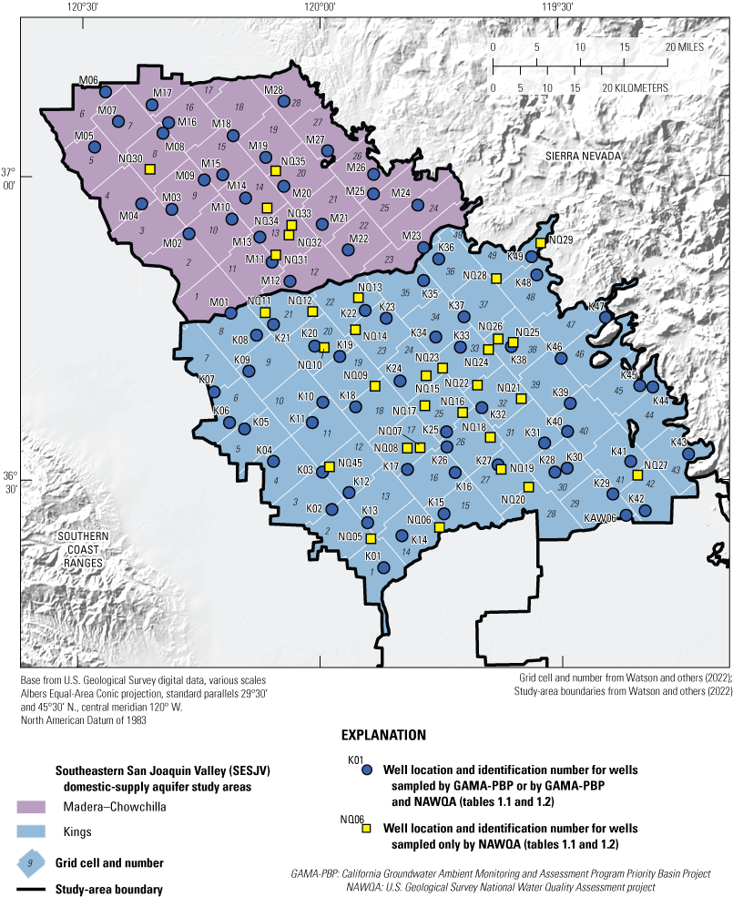
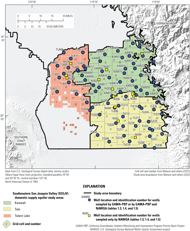
Locations of wells sampled by the U.S. Geological Survey during 2013–15 for assessment of water quality in groundwater resources used for domestic-supply wells in the southeastern San Joaquin Valley, California Groundwater Ambient Monitoring and Assessment Program Priority Basin Project (GAMA-PBP). A, Wells and grid cells in the Madera-Chowchilla and Kings study areas; and B, wells and grid cells in the Kaweah, Tule, and Tulare Lake study areas.
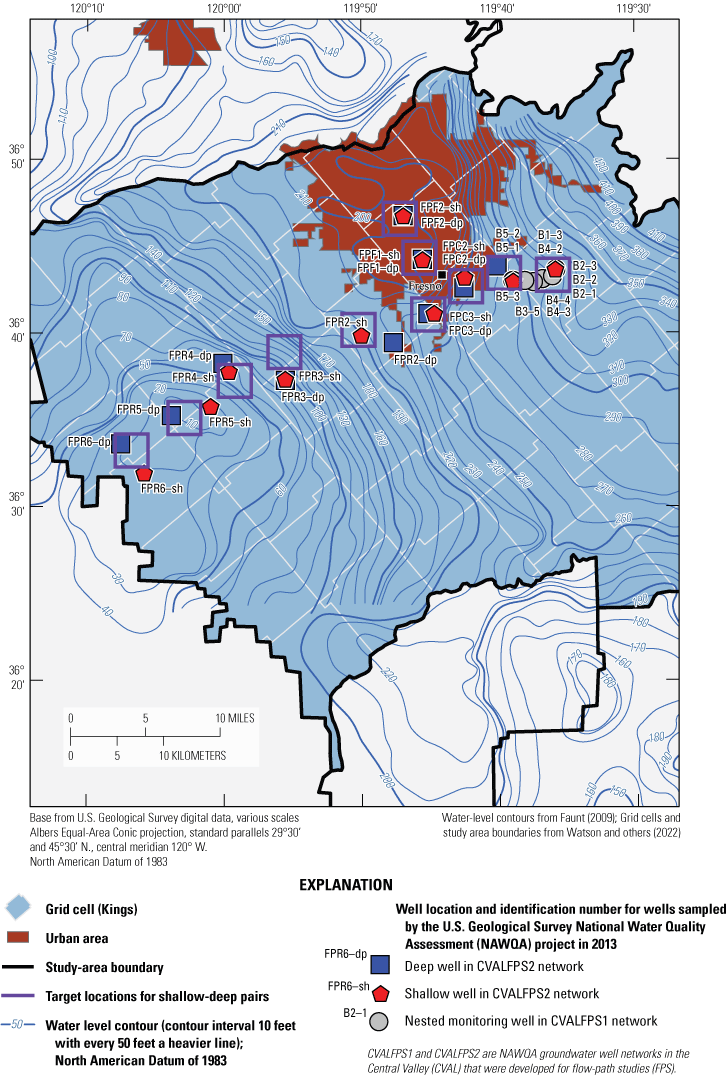
Locations of wells sampled in the National Water Quality Assessment project CVALFPS1 and CVALPFS2 networks in 2013 and modeled groundwater-level contours for spring 2001.
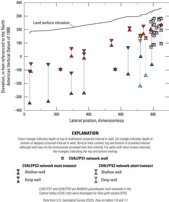
Lateral position and wells depths for wells sampled in the U.S. Geological Survey National Water Quality Assessment project (NAWQA) CVALFPS1 and CVALPAS2 networks in 2013.
Table 1.6.
Identification numbers of wells sampled in the U.S. Geological Survey National Water Quality Assessment project (NAWQA) CVALFPS1 network in 2013.[Well information is tabulated in Balkan and others (2024). United States Geological Survey (USGS) site number identifies the site in the USGS National Water Information System (U.S. Geological Survey, 2023). National Water Quality Assessment identifier (NAWQAID) identifies the network and site names used by the USGS NAWQA project. Sites with Groundwater Ambient Monitoring and Assessment identifiers (GAMAIDs) beginning with KING were sampled by Burton and Belitz (2008); sites with GAMAIDs beginning with S3-MACK are also reported in Shelton and Fram (2017). Used in this report: Kings-D, well is a domestic-supply well for the Kings study area; Kings-P, well is a public-supply wells for the Kings study area. Lateral position is the normalized distance between the valley trough (0) and the boundary between Central Valley alluvium and the Sierra Nevada (1,000; fig. 2; McPherson and Faunt, 2023). Abbreviation: na, not applicable]
Table 1.7.
Identification numbers of wells sampled in the U.S. Geological Survey National Water Quality Assessment project (NAWQA) CVALPFS2 network in 2013.[Well information is tabulated in Balkan and others (2024). United States Geological Survey (USGS) site number identifies the site in the USGS National Water Information System (U.S. Geological Survey, 2023). National Water Quality Assessment identifier (NAWQAID) identifies the network and site names used by the USGS NAWQA project. Sites with Groundwater Ambient Monitoring and Assessment identifiers (GAMAIDs) beginning with KING were sampled by Burton and Belitz (2008); sites with GAMAIDs beginning with S3-MACK are also reported in Shelton and Fram (2017). Used in this report: Kings-D, well is a domestic-supply well for the Kings study area; Kings-P, well is a public-supply wells for the Kings study area. Lateral position is the normalized distance between the valley trough (0) and the boundary between Central Valley alluvium and the Sierra Nevada (1,000; fig. 2; McPherson and Faunt, 2023). Abbreviation: na, not applicable]
References Cited
Arnold, T.L., Bexfield, L.M., Musgrove, M., Stackelberg, P.E., Lindsey, B.D., Kingsbury, J.A., Kulongoski, J.T., and Belitz, K., 2018, Groundwater-quality and select quality-control data from the National Water-Quality Assessment Project, January through December 2015, and previously unpublished data from 2013 to 2014: U.S. Geological Survey Data Series 1087, 67 p., accessed July 6, 2023, at https://doi.org/10.3133/ds1087.
Arnold, T.L., DeSimone, L.A., Bexfield, L.M., Lindsey, B.D., Barlow, J.R., Kulongoski, J.T., Musgrove, M., Kingsbury, J.A., and Belitz, K., 2016, Groundwater quality data from the National Water-Quality Assessment Project, May 2012 through December 2013 (ver. 1.1, November 2016): U.S. Geological Survey Data Series 997, 56 p., accessed July 6, 2023, at https://doi.org/10.3133/ds997.
Balkan, M., Burow, K.R., and Shelton, J.L., Fram, M.S., 2024, Data sets for status of water quality in groundwater resources used for drinking water supply in the southeast San Joaquin Valley, 2013–2015—California GAMA Priority Basin Project: U.S. Geological Survey data release, accessed November 6, 2023, at https://doi.org/10.5066/P9DCTLXV.
Bennett, G.L.,V., Fram, M.S., and Johnson, T.D., 2017, Groundwater-quality data in the Tulare shallow aquifer study unit, 2014–2015—Results from the California GAMA Priority Basin Project: U.S. Geological Survey data release, accessed July 6, 2023, at https://doi.org/10.5066/F7BP00W8.
Burow, K.R., Panshin, S.Y., Dubrovsky, N.M., Vanbrocklin, D., and Fogg, G.E., 1999, Evaluation of processes affecting 1,2-dibromo-3-chloropropane (DBCP) concentrations in ground water in the eastern San Joaquin Valley, California—Analysis of chemical data and ground-water flow and transport simulations: U.S. Geological Survey Water-Resources Investigations Report 99–4059, 57 p., accessed July 6, 2023, at https://doi.org/10.3133/wri994059.
Burow, K.R., Shelton, J.L., and Dubrovsky, N.M., 1998b, Occurrence of nitrate and pesticides in ground water beneath three agricultural land-use settings in the eastern San Joaquin Valley, California, 1993–1995: U.S. Geological Survey Water-Resources Investigations Report 97–4284, 51 p., accessed July 6, 2023, at https://pubs.usgs.gov/wri/1997/4284/report.pdf.
Burow, K.R., Stork, S.V., and Dubrovsky, N.M., 1998a, Nitrate and pesticides in ground water in the eastern San Joaquin Valley, California—Occurrence and trends: U.S. Geological Survey Water-Resources Investigations Report 98–4040, 33 p., accessed July 6, 2023, at https://pubs.usgs.gov/wri/1998/4040a/report.pdf.
Burton, C.A., and Belitz, K., 2008, Ground-water quality data in the southeast San Joaquin Valley, 2005–2006—Results from the California GAMA Program: U.S. Geological Survey Data Series 351, 103 p., accessed July 6, 2023, at https://pubs.usgs.gov/ds/351/.
California Department of Water Resources, 2023, Online System for Well Completion Reports (OSWCR) well completion reports dataset: California Natural Resources Agency website, accessed February 9, 2023, at https://data.cnra.ca.gov/dataset/well-completion-reports.
Faunt, C.C., ed., 2009, Groundwater availability of the Central Valley aquifer, California: U.S. Geological Survey Professional Paper 1766, 225 p., accessed July 6, 2023, at https://pubs.usgs.gov/pp/1766.
McPherson, K.R., and Faunt, C.C., 2023, Relative distance of California’s Central Valley from trough to valley edge and supporting data: U.S. Geological Survey data release, accessed October 19, 2023, at https://doi.org/10.5066/P9KEZJQS.
Shelton, J.L., and Fram, M.S., 2017, Groundwater quality data for the Madera/Chowchilla-Kings shallow aquifer study unit, 2013–14—Results from the California GAMA Program: U.S. Geological Survey Data Series 1019, 115 p., accessed July 6, 2023, at https://doi.org/10.3133/ds1019.
Shelton, J.L., Fram, M.S., and Belitz, K., 2009, Groundwater-quality data for the Madera-Chowchilla study unit, 2008—Results from the California GAMA Program: U.S. Geological Survey Data Series 455, 80 p., accessed July 6, 2023, at https://doi.org/10.3133/ds455.
Stork, S.V., McGregor, A.M., Balkan, M., Arroyo-Lopez, J., Borkovich, J.G., Lor, V., Peng, S., Jasper, M., Haugen, E.A., Soldavini, A.L., Estrada, C.L., McVey, C.J., Grechkosey, D.P., Koepke, J.E., Oldham, N.A., Vroman, R.C., Handley, R.A.Q., and Bennett, G.L., 2019, Attributed California water supply well completion report data for selected areas, derived from CA WCR OSCWR data (ver. 2.0, January 2023): U.S. Geological Survey data release, accessed July 6, 2023, at https://doi.org/10.5066/P9R1V41Q.
U.S. Geological Survey, 2023, USGS water data for the Nation: U.S. Geological Survey National Water Information System, accessed February 12, 2023, at https://doi.org/10.5066/F7P55KJN.
Watson, E., Johnson, T.D., and Dupuy, D.I., 2022, California Groundwater Ambient Monitoring and Assessment (GAMA) Program Domestic-Supply (Shallow) Aquifer assessment study unit boundaries and grid cells for assessment of groundwater resources (ver. 2.0, January 2023): U.S. Geological Survey data release, available at https://doi.org/10.5066/P931PZRC.
Conversion Factors
Temperature in degrees Celsius (°C) may be converted to degrees Fahrenheit (°F) as follows:
°F = (1.8 × °C) + 32.
Temperature in degrees Fahrenheit (°F) may be converted to degrees Celsius (°C) as follows:
°C = (°F − 32) / 1.8.
Datum
Vertical coordinate information is referenced to the North American Vertical Datum of 1988 (NAVD 88).
Horizontal coordinate information is referenced to the North American Datum of 1983 (NAD 83).
Altitude, as used in this report, refers to distance above the vertical datum.
Supplemental Information
Specific conductance is given in microsiemens per centimeter at 25 degrees Celsius (µS/cm at 25 °C).
Concentrations of chemical constituents in water are given in either milligrams per liter (mg/L) or micrograms per liter (µg/L).
Activities for radioactive constituents in water are given in picocuries per liter (pCi/L).
Concentrations of tritium are presented in tritium units (TU). 1 TU equals 3.19 pCi/L.
Carbon-14 data are expressed as percent modern carbon (pmC).
Results for measurements of stable isotopes of an element (with symbol E) in water, solids, and dissolved constituents commonly are expressed as the relative difference in the ratio of the number of the less abundant isotope (iE) to the number of the more abundant isotope of a sample with respect to a measurement standard.
Abbreviations
1,2,3-TCP
1,2,3-trichloropropane
1,2-DCP
1,2-dichloropropane
bls
below land surface
CAAT
2-chloro-4,6-diamino-s-triazine (didealkylatrazine)
DBCP
1,2-dibromo-3-chloropropane
DDW
Division of Drinking Water (California State Water Resources Control Board)
EDB
1,2-dibromoethane (ethylene dibromide)
EPA
U.S. Environmental Protection Agency
GAMA-PBP
California Groundwater Ambient Monitoring and Assessment Program Priority Basin Project
HAL-US
U.S. Environmental Protection Agency lifetime health advisory level
HBSL
U.S. Geological Survey health-based screening level
HHBP
U.S. Environmental Protection Agency human health benchmark for pesticides
MCL
maximum contaminant level
MCL-CA
California State Water Resources Control Board Division of Drinking Water maximum contaminant level
MCL-US
U.S. Environmental Protection Agency maximum contaminant level
MTBE
methyl tert-butyl ether
NAWQA
U.S. Geological Survey National Water Quality Assessment project
NL-CA
California State Water Resources Control Board Division of Drinking Water notification level
NWIS
National Water Information System (U.S. Geological Survey)
OSWCR
California Department of Water Resources Online System for Well Completion Reports
PCE
tetrachloroethene
RL-CA
California State Water Resources Control Board Division of Drinking Water response level
SESJV-D
groundwater resources used for domestic-supply wells in the southeastern San Joaquin Valley
SESJV-P
groundwater resources used for public-supply wells in the southeastern San Joaquin Valley
SMCL
secondary maximum contaminant level
SWRCB
California State Water Resources Control Board
TDS
total dissolved solids
TT
treatment technique level
USGS
U.S. Geological Survey
VOC
volatile organic compound
For more information concerning the research in this report, contact the
Director, California Water Science Center
U.S. Geological Survey
6000 J Street, Placer Hall
Sacramento, California 95819
https://www.usgs.gov/centers/california-water-science-center
Publishing support provided by the U.S. Geological Survey
Science Publishing Network, Sacramento Publishing Service Center
Disclaimers
Any use of trade, firm, or product names is for descriptive purposes only and does not imply endorsement by the U.S. Government.
Although this information product, for the most part, is in the public domain, it also may contain copyrighted materials as noted in the text. Permission to reproduce copyrighted items must be secured from the copyright owner.
Suggested Citation
Burow, K.R., Shelton, J.L., and Fram, M.S., 2024, Status of water quality in groundwater resources used for drinking-water supply in the southeastern San Joaquin Valley, 2013–15—California GAMA Priority Basin Project: U.S. Geological Survey Scientific Investigations Report 2024–5009, 135 p., https://doi.org/10.3133/sir20245009.
ISSN: 2328-0328 (online)
Study Area
| Publication type | Report |
|---|---|
| Publication Subtype | USGS Numbered Series |
| Title | Status of water quality in groundwater resources used for drinking-water supply in the southeastern San Joaquin Valley, 2013–15—California GAMA Priority Basin Project |
| Series title | Scientific Investigations Report |
| Series number | 2024-5009 |
| DOI | 10.3133/sir20245009 |
| Publication Date | April 25, 2024 |
| Year Published | 2024 |
| Language | English |
| Publisher | U.S. Geological Survey |
| Publisher location | Reston, VA |
| Contributing office(s) | California Water Science Center |
| Description | Report: xiii, 135 p.; Data Release |
| Country | United States |
| State | California |
| Online Only (Y/N) | Y |