

Nutrient Chemistry in the Elizabeth Lake Subwatershed: Effects of Onsite Wastewater Treatment Systems on Groundwater and Lake Water Quality, Los Angeles County, California
Prepared in cooperation with the Los Angeles Regional Water Quality Control Board
Links
- Document: Report (12.5 MB pdf) , HTML , XML
- NGMDB Index Page: National Geologic Map Database Index Page (html)
- Download citation as: RIS | Dublin Core
Acknowledgments
We thank the Los Angeles Regional Water Quality Control Board for their funding and support throughout the research process.
We thank U.S. Geological Survey employees Gregory Brewster, Matthew Hartman, Benjamin Middendorf, Michael Lee, Gregory Smith, and the U.S. Geological Survey Research Drilling Program for field work and logistical support in the preparation and collection processes of this study. We also thank Bryant Jurgens and Kirsten Faulkner (U.S Geological Survey) for their support in the noble gas analysis part of this project.
Abstract
Nutrient (nitrogen [N] and phosphorus [P] chemistry) downgradient from onsite wastewater treatment system (OWTS) was evaluated with a groundwater study in the area surrounding Elizabeth Lake, the largest of three sag lakes within the Santa Clara River watershed of Los Angeles County, California.
Elizabeth Lake is listed on the “303 (d) Impaired Waters List” for excess nutrients and is downgradient from more than 600 OWTS. The primary objective of this study was to develop a conceptual hydrogeological model to determine if discharge from OWTS is transported into shallow groundwater within the Elizabeth Lake subwatershed and contributes nutrients to Elizabeth Lake in excess of the total maximum daily load limit. An analysis of historical data and data collected for this study provided estimates of aquifer properties, such as hydraulic gradients and other parameters necessary to estimate boundary conditions. Electrical resistivity tomography (ERT) surveys were done to determine the best monitoring well locations and to estimate depth to groundwater. During 4 separate sampling events, 11 wells, 2 imported water tanks, 1 spring (sampled on March 17, 2019), and Elizabeth Lake were sampled, which occurred during February–September 2020.
ERT transects and borehole geophysical measurements indicated that there were low to high resistivity materials in the subsurface and potential perched fresh water. Most of the aquifer material was characterized as sandy silt, occasionally with mixed clays and medium gravels, and was estimated to have a hydraulic conductivity from 3.28x10⁻³ to 16.4 feet per day, a porosity from 0.34 to 0.42, and a hydraulic gradient from 0.01 to 0.03. Although bedrock was not obvious in ERT transects, all well depths were terminated at depths of an impassible confining layer observed to be a highly consolidated blue-gray clay. Depths to granitic bedrock, based on road outcrops and lithologic driller logs, varied throughout the study area. Depth to the bedrock was estimated to be shallow on the north side of Elizabeth Lake at approximately 30 feet below land surface (ft bls). Depth to bedrock is at 50 ft bls toward the east of the Elizabeth Lake subwatershed, which is at topographic ground surface to the north and south of the residential development. Groundwater levels ranged from approximately 0 to 12 ft bls during this study. Historical water levels ranged from 8 to 16 ft bls in the lower elevation of the study area and increased to depths of as much as 80 ft bls at higher elevations on the north and south boundaries of the Elizabeth Lake subwatershed.
Water-quality samples were analyzed for major ions, nutrients, dissolved organic carbon, stable isotopes, and age-dating tracers. A principal component analysis was completed to determine organic matter sources. The proportion of recharge from imported waters, used for domestic consumption, was calculated using stable water isotopes, deuterium (δD) and oxygen (δ18O). Recharge from imported waters accounted for approximately 15–71 percent of the total recharge to groundwater within the study area. Total nitrogen concentrations ranged from 0.17 to 30.9 milligrams per liter (mg/L) as N, and phosphorus, measured in the soluble form as orthophosphate, ranged from 0.03 to 0.35 mg/L as P. Nitrate concentrations in groundwater samples ranged from less than the detection limit (0.01 mg/L as N) to approximately 24 mg/L as N. Nitrate was not detected in 3 of the 12 sites sampled during the study (2 wells and Elizabeth Lake). Dissolved organic carbon concentrations ranged from 0.4 to 27 mg/L in groundwater and from 9.9 to 100 mg/L in Elizabeth Lake. Ammonium and orthophosphate concentrations generally were low in groundwater. However, elevated concentrations of ammonium in Elizabeth Lake were assumed to be due to avian waste products or biological nitrogen fixation. Groundwater ages were mostly modern (recharged since 1952), with a median recharge temperature of 13 degrees Celsius.
Redox conditions in groundwater indicated the likely occurrence of nitrate attenuation by denitrification downgradient from the wells to the south of Elizabeth Lake before groundwater discharges to the lake. Undetectable nitrate in Elizabeth Lake at the time of sampling was likely due to algal uptake. Most wells contained stable isotopes of nitrogen and oxygen in nitrate (δ15N-NO3 and δ18O-NO3) molecules with values consistent with denitrification. However, one monitoring well on the north of Elizabeth Lake (ELLA-8) had no evidence of denitrification, based on elevated concentrations of nitrate and a sufficient amount of dissolved oxygen such that the water was oxic and not favorable for the denitrification reaction. Consequently, this nitrate could be delivered to Elizabeth Lake through groundwater discharge if nitrate is not removed from the system by denitrifying bacteria downgradient from the well before the groundwater discharges into Elizabeth Lake.
The principal component analysis demonstrated that dissolved organic matter optical properties track different sources of dissolved organic matter from decayed plants, animals, and animal-derived wastes. Two wells contained strong indicators of OWTS water presence, although geochemical evidence indicated other wells may also be affected by OWTS discharge.
Introduction
In 1948, the Federal Clean Water Act (CWA) was established to restore and maintain the chemical, physical, and biological integrity of waters of the United States (U.S. Environmental Protection Agency, 2023a). In accordance with the CWA, the State of California Los Angeles Regional Water Quality Control Board (LARWQCB) established water-quality standards for all bodies of water within its region, including three lakes within the Elizabeth Lake subwatershed, Hydrologic Unit Code (HUC 180701020301 (U.S. Geological Survey, 2020), within the larger Santa Clara River watershed (HUC 18070102; U.S. Geological Survey, 2020; fig. 1; Los Angeles Regional Water Quality Control Board, 2006, 2016).
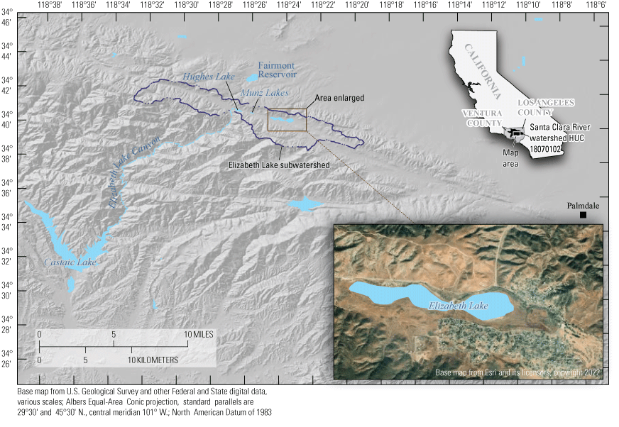
Location of Elizabeth Lake, Munz Lakes, and Hughes Lake of the Elizabeth Lake sub-watershed (Hydrologic Unit Code [HUC] 180701020301; U.S. Geological Survey, 2020) within the larger Santa Clara River watershed (Los Angeles Regional Water Quality Control Board, 2006, 2016).
The Elizabeth Lake subwatershed drains three lakes: Elizabeth Lake, Munz Lakes, and Hughes Lake. These three lakes may be individual lakes or be entirely connected depending on the annual precipitation. All three lakes may lose all water in dry years. In 1966, the Elizabeth Lake subwatershed was initially placed on the California “303(d) List” or “Impaired Waters List” for eutrophic conditions, high pH, and low dissolved oxygen (DO; Tetra Tech, 2016); the lakes also were listed for organic enrichment and trash in 1998 and 2008, respectively (Tetra Tech, 2016).
Additionally, Hughes Lake was listed for algae, odor, and fish kills from 2008 to 2010. In 2016, a total maximum daily load (TMDL) analysis was done. Identified in section 303(d)(1) of the CWA as “the load necessary to implement the applicable water-quality standards” for the nutrients nitrogen (N) and phosphorus (P), the TMDL was adopted for the lakes to meet water-quality standards that protect human and aquatic health and prevent eutrophication (Los Angeles Regional Water Quality Control Board, 2016).
Eutrophication is one of the greatest threats of degradation to freshwater ecosystems worldwide (Ansari and Gill, 2014). Excess nutrient loads entering lakes and other water systems can result in various degrees of algal enrichment leading up to hypereutrophic conditions (Dodds and others, 2009; Ansari and Gill, 20144). Eutrophic water conditions impede the use of fresh water for recreation and domestic consumption and may interfere with the native ecological diversity. Potential primary sources of nutrient loads that stimulate eutrophic conditions and excess algal growth in lakes include atmospheric deposition of nitrogen, groundwater discharge, wastewater discharge, urban runoff, agricultural and aquaculture runoff, internal recycling of nutrients within the lake, and river discharge (Anderson and others, 2002; Ansari and Gill, 2014; Harke and others, 2016; Rakhimbekova and others, 2021). Prior studies have documented that 99.90 percent of the nutrients present in the Santa Clara River lakes (Elizabeth Lake, Munz Lakes, and Hughes Lake) are a product of internal nutrient cycling from the release of nutrients stored in lakebed sediments (Los Angeles Regional Water Quality Control Board, 2016; Tetra Tech, 2016). To achieve the Santa Clara River lakes TMDL targets for nutrient load reduction, it is necessary to characterize and evaluate all potential sources and pathways by which nutrients are delivered to the lake. Figure 2 shows a simplified path of nutrient transport from onsite wastewater treatment systems (OWTS) to groundwater with possible subsequent discharge to the land or to rivers or lakes. Groundwater discharge delivering excess nutrients to lakes can contribute to conditions that support algal blooms. Primary productivity can be high at lake shorelines where groundwater discharges with excess nutrient levels are high (Naranjo and others, 2019; Rakhimbekova and others, 2021).
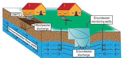
Onsite wastewater treatment systems (OWTS) discharging into groundwater and being transported by groundwater flow movement and discharging into a lake or river.
The U.S. Geological Survey (USGS), in cooperation with the Los Angeles Regional Water Quality Control Board, focused on the eastern part of the largest of the three Santa Clara River lakes, Elizabeth Lake, which is downgradient from more than 600 residential OWTS systems (fig. 3). With an average household water use of 0.36 acre-feet per year (acre-ft/yr), imported waters supply an estimated 216 acre-ft/yr of recharge into the aquifer, of which 38 acre-ft/yr is suspected of discharging into Elizabeth Lake (Izbicki, 2014; Tetra Tech, 2016). Ammonium and organic nitrogen (org-N) concentrations present in OWTS effluent can be as high as 25–60 milligrams per liter (mg/L) as N, but typical concentrations are about 40 to 45 mg/L as N (Umari and others, 1993; Wakida and Lerner, 2005; Kratzer and others, 2011; Izbicki, 2014). These concentrations may be attenuated by natural biological processes before or after entering the aquifers. Once OWTS effluent is discharged into the immediate subsurface, nutrients and other constituents can infiltrate into shallow groundwaters (Follett and Follett, 2008; Los Angeles Regional Water Quality Control Board, 2016).
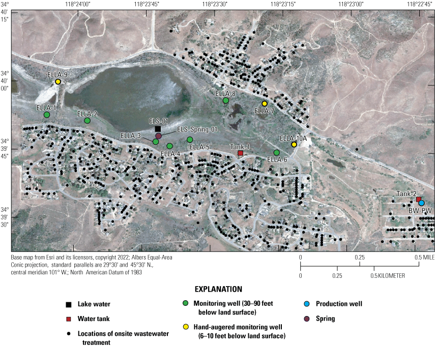
Elizabeth Lake, sample locations, and surrounding onsite wastewater treatment systems locations. Station numbers and site information are shown in table 1. Onsite wastewater treatment systems locations from Los Angeles County Sanitary Sewer Network—Consolidated Sewer Maintenance District (2006).
Densely populated areas with OWTS may present a challenge in the attenuation of effluent-derived nutrients entering the subsurface. The LARWQCB hypothesizes that local shallow groundwaters suspected of receiving OWTS effluent are discharging into Elizabeth Lake and contributing 0.02 percent of the total nutrient loads (Los Angeles Regional Water Quality Control Board, 2016; Tetra Tech, 2016120). Some ammonium (NH4+) and other inorganic N constituents such as nitrate (NO3−) and nitrite (NO2−) may be attenuated through microbiological and chemical processes of assimilation from bacteria, sorption to clay minerals, or volatilization and denitrification reactions (Kendall and McDonnell, 1998). Most of the ammonium or org-N discharged from OWTS effluent into oxic groundwaters will be transformed or mineralized to nitrate. Phosphorus is strongly sorbed onto positively charged iron (Fe) and manganese (Mn) oxides or calcium carbonate minerals and might also be removed from the system by the formation of relatively insoluble phosphate-bearing minerals, such as vivianite, apatite, and stregnite (Parfitt, 1979; Mueller and Helsel, 199688; Zhang and Huang 2007; Izbicki, 2014; Rakhimbekova and others, 2021). However, sorption of phosphorous is pH-dependent, and P transport through groundwater may occur until sorption sites become saturated, presenting problems in areas with densely located OWTS (Domagalski and Johnson, 2011).
Tetra Tech (2016) released a report using a BATHTUB model, a program that formulates a steady-state water-quality model and a nutrient mass balance. This model was used to quantify external nutrient source loads, including those from OWTS, and to establish site specific nutrient loading totals required to attain a target of no more than 20 micrograms per liter (µg/L) of chlorophyll-a in surface waters. Total chlorophyll-a results collected from surface water were used as the only primary constraint on the BATHTUB model to estimate external nutrient source contributions and to determine the load amounts needed to reach the TMDL target. Chlorophyll-a measurements used by Tetra Tech were collected from previous field study efforts by the University of California, Riverside and LARWQCB in 1992–93 and in 2014, respectively (Lund and others, 1994; Tetra Tech, 2016120; Los Angeles Regional Water Quality Control Board, 2016). Tetra Tech’s (2016) BATHTUB model estimated current loads of 761,000 pounds of phosphorus per year (lb-P/yr) and 42,500,000 pounds of nitrogen per year (lb-N/yr) entering Elizabeth Lake. Tetra Tech estimated that OWTS account for 0.02 percent of these annual totals or about 160 lb-P/yr and 961 lb-N/yr (Lund and others, 1994; Tetra Tech, 2016; Los Angeles Regional Water Quality Control Board, 2016). The LARWQCB (2016) set load allocations to 2,590 lb-P/yr and 13,800 lb-N/yr, which requires a significant reduction of 99.63 percent of total phosphorous (TP) and 99.96 percent of total nitrogen (TN) load inputs into Elizabeth Lake. This allocation includes 130.1 lb-P/yr and 770.3 lb-N/yr load reduction estimated to be sourced from OWTS and delivered to Elizabeth Lake by groundwater discharge (Los Angeles Regional Water Quality Control Board, 2016; Tetra Tech, 2016). To successfully reach these targets, the LARWQCB assigned the load allocations for external loading from OWTS to be reduced by 18.7 and 19.8 percent of existing loads estimated by Tetra Tech (2016) for TP and TN, respectively (Los Angeles Regional Water Quality Control Board, 2016).
Most of the org-N discharged into groundwater from OWTS will undergo ammonification and be converted into ammonium and then nitrate under aerobic conditions (DeSimone and Howes, 1998). The ammonium formed as a reaction of ammonification discharged from OWTS or naturally occurring in waters is rapidly oxidized by ammonium-oxidizing bacteria during aerobic conditions to form nitrite and nitrate (eq. 1). In anoxic or low oxygen parts of the aquifer, nitrate and nitrite can be removed from the system by denitrification, thus changing nitrate and nitrite to nitrogen gas (N2; eq. 2). Nitrite is formed as a by-product of nitrification and denitrification (eqs. 1, 2). Additionally, carbon from OWTS and natural sources drive the bacterial processes, such as denitrification and ammonium oxidation (eq. 2; Izbicki, 2014). Nitrification (eq. 1) and denitrification (eq. 2) formulas are shown here:
whereNH4+
is dissolved ammonium,
O2
is dissolved oxygen,
NO3-
is dissolved nitrate,
H2O
is water, and
H+
is dissolved hydrogen ion.
A variety of constituents, including dissolved organic matter (DOM) composition, stable isotopes of nitrogen and oxygen in nitrate (δ15N-NO3 and δ18O-NO3), and age dating of water, were used to help identify the presence of OWTS discharges into groundwater.
Dissolved organic matter includes a broad range of organic molecules of various sizes and compositions that are released by all living and dead plants and animals. The amount and type of DOM are obtained by measuring the fraction of light absorbed at specific ultraviolet (UV) wavelengths and subsequently released at longer wavelengths as fluorescence. Optical measurements of absorbance and fluorescence can be used for a wide range of applications for natural waters, including organic matter cycling (Coble, 2007; Tranvik and others, 2009), algal production of DOM (Lapierre and Frenette, 2009), and DOM source attribution and fingerprinting (Baker and Spencer, 2004; Carstea and others, 2009; Carpenter and others, 2013; Hansen and others, 2018a, 2018b). Common parameters and indices derived from optical data discussed later include the absorbance at individual wavelengths (for example, absorbance at 254, 280, 370, 412, and 440 nanometers [nm]) and fluorescence at specific excitation-emission (ex/em) pairs.
Information about the composition of DOM can be obtained by normalizing the absorbance or fluorescence response to another parameter, such as normalizing to dissolved organic carbon (DOC) concentration (Beggs and Summers, 2011; Hansen and others, 2016). For example, the specific UV absorbance at 254 nm (SUVA254; absorbance at 254 nm divided by DOC concentration) has been shown to be strongly correlated with the hydrophobic organic acid fraction of DOM (Spencer and others, 2012) and is a useful proxy for DOM aromatic content (Weishaar and others, 2003) and molecular weight (Chowdhury, 2013). Other indicators of DOM composition, including the ratios of different wavelengths of absorbance and fluorescence, such as freshness index (β:α), humification index (HIX), peak A to peak C (A:C), and spectral slopes (S275–295, S290–350, S350–400) across specific regions of the optical spectrum, also can be related to the molecular weight, source, and processing (biodegradation and photolytic exposure) of DOM (Hansen and others, 2016). The freshness index is an indicator of recently produced dissolved organic matter. The humification index is a measure of the presence of humic substances and/or extent of humification. DOM characterization used with other constituents, such as ammonium concentration, can be used to identify effluent. The “Methods” section of this report will explain how the earlier-mentioned methods were used to better understand the OWTS effluent nutrient sources potentially discharging into Elizabeth Lake.
Purpose and Scope
The purpose of this report is to describe a conceptual model of the groundwater flow and solute transport from OWTS effluent into Elizabeth Lake that was developed by the U.S. Geological Survey (USGS) in cooperation with the Los Angeles Regional Water Quality Control Board. The scope of this report included two electrical resistivity tomography (ERT) transects used to characterize subsurface resistivity and help determine the best locations for installation of monitoring wells. Subsurface lithologies were collected at depth during drilling to provide estimates of hydraulic conductivity. Water levels in wells were continuously monitored during the course of the study, and seasonal water-quality samples from groundwater monitoring wells and Elizabeth Lake were collected and analyzed. Depth to the bedrock was determined from approximately 10 available drillers’ logs. This study used multiple lines of evidence to provide a conceptual model and determine what nutrients are discharging into Elizabeth Lake. Electrical resistivity tomography (ERT) data can be found in Groover and others (2021). Monitoring well locations and subsurface geophysical data can be found at the Geolog Locator (https://www.usgs.gov/tools/geolog-locator, U.S. Geological Survey, 2022) using the well station numbers shown in table 1. Water-quality and water-level information is stored in the USGS National Water Information System (NWIS; U.S. Geological Survey, 2023a).
Table 1.
List of stations sampled and well construction data from drillers’ logs, Elizabeth Lake, California, February–September 2020. All data collected are publicly available on the National Water Information System (U.S. Geological Survey, 2023a).[USGS, U.S. Geological Survey; ft, feet; NAVD 88, North American Vertical Datum of 1988; ft bls, feet below land surface; —, not applicable]
General Study-Area Description
The study area is within the Elizabeth Lake subwatershed, HUC 180701020301, located in the northeastern part of Los Angeles County within the Angeles National Forest (not shown) close to the headwaters of Elizabeth Lake Canyon (fig. 1; U.S. Geological Survey, 2020). The lakes within the Elizabeth Lake subwatershed are sag ponds that formed from precipitation and accumulation of fresh water in structural depressions along the active San Andreas Fault Zone and are approximately 19 miles (mi) northwest of Palmdale, California (figs.1, 4). The three lakes, from largest to smallest and highest to lowest in elevation, are Elizabeth Lake, Munz Lakes, and Hughes Lake. This study focuses on the largest of the three lakes, Elizabeth Lake, which is within the Elizabeth Lake Census Designated Place, California.
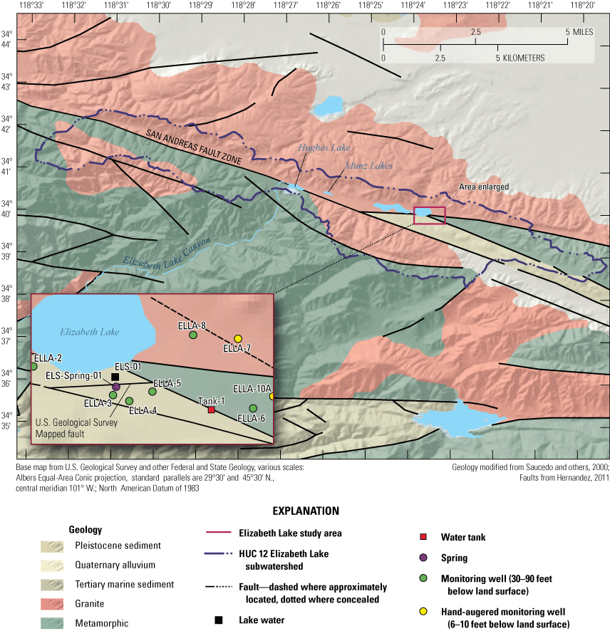
General geological features of the Elizabeth Lake study area. See table 1 for station information.
Hydrology
The Santa Clara River watershed has a Mediterranean climate, with warm dry summers and cool wet winters (Fleming and others, 2020). The Elizabeth Lake subwatershed covers 7.85 square miles (mi2), with the Elizabeth Lake drainage area accounting for 6.71 mi2 of the area and an elevation that ranges from approximately 3,380 to 4,000 feet (ft) above sea level (ASL; North American Vertical Datum of 1988 [NAVD 88]; Tetra Tech, 2016; Los Angeles Regional Water Quality Control Board, 2016; U.S. Geological Survey, 2020). Annual precipitation is estimated to be 13.6 inches per year (in/yr) using north and south bounding National Oceanic and Atmospheric Administration (NOAA) stations (USC00042941 and USC00048014) located 3 and 6 mi away from Elizabeth Lake, respectively, with most of the precipitation falling between November and March (National Oceanic and Atmospheric Administration, 2020). The Elizabeth Lake subwatershed is considered a closed system with the exception of infrequent wet El Niño years, which deliver excessive amounts of precipitation causing intermittent channels to transport water from Elizabeth Lake northwest toward Munz Lakes and Hughes Lake and farther downstream toward the Castaic Lake (fig. 1) drinking water reservoir (Tetra Tech, 2016). Most residences receive imported water from northern California for consumption, and groundwater pumping is believed to be minimal and not taken into consideration for this study. Historically, Elizabeth Lake was previously used for recreational use and stocked with trout for fishing, and a picnic area is located on the western part of the lake.
Elizabeth Lake water levels are dependent on annual rainfall and groundwater discharging into the lake. Elizabeth Lake is primarily recharged from annual precipitation and stormwater runoff from the surrounding highlands during rainfall, with suspected minimal recharge of 38 acre-ft/yr from groundwater flow (Tetra Tech, 2016). Groundwater is assumed to recharge by infiltration of Elizabeth Lake surface water during dry years; runoff infiltration from uplands, including OWTS discharge; precipitation infiltration; and underflow from surrounding consolidated rocks, which are most likely fractured because of the proximity to the San Andreas Fault Zone. During years of severe drought with little to no recharge, the three lakes have been known to periodically dry up, which was the case during an initial 2018 field visit.
Groundwater levels can vary substantially in environments of extensive faulting (Haneberg, 1995). This variability can be observed within the Elizabeth Lake subwatershed based on groundwater levels recorded on well completion reports from the Department of Water Resources (DWR) Online System for Well Completion Reports (OSWCR) database (California Department of Water Resources, 2021). Historical water levels in wells measured by the USGS and well completion reports (WCRs) in the valley of the Elizabeth Lake subwatershed were about 8–16 feet below land surface (ft bls) during the late 1960s and early 1970s. Water levels in wells assumed to be screened within the unconfined aquifer (shallower than 200 ft bls and not containing a screened interval within hard rock) were documented on WCRs and ranged from 6 to 24 ft bls in lower parts and as much as 80 ft bls in the surrounding uplands of the Elizabeth Lake subwatershed. Groundwater flows from high to low hydraulic head in unconfined aquifers with no-to-minimal groundwater pumping and is typically assumed to follow topography; thus, we inferred that groundwater flows from the surrounding uplands toward Elizabeth Lake and discharges into Elizabeth Lake when water levels are high.
Geology
The San Andreas Fault Zone is an active transform fault distinguished throughout parts of California by troughs, ridges, sag ponds, and offset channels and extends from Mexico (not shown) to the Mendocino triple junction off the coast of northern California (not shown; Arrowsmith and Zielke, 2009). The study area lies along the San Andreas Fault Zone, which is shown on figure 4. Areas along the San Andreas Fault Zone, such as the Elizabeth Lake subwatershed, are heavy faulted and contain fault splays.
According to local drillers’ logs, depth to bedrock on the western boundary of the Elizabeth Lake subwatershed was measured at approximately 100 ft bls (California Department of Water Resources, 2021). Granite outcrops are present on the north side of Elizabeth Lake and bounding the northern part of residences. Lake sediment composed of Quaternary alluvium overlies this granite. The depth of the sediment is approximately 50 ft bls adjacent to the lakebed. On the other side of the lake, metamorphic rocks are present, and the alluvium thickness is approximately 70–150 ft.
According to a California Geological Survey (CGS) geologic map (Hernandez, 2011), the Elizabeth Lake basin primarily consists of Holocene lake deposits and modern alluvial fans sourced from mouths of stream canyons, older Pleistocene alluvium and alluvial fans, some outcrops of the Tertiary Anaverde Formation, shale and arkose sandstones, and artificial fill from human construction (from debris catchment basins, reservoirs, or road alignment). The area is bounded by Late Cretaceous granodiorite to the north and a quartzo-feldspathic and amphibolite gneiss (Early Cretaceous to Proterozoic) to the south. A simplified version of geologic units is shown on figure 4 (Hernandez, 2011).
Methods
A surface geophysical survey was completed using electrical resistivity tomography, herein referred to as the “ERT survey,” to determine the approximate depth to groundwater, determine variations in aquifer material, and provide information to guide monitoring well placement (figs. 3, 4). ERT data are available from Groover and others (2021). Seven shallow single-point monitoring wells were drilled along the south, east, and northern perimeters of Elizabeth Lake; another three shallow monitoring wells were also hand augered along the perimeter of Elizabeth Lake (figs. 3, 4). Borehole geophysical logs were collected in the seven newly installed USGS monitoring wells and are available from the USGS GeoLog Locator (U.S, Geological Survey, 2022). The logs can be retrieved using the USGS station numbers available in table 1. Field identifiers in table 1 that start with “ELLA” are monitoring wells installed around the perimeter of Elizabeth Lake in Los Angeles County, California. During the course of this study, 11 wells (BW-PW, ELLA-1–9, and ELLA-10A), 2 imported water tanks (Tank-1 and Tank-2), 1 spring (ELS-Spring-01), and 1 Elizabeth Lake site (ELS-01) were sampled. Field measurements included groundwater levels (continuous and discrete) and water-quality parameters (pH, temperature, specific conductance, and DO). Water-quality samples were analyzed for major ions and select trace elements, nutrients, stable isotopes of water, stable isotopes of nitrogen and oxygen in nitrate, noble gases, tritium, and DOC (table 2).
Table 2.
Sample summary of constituents analyzed for the water-quality part of the Elizabeth Lake groundwater and lake study, Elizabeth Lake, California, March 2019–September 2020.[Data source: U.S. Geological Survey (2023a). Sample summary: Total number of well sites sampled–11; total number of surface-water sites sampled–1; total number of water tanks sampled–2. Abbreviations: DOC, dissolved organic carbon; δ 15N, stable isotope of nitrogen; δ18O, stable isotope of oxygen; δD, stable isotope of hydrogen; DO, dissolved oxygen]
Subsurface Characterization
Surface resistivity transects and borehole resistivity measurements for wells drilled for this study were collected to characterize the subsurface and infer aquifer properties. Additionally, drillers’ log lithologies were used to characterize subsurface aquifer boundaries within the Elizabeth Lake subwatershed that were not captured by geophysical measurements and wells drilled as part of this study. Surface resistivity measurements were used to estimate depth to groundwater levels and support placement decisions for monitoring wells.
Electrical Resistivity Tomography
To estimate depth to groundwater and bedrock, two ERT surveys were completed during a 3-day period, March 15–17, 2019, at the southern edge of Elizabeth Lake and on the overlying sediments (fig. 5). Resistivity measurements were taken by injecting current into the ground using two “transmitter” current electrodes and measuring the resulting voltage difference between two “receiver” electrodes (Minsley and others, 2010). Each electrode can work as either a transmitter or receiver electrode as the combination of electrode pairs used to make measurements is translated along the line (Groover and others, 2017). Electrical resistivity in ohm-meters (ohm-m) is an innate material property that is affected by (1) the amount and salinity of pore water; (2) the proportion of coarse or fine-grained material, such as clay; and (3) the fraction of metallic minerals, such as magnetite (Hubbard and Rubin, 2005; Minsley and others, 2010). The combination of these factors results in some ambiguity in interpreting data from techniques such as ERT; therefore, other data, such as borehole lithology, groundwater levels, or porewater salinity, are required to constrain processing and interpretation of ERT (Groover and others, 2017). ERT is relatively cost-efficient and can distinguish sharp contrasts in materials, such as basement to unconsolidated sediment, without detailed knowledge of the site parameters. This technique was used to determine the proper drilling method and to help plan locations for the installation of monitoring wells.
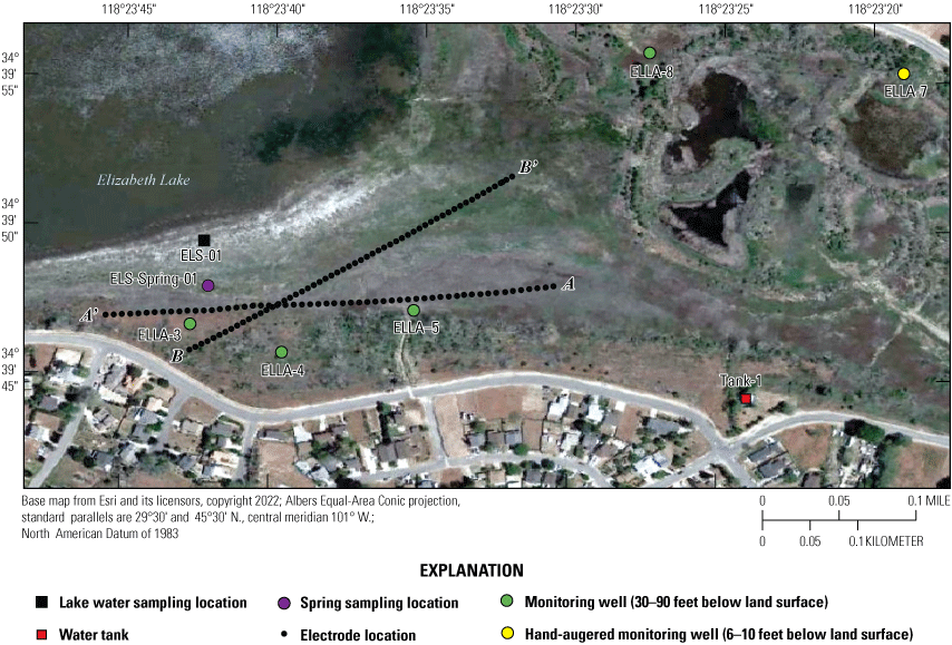
The southern part of the study site near Elizabeth Lake showing electrical resistivity tomography electrode locations for transects A–A’ (line 1) and B–B’ (line 2) measured with the Trimble Geo7x in the field (Groover and others, 2021). See table 1 for site information.
ERT data were acquired using an 8-channel SuperSting R8 resistivity/induced polarization meter (Advanced Geosciences Inc., 2011) with a maximum of 56 electrodes and a passive electrical cable system (Groover and others, 2021). Stainless steel electrode stakes, 18 inch (in.) long and 0.4-in. diameter, were installed to a minimum depth of 4 in. along the southwest side of Elizabeth Lake. Electrode and electrode stakes were positioned every 22.96 ft along Elizabeth Lake line 1 (A–A’), for a total length of 1,263 ft, and every 19.69 ft on Elizabeth Lake line 2 (B–B’) for a total length of 1,083 ft (fig. 5; Groover and others, 2021). Wider electrode spacings allow greater investigation at depth at the cost of poorer resolution of near-surface features (Binley and Kemna, 2005; Advanced Geosciences Inc., 20091; Minsley and others, 2010). In this study, electrode spacings were selected based on estimated depth to bedrock and field constraints on total survey line length. Line 1 (A–A’; fig. 5) was run from northeast to southwest paralleling the vegetated shoreline from a previous lake high stand and parallel to the approximate orientation of nearby housing developments. Line 2 (B–B'; fig. 5) was run from southwest to northeast, starting 100 ft from the road shown on figure 5 and extending toward the center of the lakebed. This line was slightly angled to avoid placing electrodes in deep standing water. Spatial data for all profiles were collected with the Trimble Geo7x differential global positioning system (GPS; Trimble, Inc., Sunnyvale, California), including latitude/longitude (referenced to World Geodetic System 1984 [WGS 84]) and projected into the North American Datum of 1983 (NAD 83) for the purposes of this report (fig. 5; Groover and others, 2021).
The ERT system used in this study allowed for eight measurements to be taken simultaneously along a single transect. Measurements were taken for a period of 1.2 seconds, equivalent to 0.83 Hertz, during which the polarity of the current electrodes was reversed (number of cycles set to 2) to minimize electrode polarization effects. The resistivity meter was powered by two 12-Volt marine batteries and injected as much as 2,000 milliamperes of current into the ground. Two separate array methods were used. The first method used the inverse Schlumberger array geometry noted for its measurement efficiency and good contrast between lateral and vertical resolution (Jamaluddin and Emi Prasetyawati Umar, 2018). The second method was dipole-dipole array geometry used to verify the inverse Schlumberger array. The dipole-dipole array has a poor signal-to-noise ratio but can resolve contrast among discrete horizontal features (Binley and Kemna, 2005).
ERT data were inverted using the robust, finite-element inversion method in Advanced Geosciences, Inc., EarthImager 2D software version 2.4.4, build 649 (Advanced Geosciences Inc., 2009). The method typically works well on datasets containing low-quality data and resolves resistivity boundaries well (Advanced Geosciences Inc., 2009). More technical information about processing techniques and parameters for ERT are available from Binley and Kemna (2005) and Minsley and others (2010). Spatial data were converted to “terrain” files and used in data processing to account for changes in elevation between electrodes. Inversion parameters were constrained by three assumptions: (1) sharp lateral contrasts in resistivity may be expected because of fault splays, (2) bedrock may be present within the depth resolution of the ERT surveys, and (3) surface moisture was likely highly saline. Geomorphic features of interest such as vegetation lineaments, coarse-grained flood channels, visible ponding of lake water, and differences in vegetation type were used to assess smoothing parameters for the inversions. Final inversions were selected to minimize the root-mean squared error (less than 5 percent) and least squared sum of errors (1.11 or less; Groover and others, 2017; Groover and others, 2021). Inverted data were compared to borehole geophysical logs in new monitoring wells to verify processing assumptions. The raw ERT data and inverted data are available in Groover and others (2021).
Monitoring Well Construction
In late 2019 and early 2020, the USGS Research Drilling Program drilled and constructed seven single-well monitoring sites around the perimeter of Elizabeth Lake as part of this study (fig. 3). These monitoring wells served two purposes: (1) characterizing the lithology and hydrogeology of the aquifer and (2) evaluating the quality of the groundwater. These seven sites were drilled using an 8-in. diameter auger drill rig and constructed of 2-in. threaded schedule 40 polyvinyl chloride (PVC) casing and screens. Wells ELLA-1 through ELLA-5 were installed on the southern perimeter, well ELLA-6 on the eastern perimeter, and well ELLA-8 on the northern perimeter of the lake. All wells were constructed with a slotted well screen in the bottom 20 ft of the well, except for well ELLA-8, which had a 10-ft screened interval. The annulus of the borehole in the screened interval was filled using a number 3 sand from the bottom of the borehole to approximately 10 ft above the screen. The sanitary seal was constructed using low permeability bentonite pellets and then sealed to land surface with a bentonite grout from the top of the sand pack to land surface. Additionally, three hand-augered shallow wells (ELLA-7, ELLA-9, and ELLA-10A) were installed using a 2-in diameter soil auger (table 1) and completed with 1-in. diameter PVC casing. The screened interval of the hand-augered wells was placed at the bottom of the PVC pipe and ranged in height from 0.2 to 2 ft long. The annulus of the hand-augered holes at these wells was backfilled with native soils. The purpose of these hand-augered wells was to provide additional monitoring locations for water-quality sampling and to assist in characterization of shallow (less than 10 ft) soils and groundwater surrounding the lake. Simplified versions of the well-construction diagrams for drilled and hand-augered sites are shown on the appendix figures 1.1–1.8. Subsamples of cutting materials are archived at the USGS California Water Science Center office in San Diego, California (not shown).
Borehole Geophysics
A suite of borehole geophysical logs was collected at the seven drilled wells to aid in the characterization of subsurface materials and to help conceptualize the subsurface geology. The geophysical logs were collected using logging tools that measured the electrical properties of the formation around the borehole (aquifer material) and the fluid in the formation. Electromagnetic (EM) induction logs (converted to resistivity) were collected to distinguish fine-grained clays and silt from coarser sand and gravel layers and to constrain ERT data. EM induction logs were completed using a Century model 9511 tool (Century Geophysical LLC, Tulsa, Oklahoma), in the upward direction at 5 ft per second. The EM logs were collected according to the manufacturer’s specifications (Century Geophysical LLC, Tulsa, Oklahoma) using a Century model 9511 tool (Century Geophysical LLC, Tulsa, Oklahoma). The tool uses an electromagnetic field to induce an electrical current in the surrounding formation (Williams and Johnson, 2004). The induced current sets up a secondary magnetic field that is measured, amplified, and then transmitted to the surface as a direct current. The magnitude of the direct current is proportional to the electrical conductivity of the formation, which is a function of lithology and pore-fluid conductivity (Keys, 1990). The volume of the material measured is a donut-shaped torus (Century Geophysical, LLC) with an inner diameter of 18 in. and an outer diameter of 50 in. Sand and gravel (or formations with low salinity porewater) tend to be more resistive than silts and clays (or formations with high salinity porewater), which tend to be more conductive (Keys, 1990). The natural-gamma logging tool measures the intensity of naturally occurring gamma-ray emissions, including material containing potassium-40, uranium-235, uranium-238, and thorium-232. Clays, volcanic material, and potassium-feldspar-rich gravel have higher intensity gamma-ray emissions (Schlumberger Limited, 1972; Hearst and Nelson, 1985; Driscoll, 1986). The natural-gamma sensors used in this study were present in the EM tool and the fluid tool; the data from the EM tool were used in all plots for simplicity. However, natural-gamma data were not used for interpretative purposes of this report.
Fluid temperature and the fluid resistivity measurements were collected with a Century Geophysical LLC model 9042 multiprobe. Data were collected in the downward direction at a consistent logging rate of 5 ft per minute to prevent any mixture of the fluid. Fluids with low salinity or low total dissolved solids (TDS) have a lower fluid resistivity response than more saline fluids (Keys, 1990).
Fluid resistivity and fluid temperature logs can be used to evaluate heterogeneity in fluid seepage rates in long-screened monitoring wells (Nawikas and others, 2016). Onsite wastewater treatment systems effluent tends to be more electrically conductive and less resistive than fresh water or rainwater and should provide a contrast with local groundwater depending on local salinity. EM induction, natural gamma, fluid resistivity, and fluid temperature data are available in the USGS Geolog Locator (U.S. Geological Survey, 2022) and may be retrieved using the USGS station number or station name in table 1.
Lithology, Hydraulic Conductivity Estimation, and Conceptual Model
Soil cuttings were collected from the auger drill rig at approximately 5-ft intervals or when a soil change was observed during installation of the seven monitoring wells. Care was taken to time the collection of the cutting sampling to the drilling rate and cutting travel time. Some discrepancies in the representativeness of drill cuttings may have occurred because of clay smear on the auger stem entrapping or contributing excess sediment or errors in the timing estimates of cuttings to travel up the auger stem. The cutting lithologies were initially characterized in the field by visually assessing grain-size distributions using a hand lens and characterizing colors using a soil color chart. The drill cuttings were later described in more detail using a binocular microscope following the Folk (1954) classification system and Wentworth grain size scale, as described by Kjos and others (2014). Grain rounding and sorting also were verified and described using a binocular microscope. Lithologies at all sites have been archived in the USGS GeoLog Locator (U.S. Geological Survey, 2022).
Hydraulic conductivity (K) and porosity (φ) were estimated for each site using lithologic descriptions of drill cuttings. This process was done following techniques and properties described by Heath (1984) and Morris and Johnson (1967). Additional information on subsurface properties around the lake, such as depth to bedrock and surrounding boundary conditions, was derived from California’s DWR OSWCR database (California Department of Water Resources, 2021).
The results from this study were combined and contextualized with historical data to develop a generalized conceptual hydrogeologic model narrative. This conceptual model includes information on boundary conditions, such as hydrostratigraphy and hydrogeologic properties, sources, sinks, and flow direction of water. Visual field observations, geologic maps, drillers’ logs, and surface resistivity were used to estimate depth to bedrock, historical water levels, and the type and location of other boundary conditions. Hydrostratigraphy and hydrogeological properties of the aquifer were characterized from descriptions of borehole lithologies. Estimated inputs and outputs and Elizabeth Lake subwatershed boundaries are based on previous works, as discussed earlier in the text.
Design and Timing of Groundwater Data Collection
The monitoring wells along the southern, eastern, and northern perimeter of Elizabeth Lake (table 1; fig. 3) were developed and instrumented with continuous water-level sensors. These monitoring wells also were sampled during four 3-day-long sampling events: (1) February 13–14, 2020; (2) June 7–9, 2020; (3) July 27–29, 2020; and (4) September 21–23, 2020. Three additional hand-augered wells (ELLA-7, ELLA-9, and ELLA-10A; table 1; fig. 3) installed at shallow (less than 10 ft) depths were also sampled throughout the four sampling periods. Well ELLA-9 was sampled during the February, June, July, and September field visits; wells ELLA-7 and ELLA-10A were installed after the first sampling period and were sampled during the June and July sample periods; during the September sampling visit, well ELLA-10A was sampled, but well ELLA-7 was not sampled. Elizabeth Lake (ELS-01) and a local well (BW-PW; table 1; fig. 3) were sampled during all four sampling trips; Elizabeth Lake (ELS-01; table 1; fig. 3) was also sampled before the start of the study on March 17, 2019, during the last day of the ERT baseline survey. Additionally, two imported water tanks, (Tank-1 and Tank-2); table 1; fig. 3) were sampled during the July sampling event to better help identify the quality and chemistry of imported water.
Water Levels
The seven 2-in. drilled monitoring wells, ELLA-1 through ELLA-6 and ELLA-8, located along the southern, eastern, and northern perimeter of Elizabeth Lake were instrumented with vented continuous water-level sensors for water-level monitoring, which occurred from March 2020 to March 2021 (fig. 3). Before sampling, the monitoring wells depth-to-water were measured from a reference mark on the well casing with an electronic water-level meter to the nearest 0.01 ft and were recorded in the field using the USGS standard field application SVMobileAQ. After the depth-to-water was measured, the discrete water-level data were documented in SVMobileAQ. Once the water-level measurements were completed, the continuous water-level sensors were removed from the borehole before a Grundfos pump was deployed to purge the well. Total purge volumes were calculated by using the water-level and total casing depth before the collection of water-quality samples. All USGS water levels, discrete and continuous, can be accessed via the USGS National Water Information System (NWIS; U.S. Geological Survey, 2023a). Water-levels also were collected from the hand-augered wells before water-quality samples were collected from the wells.
Water Quality
Water-quality samples were collected from the seven 2-in. monitoring wells (ELLA-1 through ELLA-6 and ELLA-8) using a submersible Grundfos pump with Teflon tubing and from the 1-in. hand-augered wells (ELLA-7, ELLA-9, and ELLA-10A; table 1; fig. 3) using a peristaltic pump and Teflon tubing. Elizabeth Lake was sampled at the south shoreline (site ELS-01; table 1; fig. 3) using a peristaltic pump and Teflon tubing, and the well BW-PW (table 1; fig. 3) was sampled with the already equipped 5-horsepower submersible pump. Station number and type of sample (well, tank, Elizabeth Lake water, or a spring) are shown in table 1. Field collection and processing protocols as published in the USGS National Field Manual for Collection of Water-Quality Data (U.S. Geological Survey, variously dated) were followed but without the use of methanol during the cleaning process for field sampling equipment. Methanol was not used because of the potential interference for the DOC samples. These procedures were strictly followed during the collection process, with the exception of samples collected and processed from wells ELLA-3 and ELLA-4 due to the slow recovery of water in the wells and the inability to complete a borehole three-volume purge from the well. Due to the slow recovery of water from the wells, ELLA-3 and ELLA-4 were purged 2 days before sampling to allow time for the water levels to recover. During purging, water level was monitored with an electronic tape to prevent the water level from dropping below the top of the screened interval, which would compromise aquifer water quality and structural well integrity. At the time of sampling, due to the limited amount of water availability at wells ELLA-3 and ELLA-4 during sampling, water in the well was sampled 2 days after purging upon arrival to the sites, and field parameters were collected after the sample was collected from the well.
For each sampling event, samples were collected for analyses of SC, nutrients, pH, DOC, turbidity, and alkalinity at all sites. Stable water isotopes (δ18O and δD) and major-ion samples, along with selected trace elements, were collected once during the first sampling visit from each site. An additional stable water isotope sample was collected from Elizabeth Lake (ELS-01) during the July sampling trip. Nitrogen and oxygen isotopes in nitrate (δ15N-NO3 and δ18O-NO3) were collected during the July sampling event for all sites. Additionally, tritium and noble gas samples were collected during the July 27–29, 2020, sampling event for all groundwater sites, except at BW-PW, which shut off before the sample was collected.
Water-Quality Sample Processing, Laboratory Analytical Methods, and Statistical Methods
When the field parameters stabilized and were measured, the sample line was connected to the pump tubing for collection of unfiltered and filtered samples. Filtration was completed using a 0.45-micrometer (µm) capsule filter. All samples, except for water samples analyzed for stable isotopes, were chilled on ice until they could be refrigerated or shipped to laboratories for chemical analysis. Samples requiring low pH for preservation were acidified with concentrated nitric acid such that the sample pH was lowered to less than 2 prior to shipment to the laboratory. Details of the collection and processing of all sample types are given in the National Field Manual for the Collection of Water-quality Data (U.S. Geological Survey, variously dated). DOC samples were typically shipped to the lab within 48 hours of sampling and were not acidified in the field unless holding times were expected to be exceeded. A percentage of DOC samples collected in the field were preserved using sulfuric acid (H2SO4) due to extended hold time during the 2020 coronavirus-19 (COVID-19) pandemic (July samples) and again for quality control (QC) for comparison to unacidified DOC samples (September samples).
Samples were collected and analyzed for major ions and trace elements, nutrients, alkalinity, stable isotopes of water, nitrogen and oxygen isotopes in nitrate, noble gasses, tritium, and DOC, and total dissolved solids. Water samples were analyzed by the National Water Quality Laboratory (NWQL) in Lakewood, Colorado, for major ions, nutrients, and selected trace elements, using methods by Fishman and Friedman (1989), Fishman (1993), and Garbarino and others (2002, 2006), respectively. Total dissolved solids concentrations were measured by filtering water, drying the filter, and subsequently weighing the filter (Fishman and Friedman, 1989).
Analytical methods are further described in the following sections of this report. Samples were collected during different wet and dry periods to document potential variations in water quality relative to hydrologic conditions. Early February and late March were targets for the wet sampling periods. However, late March sampling was rescheduled to June due to interruptions of fieldwork because of the 2020 COVID-19 pandemic. Thus, February and June were sampled as wet conditions (closer to the rainy season of the water), and July and late September (toward the end of the water year) were sampled to represent dry conditions. All water-quality data collected are publicly available on NWIS (U.S. Geological Survey, 2023a).
Field Water-Quality Measurements
A model EXO1 YSI multi-parameter sonde (YSI Inc., Yellow Springs, Ohio) was used to measure water temperature, specific conductance (SC), pH, and DO concentrations in the field. The sonde was calibrated for each parameter at the start of each day, prior to any sampling, and checked throughout the day upon arrival to each site. For pH, the sonde was calibrated using three buffers (pH 4, pH 7, and pH 10), according to the theoretical pH at the ambient temperature (reported by the buffer manufacturer). Specific conductance was calibrated using three standards (500 microsiemens per centimeter at 25 degrees Celsius [µS/cm at 25 °C], 1,000 μS/cm, and either 250 μS/cm or 100 μS/cm). After three casing volumes were purged from the well, the sonde was attached to a closed flow-through chamber attached to pump tubing to prevent contact between the well water and atmosphere. Once readings stabilized, three 5-minute readings were recorded for each parameter to ensure that field readings were stable and that water being sampled was from the aquifer and not the wellbore, where the median value was used as the field measurement results. Alkalinity was collected in the field and determined using the Gran titration method with a field titration kit (Fishman, 1993).
Major Ions and Trace Elements
Major ion and trace element samples were collected once for each site (table 1), except the spring (ELS-Spring-01), to determine water types and groundwater redox conditions. The major ions and trace elements sampled included calcium (Ca), magnesium (Mg), potassium (K), silica (SiO2), sodium (Na), TDS, bromide (Br), chloride (Cl), fluoride (F), sulfate (SO4), aluminum (Al), arsenic (As), barium (Ba), iron (Fe), manganese (Mn), selenium (Se), strontium (Sr), and uranium (U). Major ion samples were collected from unfiltered and unacidified water. These water samples were then filtered through 0.45-micrometer (µm) capsule filters and acidified to a low pH (less than pH 2.5) using a nitric acid preservative (U.S. Geological Survey, variously dated; National Field Manual for the Collection of Water-Quality Data). These samples were analyzed at the USGS National Water Quality Laboratory (NWQL) in Lakewood, Colorado, using methods by Fishman and Friedman (1989), Fishman (1993), and Garbarino and others (2002, 2006)38.
Trilinear diagrams were plotted using a method described by Piper (1944). Trilinear diagrams are graphical representations of the relative contribution of major ions, expressed as milliequivalents per liter to the total ionic content of the water. A percentage scale shows the cation concentrations on the upper right and lower left sides of the diamond and the anion concentrations on the upper left and lower right sides. The position of a sample on the diagram gives an indication of the chemical character of the water and allows a comparison to be made among different samples. The major ion chemistry displayed included nitrate values on the trilinear diagrams.
Nutrients
Nutrient species, including ammonium (NH4+), nitrate (NO3−), nitrite (NO2−), organic nitrogen (org-N), orthophosphate (OP), and total phosphorus (TP), were analyzed by the USGS NWQL. Nitrate and OP were analyzed by automated colorimetry, and total phosphorus and org-N were analyzed using the Kjeldahl digestion method (Patton and Truitt, 1992, 2000; Fishman, 199310132). Concentrations of N and P species were reported in mg/L as N and mg/L as P, respectively. Samples for dissolved constituents were filtered using a 0.45-µm capsule filter.
Isotopic Analysis
Oxygen-18 (18O) and deuterium 2H are naturally occurring isotopes that have a greater atomic mass than the more abundant stable isotopes of water, oxygen-16 (16O), and hydrogen-1 (1H or protium), which result in different physiochemical behavior through a process known as fractionation. The 18O and deuterium abundances are reported in delta (δ) notation as δ18O and δD in units of per mil (parts per thousand, ppt) relative to the isotopic composition of Vienna Standard Mean Ocean Water (VSMOW). The composition of δ18O and δD of precipitation is linearly correlated; this relation is known as the global meteoric water line (GMWL; Craig, 1961). The 18O and δD results can be compared to meteoric water sources falling along the GMWL to infer the recharge source and evaporation history of a sample. Typically, groundwater in the Elizabeth Lake subwatershed is assumed to be recharged by direct infiltration of precipitation from storms and intermittent streams during the winter/wet season. Additional recharge occurs from infiltration of discharge by OWTS.
Imported water from northern California typically has a lighter (more negative) δ18O and δD composition than water in many parts of southern California, and differences in composition have been used to trace and interpret movements and sources of OWTS-affected groundwater in southern California (Izbicki, 2014). Imported water is the primary water source for residences near the study area and is assumed to have an approximate δD value of −74 per mil based on results from several previous studies (Friedman and others, 1992; Gleason and others, 1994; Izbicki, 2004). Because there is only native and imported water, the percentage of imported water was calculated using the following two-part mixture formula (eq. 3):
whereδD3
is the measured value of δD in per mil of groundwater collected at each well (ELLA-1–10A),
δD2
is the assumed value of native groundwater in per mil estimated from measured values,
δD1
is the estimated value of imported water per mil (−74),
x1
is the proportion of imported water in the groundwater sample, and
x2
is the proportion of native water in the groundwater sample.
The δ15N and δ18O of dissolved nitrate in water were analyzed by continuous flow isotope-ratio mass spectrometer (CF-IRMS) using a culture of denitrifying bacteria (Pseudomonas chlororaphis aureofaciens) that converts nitrate to nitrous oxide (N2O), which serves as the analyte for mass spectrometry (Coplen and others, 2012). The N2O isotopes were then analyzed using CF-IRMS, as outlined in the Reston Stable Isotope Laboratory Techniques and Methods 10-C17 (Révész and Coplen, 2008a, b; Coplen and others, 201211023). The ratios of δ15N-NO3 results are reported in delta notation (δ) as per mil differences relative to the standard atmospheric nitrogen composition, which has a value of 0 per mil. The ratios of δ18O-NO3 results are reported as the differences relative to VSMOW. Oxygen and nitrogen isotope ratios in nitrate were used to determine nitrate sources and the extent to which denitrification occurs in the subsurface.
Noble Gases and Major Gas Components
Noble gases (helium [He], neon [Ne], argon [Ar], krypton [Kr], xenon [Xe]) are not chemically reactive, and their solubilities in groundwater are controlled primarily by physical factors, including temperature, pressure, and salinity. Noble gas concentrations in groundwater can be used in inverse models to derive parameters, such as recharge temperatures and recharge elevations. Noble gas concentrations in groundwater can also be used for groundwater-age dating, specifically deriving tritiogenic helium (3Hetrit; Heaton and Vogel, 1981). In addition, atmospheric N2 can dissolve in groundwater and is not chemically reactive. However, N2 can be released in groundwater during reducing conditions principally by denitrification. The difference between expected atmospheric N2 and total calculated N2 is referred to as “excess N2,” the product of denitrification. The temperatures of the water table and excess air at the time of recharge are controlling factors of the concentrations of these gases in the groundwater (Stute and Schlosser, 2000). Excess air entrapped in groundwater is thought to have recharged rapidly from the unsaturated zone; however, these values can be affected by fluctuating groundwater level and interactions with the atmosphere (Stute and Scholosser, 2000; Jurgens and others, 2020). These estimated recharge temperatures and excess nitrogen levels were used to evaluate hydraulic processes controlling groundwater recharge in the Elizabeth Lake subwatershed and to calculate additional proxies (3Hetrit) needed to calculate the age (time since recharge) of groundwater.
Recharge temperatures, excess air, excess N2, and 3Hetrit were calculated using measured noble gases in groundwater with the Microsoft Excel-based computer program called Dissolved Gas Modeling and Environmental Tracer Analysis (DGMETA; Jurgens and others, 2020). Samples of dissolved noble gases were modeled using the closed-system equilibrium (CE) model and the unfractionated excess air (UA) model. Additionally, salinity values were estimated from field measurements of specific conductance in water from wells at the time the sample was collected, using an empirical equation describing the relation between specific conductance and salinity (Pickering, 1981).
Samples were collected in 15 in. long, 3/8-in.-diameter copper tubes with two clamps that seal the sample off from the atmosphere (Cey and others, 2008). These samples were analyzed by the USGS Noble Gas Laboratory (USGS-NGL), using an ultralow vacuum extraction line connected to a magnetic sector mass spectrometer (Hunt, 2015). Noble gas data are important to infer recharge temperatures and paleoclimate conditions in groundwater at the time of recharge. Excess N2 and methane (CH4) may be indicators of degassing (denitrification and methanogenesis), which could potentially cause recharge temperatures to be underestimated.
Age Dating of Groundwater
Tritium (3H), a short-lived radioactive isotope of hydrogen with a half-life of 12.32 years, is not reactive within the aquifer. However, tritium experiences radioactive decay where 3H decays to its daughter isotope, 3Hetrit. Before 1952, sources of atmospheric 3H were predominantly from bombardment of nitrogen by cosmic radiation, and 3H became more abundant in the atmosphere after 1952 because of atmospheric testing of nuclear weapons from 1952 to 1962. This testing of nuclear weapons caused an immediate increase in the concentration of 3H in the atmosphere and thus in precipitation (Michel, 1976, 198983; Schlosser and others, 1989; Solomon and Cook, 2000). A short half-life makes 3H an effective age tracer for young waters (younger than 1952). Tritium activities were broadly assessed to assign water “age classifications” before more detailed age estimation was completed using the tritium-helium method (Lindsey and others, 2019). Water samples having a measured tritium activity, expressed as tritium units (TU) greater than 2.6 TU, are classified as “modern” (recharged after 1950s; Lindsey and others, 2019). Water samples having measured TU between 0.34 and 2.6 are characterized as mixed.
Samples for analysis of 3H and 3Hetrit were collected to estimate length of time since recharge (residence time; Lucas and Unterweger, 2000). To calculate the age of groundwater based on the radioactive decay of tritium, the amount of 3Hetrit must be separated from any other 3He sources in the groundwater that may affect the age. Once water is recharged from the atmosphere, 3H values decrease with decay, whereas 3Hetrit concentrations increase; thus, time since groundwater recharge can be calculated. The 3H/3Hetrit age of water can be calculated with the following equation (eq. 4):
wheret
is the age of groundwater,
t1/2
is the half-life of 3H (equal to 12.32 years),
3Hetrit
is the calculated 3Hetrit in the water sample (computed from DGMETA, in this case), and
3H
is the measured 3H in the water sample, and ln 2 is the natural logarithm of 2.
Samples of 3H were analyzed at the USGS Menlo Park Tritium Laboratory using electrolytic enrichment and liquid scintillation counting (Thatcher and others, 1977). Analyses for tritium are completed from unfiltered samples, and results are reported in tritium units (TU) or picocuries/L. Analyzing samples for 3H can reliably be used to classify groundwater age as modern (post 1950s recharge), pre-modern (pre-1950s recharge), or mixed (water of different recharge) age of the groundwater. The apparent age of groundwater since recharge also can be estimated using noble gas analyses, as described earlier in the text.
Dissolved Organic Carbon and Dissolved Organic Matter Absorbance and Fluorescence Analysis
Dissolved organic carbon (DOC) and concentration and dissolved organic matter (DOM) absorbance and fluorescence measurements were completed by the Organic Matter Research Laboratory (OMRL) at the USGS California Water Science Center in Sacramento, California (not shown). DOC concentrations, as C, were measured by a total organic carbon analyzer (TOC-LCSH, Shimadzu Scientific Instruments, Columbia, Maryland), using high-temperature catalytic combustion according to a modified version of U.S. Environmental Protection Agency (EPA) method 415.3 (Potter and Wimsatt, 2012). The accuracies and precisions of these measurements were within data-quality objectives as indicated by an internal laboratory standard (caffeine), laboratory replicates, and matrix spikes. The laboratory reporting limit for DOC concentration was 0.30 mg/L of carbon based on three times the standard deviation of a low concentration standard measured throughout an annual cycle.
According to the procedures detailed by Hansen and others (2018a), absorbance spectra and fluorescence excitation-emission matrices of DOM were measured on filtered (0.45-μm nominal pore size syringe filter) water samples at room temperature (21 degrees Celsius [°C]) in an acid-cleaned, 1-centimeter quartz cuvette (Starna Cells, Inc., Calif., USA, parts 1-Q-10, 3-Q-10). Correction procedures for optical data included instrument-specific excitation and emission corrections, baseline subtraction, normalization to the daily water Raman peak area (Murphy and others, 2010), and the removal of Rayleigh scatter lines. Concentration-related inner filter effects were corrected as described by Ohno (2002). Absorbance data are reported as absorbance units (AU), obtained directly from the instrument. Fluorescence data are expressed in Raman-normalized intensity units (RU). High concentration samples with A254>3.0 AU (A254 refers to absorbance of a sample with excitation wavelength of 254 nm) were diluted and then reanalyzed to ensure linearity in the wavelengths of interest.
Common parameters and indices derived from optical data include the absorbance at individual wavelengths (254, 280, 370, 412, and 440 nm) and fluorescence at specific excitation-emission pairs (ex260/em450, peak A; ex340/em440, peak C; ex280/em370, peak N; ex420/em460, peak Z). The emission pairs shown in the previous sentence refer to an excitation wavelength (ex) and an emission wavelength (em). For example, ex260/em450 refers to an excitation wavelength of 260 nm with a corresponding emission or fluorescence wavelength of 450 nm. The response at an individual wavelength or wavelength pair is related to the DOM concentration—the response increases as the amount of the optically active DOM pool in the sample increases. Information about the composition of DOM can be obtained by normalizing the absorbance or fluorescence response to another parameter (Beggs and Summers, 2011; Hansen and others, 2016). For example, the specific UV absorbance at 254 nm (SUVA254; absorbance at 254 nm divided by DOC concentration) has been shown to be strongly correlated with the hydrophobic organic acid fraction of DOM (Spencer and others, 2012) and can be used as a proxy for DOM aromatic content (Weishaar and others, 2003) and molecular weight (Chowdhury, 2013). Other indicators of DOM composition, including the ratios of different wavelengths (for example, β:α, HIX, A:C, and spectral slopes [S275–295, S290–350, S350–400]) across specific regions of the optical spectrum, also can be related to the molecular weight, source, and processing (for example, biodegradation and photolytic exposure) of DOM. The freshness index or β:α, is defined as the ratio of the emission intensity at 380 nanometers divided by the maximum emission intensity between 420 nanometers and 435 nanometers at an excitation wavelength of 310 nanometers. HIX, or humification index is defined as the area under the emission spectra from 435 to 480 nanometers divided by the peak area between 300 and 345 nanometers at an excitation wavelength of 254 nanometers. The A:C ratio is defined as the ratio of fluorescence intensity of “peak A” (excitation wavelength of 260 nanometers with an emission wavelength of 450 nanometers to “peak C” (excitation wavelength of 340 nanometers with an emission wavelength of 440 nanometers).
Although it is recommended that spectrophotometric analyses be measured at natural pH (Coble and others, 2014), 14 samples collected from June 27 to June 29, 2020, were preserved (1 mL of 4.5N sulfuric acid [H2SO4], pH less than 2) before optical analysis because they were expected to exceed processing times due to the 2020 pandemic. To ensure DOM comparability, aliquots of unacidified and acidified samples were collected and analyzed from three randomly chosen wells (ELLA-4, ELLA-6, ELLA-8) in September 2020 to determine if there were variations between acidified and nonacidified samples. Laboratory evaluation of optical measurements revealed acid preservation had little to no effect in the spectral region of interest where effluent is expected to have an optical signature (ultraviolet, less than 350 nm).
Statistical Analysis of Dissolved Organic Matter Spectra
Statistical analyses, including Kruskal-Wallis, Tukey’s Honest Significant Differences (HSD), principal component analysis (PCA), and discriminant analysis (DA), were completed using JMP version 14.0 (https://www.jmp.com/en_us/home.html). DA and PCA analyses are the most frequently used multivariate techniques to explore optical data because of their ability to analyze complex spatial relations, which helps improve our understanding of DOM biogeochemical processes (Baker and others, 2008; Jaffé and others, 2008; Kraus and others, 2008; Miller and McKnight 2010; Hansen and others, 2016, 2018 a, b).
The Kruskal-Wallis nonparametric test for comparing two or more independent variables and Tukey’s Honest Significant Differences (HSD) tests were used to determine if composition-based DOM optical measurements (SUVA254, HIX, β:α) statistically differed by sample category. Results of statistical tests varied based on the parameter. As discussed in Hansen and others (2016), the range of p-values varies from less than 0.0001 to 0.027. Sample classification to a particular category (OWTS affected, groundwater, and surface water) was determined by evaluation of measured chemical data obtained from this study, such as a concentration greater than 0.05 mg/L of ammonium as N), DO concentration, DOC concentration). Tanks sampled in this study (Tank-1 and Tank-2) are classified as “surface water” because they originated from surface-water sources.
Discriminant analysis is a predictive method that classifies a sample into user-defined categories (that is, OWTS affected, groundwater, or surface water) based on known responses of DOM compositional optical properties. There are many optical properties reported in the literature to characterize DOM composition (Fellman and others, 2010; Coble and others, 2014; Hansen and others, 2016). Rather than arbitrarily select which properties to evaluate in this study, we used DA to determine which of the 29 commonly reported optical properties, when evaluated together, significantly predicted assignment of samples to their respective user-defined groups (OWTS affected, groundwater, surface water). Before analysis, model level of significance (α) was set to 0.05, data were log10 transformed, and results measured below detection were replaced with 10 percent of the method detection limit (MDL; Childress and others, 1999). The subset of parameters determined to be significant by the DA were then used in a PCA to examine how spatial relations of samples were related to loadings.
The purpose of PCA is dimension reduction, in which uncorrelated linear combinations called principal components are identified. The first component explains the most variability in a dataset, and each subsequent component explains the next-largest amount of variability. Two factors define the PCA: (1) scores and (2) loadings. Scores indicate clustering or separation of variables, whereas loadings indicate the magnitude that variables affect the PCA.
Although PCA allows the simultaneous inclusion of concentration- and composition-based measurements of DOM, all optical measurements included in the PCA were composition-based—either DOC normalized or qualitative derivations—to focus on the relative difference in spectral shape, which is indicative of differences in DOM quality rather than focusing on redundant concentration-related effects. Differences in water quality, as measured by carbon-normalized optical measurements, were evaluated with respect to well location and nutrient data collected from each well.
Quality Control Samples
Quality control (QC) samples were collected to determine any variability of results due to bias in the sample collection, processing, and analysis. The three types of QC samples collected were equipment blanks (2), field replicates (4), and field blanks (3). Equipment blanks are collected and processed in a laboratory setting to determine any analytical artifacts arising from the sampling equipment, whereas field blanks are collected in the field location to determine any issues arising from that environment. A total of 48 water-quality (non-QC) samples were collected for the suite of nutrient compounds, and 9 QC samples for the suite of nutrient compounds, and other constituents, were collected to ensure that at least 10 percent of our analyzed samples were QC samples.
Two equipment blanks were collected in the laboratory before sampling in the field to confirm that the equipment used was suitable for the collection process without contributing additional artifacts to the sample results. Equipment blanks were collected by running either inorganic or organic blank water for all classes of constituents through the submersible Grundfos pump before sampling from a PVC pump stand. Similarly, three field blanks were collected using inorganic blank water and organic free blank water at field locations to evaluate any contamination that could occur during the collection, processing, shipping, or analysis phases of samples. Equipment blanks did not return any concentrations of measured constituents above the method reporting limits. Method reporting limits for all compounds are shown in table 3.
Table 3.
Reporting limits for chemical constituents analyzed in water from sampled wells, Elizabeth Lake, Los Angeles County, California, March 2019 through September 2020.[mg/L, milligrams per liter; μg/L, micrograms per liter; DOC, dissolved organic carbon; LRL, laboratory reporting limit; MDL, method reporting limit; AU, absorbance units, nm, nanometer; RU, Raman-normalized intensity units; β:α, EEM, excitation emission matrix; freshness index; HIX, humification index]
Four sequential field replicate samples were collected to identify and quantify variability in results attributed to the sampling and laboratory methods. Field replicates are sampled sequentially, meaning the replicate sample is collected after the initial environmental samples from one of the wells.
Analysis of the blank QC samples (U.S. Geological Survey, 2023a) did not indicate any substantial effect on the quality of the water-quality data from sampling or equipment, except for one field blank sample, which contained an elevated concentration of iron, and a detection of chloride. This measured iron concentration in one field blank can be explained by organic-free blank water being used for one sample instead of inorganic-free blank water. We subsequently found that the amber coating of the bottle containing organic-free blank water used in this blank is known to have some iron and likely contributed to the detection of iron in the field blank water QC sample. The correct process would have been to use inorganic-free blank water for this sample. One other detection of chloride, at a concentration of 0.14 mg/L, was measured in the same field blank sample as the one with elevated iron. That concentration was lower by two orders of magnitude relative to the chloride levels in the environmental samples and therefore did not affect the interpretation of environmental water-quality data. We hypothesized that the chloride in the field blank might be attributed to the cleaning process of the pump stand where hydrochloric acid was used for cleaning. Chloride was not detected in other blank samples, and given the low concentration in the blank relative to the environmental samples, we determined that this low-level detection would not affect the interpretation of the data.
Replicate samples were evaluated by taking the absolute value of difference between the two measurements and dividing by the average of the two measurements and multiplying by 100 to obtain the relative percent difference. Method reporting limits for all nutrient compounds are given in table 3. As measurements occurred near the detection limit, the percent differences tended to increase. Concentrations of both replicate samples are presented for each nutrient in this section.
The average relative percent difference for nitrite plus nitrate (as N) of 1.75 percent was based on four sets of replicate values from samples collected at ELLA-6, ELLA-2, ELLA-1, and ELLA-8. Replicate nitrite plus nitrate concentrations at ELLA-6 were 5.57 and 5.68 milligrams per liter as N. Replicate nitrite plus nitrate concentrations at ELLA-2 were 2.1 and 2.15 milligrams per liter as N. Replicate nitrite plus nitrate concentrations at ELLA-1 were 3.8 and 3.87 milligrams per liter as N. Replicate nitrite plus nitrate concentrations at ELLA-8 were 23.6 and 23.4 milligrams per liter as N.
The average relative percent difference for total nitrogen (as N) of 4.5 percent was based on four sets of replicate values from samples collected at ELLA-6, ELLA-2, ELLA-1, and ELLA-8. Replicate total nitrogen concentrations at ELLA-6 were 5.8 and 5.87 milligrams per liter as N. Replicate total nitrogen concentrations at ELLA-2 were 2.46 and 2.47 milligrams per liter as N. Replicate total nitrogen concentrations at ELLA-1 were 4.03 and 3.93 milligrams per liter as N. Replicate total nitrogen concentrations at ELLA-8 were 30.4 and 26.4 milligrams per liter as N.
The average relative percent difference for orthophosphate (as P) of 2.5 percent was based on four sets of replicate values from samples collected at ELLA-6, ELLA-2, ELLA-1, and ELLA-8. Replicate orthophosphate concentrations at ELLA-6 were 0.160 and 0.163 milligrams per liter as P. Replicate orthophosphate concentrations at ELLA-2 were 0.147 and 0.152 milligrams per liter as P. Replicate orthophosphate concentrations at ELLA-1 were 0.079 and 0.078 milligrams per liter as P. Replicate orthophosphate concentrations at ELLA-8 were 0.059 and 0.056 milligrams per liter as P.
The average relative percent difference for ammonium (as N) was 2 percent. For ammonium, two sets of replicates (ELLA-2 and ELLA-8) had concentrations below the detection limit. Detection limits are shown in table 3. The method reporting limit for ammonium shown in table 3 is 0.01 milligram per liter as N. The average relative percent difference for the ammonium concentrations was based on replicate values from ELLA-2 and ELLA-1, which were above the method reporting limit. Replicate ammonium concentrations measured at ELLA-2 were 0.016 and 0.017 milligrams per liter as N. The ammonium concentrations measured at ELLA-1 were 0.018 and 0.017 milligrams per liter as N.
The highest average relative percent difference for any nutrient compound was for nitrite, which was 40 percent. Nitrite (as N) was detected in all four sets of replicate samples, with detections very close to the method reporting limit of 0.001 milligrams per liter as N. Replicate nitrite concentrations measured at well ELLA-6 were 0.0177 and 0.0048 milligrams per liter as N. Replicate nitrite concentrations measured at well ELLA-2 were 0.016 and 0.017 milligrams per liter as N. Replicate nitrite concentrations measured at well ELLA-1 were 0.143 and 0.144 milligrams per liter as N. Replicate nitrite concentrations measured at well ELLA-8 were 0.001 and 0.002 milligrams per liter as N.
One set of replicate samples was collected for stable isotopes of water (δD and δ18O) at well ELLA-8. The δD measurements were −66.7 and −66.5 per mil, resulting in a relative percent difference of 0.3 percent. The δ18O measurements were −9.23 and −9.22 per mil, resulting in a relative percent difference of 0.11 percent.
One set of replicate samples was collected for stable isotopes of nitrogen (δ15N) and oxygen (δ18O) in nitrate at well ELLA-6. Relative percent differences of δ15N and δ18O were 0.6 and 1.8 percent, respectively. Replicate values of δ15N in nitrate were 11.44 and 11.51 per mil, and replicate values of δ18O in nitrate were 4.95 and 5.04 per mil.
One replicate sample for tritium in water was collected at well ELLA-6, and the relative percent difference was 3.08 percent. Replicate values of tritium were 5.4 and 5.6 pCi per liter.
Results and Discussion
This section presents the results of an aquifer characterization using ERT surveys and lithology from drill cuttings and drillers’ logs, groundwater levels, and water quality. We use the subsurface information along with water levels and water-quality data to understand the sources and movement of water within the Elizabeth Lake subwatershed. Lastly, we discuss the implications of the results and how they indicate the potential of nutrients from OWTS to discharge into the lake.
Subsurface Characterization
The subsurface was characterized using ERT, borehole geophysics, and drill-cuttings lithology. Field characterization of drilling material followed the procedure of Kjos and others (2014). This section describes data and interpretations derived from these techniques. These lithological characteristics were used to estimate hydraulic conductivity and porosity ranges (appendix 1, figs. 1.1–1.8).
Electrical Resistivity Tomography
Figure 6A shows inverted resistivity data (Groover and others, 2021) collected along Elizabeth Lake line 1 (fig. 5, line A–A’), with an electrode spacing of 22.97 ft. The surface of the line is adjusted to match the topography of the Earth’s surface to reduce possible errors in the inverted data (Minsley and others, 2010). At land surface, sediments were less resistive (20–40 ohm-m) in the top 25–35 ft aside from a channel with coarse sand that had an apparent resistivity of 50–65 ohm-m. The coarse-sand channel observed at the land surface continues downward at depth to the base of the profile below the interpreted water table. This channel may be continuous and could represent a preferential flow path from housing developments near the channel upstream toward Elizabeth Lake. The ERT data indicate this channel has migrated or been offset northeastward along the strike of the San Andreas Fault Zone approximately 135 ft from the location of a buried paleo channel at 3,046 ft above mean sea level referenced to the NAVD 88. From approximately 3,251 ft above mean sea level to 3,174 ft above mean sea level, a layer of more resistive sediment (55–100 ohm-m) overlays lower resistivity (25–30 ohm-m) sediment at depths of 3,174–3,068 ft above mean sea level. A seepage feature was observed in the field and measured along line 1 (fig. 5, line A–A’). This seepage feature is not connected to the water table; however, resistivity values are lower below the seepage feature, indicating that sediments below the feature are partially saturated. Additionally, a vegetation lineament was observed on the northeast side of the seepage feature transecting line 2 (fig. 5, line B–B’) between Elizabeth Lake and the seepage feature near the bank edge (fig. 5).
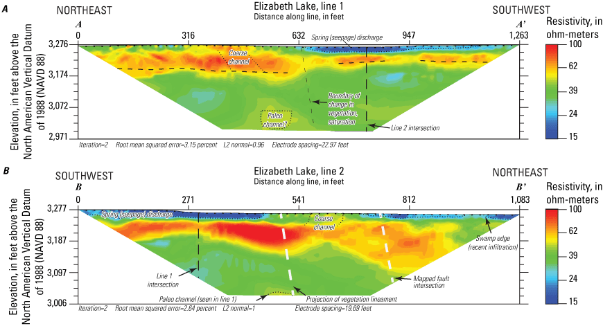
Inverted electrical resistivity tomography profiles near Elizabeth Lake, California, 2019. A, Line 1, which runs from northeast (A) to southwest (A’); and B, line 2, which runs from southwest (B) to northeast (B’). Colors indicate resistivity value, in ohm-meters (ohm-m), with warmer colors representing higher resistivities. Data from Groover and others (2021).
Figure 6B shows inverted resistivity data (Groover and others, 2021) collected along Elizabeth Lake line 2, (fig. 5, line B–B’) with an electrode spacing of 19.69 ft and a similar range of resistivity values within the profile to line 1. Surface materials have a low resistivity of 15–40 ohm-m from approximately 3,276 to 3,246 ft above NAVD 88, indicating saturation and possible saline water, moderate resistivity of 30–100 ohm-m from 3,246 to 3,141 ft above mean sea level, and moderate to high resistivity of 55–100 ohm-m from 3,141 to 3,128 ft above mean sea level. The coarse-sand channel feature observed in line 1 also was observed in line 2. Similarly, the data indicate the channel has migrated or been offset northeastward from the location of the buried paleo channel at the base of the profile since deposition occurred. Line 2 (fig. 5, line B–B’) extended toward the northeast end of Elizabeth Lake across moist ground and shallow standing water (approximately 1 in. deep) on the northeastern part of the line. Lower resistivity values below the swamp edge indicated high moisture content at depth. A mapped recent fault (Alquist-Priolo hazard classification; California Department of Conservation, 2023) did not affect the resistivity profile at depth; however, the vegetation lineament observed in the field and discussed previously controls boundaries among more resistive (60–100 ohm-m) sediment at moderately shallow depths on the southwestern half of the profile compared to the northeastern half of the profile.
Neither of the ERT profiles (Elizabeth Lake line 1 [A–A’] and line 2 [B–B’]; fig. 5) indicated the presence of bedrock because neither profile had a highly resistive signature at the bottom (fig. 6), indicating that the depth to bedrock was greater than 250 ft bls along the southeastern shore of Elizabeth Lake. However, the ERT profiles do not indicate the depth to bedrock within the surrounding area of the Elizabeth Lake subwatershed.
The presence of the lineament and seepage feature indicated an active fault splay which could force groundwater to the surface in springs. This groundwater could be effluent from OWTS moving from nearby houses toward Elizabeth Lake. The nature of the fault is unclear; thus, further research is needed to determine the hydraulic properties of the potential fault. A spring (ELS-Spring-01; table 1) located within this feature was only present during the March 2019 field visit.
Borehole Geophysics
Borehole geophysical logs were collected from the monitoring wells after drilling. Electrical resistivity is shown in figure 7 for the seven drilled monitoring wells (ELLA-1 through ELLA-6 and ELLA-8; fig. 7). Borehole resistivity, surface resistivity, and borehole lithology for wells ELLA-3, ELLA-4, and ELLA-5 are shown on figure 8. The logs for these three wells (ELLA-3, ELLA-4, and ELLA-5) displayed similar resistivity depth interval results relative to the surface resistivity transect for line 1 (line A–A’, fig. 5) that allowed a comparison to Elizabeth Lake surface resistivity results from line A–A’ and line B–B (fig. 5; Groover and others, 2021). Shallower materials surrounding the well casing had a resistivity of 0–35 ohm-m from 10 to 45 ft bls. Wells ELLA-2, ELLA-4, ELLA-5, and ELLA-6 borehole logs showed high-resistivity peaks (100 or greater ohm-m) from 35 to 40 ft bls, whereas high-resistivity peaks were deeper in wells ELLA-1 and ELLA-3 from approximately 50 to 55 ft bls. Well ELLA-8 was not drilled deep enough to include the high-resistivity peak, but the well depth was terminated at the upper extent of a high resistivity zone (approximately 30 ft bls). Wells deeper than the high-resistive peak transition back to lower resistivity of 15–30 ohm-m at deeper depths.
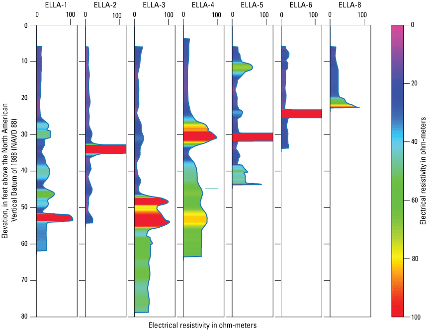
Borehole electrical resistivity profiles at depth at each U.S. Geological Survey drilled monitoring well. Colors indicate resistivity value, in ohm-meters, with warmer colors equaling higher resistivities. See table 1 for site information (Groover and others, 2021).
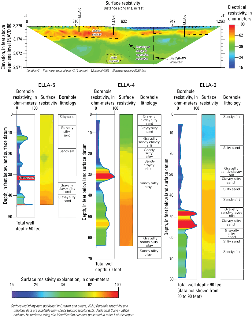
Inverted electrical resistivity tomography profiles near Elizabeth Lake, California, 2019, of line 1, which runs from northeast (A) to southwest (A’) in comparison to borehole resistivity measurements at depth for ELLA-3, ELLA-4, and ELLA-5. Colors indicate resistivity value, in ohm-meters, with warmer colors equaling higher resistivities. Data source: Groover and others (2021). See table 1 for site information. Abbreviations: NAVD 88, North American Vertical Datum of 1988; USGS, U.S. Geological Survey.
Lithology and Aquifer Properties
Lithologic descriptions were classified from drill cuttings collected at 5-ft intervals to the total depth of each well. The total depth of each well was dependent on an impassible highly consolidated blue clay layer observed during drilling. Because these wells were drilled into the surrounding lakebed, the geology was consistent with interbeds of sandy silt and gravelly sandy silt at wells ELLA-1, ELLA-2, ELLA-5, and ELLA-6 (fig. 3; table 1). In addition to interbeds of sandy silt and gravelly sandy silt, interbeds of primarily clayey-sediment were identified in the ELLA-3, ELLA-4, and ELLA-8 boreholes. Sandy silt and gravelly sandy silt were identified at all three shallow hand-augered monitoring wells: (1) ELLA-7, (2) ELLA-9, and (3) ELLA-10A. The borehole lithology for all wells can be seen in the “Borehole Lithologies” section of appendix 1 (figs. 1.1–1.8), which includes a summary of detailed notes documented by the onsite geologist during drilling and a simplified diagram of the borehole construction and lithology. During drilling, the onsite geologist noted the presence of perched water above the observed clay layer, which was likely the result of the recent storms and change in infiltration rates of sediments. This freshwater perched aquifer is likely the result of high resistivity at/near clay layers, where resistivity would be expected to have low resistivity.
The simplified lithologies were used to estimate aquifer properties. Hydraulic conductivity and porosity ranges were defined in relation to the 5-ft lithologies. Ranges of hydraulic conductivity applied to these materials were estimated from Heath (1984) and Morris and Johnson (1967). Estimated ranges of hydraulic conductivities were less than or equal to 3.3x10⁻³ feet per day (ft/d) for clay layers, from 3x10⁻³ to 16 ft/d for silt layers, from 16 to 32 ft/d for sand layers, and from 32 to 100 ft/d for poorly sorted gravel layers (appendix 1, figs. 1.1–1.8; Todd, 1959; Davis, 196925; Heath, 1984). Because the wells drilled during this study were assumed to be within an unconfined aquifer, hydraulic conductivity was specific but transmissivity was not because the thickness of the saturated zone varies with the water level. Thus, transmissivity was not estimated in this study. Porosity was estimated to be greater than 0.4 for clays and greater than 0.35 for fine gravel layers (Morris and Johnson, 1967).
Subsurface Characterization Discussion
When using borehole resistivity logs to ground-truth surface resistivity profiles, the borehole data had a greater vertical resolution (approximately 12–18 in.) compared to ERT data (half the electrode spacing). Borehole sites ELLA-3, ELLA-4, and ELLA-5 were located close to the Elizabeth Lake line 1 ERT transect, and borehole resistivity logs for these sites were compared; an estimated intersection between the location of these boreholes and line 1 is shown on figure 8. Thus, the borehole resistivity and lithologies can be used together to ground truth and assist in interpretation of the ERT transects. Although the surface resistivity was unable to distinguish small characteristics, such as thin layers, the overall patterns of the resistivity values were consistent with the borehole resistivity. The ERT data represented averages of thin layers throughout a broader area potentially making coarser sediments in the subsurface appear laterally more extensive.
The primary lithology observed in well ELLA-3, ELLA-4, and ELLA-5 boreholes was gravelly sandy silt, with occasional clay horizons documented in wells ELLA-3 and ELLA-4 boreholes. These types of deposits were consistent and expected from shallow lacustrine deposits with different evolution of lake-level heights and sediment deposition. The sediment layers, documented at 5-ft intervals, were moderately to poorly sorted, which complicated efforts to use surface resistivity to compare lithologies due to lack of high resolution in the drill cuttings. The potential mixing and time delay of sediments lifted from the borehole to the surface complicated efforts to obtain high resolution in moderately to poorly sorted sediments. Surface ERT also lacked high resolution in these types of thinly bedded sediments due to the smoothing and decreasing resolution with increasing depth (Minsley and others, 2010).
Resistivity depth trends observed in borehole logs were generally consistent with ERT inversion models. Lower resistivity was present at shallow depths, a peak at mid-level depths, and moderate resistivity below the highly resistive peak (fig. 8). Lithology and drilling observations of aquifer sediment compared to the borehole geophysics indicated that intervals with the highest resistivity may indicate a perched freshwater aquifer above the clay dominant layer. However, because of varying thickness throughout the aquifer, the clay layer was not considered a confining layer but rather a semi-confining unit that would only prevent flow where there is clay. Thus, the clay layers were believed to contribute to the presence of perched water tables during wetter months due to the change in the infiltration rate at this layer. The clay and perched water were observed during drilling, consistent with higher resistivity at these depths because rainwater and fresh water is known to have higher resistivity (30–1,000 ohm-m).
Continuous and periodic discrete water levels were used to understand the hydrologic head in the subsurface. These groundwater levels were observed to be responsive to local precipitation (figs. 9A–9C). Water was removed from the study area primarily by evaporation from Elizabeth Lake and evapotranspiration from the riparian areas surrounding Elizabeth Lake. Although not apparent in fig. 9A or 9B, diurnal fluctuations in groundwater happen, indicating loss of water by evapotranspiration. The lack of major surface outflow points near the lake further reinforces that the study area is within a closed system. The groundwater within the Elizabeth Lake subwatershed is not used for public consumption. Groundwater elevations ranged from 3,283 to 3,260 ft above NAVD 88 (fig. 9A). Groundwater depths below land surface ranged from less than 1 ft to about 16 ft during April 2020 and October 2020, respectively (fig. 9B).
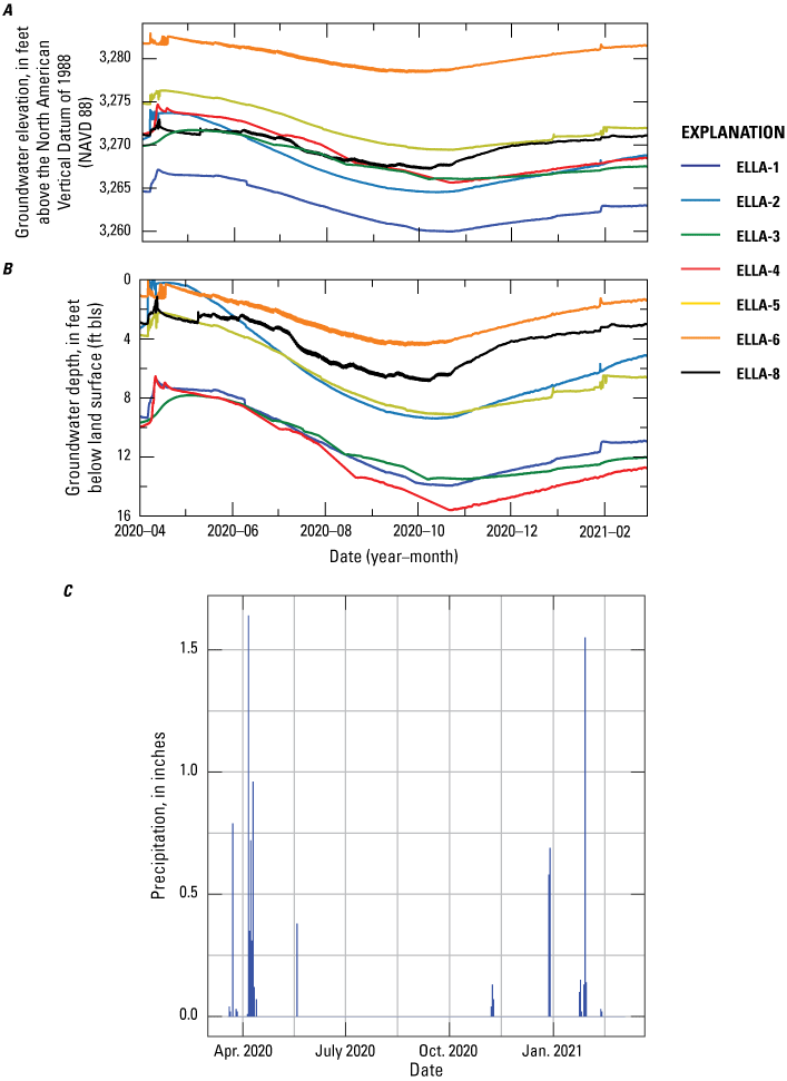
Continuously recorded water levels in U.S. Geological Survey monitoring wells instrumented with in situ vented continuous water-level sensors (U.S. Geological Survey, 2023a). A, Groundwater elevation, in feet above the North American Vertical Datum of 1988; B, groundwater depth, in feet below land surface; and C, annual precipitation within the Elizabeth Lake subwatershed (U.S. Geological Survey, 2020). Precipitation data from Prism Climate Group (Prism Climate Group, 2023). See table 1 for well station numbers. Data source: U.S. Geological Survey (2023a).
Groundwater moves from areas with high groundwater levels to areas with low groundwater levels, otherwise known as high to low hydraulic head; therefore, the general direction of groundwater movement and hydraulic gradient was inferred from contours of water levels (figs. 10A–10D). Groundwater elevations were generally highest at the eastern side of the lakebed (figs. 10A–10D), with a maximum altitude of 3,283 ft above NAVD 88 (figs. 10B, 10C). During the drier months, the highest groundwater elevation was east of Elizabeth Lake, estimated at 3,278 ft above NAVD 88 during September 2020. The slope of the water table was generally consistent with land topography contours within the study area. Groundwater within the study area was estimated to flow perpendicular to the water-level contours (figs.10A–10D). The hydraulic gradient was calculated on the south and east part of Elizabeth Lake and ranged from 0.01 to 0.03. There were not enough data on the north shore of Elizabeth Lake to contour groundwater levels or to determine groundwater flow direction or hydraulic gradient, but the contour was assumed to follow the topography and had a consistent hydraulic gradient with the southern and eastern part of the study area. This assumption was consistent with the drillers’ log of a nearby well to the north, upgradient from well ELLA-8, which had a sightly deeper groundwater level.
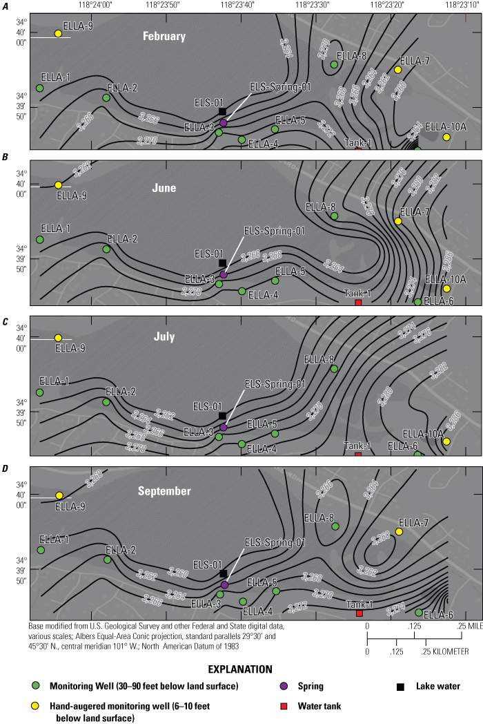
Groundwater-level contours in the lacustrine deposits surrounding Elizabeth Lake, California during A, February; B, June; C, July; and D, September 2020 sampling events. See table 1 for site information. Data source: U.S. Geological Survey (2023a).
Groundwater elevations in this region were responsive to precipitation during the wetter months, which is illustrated by the shallow groundwater-level measurements during April 2020, when wells ELLA-4 and ELLA-3 were less responsive to this precipitation signal because these wells were drilled into less hydraulically conductive sediments (figs. 9A–9C). However, during periods of no rain, groundwater elevations showed diurnal fluctuation at all drilled wells, except for ELLA-3 and ELLA-4. The daily differences between maximum and minimum fluctuations increased during drier and hotter days (figs. 9A–9C). During the year, groundwater elevations dropped by more than 5 ft from April to September, most likely because of evapotranspiration from vegetation when groundwater levels were shallower than 10 ft bls and from lateral flows to Elizabeth Lake. Groundwater elevations in all wells decline at similar rates, confirming that they were in similar aquifer materials and that potential presence of faults did not affect groundwater levels in the lakebed.
Groundwater moves slowly through the subsurface within this region. Most of the aquifer sediments were silt that was estimated to have a hydraulic conductivity of 3x10⁻³ to 16 ft/d and a porosity of 0.42. Flow is likely more restricted by fine-grained sediments, such as clay layers observed in the drilled wells, specifically in wells ELLA-3 and ELLA-4, leading to perched aquifers or a muted response of groundwater levels. All groundwater levels decreased at similar rates (fig. 9) and contained a horizontal hydraulic gradient that ranged from 0.01 to 0.03. Given the similar groundwater level observations and horizontal hydraulic gradient, we assumed that all wells were drilled within a shallow unconfined aquifer. Because all wells were in the same aquifer within the study area, we interpreted that groundwater flow direction is toward Elizabeth Lake based on observed groundwater levels, and we concluded that groundwater transport is a potential mechanism for nutrient loading from OWTS into Elizabeth Lake.
The only sources of natural recharge to Elizbeth Lake are direct precipitation, overland runoff, and groundwater discharge. However, because of the dry climate, runoff is probably limited by evapotranspiration and the soil moisture deficit. Runoff is mainly routed to Elizabeth Lake through intermittent stream channels or infiltrated into groundwater. Additionally, the diurnal water-level fluctuations seen in continuous groundwater-level data in all drilled wells, aside from wells ELLA-3 and ELLA-4 because of their muted response, indicated the lack of available water during the drier seasons (May–September) at the surface for vegetation uptake. Thus, the vegetation becomes efficient in extracting water from the subsurface during the higher temperatures throughout the day. The diurnal fluctuations are likely a result of root uptake and evaporation of shallow groundwater. The evapotranspiration of plants and evaporation of shallow groundwaters can be observed as diurnal fluctuations in the groundwater levels.
Water-Quality Results
Between March 2019 and September 2020, 201 water-quality samples were collected from 11 wells, 1 lake site, and 2 imported tanks during 4 field visits. Water-quality samples were analyzed for stable water isotopes of oxygen and hydrogen (δ18O and δD, respectively), isotopes of nitrogen and oxygen in nitrate, major-ion chemistry and selected trace elements, nutrients, field parameters, noble gases, and tritium. A wastewater effluent indicator sample was collected from Elizabeth Lake (ELS-01) during the mid-March 2019 visit. This sample was analyzed for more than 100 constituents commonly detected in effluent (Kolpin and others, 2002). Most of the constituents were either not detected or were detected at low concentrations at or near the reporting limit. Reporting limits for major and minor ions, trace elements, uranium, nutrients, DOC, absorbance, and fluorescence of dissolved carbon are shown in table 3.
Elizabeth Lake Baseline Conditions
On March 17, 2019, the last day of the surface geophysical survey, Elizabeth Lake was sampled for field parameters, nutrients, stable water isotopes, stable isotopes of nitrogen and oxygen in nitrate, DOC, and optical properties of dissolved organic matter (table 3). The surface-water samples were collected on the south shoreline of Elizabeth Lake at site ELS-01 (fig. 3). These samples provided insight into the baseline conditions of water quality in Elizabeth Lake in 2019 before the start of the study.
The SC, DO, and pH of Elizabeth Lake (ELS-01) were 5,550 µS/cm at 25 °C, 13.4 mg/L, and 8.94, respectively. Orthophosphate as P, ammonium as N, and nitrite plus nitrate (NO3+NO2, as N) concentrations were below the detection limits of 0.004, 0.01, and 0.04 mg/L, respectively (tables 3, 4). Ammonium plus org-N was detected at a concentration of 0.85 mg/L, and a DOC concentration of 12.3 mg/L was measured. Phosphorus was detected between 0.03 and 0.09 mg/L for filtered and unfiltered samples, respectively. The observed δ18O and δD values were −6.3 and −43.1 per mil, respectively. Additionally, field observations of foamy waters and algal mats were made at the sample site.
Table 4.
Constituents detected in samples collected as a preliminary sampling of U.S. Geological Survey station number 343949118234201 from Elizabeth Lake (ELS-01), California, March 17, 2019.[Data source: U.S. Geological Survey (2023a); Site information in table 1. Abbreviations: ft, feet; °C, degrees Celsius; mm/Hg, millimeters of mercury, μS/cm, microsiemens per centimeter at 25 degrees Celsius; mg/L, milligrams per liter; std units, standard units; <, less than; N, nitrogen; P, phosphorus; nm, nanometer; AU/cm, absorbance units per centimeter; ex, excitation wavelength; em, fluorescence wavelength; RU, Raman-normalized intensity units; SUVA254, specific ultraviolet light absorption at a wavelength of 254 nanometers divided by dissolved organic carbon concentration; SUVA280, specific ultraviolet light absorption at a wavelength of 280 nanometers divided by dissolved organic carbon concentration; L/mgDOC*m, liter per milligram of dissolved oxygen multiplied by meters; —, sample not collected; δD, stable isotope of hydrogen (deuterium); δ18O, stable isotope of oxygen; per mil, parts per thousand]
Elizabeth Lake Baseline Conditions Discussion
DO concentration was above the saturation level at the time of this baseline sampling. Sampling took place in the afternoon under full sun conditions. The measured DO concentration was 13.4 mg/L with a water temperature of 11.5 °C, barometric pressure of 638 mm Hg, and a specific conductance of 5,550 μs/cm at 25 °C (table 4). At the time of sample collection, water from Elizabeth Lake (ELS-01) had a measured dissolved-oxygen concentration of 13.4 mg/L, corresponding to a saturation of 150 percent. Oxygen saturation was calculated using the DOTABLES calculator (https://water.usgs.gov/water-resources/software/DOTABLES/; U.S. Geological Survey 2023b). The pH of Elizabeth lake water (ELS-01), 8.94, coupled with the high saturation level of DO, indicated that an algal bloom was taking place. These measurements also were paired with visual observations of foam, algal mats, and phytoplankton, further indicating that an algal bloom was occurring at the time the sample was collected because photosynthesis removes dissolved carbon dioxide (CO2) from the lake water (raising the pH) and adds DO (supersaturating lake water with DO). The relations among DO levels, pH, and algal blooms also is discussed by Ortiz and others (2020). Algal blooms occur when the weather is warm and there are sufficient nutrients present for algal growth. When algae die, they become readily degradable and serve as a source of mineralized N and P, increasing available nutrients in the system. The lack of detectable nitrate concentrations during the bloom indicated that Elizabeth Lake was likely nitrogen limited because the algae used all the bioavailable nitrogen. The TN:TP ratio of 12:6, which is less than the ideal Redfield ratio of 16:1, indicates that Elizabeth Lake is nitrogen limited (Redfield, 1958). The measured field parameters of Elizabeth Lake (ELS-01) and visual observance of an algal bloom are supportive of the eutrophic conditions for the lakes that were listed before this study. The algal bloom is likely responsible for the depletion of bioavailable nitrogen in the water. However, the presence of the algal bloom does not prove that any OWTS are responsible for excess nutrients being delivered into the lake via groundwater discharge.
Water Quality and Isotopic Tracers
This section presents water-quality results collected from all groundwater and surface-water sites from February 2020 to September 2020 as part of this study. These results were used to evaluate environmental conditions, fate, transport of nutrients in the aquifer, and other constituents and groundwater age that can be used to interpret the potential of nutrients from OWTS to contribute to Elizabeth Lake’s TMDL in excess.
Field Parameters
Field parameter results are shown in table 5. The median concentration of SC from groundwater sites was 918 µS/cm at 25 °C, whereas Elizabeth Lake (ELS-01) had a median SC of 9,720 µS/cm at 25 °C, a mean SC of 11,700 µS/cm at 25 °C, and a maximum SC of 21,300 µS/cm at 25 °C, which is consistent with brackish to saline lake waters (greater than 1,500 µS/cm at 25 °C; table 5; Stanton and others, 2017). The highest SC values for groundwater were measured from wells ELLA-4, ELLA-3, and ELLA-10A, at concentrations close to or more than 1,500 µS/cm at 25 °C. The lowest SCs (less than 750 µS/cm at 25 °C) were measured from wells BW-PW, ELLA-9, and ELLA-2. Specific conductance measurements from Tank-1 and Tank-2 were less than 500 µS/cm at 25 °C. For groundwater samples, the median concentration of TDS was 613 mg/L. The TDS concentration was measured by filtering a known amount of water, drying the filter at 180 °C, and weighing the dried filter.
Table 5.
Field parameter results measured from groundwater wells (ELLA-1–10A and BW-PW), water tanks (Tank-1 and Tank-2), and Elizabeth Lake (ELS-01), February–September 2020.[Data source: U.S. Geological Survey (2023a); site information from table 1. Abbreviations: mm/dd/yyyy, month/day/year; CaCO3, calcium carbonate; mg/L, milligrams per liter; HCO3, bicarbonate; CO3, carbonate; μS/cm, microsiemens per centimeter; °C, degrees Celsius; —, sample not collected, E, the value is estimated]
Dissolved-oxygen concentrations in groundwater samples ranged from 0.3 to 5.7 mg/L, with a median concentration of 1.6 mg/L (table 5). The highest DO concentrations were measured from groundwater wells during February 2020. Wells with DO less than 1.0 mg/L were tested for sulfide using a field sulfide test. Dissolved sulfide was detected from wells ELLA-3, ELLA-4, and ELLA-2, at estimated concentrations of 0.03, 0.07, and 0.10 mg/L, respectively. The pH in the groundwater measured in all sites ranged from 6.75 to 8.27, with a median value of 7.44. The pH of Elizabeth Lake (ELS-01) samples ranged from 8.37 to 10.2. The temperature of groundwater from wells ranged from 16.7 to 23.5 °C, with a median value of 12.5 °C. Groundwater temperatures were coldest during February and September sampling.
Alkalinity, Major Ions, and Trace Elements
Alkalinities (expressed in mg/L as calcium carbonate) were measured in the field and were used to calculate bicarbonate and carbonate concentrations. Bicarbonate, major ions, and trace elements data from the groundwater had observed ranges of 121–921 mg/L of bicarbonate (ELLA-9 and ELLA-10a; table 5), 35.5–294 mg/L of sodium (ELLA-9 and ELLA-5; table 6), 12.1–265 mg/L of chloride (ELLA-9 and ELLA-4; table 6), 0.27–1.84 mg/L of fluoride (ELLA-8 and ELLA-10A; table 6), 30.4–97.9 mg/L of calcium (ELLA-3 and ELLA-8; table 6), 52.0–278 mg/L of sulfate (ELLA-7 and ELLA-10A), 1.82–447 µg/L of manganese (ELLA-7 and ELLA-1), and less than 10–410 µg/L of iron (BW-PW and ELLA-4; table 6). Median concentrations of major ions chemistry and trace elements in all groundwater samples can be summarized as 241 mg/L of bicarbonate, 87 mg/L of sodium, 80 mg/L of chloride, 1.2 mg/L of fluoride, 61.0 mg/L of calcium, 127 mg/L of sulfate, 16.4 µg/L of manganese, and 10.6 µg/L of iron (table 6). Elizabeth Lake samples had a median concentration of 151 mg/L of bicarbonate, 1,570 mg/L of sodium, 1,640 mg/L of chloride, 3.2 mg/L of fluoride, 245 mg/L of calcium, 3,380 mg/L of sulfate, 118 µg/L of manganese, and less than 60 µg/L of iron (ELS-01; table 6). The median TDS concentration in groundwater was 614 mg/L, and the measured TDS concentration in Elizabeth Lake was 8,240 mg/L (ELS-01; table 6).
Table 6.
Constituents detected in groundwater wells, tanks, and surface-water samples collected from Elizabeth Lake, California, during February–September 2020.[—Left][Data source: U.S. Geological Survey (2023a); site information from table 1. Abbreviations: mm/dd/yyyy, month/day/year; mg/L, milligrams per liter; μg/L, micrograms per liter; <, actual concentration is less than the value shown; —, sample not collected]
A trilinear diagram (fig. 11) shows the relative proportions of major ions and nitrate in trilinear diagrams. The interpretation of the trilinear diagrams is discussed later in this report.
Two trace elements, arsenic and uranium, were present with a concentration greater than the maximum contaminant levels (MCLs; 10 and 30 µg/L, respectively) in a few of the sites (U.S. Environmental Protection Agency, 2022). Arsenic concentrations of 42.9, 15.5, and 13.2 µg/L, were measured in the ELLA-4, ELLA-3, and Elizabeth Lake (ELS-01) samples, respectively. One concentration of uranium of 55.2 µg/L was measured in ELS-01.
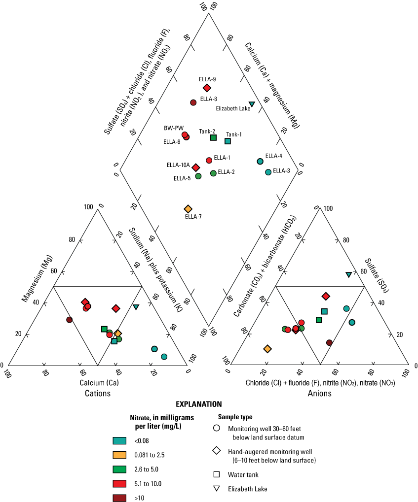
Trilinear diagram using data collected from wells, tanks, and Elizabeth Lake, California. Data source: U.S. Geological Survey (2023a). See table 1 for site information. Abbreviations: <, less than; >, greater than
Nutrients
Nutrient samples were collected and analyzed for multiple forms of phosphorus and nitrogen (table 7). Nitrite concentrations were generally low. Nitrate plus nitrite in groundwater samples (ELLA-1–10A and BW-PW) ranged from less than the detection limit of 0.04 to 27 mg/L as N with a median concentration of 4.7 mg/L as N. Nitrate was the primary form of nitrogen in 35 of the 47 nutrient samples that were collected in groundwater, but organic nitrogen was the dominant form of nitrogen in the Elizabeth Lake (ELS-01) samples (table 8). Nitrate plus nitrite concentrations were consistently below the detection limit in all ELLA-4 and ELS-01 samples and below detection in two of the four samples collected from ELLA-3 in February and September 2020. The highest concentrations of nitrate plus nitrite were detected in samples collected at ELLA-8 (table 7, fig. 12). Nitrate plus nitrite concentrations from all four sample periods collected from ELLA-8 ranged from 23.4 to 27.0 mg/L as N.
Table 7.
Results for analyses of nutrient samples collected from groundwater wells, tanks, and Elizabeth Lake, California, February–September 2020.[Data source: U.S. Geological Survey (2023a); site information from table 1. Abbreviations: mm/dd/yyyy, month/day/year; mg/L, milligrams per liter; <, indicates that actual concentration is less than the value shown; —, sample not collected; E, result was estimated]
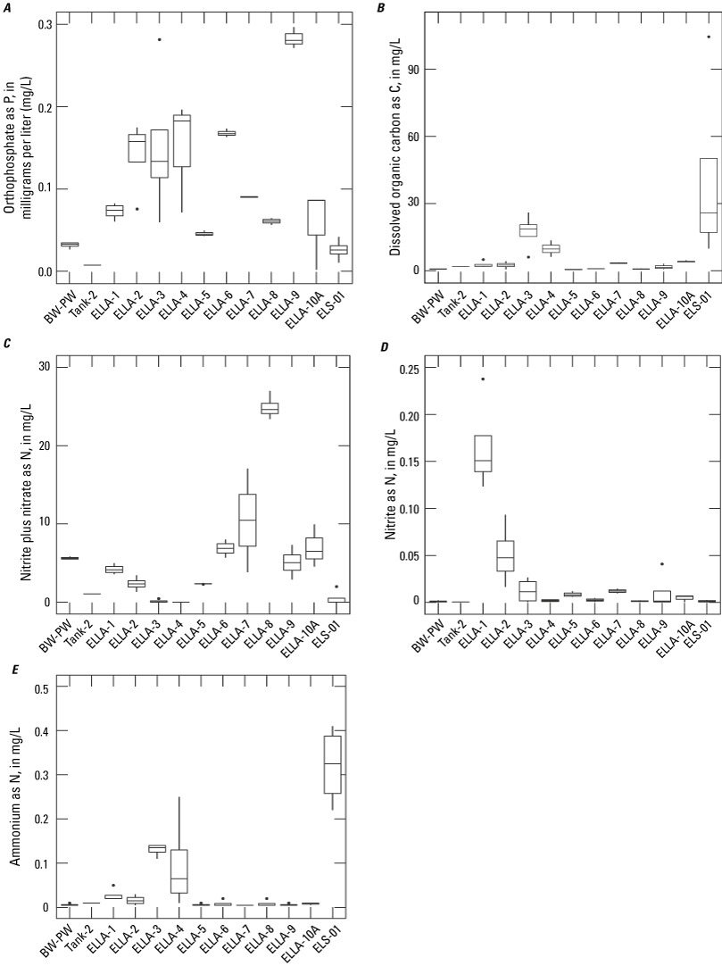
Concentrations of nutrients by site. A, orthophosphate; B, dissolved organic carbon; C, nitrate plus nitrite; D, nitrite; and E, ammonium. The boxplot for each site represents four samples. See table 1 for site information. Data source: U.S. Geological Survey (2023a).
Nitrite concentrations ranged from less than the detection limit of 0.001–0.238 mg/L as N in all samples (table 7). The median concentration of nitrite detected in groundwater samples (ELLA-1–10A and BW-PW) was 0.007 mg/L as N. Nitrite concentrations in Elizabeth Lake (ELS-01) were below 0.003 mg/L as N or below the detection limit.
Ammonium as N concentrations in groundwater samples (ELLA-1–10A and BW-PW) ranged from below the detection limit of 0.01 to 0.25 mg/L as N with a median concentration of less than 0.01 mg/L. Ammonium concentrations generally were less than the detection limit, with a few exceptions. Concentrations generally were greater than 0.05 mg/L of ammonium as N in all samples collected at well ELLA-3, July and September samples collected at well ELLA-4, and February samples collected at well ELLA-1. Ammonium concentrations in Elizabeth Lake (ELS-01) ranged from 0.22 to 0.41 mg/L and from 1.90 to 4.05 mg/L of ammonium plus org-N as N.
Orthophosphate as P was the form of phosphorus measured in all wells, the Elizabeth Lake site (ELS-01), and the imported water tanks (Tank-1 and Tank-2). Total phosphorus as P was measured at the Elizabeth Lake site (ELS-01) in addition to orthophosphate as P because of the presence of particulate matter in the lake water. Total phosphorus was also measured in the Tank-1 water but was not measured in Tank-2. Total phosphorus should have been measured in the Tank-2 water, but unfortunately, only a sample for orthophosphate was submitted, so a direct comparison of all forms of phosphorus cannot be completed. However, the two tanks both contain water imported from northern California so the nutrient concentrations should be similar. Both tanks have water delivered to southern California from the Governor Edmund G. Brown California Aqueduct (not shown). Phosphorus concentrations in ELS-01 samples ranged from 0.045 to 0.387 mg/L. Concentrations of total phosphorus from the Tank-1 (0.007 mg/L) and orthophosphate from Tank-2 (0.008 mg/L) were similar, and both were measured during the July sampling. However, a direct comparison of the two forms of phosphorus is not possible because the two analytical methods are not the same. Total phosphorus is measured from an unfiltered sample, whereas orthophosphate is measured from a filtered sample. In groundwater samples, phosphorus was measured in the form of orthophosphate and ranged from 0.03 to 0.35 mg/L as P, with a median concentration of 0.08 mg/L as P.
Dissolved organic carbon was collected during each sampling for all sites (table 1) and ranged from 0.31 to 26 milligrams per liter as carbon (mg/L as C) in groundwater samples (ELLA-1–10A and BW-PW) and from 11 to 100 mg/L in Elizabeth Lake samples (ELS-01). The DOC concentrations in the water tanks (Tank-1 and Tank-2) were similar (1.9 and 2.0 mg/L, respectively). The median DOC concentration in groundwater was 1.9 mg/L, and the mean DOC concentration in groundwater was 4.1 mg/L. The lowest concentration of DOC in groundwater (0.31 mg/L) was measured from well ELLA-5, and the highest concentration of DOC in groundwater (26 mg/L) was measured from well ELLA-3 (table 7). Concentrations of DOC in Elizabeth Lake samples (ELS-01) ranged from 9.9 mg/L during the February sampling to 100 mg/L during the late September sampling.
Isotopes
The water isotopic values ranged from −9.90 to −1.93 per mil δ18O and −74.6 to −28.9 per mil δD (table 8; fig. 13). Samples were collected for δ18O and δD from Elizabeth Lake (ELS-01) on March 19, 2019, February 13, 2020, and June 7, 2020. The δ18O and δD data of these samples ranged from −6.3 to −1.93 and −43.1 to −28.9 per mil, respectively. Samples from the water tanks had values that ranged from −9.9 to −9.6 δ18O per mil and from −74.7 to −72.9 δD per mil, respectively. The δD values from the Tank-2 results were consistent with the δD value of −74 per mil expected in imported water reported by Izbicki (2004). The δ18O and δD data in samples from the two water tanks were the most negative (isotopically light), whereas ELS-01 samples were more positive (isotopically heavy) and deviated from the GMWL, indicating that surface waters were affected by evaporation (fig. 13). The δ18O and δD data in groundwater from wells surrounding the perimeter of Elizabeth Lake ranged from −9.8 to −8.5 per mil and from −70.0 to −58.0 per mil, respectively, and had median values of −8.8 and −61.2 per mil, respectively.
Table 8.
Summary of isotopic data, estimated percentage of imported water, tritium data, estimated age, and age class in samples collected during February–July 2020, Elizabeth Lake, California.[Data source: U.S. Geological Survey (2023a). Site information in table 1. Abbreviations: mm/dd/yyyy, month/day/year; δD, stable isotope of hydrogen (deuterium) in water; δ18O of water, stable isotope of oxygen in water; δ15N of nitrate, stable isotope of nitrogen in nitrate; δ18O of nitrate, stable isotope of oxygen in nitrate; pCi/L, picocuries per liter; TU, tritium unit; —, sample not collected]
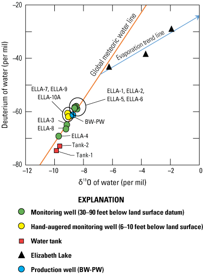
Delta oxygen-18 (δ18O) values as a function of delta deuterium (δD) in water from sampled wells, tanks, and Elizabeth Lake, California. Data source: U.S. Geological Survey (2023a). See table 1 for site information.
Elizabeth Lake δ18O and δD values plotted to the right of the GMWL, with an evaporative trend line having a slope of 3.2, which was consistent with the expected slope from evaporation (Gibson and others, 2008; fig. 13). Evaporation of Elizabeth Lake resulted in enriched δ18O and δD values in the lake water; the slope of the evaporative trend line intersects the GMWL at approximately −7 per mil δ18O and −47 per mil δD. The δ18O and δD data were most negative in water from tanks and were consistent with the expected lighter δ18O and δD of imported water. The water tanks δ18O and δD values also plotted to the right of the GMWL, indicating that the water may have been partly evaporated prior to storage. Slightly lighter isotopes were measured in Tank-1 in comparison to Tank-2, which contained a mixture that was mostly imported water mixed with small amount of BW-PW groundwater.
The δ18O and δD values were most negative in groundwater from well ELLA-4, indicating a higher percentage of imported water. The δD was most positive in groundwater from well ELLA-5, whereas the δ18O was most positive in groundwater from well ELLA-6. The calculated means of δ18O and δD measured in samples (−8.9 and −61.8 per mil, respectively) were consistent with δD for the precipitation in this region, which has been estimated at approximately −61 δD per mil (Gleason and others, 1994; Izbicki, 200458). The δD data indicated that groundwater in most of the study area was slightly isotopically heavier than water collected from the water tanks and therefore contained lower percentages of imported waters.
Using the mean δD of −61 per mil for groundwater and the δD of −47 per mil from the intersecting evaporative trend line for Elizabeth Lake samples (ELS-01; fig. 13), the mean δD end member of native groundwater was −54 per mil. The δD for imported water was estimated to be −75 per mil and was consistent with results detected in water in Tank-1 and estimated imported water values determined from a previous study (−41.1 to −101 per mil for δD; Izbicki, 2004). By using a simple two-component mixing equation (see eq. 3 in the “Isotopic Analysis” section), the percentage of imported water was calculated. The highest estimated percentages of imported waters were 71, 57, and 50 percent from wells ELLA-4, ELLA-8, and ELLA-3, respectively. The lowest percentages of imported waters were 15, 16, and 18 percent from wells ELLA-5, ELLA-2, and ELLA-1, respectively.
The nitrogen isotopes and oxygen isotopes of nitrate (δ15N-NO3 and δ18O-NO3) were only able to be determined for samples with nitrate concentrations greater than 0.06 mg/L as N that were only collected during the June sampling period (table 8). The δ15N-NO3 and δ18O-NO3 in groundwater (ELLA-1–10A and BW-PW) ranged from 3.74 to 33.5 per mil and −2.11 to 17.0 per mil, respectively. The maximum values for δ15N-NO3 and δ18O-NO3 were measured in the sample collected from well ELLA-7, the minimum value for δ18O-NO3 was measured in the sample collected from well ELLA-3, and the minimum value for δ15N-NO3 was measured in the sample collected from well ELLA-9. The median values of δ15N-NO3 and δ18O-NO3 in groundwater were 12.35 and 4.38 per mil, respectively. The potential sources of nitrate were determined with these isotopic N values. Values δ15N-NO3 of total soil N range from +2 to 5 per mil, and δ15N-NO3 of effluent is about 7 per mil and higher (Kendall and McDonnell, 1998; Hinkle and others, 2008). Additionally, δ15N-NO3 data were used to evaluate the environmental history of nitrate with respect to microbially mediated denitrification and attenuation of nitrate. Results of the δ15N-NO3 data were used to further identify the processes that control ammonium and nitrate concentrations.
The transformation of the forms of nitrogen in water occurs through different microbial processes. Nitrification can occur in the unsaturated zone and in shallow oxic groundwater. The extent of these reactions were evaluated using δ15N-NO3 and δ18O-NO3 ratios. Values of δ 15N-NO3 and δ18O-NO3 of nitrate were significantly correlated with a slope of 0.5 (coefficient of determination, R2=0.54; p-value=0.009), which is consistent with denitrification (figs. 14A, 14B; Kendall and McDonnell, 1998). Isotopic ratios of nitrogen and oxygen in nitrate change as denitrification proceeds in the sub-surface, and because this change is predictable, measurements of these isotopes provide clues to potential sources (Kendall and McDonnell, 1998). Additionally, dominant sources of N as a function of δ15N-NO3 and δ18O-NO3 were determined based on δ15N and δ18O values. Sites with detectable isotopic measurements as nitrate either indicate the presence of OWTS effluent or are affected by denitrification (fig. 14).
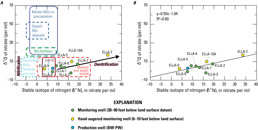
Delta oxygen-18 of nitrate (δ18O-NO3) as a function of delta nitrogen-15 of nitrate (δ15N-NO3) in wells. A, modified version of Kendall and McDonnell (1998) nitrogen source schematic; and B, trendline of (δ18O-NO3) as a function of (δ15N-NO3) with slope of 0.5 and a coefficient of determination (R2) of 0.60. Elizabeth Lake, California, 2020. Data source: U.S. Geological Survey (2023a). Modified trend line (A) from Kendall and McDonnell (1998). See table 1 for site information. NO3 indicates nitrate; NH4 indicates ammonium.
Noble Gases and Tritium
As previously stated, samples of dissolved noble gases were modeled in DGMETA (Jurgens and others, 2020) using the CE model and the unfractionated excess air (UA) model to determine recharge temperatures and to parameterize tritium-helium ages (Jurgens and others, 2020). The CE model and UA model results were compared on a case-by-case basis for each sample (fig. 15). The CE model generally predicted higher recharge temperatures, balanced helium concentrations, better fits, and predicted more incorporation of excess air (air bubbles trapped below the water table) than the UA model (fig. 15). Additionally, the CE modeled samples more accurately because the water table fluctuated more than a 4.33 ft annually, consequentially trapping large volumes of air in the water during recharge and causing the noble gases in groundwater to become fractionated (Phillips and others, 2007; Jurgens and others, 2008). Thus, results generated from the CE model were chosen as the best fit to describe the set of gas concentrations.
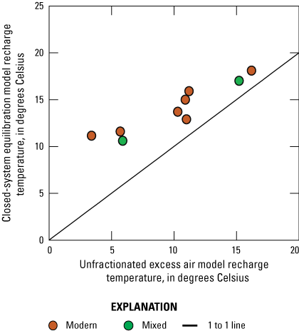
Comparison of closed-system equilibration and unfractionated excess air models based on calculated recharge temperatures of groundwaters, Elizabeth Lake, California.
Measured values of helium-4 (4He), Ne, Ar, Kr, Xe, and N2 gas concentrations were used as inputs into the DGMETA program to calculate excess air, excess N2, recharge temperatures, and 3Hetrit values (U.S. Geological Survey, 2023a). Concentrations of 4He ranged from 5.88x10⁻⁸ to 1.59x10⁻⁶ cubic centimeters at standard temperature and pressure per gram of water (cm3 at STP/g H2O), and minimum and maximum concentrations were measured in samples collected from wells ELLA-6 and ELLA-3, respectively. Ne and Ar concentrations ranged from 2.09x10⁻⁷ to 3.40x10⁻⁷ and from 3.31x10⁻⁴ to 5.28x10⁻⁴ cm3 at STP/g H2O, and median concentrations were 2.36x10⁻⁷ and 3.94x10⁻⁴ cm3 at STP/g H2O, respectively. Minimum and maximum concentrations of Ne were detected in samples collected from wells ELLA-6 and ELLA-7, respectively. Krypton concentrations ranged from 7.02x10⁻⁸ to 1.09x10⁻⁷ cm3 at STP/g H2O, with a median of 8.68x10⁻⁸ cm3 at STP/g H2O; Xe concentrations ranged from 9.59x10⁻⁹ to 1.43x10⁻⁸ cm3 at STP/g H2O, with a median of 1.16x10⁻⁸ cm3 at STP/g H2O; and N2 concentrations ranged from 0.01 to 0.02 cm3 at STP/g H2O, with a median of 0.02 cm3 at STP/g H2O. Minimum and maximum concentrations were consistently detected for Ar, Kr, Xe, and N2 in samples collected from wells ELLA-8 and ELLA-3, respectively. Calculated recharge temperatures ranged from 10.6 to 17.0 °C, with a median temperature of 13.7 °C.
Measured N2 was calculated from groundwater recharge temperatures and excess air concentrations. Excess nitrogen was calculated in samples collected from wells ELLA-1, ELLA-2, ELLA-3, ELLA-4, and ELLA-5, which indicated isotopic evidence of denitrification. Calculated concentrations of excess N2 gas (differences between measured and modeled values for samples with higher N2 than modeled values) ranged from 0.24 to 2.78 mg/L as N (U.S. Geological Survey, 2023a), with a median value of 0.86 mg/L as N. The maximum calculated concentration of N2 was present in well ELLA-3. Groundwater at wells where excess N2 was not present (wells ELLA-7, ELLA-8, ELLA-9, and ELLA-10A) had oxic conditions (DO greater than 0.50 mg/L) and were located on the north side of Elizabeth Lake. Where measured N2 values were greater than modeled values, another source of N2 is likely present, indicating excess groundwater N2 is being added to groundwater after recharge by denitrification (Heaton and Vogel, 1981).
Measured tritium activities ranged from 0.77 to 4.89 TU, with a median concentration of 1.65 TU (table 8). Groundwater samples from wells ELLA-2, ELLA-7, ELLA-9, and ELLA-10A had measured tritium activities greater than 2.6 TU and were classified as classified as “modern” (recharged after 1950s; Lindsey and others, 2019). Groundwater samples from wells ELLA-1, ELLA-3, ELLA-4, ELLA-5, ELLA-6, ELLA-8, and BW-PW had tritium activities between 0.34 and 2.6 TU and were classified as “mixed age” (containing a mixture of groundwater recharged before and after the 1950s; Lindsey and others, 2019). Groundwater samples from the study area did not indicate evidence of pre-modern samples (less than 0.34 TU; Lindsey and others, 2019).
An “apparent” age was computed for most groundwater samples based on the ratio of 3Hetrit to 3H using noble gas inputs into DGMETA. Apparent ages were not computed for groundwater samples from wells ELLA-8, ELLA-10A, and BW-PW because noble gas data could not be used to predict 3Hetrit concentrations for these wells because the DGMETA model returned unrealistic values, such as unrealistic recharge temperatures. 3Hetrit concentrations ranged from 1.20 to 99.49 TU (table 8), with a median concentration of 10.5 TU. Computed ages ranged from 6 to 86 years (table 8), indicating that some groundwater samples would be classified as “pre-modern” based on the age classifications derived from measured tritium activities. The median computed age of samples from wells with mixed groundwaters (excluding ELLA-8 and BW-PW) was 44 years, and the median computed age of groundwater from wells classified as “modern” (excluding ELLA-10A) was 7.5 years.
Water-Quality Discussion
The groundwater of the study area is fresh to slightly brackish, as indicated by measurements of specific conductance and TDS concentrations. In contrast, Elizabeth Lake is slightly saline and has TDS concentrations greater than 1,500 mg/L (Swenson and Baldwin, 1965; Stanton and others, 2017). DO concentrations, along with oxidation-reduction potential (redox) indicators in groundwater, can be used to interpret the chemical and microbial reactions that can occur. Samples with DO concentrations less than 0.5 mg/L typically indicate reducing conditions. The EPA (U.S. Environmental Protection Agency, 2023b) suggests that for healthy systems, groundwater pH values should be between 6 and 8.5, and surface-water pH values should be between 6.5 and 8.5 (fig. 16). Groundwater samples (ELLA-1–10A and BW-PW) collected in this study had a narrow range of pH values (7–8), with variable DO (0.3 to 10.2 mg/L), but samples from Elizabeth Lake (ELS-01) had consistently higher pH values (greater than 8; range was from 8.4 to 10.2) and DO concentrations (greater than 6 mg/L; fig. 16). Elizabeth Lake water was collected during the day and during an algal bloom, so elevated pH was expected. We also expected that pH values and DO concentrations would drop after daylight hours. All but one sample from ELS-01 exceeded the suggested pH thresholds for surface water (6.5–8.5) by more than 1.3 pH unit; the exception was the sample collected during the February 2020 sampling event. Higher pH values in ELS-01 were attributed to algal productivity and CO2 uptake.
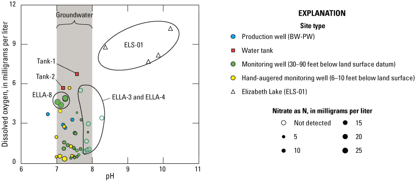
Dissolved-oxygen concentrations (in milligrams per liter) and pH values relative to nitrate concentration (in milligrams per liter) for all collected samples. Gray shaded area indicates range of pH values measured in groundwater. Data source: U.S. Geological Survey (2023a). See table 1 for site information.
According to visual observations made from local residents and field visits during the dry season before the study, Elizabeth Lake periodically dries up and leaves behind a salt efflorescence (white appearing residue), which dissolves as the lake fills with water in wet years and contributes to the TDS in the lake. Elizabeth Lake has a different molar ratio of calcium to magnesium (0.26) relative to those in domestic source water (that is, imported water) used by homes surrounding Elizabeth Lake (1.05) and to groundwater in the wells surrounding the lake (about 2.00). Major element chemistry, including ratio of calcium to magnesium, is affected by water-rock interactions. Elizabeth Lake water is supersaturated with respect to calcite (as indicated by saturation indices exceeding 1, based on thermodynamic modeling), indicating active precipitation of calcite. Active precipitation will increase the ratio of calcium to magnesium (Hem, 1985). Isotopic analysis (δD and δ18O) of groundwater from wells (ELLA-1–10A and BW-PW) and surface water from Elizabeth Lake (ELS-01) indicated an evaporative signature for Elizabeth Lake. Evaporation of Elizabeth Lake water will also drive calcite precipitation because of evaporation.
Two major sources of water to the groundwater system immediately downgradient from the developed area are local precipitation and water from OWTS. The region is arid, with an average annual rainfall of 13 in/yr (National Oceanic and Atmospheric Administration, 2020). Water used for domestic consumption in the community surrounding Elizabeth Lake is imported mainly from the Governor Edmund G. Brown California Aqueduct and has the lowest TDS concentrations (243–278 mg/L). Water used for domestic purposes eventually recharges the aquifer as OWTS effluent. Imported water was also used for minimal residential lawn and gardening irrigation and infiltrated into the groundwater. Once discharged from the OWTS, the water provides a source of recharge to the local groundwater system. Isotopic analysis of δD and δ18O indicated the domestic (imported) water was isotopically light relative to the wells (ELLA-1–10A and BW-PW) and Elizabeth Lake (ELS-01; fig. 16). Isotopes measured in groundwater from wells were clearly separated from the more highly evaporated signature of ELS-01 samples. The enriched δD data indicated that wells ELLA-3, ELLA-4, and ELLA-8 were more closely related to Tank-1 samples and are thus more affected by imported waters from OWTS effluent into groundwater upgradient from the wells than the remainder of the wells.
Relative proportions of major ions in the imported water, wells (ELLA-1–10A and BW-PW), and Elizabeth Lake (ELS-01) varied considerably on a trilinear diagram (fig. 11). Groundwater in two wells, ELLA-3 and ELLA-4, had the most sodium plus potassium relative to calcium and magnesium, and the isotopic signatures of groundwater in these wells were similar to the imported water. One likely explanation for this is that the domestic (imported) water was treated with a water softener which takes the doubly positive ions (calcium and magnesium) out of the water and replaces them with singly charged ions, such as Na. We interpret this result as the groundwater chemistry in wells ELLA-3 and ELLA-4 having been altered by OWTS. Wells ELLA-1, ELLA-3, ELLA-5, ELLA-6, ELLA-7, and ELLA-10A were supersaturated with respect to calcite, further indicating alteration of the source (imported water or recharge). Well ELLA-9, the farthest from the developed area, was undersaturated with respect to calcite and is probably the most representative of groundwater recharged mainly by local precipitation. Groundwater in six wells, ELLA-1, ELLA-2, ELLA-5, ELLA-6, ELLA-10A, and BW-PW, have similar water quality, as shown on the trilinear diagram; observed isotopic similarities indicate a similar evolution along the groundwater flow path relative to water, rock, and atmospheric interactions (figs. 13, 16). The isotopic compositions of samples from well ELLA-8 differed substantially from groundwater in all other wells, were isotopically more similar to the domestic (imported) water, and had the highest nitrate concentrations and some degree of evaporative concentration.
Trace elements, such as iron and manganese, measured in the samples from the wells indicated mostly sub-oxic conditions (less than or equal to 0.05 mg/L of iron and manganese) consistent with low-measured DO concentrations (less than or equal to 1.0 mg/L), except for well ELLA-8 (Jurgens and others, 2008; McMahon and Chapelle, 2008; McMahon and others, 2009). The method of Jurgens and others (2008) was used to identify redox conditions in the water samples. Well ELLA-8 had the highest DO concentrations, undetectable iron, and high nitrate concentrations, indicating that conditions were oxic. The oxidation-reduction conditions in groundwater in most of the wells, except for well ELLA-8, would allow denitrification reactions to happen. Most of the groundwater sampled in this system was characterized as oxic to sub-oxic based on concentrations of DO, nitrate, manganese, iron, and sulfate collected from each site after the first sampling event (February 2020). Samples from wells ELLA-1, ELLA-2, ELLA-3, and ELLA-4 were characterized as having an oxic-anoxic mixture. Wells ELLA-1 and ELLA-2 were characterized as having an oxygen-manganese reduction process (greater than or equal to 0.5 mg/L of DO and greater than or equal to 0.05 mg/L of manganese), whereas groundwater samples from wells ELLA-3 and ELLA-4 were characterized as having an oxygen-iron/sulfate reduction process (greater than or equal to 0.5 mg/L of DO, 0.5 mg/L of sulfate, greater than or equal to 0.01 mg/L of iron, and less than 0.5 mg/L of nitrate). Wells ELLA-5, ELLA-6, ELLA-7, ELLA-8, ELLA-9, and ELLA-10A were characterized as oxic. Additionally, samples from wells ELLA-3 and ELLA-4 and from Elizabeth Lake (ELS-01) contained arsenic greater than the maximum contaminant level of 10 µg/L, indicating that redox conditions or other geochemical conditions may be causing mobilization of arsenic. Mobilization of arsenic in water is frequently the result of desorption from surfaces following reduction of manganese and iron oxyhydroxides by heterotrophic microorganisms, subsequent reduction of binding sites, desorption driven by competing ions such as phosphate, or oxidation and dissolution of arsenic-bearing sulfide minerals (Neil and others, 2012; Haugen and others, 2021).
DOC concentrations likely increased as a product of the decomposition of DOM in addition to DOC concentrations pre-existing in groundwater. DOC concentrations in natural groundwater are typically below 2.0 mg/L (Thurman, 1985); however, groundwater samples collected from wells ELLA-4, ELLA-3, ELLA-10A, and ELLA-7 had measured DOC concentrations that consistently exceeded 2.0 mg/L. Groundwater samples collected from wells ELLA-2, ELLA-1, and ELLA-9 sometimes had measured DOC concentrations that exceeded 2.0 mg/L (figs. 12, 17A, 17B), potentially indicating effects of recharge from OWTS. DOC concentrations relative to nitrate and ammonium concentration are shown on figure 17. Dissolved organic carbon concentrations and nitrate concentrations showed no linear relation (fig. 17A), whereas ammonium and dissolved organic carbon have a weak linear relation (R2 = 0.5924). Sites in this study that contain low nitrate concentrations of 0.05 mg/L or less typically have DOC concentrations greater than 2.0 mg/L, which is the threshold of natural DOC in groundwater (table 7; Thurman, 1985), which indicates that OWTS may contribute DOC into groundwater (fig. 17). DOC concentrations were less than 2.0 mg/L in all groundwater samples collected from wells ELLA-5, ELLA-6, ELLA-8, and BW-PW.
Groundwater samples with high DOC concentrations generally had elevated ammonium concentrations (figs. 12, 17B). High DOC from OWTS drives heterotrophic oxidation by microbes that deplete DO and cause waters to be anoxic, which promotes the attenuation of nitrate through denitrification. Breakdown of DOC by microbes also will liberate org-N and convert the org-N to ammonium. Once DO is low enough, the ammonium will not convert to nitrate. Lakes with high algal productivity typically have 2.0–5.0 mg/L of DOC; these concentrations were consistently exceeded in Elizabeth Lake (ELS-01) samples (figs. 12, 17A; Thurman, 1985). Ammonium in Elizabeth Lake may originate from internal lake recycling or a waste product of the numerous aquatic bird species that are present on the lake, or biological fixation of gaseous nitrogen.
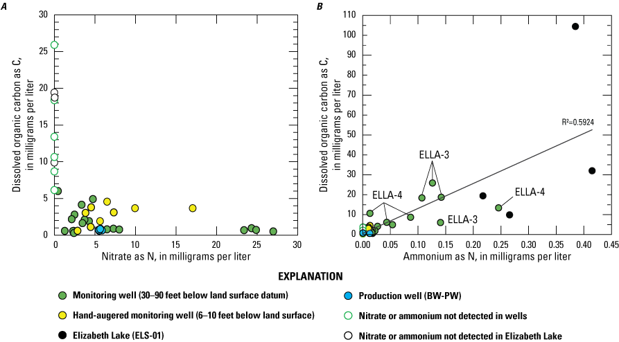
A, Dissolved organic carbon (DOC) concentrations versus concentrations of A, nitrate; and B, DOC concentrations versus concentrations of ammonium. All concentrations are presented in units of milligrams per liter. Data source: U.S. Geological Survey (2023a). See table 1 for site information.
Low concentrations of nitrate measured in groundwater indicate that removal through denitrification is occurring due to reducing conditions in parts of the aquifer where DOC is elevated (fig. 17A). Thus, the remaining ammonium is less able to oxidize to nitrate during these reducing conditions, and increased DOC in the aquifer may be decomposing and increasing ammonium concentrations. The presence of ammonium is a potential indicator for effluent or nitrification of org-N upgradient in the flow path that was not lost to sorption or volatilization. Water containing elevated DOC, ammonium, and org-N concentrations likely discharged into shallow groundwater from OWTS. Onsite wastewater treatment system discharges likely alter the redox condition in the aquifer by increasing DOC concentrations that fuel microbial productivity, decrease DO levels, and increase the potential for nitrogen removal through denitrification (Seitzinger, 1994). Sites where nitrate concentrations in groundwater are low and ammonium is present also contain detectable nitrite concentrations (fig. 12). Nitrite is a transient species in groundwater and is part of the process of the bacterial transformation of nitrate to nitrogen gas or oxidation of ammonium to nitrate. Groundwater prior to infiltration of OWTS effluent was likely oxic and favored the transformation of org-N and ammonium through nitrification. Additional evidence for the occurrence of denitrification in groundwater at wells ELLA-3 and ELLA-4 came from the September 2020 sampling, in which the presence of sulfide indicated that sulfate-reducing bacteria were present.
Nitrate in groundwater in wells ELLA-8, ELLA-9, and BW-PW may have also resulted from soil-derived nitrogen that overlaps with isotope values of the nitrogen derived from manure and septic waste (OWTS effluent) boundaries (fig. 14). Soil-derived nitrogen was likely the source in groundwater from wells ELLA-9 and BW-PW, which contained nitrate concentrations less than 10 mg/L and were not suspected of being downgradient from any OWTS; for the duration of the study, groundwater in well ELLA-8 consistently contained nitrate concentrations exceeding 20 mg/L, DOC concentrations less than 2.0 mg/L (fig. 12), and evidence of oxic waters (DO greater than 0.05 mg/L; tables 5, 7).
Orthophosphate concentrations in groundwater were variable across all the wells but were highest in wells with low DO and higher in groundwater than in the imported water (figs. 12, 18). At individual wells, orthophosphate concentrations showed little to no variability throughout the study (fig. 18). Nitrate concentrations also did not indicate a seasonal variability at individual well sites (fig. 18).
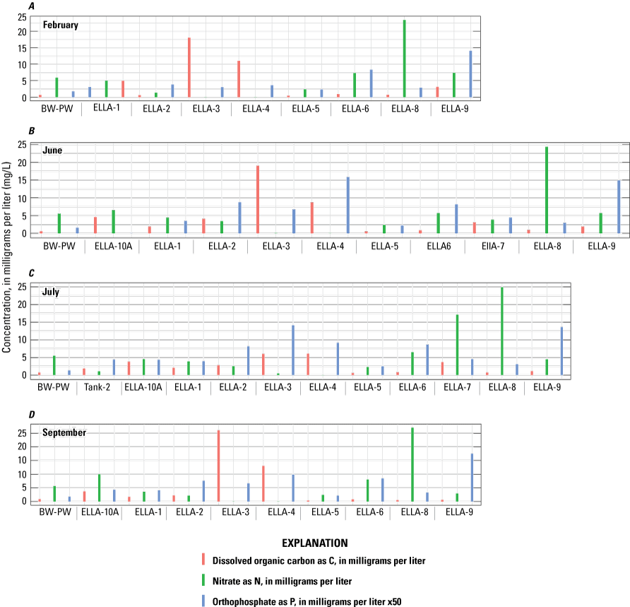
Concentrations of orthophosphate as phosphorus (P), nitrate as (N), and dissolved organic carbon as C during each sampling event in 2020 in groundwater wells. Orthophosphate concentrations shown as actual concentration multiplied by 50. A, February; B, June; C, July; and D, September. Data source: U.S. Geological Survey (2023a). See table 1 for site information.
Orthophosphate in aquifers is frequently sorbed onto oxide surfaces of iron or manganese during oxic conditions; however, sorption depends on pH, and low pH conditions favor sorption. During alkaline pH conditions, oxides may have been supersaturated with respect to orthophosphate (Domagalski and Johnson, 2011). The observed concentrations of orthophosphate in groundwater can most likely be attributed to variations in oxidation/reduction throughout the study area, redox conditions, and oxide surface availability.
The measured δD of water from Tank-1 was −75 per mil, which is consistent with previous measurements Izbicki (2004). Because of the effects of imported water on groundwater, δD values in native groundwater were estimated using precipitation values reported in Gleason and others (1994) and the intersection of the evaporation trend line of Elizabeth Lake water with the GMWL. Groundwaters that have a larger imported water ratio contain a more negative δD value than groundwaters that contain a more positive δD value. However, δD and imported ratio values within each well may vary seasonally, depending on the quantity of imported water used. The change in demand also results in variations in the groundwater flow direction (fig. 10A).
In this study area, water imported from northern California discharges into the groundwater system as recharge from OWTS. There is little landscape irrigation, and most of the water recharged is suspected to subsequently be sourced as OWTS effluent. Further evidence to support this interpretation is based on the estimated percentage of imported water of groundwater samples in wells ELLA-4, ELLA-8, and ELLA-3, which were estimated to be composed of greater than or equal to 49-percent imported water (table 8). Estimated imported water percentages in Elizabeth Lake were unable to be calculated because the lake is a mixture of recharge from direct precipitation and potential groundwater discharge to the lake. Additionally, the lake has undergone evaporative enrichment of δD and δ18O values. Of the three wells with increased imported water, well ELLA-8 was the only well with elevated concentrations of nitrate.
One possible explanation for the elevated nitrate concentrations in well ELLA-8 is OWTS-derived nitrogen, as indicated by similar δD and δ18O ratios to imported water. Because redox conditions were oxic, denitrification and attenuation of nitrate could not occur. Organic-N and ammonium from effluent were likely oxidized to nitrite and nitrate during the oxic conditions in groundwater. Vero and others (2017) noted a time lag for nitrogen moving through aquifers and denitrification. A similar time lag may have been occurring at well ELLA-8, where nitrate concentrations were increasing but denitrification had not started. However, the nitrogen and oxygen isotopes in nitrate for well ELLA-8 plot in the soil derived region (fig. 14A). Thus, the origin of the nitrate could not be determined from the available data.
Groundwater in the area contained relatively high concentrations of entrapped air; therefore, the best model to interpret dissolved gases was the CE model in DGMETA (Jurgens and others, 2020). The median average air temperatures, assumed to be the temperature at recharge in the unsaturated zone, were similar to the mean annual recharge air temperatures during spring and winter when the bulk of groundwater recharge occurs (National Oceanic and Atmospheric Administration, 2020). However, this interpretation of recharge temperature may not be correct where the water table is within approximately 6.5 ft of the surface. High recharge temperatures were determined in samples from the shallow wells (less than 10 ft deep). Of the 12 noble gas samples analyzed, the recharge temperature was 15 °C or greater in wells ELLA-7, ELLA-9, and ELLA-10A. Additionally, groundwater samples from wells on the north side of Elizabeth Lake contained higher noble gas measured concentrations of 4He than wells on the south side of Elizabeth Lake, which is likely a result of the wells to the north of the lake being shallower.
Lower excess air concentrations were calculated at wells on the north side of Elizabeth Lake, with a mean amount of 20 cm3 at STP/kg H2O, compared to those on the south side, with a mean amount of 72 cm3 at STP/kg H2O. In this arid environment, intermittent recharge events cause rapid rises of the water table (fig. 9) and can favor entrapment of air bubbles. Geogenic helium (4He) was detected in shallow groundwater samples, indicating that groundwater samples on the north side of Elizabeth Lake, such as ELLA-7 and ELLA-9, may be slightly affected by the upwelling of a mixture of mantle- or crustal-derived He (fig. 19; Kulongoski and others, 2003; Jurgens and others, 2020). Excess nitrogen gas produced from denitrification in reducing waters indicates that denitrification occurred in groundwater at all wells on the south side of Elizabeth Lake and well ELLA-6 on the east side of Elizabeth Lake. The most oxic groundwater during the time of sampling for noble gasses was obtained from wells ELLA-8, ELLA-7, and ELLA-10A. The presence of excess gas at wells with reducing redox conditions (ELLA-6, ELLA-4, ELLA-3, ELLA-5, ELLA-2, and ELLA-1) provides further evidence that denitrification is occurring.
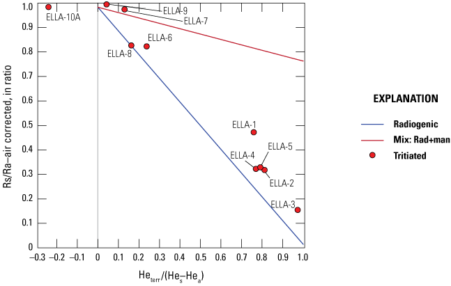
Modified Weise plot (Weise and Moser, 1987; Jurgens and others, 2020) showing mixing of groundwater endmembers generated and modified from the Dissolved Gas Modeling and Environmental Tracer Analysis. Rs=3He/4He ratio of the sample corrected for the decay of tritium; Ra=3He/4He ratio of air; Heterr=helium concentration of terrigenic origin in cubic centimeters at standard temperature and pressure per gram of water; Hes=helium concentration of the sample in cubic centimeters at standard temperature and pressure per gram of water; Hea=helium concentration of excess air in cubic centimeters at standard temperature and pressure per gram of water; Rad=radiogenic helium; Man=mantle derived helium. Data source: U.S. Geological Survey (2023a). See table 1 for site information.
Generally, groundwater ages in wells on the northern part of Elizabeth Lake contain much younger ages than groundwater on the southern part of the lake (fig. 3), with the exception of well ELLA-8. This difference in groundwater ages could potentially be an effect of well depths, which are generally deeper on the south side of the lake and are farther from recharge along runoff drainage channels.
Dissolved Organic Matter Spectral Analysis and Principal Component Analysis Model Results and Discussion
Surface-water (ELS-01, Tank-1, Tank-2, ELS-Spring-01) DOC concentrations ranged widely from 1.9 mg/L as C (Tank-2) to 100 mg/L as C (Elizabeth Lake, ELS-01). One measurement of DOC in a spring (ELS-Spring-01), which was discharging to the land surface, was also elevated with a concentration of 27 mg/L as C. These surface water concentrations were greater than most groundwater concentrations, which ranged from 0.3 mg/L as C to 4.9 mg/L as C. Groundwater affected by OWTS, discussed later, had DOC concentrations ranging from 6.0 mg/L as C to 25.7 mg/L as C and were intermediate between surface water and other groundwater (fig. 20). The two wells that showed evidence of OWTS are ELLA-3 and ELLA-4, and evidence for that is presented later in the text.
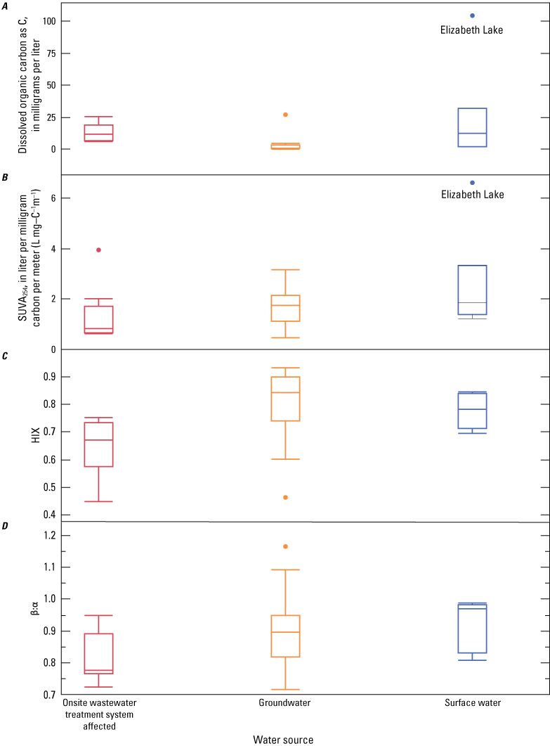
Boxplots illustrating results for A, dissolved organic carbon as C concentration; B, specific ultraviolet absorbance at a wavelength of 254 nanometers (SUVA254) divided by dissolved organic carbon concentration; C, humification index (HIX); and D, freshness index (β:α) for onsite wastewater treatment system-affected samples, groundwater samples, and surface-water samples in the Elizabeth Lake study area, California (U.S. Geological Survey, 2020). Definitions for all presented constituents are provided in table 9. Boxes represent 25th, 50th, and 75th percentile values; whiskers represent 10th and 90th percentile values. Points outside the boxes and whiskers indicate measurements that were either below the 10th percentile (low values) or above the 90th percentile (high values) of the range of values. For each constituent, results were significantly different (p<0.05) among water categories (onsite wastewater treatment affected, groundwater, surface water) based on Kruskal-Wallis and Tukey’s Honest Significant Difference (HSD) tests. See table 1 for site information. Data source: U.S. Geological Survey (2023a).
SUVA254, the absorption of light at 254 nm divided by DOC concentration (table 9) in a water sample, has been used as a proxy for DOM aromaticity (Weishaar and others, 2003) and DOM molecular weight (Chowdhury, 2013). SUVA254 results in this study (U.S. Geological Survey, 2023a) were similar to results previously reported for DOM derived from wastewater effluent (Butman and others, 2012; Goldman and others, 201241). The median SUVA254 values for OWTS affected water (that is, groundwater with concentrations greater than 0.05 mg/L of ammonium as N; ELLA-3 and ELLA-4) was 1.1 liter per milligram of carbon per meter (L mg-C−1 m−1) and ranged from 0.6 to 3.9 L mg-C−1 m−1. Median SUVA254 results in other groundwater wells and in surface water SUVA254 results (1.7 L mg-C−1 m−1 and 1.8 L mg-C−1 m−1, respectively) were higher relative to OWTS affected water (Wells, ELLA-3 and ELLA-4, 0.8 L mg-C−1 m−1).
The humification index, otherwise known as HIX (table 9), defined as the peak area of the emission spectra at 435 to 480 nanometers divided by the peak area of the emission spectra at 300 to 345 nanometers at an excitation wavelength of 254 nanometers, has long been used as an indicator of source, diagenesis, and sorptive capacity of DOM (Zsolnay and others, 1999; Ohno 200295). The humification index is unitless because the nanometers cancel out in the ratio (table 9). As degradation of DOM proceeds, the ratio of hydrogen to carbon decreases, which shifts the emission spectra of the fluorescing molecules to the longer wavelengths. Higher HIX values indicate an increasing degree of humification, with a typical reported range of 0.6–0.9 (Ohno, 2002; Chen and others, 201117). Median HIX values were higher in groundwater wells not affected by OWTS and surface water (0.84 for groundwater and 0.78 for surface water) relative to OWTS affected water (0.67). Evidence for OWTS influenced groundwater was detected in wells ELLA-3 and ELLA-4.
The freshness index (β:α, table 9) has been shown to be associated with the contribution of recently produced organic matter in the DOM pool in a water sample and is associated with the ratio of fresh-like DOM to humic-like DOM (table 9; Parlanti and others, 2000; Wilson and Xenopoulos, 2009). The freshness index is defined as the ratio of the emission intensity at 380 nanometers divided by the maximum emission intensity between 420 and 435 nanometers at an excitation wavelength of 310 nanometers. Fresh-like DOM is therefore recently deposited material from plants that has not been extensively degraded by bacterial and other processes. The freshness index was slightly lower (0.8) in OWTS affected water (Wells ELLA-3 and ELLA-4) relative to other groundwater (0.9) and surface water (1.0).
Table 9.
Dissolved organic matter (DOM) composition-based optical properties identified by discriminant analysis (DA) to significantly (p<0.05) discriminate among sample categories.[Adapted from Hansen and others, 2016, 2018a. Abbreviations: L, liter; mg, milligram; ex/em, excitation/emission; nm, nanometer; DOC, dissolved organic carbon; RU, Raman units; Sp, specific fluorescence; SUVA, specific ultraviolet absorbance; UV, ultraviolet; SpZ, fluorescence at specific excitation-emission pair excitation 420 nanometers/emission 460 nanometers; SpC, fluorescence at specific excitation-emission pairs excitation 340 nanometers/emission 440 nanometers; A:C, ratio of peak C which corresponds to an excitation wavelength of 340 nanometers and an emission wavelength of 440 nanometers to peak A which has an excitation wavelength of 260 nanometers and an emission wavelength of 450 nanometers; micrograms per liter; β:α, freshness index; HIX, humification index]
| Measurements | Calculation | Purpose | Reference |
|---|---|---|---|
| SUVA254 (L mg-C−1 m−1) | Absorption coefficient at wavelength 254 nm divided by DOC concentration | Absorbance per unit carbon. A higher number is typically associated with greater aromatic content and higher molecular weight. | Weishaar and others, 2003; Chowdhury, 2013 |
| SUVA280 (L mg-C−1 m−1) | Absorption coefficient at wavelength 280 nm divided by DOC concentration | Absorbance per unit carbon. A higher number is typically associated with greater aromatic content. | Chin and others, 1994; Hansen and others, 2018a |
| SpZ | Fluorescence at ex420/em460 divided by DOC concentration. | Fluorescence at a given ex/em pair divided by DOC concentration. | Hansen and others, 2016 |
| SpC | Fluorescence at ex340/em440 divided by DOC concentration | ||
| A:C | The ratio of fluorescence intensity of peak A (ex260/em450) to peak C (ex340/em440) | An indication of the relative amount of photosensitive humic-like DOM fluorescence in a sample. | Moran and others, 2000; Hansen and others, 2016 |
| Freshness index (β:α) | The ratio of emission intensity at 380 nm divided by the maximum emission intensity between 420 and 435 nm at an excitation wavelength of 310 nm1 | An indicator of recently produced DOM, with greater values representing a greater proportion of fresh DOM. | Parlanti and others, 2000; Wilson and Xenopoulos, 2009 |
| Humification Index (HIX) | The peak area under the emission spectra at 435 to 480 nm divided by the peak area under the emission spectra at 300 to 345 at an excitation wavelength of 254 nanometers | An indicator of humic substance content or extent of humification Higher values indicate an increasing degree of humification. | Ohno, 2002 |
Although individual optical properties can be effective indicators of DOM composition, optical properties are more informative when evaluated in combination to identify unique signatures (Hansen and others, 2016; Hansen and others, 2018b). In this case, a combination of optical properties were chosen that can help identify OWTS effluent DOM discharging into the surrounding aquifer or Elizabeth Lake. Of the 29 optical properties evaluated, 7 (2 absorbance-based: SUVA254, and SUVA280; and 5 fluorescence-based: HIX, β:α, A:C, SpC, and SpZ; table 9) were quantitatively determined by discriminant analysis to be most significant (p less than 0.05) when evaluated in combination to distinguish among the three sample categories (OWTS affected, groundwater, and surface water). Samples were predicted with an overall success rate of 100 percent. As stated previously, groundwater samples were determined to be affected by mixing with OWTS effluent water—and categorized as OWTS affected—based on independent chemical data (table 7). The independent chemical data were the ammonium and DOC concentrations. The original classification may not be definitive but was determined to be appropriate based on the available data. The two wells that sampled water determined to be affected by OWTS are ELLA-3 and ELLA-4.
A PCA was completed using the seven optical properties identified by discriminant analysis (table 9) as most significant at discriminating differences in DOM among the three sample categories (OWTS affected, groundwater, and surface water; figs. 21, 22). Principal component analysis is a statistical procedure that allows an analyst to summarize content in large datasets by means of a smaller set of summary indices that can be more easily visualized and analyzed. The first summary index is referred to as the first principal component (PC1) and the second as principal component 2 (PC2). Each principal component is given a score which shows how much of the variability of the dataset can be explained by each component. This analysis of the Elizabeth Lake groundwater and surface water dataset resulted in a model where PC1 and PC2 explained 72.1 percent of the total variability (figs. 21, 22). PC1 explained most of the variability (56.8 percent) in the dataset. Higher PC1 values generally represent samples with the highest amount of humic-like, high molecular weight DOM associated with high HIX and SUVA254, relative to samples that had lower PC1 values (wells ELLA-3 and ELLA-4). PC2 explained 15.3 percent of the dataset variability. PC2 scores are usually lower than those of PC1. Evaluation of the PC2 results indicate strong negative loadings for water types with very low SUVA254 values (approximately 1.0 L mg-C−1 m−1), which are likely associated with low molecular weight, and less aromatic DOM compounds associated with OWTS effluent. Notably, SUVA254 values less than 1.0 mg-C−1 m−1 are not commonly reported for humic substances (Weishaar and others, 2003).
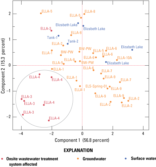
Principal components analysis model score showing each component’s calculated values in relation to the other, with each value adjusted for the mean and standard deviation. Marker color denotes sample type: Onsite wastewater treatment affected, groundwater, surface water. Blue circle indicates wells affected by onsite wastewater treatment system. Data source: U.S. Geological Survey (2023a). See table 1 for site information.
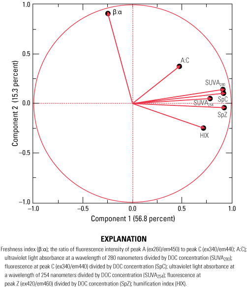
Principal components analysis model loadings showing the unrotated loading matrix between the variables and the components. The closer the value is to 1, the greater the effect of the component on the variable. Data source: U.S. Geological Survey (2023a). [exXXX/emYYY, excitation wavelength in nanometers divided by emission wavelength in nanometers]
Samples with the highest concentrations of ammonium, where ammonium exceeds 0.05 mg/L, were used to categorize groundwater samples likely to have been affected by OWTS effluent. Although nutrients like nitrate and ammonium are not definitive indicators of the presence of effluent, many studies have used them as an indicator for the presence of effluent compounds in stormwater, groundwater, and coastal marine environments (Uchiyama and others, 2014; Lee and others, 2015; Nezlin and others, 20207294). Samples with the highest concentrations of ammonium (exceeding 0.05 mg/L) were labeled in the PCA graph (fig. 21) as OWTS affected. DOM in samples from wells ELLA-3 and ELLA-4 was characterized by lower molecular weight, organic matter compounds likely derived from imported waters (that is, OWTS effluent). Sources of DOM to Elizabeth Lake were primarily soil-derived from seasonal runoff, along with DOM from decaying plant- and animal-derived waste (that is, bird waste). Optical properties measured from Elizabeth Lake (ELS-01) samples indicated humic-like, high molecular weight DOM associated with rapid transformation of the DOM pool by biological and photolytic degradation. This observation supports the conclusion that optical properties were most likely to distinguish DOM from OWTS effluent when mixed with groundwater (ELLA-3 and ELLA-4) but were less effective at tracking DOM from OWTS effluent seepage to Elizabeth Lake.
Although ammonium concentrations were highest in samples collected in wells ELLA-3 and ELLA-4 and Elizabeth Lake (ELS-01), the PCA model demonstrates that the optical properties tracked different sources of the DOM in ELS-01 relative to DOM from wells ELLA-3 and ELLA-4 (fig. 21). Elizabeth Lake DOM composition was characterized by high molecular weight and aromatic compounds (higher SUVA254, SUVA280, HIX, A:C, SpC, SpZ) likely from the release of soil-derived DOM from stormflow runoff, or internal cycling of DOM from the lakebed. By comparison, DOM composition from wells ELLA-3 and ELLA-4 was characterized by lower molecular weight organic matter compounds (lower SUVA254, SUVA280, HIX) likely derived from imported waters (that is, OWTS effluent). Previous studies have reported that sewage water often contains lower molecular weight and labile organic matter compounds (Carstea and others, 2009; Goldman and others, 2012).
Ultimately, groundwater at wells ELLA-3 and ELLA-4 seemed to be strongly affected by effluent from OWTS and consistently demonstrated evidence of denitrification. Wells ELLA-1 and ELLA-2 were also affected by OWTS effluent waters, although to a lesser extent. Most groundwaters measured had sub-oxic conditions that favor de-nitrification. Ammonium may be removed from the system only through sorption to clay minerals, annamox, or by oxidation to nitrate if oxidation/reduction conditions change downgradient. These nitrate attenuation biogeochemical conditions generally changed the environmental conditions of the water to become more alkaline, thus limiting the ability for orthophosphate sorption onto oxide minerals favored in acidic to neutral waters. Thus, ammonium and phosphorus may be delivered to Elizabeth Lake in low quantities. Additionally, where nitrate was low, DOC and ammonium were high; thus, groundwater may be delivering DOC in high concentrations to Elizabeth Lake where numerous algal and cyanobacterial taxa will potentially use it as a nutrient source when inorganic nitrogen is scarce (Paerl, 1991; Berman, 1997; Wood and others, 1999142; Vonshak and others, 2000). Well ELLA-8 contained δD values that were similar to imported water but was depleted in other indicators of OWTS effluent, such as elevated ammonium and DOC. Therefore, elevated nitrate concentrations at ELLA-8 may be attributable to oxidation of OWTS effluent. Groundwater in this part of the aquifer may contribute nitrate to Elizabeth Lake. However, additional data would be needed to test these hypotheses.
Waters affected by OWTS effluent generally plotted separately from groundwater and surface water, but considerable overlap was observed (fig. 21). The observed overlap supports the conclusion that optical properties are most likely to distinguish DOM from OWTS effluent when mixed with groundwater (wells ELLA-3 and ELLA-4) but are less effective at identifying differences in DOM in groundwater that is not mixed with OWTS effluent and DOM in surface water where mixing fractions with OWTS may be low and subject to rapid transformation by biological and photolytic degradation, leaving behind a pool of recalcitrant DOM in surface water that looks optically similar to groundwater.
Conceptual Hydrogeologic Model
A combination of field measurements and previously published drillers’ log interpretations of the groundwater system (Tetra Tech, 2016; California Department of Water Resources, 202113) were used to develop a conceptual hydrogeologic model. Although there was evidence of a blue clay layer from lithographic interpretations and subsurface resistivity values from this study, this layer varied in thickness and was assumed to be an interbedded confining unit within an unconfined aquifer. This confining unit may slow infiltration, allowing for the formation of perched aquifers during wet months, which was consistent with field conditions observed during drilling and are typical of lacustrine deposits (Anderson and others, 2002). Auger wells drilled as part of this study, drilled to depths as much as 90 ft, did not demonstrate evidence of bedrock at depth. However, well depths were limited by the ability for the auger rig to drill through impassable layers; boreholes generally terminated at depths of the highly consolidated blue clay layer. Thus, the bottom of the unconfined aquifer is assumed to be at depths around 90 ft below land surface in Pleistocene alluvium on the south side of Elizabeth Lake and at 50 ft below land surface at granitic contacts overserved in drillers’ logs, which were not part of this study, on the north side of Elizabeth Lake (fig. 4). Additional aquifer boundaries of the unconfined aquifer can be determined with drillers’ logs.
The unconfined aquifer is assumed to overlie igneous granitic rocks—to the north, south, and west of Elizabeth Lake—based on drillers’ logs archived with the DWR and geological maps (fig. 4). Using local drillers’ logs, depth to bedrock on the west boundary of the Elizabeth Lake was estimated to be approximately 100 ft below land surface. Granite outcrops present on the north side of Elizabeth Lake and were observed at road cuts and bound the northern part of residences. Lake sediments to the northeast of Elizabeth Lake, near well ELLA-8 and another well, were suspected to overlie granite at approximately 50 ft below land surface. Depth to bedrock on the eastern side of Elizabeth Lake was estimated to range from 70 to 150 ft below land surface, and the bedrock was characterized as metamorphic schists rather than granite, according to available drillers’ logs and geological maps. Where bedrock was at the surface or in contact with the aquifer at the surface to the north and south of the unincorporated town, the bottom of the unconfined aquifer should be equal to the altitude of the outcropped bedrock.
The area is heavily faulted, and to characterize the boundary condition of each fault splay would be extensive and beyond the scope of this report. Many fault splays were present along the southwest of residences on the south side of Elizabeth Lake. On the south side of one of the fault splays, groundwater levels were estimated to be at or above land surface, as evidenced by two artesian well drillers’ logs. Drillers’ logs noted that water levels ranged between 40 and 80 ft below land surface on the north side of the fault. These water-level differences indicated that the fault on the southwest part of the Elizabeth Lake Census Designated Place, California, may be a groundwater flow barrier (fig. 4). Additionally, the presence of a spring (ELS-SPRING-01), near a lineament of trees, which was observed during the ERT survey, indicated either that wells ELLA-3 and ELLA-4 were just south of a fault splay, that was also characterized as a groundwater flow barrier, or that the water table exceeded the elevation of the land surface at the location of the spring (fig. 4). Substantial differences in groundwater levels in what should have been hydrostatically connected aquifers indicated flow barriers may have been present. A seismic geophysical study of the area could better locate faults, fractures, and water-table levels to aid in the development of a high-resolution groundwater flow model.
The lithologic intervals of the unconfined aquifer characterized during the surface ERT study were broken into three separate hydrofacies relative to borehole lithologies and resistivity. The study-area sediments, which were primarily sandy silt with some clays, are estimated to have hydraulic conductivities from 3.28x10⁻³ to 16.4 ft/d, a porosity range from 0.34 to 0.42, and a hydraulic gradient range from 0.01 to 0.03. Groundwater may discharge through transmissive fractures in granitic bedrock that surrounds most of the study area. The Elizabeth Lake subwatershed was characterized as a closed system, with the exception of infrequent wet years. The boundary along the Elizabeth Lake subwatershed was assumed to be a no-flow boundary based on the rock types (granite and metamorphic rocks, fig. 4). Hydraulic conductivity is specific for the unconfined aquifer. Any future models will need better information on aquifer thickness to determine transmissivity.
Water levels vary substantially in environments of extensive faulting. Historical water levels measured by the USGS in the valley of the Elizabeth Lake subwatershed ranged from 8 to 16 ft below land surface since the 1940s. These historical water levels were consistent with water levels measured during this study. Water levels from wells assumed to be in the unconfined aquifer (shallower than 200 ft below land surface and not screened within hard rock) were documented on drillers logs’ and ranged from 6 to 24 ft below land surface in lower parts and 80 ft below land surface in the higher parts of the Elizabeth Lake subwatershed.
Non-anthropogenic hydrologic inputs to recharge into Elizabeth Lake were assumed to be contributed primarily from precipitation and stormflow runoff through ephemeral stream channels. Precipitation was estimated to be 13.6 in/yr for an approximate area of 7.85 mi2 (Tetra Tech, 2016). Natural discharge by evaporation of groundwater from the water table in desert environments was determined in the Mojave Desert at 114 in/yr; however, because of topographic differences, evaporation was assumed to be less than that of the Mojave Desert and likely did not occur at depths greater than 10 ft bls (Leighton and Phillips, 2003). With the average household use of 0.36 acre-ft/yr, imported waters supplied an estimated 216 acre-ft/yr of recharge into the aquifer, of which 38 acre-ft/yr was suspected of discharging into Elizabeth Lake (Tetra Tech, 2016). Additional recharge most likely occurred from bedrock fractures and mountain front recharge but was not quantified during this study.
Summary
The primary objectives of this study were to determine if onsite wastewater treatment systems (OWTS) effluent discharging into groundwater is responsible for delivering nutrients to Elizabeth Lake in excess of the total maximum daily load (TMDL) and to develop a conceptual hydrogeological model. The study was completed in two parts: the first part was the characterization of subsurface hydrogeology with a stratigraphic approach, and the second part was to characterize groundwater quality and surface-water quality near and in Elizabeth Lake. The subsurface of the study area was characterized by the following processes: evaluation of potential depth to bedrock from local digital elevation models and drillers’ logs; completing two electrical resistivity tomography (ERT) transects; installing 10 monitoring wells; and by characterizing subsurface aquifer lithologies, and estimating aquifer properties, such as hydraulic conductivity and porosity. The water quality in the study area was characterized by collecting water samples and analyzing for major-ion chemistry, nutrients, isotopes, and age tracers.
Based on drillers’ logs of local wells archived in the California Department of Water Resources Online System for Well Completion Reports database, the unconfined aquifer is assumed to overlie granitic and metamorphic rocks. Granitic bedrock underlies the study area on the north, west, and south sides of the Elizabeth Lake subwatershed, and metamorphic rocks underlies areas to the east. The area is heavily faulted, and there is enough evidence regarding water levels and the presence of springs in drillers’ logs to suggest that the splays of the San Andreas Fault Zone in the area may be responsible for some amount of hindrance to flow, indicating the presence of groundwater flow barriers. The fault bounding the residential homes southwest of the Elizabeth Lake Census Designated Place and the study area separates Pleistocene sediments from granites and also hinders flow. An extensive seismic geophysical study of the area would be needed to corroborate this interpretation and could better locate faults, fractures, and water-level depths for the development of any future high-resolution groundwater flow models.
The Elizabeth Lake subwatershed is characterized as a closed system, with infrequent overflow during wet years. The boundary along the Elizabeth Lake subwatershed is assumed to be a no-flow boundary. Most of the aquifer material in the boreholes drilled for the study was characterized as sandy silt, with mixed clays. Estimated hydraulic conductivity ranged from less than 3.28x10⁻³ to 16.4 ft/d in clay-to-sand-dominant layers, and estimated porosity ranged from 0.34 to 0.42. The hydraulic gradient ranged from 0.01 to 0.03. Non-anthropogenic groundwater recharge into Elizabeth Lake was assumed to be primarily from infiltration of precipitation and stormflow runoff through ephemeral stream channels. However, mountain front recharge was likely occurring in the subsurface from surrounding rock fractures based on groundwater levels in sediment near hard rock contacts. Discharge due to groundwater pumping was not included in this report because most of the water consumed is sourced from northern California. Natural discharge was dominated by evaporation, assumed to leave the aquifer system at rates of no more than 114 in/yr and no more than 10 feet below land surface. With the average household use of 0.36 acre-feet per year (acre-ft/yr) of water, imported water was estimated to contribute 216 acre-ft/yr of recharge into the aquifer, and 38 acre-ft/yr was suspected of discharging into Elizabeth Lake.
Recharge from OWTS was estimated to account for approximately 15–71 percent of imported water in groundwater sampled from the wells, with the highest imported water ratios sampled from wells ELLA-3, ELLA-4, and ELLA-8. The presence of OWTS effluent at some sites was corroborated by isotopes of nitrogen (δ15N) and oxygen (δ18O ) values and elevated dissolved organic carbon (DOC) concentrations, and optical properties of dissolved organic matter. Ammonium was the dominant form of nitrogen in wells ELLA-3, ELLA-4, and Elizabeth Lake derived from the breakdown of natural DOC and other forms of carbon or incomplete nitrification of effluent water. Groundwater samples from wells on the south side of Elizabeth Lake have stable isotope measurements consistent with slight evapotranspiration (from root uptake) and have excess nitrogen gas concentrations and nitrate isotope values consistent with denitrification. Because irrigation plays a minimal role in the area, most of the recharge of imported waters was assumed to be sourced from OWTS.
Removal of nitrate in groundwater is dependent on environmental factors, such as redox conditions and total contributing nutrients from OWTS effluent. However, nitrate removal is likely occurring farther downgradient as well. Consequently, most removal of nitrate could occur before groundwater reaches the south side of Elizabeth Lake. Because groundwater on the south part of Elizabeth Lake does not contain high nitrate concentrations, the OWTS on the south part of Elizabeth Lake are not contributing substantial amounts of nitrate to Elizabeth Lake. However, groundwater to the north of the lake may be contributing nitrate to Elizabeth Lake.
Ammonium is present in Elizabeth Lake water, and some ammonium may result from anoxic groundwater discharge of OWTS effluent affected groundwaters; however, some ammonium also may be attributable to the large populations of ducks and other birds on Elizabeth Lake. The ammonium measured in Elizabeth Lake water may also be caused by biological nitrogen fixation. Estimation of the fractions of imported waters as effluent present in samples were based on δD values; these values coupled with nitrate measured in groundwater indicated that aquifer properties are 50-percent efficient at removing nitrogen derived from OWTS sources from groundwater through denitrification by the time groundwater flow reaches well locations.
Measured ammonium concentrations detected at wells ELLA-3 and ELLA-4 in groundwaters also indicated OWTS-derived nutrients in groundwater at these sites. This finding was apparent in the principal component analysis model using optical properties of the dissolved organic matter and chemical data of water. Because of the reducing conditions of the groundwater, the only form of ammonium removal may be through sorption to minerals before groundwater discharges into the lake and possible nitrification lower in the flow path. Because of the relatively low concentrations of ammonium measured in groundwater (except from wells ELLA-3 and ELLA-4) compared to the ammonium levels in Elizabeth Lake, groundwater was assumed to not contribute to the high concentrations of ammonium measured in Elizabeth Lake. Wells ELLA-1 and ELLA-2 were likely also affected by OWTS, as indicated by detectable ammonium, slightly higher DOC relative to most other wells, nitrogen isotopes, and presence of nitrite.
Compared to nitrate, there are fewer processes that control the removal of phosphorous (P) from groundwater. In this study, the highest orthophosphate concentrations in groundwater were in samples collected from wells ELLA-3, ELLA-4, and ELLA-9. Removal of P from groundwater by sorption is dependent on pH because acidic to neutral pH is the controlling factor of sorption of P to iron (Fe) and manganese (Mn) oxide mineral grains. Elevated pH values measured at wells ELLA-3 and ELLA-4 indicated that phosphate from OWTS may have contributed to P loading and eutrophic conditions in Elizabeth Lake, but P loads were not large based on the lower concentrations of orthophosphate detected in groundwater at these wells.
Ultimately, groundwater at wells ELLA-3 and ELLA-4 was substantially affected by effluent from OWTS and consistently demonstrated evidence of denitrification. Wells ELLA-1 and ELLA-2 also were affected by OWTS effluent waters, although to a lesser extent. Most groundwaters measured have sub-oxic conditions that favor de-nitrification. These nitrate attenuation biogeochemical conditions generally change the environmental conditions of the water to become more alkaline, thus limiting the ability for orthophosphate sorption onto oxide minerals favored in acidic to neutral waters. Thus, ammonium and phosphorus may be delivered to Elizabeth Lake in low quantities. Although the evidence is not clear, Well ELLA-8 contained similar deuterium (δD) values to imported water but was depleted in other indicators of OWTS effluent, such as elevated ammonium and DOC, which may indicate that the elevated nitrate concentrations at well ELLA-8 might be attributable to oxidation of effluent. Groundwater in this part of the aquifer may contribute nitrate to Elizabeth Lake.
Nitrogen is likely not being transported to the southern part of Elizabeth Lake in significant quantities, and further research could help further identify processes controlling ammonium and orthophosphate transport. Nutrients may be transported in groundwater from OWTS and discharge into the northern part of Elizabeth Lake near ELLA-8. Transects of shallow wells could be installed and chemical conditions could be examined to determine the extent of nutrient movement.
References Cited
Anderson, D.M., Glibert, P.M., and Burkholder, J.M., 2002, Harmful algal blooms and eutrophication—Nutrient sources, composition, and consequences: Estuaries, v. 25, p. 704–726. [Available at https://doi.org/10.1007/BF02804901.]
Ansari, A.A., and Gill, S.S., eds., 2014, Eutrophication—Causes, consequences and control: Dordrecht, Netherlands, Springer, v. 2, p. 1–262, accessed May 20, 2021, at https://doi.org/10.1007/978-94-007-7814-6.
Arrowsmith, J.R., and Zielke, O., 2009, Tectonic geomorphology of the San Andreas Fault zone from high resolution topography—An example from the Cholame segment: Geomorphology, v. 113, nos. 1–2, p. 70–81. [Available at https://doi.org/10.1016/j.geomorph.2009.01.002.]
Baker, A., and Spencer, R.G.M., 2004, Characterization of dissolved organic matter from source to sea using fluorescence and absorbance spectroscopy: Science of the Total Environment, v. 333, nos. 1–3, p. 217–232. [Available at https://doi.org/10.1016/j.scitotenv.2004.04.013.]
Baker, A., Bolton, L., Newson, M., and Spencer, R.G.M., 2008, Spectrophotometric properties of surface water dissolved organic matter in an afforested upland peat catchment: Hydrological Processes, v. 22, no. 13, p. 2325–2336. [Available at https://doi.org/10.1002/hyp.6827.]
Beggs, K.M.H., and Summers, R.S., 2011, Character and chlorine reactivity of dissolved organic matter from a mountain pine beetle impacted watershed: Environmental Science & Technology, v. 45, no. 13, p. 5717–5724. [Available at https://doi.org/10.1021/es1042436.]
Berman, T., 1997, Dissolved organic nitrogen utilization by an Aphanizomenon bloom in Lake Kinneret: Journal of Plankton Research, v. 19, no. 5, p. 577–586. [Available at https://doi.org/10.1093/plankt/19.5.577.]
Binley, A., and Kemna, A., 2005, DC resistivity and induced polarization methods, chap. 5 in Rubin, Y., and Hubbard, S.S., eds., Hydrogeophysics, v. 50: Dordrecht, Netherlands, Water Science and Technology Library, Springer, p. 129–156. [Available at https://doi.org/10.1007/1-4020-3102-5_5.]
Butman, D., Raymond, P.A., Butler, K., and Aiken, G.R., 2012, Relationships between Δ14C and the molecular quality of dissolved organic carbon in rivers draining to the coast from the conterminous United States: Global Biogeochemical Cycles, v. 26, no. 4, 15 p. [Available at https://doi.org/10.1029/2012GB004361.]
California Department of Conservation, 2023, Alquist-Priolo earthquake fault zones: California Department of Conservation website, accessed February 2, 2023, at https://www.conservation.ca.gov/cgs/alquist-priolo.
California Department of Water Resources, 2021, Well completion reports (OSWCR) system: California Department of Water Resources, accessed June 15, 2021, at https://data.cnra.ca.gov/dataset/well-completion-reports.
Carpenter, K.D., Kraus, T.E.C., Goldman, J.H., Saraceno, J.F., Downing, B.D., Bergamaschi, B.A., McGhee, G., and Triplett, T., 2013, Sources and characteristics of organic matter in the Clackamas River, Oregon, related to the formation of disinfection by-products in treated drinking water: U.S. Geological Survey Scientific Investigations Report 2013–5001, 78 p., accessed August 2, 2022, at https://doi.org/10.3133/sir20135001.
Carstea, E.M., Ghervase, L., Pavelescu, G., and Savastru, D., 2009, Assessment of the anthropogenic impact on water systems by fluorescence spectroscopy: Environmental Engineering and Management Journal, v. 8, no. 6, p. 1321–1326. [Available at https://doi.org/10.30638/eemj.2009.193.]
Cey, B.D., Hudson, G.B., Moran, J.E., and Scanlon, B.R., 2008, Impact of artificial recharge on dissolved noble gases in groundwater in California: Environmental Science & Technology, v. 42, no. 4, p. 1017–1023. [Available at https://doi.org/10.1021/es0706044.]
Chen, H., Zheng, B., Song, Y., and Qin, Y., 2011, Correlation between molecular absorption spectral slope ratios and fluorescence humification indices in characterizing CDOM: Aquatic Sciences, v. 73, p. 103–112, accessed August 2, 2022, at https://doi.org/10.1007/s00027-010-0164-5.
Childress, C.J.O., Foreman, W.T., Connor, B.F., and Maloney, T.J., 1999, New reporting procedures based on long-term method detection levels and some considerations for interpretations of water-quality data provided by the U.S. Geological Survey National Water Quality Laboratory: U.S. Geological Survey Open-File Report 99–193, 19 p., accessed September 12, 2022, at https://doi.org/10.3133/ofr99193.
Chin, Y.P., Aiken, G., and O’Loughlin, E., 1994, Molecular weight, polydispersity, and spectroscopic properties of aquatic humic substances: Environmental Science & Technology, v. 28, no. 11, p. 1853–1858. [Available at https://doi.org/10.1021/es00060a015.]
Chowdhury, S., 2013, Trihalomethanes in drinking water—Effect of natural organic matter distribution: Water S.A., v. 39, no. 1, p. 1–7, accessed June 12, 2022, at https://doi.org/10.4314/wsa.v39i1.1.
Coble, P.G., 2007, Marine optical biogeochemistry—The chemistry of ocean color: Chemical Reviews, v. 107, no. 2, p. 402–418. [Available at https://doi.org/10.1021/cr050350+.]
Coble, P.G., Lead, J., Baker, A., Reynolds, D.M., and Spencer, R.G.M., 2014, Aquatic organic matter fluorescence: New York, N.Y., Cambridge University Press, 375 p., accessed October 12, 2021, at https://doi.org/10.1017/CBO9781139045452.
Coplen, T.B., Qi, H., Révész, K., Casciotti, K., and Hannon, J.E., 2012, Determination of the δ15N and δ18O of nitrate in water; RSIL lab code 2900, chap. 17 of Stable isotope-ratio methods, section C of Révész, K., and Coplen, T.B., eds., Methods of the Reston Stable Isotope Laboratory (slightly revised from version 1.0 released in 2007): U.S. Geological Survey Techniques and Methods, book 10, chap. C17, 35 p., accessed October 20, 2022, at https://pubs.usgs.gov/tm/2006/tm10c17/. [Supersedes version 1.0, released in 2007.]
Craig, H., 1961, Isotopic variations in meteoric waters: Science, v. 133, no. 3465, p. 1702–1703. [Available at https://doi.org/10.1126/science.133.3465.1702.]
DeSimone, L.A., and Howes, B.L., 1998, Nitrogen transport and transformations in a shallow aquifer receiving wastewater discharge—A mass balance approach: Water Resources Research, v. 34, no. 2, p. 271–285. [Available at https://doi.org/10.1029/97WR03040.]
Dodds, W.K., Bouska, W.W., Eitzmann, J.L., Pilger, T.J., Pitts, K.L., Riley, A.J., Schloesser, J.T., and Thornbrugh, D.J., 2009, Eutrophication of U.S. freshwaters—Analysis of potential economic damages: Environmental Science & Technology, v. 43, no. 1, p. 12–19. [Available at https://doi.org/10.1021/es801217q.]
Domagalski, J.L., and Johnson, H.M., 2011, Subsurface transport of orthophosphate in five agricultural watersheds, USA: Journal of Hydrology, v. 409, nos. 1–2, p. 157–171. [Available at https://doi.org/10.1016/j.jhydrol.2011.08.014.]
Fellman, J.B., Hood, E., and Spencer, R.G.M., 2010, Fluorescence spectroscopy opens new windows into dissolved organic matter dynamics in freshwater ecosystems—A review: Limnology and Oceanography, v. 55, no. 6, p. 2452–2462. [Available at https://doi.org/10.4319/lo.2010.55.6.2452.]
Fishman, M.J., and Friedman, L.C., 1989, Methods for determination of inorganic substances in water and fluvial sediments: U.S. Geological Survey Techniques of Water-Resources Investigations, book 5, chap. Al, accessed February 9, 2021, at https://doi.org/10.3133/twri05A1.
Fishman, M.J., ed., 1993, Methods of analysis by the U.S. Geological Survey National Water Quality Laboratory—Determination of inorganic and organic constituents in water and fluvial sediments, U.S. Geological Survey Open-File Report 93–125, 217 p., accessed July 22, 2022, at https://doi.org/10.3133/ofr93125.
Fleming, C.S., Regan, S.D., Freitag, A., and Burkart, H., 2020, Assessing the geographic variability in vulnerability to climate change and coastal hazards in Los Angeles County, California: National Oceanic and Atmospheric Administration Technical Memorandum NOS NCCOS 275, 172 p., accessed November 1, 2023, at https://doi.org/10.25923/mgca-hc06.
Folk, R.L., 1954, The distinction between grain size and mineral composition in sedimentary-rock nomenclature: The Journal of Geology, v. 62, no. 4, p. 344–359, accessed December 9, 2021, at https://doi.org/10.1086/626171.
Follett, J.R., and Follett, R.F., 2008, Relationship of environmental nitrogen metabolism to human health, chap. 4 of Hatfield, J.L., and Follett, R.F., eds., Nitrogen in the environment—Sources, problems, and management (2d ed.): Boston, Mass., Academic Press, p. 71–104, accessed July1, 2021, at https://doi.org/10.1016/B978-0-12-374347-3.00004-4.
Friedman, I., Smith, G.I., Gleason, J.D., Warden, A., and Harris, J.M., 1992, Stable isotope composition of waters in southeastern California, 1. Modern precipitation: Journal of Geophysical Research Atmospheres, v. 97, no. D5, p. 5795–5812. [Available at https://doi.org/10.1029/92JD00184.]
Garbarino, J.R., Bednar, A.J., and Burkhardt, M.R., 2002, Methods of analysis by the U.S. Geological Survey National Water Quality Laboratory—Arsenic speciation in natural-water samples using laboratory and field methods: U.S. Geological Survey Water-Resources Investigations Report 2002–4144, 40 p., accessed March 14, 2022, at https://doi.org/10.3133/wri024144.
Garbarino, J.R., Kanagy, L.K., and Cree, M.E., 2006, Determination of elements in natural-water, biota, sediment, and soil samples using collision/reaction cell inductively coupled plasma–mass spectrometry: U.S. Geological Survey Techniques and Methods, book 5, chap. B1, 87 p, accessed June 16, 2021, at https://store.usgs.gov/assets/yimages/PDF/206002.pdf.
Gibson, J.J., Birks, S.J., and Edwards, T.W.D., 2008, Global prediction of δA and δ2H-δ18O evaporation slopes for lakes and soil water accounting for seasonality: Global Biogeochemical Cycles, v. 22, no. 2. [Available at https://doi.org/10.1029/2007GB002997.]
Gleason, J.D., Veronda, G., Smith, G.I., Friedman, I., and Martin, P.M., 1994, Deuterium content of water from wells and perennial springs, southeastern California: U.S. Geological Survey Hydrologic Atlas 727. [Available at https://doi.org/10.3133/ha727.]
Goldman, J.H., Rounds, S.A., and Needoba, J.A., 2012, Applications of fluorescence spectroscopy for predicting percent wastewater in an urban stream: Environmental Science & Technology, v. 46, no. 8, p. 4374–4381. [Available at https://doi.org/10.1021/es2041114.]
Groover, K.D., Burgess, M.K., Howle, J.F., and Phillips, S.P., 2017, Electrical resistivity investigation of fluvial geomorphology to evaluate potential seepage conduits to agricultural lands along the San Joaquin River, Merced County, California, 2012–13: U.S. Geological Survey Scientific Investigations Report 2016–5172, 39 p., accessed July 10, 2022, at https://doi.org/10.3133/sir20165172.
Groover, K.D., McGregor, A.M., Ely, C.P., and Domagalski, J.L., 2021, Electrical resistivity tomography data at Elizabeth Lake, Los Angeles County, California, 2019: U.S. Geological Survey data release, accessed July13, 2022, at https://doi.org/10.5066/P9HUB01S.
Haneberg, W.C., 1995, Steady state groundwater flow across idealized faults: Water Resources Research, v. 31, no. 7, p. 1815–1820. [Available at https://doi.org/10.1029/95WR01178.]
Hansen, A.M., Fleck, J.A., Kraus, T.E.C., Downing, B.D., von Dessonneck, T., and Bergamaschi, B.A., 2018a, Procedures for using the Horiba Scientific Aqualog® fluorometer to measure absorbance and fluorescence from dissolved organic matter: U.S. Geological Survey Open-File Report 2018–1096, 31 p., accessed October 7, 2021, at https://doi.org/10.3133/ofr20181096.
Hansen, A.M., Kraus, T.E.C., Bachand, S.M., Horwath, W.R., and Bachand, P.A.M., 2018b, Wetlands receiving water treated with coagulants improve water quality by removing dissolved organic carbon and disinfection byproduct precursors: Science of the Total Environment, vs. 622–623, p. 603–613. [Available at https://doi.org/10.1016/j.scitotenv.2017.11.205.]
Hansen, A.M., Kraus, T.E.C., Pellerin, B.A., Fleck, J.A., Downing, B.D., and Bergamaschi, B.A., 2016, Optical properties of dissolved organic matter (DOM)—Effects of biological and photolytic degradation: Limnology and Oceanography, v. 61, no. 3, p. 1015–1032. [Available at https://doi.org/10.1002/lno.10270.]
Harke, M.J., Steffen, M.M., Gobler, C.J., Otten, T.G., Wilhelm, S.W., Wood, S.A., and Paerl, H.W., 2016, A review of the global ecology, genomics, and biogeography of the toxic cyanobacterium, Microcystis spp: Harmful Algae, v. 54, p. 4–20. [Available at https://doi.org/10.1016/j.hal.2015.12.007.]
Haugen, E.A., Jurgens, B.C., Arroyo-Lopez, J.A., and Bennett, G.L., 2021, Groundwater development leads to decreasing arsenic concentrations in the San Joaquin Valley, California: Science of the Total Environment, v. 771, p. 145223. [Available at https://doi.org/10.1016/j.scitotenv.2021.145223.]
Heath, R.C., 1984, Ground-water regions of the United States: U.S. Geological Survey Water Supply Paper 2242, 78 p., accessed January 21, 2021, at https://doi.org/10.3133/wsp2242.
Heaton, T.H.E., and Vogel, J.C., 1981, “Excess air” in groundwater: Journal of Hydrology, v. 50, p. 201–216. [Available at https://doi.org/10.1016/0022-1694(81)90070-6.]
Hem, J.D., 1985, Study and interpretation of the chemical characteristics of natural water (3d ed.): U.S. Geological Survey Water-Supply Paper 2254, 263 p., 4 pls., accessed February 12, 2022, at https://doi.org/10.3133/wsp2254.
Hernandez, J.L., 2011, Preliminary geologic map of the Lake Hughes 7.5’ quadrangle, Los Angeles County, California—A digital database: California Geological Survey, scale 1:24,000, 1 sheet, accessed March 11, 2022, at https://ngmdb.usgs.gov/Prodesc/proddesc_96093.htm.
Hinkle, S.R., Böhlke, J.K., and Fisher, L.H., 2008, Mass balance and isotope effects during nitrogen transport through septic tank systems with packed-bed (sand) filters: Science of the Total Environment, v. 407, no. 1, p. 324–332. [Available at https://doi.org/10.1016/j.scitotenv.2008.08.036.]
Hubbard, S.S., and Rubin, Y., 2005, Introduction to hydrogeophysics, in Rubin, Y., and Hubbard, S.S., eds., Hydrogeophysics: Berlin, Germany, Springer-Verlag, p. 3–21, accessed June17, 2022, at https://doi.org/10.1007/1-4020-3102-5_1.
Hunt, A.G., 2015, U.S. Geological Survey Noble Gas Laboratory’s standard operating procedures for the measurement of dissolved gas in water samples: U.S. Geological Survey Techniques and Methods, book 5, chap. A11, 21 p., accessed November 7, 2022, at https://doi.org/10.3133/tm5A11.
Izbicki, J.A., 2004, Source and movement of ground water in the western part of the Mojave Desert, southern California, USA: U.S. Geological Survey Water-Resources Investigations Report 2003–4313, 36 p., accessed June 11, 2022, at https://doi.org/10.3133/wri034313.
Izbicki, J.A., 2014, Fate of nutrients in shallow groundwater receiving treated septage, Malibu, CA: Groundwater, v. 52, no. S1, p. 218–233. [Available at https://doi.org/10.1111/gwat.12194.]
Jaffé, R., Mcknight, D., Maie, N., Cory, R., McDowell, W.H., and Campbell, J.L., 2008, Spatial and temporal variations in DOM composition in ecosystems—The importance of long-term monitoring of optical properties: Journal of Geophysical Research, v. 113, no. G4. [Available at https://doi.org/10.1029/2008JG000683.]
Jamaluddin and Emi Prasetyawati Umar, 2018, Identification of subsurface layer with Wenner-Schlumberger arrays configuration geoelectrical method: Earth and Environmental Science, IOP conference series, v. 118, p. 012006. [Available at https://doi.org/10.1088/1755-1315/118/1/012006.]
Jurgens, B.C., Böhlke, J., Haase, K., Busenberg, E., Hunt, A.G., and Hansen, J.A., 2020, DGMETA (version 1)—Dissolved gas modeling and environmental tracer analysis computer program: U.S. Geological Survey Techniques and Methods, book 4, chap. F5, 50 p., accessed February 19, 2022, at https://doi.org/10.3133/tm4F5.
Jurgens, B.C., Burow, K.R., Dalgish, B.A., and Shelton, J.L., 2008, Hydrogeology, water chemistry, and factors affecting the transport of contaminants in the zone of contribution of a public-supply well in Modesto, eastern San Joaquin Valley, California: U.S. Geological Survey Scientific Investigations Report 2008–5156, 78 p., accessed January 23, 2021, at https://doi.org/10.3133/sir20085156.
Keys, W.S., 1990, Borehole geophysics applied to ground-water investigations: U.S. Geological Survey Techniques of Water-Resources Investigations, book 2, chap. E2, 150 p., accessed June 19, 2021, at https://doi.org/10.3133/twri02E2.
Kjos, A.R., Densmore, J.N., Nawikas, J.M., and Brown, A.N., 2014, Construction, water-level, and water-quality data for multiple-well monitoring sites and test wells, Fort Irwin National Training Center, San Bernardino County, California, 2009–12: U.S. Geological Survey Data Series 788, 140 p., accessed October 1, 2022, at https://doi.org/10.3133/ds788.
Kolpin, D.W., Furlong, E.T., Meyer, M.T., Thurman, E.M., Zaugg, S.D., Barber, L.B., and Buxton, H.T., 2002, Pharmaceuticals, hormones, and other organic wastewater contaminants in U.S. streams, 1999–2000—A national reconnaissance: Environmental Science & Technology, v. 36, no. 6, p. 1202–1211. [Available at https://doi.org/10.1021/es011055j.]
Kratzer, C.R., Kent, R.H., Saleh, D.K., Knifong, D.L., Dileanis, P.D., and Orlando, J.L., 2011, Trends in nutrient concentrations, loads, and yields in streams in the Sacramento, San Joaquin, and Santa Ana Basins, California, 1975–2004: U.S. Geological Survey Scientific Investigations Report 2010–5228, 112 p., accessed June 11, 2022, at https://doi.org/10.3133/sir20105228.
Kraus, T.E.C., Bergamaschi, B.A., Hernes, P.J., Spencer, R.G.M., Stepanauskas, R., Kendall, C., Losee, R.F., and Fujii, R., 2008, Assessing the contribution of wetlands and subsided islands to dissolved organic matter and disinfection byproduct precursors in the Sacramento–San Joaquin River Delta—A geochemical approach: Organic Geochemistry, v. 39, no. 9, p. 1302–1318. [Available at https://doi.org/10.1016/j.orggeochem.2008.05.012.]
Kulongoski, J.T., Hilton, D.R., and Izbicki, J.A., 2003, Helium isotope studies in the Mojave Desert, California—Implications for groundwater chronology and regional seismicity: Chemical Geology, v. 202, nos. 1–2, p. 95–113. [Available at https://doi.org/10.1016/j.chemgeo.2003.07.002.]
Lapierre, J.-F., and Frenette, J.-J., 2009, Effects of macrophytes and terrestrial inputs on fluorescent dissolved organic matter in a large river system: Aquatic Sciences, v. 71, p. 15–24. [Available at https://doi.org/10.1007/s00027-009-9133-2.]
Lee, D.G., Roehrdanz, P.R., Feraud, M., Ervin, J., Anumol, T., Jia, A., Park, M., Tamez, C., Morelius, E.W., Gardea-Torresdey, J.L., Izbicki, J., Means, J.C., Snyder, S.A., and Holden, P.A., 2015, Wastewater compounds in urban shallow groundwater wells correspond to exfiltration probabilities of nearby sewers: Water Research, v. 85, p. 467–475. [Available at https://doi.org/10.1016/j.watres.2015.08.048.]
Leighton, D.A., and Phillips, S.P., 2003, Simulation of ground-water flow and land subsidence in the Antelope Valley ground-water basin, California: Water-Resources Investigations Report 2003–4016, 118 p., accessed April 19, 2023, at https://doi.org/10.3133/wri034016.
Lindsey, B.D., Jurgens, B.C., and Belitz, K., 2019, Tritium as an indicator of modern, mixed, and premodern groundwater age: U.S. Geological Survey Scientific Investigations Report 2019–5090, 18 p., accessed November 10, 2021, at https://doi.org/10.3133/sir20195090.
Los Angeles County Sanitary Sewer Network–Consolidated Sewer Maintenance District, 2006, City sanitary and private sewers maintained and not maintained by Los Angeles County sewer maintenance districts: Los Angeles County Sanitary Sewer Network–Consolidated Sewer Maintenance District, accessed March 20, 2022, at https://dpw.lacounty.gov/smd/sewernetwork/.
Los Angeles Regional Water Quality Control Board, 2006, State of the watershed—Report on surface water quality—The Santa Clara River Watershed: California Regional Water Quality Control Board, Los Angeles region, accessed September 3, 2021, at https://www.waterboards.ca.gov/rwqcb4/water_issues/programs/regional_program/Water_Quality_and_Watersheds/water_report/santa_clara/scr-w2003.pdf.
Los Angeles Regional Water Quality Control Board, 2016, Total maximum daily load for nutrients in Elizabeth Lake, Munz Lake, and Lake Hughes in the Santa Clara River Watershed: California Regional Water Quality Control Board, Los Angeles region, accessed July 22, 2022, at https://www.waterboards.ca.gov/losangeles/board_decisions/basin_plan_amendments/technical_documents/115_new/SCRLakesNutrientsdraftstaffreport062116.pd f.
Lucas, L.L., and Unterweger, M.P., 2000, Comprehensive review and critical evaluation of the half-life of tritium: Journal of Research of the National Institute of Standards and Technology, v. 105, no. 4, p. 541–549. [Available at https://doi.org/10.6028/jres.105.043.]
McMahon, P.B., and Chapelle, F.H., 2008, Redox processes and water quality of selected principal aquifer systems: Groundwater, v. 46, no. 2, p. 259–271. [Available at https://doi.org/10.1111/j.1745-6584.2007.00385.x.]
McMahon, P.B., Cowdery, T.K., Chapelle, F.H., and Jurgens, B.C., 2009, Redox conditions in selected principal aquifers of the United States: U.S. Geological Survey Fact Sheet 2009–3041, 6 p., accessed February 20, 2021 at https://doi.org/10.3133/fs20093041.
Michel, R.L., 1976, Tritium inventories of the world oceans and their implications: Nature, v. 263, no. 5573, p. 103–106. [Available at https://doi.org/10.1038/263103a0.]
Michel, R.L., 1989, Tritium deposition in the continental United States, 1953–83: U.S. Geological Survey Water-Resources Investigations Report 89–4072, 46 p., accessed January 25, 2021, at https://doi.org/10.3133/wri894072.
Miller, M.P., and McKnight, D.M., 2010, Comparison of seasonal changes in fluorescent dissolved organic matter among aquatic lake and stream sites in the Green Lakes Valley: Journal of Geophysical Research, v. 115, no. G1. [Available at https://doi.org/10.1029/2009JG000985.]
Minsley, B.J., Ball, L.B., Burton, B.L., Caine, J.S., Curry-Elrod, E., and Manning, A.H., 2010, Geophysical characterization of subsurface properties relevant to the hydrology of the Standard Mine in Elk Basin, Colorado: U.S. Geological Survey Open-File Report 2009–1284, 41 p., accessed July 8, 2021, at https://doi.org/10.3133/ofr20091284.
Moran, M.A., Sheldon, W.M.Jr., and Zepp, R.G., 2000, Carbon loss and optical property changes during long-term photochemical and biological degradation of estuarine dissolved organic matter: Limnology Oceanography, v. 45, no. 6, p. 1254–1264. [Available at https://doi.org/10.4319/lo.2000.45.6.1254.]
Morris, D.A., and Johnson, A.I., 1967, Summary of hydrologic and physical properties of rock and soil materials, as analyzed by the hydrologic laboratory of the U.S. Geological Survey: U.S. Geological Survey Water Supply Paper 1839-D, 42 p. [Available at https://doi.org/10.3133/wsp1839D.]
Mueller, D.K., and Helsel, D.R., 1996, Nutrients in the Nation’s waters—Too much of a good thing?: U.S. Geological Survey Circular 1136, 24 p., accessed October 26, 2022, at https://doi.org/10.3133/cir1136.
Murphy, K.R., Butler, K.D., Spencer, R.G.M., Stedmon, C.A., Boehme, J.R., and Aiken, G.R., 2010, Measurement of dissolved organic matter fluorescence in aquatic environments—An interlaboratory comparison: Environmental Science & Technology, v. 44, no. 24, p. 9405–9412. [Available at https://doi.org/10.1021/es102362t.]
Naranjo, R.C., Niswonger, R.G., Smith, D., Rosenberry, D., and Chandra, S., 2019, Linkages between hydrology and seasonal variations of nutrients and periphyton in a large oligotrophic subalpine lake: Journal of Hydrology, v. 568, p. 877–890. [Available at https://doi.org/10.1016/j.jhydrol.2018.11.033.]
National Oceanic and Atmospheric Administration (NOAA), 2020, Dataset search website: National Oceanic and Atmospheric Administration, accessed March 12, 2020, at https://www.ncei.noaa.gov/access/search/dataset-search.
Nawikas, J.M., O’Leary, D.R., Izbicki, J.A., and Burgess, M.K., 2016, Selected techniques for monitoring water movement through unsaturated alluvium during managed aquifer recharge: U.S. Geological Survey Open-File Report 2016–1180, 8 p., accessed June 1, 2022, at https://doi.org/10.3133/ofr20161180.
Neil, C.W., Yang, Y.J., and Jun, Y.-S., 2012, Arsenic mobilization and attenuation by mineral-water interactions—Implications for managed aquifer recharge: Journal of Environmental Monitoring, v. 14, no. 7, p. 1772–1788. [Available at https://doi.org/10.1039/c2em30323j.]
Nezlin, N.P., Beegan, C., Feit, A., Gully, J.R., Latker, A., McLaughlin, K., Mengel, M.J., Robertson, G.L., Steele, A., and Weisberg, S.B., 2020, Colored dissolved organic matter (CDOM) as a tracer of effluent plumes in the coastal ocean: Regional Studies in Marine Science, v. 35, article 101163, 10 p. [Available at https://doi.org/10.1016/j.rsma.2020.101163.]
Ohno, T., 2002, Fluorescence inner-filtering correction for determining the humification index of dissolved organic matter: Environmental Science & Technology, v. 36, no. 4, p. 742–746. [Available at https://doi.org/10.1021/es0155276.]
Ortiz, D., Palmer, J., and Wilkinson, G., 2020, Detecting changes in statistical indicators of resilience prior to algal blooms in shallow eutrophic lakes: Ecosphere, v. 11, no. 10, p. e03200. [Available at https://doi.org/10.1002/ecs2.3200.]
Paerl, H.W., 1991, Ecophysiological and trophic implications of light-stimulated amino acid utilization in marine picoplankton: Applied and Environmental Microbiology, v. 57, no. 2, p. 473–479. [Available at https://doi.org/10.1128/aem.57.2.473-479.1991.]
Parfitt, R.L., 1979, Anion adsorption by soils and soil materials: Advances in Agronomy, v. 30, p. 1–50. [Available at https://doi.org/10.1016/S0065-2113(08)60702-6.]
Parlanti, E., Wörz, K., Geoffroy, L., and Lamotte, M., 2000, Dissolved organic matter fluorescence spectroscopy as a tool to estimate biological activity in a coastal zone submitted to anthropogenic inputs: Organic Geochemistry, v. 31, no. 12, p. 1765–1781. [Available at https://doi.org/10.1016/S0146-6380(00)00124-8.]
Patton, C.J., and Truitt, E.P., 1992, Methods of analysis by the U.S. Geological Survey National Water Quality Laboratory—Determination of total phosphorus by a Kjeldahl digestion method and an automated colorimetric finish that includes dialysis: U.S. Geological Survey Open-File Report 1992–146, 39 p. [Available at https://doi.org/10.3133/ofr92146.]
Patton, C.J., and Truitt, E.P., 2000, Methods of analysis by the U.S. Geological Survey National Water Quality Laboratory—Determination of ammonium plus organic nitrogen by a Kjeldahl digestion method and an automated photometric finish that includes digest cleanup by gas diffusion: U.S. Geological Survey Open-File Report 2000–170, 31 p. [Available at https://doi.org/10.3133/ofr00170.]
Phillips, S.P., Green, C.T., Burow, K.R., Shelton, J.L., and Rewis, D.L., 2007, Simulation of multiscale ground-water flow in part of the northeastern San Joaquin Valley, California: U.S. Geological Survey Scientific Investigations Report 2007–5009, 43 p., accessed October 19, 2021, at https://doi.org/10.3133/sir20075009.
Pickering, R.J., 1981, Water quality—New tables of dissolved oxygen saturation values: U.S. Geological Survey Quality of Water Branch Technical Memorandum no. 81.11, accessed February 15, 2021, at https://water.usgs.gov/admin/memo/QW/qw81.11.html.
Piper, A.M., 1944, A graphic procedure in the geochemical interpretation of water-analyses: Eos, Transactions American Geophysical Union, v. 25, no. 6, p. 914–928. [Available at https://doi.org/10.1029/TR025i006p00914.]
Potter, B.B., and Wimsatt, J.C., 2012, USEPA method 415.3—Quantifying TOC, DOG, and SUVA: Journal—American Water Works Association, v. 104, no. 6, p. E358–E369. [Available at https://doi.org/10.5942/jawwa.2012.104.0086.]
Prism Climate Group, 2023, PRISM climate data website: Prism Climate Group, accessed February 3, 2023, at https://prism.oregonstate.edu.
Rakhimbekova, S., O’Carroll, D.M., Oldfield, L.E., Ptacek, C.J., and Robinson, C.E., 2021, Spatiotemporal controls on septic system derived nutrients in a nearshore aquifer and their discharge to a large lake: Science of the Total Environment, v. 752, p. 141262. [Available at https://doi.org/10.1016/j.scitotenv.2020.141262.]
Redfield, A.C., 1958, The biological control of chemical factors in the environment: American Scientist, v. 46, no. 3, p. 205–221, accessed July 9, 2022, at https://www.jstor.org/stable/27827150.
Révész, K., and Coplen, T.B., 2008a, Determination of the δ(2H/1H) of water—RSIL lab code 1574, in Révész, K., and Coplen, T.B., eds., Methods of the Reston Stable Isotope Laboratory: U.S. Geological Survey Techniques and Methods, book 10, chap. C1, 27 p., accessed September 19, 2021, at https://doi.org/10.3133/tm10C1.
Révész, K., and Coplen, T.B., 2008b, Determination of the δ(18O/16O) of water—RSIL lab code 489, in Révész, K., and Coplen, T.B., eds., Methods of the Reston Stable Isotope Laboratory: U.S. Geological Survey Techniques and Methods, book 10, chap. C2, 28 p., accessed December 17, 2021, at https://doi.org/10.3133/tm10C2.
Schlosser, P., Stute, M., Sonntag, C., and Münnich, K.O., 1989, Tritiogenic 3He in shallow groundwater: Earth and Planetary Science Letters, v. 94, nos. 3–4, p. 245–256. [Available at https://doi.org/10.1016/0012-821X(89)90144-1.]
Seitzinger, S.P., 1994, Linkages between organic matter mineralization and denitrification in eight riparian wetlands: Biogeochemistry, v. 25, no. 1, p. 19–39, accessed August 24, 2022, at https://doi.org/10.1007/BF00000510.
Solomon, D.K., and Cook, P.G., 2000, 3H and 3He, in Cook, P.G., and Herczeg, A.L., eds., Environmental tracers in subsurface hydrology: Boston, Mass., Springer, p. 397–424., accessed July 1, 2023, at https://doi.org/10.1007/978-1-4615-4557-6_13.
Spencer, R.G.M., Butler, K.D., and Aiken, G.R., 2012, Dissolved organic carbon and chromophoric dissolved organic matter properties of rivers in the USA: Journal of Geophysical Research, v. 117, no. G3. [Available at https://doi.org/10.1029/2011JG001928.]
Stanton, J.S., Anning, D.W., Brown, C.J., Moore, R.B., McGuire, V.L., Qi, S.L., Harris, A.C., Dennehy, K.F., McMahon, P.B., Degnan, J.R., and Böhlke, J.K., 2017, Brackish groundwater in the United States: U.S. Geological Survey Professional Paper 1833, 185 p., accessed February 25, 2021, at https://doi.org/10.3133/pp1833.
Stute, M., and Schlosser, P., 2000, Atmospheric noble gases, in Cook, P.G., and Herczeg, A.L., eds., Environmental tracers in subsurface hydrology: Boston, Mass., Springer, p. 349–377., accessed November 12, 2022, at https://doi.org/10.1007/978-1-4615-4557-6_11.
Swenson, H.A., and Baldwin, H.L., 1965, A primer on water quality: U.S. Geological Survey General Interest Publication, 27 p., accessed July 1, 2021, at https://doi.org/10.3133/7000057.
Tetra Tech, 2016, Nutrient TMDL support for Santa Clara River Watershed lakes—Lake Elizabeth, Munz Lake, and Lake Hughes—Task 1 report sections: Research Triangle Park, North Carolina, Tetra Tech, 70 p., accessed August 27, 2022, at https://www.waterboards.ca.gov/losangeles/board_decisions/basin_plan_amendments/technical_documents/115_new/SCRLakesTechnicalSupportDocument.pdf.
Thatcher, L.L., Janzer, V.J., and Edwards, K.W., 1977, Methods for determination of radioactive substances in water and fluvial sediments: U.S. Geological Survey Techniques of Water Resources Investigations, book 5, chap. A5, 95 p., accessed February 28, 2021, at https://doi.org/10.3133/twri05A5.
Thurman, E.M., 1985, Organic geochemistry of natural waters: Springer Dordrecht, Developments in biogeochemistry series, v. 2. [Available at https://doi.org/10.1007/978-94-009-5095-5.]
Todd, D.K., 1959, Annotated bibliography on artificial recharge of ground water through 1954: U.S. Geological Survey Water Supply Paper 1477, 155 p., accessed August 30, 2021, at https://doi.org/10.3133/wsp1477.
Tranvik, L.J., Downing, J.A., Cotner, J.B., Loiselle, S.A., Striegl, R.G., Ballatore, T.J., Dillon, P., Finlay, K., Fortino, K., Knoll, L.B., Kortelainen, P.L., Kutser, T., Larsen, S., Laurion, I., Leech, D.M., McCallister, S.L., McKnight, D.M., Melack, J.M., Overholt, E., Porter, J.A., Prairie, Y., Renwick, W.H., Roland, F., Sherman, B.S., Schindler, D.W., Sobek, S., Tremblay, A., Vanni, M.J., Verschoor, A.M., von Wachenfeldt, E., and Weyhenmeyer, G.A., 2009, Lakes and reservoirs as regulators of carbon cycling and climate: Limnology and Oceanography, v. 54, no. 6, part 2, p. 2298–2314. [Available at https://doi.org/10.4319/lo.2009.54.6_part_2.2298.]
Uchiyama, Y., Idica, E.Y., McWilliams, J.C., and Stolzenbach, K.D., 2014, Wastewater effluent dispersal in southern California bays: Continental Shelf Research, v. 76, p. 36–52. [Available at https://doi.org/10.1016/j.csr.2014.01.002.]
Umari, A.M.J., Martin, P., Schroeder, R.A., Duell, L.F.W., Jr., and Fay, R.G., 1993, Potential for ground-water contamination from movement of wastewater through the unsaturated zone, upper Mojave River Basin, California: U.S. Geological Survey Water-Resources Investigations Report 93–4137, 117 p., accessed February 22, 2021, at https://doi.org/10.3133/wri934137.
U.S. Environmental Protection Agency, 2022, Drinking water requirements for states and public water systems: U.S. Environmental Protection Agency website, accessed April 17, 2023, at https://www.epa.gov/dwreginfo/chemical-contaminant-rules.
U.S. Environmental Protection Agency, 2023a, History of the Clean Water Act: U.S. Environmental Protection Agency website, accessed December 19, 2021, at https://www.epa.gov/laws-regulations/history-clean-water-act#:~:text=The%20Federal%20Water%20Pollution%20Control,Clean%20Water%20Act%20(CWA).
U.S. Environmental Protection Agency, 2023b, pH: U.S. Environmental Protection Agency website, accessed February 8, 2023, at https://www.epa.gov/caddis-vol2/ph.
U.S. Geological Survey, 2020, The National Watershed Boundary Dataset lookup: U.S. Geological Survey website, accessed August 22, 2021, at https://water.usgs.gov/wsc/a_api/wbd/subwatershed18/180701020301.html.
U.S. Geological Survey, 2022, USGS GeoLog Locator: U.S. Geological Survey database, accessed November 15, 2022, at https://doi.org/10.5066/F7X63KT0.
U.S. Geological Survey, 2023a, USGS water data for the Nation: U.S. Geological Survey National Water Information System database, accessed January 10, 2023, at https://doi.org/10.5066/F7P55KJN.
U.S. Geological Survey, 2023b, DOTABLES: online program, accessed October 13, 2023, at https://water.usgs.gov/water-resources/software/DOTABLES/.
U.S. Geological Survey, variously dated, National field manual for the collection of water-quality data: U.S. Geological Survey Techniques of Water-Resources Investigations, book 9, chaps. A1–A9, accessed June 1, 2020, at https://water.usgs.gov/owq/FieldManual/.
Vero, S.E., Basu, N.B., Van Meter, K., Richards, K.G., Mellander, P., Healy, M.G., and Fenton, O., 2017, Review—The environmental status and implications of the nitrate time lag in Europe and North America: Hydrogeology Journal, v. 26, no. 1, p. 7–22. [Available at https://doi.org/10.1007/s10040-017-1650-9.]
Vonshak, A., Cheung, S.M., and Chen, F., 2000, Mixotrophic growth modifies the response of Spirulina (Arthrospira) platensis (Cyanobacteria) cells to light: Journal of Phycology, v. 36, no. 4, p. 675–679. [Available at https://doi.org/10.1046/j.1529-8817.2000.99198.x.]
Wakida, F.T., and Lerner, D.N., 2005, Non-agricultural sources of groundwater nitrate—A review and case study: Water Research, v. 39, no. 1, p. 3–16. [Available at https://doi.org/10.1016/j.watres.2004.07.026.]
Weise, S., and Moser, H., 1987, Groundwater dating with helium isotopes, in Isotope techniques in water resources development—Proceedings of an international symposium on the use of isotope techniques in water resources development, March 30–April 3, 1987: Vienna, Austria, International Atomic Energy Agency, p. 105–126. [Available at https://inis.iaea.org/Search/search.aspx?orig_q=RN:19054247.]
Weishaar, J.L., Aiken, G.R., Bergamaschi, B.A., Fram, M.S., Fujii, R., and Mopper, K., 2003, Evaluation of specific ultraviolet absorbance as an indicator of the chemical composition and reactivity of dissolved organic carbon: Environmental Science & Technology, v. 37, no. 20, p. 4702–4708. [Available at https://doi.org/10.1021/es030360x.]
Williams, J.H., and Johnson, C.D., 2004, Acoustic and optical borehole-wall imaging for fractured-rock aquifer studies: Journal of Applied Geophysics, v. 55, nos. 1–2, p. 151–159. [Available at https://doi.org/10.1016/j.jappgeo.2003.06.009.]
Wilson, H.F., and Xenopoulos, M.A., 2009, Effects of agricultural land use on the composition of fluvial dissolved organic matter: Nature Geoscience, v. 2, no. 1, p. 37–41. [Available at https://doi.org/10.1038/ngeo391.]
Wood, B.J.B., Grimson, P.H.K., German, M.T., and Turner, M., 1999, Photoheterotrophy in the production of phytoplankton organisms: Progress in Industrial Microbiology, v. 35, p. 175–183. [Available at https://doi.org/10.1016/S0079-6352(99)80110-6.]
Zhang, J.Z., and Huang, X.L., 2007, Relative importance of solid-phase phosphorus and iron on the sorption behavior of sediments: Environmental Science & Technology, v. 41, no. 8, p. 2789–2795. [Available at https://doi.org/10.1021/es061836q.]
Zsolnay, A., Baigar, E., Jimenez, M., Steinweg, B., and Saccomandi, F., 1999, Differentiating with fluorescence spectroscopy the sources of dissolved organic matter in soils subjected to drying: Chemosphere, v. 38, no. 1, p. 45–50. [Available at https://doi.org/10.1016/S0045-6535(98)00166-0.]
Appendix 1
Borehole Lithologies
The figures in this appendix present subsurface illustrations of each well based on subsurface lithologies, borehole construction, borehole geophysical measurements, and estimated hydraulic conductivity for each lithology type. Figure 3, in the main body of the report, shows the location of each monitoring well used in this study. Natural gamma logs collected after drilling display results of the strength of gamma emission rays. However, because gamma logs were measured after construction was completed, the logs represent well construction material rather than borehole material and serve as verification checks of borehole materials surrounding the casings. Peaks of natural gamma seen on figures 1.1–1.8 are consistent with sanitary seal depths and ancillary fill.
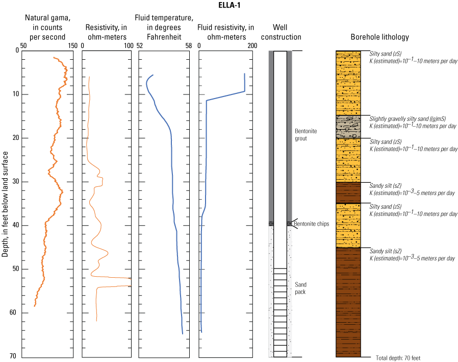
Geophysical logs, well-construction diagram, borehole lithology, and estimated hydraulic conductivity for single-well monitoring site ELLA-1 (07N/14W-30K1S). Data source: U.S. Geological Survey GeoLog Locator (U.S. Geological Survey, 2022). Site information in table 1.
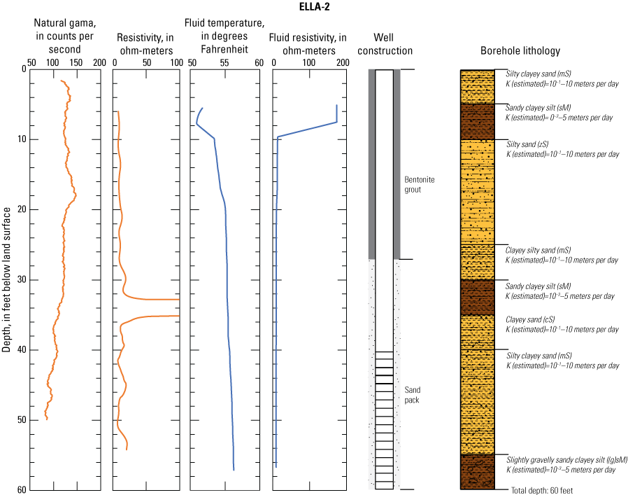
Geophysical logs, well-construction diagram, borehole lithology, and estimated hydraulic conductivity for single-well monitoring site ELLA-2 (07N/14W-30K2S). Data source: U.S. Geological Survey GeoLog Locator (U.S. Geological Survey, 2022). Site information in table 1.
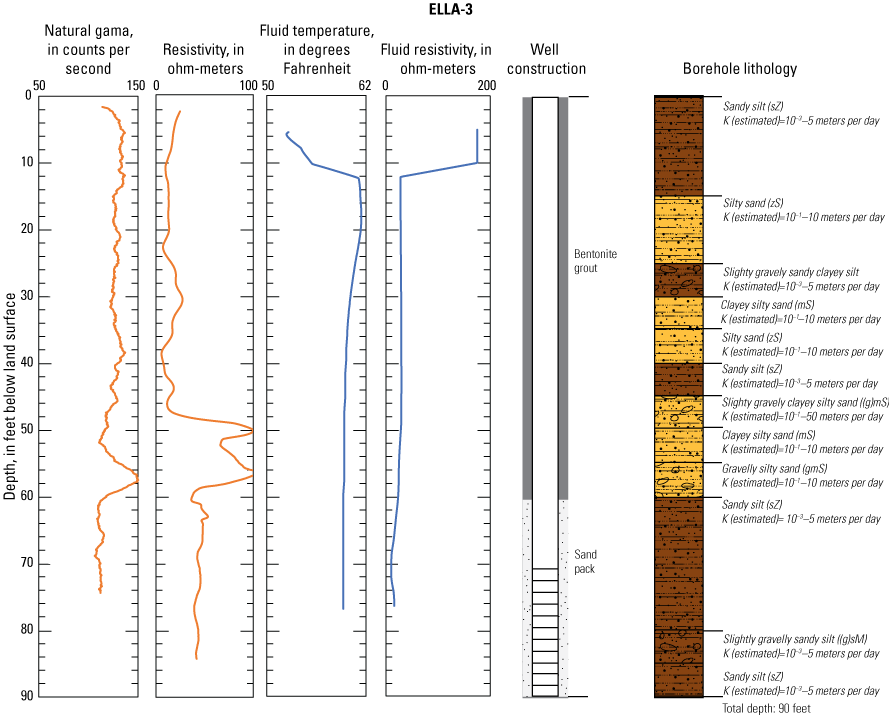
Geophysical logs, well-construction diagram, borehole lithology, and estimated hydraulic conductivity for single-well monitoring site ELLA-3 (07N/14W-30R1S). Data source: U.S. Geological Survey GeoLog Locator (U.S. Geological Survey, 2022). Site information in table 1.
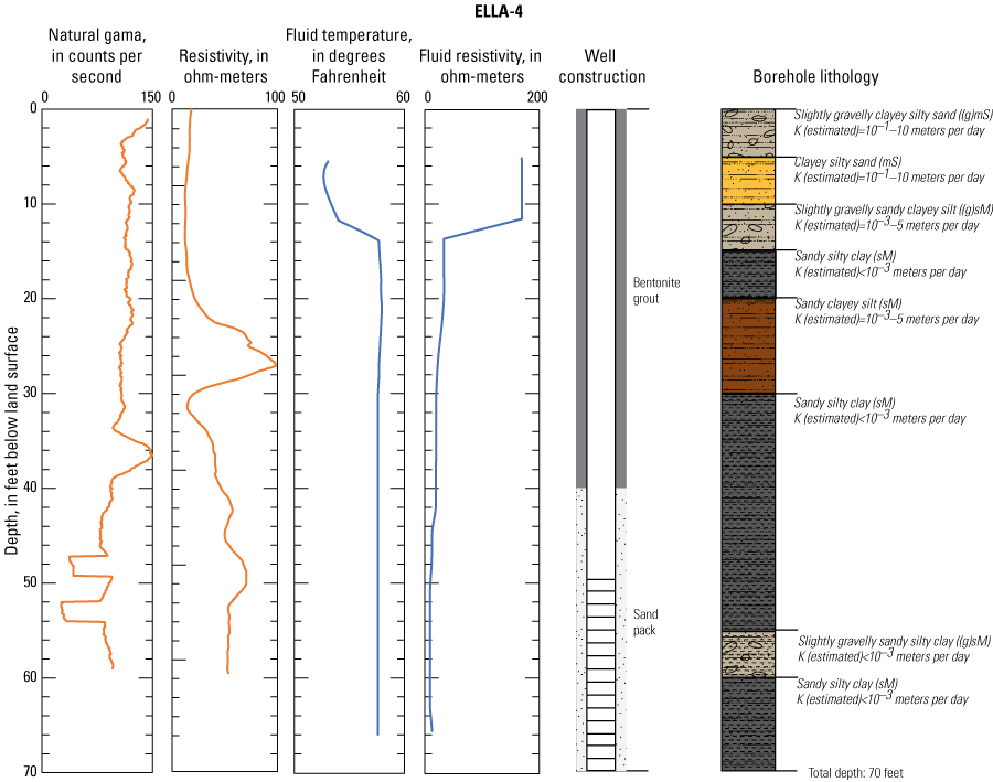
Geophysical logs, well-construction diagram, borehole lithology, and estimated hydraulic conductivity for single-well monitoring site ELLA-4 (07N/14W-29N1S). Data source: U.S. Geological Survey GeoLog Locator (U.S. Geological Survey, 2022). Site information in table 1.
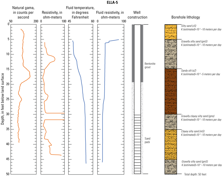
Geophysical logs, well-construction diagram, borehole lithology, and estimated hydraulic conductivity for single-well monitoring site ELLA-5 (07N/14W-29M1S). Data source: U.S. Geological Survey GeoLog Locator (U.S. Geological Survey, 2022). Site information in table 1.
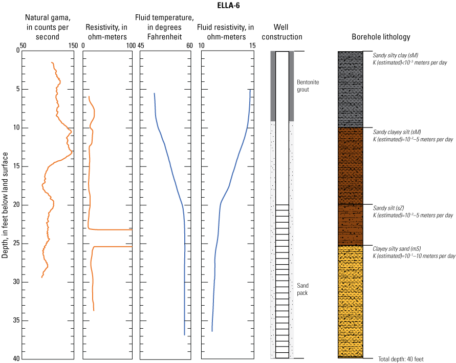
Geophysical logs, well-construction diagram, borehole lithology, and estimated hydraulic conductivity for single-well monitoring site ELLA-6 (07N/14W-29P1S). Data source: U.S. Geological Survey GeoLog Locator (U.S. Geological Survey, 2022). Site information in table 1.
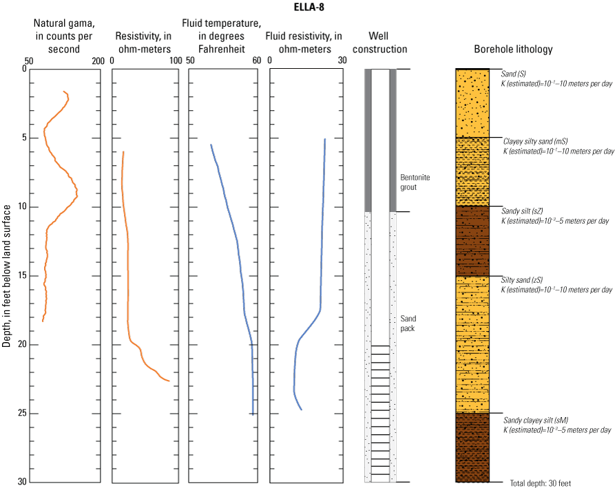
Geophysical logs, well-construction diagram, borehole lithology, and estimated hydraulic conductivity for single-well monitoring site ELLA-8 (07N/14W-29M2S). Data source: U.S. Geological Survey GeoLog Locator (U.S. Geological Survey, 2022). Site information in table 1.
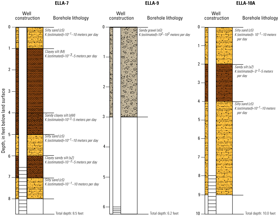
Geophysical logs, well-construction diagram, borehole lithology, and estimated hydraulic conductivity for single-well monitoring sites A, ELLA-7 (07N/14W-29L1S); B, ELLA-9 (07N/14W-30K3S); and C, ELLA-10A (07N/14W-29P2S). Data source: U.S. Geological Survey GeoLog Locator (U.S. Geological Survey, 2022). Site information in table 1.
Reference Cited
U.S. Geological Survey, 2022, USGS GeoLog Locator: U.S. Geological Survey database, accessed November 15, 2022, at https://doi.org/10.5066/F7X63KT0.
Conversion Factors
U.S. customary units to International System of Units
Temperature in degrees Celsius (°C) may be converted to degrees Fahrenheit (°F) as follows:
°F = (1.8 × °C) + 32.
Datum
Vertical coordinate information is referenced to the North American Vertical Datum of 1988 (NAVD 88).
Horizontal coordinate information is referenced to North American Datum of 1983 (NAD 83).
Altitude, as used in this report, refers to distance above the vertical datum.
Latitudes and longitudes are referenced to the World Geodetic System 1984 (WGS 84).
Groundwater levels below land surface are given in feet below land surface (ft bls).
Supplemental Information
Well depths and water levels are reported in feet/inches. These values are stored in feet/inches in the U.S. Geological Survey National Water Information System (NWIS; U.S. Geological Survey, 2023a), and they are reported on the National Water Information System website in feet/inches (https://waterdata.usgs.gov/nwis/).
Specific conductance is given in microsiemens per centimeter at 25 degrees Celsius (µS/cm at 25 °C).
Concentrations of chemical constituents in water are given in either milligrams per liter (mg/L) or micrograms per liter (µg/L).
Activities for radioactive constituents in water are given in picocuries per liter (pCi/L).
A tritium unit (TU) is equal to 3.19 picocuries per liter.
Trace gases (helium, neon, argon, krypton, xenon, and nitrogen) have the units of cubic centimeters at standard temperature and pressure per gram of water (cm3 at STP/g H2O). Standard temperature and pressure refer to 1 atmosphere of pressure at 0 degrees Celsius.
The element helium (He) has atoms with different masses: Helium-3 (3He) has two protons and one neutron in its nucleus, and helium-4 (4He) has two protons and two neutrons in its nucleus.
The isotopic ratio of helium in a sample can be expressed as δ 3He in units of percent:
δ(3He/ 4He) = [((3He/ 4He)sample/ (3He/ 4He)air))−1] X 100
Results for measurements of stable isotopes of an element in water, solids, and dissolved constituents commonly are expressed as the relative difference in the ratio of the number of the less abundant isotope to the number of the more abundant isotope of a sample with respect to a measurement standard. The oxygen-18 (18O) and deuterium (δD) abundances are reported in delta (δ) notation as stable isotope of nitrogen (δ18O) and δD in units of per mil (parts per thousand, ppt) relative to the isotopic composition of Vienna Standard Mean Ocean Water (VSMOW).
Absorbance units (AU) for dissolved organic matter are given in AU, absorbance units obtained from the analytical device.
Dissolved organic carbon (DOC) concentrations are given in milligrams per liter as carbon (mg/L as C).
Specific Ultraviolet Absorbance at 254 nanometers (SUVA254) results are given as liter per milligram of carbon per meter (L mg-C−1-m−1).
Fluorescence of dissolved organic matter is given in Raman-normalized intensity units (RU).
The electrical resistance tomography (ERT) system used in this study allowed for eight measurements to be taken at a time along a single transect. Measurements were taken for a period of 1.2 seconds, equivalent to 0.83 Hertz, during which the polarity of the current electrodes was reversed (number of cycles set to 2) to minimize electrode polarization effects. The resistivity meter was powered by two 12-Volt marine batteries and injected as much as 2,000 milliamperes of current into the ground.
Electrical resistivity ρ in ohm-meters (ohm-m) can be converted to electrical conductivity σ in siemens per meter (S/m) as follows: σ=1/ρ. Electrical conductivity σ in siemens per meter (S/m) can be converted to electrical resistivity ρ in ohm-meters (ohm-m) as follows: ρ=1/σ.
Absorbance wavelengths are given in nanometers (nm).
Phosphorus loads are given in pounds of phosphorus per year (lb-P/yr).
Nitrogen loads are given in pounds of nitrogen per year (lb-N/yr).
Humification index (HIX) is an indicator of humic substance content or extent of humification and is the area under the emission spectra at 435 to 480 nanometers divided by the peak area under the emission spectra at 300 to 345 with an excitation wavelength of 254 nanometers.
Freshness index (β:α) is an indicator of recently produced dissolved organic matter and is the ratio of emission intensity at 380 nm divided by the maximum emission intensity between 420 and 435 nm at excitation 310 nm.
Milliequivalents per liter are defined by the following formula: milliequivalents per liter=((mass of the constituent)*(charge of constituent))/molecular weight. Mass and molecular weight are given in milligrams.
Abbreviations
A:C
The ratio of fluorescence intensity of peak A (excitation of 260 and emission of 450 nanometers to peak C (excitation at 340 and emission at 440 nanometers)
δD
deuterium
3H
tritium
3Hetrit
tritiogenic helium-3
CE
closed-system equilibrium model
CWA
Clean Water Act
DA
discriminant analysis
DGMETA
dissolved gas modeling and environmental tracer analysis
DO
dissolved oxygen
DOC
dissolved organic carbon
DOM
dissolved organic matter
DWR
Department of Water Resources
em
emission wavelength
ERT
electrical resistivity tomography
ex
excitation wavelength
F
fluoride
Fe
iron
GMWL
global meteoric water line
HIX
humification index
HSD
Tukey’s Honest Standard Deviation
Kr
krypton
LARWQCB
Los Angeles Regional Water Quality Control Board
Mn
manganese
N
nitrogen
N2
nitrogen gas
N2O
nitrous oxide
NWQL
National Water Quality Lab
org-N
organic nitrogen
OSWCR
Online System for Well Completion Reports
OWTS
onsite wastewater treatment systems
P
phosphorus
PCA
principal component analysis
PVC
polyvinyl chloride
QC
quality control
SC
specific conductance
SpC
Fluorescence at excitation of 420 nanometers with emission at 460 nanometers divided by dissolved organic carbon concentration
SpZ
Fluorescence at excitation wavelength of 420 and emission at 460 nanometers divided by dissolved organic carbon concentration
SUVA254
Specific Ultraviolet Light Absorption at 254 nanometers divided by dissolved organic carbon concentration
SUVA280
Specific Ultraviolet Light Absorption at 280 nanometers divided by dissolved organic carbon concentration
TDS
total dissolved solids
TMDL
total maximum daily load
TN
total nitrogen
TP
total phosphorus
USGS
U.S. Geological Survey
UV
ultraviolet
Xe
xenon
For more information concerning the research in this report, contact the
Director, California Water Science Center
U.S. Geological Survey
6000 J Street, Placer Hall
Sacramento, California 95819
https://www.usgs.gov/centers/california-water-science-center
Publishing support provided by the U.S. Geological Survey
Science Publishing Network, Sacramento Publishing Service Center
Disclaimers
Any use of trade, firm, or product names is for descriptive purposes only and does not imply endorsement by the U.S. Government.
Although this information product, for the most part, is in the public domain, it also may contain copyrighted materials as noted in the text. Permission to reproduce copyrighted items must be secured from the copyright owner.
Suggested Citation
McGregor, A.M., Domagalski, J.L., Groover, K.D., Hansen, A.M., and Brown, A.A., 2024, Nutrient chemistry in the Elizabeth Lake subwatershed—Effects of onsite wastewater treatment systems on groundwater and lake water quality, Los Angeles County, California: U.S. Geological Survey Scientific Investigations Report 2024–5012, 70 p., https://doi.org/10.3133/sir20245012.
ISSN: 2328-0328 (online)
Study Area
| Publication type | Report |
|---|---|
| Publication Subtype | USGS Numbered Series |
| Title | Nutrient chemistry in the Elizabeth Lake subwatershed—Effects of onsite wastewater treatment systems on groundwater and lake water quality, Los Angeles County, California |
| Series title | Scientific Investigations Report |
| Series number | 2024-5012 |
| DOI | 10.3133/sir20245012 |
| Publication Date | April 16, 2024 |
| Year Published | 2024 |
| Language | English |
| Publisher | U.S. Geological Survey |
| Publisher location | Reston, VA |
| Contributing office(s) | California Water Science Center |
| Description | vii, 70 p. |
| Country | United States |
| State | California |
| County | Los Angeles County |
| Other Geospatial | Elizabeth Lake subwatershed |
| Online Only (Y/N) | Y |