

Evaluation of Groundwater Resources in the Upper White River Basin within Mount Rainier National Park, Washington State, 2020
Links
- Document: Report (5.2 MB pdf) , HTML , XML
- Data Release: USGS data release - Soil water balance model of the White River basin, Mount Rainier National Park, Washington, USA
- Version History: Version History
- NGMDB Index Page: National Geologic Map Database Index Page (html)
- Download citation as: RIS | Dublin Core
Acknowledgments
The authors would like to thank Rebecca Lofgren with the National Park Service for her help with coordinating and advising on this project. Additional thanks are extended to Adam Opryszek, Rusty Sherman, Steve Sissel, and Alison Tecca for their assistance in the field.
Abstract
The U.S. Geological Survey (USGS), in cooperation with the National Park Service, investigated groundwater gains and losses on the upper White River within Mount Rainier National Park in Washington. This investigation was conducted using stream discharge measurements at 14 locations within 7 reaches over a 6.5-mile river length from near the White River’s origin at the terminus of the Emmons Glacier on Mount Rainier to the White River Entrance near the northeast boundary of Mount Rainier National Park. Locations selected for the stream discharge measurements were on the main channel of the White River and on tributary streams near their confluence with the White River.
A soil-water-balance (SWB) model analysis was also performed on the White River basin to estimate groundwater recharge throughout the basin during the time of the study. Analyses were made for the White River basin at the sub-basin (zone) scale to determine groundwater input to the stream for individual stream reaches. The gridded SWB model was simulated at a 10-meter (m) horizontal resolution, where recharge simulations were constructed using five spatially distributed datasets. Daily climate data as input for the simulation included gridded daily precipitation and air temperature.
Upon analysis of the seepage run results, three of the seven reaches showed groundwater gains in this study. The SWB model results were used in conjunction with the baseflow gain totals in the reaches to estimate the length of time for recharge to become base flow. Further analysis estimated the rates of groundwater flow in the zones with adjacent gaining reaches. A streamflow gain curve was created from a simple flow model for each of the zones to relate the recharge from the zones to the adjacent reaches on the White River and tributaries. The fit of the streamflow gain curve to the calculated streamflow gain during the seepage run was used to analyze where the recharge from each zone resulted as streamflow gain. Consecutive reach losses from zones D and L were immediately followed downstream by a relatively large gain in zone GH, indicating that the gain in the reach adjacent to zone GH could be from the recharge in zones D and L.
Introduction
Mount Rainier National Park received more than 1.6 million recreation visitors in 2021 (National Park Service Social Science Program [NPS SSP], 2022) and relies primarily on streams and lakes fed by snowmelt and melting glaciers for the water supply of its local visitor and operational facilities. Within the upper White River area of Mount Rainier National Park (fig. 1), surface water is the sole source of water for these uses and park managers are interested in exploring groundwater as a supplemental source. An investigation of the availability of groundwater in the upper White River basin, upstream from the White River Entrance, was proposed as a means of identifying additional water sources to help Mount Rainier National Park adapt to increasing demand and reduced water supplies in the future.
In this study, the U.S. Geological Survey (USGS), in cooperation with the National Park Service, performed an investigation of the groundwater resources of the upper White River basin. The objective of this project is to estimate the groundwater inflows and outflows (groundwater balance) for the purpose of informing park managers regarding the potential to access and use groundwater.
Purpose and Scope
The purpose of this report was to assess the available groundwater resources within the upper White River basin and provide Mount Rainier National Park water managers with information that helps them identify potential supplemental water supplies for visitor and operational facilities. This report focused on the upper White River basin, from the terminus of the Emmons Glacier to the White River Entrance in the western portion of Mount Rainier National Park (fig. 1). In order to estimate the groundwater discharge component of streamflow, measurements were made at 14 locations along the upper White River and several of its tributaries over a 2-day period, from September 21 to 22, 2020. Estimates of daily groundwater recharge to the upper White River basin were made using the soil-water-balance (SWB) model for the year 2020 in order to determine groundwater input to the stream.
Description of Study Area
The study area is the upper White River basin in Mount Rainier National Park, with the western edge of the area beginning near the terminus of the Emmons Glacier and extending to the eastern park boundary (fig. 1). The study area is about 35 square miles (m2). Flowing from west to east, the section of the White River included in this study passes the confluence with the Inter Fork River, the White River Campground, and the White River Entrance that includes the White River Ranger Station prior to reaching the park boundary. Beyond the park boundary, the White River generally flows north before turning west near Greenwater, Washington. The northern extent of the study area is near Frozen Lake, which is about 1.2 miles (mi) northwest of Sunrise Visitor Center, and the southern boundary of the study area is the ridge extending east from the Fryingpan Glacier.
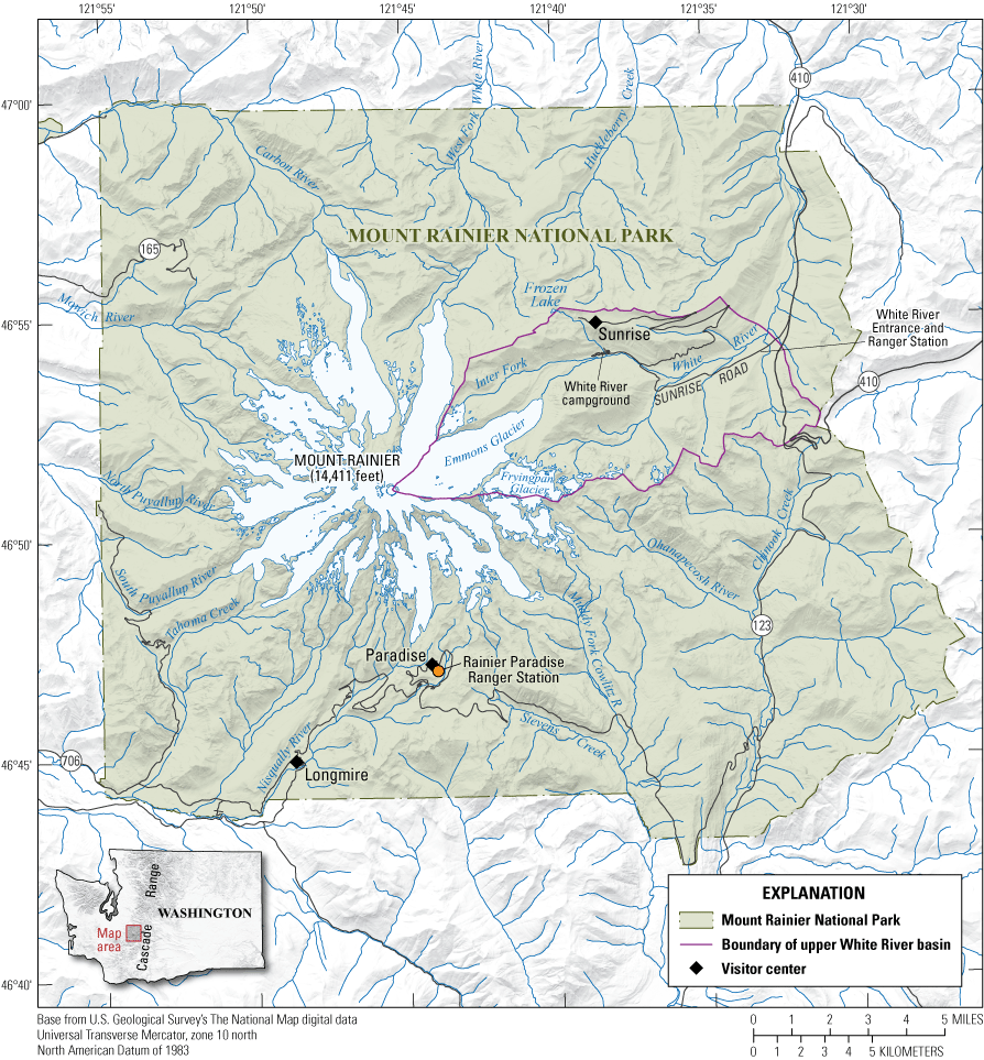
Location of study area, Mount Rainier National Park, Washington.
Geologic Setting
Mount Rainier, which is 14,410 feet (ft) in elevation, is a widely glaciated, active composite volcano on the west slope of the Cascade Range in Washington State. It is primarily composed of andesitic and dacite lava flows built upon a base of altered volcanic and granitic rocks (Fiske and others, 1963). Some of the youngest rocks consist of unconsolidated glacial and glaciofluvial debris, mudflows, and ash and pumice deposits, with the most recent pyroclastic eruptions occurring as recently as 500 years ago (Fiske and others, 1963). There are 26 named glaciers that cover portions of Mount Rainier, and they serve as the headwaters for 5 major rivers: the Cowlitz, Nisqually, Puyallup, Carbon, and White Rivers. The Emmons Glacier, on the northeast flank of the volcano, is at the headwaters of the White River (Pringle, 2008).
The Emmons Glacier and the White River have eroded through Mount Rainier’s volcanic material into the Keechelus andesitic series. However, the distribution of these formations is now hidden by the glacier and its deposits, and by the large areas of talus on the slopes above the lateral moraines (Fahnestock, 1963). Glacial valley fills are mostly covered by volcaniclastic material in the upper White River and West Fork White River valleys, primarily from the Osceola Mudflow that occurred about 5,600 years ago (Crandell, 1971; Crandell and Miller, 1974). The White River valley contains mostly alluvial deposits made up of sand, gravel, and cobbles. Alluvial sediments are relatively consistent down the length of the valley with median grain-size diameters of about 30–50 millimeters (mm; Anderson and Jaeger, 2020).
Climate
Mount Rainier’s location on the west side of the Cascade Range drainage divide and its proximity to the Pacific Ocean significantly affect the area’s climate in both summer and winter (Fahnestock, 1963). The following climate data are derived from the 1991–2020 monthly and annual normals provided by the National Oceanic and Atmospheric Administration (National Oceanic and Atmospheric Administration, 2022) for Rainier Paradise Ranger Station, Washington (station ID USC00456898), which is about 10 mi southwest of Sunrise Visitor Center. Mean annual precipitation was about 116 inches (in.), with November, December, and January each averaging 17–18 in. of monthly precipitation. Summers (June–August) are normally dry, with a mean total precipitation of 6.89 in. Mean monthly temperature is about 27 degrees Fahrenheit (°F) in December and about 54 °F in August. Glacial meltwater from the Emmons Glacier to the White River is generally at its highest when annual temperatures are at their highest in late summer. The rain-snow mixed-precipitation that is typical of the White River basin has contributed to the area’s largest-magnitude floods. These floods occur in fall and winter, associated with atmospheric rivers (Neiman and others, 2011; Konrad and Dettinger, 2017). Smaller floods associated with snowmelt have occurred in the spring.
Methods and Results
Stream discharges were measured at 14 sites to estimate the interaction of groundwater and surface water for the upper White River and its tributaries. A SWB model was used to estimate the amount and timing of groundwater recharge within the basin. A simple flow model was used to develop a conceptual understanding of the relation of groundwater recharge to groundwater discharge to streams.
Several assumptions were made about the general flow of water through the basin for this study. It was assumed that groundwater flows in the direction of the land-surface gradient and that it will discharge to its adjacent downgradient stream reach unless it is a losing reach. For areas with glacial cover, it was assumed that glacial melt results in groundwater recharge underneath the glacier and runoff at the toe of the glacier. For the remainder of the study area without glacial cover, the groundwater budget components consist of groundwater recharge from precipitation and groundwater discharge to streams. Groundwater outflow from the watershed at the outlet of the study area is assumed to be small with respect to other components and is therefore not considered in this study.
Stream Discharge Measurements
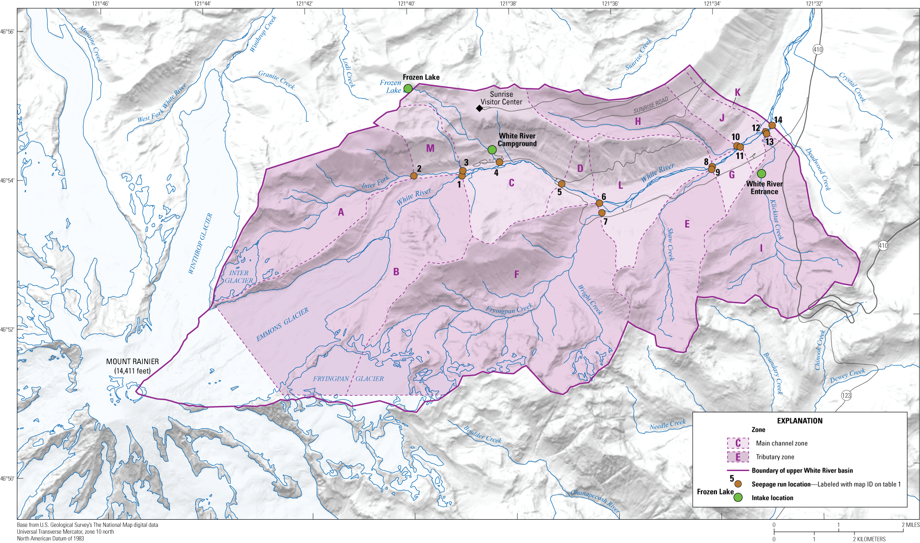
From September 21 to September 22, 2020, low-flow synoptic stream discharge measurements were made at 14 sites on the White River and its tributaries to determine streamflow gains from or losses to groundwater between sites, hereafter referred to as a “seepage run” (table 1; fig. 2). The period for measurement was selected because the prevailing cool temperatures would minimize glacial melt contributions to stream discharge and was prior to the region’s rainy season, minimizing runoff contributions to stream discharge (National Oceanic and Atmospheric Administration, 2022). During this period, stream discharge was steady and at or near the lowest values of the year, resulting in the best conditions for estimating the rate of transfer of water between groundwater and streams (Rosenberry and LaBaugh, 2008; fig. 2). Cross-sectional areas were measured and velocity was recorded at these locations using a hand-held velocity meter to estimate discharge using the velocity-area method (Rantz and others, 1982). Stream discharge measurements are available from the USGS National Water Information System (NWIS; U.S. Geological Survey, 2022).
Table 1.
Map identification numbers and their respective U.S. Geological Survey station identifiers and names.[Station locations are shown in figure 2. Abbreviations: ID, identification number; USGS, U.S. Geological Survey]
Streamflow gain from or loss to groundwater (seepage gain or loss) was calculated for seven sections of the White River between sites (reaches), using the Williams (2011) equation below:
whereOd
is discharge measured at the downstream end of the reach, in cubic feet per second (ft3/s),
Ou
is discharge measured at the upstream end of the reach, in ft3/s, and
T
is the sum of tributary inflows, in ft3/s.
Each site on the White River was upstream from a tributary confluence except for sites 2 and 5. Site 2 was the most upstream on the White River and site 5 is where Sunrise Road crosses the White River, the location of a historical USGS stream gage (12096600). Stream discharge measurement stations are shown in figure 2, and the corresponding zones and reach numbers are shown below in table 2.
Table 2.
White River reaches and their adjacent map IDs and zone identifiers.[Abbreviations: ID, identification number; –, no data given]
Upper White River drainage basin in Mount Rainier National Park, Washington.
Soil-Water Balance Model
The soil-water-balance (SWB) model v. 1.2 (Westenbroek and others, 2010) provided gridded estimates for groundwater recharge (fig. 3). The SWB calculates water-balance components at daily time steps for each model cell using a modified Thornthwaite Mather soil-water-balance approach. Seven spatially distributed (gridded) input datasets were used to drive SWB recharge simulations: daily climate data (precipitation, maximum and minimum air temperature), land cover, flow direction, and soil properties (hydrologic soil group and available soil-water capacity). All input and output datasets for the SWB were resampled to a uniform cell size of 10 meters (m) for the 35 m2 study area. The model run was set up for January 1999–December 2020, with the year 1999 being used as the initialization period. Results were reported for January 2000–December 2020. The SWB model and output used in this study are available in Headman (2022).
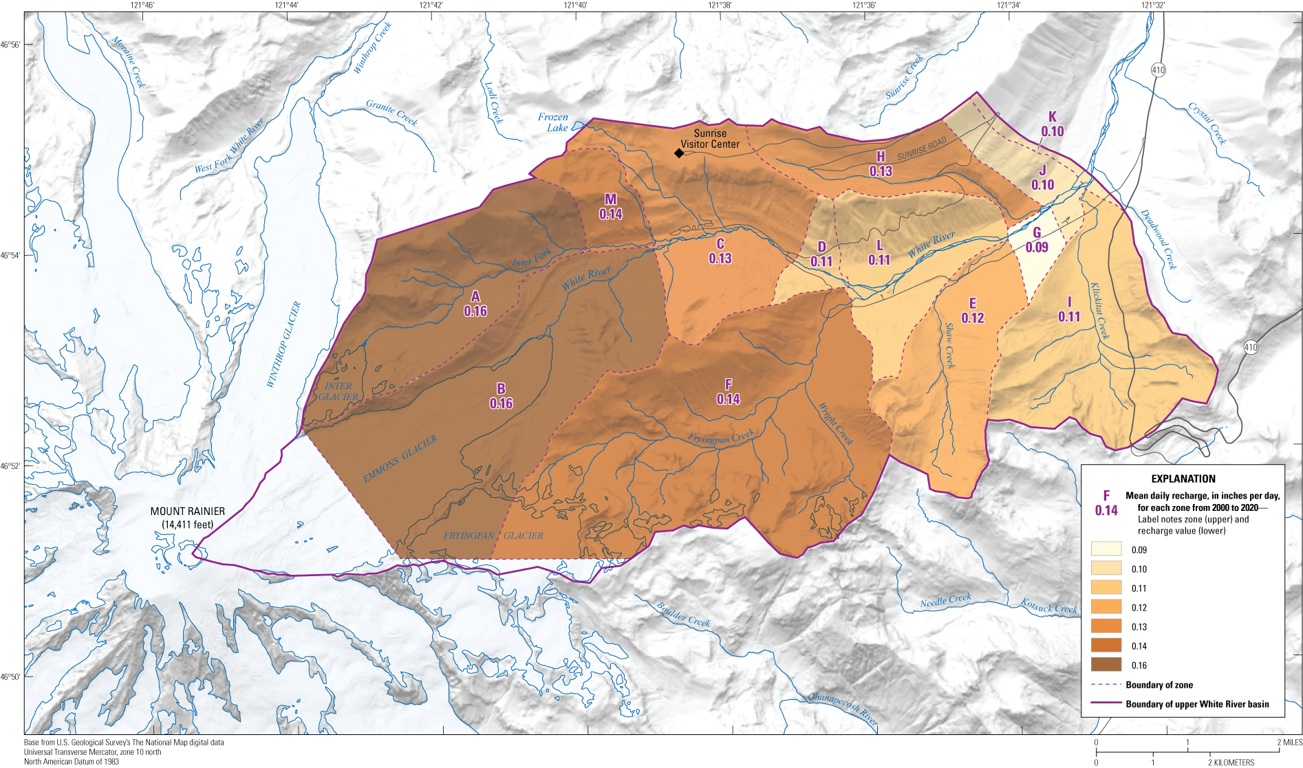
Mean daily recharge by study area zone, in Mount Rainier National Park, Washington.
Daily climate input datasets included precipitation (inches) and maximum and minimum temperature (Fahrenheit). Daily climate data were obtained from the Daymet dataset available from Oak Ridge National Laboratory (Thornton and others, 2022). The Daymet climate data were computed through interpolation from spatially referenced observation stations and available in 2-degree areas at a spatial resolution of 1 kilometer (km) for all of North America. Daily Daymet climate data were obtained for the study area for the period from January 1999 through December 2020.
The 2016 National Land Cover Database (Wickham and others, 2021) was used to characterize land cover. The NLCD is produced by the Multi-Resolution Land Characteristics consortium to describe land-cover characteristics across the United States using a 16-class classification schema at a resolution of 100 ft. The NLCD was obtained from https://www.mrlc.gov/data/nlcd-2016-land-cover-conus (Wickham and others, 2021). The NLCD data were resampled to the 10 m cell size of the SWB model using a majority sampling technique in ArcGIS (ESRI, 2021). A comparison of the resampled and original gridded datasets indicated that the spatial pattern for the principal land-cover classes in the study area were similar.
The flow direction grid was generated from light detection and ranging (lidar) elevation data at 6 ft resolution (Watershed Sciences, 2009) accessed via the Washington Lidar Portland D8 flow-routing convention of Lehner and others (2008). D8 Flow Routing is a hydrological modeling method used to simulate the movement of water through a digital elevation model (DEM) in eight flow directions. In this approach, each grid cell is assigned a flow direction based on the steepest descent, and flow is directed toward one of the eight neighboring cells.
Individual lidar files were combined and resampled to the 10 m cell size of the SWB model using a mean sampling technique in ArcGIS. The resulting elevation grid was processed to smooth over small sinks that were artifacts of data processing and the D8 flow-direction grid was then generated with the ArcGIS “flow direction” tool.
Two gridded datasets of soil properties, hydrologic soil group (HSG), and available water capacity (AWC) were compiled by the U.S. Department of Agriculture Natural Resources Conservation Service (NRCS) for the United States. The NRCS classified HSGs in four groups (A, B, C, and D) on a continuum from high infiltration capacity with low runoff potential to low infiltration capacity with high runoff potential. The AWC is the amount of water a particular soil column can hold at various depths; the AWC for the top meter of soil was used by the SWB model. Data for HSG and AWC were obtained from the NRCS Gridded Soil Survey Geographic (gSSURGO) database (National Resources Conservation Service, 2021). The HSG and AWC grids were resampled using ArcGIS raster resampling tool to 10 m cells using the majority technique for HSG data and the mean sampling technique for AWC data.
The equations used by the SWB model to calculate recharge do not have an input for contribution from glacial melt. The recharge input from glaciated areas was limited to precipitation that occurred during the model simulation. To adjust for this limitation, recharge from snow and (or) ice in areas covered by glaciers in the SWB model area was calculated using a snowmelt rate of 1.5 mm per day (as snow-water equivalent) per average degree Celsius where the daily maximum air temperature (Tmax) is above the freezing point (Westenbroek and others, 2010). The landcover for perennial snow and ice, using a runoff curve number of 40 and a root zone depth of 0, is used by SWB for areas with glacial cover. Daily evapotranspiration was computed using the method of Hargreaves and Samani (1985).
Additional non-gridded inputs were required for SWB model for each combination of HSG and land cover type. These data were provided as a table and included runoff curve numbers, vegetation routing depths, maximum infiltration rates, and maximum daily recharge rates used by Gendaszek and Welch (2018), Tillman (2015), and Westenbroek and others (2010).
Stream Discharge Correction for Glaciated Areas
In glaciated areas, streamflow can fluctuate on a diurnal cycle with higher flows during the warmer hours of the day when glacier melting rates are high, and lower flows during the cooler hours of the night when glacier melting rates are low. Stream discharge measurements made during the seepage run were taken at various times over 2 consecutive days. Given the diurnal nature of glacial melting, the amount of glacial melt water contributing to stream discharge varied with the timing of measurement. Two methods were evaluated to estimate and exclude the glacial meltwater contribution from stream discharge measurements using available stream discharge data.
One method evaluated the use of continuous discharge records from a downstream stream gage to estimate the diurnal changes in glacial melt contributions to White River discharge. The nearest gage, upper White River basin (USGS gage 12097000), is about 21 river miles downstream from the park entrance. After review, this method was not useful because additional tributary inflow and travel time over the 21 river miles downstream introduced too much variability to estimate glacier meltwater contributions to base flow in the study area.
A second method evaluated stream discharge measurements collected during the seepage run to estimate the diurnal changes in glacial melt contributions to White River discharge. Site 5 was measured twice during the seepage run: at 1910 hours on September 21 and at 0854 hours on September 22. The change in discharge that occurred during the length of time between the morning and evening measurement was used to estimate the diurnal change in discharge due to glacial melt.
The rate of change in discharge throughout the day is assumed to be a linear increase with respect to time, typical of the rising limb on a simplified hydrograph showing a diurnal response to glacial melt (Singh and Singh, 2001). The relationship between the amount of time between measurements and the change in discharge at site 5 was therefore used to estimate the increase in discharge in ft3/s due to glacial melt for measurements at other sites on the White River based on the time of measurement. This method was used to adjust the discharge by the amount of time that had lapsed from the first station 5 measurement to reduce each station’s measured discharge by its approximate contribution from increased glacial melt (table 3). These discharge values were determined using the following equation:
whereQadj
is the adjusted discharge, in ft3/s;
Q
is the measured discharge, in ft3/s;
T
is the time of measurement;
T1
is the time of the morning measurement at site 5;
T2
is the time of the evening measurement at site 5;
Q1
is the measured discharge during the morning measurement at site 5, in ft3/s; and
Q2
is the measured discharge during the evening measurement at site 5, in ft3/s.
The consistent air temperatures during the 2 days where measurements were collected allowed for the assumption that the minimum and maximum discharge was the same during these days. The measurements were then treated as having been collected in the same day for the sake of relating this elapsed time with discharge. The length of time between the morning measurement and the time each measurement was taken was used to correct the measured discharge and estimate an “adjusted” discharge (table 3).
Table 3.
Stream discharge measurements on the White River in Mount Rainier National Park, Washington, September 21–22, 2020.[Time of collection: Time is written in 24-hour time standards. Abbreviations: ft3/s, cubic feet per second; ID, identification number; –, no data given]
Streamflow Gain or Loss and Base-Flow Calculations
The adjusted discharge measurements from White River sites and discharge measurements from the tributary sites were used to calculate streamflow gain and loss (see the equation in “Methods” section) and base-flow contribution to the White River for each reach (table 4).
Table 4.
Summary of calculations for White River streamflow gain and loss estimation, Mount Rainier National Park, Washington.[Measurement error: Based on uncertainty ratings for streamflow measurements (Sauer and Meyer, 1992). Root mean square error: Root mean square error (RMSE) calculations were based on the error associated with the discharge measurements that were used to calculate the estimated streamflow gain or loss. For measurements that had an error range, the larger of the two numbers in the range was used to calculate the RMSE. An error of 12 percent was used to calculate the RMSE for the measurements that had an error of >±8. Abbreviations: ID, identification number; –, no data given; Od, discharge measured at the downstream end of the reach, in ft3/s; Ou, discharge measured at the downstream end of the reach, in ft3/s; T, the sum of tributary inflows, in ft3/s; %, percent; +, gain; −, loss; ±, plus or minus; >, greater than; ft3/s, cubic feet per second]
Upon analysis of the results from the seepage run, three of the reaches were found to be gaining reaches: M2–3, C3–5, and G8–11 (table 4). Analysis of the remaining four segments showed losing reaches.
Relation of Groundwater Recharge to Groundwater Discharge to Streams
Recharge zones A–M were delineated for drainage areas that corresponded to reaches on the White River and its tributaries (fig. 2). Delineation for these zones was achieved by drawing flow lines perpendicular to topographic contours, generally starting with locations that marked the ends and beginnings of each of the reaches, to the point where the drawn flow lines met a ridge. Recharge values were determined for each zone by averaging the SWB simulated recharge grid cell values contained in each zone and converting the recharge value to ft3/s (fig. 3). Recharge from these zones was then used to estimate the groundwater discharge to each of the reaches. Zones M, C, D, L, G, J, and K corresponded to reaches on the White River and were the focus of the comparison of zone recharge and streamflow gains or losses within each zone (table 2; fig. 2). To interpret the results of this comparison, a simple flow model was applied, which is described in the section “Flow Model and Assumptions.”
Flow Model and Assumptions
For this analysis, each zone is treated as a system in which recharge is the input, or forcing. An increase in the forcing results in an increase in the water table, steepening the hydraulic gradient toward the stream, which results in an increase in groundwater flow into the stream. Conceptually, this is illustrated in figure 4A, which shows an increase in springtime recharge resulting from combined snowmelt and precipitation, followed by recharge recession during summer. The response in streamflow gain is simplified and represented by a rising limb and falling limb, each linear, which results in a simple triangle. The peak in streamflow gain lags behind the recharge forcing and is spread out temporally because of the groundwater storage capacity. Storage in groundwater is the reason that streamflow gains can occur throughout summer when recharge becomes nearly zero. The peak in streamflow gain occurs as a lagged response to the peak in recharge, which is hereafter referred to as “peak-to-peak lag time” (fig. 4A). The lag time does not represent a travel time of water molecules; rather, this is the response time corresponding to the transfer of pressure through the groundwater system. Mathematically, this process is well described by convolution, the basis of unit-hydrograph theory (Singh, 1988; Long and Mahler, 2013).
To illustrate how the concept shown in figure 4A applies to this study, a dot along the falling limb of the triangle represents a hypothetical measurement of the streamflow gain during late summer. Because this streamflow gain measurement is the only one available, the peak response time and magnitude cannot be known; however, a minimum and maximum range of the peak-to-peak lag time can be estimated, where the minimum would be concurrent with the recharge peak (peak-to-peak lag=0). It was assumed that the falling limb could not be steeper than the rising limb, an assumption that is consistent with unit-hydrograph theory (Singh, 1988; Long and Mahler, 2013), and therefore, the latest peak response in streamflow gain would be determined by an isosceles triangle that passes through the data point representing the measured streamflow gain (fig. 4). Additional assumptions:
-
(1) the start of the rising limb is concurrent with the initial rise in the recharge rate;
-
(2) for conservation of mass, the volume under the recharge curve is equal to the volume under the response curve; and
-
(3) the base of the recharge curve for computing this volume is defined by a straight line from initial rise in recharge to the base of the recharge curve when it has fallen to zero (fig. 4B). Figure 4 and associated assumptions describe a simple flow model that was applied to each zone in this study to better understand and quantify how recharge-discharge relations differ for the different zones.
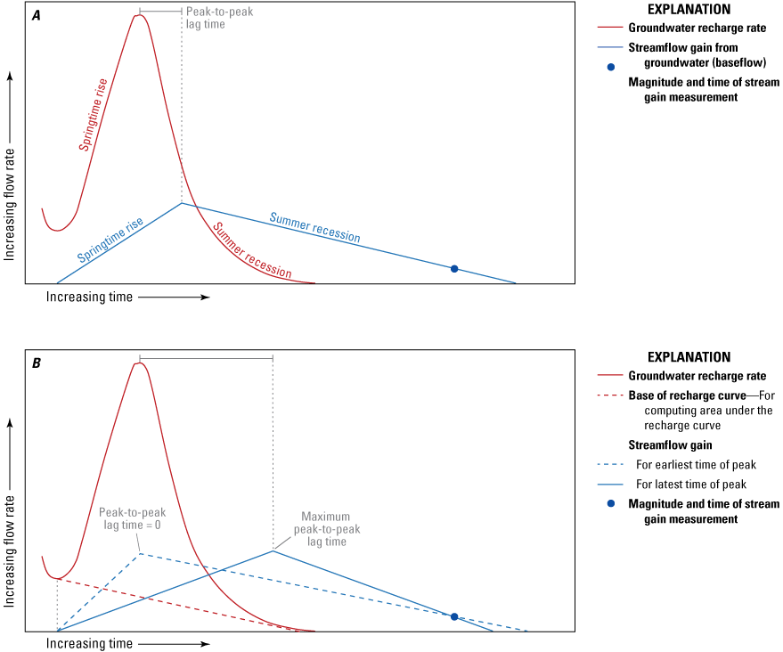
Example recharge and stream gain relationship between increasing flow rate and increasing time. The rise in the recharge rate results from springtime snowmelt and precipitation increases (A); example recharge and streamflow gain relationship (B).
Flow Model Applied to Each Zone
A 4-week moving average was applied to the estimated daily recharge rate for each zone to account for the dispersive mixing of recharge water in the unsaturated zone and near the water table. This moving average was used as the recharge forcing function for this analysis. The recharge that began in late February 2020 was assumed to be the primary source of the streamflow gain in the White River during the September 2020 measurement.
The flow model was applied to three zones that correspond to gaining reaches on the White River (reaches M2–3, C3–5, and G8–11, zones M, C, and G, respectively; fig. 2). The discharge measurement, streamflow gain estimate, and corresponding zone recharge estimate from the model for each reach are shown in figure 5. The zone recharge was considered as a 4-week moving average, represented in the figures at the date that falls in the middle of the 4-week time window. The streamflow gain estimate in each of these figures shows the streamflow gain curve with its peak occurring at the maximum time from its initial rise, equal to the time for the streamflow gain rate to return to zero from its peak. This allows for comparison of peak-to-peak lag time between each of the zones.
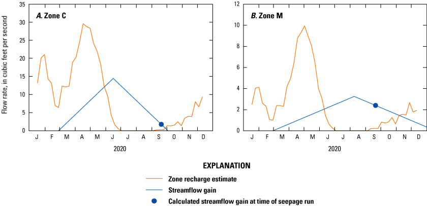
Model zone C recharge and streamflow gain in reach C3–5 (A) and model zone M recharge and streamflow gain in reach M2–3 (B).
An analysis similar to the one done for the zones on the White River was done for the zones representing each of the tributaries (zones A, B, E, F, GH, I, and K) to provide a comparison of the alluvial areas in each of the tributary streams in these zones. For these zones, the amount of gain in the tributary stream is measured by treating the headwater of the stream as having zero discharge, representing the OU term from the equation in the “Methods” section. Therefore, the streamflow gain for the adjacent reach in each of these zones is equal to the discharge measured at the station at the downstream end of the zone. Glaciers are present in zones A, B, and F. Streamflow gain curves were estimated for these zones but due the limited ability of SWB to estimate recharge in areas with glacial cover, the results were not expected to be accurate. The zones with glacial presence in the published SWB model were slightly truncated from the full basin delineation, most notably in zone B. The same analysis performed for the main stem recharge zones, where response rates were estimated using the two areas on each side of the stream and their respective distances to the stream, was also completed for the tributary zones. This is shown in figure 6. For zone B (fig. 6B), recharge was less than the measured streamflow gain, which is further discussed later in this section.
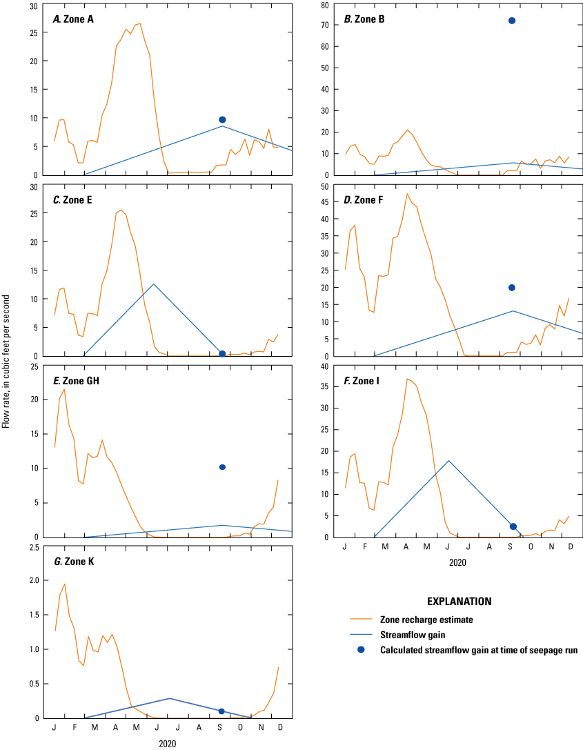
Recharge and streamflow gain for model zone A (A), model zone B (B), model zone E (C), model zone F (D), model zone GH (E), model zone I (F), and model zone K (G).
Table 5.
Summary of recharge calculations in zones adjacent to gaining reaches.[Abbreviations: ft3/s, cubic feet per second; d, days; –, no data given]
Reach G8–11 showed the largest gain of any of the reaches, 10.2 ft3/s (table 4). Further analysis of reach G8–11 revealed that the tributary stream in zone H enters the White River Valley alluvium at the base of the steeply sloping valley wall, where it parallels the White River for a length of about 1,500 ft prior to exiting zone H and entering the White River (fig. 2). The proximity of this tributary parallel to the White River, its location within the White River alluvium, and the large increase in base flow within reach G8–11 indicate that zone H likely discharges much of its recharge as base flow directly to the White River within reach G8–11. Therefore, the recharge for zone H was combined with that of zone G, and these two zones were analyzed together as a single zone (zone GH) associated with reach G8–11 (fig. 6E). The error associated with the streamflow gain analysis for zones G and H (92.3 and 96.7 percent, respectfully) was reduced by combining the two zones, as the error with the zone GH analysis was 82.8 percent.
Streamflow gain for zone B was more than three times larger than the peak recharge rate (fig. 6B). Discharge from the toe of the glacier was not measured, and most of the discharge at station 1 is assumed to be provided by glacier melt. Because recharge was estimated for the area downslope of the glacier, discharge at the toe of the glacier would be needed for this analysis to be applicable. Zones A and F also include glaciers that are smaller and occupy smaller proportions of the zones than zone B. This analysis was applied to those zones, while accepting that the glaciers in these zones may introduce error.
Flow Model Application to Combined Zones
To perform the same analysis for the upper White River basin as a single zone that was done for each of the individual zones within the basin, the cumulative estimated recharge for all non-glacial zones (zones C, E, GH, I, K, M) were plotted with the total gain measured between the most upstream and most downstream stream discharge measurement locations (locations 1 and 14, respectively), 28.8 ft3/s (fig. 7). Zones A, B, and F were excluded from this analysis due to the large glacial presence in the zones and the associated lack of accuracy with its SWB-modeled recharge estimate. The peak-to-peak for this area was 74.4 days, which was comparable to the peak-to-peak distance found in the analyses done for individual zones (see row “All,” table 5; fig. 7).
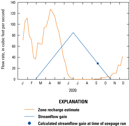
Zone recharge estimate and streamflow gain for all non-glacial zones.
Discussion
For zones with gaining reaches, the estimated streamflow gain curve shown in the flow model was either able to fit the calculated streamflow gain from the measurements taken in the White River and tributaries at the time of the seepage run, or the streamflow gain estimated by the flow model fell below this calculated streamflow gain. For zones where the calculated streamflow gain fit the flow model, the quantity of water that entered the ground as recharge in the zone was consistent with the calculated streamflow gain at the time of measurement. Conversely, the zones with losses or zones with gains where the model fails to fit the recharge to the calculated streamflow gain indicate that the rate of streamflow gain in the reach cannot be fully accounted for by the estimated recharge. The sequence zones for which the model can be fit, zones where the model does not fit, and zones with a losing stream reach can be used to draw inferences and develop a conceptual model of groundwater flow in the White River basin.
The flow model did not fit the calculated streamflow gains in the tributary zones where glaciers were present (zones A, B, and F; fig. 2). SWB’s inability to accurately estimate the contribution of glacial melt to the White River and its tributaries likely underestimated the recharge to these zones, resulting in discharge measurements that did not fit the flow model.
Zones M and C are the uppermost two zones without glaciers. These zones had calculated streamflow gains that fit the flow model (fig. 5), indicating that the streamflow gains could have been generated in totality by the recharge within those zones.
The next two zones downstream are D and L, for which streamflow losses were calculated. The flow model does not apply to zones with losses calculated in their adjacent reaches because recharge into groundwater is not returning to the surface as streamflow. If recharge is not returning to the surface within these zones, we assume that groundwater is moving farther down-valley before emerging as streamflow.
Zone GH is immediately downstream from zones D and L, and its calculated streamflow gain did not fit the flow model; that is, the streamflow gain was larger than what could be supplied by the estimated recharge within that zone (fig. 6E). Zones in this category suggest either an inaccuracy in the calculated recharge, as seen in the zones with glaciers, or that groundwater is entering the zone from an additional source to that of recharge within that zone. In the case of zone GH, there is not enough recharge within the zone to account for the streamflow gain for this reach. The losses in zones D and L combined with the gain in zone GH that was too large to be accounted for by the recharge in that zone indicate that recharge in zones D and L discharge to the downstream reach in zone GH. Losing stream water in zones D and L also might be re-emerging as streamflow in zone GH.
Zones J and K are immediately downstream from zone GH and are at the downstream end of the project area. Similar to that of zones D and L that are upstream from zone GH, zone J was a losing reach and zone K was a gaining reach, though unlike zone GH, zone K fits the model (fig. 6G). Recharge from zone J could be discharging to zone K or to the White River farther downstream beyond the study area.
Excluding zones with glaciers, the flow model fit the cumulative estimated recharge for the combined zones with the calculated streamflow gain within those zones (fig. 7). This indicates that streamflow gains for the basin as whole are balanced with recharge, although recharge within each zone does not necessarily return as streamflow within the same zone.
Limitations and Additional Assumptions
Several assumptions were made in the process of analyzing the data collected and used for this study. This section summaries the limitations with the accuracy of the information presented and the interpretations that can be made from it.
The equipment used to measure stream velocity and methods used to calculate stream discharge both provide estimations of discharge and are done in accordance with USGS procedures, but the measurements are susceptible to error. Instrument accuracy, changing stage during measurement, and the spacing of observation verticals in a cross section are among the factors that can contribute to measurement errors (Rantz and others, 1982). The estimated error range for each of the stream velocity measurements is shown in table 4. Though the streamflow gains and losses are within the range of error in some of the measurements, the measured discharge value is what is considered for this analysis.
Diurnal fluctuation of discharge in the White River due to glacial contribution was estimated and base flow (adjusted discharge) was represented by normalizing to the station that was measured twice using the amount of time from the earlier of the two measurements. The seepage run was done over 2 days, but it was assumed that the difference in hydrologic conditions between the 2 days was negligible enough to treat the times of station collection as being in the same day when normalizing to approximate base flow. The daily minimum and maximum temperatures for the week leading up to and including the dates of the seepage run for Rainier Paradise Ranger Station, Washington, are shown in figure 8 (National Oceanic and Atmospheric Administration, 2023).
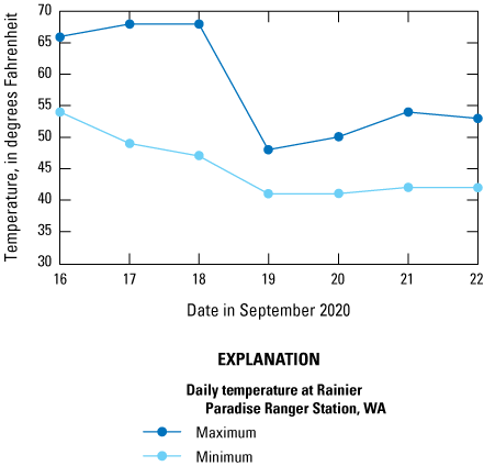
Temperatures at Rainier Paradise Ranger Station, Mount Rainier National Park, Washington (WA).
Output from a published SWB model was used for calculations and analysis in this study. This SWB model had its own set of assumptions and limitations for the input data and methods used for its completion. The magnitude of recharge in ft3/s was estimated for each zone on a weekly time step using SWB output. The accuracy of SWB recharge estimations made in zones A, B, and F is limited due to the presence of glaciers in these zones, as SWB does not have the ability to accurately estimate glacial melt. The recharge output data from SWB was compared with the seepage run results and analysis, but data were not available for a location-specific SWB lookup table or for approaches that could be used to calibrate the SWB data such as water-table fluctuation or chloride mass-balance. Although the seepage run provided a limited comparison to recharge, the estimated recharge fit the flow model presented in the methods section for all stream reaches except for those that could be explained in other ways.
The streamflow gain estimation method isolates the most recent recharge peak by adding together the 4-week moving average recharge amounts and subtracting the baseline under the curve to use this volume of water to estimate the streamflow gain. The time between the recharge peak and the streamflow gain peak is estimated using the method where the rising and falling limbs are equivalent. Two assumptions were made using this estimation method: that the most recent recharge peak caused a peak in base flow prior to the stream discharge measurement and that the September base flow was in recession. The resulting streamflow gain curve assumes that the time it takes for the streamflow gain that results from the isolated recharge to reach its peak takes no longer than it does for the streamflow gain to return to zero.
Summary
The method used to relate the soil-water-balance model (SWB)-calculated recharge to streamflow gain in the White River led to some general observations about the accuracy of the conceptual model and what it implies about the availability of water in the White River alluvial areas, specifically with regard to the zones with glaciers and the reaches with relatively high streamflow gain.
Glaciers were present in zones A, B, and F, and the SWB model underestimated the amount of recharge that resulted as streamflow gain from these areas due to its limited ability to calculate recharge from glacial areas. Furthermore, the larger area of glacial cover in zone B resulted in the conceptual model being less accurate compared with that of zones A and F (figs. 6A, 6B, and 6D).
The discharge measured on the White River and recharge analysis performed on the White River basin indicates reaches of stream discharge are likely to be gaining during late summer, when conditions are typically at their driest of the year. The relatively large gain in stream discharge in reach G8–11, consecutive losses in the two reaches immediately upstream (reaches D5–6 and L6–8), and the measured discharge point failing to fit the streamflow gain curve for zone GH suggest that the recharge from zones D and L does not inflow to the White River as streamflow gain in the reaches that are adjacent to these zones. The analysis presented in this study indicates that recharge from zones D and L likely takes alluvial pathways that prevent it from entering the White River as streamflow gain until reach G8–11.
References Cited
Anderson, S.W., and Jaeger, K.L., 2020, Coarse sediment dynamics in a large glaciated river system—Holocene history and storage dynamics dictate contemporary climate sensitivity: Geological Society of America Bulletin, v. 133, nos. 5–6, p. 899–922, accessed October 15, 2022, at https://pubs.geoscienceworld.org/gsa/gsabulletin/article/133/5-6/899/590467/Coarse-sediment-dynamics-in-a-large-glaciated.
Crandell, D.R., 1971, Postglacial lahars from Mount Rainier volcano, Washington: U.S. Geological Survey Professional Paper 677, 75 p., accessed June 15, 2022, at https://pubs.er.usgs.gov/publication/pp677.
Crandell, D.R., and Miller, R.D., 1974, Quaternary stratigraphy and extent of glaciation in the Mount Rainier region, Washington: U.S. Geological Survey Professional Paper 847, 59 p., accessed August 10, 2022, at https://pubs.er.usgs.gov/publication/pp847.
Fahnestock, R.K., 1963, Morphology and hydrology of a glacial stream—White River, Mount Rainier, Washington: U.S. Geological Survey Professional Paper 422-A, chapter A, p. A1–A70, accessed May 5, 2022, at https://pubs.er.usgs.gov/publication/pp422A.
Fiske, R.S., Hopson, C.A., and Waters, A.C., 1963, Geology of Mount Rainier National Park, Washington: U.S. Geological Survey Professional Paper 444, 93 p., accessed January 14, 2023, at https://www.morageology.com/pubs/62.pdf.
Gendaszek, A.S., and Welch, W.B., 2018, Water budget of the upper Chehalis River Basin, southwestern Washington: U.S. Geological Survey Scientific Investigations Report 2018-5084, 17 p., accessed February 15, 2022, at https://doi.org/10.3133/sir20185084.
Hargreaves, G. H., and Samani, Z. A., 1985, Reference crop evapotranspiration from temperature: Applied Engineering in Agriculture, v. 1, no. 2, p. 96–99, accessed January 15, 2022, at https://doi.org/10.13031/2013.26773.
Headman, A.O., 2022, Soil water balance model of the White River basin, Mount Rainier National Park, Washington, USA: U.S. Geological Survey data release, accessed September 15, 2022, at https://doi.org/10.5066/P9KI310W.
Konrad, C.P., and Dettinger, M.D., 2017, Flood runoff in relation to water vapor transport by atmospheric rivers over the western United States, 1949–2015: Geophysical Research Letters, vol. 44, no. 22, p. 11,456–11,462, accessed February 3, 2023, at https://agupubs.onlinelibrary.wiley.com/doi/abs/10.1002/2017GL075399.
Lehner, B., Verdin, K., and Jarvis, A., 2008, New global hydrography derived from spaceborne elevation data: Washington, D.C., Eos, v. 89, no. 10, p. 93–94, accessed March 1, 2022, at https://doi.org/10.1029/2008EO100001.
National Park Service Social Science Program [NPS SSP], 2022, Visitation statistics for Mount Rainier National Park: National Park Service database accessed on July 6, 2022, at https://www.nps.gov/subjects/socialscience/highlights.htm.
Neiman, P.J., Schick, L.J., Ralph, F.M., Hughes, M., and Wick, G.A., 2011, Flooding in western Washington—The connection to atmospheric rivers: Journal of Hydrometeorology, vol. 12, no. 6, p. 1337–1358, accessed April 15, 2022, at https://journals.ametsoc.org/configurable/content/journals$002fhydr$002f12$002f6$002f2011jhm1358_1.xml?t:ac=journals%24002fhydr%24002f12%24002f6%24002 f2011jhm1358_1.xml.
National Oceanic and Atmospheric Administration, 2022, U.S. climate normals for Paradise, Washington—1991–2020: National Centers for Environmental Information U.S. climate normals database, accessed November 15, 2022, at https://www.ncei.noaa.gov/access/us-climate-normals/.
National Oceanic and Atmospheric Administration, 2023, Climatological data for RAINIER PARADISE RS, WA—September 2020: National Centers for Environmental Information, accessed January 31, 2023, at https://www.weather.gov/wrh/Climate?wfo=sew.
National Resources Conservation Service, 2021, Web Soil Survey: United States Department of Agriculture, web, accessed October 18, 2021, at https://websoilsurvey.sc.egov.usda.gov/.
Pringle, P.T., 2008, Roadside geology of Mount Rainier National Park and vicinity—Information Circular 107: Washington State Department of Natural Resources, Division of Geology and Earth Resources, 200 p., accessed December 1, 2021, at https://fortress.wa.gov/dnr/geologydata/Publications/ic107_mt_rainier_road_guide.pdf.
Rosenberry, D.O., and LaBaugh, J.W., 2008, Field techniques for estimating water fluxes between surface water and ground water: U.S. Geological Survey Techniques and Methods 4–D2, 128 p. [Also available at https://pubs.usgs.gov/tm/04d02/.]
Sauer, V.B., and Meyer, R.W., 1992, Determination of error in individual discharge measurements: U.S. Geological Survey Open-File Report 92–144, 21 p. [Also available at https://pubs.usgs.gov/of/1992/ofr92-144/.]
Thornton, M.M., Shrestha, R., Wei, Y., Thornton, P.E., Kao, S-C., and Wilson, B.W., 2022, Daymet—Daily surface weather data on a 1-km grid for North America, version 4 R1: Oak Ridge, Tennessee, ORNL DAAC, accessed December 15, 2022, at https://doi.org/10.3334/ORNLDAAC/2129.
Tillman, F.D., 2015, Documentation of input datasets for the soil-water balance groundwater recharge model of the Upper Colorado River Basin: U.S. Geological Survey Open-File Report 2015–1160, 17 p. [Also available at https://doi.org/10.3133/ofr20151160.]
U.S. Geological Survey, 2022, National Water Information System: U.S. Geological Survey web interface, https://doi.org/10.5066/F7P55KJN, accessed February 15, 2022, at https://nwis.waterdata.usgs.gov/nwis/dv.
Watershed Sciences, 2009, LiDAR remote sensing data collection—Mount Rainier, Washington data set: Washington State LiDAR Portal, accessed November 1, 2021, at https://lidarportal.dnr.wa.gov/.
Wickham, J., Stehman, S.V., Sorenson, D.G., Gass, L., and Dewitz, J.A., 2021, Thematic accuracy assessment of the NLCD 2016 land cover for the conterminous United States: Remote Sensing of Environment, v. 257, article 112357, at https://doi.org/10.1016/j.rse.2021.112357.
Conversion Factors
U.S. customary units to International System of Units
Temperature in degrees Fahrenheit (°F) may be converted to degrees Celsius (°C) as follows:
°C = (°F – 32) / 1.8.
For information about the research in this report, contact the
Director, Washington Water Science Center
U.S. Geological Survey
934 Broadway, Suite 300
Tacoma, Washington 98402
https://www.usgs.gov/centers/washington-water-science-center
Manuscript approved on February 13, 2024
Publishing support provided by the U.S. Geological Survey
Science Publishing Network, Tacoma Publishing Service Center
Edited by Jeff Suwak and Vanessa Ball
Layout and design by Luis Menoyo
Illustration support by Joseph Mangano
Disclaimers
Any use of trade, firm, or product names is for descriptive purposes only and does not imply endorsement by the U.S. Government.
Although this information product, for the most part, is in the public domain, it also may contain copyrighted materials as noted in the text. Permission to reproduce copyrighted items must be secured from the copyright owner.
Suggested Citation
Fuhrig, L.T., Long, A.J., and Headman, A.O., 2024, Evaluation of groundwater resources in the Upper White River Basin within Mount Rainier National Park, Washington State, 2020 (ver. 1.1, March 2024): U.S. Geological Survey Scientific Investigations Report 2024–5015, 19 p., https://doi.org/10.3133/sir20245015.
ISSN: 2328-0328 (online)
Study Area
| Publication type | Report |
|---|---|
| Publication Subtype | USGS Numbered Series |
| Title | Evaluation of groundwater resources in the Upper White River Basin within Mount Rainier National Park, Washington State, 2020 |
| Series title | Scientific Investigations Report |
| Series number | 2024-5015 |
| DOI | 10.3133/sir20245015 |
| Edition | Version 1.0: March 25, 2024; Version 1.1: March 29, 2024 |
| Publication Date | March 25, 2024 |
| Year Published | 2024 |
| Language | English |
| Publisher | U.S. Geological Survey |
| Publisher location | Reston, VA |
| Contributing office(s) | Washington Water Science Center |
| Description | Report: vi, 19 p.; Data Release |
| Country | United States |
| State | Washington |
| Other Geospatial | Mount Rainier National Park |
| Online Only (Y/N) | Y |