

Monitoring and Simulation of Hydrology, Suspended Sediment, and Nutrients in Selected Tributary Watersheds of Lake Erie, New York
Links
- Document: Report (49.3 MB pdf) , HTML , XML
- Data Releases:
- USGS data release - Data and rloadest models used to estimate sediment and nutrient loads in selected New York tributaries to eastern Lake Erie
- USGS data release - SWAT Model Archive for Simulation of Hydrology, Suspended Sediment and Nutrients in Selected Tributary Watersheds of Lake Erie, New York
- NGMDB Index Page: National Geologic Map Database Index Page (html)
- Download citation as: RIS | Dublin Core
Acknowledgments
The authors would like to thank Allen Young of the U.S. Department of Agriculture Natural Resources Conservation Service for his help in developing the agricultural management and hypothetical modeling scenarios and Rosaleen Nogle of the Buffalo Sewer Authority for providing data for the green infrastructure scenario. We also thank Shannon Dougherty, Karen Stainbrook, and Lauren Townley of the New York State Department of Environmental Conservation for their help with designing the project and compiling the point source data. We thank Raghavan Srinivasan of Texas A&M University for providing a Linux version of the Soil and Water Assessment Tool. Jeff Falgout and Natalya Rapstine of the U.S. Geological Survey (USGS) helpfully provided aided with the use of the USGS Yeti supercomputer. The authors thank Amy M. Russell of the USGS and Raghavan Srinivasan and Sagarika Roth of Texas A&M University for reviewing a draft of this manuscript.
Abstract
The U.S. Geological Survey, in cooperation with Erie County, New York, the New York State Department of Environmental Conservation, and the Great Lakes Restoration Initiative, collected water-quality samples in nine selected New York tributaries to Lake Erie, computed estimates of suspended sediment and nutrient loads using the R scripting package rloadest and used the Soil and Water Assessment Tool (SWAT) to simulate hydrology and suspended sediment and nutrient loads from these tributaries. This project was undertaken to better understand the water quality of New York’s inputs into eastern Lake Erie.
Water-quality samples for suspended sediment, nitrogen, and phosphorus were collected at 19 sampling sites in the Lake Erie Basin in New York. Daily and monthly suspended sediment and nutrient loads were computed with regressions of streamflow and suspended sediment and nutrient concentrations using rloadest.
SWAT models of nine watersheds were created using publicly available data; and the loads were calculated by rloadest. Twenty-six SWAT model scenarios were created to explore the effects that best management practices (BMPs; 21 scenarios), point source discharges (4 scenarios), and green infrastructure (1 scenario) can have on the water quality of the nine tributaries to Lake Erie. BMP scenarios for the watershed models included combinations of agricultural BMPs applied at varying implementation levels across the study watersheds, including cover crops, reduced tillage, nutrient management plans, and filter strips. The BMP scenarios showed small reductions of total nitrogen and total phosphorus. The scenarios have variable suspended sediment load results, with both increases and decreases of sediment modeled. The point source scenarios result in lower total phosphorus loads. The green infrastructure scenario shows only minimal reduction of suspended sediment and nutrient loads from the Buffalo River watershed but shows substantial reductions locally.
Introduction
The U.S. Geological Survey (USGS), in cooperation with Erie County, New York, the New York State Department of Environmental Conservation, and the Great Lakes Restoration Initiative created nine Soil and Water Assessment Tool (SWAT) models of select watersheds in New York within the Eastern Lake Erie Basin.
The section of Eastern Lake Erie Basin in New York has an area of 6,137 square kilometers (km2) and stretches from the border of New York State with Pennsylvania to the confluence of the Niagara River with Lake Ontario. The study area in this report includes nine subwatersheds with a total area of 4,941 km2 (fig. 1) selected for SWAT simulation to represent the Eastern Lake Erie Basin section in New York. These nine subwatersheds capture a broad range of watershed area, topography, land cover, management, soil, and slope types characteristic of the Eastern Lake Erie Basin section in New York. The selected areas are the Big Sister Creek, Buffalo River, Canadaway Creek, Cattaraugus Creek, Chautauqua Creek, Crooked Brook, Eighteenmile Creek, Walnut Creek, and Tonawanda Creek watersheds.
SWAT is a physically based, watershed-scale hydrologic and water-quality model that has been extensively used throughout the United States and the world (Arnold and others, 1998; Douglas-Mankin and others, 2010; Gassman and others, 2007). SWAT uses input land cover, management, soils, elevation, weather, and other data. The SWAT model provides continuous simulation of hydrologic and water-quality processes on a daily time step and permits the assessment of how land-management practices affects water, suspended sediment, and nutrient yields in small or large watersheds with varying soils, land covers, and management conditions over long periods of time. SWAT has widely been used in total maximum daily load applications (Tetra Tech, Inc., 2015), watershed planning (Santhi and others, 2006), and in assessment of best management practices (BMPs; Bosch and others, 2013).
Baseline scenarios were simulated for the 9 watersheds, and an additional 26 scenarios were tested on the 7 calibrated watershed models: 7 low, 7 medium, and 7 high BMP scenarios, 4 point-source discharge limit scenarios, and 1 green infrastructure scenario. SWAT baseline results in this study help identify areas in the study watersheds that contribute large suspended sediment and nutrient loads. The additional scenarios assess how BMP implementation, point-source discharge limits, and addition of green infrastructure may affect suspended sediment and nutrient loads delivered to eastern Lake Erie.
The objective of this study was to better understand the water quality of New York’s inputs into Lake Erie. Specifically, this study provides (1) information regarding the regional hydrologic system and its associated water-quality processes, (2) water resource information that local, State, and Federal entities can use for planning and management purposes, and (3) data that can be used to advance understanding of regional and temporal variations in hydrologic conditions in the study area.
Western Lake Erie has received considerable attention in recent years because of the reemergence of harmful algal blooms that have threatened the drinking water supplies of coastal communities, created a large zone of anoxic water in the lake, and affected shoreline beach and fishery health. Multiple studies have found that agriculture is the leading cause of impairment of waters in Lake Erie (Duncan and others, 2017; Michalak and others, 2013; Scavia and others, 2014; Smith and others, 2015b). Eastern Lake Erie is also stressed by a large population, invasive aquatic species, and large wastewater and agricultural runoff contributions (Buffalo Niagara Riverkeeper, 2014).
A goal of the “U.S. Action Plan for Lake Erie” (U.S. Environmental Protection Agency [EPA], 2018) is for eastern Lake Erie to maintain algae levels below the level constituting a nuisance condition. The majority of historical nuisance benthic algal blooms in eastern Lake Erie were caused by the green algae Cladophora. Cladophora was first documented in the Great Lakes in the 1930s. Since the late 1980s, the extent of Cladophora has steadily been increasing and reaching nuisance levels across the Great Lakes. The most recent recommendations for the Great Lakes Water Quality Agreement Annex 4 (nutrients) subcommittee (Mary Anne Evans, USGS, written commun., 2022) have not set phosphorus loading targets for the Eastern Lake Erie Basin because of the lack of scientific consensus on environmental factors and phosphorus loads and their potential cause to algal blooms in eastern Lake Erie. The Lake Erie Eastern Basin Task Team has instead set out to gather more information on what management efforts are necessary for controlling Cladophora and other algae.
Erie County, on behalf of the Lake Erie Watershed Protection Alliance, in collaboration with the New York State Department of Environmental Conservation (NYSDEC), is developing a nine-element watershed management plan of the Eastern Lake Erie Basin section in New York, which includes the Niagara River Basin, with financial support from the New York Department of State and the Great Lakes Restoration Initiative. A nine-element watershed management plan consistent with guidance from the NYSDEC would identify and quantify sources of pollutants, determine water-quality goals or targets, and describe the BMPs needed to reach said goals or targets.
The SWAT model results in this study may be used by water-resource managers to inform the nine-element watershed plan for the Eastern Lake Erie Basin section in New York. This study may also benefit Federal, State, and county governments and the residents in the study area by providing a quantitative understanding of the sources of nutrients entering streams; assessing the effects of land cover change, BMPs, and point source scenarios; and providing a means to compute suspended sediment and nutrient load estimates for these nine tributaries to the Eastern Lake Erie Basin.
Purpose and Scope
To support the development of a nine-element watershed plan for the New York part of Eastern Lake Erie Basin, the USGS, in cooperation with the NYSDEC, performed water-quality monitoring and developed SWAT models of nine tributary watersheds to Lake Erie. Water-quality monitoring data was regressed against daily streamflow using rloadest, the R package (R Core Team, 2018) for the Load Estimator (LOADEST) regression model, to provide suspended sediment and nutrient loads for SWAT model calibration.
The purpose of this report is to describe water-quality monitoring, loads computation, watershed model development, calibration and validation, and the resulting simulated hydrology and sediment and nutrient loads for nine SWAT watershed models in western New York that drain to Lake Erie (fig. 1). The models were calibrated to streamflow, suspended sediment, phosphorus, and nitrogen loads quantified at USGS streamgages. Modeling scenarios were developed to determine the effect of BMPs on streamflow and water quality. Additional modeling scenarios related to point sources and green infrastructure were explored. Model limitations are discussed.
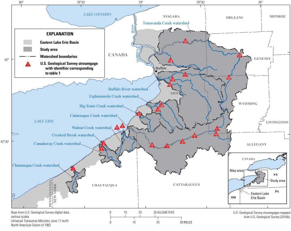
Map showing the nine study watersheds and simplified hydrology of main stem streams in New York.
Description of Study Area
The study area consists of nine New York watersheds draining into the eastern side of Lake Erie (fig. 1). The selected watersheds are Big Sister Creek, Buffalo River, Canadaway Creek, Cattaraugus Creek, Chautauqua Creek, Crooked Brook, Eighteenmile Creek, Walnut Creek, and Tonawanda Creek (fig. 2). These watersheds are in western New York and together encompass parts of Erie, Niagara, Cattaraugus, Chautauqua, Orleans, Genesee, Wyoming, and Allegany Counties. During the fall of 2017, seven new USGS water-quality streamgages (sites 1, 2, 4, 5, 12–14 in table 1) were installed in the study area. These sites plus 12 existing sites monitor streamflow and water-quality of these watersheds (table 1). Data from 15 streamgages with daily streamflow records (sites 1, 2, 4–6, and 12–21 in table 1) were used to calibrate and validate the SWAT model for streamflow. Data from 13 sites with daily streamflow and water-quality monitoring (sites 1, 2, 4–6, and 12–19 in table 1) were used to create rloadest models of loads that were then used to calibrate and validate the SWAT model for water-quality constituents.
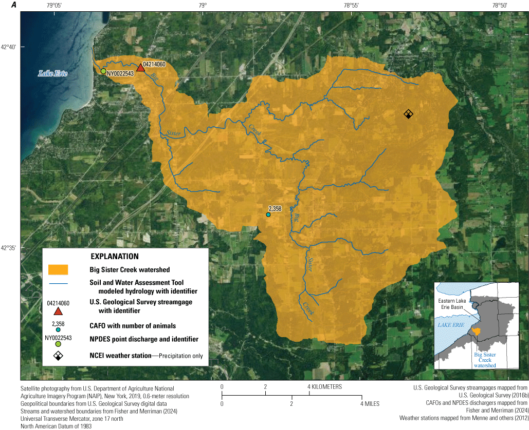
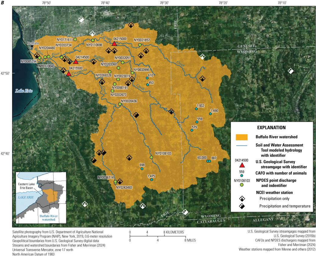
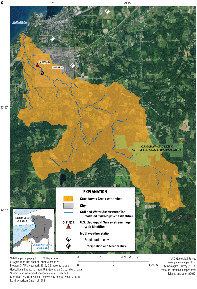
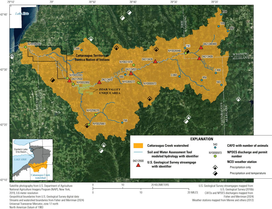
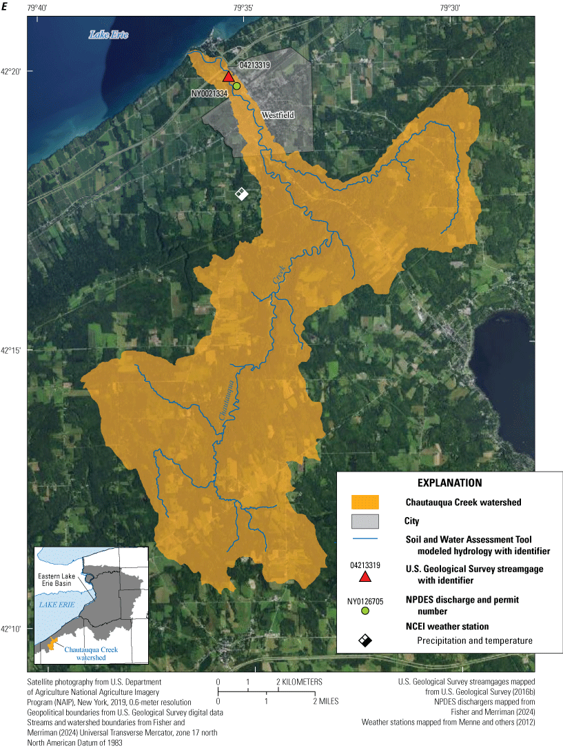
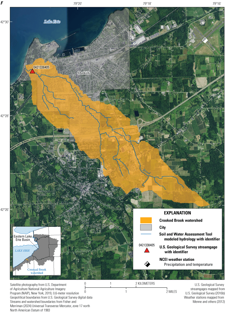
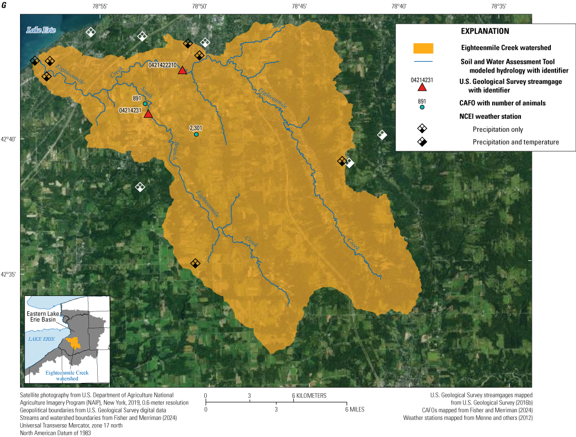
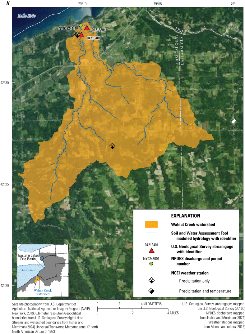

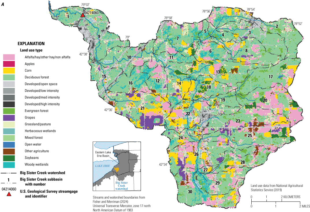
Maps of Soil and Water Assessment Tool basins with locations of U.S. Geological Survey streamgages, concentrated animal feeding operations (CAFOs), National Pollutant Discharge Elimination System (NPDES) point discharges, National Centers for Environmental Information (NCEI) weather stations, and modeled hydrology in the A, Big Sister Creek; B, Buffalo River; C, Canadaway Creek; D, Cattaraugus Creek; E, Chautauqua Creek; F, Crooked Brook; G, Eighteenmile Creek; H, Walnut Creek; and I, Tonawanda Creek watershed models, New York.
Table 1.
U.S. Geological Survey streamflow and water-quality streamgage monitoring sites for the selected tributary watersheds of Lake Erie, New York, examined in this study.[Data are from U.S. Geological Survey (2016a). Baseflow index (BFI) calculated with software from Arnold and Allen (1999) using data in U.S. Geological Survey (2016b). Site numbers correspond to the sites in figure 1. Water-quality data collected include nitrogen, phosphorus, and suspended-sediment concentrations. km2, square kilometer; NY, New York; —, no data; S Br, South Branch; Cr, Creek; Rd, Road]
The studied tributary watersheds are mostly forested, with deciduous forest covering 24.25–69.33 percent of the watershed areas (table 2; fig. 3; National Agricultural Statistics Service [NASS], 2019). There are several concentrated animal feeding operations (CAFOs) in many of the watersheds, the majority being dairies (fig. 2). The outer limits of the City of Buffalo, New York, and its suburbs are near the easternmost end of Lake Erie (fig. 2B). Near the southern lakeshore are small communities and vineyards. There were 43 modeled National Pollutant Discharge Elimination System (NPDES) point source discharges in the watersheds (table 3; fig. 2), 30 of which were from municipal sources.

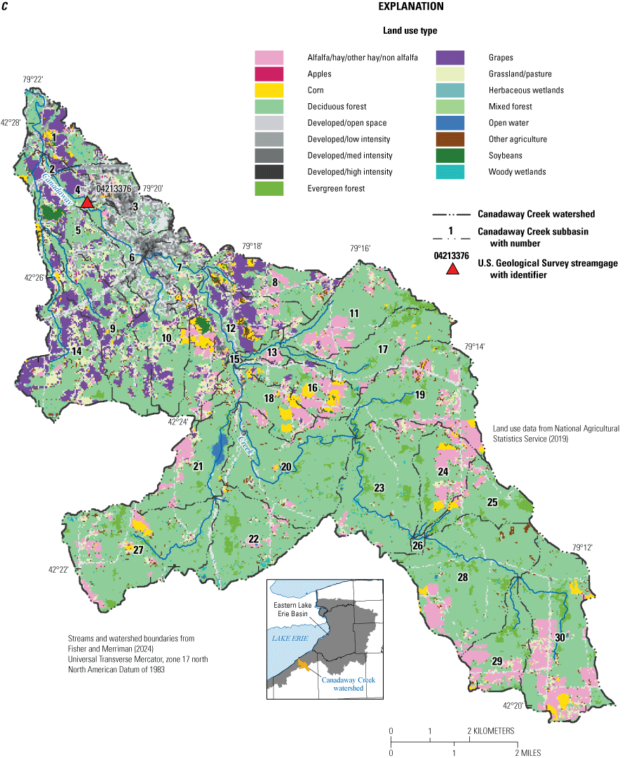
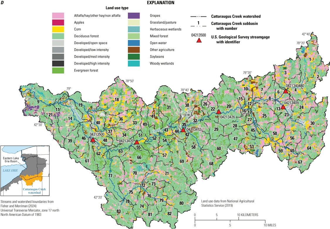
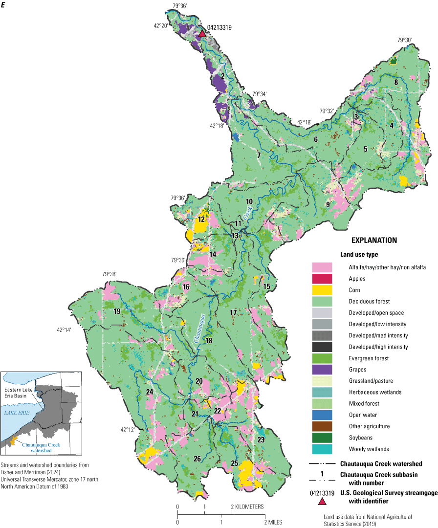
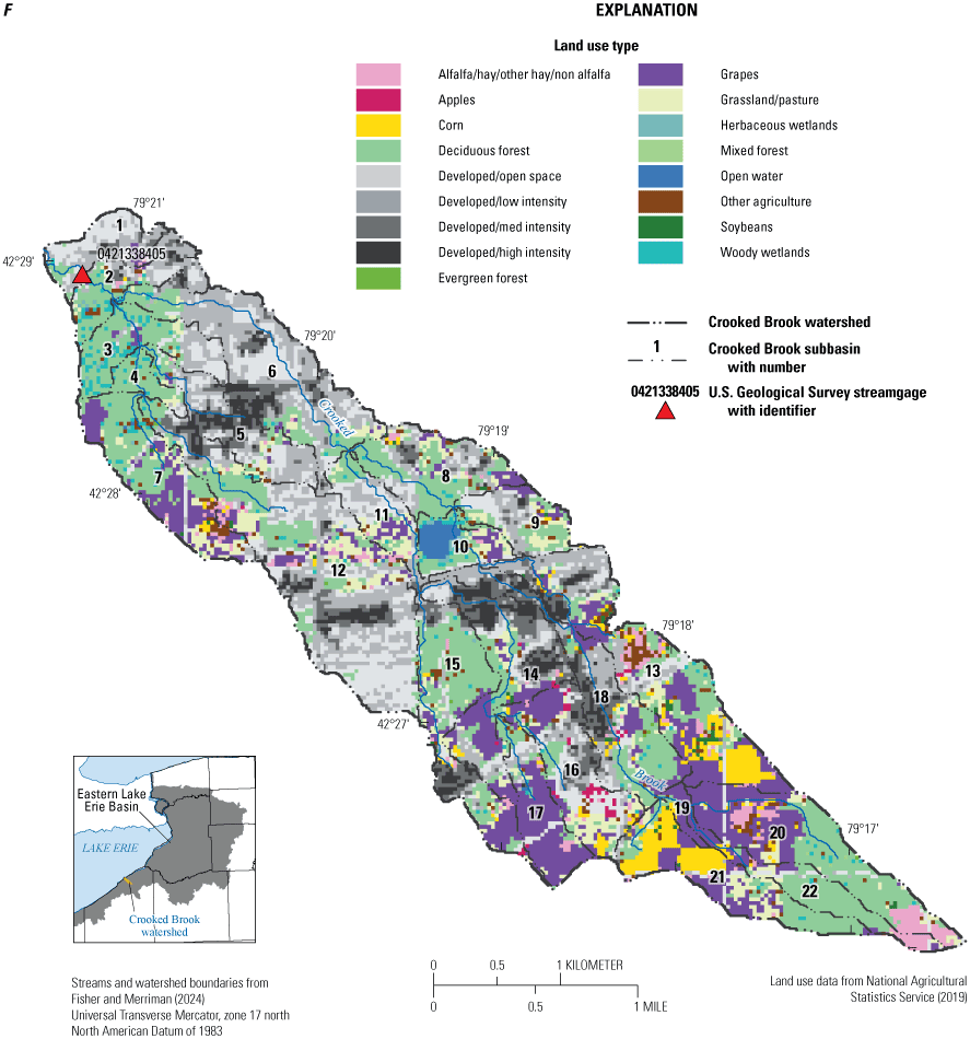

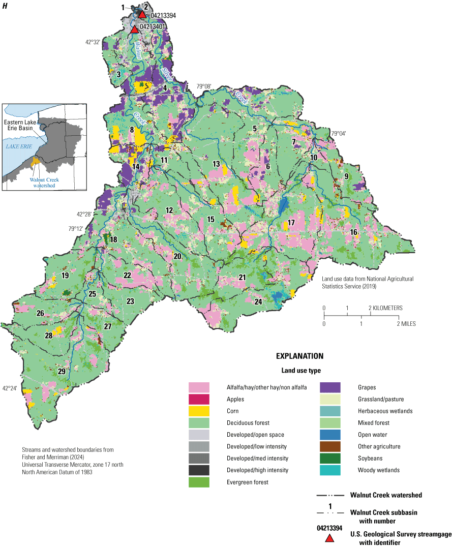
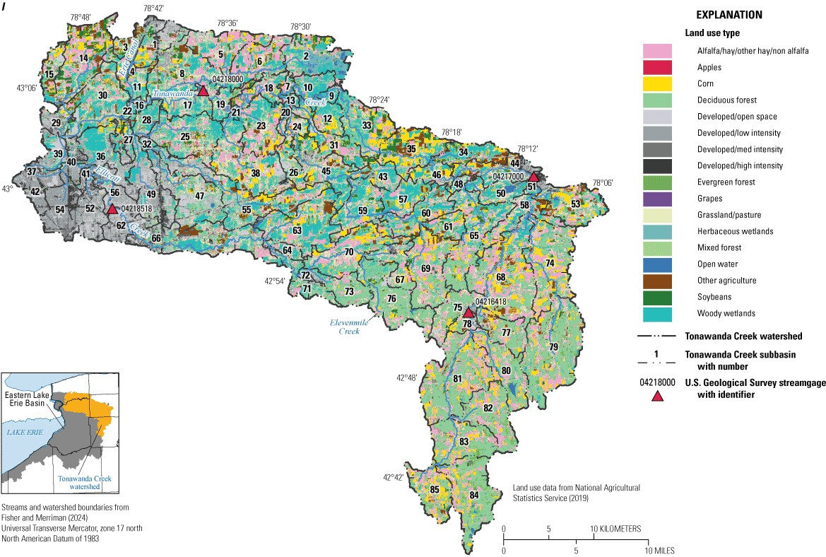
Maps of Soil and Water Assessment Tool basins with land cover, locations of U.S. Geological Survey streamgages, and modeled hydrology and subbasins of the A, Big Sister Creek; B, Buffalo River; C, Canadaway Creek; D, Cattaraugus Creek; E, Chautauqua Creek; F, Crooked Brook; G, Eighteenmile Creek; H, Walnut Creek; and I, Tonawanda Creek watershed models, New York.
Table 2.
Land cover of selected tributary watersheds of Lake Erie, New York, examined in this study, in 2018.[Land cover data are from the National Agricultural Statistics Service (2019)]
Table 3.
Point sources registered with the National Pollutant Discharge Elimination System of selected tributary watersheds of Lake Erie, New York, examined in this study.[Point-source data and treatment information are from the New York Department of Environmental Conservation (Fisher and Merriman, 2024). Nutrient speciation ratios are from the Chesapeake Bay Program (2010). See model subbasins in figure 3. NPDES, National Pollutant Discharge Elimination System; CO, county; SD, sewer district; STP, sewage treatment plant; St, street; WWTP, wastewater treatment plant; No, number; —, no data]
Physiographically, the Eastern Lake Erie Basin is within the Eastern Lake section of the Central Lowland province of the Interior Plains region, and the Southern New York section of the Appalachian Plateaus province of the Appalachian Highlands region. The area near Lake Erie has lower elevations and shallower slopes than the rolling hills to the east and southeast. The study area watersheds range in size from the very small 13.5 km2 Crooked Brook watershed to the 1,129 km2 Cattaraugus Creek watershed (fig. 1).
There is a size discrepancy between the drainage areas given for the USGS streamgages in table 1 and the SWAT-delineated watershed areas in table 4 because of the following reasons: (1) the different locations used to define a drainage area and (2) different digital elevation models (DEM) used to delineate areas. Firstly, the intersection of the tributary with Lake Erie was used as the SWAT watershed outlet in delineation, whereas the drainage areas in table 1 were delineated at the streamgage location. The streamgages are upstream from the tributary’s confluence with Lake Erie (fig. 2). Secondly, drainage areas corresponding to USGS streamgages in table 1 were delineated using StreamStats (USGS, 2016a), which uses light detection and ranging (lidar) point clouds from the 3D Elevation Program (https://www.usgs.gov/3d-elevation-program) as a DEM. For the SWAT model, the USGS National Elevation Dataset 1/9 arc-second (3.4 meter; https://apps.nationalmap.gov/viewer/) was used as its DEM to delineate watershed areas (table 4). The Big Sister Creek, Chautauqua Creek, and Crooked Brook watersheds delineated for the SWAT models were smaller than the drainage areas determined by StreamStats. The differences in the watersheds’ areas were about 1 km2 or less. This report uses watershed areas delineated using the SWAT model (table 4).
Table 4.
Properties of the study watershed models for selected tributary watersheds of Lake Erie, New York, examined in this study.[Data are from Fisher and Merriman (2024). km2, square kilometer, >, greater than; HRU, hydrologic response unit]
Description of the Study Area Watersheds
Following are physical descriptions of the nine study area watersheds in western New York, including land cover statistics and water quality.
Big Sister Creek Watershed
The 124.3 km2 Big Sister Creek watershed is in Erie County, situated between the Cattaraugus Creek and Eighteenmile Creek watersheds (fig 1). The land cover in this watershed (table 2; fig. 3) is almost half deciduous forest (46.89 percent), with small amounts of agriculture: hay and alfalfa (12.86 percent), corn (7.95 percent), and soybeans (1.95 percent). Vineyards cover a small amount of land on the southwestern side on the watershed (2.51 percent). Other land covers include developed (8.73 percent), woody wetlands (5.65 percent), mixed forest (1.73 percent), and evergreen forest (2.76 percent). There is one CAFO in this watershed (fig. 2). The average slope of the Big Sister Creek watershed is 1.99 percent (table 4). The soils are primarily poorly or very poorly drained (Natural Resources Conservation Service [NRCS], 2019). Tile drainage is used in an estimated 0.87 percent of the total watershed area (table 4; the “Tile Drainage Parameterization” section discusses how tile drainage was estimated).
The NYSDEC (2019) found that the Big Sister Creek watershed is impaired by nutrients, suspended sediment, low dissolved oxygen, and pathogens. Observed nutrient concentrations may be caused by urban and storm runoff, whereas the low dissolved oxygen, pathogens, and suspended sediment may be caused by on-site septic systems.
Buffalo River Watershed
The Buffalo River is formed by the confluence of Buffalo Creek and Cayuga Creek 13.68 kilometers (km) upstream from Lake Erie. Cazenovia Creek joins the Buffalo River 9.27 km upstream from Lake Erie. Cazenovia, Buffalo, and Cayuga Creeks have similar drainage areas, ranging from 30 to 33 percent of the Buffalo River watershed, but the area draining to the streamgages varies by subwatershed (table 1). The largest of these drainage areas is to streamgage 04214500 on Buffalo Creek, that has a drainage area of 368 km2. The drainage area to streamgage 04215500 on Cazenovia Creek is similar in size to the area drained to the Buffalo Creek streamgage, draining 350 km2, whereas the area draining to streamgage 04215000 on Cayuga Creek has a 250 km2 drainage area. Its watershed (1,107.6 km2 area) is primarily in Erie County, and the headwaters of Cayuga and Buffalo Creeks are in western Wyoming County (fig. 1). A small part of the northern part of Cayuga Creek subwatershed is in Genesee County.
The average slope of the Buffalo River watershed is 3.65 percent (table 4). About half of Buffalo Creek and Cazenovia Creek subwatersheds have slopes greater than (>) 5 percent; most slopes (65 percent) in Cayuga Creek subwatershed are less than (<) 5 percent. The Cazenovia Creek and Cayuga Creek subwatersheds soils are primarily poorly or very poorly drained (91 and 80 percent of the total area, respectively) (NRCS, 2019). The Buffalo Creek subwatershed soils are poorly drained (50 percent) and partly well drained and very poorly drained (25 percent each; NRCS, 2019).
The land covers of each these three subwatersheds are similar; however, there is more deciduous forest in the Cazenovia Creek subwatershed (57.3 percent) than Cayuga Creek (42.9 percent) and Buffalo Creek (40.9 percent) subwatersheds (fig. 3B; NASS, 2019). Cayuga and Buffalo Creeks subwatersheds have more row crop agriculture (approximately 12 percent for both watersheds) than Cazenovia Creek subwatershed (2.0 percent). Less tile drainage was estimated in the Cazenovia Creek subwatershed (1 percent of the total area) than in Buffalo Creek subwatershed (13 percent of the total area) and Cayuga Creek subwatershed (14 percent) subwatersheds.
The following impairment data and interpretations are from the NYSDEC (2019). The Buffalo River watershed, from the confluence of Buffalo Creek and Cayuga Creek to Lake Erie, is impaired by polychlorinated biphenyls, low dissolved oxygen, pathogens, and suspended sediment. The causes of the known and suspected impairments are combined sewer overflows, urban runoff, stormwater runoff, industrial inputs, hazardous waste sites, and habitat and hydrologic stream modification. Buffalo Creek, from its source to the confluence of Buffalo Creek and Cayuga Creek, is impaired by suspended sediment and thought to be impaired by nutrients, pathogens, and elevated water temperature. The elevated sediment is from streambank erosion and urban and storm runoff. The elevated nutrients and pathogens are thought to be from agriculture, and the elevated temperature is thought to be from on-site septic systems and road bank erosion. The Cazenovia Creek subwatershed is impaired by pathogens from sewer and septic system discharge and urban and storm runoff. The Cayuga Creek watershed is impaired from pathogens and thought to be impaired from elevated nutrients and suspended sediment, metals, polycyclic aromatic hydrocarbons (PAHs), and low dissolved oxygen. The pathogen impairments are caused by sanitary discharges and the elevated nutrients and suspended sediment, metals, polycyclic aromatic hydrocarbons, and low dissolved oxygen are thought to be caused by on-site septic systems, streambank erosion, urban and storm runoff, and agriculture.
Canadaway Creek Watershed
The Canadaway Creek watershed, which has an area of 101.5 km2, is entirely inside Chautauqua County (fig. 1). Some low-lying areas of the Village of Fredonia near Canadaway Creek have flooded during storms (Lumia and Johnston, 1984). The average slope of the Canadaway Creek watershed is 9.41 percent (table 4). Approximately 65 percent of the watershed is forested, 8.69 percent is developed, 9.00 percent is hay and alfalfa, and 5.49 percent is pasture (table 2). The watershed has several vineyards covering about 6 percent of the watershed, primarily located near Lake Erie. The remaining land cover consists of fruit and vegetable cultivation. It is thought to be impaired by elevated suspended sediment caused by nonpoint sources, logging activities, and natural streambank erosion of highly erodible soils in the watershed (NYSDEC, 2019). Canadaway Creek Wildlife Management Area (https://www.dec.ny.gov/outdoor/82659.html) is in the upstream part of the watershed with steep slopes that may contribute to the natural streambank erosion in the watershed. The average slope of the Canadaway Creek watershed is 9.41 percent (table 4). The majority of soils are poorly drained (58 percent) or very poorly drained (18 percent), whereas a minority of the soils are well or moderately well drained (25 percent; NRCS, 2019).
Cattaraugus Creek Watershed
The Cattaraugus Creek watershed has an area of 1,437.6 km2 (table 1). The headwaters of the Cattaraugus Creek watershed lie in southwestern Wyoming County and northwestern Allegany County, but most of the watershed straddles the boundary of Erie and Cattaraugus Counties (fig. 1). Cattaraugus Creek is part of the county boundary between Cattaraugus and Erie Counties and between Chautauqua and Erie Counties near the watershed outlet to Lake Erie. Part of the Cattaraugus Territory of Seneca Nation of Indians is also in the watershed (fig. 2D). Cattaraugus Creek watershed is the least urbanized of any of the modeled watersheds (fig. 3). Over 50 percent of the watershed is forested, 4.61 percent is developed, and 2.05 percent of the watershed is wetlands (table 2). The remaining land cover of this watershed is agricultural.
Relief of the watershed is 535 meters (m), with an average watershed slope of 9.37 percent (table 4). Upstream areas have steep slopes and wide ridges (NRCS, 2009). Downstream areas have low relief, and the topography ranges from flat to rolling plains. The south side of the watershed has wide, flat valleys with sluggish streams. Over two-thirds of the soils are poorly or very poorly drained (NRCS, 2019). Less than 3 percent of the watershed is estimated to have tile drainage (table 4).
The Cattaraugus Creek watershed is impaired by suspended sediment and nutrients from streambank erosion and agriculture (NYSDEC, 2019). Some of the suspended sediment loading is thought by the NYSDEC (2019) to be natural streambank erosion because of highly erodible soils in the watershed. The Clear Creek subwatershed of the Cattaraugus Creek watershed has no known ecological impairments (NYSDEC, 2019).
Chautauqua Creek Watershed
The Chautauqua Creek watershed is the most southern and western watershed out of the selected study watersheds (fig. 1). Its area is 90.6 km2 (table 1), and it lies entirely in Chautauqua County. Chautauqua Creek watershed has the most forested land cover out of the study watersheds; 69.33 percent of the watershed’s land cover is deciduous forest, 5.90 percent is evergreen forest, and 0.27 percent is mixed forest (table 2; fig. 3E). Less than 5 percent of its area is developed. Hay and alfalfa (8.85 percent) is the largest agricultural land cover in the watershed. There is some vineyard cover (1.22 percent) scattered close to the outlet to Lake Erie. Eighty-four percent of Chautauqua Creek watershed soils are poorly or very poorly drained (NRCS, 2019). This watershed has an average slope of 10.66 percent, the highest out of the studied watersheds (table 4).
The NYSDEC (2019) states that Chautauqua Creek is a water supply for the village of Westfield, N.Y.; agricultural pastureland is suspected of contributing pathogens and causing impairment of Chautauqua Creek.
Crooked Brook Watershed
The Crooked Brook is the smallest watershed (13.4 km2) modeled in this report (fig. 1). This watershed is within Chautauqua County and is adjacent to the Canadaway Creek watershed on its western boundary. The average slope of this watershed is 3.02 percent (table 4). Developed land cover of the city of Dunkirk makes up 42.76 percent of the watershed (table 2). Deciduous forest accounts for 24.25 percent of the land cover. Vineyards are common in the headwaters in the southeastern area of the watershed and near the Crooked Brook outlet, accounting for 14.97 percent of the land cover. Fifty-one percent of the soils in Crooked Brook watershed are well drained (NRCS, 2019). The Crooked Brook watershed is impaired by nutrients caused by sewage waste, municipal and industrial sources, and likely by urban runoff (NYSDEC, 2019). Whereas the other watersheds have streamgages with daily hydrologic data available, only approximately monthly discharge and water-quality measurements were taken at USGS streamgage 0421338405 in the Crooked Brook watershed during this study.
Eighteenmile Creek Watershed
Eighteenmile Creek watershed has an area of 306.8 km2 (table 1) and is entirely in Erie County (fig. 1). Land cover of the Eighteenmile Creek watershed is over 56.38 percent forested (table 2). Developed land covers 8.56 percent of the watershed. The land cover categorized as hay and alfalfa is 13.73 percent. The remaining land cover is of various crops, wetlands, and open water. There are two CAFOs and no point sources in this watershed (fig. 2G). Over 80 percent of the watershed has poorly or very poorly drained soils (NRCS, 2019). Its average slope is 7.48 percent (table 4). The tributary South Branch Eighteenmile Creek drains 94.8 km2 at USGS streamgage 04214231 (table 1; fig. 2G). This streamgage receives streamflow from 31 percent of the watershed.
The Eighteenmile Creek watershed is thought to be impaired by suspended sediment, polychlorinated biphenyls, pathogens, and elevated water temperatures caused by streambank erosion, urban and storm runoff, agriculture, hydrologic modification, and contaminated sediment. However, the South Branch Eighteenmile Creek tributary subwatershed has no known impairments (NYSDEC, 2019).
Walnut Creek Watershed
The Walnut Creek watershed has an area of 130.4 km2 (table 1). Walnut Creek and its tributary Silver Creek join together approximately 0.2 km upstream from the mouth at Lake Erie (fig. 2H). About half of the total watershed area, 60.8 km2, is in the Silver Creek subwatershed. The combined watershed is primarily in Chautauqua County, with a small part in Cattaraugus County (fig. 1).
Deciduous forest is the predominant land cover in this watershed (table 2), with less deciduous forest in the Silver Creek subwatershed (55.3 percent) in comparison to the rest of Walnut Creek watershed (62.4 percent; fig. 3H). The second most common land cover is hay and alfalfa. The Silver Creek subwatershed and the remaining Walnut Creek watershed have a similar area of land in use for vineyards (5.0 percent in Silver Creek subwatershed and 4.2 percent in the rest of Walnut Creek watershed). Soils primarily have a slight slope and are mostly poorly or very poorly drained (NRCS, 2019). Less than 1 percent of the watershed was estimated to have tile drainage (table 4). Average slope of the watershed is 7.84 percent (table 4).
The NYSDEC (2019) found that Silver Creek subwatershed is impaired with low dissolved oxygen and suspended sediment and nutrients caused by local municipal discharges, streambank erosion because of highly erodible soils, logging activities, and other nonpoint sources. The rest of Walnut Creek watershed is impaired by nutrient runoff from agricultural nonpoint sources, streambank erosion, and logging activities (NYSDEC, 2019). This part of the watershed is also thought to be impaired by low dissolved oxygen and suspended sediment which is likely because of highly erodible soils throughout the watershed (NYSDEC, 2019).
Tonawanda Creek Watershed
The Tonawanda Creek watershed is the northernmost of the selected watersheds with an area of 1,630.1 km2 (fig. 1). It is the largest tributary watershed to Lake Erie in New York State (NYS). Its headwaters are in Wyoming County, and Tonawanda Creek flows north through Genesee County and west through Erie County to the Niagara River (fig. 2I). Tonawanda Creek is a part of the Erie Canal (the Erie Canal is locally known as the “New York State Barge Canal”); as such, Tonawanda Creek is regularly dredged from Pendleton, New York, to its mouth at the Niagara River.
Ellicott Creek is the largest tributary to Tonawanda Creek, which begins in the northwest corner of Wyoming County (fig. 2I). Ellicott Creek flows west along the southern boundary of the Tonawanda Creek watershed, and Ellicott Creek joins Tonawanda Creek approximately 0.59 km from its mouth at the Niagara River. Many tributaries of Ellicott Creek have been modified for stormwater conveyance (Buffalo Niagara Riverkeeper, 2014).
The mouth of the Tonawanda Creek is in a developed area (fig. 3I). The eastern part of the watershed is principally agricultural mixed with deciduous forest. Deciduous forest is the dominant land cover of the watershed (24.63 percent), followed by developed (17.35 percent) and woody wetlands (14.92 percent; table 2). The most upstream part of the watershed (primarily in Wyoming County) has steeper slopes. Slopes flatten to the western part of the watershed closer to Lake Erie.
Climate
This study area has a humid continental climate, with heavy climatic influences from Lake Erie to the west and Lake Ontario to the north. Half of the snowfall in winter is caused by early-season lake-effect precipitation. Summers are relatively dry compared to the rest of the northeast United States because the cool water of Lake Erie inhibits storm development (Great Lakes Integrated Sciences and Assessments, undated). Average annual precipitation from 2006 to 2020 was 1,062.23 millimeters (mm) and average annual snowfall was 2,225.04 mm for the city of Buffalo, New York (National Centers for Environmental Information [NCEI], 2023). During the modeling period (2017–19), the average annual temperature ranged from −17.5 to 27.6 °C and the annual precipitation was 1,059 to 1,232 mm, respectively, at the Buffalo Niagara International Airport (Menne and others, 2012).
Geology
The New York part of the Eastern Lake Erie Basin is underlain by bedrock of Silurian and Devonian age and consists primarily of layered shale, limestone, and dolostone (La Sala, 1968). The layers gently dip to the south at about 6–8 meters per kilometer with the oldest bedrock found to the north. In the north, gypsum deposits (calcium sulfate) can be found in the shale, which can also affect that region’s water quality. The shale bedrock comprises mostly black shale, indicating a rich organic origin, and contains elements including iron, manganese, and sulfur that can affect both groundwater and surface-water quality. The limestone and dolostone can locally contribute dissolved calcium and magnesium and a higher pH to groundwater than areas without these rocks.
Soils in the basin are derived from the erosion of the bedrock and deposition of sediments during and following glacial recession. The glacial deposits that overlie the bedrock consist of the following (La Sala, 1968):
-
(1) till, which is a nonsorted and compacted mixture of clay, silt, sand, and gravel deposited directly from the ice sheet to the bedrock surface;
-
(2) lake deposits, which are bedded clay, silt, and sand that settled out in proglacial lakes fed by the melting ice, found in most north-draining valleys in New York; and
-
(3) bedded sand and gravel deposits, which were laid down in the south-draining valleys in New York.
The glacial deposits are generally <15 m thick in the northern study watersheds and in the uplands throughout the study area, whereas thicker glacial deposits are found in the deeply eroded valleys in the southern study watersheds. Postglacial unconsolidated deposits are alluvium which were deposited by streams, and organic wetland deposits formed by accumulation of decayed plant matter in poorly drained areas throughout the basin (La Sala, 1968).
Methods
The following are methods of water-quality data collection, calculation of suspended sediment and nutrient loads, and development of SWAT models, model calibration, and model scenarios to test implementation of BMPs, green infrastructure, and the effect of point sources on water quality. Water-quality samples were collected from 14 tributaries across the nine study watersheds. Subsamples underwent laboratory analysis for constituent concentrations. Daily loads of the constituents were estimated using the R package rloadest and compiled to a monthly total. The estimated monthly loads were compared against simulated loads from the SWAT models. The SWAT model results from calibration and validation periods were statistically analyzed. The SWAT models were then used to test the effects of different BMP combinations and implementation levels on constituent loads.
Water-Quality Monitoring Data Collection
Water-quality samples were collected for concentration analysis of chlorophyll a and pheophytin a, orthophosphate, total phosphorus, total Kjeldahl nitrogen (nitrogen from ammonia and ammonium plus organic nitrogen), nitrate, nitrite, ammonia, suspended solids, suspended sediment, turbidity, and chloride. Field observations were made of water temperature, dissolved oxygen concentration, pH, specific conductivity, and turbidity. There were 361 water-quality samples collected from 14 sites in the 9 study watersheds (sites 1–6 and 12–19 in table 1) approximately monthly between November 2017 and November 2019 (fig. 4). This sample set included 305 regular samples, 35 replicate samples, and 21 blank samples. Sample locations were selected to provide representative coverage of the study watersheds, and to include as much of the drainage area to Lake Erie in New York as possible while remaining above backwater from the lake. Samples were collected at six established streamgages (sites 6, 15, 16, 17, 18, and 19 in table 1), seven newly established streamgages (sites 1, 2, 4, 5, 12, 13, and 14 in table 1), and one small, ungaged tributary close to Lake Erie (site 3 in table 1).
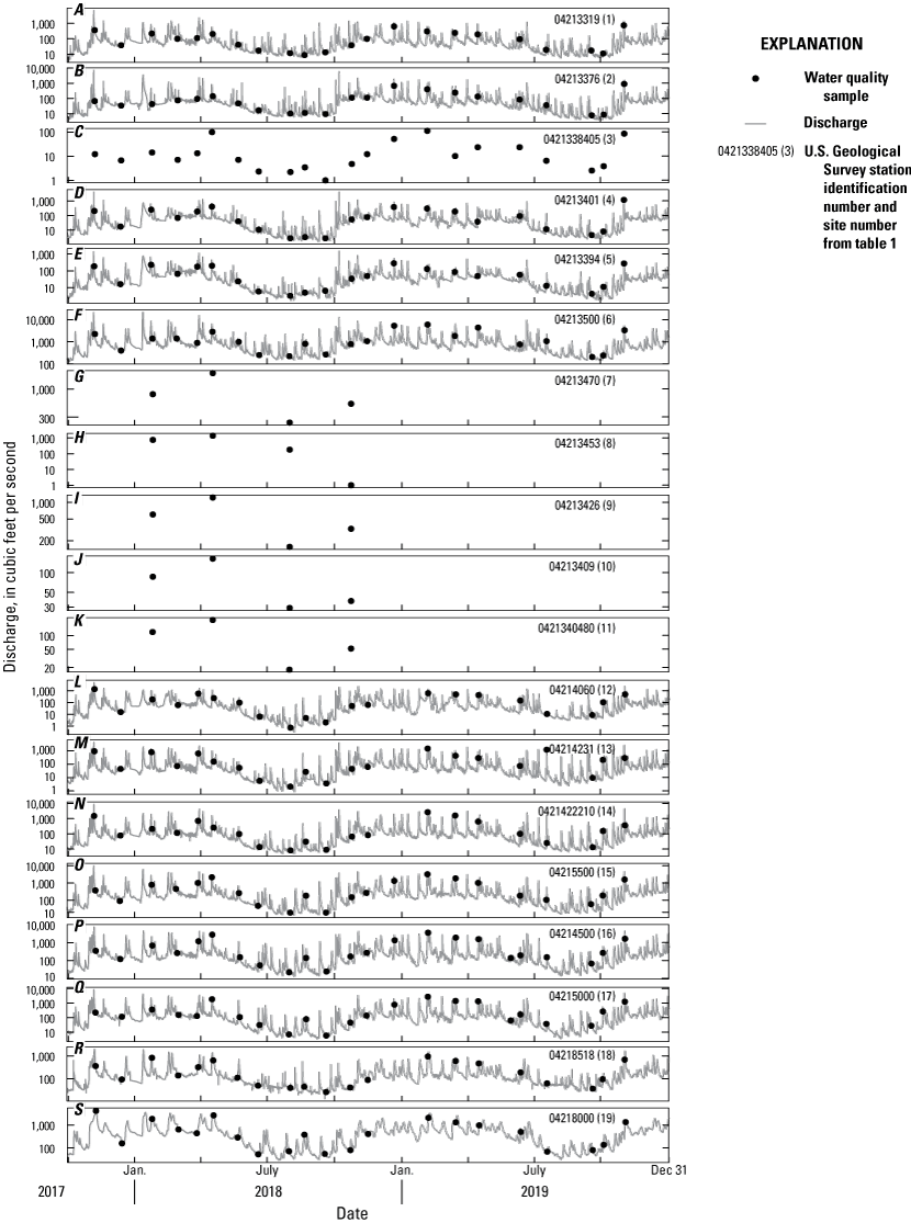
Graphs (A–S) of time series of discharge and water-quality samples collected at study sites on tributaries to Lake Erie, New York.
In 2018, 25 additional samples, including 20 regular samples, 4 replicate samples, and one blank sample were collected from 5 ungaged sites on Cattaraugus Creek and its tributaries (sites 7 to 11 in table 1); these sites were sampled approximately quarterly to investigate variation of water-quality constituents within the Cattaraugus Creek watershed. Discharge was measured at each of these sites when a water-quality sample was collected (fig. 4).
In the first water year (October 2017–September 2018), samples were collected on a regular schedule; in the second year (October 2018–September 2019), high flow events were targeted for sampling. Some scheduled, monthly samples were not collected because of the lapse in Federal appropriation and government shutdown in December 2018. Other scheduled samples were not collected in May and August 2019 because high flows did not occur at a time when crews could sample them. Water-quality samples were collected using the equal-width-increment method and depth integrating isokinetic samplers, as specified in the National Field Manual for Collection of Water Quality Samples (USGS, variously dated), whenever possible. Exceptions to standard sampling protocols were documented on field notes and coded in sample metadata. Low-flow samples were collected by wading (fig. 5), and high flow samples were collected from bridges (fig. 6). Samplers used included the DH-81, DH-95, and D-74AL (Davis and Federal Interagency Sedimentation Project, 2005) except when flow velocities were outside the isokinetic range of the samplers. When velocities were too low, grab samples were collected with open-mouth bottles. When velocities were too high, samples were collected using weighted bottle samplers. Equal-width-increment samples were collected except in the case of rapidly changing conditions during high flow events, when depth integrating or grab samples were collected at the centroids of the left, center, and right channel sections. During sample collection, field measurements of temperature, pH, dissolved oxygen, specific conductivity, and turbidity were made using a multiparameter probe (YSI, Inc. 6-Series Multiparameter Water Quality Sonde) at locations and for durations intended to represent cross-channel conditions. The field observations, water-quality data, methods, and metadata are available in the National Water Information System (USGS, 2016b).
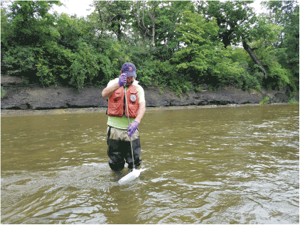
Photograph of low-flow water-quality sample collection with a DH-81 sampler at streamgage 04214500 (site 16 in table 1) on Buffalo Creek, New York, on July 17, 2019. Photograph by Elizabeth Nystrom, U.S. Geological Survey.
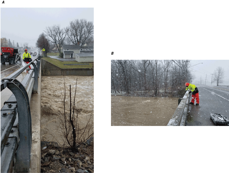
Photographs of high-flow water-quality sample collection with a DH-95 sampler at A, streamgage 04214500 (site 16 in table 1) on Buffalo Creek, New York, on April 16, 2018; photograph by Elizabeth Nystrom, U.S. Geological Survey; and B, Streamgage 04215000 (site 17 in table 1) on Cayuga Creek, New York, on April 16, 2018; photograph by Elizabeth Nystrom, U.S. Geological Survey.
Samples were composited in 8-liter plastic churns for splitting into individual bottles for laboratory analysis. After splitting, subsamples for chlorophyll a, pheophytin a, and orthophosphate) analysis were filtered. Subsamples for chlorophyll a and pheophytin a analysis were filtered using a hand-operated vacuum pump and 0.7-micron, glass-fiber filter. Subsamples for orthophosphate analysis were filtered through a 0.45-micron filters using a syringe. Subsamples for analysis of some nutrients, including total Kjeldahl nitrogen (nitrogen from ammonia and ammonium plus organic nitrogen), nitrate, and nitrite, were unfiltered and acidified using sulfuric acid. All subsamples were stored on ice before shipping except samples of suspended sediment (which were unrefrigerated) and chlorophyll a and pheophytin a (which were frozen). Subsamples collected for analyses with short hold times (nutrients) were shipped overnight daily from the field to analyzing laboratories. Subsamples collected for some analyses (suspended sediment, chlorophyll a and pheophytin a) were held and shipped in batches at a later date. Subsamples for chlorophyll a and pheophytin a analysis were shipped on dry ice. Samples were sent to several laboratories for analysis, including ALS (https://www.alsglobal.com/; for nitrite, nitrate plus nitrite, calculated nitrate, total solids, and total dissolved solids), the USGS National Water Quality Laboratory (for total Kjeldahl nitrogen, total phosphorus, chlorophyll a, and pheophytin a), the USGS Soil and Low-Ionic-Strength Water Quality Laboratory (for ammonia, chloride, orthophosphate, and turbidity), and the USGS Kentucky Sediment Laboratory (for suspended sediment).
Development of rloadest Suspended Sediment and Nutrient Load Estimates
The rloadest package (Lorenz and others, 2013; Runkel and De Cicco, 2017), in the R programming language (R Core Team, 2018), was used to evaluate, and when appropriate data were available, to create models to estimate loads from 13 study sites where daily streamflow and water-quality monitoring data were present (sites 1–6 and 12–19 in table 1). The R package rloadest was developed from the Fortran program LOADEST (Runkel and others, 2004). Constituents evaluated for rloadest analysis included total phosphorus, orthophosphate, total nitrogen, nitrate plus nitrite, ammonium, and suspended sediment. For each constituent model, the rloadest program computes regression coefficients by means of the maximum likelihood estimation method (Wolynetz, 1979). For each constituent, three predefined models (Runkel and others, 2004) were tested (table 5), and the models were ranked based on Akaike information criterion scores (Helsel and Hirsch, 2002). Then, diagnostic plots were created to assess the variance (as a function between predicted values and time, season, and discharge) and the normality of each model’s residuals.
Table 5.
The three predefined regression models from rloadest evaluated at each site and when appropriate used to estimate loads of nutrients and suspended sediment.[Equations are from Lorenz and others (2013); Runkel and De Cicco (2017); Runkel and others (2004). lnL, natural log of constituent load; a, coefficient; lnQ, natural log of streamflow minus center of natural log of streamflow; dtime, decimal time minus center of decimal time]
Additionally, the rloadest program computes bias diagnostics that compare estimated constituent loads to observed loads. Load bias percentage is the percentage that the model overestimates (negative number) or underestimates (positive number) the sum of the estimated constituent loads compared to the sum of the observed loads. The partial load ratio is a ratio of the sum of the estimated constituent loads to the sum of the observed loads, which indicates modeled constituent loads were overestimated (>1) or underestimated (<1). The Nash-Sutcliffe efficiency (NSE) is computed by rloadest and provides a measure of model fit that ranges from −∞ (no relation) to 1 (perfect fit). These diagnostics and the graphed residuals were used to select the model that most appropriately estimated loads for each constituent at each site. Models with an inappropriate number of variables compared to the number of samples were not evaluated because of the likelihood of overfitting. In general, 1 model variable (including the intercept) per 10 samples was considered appropriate (Peduzzi and others, 1996).
Once rloadest models were created for each site and constituent, daily mean discharge values could be used to estimate constituent loads. The R package waterData (Ryberg and Vecchia, 2012) was used to screen each site’s discharge record for missing daily mean discharge values or those equal to 0. One of the 13 sites had 1 missing daily mean discharge value; this value was filled with an estimated value using the waterData package fillMiss function. After the discharge records were complete, daily mean discharge was used to estimate loads for each constituent that meets assumptions needed for the rloadest model at each site. Using the adjusted maximum likelihood estimation method, rloadest computed 90-percent prediction intervals (Cohn, 2005). Retransformation bias was automatically corrected by application of a bias correction factor (Bradu and Mundlak, 1970; Cohn, 1988, 2005). All suspended sediment and nutrient load models and estimates are in Bunch (2024).
SWAT Model Development
The SWAT toolbar ArcSWAT 2012 (Texas A&M AgriLife Research, 2022) for the mapping software ArcGIS (Esri, Redlands, Calif.) was used to create the models. SWAT revision 670 was used to model the study watersheds. All spatial data layers were set to the North American Vertical Datum of 1988, with the projection of Universal Transverse Mercator Zone 17N. The DEM used was from the USGS 1/9 arc-second (3.4 m) National Elevation Dataset (USGS, undated). Stream data was taken from the National Hydrography Dataset Plus (USGS, 2019); streams were burned into the DEM as the stream network. The ArcSWAT automatic watershed delineator was used to delineate subbasins within the study watersheds (fig. 3). Subbasin size for each studied watershed was manipulated by changing the location of subbasin outlets so that the area of each subbasin was within an order of magnitude of each other and to approximately match the size of USGS 12-digit hydrologic unit code watersheds (USGS, 2019). Additionally, the USGS streamgages were set as subbasin outlets for model calibration and validation (fig. 2; table 1). The locations of subbasin outlets were manually changed to match outlets of the 12-digit hydrologic unit code watersheds, USGS gages, or to improve spatial precision of important hydrologic features, such as the Erie Canal in the Tonawanda Creek watershed. The watershed outlets for all models were the intersection of the main stream of interest (for example, Cattaraugus Creek of the Cattaraugus Creek watershed) and Lake Erie. The 2018 Cropland Data Layer (CDL; NASS, 2019) was used to provide land-cover data and the Soil Survey Geographic Database (SSURGO; NRCS, 2019) was used to provide soil data. Slope classes were set within ArcSWAT to best represent the topography of each watershed (table 4).
Hydrologic response units (HRUs) are unique topological areas within each subbasin. They are the smallest area unit in SWAT that is independently simulated. HRUs are delineated by the unique combination of subwatershed, land cover type, soil type, and slope class. The combination of these data layers produces thousands of delineated HRUs per study watershed. HRU thresholds were set to a minimum area of 1 hectare (ha), where HRUs smaller than 1 ha were removed and combined with adjacent, larger HRUs to reduce model complexity and processing time. Exceptions to HRU threshold processing were set so that any HRUs with a land cover type classified as septic were not recombined to preserve this land cover type.
SWAT Model Parameterization
SWAT model parameters are changed from default values to represent real-world conditions in a process called parametrization. Model parameters are applied at three different levels: (1) watershed; (2) subbasin; and (3) HRU. Watershed level parameters mostly set the equations or water-quality parameters used throughout the watershed. Groupings of subbasins or HRUs are commonly lumped together to represent similar areas, land covers, management, weather, and so on. Major watersheds are divided into tributary subwatersheds with corresponding subbasins. For example, the Walnut Creek watershed has a tributary of Silver Creek which drains about half of the watershed. Those subbasins that contribute to Silver Creek make the area called “Silver Creek subwatershed” (subbasins 4–7, 9, 10, 13, 16, 17, 21, and 24 in fig. 3H) in this report, and subbasins that contribute to Walnut Creek make the area called “Walnut Creek subwatershed” (subbasins 8, 11, 12, 14, 15, 18–20, 22, 23, and 25–29 in fig. 3H) in this report. One example of HRU groupings is that all forested HRUs throughout a watershed model have the same parameter values for forest land use in this report. SWAT saves its parameters in several different files. Each file type contains multiple parameters; SWAT parameters discussed in this report will take the format of “PARAMETER_NAME.file name.”
Watershed level equations are discussed in the following text; a full description of the following methods used in this study can be found in Neitsch and others (2002). The watershed parameters are stored in the .bsn file. SWAT uses the Soil Conservation Service (SCS) curve number (CN) method (Mockus, 1964) to calculate runoff from HRUs on a daily basis (the U.S. Department of Agriculture [USDA] Soil Conservation Service is now the USDA Natural Resources Conservation Service). In SWAT, HRUs are assigned a CN from 30 to 99; low numbers correspond to low runoff potential, whereas larger numbers correspond to high runoff potential. The runoff CN is a function of slope, land use, soil hydrologic group, soil permeability, and soil moisture. Daily CNs were calculated in the Big Sister Creek and Walnut Creek watersheds as a function of plant evapotranspiration (ICN.bsn set to 1) rather than soil moisture. The other watershed models calculated the CN from soil moisture with adjustments for tile drainage (ICN.bsn set to 2). Potential evapotranspiration was calculated with the Penman-Monteith Method (IPET.bsn set to 1; Neitsch and others 2002) using input weather data, described below. Because all simulations started in January, the models were initialized with snow present in all subbasins (snow_sub.sub set to 150). Channel routing was simulated with the Muskingum method (IRTE.bsn set to 1), as the simulated streamflow performed better than the default variable storage method in most of the watersheds. The new soil phosphorus model (SOL_P_MODEL.bsn set to 1) was used because this algorithm was recommended by White and others (2009) to accurately model phosphorus loads from manure. The instream water-quality model, QUAL2E, is integrated with SWAT to simulate in-stream water-quality processes. QUAL2E simulates nutrient cycles, algae production, oxygen demand and uptake, and atmospheric aeration (Migliaccio and others, 2007). QUAL2E was used in this study by setting the IWQ.bsn parameter to 1.
Collection of Climate Data
Daily precipitation, temperature, and wind speed data from January 1, 1984, to December 31, 2019, were acquired from the National Oceanic and Atmospheric Administration National Centers for Environmental Information weather stations (Menne and others, 2012) for input to the SWAT model (table 6). A subbasin could have different weather stations for precipitation, temperature, wind speed, or relative humidity. The closest weather station for each weather element to each subbasin’s centroid was used (fig. 2). Precipitation and temperature files were processed to replace missing data with values from the nearest weather station. Relative humidity data in New York were obtained from the Iowa Environmental Mesonet (2019). The SWAT weather generator was used to calculate daily values for solar radiation.
Table 6.
Weather stations used in the watershed models for the selected tributary watersheds of Lake Erie, New York, examined in this study.[Global Historical Climate Network (GHCN) data from Menne and others (2012). Relative humidity (RH) data are from Iowa Environmental Mesonet (2019). N, north; S, south; E, east; W, west; NY, New York; PA, Pennsylvania; US, United States; AWOS, Automated Weather Observing System; P, precipitation; Tona, Tonawanda Creek; Buff, Buffalo River; Tmp, temperature; Catt, Cattaraugus Creek; W, wind speed; BgS, Big Sister Creek; E18, Eighteenmile Creek; Cay, Canadaway Creek; Ch, Chautauqua Creek; Cr, Crooked Brook; Walnut, Walnut Creek; NA, not applicable]
Channel and Canal Parameterization
ArcSWAT calculates several parameters for each subbasin, including subbasin area, channel dimensions, and channel slopes from the DEM. SWAT simulates one main channel and one tributary channel per model subbasin saved in the .rte and .sub files, respectively. These parameters, among others discussed in this section, characterize the channels which affect modeled streamflow.
The Manning's roughness coefficient, commonly known as “Manning’s n,” is used in the calculation of channel flow time of concentration—the time it takes for flow from the upstream channels to reach the subbasin outlet. Manning’s n values were selected from Chow (1959) for the study watershed's main stem and tributary channels, represented in SWAT by the parameters of CH_N2.rte for the main stem channels and CH_N1.sub for the tributary channels. Each SWAT subbasin has a Manning’s n value for the main stem channel and the tributary channel. The Manning’s n values for main channels (CH_N2.rte) were set to 0.040 to represent mountain streams with no vegetation and gravels in the channel. For subbasins downstream from USGS streamgage 04213500 on Cattaraugus Creek at Gowanda, N.Y., main stem Manning's n (CH_N2.rte) values were set to 0.025 to represent gravelly stream bottoms. For tributary channels that were unmaintained with dense brush, CH_N1.sub were set to 0.10; this applied to the Buffalo River, Canadaway Creek, Cattaraugus Creek, and Walnut Creek watersheds. The default value of Manning's n, a value of 0.014, was applied to the other watershed tributaries (CH_N1.sub), including Big Sister Creek, Chautauqua Creek, and Eighteenmile Creek watersheds. Flood-control diversions and dredging on Ellicott Creek (Wooster and Matthies, 2008), in the Tonawanda Creek watershed, were represented by setting Manning's n of main channels (CH_N2.rte) to 0.028 (subbasins 63, 64, 67, 70–73, and 76 in fig. 3I).
As a part of the Erie Canal, Tonawanda Creek from Pendleton, N.Y., to Lockport, N.Y., was modified to have a flat hydraulic slope to aid boats in river navigation. From May to October every year, the Lockport lock is opened, which causes the direction of streamflow to be reversed (fig. 2I). Approximately 31.15 cubic meters per second (m3/s) of water flows upstream Tonawanda Creek, exits Tonawanda Creek watershed at Lockport, and continues northeast (Wooster and Matthies, 2008). To simulate the backflow out of the watershed in the Tonawanda Creek model, monthly point sources were added to subbasins 3, 4, 11, 22, 30, 37, and 39 (fig. 3I) that intersect Tonawanda Creek. The average simulated flows during the months of May to October were multiplied by negative 1 to reverse the simulated flow. During months when the Lockport lock would be closed, the point-source flows were set to 0. The main channel slopes (CH_S2.rte) in these Erie Canal subbasins were set to 0.02 meter height per meter width to mimic the flat hydraulic slope of Tonawanda Creek. The main channel Manning's n (CH_N2.rte) of the Erie Canal was set to 0.028 to represent dredged channel bottoms (Chow, 1959).
The Buffalo River from its outlet at Lake Erie to roughly 9.65 km upstream was designated a Federal navigation channel and has been dredged every 2 years by the U.S. Army Corps of Engineers (USACE; USACE, 2010). The depth of this channel has been maintained at 6.7 m beneath the Low Water Datum of Lake Erie (The Low Water Datum of Lake Erie is currently defined as 173.5 m above the 1985 International Great Lakes Datum [USACE, undated b; National Oceanic and Atmosphere Administration, undated]) and the bottom width of the channel was measured as 45.72 m (USACE, 2010). Side slopes have been maintained at a ratio of 1:3 height to width. To simulate the dredged channel bottom, the main stem Manning's n value (CH_N2.rte) for the Buffalo River was set to 0.028 in subbasin 9 (fig. 3B), which encompassed the majority of the Federal navigation channel.
Historically, there were several projects performed to stabilize the banks of Eighteenmile Creek, where rocks were applied to many sections of the banks of Eighteenmile Creek. These projects were done in subbasin 16 (fig. 3G). The main stem Manning's n value (CH_N2.rte) in SWAT was modified to 0.07 for this subbasin.
Groundwater Parameterization
SWAT partitions groundwater into shallow and deep aquifers for each model subbasin. Water in the shallow aquifer contributes water to streamflow (known as baseflow) and water in the deep aquifer is assumed to leave the watershed (Neitsch and others, 2002). To estimate the two SWAT groundwater parameters baseflow alpha factor (ALPHA_BF.gw) and groundwater delay time (GW_DELAY.gw), a baseflow separation algorithm by Arnold and Allen (1999) was used on the daily flow data from streamgage sites 1, 2, 4–6, and 12–21 in table 1. The baseflow alpha factor gives the response of the groundwater to recharge. The groundwater delay time is the number of days for flow to percolate through the soil profile to reach the shallow aquifer—this is a function of hydrologic properties of the shallow aquifer’s geology and the depth to the water table. Other groundwater parameters were set using automatic calibration in the Soil and Water Assessment Tool Calibration and Uncertainty Program (SWAT-CUP); use of SWAT-CUP is described later in the “SWAT Model Calibration and Validation” section.
Management Schedules and Parameterization
All HRUs require a management schedule to define how the land represented by the HRU are used throughout the SWAT simulation. SWAT management schedules can be any length, but they must have at least 1 year. Urban areas, forests, or wetlands typically use the same operations year after year. For example, wetlands are represented in the default management schedule with only two operations per year: the start and end of the growing season. This 1 year of management is then repeated for each year of the SWAT simulation period. Default management schedules for agricultural areas show only the start and end of the growing season for single crop and an autofertilizer which applies a variable quantity of fertilizer depending on crop nutrient needs. Agricultural areas commonly grow different crops in a temporal pattern, referred to as a crop rotation; simulated crop rotations for agricultural areas are discussed in the following section. Additionally, grazing livestock are present within the watersheds. Management schedules for grazing livestock are not a default option within SWAT and their management schedules must be developed. For this report, management schedules will be referred to as “rotations.” For example, the management schedule for forest land cover is “forest rotation.”
The 16 different rotations used in the models are: apple, barren, beef cattle, CAFOs (combining dairy CAFO and poultry CAFO), cash grain, continuous corn, dairy, forest, vineyard, horse, other agriculture, pasture, septic, urban, water, and wetlands. Not every watershed model used every rotation; some land covers in table 2 were not present in all watersheds or not present at great enough quantities to pass the HRU threshold—previously discussed in the “SWAT Model Development” section. The following section described how the rotations were created and applied per HRU so that the management of the study watersheds was simulated as accurately as possible.
For the results reported in this document, some of the similar land covers are lumped together into the same rotation. All forest land covers (deciduous, evergreen, and mixed) are reported together in the forest rotation. The two different wetland types (herbaceous and woody) are reported together in the wetland rotation. The results for the four developed land cover types are reported together in the urban rotation. The “other agriculture” rotation contains the remaining agricultural land covers (oats, potatoes, range, winter wheat; fig. 3); this rotation used all default management schedules and parameters.
Management schedules were created to customize agricultural operations, including fertilizer application quantity and timing, crop type, tillage, and harvest for each crop rotation. To determine the HRUs receiving agricultural rotations, 5 years (from 2014 to 2018) of CDL layers (NASS, 2015, 2016, 2017, 2018, 2019) were combined and the principal crop growing in each HRU was recorded for each of the 5 years. A dairy HRU was defined as a HRU with at least 3 years of alfalfa or pasture and at least 1 year of silage corn or soybeans out of 5 years of CDL data. A cash grain HRU was defined as an HRU with at least 2 years planted with corn or soybeans out of 5 years of CDL data. Continuous corn HRUs were defined as an HRU with at least 3 years of corn out of 5 years of CDL data. Pasture HRUs were defined as an HRU with more than 2 years of pasture or hay and no corn or soybeans grown out of 5 years of CDL data. All other land covers listed in table 2 (excluding corn, soybeans, hay, alfalfa, or pasture) used the management schedule defaults, unless described otherwise in the sections below.
Three management schedules were developed for the following HRUs: (1) dairy HRUs, (2) cash grain HRUs, and (3) continuous corn HRUs. For dairy HRUs, 3 years of corn silage was followed by 5 years of hay in SWAT (table 7). Cash grain HRUs were simulated as 2 years of corn grain followed by 1 year of soybeans (table 8). In continuous corn HRUs, continuous corn rotations were simulated by repeating the schedule of the first year of the cash crop schedule for every year of simulation (table 8). Management schedules for pasture HRUs used SWAT default management.
Table 7.
Simulated conventional and best management practice schedules for dairy rotation used in watershed models for the selected tributary watersheds of Lake Erie, New York, examined in this study.[The data in this table were used for simulating poultry CAFOs after replacing liquid dairy manure of the conventional dairy rotation with poultry litter; poultry litter described in Chiang and others (2010). kg/ha, kilogram per hectare; —, no data]
Incorporated manure application was simulated in the Soil and Water Assessment Tool by setting the parameter FRT_SURF.mgt parameter (fraction of fertilizer applied to the top 10 millimeters of soil) to 0.1.
Subsurface liquid manure injection was simulated in the Soil and Water Assessment Tool by setting the frt_surf parameter (fraction of fertilizer applied to the top 10 millimeters of soil) to 0.01.
Table 8.
Simulated conventional and best management practice schedules for the cash grain and continuous corn rotations used in watershed models for the selected tributary watersheds of Lake Erie, New York, examined in this study.[—, no data; kg/ha, kilogram per hectare; FRT_SURF.mgt, fraction of fertilizer applied to the top 10 millimeters of soil]
For continuous corn rotations, the first year of data in this table is repeated for all following years.
Subsurface manure injections were simulated in the Soil and Water Assessment Tool by setting the FRT_SURF.mgt parameter (fraction of fertilizer applied to the top 10 millimeters of soil) to 0.01.
Side-dressed fertilizer was simulated in the Soil and Water Assessment Tool by setting the FRT_SURF.mgt parameter (fraction of fertilizer applied to the top 10 millimeters of soil) to 0.9.
Broadcast manure applications were simulated in the Soil and Water Assessment Tool by setting the FRT_SURF.mgt parameter (fraction of fertilizer applied to the top 10 millimeters of soil) to 0.95.
The fertilizer (28 percent urea) was represented in the Soil and Water Assessment Tool fertilizer database with the following parameter values: mineral nitrogen (MIN-N) set to 0.280, and mineral phosphorus (MIN-P), organic nitrogen (ORG-N), organic phosphorus (ORG-P), and ratio of ammonia as nitrogen to mineral nitrogen (NH3-N/MIN-N) set to 0.
Management Schedules for Beef Cattle and Horse Rotations
Grazing by beef cattle and horses was simulated in the watersheds. Management schedules for beef cattle are in table 9 and for horses in table 10. The 2017 Census of Agriculture livestock counts by county were downloaded from the USDA National Agricultural Statistics Service (National Agricultural Statistics Service, undated). Livestock were assumed to be evenly distributed across the counties. Horses were simulated on HRUs that were classified with open urban area (URBN) land cover; beef cattle were simulated on HRUs with land cover of rangeland (RNGB) or pasture (PAST). Horses and beef cattle were simulated as grazing from April 15 to October 30, thus the number of grazing days (GRZ_DAYS.mgt) was set to 199 in SWAT. The dry weight amount of manure produced daily by animal (MANURE_KG.mgt) was calculated using values from the standards manual “Manure Production and Characteristics” (American Society of Agricultural Engineers, 2005). For horses, the amount of biomass consumed per animal (BIO_EAT.mgt) was assumed to be 12.5 kilograms (kg) of grass daily, with a 30 percent dry weight, which was assumed to be equal to the amount of biomass trampled (BIO_TRMP.mgt). Following conventional practice, simulated horse manure was accumulated and stored over the winter and was surface applied during the spring. There was another simulated surface application of horse manure in the fall. For beef cattle HRUs, BIO_EAT.mgt and BIO_TRMP.mgt parameters were set to 8 and 3, respectively, using assumptions from Merriman and others (2018b). In the simulations, beef cattle manure was surface applied every 2 weeks during the cold months until grazing began again on April 15.
Table 9.
Simulated conventional and best management practice schedules for the beef cattle rotation in watershed models for the selected tributary watersheds of Lake Erie, New York, examined in this study.[kg/ha, kilogram per hectare; —, no data]
Table 10.
Simulated management schedule for the horse rotation in watershed models for the selected tributary watersheds of Lake Erie, New York, examined in this study.[kg/ha, kilogram per hectare]
Concentrated Animal Feeding Operations
A CAFO is an animal feeding facility that meets animal size thresholds and confines those animals for more than 45 days in any 12-month period. CAFOs are found throughout the study watersheds. Adjustments to HRU management schedules were required to account for high manure production in HRUs that have CAFOs. Customization of management schedules depending on the presence of CAFOs (referred to as “CAFO HRUs”) allowed the SWAT models to accurately simulate the agricultural conditions in the study watersheds. CAFO locations were provided by the NYSDEC and published in Fisher and Merriman (2024) with information on the affected area, quantity of manure applied, and the number and type of animals. For the modeled CAFOs, daily mean manure production and nutrient content were obtained for each animal type from the American Society of Agricultural Engineers (2005). The majority of CAFOs in the study area are dairies.
There is an equine CAFO in the Tonawanda Creek watershed. Based on interviews with USDA personnel, the equine CAFO removes manure from its site, and thus was not considered in this study.
Management Schedules for Dairy Concentrated Animal Feeding Operations
Dairy farms are considered CAFOs if they have 300 or more cows. The CAFOs were overlaid spatially on the HRU framework to determine which HRUs should be simulated as CAFOs. HRUs closest to the CAFO location and designated as dairy or pasture were categorized as CAFOs. HRUs simulated as CAFOs required modifications to the management schedule operations so that the SWAT simulation included the manure rates produced by the CAFOs. Whenever a CAFO location overlapped a dairy rotation HRU, the CAFO manure application schedule for that HRU used the baseline management of dairy rotations shown in table 7, but the application rate of manure was modified to match the CAFO data from the NYSDEC. On pasture HRUs used for dairy cattle grazing, CAFO manure applications were simulated after hay cuttings. The manure application rate was found for each CAFO by dividing the total quantity of manure applied by the CAFO land area.
Management Schedule for Poultry Concentrated Animal Feeding Operations
There are two poultry CAFOs in the study area: one in the Buffalo River watershed and another in the Tonawanda Creek watershed. The poultry CAFO in the Tonawanda Creek watershed was simulated by replacing liquid dairy manure for the conventional rotation in table 7 with poultry litter (droppings mixed with used bedding and spilled feed) in SWAT. Parameters for untreated poultry litter as described in Chiang and others (2010) were added to the SWAT fertilizer database (Neitsch and others, 2002). Based on interviews with USDA personnel, the poultry CAFO in the Buffalo River watershed did not spread any litter on the surrounding agricultural fields, thus poultry litter application was not modeled in that watershed.
Management Schedules for Vineyard Rotations
Management of vineyards (primarily for grape juice production) in the study area was derived from an interview with a local viticulture expert in 2019. Vineyards were simulated by setting the current age of crops (CURYR_MAT.mgt) to 50 years in SWAT, and the simulated management schedule included a fertilizer application in June and biomass harvest in October (table 11). Vineyard rotations were applied on HRUs that have grapes as the land cover.
Table 11.
Simulated management schedule for the vineyard rotation in watershed models for the selected tributary watersheds of Lake Erie, New York, examined in this study.[kg/ha, kilogram per hectare]
| Date | Vineyard rotation schedule |
|---|---|
| May 5 | Start growing season |
| June 15 | 56 kg/ha fertilizer application1 |
| Oct. 10 | Biomass harvest |
This fertilizer (28 percent urea) was added to the Soil and Water Assessment Tool fertilizer database with the following parameter values: mineral nitrogen (MIN-N) set to 0.280, and mineral phosphorus (MIN-P), organic nitrogen (ORG-N), organic phosphorus (ORG-P), and ratio of ammonia as nitrogen to mineral nitrogen (NH3-N/MIN-N) set to 0. The default FRT_SURF.mgt parameter value (fraction of fertilizer applied to the top 10 millimeters of soil) was used, 0.2.
Management Schedules and Parameters for Nonagricultural Rotations
Other land cover types listed in table 2 were simulated in SWAT with the default management schedules, with the exception of apple orchards (apple land cover), forests, and wetlands. The apples orchards, forests, and wetlands were initialized as growing at the beginning of the SWAT simulation period by setting the parameter IGRO.mgt to 1. These were simulated as mature forests and wetlands by setting the current age of trees (CURYR_MAT.mgt) parameter to 30 years for deciduous forests and apple orchards, 10 years for evergreen forests and forested wetlands, 20 years for mixed forest, and 5 years for herbaceous wetlands. Manning's n for overland flow (OV_N.hru), and maximum canopy storage (CANMX.hru) were varied by land cover (table 12). Forest parameters had the largest effect on model results out of all the land cover parameters because of the dominance of forested land cover throughout the watersheds. Recent research indicates that the plant database (plant.dat) parameters are important for model calibration in heavily forested watersheds to properly account for evapotranspiration (Yang and others, 2018, 2019; Yang and Zhang, 2016).
Table 12.
Manning's roughness coefficients and canopy cover parameters by land cover used in watershed models for the selected tributary watersheds of Lake Erie, New York, examined in this study.[SWAT, Soil and Water Assessment Tool]
Septic land cover type was added to the land cover in a process described in the “Septic System Parameterization” section. It is not included in table 2 and figure 3.
The SWAT land-use code refers specifically to the SWAT land-use code used in the SWAT plant growth database (Neitsch and others, 2002).
Tile Drainage Parameterization
Tile drainage was simulated on select agricultural HRUs using the DRAINMOD equations (ITDRN.bsn set to 1) based on the Hooghoudt and Kirkham equations (Moriasi and others, 2013). Tile drainage was assumed when agricultural HRUs (those for dairy, CAFO, cash grain, or continuous corn) had poorly or very poorly drained soils and low slopes (<2 percent). Calculated tile drainage area was variable across the study watersheds, ranging from 0.06 percent in the Canadaway Creek watershed to 10.6 percent in the Tonawanda Creek watershed (table 4). Simulated tile drainage depth (DDrain.mgt) was set to 609.6 mm in SWAT. The depth to impervious layer (DEP_IMP.hru) on tiled HRUs was set to 1,000 mm, beneath the simulated tile drainage depth, to ensure tile drainage is not impeded by the presence of an impervious layer in SWAT (Boles and others, 2015). For HRUs that do not have tile drainage, the parameter DEP_IMP.hru used the default value of 6,000 mm. No pumping from tile drainage was occurring in the basins, thus pump capacity (PC.sdr) parameter was set to 0 in SWAT.
Septic System Parameterization
Septic systems were identified in the study watersheds using the NYS Tax Parcel Centroid Points map layer (New York State Geographic Information Systems [GIS] Clearinghouse, undated), by selecting all points where the sewer description (SEWER_DESC) field was “private.” This layer was overlaid with known water utility service areas to generate a layer of HRUs using septic systems (Fisher and Merriman, 2024). The private septic systems within the water utilities service area were assumed to be hooked up to the municipal wastewater treatment utility and were removed from the septic layer. The remaining septic system points were converted to a raster layer at the same resolution as the land cover layer, 10 m, and then were overlaid onto the land cover layer. This allowed for septic systems to be used as a land cover with the input land cover code of “SEPT.” The septic land covers were excluded from the land cover threshold, meaning the total area of septic land cover was maintained in each subbasin. All HRUs with land cover designation of “SEPT” were modeled as generic conventional septic system (ISEP_TYP.sep set to 1) by activating septic systems on those HRUs (ISEP_OPT.bsn set to 1). Model defaults were used for the rest of the septic parameters. None of the study watersheds have a large presence of septic fields; septic areas are present in 1 percent or less of all study watersheds.
Irrigation and Water Use Parameterization
Site-specific, monthly water withdrawal data from surface water and groundwater sources were available from 2010 to 2018 (NYSDEC, 2020). If more than one water user with the same water source was in the same subbasin, then water use in that subbasin was summed, as SWAT only allows one water user by source type per subbasin. When the water source was from a groundwater, pond, or reservoir source, the monthly average use was compiled by subbasin in the water use files (.wus). Groundwater withdrawals were separated into shallow (WUSHAL.wus) or deep (WUDEEP.wus) aquifers by provided well depth; deep groundwater withdrawals were assumed to be from wells over 30.5 m deep. Point source files were used for withdrawals from streams as they can be exactly specified as a monthly times series (the same format of the observed water use data), rather than using monthly average removals required in the format of the .wus files. Water use withdrawals from streams were entered into the point source files as a negative number to signify a withdrawal.
When the water use of a water user was classified as irrigation, simulated irrigation was applied to HRUs in the management files (.mgt) that corresponded with the location of the source withdrawal. In the management files, the observed monthly water use data was disaggregated into daily irrigation applications, unless irrigation occurred on urban or grassland HRUs. The monthly irrigation volume on urban or grassland HRUs was disaggregated and applied by heat unit scheduling.
Ponds and Wetlands Parameterization
SWAT uses the .pnd files to parameterize ponds and wetlands by subbasin. The U.S. Fish and Wildlife Service National Wetlands Inventory (U.S. Fish and Wildlife Service, 2016) was used to estimate the land area used for the ponds and wetlands. Default parameters were used for all suspended sediment and nutrient related inputs for ponds and wetlands, and other parameters were estimated based on the size of the pond or wetland.
Point Source Parameterization
Monthly point source data from 2013 to 2019 were provided by the NYSDEC (table 3; Fisher and Merriman, 2024). Additional data for some point sources were obtained from the EPA’s Enforcement and Compliance History Online database for the period from 2007 to 2019 (EPA, undated). For point-source data prior to 2007, long-term, monthly averages of the reported data were used. Total nitrogen was assumed to be 21 milligrams per liter (mg/L) where nitrogen data were not reported for a point source; this assumption is based on average nutrient removal efficiencies by various wastewater treatment plant types from Qiu and others (2010). Total phosphorus was assumed to be 3 mg/L and dissolved oxygen was assumed to be 5 mg/L when the respective data was not available for a point source; these assumptions are based on the recommendations of Section 7 of the Chesapeake Bay Phase 5.3 Community Watershed Model (Chesapeake Bay Program, 2010). Total nitrogen was speciated into ammonia, nitrate, nitrite, and organic nitrogen; total phosphorus was speciated into organic and mineral phosphorus (mineral phosphorus was assumed to be orthophosphate for use in SWAT) based on facility type and treatment (Chesapeake Bay Program, 2010). Where quarterly data existed for a given parameter, missing data were filled by interpolating the interquartile range. After data gaps were filled, if more than one discharger was in the same subbasin, then all discharge and effluent loads in that subbasin were summed, as SWAT only allows one point source per model subbasin.
SWAT Model Calibration and Validation
Quantitative statistics including NSE, the coefficient of determination (R2), and percent bias (PBIAS), and visual examination of hydrographs were used to evaluate model performance (Moriasi and others, 2007, 2015). The NSE value ranges from −∞ (no relation) to 1 (perfect fit), where a value of 0.75 to 1 indicates a very good model fit, 0.65 to 0.75 is good, 0.50 to 0.65 is satisfactory, and <0.5 is unsatisfactory. NSE is the most accepted and implemented statistical standard for the evaluation of performance in watershed modeling (Daggupati and others, 2015; Gassman and others, 2007; Mankin and others, 2002) and is well-known for estimating peaks of model responses. R2 is used to evaluate the fit of simulated data to observed data. Higher values of R2 demonstrate a better fit of the simulated data to the observed data. There is only one ranking threshold for R2: an R2 value greater than or equal to (≥) 0.5 is satisfactory. On the other hand, PBIAS is used to assess the average tendency of system response. The optimal value of PBIAS is 0.0 percent, indicating no model bias. Absolute PBIAS values of less than or equal to (≤) 10 percent for flow, ≤15 percent for suspended sediment, and ≤25 percent for nutrients indicate a very good model fit. A good model fit is found when absolute PBIAS values range from 10 to 15 percent for flow, from 15 to 30 percent for suspended sediment, and from 25 to 40 percent for nutrients. Absolute PBIAS values from 15 to 25 percent for flow, 30 to 55 percent for suspended sediment, and 40 to 70 percent for nutrients indicate satisfactory model performance. Absolute PBIAS values ≥25 percent for flow, ≥55 percent for suspended sediment, and ≥70 percent for nutrients indicate unsatisfactory model performance. Positive values of PBIAS indicate that the model underestimates bias, while negative values indicate that the model overestimates bias (Gupta and others, 1999).
Model calibration for hydrology was run on the USGS supercomputer Yeti using SWAT-CUP. SWAT-CUP is an automatic calibration program for SWAT (Eawag, 2013). The Yeti supercomputer uses the Linux operating system (https://www.linux.org/), thus the software must be formatted for the Linux operating system. The SWAT executable file for Linux is available on the SWAT website (https://swat.tamu.edu/software/swat-executables/); the SWAT revision 670 executable file is published in Fisher and Merriman (2024). The SWAT-CUP for Linux program was obtained from 2W2E GmbH (K. Abbaspour, 2W2E GmbH, written commun., 2019). SWAT-CUP was run on Microsoft Windows for suspended sediment and nutrient calibration. Also, sensitivity analysis was performed using SWAT-CUP for Tonawanda Creek watershed and Chautauqua Creek watershed models (app. 1).
Streamflow and water-quality calibration was performed from the beginning of the monitoring periods (shown by site in table 1) until 2018 for the Big Sister Creek, Canadaway Creek, Chautauqua Creek, Eighteenmile Creek, and Walnut Creek watersheds. Longer hydrologic calibration periods were possible in Buffalo River, Cattaraugus Creek, and Tonawanda Creek watersheds because of long-term data. A warmup period of 5 years was used in all models to allow for the models’ initial conditions to stabilize. Water-quality loads used in calibration were computed with rloadest regression with the hydrologic record (see “Development of rloadest Suspended Sediment and Nutrient Load Estimates” section); therefore, the water-quality calibration period coincided with the hydrologic period of record for the Big Sister Creek, Canadaway Creek, Chautauqua Creek, Eighteenmile Creek, and Silver and Walnut Creek watersheds. The Buffalo River, Cattaraugus Creek, and Tonawanda Creek watersheds had longer hydrologic records, so the water-quality calibration period coincided with the water-quality data collection from 2017 through 2018. The model validation period for streamflow and water-quality parameters was from January 1 to December 31, 2019, for all models. SWAT-simulated nitrate as nitrogen loads were calibrated to the rloadest calculated nitrate plus nitrite loads.
Definitions of default values and ranges for model parameters are given in table 13. The calibrated values for these parameters per watershed are in table 14. Groupings of parameter types, such as snow parameters and hydrologic parameters, were calibrated with different methods depending on the nature of the parameter and available data. For the watersheds with more than one USGS streamgage, the model parameters were spatially calibrated to each separate streamgage, starting with parameters at the most upstream streamgage. For example, the Tonawanda Creek watershed model was calibrated for hydrology parameters to four USGS streamgages, three of those on Tonawanda Creek. Parameters for the most upstream streamgage on Tonawanda Creek (streamgage 04216418; Tonawanda Creek at Attica, N.Y.) were calibrated first, then calibration moved downstream to the next streamgage (04217000; Tonawanda Creek at Batavia, N.Y.), and then finally the parameters were calibrated at most downstream streamgage on the Tonawanda Creek at Rapids, N.Y. (streamgage 04218000). Parameters for the fourth streamgage in the Tonawanda Creek watershed on the tributary Ellicott Creek (streamgage 04218518) were calibrated separately. There are three streamgages in the Buffalo River watershed, one each on its main branches: Cazenovia, Buffalo, and Cayuga Creeks. Parameters for the watersheds of each branch were calibrated separately. There are five water-quality monitoring sites in the Cattaraugus Creek watershed, but only one of these has daily streamflow data, streamgage 04213500 on Cattaraugus Creek. Therefore, the Cattaraugus Creek watershed model was calibrated for streamflow at this site. Spatial calibration is indicated in table 14 by specifying different parameter values for different subwatersheds.
Table 13.
Soil and Water Assessment Tool calibration parameters, descriptions, ranges, and default values used for watershed models for the selected tributary watersheds of Lake Erie, New York, examined in this study.[°C, degree Celsius; mm water/(°C×d), millimeter water per degree Celsius multiplied by day; mm, millimeter; HRU, hydrologic response unit; mm/hr, millimeter per hour; mg/L, milligram per liter; m3/Mg, cubic meter per megagram; mg/kg, milligram per kilogram; mg/(m2×d), milligram per square meter multiplied by day]
Table 14.
Soil and Water Assessment Tool calibration values of model parameters for watershed models for the selected tributary watersheds of Lake Erie, New York, examined in this study.[Parameters, default values, and ranges are defined in table 13. Buff, Buffalo River subwatershed; %, percent; Silver, Silver Creek subwatershed; Walnut, Walnut Creek subwatershed; Ell, Ellicott Creek subwatershed; SBR, South Branch Eighteenmile Creek subwatershed ; sub, subbasin; —, no data; Cay, Cayuga Creek subwatershed; Caz, Cazenovia Creek subwatershed; Rapids, portion of Tonawanda Creek subwatershed upstream from streamgage 04218000 and downstream from streamgage 04217000; Bat, portion of Tonawanda Creek subwatershed upstream from streamgage 04217000 and downstream from 04216418; Attica, portion of Tonawanda Creek subwatershed upstream from the Attica streamgage 04216418; Tona, Tonawanda Creek subwatershed; QUAL2E, Enhanced Stream Water Quality Model]
Spatial calibration for the Buffalo River watershed was separated by three main tributaries: Cayuga Creek (Cay), Cazenovia Creek (Caz), and Buffalo Creek (Buff).
Chautauqua Creek watershed was not calibrated for suspended sediment or nutrients. All parameters not listed are defaults.
Spatial calibration for the Eighteenmile Creek watershed was separated into two subwatersheds: Eighteenmile Creek and South Branch Eighteenmile Creek (SBR).
Spatial calibration for the Walnut Creek watershed was separated into two subwatersheds: Silver and Walnut Creeks.
Spatial calibration for the Tonawanda Creek watershed was separated into two or four subwatersheds depending on where data were available. The two subwatersheds were Ellicott Creek (Ell) and Tonawanda Creek (Tona). For the four subwatersheds, this divides the Tonawanda creek subwatershed (Tona) further based on the location of the three streamgages on Tonawanda Creek (Rapids, Batavia [Bat], and Attica) and the existing subwatershed of Ellicott Creek (Ell).
CN2 and SOL_AWC values were increased by the percentage listed. Negative values indicate the values were decreased by the percentage listed.
Snow parameters were first calibrated as recommended by Abbaspour and others (2018) to set an appropriate volume of water in winter months. Snow parameters are typically calibrated at the watershed spatial scale, but some models with multiple streamgages performed differently in the winter months.
Groundwater parameters were calibrated after snow parameters. A baseflow separation (Arnold and Allen, 1999) was applied on streamgages with over 2 years of hydrologic data (table 1) to determine the percentage of flow from groundwater sources. The groundwater parameters baseflow alpha factor, ALPHABF.gw, and groundwater delay time, GW_DELAY.gw, were also estimated by the baseflow separation algorithm. For streamgages with less than 2 years of hydrologic data, ALPHABF.gw and GW_DELAY.gw were set using automatic calibration in SWAT-CUP.
SWAT Model Scenarios
Models created with the previously described calibration parameters in table 13 and 14 are called the baseline scenarios. Further model scenarios tested the following: (1) implementation of selected BMPs, (2) effects from decreasing the phosphorus treatment limits on loads exported from point sources, or (3) the effect of green infrastructure (land use change, permeable pavement, and rain gardens). These three scenario types were developed in collaboration with Erie County and NYSDEC (table 15) and are described in the following sections.
Table 15.
Number and type of simulation scenarios run per study watershed model for the selected tributary watersheds of Lake Erie, New York, examined in this study.[—, no scenario]
Best Management Practice Scenarios
Three BMP implementations scenarios; low, medium, and high; were developed to test the effect of BMPs on watershed streamflow, surface runoff, and water quality. BMPs were implemented on HRUs with the following agricultural rotations: dairy, beef cattle, continuous corn, and cash grain. The simulation specifications of these rotations are described in the section “Management Schedules and Parameterization.” The simulated BMPs are dependent on the type and schedules of simulated agricultural rotations (for example, for the agricultural management schedule of dairy rotation with a BMP applied, see table 7). After simulations were run, data were analyzed to understand the effectiveness the implementation levels and of individual BMPs and BMP combinations on runoff and water quality. No BMP scenarios were run on the Crooked Brook watershed model, which had insufficient streamflow data for calibration, or on the Chautauqua Creek watershed model, which failed calibration and validation (see section “Chautauqua Creek Watershed Model Calibration and Validation”). The low, medium, and high BMP implementation levels were run on agricultural HRUs of the 7 remaining watershed models for a total of 21 BMP model scenarios per agricultural rotation described as follows.
BMPs selected for model scenarios were cover crops (CC), filter strips (FS), reduced tillage (RT), and nutrient management plan (NMP). The selected BMPs were chosen because they were seen as the most likely to be used within the study watersheds. BMPs were modeled with low, medium, and high levels of implementation. The CC, NMP, and RT all occur on the HRU and affect the crop rotation schedules (tables 7, 8, and 9); these will be referred to as infield BMPs, as they occur in the farm field. FS are not infield BMPs; the FS intercepts runoff as it leaves the field and does not disrupt the conventional crop rotation schedules. The medium and high scenarios had multiple BMPs simulated on the same HRU; for the purpose of this report, multiple BMPs will be referred to as BMP combinations. When this occurs, a plus sign (+) is used between the abbreviation of the BMPs to denote multiple BMPs on the same HRU. For example, CC+NMP means that CC and NMP were both applied to the same HRU. The scenarios were as follows:
-
• Low scenario: 10 percent of agricultural areas had a single infield BMP (CC, NMP, or RT) implemented and FS applied to 2.5 percent of agricultural areas;
-
• Medium scenario: the low scenario, plus 10 percent of agricultural areas had two infield BMPs (CC+NMP, CC+RT, or NMP+RT) implemented, and FS applied to 5 percent of agricultural areas; and
-
• High scenario: the medium scenario, plus CC+NMP+RT applied to 10 percent of agricultural areas, and FS applied to 10 percent of agricultural areas.
The low scenario applied either CC, NMT, or RT evenly to a total of 10 percent of the agricultural HRUs in each watershed. The BMPs were applied to randomly selected agricultural HRUs. Each selected infield BMP (CC, NMP, or RT) covers a total of 3.33 percent of the watershed’s agricultural area. FS were simulated on an additional 2.5 percent of the agricultural area and applied to randomly selected agricultural HRUs.
The medium scenario incorporated the low scenario and added combinations of two infield BMPs to an additional 10 percent of the agricultural areas. The three combinations of infield BMPs were the following: CC+RT, CC+NMP, and NMP+RT. The three different BMP combinations each cover 3.33 percent of the watershed’s area. With these 3 combinations and the 3 single BMPs implemented in the low scenario, 20 percent of the agricultural area was simulated with a BMP or BMP combination in the medium scenario. FS were simulated on an additional 2.5 percent of the agricultural areas for a total of 5 percent of the agricultural area.
The high scenario used a combination of three infield BMPs (CC+NMP+RT) on an additional 10 percent of the agricultural areas for a total of 30 percent of the agricultural area with at least one infield BMP applied. FS were simulated on an additional 5 percent of the agricultural area for a total of 10 percent of the agricultural area.
Modifications for BMPs implemented in dairy rotations in comparison to a conventional dairy rotation are shown in table 7. In dairy rotations with CC implemented, the cover crop used was cereal rye. It was planted in October and harvested the following May. When the cover crop was grown, the fall dairy manure application was moved to early October rather than the first of November. The fall tillage was also removed. For dairy rotations with the NMP, the volume of fertilizer applied in the spring of the first and second years was reduced and the manure application method was changed to subsurface injection during in the years with corn silage planted. Subsurface manure injection was modeled by changing the fraction of fertilizer applied to the top 10 millimeters of soil (FRT_SURF.mgt) to 0.01, which applies 99 percent of the manure to the soil subsurface. The side-dress application of fertilizer was removed in the first year and reduced in the second year. Dairy rotations with RT had spring and fall tillage changed to conservation tillage on years with corn silage planted (table 7). Management was not changed years on hay was grown (years 4-8 in table 7) for NMP and RT.
Modifications for BMPs implemented in cash grain and continuous corn rotations in comparison to the conventional rotations are shown in table 8. CC were implemented by planting cereal rye in October and harvesting it in May. For RT implementation, conservation tillage replaced the spring tillage in every year of the rotation. In June of the first and second years of the rotation, the volume of the side-dress fertilizer was reduced, and the fertilizer application method was changed to subsurface injection to simulate NMPs.
No BMPs were modeled on CAFOs as it was assumed that NMPs were already implemented. FS or NMPs were simulated on beef cattle HRUs. NMPs on beef cattle HRUs were simulated by assuming that manure was stored over the winter period instead of applied in biweekly applications. Beef cattle would be inside during cold months (November 1 to April 14), and the facilities were assumed to have manure storage, so manure applications were not simulated during winter (table 9). FS on beef cattle HRUs were modeled using SWAT defaults for all rotation types.
Point Source Scenarios
To find the effect of phosphorus loading to the watersheds from point sources, additional scenarios were simulated by decreasing the limit of total phosphorus in effluent of selected point-source discharges. There were four different point source scenarios: two for the Tonawanda Creek, one for Big Sister Creek, and one for Buffalo River watersheds. Two different total phosphorus limits were used: 0.5 mg/L and 1.0 mg/L. To calculate the total phosphorus loads in the point source scenarios’ inputs, the flow rate was multiplied by the total phosphorus limit and then speciated into mineral and organic phosphorus (see the previous section “Point Source Parameterization”). Occasionally, the calculated total phosphorus load for the scenario would be greater than observed total phosphorus load. In that case, the lower value was used for the scenario. The following are the four point source scenarios (table 3):
-
• The first Tonawanda point-source scenario (Tonawanda scenario 1) changed the total phosphorus limit to 0.5 mg/L on three discharges: NY0025950 (in subbasin 40), NY0026514 (in subbasin 50), and NY0021849 (in subbasin 75; table 3; fig. 3I).
-
• The second Tonawanda point-source scenario (Tonawanda scenario 2) included the settings of scenario 1 and changed the total phosphorus limit to 1 mg/L on three discharges: NY0031003 (in subbasin 45), NY0108430 (in subbasin 59), and NY0020541 (in subbasin 72; table 3; fig. 3I).
-
• The Buffalo point-source scenario changed the total phosphorus limit to 1 mg/L total phosphorus on one discharge: NY0108103 (in subbasin 47; table 3; fig. 3B).
-
• The Big Sister point-source scenario changed the phosphorus limit to 0.5 mg/L total phosphorus on one discharge: NY0022543 (in subbasin 1; table 3; fig. 3A).
Green Infrastructure Scenario
The Buffalo Sewer Authority of the City of Buffalo, N.Y., has heavily invested in green infrastructure, specifically permeable pavement and rain gardens, in the Buffalo urban area. To find the effect of green infrastructure on runoff water quality, a simulated green infrastructure scenario was developed for the Buffalo River watershed. Permeable pavement and rain gardens are in the most downstream subbasin (subbasin 9; fig. 3B). Both these BMPs were modeled in the low-impact development file (.lid) using the fraction of the impervious area that the BMPs covered and default parameters. There were 0.471 ha of permeable pavement and 0.826 ha of rain garden modeled. Additionally, the Buffalo Sewer Authority has demolished vacant buildings and returned those areas to vacant grass lots. The implementation of vacant grass lots were modeled by changing the SWAT land use type (URBLU.mgt), referenced by the urban parameters database (Neitsch and others, 2002), from high density urban to low density residential. This reduced the fraction of impervious area from 0.6 to 0.12 and reduced the runoff CN. The Manning’s n value for overland flow (OV_N.hru) was increased to 0.03 account for the grassed land cover (Chow, 1959). Vacant lots are in subbasins 9, 11, and 20 and cover 2.33, 0.63, and 0.03 km2, respectively.
Calculation of SWAT Model Results
SWAT results are returned on multiple scales and in multiple formats. Suspended sediment and nutrient outputs are given as yields at the HRU and subbasin levels and as loads at the watershed level. A load is the mass of a constituent discharged past a point in a watershed. A yield is the constituent load per unit area of the contributing watershed.
The BMP scenarios were designed to increase the number of BMPs between scenarios by building each successive level of BMP implementation upon the previous scenario. The low scenario applied single BMPs. The medium scenario additionally applied combinations of two BMPs (CC+NMP, CC+RT, NMP+RT). The high scenario additionally applied the combination of three BMPs (CC+NMP+RT). BMPs were applied at the HRU scale; select HRUs had one, two, or three BMPs applied depending on the scenario (low, medium, or high, respectively). An HRU with a BMP in the low scenario has the same BMP applied in the medium and high scenarios. Thus, results at the HRU scale from BMP and BMP combinations from the high scenario can be compiled and analyzed together. Watershed-level results are presented by low, medium, or high scenario as the cumulative effect of all the BMPs combined in each scenario.
After the SWAT scenarios were run, model outputs were analyzed to understand the effectiveness of individual BMPs and BMP combinations on runoff and water quality at the HRU, subbasin, and watershed scales. The average annual suspended sediment and nutrient loads were calculated for the baseline and BMP scenarios at the HRU and watershed scales. Average annual runoff and suspended sediment and nutrient yields were also calculated at the HRU scale. Watershed-scale reductions were calculated by the percent difference in the average annual loads of the test scenario compared to the baseline scenario. Similarly, HRU-scale reductions for BMPs were calculated as the percent difference in yield of the test scenario compared to the baseline scenario.
Results of Data Collection
Results of the water-quality sampling are compiled in boxplots shown in figure 7. Total phosphorus concentrations range from 0.004 to 2.07 mg/L with the maximum value observed at streamgage 04214231 (South Branch Eighteenmile Creek; fig. 7A). Distributions of total phosphorus concentrations show less variability among streamgages compared to orthophosphate concentrations. Streamgage 04218000 (Tonawanda Creek) had the highest median concentration for both total phosphorus (0.094 mg/L; fig. 7A) and orthophosphate (0.015 mg/L; fig. 7B). Total nitrogen ranged from 0.12 to 16.0 mg/L with the maximum value also occurring at streamgage 04214231 (South Branch Eighteenmile Creek; fig. 7C). Median nitrite plus nitrate concentrations were highest at five Cattaraugus Creek streamgages, although only four samples were taken at each of these locations, with a maximum value of 3.06 mg/L from streamgage 04215000 (Cayuga Creek; fig. 7D). Streamgage 04218518 (Ellicott Creek) had both the highest median (0.096 mg/L) and maximum (0.311 mg/L) ammonia concentrations (fig. 7E). The highest median (116.0 mg/L) suspended sediment concentrations were at streamgage 04213500 (Cattaraugus Creek), and the maximum value of 6,690 mg/L suspended sediment was measured at streamgage 04214231 (South Branch Eighteenmile Creek; fig. 7F).
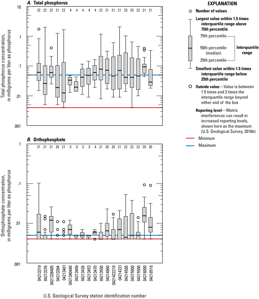

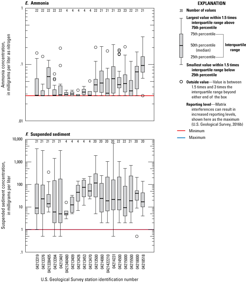
Boxplots of concentrations of A, Total phosphorus; B, Orthophosphate; C, Total nitrogen; D, Nitrate plus nitrite; E, Ammonia; and F, Suspended sediment at the 19 water-quality streamgages (site numbers 1–19, table 1) in New York, from November 2017 to November 2019. Data from U.S. Geological Survey (2016b).
Results of rloadest Models for Suspended Sediment and Nutrient Load Estimates
In total, 46 rloadest models were created for the 13 streamgage sites that had data that met the requirements needed for rloadest analysis. The rloadest results are listed in table 16. Of the 13 sites, rloadest models were created for total phosphorus at 12 sites, total nitrogen at all 13 sites, nitrate plus nitrite at 5 sites, ammonium at 5 sites, and suspended sediment concentration at 11 of the 13 sites. Orthophosphate samples were highly censored and did not produce any viable models at the study sites. Model results that had high bias or nonsignificant model variables were not considered. All model results and associated data are available in Bunch (2024).
Table 16.
Summary statistics of rloadest models used to compute loads at selected U.S. Geological Survey water-quality streamgages.[Data from Bunch (2024). Site numbers correspond to the sites in figure 1. The rloadest regression models are described in table 5. NA, not applicable because there was no rloadest model created; —, no data]
Results of SWAT Model Calibration and Validation
Calculated calibration and validation statistics for the SWAT models are summarized in table 17. SWAT model results were compared to observed streamflow measurements and rloadest calculated constituent loads. The Chautauqua Creek watershed failed calibration; the computed NSE and PBIAS values were unsatisfactory (NSE<0.5; PBAIS≥±25). Crooked Brook watershed was not calibrated because of the lack of long-term daily streamflow measurements. These two models were excluded from table 17 and all model scenarios. The SWAT models generally underestimated monthly average streamflow, monthly suspended sediment loads, and monthly nutrient loads in winter and spring months; these months typically had the largest streamflow and loads, and simulation discrepancies in these months result in lower rankings in calibration statistics. Generally, the growing season (May to September) was well represented. Simulated streamflow was lower in the warmer months than in other months and represented baseflow conditions. Correspondingly, simulated suspended sediment and nutrient loads matched calculated rloadest loads better in warmer months than in colder months. Ammonium was not directly calibrated and is not shown in the following calibration graphs.
Table 17.
Calibration and validation statistics computed on the monthly average streamflow and monthly suspended sediment and nutrient loads for the calibrated Soil and Water Assessment Tool watershed models for selected tributary watersheds of Lake Erie, New York.[Calibration statistics were calculated from simulated results in Fisher and Merriman (2024), observed flow data from U.S. Geological Survey (2016b), and load data from Bunch (2024). Nitrate as nitrogen loads simulated by the Soil and Water Assessment Tool were calibrated to the rloadest calculated nitrate plus nitrite loads (table 16). Crooked Brook watershed model is not included due to lack of daily streamflow data. —, not computed]
Indicates a very good rating according to Moriasi and others (2007). Shaded in green for visibility.
Indicates a good rating according to Moriasi and others (2007). Shaded in yellow for visibility.
Indicates a satisfactory rating according to Moriasi and others (2007). Shaded in gray for visibility.
Indicates an unsatisfactory rating according to Moriasi and others (2007).
Big Sister Creek Watershed Model Calibration and Validation
The Big Sister Creek watershed SWAT model was calibrated for monthly average streamflow and monthly suspended sediment and monthly total nutrient loads at USGS streamgage 04214060, 3.91 km from the watershed outlet (table 17; fig. 8). NSE statistics were rated good for monthly streamflow and monthly suspended sediment, total phosphorus, and total nitrogen loads (table 17). PBIAS ratings for monthly suspended sediment and monthly total nutrient loads are very good, whereas the PBIAS for streamflow were rated satisfactory (table 17). All R2 values are ≥0.68 (table 17), except for ammonium which has an R2 value of 0.48. The simulated flow was underestimated during peak flows (fig. 8). During the largest peak in streamflow during the simulation period (November 2017), the model underestimated suspended sediment and nutrient loads. The nitrate plus nitrite loads estimated by rloadest were not statistically significant and were not calibrated.
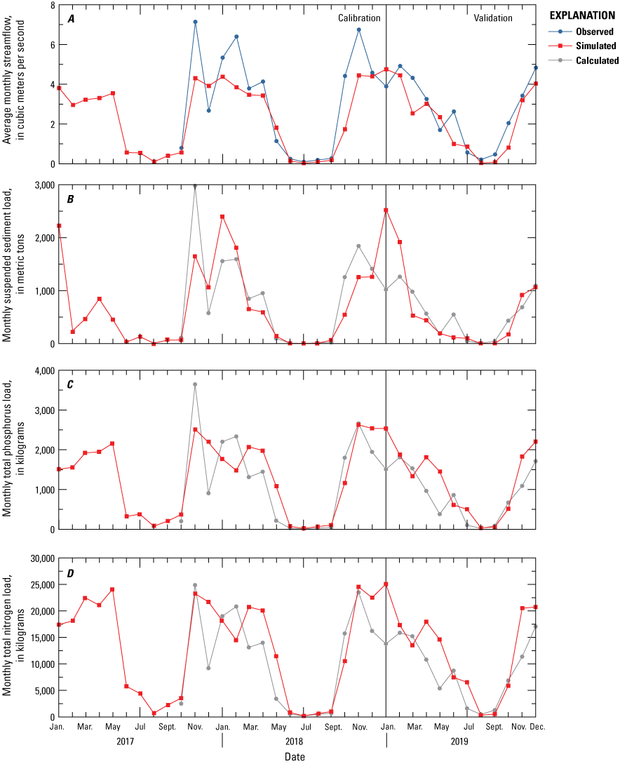
Graphs comparing Soil and Water Assessment Tool simulated monthly streamflow and loads to observed monthly streamflow or rloadest calculated loads from January 2017 to December 2019 at U.S. Geological Survey streamgage 04214060 on Big Sister Creek, in the Big Sister Creek watershed, New York, of A, Average streamflow; B, Suspended sediment load; C, Total phosphorus load; and D, Total nitrogen load.
As shown in table 17, model performance in the validation period was not rated as highly as in the calibration period. Only the NSE value for monthly average streamflow was rated good. The NSE statistics for the other estimated constituents (monthly suspended sediment and monthly total phosphorus and nitrogen loads) were rated unsatisfactory. PBIAS, however, was rated good for monthly suspended sediment, monthly total nitrogen, and monthly total phosphorus load values. The model overestimated the monthly suspended sediment and monthly total nutrient loads in the month of January 2019 (fig. 8). An ice jam was reported on Big Sister Creek on February 5, 2019 (USACE, undated a); the breakup of ice jams can mobilize significant amounts of suspended sediment and nutrients.
Buffalo River Watershed Model Calibration and Validation
The Buffalo River watershed SWAT model was calibrated to the streamgages on its three main tributaries. For the model calibration at the Cazenovia Creek at Ebenezer, N.Y. (streamgage 04215500), and Cayuga Creek near Lancaster, N.Y. (streamgage 04215000), streamgages, the NSE and PBIAS statistics were rated good and very good for streamflow (table 17). The streamflow had satisfactory NSE and good PBIAS ratings at streamgage 04214500, the Buffalo Creek streamgage. The negative PBIAS value at streamgage 04215000 indicates that streamflow was overestimated, whereas the positive PBIAS values at the other two tributary streamgages in this watershed show that simulated streamflow was underestimated compared to observed values. Winter flows were generally underestimated (figs. 9, 10, 11), with the exception of flows during January 2018 at 04214500 and 04215500 streamgages and both January and February 2018 at streamgage 04215000. Peaks in streamflow and loads in November 2017 at all three streamgages were underestimated by the models.
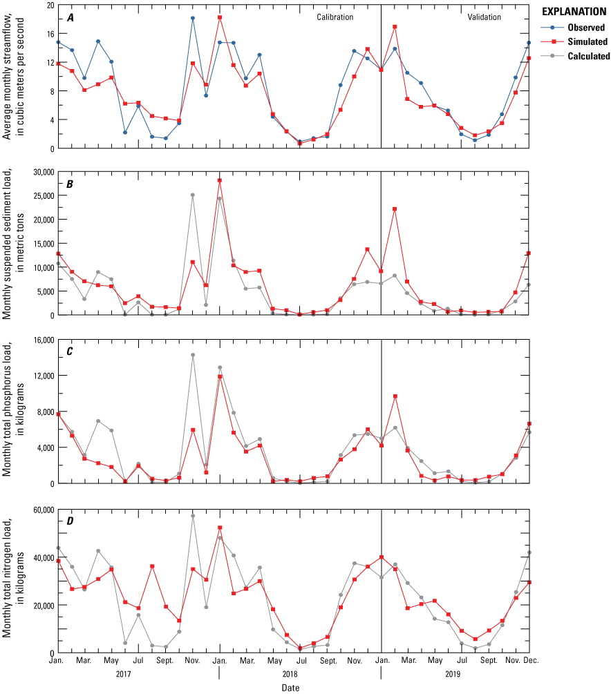
Graphs comparing Soil and Water Assessment Tool simulated monthly streamflow and loads to observed monthly streamflow or rloadest calculated loads from January 2017 to December 2019 at U.S. Geological Survey streamgage 04215500 on Cazenovia Creek, in the Buffalo River watershed, New York, of A, Average streamflow; B, Suspended sediment load; C, Total phosphorus load; and D, Total nitrogen load.
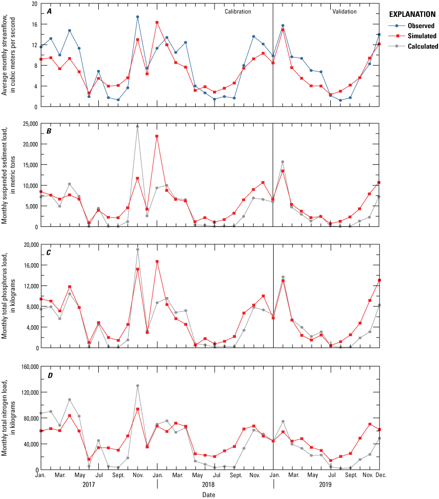
Graphs comparing Soil and Water Assessment Tool simulated monthly streamflow and loads to observed monthly streamflow or rloadest calculated loads from January 2017 to December 2019 at U.S. Geological Survey streamgage 04214500 on Buffalo Creek, in the Buffalo River watershed, New York, of A, Average streamflow; B, Suspended sediment load; C, Total phosphorus load; and D, Total nitrogen load.
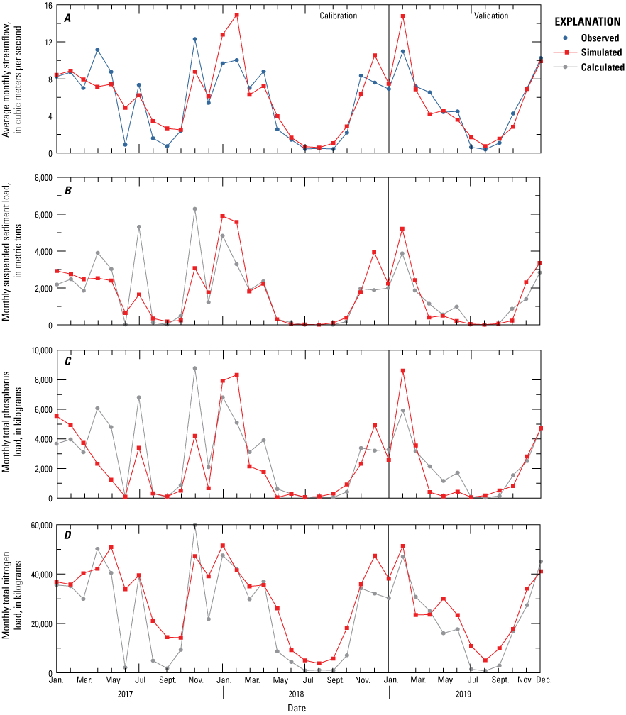
Graphs comparing Soil and Water Assessment Tool simulated monthly streamflow and loads to observed monthly streamflow or rloadest calculated loads from January 2017 to December 2019 at U.S. Geological Survey streamgage 04215000 on Cayuga Creek, in the Buffalo River watershed, New York, of A, Average streamflow; B, Suspended sediment load; C, Total phosphorus load; and D, Total nitrogen load.
Monthly suspended sediment load NSE calibration values at the streamgages 04214500, 04215500, and 04215000 were rated unsatisfactory, good, and satisfactory (table 17), respectively. At streamgages 04214500 and 04215500, monthly suspended sediment load calibration PBIAS values were rated good. Negative PBIAS values indicate that simulated monthly suspended sediment loads were overestimated at these two streamgages. The streamgage 04215000 PBIAS rating was rated very good (1.70 percent) for suspended sediment and was only slightly underestimated. R2 for monthly suspended sediment load at 04214500 was rated unsatisfactory.
At two of the three tributary streamgages, NSE statistics of simulated monthly total phosphorus loads were rated good in the calibration period (table 17). PBIAS values at all three streamgages were rated good or very good for monthly total phosphorus loads. The R2 values for simulated monthly total phosphorus loads were satisfactory. The NSE and PBIAS statistics for the simulated total phosphorus loads at streamgage 04215000 were rated unsatisfactory and very good, respectively. The NSE ratings for monthly total phosphorus loads at streamgages 04215500 and 04214500 were good. PBIAS values were rated very good for simulated monthly total phosphorus loads at streamgages 04214500 and 04215000. The calculated PBIAS statistic for simulated total phosphorus loads at streamgage 04214500 was negative, indicating that the model overestimated total phosphorus loads at this location, whereas the PBIAS value was positive for simulated total phosphorus at streamgage 04215000, indicating that the model underestimated total phosphorus loads at this streamgage.
NSE statistics for monthly total nitrogen load calibration were rated at least satisfactory and PBIAS statistics were rated good or very good at all three streamgages in the Buffalo River watershed (table 17). All R2 values were rated satisfactory for total nitrogen. The NSE, PBIAS, and R2 statistics for ammonium calibration data at streamgage 04214500 were all rated unsatisfactory.
In the validation period, the NSE statistics for streamflow were rated very good for all three streamgages (table 17). NSE validation statistics for monthly suspended sediment loads were rated good at streamgages 04214500 and 04215000 and unsatisfactory for streamgage 04215500. Most discrepancies between the simulated and the rloadest loads occurred in winter months; especially for the difference between calculated rloadest and simulated loads in February 2019 at the streamgage 04215500. Buffalo Creek had two ice jams at its intersection with NYS Route 277, near streamgage 04214500 on January 25 and February 4, 2019 (USACE, undated a); the later ice jam caused flooding. It is unknown how long exactly each of the ice jams lasted. A field crew documented the second ice jam (fig. 12). The simulated suspended sediment load for February 2019 was over 20,000 metric tons greater than the rloadest load at streamgage 04215500. Validation statistics for simulated total phosphorus loads were rated good for streamgage 04215500 and satisfactory for streamgages 04214500 and 04215000. NSE validation statistics for total nitrogen were rated good for streamgage 04215500 and very good for streamgage 04215000; the NSE validation statistic for total nitrogen for streamgage 04214500 was rated unsatisfactory. Monthly total nitrogen loads for streamgage 04214500 were overestimated in the growing seasons (fig. 10D), as were suspended sediment and total phosphorus loads from July to December 2019.
Photograph of ice jam at U.S. Geological Survey streamgage 04214500 (site 16 in table 1) on Buffalo Creek, New York, on February 5, 2019. Photograph by Elizabeth Nystrom, U.S. Geological Survey.
Canadaway Creek Watershed Model Calibration and Validation
Figure 13 shows the Canadaway Creek watershed model simulated flows and loads compared to the observed streamflow and rloadest suspended sediment and nutrient loads. Flooding on Canadaway Creek on November 5, 2017, caused an overnight bridge closure and evacuations (WIVB-TV, 2017). This corresponds to a peak flow recorded at USGS streamgage 04213376 (USGS, 2016b). Because of this flood, the month of November 2017 had an observed streamflow peak and elevated monthly suspended sediment, total phosphorus, and nitrogen loads higher than previous months (fig. 13). There was a substantial streamflow peak for the month of January 2018. Figure 13 shows that SWAT underestimated the monthly average streamflow, monthly suspended sediment load, and monthly total nutrient loads; this January peak makes up about 73 and 22 percent of the monthly total phosphorus and monthly total nitrogen loads, respectively, for 2018, at streamgage 04213376. The January 2018 peak was removed from the monthly total phosphorus and monthly total nitrogen calibration dataset, that caused an improvement of the model calibration statistics. Table 17 reflects the removal of the January 2018 peak from the calibration dataset. After the removal of the January 2018 calibration data for streamgage 04213376, PBIAS values were rated satisfactory and good for monthly total phosphorus and total nitrogen loads, respectively; the NSE values were both rated satisfactory for monthly total phosphorus and nitrogen loads.
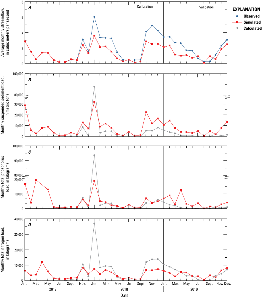
Graphs comparing Soil and Water Assessment Tool simulated monthly streamflow and loads to observed monthly streamflow or rloadest calculated loads from January 2017 to December 2019 at U.S. Geological Survey streamgage 04213376 on Canadaway Creek, in the Canadaway Creek watershed, New York, of A, Average streamflow; B, Suspended sediment load; C, Total phosphorus load; and D, Total nitrogen load.
For validation of the Canadaway Creek model, NSE values for monthly average streamflow, suspended sediment load, and total phosphorus load were rated unsatisfactory (table 17). The PBIAS value for monthly total nitrogen load was rated very good, but the NSE value for monthly total nitrogen load was rated unsatisfactory. Monthly average streamflow was usually underestimated, monthly total nitrogen load values were underestimated and overestimated, and monthly suspended sediment and monthly total phosphorus loads were usually overestimated (fig. 13).
Cattaraugus Creek Watershed Model Calibration and Validation
The streamgage (04213500) used for calibration of the Cattaraugus Creek watershed is 29.5 km upstream from Lake Erie (fig. 2D). The subbasin upstream from the streamgage encompasses about 78 percent of the entire watershed. Withdrawals from the stream had a small effect (<1 percent) on the flow at this point during the study except when a large discharge was released from a wastewater treatment plant (Cattaraugus STP, identifier NY0025861; table 3) in June 2014.
For calibration of the Cattaraugus Creek watershed model, monthly average streamflow and monthly suspended sediment load were rated very good for NSE and good for PBIAS (table 17). The positive PBIAS value (14.82) for the Cattaraugus Creek model calibration period indicates that the model underestimated streamflow (fig. 14). Calibration NSE was rated satisfactory for monthly total phosphorus load and rated good for monthly total nitrogen load. PBIAS values were rated very good for monthly total phosphorus, monthly total nitrogen, and monthly nitrate as nitrogen loads. Monthly total suspended sediment, monthly total nitrogen, monthly nitrate as nitrogen, and monthly total phosphorus loads also have a calibration PBIAS value of <0, indicating that the model overestimated these constituents in the calibration period.
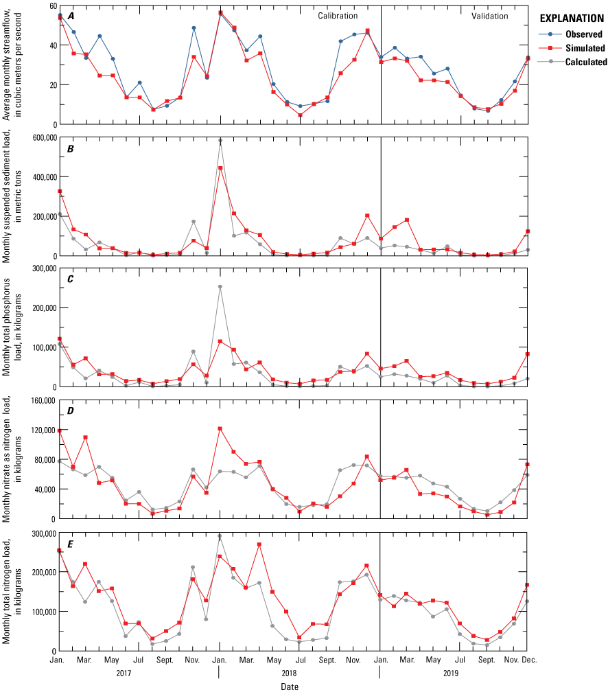
Graphs comparing Soil and Water Assessment Tool simulated monthly streamflow and loads to observed monthly streamflow or rloadest calculated loads from January 2017 to December 2019 at U.S. Geological Survey streamgage 04213500 on Cattaraugus Creek, in the Cattaraugus Creek watershed, New York, of A, Average streamflow; B, Suspended sediment load; C, Total phosphorus load; D, Nitrate as nitrogen load; and E, Total nitrogen load. SWAT-simulated nitrate as nitrogen loads were calibrated to the rloadest calculated nitrate plus nitrite loads (table 16).
Average monthly streamflow was underestimated, and monthly suspended sediment, monthly total nitrogen, and monthly total phosphorus loads were overestimated during the validation period (table 17). The NSE value was rated very good and the PBIAS value was rated good for streamflow in the validation period. Simulated monthly suspended sediment and monthly total phosphorus loads did not have a relation with the estimated rloadest values; the NSE value was <0, and the PBIAS value was rated unsatisfactory for both constituents. The validation NSE value for total nitrogen was rated good, whereas the PBIAS value for total nitrogen was rated very good. Ice jams were reported on Cattaraugus Creek on January 11, 2018, and February 5, 2019 (USACE, undated a); both were downstream of streamgage 04213500.
Chautauqua Creek Watershed Model Calibration and Validation
The SWAT model of the Chautauqua Creek watershed was not rated with satisfactory calibration statistics for monthly average streamflow (table 17). In the calibration period, the Chautauqua Creek SWAT model underestimated monthly average streamflow in winter and spring from November 2017 to April 2018, whereas the model had agreement between simulated and observed monthly average streamflow during the growing season from May to September 2018 (fig. 15). Because model calibration statistics for monthly average streamflow were unsatisfactory, model calibration of suspended sediment and nutrient loads were not attempted. Model result validation statistics were also not calculated.
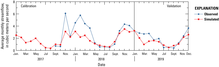
Graph comparing observed monthly and Soil and Water Assessment Tool simulated monthly streamflow from January 2017 to December 2019 at U.S. Geological Survey streamgage 04213319 on Chautauqua Creek, in the Chautauqua Creek watershed, New York.
Crooked Brook Watershed Model Calibration and Validation
Daily suspended sediment and nutrient loads were not available at Crooked Brook watershed because of the lack of daily streamflow data. As daily streamflow data were not available, monthly loads could not be calculated with rloadest. Because of this, the Crooked Brook watershed model was not calibrated. Instead of traditional model calibration, model calibration parameters were transferred from the adjacent Canadaway Creek watershed model, thus the model of the Crooked Brook watershed uses the same calibration parameters as the Canadaway Creek watershed model shown in table 14. Crooked Brook and other uncalibrated models are not included in table 17. Figure 16 depicts the instantaneous streamflow and daily loads. Observed low streamflow and loads appear to match the simulated datasets, but simulated peaks of streamflow and loads often do not match the observed streamflow and rloadest calculated load peaks. The monitoring data most likely did not capture the peak streamflow, which will skew the comparison between simulated and observed streamflow.
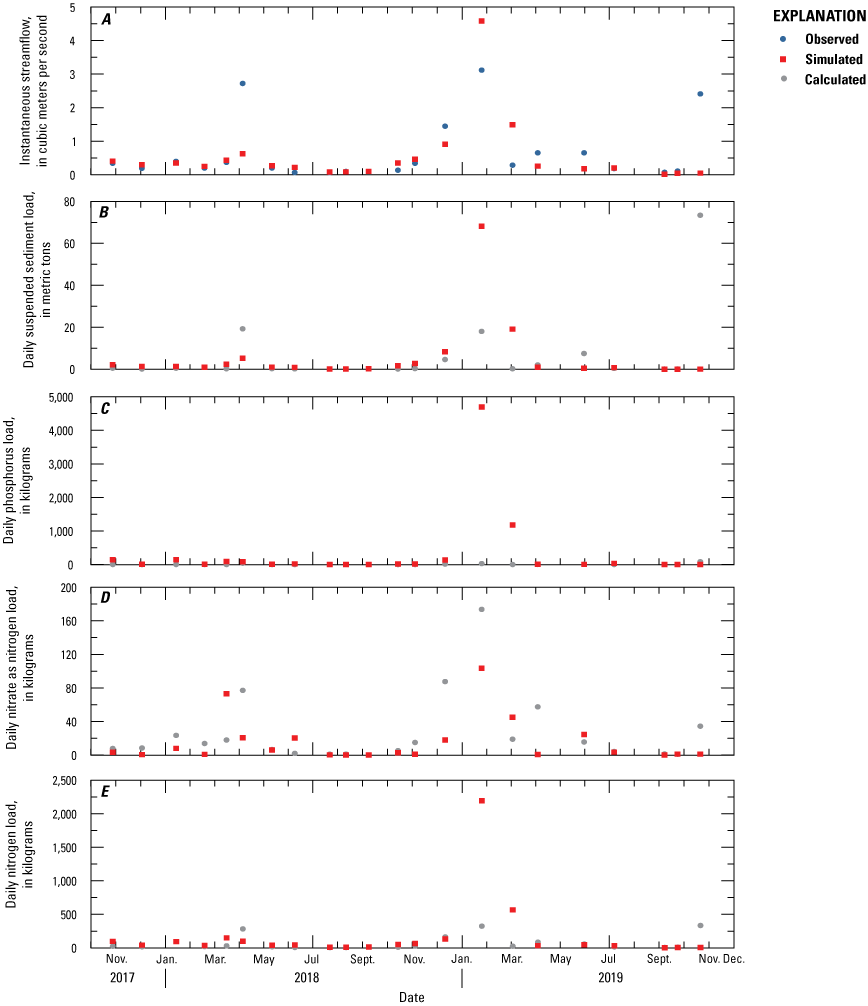
Graphs comparing Soil and Water Assessment Tool simulated daily streamflow and loads to observed daily streamflow or rloadest calculated loads from January 2017 to December 2019 at U.S. Geological Survey streamgage 0421338405 on Crooked Brook, in the Crooked Brook watershed, New York, of A, Instantaneous streamflow; B, Daily suspended sediment load; C, Daily total phosphorus load; D, Daily nitrate as nitrogen load; and E, Daily total nitrogen load. SWAT-simulated nitrate as nitrogen loads were calibrated to the rloadest calculated nitrate plus nitrite loads (table 16).
Eighteenmile Creek Watershed Model Calibration and Validation
The Eighteenmile Creek watershed SWAT model was calibrated at the two streamgages within the watershed (table 17). Following are the calibration statistics for the South Branch Eighteenmile Creek at USGS streamgage 04214231. Calibration NSE values for monthly average streamflow and monthly total nitrogen load were rated good. Monthly suspended sediment loads were not available at streamgage 04214231 (sediment parameters were calibrated at USGS streamgage 0421422210 and these parameters were used for the entire watershed). Calibration NSE values for monthly total phosphorus and nitrate as nitrogen loads at streamgage 04214231 were rated unsatisfactory, but the calibration PBIAS value for monthly total phosphorus load was rated very good. Streamflow and nitrate as nitrogen had satisfactory PBIAS ratings for the calibration period. Calibration NSE and PBIAS for total nitrogen were rated good and very good, respectively, at streamgage 04214231.
In the calibration period, total phosphorus was overestimated at USGS streamgage 04214231 (PBIAS<0; table 17). The SWAT model overestimated total phosphorus for most months in the calibration period (fig. 17B); February 2018 total phosphorus loads were overestimated by about 2,000 kg in the calibration period. Monthly nitrate as nitrogen and total nitrogen loads were underestimated during most months during winter of 2018 to 2019, similar to the underestimated streamflow (figs. 17A, C, D).
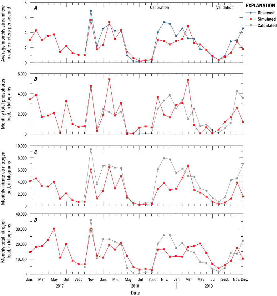
Graphs comparing Soil and Water Assessment Tool simulated to observed or rloadest calculated monthly measurements from January 2017 to December 2019 at U.S. Geological Survey streamgage 04214231 on South Branch Eighteenmile Creek, in the Eighteenmile Creek watershed, New York, of A, Average streamflow; B, Total phosphorus load; C, Nitrate as nitrogen load; and D, Total nitrogen load.
The following are calibration statistics for the SWAT model of Eighteenmile Creek at USGS streamgage 0421422210, which drains 159 km2 on the eastern side of the watershed, approximately half of the watershed (table 1; fig. 2G). The NSE and PBIAS values for streamflow were rated very good and satisfactory, respectively (table 17). Monthly suspended sediment and total nitrogen loads had calibration NSE values that were rated satisfactory and calibration PBIAS values that were rated very good, whereas monthly total phosphorus and nitrate as nitrogen loads have calibration NSE values what were rated good and calibration PBIAS values that were rated very good. Simulated monthly average streamflow closely matched observed monthly average streamflow during October 2017 and November 2017 (fig. 18A) in the calibration period, whereas the other SWAT models for the study watersheds tended to underestimate streamflow during November 2017. The following winter, however, simulated monthly average streamflow did not match observed streamflow as closely. Simulated monthly total phosphorus and monthly total nitrogen were overestimated by the model (PBIAS<0). Late spring, in both the calibration and validation periods, had the most discrepancies in the simulated total phosphorus and total nitrogen loads compared to the rloadest values (figs. 17C, E).
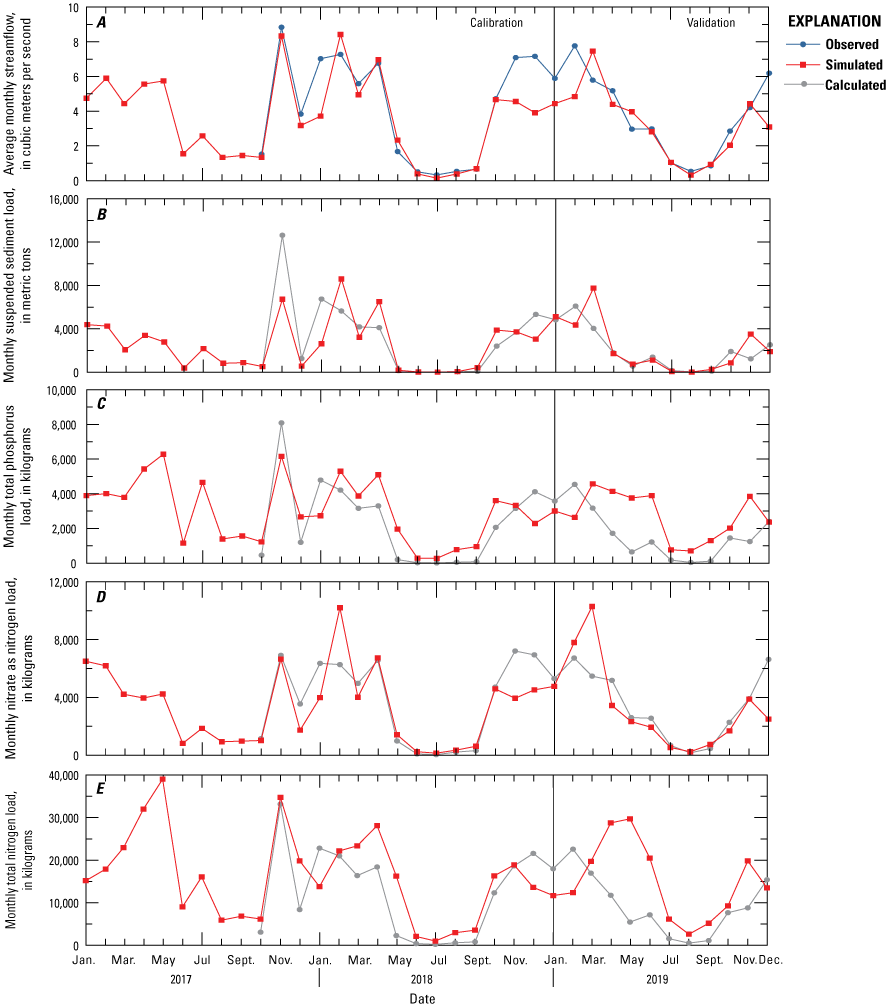
Graphs comparing Soil and Water Assessment Tool simulated to observed or rloadest calculated monthly measurements from January 2017 to December 2019 at U.S. Geological Survey streamgage 0421422210 on Eighteenmile Creek, in the Eighteenmile Creek watershed, New York, of A, Average streamflow; B, Suspended sediment load; C, Total phosphorus load; D, Nitrate as nitrogen load; and E, Total nitrogen load. SWAT-simulated nitrate as nitrogen loads were calibrated to the rloadest calculated nitrate plus nitrite loads (table 16).
In the validation period for the SWAT models at both Eighteenmile Creek watershed streamgages, all NSE values were rated unsatisfactory, except for monthly average streamflow at streamgage 0421422210 (table 17). Only monthly average streamflow, monthly suspended sediment load, and monthly nitrate as nitrogen load at streamgage 0421422210 have R2 values that were rated satisfactory. PBIAS values for the validation period at both streamgages were all rated from satisfactory to very good. At streamgage 0421422210, PBIAS values were rated good for monthly average streamflow, very good for monthly suspended sediment and nitrate as nitrogen loads, and satisfactory for monthly total phosphorus and monthly total nitrogen loads. PBIAS values at streamgage 04214231 were rated satisfactory for monthly streamflow, very good for monthly total phosphorus and total nitrogen, and good for nitrate as nitrogen. Most constituents were underestimated in the validation period (PBIAS>0), but monthly total nitrogen was overestimated at streamgage 04214231, and monthly suspended sediment, total phosphorus, and total nitrogen were overestimated at streamgage 0421422210 (PBIAS<0).
Walnut Creek Watershed Model Calibration and Validation
The Walnut Creek watershed model was calibrated to two streamgages (table 17). At both streamgages, calibration NSE values were rated good and calibration PBIAS values were rated very good for streamflow. Because of the lack of statistically significant rloadest models (table 16), monthly suspended sediment and nitrate as nitrogen loads were not calibrated at the Silver Creek streamgage (streamgage 04213394), and monthly total phosphorus loads were not calibrated at the Walnut Creek streamgage (streamgage 04213401). At streamgage 04213394, monthly total phosphorus and total nitrogen loads for both NSE and PBIAS calibration values were rated very good. At streamgage 04213401, the calibration NSE value and the PBIAS value for nitrate as nitrogen was rated unsatisfactory and satisfactory, respectively. Nitrate as nitrogen loads were underestimated for most months at streamgage 04213401 in both the calibration and validation periods (fig. 19C). Ice jams downstream from the streamgages were reported on both Silver and Walnut Creeks on January 11, 2018 (USACE, undated a), which may affect the accuracy of the rloadest load calculations. It is possible that the ice jam caused the large peak in the rloadest monthly suspended sediment load for January 2018 (fig. 19B), where SWAT underestimated the simulated monthly suspended sediment load by over 10,000 metric tons. Similarly, simulated total phosphorus and total nitrogen loads were underestimated at streamgage 04213394 in comparison to the rloadest peaks during the month of the ice jams, January 2018 (fig. 20).
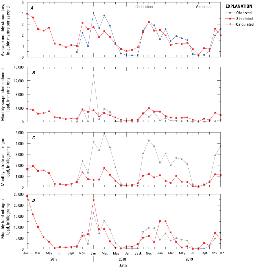
Graphs comparing Soil and Water Assessment Tool simulated to observed or rloadest calculated monthly measurements from January 2017 to December 2019 at U.S. Geological Survey streamgage 04213401 on Walnut Creek, in the Walnut Creek watershed, New York, of A, Average streamflow; B, Suspended sediment load; C, Nitrate as nitrogen; and D, Total nitrogen load. SWAT-simulated nitrate as nitrogen loads were calibrated to the rloadest calculated nitrate plus nitrite loads (table 16).
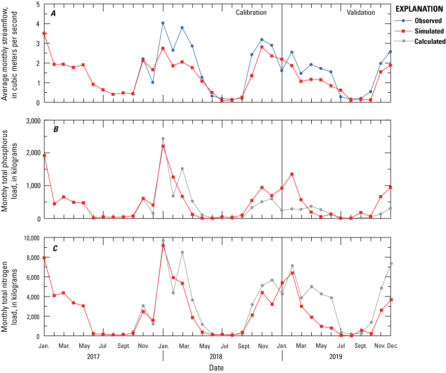
Graphs comparing Soil and Water Assessment Tool simulated to observed or rloadest calculated monthly measurements from January 2017 to December 2019 at U.S. Geological Survey streamgage 04213394 on Silver Creek, in the Walnut Creek watershed, New York, of A, Average streamflow; B, Total phosphorus load; and C, Total nitrogen load.
For the validation period, monthly streamflow NSE values were rated satisfactory for both streamgages (table 17). The very low absolute PBIAS values at both streamgages for streamflow indicate that simulated monthly streamflow closely matched observed streamflow. At streamgage 04213401, PBIAS values for monthly suspended sediment and total nitrogen loads were <0, which indicates these constituents were overestimated. NSE values for total nitrogen loads at streamgage 04213401 and for total phosphorus and total nitrogen loads at streamgage 04213394 were negative, indicating unacceptable performance in the validation period. Despite the negative NSE values, the PBIAS value for monthly total nitrogen load at streamgage 04213394 was rated very good, and the PBIAS value for total nitrogen at streamgage 04213401 was rated good. Model simulations overestimated total phosphorus loads during winter months in 2019 at streamgage 04213394 (fig. 20B).
Tonawanda Creek Watershed Model Calibration and Validation
The Tonawanda Creek watershed model was calibrated for monthly streamflow at four streamgages in the Tonawanda Creek watershed (table 17; figs. 21, 22, 23, 24). Three of the streamgage datasets had calibration NSE values for streamflow that were rated very good, and calibration PBIAS values that were rated good or very good (table 17). R2 for streamflow was >0.85 for datasets from all four streamgages, indicating a strong correlation between observed and the SWAT simulated streamflow. Streamflow was underestimated at all four streamgages (PBIAS>0); this was evident especially during the winter periods (figs. 21A, 22A, 23, 24). During the winter of 2017–8, the monthly streamflow at the Ellicott Creek streamgage (04218518) appeared to be underestimated but a daily graph (not presented; Fisher and Merriman, 2024) showed that three winter peaks were overestimated (fig. 21A). The greatest discrepancy between observed and simulated streamflow occurred at streamgage 04218000 (fig. 22A).
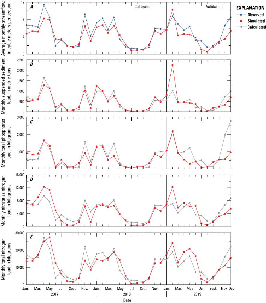
Graphs comparing Soil and Water Assessment Tool simulated to observed or rloadest calculated monthly measurements from January 2017 to December 2019 at U.S. Geological Survey streamgage 04218518 on Ellicott Creek, in the Tonawanda Creek watershed, New York, of A, Average streamflow; B, Suspended sediment load; C, Total phosphorus load; D, Nitrate as nitrogen load; and E, Total nitrogen load.
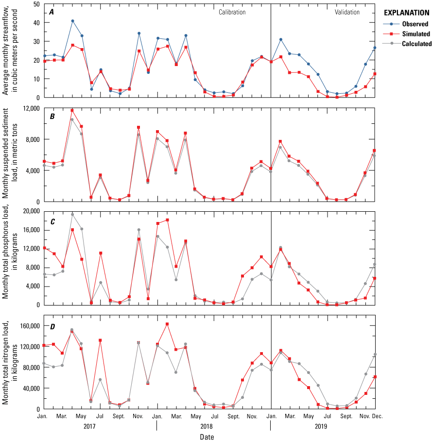
Graphs comparing Soil and Water Assessment Tool simulated to observed or rloadest calculated monthly measurements from January 2017 to December 2019 at U.S. Geological Survey streamgage 04218000 on Tonawanda Creek, in the Tonawanda Creek watershed, New York, of A, Average streamflow; B, Suspended sediment load; C, Total phosphorus load; and D, Total nitrogen load.
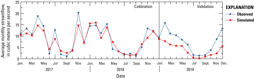
Graph comparing observed and Soil and Water Assessment Tool simulated monthly streamflow from January 2017 to December 2019 at U.S. Geological Survey streamgage 04217000 on Tonawanda Creek, in the Tonawanda Creek watershed, New York.
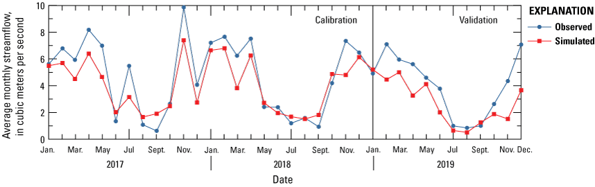
Graph comparing observed and Soil and Water Assessment Tool simulated monthly streamflow from January 2017 to December 2019 at U.S. Geological Survey streamgage 04216418 on Tonawanda Creek, in the Tonawanda Creek watershed, New York.
Water-quality monitoring data were available for only two streamgages in the Tonawanda Creek watershed: streamgage 04218000 on Tonawanda Creek in the hamlet of Rapids, N.Y., and streamgage 04218518 on Ellicott Creek (table 1). For the calibration period, the suspended sediment NSE and PBIAS values for both streamgages were rated very good (table 17). The simulated suspended sediment loads (figs. 21B, 22B) closely matched the rloadest calculated loads at both streamgages. At streamgage 04218000 (fig. 22B), suspended sediment peak loads were overestimated in April, May, and November 2017 and January, February, April, and December 2018 in the calibration period (fig. 22B). For calibration at streamgage 04218000, the monthly total phosphorus and total nitrogen NSE values were rated good and the PBIAS values were rated very good. For calibration at streamgage 04218518, the monthly total phosphorus and total nitrogen NSE and PBIAS values were rated very good.
Nitrate plus nitrite rloadest loads were only available in the Tonawanda Creek watershed for streamgage 04218518 (table 16). The nitrate as nitrogen NSE value was rated satisfactory, and the PBIAS value was rated very good in the calibration period (table 17). Monthly nitrate as nitrogen loads were overestimated in February to June of 2017 and was underestimated during periods of low flow and most months for the rest of the calibration period (fig. 21D). For streamgage 04218518, total nitrogen load calibration NSE and PBIAS values were rated very good. In the calibration period, winter monthly total nitrogen load peaks were underestimated for streamgage 04218518 (fig. 21E), but generally overestimated for streamgage 04218000 (fig. 22D).
The Tonawanda Creek watershed model did not perform well in the validation period (table 17). R2 values in the validation period, except for total phosphorus and ammonium loads at streamgage 04218518, were satisfactory. The model underestimated monthly average streamflow at all gages during the validation period (PBIAS>0). Only streamgage 04218518 had a validation NSE value for monthly average streamflow that was rated satisfactory and a good validation PBIAS value; statistics at the other three streamgages had unsatisfactory NSE and PBIAS values. At streamgage 04218518, all NSE values for suspended sediment and nutrient loads were unsatisfactory during the validation period. Streamgage 04218518 had very good PBIAS ratings for monthly suspended sediment, nitrate as nitrogen, ammonium, and total nitrogen loads, and a good PBIAS rating for monthly total phosphorus load. On February 5, 2019, an ice jam was reported on Ellicott Creek upstream from streamgage 04218518 (USACE, undated a); there was a large difference that month, February 2019, between the rloadest calculated and simulated suspended sediment loads for streamgage 04218518 (fig. 21B).
At streamgage 04218000 during the validation period, PBIAS ratings were very good for orthophosphate and total phosphorus loads, good for monthly total nitrogen load, satisfactory for suspended sediment and ammonium loads, and unsatisfactory for monthly average streamflow (table 17). Validation NSE values for streamgage 04218000 were rated as unsatisfactory, except for total phosphorus and total nitrogen loads which had a very good and a satisfactory NSE ratings, respectively. The validation NSE value of 0 for streamflow of streamgage 04217000 indicates that there was no relation between the observed and simulated streamflow.
SWAT Model Results
In the following section, model results are presented in terms of loads and yields. Loads and yields are presented on an average annual basis computed as the average of annual loads and yields for the two calibration years. A load is the mass of a constituent discharged past a point in a watershed. A yield is the constituent load per unit area of the contributing watershed. Suspended sediment loads are reported in metric tons, and suspended sediment yields are reported in metric tons per hectare (t/ha). Nutrient loads and yields are reported in kilograms (kg) and kilograms per hectare (kg/ha), respectively. All nitrate loads and yields are in the form of nitrate as nitrogen. Reductions are the percent change in average annual loads from the baseline simulations to the test scenarios.
Baseline Loads per Watershed Model
The calibrated watershed models are used as baseline scenarios to show the estimated conditions of the watersheds. The following are the simulated, average annual loads from SWAT. Baseline average annual suspended sediment loads range from 803 metric tons in the Crooked Brook watershed to 495,400 metric tons in the Cattaraugus Creek watershed (fig. 25A). Baseline average annual nitrate as nitrogen loads ranged from 3,107 kg in the Cooked Branch watershed to 949,500 kg in Buffalo River watershed (fig. 25B). Baseline average annual total orthophosphate loads ranged from 4,079 kg in the Crooked Branch watershed to 143,850 kg in the Buffalo River watershed (fig. 25C). Baseline average annual total nitrogen loads ranged from 25,620 kg in the Crooked Branch watershed to 2,176,000 kg in Cattaraugus Creek watershed (fig. 25D). Baseline average annual total phosphorus loads ranged from 19,070 kg in the Walnut Creek watershed to 642,650 kg in Cattaraugus Creek watershed (fig. 25E).
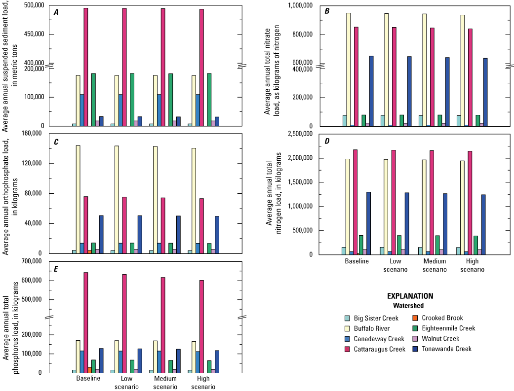
Bar charts showing A, Average annual suspended sediment load; B, Average annual nitrate as nitrogen load; C, Average annual orthophosphate load; D, Average annual total nitrogen load; and E, Average annual total phosphorus load, by best management practice implementation scenario and watershed at selected watershed outlets of Lake Erie, New York. Crooked Brook watershed only has the baseline scenario displayed.
The largest simulated suspended sediment, total nitrogen, and total phosphorus loads were exported from the Cattaraugus Creek watershed model (fig. 25A, D, and E). This falls in line with findings from Koltun (2021), who found that the streamgage used for calibration of the Cattaraugus Creek watershed in this study, USGS streamgage 04213500 (Cattaraugus Creek at Gowanda, New York), had the highest flow weighted mean phosphorus concentration and the highest average annual phosphorus yield out of 23 monitored streamgages across the Great Lakes region. Other monitored streamgages in Koltun (2021) had larger estimated phosphorus loads than those at streamgage 04213500, but the Cattaraugus Creek streamgage had a relatively small flow volume which accounts for the lower load. Simulated average annual total phosphorus loads from the Buffalo River, Tonawanda Creek, and Canadaway Creek watersheds are between 115,000 and 180,000 kg. Most of the simulated total phosphorus loads were in the organic phosphorus form, except for the Buffalo River watershed where the simulated total phosphorus was primarily in the soluble form as orthophosphate. The Big Sister Creek watershed and the Walnut Creek watershed have lower baseline total phosphorus loads than the Crooked Brook watershed (fig. 25), even though those watersheds are 9.25 and 9.70 times the size of the Crooked Brook watershed, respectively. Of the study watersheds, the Crooked Brook watershed has the highest relative area of urban land cover (42.76 percent) and grapes (14.97 percent), and the lowest relative area of forest (24.47 percent; table 2).
Model results from the Buffalo River and the Tonawanda Creek watersheds had most simulated nitrogen in the form of nitrate as nitrogen (fig. 25B and D). These two watershed models had the second and third highest simulated baseline total nitrogen of the study watersheds, respectively. Buffalo River watershed had a baseline average annual total nitrogen load of just under 2 million kg. The baseline average annual total nitrogen load of the Tonawanda Creek watershed was 1.3 million kg. The Eighteenmile Creek watershed model exported approximately 400,000 kg of total nitrogen in the baseline simulation. The Crooked Brook watershed model had the lowest baseline total nitrogen loads.
BMP scenario results indicate small, gradual decreases of constituent loads as BMPs are implemented at increasing levels. Across the seven watersheds models examined, reductions in suspended sediment loads range from −0.06 to 2.85 percent, in total nitrogen loads range from 0.25 to 4.20 percent, and in total phosphorus loads range from 0.28 to 8.55 percent (fig. 26). The highest reduction of suspended sediment and nutrient loads are found in the Tonawanda Creek watershed with the high BMP scenario.
Effects of Best Management Practice Scenarios on Suspended Sediment and Nutrient Loads
Simulated nutrient loads by BMP scenario and watershed model are presented in figure 25. Figure 26 compares the low, medium, and high BMP scenarios as percent change in constituent loads. In figure 25, negative changes indicate that loads increased, whereas positive changes indicate that loads decreased.
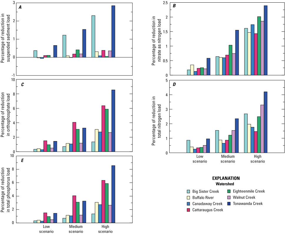
Bar charts showing percent reduction of average annual total loads of A, Suspended sediment; B, Nitrate as nitrogen; C, Orthophosphate; D, Total nitrogen; and E, Total phosphorus loads, by scenario and watershed at study watershed outlets of Lake Erie, New York. Negative values indicate an increase in suspended sediment or nutrient loads, whereas positive values indicate a decrease in loads.
Effects of Rotation on Suspended Sediment and Nutrient Loads and Yields
Average annual suspended sediment and nutrient loads by rotation were compiled for the baseline scenarios (fig. 27) and simulated suspended sediment and nutrient yields by rotation for the baseline scenarios are presented in table 18. Figure 27 does not include loads for the rotations of apple and barren because the loads from these rotations were too small for the scales for any watershed on this graph, but yields for apple and barren rotations are present for applicable watersheds in table 18. Suspended sediment and nutrient loads and yields vary by watershed and rotation. Rotations classified as water, which usually indicates a pond or lake, have 0 kg/ha suspended sediment and nutrient yields. Suspended sediment yields ranged from 0.01 kg/ha for apple orchards in the Crooked Brook watershed model to 88.14 kg/ha from beef cattle in the Canadaway Creek watershed model. Total phosphorus yields ranged from 0.01 kg/ha for wetlands in the Buffalo River and Walnut Creek watershed models to 159.27 kg/ha for the dairy rotation in the Crooked Brook watershed model, where most of the phosphorus yield was in the sediment bound phosphorus form. Only agricultural rotations (beef cattle, CAFOs, cash grain, continuous corn, or dairy) produced phosphorus from tile drains, as tile drainage was not simulated on other rotations. Additionally, SWAT can only simulate the soluble forms of nitrogen and phosphorus in tile drainage (Neitsch and other, 2002), therefore only nitrate as nitrogen or orthophosphate were accounted for from the tile drainage areas. Canadaway Creek and Crooked Brook watershed models were the only two watershed models that exported orthophosphate from groundwater (table 18), but all models contributed nitrate as nitrogen from groundwater.
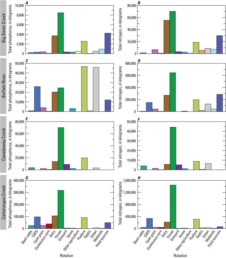
Bar charts showing average annual nutrient loads by rotation and point-source discharges in A and B, Big Sister Creek watershed; C and D, Buffalo River watershed; E and F, Canadaway Creek watershed; G and H, Cattaraugus Creek watershed; I and J, Eighteenmile Creek watershed; K and L, Walnut Creek watershed; and M and N, Tonawanda Creek watershed of Lake Erie, New York. CAFO, concentrated animal feeding operation. Apple and barren rotations are not shown.
Table 18.
Simulated average annual suspended sediment and nutrient yields in selected tributary watersheds of Lake Erie, New York, by rotation in the Soil and Water Assessment Tool watershed models.[Data are from Fisher and Merriman (2024). Chautauqua Creek watershed is not included. The concentrated animal feeding operations (CAFOs) rotation for the Tonawanda Creek watershed includes dairy CAFOs and a poultry CAFO; the CAFOs rotation for all other watersheds contains dairy CAFOs only. Ha, hectare; t/ha, metric ton per hectare; kg/ha, kilogram per hectare; Lateral N, nitrate moving in the soil water]
The dominant species of total phosphorus in simulated average annual yields varied by watershed (table 18). For four of the watershed models (Walnut, Eighteenmile, Big Sister, and Cattaraugus Creeks), organic phosphorus was the predominant form of phosphorus in the simulated yields. Orthophosphate was the main form of phosphorus in Tonawanda Creek and Buffalo River watershed models. In the Canadaway Creek watershed model, most of the phosphorus yield was sediment bound. Average annual total phosphorus yields ranged from 0.01 kg/ha for wetlands in the Buffalo River and Walnut Creek watershed models to 154.32 kg/ha for dairy rotations in the Crooked Brook watershed model, where most of the phosphorus yield was sediment bound.
Average annual total nitrogen yields ranged from 0.29 kg/ha for wetlands in the Walnut Creek watershed model to 593.621 kg/ha for the septic rotation in the Big Sister Creek watershed model (table 18). The largest total nitrogen yields came from septic rotations; the largest of these came from the Big Sister Creek watershed model. The Cattaraugus Creek, Buffalo River, and Eighteenmile Creek watershed models all had average annual total nitrogen yields >100 kg/ha. Approximately 30 percent of the nitrogen yield in the Walnut Creek watershed model was derived from lateral sources, whereas all other watershed models had <5 percent of nitrogen yields from lateral sources.
Generally, large amounts of nutrient loads were derived from forested rotations (fig. 27), as the watershed models had high amounts of forest land cover (fig. 3; table 2). Forest rotation was the most prevalent land area for all watershed models except for the Crooked Brook watershed model (table 18). Average annual suspended sediment yields for forest rotations ranged from 0.03 kg/ha for the Big Sister Creek watershed model to 11.25 kg/ha for the Cattaraugus Creek watershed model. Average annual total phosphorus yields for forests ranged from 0.13 kg/ha in the Tonawanda Creek watershed model to 6.66 kg/ha in the Canadaway Creek watershed model. Most of the nitrogen yields from forest rotations was in the organic form for all watershed models. Average annual nitrate as nitrogen loads from surface runoff were about 2 to 27 percent and nitrate as nitrogen loads from baseflow were about 0 to 11 percent of total nitrogen exported from forests.
Septic systems contributed flow and nutrients to streamflow in all models (table 18). Average annual total phosphorus loads from septic rotations were highest in the Buffalo River watershed model and lowest with the Walnut Creek watershed model (fig. 27). Most of the total phosphorus from septic rotations was organic phosphorus for most watershed models (table 18), except for Tonawanda Creek and Buffalo River watershed models where the orthophosphate was the majority phosphorus species. Total nitrogen loads from septic rotations were highest in the Cattaraugus Creek watershed model and lowest with the Canadaway Creek watershed model (fig. 27). Most nitrogen yields from the septic rotation were derived from nitrate as nitrogen in groundwater except for the Canadaway Creek and Crooked Brook watershed models (table 18).
For urban rotations, average annual suspended sediment yields ranged from 0.55 kg/ha in the Big Sister Creek watershed model to 8.99 kg/ha in the Eighteenmile Creek watershed model (table 18). The Crooked Brook watershed model had the largest average annual total phosphorus yield from its urban rotation (13.38 kg/ha). The urban total phosphorus yields for Big Sister Creek and Buffalo River watershed models were predominantly in the orthophosphate form. For urban yields from the Walnut Creek watershed model, approximately half of the total phosphorus yield was in the organic phosphorus form. The lowest urban rotation yields of total phosphorus (0.69 kg/ha) and total nitrogen (6.43 kg/ha) were in the Tonawanda Creek watershed model. The largest urban total nitrogen yields (21.45 kg/ha) were in the Cattaraugus Creek watershed model.
Total phosphorus yields for beef cattle rotations were greater than the total phosphorus yields for CAFOs rotations in all watershed models, except for the Buffalo River watershed model where average annual total phosphorus yields were 6.43 kg/ha for the CAFO rotation and 3.77 kg/ha for the beef cattle rotation (table 18). The majority of the total phosphorus yields for beef cattle rotations were in the sediment bound phosphorus form except for the Canadaway Creek and Walnut Creek watershed models. The majority of the total phosphorus yield for CAFOs was in the orthophosphate form, except for the Tonawanda Creek watershed model (CAFOs were not modeled in the Canadaway Creek and the Walnut Creek watershed models). The largest total phosphorus yields from beef cattle and CAFO rotations were from the Canadaway Creek and Cattaraugus Creek watershed models, respectively. The Cattaraugus Creek watershed model had the largest average annual total phosphorus loads from beef cattle and CAFO rotations (fig. 27).
Of the agricultural rotations simulated (cash grain, continuous corn, and dairy rotations), dairy rotations had the greatest average annual loads of total phosphorus and total nitrogen (fig. 27). The largest total nitrogen and total phosphorus loads from agricultural rotations came from the Cattaraugus Creek watershed model, and the largest suspended sediment loads were exported from the Tonawanda Creek watershed model. Phosphorus from agricultural rotations was mostly in the form of sediment bound phosphorus with the exception of the Big Sister Creek, Walnut Creek, and Buffalo River watershed models (table 18). In the Big Sister Creek and Walnut Creek models, the majority of phosphorus was organic phosphorus. In the Buffalo River watershed model, the majority of phosphorus was orthophosphate. The total nitrogen loads from agriculture were mostly organic nitrogen, with the exception of the Big Sister Creek watershed model where the majority of nitrogen was nitrate.
Effect of Best Management Practices on Runoff and Water Quality at the Hydrologic Response Unit-Scale
BMPs were evaluated per selected agricultural rotation (dairy, beef cattle, continuous corn, or cash grain) for effectiveness at the HRU scale. The BMPs had varying levels of effectiveness (table 19). FS had no or very little (0.00 to 1.09 percent) effect on runoff but was the most effective BMP for reducing suspended sediment and nutrients loads. FS had the largest reductions in suspended sediment and total phosphorus loads on cash grain rotations, 98.41 and 81.96 percent, respectively (table 19).
Table 19.
Percent reductions in average annual surface runoff and suspended sediment and nutrient yields in selected tributary watersheds of Lake Erie, New York, by single or combined best management practices in seven of the Soil and Water Assessment Tool watershed models.[Data are from Fisher and Merriman (2024). Negative values indicate an increase in surface runoff, suspended sediment, or nutrients. HRU, hydrologic response unit; FS, filter strips; NMP, nutrient management plan; CC, cover crops; RT, reduced tillage]
CC+NMP+RT and CC+RT generally had the highest percent reductions of any other infield (that is, applied directly on the agricultural field, meaning all BMPs excluding FS) BMP or BMP combination (table 19). CC+NMP+RT had the highest suspended sediment, total phosphorus, nitrate as nitrogen, and total nitrogen yield reductions in the Walnut Creek watershed model. On dairy rotations, CC+NMP+RT typically had lower reductions than either cash grain or continuous corn rotations. Some watershed models had negative orthophosphate reductions (Buffalo River and Canadaway Creek for all rotations; Cattaraugus Creek for cash grain and continuous corn rotations; and dairy rotations in Walnut Creek watershed).
HRUs with RT that had large reductions in suspended sediment yields correspond to HRUs that started the simulation period with several consecutive years of alfalfa. These same HRUs also had negative orthophosphate reductions for RT, an effect seen previously in many midwestern studies where conservation tillage can increase runoff by not incorporating added nutrients (Smith and others, 2015a). Not all HRUs may equally see this effect, as those with 2 or 3 years of corn silage at the beginning of the warmup period have positive orthophosphate and total phosphorus reductions and negative suspended sediment reductions.
Continuous corn rotations had negative average suspended sediment reductions in the Big Sister Creek, Buffalo River, Cattaraugus Creek, and Eighteenmile Creek watershed models (table 19).
Beef cattle rotations only simulated FS or NMP (table 19), as grazing cattle would interfere with the management operations in CC or RT. Suspended sediment, orthophosphate, total phosphorus, nitrate as nitrogen, and total nitrogen yield reductions from FS in beef cattle rotations were all positive and greater than NMP reductions for the same rotation in all watersheds (Buffalo River watershed only had FS simulated on beef cattle rotations). Suspended sediment reductions from FS in beef cattle rotations ranged 16.48 to 82.51 percent; orthophosphate reductions ranged from 45.98 to 83.52 percent, and total phosphorus reductions ranged from 45.18 to 81.60 percent. All watershed models have negative total nitrogen reductions for NMP in beef cattle rotations. Canadaway Creek, Cattaraugus Creek, Eighteenmile Creek, and Tonawanda Creek watershed models all have negative suspended sediment reductions for NMP in beef cattle rotations. Canadaway Creek also has a negative orthophosphate reduction for NMP in beef cattle rotations.
Effect of Point Source Phosphorus Inputs on Water Quality
There are four different point source scenarios: two for the Tonawanda Creek watershed, one for the Big Sister Creek watershed, and one for the Buffalo River watershed. The only change in the input of these scenarios from the baseline is the phosphorus concentration of select point source discharges (see “SWAT Model Scenarios” section for more information on the constraints placed on phosphorus), and as such the point source scenario results have the same results as the baseline simulations for all constituents other than phosphorus species.
One point-source scenario was tested in the Big Sister Creek watershed model. The point-source scenario exported the least amount of orthophosphate and total phosphorus of any of the scenarios for the Big Sister Creek watershed model.
The Buffalo River watershed point source scenario reduced phosphorus inputs from the point source identifier NY0108103 (table 3) in subbasin 47. The resulting reduction of average annual phosphorus loads from NY0108103 were minimal, and less than the phosphorus load reduction from the low BMP scenario.
On an average annual basis, Tonawanda point-source scenario 1 reduced average annual orthophosphate and total phosphorus loads by 5.95 and 3.15 percent, respectively, whereas the Tonawanda point-source scenario 2 reduced average annual orthophosphate and total phosphorus loads by 10.58 and 5.60 percent, respectively (table 20). Total phosphorus reductions in scenario 1 were similar to the reductions in the Tonawanda Creek medium BMP scenario, both about 3 percent. Tonawanda scenario 2 caused a greater total phosphorus reduction than the medium BMP scenario but not greater than the high BMP scenario. The largest reductions in the point sources scenarios were of orthophosphate; orthophosphate load reductions in scenario 1 and scenario 2 were larger than the reductions from the three BMP scenarios.
Table 20.
Reductions in average annual orthophosphate and total phosphorous loads by point-source scenario in three of the Soil and Water Assessment Tool watershed models for selected tributary watersheds of Lake Erie, New York.[Data are from Fisher and Merriman (2024). See model subbasins in figure 3. NPDES, National Pollutant Discharge Elimination System; kg, kilogram; mg/L, milligram per liter]
Model Results by Watershed
Results were different for each watershed model because of the different characteristics of each watershed. The following sections present the results per watershed model.
Big Sister Creek Watershed
The baseline Big Sister Creek watershed model had the second lowest average annual suspended sediment loads and the lowest average annual phosphorus loads of any of the study watersheds (fig. 25). For the Big Sister Creek watershed model, the baseline simulated average annual loads were 8,625 metric tons of suspended sediment, 195,250 kg of total nitrogen, 7,640 kg of orthophosphate, and 19,965 kg of total phosphorus (fig. 25). When loads are compared by rotation (fig. 27A), forests were the highest contributor and point sources were the second highest contributor of total phosphorus loads. There is one point source discharge in the Big Sister Creek watershed model (identifier NY0022543; table 3) near the outlet of Big Sister Creek to Lake Erie and downstream of the Big Sister Creek streamgage. This point source contributed about 11.5 percent of the simulated streamflow and 19 percent of the simulated total phosphorus load to the baseline Big Sister Creek watershed model.
Yields by rotation for the Big Sister Creek watershed model are presented in table 18. Beef cattle rotations had the largest average annual total phosphorus yield out of all simulated rotations that produced nutrients, 4.70 kg/ha, but it occupied a relatively small area, thus the beef cattle rotation was responsible for only a small amount of the watershed model’s total phosphorus load (fig. 27A). Septic rotation had the highest average annual total nitrogen yields in the Big Sister Creek watershed by far, with the majority of nitrogen coming from nitrate as nitrogen in groundwater. Because septic rotations had the least area in this watershed, 10.73 ha, there were minimal loads.
The point source, dairy, and pasture rotations were the largest manufactured sources of simulated nutrient loads, whereas forests exported the most total phosphorus and total nitrogen overall; approximately half of the watershed model was covered by forest (table 18; figs. 27A, B). Forests had the lowest average annual suspended sediment yield, second lowest total nitrogen yield, and third lowest total phosphorus yield out of all rotations in the Big Sister Creek watershed model (table 18). The pasture rotation accounted for 13 percent of the model area (table 18), was the fourth largest phosphorus exporter (fig. 27A), and was the fourth largest total nitrogen load exporter (fig. 27B); whereas the dairy rotation accounted for 14 percent of the model area (table 18), was the third largest total phosphorus load exporter (fig. 27A), and was the second largest total nitrogen load exporter in the Big Sister Creek watershed model (fig. 27B).
Results by Low, Medium, and High Best Management Practice Scenarios
Simulated load reductions because of BMP scenarios in the Big Sister Creek watershed model are shown in figures 25 and 26. Simulated average annual suspended sediment loads decreased from baseline loads in the low, medium, and high scenarios by 0.37, 1.22, and 2.30 percent, respectively (fig. 25A). Simulated average annual orthophosphate loads decreased with the low, medium, and high scenarios by 0.86, 1.54, and 2.68 percent, respectively (fig. 25C). Simulated average annual total phosphorus loads decreased from the low, medium, and high scenarios of 0.33, 0.70, and 1.35 percent, respectively (fig. 25E). Simulated average annual total nitrogen loads were reduced by 0.18, 0.64, and 1.61 percent in the low, medium, and high scenarios, respectively (fig. 25D).
The low, medium, and high BMP scenarios simulated decreases of suspended sediment and nutrient loads in the Big Sister Creek watershed model (fig. 26). The average annual suspended sediment load decreased 2.20, 6.50, and 14.4 percent from the low, medium, and high scenarios, respectively (fig. 26A). Average annual orthophosphate decreased 1.77, 3.04, and 5.73 percent from the low, medium, and high scenarios, respectively (fig. 26C). Average annual total phosphorus loads decreased 0.26, 0.59, and 1.28 percent from the baseline scenario in the low, medium, and high scenarios, respectively (fig. 26E).
In general, simulated decreases for each constituent from the BMP scenarios were most notable in subbasins in the southeast part of the watershed (fig. 28). The highest baseline values across all constituents (fig. 28) were simulated in subbasins 25 through 30 (fig. 3A) likely because of the steep slopes, poorly drained soils, and little tile drainage in these subbasins. The downstream subbasins generally have lower yields of suspended sediment and nutrients than the upstream subbasins (fig. 28). Subbasin 25 (fig. 3A) had the highest surface runoff, suspended sediment, and orthophosphate yields throughout all the BMP scenarios (figs. 28A, B, C). Subbasin 25 also had the highest area of very poorly drained soils, over 3,800 km2, and most slopes in subbasin 25 also are steeper than 2 percent; both conditions lead to increased runoff and erosion. Additionally, as only a very small part (0.05 km2) of subbasin 25 was simulated with tile drainage, most suspended sediment and nutrients exported were from overland flow. In subbasin 25, suspended sediment, orthophosphate, and total phosphorus were reduced by about 12, 5, and 4 percent, respectively, in comparison from the baseline to the high scenario.
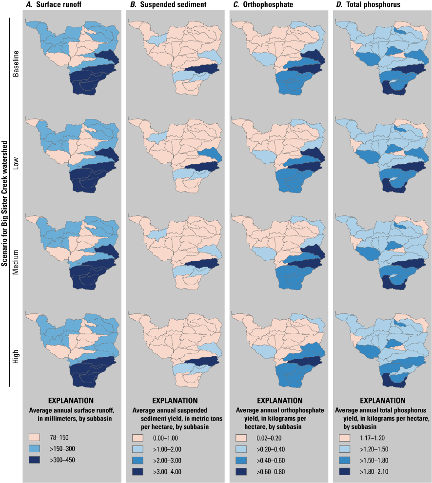
Maps showing average annual A, Surface runoff; B, Suspended sediment yield; C, Orthophosphate yield; and D, Total phosphorus yield, by scenario and subbasin, Big Sister Creek watershed model, New York. See figure 3 for subbasin identifiers.
Results by Best Management Practice
The BMPs and BMP combinations that were simulated as part of the low, medium, and high implementation scenarios were individually analyzed on the HRUs for nutrient and suspended sediment reduction performance (fig. 29). Most simulated BMPs in the Big Sister Creek watershed model reduced suspended sediment and total phosphorus yields (fig. 29), but some increased orthophosphate yields, especially on HRUs with cash grain rotations. FS reduced suspended sediment, orthophosphate, and total phosphorus more than any other BMP in any agricultural rotation schedule. On dairy rotations, FS suspended sediment yield reductions ranged from 0.00 to 100.00 percent, orthophosphate yield reductions ranged from 0.00 to 85.00 percent, and total phosphorus yield reductions ranged from 0.38 to 77.59 percent (figs. 29A, B, C). There were five HRUs with no change in any suspended sediment or nutrient reductions from FS on dairy rotations (fig. 29A, B, C); these all have a low CN value (31) and well drained soils. When these five HRUs were removed from the results, yield reductions from the 31 other HRUs for FS ranged from 74.86 to 100.00 percent for suspended sediment, from 62.78 to 85.00 percent for orthophosphate, and from 0.38 to 77.59 percent for total phosphorus.
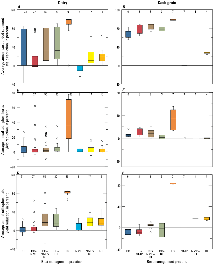
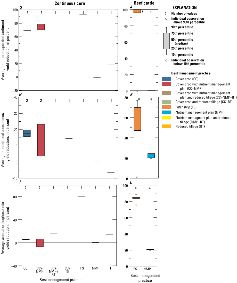
Boxplots of simulated reduction of average annual yield, in percent, in surface runoff from A–C, Dairy rotations; D–F, Cash grain rotations; G–I, Continuous corn rotations; and J–L, Beef cattle rotations, because of selected best management practices in Big Sister Creek watershed model, New York. Negative values indicate an increase in suspended sediment or nutrients.
Dairy rotations made up 14 percent of the area of the Big Sister Creek watershed model (table 19). BMPs were simulated on 195 dairy HRUs. Of the single BMPs implemented excluding FS, CC caused the greatest simulated average annual suspended sediment yield reduction from dairy rotations, with an average reduction of 31.39 percent. NMP caused a negative average annual suspended sediment yield reduction (an increase) of −7.46 percent (table 19; fig. 29A). CC caused a slight negative average annual nitrate as nitrogen yield reduction (an increase) of −0.73 percent (table 19). CC+RT caused greater average annual suspended sediment and total phosphorus yield reductions than CC+NMP+RT (table 19; figs. 29A, B), whereas orthophosphate (table 19; fig. 29C), nitrate as nitrogen (table 19), and total nitrogen yield reductions (table 19) were greater for CC+NMP+RT than CC+RT. Reductions for suspended sediment (table 19; fig. 29A), orthophosphate (table 19; fig. 29C), and nitrate as nitrogen (table 19) for CC+NMP were less than those for both CC+NMP+RT and CC+RT. Addition of RT to another BMP caused greater reductions of the average annual suspended sediment, orthophosphate, and total phosphorus yields (table 19); except for CC+NMP+RT, where the TP reduction (5.10 percent) was slightly less than the total phosphorus reduction caused by CC+NMP (5.86 percent).
The cash grain rotation made up <1 percent of the Big Sister Creek watershed model area (table 18). BMPs were applied to 44 cash grain HRUs (table 19). Examining only infield BMPs on the cash grain rotation, CC+NMP+RT caused the greatest reduction of average annual suspended sediment yield, 81.71 percent (table 19; fig. 26D), NMP+RT caused the largest average annual orthophosphate yield reduction (17.6 percent; table 19; fig. 26F), and CC+NMP caused the largest average annual reductions of total phosphorus and total nitrogen (table 19; fig. 29E). CC+NMP also caused a negative average orthophosphate reduction (an increase; table 19; fig. 29F). Average annual suspended sediment or nutrient yield changes (increases or decreases) because of NMP on cash grain rotations were all <1 percent (table 19; figs. 29D, E, F).
On the beef cattle rotation, FS and NMP were simulated on 6 and 4 HRUs, respectively (table19; figs. 29J, K, L). FS on beef cattle rotations caused average annual yield reductions of 82.51 percent suspended sediment, 83.52 percent orthophosphate, 52.36 percent total phosphorus, 92.27 percent nitrate as nitrogen, and 16.41 percent total nitrogen (table 19). NMP caused average annual yield reductions of 0.00 percent suspended sediment, 20.80 percent orthophosphate, and 21.45 percent total phosphorus; however, NMP implementation on the beef cattle rotation caused average annual reductions in nitrate as nitrogen of −11.84 percent and in total nitrogen of −33.47 percent.
Point Source Scenario
The Big Sister point source scenario had the largest simulated reductions of any of the scenarios performed with the Big Sister Creek watershed model. On an average annual basis, the Big Sister Creek point-source scenario reduced orthophosphate and total phosphorus load at the watershed outlet by 5.84 and 3.26 percent, respectively (table 20). There was an average annual difference of 446.50 kg orthophosphate and 650.00 kg total phosphorus between the baseline and the point-source scenarios.
Buffalo River Watershed
The Buffalo River watershed is the third largest of the study watersheds. It exported the third largest average annual suspended sediment loads (175,450 metric tons) and the second largest total nitrogen (1,982,500 kg) and total phosphorus (170,500 kg) loads (fig. 25). Suspended sediment loads from the Buffalo River watershed model were more similar to those in the Eighteenmile Creek watershed model which is 800 km2 smaller than the Buffalo River watershed. The Buffalo River watershed model had the greatest average annual nitrate as nitrogen load (949,500 kg) out of all the study watersheds.
The subwatersheds of three main tributaries in the Buffalo River watershed each cover a similar area, from 30 to 33 percent of the total watershed. The largest of these, the Buffalo Creek subwatershed (at streamgage 04214500) has an area of 368 km2 and contributed the largest total nitrogen and total phosphorus loads (about 30 and 42 percent, respectively). The largest percentage of flow (35 percent) came from Cazenovia Creek subwatershed, which has an area of 350 km2. The Cazenovia Creek subwatershed also carried the largest suspended sediment load of the three tributaries, about 44 percent of the watershed’s total load.
Loads by rotation in the Buffalo River watershed model are shown in figure 27B. Forests contributed the most suspended sediment and total nitrogen out of all rotations. Pasture and urban areas were the highest exporters of total phosphorus; these two rotations comprised the second and third largest areas of the Buffalo River watershed (table 18). Pasture had a moderately low average annual total phosphorus yield (2.81 kg/ha), the majority of which was in the form of orthophosphate. Urban areas had the fifth highest total phosphorus yield in the watershed model out of all rotations. Beef cattle, which had the greatest total phosphorus yields and second largest suspended sediment and total nitrogen yields (table 18), occupied the smallest area out of the studied agricultural rotations, and exported minimal amounts of total phosphorus and total nitrogen (fig. 27B). Septic rotations had the highest total nitrogen yields, yet it contributed <1 percent of the watershed model’s total nitrogen load.
There are 18 point source discharges in the Buffalo River watershed model (table 3). In the baseline scenario, point sources exported 7 percent and 16 percent of the watershed model’s total phosphorus and total nitrogen loads, respectively. In the subwatersheds of Buffalo and Cayuga Creeks, contributions from point sources and withdrawals from streams were nominal and had minor effects on streamflow; the majority of effects were from point sources contributing to Cazenovia Creek.
There are four point sources contributing to Cazenovia Creek (NYSDEC, 2020); monthly discharge from point sources ranged from 0 to 11 percent of Cazenovia Creek's streamflow (Fisher and Merriman, 2024). The largest volumetric contributions from point sources to streamflow occurred during winter and spring, but the largest percent contribution to streamflow occurred in summer (July–September) when the streamflow of Cazenovia Creek was lowest. In the baseline simulation, these four point sources contributed nominal amounts of suspended sediment, <0.02 percent of the total simulated suspended sediment load from Cazenovia Creek. Discharge from NY0110043 (table 3) contributed the largest amount of total nitrogen and total phosphorus in the Cazenovia Creek subwatershed baseline simulation. Additionally, stream withdrawals from the west branch of Cazenovia Creek were seen in winter months, usually November through March (NYSDEC, 2020). However, these withdrawals made up <0.2 percent of the average annual streamflow.
The highest surface runoff, orthophosphate, and total phosphorus yields occurred mostly in the northwestern and central parts of the watershed model, especially near where Cayuga Creek and Buffalo Creek converge (fig. 30). Surface runoff was highest in subbasins 7 and 19, which have very steep slopes, over 20 percent gradient in places. They also have poorly drained to very poorly drained soils which could lead to higher surface runoff than other places in the watershed model. The high values of surface runoff and orthophosphate and total phosphorus yields in the northwestern part of the watershed model, particularly subbasins 6, 10, 12, and 17, were influenced by the convergence of Cayuga and Buffalo Creeks. Subbasin 17 also contains three municipal point source discharges which may increase nutrient concentrations and loads. Much of the upland area is covered by deciduous forest and agriculture (fig. 3B). Further downstream, the land cover is mostly urban; the land cover is almost exclusively urban at the junction of the Buffalo River with Lake Erie. Orthophosphate and total phosphorus yields were also higher in the central part of the watershed model than other parts, especially subbasins 27 and 32, compared with the rest of the watershed model outside of the northwestern part of the watershed. Subbasin 27 and especially subbasin 32 are dominated by agricultural land cover, made up of mostly corn and alfalfa with some soybean (fig. 3B). Suspended sediment yields were highest in subbasin 43 in the southern part of the watershed model. Subbasin 43 has steep slopes, many of which are 10 percent or greater, and this subbasin mostly has very poorly drained soils.
Results by Low, Medium, and High Best Management Practice Scenarios
The Buffalo River watershed model BMP scenarios results are shown in figure 26. The medium scenario and high scenario reduced average annual suspended sediment loads by 0.09 and 0.31 percent, respectively, whereas the low scenario had a slight negative reduction (increase) of suspended sediment loads (−0.03 percent). The low, medium, and high BMP scenarios reduced average annual orthophosphate loads by 0.31, 0.80, and 2.36 percent from the baseline load, respectively. Average annual total nitrogen loads in the low, medium, and high scenarios were reduced by 0.40, 0.88, and 1.97 percent from the baseline load, respectively. Average annual total phosphorus loads in the low, medium, and high scenarios decreased 0.41, 1.14, and 3.08 percent from the baseline load, respectively. In general, reductions for each constituent are noted particularly in subbasins in the middle part of the watershed (fig. 30).
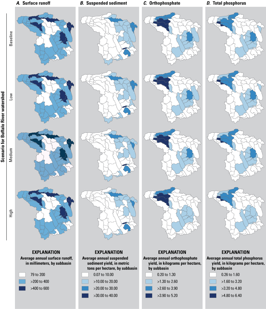
Maps showing average annual A, Surface runoff; B, Suspended sediment yield; C, Orthophosphate yield; and D, Total phosphorus yield, by scenario and subbasin, Buffalo River watershed model, New York. See figure 3 for subbasin identifiers.
Results by Best Management Practice
BMPs were evaluated for effectiveness at the HRU level, shown by the boxplots in figure 31. The average annual yield reductions resulting from the implementation of the scenario BMPs are shown in table 19. The range in suspended sediment and nutrient yield reductions from a single BMPs (CC, NMP, RT, FS) were generally smaller than the BMP combinations; however, applying more BMPs per HRU did not necessarily result in greater nutrient reductions. On HRUs with cash grain rotations, the CC+NMP+RT combination had the greatest average annual total phosphorus yield reduction for infield BMPs (all BMPs excluding FS) but the second lowest orthophosphate yield reduction (table 19). CC+RT had a higher suspended sediment yield reduction compared to CC+NMP+RT. CC+NMP+RT had the lowest orthophosphate reduction in the dairy rotations.
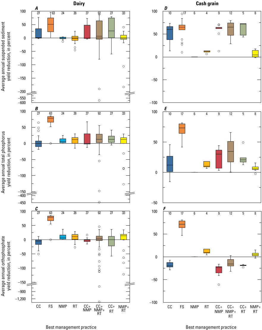
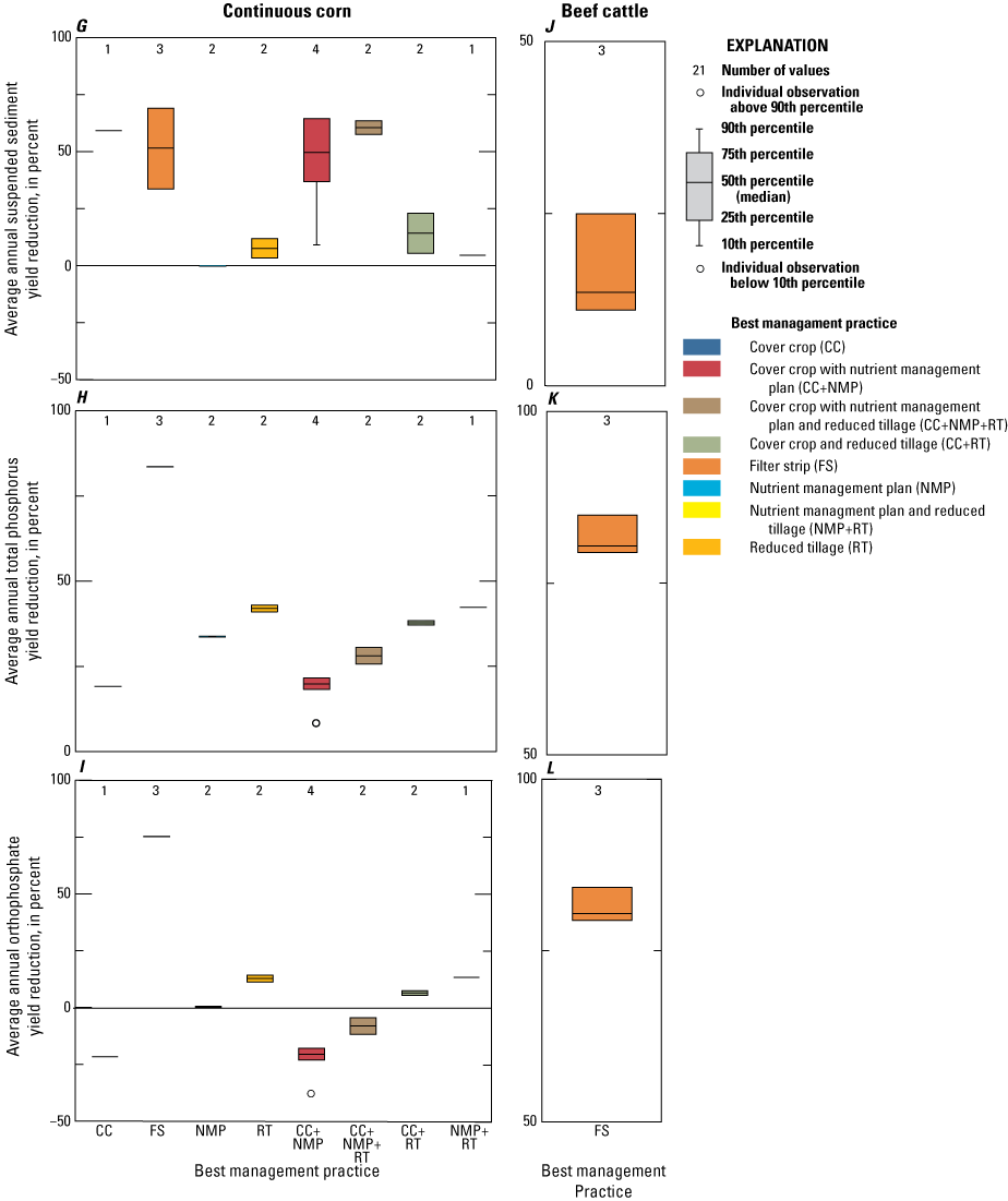
Boxplots of simulated reduction of average annual suspended sediment and nutrient yields, in percent, in surface runoff from A–C, Dairy rotations; D–F, Cash grain rotations; G–I, Continuous corn rotations; and J–L, Beef cattle rotations, because of selected best management practices in the Buffalo River watershed model, New York. Negative values indicate an increase in yield.
Overall, FS were the most effective BMP for reducing orthophosphate and total phosphorus in the Buffalo River watershed model, no matter the agricultural rotation (table 19; fig. 31). FS reduced the average annual orthophosphate yield by 70.41 percent on cash grain rotations, 75.31 percent on continuous corn rotations, 69.08 percent on dairy rotations, and 81.35 percent on beef cattle rotations. FS reductions were very similar for total phosphorus, where average annual total phosphorus yield was reduced by 71.15 percent on cash grain rotations, 76.46 percent on continuous corn rotations, 69.04 percent on dairy rotations, and 81.60 percent on beef cattle rotations. Additionally, FS reduced the average annual suspended sediment yield by 59.88 percent on cash grain rotations, 51.39 percent on continuous corn rotations, 50.80 percent on dairy rotations, and 16.48 percent on beef cattle rotations.
In the Buffalo River watershed model, CC reduced suspended sediment and total phosphorus yields for cash grain, continuous corn, and dairy rotations, but increased orthophosphate yield (table 19; fig. 31). CC reduced average annual suspended sediment by 51.49 percent on cash grain rotations, 59.20 percent on continuous corn rotations, and 16.11 percent on dairy rotations, whereas total phosphorus yield reductions were less: 12.83 percent on cash grain rotations, 30.26 percent on continuous corn rotations, and 3.79 percent on dairy rotations (table 19). Average annual orthophosphate yield was reduced by −18.76 percent on cash grain rotations, 21.39 percent on continuous corn rotations, and 9.64 percent on dairy rotations. For dairy rotations, orthophosphate yield increases may be because of the removal of the chisel tillage after the fall (table 7, years 1–3 October).
For cash grain and dairy rotations, when CC were combined with any other BMP, these rotations have higher reductions of suspended sediment and total phosphorus yields than when CC were used alone (table 19; fig. 31). All cash grain and dairy rotations that included CC increased orthophosphate yield. For the cash grain rotations, the trio CC+NMP+RT increased orthophosphate yield the least, whereas in the dairy rotation this combination increased orthophosphate yield more than any other BMP combination. For continuous corn rotations, the BMP performances were mixed. CC+NMP had lower suspended sediment, nitrate as nitrogen, and total phosphorus yield reductions than CC+NMP+RT. CC+RT had lower suspended sediment and higher total phosphorus yield reductions than CC+NMP+RT. For continuous corn rotations, CC and CC combinations with other BMPs, except for CC+RT, resulted in negative orthophosphate average annual yield reductions.
In the Buffalo River watershed model, NMP very minimally increased the average annual suspended sediment yield in cash grain and continuous corn rotations (table 19; figs. 31D, G), whereas NMP reduced orthophosphate and total phosphorus yields. NMP reduced the average annual suspended sediment yield by −0.08 percent on cash grain rotations, −0.14 percent on continuous corn rotations, and −0.82 on dairy rotations (table 19). Cash grain and continuous corn rotations had slight orthophosphate and total phosphorus yield reductions because of NMP, on average, under 1 percent. Dairy rotations with NMP had an average annual orthophosphate yield reduction of 9.74 percent and a total phosphorus yield reduction of 8.72 percent. For continuous corn rotations, NMP used in combination with other BMPs was generally more effective at reducing suspended sediments and nutrient yields than NMP alone (table 19; figs. 31G, H, I). However, CC or RT had higher suspended sediment and nutrient yield reductions alone than when used in NMP combinations. The relation between BMP combinations involving NMP was also found on dairy and cash grain rotations, except for CC+NMP where yield reductions of suspended sediment and total phosphorus were higher than CC alone, and on dairy rotations where NMP had the highest reductions of orthophosphate out of all BMPs excluding FS.
Some BMPs caused changes to the water balance in the Buffalo River watershed model (Fisher and Merriman, 2024). When RT was applied, percolation and groundwater recharge was increased, and surface runoff was decreased. RT increased percolation by an average of 45 percent, with the change in percolation ranging from 0 to 177 mm. The largest increases in percolation and recharge were found when NMP+RT was applied, at a maximum of 294 and 195 mm, respectively. Surface runoff was decreased the most out of any BMP combination when all three BMPs (CC+NMP+RT) were applied (table 19). The combination of CC+NMP+RT also increased percolation and recharge (an average of 45 percent and 41 percent); and these increases, because of CC+NMP+RT, were greater than RT alone but less than the NMP+RT combination. Minimal average changes to percolation and recharge were found when CC and NMP were applied separately. On average, CC reduced percolation by 0.04 mm and recharge by 0.1 mm. NMP increased percolation by 0.56 mm and recharge by 0.73 mm, on average. The combination of CC+NMP reduced percolation by 0.44 mm and recharge by 0.38 mm. No changes to the water balance were observed with FS.
Average annual yield reductions in the Buffalo River watershed model because of RT were similar across all rotations (table 19), with an exception for the increase of suspended sediment from dairy rotations. In dairy rotations, HRUs treated with RT had the third highest orthophosphate and fourth highest total phosphorus yield reductions out of all BMP combinations but a suspended sediment yield reduction of −2.16 percent (which is an increase in suspended sediment). However, when RT+CC was applied in the dairy rotation, the average annual suspended sediment, orthophosphate, and total phosphorus yield reductions were higher than when compared to either CC or RT alone. Average annual reductions in suspended sediment, orthophosphate, and total phosphorus yield were low (<4 percent) for the NMP+RT combination. For cash grain rotations, HRUs with RT had the second highest orthophosphate, third highest total phosphorus, and third lowest suspended sediment yield reductions. When NMP+RT was simulated, yield reductions were less than for RT alone, but higher than NMP. Average suspended sediment yield reductions from CC+RT was 61.72 percent in comparison to a 51.49 percent reduction from CC, but the suspended sediment yield reduction from CC+RT was 6 times higher than from RT alone. For CC+RT, the average annual reduction in total phosphorus yield was 24.70 percent, which was higher than from RT (11.26 percent) or CC (12.83 percent) alone. Average annual orthophosphate yield reductions decreased when CC+RT was combined, in comparison to CC or RT alone; orthophosphate yield reductions were 10.07 percent for RT, −18.76 percent for CC, and −19.03 percent for CC+RT. For continuous corn rotations, HRUs with RT applied had the third highest orthophosphate and second lowest total phosphorus yield reductions and the third lowest suspended sediment yield reduction out of all BMP combinations.
On dairy rotations, there were several outlier data points for the CC+NMP+RT combination where there were large negative values for average annual orthophosphate yield reductions (fig. 31C), indicating that orthophosphate yield increased with this BMP application (Fisher and Merriman, 2024). Most of the HRUs with these outlier data had very poorly drained soils with tile drainage. One HRU had an extremely large increase in orthophosphate yield. It is unknown why this HRU performed so differently from the other HRUs. This HRU also coincided with a large decrease in the SWAT-calculated, nitrogen-related crop stress on years when the cover crop was growing; however, other HRUs with this rotation show this decrease as well, but to a lesser degree. The suspended sediment yield reduction for this HRU was 41.90 percent. This HRU had two negative reductions (increases) in average annual yield: −1,328.42 for orthophosphate and −446.40 for total phosphorus.
Green Infrastructure Scenario
In subbasin 9 of the Buffalo River watershed model, the combination of permeable pavement and rain garden infrastructure reduced the average annual surface runoff, suspended sediment, orthophosphate, total phosphorus, and nitrate as nitrogen loads by 10.7, 15.4, 8.3, 10.7, and 11.6 percent, respectively. Average annual total nitrogen yield was reduced by −0.7 percent (an increase). Because these BMPs were applied on the subbasin scale (both permeable pavement and rain garden infrastructures were applied in the .lid file for subbasin 9), it was not possible to find the effectiveness of permeable pavement or rain gardens individually.
At the HRU level, the effect of removing buildings and impervious surfaces and restoring them as grassed vacant lots was tested on six HRUs. On these six HRUs, changing the land cover caused the following reductions: average annual surface runoff ranging from 34.1 to 84.4 percent, orthophosphate yield ranging from 19.9 to 74.6 percent, and total phosphorus yield ranging from 38.2 to 84.7 percent. The transition to grassed vacant lots generally reduced suspended sediment yields; average annual suspended sediment reductions ranged from 33.1 to 93.4 percent for five of the HRUs. The other vacant lot increased suspended sediment yield by 44 percent.
The simulated green infrastructure practices covered 0.27 percent of the Buffalo River watershed. This scenario reduced suspended sediment load by 150 metric tons, orthophosphate load by 100 kg, and total phosphorus load by 200 kg on an average annual basis at the watershed outlet. This was 0.09, 0.07, and 0.12 percent of the Buffalo River watershed model’s average annual suspended sediment, orthophosphate, and total phosphorus loads. Total nitrogen was reduced by 500 kg, equivalent to 0.03 percent of the watershed’s average annual load. While none of these reductions were greater than 1 percent of the watershed model’s loads, reductions from the green infrastructure practices were similar to those from the point source scenario. Model results indicate that instituting both green infrastructure and point-source load limits could reduce average annual loads by 1,000 kg total nitrogen (0.05 percent) and 500 kg total phosphorus (0.29 percent) in the Buffalo River watershed.
Point Source Scenario
For the Buffalo River watershed model point-source scenario, loads from one point source in the Cazenovia Creek subwatershed (subbasin 47) were reduced (table 20). There were no phosphorus monitoring data available for the point source (NY0108103; table 3), thus a 3 mg/L total phosphorus constant effluent concentration was assumed for the baseline scenario. For this scenario, the effluent reduction to 1 mg/L total phosphorus concentration resulted in a reduction by 67 percent of total phosphorus. At the watershed model outlet, average annual orthophosphate and total phosphorus loads were reduced 200 and 300 kg, respectively (table 20). There were reductions of 0.14 and 0.18 percent of orthophosphate and total phosphorus loads, respectively, for the entire Buffalo River watershed model. The Buffalo point-source scenario was less effective at reducing orthophosphate and total phosphorus loads than the low BMP scenario.
Canadaway Creek Watershed
For the Canadaway Creek watershed model, the baseline simulated average annual loads were 109,280 metric tons of suspended sediment, 65,665 kg of total nitrogen, 13,835 kg of orthophosphate, and 115,205 kg of total phosphorus (fig. 25). Nitrate as nitrogen and total nitrogen loads for this watershed model were among the lowest of the study watersheds (fig. 25). The Canadaway Creek watershed model had the fourth highest suspended sediment and total phosphorus loads. Total phosphorus loads for this watershed model were very similar to those from the Tonawanda Creek watershed model, even though the Tonawanda Creek watershed model is considerably larger in size (16 times larger).
Loads by rotation for the Canadaway Creek watershed model are displayed in figures 27E and F. Point sources were not modeled in this watershed model. Forest rotations exported the largest total nitrogen and total phosphorus loads out of all rotations, consistent with forested land covering the greatest percentage (64.91; table 2) of the watershed. Pasture and dairy produced the second and third highest total phosphorus loads out of all rotations.
Results by Low, Medium, and High Best Management Practice Scenarios
Figure 26 shows the percent reduction in constituent loads at the Canadaway Creek watershed model outlet from BMP implementation. Average annual surface runoff in the Canadaway Creek watershed model had an overall decrease from baseline conditions to the high scenarios of 0.03 percent (Fisher and Merriman, 2024); no change to surface runoff was seen in the low and medium scenarios. The low and medium scenarios both slightly increased average annual suspended sediment loads, denoted by negative reductions of −0.06 and −0.01 percent, respectively. The high scenario decreased average annual suspended sediment loads by 0.09 percent (fig. 26A). Average annual total nitrogen loads decreased by 0.25, 0.66, and 1.77 percent in the low, medium, and high scenarios, respectively (26D). The average annual orthophosphate loads decreased from the baseline by 0.11, 0.43, and 1.16 percent, respectively, in the low, medium, and high scenarios (fig. 26C). Model simulated average annual total phosphorus loads for the low, medium, and high scenarios decreased by 0.28, 1.07, and 2.73 percent, respectively (fig. 26E). Comparing the high scenario to the baseline, average annual loads were reduced by 95 metric tons of suspended sediment, 187 kg of nitrate as nitrogen, 160 kg of orthophosphate, 1,160 kg of total nitrogen, and 3,145 kg of total phosphorus (fig. 25).
In general, decreases for each constituent in each BMP scenario are noted particularly in subbasins in the central part of the watershed model (fig. 32). Similarly, the highest surface runoff was generally in the central part of the watershed model, particularly in subbasins 8 and 9. However, the BMP scenarios had minimal effect on change in surface runoff in the Canadaway Creek watershed model. The highest suspended sediment yield occurred in subbasin 24, and generally in the central part of the watershed model. The slopes in subbasin 24 are mostly between 2 and 20 percent, with poorly drained soils, and with only two HRUs that had tile drainage. The combination of these factors can create conditions that exacerbate suspended sediment runoff. The highest orthophosphate yield occurred generally in the northwestern part of the watershed model, especially in subbasin 8. Subbasin 8 is characterized by a large area of grapes land cover (fig. 3C), and the Canadaway Creek watershed has the second highest percentage of grapes land cover out of the nine watersheds (table 2). The other subbasins with relatively high orthophosphate yield also had a relatively high percentage of land cover as grapes and developed land (table 2; fig. 3). Total phosphorus yield was consistently high throughout the entire watershed model. Agricultural land cover is spread throughout the Canadaway Creek watershed (fig. 3C); the corresponding agricultural rotations of dairy, beef cattle, cash grain, horse, continuous corn, pasture, and vineyards are common across the watershed (13 to 53 kg/ha), which likely causes the high total phosphorus yields throughout the watershed model (fig. 32).
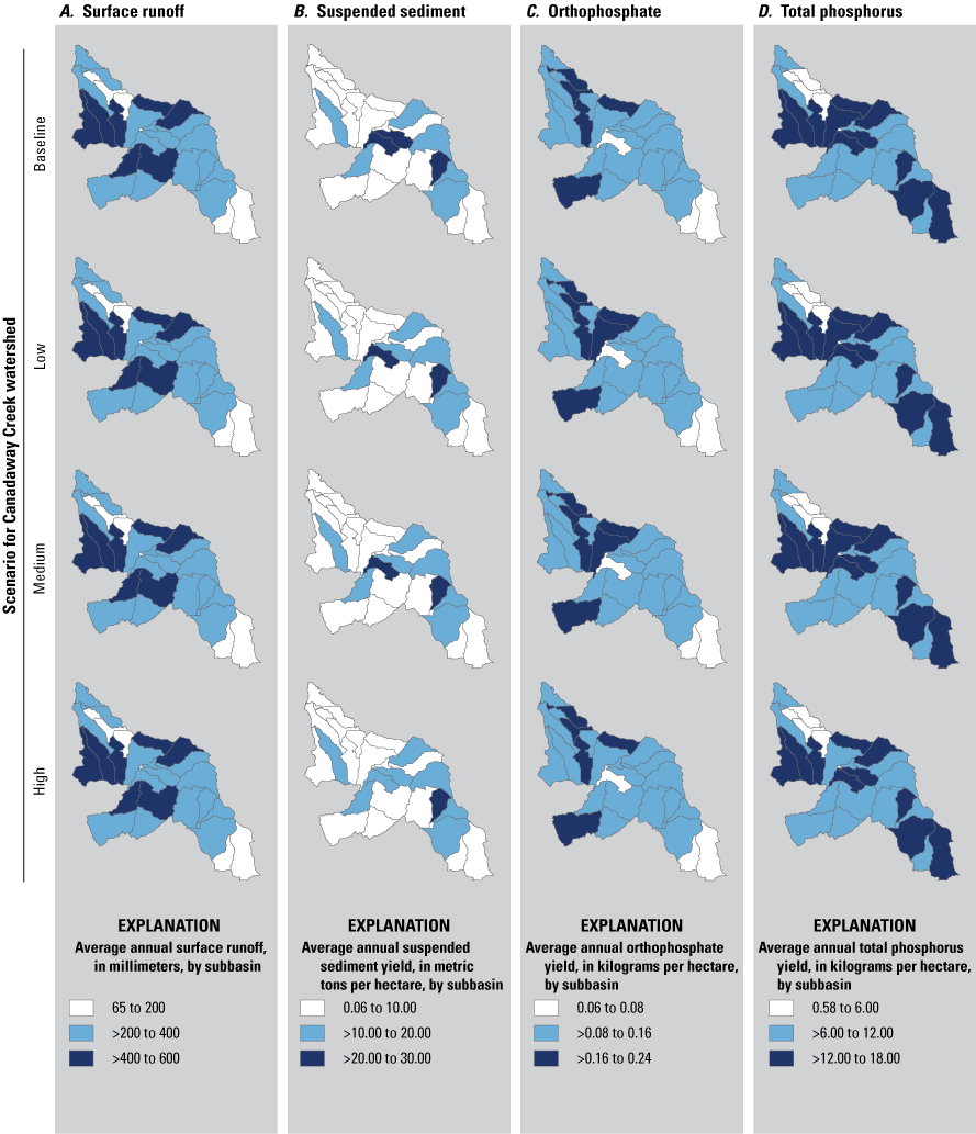
Maps showing average annual A, Surface runoff; B, Suspended sediment yield; C, Orthophosphate yield; and D, Total phosphorus yield, by scenario and subbasin, Canadaway Creek watershed, New York. See figure 3 for subbasin identifiers.
Results by Best Management Practice
The following is a discussion of average annual yield reductions for dairy rotations in the Canadaway Creek watershed model. For dairy rotations, the greatest reductions in average annual suspended sediment, orthophosphate, and total phosphorus yields were from CC+RT, FS, and CC+RT, respectively (table 19; fig 33A, B, C). For singular BMPs simulated on dairy rotations, RT had the greatest suspended sediment reduction, and FS had the greatest orthophosphate and total phosphorus reductions (table 19; fig. 33A, B, C). Counting BMP combinations as well, CC had the lowest suspended sediment yield reduction and CC+NMP+RT had the lowest orthophosphate yield reduction; both values were negative, indicating that these BMPs would increase the suspended sediment and orthophosphate exported on dairy rotations. When an additional or two additional BMPs were added to CC, suspended sediment reduction was less effective than with CC alone, apart from the CC+RT combination. Orthophosphate reductions decreased when other BMPs were added to CC (except CC+NMP). All dairy rotation BMPs had positive values for total phosphorus reductions. On dairy rotations, suspended sediment reductions improved when any BMP was added to NMP; orthophosphate and total phosphorus reductions increased for CC+NMP combinations. However, CC+NMP and FS were the only two BMPs on dairy rotations that had positive percent reductions for suspended sediment, orthophosphate, and total phosphorus, meaning that all other BMP combinations caused at least one of these three constituents to increase. All dairy rotation BMPs had positive average and median values for total phosphorus reductions (average values are given in table 19; median values are shown in fig. 33B).
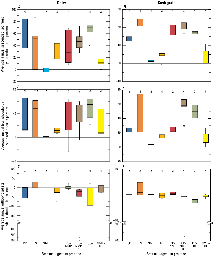
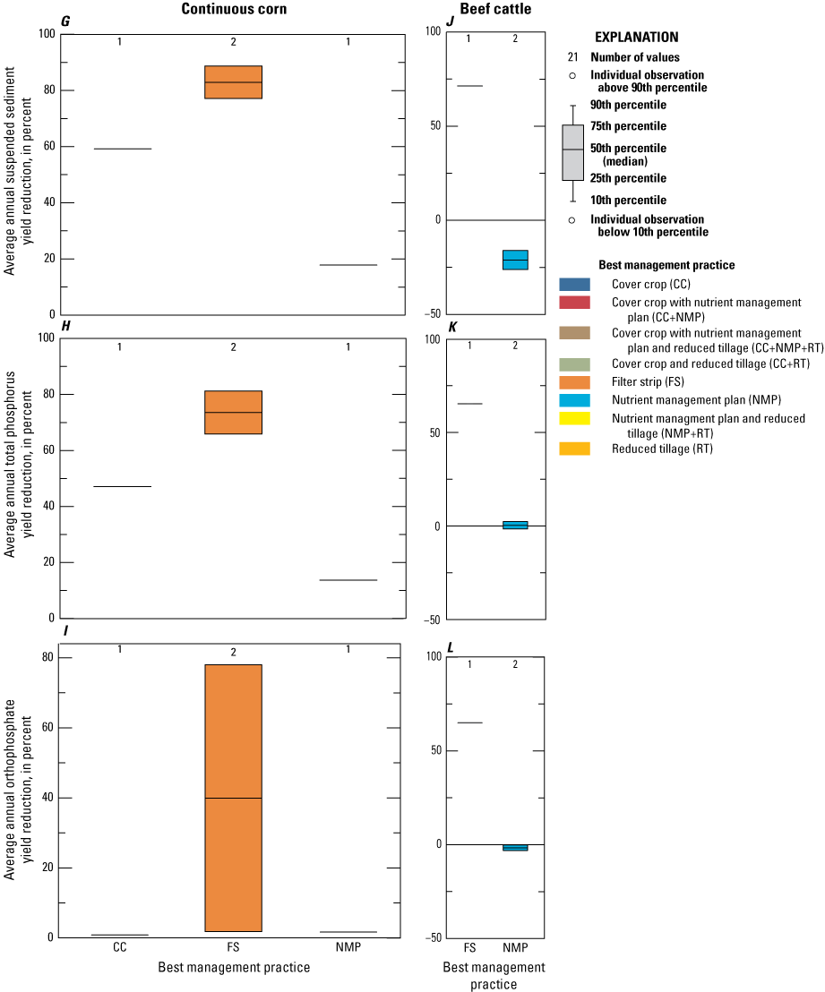
Boxplots of simulated reduction of average annual suspended sediment and nutrient yields, in percent, in surface runoff from A–C, Dairy rotations; D–F, Cash grain rotations; G–I, Continuous corn rotations; and J–L, Beef cattle rotations, because of selected best management practices in Canadaway Creek watershed model, New York. Negative values indicate an increase in yield.
The following discussion of cash grain yield reductions for the Canadaway Creek watershed model are shown in figures 33D, E, and F. FS had the greatest average annual reductions in suspended sediment, orthophosphate, and total phosphorus yields (table 19; fig. 33D, E, F). When excluding FS, CC+NMP+RT had the greatest average annual reductions in all suspended sediment and total phosphorus yields, but the greatest average annual increases in orthophosphate (table 19). CC, NMP, and CC+NMP all had reductions in average annual suspended sediment, orthophosphate, and total phosphorus yields (table 19; fig. 33D, E, F). NMP had modest reductions of average annual yields for these constituents, 1.59 percent for orthophosphate and 5.61 percent for suspended sediment (table 19), and CC had greater average annual yield reductions (2.26 percent for orthophosphate and 54.40 percent for suspended sediment (table 19; fig. 33D, F). CC+NMP had higher yield reductions than CC alone; CC+NMP caused reductions of the average annual suspended sediment yield by 73.75 percent, of the average annual orthophosphate yield by 5.80 percent, and of the average annual total phosphorus yield by 25.03 percent (table 19; fig. 33D, E, F). RT had greater suspended sediment and total phosphorus reductions of average annual yield than NMP, but NMP had greater orthophosphate average annual yield reductions than RT (table 19; fig. 33D, E, F).
Three BMPs were simulated with continuous corn rotations on four HRUs for the Canadaway Creek watershed model; these results are shown in the boxplots in figures 33G, H, and I. All BMPs improved suspended sediment, orthophosphate, and total phosphorus yields in comparison to the baseline scenario (table 19; figs. 33G, H, I). FS were the most effective BMP; it had the greatest average reductions in all suspended sediment, orthophosphate, and total phosphorus yields (table 19; figs. 33G, H, I). CC were more effective at reducing suspended sediment and total phosphorus yields than NMP, and NMP was more effective at reducing orthophosphate yields than CC (table 19; figs. 33G, H, I).
Reductions below the 10th percentile are treated as outliers (fig. 33). The CC+NMP+RT BMP combination produced outliers in orthophosphate reduction: two outliers in the dairy rotation (fig. 33C) and one outlier in the cash grain rotation (fig. 33F). These three outliers represent increases in orthophosphate. The soils in the Canadaway Creek watershed were either poorly drained or very poorly drained, and the HRUs with outlier reductions did not have tile drainage simulated and had higher CN values for subbasins 83–87. These HRUs with an outlier performance had an increase in surface runoff in comparison to the baseline scenario (Fisher and Merriman, 2024).
Cattaraugus Creek Watershed
The Cattaraugus Creek watershed model had the largest simulated suspended sediment, total nitrogen, and total phosphorus loads of any of the study watersheds (fig. 25). For the Cattaraugus Creek watershed model, the baseline average annual simulated loads were 495,400 metric tons of suspended sediment, 2,176,000 kg of total nitrogen, 75,980 kg of orthophosphate, and 642,650 kg of total phosphorus (fig. 25). The Cattaraugus Creek watershed is 330 km2 larger than the Buffalo River watershed, and its simulated average annual loads for suspended sediment, total nitrogen, and total phosphorus were 2.8, 1.1, and 3.7 times those from the Buffalo River watershed model, respectively. The average annual suspended sediment loads were 2.7 times greater than the Eighteenmile Creek watershed model that had the next highest suspended sediment loads.
The nine studied point sources in the Cattaraugus Creek watershed (table 3) did not have a major effect on baseline streamflow or loads. Point sources contributed approximately 5.7 percent of the watershed model’s streamflow and <10 percent of the watershed model's total nitrogen and total phosphorus load.
The following discussion compares the average annual loads (figs. 27G, H) and yields (table 18) in the Cattaraugus Creek watershed model per rotation. The forest rotation exported the greatest total nitrogen and total phosphorus loads because of the predominance of this land cover in the Cattaraugus Creek watershed (table 2; fig. 3D); 60 percent of the watershed model land cover is forest (table 18). Forest rotation contributed 41 percent of the total nitrogen and 56 percent of the total phosphorus loads (figs. 27G, H), and total nitrogen and total phosphorus yields from forest rotation were tied for the third smallest yield of the rotations (table 18). CAFOs exported the second most total nitrogen, 13 percent, and third most total phosphorus, 13 percent, out of the agricultural rotations. The dairy rotation contributed 14 percent of total phosphorus loads and 8 percent of total nitrogen loads. Twelve percent of the watershed model’s total nitrogen and total phosphorus loads came from pasture. Whereas beef cattle rotations only constituted 1 percent of the watershed model area (table 18), beef cattle accounts for 3 percent of the watershed model’s total phosphorus load and 2 percent of its total nitrogen load. Beef cattle rotations had the highest yields for suspended sediment, organic phosphorus, sediment bound phosphorus, total phosphorus, and organic nitrogen (table 18). Cash grain, continuous corn, and dairy rotations had the second through fourth highest total phosphorus yields (table 18). Septic rotation had the highest total nitrogen yields, with the majority coming from nitrate as nitrogen in the groundwater (table 18). Because the septic rotation accounted for 0.1 percent of the watershed model area, it only had a minor effect on the watershed model’s total nitrogen load.
Results by Low, Medium, and High Best Management Practice Scenarios
All three BMP scenarios decreased loads to Lake Erie in comparison to baseline conditions in the Cattaraugus Creek watershed model (figs. 25, 26). Each implementation scenario applied BMPs that changed agricultural management on approximately 2,490 ha. Average annual suspended sediment loads decreased by 0.10, 0.18, and 0.38 percent in the low, medium, and high scenarios, respectively (fig. 26A). Average annual orthophosphate loads decreased by 0.92, 2.22, and 3.49 percent in the low, medium, and high scenarios, respectively (fig. 26C). Average annual total nitrogen loads decreased by 0.34, 0.87, to 1.47 percent in the low, medium, and high scenarios, respectively (fig. 26D). Average annual total phosphorus loads decreased by 1.51, 4.06, and 6.36 percent in the low, medium, and high scenarios, respectively (fig. 26E). The total phosphorus reductions corresponded to decreases of averages of 9,700 kg, 26,100 kg, and 40,850 kg per year in the low, medium, and high scenarios, respectively (fig. 25E).
In general, decreases for each constituent were noted in subbasins in the western and eastern parts of the watershed (fig. 34). The upland subbasins in the eastern part of the Cattaraugus Creek watershed model had the most surface runoff; this part of the watershed model is characterized by hilly terrain with slopes mostly ranging from 5 to >20 percent. Subbasin 36 had the highest surface runoff (fig. 34A) which may be because of the large agricultural footprint combined with the predominance of very poorly drained soils. The highest suspended sediment yields were in subbasins 62 and 63 just upstream of USGS streamgage 04213500 on Cattaraugus Creek (fig. 34B). The stretch of Cattaraugus Creek through the Zoar Valley Unique Area (fig. 2D) is very steep and well known for erosion of sediment into the creek (La Sala, 1968). Subbasins 62 and 63 are dominated by slopes ranging from 5 to >20 percent. The highest orthophosphate yields were in subbasins 18 and 36 (fig. 34C), which both had a substantial agricultural footprint dominated by corn and hay with some alfalfa, soybeans, and other crops (fig. 3D). Total phosphorus yields were highest in subbasin 36 and a cluster of subbasins in the western and eastern part of the watershed model (fig. 34D). The entire eastern part of the watershed model also had a substantial agricultural footprint, such as in subbasins 18 and 36, where the dominant crops were hay, corn, and alfalfa (fig. 3D). The eastern part of the watershed has a hilly landscape with steep slopes which may, in combination with agriculture, be the source of some of the total phosphorus yield in that area (fig. 34D).
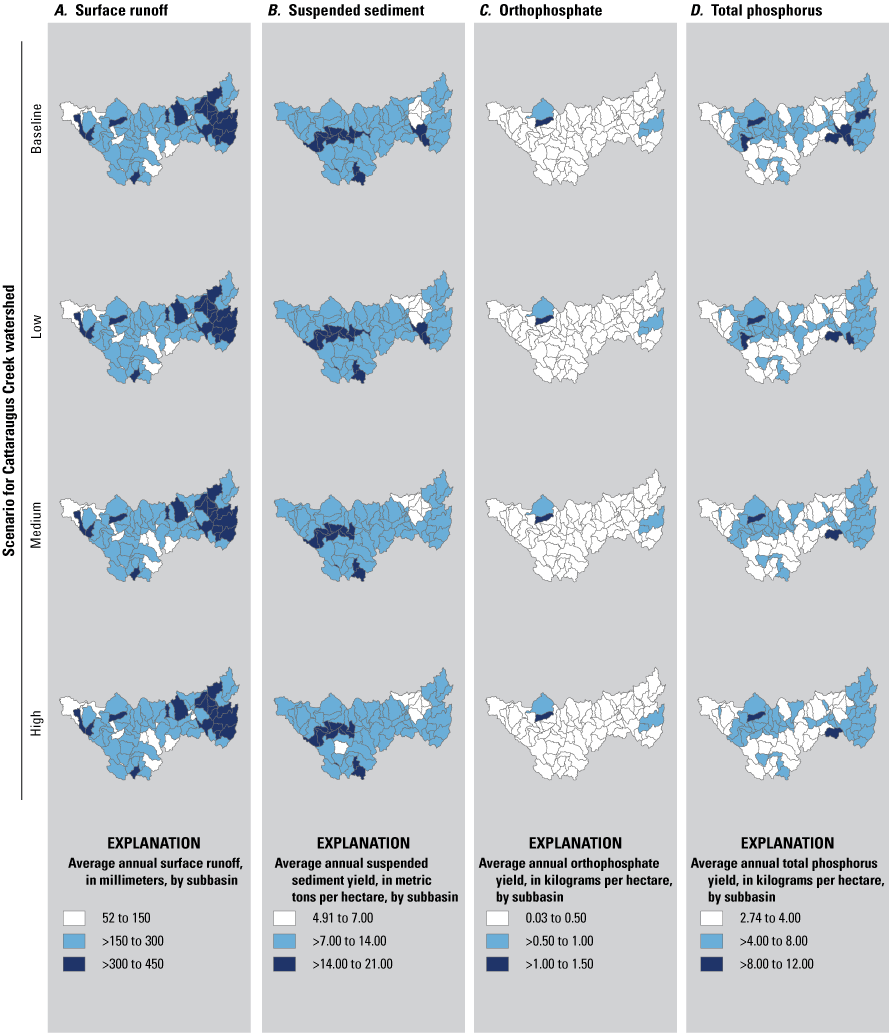
Maps showing average annual A, Surface runoff; B, Suspended sediment yield; C, Orthophosphate yield; and D, Total phosphorus yield, by scenario and subbasin, Cattaraugus Creek watershed, New York. See figure 3 for subbasin identifiers.
Results by Best Management Practice
Six percent of the Cattaraugus Creek watershed model area was simulated with a dairy rotation (table 18); BMP results in dairy rotations are explained in the following discussion. A BMP or a BMP combination were simulated on 416 dairy HRUs (table 19); yield reductions are shown as boxplots in figures 35A–C. NMP was the only BMP with increases in suspended sediment and total phosphorus yields (negative reductions in table 19); suspended sediment and total phosphorus average annual yield changes were positive for all other BMPs or BMP combinations. CC, CC+NMP, and CC+RT had negative average annual yield reductions (increases) for orthophosphate; all other BMPs and combinations caused decreases of average annual orthophosphate yield. FS had the greatest reductions of average annual suspended sediment and total phosphorus yields. On dairy rotations, average annual suspended sediment and total phosphorus yield reductions for CC alone (21.95 and 20.04 percent, respectively) were comparable to BMP combinations with CC, ranging between 15.73 and 23.34 percent for suspended sediment and 20.09 and 21.28 percent for total phosphorus. Additionally, the range of suspended sediment and total phosphorus average annual yield reductions for CC BMPs were small. Generally, when BMP combinations were applied to an HRU on dairy rotations, orthophosphate and total phosphorus average annual yield reductions were greater than reductions from single BMPs; however, some BMP combinations had lower average annual yield reductions than single BMPs. For example, when NMP+RT were applied, suspended sediment and total phosphorus average annual yield reductions were less than RT alone but greater than NMP alone. CC+NMP average annual yield reductions were greater than CC or NMP alone, except for orthophosphate. CC+NMP+RT had lower reductions of suspended sediment and total phosphorus average annual yields when compared with CC+NMP but greater than NMP+RT.
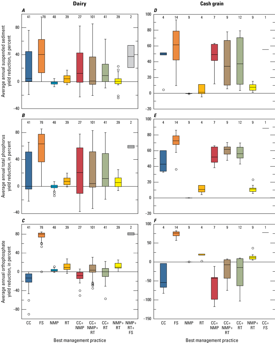
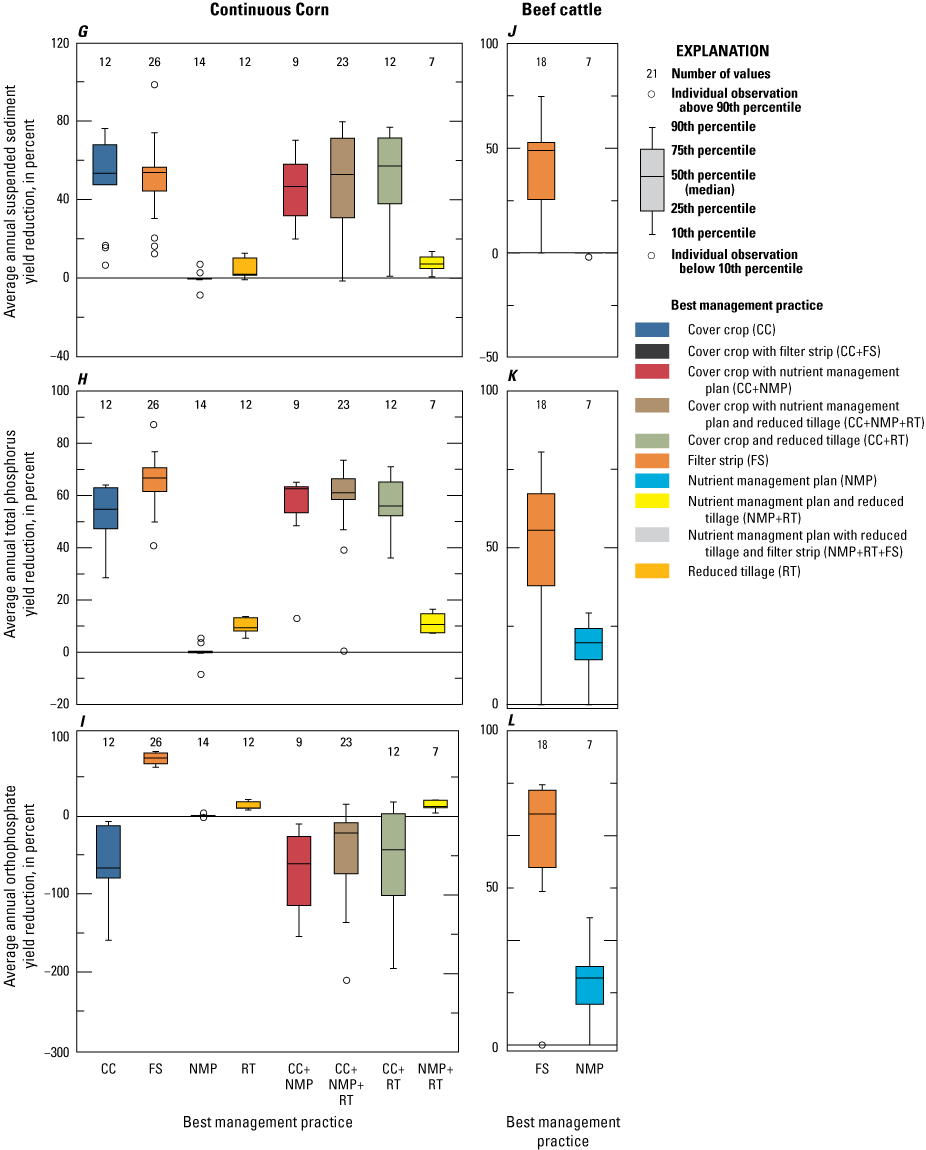
Boxplots of simulated reduction of average annual suspended sediment and nutrient yields, in percent, in surface runoff from A–C, Dairy rotations; D–F, Cash grain rotations; G–I, Continuous corn rotations; and J–L, Beef cattle rotations, because of selected best management practices in the Cattaraugus Creek watershed model, New York. Negative values indicate an increase in yield.
Reductions of average annual yields from cash grain rotations are shown in the boxplots in figures 35 D, E, and F and discussed as following. Sixty-nine BMPs were simulated on 1,225.82 ha (table 19). NMP was the only BMP with a negative average annual suspended sediment yield reduction (an increase), −0.12 percent (fig. 35D). For NMP, average annual total phosphorus (fig. 35E) and orthophosphate (fig. 35F) yield reductions were also small, 0.29 and 0.02 percent, respectively. All cash grain rotations with CC or BMP combinations with CC had negative average annual orthophosphate yield reductions (increases); all other BMPs and BMP combinations had positive average annual orthophosphate yield reductions (fig. 35F). All BMPs and BMP combinations caused average annual total phosphorus yield reductions from cash grain rotations (fig. 35E). FS caused the greatest reductions of average annual suspended sediment, orthophosphate, and total phosphorus yields from cash grain rotations (figs. 35D, E, F). Of all simulated BMPs excluding FS, CC+NMP caused the greatest average suspended sediment reductions (fig. 35D); CC+NMP+RT caused the greatest average total phosphorus reductions (fig. 35E); and NMP+RT caused the greatest average orthophosphate reductions (fig. 35F). NMP+RT caused greater reductions in suspended sediment and total phosphorus yields than either NMP or RT alone (figs. 35D, F). CC+RT caused greater reductions in suspended sediment and total phosphorus yields than either CC or RT alone.
Figures 35G, H, and I are boxplots of simulated yield reductions of suspended sediment, total phosphorus, and orthophosphate from continuous corn rotations. There were 115 BMPs examined on 2,013.55 ha of continuous corn rotations in the Cattaraugus Creek watershed model (table 19). FS caused the greatest reductions of average annual suspended sediment, total phosphorus, and orthophosphate yields from continuous corn rotations (table 19). All BMPs and BMP combinations reduced average annual suspended sediment yields, except for NMP, which had a slightly negative (−0.12 percent) reduction (an increase; fig 35G). CC and any of its combinations caused a negative reduction (increase) of average annual orthophosphate yields, whereas average suspended sediment reductions ranged from 46.6 to 48.9 percent, and average annual total phosphorus reductions ranged from 52 to 58.7 percent (figs. 35I, G, H). NMP+RT and RT caused similar continuous corn rotation results, with average annual yield reductions in orthophosphate of 12.79 and 12.70 percent, respectively (table 19). CC+NMP+RT caused the second largest average annual yield reduction in total phosphorus and an increase in orthophosphate average annual yield reduction (table 19).
Eighteenmile Creek Watershed
For the Eighteenmile Creek watershed model, the baseline simulated loads were 182,200 metric tons of suspended sediment, 79,920 kg of nitrate as nitrogen, 399,600 kg of total nitrogen, 14,175 kg of orthophosphate, and 68,225 kg of total phosphorus (fig. 25). Simulated average annual suspended sediment loads from the Eighteenmile Creek watershed model were comparable with those of the Buffalo River watershed model, which is 3.6 times larger in area. The average annual suspended sediment load was the second highest of the study watershed models (fig. 25A). Average annual total phosphorus and total nitrogen loads were the fourth and fifth highest of the study watersheds (figs. 25D, E). Nitrate as nitrogen was 20 percent of the total nitrogen load; the majority (75 percent) of the total nitrogen load was in the organic form (table 18). Orthophosphate was about 21 percent of the average annual total phosphorus load (table 18).
Loads were calculated by the amount of rotation area and the average annual yield per rotation. The forest rotation had the lowest total phosphorus yields (table 18) but exported the highest total nitrogen and second highest total phosphorus loads (figs. 27I, J). The forest rotation corresponds to about 61 percent of the Eighteenmile Creek watershed model land cover (table 18). The greatest total phosphorus and the second greatest total nitrogen loads in the watershed model came from the dairy rotation (figs. 27I, J), as dairy rotations had the second highest suspended sediment and organic phosphorus yields (table 18). The dairy rotation was responsible for the second highest suspended-sediment bound phosphorus yields (table 18). Among all the study watersheds, the model calculated total phosphorus loads from the dairy rotation were the third largest (fig. 27I); the dairy rotation covered almost 6,000 ha, the rotation with the third most area in the Eighteenmile Creek watershed model (table 18). Out of the rotations studied, pasture contributed the third most total phosphorus and total nitrogen (figs. 27I, J); yields from the pasture rotation were low (table 18), but pasture was the second most prevalent rotation in the Eighteenmile Creek watershed model after forests (table 18). The urban and CAFO rotations contributed relatively large amounts of total phosphorus and total nitrogen (figs. 27I, J), as they were the fourth and fifth most predominant rotations in the watershed (table 18). Urban total phosphorus and total nitrogen yields were relatively low compared to the other rotations, and total phosphorus yields for CAFOs were lower than the average annual total phosphorus yield for the watershed model (table 18). Septic total nitrogen yields were the largest out of the rotations (table 18), but because of the low amount of area in the septic rotation it had a low effect on the watershed model’s total nitrogen loads (fig. 27J). No point sources were modeled in this watershed model.
Results by Low, Medium, and High Best Management Practice Scenarios
Figure 26 shows the effect of BMP scenarios on the simulated loads from Eighteenmile Creek watershed. Average annual suspended sediment loads decreased from the baseline by 0.11, 0.41, and 0.05 percent in the low, medium, and high scenarios, respectively (fig. 26A). Average annual orthophosphate loads decreased by 0.67, 2.54, and 4.66 percent in the low, medium, and high scenarios, respectively (fig. 26C). Average annual total nitrogen loads decreased by 0.38, 1.21, to 2.49 percent in the low, medium, and high scenarios, respectively (fig. 26D). Average annual total phosphorus loads decreased by 0.96, 3.09, and 5.88 percent in the low, medium, and high scenarios, respectively (fig. 26E).
In general, because of the BMP scenarios, decreases of surface runoff, suspended sediment, and total phosphorus are noted in subbasins in the southern, central, and northern parts of the watershed model (figs. 36A, B, D). The subbasins of the Eighteenmile Creek in the southeast have the highest surface runoff of the watershed model, particularly subbasins 14 through 23 (figs. 3G, 36A). The southern part of the watershed model has much steeper slopes than the northwestern part of the watershed model. In subbasins 14 through 23, the slope percentages range mostly from 1 to 16 percent, the soils are mostly made up of poorly drained and very poorly drained soils, and there is little tile drainage. All these factors combined likely cause high surface runoff in these subbasins of the Eighteenmile Creek watershed model. The highest suspended sediment yield was simulated in subbasin 19, upstream from USGS streamgage 04214231 on South Branch Eighteenmile Creek in Eden Valley, N.Y. Subbasin 19 (fig. 3G) has steep slopes, mostly very poorly drained soils, and very little tile drainage that may contribute to increased suspended sediment runoff in this subbasin. The highest orthophosphate yield came from subbasin 11, that contains two relatively large CAFOs; one with 891 animals and the other with 2,301 animals. This subbasin also had high percentages of agricultural and wetland land cover which may contribute to high orthophosphate yields (fig. 3). The highest total phosphorus yields occurred in subbasins along the main branches of Eighteenmile and South Branch Eighteenmile Creeks and a large tributary in subbasin 15 upstream from the confluence of the two creeks (figs. 3G, 36D). These subbasins had the highest percentage of agricultural land cover throughout the watershed model and were dominated by hay and alfalfa, corn, and soybeans (fig. 3G).
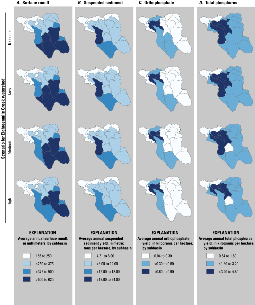
Maps showing average annual A, Surface runoff; B, Suspended sediment yield; C, Orthophosphate yield; and D, Total phosphorus yield, by scenario and subbasin, Eighteenmile Creek watershed, New York. See figure 3 for subbasin identifiers.
Results by Best Management Practice
The agricultural BMPs were examined for suspended sediment and nutrient reductions by rotation (fig. 37). Overall, FS were the best performing BMP for all agricultural rotations simulated. Generally, two or more BMPs had greater reductions than single BMPs.
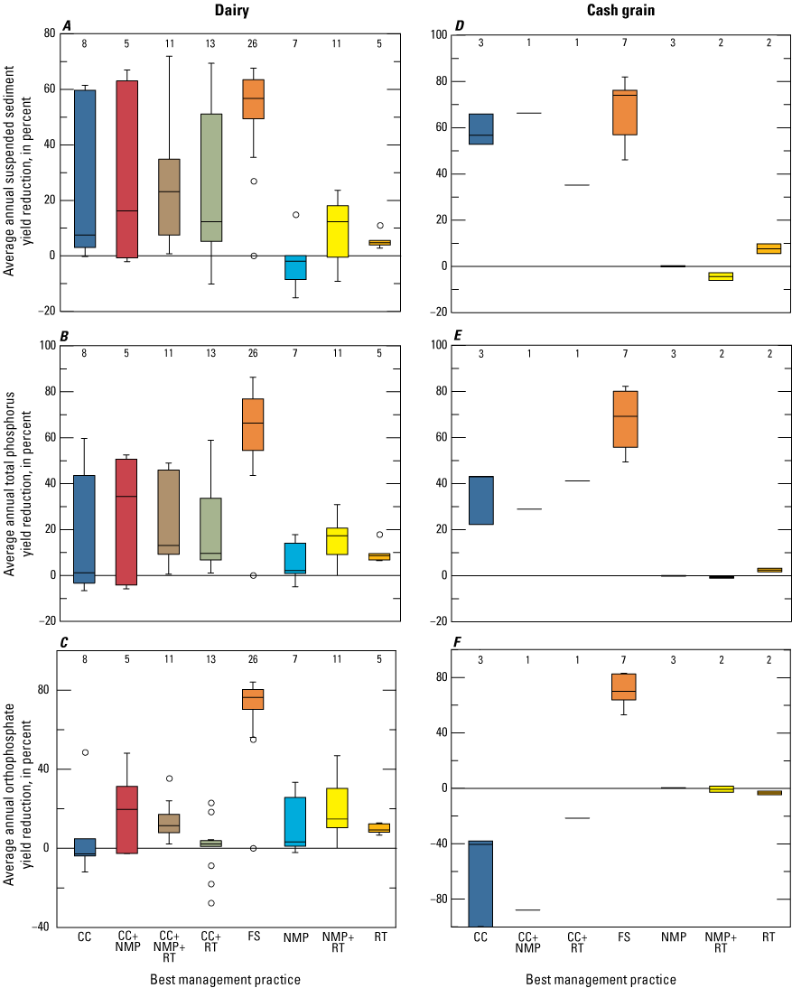
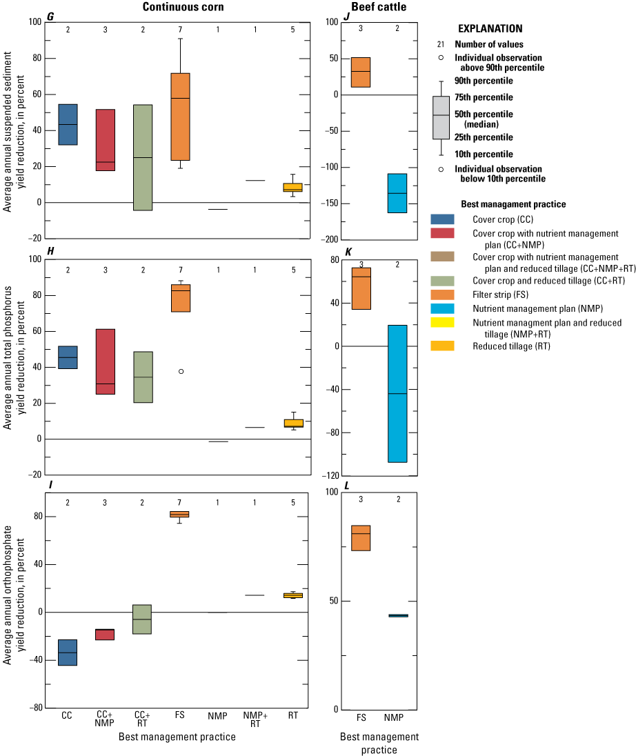
Boxplots of simulated reduction of average annual suspended sediment and nutrient yields, in percent, in surface runoff from A–C, Dairy rotations; D–F, Cash grain rotations; G–I, Continuous corn rotations; and J–L, Beef cattle rotations, because of selected best management practices in the Eighteenmile Creek watershed model, New York. Negative values indicate an increase in yield.
Eighty-five percent of the agricultural land in the Eighteenmile Creek watershed model was simulated with a dairy rotation (table 18). As such, there were more dairy BMPs with a wider range of reductions compared to the other rotations with BMPs (figs. 37A-L). On the dairy rotation, NMP was the only BMP that had a negative average annual suspended sediment reduction (an increase; table 19; fig. 37A). FS were the best performing BMP; average annual yield reductions were 52.00 percent for suspended sediment, 69.62 percent for orthophosphate, and 62.21 percent for total phosphorus (table 19). CC+NMP was the best performing combined BMP for reducing average annual suspended sediment, orthophosphate, and total phosphorus yields from the dairy rotation (table 19). For the single infield BMPs, CC had the greatest reductions for average annual suspended sediment and total phosphorus yields; NMP had the greatest reduction for average annual orthophosphate yields (table 19). On the dairy rotation, the BMP combination CC+NMP+RT had a lower average annual suspended sediment yield reduction than CC+NMP, CC+RT, and NMP+RT, a lower average annual orthophosphate yield reduction than CC+RT and NMP+RT, and lower average annual total phosphorus yield reduction than CC+NMP (table 19).
Figures 37D, E, and F show the boxplots for the cash grain rotation in the Eighteenmile Creek watershed model. FS were the best performing BMP for reducing average annual suspended sediment, orthophosphate, and total phosphorus yields from cash grain rotations (table 19; figs. 37D, E, F), and CC+NMP had the second highest average annual suspended sediment yield reduction (table 19; fig. 37D). FS and NMP were the only BMPs with positive average annual orthophosphate yield reductions on the cash grain rotation (table 19; fig. 37F). NMP+RT caused a negative average annual total phosphorus yield reduction (an increase); all other BMPs and BMP combinations reduced average annual total phosphorus yields on the cash grain rotation (table 19; fig 37E).
Approximately 6 percent of the agricultural area of the Eighteenmile Creek watershed was simulated with a continuous corn rotation (table 18). FS were by far the most effective BMP on the continuous corn rotation, with the greatest reductions of average annual suspended sediment, orthophosphate, and total phosphorus yields (table 19; figs. 37G, H, I). NMP simulated with continuous corn rotations caused negative reductions (increases) of average annual suspended sediment and total phosphorus yields and no change of orthophosphate yields (table 19; figs. 37G, H, I). CC or any BMP combined with CC simulated on continuous corn rotations caused negative average annual orthophosphate yield reductions (increases) and reduced suspended sediment and total phosphorus yields (table 19; figs. 37G, H, I).
Only FS and NMP were evaluated on beef cattle rotations in the Eighteenmile Creek watershed model (table 18). NMP caused negative average annual suspended sediment and total phosphorus yield reductions (increases) from beef cattle rotations (table 19; figs. 37J, K). FS caused a 31.64 percent reduction of average annual suspended sediment yield, a 79.70 percent reduction of average annual orthophosphate yield, and a 57.11 percent reduction of average annual total phosphorus yield from beef cattle rotations.
Walnut Creek Watershed
The baseline simulated average annual loads from the Walnut Creek watershed model were 18,225 metric tons of suspended sediment, 107,300 kg of total nitrogen, 5,624 kg of orthophosphate, and 19,070 kg of total phosphorus (fig. 25).
There is a single point source in the Walnut Creek watershed model at its outlet to Lake Erie, identifier NY0022411 (table 3). NY0022411 is downstream from the Silver Creek and Walnut Creek confluence. It delivered about 1.8 percent of the nitrogen and 9.5 percent of the annual phosphorus loads in the watershed model (Fisher and Merriman, 2024). It contributed more total phosphorus from any other source except for the pasture rotation (fig. 27K).
Forest was the largest rotation in this watershed model and exported the most total phosphorus and total nitrogen (figs. 27K, L). Phosphorus yields in any form from forests were some of the lowest total phosphorus yields from any rotation in this watershed model (table 18). Pasture was the second most predominant rotation in the Walnut Creek watershed (table 18), and most phosphorus and nitrogen exported from the corresponding pasture agricultural rotation were primarily in the organic form (table 18). The beef cattle rotation had the highest total phosphorus and total nitrogen yields out of all agricultural rotations in the Walnut Creek watershed (table 18), but beef cattle rotations exported relatively small loads (figs. 27K, L) because of their relatively small total area.
Results by Low, Medium, and High Best Management Practice Scenarios
Results of the BMP scenarios in the Walnut Creek watershed model scenarios are shown in figure 26. There was no change in suspended sediment loads from the baseline to the low scenario, but the medium and high scenarios decreased simulated average annual suspended sediment loads by 0.19 and 0.36 percent (fig. 26A). The low, medium, and high scenarios decreased simulated average annual orthophosphate loads by 0.2, 0.44, and 0.84 percent from the baseline, respectively, and decreased simulated average annual total nitrogen loads by 0.51, 1.54, and 3.20, respectively (figs. 26C, B). The low, medium, and high scenarios decreased average annual total phosphorus loads by 0.50, 1.18, and 2.65 percent from the baseline scenario, respectively (fig. 26E).
In general, decreases for each constituent are noted particularly in subbasins in the southern part of the watershed model (fig. 38). The highest surface runoff in the Walnut Creek watershed model occurred in subbasins 12 and 15 (fig. 3H) in the central part of the watershed model (fig. 38). The majority of slopes of subbasins 12 and 13 are between 2 and 10 percent and have poorly drained soils to very poorly drained soils (NRCS, 2019). The highest suspended sediment yields were from subbasin 22 (figs. 3H, 38B). The majority of slopes in subbasin 22 are between 5 and 20 percent, have poorly drained soils, and have no tile drainage. Subbasin 2 (fig. 3H) has the highest average annual orthophosphate yield in the watershed model (fig. 38C), nearly double the next highest subbasin orthophosphate yields. The land cover in subbasin 2 is exclusively developed (fig. 3H), which may contribute to the high yield of orthophosphate in this subbasin. The highest average annual total phosphorus yield was from subbasin 22, in the southwest part of the watershed model (fig. 3H); these subbasins also had high average annual total phosphorus yields (fig. 38D). The areas where the high total phosphorus yields were found to correspond to subbasins that also had high surface runoff and suspended sediment yield; that may indicate the total phosphorus yields in the central part of the watershed model was also from surface runoff (figs. 38A, B, D).
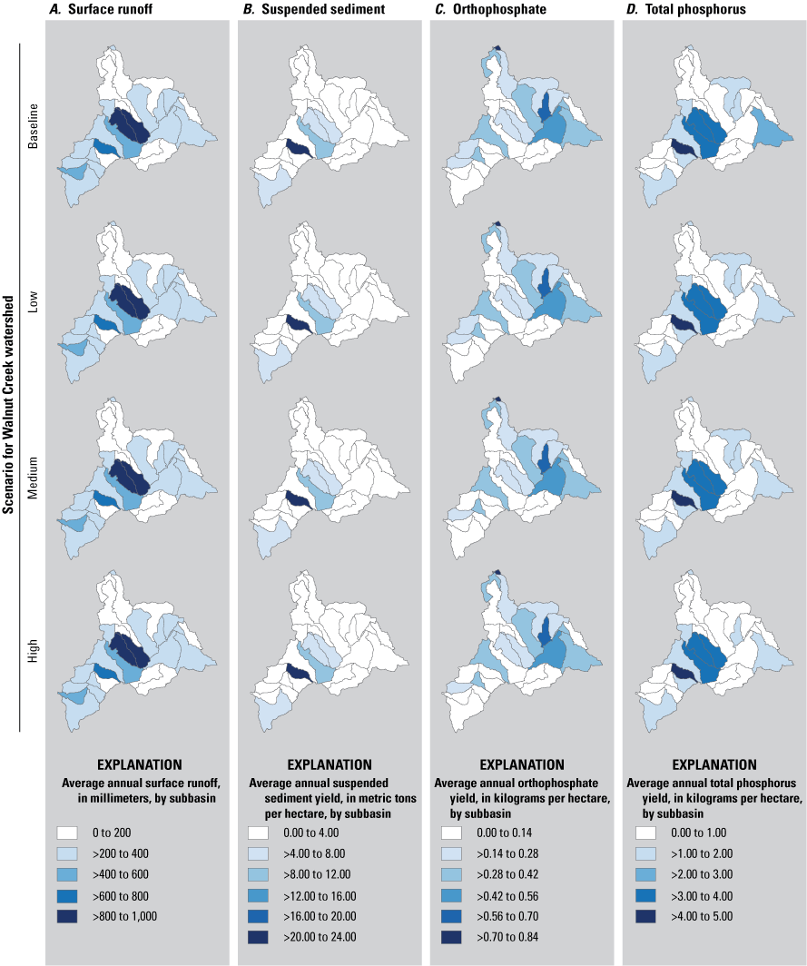
Maps showing average annual A, Surface runoff; B, Suspended sediment yield; C, Orthophosphate yield; and D, Total phosphorus yield, by scenario and subbasin, Walnut Creek watershed, New York. See figure 3 for subbasin identifiers.
Results by Best Management Practice
BMPs and BMP combinations were evaluated for effectiveness in reducing suspended sediment and nutrients in the Walnut Creek watershed model (table 19; fig. 39). FS were the most effective at reducing average annual suspended sediment and nutrient yields from all rotations where it was simulated (table 19; fig. 39). CC+NMP+RT was the next most effective BMP combination for average annual suspended sediment and total phosphorus yield reductions in the Walnut Creek watershed model (table 19), but this combination caused a negative orthophosphate yield reduction in the dairy rotation (an increase; table 19; fig. 39C), and the orthophosphate reductions from the cash grain rotation were small, less than a tenth of the total phosphorus yield reduction (table 19; figs. 39E, F). NMP caused negative average annual suspended sediment and total phosphorus yield reductions (increases) in both cash grain and dairy rotations (table 19; figs. 39D, E, A, B). In cash grain rotations, average annual suspended sediment, orthophosphate, and total phosphorus yield reductions because of NMP+RT and RT were almost identical (table 19; figs. 39D, E, F); there was one BMP simulated on one HRU each. Generally, two BMPs combined performed better than a single BMP, but not all yield reductions were improved when BMPs were combined. For example, CC+RT on dairy rotations had better average annual suspended sediment and total phosphorus yield reductions (25.48 and 17.76 percent, respectively) when compared to RT (8.47 and 5.78 percent, respectively), but suspended sediment reductions from CC+RT and CC (25.48 and 25.61 percent, respectively) on the dairy rotation were almost identical. Average annual total phosphorus reductions caused by CC on the dairy rotation were 21.54 percent, more than the total phosphorus reduction from CC+RT (table 19; figs. 39A, B, C).
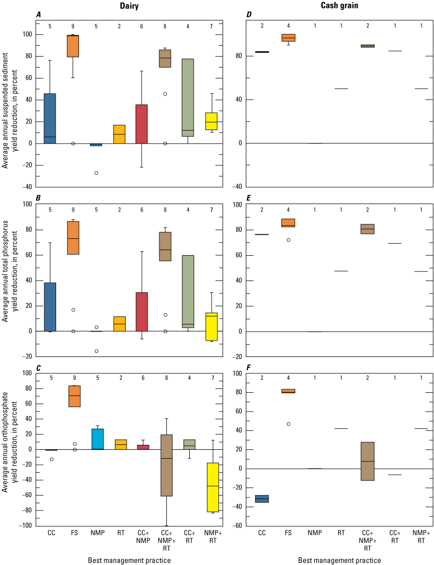
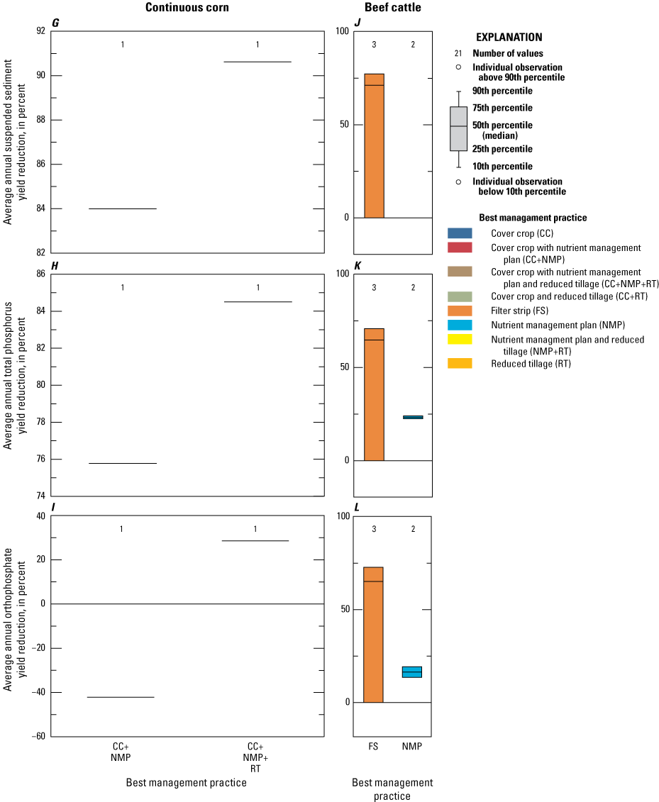
Boxplots of simulated reduction of average annual suspended sediment and nutrient yields, in percent, in surface runoff from A–C, Dairy rotations; D–F, Cash grain rotations; G–I, Continuous corn rotations; and J–L, Beef cattle rotations, because of selected best management practices in the Walnut Creek watershed model, New York. Negative values indicate an increase in yield.
Tonawanda Creek Watershed
For the Tonawanda Creek watershed model, the simulated baseline average annual loads were 32,835 metric tons of suspended sediment, 1,297,000 kg of total nitrogen, 50,625 kg of orthophosphate, and 128,600 kg of total phosphorus (fig. 25). Total phosphorus loads for the Tonawanda Creek watershed model were very similar to those from the Canadaway Creek watershed model, even though the Tonawanda Creek watershed model area is 16 times larger than the Canadaway Creek model area.
The Tonawanda Creek watershed model showed a large amount of erosion in the area of the headwaters (fig. 40). Suspended sediment load estimates in the Tonawanda Creek headwaters at USGS streamgage 04216418 at Attica were greater than the subbasin outlet suspended sediment load estimates and comparable with the suspended sediment load at the downstream streamgage 04218000 at Rapids. This indicates that the model simulated suspended sediment deposition along the stream reaches between the two gages.
Simulated nutrient loads in the Tonawanda Creek watershed baseline scenario increased downstream. The most upstream streamgage on Tonawanda Creek, 04216418 (site 20 on fig. 1) was simulated with 19.5 percent of the model output total nitrogen load and 32 percent of the model output total phosphorus load (Fisher and Merriman, 2024). Downstream from 04216418, streamgage 04217000 at Batavia was simulated with 35.6 percent of the model output total nitrogen load and 56 percent of the model output total phosphorus load. The downstream-most streamgage on Tonawanda Creek, 04218000 at Rapids, was simulated with approximately 67 percent of the model output total nitrogen load and 69 percent of the model output total phosphorus load. Simulation data from streamgage 04218518 showed that Ellicott Creek contributed 0 percent of the total nitrogen load, and 6 percent of the total phosphorus load.
Point-source effluent made up 1.3–10.9 percent of the monthly average flow in the Tonawanda Creek watershed model (this statement is comparing point source data from EPA [undated] to the simulated model output [Fisher and Merriman, 2024]). More effluent discharge from point sources enters streams in the late summer months than the rest of the year. Additionally, Tonawanda Creek loses a large part of flow May through October to the Erie Canal at Lockport lock (see “Channel and Canal Parameterization” section; fig. 2I). The point sources were the largest studied contributors of average annual total phosphorus load in the Tonawanda Creek watershed model (fig. 27M); point sources contributed about a third of the average annual total phosphorus and total nitrogen loads. Three of the point sources are upstream from USGS streamgage 04217000 on Tonawanda Creek at Batavia: identifiers NY0003077, NY0243752, and NY0025950 (table 3). Point source NY0025950 was the largest source of nutrients in the Tonawanda Creek watershed model. These three point sources contributed 2.8 percent and 1.2 percent of the watershed model’s total nitrogen and total phosphorus loads, respectively. Five point sources are between USGS streamgages 04218000 on Tonawanda Creek at Rapids and 04217000 on Tonawanda Creek at Batavia (fig. 2I). Three of these five point sources are municipal wastewater treatment facilities and the other two are industrial discharges (table 3). These five point sources accounted for 18.1 percent and 4.2 percent of the total nitrogen and total phosphorus loads in the Tonawanda Creek watershed model, respectively. Two of the five point sources between streamgages 0421800 and 04217000 discharged flow and nutrient loads to Ellicott Creek: NPDES identifiers NY0228346 and NY0020541. Point sources NY0228346 and NY0020541 contributed a minor amount (approximately 2 percent) to the average annual total nitrogen load entering Ellicott Creek but roughly a quarter of the total phosphorus loads entering Ellicott Creek.
Nutrient loads from the Tonawanda Creek watershed model were predominantly from dairies, point sources, and CAFOs (figs. 27M, N). Point sources and the dairy rotation each exported about thirty percent (42,586 kg and 42,301 kg, respectively) of the watershed model’s average annual total phosphorus load (Fisher and Merriman, 2024). The dairy rotation made the greatest contribution to average annual suspended sediment and total nitrogen loads (approximately 57 percent and 25 percent). On an average annual basis, CAFOs exported 23,283 kg of total phosphorus (fig. 27M), the third highest load out of all rotations, and 116,031 tons of suspended sediment, the second highest load. Urban and forest rotations both exported about 8,000 kg of total phosphorus on an average annual basis; these were the fourth and fifth highest total phosphorus loads from the watershed model (fig. 27M). Urban, wetlands, and forest rotations each exported an average of over 100,000 kg total nitrogen per year (fig. 27N). While suspended sediment and nutrient yields from the forest rotations are generally low (table 18), forest areas covered the largest area in the Tonawanda Creek watershed model out of any other rotation and therefore has the fourth largest total phosphorus and fifth largest total nitrogen loads (figs. 27M, N). The forest rotation did not produce high total phosphorus and total nitrogen loads because of the relatively low nutrient yields and because Tonawanda Creek watershed has the least forested area of all the watersheds modeled (table 2).
Yields by rotation are shown in table 18. Total phosphorus yields in the Tonawanda Creek watershed model were mostly in the sediment bound form. Total phosphorus yields were the highest from beef cattle and horse rotations. Beef cattle and horse rotations both cover a small percentage of the Tonawanda Creek watershed land area (each are approximately 0.4 percent of the total watershed model area) and contributed a relatively small amount of the average annual suspended sediment and total phosphorus loads (fig. 27M). Beef cattle and horse rotations contributed 3.4 percent and 1.4 percent of the total phosphorus loads, respectively. About 19 percent of the total phosphorus yield was orthophosphate from surface runoff, 6 percent was organic phosphorus from surface runoff, and <1 percent was orthophosphate from tile drainage (table 18).
The majority of total nitrogen yields from the Tonawanda Creek watershed model were in the organic form (table 18). Beef cattle and horse rotations had the second and fourth highest total nitrogen yields (table 18), but these contributed a relatively small amount of the total nitrogen load from the watershed model (fig. 27N). Eight percent of the total nitrogen load was exported from wetlands (fig. 27N). Most (92 percent) of this nitrogen was in the organic form (table 18). Nitrate as nitrogen from lateral flow and groundwater contributed about 5 and 2 percent of the total nitrogen load, respectively (Fisher and Merriman, 2024). Nitrate as nitrogen in surface runoff and in tile drainage contributed about 17 percent and 14 percent, respectively, of the total nitrogen load.
Results by Low, Medium, and High Best Management Practice Scenarios
Figure 26 shows the results of the BMP scenarios in the Tonawanda Creek watershed model. In comparison to the baseline Tonawanda Creek watershed scenario, average annual suspended sediment loads were reduced by 0.65, 1.54, and 2.85 percent in the low, medium, and high scenarios, respectively; total nitrogen loads were reduced by 0.96, 2.35, and 4.20 percent in the low, medium, and high scenarios, respectively; and total phosphorus loads were reduced by 1.44, 3.27, to 8.55 percent in the low, medium, and high scenarios, respectively.
In general, BMP implementation caused decreases for each constituent, particularly in subbasins in the eastern and southeastern parts of the Tonawanda Creek watershed model. The highest surface runoff was in the western, eastern, and southeastern parts of the watershed model (fig. 40A). Subbasins in the eastern and southeastern parts of the watershed have steep slopes and poorly to very poorly drained soils. The western part of the watershed model generally has shallower slopes in comparison to the eastern and southeastern parts of the watershed, and the subbasins with high surface runoff were in areas with heavy urban or agricultural land cover. Subbasin 85 (fig. 3I) had the highest suspended sediment yield (fig. 40B); this subbasin has higher elevations in comparison to the other subbasins in the Tonawanda Creek model. Over 72 percent of the Tonawanda Creek watershed model is agricultural land with variable slopes, mostly between 2 and 20 percent, which together may have exacerbated suspended sediment yield in subbasin 85. Orthophosphate and total phosphorus yields were highest in the southeastern part of the Tonawanda Creek watershed model (figs. 40C, D); the highest yield of orthophosphate came from subbasin 82 (figs. 3I, 40C) and the highest yield of total phosphorus comes from subbasin 85 (figs. 3I, 40C). Subbasin 82 had a large CAFO near the subbasin outlet with over 5,500 animals (fig. 2I). The highest concentration of CAFOs in the watershed model lie in the east and southeast, with nine CAFOs totaling over 15,000 animals (fig. 2I). This part of the watershed model also contains the highest percentage of agricultural land (fig. 3I), which, in combination with CAFOs, likely contributed substantial nutrients to the simulated watershed results.
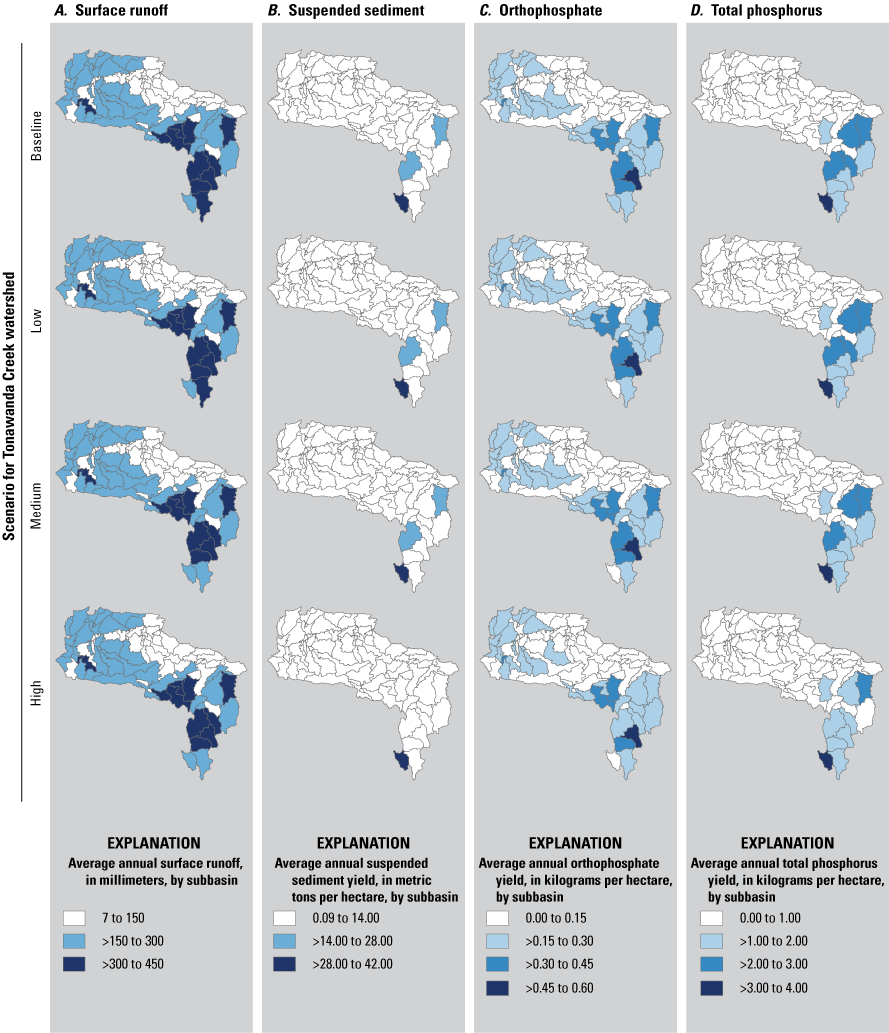
Maps showing average annual A, Surface runoff; B, Suspended sediment yield; C, Orthophosphate yield; and D, Total phosphorus yield, by scenario and subbasin, Tonawanda Creek watershed, New York. See figure 3 for subbasin identifiers.
Results by Best Management Practice
BMPs and BMP combinations tested on dairy, cash grain, continuous corn, and beef cattle rotations were evaluated for effectiveness in reducing suspended sediment and nutrient yields in the Tonawanda Creek watershed model (table 19; fig. 41). Overall, FS were the most effective BMP for reducing average annual suspended sediment and total phosphorus yields on the agricultural rotations tested (table 19; figs. 41A–F, J–L). NMP caused increases (negative reductions) of average annual yields, including sediment and total phosphorus yields from dairy and cash grain rotations, orthophosphate yields from cash grain and continuous corn rotations, and suspended sediment yields from beef cattle rotations (table 19; figs. 41A, B, D, E, F, I, J).
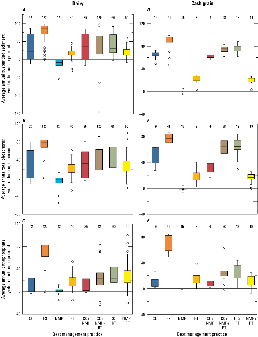
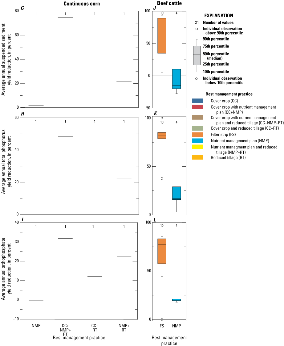
Boxplots of simulated reduction of average annual suspended sediment and nutrient yields, in percent, in surface runoff from A–C, Dairy rotations; D–F, Cash grain rotations; G–I, Continuous corn rotations; and J–L, Beef cattle rotations, because of selected best management practices in Tonawanda Creek watershed model, New York. Negative values indicate an increase in yield.
Over 14 percent of the Tonawanda Creek watershed model area was in a dairy rotation (table 18). Figures 41A, B, and C and table 19 show the reductions in average annual constituent yields from BMP implementation on dairy rotations. FS caused the greatest reductions of average annual suspended sediment, orthophosphate, and total phosphorus yields from dairy rotations, like in the other watershed models. CC+RT caused the second greatest reductions of average annual suspended sediment, orthophosphate, and total phosphorus yields (table 19). On dairy rotations, CC+RT caused greater average annual yield reductions of all constituents than CC+NMP+RT, except for total nitrogen. BMPs caused positive constituent reductions on dairy rotations, except for average annual suspended sediment and total phosphorus yields when NMP was applied, and except for total nitrogen when NMP+RT was applied. CC combinations with NMP or RT caused greater average annual constituent yield reductions, except for total nitrogen, from dairy rotations than CC alone; CC+NMP caused average annual reductions of suspended sediment, orthophosphate, and total phosphorus yields of 36.59, 13.37, and 32.96 percent, respectively; CC+RT caused reductions of average annual suspended sediment, orthophosphate, and total phosphorus yields of 41.62, 30.97, and 44.06 percent, respectively. Average annual suspended sediment, orthophosphate, and total phosphorus yield reductions were lower because of NMP or RT than because of CC.
Figures 41D, E, and F show average annual constituent yield reductions because of BMPs applied on cash grain rotations. Of the infield BMPs (excluding FS), CC+RT caused the greatest reductions in average annual suspended sediment and total phosphorus (table 19). CC+NMP+RT caused similar but slightly lower average annual suspended sediment and total phosphorus and slightly higher orthophosphate yield reductions. CC+RT and CC+NMP on cash grain rotations caused greater yield reductions than NMP alone; CC+RT yield reductions were generally greater than CC, but yield reductions from CC were generally greater than CC+NMP. Yield reductions from cash grain rotations because of NMP+RT were similar to the yield reductions because of RT but were much higher than the yield reductions because of NMP.
Only a single continuous corn HRU each was simulated with the BMP combinations NMP, NMP+RT, CC+RT, and CC+NMP+RT (table 19; figs. 41G, H, I). Average annual suspended sediment yield reductions because of the BMPs in the continuous corn rotation ranged from 2.01 to 75.11 percent; average annual orthophosphate yield reductions ranged from −0.44 to 31.80 percent; and average annual total phosphorus yield reductions ranged from 0.81 to 51.76 percent (table 19). All the lowest reductions (including negative reductions; increases) were because of NMP, except the reduction of total nitrogen where NMP+RT caused the lowest reduction (table 19). CC+NMP+RT caused the highest reductions of average annual suspended sediment and orthophosphate yields from the continuous corn rotation, but CC+RT caused the highest average annual total phosphorus yield reductions (table 19). FS were not simulated on continuous corn rotations in the Tonawanda Creek watershed.
NMP and FS were evaluated on beef cattle rotations (table 19; figs. 41J, K, L). NMP caused average annual reductions in annual orthophosphate and total phosphorus yields (19.82 and 16.56 percent, respectively) and an increase in average annual suspended sediment yields (−11.03 percent; an increase). FS caused high reductions (>60 percent) of average annual suspended sediment, nitrate as nitrogen, orthophosphate, and total phosphorus yields.
Point Source Scenarios
Point-source reduction data are presented in table 20. The point source scenarios for Tonawanda Creek watershed model did not reduce suspended sediment or nitrogen loads, but the average annual total phosphorus load was reduced by 3.15 and 5.60 percent in the two scenarios, respectively (see section “Effect of Point Source Phosphorus Inputs on Water Quality”; table 20).
In Tonawanda Creek watershed point source scenario 1, the total phosphorus was limited to 0.5 mg/L for three discharges: NY0025950 (in subbasin 40), NY0026514 (in subbasin 50), and NY0021849 (in subbasin 75; table 3; fig. 3I). With point source scenario 1, monthly effluent phosphorus loads from the point sources were reduced by 2 to 58 percent in subbasin 40, by 7 to 90 percent in subbasin 50, and by 2 to 52 percent in subbasin 75 in comparison to reported phosphorus effluent loads (EPA, undated). The 90 percent reduction in subbasin 50 corresponded to an event in March 2018 when facility NY0026514 had a Non-Reportable Noncompliance Effluent Violation (EPA, undated), where total phosphorus in the effluent was measured as 400 percent over the facility’s normal total phosphorus concentration. Regional NYSDEC staff considered this extreme value to be a laboratory error; all other phosphorus measurements during March 2018 were below the permit limit.
The Tonawanda scenario 2 included the settings of scenario 1 and changed the total phosphorus limit to 1 mg/L on three additional discharges: NY0031003 (in subbasin 45), NY0108430 (in subbasin 59), and NY0020541 (in subbasin 72; table 3; fig. 3I). None of the managing facilities had monitoring data available for their total phosphorus loads (table 3), and their baseline effluent phosphorus concentration was assumed to be 3 mg/L. Thus, reducing the total phosphorus effluent limit to 1.0 mg/L reduced the effluent total phosphorus load from the point sources by 67 percent.
On an average annual basis, Tonawanda point-source scenario 1 reduced exported orthophosphate and total phosphorus loads by 5.95 and 3.15 percent, respectively, from the baseline, whereas the Tonawanda point-source scenario 2 reduced orthophosphate and total phosphorus loads by 10.58 and 5.60 percent, respectively (table 20). Total phosphorus reductions in scenario 1 were similar to the reductions in the Tonawanda Creek medium BMP scenario, both about 3 percent. Tonawanda scenario 2 caused a greater total phosphorus reduction than the medium BMP scenario but not greater than the high BMP scenario (table 20; fig. 26E). The largest reductions in the point sources scenarios were from orthophosphate; orthophosphate load reductions in scenario 1 and scenario 2 (5.95 and 10.58 percent, respectively) were larger than the reductions from the three BMP scenarios (table 20; fig. 26C).
Model Limitations
The reliability of model projections and calculations hinges on the ability of the model to achieve calibration targets and to document its representation of watershed dynamics. The models developed for this study were calibrated with the assumption that the calibration data collected for this project are the best possible data available. There is potential error introduced during each step of the modeling process: streamflow measurement, sample collection, constituent analysis, load regression calculations, and model calibration. Potential errors in streamflow measurements, water-quality monitoring, and constituent analysis have not been calculated for this project. The short calibration period hampered model calibration of the smaller subbasins. The calibration period of the Canadaway Creek and Chautauqua Creek watersheds were restricted to a single growing season in summer 2018 and one winter season 2017–18 plus two months of winter at the end of 2018 (site 1 and 2 in table 1). SWAT underestimates streamflow in the winter periods. This corresponds to periods where there are only one or two streamflow measurements from many of the streamgages that were used in calibration of the models. This is the case at USGS streamgage 04213319 on Chautauqua Creek (USGS, 2022), where at the time of the model calibration (2022) there was two January and one February flow measurements collected. Twenty-two water-quality samples were taken at streamgage 04213319; and of those, only two were taken in February. More peak flow measurements and water-quality sampling could improve the load regressions and SWAT model calibration, which could lead to more accurate SWAT simulations of Canadaway Creek and Chautauqua Creek watersheds.
In general, the SWAT model poorly simulates flow during winter conditions (Rahman and others, 2011). In this study, snowfall, snowmelt, and frozen streams and soils were simulated with varying success. A temperature index method is used to trigger snowfall in SWAT, where any input precipitation is considered as snowfall when the input temperature drops below a user-defined threshold (SFTMP; Neitsch and others, 2002). When the average air temperature rises above a user specified temperature threshold (SMTMP), snowpack melt is simulated. Snowpack melt because of solar radiation is not considered. Sometimes the rises in temperature that cause snowmelt are brief and are not reflected in the simulated daily temperature, causing snowmelt to be underestimated. Additionally, lake effect snows, where moisture from cold air passes over the warmer Great Lakes and creates localized heavy snows, are not simulated in SWAT. Lake effect snows can cause very intense snow falls that would strongly affect the water budget in the smaller watersheds but may not be measured by a precipitation station. As a result, SWAT may not accurately simulate the winter precipitation of the study watersheds.
Effects on streamflow from log jams and frozen water are also not considered by SWAT (Lévesque and others, 2010). There was at least one large ice jam in the Walnut Creek watershed during the calibration period (Post-Journal, 2018). Analysis of suspended sediment loads showed a large increase in suspended sediment corresponding to this reported ice jam in January 2018. Another ice jam was observed on Buffalo Creek (fig. 12) during the model validation period. It is unknown how long the ice jams lasted or their exact effect on streamflow or water quality once released.
Additionally, weather datasets are temporal and spatial, but the weather inputs used for SWAT were taken from the weather station closest to the centroid of each subbasin. If any weather data were missing, they were filled in with data from the next closest weather station. The loss of detailed spatial data distribution across the land surface can allow for precipitation events to be missed, overestimated, or underestimated in model calculations, which affects the amount of surface runoff and thus the suspended sediment and nutrient yields and loads computed by the model. SWAT also does not consider the spatial aspect of snowfall or snowmelt over HRUs. Because the actual snowpack is spatially uneven but simulated evenly over the watershed area, simulated snowfall could be especially important in these watersheds where snowmelt has a major influence on the hydrograph.
Furthermore, watershed modeling is a generalized representation of watershed processes. Management schedules and operations were simplified and generalized to model the nine different watersheds encompassing eight different counties. Typically, agricultural management decisions on each field are affected by complex factors influenced by weather, soil and economic conditions, among others (Hutchinson and Christiansen, 2013; Merriman and others, 2018a, b; Merriman and others, 2019). SWAT uses daily time series inputs for weather, but generalized dates were used for planting, tilling, harvest, and other management operations. This means the SWAT simulated operation occurs on the scheduled day even if field conditions may delay real-life operations. Real-world operations could affect the simulation of nutrient runoff event; for example, applying fertilizer prior to a precipitation event is known to increase nutrient runoff (Komiskey and others, 2011). If a precipitation event occurs prior to or on the day of a planned operation, a producer would delay their operations if fields were wet. In SWAT, the operation would occur whether precipitation had occurred or not.
In the SWAT model simulations, baseline conditions assumed that all agricultural HRUs used conventional management, neglecting any BMPs that may have been implemented. A comprehensive BMP database for the study area does not exist. The SWAT loads were calibrated to match the rloadest loads, but certain parameters may be adjusted incorrectly. The models may need adjustment to account for the current level of BMP implementation. Because BMP implementation was unknown and not accounted for, it is possible that loads from HRUs that have BMPs implemented were overestimated.
HRUs are limited to a single crop growing at a time. This may be an issue in vineyards where grape vines are grown on trellises above grass, which act as ground cover. Also, a mix of different grasses are typically implemented as CC. CC were modeled in this study by using the predominant grass in the mix. Many CC are also being interseeded into standing crops, which allows CC to become established earlier and reach maturity more quickly than waiting to plant CC after the main crop is harvested (Merriman and others, 2019). Neglecting these growing grasses would change the simulated evapotranspiration and thus increase simulated runoff. Bieger and others (2017) presented a new version of SWAT, SWAT+, that permits multiple crops on an HRU, thereby incorporating these innovative CC methods that should improve model calibration of evapotranspiration and runoff. Coding operations in SWAT+ may also be used to simulate the delay of field operations if simulated soil moisture is high when actual field operations would also be delayed.
Tile drainage for the watersheds was estimated based on land slope, hydrologic soil group type, and land cover. If tile drainage is underestimated, surface runoff and the suspended sediment and nutrients that are carried in tile drainage will be overestimated on those HRUs where tile drainage occurs. Sediment bound phosphorus from tile drainage is excluded by the version of the SWAT code used in this study (Merriman and others, 2018b). Field monitoring results on dairies in the East River, Wisconsin show that an average of 7 percent of total phosphorus leaves the field through tile drainage annually, with phosphorus partitioned as 60 percent orthophosphate and 40 percent particulate phosphorus (Merriman and others, 2019). Other edge-of-field monitoring in eastern Wisconsin shows that total phosphorus exported through tile drainage ranges from 17 percent to 41 percent of the total phosphorus load (Madison and others, 2014). These New York study watersheds are estimated to have a much lower amount of tile drained areas (0.06 to 10.60 percent) than the Wisconsin watershed studied in Merriman and others (2019); therefore, the contribution of phosphorus from tile drains is expected to have little impact in the New York part of the Eastern Lake Erie Basin.
Water additions and withdrawals were not always accounted for in the input datasets or SWAT simulation. Although there were monthly data available for water use and point-source water withdrawals, these data did not encompass all withdrawals. Many water users or dischargers fall beneath reporting requirements, and as such there are withdrawals that were likely not included in the modeling datasets. In addition, some point source dischargers are only required to report quarterly. It is possible that a large nutrient load in daily effluent is not accounted for in the input datasets. Any irrigation, other than what was stated in the “Irrigation and Water Use” section, was not simulated. As a result, the SWAT simulations of water withdrawals and additions may be erroneous.
Summary
The U.S. Geological Survey, in cooperation with the New York State Department of Environmental Conservation, studied nine select watersheds in New York that are part of the Eastern Lake Erie Basin. The study watersheds were Big Sister Creek, Chautauqua Creek, Canadaway Creek, Crooked Brook, Walnut Creek, Cattaraugus Creek, Eighteenmile Creek, Buffalo River, and Tonawanda Creek. Water-quality samples were collected from November 2017 to November 2019. Suspended sediment and nutrient loads were calculated by rloadest linear regression of the water-quality sampling data and streamflow data from 13 U.S. Geological Survey streamgages. Nine Soil and Water Assessment Tool (SWAT) models of the watersheds were created to understand baseline suspended sediment and nutrients in the study watersheds. Streamflow from these models were calibrated to streamflow data from 15 U.S. Geological Survey streamgages. SWAT simulated suspended sediment and nutrient loads were calibrated to the loads calculated by rloadest. The calibration periods for the models had variable start dates in 2017 and ended on December 31, 2018. The validation period for all models was from January 1, 2019, to December 31, 2019.
Monthly Nash-Sutcliffe efficiency (NSE), coefficient of determination (R2), and percent bias (PBIAS) values were determined for simulated hydrology and suspended sediment and nutrient loads. For the streamflow calibration, NSE statistics are greater than 0.5 for streamgages in all watershed models, except at the Chautauqua Creek watershed model (USGS streamgage 04213319). The SWAT model of the Chautauqua Creek watershed failed streamflow calibration. The streamflow NSE value was less than 0.5, which indicates that an average of the observed streamflow would better represent observed conditions than the model. Because hydrology calibration failed for the Chautauqua Creek watershed model, water-quality calibration was not attempted for this watershed. The SWAT model of the Crooked Brook watershed was not calibrated because of the lack of daily streamflow data. Ten sites each have very good and good PBIAS ratings, 3 sites have satisfactory PBIAS ratings, and 1 site has an unsatisfactory PBIAS rating for hydrology calibration. At 7 of 10 water-quality streamgages, model calculated suspended sediment loads were rated satisfactory or better (NSE greater than 0.5), with the exception of model results at three U.S. Geological Survey streamgages (04214500 in the Buffalo River watershed, 04213376 in the Canadaway Creek watershed, and 04213401 in the Walnut Creek watershed) which did not achieve NSE values greater than 0.5. For suspended sediment loads, six sites have very good PBIAS ratings; three sites have good PBIAS ratings, and one site had an unsatisfactory PBIAS rating. Where total phosphorus loading data was available, 9 of 11 streamgage datasets received NSE values greater than 0.5. Of these, two sites have very good NSE ratings, five sites have good NSE ratings, and two sites have satisfactory NSE rating. Also, for simulated total phosphorus loads, nine sites have very good PBIAS ratings and one good and one satisfactory PBIAS rating. All sites calibrated for total nitrogen (12 streamgage datasets) have NSE values greater than 0.5. For PBIAS ratings of total nitrogen loads, 10 sites have very good, and 2 sites have good ratings. Of the five sites with nitrate plus nitrate rloadest data, all have satisfactory or better PBIAS ratings and two sites have satisfactory or better NSE ratings. For all constituents, absolute values of PBIAS ranges from 0.32 to 208.34 percent. Depending on the watershed and constituent, the PBAIS values indicated that the constituents were both over- and underestimated. The models tended to underestimate flow in the winter months. Validation statistics of NSE, R2, and PBIAS were generally not rated as highly as the statistics in the calibration period. NSE ratings for 37 streamgage datasets were unsatisfactory. Poor validation statistics indicate that a robust calibration dataset is needed that includes flow measurements and water-quality sampling during winter months when flows and loads are highest.
The study watersheds were heavily forested. Forest was the predominant land cover type in all watersheds, comprising 24.25–69.33 percent of the watershed areas. Correspondingly, many of the largest loads in the study watershed models were from forests. Moderate nutrient yields combined with large areas of forest land cover explain the large loads contributed from forested land. Agriculture, especially in the Buffalo River, Cattaraugus Creek, Eighteenmile Creek, and Tonawanda Creek watersheds, had a large effect on simulated total phosphorus and total nitrogen loads.
Septic systems only contributed a small amount of the watershed models’ total nitrogen loads because of the small amount of land simulated; however, septic areas were found to have very large total nitrogen yields in the majority of the models. Beef cattle rotations had large total phosphorus and total nitrogen yields, but the limited area of this rotation resulted in small total phosphorus and total nitrogen loads from this rotation.
Point sources contributed a large amount of flow and nutrients in several watershed models. Point sources contributed approximately 29 percent of the total nitrogen loads and 33 percent of the total phosphorus loads to Tonawanda Creek watershed model. In the Buffalo River watershed model, point sources contributed 0.07 percent of the suspended sediment, 40 percent of the total nitrogen, and 4 percent of the total phosphorus loads in the watershed. A single point source discharge in the Big Sister Creek watershed model delivered 11.5 percent of the streamflow and 19 percent of the total phosphorus load. Point sources had a smaller effect on the overall loads in the Cattaraugus Creek and Walnut Creek watershed models than in the other watershed models.
The seven calibrated SWAT models were also tested with 26 scenarios including point-source discharge limits, green infrastructure, and agricultural best management practices to find the effect of these potential actions on suspended sediment and nutrients. Scenarios intended to reduce phosphorus loads from point sources in the Big Sister Creek, Buffalo River, and Tonawanda Creek watershed models reduced total phosphorus in a range from 0.18 to 5.60 percent. Green infrastructure practices of permeable pavement, rain gardens, and conversion of vacant buildings to grassed lots covered 0.27 percent of the Buffalo River watershed area. Modeling indicated these practices could reduce the loading of 150 metric tons of suspended sediment, 500 kilograms of total nitrogen, and 200 kilograms of total phosphorus to Lake Erie.
Best management practices (BMPs) in low (10 percent of agricultural areas implemented with BMPs), medium (20 percent of agricultural areas implemented with BMPs), and high (30 percent of agricultural areas implemented with BMPs) scenarios were tested on the watershed models and caused large average annual suspended sediment and nutrient reductions at the hydrologic response unit scale. Across the watershed models, filter strips were generally the most effective BMP out of all tested BMPs, including BMP combinations, for reducing suspended sediment, orthophosphate, total phosphorus, nitrate as nitrogen, and total nitrogen. Generally, multiple BMPs performed better at reducing suspended sediment and nutrient yields than a single BMP alone. Some BMPs, especially nutrient management plans, were shown to increase nutrient yields. Because of the low amount of area covered by BMP scenarios, reductions were small at the watershed scale; none of the scenarios resulted in suspended sediment or nutrient load reductions greater than 13 percent. The largest changes in suspended sediment and nutrient loads were found from the high BMP implementations scenario in the Tonawanda Creek watershed model. The BMP scenarios indicate that as more areas incorporate BMPs, the loads simulated from the watershed models decrease. The models and model results are available in Fisher and Merriman (2024).
References Cited
Abbaspour, K.C., Vaghefi, S.A., and Srinivasan, R., 2018, A guideline for successful calibration and uncertainty analysis for soil and water Assessment—A review of papers from the 2016 International SWAT Conference: Water, v. 10, no. 1, 18 p. [Also available at https://doi.org/10.3390/w10010006.]
American Society of Agricultural Engineers, 2005, Manure production and characteristics (revised 2019): American Society of Agricultural Engineers Standard D384.2, 32 p. [Authorship in the 2019 revision is the American Society of Agricultural and Biological Engineers. Also available at https://webstore.ansi.org/standards/asabe/asaed384mar2005r2019.]
Arnold, J.G., and Allen, P.M., 1999, Automated methods for estimating baseflow and ground water recharge from streamflow records: Journal of the American Water Resources Association, v. 35, no. 2, p. 411–424. [Also available at https://doi.org/10.1111/j.1752-1688.1999.tb03599.x.]
Arnold, J.G., Srinivasan, R., Muttiah, R.S., and Williams, J.R., 1998, Large area hydrologic modeling and assessment part I—Model development: Journal of the American Water Resources Association, v. 34, no. 1, p. 73–89. [Also available at https://doi.org/10.1111/j.1752-1688.1998.tb05961.x.]
Bieger, K., Arnold, J.G., Rathjens, H., White, M.J., Bosch, D.D., Allen, P.M., Volk, M., and Srinivasan, R., 2017, Introduction to SWAT+, a completely restructured version of the Soil and Water Assessment Tool: Journal of the American Water Resources Association, v. 53, no. 1, p. 115–130. [Also available at https://doi.org/10.1111/1752-1688.12482.]
Boles, C.M.W., Frankenberger, J.R., and Moriasi, D.N., 2015, Tile drainage simulation in SWAT2012—Parameterization and evaluation in an Indiana watershed: Transactions of the ASABE, v. 58, no. 5, p. 1201–1213. [Also available at https://doi.org/10.13031/trans.58.10589.]
Bosch, N.S., Allan, J.D., Selegean, J.P., and Scavia, D., 2013, Scenario-testing of agricultural best management practices in Lake Erie watersheds: Journal of Great Lakes Research, v. 39, no. 3, p. 429–436. [Also available at https://doi.org/10.1016/j.jglr.2013.06.004.]
Bradu, D., and Mundlak, Y., 1970, Estimation in lognormal linear models: Journal of the American Statistical Association, v. 65, no. 329, p. 198–211. [Also available at https://doi.org/10.1080/01621459.1970.10481074.]
Buffalo Niagara Riverkeeper, 2014, Chapter 2—Watershed characterization, of Healthy Niagara—Niagara River watershed management plan (phase 1): New York State Department of State report, prepared by Buffalo Niagara Riverkeeper, 35 p., accessed October 8, 2021, at https://bnwaterkeeper.org/wp-content/uploads/2015/03/Chapter-2-Characterization-FINAL.pdf.
Bunch, A.R., 2024, Data and rloadest models used to estimate sediment and nutrient loads in selected New York tributaries to eastern Lake Erie: U.S. Geological Survey data release, https://doi.org/10.5066/P9N6IQZT.
Chiang, L., Chaubey, I., Gitau, M.W., and Arnold, J.G., 2010, Differentiating impacts of land use changes from pasture management in a CEAP watershed using the SWAT model: Transactions of the ASABE, v. 53, no. 5, p. 1569–1584. [Also available at https://doi.org/10.13031/2013.34901.]
Cohn, T.A., 1988, Adjusted maximum likelihood estimation of the moments of lognormal populations from type 1 censored samples: U.S. Geological Survey Open-File Report 88–350, 34 p. [Also available at https://doi.org/10.3133/ofr88350.]
Cohn, T.A., 2005, Estimating contaminant loads in rivers—An application of adjusted maximum likelihood to type 1 censored data: Water Resources Research, v. 41, no. 7, article W07003, 13 p. [Also available at https://doi.org/10.1029/2004WR003833.]
Davis, B.E., and Federal Interagency Sedimentation Project, 2005, A guide to the proper selection and use of Federally approved sediment and water-quality samplers: U.S. Geological Survey Open-File Report 2005-1087, 20 p., accessed June 10, 2024, at https://doi.org/10.3133/ofr20051087.
Daggupati, P., Pai, N., Ale, S., Douglas-Mankin, K.R., Zeckoski, R.W., Jeong, J., Parajuli, P.B., Saraswat, D., and Youssef, M.A., 2015, A recommended calibration and validation strategy for hydrologic and water quality models: Transactions of the ASABE, v. 58, no. 6, p. 1705–1719. [Also available at https://doi.org/10.13031/trans.58.10712.]
Douglas-Mankin, K.R., Srinivasan, R., and Arnold, J.G., 2010, Soil and Water Assessment Tool (SWAT) model—Current developments and applications: Transactions of the ASABE, v. 53, no. 5, p. 1423–1431. [Also available at https://doi.org/10.13031/2013.34915.]
Duncan, E.W., King, K.W., Williams, M.R., LaBarge, G., Pease, L.A., Smith, D. R., and Fausey, N.R., 2017, Linking soil phosphorus to dissolved phosphorus losses in the Midwest: Agricultural & Environmental Letters, v. 2, no. 1, 5 p. [Also available at https://doi.org/10.2134/ael2017.02.0004.]
Eawag, 2013, SWAT-CUP 2012 (version 5.1.6): Eawag software release, accessed March 6, 2018, at https://www.NeprashTechnology.ca.
Fisher, B.N., and Merriman, K.R., 2024, SWAT model archive for simulation of hydrology, suspended sediment and nutrients in selected tributary watersheds of Lake Erie, New York: U.S. Geological Survey data release, https://doi.org/10.5066/P9U2IF5I.
Gassman, P.W., Reyes, M.R., Green, C.H., and Arnold, J.G., 2007, The soil and water assessment tool—Historical development, applications, and future research directions: Transactions of the ASABE, v. 50, no. 4, p. 1211–1250. [Also available at https://doi.org/10.13031/2013.23637.]
Gupta, H.V., Sorooshian, S., and Yapo, P.O., 1999, Status of automatic calibration for hydrologic models—Comparison with multilevel expert calibration: Journal of Hydrologic Engineering, v. 4, no. 2, p. 135–143. [Also available at https://doi.org/10.1061/(ASCE)1084-0699(1999)4:2(135).]
Helsel, D.R., and Hirsch, R.M., 2002, Statistical methods in water resources—Hydrologic analysis and interpretation: U.S. Geological Survey Techniques of Water-Resources Investigations, book 4, chap. A3, 510 p. [Also available at https://doi.org/10.3133/twri04A3. Superseded in 2020 by U.S. Geological Survey Techniques and Methods, book 4, chap. A3, available at https://doi.org/10.3133/tm4A3.]
Hutchinson, K.J., and Christiansen, D.E., 2013, Use of the Soil and Water Assessment Tool (SWAT) for simulating hydrology and water quality in the Cedar River Basin, Iowa, 2000–10: U.S. Geological Survey Scientific Investigations Report 2013–5002, 36 p. [Also available at https://doi.org/10.3133/sir20135002.]
Iowa Environmental Mesonet, 2019, ASOS/AWOS global METAR data download: Iowa State University Iowa Environmental Mesonet database, accessed July 8, 2019, at https://mesonet.agron.iastate.edu/request/download.phtml?network=NY_ASOS.
Koltun, G.F., 2021, Estimated total phosphorus loads for selected sites on Great Lakes tributaries, water years 2014–2018: U.S. Geological Survey Open-File Report 2020–1145, 13 p., accessed September 12, 2022, at https://doi.org/10.3133/ofr20201145.
Komiskey, M.J., Stuntebeck, T.D., Frame, D.R., and Madison, F.W., 2011, Nutrients and sediment in frozen-ground runoff from no-till fields receiving liquid-dairy and solid-beef manures: Journal of Soil and Water Conservation, v. 66, no. 5, p. 303–312. [Also available https://doi.org/10.2489/jswc.66.5.303.]
La Sala, A.M., Jr., 1968, Ground-water resources of the Erie-Niagara Basin, New York: New York State Water Resources Commission Basin Planning Report ENB-3, prepared by the U.S. Geological Survey, 114 p., 5 pl. [Also available at https://archive.org/details/usgswaterresourcesnewyork-enb_3/enb_3/.]
Lévesque, É., Anctil, F., Griensven, A., van, and Beauchamp, N., 2010, Evaluation of streamflow simulation by SWAT model for two small watersheds under snowmelt and rainfall: Hydrological Sciences Journal, v. 53, no. 5, p. 961–976. [Also available at https://doi.org/10.1623/hysj.53.5.961.]
Lorenz, D.L., Runkel, R.L., and De Cicco, L., 2013, rloadest—USGS water science R functions for LOAD ESTimation of constituents in rivers and streams: U.S. Geological Survey software release, accessed September 12, 2018, at https://github.com/USGS-R/rloadest.
Lumia, R., and Johnston, W.H., 1984, Floods of August 7–8, 1979, in Chautauqua County, New York, with Hydraulic Analysis of Canadaway Creek in the Village of Fredonia: U.S. Geological Survey Water-Resources Investigations Report 83–4211, 16 p. [Also available at https://doi.org/10.3133/wri834211.]
Madison, A.M., Ruark, M.D., Stuntebeck, T.D., Komiskey, M.J., Good, L.W., Drummy, N., and Cooley, E.T., 2014, Characterizing phosphorus dynamics in tile-drained agricultural fields of eastern Wisconsin: Journal of Hydrology, v. 519, part A, p. 892–901. [Also available at https://doi.org/10.1016/j.jhydrol.2014.08.016.]
Mankin, K.R., DeAusen, R.D., and Barnes, P.L., 2002, Assessment of a GIS‐AGNPS interface model: Transactions of the ASAE, v. 45, no. 5, p. 1375–1383. [Also available at https://doi.org/10.13031/2013.11074.]
Menne, M.J., Durre, I., Korzeniewski, B., McNeal, S., Thomas, K., Yin, X., Anthony, S., Ray, R., Vose, R.S., Gleason, B.E., and Houston, T.G., 2012, Global historical climatology network—Daily (GHCN-daily), version 3 [revised December 15, 2021]: National Oceanic and Atmospheric Administration dataset, accessed December 31, 2021, at https://doi.org/10.7289/V5D21VHZ.
Merriman, K.R., Daggupati, P., Srinivasan, R., and Hayhurst, B., 2019, Assessment of site-specific agricultural best management practices in the Upper East River watershed, Wisconsin, using a field-scale SWAT model: Journal of Great Lakes Research, v. 45, no. 3, p. 619–641. [Also available at https://doi.org/10.1016/j.jglr.2019.02.004.]
Merriman, K.R., Daggupati, P., Srinivasan, R., Toussant, C., Russell, A.M., and Hayhurst, B., 2018a, Assessing the impact of site-specific BMPs using a spatially explicit, field-scale SWAT model with edge-of-field and tile hydrology and water-quality data in the Eagle Creek watershed, Ohio: Water (Basel, Switzerland), v. 10, no. 10, 37 p. [Also available at https://doi.org/10.3390/w10101299.]
Merriman, K.R., Russell, A.M., Rachol, C.M., Daggupati, P., Srinivasan, R., Hayhurst, B.A., and Stuntebeck, T.D., 2018b, Calibration of a field-scale Soil and Water Assessment Tool (SWAT) model with field placement of best management practices in Alger Creek, Michigan: Sustainability (Basel, Switzerland), v. 10, no. 3, 23 p. [Also available at https://doi.org/10.3390/su10030851.]
Michalak, A.M., Anderson, E.J., Beletsky, D., Boland, S., Bosch, N.S., Bridgeman, T.B., Chaffin, J.D., Cho, K., Confesor, R., Daloğlu, I., DePinto, J.V., Evans, M.A., Fahnenstiel, G.L., He, L., Ho, J.C., Jenkins, L., Johengen, T.H., Kuo, K.C., LaPorte, E., Liu, X., McWilliams, M.R., Moore, M.R., Posselt, D.J., Richards, R.P., Scavia, D., Steiner, A.L., Verhamme, E., Wright, D.M., and Zagorski, M.A., 2013, Record-setting algal bloom in Lake Erie caused by agricultural and meteorological trends consistent with expected future conditions: Proceedings of the National Academy of Sciences, v. 110, no. 16, p. 6448–6452. [Also available at https://doi.org/10.1073/pnas.1216006110.]
Migliaccio, K.W., Chaubey, I., and Haggard, B.E., 2007, Evaluation of landscape and instream modeling to predict watershed nutrient yields: Environmental Modelling & Software, v. 22, no. 7, p. 987–999. [Also available at https://doi.org/10.1016/j.envsoft.2006.06.010.]
Mockus, V., 1964, Chaps. 4–10 (Amend. 6, March 1985) of Hydrology, section 4 of National engineering handbook: U.S. Department of Agriculture publication 210-VI-NEH-4, variously paged, accessed June 30, 2023, at https://archive.org/details/CAT71334647003/page/n585/mode/2up.
Moriasi, D.N., Arnold, J.G., Van Liew, M.W., Binger, R.L., Harmel, R.D., and Veith, T.L., 2007, Model evaluation guidelines for systematic quantification of accuracy in watershed simulations: Transactions of the ASABE, v. 50, no. 3, p. 885–900. [Also available at https://doi.org/10.13031/2013.23153.]
Moriasi, D.N., Gitau, M.W., Pai, N., and Daggupati, P., 2015, Hydrologic and water quality models—Performance measures and evaluation criteria: Transactions of the ASABE, v. 58, no. 6, p. 1763–1785. [Also available at https://doi.org/10.13031/trans.58.10715.]
Moriasi, D.N., Gowda, P.H., Arnold, J.G., Mulla, D.J., Ale, S., Steiner, J.L., and Tomer, M.D., 2013, Evaluation of the Hooghoudt and Kirkham tile drain equations in the Soil and Water Assessment Tool to simulate tile flow and nitrate-nitrogen: Journal of Environmental Quality, v. 42, no. 6, p. 1699–1710. [Also available at https://doi.org/10.2134/jeq2013.01.0018.]
National Agricultural Statistics Service [NASS], [undated], Quick stats: U.S. Department of Agriculture database, accessed December 16, 2020, at https://quickstats.nass.usda.gov/.
National Agricultural Statistics Service [NASS], 2015, 2014 New York cropland data layer—NASS/USDA: U.S. Department of Agriculture dataset, accessed March 12, 2019, at https://www.nass.usda.gov/Research_and_Science/Cropland/Release/index.php.
National Agricultural Statistics Service [NASS], 2016, 2015 New York cropland data layer—NASS/USDA: U.S. Department of Agriculture dataset, accessed March 12, 2019, at https://www.nass.usda.gov/Research_and_Science/Cropland/Release/index.php.
National Agricultural Statistics Service [NASS], 2017, 2016 New York cropland data layer—NASS/USDA: U.S. Department of Agriculture dataset, accessed March 12, 2019, at https://www.nass.usda.gov/Research_and_Science/Cropland/Release/index.php.
National Agricultural Statistics Service [NASS], 2018, 2017 New York cropland data layer—NASS/USDA: U.S. Department of Agriculture dataset, accessed March 12, 2019, at https://www.nass.usda.gov/Research_and_Science/Cropland/Release/index.php.
National Agricultural Statistics Service [NASS], 2019, 2018 New York cropland data layer—NASS/USDA: U.S. Department of Agriculture dataset, accessed March 12, 2019, at https://www.nass.usda.gov/Research_and_Science/Cropland/Release/index.php.
National Oceanic and Atmospheric Administration [NOAA], [undated], Low water datum: National Oceanic and Atmospheric Administration website, accessed June 2, 2020, at https://tidesandcurrents.noaa.gov/datum-updates/igld/lowWaterDatum.html.
National Centers for Environmental Information [NCEI], 2023, U.S. climate normals quick access [Buffalo and New York City time series]: National Oceanic and Atmospheric Administration website, accessed November 29, 2023, at https://www.ncei.noaa.gov/access/us-climate-normals/.
Natural Resources Conservation Service [NRCS], 2019, Web soil survey: U.S. Department of Agriculture Soil Survey Geographic Database, accessed July 17, 2019, at https://websoilsurvey.sc.egov.usda.gov/App/HomePage.htm.
Neitsch, S.L., Arnold, J.G., Kiniry, J.R., Williams, J.R., and King, K.W., 2002, Soil and water assessment tool theoretical documentation—Version 2000: Texas A&M University TWRI Report TR–191, GSWRL Report 02-01, BRC Report 02-05, 458 p., 2 app., accessed October 16, 2023, at https://swat.tamu.edu/media/1290/swat2000theory.pdf.
New York State Department of Environmental Conservation [NYSDEC], [2019], Waterbody inventory/priority waterbodies list: New York State Department of Environmental Conservation web page, accessed June 19, 2019, at https://www.dec.ny.gov/chemical/36730.html.
New York State Department of Environmental Conservation [NYSDEC], 2020, DECinfo locator [water withdrawal annual reports, 2010–18]: New York State Department of Environmental Conservation database, accessed January 21, 2020, at https://gisservices.dec.ny.gov/gis/dil/.
New York State Geographic Information Systems (GIS) Clearinghouse, [undated], NYS tax parcel centroid points [updated April, 2019]: New York State Geographic Information Systems (GIS) Clearinghouse dataset, accessed July 18, 2019, at https://gis.ny.gov/parcels/.
Peduzzi, P., Concato, J., Kemper, E., Holford, T.R., and Feinstein, A.R., 1996, A simulation study of the number of events per variable in logistic regression analysis: Journal of Clinical Epidemiology, v. 49, no. 12, p. 1373–1379. [Also available at https://doi.org/10.1016/S0895-4356(96)00236-3.]
Post-Journal, 2018, Ice jam reported in Silver Creek; flood warning issued: The Post-Journal web page, accessed October 22, 2020, at https://www.post-journal.com/news/local-news/2018/01/ice-jam-reported-in-silver-creek/.
Qiu, Y., Shi, H., and He, M., 2010, Nitrogen and phosphorous removal in municipal wastewater treatment plants in China—A review: International Journal of Chemical Engineering, v. 2010, 10 p. [Also available at https://doi.org/10.1155/2010/914159.]
R Core Team, 2018, R—A language and environment for statistical computing: Vienna, Austria, R Foundation for Statistical Computing, accessed September 12, 2018, at https://www.r-project.org/.
Rahman, M.M., Lin, Z., and Moriasi, D.N., 2011, Applying SWAT for impact analysis of tile drainage on streamflow in a snow dominated watershed—2011 ASABE Annual International Meeting, Louisville, Ky., August 7–10, 2011, [Proceeding]: Saint Joseph, Mich., American Society of Agricultural and Biological Engineers, paper no. 1110866, 14 p. [Also available at https://doi.org/10.13031/2013.37343.]
Runkel, R.L., Crawford, C.G., and Cohn, T.A., 2004, Load estimator (LOADEST)—A FORTRAN program for estimating constituent loads in streams and rivers: U.S. Geological Survey Techniques and Methods book 4, chap. A5, 69 p., accessed September 12, 2018, at https://water.usgs.gov/software/loadest/doc/.
Runkel, R.L., and De Cicco, L.A., 2017, USGS water science R functions for LOAD ESTimation of constituents in rivers and streams (v.0.4.5): R package, accessed September 12, 2018, at https://github.com/USGS-R/rloadest.
Ryberg, K.R., and Vecchia, A.V., 2012, waterData—An R package for retrieval, analysis, and anomaly calculation of daily hydrologic time series data, version 1.0: U.S. Geological Survey Open-File Report 2012–1168, 8 p. [Also available at https://doi.org/10.3133/ofr20121168.]
Santhi, C., Srinivasan, R., Arnold, J.G., and Williams, J.R., 2006, A modeling approach to evaluate the impacts of water quality management plans implemented in a watershed in Texas: Environmental Modelling & Software, v. 21, no. 8, p. 1141–1157. [Also available at https://doi.org/10.1016/j.envsoft.2005.05.013.]
Scavia, D., Allan, J.D., Arend, K.K., Bartell, S., Beletsky, D., Bosch, N.S., Brandt, S.B., Briland, R.D., Daloğlu, I., DePinto, J.V., Dolan, D.M., Evans, M.A., Farmer, T.M., Goto, D., Han, H., Höök, T.O., Knight, R., Ludsin, S.A., Mason, D., Michalak, A.M., Peter Richards, R., Roberts, J.J., Rucinski, D.K., Rutherford, E., Schwab, D.J., Sesterhenn, T.M., Zhang, H., and Zhou, Y., 2014, Assessing and addressing the re-eutrophication of Lake Erie—Central basin hypoxia: Journal of Great Lakes Research, v. 40, no. 2, p. 226–246. [Also available at https://doi.org/10.1016/j.jglr.2014.02.004.]
Smith, D.R., Francesconi, W., Livingston, S.J., and Huang, C.-h., 2015a, Phosphorus losses from monitored fields with conservation practices in the Lake Erie Basin, USA: Ambio, v. 44, Supplement 2, p. 319–331, accessed December 31, 2020, at https://doi.org/10.1007/s13280-014-0624-6.
Smith, D.R., King, K.W., and Williams, M.R., 2015b, What is causing the harmful algal blooms in Lake Erie?: Journal of Soil and Water Conservation, v. 70, no. 2, p. 27A–29A. [Also available at https://doi.org/10.2489/jswc.70.2.27A.]
Tetra Tech, Inc., 2015, Lake Champlain Basin SWAT model configuration, calibration and validation: U.S. Environmental Protection Agency, prepared by Tetra Tech, Inc., Fairfax, Va., 52 p. [Also available at https://www.epa.gov/sites/default/files/2015-09/documents/swat-model-configuration-calibration-validation.pdf.]
Texas A&M AgriLife Research, 2022, ArcSWAT for ArcGIS 10.8 (ver. 2012.10_8.25): Texas A&M University software release, accessed December 31, 2022, at https://swat.tamu.edu/software/arcswat/.
U.S. Army Corps of Engineers [USACE], [undated] a, CRREL ice jam database: U.S. Army Corps of Engineers, Cold Regions Research and Engineering Laboratory, Ice Engineering Group database, accessed April 5, 2022, at https://icejam.sec.usace.army.mil/ords/f?p=1001:7.
U.S. Army Corps of Engineers [USACE], [undated] b, Ordinary high water mark and low water datum: U.S. Army Corps of Engineers website, accessed July 18, 2022, at https://www.lre.usace.army.mil/Missions/Great-Lakes-Information/Links/Ordinary-High-Water-Mark-and-Low-Water-Datum/.
U.S. Army Corps of Engineers [USACE], 2010, Finding of no significant impact and environmental assessment—Buffalo Harbor dredging Great Lakes restoration initative [sic] Erie County, Buffalo, New York: Buffalo Niagara Waterkeeper report, prepared by U.S. Army Corps of Engineers, Buffalo District, Buffalo, N.Y, [variously paged; 171 p.], accessed October 8, 2021, at https://bnwaterkeeper.org/wp-content/uploads/2014/09/CorpsDredgingFONSI.pdf.
U.S. Department of Agriculture National Agriculture Imagery Program, 2019, NAIP/USDA_CONUS_PRIME (ImageServer) [New York]: U.S. Department of Agriculture database, accessed 2019, at https://gis.apfo.usda.gov/arcgis/rest/services/NAIP/USDA_CONUS_PRIME/ImageServer.
U.S. Environmental Protection Agency [EPA], [undated], Enforcement and compliance history online: U.S. Environmental Protection Agency database, accessed October 29, 2019, at https://echo.epa.gov/.
U.S. Environmental Protection Agency [EPA], 2018, U.S. action plan for Lake Erie—Commitments and strategy for phosphorus reduction: U.S. Environmental Protection Agency report, 114 p., accessed September 12, 2022, at https://www.epa.gov/sites/default/files/2018-03/documents/us_dap_final_march_1.pdf.
U.S. Fish and Wildlife Service, 2016, National wetlands inventory version 2: U.S. Fish and Wildlife Service database, accessed February 25, 2019, at http://www.fws.gov/wetlands/.
U.S. Geological Survey [USGS], [undated], National elevation dataset (NED) 1/3 arc-second: U.S. Geological Survey dataset, accessed June 16, 2019, at https://viewer.nationalmap.gov/viewer/. [Now available at https://apps.nationalmap.gov/viewer/.]
U.S. Geological Survey [USGS], [variously dated], National field manual for the collection of water-quality data, section A of Handbooks for water-resources investigations: U.S. Geological Survey Techniques of Water-Resources Investigations, book 9, 10 chap. (A0–A8, A10), accessed January 5, 2019, at https://pubs.water.usgs.gov/twri9A.
U.S. Geological Survey [USGS], 2016a, StreamStats (ver. 4.14.0, April 2023): U.S. Geological Survey database, accessed April 23, 2023, at http://streamstats.usgs.gov.
U.S. Geological Survey [USGS], 2016b, USGS water data for the Nation: U.S. Geological Survey National Water Information System database, accessed January 4, 2022, at https://doi.org/10.5066/F7P55KJN.
U.S. Geological Survey [USGS], 2019, National hydrography dataset: U.S. Geological Survey database, accessed March 8, 2019, at https://www.usgs.gov/core-science-systems/ngp/national-hydrography/access-national-hydrography-products.
U.S. Geological Survey [USGS], 2022, Streamflow measurements for New York—USGS 04213319 Chautauqua Creek below Westfield NY: U.S. Geological Survey National Water Information System database, accessed June 7, 2022, at https://waterdata.usgs.gov/ny/nwis/measurements?site_no=04213319.
WIVB-TV, 2017, Rising creek prompts evacuation in Fredonia: Nexstar Media Inc. web page, accessed November 9, 2023, at https://www.wivb.com/news/rising-creek-prompts-evacuation-in-fredonia/.
White, M.J., Storm, D.E., Smolen, M.D., and Zhang, H., 2009, Development of a quantitative pasture phosphorus management tool using the SWAT model: Journal of the American Water Resources Association, v. 45, no. 2, p. 397–406. [Also available at https://doi.org/10.1111/j.1752-1688.2008.00295.x.]
Wolynetz, M.S., 1979, Algorithm AS 139—Maximum likelihood estimation in a linear model from confined and censored normal data: Journal of the Royal Statistical Society, Series C (Applied Statistics), v. 28, no. 2, p. 195–206. [Also available at https://doi.org/10.2307/2346749.]
Wooster, M., and Matthies, L., 2008, Buffalo and Niagara Rivers habitat assessment and conservation framework: Buffalo Niagara Riverkeeper report, prepared by authors under contract, 109 p., accessed October 1, 2020, at https://www.dec.ny.gov/docs/regions_pdf/bnrhabreport.pdf.
Yang, Q., Almendinger, J.E., Zhang, X., Huang, M., Chen, X., Leng, G., Zhou, Y., Zhao, K., Asrar, G.R., Srinivasan, R., and Li, X., 2018, Enhancing SWAT simulation of forest ecosystems for water resource assessment—A case study in the St. Croix River basin: Ecological Engineering, v. 120, p. 422–431. [Also available at https://doi.org/10.1016/j.ecoleng.2018.06.020.]
Yang, Q., and Zhang, X., 2016, Improving SWAT for simulating water and carbon fluxes of forest ecosystems: Science of the Total Environment, v. 569–570, p. 1478–1488. [Also available at https://doi.org/10.1016/j.scitotenv.2016.06.238.]
Yang, Q., Zhang, X., Almendinger, J.E., Huang, M., Leng, G., Zhou, Y., Zhao, K., Asrar, G.R., Li, X., and Qiu, J., 2019, Improving the SWAT forest module for enhancing water resource projections—A case study in the St. Croix River basin: Hydrological Processes, v. 33, no. 5, p. 864–875. [Also available at https://doi.org/10.1002/hyp.13370.]
Appendix 1. Sensitivity Analysis of Soil and Water Assessment Tool Model Parameters
Table 1.1.
Soil and Water Assessment Tool sensitive parameters for the Chautauqua Creek and Tonawanda Creek watershed models, New York.Conversion Factors
International System of Units to U.S. customary units
Temperature in degrees Celsius (°C) may be converted to degrees Fahrenheit (°F) as follows:
°F = (1.8 × °C) + 32.
Datums
Vertical coordinate information is referenced to the North American Vertical Datum of 1988 (NAVD 88).
Horizontal coordinate information is referenced to the North American Datum of 1983 (NAD 83).
The Low Water Datum is referenced to the International Great Lakes Datum 1985 (IGLD 1985).
Supplemental Information
Concentrations of chemical constituents in water are in milligrams per liter (mg/L).
Abbreviations
>
greater than
≥
greater than or equal to
<
less than
≤
less than or equal to
ArcSWAT
ArcGIS extension for Soil and Water Assessment Tool
BMP
best management practice
CAFO
concentrated animal feeding operation
CC
cover crops
CDL
Cropland Data Layer
CN
curve number
DEM
digital elevation model
EPA
U.S. Environmental Protection Agency
FS
filter strips
HRU
hydrologic response unit
LOADEST
Load Estimator (model)
NASS
National Agricultural Statistics Service
NCEI
National Centers for Environmental Information
NMP
nutrient management plan
NPDES
National Pollutant Discharge Elimination System
NRCS
Natural Resources Conservation Service
NSE
Nash-Sutcliffe efficiency
NYS
New York State
NYSDEC
New York State Department of Environmental Conservation
PBIAS
percent bias
R2
coefficient of determination
RT
reduced tillage
SWAT
Soil and Water Assessment Tool
SWAT-CUP
Soil and Water Assessment Tool Calibration and Uncertainty Program
USACE
U.S. Army Corps of Engineers
USDA
U.S. Department of Agriculture
USGS
U.S. Geological Survey
For more information about this report, contact:
Director, New York Water Science Center
U.S. Geological Survey
425 Jordan Road
Troy, NY 12180–8349
dc_ny@usgs.gov
or visit our website at
https://www.usgs.gov/centers/ny-water
Publishing support provided by the Pembroke, Baltimore, and Reston Publishing Service Centers
Disclaimers
Any use of trade, firm, or product names is for descriptive purposes only and does not imply endorsement by the U.S. Government.
Although this information product, for the most part, is in the public domain, it also may contain copyrighted materials as noted in the text. Permission to reproduce copyrighted items must be secured from the copyright owner.
Suggested Citation
Merriman, K.R., Fisher, B.N., Nystrom, E.A., Bunch, A.R., Welk, R.J., and Kappel, W.M., 2024, Monitoring and simulation of hydrology, suspended sediment, and nutrients in selected tributary watersheds of Lake Erie, New York: U.S. Geological Survey Scientific Investigations Report 2024–5022, 152 p., https://doi.org/10.3133/sir20245022.
ISSN: 2328-0328 (online)
Study Area
| Publication type | Report |
|---|---|
| Publication Subtype | USGS Numbered Series |
| Title | Monitoring and simulation of hydrology, suspended sediment, and nutrients in selected tributary watersheds of Lake Erie, New York |
| Series title | Scientific Investigations Report |
| Series number | 2024-5022 |
| DOI | 10.3133/sir20245022 |
| Publication Date | August 13, 2024 |
| Year Published | 2024 |
| Language | English |
| Publisher | U.S. Geological Survey |
| Publisher location | Reston, VA |
| Contributing office(s) | New York Water Science Center |
| Description | Report: xii, 152 p.; 2 Data Releases |
| Country | United States |
| State | New York |
| Other Geospatial | Lake Erie watershed |
| Online Only (Y/N) | Y |
| Additional Online Files (Y/N) | N |